The Bangladesh Development Studies
109
BANGLADESH UNNAYAN GOBESHONA PROTISHTHAN (BANGLADESH INSTITUTE OF DEVELOPMENT STUDIES) E-17, AGARGAON, SHER-E-BANGLA NAGAR DHAKA-1207, BANGLADESH The Protishthan carries out basic research studies on the problems of development in Bangladesh. It also provides training in socio-economic analysis and research methodology for the professional members of its staff and for members of other organisations concerned with development problems. BOARD OF TRUSTEES Chairman: The Minister for Planning, ex-officio Trustees: A Member of the Planning Commission to be nominated by the Chairman The Director General of the Protishthan, ex-officio The Chairman or a Member of the University Grants Commission to be nominated by it The Governor, Bangladesh Bank, ex-officio The Secretary, Ministry of Finance, ex-officio The Secretary, Ministry of Education, ex-officio Two Senior Fellows of the Protishthan Three Senior Staff Members of the Protishthan Director General, Bangladesh Rural Development Board, Ex-officio One Trustee to be appointed by the President DIRECTOR GENERAL: Mustafa K Mujeri Manuscript in duplicate and editorial correspondence should be addressed to the Executive Editor, The Bangladesh Development Studies, BIDS, E-17, Agargaon, Sher-e-Bangla Nagar, Dhaka, G.P.O. Box No. 3854, Bangladesh, Fax: 880-2- 8113023,Website: www.bids.org.bd. Style Instructions for guidance in preparing manuscript in acceptable form is appended and may also be provided upon request. All business correspondence should be addressed to the Chief Publication Officer at the above address. Annual Subscriptions (Four issues per year): Inland: Individuals: Tk.500 Institutions: Tk.600 Foreign (By Air Mail): Individuals: US$100 Institutions: US$200
-
Upload
independent -
Category
Documents
-
view
2 -
download
0
Transcript of The Bangladesh Development Studies
BANGLADESH UNNAYAN GOBESHONA PROTISHTHAN (BANGLADESH INSTITUTE OF DEVELOPMENT STUDIES)
E-17, AGARGAON, SHER-E-BANGLA NAGAR DHAKA-1207, BANGLADESH
The Protishthan carries out basic research studies on the problems of development in Bangladesh. It also provides training in socio-economic analysis and research methodology for the professional members of its staff and for members of other organisations concerned with development problems.
BOARD OF TRUSTEES Chairman: The Minister for Planning, ex-officio Trustees: A Member of the Planning Commission to be nominated by the Chairman The Director General of the Protishthan, ex-officio The Chairman or a Member of the University Grants Commission to be nominated by it The Governor, Bangladesh Bank, ex-officio The Secretary, Ministry of Finance, ex-officio The Secretary, Ministry of Education, ex-officio Two Senior Fellows of the Protishthan
Three Senior Staff Members of the Protishthan Director General, Bangladesh Rural Development Board, Ex-officio One Trustee to be appointed by the President
DIRECTOR GENERAL: Mustafa K Mujeri
Manuscript in duplicate and editorial correspondence should be addressed to the Executive Editor, The Bangladesh Development Studies, BIDS, E-17, Agargaon, Sher-e-Bangla Nagar, Dhaka, G.P.O. Box No. 3854, Bangladesh, Fax: 880-2-8113023,Website: www.bids.org.bd. Style Instructions for guidance in preparing manuscript in acceptable form is appended and may also be provided upon request.
All business correspondence should be addressed to the Chief Publication Officer at the above address.
Annual Subscriptions (Four issues per year): Inland: Individuals: Tk.500 Institutions: Tk.600
Foreign (By Air Mail): Individuals: US$100 Institutions: US$200
The Bangladesh Development Studies
Volume XXXIV March 2011 No. 1
Articles
1 Nor Hayati Bt Ahmad : The Impact of 1998 and 2008 Financial Mohamad Akbar Noor Crises on Profitability of Islamic Banks Bin Mohamad Noor
23 Monzur Hossain : Asset Price Bubble and Farhana Rafiq Banks: The Case of Japan
39 Mohammad Amzad Hossain : Money-Income Causality in Bangladesh: An Error Correction Approach
Notes
59 Md Abul Quasem : Conversion of Agricultural Land to Non-agricultural Uses in Bangladesh: Extent and Determinants
87 Mia Mahmudur Rahim : Initial Trade Policy Focus of the High Performing Asian Economies: A Critical Assessment
Book Review
103 M Asaduzzaman : The Bengal Delta: Ecology, State and Social Change, 1840-1943
EDITORIAL BOARD : Mustafa K Mujeri Chairman & Executive Editor : Binayak Sen Associate Editor : M Asaduzzaman Member : Zaid Bakht Member : Rushidan Islam Rahman Member
EDITORIAL ADVISORY BOARD: Rehman Sobhan : Nurul Islam : Mosharaff Hossain
CHIEF PUBLICATION OFFICER : Mohammad Meftaur Rahman
International Editorial Advisory Board Amartya Sen Harvard University
Salim Rashid University of Illinois, Urbana- Champaign
Keith B Griffin Professor Emeritus University of California, Riverside
J B Parkinson Professor Emeritus Nottingham University
Nurul Islam IFPRI, Washington, D.C.
Just Faaland Chr. Michelsen Institute, Bergen
A R Khan Professor Emeritus University of California, Riverside
Kaushik Basu Chief Economic Advisor Ministry of Finance North Block, New Delhi
Frances Stewart University of Oxford
S R Osmani University of Ulster
Copyright BIDS, March 2011
Bangladesh Development Studies Vol. XXXIV, March 2011, No. 1
The Impact of 1998 and 2008 Financial Crises on Profitability of Islamic Banks
NOR HAYATI BT AHMAD*
MOHAMAD AKBAR NOOR BIN MOHAMAD NOOR**
The paper investigates the profitability of 78 Islamic banks in 25 countries for the period of 1992-2009. The Fixed Effect Model (FEM) used to analyse profitability shows that profit efficiency is positive and statistically significant with operating expenses against asset, equity, high income countries and non-performing loans against total loans. Interestingly, the empirical results show that more profitable banks are those that have higher operating expenses against asset, more equity against asset and concentrated at high income countries demonstrating close relationship between monetary factors in determining Islamic banks profitability. The findings for 1998 Asian Financial Crisis and 2008 Global Financial Crisis are negative and imply that Islamic banks’ profitability has not been impacted during Asian and Global Financial crises.
I. INTRODUCTION
Islamic banks today exist in all parts of the world, and are looked upon as a viable alternative system which has many things to offer. While it was initially developed to fulfill the needs of Muslims, Islamic banking has now gained universal acceptance. Islamic banking is recognised as one of the fastest growing areas in banking and finance. Since the opening of the first Islamic bank in Egypt in 1963, Islamic banking has grown rapidly all over the world. The number of Islamic financial institutions worldwide has risen to over 300 today in more than 75 countries concentrated mainly in the Middle East and Southeast Asia (with Bahrain and Malaysia the biggest hubs), but are also appearing in Europe and the United States. The Islamic banking total assets worldwide are estimated to have exceed $250 billion and are growing at an estimated pace of 15 per cent a year. Zaher and * Professor of Banking and Risk Management, College of Business, Universiti Utara Malaysia. ** Supply Chain Management Department, PETRONAS Carigali Sdn Bhd, Malaysia and College of Business, Universiti Utara Malaysia.
Bangladesh Development Studies
2
Hassan (2001) suggested that Islamic banks are set to control some 40-50 per cent of Muslim savings by 2009/10.
The Islamic resurgence in the late 1960s and 1970s, further intensified by the 1975 oil price boom, which introduced a huge amount of capital inflows to Islamic countries, has initiated the call for a financial system that allows Muslim to transact in a system that is in line with their religious beliefs. Muslims throughout the world has only conventional financial system to fulfill their financial needs before the re-emergence of the Islamic financial system as an alternative and comply with Islamic principles (Sufian and Noor 2008).
Islamic financial products are aimed primarily to the investors who want to comply with the Islamic laws (Syaria’) that govern Muslim's daily life. The Syaria’ law forbids giving or receiving riba’1 because earning profit from an exchange of money against money is considered immoral and mandate that all financial transactions to be based on real economic activity; and prohibit investment in sectors such as tobacco, alcohol, gambling, and armaments. Despite that, Islamic financial institutions are providing an increasingly broad range of financial services, such as fund mobilisation, asset allocation, payment and exchange settlement services, and risk transformation and mitigation. Despite the growing interest and the rapid growth of the Islamic banking and finance industry, analysis of Islamic banking at a cross-country level is still at its infancy. This could partly be due to the unavailability of data, as most of the Islamic financial institutions, particularly in the Asian region, are not publicly traded.
The aim of this paper is to fill a demanding gap in the literature by providing the latest empirical evidence on the profit performance of Islamic banks in the World during the period 1992 to 2009. The profit efficiency estimate of each Islamic bank is computed by using the least square method of Fixed Effects Model (FEM) to control for bank-specific effects. This paper also seeks to provide clear empirical evidence on the impact of various explanatory variables on the World Islamic banking profitability performance sector that touch several interesting issues, primarily 1998 Asian Financial Crisis and 2008 Global Financial Crisis. To
1 Riba’ the English translation of which is usury is prohibited in Islam and is acknowledged by all Muslims. The prohibition of riba’ is clearly mentioned in the Quran, the Islam's holy book and the traditions of Prophet Muhammad (sunnah). The Quran states: "Believers! Do not consume riba’, doubling and redoubling…" (3.130); "God has made buying and selling lawful and riba’ unlawful… (2:274).
Ahmad & Noor: The Impact of 1998 and 2008 Financial Crises 3
list a few, the impact of total assets, deposit, inflation and country income level towards Islamic banks profit efficiency.
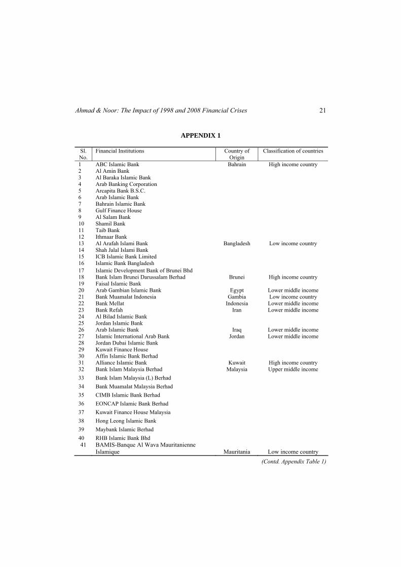
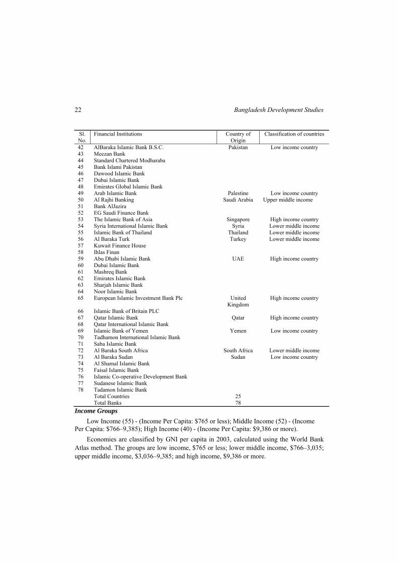
Since the countries of coverage are span across 25 countries, we will also study the profitability result based on the Islamic bank country of origin. The countries are diversified in terms of the economic activity; we divided the classification by using 2003 Gross National Income (GNI) published by World Bank. According to 2003 GNI per capita, calculated using the World Bank Atlas method2, the income groups are: low income, $765 or less; middle income, $766–$9,385; and high income, $9,386 or more.
Based on 2003 GNI report, some high income countries may also be developing countries. Our samples in the paper will include this particular country and study the differences of country background into the profitability of Islamic Banks. The Gulf Cooperation Council (GCC), for example, are classified as developing high–income countries. This paper unfolds as follows. Section II provides an overview of the related studies in the literature, followed by a section that outlines the method used and choice of input and output variables for the efficiency model. Section IV reports the empirical findings. Section V concludes and offers avenues for future research.
II. REVIEW OF THE LITERATURE
While there have been extensive literatures examining the profit efficiency features of the contemporary banking sector, particularly the U.S. and European banking markets, the work on Islamic banking is still in its infancy. Typically, studies on Islamic bank efficiency have focused on theoretical issues and the empirical work has relied mainly on the analysis of descriptive statistics rather than rigorous statistical estimation (El-Gamal and Inanoglu 2004). However, this is gradually changing as a number of recent studies have sought to apply various frontier techniques to estimate the efficiency of Islamic banks. Hassan (2005) examined the relative cost, profit, X-efficiency, and productivity of the world Islamic Banking industry. The results also show that all five efficiency measures are highly correlated with ROA and ROE, suggesting that these efficiency measures can be used concurrently with the conventional accounting ratios in determining Islamic banks’ performance.
2Atlas conversion factor, calculating gross national income (GNI—formerly referred to as GNP) and GNI per capita in U.S. dollars for certain operational purpose’s, the World Bank uses the Atlas conversion factor. The purpose of the Atlas conversion factor is to reduce the impact of exchange rate fluctuations in the cross-country comparison of national incomes.
Bangladesh Development Studies
4
The empirical studies on the performance of banking sectors have focused on the Returns On Assets (ROA), Returns On Equity (ROE), and net interest margins. It has traditionally explored the impact of bank-specific factors such as risk, market power, size and capitalisation on bank performance. More recently, research has focused on the impact of macroeconomic factors on bank performance.
To date, empirical researches have focused mainly on a specific country mainly the US banking system (Angbazo 1997, DeYoung and Rice 2004, Bhuyan and Williams 2006) and the banking systems in the western and developed countries such as New Zealand (Ho and Tripe 2002), Australia (Williams 2003), UK (Kosmidou et al. 2008) and Greece (Pasiouras and Kosmidou 2007). On the other hand, fewer studies have looked at bank performance in developing economies. Guru, Staunton and Balashanmugam (2002) examine the determinants of bank profitability in Malaysia. They employ a sample of 17 commercial banks during the 1986–1995 periods. The profitability determinants were divided into two main categories, namely the internal determinants (liquidity, capital adequacy and expenses management) and the external determinants (ownership, firm size and economic conditions). The findings revealed that efficient expenses management was one of the most significant in explaining high bank profitability. Among the macro indicators, high interest ratio was associated with low bank profitability and inflation was found to have a positive effect on bank performance.
Heffernan and Fu (2008) examine the performance of different types of Chinese banks during the period 1999–2006. The results suggest that economic value added and the net interest margin do better than the more conventional measures of profitability, namely Return On Average Assets (ROAA) and Return On Average Equity (ROAE). Some macroeconomic variables and financial ratios are significant with the expected signs. Though the type of bank is influential, bank size is not. Neither the percentage of foreign ownership nor bank listings has a discernable effect.
Ben Naceur and Goaied (2008) examine the impact of bank characteristics, financial structure and macroeconomic conditions on Tunisian banks’ net-interest margin and profitability during the period of 1980–2000. They suggest that banks that hold a relatively high amount of capital and higher overhead expenses tend to exhibit higher net-interest margin and profitability levels, while size is negatively related to bank profitability. During the period under study, they find that stock market development has positive impact on banks’ profitability. The empirical findings suggest that private banks are relatively more profitable than their state-
Ahmad & Noor: The Impact of 1998 and 2008 Financial Crises 5
owned counterparts. The results suggest that macroeconomic conditions have no significant impact on Tunisian banks’ profitability.
Ben Naceur and Omran (2008) examine the influence of bank regulations, concentration, financial and institutional development on Middle East and North Africa (MENA) countries commercial banks’ margin and profitability during the period 1989–2005. They find that bank-specific characteristics, in particular bank capitalisation and credit risk, have positive and significant impact on banks’ net interest margin, cost efficiency and profitability. On the other hand, macroeconomic and financial development indicators have no significant impact on bank performance. More recently, Sufian and Habibullah (2009) examine the determinants of the profitability of the Chinese banking sector during the post-reform period of 2000–2005. The empirical findings suggest that all the determinant variables have statistically significant impact on China banks profitability. However, the impacts are not uniform across bank types. They find that liquidity, credit risk and capitalization have positive impacts on the State-Owned Commercial Banks (SOCBs) profitability, while the impact of cost is negative. Similar to their SOCB counterparts, they find that Joint Stock Commercial Banks (JSCBs) with higher credit risk tend to be more profitable, whereas higher cost results in a lower JSCB profitability level. During the period under study, the empirical findings suggest that size and cost results in a lower city commercial banks (CITY) profitability, whereas the more diversified and relatively better capitalised CITY tend to exhibit higher profitability levels. The impact of economic growth is positive, while growth in money supply is negatively related to the SOCB and CITY profitability levels.
More recently Sufian (2010) suggest that overall economic freedom and business freedom exerts positive impacts on the profitability of the Malaysian banking sector. The positive sign of the coefficient indicates that higher (lower) freedom on the activities that banks can undertake increases (reduces) banks’ profitability, which is consistent with the view that less regulatory control allows banks to engage in various activities enabling banks to exploit economies of scale and scope and generate income from non-traditional sources. Furthermore, higher freedom on entrepreneurs to start businesses is conducive to job creation and consequently increases banks’ profitability. He also find that freedom from corruption has a significant positive impact on Malaysian banks’ profitability.
Bangladesh Development Studies
6
III. METHODOLOGY To test the relationship between bank profitability and the bank-specific and
macroeconomic determinants described earlier, we estimate a linear regression model in the following form:
yit = b0it + bijt Xijt + bejt Xejt + εit (1)
where i refers to an individual bank; t refers to year; yjt refers to the ROE and is the observation of a bank i in a particular year t; Xi represents the internal factors (determinants) of a bank; Xe represents the external factors (determinants) of a bank; εit is a normally distributed variable disturbance term. We apply the Ordinary Least Square (OLS) method, while the standard errors are calculated by using White’s (1980) transformation to control for cross-section heteroskedasticity. As a robustness checks, the empirical setting is also performed by using the least square method of Fixed Effects Model (FEM) to control for bank-specific effects. The opportunity to use a fixed effects rather than a random effects model has been tested with the Hausman test. Extending equation (1) to reflect the numbers of explanatory variables as described in Table 1, the baseline model is formulated as follows:
φjt = α + β1OE/TA + β2EQUITY/TA + β3LNTA
+ β4LOANS/TA + β5LNDEPO+ β6NPL/TL
+ β7LNGDP+ β8INFLATION + β9MARKET+
β10ΣDUMMY (AFC, GFC, MENA, ASIA, LOW, MEDIUM, HIGH)+ εj
The dependent variable is ROE; ROE is proxy measure of bank’s profitability calculated as net income after tax divided by total shareholders’ equity; OE/TA is a measure of bank operating expenses against total asset; EQUITY/ TA is a measure of bank leverage intensity measured by banks’ total shareholders’ equity divided by total assets; LNTA is the size of the bank’s total asset measured as the natural logarithm of total bank assets; LOANS/TA is a measure of bank’s loans intensity calculated as the ratio of total loans to bank total assets; LNDEPO is a measure of bank’s market share calculated as a natural logarithm of total bank deposits;
Ahmad & Noor: The Impact of 1998 and 2008 Financial Crises 7
NPL/TL is a measure of banks risk calculated as non performing loans divided by total loans; LNGDP is country gross domestic product of the country’s measured as the natural logarithm of gross domestic product; INFLATION is country inflation rates; MARKET is overall stock market capitalization size of the country’s bank operated; DUMMY is a dummy variables which takes a value of 1 for AFC, 0 otherwise; same apply for GFC, MENA, ASIA, LOW, MEDIUM, and HIGH where each variable takes a value of 1, 0 otherwise.
III.1 Performance Measure
In the literature, bank profitability, typically measured by the ROA and the ROE, is usually expressed as a function of internal and external determinants. Internal determinants are factors that are mainly influenced by a bank’s management decisions and policy objectives. Such profitability determinants are the level of liquidity, provisioning policy, capital adequacy, expenses management and bank size. On the other hand, the external determinants, both industry and macroeconomic related, are variables that reflect the economic and legal environments where the financial institution operates. Following Pasiouras and Kosmidou (2007), Ben Naceur and Goaied (2008), Kosmidou (2008), and Sufian and Habibullah (2009), among others, the dependent variable used in this study is ROA while our study adopted ROE as our dependent variables. ROE reflects how effectively a bank management utilising its shareholders funds in providing returns. Since ROA tends to be lower for financial intermediaries, most banks utilise financial leverage heavily to increase ROE to competitive levels.
III.2 Definition and the Choice of Variables Due to entry and exit factor, the efficiency frontier is constructed by using an
unbalanced sample of Islamic banks operating in the World during the period 1992-2009 (see Appendix 1). We collected our bank-specific variables from the financial statements of a sample of World Islamic banks operating over the period 1992–2009 available in the Bankscope database by IBCA and sourced from individual Islamic bank’s annual balance sheet and income statements. The BankScope database converts the data to common international standards to facilitate comparisons and all financial information is reported both in local currency and in US dollar. We also convert local currency that not US dollar into US dollar for data sourced directly
Bangladesh Development Studies
8
from the Islamic banks. We are able to collect several internal and external determinants as listed in Table I that stated internal as bank characteristic and external as economic condition.
III.3 Internal Determinants The bank characteristic variables included in the regressions are Total Loans
divided by Total Assets (LOANS/TA), Log of Total Assets (LNTA), Non Performing Loans divided by Total Loans (NPL/TL), Log of Total Deposit (LNDEPO), Operating Expenses divided by Total Assets (OE/TA) and book value of stockholders’ equity as a fraction of total assets (EQUITY/ TOTAL ASSET).
Liquidity risk, arising from the possible inability of banks to accommodate decreases in liabilities or to fund increases on the assets’ side of the balance sheet, is considered an important determinant of bank profitability. The loans market, especially credit to households and firms, is risky and has a greater expected return than other bank assets, such as government securities. Thus, one would expect a positive relationship between liquidity (LOANS/TA) and profitability (Bourke 1989). It could be the case, however, that the fewer the funds tide up in liquid investments, the higher we might expect the profitability to be (Eichengreen and Gibson 2001). The LNTA variable is included in the regression as a proxy of size to capture the possible cost advantages associated with size (economies of scale). This variable controls for cost differences and product and risk diversification according to the size of the bank. The first factor could lead to a positive relationship between size and bank profitability if there are significant economies of scale (Akhavein, Berger and Humphrey 1997, Bourke 1989, Molyneux and Thornton 1992, Bikker and Hu 2002, Goddard,Molyneox and Wilson 2004), whereas the second to a negative one, if increased diversification leads to lower credit risk and thus lower returns.
Other researchers, however, conclude that marginal cost savings can be achieved by increasing the size of the banking firm, especially as markets develop (Berger et al. 1995, Boyd and Runkle 1993). In essence, LNTA may lead to positive effects on bank profitability if there are significant economies of scale. On the other hand, if increased diversification leads to higher risks, the variable may exhibit negative effects.
The ratio of Operating Expenses to Total Assets (OE/TA) is used to provide information on the variations of bank operating costs. The variable represents total amount of wages and salaries, as well as the costs of running branch office facilities. For the most part, the literature argues that reduced expenses improve the efficiency and hence raise the profitability of a financial institution, implying a negative
Ahmad & Noor: The Impact of 1998 and 2008 Financial Crises 9
relationship between operating expenses ratio and profitability (Bourke 1989). However, Molyneux and Thornton (1992) observed a positive relationship, suggesting that high profits earned by banks may be appropriated in the form of higher payroll expenditures paid to more productive human capital. In any case, it should be appealing to identify the dominant effect in a developing banking environment like Malaysia. EQUITY/TA is included in the regressions to examine the relationship between profitability and bank capitalisation. Even though leverage (capitalisation) has been demonstrated to be important in explaining the performance of financial institutions, its impact on bank profitability is ambiguous. As lower capital ratios suggest a relatively risky position, one might expect a negative coefficient on this variable (Berger 1995). However, it could be the case that higher levels of equity would decrease the cost of capital, leading to a positive impact on bank profitability (Molyneux 1993). Moreover, an increase in capital may raise expected earnings by reducing the expected costs of financial distress, including bankruptcy (Berger 1995).
III.4 External Determinants The economic condition variables included in the regressions are Total Loans
divided by Total Assets (LOANS/TA), Log of Total Assets (LNTA), Non Performing Loans divided by Total Loans (NPL/TL), Log of Total Deposit (LNDEPO), Operating Expenses divided by Total Assets (OE/TA) and book value of stockholders’ equity as a fraction of total assets (EQUITY/ TOTAL ASSET).
Bank profitability is sensitive to macroeconomic conditions despite the trend in the industry towards greater geographic diversification and larger use of financial engineering techniques to manage risk associated with business cycle forecasting., Higher economic growth generally encourages bank to lend more and permits them to charge higher margins, as well as improving the quality of their assets. Neely and Wheelock (1997) use per-capita income and suggest that this variable exerts a strong positive effect on bank earnings. Demirguc-Kunt and Huizinga (2001) and Bikker and Hu (2002) identify possible cyclical movements in bank profitability, i.e. the extent to which bank profits are correlated with the business cycle. Their findings suggest that such correlation exists, although the variables used were not direct measures of the business cycle. To measure the relationship between economic and market conditions and bank profitability, Natural Log of Gross Domestic Product (LNGDP) and INFL (the inflation rate) are used. Bank performance is expected to be sensitive to macroeconomic control variables. The impact of macroeconomic variables on bank performance has recently been highlighted in the literature. We use the log of GDP as a control for cyclical output
Bangladesh Development Studies
10
effects, which we expect to have a positive influence on bank profitability. As GDP growth slows down, in particular during recessions, credit quality tends to deteriorate and default rate increases, thus reducing bank profitability. We also account for macroeconomic risk by controlling for the rate of inflation (INFL). The extent to which inflation affects bank profitability depends on whether future movements in inflation are fully anticipated, which in turn depends on the ability of banks to accurately forecast its future movements. An inflation rate that is fully anticipated raises profits as banks can appropriately adjust interest rates to increase revenues, while an unanticipated change could raise costs due to imperfect interest rate adjustment (Perry 1992). Earlier studies by among others Bourke (1989), Molyneux and Thornton (1992), Demirguc-Kunt and Huizinga (1999) have found a positive relationship between inflation and bank performance.
To examine the impact of market capitalisation on bank profitability, an overall index, MARKET has been added to the variables list. We introduce 2 variables AFC and GFC to identify the impact of 1998 Asian Financial Crisis and 2008 Global Financial Crisis towards Islamic banks profitability. It has been entered in regression models 2, 4 and 6 and 3, 5 and 7 respectively. To further examine the Islamic banks origin impact on bank profitability, we introduce region index, namely MENA and ASIA, to represent banks origin from Middle East and North Africa (MENA) and Asian countries (ASIA) is entered in regression models 4 and 5 and 6 and 7 respectively. Finally, to test impact of country income level towards Islamic bank profitability, we introduce LOW, MEDIUM and HIGH as variables and been entered in regression models 8, 9 and 10 respectively.
IV. RESULTS
In this section, we will discuss the performance profitability of the World Islamic banking sectors, measured by the Fixed Effect Model (FEM). The regression results focusing on the relationship between bank profitability and the explanatory variables are presented in Table 1.
IV.1 The Islamic Banks’ Profitability Performance Based on literature, bank profitability is typically measured by return on equity
(ROE) and/ or return on asset (ROA) and usually expressed as a function of internal and external determinants.
Internal determinants are factors that are mainly influenced by a bank’s management decisions and policy objectives. Such profitability determinants are the level of liquidity, provisioning policy, capital adequacy, expenses management, and
Ahmad & Noor: The Impact of 1998 and 2008 Financial Crises 11
bank size. On the other hand, the external determinants, both industry and macroeconomic related, are variables that reflect the economic and legal environments where the financial institution operates (Sufian and Habibullah 2009).
We will select ROE as dependent variable based on several reasons. Of all the fundamental ratios that measure profitability, one of the most important is return on equity. It is a basic test of how effectively a company's management uses investors' money. By measuring how much earnings a company can generate from assets, ROE offers a gauge of profit-generating efficiency. Firms that do a good job of milking profit from their operations typically have a competitive advantage, a feature that normally translates into superior returns for investors. The other factor as to why ROE has been selected is due to DuPont analysis3 that breaks down ROE into three distinct elements. This analysis will enable details analysis to understand the source of superior (or inferior) return by comparison with companies in similar industries (or between industries). DuPont analysis tells us that ROE is affected by three things: Operating efficiency, which is measured by profit margin; Asset use efficiency, which is measured by total asset turnover; and Financial leverage, which is measured by the equity multiplier.
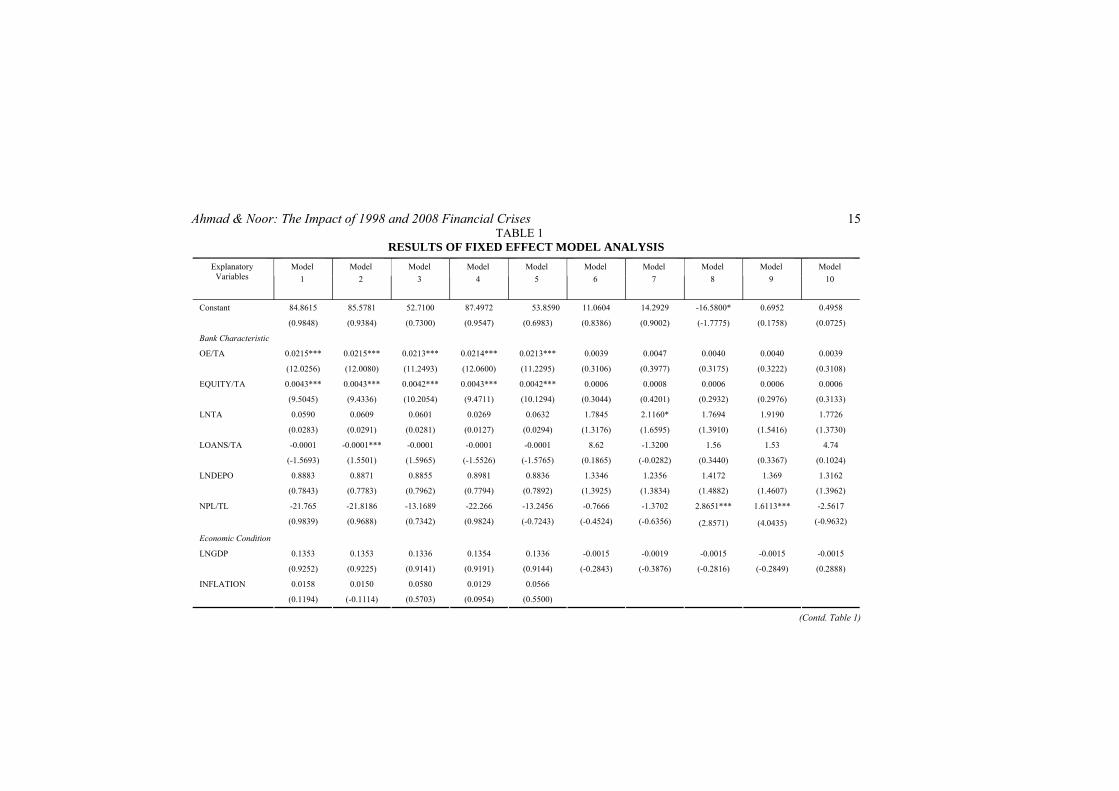
The regression results focusing on the relationship between bank profitability and the explanatory variables are presented in Table 1. The model performs reasonably well with most variables remaining stable across the various regressions tested. The explanatory power of the models is reasonably high, while the F-statistics for all models is significant at the 1% level for model 1 to model 5 and 5% level for model 6 to model 10. The adjusted R2 is 18% for model 1 to 5 and 8% for model 6 to 10, this is more lower compared to Kosmidou et al. (2008) at 92% and Sufian (2010) at 75%.
The ratio of Operating Expenses to Total Assets (OE/TA) is used to provide information on the bank operating costs against asset have. The variable represents total amount of overhead expenses, wages and salaries, as well as the costs of running branch office facilities inclusive utilities, stationary, etc. against bank assets. For the most part, the literature argues that reduced expenses improve the efficiency and hence raise the profitability of a financial institution, implying a negative relationship between operating expenses ratio and profitability (Bourke
3 A method of performance measurement that was started by the DuPont Corporation in the 1920s. With this method, assets are measured at their gross book value rather than at net book value in order to produce a higher return on equity (ROE). It is also known as “DuPont identity.”
Bangladesh Development Studies
12
1989). The result exhibits positive relationship with bank profitability at all 10 models with 5 models is statistically significant at the 1% level. The result justification that talent is attracted to benefit and financial returns offered by organisation in working environment is also applicable in Islamic bankings on justifying strong positive relationship between bank profitability with OE/TA ratio. This is consistent with Molyneux and Thornton (1992) who observed a positive relationship, suggesting that high profits earned by banks may be appropriated in the form of higher payroll expenditures paid to more productive human capital.
Referring to the impact of capitalisation, it is observed from Table 1 that EQUITY/TA exhibits positive relationship with profitability and is statistically significant at 1% level. But when we control for GNI country income, the result is still positive but not significant. This is consistent with previous studies (Isik and Hassan 2003, Staikouras and Wood 2003, Sufian and Habibullah 2009) providing support to the argument that well capitalised banks face lower costs of going bankrupt, thus lowers their funding cost, or that they have lower needs for external funding resulting in higher profitability. Nevertheless, strong capital structure is essential for banks in emerging economies since it provides additional strength to withstand financial crises and increased safety for depositors during unstable macroeconomic conditions.
The LNTA variable is included in the regression models as a proxy of size to capture the possible cost advantages associated with size (economies of scale). This variable controls for cost differences and product and risk diversification according to the size of the bank. The findings indicate that LNTA, as a proxy of bank’s size, shows positive sign, suggesting larger banks tend to be more profitable. Concerning the liquidity results, LOANS/TA has a negative relationship with profit efficiency levels. There may be decreasing returns to scale through the allocation of fixed costs (e.g. research or risk management) over a higher volume of services or from efficiency gains from a specialised workforce, while LNDEPO reveals positive relationship with profit efficiency. Although it is not statistically significant at the considered levels, it is perceived that the more deposit the bank’s receive, higher will be loan disbursement that is positively correlated with bank revenue translating into higher profits.
For credit risk result, the impact of credit risk (NPL/TL) has a negative relationship with bank profitability, this generally suggesting that banks with higher credit risk exhibit lower profitability levels. The results imply that World Islamic banks should focus more on credit risk management, which has been proven to be problematic in the recent past. Sufian and Habibullah (2009) also find similar result
Ahmad & Noor: The Impact of 1998 and 2008 Financial Crises 13
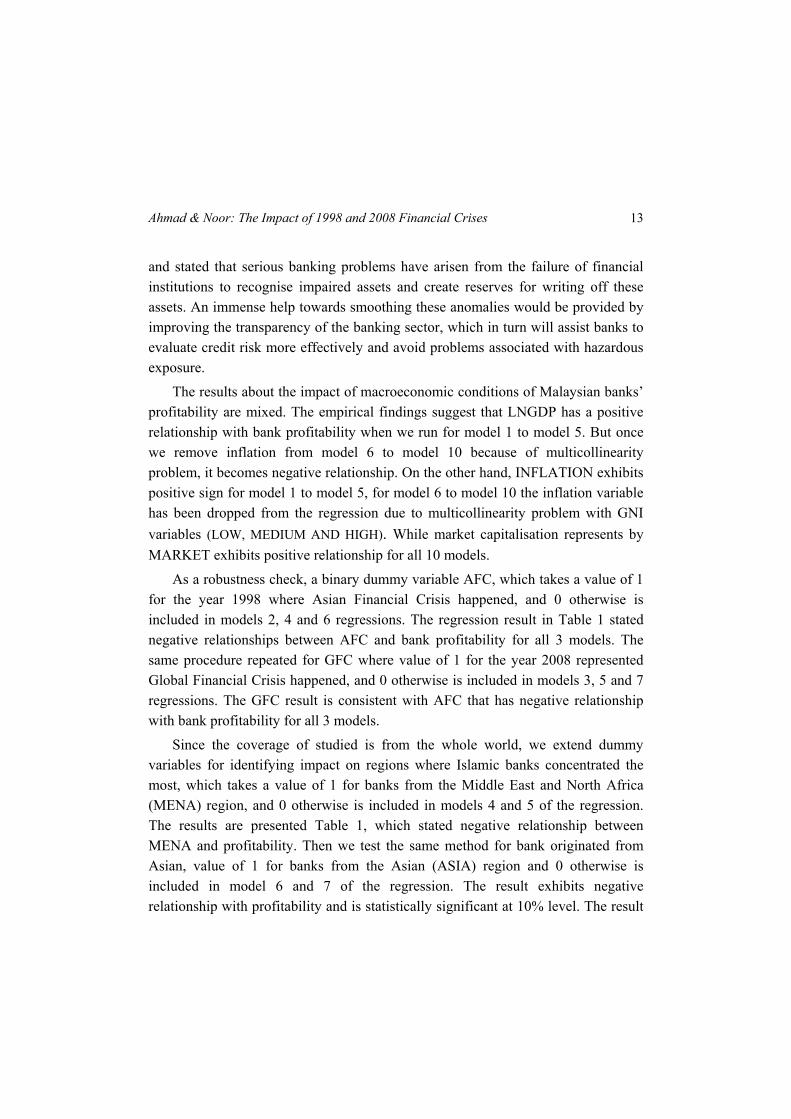
and stated that serious banking problems have arisen from the failure of financial institutions to recognise impaired assets and create reserves for writing off these assets. An immense help towards smoothing these anomalies would be provided by improving the transparency of the banking sector, which in turn will assist banks to evaluate credit risk more effectively and avoid problems associated with hazardous exposure.
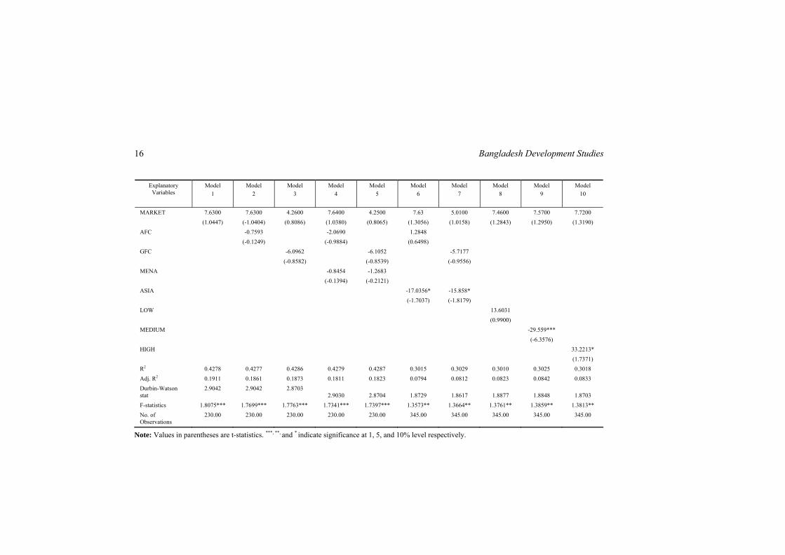
The results about the impact of macroeconomic conditions of Malaysian banks’ profitability are mixed. The empirical findings suggest that LNGDP has a positive relationship with bank profitability when we run for model 1 to model 5. But once we remove inflation from model 6 to model 10 because of multicollinearity problem, it becomes negative relationship. On the other hand, INFLATION exhibits positive sign for model 1 to model 5, for model 6 to model 10 the inflation variable has been dropped from the regression due to multicollinearity problem with GNI variables (LOW, MEDIUM AND HIGH). While market capitalisation represents by MARKET exhibits positive relationship for all 10 models.
As a robustness check, a binary dummy variable AFC, which takes a value of 1 for the year 1998 where Asian Financial Crisis happened, and 0 otherwise is included in models 2, 4 and 6 regressions. The regression result in Table 1 stated negative relationships between AFC and bank profitability for all 3 models. The same procedure repeated for GFC where value of 1 for the year 2008 represented Global Financial Crisis happened, and 0 otherwise is included in models 3, 5 and 7 regressions. The GFC result is consistent with AFC that has negative relationship with bank profitability for all 3 models.
Since the coverage of studied is from the whole world, we extend dummy variables for identifying impact on regions where Islamic banks concentrated the most, which takes a value of 1 for banks from the Middle East and North Africa (MENA) region, and 0 otherwise is included in models 4 and 5 of the regression. The results are presented Table 1, which stated negative relationship between MENA and profitability. Then we test the same method for bank originated from Asian, value of 1 for banks from the Asian (ASIA) region and 0 otherwise is included in model 6 and 7 of the regression. The result exhibits negative relationship with profitability and is statistically significant at 10% level. The result
Bangladesh Development Studies
14
is interesting since Asian Islamic banks are less profitable than MENA Islamic banks.
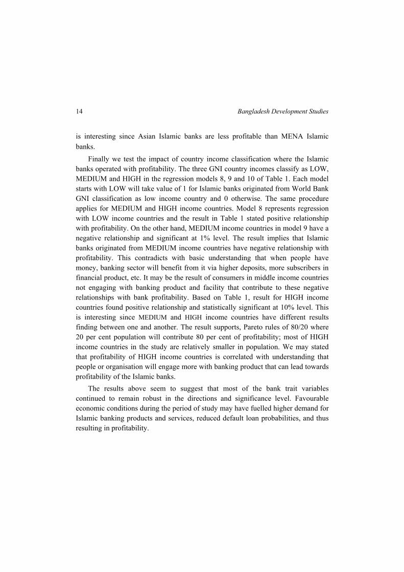
Finally we test the impact of country income classification where the Islamic banks operated with profitability. The three GNI country incomes classify as LOW, MEDIUM and HIGH in the regression models 8, 9 and 10 of Table 1. Each model starts with LOW will take value of 1 for Islamic banks originated from World Bank GNI classification as low income country and 0 otherwise. The same procedure applies for MEDIUM and HIGH income countries. Model 8 represents regression with LOW income countries and the result in Table 1 stated positive relationship with profitability. On the other hand, MEDIUM income countries in model 9 have a negative relationship and significant at 1% level. The result implies that Islamic banks originated from MEDIUM income countries have negative relationship with profitability. This contradicts with basic understanding that when people have money, banking sector will benefit from it via higher deposits, more subscribers in financial product, etc. It may be the result of consumers in middle income countries not engaging with banking product and facility that contribute to these negative relationships with bank profitability. Based on Table 1, result for HIGH income countries found positive relationship and statistically significant at 10% level. This is interesting since MEDIUM and HIGH income countries have different results finding between one and another. The result supports, Pareto rules of 80/20 where 20 per cent population will contribute 80 per cent of profitability; most of HIGH income countries in the study are relatively smaller in population. We may stated that profitability of HIGH income countries is correlated with understanding that people or organisation will engage more with banking product that can lead towards profitability of the Islamic banks.
The results above seem to suggest that most of the bank trait variables continued to remain robust in the directions and significance level. Favourable economic conditions during the period of study may have fuelled higher demand for Islamic banking products and services, reduced default loan probabilities, and thus resulting in profitability.
Ahmad & Noor: The Impact of 1998 and 2008 Financial Crises 15TABLE 1
RESULTS OF FIXED EFFECT MODEL ANALYSIS Explanatory
Variables Model
1 Model
2 Model
3 Model
4 Model
5 Model
6 Model
7
Model 8
Model 9
Model 10
84.8615 85.5781 52.7100 87.4972 53.8590 11.0604 14.2929 -16.5800* 0.6952 0.4958 Constant
(0.9848) (0.9384) (0.7300) (0.9547) (0.6983) (0.8386) (0.9002) (-1.7775) (0.1758) (0.0725)
Bank Characteristic
0.0215*** 0.0215*** 0.0213*** 0.0214*** 0.0213*** 0.0039 0.0047 0.0040 0.0040 0.0039 OE/TA
(12.0256) (12.0080) (11.2493) (12.0600) (11.2295) (0.3106) (0.3977) (0.3175) (0.3222) (0.3108)
0.0043*** 0.0043*** 0.0042*** 0.0043*** 0.0042*** 0.0006 0.0008 0.0006 0.0006 0.0006 EQUITY/TA
(9.5045) (9.4336) (10.2054) (9.4711) (10.1294) (0.3044) (0.4201) (0.2932) (0.2976) (0.3133)
0.0590 0.0609 0.0601 0.0269 0.0632 1.7845 2.1160* 1.7694 1.9190 1.7726 LNTA
(0.0283) (0.0291) (0.0281) (0.0127) (0.0294) (1.3176) (1.6595) (1.3910) (1.5416) (1.3730)
-0.0001 -0.0001*** -0.0001 -0.0001 -0.0001 8.62 -1.3200 1.56 1.53 4.74 LOANS/TA
(-1.5693) (1.5501) (1.5965) (-1.5526) (-1.5765) (0.1865) (-0.0282) (0.3440) (0.3367) (0.1024)
0.8883 0.8871 0.8855 0.8981 0.8836 1.3346 1.2356 1.4172 1.369 1.3162 LNDEPO
(0.7843) (0.7783) (0.7962) (0.7794) (0.7892) (1.3925) (1.3834) (1.4882) (1.4607) (1.3962)
-21.765 -21.8186 -13.1689 -22.266 -13.2456 -0.7666 -1.3702 2.8651*** 1.6113*** -2.5617 NPL/TL
(0.9839) (0.9688) (0.7342) (0.9824) (-0.7243) (-0.4524) (-0.6356) (2.8571) (4.0435) (-0.9632)
Economic Condition
0.1353 0.1353 0.1336 0.1354 0.1336 -0.0015 -0.0019 -0.0015 -0.0015 -0.0015 LNGDP
(0.9252) (0.9225) (0.9141) (0.9191) (0.9144) (-0.2843) (-0.3876) (-0.2816) (-0.2849) (0.2888)
0.0158 0.0150 0.0580 0.0129 0.0566 INFLATION
(0.1194) (-0.1114) (0.5703) (0.0954) (0.5500)
(Contd. Table 1)
Bangladesh Development Studies
16
Explanatory Variables
Model 1
Model 2
Model 3
Model 4
Model 5
Model 6
Model 7
Model 8
Model 9
Model 10
7.6300 7.6300 4.2600 7.6400 4.2500 7.63 5.0100 7.4600 7.5700 7.7200 MARKET (1.0447) (-1.0404) (0.8086) (1.0380) (0.8065) (1.3056) (1.0158) (1.2843) (1.2950) (1.3190)
-0.7593 -2.0690 1.2848 AFC (-0.1249) (-0.9884) (0.6498) -6.0962 -6.1052 -5.7177 GFC (-0.8582) (-0.8539) (-0.9556) -0.8454 -1.2683 MENA (-0.1394) (-0.2121) -17.0356* -15.858* ASIA (-1.7037) (-1.8179) 13.6031 LOW (0.9900) -29.559*** MEDIUM (-6.3576) 33.2213* HIGH (1.7371)
R2 0.4278 0.4277 0.4286 0.4279 0.4287 0.3015 0.3029 0.3010 0.3025 0.3018 Adj. R2 0.1911 0.1861 0.1873 0.1811 0.1823 0.0794 0.0812 0.0823 0.0842 0.0833 Durbin-Watson stat
2.9042 2.9042 2.8703 2.9030 2.8704 1.8729 1.8617 1.8877 1.8848 1.8703
F-statistics 1.8075*** 1.7699*** 1.7763*** 1.7341*** 1.7397*** 1.3573** 1.3664** 1.3761** 1.3859** 1.3813** No. of Observations
230.00 230.00 230.00 230.00 230.00 345.00 345.00 345.00 345.00 345.00
Note: Values in parentheses are t-statistics. ***, **, and * indicate significance at 1, 5, and 10% level respectively.
Ahmad & Noor: The Impact of 1998 and 2008 Financial Crises 17
V. CONCLUSIONS AND DIRECTIONS FOR FUTURE RESEARCH
By using an unbalanced bank level panel data, the present study attempts to examine World Islamic Banks performance profitability during the period 1992-2009. We find that the larger, more diversified, and better capitalized banks are relatively more profitable. The empirical findings seem to support the expense preference theory, which could be explained by the more highly qualified and professional management that requires higher remuneration packages. On the other hand, we find that higher credit risk has negative impact on bank profitability.
In this paper, we examine the profitability performance of the World Islamic banks that consist of 25 countries namely Bahrain, Bangladesh, Brunei, Egypt, Gambia, Indonesia, Iran, Iraq, Jordan, Kuwait, Malaysia, Mauritania, Pakistan, Palestine, Saudi Arabia, Singapore, Syria, Thailand, Turkey, United Arab Emirates, Qatar, Yemen, South Africa, Sudan and Yemen during the period of 1992-2009 with 78 Islamic banks involved. The profitability performance of individual banks is evaluated using Fixed Income Model (FEM) against a set of bank specific variables.
The Fixed Effect Model (FEM) result that has been used for analysing profitability proposed that profit efficiency is positively and significantly associated with operating expenses against asset, equity, HIGH income countries and non performing loans against total loans specifically for models 8 and 9 that positively significant at 1 per cent level. The empirical results show that more profitable banks are those that have higher operating expenses against asset, more equity against asset and concentrated at high income countries. The results also suggest that favourable economic conditions exhibit positive relationship with profit efficiency. The impact of 1998 and 2008 financial crises have been examined in the study. The finding for both crises is negative and non significant. It implies that world Islamic banks’ profitability does not impacted during Asian and Global Financial crises.
Due to its limitations, the paper could be extended in a variety of ways. Firstly, the scope of this study could be further extended to investigate other variables such as taxation and regulation indicators. Secondly, it is suggested that further analysis into the investigation of the Islamic banking sector efficiency to consider risk exposure factors. Finally, investigation of changes in productivity over time as a result of technical change or technological progress or regress by employing the Malmquist Total Factor Productivity Index could yet be another extension to the paper.
Despite these limitations, the findings of this study are expected to contribute significantly to the existing knowledge on the operating performance of the World Islamic banking industry. Nevertheless, the study has also provided further insight
Bangladesh Development Studies
18
to bank specific management as well as the policymakers with regard to attaining optimal utilisation of capacities, improvement in managerial expertise etc. This may also facilitate directions for sustainable competitiveness of World Islamic banking operations in the future.
REFERENCES
Akhavein, J., A.N. Berger and D.B. Humphrey. 1997. “The Effects of Megamergers on Efficiency and Prices: Evidence from a Bank Profit Function.” Review of Industrial Organization, 12(1):95–139.
Angbazo, L. 1997. “Commercial Bank Net Interest Margins, Default Risk, Interest Rate Risk, and Off Balance sheet Banking.” Journal of Banking and Finance, 21:55–87.
Berger, A.N. 1995. “The Relationship between Capital and Earnings in Banking.” Journal Money, Credit and Banking, 27:432–456.
Berger, A.N. and D.B.Humphrey.1997. “Efficiency of Financial Institutions: International Survey and Directions for Future Research.” European Journal of Operational Research, 98 (2): 175-212.
Ben Naceur, S. and M.Goaied.2008. “The Determinants of Commercial Bank Interest Margin and Profitability: Evidence from Tunisia.” Frontiers in Finance and Economics. 5 (1):106–130.
Ben Naceur, S. and M.Omran.2008. “The Effects of Bank Regulations, Competition and FinancialReforms on Mena Banks’ Profitability.” Working Paper, Economic Research Forum,Cairo, Egypt.
Berger, A.N., A.K. Kashyap and J.M. Scalise.1995. “The Transformation of the U.S. Banking Industry: What a Long, Strange Trip It’s Been.” Brookings Papers on Economic Activity, 2: 55-218.
Bhuyan, R. and D.L. Williams. 2006. “Operating Performance of the US Commercial Banks after IPOs: An Empirical Evidence.” Journal of Commercial Banking and Finance, 5 (1–2):68–95.
Bikker, J. and H. Hu. 2002. “Cyclical Patterns in Profits, Provisioning and Lending of Banks and Procyclicality of the New Basel Capital Requirements.” BNL Quarterly Review, 221:143–175.
Bourke, P. 1989. “Concentration and Other Determinants of Bank Profitability in Europe, North America and Australia.” Journal of Banking and Finance, 13:65–79.
Ahmad & Noor: The Impact of 1998 and 2008 Financial Crises 19
Boyd, J. and D. Runkle.1993. “Size and Performance of Banking Firms: Testing the Predictions Theory.” Journal of Monetary Economics, 31:47–67.
Demirguc-Kunt, A. and H.Huizinga.1999. “Determinants of Commercial Bank Interest Margins and Profitability: Some International Evidence.” World Bank Economic Review, 13:379–408.
Demirguc-Kunt, A. and H. Huizinga. 2001. “Financial Structure and Bank Profitability.” In Demirguc-Kunt, A. and Levine, R. (eEds.), Financial Structure and Economic Growth: A Cross Country Comparison of Banks, Markets and Development. Cambridge, MA :MIT Press.
DeYoung, R. and T. Rice.2004. “Non-interest Income and Financial Performance at US Commercial Banks.” Financial Review, 39(1):101–127.
Eichengreen, B. and H.D. Gibson. 2001. “Greek Banking at the Dawn of the New Millennium.” Discussion Paper, Centre of Economic and Policy Research, London, UK.
Goddard, J., P. Molyneux and J. Wilson. 2004. “Dynamic of Growth and Profitability in Banking.” Journal Money, Credit and Banking, 36:1069–1090.
Guru, B.K., Staunton, J. and B. Balashanmugam.2002. “Determinants of Commercial Bank Profitability in Malaysia.” Multimedia University Working Paper, Cyberjaya, Malaysia.
Hassan, M.K. 2005. “The Cost, Profit and X-Efficiency of Islamic Banks.” Paper presented at the 12th ERF Annual Conference, 19th-21st December, Egypt.
Heffernan, S. and M. Fu. 2008. “The Determinants of Bank Performance in China.” EMG Working Paper Series.
Ho, M.T. and D. Tripe.2002. “Factors Influencing the Performance of Foreign Owned Banks in New Zealand.” Journal International Financial Markets, Institutions and Money, 12:341–357.
Isik, I. and M.K. Hassan. 2003. “Efficiency, Ownership and Market Structure, Corporate Control and Governance in the Turkish Banking Industry.” Journal of Business Finance and Accounting ,30 (9-10):1363-1421.
Kosmidou, K. 2008. “The Determinants of Banks’ Profits in Greece during the Period of EU Financial Integration.” Managerial Finance, 34 (3):146–159.
Molyneux, P. 1993. Structure and Performance in European Banking. University of Wales Bangor, Bangor, UK. Mimeo.
Molyneux, P. and J. Thornton. 1992. “Determinants of European Bank Profitability: A Note.” Journal Banking and Finance, 16:1173–1178.
Bangladesh Development Studies
20
Neely, M. and D. Wheelock.1997. “Why Does Bank Performance Vary Across States?” Federal Reserve Bank St. Louis Review, March:27–38.
Pasiouras, F. and K.Kosmidou. 2007. “Factors Influencing the Profitability of Domestic and Foreign Commercial Banks in the European Union.” Research in International Business and Finance, 21:223–237.
Perry, P. 1992. “Do Banks Gain or Lose from Inflation.” Journal Retail Banking, 14 (2): 25–40.
Staikouras, C. and G.Wood. 2003. “The Determinants of Bank Profitability in Europe.” Paper presented at the European Applied Business Research Conference, Venice, 9-13 June.
Sufian, F. and M.A.N.M. Noor. 2009. “The Determinants of Islamic Bank’s Efficiency Changes: Empirical Evidence from the MENA and Asian Countries Islamic Banking Sectors.” International Journal of Islamic and Middle Eastern Finance and Management, 2(2):120-138
Sufian, F. and M.S. Habibullah. 2009. “Bank Specific and Macroeconomic Determinants of Bank Profitability: Empirical Evidence from the China Banking Sector.” Frontiers of Economics in China, 4 (2):274–291.
Sufian, F., M.S., Habibullah. 2010. “Does Economic Freedom Fosters Banks’ Performance? Panel Evidence from Malaysia.” Journal of Contemporary Accounting & Economics, doi: 10.1016/j.jcae.2010.09.003
Sufian, F. 2010. “Developments in the Performance of the Malaysian Banking Sector: Opportunity Cost of Regulatory Compliance.” Int. J. Business Competition and Growth, 1 (1):85–103.
White, H.J. 1980. “A Heteroskedasticity-consistent Covariance Matrix Estimator and a Direct Test for Heteroskedasticity.” Econometrica, 48:817–838.
Williams, B. 2003. “Domestic and International Determinants of Bank Profits: Foreign Banks in Australia.” Journal of Banking and Finance, 27:1185–1210.
Zaher, T.S. and M.K. Hassan. 2001. “A Comparative Literature Survey of Islamic Finance and Banking.” Financial Markets, Institutions & Instruments ,10 (4): 155-199.
Ahmad & Noor: The Impact of 1998 and 2008 Financial Crises 21
APPENDIX 1
Sl. No.
Financial Institutions Country of Origin
Classification of countries
1 ABC Islamic Bank Bahrain High income country 2 Al Amin Bank 3 Al Baraka Islamic Bank 4 Arab Banking Corporation 5 Arcapita Bank B.S.C. 6 Arab Islamic Bank 7 Bahrain Islamic Bank 8 Gulf Finance House 9 Al Salam Bank 10 Shamil Bank 11 Taib Bank 12 Ithmaar Bank 13 Al Arafah Islami Bank Bangladesh Low income country 14 Shah Jalal Islami Bank 15 ICB Islamic Bank Limited 16 Islamic Bank Bangladesh 17 Islamic Development Bank of Brunei Bhd 18 Bank Islam Brunei Darussalam Berhad Brunei High income country 19 Faisal Islamic Bank 20 Arab Gambian Islamic Bank Egypt Lower middle income 21 Bank Muamalat Indonesia Gambia Low income country 22 Bank Mellat Indonesia Lower middle income 23 Bank Refah Iran Lower middle income 24 Al Bilad Islamic Bank 25 Jordan Islamic Bank 26 Arab Islamic Bank Iraq Lower middle income 27 Islamic International Arab Bank Jordan Lower middle income 28 Jordan Dubai Islamic Bank 29 Kuwait Finance House 30 Affin Islamic Bank Berhad 31 Alliance Islamic Bank Kuwait High income country 32 Bank Islam Malaysia Berhad Malaysia Upper middle income 33 Bank Islam Malaysia (L) Berhad 34 Bank Muamalat Malaysia Berhad 35 CIMB Islamic Bank Berhad 36 EONCAP Islamic Bank Berhad 37 Kuwait Finance House Malaysia 38 Hong Leong Islamic Bank 39 Maybank Islamic Berhad 40 RHB Islamic Bank Bhd 41 BAMIS-Banque Al Wava Mauritanienne
Islamique Mauritania Low income country (Contd. Appendix Table 1)
Bangladesh Development Studies
22
Sl. No.
Financial Institutions Country of Origin
Classification of countries
42 AlBaraka Islamic Bank B.S.C. Pakistan Low income country 43 Meezan Bank 44 Standard Chartered Modharaba 45 Bank Islami Pakistan 46 Dawood Islamic Bank 47 Dubai Islamic Bank 48 Emirates Global Islamic Bank 49 Arab Islamic Bank Palestine Low income country 50 Al Rajhi Banking Saudi Arabia Upper middle income 51 Bank AlJazira 52 EG Saudi Finance Bank 53 The Islamic Bank of Asia Singapore High income country 54 Syria International Islamic Bank Syria Lower middle income 55 Islamic Bank of Thailand Thailand Lower middle income 56 Al Baraka Turk Turkey Lower middle income 57 Kuwait Finance House 58 Ihlas Finan 59 Abu Dhabi Islamic Bank UAE High income country 60 Dubai Islamic Bank 61 Mashreq Bank 62 Emirates Islamic Bank 63 Sharjah Islamic Bank 64 Noor Islamic Bank 65 European Islamic Investment Bank Plc United
Kingdom High income country
66 Islamic Bank of Britain PLC 67 Qatar Islamic Bank Qatar High income country 68 Qatar International Islamic Bank 69 Islamic Bank of Yemen Yemen Low income country 70 Tadhamon International Islamic Bank 71 Saba Islamic Bank 72 Al Baraka South Africa South Africa Lower middle income 73 Al Baraka Sudan Sudan Low income country 74 Al Shamal Islamic Bank 75 Faisal Islamic Bank 76 Islamic Co-operative Development Bank 77 Sudanese Islamic Bank 78 Tadamon Islamic Bank Total Countries 25 Total Banks 78
Income Groups Low Income (55) - (Income Per Capita: $765 or less); Middle Income (52) - (Income
Per Capita: $766–9,385); High Income (40) - (Income Per Capita: $9,386 or more). Economies are classified by GNI per capita in 2003, calculated using the World Bank
Atlas method. The groups are low income, $765 or less; lower middle income, $766–3,035; upper middle income, $3,036–9,385; and high income, $9,386 or more.
Bangladesh Development Studies Vol. XXXIV, March 2011, No. 1
Asset Price Bubble and Banks: The Case of Japan
MONZUR HOSSAIN*
FARHANA RAFIQ**
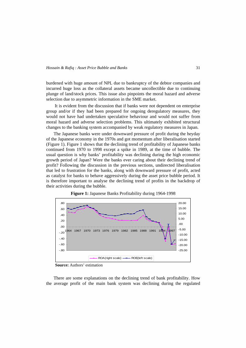
This paper analyses the behaviour of the Japanese banks at the outset of the asset price bubble in the late 1980s. The paper argues that with the advent of financial deregulations, the declining trend of profitability forced the banks to exhibit speculative behaviour during the asset price bubble period (mid-1980s) to increase short term profit. This has ultimately led to the banking crisis after the burst of the bubble in 1989. Our empirical results support this argument. The paper also attempts to provide a comprehensive description of a number of interrelated structural changes in the financial system of Japan during 1977-2003 that opens up the domain of possibility for rethinking the issues related to change in policies. The case of Japan in the context of the rise and burst of the asset price bubble and subsequent banking crisis could be instructive for many countries including Bangladesh that are facing the asset price bubble situation. Japanese experience suggests that monetary policy should respond to asset bubbles in a cautious and moderate manner in order to avoid economic distortions. The lessons that can be learned from the Japanese experience are: (i) central bank’s role to burst bubbles must depend on the degree of efficiency of the financial sector, and (ii) the speed to burst the bubble must be based on the overall economic situation.
I. INTRODUCTION
The emergence and burst of the bubble economy in Japan in the late 1980s were mostly characterised by the commercial banks’ aggressive behaviour, collapse of some banks and debtor companies with a huge burden of non-performing loans (NPL). About 180 banks were failed in the 1990s and subsequently a prolonged
* Research Fellow, Bangladesh Institute of Development Studies. ** Lecturer, Department of Economics, American International University, Dhaka, Bangladesh.
Bangladesh Development Studies
24
stagnant period for the Japanese economy started. Naturally, the question arises: were the banks responsible for creating the bubble that subsequently led to the banking crisis of the 1990s? This also raises curiosity as to why the most successful banking system of the 1960s and the 1970s has failed? Did the deregulatory measures indicate any structural changes in the financial system that contributed to the failure of the banks? The paper attempts to shed some insights into these questions.
Many authors have tried to analyse the situation from various aspects (see, Aoki and Patrick 1994, Okina et al. 2001, Hossain 2005, Aoki and Patrick 1994) expressed concern about the structural changes that occurred in the financial system of Japan. They argued that the asset-price bubble in the late 1980s was partially created by the erosion of the coherence and integrity of the regulatory framework. According to them, with diminishing opportunity for traditional lending and limited access to bond-related services during the protracted monetary easing of the mid 1980s, banks started to increase lending to real estate companies and non-banks. This also revealed the banks’ weak monitoring capacity in the newly emerged market environment.
Okina et al. (2001) identified some other reasons for the emergence of the bubble in the late 1980s and the subsequent banking crisis. These are aggressive bank behaviour, protracted monetary easing, taxation and regulation on land, weak mechanism to impose discipline on economic agents, self confidence of economic agents, etc. In line with the views of Okina et al. (2001), Hossain (2005) argued that weaknesses in the corporate governance of banks were crucial for the banking crisis in the 1990s, rather than asset price bubble and financial deregulations.
In this paper we take the view that financial liberalisation was started in the early 1980s without making financial institutions prepared properly for the changing situation. As a result, financial institutions could not cope with the situation instantly and indulged in some speculative behaviour. Of course, such behaviour may be associated with corporate governance problem, as Hossain (2005) argued. Therefore, analysis of banks’ profitability is important as this has led to a sharp response from banks to the structural changes that occurred in the Japanese banking system in the 1980s. Although the deregulatory measures were partial in nature, these measures created problems in functioning of the banks as they were not fully prepared for moving toward competitiveness. Thus the paper analyses the behaviour of the financial institutions by taking their profitability issue into consideration. We use aggregate data for the period 1977-2003 to analyse bank profitability. Since the data resembles time-series properties, ordinary least square regression is not appropriate. Therefore, we apply Vector Error Correction Model (VECM) to assess
Hossain & Rafiq : Asset Price Bubble and Banks 25
the long run and short run relationship between bank profitability and other macroeconomic and monetary variables.
The paper is organised as follows. After introduction, Section II provides an overview of the Japanese financial system. Section III highlights various aspects of banks behaviour during the asset price bubble. Section IV describes methodology and data and Section V discusses empirical results on bank profitability. Section VI concludes the paper.
II. JAPANESE FINANCIAL SYSTEM: AN OVERVIEW
II.1 The Main-bank System The Japanese financial system is predominantly bank-based. Post-war Japanese
financial system was highly regulated and banks were heavily dependent on Bank of Japan’s (BOJ) subsidies (window guidance) and borrowings of enterprise groups. The characteristics of Japanese model of financial system during post-war period included high debt/equity ratios, greater reliance on bank loans than securities markets, closer relationship between banks and borrowers, extensive corporate cross-shareholding, greater guidance from the government in credit allocation, etc. The system is well known as the “main bank” system. It is evident from many research works that this “main bank” system contributed greatly to the post-war economic growth of Japan although the varieties of functions played by the main bank were not associated with the usual concept of commercial banking. This type of Japanese banking system is characterised by clearly defined structural policy of the government for stimulating and maintaining specialisation among financial institutions. The changes were not made to achieve maximum competition in a free market (Wallich and Wallich 1976).
There is a vast literature on how the main bank system played a very important role in Japanese economy and financial system. The core of an enterprise group is usually a bank that is called Main Bank. Pre-war Zaibatsu and post-war Keiretsu are examples of such types of enterprise groups, with the big six being Mitsui, Mitsubishi, Sumitomo, Fuyo, Sanwa and Ikkan. Group affiliation interlocks stock shares among industrial enterprises, banks and other financial institutions. The arrangements between main bank and group involved both financial and non-financial aspects. The financial arrangements included the sharing of financial risk through mutual support, preferential loans from the financial institutions and the control of stock voting power through ownership within the group. The non-financial arrangements included joint sale and purchase arrangements, assured markets and sources of supply, technological affinity, combined research, and cooperative planning. This structure of Japanese banks might be relevant to the so-
Bangladesh Development Studies
26
called “Industrial bank” (also available in Germany as House bank) rather than modern commercial bank.
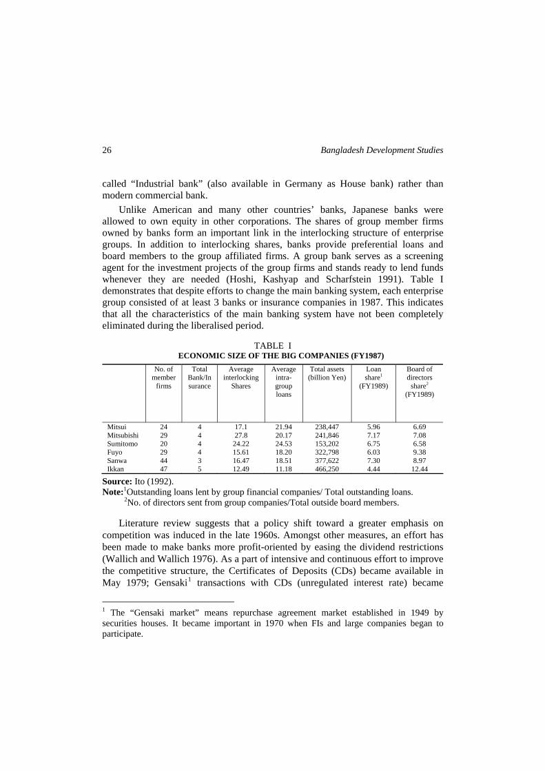
Unlike American and many other countries’ banks, Japanese banks were allowed to own equity in other corporations. The shares of group member firms owned by banks form an important link in the interlocking structure of enterprise groups. In addition to interlocking shares, banks provide preferential loans and board members to the group affiliated firms. A group bank serves as a screening agent for the investment projects of the group firms and stands ready to lend funds whenever they are needed (Hoshi, Kashyap and Scharfstein 1991). Table I demonstrates that despite efforts to change the main banking system, each enterprise group consisted of at least 3 banks or insurance companies in 1987. This indicates that all the characteristics of the main banking system have not been completely eliminated during the liberalised period.
TABLE I ECONOMIC SIZE OF THE BIG COMPANIES (FY1987)
No. of member
firms
Total Bank/Insurance
Average interlocking
Shares
Average intra-group loans
Total assets (billion Yen)
Loan share1
(FY1989)
Board of directors
share2
(FY1989)
Mitsui 24 4 17.1 21.94 238,447 5.96 6.69 Mitsubishi 29 4 27.8 20.17 241,846 7.17 7.08 Sumitomo 20 4 24.22 24.53 153,202 6.75 6.58 Fuyo 29 4 15.61 18.20 322,798 6.03 9.38 Sanwa 44 3 16.47 18.51 377,622 7.30 8.97 Ikkan 47 5 12.49 11.18 466,250 4.44 12.44
Source: Ito (1992). Note:1Outstanding loans lent by group financial companies/ Total outstanding loans.
2No. of directors sent from group companies/Total outside board members.
Literature review suggests that a policy shift toward a greater emphasis on competition was induced in the late 1960s. Amongst other measures, an effort has been made to make banks more profit-oriented by easing the dividend restrictions (Wallich and Wallich 1976). As a part of intensive and continuous effort to improve the competitive structure, the Certificates of Deposits (CDs) became available in May 1979; Gensaki1 transactions with CDs (unregulated interest rate) became
1 The “Gensaki market” means repurchase agreement market established in 1949 by securities houses. It became important in 1970 when FIs and large companies began to participate.
Hossain & Rafiq : Asset Price Bubble and Banks 27
increasingly popular, as there is no transaction tax on CDs. The Tegata2 market, freed from interest rate regulation, also grew in the 1980s. During this period, restrictions on fund-raising in the securities market by firms were removed and major firms became less dependent on bank borrowing. These deregulations were aimed at strengthening capital market. The decade of 1980 might be termed as undirected deregulations as like a “boat without sail.” Aoki and Patrick (1994) termed the banking system of that time as “market-embedded main bank system” since some elements of the main bank system remained valid. Such untargeted liberalisation policies created many problems for the economy and the financial sector while switching from regulated regime to a complex partially liberalised regime.
As a compensation for reduced dependency of enterprise groups by these regulatory frameworks, banks are allowed to expand their businesses in risk market (security and insurance), capital market (investment banking) as well as money market. In fact, this model follows universal banking system although economists have no consensus on the economies of scale of universal banking (Caprio 1994). One of the counter arguments is that commercial banking activities are less risky than the security operations, so risky security business may affect the commercial banking activities.
II.2 Financial Liberalisation The structural changes in the Japanese financial system have been started from
the mid–1970s (Sujuki 1987). The main features of these deregulations were interest rate deregulation, relaxation of regulation to raise funds in the securities and investment market by firms, initiation of freely floating exchange rate and allowing banks and firms to participate in the capital market, etc. to increase the ability of the Japanese banking system to meet international competition. These deregulations also targeted the dissolution of cross-shareholdings.3 Many have attributed that financial liberalisation policies were also needed to finance government budget deficit through allowing banks to participate in the bond market. There was a sharp increase in government budget deficits in the late 1970s and to finance the deficit,
2 The Tegata (bill discount) market is a short-term financing market for two-weeks to six-weeks. It was spun off from the call market in 1971. 3The Anti Monopoly Law Reform, 1977 was one-step forward in reducing cross-shareholding. Okabe (2001) shows that cross-shareholding is gradually reducing in the Japanese financial system.
Bangladesh Development Studies
28
there was a need to sell large amounts of government bonds (see Cargill and Royama 1988).
The developments in regulatory frameworks after 1990 allowed banks to do business in both the capital and risk market. Under these regulatory frameworks, Japanese banks were given license to do conventional non-banking activities like lease financing, investment and merchant banking, underwriting, insurance business, etc. Thus, these types of regulatory frameworks allowed banks to expand their businesses in risk market (security and insurance), capital market (investment banking) as well as money market. This model follows universal banking-type system rather than modern commercial banking.
Some of the deregulatory measures are noteworthy. The interest rates for large-amount time deposits (LTDs) were deregulated in 1985, thus the share of these deposits in the money supply had skyrocketed. The lowering of the minimum deposit amount for money market certificates (MMCs) to 10 million yen in October 1987 made those certificates more popular among households. The Anti-Monopoly Law Reform of 1977 specified that all financial institutions must reduce their share holdings from 10 per cent to below 5 per cent by December 1987.4 Although this law was aimed at dissolution of cross-shareholdings, there was no limit on the total number of different stocks a bank can hold. By this law, a bank’s holding of different stocks can exceed its total capital, which might carry risk for the banking business. Since bank’s money are the depositors short-term money, share holding in equity of its enterprise groups sometimes may create mismatch in maturity and loan portfolio.5
After the collapse of the bubble, the important structural changes started by the Financial System Reform Act, 1992 (enforced in April 1993) that has allowed banks to conduct trust businesses either through trust bank subsidiaries or by themselves and securities business through securities subsidiaries subject to the permission of the Prime Minister. Later, the Financial System Reform Law of 1998 was enacted which allows banks to conduct insurance businesses through subsidiaries from 4 By this reform the policy of 1951 again revived. 5 It is widely argued that Ministry of Finance (MOF) has been very deliberate in asserting authority over banks, merging banks, and controlling the system. Moreover, Japanese socio-cultural activities have been rooted in the form of “group” activities or “joint” decision; Zaibatsu, Keiretsu, and the main bank system were a reflection of this “group” phenomenon. With the financial deregulations, is the authoritarian role of MOF shrinking or is the “group phenomenon” of Japanese culture getting eliminated? The interesting thing is that the structural changes in the financial system can be explained as the two sides—industrial banking and universal banking, of the same coin “convoy system.”
Hossain & Rafiq : Asset Price Bubble and Banks 29
October 2000. Since March 1998, banks are allowed to establish bank-holding companies that can own a securities subsidiary. Banks were allowed to sell investment trusts at their counter from December 1998. This policy shift was necessary as the bad loans consequences of the bursting bubble result in a weaker banking system that needs further deregulations, particularly permitting banks to engage in bond underwriting and related services more liberally.
Non-bank financial institutions (NBFIS), consumer-financing institutions, insurance companies, etc. are mostly working as a subsidiary company of the banks. They are heavily dependent on banks for their funding. However, the scope of business has opened up a wide range of business possibility for the banks that indicates a significant change in their structure compared to the structure before 1980.
III. ASSET PRICE BUBBLE (1987-89) AND BANKS’ BEHAVIOUR
With the advent of liberalisation in the 1970s and 1980s, market forces unleashed on the hitherto regulated environment. In this market upheaval, banks lost their big customers as they were shifted away from bank borrowing towards other financing methods including retained profits, corporate bonds, international financial market, etc. Due to decrease of the large firms’ dependency on banks borrowing, banks shifted aggressively their mode of investment to the small and medium enterprises (SMEs), NBFIs and real estate businesses.
Along with the structural changes in the Japanese financial system, the “monetary phenomenon” made the situation more critical. In order to counter the recession brought about by the rapid appreciation of the yen after the Plazza Accord in 1985, the BoJ lowered discount rate five times as part of monetary easing between 1986 and 1987. At that time, money supply was increased by more than 10 per cent. The commercial banks took this opportunity of protracted monetary easing to lend aggressively to the SMEs and real estate market in order to increase their short term profit. This has been possible due to lack of prudential regulations. Also, lower tax on holding of land and higher tax on transaction of land created demand and supply gap in the real estate sector, which contributed to rapid rise of asset prices. With these favourable situations, banks lent aggressively to the SMEs and contributed in creating asset price bubble and transmitting the shocks to the economy after collapse of the bubble.
Here it might be important to note the way the bubble had burst. As part of BoJ’s monetary tightening and government’s effort to curb land prices, the bubble started to burst in 1990, leading to asset prices falling sharply, many debtor
Bangladesh Development Studies
30
companies becoming bankrupt, and creditor companies having a huge burden of non-performing loan (accumulated direct write-offs stood around 9 per cent of GDP in 1999; Okina et al. 2001).
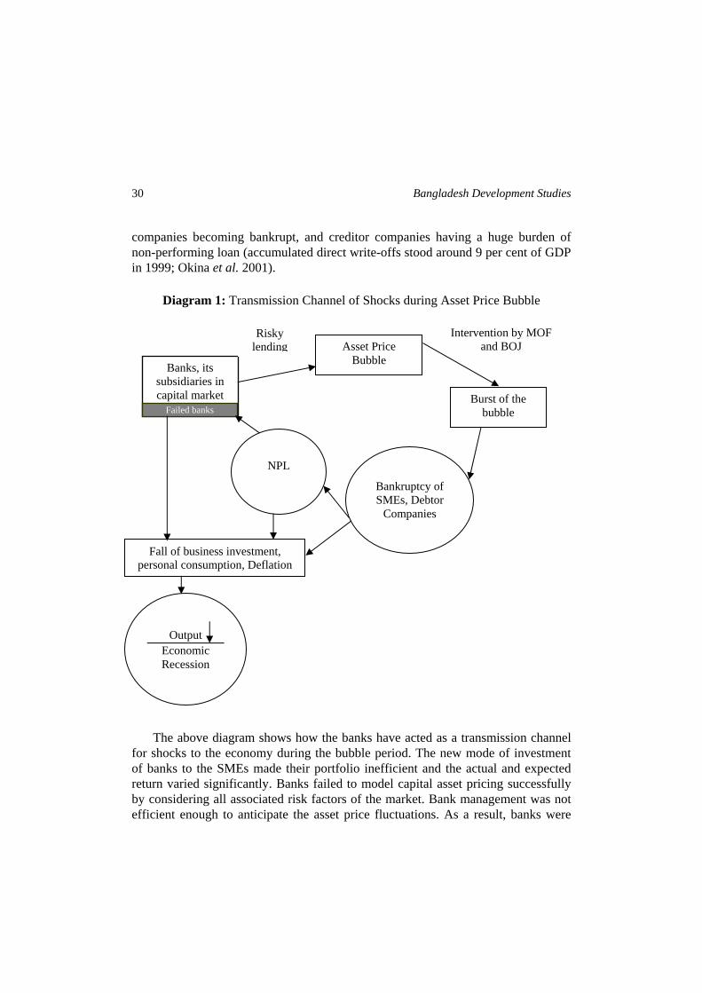
Diagram 1: Transmission Channel of Shocks during Asset Price Bubble
Banks, its subsidiaries in capital market
Failed banks
Asset Price Bubble
Burst of the bubble
Bankruptcy of SMEs, Debtor
Companies
NPL
Fall of business investment, personal consumption, Deflation
Output
Economic Recession
Risky lending
Intervention by MOF and BOJ
The above diagram shows how the banks have acted as a transmission channel
for shocks to the economy during the bubble period. The new mode of investment of banks to the SMEs made their portfolio inefficient and the actual and expected return varied significantly. Banks failed to model capital asset pricing successfully by considering all associated risk factors of the market. Bank management was not efficient enough to anticipate the asset price fluctuations. As a result, banks were
Hossain & Rafiq : Asset Price Bubble and Banks 31
burdened with huge amount of NPL due to bankruptcy of the debtor companies and incurred huge loss as the collateral assets became uncollectible due to continuing plunge of land/stock prices. This issue also pinpoints the moral hazard and adverse selection due to asymmetric information in the SME market.
It is evident from the discussion that if banks were not dependent on enterprise group and/or if they had been prepared for ongoing deregulatory measures, they would not have had undertaken speculative behaviour and would not suffer from moral hazard and adverse selection problems. This ultimately exhibited structural changes to the banking system accompanied by weak regulatory measures in Japan.
The Japanese banks were under downward pressure of profit during the heyday of the Japanese economy in the 1970s and got momentum after liberalisation started (Figure 1). Figure 1 shows that the declining trend of profitability of Japanese banks continued from 1970 to 1998 except a spike in 1989, at the time of bubble. The usual question is why banks’ profitability was declining during the high economic growth period of Japan? Were the banks ever caring about their declining trend of profit? Following the discussion in the previous sections, undirected liberalisation that led to frustration for the banks, along with downward pressure of profit, acted as catalyst for banks to behave aggressively during the asset price bubble period. It is therefore important to analyse the declining trend of profits in the backdrop of their activities during the bubble.
Figure 1: Japanese Banks Profitability during 1964-1998
-.80
-.60
-.40
-.20
.00
.20
.40
.60
.80
1964 1967 1970 1973 1976 1979 1982 1985 1988 1991 1994 1997
-25.00
-20.00
-15.00
-10.00
-5.00
.00
5.00
10.00
15.00
20.00
ROA(right scale) ROE(left scale)
Source: Authors’ estimation
There are some explanations on the declining trend of bank profitability. How the average profit of the main bank system was declining during the regulated
Bangladesh Development Studies
32
period can be explained as follows. “Over-loan”, that is, borrowing from the central bank with low discount rate and lending it to enterprises with high interest rate was one of the main sources of profitability of banks. City banks (larger banks) have lent more funds than they could raise through deposit mobilisation, while regional banks had surplus of budget. So there was an imbalance of fund. Sometimes, to meet up the enterprise groups’ excess demand for money, bank borrowed from call money market with high interest rate and lent it to its affiliated firm with the existing (usually lower) interest rate. This preferential loan contributed towards the declining trend of bank profit. Thus, borrowing short and lending long created a mismatch in the financial system as there are some maturity gap (exact data are not available) between the deposit fund and loan portfolio. This structural weakness affected profitability of the “main bank” system of Japan. Perhaps, banks were not much aware about the profit because they were competing amongst themselves for market share rather than profit (Yoshino and Sakakibara 2002), and they were backed by the group. Lending risk analysis could be biased due to the presence of directors of enterprise firms in banks. There is also possibility of window dressing6 in bank’s profit, which could overestimate the actual profit of banks.
With the pace of financial deregulation that started in the mid–1970s, capital market became more open to large firms and large firms’ dependency on banks’ borrowing gradually declined. The scope of cross-shareholding had also shrunk. As the banks lost their large corporate customers, they rushed to find new borrowers and projects. This situation compelled banks to think about the profitability for their survival and they found themselves in the surface of tough reality. Protracted monetary easing after Plaza Accord added fuel to their efforts of increasing short term profit.
Another factor is the Postal Saving Scheme that also contributed to the low profitability of banks as it created distortion in the financial market by paying higher interest rates than banks. The interest rates of the postal certificates are not determined by the market considering the risk and return. It is also not possible for banks to compete with postal savings by offering higher interest rates due to some unfavourable situations of the economy, such as deflation. This is an important issue for the financial sector of Japan as the deposit of Postal savings scheme stood at around 30 per cent of the total bank deposits due to its favourable interest rate (Yoshino 2000).
6Bank sometimes manipulate their financial statements to show an inflated position of their performance by taking favour from their own enterprise group. This unfair means is termed as Window Dressing.
Hossain & Rafiq : Asset Price Bubble and Banks 33
IV. DATA AND METHODOLOGY
The main objective of this paper is to analyse the profitability of Japanese banks and examine whether the monetary phenomenon and overheated economic activity had any influence on banks profitability. The profitability variable is represented by two alternative measures: the ratio of profits to assets, i.e. the return on assets (ROA) and the profits to equity ratio, i.e. the return on equity (ROE). In principle, ROA reflects the ability of a bank’s management to generate profits from the bank’s assets, although it may be biased due to off-balance-sheet activities. ROE indicates the return to shareholders on their equity and equals ROA times the total assets-to-equity ratio. The latter is often referred to as the bank’s equity multiplier, which measures financial leverage. Banks with lower leverage (higher equity) will generally report higher ROA, but lower ROE. Since an analysis of ROE disregards the greater risks associated with high leverage and financial leverage is often determined by regulation, ROA emerges as the key ratio for the evaluation of bank profitability (IMF 2002). Both ROA and ROE are measured as running year averages.7
To assess the effects of various factors on bank profitability, we choose only a few variables that are important in the light of our previous discussion. The regression model is specified as follows:
tittit MBROA ,, εδβα +++= (1)
where Bi,t is a vector of bank-specific variables at time t. Only total asset of banks is considered here to represent the bank size because economies of scale can lead bigger banks to operate with lower average costs, which could be an indicator of profitability irrespective of other condition. The logarithm of total asset is also a measure of bank size. Mt is a vector of time-varying macroeconomic variables, such as GDP growth, money supply (M2+CD) and central bank discount rate. Land price index is used as a proxy of asset price bubble. These variables are considered to capture the effects of macroeconomic and monetary phenomenon in the profitability of Japanese banks (Figure 2).The data are collected from the BoJ website and the IFS of the IMF.
Since we use the aggregate data for the period 1977-2002, macroeconomic variables are subject to time series properties. Therefore, we test the unit root properties of the macro and monetary variables by applying the Augmented Dickey-Fuller (ADF) test. The hypothesis of no unit root cannot be rejected at 5 per cent 7 Figure 1 presents ROA and ROE for the Japanese banking sector. The two ratios follow similar paths, increasing over time with a spike in 1999.
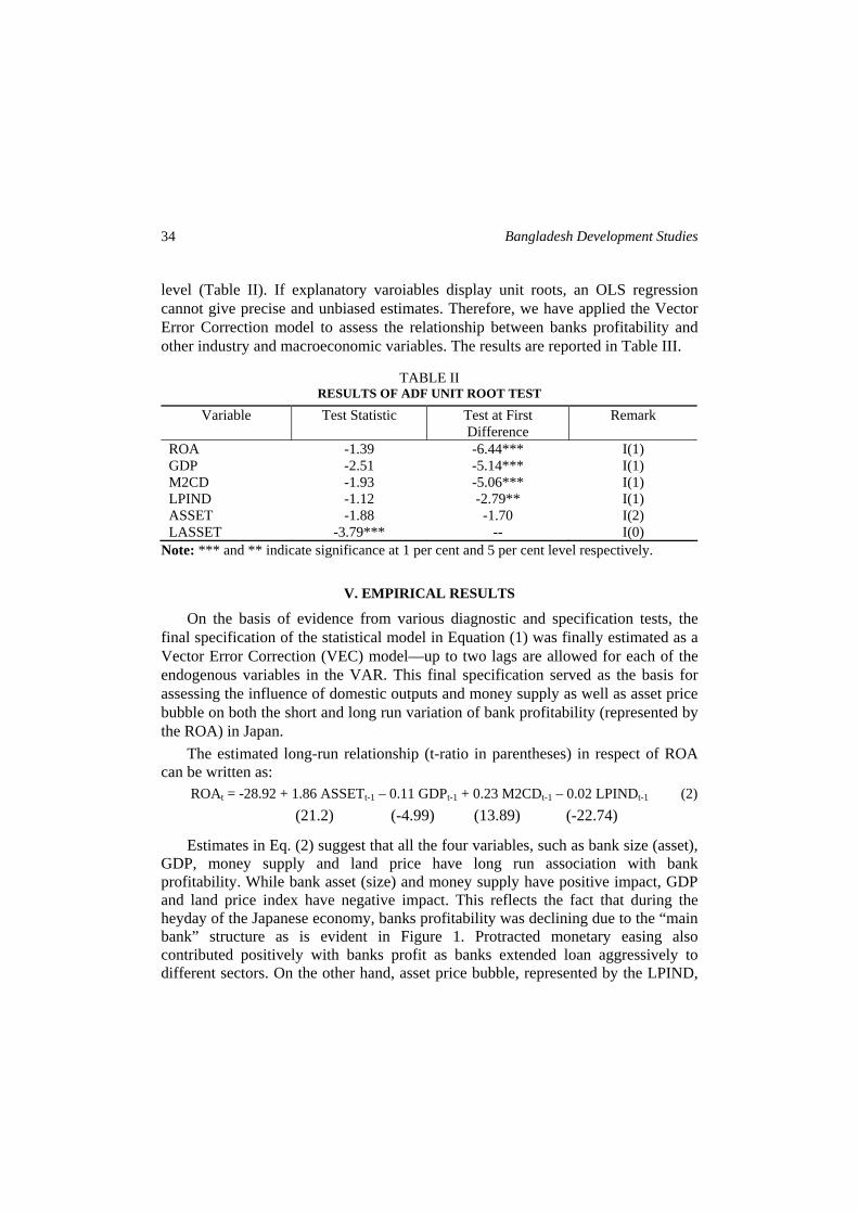
Bangladesh Development Studies
34
level (Table II). If explanatory varoiables display unit roots, an OLS regression cannot give precise and unbiased estimates. Therefore, we have applied the Vector Error Correction model to assess the relationship between banks profitability and other industry and macroeconomic variables. The results are reported in Table III.
TABLE II RESULTS OF ADF UNIT ROOT TEST
Variable Test Statistic Test at First Difference
Remark
ROA -1.39 -6.44*** I(1) GDP -2.51 -5.14*** I(1) M2CD -1.93 -5.06*** I(1) LPIND -1.12 -2.79** I(1) ASSET -1.88 -1.70 I(2) LASSET -3.79*** -- I(0)
Note: *** and ** indicate significance at 1 per cent and 5 per cent level respectively.
V. EMPIRICAL RESULTS
On the basis of evidence from various diagnostic and specification tests, the final specification of the statistical model in Equation (1) was finally estimated as a Vector Error Correction (VEC) model—up to two lags are allowed for each of the endogenous variables in the VAR. This final specification served as the basis for assessing the influence of domestic outputs and money supply as well as asset price bubble on both the short and long run variation of bank profitability (represented by the ROA) in Japan.
The estimated long-run relationship (t-ratio in parentheses) in respect of ROA can be written as:
ROAt = -28.92 + 1.86 ASSETt-1 – 0.11 GDPt-1 + 0.23 M2CDt-1 – 0.02 LPINDt-1 (2) (21.2) (-4.99) (13.89) (-22.74)
Estimates in Eq. (2) suggest that all the four variables, such as bank size (asset), GDP, money supply and land price have long run association with bank profitability. While bank asset (size) and money supply have positive impact, GDP and land price index have negative impact. This reflects the fact that during the heyday of the Japanese economy, banks profitability was declining due to the “main bank” structure as is evident in Figure 1. Protracted monetary easing also contributed positively with banks profit as banks extended loan aggressively to different sectors. On the other hand, asset price bubble, represented by the LPIND,
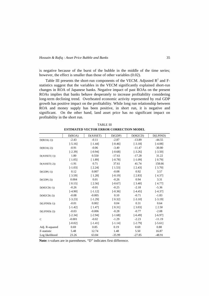
Hossain & Rafiq : Asset Price Bubble and Banks 35
is negative because of the burst of the bubble in the middle of the time series; however, the effect is smaller than those of other variables (0.02).
Table III presents the short-run components of the VECM. Adjusted R2 and F-statistics suggest that the variables in the VECM significantly explained short-run changes in ROA of Japanese banks. Negative impact of past ROAs on the present ROAs implies that banks behave desperately to increase profitability considering long-term declining trend. Overheated economic activity represented by real GDP growth has positive impact on the profitability. While long run relationship between ROA and money supply has been positive, in short run, it is negative and significant. On the other hand, land asset price has no significant impact on profitability in the short run.
TABLE III ESTIMATED VECTOR ERROR CORRECTION MODEL
D(ROA) D(ASSET) D(GDP) D(M2CD) D(LPIND) D(ROA(-1)) -2.43 -0.11 -2.87 -13.89 -44.55 [-5.16] [-1.44] [-0.46] [-3.18] [-4.08] D(ROA(-2)) -0.91 -0.06 -3.40 -11.47 -30.80 [-2.39] [-0.94] [-0.68] [-3.26] [-3.50] D(ASSET(-1)) 1.80 0.550 -17.61 -17.28 31.22 [ 1.05] [ 1.89] [-0.78] [-1.09] [ 0.79] D(ASSET(-2)) -1.91 0.71 37.61 41.74 158.66 [-1.03] [ 2.24] [ 1.53] [ 2.43] [ 3.70] D(GDP(-1)) 0.12 0.007 -0.08 0.92 3.57 [ 3.59] [ 1.28] [-0.19] [ 2.83] [ 4.37] D(GDP(-2)) 0.004 0.01 -0.26 0.94 3.31 [ 0.15] [ 2.56] [-0.67] [ 3.40] [ 4.77] D(M2CD(-1)) -0.26 -0.01 -0.25 -2.18 -5.36 [-4.90] [-1.12] [-0.36] [-4.45] [-4.37] D(M2CD(-2)) -0.08 -0.005 0.10 -0.71 -1.83 [-3.23] [-1.29] [ 0.32] [-3.10] [-3.19] D(LPIND(-1)) -0.01 0.002 0.04 0.31 0.64 [-1.42] [ 1.47] [ 0.31] [ 3.03] [ 2.50 D(LPIND(-2)) -0.03 -0.006 -0.28 -0.77 -2.08 [-2.34] [-2.94] [-1.68] [-6.49] [-6.97] C -0.001 -0.02 -1.29 -2.23 -11.19 [-0.02] [-1.41] [-1.14] [-2.79] [-5.61] Adj. R-squared 0.69 0.85 0.19 0.69 0.88 F-statistic 5.48 12.74 1.48 5.50 16.87 Log likelihood 23.26 63.84 -35.99 -27.85 -48.91
Note: t-values are in parentheses. “D” indicates first difference.
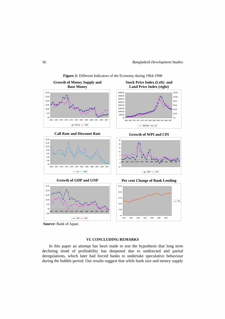
Bangladesh Development Studies
36
Figure 2: Different Indicators of the Economy during 1964-1998
Growth of Money Supply and Base Money
.00
5.00
10.00
15.00
20.00
25.00
30.00
1964 1967 1970 1973 1976 1979 1982 1985 1988 1991 1994 1997
M2+CD HPM
Call Rate and Discount Rate
.00
2.00
4.00
6.00
8.00
10.00
12.00
14.00
1964 1967 1970 1973 1976 1979 1982 1985 1988 1991 1994 1997
CR DISC
Growth of GDP and GNP
-5.00
.00
5.00
10.00
15.00
20.00
25.00
1964 1967 1970 1973 1976 1979 1982 1985 1988 1991 1994 1997
GNP GDP
Source: Bank of Japan.
Stock Price Index (Left) and Land Price Index (right)
.00
5000.00
10000.00
15000.00
20000.00
25000.00
30000.00
35000.00
40000.00
1964 1967 1970 1973 1976 1979 1982 1985 1988 1991 1994 1997.00
20.00
40.00
60.00
80.00
100.00
120.00
NIKK225 LPI
Growth of WPI and CPI
-10
-5
0
5
10
15
20
25
1964 1967 1970 1973 1976 1979 1982 1985 1988 1991 1994 1997
WPI CPI
Per cent Change of Bank Lending
.00
5.00
10.00
15.00
20.00
25.00
1978 1981 1984 1987 1990 1993 1996
BL
VI. CONCLUDING REMARKS
In this paper an attempt has been made to test the hypothesis that long term declining trend of profitability has deepened due to undirected and partial deregulations, which later had forced banks to undertake speculative behaviour during the bubble period. Our results suggest that while bank size and money supply
Hossain & Rafiq : Asset Price Bubble and Banks 37
have a positive and significant association with banks’ profitability, GDP growth has negative effect. Asset price bubble has negative effect on profitability in the long run; however, it has no significant short-run effect. This supports the assumption that asset price bubble has no such significant effect on bank profitability in the short run, rather long term declining trend of profitability due to the main banking system has had effect on banks aggressive behaviour during the bubble period. Monetary easing at that time also added fuel to the situation. The results also indicate that undirected financial liberalisation might have affected banks profitability, which ultimately led to a crisis after burst of the bubble.
Thus, the two issues—partial or undirected financial deregulation and monetary policy measures during the bubble period–were perceived to have contributed to the speculative behaviour of the banks. As discussed in the paper, the timing and pace of monetary policy measures to burst the bubble was not deemed as appropriate. This has led to the prolonged banking and economic crisis in Japan in the 1990s. The issue underscores the need for analysing the change in policies.
The case of Japan in the context of the rise and burst of the asset price bubble and subsequent banking crisis could be instructive for many countries including Bangladesh that are facing the asset price bubble situation. Bubbles generally arise out of some combination of irrational exuberance, jumps forward in technology and financial deregulation, for which the connection between monetary conditions and the rise of bubbles cannot be denied. Japanese experience suggests that monetary policy should respond to asset bubbles in a cautious and moderate manner in order to avoid economic distortions. The lessons that can be learned from the Japanese experience are: (i) central bank’s role to burst bubbles must depend on the degree of efficiency of the financial sector; and (ii) the speed to burst the bubble must be based on the overall economic situation.
REFERENCES
Aoki, M. and H.Patrick (eds.). 1994. The Japanese Main Bank System: Its Relevance for Developing and Transforming Economies. Oxford: Clarendon Press.
Caprio, Gerand, Folkert Landan and Lane Timothy D. 1994. Building Sound Finance in Emerging Market Economics. Proceeding of a conference held in Washington D.C., June 10-11, 1993, IMF.
Cargll, Thomas F. and Shoichi Royama. 1988. The Transition of Finance in Japan and the U.S. Stanford CA: Hoover Press.
Caves, R. and M. Uekusa. 1976. Industrial Organization in Japan. Brookings Institution.
Bangladesh Development Studies
38
Hossain, Monzur. 2005. “Can Japan Avert any Future Banking Crisis?” Applied Economics Letters (Taylor & Francis, UK), 12(7): 425-429.
Hoshi, T., A. Kashyap, and D. Scharfstein. 1991. “Corporate Structure, Liquidity and Investment: Evidence from Japanese Industrial Groups.” Quarterly Journal of Economics, 106 (February): 33-60.
IMF (International Monetary Fund). 2002. “Financial Soundness Indicators: Analytical Aspects and Country Practices.” Occasional Paper 212, Washington.
Ito, T. 1992. The Japanese Economy. MIT Press. Okabe, M. 2001. “Are Cross-shareholding of Japanese Corporations Dissolving? Evolution
and Implications.” Nissan Occasional Paper Series No. 33. Okina, K. et al. 2001. “The Asset Price Bubble and Monetary Policy: Japan’s Experience in
the Late 1980s and the Lessons.” Monetary and Economic Studies (Special Edition), February.
Suzuki, Y. 1987. The Japanese Financial System. Oxford: Clarendon Press. Wallich, H. and M.Wallich. 1976. “Banking and Finance.” Chapter 4 of the book “Asia’s
New Giant- How the Japanese Economy Works”, eds. H.Patrick and H. Rosovosky. The Brookings Institution.
Yoshino, N. 2000. “Japan’s Financial System, Asian Financial Crisis.” In Economic Issues in Contemporary Japan: Money, Banking and Foreign Investment, by N Yoshino, M. Kuhara, M.Lacktorin, and R.Kopp. YUHIKAKU.
Yoshino, N. and E. Sakakibara 2002. The Current State of the Japanese Economy and Remedies. Asian Economic Papers. MIT press.
Bangladesh Development Studies Vol. XXXIV, March 2011, No. 1
Money-Income Causality in Bangladesh: An Error Correction Approach
MOHAMMAD AMZAD HOSSAIN*
The causal relationship between money and income remains a contentious and lively issue in the literature. Even though the literature on this issue is voluminous, however, for Bangladesh it is quite nascent. A few earlier studies suffer from methodological deficiency as they did not take into consider the time series properties of the variables. The objective of this paper is to look on the causality between money and income in Bangladesh. The paper differs from the earlier ones regarding data used and econometric techniques applied. The main contribution of the paper is to address the issue of short run dynamics of the money income relationship within a long run relationship. The empirical results show that money supply and income are cointegrated, implying that there is stable long run relationship between them. The estimated error correction model shows that there is bidirectional causality between money and income, implying that monetary policy should be undertaken to realise the basic macroeconomic goals of achieving higher level of output.
I. INTRODUCTION
The explanatory power of money over aggregate economic activity remains a contentious and empirical issue in the literature. The causal nexus between money supply and output has an important implication for the theoretical debate on whether money matters. Besides, the conduct of monetary policy with the aim of macroeconomic stabilisation hinges upon, among other things, whether money is causally linked to the ultimate policy goals. However, to achieve higher output, full employment and price level stability based on controlling the growth of money supply crucially depends on two prerequisites: first, development of an effective procedure for controlling the rate of growth of money stock and second, close identification of the linkages between the desired growth rate of money and the final * Associate Professor, Department of Economics, Jahangirnagar University, Savar, Dhaka, Bangladesh. This paper is based on author’s research monograph submitted to the University Grants Commission of Bangladesh, Dhaka. The author wishes to thank the UGC for funding the project.
Bangladesh Development Studies
40
objectives (Zaki 1995). Despite a large and growing body of theoretical and empirical literature, there has not emerged any consensus regarding the overall evidence of causality.
A good number of studies have been conducted on the money and in real economic activity both in developed and developing countries; however, for Bangladesh it is quite nascent. A few early studies conducted by Jones and Sattar (1988) and Chowdhury, Dao and Wahid (1995) suffer from methodological deficiency as they did not take into consider the time series properties of the variables. The salient aim of this paper is to take another look at the causality between money supply and the output growth. This paper differs from the existing studies in the following ways. First, we use a most recent quarterly data set over the period 1974-2008 to examine the dynamic linkage between money and income.
Second, the analysis is intended to be comprehensive in that it takes into account of various modeling issues that arise in causality framework. It studied the stationary properties of the considered variables in the context of Bangladesh. The paper also applied Augmented Dicky Fuller (ADF) and Phillips-Perron (PP) tests to examine the time series properties of money supply and income. Johansen and Juselius test has been applied to examine the cointegration properties of the variables.
Finally, the paper examines both short-term and long-term dynamic relationships between the considered variables within an error-correction framework. By and large, this paper is an improvement over the existing literature on money supply and other variables in terms of the data used and techniques employed.
This paper is divided into five sections. Following introduction, a survey of the literature is presented in section II. Section III sets out the framework for the analysis of causality, conintegration and error correction models. It also identifies and defines the variable considered. Section IV examines and discusses the time series properties of the variables. Finally, section V concludes the paper.
II. REVIEW OF THE LITERATURE
II.1 Theoretical Debate
There has been a long debate in the literature on the causal nexus among money, income and prices, which dates back to 1752 following the publication of David Hume’s “Of Money”. Hume concludes that there exists a proportional relationship between money supply and the absolute price level. The classical
Hossain: Money-Income Causality in Bangladesh 41
school explained that changes in prices, the most important target variable in achieving stabilisation, is basically due to changes in money supply. However, Keynesians criticised and rejected the proportionality between money supply and prices due to its instability in explaining the causes and remedies for the great economic debacle like Great Depression of 1930s. The Keynesians held the view that money does not play an active role in changing income and prices nor does it causes instability in the economy. According to them, it is not the quantity of money but the effective demand which is caused by autonomous spending, that constitutes investment by business and government spending is the main source of instability. In fact, a change in money supply is diluted by the opposite change in the velocity. Thus the change in wages, the price level and the rate of inflation are non-monetary phenomena and are caused by structural factors. However, they believe that change in income causes changes in money stock via demand for money implying that the direction of causation runs from income to money without any feedback (Froyen 2004).
The Keynesian ideas came under serious criticism by Monetarists (lead by Milton Friedmen) in the backdrop of the presence of high inflation in different countries after World War II due to the adoption of cheap monetary policy. The Monetarists argue that money plays an active role and leads to the changes in income and prices. There is unidirectional causation that runs from money to income and prices. The argument is that for increasing expenditure (without increase in taxes) government adopts cheap monetary policy i.e. print money which accrues in the hands of taxpayers which leads to the persistent rise in the price level. This argument attributes to the Monetarists contention that inflation is always and everywhere a monetary phenomena (Blanchard, Johnson and Melino 2003). The proponent of Monetarists is the New Classical School / Rational Expectation School, which argues that money supply along with information asymmetries causes the change in income and prices. While the opponent is the Real Business Cycle School/New Classical Macro Economics, which treats money supply as endogenous and concludes that monetary policy is irrelevant. They held the view that neither the money supply nor the information asymmetries but the random change in production technology (i.e. technological shock) is the dominant source of changes in the income and price level in the economy. The Banking School also treats money supply as an endogenous variable which depends on business condition. That is money supply passively responds to the demand for it (Blanchard, Johnson and Melino 2003).
The unidirectional causation from money to income and prices has challenged in the last decades. Fischer (1962) claims the possibility of reverse causation and
Bangladesh Development Studies
42
concludes that there is mutual interaction between money and other macro variables. Friedman and Schwartz (1963) also support this argument by stating that though the influence of money to economic activity is predominant, there is also the possibility of influences running the other way (at least in the short run). The Banking school also supports the reverse causation between money and income, thereby arguing for endogeneity of money supply (Froyen 2004).
The above discussion reveals that there is a linkage between money and aggregate output in the economy. However, it is not clear whether the causality is unidirectional or bidirectional. This debate is further intensified by the empirical studies.
II.2 Empirical Studies Sims (1972) has opened up the new and active area of research on the empirical
causal relationship between money and income. Based on Granger causality, Sims developed a test of causality and applied it to the U.S. data and found the evidence of unidirectional causality between money to income as claimed by the Monetarists. However, this result was challenged by the succeeding studies. By applying the Sims test in Canadian economy Barth and Bennett (1974) found bidirectional causality between money and income. Applying Sims test to the U.K. data Williams, Goodhart and Gowland (1976) found unidirectional causality from income to money, which is opposite of the Sims U.S. result. However, Sims result was supported by Brillembourg and Khan (1979) who use a longer data set. Analysing the Canadian data Hasio (1979) found feedback between money supply (M1) and GNP, while unidirectional causal flow from money to income, when M2 is used as measure of money. Hasio (1981) also found the same result from U.S. money and income data. Using the data set for six industrialised countries Dyreyes, Starleaf and Wang (1980) found bidirectional causality between money and income in the U.S., while they found unidirectional causality from money to income in Canada, contrary to Barth and Bennett (1974). However, they got the unidirectional causality from income to money in the U.K., which supports the result of Williams. Goodhart and Gowland (1976). Biswas and Saunders (1988) provide further empirical evidence on the money-income relationship from the U.S. data which supports Sims.
Using Singapore data Lee and Li (1983) found bidirectional causality between income and money and unidirectional causality from money to prices. Joshi and Joshi (1985) found bidirectional causality between money and income in India, while for the same country Rangarajan and Arif (1990) found unidirectional causality from money to income. Biswas and Saunders (1999) found that income
Hossain: Money-Income Causality in Bangladesh 43
and money supply are cointegrated in India. Thus, establishing a stable relationship between these two variables over longer time period. Upon establishment of cointegration between money and income this study conducted error correction estimates and found the existence of feedback between the two variables. Khan and Siddiqui (1990) found unidirectional causality from income to money in Pakistan. Using Geweke’s approach Kee-Giap Tan and Chee-seng (1995) found bidirectional causality between money and income in Malaysia. This result supports Zubaidi and Yusop (1996).
Some of the recent studies also establish the causal relationship among money, income and price. Using time series data from 1960 to 2008 Climobi and Uche. (2010) found that M2 appears to have a strong unidirectional causal effect on the real output as well as on prices. The similar result has also found by Majid (2007) for the Malaysian economy. Yadav (2009) examined the cointegration and causality between money and income for the Indian economy. Using the data for the period 1950/51-2006/07 the study found the bidirectional causality between GNP and money supply. Psaradakis, Morten and Mortin (2002) applied different econometric techniques to examine the money output relationship. Using a VAR model with time varying parameters for the U.S. data for the period 1959:1-2001:2 the paper found that causality relationship between money and output changes over time.
II.3 The Bangladesh Perspective As to the empirical evidence on Bangladesh, there are a few studies (Jones and
Sattar 1988, Chowdhury, Dao and Wahid 1995, Ahmed 2000) linking money, prices, income and interest rate, but no substantial study using appropriate econometric methodology considering the time series properties of data.
With the aid of Granger causality test based on monthly data (June 1974 through December 1985), Jones and Sattar (1988) were able to examine the causal link between money–income and money–inflation in Bangladesh. Using several arbitrary lag lengths they concluded that money causes prices in Bangladesh in the short run, with a lag in general of twelve month, which disappears in the long run. They also found the evidence of unidirectional impact of money on output, with a lag of twenty four to thirty six months. The implication of their result is that monetary expansion could have a significant impact on output growth, although as a consequence the economy may experience moderate to high inflation in the short run.
By applying multivariate vector autoregressive (VAR) model Chowdhury, Dao and Wahid (1995) explore the relationship between money, prices, output and the
Bangladesh Development Studies
44
exchange rate in Bangladesh. Using quarterly data for the period 1974 to 1992 the study concluded that the inflationary process of Bangladesh cannot be explained solely by the “monetarist” or the “structuralist” explanation. That is, there is no straightforward cause and effect relationship between money and inflation, while money supply exerts a significant unidirectional impact on real output.
Ahmed (2000) attempts to investigate the issue of multivariate causality among money, interest rate, prices and output for three South Asian countries namely, Bangladesh, India and Pakistan in a multivariate framework using quarterly data for the period 1967-1996 for India, 1972-1997 for Pakistan and 1974-1998 for Bangladesh. The study concludes that monetary policy has crucial importance in determining output in Bangladesh. This study also found that interest rate and money as block cause output and price but output and price do not cause interest and money in Bangladesh.
It is evident from the above studies that causal relationship between money and income is unidirectional in Bangladesh. However, the reliability of the above result may be undermined as they did not examine the time series properties of the data such as stationarity and co-integration and using arbitrary lag length they conclude whether the relationship among variables is short run or long run. This study is an improvement over the existing studies as it examined the stationarity and co-integration approach and applied the error correction approach to understand the short run implication of long run relationship among considered variables. Consequently, two issues need to be considered. The first issue is the existence of stability of the relationship between money and income over longer period of time. It is important to determine whether a stable relationship between monetary changes and nominal income changes in the long run. If so, then monetary policy will have important implications on the Bangladesh economy in the long run. The second issue is related to the impact of monetary changes on nominal income in the short run. The subject matter of this study is to provide short run dynamics of the money-income relationship in Bangladesh, i.e. how do money affect nominal income in the short run.
III. DATA AND METHODOLOGY
III.1 Data This study is based on annual data covering 1974 to 2008 taken from the IMF,
International Financial Statistics (IFS) CD-Rom supplemented by IMF, IFS Yearbook. Some of the early literature (Ibrahim 1999) shows that M2 is a preferable intermediate target to stabilise the economy and M2 is found to be cointegrated with other macrovariables and is thus superior as a long run policy variable; while Jones
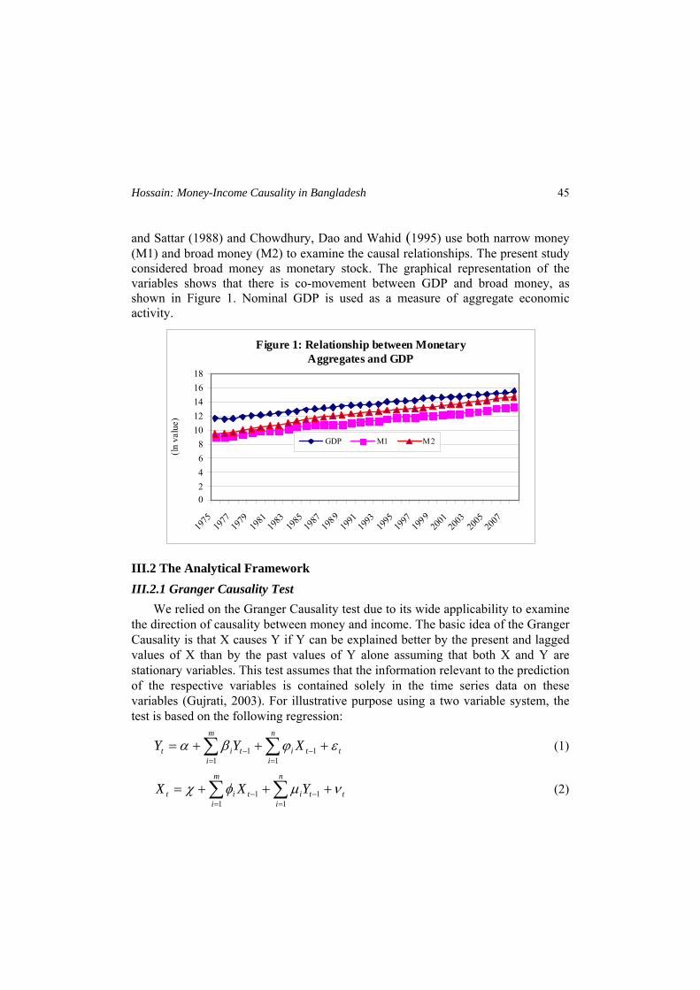
Hossain: Money-Income Causality in Bangladesh 45
and Sattar (1988) and Chowdhury, Dao and Wahid (1995) use both narrow money (M1) and broad money (M2) to examine the causal relationships. The present study considered broad money as monetary stock. The graphical representation of the variables shows that there is co-movement between GDP and broad money, as shown in Figure 1. Nominal GDP is used as a measure of aggregate economic activity.
Figure 1: Relationship between Monetary Aggregates and GDP
02468
1012141618
1975
1977
1979
1981
1983
1985
1987
1989
1991
1993
1995
1997
1999
2001
2003
2005
2007
(ln v
alue
)
GDP M1 M2
III.2 The Analytical Framework III.2.1 Granger Causality Test
We relied on the Granger Causality test due to its wide applicability to examine the direction of causality between money and income. The basic idea of the Granger Causality is that X causes Y if Y can be explained better by the present and lagged values of X than by the past values of Y alone assuming that both X and Y are stationary variables. This test assumes that the information relevant to the prediction of the respective variables is contained solely in the time series data on these variables (Gujrati, 2003). For illustrative purpose using a two variable system, the test is based on the following regression:
∑ ∑= =
−− +++=m
i
n
ittitit XYY
1 111 εϕβα (1)
∑ ∑= =
−− +++=m
i
n
ittitit YXX
1 111 νμφχ (2)
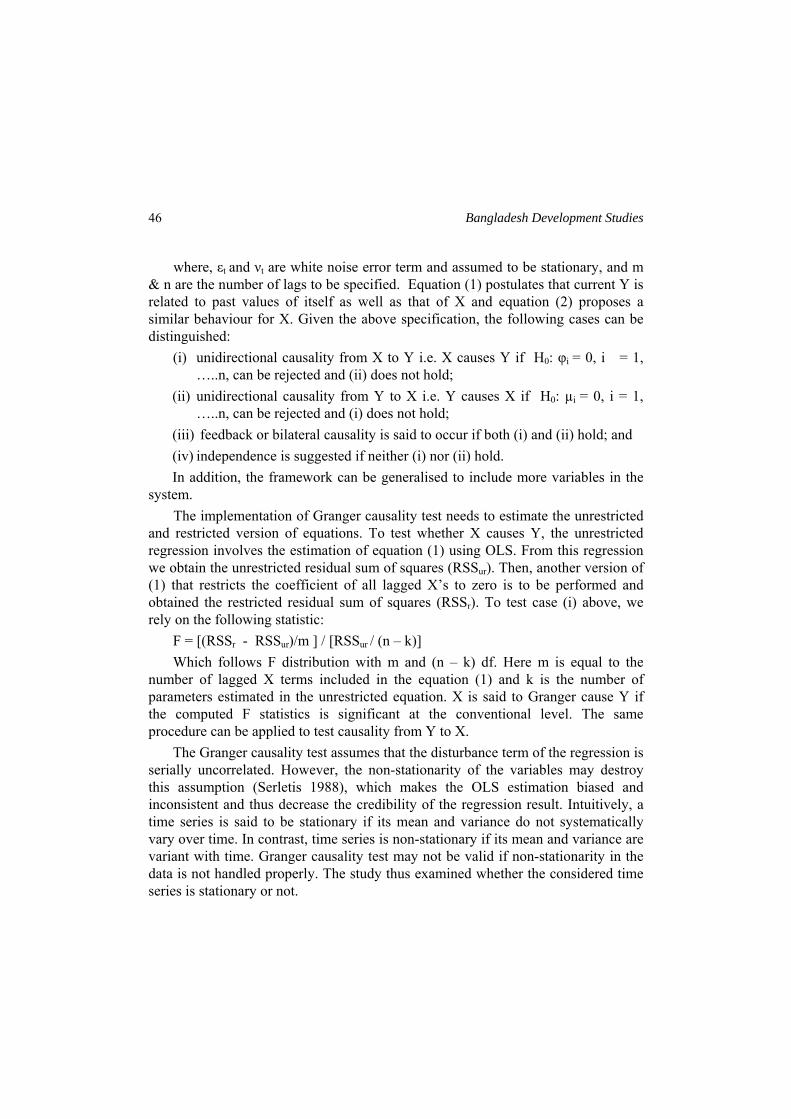
Bangladesh Development Studies
46
where, εt and νt are white noise error term and assumed to be stationary, and m & n are the number of lags to be specified. Equation (1) postulates that current Y is related to past values of itself as well as that of X and equation (2) proposes a similar behaviour for X. Given the above specification, the following cases can be distinguished:
(i) unidirectional causality from X to Y i.e. X causes Y if H0: φi = 0, i = 1, …..n, can be rejected and (ii) does not hold;
(ii) unidirectional causality from Y to X i.e. Y causes X if H0: µi = 0, i = 1, …..n, can be rejected and (i) does not hold;
(iii) feedback or bilateral causality is said to occur if both (i) and (ii) hold; and (iv) independence is suggested if neither (i) nor (ii) hold. In addition, the framework can be generalised to include more variables in the
system. The implementation of Granger causality test needs to estimate the unrestricted
and restricted version of equations. To test whether X causes Y, the unrestricted regression involves the estimation of equation (1) using OLS. From this regression we obtain the unrestricted residual sum of squares (RSSur). Then, another version of (1) that restricts the coefficient of all lagged X’s to zero is to be performed and obtained the restricted residual sum of squares (RSSr). To test case (i) above, we rely on the following statistic:
F = [(RSSr - RSSur)/m ] / [RSSur / (n – k)] Which follows F distribution with m and (n – k) df. Here m is equal to the
number of lagged X terms included in the equation (1) and k is the number of parameters estimated in the unrestricted equation. X is said to Granger cause Y if the computed F statistics is significant at the conventional level. The same procedure can be applied to test causality from Y to X.
The Granger causality test assumes that the disturbance term of the regression is serially uncorrelated. However, the non-stationarity of the variables may destroy this assumption (Serletis 1988), which makes the OLS estimation biased and inconsistent and thus decrease the credibility of the regression result. Intuitively, a time series is said to be stationary if its mean and variance do not systematically vary over time. In contrast, time series is non-stationary if its mean and variance are variant with time. Granger causality test may not be valid if non-stationarity in the data is not handled properly. The study thus examined whether the considered time series is stationary or not.
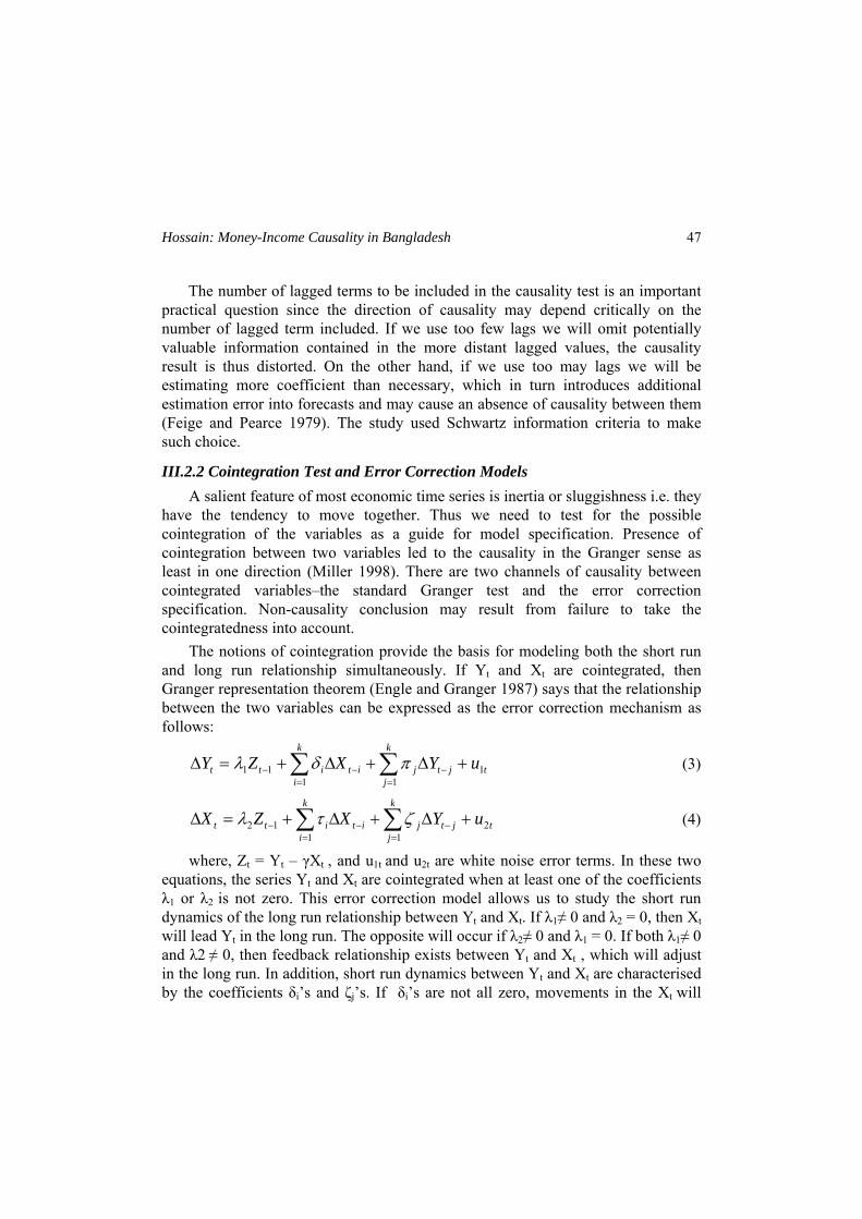
Hossain: Money-Income Causality in Bangladesh 47
The number of lagged terms to be included in the causality test is an important practical question since the direction of causality may depend critically on the number of lagged term included. If we use too few lags we will omit potentially valuable information contained in the more distant lagged values, the causality result is thus distorted. On the other hand, if we use too may lags we will be estimating more coefficient than necessary, which in turn introduces additional estimation error into forecasts and may cause an absence of causality between them (Feige and Pearce 1979). The study used Schwartz information criteria to make such choice.
III.2.2 Cointegration Test and Error Correction Models A salient feature of most economic time series is inertia or sluggishness i.e. they
have the tendency to move together. Thus we need to test for the possible cointegration of the variables as a guide for model specification. Presence of cointegration between two variables led to the causality in the Granger sense as least in one direction (Miller 1998). There are two channels of causality between cointegrated variables–the standard Granger test and the error correction specification. Non-causality conclusion may result from failure to take the cointegratedness into account.
The notions of cointegration provide the basis for modeling both the short run and long run relationship simultaneously. If Yt and Xt are cointegrated, then Granger representation theorem (Engle and Granger 1987) says that the relationship between the two variables can be expressed as the error correction mechanism as follows:
∑ ∑= =
−−− +Δ+Δ+=Δk
i
k
jtjtjititt uYXZY
1 1111 πδλ (3)
∑ ∑= =
−−− +Δ+Δ+=Δk
i
k
jtjtjititt uYXZX
1 1212 ζτλ (4)
where, Zt = Yt – γXt , and u1t and u2t are white noise error terms. In these two equations, the series Yt and Xt are cointegrated when at least one of the coefficients λ1 or λ2 is not zero. This error correction model allows us to study the short run dynamics of the long run relationship between Yt and Xt. If λ1≠ 0 and λ2 = 0, then Xt will lead Yt in the long run. The opposite will occur if λ2≠ 0 and λ1 = 0. If both λ1≠ 0 and λ2 ≠ 0, then feedback relationship exists between Yt and Xt , which will adjust in the long run. In addition, short run dynamics between Yt and Xt are characterised by the coefficients δi’s and ζj’s. If δi’s are not all zero, movements in the Xt will
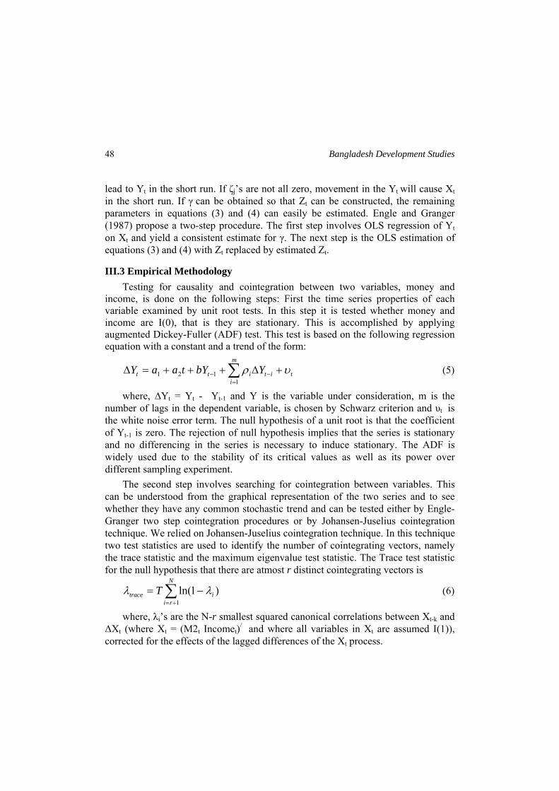
Bangladesh Development Studies
48
lead to Yt in the short run. If ζj’s are not all zero, movement in the Yt will cause Xt in the short run. If γ can be obtained so that Zt can be constructed, the remaining parameters in equations (3) and (4) can easily be estimated. Engle and Granger (1987) propose a two-step procedure. The first step involves OLS regression of Yt on Xt and yield a consistent estimate for γ. The next step is the OLS estimation of equations (3) and (4) with Zt replaced by estimated Zt.
III.3 Empirical Methodology Testing for causality and cointegration between two variables, money and
income, is done on the following steps: First the time series properties of each variable examined by unit root tests. In this step it is tested whether money and income are I(0), that is they are stationary. This is accomplished by applying augmented Dickey-Fuller (ADF) test. This test is based on the following regression equation with a constant and a trend of the form:
∑=
−− +Δ+++=Δm
itititt YbYtaaY
1121 υρ (5)
where, ∆Yt = Yt - Yt-1 and Y is the variable under consideration, m is the number of lags in the dependent variable, is chosen by Schwarz criterion and υt is the white noise error term. The null hypothesis of a unit root is that the coefficient of Yt-1 is zero. The rejection of null hypothesis implies that the series is stationary and no differencing in the series is necessary to induce stationary. The ADF is widely used due to the stability of its critical values as well as its power over different sampling experiment.
The second step involves searching for cointegration between variables. This can be understood from the graphical representation of the two series and to see whether they have any common stochastic trend and can be tested either by Engle-Granger two step cointegration procedures or by Johansen-Juselius cointegration technique. We relied on Johansen-Juselius cointegration technique. In this technique two test statistics are used to identify the number of cointegrating vectors, namely the trace statistic and the maximum eigenvalue test statistic. The Trace test statistic for the null hypothesis that there are atmost r distinct cointegrating vectors is
∑+=
−=N
riitrace T
1
)1ln( λλ (6)
where, λi’s are the N-r smallest squared canonical correlations between Xt-k and ΔXt (where Xt = (M2t Incomet)/ and where all variables in Xt are assumed I(1)), corrected for the effects of the lagged differences of the Xt process.
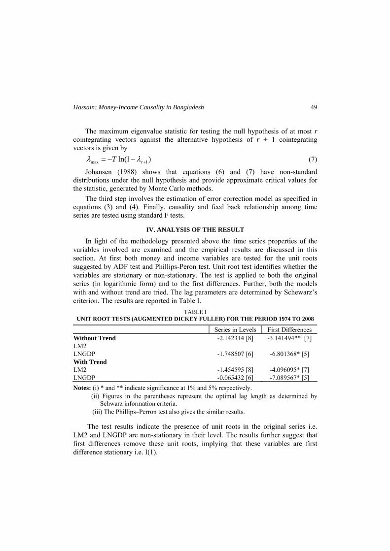
Hossain: Money-Income Causality in Bangladesh 49
The maximum eigenvalue statistic for testing the null hypothesis of at most r cointegrating vectors against the alternative hypothesis of r + 1 cointegrating vectors is given by
)1ln( 1max +−−= rT λλ (7)
Johansen (1988) shows that equations (6) and (7) have non-standard distributions under the null hypothesis and provide approximate critical values for the statistic, generated by Monte Carlo methods.
The third step involves the estimation of error correction model as specified in equations (3) and (4). Finally, causality and feed back relationship among time series are tested using standard F tests.
IV. ANALYSIS OF THE RESULT
In light of the methodology presented above the time series properties of the variables involved are examined and the empirical results are discussed in this section. At first both money and income variables are tested for the unit roots suggested by ADF test and Phillips-Peron test. Unit root test identifies whether the variables are stationary or non-stationary. The test is applied to both the original series (in logarithmic form) and to the first differences. Further, both the models with and without trend are tried. The lag parameters are determined by Schewarz’s criterion. The results are reported in Table I.
TABLE I UNIT ROOT TESTS (AUGMENTED DICKEY FULLER) FOR THE PERIOD 1974 TO 2008
Series in Levels First Differences Without Trend -2.142314 [8] -3.141494** [7] LM2 LNGDP -1.748507 [6] -6.801368* [5] With Trend LM2 -1.454595 [8] -4.096095* [7] LNGDP -0.065432 [6] -7.089567* [5] Notes: (i) * and ** indicate significance at 1% and 5% respectively. (ii) Figures in the parentheses represent the optimal lag length as determined by Schwarz information criteria. (iii) The Phillips–Perron test also gives the similar results.
The test results indicate the presence of unit roots in the original series i.e. LM2 and LNGDP are non-stationary in their level. The results further suggest that first differences remove these unit roots, implying that these variables are first difference stationary i.e. I(1).
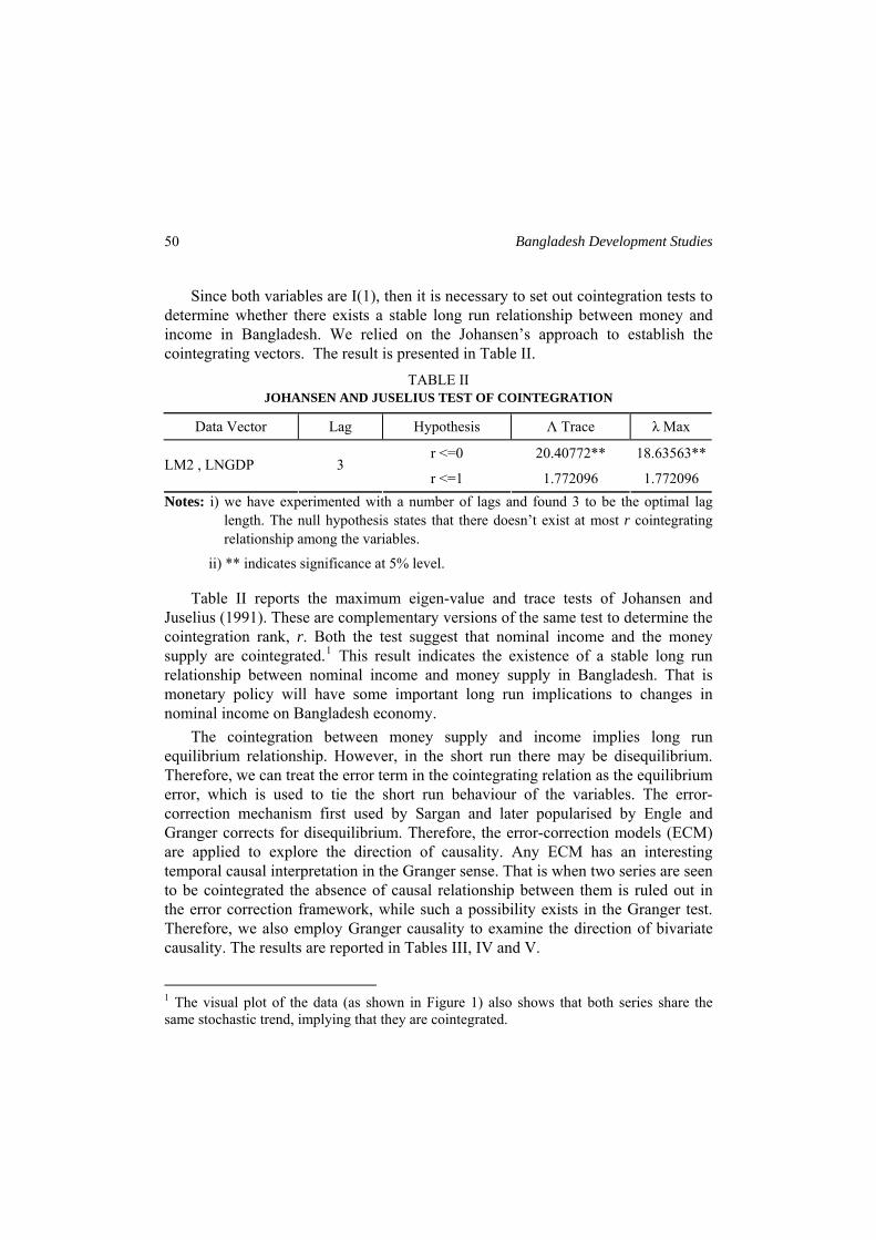
Bangladesh Development Studies
50
Since both variables are I(1), then it is necessary to set out cointegration tests to determine whether there exists a stable long run relationship between money and inco
GRATION
Data Vector Lag s Λ Trace λ Max
me in Bangladesh. We relied on the Johansen’s approach to establish the cointegrating vectors. The result is presented in Table II.
TABLE II JOHANSEN AND JUSELIUS TEST OF COINTE
Hypothesi
r <=0 20.40772** 18.63563** LM2
1 , LNGDP 3
r <=1 1.772096 .772096Notes: i) we ha
lengthve experime d with a num lags and f th . The null hy hesis states ere doesn’t st r c
ii)
Ta lue and trace tests of Johansen and Juselius (1991). These ar ons of the same test to determine the coin
short run there may be disequilibrium. The
ntepot
ber of ound 3 to be e optimal lag that th exist at mo ointegrating
relationship among the variables.
** indicates significance at 5% level.
ble II reports the maximum eigen-vae complementary versi
tegration rank, r. Both the test suggest that nominal income and the money supply are cointegrated.1 This result indicates the existence of a stable long run relationship between nominal income and money supply in Bangladesh. That is monetary policy will have some important long run implications to changes in nominal income on Bangladesh economy.
The cointegration between money supply and income implies long run equilibrium relationship. However, in the
refore, we can treat the error term in the cointegrating relation as the equilibrium error, which is used to tie the short run behaviour of the variables. The error-correction mechanism first used by Sargan and later popularised by Engle and Granger corrects for disequilibrium. Therefore, the error-correction models (ECM) are applied to explore the direction of causality. Any ECM has an interesting temporal causal interpretation in the Granger sense. That is when two series are seen to be cointegrated the absence of causal relationship between them is ruled out in the error correction framework, while such a possibility exists in the Granger test. Therefore, we also employ Granger causality to examine the direction of bivariate causality. The results are reported in Tables III, IV and V.
1 The visual plot of the data (as shown in Figure 1) also shows that both series share the same stochastic trend, implying that they are cointegrated.
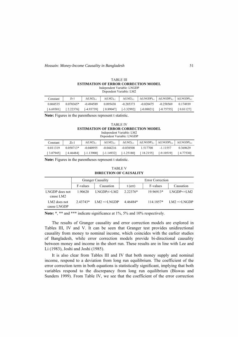
Hossain: Money-Income Causality in Bangladesh 51
TABLE III ESTIMATION OF ERROR CORRECTION MODEL
Independent Variable: LNGDP Depen LM2
Constant Zt-1 NGDP)t-2 Δ(LNGDP)t-3
dent Variable:
Δ(LM2)t-1 Δ(LM2)t-2 Δ(LM2)t-3 Δ(LNGDP)t-1 Δ(L
0.068535 0.070365* -0.494589 -0.020475 -0.258569 0.174939 0.095438 -0.285373 [ 6.693 [ 2.223 [- [ 0.890 [- [- 01] 76] 4.93739] 47] 3.32992] 0.08821] [-0.75755] [ 0.81127]
N re re p at
ECTION MODEL Independent Variable: LM2
Depend NGDP
Constant Zt-1 t-2 Δ(LNGDP)t-3
ote: Figu s in the pa ntheses re resent t st istic.
TABLE IV ESTIMATION OF ERROR CORR
ent Variable: L
Δ(LM2)t-1 Δ(LM2)t-2 Δ(LM2)t-3 Δ(LNGDP)t-1 Δ(LNGDP)
0.011319 0.050713* -0.040955 1.517708 -1.11557 0.369629 -0.044216 -0.038508 [ 3.079 [ 4.464 [- [- [- [ [- 45] 84] 1.13900] 1.14932] 1.25180] 18.2155] 9.10519] [ 4.77530]
N re r ep at
ALITY
Granger Causality Error Correction
ote: Figu s in the pa entheses r resent t st istic.
TABLE V DIRECTION OF CAUS
F-values F-values Causation Causation t (err)
LNGDP does not caus M2
1.9 LM2 2.22376* 19.96913* e L
0620 LNGDP≠> LNGDP=>LM2
LM2 does not cause LNGDP
2.43743* LM2 =>LNGDP 4.46484* 114.1857* LM2 =>LNGDP
N *** si , % re
unidirectional
cau
m long run equilibrium. The coefficient of the erro
ote: *, ** and indicate gnificance at 1% 5% and 10 spectively.
The results of Granger causality and error correction models are explored inTables III, IV and V. It can be seen that Granger test provides
sality from money to nominal income, which coincides with the earlier studies of Bangladesh, while error correction models provide bi-directional causality between money and income in the short run. These results are in line with Lee and Li (1983), Joshi and Joshi (1985).
It is also clear from Tables III and IV that both money supply and nominal income, respond to a deviation fro
r correction term in both equations is statistically significant, implying that both variables respond to the discrepancy from long run equilibrium (Biswas and Sunders 1999). From Table IV, we see that the coefficient of the error correction
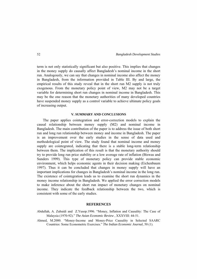
Bangladesh Development Studies
52
term is not only statistically significant but also positive. This implies that changes in the money supply do causally affect Bangladesh’s nominal income in the short run. Analogously, we can say that changes in nominal income also affect the money in Bangladesh, from the information provided in Table III. By and large, the empirical results of this study reveal that in the short run M2 supply is not truly exogenous. From the monetary policy point of view, M2 may not be a target variable for determining short run changes in nominal income in Bangladesh. This may be the one reason that the monetary authorities of many developed countries have suspended money supply as a control variable to achieve ultimate policy goals of increasing output.
V. SUMMARY AND CONCLUSIONS
The paper applies cointegration and error-correction models to explain the causal relationship between ominal income in Bangladesh. The main the issue of both short run
Abdullah, A. Zubaidi and Z.Yusop.1996. “Money, Inflation and Causality: The Case of Malaysia (1970-92).” The Asi , XXXVIII: 44-51.
Ahmed, M.2000. “Money-Income and Money-Price Causality in Selected SAARC
money supply (M2) and n contribution of the paper is to address
and long run relationship between money and income in Bangladesh. The paper is an improvement over the early studies in the sense of data used and methodological point of view. The study found that nominal income and money supply are cointegrated, indicating that there is a stable long-term relationship between them. The implication of this result is that the monetary authority should try to provide long run price stability or a low average rate of inflation (Biswas and Sunders 1999). This type of monetary policy can provide stable economic environment, which helps economic agents in their decision making (Eichenbaum 1997). Thus it can be concluded that changes in money supply will have an important implications for changes in Bangladesh’s nominal income in the long run. The existence of cointegration leads us to examine the short run dynamics in the money income relationship in Bangladesh. We applied the error correction models to make inference about the short run impact of monetary changes on nominal income. They indicate the feedback relationship between the two, which is consistent with some of the early studies.
REFERENCES
an Economic Review
Countries: Some Econometric Exercises.” The Indian Economic Journal, 50 (1).
Hossain: Money-Income Causality in Bangladesh 53
Barth, J. and J.Bannett.1974. “The Role of Money in the Canadian Economy: An Empirical Test.” Canadian Journal of Economics, 30(6)
Bhanumurthy, N.R. and T. M Paul.2000. “Money Supply, Output and Price Level Relationship in India.” The Indian Economic Journal, 47 (1)
Bangladesh: A Dynamic Analysis.” Applied Economic Letters, 2 (3).
487.
conomics and
Eichen May, pp. 236-239.
, 55: 251-276.
ook in Monetary Economics, Vol.2.Amsterdam: North Holland.
31-54.
Development Studies, 16 (1).
Biswas, B. and J. P.Saunders. 1999. “Money-Income Causality: A Vector Error Correction Analysis.” The Indian Economic Journal, 46 (1).
Blanchard, O., D. Johnson and A.Melino. 2003. Macroeconomics, 2nd edition. Prentice Hall, Toronto.
Chowdhury, A.R., M. Q. Dao and A. N. M. Wahid. 1995. “Monetary Policy, Output and Inflation in
Climobi, P. O. and U.C. Uche 2010. “Money, Price and Output: A Causality test for Nigeria.” American Journal of Scientific Research, 8: 78 – 87.
Dereyes, F., D. Starleaf and G.Wang. 1980. “Test of Direction of Causation between Money and Income in Six Countries.” Southern Economic Journal, 477-
Edger, L. Feige and Douglas K. Pearce. 1979. “The Causal Relationship between Money and Income: Some Caveats for Time Series Analysis.” The Review of EStatistics, 61(4). baum, M. 1997. “Some Thoughts on Practical Stabilization Policy.” American Economic Review,
Engle, R. and C. W. J. Granger. 1987. “Cointegreation and Error Correction: Representation, Estimation and Testing.” Econometrica
Friedman, M. and A. J.Schwartz 1963. A Monetary History of the United States. Princeton, N.J.
Fischer, S.1962. Rules Versus Discretion in Monetary Policy, in Friedman and Hahn eds. Handb
Froyen, T.R.2004. Macroeconomics: Theories and Polices, 8th edition. Prentice Hall, N.J. Basic EconometricsGujarati, D.N., 2003. . New York:Mcgraw Hill.
Income Data.” JournalHasio, C.1979. “Autoregressive Modeling of Canadian Money and of American Statistical Association, 74.
Hasio, C.1981. “Autoregressive Modeling and Money Income Causality Direction.” Journal of Monetary Economics, 7.
Hume, D. 1752. “Of Money”. Reprinted in Money and Banking (ed. A. A. Walters), Harmondsworth: Penguin.
Johansen, S. 1988. “Statistical Analysis of Cointegrating Vectors.” Journal of Economic Dynamics and Control, 12: 2
Jones, J. D. and Z.Sattar. 1988. “Money, Inflation Output and Causality: The Bangladesh Case, 1974 - 1985.” The Bangladesh
Bangladesh Development Studies
54
Joshi, K. and S.Joshi 1985. “Money Income and Causality: A Case Study for India.” Arthavikas, 45 (1)
Khee Giap Tan and Chee-Seng Cheng.1995. “The Causal Nexus of Money, Output and Prices in Malaysia.” Applied Economics, 27 (12}:1245 – 1251.
136.
and International Development.
Miller,tion Modeling.” Journal of Money, Credit and Banking, 23 (2).
tics, 6 (3).
Verma Prices in India.” The
omic Review, June: 417 – 423.
Khan, A. and A Siddiqui. 1990. “Money Prices and Economic Activity in Pakistan: A Test of Causal Relation.” Pakistan Economic and Social Review, 121-
Lee, S. and W. Li. 1983. “Money, Income and Prices and their Lead-lag Relationship in Singapore.” Singapore Economic Review, 73 – 87.
Majid, A. M. Z. 2007. “Causality link between Money, Output and Prices in Malaysia: An Empirical Reexamination.” Applied Econometrics 7(1). S. M.1998. “Monetary Dynamic: An Application of Cointegration and Error Correc
Psaradakis, Z., O. R. Morten and S.Martin. 2002. Markov Switching Causality and the Money-Output Relationship (mimeo). Birkbeck College, London.
Rangarajan, C. and R.R.Arif. 1990. “Money, Output and Prices: A Macro Econometric Model.” Economic and Political Weekly, April 21.
Serletis, A.1988. “The Empirical Relationship between Money, Prices and Income Revisited.” Journal of Business and Economic Statis
Sims, A. C.1972. “Money, Income and Causality.” The American Economic Review, 62. , S. and S.Kumar. 1994. “Causality between Money Supply andIndian Economic Journal, 42 (1).
Williams, W., C. Goodhart, and D.Gowland. 1976. “Money, Income and Causality: The U.K. Experience.” American Econ
Yadav, I. S. 2009. Co-integration, Causality, Money and Income in India (mimeo). Department of Economics, University of Hyderabad, India.
Zaki, M.Y.1995. “Forecasting the Money Multiplier and the Control of Money Supply in Egypt.” Journal of Development Studies, 32(1).
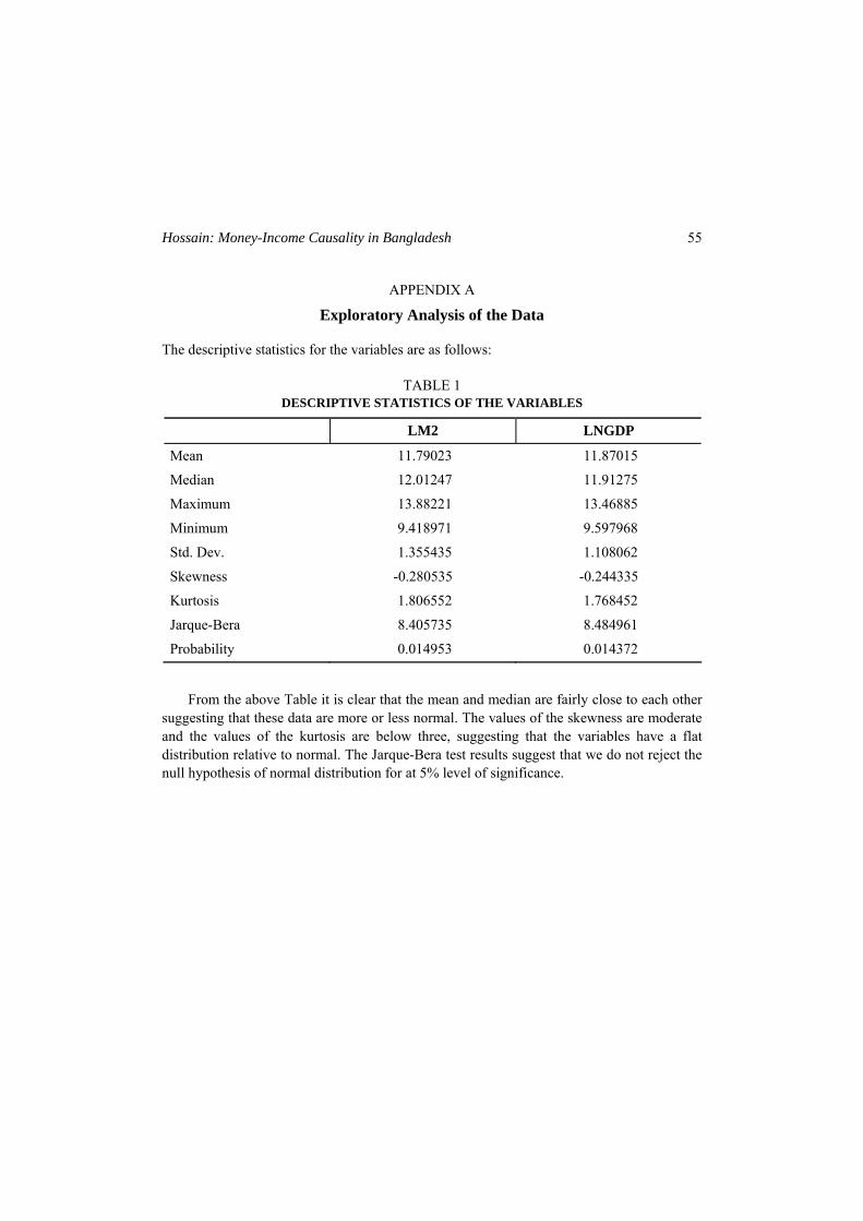
Hossain: Money-Income Causality in Bangladesh 55
APPENDIX A
Exploratory Analysis of the Data
The descriptive statistics for the variables are as follows:
TABLE 1 DESCRIPTIVE STATISTICS OF THE VARIABLES
LM2 LNGDP
Mean 11.79023 11.87015
Median 12.01247 11.91275
Maximum 13.88221 13.46885
Minimum 9.418971 9.597968
Std. Dev. 1.355435 1.108062
Skewness -0.280535 -0.244335
Kurtosis 1.806552 1.768452
Jarque-Bera 8.405735 8.484961
Probability 0.014953 0.014372
From the above Table it is clear that the mean and median are fairly close to each other
suggesting that these data are more or less normal. The values of the skewness are moderate and the values of the kurtosis are below three, suggesting that the variables have a flat distribution relative to normal. The Jarque-Bera test results suggest that we do not reject the null hypothesis of normal distribution for at 5% level of significance.
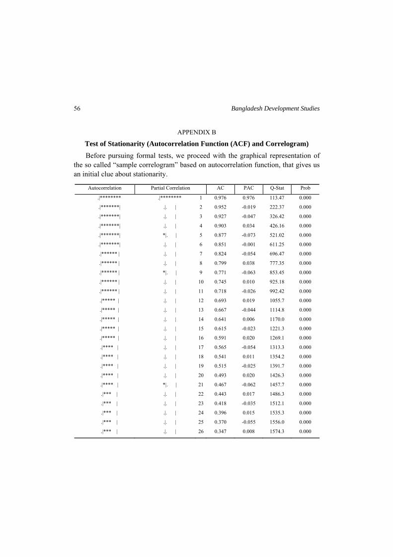
Bangladesh Development Studies
56
APPENDIX B
Test of Stationarity (Autocorrelation Function (ACF) and Correlogram) Before pursuing formal tests, we proceed with the graphical representation of
the so called “sample correlogram” based on autocorrelation function, that gives us an initial clue about stationarity.
Autocorrelation Partial Correlation AC PAC Q-Stat Prob
.|******** .|******** 1 0.976 0.976 113.47 0.000
.|*******| .|. | 2 0.952 -0.019 222.37 0.000
.|*******| .|. | 3 0.927 -0.047 326.42 0.000
.|*******| .|. | 4 0.903 0.034 426.16 0.000
.|*******| *|. | 5 0.877 -0.073 521.02 0.000
.|*******| .|. | 6 0.851 -0.001 611.25 0.000
.|****** | .|. | 7 0.824 -0.054 696.47 0.000
.|****** | .|. | 8 0.799 0.038 777.35 0.000
.|****** | *|. | 9 0.771 -0.063 853.45 0.000
.|****** | .|. | 10 0.745 0.010 925.18 0.000
.|****** | .|. | 11 0.718 -0.026 992.42 0.000
.|***** | .|. | 12 0.693 0.019 1055.7 0.000
.|***** | .|. | 13 0.667 -0.044 1114.8 0.000
.|***** | .|. | 14 0.641 0.006 1170.0 0.000
.|***** | .|. | 15 0.615 -0.023 1221.3 0.000
.|***** | .|. | 16 0.591 0.020 1269.1 0.000
.|**** | .|. | 17 0.565 -0.054 1313.3 0.000
.|**** | .|. | 18 0.541 0.011 1354.2 0.000
.|**** | .|. | 19 0.515 -0.025 1391.7 0.000
.|**** | .|. | 20 0.493 0.020 1426.3 0.000
.|**** | *|. | 21 0.467 -0.062 1457.7 0.000
.|*** | .|. | 22 0.443 0.017 1486.3 0.000
.|*** | .|. | 23 0.418 -0.035 1512.1 0.000
.|*** | .|. | 24 0.396 0.015 1535.3 0.000
.|*** | .|. | 25 0.370 -0.055 1556.0 0.000
.|*** | .|. | 26 0.347 0.008 1574.3 0.000
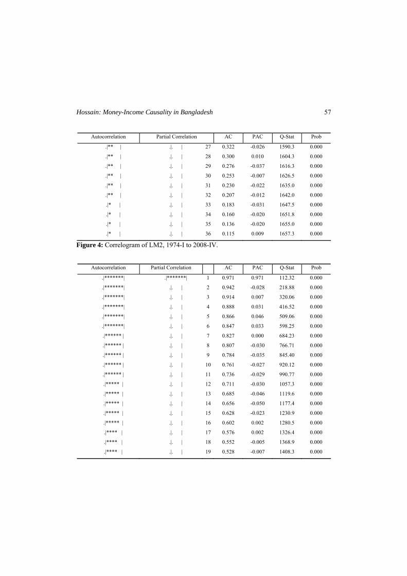
Hossain: Money-Income Causality in Bangladesh 57
Autocorrelation Partial Correlation AC PAC Q-Stat Prob
.|** | .|. | 27 0.322 -0.026 1590.3 0.000
.|** | .|. | 28 0.300 0.010 1604.3 0.000
.|** | .|. | 29 0.276 -0.037 1616.3 0.000
.|** | .|. | 30 0.253 -0.007 1626.5 0.000
.|** | .|. | 31 0.230 -0.022 1635.0 0.000
.|** | .|. | 32 0.207 -0.012 1642.0 0.000
.|* | .|. | 33 0.183 -0.031 1647.5 0.000
.|* | .|. | 34 0.160 -0.020 1651.8 0.000
.|* | .|. | 35 0.136 -0.020 1655.0 0.000
.|* | .|. | 36 0.115 0.009 1657.3 0.000
Figure 4: Correlogram of LM2, 1974-I to 2008-IV.
Autocorrelation Partial Correlation AC PAC Q-Stat Prob
.|*******| .|*******| 1 0.971 0.971 112.32 0.000
.|*******| .|. | 2 0.942 -0.028 218.88 0.000
.|*******| .|. | 3 0.914 0.007 320.06 0.000
.|*******| .|. | 4 0.888 0.031 416.52 0.000
.|*******| .|. | 5 0.866 0.046 509.06 0.000
.|*******| .|. | 6 0.847 0.033 598.25 0.000
.|****** | .|. | 7 0.827 0.000 684.23 0.000
.|****** | .|. | 8 0.807 -0.030 766.71 0.000
.|****** | .|. | 9 0.784 -0.035 845.40 0.000
.|****** | .|. | 10 0.761 -0.027 920.12 0.000
.|****** | .|. | 11 0.736 -0.029 990.77 0.000
.|***** | .|. | 12 0.711 -0.030 1057.3 0.000
.|***** | .|. | 13 0.685 -0.046 1119.6 0.000
.|***** | .|. | 14 0.656 -0.050 1177.4 0.000
.|***** | .|. | 15 0.628 -0.023 1230.9 0.000
.|***** | .|. | 16 0.602 0.002 1280.5 0.000
.|**** | .|. | 17 0.576 0.002 1326.4 0.000
.|**** | .|. | 18 0.552 -0.005 1368.9 0.000
.|**** | .|. | 19 0.528 -0.007 1408.3 0.000
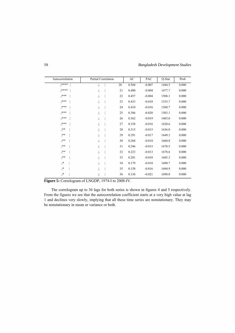
Bangladesh Development Studies
58
Autocorrelation Partial Correlation AC PAC Q-Stat Prob
.|**** | .|. | 20 0.504 -0.007 1444.5 0.000
.|**** | .|. | 21 0.480 -0.004 1477.7 0.000
.|*** | .|. | 22 0.457 -0.004 1508.1 0.000
.|*** | .|. | 23 0.433 -0.010 1535.7 0.000
.|*** | .|. | 24 0.410 -0.016 1560.7 0.000
.|*** | .|. | 25 0.386 -0.020 1583.1 0.000
.|*** | .|. | 26 0.362 -0.019 1603.0 0.000
.|*** | .|. | 27 0.338 -0.016 1620.6 0.000
.|** | .|. | 28 0.315 -0.015 1636.0 0.000
.|** | .|. | 29 0.291 -0.017 1649.3 0.000
.|** | .|. | 30 0.268 -0.018 1660.8 0.000
.|** | .|. | 31 0.246 -0.015 1670.5 0.000
.|** | .|. | 32 0.223 -0.013 1678.6 0.000
.|** | .|. | 33 0.201 -0.010 1685.3 0.000
.|* | .|. | 34 0.179 -0.010 1690.7 0.000
.|* | .|. | 35 0.158 -0.016 1694.9 0.000
.|* | .|. | 36 0.136 -0.021 1698.0 0.000
Figure 5: Correlogram of LNGDP, 1974-I to 2008-IV.
The correlogram up to 36 lags for both series is shown in figures 4 and 5 respectively. From the figures we see that the autocorrelation coefficient starts at a very high value at lag 1 and declines very slowly, implying that all these time series are nonstationary. They may be nonstationary in mean or variance or both.
Bangladesh Development Studies Vol. XXXIV, March 2011, No. 1
Conversion of Agricultural Land to Non-agricultural Uses in Bangladesh:
Extent and Determinants MD ABUL QUASEM*
Bangladesh is a land scarce country where per capita cultivated land is only 12.5 decimals. It is claimed that every year about one per cent of farm land in the country is being converted to non-agricultural uses (such high rate of conversion will not only hamper agricultural production but will have adverse impact on food security). The present study estimates the rate of land conversion and consequent loss of agricultural production of the country besides determining the factors affecting such conversion. The study is based mainly on field survey covering 24 villages from six divisions of the country Annual Conversion of farm land is estimated to be 0.56 per cent and the country’s loss of rice production is also estimated to be between 0.86 and 1.16 per cent. The converted land is predominantly used for construction of houses, followed by roads and establishment of business enterprises. The land poor records higher rate of land conversion. The two principal determining factors for such conversion are found to be land ownership size of a household and the non-agricultural occupation of household heads. To arrest the existing rate of land conversion, the surveyed households suggest for more profitable rates of return from farming activities besides imposing special sales tax for conversion of farm land.
I. INTRODUCTION
I.1 Background of the Study
With the growth of a country’s economy, agricultural land is usually transferred to non-agriculture as the demand for non-farm products and services increases. This * The author is a former Senior Research Fellow of the Bangladesh Institute of Development Studies (BIDS), Dhaka. He expresses his deep sense of gratitude to the anonymous referee for his wide ranging comments on the paper. He is grateful to the Krishi Gobeshana Foundation (GKF), Dhaka for financing the research project, “Agricultural Land Loss and Food Security in Bangladesh: An Assessment” carried out in collaboration with the Bangladesh Unnayan Parishad (BUP), Dhaka. His sincere gratitudes is also due to several researchers of BIDS, GKF and BUP for their valuable suggestions while carrying out the study.
Bangladesh Development Studies
60
is specially so when the country’s population and its per capita income rise. Transfer of farm land to non-agriculture is also needed for expansion of housing facilities in both rural and urban localities. Such transfer is also evidenced in building infrastructures such as roads, markets, educational institutions, electricity and industrial establishments, etc.
We are not aware of the extent of conversion of farm land for non-agricultural uses in Bangladesh and consequent production losses in agriculture. It is generally claimed that in Bangladesh every year over 80 thousand hectares of agricultural land i.e. nearly one per cent a year (Planning Commission 2009) is being converted to non-agriculture. This is definitely a matter of serious concern for the land-scarce country like Bangladesh where per capita cultivated area is only 15 decimals. This is too meagre an amount for the country’s food security as the productivity of land in Bangladesh is also low. Another case study, carried out in 2004 by Directorate of Land Records and Surveys (DLRS) of the Ministry of Land in Palas Upazilla of Narsingdi and Sonargaon of Narayanganj district, observed a substantial decline in the share of agricultural land to the extent of 27 per cent in Palas and 16 per cent in Sonargaon during the period of 20 and 25 years respectively (1983-2003; 1978-2003) i.e. more than one per cent per year. On the other hand, there has been several-fold increase in the area under housing and permanent fallows in both these areas.
The recently completed report on Agriculture Sample Survey of Bangladesh-2005 by Bangladesh Bureau of Statistics (BBS) does not, however, show such high rate of decline in cultivated land. Total cultivated land of all holdings in rural Bangladesh amounts to 17.77 million acres in 2005 which was almost the same in 1996 i.e. before nine years (Table I). This is difficult to explain. It seems to be due to conversion of forest and low lying fishing land as well as newly accreted char land to crop cultivations; this needs careful investigation. It may, however, be noted that the cultivated area per farm household has over time reduced to 1.20 acres in 2005 from 1.50 acres, recorded in 1996. This is largely due to a sharp rise in the number of rural farm households, by 24 per cent, from 11.8 million in 1996 to 14.7 million in 2005.
The recently completed Agricultural Census-2008 finds the number of farm households (14.40 million) almost equal to the figure of 2005 (14.47 million) accounting for 56.74 per cent of total rural households of the country. During the 12 year period of 1996 to 2008 the number of rural families increased from 17.8 million to 25.36 million i.e. an increase by 42.5 per cent. All these new families must have residential accommodations largely derived from the existing Agricultural land, indicating their absolute decline over time. The Government of
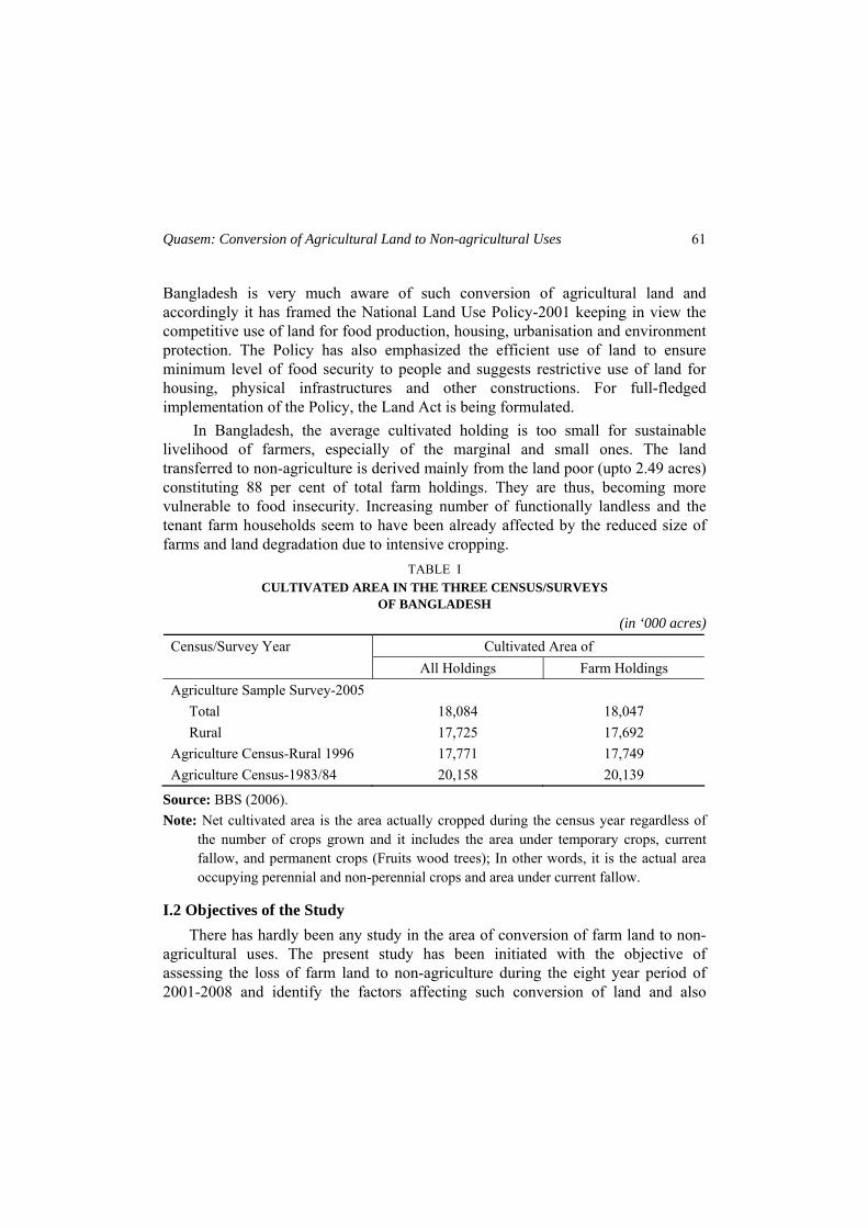
Quasem: Conversion of Agricultural Land to Non-agricultural Uses 61
Bangladesh is very much aware of such conversion of agricultural land and accordingly it has framed the National Land Use Policy-2001 keeping in view the competitive use of land for food production, housing, urbanisation and environment protection. The Policy has also emphasized the efficient use of land to ensure minimum level of food security to people and suggests restrictive use of land for housing, physical infrastructures and other constructions. For full-fledged implementation of the Policy, the Land Act is being formulated.
In Bangladesh, the average cultivated holding is too small for sustainable livelihood of farmers, especially of the marginal and small ones. The land transferred to non-agriculture is derived mainly from the land poor (upto 2.49 acres) constituting 88 per cent of total farm holdings. They are thus, becoming more vulnerable to food insecurity. Increasing number of functionally landless and the tenant farm households seem to have been already affected by the reduced size of farms and land degradation due to intensive cropping.
TABLE I CULTIVATED AREA IN THE THREE CENSUS/SURVEYS
OF BANGLADESH (in ‘000 acres)
Cultivated Area of Census/Survey Year All Holdings Farm Holdings
Agriculture Sample Survey-2005 Total 18,084 18,047 Rural 17,725 17,692
Agriculture Census-Rural 1996 17,771 17,749 Agriculture Census-1983/84 20,158 20,139
Source: BBS (2006). Note: Net cultivated area is the area actually cropped during the census year regardless of
the number of crops grown and it includes the area under temporary crops, current fallow, and permanent crops (Fruits wood trees); In other words, it is the actual area occupying perennial and non-perennial crops and area under current fallow.
I.2 Objectives of the Study There has hardly been any study in the area of conversion of farm land to non-
agricultural uses. The present study has been initiated with the objective of assessing the loss of farm land to non-agriculture during the eight year period of 2001-2008 and identify the factors affecting such conversion of land and also
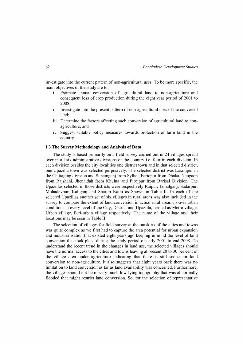
Bangladesh Development Studies
62
investigate into the current pattern of non-agricultural uses. To be more specific, the main objectives of the study are to:
i. Estimate annual conversion of agricultural land to non-agriculture and consequent loss of crop production during the eight year period of 2001 to 2008;
ii. Investigate into the present pattern of non-agricultural uses of the converted land;
iii. Determine the factors affecting such conversion of agricultural land to non-agriculture; and
iv. Suggest suitable policy measures towards protection of farm land in the country.
I.3 The Survey Methodology and Analysis of Data
The study is based primarily on a field survey carried out in 24 villages spread over in all six administrative divisions of the country i.e. four in each division. In each division besides the city localities one district town and in that selected district, one Upazilla town was selected purposively. The selected district was Laxmipur in the Chittaging division and Sunamganj from Sylhet, Faridpur from Dhaka, Naogaon from Rajshahi, Jhenaidah from Khulna and Pirojpur from Barisal Division. The Upazillas selected in those districts were respectively Raipur, Jamalganj, Sadarpur, Mohadevpur, Kaliganj and Sharup Kathi as Shown in Table II. In each of the selected Upazillas another set of six villages in rural areas was also included in the survey to compare the extent of land conversion in actual rural areas vis-avis urban conditions at every level of the City, District and Upazilla, termed as Metro village, Urban village, Peri-urban village respectively. The name of the village and their locations may be seen in Table II .
The selection of villages for field survey at the outskirts of the cities and towns was quite complex as we first had to capture the area potential for urban expansion and industrialisation that existed eight years ago keeping in mind the level of land conversion that took place during the study period of early 2001 to end 2008. To understand the recent trend in the changes in land use, the selected villages should have the normal access to the cities and towns leaving at present 20 to 30 per cent of the village area under agriculture indicating that there is still scope for land conversion to non-agriculture. It also suggests that eight years back there was no limitation to land conversion as far as land availability was concerned. Furthermore, the villages should not be of very much low-lying topography that was abnormally flooded that might restrict land conversion. So, for the selection of representative
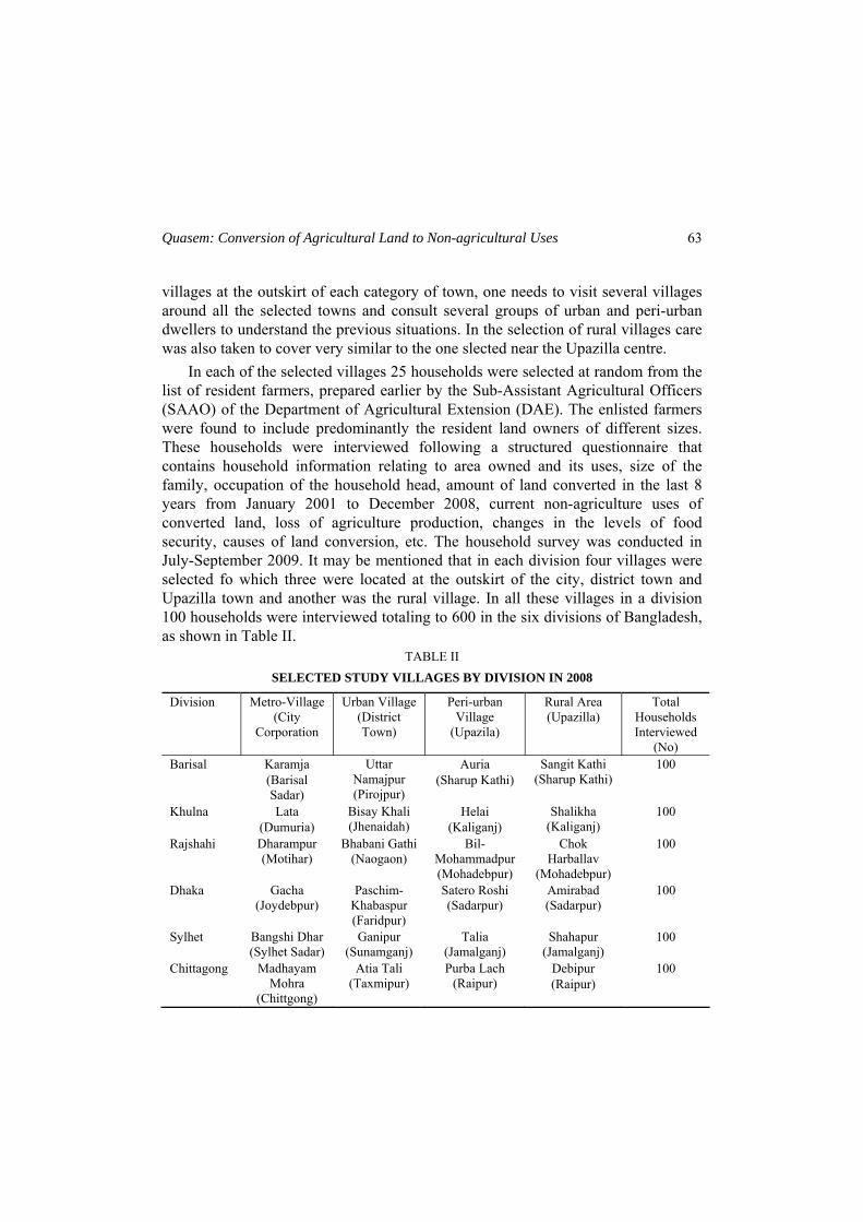
Quasem: Conversion of Agricultural Land to Non-agricultural Uses 63
villages at the outskirt of each category of town, one needs to visit several villages around all the selected towns and consult several groups of urban and peri-urban dwellers to understand the previous situations. In the selection of rural villages care was also taken to cover very similar to the one slected near the Upazilla centre.
In each of the selected villages 25 households were selected at random from the list of resident farmers, prepared earlier by the Sub-Assistant Agricultural Officers (SAAO) of the Department of Agricultural Extension (DAE). The enlisted farmers were found to include predominantly the resident land owners of different sizes. These households were interviewed following a structured questionnaire that contains household information relating to area owned and its uses, size of the family, occupation of the household head, amount of land converted in the last 8 years from January 2001 to December 2008, current non-agriculture uses of converted land, loss of agriculture production, changes in the levels of food security, causes of land conversion, etc. The household survey was conducted in July-September 2009. It may be mentioned that in each division four villages were selected fo which three were located at the outskirt of the city, district town and Upazilla town and another was the rural village. In all these villages in a division 100 households were interviewed totaling to 600 in the six divisions of Bangladesh, as shown in Table II.
TABLE II SELECTED STUDY VILLAGES BY DIVISION IN 2008
Division Metro-Village (City
Corporation
Urban Village (District Town)
Peri-urban Village
(Upazila)
Rural Area (Upazilla)
Total Households Interviewed
(No) Barisal Karamja
(Barisal Sadar)
Uttar Namajpur (Pirojpur)
Auria (Sharup Kathi)
Sangit Kathi (Sharup Kathi)
100
Khulna Lata (Dumuria)
Bisay Khali (Jhenaidah)
Helai (Kaliganj)
Shalikha (Kaliganj)
100
Rajshahi Dharampur (Motihar)
Bhabani Gathi (Naogaon)
Bil-Mohammadpur (Mohadebpur)
Chok Harballav
(Mohadebpur)
100
Dhaka Gacha (Joydebpur)
Paschim-Khabaspur (Faridpur)
Satero Roshi (Sadarpur)
Amirabad (Sadarpur)
100
Sylhet Bangshi Dhar (Sylhet Sadar)
Ganipur (Sunamganj)
Talia (Jamalganj)
Shahapur (Jamalganj)
100
Chittagong Madhayam Mohra
(Chittgong)
Atia Tali (Taxmipur)
Purba Lach (Raipur)
Debipur (Raipur)
100
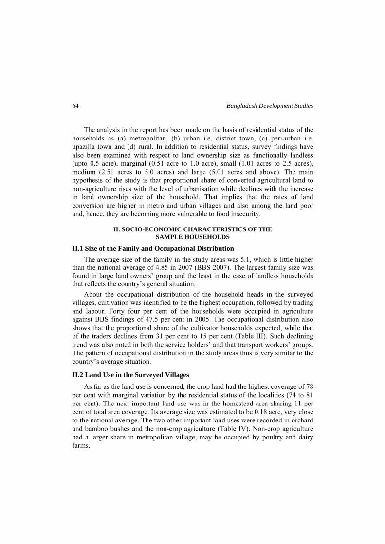
Bangladesh Development Studies
64
The analysis in the report has been made on the basis of residential status of the households as (a) metropolitan, (b) urban i.e. district town, (c) peri-urban i.e. upazilla town and (d) rural. In addition to residential status, survey findings have also been examined with respect to land ownership size as functionally landless (upto 0.5 acre), marginal (0.51 acre to 1.0 acre), small (1.01 acres to 2.5 acres), medium (2.51 acres to 5.0 acres) and large (5.01 acres and above). The main hypothesis of the study is that proportional share of converted agricultural land to non-agriculture rises with the level of urbanisation while declines with the increase in land ownership size of the household. That implies that the rates of land conversion are higher in metro and urban villages and also among the land poor and, hence, they are becoming more vulnerable to food insecurity.
II. SOCIO-ECONOMIC CHARACTERISTICS OF THE SAMPLE HOUSEHOLDS
II.1 Size of the Family and Occupational Distribution The average size of the family in the study areas was 5.1, which is little higher
than the national average of 4.85 in 2007 (BBS 2007). The largest family size was found in large land owners’ group and the least in the case of landless households that reflects the country’s general situation.
About the occupational distribution of the household heads in the surveyed villages, cultivation was identified to be the highest occupation, followed by trading and labour. Forty four per cent of the households were occupied in agriculture against BBS findings of 47.5 per cent in 2005. The occupational distribution also shows that the proportional share of the cultivator households expected, while that of the traders declines from 31 per cent to 15 per cent (Table III). Such declining trend was also noted in both the service holders’ and that transport workers’ groups. The pattern of occupational distribution in the study areas thus is very similar to the country’s average situation.
II.2 Land Use in the Surveyed Villages
As far as the land use is concerned, the crop land had the highest coverage of 78 per cent with marginal variation by the residential status of the localities (74 to 81 per cent). The next important land use was in the homestead area sharing 11 per cent of total area coverage. Its average size was estimated to be 0.18 acre, very close to the national average. The two other important land uses were recorded in orchard and bamboo bushes and the non-crop agriculture (Table IV). Non-crop agriculture had a larger share in metropolitan village, may be occupied by poultry and dairy farms.
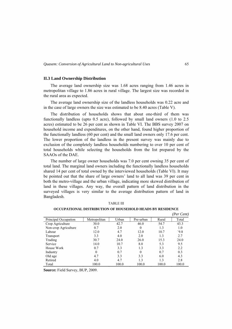
Quasem: Conversion of Agricultural Land to Non-agricultural Uses 65
II.3 Land Ownership Distribution
The average land ownership size was 1.68 acres ranging from 1.46 acres in metropolitan village to 1.86 acres in rural village. The largest size was recorded in the rural area as expected.
The average land ownership size of the landless households was 0.22 acre and in the case of large owners the size was estimated to be 8.40 acres (Table V).
The distribution of households shows that about one-third of them was functionally landless (upto 0.5 acre), followed by small land owners (1.0 to 2.5 acres) estimated to be 26 per cent as shown in Table VI. The BBS survey 2007 on household income and expenditures, on the other hand, found higher proportion of the functionally landless (60 per cent) and the small land owners only 17.6 per cent. The lower proportion of the landless in the present survey was mainly due to exclusion of the completely landless households numbering to over 10 per cent of total households while selecting the households from the list prepared by the SAAOs of the DAE.
The number of large owner households was 7.0 per cent owning 35 per cent of total land. The marginal land owners including the functionally landless households shared 14 per cent of total owned by the interviewed households (Table VI). It may be pointed out that the share of large owners’ land to all land was 39 per cent in both the metro-village and the urban village, indicating more skewed distribution of land in these villages. Any way, the overall pattern of land distribution in the surveyed villages is very similar to the average distribution pattern of land in Bangladesh.
TABLE III OCCUPATIONAL DISTRIBUTION OF HOUSEHOLD HEADS BY RESIDENCE
(Per Cent) Principal Occupation Metropolitan Urban Pre-urban Rural Total Crop Agriculture 30.0 42.7 46.0 54.7 43.3 Non-crop Agriculture 0.7 2.0 0 1.3 1.0 Labour 12.0 4.7 12.0 10.7 `9.8 Transport 3.3 4.0 2.0 1.3 2.7 Trading 30.7 24.0 26.0 15.3 24.0 Service 14.0 10.7 8.0 5.3 9.5 House Work 0.7 3.3 1.3 3.3 2.2 Industry 0 0.7 0 0.7 0.3 Old age 4.7 3.3 3.3 6.0 4.3 Retired 4.0 4.7 1.3 1.3 2.8 Total 100.0 100.0 100.0 100.0 100.0
Source: Field Survey, BUP, 2009.
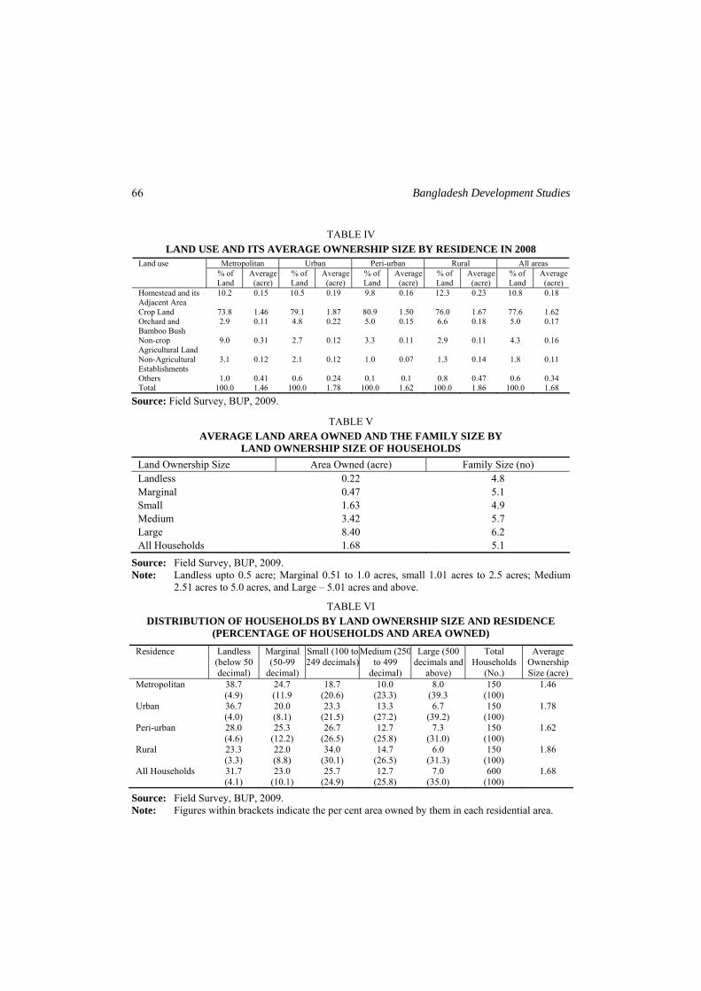
Bangladesh Development Studies
66
TABLE IV LAND USE AND ITS AVERAGE OWNERSHIP SIZE BY RESIDENCE IN 2008
Metropolitan Urban Peri-urban Rural All areas Land use % of Land
Average (acre)
% of Land
Average (acre)
% of Land
Average (acre)
% of Land
Average (acre)
% of Land
Average (acre)
Homestead and its Adjacent Area
10.2 0.15 10.5 0.19 9.8 0.16 12.3 0.23 10.8 0.18
Crop Land 73.8 1.46 79.1 1.87 80.9 1.50 76.0 1.67 77.6 1.62 Orchard and Bamboo Bush
2.9 0.11 4.8 0.22 5.0 0.15 6.6 0.18 5.0 0.17
Non-crop Agricultural Land
9.0 0.31 2.7 0.12 3.3 0.11 2.9 0.11 4.3 0.16
Non-Agricultural Establishments
3.1 0.12 2.1 0.12 1.0 0.07 1.3 0.14 1.8 0.11
Others 1.0 0.41 0.6 0.24 0.1 0.1 0.8 0.47 0.6 0.34 Total 100.0 1.46 100.0 1.78 100.0 1.62 100.0 1.86 100.0 1.68
Source: Field Survey, BUP, 2009.
TABLE V AVERAGE LAND AREA OWNED AND THE FAMILY SIZE BY
LAND OWNERSHIP SIZE OF HOUSEHOLDS Land Ownership Size Area Owned (acre) Family Size (no) Landless 0.22 4.8 Marginal 0.47 5.1 Small 1.63 4.9 Medium 3.42 5.7 Large 8.40 6.2 All Households 1.68 5.1
Source: Field Survey, BUP, 2009. Note: Landless upto 0.5 acre; Marginal 0.51 to 1.0 acres, small 1.01 acres to 2.5 acres; Medium
2.51 acres to 5.0 acres, and Large – 5.01 acres and above.
TABLE VI DISTRIBUTION OF HOUSEHOLDS BY LAND OWNERSHIP SIZE AND RESIDENCE
(PERCENTAGE OF HOUSEHOLDS AND AREA OWNED)
Residence Landless (below 50 decimal)
Marginal (50-99
decimal)
Small (100 to 249 decimals)
Medium (250to 499
decimal)
Large (500 decimals and
above)
Total Households
(No.)
Average Ownership Size (acre)
Metropolitan 38.7 (4.9)
24.7 (11.9
18.7 (20.6)
10.0 (23.3)
8.0 (39.3
150 (100)
1.46
Urban 36.7 (4.0)
20.0 (8.1)
23.3 (21.5)
13.3 (27.2)
6.7 (39.2)
150 (100)
1.78
Peri-urban 28.0 (4.6)
25.3 (12.2)
26.7 (26.5)
12.7 (25.8)
7.3 (31.0)
150 (100)
1.62
Rural 23.3 (3.3)
22.0 (8.8)
34.0 (30.1)
14.7 (26.5)
6.0 (31.3)
150 (100)
1.86
All Households 31.7 (4.1)
23.0 (10.1)
25.7 (24.9)
12.7 (25.8)
7.0 (35.0)
600 (100)
1.68
Source: Field Survey, BUP, 2009. Note: Figures within brackets indicate the per cent area owned by them in each residential area.
Quasem: Conversion of Agricultural Land to Non-agricultural Uses 67
III. AGRICULTURAL LAND CONVERTED TO NON-AGRICULTURE
III.1 Amount of Land Converted
The current survey estimated that during the eight year study period of 2001 to 2008, 46.25 acres of agricultural land was converted to non-agriculture (Table VII). In such conversion 251 land owners i.e. 42 per cent of interviewed households were involved. Land converters during the period were maximum in metro-village (54 per cent) and the lowest in peri-urban and rural villages (35 per cent). Among the divisions, Dhaka recorded the highest proportion of converters (52 per cent) in the area and the least in Sylhet (27 per cent) as shown in Annexure Table I.
Conversion of agricultural land with respect to total land owned in the year 2001 in the surveyed villages during the study period amounts to 4.50 per cent or 0.56 per cent per year. The annual rate of conversion varies from 0.25 to 0.74 per cent in peri-urban and urban-village respectively (Table VII). The present estimate is lower than the previous figure of about one per cent, often quoted. The higher rates of conversion in the current survey were noted in both urban and metro-villages as hypothesised. This is considered to be mainly due to higher price of land (Annexure Table II). It is also important to note that the price of homestead land is higher by 45 per cent compared to that of farm land, recording wide variation among the Divisions. Farm land in Sylhet is observed to be cheapest as it is generally single cropped and people do not prefer farming. The lower conversion in peri-urban villages might be due to stagnation in physical infrastructure building and in the functioning of the local government-Upazilla Parishad during the period.
III.2 Conversion of Land by Division
About the annual rate of conversion of land by region, the highest rate of conversion during the period was recorded in Dhaka division (estimated to be 1.45 per cent per year), while the lowest rate of conversion was experienced in Khulna division, only 0.26 per cent a year (Annexure Table I). Chittagong and Sylhet divisions had the conversion rate of 0.45 and 0.47 per cent respectively.
Average amount of land converted during the period amounts to 18.4 decimals by the converter households and 7.7 decimals when considered all households. Among the converters it was as high as 28.5 decimals in Dhaka Division, while the lowest was in Barisal (7.6 decimals) as shown in Annexure Table III. According to residential status, maximum converted area per household was recorded in both rural and urban area (24.8 decimals each). Of all the converters the highest number was observed in the metro-villages constituting about one-third of this total household in this category.
Bangladesh Development Studies
68
III.3 Conversion of Land by Land Ownership Size
According to land ownership size the proportion of land converters generally increases with their size, the average being 42 per cent. It increases from 30 per cent among landless households to 35 per cent among the large landowners during 2001 to 2008, which is expected (Table VIII). But in terms of land owned by them, the highest rate of conversion was recorded among the functionally landless households estimated to be 23 per cent or 2.9 per cent a year and the lowest among the large land ownership groups (1.6 per cent) or only 0.2 per cent of their land per year. In the remaining three other groups, the rate of conversion was observed to be about 0.6 per cent per year. The highest rate of conversion among landless households suggests that they are becoming more vulnerable to food security, especially when their land ownership size is alarmingly low (0.22 acre).
III.4 Land Converted under Different Possessions
During the eight year study period, land was converted to non-agricultural uses under different possession rights other than self-ownership. Some land was sold, some acquired by the government and some was donated. The data show that the major proportion (45 per cent) of the converted was sold while only 34 per cent was converted under self ownership, where peri-urban village dominate covering 55 per cent of total converted land (Table IX). Land acquired by the government had also significant share (19 per cent), mostly observed in urban village (38 per cent). It may be noted that conversion after sales was substantially high in rural and in metro-village, as compared to other this categories. Such analysis by land ownership size indicates that 63 per cent of large land owners’ converted land took place under self-ownership, while only 17 per cent was in the case of landless category (Table X). Conversion that occurred after sales of the land was quite high among the medium land owners. Surprisingly, over half of the converted land of the landless households was derived from acquired land. Such share for the large land owners was negligible (2.1 per cent), indicating that the land poor is more adversely affected by the acquisition of land by the state.
III.5 Share of Crop Land to Converted Land It has been observed that of the total converted agricultural land, crop land
occupied 90 per cent where different crops were cultivated. The remaining 10 per cent was used either in bamboo bushes and jungles or left fallow. There was some
Quasem: Conversion of Agricultural Land to Non-agricultural Uses 69
land where unplanned orchards and trees were also grown. The share of crop land was the highest in rural villages (95 per cent) and the lowest (85 per cent) in both the peri-urban and metropolitan villages (Table VII).1 Among the five land ownership categories, the share of crop land in the converted land was the highest (93 per cent) in small category and the lowest (85 per cent) among the marginal land category (Table VIII). In Dhaka division, 95 per cent of the converted land was derived from crop land, indicating that there is little scope for further urban expansion in the division without losing valuable crop land, which is a matter of serious concern.
III.6 Agricultural Land Converted at the National Level
According to our estimate, agricultural land is being converted at a rate of 0.56 per cent per year. On the basis of this rate of conversion and the country’s total cultivated area of all farm households amounting to 7.19 million hectares in 1996, conversion of land amounts to 40,452 hectares per year.
Another estimate based on annual per household conversion of land @ 0.0096 acre {(46.25 acres ÷ 600) ÷ 8} and the rural land owning households numbering to 16.01 million or {(17.828 − 1.815 or 10.18% completely landless)} in 1996 annual converted land is estimated to be 62,478 hectares. None of these estimates is close to the previously quoted figure of over 80,000 hectares. Furthermore if the previously quoted figure of 80,000 hectares is taken into account, total converted land in the country comes to 720,000 hectares during the nine year period of 1996 to 2005. But the total cultivated area in rural Bangladesh remains almost the same (17.77 million acres) in both the years of 1996 and 2005 with marginal difference of only 46,000 acres. We may, therefore, conclude that the previous figure of land conversion is an over estimate.
1 Chi-square test shown that there was statistically significant difference in the rate of conversion of land between the urban and peri-urban village.
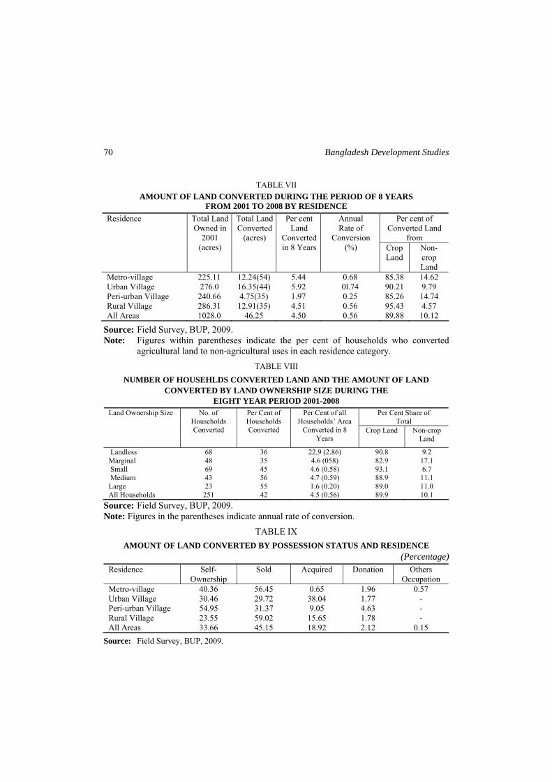
Bangladesh Development Studies
70
TABLE VII AMOUNT OF LAND CONVERTED DURING THE PERIOD OF 8 YEARS
FROM 2001 TO 2008 BY RESIDENCE Per cent of
Converted Land from
Residence
Total Land Owned in
2001 (acres)
Total Land Converted
(acres)
Per cent Land
Converted in 8 Years
Annual Rate of
Conversion (%) Crop
Land Non-crop Land
Metro-village 225.11 12.24(54) 5.44 0.68 85.38 14.62 Urban Village 276.0 16.35(44) 5.92 0l.74 90.21 9.79 Peri-urban Village 240.66 4.75(35) 1.97 0.25 85.26 14.74 Rural Village 286.31 12.91(35) 4.51 0.56 95.43 4.57 All Areas 1028.0 46.25 4.50 0.56 89.88 10.12
Source: Field Survey, BUP, 2009. Note: Figures within parentheses indicate the per cent of households who converted
agricultural land to non-agricultural uses in each residence category.
TABLE VIII NUMBER OF HOUSEHLDS CONVERTED LAND AND THE AMOUNT OF LAND
CONVERTED BY LAND OWNERSHIP SIZE DURING THE EIGHT YEAR PERIOD 2001-2008
Per Cent Share of Total
Land Ownership Size
No. of Households Converted
Per Cent of Households Converted
Per Cent of all Households’ Area
Converted in 8 Years
Crop Land Non-crop Land
Landless 68 36 22,9 (2.86) 90.8 9.2 Marginal 48 35 4.6 (058) 82.9 17.1 Small 69 45 4.6 (0.58) 93.1 6.7 Medium 43 56 4.7 (0.59) 88.9 11.1 Large 23 55 1.6 (0.20) 89.0 11.0 All Households 251 42 4.5 (0.56) 89.9 10.1
Source: Field Survey, BUP, 2009. Note: Figures in the parentheses indicate annual rate of conversion.
TABLE IX AMOUNT OF LAND CONVERTED BY POSSESSION STATUS AND RESIDENCE
(Percentage) Residence Self-
Ownership Sold Acquired Donation Others
Occupation Metro-village 40.36 56.45 0.65 1.96 0.57 Urban Village 30.46 29.72 38.04 1.77 - Peri-urban Village 54.95 31.37 9.05 4.63 - Rural Village 23.55 59.02 15.65 1.78 - All Areas 33.66 45.15 18.92 2.12 0.15
Source: Field Survey, BUP, 2009.
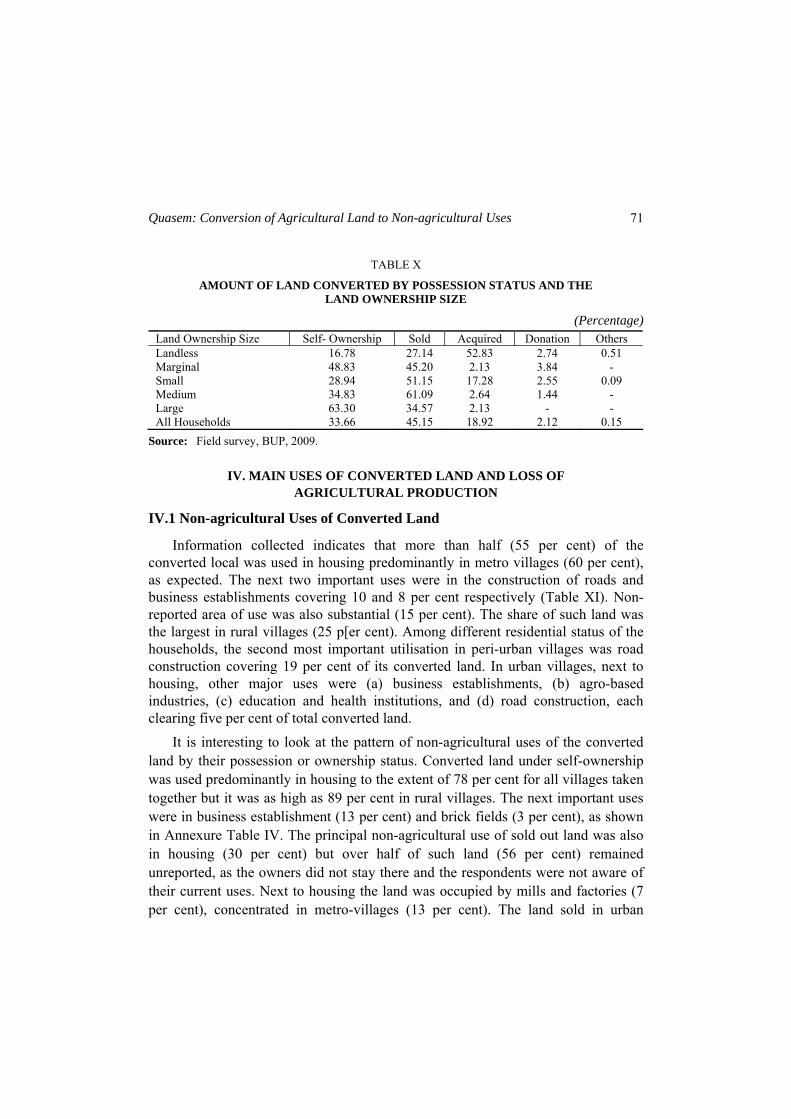
Quasem: Conversion of Agricultural Land to Non-agricultural Uses 71
TABLE X AMOUNT OF LAND CONVERTED BY POSSESSION STATUS AND THE
LAND OWNERSHIP SIZE
(Percentage) Land Ownership Size Self- Ownership Sold Acquired Donation Others Landless 16.78 27.14 52.83 2.74 0.51 Marginal 48.83 45.20 2.13 3.84 - Small 28.94 51.15 17.28 2.55 0.09 Medium 34.83 61.09 2.64 1.44 - Large 63.30 34.57 2.13 - - All Households 33.66 45.15 18.92 2.12 0.15
Source: Field survey, BUP, 2009.
IV. MAIN USES OF CONVERTED LAND AND LOSS OF AGRICULTURAL PRODUCTION
IV.1 Non-agricultural Uses of Converted Land
Information collected indicates that more than half (55 per cent) of the converted local was used in housing predominantly in metro villages (60 per cent), as expected. The next two important uses were in the construction of roads and business establishments covering 10 and 8 per cent respectively (Table XI). Non-reported area of use was also substantial (15 per cent). The share of such land was the largest in rural villages (25 p[er cent). Among different residential status of the households, the second most important utilisation in peri-urban villages was road construction covering 19 per cent of its converted land. In urban villages, next to housing, other major uses were (a) business establishments, (b) agro-based industries, (c) education and health institutions, and (d) road construction, each clearing five per cent of total converted land.
It is interesting to look at the pattern of non-agricultural uses of the converted land by their possession or ownership status. Converted land under self-ownership was used predominantly in housing to the extent of 78 per cent for all villages taken together but it was as high as 89 per cent in rural villages. The next important uses were in business establishment (13 per cent) and brick fields (3 per cent), as shown in Annexure Table IV. The principal non-agricultural use of sold out land was also in housing (30 per cent) but over half of such land (56 per cent) remained unreported, as the owners did not stay there and the respondents were not aware of their current uses. Next to housing the land was occupied by mills and factories (7 per cent), concentrated in metro-villages (13 per cent). The land sold in urban
Bangladesh Development Studies
72
villages was largely used for office buildings and other public utilities (11 per cent), next to housing (44 per cent). Converted land in others’ possessions e.g. acquired, donations, etc. had the substantial use in the construction of road to the extent of 57 per cent of such category land (Annexure Table IV). The next important use was by health and educational organisations, especially in metro villages. In peri-urban villages, public welfare institutions had also significant share of converted land.
There were wide regional variations in the non-agricultural use of converted land. For example, housing in Barisal covered as high as 77%; while it was only 41% in Sylhet where the requirement for new houses seemed lower. In Sylhet, the second most important use was the construction of roads occupying 29 per cent of land. In Dhaka, non-reported area was of claimed the largest share (31 per cent) of land, either used or not. In Barisal, public welfare establishments covered 12 per cent, the highest among six divisions.
Non-agricultural uses are also found different when examined by the land ownership size of households although the housing claimed the maximum share in all the categories. Small land owners had the highest proportion (62 per cent) in housing while the medium owners had the lowest (42 per cent) still occupying the maximum proportion. In the large ownership size, next to housing, the next largest share (19 per cent) claimed by the business establishment but it had the least more among the small land owners (Table XII). Road construction claimed 16 per cent of the medium owners’ converted land. In the landless group, the second highest proportional share (8.9 per cent) was occupied by health business enterprises as well as education and health organisations.
IV.2 Previous Uses of Converted Land
As mentioned earlier, of total converted agricultural land, 90 per cent was crop land where different crops and vegetables were grown. Collected data show that 92 per cent of crop land was under paddy and about 6 per cent was used for vegetables. The area under vegetables was higher (27 per cent) in peri-urban villages. Among different land ownership groups, the proportional shares of paddy land varied little, the highest being among the large land owners (97 per cent). In the case of vegetables, marginal land owners had the highest share (12 per cent). Before conversion, non-crop land which was kept almost unutilised amounted to 78 per cent, ranging between 81 and 97 per cent in metropolitan and peri-urban villages respectively. One-tenth of the land was occupied by bamboo bushes and trees,
Quasem: Conversion of Agricultural Land to Non-agricultural Uses 73
mostly in urban areas (23 per cent). There were some scattered plots where vegetables were grown, accounting for only 6.0 per cent of land. The pattern of land use as practised before conversion indicates that the conversion of land to non-agricultural uses has adversely affected agricultural production, which is estimated below.
IV.3 National Production Loss Based on Current Field Survey
According to the present field survey, production of different crops and vegetables is lost due to conversion of farm land to non-agriculture. The main crops lost were HYV paddy, local paddy and vegetables; and total annual loss of production was reported to be Tk.22,774 per acre (Table XIII). On the basis of annual production losses of Tk.22,774 per acre, the country’s total loss from converted land of 40,452 hectares of 99,512 acre i.e. @ 0.56% as estimated earlier, stands at Tk. 228 crore per year.
IV.4 Estimated National Loss of Rice Production It may be relevant to estimate the amount of losses of rice production due to
conversion of agricultural land in Bangladesh. Annual loss of rice production has been assessed on the basis of 5.12 acres of crop land as determined earlier. If the converted land is double cropped by Boro (HYV) and half by Aman (HYV) and half by local Aman considering all areas under cultivation of paddy, total amount of annual loss of paddy from the converted land (5.12 acres) roughly amounts to 465 maunds @ 90 maunds per acre or 0.028 ton per household. Total land-owning households in Bangladesh being 16.01 million, total loss of paddy production in the country amounts to 0.448 million or 4.5 lakh ton, which is equivalent to 3.02 lakh tons of rice and thus, with respect to country’s total production of 27 million metric tons, it stands at about 1.16 per cent. Another estimate based on the proportion of agricultural land converted amounting to 5,0995 million acres and per acre annual loss of rice (2.24 ton/acre) reported above stands at 0.223 million tons i.e. 0.86 per cent of the country’s annual production of rice. It would thus appear that due to conversion of agricultural land to non-agriculture, annual loss of rice production amounts to between 0.86 and 1.16 per cent of the country’s total rice production, which is not a negligible amount.
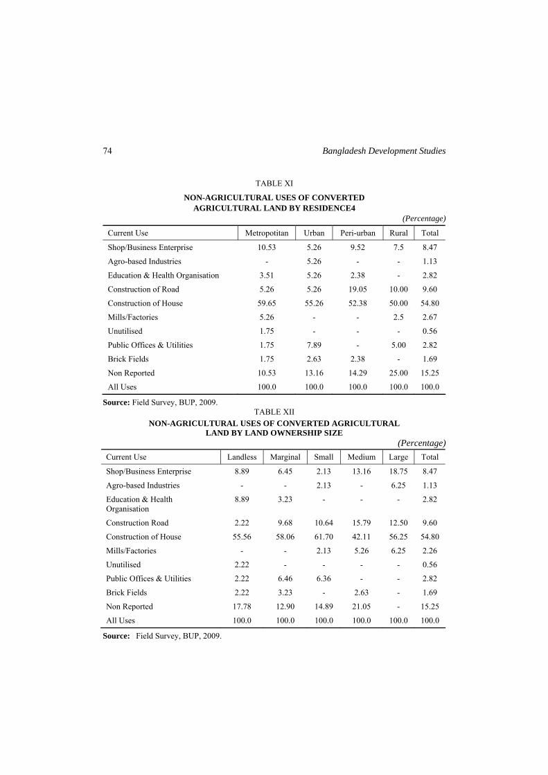
Bangladesh Development Studies
74
TABLE XI
NON-AGRICULTURAL USES OF CONVERTED AGRICULTURAL LAND BY RESIDENCE4
(Percentage)
Current Use Metropotitan Urban Peri-urban Rural Total
Shop/Business Enterprise 10.53 5.26 9.52 7.5 8.47
Agro-based Industries - 5.26 - - 1.13
Education & Health Organisation 3.51 5.26 2.38 - 2.82
Construction of Road 5.26 5.26 19.05 10.00 9.60
Construction of House 59.65 55.26 52.38 50.00 54.80
Mills/Factories 5.26 - - 2.5 2.67
Unutilised 1.75 - - - 0.56
Public Offices & Utilities 1.75 7.89 - 5.00 2.82
Brick Fields 1.75 2.63 2.38 - 1.69
Non Reported 10.53 13.16 14.29 25.00 15.25
All Uses 100.0 100.0 100.0 100.0 100.0
Source: Field Survey, BUP, 2009. TABLE XII
NON-AGRICULTURAL USES OF CONVERTED AGRICULTURAL LAND BY LAND OWNERSHIP SIZE
(Percentage) Current Use Landless Marginal Small Medium Large Total
Shop/Business Enterprise 8.89 6.45 2.13 13.16 18.75 8.47
Agro-based Industries - - 2.13 - 6.25 1.13
Education & Health Organisation
8.89 3.23 - - - 2.82
Construction Road 2.22 9.68 10.64 15.79 12.50 9.60
Construction of House 55.56 58.06 61.70 42.11 56.25 54.80
Mills/Factories - - 2.13 5.26 6.25 2.26
Unutilised 2.22 - - - - 0.56
Public Offices & Utilities 2.22 6.46 6.36 - - 2.82
Brick Fields 2.22 3.23 - 2.63 - 1.69
Non Reported 17.78 12.90 14.89 21.05 - 15.25
All Uses 100.0 100.0 100.0 100.0 100.0 100.0
Source: Field Survey, BUP, 2009.
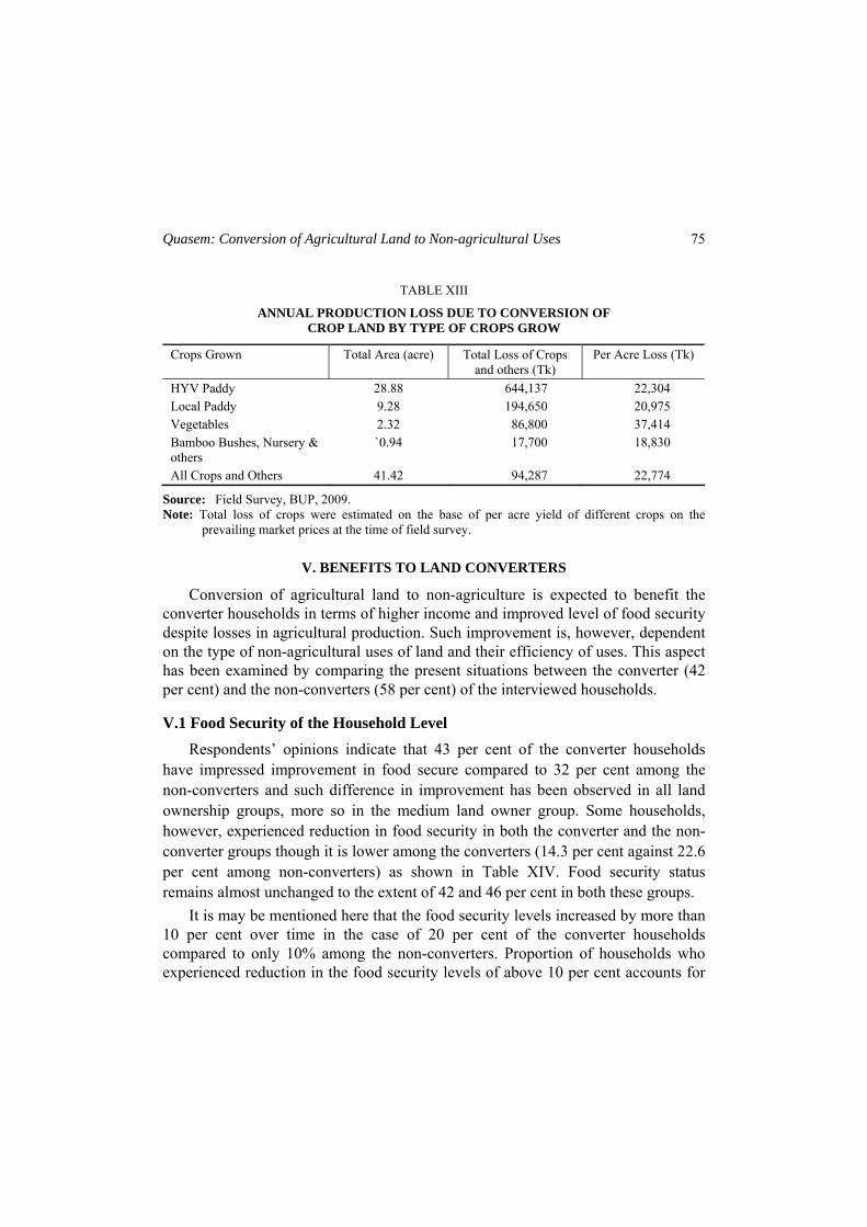
Quasem: Conversion of Agricultural Land to Non-agricultural Uses 75
TABLE XIII
ANNUAL PRODUCTION LOSS DUE TO CONVERSION OF CROP LAND BY TYPE OF CROPS GROW
Crops Grown Total Area (acre) Total Loss of Crops and others (Tk)
Per Acre Loss (Tk)
HYV Paddy 28.88 644,137 22,304 Local Paddy 9.28 194,650 20,975 Vegetables 2.32 86,800 37,414 Bamboo Bushes, Nursery & others
`0.94 17,700 18,830
All Crops and Others 41.42 94,287 22,774
Source: Field Survey, BUP, 2009. Note: Total loss of crops were estimated on the base of per acre yield of different crops on the
prevailing market prices at the time of field survey.
V. BENEFITS TO LAND CONVERTERS
Conversion of agricultural land to non-agriculture is expected to benefit the converter households in terms of higher income and improved level of food security despite losses in agricultural production. Such improvement is, however, dependent on the type of non-agricultural uses of land and their efficiency of uses. This aspect has been examined by comparing the present situations between the converter (42 per cent) and the non-converters (58 per cent) of the interviewed households.
V.1 Food Security of the Household Level Respondents’ opinions indicate that 43 per cent of the converter households
have impressed improvement in food secure compared to 32 per cent among the non-converters and such difference in improvement has been observed in all land ownership groups, more so in the medium land owner group. Some households, however, experienced reduction in food security in both the converter and the non-converter groups though it is lower among the converters (14.3 per cent against 22.6 per cent among non-converters) as shown in Table XIV. Food security status remains almost unchanged to the extent of 42 and 46 per cent in both these groups.
It is may be mentioned here that the food security levels increased by more than 10 per cent over time in the case of 20 per cent of the converter households compared to only 10% among the non-converters. Proportion of households who experienced reduction in the food security levels of above 10 per cent accounts for
Bangladesh Development Studies
76
10 per cent among the converter households compared to 15 per cent in the case of non-converter households.2
Improvement in the food security levels of the converter households over the non-converters as reported above is not, however, reflected in the amount of consumption of at least three food items e.g. rice, flour and pulses. Rough estimates indicate equal levels of consumption in both these groups either in aggregate or by land ownership size. It may be mentioned that daily per capita consumption of cereals and pulses in the present study was estimated to be 450 gms and 20 gms respectively by the converter households which is marginally higher than the national average of 409 gms and 14.2 gms recorded in 2005 (BBS 2007).
V.2 Income of the Households
It is interesting to note that income of the converter households was observed to be higher by about 50 per cent over that of the non-converters household. Such higher income was recorded in all size ownership groups, but more so among the marginal and the large land owners. The converters have also higher share of income from trade and businesses (42 per cent against 36 per cent) and different services (24 per cent against 22 per cent).
It may be pointed out that the improved level of food security among the converter households may not be due to land conversion alone. It could be the combined outcome of several factors such as land ownership size of the households, their levels of education, occupational status, etc. It may, however, be mentioned that the average size of land owned by a converter household is substantially higher ( ) over the non-converters’ owned area and (prominently observed among the land rich). They had also higher land ownership size in 2001 (2.22 acres). The converter households might also be more favourably located in terms of the infrastructure development of the area. This, however, needs further investigation. Furthermore, the average value of household assets is found to be almost equal among both the converter and the non-converter households. Substantial differences are, however, noticed in the case of non-housing assets i.e. in terms of agricultural equipment, livestock, plantations, etc. It is found to be double for converter households. The average value of such productive assets of these households is estimated to be Tk.92,458.
2 These figures are based on perception of the respondents in the field survey.
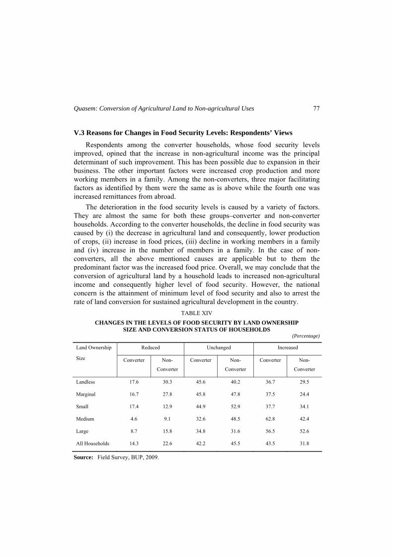
Quasem: Conversion of Agricultural Land to Non-agricultural Uses 77
V.3 Reasons for Changes in Food Security Levels: Respondents’ Views
Respondents among the converter households, whose food security levels improved, opined that the increase in non-agricultural income was the principal determinant of such improvement. This has been possible due to expansion in their business. The other important factors were increased crop production and more working members in a family. Among the non-converters, three major facilitating factors as identified by them were the same as is above while the fourth one was increased remittances from abroad.
The deterioration in the food security levels is caused by a variety of factors. They are almost the same for both these groups–converter and non-converter households. According to the converter households, the decline in food security was caused by (i) the decrease in agricultural land and consequently, lower production of crops, (ii) increase in food prices, (iii) decline in working members in a family and (iv) increase in the number of members in a family. In the case of non-converters, all the above mentioned causes are applicable but to them the predominant factor was the increased food price. Overall, we may conclude that the conversion of agricultural land by a household leads to increased non-agricultural income and consequently higher level of food security. However, the national concern is the attainment of minimum level of food security and also to arrest the rate of land conversion for sustained agricultural development in the country.
TABLE XIV CHANGES IN THE LEVELS OF FOOD SECURITY BY LAND OWNERSHIP
SIZE AND CONVERSION STATUS OF HOUSEHOLDS (Percentage)
Reduced Unchanged Increased Land Ownership
Size Converter Non-
Converter
Converter Non-
Converter
Converter Non-
Converter
Landless 17.6 30.3 45.6 40.2 36.7 29.5
Marginal 16.7 27.8 45.8 47.8 37.5 24.4
Small 17.4 12.9 44.9 52.9 37.7 34.1
Medium 4.6 9.1 32.6 48.5 62.8 42.4
Large 8.7 15.8 34.8 31.6 56.5 52.6
All Households 14.3 22.6 42.2 45.5 43.5 31.8
Source: Field Survey, BUP, 2009.
Bangladesh Development Studies
78
VI. DETERMINANTS OF LAND CONVERSION
VI.1 Determinants of Land Conversion: Regression Results
Conversion of agricultural land to non-agriculture is dependent on a variety of factors such as number of members in a family, income earning possibilities from agriculture and non-agriculture uses of land besides state acquisition for construction of roads and institutional building, etc. Regressions analyses in this regard can provide better explanation by identifying the factors that determine the amount of land area to be converted to non-agriculture by the households. To this end, linear regression model is fitted taking into account several explanatory variables for the year 2001.* The independent variables used in the model are:
i) Total land owned by household :T-LAND (decimals); ii) Homestead land owned by a household : HOME (decimals); iii) Proportion of non-crop land to total land owned : PNC (%) iv) Primary occupation of the household head : P-OCCUP (agriculture=0 &
non-agriculture=1) v) Years of schooling of the household head : (number); vi) Per capita annual income : PCI (Tk); vii) Household assets other than housing : Asset (Tk); viii) Disaster losses : DISASTER (Tk); ix) Study Area Dummy (Rural = 0); x) Dummy for Peri-urban (PERI-UR=1); xi) Dummy for Urban (URBAN=2); xii) Dummy for Metro (METRO=3).
The linear regression exercise hypothesises that the area of agricultural land converted by a household rises with the increase in its land ownership size, homestead area and proportional share of non-crop land to total land owned. Household heads with non-agricultural occupations and their years of schooling are also expected to encourage land conversion as they are more exposed to non-agricultural activities. Per capita annual income and value of non-housing assets i.e. agricultural equipment, livestock’s, etc. are considered to have negative impact on land conversion as they can use their land better for higher agricultural production and more income. About the dummy variable rural village is taken to be ‘0’ i.e. with * Similar exercise has also been carried out for the data of 2008 and the results are found to be quite similar.
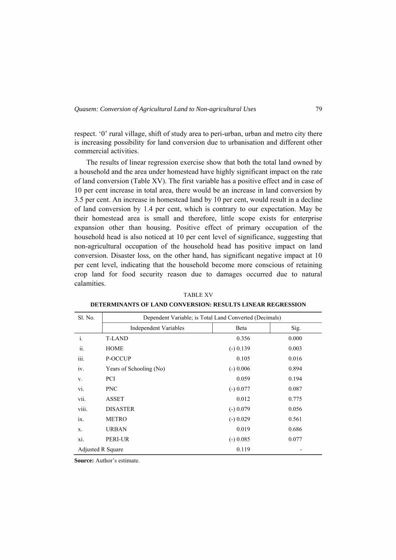
Quasem: Conversion of Agricultural Land to Non-agricultural Uses 79
respect. ‘0’ rural village, shift of study area to peri-urban, urban and metro city there is increasing possibility for land conversion due to urbanisation and different other commercial activities.
The results of linear regression exercise show that both the total land owned by a household and the area under homestead have highly significant impact on the rate of land conversion (Table XV). The first variable has a positive effect and in case of 10 per cent increase in total area, there would be an increase in land conversion by 3.5 per cent. An increase in homestead land by 10 per cent, would result in a decline of land conversion by 1.4 per cent, which is contrary to our expectation. May be their homestead area is small and therefore, little scope exists for enterprise expansion other than housing. Positive effect of primary occupation of the household head is also noticed at 10 per cent level of significance, suggesting that non-agricultural occupation of the household head has positive impact on land conversion. Disaster loss, on the other hand, has significant negative impact at 10 per cent level, indicating that the household become more conscious of retaining crop land for food security reason due to damages occurred due to natural calamities.
TABLE XV DETERMINANTS OF LAND CONVERSION: RESULTS LINEAR REGRESSION
Dependent Variable; is Total Land Converted (Decimals) Sl. No.
Independent Variables Beta Sig.
i. T-LAND 0.356 0.000
ii. HOME (-) 0.139 0.003
iii. P-OCCUP 0.105 0.016
iv. Years of Schooling (No) (-) 0.006 0.894
v. PCI 0.059 0.194
vi. PNC (-) 0.077 0.087
vii. ASSET 0.012 0.775
viii. DISASTER (-) 0.079 0.056
ix. METRO (-) 0.029 0.561
x. URBAN 0.019 0.686
xi. PERI-UR (-) 0.085 0.077
Adjusted R Square 0.119 -
Source: Author’s estimate.
Bangladesh Development Studies
80
VI.2 Arresting Land Conversion: Respondents’ Opinions It is wieldy recognised that conversion of land should be discouraged in
Bangladesh for ensuring food security in the country. The respondents have put forward some suggestions for arresting the current rate of land conversion. Their recommendations include the following (Table XVI):
(i) agriculture should be made more profitable and attractive (49 per cent); (ii) special tax should be imposed on conversion of land (30 per cent); (iii) area-wise ceiling may be fixed for non-agricultural uses of land (11 per
cent); (iv) tax exemption may be offered for commercial farms and the agro-based
industries (10 per cent).
While asking the respondents’ views towards increasing profitability of agriculture, they emphasise for raising of crop prices in the harvest seasons, ensured timely supplies of agricultural inputs at reasonable prices, and productivity increase of land through adoption of modern technologies and effective agricultural extension services. These suggestions are almost equally applicable to all land ownership groups and the residential status of the households. Also, little differences are observed in their views when compared between land converters and non-converters.
Open discussions with the respondents in this regard also reveal that there should be immediate control for non-agricultural use, population growth and introduction of special tax on converted land; and area specific ceiling may also be imposed to restrict indiscriminate conversion of farm land. The above mentioned suggestions lead us to conclude that to arrest the present rate of land conversion two things are essential. These are (a) strict population control to restrict faster expansion of housing and road construction, and (b) making agriculture more profitable and attractive.
The government of Bangladesh is, however, aware of the existing problems and accordingly, it is formulating strategies towards “Compact Townships” for rural people (Planning Commission 2009). It has also emphasised the implementation of National Land Use Policy 2001, towards restriction of unplanned housing and road construction. In this context, proper policy formulation and adequate institutional mechanism assume special significance.
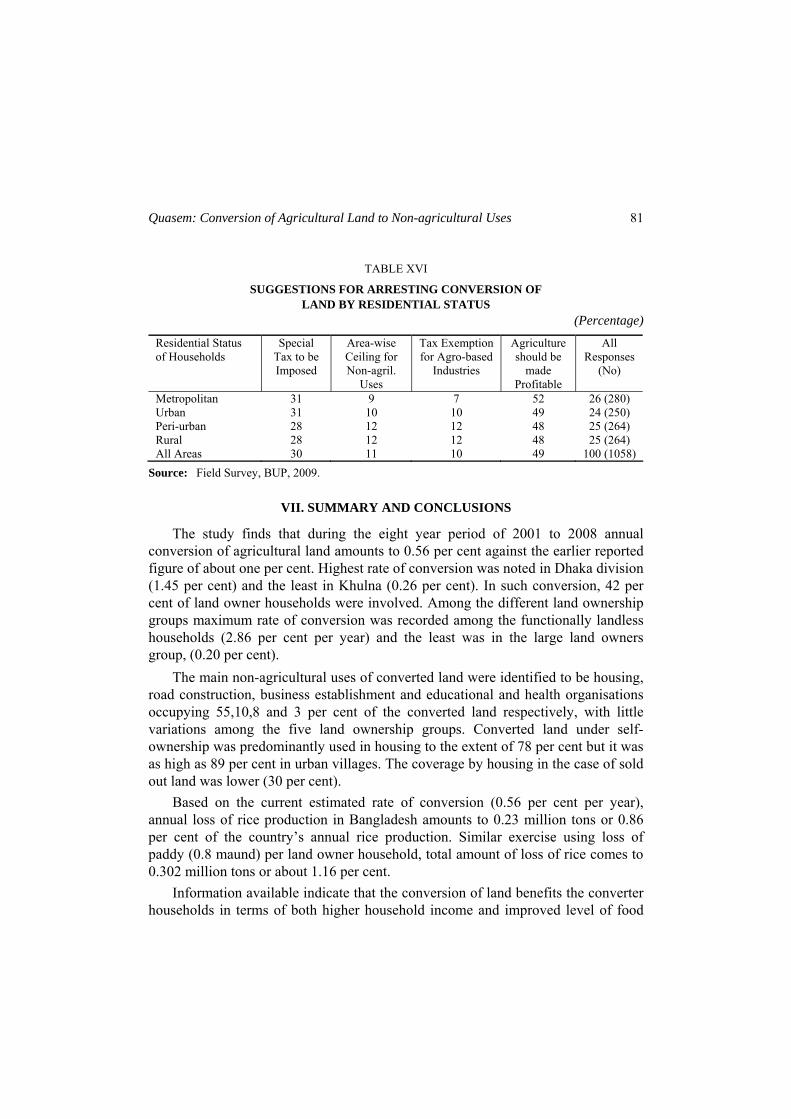
Quasem: Conversion of Agricultural Land to Non-agricultural Uses 81
TABLE XVI
SUGGESTIONS FOR ARRESTING CONVERSION OF LAND BY RESIDENTIAL STATUS
(Percentage)
Residential Status of Households
Special Tax to be Imposed
Area-wise Ceiling for Non-agril.
Uses
Tax Exemption for Agro-based
Industries
Agriculture should be
made Profitable
All Responses
(No)
Metropolitan 31 9 7 52 26 (280) Urban 31 10 10 49 24 (250) Peri-urban 28 12 12 48 25 (264) Rural 28 12 12 48 25 (264) All Areas 30 11 10 49 100 (1058)
Source: Field Survey, BUP, 2009.
VII. SUMMARY AND CONCLUSIONS
The study finds that during the eight year period of 2001 to 2008 annual conversion of agricultural land amounts to 0.56 per cent against the earlier reported figure of about one per cent. Highest rate of conversion was noted in Dhaka division (1.45 per cent) and the least in Khulna (0.26 per cent). In such conversion, 42 per cent of land owner households were involved. Among the different land ownership groups maximum rate of conversion was recorded among the functionally landless households (2.86 per cent per year) and the least was in the large land owners group, (0.20 per cent).
The main non-agricultural uses of converted land were identified to be housing, road construction, business establishment and educational and health organisations occupying 55,10,8 and 3 per cent of the converted land respectively, with little variations among the five land ownership groups. Converted land under self-ownership was predominantly used in housing to the extent of 78 per cent but it was as high as 89 per cent in urban villages. The coverage by housing in the case of sold out land was lower (30 per cent).
Based on the current estimated rate of conversion (0.56 per cent per year), annual loss of rice production in Bangladesh amounts to 0.23 million tons or 0.86 per cent of the country’s annual rice production. Similar exercise using loss of paddy (0.8 maund) per land owner household, total amount of loss of rice comes to 0.302 million tons or about 1.16 per cent.
Information available indicate that the conversion of land benefits the converter households in terms of both higher household income and improved level of food
Bangladesh Development Studies
82
security. But the estimate of actual consumption of rice, flour and pulses was found to be almost equal. Improvement in the food security among the converter households was reportedly due to higher non-agricultural income, facilitated by expansion of business.
The regression exercise carried out identifies the following factors that have significant effects on the rate of conversion of agricultural land are:
(i) total land area owned by a household; (ii) homestead area owned; (iii) primary occupation of the households head; and (iv) disaster losses incurred during the study period. The regression coefficient shows that 10 per cent increase in total area owned
by a household leads to rise in the conversion of land by 3.5 per cent; while the increase in homestead area by 10% reduces land conversion by 1.4 per cent. Perhaps, the area under homestead is small and has little scope for expansion. Non-agricultural occupation of the household heads also encourages land conversion.
The main policy suggestions to arrest the magnitude of land conversion are: agricultural occupations need to be made more profitable and attractive compared to non-agriculture and at the same time special tax may be imposed on the conversion of crop land. Area specific ceiling for different non-agricultural uses may be determined and imposed in industrialisation and urbanisation. Open discussions with the respondents in this regard suggest strict control on population growth, creation of more employment opportunities in rural non-farm sector and increase of land productivity through adoption of modern technologies, to be facilitated by the use of hybrid and high yielding seeds, uninterrupted supply of electricity to the irrigation equipment and adequate agricultural credit at subsidised rates of interest. In the adoption of new technologies, improved farm management practices are required.
REFERENCES
Bangladesh Bureau of Statistics 2009: Preliminary Report on Agricultural Census – 2008. Government of the People’s Republic of Bangladesh, Dhaka.
–––––––2007. Household Income and Expenditure Survey of Bangladesh. Government of the People’s Republic of Bangladesh, Dhaka.
–––––––2006. Agriculture Sample Survey of Bangladesh-2005, National Volum-1. Government of the People’s Republic of Bangladesh, Dhaka.
Quasem: Conversion of Agricultural Land to Non-agricultural Uses 83
Government of the People’s Republic of Bangladesh, 2001. National Land Use Policy, Bangladesh Gazette, June 2001.
Ministry of Land 2004: GIS Atlas on Land Use and Environment-Palas and Sonargaon Upazillas Government of the People’s Republic of Bangladesh, Dhaka.
Planning Commission 2009. Steps Towards Change – National Strategy for Accelerated Poverty Reduction II (Revised). FY 2009-11. Government of the People’s Republic of Bangladesh, Dhaka.
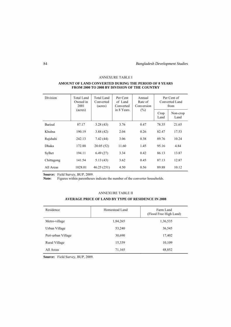
Bangladesh Development Studies
84
ANNEXURE TABLE I AMOUNT OF LAND CONVERTED DURING THE PERIOD OF 8 YEARS
FROM 2000 TO 2008 BY DIVISION OF THE COUNTRY
Per Cent of Converted Land
from
Division Total Land Owned in
2001 (acres)
Total Land Converted
(acres)
Per Cent of Land
Converted in 8 Years
Annual Rate of
Conversion (%)
Crop Land
Non-crop Land
Barisal 87.17 3.28 (43) 3.76 0.47 78.35 21.65
Khulna 190.19 3.88 (42) 2.04 0.26 82.47 17.53
Rajshahi 242.13 7.42 (44) 3.06 0.38 89.76 10.24
Dhaka 172.88 20.05 (52) 11.60 1.45 95.16 4.84
Sylhet 194.11 6.49 (27) 3.34 0.42 86.13 13.87
Chittagong 141.54 5.13 (43) 3.62 0.45 87.13 12.87
All Areas 1028.01 46.25 (251) 4.50 0.56 89.88 10.12
Source: Field Survey, BUP, 2009. Note: Figures within parentheses indicate the number of the converter households.
ANNEXURE TABLE II
AVERAGE PRICE OF LAND BY TYPE OF RESIDENCE IN 2008
Residence Homestead Land Farm Land (Flood Free High Land)
Metro-village 1,84,265 1,36,535
Urban Village 53,240 36,545
Peri-urban Village 30,690 17,402
Rural Village 15,339 10,109
All Areas 71,165 48,852
Source: Field Survey, BUP, 2009.
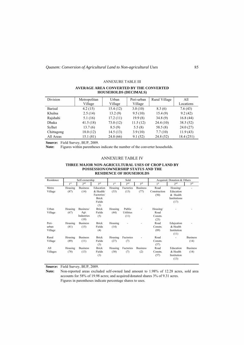
Quasem: Conversion of Agricultural Land to Non-agricultural Uses 85
ANNEXURE TABLE III
AVERAGE AREA CONVERTED BY THE CONVERTED HOUSEHOLDS (DECIMALS)
Division Metropolitan Village
Urban Village
Peri-urban Village
Rural Village All Locations
Barisal 4.2 (15) 15.4 (12) 3.0 (10) 8.3 (6) 7.6 (43) Khulna 2.5 (14) 13.2 (9) 9.5 (10) 15.4 (9) 9.2 (42) Rajshahi 5.1 (16) 17.2 (11) 19.9 (8) 34.8 (9) 16.8 (44) Dhaka 41.5 (18) 73.0 (12) 11.5 (12) 24.4 (10) 38.5 (52) Sylhet 13.7 (6) 8.5 (9) 5.5 (8) 58.5 (8) 24.0 (27) Chittagong 18.0 (12) 14.5 (13) 3.9 (10) 7.7 (10) 11.9 (43) All Areas 15.1 (81) 24.8 (66) 9.1 (52) 24.8 (52) 18.4 (251)
Source: Field Survey, BUP, 2009. Note: Figures within parentheses indicate the number of the converter households.
ANNEXURE TABLE IV THREE MAJOR NON-AGRICULTURAL USES OF CROP LAND BY
POSSESSION/OWNERSHIP STATUS AND THE RESIDENCE OF HOUSEHOLDS
Self-ownership Sold Acquired, Donation & Others Residence 1st 2nd 3rd 1st 2nd 3rd 1st 2nd 3rd
Metro Village
Housing (87)
Business (14)
Education & Health/ Factories/
Brick Fields
(3)
Housing (33)
Factories (13)
Business (77)
Road Construction
(50)
Housing/ Education & Health
Institutions (17)
-
Urban Village
Housing (67)
Business/ Agr.
Industries (10)
Brick Fields
(5)
Housing (44)
Public Utilities
(11)
- Housing/ Road
Constn. (25)
- -
Peri- urban Village
Housing (81)
Business (15)
Brick Fields
(4)
Housing (14)
- - Road Constn.
(89)
Edujcation & Health Institution
(11)
-
Rural Village
Housing (89)
Business (11)
Brick Fields
(3)
Housing (27)
Factories (7)
- Road Constn.
(57)
- Business (14)
All Villages
Housing (78)
Business (13)
Brick Fields
(3)
Housing (30)
Factories (7)
Business (2)
Road Constn.
(57)
Education & Health Institution
(13)
Business (14)
Source: Field Survey, BUP, 2009. Note: Non-reported areas excluded self-owned land amount to 1.98% of 12.28 acres, sold area
accounts for 58% of 19.98 acres; and acquired/donated shares 3% of 9.31 acres. Figures in parentheses indicate percentage shares to uses.
Bangladesh Development Studies Vol. XXXIV, March 2011, No. 1
Initial Trade Policy Focus of the High Performing Asian Economies: A Critical
Assessment MIA MAHMUDUR RAHIM*
It is generally agreed that national trade policies of Singapore, South Korea, Taiwan and Hong Kong played an important role behind the success of the High Performing Asian Economies (HPAEs). These countries exercised different policies with different implementation strategies at the initial stages of their economic success but resulted almost the same success. Thus, on the one hand, they followed some different ways following their specific needs and, on the other hand, maintained the same underlying principles for their national trade policies. They were although pragmatic in their economic policy focus, they did not adopt any common model or blueprint policy rather their strategies were followed by their specific strength, weakness and goals.
I. INTRODUCTION
There is a remarkable record of high and sustained economic growth from 1965 to 1990 in twenty three East Asian economies. In this area, most of the runaway growth focuses on eight economies, sometimes collectively referred to as the “High Performing Asian Economies” (or HPAEs). Japan, the “Four Tigers”, Hong Kong, South South Korea, Singapore and Taiwan, and the three ‘Newly Industrialising Economies’ (or ‘NIEs’) of Southeast Asia, Malaysia, Thailand and Indonesia amongst twenty three economies of Asia achieved higher growth than any other regions of the world (World Bank 1993).
The nature of HPAEs economic growth put HPAE countries together to formulate a cluster, though their economies are remarkably diverse. Among these countries some are the richest while some are the poorest developing countries in the world; some are the most populous whereas some are the least; some are full of natural resources where others are not (World Bank 1993). These countries are also different in their infrastructural set up, environmental challenges and socio- *PhD Candidate, Macquaire Law School, Macquaire University, Australia.
Bangladesh Development Studies
88
political culture. These differences lead the background of East Asian countries’ economic success to a diverged success. Accordingly, different studies conclude different reasons for this economic success. Though these countries at the initial stage of their economic success exercised different policies in different ways, nevertheless these resulted in stories of tremendous success (World Bank 1993).
With these backdrops, this paper argues that “pragmatism” was the basis of their diverse national trade policies. For the thematic construct of this paper, neither any particular policy nor any particular issue in policies has been discussed. Rather, the focus of this paper is on the nature of general trade policies that contributed to the economic success of HPAEs at its initial stages. It attempts to establish the above mentioned central argument by monitoring four parameters of pragmatism the HPAEs adapted: pragmatism in trade policy priority setting; pragmatism in policy orientation; pragmatism in trade policy focus; and pragmatism in policy implementation strategies.
II. TRADE POLICY PRIORITY SETTING
HPAEs countries did not follow the copy book policies for their economic progress. At the same time, they did not stick to any fixed ideology based policies. Rather they frequently moderate/alter policies which seemed to be less productive in its application. During 1965 to 1990 these countries shifted their policy stand frequently. Simultaneously, they were not rigid to any particular policy and focused more on the needs rather than the policy itself.
Geographically some countries of HPAEs are very small in size. Some other countries though bigger in size, but per capita land are no less than some other small countries. Prior to the beginning of their success, China and South Korea depended on food aids. But all these countries had an adaptable plus disciplined labour force (Leipziger 1993). They concentrated on these resources and created intensive policies for its further development and ensuring its maximum use. In the early 1970s, except Thailand and Indonesia, all other HPAEs countries successfully increased their rate of secondary education and expenditure on educational quality and quantity. Using imported technologies for turning educated manpower to skilled labour force and incentives to their expatriates to endeavour rapid productivity were a unique prioritisation of their early policy framing.
In these countries noticeable changes can be seen in the cognitive skills of school-levels that are today comparable to, and sometimes better than those of developed countries. Their policy further tends to set up a sustainable skilled labour market (Leipziger 1993). Therefore, they introduced minimum wage legislation,
Rahim: Initial Trade Policy Focus of the High Performing Asian Economies 89
public sector pay policy, multinational company labour policies, labour movement policies and laws allowing trade unionism/collective bargaining. Thus they completed the policy cycle in this regard. Their policies for upgrading educational quality and quantity automatically generated rapid demographic transitions that eventually build their base for economic success. The HPAEs rapid transition from high to low birth and death rates in comparison to Europe and North America and the rest of the developing world is a unique example concerning this. Initially, they were also keen in population size. At the begining of their economic growth, they were able to have a remarkably steep decline in population growth rate compared to some other developing countries.
Rather than following the economic success in Europe and North America, they set their policy objectives along with their weaknesses and necessities in economic terms. They hardly went beyond their reality of that time. South Korea was divided and was at the horn of cold-war environment; Taiwan was compelled to assert its economic independence; Singapore as a small city state was attempting to reach nationhood; and Hong Kong was just a market outpost of China. In full consideration of these gruesome national vulnerabilities these states set their policies for economic success (Riedel 1998). While at the same period some developing states devoted to more military power and political shift towards communism. Differences in prioritising policy focuses result differently: in these days, North Korea, Bolivia and Pakistan are economically far behind of HPAE countries.
During 1980 to 1990 HPAEs started transiting from agro based production to international trade based industrial production. At this stage of economic growth, other than Singapore, all countries of this region were trying to develop their technical strength concerning their agro based production. Socio-political focus therefore changed and shifted towards the want of technical knowhow and capital investment. As they were developing their infrastructure, they were not in a position to finance for their economic shifting from traditional agriculture based economy towards export oriented industrial economy. The impact of these factors on agriculture in these countries was twofold. First, agricultural output increased and second, agricultural share in GDP declined (World Bank 1993). Both of these impacts are pro industrialisation. However, (at the primary stage) till the middle of their economic success agriculture’s share in the economies of the six HPAEs with substantial agricultural sectors (Indonesia, Japan, South Korea, Malaysia, Thailand and Taiwan (Chinese Taipei)) rapidly declined than other developing countries as well as increased substantially in both agricultural output and productivity. Different policy implementation for different countries accounted for these two

Bangladesh Development Studies
90
concurrent but opposite phenomenon, such as: land reform policies especially in South Korea and Taiwan; adoptions of agricultural extension services, building of better infrastructure: roads, bridges and transportation especially in former Japanese colonies (South Korea and Taiwan); heavy investments in rural areas: roads, bridges, transportation, electricity, water and sanitation (e.g. Indonesia); and low levels of direct and indirect taxation in agricultural sector. HPAE countries did not support all their industries at the beginning; rather, their policy was focused to support selected industries or pick “winners”. In the 1980s Malaysia abandoned their selective industrial policies; South Korea went back from their heavy and chemical industrial drive in 1979-1980 and likewise Singapore did not proceed further with their high wage policy from 1985.
Let us concentrate on the situations of Japan, South Korea and Taiwan now. In the early post war period, Japan targeted five basic industries: steel, shipbuilding, coal, power and fertiliser. In the 1950s, after some significant opposition, it marked automobile industry as its target, while computers became the focus of attention during the 1960s (Rapp 1975). While industrial targeting was scaled back in the 1970s and 1980s, the Japanese government continued to promote the development of certain sectors (such as high definition TV and advanced computer technologies) with varying degrees of success. In the late 1960s and early 1970s, the South Korean government aimed for infant industries, typically by supporting the creation of large-scale enterprises that were accorded as temporary monopolies. Notable examples include cement, fertiliser, and petroleum refining in the early 1960s; steel and petrochemicals in the late 1960s and early 1970s; and shipbuilding, other chemicals, capital goods, and durable consumer items in the mid-to-late 1970s. Taiwan and Singapore were frequent in their policy priority setting and new policy inductions. For example, Taiwan started providing preferential loans, technological help, and management support to certain “strategic” industries since the early 1980s, no sooner it had experienced its less competitive advantage in labour-intensive manufacturing (Yang 1993). Like some other HPAEs, Taiwan did not try to rebuild its labor market. Singapore at the beginning of its industrlisation concentrated on “labour-intensive” industries as it needed to provide jobs to all it’s citizen. At this stage, Singapore successfully served MNCs requirements. But the important issue was that it shifted towards “high wages high skills policies” very quickly to create a strong base for future economic stability. By 1972, Singapore raised the wages and pushed the employees to train their workers and pay them more. When the workers were getting more monies then Singapore channeled these extra monies to Central Provident Fund (CPF) and Housing Development Board (HDB). In this way, the money CPF gathered was invested successfully and HDB
Rahim: Initial Trade Policy Focus of the High Performing Asian Economies 91
assured homes for every citizen. Furthermore, from 1990 Singapore shifted its policies from “skill intensive” labour force towards “knowledge based” manpower (Simon 2006).
III. TRADE POLICY ORIENTATION
HPAEs did not follow any general criterions for its trade policies, rather it was selective: each country prioritised its own necessity and therefore no resemblance can be found in its choice(s). But the pattern of their policies, that is, the pragmatic selection of industrial sector was common to all these countries. South Korea, during 1961 to 1971, depended on the comprehensive use of public instrument for its industrialisation. The South Korean government mostly patronised labour intensive manufacturing such as heavy and chemical industries. The South Korean government gave protection and incentives to these industries; the government even carefully monitored the total infrastructure of these industries.1 At that time while India and Brazil were trying to boost their economy through importing, South Korea was subsidising its ship building, petro chemical and metal industries with a view to be the leader in international market(s) for these products. The most remarkable thing of South Korea’s policy was that it measured its selective industrial policy success through export performances and stopped providing subsidies no sooner had those industries crossed the breaking points (Leipziger 1993). In fact, their policies were based on socialised nature of risk bearing and tight governmental control on the financial system, which led to its success in these selected industries. However, South Korea changed its focus from heavy and chemical industries from 1979 and liberalised governmental support to all growing industries. At this period South Korea also loosened its governmental control on the financial sector.
The case of Singapore can be discussed in brief at this juncture. Singapore framed its industrial policies according to its resources and ingredients needed to achieve its goal(s). Singapore, at its early stage, rightly pointed out that it did not have necessary capital and technologies and therefore planned to depend on multinational companies. From the beginning, its policies were to build up a well structured skilled manpower. Singapore’s First Five-Year Plan focused on technical education, schooling infrastructure and birth control. The Employment Act 1967 degrades worker’s rights to facilitate foreign direct investment (FDI) (Leipziger 1993). To support it further, the multinational companies Industrial Relations Act 1968 pioneered three year collective bargaining agreements. In 1972 National Wage
1 UNCTAD, UNCTAD bolsters analysis of the economic model underpinning threats Asian miracle, Press Release: TAD/INF/PR/9602 16/02/96
Bangladesh Development Studies
92
Council was set up to keep Singapore’s skilled manpower in right track by providing adequate wages. But from the initial period till today, Singapore has been maintaining its standard of measuring wage limit for industrial workers according to its productivity and standard of living (Riedel 1998). At the end of its first phase of economic success, Singapore settled its industrial policies towards higher technology and higher value added industries. In the 1970s, it introduced high wage policy as a shift from traditional labour intensive industries. It is worth mentioning here that Singapore had a remarkable policy during the first recession of 1980: in lieu of devaluating currency it cut wages. By doing so Singapore managed to keep high FDI flow which also ensured a competitive edge in comparison with other developing countries of that period. They changed their industrial development strategies in a process of “finding niches, and sezing opportunities” (Simon 2006). But at the same time Singapore was very practical regarding the opportunities too: before establishing a zoo they built a bird park and the rationale was that the cost of foods for the bird park is lesser than the cost of meat for the animals in the zoo (Simon 2006).
Let’s move the focal point to Indonesia following the same line of argument. Akin to South Korea, Indonesia also attempted to foster its industrial policy at the beginning of the 1980s with a view to create its own dynamic comparative advantage. It prepared an Industrial Policy List according to which industrial entry was directly controlled; capacity limits set; local content requirements enforced and foreign investment being greatly discouraged. Its policy was to build its own heavy industries utilising own resources and thereby attempted to move into ‘upstream activities’ and to produce more market values to its goods, commodities and multifarious services. Although it subsidised credits and provided extra trade protection to construct steel, plastic and petro chemicals industries according to its plans, unfortunately, failed to accomplish its purpose. Indonesia did not liberalise its policy for foreign capital and technology and did not build up efficient institutional support like Singapore. The Indonesian case can be compared to South Korean situation that adopted similar kind of strategy. Nevertheless, Indonesia changed its traditional mind set of policy grafting and took non-pragmatic strategies from 1985 onwards (Raghavan).2 By the year 1989 it reduced public shares in industrial sectors from 43 per cent to 23 per cent and managed to get a handsome foreign capital investment.
“Look East Policy” was the underlying principle of Malaysian industrial policy at the initial stage (Leipziger and Vinod 1993). Resembling South Korea, it formed
2 Raghavan C, UNCTAD to formulate East Asia lessons for Africa, www.twnside.org.sg/index.htm
Rahim: Initial Trade Policy Focus of the High Performing Asian Economies 93
a public holding company naming Heavy Industries Corporation of Malaysia aiming to upsurge all critical industries. Malaysia welcomed foreign investment and joint ventures from the beginning. In its policies, however, Malaysia was quite selective. Mitshubushi, a giant Japanese automobile company conjoining with Malaysia made an automobile brand called Proton Saga. This automobile brand depended on huge subsidies and in the long run could not succeed (Leipziger and Vinod 1993). One of the root cause(s) of its failure can be assumed that Malaysia failed to incorporate the notion of international competitiveness in its policy. Another strategic loophole of Malaysia is that it did not concentrate on making a host of managerial strength which Singapore did (at the very outset of their economic progress). Malaysia did not carry out the publicly managed industrial policies and turned to privatise most of its stooping industries by 1981.
It can be recalled that HPAEs did not follow the same policy for its economic success at its initial stage; rather, policies were tailored according to its own necessity and strengths.3 But HPAEs had similarities in its policy orientation behaviour. Comparing between the success of policies of South Korea and Singapore on the one hand and the policies of Indonesia and Malaysia on the other hand, firstly, it becomes evident that in South Korea and Singapore industrial policies were in compliance to the international level of efficiency but the policies of Indonesia and Malaysia were centered around the changes of ownership and employment patterns. Secondly, while Singapore and South Korea evaluated their policies through the overall macroeconomic success rate, Malaysia and Indonesia judged the policies based on the performance of selected industries. Thirdly, without much consideration of international market and competitors, Indonesia and Malaysia devoted entirely on their local strengths. Finally, Indonesian and Malaysian policies for industrial development at their initial stages were based on expectations and desires, except for their domestic strengths. But one major point is common for all these four countries: in terms of policy strategies they were not rigid to any particular policy and shifted or adjusted with their policy strand as and when required.
Taiwan historically proclaimed to own the economic infrastructure during Japanese colonialism and entrepreneur talent from the main land China. On top of it, Taiwan was further enhanced by a huge aid from Americans. Apart from these lucrative backdrops, Taiwan’s economic success at the preliminary stage owes debt to its domestic policies. One positive aspect of Taiwan cannot but be applauded:
3 UNCTAD, UNCTAD bolsters analysis of the economic model underpinning threats Asian miracle, Press Release: TAD/INF/PR/9602 16/02/96
Bangladesh Development Studies
94
Taiwan was successful in its land management and comparative social distribution of national wealth before its massive drive for economic success. Its trade policies first focused on its imported items and gradually it put greater effort in export driven economics during 1958 to 1972. To create a favourable environment for the foreign investors, the government of Taiwan started providing more incentives and for doing such Taiwan was able to offset anti-export bias. At the beginning of its export oriented economic success it concentrated in labour oriented industries but gradually shifted towards more self-reliant strategy with large investment(s) in industrial infrastructure and import substitution. With this policy Taiwan controlled its public enterprises and some of these are remarkably successful. While China Steel Corporation enjoyed the benefit of this policy, many of Taiwanese industries failed to compete in international market(s). Taiwan again shifted its industrial policies since it marked that with these policies Taiwan had failed to raise effective competitiveness and a strongly consistent international market (Rao 200). In 1980 it switched to the policies that emphasised liberalisation of trade and export development (Leipziger and Vinod 1993). With these pragmatic changes in Taiwanese national trade policy focus it ensured a remarkable lift on the face of its economic success.
Hong Kong, because of its previous orientation to appropriate trade policies got an advantage among the HPAEs. Hong Kong started far ahead than its neighbouring developing economies. From the beginning it patronised free economic policies for export oriented heavy industries but it supported directly the domestic entrepreneurs to make them able to catch up heavy industries by-products. Hong Kong’s policy was liberal, it believed in “positive nonintervention” (Leipziger and Vinod 1993)
from the beginning. Therefore, Hong Kong necessarily shifted its policies as and when required though it was much lesser than other HPAEs.
Initially, in Thailand’s trade policies there were some attempts for building its domestic industries but these attempts were not as compact as South Korea and Taiwan. Considering its experiences of domestic trade policy practices during 1960 to 1970, Thailand changed its policy focus and turned to free market economic policies. Its main interest was to build capital intensive industrial promotion from the beginning. Eastern Seaboard was the project which can be quoted to exemplify success as well as failure. Like other HPAEs Thailand also did not keep complying with its failures rather shaped its policies according to the need of its economy observing the international competitiveness of market(s). Thailand was wise in not experimenting with its policy decisions. For example, the costlier and inefficient parts of Eastern Seaboard project were sharply cut short (Leipziger and Vinod 1993). During the 1970s, its policies were more focused on import substitution.
Rahim: Initial Trade Policy Focus of the High Performing Asian Economies 95
With this import centric industrialisation Thailand seemed to dwindle in balancing its payment strength. As it happens to be the cases of most HPAEs, Thailand also turned its policies towards export development and import liberalization. By the 1980s, Thailand reduced protections to its domestic industries and created Board of Investment with a clear mandate of promoting FDI. At the later part of initial stage of economic progress its industrial policies were the least related with public–financed industrialisation; rather it was pro private infrastructure development.
IV. TRADE POLICY FOCUS
In many ways, the East Asian orientation towards international trade was different from other developing countries. Ideologically, these countries complied with the basic concepts of free economy while maintaining considerable barriers; they prioritised the demands arisen from necessities to their context and likewise shifted from the basic principles of liberal economy. They were keen in attracting international investment(s) as well as protecting their domestic production.
While Hong Kong and Singapore achieved openness by ending all restrictions on imports and giving free rein to the export sector, Japan, South Korea and Taiwan, in contrast, maintained significant trade barriers during their early period of rapid growth. But the most remarkable thing is that Singapore and Hong Kong opened their economy after a long experiment on their domestic strength. South Korea and Taiwan pulled off most of their restriction on international trade by the 1970. Japan lowered its tariffs in successive rounds of multilateral trade negotiations under GATT, so that they were in line with those of other OECD countries by the early 1970s. The decline in South Korea's and Taiwan's tariff rates was more gradual than in Japan. South Korea's nominal tariff rate averaged nearly 40 per cent in the middle of 1960, 21 per cent at the beginning of the 1980s, and around 12 per cent at the beginning of the 1990s. The corresponding levels for Taiwan were 35 per cent, 31 per cent and 10 per cent (Chen and Hou 1993). Significant nontariff barriers were maintained as well, although they too were reduced later. For example, in South Korea, 40 per cent of import items were either prohibited or restricted in 1973. By 1981, this ratio had fallen, but to a still high 25 per cent. Further declines in the 1980s lowered the ratio to 3 per cent by 1991 (Nam 1995). In Taiwan, commodities that were subject to varying kinds of import restrictions fell from about half of all importable in the middle of the 1960s to less than 3 per cent by the early 1980s (Nam 1995). Moreover, these measures were generally implemented uniformly across sectors and applied to all potential exporters without any discrimination. Thus policymakers in these countries appear to have been committed to increase exports generally, with less regard for the
Bangladesh Development Studies
96
specific commodity exported at the initial stage. The net outcome of this mix of policies was that the effective tariff protection rates in a number of manufacturing sectors–reflecting the incentive for firms to target domestic rather than international markets–were “moderate” and at times negative. Thus East Asian policies tended to favour close integration with world markets. This was ultimately reflected in their trade and growth performance. Following this underlying principle of HPAE countries, all East Asian exporters had fairly uniform incentives for exporting across virtually all industries and activities, with varying degrees of import barriers and this was an utmost necessity for them while venturing for their initial international trade. At the initial stages, all HPAE countries considerably tried to subsidise their domestic industries that were against the neoclassical trade policies. These were intended to offset the incentives created by existing tariff and nontariff import barriers to produce for protected industries in the domestic markets.4 Malaysia, at the beginning of its domestic industrial development, started growing palm oil with direct assistance of its government: now the largest palm oil producer. Pohang Steel Complex in South Korea was built by the government and still is a public property. These direct incentives did not harm their international trades because the policies of HPAE countries ensured that import protections were not laden with anti export bias. Malaysian government encouraged and supported many multinationals to build electronics producing plant and because of their active and quite non biased policies Malaysia is now one of the biggest exporters of semiconductors. In fact, these countries did not carry out incentive programs for long- rather gradually changed their incentive policies in line with the international trade. For example, the explicit export subsidy related policies in South Korea were important in offsetting trade barriers only up to the middle of 1960 (Nam 1995).
Free entry of imports which provides inputs to the export sector appears to have sufficed to open the import sector significantly in spite of trade barriers. As the export sector diversified, the range of goods imported also increased, accounting for some of the tendency towards trade liberalisation cited above. For example, in South Korea, the number of automatically approved import items increased from 800 in the late 1960s to 5,600 in the early 1980s and nearly 10,000 in the early 1990s ( Glick and Moreno 1997). This partially reflected the impact of exemptions for goods directed to the export sector. In addition, as the export sector boomed, so did the volume of imported inputs. This may explain why import/GDP ratios in East Asian economies increased to much higher levels than in Latin America, even in the
4 UNCTAD, UNCTAD bolsters analysis of the economic model underpinning threats Asian miracle, Press Release: TAD/INF/PR/9602 16/02/96
Rahim: Initial Trade Policy Focus of the High Performing Asian Economies 97
more protected South Korean and Taiwanese economies. The main effect of trade restrictions may have been to bias the composition of imports towards intermediate goods rather than the final goods. However, almost all HPAE countries’ policies regarding subsidies to their domestic industries were nearly the same in pattern and they all shifted from this subsidy based industrialisation since they realised that credit subsidies could not create any overall profits from international market.
V. IMPLEMENTATION STRATEGIES
Theoretically policy framing process should include all stakeholders. Every stage of actors and beneficiaries need to be participating in this process. But in most of the developing countries this process is not followed and, in contrast to the theoretical policy making process, bureaucracies underplay the most significant role in this process. It is a common phenomenon in most of the Asian countries that it can either facilitate policy reform or prevent this process. But from the early stages of HPAEs economic progress bureaucrats and technocrats became involved in the makeup of the part of political mandate for reform. They were not at the driver’s seat rather worked hand in hand with the politicians. In Singapore bureaucrats were the part and parcel of any policy implementation. Where the “Second Industrial Restructuring” and “The Next Lap” were political innovation, bureaucrats mostly contributes in creation of policies for creating “Hub” culture in Singapore for this region (Wong 2001). They were focused toward the actual data that speaks the reality. Mr. Ngaim Tong Dow, a retire Permanent Secretary of Singaporean government, in one of his interview mentioned that the founding Finance and Planning Minister Dr. Goh Keng Swee was used to prepare and change his budget policies according to related data and he never went beyond the scope of it, rather changed his desires following the data. Like some other nations Singapore did not planned any policy that are beyond its reach. Singapore was successful in keeping economic policies from the political whim (Simon 2006). In Malaysia and Indonesia technocrats were allowed substantial freedom in economic management programs. In South Korea, President Park built a remarkable group with the technocrats and they were entrusted in all policy level activities for implementing his vision of South Korean development. Though these examples do not mark any finality for economic success but this bureaucratic integration with the public policies helped HPAEs to keep budget deficits within the limits of macroeconomic stability (even though the actual budget deficits varied considerably). Singapore consistently avoided fiscal deficits while Indonesia enacted a balanced budget law that generated budget surpluses in the early 1990s. Malaysia's fiscal deficit peaked at 18 per cent of GDP in 1982 and Thailand's public deficit averaged 5.8 per cent between 1980
Bangladesh Development Studies
98
and 1988. In this regard it is significant that many developing countries scores of policies ended in dreadfully poor result though they had efficient bureaucracy and visionary leadership(s). To implement their trade policies political leaders of these countries rightly traced out that there should be a peaceful society and for a peaceful society it is necessary to have an equal distribution of income among the citizen.
Industrial policy appeared to be most successful when governments tried to “encourage” rather than “pick” individual winners to compete in world markets; with the marketplace being the ultimate arbiter of whether continued support of an industry was warranted. For example, even when East Asian governments did support infant industries (World Bank 1994), it was always expected that these industries would emerge as competitive exporters (Chang 2001). Indeed, the signal to the South Korean government that the heavy and chemical industry drive was not achieving its intended results signified that the new industries could not, with few exceptions, export profitably. Thus, there were few activities within the domestic economy for which producers could anticipate continued shelter from international competitive pressures. In this sense, the ability to export competitively became the ‘market test’ that was used by the authorities. The expectation that firms should eventually export provided a clear discipline for both the businessmen and government officials.
Again, since the late 1960s the Singaporean government has been investing in state-owned enterprises and providing incentives attracting private investors into certain key sectors, although without an explicit effort to pick individual “winners”. From the middle of the 1970s until the middle of 1980, Singapore also attempted to steer production towards more skill-intensive industries by raising wages through administrative guidance.
Through this policy implementation these countries were gradually successful in maintaining a stable social coherence. This stability played an important role behind the smooth functioning of the key variables of economic success at the initial stages of HPAEs even till today. HPAEs maintained low inflation rates for extended periods of time--a remarkable achievement, given that 1980-93 was a difficult period for other developing economies (Western 2000). In these countries equality of income was more than a change brought about by policy than an inheritance. Most of the low and middle income countries were not able to achieve similar equality of income or assets (World Bank 1993).
To sustain export drives, HPAE countries also focused on implementing a strong culture of entrepreneurship. The traditional culture of trade had to be changed rapidly to cope to counter the western trade partners. Singapore and South
Rahim: Initial Trade Policy Focus of the High Performing Asian Economies 99
Korea totally changed their trade management culture at the very beginning. This positive and adaptive bent of mind in changing and restructuring policies facilitated them to maximise their trade gains. In Singapore, state owned corporations behaved commercially and trailed the principle of competition (Leipziger and Vinod 1993). Other Singaporean companies tracked back the national companies. In South Korea, these shifting activities were huge. They had to create a new set of culture for domestic entrepreneurship. Local business firms were encouraged to follow Japanese trading companies and local firms were compensated for this new entrepreneurship. In this regard HPAE countries followed each other and pulled alongside with international standard quickly. For the initial stage this shifting was compulsory. However, this policy implementation helped these countries to build up a stable domestic savings. This saving culture ultimately helped domestic entrepreneurs to tie up with foreign capitals for joint ventures at the initial stage of their economic success. In this region, public investment and the share of private investment in public investment are higher than elsewhere in the developing world. Nowadays domestic savings and investments in the HPAEs are significantly higher than in other economies: they averaged about 35 per cent of GDP, compared to 15 per cent in Sub-Saharan Africa, 19 per cent in Latin-America/Caribbean and 20 per cent in developed economies (World Bank 1993).
In the beginning all HPAE countries were more eager to accumulate further foreign capital till their growth engine sparked. They created, rejected and shifted their policies frequently to attract foreign investments and their sustainable use. Other developing countries did in the same way but could not succeed to raise domestic savings in the way HPAE countries did. Therefore, right after the spark in their economic success, HPAE countries became capable of using their savings to continue the progress without incurring any foreign liabilities. These countries were committed all along in their policies and policy implementations to become players of the global scenario. For example, in 1972, to face the sharp increase of oil prices, like most of other countries, Singapore did not flinch. Since it does not have any mineral oil resources, it decided that “Singaporeans would have to shallow the medicine in one gulp since the inflation rate was well over 20 per cent (Simon 2006). Due to the rising demand in Asia and volatile situation in the Middle East, oil prices have increased drastically in 2004-05. This has affected the national budget of many countries. Indonesia oil subsidies amounted to 2.5 per cent of their GDP.5 However, Singapore was not affected in this way and never looked back since.
5 http//news.bbc.co.uk/2/hi/Asia-pacific/4307433.stm (16.01.2008)
Bangladesh Development Studies
100
VI. CONCLUSION
It is evident that along with the other factors, pragmatic national trade policies contributed a lot to the HPAE countries. The basic as well as common notions into their national economic policies were (Lauridsen 1995):
• Proper navigation of the trade policy focus • Flexibility into the trade policy dimension • Coherence in related factors and policies • Competitiveness in policy attitude. This paper examines the nature and role of general national trade policies of the
HPAEs at their initial stages of economic success with the fundamental argument that the policies adopted by HPAE countries were essentially pragmatic in nature. They did not adopt any greater outward policy implementation strategy by following any common model or blueprint; in other words, no theoretical approach can fully be accounted for the HPAE countries economic success (Lauridsen 1995). But each of the HPAE countries successfully maintained macroeconomic stability through their own mastered economic policies. Pragmatic norms in trade policies during the initial stages of HPAE countries now have an enormous appeal to a number of newly emerging economies.
Rahim: Initial Trade Policy Focus of the High Performing Asian Economies 101
REFERENCES
Chang, H-J.2001. “Rethinking East Asian industrial Policy- Past Records and Future Prospects.” In P. H Wong and Chee-Yuen NG (eds.), Industrial Policy, Innovation & Economic Growth: The Experience of Japan and the Asian NIEs. Singapore: Singapore University Press.
Chen, Tain-Jy and Chi-ming Hou. 1993. “The Political Economy of Trade Protection in the Republic of China on Taiwan.” In Takatoshi Ito and Anne Krueger (eds.), Trade and Protectionism. Chicago: The University of Chicago Press.
Leipziger Danny M. and Thomas Vinod.1993. Lessons of East Asia-An overview of Country Experience. Washington D.C: World Bank.
Nam, Chong-Hyun. 1995. “The Role of Trade and Exchange Rate Policy in South Korea's Growth.” In Takatoshi Ito and Anne Krueger (ed.), Growth Theories in Light of the East Asian Experience. Chicago: The University of Chicago Press.
Raghavan, C. UNCTAD to formulate East Asia lessons for Africa. www.twnside.org.sg/index.htm
Rao. Bhanoji. 200.East Asian Economies: The Miracle, a Crisis and the Future. McGraw-Hill,Singapore, , p61
Rapp, William. 1975. “Japan's Industrial Policy.” In Isaiah Frank (ed.), The Japanese Economy in International Perspective. Baltimore: The Johns Hopkins University Press.
Reuven, Glick and Ramon Moreno.1997. “The East Asian miracle: growth because of government intervention and protectionism or in spite of it?” Business Economics, http://findarticles.com/p/articles (15/11/08)
Riedel, J. 1998. “Economic Development in East Asia: Doing What Comes Naturally?” In Hughes, H.(ed.) Achieving Industrialization in East Asia. Cambridge:Cambridge University Press.
Simon S.C.Tay (ed).2006. A Mandarin and the making of Public Policy :Reflections by Ngiam Tong Dow. Singapore: NUS Press.
UNCTAD. UNCTAD bolsters analysis of the economic model underpinning threats Asian miracle. Press Release: TAD/INF/PR/9602 16/02/96
Western Devid L. 2000. East Asia : Growth , Crisis and Recovery. World Scientific, Singapore
Wong.P-K. 2001. “The Role of the State in Singapore’s Industrial Development.” In Wong P. H and Chee-Yuen NG (eds.), Industrial Policy, Innovation & Economic Growth: The Experience of Japan and the Asian NIEs, Singapore: Singapore University Press.
Bangladesh Development Studies
102
World Bank. 1993. The East Asian Miracle: Economic Growth and Public Policy. New York: Oxford University Press.
––––––––1994.East Asians Trade and Investment : Regional and Global Gains from Liberalization, Washington D.C:The World Bank
Yang, Ya-Hwei. 1993. “Government Policy and Strategic Industries in Taiwan.” In Takatoshi Ito and Anne Krueger (eds.) Trade and Protectionism. Chicago: The University of Chicago Press.
http//news.bbc.co.uk/2/hi/Asia-pacific/4307433.stm (16.01.2008)
Book Review Bangladesh Development Studies Vol. XXXIV, March 2011, No. 1
The Bengal Delta: Ecology, State and Social Change, 1840-1943
By Iftekhar Iqbal, Palgrave Macmillan, UK, 2010, pp.268+xx
Agriculture which followed gathering and hunting, and pastoralism in the evolution of human society was possible due to the observation that seeds of grain or fruits falling on to the soil germinate upon natural watering by rainfall and later provide the bounty that sustained much larger population than had been possible before. It was also observed that not all plants grow everywhere or under all natural conditions. That gave rise to screening of crops by season and ecological conditions. That agriculture is determined by ecological factors has thus been known for millennia.
Agriculture, however, had another great role to play in the history of mankind and does so even now. Managed agriculture gave rise, for the first time, to the abundance of food and other agricultural products over the amount necessary to feed all and for processing for other uses. While we do not want to go into the details of how states arose and how the peasants and the State sometime mediated by other groups (landlords, zemindars or aristocrats), some time not were linked with each other for appropriation of the surplus by the kings, emperors, khans and mandarins of all sorts, the fact remains that these were the core functions of the State to maintain its authority whether within its boundaries or trying to extending that without. And naturally as land was the crucible upon which agriculture had been practised, it was around land that these superstructures were built.
Dr. Iftekhar Iqbal in his book, The Bengal Delta: Ecology State and Social Change, 1840-1943, argues that the ecology of Bengal delta determined in an intricate manner the relationships among the British colonial State, the intermediary groups of zemindars under permanently settled and not so settled areas in the Bengal delta and the peasants sub-divided into various groups based on their revenue obligations to the State or other such groups. These interactions led to various social and economic changes during the colonial period in this part of the world. One of the first points that the author makes is that despite ecology (he has
Bangladesh Development Studies
104
used ecology and environment interchangeably) being a core factor in determining the practice of agriculture and consequently the surplus siphoned off by the State through various revenue administrative mechanisms, there had been little analysis of these linkages so far in the historiography of this period. The author has discussed several issues related to his notion of ecology including the roes of railways and water hyacinths. In my review, however, I shall concentrate only on the first few chapters, particularly the author’s treatment of the ecology-peasant- linkages.
I have immensely enjoyed reading the book, although it must be said that not all my hopes have been fulfilled. These I will come to shortly. The author has tried to bring in issues of the river system in the then Bengal, as the giver and sustainer of life and livelihood in Bengal delta, how wastelands (fallow or forested) have been settled and revenues determined, how railways and hyacinths interacted adversely with these river and water flows and thus disrupted severely the “normal” agriculture. In course of this, he has brought in a somewhat detailed discussion of the so called the Dufferin report (officially titled, “Report on the Condition of the Lower Classes of Population in Bengal, 1888”). This has particularly been enjoyed because it gives a peep into the economic conditions of people in rural Bangladesh exactly 123 years before now, although many would think the narration to be rather much more positive than possibly it had been, in several parts of Bangladesh in Rajshahi and Chittagong and Dhaka Divisions. Let me digress here a little Given that we are now debating again the role of population growth and the acute scarcity of land for cultivation and the unrelenting transfer of land from farming to non-farming purposes as well as how well-being of the people in general still leave much to be desired, the Dufferin report may be examined thoroughly to understand properly the changes that have come about in the society. The particular, when I look at the Report, I find the reporting from various districts to be of varying content and quality, some much more explicit and detailed than others. But there is a way perhaps to get an aggregate picture of several indicators of well-being and see if the claims made by the collectors and settlement officers were really that much positive. After all, do not forget the writing of Bankim Chandra Chatterjee who was a Deputy Magistrate in several districts in Bengal, as to how statistics get “corrected” at several levels from the Chowkidar (village police) upwards to the Collector Sahib and thus bears little resemblance to what is on the ground. One can not vouch that this has not happened in case of the Dufferin Report. I exhort my economist friends to get hold of the report (one copy is available at the BIDS library) and see the information from the present day Bangladesh be aggregated somehow and also analysed to see if whatever ecological information are available
Asaduzzaman: Book Review 105
can be used to supplement or refute the author’s analysis. In this regard two other reports may become important, one is the Statistical Account of Bengal by Hunter (in 1870’s) and the other is the Plot to Plot Enumeration Survey by Ishaque in 1940’s (both are in BIDS library, the latter is also partly available on-line).
Coming back now to the basic thesis of the author, I have no problem in principle with the notion that ecology had been the determinant of the rhythm of agriculture, its bounties and consequently the surplus generated and distributed during the period of 100 years under consideration. I am, however, dismayed at the manner in which the author has treated ecology. Nowhere has he clearly explained what ecology is to him in the particular context. He has castigated others for equating ecology with forests without giving much thought to other agriculture related aspects of ecology. Yet, he himself has given much effort at narrating how the Sundarbans has been claimed for cultivation to the extent that he has chosen as the cover of the book a drawing of a village home and surroundings in a clearing of the Sundarbans.
The author’s discussion indicates clearly that the river system of Bengal is a major element of the ecology. That is true. But is that all? Agro-ecology includes the intricate intermingling of the water system (here from rivers, but what about rainfall?), the soil characteristics again partly defined by the river system but not all (as part is determined geologically as in the khior areas of Barind tract), the natural vegetation, partly forests, but also others as well as the cropping patterns practised and of course all kinds of animal, insects and microscopic life that interact with them. Regarding health of people, he has referred to their lassitude during summer but not thought about how a hot and humid condition can as well give rise to insects and pest and pestilence as well and create havoc with crops. What did the peasants do then at such times of partial or total crop failure? How did they pay the land revenue, by under-raiyats to raiyats, raiyats to the zemindar and finally by the zemindar to the State? The author is silent on that although he has discussed at length the apparent tilt of the State more in favour of the peasants than the zemindars who were created by the British under the Permanent Settlement (PS) as the popular image goes as a group of ardent supporters of the colonial government.
Given the limitation of his own concept of ecology, the author has from time to time mentioned it as a major factor in the agricultural system but not stated clearly as to how the rhythm of agriculture been influenced by this physical aspect of ecology which then leads to the surplus from output from land on which the peasant, the State and the zemindar all make a claim. But was the surplus itself or the revenue mechanism influenced directly and if so how by this ecology? Although
Bangladesh Development Studies
106
not so explicitly asked, sometime, it seems that the author has asked this question but apart from the assertion, he has not shown any direct link.
The PS rules applied to the land under cultivation at a specific date and later on as those lands remaining outside the purview of the Settlement at that time were reclaimed for cultivation those still remained outside the Settlement so much so that at points in time the land under PS was smaller in aggregate size than the not-permanently settled land. The author gives the impression that this was the effect of the ecology. Was it so, or was it due to the rules under the PS? Did the PS specifically applied to certain ecological jurisdiction and not others by design? If so what was that? It was purely for the reason that the surplus and consequently revenue from cultivate land was far greater and sustainable than that from the so called wasteland. The link between the provisions of the PS and the ecology was tenuous at best.
The section titled “The reclamation process and the rise of the occupancy raiyats” must be read by those who want to acquaint themselves with the process of land grant after reclamation of wasteland and fixation of revenue. This is a highly interesting section. But alas! The narration gives one little understanding of the relationship of the reclamation and settlement process with the particular ecology espoused by the author. For example, much has been made of the rights of the abadkar (who actually cleared and made the land cultivable) which was as stated by the author zealously guarded by the colonial State against the wishes of the zemindars wanted their (abadkars) rights to be held as they (zemindars) pleased. This is as good as claimed. But did it have to do with the ecology? Did it mean that there was actually shortage of labour to do such clearing or reclamation of heavily forested or dynamically unstable chars and diaras in the rivers and that unless the rights of the abadkars who became occupancy raiyats were safeguarded they would not be interested to do such reclamation. In that case the particular forest or river ecology indirectly had something to do with the post-reclamation rights. But this issue was not pursued although at one point the internal migration of labour from economically backward regions to where wasteland abounded has been mentioned. But this statement seems odd, the author perhaps wanted to say of migration from land scarce to land abundant areas. and thus we have no way of understanding why the ecology will be a major determining factor behind the reclamation process, the rights of the abadkar or the State’s insistence of written rights.
And these issues had been followed up by the so-called political ecology of the faraizi movement started by Haji Shariatullah and spread and strengthened further by his son Dudu Miyan and grandson Noa Miyan. The description here lays bare how the zemindars and indigo planters actually fleeced the peasants against which
Asaduzzaman: Book Review 107
the faraizis rose up. The story of peasants’ economic well-being described rather uncritically earlier thus appears to be a chimera. The oppressive conditions that PS imposed upon the Bengal peasantry has been observed in no uncertain words by others, for example, Badruddin Umar in his Chirosthayee Bandobasto O Banglar Krishak (Permanent Settlement and the Bengal Peasantry). But aside from this how did these really relate to the ecology apart from what has been observed before or that Bengal delta had been rather suitable for indigo plantation? That the agro-ecology had been suitable for indigo plantation had nothing to do with the oppression of the peasantry, it was the colonial exploitation, pure and simple, which had. Blaming Nature when the man made rules decide how nature is to be used is an unhelpful analytical method at best.
A full hundred years is under review here and certainly a lot has changed within this period in terms of economic, social, political, technological and ecological. True the author later brings in two aspects of change both possibly influencing the ecology and consequently the sustained surplus generation from agriculture, viz., the spread of railways obstructing in many cases natural flows of water over land and thus causing water-logging in many areas and disrupting the previous normal ecology, and the spread of water hyacinth choking the water bodies and fields of crops. While these two are treated separately (although I do not go into their reviews here), Chapters 2-4 goes back and forth in time (and not even mentioning as to what time period is being referred to leaving the reader to make his/her guess) as if the whole period had been a static one. This I think is doing a disservice to the analysis of social and economic history of the Bengal peasants.
The book apparently has a limited success in linking ecology to socio-legal, economic and administrative organisation of cultivation, surplus generation and the tensions among the various social classes and between them and the colonial State in appropriating that surplus. Yet, this remains a good read for those who wants to know about how the rural society was organised in certain respects during the 100 years or so prior to independence from the British. The other commendable point here is the extensive bibliography that has been provided. Stout hearted readers may read those and make their own conclusions, if they so desire.
M. Asaduzzaman Research Director Bangladesh Institute of Development Studies

![Rural Development Academy [RDA] Bogura, Bangladesh](https://static.fdokumen.com/doc/165x107/633366825c229e42ad09e485/rural-development-academy-rda-bogura-bangladesh.jpg)