Tari¤Wars in the Ricardian Model with a Continuum of Goods

Marcus Opp�

July 30, 2007

Abstract

This paper derives the optimum tari¤ rate policy within the Ricardian framework ofDornbusch-Fischer-Samuelson (1977) and analyzes the comparative statics of the associ-ated Nash equilibrium. First, it is established that the optimum tari¤ schedule involves auniform tari¤ rate (across goods) which is inversely related to the import demand elasticityof the other country. The impact of absolute productivity advantage and the size of the la-bor force on this tari¤ rate are shown to be equivalent such that a single measure of relativee¤ective size summarizes their joint e¤ect. Using this measure, I show that a su¢ cientlylarge economy will prefer the ine¢ cient Nash equilibrium outcome over Free Trade due toits quasi-monopolistic power on world markets. The static Nash equilibrium analysis isshown to be directly relevant within the framework of a dynamic game which can be usedto characterize self-enforcing trade agreements.

JEL classi�cation: C72, F11, F13.

Keywords: Optimum Tari¤ Rates, Ricardian Trade Models, WTO, Gains from Trade

�PhD Program, Graduate School of Business at the University of Chicago, 5807 South Woodlawn Avenue,Chicago, Illinois 60637. The author can be contacted via email at mopp@ChicagoGSB.edu or phone/fax (773)752 4681. I am grateful for the outstanding support I received from Bob Lucas throughout the course of writingthis paper. Moreover, I would like to thank Robert Staiger, the co-editor, and two anonymous referees for a verythoughtful and detailed analysis of my paper. In addition, I am thankful to Fernando Alvarez, Christian Broda,Thomas Chaney, Doug Diamond, Pedro Gete, Samuel Kortum, Fernando Mejía, Christian Opp, Tiago Pinheiroand Ioanid Rosu for helpful suggestions. I acknowledge great feedback from the participants of the EconomicsStudent Working Group and the Capital Theory Working Group at the University of Chicago. All remainingerrors are mine.

1

1 Introduction

"Full-blown" general equilibrium models featuring multiple goods and a production sector likethe Eaton-Kortum model (2002) have become standard to study the determinants of trade�ows such as technology and geography. In contrast, strategic trade barriers in the form oftari¤ rates are mostly studied within a two-good exchange economy setup or even assumedto be exogenously given.1 This paper aims to bridge that gap within a particularly simplegeneral equilibrium framework �namely the Ricardian Model à la Dornbusch-Fischer-Samuelson(henceforth labeled DFS) �which allows me to study the role of technology in the form ofabsolute and comparative advantage and transportation cost for optimum tari¤ policies.

I follow the traditional economic approach to this subject by not explicitly consideringpolitical factors and viewing optimum tari¤ rates as optimal strategic decisions within a singleperiod non-cooperative game. While government actions may realistically involve politicalconsiderations (see Grossman and Helpman, 1995), such a model extension does not o¤er aseparate rationale for trade agreements which are designed to escape the terms-of-trade drivenprisoner�s dilemma in a Nash equilibrium (see Bagwell and Staiger, 1999).2

Within the just described framework the optimum tari¤ rate schedule is uniform acrossgoods.3 The key factor for this result is that the Cobb-Douglas demand function implies aunitary income elasticity for each good and zero cross price elasticities, and is as such a specialcase for the analysis of optimum tari¤ rates with multiple goods. By reducing the tari¤ choiceto a one-dimensional problem, I am able to derive a simple optimality condition which canbe used to calculate optimum response functions for arbitrary speci�cations of technology andtaste within the DFS setup. The expression is shown to be inversely related to an appropriatelyde�ned import demand elasticity of the other country. The main determinant of tari¤ rates isgiven by productivity adjusted relative size (� GDP ratio). Larger economies (either drivenby the size of the labor force, e.g. China, or productivity, e.g. Germany) will apply highertari¤ rates in the Nash equilibrium. The intuition behind my results is as follows: Smalleconomies are heavily dependent on trade and therefore possess a relatively inelastic importdemand function. This can be exploited by bigger and more productive countries through thelever of tari¤ rates to achieve terms-of-trade e¤ects (intensive margin) while hardly increasingine¢ cient home production (extensive margin). The e¤ect of comparative advantage is alsoquite intuitive. Smaller comparative advantage �i.e. a more similar production technology �will imply a larger demand reduction for a �xed increase in tari¤ rates and therefore reducesthe optimum tari¤ rate. Natural trade barriers in the form of transportation cost limit thescope of tari¤ rate policies to achieve terms-of-trade e¤ects and therefore reduce optimum tari¤rates, too.

The welfare analysis implies that the market power of su¢ ciently large economies is sostrong that they can be better o¤ in a Nash equilibrium of tari¤s than in a free trade regime.In such a situation, the small economy bears (more than) the full deadweight loss of the globally

1As the analysis of Alvarez and Lucas (2005) shows a general equilibrium analysis can become quite compli-cated.

2The fact that politicians seem to be relatively agnostic about terms-of-trade e¤ects does not invalidate themain forces of this paper as terms-of-trade e¤ects can be equivalently framed in terms of market access, whichis a more frequently voiced concern of politicians. This insight is pointed out by Bagwell and Staiger (2001).

3 It is interesting to note that the US senators Schumer and Graham proposed a �at 27.5% import tari¤ onall Chinese manufacturing goods.

2

ine¢ cient tari¤ equilibrium. Another interesting feature of the Nash equilibrium is that theterms-of-trade will (approximatively) only re�ect di¤erences in productivity, but not di¤erencesin the size of the labor force. In contrast to the original DFS paper (with exogenous tari¤ rates),a small country will not be able to capture the specialization gains that arise from the focus onthe production of goods with the highest comparative advantage.

The Nash equilibrium analysis can be used as a stepping stone to study the nature of self-enforcing trade agreements in the spirit of Bagwell and Staiger (1990 and 1995) and Bondand Park (2002). The static Nash equilibrium outcome determines the (o¤-equilibrium path)punishment payo¤s for deviating from a trade agreement. Intuitively, free trade will never besustainable (even as the discount factor goes to 1) if the economies are su¢ ciently asymmetric,i.e. if one economy exceeds the threshold size to win a tari¤ war. Since the required thresholdsize is shown to be decreasing in transportation cost my analysis predicts that it is easier tosustain regional rather than global free-trade zones.4

My paper is related to various lines of research. General treatments on the optimum tari¤structure with multiple goods go back to Graa¤ (1949/50) and more recently Bond (1990)and Feenstra (1986). Their analysis yields conditions (e.g. on the substitution matrix) whichcan generate more complicated tari¤ structures such as subsidies for some goods. Due to theabove described properties of Cobb-Douglas preferences the optimum tari¤ structure turnsout to be particularly simple in the DFS setup and consistent with this literature. However,my analysis seems to be in contradiction with the result obtained by Itoh and Kiyono (1989)who �nd export subsidies to be welfare-enhancing in the DFS model (i.e. with Cobb-Douglaspreferences!). This apparent contradiction on the role of export subsidies � interpretable asnegative tari¤ rates � can be easily resolved as their paper does not suggest optimality butsolely a welfare improvement of a (carefully designed) export-subsidy policy relative to freetrade.

The dominant part of the existing literature on tari¤ games uses an exchange economy setupto analyze the strategic choice of tari¤ rates. This approach is largely inspired by Johnson�sseminal paper "Optimum Tari¤ Rates" (1958). He �nds that a Nash equilibrium of tari¤s doesnot necessarily result in a Prisoner�s Dilemma situation in which both countries are worse o¤than under a free trade regime. Most of the subsequent papers focus on generalized preferences(Gorman, 1958), the impact of relative size (Kennan and Riezman, 1988) or existence of equilib-ria (Otani, 1980). By incorporating a production sector into the analysis, Syropoulos (2002) isable to signi�cantly improve upon the previous literature. Using a generalized Heckscher-Ohlinsetup (2 countries, 2 commodities and homothetic preferences), he proves the existence of athreshold size level that will cause the bigger country to prefer a tari¤-equilibrium over freetrade.5

McLaren (1997) develops an innovative paper in the spirit of Grossman/Hart (1986) thatyields the counterintuitive result that small countries may prefer an anticipated trade warrelative to an anticipated trade negotiation.6 The key driver for this result is that an irreversible

4 I am grateful to an anonymous referee for hinting at this interpretation.5As opposed to the the Ricardian framework employed in my paper the Heckscher-Ohlin theory explains gains

from trade by di¤erences in factor endowments rather than technology across countries. My paper can be seenas a response to the concluding remarks of Syropoulos who states that "it would be interesting to examine howtechnology a¤ects outcomes in tari¤ wars" and "it would be worthwhile to investigate whether the �ndings on therelationship between relative country size and tari¤ war outcomes remain intact in multi-commodity settings".

6This situation can occur if the production is relatively similar in terms of absolute and comparative advantage.

3

investment in the export sector by the small country in period 1 will reduce the threat pointin negotiation talks in period 2 (after the investment is sunk). Despite the di¤erent underlyingeconomic setup, it is con�rmed that small size brings about a strategic disadvantage.

My paper is organized as follows. In section 2 I will present the framework of the RicardianModel and the standard general equilibrium results with exogenous taxes. In section 3 I willderive the optimum tari¤ rate formula and discuss the comparative statics of the optimumresponse function. Section 4 will present the detailed features of the Nash equilibrium intari¤s. The implications of my static analysis for trade agreements within a dynamic contextare discussed in section 5. Section 6 concludes. For ease of exposition, the proofs of all keypropositions are moved to the appendix, while the intuition is delivered in the main text.

2 DFS Framework

2.1 Setup

The purpose of this section is to compactly describe the general framework of the RicardianModel à la DFS. The setup consists of two competitive economies (home country and foreigncountry) with respective labor endowments L and L�. Note, that asterisks are used throughoutthe paper to refer to the foreign country. Without loss of generality, I normalize the size of thelabor force (L�) and wage rate (w�) of the foreign country to unity such that the relative size ofthe home country is simply given by its absolute size L and the wage rate of the home countryis equal to the relative wage rate !.

Technology There exists a continuum of goods (z) which are indexed over the interval [0; 1]and produced competitively with a linear technology in labor. The labor unit requirementfunction a (z) speci�es how many labor units are required to produce one unit of good z in thehome country. Analogously, a� (z) represents the labor unit requirement function of the foreigncountry. The ratio of a (z) and a� (z) is de�ned as A (z):

A (z) � a� (z)

a (z)(1)

Goods are ordered in terms of decreasing comparative advantage of the home country,which implies that the function A (z) is decreasing in z over the domain [0; 1]. The log transfor-mation of A (z) �denoted as ~A (z) �yields the productivity (dis)advantage of the home countryin percentage terms:

~A (z) � log [A (z)] (2)

This function is assumed to be twice di¤erentiable and bounded over the domain [0; 1]. Inorder to analyze the comparative statics of technology it is useful to introduce the family offunctions ~A (zj�; ):

~A (zj�; ) = �+ ~AN (z) (3)

4

where � =R 10~A (z) dz governs the average absolute productivity advantage of the home country

and governs comparative advantage. By construction, we have:R 10~AN (z) dz = 0 such that

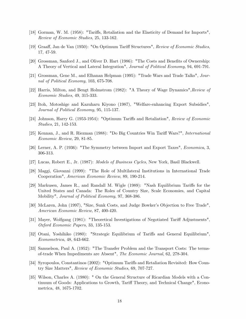
positive values of ~AN (z) imply a comparative advantage in home country production for therespective good z: Changes in � induce parallel shifts of ~A (z) (holding �xed) while changesof correspond to changes in the slope (holding average productivity at �). Higher values of magnify the comparative advantage e¤ects resulting in greater gains from trade. A particularlysimple functional form is used to create the graphs of the paper (see Figure 1):

~A (zj�; ) = �+ (0:5� z) (4)

This loglinear speci�cation can be interpreted as a �rst order approximation of the true func-tion.7

Preferences Like in the original DFS paper the representative agent of each economy pos-sesses a Cobb-Douglas utility function over the range of goods:

U (c) =1R0

b (z) log (c (z))dz

U� (c�) =1R0

b� (z) log (c�(z))dz

(5)

where the expenditure shares b (z) and b� (z) satisfy:

1Z0

b (z) dz =

1Z0

b� (z) dz = 1 (6)

The �gures in the present text are calculated under the assumption that both countries valueall goods equally, i.e. b (z) = b� (z) = 1:

Trade barriers I allow for two types of trade barriers: Import tari¤s (t; t�) and transporta-tion cost (�). The latter are in the form of symmetric iceberg transportation cost (Samuelson1954), which implies that only a fraction of exported goods eventually arrives in the othercountry. This fraction is given by exp (��). Import tari¤s are applied to all goods that arrivein the import country and redistributed to the consumers. Since it turns out to be optimalto charge a uniform tari¤ rate across all goods, I will use this result from the very beginningto simplify the analysis. Export tari¤s do not have to be explicitly considered due to Lerner�s"Symmetry-Result".

2.2 General Equilibrium

The purpose of this section is to highlight the main implications of the DFS model with exoge-nous tari¤s. The main contribution of the original paper is to show that the incorporation oftrade barriers (tari¤s, transportation cost) into a Ricardian Model with a continuum of goods

7An earlier version of this paper focused solely on this speci�cation (seehttp://home.uchicago.edu/~mopp/Research/Tari¤.pdf).

5

gives rise to an endogenously determined non-traded sector in equilibrium. The equilibriumconditions on the three endogenous variables �the equilibrium wage rate ! and the boundarygoods for domestic production in the home and foreign country (�z; �z�) �can be summarized inthe following system of equations (see derivation in Appendix A):

f1 (x; q) = log (!) + log�1+��t�

1����+ log

�1��1+�t

�+ log (L) = 0

f2 (x; q) = log (!)� log (1 + t)� ��h�+ ~AN (�z)

i| {z }

~A(�z)

= 0

f3 (x; q) = log (!)+ log (1 + t�) + ��h�+ ~AN (�z

�)i

| {z }~A(�z�)

= 0

(7)

where: � (�z) =�zR0

b (z) dz and �� (�z�) =1R�z�b� (z) dz

The �rst equation is obtained by imposing balance of trade. Note that � and �� represent theshare of domestic income that each country spends on domestically produced goods. For nota-tional convenience, the arguments �z and �z� are omitted from the functions � and �� throughoutthe text. The second and third equation pin down the boundary goods for domestic productionat which the cost of domestic production equals the cost of importing the good adjusted for thetari¤ fare and transportation cost. The home country produces goods on the interval [0; �z] andimports goods on the interval [�z; 1]: Likewise the foreign country imports goods on the interval[0; �z�] and produces goods domestically on the interval [�z�; 1].

One can represent the above described system more concisely by stacking the endoge-nous variables in the vector x = [log (!) ; �z; �z�] and the exogenous variables in the vectorq = [t; t�; log (L) ; �]:

f (x; q) = 0 (8)

The comparative statics can be obtained by applying the implicit function theorem. Thetotal derivative of the i-th element of vector x with respect to the j-th element of vector isgiven by i; j element of the matrix:

Dq� (q) = � [Dxf ]�1Dqf (9)

where � (q) is the solution for x and Dxf;Dqf represent the respective Jacobians. The algebracon�rms the well understood positive e¤ect of tari¤s on the terms-of-trade. The economicintuition is as follows. By imposing a tari¤ on import goods, the home country increases the�nal consumption prices of foreign goods which in turn reduces demand for those goods in thehome country. At the old equilibrium prices (before imposing the tari¤) the balance of tradecondition will no longer hold as the foreign country will demand too many import goods. Inorder to eliminate the excess demand for import goods in the foreign country, the terms-of-tradehave to deteriorate (improve) from the perspective of the foreign (home) country. This causesthe equilibrium wage rate of the home country to rise (intensive margin). Since the equilibriumwage rate rises relatively less than the price of import goods (i.e. the tari¤ rate increase) thehome country will increase home production as a response to its own tari¤ increase (extensivemargin).

6

Domestic production is increasing in trade barriers (t, t�; �) and increasing in productivity� and size L. It seems quite intuitive that larger and more productive economies producea greater range of goods. Interestingly, log(L) and � have exactly the same impact on theboundary goods �z and �z� which results from the linear technology (see derivation in AppendixC): This means that knowledge of the productivity adjusted relative size L exp (�) - i.e. e¤ectiverelative size - summarizes the separate e¤ects of size and productivity on the boundary goods.For the discussion of optimum tari¤ rates this measure of e¤ective size, precisely its logarithm(c), will become of crucial importance. E¤ective relative size is also closely to the amount ofgoods that can be produced under autarky, i.e. the size of the economy (production capacity).8

c � log (L exp�) = logL+ � (10)

For illustration purposes it is also convenient to de�ne a normalized measure of c denoted as : R! [0; 1]:

(c) � exp (c)

1 + exp (c)(11)

This measure can be interpreted as the economic weight of a country, as the "weights" (c)and (c�) = (�c) add up to one. The in�nitesimally small country gets a weight of zero, thein�nitely large country a weight of one.9

3 Optimum Response Function

3.1 Derivation

So far, the analysis has treated tari¤ rates similar to transaction cost, i.e. as exogenously giventrade barriers. However, in contrast to transportation cost, import tari¤s are choice variablesfor the respective government and a¤ect national income.10 Both governments are assumed tochoose the optimal tari¤ rate for their respective country. As such, they try to maximize theutility of the representative agent given the tari¤ rate decision of the other country. In general,tari¤ rates could vary across goods. However, proposition 1 provides a justi�cation for my focuson uniform tari¤ rates.

Proposition 1 If the demand function is of Cobb-Douglas type, it is optimal to impose auniform tari¤ rate across all import goods.

Proof. See Appendix D.1.

The idea of the proof is relatively simple. First, I show that the marginal tari¤ rate tM (atthe boundary good) and an appropriately de�ned average tari¤ rate �t are su¢ cient statisticsfor an arbitrary taxation schedule t (z) to determine the vector of endogenous variables x (seeAppendix A). Secondly, I split up the utility maximization problem over the schedule t (z)

8For any speci�c good the relative production capacity (number of available labor units / number of requiredlabor units) of both countries is given by C (z) = L

a(z)= L�

a�(z) = LA(z): Taking logarithms and averaging over allgoods implies that we can de�ne c � log (L) + �:

9The careful reader will notice that the function (x) is identical to the CDF of the logistic distribution.10 If tari¤ rebates were simply lost � as in the case of iceberg transportation cost � the optimum tari¤ rate

would be zero.

7

into two parts by �rst solving the subproblem of the welfare optimizing tari¤ rate policy t (z)conditional on the choice of tM and �t and then maximizing over the choice of tM and �t. Thesolution to the subproblem results in uniform tari¤ rates, which delivers the claimed result.

Now, two variables (t; t�) summarize the tari¤ rate policies of both countries, such thatwe can write the derived equilibrium utility of the representative agent in the home countryV (t; t�;q) and the foreign country V � (t; t�; q) as a function of the tari¤ rates and the exogenousparameters. Formally, the optimum tari¤ rate is determined by setting the partial derivativeof the indirect utility function with respect to the tari¤ rate equal to zero:

@V

@t= 0 and

@V �

@t�= 0 (12)

The solution to this problem results in the following expression:

Proposition 2 The optimum tari¤ rate in the DFS model topt can be expressed as follows:

topt = (1� ��)1 + ��t�

1 + t�� ~A0 (�z�)b� (�z�)

=1

"� � 1 (13)

t�opt = (1� �)1 + �t

1 + t

� ~A0 (�z)b (�z)

=1

"� 1 (14)

In order to interpret this result in terms of import demand elasticities ("; "�), I introducean appropriately de�ned measure for this setup. The import demand M of the home countryon the world market (valued in terms of its own currency) is given by:

M = Ly1� �1 + t

= L!1� �1 + �t

(15)

The "price" of an import good in local currency is proportional to the inverse of ! such thatwe can de�ne the import demand elasticity as:

" =d logM

d log!= 1 +

@ logh1��1+�t

i@�

@�

@�z

@�z

@ log!= 1 +

1

t�opt(16)

This pricing formula is identical to the optimal markup that a monopolistic �rm charges

over marginal cost MC, i.e. p =�1 + 1

"(D)�1

�MC. To see this analogy, it is useful to apply

the Lerner symmetry result, such that one can interpret the tari¤ rate formula as the optimalexport tari¤, i.e. the markup on cost. Thus, by applying optimum tari¤ rates a country acts asmonopolist for the goods it exports, which leads to a costly reduction in the volume of trade.

From a computational point, these formulae are progress, as one can now calculate optimumresponse functions for arbitrary technology and taste speci�cations (in conjunction with theother three equilibrium conditions) in the DFS model. Before turning to the general propertiesof the optimum response function in the next chapter, I want to note that the optimum tari¤only depends on the relative labor unit requirement function A (z), but not separately on thelabor unit requirement functions a (z) and a� (z).

8

3.2 Comparative Statics

This section aims to lay out the general properties of the optimum response function g (t�) ofthe home country. The foreign country�s optimum response function g� (t) follows by symmetry.Thus, the fourth equilibrium condition (in addition to the conditions outlined in equation 7) isgiven by:

f4 (x; q) = t+ (1� �� (�z�)) 1+��(�z�)t�

1+t�~A0(�z�)b�(�z�) = 0 (17)

Again the comparative statics are obtained via the implicit function theorem. Now, thevector of endogenous variables x includes the tari¤ rate t. In order to be able to sign thederivatives of the optimum response function I need to make a mild technical assumption:

Assumption 1 @f4@�z� < 0

Since the DFS framework neither speci�es the sign of the second derivatives of the relativelabor unit requirement function nor the �rst derivatives of the expenditure share function b� (�z�),the sign cannot be determined in general (see discussion in Appendix B). However, numericalexercises with various functional forms reveal that this assumption is purely technical andshould not at all be considered as restrictive.11 Hence, for the rest of the analysis I will assumethat the assumption is satis�ed. This implies:

Proposition 3 The optimum response function has the following properties:

- Decreasing in the other country�s tari¤ rate @g@t� < 0

@g�

@t < 0��

- Decreasing in the transportation cost @g@� < 0

@g�

@� < 0 �

- Increasing in the dispersion parameter @g@ > 0

@g�

@ > 0 �

- Increasing in a country�s relative production capacity @g@c > 0

@g�

@c < 0 �

� Assumption 1 is necessary and su¢ cient, �� Assumption 1 is su¢ cient.

Proof. See Appendix D.3.

Thus, tari¤s are strategic substitutes (see Figure 2). The intuition behind this result is thathigher foreign tari¤ rates increase trade barriers that exogenously reduce trade volume (liketransportation cost) such that the room for imposing own trade restrictions without heavilyreducing or even shutting down trade is limited.

Proposition 4 The strategic substitutability is less than perfect, i.e.����d log (1 + topt)d log (1 + t�)

���� < 1Proof. See Appendix D.4.

11For t� relatively small the term1+��(�z�)t�

1+t� is approximately equal to one such that the term (1� ��) dom-inates the comparative statics. This assumption will always be satis�ed if one uses the technology speci�cationunderlying the Eaton-Kortum model (2002).

9

Proposition 4 implies, that an increase in the tari¤ rate of the foreign country will lead toa decrease in the home country tari¤ rate that does not fully compensate for the trade barrierimposed by the foreign country, i.e. the non-traded sector (goods in the range between �z� and�z) will expand. It can be shown, that strategic substitutability is increasing in size, i.e. largereconomies respond stronger to an increase in the tari¤ rate of the other country.

An increase in natural trade barriers (transportation cost) has qualitatively the same neg-ative e¤ect on the optimum tari¤ rate as an increase in the other country�s tari¤ rate. A �at-ter relative labor unit requirement function (lower ) implies smaller specialization advantageswhich causes domestic and foreign production to be more similar and hence more substitutable.Hence, a �xed increase in tari¤ rates results in a larger demand reduction for �atter functions~A (z) such that the optimum tari¤ rate will be smaller.

The positive marginal impact of the parameter c implies that countries with a higher ef-fective size can exploit the import dependency of the other country (and the associated lowerimport demand elasticity). The relationship is monotone, as the harmful side-e¤ects of tari¤s(ine¢ cient expansion of home production and price increase of import products) weigh smallerand the terms-of-trade e¤ect becomes stronger the greater the economic weight of one country.12

Moreover, it is possible to determine the optimum tari¤ rate policy of a "small" economy:13

Corollary 1 As the home economy becomes in�nitesimally small, the tari¤ rate approacheszero:

limc!0

g (t�) = 0

Proof. In the limit the foreign country�s consumption share of domestically produced goodsapproaches 1; i.e. limc!0 �� = 1 and limc!0 �z� = 0. Therefore, we have:

topt = lim��!1

(1� ��) 1 + ��t�

1 + t�� ~A0 (0)b� (0)

=� ~A0 (0)b� (0)

lim��!1

(1� ��) = 0

4 Nash Equilibrium

4.1 Existence

A Nash equilibrium in tari¤ rates is obtained, once both countries have no incentive to deviatefrom their chosen tari¤ rate. Formally, a Nash equilibrium is characterized by an additionalequilibrium condition that ensures the optimality of the foreign country�s tari¤ rate t�, the �fthelement of the vector of endogenous variables x.

f5 (x; q) = t� + (1� �� (�z�)) 1+��(�z�)t�

1+t�~A0(�z�)b�(�z�) = 0 (18)

12Consider the extreme case when the home country is in�nitely large/productive such that all goods areproduced domestically even without tari¤s.13The boundedness assumption plays a key role. A violation of boundedness such as in the Eaton-Kortum

speci�cation of technology can imply strictly positive tari¤ rates even for the in�nitesimally small country.

10

The optimum response functions for two parameter constellations are depicted in Figure 2.The intersection point constitutes a Nash equilibrium in tari¤ rates which is characterized bystrictly positive trade �ows. No-Trade Nash equilibria can occur, if both countries choose aprohibitively high tari¤ rate tproh, i.e. a tari¤ rate that exhausts the specialization advantageadjusted for transport cost. Formally a prohibitive tari¤ rate (given that the other countryimposes no tari¤ barriers) satis�es the following relation:14

log (1 + tproh:) > ~A (0)� ~A (1)� 2� (19)

There exists a continuum of No-trade equilibria all of which are uninteresting, as applying aprohibitive tari¤ rate is weakly dominated. In the following analysis I will only consider interiorNash equilibria.

Proposition 5 There exists a unique interior Nash equilibrium in tari¤s that Pareto dominatesany No-Trade Nash equilibrium

Proof. See Appendix E.1.

The existence of a unique equilibrium is established by applying the Contraction MappingTheorem. The contraction property follows directly from the fact that the slope of the optimumresponse function is less than one (see Proposition 4).

4.2 Tari¤Rates

The comparative statics in the Nash equilibrium are driven by the direct e¤ects of the exogenousparameters on the optimum response function as well as the feedback e¤ect through the strategictari¤ choice of the other country. In case of the size parameter c, the feedback e¤ect ampli�esthe original e¤ect. This is because as the home economy becomes relatively larger (and thusthe foreign economy smaller) the foreign economy will apply lower tari¤ rates which in turnincreases the tari¤ rate of the home country due to strategic substitutability (see proposition4). This results in the following claim:

Proposition 6 The Nash equilibrium tari¤ rate is increasing in relative e¤ective size.

In the case of transportation cost parameter �, the feedback e¤ect counters the direct e¤ect.Holding the other country�s tari¤ rate �xed, an increase in transportation cost lowers theoptimum tari¤ rate of both countries. On the other hand, due to strategic substitutability alower tari¤ rate of the foreign country increases the home country tari¤ rate. Without furtherrestrictions the net e¤ect could go either way. However, in all relevant scenarios the direct e¤ectis expected to dominate because precisely when the sensitivity to the foreign country�s tari¤rate decision is large �when the home economy is large � it is also the case that the (small)foreign country will hardly adjust its tari¤ rate to changes in transportation cost (see Figure

14The restriction can be obtained by subtracting the equilibrium condition on the boundary good for theforeign country from the boundary good condition of the home country, i.e. f3 (x; q) � f2 (x; q) ; and using theno-trade condition on the boundary goods (�z� = 0 and �z = 1 ): For the log-linear technology speci�cation, a logtari¤ rate greater than � 2� is prohibitive.

11

3) .15 Moreover note, that at most one country may increase its tari¤ rate as a response to anincrease in transportation cost. Therefore, for economies of equal size (c = 0) the net e¤ect willbe unambiguous and both countries will lower their tari¤ rate (as a response to an increase intransportation cost) due to symmetry.

The Nash equilibrium comparative statics of the dispersion parameter features the sametension between the direct and the feedback e¤ect. While the direct e¤ect implies higher tari¤sfor both countries if the gains from trade are greater the feedback e¤ect goes the opposite way.As for the case of transportation cost, the direct e¤ect is expected to dominate (see Figure 3).

4.3 Terms-of-Trade and Welfare

Since the improvement of terms-of-trade is central to our analysis, it is helpful to revisit akey result from the original DFS model (with exogenous tari¤s). Small countries (i.e. lowrelative size L) face signi�cantly better terms-of-trade and bene�t the most from free trade.The intuition for this result is that small countries can specialize their production on goodswith the highest comparative advantage whereas the large country has to supply the remainderof the goods (for a formal derivation see Appendix C). However, the strategic disadvantage ofbeing small mitigates this positive e¤ect in the Nash equilibrium. As shown in the previoussection, smaller (larger) countries apply lower (higher) equilibrium tari¤ rates. Since the relativewage rate is an increasing function of the own tari¤ rate and a decreasing function of theother country�s tari¤ rate, relative size will in�uence the wage rate positively through thischannel. Whether this strategic e¤ect possesses signi�cant impact depends on the speci�cationof technology. The log-linear approximation (see Figure 4) reveals that the large specializationbene�ts for the small country (driven by comparative advantage) are almost completely wiped-out in the Nash equilibrium such that the terms of trade will only represent the absolutetechnology advantage �.

The just described terms-of-trade e¤ect will also play an important role for the welfareanalysis. Since the Nash equilibrium is not Pareto optimal both countries could increase theirwelfare by removing all tari¤s and split up the surplus. In order to measure welfare losses foreach country I determine the required log rate of consumption growth � that equalizes theutility obtained in the Nash equilibrium (N) and free trade (F ).16 Therefore � is de�ned as:

VF�e�cF

�� t = 0; t� = 0� � VN (cN j t = tN ; t� =t�N ) (20)

Due to the simple form of the utility function the required growth rate of consumption is givenby the di¤erence of the utility levels:

�V = VN � VF (21)

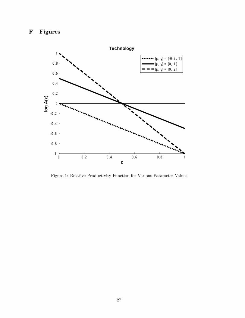
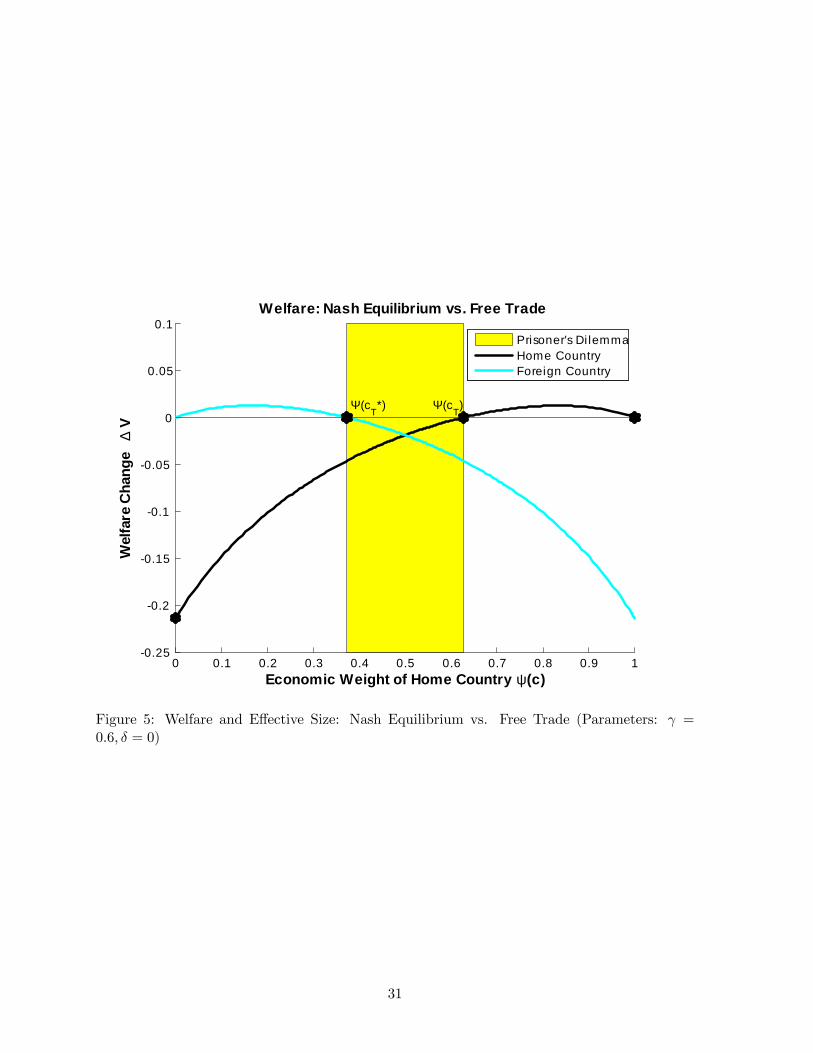
The following lemma describes intuitive properties of the welfare measure �V (see Figure 5).

Lemma 1 �V is a function of c; � and and has the following limit properties:1) limc!0�V (c; ; �) < 02) limc!1�V (c; ; �) = 0

3) limc!1@�V (c; ;�)

@c < 0

15Numerical results for various functional forms (see subsequent section) con�rm this claim.16This welfare measure has been proposed by Lucas (1987) and Alvarez, Lucas (2005).

12

Proof. See Appendix E.3.

First of all, since this measure only captures changes between free trade and the Nashequilibrium, it is driven by the strategic choices of tari¤ rates. As tari¤ rates only depend onsize L and productivity � through their e¤ect on the parameter c, so does the welfare measure�V . The �rst limit property states that the in�nitesimally small economy will surely be worseo¤ in the Nash equilibrium than under free trade where it faces the best terms-of-trade. Incontrast, the in�nitely large economy will be equally well o¤ in the Nash equilibrium as underfree trade because welfare converges to the autarky level in both situations. The last propertystates that the in�nitely large country would bene�t from an extension of the economy of itstrading partner (from which monopoly rents can be extracted).

As in Syropoulos (2002), these limit properties (together with continuity) are su¢ cient toestablish existence of a unique threshold size cT at which a country is indi¤erent between theNash equilibrium outcome and and Free Trade:

Proposition 7 A country prefers the Nash-Equilibrium outcome over Free Trade if its e¤ectiverelative size c exceeds the threshold level cT ( ; �).

Since the structure of the proof is essentially identical to Syropoulos�treatment, a rigorousproof of existence and uniqueness is omitted. A graphical illustration is provided in Figure 5.The idea is as follows. Properties 2) and 3) ensure that it is possible to be better o¤ in theNash equilibrium than under free trade (i.e. �V > 0 for c very large). By property 1), thesmall country will be worse o¤ in the Nash equilibrium such that �V is negative for small c:The existence of the threshold size level follows by continuity.

If the expenditure functions b (z) and b� (z) coincide, then the threshold size level of bothcountries will be identical by symmetry. The threshold size level is greater than 0, because aNash equilibrium induces Pareto ine¢ cient production. Hence, when the countries are of equalsize they will be both worse o¤ than in the free trade scenario. Such a Prisoner�s Dilemmasituation will always occur provided that the size asymmetries are not too great, i.e. wheneverjcj < cT .

In addition to the veri�cation of Syropoulos� core existence result (albeit in a di¤erentframework), I am able to analyze the impact of transportation cost and comparative advantageon the threshold size level cT : Two easily interpretable assumptions are required:

Assumption 2 @�V (cT ; ;�)@ < 0

Assumption 3 @�V (cT ; ;�)@� > 0

Assumption 2 implies that an increase in comparative advantage will imply greater welfaregains in the Free-Trade situation than in the Nash equilibrium (for a country at the thresholdsize). Assumption 3 implies that transportation cost are relatively more harmful under freetrade than in the Nash equilibrium (for a country at the threshold size). For the rest of thispaper, I will assume that these assumptions are satis�ed:

13

Proposition 8 The threshold level cT is an increasing function of and a decreasing functionof �.

Proof. The threshold size level is characterized by the following implicit function:

�V (cT ; ; �) = 0

By the implicit function theorem, we obtain:

h@cT@

@cT@�

i= �

�@�V (cT ; ; �)

@c

�| {z }

>0

�124 @�V (cT ; ; �)

@ | {z }<0

@�V (cT ; ; �)

@�| {z }>0

35| {z }

see Assumptions 2+3

The partial derivative with respect to size must be positive at the threshold size level whichfollows directly from the discussion of Proposition 7 and Figure 5.

For the log-linear speci�cation of technology, the required threshold cT size turns out to bea particularly simple linear function of and � (see Figure 6).

5 Implications for Self-Enforcing Trade Agreements

The goal of this section is to discuss the general implications of the static Nash equilibriumanalysis for cooperative trade agreements within a dynamic context. Rather than solving forthe optimal dynamic contract, I want to highlight the key intuitions that can be obtainedfrom the static analysis and point to the relevant extensions in a dynamic setup.17 It is wellunderstood that any trade agreement has to be self-enforcing due to the lack of internationalcourts with real enforcement power. Thus, a sustainable (subgame perfect) contract requiresthat the short-run bene�t from a unilateral tari¤ choice (i.e. setting the static best responsetari¤s given by equations 13 and 14) must be overwhelmed by the long-run cost resulting fromthe retaliation of the other country.18 Due to the lack of commitment such a punishment bythe other country has to be itself credible, i.e. subgame perfect. The static Nash equilibriumoutcome can be used as such an o¤-equilibrium path threat point to induce cooperation on theequilibrium path.19

Due to asychronous nature of the cost and bene�t of reneging on a contract, impatienceplays a central role for the Pareto set of equilibrium contracts. The folk theorem implies thatas the discount factor approaches one, virtually any tari¤ pair on the contract curve �the set ofinternationally e¢ cient tari¤ combinations that yield higher utility than the Nash outcome (seeMayer, 1981) �becomes self-enforcing.20 However, the static analysis reveals that this contractcurve may not include reciprocal free trade in which case free trade is not sustainable (evenin the limit). Such a situation will always occur in the presence of su¢ cient size asymmetries,

17A rigorous derivation of the optimal dynamic contract using the ingenious machinery of Abreu et al. (1990)is interesting enough in its own right and beyond the scope of this paper.18A summary of this literature is found in chapter 6 of Bagwell and Staiger (2002).19Friedman�s (1971) formal analysis of oligopolistic structures uses this idea �rst. Bagwell and Staiger (2002)

show that there is also a limited role for on-equilibrium path retaliation within the GATT framework. This ideais not explored further in this paper.20E¢ cient tari¤ combinations satisfy: (1 + t) (1 + t�) = 1.

14

i.e. if one economy exceeds the threshold size level cT .21 As the threshold size cT is decreasingin transportation cost, it is easier to sustain free-trade agreements among countries which aregeographically closer. Thus, my analysis is consistent with the regional focus of most free tradezones across the world such as NAFTA or the EU.

An interesting implication of the repeated games analysis is that the e¢ cient contractscan feature non-trivial dynamics even in a physically stationary environment. The e¢ cientintertemporal provision of incentives without commitment requires the agent with the strongestincentive to deviate to obtain back-loaded payo¤s.22 Applied to our setting, we can state thatthe welfare-maximizing contract for the small country (i.e. the contract on the Pareto frontierwhich is chosen when the small country has full bargaining power) necessarily involves front-loaded bene�ts to the small and back-loaded bene�ts to the large country. This is consistentwith Bond and Park�s analysis (2002), who use the gradual nature of the trade liberalizationbetween Poland and the EU as an empirical example.

Despite these interesting predictions within a stationary environment, the assumption ofstationarity in a clearly non-stationary world prevents the analysis of important dynamics thatmatter for trade agreements.23 Especially of interest is how the anticipated strong growthof the BRIC countries, most notably China, in�uences trade agreements.24 The dynamicsspeci�cation does not require separate processes for productivity � and the demographics L, asboth can be conveniently summarized by e¤ective relative size c. Intuitively, one would expectthat anticipated strong growth diminishes the usefulness of providing front-loaded contracts tosuch economies, as they will have greater incentives to renege on a contract in the future.

Moreover, it is interesting to study the e¤ect of comparative advantage through time seriesvariations in the dispersion parameter . The static analysis suggests, that in times whenspecialization gains are high (and expected to stay high) free trade agreements should be easierto implement as the threshold size cT has been shown to be an increasing function of . Theintuitive appeal is clear: larger specialization gains are more bene�cial under cooperation thanin the ine¢ cient Nash equilibrium. Moreover, under the assumption that gains from tradefollow a predictable trend, one can explain the gradual nature of trade agreements � mostnotably the GATT rounds of negotiations.25

6 Conclusion

The analysis of this paper has suggested that the rigorous understanding of the static Nashequilibrium outcome can be viewed as a stepping stone to the more complicated analysis ofself-enforcing trade agreements within a dynamic context. In order to study the importantimpact of growth dynamics on the sustainability and evolution of trade agreements it seems

21This is a su¢ cient condition, i.e. even when one country�s relative size is slightly smaller than cT , free trademay not be sustainable as the small country does not apply a zero tari¤ rate when its relative country size is�cT :22The intuition goes back to the seminal paper of Harris and Holmstrom (1982) within the labor market

context.23 In this spirit, Bagwell and Staiger (1995) use a dynamic partial equilibrium model to explain the counter-

cyclical nature of trade barriers.24The term BRIC countries refers to the emerging market economies Brazil, Russia, India and China.25This idea is somewhat a reduced form implication of the analysis by Devereux (1997) who assumes that

production technologies exhibit "learning by doing" features which generate predictable specialization gains.

15

worthwhile to prefer a more complicated dynamic game setup over a strictly repeated gameframework. This line of research might produce interesting implications about the relationshipbetween trade, growth and technology di¤usion.

Within a multiperiod setup, it is also possible to meaningfully relax the assumption ofperiod-by-period balanced trade and replace it by a present value constraint. Speci�cally, onecan address the interaction of the optimal dynamic government debt and trade policy in anenvironment without commitment. Comparative advantage on the production side might notonly be helpful for enforcing trade agreements, but also for inducing repayment of sovereigndebt.26 This intution goes back to Bernheim and Whinston (1990) who �nd that cooperativebehavior is easier to sustain among �rms with multimarket contact.

Instead of abandoning the static framework, one could understand the derived Nash equi-librium tari¤ rates as empirical predictions for observed tari¤ rates.27 In order to meaningfullytest whether applied tari¤ rates are increasing in the size of the economy and comparativeadvantage and decreasing in transportation cost (distance) historical tari¤ data of Non-WTOcountries needs to be used. This would be very much in the spirit of Broda et al. (2006).28

Interesting datasets can also be obtained by going back further in time. For example, at thebeginning of the 19th century countries like Germany consisted essentially of a myriad of inde-pendent states �ranging from the small free city of Frankfurt to the large state of Prussia �allwith a separate tari¤ system.29

26This analysis is relevant in the light of the famous Bulow and Rogo¤ (1989) result who show that sovereigndebt is not sustainable without e¤ective sanctions. Such sanctions can be achieved through trade policy.27On the theory side, one might want to extend the static analysis by allowing for more general classes of

preferences such as in Wilson (1980). Another idea is to abandon the 2 country framework as in Alvarez andLucas (2005) which would also allow the examination of multilateral enforcement of trade agreements in thespirit of Maggi (1999).28The authors, however, do not �nd convincing support for a (linear) relation between size and applied tari¤

rates in their sample. Another prediction of my analysis �uniformity of tari¤ rates �is probably more of technicalrather than practical relevance.29A common system was not in place before the creation of the "Deutscher Zollverein" in 1834.

16

References

[1] Alvarez, Fernando, and Robert E. Lucas, Jr. (2006): "General Equilibrium Analysis ofthe Eaton-Kortum Model of International Trade", NBER Working paper 11764.

[2] Bagwell, Kyle, and Robert W. Staiger (1990): "A Theory of Managed Trade", AmericanEconomic Review, 80, 779-795.

[3] Bagwell, Kyle, and Robert W. Staiger (1995): "Protection and the Business Cycle", NBERWorking paper 5168.

[4] Bagwell, Kyle, and Robert W. Staiger (1999): "An Economic Theory of GATT", AmericanEconomic Review, 89, 215-248.

[5] Bagwell, Kyle, and Robert W. Staiger (2001): "Reciprocity, non-discrimination and prefer-ential agreements in the multilateral trading system", European Journal of Political Econ-omy, 17, 281-325.

[6] Bagwell, Kyle, and Robert W. Staiger (2002): The Economics of the World Trading Sys-tem, Cambridge, MA: MIT Press.

[7] Bernheim, B. Douglas and Michael D. Whinston (1990): "Multimarket Contact and Col-lusive Behavior", Rand Journal of Economics, 21, 1-26.

[8] Bond, Eric W. (1990): "The Optimal Tari¤Structure in Higher Dimensions", InternationalEconomic Review, 31, 103-116.

[9] Bond, Eric W., and Jee-Hyeong Park (2002): "Gradualism in Trade Agreements withAsymmetric Countries", Review of Economic Studies, 69, 379-406.

[10] Broda, Christian, Nuno Limão and David E. Weinstein (2006): "Optimal Tari¤s: TheEvidence", NBER Working paper 12033.

[11] Bulow, Jeremy, and Kenneth Rogo¤ (1989): "Sovereign Debt: Is to forgive to forget?",American Economic Review, 79, 43-50.

[12] Dixit, Avinash K. (1987): Strategic Aspects of Trade Policy, in T. Bewley (ed.) Advancesin Economic Theory, Fifth World Congress, Cambridge: Cambridge University Press.

[13] Devereux, Michael B. (1997): "Growth, Specialization, and Trade Liberalization", Inter-national Economic Review, 38, 565-585.

[14] Dornbusch, Rüdiger, Stanley Fischer, and Paul A. Samuelson (1977): "Comparative Ad-vantage, Trade, and Payments in a Ricardian Model with a Continuum of Goods", Amer-ican Economic Review, 67, December, 823-839.

[15] Eaton, Jonathan, and Samuel Kortum (2002): "Technology, Geography, and Trade",Econometrica, 70, 1741-1779.

[16] Feenstra, Robert C. (1986): "Trade Policy with Several Goods and �Market Linkages�",Journal of International Economics, 20, 249-267.

[17] Friedman, James W. (1971): "A Non-Cooperative Equilibrium for Supergames", Reviewof Economic Studies, 38, 1-12.

17

[18] Gorman, W. M. (1958): "Tari¤s, Retaliation and the Elasticity of Demand for Imports",Review of Economic Studies, 25, 133-162.

[19] Graa¤, Jan de Van (1950): "On Optimum Tari¤ Structures", Review of Economic Studies,17, 47-59.

[20] Grossman, Sanford J., and Oliver D. Hart (1986): "The Costs and Bene�ts of Ownership:A Theory of Vertical and Lateral Integration", Journal of Political Economy, 94, 691-791.

[21] Grossman, Gene M., and Elhanan Helpman (1995): "Trade Wars and Trade Talks", Jour-nal of Political Economy, 103, 675-708.

[22] Harris, Milton, and Bengt Holmstrom (1982): "A Theory of Wage Dynamics",Review ofEconomic Studies, 49, 315-333.

[23] Itoh, Motoshige and Kazuharu Kiyono (1987), "Welfare-enhancing Export Subsidies",Journal of Political Economy, 95, 115-137.

[24] Johnson, Harry G. (1953-1954): "Optimum Tari¤s and Retaliation", Review of EconomicStudies, 21, 142-153.

[25] Kennan, J., and R. Riezman (1988): "Do Big Countries Win Tari¤ Wars?", InternationalEconomic Review, 29, 81-85.

[26] Lerner, A. P. (1936): "The Symmetry between Import and Export Taxes", Economica, 3,306-313.

[27] Lucas, Robert E., Jr. (1987): Models of Business Cycles, New York, Basil Blackwell.

[28] Maggi, Giovanni (1999): "The Role of Multilateral Institutions in International TradeCooperation", American Economic Review, 89, 190-214.

[29] Markusen, James R., and Randall M. Wigle (1989): "Nash Equilibrium Tari¤s for theUnited States and Canada: The Roles of Country Size, Scale Economies, and CapitalMobility", Journal of Political Economy, 97, 368-386.

[30] McLaren, John (1997), "Size, Sunk Costs, and Judge Bowker�s Objection to Free Trade",American Economic Review, 87, 400-420.

[31] Mayer, Wolfgang (1981): "Theoretical Investigations of Negotiated Tari¤ Adjustments",Oxford Economic Papers, 33, 135-153.

[32] Otani, Yoshihiko (1980): "Strategic Equilibrium of Tari¤s and General Equilibrium",Econometrica, 48, 643-662.

[33] Samuelson, Paul A. (1952): "The Transfer Problem and the Transport Costs: The terms-of-trade When Impediments are Absent", The Economic Journal, 62, 278-304.

[34] Syropoulos, Constantinos (2002): "Optimum Tari¤s and Retaliation Revisited: How Coun-try Size Matters", Review of Economic Studies, 69, 707-727.

[35] Wilson, Charles A. (1980): " On the General Structure of Ricardian Models with a Con-tinuum of Goods: Applications to Growth, Tari¤ Theory, and Technical Change", Econo-metrica, 48, 1675-1702.

18

A General Equilibrium with Arbitrary Tari¤ Schedule

Tari¤-adjusted prices in the home country and foreign country are given by:

p (z) =

�!a (z)a� (z) exp (�) (1 + t (z))

for z 6 �zelse

p� (z) =

�!a (z) exp (�) (1 + t� (z))a� (z)

for z 6 �z�else

(22)

The boundary goods satisfy: �z = A�1�

!1+tM

e���and �z� = A�1

�! (1 + t�M ) e

��where tM is

the marginal tax rate. The balance of trade condition implies:

Ly

1Z�z

b (z)

1 + t (z)dz = y�

1Z�z

b� (z)

1 + t� (z)dz (23)

which we can rewrite concisely as:

Ly (1� �)1 + �t

=y� (1� ��)1 + �t�

(24)

where the average tari¤ rates are de�ned appropriately:

1

1 + �t� 1

1� �

1Z�z

b (z)

1 + t (z)dz and

1

1 + �t�� 1

1� ��

�z�Z0

b� (z)

1 + t (z)dz

The tari¤ rebates per capita in the home country are given by:

r = y

1Z�z

b (z) t (z)

1 + t (z)dz = y

1Z�z

b (z)

�1� 1

1 + t (z)

�dz = y (1� �)

�t

1 + �t(25)

Income per capita is the sum of the wage rate and the tari¤ income, i.e. y = !+ r. We obtain:

y = !1 + �t

1 + ��tand y� =

1 + �t�

1 + ���t�(26)

Using the balance of trade condition (equation 24) and the income per capita from equation 26yields:

! =1 + ��t

1 + ���t�1� ��1� � =L (27)

The boundary goods �z and �z� satisfy:

log (!)� log (1 + tM )� ~A (�z)� � = 0

log (!)+ log (1 + t�M )� ~A (�z�) + � = 0(28)

Equations 27 and 28 show that the e¤ect of the tari¤ rate schedule t (z) on the boundarygoods and the equilibrium wage rate can be summarized by the marginal tari¤ rate tM and theweighted average tari¤ rate �t.

19

B Partial Derivatives

The signs of these partial derivatives can be determined for sure:

Term Expression Sign Term Expression Signf1�z �b (�z) 1+t

(1+�t)(1��) < 0 f3�z� � ~A0N (�z�) > 0

f1�z� �b� (�z�) 1+t�

(1+��t�)(1���) < 0 f3t�1

1+t� > 0

f1t � �1+�t < 0 f4t�

1���1+t�

t1+��t� > 0

f1t���

1+��t� > 0 f4 f3�z� f1�z�

< 0

f2�z � ~A0N (�z) > 0 f5t1��1+t

t�

1+�t > 0

f2t � 11+t < 0 f5

f2�z f1�z

< 0

By construction, we can claim that ~A0 (z) < 0. The signs of f2 = � ~AN (�z) and f3 = � ~AN (�z�)are uncertain. The signs of f4�z� and f5�z are given by assumption 1.

f4�z� = ~A0 (�z�)| {z }<0

1� t� (1� 2��)1 + t�| {z }see below�

+ (1� ��) 1 + ��t�

1 + t�| {z }>0

d

d�z�

~A0 (�z�)

b� (�z�)| {z }?

< 0

f5�z = � ~A0 (�z)| {z }>0

1� t (1� 2�)1 + t| {z }

see below�

+ (1� �) 1 + �t1 + t| {z }

>0

d

d�z

~A0 (�z)

b (�z)| {z }?

> 0

�The relevant terms are surely positive if the respective tax rates t; t� are smaller than 100%.Moreover, the term can only become negative if the imports sectors are relatively large (whichis highly unlikely if the tax rates are higher than 100%). The terms indicated by the "?" willdrop out for the log-linear speci�cation and a �at expenditure share function. Economic theorygives us no guidance on the general sign of these terms.

C Comparative Statics in the DFS Model

The equilibrium conditions are outlined in equation 7. The Jacobians DXf and DQf need tobe computed in order to apply the Implicit Function Theorem (see equation 9):

DXf =

24 1 f1�z f1�z�

1 f2�z 01 0 f3�z�

35 and Dqf =

24 f1t f1t� 1 0 0f2t 0 0 �1 �10 f3t� 0 1 �1

35The partials fij =

@fi@j are listed in Appendix B. The determinant of DXf is strictly positive,

which enables us to apply the Implicit Function Theorem:

det (DXf) = �f1�z�f2�z � f1�zf3�z� + f2�zf3�z� = f2�zf3�z�� > 0

where � = "+"��1 represents the Marshall-Lerner condition for market stability which is surelysatis�ed. The comparative statics (adjusted by the positive determinant) Dq� (q) �det (DX) aregiven by:

20

Term t logL � �

log! (f1�zf2t � f1tf2�z) f3�z�| {z }>0

�f2�zf3�z�| {z }<0

f1�z�f2�z � f1�zf3�z�| {z }?

�f1�z�f2�z � f1�zf3�z�| {z }>0

�z f1�z�f2t + (f1t � f2t) f3�z�| {z }>0

f3�z�|{z}>0

�2f1�z� + f3�z�| {z }>0

f3�z�|{z}>0

�z� �f1�zf2t + f1tf2�z| {z }<0

f2�z|{z}>0

2f1�z � f2�z| {z }<0

f2�z|{z}>0

It can be directly inferred that the partials of the boundary goods �z and �z� with respect tosize logL and absolute productivity � are identical.

D Optimum Response Function

D.1 Proof of Proposition 1: Uniform Tari¤Rates

Let us write out the derived utility function Vmax as:

Vmax = maxft(z)g

1Z0

b (z) log (b (z) y=p (z)) dz

= maxft(z)g

log (y) +K ��zZ0

b (z) log (a (z)!) dz �1Z�z

b (z) log (a� (z)) dz � � (1� �)

| {z }v(tM ;�t)

�1Z�z

b (z) log (1 + t (z)) dz

where K =

1Z0

b (z) log (b (z)) dz). Appendix A reveals that y; !; �z and � are determined by the

choice of the marginal tax rate tM and the average tax rate �t such that the terms in v (tM ; �t)solely require knowledge of tM and �t instead of the exact tari¤ rate schedule t (z) : We nowbreak the maximization part into two steps.

1. Maximize tax rate policy t (z) conditional on �xed tM and �t

2. Maximize over the choice tM and �t

Vmax = maxftM ;�tg

maxf t(z)jtM ;�tg

264v (tM ; �t)� 1Z�z(tM ;�t)

b (z) log (1 + t (z)) dz

375= maxftM ;�tg

264v (tM ; �t)� minf t(z)jtM ;�tg

1Z�z(tM ;�t)

b (z) log (1 + t (z)) dz

37521

The inner problem (note that �z is �xed conditional on tM and �t) can be stated as:

mint(z)

1Z�z(tM ;�t)

b (z) log (1 + t (z)) dz s.t.

t (�z)� tM = 01Z�z

b(z)1+t(z)dz �

1��1+�t = 0

The �rst order conditions with respect to t (z) imply:

1 + t (z) = �

Since the Lagrange-Multiplier � is independent of z we have established that t (z) = �t =tM :

D.2 Proof of Proposition 2: Tari¤Rate Formula

The derived utility function can be expressed as:

V = log (y)��zZ0

b (z) log (a (z)!) dz �1Z�z

b (z) log (a� (z)) dz � [log (1 + t) + �] (1� �)

= (1� � (�z)) [log! � �]� log (1 + � (�z) t)��zZ0

b (z) log (a (z)) dz �1Z�z

b (z) log (a� (z)) dz + � (�z) log (1 + t)

Note that the irrelevant constant term

1Z0

b (z) log (b (z)) dz has been eliminated. The partials

are given by: h@V@t

@V@�z

@V@log!

i=h� (1��)�t(1+t)(1+�t) � b(�z)

1+�t 1� �i

where I have used �0 (�z) = b (�z) and log (1 + t) + �+ ~A (�z)� log (!)� t1+�t = 0. The �rst-order

condition implies:@V

@t+@V

@�z

d�z

dt+

@V

@log!

dlog!

dt= 0

Using the comparative statics results from Appendix C we obtain after simple algebraic ma-nipulations:

t = (1� ��)1 + ��t�

1 + t�� ~A0 (�z�)b� (�z�)

= �f3�z�

f1�z�= (1� ��) 1 + �

�t�

1 + t�� ~A0 (�z�)b� (�z�)

The optimum tari¤ rate condition for the foreign country follows by symmetry.

22

D.3 Proof of Proposition 3: Properties of the Optimum Response Function

Again, we need to calculate the Jacobians to apply the Implicit Function Theorem:

DXfR =

26641 f1�z f1�z� f1t1 f2�z 0 f2t1 0 f3�z� 00 0 f4�z� 1

3775 and DqfR =

2664f1t� 1 0 0 00 0 �1 �1 f2 f3t� 0 1 �1 f3 f4t� 0 0 0 f3�z�

f1�z�

3775where xR =

�w �z �z� t

�0and qR =

�t� logL � �

�0: The subscript R refers to

"Optimum Response".

det (DXfR) = f2�zf3�z� � f1�zf3�z� � f1�zf2tf4�z� � f2�zf1�z� + f2�zf1tf4�z� > 0

The comparative statics (adjusted by determinant) DqfR� (q) � det (DXfR) are given by:

@g@c � det (DXfR) = �f4�z�f2�z > 0@g@� � det (DXfR) = (�2f1�z + f2�z) f4�z� < 0@g@t� � det (DXfR) = f4t�f2�zf3�z�� + f4�z�

�f1�zf3t� � f2�z 1���

(1+��t�)(1+t�)

�< 0

@g@ � det (DXfR) =

"f2�zf3�z� ("��1) + f2�z (("� 1) f2 � f3 ") f4�z� + f3�z�= > 0

where � = "+"��1. Note that "; "� are both greater than 1:Moreover, note that the partials ofthe tari¤ rate with respect to size logL and absolute productivity � are identical (summarizedby c). The signs and expressions for each term are shown in Appendix B.

D.4 Proof of Proposition 4: Strategic Substitutability

We can rewrite the det (DxfR) as:

det (DXfR) = f2�z

�f3�z�� �

f4�z�

1 + t

�"� 1 + � (1 + t)

1 + �t

��Now, we can determine the degree of strategic substitutability, i.e. �t;t� =

��� d log(1+t)d log(1+t�)

����t;t� =

tf3�z�� � f4�z��1+��t�

1��� ("� 1) + 1�

1 + ��t�

1� ��| {z }>1

(1 + t) f3�z�� � f4�z�

0BB@1+��t�1��� ("� 1) +

1 + ��t�

1� ��� (1 + t)

1 + �t| {z }>1

1CCA< 1

23

E Nash Equilibrium

E.1 Proof of Proposition 5: Existence of Nash Equilibrium

Let (S; �) de�ne the complete metric space with S = [0; ~A (0)� ~A (1)� 2�] and � = jx� yj andde�ne the operator T � : S ! S with T �x = ~g� (~g (x)) where ~g represents the optimum responsefunction for log tari¤ rates log(1 + t). T � is a contraction since the optimum response functions~g (log (1 + t�)) and ~g� (log (1 + t)) are continuous functions with slope uniformly less than onein absolute value (by proposition 4). Hence, we can invoke the Contraction Mapping theoremwhich guarantees the existence of a unique �xed point in S. This �xed point constitutes theNash Equilibrium tari¤ rate of the foreign country. An analogous argument with Tx = ~g (~g� (x))yields the unique Nash Equilibrium tari¤ rate log(1 + tN ) of the home country. An interiorNash equilibrium Pareto dominates the No-Trade Nash equilibrium (autarky), since this option(no trade) is available in the action set of each country (choosing a prohibitive tari¤ rate of~A (0)� ~A (1)� 2�).

E.2 Proof of Proposition 6: Comparative Statics

Again, we need to calculate the Jacobians to apply the Implicit Function Theorem (equation9):

DXfN =

2666641 f1�z f1�z� f1t f1t�

1 f2�z 0 f2t 01 0 f3�z� 0 f3t�

0 0 f4�z� 1 f4t�

0 f5�z 0 f5t 1

377775 and DqfN =

26666641 0 0 0

0 �1 �1 � ~AN (�z)0 1 �1 � ~AN (�z�)0 0 0 f3�z�

f1�z�

0 0 0 f2�z f1�z

3777775where xN =

�w �z �z� tN t�N

�0and qN =

�logL � �

�0: The subscript N refers to

"Nash Equilibrium".

Lemma 2 The determinant of DXfN is positive.

Proof. Omitted.

@tN@ logL

=@tN@�

=�f2�zf4�z� + (f3�z�f4t� � f3t�f4�z�) f5�z

DXfN> 0 (29)

The signs and expressions for each term are shown in Appendix B. As discussed in the text,the signs of the partials @tN@� and @tN

@ cannot be determined in general.

24

E.3 Proof of Lemma 1: Welfare Measure

If we subtract the derived utility under free trade and in the Nash equilibrium, we obtain:

�V =(1� �N ) [log (1���N )� log (1 + ��N t�N )� log (1� �N )]� (30)

(1� �F ) [log (1���F )� log (1� �F )] + (c+ �) (�N � �F )

+

�zNZ�zF

b (z) ~AN (z) dz + �N log

�1 + tN1 + �N tN

�

Since the e¤ect of logL and � on �N ; ��N ; tN ; t�N ; �zN and �zF (see Appendix C and E.2) can

be summarized by e¤ective relative size c , we can write �V as a function of c: The �rst twoproperties claimed in Lemma 1 are discussed in the text. The third property limc!1

@�V (c; ;�)@c

is proved here. First, in the limit (as the home country gets in�nitely large) the home countrywill produce all goods domestically, i.e.:

limc!1

�N = limc!1

�zN = limc!1

�F = limc!1

�zF = 1 (31)

Let us denote �N =��zN �z�N tN t�N

�and �F =

��zF �z�F

�: It is tedious to verify that

there exists a common constant B such that for every element j of the vectors �N and �F :

0 < limc!1

���� 1

1� �Nd�N (j)

dc

���� < B (32)

0 < limc!1

���� 1

1� �Fd�F (j)

dc

���� < B (33)

The limits of the partials of the welfare measure �V (as in equation 30) are given by:

Term Expression Limit@�V@�zN

b(�zN )1+tN�N

b(1)1+t

@�V@�z�N

(1��N )(1+t�N)(1���N)(1+�

�N t

�N)b� (�z�N ) 0

@�V@tN

(1��N )�N(1+tN )(1+�N tN )

0

@�V@t�N

� (1��N )��N1+��N t

�N

0@�V@�zF

�b (�zF ) �b (1)@�V@�z�F

�1��F1���F

b� (�z�F ) 0

The bounds on the derivatives in equations 32 and 33 imply that the sign of the total derivativeof the welfare measure with respect to size (in the limit) is given by:

sgn�limc!1

d

dc�V

�= sgn

�limc!1

@�V

@�zN

d�zNdc

� limc!1

@�V

@�zF

d�zFdc

�= sgn

�b (1)

1 + tNlimc!1

d�zNdc

� b (1) limc!1

d�zFdc

�The sign of this term will be negative if and only if

limc!1

d�zNdcd�zFdc

< 1 + tN

25

The rest of the proof will show that limc!1d�zNdcd�zFdc

� 1 such that the total derivative ddc�V will

surely be negative in the limit. Note that with the exception of f1�z all the terms listed inAppendix B are bounded. One can easily verify that:

limc!1

(1� �N ) f1�zN = limc!1

(1� �F ) f1�zF = �b (1)

The limits of the determinants (see Appendix C and E.2) are given by:

limc!1

(1� �F ) det (DXfF ) = b (1) f3�z�

limc!1

(1� �N ) det (DXfN ) = b (1) (f3�z� + f1tf4�z�)

Now, we can determine:

limc!1

d�zNdcd�zFdc

= limc!1

f4�z�f1t+f3�z�det(DXfN )

f3�z�det(DXfF )

= limc!1

1� �N1� �F

� 1

Since the consumption of domestically produced goods is always greater in the Nash equilibriumthan under free (i.e. �N � �F ), the ratio must be smaller than one. This completes the proof.

26

F Figures

0 0.2 0.4 0.6 0.8 1­1

­0.8

­0.6

­0.4

­0.2

0

0.2

0.4

0.6

0.8

1Technology

z

log 

A(z

)

[µ, γ] = [­0.5, 1][µ, γ] = [0, 1][µ, γ] = [0, 2]

Figure 1: Relative Productivity Function for Various Parameter Values

27

0 0.2 0.4 0.6 0.8 10

0.1

0.2

0.3

0.4

0.5

0.6

0.7

0.8

0.9

1

γ=0.5

γ=0.5

γ=1

γ=1

  NE

  NE

Tariff Rate of Foreign Country log(1+t*)

Tari

ff R

ate 

of H

ome 

Cou

ntry

 log(

1+t)

Optimum Response Functions

g(t*), γ=0.5g*(t), γ=0.5g(t*), γ=1g*(t), γ=1

Figure 2: Optimum Response Functions and Nash Equilibria (c = 0)

28

0 0.2 0.4 0.6 0.8 10

0.05

0.1

0.15

0.2

0.25

0.3

0.35

0.4

0.45

Economic Weight ψ(c)

Nas

h E

quili

briu

m T

ariff

 Rat

e t

N

Efffect of Size

γ = 0.4γ = 0.6γ = 0.8

0 0.1 0.2 0.3 0.40

0.05

0.1

0.15

0.2

0.25

0.3

0.35

0.4

0.45

Transportation Cost δ

Nas

h E

quili

briu

m T

ariff

 Rat

e t

N

Effect of Trade Barriers

γ = 0.4γ = 0.6γ = 0.8

Figure 3: Comparative Statics Nash Equilibrium (Parameters: left panel: � = 0; right panel:c = 1)

29

0 0.2 0.4 0.6 0.8 10.7

0.8

0.9

1

1.1

1.2

1.3

1.4

1.5

 eµ­ γ/2+δ

 eµ+γ/2­ δ

Economic Weight of Home Country ψ(log(L))

Equ

ilibr

ium

 Wag

e R

ate

ω

Terms­of­Trade and Size

Nash Equi l ibriumFree Trade

Figure 4: Terms of Trade and Size: Nash Equilibrium vs. Free Trade (Parameters � = 0; =0:6; � = 0)

30

0 0.1 0.2 0.3 0.4 0.5 0.6 0.7 0.8 0.9 1­0.25

­0.2

­0.15

­0.1

­0.05

0

0.05

0.1

Ψ(cT*) Ψ(c

T)

Economic Weight of Home Country ψ(c)

Wel

fare

 Cha

nge

∆ V

Welfare: Nash Equilibrium vs. Free Trade

Prisoner's Di lemmaHome CountryForeign Country

Figure 5: Welfare and E¤ective Size: Nash Equilibrium vs. Free Trade (Parameters: =0:6; � = 0)

31

0 0.05 0.1 0.15 0.20.4

0.42

0.44

0.46

0.48

0.5

0.52

0.54

0.56

0.58

Transportation Cost δ

Thre

shol

d S

ize 

cT

Trade Barriers and Threshold Size

γ = 0.4γ = 0.6γ = 0.8

Figure 6: E¤ects of Trade Barriers and Comparative Advantage on the Threshold Size

32