Tariff Evasion and Customs Corruption:Does Pre-Shipment Inspection Help?∗

José Anson†

Olivier Cadot‡

Marcelo Olarreaga§

Abstract

This paper provides a new approach to the evaluation of pre-shipmentinspection (PSI) programs as ways of improving tariff-revenue collec-tion and reducing fraud when customs administrations are corrupt.We build a model highlighting the contribution of surveillance firms tothe generation of information and describing how incentives for fraudand collusive behaviour between importers and customs are affectedby the introduction of PSI. It is shown theoretically that the intro-duction of PSI has an ambiguous effect on the level of customs fraud.Empirically, our econometric results suggest that PSI reduced fraudin the Philippines; it increased it in Argentina and had not significantimpact in Indonesia.

JEL classification numbers: F10, F11, F13Keywords: Trade, Tariff Revenue, Corruption, Pre Shipment Inspec-tion.

∗This research was produced as part of a World Bank research program on Customscorruption and Pre-Shipment Inpsection services. We are grateful to Nigel Balchin, Caro-line Freund, Fred Herren, Francis Ng, Alessandro Nicita, Jerzy Rozanski, Maurice Schiff,Shang-Shin Wei, Luc De Wulf and participants at seminars at the Troisieme Cycle Ro-mand in Crans-Montana and the World Bank for very helpful comments and suggestions.We retain however sole responsibility for any remaining error. The views expressed hereare those of the authors and should not be attributed to the institutions to which they areaffiliated.

†HEC Lausanne; e-mail: jose.anson@hec.unil.ch.‡HEC Lausanne, CERDI and CEPR; olivier.cadot@hec.unil.ch.§World Bank and CEPR; molarreaga@worldbank.org

N -T S

First introduced in Zaire in 1963 and adopted since then by over fiftycountries worldwide, Pre-Shipment Inspection (PSI) consists of requiringimports to be inspected by a private surveillance company at embarkationports or airports or in the exporter firms’ premises, instead of just at the im-porting country’s customs. Originally, PSI was intended to fight the use ofoverinvoiced imports to evade capital controls. As capital controls were pro-gressively phased out, the attention of governments shifted to import-tariffevasion and, starting with Indonesia’s program in 1985, the mission assignedto PSI accordingly changed to curbing under invoicing.The objective of this paper is to provide a new approach to the evaluation

of PSI programs as ways of reducing customs fraud. After providing someinconclusive prima facie evidence for sixteen developing countries for whichwe had trade data before and after the introduction of PSI services, we adopta more structural approach. We first set up a simple game-theoretic modelof tariff evasion and customs effort generating testable predictions aboutthe relationship between tariff rates and evasion. The model relies on aninformation-production framework developed by Aghion and Tirole (1997)and applied to corruption problems by Anson (2003). The idea is essentiallythat customs must spend costly resources assessing the value of shipmentsand that the outcome of their effort is stochastic (that is, higher levels ofeffort only reduce the likelihood of errors). This idea seems particularly wellsuited to a customs-operation context where officers must determine howthoroughly they inspect shipments knowing that exact valuation may beelusive even after careful inspection (especially for capital equipment whichrequires technical knowledge to be properly valued). In this context, whatPSI does is to provide additional information on shipment value. In a per-fect world, this information would only be used by the client government tocontrol fraud. But this additional information is now available to a poten-tially corrupt customs officers which can use it to extract higher rents fromimporters through bribery arrangements, leading to higher customs fraud.Thus, whether PSI increases or reduces customs fraud becomes an em-

pirical question. We tested our structural model on panels of disaggregatedtrade data for three developing countries that have used PSI services (Ar-gentina, Philippines and Indonesia). Our estimates suggest that customsfraud increased in Argentina after the introduction of PSI services, it wasreduced in the Philippines and there was no impact in the case of Indonesia.

1 Introduction

First introduced in Zaire in 1963 and adopted since then by over fifty coun-

tries worldwide, Pre-Shipment Inspection (PSI) consists of requiring imports

to be inspected by a private surveillance company1 at embarkation ports

or airports or in the exporter firms’ premises, instead of just at the im-

porting country’s customs. Originally, PSI was intended to fight the use of

overinvoiced imports to evade capital controls. As capital controls were pro-

gressively phased out, the attention of governments shifted to import-tariff

evasion and, starting with Indonesia’s program in 1985, the mission assigned

to PSI accordingly changed to curbing under invoicing.

Whether they look for over- or underinvoiced imports, surveillance com-

panies are entrusted by client governments with the assessment of an im-

portant tax base and become, de facto, quasi tax collectors, even if tariff

collection remains de jure under state authority. Although private tax col-

lection is, by itself, an old practice,2 outsourcing such a key state function to

the private sector can nonetheless be perceived by governments as a major

delegation of authority, compounded by a sense of loss of sovereignty if those

companies are foreign ones. To be politically acceptable, thus, PSI needs to

be justified by strong arguments (for a brief review of those arguments, see

Ramirez, 1992 or Byrne, 1995; on the difficulties encountered by the WTO

Agreement on Customs Valuation in developing countries, see Goorman and

1The market is dominated by a small number of companies: Geneva-based SociétéGénérale de Surveillance (SGS) and Cotecna, Paris-based Bureau Veritas, London-BasedInchcape Testing Services International (ITSI), and Houston-based Inspectorate America.

2“Tax farming”, consisting of trusting tax collection to private individuals allowed toretain a percentage of tax revenue, was widespread among Europe’s monarchies up to theXVIIIth century. On this, see e.g. Stella (1993).

1

De Wulf, 2003).

In the absence of PSI, customs operations in developing countries have

been plagued by two problems. First, when collusive corruption between

customs administrations and importers is widespread (as it is in many of the

least developed countries), underinvoicing is neither reported nor corrected,

depriving cash-constrained governments of much-needed tax revenue. Sec-

ond, inefficient customs operations –long clearance times and complicated

procedures– act as dissipative trade barriers, i.e. barriers that raise the

cost of imports without generating revenue. Corruption and inefficiency are

often two faces of the same coin as customs officers deliberately obstruct

procedures in order to force traders to pay bribes. These are very serious

issues which help explain why countries having reformed their trade regime

but not their customs administration have sometimes failed to reap the full

benefits of trade liberalization. Faced with a lack of political will to imple-

ment effective customs reforms, the World Bank and other donor institutions

have sometimes recommended the outsourcing of customs operations to the

private sector with the objective of providing a parallel information system

that enables the government to control the tax collection functions of its own

burocracy (see Low, 1995).

Has PSI really helped mitigating the problems that prompted its use?

To our knowledge, there have been to date only two attempts at measur-

ing in a systematic way PSI’s impact on collected tariff revenue. First, a

report by Argentina’s Latin American Economic Research Foundation, com-

missioned in 1999 by SGS (FIEL 1999), compared the unit values of imports

into Argentina with unit values of similar goods destined to Chile. On the

2

assumption that Chilean customs are by and large uncorrupt, the discrep-

ancy between unit values was taken as a proxy for underinvoicing of ship-

ments to Argentina. FIEL found indeed that underinvoicing was curbed by

the introduction of PSI. One problem with FIEL’s methodology is that the

introduction of PSI services may have been accompanied with other tariff

and/or customs reforms.3 Moreover, even if we fully attribute the decline in

underinvoicing to the introduction of PSI services, one may wonder whether

this decline was sufficiently large to compensate for the budgetary cost of

PSI (typically around one percent of imports; see next section).

More recently, Yang (2002) assessed the performance of the Philippines’

PSI program, taking advantage of its staggered implementation. As a pro-

gressively larger number of source countries were included, he showed that

imports covered by the program were increasingly diverted to tax-exempt

export processing zones, and from there illegally brought onto the domestic

market.4 Thus, in the presence of tax loopholes, PSI seemed to have affected

the form of fraud rather than its extent. Yang’s results for the Philippines

were reinforced by panel estimation of a measure of underinvoicing (discussed

below) on tariff rates and a dummy variable equal to one for country/year

pairs with PSI programs in force. The PSI dummy was insignificant, sug-

gesting no statistically traceable effect of PSI on collected tariff revenue.

By its very nature, like all forms of fraud, tariff evasion cannot be mea-

sured directly, so roundabout methods must be used. The most common one

3Some have argued that a more uniform tariff structure may reduce tariff evasion; seeGatti, 1999.

4Yang explains why such trade deflection did not take place before the program’s in-troduction by arguing that if PSI raises the variable cost of fraud while deflection to theEPZ involves a fixed cost, PSI can make deflection attractive when it was not before.

3

consists of comparing the records of source and destination customs. Traders

attempting to evade import tariffs will underinvoice the value of shipments

to destination customs while no such incentive exists at origin ones. In the

presence of import-tariff evasion, discrepancies between source and destina-

tion trade data reported to Comtrade by national customs will thus reflect

not just CIF/FOB differences and measurement errors (on this, see De Wulf,

1981, or Feenstra and Hanson, 2000) but also the extent of deliberate under-

invoicing.

There are several potential problems with this method. One is that for

the very reason that they are primarily interested in collecting tariffs and ver-

ifying compliance with domestic regulations, customs monitor imports more

carefully than (if at all) exports. Thus, exports are subject to significant

measurement errors. However, exporters are legally liable for their declara-

tions to customs. If, upon audit by their home country’s fiscal authorities

(say, for corporate profits tax verification), they were shown to have double

accounts, they would be in breach of tax laws. One may suppose that they

will avoid putting themselves in such a situation without a good reason to

do so.

Another problem is that, until all governments adopt the WTO’s “trans-

action value” principle, idiosyncratic regulations may bias customs-recorded

values. For instance, until 1996 the Philippino government enforced a Home

Consumption Value (HCV) rule according to which imports into the Philip-

pines had to be valued at the exporting country’s first-level-of-distribution

price. Thus, goods imported from, say, Switzerland and sold in the Philip-

pines at a fraction of their Swiss price had nevertheless to be reported at

4

their Swiss ex-factory price instead of at the transaction’s actual price. The

HCV rule biased downward the degree of underinvoicing apparent in trade

statistics.5 None of these issues is serious enough to jettison the comparison-

of-trade-values method, but they suggest that care must be exercised in its

use.

Based on this method Fisman and Wei (2001) found that import-tariff

evasion between Hong-Kong and mainland China is significant, both through

underinvoicing and through (presumably deliberate) misclassification of im-

ports into tariff lines with lower rates. They also found a positive relationship

between tariff rates and underinvoicing.

If the idea that higher tariffs encourage fraud sounds plausible a priori,

the relationship may not, as a matter of fact, be so clear-cut. For instance,

categories of goods with high tariffs may be those most carefully scrutinized

by customs, so trying to fraud in those categories may be just the wrong

thing to do. Indeed, the relationship between tax rates and tax evasion can

theoretically go either way (see Slemrod and Yitshaki, 2000, for a survey).

In this paper, we first provide prima-facie evidence on the impact of PSI

on tariff evasion in different countries using nonparametric methods. For each

country and year, we derive kernel densities of the degree of underinvoicing

across tariff lines. We then retrieve cumulative distribution functions (CDF)

and propose a simple test: when the pre-PSI CDF of the underinvoicing

variable dominates the post-PSI one in the first order, PSI can be said to

have reduced underinvoicing.

5We are grateful to the SGS for providing this information. On this, see also Medallaet al. (1993, 1999).

5

Second, we set up a simple game-theoretic model of tariff evasion and cus-

toms effort generating testable predictions about the relationship between

tariff rates and evasion. The model relies on an information-production

framework developed by Aghion and Tirole (1997) and applied to corrup-

tion problems by Anson (2003). The idea is essentially that customs must

spend costly resources assessing the value of shipments and that the outcome

of their effort is stochastic (that is, higher levels of effort only reduce the

likelihood of errors). This idea seems particularly well suited to a customs-

operation context where officers must determine how thoroughly they inspect

shipments knowing that exact valuation may be elusive even after careful in-

spection (especially for capital equipment which requires technical knowledge

to be properly valued). In this context, what PSI does is to provide addi-

tional information on shipment value. In a perfect world, this information

would only be used by the client government to control fraud. Alternatively,

if government authorities fail to use the information through audits and rec-

onciliation, it simply generates informational rents for corrupt customs officer

that they will share with importers through bribery arrangements.

Thus, with endogenous customs effort, importers deciding how much they

underinvoice must avoid attracting customs’ curiosity, not so much because of

penalty tariffs but because uncovered fraud improves the bargaining position

of corrupt customs officers. The model shows that the introduction of PSI

services has an ambiguous impact on the extent of customs fraud. The model

also shows that irrespective of the presence of PSI, there tends to be less

underinvoicing in product categories with high tariff rates because those are

subject to more careful inspection and importers know it.

6

We test this prediction by structural estimation of the model’s first-order

condition on panels of disaggregated imports for several countries and years

and find that indeed, underinvoicing is inversely related to tariff rates. Our

estimates also suggest that the extent of fraud might increase or decrease

after PSI’s introduction.

The paper is organized as follows. Section 2 briefly describes PSI proce-

dures. Section 3 presents nonparametric test results for a sample of countries.

Section 4 sets out the model, and section 5 presents the econometric analysis

and results. Section 6 concludes.

2 PSI procedures

Import procedures under PSI vary, but the typical one is roughly as follows.6

The trader operating in the port of shipment must first provide the PSI

company’s local agent with a detailed description of the shipment, which

is then inspected. Upon inspection, the PSI company issues a Report of

Findings, which falls into two categories: a Clean Report of Finding (CRF),

when the PSI company confirms the trader’s declaration or a Discrepancy

Report (DR) when the PSI uplifts the value declared by the trader. The

CRF or DR serves as a basis for the determination of applicable import-

tax regime (tariff line, special regimes, exemptions etc...) and is sent to the

destination port’s customs and PSI company agent. In addition, it is also sent

for reconciliation purposes to the client government’s Ministry of Finance;

the extent of reconciliation between customs data and the CRF/DR by the

6For a more detailed description, see Low (1995), page 9.

7

Ministry of Finance varies across countries, but the reconciliation rates tend

to be low.

At the destination port, the importer or a registered commissioner for-

wards one copy of the report to the appropriate customs office, together with

a set of official customs documents on the basis of which duties payable are

assessed. On the basis of these two sets of documents (CRF/DR and customs

documents) the PSI company calculates all taxes and duties, which are paid

by the importer or commissioner to a designated bank account, from which

they are transferred to the Customs’ account at the Central Bank and then

finally to the Treasury. To these duties, the PSI company adds a fee paid

by the importer, typically about 1% with a minimum amount.7 Shipments

landing at the port of destination without having been inspected at the port

of embarkation are liable to destination inspection, with penalties for repeat

offenses (typically, additional taxes on the second occurrence and seizure

thereafter). Customs also sometimes perform independent inspections (in

addition to PSI).

Disputes between importers and the PSI companies should in principle be

settled by an arbitration body, but few PSI-using countries have set up such

bodies. In their absence, importers have no recourse in case of dispute with

the PSI company beyond the right to a second inspection, usually performed

in the 48 hours following the complaint.

7For instance, in a number of countries, SGS charges 1.05% of shipment value overa de minimis threshold of $5,000 with a minimum fee of SFr 450 (around $300). Forsmall shipments, this may add substantially to the burden of import tariffs (a $300 feeon a $5,000 shipment represents an ad-valorem equivalent of 6.15%) and this may havenon-negligeable effects in LDCs (least developed countries) where median shipment size issmall. See WTO (1999).

8

3 PSI and underinvoicing: prima-facie evi-

dence

This section provides evidence on tariff evasion before and after the introduc-

tion of PSI services for a subsample of 16 countries, for which trade data was

available during a sufficient number of periods preceding and following the

introduction of PSI, among a set of 52 countries that have used PSI services

at some point in time.8 The method used here is based on a comparison

between the trade statistics of source and destination countries at the tariff-

line level. In the absence of fraud, source and destination flows should be

identical up to measurement errors and the difference between CIF and FOB

valuations. Thus, the density function of the differences between the depar-

ture and arrival records should closely resemble a normal density centered

around the CIF-FOB difference. Irregularities or ‘thick tails’ can reflect two

economic forces, noted in the introduction: underinvoicing meant to avoid

import duties, or overinvoicing meant to evade capital controls or local taxes.

In order to measure the extent of tariff evasion, we look at bilateral export

flows from the EU to all countries having used PSI services, taking export

values reported by EU customs shipments’ true values (call it V ) and import

values reported by destination countries as underinvoiced values (v). We

then estimate, using the Kernel method, the weighted9 density function of

the ratio ω ≡ (V − v)/V averaged over 5 years preceding and following the

8The 16 countries correspond to the number of countries for which we have trade dataavailable before and after the introduction of PSI services. The econometric results in thenext section are only give for 3 of these sixteen countries, for which we also had tariff databefore and after the introduction of PSI services.

9Weighted by a measure of the volume of trade.

9

introduction of PSI.

Figure 1 plots the difference between EU-Switzerland bilateral flows recorded

by source and destination customs, in value. The density, while perhaps more

easily approximated by a double exponential density than by a normal one,

is indeed symmetric and regular.

By contrast, comparable densities for developing countries (three of which

are reported in Figures 2-7)10 are highly irregular and suggest that more

than measurement errors are at work. For those, evidence of underinvoicing

largely dominates evidence of overinvoicing, as the distributions tend to be

skewed to the right indicating that in a large number of transactions the

value declared at the importing country is smaller than the value declared at

the embarkation port. This is consistent with the fact that capital controls

have largely been phased out.

In order to get a more precise estimate of the shift in underinvoicing

frequencies, Table 1 shows the probability that the true value is larger than

the declared import value before and after the introduction of the PSI in

each of those three countries. It also shows the probability that the ratio ω

takes a value in the right-hand tail11 of the distribution, i.e. the likelihood

of observing signficant levels of underinvoicing (both in terms of value and

quantity).

A sharper test is based on the notion of first-order stochastic dominance.

Consider two cumulative distribution functions F 1 and F 2, both defined on

10These are the three countries for which we also have tariff data before and after theintroduction of PSI services and that we therefore use in our econometric analysis in thenext section.11Deviations higher than 80 %.

10

R. F 1 is said to dominate F 2 in the first order if

F 1(x) < F 2(x) ∀x ∈ R.

The relationship between F 1 and F 2 and their respective densities f 1 and f 2

is shown in Figure 8. In Figure 1 F 1 stochastically dominates F 2 in the first

order, as it always lies below F 2, indicating that the probability of x being

larger than a certain number is always larger when the distribution takes the

form of f 1.

Intuitively, first-order stochastic dominance describes a shift to the right

of the density function such that the CDF’s never cross. In our context,

a shift to the right corresponds to more fraud. Therefore we can say that

PSI is unambiguously successful if the pre-PSI distribution of ω dominates

its post-PSI distribution in the first order. The test does not require any

assumption about the relevant distributions (which the kernel technique does

not characterize mathematically) but simply a plot of the relevant CDFs. By

this test, the introduction of PSI was a success in six out of sixteen countries

for which we have data available (Indonesia, Kenya, Mozambique, Niger,

Senegal and Togo). It was a failure in two (Ecuador, and Madagascar); and

the test is inconclusive for eight others (Argentina, Bolivia, Ghana, Guinee,

Malawi, Mali, Peru and the Philippines). Figures 9-11 below show the kernel

density and CDF estimates for three countries for which we will also report

econometric results later on in this paper: Argentina, Indonesia, and the

Philippines.

As mentioned above, and as can be seen from Figures 9-11, only Indone-

sia’s CDFs represent an a priori clear-cut case in favour of PSI, since CDF

11

curves before and after the introduction of PSI do not cross, and correspond

to a displacement from the right (without PSI) to the left (with PSI). More

interestingly, Indonesia’s case is confirmed as an a priori success of PSI re-

gardless of whether we choose the years preceding the introduction of PSI12

(1985) or those following the withdrawal of the program13 (1997) to conduct

the ” with and without ” analysis. In each case, the extent of fraud appears

to be lower in the presence of PSI, an evidence which is both confirmed by

the PSI company itself (SGS) and the recent complaints of the Indonesian

private sector on customs behavior. Note that these results are robust to the

type of trade data used, i.e. values or quantities. Yet whether this seemingly

lower level of fraud is related to pure PSI effects still remain to be confirmed

by a further theoretical approach and its proper econometric testing, enabling

to disentangle between what is really due to PSI and what was the result of

other factors.

As for Argentina, CDFs curves cross both at the lower and upper tails of

the distribution, suggesting a worsening of extreme deviations cases in the

presence of PSI. Since a conclusion cannot be drawn a priori in the Argen-

tinian case, the evaluation of PSI efficiency for reducing fraud is entirely left

to the approach which is developed in the next two sections. The Philip-

pines CDFs do not provide an unambiguous answer either. Finally note that

the CDFs curves, whether crossing or not, are rather close from each other,

12The years used to build the Kernel densities are then 1980, 1981, 1982, 1983 and 1984for the ” without PSI ” density curve, and, 1985, 1986, 1987, 1988 and 1989 for the ” withPSI ” density curve.13The years used to build the Kernel densities are then 1997, 1998, 1999, 2000 and 2001

for the ” without PSI ” density curve, and, 1992, 1993, 1994, 1995 and 1996 for the ” withPSI ” density curve.

12

which The a priori suggests that the introduction of PSI had a weak impact

on customs fraud.

The first-order dominance test, however, is both too strong and not

enough. It is too strong in the sense that any crossing of the CDFs is

enough to reject the hypothesis that fraud was reduced, even if this crossing

is due to an irregularity in the density function (potentially itself the result

of measurement errors). At the same time, it is not strong enough in that

any arbitrarily small translation of the same distribution along the real axis

qualifies as dominance. Therefore we turn now to a more formal approach.

4 Underinvoicing: an analytical setup

We explore the issues described above through a simple model featuring two

components. First, a “positive” (i.e. descriptive) component sets out the

strategic interaction between two classes of agents, importers and customs.

The environment in which these agents make decisions (declared value for

importers, inspection intensity for customs) is potentially affected by the

presence and efficiency of a PSI company. Timing and information are speci-

fied precisely through the use of an extensive-form game. Second, a “norma-

tive” (i.e. policy choice) component features two types of control variables at

the government’s disposal: internal-incentive variables (bonuses to customs

officers for fraud catches and sanctions for uncovered collusion with fraud-

ing importers) and external-incentive ones (intensity of use of PSI-provided

information through reconciliation of customs and PSI data). The use of ex-

ternal (PSI-supplied) information acts as an incentive device provided that

13

it is common knowledge, because it affects the effort and collusion decisions

of customs through the probability of being caught.14 Both importers and

customs are assumed purely opportunistic, which means that importers min-

imize tariff payments while customs maximize bribe and bonus income net of

expected sanctions and the disutility of effort. Ethical considerations could

be added easily to the objective function of customs but would add little to

the analysis.15

We focus on a single transaction, for which the sequence of events is as

follows. An importer chooses the declared value v of a shipment worth V

on which a tariff is applicable at ad-valorem rate t. V is known only to

the importer.16 At the port of embarkation, a PSI company inspects the

shipment and reports its own estimate of shipment value in documentation

sent to the destination port’s customs, together with the importer’s initial

declaration. To fix ideas, think of the good being shipped as a piece of

machinery whose valuation requires technical knowledge. With probability

p, the PSI company possesses or acquires the required technical information

and is able to value the shipment correctly at V . With probability 1 − p,it fails and simply reports the importer’s declared value v. We will treat p,

which can be thought of as the PSI company’s reliability, as a parameter.

The next stage takes place at the destination port’s customs where the

shipment and accompanying documentation are inspected.17 Prior to inspec-

14We abstract from outright smuggling which entirely bypasses customs clearance andfor which pre-shipment inspection provides no solution.15This also implies that we have very little to say regarding the welfare of customs

officers in different equilibrium.16Focusing on a single transactions allows us to ignore shipment size issues, so V can be

thought of as either total or unit value.17In principle, shipments subject to PSI are not liable to second inspection by destination

14

tion, shipment value is considered by customs as a random variable V . The

(subjective) prior distribution of V does not need to be specified in what

follows. Customs observe two signals on the basis of which they can update

their prior: one from the importer and one from the PSI company. The pair

of valuations provided in the two documents (importer declaration first, PSI

document second) is either (v, V ) or (v, v). In the former case, which occurs

with probability p,18 customs obtain the correct valuation directly from the

PSI company. In the latter, which occurs with probability 1− p, they inferthat the PSI company is simply reporting the importer’s declaration which,

in an interior equilibrium, they know to be wrong.19 In that case they under-

take inspection.20 The surprising notion that customs undertake inspection

only when PSI documents and importer declaration match comes from the

fact that the importer’s initial declaration to the PSI company is also sent to

customs with the CRF or DR with no possibility for opportunistic revision.21

customs upon landing. Practices vary widely across countries, with ‘second-inspection’rates ranging from 5% for some countries to 100% for others (e.g. Nigeria). There is nooverall statistics on the rate of second inspection but a surveillance company estimates itat around 40% of shipments worldwide.18As a simplification, we assume that p is the PSI company’s probability of finding

the shipment’s true value whether the importer declared truthfully or not. Letting thePSI company update its beliefs using v would complicate the model’s description withoutaffecting its results.19As will later become clearer, for some paramater values, it is possible to construct a

“no-fraud” equilibrium assessment (set of strategies and beliefs) in which importers neverfraud (v = V ) and customs beliefs are consistent with this. We will henceforth disregardthis case, although it may of course occur in reality.20Instead of being assumed, the situation in which customs do not perform second

inspections at the destination port emerges endogenously as the equilibrium outcome whenp = 1 (see below).21If it could be revised, then each time the PSI company followed the importer’s initial

declaration, the importer would underdeclare even further at customs in order to createthe illusion that the PSI’s higher valuation was the correct one. Customs’ beliefs wouldtherefore need to take account of this strategic behaviour.

15

Let inspection intensity (effort) be measured by a continuous variable e ∈[0, 1] with quadratic effort cost c(e) = e2/2. Quadratic effort cost guarantees

a closed-form solution. As in Aghion-Tirole, we will interpret e both as

a measure of customs effort and as the (endogenous) probability that the

valuation obtained is correct. When the valuation is correct, customs know

that it is so. The assumption is that the information can be readily verified.

Failing to produce the information, customs can only use v as a signal to

update their beliefs about shipment value. Even if they know, because the

game’s parameters are common knowledge, that importers always underin-

voice in equilibrium, customs have in this case no verifiable information to

support a fraud claim. In order to avoid introducing an element of arbitrari-

ness in the model, we will then suppose that no fraud claim can be made, so

that customs’ beliefs are, in this particular instance, inconsequential.

Knowing customs’ information set, the importer decides on a bribe of-

fer β expressed as a fraction of fraud value, which customs can accept or

reject. Finally, the government reconciles through random audits the infor-

mation provided by PSI and customs. Audit probability is π and is a policy

variable.22 Fraud, whether uncovered through audit or through customs re-

ports, is met with a punitive tariff surcharge at ad-valorem rate T . Customs’

“catches” are rewarded with a bonus b expressed as a fraction of tariff rev-

enue recovered,23 whereas cases of collusion between customs and frauding

22Reconciliation between PSI- and customs-provided information is very irregular. Asurveillance company estimates the reconciliation ratio at around one third of all transac-tions subjected to PSI.23In practice, rewarding customs officers with a percentage of catches is relatively un-

common. Incentive systems are however increasingly introduced as part of customs reformpackage and often include staff funds rather than individual rewards. There is no database

16

importers are met with sanctions on customs officers. Those sanctions are

assumed to have the form

k = k0 + k1(V − v)t

i.e. including a constant and an amount proportional to the uncovered fraud.

These two components are unlikely to be there simultaneously but their in-

clusion in the formulation makes it possible to explore two alternative inter-

pretations: when k1 = 0 the penalty is fixed (say, the officer is fired), whereas

when k0 = 0 the penalty is a fine or sanction (say, suspension without salary)

proportional to the severity of the offense. The game is solved backwards.

4.1 Equilibrium

4.1.1 Rent-sharing in collusive equilibria

In the last stage of the game, customs, faced with a bribe offer β, decide

to accept it or not. The information available to customs is a triplet I =

(νI , νP , νC) describing, in this order, the importer’s declaration νI , the PSI’s

valuation νP , and customs’ own valuation νC. If any one of I’s three elements

is V , customs knows the shipment’s true value with certainty and it knows

that it knows. Let x ∈ {1, 0} be the customs’ decision decision to accept thebribe or not, with the convention that x = 1 means acceptance. Three cases

must be considered.

Suppose first that the PSI company succeeds in valuing the shipment

comparing such incentive schemes but a customs analyst interviewed for this paper putthe most common bonus rate at around 20% of the value of catches.

17

correctly (νP = V ). The state of information is IP = (v, V, .). Knowing

shipment value, customs considers inspection unnecessary and sets e = 0.

Accepting a bribe offer β is risky because it could be uncovered through rec-

onciliation of PSI and customs-provided documents; alternatively, reporting

the discrepancy and charging the importer accordingly does not buy customs

officers any bonus since the "catch" is really the surveillance firm’s.24 Thus,

customs’ expected utility given the state of information is:

u(x; IP ) =

(β − πk1) (V − v)t− πk0 if x = 1

0 if x = 0.

This defines the customs’ participation constraint, i.e. the minimum bribe

that customs can accept given the risk of detection. The importer sets β

so as to satisfy the constraint exactly, i.e. to leave customs just indifferent

between accepting and not. The bribe is then always accepted, under the

usual assumption that a binding participation constraint makes the contract

acceptable. Solving and rearranging gives

βP = πk1 +πk0

(V − v)t (1)

where the subscript means that βP is the bribe offered when the shipment’s

value has been reassessed by the PSI company.

Next, suppose that the PSI company does not correct the value of the

shipment (i.e., issues a CRF), reporting instead νP = v. Then two cases

arise, depending on whether customs is successful or not in its own valuation

24Adding a bonus when x = 0 does not alter the results qualitatively.

18

effort. If it is, the state of information is IC = (v, v, V ). The importer offers

again a bribe β, although at a different rate. Because PSI documents create

no risk of ‘hostile’ reconciliation by the government, collusion is now risk-free

for customs and

u(x; IC) =

β(V − v)t if x = 1

b(V − v)t if x = 0,

so the bribe offer is now βC = b.25

Finally, if customs is unsuccessful in its own valuation effort, the state of

information is II = (v, v, v); no credible threat of fraud claim can be made.

Thus

u(x; II) =

β(V − v)t if x = 1

0 if x = 0,

which gives βI = 0 (no bribe).

4.1.2 Customs Inspection intensity

In our model, inspection takes place only when documentation provided by

the PSI company is deemed uninformative by customs. In that case, ex ante,

V is a random variable V with expectation E(V ) and the inspection-intensity

problem is:

maxe

eβC E V − v t− e2

2= eb E V − v t− e

2

2

25Thus, increasing the bonus for catching fraud increases the bargaining power of thecustoms officer when facing the bribing importer.

19

which gives

e(v) = b E V − v t. (2)

Thus, equilibrium inspection intensity is increasing in the government-provided

bonus b, in the tariff rate t, and in the level of fraud. Note that inspection is

undertaken by customs only when the PSI valuations are considered uninfor-

mative because identical with importer-provided declarations. Thus, average

inspection intensity is

E[e(v)] = (1− p)b E V − v t, (3)

which decreases with the efficiency of the PSI company. In other words, PSI

efficiency is a strategic substitute for customs effort. Thus, the situation in

which PSI operates smoothly at the embarkation port and customs never

re-inspects at the destination port is the endogenous outcome of the model

(rather than assumed) when p = 1.

4.1.3 Equilibrium declaration

From now on, we will suppose that customs’ (subjective) distribution for

V is centered on the shipment’s true value, so E V = V , and that this is

known to the importer (but not to customs itself).26 The importer’s problem

is to choose the declared value that minimizes the sum of duty payments and

26If customs knew what distribution V is drawn from and that this distribution is cen-tered on V , they could infer V and the information-production problem would disappear.

20

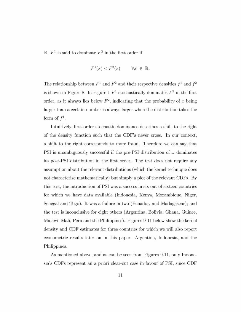
expected penalties given equilibrium play in all subgames, that is,

minvp [βP (V − v)t+ (1− π)vt+ πV (t+ T )]

+(1− p) [vt+ eβC(V − v)t]s.t.

βP =πk

(V − v)t ,βC = b,

e = b (V − v) t.

The maximand has the following interpretation. Either the shipment’s value

is reassessed by the PSI company (an event with probability p) or not. If

yes, upon arrival a bribe βP is paid to customs no matter what. If collusion

with customs is uncovered by reconciliation (an event with probability π),

the duty paid is V (t + T ) i.e. includes a penalty rate and is applied on the

true value V . If not, duty paid is vt. If no reassessment, customs undertake

inspection with intensity e. Duty is paid on the declared value v no matter

what. If inspection is successful (an event with probability e), in addition a

bribe is paid at rate βC.

Without the constraints, the importer’s problem would always yield a

corner solution since the cost function to be minimized is linear in v. Thus

interior solutions (partial fraud) come from the importer’s recognition that

a low declared value triggers more careful inspection.27

27As V is unkown, a lower v triggers more careful inspection not because it is suspect,but because the expected return to inspection is an increasing function of E V − v nomatter what the distribution of V is.

21

Let δ = V − v be the degree of fraud. Expressed in terms of δ, the firstorder condition is:

δ =1

2b2t

1− πp (1 + k1)

1− p . (4)

It is easily verified that the game without PSI is outcome-equivalent to a

game with PSI but with p = 0. Letting

α ≡ 1− πp (1 + k1)

1− p , (5)

we have thus

δ =

α/2b2t with PSI,

1/2b2t without.(6)

We have refrained from using Kuhn-Tucker conditions for ease of notation

but it should be clear that corner solutions can be obtained at δ = V (total

fraud, which can be thought of as smuggling) when α is large enough, or

at δ = 0 when α < 0. In the latter case fraud is entirely eliminated by the

introduction of PSI. Two points are worth noting. First, unlike what has

often been suggested (Goorman and De Wulf, 2003 and Low, 1995), perfect

reconciliation (i.e., π = 1 does not necessarily lead to the elimination of

customs fraud (δ = 0) if the PSI company is not very efficient (p << 1) (and

the proportional part of the penalty is not very large, i.e., k1 ≈ 0). A fullerdiscussion of the effect of introducing PSI is differed until the next section.

22

4.2 Comparative statics

The model generates both positive and normative results which can be de-

rived as comparative-statics properties. As for positive results, the first and

most surprisingly is that fraud declines with the tariff for a wide range of

parameter values. This surprising result, which stands in contrast with the

findings of Fisman andWei (2001), is due to the strategic interaction between

importer and customs. With collusive rent-sharing, a higher tariff raises

customs’ incentive to find verifiable evidence of fraud, since such evidence

improves customs’ bargaining position (more exactly its participation con-

straint). This strategic effect reduces the importer’s fraud rent and swamps

the direct effect that a higher tariff exerts on the return to fraud, reducing

its equilibrium level.28 Because the inverse relationship between δ and t is

somewhat counterintuitive, it provides a test of the model’s validity as a

descriptive tool.

As for normative results, raising the power of incentives facing customs

through an increase in the bonus rate b reduces the equilibrium level of fraud,

an intuitive result since fraud is encouraged by collusion with customs. So

does raising the frequency of audits (π) and the rate of sanctions.

By (6), the introduction of PSI reduces the degree of fraud if and only if

α < 1, i.e. if π (1 + k1) > 1. The model highlights the interdependence of PSI

28That the indirect effects (through customs’ effort) always swamps the direct effect(through fraud revenue) may seem surprising, but recall that without the indirect effectthe problem admits only corner solutions because the importer’s minimand is linear int. The fact that fraud is observed and is less than one hundred percent suggests, inthis model’s logic, that the desire to avoid attracting customs attention through grossunderinvoicing is indeed a key consideration (in accordance with intuition). The inverserelationship with t then follows directly from the algebra.

23

efficiency (p) and reconciliation rates (π) in curbing fraud. Differentiating

(5) with respect to p at the two extreme values of π gives

∂α

∂p=1− π (1 + k1)

(1− p)2 =

−k1/ (1− p)2 if π = 1

1/ (1− p)2 if π = 0.(7)

It can be shown that there is a single point where ∂α/∂p changes sign. Thus,

more efficient PSI (a higher p) reduces fraud only when the rate of recon-

ciliation (π) is high enough. When π = p = 1, α is negative and a corner

solution is obtained at δ = 0 (no fraud). It can be also seen that when π is

high enough to make ∂α/∂p negative (upper part of 7) the latter goes up in

absolute value with increases in k1, the rate of sanctions on customs officers.

This set of results highlights the complementarity of PSI with government

efforts to fight customs corruption through internal incentives (k1) and to

make use of PSI information (π).

The intuition of the case in which the introduction of PSI ends up raising

fraud is as follows. When fraud is uncovered through PSI (case IP ) the

bargaining position of corrupt customs is weak due to the fact that reporting

the fraud brings no bonus. Therefore the informational rent generated by

PSI is entirely captured by the importer, which raises the return to fraud.

There is then more fraud in equilibrium. Introducing a bonus for when

customs officers report fraud uncovered by PSI or letting the rent be shared

by the Nash bargaining solution would weaken this mechanism but would not

necessarily reverse it.29 Thus, in general whether PSI reduces tariff evasion

is an empirical question.

29For instance, introducing a bonus at rate b1 for customs officers using PSI data to

24

In models of information production in which efforts are strategic sub-

stitutes, the arrival of an additional information-producing agent can either

raise or lower aggregate information production, depending on whether the

agent’s direct contribution to aggregate effort offsets or not the negative ef-

fect of her arrival on the marginal effort of other agents. Here, customs effort

is indeed decreasing in the PSI company’s efficiency, as E(e) is a decreasing

function of p (see (3)). However aggregate information production neces-

sarily goes up with the introduction of PSI. To see this, define φ to be the

probability that the shipment’s true value is established by either customs

or the PSI firm. With PSI,

φ = p + e(1− p)= p + (1− p)b(V − v)t

using (2). Without PSI, customs’ effort is still given by (2), so

φ = b(V − v)t.

report fraud would change (7) into

∂α

∂p=1− [b1 + π (1 + k1)]

(1− p)2 =− (b1 + k1) / (1− p)2 if π = 1(1− b1) / (1− p)2 if π = 0.

Obviously, qualitative results would not change as long as the bonus rate is less than one(which it realistically has to be), but increases in p would have a stronger effect when π ishigh enough.

25

It is easily seen that

φ− φ = p [1− b(V − v)t]= p [1− e(v)] > 0

where the last inequality follows from the fact that e is a probability. The

reason for this result is that information production is here sequential in-

stead of simultaneous, as it is in Aghion-Tirole or Anson. Once PSI has

been observed to fail, customs face essentially the same problem that they

would without PSI, so they do not free-ride on PSI effort. This means that

information-production efforts are additive.

In sum, the introduction of PSI unambiguously improves the state of

information. However, its effect on fraud is only indirect, and the model’s

answer to the question ‘does PSI help?’ is reflected in the slope difference

between the upper and lower parts of (6). We now turn to an empirical test

of the model’s predictions.

5 Econometric estimation

This section presents an attempt to estimate structurally first-order condition

(6) on panels of imports from the EU, disaggregated at the SITC2 5 digit

level for PSI-using countries. The initial sample included 52 countries. Of

those, 16 had disaggregated trade data for a sufficient number of years before

the introduction of a PSI program and a sufficient number of years after.

Among those 16, 6 had tariff data as well, but only 3 for years preceding and

following the introduction of PSI (i.e. Argentina, Philippines and Indonesia).

26

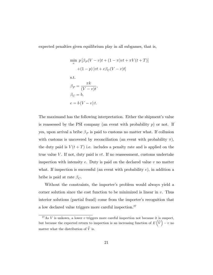
Thus, the final sample has 3 countries, each with between 5, 799 and 7, 019

observations (tariff lines at the SITC 5 digit level). Trade data is from the

UN’s Comtrade database and tariff data from UNCTAD’s Trains.

5.1 Procedure

The equation to be tested is a stochastic version of equation (6) estimated by

country after pooling pre- and post-PSI years respectively. As heteroskedas-

ticity is likely to be an issue, Eicker-White heteroskedasticity consistent es-

timators are provided. We will thus be able, without specifying the type of

heteroskedasticity, to make valid inferences based on the results of ordinary

least squares. In order to avoid having V on both the RHS and LHS, we

rewrite (6) as

v(V, t) =

V − α/2b2t with PSI,

V − 1/2b2t without.

Although the model has no constant, we add time effects to pick up the

influence of out-of-model changes in the environment. The effect of tariff

changes and customs reforms involving changes in incentive structures should

be picked up by parameter estimates, but other changes in the environment

need to be controlled for.

In order to account for positive deviations of v from V (those are aber-

rations in the model but nevertheless present in the sample) we interact

1/t with a dummy variable z equal to one when v < V (the normal case).

Although several approaches are possible to deal with this problem, none

yielded drastically different results and we view this one as a better alter-

native than dropping altogether the “problem” lines, which would bias the

27

sample.30 Finally, the dummy variable τ is equal to one in PSI years and zero

otherwise. PSI years are 1998-2000 for Argentina, 1993-1995 and 1998-2000

for the Philippines, and 1989-90, 1993, 1995-6 for Indonesia. The holes in

PSI years for Indonesia and the Philippines are years without tariff data.

Letting subscripts i and k refer respectively to periods and commodities,

the transformed structural equation to be estimated is:

vik =

T

i=1

β0idi + β1Vik + β2zikτ itik

+ β3zik(1− τ i)

tik+ εik (8)

where εik is an error term. Note that source custom values are FOB whereas

destination values are CIF, so in order to interpret the former as true values

and the latter as ‘underinvoiced’ values, the CIF/FOB difference must be

taken into account.

The model’s predictions are β1 = θ > 1, where θ is the CIF/FOB ratio,

β2 = −α/2b2 < 0, and β3 = −1/2b2 < 0. Some of the model’s structural

parameters can be retrieved from the estimates. For instance, b = 1/2β3

and α = β2/β3. Using an interview-provided “guesstimate” of π equal to 0.3

(see supra), the implied estimates for α and b can be used to get one for p

under different hypotheses for k1.

5.2 Results

Robust regression results are shown for Argentina, the Philippines and In-

donesia (with numbers of observations ranging between 5, 799 and 7, 019 for

30Our method implies that the influence of observations with v > V is picked up by theconstants (year effects) and the error term, which is appropriate if those observations arethought of as measurement errors.

28

each regression) in Table 2. As predicted by the model, for all countries

the coefficient on 1/tik is negative31 (recall that the dependent variable is

v rather than the degree of fraud) and always significant at the 1% level.

β2 ranges across regressions between −25, 076 (for Argentina) and −10, 752(for Indonesia); β3 ranges between −15, 824 (Philippines) and −8, 218 (Ar-gentina).

One of the model’s implications is that PSI reduces fraud when α is

smaller than one. As α = β2/β3, we have

α =

3.051 for Argentina,

0.585 for the Philippines,

1.257 for Indonesia.

Thus, the point estimates suggests that customs fraud has increases with

the introduction of PSI services in Argentina and Indonesia. Testing the

null hypothesis that α = 1 (no effect for PSI) gives Wald test statistics of

F (1, 5893) = 56.74 for Argentina, F (1, 7006) = 7.28 for the Philippines, and

F (1, 5789) = 1.02 for Indonesia. The null hypothesis is accepted for Indone-

sia, for which PSI appears to have had no traceable effect, but rejected for the

other two countries. In the Philippines, PSI helped, whereas in Argentina, it

seems to have made things worse.32

Implied estimates of b (the bonus rate for catches, a proxy for inter-

31We also estimated the model by country and year, and got a significant negativecoefficient on 1/tk in 47 regressions out of 49.32Note that our estimation does not control for evasion of customs tariffs through the

more intese use of duty free zones, which Yang (2003) suggest were an importance forcein evading customs tariffs in the Phillipines after the introduction of PSI services. Takingthis account may weakened even further the case for PSI services.

29

nal incentives in customs administrations) are b = 0.00780 for Argentina,

b = 0.00562 for the Philippines and b = 0.00765 for Indonesia, suggesting

very weak incentives. These low estimates are in accordance with anecdo-

tal evidence. Substituting estimated values for b and using π = 0.3 gives

estimates of p (the frequency of catches by PSI firms) depending on k1. For

Argentina, for instance, we get p(0) = 0.745 and limk1→∞ p = 1. For the

Philippines, we get p(2.3) = 1 and limk1→∞ p = 0 (k1 cannot be lower than

2.3 when α is less than one). The fact that implied estimates of p are between

zero and one is consistent with the model where p is a probability.

Finally, β1 provides an estimate of CIF/FOB ratios equal to 0.987 for

Argentina, 1.329 for the Philippines and 1.150 for Indonesia. The estimate

for Argentina is clearly biased downward, but the upper bound of the 95 %

confidence interval (equal to 1.03675) is nevertheless above unity. The other

two estimates are plausible. In sum, most estimates of the model’s para-

meters, direct or implied, are in plausible ranges, vindicating the approach

taken in section 4.

6 Concluding Remarks

This paper attacked the title’s question (‘does PSI help reducing tariff eva-

sion?’) from two perspectives. First, we showed prima-facie evidence based

on non-parametric methods suggesting a mixed picture, with some cases of

unambiguous reductions in evasion and others suggesting no improvement.

The problem with this approach is that it does not control for other tariff

and customs reforms that may have occurred simultaneously when trying to

30

evaluate the impact of the introduction of PSI services in client countries.

The second approach corrects for this and uses a structural model. We

derived a simple game-theoretic setup with strategic interaction between im-

porters’ fraud decisions and customs’ effort. The model has positive and

normative implications. It highlights that importers understand that cus-

toms have a sharper eye on high-rate tariff lines, making fraud trickier (if

potentially more lucrative) in those lines. Denunciation fears act only as

off-equilibrium threats, the equilibrium being generally one with collusion

between frauders and corrupt customs. Based on relatively straightforward

strategic interaction, the model predicts less fraud in tariff lines with high

rates (because those are the ones on which customs focus their attention).

This counterintuitive prediction provides a test of the model against the

traditional, intuitive approach that higher tariff rates encourage fraud. Per-

haps more importantly, the model suggests that PSI’s impact on the extent

of fraud is theoretically ambiguous. The reason is, intuitively, that PSI pro-

duces information which is only worth what the client government authorities

decide to do with it. PSI may even have a perverse effect in de‘-motivating’

customs. This effect appears indirectly in our model through the following

mechanism. When reporting fraud uncovered by PSI, customs officers do

not expect to receive bonuses (as opposed to when they uncover fraud them-

selves). Their only motivation to report PSI data and force importers to pay

penalty duties is the threat of sanctions if data is later reconciled. When the

frequency of reconciliation is low (as it typically is) that incentive is weak.

This, in turn, creates a situation where collusion between frauding importers

and customs is likely. At the same time, the weakness of customs’ incen-

31

tive to report affects out-of-equilibrium payoffs in a way that strengthens

the bargaining position of importers, raising the equilibrium return to fraud

and, consequently, the incentive to fraud. If the chain of incentive effects

just described may seem somewhat indirect, its final outcome (demobilized

customs) has been widely observed in countries adopting PSI (Low, 1995 and

Goorman and De Wulf, 2003).

Finally, we tested the model on panels of imports between the EU and

PSI-using countries at a high degree of disaggregation and found that its ba-

sic prediction (fraud being inversely related to tariff rates) was strongly sup-

ported by the data. Structural parameter estimates are in plausible ranges,

giving support to our modeling approach. Finally, econometric results for the

three countries for which we have tariff and trade data before and after PSI

suggest that the introduction of PSI in those countries led to an increase in

the extent of fraud in Argentina, lending support to the model’s claim that

indirect (incentive) effects can dominate direct (information-production) ef-

fects, and was clearly successful only in the Philippines. Indonesia appears

as a mixed case.

References

[1] Aghion, Philippe, and Jean Tirole (1997), “Formal and Real Authority

in Organizations”; Journal of Political Economy 105, 1-29.

[2] Anson, Jose (2003), “Costly Information Acquisition and the Power of

Lobbies"; mimeo, University of Lausanne.

32

[3] Byrne, Peter (1995), “An Overview of Privatization in the Area of Tax

Administration”; Bulletin for International Fiscal Documentation 49,

10-16.

[4] De Wulf, Luc (1981), “Statistical Analysis of Under- and Overinvoicing

of Imports”, Journal of Public Economics 8, 303-323.

[5] Dutz, Mark (1996), “Observations on the Use and Usefulness of Pres-

Shipment Inspection Services”; mimeo, The World Bank.

[6] Feenstra, Robert, and Gordon Hanson (2000), “Aggregation Bias in the

Factor Content of Trade: Evidence from US Manufacturing”, American

Economic Review 90, 155-160.

[7] Fisman, Raymond, and Shang-Jin Wei (2001), “Tax Rates and Tax

Evasion: Evidence from ‘Missing Imports’ in China"; NBER working

paper 8551.

[8] Fundacion Investigaciones Economicas Latinoamericanas (1999), “Cus-

toms Control in an Open Economy: The Case of the Preshipment In-

spection Program in Argentina“; mimeo.

[9] Gatti, Roberta (1999), “Corruption and trade tariffs or a case for uni-

form tariffs”, Policy Research Working Papers # 2216.

[10] Goorman, Adrien and Luc De Wulf (2003), “Customs valuations under

the new WTO rules: problems and possible measures with particular

attention for developing countries”, mimeo, The World Bank.

33

[11] Johnson, Noel (2001) “Committing to Civil Service Reform: The

Performance of Pre-Shipment Inspection under Different Institutional

Regimes”; mimeo, Washington University at St Louis.

[12] Low, Patrick (1995), “Preshipment Inspection Services”, World Bank

Discussion Paper 278..

[13] Medalla, Erlinga, L.C. de Dios and R. Aldaba (1003), “Effects of HCV

Valuation: A Policy Paper”; PhilExport/USAID.

[14] – and Leah Panganiban-Castro (1999), “The Effects of Shifting to

Transaction Value and Other Issues”; Final Report, PhilExport/USAID.

[15] Ramirez Acuna, Luis (1992), “Privatization of Tax Administration”, in

Bird and Casanegra, eds., Improving Tax Administration in Developing

Countries.

[16] Slemrod, Joel, and Shlomo Yitzhaki (2000), “Tax Avoidance, Evasion,

and Administration”; NBER working paper 7473.

[17] Stella, Peter (1993), “Tax Farming: A Radical Solution for Developing

Country Tax Problems?", IMF Staff Papers 40.

[18] WTO (1999) Examen des Politiques Commerciales: Republique de

Guinee; Geneva: WTO.

[19] Yang, Dean (2003), “How Easily do Lawbreakers Adapt to Increased

Enforcement? Philippine Smugglers Responses to a Common Customs

Reform”; mimeo, Harvard.

34

Table 1: Tariff evasion before and after PSI

Country Values Quantities

Pr(δ > 0) Pr(δ > 0.8) Pr(δ > 0) Pr(δ > 0.8)

Indonesia (.55, .63) (.10, .17) (.58, .61) (.08, .14)

Philippines (.69, .68) (.15, .10) (.57, .62) (.13, .09)

Argentina (.62, .51) (.03, .03) (.71, .61) (.04, .07)

Note: Values reported in parentheses: without PSI first, with PSI second.

35

Table 2: Estimation ResultsVariable Argentina Philippines Indonesia

Vik 0.987∗∗∗(0.026)

1.329∗∗∗(0.197)

1.150∗∗∗(0.099)

(zikτ i)/tik −25076.45∗∗∗(1791.95)

−9260.48∗∗∗(2137.09)

−10752.15∗∗∗(1720.86)

(zik(1− τ i))/tik −8218.49∗∗∗(1348.83)

−15823.84∗∗∗(2173.71)

−8553.79∗∗∗(1613.14)

d1988 332.75∗(191.18)

d1989 180.70(191.60)

775.36∗∗∗(170.04)

d1990 650.28∗∗(270.19)

690.50∗∗∗(238.19)

d1991

d1992 103.24(244.33)

d1993 −89.60(198.28)

1469.34∗∗∗(354.06)

d1994 297.05(241.22)

d1995 593.02∗∗∗(134.71)

198.68(283.99)

907.71∗∗∗(329.27)

d1996 563.64∗∗∗(151.09)

1240.62∗∗∗(306.21)

d1997 808.95∗∗∗(170.37)

d1998 1640.14∗∗∗(173.02)

869.10∗∗(337.13)

d1999 1658.94∗∗∗(151.59)

1148.22∗∗(471.20)

818.70∗∗∗(218.19)

d2000 1503.14∗∗∗(131.18)

1125.06∗(611.32)

645.19∗∗∗(204.20)

Number of observations 5902 7019 5799

Adjusted R2 0.8716 0.2984 0.7027

F-Stat 646.88 103.06 282.05

Note: standard error of coefficient between parenthesis

36

Figure 1: Switzerland’s Kernel Density

fxv1

999

Kernel Density Estimatedevvalue

-1 0 1

.016779

2.16625

37

Figure 2: Kernel Density For Value Deviations (Argentina)

Argentinavalue_deviation

density: devvalue_without density: devvalue_with

-1 0 1

0

1.37561

Figure 3: Kernel Density For Quantity Deviations (Argentina)

Argentinaquantity_deviation

density: devqty_without density: devqty_with

-1 0 1

0

1.46307

38

Figure 4: Kernel Density for Value Deviations (Philippines)

Phillipinesvalue_deviation

density: devvalue_without density: devvalue_with

-1 0 1

0

.922202

Figure 5: Kernel Density For Quantity Deviations (Philippines)

Philippinesquantity_deviation

density: devqty_without density: devqty_with

-1 0 1

0

1.0141

39

Figure 6: Kernel Density for Value Deviations (Indonesia)

Indonesiavalue_deviation

density: devvalue_without density: devvalue_with

-1 0 1

0

.924511

Figure 7: Kernel Density For Quantity Deviations (Indonesia)

Indonesiaquantity_deviation

density: devqty_without density: devqty_with

-1 0 1

0

.969433

40

Figure 8: First Order Stochastic Dominance

F1

F2

f2 f1

x

x

Figure 9: CDFs for Argentina (values)

CDF Argentina

0

0.2

0.4

0.6

0.8

1

1.2

-1 -0.8 -0.6 -0.4 -0.2 0 0.2 0.4 0.6 0.8 1

w ithout PSI

w ith PSI

41

Figure 10: CDFs for the Philippines (values)

CDF Philippines

0

0.2

0.4

0.6

0.8

1

1.2

-1 -0.8 -0.6 -0.4 -0.2 0 0.2 0.4 0.6 0.8 1

without PSI

with PSI

Figure 11: CDFs for Indonesia (values)

CDF Indonesia

0

0.2

0.4

0.6

0.8

1

1.2

-1 -0.8 -0.6 -0.4 -0.2 0 0.2 0.4 0.6 0.8 1

w ith PSI

w ithout PSI

42