Systematic Protein LocationMapping Reveals Five PrincipalChromatin Types in Drosophila CellsGuillaume J. Filion,1,5 Joke G. van Bemmel,1,5 Ulrich Braunschweig,1,5 Wendy Talhout,1 Jop Kind,1 Lucas D. Ward,3,4,6

Wim Brugman,2 Ines J. de Castro,1,7 Ron M. Kerkhoven,2 Harmen J. Bussemaker,3,4 and Bas van Steensel1,*1Division of Gene Regulation2Central Microarray Facility

Netherlands Cancer Institute, Plesmanlaan 121, 1066 CX Amsterdam, The Netherlands3Department of Biological Sciences, Columbia University, 1212 Amsterdam Avenue, New York, NY 10027, USA4Center for Computational Biology and Bioinformatics, Columbia University, 1130 St. Nicholas Avenue, New York, NY 10032, USA5These authors contributed equally to this work6Present address: Computer Science and Artificial Intelligence Laboratory, Massachusetts Institute of Technology, Cambridge,

MA 02139, USA7Present address: Genome Function Group, MRC Clinical Sciences Centre, Imperial College School of Medicine,

Hammersmith Hospital Campus, Du Cane Road, London W12 0NN, UK*Correspondence: b.v.steensel@nki.nl

DOI 10.1016/j.cell.2010.09.009

SUMMARY

Chromatin is important for the regulation of transcrip-tionandother functions, yet thediversity of chromatincomposition and the distribution along chromo-somes are still poorly characterized. By integrativeanalysis of genome-wide binding maps of 53 broadlyselected chromatin components in Drosophila cells,we show that the genome is segmented into fiveprincipal chromatin types that are defined by uniqueyet overlapping combinations of proteins and formdomains that can extend over > 100 kb. We identifya repressive chromatin type that covers about halfof the genome and lacks classic heterochromatinmarkers. Furthermore, transcriptionally active eu-chromatin consists of two types that differ in molec-ular organization and H3K36 methylation and regu-late distinct classes of genes. Finally, we provideevidence that the different chromatin types help totarget DNA-binding factors to specific genomicregions. These results provide a global view of chro-matin diversity and domain organization in a meta-zoan cell.

INTRODUCTION

Chromatin consists of DNA and all associated proteins. The

scaffold of chromatin is formed by nucleosomes, which are

histone octamers in a tight complex with DNA. This scaffold

serves as the docking platform for hundreds of structural and

regulatory proteins. Furthermore, histones carry a variety of

posttranslational modifications that form recognition sites for

212 Cell 143, 212–224, October 15, 2010 ª2010 Elsevier Inc.

specific proteins (Berger, 2007; Rando and Chang, 2009). The

local composition of chromatin is a major determinant of the

transcriptional activity of a gene; some chromatin proteins

enhance transcription, whereas others have repressive effects.

Traditionally, chromatin was divided into heterochromatin and

euchromatin. There is now ample evidence that a finer classifica-

tion is required. For example, in Drosophila, at least two types of

heterochromatin exist that have distinct regulatory functions and

consist of different proteins. The first type is marked by Poly-

comb group (PcG) proteins and methylation of lysine 27 of

histone H3 (H3K27). PcG chromatin forms large continuous

domains; it is a repressive type of chromatin that primarily regu-

lates genes with developmental functions (Sparmann and van

Lohuizen, 2006). The second type is marked by heterochromatin

protein 1 (HP1) and several associated proteins, combined with

methylation of H3K9. This type of heterochromatin can also

cover large genomic segments, particularly around centro-

meres. Reporter genes integrated in or near HP1 heterochro-

matin tend to be repressed, but paradoxically, many genes

that are naturally bound by HP1 are transcriptionally active

(Hediger and Gasser, 2006). Direct comparison of genome-

wide binding maps indicates that PcG and HP1 heterochromatin

are nonoverlapping (de Wit et al., 2007).

HP1 and PcG chromatin illustrate two important principles of

chromatin organization: each type is marked by unique combi-

nations of proteins and can cover long stretches of DNA. But

are there other major types of chromatin that follow these

same principles? For example, is euchromatin also organized

into domains with distinct protein compositions? Are there

additional types of repressive chromatin that have remained

unnoticed?

In order to address these questions, we generated genome-

wide location maps of 53 broadly selected chromatin proteins

and four key histone modifications in Drosophila cells, providing

A

C

B

Principal component analysis

Hidden Markov model

53 ch

rom

atin

prot

eins

16000 16200 16400 16600 16800 17000

Position on chr2L (kb)

PC1PC2PC3

type

16000 16200 16400 16600 16800 17000

Position on chr2L (kb)

MRG15SU(VAR)3−7SU(VAR)3−9

HP6HP1LHR

CAF1ASF1

MUS209TOP1

RPII18SIR2

RPD3CDK7DSP1DF31MAX

PCAFASH2HP1cCtBPJRA

BRMECRBCD

MED31SU(VAR)2−10

LOLALGAF

CG31367ACT5C

TIP60MNT

SIN3ATBP

DWGPHOLPROD

BEAF32bSU(HW)

LAMD1H1

SUUREFFIAL

GROPHO

CTCFPC

E(Z)PCLSCE

Genes+-

−20

−10

010

20PC

1

−15 −10 −5 0 5 10 15PC2

−15 −10 −5 0 5 10 15

−15

−10

−50

510

PC2PC

3

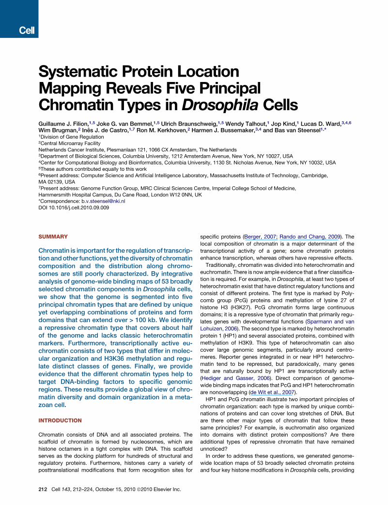
Figure 1. Overview of Protein Binding Profiles and Derivation of the Five-Type Chromatin Segmentation

(A) Sample plot of all 53 DamID profiles (log2 enrichment over Dam-only control). Positive values are plotted in black and negative values in gray for contrast.

Below the profiles, genes on both strands are depicted as lines with blocks indicating exons.

(B) Two-dimensional projections of the data onto the first three principal components. Colored dots indicate the chromatin type of probed loci as inferred by

a five-state HMM.

(C) Values of the first three principal components along the region shown in (A), with domains of the different chromatin types after segmentation by the five-state

HMM highlighted by the same colors as in (B).

See also Figure S1 and Table S1.

a rich description of chromatin composition along the genome.

By integrative computational analysis, we identified, aside from

PcG and HP1 chromatin, three additional principal chromatin

types that are defined by unique combinations of proteins. One

of these is a type of repressive chromatin that covers �50% of

the genome. In addition, we identified two types of transcription-

ally active euchromatin that are bound by different proteins and

harbor distinct classes of genes.

RESULTS

Genome-wide Location Maps of 53 Chromatin ProteinsWe constructed a database of high-resolution binding profiles of

53 chromatin proteins in the embryonicDrosophila melanogaster

cell line Kc167 (Figure 1A and Figure S1A available online). In

order to obtain a representative cross-section of the chromatin

proteome, we selected proteins from most known chromatin

protein complexes, including a variety of histone-modifying

enzymes, proteins that bind specific histone modifications,

general transcription machinery components, nucleosome re-

modelers, insulator proteins, heterochromatin proteins, struc-

tural components of chromatin, and a selection of DNA-binding

factors (DBFs) (Table S1). For�40 of these proteins, full-genome

high-resolution binding maps have not previously been reported

in any Drosophila cell type or tissue. Though chromatin immuno-

precipitation (ChIP) is widely used to map protein-genome inter-

actions (Collas, 2009), large-scale application of this method is

hampered by the limited availability of highly specific antibodies.

Cell 143, 212–224, October 15, 2010 ª2010 Elsevier Inc. 213

Moreover, at least for some chromatin proteins, ChIP results can

greatly depend on the choice of crosslinking reagents (Wang

et al., 2009) and can be unreliable for proteins with short resi-

dence times (Gelbart et al., 2005; Schmiedeberg et al., 2009).

We therefore used the DamID technology, which does not

require crosslinking or antibodies. With DamID, DNA adenine

methyltransferase (Dam) fused to a chromatin protein of interest

deposits a stable adenine-methylation ‘‘footprint’’ in vivo at the

interaction sites of the chromatin protein so that even transient

interactions may be detected (van Steensel et al., 2001). Note

that the fusion protein is expressed at very low levels, averting

overexpression artifacts. The DamID profiles of all 53 proteins

were generated in duplicate under standardized conditions

and were detected using oligonucleotide microarrays that query

the entire fly genome at�300 bp intervals. Comparisons to pub-

lished and new ChIP data confirm the overall reliability of the

DamID data (Figure S1B), which was also reported in previous

comparative studies (Moorman et al., 2006; Negre et al., 2006).

For reference purposes, we also generated ChIP maps of

histone H3 and the histone marks H3K4me2, H3K9me2,

H3K27me3, and H3K79me3 on the same array platform.

Most of the Fly Genome Interacts with NonhistoneChromatin ProteinsComparison of the DamID profiles for all 53 proteins shows

a variety of binding patterns (Figure 1A). Nevertheless, several

sets of proteins exhibit profiles that are similar. Some similarities

were anticipated, such as for PC, PCL, SCE, and E(Z), which are

all PcG proteins (Sparmann and van Lohuizen, 2006), and for

HP1, SU(VAR)3-9, LHR, and HP6, which are part of classic

HP1-type heterochromatin (Greil et al., 2007). We also observe

extensive colocalization of Lamin (LAM), histone H1 (H1),

Effete (EFF), Suppressor of Underreplication (SUUR), and the

AT-hook protein D1, which have not been linked previously

except for LAM and SUUR (Pindyurin et al., 2007). There is a

prominent overlap in the binding patterns of a large set of �30

proteins, including histone-modifying enzymes (e.g., RPD3 and

SIR2), components of the basal transcription machinery (e.g.,

CDK7 and TBP), and others detailed below.

In order to identify target and nontarget loci for each protein,

we applied a two-state hidden Markov model (HMM) to each

individual binding map (Extended Experimental Procedures).

This method identifies themost likely segmentation into ‘‘bound’’

and ‘‘unbound’’ probed loci. According to the resulting binary

classifications, the genome-wide occupancy by individual

proteins varies broadly, ranging from about 2% (GRO) to 79%

(IAL). Of interest, 99.99% of the probed loci are bound by at least

one protein and 99.6% by at least three proteins. This indicates

that, at least at the resolution of our maps, essentially no part of

the fly genome is permanently in a configuration that consists of

nucleosomes only. Approximately 1% of the genome shows

extremely high protein occupancy, being bound by 36–44 of

the 53 mapped proteins.

Principal Chromatin Types Defined by Combinationsof ProteinsNext, we used a computational classification strategy to identify

themajor types of chromatin, defined as distinct combinations of

214 Cell 143, 212–224, October 15, 2010 ª2010 Elsevier Inc.

proteins that are recurrent throughout the genome. To identify

such combinations, we initially performed principal component

analysis on the 53 quantitative DamID profiles to reduce the

dimensionality of the data. We then focused on the first three

principal components, which together account for 57.7% of

the total variance. By projecting the genomic sites on the prin-

cipal components, we could distinguish five distinct lobes in

the three-dimensional scatter plot (Figure 1B). No additional

distinct lobes could be observed upon further inspection of

higher-level principal components. Importantly, the five groups

were also clearly separated when using the previously defined

binary target definitions (Figure S1C), showing that this result is

robust to different quantification methods.

Having established that classification into five types properly

summarizes the data, we fitted a five-state HMM onto the first

three principal components. Thus, every probed sequence in

the genome was assigned one of five exclusive chromatin types

(Extended Experimental Procedures). To avoid semantic confu-

sion, and in line with the Greek word chroma (color), we labeled

each of the five protein signatures with a color (BLUE, GREEN,

BLACK, RED, and YELLOW). The HMM classification produced

a mosaic pattern of chromosomal domains that vary widely in

length (Figure 1C). We emphasize that this segmentation is

purely data driven, without using any other knowledge besides

the 53 DamID profiles. The segmentation is generally robust:

removal of any of the proteins except for PC still yields a five-

state classification that is, on average, 96.7% identical to the

model obtained with all 53 proteins. A detailed analysis of the

robustness is summarized in Figure S1D.

Domain Organization of Chromatin TypesThe five types of chromatin differ substantially in their genome

coverage, numbers of domains, and numbers of genes (Fig-

ure 2A). We identified a total of 8428 domains that typically range

from �1 to 52 kb (5th–95th percentiles) with a median length of

6.5 kb, although the size distribution depends on the chromatin

type (Figure 2B). 441 domains are larger than 50 kb, and 155

are larger than 100 kb, with the largest domain being 737 kb.

Many individual domains include multiple neighboring genes

(Figure 2C), the largest number of which within a single domain

is 139 (for a centromere-proximal GREEN domain). Taken

together, these data indicate that the fly genome is generally

organized into large regions that are covered by specific combi-

nations of proteins.

BLUE and GREEN Chromatin Correspond to KnownHeterochromatin TypesVisualization of the protein occupancy in each of the five chro-

matin types (Figure 3A) shows that most proteins are not

confined to a single chromatin type. Rather, the five chromatin

types are defined by unique combinations of proteins. Impor-

tantly, BLUE and GREEN chromatin closely resemble previously

identified chromatin types. GREEN chromatin corresponds to

classic heterochromatin that is marked by SU(VAR)3-9, HP1,

and the HP1-interacting proteins LHR and HP6. As described

previously (Ebert et al., 2006; Greil et al., 2007), this type of chro-

matin is prominent in pericentric regions and on chromosome 4

(Figure S2A). To further validate this classification, we conducted

A

B C D

Genome coverage

117 Mb

Number of domains

8428 domains

All genes

15145 genes

Silent genes

4229 silent genes

Length of domains

040

800

200

020

0

coun

t0

200

Domain length (kb)0 10 20 30 40

025

0

>50

Number of genes per domain

020

00

600

030

0

coun

t0

200

Number of genes / domain

050

0

0 1 2 3 4 5 6 7 8 9 10 >10

mRNA expression

020

400

400

015

00

gene

cou

nt

040

00

100

−1 0 1 2 3 4

log10(RNA tag count)

no ta

gs

Figure 2. Characteristics of the Five Chromatin Types

(A) Coverage and gene content of chromatin domains of each type. The chromatin type of a gene is defined as the chromatin type at its transcription start site

(TSS). Gray sectors correspond to geneswhose TSSmaps at the transition between two chromatin types. Silent genes have an average RNA tag count less than 1

per million total tags (see D).

(B) Length distribution of chromatin domains, i.e., genomic segments covered contiguously by one chromatin type.

(C) Distribution of the number of genes per chromatin domain. Because some genes overlap with more than one domain, genes are assigned to a chromatin type

based on the type at the transcription start site.

(D) Histogram of mRNA expression determined by RNA tag profiling. Data are represented as log10 (tags per million total tags).

Dashed vertical lines in (B)–(D) indicate medians.

genome-wide ChIP of H3K9me2, a histone mark that is predom-

inantly generated by SU(VAR)3-9 and bound by HP1 (Hediger

and Gasser, 2006) . Indeed, H3K9me2 is highly and specifically

enriched in GREEN chromatin (Figure 3B).

BLUE chromatin corresponds to PcG chromatin, as shown by

the extensive binding by the PcG proteins PC, E(Z), PCL, and

SCE. Indeed, well-known PcG target loci such as the Hox

gene clusters are localized in BLUE domains (Figure S2B).

Furthermore, genome-wide ChIP of H3K27me3, the histone

mark that is generated by E(Z) and recognized by PC (Sparmann

and van Lohuizen, 2006), is highly enriched in BLUE chromatin

(Figure 3B). We emphasize that these histone modification

profiles serve as independent validation because they were not

used in the five-state HMMclassification. The fact that twomajor

well-known chromatin types were faithfully recovered indicates

that our chromatin classification strategy is biologically mean-

ingful.

Of interest, we identified several additional proteins that mark

BLUE or GREEN chromatin, or both. For example, moderate

degrees of occupancy of the histone deacetylase (HDAC)

RPD3 occur in both BLUE and GREEN chromatin, in accordance

with known biochemical and genetic interactions of RPD3 with

PcG proteins as well as SU(VAR)3-9 (Czermin et al., 2001; Tie

et al., 2003). The presence of EFF in BLUE chromatin is consis-

tent with a reported role of this protein in PcG-mediated silencing

(Fauvarque et al., 2001).

Cell 143, 212–224, October 15, 2010 ª2010 Elsevier Inc. 215

BA

MRG15SIR2

RPD3DF31

RPII18BEAF32B

TOP1SIN3AASH2MAX

ASF1DSP1PCAFCDK7HP1C

JRACTBPCAF1

MUS209TIP60

TBPMNTDWG

PHOLSU(VAR)3−7

PRODACT5C

GROPHO

MED31BCD

SU(VAR)2−10GAF

CG31367LOLAL

ECRBRM

CTCFIALH1D1

SUURLAMEFF

SU(HW)PC

E(Z)PCLSCEHP6LHRHP1

SU(VAR)3−9

0 0.5 1

Fraction of bound loci

−10

12

H3K9me2

log2

(H3K

9me2

ChI

P / H

3 C

hIP)

−3−2

−10

1

H3K27me3

log2

(H3K

27m

e3 C

hIP

/ H3

ChI

P)−2

−10

12

3

H3K79me3

log2

(H3K

79m

e3 C

hIP

/ H3

ChI

P)

−2−1

01

23

H3K4me2

log2

(H3K

4me2

ChI

P / H

3 C

hIP)

−1.0

−0.5

0.0

0.5

Histone H3

log2

(H3

ChI

P / i

nput

)

Figure 3. Chromatin Types Are Characterized by Distinctive Protein Combinations and Histone Modifications

(A) Fraction of all probed genomic loci within each chromatin type that is bound by each protein. Bound loci were determined separately for each protein as

described in the text.

(B) Levels of histone H3 and four histone modifications as determined by genome-wide ChIP. The distribution of values is shown as ‘‘violin plots,’’ which are

symmetrized density plots of binding values per chromatin type: the wider the violin, the more data points are associated to that value. Dashed horizontal lines

indicate the median binding value for each chromatin type. Histone modification ChIP data were normalized to H3 occupancy.

See also Figure S2.

BLACK Chromatin Is the Prevalent Typeof Repressive ChromatinBLACK chromatin covers 48%of the probed genome and is thus

by far the most abundant type (Figure 2A). With a median size of

17 kb and with 134 domains larger than 100 kb, BLACK chro-

matin domains tend to be longer than domains of the four other

types (Figure 2B). BLACK chromatin is overall relatively gene

poor (Figure 2A; compare genome coverage and number of

genes), but it nevertheless harbors 4162 genes. By mRNA

high-throughput sequencing, we detected no transcriptional

activity (<1 mRNA molecule per 10 million) for 66% of the genes

in BLACK chromatin, whereas the remaining 34% have very low

activity (Figure 2D). This is in agreement with the low coverage of

BLACK chromatin by RPII18, a subunit shared by all three RNA

polymerases (Figure 3A), and a lack of the active histone marks

H3K4me2 and H3K79me3 as detected by ChIP (Figure 3B). We

note that the majority of silent genes in the genome are located

216 Cell 143, 212–224, October 15, 2010 ª2010 Elsevier Inc.

in BLACK chromatin (Figure 2A). Thus, BLACK chromatin is

a distinctively silent type of chromatin that covers a large part

of the genome.

BLACK chromatin is almost universally marked by four of the

53 mapped proteins: histone H1, D1, IAL, and SUUR, whereas

SU(HW), LAM, and EFF are also frequently present (Figure 3A).

Close-up views show that H1, D1, IAL, SUUR, and LAM have

a broad distribution within BLACK domains, whereas SU(HW)

exhibits a distinct, more focal pattern (Figure 4A).

Given that genes in BLACK chromatin are expressed at very

low levels, we asked whether BLACK chromatin actively

represses transcription or merely forms secondary to a lack of

transcription. In the former model, transgenes inserted into

BLACK chromatin may exhibit reduced transcription, whereas,

in the latter model, transgenes should be unaffected. To test

this, we examined a data set of 2852 random P element inser-

tions that carry a mini-white eye color reporter gene. For each

A

C

B D

GREEN BLUE BLACK RED YELLOW

HC

NE

s pe

r M

B0

2040

6080

100

log 2

(Dam

−H

1/D

am)

H1

−3

−1

1

log 2

(Dam

−S

UU

R/D

am)

SUUR

−1.

50.

5

log 2

( Dam

−D

1/D

am)

D1

−1.

50.

5

log 2

( Dam

−La

m/D

am)

LAM

−1

01

log 2

(Dam

−E

FF

/Dam

) EFF

−1.

00.

0

log 2

(Dam

−IA

L/D

am)

IAL

−1.

00.

0

log 2

(Dam

−S

U(H

W)/

D.) SU(HW)

−1

12

Genes

Type

16000 16100 16200 16300 16400 16500

Position on chr2R (kb)

GREEN BLUE BLACK RED YELLOW

Fra

ctio

n of

sile

nced

tran

sgen

es

0.0

0.1

0.2

0.3

0.4

26 302 307 841 1345

weakmediumstrong

Silencing:

S2 cellslarval tubulelarval salivary glandlarval midgutlarval hindgutlarval trachea

larval CNSlarval fat body

larval carcasstubulesalivary glandcropmidguthindgut

fat bodyvirgin spermathecamated spermatheca

heart

headeyebrainthorac. ganglionovarytestismale access. glandscarcasswhole fly

difference fromgenome mean

(log10)

−2 0 2

4,086 BLACK genes

Figure 4. Properties of BLACK Chromatin

(A) Sample plots of binding profiles of the six proteins that are the most prevalent in BLACK chromatin. Genes on both strands, as well as chromatin types, are

depicted below the profiles. Gray blocks in the background correspond to BLACK chromatin domains.

(B) Silencing of a white reporter gene in 2852 P element insertions in adult eyes (Babenko et al., 2010) separated by chromatin type in Kc cells. The fraction of

silenced insertions is higher among those overlapping with BLACK regions than in the rest of the genome (p < 2.2*10�16, chi-square test).

(C) Relative expression levels (log10 scale, normalized to genome-wide average) of BLACK genes in various tissues (Chintapalli et al., 2007).

(D) Density of highly conserved noncoding elements (HCNEs) per chromatin type.

of these insertions, the expression level was previously scored

and the integration site mapped (Babenko et al., 2010). Strik-

ingly, of 307 insertions located in BLACK regions, 36% exhibited

various degrees of w silencing, compared to 13% genome wide

(Figure 4B). Moreover, repression of transgene insertions in

BLACK chromatin ismore pronounced than in BLUE andGREEN

chromatin. This result strongly indicates that BLACK chromatin

has an active role in transcriptional silencing.

Developmental Regulation of Genes in BLACKChromatinNot all genes in BLACK regions are expected to remain silenced

in various tissues. Indeed, a survey of tissue expression profiling

data (Chintapalli et al., 2007) indicates that genes in BLACK

chromatin can become active, although their expression tends

to be restricted to a few tissues only (Figure 4C). This suggests

that BLACK chromatin domains, as defined in Kc167 cells, can

be remodeled into a different chromatin type in some cell types.

Consistent with this dynamic regulation, BLACK chromatin is

particularly rich in highly conserved noncoding elements

(HCNEs) (Figure 4D), which are thought to mediate gene regula-

tion (Engstrom et al., 2007). The density of HCNEs in BLACK

chromatin is comparable to that in BLUE chromatin, which

harbors many developmentally regulated genes (Tolhuis et al.,

2006), and is much higher than in the other three chromatin

types. Together, these data suggest that BLACK chromatin is,

at least in part, under developmental control.

YELLOW and RED Chromatin Are Two Distinct Typesof EuchromatinIn contrast to BLACK and BLUE chromatin, RED and YELLOW

chromatin have hallmarks of transcriptionally active euchro-

matin. Most genes in these two chromatin types produce

substantial amounts of mRNA (Figure 2D), and levels of RNA

polymerase (Figure 3A), H3K4me2, and H3K79me3 are typically

high, whereas levels of H3K9me2 and H3K27me3 are low

(Figure 3B).

RED andYELLOWchromatin share various chromatin proteins

(Figure 3A). Among these are the HDACs RPD3 and SIR2, as well

as the RPD3-interacting protein SIN3A. HDACs have recently

also been found in transcriptionally active chromatin in human

cells (Wang et al., 2009). Other proteins that are highly abundant

in both RED and YELLOW chromatin include DF31, a little-

studied protein that drives chromatin decondensation in vitro

(Crevel et al., 2001); ASH2, a homolog of a subunit of a H3K4

methyltransferase complex in yeast and vertebrate cells (Nagy

et al., 2002); and MAX, a DBF that is part of the MYC network of

regulators of growth and proliferation (Orian et al., 2003).

Aside from these similarities, RED and YELLOW chromatin

display striking differences. RED chromatin is abundantly

Cell 143, 212–224, October 15, 2010 ª2010 Elsevier Inc. 217

A B

C

D

−0.

50.

51.

01.

52.

0

−5 0 5

Relative position from 5' end (kb)

log 2

(Dam

−M

RG

15D

am)

−5 0 5

Relative position from 3' end (kb)

−1

01

23

4

H3K36me3

−5 0 5

Relative position from 5' end (kb)

log 2

(H3K

36m

e3in

put)

−5 0 5

Relative position from 3' end (kb)

MRG15

−10

12

34

ORC binding

OR

C e

nric

hmen

t

−20

−10

010

20

Replication timing

log2

(Ear

ly /

Late

)

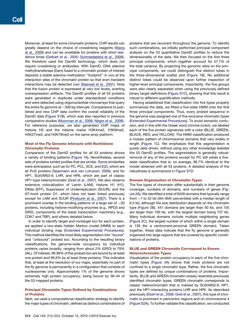
Figure 5. RED and YELLOW Are Two Distinct Types of

Euchromatin

(A) Violin plots of replication timing (Schwaiger et al., 2009) per

chromatin type.

(B) Violin plots of origin of replication complex 2 (ORC2) binding

(MacAlpine et al., 2010) per chromatin type.

(C) Average binding of MRG15 around 50 and 30 ends of genes in

RED and YELLOW chromatin. (Left) Alignment to transcript 50

ends. (Right) Alignment to 30 ends. Only genes that are entirely

within one chromatin type are depicted.

(D) Average enrichment of H3K36me3 (Bell et al., 2010), plotted as

in (C).

marked by several proteins that are mostly absent from the

four other chromatin types (Figure 3A). Among these are the

nucleosome-remodeling ATPase Brahma (BRM); the regulator

of chromosome structure SU(VAR)2-10; the Mediator subunit

MED31; the 55 kDa subunit of CAF1, present in various

histone-modifying complexes (Martınez-Balbas et al., 1998; Tie

et al., 2001); and several DBFs, including the ecdysone receptor

(ECR), GAGA factor (GAF), and Jun-related antigen (JRA).

These differences in protein composition prompted us to

investigate the timing of DNA replication during S phase, which

is known to differ in relation with chromatin marks (Gilbert,

2002). Analysis of a genome-wide replication timing map from

Kc167 cells (Schwaiger et al., 2009) shows that DNA in RED

and YELLOW chromatin is generally replicated early in S phase,

as may be expected for euchromatin. However, RED chromatin

tends to be replicated even earlier than YELLOW chromatin

(Figure 5A). This coincides with a strong enrichment of origin

218 Cell 143, 212–224, October 15, 2010 ª2010 Elsevier Inc.

recognition complex (ORC) binding in RED chromatin,

as mapped by ChIP (MacAlpine et al., 2010) (Fig-

ure 5B), suggesting that DNA replication is often initi-

ated in RED chromatin. These observations further

underscore that RED and YELLOW chromatin are

distinct types of euchromatin.

Active Genes in YELLOW, but Not RED,Chromatin Carry H3K36me3Only one protein of the data set is abundant in

YELLOW, but not in RED, chromatin: MRG15, which

is a chromodomain-containing protein. Because

human MRG15 has previously been reported to bind

H3K36me3 (Zhang et al., 2006), we compared the

fine distribution of MRG15 and H3K36me3 along

genes within the two chromatin types (Bell et al.,

2010). Indeed, both are highly enriched along genes

in YELLOW chromatin but are nearly absent from

RED chromatin (Figures 5C and 5D). These data are

consistent with binding of MRG15 to H3K36me3

in vivo. Of interest, H3K36me3 was previously thought

to be a universal marker of elongating transcription

units (Lee and Shilatifard, 2007; Rando and Chang,

2009). Our analysis reveals that, at least in Drosophila

Kc167 cells, this histone mark is mostly absent from

genes lying in RED chromatin, even though these

genes are expressed at similar levels as genes in YELLOW

chromatin (Figure 2D).

RED and YELLOW Chromatin Mark Different Typesof GenesThe substantial differences between RED and YELLOW chro-

matin suggested that the genes that they harbor may be

regulated by two globally distinct pathways. We therefore inves-

tigated whether genes located in RED and YELLOW chromatin

have different characteristics. We began by comparing the

embryonic tissue expression patterns of genes in the two chro-

matin types. Strikingly, genes with a broad expression pattern

over many embryonic stages and tissues (Tomancak et al.,

2007) are highly enriched in YELLOW chromatin, whereas genes

with more restricted expression patterns are depleted

(Figure 6A). Consistent with this, gene ontology (GO) analysis

revealed that universal cellular functions such as ‘‘ribosome,’’

proteinaceous extracellular matrixextracellular regionreceptor bindingcellular component movementtranscription factor activitybehaviorplasma membranemulticellular organismal development

intracellularnucleusnucleic acid metabolic processstructural molecule activityDNA metabolic processstructural constituent of ribosomeribosomeDNA repair

Fraction of Genes0.0 0.2 0.4 0.6 0.8 1.0

1812074173157163285934

2926109872622017715515880

all genes broad tissue−specific

Frac

tion

of g

enes

0.0

0.2

0.4

0.6

0.8

1.0

A B

C

D

−10

12

3

FAIRE

log 2

(FAI

RE

/ inp

ut)

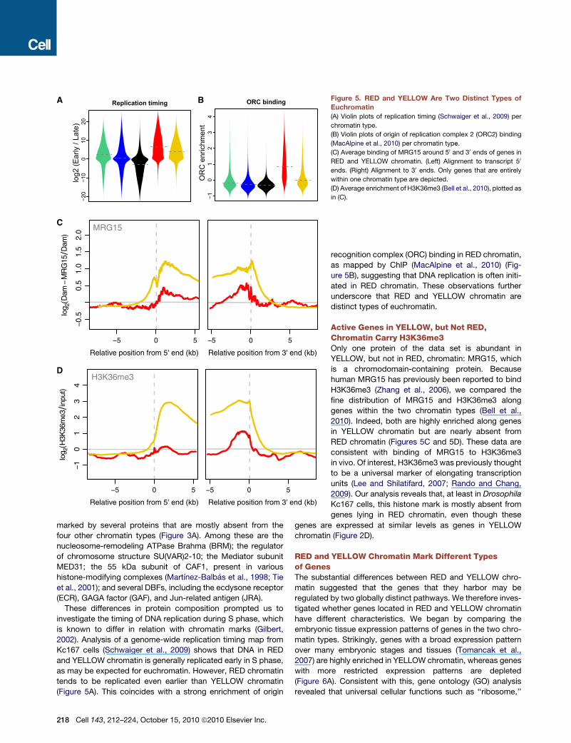
Figure 6. Genes in RED and YELLOW Differ in Regulation and Function

(A) Distribution of genes having ‘‘broad’’ and ‘‘tissue-specific’’ expression patterns (defined in Tomancak et al., 2007) over the five chromatin types. Left bar shows

distribution of all genes for comparison.

(B–C) GO slim categories that are significantly enriched (B) or depleted (C) in RED compared to YELLOW genes. Bars indicate the fraction of RED and YELLOW

genes for the given category (BLACK, GREEN, and BLUE are not considered here). Vertical dotted line represents the distribution expected by random chance.

The total numbers of RED and YELLOW genes within each category are indicated on the left.

(D) Violin plots of the log2 FAIRE signal per chromatin type (Braunschweig et al., 2009).

See also Figure S3.

‘‘DNA repair,’’ and ‘‘nucleic acid metabolic process’’ are almost

exclusively found in YELLOW chromatin (Figure 6B), whereas

genes in RED chromatin are linked to more specific processes

such as ‘‘receptor binding,’’ ‘‘defense response,’’ ‘‘transcription

factor activity,’’ and ‘‘signal transduction’’ (Figure 6C). Such

specific functions and expression patterns require complex

mechanisms of gene regulation. Indeed, intergenic regions in

RED domains contain about 2-fold more HCNEs than YELLOW

chromatin (Figure 4D), although not as much as BLACK and

BLUE chromatin. Furthermore, genome-wide formaldehyde-as-

sisted identification of regulatory elements (FAIRE) (Braunsch-

weig et al., 2009; Giresi et al., 2007) points to a high density of

regulatory chromatin complexes in RED chromatin (Figure 6D).

Motif Binding by DBFs Is Guided by Chromatin TypesChromatin can affect the ability of DBFs to bind to their cognate

binding sequences, which is thought to explain why, in vivo,

most DBFs bind to only a small subset of their recognition motifs

in the genome (Beato and Eisfeld, 1997). We investigated how

the five chromatin types might modulate DBF-DNA interactions.

We focused on five DBFs in our data set (JRA, MNT, GAF, CTCF,

and SU(HW)) for which the sequence-specificity is well charac-

terized. We first calculated the expected genomic binding

pattern of each DBF based on the occurrence of sequence

motifs that match the known DBF recognition motif. The exact-

ness of these matches is taken into account, yielding for each

DamID-probed locus a predicted relative affinity for the DBF

(Foat et al., 2006). Genome-wide comparison of this sequence-

based predicted affinity and actual protein occupancy indicated

only weak to moderate correlations (Spearman’s rho ranging

from 0.04 to 0.35; dashed gray curves in Figure 7A; Figure S4).

This suggests that chromatin indeed has substantial modulating

effects on DBF-motif interactions.

We then repeated this correlation analysis by chromatin type.

Surprisingly, this revealed that each DBF has its own depen-

dence on chromatin context (Figure 7A and Figure S4). GAF

and JRA both bind to their respective motif variants over a range

of affinities in RED chromatin, but not in the other chromatin

types; MNT binds to its motifs only in RED and YELLOW;

CTCF preferentially binds its motifs in RED and BLUE chromatin;

SU(HW) recognizes its motifs most efficiently in BLACK, BLUE,

and RED chromatin. Thus, each of the five chromatin types is

conducive to DNA binding by specific subsets of DBFs. Some

chromatin types may also weakly bind certain DBFs indepen-

dently of DNA interactions, as suggested by the varying DamID

baseline levels in loci that lack high-affinity motifs (e.g., for SU

(HW) and CTCF; Figure 7A).

Four out of five DBFs exhibit a preference for their motif in RED

chromatin. We wondered whether RED chromatin might have an

intrinsic property suchas ‘‘openness’’ or nucleosome remodeling

activity thatwouldgenerally facilitateDBFaccess. To test this,we

generated a DamID profile for the DNA-binding domain (DBD) of

yeast Gal4. This foreign DBD is not expected to have specific

protein-protein interactions with Drosophila chromatin, and its

recognition motif occurs randomly throughout the fly genome.

We observed similar interactions of Gal4-DBD with its cognate

motifs in all five chromatin types (Figure 7A, bottom-right). This

indicates that RED chromatin does not have a general positive

effect on protein-DNA interactions and that high DBF occupancy

in this chromatin type is more likely due to specific targeting

mechanisms for each DBF. In summary, these results indicate

that the five chromatin types together act as guides that help to

target DBFs to specific regions of the genome even though the

cognate binding motifs are broadly distributed (Figure 7B).

DISCUSSION

By systematic integration of 53 protein location maps, we found

that the Drosophila genome is packaged into a mosaic of five

principal chromatin types, each defined by a unique combination

Cell 143, 212–224, October 15, 2010 ª2010 Elsevier Inc. 219

0 20 40 60 80 100

0.0

0.5

1.0

1.5GAF

0 20 40 60 80 100

−0.2

0.0

0.2

0.4

0.6

0.8

1.0 MNT

70 75 80 85 90 95 100

0.0

0.5

1.0

CTCF

70 75 80 85 90 95 100

−0.5

0.0

0.5

1.0

1.5

2.0 SU(HW)

0 20 40 60 80 100

0.0

0.5

1.0

1.5 JRA

0 20 40 60 80 100

−0.4

−0.2

0.0

0.2

0.4

0.6 GAL4

A

B

Sequence affinity (rank %) Sequence affinity (rank %) Sequence affinity (rank %)

Dam

ID s

core

Dam

ID s

core

Dam

ID s

core

Figure 7. Binding of DBFs to Their Cognate Motifs Is Differentially Guided by Chromatin Types(A) Correlations between predicted DNA affinity and actual binding detected by DamID, genome-wide (gray dashed lines), or for each chromatin type (solid lines)

for six DBFs as indicated. Curves are loess-fitted lines; raw data are shown in Figure S4.

(B) Cartoon model depicting the specific guidance of DBFs to their cognate motifs in only certain chromatin types, illustrated for CTCF and MNT. DBF binding to

its cognate motif (gray box) is guided by protein-protein interactions. The presence of specific interactors (colored shapes) only in some chromatin types may

account for targeting.

See also Figure S4.

of proteins. Extensive evidence demonstrates that the five types

differ in a wide range of characteristics aside from protein

composition, such as biochemical properties, transcriptional

activity, histone modifications, replication timing, and DBF tar-

geting, as well as sequence properties and functions of the

embedded genes. This validates our classification by indepen-

dent means and provides important insights into the functional

properties of the five chromatin types.

The Number of Chromatin StatesIdentifying five chromatin states out of the binding profiles of 53

proteins comes out as a surprisingly low number (one can form

�1016 subsets of 53 elements). We emphasize that the five chro-

220 Cell 143, 212–224, October 15, 2010 ª2010 Elsevier Inc.

matin types should be regarded as the major types. Some may

be further divided into subtypes, depending on how fine-grained

one wishes the classification to be. For example, within each of

the transcriptionally active chromatin types, promoters and 30

ends of genes exhibit (mostly quantitative) differences in their

protein composition (data not shown) and thus could be re-

garded as distinct subtypes. However, these local differences

are minor relative to the differences between the five principal

types that we describe here. We cannot exclude that the accu-

mulation of binding profiles of additional proteins would reveal

other novel chromatin types. We also anticipate that the pattern

of chromatin types along the genome will vary between cell

types. For example, many genes that are embedded in BLACK

chromatin (defined in Kc167 cells) are activated in some other

cell types (Figure 4C). Thus, the chromatin of these genes is likely

to switch to an active type.

Whereas the integration of data for 53 proteins provides

substantial robustness to the classification of chromatin along

the genome, a subset of only five marker proteins (histone H1,

PC, HP1, MRG15, and BRM), which together occupy 97.6% of

the genome, can recapitulate this classification with 85.5%

agreement (Figure S1E). Assuming that no unknown additional

principal chromatin types exist in some cell types, DamID or

ChIP of this small set of markers may thus provide an efficient

means to examine the distribution of the five chromatin types

in various cells and tissues, with acceptable accuracy.

BLACK Chromatin: A Distinct Type of RepressiveChromatinPrevious work on the expression of integrated reporter genes

(Handler and Harrell, 1999; Kelley and Kuroda, 2003; Markstein

et al., 2008) had suggested that most of the fly genome is tran-

scriptionally repressed, contrasting with the low coverage of

PcG and HP1-marked chromatin. BLACK chromatin, which

consists of a previously unknown combination of proteins and

covers about half of the genome, may account for these obser-

vations. Essentially all genes in BLACK chromatin exhibit

extremely low expression levels, and transgenes inserted in

BLACK chromatin are frequently silenced, indicating that BLACK

chromatin constitutes a strongly repressive environment. Impor-

tantly, BLACK chromatin is depleted of PcG proteins, HP1, SU

(VAR)3-9, and associated proteins and is also the latest to

replicate, underscoring that it is different from previously charac-

terized types of heterochromatin (here identified as BLUE and

GREEN chromatin).

The proteins that mark BLACK domains provide important

clues to the molecular biology of this type of chromatin. Loss

of LAM, EFF, or histone H1 causes lethality during Drosophila

development (Cenci et al., 1997; Lenz-Bohme et al., 1997; Lu

et al., 2009). Extensive in vitro and in vivo evidence has sug-

gested a role for H1 in gene repression, most likely through

stabilization of nucleosome positions (Laybourn and Kadonaga,

1991; Wolffe and Hayes, 1999; Woodcock et al., 2006). The

enrichment of LAM points to a role of the nuclear lamina in

gene regulation in BLACK chromatin (Pickersgill et al., 2006),

consistent with the long-standing notion that peripheral chro-

matin is silent (Towbin et al., 2009). Depletion of LAM causes

derepression of several LAM-associated genes (Shevelyov

et al., 2009), whereas artificial targeting of genes to the nuclear

lamina can reduce their expression (Finlan et al., 2008; Reddy

et al., 2008), suggesting a direct repressive contribution of the

nuclear lamina in BLACK chromatin. D1 is a little-studied protein

with 11 AT-hook domains. Overexpression of D1 causes ectopic

pairing of intercalary heterochromatin (Smith and Weiler, 2010),

suggesting a role in the regulation of higher-order chromatin

structure. SUUR specifically regulates late replication on poly-

tene chromosomes (Zhimulev et al., 2003), which is of interest

because BLACK chromatin is particularly late replicating. EFF

is highly similar to the yeast and mammalian ubiquitin ligase

Ubc4 that mediates ubiquitination of histone H3 (Liu et al.,

2005; Singh et al., 2009), raising the possibility that nucleosomes

in BLACK chromatin may carry specific ubiquitin marks. These

insights suggest that BLACK chromatin is important for chromo-

some architecture as well as gene repression and provide

important leads for further study of this previously unknown yet

prevalent type of chromatin.

RED and YELLOW: Distinct Types of EuchromatinIn RED and YELLOW chromatin, most genes are active, and

the overall expression levels are similar between these two

chromatin types. However, RED and YELLOW chromatin differ

in many respects. One of the conspicuous distinctions is the

disparate levels of H3K36me3 at active transcription units. This

histone mark is thought to be laid down in the course of tran-

scription elongation and may block the activity of cryptic

promoters inside of the transcription unit (Li et al., 2007). Why

active genes in RED chromatin lack H3K36me3 remains to be

elucidated.

The remarkably high protein occupancy in RED chromatin

suggests that RED domains are ‘‘hubs’’ of regulatory activity.

This may be related to the predominantly tissue-specific expres-

sion of genes in RED chromatin, which presumably requires

many regulatory proteins. We note that our DamID assay inte-

grates protein binding events over nearly 24 hr, so it is likely

that not all proteins bind simultaneously; some proteins may

bind only during a specific stage of the cell cycle. It is highly

unlikely that the high protein occupancy in RED chromatin

originates from an artifact of DamID, e.g., caused by a high

accessibility of RED chromatin. First, all DamID data are cor-

rected for accessibility using parallel Dam-only measurements.

Second, several proteins, such as EFF, SU(VAR)3-9, and histone

H1, exhibit lower occupancies in RED than in any other chro-

matin type. Third, ORC also shows a specific enrichment in

RED chromatin even though it was mapped by ChIP, by another

laboratory, and on another detection platform (MacAlpine et al.,

2010). Fourth, DamID of Gal4-DBD does not show any enrich-

ment in RED chromatin.

RED chromatin resembles DBF binding hot spots that were

previously discovered in a smaller-scale study inDrosophila cells

(Moorman et al., 2006). Discrete genomic regions targeted by

many DBFs have recently also been found in mouse ES cells

(Chen et al., 2008); hence, it is tempting to speculate that an

equivalent of RED chromatin may also exist in mammalian cells.

Housekeeping and dynamically regulated genes in budding

yeast also exhibit a dichotomy in chromatin organization (Tirosh

and Barkai, 2008), which may be related to our distinction

between YELLOW and RED chromatin. The observations that

RED chromatin is generally the earliest to replicate and is

strongly enriched in ORC binding suggest that this chromatin

type may be not only involved in transcriptional regulation, but

also in the control of DNA replication.

Chromatin Types as Guides for DBF TargetingOur analysis of DBF binding indicates that the five chromatin

types together act as a guidance system to target DBFs to

specific genomic regions. This system directs DBFs to certain

genomic domains even though the DBF recognition motifs are

more widely distributed. We propose that targeting specificity

is, at least in part, achieved through interactions of DBFs with

Cell 143, 212–224, October 15, 2010 ª2010 Elsevier Inc. 221

particular partner proteins that are present in some of the five

chromatin types, but not in others (Figure 7B). The observation

that yeast Gal4-DBD binds its motifs with nearly equal efficiency

in all five chromatin types suggests that differences in compac-

tion among the chromatin types represent overall a minor factor

in the targeting of DBFs. Although additional studies will be

needed to further investigate the molecular mechanisms of

DBF guidance, the identification of five principal types of chro-

matin provides a firm basis for future dissection of the roles of

chromatin organization in global gene regulation.

EXPERIMENTAL PROCEDURES

Constructs

DamID constructs used for this study are listed in Table S1. New constructs

were cloned by TOPO cloning and GATEWAY recombination as described

(Braunschweig et al., 2009) or by Cre-mediated recombination. For the latter,

we generated an acceptor vector containing the Hsp70 promoter upstream of

myc-epitope tagged Dam, using the Creator Acceptor Vector Construction Kit

(Clontech, 631618). Chromatin protein open reading frames from pDNR-Dual

donor vectors (Drosophila Genomics Resource Center, Bloomington) were

cloned into the acceptor vector using the Creator DNA Cloning Kit (Clontech

PT3460-1). Nuclear localization was checked for all Dam-fusion proteins by

immunofluorescence microscopy with the 9E10 anti-Myc antibody (Santa

Cruz Biotechnology) after heat shock-induced expression as described (Greil

et al., 2007). Only MNT, GRO, and IAL gave weak nuclear signals but were not

discarded because MNT and GRO were successfully mapped by DamID in

previous studies (Bianchi-Frias et al., 2004; Orian et al., 2003) and IAL binds

metaphase chromosomes (Giet and Glover, 2001).

DamID, ChIP, and Microarrays

DamID assays were carried out under standardized conditions as described

previously (Moorman et al., 2006), with a minor modification: proteins were

grouped in sets sharing the same Dam-only controls for hybridization

purposes. For each group, three to five DamID assays on Dam alone were

carried out in parallel, the product of which was pooled before labeling.

ChIP and subsequent linear amplification reactions were done as described

(Kind et al., 2008) using anti-H3K27me3 (07-449) and anti-H3K4me2

(07-030) from Upstate Biotechnology; anti-H3K9me2 (1220) and anti-H3

(1791) from Abcam; affinity-purified anti-H1 serum (Braunschweig et al.,

2009); and anti-H3K79me3 (Schubeler et al., 2004) kindly provided by Fred

van Leeuwen. Fluorescent labeling of DamID and ChIP samples and two-color

hybridizations on custom-designed 385k NimbleGen arrays (Braunschweig

et al., 2009) were performed according to NimbleGen’s array users guide,

version 4.0. Arrays were scanned at 5 mm resolution, and raw data were

extracted using NimbleScan software. The identity of the hybridized material

was tracked by the presence of unique oligonucleotide spikes in each sample.

Furthermore, because the Dam-fusion expression vectors are produced in

Dam-positive bacteria, small amounts of the transfected plasmids are coam-

plified in the methylation-specific amplification protocol. This leads to a strong

signal in the open reading frame of the mapped protein, which allows us to

verify the identity of the used vector from the microarray data alone. This

open reading frame was masked before further data analysis.

Digital Gene Expression

Total RNA was isolated from growing Kc cells using TriZOL (Invitrogen), and

remaining DNA was degraded by shearing and DNaseI digestion. Poly(A)

RNA tag sequencing was carried out on an Illumina Solexa GAII using the

tag profiling kit with DpnII. Two RNA samples yielded 7.4 and 9.0 million reads.

Tags were mapped by BLAST, requiring at most two mismatches and eleven

consecutively matching bases. Only the tags mapping to the last GATC of

a transcript (FlyBase release 5.8) were counted and represented 70.3% and

69.4% of the total number of reads, respectively. Counts were normalized to

the total number of reads, and replicates were averaged.

222 Cell 143, 212–224, October 15, 2010 ª2010 Elsevier Inc.

Data Availability and Analysis

Computational methods are described in the Extended Experimental Proce-

dures.

ACCESSION NUMBERS

DamID, ChIP, and expression data, as well as binarized DamID data and a list

of the coordinates of all identified chromatin domains are available from

NCBI’s Gene Expression Omnibus, accession number GSE22069.

SUPPLEMENTAL INFORMATION

Supplemental Information includes Extended Experimental Procedures,

five figures, and one table and can be found with this article online at

doi:10.1016/j.cell.2010.09.009.

ACKNOWLEDGMENTS

We thank Francesco Russo for help with vector cloning; Marja Nieuwland and

Arno Velds for help with RNA tag sequencing; Dirk Schubeler’s laboratory for

sharing H3K36 methylation data prior to publication; and Reuven Agami, Fred

van Leeuwen, Wouter Meuleman, Ludo Pagie, and Aleksey Pindyurin for help-

ful suggestions. Supported by an EMBO long-term fellowship to J.K.; National

Institutes of Health grants T32GM082797, R01HG003008, and U54CA121852

to L.D.W. and H.J.B.; and grants from the Netherlands Genomics Initiative,

NWO-ALW VICI, and an EURYI Award to B.v.S.

Received: June 10, 2010

Revised: August 2, 2010

Accepted: August 27, 2010

Published online: September 30, 2010

REFERENCES

Babenko, V.N., Makunin, I.V., Brusentsova, I.V., Belyaeva, E.S., Maksimov,

D.A., Belyakin, S.N., Maroy, P., Vasil’eva, L.A., and Zhimulev, I.F. (2010).

Paucity and preferential suppression of transgenes in late replication domains

of the D. melanogaster genome. BMC Genomics 11, 318.

Beato, M., and Eisfeld, K. (1997). Transcription factor access to chromatin.

Nucleic Acids Res. 25, 3559–3563.

Bell, O., Schwaiger, M., Oakeley, E.J., Lienert, F., Beisel, C., Stadler, M.B., and

Schubeler, D. (2010). Accessibility of the Drosophila genome discriminates

PcG repression, H4K16 acetylation and replication timing. Nat. Struct. Mol.

Biol. 17, 894–900.

Berger, S.L. (2007). The complex language of chromatin regulation during

transcription. Nature 447, 407–412.

Bianchi-Frias, D., Orian, A., Delrow, J.J., Vazquez, J., Rosales-Nieves, A.E.,

and Parkhurst, S.M. (2004). Hairy transcriptional repression targets and

cofactor recruitment in Drosophila. PLoS Biol. 2, E178.

Braunschweig, U., Hogan, G.J., Pagie, L., and van Steensel, B. (2009). Histone

H1 binding is inhibited by histone variant H3.3. EMBO J. 28, 3635–3645.

Cenci, G., Rawson, R.B., Belloni, G., Castrillon, D.H., Tudor, M., Petrucci, R.,

Goldberg, M.L., Wasserman, S.A., and Gatti, M. (1997). UbcD1, a Drosophila

ubiquitin-conjugating enzyme required for proper telomere behavior. Genes

Dev. 11, 863–875.

Chen, X., Xu, H., Yuan, P., Fang, F., Huss,M., Vega, V.B.,Wong, E., Orlov, Y.L.,

Zhang, W., Jiang, J., et al. (2008). Integration of external signaling pathways

with the core transcriptional network in embryonic stem cells. Cell 133,

1106–1117.

Chintapalli, V.R., Wang, J., and Dow, J.A. (2007). Using FlyAtlas to identify

better Drosophila melanogaster models of human disease. Nat. Genet. 39,

715–720.

Collas, P. (2009). The state-of-the-art of chromatin immunoprecipitation.

Methods Mol. Biol. 567, 1–25.

Crevel, G., Huikeshoven, H., and Cotterill, S. (2001). Df31 is a novel nuclear

protein involved in chromatin structure in Drosophila melanogaster. J. Cell

Sci. 114, 37–47.

Czermin, B., Schotta, G., Hulsmann, B.B., Brehm, A., Becker, P.B., Reuter, G.,

and Imhof, A. (2001). Physical and functional association of SU(VAR)3-9 and

HDAC1 in Drosophila. EMBO Rep. 2, 915–919.

de Wit, E., Greil, F., and van Steensel, B. (2007). High-resolution mapping

reveals links of HP1 with active and inactive chromatin components. PLoS

Genet. 3, e38.

Ebert, A., Lein, S., Schotta, G., and Reuter, G. (2006). Histonemodification and

the control of heterochromatic gene silencing in Drosophila. Chromosome

Res. 14, 377–392.

Engstrom, P.G., Ho Sui, S.J., Drivenes, O., Becker, T.S., and Lenhard, B.

(2007). Genomic regulatory blocks underlie extensive microsynteny conserva-

tion in insects. Genome Res. 17, 1898–1908.

Fauvarque, M.O., Laurenti, P., Boivin, A., Bloyer, S., Griffin-Shea, R., Bourbon,

H.M., and Dura, J.M. (2001). Dominant modifiers of the polyhomeotic extra-

sex-combs phenotype induced by marked P element insertional mutagenesis

in Drosophila. Genet. Res. 78, 137–148.

Finlan, L.E., Sproul, D., Thomson, I., Boyle, S., Kerr, E., Perry, P., Ylstra, B.,

Chubb, J.R., and Bickmore, W.A. (2008). Recruitment to the nuclear periphery

can alter expression of genes in human cells. PLoS Genet. 4, e1000039.

Foat, B.C., Morozov, A.V., and Bussemaker, H.J. (2006). Statistical mechan-

ical modeling of genome-wide transcription factor occupancy data by

MatrixREDUCE. Bioinformatics 22, e141–e149.

Gelbart, M.E., Bachman, N., Delrow, J., Boeke, J.D., and Tsukiyama, T. (2005).

Genome-wide identification of Isw2 chromatin-remodeling targets by localiza-

tion of a catalytically inactive mutant. Genes Dev. 19, 942–954.

Giet, R., and Glover, D.M. (2001). Drosophila aurora B kinase is required for

histone H3 phosphorylation and condensin recruitment during chromosome

condensation and to organize the central spindle during cytokinesis. J. Cell

Biol. 152, 669–682.

Gilbert, D.M. (2002). Replication timing and transcriptional control: beyond

cause and effect. Curr. Opin. Cell Biol. 14, 377–383.

Giresi, P.G., Kim, J., McDaniell, R.M., Iyer, V.R., and Lieb, J.D. (2007). FAIRE

(Formaldehyde-Assisted Isolation of Regulatory Elements) isolates active

regulatory elements from human chromatin. Genome Res. 17, 877–885.

Greil, F., de Wit, E., Bussemaker, H.J., and van Steensel, B. (2007). HP1

controls genomic targeting of four novel heterochromatin proteins in

Drosophila. EMBO J. 26, 741–751.

Handler, A.M., and Harrell, R.A., 2nd. (1999). Germline transformation of

Drosophila melanogaster with the piggyBac transposon vector. Insect Mol.

Biol. 8, 449–457.

Hediger, F., and Gasser, S.M. (2006). Heterochromatin protein 1: don’t judge

the book by its cover! Curr. Opin. Genet. Dev. 16, 143–150.

Kelley, R.L., and Kuroda, M.I. (2003). The Drosophila roX1 RNA gene can

overcome silent chromatin by recruiting the male-specific lethal dosage

compensation complex. Genetics 164, 565–574.

Kind, J., Vaquerizas, J.M., Gebhardt, P., Gentzel, M., Luscombe, N.M.,

Bertone, P., and Akhtar, A. (2008). Genome-wide analysis reveals MOF as

a key regulator of dosage compensation and gene expression in Drosophila.

Cell 133, 813–828.

Laybourn, P.J., and Kadonaga, J.T. (1991). Role of nucleosomal cores and

histone H1 in regulation of transcription by RNA polymerase II. Science 254,

238–245.

Lee, J.S., and Shilatifard, A. (2007). A site to remember: H3K36 methylation

a mark for histone deacetylation. Mutat. Res. 618, 130–134.

Lenz-Bohme, B., Wismar, J., Fuchs, S., Reifegerste, R., Buchner, E., Betz, H.,

and Schmitt, B. (1997). Insertional mutation of the Drosophila nuclear

lamin Dm0 gene results in defective nuclear envelopes, clustering of nuclear

pore complexes, and accumulation of annulate lamellae. J. Cell Biol. 137,

1001–1016.

Li, B., Gogol, M., Carey, M., Pattenden, S.G., Seidel, C., and Workman, J.L.

(2007). Infrequently transcribed long genes depend on the Set2/Rpd3S

pathway for accurate transcription. Genes Dev. 21, 1422–1430.

Liu, Z., Oughtred, R., and Wing, S.S. (2005). Characterization of E3Histone,

a novel testis ubiquitin protein ligase which ubiquitinates histones. Mol. Cell.

Biol. 25, 2819–2831.

Lu, X., Wontakal, S.N., Emelyanov, A.V., Morcillo, P., Konev, A.Y., Fyodorov,

D.V., and Skoultchi, A.I. (2009). Linker histone H1 is essential for Drosophila

development, the establishment of pericentric heterochromatin, and a normal

polytene chromosome structure. Genes Dev. 23, 452–465.

MacAlpine, H.K., Gordan, R., Powell, S.K., Hartemink, A.J., and MacAlpine,

D.M. (2010). Drosophila ORC localizes to open chromatin and marks sites of

cohesin complex loading. Genome Res. 20, 201–211.

Markstein, M., Pitsouli, C., Villalta, C., Celniker, S.E., and Perrimon, N. (2008).

Exploiting position effects and the gypsy retrovirus insulator to engineer

precisely expressed transgenes. Nat. Genet. 40, 476–483.

Martınez-Balbas, M.A., Tsukiyama, T., Gdula, D., and Wu, C. (1998).

Drosophila NURF-55, a WD repeat protein involved in histone metabolism.

Proc. Natl. Acad. Sci. USA 95, 132–137.

Moorman, C., Sun, L.V., Wang, J., de Wit, E., Talhout, W., Ward, L.D., Greil, F.,

Lu, X.J., White, K.P., Bussemaker, H.J., and van Steensel, B. (2006). Hotspots

of transcription factor colocalization in the genome of Drosophila mela-

nogaster. Proc. Natl. Acad. Sci. USA 103, 12027–12032.

Nagy, P.L., Griesenbeck, J., Kornberg, R.D., and Cleary, M.L. (2002). A tri-

thorax-group complex purified from Saccharomyces cerevisiae is required

for methylation of histone H3. Proc. Natl. Acad. Sci. USA 99, 90–94.

Negre, N., Hennetin, J., Sun, L.V., Lavrov, S., Bellis, M., White, K.P., and

Cavalli, G. (2006). Chromosomal distribution of PcG proteins during

Drosophila development. PLoS Biol. 4, e170.

Orian, A., van Steensel, B., Delrow, J., Bussemaker, H.J., Li, L., Sawado, T.,

Williams, E., Loo, L.W., Cowley, S.M., Yost, C., et al. (2003). Genomic binding

by the Drosophila Myc, Max, Mad/Mnt transcription factor network. Genes

Dev. 17, 1101–1114.

Pickersgill, H., Kalverda, B., de Wit, E., Talhout, W., Fornerod, M., and

van Steensel, B. (2006). Characterization of the Drosophila melanogaster

genome at the nuclear lamina. Nat. Genet. 38, 1005–1014.

Pindyurin, A.V., Moorman, C., de Wit, E., Belyakin, S.N., Belyaeva, E.S.,

Christophides, G.K., Kafatos, F.C., van Steensel, B., and Zhimulev, I.F.

(2007). SUUR joins separate subsets of PcG, HP1 and B-type lamin targets

in Drosophila. J. Cell Sci. 120, 2344–2351.

Rando, O.J., and Chang, H.Y. (2009). Genome-wide views of chromatin

structure. Annu. Rev. Biochem. 78, 245–271.

Reddy, K.L., Zullo, J.M., Bertolino, E., and Singh, H. (2008). Transcriptional

repression mediated by repositioning of genes to the nuclear lamina. Nature

452, 243–247.

Schmiedeberg, L., Skene, P., Deaton, A., and Bird, A. (2009). A temporal

threshold for formaldehyde crosslinking and fixation. PLoS ONE 4, e4636.

Schubeler, D., MacAlpine, D.M., Scalzo, D., Wirbelauer, C., Kooperberg, C.,

van Leeuwen, F., Gottschling, D.E., O’Neill, L.P., Turner, B.M., Delrow, J.,

et al. (2004). The histone modification pattern of active genes revealed

through genome-wide chromatin analysis of a higher eukaryote. Genes Dev.

18, 1263–1271.

Schwaiger, M., Stadler, M.B., Bell, O., Kohler, H., Oakeley, E.J., and

Schubeler, D. (2009). Chromatin state marks cell-type- and gender-specific

replication of the Drosophila genome. Genes Dev. 23, 589–601.

Shevelyov, Y.Y., Lavrov, S.A., Mikhaylova, L.M., Nurminsky, I.D., Kulathinal,

R.J., Egorova, K.S., Rozovsky, Y.M., and Nurminsky, D.I. (2009). The B-type

lamin is required for somatic repression of testis-specific gene clusters.

Proc. Natl. Acad. Sci. USA 106, 3282–3287.

Singh, R.K., Kabbaj, M.H., Paik, J., and Gunjan, A. (2009). Histone levels are

regulated by phosphorylation and ubiquitylation-dependent proteolysis. Nat.

Cell Biol. 11, 925–933.

Cell 143, 212–224, October 15, 2010 ª2010 Elsevier Inc. 223

Smith, M.B., and Weiler, K.S. (2010). Drosophila D1 overexpression induces

ectopic pairing of polytene chromosomes and is deleterious to development.

Chromosoma 119, 287–309.

Sparmann, A., and van Lohuizen, M. (2006). Polycomb silencers control cell

fate, development and cancer. Nat. Rev. Cancer 6, 846–856.

Tie, F., Furuyama, T., Prasad-Sinha, J., Jane, E., and Harte, P.J. (2001).

The Drosophila Polycomb Group proteins ESC and E(Z) are present in

a complex containing the histone-binding protein p55 and the histone

deacetylase RPD3. Development 128, 275–286.

Tie, F., Prasad-Sinha, J., Birve, A., Rasmuson-Lestander, A., and Harte, P.J.

(2003). A 1-megadalton ESC/E(Z) complex from Drosophila that contains

polycomblike and RPD3. Mol. Cell. Biol. 23, 3352–3362.

Tirosh, I., and Barkai, N. (2008). Two strategies for gene regulation by promoter

nucleosomes. Genome Res. 18, 1084–1091.

Tolhuis, B., deWit, E., Muijrers, I., Teunissen, H., Talhout, W., van Steensel, B.,

and van Lohuizen, M. (2006). Genome-wide profiling of PRC1 and PRC2

Polycomb chromatin binding in Drosophila melanogaster. Nat. Genet. 38,

694–699.

Tomancak, P., Berman, B.P., Beaton, A., Weiszmann, R., Kwan, E.,

Hartenstein, V., Celniker, S.E., and Rubin, G.M. (2007). Global analysis of

patterns of gene expression during Drosophila embryogenesis. Genome

Biol. 8, R145.

224 Cell 143, 212–224, October 15, 2010 ª2010 Elsevier Inc.

Towbin, B.D., Meister, P., and Gasser, S.M. (2009). The nuclear envelope—

a scaffold for silencing? Curr. Opin. Genet. Dev. 19, 180–186.

van Steensel, B., Delrow, J., and Henikoff, S. (2001). Chromatin profiling using

targeted DNA adenine methyltransferase. Nat. Genet. 27, 304–308.

Wang, Z., Zang, C., Cui, K., Schones, D.E., Barski, A., Peng, W., and Zhao, K.

(2009). Genome-wide mapping of HATs and HDACs reveals distinct functions

in active and inactive genes. Cell 138, 1019–1031.

Wolffe, A.P., and Hayes, J.J. (1999). Chromatin disruption and modification.

Nucleic Acids Res. 27, 711–720.

Woodcock, C.L., Skoultchi, A.I., and Fan, Y. (2006). Role of linker histone in

chromatin structure and function: H1 stoichiometry and nucleosome repeat

length. Chromosome Res. 14, 17–25.

Zhang, P., Du, J., Sun, B., Dong, X., Xu, G., Zhou, J., Huang, Q., Liu, Q., Hao,

Q., and Ding, J. (2006). Structure of human MRG15 chromo domain and its

binding to Lys36-methylated histone H3. Nucleic Acids Res. 34, 6621–6628.

Zhimulev, I.F., Belyaeva, E.S., Makunin, I.V., Pirrotta, V., Volkova, E.I.,

Alekseyenko, A.A., Andreyeva, E.N., Makarevich, G.F., Boldyreva, L.V.,

Nanayev, R.A., and Demakova, O.V. (2003). Influence of the SuUR gene on

intercalary heterochromatin in Drosophila melanogaster polytene chromo-

somes. Chromosoma 111, 377–398.

Supplemental Information

EXTENDED EXPERIMENTAL PROCEDURES

Data AnalysisMicroarray Data

Microarray data normalization and analysis were performed with R (R Development Core Team, 2009). All DamID data were sub-

jected to loess normalization. The median correlation between independent replicate experiments was 0.72.

The DamID procedure relies on laying amethylation ‘‘footprint’’ on the DNA at GATC sites, themotif that is recognized by Dam. The

methylation is subsequently assayed by the enzyme DpnI that specifically cuts DNA on methylated GATC sites. For those reasons,

the target material in DamID experiments consists of DNA fragments flanked by GATC sites. Those fragments are typically 200-300

bp in size, but can be longer and hybridize to several probes of the array. To avoid this complication, the main text refers to them as

‘‘probed loci.’’ For the sake of clarity, they will be referred to as ‘GATC fragments’ in the present document.

The array platform covers 183,258GATC fragments (FlyBase release 5) on six chromosome arms.When several probesmapped to

the same GATC fragment, we averaged their normalized log2 ratio to obtain a single score per GATC fragment.

Alignment Plots

CustomR scripts were used to calculate average binding profiles around 5’ and 3’ ends of genes. Genomic locations were converted

to coordinates relative to the nearest 5’ (respectively 3’) end of a gene, before applying a running median with a window covering 2%

of the plotted data. To ensure that points are aligned only once, windows around the end of a gene range from the midpoint of the

gene to the mid distance to the next gene. For 5’ (respectively 3’) alignments, genes that had an upstream (downstream) neighbor in

tandem orientation closer than 500 bp were excluded. This was done to avoid that features in 3’ (5’) of a gene would influence the

alignment plot.

Highly Conserved Noncoding Elements

Highly conserved noncoding elements (HCNEs) were defined as sequences of minimal length 50 bp and having at least 98% identity

with another species (Engstrom et al., 2007). Accordingly, we mapped HCNEs by aligning the introns and intergenic regions of

Drosophila melanogaster (FlyBase release 5.17) to the genome of D. mojavensis (FlyBase release 1) by exonerate (Slater and Birney,

2005).

Mapping Digital Gene Expression Tags

Mapping of Digital Gene Expression tagswas carried out by BLAST.We prepared a database of tags consisting of the 23 nucleotides

downstream of the last GATC site of every annotated transcript. Using the BLAST default parameters to map the Solexa reads

against this database, we could map 70.3% and 69.4% of the total number of reads from both experiments, respectively. All hits

had at most two mismatches. Counts per gene were computed by adding up the counts of all the transcripts of a given gene. Counts

were then normalized to the total number of reads per experiment and replicates were averaged. Gene mapping informations were

taken from D. melanogaster FlyBase release 5.8.

GO Analysis

The GO Slim terms for D. melanogaster were downloaded from http://www.geneontology.org/GO_slims/archived_GO_slims/

goslim_Drosophila.0200. The obsolete terms were updated according to the data obtained from http://www.geneontology.org/

ontology/obo_format_1_2/gene_ontology_ext.obo (date: 09:11:2009 14:57). Gene associations were downloaded from http://

www.geneontology.org/cgi-bin/downloadGOGA.pl/gene_association.fb.gz (CVS version 1.159). Genes were further associated

with all the terms higher in the GO hierarchy as indicated by the ‘‘is a’’ and ‘‘part of’’ keywords. Enrichment or depletion for GO terms

were tested against the hypergeometric distribution, at alpha level 0.01 (correcting for multiple testing by the Bonferroni method).

FlyAtlas Data

We took the log10 of the intensity reads from the FlyAtlas database (Chintapalli et al., 2007) and mean normalized them. 4086 genes

from the database were annotated as BLACK in our study. The genes were clustered by using the hclust and dist functions from R

with default parameters.

Analysis of DNA-Binding Factor Targeting

First we obtained a position-specific affinity matrix (PSAM) for each of the DBFs in our compendium. For each separate chromatin

type, we subtracted the type-specific mean DamID log2 ratio from all GATC fragments assigned to it. This was done to prevent the

inferred PSAMs from converging to a motif with vastly different abundance among the chromatin types. For each DBF, we then used

the OptimizePSAM tool from the REDUCE suite (http://bussemakerlab.org/software/REDUCE/) to fit a PSAM to the 10,000 GATC

fragments with the highest DamID signal, expected to cover an adequate range of binding affinities. A 2 kb window around the center

of the GATC fragment was associated with each DamID log2 ratio. To seed the fit, we used a consensus motif based on the known

binding preferences of each factor (AGGTGGCGC for CTCF; GAGAG for GAF; CGGN(11)CCG for GAL4; TGMSWMA for JRA;

CACGTG for MNT; and GCATAYYY for SU(HW)). Optimal relative affinity parameters were determined for each nucleotide position

with this consensus, as well as 3–4 flanking nucleotide positions on each side.

We used the inferred PSAM corresponding to each DBF to predict its relative in vitro binding affinity to the 2 kb region using the

AffinityProfile tool. To analyze the trend between predicted affinity and DamID log2 ratio, affinities were first converted to ranks, and

the loess function from the R language was used (using span = 1/10) to fit a smooth curve for each chromatin type. Statistical

Cell 143, 212–224, October 15, 2010 ª2010 Elsevier Inc. S1

significance of the association between predicted affinity and DamID log2 ratios was determined using a rank correlation (imple-

mented in the function cor.test(method=‘‘spearman’’) in R).

Hidden Markov ModelsDamID Data Structure

DamID log2 ratios (Dam fusion protein over Dam only) of biological replicates were loess-normalized and averaged to give a probe-

wise estimated log2 ratio. Since several probes of the array canmap to the sameGATC fragment of index k, we averaged the normal-

ized log2 ratios of those probes into a single score xk. In our experience, after loess normalization, the Student’s t represents an excel-

lent approximation of the distribution of xk, whereas the Gaussian does not (see Figure S5A).

The DamID profile of protein FBpp0074431 used in Figure S5A showed no specific target. As a result, the distribution of the scores

xk is unimodal. Note that when a protein binds specific targets, the distribution of scores is actually a mixture of two Student’s t distri-

butions. Another peak centered around a higher average score corresponds to the score distribution of the bound loci.

Target Identification

To identify the binding sites of the protein of interest, we assume the existence of two states: ‘unbound’ and ‘bound.’ Intuitively,

a GATC fragment will be more likely in state ‘bound,’ say, if its DamID score is close to the mean score of all GATC fragments in

the state ‘bound,’ and if its immediate neighbors are also in the state ‘bound.’ Hidden Markov Models (HMMs) provide a statistical

framework to integrate the information of probes along with their neighbors and provide tractable algorithms to find the most likely

segregation into ‘unbound’ and ‘bound,’ i.e. the optimal set of targets (Cappe et al., 2005).

The fundamental concept of HMMs is to use the linear ordering of the observations to decompose their probability into a transition

term and an emission term. The transition term is the probability of going from one state to another at any single jump, for example the

probability of going from ‘unbound’ to ‘bound’ between two consecutive GATC fragments. Those probabilities are defined and can

be estimated. The emission termdescribes the probability of the observation given a state, for example the probability that the DamID

score would equal xk given that the GATC fragment is in state ‘bound’. Parameter estimation in the HMM framework is typically

carried out through the Baum-Welch algorithm, which is a particular case of EM (Estimation-Maximization) algorithm (Dempster

et al., 1976). Each iteration of the algorithm consists in computing the expected likelihood of the model and then finding the values

of the parameters for which this quantity is maximal. The form of the likelihood function allows to carry out the computation indepen-

dently for the transition parameters, through the Forward-Backward algorithm, and the emission parameters. Computing and opti-

mizing the expected likelihood of the emission parameters depends on the distribution.

In the case of the Student’s t distribution, this can be done by an EM algorithm. Because the Baum-Welch algorithm is itself an EM

algorithm, their iterations can be combined in a single EM algorithm optimizing both transition and emission parameters. However,

the convergence of the EM algorithm is very slow in the case of the Student’s t distribution, motivating the use of an alternative algo-

rithm termed MCECM (Liu and Rubin, 1995). This algorithm, specifically designed for the Student’s t distribution, features a 4-step

iteration. First, the degree of freedom n is fixed and the expected likelihood is computed and maximized as a function of the other

parameters (m and s2). Then m and s2 are fixed and the expected likelihood is computed and maximized as a function of n. We

combined the MCECM, and the Baum-Welch algorithms into an algorithm allowing efficient parameter estimation of HMMs with

Student’s t distribution.

Detailed Derivation

We model the series of DamID scores xk ðk = 1;. ;NÞ by a two-state HMM with emissions following a Student’s t distribution. The

states ‘unbound’ and ‘bound’ are denoted S0 and S1, respectively. Target identification amounts to inferring themost likely sequence

of states ðS1;. ;SNÞ. Given Sk =Siði = 0; 1Þ, xk follows a Student’s t distribution with mean mi, variance s2i and n degrees of freedom.

Note that n is the same for both states. The transition between the states are described by the 232 matrix Q. We will refer to the

probability of transition from state Si to state Sj by QðSi;SjÞ.We will denote qðtÞ = ðmðtÞ

0 ;mðtÞ1 ;s

2ðtÞ0 ;s

2ðtÞ1 ; nðtÞ;QðtÞÞ the vector of parameters at iteration t of the algorithm. Following the Baum-Welch

procedure, we will write the full log-likelihood of the observations (i.e., the likelihood of the observed and unobserved variables) and

iteratively maximize its expected value conditional on the observed data and the current values of the parameters.

The likelihood of the Student’s t distribution is best described as that of a Gaussian random variable with random variance. More

specifically, X � tðm; s2; nÞif and only if X � Nðm;s2=tÞ and t � c2ðnÞ, where X and t are independent. Importantly, t is not observed.

Note that ~s2, the variance of X, is not s2, but rather a function of ðs2; nÞ. The complete log-likelihood of X is decomposed as a sum of

two terms: the log-likelihood of the Gaussian variable, ‘N, and that of the c2 variable, ‘c2 .

‘�m; s2; n

��x; t�= ‘N�m; s2

��x; t�+ ‘c2ðnjtÞ (1)

= � 1

2log2p� logs+

ðx � mÞ2t2s2

+

�n=2log2 � logGðn=2Þ � t=2+ ðn=2� 1Þlogt

From this, we can write the complete log-likelihood of the data as:

S2 Cell 143, 212–224, October 15, 2010 ª2010 Elsevier Inc.

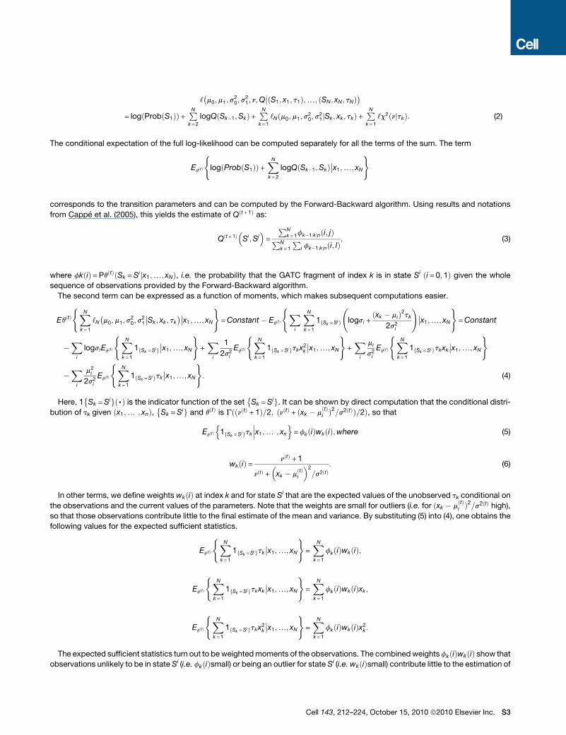
‘�m0;m1;s

20; s

21; n;Q

��ðS1; x1; t1Þ;.; ðSN; xN; tNÞ�

= logðProbðS1ÞÞ+PNk = 2

logQðSk�1;SkÞ+PNk = 1

‘Nðm0;m1;s20; s

21jSk ; xk ; tkÞ+

PNk = 1

‘c2ðnjtkÞ: (2)

The conditional expectation of the full log-likelihood can be computed separately for all the terms of the sum. The term

EqðtÞ

(logðProbðS1ÞÞ+

XNk = 2

logQðSk�1;SkÞ��x1;.; xN

)

corresponds to the transition parameters and can be computed by the Forward-Backward algorithm. Using results and notations

from Cappe et al. (2005), this yields the estimate of Qðt + 1Þ as:

Qðt +1Þ�Si;Sj

�=

PNk = 1fk�1:kjnði; jÞPN

k = 1

Pl fk�1:kjnði; lÞ

; (3)

where fkðiÞ=PqðtÞðSk =Sijx1;.; xNÞ, i.e. the probability that the GATC fragment of index k is in state Si ði = 0; 1Þ given the whole

sequence of observations provided by the Forward-Backward algorithm.

The second term can be expressed as a function of moments, which makes subsequent computations easier.

EqðtÞ(XN

k =1

‘N�m0;m1; s

20; s

21

��Sk ; xk ; tk���x1;.; xN

)=Constant � EqðtÞ

(Xi

XNk = 1

1fSk =Sig

logsi +

ðxk � miÞ2tk2s2

i

!��x1;.; xN

)=Constant

�Xi

logsiEqðtÞ

(XNk = 1

1fSk =Sig��x1;.; xN

)+Xi

1

2s2i

EqðtÞ

(XNk = 1

1fSk =Sigtkx2k

��x1;.; xN

)+Xi

mi

s2i

EqðtÞ

(XNk = 1

1fSk =Sigtkxk��x1;.; xN

)

�Xi

m2i

2s2i

EqðtÞ

(XNk = 1

1fSk =Sigtk��x1;.; xN

): (4)

Here, 1 Sk =Si ð,Þg�is the indicator function of the set Sk =Sig�

. It can be shown by direct computation that the conditional distri-

bution of tk given ðx1;. ; xnÞ, Sk =Sig�and qðtÞ is GððnðtÞ + 1Þ=2; ðnðtÞ + ðxk � m

ðtÞi Þ2=s2ðtÞÞ=2Þ, so that

EqðtÞ

n1fSk =Sigtk

���x1;. ; xn

o=fkðiÞwkðiÞ;where (5)

wkðiÞ= nðtÞ + 1

nðtÞ +�xk � m

ðtÞi

�2=s2ðtÞ

: (6)

In other terms, we define weights wkðiÞ at index k and for state Si that are the expected values of the unobserved tk conditional on

the observations and the current values of the parameters. Note that the weights are small for outliers (i.e. for ðxk � mðtÞi Þ2=s2ðtÞ high),

so that those observations contribute little to the final estimate of the mean and variance. By substituting (5) into (4), one obtains the

following values for the expected sufficient statistics.

EqðtÞ

(XNk = 1

1fSk =Sigtk��x1;.; xN

)=XNk = 1

fkðiÞwkðiÞ;

EqðtÞ

(XNk = 1

1fSk =Sigtkxk��x1;.; xN

)=XNk = 1

fkðiÞwkðiÞxk ;

EqðtÞ

(XNk = 1

1fSk =Sigtkx2k

��x1;.; xN

)=XNk = 1

fkðiÞwkðiÞx2k :

The expected sufficient statistics turn out to beweightedmoments of the observations. The combinedweights fkðiÞwkðiÞ show that

observations unlikely to be in state Si (i.e. fkðiÞsmall) or being an outlier for state Si (i.e. wkðiÞsmall) contribute little to the estimation of

Cell 143, 212–224, October 15, 2010 ª2010 Elsevier Inc. S3

mean and variance for state Si. The updated values of m0;m1; s20 and s21 are the ones that maximize the expected log-likelihood. They

are obtained by differentiating (4) with respect to the parameters:

mðt + 1Þi =

PNk =1fkðiÞwkðiÞxkPNk = 1fkðiÞwkðiÞ

; (7)

s2ðt + 1Þi =

PNk =1fkðiÞwkðiÞ

�xk � m

ðt + 1Þi

�2PN

k = 1fkðiÞ: (8)

Following the EMprocedure, one could update nðtÞ by differentiating the last term of (2). However this procedure proves to give slow

convergence. Instead, we used the idea of the MCECM algorithm (Liu and Rubin, 1995), which is substantially faster than the EM in

terms of number of cycles. This involves performing another Forward-Backward pass with parameters~qðtÞ= ðmðt +1Þ

0 ;mðt + 1Þ1 ; s

2ðt +1Þ0 ;s

2ðt + 1Þ1 ; nðtÞ;Qðt + 1Þ; Þ and computing the weights wkðiÞ again through formula (6) before differentiating the

last term of (2). Let

~wk =Xi

fkðiÞwkðiÞ: (9)

The weights ~wk are the weighted averages of the weights wkðiÞ and are designed to be small for observations that are outliers in

every state. The updated value nðt + 1Þ is then the value n such that

1� j�n2

�+ log

�n2

�+1

N

XNk =1

log�~wk

�� ~wk +1

N

XNk =1

j

�n+ 1

2

� log

�n+ 1

2

= 0; (10)

where jðzÞ is the digamma function i.e. jðzÞ=dlogGðzÞ=dz. The solution of this equation is computed numerically (by dichotomy).

Here is a summary of the different steps carried out at each cycle of the algorithm, where CM stands for ‘constrained’ or ‘condi-

tional’ maximization (Liu and Rubin, 1995).

E-step 1: Compute the Forward-Backward smoothing estimates using qðtÞ and compute the weights wkðiÞ through (6).

CM-step 1: Update the transition probabilities through (3), the estimated means through (7), and the estimated variances through

(8).

E-step 2: Compute the Forward-Backward smoothing estimates using ~qðtÞ

and compute the weights again through (6). Compute

the averaged weights ~wk through (9).

CM-step 2: Compute nðt +1Þ by solving (13).

After multiple cycles, the estimates usually converge to stable values, at which point the algorithm is stopped. The most likely

sequence of states ðS1;. ;SNÞ is then computed through the Viterbi algorithm.

Virtual Bridging

Gaps in the array design are filled by virtual positions for which emissions are not available (NA). Gaps longer than 2D are bridged by

L=ðD� 1Þ virtual positions, where D is the mean distance between two consecutive GATC fragment ‘start’ positions and L is the gap

size.

The emission probability of those virtual positions is set to 1 for every state. As a consequence, virtual bridging directly influences

the estimation of the transition probabilities Q in the modified Baum-Welch algorithm presented above because it modifies the

spacing between reads.

Multidimensional Inference

The modified Baum-Welch algorithm presented above can easily be applied to the case of multidimensional measurements. These

are typically different binding profiles, or different linear combinations of binding profiles.

Assume thatmeasurements xk ðk = 1;. ;N) are now p -dimensional vectors, such that xk;p denotes the value of the k th read in the p

th dimension. The distribution of xk given Sk =Si is a multidimensional Student’s t variable with mean vector mi, and mean variance

matrix ~Si and n degrees of freedom.

Again, the likelihood of the multidimensional Student’s t distribution is described as that of a multidimensional Gaussian random

variable with random variance. X � Tðm;S; nÞif and only if X � Nðm;S=tÞ and t � c2ðnÞ, where X and t are independent. Again ~S, the

variance matrix of X, is not S, but rather a function of ðS; nÞ.Formula (6) giving the weights is replaced by

wkðiÞ= nðtÞ +p

nðtÞ +�xk � m

ðtÞi

�2=s2ðtÞ

: (11)

S4 Cell 143, 212–224, October 15, 2010 ª2010 Elsevier Inc.

The sufficient statistics now include the cross-products of xk, and equation (8) should be replaced by

Sðt + 1Þi ðp;qÞ=

PNk = 1fkðiÞwkðiÞ

�xk;p � m

2ðt + 1Þi;p

��xk;q � m

2ðt + 1Þi;q

�PN

k = 1fkðiÞ: (12)

Equation (10) giving the updated value of n is replaced by

1� j�n2

�+ log

�n2

�+1

N

XNk = 1

log�~wk

�� ~wk +1

N

XNk =1

j

�n+p

2

� log

�n+p

2

= 0: (13)

TheMCECMprocedure outlined at the end of ‘‘Detailed Derivation’’ can be applied to identify targets in amultidimensional setting.

Also, the procedure simply extends to the case of more than two states. Ifm is the number of states, the matrix Q is anm3mmatrix

and equation (3) is still valid. The bounds of the sum in equation (4) and (9) have been left out on purpose so that all the formulas hold

irrespective of the number of states.

Definition of the Chromatin TypesDetermining the Number of States

By compiling the DamID scores of the 53 profiles, the probed genome can be viewed as a cloud of points in a 53-dimensional space.

In this space, two GATC fragments are close to each other if they are bound by the same proteins (irrespective of their genomic coor-

dinates). Principal Component Analysis (PCA) gives the approximation of the cloud in lower dimensions that best preserves the over-

all spread (i.e. the variance) of the cloud. Each recurrent protein binding signature should appear as an individual lobe of the projected

cloud. Importantly, one expects the projected coordinates to be distributed as a Student’s t variable because they are weighted aver-

ages of the DamID binding scores, meaning that the projected cloud can be described by the multi-state multi-dimensional HMM

presented above.

We performed scaled PCA on the 53 profiles and examined the projection of the cloud on the first principal components. It imme-

diately appeared that at least three components are required to give a qualitative representation of the data, because a distinct sub-

cloud separates in the third component. The projection on the first 3 principal components reveals 5 distinct lobes. Whereas the plot

shown in Supplementary Figure 5B suggests that the fourth component might be included in the analysis, none of the 5 clouds forks

into multiple sub-clouds in the fourth or higher order principal components. Therefore, we reduced the data to its first 3 principal

components.

A substantial part of the variance in tiling array experiments is noise. For example, discretizing a DamID binding profile by a two-

state HMM accounts for approximately 40% of the total variance (the median score out of 53 profiles is 39.4%). In comparison, the

total variance captured by the first 3 principal components is 57.7%. This figure suggests that the procedure efficiently removes the

technical variation from the dataset without causing a strong loss of information.

Mapping the Chromatin Types

Fitting an HMM to the original dataset would involve estimating 7,441 parameters (53 4 transition parameters, 53 53means, 53 53

variances, 53 1374 covariances and 1 degree of freedom). In contrast, if the dataset is replaced by its projections on the first 3 prin-

cipal components, the number of parameters drops to 66 (5 3 4 transition parameters, 53 3 means, 53 3 variances, 53 3 covari-

ances and 1 degree of freedom), representing a substantial gain of robustness.

To map the chromatin types in the fly genome, we used the method described in ‘‘Multidimensional Inference’’ with 5 states. The

initial degree of freedom was set to 6. The initial means of the modified Baum-Welch algorithm were determined visually. The initial

covariance matrices were set to the covariance matrix of the 3-dimensional cloud. Note that within each lobe, the projections on the

principal components may be correlated, even if their correlation is null on the whole dataset. Thus, after the first iteration the terms in

equation (12) are not expected to be 0 for psq.

The output of the modified Baum-Welch algorithm showed some sensitivity to initial parameter values, mainly to the means. For

some initial values, the modified Baum-Welch algorithm failed to identify 5 clearly separated states. However, there was only one

fitted model where the states were clearly separated, showing that the segmentation is robust to initial conditions.

The initial DamID binding values and final state calls are provided as supplementary files. An implementation of the procedure as an

R package (R Development Core Team, 2009) is available upon request.

SUPPLEMENTAL REFERENCES

Bushey, A.M., Ramos, E., and Corces, V.G. (2009). Three subclasses of a Drosophila insulator show distinct and cell type-specific genomic distributions. Genes

Dev. 23, 1338–1350.

Cappe, O., Moulines, E., and Ryden, T. (2005). Inference in Hidden Markov Models (Springer), pp. 369.

Chintapalli, V.R., Wang, J., and Dow, J.A. (2007). Using FlyAtlas to identify better Drosophila melanogastermodels of human disease. Nat. Genet. 39, 715–720.

Dempster, A.P., Laird, M., and Rubin, D.B. (1976). Maximum likelihood from Incomplete Data via the EM Algorithm. J.R. Stat. Soc., B 39, 1–38.

Cell 143, 212–224, October 15, 2010 ª2010 Elsevier Inc. S5

Engstrom, P.G., Ho Sui, S.J., Drivenes, O., Becker, T.S., and Lenhard, B. (2007). Genomic regulatory blocks underlie extensive microsynteny conservation in

insects. Genome Res. 17, 1898–1908.

Liu, C., and Rubin, D.B. (1995). ML estimation of the t distribution using EM and its extensions, ECM and ECME. Statist. Sinica 5, 19–39.

R Development Core Team. 2009. R: A Language and Environment for Statistical Computing. http://www.R-project.org

Slater, G.S., and Birney, E. (2005). Automated generation of heuristics for biological sequence comparison. BMC Bioinformatics 6, 31.

S6 Cell 143, 212–224, October 15, 2010 ª2010 Elsevier Inc.

AMRG15

SU(VAR)3−7SU(VAR)3−9

HP6HP1LHR

CAF1ASF1

MUS209TOP1

RPII18SIR2

RPD3CDK7DSP1DF31MAX

PCAFASH2HP1cCtBPJRA

BRMECRBCD

MED31SU(VAR)2−10

LOLALGAF

CG31367ACT5C

TIP60MNT

SIN3ATBP

DWGPHOLPROD

BEAF32bSU(HW)

LAMD1H1

SUUREFFIAL

GROPHO

CTCFPC

E(Z)PCLSCE

16400 16500 16600 16700 16800 16900Postition on chr2L (kb)

Type

Genes

B C

D

log 2

(Dam

−H

1/D

am)

H1 DamID

−4

−2

0

log 2

(H1

ChI

P/in

put)

H1 ChIP

−1.

00.

00.

5

Genes

11650 11750 11850 11950 12050 12150 12250 12350 12450 12550 12650

Position on chr2L (kb)

log 2

(Dam

−S

U(H

W)/

Dam

) SU(HW) DamID

−1

01

23

log 2

(SU

(HW

) C

hIP

/inpu

t) SU(HW) ChIP

−1

12

34

Genes

6800 6900 7000 7100 7200 7300 7400 7500 7600 7700 7800

Position on chr2R (kb)

log 2

(Dam

−C

TC

F/D

am) CTCF DamID

−0.

51.

52.

5

log 2

(CT

CF

ChI

P/in

put) CTCF ChIP

−1

12

34

Genes

400 500 600 700 800 900 1000 1100 1200 1300 1400

Position on chr2L (kb)

E

−6 −4 −2 0

−4−2

02

46

PC1

−6 −4 −2 0 2 4 6

−4−2

02

46

PC2

PC3

−5 0

05

1015

PC1

−5 0 5

−20

24

68

PC2

PC3

35 40 45 50

020

4060

8010

0

Robustness of the classification

Subsample size

Estim

ated

per

cent

age

% Faithful segmentations% Overlap with current segmentation

5PC2

2 4 6PC2

Figure S1. Validation of DamID and Robustness Analysis of the Five-Type segmentation, Related to Figure 1

(A) Magnification of the 53 DamID profiles as depicted in Figure 1. Traces show log2 DamID ratios, and width of black bars represents the length of DpnI restriction

fragments.

(B) Comparisons of DamID (Braunschweig et al., 2009) and ChIP for histone H1 (this study), SU(HW), and CTCF (Bushey et al., 2009). All data sets were subjected

to running mean smoothing with a window of three data points. Genes on the top and bottom strand are depicted as lines with blocks indicating exons.

(C) The five-state classification is robust to the quantification method. DamID profiles for each protein were binarized before projection onto the first three prin-

cipal components. The shape of the cloud is different from the one shown inmain Figure 1B, but the five types still form separated clouds in the first three principal

components.

(D) Sensitivity analysis of the segmentation. The principal component analysis and HMM procedure was applied as in Figure 1 to data sets where one or more

proteins were left out. It is expected that smaller sets will not always exhibit all five states; for example, a subset that lacks the four PcG proteins will not identify

the BLUE state. In that case, the loci formerly assigned to BLUE will be assigned to another color by the HMM. We call such a segmentation ‘‘unfaithful.’’ On the

contrary, ‘‘faithful’’ segmentations show no replacement of a color by another. The percentage of overlap between the current segmentation (based on the

complete data set) and unfaithful segmentations is irrelevant: it mostly reflects the size of the type that has been replaced. For example if BLUE has been replaced

by another color at least 20% of the calls will differ (i.e., all the former BLUE calls). For subsets of 35–51 proteins, 50 samples were drawn at random without

replacement. For subsets of 52 proteins, all possible 53 subsets were tested. For each subsample size, the percentage of faithful segmentations (thin lines)

and their mean percentage of overlap with the current segmentation (thick lines) were determined. Vertical bars represent ± standard deviations. The plot shows

that larger sets of proteins give an increasingly reliable discovery of the five states. Faithful segmentations show substantial agreement with the current definition,

even for smaller sample sizes. Thus, identification of the states is sensitive to protein choice, but the classification itself is robust.

(E) Minimal set of proteins defining the five types. A carefully selected set of five proteins (histone H1, PC, HP1, MRG15, and BRM) summarizes the segmentation

in 5 types. The data points were projected on their first three principal components, showing that the types are clearly visible with this minimal set of proteins. The

coloring was obtained by applying the HMM to the first three principal components, exactly as was done for the 53 proteins. The agreement with the 53 profile

segmentation is 85.5%.

Cell 143, 212–224, October 15, 2010 ª2010 Elsevier Inc. S7

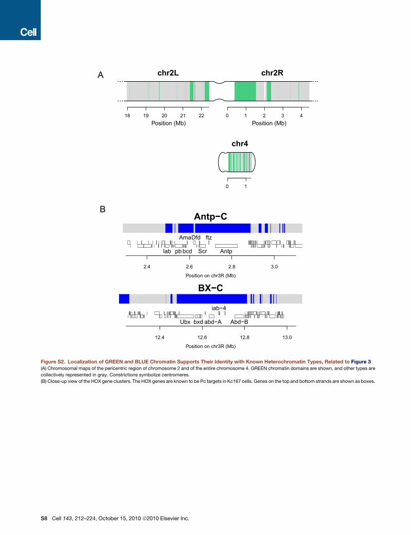
18 19 20 21 22Position (Mb)

chr2L chr2R

0 1 2 3 4Position (Mb)

0 1

chr4

A

BAntp−C

AmaDfd ftz

lab pb bcd Scr Antp

2.4 2.6 2.8 3.0

Position on chr3R (Mb)

BX−C

iab−4

Ubx bxd abd−A Abd−B

12.4 12.6 12.8 13.0

Position on chr3R (Mb)

Figure S2. Localization of GREEN and BLUE Chromatin Supports Their Identity with Known Heterochromatin Types, Related to Figure 3

(A) Chromosomal maps of the pericentric region of chromosome 2 and of the entire chromosome 4. GREEN chromatin domains are shown, and other types are

collectively represented in gray. Constrictions symbolize centromeres.

(B) Close-up view of the HOX gene clusters. The HOX genes are known to be Pc targets in Kc167 cells. Genes on the top and bottom strands are shown as boxes.

S8 Cell 143, 212–224, October 15, 2010 ª2010 Elsevier Inc.

A

B

16.2 16.4 16.6 16.8 17.0 17.2

Position on chr2L (Mb)

P

rote

ins

boun

d

018

36

Protein count per locus

Freq

uenc

y

015

000

Freq

uenc

y

040

010

00

Freq

uenc

y

015

00

Freq

uenc

y

030

00

Freq

uenc

y

060

014

00

0 10 20 30 40Number of bound proteins (out of 53 proteins)

Figure S3. Chromatin Types Differ Widely in Their Total Protein Occupancy, Related to Figure 6

(A) Sample plot of the total occupancy (out of 53 mapped proteins) on a 1Mb segment of chromosome 2L. The height of each vertical line indicates the number of

proteins bound to a locus. The color of the line indicates the local chromatin type.

(B) Histograms of total occupancy distributions per chromatin type. Gray vertical dashed lines indicate median values.

Cell 143, 212–224, October 15, 2010 ª2010 Elsevier Inc. S9

Position Position Position Position Position Position

Dam

ID s

core

Dam

ID s

core

Dam

ID s

core

Dam

ID s

core

Dam

ID s

core

Dam

ID s

core

A

B

0 10020 40 60 80 0 10020 40 60 80 0 10020 40 60 80 0 10020 40 60 80 0 10020 40 60 80 0 10020 40 60 80

Figure S4. Chromatin Types Guide DBF Binding to Their Motifs, Related to Figure 7

(A) Optimized position-specific affinity matrices for 5 Drosophila DBFs and Gal4-DBD (see Extended Experimental Procedures for details).

(B) Distributions of relative affinites of GATC fragments mapping within each of the five types. For each chromatin type, DamID scores of GATC fragments ranked

by the predicted affinity of a 2 kb window around its center. Gray lines represent the loess fit. Last row: superimposed loess fits for the five chromatin types.

Colored numbers indicated the Spearman’s rank correlation coefficients of DamID value with predicted affinities.

S10 Cell 143, 212–224, October 15, 2010 ª2010 Elsevier Inc.

−2 −1 0 1 2

0.0

0.5

1.0

1.5

2.0

2.5

Distribution of x scores

x score

Den

sity

Observed x scoresFitted Student's tFitted Gaussian

1 4 7 10 14 18 22 26 30 34 38 42 46 50

Principal Components

Frac

tion

of to

tal v

aria

nce

0.0

0.1

0.2

0.3

0.4

A B

Figure S5. Addendum to the Analytical Methods, Related to Extended Experimental Procedures

(A) The scores x follow a Student’s t distribution. The plot shows the density of loess-normalized and averaged per GATC fragments log2 ratios of the DamID

profile of protein FBpp0074431 (black line). DamID for this protein shows no specific signal, and no targets were detected. The red line is the density of Student’s

t distribution fitted by maximum likelihood, and the blue line is the density of a fitted Gaussian distribution.

(B) Variance accounted for by individual principal components.

Cell 143, 212–224, October 15, 2010 ª2010 Elsevier Inc. S11