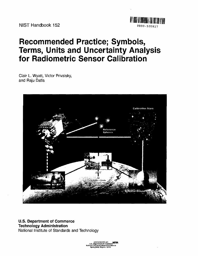
NIST Handbook 152111111111 1111111111111111111 III

PB99-105827

Recommended Practice; Symbols,Terms, Units and Uncertainty Analysisfor Radiometric Sensor Calibration

Clair L. Wyatt, Victor Privalsky,and Raju Datla

u.s. Department of CommerceTechnology AdministrationNational Institute of Standards and Technology

u.s. D~~~~~~~Co~~~~~erce~National Technicallnfonnation Service

Springfield, Virginia 22161

The National Institute of Standards and Technology was established in 1988 by Congress to "assist industry inthe development of technology ... needed to improve product quality, to modernize manufacturing processes,

to ensure product reliability ... and to facilitate rapid commercialization ... of products based on new scientificdiscoveries.' ,

NIST, originally founded as the National Bureau of Standards in 1901, works to strengthen U.S. industry'scompetitiveness; advance science and engineering; and improve public health, safety, and the environment. Oneof the agency's basic functions is to develop, maintain, and retain custody of the national standards ofmeasurement, and provide the means and methods for comparing standards used in science, engineering,manufacturing, commerce, industry, and education with the standards adopted or recognized by the FederalGovernment.

As an agency of the U.S. Commerce Department's Technology Administration, NIST conducts basic andapplied research in the physical sciences and engineering, and develops measurement techniques, testmethods, standards, and related services. The Institute does generic and precompetitive work on new andadvanced technologies. NIST's research facilities are located at Gaithersburg, MD 20899, and at Boulder, CO 80303.Major technical operating units and their principal activities are listed below. For more information contact thePublications and Program Inquiries Desk, 301-975-3058.

Office of the Director• National Quality Program• International and Academic Affairs

Technology Services• Standards Services• Technology Partnerships• Measurement Services• Technology Innovation• Information Services

Advanced Technology Program• Economic Assessment• Information Technology and Applications• Chemical and Biomedical Technology• Materials and Manufacturing Technology• Electronics and Photonics Technology

Manufacturing Extension PartnershipProgram• Regional Programs• National Programs• Program Development

Electronics and Electrical EngineeringLaboratory• Microelectronics• Law Enforcement Standards• Electricity• Semiconductor Electronics• Electromagnetic Fields I

• Electromagnetic Technologyl• Optoelectronics I

Chemical Science and TechnologyLaboratory• Biotechnology• Physical and Chemical Properties2

• Analytical Chemistry• Process Measurements• Surface and Microanalysis Science

I At Boulder, CO 80303.2Some elements at Boulder, CO.

Physics Laboratory• Electron and Optical Physics• Atomic Physics• Optical Technology• Ionizing Radiation• Time and Frequencyl• Quantum Physicsl

Materials Science and EngineeringLaboratory• Intelligent Processing of Materials• Ceramics• Materials Reliabilityl• Polymers• Metallurgy• NIST Center for Neutron Research

Manufacturing EngineeringLaboratory• Precision Engineering• Automated Production Technology• Intelligent Systems• Fabrication Technology• Manufacturing Systems Integration

Building and Fire ResearchLaboratory• Structures• Building Materials• Building Environment• Fire Safety Engineering• Fire Science

Information Technology Laboratory• Mathematical and Computational Sciences2

• Advanced Network Technologies• Computer Security• Information Access and User Interfaces• High Performance Systems and Services• Distributed Computing and Information Services• Software Diagnostics and Conformance Testing

NIST Handbook 152

Recommended Practice; Symbols,Terms, Units and Uncertainty Analysisfor Radiometric Sensor Calibration

Dr. Clair L. Wyatt, Professor EmeritusElectrical Engineering Department

and

Dr. Victor Privalsky, Sr. ScientistSpace Dynamics LaboratoryUtah State University

and

Dr. Raju DatlaOptical Technology DivisionPhysics LaboratoryNational Institute of Standards and TechnologyGaithersburg, MD 20899-0001

September 1998

U.S. DEPARTMENT OF COMMERCE, William M. Daley, SecretaryTechnology Administration, Gary R. Bachula, Acting Under Secretary for TechnologyNational Institute of Standards and Technology, Raymond G. Kammer, Director

PROTECTED UNDER INTERNATIONAL COPYRIGHTALL RIGHTS RESERVED.NATIONAL TECHNICAL INFORMATION SERVICEU.S. DEPARTMENT OF COMMERCE

National Institute of Standards and Technology Handbook 152Nat!. Inst. Stand. Techno!. Handb. 152, 120 pages (Sept. 1998)

CODEN: NIHAE2

u.S. GOVERNMENT PRINTING OFFICEWASHINGTON: 1998

For sale by the Superintendent of Documents, U.S. Government Printing Office, Washington, DC 20402-9325

FOREWARD

Uniform terminology and common practices of uncertainty analysis are absolutely crucial

for the ground based or space based radiometry projects of the National Aeronautics and Space

Administration (NASA), the National Oceanographic and Atmospheric Administration (NOAA)

and the Department ofDefense (DoD) to exchange scientific data and results without the need for

duplication and repetition. The economic impact is even greater for exchanging data and results

around the world on global studies which is only possible through uniformity of terminology and

data analysis standards.

This need for developing a common practice for quantities, symbols, units and uncertainty

analysis has been recognized by scientists and engineers around the world. The first step taken to

my knowledge recently was the establishment of Space Based Observation Systems Committee on

Standards (SBOS COS) in 1988 by the American Institute of Aeronautics and Astronautics

(AIAA). As a historical perspective, the letter by Christopher Stevens of Jet Propulsion

Laboratory that shows various meetings in this endeavor and the overview on "AIAA activities in

Calibration Standards" by Edward Koenig ofITT Aerospace/ Communications Division is

reproduced in Appendix 1. It also lists the members of the subcommittee on sensor systems. I

would like to join with Clair Wyatt, the principal author of this document, in acknowledging the

efforts of various people in that list who helped in preparing this document. It is being published

as a NIST Handbook recommending it to be a common practice for optical radiation metrology.

It primarily deals with terms, symbols and definitions in radiometry based on the International

Standards Organization (ISO) definitions ofbasic radiometric quantities. The sensor systems

calibration methodology is based on the measurement equation approach that has been in practice

from the beginning at the National Institute of Standards and Technology (NIST). The uncertainty

analysis is based on the ISO Guide to the Expression ofUncertainty in Measurement, ISO/TAG

4/WG3.

Raju Datla, Optical Technology Division, NIST

111

PREFACE

This recommended practice introduces several new entities. Of concern are the terms,

symbols, and units (nomenclature) used to describe sources, sensor performance analysis,

calibration, and uncertainty analysis of radiometric sensors. The definitions given in this document

are limited to those that apply to radiometric calibration and do not include illumination terms. It

has been the authors' dream to create a document like this to facilitate communication and

dissemination of knowledge throughout the optical community. It is heartening to note that one of

the authors, Dr. V. Privalsky was already chosen by the Russian Space Agency to translate this

document into Russian.

The contents of this document were presented as a tutorial at the Fifth Infrared

Radiometric Sensor Calibration Symposium that was held by Space Dynamics Laboratory /Utah

State University in Logan, Utah, in May 1995. The document was revised based on the comments

of the participants to its present form.

Authors.

Key Words: Radiometry, Sensor Calibration, Uncertainty Analysis

IV

TABLE OF CONTENTS

FORWARD " 111

PREFACE IV

INTRODUCTION 1

1. PART 1: SYMBOLS, TERMS, AND UNITS 2

1.1 DEFINITIONS 2

1.1.1 WAVELENGTHIWAVE NUMBER 2

1.1.2 FLUX 3

1.2 GEOMETRICAL PROPERTIES OF SOURCES 3

1.2.1 RADIANCEfPHOTON RADIANCE 3

1.2.2 RADIANT EXITANCEfPHOTON EXITANCE 4

1.2.3 RADIANT INTENSITYfPHOTON INTENSITY 4

1.2.4 IRRADIANCEfPHOTON IRRADIANCE 6

1.2.5 FIELD ENTITIES 6

1.3 SPECTRAL FLUX 6

1.4 THE GEOMETRY OF RADIATION TRANSFER 7

1.4.1 PROJECTED AREA 7

1.4.2 SOLID ANGLE 9

1.4.3 PROJECTED SOLID ANGLE 10

1.5 SENSOR PARAMETERS 11

1.5.1 RELATIVE SPATIAL RESPONSIVITY . . . . . . . . . . . . . . . . . . . . . . . . . . . . . 11

1.5.2 ENCIRCLED (ENSQUARED) ENERGY 12

1.5.3 THROUGHPUT AND RELATIVE APERTURE 12

2. PART II: THE RADIOMETRIC SENSOR CALIBRATION 15

2.1 THE MEASUREMENT EQUATION 15

v

EXAMPLE 1 24

2.2 CALIBRATION EQUATIONS 26

2.2.1 RADIOMETER RADIANCE CALIBRATION EQUATION 28

2.2.2 RADIOMETER IRRADIANCE CALIBRATION EQUATION 30

2.2.3 SPECTROMETER CALIBRATION EQUATION 31

EXA.MPLE 2 33

3. PART III: UNCERTAINTY ANALYSIS 37

3.1 DEFINITIONS 37

3.2 UNCERTAINTY ANALYSIS FOR SENSOR CALIBRATION 39

3.2.1 CALIBRATION SNAPSHOTS 39

3.2.2 NOISE 41

3.2.3 NONLINEARITY 41

3.2.4 NONUNIFORM AREA RESPONSIVITY 44

3.2.5 ANGULAR SPATIAL RESPONSIVITY 46

3.2.6 MTF CORRECTION UNCERTAINTY 48

3.2.7 CALIBRATION STANDARD SOURCE UNCERTAINTY 49

3.2.8 ABSOLUTE RESPONSIVITY UNCERTAINTY 50

3.2.9 NONUNIFORM SPECTRAL RESPONSE 53

3.2.10 BAND-TO-BAND UNCERTAINTY 57

3.3 PROPAGATION OF UNCERTAINTIES - COMBINED STANDARD

UNCERTAINTY 58

3.3.1 OLD TERMINOLOGY AND RECOMMENDED PRACTICE 59

EXA.MPLE 3 63

4. REFERENCES 73

VI

TABLES

TABLE 1. BASIC RADIOMETRIC TERMS, SYMBOLS, AND UNITS 5

TABLE 2. SOURCE SPECTRAL TERMS, SYMBOLS, AND UNITS 8

TABLE 3. GONIOMETRIC TERMS AND UNITS 14

TABLE 4. SYSTEM PERFORMANCE TERMS, SYMBOLS, AND UNITS 22

TABLE 5. SYSTEM CALIBRATION TERMS, SYMBOLS, AND UNITS 29

TABLE 6. UNCERTAINTY ANALYSIS SYMBOLS AND TERMS 40

FIGURES

FIGURE 1.

FIGURE 2.

FIGURE 3.

FIGURE 4.

FIGURE 5.

FIGURE 6.

FIGURE 7.

FIGURE 8.

FIGURE 9.

ILLUSTRATION OF THE PROJECTED AREA 9

ILLUSTRATION OF SOLID ANGLE AND PROJECTED SOLID ANGLE . 10

SCHEMATIC FOR A SIMPLE OPTICAL SYSTEM ILLUSTRATING THE

HALF-ANGLE FIELD-OF-VIEW (Q AND THE CONE HALF-ANGLE a. .. 13

RELATIVE RESPONSE AND SPECTRAL RADIANCE OF A FILTER

RADIOMETER 24

ILLUSTRATION OF DATA LINEARIZATION. THE ORIGINAL DATA­

CIRCLE, LINEARIZED DATA-SQUARE, SOLID CURVE IS THE IDEAL

LINEAR RESPONSE. . 43

ISOMETRIC 3-DIMENSIONAL VIEW OF THE SPATIAL RESONSE OF AN

INFRARED DETECTOR. 47

POINT (---) AND LINE-SPREAD (---) FUNCTION MTF FOR

ASENSOR 48

TYPICAL BANDPASS INTERFERENCE FILTER TRANSMITTANCE 55

STANDARD UNCERTAINTY (I-SIGMA GIVEN IN PERCENT) OF THE

EXTENDED- AREA SOURCE ABSOLUTE RESPONSIVITY

CALIBRATION 65

VII

FIGURE 10. RELATIVE SPECTRAL RESPONSE AJA.) FOR THE EXTENDED-AREA

SOURCE ABSOLUTE CALIBRATION 66

FIGURE 11. SCANS OBTAINED FOR THE POINT-SOURCE ABSOLUTE IRRADIANCE

RESPONSIVITY CALffiRATION 66

FIGURE 12. STANDARD UNCERTAINTY (1- SIGMA) OF THE POINT-SOURCE

ABSOLUTE IRRADIANCE RESPONSIVITY CALffiRATION 67

FIGURE 13. RELATIVE SPECTRAL RESPONSE pdA.) FOR THE POINT-SOURCE

ABSOLUTE CALffiRATION 68

FIGURE 14. SCANS OBTAINED FOR THE EXTENDED-AREA SOURCE ABSOLUTE

RADIANCE RESPONSIVITY CALffiRATION . . . . . . . . . . . . . . . . . . . . . 70

APPENDIX

APPENDIX 1 77

APPENDIX 2 91

Vlll

INTRODUCTION

This handbook provides recommendations for nomenclature, terms, symbols, units and

uncertainty analysis associated with the calibration of radiometric sensor systems. The scope

includes the radiant properties of sources; the geometry of radiation transfer; the measurement

equation used to predict sensor response; the calibration equation used to convert sensor response

to engineering units (radiance, irradiance, etc.); and the uncertainty analysis.

The contents are organized to correspond, somewhat, to the normal flow offlux (source to

sensor) and of analysis (predicted performance to generation of calibration equations and

uncertainty analysis). This document expands on the current practice of radiometry as described

in a recent NIST Technical Note [1].

The definitions of radiometric terms, symbols, and units in this document conform to the

definitions accepted by the International Standards Organizations (ISO)[2]. These standards

include quantities that are functions ofwavelength (frequency or wavenumber); they may be

designated by the same term preceded by the adjective spectral and by the same symbol followed

by A, v, or oin parenthesis; for example spectral emissivity ~A). On the other hand, if the

spectralpower density, or spectral power concentration [3] is considered, it may also be

designated by the name ofthe quantity and by the symbol for the quantity with the subscript A ( v,

or 0); for example the spectral radiance,

elLL =-A dA (1)

Note that LA [W/(m3sr)] corresponds to watts per unit area per unit wavelength [(W/(m2sr»)/llm]

rather than watts per unit volume. Generally, wavelength is expressed in micrometers (11m) for

infrared and in nanometers (nm) for ultraviolet and visible regions ofthe spectrum. The integrated

quantity is given by

(2)

with units [W/(m2sr)]. In this document the NIST Guide for the Use ofthe International System

1

ofUnits (SI) is followed [4]. Also, the SI base units for quantities are in square brackets when

they are introduced for the first time.

The terms used for uncertainty analysis conform to the ISO Guide to the Expression of

Uncertainty in Measurement [5]. Based on the ISO Guide, NIST developed the guidelines for

uncertainty analysis. The document describing these guidelines is added as Appendix 2 [6].

Those aspects of the ISO Guide that impinge upon this document are as follows. The standard

uncertainty refers to components ofuncertainty including both random and systematic effects.

Note that the term random is used rather than the term "precision," and that the term systematic is

used rather than the term "bias." The term combined standard uncertainty is used rather than the

term "accuracy" and has reference to propagated uncertainties. Finally, the term uncertainty

analysis is used rather than the term "error analysis."

1. PART 1: SYMBOLS, TERMS, AND UNITS

1.1 DEFINITIONS

As indicated above, the scope of this document is limited to those symbols, terms, and units

frequently used in the calibration of radiometric and spectrometric systems. Consequently, there is

no attempt to create an exhaustive list of terms.

In order to avoid large or small numerical values, decimal multiples and sub-multiples of the SI

units are added to the system making use of the standard prefixes [7]; for example, centimeter

with a factor of 10-2 and a symbol of cm, nanometer with a factor of 10-9 and a symbol ofnm, and

micrometer with a factor of 10-6 and a symbol of Ilm.

The ISO standard also addresses the question of alternative names and symbols for various

terms. It also recognizes a class of"supplementary" units like the radian and steradian as a class of

dimensionless units [8].

1.1.1 WAVELENGTHIWAVENUMBER

The wavelength A [m] is defined as the distance between two adjacent points in a periodic wave

having the same phase. The wavenumber (7 [mol] is the number ofwaves in a given length

interval.

2

1.1.2 FLUX

The radiant energy flux (Pe [J/s or W] is the power emitted, transferred or received; (Pp [S·l] is

the quanta-rate emitted, transferred or received. The subscripts e and p refer to energy and photon

rates respectively. The symbol (P is used without subscripts when it is clear from the context.

1.2 GEOMETRICAL PROPERTIES OF SOURCES

Sources are characterized in terms of geometrical properties to facilitate calculations using the

geometry of radiation transfer [9]. Table 1 provides a list of terms, units, and symbols for

characterizing sources. Also indicated in the table are the types of geometrical information

inherent in the entity: positional andlor directional. Definitions are given, in the sections to

follow, for each of the source characterizations listed in Table 1.

1.2.1 RADIANCEIPHOTON RADIANCE

The average radiance Lave of a source is the ratio of the total flux [W] to the product of the

projected source area As cos () and the solid angle (Us into which the radiation is emitted. The

subscript s refers to the source. This definition also holds for average photon radiance except the

total flux has units of photons per unit time [S·l]. The radiance L at a point on the source in a

certain direction is given by

(3)

The radiance is a measure of the flux of a source per unit area per unit solid angle at a point and in

the direction of propagation. Thus the radiance provides the most general description of the

source since it contains both positional and directional information. The total flux is given by

(4)

3

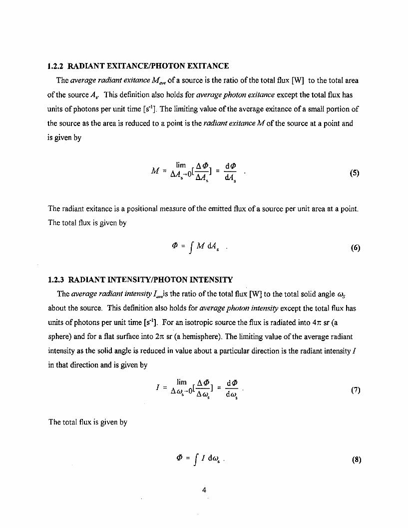
1.2.2 RADIANT EXITANCE/PHOTON EXITANCE

The average radiant exitance Mave ofa source is the ratio of the total flux [W] to the total area

of the source As. This definition also holds for average photon exitance except the total flux has

units of photons per unit time [S·l]. The limiting value of the average exitance ofa small portion of

the source as the area is reduced to a point is the radiant exitance M of the source at a point and

is given by

M _ lim [/}. tP]- /}.As ....O /}.A

s(5)

The radiant exitance is a positional measure of the emitted flux of a source per unit area at a point.

The total flux is given by

(6)

1.2.3 RADIANT INTENSITY/PHOTON INTENSITY

The average radiant intensity Iav)s the ratio of the total flux [W] to the total solid angle {Us

about the source. This definition also holds for average photon intensity except the total flux has

units of photons per unit time [S·l]. For an isotropic source the flux is radiated into 41t sr (a

sphere) and for a flat surface into 21t sr (a hemisphere). The limiting value of the average radiant

intensity as the solid angle is reduced in value about a particular direction is the radiant intensity I

in that direction and is given by

dtP(7)

The total flux is given by

(8)

4

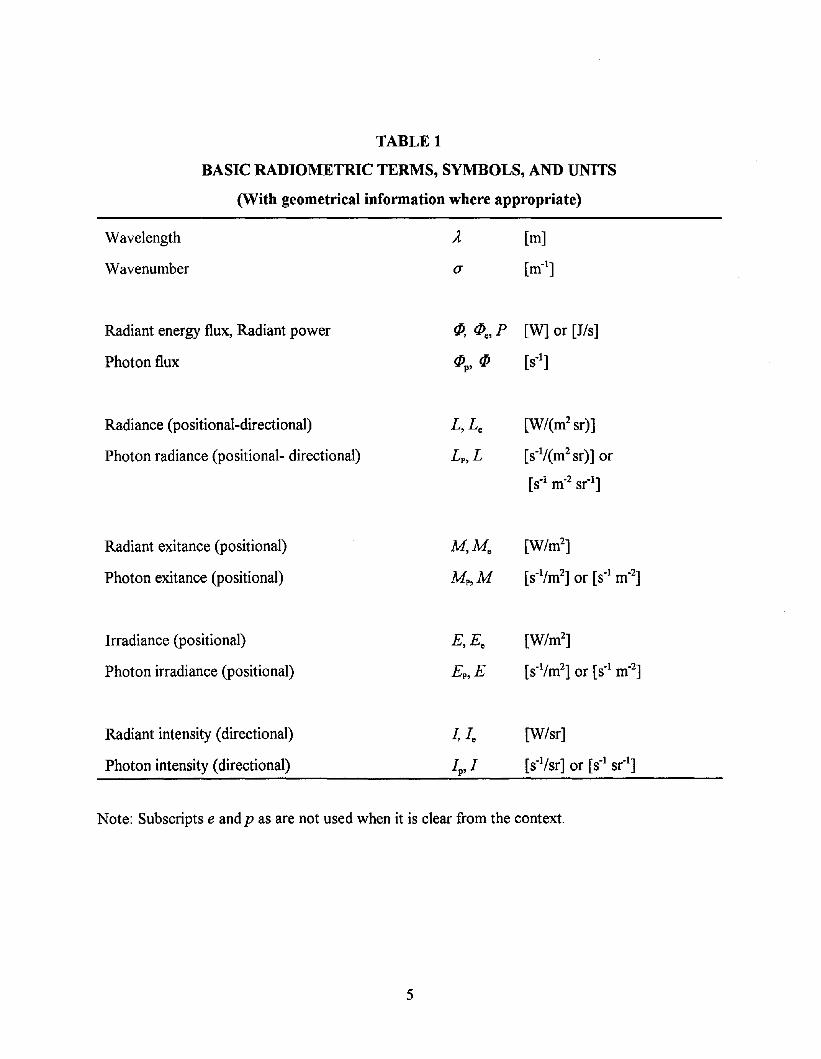
TABLE 1

BASIC RADIOMETRIC TERMS, SYMBOLS, AND UNITS

(With geometrical information where appropriate)

Wavelength

Wavenumber a

Radiant energy flux, Radiant power

Photon flux

if), tPc, P [W] or [J/s]

tPP

' tP [S·l]

Radiance (positional-directional)

Photon radiance (positional- directional)

Radiant exitance (positional)

Photon exitance (positional)

Irradiance (positional)

Photon irradiance (positional)

Radiant intensity (directional)

Photon intensity (directional)

[W/(m2 sr)]

[s-I/(m2 sr)] or

[sol m-2 sr-l]

[W/m2]

[s·l/m2] or [S·l m-2]

[W/m2]

[s·l/m2] or [S·l m-2]

[W/sr]

[s·l/sr] or [S-l sr-l]

Note: Subscripts e and p as are not used when it is clear from the context.

5

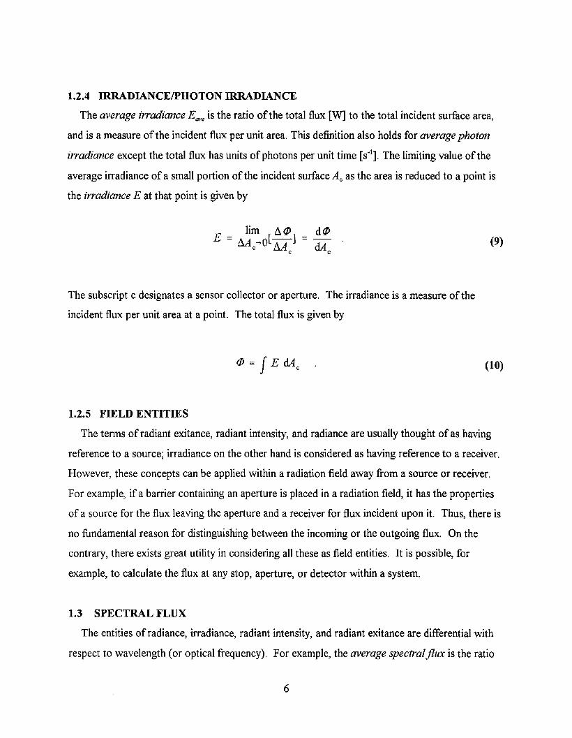
1.2.4 IRRADIANCEIPHOTON IRRADIANCE

The average irradiance Eave is the ratio ofthe total flux [W] to the total incident surface area,

and is a measure of the incident flux per unit area. This definition also holds for average photon

irradiance except the total flux has units of photons per unit time [S·l]. The limiting value of the

average irradiance of a small portion of the incident surface Ac as the area is reduced to a point is

the irradiance E at that point is given by

(9)

The subscript c designates a sensor collector or aperture. The irradiance is a measure of the

incident flux per unit area at a point. The total flux is given by

(10)

1.2.5 FIELD ENTITIES

The terms of radiant exitance, radiant intensity, and radiance are usually thought of as having

reference to a source; irradiance on the other hand is considered as having reference to a receiver.

However, these concepts can be applied within a radiation field away from a source or receiver.

For example, if a barrier containing an aperture is placed in a radiation field, it has the properties

of a source for the flux leaving the aperture and a receiver for flux incident upon it. Thus, there is

no fundamental reason for distinguishing between the incoming or the outgoing flux. On the

contrary, there exists great utility in considering all these as field entities. It is possible, for

example, to calculate the flux at any stop, aperture, or detector within a system.

1.3 SPECTRAL FLUX

The entities of radiance, irradiance, radiant intensity, and radiant exitance are differential with

respect to wavelength (or optical frequency). For example, the average spectralflux is the ratio

6

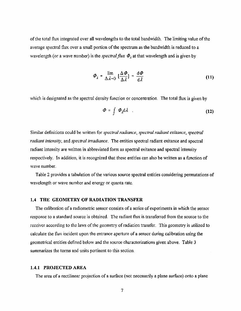
of the total flux integrated over all wavelengths to the total bandwidth. The limiting value of the

average spectral flux over a small portion of the spectrum as the bandwidth is reduced to a

wavelength (or a wave number) is the spectralflux (/J,i at that wavelength and is given by

(/J - lim [ Do (/J] _ d (/JA - DoA~O DoA - dA (11)

which is designated as the spectral density function or concentration. The total flux is given by

(12)

Similar definitions could be written for spectral radiance, spectral radiant exitance, spectral

radiant intensity, and spectral irradiance. The entities spectral radiant exitance and spectral

radiant intensity are written in abbreviated form as spectral exitance and spectral intensity

respectively. In addition, it is recognized that these entities can also be written as a function of

wave number.

Table 2 provides a tabulation of the various source spectral entities considering permutations of

wavelength or wave number and energy or quanta rate.

1.4 THE GEOMETRY OF RADIATION TRANSFER

The calibration ofa radiometric sensor consists of a series of experiments in which the sensor

response to a standard source is obtained. The radiant flux is transferred from the source to the

receiver according to the laws of the geometry of radiation transfer. This geometry is utilized to

calculate the flux incident upon the entrance aperture of a sensor during calibration using the

geometrical entities defined below and the source characterizations given above. Table 3

summarizes the terms and units pertinent to this section.

1.4.1 PROJECTED AREA

The area ofa rectilinear projection ofa surface (not necessarily a plane surface) onto a plane

7

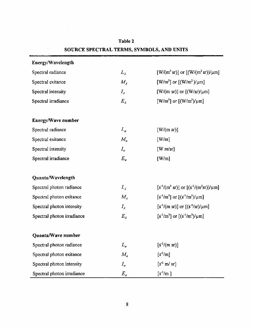
Table 2

SOURCE SPECTRAL TERMS, SYMBOLS, AND UNITS

EnergyIWavelength

Spectral radiance

Spectral exitance

Spectral intensity

Speetral irradiance

[W/(m3 sr)] or [(W/(m2 sr»)/Jlm]

[W/m3] or [(W/m2 )/Jlm]

[W/(m sr)] or [(W/sr)/Jlm]

[W/m3] or [(W/m2)/Jlm]

EnergylWave number

Spectral radiance L u [W/(m sr)]

Spectral exitance M u [W/m]

Spectral intensity 1u [W rn/sr]

Spectral irradiance Eu [W/m]

QuantalWavelength

Spectral photon radiance

Spectral photon exitance

Spectral photon intensity

Spectral photon irradiance

[s·1/(m3 sr)] or [(s·1/(m2sr»)/Jlm]

[s·1/m3] or [(s·1/m2)/Jlm]

[s·l/(m sr)] or [(s·l/sr)/Jlm]

[s·1/m3] or [(s·1/m2)/Jlm]

QuantalWave number

Spectral photon radiance L u [s·l/(m sr)]

Spectral photon exitance M u [s·l/m]

Spectral photon intensity 1u [S·l rn/ sr]

Spectral photon irradiance Eu [s·l/m]

8

perpendicular to the direction of the projection is the projected area as illustrated in Figure 1 and

is given by

Ap =JcosO dA .

I II A JI r Ik- -"r -----.. 1'..... ......,---

Figure 1. llIustration of the projected area.

1.4.2 SOLID ANGLE

dAp

(13)

The solid angle element dUJ of a cone formed by straight lines from a single point (the vertex)

is numerically equivalent to the area intercepted on the surface of a unit hemisphere centered at

the vertex which is illustrated in Figure 2, and dUJ = sin 0 dO d¢J. Therefore, the solid angle UJ for

a right circular cone with its center on the Z-axis will be

UJ = fo2Ttd¢J fo8sinO dO = 2n(1-cosB)

9

(14)

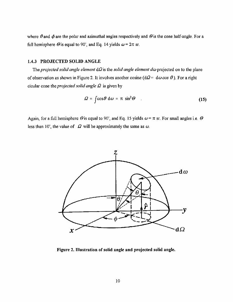
where {} and </J are the polar and azimuthal angles respectively and t9is the cone half-angle. For a

full hemisphere eis equal to 90°, and Eq. 14 yields (U= 21t sr.

1.4.3 PROJECTED SOLID ANGLE

The projected solid angle element dQ is the solid angle element d(U projected on to the plane

of observation as shown in Figure 2. It involves another cosine (dQ= d(U cos 8). For a right

cicular cone the projected solid angle Q is given by

(15)

Again, for a full hemisphere eis equal to 90°, and Eq. 15 yields (U= 1t Sf. For small angles i.e. eless than 10°, the value of Q will be approximately the same as (u.

z

dco

-L-----~~--t-'::T::---;--r--y

Figure 2. Illustration of solid angle and projected solid angle.

10

1.5 SENSOR PARAMETERS

The measurement equation includes, in addition to the source and geometry of radiation terms,

the sensor parameters as given below. In general, the Greek symbol p is used for relative sensor

responsivity while the italic R is used for the absolute values. However, the notation of the italic

symbol Sr for relative sensor responsivity and the italic S for the absolute value is sometimes used

in the literature based on the notation of the International Commission on Illumination (CIE) [3].

There have been considerable discussions between Fred Nicodemus of the National Bureau of

Standards (NBS, now NIST) and others in the late 70s [9] on what symbols to be used for these

quantities. The use ofcommon symbols for these derived quantities is desirable, but not essential

as long as they are properly defined and consistently used in a document. However, the use of

common symbols for basic quantities that are connected to SI units is highly recommended as laid

out in this document.

1.5.1 RELATIVE SPATIAL RESPONSIVITY

If deployed in space, the radiometric sensor aperture is bombarded with unwanted flux which

arrives from outside the instrument's field ofview, such as the sun, earth, stars, atmosphere etc.

The sensor output for a spatially pure measurement is a function of the radiant flux originating

from the target (within the sensor field of view) and is completely independent of any flux arriving

at the instrument aperture from outside this region. Thus, the characterization of the spatial

response, or angular field of view of a sensor, is an essential part of the sensor calibration. In this

regard, the sensor relative spatial responsivity p(8, ¢) is defined as the function that gives the

dependence of the spatial responsivity over the sensor's entire hemispherical view relative to the

peak responsivity in the direction of its optic axis. Thus, p(8, ¢) is unitless and is the normalized

point-response function which is obtained as the measured off-axis response to a point source.

This function can be integrated to provide the solid-angle field-of-view as

Q = f P(B,¢)dQ(hemisph)

11

(16)

A detailed discussion on how to determine the sensor field-of-view from the off-axis response to a

point source is given in Ch.1O Ref [15].

1.5.2 ENCIRCLED (ENSQUARED) ENERGY

The encircled energy or ensquared energy ec is unitless and is defined as the ratio of the energy

incident upon a circular or square detector to the total energy in the image of a point-target on the

detector. This image is generally spread out because of imperfect imaging and is called the point

spread function. The encircled energy is significant only when the point spread function width

becomes a factor in determining the senor response. For example, the simplest case is that the

point spread function causes radiation to fall outside the detector active area. An example of a

less extreme case is when the point spread function must be averaged over a spatially nonuniform

region of the detector. It should be noted that the encircled energy is in general unity for the

image of an extended- area source.

1.5.3 THROUGHPUT AND RELATIVE APERTURE

Throughput and relative aperture orf-number are unitless measures of the "flux gathering

power" of an optical system and are defined in reference to Figure 3 where AFS is the area of the

field stop. The sensor throughput is defined as the product of the entrance pupil area Ac and its

projected field-of-view f}c, [m2 sr] and can be written as

(17)

which is Ac 1t sin2 (9for a circularly symetrical field-of-view for angles where tan (9 ~ sin (9.

The relative aperture F or F/# is given as the ratio of the effective focallengthfto the entrance

pupil diameter D, and is given by the following equation in terms of the index of refraction nand

the cone half-angle a for angles where tan a ~ sin a.

F =flD = (2n sinar1

12

(18)

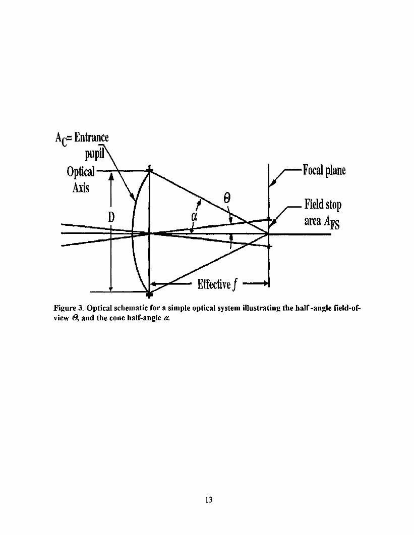
AC=Entrancepupil

Optical~~-----.Axis

D

~....--- Effectivef - ...-~--~

Focal plane

Field stoparea AFS

Figure 3. Optical schematic for a simple optical system illustrating the half -angle field-of­view 8, and the cone half-angle a.

13

TABLE 3

GONIOMETRIC TERMS AND UNITS

Polar angle () [degree]

Azimuthal angle <P [degree]

Field-of-view half-angle e [degree]

Relative aperture F unitless

Cone half-angle a [degree]

Entrance pupil diameter D [m]

Projected area Ap [m2]

Solid-angle UJ [sr]

Projected solid-angle {} [sr]

Throughput A{} [m2 sr]

Index of refraction n unitless

Effective focal length f m

Field stop area AFS m2

Note: The equations containing e are only valid for a solid angle represented as a right circular

cone with its central axis coincident with the sensor optical axis, and erepresents the half-angle

for a circularly symmetric field-of-view.

14

2. Part IT: THE RADIOMETRIC SENSOR CALffiRATION

Radiometric calibration is accomplished in a series of experiments in which the sensor output is

observed in response to a number of standard sources. It is necessary to evaluate the sensor

performance in the spatial, spectral, and temporal domains as well as to measure the noise and

nonlinear characteristics of the system. These experiments are expressed in terms of a

measurement equation.

Henry Kostkowski and Fred Nicodemus of the National Bureau of Standards (now NIST)

introduced the concept of a "measurement equation."[9][10][II] In order to solve this equation

it is necessary to measure pertinent quantities, or obtain all pertinent sensor component

specifications from the manufacturer of the sensor. This equation is also called the "system

performance equation" in the literature. [10] This equation is especially useful in the efficient

design of calibration experiments and evaluating measurement uncertainties.

The measurement equation can also be used to determine calibration coefficients for the

reduction of field data to convert sensor response to incident flux. This is obtained by what

amounts to an inversion of the dependent and independent variables.

Thus, the calibration equation provides incident radiant flux in terms of the sensor

output. In the following, Section 2.1 develops the measurement equations and Section 2.2

provides the corresponding calibration equations for both radiometers and spectrometers.

2.1 THE MEASUREMENT EQUATION

The purpose of this section is to begin with a general statement of the measurement equation

which is written in terms of sensor and standard source parameters that is valid for radiometers

(both spatial and large-field single-detector systems) and spectrometers. Then, solutions of this

general measurement equation are illustrated for the specific cases of a spatial radiometer and a

spectrometer.

The measurement equation yields sensor output for a specific source configuration. It is a

system equation; i.e., it models the sensor system performance in temis of the subsystem and

component specifications. Table 4 summarizes the new terms introduced in this section.

15

The development given below is based upon the response of a typical detector element of a

spatial radiometer and is also valid for a large-field single-detector radiometer. The measurement

equation is also valid for a spectrometer. This follows from the concept that the spectrometer

provides measurements over a series of sub-bands while the radiometer is considered as the

degenerate case of the spectrometer where the number of sub-bands reduces to one.

The equation cannot be written without first making some assumptions: The most general form

ofthe equation assumes the flux is in units of radiance L (positional and directional), is written for

wavelength, and the response is given in volts. In general the response could be in digital counts,

amperes, film density, pen deflection, etc. The development presented here completely neglects

polarization, time, and source coherence and follows the general treatment of the subject given in

Ch.5 Ref [9] where the calibration problems for various applications in radiometry have already

been discussed in detail. However, the treatment below illustrates the application of the

measurement equation approach for the calibration of a sensor to be deployed in space for

observing point sources as well as extended sources.

The general form of the measurement equation illustrates that the response r, for a filter

radiometer with a chosen filter nominally at Aoor for a spectroradiometer at a wavelength setting

of Ao , is obtained by integration over the appropriate variables

(19)

where

A is wavelength variable of integration over the spectral bandpass

G is the electronic gain

L J is the source spectral radiance

RICA, Ao) is the system absolute (bandpass) spectral responsivity

As is the source area

(Us is the solid angle subtended by the sensor entrance pupil at the source.

Notice that Eq. (19) is written in terms of source area and the solid angle subtended by the

16

detector at the source to make it convenient to use for the case of point sources as well. By

reciprocity theorem, Eq.(19) is identical to Eq. (3.11) ofRef [9]. For the purpose of discussions

in this document the subscript ,10 is mostly redundant and so it will be dropped and then it would.be equivalent to Eq. (5.30) in Ch.5 Ref [9]. However, a comprehensive treatment ofEq. (19)

with ,10 included can be found in chapters 7 and 8 in Ref [9].

In writing Eq. 19, the absolute bandpass spectral responsivity RiA) is assumed to be spatially

uniform as a first approximation. It is made up of all wavelength sensitive elements and can be

expressed as

(20)

where by definition

(21)

is the system relative spectral responsivity, and where

RD(A) is the detector absolute responsivity

riA) is the absolute filter transmittance

ec(A) is the encircled or ensquared energy for a point-target. It is a measure of the percent

(expressed as a decimal) of the energy in the point-spread function that is incident upon a detector

element, and applies to an imaging radiometer. It is unity for an extended source or for a large­

field radiometer.

y(A) is the optical efficiency. This term includes reflectance and/or transmittance losses in

addition to the filter losses.

The term max{Rr(A)} is the peak system spectral responsivity over the bandwidth.

17

The measurement equation (19) is quite general and is applicable to any radiometry problem

involving incoherent radiation. However, there is no unique general solution to this measurement

equation. Even if the spectral responsivity RICA) is completely characterized as a function of

position, direction and wavelength, there are an unlimited number of spectral radiance functions

LA that would produce the same observed signal r. As observed by Kostkowski and Nicodemus,

[Ref.[9] Ch.5], "the practical solution is usually to try to select a measuring instrument and a

measurement configuration to satisfy certain conditions, at least with a desired degree of

approximation, that will make it possible to modify the measurement equation to include the

desired radiometric quantity such as LA and to obtain a unique solution. The kinds of conditions

include the constancy or the approximate constancy of a radiation quantity such as LA or of the

responsivity relative to one or more radiation parameters so that these functions can be brought

outside one or more integrals, the use of an average to replace one or more of the integrals, and

the use of the relative spectral distribution, if known such as by using standard sources for

calibration, of the otherwise unknown radiometric quantity being measured. The major advantages

ofusing the measurement equation are that it makes clear that such conditions must be sought and

provides insight and a systematic approach towards finding them. In fact, without such an

approach, it is highly unlikely that one can make state-of-the-art measurements, or even less

accurate measurements, with a meaningful estimate of the uncertainty."

For the purpose of this document, as a first step, we assume that the spatial and spectral

domains are independent and that the radiance is spatially uniform in Eq. (19) so that the variables

can be separated as

(22)

then the indicated integrations can be performed. The integral

(23)

is the source throughput which applies to both the radiometer and the spectrometer, and by the

18

invariance theorem [13] is numerically equal to the sensor throughput Ac Dc where Ac is the sensor

entrance pupil area and Dc is the projected solid angle subtended by the source at the entrance

pupil. Dc is the sensor field-of-view for a uniform extended-area source. For point targets that do

not fill the field-of-view it is necessary to make use of the source throughput. The following

assumes the appropriate throughput can be represented by ADwithout subscripts.

The integration of the spectral parameters ofEq. (22) is given using Eq. (21) by

and where for a radiometer

n

LN = JLJP1(A)dA = L L j Pj LlAj

j=1

(24)

(25)

is the normalized radiance at the radiometer entrance pupil. In other words, it is the effective

radiance that is responsible for the sensor output. Note, the normalization applies to the bandpass

spectral responsivity [14] and the normalized flux given by Eq. (25) depends upon how this

responsivity was normalized. Typically it is peak normalized [14] by the use ofEq. (21) to give

the relative spectral responsivity PJ.(A).

Generally PJ.(A) is not analytic and can only be represented by a set (array) of numbers obtained

in an empirical test. Various methods to measure PJ.(A) independently have been discussed in detail

in Ch.7 Ref [9]. For the calibration of the sensor using a standard source LA is known. In this case

the integration can be approximated by numerical methods as illustrated in the right-hand term of

Eq. (25) where Pi is the set of n values of the response function and LlA; is the corresponding

wavelength interval. Example 1 shows evaluation of4 using Eq. (25) for a sensor calibration.

To illustrate the recommended practice, we deduce from Eq.(19) working measurement

equations for a broadband radiometer and a high resolution spectral radiometer.

19

The measurement equation (19) can be simplified for a radiometer using Eqs. (23) and (24) as

r = G max{Rxf,-l)} LN Ail (26)

The final and most useful form ofthe measurement equation is written in terms of the radiance

responsivity RL and the normalized radiance LN as

(27)

where from Eq. (26)

(28)

Equation (27) is the working measurement equation for a broadband radiometer. It is useful in

predicting the radiometer response to an extended or a point source: The radiance responsivity RL

in Eq. (28) is calculated by using a combination of measured and estimated system and component

specifications. The gain G is obtained from measurements and system specifications, the

throughput Ailis calculated using Eq. (23) and max{R1( A)} is obtained from Eq. (20) through

measurements and system specifications of Ro(.Il), tiA),t'c(A) andy(A). The normalized radiance

L N is calculated for a particular source using Eq. (25). Analysis of the predicted performance using

the measurement equation helps to optimize the design before building the sensor. The calibration

of this type of radiometer will be discussed in Section2.2.1.

For a high resolution spectrometer the assumption can usually be made that the spectral

radiance LA is constant over the spectral bandpass; then the integration indicated in Eq. (29) yields

the spectrometer spectral bandwidth (resolution) OA. as the normalization factor

(29)

20

The spectrometer obtains measurements of the spectral radiance LA' Thus, Eq. (26) is written for

any sub-band of the spectrometer as

(30)

As with the radiometer, the most useful version of the measurement equation for the

spectrometer is given in terms of the spectral radiance responsivity RL and the spectral radiance

LA

(31)

where RL is given by

(32)

Equations (31) through (32) are valid for any spectrometer sub-band and consequently the

spectral radiance responsivity exhibits different values for each sub-band. Equation (31) is the

working measurement equation for a high resolution spectral radiometer for each sub-band

provided the spectral radiance function is invariant over that bandwidth. The prediction of the

performance of a circular variable filter spectral radiometer (CVF) using Eq. (31) is given in

example 2 following Section 2.2.3. The calibration of this type ofspectroradiometer is discussed

in Section 2.2.2. In case the spectral radiance function is not constant over the bandwidth, the

measurement problem becomes that of a radiometer and Eq. (27) becomes the working

measurement equation at each wavelength setting of the spectroradiometer and normalized

radiometric quantity will be the one generally measured.

It is to be noted that working measurement equations, similar to Eqs. (27) and (31) for the

respective radiometers can be written for the radiant exitance responsivity, the radiant intensity

responsivity, and the irradiance responsivity. For brevity, we will drop the word "working" and

simply refer Eqs.(27) and (31) as measurement equations in the rest of the document.

21

TABLE 4

MEASUREMENT EQUATION TERMS, SYMBOLS, AND UNITS

Sensor response r [V]

Detector absolute responsivity Rn(A) [VIW]

Sensor relative spatial responsivity or field-of-view p( (J, </J) [unitless]

Electronic gain G [unitless]

Encircled or ensquared energy Ec(A) [unitless]

Absolute bandpass spectral responsivity RI(A) [VIW]

System relative spectral responsivity Pr(A) [unitless]

Peak spectral bandpass responsivity max{RrCA)} [VIW]

Absolute filter transmittance Z"F(A) [unitless]

Optical efficiency r(A) [unitless]

Source area As [m2]

Source projected Solid-angle Os [sr]

Sensor throughput OeAc [m2sr]

Sensor entrance pupil area Ac [m2]

Sensor projected solid-angle Oc [sr]

Normalized Radiance LN [w/(m2sr)]

22

In developing the measurement equations (27) and (31), the responsivity, ofEq. (20), is termed

R1(A). The subscript "1" comes from the notion that the value of the responsivity is constantly

changing as the spectrometer scans; in order that it can be evaluated for a given wavelength it is

visualized that we have stopped the spectrometer at that wavelength for an "instant"; thus the

term "instantaneous responsivity" often found in literature. The instantaneous responsivity is

dominated by the monochromator (filter) and in the ideal, exhibits nonzero values only within the

bandpass.

On the other hand, the system responsivity is termed RL . The subscript L comes from the

symbol for radiance. The spectral radiance also changes with wavelength as the spectrometer

scans. However, in this case the radiance responsivity is dominated by the detector response.

Examination ofExample 2 shows that for a CVF spectroradiometer, using a Si-As detector, the

responsivity is proportional to wavelength squared. The response at 10 11m is about 4 times what

it is at 5 11m and the response at 20 11m is about 4 times what it is at 10 11m. The output voltage

provides a distorted representation of the incident spectrum because of this system (detector)

weighting.

Equation (27) for the radiometer and Eq. (31) for the spectral radiometer are deduced from Eq.

(19) under the assumption that both the radiometric quantity such as LJ and the responsivity R1(A)

are uniform and isotropic throughout the beam of radiation incident on the entrance limiting

aperture of the radiometer. When the responsivity is uniform and isotropic, but the spectral

radiance is not or when the responsivity is not uniform, but the spectral radiance is then Eq. (7.24)

or Eq.(7.26) respectively given in Ch.7 Ref [9] would be valid. In case of spatial nonuniformity of

responsivity in the field of view of the sensor, its dependence on 0 and ifJ coordinates would be

represented by the relative angular responsivity function, p( 8,ifJ). In any case, the quantities that

are not uniform would be expressed as weighted averages over the incident beam area and the

solid angle. IfbothLJ and Rr(A) are not uniform and isotropic throughout the beam of interest

then it is best advised that the beam of interest be reduced in size until at least one of the above

quantities is sufficiently uniform and isotropic for the accuracy required in solving the

measurement Eq.(19).

23

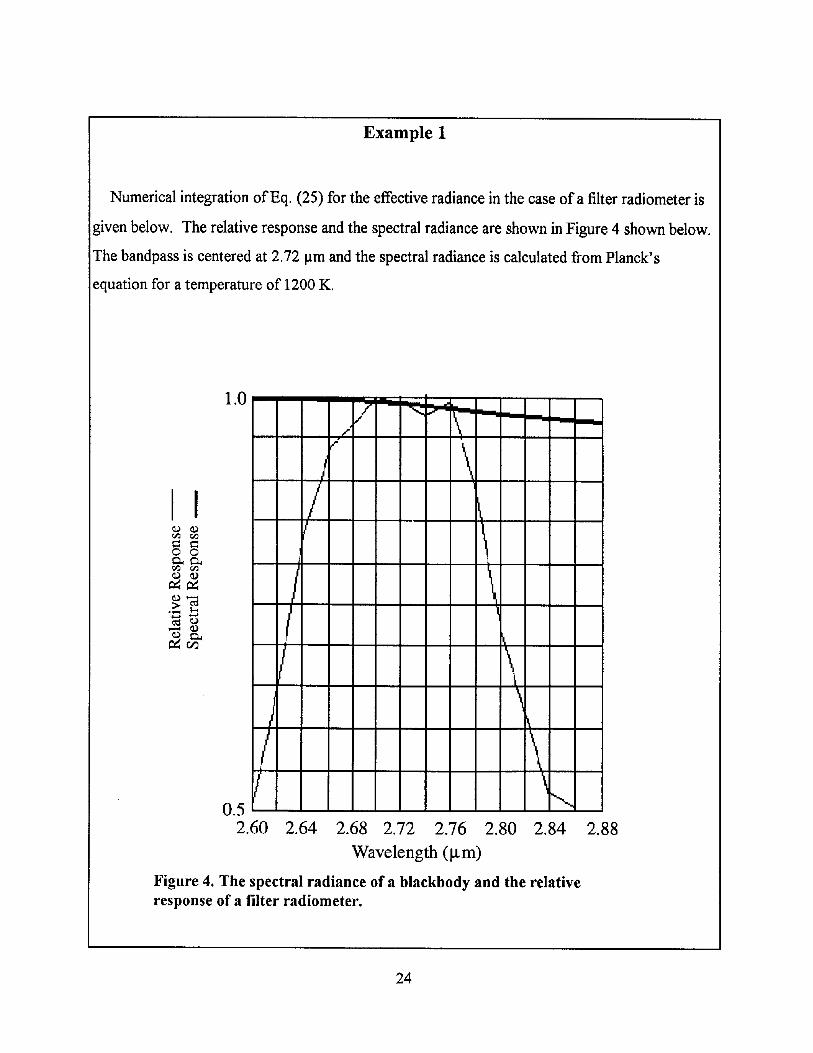
Example 1

Numerical integration ofEq. (25) for the effective radiance in the case of a filter radiometer is

given below. The relative response and the spectral radiance are shown in Figure 4 shown below.

The bandpass is centered at 2.72 flm and the spectral radiance is calculated from Planck's

equation for a temperature of 1200 K.

1.0

2.88

~/ -.......::

1\",,'

/'

\J

/ ItII

\J \I

II 1\\

J ~

I 1\il \

f'..-0.52.60 2.64

I I

2.68 2.72 2.76 2.80 2.84Wavelength (J..lrn)

Figure 4. The spectral radiance of a blackbody and the relativeresponse of a filter radiometer.

24

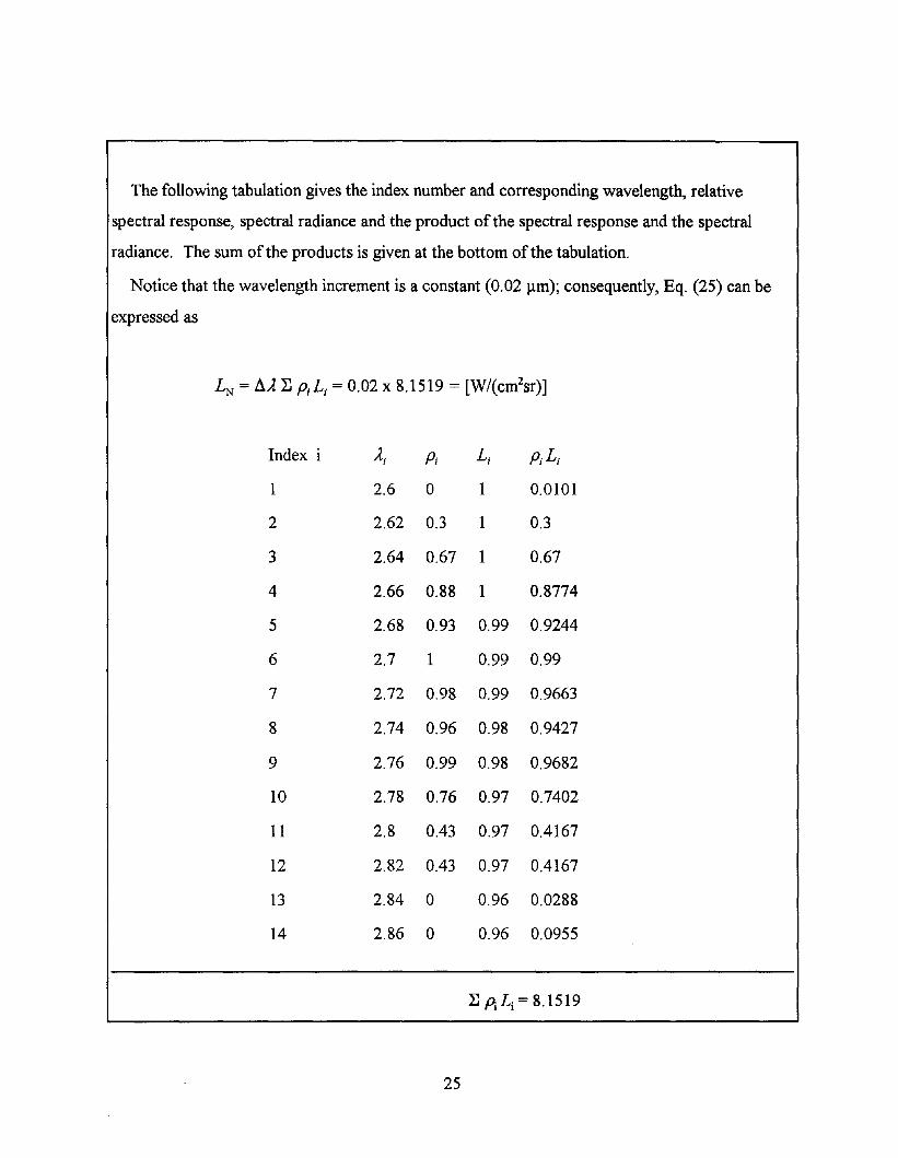
The following tabulation gives the index number and corresponding wavelength, relative

spectral response, spectral radiance and the product of the spectral response and the spectral

radiance. The sum ofthe products is given at the bottom ofthe tabulation.

Notice that the wavelength increment is a constant (0.02 11m); consequently, Eq. (25) can be

expressed as

LN = L\A ~ piLi = 0.02 x 8.1519 = [W/(cm2sr)]

Index i A; Pi Li piLi

1 2.6 0 1 0.0101

2 2.62 0.3 1 0.3

3 2.64 0.67 1 0.67

4 2.66 0.88 1 0.8774

5 2.68 0.93 0.99 0.9244

6 2.7 1 0.99 0.99

7 2.72 0.98 0.99 0.9663

8 2.74 0.96 0.98 0.9427

9 2.76 0.99 0.98 0.9682

10 2.78 0.76 0.97 0.7402

11 2.8 0.43 0.97 0.4167

12 2.82 0.43 0.97 0.4167

13 2.84 0 0.96 0.0288

14 2.86 0 0.96 0.0955

25

2.2 CALffiRATION EQUATIONS

In general, the goal of a calibration is to use the working measurement equation to deduce the

unknown radiometric quantity by in situ comparison with that of a standard under an identical

geometrical setup. In that case, the associated geometrical factors cancel leaving the solution for

the unknown radiometric quantity in terms ofjust the two measured output signals (unknown and

the standard) and the known value for the standard. Alternately, the standard could be used to

evaluate the responsivity first and then the calibrated responsivity is used in the solution of the

measurement equation to measure the unknown quantity from signals measured under the same or

known geometrical conditions. In either case the solutions are expressed as equations and are also

called the calibration equations. Table 5 summarizes the new terms introduced in Section 2.

In the calibration and uncertainty analysis of complex electro-optical sensors, the goal is first to

design calibration experiments using a standard source where necessary, and independently

characterize the sensor responsivity in the spectral, spatial, and temporal domains. The working

measurement equations such as Eqs.(27) and (31) are generally derived for the major domain that

is the spectral part with certain assumptions made regarding the spatial and other domains.

Therefore, the quantity that is most important to measure independently is the relative spectral

responsivity, PI (.ti) ofthe sensor system. For spatial and other domains, deviations from the

assumptions are assessed and applied as corrections to the measurement equations. Solutions to

the modified measurement equations are obtained from the system level results of the calibration

experiment and are compared with predictions from component level specifications and

measurements. This procedure allows the accurate calibration of the sensor and determination of

the overall uncertainty budget. Example 2 at the end of Section 2.2.3 is an illustration ofthe

prediction from component level specifications and measurements for a CVF spectroradiometer.

Example 3 given at the end of Section 3 illustrates the system level calibration for the same

instrument. Various excellent references are given below that elaborate on the above procedure.

1. The spectral characterization which is the major part of the calibration experiment involves

testing for out-of-band leakage, determining the instrument function PI. (.ti), determining

the absolute radiance responsivity, RL (.ti) and relative spectral responsivity PI (.ti). It is

discussed in detail in Ch.13 Ref [15]. Also, a comprehensive discussion ofvarious

26

methods to determine PI (.4) can be found in Ch.7 Ref [9].

2. Regarding other domains of characterization that allow corrections to be made to the

measurement equation are noise and possible nonlinearities over the dynamic range of

response. A detailed discussion ofthe evaluation ofnoise signal can be found in Ch. 8 Ref

[15]. The dark signal results in a constant offset ro which should be subtracted from the

raw signal rT to give the offset corrected signal roc = (rT - r o)'

All systems exhibit some degree of nonlinearity. The evaluation of the sensor transfer

function that corrects for any nonlinearity in the response yields the nonlinear offset

correction operator FNL . It is introduced in Section 2.2.1 and is described in Section 3.2.3,

but a thorough discussion can be found in Ref [12] and Ch. 9 Ref [15].

3. Regarding the spatial characterization:

1. Evaluating the corrections of nonuniformity of pixel to pixel response for the case of an

array detector is introduced in Section2.2.1 and is discussed in Section3 .2.4. It is called

the flat-field correction and is given by the operator matrix denoted by FFF .

2. The spatial field-of-view characterization is very important to assess the sensor

performance for the desired linear field-of-view. It is discussed in Section 3.2.5 as angular

spatial responsivity characterization. The way to obtain the transfer function for the

desired linear field-of-view for the sensor is discussed in Chapters 10 and 11 in Ref [15].

3. The Modulation Transfer Function (MTF) is another spatial parameter to be

characterized to make necessary corrections and is discussed in Section 3.2.6. A more

detailed discussion can be found in Ch. 13 Ref [11].

4. The temporal characterization of the sensor response is discussed in Ch.14 Ref [15].

Therefore, the calibration experiment which includes evaluation ofall the corrections and

characterizations listed above yields the sensor response as a function of the radiant, spectral,

spatial, and temporal properties of a standard source. The calibration equation is derived from

these data in what amounts to an inversion of the measurement equation. This yields the radiant,

spatial, spectral, and temporal properties of a target-source as a function of the sensor response.

In the next few sections the calibration equations are given for a broad band radiometer and a

spectroradiometer.

27

2.2.1 RADIOMETER RADIANCE CALmRATION EQUATION

This section uses the imaging radiometer as an example and the measurement Eq. (27) applies

for its calibration. The imaging radiometer generates a scene matrix through the use ofan area

staring array or a linear array and a scanning mirror. The development to follow is valid for each

element of a imaging radiometer or for a single element radiometer. For simplicity of expression

the following relationships are not expressed in matrix form; however, it must be understood that

the indicated relations must be applied to each detector element in the array.

The relative spectral responsivity PI (A) is to be determined first as described in Section 13-3

Ref [15]. Then the calibration experiment is conducted to measure response r to a standard

extended-area source radiance. The normalized radiance LN from the standard source incident

upon the sensor entrance pupil is calculated using Eq. (25). Then the absolute radiance

responsivity RL is obtained from the measurement equation (27). However, in order to use Eq.

(27) the response rT has to be corrected for offset, flat-field and nonlinearity as explained in the

previous section. The magnitude ofRL can be determined from a single measurement; but, a

redundancy of data is necessary to determine the uncertainty.

The calibration equation is then written in the form ofthe inversion of the measurement

equation, Eq. (27) with all the necessary corrections applied which will be used for measuring the

target-source radiance as shown below.

(33)

where

rT is the raw response

r 0 is the offset correction

FNL is the nonlinearity correction

FFF is the flat-field correction

RL is the absolute radiance responsivity

LN is the normalized radiance

28

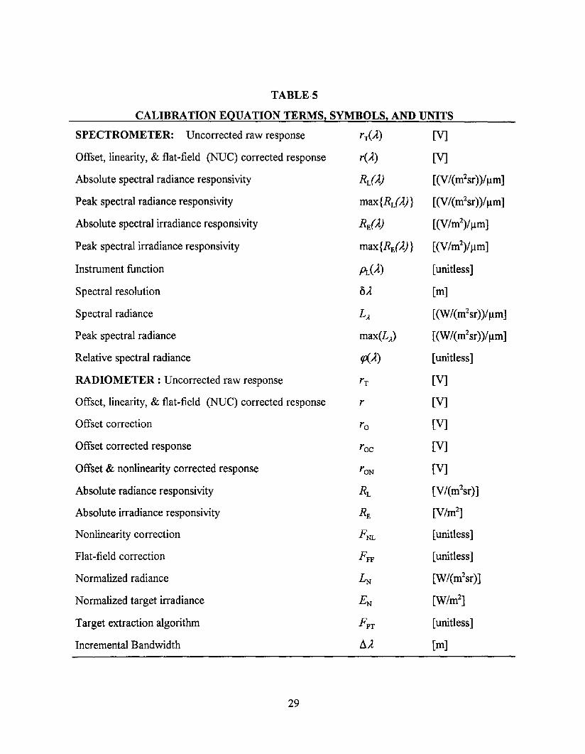
TABLES

CALIBRATION EQUATION TERMS, SYMBOLS, AND UNITS

SPECTROMETER: Uncorrected raw response riA) [V]

Offset, linearity, & flat-field (NUC) corrected response rCA) [V]

Absolute spectral radiance responsivity RdA) [(V/(m2sr»/~m]

Peak spectral radiance responsivity max{RdA)} [(V/(m2sr»)/~m]

Absolute spectral irradiance responsivity RE(A) [(V/m2)/~m]

Peak spectral irradiance responsivity max{RE( A) } [(VIm2)1~m]

Instrument function PL(A) [unitless]

Spectral resolution OA [m]

Spectral radiance LA [(W/(m2sr»)/~m]

Peak spectral radiance max(L;.) [(W/(m2sr»/~m]

Relative spectral radiance ~A) [unitless]

RADIOMETER: Uncorrected raw response rT [V]

Offset, linearity, & flat-field (NUC) corrected response r [V]

Offset correction r0 [V]

Offset corrected response roc [V]

Offset & nonlinearity corrected response rON [V]

Absolute radiance responsivity RL [V/(m2sr)]

Absolute irradiance responsivity RE [V/m2]

Nonlinearity correction FNL [unitless]

Flat-field correction FFF [unitless]

Normalized radiance LN [W/(m2sr)]

Normalized target irradiance EN [W/m2]

Target extraction algorithm FPT [unitless]

Incremental Bandwidth LlA [m]

29

As explained earlier in Section 2.2. the correction operators, correcting the raw response rT for

offset error, nonlinearity, and uniform response over an area array tend to provide an "ideal"

radiometer response r expressed in the measurement equation (27). The derivation of each of the

corrections,o ,FNL, FFF. in the above equation is given in Section 3.2.2, Section 3.2.3 and Section

3.2.4 respectively in discussing their uncertainities. Note that FIT and FNLrepresent mathematical

operators rather than scalars, namely, the operation of introducing the flat-field (for arrayed

systems) and non-linearity corrections..

In many applications the normalized radiance LN' itselfwould be the desired radiometric

quantity. On the other hand, if radiance LA is the desired radiometric quantity, Eq. (28) has to be

deconvolved and the procedures are described in Ch. 8 Ref [9]. A simplified procedure under

special conditions is discussed in Section 3.2.9 in this document for the measurement of the total

radiance LT integrated over the band A] to A2 for a broad band radiometer along with associated

uncertainty analysis.

2.2.2 RADIOMETER IRRADIANCE CALmRATION EQUATION

This section uses the spatial radiometer as an example. The development to follow is valid for

the measurement of an isolated point-target in the scene and derives the scalar target irradiance

from the response matrix. This is accomplished with a "target extraction" algorithm which to a

first approximation sums the response from those pixels stimulated by the image. The effect of

summing the response from several pixels is an improvement in signal-to-noise-ratio. This

summing operation is represented by FpT which includes the algorithm to provide a scalar measure

of the incident irradiance from the array image.

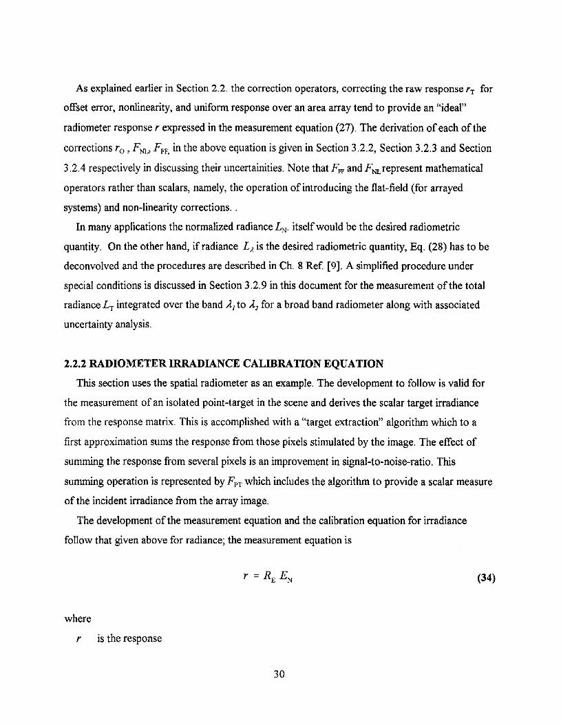
The development of the measurement equation and the calibration equation for irradiance

follow that given above for radiance; the measurement equation is

(34)

where

, is the response

30

RE is the absolute irradiance responsivity

EN is the normalized irradiance

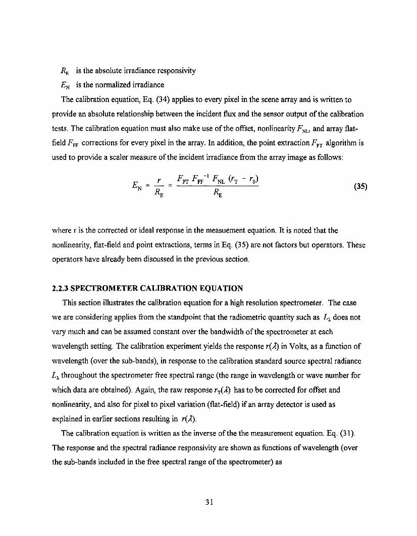
The calibration equation, Eq. (34) applies to every pixel in the scene array and is written to

provide an absolute relationship between the incident flux and the sensor output of the calibration

tests. The calibration equation must also make use of the offset, nonlinearity FNL, and array flat­

field FFF corrections for every pixel in the array. In addition, the point extraction F PT algorithm is

used to provide a scaler measure of the incident irradiance from the array image as follows:

FpT FFF- 1 FNL (rT - ro)

RE

(35)

where r is the corrected or ideal response in the measuement equation. It is noted that the

nonlinearity, flat-field and point extractions, terms in Eq. (35) are not factors but operators. These

operators have already been discussed in the previous section.

2.2.3 SPECTROMETER CALIBRATION EQUATION

This section illustrates the calibration equation for a high resolution spectrometer. The case

we are considering applies from the standpoint that the radiometric quantity such as L.}.. does not

vary much and can be assumed constant over the bandwidth of the spectrometer at each

wavelength setting. The calibration experiment yields the response rCA) in Volts, as a function of

wavelength (over the sub-bands), in response to the calibration standard source spectral radiance

LA. throughout the spectrometer free spectral range (the range in wavelength or wave number for

which data are obtained). Again, the raw response rT(A) has to be corrected for offset and

nonlinearity, and also for pixel to pixel variation (flat-field) if an array detector is used as

explained in earlier sections resulting in rCA).

The calibration equation is written as the inverse of the the measurement equation. Eq. (31).

The response and the spectral radiance responsivity are shown as functions ofwavelength (over

the sub-bands included in the free spectral range of the spectrometer) as

31

(36)

A simple scan, yielding the output voltage corresponding to the incident flux for each sub-band in

the free-spectral-range provides enough information to calculate RdA) for each sub-band.

However, a redundancy of data is necessary to test for spectral purity and determine the

uncertainties. The procedure for analysing the data to determine RdA) is discussed in detail in

Section 13-7 Ref [15]. The uncertainty analysis is given in Sec 3.2.8 in this document.

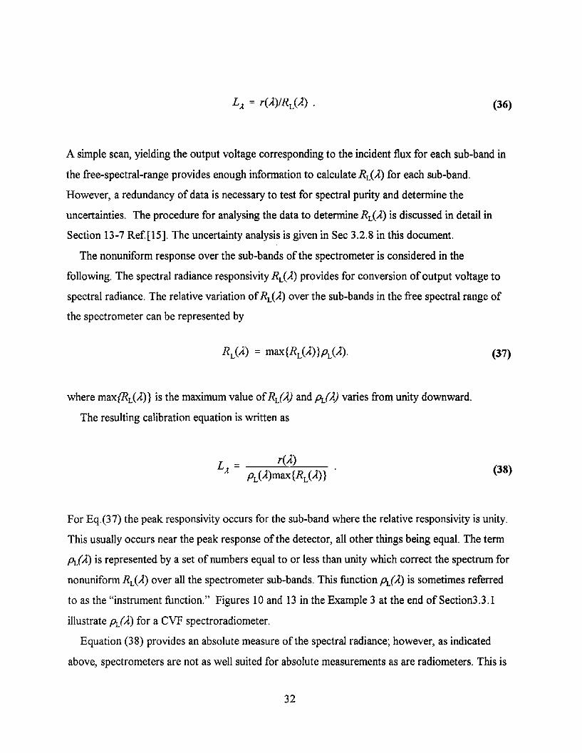
The nonuniform response over the sub-bands of the spectrometer is considered in the

following. The spectral radiance responsivity RdA) provides for conversion ofoutput voltage to

spectral radiance. The relative variation ofRL(A) over the sub-bands in the free spectral range of

the spectrometer can be represented by

(37)

where max(RdA) } is the maximum value ofRdA) and PL(A) varies from unity downward.

The resulting calibration equation is written as

(38)

For Eq.(37) the peak responsivity occurs for the sub-band where the relative responsivity is unity.

This usually occurs near the peak response of the detector, all other things being equal. The term

PL(A) is represented by a set of numbers equal to or less than unity which correct the spectrum for

nonuniform RdA) over all the spectrometer sub-bands. This function PL(A) is sometimes referred

to as the "instrument function." Figures 10 and 13 in the Example 3 at the end of Section3.3.l

illustrate PL(A) for a CVF spectroradiometer.

Equation (38) provides an absolute measure of the spectral radiance; however, as indicated

above, spectrometers are not as well suited for absolute measurements as are radiometers. This is

32

because the sensor is generally much more complex and the uncertainties are therefore greater.

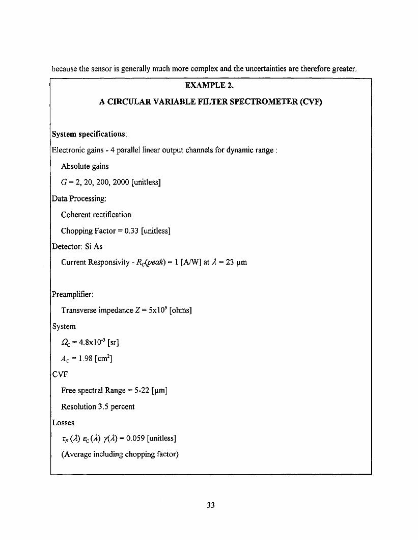
EXAMPLE 2.

A CIRCULAR VARIABLE FILTER SPECTROMETER (CVF)

System specifications:

Electronic gains - 4 parallel linear output channels for dynamic range:

Absolute gains

G =2, 20, 200, 2000 [unitless]

Data Processing:

Coherent rectification

Chopping Factor =0.33 [unitless]

Detector: Si As

Current Responsivity - Rc(peak) = 1 [AIW] at .11= 23 ~m

Preamplifier:

Transverse impedance Z = 5x109 [ohms]

System

[)c =4.8xlO-3 [sr]

Ac = 1.98 [cm2]

CVF

Free spectral Range = 5-22 [~m]

Resolution 3.5 percent

Losses

'F (A) eC<A) y(A) = 0.059 [unitless]

(Average including chopping factor)

33

Test Conditions:

Standard blackbody Source Spectral Radiance:

Ll94.7 K, 5 Jlm) =2.42xl0-13 [(W/(cm2sr»/Jlm]

Ll94.7 K, 10 Jlm) =3.00xI0·8 [(W/(cm2sr»/Jlm]

Ll94.7 K, 20 Jlm) = 1.87xlO-6 [(W/(cm2sr»/Jlm]

The following analysis shows how to find the output voltage for each gain channel for each source

spectral radiance.

Equations:

max {RI (A)} = RD(A) 'F(A) t'c(A) rCA) [V/W]

for PI (A) = 1 (peak)

rCA) = G max {RICA)} LA 5A Ail [V]

Discussion:

A solution ofthe measurement equation can be obtained through the use of a combination of

measured and estimated system and component specifications as illustrated here:

Extended dynamic range is provided through the use of4 parallel linear output channels. The

dynamic range of the high-gain (G2000) channel is given by the ratio of the full-scale output to the

rms noise. For the spectrometer used in this example the G2000 rms noise voltage is 37 mv and

full scale output is 10 V giving a dynamic range of270. This is extended by a factor often for

each of the three remain channels to a total dynamic range of270,000;

A light chopper, in connection with coherent rectification, is utilized to avoid problems with dc

drift. A loss-factor of 0.33 is introduced by the chopper and the noise-bandwidth is increased by a

factor of2. However these losses are small compared to the improvement achieve by this means.

The photoconductive silicon-arsenic detector is operated at helium temperatures (5 to 10

degrees Kelvin) and is modeled as a high-impedance current source. It exhibits a peak current

responsivitv of about 1 NW at 23 Ilm. The variation of responsivity with wavelength is

34

approximated with the expression

Ro (A) = RcCpeak) Z A/23 [A/W] = 2.17x108 A [V/W]

The low-noise preamplifier operates in the "transverse impedance amplifier" (TIA) mode

converting the detector current to a voltage so that the voltage responsivity ofthe detector-TIA

system is given by the product of the current responsivity and the impedance ofthe amplifier.

The monochromator used in this spectrometer is a "circular variable filter" which consists of an

interference filter, sometimes referred to as a "wedge" filter because the thickness of the

interference layers varies with angular position so that the filter can be made to scan with

wavelength as the filter is rotated physically over a slit-detector. The resolution ofthe filter, to a

first approximation, is a fixed percentage of the wavelength, typically 2 to 5 percent. The

resolution for this 3.5 percent filter can be modeled as a function ofwavelength as

&A = .035A

The losses consist of the peak transmittance ofthe filter bandpass as well as estimates for other

optical losses in lenses and or mirrors and the chopping factor.

The spectral radiances used in this example are taken from a solution to Planck's Equation.

A more accurate modeling ofthe sensor response can often be obtained through the use of

measured detector and filter data each ofwhich can be represented as a set ofnumbers (a linear

array) and the use ofmatrix multiplication to obtain the desired results. Often this requires

conversion and re-sampling of the data in order to take the product of two arrays which do not

use the same units (wavelength or wave number) or which do not have the same wavelength

interval.

max{R1 (A)} = 2.17xl08 A0.059 = 1.28xl07 A [VIW]

r = G 4.26xl03 A2 LA [V]

35

Example solution for G = 2 and A= 20 ~m

r = 2 x 4.26x103X 202

X 1.87xlO-6 = 6.38 [V]

TABULATION OF SOLUTIONS

Output volts as a function of wavelength and gains

A(~m)

5

10

20

G2

5.16xlO-s

2.56xlO-2

6.38

G20

5.16xlO-7

2.56x10-1

63.8

G200

5.16xlO-6

2.56

638

G2000

5.16x10·s

25.6

6380

The spectral radiance responsivity RL (A) is obtained as the ratio of the output, given in the

tabulation above, to the incident spectral radiance L(A) as given below.

TABULATION OF SOLUTIONS

Spectral Radiance Responsivity as a function of

wavelength and gains.

G2

2.13xlOs

8.53x10s

3.41x106

G20

2.13x106

8.53x106

3.41x107

36

G200

2.13x107

8.53x107

3.41xlOs

G2000

2.13xlOs

8.53x10s

3.41x109

3. PART ill: UNCERTAINTY ANALYSIS

This section addresses uncertainty analysis in multivariable radiometric systems. The primary

contributors to measurement uncertainty are the effects of noise, nonlinearity, nonuniform

detector array response, nonideal spectral and spatial responsivity, and standard calibration

source uncertainty. Methods used to provide uncertainty estimates have been controversial and

methodology has evolved over the years [16]. The approach suggested here is based upon the

NIST guidelines (Appendix 2) which are derived from ISO Guide referenced earlier [5].

The uncertainty analysis is an essential part of calibration. The independent characterization of

sensor parameters includes estimates ofuncertainty which are propagated to a statement of

measurement uncertainty.

Statistical analysis of sensor response data is based upon the following assumptions:

1) the source has a large thermal time constant so that it can be regarded as time invariant;

2) the sensor response is not time-dependent, that is, it has no drift;

3) the noise created by the sensor has a normal distribution and its consecutive values are

statistically independent of each other (Gaussian white noise);

4) the resulting statistical uncertainty in the measurements is a Gaussian random variable.

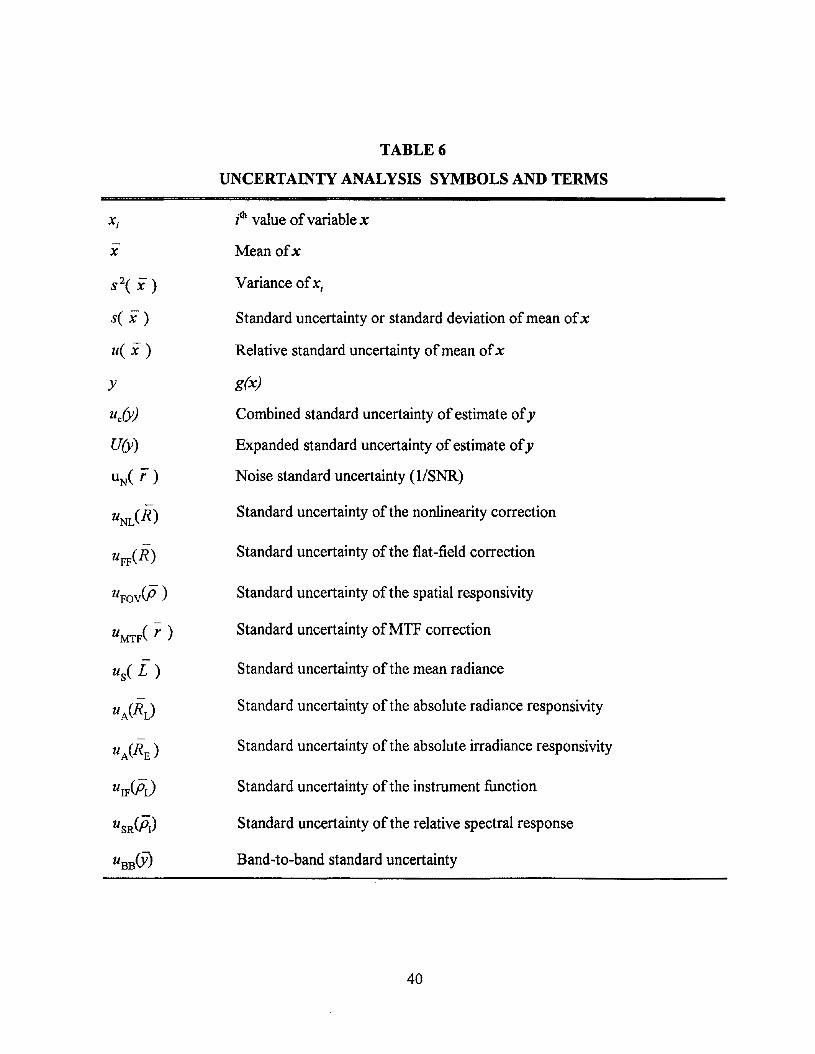
Table 6 summarizes the new terms introduced in this section. Please note that in the case when

we are dealing with a single detector, the responsivity function is a scalar, while for arrays it is a

matrix. This means that respective changes in the mathematical expressions and the physical

meaning for these two cases should be kept in mind.

3.1 DEFINITIONS

When N statistically independent samples (measurements) of a random variable x = {xjJ x2• ... }

are available, the mean value and variance are defined as

1 N

X = -I: Xi (39)N i =l

and

37

1 NS2(X) = L (x; - i)2

N - 1;=1(40)

respectively. The positive square root, sex;) is the experimental standard deviation. The standard

deviation of the estimate of the mean value i, is

(41)

and is measured in units ofx. The ISO guide defines s(i) as the standard uncertainty, u(i). The

relative standard uncertainty is given by the ratio of the standard uncertainty [Eq. (41)] to the

u(XJ = s~x (42)

where uri) approaches infinity as the mean tends to zero; however, it is generally taken that

radiometric measurements are not useful when the mean value is less than the standard deviation.

In what follows, the relative uncertainty [Eq. (42)] is always used to determine the quality ofa

measurement and the term "relative" is dropped hereafter for simplicity ofexpression.

The ISO Guide defines the combined standard uncertainty for M statistically independent

components as

M

uiy) = [L uf(X)]1/2.j=1

(43)

The uncertainty determined by statistical techniques on the basis of direct measurements is

referred to in the ISO Guide as Type A while those which are evaluated by other means (e.g., on

the basis of a prior assumption), as Type B. Identification and thorough analysis of the

components is given in Appendix 2. Finally, the expanded standard uncertainty is denoted in the

ISO Guide as U and is obtained for an approximate level ofconfidence (the interval that will cover

38

the true value of the estimated parameter with a given confidence) using the coverage factor k.

Thus U = k uc(y) and the value of the measured parameter y =y± U where y is the measurement

result. For example approximately 95% ofthe measurements will fall within ±2uc(y) ofthe mean

which corresponds to the case k ~ 2. A 99% level of confidence corresponds to k ~ 3.

Components ofuncertainty are developed in the following sections for radiometric and

spectrometric measurements using the ISO terminology where applicable. Extensions of the

recommended terminology are required in some cases not covered by the Guide.

3.2 UNCERTAINTY ANALYSIS FOR SENSOR CALIBRATON

The measurement equations such as Eq. (27) and Eq. (31) form the basis for the uncertainty

analysis in the measurement of the radiometric quantities using the calibration equations. The

uncertainties associated with corrections to the raw response rT of the sensor are discussed in

Section 3.2.1 through Section 3.2.6. The standard source uncertainty for the calibration

experiment using the measurement equation is discussed in Section 3.2.7. The uncertainties in

determining the absolute radiance responsivity RL and associated instrument function A are

discussed in Section3.2.8. Section 3.2.9 and Section 3.2.10 address uncertainties in special

measurements using the measurement equations. Section 3.2.9 shows the discussion of

uncertainities in determining the radiance of a source in a broad band wavelength interval using

the measuement equations for a broad band radiometer. Section 3.2.10 discusses the uncertainty

in determining the ratio of radiances between two bands of a broad band radiometer or a

spectroradiometer.

3.2.1 CALIBRATION SNAPSHOTS

Responsive parameters are measured experimentally, during calibration, using a technique that

provides data uncorrupted by noise. This is accomplished using a snapshot of data (a series of

measurements) and is based upon the assumption that for a time-invariant calibration source, the

dominant uncertainty mechanism is responsivity uncertainty.

39

-x

S2( x)

s( x)

u( x)

y

uly)

U(y)

uN( r)

-uA(RJ

TABLE 6

UNCERTAINTY ANALYSIS SYMBOLS AND TERMS

i th value ofvariable x

Meanofx

Variance ofx;

Standard uncertainty or standard deviation of mean ofx

Relative standard uncertainty of mean ofx

g(x)

Combined standard uncertainty of estimate ofy

Expanded standard uncertainty of estimate ofy

Noise standard uncertainty (l/SNR)

Standard uncertainty of the nonlinearity correction

Standard uncertainty of the flat-field correction

Standard uncertainty of the spatial responsivity

Standard uncertainty ofMTF correction

Standard uncertainty of the mean radiance

Standard uncertainty of the absolute radiance responsivity

Standard uncertainty of the absolute irradiance responsivity

Standard uncertainty of the instrument function

Standard uncertainty of the relative spectral response

Band-to-band standard uncertainty

40

Equation (41) indicates that essentially "noise-free" determinations ofthe response can be

obtained by making N arbitrarily large in the calibration snapshot. It is assumed that uncertainty

analysis given in the sections to follow is based upon noise-free response to invariant sources

when possible.

3.2.2 NOISE

The subject of this section is the uncertainty introduced by random noise in a sensor response r

and its effect upon field measurements using the calibration equations. It is essentially a measure

of the repeatability of data. The response to a source is obtained at intervals throughout the

sensor dynamic range as part of the calibration. In each snapshot a series ofN samples, r = (rt> r2,

...., rN), are obtained. The variance of each snapshot response is given by

where the mean is given by

_ 1 N

r = - L r;.N ;=1

(44)

(45)

An estimate of the I-sigma (one standard deviation, or root-mean-square deviation) confidence

interval for a single measurement is given by the ratio of the standard deviation to the mean

response following Eq. (42) as

uJr} = sC[> = 1r SNR

(46)

This is a Type A component ofuncertainty and is defined as the noise standard uncertainty and

is equal to the inverse ofthe signal-to-noise ratio (SNR).

3.2.3 NONLINEARITY

41

This section provides an analysis ofuncertainty introduced by nonlinearity in the absolute

responsivity RL or RE in the measurement equations. This uncertainty applies to the operation of

an individual detector either in an array or in single detector systems. Note that in this section, we

are interested in the nonlinearity of RL or RE and not on absolute values. The uncertainty in their

absolute values is discussed in Section 3.2.8.

Nonlinear response in sensor systems is common and has a major impact upon measurement

uncertainty. Careful characterization of the sensor response to a spatially, spectrally, and

temporally invariant source over the entire dynamic range provides the response rT as a function

of the flux f/J. A thorough analysis of the nonlinearity response can be found in Ch. 9 Ref [15] and

Ref [12].

Analysis here is based upon the data-set described in Section 3.2.1, above. The mean value of

each snapshot provides a measure of the offset r0 (dark noise response) and the linearity

(throughout the dynamic range). The offset- corrected response roc is given as a function offlux

f/J,

(47)

The standard source flux is varied for each snapshot but the source is maintained invariant with

respect to the spatial and spectral domains in order to isolate nonlinear effects from other

uncertainties.

The dependent and independent variables are inverted to provide flux as a function of response:

(48)

which is similar to Eq. (11.8) Ref 12 and the functional relationship is obtained by best-fit analysis

assuming a form for g-l.

For example, a second-degree equation has been used for Eq.(48) which is similar to Eq. (9.10)

Ref [15] where the flux is given as

f/J=ar +a r 2loc 20c

42

(49)

for offset-corrected response. The flux for a linear system is given by

([J=ar1 (50)

Eliminating ([J between Eqs.(49) and (50) yields the nonlinear offset correction operator FNL [see

Eq. (33)] as

ar = FNL[roc] = roc + ~ r 2a oc

1(51)

which indicates that the nonlinearity is described by the ratio ofa2 to aJ• Mathematical modeling

to arrive at FNL i.e aJ and a2 is given in Section 9.3 Ref[15].

Figure 5 illustrates the ideal linear system transfer function as a solid line with the offset and

linearity corrected response data superimposed. These data used the form ofEq. (51) but were

partitioned to reduce the uncertainty.

1

~10-1

~....~ 10-2-~

10-3

10-4 Low Range High Range

Detector Response (counts)

Figure 5. Illustration of data linearization. The original data - circle,linearized data- square, solid curve is the ideal linear response.

43

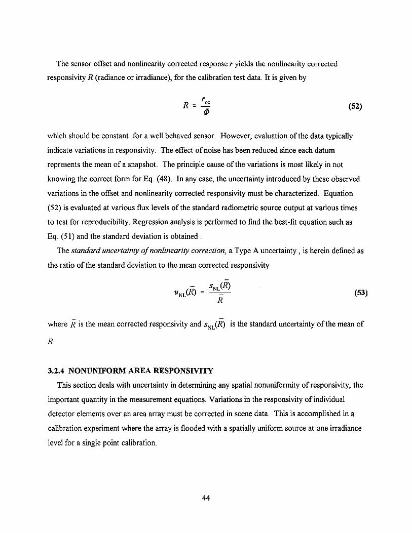
The sensor offset and nonlinearity corrected response r yields the nonlinearity corrected

responsivity R (radiance or irradiance), for the calibration test data. It is given by

'ocR -­(P

(52)

which should be constant for a well behaved sensor. However, evaluation of the data typically

indicate variations in responsivity. The effect of noise has been reduced since each datum

represents the mean of a snapshot. The principle cause of the variations is most likely in not

knowing the correct form for Eq. (48). In any case, the uncertainty introduced by these observed

variations in the offset and nonlinearity corrected responsivity must be characterized. Equation

(52) is evaluated at various flux levels of the standard radiometric source output at various times

to test for reproducibility. Regression analysis is performed to find the best-fit equation such as

Eq. (51) and the standard deviation is obtained.

The standard uncertainty ofnonlinearity correction, a Type A uncertainty, is herein defined as

the ratio of the standard deviation to the mean corrected responsivity

(53)

- -where R is the mean corrected responsivity and SNL(R) is the standard uncertainty of the mean of

R.

3.2.4 NONUNIFORM AREA RESPONSIVITY

This section deals with uncertainty in determining any spatial nonuniformity of responsivity, the

important quantity in the measurement equations. Variations in the responsivity of individual

detector elements over an area array must be corrected in scene data. This is accomplished in a

calibration experiment where the array is flooded with a spatially uniform source at one irradiance

level for a single point calibration.

44

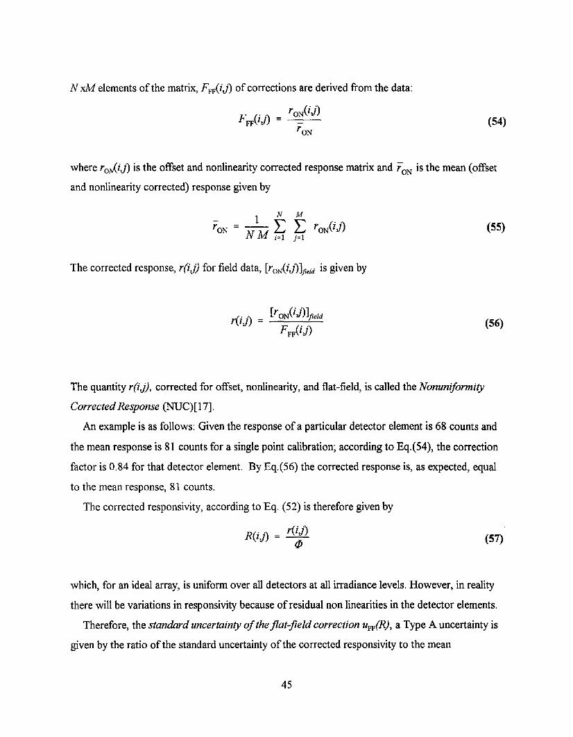
N xM elements of the matrix, FFF(i,j) of corrections are derived from the data:

(54)

where roJi.}) is the offset and nonlinearity corrected response matrix and rON is the mean (offset

and nonlinearity corrected) response given by

_ 1 N M ..

rON = - L L rON(lJ)N M i=1 j=1

The corrected response, r(i.}) for field data, [roN(i.})]field is given by

r(ij) = [roN(ij)]jieldFFiij)

(55)

(56)

The quantity r(i,j), corrected for offset, nonlinearity, and flat-field, is called the Nonunijormity

Corrected Response (NUC)[17].

An example is as follows: Given the response of a particular detector element is 68 counts and

the mean response is 81 counts for a single point calibration; according to Eq.(54), the correction

factor is 0.84 for that detector element. By Eq.(56) the corrected response is, as expected, equal

to the mean response, 81 counts.

The corrected responsivity, according to Eq. (52) is therefore given by

R( ' .) - r(ij)IJ ---tP

(57)

which, for an ideal array, is uniform over all detectors at all irradiance levels. However, in reality

there will be variations in responsivity because of residual non linearities in the detector elements.

Therefore, the standard uncertainty ofthe flat-field correction uFF(R), a Type A uncertainty is

given by the ratio of the standard uncertainty of the corrected responsivity to the mean

45

responsivity over the irradiance levels of interest. This is expressed as

-- _ s(R)uFiR)

R

3.2.5 ANGULAR SPATIAL RESPONSIVITY

(58)

In this section, the uncertainty ofdetermining any angular dependence ofresponsivty to correct

for it in the measurement equations is analyzed. A single detector system with a wide angle

nonuniform field-of-view is discussed. The sensor responsive parameters are independently

determined by experimentally evaluating the response to a standard source whose properties are

independent of direction and time. For example, the relative spatial response p(O, ¢» of a practical

IR sensor exhibits nonuniform response to a point source over the field-of-view as illustrated in

Figure 6. It is assumed that the sensor pointing accuracy is adequate to guarantee that the target

falls somewhere within the "inner-core" of the field-of-view but that its exact location within the

inner-core cannot be known. It may also be assumed that the probability is equally likely that it

will fall anywhere within the inner-core but zero that it will fall outside the inner-core.

The problem ofuncertainty analysis in this case is to characterize the uncertainty associated

with spatial variations in responsivity within the inner-core. Calibration of the spatial response

function p(i,}) consists of mapping the relative response to a point target. The absolute calibration

of the sensor is "normalized" to some arbitrary point in the inner-core of the field-of-view. The

relative error e(i,}) associated with a target imaged on the (i,})th grid position is given by the ratio

of the relative spatial response p(i,}) to the normalizing relative response PN minus one:

P(iJ) - PNe(iJ) =----

PN(59)

For example, assuming peak normalization, i.e., PN = 1 and p(i,}) = 0.85; the error as given by

Eq. (59) is -0.15. This means, that neglecting all other errors, the sensor underestimates the

measured flux by 15%.

46

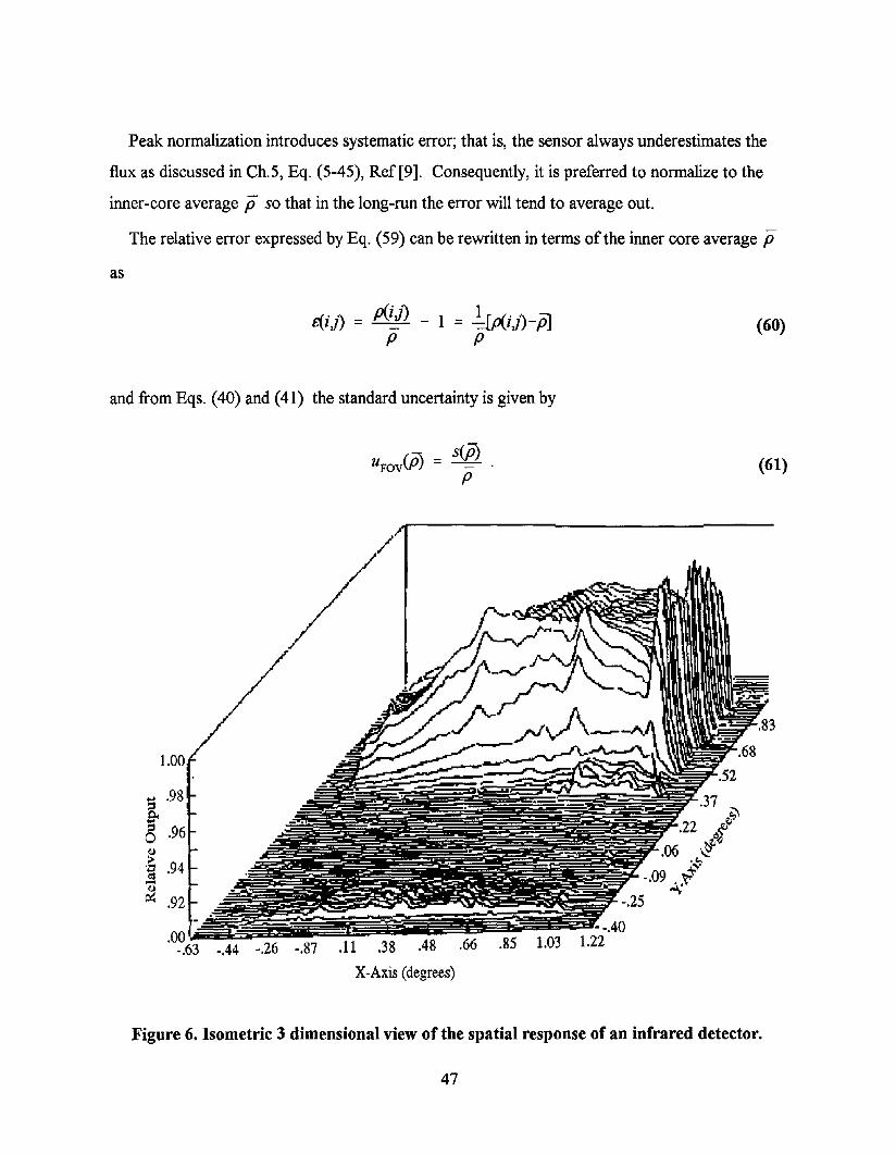
Peak normalization introduces systematic error; that is, the sensor always underestimates the

flux as discussed in Ch.5, Eq. (5-45), Ref [9]. Consequently, it is preferred to normalize to the

inner-core average ji so that in the long-run the error will tend to average out.

The relative error expressed by Eq. (59) can be rewritten in terms of the inner core average ji

as

cf' .) _ p(ij) _ 1 1r,.,{··) ;;'Jc,,\lJ - --=- = -=u'\lJ -PJ

P P

and from Eqs. (40) and (41) the standard uncertainty is given by

.....98::sE<8 .96<l.l>'.g .94

~ .92

'0?63 -.44 -.26 -.87 .11 .38 .48 .66 .85

X-Axis (degrees)

(60)

(61)

.83

.68~;::7Y"''l\~ ~~.52

.37c.;..~.

.22 o~'t>~'()

.06 ~,.~

-.09~~-.25

• -.401.22

Figure 6. Isometric 3 dimensional view of the spatial response of an infrared detector.

47

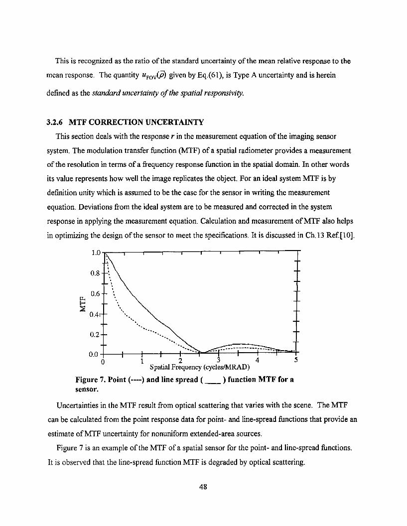
This is recognized as the ratio of the standard uncertainty of the mean relative response to the

mean response. The quantity uFov(ii) given by Eq.(61), is Type A uncertainty and is herein

defined as the standard uncertainty ofthe spatial responsivity.

3.2.6 MTF CORRECTION UNCERTAINTY

This section deals with the response r in the measurement equation of the imaging sensor

system. The modulation transfer function (MTF) of a spatial radiometer provides a measurement

of the resolution in terms of a frequency response function in the spatial domain. In other words

its value represents how well the image replicates the object. For an ideal system MTF is by

definition unity which is assumed to be the case for the sensor in writing the measurement

equation. Deviations from the ideal system are to be measured and corrected in the system

response in applying the measurement equation. Calculation and measurement ofMTF also helps

in optimizing the design of the sensor to meet the specifications. It is discussed in Ch.l3 Ref[lO].

1.0

0.8

·0.6 ··~ ·.E-o ..~ •..

0.41 ........0.2

0.0 -l---+-----1I---+--+-=.:.~-===..:.:.r--+_-t_4=....,..

o 1 2 3 4 5Spatial Frequency (cyclesIMRAD)

Figure 7. Point (----) and line spread ( __ ) function MTF for asensor.

Uncertainties in the MTF result from optical scattering that varies with the scene. The MTF

can be calculated from the point response data for point- and line-spread functions that provide an

estimate ofMTF uncertainty for nonuniform extended-area sources.

Figure 7 is an example of the MTF ofa spatial sensor for the point- and line-spread functions.

It is observed that the line-spread function MTF is degraded by optical scattering.

48

It is likely that the best estimate of the MTF lies between the two bounds for practical source

spatial distributions and is zero outside that range and that any value ofMTF (for a given spatial

frequency) within that range is equally probable. In this case the best estimate is the midpoint:

MTF = l[MTF(line) + MTF(point)]2

(62)

and if the difference [MTF(point) - MTF(line)] be denoted by 2a, then the standard uncertainty of

the MTF correction, which is a Type B component, is given by [Appendix 2,4.6]

-- a 2u (r) = u(MTF) = [_]1/2

MTF 3

3.2.7 CALffiRATION STANDARD SOURCE UNCERTAINTY

(63)

Generally, blackbody simulators serve as calibration standards for sensor systems to measure

and evaluate unknowns in the measurement equation. Commercial sources are available which

exhibit large thermal time constants and may be considered noise-free. Cavity blackbody

simulators exhibit emissivity values close to unity; consequently, the source uncertainty is related

primarily to temperature uncertainty. Blackbody flux uncertainty can be related to temperature

uncertainty using Planck's equation. NIST performs calibrations ofblackbody sources and

provides uncertainty estimates for each temperature setting.

The effective flux for a radiometric calibration can be obtained by Wien distribution law,

an approximation to the Planck's equation. Considering the Planck's function to be essentially not

varying over the spectrometer bandwidth OA:

(64)

where the radiation constants, C1 = 1.19 10-16 [W . m . sr-1] and C2 = 1.44 10-2

[ m .K]. This

49

approximation to the Planck's equation is good to better than 1% for all (A . 1) < 3.1 10-3 [m . K].

The rate of change ofradiance with temperature is obtained by taking the derivative ofEq. (62)

with respect to temperature. Therefore,

(65)

where exp(ciA1»>l.

Typically, the temperature uncertainty is specified as T±ti.T. The corresponding radiance

uncertainty is L±ti.L. When there is no specific information about the possible values ofL within

the range, it may be assumed that it is equally probable for L to lie within the range ofL-ti.L to

L+ti.L and the probability that L lies outside this range is zero. Then, according to the ISO Guide

[4], the best estimate of the source radiance is at the midpoint L (given by Eq.(62) and the source

variance is

s/(L) = ti.L 2/3 .

The standard source uncertainty is therefore

-- slL) ti.L

uIL) = -_- = -L {iL

(66)

(67)

It corresponds to the standard uncertainty ofthe mean radiance which is a Type B component of

uncertainty.

3.2.8 ABSOLUTE RESPONSIVITY UNCERTAINTY

The topic of this section deals with the absolute responsivity (radiance or irradiance) in the

measurent equations such as Eq.(27), Eq. (31) and Eq. (34). First we deal with the absolute

calibration of the radiometer and then with the spectrometer.

The absolute responsivity is determined in a series of tests in which the NUC response is

50

observed as the standard source temperature is varied over the range ofvalues expected in the

field measurements. This test is often referred to as the "spectral purity" or "out-of- band

leakage" calibration test as discussed in Ch.13-5 Ref [15]. As the temperature of the source is

varied, the flux is shifted relative to possible leak regions. Excessive response is observed when

the wavelength of peak flux is shifted into a leak region.

The results of the spectral purity test can be examined for a systematic change in responsivity

as a function of the calibration standard source temperature. In the absence of a systematic

change, the mean responsivity may be the best estimate of the absolute responsivity. As with the

nonlinearity, it is the absolute responsivity that should be invariant.

The uncertainty resulting from the observed variations must be estimated as follows: The

absolute radiance responsivity is given by

(68)

where LN depends upon the source temperature and the relative spectral responsivity pl},,). The

standard uncertainty ofthe absolute radiance responsivity uA(RJ, which is a type A component,

is obtained as the ratio of the standard uncertainty of the absolute radiance responsivity to the

mean absolute radiance responsivity:

(69)

where RL is the mean radiance responsivity and s(RJ is the standard deviation of RL .

Similar terms can be written for the standard uncertainty ofthe absolute irradiance

responsivity s(RE).

Spectrometers can also be calibrated for absolute spectral radiance measurements, as given in

Examples 2 and 3, although they are generally utilized to measure the relative spectrum. The

spectral purity test is also used in the case of the spectrometer, the difference being that the

uncertainty must be determined for each sub-band of the spectrometer and is therefore a function

ofwavelength,

51

The mean responsivity is given by the ratio of the mean response to the incident spectral

radiance:

R(A) = 1\A)L L

A

(70)

(71)

where LA' which is the spectral radiance, depends upon the source temperature and the

wavelength. The experimental procedure for measuring the absolute radiance responsivity is

discussed in Section 13-6 in Ref [15]. Figure 9 and Figure 12 in Example 3 given at the end of

Section 3.3.1 show the standard uncertainty ofthe absolute radiance responsivity determined for

a CVF spectroradiometer using an extended source and a point source respectively.

The "instrument function" is defined in Section 2.2.3 as the normalized spectral radiance

responsivity PL(A), see Eq. [37],

(72)

which is

(73)

The scatter in the sensor absolute responsivity, observed in the spectral purtiy test, for offset

and nonlinearity corrected response applies equally to the relative spectral radiance responsivity

PL(A) which is the instrument function. Therefore the standard uncertainty ofthe instrument

52

function UIF<PJ, which is a Type A component, is obtained using equation similar to Eq. (69).

3.2.9 NONUNIFORM SPECTRAL RESPONSE

This section deals with uncertainties that result from nonideal spectral bandpass response

characteristics of radiometers as opposed to errors in determining the spectral response function

considered in Section3.2.8. These uncertainties exist even when the spectral response function is

known to a high degree of confidence. Only specific cases are considered here and a thorough

analysis can be found in Ch. 8 Ref. [9].

The data analyst can correct for this type of uncertainty provided sufficient supplemental data

are available from measurement or theory. In the absence of such data, the analyst must provide

uncertainty estimates. These may be systematic uncertainties. The error introduced by nonideal

performance parameters can be catastrophic if no provisions are undertaken to make corrections.~

Errors associated with the nonideal spectral response can best be understood in terms of a

measurement goal, which is to obtain a measure of total radiance LT integrated over the spectral

range of Al to A2. This can be expressed as

(74)

The actual output response from a radiometer is given by the measurement equations, Eqs. (24);

(25), and (26). Therefore,

r = GAil max{R1(A)}f PI(A)LAdAo

(75)

where Pr(A) is the sensor relative spectral response function, the integration is carried out over all

wavelengths, and max{RlA)} is the systems peak responsivity.

The best that can be done is to obtain the measured radiance L M implied by Eq. (75):

53

LM = r[AQ G max{RI(A)r1 = f PI(A)LAdAo

However, based upon Eq. (76), LM is equal to LT only if

A]

f LA dA = f PI(A)LAdAA] 0

(76)

(77)

The ideal sensor is one for which A(A) is unity between Al and A2 and is zero elsewhere; then Eq.

(77) is identically true.

Unfortunately, the spectral response function is never ideal in practical sensors. A spectral

bandpass filter is illustrated in Figure 8. The nonuniform transmittance and finite slope are typical

of any physically realizable filters.

For a practical sensor, Eq.(77) is true for the limiting case where the radiance is uniform (Le.,

LA = const) over the entire responsive region, that is, for nonzero values ofA(A). Then Eq. (77)

becomes

A]

f dA = f plA)dAA] 0

(78)

and gives the condition required for LM = LT, namely, that of area equivalence. The ideal square

spectral bandpass is represented by the left side ofEq. (78) for which the bandpass is from Al to

A2. The area-equivalent effective bandpass of the nonideal response function is given by the right

side ofEq. (78). The nonideal response is said to be equivalent to the ideal response because

there is equal area under each curve.

The meaning of such a measurement is limited to the following: "Provided that LA is spectrally

uniform, the total radiance has a magnitude given by Eq.(78)." The recommended practice is to

54

0.85 t----+-----+---+---+--+--+--+--f---+-~-4-__+-_t

0.80

0.75

0.70

~:: ~~0.55 ~

8 0.50

~ 0.45--.~ 0.40~~ 0.35

0.30

0.25

0.20

0.15

0.10

0.05

0.00:+-----'1r-:--r--='--:---f----:--T---i--+----I----lI--4----I--+5.0 6.0 7.0 8.0 9.0 10.0 1.0 12.0

Wavelength (J.Lm)Figure 8. Typical bandpass interference filter transmittance.

calculate the radiance from Eq. (78), which depends upon how the relative spectral response prAyis normalized. It can be normalized to the mean of an "inner-band" or to the peak. In any case

the calibration report should indicate the type of normalization used [14,19].

It should also be noted that peak normalization guarantees a bias in the measured radiance in as

much as the response over the bandpass is less than, or equal to, the peak response; this means the

radiance is underestimated as discussed in Ch. 5, Eq. (5.45) Ref [9].

Corrections for nonuniform spectral bandpass can be provided if the source spectrum is known

from theory or measurement [16]. Equation (76) can be rewritten as

55

A2

L T = max(L.J f ~1) d1AJ

(79)

where max(Lj is the peak ofLA with units [(W/(m2sr»/~m] and ~1) represents the relative

spectral radiance [unitless], or the "relative spectrum." Therefore, corrections for nonuniform

spectral bandpass can be made upon the basis that ~1) can be independently determined by

theory or measurement so that only max(Lj need be determined by the radiometric measurement.

Then Eq. (77) becomes

r = GAil max{RI(1)} max(L.J fPI ~1)d1

o

from which max(Lj can be obtained for a measurement as

rmax{LA} =-----------

GAil max{RI(1)} f PI(1)~1)d1

o

(80)

(81)

Note that r is obtained from the measurement, max{R.(1)}, PI(1), G and Ail are obtained from

the calibration. Thus max(Lj is determined and the total radiance LT can be calculated using

Eq.(81) over any region 1 1 to 12provided ~1) is known over that region.

This discussion leads to the conclusion that the best sensor design is one that incorporates both

radiometric and spectrometric measurements.

It is necessary to estimate the uncertainty in the likely event that the source spectrum is

unknown and corrections cannot be made. This is difficult. because any estimation ofuncertainty

must be made upon the assumption of some source spectral distribution. A limiting case, namely a

single line-source, can be investigated as follows. First, it is necessary to assume that the

56

line-source is guaranteed to fall within some nominal band. Then, the mean and variance can be

calculated for that band from the measured spectral response data. In this case, the uncertainty is

given by

(82)

where this is defined as the standard uncertainty of the relative spectral response usR<A), which

is a Type A component ofuncertainty. For example, examination ofFigure 8 indicates variations

of the order of±20 percent in the spectral transmittance of a typical filter which will be a major

contributor to the relative spectral responsivity in a broad band radiometer.

3.2.10 BAND-TO-BAND UNCERTAINTY

The band-to-band uncertainty is of interest because certain discrimination algorithms are based

upon ratios of irradiances measured in appropriate radiometer bands. The target temperature can

be related to a band ratio by Planck's equation, for example. This discussion is applicable to

measurements with a spectrometer or a multiband radiometer.

The band-to-band uncertainty can be determined using the same data as obtained for the

spectral purity test given in Section 3.2.8. In this case, a series ofmeasurements is obtained

where the temperature of a standard blackbody source is varied over the range expected in the

measurements. These data are obtained simultaneously in multiple radiometric bands for the

radiometer and over the spectrum for the spectrometer. The absolute responsivity is calculated

for each band and for each temperature. The ratio of the ith and jth bands is

(83)

which should be invariant over the range of source temperatures in the same pair ofbands. The

spread in the ratio provides a measure of the band-to-band uncertainty.

The best estimate of the uncertainty of the band ratio measurements is given by the ratio ofthe

57

standard deviation ofy to the meany, The standard deviation ofy is given in terms of the means,

variances, and covariances ofR; and Rj" Thus,the band-to-band standard uncertainty, which is a

Type A component, is given by

cov(R " R.) 1/2- 2 I J]R; Rj

(84)

where cov(R;, R) is the covariance between R; and Rj .

There is a possibility that the variance ofy tends to zero if the covariance has the proper

magnitude and sign. This would happen if the noise fluctuations were completely correlated so

that each erroneous observation ofR; would be exactly compensated for by a corresponding

erroneous observation of~ [18].

This calculation, estimating the ratio uncertainty, is completed for the multiband radiometer in

order to obtain the uncertainty for all possible band ratios. For the spectrometer, the uncertainty

is obtained for all sub-bands over the entire measured spectrum as a function ofwavelength.

3.3 PROPAGATION OF UNCERTAINTIES -COMBINED STANDARD UNCERTAINTY

In general, the ISO standard, Guide to the Expression ofUncertainty in Measurement,

commonly called the GUM [5] and NIST guide lines (Appendix 2) recommend the uncertainty of

the results ofa measurement be expressed as a standard deviation (the positive square root of the

variance), see Eq. (41), and be termed the Standard uncertainty. The uncertainty in the result ofa

measurement generally consists of several components ofuncertainty. The term combined

standard uncertainty is recommended to be used and that these components be combined, using

the law ofuncertainty propagation, by the positive square root of the sum ofthe variances and

covariances of these components, see Eq. (43). This is the root-sum-square (RSS) method.

The ISO standard also recommends the use of a coverage factor of2, used as a multiplier of

the combined uncertainty, in order to obtain an expanded uncertainty in which the uncertainty

interval is approximately 95 percent. Although, coverage and expanded uncertainty have not yet

been utilized in specifying or qualification testing in the field of radiometry and spectrometry, they

58

should be incorporated in such future documentation as the American National Standard Institute

(ANSI) officially adopted the ISO standard as the American National Standard. The new standard

is ANSIINCSL Z540-2-1997, and its full title is American National Standard for Expressing

Uncertainty-U.S. Guide to the Expression ofUncertainty. Also, the National Conference of

Standards Laboratories (NCSL), which has broad representation from U.S. industry incorporated

the basic principles of the ISO standard and the NIST guidelines in its Recommended Practice R­

12, Determining and Reporting Measurement Uncertainties.

3.3.1 OLD TERMINOLOGY AND RECOMMENDED PRACTICE

The terms precision and accuracy have been used widely in expressing the uncertainty of

measurement results in the literature. There has been quite a variance in the interpretation of these

terms and their usage, and NIST guidelines discuss this issue in section D.l in Appendix 2.

However, these concepts have been used in the application of electro-optical sensors with the

following definitions. The term precision is defined to include the residual and non-ideal

uncertainties besides the uncertainties of repeatability and reproducibility ofmeasurements made

with the sensor. The term accuracy is defined to refer to absolute measurements which implies

tying the measurements to an absolute scale. For example, the precision of a measurement

obtained with a spectrometer deals with the uncertainty of the relative energy in various sub-bands

besides the repeatability and reproducibility of those values. However, it is the uncertainty of

absolute energy in a sub-band that is of interest in radiometry which is expressed by the term

accuracy. In other words, the definition ofprecision differs from the widely accepted definition

discussed in section D.1.2 in Appendix 2 which is just the uncertainty due to repeatability and

reproducibility of measurements. Such variation in the usage of the term precision leads to

confusion. The same is the case for the definition ofaccuracy as discussed in section D.1.1.1 in

Appendix 2. Therefore, the terms precision and accuracy are considered as old terminology the

usage ofwhich is recommended to be replaced with unambiguous terms pre final combined

standard uncertainty and combined standard uncertainty respectively. Therefore, the concept of

precision in old terminology as defined earlier for sensor system calibrations fits well with the

definition of the term pre final combined standard uncertainty as it includes all the uncertainties

59

except the uncertainty associated with the absolute standard. Similarly, the concept of accuracy in

the old terminology fits well with the term combined standard uncertainty ofthe sensor

performance in the new terminology which is defined as the positive square root of the sum ofthe

variances and covariances of the combined uncertainty of the sensor and the standard source

uncertainty. It is to be noted that all the uncertainties referred to in this document are relative to

their mean values and expressed as percentages based on Eq. 42 as discussed in section D.l.4 in

Appendix 2.

In dealing with electro-optical systems, the sources ofuncertainty inherent in the sensor

performance including that of repeatability and reproducibility can be broadly classified as

follows:

1. Noise: It is caused by the random variations in sensor response due to photon, thermal, and

quantization effects. The noise uncertainty is a repeatability uncertainty and can be made

negligibly small by taking sufficient data points in each snapshot as discussed in section 3.2.2.

2. Residual uncertainties: These uncertainties arise from corrections ofoffset, nonlinearity, and

nonuniform response as discussed in sections 3.2.3 and 3.2.4. Reproducibility variations in sensor

response are evaluated as part of residual uncertainties.

3. Uncertainties due to Nonideal response: These uncertainties arise from nonuniform spatial and

spectral response of the sensor as discussed in sections 3.2.5, 3.2.6, 3.2.8, 3.2.9, and 3.2.10.

The following are examples of several measurement goals and the associated uncertainty

estimates.

Generally an integrating radiometer is utilized to obtain absolute measurements ofradiance or

irradiance of a target source or background. Two types of integrating radiometers are illustrated

here:

The first example, a spatial or imaging radiometer, provides a measure of the energy integrated

over a relatively wide spectral band, but provides an image of the target or distribution of the

background. The calibration Eq. (33) in section 2.2.1 would be applicable to evaluate the

uncertainties. However, it should be noted that the nonlinearity of response in each pixel is

evaluated in the case of the array detector as part of its nonuniformity ofresponse as discussed in

section 3.2.4. An estimate of the combined standard uncertainty of such a spatial, or imaging,

60

radiometer is given by

(85)

which includes the effects ofnon-uniformity corrections (NUC) given by the first two terms,

modulation transfer function, absolute response (spectral purity), and standard source radiance

uncertainty. The image (as opposed to an absolute distribution) may be the only measurement goal

of an imaging radiometer and in this case the standard source uncertainty terms would not be

included in Eq. 85, and the resultant uncertainty is pre final combined standard uncertainty which

is equivalent to precision in the old terminology..

The second example, is that of a spatial and wavelength integrating radiometer, which measures

the total radiance integrated over a relatively large spatial (FOV) region and a relatively large

spectral bandwidth. Again, Eq. (33) would be applicable to evaluate uncertainties. However, such

a radiometer typically uses a light chopper and coherent rectification so that offset and flat-field

corrections do not apply; but, uncertainties due to nonlinear response given by Eq. (53),

nonuniform spectral response given by Eq. (82), and a nonuniform field-of-view (FOV) response

given by Eq. (61) apply. In this case the combined standard uncertainty is given by

(86)

which also includes absolute radiance responsivity (spectral purity) given by Eq. (70) and standard

source uncertainty given by Eq. (67).

Nonideal spatial and spectral response can be large contributors to radiometric measurement

uncertainty; optical designs are available which can result in nearly-ideal field ofview response.

Nonuniform spectral response uncertainties can be reduced by optimal "square" filter design and

flat or uniformly responsive detectors or by accompanying bore-sighted spectrometer

measurements as indicated in Section 3.2.9.

A spectrometer is normally used to measure the relative spectral radiance (the spectrum) of a

61

source; however, a spectrometer can be calibrated for the absolute spectral radiance in which case

it is sometimes referred to as a spectro-radiometer.

The components ofuncertainty that should be included in an uncertainty analysis of a

spectrometer depend upon the sensor design to a great extent. For example, offset error and

nonlinearity correction are not possible for an interferometer (multiplex) spectrometer. On the

other hand, the circular variable filter (CVF) (sequential) spectrometer is subject to nonlinearity

problems. Nonuniform spectral response uncertainty does not apply to the high resolution

spectrometer.

Example 3 given below illustrates the calibration and uncertainty analysis for a CVF

spectrometer for relative and standard uncertainties, and for radiance and irradiance sources.

62

EXAMPLE 3

CmCULAR VARIABLE FILTER (CVF) SPECTRORADIOMETER

Calibration and uncertainty analysis for a CVF spectroradiometer illustrates most of the

calibration and uncertainty aspects ofboth a radiometer and a spectrometer, point-source

(irradiance) and extended-area (radiance). The sensor specifications are given in Example 2.

A spectroradiometer is a spectrometer calibrated for absolute measurements; hence, the term

spectroradiometer. Example 2 discussed earlier in Section 2, provided a prediction ofperformance

using the measurement equation. This example illustrates the details ofa practical calibration and

uncertainty analysis.

Calibration tests.

The calibration tests to which the CVF spectroradiometer were subjected are as follows:

1. Dark-noise

2. Nonlinearity

3. Spectral scan position

4. Spectral resolution

5. Field ofView

6. Extended-area source absolute radiance calibration (spectral purity)

7. Point source absolute irradiance calibration (spectral purity)

This sensor has only one detector; consequently the flat-field correction 'and associated

uncertainty does not apply as it would with a spacial sensor.

Uncertainties

The uncertainties ofinterest here are as follows.

1. Noise uncertainty u~li1=1/SNR (See Section 3.2.2)

63

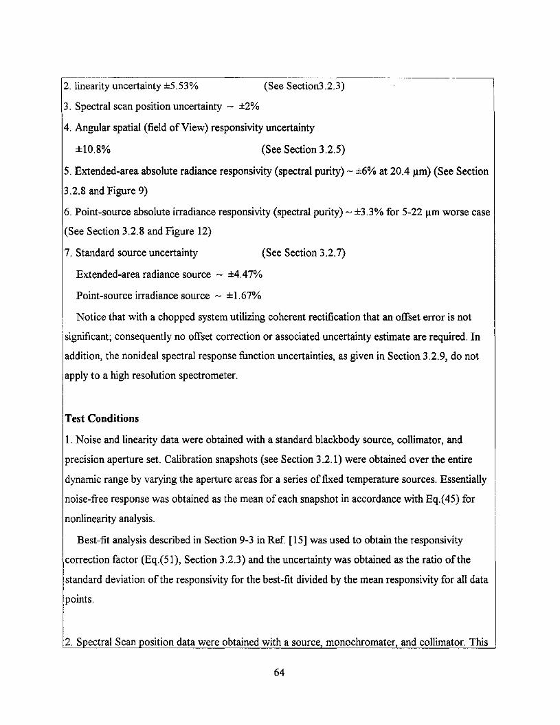
2. linearity uncertainty ±5.53% (See Section3.2.3)

3. Spectral scan position uncertainty - ±2%

4. Angular spatial (field ofView) responsivity uncertainty

±10.8% (See Section 3.2.5)

5. Extended-area absolute radiance responsivity (spectral purity) - ±6% at 20.4 J.lm) (See Section

3.2.8 and Figure 9)

6. Point-source absolute irradiance responsivity (spectral purity) - ±3.3% for 5-22 J.lm worse case

(See Section 3.2.8 and Figure 12)

7. Standard source uncertainty (See Section 3.2.7)

Extended-area radiance source - ±4.47%

Point-source irradiance source - ±1.67%

Notice that with a chopped system utilizing coherent rectification that an offset error is not

significant; consequently no offset correction or associated uncertainty estimate are required. In

addition, the nonideal spectral response function uncertainties, as given in Section 3.2.9, do not

apply to a high resolution spectrometer.

Test Conditions

1. Noise and linearity data were obtained with a standard blackbody source, collimator, and

precision aperture set. Calibration snapshots (see Section 3.2.1) were obtained over the entire

dynamic range by varying the aperture areas for a series of fixed temperature sources. Essentially

noise-free response was obtained as the mean of each snapshot in accordance with Eq.(45) for

nonlinearity analysis.

Best-fit analysis described in Section 9-3 in Ref [15] was used to obtain the responsivity

correction factor (Eq.(51), Section 3.2.3) and the uncertainty was obtained as the ratio of the

standard deviation of the responsivity for the best-fit divided by the mean responsivity for all data

points.

2. Spectral Scan position data were obtained with a source. monochromater and collimator. This

64

9.0~---.------r---,...--..,

Figure 9. Standard uncertainty of theextended-area source absoluteresponsivity calibration (I-sigma valuesgiven as percentages).

23

,,,,',• t It ,t ••• tt. ·....t ••• : •

.t •• • ....." '..

, I '. ",,\' , ~ ,,I

, I

,,

.16 18 21

Wavelength (!J.m)

,,

, .• .t +f,

'"

,, ,, I

4.5

7.5Segment 1 covers 5.5 to 49.3 percent scan which

corresponds to 4.80 to 8.86 /lm.

Segment 2 covers 57 to 74.5 percent scan which

corresponds to 8.87 to 13.63 11m.

Segment 3 covers 80.2 to 100 percent scan which

corresponds to 13.7 to 22.85 11m.

CVF spectrometer utilizes a 3-segment composite

filter.

Discontinuities are observed in the response and

derived spectral parameters as shown below.

A data-set ofwavelength vs. scan position

(percent scan) were obtained and best-fit to linear

functions for each filter segment. Mean and

standard deviation were obtained to provide

corresponding calibration equations and uncertainty for each segment.

3. Spectral resolution data were obtained by stimulating the sensor with a blackbody source filter

with narrow band filters, and a polystyrene absorption cell.

4. The angular spatial (field of view) response were obtained as the response to a point source,

generated by a pointing mirror collimator, for a 25 x 25 matrix. See Section 3.2.5. An inner-core

was defined and the inner-core mean response was determined as 0.804. The uncertainty was

estimated for a worse-case assumption that the target is a point source within the inner core. The

uncertainty is given by the standard deviation over the mean relative responsivity.

5. Extended-area absolute radiance responsivity (spectral purity) test was obtained with a full-field

full-aperture uniform extended-area source (see Section 3.2.7). The response was obtained over

65

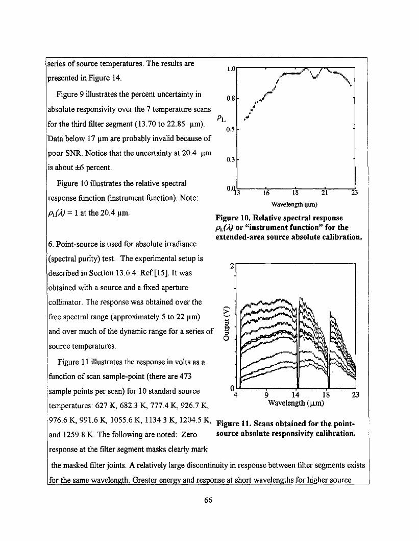
0.3

2.------------.....,

239 14 18Wavelength (J.1m)

oL.I------,r-----,lI---,.I~-....I

4

1.0r----.,..---""'T""~III:wr,~....,I'....,....,..--­....-' 1,.' .."""'".t ..... tt,

I ~~ ~

tt+*'.'" ....."It•,'"

0.8

0'Q1;:;-3---:"':16:---....18~--:2*1--~23

Wavelength UJm)

Figure 10. Relative spectral responsepd),,) or "instrument function" for theextended-area source absolute calibration.

6. Point-source is used for absolute irradiance

(spectral purity) test. The experimental setup is

described in Section 13.6.4. Ref.[15]. It was

obtained with a source and a fixed aperture

collimator. The response was obtained over the

free spectral range (approximately 5 to 22 Ilm)

and over much of the dynamic range for a series of

source temperatures.

Figure 11 illustrates the response in volts as a

function of scan sample-point (there are 473

sample points per scan) for 10 standard source

temperatures: 627 K, 682.3 K, 777.4 K, 926.7 K,

series of source temperatures. The results are

presented in Figure 14.

Figure 9 illustrates the percent uncertainty in

absolute responsivity over the 7 temperature scans

for the third filter segment (13.70 to 22.85 Ilm).

Data below 17 Ilm are probably invalid because of

poor SNR. Notice that the uncertainty at 20.4 Ilm

is about ±6 percent.

Figure 10 illustrates the relative spectral

response function (instrument function). Note:

fJL(),,) = 1 at the 20.4 Ilm.

976.6 K, 991.6 K, 1055.6 K, 1134.3 K, 1204.5 K, Figure 11. Scans obtained for the point­

and 1259.8 K. The following are noted: Zero source absolute responsivity calibration.

response at the filter segment masks clearly mark

the masked filter joints. A relatively large discontinuity in response between filter segments exists

for the same wavelen h. Greater ener

66

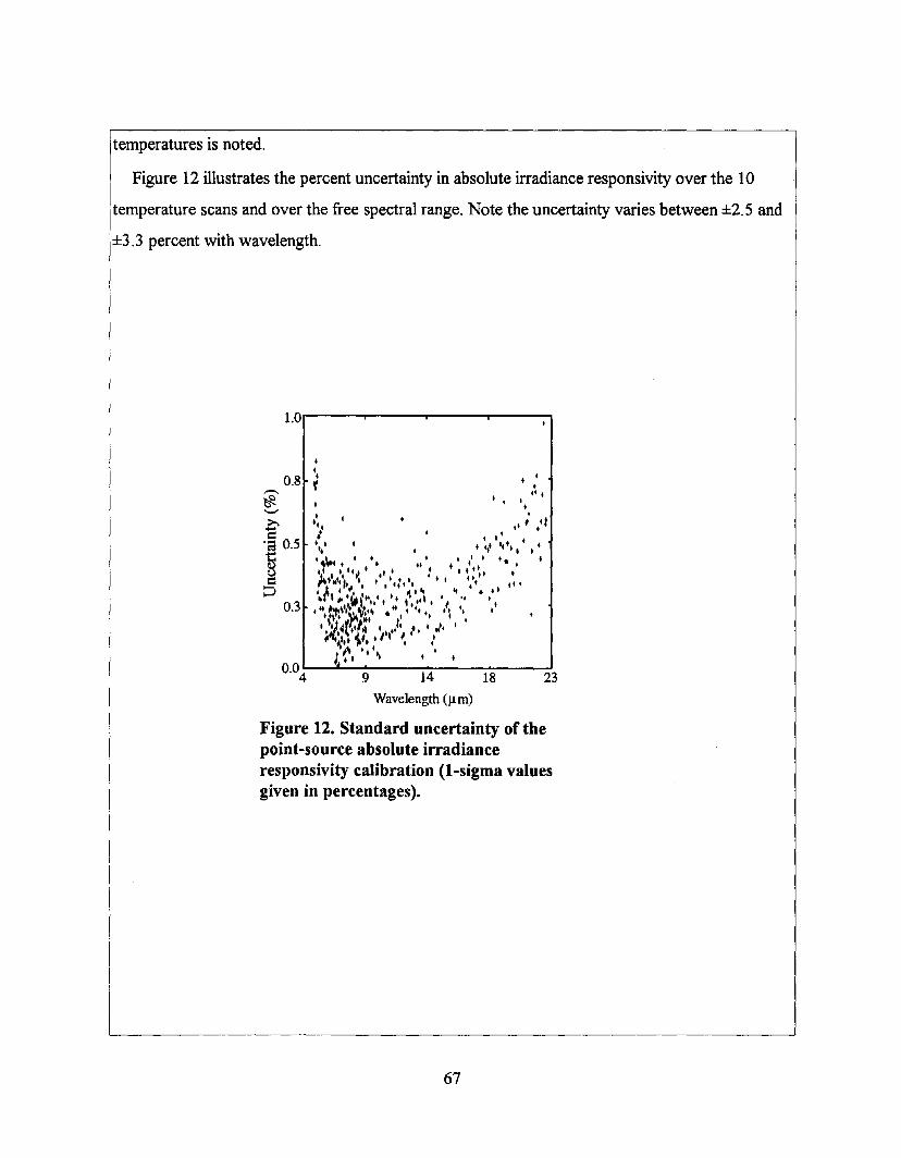
temperatures is noted.

Figure 12 illustrates the percent uncertainty in absolute irradiance responsivity over the 10

temperature scans and over the free spectral range. Note the uncertainty varies between ±2. 5 and

±3.3 percent with wavelength.

1.0,..---.......----r----...-----.

t

•'1

l

• t•,"

• t It,II , :1

t.t t.... • .... I.'., "'WI .... t. tlt.t ,I" II ..

.' • 11.1 I • I • , • t I, •..t.. ..... ' 't .. .. I .ttr t"tt" 't" .t, I"1 1 I I •• ~ It .,..rl" "~\'" I I, ".1 ' '1 I,.. I, I 'I I I' I

.. " ~\,,,. ",.. • +t .. It • • t I, ..

'(~' (~.*' I' , t I, ~., ".":,,, . I • I • ' ..', '

I .~ 11." ",' I I II ~" "/I" ' , ..,\ '.' ,

; , • I, • •

••0.8 .;

,-..,~'-"

~.~ 0.5iU

~0.3

23189 14

Wavelength (j.l.m)

Figure 12. Standard uncertainty of thepoint-source absolute irradianceresponsivity calibration (I-sigma valuesgiven in percentages).

67

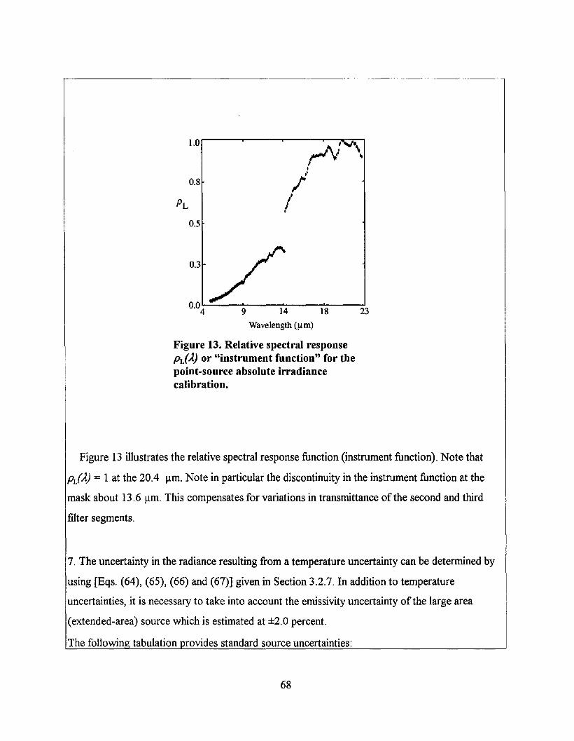
1.0

rJ'l \II

•0.8 I

PL /I

0.5

0.3

0.04""'----...9----:"1"':-4---1~8~-~23

Wavelength (~m)

Figure 13. Relative spectral responsefJL(1) or "instrument function" for thepoint-source absolute irradiancecalibration.

Figure 13 illustrates the relative spectral response function (instrument function). Note that

prf1) = 1 at the 20.4 J-lm. Note in particular the discontinuity in the instrument function at the

mask about 13.6 J-lm. This compensates for variations in transmittance of the second and third

filter segments.

7. The uncertainty in the radiance resulting from a temperature uncertainty can be determined by

using [Eqs. (64), (65), (66) and (67)] given in Section 3.2.7. In addition to temperature

uncertainties, it is necessary to take into account the emissivity uncertainty of the large area

(extended-area) source which is estimated at ±2.0 percent.

The followin tabulation rovides standard source uncertainties:

68

STANDARD SOURCE UNCERTAINTIES

Temperatures [K] Wavelength [Ilm] Uncertainty [%]

71*

83

95

627**

944

1260

627

944

1260

627

944

1260

20.4

20.4

20.4

5

5

5

10

10

10

22

22

22

4.47

2.96

3.01

1.67

0.71

0.38

0.76

0.29

0.14

0.25

0.08

0.04

* Data for the extended area source including emissivity uncertainty and fa! a temperature

uncertainty of 0.5 degree. **Data for the source for a temperature uncertainty of4 degrees.

The above tabulation gives the radiance uncertainty over the range oftemperatures used in the

absolute (spectral purity) calibration and over the range ofwavelength used.

Discussion

A cardinal rule of calibration is that one should calibrate a sensor under the same conditions for

69

which it is to be used. This suggests that the absolute radiance calibration should be obtained with

an extended-area source. However, the low-temperature extended-area source has a wavelength

distribution which is nearly a step-function; that is, there is no response below about 15 Jlm when

the source temperature is reduced such that the sensor is not saturated at 20 Jlm. Figure 14

illustrates the response in volts as a function of scan sample-point (there are 473 sample points

(sub-bands) per scan) for 10 standard source temperatures ofwhich 7 are identified from the top

down: 94.7 K, 90.3 K, 85.2 K, 81.6 K, 78.2 K, 74.4 K, 70.8. K. Note the rapid fall offin energy

and response at short wavelengths.

5

oL-_-.....-__.....L....I~~4

The flux must be greatly attenuated to permit

using higher temperature sources to achieve a more

uniform response over the entire spectral range. A

collimator used with a very small aperture, a

neutral density filter, or a combination of collimator

and filter can be used to provide the necessary

attenuation. However, the uncertainties are difficult

to evaluate for the collimator and require a

knowledge of the uncertainty of the aperture area,

the collimator focal length, scattering effects, and

mirror reflectance. The use of a neutral densityFigure 14. Scans obtained for

filter provides added uncertainties which are a the extended-area source

function ofwavelength. absolute responsivity calibration.

These problems are resolved by using the collimator and small aperture (which are less likely to

be wavelength dependent) with a point source to determine the instrument function (See Section

3.2.8) which is the relative spectral responsivity shown in Figure13 over the free spectral range of

the spectrometer. Note: FigurelO and Figure13 overlap for the wavelengths covered. However,

Figure 13 obtained by the point source absolute irradiance test covers the full spectral range. The

extended area source calibration at the wavelength ofmaximum responsivity - 20.4 Jlm. is used to

"anchor" the instrument function to obtain an absolute radiance calibration of the s ectrometer.

70

The point-source calibration can be used to provide an absolute irradiance calibration of the

spectrometer. The uncertainty in the absolute irradiance responsivity calibration is shown in Figure

12. This uncertainty also reflects in the instrument function as discussed in Section 3.2.8.

Uncertainty analysis

It is recommended that the uncertainty be evaluated for a specified SNR for both writing of

sensor specifications and qualification testing. This is most appropriately done for infinite SNR.

This provides an optimistic uncertainty characterization that depends only upon sensor residual

uncertainties (nonlinear correction, etc.) and nonideal uncertainties (nonideal spectral and spatial

response). Thus, the uncertainty estimates given below neglect the effects of noise, i.e. the SNR is

assumed to be infinite.

It should be noted that source uncertainties and absolute calibration uncertainties vary with

wavelength; in the calculations given below, uncertainties are given for the measurement of

radiance and irradiance based upon the worse case performance of the CVF spectroradiometer at

a particular wavelength setting. In addition, there is an intrinsic wavelength uncertainty of± 2%

according to the characterization data given earlier.

Point source uncertainty

An estimate of the pre final combined standard uncertainty of a measurement of irradiance is

given for the components ofuncertainty given above by

for large SNR which includes the nonlinearity 5.53%, absolute irradiance responsivity (point­

source) 3.3%, and the angular (field-of-view) spatial uncertainties 10.8%, the latter ofwhich

dominate in this case. Therefore, the pre final expanded uncertainty, Up (E) = 2 up(E) will be ±

25% as discussed in section 3.1.

71

The combined standard uncertainty ofa measurement ofirradiance is given by

for large SNR which includes the relative combined standard uncertainty and of the standard

source uncertainty 1.67%. Therefore, the expanded standard uncertainty, Uc (E) = 2 uc(E) will be

±25% .

Extended-area uncertainty

An estimate of the pre final combined standard uncertainty of a measurement ofradiance is

obtained for the components of uncertainty given above by

for large SNR which includes the nonlinearity 5.53%, point source absolute irradiance

responsivity uncertainty(used for the instrument function over 5 to 22 11m) 3.3%, and extended­

area absolute radiance responsivity uncertainty (used to anchor the instrument function at 20.4

11m) 6%. Therefore, the pre final expanded uncertainty Up = 2 ulL) will be ± 18% as discussed

in section 3.1. The combined standard uncertainty of a measurement ofradiance is given by

for large SNR which includes the relative combined standard uncertainty 8.8% and the standard

source uncertainty 4.4%. Therefore, the expanded uncertainty, Uc = 2 uc(L) will be ± 20% .

As an epilogue, we might point out that the uncertainty analysisfor remote sensing sensors is

rather complex and needs to be carefully defined and documented as recommended here. Also,

the uncertainties/or IR sensors as shown in the example 3 are in general large compared to the

72

desired goals and the challenge for the calibration community atpresent is to bring these

combined standard uncertaintiesfor IR sensors to single digit levels to meet various science

objectives.

4. REFERENCES

[1] A.C. Parr, "A National Measurement System for Radiometry, Photometry, and Pyrometry

Based upon Absolute Detectors," NIST Technical Note 1421, U.S. Government Printing Office,

Washington, DC 20402-9325, 1996.

[2] "Quantities and units- Part 6: Light and related electro-magnetic radiations," ISO

STANDARDS HANDBOOK, QUANTITIES AND UNITS, UDC 389.15; Third edition, 1993,

pp. 121-146.

[3] "International Lighting Vocabulary," 3rd Ed., Publ. CIE No. 17(E-11), common to the

CIE and IEC, International Electrotechnical Commission (IEC), International Commission on

Illumination (CIE). Bur. Cent. CIE, Paris 1970.

I

[4] B.N. Taylor,Guide for the use of the International System ofUnits (SI)," NIST Special

Publication 811, U.S. Government Printing Office, Washington, DC 20402-9325,1995.

[5] "Guide to the Expression ofUncertainty in Measurement," ISO/TAG 4/WG 3:

International Organization for Standardization, Geneva, Switzerland, 1993.

[6] B.N. Taylor and C.E. Kuyatt, "Guide for Evaluating and Expressing the Uncertainty of

NIST Measurement Results," NIST Technical Note 1279, January 1993.

[7] "Quantities and units- Part 0: General Principles," ISO STANDARDS HANDBOOK,

QUANTITIES AND UNITS, UDC 389.15, Third edition, 1993, p. 5.

73

[8] Reference 6 above, pp. 11-13.

[9] F.E. Nicodemus, "Self-Study Manual on Optical Radiation Measurements," NBS

Technical Note 910-1, 910-2 & 910-4 Ch. 1 to 8 (1976), U.S. Government Printing Office,

Washington, DC 20402-9325. On a limited basis these documents are available from the Optical

Technology Division, NIST, Gaithersburg, MD 20899-0001

[10] C.L. Wyatt, "Electro-optical System Design," McGraw-Hill Incorporated, NY, 1991, Ch.

8, pp. 111-122

[11] H.I. Kostkowski, "Reliable Spectroradiometry," Spectroradiometry Consulting, La Plata,

MD 1997, p. 6.

[12] I.B.Shumaker, "Self-Study Manual on Optical Radiation Measurements," NBS Technical

Note 910-7, Ch. 11 (1984), U.S. Government Printing Office, Washington, DC 20402-9325. On a

limited basis these documents are available from the Optical Technology Division, NIST,

Gaithersburg, MD 20899-0001;

[13] F.E. Nicodemus, "Radiometry." In "Optical Instrument," Part 1 (R. Kingslake, ed.),

Applied Optics and Optical Engineering, Vol. 4, Ch. 8. Academic Press, New York, 1967.

[14] F.E. Nicodemus, "Normalization in Radiometry," Appl. Opt. 12, 1973, pp. 2960-2973.

[15] C.L. Wyatt, "Radiometric Calibration: Theory and Methods," Academic Press, New

York, N.Y., 1978, pp. 119-125

[16] R.B. Abernethy and B. Ringhiser, "The History and Statistical Development of the New

ASME/SAE/AIAAlISO Measurement Uncertainty Methodology," AIAAlSAE/ASME/ASEE 21st

Joint Propulsion Conference. Monterey, CA., July 8-10, 1985, p. 1.

74

[17] D.A. Scribner, K.A. Sarkady, IT. Caulfield, M.R. Kruer, G. Katz, and C.J. Gridley,

"Nonuniformity Correction for Staring IR Focal Plane Arrays using Scene-based Techniques,"

Infrared Detectors, Focal-plane Arrays, SPIE, Vol. 1308, 1990, pp. 224-234.

[18] Philip R. Bevington, "Data Reduction and Error Analysis for the Physical Sciences,"

McGraw-Hill Book Co., N.Y., 1969, pp. 56-65.

[19] F.E. Nicodemus and G.I Zissis, "Report ofBAMIRAC-Methods ofRadiometric

Calibration, " ARPA Contract No. SD-91, Rep. No. 4613-20-R (ODC No. AD-289, 375),

University ofMichigan, Infrared Lab., Ann Arbor, Michigan, 1962, p. 15.

75

APPENDIX 1

RECENT HISTORICAL RECORD THAT LED

TO THIS DOCUMENT PREPARATION.

77

Jet Propulsion LaboratoryCalifornia Institute of Technology

4800 Oak Grove DrivePasadena California 91109

(818) 354·4321

JPLAugust 10, 1992

Dear Colleage:

The Sensing Systems Working Group of the AIAA Space-Based ObservationSystems Committee on Standards (SBOS COS) has initiated an effort toaddress the concern that many and diverse approaches are utilized todetermine the characteristics and performance of space-borne remote sensingsystems. To begin to address the issue of comparability among data setsobtained from multiple space-borne sensors, the Sensing Systems WorkingGroup is forming task teams to evaluate the need for sensor system calibrationstandards, practices or guidelines. The purpose of this letter is to provide youwith information on the approach being taken to the issue of space-bornesensing systems calibration standards and to solicit your participation on a taskteam to specifically focus on visible to short-wave infrared sensor calibration (.5Ilm to 2.5 Ilm).

A brief overview on "AIAA Activities in Calibration Standards" by Edward W.Koenig is enclosed for your information. This paper describes the rationale forthe SBOS COS, the efforts on sensor calibration and the relationship betweenthe COS and the American National Standards Institute (ANSI).

The Visible-SWIR sensor task team will meet for the first time at the upcomingAIAA Annual Conference to be held September 23 - 25, 1992 at the Hyatt Hotel,Washington, DC, on the "Importance of Standards to Mission Success".Subsequent meetings are planned to be held: January 11 -13, 1992 inconjunction with the 31 st Aerospace Science Meeting in Reno, Nevada, on"Sensor Calibration"; May 19 - 21, 1993 at the Hyatt Crystal City (two weeksafter the AIAA annual meeting on "Interoperability in Command and Control");and September/October (TBD) 1993 in conjunction with the Computing inAerospace meeting to be held in Albuquerque, New Mexico, "DataComparison".

The objectives of the first Visible-SWIR task team meeting will be to formulateand agree upon a strategy for addressing the most important aspects ofcalibration of space-borne remote sensing instruments, to plan the scope of thefollowing workshops and to define the product(s) to be produced by the team.

A tentative agenda for our first meeting is as follows:

1. Identification and discussion of Visible-SWIR calibrationissues and problems.

2. Define focus of team effort and select highest priorityissues to be addressed.

79

Jet Propulsion LaboratoryCalifornia Institute of Technology

3. Develop a strategy to understand, define and resolve issues.

4. Planning of future workshops.

5. Assignment of responsibilities.

A listing of top-level discussion topics for you to consider prior to our firstmeeting includes:

1. Detector/focal plane characterization and calibration.

2. Optical system calibration.

3. Optical filter characterization and calibration.

4. Focal plane/signal processing performancecharacterization.

5. Sensor system calibration.

6. Reference sources and standards.

7. Radiometric response characterization.

8. In-flight calibration.

9 Reproducibility of tests and test configurations.

10. Intercomparison of sensor systems.

11. Long term stability and knowledge.

12. Environmental effects on system performance andcalibration.

If you are interested in participating in the Visible-SWIR calibration team effort,please contact me.

~~Christopher M. Stevens

Manager, Imaging Systems SectionTelephone # (818) 354-5545

FAX # (818) 354-8887EMAIL: CSTEVENS@nasamail.jpl.nasa.gov

CMS:mdd

80

Presented to 2nd Annual SDIUSU Symposium on Cryogenic Infrared

Radiometric Sensor Calibration, Sept. 18-20,1991, Logan UT

American Institute of Aeronautics and Astronautics (AIAA) Activities in Calibration Standards

Edward W. Koenig *

Sensing Systems Working Group Chairman

AIAA-SBOS COS

INTRODUCTION

The American Institute of Aeronautics and Astronautics (AIAA) initiated a special task group to

specifically address the problems and advances in spaceborne observation systems. The AIAA

Space-Based Observation Systems Committee on Standards (SBOS COS) was brought into being

in 1988 as a means of providing a source of information relating to many of the issues in the areas

of Sensing Systems, Communications and Data, Operations, Software Reliability, Spacecraft and

Liaison. Working Groups within the COS place emphasis on tasks which are limiting the accuracy,

efficiency or other significant qualities of the systems. As long-term activities the tasks were

selected for their generic ability to aid future systems, not expecting impact on near term system

design or present contractual work in progress.

In the Sensing Systems Working Group the initial concern was for the widely diverse approaches

being taken in the definition, performance and evaluation of sensor systems. The first task taken

was to develop a set of definitions and physical constants related to spaceborne sensors. This

effort has continued, and is being merged with the present tasks, which are to establish calibration

standards, guidelines or recommended practices. This has now resulted in the formation oftwo

task teams within the working group and plans are being formulated for an additional four task

*Edward Koenig - a staff engineer with ITT Aerospace/Communications Division in Fort Wayne,

IN

81

teams. The approach is to separate the tasks by spectral bands since the details of detection, test

and evaluation are so much different for various ranges of the spectrum. We have selected the

following spectral bands as the general limits for initial consideration.

Passive Sensors

Ultraviolet

Solar

Infrared

Microwave

0.2 to 0.5 11m

0.5 to 2.5 11m

2.5 to 30 11m

1 to 300 Gigahertz

Active Sensors

Optical

Microwave

The activities of these task groups are expected to lead to a better definition of sensor

characterization and performance evaluation as well as overcome major differences in sensor

calibration. The results will be coming from a diverse group of persons, not specifically committed

to a given program or project as is often the case.

ROLE OF THE AIAA

The role of the AIAA Standards Program is to ensure the continued enhancement of aerospace

industry-wide efficiency and productivity. This is to be achieved by the development of scientific

and technical standards document where a need has been identified. The purpose is to pursue

standards to be approved as American National Standards. One objective is to have AIAA

Standards documents adopted by the Department ofDefense- and be listed-d in the DoD Index of

specifications and Standards (DODISS) whenever this is appropriate. The AIAA Standards

program consists of the development ofand publication of scientific and technical standards and

data. The technical scope of these standards documents covers all areas of interest to AIAA

Technical Committees, including systems, components, materials, products, technologies,

methods and practices in aerospace applications. Standards may cover such topics as health,

safety, design, testing, construction, maintenance, performance, environment, operation of

aerospace devices, equipment, and methods. Published standards documents are offour kinds:

Standards, Recommended Practices, Guides, and Special Project Reports.

82

The AIAA will cooperate and coordinate with all other competent standards bodies worldwide in

the technical areas within the scope ofthe AIAA Standards Program. Consensus is used as the

tool to reach agreement on any given item. A process is in place for review and approval by the

individuals, consultants, committees and working groups to which the document is presented.

Publication means that the document achieved consensus ofthe community which typically

consists of representatives from government, industry, and academia. Special Project Reports may

be published without the consensus procedure. The use of AIAA Standards is entirely voluntary,

there is no inherent commitment for any user to adhere to any standards report. Compliance with

AIAA Standards documents does not guarantee quality or satisfactory application.

The AIAA will not engage in testing or certification of products, systems, or any other device or

method, for demonstrating compliance with AIAA's Standards Documents. It will not consider

any patents which may apply to the subject matter of a report or standard. Prospective users are

responsible for protecting themselves against liabilities or infringement ofpatents or copyrights.

No individual, group, or committee, whether members of AIAA or not, is authorized to express

opinions or act in any way in these matters in the name ofAIAA or on behalf ofAIAA. The AIAA

assumes no responsibility for the use or interpretation of its standards documents. Standards

documents follow the same pattern ofthe AIAA published documents which comprise Standards,

Recommended Practices, Guides, and Special Project Reports.

A Committee on Standards (COS) for a specific discipline is directly responsible to STC and shall

1) Develop standards within its scope, 2) Maintain standards within its scope, with review every

five years, 3) Achieve a consensus on action proposed, 4) Ensure that duplication of standards is

minimized, 6) Advise on standards within its scope, 7) Report the status of standards at least

annually to the STC, 8) Document discussions on developing or revising standards and send

reports to the Administrator

American National Standards Institute (ANSI)

The American National Standards Institute has been the cornerstone ofU S activities for

83

voluntary standards ANSI is a private, nonprofit organization with a broad membership ofabout

1,000 companies, 30 U S government agencies, 250 professional, technical, and trade societies,

and labor and consumer groups Our SBOS COS, through the AIAA, is an accredited standards

organization ofANSI, which approves American National Standards and represents U S interests

in forums such as the International Organization for Standardization (ISO) After a working group

develops a document it goes through the SBOS COS approval and AIAA approval, then is

submitted to ANSI for approval After ANSI approval AIAA will publish the standard with an

ANSI number

Space-Based Observation Systems Committee on Standards

The Space-Based Observation Systems Committee on Standards (SBOS COS) is one of these

AIAA sponsored committees It was established to specifically look at the problems facing the

general field of new and developing spacecraft to prepare for the use of standards, wherever

appropriate and beneficial These standards, if extended to a number of spacecraft and multiplicity

of similar instruments, will reduce the complexity of assembly and operation, and improve

utilization of the data from these systems The charter of the SBOS-COS is the "Adoption of,

modification, development, and recommendation of standards, recommended practices, and

guidelines relating to satellite subsystems (space segment and ground segment) that study the

earth and its environment in space with the following specific requirements:

Specific to space-based observation disciplines

Applicable to multiple programs and/or missions

Economically viable, with emphasis on life-cycle cost savings

Must include recommended method of implementation

Must have clearly defined benefits to multiple contractors,

Government agencies, and users, and

Coordinated with relevant National and international activities

As such the AIAA SBOS COS which is chaired by Mrs. Andrea F. Sebera, previously of Space

SystemslLoral and Dr. Neville Marzwell ofNASNJet Propulsion Laboratory in Pasadena as Vice

84

Chair has been active in the formation ofworking groups with individual responsibilities in the

areas of:

Technical Coordination; chairman Lawrence M.G. Enomoto, Esq., which completed a

comprehensive document"1991 Earth Observations Directory: A Worldwide Listing of

Government Institutions and Related Groups" under the technical leadership ofDr. Paul Uhlir.

This committee will continue to coordinate US and international information to aid interface

within the observation satellite community.

Communications and Data Systems; Chairman Charles Baird, has task groups working on a

Security and Privacy Project, Upper Layers Project, Tools for Communications Systems,

Command and Controls Project and Data Compression Standards. Details of these projects, as

with others in the COS are described in the SBOS Orbiter, the newsletter of the COS.

Space Operations Working Group; chairman George C. Jackson, developed a Guideline for

Human Computer Interfaces and is working on a Guideline for Satellite Autonomy.

Sensing Systems Working Group; chairman Edward W. Koenig; developing a document on

Space-based Sensor Systems Terms and Physical Constants, and setting up task groups on

calibration as described earlier.

Software Reliability Working Group; chairman Ted Keller, is working on a: Standardized Software

Reliability Model as a recommended practice.

Spacecraft Working Group; chairman Dr. Janet Bare is working on interfaces, components,

subsystems, spacecraft buses, testing and calibration, particularly focusing on small satellites. A

database of Characteristics of Satellites and Payloads has been developed and is now available in

preliminary form.

85

The SBOS COS has just completed a joint NASAlNASDNAIAA meeting in Tsukuba, Japan,

June 26-28, 1991 to discuss international cooperation efforts in Earth Observing Missions. The

results were encouraging in having the opportunity to discuss detailed common needs and

approaches to improved international communication on interfaces and standards.

The next SBOS COS quarterly meeting will be held in Huntsville, Alabama, from November 13 to

15 and will be dedicated to Extra-terrestrial Exploration. The follow-on meeting will be in the Jet

Propulsion Laboratory on February 5 to 7, 1992, and will be dedicated to Autonomous Light

Spacecraft.

The AIAA SBOS COS is firmly committed to the stand that U.S. industry needs to be involved in

standards development to assure continuous leadership in space-based observation systems.

A Perspective on Calibration

In the efforts to review and evaluate the needs of the sensor community in the area ofcalibration it

became clear that a number of factors and requirements were emerging which need to be

addressed in the calibration of instruments. The needs are seen as:

Definitions: The selection and definition of terms used specifically in sensor systems needs to be

improved. An example of an attempt to improve this situation is the report by Dr. Wyatt on the

definition and application of accuracy and precision to infrared systems. The need for definitions

which stand up to examination and test and the selection of terms for universal use in the industry

is very important. Each of the task teams will establish the terms for their particular part of the

state of the art and have them reviewed by the SBOS COS to correlate with other groups and

with a set of terms already in review by the committee.

Pre-flight calibration sources: The design of calibration sources should follow guidelines

established by the most experienced users. Designs must include consideration for uniformity,

blackness, thermal stability, thermal sensor placement, control and cleanliness. The method of

86

establishing the accuracy of calibration target temperatures must include use of calibrated

thermistors or platinum resistance thermometers (PRT) having direct transfer from basic

standards. The circuits used to measure these resistances for data collection should also be tested

for stability and accuracy. The use of common interface circuits having stability, accuracy and

noise rejection should be considered. When possible, providing comparison with other targets or

standards will verify the quality of the calibration. An approach used in the calibration ofvisible

channels of the NOAA series of instruments is to use a common calibration target for all

instruments. This is a well characterized standard calibration target moved around within the test

facility. This general technique could be applied to infrared targets where comparison with the

special unit would provide the continuity of standard calibration. It might be possible to use a

traveling standard source for final calibration. In this regard there is a real need for a common

source for comparative tests, such as a facility where targets may be taken for tests of emissivity,

uniformity, temperature accuracy, and stability. Ifwe are to ever relate instruments of different

types on a given spacecraft and instruments of similar types on a series of spacecraft we must have

a more common technique for calibrating the variety oftargets.

Evaluation techniques: The methods of collection of data, calculation of ac~uracy, precision,

non-linearity, stability, background noise, system noise, dynamic range, and other

characterizations of instruments varies greatly from laboratory to laboratory. The use of a

common approach to the definitions, algorithms, characteristic qualities and even the method of

reporting the output of the calibration would be beneficial for all.

Construction of reference targets: The method of construction of infrared calibration targets

varies widely. Obviously the instrument requirements set the size, and the mounting configuration

sets many ofthe physical characteristics. For static (staring) tests the use ofa round reference

surface surrounded by a wall that is as deep as the width ofthe target is typically used. All

surfaces are covered with honeycomb and painted black. The combination ofpaint emissivity,

honeycomb dimensions and wall depth determine the (non-blackness) of the target. A good target

will have an effective emissivity of over 99%. The use of common paints, cell dimensions and

87

depth-to-width ratios will help provide commonality between instrument calibrations. All of this

combines to determine the radiometric error contributed by the target and is a part of the absolute

radiometric accuracy definition for a given instrument.

In-orbit calibration: Most meteorological and other science oriented satellites use a blackbody

reference at a known temperature and space as a two point calibration of the slope (radiance per

count) and offset (counts at zero radiance). This has been adequate for many missions but is not

sufficient when non-linearity of the sensor or potential changes in spectral characteristics are

necessary to characterize the system. In general the use of a black honeycomb surface on the body

of the instrument, viewed through the complete optic system, including the scan mirror, provided

a suitable IR source. A full view of space provided the cold reference. Now, with large area

arrays, varieties of spectrometers and specialty instruments the needs for spectral calibration,

linearity, and stability are expanding the requirements and sophistication of on-board calibration

targets and procedures. The problem ofa truly accurate and stable solar spectrum calibration

source is still with us, with several approaches being reviewed for the EOS program.

Long term calibration: The international community is searching for means ofusing earth targets

and space targets as long term calibration sources for a large variety of instruments. Studies of

White Sands, various deserts, coastal areas, clouds, moon, stars and the sun as sources is

continuing to define common sources for inter-calibration of instruments and for detection oflong

term degradation of sensors. In general the limitations ofground targets to ,moisture, sun angles,

area size, spectral definition, atmospheric interference effects and other factors has limited the

estimated accuracy to the order of 10%. This is not good enough for the levels of accuracy

required for most scientific oriented sensors. The dependence on in-orbit targets will therefore

continue.

Data retrieval and comparison: When a group of data sets are collected form various instruments

with a common goal the data most likely will require reformatting, recalibration, annotation, and

be changed to a different computer language and printed differently in order to compare results.

88

The need exists for some standard approaches to identifiers, format, references, and database to

permit easier distribution and use of the data. The problems faced by the Earth Observation

Systems Data Information System (EOSDIS) in collecting data from historical files, present and

future files and presenting a format for user evaluation are enormous. We should probably use the

EOSDIS as the baseline for setting guidelines for all data collection and distribution systems.

CONCLUSIONS

The sensor development community needs to be aware ofthe activities ofthe AIAA and ANSI in

the preparation of standards, guidelines and recommended practices and the procedures to

generate and obtain them. The ANSI standards provide a common denominator ofgovernment,

industry and international scope to bring the community together in its methodology in design,

interfaces, operation and utilization of sensor systems.

We tend to become engrossed in our own portion of a project or technology and develop our own

approach to calibration, evaluation and dissemination. The use ofguidelines for many ofthese

tasks will cause some added effort in the preparation oftest methods but will make the results

more universal and aid the whole community over a long period.

Calibration of sensors is a complex and demanding task. Diligence in establishing scientific validity

to each part of the test is important. It is also important to prepare for the calibration and to

present the data using the best knowledge and experience ofthe world's experts. In the

establishment ofguidelines, reviewed by the whole community, we have the opportunity to

include that expertise. The AIAA SBOS COS and its task groups are available to support that

effort.

89

December 21, 1992

SBOS-COS Sensor Systems Subcommittee

IR Sensor Calibration Standards Task Group

David BoxBall Aerospace Corp.

Jerry BronsonBoeing Company

Carol 1. BrueggeJet Propulsion Laboratory

Raju DadaNISTlRadiometric Physics Division

Roy GavinITT Aerospace/Communications

Edward Koenig8825 Beacon Woods PlaceFt. Wayne, TIN 46804

Andrew LazarewiczMission Research Corp

Paul MenzelNOAA/NESDIS, EIRA 24

James M. PalmerU ofArizona- Optical Sciences Center

David B. PollockTeledyne Brown Engineering

Richard RaperCalspan Corp. MS 640Arnold Air Force Base, TN 37389

90

Milton TriplettNichols Research Corp

Tom WallaceNichols Research Corporation

Mike WeinrebNOAA/NESDIS, Code EIRA 14

Clair WyattSpace Dynamics LaboratoryUtah State University

Ray YoungCalspan Corp. MS 640Arnold Air Force Bas~, TN 37389

APPENDIX 2

GUIDELINES FOR EVALUATING ANDEXPRESSING THE UNCERTAINTY OF NIST

MEASUREMENT RESULTSNIST TECHNICAL NOTE 1297

91

NIST Technical Note 12971994 Edition

Guidelines for Evaluating and Expressingthe Uncertainty of NIST Measurement Results

Barry N. Taylor and Chris E. Kuyatt

Physics LaboratoryNational Institute of Standards and TechnologyGaithersburg, MD 20899

(Supersedes NIST Technical Note 1297, January 1993)

September 1994

u.s. Department of CommerceRonald H. Brown, Secretary

Technology AdministrationMary L. Good, Under Secretary for Technology

National Institute of Standards and TechnologyArati Prabhakar, Director

Guidelines for Evaluating and Expressing the Uncertainty of NIST Measurement Results

Preface to the 1994 Edition

The previous edition, which was the first, of this National

Institute of Standards and Technology (NIST) Technical

Note (TN 1297) was initially published in January 1993. A

second printing followed shortly thereafter, and in total

some 10000 copies were distributed to individuals at NIST

and in both the United States at large and abroad - to

metrologists, scientists, engineers, statisticians, and others

who are concerned with measurement and the evaluation

and expression of the uncertainty of the result of ameasurement. On the whole, these individuals gave TN

1297 a very positive reception. We were, of course, pleased

that a document intended as a guide to NIST staff was alsoconsidered to be of significant value to the international

measurement community.

Several of the recipients of the 1993 edition of TN 1297

asked us questions concerning some of the points it

addressed and some it did not. In view of the nature of thesubject of evaluating and expressing measurementuncertainty and the fact that the principles presented in

TN 1297 are intended to be applicable to a broad range of

measurements, such questions were not at all unexpected.

It soon occurred to us that it might be helpful to the current

and future users of TN 1297 if the most important of thesequestions were addressed in a new edition. To this end, we

have added to the 1993 edition of TN 1297 a new appendix

- Appendix D - which attempts to clarify and give

additional guidance on a number of topics, including the use

of certain terms such as accuracy and precision. We hope

that this new appendix will make this 1994 edition of

TN 1297 even more useful than its predecessor.

We also took the opportunity provided us by the preparation

of a new edition of TN 1297 to make very minor word

changes in a few portions of the text. These changes weremade in order to recognize the official publication in

October 1993 of the ISO Guide to the Expression of

Uncertainty in Measurement on which TN 1297 is based

(for example, the reference to the Guide was updated); and

to bring TN 1297 into full harmony with the Guide (for

example, "estimated correction" has been changed to

simply "correction," and "can be asserted to lie" has been

changed to "is believed to lie").

September 1994

B~~Barry N. Taylor

~t~Chris E. Kuyatt

Guidelines for Evaluating and Expressing the Uncertainty of NIST Measurement Results

FOREWORJ)(to the 1993 Edition)

Results of measurements and conclusions derived from them

constitute much of the technical information produced by

NIST. It is generally agreed that the usefulness ofmeasurement results, and thus much of the information that

we provide as an institution, is to a large extent determined

by the quality of the statements of uncertainty that

accompany them. For example, oonly if quantitative and

thoroughly documented statements of uncertainty accompany

the results of NIST calibrations can the users of our

calibration services establish their level of traceability to the

U.S. standards of measurement maintained at NIST.

Although the vast majority of NIST measurement results areaccompanied by quantitative statements of uncertainty, there

has never been a uniform approach at NIST to theexpression of uncertainty. The use of a single approach

within the Institute rather than many different approacheswould ensure the consistency of our outputs, thereby

simplifying their interpretation.

To address this issue, in July 1992 I appointed a NIST AdHoc Committee on Uncertainty Statements and charged it

with recommending to me a NIST policy on this important

topic. The members of the Committee were:

D. C. CranmerMaterials Science and Engineering Laboratory

K. R. EberhardtComputing and Applied Mathematics Laboratory

R. M. JudishElectronics and Electrical Engineering Laboratory

R. A. KamperOffice of the Director, NIST/Boulder Laboratories

C. E. KuyattPhysics Laboratory

J. R. RosenblattComputing and Applied Mathematics Laboratory

J. D. SimmonsTechnology Services

L. E. SmithOffice of the Director, NIST; Chair

D. A. SwytManufacturing Engineering Laboratory

B. N. TaylorPhysics Laboratory

R. L. WattersChemical Science and Technology Laboratory

This action was motivated in part by the emerginginternational consensus on the approach to expressing

uncertainty in measurement recommended by the

International Committee for Weights and Measures (CIPM).The movement toward the international adoption of the

CIPM approach for expressing uncertainty is driven to a

large extent by the global economy and marketplace; its

worldwide use will allow measurements performed in

different countries and in sectors as diverse as science,

engineering, commerce, industry, and regulation to be more

easily understood, interpreted, and compared.

At my request, the Ad Hoc Committee carefully reviewed

the needs of NIST customers regarding statements ofuncertainty and the compatibility of those needs with the

CIPM approach. It concluded that the CIPM approach could

be used to provide quantitative expressions of measurementuncertainty that would satisfy our customers' requirements.

The Ad Hoc Committee then recommended to me a specificpolicy for the implementation of that approach at NIST. I

enthusiastically accepted its recommendation and the policyhas been incorporated in the NIST Administrative Manual.(It is also included in this Technical Note as Appendix C.)

To assist the NIST staff in putting the policy into practice,

two members of the Ad Hoc Committee prepared this

Technical Note. I believe that it provides a helpful discussionof the CIPM approach and, with its aid, that the NIST policycan be implemented without excessive difficulty. Further, Ibelieve that because NIST statements of uncertainty resulting

from the policy will be uniform among themselves andconsistent with current international practice, the policy will

help our customers increase their competitiveness in thenational and international marketplaces.

January 1993

John W. LyonsDirector,

National Institute of Standards and Technology

Guidelines for Evaluating and Expressing the Uncertainty of NISf Measurement Results

GUIDELINES FOR EVALUATING AND EXPRESSING THEUNCERTAINTY OF NlST MEASUREMENT RESULTS

1. Introduction

1.1 In October 1992, a new policy on expressing

measurement uncertainty was instituted at NIST. This

policy is set forth in "Statements of Uncertainty AssociatedWith Measurement Results," Appendix E, NIST Technical

Communications Program, Subchapter 4.09 of the

Administrative Manual (reproduced as Appendix C of these

Guidelines) .

1.2 The new NIST policy is based on the approach to

expressing uncertainty in measurement recommended by the

CIPM1 in 1981 [1] and the elaboration of that approach

given in the Guide to the Expression of Uncertainty in

Measurement (hereafter called the Guide), which was

prepared by individuals nominated by the BIPM, IEC, ISO,

or OIML [2].1 The CIPM approach is founded onRecommendation INC-l (1980) of the Working Group onthe Statement of Uncertainties [3]. This group was

convened in 1980 by the BIPM as a consequence of a 19772

request by the CIPM that the BIPM study the question of

reaching an international consensus on expressing

uncertainty in measurement. The request was initiated bythen CIPM member and NBS Director E. Ambler. A 19852

request by the CIPM to ISO asking it to develop a broadlyapplicable guidance document based on Recommendation

INC-l (1980) led to the development of the Guide. It is atpresent the most complete reference on the general

application of the CIPM approach to expressingmeasurement uncertainty, and its development is givingfurther impetus to the worldwide adoption of that approach.

1.3 Although the Guide represents the currentinternational view of how to express uncertainty inmeasurement based on the CIPM approach, it is a rather

lengthy document. We have therefore prepared thisTechnical Note with the goal of succinctly presenting, in

the context of the new NIST policy. those aspects of the

Guide that will be of most use to the NIST staff in

implementing that policy. We have also included some

ICIPM: International Committee for Weights and Measures; BIPM:International Bureau of Weights and Measures; lEC: InternationalElectrotechnical Commission; ISO: International Organization forStandardization; OIML: International Organization of Legal Metrology.

2These dates have been corrected from those in the first (1993) edition ofTN 1297 and in the Guide.

suggestions that are not contained in the Guide or policy but

which we believe are useful. However, none of the

guidance given in this Technical Note is to be interpreted as

NIST policy unless it is directly quoted from the policy

itself. Such cases will be clearly indicated in the text.

1.4 The guidance given in this Technical Note is intended

to be applicable to most, if not all, NIST measurement

results, including reSults associated with

- international comparisons of measurement standards,

- basic research,

- applied research and engineering,

- calibrating client measurement standards,

- certifying standard reference materials, and

- generating standard reference data.

Since the Guide itself is intended to be applicable to similarkinds of measurement results, it may be consulted for

additional details. Classic expositions of the statistical

evaluation of measurement processes are given in references[4-7].

2. Classification of Components of Uncertainty

2.1 In general, the result of a measurement is only an

approximation or estimate of the value of the specificquantity subject to measurement, that is, the measurand,and thuS the result is complete only when accompanied bya quantitative statement of its uncertainty.

2.2 The uncertainty of the result of a measurementgenerally consists of several components which, in theCIPM approach, may be grouped into two categoriesaccording to the method used to estimate their numerical

values:

A. those which are evalUated by statistical methods,

B. those which are evaluated by other means.

2.3 There is not always a simple correspondence betweenthe classification of uncertainty components into categories

A and B and the commonly used classification ofuncertainty components as "random" and "systematic." The

nature of an uncertainty component is conditioned by theuse made of the corresponding quantity, that is, on how that

Guidelines for Evaluating and Expressing the Uncertainty of NIST Measurement Results

quantity appears in the mathematical model that describes

the measurement process. When the corresponding quantityis used in a different way, a "random" component may

become a "systematic" component and vice versa. Thus the

terms "random uncertainty" and "systematic uncertainty"

can be misleading when generally applied. An alternative

nomenclature that might be used is

"component of uncertainty arising from a random

effect, "

"component of uncertainty arising from a systematic

effect, "

where a random effect is one that gives rise to a possible

random error in the current measurement process and a

systematic effect is one that gives rise to a possible

systematic error in the current measurement process. In

principle, an uncertainty component arising from a

systematic effect may in some cases be evaluated by method

A while in other cases by method B (see subsection 2.2), as

may be an uncertainty component arising from a random

effect.

NOTE - The difference between error and uncertainty should always

be borne in mind. For example, the result of a measurement after

correction (see subsection 5.2) can unknowably be very close to the

unknown value of the measurand, and thus have negligible error, even

though it may have a large uncertainty (see the Guide [2]).

2.4 Basic to the CIPM approach is representing each

component of uncertainty that contributes to the uncertainty

of a measurement result by an estimated standard deviation,

termed standard uncertainty with suggested symbol uj ,

and equal to the positive square root of the estimated. 2vanance U j •

2.5 It follows from subsections 2.2 and 2.4 that an

uncertainty component in category A is represented by a

statistically estimated standard deviation Sj, equal to the

positive square root of the statistically estimated variance

s7, and the associated number of degrees of freedom ~.

For such a component the standard uncertainty is uj = Sj'

The evaluation of uncertainty by the statistical analysis of

series of observations is termed a Type A evaluation (of

uncertainty).

2.6 In a similar manner, an uncertainty component in

category B is represented by a quantity Uj' which may be

considered an approximation to the corresponding standard

deviation; it is equal to the positive square root of u;,which may be considered an approximation to the

corresponding variance and which is obtained from an

assumed probability distribution based on all the availableinformation (see section 4). Since the quantity u; is treatedlike a variance and uj like a standard deviation, for such a

component the standard uncertainty is simply uj •

The evaluation of uncertainty by means other than the

statistical analysis of series of observations is termed a

Type B evaluation (of uncertainty).

2.7 Correlations between components (of either category)

are characterized by estimated covariances [see Appendix

A, Eq. (A-3)] or estimated correlation coefficients.

3. Type A Evaluation of Standard Uncertainty

A Type A evaluation of standard uncertainty may be based

on any valid statistical method for treating data. Examples

are calculating the standard deviation of the mean of a

series of independent observations [see Appendix A,

Eq. (A-5)]; using the method of least squares to fit a curve

to data in order to estimate the parameters of the curve and

their standard deviations; and carrying out an analysis of

variance (ANOVA) in order to identify and quantify

random effects in certain kinds of measurements. If the

measurement situation is especially complicated, one should

consider obtaining the guidance of a statistician. The NIST

staff can consult and collaborate in the development of

statistical experiment designs, analysis of data, and other

aspects of the evaluation of measurements with the

Statistical Engineering Division, Computing and Applied

Mathematics Laboratory. Inasmuch as this Technical Note

does not attempt to give detailed statistical techniques for

carrying out Type A evaluations, references [4-7], and

reference [8] in which a general approach to quality control

of measurement systems is set forth, should be consulted

for basic principles and additional references.

4. Type B Evaluation of Standard Uncertainty

4.1 A Type B evaluation of standard uncertainty is usually

based on scientific judgment using all the relevant

information available, which may include

- 'previous measurement data,

- experience with, or general knowledge of, the

behavior and property of relevant materials and

instruments,

- manufacturer's specifications,

- data provided in calibration and other reports, and

- uncertainties assigned to reference data taken from

handbooks.

Guidelines for Evaluating and Expressing the Uncertainty of NIST Measurement Results

Some examples of Type B evaluations are given in

subsections 4.2 to 4.6.

4.2 Convert a quoted uncertainty that is a stated multiple

of an estimated standard deviation to a standard uncertainty

by dividing the quoted uncertainty by the multiplier.

4.3 Convert a quoted uncertainty that defmes a

"confidence interval" having a stated level of confidence

(see subsection 5.5), such as 95 or 99 percent, to a standard

uncertainty by treating the quoted uncertainty as if a normal

distribution had been used to calculate it (unless otherwise

indicated) and dividing it by the appropriate factor for such

a distribution. These factors are 1.960 and 2.576 for the

two levels of confidence given (see also the last line of

Table B.I of Appendix B).

4.4 Model the quantity in question by a normal

distribution and estimate lower and upper limits a_ and a+

such that the best estimated value of the quantity is

(a+ + aJ/2 (i.e., ~e center of the limits) and there is Ichance out of 2 (i.e., a 50 percent probability) that the

value of the quantity lies in the interval a_ to a+. Then

Uj "" 1.48a, where a = (a+ - a_)/2 is the half-width of

the interval.

4.5 Model the quantity in question by a normal

distribution-and estimate lower and upper limits a_ and a+

such that the best estimated value of the quantity is

(a+ + a_)/2 and there is about a 2 out of 3 chance (i.e.,a 67 percent probability) that the value of the quantity lies

in the interval a_ to a+. Then uj "" a, where

a = (a+ - aJ/2.

4.6 Estimate lower and upper limits a_ and a+ for the

value of the quantity in question such that the probability

that the value lies in the interval a_ to a+ is, for all

practical purposes, 100 percent. Provided that there is no

contradictory information, treat the quantity as if it is

equally probable for its value to lie anywhere within the

interval a_ to a+; that is, model it by a uniform or

rectangular probability distribution. The best estimate of the

value of the quantity is then (a+ + aJ/2 with uj = afV3,

where a = (a+ - a_)/2.

If the distribution used to model the quantity is triangularrather than rectangular, then uj = afV6.

If the quantity in question is modeled by a normaldistribution as in subsections 4.4 and 4.5, there are nofinite limits that will contain 100 percent of its possible

values. However, plus and minus 3 standard deviations

about the mean of a normal distribution corresponds to

99.73 percent limits. Thus, if the limits a_ and a+ of a

normally distributed quantity with mean (a+ + 0_)/2 are

considered to contain "almost all" of the possible values of

the quantity, that is, approximately 99.73 percent of them,

then Uj "" a/3, where a = (a+ - aJ/2.

The rectangular distribution is a reasonable default model

in the absence of any other information. But if it is known

that values of the quantity in question near the center of the

limits are more likely than values close to the limits, a

triangular or a normal distribution may be a better model.

4.7 Because the reliability of evaluations of components

of uncertainty depends on the quality of the information

available, it is recommended that all parameters upon which

the measurand depends be varied to the fullest extent

practicable so that the evaluations are based as much as

possible on observed data. Whenever feasible, the use of

empirical models of the measurement process founded on

long-term quantitative data, and the use of check standardsand control charts that can indicate if a measurement

process is under statistical control, should be part of the

effort to obtain reliable evaluations of components of

uncertainty [8]. Type A evaluations of uncertainty based on

limited data are not necessarily more reliable than soundly

based Type B evaluations.

5. Combined Standard Uncertainty

5.1 The combined standard uncertainty of a measure­

ment result, suggested symbol uc ' is taken to represent theestimated standard deviation of the result. It is obtained by

combining the individual standard uncertainties Ui (and

covariances as appropriate), whether arising from a Type A

evaluation or a Type B evaluation, using the usual method

for combining standard deviations. This method, which is

summarized in Appendix A [Eq. (A-3)], is often called the

law ofpropagation ofuncenainty and in common parlance

the "root-sum-of-squares" (square root of the sum-of-the­

squares) or "RSS" method of combining uncertaintycomponents estimated as standard deviations.

NOTE - The NIST policy also allows the use of established and

documented methods equivalent to the "RSS" method. such as the

numerically based "bootstrap" (see Appendix C).

5.2 It is assumed that a correction (or correction factor)is applied to compensate for each recognized systematiceffect that significantly influences the measurement result

and that every effort has been made to identify such effects.

The relevant uncertainty to associate with each recognized

systematic effect is then the standard uncertainty of the

Guidelines for Evaluating and Expressing the Uncertainty of NIST Measurement Results

appl~ed correction. The correction may be either positive,negative, or zero, and its standard uncertainty may in somecases be obtained from a Type A evaluation while in othercases by a Type B evaluation.

NOTES

1 The uncertainty of a correction applied to a measurement result to

compensate for a systematic effect is not the systematic error in the

measurement result due to the effect. Rather, it is a measure of the

uncertainty of the result due to incomplete knowledge of the required

value of the correction. The terms "error" and "uncertainty" should

not be confused (see also the note of subsection 2.3).

2 Although it is strongly recommended that corrections be applied for

all recognized significant systematic effects, in some cases it may not

be practical because of limited resources. Nevertheless, the expression

of uncertainty in such cases should conform with these guidelines to­

the fullest possible extent (see the Guide [2]).

5.3 The combined standard uncertainty ue is a widely

employed measure of uncertainty. The NIST policy on

expressing uncertainty states that (see Appendix C):

Commonly, ue is used for reporting results of

determinations of fundamental constants, fundamentalmetrological research, and international comparisons

of realizations of SI units.

Expressing the uncertainty of NIST's primary cesiumfrequency standard as an estimated standard deviation is an

example of the use of ue in fundamental metrologicalresearch. It should also be noted that in a 1986

recommendation [9], the CIPM requested that what is nowtermed combined standard uncertainty ue be used "by all

participants in giving the results of all internationalcomparisons or other work done under the auspices of the

CIPM and Comites Consultatifs."

5.4 In many practical measurement situations,theprobability distribution characterized by the measurement

result Y and its combined standard uncertainty ue(Y) isapproximately normal (Gaussian). When this is the case andue(Y) itself has negligible uncertainty (see Appendix B),

ue(Y) defmes an interval Y - ue(Y) to Y + ue(Y) about themeasurement result Y within which the value of the

measurand Y estimated by Y is believed to lie with a levelof confidence of approximately 68 percent. That is, it isbelieved with an approximate level of confidence of 68

percent that Y - ue(Y) :s: Y :s: Y + Ue(Y) , which is

commonly written as Y = Y ± ue(y).

The probability distribution characterized by themeasurement result and its combined standard uncertaintyis approximately normal when the conditions of the CentralLimit Theorem are met. This is the case, often encountered

in practice, when the estimate y of the measurand Y is notdetermined directly but is obtained from the estimatedvalues of a significant number of other quantities [seeAppendix A, Eq. (A-I)] describable by well-behaved

probability distributions, such as the normal and rectangular

distributions; the standard uncertainties of the estimates of

these quantities contribute comparable amounts to the

combined standard uncertainty ue(Y) of the measurement

result y; and the linear approximation implied by Eq. (A-3)in Appendix A is adequate.

NOTE - If uc(y) has non-negligible uncertainty, the level of

confidence will differ from· 68 percent. The procedure given in

Appendix B has been proposed as a simple expedient for

approximating the level of confidence in these cases.

5.5 The term "confidence interval" has a specific

definition in statistics and is only applicable to intervals

based on ue when certain conditions are met, including that

all components of uncertainty that contribute to ue be

obtained from Type A evaluations. Thus, in theseguidelines, an interval based on ue is viewed as

encompassing a fraction p of the probability distributioncharacterized by the measurement result and its combined

standard uncertainty, and p is the coverage probability or

level of confidence of the interval.

6. Expanded Uncertainty

6.1 Although the combined standard uncertainty ue isused to express the uncertainty of many NIST measurement

results, for some commercial, industrial, and regulatoryapplications of NIST results (e.g., when health and safety

are concerned), what is often required is a measure of

uncertainty that dermes an interval about the measurementresult y within which the value of the measurand Y isconfidently believed to lie. The measure of uncertaintyintended to meet this requirement is termed expandeduncertainty, suggested symbol U, and is obtained by

multiplying ue(y) by a coverage factor, suggested symbol

k. Thus U = kue(y) and it is confidently believed thaty - U :s: Y :s: y + U, which is commonly written as

Y = Y ± U.

It is to be understood that subsection 5.5 also applies to the

interval dermed by expanded uncertainty U.

6.2 In general, the value of the coverage factor k is

chosen on the basis of the desired level of confidence to beassociated with the interval dermed by U = kue• Typically,k is in the range 2 to 3. When the normal distribution

applies and ue has negligible uncertainty (see subsection

5.4), U = 2ue (Le., k = 2) dermes an interval having a

Guidelines for Evaluating and Expressing the Uncertainty of NIST Measurement Results

level. of confidence of approximately 95 percent, and

U = 3uc (i.e., k = 3) defmes -an interval having a level of

confidence greater than 99 percent.

NOTE - For a quantity Z described by a normal distribution with

expectation IJz and standard deviation u, the interval IJz ± ku

encompasses 68.27, 90, 95.45, 99, and 99.73 percent of the

distribution for k = I, k = 1.645, k = 2, k = 2.576, and k = 3,

respectively (see the last line of Table B.l of Appendix B).

6.3 Ideally, one would like to be able to choose a specific

value of k that produces an interval corresponding to a well­

defmed level of confidence p, such as 95 or 99 percent;

equivalently, for a given value of k, one would like to be

able to state unequivocally the level of confidence

associated with that interval. This is difficult to do in

practice because it requires knowing in considerable detail

the probability distribution of each quantity upon which the

measurand depends and combining those distributions to

obtain the distribution of the measurand.

NOTE - The more thorough the investigation of the possible existence

of non-trivial systematic effects and the more complete the data upon

which the estimates of the corrections for such effects are based, the

closer one can get to this ideal (see subsections 4.7 and 5.2).

6.4 The CIPM approach does not specify how the relation

between k and p is to be established. The Guide [2] andDietrich [10] give an approximate solution to this problem

(see Appendix B); it is possible to implement others which

also approximate the result of combining the probabilitydistributions assumed for each quantity upon which the

measurand depends, for example, solutions based on

numerical methods.

6.5 In light of the discussion of subsections 6. i -6.4, andin keeping with the practice adopted by other nationalstandards laboratories and several metrological

organizations, the stated NIST policy is (see Appendix C):

Use expanded uncertainty U to report the results of

all NIST measurements other than those for which Uc

has traditionally been employed. To be consistent

with current international practice, the value of k tobe used at NIST for calculating U is, by convention,

k = 2. Values of k other than 2 are only to be usedfor specific applications dictated by established anddocumented requirements.

An example of the use of a value of k other than 2 is taking

k equal to a t-factor obtained from the t-distribution when

Uc has low degrees of freedom in order to meet the dictatedrequirement of providing a value of U = kuc that dermes

an interval having a level of confidence close to 95 percent.

(See Appendix B for a discussion of how a value of k that

produces such a value of U might be approximated.)

6.6 The NIST policy provides for exceptions as follows(see Appendix C):

It is understood that any valid statistical method thatis technically justified under the existing

circumstances may be used to determine theequivalent of Uj, uc , or U. Further, it is recognized

that international, national, or contractual agreementsto which NIST is a party may occasionally require

deviation from NIST policy. In both cases, the report

of uncertainty must document what was done and

why.

7. Reporting Uncertainty

7.1 The stated NIST policy regarding reportinguncertainty is (see Appendix C):

Report U together with the coverage factor k used to

obtain it, or report uc '

When reporting a measurement result and itsuncertainty, include the following information in the

report itself or by referring to a published document:

- A list of all components of standard uncertainty,together with their degrees of freedom where

appropriate, and the resulting value of uc ' The

components should be identified according to the

method used to estimate their numerical values:

A. those which are evaluated by statisticalmethods,

B. those which are evaluated by othermeans.

- A detailed description of how each component ofstandard uncertainty was evaluated.

- A description of how k was chosen when k is nottaken equal to 2.

It is often desirable to provide a probabilityinterpretation, such as a level of confidence, for theinterval defmed by U or uc ' When this is done, thebasis for such a statement must be given.

7.2 The NIST requirement that a full description of whatwas done be given is in keeping with the generally accepted

view that when reporting a measurement result and itsuncertainty, it is preferable to err on the side of providing

Guidelines for Evaluating and Expressing the Uncertainty of NIST Measurement Results

too ~uch information rather than too little. However, whensuch details are provided to the'users of NIST measurementresults by referring to published documents, which is oftenthe case when such results are given in calibration and test

reports and certificates, it is imperative that the referenced

documents be kept up-to-date so that they are consistentwith the measurement process in current use.

7.3 The last paragraph of the NIST policy on reporting

uncertainty (see subsection 7.1 above) refers to the

desirability of providing a probability interpretation, such as

a level of confidence, for the interval defmed by U or uc '

The following examples show how this might be done whenthe numerical result of a measurement and its assigneduncertainty is reported, assuming that the published detailed

description of the measurement provides a sound basis forthe statements made. (In each of the three cases, thequantity whose value is being reported is assumed to be a

nominal 100 g standard of mass ms')

ms = (100.021 47 ± 0.000 70) g, where the number

following the symbol ± is the numerical value of an

expanded uncertainty U = kuc' with U determined froma combined standard uncertainty (Le., estimated standard

deviation) Uc = 0.35 mg and a coverage factor k = 2.Since it can be assumed that the possible estimatedvalues of the standard are approximately normallydistributed with approximate standard deviation uc' theunknown value of the standard is believed to lie in the

interval defmed by U with a level of confidence of

approximately 95 percent.

ms = (100.021 47 ± 0.000 79) g, where the numberfollowing the symbol ± is the numerical value of an

expanded uncertainty U = kuc ' with U determined froma combined standard uncertainty (Le., estimated standard

deviation) Uc = 0.35 mg and a coverage factor k = 2.26based on the t-distribution for v = 9 degrees offreedom, and defmes an interval within which theunknown value of the standard is believed to lie with alevel of confidence of approximately 95 percent.

ms = 100.021 47 g with a combined standarduncertainty (Le., estimated standard deviation) of

Uc = 0.35 mg. Since it can be assumed that the possibleestimated values of the standard are approximatelynormally distributed with approximate standard deviationuc ' the unknown value of the standard is believed to liein the interval ms ± Uc with a level of confidence ofapproximately 68 percent.

When providing such probability interpretations of the

intervals defmed by U and uc ' subsection 5.5 should be

recalled. In this regard, the interval defmed by U in thesecond example might be a conventibnal confidence interval

(at least approximately) if all the components of uncertaintyare obtained from Type A evaluations.

7.4 Some users of NIST measurement results may

automatically interpret U = 2uc and Uc as quantities thatdefine intervals having levels of confidence corresponding

to those of a normal distribution, namely. 95 percent and

68 percent, respectively. Thus, when reporting either

U = 2uc or uc ' if it is known that the interval which

U = 2uc or Uc defmes has a level of confidence that differs

significantly from 95 percent or 68 percent, it should be sostated as an aid to the users of the measurement result. Inkeeping with the NIST policy quoted in subsection 6.5,

when the measure of uncertainty is expanded uncertainty U,one may use a value of k that does lead to a value of U thatdefines an interval having a level of confidence of 95percent if such a· value of U is necessary for a specific

application dictated by an established and documentedrequirement.

7.5 In general, it is not possible to know in detail all ofthe uses to which a particular NIST measurement result willbe put. Thus, it is usually inappropriate to include in the

uncertainty reported for a NIST result any component thatarises from a NIST assessment of how the result might beemployed; the quoted uncertainty should normally be theactual uncertainty obtained at NIST.

7.6 It follows from subsection 7.5 that for standards sentby customers to NIST for calibration, the quoted

uncertainty should not normally include estimates of theuncertainties that may be introduced by the return of thestandard to the customer's laboratory or by its use there asa reference standard for other measurements. Such

uncertainties are due, for example, to effects arising fromtransportation of the standard to the customer's laboratory,including mechanical damage; the passage of time; and

differences between the environmental conditions at the

customer's laboratory and at NIST. A caution may beadded to the reported uncertainty if any such effects arelikely to be significant and an additional uncertainty forthem may be estimated and quoted. If, for the convenience

of the customer, this additional uncertainty is combinedwith the uncertainty obtained at NIST, a clear statementshould be included explaining that this has been done.

Such considerations are also relevant to the uncertaintiesassigned to certified devices and materials sold by NIST.

However, well-justified, normal NIST practices, such asincluding a component of uncertainty to account for the

Guidelines for Evaluating and Expressing the Uncertainty of NIST Measurement Results

instability of the device or material when it is known to be

significant, are clearly necessary if the assigned

uncertainties are to be meaningful.

[6] M. G. Natrella, Experimental Statistics, NBS

Handbook 91 (U.S. Government Printing Office,

Washington, DC, 1963; reprinted October 1966 withcorrections).

8. References

[1] CIPM, BIPM Proc.-Verb. Com. Int. Poids etMesures 49,8-9,26 (1981) (in French); P. Giacomo,

"News from the BIPM," Metrologia 18, 41-44

(1982).

[2] ISO, Guide to the Expression of Uncertainty inMeasurement (International Organization for

Standardization, Geneva, S,,;:itzerland, 1993). This

Guide was prepared by ISO Technical Advisory

Group 4 (TAG 4), Working Group 3 (WG 3).

ISO/TAG 4 has as its sponsors the BIPM, IEC, IFCC

(International Federation of Clinical Chemistry), ISO,

IUPAC (International Union of Pure and AppliedChemistry), IUPAP (International Union of Pure and

Applied Physics), and OIML. Although the individual

members of WG 3 were nominated by the BIPM,

IEC, ISO, or OIML, the Guide is published by ISO

in the name of all seven organizations. NIST staff

members may obtain a single copy of the Guide from

the NIST Calibration Program.

[7] G. E. P. Box, W. G. Hunter, and J. S. Hunter,

Statistics for Experimenters (John Wiley & Sons,

New York, NY, 1978).

[8] C. Croarkin, Measurement Assurance Programs, PartII: Development and Implementation, NBS Special

Publication 676-11 (U.S. Government Printing Office,

Washington, DC, 1985).

[9] CIPM, BIPM Proc.-Verb. Com. Int. Poids etMesures 54, 14,35 (1986) (in French); P. Giacomo,

"News from the BIPM," Metrologia 24, 45-51

(1987).

[10] C. F. Dietrich, Uncertainty, Calibration andProbability, second edition (Adam Hilger, Bristol,

U.K., 1991), chapter 7.

Appendix A

Law of Propagation of Uncertainty

A.l In many cases a measurand Y is not measured

directly, but is determined from N other quantities

Xl' X2 , • • • , XN through a functional relation f:

A.2 An estimate of the measurand or output quantity Y,denoted by y, is obtained from Eq. (A-I) using inputestimates Xl' ~, . . . ,XN for the values of the N inputquantities Xl' X2 , ••• ,XN • Thus the output estimate y,which is the result of the measurement, is given by

Included among the quantities Xi are corrections (orcorrection factors) as described in subsection 5.2, as well

as quantities that take into account other sources of

variability, such as different observers, instruments,

samples, laboratories, and times at which observations are

made (e.g., different days). Thus the function f of

Eq. (A-I) should express not simply a physical law but a

measurement process, and in particular, it should contain all

quantities that can contribute a significant uncertainty to the

measurement result.

(A-2)

[5] J. Mandel, The Statistical Analysis of ExperimentalData (lnterscience-Wiley Publis?ers, New York, NY,1964, out of print; corrected and reprinted, Dover

Publishers, New York, NY, 1984).

[4] C. Eisenhart, "Realistic Evaluation of the Precision

and Accuracy of Instrument Calibration Systems," J.

Res. Natl. Bur. Stand. (U.S.) 67C, 161-187 (1963).

Reprinted, with corrections, in PrecisionMeasurement and Calibration: Statistical Conceptsand Procedures, NBS Special Publication 300, Vol.I, H. H. Ku, Editor (U.S. Government Printing

Office, Washington, DC, 1969), pp. 21-48.

[3] R. Kaarls, "Rapport du Groupe de Travail sur

I 'Expression des Incertitudes au Comite International

des Poids et Mesures," Proc. -Verb. Com. Int. Poidset Mesures 49, AI-Al2 (1981) (in French); P.

Giacomo, "News from the BIPM," Metrologia 17,69-74 (1981). (Note that the fmal English-language

version of Recommendation INC-l (1980), published

in an internal BIPM report, differs slightly from thatgiven in the latter reference but is consistent with the

authoritative French-language version given in the

former reference.)

Guidelines for Evaluating and Expressing the Uncertainty of NIST Measurement Results

A.3 The combined standard uncertainty of themeasurement result y, designated by uc(y) and taken torepresent the estimated standard deviation of the result, isthe positive square root of the estimated variance ~(y)

obtained from

where a = (a+ - a->/2 (see subsection 4.6).

NOTE - When Xi is obtained from an assumed distribution. the

associated variance is appropriately written as u2(X;) and the associated

standard uncertainty as u(Xi). but for simplicity, u2(Xi) and u(x;) are

used. Similar considerations apply to the symbols u~(y) and uc(y).

and the -standard uncertainty U(Xi) to be associated with Xi isthe estimated standard deviation of the mean

and the standard uncertainty U(Xi) to be associated with Xi is

the positive square root of the variance of the distribution

Coverage Factors

The four-step procedure is included in these guidelines

because it is expected to fmd broad acceptance

internationally, due in part to its computational

convenience, in much the same way that k = 2 has become

the conventional coverage factor. However, although theprocedure is based on a proven approximation, it should not

be interpreted as being rigourous because the approximation

is extrapolated to situations where its applicability has yet

to be fully investigated.

B.2 To estimate the value of such a coverage factor

requires taking into account the uncertainty of uc(y), that is,

how well uc(y) estimates the standard deviation associated

with the measurement result. For an estimate of the

standard deviation of a normal distribution, the degrees of

freedom of the estimate, which depends on the size of thesample on which the estimate is based, is a measure of its

uncertainty. For a combined standard uncertainty uc(y), the

"effective degrees of freedom" veff of uc(y), which is

approximated by appropriately combining the degrees offreedom of its components, is a measure of its uncertainty.

Hence veff is a key factor in determining kp • For example,

if veff is less than about 11, simply assuming that the

uncertainty of uc(y) is negligible and taking k =2 may be

inadequate if an expanded .uncertainty U = kuc(y) thatdefines an interval having a level of confidence close to 95

percent is required for a specific application. More

Appendix B

B.t This appendix summarizes a conventional procedure,

given by the Guide [2] and Dietrich [10], intended for use

in calculating a coverage factor k when the conditions of the

Central Limit Theorem 1lre met (see subsection 5.4) and (1)

a value other than k = 2 is required for a specific

application dictated by an established and documented

requirement; and (2) that value of k must provide an

interval having a level of confidence close to a specified

value. More specifically, it is intended to yield a coverage

factor kp that produces an expanded uncertainty

Up = kpuc(Y) that defmes an interval y - Up =:; Y =:;

Y + Up, which is commonly written as Y = Y ± Up,having an approximate level of confidence p.

(A-7)

(A-6)

(A-4)

(A-5)

(A-3)

U(Xi) = a/f3,

- 1 nx· = X· = - LX. klIn k=l I, '

A.4 As an example of a Type A evaluation, consider an

input quantity Xi whose value is estimated from nindependent observations Xi,k of Xi obtained under the sameconditions of measurement. In this case the input estimate

Xi is usually the sample mean

A.5 As an example of a Type B evaluation, consider an

input quantity Xi whose value is estimated from an assumed

rectangular probability distribution of lower limit a_ and

upper limit a+. In this case the input estimate is usually the

expectation of the distribution

Equation (A-3) is based on a first-order Taylor series

approximation of Y = j(X1, X2 , • • • ,XN) and is

conveniently referred to as the law of propagation ofuncenainty. The partial derivatives aflaxi (often referred to

as sensitivity coefficients) are equal to aflaXi evaluated atXi = Xi; U(Xi) is the standard uncertainty associated with the

input estimate xi; and u(xi ,x) is the estimated covariance

associated with Xi and Xj'

Guidelines for Evaluating and Expressing the Uncertainty of NIST Measurement Results

specifically, according to Table B.l (to be discussed

below), if vcff = 8, k.;s = 2.3- rather than 2.0. In this case,

and in other similar cases where Vcff of uc(y) iscomparatively small and an interval having a level ofconfidence close to a specified level is required, it is

unlikely that the uncertainty of uc(y) would be considered

negligible. Instead, the small value of "eff' and thus the

uncertainty of uc(y), would probably be taken into account

when determining kp •

B.3 The four-step procedure for calculating kp is as

follows:

1) Obtain Y and uc(y) as indicated in Appendix A.

2) Estimate the effective degrees of freedom veff of uc(y)

from the Welch-Satterthwaite formula

(B-1)

obtained from a Type A evaluation is determined by

appropriate statiStical methods [7]. In the common case

di~cussed in subsection A.4 where Xi =Xi and u(xi ) =s(Xi), the degrees of freedom of u(xi ) is Vi = n - 1. If m

parameters are estimated by fitting a curve to n data pointsby the method of least squares, the degrees of freedom of

the standard uncertainty of each paramter is n - m.

The degrees of freedom to associate with a standard

uncertainty U(Xi) obtained from a Type B evaluation is moreproblematic." However, it is common practice to carry out

such evaluations in a manner that ensures that an

underestimation is avoided. For example, when lower and

upper limits a_ and a+ are set as in the case discussed in

subsection A.5, they are usually chosen in such a way that

the probability of the quantity in question lying outside

these limits is in fact extremely small. Under the

assumption that this practice is followed, the degrees of

freedom of u(xi) may be taken to be Vi -+ 00.

NOTE - See the Guide [2] for a possible way to estimate 'I when this

assumption is not justified~

where ci == af/ axi , all of the U(xi) are mutually statistically

independent, Vi is the degrees of freedom of u(xi)' and

N

veff ~ LVi'i=1

(B-2)

3) Obtain the t-factor tp(vcff) for the required level of

confidence p from a table of values of tp( v) from the

t-distribution, such as Table B.l of this Appendix. If Veff isnot an integer, which will usually be the case, either

interpolate or truncate vcff to the next lower integer.

The degrees of freedom of a standard uncertainty U(xi)

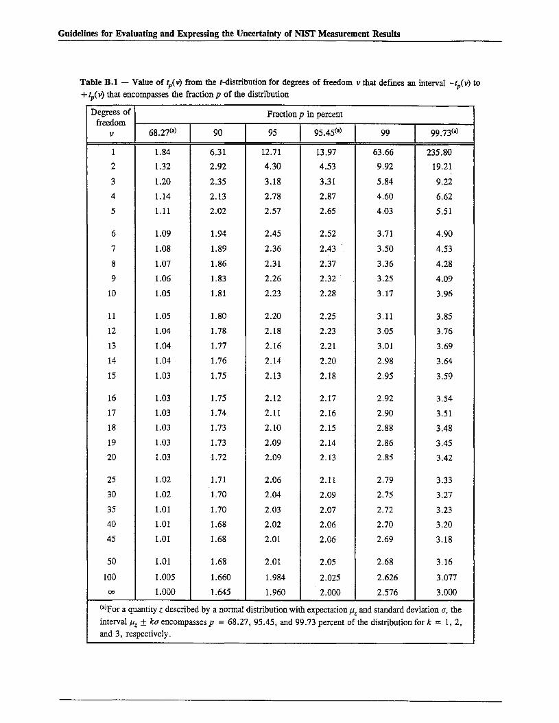
Guidelines for Evaluating and Expressing the Uncertainty of NIST Measurement Results

Table B.t - Value of tp<v) from the t-distribution for degrees of freedom v that defmes an interval -tp(v) to+ tp( v) that encompasses the fraction p of the distribution

Degrees of Fraction p in percentfreedom

v 68.27(a) 90 95 95.45(a) 99 99.73(a)

1 1.84 6.31 12.71 13.97 63.66 235.80

2 1.32 2.92 4.30 4.53 9.92 19.21

3 1.20 2.35 3.18 3.31 5.84 9.22

4 1.14 2.13 2.78 2.87 4.60 6.62

5 1.11 2.02 2.57 2.65 4.03 5.51

6 1.09 1.94 2.45 2.52 3.71 4.90

7 1.08 1.89 2.36 2.43 3.50 4.53

8 1.07 1.86 2.31 2.37 3.36 4.28

9 1.06 1.83 2.26 2.32 3.25 4.09

10 1.05 1.81 2.23 2.28 3.17 3.96

11 1.05 1.80 2.20 2.25 3.11 3.85

12 1.04 1.78 2.18 2.23 3.05 3.76

13 1.04 1.77 2.16 2.21 3.01 3.69

14 1.04 1.76 2.14 2.20 2.98 3.64

15 1.03 1.75 2.13 2.18 2.95 3.59

16 1.03 1.75 2.12 2.17 2.92 3.54

17 1.03 1.74 2.11 2.16 2.90 3.51

18 1.03 1.73 2.10 2.15 2.88 3.48

19 1.03 1.73 2.09 2.14 2.86 3.45

20 1.03 1.72 2.09 2.13 2.85 3.42

25 1.02 1.71 2.06 2.11 2.79 3.33

30 1.02 1.70 2.04 2.09 2.75 3.27

35 1.01 1.70 2.03 2.07 2.72 3.23

40 1.01 1.68 2.02 2.06 2.70 3.20

45 1.01 1.68 2.01 2.06 2.69 3.18

50 1.01 1.68 2.01 2.05 2.68 3.16

100 1.005 1.660 1.984 2.025 2.626 3.077

00 1.000 1.645 1.960 2.000 2.576 3.000

(a)For a quantity Z described by a normal distribution with expectation J.lz and standard deviation a, the

interval J.lz ± ka encompasses p = 68.27,95.45, and 99.73 percent of the distribution for k = 1,2,and 3, respectively.

Guidelines for Evaluating and Expressing the Uncertainty of NIST Measurement Results

Appendix C

NIST Technical Communications Program

APPENDIXE

STATEMENTS OF UNCERTAINTY ASSOCIATED WITHMEASUREMENT RESULTS

A measurement result is complete only when

accompanied by a quantitative statement of its

uncertainty. This policy requires that NIST measurement

results be accompanied by such statements and that a

uniform approach to expressing measurement uncertainty

be followed.

1. Background

Since the early 1980s, an international consensus has

been developing on a uniform approach to the expression

of uncertainty in measurement. Many of NIST's sister

national standards laboratories as well as a number of

important metrological organizations, including the

Western European Calibration Cooperation (WECC) and

EUROMET, have adopted the approach recommended by

the International Committee for Weights and Measures

(CIPM) in 1981 [1] and reaffIrmed by the CIPM in 1986

[2].

Equally important, the CIPM approach has come into use

in a significant number of areas at NIST and is also

becoming accepted in U.S. industry. For example, the

National Conference of Standards Laboratories (NCSL)

is using it to develop a Recommended Practice on

measurement uncertainty for NCSL member laboratories.

The CIPM approach is based on Recommendation INC-1

(1980) of the Working Group on the Statement of

Uncertainties [3]. This group was convened in 1980 by the

International Bureau of Weights and Measures (BIPM) in

response to a request by the CIPM. More recently, at the

request of the CIPM, a joint BIPM/lEC/ISO/OlMLworking group developed a comprehensive reference

document on the general application of the CIPM

approach titled Guide to the Expression of Uncertainty inMeasurement [4] (IEC: International Electrotechnical

NIST Administrative Manual

Commission; ISO: International Organization for

Standardization; OIML: International Organization of

Legal Metrology). The development of the Guide is

prO\:iding further impetus to the worldwide adoption of

the CIPM approach.

2. Policy

All NIST measurement results are to be accompanied by

quantitative statements of uncertainty. To ensure that

such statements are consistent with each other and with

present international practice, this NIST policy adopts in

substance the approach to expressing measurement

uncertainty recommended by the International Committee

for Weights and Measures (CIPM). The CIPM approach

as adapted for use by NIST is:

1) Standard Uncertainty: Represent each component of

uncertainty that contributes to the uncertainty of the

measurement result by an estimated standard deviation

ui' termed standard uncertainty, equal to the positive

square root of the estimated variance U7.

2) Combined Standard Uncertainty: Determine the

combined standard uncertainty Uc of the measurement

result, taken to represent the estimated standard

deviation of the result, by combining the individual

standard uncertainties ui (and covariances as

appropriate) using the usual "root-sum-of-squares"

method, or equivalent established and documented

methods.

Commonly, Uc is used for reporting results of

determinations of fundamental constants, fundamental

metrological research, and international comparisons of

realizations of SI units.

4.09 Appendix E

Guidelines for Evaluating and Expressing the Uncertainty of NIST Measurement Results

NIST Technical Communications Program

3) Expanded Uncertainty: Determine an expanded

uncertainty U by multiplying Uc by a coverage factor k:

U = kuc ' The purpose of U is to provide an interval

y - U to y + U about the result y within which the

value of Y, the specific quantity subject to

measurement and estimated by y, can be asserted to lie

with a high level of confidence. Thus one can

confidently assert that y - U :::;; y:::;; y + U, which is

commonly written as Y = Y ± U.

Use expanded uncertainty U to report the results of all

NIST measurements other than those for which Uc hastraditionally been employed. To be consistent with

current international practice, the value of k to beused at NIST for calculating U is, by convention,k = 2. Values of k other than 2 are only to be used forspecific applications dictated by established anddocumented requirements.

4) Reporting Uncertainty: Report U together with the

coverage factor k used to obtain it, or report uc '

When reporting a measurement result and itsuncertainty, include the following information in thereport itself or by referring to a published document:

- A list of all components of standard uncertainty,together with their degrees of freedom whereappropriate, and the resulting value of uc' Thecomponents should be identified according to themethod used to estimate their numerical values:

A. those which are evaluated by statisticalmethods,

B. those which are evaluated by other means.

- A detailed description of how each component ofstandard uncertainty was evaluated.

- A description of how k was chosen when k is not

taken equal to 2.

It is often desirable to provide a probabilityinterpretation, such as a level of confidence, for theinterval defmed by U or uc' When this is done, thebasis for such a statement must be given.

NIST Administrative Manual

ii

Additional guidance on the use of the CIPM approach atNIST may be found in Guidelines for Evaluating and

Expressing the Uncertainty ofMST Measurement Results

[5]. A more detailed discussion of the CIPM approach is

given in the Guide to the Expression of Uncertainty in

Measurement [4]. Classic expositions of the statistical

evaluation of measurement processes are given inreferences [6-8].

3. Responsibilities

a. Operating Unit Directors are responsible for

compliance with this policy.

b. The Statistical Engineering Division, Computing andApplied Mathematics Laboratory, is responsible forproviding technical advice on statistical methods forevaluating and expressing the uncertainty of NISTmeasurement results.

c. NIST Editorial Review Boards are responsible forensuring that statements of measurement uncertainty areincluded in NIST publications and other technical outputsunder their jurisdiction which report measurement resultsand that such statements are in conformity with thispolicy.

d. The Calibrations Advisory Group is responsible forensuring that calibration and test reports and othertechnical outputs under its jurisdiction are in compliancewith this policy.

e. The Standard Reference Materials and StandardReference Data programs are responsible for ensuring thattechnical outputs under their jurisdiction are incompliance with this policy.

f. Authors, as part of the process of preparingmanuscripts and other technical outputs, are responsiblefor formulating measurement uncertainty statementsconsistent with this policy. These statements must bepresent in drafts submitted for NIST review and approval.

4.09 Appendix E

Guidelines for Evaluating and Expressing the Uncertainty of NIST Measurement Results

NIST Technical Communications Program

4. Exceptions

It is understood that any valid statistical method that is

technically justified under the existing circumstances may

be used to determine the equivalent of ui ' uC ' or U.Further, it is recognized that international, national, or

contractual agreements to which NIST is a party may

occasionally require deviation from this policy. In both

cases, the report of uncertainty must document what was

done and why.

5. References Cited

[1] CIPM, BIPM Proc. Verb. Com. Int. Poids et Mesures49, 8-9,26 (1981) (in French); P. Giacomo, "News

from the BIPM," Metrologia 18, 41-44 (1982).

[2] CIPM, BIPM Proc.-Verb. Com. Int. Poids et Mesures54, 14, 35 (1986) (in French); P. Giacomo, "News

from the BIPM," Metrologia 24, 45-51 (1987).

[3] R. Kaarls, "Rapport du Groupe de Travail sur

l'Expression des Incertitudes au Comite

International des Poids et Mesures," Proc. -Verb.Com. Int. Poids et Mesures 49, AI-A12 (1981) (in

French); P. Giacomo, "News from the BIPM,"

Metrologia 17, 69-74 (1981). (Note that the fmal

English-language version of Recommendation INC­

1 (1980), published in an internal BIPM report,

differs slightly from that given in the latter

reference but is consistent with the authoritative

French-language version given in the former

reference.)

[4] ISO, Guide to the Expression of Uncertainty inMeasurement, prepared by ISO Technical Advisory

Group 4 (TAG 4), Working Group 3 (WG 3),

NIST Administrative Manual

iii

October 1993. ISO/TAG 4 has as its sponsors the

BIPM, IEC, IFCC (International Federation of

Clinical Chemistry), ISO, IUPAC (International

Union of Pure and Applied Chemistry), IUPAP

(International Union of Pure and Applied Physics),

and OIML. Although the individual members of

WG 3 were nominated by the BIPM, IEC, ISO, or

OIML, the Guide is published by ISO in the name

of all seven organizations. NIST staff members may

obtain a single copy of the Guide from the NIST

Calibration Program.

[5] B. N. Taylor and C. E. Kuyatt, Guidelines forEvaluating and Expressing the Uncertainty of NISTMeasurement Results, NIST Technical Note 1297,

prepared under the auspices of the NIST Ad Hoc

Committee on Uncertainty Statements (U.S.

Government Printing Office, Washington, DC,

January 1993).

[6] C. Eisenhart, "Realistic Evaluation of the Precision

and Accuracy of Instrument Calibration Systems,"

1. Res. Nat!. Bur. Stand. (U.S.) 67C, 161-187 (1963).

Reprinted, with corrections, in PrecisionMeasurement and Calibration: Statistical Conceptsand Procedures, NBS Special Publication 300, Vol.

I, H. H. Ku, Editor (U.S. Government Printing

Office, Washington, DC, 1969), pp. 21-48.

[7] J. Mandel, The Statistical Analysis of ExperimentalData (Interscience-Wiley Publishers, New York,

NY, 1964, out of print; corrected and reprinted,

Dover Publishers, New York, NY, 1984).

[8] M. G. Natrella, Experimental Statistics, NBS

Handbook 91 (U.S. Government Printing Office,

Washington, DC, 1963; reprinted October 1966 with

corrections).

4.09 Appendix E

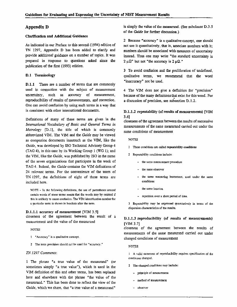
Guidelines for Evaluating and Expressing the Uncertainty of NIST Measurement Results

Appendix D

Clarification and Additional Guidance

As indicated in our Preface to this second (1994) edition ofTN 1297, Appendix 0 has been added to clarify and

provide additional guidance on a number of topics. It was

prepared in response to questions asked since the

publication of the first (1993) edition.

D.1 Tenninology

D.1.1 There are a number of terms that are commonly

used in connection with the subject of measurementuncertainty, such as accuracy of measurement,reproducibility of results of measurements, and correction.One can avoid confusion by using such terms in a way thatis consistent with other international documents.

Definitions of many of these terms are given in the

International Vocabulary of Basic and General Terms in

Metrology [0.1], the title of which is commonly

abbreviated VIM. The VIM and the Guide may be viewed

as companion documents inasmuch as the VIM, like the

Guide, was developed by ISO Technical Advisory Group 4

(TAG 4), in this case by its Working Group I (WG 1); and

the VIM, like the Guide, was published by ISO in the nameof the seven organizations that participate in the work of

TAG 4. Indeed, the Guide contains the VIM definitions of24 relevant terms. For the convenience of the users of

TN 1297, the defmitions of eight of these terms are

included here.

NOTE - In the following deftnitions, the use of parentheses around

certain words of some terms means that the words may by omitted if

this is unlikely to cause confusion. The VIM identification number for

a particular term is shown in brackets after the term.

D.1.1.1 accuracy of measurement [VIM 3.5]closeness of the agreement between the result of a

measurement and the value of the measurand

NOTES

"Accuracy" is a qualitative concept.

2 The term precision should not be used for "accuracy."

TN 1297 Comments:

1 The phrase "a true value of the measurand" (orsometimes simply "a true value"), which is used in the

VIM defmition of this and other terms, has been replacedhere and elsewhere with the phrase "the value of themeasurand." This has been done to reflect the view of theGuide, which we share, that "a true value of a measurand"

is simply the value of the measurand. (See subclause 0.3.5of the Guide for further discussion.)

2 Because "accuracy" is a qualitative concept, one shouldnot use it quantitatively, that is, associate numbers with it;numbers should be associated with measures of uncertaintyinstead. Thus one may write "the standard uncertainty is

2 110" but not "the accuracy is 2 110."

3 To avoid confusion and the proliferation of undefmed,

qualitative terms, we recommend that the word

"inaccuracy" not be used.

4 The VIM does not give a definition for "precision"

because of the many definitions ~at exist for this word. Fora discussion of precision, see subsection 0.1.2.

D.1.1.2 repeatability (of results of measurements) [VIM3.6]closeness of the agreement between the results of successivemeasurements of the same measurand carried out under the

same conditions of measurement

NOTES

These conditions are called repeatability conditions

2 Repeatability conditions include:

- the same measurement procedure

- the same observer

- the same measuring instrument, used under the same

conditions

- the same location

- repetition over a shon period of time.

3 Repeatability may be expressed quantitatively in terms of the

dispersion characteristics of the results.

D.1.1.3 reproducibility (of results of measurements)[VIM 3.7]closeness of the agreement between the results ofmeasurements of the same measurand carried out underchanged conditions of measurement

NOTES

I A valid statement of reproducibility requires speciftcation of the

conditions changed.

2 The changed conditions may include:

- principle of measurement

- method of measurement

- observer

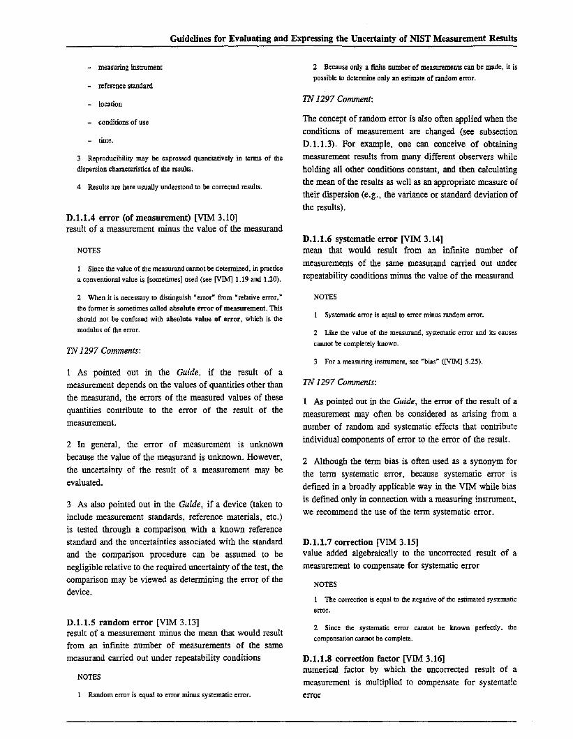
- measuring instrument

- reference standard

- location

Guidelines for Evaluating and Expressing the Uncertainty of NIST Measurement Results

2 Because only a finite number of measurements can be made, it is

possible to determine only an estimate of random error.

TN 1297 Comment:

- conditions of use

- time.

3 Reproducibility may be expressed quantitatively in terms of the

dispersion characteristics of the results.

4 Results are here usually understood to be corrected results.

D.1.1.4 error (of measurement) [VIM 3.10]result of a measurement minus the value of the measurand

NOTES

1 Since the value of the measurand cannot be determined. in practice

a conventional value is [sometimes] used (see [VIM] 1.19 and 1.20).

2 When it is necessary to distinguish "error" from "relative error."

the former is sometimes called absolute error of measurement. This

should not be confused with absolute value of error. which is the

modulus of the error.

TN 1297 Comments:

1 As pointed out in the Guide, if the result of ameasurement depends on the values of quantities other than

the measurand, the errors of the measured values of thesequantities contribute to the error of the result of the

measurement.

2 In general, the error of measurement is unknown

because the value of the measurand is unknown. However,

the uncertainty of the result of a measurement may be

evaluated.

3 As also pointed out in the Guide, if a device (taken toinclude measurement standards, reference materials, etc.)is tested through a comparison with a known referencestandard and the uncertainties associated with the standardand the comparison procedure can be assumed to be

negligible relative to the required uncertainty of the test, thecomparison may be viewed as determining the error of thedevice.

D.I.l.S random error [VIM 3.13]result of a measurement minus the mean that would resultfrom an infmite number of measurements of the samemeasurand carried out under repeatability conditions

NOTES

1 Random error is equal to error minus systematic error.

The concept of random error is also often applied when the

conditions of measurement are changed (see subsectionD.1.1.3). For example, one can conceive of obtaining

measurement results from many different observers while

holding all other conditions constant, and then calculating

the mean of the results as well as an appropriate measure oftheir dispersion (e.g., the variance or standard deviation of

the results).

D.1.1.6 systematic error [VIM 3.14]mean that would result from an infmite number of

measurements of the same measurand carried out under

repeatability conditions minus the value of the measurand

NOTES

Systematic error is equal to error minus random error.

2 Like the value of the measurand, systematic error and its causes

cannot be completely known.

3 For a measuring instrument. see "bias" ([VIM] 5.25).

TN 1297 Comments:

1 As pointed out in the Guide, the error of the result of ameasurement may often be considered as arising from a

number of random and systematic effects that contribute

individual components of error to the error of the result.

2 Although the term bias is often used as a synonym for

the term systematic error, because systematic error is

defined in a broadly applicable way in the VIM while bias

is defmed only in connection with a measuring instrument,

we recommend the use of the term systematic error.

D.l.1.7 correction [VIM 3.15]value added algebraically to the uncorrected result of ameasurement to compensate for systematic error

NOTES

I The correction is equal to the negative of the estimated systematic

error.

2 Since the systematic error cannot be known perfectly. the

compensation cannot be complete.

D.I.I.S correction factor [VIM 3.16]numerical factor by which the uncorrected result of a

measurement is multiplied to compensate for systematic

error

Guidelines for Evaluating and Expressing the Uncertainty of NIST Measurement Results

NOTE - Since the systematic error cannot be known perfectly. the

compensation cannot be complete, .

D.1.2 As indicated in subsection D.1.1.1, TN 1297comment 4, the VIM does not give a defInition for the

word "precision." However, ISO 3534-1 [0.2] dermes

precision to mean "the closeness of agreement between

independent test results obtained under stipulated

conditions." Further, it views the concept of precision as

encompassing both repeatability and reproducibility (see

subsections D.1.1.2 and D.1.1.3) since it dermes

repeatability as "precision under repeatability conditions, "and reproducibility as "precision under reproducibilityconditions." Nevertheless, precision is often taken to mean

simply repeatability.•

The term precision, as well as the terms accuracy,repeatability, reproducibility, variability, and uncertainty,are examples of terms that represent qualitative concepts

and thus should be used with care. In particular, it is our

strong recommendation that such terms not be used as

synonyms or labels for quantitative estimates. For example,the statement "the precision of the measurement results,

expressed as the standard deviation obtained underrepeatability conditions, is 2 110" is acceptable, but thestatement "the precision of the measurement results is 2110" is not. (See also subsection D.1.1.1, TN 1297

comment 2.)

Although reference [0.2] states that "The measure ofprecision is usually expressed in terms of imprecision andcomputed as a standard deviation of the test results," werecommend that to avoid confusion, the word "imprecision"

not be used; standard deviation and standard uncertainty arepreferred, as appropriate (see subsection D.1.5).

It should also be borne in mind that the NIST policy onexpressing the uncertainty of measurement results normallyrequires the use of the terms standard uncertainty,

combined standard uncertainty, expanded uncertainty, ortheir "relative" forms (see subsection D.1.4), and thelisting of all components of standard uncertainty. Hence theuse of terms such as accuracy, precision, and bias should

normally be as adjuncts to the required terms and theirrelationship to the required terms should be made clear.This situation is similar to the NIST policy on the use ofunits that are not part of the 51: the SI units must be statedfIrst, with the units that are not part of the SI in parentheses(see subsection D.6.2).

D.1.3 The designations"A" and "B" apply to the two

distinct methods by which uncertainty components may beevaluated. However, for convenience, a standard

uncertainty obtained from a Type A evaluation may becalled a Type A standard uncenainty; and a standarduncertainty obtained from a type B evaluation may be calleda Type B standard uncenainty. This means that:

(1) "A" and "B" have nothing to do with the traditional

terms "random" and "systematic";

(2) there are no "Type A errors" or "Type B errors";

and

(3) "Random uncertainty" (Le., an uncertainty

component that arises from a random effect) is not asynonym for Type A standard uncertainty; and

"systematic uncertainty" (Le., an uncertainty componentthat arises from a correction for a systematic error) isnot a synonym for Type B standard uncertainty.

In fact, we recommend that the terms "random uncertainty"and "systematic uncertainty" be avoided because the

adjectives "random" and "systematic," while appropriatemodifIers for the word "error," are not appropriate

modifIers for the word "uncertainty" (one can hardly

imagine an uncertainty component that varies randomly or

that is systematic).

D.1.4 If u(xi) is a standard uncertainty, then u(xi)/ Ixd 'xi;cO, is the corresponding relative standard uncenainty; if

uc(Y) is a combined standard uncertainty, then uc(Y)/IYI,Y ;c0, is the corresponding relative combined standard

uncenainty; and if U=kuc(Y) is an expanded uncertainty,then U/ IY I, y;c 0, is the corresponding relative expanded

uncenainty. Such relative uncertainties may be readilyindicated by using a subscript "r" for the word "relative."

Thus Ur(Xi ) = u(Xi)/ lXii, uciY) = uc(Y)/ IYI, and Ur=U/ Iy I·

D.l.S As pointed out in subsection D.1.2, the use of theterms standard uncertainty, combined standard uncertainty,expanded uncertainty, or their equivalent "relative" forms(see subsection D.1.4), is normally required by NISTpolicy. Alternate terms should therefore play a subsidiaryrole in any NIST publication that reports the result of ameasurement and its uncertainty. However, since it will

take some time before the meanings of these terms becomewell known, they should be defIned at the beginning of apaper or when fIrst used. In the latter case, this may bedone by writing, for example, "the standard uncertainty

(estimated standard deviation) is u(R) =2 110"; or "theexpanded uncertainty (coverage factor k=2 and thus a two­

standard-deviation estimate) is U=4 110."

It should also be recognized that, while an estimatedstandard deviation that is a component of uncertainty of a

Guidelines for Evaluating and Expressing the Uncertainty of NIST Measurement Results

measurement result is properly called a "standard

uncertainty," not every estimated standard deviation is

necessarily a standard uncertainty.

terms, and therefore suggest that NIST authors considerusing them.

D.2 Identification of uncertainty components

D.1.6 Words such as "estimated" or "limits of" should

normally not be used to modify "standard uncertainty,"

"combined standard uncertainty," "expanded uncertainty,"

the "relative" forms of these terms (see subsection 0 .1.4),

or more generally "uncertainty." The word "uncertainty,"

by its very nature, implies that the uncertainty of the result

of a measurement is an estimate and generally does not

have well-defmed limits.

D.1.7 The phrase "components of uncertainty that

contribute to the uncertainty of the measurement result" can

have two distinct meanings. For example, if the input

estimates xj are uncorrelated, Eq. (A-3) of Appendix A may

be written as

D.2.1 The NIST policy on expressing measurement

uncertainty states that all components of standard

uncertainty "should be identified according to the method

used to estimate their numerical values: A. those which are

evaluated by statistical methods, B. those which areevaluated by other means."

Such identification will usually be readily apparent in the

"detailed description of how each component of standard

uncert~ty was evaluated" that is required by the NIST

policy. However, such identification can also be given in a

table which lists the components of standard uncertainty.

Tables 0.1 and 0.2, which are based on the end-gauge

D.1.8 The VIM gives the name "experimental standard

deviation of the mean" to the quantity seX) of Eq. (A-5) ofAppendix A of this Technical Note, and the name

"expe~mental standard deviation" to the quantity s(Xj•k) =Vii s(Xj). We believe that these are convenient, descriptive

When one gives the components of uncertainty of a resultof a measurement, it is recommended that one also give thestandard uncertainties u(xj) of the input estimates Xj, the

sensitivity coefficients cj == atlaxj , and the standarduncertainties uj ( y) = Icj Iu(xj) of which the combinedstandard uncertainty uc(y) is composed (so-called standarduncertainty components of combined standard uncertainty).

In Eq. (D-1), both u(x) and Uj(Y) can be consideredcomponents of uncertainty of the measurement result y.This is because the u(xj) are the standard uncertainties of

the input estimates Xj on which the output estimate or

measurement result y depends; and the Uj(y) are the

standard uncertainties of which the combined standard

uncertainty uc(y) of the measurement result y is composed.In short, both u(xj ) and u;( y) can be viewed as components

of uncertainty that give rise to the combined standarduncertainty uc(y) of the measurement result y. This implies

that in subsections 2.4 to 2.6, 4.4 to 4.6, and 6.6; in 1) and2) of section 2 of Appendix C; and in section 4 of

Appendix C, the symbols uj , Sj, or Uj may be viewed asrepresenting either u(x) or uj(y).

Table D.l - yncertainty Budget:End-Gauge Calibration

Source ofStandard

uncertaintyuncertainty

(nm)

Calibration of standard endgauge 25 (B)

Measured difference betweenend gauges:

repeated observations 5.8 (A)

random effects ofcomparator 3.9 (A)

systematic effects ofcomparator 6.7 (B)

Thermal expansion ofstandard end gauge 1.7 (B)

Temperature of test bed:

mean temperature of bed 5.8 (A)

cyclic variation oftemperature of room 10.2 (B)

Difference in expansioncoefficients of end gauges 2.9 (B)

Difference in temperatures ofend gauges 16.6 (B)

Combined standard uncertainty: uc(l) = 34 nm

(0-1)N N

u; = L [c j U(X)]2 E L u;(Y),j = 1 j= 1

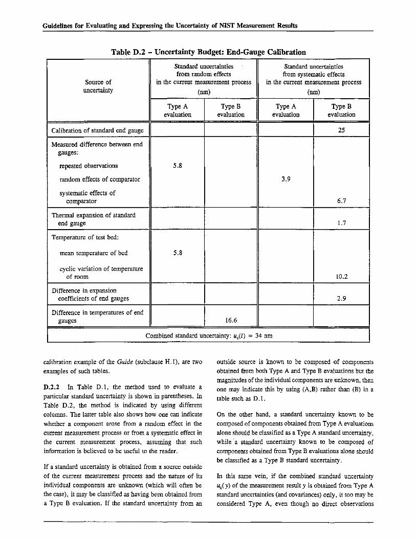
Guidelines for Evaluating and Expressing the Uncertainty of NIST Measurement Results

Table D.2 - Uncertainty Budget: End-Gauge Calibration

Standard uncertainties Standard uncertaintiesfrom random effects from systematic effects

Source of in the current measurement process in the current measurement processuncertainty (nm) (nm)

Type A Type B Type A Type Bevaluation evaluation evaluation evaluation

Calibration of standard end gauge 25

Measured difference between endgauges:

repeated observations 5.8

random effects of comparator 3.9

systematic effects ofcomparator 6.7

Thermal expansion of standardend gauge 1.7

Temperature of test bed:

mean temperature of bed 5.8

cyclic variation of temperatureof room 10.2

Difference in expansioncoefficients of end gauges 2.9

Difference in temperatures of endgauges 16.6

Combined standard uncertainty: uc(l) = 34 nm

calibration example of the Guide (subclause H.I), are two

examples of such tables.

D.2.2 In Table D.I, the method used to evaluate a

particular standard uncertainty is shown in parentheses. InTable D.2, the method is indicated by using different

columns. The latter table also shows how one can indicate

whether a component arose from a random effect in the

current measurement process or from a systematic effect in

the current measurement process, assuming that such

information is believed to be useful to the reader.

If a standard uncertainty is obtained from a source outside

of the current measurement process and the nature of itsindividual components are unknown (which will often be

the case), it may be classified as having been obtained froma Type B evaluation. If the standard uncertainty from an

outside source is known to be composed of components

obtained from both Type A and Type B evaluations but the

magnitudes of the individual components are unknown, then

one may indicate this by using (A,B) rather than (B) in a

table such as D.l.

On the other hand, a standard uncertainty known to be

composed of components obtained from Type A evaluations

alone should be classified as a Type A standard uncertainty,

while -a standard uncertainty known to be composed of

components obtained from Type B evaluations alone shouldbe classified as a Type B standard uncertainty.

In this same vein, if the combined standard uncertainty

uc(y) of the measurement result y is obtained from Type Astandard uncertainties (and covariances) only, it too may be

considered Type A, even though no direct observations

Guidelines for Evaluating and Expressing the Uncertainty of NIST Measurement Results

were made of the measurand Yof which the measurement

result y is an estimate. Similarly, if a combined standarduncertainty is obtained from Type B standard uncertainties(and covariances) only, it too may be considered Type B.

D.3 Equation (A-2)

of measurement. In this case, the uncertainty depends not

only on the repeatability and reproducibility of themeasurement results (see subsections 0.1.1.2 and 0.1.1.3),

but also on how well one believes the standard

measurement method has been implemented. (See exampleH.6 of the Guide.)

Or the output estimate y may be expressible simply as

D.3.1 In the most general sense, Eq. (A-2) of Appendix

A of this Technical Note,

Xl = gl(WI' wz' , wx)

Xz =gizl' Zz' , ZL)

etc.

When reporting the estimated value and uncertainty of such

a measurand, one should always make clear that the

measurand is defined by a particular method of

measurement and indicate what that method is. One should

also give the measurand a name which indicates that it is

defmed by a measurement method, for example, by adding

a modifier such as "conventional." (See also subsection

0.6.1)

D.4.2 There are national as well as international

standards that discuss the characterization of test methods

by interlaboratory comparisons. Execution of test methods

according to these standards, both in the characterization

stage and in subsequent measurement programs, often calls

for the expression of uncertainties in terms of defmed

measures of repeatability and reproducibility. When NISTauthors participate in such characterization or measurement

programs, NIST policy allows for the results to be

expressed as required by the relevant standards (seeAppendix C, section 4). However, when NIST authorsdocument work according to such standards, they should

consider making the resulting publication understandable to

a broad audience. This might be achieved in part by giving

definitions of the terms used, perhaps in a footnote. If.possible, NIST authors should relate these terms to those of

this Technical Note and of the Guide.

(A-2)

is a symbolic representation of the procedure (or algorithm)

used to obtain the output estimate y, which is the result of

~he measurement, from the individual input estimates Xi'

For example, some of the Xi may themselves depend on

additional input estimates:

where the Ci are corrections, for example, for the operator,

for the ambient temperature, for the laboratory, etc. Some

or all of the Ci may be estimated to be near zero based onthe available information, but they can still have standarduncertainties that are large enough to contribute

significantly to the combined standard uncertainty of themeasurement result and which therefore must be evaluated.

NOTE - In some situations, a correction for a particular effect and its

standard uncertainty are estimated to be negligible relative to the

required combined standard uncertainty of the measurement result, and

for added confidence, an experimental test is carried out that confirms

the estimate but the standard uncertainty of the test result is not

negligible. In such cases, if other evidence indicates that the estimate

is in fact reliable, the standard uncertainty of the test result need not

be included in the uncertainty budget and both the correction and its

standard uncertainty can be taken as negligible.

If a test method is employed at NIST to obtainmeasurement results for reasons other than those described

above, it is expected that the uncertainties of these

measurement results will be evaluated and reportedaccording to section 2 of the NIST policy (see AppendixC). This would be the case, for example, if measurementresults from a characterized test method are compared to

those from a new method of measurement which has notbeen characterized by interlaboratory comparisons.

D.4 Measurand defined by the measurement method;

characterization of test methods; simple calibration

D.4.1 The approach to evaluating and expressing theuncertainty of a measurement result on which the NISTpolicy and this Technical Note are based is applicable toevaluating and expressing the uncertainty of the estimated

value of a measurand that is defined by a standard method

D.4.3 When an unknown standard is calibrated in terms

of a known reference standard at lower levels of the

measurement hierarchy, the uncertainty of the result of

calibration may have as few as two components: a singleType A standard uncertainty evaluated from the pooledexperimental standard deviation that characterizes the

calibration process; and a single Type B (or possibly

Guidelines for Evaluating and Expressing the Uncertainty of NIST Measurement Results

Type A) standard uncertainty obtained from the calibrationcertificate of the known reference standard.

NOTE - The possibility of unsuspected systematic effects in the

calibration process used to calibrate the unknown standard should,

however, not be overlooked.

D.S Ip and the quantile 11 - 4

D.S.1 As pointed out in the Guide, the t-distribution is

often tabulated in quantiles. That is, values of the quantile

t1_ a are given, where 1 - a denotes the cumulative

probability and the relation

Itl-a1 - a = f(t, v)dt

-00

defines the quantile, where f is the probability density

function of t. Thus tp of this Technical Note and of theGuide and t1-a are related by p = 1 - 2 a. For example, the

value of the quantile to.975' for which 1 - a =0.975 anda =0.025, is the same as tiv) for p = 0.95. It should be

noted, however, that in reference [D.2] the symbol p isused for the cumulative probability 1 - a, and the resulting

t/v) is called the "quantile of order p of the t variable with

v degrees of freedom. " Clearly, the values of t/v) defined

in this way differ from the values of t/v) defmed as in thisTechnical Note and in the Guide, and given in Table B.l

(which is of the same form as that given in reference [l0]).Thus, one must use tables of tabulated values of t/v) with

some care.

D.6 Uncertainty and units of the Sf; proper use of theSf and quantity and unit symbols

D.6.1 As pointed out in the Guide, the result of a

measurement is sometimes expressed in terms of theadopted value of a measurement standard or in terms of aconventional reference value rather than in terms of therelevant unit of the SI. (This is an example of a situation in

which all significant components of uncertainty are nottaken into ~ccount.) In such cases the magnitude of theuncertainty ascribable to the measurement result may besignificantly smaller than when that result is expressed inthe relevant SI unit. This practice is not disallowed by theNIST policy, but it should always be made clear when thepractice is being followed. In addition, one should alwaysgive some indication of the values of the components ofuncertainty not taken into account. The following example

is taken from the Guide. (See also subsection D.4.1.)

EXAMPLE - A high~ Zener vollage standard is calibrated by

comparison with a Josephson effect voltage reference based on the

conventional value of the Josephson constant recommended for

international use by the CIP:M. The relative combined standard

uncertainty Ue(Vs )/Vs of the calibrated potential difference Vs of the

Zener standard is 2 x 10-& when Vs is reponed in terms of the

conventional value, but ll::(Vs )/Vs is 4x 10-7 when Vs is reponed in

terms of the 51 unit of potential difference, the volt (V), because of the

additional uncertainty associated with the 51 value of the Josephson

constant.

D.6.2 NIST Special Publication 811,1995 Edition [D.3],gives guidance on the use of the SI and on the rules and

style conventions regarding quantity and unit symbols. In

particular, it elaborates upon the NIST policy regarding the

SI and explains why abbreviations such as ppm and ppb and

terms such as normality and molarity should not be used.NIST authors should consult NIST SP 811 if they have anyquestions concerning the proper way to express the values

of quantities and their uncenainties.

D.7 References

[D.l] ISO, International Vocabulary of Basic and General

Terms in Metrology, second edition (InternationalOrganization for Standardization. Geneva, Switzerland,1993). This document (abbreviated VIM) was prepared by

ISO Technical Advisory Group 4 (TAG 4), Working Group1 (WG 1). ISOITAG 4 has as its sponsors the BIPM, IEC,IFCC (International Federation of Clinical Chemistry), ISO,IUPAC (International Union of Pure and AppliedChemistry), IUPAP (International Union of Pure and

Applied Physics), and OIML. The individual members ofWG 1 were nominated by BIPM, lEC, IFCC, ISO, IUPACIUPAP, or OIML, and the document is published by ISO

in the name of all seven organizations. NIST staff membersmay obtain a single copy of the VIM from the NISTCalibration Program.

[D.2] ISO 3534-1:1993, Statistics- Vocabulary and

symbols - Part 1: Probabilicy and general statistical terms

(International Organization for Standardization, Geneva,Switzerland, 1993).

[D.3] B. N. Taylor, Guidefor the Use of the International

System of Units (51), r-.1ST Special Publication 811, 1995Edition (U.S. Government Printing Office, Washington,DC, Apri11995).