Students Solutions Manual
182
Students Solutions Manual Fundamentals of Machine Learning for Predictive Data Analytics
-
Upload
khangminh22 -
Category
Documents
-
view
8 -
download
0
Transcript of Students Solutions Manual

Students Solutions ManualFundamentals of Machine Learning for Predictive Data Analytics


Students Solutions ManualFundamentals of Machine Learning for Predictive Data Analytics
Algorithms, Worked Examples, and Case Studies
Second Edition
John D. Kelleher, Brian Mac Namee, and Aoife D’Arcy
The MIT PressCambridge, MassachusettsLondon, England


Contents
Notation vii
I INTRODUCTION TO MACHINE LEARNING ANDDATA ANALYTICS
1 Machine Learning for Predictive Data Analytics (Exercise Solutions) 3
2 Data to Insights to Decisions (Exercise Solutions) 7
3 Data Exploration (Exercise Solutions) 13
II PREDICTIVE DATA ANALYTICS
4 Information-Based Learning (Exercise Solutions) 35
5 Similarity-Based Learning (Exercise Solutions) 51
6 Probability-Based Learning (Exercise Solutions) 61
7 Error-Based Learning (Exercise Solutions) 71
8 Deep Learning (Exercise Solutions) 83
9 Evaluation (Exercise Solutions) 133

vi Contents
III BEYOND PREDICTION
10 Beyond Prediction: Unsupervised Learning (Exercise Solutions) 149
11 Beyond Prediction: Reinforcement Learning (Exercise Solutions) 159
Bibliography 167

Notation
In this section we provide a short overview of the technical notation used throughout thisbook.
Notational ConventionsThroughout this book we discuss the use of machine learning algorithms to train pre-
diction models based on datasets. The following list explains the notation used to referto different elements in a dataset. Figure 0.1[vii] illustrates the key notation using a simplesample dataset.
ID Name Age Country Rating
1 Brian 24 Ireland B
2 Mary 57 France AA
3 Sinead 45 Ireland AA
4 Paul 38 USA A
5 Donald 62 Canada B
6 Agnes 35 Sweden C
7 Tim 32 USA B
DRating=AA
D
d7
d5[3]
d[1]
t4
Figure 0.1How the notation used in the book relates to the elements of a dataset.

viii Notation
Datasets‚ D denotes a dataset.‚ A dataset is composed of n instances, pd1, t1q to pdn, tnq, where d is a set of m descriptive
features, and t is a target feature.‚ A subset of a dataset is denoted by D with a subscript to indicate the definition of the
subset. For example, D f“l represents the subset of instances from the dataset D wherethe feature f has the value l.
Vectors of Features‚ Lowercase boldface letters refer to a vector of features. For example, d denotes a vector
of descriptive features for an instance in a dataset, and q denotes a vector of descriptivefeatures in a query.
Instances‚ Subscripts are used to index into a list of instances.‚ xi refers to the ith instance in a dataset.‚ di refers to the descriptive features of the ith instance in a dataset.
Individual Features‚ Lowercase letters represent a single feature (e.g., f , a, b, c . . .).‚ Square brackets rs are used to index into a vector of features (e.g., d r js denotes the value
of the jth feature in the vector d).‚ t represents the target feature.
Individual Features in a Particular Instance‚ di r js denotes the value of the jth descriptive feature of the ith instance in a dataset.‚ ai refers to the value for feature a of the ith instance in a dataset.‚ ti refers to the value of the target feature of the ith instance in a dataset
Indexes‚ Typically, i is used to index instances in a dataset, and j is used to index features in a
vector.
Models‚ We useM to refer to a model.‚ Mw refers to a modelM parameterized by a parameter vector w.‚ Mwpdq refers to the output of a modelM parameterized by parameters w for descriptive
features d.

Notation ix
Set Size‚ Vertical bars | | refer to counts of occurrences (e.g., |a “ l| represents the number of
times that a “ l occurs in a dataset).
Feature Names and Feature Values‚ We use a specific typography when referring to a feature by name in the text (e.g., PO-
SITION, CREDITRATING, and CLAIM AMOUNT).‚ For categorical features, we use a specific typography to indicate the levels in the domain
of the feature when referring to a feature by name in the text (e.g., center, aa, and softtissue).
Notational Conventions for ProbabilitiesFor clarity there are some extra notational conventions used in Chapter 6[243] on probability.
Generic Events‚ Uppercase letters denote generic events where an unspecified feature (or set of features)
is assigned a value (or set of values). Typically, we use letters from the end of thealphabet—e.g., X, Y , Z—for this purpose.
‚ We use subscripts on uppercase letters to iterate over events. So,ř
i PpXiq should beinterpreted as summing over the set of events that are a complete assignment to thefeatures in X (i.e., all the possible combinations of value assignments to the features inX).
Named Features‚ Features explicitly named in the text are denoted by the uppercase initial letters of their
names. For example, a feature named MENINGITIS is denoted by M.
Events Involving Binary Features‚ Where a named feature is binary, we use the lowercase initial letter of the name of the
feature to denote the event where the feature is true and the lowercase initial letter pre-ceded by the symbol to denote the event where it is false. So, m will represent theevent MENINGITIS “ true, and m will denote MENINGITIS “ false.
Events Involving Non-Binary Features‚ We use lowercase letters with subscripts to iterate across values in the domain of a fea-
ture.‚ So
ř
i Ppmiq “ Ppmq ` Pp mq.‚ In situations where a letter, for example, X, denotes a joint event, then
ř
i PpXiq shouldbe interpreted as summing over all the possible combinations of value assignments to thefeatures in X.

x Notation
Probability of an Event‚ The probability that the feature f is equal to the value v is written Pp f “ vq.
Probability Distributions‚ We use bold notation Ppq to distinguish a probability distribution from a probability mass
function Ppq.‚ We use the convention that the first element in a probability distribution vector is the
probability for a true value. For example, the probability distribution for a binary feature,A, with a probability of 0.4 of being true would be written PpAq “ă 0.4, 0.6 ą.
Notational Conventions for Deep LearningFor clarity, some additional notational conventions are used in Chapter 8[381] on deep learn-ing.
Activations‚ The activation (or output) of single neuron i is denoted by ai
‚ The vector of activations for a layer of neurons is denoted by apkq where k identifies thelayer.
‚ A matrix of activations for a layer of neurons processing a batch of examples is denotedby Apkq where k identifies the layer.
Activation Functions‚ We use the symbol ϕ to generically represent activation functions. In some cases we
use a subscript to indicate the use of a particular activation function. For example, ϕS M
indicates the use of a softmax function activation function, whereas ϕReLU indicates theuse of a rectified linear activation function.
Categorical Targets In the context of handling categorical target features (see Section8.4.3[463]) using a softmax function, we use the following symbols:
‚ We use the ‹ symbol to indicate the index of the true category in the distribution.‚ We use P to write the true probability distribution over the categories of the target; P to
write the distribution over the target categories that the model has predicted; and P‹ toindicate the predicted probability for the true category.
‚ We write t to indicate the one-hot encoding vector of a categorical target.‚ In some of the literature on neural networks, the term logit is used to refer to the result of
a weighted sum calculation in a neuron (i.e., the value we normally denote z). In partic-ular, this terminology is often used in the explanation of softmax functions; therefore, inthe section on handling categorical features, we switch from our normal z notation, andinstead follow this logit nomenclature, using the notation l to denote a vector of logitsfor a layer of neurons, and li to indicate the logit for the ith neuron in the layer.

Notation xi
Elementwise Product‚ We use d to denote an elementwise product. This operation is sometimes called the
Hadamard product.
Error Gradients (Deltas) δ‚ We use the symbol δ to indicate the rate of change of the error of the network with
respect to changes in the weighted sum calculated in a neuron. These δ values are theerror gradients that are backpropagated during the backward pass of the backpropagationalgorithm. We use a subscript to identify the particular neuron that the δ is associatedwith; for example, δi is the δ for neuron i and is equivalent to the term BE
Bzi. In some cases
we wish to refer to the vector of δs for the neurons in a layer l; in these cases we writeδplq
Network Error‚ We use the symbol E to denote the error of the network at the output layer.
Weights‚ We use a lowercase w to indicate a single weight on a connection between two neurons.
We use a double subscript to indicate the neurons that are connected, with the conventionthat the first subscript is the neuron the connection goes to, and the second subscript isthe neuron the connection is from. For example, wi,k is the weight on the connectionfrom neuron k to neuron i.
‚ We use ∆wi,k to write the sum of error gradients calculated for the weight wi,k. We sumerrors in this way during batch gradient descent with which we sum over the examplesin the batch; see Equation (8.30)[416] and also in cases in which the weight is shared by anumber of neurons, whether in a convolutional neural network or during backpropagationthrough time.
‚ We use a bold capital W to indicate a weight matrix, and we use a superscript in bracketsto indicate the layer of the network the matrix is associated with. For example, Wpkq isthe weight matrix for the neurons in layer k. In an LSTM network we treat the neuronsin the sigmoid and tanh layers within each gate as a separate layer of neurons, and sowe write Wp f q for the weight matrix for the neurons in the forget gate, and so on forthe weight matrices of the other neuron layers in the other gates. However, in a simplerecurrent network we distinguish the weight matrices on the basis of whether the matrixis on the connections between the input and the hidden layer, the hidden layer and theoutput, or the activation memory buffer and the hidden layer. Consequently, for thesematrices it is important to highlight the end of the connections the weights are appliedto; we use a double subscript (similar to the subscript for a single weight), writing Whx
for the weight matrix on the connections between the input (x) and the hidden layer (h).
Weighted Sums and Logits

xii Notation
‚ We use a lowercase z to represent the result of the weighted sum of the inputs in a neuron.We indicate the identity of the neuron in which the calculation occurred using a subscript.For example, zi is the result of the weighted sum calculation carried out in neuron i. Note,however, that in the section on Handling Categorical Target features, we switch to theterm logit to refer to the output of the weight sum in a neuron and update the notationto reflect this switch; see the previous notation section on Categorical Targets for moredetails.
‚ The vector of weighted sums for a layer of neurons is denoted by zpkq where k identifiesthe layer.
‚ A matrix of weighted sums calculations for a layer of neurons processing a batch ofexamples is denoted by Zpkq where k identifies the layer.
Notational Conventions for Reinforcement LearningFor clarity there are some extra notational conventions used in Chapter 11[637] on reinforce-ment learning (this chapter also heavily uses the notation from the probability chapter).
Agents, States, and Actions‚ In reinforcement learning we often describe an agent at time t taking an action, at, to
move from its current state, st, to the next state, st`1.‚ An agent’s current state is often modeled as a random variable, S t. We therefore often
describe the probability that an agent is in a specific state, s, at time t as PpS t “ sq.‚ Often states and actions are explicitly named, in which case we use the following for-
matting: STATE and action.
Transition Probabilities‚ We use the Ñ notation to represent an agent transitioning from one state to another.
Therefore, the probability of an agent moving from state s1 to state s2 can be written
Pps1 Ñ s2q “ PpS t`1 “ s2 | S t “ s1q
‚ Often we condition the probability of an agent transitioning from one state, s1, to another,s2, on the agent taking a specific action, a. We write this
Pps1aÝÑ s2q “ PpS t`1 “ s2 | S t “ s1, At “ aq

Notation xiii
‚ The dynamics of an environment in which an agent transitions between states, a Markovprocess, can be captured in a transition matrix
P “
»
—
—
—
—
–
Pps1 Ñ s1q Pps1 Ñ s2q . . . Pps1 Ñ snq
Pps2 Ñ s1q Pps2 Ñ s2q . . . Pps2 Ñ snq
......
. . ....
Ppsn Ñ s1q Ppsn Ñ s2q . . . Ppsn Ñ snq
fi
ffi
ffi
ffi
ffi
fl
‚ When agent decisions are allowed, leading to a Markov decision process (MDP), thenthe dynamics of an environment can be captured in a set of transition matrices, one foreach action. For example
P a “
»
—
–
Pps1aÝÑ s1q Pps1
aÝÑ s2q . . . Pps1
aÝÑ snq
Pps2aÝÑ s1q Pps2
aÝÑ s2q . . . Pps2
aÝÑ snq
.
.
....
. . ....
PpsnaÝÑ s1q Ppsn
aÝÑ s2q . . . Ppsn
aÝÑ snq
fi
ffi
fl


I INTRODUCTION TO MACHINE LEARNING AND DATA ANALYTICS


1 Machine Learning for Predictive Data Analytics (Exercise Solutions)
1. What is predictive data analytics?
Predictive data analytics is a subfield of data analytics that focuses on build-ing models that can make predictions based on insights extracted from historicaldata. To build these models, we use machine learning algorithms to extract pat-terns from datasets.
2. What is supervised machine learning?
Supervised machine learning techniques automatically learn the relationship be-tween a set of descriptive features and a target feature from a set of historicalinstances. Supervised machine learning is a subfield of machine learning. Ma-chine learning is defined as an automated process that extracts patterns from data.In predictive data analytics applications, we use supervised machine learningto build models that can make predictions based on patterns extracted from his-torical data.
3. Machine learning is often referred to as an ill-posed problem. What does this mean?
Machine learning algorithms essentially search through all the possible patternsthat exist between a set of descriptive features and a target feature to find the bestmodel that is consistent with the training data used. It is possible to find multi-ple models that are consistent with a given training set (i.e., that agree with alltraining instances). For this reason, inductive machine learning is referred to asan ill-posed problem, as there is typically not enough information in the train-ing data to choose a single best model. Inductive machine learning algorithmsmust somehow choose one of the available models as the best. The images be-low show an example of this. All the models are somewhat consistent with thetraining data, but which one is best?

4 Chapter 1 Machine Learning for Predictive Data Analytics (Exercise Solutions)
●
●
●
●
●
0 20 40 60 80 100
2000
040
000
6000
080
000
Age
Inco
me
●
●
●
●
●
0 20 40 60 80 100
2000
040
000
6000
080
000
Age
Inco
me
●
●
●
●
●
0 20 40 60 80 100
2000
040
000
6000
080
000
Age
Inco
me
●
●
●
●
●
0 20 40 60 80 100
2000
040
000
6000
080
000
Age
Inco
me
4. The following table lists a dataset from the credit scoring domain that we discussed inthe chapter. Underneath the table we list two prediction models consistent with thisdataset, Model 1 and Model 2.
LOAN-SALARY
ID OCCUPATION AGE RATIO OUTCOME
1 industrial 39 3.40 default2 industrial 22 4.02 default3 professional 30 2.7 0 repay4 professional 27 3.32 default5 professional 40 2.04 repay6 professional 50 6.95 default7 industrial 27 3.00 repay8 industrial 33 2.60 repay9 industrial 30 4.5 0 default
10 professional 45 2.78 repay
Model 1if LOAN-SALARY RATIO ą 3.00 then
OUTCOME = defaultelse
OUTCOME = repayend if

5
Model 2if AGE“ 50 then
OUTCOME = defaultelse if AGE“ 39 then
OUTCOME = defaultelse if AGE“ 30 and OCCUPATION = industrial then
OUTCOME = defaultelse if AGE“ 27 and OCCUPATION = professional then
OUTCOME = defaultelse
OUTCOME = repayend if
(a) Which of these two models do you think will generalize better to instances notcontained in the dataset?
Model 1 is more likely to generalize beyond the training dataset because it issimpler and appears to be capturing a real pattern in the data.
(b) Propose an inductive bias that would enable a machine learning algorithm to makethe same preference choice that you made in Part (a).
If you are choosing between a number of models that perform equally wellthen prefer the simpler model over the more complex models.
(c) Do you think that the model that you rejected in Part (a) of this question is over-fitting or underfitting the data?
Model 2 is overfitting the data. All of the decision rules in this model thatpredict OUTCOME = default are specific to single instances in the dataset.Basing predictions on single instances is indicative of a model that is overfit-ting.


2 Data to Insights to Decisions (Exercise Solutions)
1. An online movie streaming company has a business problem of growing customerchurn—subscription customers canceling their subscriptions to join a competitor.Create a list of ways in which predictive data analytics could be used to help addressthis business problem. For each proposed approach, describe the predictive model thatwill be built, how the model will be used by the business, and how using the modelwill help address the original business problem.
‚ [Churn prediction] A model could be built that predicts the propensity, orlikelihood, that a customer will cancel their subscription in the next threemonths. This model could be run every month to identify the customers towhom the business should offer some kind of bonus to entice them to stay.The analytics problem in this case is to build a model that accurately predictsthe likelihood of customers to churn.
‚ [Churn explanation] By building a model that predicts the propensity of cus-tomers to cancel their subscriptions, the analytics practitioner could identifythe factors that correlate strongly with customers choosing to leave the ser-vice. The business could then use this information to change its offerings soas to retain more customers. The analytics problem in this case would be toidentify a small set of features that describe the company’s offerings that areimportant in building an accurate model that predicts the likelihood of individ-ual customers to churn.
‚ [Next-best-offer prediction] The analytics practitioner could build a next-best-offer model that predicts the likely effectiveness of different bonuses thatcould be offered to customers to entice them to stay with the service. Thecompany could then run this model whenever contacting a customer believedlikely to leave the service and identify the least expensive bonus that is likelyto entice the customer to remain a subscriber to the service. The analytics

8 Chapter 2 Data to Insights to Decisions (Exercise Solutions)
problem in this case would be to build the most accurate next-best-offer modelpossible.
‚ [Enjoyment prediction] Presumably, if the company offered a better serviceto its customers, fewer customers would churn. The analytics practitionercould build a model that predicted the likelihood that a customer would en-joy a particular movie. The company could then put in place a service thatpersonalized recommendations of new releases for its customers and thus re-duce churn by enticing customers to stay with the service by offering them abetter product. The analytics problem in this case would be to build a modelthat predicted, as accurately as possible, how much a customer would enjoy agiven movie.
2. A national revenue commission performs audits on public companies to find and finetax defaulters. To perform an audit, a tax inspector visits a company and spends anumber of days scrutinizing the company’s accounts. Because it takes so long andrelies on experienced, expert tax inspectors, performing an audit is an expensive exer-cise. The revenue commission currently selects companies for audit at random. Whenan audit reveals that a company is complying with all tax requirements, there is a sensethat the time spent performing the audit was wasted, and more important, that anotherbusiness who is not tax compliant has been spared an investigation. The revenue com-missioner would like to solve this problem by targeting audits at companies who arelikely to be in breach of tax regulations, rather than selecting companies for audit atrandom. In this way the revenue commission hopes to maximize the yield from theaudits that it performs.
To help with situational fluency for this scenario, here is a brief outline of how com-panies interact with the revenue commission. When a company is formed, it registerswith the company registrations office. Information provided at registration includesthe type of industry the company is involved in, details of the directors of the com-pany, and where the company is located. Once a company has been registered, it mustprovide a tax return at the end of every financial year. This includes all financial de-tails of the company’s operations during the year and is the basis of calculating the taxliability of a company. Public companies also must file public documents every yearthat outline how they have been performing, details of any changes in directorship,and so on.
(a) Propose two ways in which predictive data analytics could be used to help ad-dress this business problem.1 For each proposed approach, describe the predictive
1. Revenue commissioners around the world use predictive data analytics techniques to keep their processes asefficient as possible. Cleary and Tax (2011) is a good example.

9
model that will be built, how the model will be used by the business, and howusing the model will help address the original business problem.
One way in which we could help to address this business problem using pre-dictive data analytics would be to build a model that would predict the likelyreturn from auditing a business—that is, how much unpaid tax an audit wouldbe likely to recoup. The commission could use this model to periodically amake a prediction about every company on its register. These predictionscould then be ordered from highest to lowest, and the companies with thehighest predicted returns could be selected for audit. By targeting auditsthis way, rather than through random selection, the revenue commissionersshould be able to avoid wasting time on audits that lead to no return.Another, related way in which we could help to address this business prob-lem using predictive data analytics would be to build a model that wouldpredict the likelihood that a company is engaged in some kind of tax fraud.The revenue commission could use this model to periodically a make a pre-diction about every company on its register. These predictions could then beordered from highest to lowest predicted likelihood, and the companies withthe highest predicted propensity could be selected for audit. By targeting au-dits at companies likely to be engaged in fraud, rather than through randomselection, the revenue commissioners should be able to avoid wasting timeon audits that lead to no return.
(b) For each analytics solution you have proposed for the revenue commission, out-line the type of data that would be required.
To build a model that predicts the likely yield from performing an audit, thefollowing data resources would be required:‚ Basic company details such as industry, age, and location
‚ Historical details of tax returns filed by each company
‚ Historical details of public statements issued by each company
‚ Details of all previous audits carried out, including the outcomesTo build a model that predicts the propensity of a company to commit fraud,the following data resources would be required:‚ Basic company details such as industry, age, and location
‚ Historical details of tax returns filed by each company
‚ Historical details of public statements issued by each company

10 Chapter 2 Data to Insights to Decisions (Exercise Solutions)
‚ Details of all previous audits carried out
‚ Details of every company the commission has found to be fraudulent
(c) For each analytics solution you have proposed, outline the capacity that the rev-enue commission would need in order to utilize the analytics-based insight thatyour solution would provide.
Utilizing the predictions of expected audit yield made by a model would bequite easy. The revenue commission already have a process in place throughwhich they randomly select companies for audit. This process would simplybe replaced by the new analytics-driven process. Because of this, the com-mission would require little extra capacity in order to take advantage of thissystem.Similarly, utilizing the predictions of fraud likelihood made by a model wouldbe quite easy. The revenue commission already have a process in placethrough which they randomly select companies for audit. This process wouldsimply be replaced by the new analytics-driven process. Because of this, thecommission would require little extra capacity in order to take advantage ofthis system.
3. The table below shows a sample of a larger dataset containing details of policyholdersat an insurance company. The descriptive features included in the table describe eachpolicy holders’ ID, occupation, gender, age, the value of their car, the type of insurancepolicy they hold, and their preferred contact channel.
MOTOR POLICY PREF
ID OCCUPATION GENDER AGE VALUE TYPE CHANNEL
1 lab tech female 43 42,632 planC sms2 farmhand female 57 22,096 planA phone3 biophysicist male 21 27,221 planA phone4 sheriff female 47 21,460 planB phone5 painter male 55 13,976 planC phone6 manager male 19 4,866 planA email7 geologist male 51 12,759 planC phone8 messenger male 49 15,672 planB phone9 nurse female 18 16,399 planC sms
10 fire inspector male 47 14,767 planC email
(a) State whether each descriptive feature contains numeric, interval, ordinal, categor-ical, binary, or textual data.

11
ID Ordinal MOTORVALUE NumericOCCUPATION Textual POLICYTYPE OrdinalGENDER Categorical AGE NumericPREFCHANNEL Categorical
(b) How many levels does each categorical, binary, or ordinal feature have?
ID 10 are present in the sample, but there islikely to be 1 per customer
GENDER 2 (male, female)POLICYTYPE 3 (planA, planB, planC)PREFCHANNEL 3 (sms, phone, email)
4. Select one of the predictive analytics models that you proposed in your answer toQuestion 2 about the revenue commission for exploration of the design of its analyt-ics base table (ABT).
For the answers below, the audit yield prediction model is used.
(a) What is the prediction subject for the model that will be trained using this ABT?
For the audit yield prediction model, the prediction subject is a company. Weare assessing the likelihood that an audit performed on a company will yielda return, so it is the company that we are interested in assessing.
(b) Describe the domain concepts for this ABT.
The key domain concepts for this ABT are‚ Company Details: The details of the company itself. These could be
broken down into details about the activities of the company, such asthe locations it serves and the type of business activities it performs,Business Activities, and information provided at the time of registration,Registration.
‚ Public Filings: There is a wealth of information in the public documentsthat companies must file, and this should be included in the data used totrain this model.

12 Chapter 2 Data to Insights to Decisions (Exercise Solutions)
‚ Director Details: Company activities are heavily tied to the activities oftheir directors. This domain concept might be further split into detailsabout the directors themselves, Personal Details, and details about othercompanies that the directors have links to, Other Companies.
‚ Audit History: Companies are often audited multiple times, and it islikely that details from previous audits would be useful in predicting thelikely outcome of future audits.
‚ Yield: It is important not to forget the target feature. This would comefrom some measure of the yield of a previous audit.
(c) Draw a domain concept diagram for the ABT.
The following is an example domain concept diagram for the the audit yieldprediction model.
AuditYield
Prediction
PublicFilings
DirectorDetails
CompanyDetails
AuditHistory Yield
PersonalDetails
OtherCompanies
BusinessActivities Registration
(d) Are there likely to be any legal issues associated with the domain concepts youhave included?
The legal issues associated with a set of domain concepts depend primar-ily on the data protection law within the jurisdiction within which we areworking. Revenue commissions are usually given special status within dataprotection law and allowed access to data that other agencies would not begiven. For the domain concepts given above, the one most likely to causetrouble is the Director Details concept. It is likely that there would be is-sues associated with using personal details of a company director to makedecisions about a company.

3 Data Exploration (Exercise Solutions)
1. The table below shows the age of each employee at a cardboard box factory.
ID 1 2 3 4 5 6 7 8 9 10AGE 51 39 34 27 23 43 41 55 24 25
ID 11 12 13 14 15 16 17 18 19 20AGE 38 17 21 37 35 38 31 24 35 33
Based on this data, calculate the following summary statistics for the AGE feature:
(a) Minimum, maximum, and range
By simply reading through the values we can tell that the minimum value forthe AGE feature is: 17.
By simply reading through the values we can tell that the maximum value forthe AGE feature is: 55.
The range is simply the difference between the highest and lowest value:
rangepAGEq “ p55´ 17q
“ 38
(b) Mean and median

14 Chapter 3 Data Exploration (Exercise Solutions)
We can calculate the mean of the AGE feature as follows:
AGE “1
20ˆ p51` 39` 34` 27` 23` 43` 41` 55` 24` 25
` 38` 17` 21` 37` 35` 38` 31` 24` 35` 33q
“67120
“ 33.55
To calculate the median of the AGE feature we first have to arrange the AGE
values in ascending order:17, 21, 23, 24, 24, 25, 27, 31, 33, 34, 35, 35, 37, 38, 38, 39, 41, 43, 51, 55
Because there are an even number of instances in this small dataset we takethe mid-point of the middle two values as the median. These are 34 and 35and so the median is calculated as:
medianpAGEq “ p34` 35q{2
“ 34.5
(c) Variance and standard deviation
To calculate the variance we first sum the squared differences between eachvalue for AGE and the mean of AGE. This table illustrates this:
ID AGE´
AGE´ AGE¯ ´
AGE´ AGE¯2
1 51 17.45 304.502 39 5.45 29.703 34 0.45 0.204 27 -6.55 42.905 23 -10.55 111.306 43 9.45 89.307 41 7.45 55.508 55 21.45 460.109 24 -9.55 91.2010 25 -8.55 73.1011 38 4.45 19.8012 17 -16.55 273.9013 21 -12.55 157.5014 37 3.45 11.9015 35 1.45 2.1016 38 4.45 19.8017 31 -2.55 6.5018 24 -9.55 91.2019 35 1.45 2.1020 33 -0.55 0.30
Sum 1,842.95

15
Based on the sum of squared differences value of 1, 842.95 we can calculatethe variance as:
varpAGEq “1,842.9520´ 1
“ 96.9974
The standard deviation is calculated as the square root of the variance, so:
sdpAGEq “
b
var pAGEq
“ 9.8487
(d) 1st quartile (25th percentile) and 3rd quartile (75th percentile)
To calculate any percentile of the AGE feature we first have to arrange theAGE values in ascending order:17, 21, 23, 24, 24, 25, 27, 31, 33, 34, 35, 35, 37, 38, 38, 39, 41, 43, 51, 55
We then calculate the index for the percentile value as:
index “ nˆi
100
where n is the number of instances in the dataset and i is the percentile wewould like to calculate. For the 25th percentile:
index “ 20ˆ25
100“ 5
Because this is a whole number we can use this directly and so the 25th
percentile is at index 5 in the ordered dataset and is 24.
For the 75th percentile:
index “ 20ˆ75
100“ 15
Because this is a whole number we can use this directly and so the 75th
percentile is at index 15 in the ordered dataset and is 38.
(e) Inter-quartile range

16 Chapter 3 Data Exploration (Exercise Solutions)
To calculate the inter-quartile range we subtract the lower quartile value fromthe upper quartile value:
IQRpAGEq “ p38´ 24q
“ 14
(f) 12th percentile
We can use the ordered list of values above once more. For the 12th per-centile:
index “ 20ˆ12
100“ 2.4
Because index is not a whole number we have to calculate the percentile asfollows:
ithpercentile “ p1´ index f q ˆ aindex w ` index f ˆ aindex w`1
Because index “ 2.4, index w “ 2 and index f “ 0.4. Using index w “ 2we can look up AGE2 to be 21 AGE2`1 to be 23. Using this we can calculatethe 12th percentile as:
12thpercentile ofAGE “ p1´ 0.4q ˆ AGE2 ` 0.4ˆ AGE2`1
“ 0.6ˆ 21` 0.4ˆ 23
“ 21.8
2. The table below shows the policy type held by customers at a life insurance company.
ID POLICY
1 Silver2 Platinum3 Gold4 Gold5 Silver6 Silver7 Bronze
ID POLICY
8 Silver9 Platinum10 Platinum11 Silver12 Gold13 Platinum14 Silver
ID POLICY
15 Platinum16 Silver17 Platinum18 Platinum19 Gold20 Silver
(a) Based on this data, calculate the following summary statistics for the POLICY
feature:

17
i. Mode and 2nd mode
To calculate summary statistics for a categorical feature like this we startby counting the frequencies of each level for the feature. These are shownin this table:
Level Frequency ProportionBronze 1 0.05Silver 8 0.40Gold 4 0.20Platinum 7 0.35
The proportions are calculated as the frequency of each level divided bythe sum of all frequencies.
The mode is the most frequently occurring level and so in this case isSilver.
The 2nd mode is the second most frequently occurring level and so in thiscase is Platinum.
ii. Mode % and 2nd mode %
The mode % is the proportion of occurrence of the mode and in this casethe proportion of occurrence of Silver is 40%.
The mode % of the 2nd mode, Platinum, is 35%.
(b) Draw a bar plot for the POLICY feature.
A bar plot can be drawn from the frequency table given above:
Bronze Silver Gold PlatinumPolicies
Den
sity
02
46
8
We can use proportions rather than frequencies in the plot:

18 Chapter 3 Data Exploration (Exercise Solutions)
Bronze Silver Gold PlatinumPolicies
Den
sity
0.0
0.1
0.2
0.3
0.4
In order to highlight the mode and 2nd mode we could order the bars in theplot by height:
Silver Platinum Gold BronzePolicies
Den
sity
0.0
0.1
0.2
0.3
0.4
This, however, is not an especially good idea in this case as the data, althoughcategorical, has a natural ordering and changing this in a visualisation couldcause confusion.

19
3. An analytics consultant at an insurance company has built an ABT that will be used totrain a model to predict the best communications channel to use to contact a potentialcustomer with an offer of a new insurance product.1 The following table contains anextract from this ABT—the full ABT contains 5,200 instances.
HEALTH HEALTH
MOTOR MOTOR HEALTH HEALTH DEPS DEPS PREF
ID OCC GENDER AGE LOC INS VALUE INS TYPE ADULTS KIDS CHANNEL
1 Student female 43 urban yes 42,632 yes PlanC 1 2 sms2 female 57 rural yes 22,096 yes PlanA 1 2 phone3 Doctor male 21 rural yes 27,221 no phone4 Sheriff female 47 rural yes 21,460 yes PlanB 1 3 phone5 Painter male 55 rural yes 13,976 no phone
.
.
....
.
.
.
14 male 19 rural yes 48,66 no email15 Manager male 51 rural yes 12,759 no phone16 Farmer male 49 rural no no phone17 female 18 urban yes 16,399 no sms18 Analyst male 47 rural yes 14,767 no email
.
.
....
.
.
.
2747 female 48 rural yes 35,974 yes PlanB 1 2 phone2748 Editor male 50 urban yes 40,087 no phone2749 female 64 rural yes 156,126 yes PlanC 0 0 phone2750 Reporter female 48 urban yes 27,912 yes PlanB 1 2 email
.
.
....
.
.
.
4780 Nurse male 49 rural no yes PlanB 2 2 email4781 female 46 rural yes 18,562 no phone4782 Courier male 63 urban no yes PlanA 2 0 email4783 Sales male 21 urban no no sms4784 Surveyor female 45 rural yes 17,840 no sms
.
.
....
.
.
.
5199 Clerk male 48 rural yes 19,448 yes PlanB 1 3 email5200 Cook 47 female rural yes 16,393 yes PlanB 1 2 sms
The descriptive features in this dataset are defined as follows:
‚ AGE: The customer’s age
‚ GENDER: The customer’s gender (male or female)
‚ LOC: The customer’s location (rural or urban)
‚ OCC: The customer’s occupation
1. The data used in this question have been artificially generated for this book. Channel propensity modeling isused widely in industry; for example, see Hirschowitz (2001).

20 Chapter 3 Data Exploration (Exercise Solutions)
‚ MOTORINS: Whether the customer holds a motor insurance policy with the com-pany (yes or no)
‚ MOTORVALUE: The value of the car on the motor policy
‚ HEALTHINS: Whether the customer holds a health insurance policy with the com-pany (yes or no)
‚ HEALTHTYPE: The type of the health insurance policy (PlanA, PlanB, or PlanC)
‚ HEALTHDEPSADULTS: How many dependent adults are included on the healthinsurance policy
‚ HEALTHDEPSKIDS: How many dependent children are included on the healthinsurance policy
‚ PREFCHANNEL: The customer’s preferred contact channel (email, phone, or sms)
The consultant generated the following data quality report from the ABT (visualiza-tions of binary features have been omitted for space saving).
% 1st 3rd Std.Feature Count Miss. Card. Min. Qrt. Mean Median Qrt. Max. Dev.AGE 5,200 0 51 18 22 41.59 47 50 80 15.66MOTORVALUE 5,200 17.25 3,934 4,352 15,089.5 23,479 24,853 32,078 166,993 11,121HEALTHDEPSADULTS 5,200 39.25 4 0 0 0.84 1 1 2 0.65HEALTHDEPSKIDS 5,200 39.25 5 0 0 1.77 2 3 3 1.11
2nd 2nd
% Mode Mode 2nd Mode ModeFeature Count Miss. Card. Mode Freq. % Mode Freq. %GENDER 5,200 0 2 female 2,626 50.5 male 2,574 49.5LOC 5,200 0 2 urban 2,948 56.69 rural 2,252 43.30OCC 5,200 37.71 1,828 Nurse 11 0.34 Sales 9 0.28MOTORINS 5,200 0 2 yes 4,303 82.75 no 897 17.25HEALTHINS 5,200 0 2 yes 3,159 60.75 no 2,041 39.25HEALTHTYPE 5,200 39.25 4 PlanB 1,596 50.52 PlanA 796 25.20PREFCHANNEL 5,200 0 3 email 2,296 44.15 phone 1,975 37.98

21D
ensi
ty
20 30 40 50 60 70 80
0.00
0.02
0.04
0.06
0.08
0.10
Den
sity
0 50000 100000 1500000.00
000
0.00
001
0.00
002
0.00
003
0 1 2
Den
sity
0.00
0.10
0.20
0.30
AGE MOTORVALUE HEALTHDEPSADULTS
0 1 2 3
Den
sity
0.00
0.05
0.10
0.15
0.20
0.25
PlanA PlanB PlanC
Den
sity
0.0
0.1
0.2
0.3
Email Phone SMS
Den
sity
0.0
0.1
0.2
0.3
0.4
HEALTHDEPSKIDS HEALTHTYPE PREFCHANNEL
Discuss this data quality report in terms of the following:
(a) Missing values
Looking at the data quality report, we can see continuous and categoricalfeatures that have significant numbers of missing: MOTORVALUE (17.25%),HEALTHDEPSADULTS (39.25%), HEALTHDEPSKIDS (39.25%), OCC (37.71%),and HEALTHTYPE (39.25%).The missing values in the OCC feature look typical of this type of data. Alittle over a third of the customers in the dataset appear to have simply notprovided this piece of information. We will discuss this feature more undercardinality, but given the large percentage of missing values and the highcardinality of this feature, imputation is probably not a good strategy. Ratherthis feature might be a good candidate to form the basis of a derived flagfeature that simply indicates whether an occupation was provided or not.

22 Chapter 3 Data Exploration (Exercise Solutions)
Inspecting rows 14 to 18 of the data sample given above, we can easily see thereason for the missing values in the HEALTHDEPSADULTS, HEALTHDEP-SKIDS, and HEALTHTYPE. These features always have missing values whenthe HEALTHINS feature has a value of no. From a business point of view, thismakes sense—if a customer does not hold a health insurance policy, then thedetails of a health insurance policy will not be populated. This also explainswhy the missing value percentages are the same for each of these features.The explanation for the missing values for the MOTORVALUE feature is, infact, the same. Looking at rows 4780, 4782, and 4783, we can see thatwhenever the MOTORINS feature has a value of no, then the MOTORVALUE
feature has a missing value. Again, this makes sense—if a customer does nothave a motor insurance policy, then none of the details of a policy will bepresent.
(b) Irregular cardinality
In terms of cardinality, a few things stand out. First, the AGE feature has arelatively low cardinality (given that there are 5,200 instances in the dataset).This, however, is not especially surprising as ages are given in full years, andthere is naturally only a small range possible—in this data, 18– 80.The HEALTHDEPSADULTS and HEALTHDEPSKIDS features are interestingin terms of cardinality. Both have very low values, 4 and 5 respectively. It isworth noting that a missing value counts in the cardinality calculation. Forexample, the only values present in the data for HEALTHDEPSADULTS are0, 1, and 2, so it is the presence of missing values that brings cardinality to4. We might consider changing these features to categorical features giventhe small number of distinct values. This, however, would lose some of themeaning captured in these features, so it should only be done after carefulexperimentation.The OCC feature is interesting from a cardinality point of view. For a cat-egorical feature to have 1,830 levels will make it pretty useless for buildingmodels. There are so many distinct values that it will be almost impossibleto extract any patterns. This is further highlighted by the fact that the modepercentage for this feature is just 0.34%. This is also why no bar plot isprovided for the OCC feature—there are just too many levels. Because ofsuch high cardinality, we might just decide to remove this feature from theABT. Another option would be to attempt to derive a feature that works at ahigher level, for instance, industry, from the OCC feature. So, for example,occupations of Occupational health nurse, Nurse, Osteopathic doctor, and

23
Optometry doctor would all be transformed to Medical. Creating this newderived feature, however, would be a non-trivial task and would rely on theexistence of an ontology or similar data resource that mapped job titles toindustries.
(c) Outliers
Only the MOTORVALUE feature really has an issue with outliers. We cansee this in a couple of ways. First, the difference between the median andthe 3rd quartile and the difference between the 3rd quartile and the maximumvalues are quite different. This suggests the presence of outliers. Second,the histogram of the MOTORVALUE feature shows huge skew to the righthand side. Finally, inspecting the data sample, we can see an instance of avery large value, 156,126 on row 2749. These outliers should be investigatedwith the business to determine whether they are valid or invalid, and basedon this, a strategy should be developed to handle them. If valid, a clamptransformation is probably a good idea.
(d) Feature distributions
To understand the distributions of the different features, the visualizationsare the most useful part of the data quality report. We’ll look at the con-tinuous features first. The AGE feature has a slightly odd distribution. Wemight expect age in a large population to follow a normal distribution, butthis histogram shows very clear evidence of a multimodal distribution. Thereare three very distinct groups evident: One group of customers in their earlytwenties, another large group with a mean age of about 48, and a small groupof older customers with a mean age of about 68. For customers of an insur-ance company, this is not entirely unusual, however. Insurance products tendto be targeted at specific age groups—for example, tailored motor insurance,health insurance, and life insurance policies—so it would not be unusual fora company to have specific cohorts of customers related to those products.Data with this type of distribution can also arise through merger and ac-quisition processes at companies. Perhaps this insurance company recentlyacquired another company that specialized in the senior travel insurance mar-ket? From a modeling point of view, we could hope that these three groupsmight be good predictors of the target feature, PREFCHANNEL.It is hard to see much in the distribution of the MOTORVALUE feature be-cause of the presence of the large outliers, which bunch the majority of the
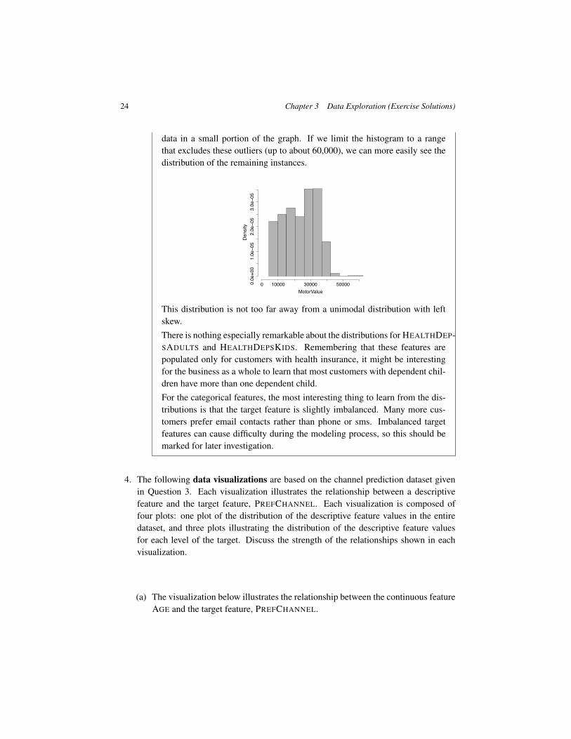
24 Chapter 3 Data Exploration (Exercise Solutions)
data in a small portion of the graph. If we limit the histogram to a rangethat excludes these outliers (up to about 60,000), we can more easily see thedistribution of the remaining instances.
MotorValue
Den
sity
0 10000 30000 500000.0e
+00
1.0e−05
2.0e−05
3.0e−05
This distribution is not too far away from a unimodal distribution with leftskew.There is nothing especially remarkable about the distributions for HEALTHDEP-SADULTS and HEALTHDEPSKIDS. Remembering that these features arepopulated only for customers with health insurance, it might be interestingfor the business as a whole to learn that most customers with dependent chil-dren have more than one dependent child.For the categorical features, the most interesting thing to learn from the dis-tributions is that the target feature is slightly imbalanced. Many more cus-tomers prefer email contacts rather than phone or sms. Imbalanced targetfeatures can cause difficulty during the modeling process, so this should bemarked for later investigation.
4. The following data visualizations are based on the channel prediction dataset givenin Question 3. Each visualization illustrates the relationship between a descriptivefeature and the target feature, PREFCHANNEL. Each visualization is composed offour plots: one plot of the distribution of the descriptive feature values in the entiredataset, and three plots illustrating the distribution of the descriptive feature valuesfor each level of the target. Discuss the strength of the relationships shown in eachvisualization.
(a) The visualization below illustrates the relationship between the continuous featureAGE and the target feature, PREFCHANNEL.

25
Age
Den
sity
20 30 40 50 60 70 80
0.00
0.02
0.04
0.06
0.08
0.10
PrefChannel = SMS
Age
Den
sity
20 30 40 50 60 70 80
0.00
0.05
0.10
0.15
0.20
PrefChannel = Phone
Age
Den
sity
20 30 40 50 60 70 80
0.00
0.05
0.10
0.15
0.20
PrefChannel = Email
AgeD
ensi
ty
20 30 40 50 60 70 80
0.00
0.05
0.10
0.15
0.20
This visualization suggests a strong relationship between the AGE descrip-tive feature and the target feature, PREFCHANNEL. Overall we can see thatthe individual histograms for each data partition created by the different tar-get levels are different from the overall histogram. Looking more deeply, wecan see that the customers whose preferred channel is sms are predominantlyyounger. This is evident from the high bars in the 18–25 region of the his-togram and the fact that there are very few instances in the age range above60. We can see the opposite pattern for those customers whose preferredchannel is phone. There are very few customers below 40 in this group. Thehistogram for the email group most closely matches the overall histogram.
(b) The visualization below illustrates the relationship between the categorical featureGENDER and the target feature PREFCHANNEL.

26 Chapter 3 Data Exploration (Exercise Solutions)
female maleGender
Den
sity
0.0
0.1
0.2
0.3
0.4
0.5
female male
PrefChannel = SMS
Gender
Den
sity
0.0
0.1
0.2
0.3
0.4
0.5
female male
PrefChannel = Phone
Gender
Den
sity
0.0
0.1
0.2
0.3
0.4
0.5
female male
PrefChannel = Email
GenderD
ensi
ty0.
00.
10.
20.
30.
40.
5
Each individual bar plot of GENDER created when we divide the data by thetarget feature is almost identical to the overall bar plot, which indicates thatthere is no relationship between the GENDER feature and the PREFCHANNEL
feature.

27
(c) The visualization below illustrates the relationship between the categorical featureLOC and the target feature, PREFCHANNEL.
Rural UrbanLoc
Den
sity
0.0
0.1
0.2
0.3
0.4
0.5
Rural Urban
PrefChannel = SMS
Loc
Den
sity
0.0
0.1
0.2
0.3
0.4
0.5
0.6
Rural Urban
PrefChannel = Phone
Loc
Den
sity
0.0
0.1
0.2
0.3
0.4
0.5
0.6
Rural Urban
PrefChannel = Email
Loc
Den
sity
0.0
0.1
0.2
0.3
0.4
0.5
0.6
The fact that the individual bar plots for each data partition are different fromthe overall bar plot suggests a relationship between these two features. Inparticular, for those customer’s whose preferred channel is phone, the overallratio between rural and urban locations is reversed—quite a few more ruralcustomers prefer this channel. In the other two channel preference groups,sms and email, there are quite a few more urban dwellers. Together, thisset of visualizations suggests that the LOC is reasonably predictive of thePREFCHANNEL feature.
5. The table below shows the scores achieved by a group of students on an exam.
ID 1 2 3 4 5 6 7 8 9 10SCORE 42 47 59 27 84 49 72 43 73 59
ID 11 12 13 14 15 16 17 18 19 20SCORE 58 82 50 79 89 75 70 59 67 35
Using this data, perform the following tasks on the SCORE feature:

28 Chapter 3 Data Exploration (Exercise Solutions)
(a) A range normalization that generates data in the range p0, 1q
To perform a range normalization, we need the minimum and maximum ofthe dataset and the high and low for the target range. From the data we cansee that the minimum is 27 and the maximum is 89. In the question we aretold that the low value of the target range is 0 and that the high value is 1.Using these values, we normalize an individual value using the followingequation:
a1
i “ai ´ minpaq
maxpaq ´ minpaqˆ phigh´ lowq ` low
So, the first score in the dataset, 42, would be normalized as follows:
a1
i “42´ 2789´ 27
ˆ p1´ 0q ` 0
“1562
“ 0.2419
This is repeated for each instance in the dataset to give the full normalizeddata set as
ID 1 2 3 4 5 6 7 8 9 10SCORE 0.24 0.32 0.52 0.00 0.92 0.35 0.73 0.26 0.74 0.52
ID 11 12 13 14 15 16 17 18 19 20SCORE 0.50 0.89 0.37 0.84 1.00 0.77 0.69 0.52 0.65 0.13
(b) A range normalization that generates data in the range p´1, 1q
This normalization differs from the previous range normalization only in thatthe high and low values are different—in this case, ´1 and 1. So the firstscore in the dataset, 42, would be normalized as follows:
a1
i “42´ 2789´ 27
ˆ p1´ p´1qq ` p´1q
“1562ˆ 2´ 1
“ ´0.5161

29
Applying this to each instance in the dataset gives the full normalized datasetas
ID 1 2 3 4 5 6 7 8 9 10SCORE -0.52 -0.35 0.03 -1.00 0.84 -0.29 0.45 -0.48 0.48 0.03
ID 11 12 13 14 15 16 17 18 19 20SCORE 0.00 0.77 -0.26 0.68 1.00 0.55 0.39 0.03 0.29 -0.74
(c) A standardization of the data
To perform a standardization, we use the following formula for each instancein the dataset:
a1
i “ai ´ asdpaq
So we need the mean, a, and standard deviation, sdpaq, for the feature to bestandardized. In this case, the mean is calculated from the original dataset as60.95, and the standard deviation is 17.2519. So the standardized value forthe first instance in the dataset can be calculated as
a1
i “42´ 60.95
17.2519“ ´1.0984
Standardizing in the same way for the rest of the dataset gives us the follow-ing:
ID 1 2 3 4 5 6 7 8 9 10SCORE -1.10 -0.81 -0.11 -1.97 1.34 -0.69 0.64 -1.04 0.70 -0.11
ID 11 12 13 14 15 16 17 18 19 20SCORE -0.17 1.22 -0.63 1.05 1.63 0.81 0.52 -0.11 0.35 -1.50
6. The following table shows the IQs for a group of people who applied to take part in atelevision general-knowledge quiz.
ID 1 2 3 4 5 6 7 8 9 10IQ 92 107 83 101 107 92 99 119 93 106
ID 11 12 13 14 15 16 17 18 19 20IQ 105 88 106 90 97 118 120 72 100 104
Using this dataset, generate the following binned versions of the IQ feature:

30 Chapter 3 Data Exploration (Exercise Solutions)
(a) An equal-width binning using 5 bins.
To perform an equal-width binning, we first calculate the bin size as rangeb
where b is the number of bins. In this case, this is calculated as 120´725 “ 9.6,
where 72 and 120 are the minimum and maximum values. Using the bin,size we can calculate the following bin ranges.
Bin Low High1 72.0 81.62 81.6 91.23 91.2 100.84 100.8 110.45 110.4 120.0
Once we have calculated the boundaries, we can use these to determine thebin to which each result belongs.
ID IQ IQ (BIN)1 92 Bin-32 107 Bin-43 83 Bin-24 101 Bin-45 107 Bin-46 92 Bin-37 99 Bin-38 119 Bin-59 93 Bin-310 106 Bin-4
ID IQ IQ (BIN)11 105 Bin-412 88 Bin-213 106 Bin-414 90 Bin-215 97 Bin-316 118 Bin-517 120 Bin-518 72 Bin-119 100 Bin-320 104 Bin-4
It is interesting to graph a histogram of the values in the dataset according tothe bin boundaries as well as a bar plot showing each of the bins created.
IQ
Den
sity
80 90 100 110 120
0.00
0.01
0.02
0.03
0.04
0.05
0.06
Bin−1 Bin−2 Bin−3 Bin−4 Bin−5IQ
Freq
uenc
y0
12
34
56
7
We can see from these graphs that a lot of instances belong to the middle binsand very few in the high and low bins.
31
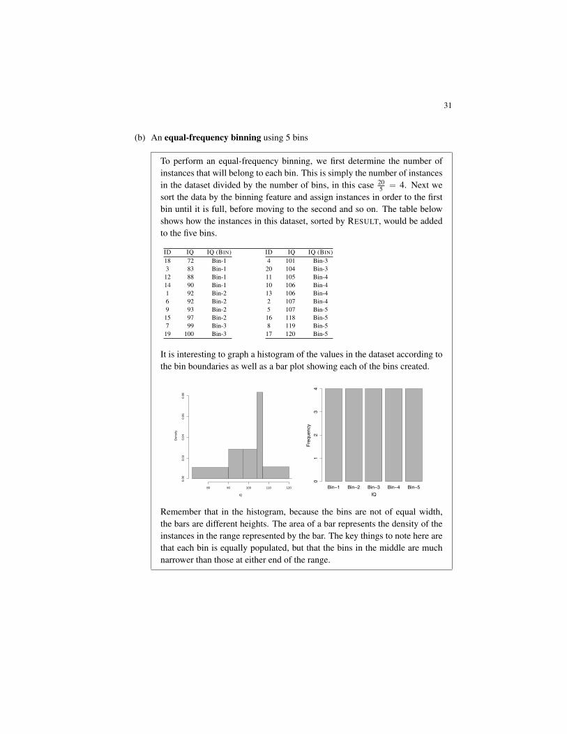
(b) An equal-frequency binning using 5 bins
To perform an equal-frequency binning, we first determine the number ofinstances that will belong to each bin. This is simply the number of instancesin the dataset divided by the number of bins, in this case 20
5 “ 4. Next wesort the data by the binning feature and assign instances in order to the firstbin until it is full, before moving to the second and so on. The table belowshows how the instances in this dataset, sorted by RESULT, would be addedto the five bins.
ID IQ IQ (BIN)18 72 Bin-13 83 Bin-112 88 Bin-114 90 Bin-11 92 Bin-26 92 Bin-29 93 Bin-215 97 Bin-27 99 Bin-319 100 Bin-3
ID IQ IQ (BIN)4 101 Bin-320 104 Bin-311 105 Bin-410 106 Bin-413 106 Bin-42 107 Bin-45 107 Bin-516 118 Bin-58 119 Bin-517 120 Bin-5
It is interesting to graph a histogram of the values in the dataset according tothe bin boundaries as well as a bar plot showing each of the bins created.
IQ
Den
sity
80 90 100 110 120
0.00
0.02
0.04
0.06
0.08
Bin−1 Bin−2 Bin−3 Bin−4 Bin−5IQ
Freq
uenc
y0
12
34
Remember that in the histogram, because the bins are not of equal width,the bars are different heights. The area of a bar represents the density of theinstances in the range represented by the bar. The key things to note here arethat each bin is equally populated, but that the bins in the middle are muchnarrower than those at either end of the range.


II PREDICTIVE DATA ANALYTICS


4 Information-Based Learning (Exercise Solutions)
1. The image below shows a set of eight Scrabble pieces.
(a) What is the entropy in bits of the letters in this set?
We can calculate the probability of randomly selecting a letter of each typefrom this set: PpOq “ 3
8 , PpXq “ 18 , PpYq “ 1
8 , PpMq “ 18 , PpRq “ 1
8 ,PpNq “ 1
8 .
Using these probabilities, we can calculate the entropy of the set:
´
ˆ
38ˆ log2
ˆ
38
˙
`
ˆ
18ˆ log2
ˆ
18
˙˙
ˆ 5˙
“ 2.4056 bits
Note that the contribution to the entropy for any letter that appears only onceis the same and so has been included 5 times—once for each of X, Y, M, R,and N.
(b) What would be the reduction in entropy (i.e., the information gain) in bits if wesplit these letters into two sets, one containing the vowels and the other containingthe consonants?
Information gain is the reduction in entropy that occurs after we split theoriginal set. We know that the entropy of the initial set is 2.4056 bits. We cal-culate the remaining entropy after we split the original set using a weighted

36 Chapter 4 Information-Based Learning (Exercise Solutions)
summation of the entropies for the new sets. The two new sets are vowels{O,O,O} and consonants {X,Y,M,R,N}.The entropy of the vowel set is
´
ˆ
33ˆ log2
ˆ
33
˙˙
“ 0 bits
The entropy of the consonant set is
´
ˆˆ
15ˆ log2
ˆ
15
˙˙
ˆ 5˙
“ 2.3219 bits
The weightings used in the summation of the set entropies are just the relativesize of each set. So, the weighting of the vowel set entropy is 3
8 , and theweighting of the consonant set entropy is 5
8 .This gives the entropy remaining after we split the set of letters into vowelsand consonants as
rem “38ˆ 0`
58ˆ 2.3219 “ 1.4512 bits
The information gain is the difference between the initial entropy and theremainder:
IG “ 2.4056´ 1.4512 “ 0.9544 bits
(c) What is the maximum possible entropy in bits for a set of eight Scrabble pieces?
The maximum entropy occurs when there are eight different letters in the set.The entropy for a set with this distribution of letters is
ˆ
18ˆ log2
ˆ
18
˙˙
ˆ 8 “ 3 bits
(d) In general, which is preferable when you are playing Scrabble: a set of letters withhigh entropy or a set of letters with low entropy?
In general, sets of letters with high entropy are preferable to lower entropysets because the more diverse the letters in the set, the more words you arelikely to be able to make from the set.

37
2. A convicted criminal who reoffends after release is known as a recidivist. The follow-ing table lists a dataset that describes prisoners released on parole and whether theyreoffended within two years of release.1
GOOD DRUG
ID BEHAVIOR AGE ă 30 DEPENDENT RECIDIVIST
1 false true false true2 false false false false3 false true false true4 true false false false5 true false true true6 true false false false
This dataset lists six instances in which prisoners were granted parole. Each of theseinstances is described in terms of three binary descriptive features (GOOD BEHAV-IOR, AGE ă 30, DRUG DEPENDENT) and a binary target feature (RECIDIVIST). TheGOOD BEHAVIOR feature has a value of true if the prisoner had not committed anyinfringements during incarceration, the AGE ă 30 has a value of true if the prisonerwas under 30 years of age when granted parole, and the DRUG DEPENDENT featureis true if the prisoner had a drug addiction at the time of parole. The target feature,RECIDIVIST, has a true value if the prisoner was arrested within two years of beingreleased; otherwise it has a value of false.
(a) Using this dataset, construct the decision tree that would be generated by the ID3algorithm, using entropy-based information gain.
The first step in building the decision tree is to figure out which of the threedescriptive features is the best one on which to split the dataset at the rootnode (i.e., which descriptive feature has the highest information gain). Thetotal entropy for this dataset is computed as follows:
H pRECIDIVIST,Dq
“ ´ÿ
lP!true,
false
)
PpRECIDIVIST “ lq ˆ log2 pPpRECIDIVIST “ lqq
“ ´``3{6 ˆ log2p
3{6q˘
``3{6 ˆ log2p
3{6q˘˘
“ 1.00 bit
1. This example of predicting recidivism is based on a real application of machine learning: parole boards dorely on machine learning prediction models to help them when they are making their decisions. See Berk andBleich (2013) for a recent comparison of different machine learning models used for this task. Datasets dealingwith prisoner recidivism are available online, for example, catalog.data.gov/dataset/prisoner-recidivism/. Thedataset presented here is not based on real data.

38 Chapter 4 Information-Based Learning (Exercise Solutions)
The table below illustrates the computation of the information gain for eachof the descriptive features:
Split by Partition Info.Feature Level Part. Instances Entropy Rem. GainGOOD true D1 d4,d5,d6 0.9183
0.9183 0.0817BEHAVIOR false D2 d1,d2,d3 0.9183
AGE ă 30true D3 d1,d3 0
0.5409 0.4591false D4 d2,d4,d5,d6 0.8113
DRUG true D5 d5 00.8091 0.1909
DEPENDENT false D6 d1,d2,d3,d4,d6 0.9709
AGE ă 30 has the largest information gain of the three features. Conse-quently, this feature will be used at the root node of the tree. The figurebelow illustrates the state of the tree after we have created the root node andsplit the data based on AGE ă 30.
Age < 30
D3 ID Good Behavior Drug Dependent Recidivist
1 false false true3 false false true
true
D4
ID Good Behavior Drug Dependent Recidivist 2 false false false4 true false false5 true true true6 true false false
false
In this image we have shown how the data moves down the tree based on thesplit on the AGE ă 30 feature. Note that this feature no longer appears inthese datasets because we cannot split on it again.The dataset on the left branch contains only instances where RECIDIVIST istrue and so does not need to be split any further.The dataset on the right branch of the tree (D4) is not homogenous, so weneed to grow this branch of the tree. The entropy for this dataset, D4, iscalculated as follows:
H pRECIDIVIST,D4q
“ ´ÿ
lP!true,
false
)
PpRECIDIVIST “ lq ˆ log2 pPpRECIDIVIST “ lqq
“ ´``1{4 ˆ log2p
1{4q˘
``3{4 ˆ log2p
3{4q˘˘
“ 0.8113 bits
The table below shows the computation of the information gain for the GOOD
BEHAVIOR and DRUG DEPENDENT features in the context of theD4 dataset:

39
Split by Partition Info.Feature Level Part. Instances Entropy Rem. GainGOOD true D7 d4,d5,d6 0.918295834
0.4591 0.3522BEHAVIOR false D8 d2 0
DRUG true D9 d5 00 0.8113
DEPENDENT false D10 d2,d4,d6 0
These calculations show that the DRUG DEPENDENT feature has a higher in-formation gain than GOOD BEHAVIOR: 0.8113 versus 0.3522 and so shouldbe chosen for the next split.The image below shows the state of the decision tree after the D4 partitionhas been split based on the feature DRUG DEPENDENT.
Age < 30
D3 ID Good Behavior Drug Dependent Recidivist
1 false false true3 false false true
true
Drug Dependent
false
D9 ID Good Behavior Recidivist
5 true true
true
D10
ID Good Behavior Recidivist 2 false false4 true false6 true false
false
All the datasets at the leaf nodes are now pure, so the algorithm will stopgrowing the tree. The image below shows the tree that will be returned bythe ID3 algorithm:
Age < 30
true
true
Drug Dependent
false
true
true
false
false
(b) What prediction will the decision tree generated in Part (a) of this question returnfor the following query?
GOOD BEHAVIOR = false,AGE ă 30 = false,DRUG DEPENDENT = true

40 Chapter 4 Information-Based Learning (Exercise Solutions)
RECIDIVIST = true
(c) What prediction will the decision tree generated in Part (a) of this question returnfor the following query?
GOOD BEHAVIOR = true,AGE ă 30 = true,DRUG DEPENDENT = false
RECIDIVIST = true
3. The following table lists a sample of data from a census.2
MARITAL ANNUAL
ID AGE EDUCATION STATUS OCCUPATION INCOME
1 39 bachelors never married transport 25K–50K2 50 bachelors married professional 25K–50K3 18 high school never married agriculture ă25K4 28 bachelors married professional 25K–50K5 37 high school married agriculture 25K–50K6 24 high school never married armed forces ă25K7 52 high school divorced transport 25K–50K8 40 doctorate married professional ą50K
There are four descriptive features and one target feature in this dataset, as follows:
‚ AGE, a continuous feature listing the age of the individual;
‚ EDUCATION, a categorical feature listing the highest education award achieved bythe individual (high school, bachelors, doctorate);
‚ MARITAL STATUS (never married, married, divorced);
‚ OCCUPATION (transport = works in the transportation industry; professional =doctor, lawyer, or similar; agriculture = works in the agricultural industry; armedforces = is a member of the armed forces); and
‚ ANNUAL INCOME, the target feature with 3 levels (ă25K, 25K–50K, ą50K).
(a) Calculate the entropy for this dataset.
2. This census dataset is based on the Census Income Dataset (Kohavi, 1996), which is available from the UCIMachine Learning Repository (Bache and Lichman, 2013) at archive.ics.uci.edu/ml/datasets/Census+Income/.

41
H pANNUAL INCOME,Dq
“ ´ÿ
lP
#
ă25K,25K–50K,ą50K
+
PpAN. INC. “ lq ˆ log2 pPpAN. INC. “ lqq
“ ´
ˆˆ
28ˆ log2
ˆ
28
˙˙
`
ˆ
58ˆ log2
ˆ
58
˙˙
`
ˆ
18ˆ log2
ˆ
18
˙˙˙
“ 1.2988 bits
(b) Calculate the Gini index for this dataset.
Gini pANNUAL INCOME,Dq
“ 1´ÿ
lP
#
ă25K,25K–50K,ą50K
+
PpAN. INC. “ lq2
“ 1´
˜
ˆ
28
˙2
`
ˆ
58
˙2
`
ˆ
18
˙2¸
“ 0.5313
(c) In building a decision tree, the easiest way to handle a continuous feature is todefine a threshold around which splits will be made. What would be the optimalthreshold to split the continuous AGE feature (use information gain based on en-tropy as the feature selection measure)?
First sort the instances in the dataset according to the AGE feature, as shownin the following table.
ID AGE ANNUAL INCOME
3 18 ă25K6 24 ă25K4 28 25K–50K5 37 25K–50K1 39 25K–50K8 40 ą50K2 50 25K–50K7 52 25K–50K
Based on this ordering, the mid-points in the AGE values of instances thatare adjacent in the new ordering but that have different target levels definethe possible threshold points. These points are 26, 39.5, and 45.

42 Chapter 4 Information-Based Learning (Exercise Solutions)
We calculate the information gain for each of these possible threshold pointsusing the entropy value we calculated in part (a) of this question (1.2988 bits)as follows:
Split by Partition Info.Feature Partition Instances Entropy Rem. Gain
ą26D1 d3,d6 0
0.4875 0.8113D2 d1,d2,d4,d5,d7,d8 0.6500
ą39.5D3 d1,d3,d4,d5,d6 0.9710
0.9456 0.3532D4 d2,d7,d8 0.9033
ą45D5 d1,d3,d4,d5,d6,d8 1.4591
1.0944 0.2044D6 d2,d7 0
The threshold AGE ą 26 has the highest information gain, and consequently,it is the best threshold to use if we are splitting the dataset using the AGE
feature.
(d) Calculate information gain (based on entropy) for the EDUCATION, MARITAL
STATUS, and OCCUPATION features.
We have already calculated the entropy for the full dataset in part (a) of thisquestion as 1.2988 bits. The table below lists the rest of the calculations forthe information gain for the EDUCATION, MARITAL STATUS, and OCCUPA-TION features.
Split by Partition Info.Feature Level Instances Gini Index Rem. Gain
EDUCATION
high school d3,d5,d6,d7 1.00.5 0.7988bachelors d1,d2,d3 0
doctorate d8 0
MARITAL STATUS
never married d1,d3,d6 0.91830.75 0.5488married d2,d4,d5,d8 0.8113
divorced d7 0
OCCUPATION
transport d1,d7 0
0.5944 0.7044professional d2,d4,d8 0.9183agriculture d3,d5 1.0
armed forces d6 0
(e) Calculate the information gain ratio (based on entropy) for EDUCATION, MAR-ITAL STATUS, and OCCUPATION features.
In order to calculate the information gain ratio of a feature, we divide theinformation gain of the feature by the entropy of the feature itself. We have

43
already calculated the information gain of these features in the preceding partof this question:‚ IG(EDUCATION,D) = 0.7988
‚ IG(MARITAL STATUS,D) = 0.5488
‚ IG(OCCUPATION,D) = 0.7044We calculate the entropy of each feature as follows:
H pEDUCATION,Dq
“ ´ÿ
lP
#
high school,bachelors,doctorate
+
PpED. “ lq ˆ log2 pPpED. “ lqq
“ ´
ˆˆ
48ˆ log2
ˆ
48
˙˙
`
ˆ
38ˆ log2
ˆ
38
˙˙
`
ˆ
18ˆ log2
ˆ
18
˙˙˙
“ 1.4056 bits
H pMARITAL STATUS,Dq
“ ´ÿ
lP
#
never married,married,divorced
+
PpMAR. STAT. “ lq ˆ log2 pPpMAR. STAT. “ lqq
“ ´
ˆˆ
38ˆ log2
ˆ
38
˙˙
`
ˆ
48ˆ log2
ˆ
48
˙˙
`
ˆ
18ˆ log2
ˆ
18
˙˙˙
“ 1.4056 bits
H pOCCUPATION,Dq
“ ´ÿ
lP
$
&
%
transport,professional,agriculture,armed forces
,
.
-
PpOCC. “ lq ˆ log2 pPpOCC. “ lqq
“ ´p
ˆ
28ˆ log2
ˆ
28
˙˙
`
ˆ
38ˆ log2
ˆ
38
˙˙
`
ˆ
28ˆ log2
ˆ
28
˙˙
`
ˆ
18ˆ log2
ˆ
18
˙˙
q
“ 1.9056 bits
We can now calculate the information gain ratio for each feature as:
‚ GR(EDUCATION,D) “0.79881.4056
“ 0.5683

44 Chapter 4 Information-Based Learning (Exercise Solutions)
‚ GR(MARITAL STATUS,D) “0.54881.4056
“ 0.3904
‚ GR(OCCUPATION,D) “0.70441.9056
“ 0.3696
(f) Calculate information gain using the Gini index for the EDUCATION, MARITAL
STATUS, and OCCUPATION features.
We have already calculated the Gini index for the full dataset in part (b) ofthis question as 0.5313. The table below lists the rest of the calculations ofinformation gain for the EDUCATION, MARITAL STATUS, and OCCUPATION
features.
Split by Partition Info.Feature Level Instances Gini Index Rem. Gain
EDUCATION
high school d3,d5,d6,d7 0.50.25 0.2813bachelors d1,d2,d3 0
doctorate d8 0
MARITAL STATUS
never married d1,d3,d6 0.44440.3542 0.1771married d2,d4,d5,d8 0.375
divorced d7 0
OCCUPATION
transport d1,d7 0
0.2917 0.2396professional d2,d4,d8 0.4444agriculture d3,d5 0.5
armed forces d6 0
4. The following diagram shows a decision tree for the task of predicting heart disease.3
The descriptive features in this domain describe whether the patient suffers from chestpain (CHEST PAIN) and the blood pressure of the patient (BLOOD PRESSURE). Thebinary target feature is HEART DISEASE. The table beside the diagram lists a pruningset from this domain.
3. This example is inspired by the research reported in Palaniappan and Awang (2008).
45
Chest Pain [true]
Blood Pressure [false]
false
true
true
true
high
false
low
CHEST BLOOD HEART
ID PAIN PRESSURE DISEASE
1 false high false2 true low true3 false low false4 true high true5 false high false
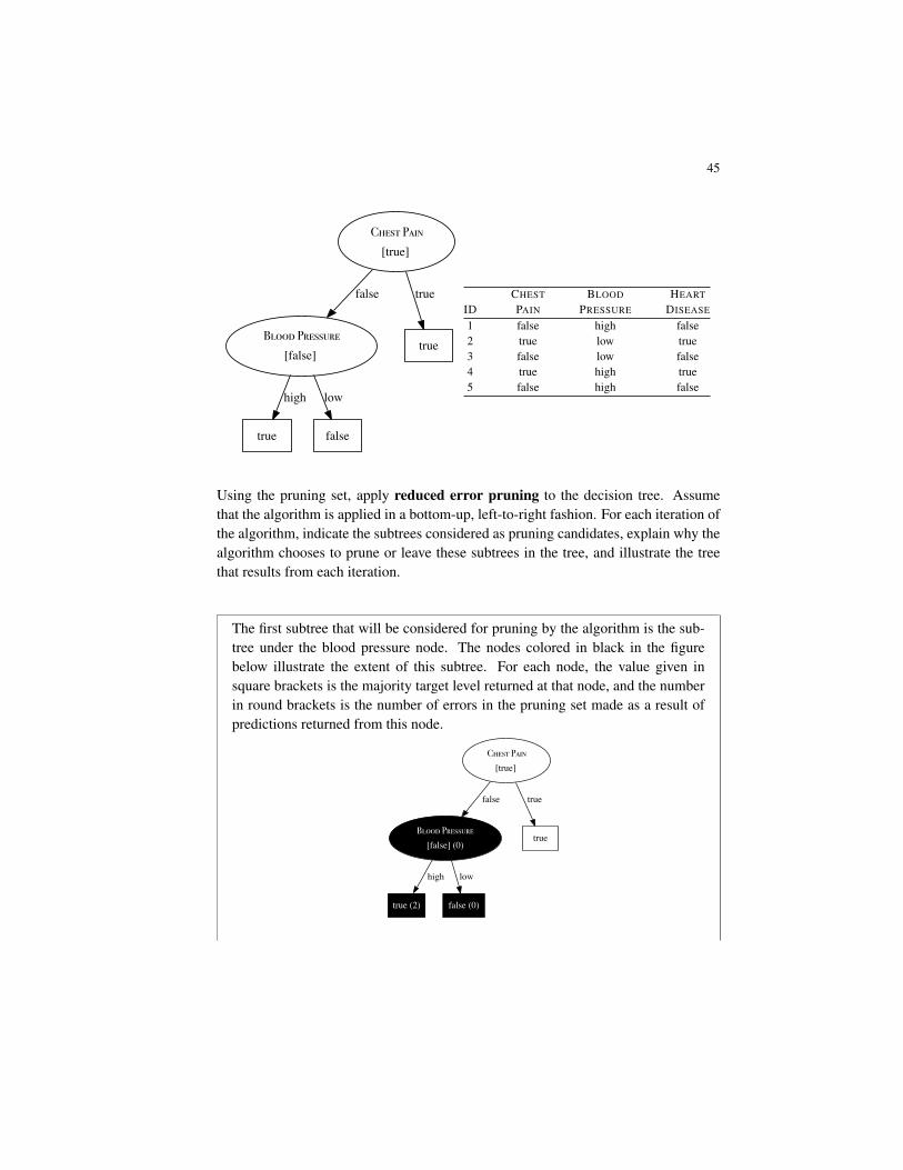
Using the pruning set, apply reduced error pruning to the decision tree. Assumethat the algorithm is applied in a bottom-up, left-to-right fashion. For each iteration ofthe algorithm, indicate the subtrees considered as pruning candidates, explain why thealgorithm chooses to prune or leave these subtrees in the tree, and illustrate the treethat results from each iteration.
The first subtree that will be considered for pruning by the algorithm is the sub-tree under the blood pressure node. The nodes colored in black in the figurebelow illustrate the extent of this subtree. For each node, the value given insquare brackets is the majority target level returned at that node, and the numberin round brackets is the number of errors in the pruning set made as a result ofpredictions returned from this node.
Chest Pain [true]
Blood Pressure [false] (0)
false
true
true
true (2)
high
false (0)
low

46 Chapter 4 Information-Based Learning (Exercise Solutions)
The root node of this subtree returns false, and this results in 0 errors in thepruning set. The sum of the errors for the two leaf nodes of this subtree is 2. Thealgorithm will prune this subtree because the number of errors resulting from theleaf nodes is higher than the number of errors resulting from the root node.The figure below illustrates the structure of the tree after the subtree under theBLOOD PRESSURE node is pruned. This figure also highlights the extent of thesubtree that is considered for pruning in the second iteration of the algorithm (theentire tree in this case).
Chest Pain [true] (3)
false (0)
false
true (0)
true
The root node of this tree returns true as a prediction, and consequently, it resultsin 3 errors on the pruning set. By contrast the number of errors made at each ofthe leaf nodes of this tree is 0. Because the number of errors at the leaf nodesis less than the number of errors at the root node, this tree will not be pruned.At this point all the non-leaf nodes in the tree have been tested, so the pruningalgorithm will stop, and this decision tree is the one that is returned by the pruningalgorithm.
5. The following table4 lists a dataset containing the details of five participants in a heartdisease study, and a target feature RISK, which describes their risk of heart disease.Each patient is described in terms of four binary descriptive features
‚ EXERCISE, how regularly do they exercise
‚ SMOKER, do they smoke
‚ OBESE, are they overweight
‚ FAMILY, did any of their parents or siblings suffer from heart disease
4. The data in this table has been artificially generated for this question, but is inspired by the results from theFramingham Heart Study: www.framinghamheartstudy.org.

47
ID EXERCISE SMOKER OBESE FAMILY RISK
1 daily false false yes low2 weekly true false yes high3 daily false false no low4 rarely true true yes high5 rarely true true no high
(a) As part of the study, researchers have decided to create a predictive model toscreen participants based on their risk of heart disease. You have been asked toimplement this screening model using a random forest. The three tables belowlist three bootstrap samples that have been generated from the above dataset. Us-ing these bootstrap samples, create the decision trees that will be in the randomforest model (use entropy-based information gain as the feature selection crite-rion).
ID EXERCISE FAMILY RISK
1 daily yes low2 weekly yes high2 weekly yes high5 rarely no high5 rarely no high
Bootstrap Sample A
ID SMOKER OBESE RISK
1 false false low2 true false high2 true false high4 true true high5 true true high
Bootstrap Sample B
ID OBESE FAMILY RISK
1 false yes low1 false yes low2 false yes high4 true yes high5 true no high
Bootstrap Sample C
The entropy calculation for Bootstrap Sample A is:
H pRISK, BoostrapS ampleAq
“ ´ÿ
lP!
low,high
)
PpRISK “ lq ˆ log2 pPpRISK “ lqq
“ ´
ˆˆ
15ˆ log2
ˆ
15
˙˙
`
ˆ
45ˆ log2
ˆ
45
˙˙˙
“ 0.7219 bits
The information gain for each of the features in Bootstrap Sample A is asfollows:

48 Chapter 4 Information-Based Learning (Exercise Solutions)
Split by Partition Info.Feature Level Instances Entropy Rem. Gain
EXERCISE
daily d1 00 0.7219weekly d2,d2 0
rarely d5,d5, 0
FAMILYyes d1,d2,d2 0.9183
0.5510 0.1709no d5,d5 0
These calculations show that the EXERCISE feature has the highest informa-tion gain of the descriptive features in Bootstrap Sample A and should beadded as the root node of the decision tree generated from Bootstrap SampleA. What is more, splitting on EXERCISE generates pure sets. So, the decisiontree does not need to be expanded beyond this initial test and the final treegenerated for Bootstrap Sample A will be as shown below.
Exercise
low
daily
high
weekly
high
rarely
By chance, Bootstrap Sample B has the same distribution of target featurevalues as Bootstrap Sample A, so the entropy calculation for Bootstrap Sam-ple B is the same as the calculation for Bootstrap Sample A:
H pRISK, BoostrapS ampleBq
“ ´ÿ
lP!
low,high
)
PpRISK “ lq ˆ log2 pPpRISK “ lqq
“ ´
ˆˆ
15ˆ log2
ˆ
15
˙˙
`
ˆ
45ˆ log2
ˆ
45
˙˙˙
“ 0.7219 bits
The information gain for each of the features in Bootstrap Sample B is asfollows:
Split by Partition Info.Feature Level Instances Entropy Rem. Gain
SMOKERtrue d2,d2,d4,d5 0
0 0.7219false d1 0
OBESEtrue d4,d5 0
0.5510 0.1709false d1,d2,d2 0.9183
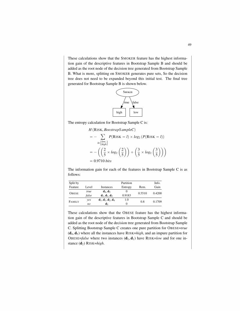
49
These calculations show that the SMOKER feature has the highest informa-tion gain of the descriptive features in Bootstrap Sample B and should beadded as the root node of the decision tree generated from Bootstrap SampleB. What is more, splitting on SMOKER generates pure sets, So the decisiontree does not need to be expanded beyond this initial test. The final treegenerated for Bootstrap Sample B is shown below.
Smoker
high
true
low
false
The entropy calculation for Bootstrap Sample C is:
H pRISK, BoostrapS ampleCq
“ ´ÿ
lP!
low,high
)
PpRISK “ lq ˆ log2 pPpRISK “ lqq
“ ´
ˆˆ
25ˆ log2
ˆ
25
˙˙
`
ˆ
35ˆ log2
ˆ
35
˙˙˙
“ 0.9710 bits
The information gain for each of the features in Bootstrap Sample C is asfollows:
Split by Partition Info.Feature Level Instances Entropy Rem. Gain
OBESEtrue d4,d5 0
0.5510 0.4200false d1,d1,d2 0.9183
FAMILYyes d1,d1,d2,d4 1.0
0.8 0.1709no d5 0
These calculations show that the OBESE feature has the highest informa-tion gain of the descriptive features in Bootstrap Sample C and should beadded as the root node of the decision tree generated from Bootstrap SampleC. Splitting Bootstrap Sample C creates one pure partition for OBESE=true(d4,d5) where all the instances have RISK=high, and an impure partition forOBESE=false where two instances (d1,d1) have RISK=low and for one in-stance (d2) RISK=high.

50 Chapter 4 Information-Based Learning (Exercise Solutions)
Normally this would mean that we would continue to split the impure parti-tion to create pure sets. However, in this instance there is only one featurethat we can still use to split this partition, the FAMILY feature, and all theinstances in this partition have the same level for this feature FAMILY=yes.Consequently, instead of splitting this partition further we simply create aleaf node with the majority target level within the partition: RISK=low. So,the final tree generated for Bootstrap Sample C will be as shown below.
Obese
high
true
low
false
(b) Assuming the random forest model you have created uses majority voting, whatprediction will it return for the following query:
EXERCISE=rarely, SMOKER=false, OBESE=true, FAMILY=yes
Each of the trees in the ensemble will vote as follows:‚ Tree 1: EXERCISE=rarelyÑ RISK=high
‚ Tree 2: SMOKER=falseÑ RISK=low
‚ Tree 3: OBESE=trueÑ RISK=high
So, the majority vote is for RISK=high, and this is the prediction the modelwill return for this query.

5 Similarity-Based Learning (Exercise Solutions)
1. The table below lists a dataset that was used to create a nearest neighbor model thatpredicts whether it will be a good day to go surfing.
ID WAVE SIZE (FT) WAVE PERIOD (SECS) WIND SPEED (MPH) GOOD SURF
1 6 15 5 yes2 1 6 9 no3 7 10 4 yes4 7 12 3 yes5 2 2 10 no6 10 2 20 no
Assuming that the model uses Euclidean distance to find the nearest neighbor, whatprediction will the model return for each of the following query instances?
ID WAVE SIZE (FT) WAVE PERIOD (SECS) WIND SPEED (MPH) GOOD SURF
Q1 8 15 2 ?Q2 8 2 18 ?Q3 6 11 4 ?
The table below lists the training instances along with the distances between eachtraining instance and each query. The distance between each query instance andits nearest training instance is highlighted in bold.
WAVE WAVE WIND GOOD Euc. Dist. Euc. Dist. Euc. Dist.ID SIZE (FT) PERIOD (SECS) SPEED (MPH) SURF to Q1 to Q2 to Q31 6 15 5 yes 3.61 18.49 4.122 1 6 9 no 13.38 12.08 8.663 7 10 4 yes 5.48 16.16 1.414 7 12 3 yes 3.32 18.06 1.735 2 2 10 no 16.40 10.00 11.536 10 2 20 no 22.29 2.83 18.79

52 Chapter 5 Similarity-Based Learning (Exercise Solutions)
From this table we can see that‚ The nearest neighbor to Q1 is training instance d4 which is 3.32 units away
from Q1. This training instance has a target level of GOOD SURF=yes. So themodel will predict GOOD SURF=yes for Q1.
‚ The nearest neighbor to Q2 is training instance d6 which is 2.83 units awayfrom Q2. This training instance has a target level of GOOD SURF=no. So themodel will predict GOOD SURF=no for Q2.
‚ The nearest neighbor to Q3 is training instance d3 which is 1.41 units awayfrom Q3. This training instance has a target level of GOOD SURF=yes. So themodel will predict GOOD SURF=yes for Q3.
2. Email spam filtering models often use a bag-of-words representation for emails. Ina bag-of-words representation, the descriptive features that describe a document (inour case, an email) each represent how many times a particular word occurs in thedocument. One descriptive feature is included for each word in a predefined dictio-nary. The dictionary is typically defined as the complete set of words that occur in thetraining dataset. The table below lists the bag-of-words representation for the follow-ing five emails and a target feature, SPAM, whether they are spam emails or genuineemails:
‚ “money, money, money”
‚ “free money for free gambling fun”
‚ “gambling for fun”
‚ “machine learning for fun, fun, fun”
‚ “free machine learning”
Bag-of-WordsID MONEY FREE FOR GAMBLING FUN MACHINE LEARNING SPAM
1 3 0 0 0 0 0 0 true2 1 2 1 1 1 0 0 true3 0 0 1 1 1 0 0 true4 0 0 1 0 3 1 1 false5 0 1 0 0 0 1 1 false
(a) What target level would a nearest neighbor model using Euclidean distance re-turn for the following email: “machine learning for free”?
The bag-of-words representation for this query is as follows:

53
Bag-of-WordsID MONEY FREE FOR GAMBLING FUN MACHINE LEARNING SPAM
Query 0 1 1 0 0 1 1 ?
The table below shows the calculation of the Euclidean distance between thequery instance and each of the instances in the training dataset:
pq rir ´ d j rirq2 EuclideanID MONEY FREE FOR GAMBLING FUN MACHINE LEARNING Distance1 9 1 1 0 0 1 1 3.60562 1 1 0 1 1 1 1 2.44953 0 1 0 1 1 1 1 2.23614 0 1 0 0 9 0 0 3.16235 0 0 1 0 0 0 0 1
Based on these distance calculations, the nearest neighbor to the query isinstance d5, for which SPAM = false. Consequently, the model will return aprediction of SPAM = false for this query.
(b) What target level would a k-NN model with k “ 3 and using Euclidean distancereturn for the same query?
Based on the distance calculations in part (a) of this question, the three near-est neighbors to the query are instances d5, d3, and d2. The majority of thesethree neighbors have a target value of SPAM = true. Consequently, the 3-NNmodel will return a prediction of SPAM = true.
(c) What target level would a weighted k-NN model with k “ 5 and using a weightingscheme of the reciprocal of the squared Euclidean distance between the neighborand the query, return for the query?
The weights for each of the instances in the dataset are
ID Weights
11
3.60562 “ 0.0769
21
2.44952 “ 0.1667
31
2.23612 “ 0.2
41
3.16232 “ 0.1
5112 “ 1

54 Chapter 5 Similarity-Based Learning (Exercise Solutions)
The total weight for the SPAM = true target level is 0.0769` 0.1667` 0.2 “0.4436. The total weight for the SPAM = false target level is 0.1 ` 1 “ 1.1.Consequently, the SPAM = false has the maximum weight, and this is theprediction returned by the model.
(d) What target level would a k-NN model with k “ 3 and using Manhattan distancereturn for the same query?
The table below shows the calculation of the Manhattan distance between thequery bag-of-words vector and each instance in the dataset:
abspq rir ´ d j rirq ManhattanID MONEY FREE FOR GAMBLING FUN MACHINE LEARNING Distance1 3 1 1 0 0 1 1 72 1 1 0 1 1 1 1 63 0 1 0 1 1 1 1 54 0 1 0 0 3 0 0 45 0 0 1 0 0 0 0 1
Based on these Manhattan distance calculations, the three nearest neighborsto the query are instances d5, d4, and d3. The majority of these three neigh-bors have a target value of SPAM = false. Consequently, the 3-NN modelusing Manhattan distance will return a prediction of SPAM = false.
(e) There are a lot of zero entries in the spam bag-of-words dataset. This is indicativeof sparse data and is typical for text analytics. Cosine similarity is often a goodchoice when dealing with sparse non-binary data. What target level would a 3-NNmodel using cosine similarity return for the query?
In order to calculate the cosine similarity between the query and each in-stance in the dataset, we first need to calculate the vector length of eachinstance and the query. The table below illustrates the calculation of thesevector lengths.
VectorID d rir2 Sum Length1 9 0 0 0 0 0 0 9 32 1 4 1 1 1 0 0 8 2.82843 0 0 1 1 1 0 0 3 1.73214 0 0 1 0 9 1 1 12 3.46415 0 1 0 0 0 1 1 3 1.7321
Query 0 1 1 0 0 1 1 4 2

55
The second component we need to calculate is the dot product between thequery and each instance. The table below illustrates the calculation of thesedot products.
DotPair pq rir ˆ d j rirq Productpq,d1q 0 0 0 0 0 0 0 0pq,d2q 0 2 1 0 0 0 0 3pq,d3q 0 0 1 0 0 0 0 1pq,d4q 0 0 1 0 0 1 1 3pq,d5q 0 1 0 0 0 1 1 3
We can now calculate the cosine similarity for each query-instance pair bydividing the relevant dot product by the product of the respective vectorlengths. These calculations are shown below.
Pair Cosine Similarity
pq,d1q0
3ˆ 2“ 0
pq,d2q3
2.8285ˆ 2“ 0.5303
pq,d3q1
1.7321ˆ 2“ 0.2887
pq,d4q3
3.4641ˆ 2“ 0.4330
pq,d5q3
1.7321ˆ 2“ 0.8660
When we use a similarity index, such as cosine similarity, the higher thenumber, the more similar the instances. Given this, the three most similarinstances in the dataset to the query are instances d5, d2, and d4. The majorityof these three neighbors have a target value of SPAM = false. Consequently,the 3-NN model will return a prediction of SPAM = false.
3. The predictive task in this question is to predict the level of corruption in a countrybased on a range of macroeconomic and social features. The table below lists somecountries described by the following descriptive features:
‚ LIFE EXP., the mean life expectancy at birth
‚ TOP-10 INCOME, the percentage of the annual income of the country that goes tothe top 10% of earners
‚ INFANT MORT., the number of infant deaths per 1,000 births
‚ MIL. SPEND, the percentage of GDP spent on the military
‚ SCHOOL YEARS, the mean number years spent in school by adult females

56 Chapter 5 Similarity-Based Learning (Exercise Solutions)
The target feature is the Corruption Perception Index (CPI). The CPI measuresthe perceived levels of corruption in the public sector of countries and ranges from 0(highly corrupt) to 100 (very clean).1
COUNTRY LIFE TOP-10 INFANT MIL. SCHOOL
ID EXP. INCOME MORT. SPEND YEARS CPIAfghanistan 59.61 23.21 74.30 4.44 0.40 1.5171Haiti 45.00 47.67 73.10 0.09 3.40 1.7999Nigeria 51.30 38.23 82.60 1.07 4.10 2.4493Egypt 70.48 26.58 19.60 1.86 5.30 2.8622Argentina 75.77 32.30 13.30 0.76 10.10 2.9961China 74.87 29.98 13.70 1.95 6.40 3.6356Brazil 73.12 42.93 14.50 1.43 7.20 3.7741Israel 81.30 28.80 3.60 6.77 12.50 5.8069USA 78.51 29.85 6.30 4.72 13.70 7.1357Ireland 80.15 27.23 3.50 0.60 11.50 7.5360UK 80.09 28.49 4.40 2.59 13.00 7.7751Germany 80.24 22.07 3.50 1.31 12.00 8.0461Canada 80.99 24.79 4.90 1.42 14.20 8.6725Australia 82.09 25.40 4.20 1.86 11.50 8.8442Sweden 81.43 22.18 2.40 1.27 12.80 9.2985New Zealand 80.67 27.81 4.90 1.13 12.30 9.4627
We will use Russia as our query country for this question. The table below lists thedescriptive features for Russia.
COUNTRY LIFE TOP-10 INFANT MIL. SCHOOL
ID EXP. INCOME MORT. SPEND YEARS CPIRussia 67.62 31.68 10.00 3.87 12.90 ?
(a) What value would a 3-nearest neighbor prediction model using Euclidean distancereturn for the CPI of Russia?
The table below lists the countries in the dataset and their CPI values byincreasing Euclidean distance from Russia (column 2).
1. The data listed in this table is real and is for 2010/11 (or the most recent year prior to 2010/11 when the datawas available). The data for the descriptive features in this table was amalgamated from a number of surveysretrieved from Gapminder (www.gapminder.org). The Corruption Perception Index is generated annually byTransparency International (www.transparency.org).

57
ID Euclideanpq,diq CPIArgentina 9.7805 2.9961China 10.7898 3.6356U.S.A 12.6033 7.1357Egypt 13.7217 2.8622Brazil 14.7394 3.7741U.K. 15.0621 7.7751Israel 16.0014 5.8069Ireland 16.0490 7.5360New Zealand 16.3806 9.4627Canada 17.2765 8.6725Australia 18.1472 8.8442Germany 18.2352 8.0461Sweden 19.8056 9.2985Afghanistan 66.5419 1.5171Haiti 69.6705 1.7999Nigeria 75.2712 2.4493
The nearest three neighbors to Russia are Argentina, China, and U.S.A. TheCPI value that will be returned by the model is the average CPI score forthese three neighbors, which is
2.9961` 3.6356` 7.13573
“ 4.5891
(b) What value would a weighted k-NN prediction model return for the CPI of Rus-sia? Use k “ 16 (i.e., the full dataset) and a weighting scheme of the reciprocal ofthe squared Euclidean distance between the neighbor and the query.
The table below shows the calculations required to answer this question.
ID Euclideanpq,diq CPI Weight WeightˆCPIArgentina 9.7805 2.9961 0.0105 0.0313China 10.7898 3.6356 0.0086 0.0312U.S.A 12.6033 7.1357 0.0063 0.0449Egypt 13.7217 2.8622 0.0053 0.0152Brazil 14.7394 3.7741 0.0046 0.0174U.K. 15.0621 7.7751 0.0044 0.0343Israel 16.0014 5.8069 0.0039 0.0227Ireland 16.0490 7.5360 0.0039 0.0293New Zealand 16.3806 9.4627 0.0037 0.0353Canada 17.2765 8.6725 0.0034 0.0291Australia 18.1472 8.8442 0.0030 0.0269Germany 18.2352 8.0461 0.0030 0.0242Sweden 19.8056 9.2985 0.0025 0.0237Afghanistan 66.5419 1.5171 0.0002 0.0003Haiti 69.6705 1.7999 0.0002 0.0004Nigeria 75.2712 2.4493 0.0002 0.0004Sum Weight: 0.0637Sum Weightˆ CPI: 0.3665

58 Chapter 5 Similarity-Based Learning (Exercise Solutions)
The value returned by the model is the sum of the instance weights multipliedby the instance target value divided by the sum of the instance weights:
0.36650.0637
“ 5.7507
(c) The descriptive features in this dataset are of different types. For example, someare percentages, others are measured in years, and others are measured in countsper 1,000. We should always consider normalizing our data, but it is particularlyimportant to do this when the descriptive features are measured in different units.What value would a 3-nearest neighbor prediction model using Euclidean distancereturn for the CPI of Russia when the descriptive features have been normalizedusing range normalization?
The table below lists the range-normalized descriptive features and the un-normalized CPI.
COUNTRY LIFE TOP-10 INFANT MIL. SCHOOL
ID EXP. INCOME MORT. SPEND YEARS CPIAfghanistan 0.3940 0.0445 0.8965 0.6507 0.0000 1.5171Haiti 0.0000 1.0000 0.8815 0.0000 0.2174 1.7999Nigeria 0.1698 0.6313 1.0000 0.1384 0.2681 2.4493Egypt 0.6869 0.1762 0.2145 0.2652 0.3551 2.8622Argentina 0.8296 0.3996 0.1359 0.0963 0.7029 2.9961China 0.8053 0.3090 0.1409 0.2786 0.4348 3.6356Brazil 0.7582 0.8148 0.1509 0.2004 0.4928 3.7741Israel 0.9785 0.2629 0.0150 1.0000 0.8768 5.8069U.S.A 0.9034 0.3039 0.0486 0.6922 0.9638 7.1357Ireland 0.9477 0.2016 0.0137 0.0757 0.8043 7.5360U.K. 0.9459 0.2508 0.0249 0.3749 0.9130 7.7751Germany 0.9501 0.0000 0.0137 0.1818 0.8406 8.0461Canada 0.9702 0.1063 0.0312 0.1996 1.0000 8.6725Australia 1.0000 0.1301 0.0224 0.2651 0.8043 8.8442Sweden 0.9821 0.0043 0.0000 0.1760 0.8986 9.2985New Zealand 0.9617 0.2242 0.0312 0.1547 0.8623 9.4627
We also need to normalize the query in order to generate a prediction, sowe show the normalized version of the descriptive features for Russia in thetable below.
COUNTRY LIFE TOP-10 INFANT MIL. SCHOOL
ID EXP. INCOME MORT. SPEND YEARS CPIRussia 0.6099 0.3754 0.0948 0.5658 0.9058 ?

59
The table below lists the countries in the dataset by increasing Euclideandistance—calculated using the normalized descriptive features—between Rus-sia and the country (column 2). Notice that this ordering is different from theordering of the countries when we used the unnormalized descriptive fea-tures.
ID Euclideanpq,diq CPIEgypt 0.00004 2.8622Brazil 0.00048 3.7741China 0.00146 3.6356Afghanistan 0.00217 1.5171Argentina 0.00233 2.9961United States 0.00742 7.1357United Kingdom 0.01275 7.7751Ireland 0.01302 7.5360Germany 0.01339 8.0461New Zealand 0.01531 9.4627Canada 0.01685 8.6725Israel 0.01847 5.8069Sweden 0.01918 9.2985Australia 0.02316 8.8442Nigeria 0.03753 2.4493Haiti 0.13837 1.7999
In this instance, the three nearest neighbors to Russia are Egypt, Brazil, andChina. The CPI value that will be returned by the model is the average CPIscore for these three neighbors:
2.8622` 3.7741` 3.63563
“ 3.4240
(d) What value would a weighted k-NN prediction model—with k “ 16 (i.e., the fulldataset) and using a weighting scheme of the reciprocal of the squared Euclideandistance between the neighbor and the query—return for the CPI of Russia whenit is applied to the range-normalized data?
The table below shows the calculations required to answer this question.

60 Chapter 5 Similarity-Based Learning (Exercise Solutions)
ID Euclideanpq,diq CPI Weight WeightˆCPIEgypt 0.00004 2.8622 809,250,011.4 2,316,224,862.0Brazil 0.00048 3.7741 4,284,287.3 16,169,371.4China 0.00146 3.6356 471,369.7 1,713,699.1Afghanistan 0.00217 1.5171 211,391.8 320,701.1Argentina 0.00233 2.9961 184,029.5 551,366.0United States 0.00742 7.1357 18,176.9 129,704.9United Kingdom 0.01275 7.7751 6,154.1 47,849.0Ireland 0.01302 7.5360 5,899.5 44,459.1Germany 0.01339 8.0461 5,575.7 44,863.0New Zealand 0.01531 9.4627 4,263.8 40,347.0Canada 0.01685 8.6725 3,520.9 30,535.1Israel 0.01847 5.8069 2,932.5 17,028.7Sweden 0.01918 9.2985 2,717.1 25,265.1Australia 0.02316 8.8442 1,864.8 16,492.9Nigeria 0.03753 2.4493 710.1 1,739.3Haiti 0.13837 1.7999 52.2 94.0Sum Weight: 814,452,958Sum Weightˆ CPI: 2,335,378,378
The value returned by the model is the sum of the instance weights multipliedby the instance target value divided by the sum of the instance weights:
2,335,378,378814,452,958
“ 2.8674
(e) The actual 2011 CPI for Russia was 2.4488. Which of the predictions made wasthe most accurate? Why do you think this was?
The most accurate prediction made was the one based on normalized datausing the weighted k-NN model, 2.8674. There are two main reasons for this.First, this example illustrates the importance of normalizing data. Becausethe data ranges in this dataset are so different from each other, normalizationis crucial. The second main reason is the small size of the dataset. Usingthree nearest neighbors probably tends to underfit slightly for such a smalldataset. Using weighted distances allows for this.

6 Probability-Based Learning (Exercise Solutions)
1. (a) Three people flip a fair coin. What is the probability that exactly two of them willget heads?
There are 8 possible outcomes:
Person1 Person2 Person3Heads Heads HeadsHeads Heads TailsHeads Tails HeadsHeads Tails TailsTails Heads HeadsTails Heads TailsTails Tails HeadsTails Tails Tails
In 3 of these outcomes there are 2 Heads. So the probability of exactly twopeople getting heads is
38“ 0.375
(b) Twenty people flip a fair coin. What is the probability that exactly eight of themwill get heads?
We could use the same approach as we used in part (a) to answer this ques-tion: list all possible outcomes and count the number of outcomes that matchour criteria. However, this approach doesn’t scale up to problems where thereare a lot of possible outcomes. For example, in part (a) with 3 people flippingthe coin there were 23 “ 8 possible outcomes. However, now with 20 people

62 Chapter 6 Probability-Based Learning (Exercise Solutions)
flipping the coin there are 220 “ 1,048,576 possible outcomes—clearly, toomany outcomes for us to list out. So what should we do?Because each coin flip is independent of the others, the coin flips can beviewed as a sequence of independent binary experiments. Consequently, wecan calculate the probability of getting k outcomes, each with a probabilityof p, in a sequence of n experiments using the binomial distribution as
ˆ
nk
˙
ˆ pk ˆ p1´ pqn´k
where n is the number of binary experiments, k is the number of particularresults we are looking for (e.g., the number of heads we are looking for),and p is the probability of getting the result we are looking for (e.g., theprobability of getting a head).So, we can calculate the probability of the event where exactly 8 of the coinflips comes up heads using the binomial distribution as followsˆ
208
˙
ˆ 0.58 ˆ p1´ 0.5q20´8 “20!
8!ˆ p20´ 8q!ˆ 0.58 ˆ 0.512
“ 125970ˆ 0.00390625ˆ 0.000244141
“ 0.120134354
Note: the ! symbol represents the factorial operation, for example
6! “ 6ˆ 5ˆ 4ˆ 3ˆ 2ˆ 1 “ 720
(c) Twenty people flip a fair coin. What is the probability that at least four of themwill get heads?
The probability that at least 4 people will get heads is equal to 1 minus prob-ability that less then 4 people will get heads.The probability that less then 4 people will get heads is simply the sum ofthe following probabilities:‚ the probability that exactly 3 people will get heads
‚ the probability that exactly 2 people will get heads
‚ the probability that exactly 1 person will get headsWe can calculate each of these probabilities using the binomial distributionas follows:

63
The probability of exactly 3 people getting heads:ˆ
203
˙
ˆ 0.53 ˆ p1´ 0.5q20´3 “20!
3!ˆ p20´ 3q!ˆ 0.53 ˆ 0.517
“ 1140ˆ 0.125ˆ p7.62939ˆ 10´6q
“ 0.001087189
The probability of exactly 2 people getting heads:ˆ
202
˙
ˆ 0.52 ˆ p1´ 0.5q20´2 “20!
2!ˆ p20´ 2q!ˆ 0.52 ˆ 0.518
“ 190ˆ 0.25ˆ p3.8147ˆ 10´6q
“ 0.000181198
The probability of exactly 1 person getting heads:ˆ
201
˙
ˆ 0.51 ˆ p1´ 0.5q20´1 “20!
1!ˆ p20´ 1q!ˆ 0.51 ˆ 0.519
“ 20ˆ 0.5ˆ p1.90735ˆ 10´6q
“ 0.0000190735
Probability of 3 people or less getting heads is:
0.001087189` 0.000181198` 0.0000190735 “ 0.0012874605
So the probability of at least 4 people getting heads is:
1´ 0.0012874605 “ 0.9987125
2. The table below gives details of symptoms that patients presented and whether theywere suffering from meningitis.
ID HEADACHE FEVER VOMITING MENINGITIS
1 true true false false2 false true false false3 true false true false4 true false true false5 false true false true6 true false true false7 true false true false8 true false true true9 false true false false
10 true false true true
Using this dataset, calculate the following probabilities:

64 Chapter 6 Probability-Based Learning (Exercise Solutions)
(a) PpVOMITING “ trueq
This can be calculated easily by counting:PpVOMITING “ trueq “ 6
10 “ 0.6
(b) PpHEADACHE “ falseq
This can be calculated easily by counting:PpHEADACHE “ falseq “ 3
10 “ 0.3
(c) PpHEADACHE “ true,VOMITING “ falseq
This can be calculated easily by counting:PpHEADACHE “ true,VOMITING “ falseq “ 1
10 “ 0.1Or using the product rule:PpHEADACHE “ true,VOMITING “ falseq “ PpHEADACHE “ true |VOMITING “ falseq ˆ PpVOMITING “ falseq “ 1
4 ˆ410 “ 0.1
(d) PpVOMITING “ false | HEADACHE “ trueq
This can be calculated easily by counting:PpVOMITING “ false | HEADACHE “ trueq “ 1
7 “ 0.1429
(e) PpMENINGITIS | FEVER “ true,VOMITING “ falseq
This can be calculated easily by counting. First,PpMENINGITIS “ true | FEVER “ true,VOMITING “ falseq “ 1
4 “ 0.25.Then,PpMENINGITIS “ false | FEVER “ true,VOMITING “ falseq “ 3
4 “ 0.75So,PpMENINGITIS | FEVER “ true,VOMITING “ falseq “ 〈0.25, 0.75〉
3. Predictive data analytics models are often used as tools for process quality control andfault detection. The task in this question is to create a naive Bayes model to monitora wastewater treatment plant.1 The table below lists a dataset containing details ofactivities at a wastewater treatment plant for 14 days. Each day is described in terms
1. The dataset in this question is inspired by the Waste Water Treatment Dataset that is available from the UCIMachine Learning repository (Bache and Lichman, 2013) at archive.ics.uci.edu/ml/machine-learning-databases/water-treatment. The creators of this dataset reported their work in Bejar et al. (1991).

65
of six descriptive features that are generated from different sensors at the plant. SS-IN measures the solids coming into the plant per day; SED-IN measures the sedimentcoming into the plant per day; COND-IN measures the electrical conductivity of thewater coming into the plant.2 The features SS-OUT, SED-OUT, and COND-OUT arethe corresponding measurements for the water flowing out of the plant. The targetfeature, STATUS, reports the current situation at the plant: ok, everything is workingcorrectly; settler, there is a problem with the plant settler equipment; or solids, thereis a problem with the amount of solids going through the plant.
SS SED COND SS SED COND
ID -IN -IN -IN -OUT -OUT -OUT STATUS
1 168 3 1,814 15 0.001 1,879 ok2 156 3 1,358 14 0.01 1,425 ok3 176 3.5 2,200 16 0.005 2,140 ok4 256 3 2,070 27 0.2 2,700 ok5 230 5 1,410 131 3.5 1,575 settler6 116 3 1,238 104 0.06 1,221 settler7 242 7 1,315 104 0.01 1,434 settler8 242 4.5 1,183 78 0.02 1,374 settler9 174 2.5 1,110 73 1.5 1,256 settler
10 1,004 35 1,218 81 1,172 33.3 solids11 1,228 46 1,889 82.4 1,932 43.1 solids12 964 17 2,120 20 1,030 1,966 solids13 2,008 32 1,257 13 1,038 1,289 solids
(a) Create a naive Bayes model that uses probability density functions to model thedescriptive features in this dataset (assume that all the descriptive features are nor-mally distributed).
The prior probabilities of each of the target feature levels are
PpSTATUS “ okq “4
13“ 0.3077
PpSTATUS “ settlerq “5
13“ 0.3846
PpSTATUS “ okq “4
13“ 0.3077
2. The conductivity of water is affected by inorganic dissolved solids and organic compounds, such as oil.Consequently, water conductivity is a useful measure of water purity.

66 Chapter 6 Probability-Based Learning (Exercise Solutions)
To create the probability density functions required by the model, we simplyneed to fit a normal distribution to each feature for each level of the target.To do this, we calculate the mean and standard deviation for each feature forthe set of instances where the target takes a given value. The table belowlists the normal probability distributions fitted to each descriptive feature andtarget level.
PpSS-IN | okq = N`
x, µ “ 189, σ “ 45.42˘
PpSED-IN | okq = N`
x, µ “ 3.125, σ “ 0.25˘
PpCOND-IN | okq = N`
x, µ “ 1,860.5, σ “ 371.4˘
PpSS-OUT | okq = N`
x, µ “ 18, σ “ 6.06˘
PpSED-OUT | okq = N`
x, µ “ 0.054, σ “ 0.10˘
PpCOND-OUT | okq = N`
x, µ “ 2,036, σ “ 532.19˘
PpSS-IN | settlerq = N`
x, µ “ 200.8, σ “ 55.13˘
PpSED-IN | settlerq = N`
x, µ “ 4.4, σ “ 1.78˘
PpCOND-IN | settlerq = N`
x, µ “ 1,251.2, σ “ 116.24˘
PpSS-OUT | settlerq = N`
x, µ “ 98, σ “ 23.38˘
PpSED-OUT | settlerq = N`
x, µ “ 1.018, σ “ 1.53˘
PpCOND-OUT | settlerq = N`
x, µ “ 1,372, σ “ 142.58˘
PpSS-IN | solidsq = N`
x, µ “ 1,301, σ “ 485.44˘
PpSED-IN | solidsq = N`
x, µ “ 32.5, σ “ 11.96˘
PpCOND-IN | solidsq = N`
x, µ “ 1,621, σ “ 453.04˘
PpSS-OUT | solidsq = N`
x, µ “ 49.1, σ “ 37.76˘
PpSED-OUT | solidsq = N`
x, µ “ 1,293, σ “ 430.95˘
PpCOND-OUT | solidsq = N`
x, µ “ 832.85, σ “ 958.31˘
(b) What prediction will the naive Bayes model return for the following query?
SS-IN = 222, SED-IN = 4.5, COND-IN = 1,518, SS-OUT = 74 SED-OUT = 0.25,COND-OUT = 1,642
The calculation for STATUS = ok:

67
Ppokq = 0.3077PpSS-IN | okq = N
`
222, µ “ 189, σ “ 45.42˘
= 0.0068PpSED-IN | okq = N
`
4.5, µ “ 3.125, σ “ 0.25˘
= 4.3079ˆ 10´7
PpCOND-IN | okq = N`
1,518, µ “ 1,860.5, σ “ 371.4˘
= 0.0007PpSS-OUT | okq = N
`
74, µ “ 18, σ “ 6.06˘
= 1.7650ˆ 10´20
PpSED-OUT | okq = N`
0.25, µ “ 0.054, σ “ 0.10˘
= 0.5408PpCOND-OUT | okq = N
`
1,642, µ “ 2,036, σ “ 532.19˘
= 0.0006
˜
mź
k“1
Ppq rks | okq
¸
ˆ Ppokq “ 3.41577ˆ 10´36
The calculation for STATUS = settler:
Ppsettlerq = 0.3846PpSS-IN | settlerq = N
`
222, µ “ 200.8, σ “ 55.13˘
= 0.0067PpSED-IN | settlerq = N
`
4.5, µ “ 4.4, σ “ 1.78˘
= 0.2235PpCOND-IN | settlerq = N
`
1,518, µ “ 1,251.2, σ “ 116.24˘
= 0.0002PpSS-OUT | settlerq = N
`
74, µ “ 98, σ “ 23.38˘
= 0.0101PpSED-OUT | settlerq = N
`
0.25, µ “ 1.018, σ “ 1.53˘
= 0.2303PpCOND-OUT | settlerq = N
`
1,642, µ “ 1,372, σ “ 142.58˘
= 0.0005
˜
mź
k“1
Ppq rks | settlerq
¸
ˆ Ppsettlerq “ 1.53837ˆ 10´13
The calculation for STATUS = solids:
Ppsolidsq = 0.3077PpSS-IN | solidsq = N
`
x, µ “ 1,301, σ “ 485.44˘
= 6.9496ˆ 10´5
PpSED-IN | solidsq = N`
x, µ “ 32.5, σ “ 11.96˘
= 0.0022PpCOND-IN | solidsq = N
`
x, µ “ 1,621, σ “ 453.04˘
= 0.0009PpSS-OUT | solidsq = N
`
x, µ “ 49.1, σ “ 37.76˘
= 0.0085PpSED-OUT | solidsq = N
`
x, µ “ 1,293, σ “ 430.95˘
= 1.0291ˆ 10´5
PpCOND-OUT | solidsq = N`
x, µ “ 832.85, σ “ 958.31˘
= 0.0003
˜
mź
k“1
Ppq rks | solidsq
¸
ˆ Ppsolidsq “ 1.00668ˆ 10´21
Recall that because we are using the heights of the PDFs rather than calculat-ing the actual probabilities for each feature taking a value, the score of eachtarget level is a relative ranking and should not be interpreted as a probability.

68 Chapter 6 Probability-Based Learning (Exercise Solutions)
That said, the target level with the highest ranking is STATUS = settler. Thisindicates that there was a problem with the plant’s settler equipment on theday of the query.
4. The following is a description of the causal relationship between storms, the behaviorof burglars and cats, and house alarms:
Stormy nights are rare. Burglary is also rare, and if it is a stormy night, burglars arelikely to stay at home (burglars don’t like going out in storms). Cats don’t like storms either,and if there is a storm, they like to go inside. The alarm on your house is designed to betriggered if a burglar breaks into your house, but sometimes it can be set off by your catcoming into the house, and sometimes it might not be triggered even if a burglar breaks in(it could be faulty or the burglar might be very good).
(a) Define the topology of a Bayesian network that encodes these causal relationships.
The figure below illustrates a Bayesian network that encodes the describedcausal relationships. Storms directly affect the behavior of burglars and cats,and this is reflected by links from the storm node to the burglar and catnodes. The behavior of burglars and cats both affect whether the alarm goesoff, and hence there are links from each of these nodes to the alarm node.
Storm
Burglar Cat
Alarm
(b) The table below lists a set of instances from the house alarm domain. Using thedata in this table, create the conditional probability tables (CPTs) for the networkyou created in Part (a) of this question.
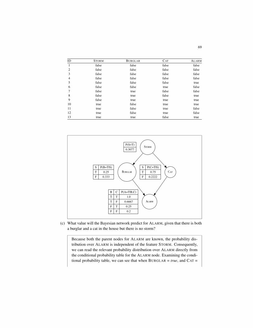
69
ID STORM BURGLAR CAT ALARM
1 false false false false2 false false false false3 false false false false4 false false false false5 false false false true6 false false true false7 false true false false8 false true false true9 false true true true10 true false true true11 true false true false12 true false true false13 true true false true
Storm
Burglar Cat
P(S=T)0.3077
Alarm
STF
P(B=T|S)0.250.333
STF
P(C=T|S)0.750.2222
BTTFF
CTFTF
P(A=T|B,C)1.0
0.66670.250.2
(c) What value will the Bayesian network predict for ALARM, given that there is botha burglar and a cat in the house but there is no storm?
Because both the parent nodes for ALARM are known, the probability dis-tribution over ALARM is independent of the feature STORM. Consequently,we can read the relevant probability distribution over ALARM directly fromthe conditional probability table for the ALARM node. Examining the condi-tional probability table, we can see that when BURGLAR = true, and CAT =

70 Chapter 6 Probability-Based Learning (Exercise Solutions)
true, then ALARM = true is the MAP prediction. In other words, the networkwould predict that the alarm would sound in this situation.
(d) What value will the Bayesian network predict for ALARM, given that there is astorm but we don’t know if a burglar has broken in or where the cat is?
In this case, the values of the parents of the target feature are unknown. Con-sequently, we need to sum out both the parents for each value of the target.The network would calculate the probability of the event ALARM = true asfollows:
Ppa | sq “Ppa, sqPpsq
“
ř
i, j Ppa, Bi,C j, sq
Ppsqÿ
i, j
Ppa, Bi,C j, sq “ÿ
i, j
Ppa | Bi,C jq ˆ PpBi | sq ˆ PpC j | sq ˆ Ppsq
“ pPpa | b, cq ˆ Ppb | sq ˆ Ppc | sq ˆ Ppsqq
` pPpa | b, cq ˆ Ppb | sq ˆ Pp c | sq ˆ Ppsqq
` pPpa | b, cq ˆ Pp b | sq ˆ Ppc | sq ˆ Ppsqq
` pPpa | b, cq ˆ Pp b | sq ˆ Pp c | sq ˆ Ppsqq
“ p1.0ˆ 0.25ˆ 0.75ˆ 0.3077q ` p0.6667ˆ 0.25ˆ 0.25ˆ 0.3077q
` p0.25ˆ 0.75ˆ 0.75ˆ 0.3077q ` p0.2ˆ 0.75ˆ 0.25ˆ 0.3077q
“ 0.125324
Ppa | sq “Ppa, sqPpsq
“0.125324
0.3077“ 0.4073
This implies that PpALARM “ falseq “ 0.5927, so in this instance, ALARM
= false is the MAP level for the target, and this is the prediction the modelwill return.

7 Error-Based Learning (Exercise Solutions)
1. A multivariate linear regression model has been built to predict the heating load in aresidential building on the basis of a set of descriptive features describing the charac-teristics of the building. Heating load is the amount of heat energy required to keep abuilding at a specified temperature, usually 65˝ Fahrenheit during the winter regard-less of outside temperature. The descriptive features used are the overall surface areaof the building, the height of the building, the area of the building’s roof, and the per-centage of wall area in the building that is glazed. This kind of model would be usefulto architects or engineers when designing a new building.1 The trained model is
HEATING LOAD “´ 26.030` 0.0497ˆ SURFACE AREA
` 4.942ˆ HEIGHT ´ 0.090ˆ ROOF AREA
` 20.523ˆ GLAZING AREA
Use this model to make predictions for each of the query instances shown in the fol-lowing table.
SURFACE ROOF GLAZING
ID AREA HEIGHT AREA AREA
1 784.0 3.5 220.5 0.252 710.5 3.0 210.5 0.103 563.5 7.0 122.5 0.404 637.0 6.0 147.0 0.60
1. This question is inspired by Tsanas and Xifara (2012), and although the data used is artificially generated,it is based on the Energy Efficiency Dataset available from the UCI Machine Learning Repository (Bache andLichman, 2013) at archive.ics.uci.edu/ml/datasets/Energy+efficiency/.

72 Chapter 7 Error-Based Learning (Exercise Solutions)
Calculating the predictions made by the model simply involves inserting the de-scriptive features from each query instance into the prediction model.
1: ´26.030` 0.0497ˆ 784.0` 4.942ˆ 3.5´ 0.090ˆ 220.5` 20.523ˆ 0.25“ 15.5
2: ´26.030` 0.0497ˆ 710.5` 4.942ˆ 3.0´ 0.09ˆ 210.5` 20.523ˆ 0.10“ 7.2
3: ´26.03` 0.0497ˆ 563.5` 4.942ˆ 7.0´ 0.09ˆ 122.5` 20.523ˆ 0.40“ 33.8
4: ´26.03` 0.0497ˆ 637.0` 4.942ˆ 6.0´ 0.09ˆ 147.0` 20.523ˆ 0.60“ 34.4
2. You have been hired by the European Space Agency to build a model that predictsthe amount of oxygen that an astronaut consumes when performing five minutes ofintense physical work. The descriptive features for the model will be the age of theastronaut and their average heart rate throughout the work. The regression model is
OXYCON “ w r0s ` w r1s ˆ AGE ` w r2s ˆ HEARTRATE
The table that follows shows a historical dataset that has been collected for this task.
HEART
ID OXYCON AGE RATE
1 37.99 41 1382 47.34 42 1533 44.38 37 1514 28.17 46 1335 27.07 48 1266 37.85 44 145
HEART
ID OXYCON AGE RATE
7 44.72 43 1588 36.42 46 1439 31.21 37 13810 54.85 38 15811 39.84 43 14312 30.83 43 138
(a) Assuming that the current weights in a multivariate linear regression model arew r0s “ ´59.50, w r1s “ ´0.15, and w r2s “ 0.60, make a prediction for eachtraining instance using this model.
The following table shows the predictions made using the given model weights.

73
ID OXYCON AGE HEART RATE Prediction1 37.99 41 138 17.152 47.34 42 153 26.003 44.38 37 151 25.554 28.17 46 133 13.405 27.07 48 126 8.906 37.85 44 145 20.907 44.72 43 158 28.858 36.42 46 143 19.409 31.21 37 138 17.7510 54.85 38 158 29.6011 39.84 43 143 19.8512 30.83 43 138 16.85
(b) Calculate the sum of squared errors for the set of predictions generated in Part (a).
The following table shows the predictions made by the model and sum ofsquared error calculation based on these predictions.
Initial Weightsw r0s: -59.50 w r1s: -0.15 w r2s: 0.60
Iteration 1Squared errorDelta errorDelta errorDelta
ID OXYCON Prediction Error Error pD,w r0sq pD,w r1sq pD,w r2sq1 37.99 17.15 20.84 434.41 20.84 854.54 2,876.262 47.34 26.00 21.34 455.41 21.34 896.29 3,265.053 44.38 25.55 18.83 354.60 18.83 696.74 2,843.454 28.17 13.40 14.77 218.27 14.77 679.60 1,964.935 27.07 8.90 18.17 330.09 18.17 872.08 2,289.206 37.85 20.90 16.95 287.35 16.95 745.86 2,457.947 44.72 28.85 15.87 251.91 15.87 682.48 2,507.718 36.42 19.40 17.02 289.72 17.02 782.98 2,434.049 31.21 17.75 13.46 181.26 13.46 498.14 1,857.9210 54.85 29.60 25.25 637.57 25.25 959.50 3,989.5211 39.84 19.85 19.99 399.47 19.99 859.44 2,858.1212 30.83 16.85 13.98 195.52 13.98 601.25 1,929.61
Sum 4,035.56 216.48 9,128.90 3,1273.77Sum of squared errors (S um{2) 2,017.78
(c) Assuming a learning rate of 0.000002, calculate the weights at the next iterationof the gradient descent algorithm.
To calculate the updated weight values we apply the weight update rule formultivariate linear regression with gradient descent for each weight as fol-

74 Chapter 7 Error-Based Learning (Exercise Solutions)
lows (using errorDelta values given in the answer to the previous part):
w r0s Ð w r0s ` αˆ errorDeltapD,w r0sqÐ ´59.50` 0.000002ˆ 216.48
Ð ´59.4996
w r1s Ð w r1s ` αˆ errorDeltapD,w r1sqÐ ´0.15` 0.000002ˆ 9128.9
Ð ´0.1317
w r2s Ð w r2s ` αˆ errorDeltapD,w r2sqÐ 0.60` 0.000002ˆ 31273.77
Ð 0.6625
(d) Calculate the sum of squared errors for a set of predictions generated using thenew set of weights calculated in Part (c).
The new sum of squared errors calculated using these new weights is given bythe following table.
SquaredID OXYCON Prediction Error Error1 37.99 26.53 11.46 131.382 47.34 36.34 11.00 121.073 44.38 35.67 8.71 75.874 28.17 22.56 5.61 31.535 27.07 17.66 9.41 88.566 37.85 30.77 7.08 50.107 44.72 39.52 5.20 27.088 36.42 29.18 7.24 52.379 31.21 27.06 4.16 17.2710 54.85 40.18 14.67 215.3111 39.84 29.58 10.26 105.2112 30.83 26.27 4.57 20.84
Sum 936.57Sum of squared errors (S um{2) 468.29
3. A multivariate logistic regression model has been built to predict the propensity ofshoppers to perform a repeat purchase of a free gift that they are given. The descrip-tive features used by the model are the age of the customer, the socioeconomic bandto which the customer belongs (a, b, or c), the average amount of money the customerspends on each visit to the shop, and the average number of visits the customer makes

75
to the shop per week. This model is being used by the marketing department to deter-mine who should be given the free gift. The weights in the trained model are shownin the following table.
Feature WeightIntercept (w r0s) -3.82398AGE -0.02990SOCIOECONOMIC BAND B -0.09089SOCIOECONOMIC BAND C -0.19558SHOP VALUE 0.02999SHOP FREQUENCY 0.74572
Use this model to make predictions for each of the following query instances.
SOCIOECONOMIC SHOP SHOP
ID AGE BAND FREQUENCY VALUE
1 56 b 1.60 109.322 21 c 4.92 11.283 48 b 1.21 161.194 37 c 0.72 170.655 32 a 1.08 165.39
Calculating the predictions made by the model simply involves inserting the de-scriptive features from each query instance into the prediction model. The onlyextra thing that must be considered in this case is the categorical descriptive fea-ture SOCIOECONOMIC BAND. We can note from the regression equation thatthis one feature has been expanded into two: SOCIOECONOMIC BAND B andSOCIOECONOMIC BAND C. These are binary features, indicating that the orig-inal feature was set to the level b or c. It is assumed that when both of thesefeatures are set to 0, then the original feature was set to a (the choice of whichlevel to leave out is arbitrary). The other pieces of information required are thatthe yes level is the positive level, and the classification threshold is 0.5.With this information, the predictions can be made as follows:
1: Logisticp´3.82398 ` ´0.0299 ˆ 56 ` ´0.09089 ˆ 1 ` ´0.19558 ˆ 0 `0.74572ˆ 1.6` 0.02999ˆ 109.32q“ Logisticp´1.12q “ 1
1`e1.12
“ 0.25 ñ no
2: Logisticp´3.82398 ` ´0.0299 ˆ 21 ` ´0.09089 ˆ 0 ` ´0.19558 ˆ 1 `0.74572ˆ 4.92` 0.02999ˆ 11.28q

76 Chapter 7 Error-Based Learning (Exercise Solutions)
“ Logisticp´0.64q “ 11`e0.64
“ 0.35 ñ no
3: Logisticp´3.82398 ` ´0.0299 ˆ 48 ` ´0.09089 ˆ 1 ` ´0.19558 ˆ 0 `0.74572ˆ 1.21` 0.02999ˆ 161.19q“ Logisticp0.39q “ 1
1`e´0.39
“ 0.60 ñ yes
4: Logisticp´3.82398 ` ´0.0299 ˆ 37 ` ´0.09089 ˆ 0 ` ´0.19558 ˆ 1 `0.74572ˆ 0.72` 0.02999ˆ 170.65q“ Logisticp0.53q “ 1
1`e´0.53
“ 0.63 ñ yes
5: Logisticp´3.82398 ` ´0.0299 ˆ 32 ` ´0.09089 ˆ 0 ` ´0.19558 ˆ 0 `0.74572ˆ 1.08` 0.02999ˆ 165.39q“ Logisticp0.98q “ 1
1`e´0.98
“ 0.73 ñ yes
4. The use of the kernel trick is key in writing efficient implementations of the supportvector machine approach to predictive modelling. The kernel trick is based on the factthat the result of a kernel function applied to a support vector and a query instance isequivalent to the result of calculating the dot product between the support vector andthe query instance after a specific set of basis functions have been applied to both—inother words, kernel pd,qq “ φφφ pdq ¨ φφφ pqq.
(a) Using the support vector⟨d r1s ,d r2s
⟩and the query instance
⟨q r1s ,q r2s
⟩as
examples, show that applying a polynomial kernel with p “ 2, kernelpd,qq “pd ¨ q` 1q2, is equivalent to calculating the dot product of the support vector andquery instance after applying the following set of basis functions:
φ0p⟨d r1s ,d r2s
⟩q “ d r1s2 φ1p
⟨d r1s ,d r2s
⟩q “ d r2s2
φ2p⟨d r1s ,d r2s
⟩q “
?2ˆ d r1s ˆ d r2s φ3p
⟨d r1s ,d r2s
⟩q “
?2ˆ d r1s
φ4p⟨d r1s ,d r2s
⟩q “
?2ˆ d r2s φ5p
⟨d r1s ,d r2s
⟩q “ 1

77
To answer this question we should first calculate the result of applying thepolynomial kernel function to the support vector and query instance:
kernelpd,qq “ pd ¨ q` 1q2
“p⟨d r1s ,d r2s
⟩¨⟨q r1s ,q r2s
⟩` 1q2
“pd r1s ˆ q r1s ` d r2s ˆ q r2s ` 1q2
“pd r1s ˆ q r1s ` d r2s ˆ q r2s ` 1q ˆ pd r1s ˆ q r1s ` d r2s ˆ q r2s ` 1q
“ pd r1s ˆ q r1sq2 ` pd r1s ˆ q r1s ˆ d r2s ˆ q r2sq ` pd r1s ˆ q r1sq
` pd r2s ˆ q r2s ˆ d r1s ˆ q r1sq ` pd r2s ˆ q r2sq2 ` pd r2s ˆ q r2sq` pd r1s ˆ q r1sq ` pd r2s ˆ q r2sq ` 1
“pd r1s ˆ q r1sq2 ` pd r2s ˆ q r2sq2 ` 2ˆ pd r1s ˆ q r1s ˆ d r2s ˆ q r2sq` 2ˆ pd r1s ˆ q r1sq ` 2ˆ pd r2s ˆ q r2sq ` 1
We then apply the set of basis functions to the support vector
φφφ pdq “⟨φ0 pdq , φ1 pdq , φ2 pdq , φ3 pdq , φ4 pdq , φ5 pdq
⟩“
⟨d r1s2 ,d r2s2 ,
?2ˆ d r1s ˆ d r2s ,
?2ˆ d r1s ,
?2ˆ d r2s , 1
⟩and to the query instance:
φφφ pqq “⟨φ0 pqq , φ1 pqq , φ2 pqq , φ3 pqq , φ4 pqq , φ5 pqq
⟩“
⟨q r1s2 ,q r2s2 ,
?2ˆ q r1s ˆ q r2s ,
?2ˆ q r1s ,
?2ˆ q r2s , 1
⟩we then calculate the dot product between the transformed support vectorand query instance as:
φφφ pdq ¨ φφφ pqq “⟨d r1s2 ,d r2s2 ,
?2ˆ d r1s ˆ d r2s ,
?2ˆ d r1s ,
?2ˆ d r2s , 1
⟩¨⟨q r1s2 ,q r2s2 ,
?2ˆ q r1s ˆ q r2s ,
?2ˆ q r1s ,
?2ˆ q r2s , 1
⟩“d r1s2 ˆ q r1s2 ` d r2s2 ˆ q r2s2 `
?2ˆ d r1s ˆ d r2s ˆ
?2ˆ q r1s ˆ q r2s
`?
2ˆ d r1s ˆ?
2ˆ q r1s `?
2ˆ d r2s ˆ?
2ˆ q r2s ` 1ˆ 1
“pd r1s ˆ q r1sq2 ` pd r2s ˆ q r2sq2 ` 2ˆ pd r1s ˆ q r1s ˆ d r2s ˆ q r2sq` 2ˆ pd r1s ˆ q r1sq ` 2ˆ pd r2s ˆ q r2sq ` 1
This is equivalent to the the result of applying the polynomial kernel func-tion calculated above which demonstrates that these two calculations areequivalent–in other words kernel pd,qq “ φφφ pdq ¨ φφφ pqq.

78 Chapter 7 Error-Based Learning (Exercise Solutions)
(b) A support vector machine model has been trained to distinguish between dosagesof two drugs that cause a dangerous interaction and those that interact safely. Thismodel uses just two continuous features, DOSE1 and DOSE2, and two target lev-els, dangerous (the positive level, `1) and safe (the negative level, ´1). Thesupport vectors in the trained model are shown in the following table.
DOSE1 DOSE2 CLASS
0.2351 0.4016 +1-0.1764 -0.1916 +10.3057 -0.9394 -10.5590 0.6353 -1
-0.6600 -0.1175 -1
In the trained model the value of w0 is 0.3074, and the values of the ααα parametersare 〈7.1655, 6.9060, 2.0033, 6.1144, 5.9538〉.
i. Using the version of the support vector machine prediction model that usesbasis functions (see Equation 7.46) with the basis functions given in Part (a),calculate the output of the model for a query instance with DOSE1 “ 0.90 andDOSE2 “ ´0.90.
The first step in this calculation is to transform the support vectors usingthe set of basis functions
φφφ p〈0.2351, 0.4016〉q “ 〈0.0553, 0.1613, 0.1335, 0.3325, 0.5679, 1.0〉
φφφ p〈´0.1764,´0.1916〉q “ 〈0.0311, 0.0367, 0.0478,´0.2495,´0.2710, 1.0〉
φφφ p〈0.3057,´0.9394〉q “ 〈0.0935, 0.8825,´0.4061, 0.4323,´1.3285, 1.0〉
φφφ p〈0.5590, 0.6353〉q “ 〈0.3125, 0.4036, 0.5022, 0.7905, 0.8984, 1.0〉
φφφ p〈´0.6600,´0.1175〉q “ 〈0.4356, 0.0138, 0.1097,´0.9334,´0.1662, 1.0〉
The query instance then also needs to be transformed
φφφ p〈0.91,´0.93〉q “ 〈0.8281, 0.8649,´1.1968, 1.2869,´1.3152, 1.0〉

79
The output of the support vector machine can then be calculated as:
Mααα,φφφ,0.3074p〈0.91,´0.93〉q
“ p´1ˆ 7.1655ˆ p〈0.0553, 0.1613, 0.1335, 0.3325, 0.5679, 1.0〉
¨ 〈0.8281, 0.8649,´1.1968, 1.2869,´1.3152, 1.0〉q ` 0.3074q
` p1ˆ 6.9060ˆ p〈0.0311, 0.0367, 0.0478,´0.2495,´0.2710, 1.0〉
¨ 〈0.8281, 0.8649,´1.1968, 1.2869,´1.3152, 1.0〉q ` 0.3074q
` p1ˆ 2.0033ˆ p〈0.0935, 0.8825,´0.4061, 0.4323,´1.3285, 1.0〉
¨ 〈0.8281, 0.8649,´1.1968, 1.2869,´1.3152, 1.0〉q ` 0.3074q
` p1ˆ 6.1144ˆ p〈0.3125, 0.4036, 0.5022, 0.7905, 0.8984, 1.0〉
¨ 〈0.8281, 0.8649,´1.1968, 1.2869,´1.3152, 1.0〉q ` 0.3074q
` p1ˆ 5.9538ˆ p〈0.4356, 0.0138, 0.1097,´0.9334,´0.1662, 1.0〉
¨ 〈0.8281, 0.8649,´1.1968, 1.2869,´1.3152, 1.0〉q ` 0.3074q
“5.3689` 7.4596´ 8.9686´ 4.8438´ 1.2331
“´ 2.2170
Because the output of the model is negative the model makes a predictionof the negative level—safe.
ii. Using the version of the support vector machine prediction model that uses akernel function (see Equation 7.47) with the polynomial kernel function, cal-culate the output of the model for a query instance with DOSE1 “ 0.22 andDOSE2 “ 0.16.
The output of the model can be calculated as
Mααα,φφφ,0.3074p〈0.22, 0.16〉q
“
´
´1ˆ 7.1655ˆ p〈0.2351, 0.4016〉 ¨ 〈0.22, 0.16〉` 1q2 ` 0.3074¯
`
´
1ˆ 6.9060ˆ p〈´0.1764,´0.1916〉 ¨ 〈0.22, 0.16〉` 1q2 ` 0.3074¯
`
´
1ˆ 2.0033ˆ p〈0.3057,´0.9394〉 ¨ 〈0.22, 0.16〉` 1q2 ` 0.3074¯
`
´
1ˆ 6.1144ˆ p〈0.559, 0.6353〉 ¨ 〈0.22, 0.16〉` 1q2 ` 0.3074¯
`
´
1ˆ 5.9538ˆ p〈´0.66,´0.1175〉 ¨ 〈0.22, 0.16〉` 1q2 ` 0.3074¯
“9.2314` 6.2873´ 1.3769´ 8.8624´ 3.8536
“1.4257

80 Chapter 7 Error-Based Learning (Exercise Solutions)
Because the output of the model is positive, the model predicts the positivelevel—dangerous.
iii. Verify that the answers calculated in Parts (i) and (ii) of this question wouldhave been the same if the alternative approach (basis functions or the polyno-mial kernel function) had been used in each case.
First we will calculate the output of the model for the query instance〈0.91,´0.93〉 using the polynomial kernel
Mααα,φφφ,0.3074p〈0.91,´0.93〉q
“
´
´1ˆ 7.1655ˆ p〈0.2351, 0.4016〉 ¨ 〈0.91,´0.93〉` 1q2 ` 0.3074¯
`
´
1ˆ 6.9060ˆ p〈´0.1764,´0.1916〉 ¨ 〈0.91,´0.93〉` 1q2 ` 0.3074¯
`
´
1ˆ 2.0033ˆ p〈0.3057,´0.9394〉 ¨ 〈0.91,´0.93〉` 1q2 ` 0.3074¯
`
´
1ˆ 6.1144ˆ p〈0.559, 0.6353〉 ¨ 〈0.91,´0.93〉` 1q2 ` 0.3074¯
`
´
1ˆ 5.9538ˆ p〈´0.66,´0.1175〉 ¨ 〈0.91,´0.93〉` 1q2 ` 0.3074¯
“5.3689` 7.4596´ 8.9686´ 4.8438´ 1.2331
“´ 2.2170
This is the same result calculated previously, and would lead to the sameprediction.Next we will calculate the output of the model for the query instance〈0.22, 0.16〉 using the set of basis functions. To this, first the query in-stance needs to be transformed using the basis functions
φφφ p〈0.22, 0.16〉q “ 〈0.0484, 0.0256, 0.0498, 0.3111, 0.2263, 1.0〉

81
The output of the support vector machine can then be calculated as:
Mααα,φφφ,0.3074p〈0.22, 0.16〉q
“ p´1ˆ 7.1655ˆ p〈0.0553, 0.1613, 0.1335, 0.3325, 0.5679, 1.0〉
¨ 〈0.0484, 0.0256, 0.0498, 0.3111, 0.2263, 1.0〉q ` 0.3074q
` p1ˆ 6.9060ˆ p〈0.0311, 0.0367, 0.0478,´0.2495,´0.2710, 1.0〉
¨ 〈0.0484, 0.0256, 0.0498, 0.3111, 0.2263, 1.0〉q ` 0.3074q
` p1ˆ 2.0033ˆ p〈0.0935, 0.8825,´0.4061, 0.4323,´1.3285, 1.0〉
¨ 〈0.0484, 0.0256, 0.0498, 0.3111, 0.2263, 1.0〉q ` 0.3074q
` p1ˆ 6.1144ˆ p〈0.3125, 0.4036, 0.5022, 0.7905, 0.8984, 1.0〉
¨ 〈0.0484, 0.0256, 0.0498, 0.3111, 0.2263, 1.0〉q ` 0.3074q
` p1ˆ 5.9538ˆ p〈0.4356, 0.0138, 0.1097,´0.9334,´0.1662, 1.0〉
¨ 〈0.0484, 0.0256, 0.0498, 0.3111, 0.2263, 1.0〉q ` 0.3074q
“9.2314` 6.2873´ 1.3769´ 8.8624´ 3.8536
“1.4257
Again, this output is the same as that calculated previously using the poly-nomial kernel function.
iv. Compare the amount of computation required to calculate the output of thesupport vector machine using the polynomial kernel function with the amountrequired to calculate the output of the support vector machine using the basisfunctions.
It is clear, even in this small example, that the calculation using the poly-nomial kernel function is much more efficient than the calculation usingthe basis function transformation. Making the transformation using thebasis functions and calculating the dot product in this higher dimensionalspace takes much more computational effort than calculating the polyno-mial kernel function. This is the advantage of the kernel trick.


8 Deep Learning (Exercise Solutions)
1. The following image shows an artificial neuron that takes three inputs
Σ ϕ
= 1d0
d1
d2
d3
w0 = 0.20
w1 = −0.10
w2 = 0.15
w3=
0.05
Mw(d)
(a) Calculate the weighted sum for this neuron for the input vector
d “ r0.2, 0.5, 0.7s
z “ p1ˆ w0q ` p0.2ˆ w1q ` p0.5ˆ w2q ` p0.7ˆ w3q
“ p1ˆ 0.2q ` p0.2ˆ´0.1q ` p0.5ˆ 0.15q ` p0.7ˆ 0.05q
“ 0.2`´0.02` 0.075` 0.035
“ 0.29
(b) What would be the output from this neuron if the activation function ϕ is a thresh-old activation with θ “ 1?

84 Chapter 8 Deep Learning (Exercise Solutions)
Using a threshold activation function the weighted sum z is mapped to anoutput as follows:
Mwpdq “
#
1 if z ě θ
0 otherwise
In this instance z “ 0.29 and θ “ 1 and soMwpdq “ 0
(c) What would be the output from this neuron if the activation function ϕ is the lo-gistic function?
The logistic function is defined as:
logisticpzq “1
1` e´z
For z “ 0.29 the result of this calculation is: 0.571996133
(d) What would be the output from this neuron if the activation function ϕ is the rec-tified linear function?
The rectified linear function is defined as:
recti f ierpzq “ maxp0, zq
For z “ 0.29 the output of the rectified linear function is 0.29.
2. The following image shows an artificial neural network with two sensing neurons(Neurons 1 and 2) and 3 processing neurons (Neurons 3, 4, and 5)
1 3
5
2 4
w3,1=0.1
w4,1=
0.2
w3,2=0.5
w4,2=0.4
w5,3=0.3
w5,4=0.7
w3,0=0.6
w4,0=0.8
w5,0=0.9

85
(a) Assuming that the processing neurons in this network use a logistic activationfunction, what would be the output of Neuron 5 if the network received the inputvector: Neuron 1 = 0.7 and Neuron 2 = 0.3?
The weighted sum calculation for Neuron 3 is:
z3 “ p0.6ˆ 1q ` p0.1ˆ 0.7q ` p0.5ˆ 0.3q
“ p0.6q ` p0.07q ` p0.15q
“ 0.82
The weighted sum calculation for Neuron 4 is:
z4 “ p0.8ˆ 1q ` p0.2ˆ 0.7q ` p0.4ˆ 0.3q
“ p0.8q ` p0.14q ` p0.12q
“ 1.06
Using a logistic activation function the activation for Neuron 3 is:
a3 “ logisticpz3q
“1
1` e´0.82
“ 0.69423634
Using a logistic activation function the activation for Neuron 4 is:
a4 “ logisticpz4q
“1
1` e´1.06
“ 0.742690545
The weighted sum calculation for Neuron 5 can now be calculated as:
z5 “ p0.9ˆ 1q ` p0.3ˆ 0.69423634q ` p0.7ˆ 0.742690545q
“ p0.9q ` p0.208270902q ` p0.519883382q
“ 1.628154284
And the final output of the network can now be calculated by passing z5
through the activation function for Neuron 5, which for this question is the

86 Chapter 8 Deep Learning (Exercise Solutions)
logistic function:
a5 “ logisticpz5q
“1
1` e´1.628154284
“ 0.835916637
(b) Assuming that the processing neurons in this network use a ReLU activation func-tion, what would be the output of Neuron 5 if the network received the input vec-tor: Neuron 1 = 0.7 and Neuron 2 = 0.3?
From the solutions to part one of this question the weighted sum calculationsfor Neurons 3 and 4 are as follows:
z3 “ 0.82
z4 “ 1.06
Both of these values are greater than 0 and so using the rectifier function(maxp0, zq) as an activation function the activations for each of these neuronsis:
a3 “ 0.82
a4 “ 1.06
The weighted sum calculation for Neuron 5 can now be calculated as:
z5 “ p0.9ˆ 1q ` p0.3ˆ 0.82q ` p0.7ˆ 1.06q
“ p0.9q ` p0.246q ` p0.742q
“ 1.888
z5 is greater than 0 and so passing this value through the recitifier activationfunction (maxp0, zq) does not change it, and so the activation for Neuron 5(and the output of the network) is:
a5 “ 1.888
(c) The following image provides a template diagram for the sequence of matrix op-erations that our neural network would use to process the input vector Neuron 1 =

87
0.7 and Neuron 2 = 0.3. Assuming that the processing neurons in the network usea ReLU activation function, fill in the diagram with the appropriate weights, biasterms, weighted sum values, and activations.
0.6 0.1 0.5
0.8 0.2 0.4
Hidden LayerWeight Matrix
1.0
0.7
0.3
ActivationsInput Layer
= 0.82
1.06
z(1)
ϕ0.82
1.06
ActivationsHidden Layer
0.9 0.3 0.7
Output LayerWeight Matrix 1.00
0.82
1.06
ActivationsHidden Layer
= 1.888
z(2)
ϕ 1.888
Output
+ d[0]= 1
0.6 0.1 0.5
0.8 0.2 0.4
Hidden LayerWeight Matrix
1.0
0.7
0.3
ActivationsInput Layer
= 0.82
1.06
z(1)
ϕ0.82
1.06
ActivationsHidden Layer
0.9 0.3 0.7
Output LayerWeight Matrix 1.00
0.82
1.06
ActivationsHidden Layer
= 1.888
z(2)
ϕ 1.888
Output
+ d[0]= 1
3. The following image shows an artificial network with two layers of linear neurons(i.e., neurons that have no activation function and whose output is simply the result ofthe weighted sum of their inputs). Furthermore, these neurons have no bias terms.
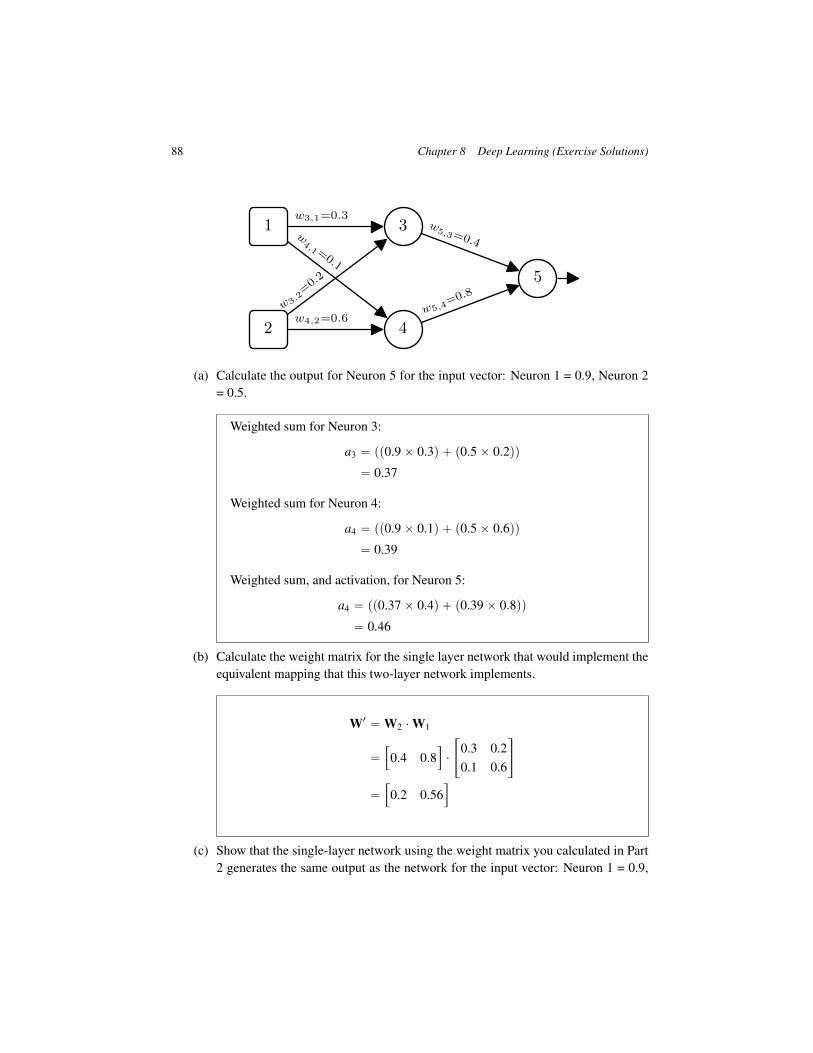
88 Chapter 8 Deep Learning (Exercise Solutions)
1 3
5
2 4
w3,1=0.3
w4,1=
0.1
w3,2=0.2
w4,2=0.6
w5,3=0.4
w5,4=0.8
(a) Calculate the output for Neuron 5 for the input vector: Neuron 1 = 0.9, Neuron 2= 0.5.
Weighted sum for Neuron 3:
a3 “ pp0.9ˆ 0.3q ` p0.5ˆ 0.2qq
“ 0.37
Weighted sum for Neuron 4:
a4 “ pp0.9ˆ 0.1q ` p0.5ˆ 0.6qq
“ 0.39
Weighted sum, and activation, for Neuron 5:
a4 “ pp0.37ˆ 0.4q ` p0.39ˆ 0.8qq
“ 0.46
(b) Calculate the weight matrix for the single layer network that would implement theequivalent mapping that this two-layer network implements.
W1 “ W2 ¨W1
“
”
0.4 0.8ı
¨
«
0.3 0.20.1 0.6
ff
“
”
0.2 0.56ı
(c) Show that the single-layer network using the weight matrix you calculated in Part2 generates the same output as the network for the input vector: Neuron 1 = 0.9,

89
Neuron 2 = 0.5.
activation “”
0.2 0.56ı
¨
«
0.90.5
ff
“ pp0.2ˆ 0.9q ` p0.56ˆ 0.5qq
“ 0.46
4. The following image illustrates the topology of a simple feedforward neural networkthat has a single sensing neuron (Neuron 1), a single hidden processing neuron (Neu-ron 2), and a single processing output neuron (Neuron 3).
1 2 3w2,1=0.2 w3,2=0.3
w2,0=0.1 w3,0=0.1
(a) Assuming that the processing neurons use logistic activation functions, that theinput to the network is Neuron 1 = 0.2 and that the desired output for this input is0.7:
i. Calculate the output generated by the network in response to this input.
z2 “ ppw2,0 ˆ 1q ` pw2,1 ˆ 0.2qq
“ pp0.1ˆ 1q ` p0.2ˆ 0.2qq
“ 0.14
a2 “ logisticp0.14q
“ 0.534942945
z3 “ ppw3,0 ˆ 1q ` pw3,2 ˆ a2qq
“ pp0.1ˆ 1q ` p0.3ˆ 0.534942945qq
“ 0.260482884
a3 “ logisticp0.260482884q
“ 0.564754992

90 Chapter 8 Deep Learning (Exercise Solutions)
ii. Calculate the δ values for each of the neurons in the network (i.e., δ3, δ2).
Calculations for δ3:
BE
Ba3“ ´ptk ´ akq
“ ´ p0.7´ 0.564754992q
“ ´0.135245008
Ba3
Bz3“ logisticpz3q ˆ p1´ logisticpz3qq
“ 0.564754992ˆ p1´ 0.564754992q
“ 0.245806791
δ3 “BE
Ba3ˆBa3
Bz3
“ ´0.135245008ˆ 0.245806791
“ ´0.033244142
Calculations for δ2:
BE
Ba2“ w3,2 ˆ δ3
“ 0.3ˆ´0.033244142
“ ´0.009973242
Ba2
Bz2“ logisticpz2q ˆ p1´ logisticpz2qq
“ 0.534942945ˆ p1´ 0.534942945q
“ 0.248778991
δ2 “BE
Ba2ˆBa2
Bz2
“ ´0.009973242ˆ 0.248778991
“ ´0.002481133
iii. Using the δ values you calculated above, calculate the sensitivity of the errorof the network to changes in each of the weights of the network (i.e., BE{Bw3,2,

91
BE{Bw3,0, BE{Bw2,1, BE{Bw2,0).
To calculate the sensitivity of the error of the network to changes in aweight we multiply the δ for the neuron that uses the weight in its weightedsum by the activation (or input) that the weight was applied to in the cal-culation of the weight sum. The calculations for each of the weights isshown below.
BE
Bw3,2“ δ3 ˆ a2
“ ´0.033244142ˆ 0.534942945
“ ´0.017783719
BE
Bw3,0“ δ3 ˆ a0
“ ´0.033244142ˆ 1
“ ´0.033244142
BE
Bw2,1“ δ2 ˆ a1
“ ´0.002481133ˆ 0.2
“ ´0.000496227
BE
Bw2,0“ δ2 ˆ a0
“ ´0.002481133ˆ 1
“ ´0.002481133
iv. Assuming a learning rate of α “ 0.1, calculate the updated values for each ofthe weights in the network (w3,2,w3,0,,w2,1,w2,0,) after the processing of thissingle training example.
We update weights as follows:
wt`1i,k “ wt
i,k ´ αˆBE
Bwi,k

92 Chapter 8 Deep Learning (Exercise Solutions)
The calculation for each weight update is below:
wt`13,2 “ wt
3,2 ´ αˆBE
Bw3,2
“ 0.3´ 0.1ˆ´0.017783719
“ 0.301778372
wt`13,0 “ wt
3,0 ´ αˆBE
Bw3,0
“ 0.1´ 0.1ˆ´0.033244142
“ 0.103324414
wt`12,1 “ wt
2,1 ´ αˆBE
Bw2,1
“ 0.2´ 0.1ˆ´0.000496227
“ 0.200049623
wt`12,0 “ wt
2,0 ´ αˆBE
Bw2,0
“ 0.1´ 0.1ˆ´0.002481133
“ 0.100248113
v. Calculate the reduction in the error of the network for this example using thenew weights, compared with using the original weights.
The output for the network using the new weights is:
z2 “ ppw2,0 ˆ 1q ` pw2,1 ˆ 0.2qq
“ pp0.100248113ˆ 1q ` p0.200049623ˆ 0.2qq
“ 0.140258038
a2 “ logisticp0.140258038q
“ 0.535007139

93
z3 “ ppw3,0 ˆ 1q ` pw3,2 ˆ a2qq
“ pp0.103324414ˆ 1q ` p0.301778372ˆ 0.535007139qq
“ 0.264777998
a3 “ logisticp0.264777998q
“ 0.565810465
The error with the new weights is:
Error1 “ 0.7´ 0.565810465
0.134189535
Subtracting this new error from the error with the original weights (whichwe calculated as part of the calculation for δ3 above) gives us the reductionin error:
Error Reduction “ 0.135245008´ 0.134189535
“ 0.001055473
(b) Assuming that the processing neurons are ReLUs, that the input to the network isNeuron 1 = 0.2, and that the desired output for this input is 0.7:
i. Calculate the output generated by the network in response to this input.
z2 “ ppw2,0 ˆ 1q ` pw2,1 ˆ 0.2qq
“ pp0.1ˆ 1q ` p0.2ˆ 0.2qq
“ 0.14
a2 “ recti f ierp0.14q
“ maxp0, 0.14q
“ 0.14
z3 “ ppw3,0 ˆ 1q ` pw3,2 ˆ a2qq
“ pp0.1ˆ 1q ` p0.3ˆ 0.14qq
“ 0.142

94 Chapter 8 Deep Learning (Exercise Solutions)
a3 “ recti f ierp0.142q
“ maxp0, 0.142q
“ 0.142
ii. Calculate the δ values for each of the neurons in the network (i.e., δ3, δ2).
Calculations for δ3:
BE
Ba3“ ´ptk ´ akq
“ ´ p0.7´ 0.142q
“ ´0.558
Ba3
Bz3“
#
1 if z3 ą 1
0 otherwise
“ 1
δ3 “BE
Ba3ˆBa3
Bz3
“ ´0.558ˆ 1
“ ´0.558
Calculations for δ2:
BE
Ba2“ w3,2 ˆ δ3
“ 0.3ˆ´0.558
“ ´0.1674
Ba2
Bz2“
#
1 if z2 ą 1
0 otherwise
“ 1
δ2 “BE
Ba2ˆBa2
Bz2
“ ´0.1674ˆ 1
“ ´0.1674

95
iii. Using the δ values you have calculated in the preceding, calculate the sensitiv-ity of the error of the network to changes in each of the weights of the network(i.e., BE{Bw3,2, BE{Bw3,0, BE{Bw2,1, BE{Bw2,0).
To calculate the sensitivity of the error of the network to changes in aweight we multiply the δ for the neuron that uses the weight in its weightedsum by the activation (or input) that the weight was applied to in the cal-culation of the weight sum. The calculations for each of the weights isshown below.
BE
Bw3,2“ δ3 ˆ a2
“ ´0.558ˆ 0.14
“ ´0.07812
BE
Bw3,0“ δ3 ˆ a0
“ ´0.558ˆ 1
“ ´0.558
BE
Bw2,1“ δ2 ˆ a1
“ ´0.1674ˆ 0.2
“ ´0.03348
BE
Bw2,0“ δ2 ˆ a0
“ ´0.1674ˆ 1
“ ´0.1674
iv. Assuming a learning rate of α “ 0.1, calculate the updated values for eachof the weights in the network (w3,2,w3,0,,w2,1,w2,0) after the processing of thissingle training example.
We update weights as follows:
wt`1i,k “ wt
i,k ´ αˆBE
Bwi,k

96 Chapter 8 Deep Learning (Exercise Solutions)
The calculation for each weight update is below:
wt`13,2 “ wt
3,2 ´ αˆBE
Bw3,2
“ 0.3´ 0.1ˆ´0.07812
“ 0.307812
wt`13,0 “ wt
3,0 ´ αˆBE
Bw3,0
“ 0.1´ 0.1ˆ´0.558
“ 0.1558
wt`12,1 “ wt
2,1 ´ αˆBE
Bw2,1
“ 0.2´ 0.1ˆ´0.03348
“ 0.203348
wt`12,0 “ wt
2,0 ´ αˆBE
Bw2,0
“ 0.1´ 0.1ˆ´0.1674
“ 0.11674
v. Calculate the reduction in the error for this example using the new weights forthe network, compared with using the original weights.
The output for the network using the new weights is:
z2 “ ppw2,0 ˆ 1q ` pw2,1 ˆ 0.2qq
“ pp0.11674ˆ 1q ` p0.203348ˆ 0.2qq
“ 0.1574096
a2 “ recti f ierp0.1574096q
“ maxp0, 0.1574096q
“ 0.1574096

97
z3 “ ppw3,0 ˆ 1q ` pw3,2 ˆ a2qq
“ pp0.1558ˆ 1q ` p0.307812ˆ 0.1574096qq
“ 0.204252564
a3 “ recti f ierp0.204252564q
“ maxp0, 0.204252564q
“ 0.204252564
The error with the new weights is:
Error1 “ 0.7´ 0.204252564
0.495747436
Subtracting this new error from the error with the original weights (whichwe calculated as part of the calculation for δ3 above) gives us the reductionin error:
Error Reduction “ 0.558´ 0.495747436
“ 0.062252564
5. The following image illustrates the topology of a simple feedforward neural networkthat has a single sensing neuron (Neuron 1), three hidden processing neuron (Neurons2, 3, and 4), and a single processing output neuron (Neuron 5).
3
1 2 5
4
w2,1=0.3w3,2
=0.2
w4,2=0.5
w5,3=0.4
w5,4=0.6
w2,0=0.1
w3,0=0.1
w4,0=0.1
w5,0=0.1
(a) Assuming that the processing neurons use logistic activation functions, that theinput to the network is Neuron 1 = 0.5 and that the desired output for this input is0.9:
i. Calculate the output generated by the network in response to this input.

98 Chapter 8 Deep Learning (Exercise Solutions)
z2 “ ppw2,0 ˆ 1q ` pw2,1 ˆ 0.5qq
“ pp0.1ˆ 1q ` p0.3ˆ 0.5qq
“ 0.25
a2 “ logisticp0.25q
“ 0.562176501
z3 “ ppw3,0 ˆ 1q ` pw3,2 ˆ a2qq
“ pp0.1ˆ 1q ` p0.2ˆ 0.562176501qq
“ 0.2124353
a3 “ logisticp0.2124353q
“ 0.552909994
z4 “ ppw4,0 ˆ 1q ` pw4,2 ˆ a2qq
“ pp0.1ˆ 1q ` p0.5ˆ 0.552909994qq
“ 0.38108825
a4 “ logisticp0.38108825q
“ 0.594135549
z5 “ ppw5,0 ˆ 1q ` pw5,3 ˆ a3q ` pw5,4 ˆ a4qq
“ pp0.1ˆ 1q ` p0.4ˆ 0.552909994q ` p0.6ˆ 0.594135549qq
“ 0.677645327
a5 “ logisticp0.677645327q
“ 0.663212956
ii. Calculate the δ values for each of the processing neurons in the network (i.e.,δ5, δ4, δ3, δ2).

99
Calculations for δ5:
BE
Ba5“ ´ptk ´ akq
“ ´ p0.9´ 0.663212956q
“ ´0.236787044
Ba5
Bz5“ logisticpz5q ˆ p1´ logisticpz5qq
“ 0.677645327ˆ p1´ 0.677645327q
“ 0.223361531
δ3 “BE
Ba5ˆBa5
Bz5
“ ´0.236787044ˆ 0.223361531
“ ´0.052889117
Calculations for δ4:
BE
Ba4“ w5,4 ˆ δ5
“ 0.6ˆ´0.052889117
“ ´0.03173347
Ba4
Bz4“ logisticpz4q ˆ p1´ logisticpz4qq
“ 0.594135549ˆ p1´ 0.594135549q
“ 0.241138498
δ4 “BE
Ba4ˆBa4
Bz4
“ ´0.03173347ˆ 0.241138498
“ ´0.007652161
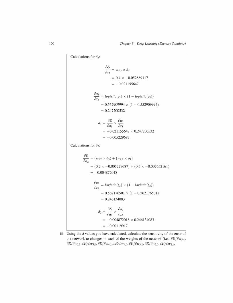
100 Chapter 8 Deep Learning (Exercise Solutions)
Calculations for δ3:
BE
Ba3“ w5,3 ˆ δ5
“ 0.4ˆ´0.052889117
“ ´0.021155647
Ba3
Bz3“ logisticpz3q ˆ p1´ logisticpz3qq
“ 0.552909994ˆ p1´ 0.552909994q
“ 0.247200532
δ3 “BE
Ba3ˆBa3
Bz3
“ ´0.021155647ˆ 0.247200532
“ ´0.005229687
Calculations for δ2:
BE
Ba2“ pw3,2 ˆ δ3q ` pw4,2 ˆ δ4q
“ p0.2ˆ´0.005229687q ` p0.5ˆ´0.007652161q
“ ´0.004872018
Ba2
Bz2“ logisticpz2q ˆ p1´ logisticpz2qq
“ 0.562176501ˆ p1´ 0.562176501q
“ 0.246134083
δ2 “BE
Ba2ˆBa2
Bz2
“ ´0.004872018ˆ 0.246134083
“ ´0.00119917
iii. Using the δ values you have calculated, calculate the sensitivity of the error ofthe network to changes in each of the weights of the network (i.e., BE{Bw5,4,
BE{Bw5,3, BE{Bw5,0, BE{Bw4,2, BE{Bw4,0, BE{Bw3,2, BE{Bw3,0, BE{Bw2,1,

101
BE{Bw2,0).
To calculate the sensitivity of the error of the network to changes in aweight we multiply the δ for the neuron that uses the weight in its weightedsum by the activation (or input) that the weight was applied to in the cal-culation of the weight sum. The calculations for each of the weights isshown below.
BE
Bw5,4“ δ5 ˆ a4
“ ´0.052889117ˆ 0.594135549
“ ´0.031423304
BE
Bw5,3“ δ5 ˆ a3
“ ´0.052889117ˆ 0.552909994
“ ´0.029242921
BE
Bw5,0“ δ5 ˆ a0
“ ´0.052889117ˆ 1
“ ´0.052889117
BE
Bw4,2“ δ4 ˆ a2
“ ´0.007652161ˆ 0.562176501
“ ´0.004301865
BE
Bw4,0“ δ4 ˆ a0
“ ´0.007652161ˆ 1
“ ´0.007652161
BE
Bw3,2“ δ3 ˆ a2
“ ´0.005229687ˆ 0.562176501
“ ´0.002940007

102 Chapter 8 Deep Learning (Exercise Solutions)
BE
Bw3,0“ δ3 ˆ a0
“ ´0.005229687ˆ 1
“ ´0.005229687
BE
Bw2,1“ δ2 ˆ a1
“ ´0.00119917ˆ 0.5
“ ´0.000599585
BE
Bw2,0“ δ2 ˆ a0
“ ´0.00119917ˆ 1
“ ´0.00119917
iv. Assuming a learning rate of α “ 0.1, calculate the updated values for each ofthe weights in the network (w5,4, w5,3, w5,0, w4,2, w4,0, w3,2, w3,0,, w2,1, w2,0,)after the processing of this single training example.
We update weights as follows:
wt`1i,k “ wt
i,k ´ αˆBE
Bwi,k
The calculation for each weight update is below:
wt`15,4 “ wt
5,4 ´ αˆBE
Bw5,4
“ 0.6´ p0.1ˆ´0.031423304q
“ 0.60314233
wt`15,3 “ wt
5,3 ´ αˆBE
Bw5,3
“ 0.4´ p0.1ˆ´0.029242921q
“ 0.402924292

103
wt`15,0 “ wt
5,0 ´ αˆBE
Bw5,0
“ 0.1´ p0.1ˆ´0.052889117q
“ 0.105288912
wt`14,2 “ wt
4,2 ´ αˆBE
Bw4,2
“ 0.5´ p0.1ˆ´0.004301865q
“ 0.500430187
wt`14,0 “ wt
4,0 ´ αˆBE
Bw4,0
“ 0.1´ p0.1ˆ´0.007652161q
“ 0.100765216
wt`13,2 “ wt
3,2 ´ αˆBE
Bw3,2
“ 0.2´ p0.1ˆ´0.002940007q
“ 0.200294001
wt`13,0 “ wt
3,0 ´ αˆBE
Bw3,0
“ 0.1´ p0.1ˆ´0.005229687q
“ 0.100522969
wt`12,1 “ wt
2,1 ´ αˆBE
Bw2,1
“ 0.3´ p0.1ˆ´0.000599585q
“ 0.300059958
wt`12,0 “ wt
2,0 ´ αˆBE
Bw2,0
“ 0.1´ p0.1ˆ´0.00119917q
“ 0.100119917

104 Chapter 8 Deep Learning (Exercise Solutions)
v. Calculate the reduction in the error of the network for this example using thenew weights, compared with using the original weights.
The output for the network using the new weights is:
z2 “ ppw2,0 ˆ 1q ` pw2,1 ˆ 0.5qq
“ pp0.100119917ˆ 1q ` p0.300059958ˆ 0.5qq
“ 0.250149896
a2 “ logisticp0.250149896q
“ 0.562213395
z3 “ ppw3,0 ˆ 1q ` pw3,2 ˆ a2qq
“ pp0.100522969ˆ 1q ` p0.200294001ˆ 0.562213395qq
“ 0.213130939
a3 “ logisticp0.213130939q
“ 0.55308195
z4 “ ppw4,0 ˆ 1q ` pw4,2 ˆ a2qq
“ pp0.100765216ˆ 1q ` p0.500430187ˆ 0.562213395qq
“ 0.38211377
a4 “ logisticp0.38211377q
“ 0.594382817
z5 “ ppw5,0 ˆ 1q ` pw5,3 ˆ a3q ` pw5,4 ˆ a4qq
“ pp0.105288912ˆ 1q ` p0.402924292ˆ 0.55308195q ` p0.60314233ˆ 0.594382817qq
“ 0.686636503
a5 “ logisticp0.686636503q
“ 0.665218283

105
The error with the new weights is:
Error1 “ 0.9´ 0.665218283
0.234781717
Subtracting this new error from the error with the original weights (whichwe calculated as part of the calculation for δ3 above) gives us the reductionin error:
Error Reduction “ 0.236787044´ 0.234781717
“ 0.002005326
(b) Assuming that the processing neurons are ReLUs, that the input to the network isNeuron 1 = 0.5 and that the desired output for this input is 0.9
i. Calculate the output generated by the network in response to this input.
z2 “ ppw2,0 ˆ 1q ` pw2,1 ˆ 0.5qq
“ pp0.1ˆ 1q ` p0.3ˆ 0.5qq
“ 0.25
a2 “ recti f ierp0.25q
“ maxp0, 0.25q
“ 0.25
z3 “ ppw3,0 ˆ 1q ` pw3,2 ˆ a2qq
“ pp0.1ˆ 1q ` p0.2ˆ 0.25qq
“ 0.15
a3 “ recti f ierp0.15q
“ maxp0, 0.15q
“ 0.15
z4 “ ppw4,0 ˆ 1q ` pw4,2 ˆ a2qq
“ pp0.1ˆ 1q ` p0.5ˆ 0.25qq
“ 0.225

106 Chapter 8 Deep Learning (Exercise Solutions)
a4 “ recti f ierp0.225q
“ maxp0, 0.225q
“ 0.225
z5 “ ppw5,0 ˆ 1q ` pw5,3 ˆ a3q ` pw5,4 ˆ a4qq
“ pp0.1ˆ 1q ` p0.4ˆ 0.15q ` p0.6ˆ 0.225qq
“ 0.295
a5 “ recti f ierp0.295q
“ maxp0, 0.295q
“ 0.295
ii. Calculate the δ values for each of the processing neurons in the network (i.e.,δ5, δ4, δ3, δ2).
Calculations for δ5:
BE
Ba5“ ´ptk ´ akq
“ ´ p0.9´ 0.295q
“ ´0.605
Ba5
Bz5“
#
1 if z5 ą 1
0 otherwise
“ 1
δ5 “BE
Ba5ˆBa5
Bz5
“ ´0.605ˆ 1
“ ´0.605
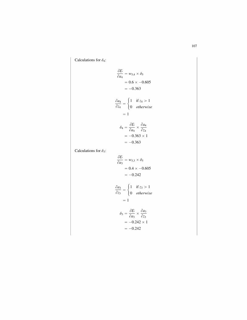
107
Calculations for δ4:
BE
Ba4“ w5,4 ˆ δ5
“ 0.6ˆ´0.605
“ ´0.363
Ba4
Bz4“
#
1 if z4 ą 1
0 otherwise
“ 1
δ4 “BE
Ba4ˆBa4
Bz4
“ ´0.363ˆ 1
“ ´0.363
Calculations for δ3:
BE
Ba3“ w5,3 ˆ δ5
“ 0.4ˆ´0.605
“ ´0.242
Ba3
Bz3“
#
1 if z3 ą 1
0 otherwise
“ 1
δ3 “BE
Ba3ˆBa3
Bz3
“ ´0.242ˆ 1
“ ´0.242

108 Chapter 8 Deep Learning (Exercise Solutions)
Calculations for δ2:
BE
Ba2“ pw3,2 ˆ δ3q ` pw4,2 ˆ δ4q
“ p0.2ˆ´0.242q ` p0.5ˆ´0.363q
“ ´0.2299
Ba2
Bz2“
#
1 if z2 ą 1
0 otherwise
“ 1
δ2 “BE
Ba2ˆBa2
Bz2
“ ´0.2299ˆ 1
“ ´0.2299
iii. Using the δ values you have calculated, calculate the sensitivity of the error ofthe network to changes in each of the weights of the network (i.e., BE{Bw5,4,
BE{Bw5,3, BE{Bw5,0, BE{Bw4,2, BE{Bw4,0, BE{Bw3,2, BE{Bw3,0, BE{Bw2,1, BE{Bw2,0).
To calculate the sensitivity of the error of the network to changes in aweight we multiply the δ for the neuron that uses the weight in its weightedsum by the activation (or input) that the weight was applied to in the cal-culation of the weight sum. The calculations for each of the weights isshown below.
BE
Bw5,4“ δ5 ˆ a4
“ ´0.605ˆ 0.225
“ ´0.136125
BE
Bw5,3“ δ5 ˆ a3
“ ´0.605ˆ 0.15
“ ´0.09075

109
BE
Bw5,0“ δ5 ˆ a0
“ ´0.605ˆ 1
“ ´0.605
BE
Bw4,2“ δ4 ˆ a2
“ ´0.363ˆ 0.25
“ ´0.09075
BE
Bw4,0“ δ4 ˆ a0
“ ´0.363ˆ 1
“ ´0.363
BE
Bw3,2“ δ3 ˆ a2
“ ´0.242ˆ 0.25
“ ´0.0605
BE
Bw3,0“ δ3 ˆ a0
“ ´0.242ˆ 1
“ ´0.242
BE
Bw2,1“ δ2 ˆ a1
“ ´0.2299ˆ 0.5
“ ´0.11495
BE
Bw2,0“ δ2 ˆ a0
“ ´0.2299ˆ 1
“ ´0.2299
iv. Assuming a learning rate of α “ 0.1, calculate the updated values for each ofthe weights in the network (w5,4, w5,3, w5,0, w4,2, w4,0, w3,2, w3,0,, w2,1, w2,0,)

110 Chapter 8 Deep Learning (Exercise Solutions)
after the processing of this single training example.
We update weights as follows:
wt`1i,k “ wt
i,k ´ αˆBE
Bwi,k
The calculation for each weight update is below:
wt`15,4 “ wt
5,4 ´ αˆBE
Bw5,4
“ 0.6´ p0.1ˆ´0.136125q
“ 0.6136125
wt`15,3 “ wt
5,3 ´ αˆBE
Bw5,3
“ 0.4´ p0.1ˆ´0.09075q
“ 0.409075
wt`15,0 “ wt
5,0 ´ αˆBE
Bw5,0
“ 0.1´ p0.1ˆ´0.605q
“ 0.1605
wt`14,2 “ wt
4,2 ´ αˆBE
Bw4,2
“ 0.5´ p0.1ˆ´0.09075q
“ 0.509075
wt`14,0 “ wt
4,0 ´ αˆBE
Bw4,0
“ 0.1´ p0.1ˆ´0.363q
“ 0.1363
wt`13,2 “ wt
3,2 ´ αˆBE
Bw3,2
“ 0.2´ p0.1ˆ´0.0605q
“ 0.20605

111
wt`13,0 “ wt
3,0 ´ αˆBE
Bw3,0
“ 0.1´ p0.1ˆ´0.242q
“ 0.1242
wt`12,1 “ wt
2,1 ´ αˆBE
Bw2,1
“ 0.3´ p0.1ˆ´0.11495q
“ 0.311495
wt`12,0 “ wt
2,0 ´ αˆBE
Bw2,0
“ 0.1´ p0.1ˆ´0.2299q
“ 0.12299
v. Calculate the reduction in the error of the network for this example using thenew weights, compared with using the original weights.
The output for the network using the new weights is:
z2 “ ppw2,0 ˆ 1q ` pw2,1 ˆ 0.5qq
“ pp0.12299ˆ 1q ` p0.311495ˆ 0.5qq
“ 0.2787375
a2 “ recti f ierp0.2787375q
“ maxp0, 0.2787375q
“ 0.2787375
z3 “ ppw3,0 ˆ 1q ` pw3,2 ˆ a2qq
“ pp0.1242ˆ 1q ` p0.20605ˆ 0.2787375qq
“ 0.181633862

112 Chapter 8 Deep Learning (Exercise Solutions)
a3 “ recti f ierp0.181633862q
“ maxp0, 0.181633862q
“ 0.181633862
z4 “ ppw4,0 ˆ 1q ` pw4,2 ˆ a2qq
“ pp0.1363ˆ 1q ` p0.509075ˆ 0.2787375qq
“ 0.278198293
a4 “ recti f ierp0.278198293q
“ maxp0, 0.278198293q
“ 0.278198293
z5 “ ppw5,0 ˆ 1q ` pw5,3 ˆ a3q ` pw5,4 ˆ a4qq
“ pp0.1605ˆ 1q ` p0.409075ˆ 0.181633862q ` p0.6136125ˆ 0.278198293qq
“ 0.405507822
a5 “ recti f ierp0.405507822q
“ maxp0, 0.405507822q
“ 0.405507822
The error with the new weights is:
Error1 “ 0.9´ 0.405507822
0.494492178
Subtracting this new error from the error with the original weights (whichwe calculated as part of the calculation for δ3 above) gives us the reductionin error:
Error Reduction “ 0.605´ 0.494492178
“ 0.110507822
6. The following image illustrates the topology of a feedforward neural network that hastwo sensing neurons (Neurons 1 and 2), two hidden processing neuron (Neurons 3,and 4), and two processing output neurons (Neurons 5 and 6).

113
1 3 5
2 4 6
w3,1=−0.1w4,1=0.2
w3,2=−0.2
w4,2=0.3
w5,3=−0.1w6,3=0.1
w5,4=0.2
w6,4=−0.2
w3,0=0.1
w4,0=0.1
w5,0=0.1
w6,0=0.1
(a) Assuming that the processing neurons use logistic activation functions, that theinput to the network is Neuron 1 = 0.3 and Neuron 2 = 0.6, and that the desiredoutput for this input is Neuron 5 = 0.7 and Neuron 6 = 0.4:
i. Calculate the output generated by the network in response to this input.
z3 “ ppw3,0 ˆ 1q ` pw3,1 ˆ a1q ` pw3,2 ˆ a2qq
“ pp0.1ˆ 1q ` p´0.1ˆ 0.3q ` p´0.2ˆ 0.6qq
“ ´0.05
a3 “ logisticp´0.05q
“ 0.487502604
z4 “ ppw4,0 ˆ 1q ` pw4,1 ˆ a1q ` pw4,2 ˆ a2qq
“ pp0.1ˆ 1q ` p0.2ˆ 0.3q ` p0.3ˆ 0.6qq
“ 0.34
a4 “ logisticp0.34q
“ 0.584190523
z5 “ ppw5,0 ˆ 1q ` pw5,3 ˆ a3q ` pw5,4 ˆ a4qq
“ pp0.1ˆ 1q ` p´0.1ˆ 0.487502604q ` p0.2ˆ 0.584190523qq
“ 0.168087844

114 Chapter 8 Deep Learning (Exercise Solutions)
a5 “ logisticp0.168087844q
“ 0.541923301
z6 “ ppw6,0 ˆ 1q ` pw6,3 ˆ a3q ` pw6,4 ˆ a4qq
“ pp0.1ˆ 1q ` p0.1ˆ 0.487502604q ` p´0.2ˆ 0.584190523qq
“ 0.031912156
a6 “ logisticp0.031912156q
“ 0.507977362
ii. Calculate the sum of squared errors for this network for this example.
S S E “ pt5 ´ a5q2 ` pt6 ´ a6q
2
“ p0.7´ 0.541923301q2 ` p0.4´ 0.507977362q2
“ p0.158076699q2 ` p´0.107977362q2
“ 0.036647354
iii. Calculate the δ values for each of the processing neurons in the network (i.e.,δ6, δ5, δ4, δ3).
Calculations for δ6:
BE
Ba6“ ´pt6 ´ a6q
“ ´ p0.4´ 0.507977362q
“ ´ p´0.107977362q
“ 0.107977362
Ba6
Bz6“ logisticpz6q ˆ p1´ logisticpz6qq
“ 0.507977362ˆ p1´ 0.507977362q
“ 0.249936362

115
δ6 “BE
Ba6ˆBa6
Bz6
“ 0.107977362ˆ 0.249936362
“ 0.026987469
Calculations for δ5:
BE
Ba5“ ´pt5 ´ a5q
“ ´ p0.7´ 0.541923301q
“ ´0.158076699
Ba5
Bz5“ logisticpz5q ˆ p1´ logisticpz5qq
“ 0.541923301ˆ p1´ 0.541923301q
“ ´0.039241345
δ3 “BE
Ba5ˆBa5
Bz5
“ ´0.158076699ˆ 0.248242437
“ ´0.039241345
Calculations for δ4:
BE
Ba4“ pw5,4 ˆ δ5q ` pw6,4 ˆ δ6q
“ p0.2ˆ´0.039241345q ` p´0.2ˆ 0.026987469q
“ ´0.013245763
Ba4
Bz4“ logisticpz4q ˆ p1´ logisticpz4qq
“ 0.584190523ˆ p1´ 0.584190523q
“ 0.242911956
δ4 “BE
Ba4ˆBa4
Bz4
“ ´0.013245763ˆ 0.242911956
“ ´0.003217554

116 Chapter 8 Deep Learning (Exercise Solutions)
Calculations for δ3:
BE
Ba3“ pw5,3 ˆ δ5q ` pw6,3 ˆ δ6q
“ p´0.1ˆ´0.039241345q ` p0.1ˆ 0.026987469q
“ 0.006622881
Ba3
Bz3“ logisticpz3q ˆ p1´ logisticpz3qq
“ 0.487502604ˆ p1´ 0.487502604q
“ 0.249843815
δ3 “BE
Ba3ˆBa3
Bz3
“ 0.006622881ˆ 0.249843815
“ 0.001654686
iv. Using the δ values you calculated above, calculate the sensitivity of the errorof the network to changes in each of the weights of the network (i.e., BE{Bw6,4,BE{Bw6,3, BE{Bw6,0, BE{Bw5,4, BE{Bw5,3, BE{Bw5,0, BE{Bw4,2, BE{Bw4,1,BE{Bw4,0, BE{Bw3,2, BE{Bw3,1, BE{Bw3,0).
To calculate the sensitivity of the error of the network to changes in aweight we multiply the δ for the neuron that uses the weight in its weightedsum by the activation (or input) that the weight was applied to in the cal-culation of the weight sum. The calculations for each of the weights isshown below.
BE
Bw6,4“ δ6 ˆ a4
“ 0.026987469ˆ 0.584190523
“ 0.015765824
BE
Bw6,3“ δ6 ˆ a3
“ 0.026987469ˆ 0.487502604
“ 0.013156461

117
BE
Bw5,0“ δ6 ˆ a0
“ 0.026987469ˆ 1
“ 0.026987469
BE
Bw5,4“ δ5 ˆ a4
“ ´0.039241345ˆ 0.584190523
“ ´0.022924422
BE
Bw5,3“ δ5 ˆ a3
“ ´0.039241345ˆ 0.487502604
“ ´0.019130258
BE
Bw5,0“ δ5 ˆ a0
“ ´0.039241345ˆ 1
“ ´0.039241345
BE
Bw4,2“ δ4 ˆ a2
“ ´0.003217554ˆ 0.6
“ ´0.001930532
BE
Bw4,1“ δ4 ˆ a1
“ ´0.003217554ˆ 0.3
“ ´0.000965266
BE
Bw4,0“ δ4 ˆ a0
“ ´0.003217554ˆ 1
“ ´0.003217554
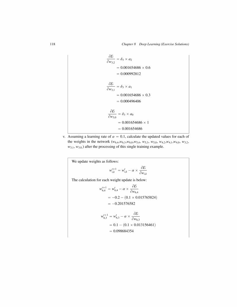
118 Chapter 8 Deep Learning (Exercise Solutions)
BE
Bw3,2“ δ3 ˆ a2
“ 0.001654686ˆ 0.6
“ 0.000992812
BE
Bw3,1“ δ3 ˆ a1
“ 0.001654686ˆ 0.3
“ 0.000496406
BE
Bw3,0“ δ3 ˆ a0
“ 0.001654686ˆ 1
“ 0.001654686
v. Assuming a learning rate of α “ 0.1, calculate the updated values for each ofthe weights in the network (w6,4,w6,3,w6,0,w5,4, w5,3, w5,0, w4,2,w4,1,w4,0, w3,2,w3,1, w3,0,) after the processing of this single training example.
We update weights as follows:
wt`1i,k “ wt
i,k ´ αˆBE
Bwi,k
The calculation for each weight update is below:
wt`16,4 “ wt
6,4 ´ αˆBE
Bw6,4
“ ´0.2´ p0.1ˆ 0.015765824q
“ ´0.201576582
wt`16,3 “ wt
6,3 ´ αˆBE
Bw6,3
“ 0.1´ p0.1ˆ 0.013156461q
“ 0.098684354

119
wt`16,0 “ wt
5,0 ´ αˆBE
Bw6,0
“ 0.1´ p0.1ˆ 0.026987469q
“ 0.097301253
wt`15,4 “ wt
5,4 ´ αˆBE
Bw5,4
“ 0.2´ p0.1ˆ´0.022924422q
“ 0.202292442
wt`15,3 “ wt
5,3 ´ αˆBE
Bw5,3
“ ´0.1´ p0.1ˆ´0.019130258q
“ ´0.098086974
wt`15,0 “ wt
5,0 ´ αˆBE
Bw5,0
“ 0.1´ p0.1ˆ´0.039241345q
“ 0.103924135
wt`14,2 “ wt
4,2 ´ αˆBE
Bw4,2
“ 0.3´ p0.1ˆ´0.001930532q
“ 0.300193053
wt`14,1 “ wt
4,1 ´ αˆBE
Bw4,1
“ 0.2´ p0.1ˆ´0.000965266q
“ 0.200096527

120 Chapter 8 Deep Learning (Exercise Solutions)
wt`14,0 “ wt
4,0 ´ αˆBE
Bw4,0
“ 0.1´ p0.1ˆ´0.003217554q
“ 0.100321755
wt`13,2 “ wt
3,2 ´ αˆBE
Bw3,2
“ ´0.2´ p0.1ˆ 0.000992812q
“ ´0.200099281
wt`13,1 “ wt
3,1 ´ αˆBE
Bw3,1
“ ´0.1´ p0.1ˆ 0.000496406q
“ ´0.100049641
wt`13,0 “ wt
3,0 ´ αˆBE
Bw3,0
“ 0.1´ p0.1ˆ 0.001654686q
“ 0.099834531
vi. Calculate the reduction in the sum of squared error of the network for this ex-ample using the new weights, compared with using the original weights.
The output for the network using the new weights is:
z3 “ ppw3,0 ˆ 1q ` pw3,1 ˆ a1q ` pw3,2 ˆ a2qq
“ pp0.099834531ˆ 1q ` p´0.100049641ˆ 0.3q ` p´0.200099281ˆ 0.6qq
“ ´0.050239929
a3 “ logisticp´0.050239929q
“ 0.487442659

121
z4 “ ppw4,0 ˆ 1q ` pw4,1 ˆ a1q ` pw4,2 ˆ a2qq
“ pp0.100321755ˆ 1q ` p0.200096527ˆ 0.3q ` p0.300193053ˆ 0.6qq
“ 0.340466545
a4 “ logisticp0.340466545q
“ 0.584303848
z5 “ ppw5,0 ˆ 1q ` pw5,3 ˆ a3q ` pw5,4 ˆ a4qq
“ pp0.103924135ˆ 1q ` p´0.098086974ˆ 0.487442659q ` p0.202292442ˆ 0.584303848qq
“ 0.174312611
a5 “ logisticp0.174312611q
“ 0.543468144
z6 “ ppw6,0 ˆ 1q ` pw6,3 ˆ a3q ` pw6,4 ˆ a4qq
“ pp0.097301253ˆ 1q ` p0.098684354ˆ 0.487442659q ` p´0.201576582ˆ 0.584303848qq
“ 0.027622244
a6 “ logisticp0.027622244q
“ 0.506905122
If we now calculate the sum of squared errors on this example for thisnetwork using the new weights we get:
S S E “ pt5 ´ a5q2 ` pt6 ´ a6q
2
“ p0.7´ 0.543468144q2 ` p0.4´ 0.506905122q2
“ p0.156531856q2 ` p´0.106905122q2
“ 0.035930927
Subtracting this new error from the error with the original weights (whichwe calculated as part of the calculation for δ3 above) gives us the reductionin error:
Error Reduction “ 0.036647354´ 0.035930927
“ 0.000716426

122 Chapter 8 Deep Learning (Exercise Solutions)
(b) Assuming that the processing neurons use a rectifier activation functions, that theinput to the network is Neuron 1 = 0.3 and Neuron 2 = 0.6 and that the desiredoutput for this input is Neuron 5 = 0.7 and Neuron 6 = 0.4:
i. Calculate the output generated by the network in response to this input.
z3 “ ppw3,0 ˆ 1q ` pw3,1 ˆ a1q ` pw3,2 ˆ a2qq
“ pp0.1ˆ 1q ` p´0.1ˆ 0.3q ` p´0.2ˆ 0.6qq
“ ´0.05
a3 “ recti f ierp´0.05q
“ maxp0,´0.05q
“ 0
z4 “ ppw4,0 ˆ 1q ` pw4,1 ˆ a1q ` pw4,2 ˆ a2qq
“ pp0.1ˆ 1q ` p0.2ˆ 0.3q ` p0.3ˆ 0.6qq
“ 0.34
a4 “ recti f ierp0.34q
“ maxp0, 0.34q
“ 0.34
z5 “ ppw5,0 ˆ 1q ` pw5,3 ˆ a3q ` pw5,4 ˆ a4qq
“ pp0.1ˆ 1q ` p´0.1ˆ 0q ` p0.2ˆ 0.34qq
“ 0.168
a5 “ recti f ierp0.168q
“ maxp0, 0.168q
“ 0.168
z6 “ ppw6,0 ˆ 1q ` pw6,3 ˆ a3q ` pw6,4 ˆ a4qq
“ pp0.1ˆ 1q ` p0.1ˆ 0q ` p´0.2ˆ 0.34qq
“ 0.032

123
a6 “ recti f ierp0.032q
“ maxp0, 0.032q
“ 0.032
ii. Calculate the sum of squared errors for this network on this example.
S S E “ pt5 ´ a5q2 ` pt6 ´ a6q
2
“ p0.7´ 0.168q2 ` p0.4´ 0.032q2
“ p0.532q2 ` p0.368q2
“ 0.418448
iii. Calculate the δ values for each of the processing neurons in the network (i.e.,δ6, δ5, δ4, δ3).
Calculations for δ6:
BE
Ba6“ ´pt6 ´ a6q
“ ´ p0.4´ 0.032q
“ ´ p0.368q
“ ´0.368
Ba6
Bz6“
#
1 if z6 ą 1
0 otherwise
“ 1
δ6 “BE
Ba6ˆBa6
Bz6
“ ´0.368ˆ 1
“ ´0.368
Calculations for δ5:
BE
Ba5“ ´pt5 ´ a5q
“ ´ p0.7´ 0.168q
“ ´0.532

124 Chapter 8 Deep Learning (Exercise Solutions)
Ba5
Bz5“
#
1 if z5 ą 1
0 otherwise
“ 1
δ5 “BE
Ba5ˆBa5
Bz5
“ ´0.532ˆ 1
“ ´0.532
Calculations for δ4:
BE
Ba4“ pw5,4 ˆ δ5q ` pw6,4 ˆ δ6q
“ p0.2ˆ´0.532q ` p´0.2ˆ´0.368q
“ ´0.0328
Ba4
Bz4“
#
1 if z4 ą 1
0 otherwise
“ 1
δ4 “BE
Ba4ˆBa4
Bz4
“ ´0.0328ˆ 1
“ ´0.0328
Calculations for δ3:
BE
Ba3“ pw5,3 ˆ δ5q ` pw6,3 ˆ δ6q
“ p´0.1ˆ´0.532q ` p0.1ˆ´0.368q
“ 0.0164
Ba3
Bz3“
#
1 if z3 ą 1
0 otherwise
“ 0

125
δ3 “BE
Ba3ˆBa3
Bz3
“ 0.0164ˆ 0
“ 0
iv. Using the δ values you calculated above, calculate the sensitivity of the errorof the network to changes in each of the weights of the network (i.e., BE{Bw6,4,BE{Bw6,3, BE{Bw6,0, BE{Bw5,4, BE{Bw5,3, BE{Bw5,0, BE{Bw4,2, BE{Bw4,1,BE{Bw4,0, BE{Bw3,2, BE{Bw3,1, BE{Bw3,0).
To calculate the sensitivity of the error of the network to changes in aweight we multiply the δ for the neuron that uses the weight in its weightedsum by the activation (or input) that the weight was applied to in the cal-culation of the weight sum. The calculations for each of the weights isshown below.
BE
Bw6,4“ δ6 ˆ a4
“ ´0.368ˆ 0.34
“ ´0.12512
BE
Bw6,3“ δ6 ˆ a3
“ ´0.368ˆ 0
“ 0
BE
Bw5,0“ δ6 ˆ a0
“ ´0.368ˆ 1
“ ´0.368
BE
Bw5,4“ δ5 ˆ a4
“ ´0.532ˆ 0.34
“ ´0.18088

126 Chapter 8 Deep Learning (Exercise Solutions)
BE
Bw5,3“ δ5 ˆ a3
“ ´0.532ˆ 0
“ 0
BE
Bw5,0“ δ5 ˆ a0
“ ´0.532ˆ 1
“ ´0.532
BE
Bw4,2“ δ4 ˆ a2
“ ´0.0328ˆ 0.6
“ ´0.01968
BE
Bw4,1“ δ4 ˆ a1
“ ´0.0328ˆ 0.3
“ ´0.00984
BE
Bw4,0“ δ4 ˆ a0
“ ´0.0328ˆ 1
“ ´0.0328
BE
Bw3,2“ δ3 ˆ a2
“ 0ˆ 0.6
“ 0
BE
Bw3,1“ δ3 ˆ a1
“ 0ˆ 0.3
“ 0

127
BE
Bw3,0“ δ3 ˆ a0
“ 0ˆ 1
“ 0
v. Assuming a learning rate of α “ 0.1, calculate the updated values for each ofthe weights in the network (w6,4,w6,3,w6,0,w5,4, w5,3, w5,0, w4,2,w4,1,w4,0, w3,2,w3,1, w3,0,) after the processing of this single training example.
We update weights as follows:
wt`1i,k “ wt
i,k ´ αˆBE
Bwi,k
The calculation for each weight update is below:
wt`16,4 “ wt
6,4 ´ αˆBE
Bw6,4
“ ´0.2´ p0.1ˆ´0.12512q
“ ´0.187488
wt`16,3 “ wt
6,3 ´ αˆBE
Bw6,3
“ 0.1´ p0.1ˆ 0q
“ 0.1
wt`16,0 “ wt
5,0 ´ αˆBE
Bw6,0
“ 0.1´ p0.1ˆ´0.368q
“ 0.1368
wt`15,4 “ wt
5,4 ´ αˆBE
Bw5,4
“ 0.2´ p0.1ˆ´0.18088q
“ 0.218088

128 Chapter 8 Deep Learning (Exercise Solutions)
wt`15,3 “ wt
5,3 ´ αˆBE
Bw5,3
“ ´0.1´ p0.1ˆ 0q
“ ´0.1
wt`15,0 “ wt
5,0 ´ αˆBE
Bw5,0
“ 0.1´ p0.1ˆ´0.532q
“ 0.1532
wt`14,2 “ wt
4,2 ´ αˆBE
Bw4,2
“ 0.3´ p0.1ˆ´0.01968q
“ 0.301968
wt`14,1 “ wt
4,1 ´ αˆBE
Bw4,1
“ 0.2´ p0.1ˆ´0.00984q
“ 0.200984
wt`14,0 “ wt
4,0 ´ αˆBE
Bw4,0
“ 0.1´ p0.1ˆ´0.0328q
“ 0.10328
wt`13,2 “ wt
3,2 ´ αˆBE
Bw3,2
“ ´0.2´ p0.1ˆ 0q
“ ´0.2
wt`13,1 “ wt
3,1 ´ αˆBE
Bw3,1
“ ´0.1´ p0.1ˆ 0q
“ ´0.1

129
wt`13,0 “ wt
3,0 ´ αˆBE
Bw3,0
“ 0.1´ p0.1ˆ 0q
“ 0.1
vi. Calculate the reduction in the sum of squared error of the network for this ex-ample using the new weights, compared with using the original weights.
The output for the network using the new weights is:
z3 “ ppw3,0 ˆ 1q ` pw3,1 ˆ a1q ` pw3,2 ˆ a2qq
“ pp0.1ˆ 1q ` p´0.1ˆ 0.3q ` p´0.2ˆ 0.6qq
“ ´0.05
a3 “ recti f ierp´0.05q
“ maxp0,´0.05q
“ 0
z4 “ ppw4,0 ˆ 1q ` pw4,1 ˆ a1q ` pw4,2 ˆ a2qq
“ pp0.10328ˆ 1q ` p0.200984ˆ 0.3q ` p0.301968ˆ 0.6qq
“ 0.344756
a4 “ recti f ierp0.344756q
“ maxp0, 0.344756q
“ 0.344756
z5 “ ppw5,0 ˆ 1q ` pw5,3 ˆ a3q ` pw5,4 ˆ a4qq
“ pp0.1532ˆ 1q ` p´0.1ˆ 0q ` p0.218088ˆ 0.344756qq
“ 0.228387147
a5 “ recti f ierp0.228387147q
“ maxp0, 0.228387147q
“ 0.228387147

130 Chapter 8 Deep Learning (Exercise Solutions)
z6 “ ppw6,0 ˆ 1q ` pw6,3 ˆ a3q ` pw6,4 ˆ a4qq
“ pp0.1368ˆ 1q ` p0.1ˆ 0q ` p´0.187488ˆ 0.344756qq
“ 0.072162387
a6 “ recti f ierp0.072162387q
“ maxp0, 0.072162387q
“ 0.072162387
If we now calculate the sum of squared errors on this example for thisnetwork using the new weights we get:
S S E “ pt5 ´ a5q2 ` pt6 ´ a6q
2
“ p0.7´ 0.228387147q2 ` p0.4´ 0.072162387q2
“ p0.471612853q2 ` p0.327837613q2
“ 0.329896184
Subtracting this new error from the error with the original weights (whichwe calculated as part of the calculation for δ3 above) gives us the reductionin error:
Error Reduction “ 0.418448´ 0.329896184
“ 0.088551816
7. Assuming a fully connected feedforward network where all the neurons uses a linearactivation function (i.e., ai “ zi) and with the following topology:
(a) 100 neurons in the input layer
(b) 5 hidden layers with 2,000 neurons in each layer
(c) 10 neurons in the output layer
If all the inputs to the network have been standardized to have a mean value of 0 anda standard deviation of 1, and the initial weights for the network are sampled from anormal distribution with mean 0.0 and standard deviation of σ “ 0.01, then:
(a) Calculate the variance of the z values across for the neurons in the first hiddenlayer in the first iteration of training.
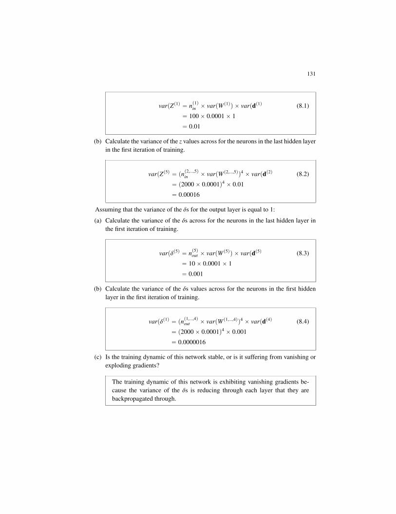
131
varpZp1q “ np1qin ˆ varpWp1qq ˆ varpdp1q (8.1)
“ 100ˆ 0.0001ˆ 1
“ 0.01
(b) Calculate the variance of the z values across for the neurons in the last hidden layerin the first iteration of training.
varpZp5q “ pnp2,...,5qin ˆ varpWp2,...,5qq4 ˆ varpdp2q (8.2)
“ p2000ˆ 0.0001q4 ˆ 0.01
“ 0.00016
Assuming that the variance of the δs for the output layer is equal to 1:
(a) Calculate the variance of the δs across for the neurons in the last hidden layer inthe first iteration of training.
varpδp5q “ np5qout ˆ varpWp5qq ˆ varpdp5q (8.3)
“ 10ˆ 0.0001ˆ 1
“ 0.001
(b) Calculate the variance of the δs values across for the neurons in the first hiddenlayer in the first iteration of training.
varpδp1q “ pnp1,...,4qout ˆ varpWp1,...,4qq4 ˆ varpdp4q (8.4)
“ p2000ˆ 0.0001q4 ˆ 0.001
“ 0.0000016
(c) Is the training dynamic of this network stable, or is it suffering from vanishing orexploding gradients?
The training dynamic of this network is exhibiting vanishing gradients be-cause the variance of the δs is reducing through each layer that they arebackpropagated through.


9 Evaluation (Exercise Solutions)
1. The table below shows the predictions made for a categorical target feature by a modelfor a test dataset. Based on this test set, calculate the evaluation measures listed below.
ID Target Prediction1 false false2 false false3 false false4 false false5 true true6 false false7 true true
ID Target Prediction8 true true9 false false
10 false false11 false false12 true true13 false false14 true true
ID Target Prediction15 false false16 false false17 true false18 true true19 true true20 true true
(a) A confusion matrix and the misclassification rate
The confusion matrix can be written as
Predictiontrue false
Target true 8 1false 0 11
Misclassification rate can be calculated as
misclassi f ication rate “pFP` FNq
pT P` T N ` FP` FNq
“p0` 1q
p8` 11` 0` 1q
“ 0.05
(b) The average class accuracy (harmonic mean)

134 Chapter 9 Evaluation (Exercise Solutions)
First, we calculate the recall for each target level:
recalltrue “89“ 0.889
recallfalse “1111“ 1.000
Then we can calculate a harmonic mean as
average class accuracyHM “1
1|levelsptq|
ÿ
lPlevelsptq
1recalll
“1
12
ˆ
10.889
`11
˙
“ 0.941
(c) The precision, recall, and F1 measure
We can calculate precision and recall as follows (assuming that the true targetlevel is the positive level):
precision “T P
pT P` FPq
“8
p8` 0q
“ 1.000
recall “T P
pT P` FNq
“8
p8` 1q
“ 0.889
Using these figures, we can calculate the F1 measure as
F1 measure “ 2ˆpprecisionˆ recallqpprecision` recallq
“ 2ˆp1.000ˆ 0.889qp1.000` 0.889q
“ 0.941

135
2. The table below shows the predictions made for a continuous target feature by twodifferent prediction models for a test dataset.
Model 1 Model 2ID Target Prediction Prediction1 2,623 2,664 2,6912 2,423 2,436 2,3673 2,423 2,399 2,4124 2,448 2,447 2,4405 2,762 2,847 2,6936 2,435 2,411 2,4937 2,519 2,516 2,5988 2,772 2,870 2,8149 2,601 2,586 2,583
10 2,422 2,414 2,48511 2,349 2,407 2,47212 2,515 2,505 2,58413 2,548 2,581 2,60414 2,281 2,277 2,30915 2,295 2,280 2,296
Model 1 Model 2ID Target Prediction Prediction16 2,570 2,577 2,61217 2,528 2,510 2,55718 2,342 2,381 2,42119 2,456 2,452 2,39320 2,451 2,437 2,47921 2,296 2,307 2,29022 2,405 2,355 2,49023 2,389 2,418 2,34624 2,629 2,582 2,64725 2,584 2,564 2,54626 2,658 2,662 2,75927 2,482 2,492 2,46328 2,471 2,478 2,40329 2,605 2,620 2,64530 2,442 2,445 2,478
(a) Based on these predictions, calculate the evaluation measures listed below for eachmodel.
i. The sum of squared errors
The sum of squared errors for Model 1 can be calculated as follows.

136 Chapter 9 Evaluation (Exercise Solutions)
Model 1ID Target Pred. Error Error2 |Error| SST SST2
1 2,623.4 2,664.3 40.9 1,674.2 40.9 173.5 30,089.52 2,423.0 2,435.9 12.9 167.4 12.9 -54.9 3,017.93 2,423.3 2,398.5 -24.8 615.0 24.8 -92.3 8,528.04 2,448.1 2,447.1 -1.1 1.2 1.1 -43.8 1,918.85 2,761.7 2,847.3 85.7 7,335.9 85.7 356.4 127,043.96 2,434.9 2,411.2 -23.7 560.9 23.7 -79.6 6,341.47 2,519.0 2,516.4 -2.6 6.7 2.6 25.5 652.88 2,771.6 2,870.2 98.6 9,721.7 98.6 379.4 143,913.29 2,601.4 2,585.9 -15.6 242.0 15.6 95.0 9,028.810 2,422.3 2,414.2 -8.1 65.0 8.1 -76.7 5,875.611 2,348.8 2,406.7 57.9 3,352.0 57.9 -84.1 7,079.612 2,514.7 2,505.2 -9.4 89.3 9.4 14.4 206.213 2,548.4 2,581.2 32.8 1,075.2 32.8 90.3 8,157.214 2,281.4 2,276.9 -4.5 20.4 4.5 -214.0 45,776.815 2,295.1 2,279.7 -15.4 238.5 15.4 -211.2 44,597.116 2,570.5 2,576.6 6.1 37.2 6.1 85.7 7,346.217 2,528.1 2,510.2 -17.9 320.8 17.9 19.4 375.118 2,342.2 2,380.9 38.7 1,496.9 38.7 -110.0 12,093.619 2,456.0 2,452.1 -3.9 15.1 3.9 -38.8 1,501.820 2,451.1 2,436.7 -14.4 208.5 14.4 -54.2 2,934.921 2,295.8 2,307.2 11.4 129.8 11.4 -183.7 33,730.722 2,405.0 2,354.9 -50.1 2,514.9 50.1 -136.0 18,492.123 2,388.9 2,418.1 29.2 853.2 29.2 -72.8 5,297.224 2,629.5 2,582.4 -47.1 2,215.7 47.1 91.5 8,380.025 2,583.8 2,563.5 -20.3 411.7 20.3 72.7 5,281.626 2,658.2 2,662.0 3.9 15.1 3.9 171.2 29,298.727 2,482.3 2,491.8 9.4 88.6 9.4 0.9 0.828 2,470.8 2,477.7 6.9 47.7 6.9 -13.1 172.629 2,604.9 2,619.8 14.9 221.7 14.9 128.9 16,624.430 2,441.6 2,444.9 3.3 10.9 3.3 -46.0 2,117.8
Mean 2,490.9 2,497.3 6.5 1,125.1 23.7 6.5 19,529.1Std Dev 127.0 142.0 33.5 2,204.9 24.1 142.0 34,096.6
sum o f squared errors “12
nÿ
i“1
pti ´Mpdiqq2
“ 16,876.6
The sum of squared errors for Model 2 can be calculated as follows.
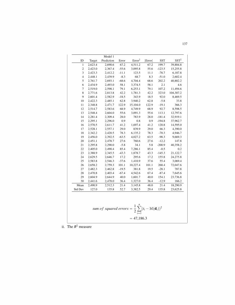
137
Model 1ID Target Prediction Error Error2 |Error| SST SST2
1 2,623.4 2,690.6 67.2 4,511.2 67.2 199.7 39,884.82 2,423.0 2,367.4 -55.6 3,095.8 55.6 -123.5 15,255.83 2,423.3 2,412.2 -11.1 123.5 11.1 -78.7 6,187.84 2,448.1 2,439.9 -8.3 68.7 8.3 -51.0 2,602.45 2,761.7 2,693.1 -68.6 4,704.4 68.6 202.2 40,882.26 2,434.9 2,493.0 58.1 3,374.5 58.1 2.1 4.67 2,519.0 2,598.1 79.1 6,253.1 79.1 107.2 11,494.68 2,771.6 2,813.8 42.2 1,781.3 42.2 323.0 104,307.29 2,601.4 2,582.9 -18.5 343.9 18.5 92.0 8,469.5
10 2,422.3 2,485.1 62.8 3,940.2 62.8 -5.8 33.811 2,348.8 2,471.7 122.9 15,104.0 122.9 -19.1 366.312 2,514.7 2,583.6 68.9 4,749.9 68.9 92.7 8,598.513 2,548.4 2,604.0 55.6 3,091.3 55.6 113.1 12,797.614 2,281.4 2,309.4 28.0 783.9 28.0 -181.4 32,919.115 2,295.1 2,296.0 0.9 0.8 0.9 -194.8 37,962.716 2,570.5 2,611.7 41.2 1,697.4 41.2 120.8 14,595.017 2,528.1 2,557.1 29.0 839.9 29.0 66.3 4,390.018 2,342.2 2,420.5 78.3 6,135.2 78.3 -70.3 4,946.719 2,456.0 2,392.5 -63.5 4,027.2 63.5 -98.3 9,669.320 2,451.1 2,478.7 27.6 760.6 27.6 -12.2 147.821 2,295.8 2,290.0 -5.8 34.1 5.8 -200.9 40,358.222 2,405.0 2,490.4 85.4 7,286.1 85.4 -0.5 0.223 2,388.9 2,345.5 -43.3 1,878.7 43.3 -145.3 21,122.724 2,629.5 2,646.7 17.2 295.6 17.2 155.8 24,275.825 2,583.8 2,546.3 -37.6 1,410.9 37.6 55.4 3,069.426 2,658.2 2,759.3 101.1 10,227.4 101.1 268.4 72,047.627 2,482.3 2,462.8 -19.5 381.8 19.5 -28.1 787.828 2,470.8 2,403.4 -67.4 4,542.6 67.4 -87.4 7,645.629 2,604.9 2,644.9 40.0 1,601.7 40.0 154.1 23,736.830 2,441.6 2,478.0 36.4 1,327.0 36.4 -12.9 166.2
Mean 2,490.9 2,512.3 21.4 3,145.8 48.0 21.4 18,290.9Std Dev 127.0 135.8 52.7 3,382.5 29.4 135.8 23,625.8
sum o f squared errors “12
nÿ
i“1
pti ´Mpdiqq2
“ 47,186.3
ii. The R2 measure

138 Chapter 9 Evaluation (Exercise Solutions)
The R2 measure is calculated as
R2 “ 1´sum o f squared errorstotal sum o f squares
The sum of squared error values from the previous part can be used. So,for Model 1,
total sum o f squares “12
nÿ
i“1
`
ti ´ t˘2
“ 292,937.1
and
R2 “ 1´16,876.6
292,937.1“ 0.942
For Model 2,
total sum o f squares “ 274,363.1
and
R2 “ 1´47,186.3
274,363.1“ 0.828
(b) Based on the evaluation measures calculated, which model do you think is per-forming better for this dataset?
Model 1 has a higher R2 value than Model 2, 0.942 compared to 0.828, whichindicates that it is better able to capture the pattern in this dataset. An R2
value this high suggests quite a powerful model.
3. A credit card issuer has built two different credit scoring models that predict thepropensity of customers to default on their loans. The outputs of the first model for atest dataset are shown in the table below.

139
ID Target Score Prediction1 bad 0.634 bad2 bad 0.782 bad3 good 0.464 good4 bad 0.593 bad5 bad 0.827 bad6 bad 0.815 bad7 bad 0.855 bad8 good 0.500 good9 bad 0.600 bad10 bad 0.803 bad11 bad 0.976 bad12 good 0.504 bad13 good 0.303 good14 good 0.391 good15 good 0.238 good
ID Target Score Prediction16 good 0.072 good17 bad 0.567 bad18 bad 0.738 bad19 bad 0.325 good20 bad 0.863 bad21 bad 0.625 bad22 good 0.119 good23 bad 0.995 bad24 bad 0.958 bad25 bad 0.726 bad26 good 0.117 good27 good 0.295 good28 good 0.064 good29 good 0.141 good30 good 0.670 bad
The outputs of the second model for the same test dataset are shown in the table below.
ID Target Score Prediction1 bad 0.230 bad2 bad 0.859 good3 good 0.154 bad4 bad 0.325 bad5 bad 0.952 good6 bad 0.900 good7 bad 0.501 good8 good 0.650 good9 bad 0.940 good10 bad 0.806 good11 bad 0.507 good12 good 0.251 bad13 good 0.597 good14 good 0.376 bad15 good 0.285 bad
ID Target Score Prediction16 good 0.421 bad17 bad 0.842 good18 bad 0.891 good19 bad 0.480 bad20 bad 0.340 bad21 bad 0.962 good22 good 0.238 bad23 bad 0.362 bad24 bad 0.848 good25 bad 0.915 good26 good 0.096 bad27 good 0.319 bad28 good 0.740 good29 good 0.211 bad30 good 0.152 bad
Based on the predictions of these models, perform the following tasks to compare theirperformance.
(a) The image below shows an ROC curve for each model. Each curve has a pointmissing.

140 Chapter 9 Evaluation (Exercise Solutions)
Calculate the missing point in the ROC curves for Model 1 and Model 2. To gen-erate the point for Model 1, use a threshold value of 0.51. To generate the pointfor Model 2, use a threshold value of 0.43.
To plot an ROC curve, it is easiest to sort the data according to the predic-tion scores generated. Based on the threshold being used to find a point forthe ROC plot, we can create a new set of predictions from which we willcalculate the true positive rate (TPR) and the false positive rate (FPR) thatare used to plot the ROC curve. The table below shows the prediction scoresfor Model 1 in ascending order, the new predictions based on a threshold of0.51, as well as the outcome of each of these predictions—whether it is a truepositive (TP), false positive (FP), true negative (TN), or false negative (FN).

141
ID Target Score Prediction Outcome28 good 0.064 good TN16 good 0.072 good TN26 good 0.117 good TN22 good 0.119 good TN29 good 0.141 good TN15 good 0.238 good TN27 good 0.295 good TN13 good 0.303 good TN19 bad 0.325 good FN14 good 0.391 good TN3 good 0.464 good TN8 good 0.500 good TN12 good 0.504 good FP17 bad 0.567 bad TP4 bad 0.593 bad TP9 bad 0.600 bad TP21 bad 0.625 bad TP1 bad 0.634 bad TP30 good 0.670 bad FP25 bad 0.726 bad TP18 bad 0.738 bad TP2 bad 0.782 bad TP10 bad 0.803 bad TP6 bad 0.815 bad TP5 bad 0.827 bad TP7 bad 0.855 bad TP20 bad 0.863 bad TP24 bad 0.958 bad TP11 bad 0.976 bad TP23 bad 0.995 bad TP
Based on these predictions, we can build a confusion matrix from which wecan calculate the true positive rate and false positive rate that we use to plota point in ROC space. The confusion matrix for Model 1 using a thresholdof 0.48 is shown below.
Predictionbad good
Target bad 16 1good 1 12

142 Chapter 9 Evaluation (Exercise Solutions)
So we can calculate the TPR and FPR as
T PR “ 1616`1 “ 0.9412
FPR “ 112`1 “ 0.0769
Using these figures, we can plot an extra point on the ROC curve and connectit to the existing points to complete the curve (other points for other thresh-olds are required to complete the curve, but they all result in the same TPRscore and so a horizontal line).
The table below shows the prediction scores for Model 2 in ascending order,the new predictions based on a threshold of 0.43, as well as the outcome ofeach of these predictions—whether it is a true positive (TP), false positive(FP), true negative (TN), or false negative (FN).

143
ID Target Score Prediction Outcome26 good 0.096 good TN30 good 0.152 good TN3 good 0.154 good TN29 good 0.211 good TN1 bad 0.230 good FN22 good 0.238 good TN12 good 0.251 good TN15 good 0.285 good TN27 good 0.319 good TN4 bad 0.325 good FN20 bad 0.340 good FN23 bad 0.362 good FN14 good 0.376 good TN16 good 0.421 good TN19 bad 0.480 bad TP7 bad 0.501 bad TP11 bad 0.507 bad TP13 good 0.597 bad FP8 good 0.650 bad FP28 good 0.740 bad FP10 bad 0.806 bad TP17 bad 0.842 bad TP24 bad 0.848 bad TP2 bad 0.859 bad TP18 bad 0.891 bad TP6 bad 0.900 bad TP25 bad 0.915 bad TP9 bad 0.940 bad TP5 bad 0.952 bad TP21 bad 0.962 bad TP
Based on these predictions, we can build a confusion matrix from which wecan calculate the true positive rate and false positive rate that we use to plota point in ROC space. The confusion matrix for Model 2 using a thresholdof 0.48 is shown below.
Predictionbad good
Target bad 13 4good 3 10

144 Chapter 9 Evaluation (Exercise Solutions)
So we can calculate the TPR and FPR as
T PR “ 1313`4 “ 0.7647
FPR “ 310`3 “ 0.2308
Using these figures, we can plot an extra point on the ROC curve and connectit to the existing points to complete the curve (other points for other thresh-olds are required to complete the curve, but they all result in the same TPRscore and so a horizontal line).
For completeness, we show both complete curves together below.
0.0 0.2 0.4 0.6 0.8 1.0
0.0
0.2
0.4
0.6
0.8
1.0
False Positive Rate
True
Pos
itive
Rat
e
Model 1 (0.955)Model 2 (0.851)
(b) The area under the ROC curve (AUC) for Model 1 is 0.955 and for Model 2 is0.851. Which model is performing best?

145
Based on the higher AUC, we can conclude that Model 1 is performing betterat this task. Furthermore, the ROC curve for Model 1 dominates the curvefor Model 2 (i.e., is always higher), which means that there is no operatingpoint (or threshold value) for which Model 2 is better.
(c) Based on the AUC values for Model 1 and Model 2, calculate the Gini coefficientfor each model.
The Gini coefficient is calculated as
Gini coe f f icient “ p2ˆ ROC indexq ´ 1
So for Model 1, the Gini coefficient is
Gini coe f f icient “ p2ˆ 0.955q ´ 1 “ 0.91
For Model 2, the Gini coefficient is
Gini coe f f icient “ p2ˆ 0.851q ´ 1 “ 0.702
4. A retail supermarket chain has built a prediction model that recognizes the householdthat a customer comes from as being one of single, business, or family. After deploy-ment, the analytics team at the supermarket chain uses the stability index to monitorthe performance of this model. The table below shows the frequencies of predictionsof the three different levels made by the model for the original validation dataset at thetime the model was built, for the month after deployment, and for a monthlong periodsix months after deployment.
Original 1st New 2nd NewTarget Sample Sample Samplesingle 123 252 561
business 157 324 221family 163 372 827
Bar plots of these three sets of prediction frequencies are shown in the following im-ages.

146 Chapter 9 Evaluation (Exercise Solutions)
Original Sample 1st New Sample 2nd New Sample
single business familyTarget
Den
sity
0.0
0.1
0.2
0.3
0.4
0.5
single business familyTarget
Den
sity
0.0
0.1
0.2
0.3
0.4
0.5
single business familyTarget
Den
sity
0.0
0.1
0.2
0.3
0.4
0.5
Calculate the stability index for the two new periods and determine whether the modelshould be retrained at either of these points.
The stability index is calculated as
stability index “ÿ
lPlevels
ˆˆ
|At“l|
|A|´|Bt“l|
|B|
˙
ˆ loge
ˆ
|At“l|
|A|{|Bt“l|
|B|
˙˙
where l is a target level, |A| refers to the size of the test set on which performancemeasures were originally calculated, |At“l| refers to the number of instances inthe original test set for which the model made a prediction of level l for targett, |B| and |Bt“l| refer to the same measurements on the newly collected dataset.The following table shows the components of calculating this for the two newperiods.
Original 1st New Sample 2nd New SampleTarget Count % Count % SIt Count % SIt
single 123 0.2777 252 0.2658 0.00052 561 0.3487 0.01617business 157 0.3544 324 0.3418 0.00046 221 0.1374 0.20574
family 163 0.3679 372 0.3924 0.00157 827 0.5140 0.04881Sum 443 948 0.003 1,609 0.271
For the first new sample, the stability index is 0.003, which indicates that thereis practically no difference between the distribution of target levels predicted forthe original validation dataset and for the data in the newt period.For the second sample, the stability index is 0.271, which indicates a massivedifference between the distribution of target levels at this point in time comparedto the distribution predicted for the original validation set. This suggests thatconcept drift has occurred and that the model should be retrained.

III BEYOND PREDICTION


10 Beyond Prediction: Unsupervised Learning (Exercise Solutions)
1. The following table shows a small dataset in which each instance describes measure-ments taken using three sensors when a valve in an oil well was opened. The threedescriptive features, PRESSURE, TEMPERATURE, and VOLUME measure character-istics of the oil flowing through the valve when it was opened. The k-means clus-tering approach is to be applied to this dataset with k “ 3 and using Euclideandistance. The initial cluster centroids for the three clusters C1, C2 , and C3 arec1 “ 〈´0.929,´1.040,´0.831〉, c2 “ 〈´0.329,´1.099, 0.377〉, and c3 “ 〈´0.672,´0.505, 0.110〉. The following table also shows the distance to these three clustercenters for each instance in the dataset.
Cluster Distances Iter. 1ID PRESSURE TEMPERATURE VOLUME Distpdi, c1q Distpdi, c2q Distpdi, c3q
1 -0.392 -1.258 -0.666 0.603 1.057 1.1172 -0.251 -1.781 -1.495 1.204 1.994 2.0933 -0.823 -0.042 1.254 2.314 1.460 1.2434 0.917 -0.961 0.055 2.049 1.294 1.6545 -0.736 -1.694 -0.686 0.697 1.284 1.4326 1.204 -0.605 0.351 2.477 1.611 1.8947 0.778 -0.436 -0.220 1.911 1.422 1.4898 1.075 -1.199 -0.141 2.125 1.500 1.8969 -0.854 -0.654 0.771 1.650 0.793 0.702
10 -1.027 -0.269 0.893 1.891 1.201 0.89211 -0.288 -2.116 -1.165 1.296 1.848 2.09012 -0.597 -1.577 -0.618 0.666 1.136 1.29813 -1.113 -0.271 0.930 1.930 1.267 0.96014 -0.849 -0.430 0.612 1.569 0.879 0.53815 1.280 -1.188 0.053 2.384 1.644 2.069
(a) Assign each instance to its nearest cluster to generate the clustering at the firstiteration of k-means on the basis of the initial cluster centroids.

150 Chapter 10 Beyond Prediction: Unsupervised Learning (Exercise Solutions)
The clusters to be assigned to each instance are shown below.
Cluster Distances Iter. 1 Iter. 1ID PRESSURE TEMP. VOLUME Distpdi, c1q Distpdi, c2q Distpdi, c3q Cluster
1 -0.392 -1.258 -0.666 0.603 1.057 1.117 C1
2 -0.251 -1.781 -1.495 1.204 1.994 2.093 C1
3 -0.823 -0.042 1.254 2.314 1.460 1.243 C3
4 0.917 -0.961 0.055 2.049 1.294 1.654 C2
5 -0.736 -1.694 -0.686 0.697 1.284 1.432 C1
6 1.204 -0.605 0.351 2.477 1.611 1.894 C2
7 0.778 -0.436 -0.220 1.911 1.422 1.489 C2
8 1.075 -1.199 -0.141 2.125 1.500 1.896 C2
9 -0.854 -0.654 0.771 1.650 0.793 0.702 C3
10 -1.027 -0.269 0.893 1.891 1.201 0.892 C3
11 -0.288 -2.116 -1.165 1.296 1.848 2.090 C1
12 -0.597 -1.577 -0.618 0.666 1.136 1.298 C1
13 -1.113 -0.271 0.930 1.930 1.267 0.960 C3
14 -0.849 -0.430 0.612 1.569 0.879 0.538 C3
15 1.280 -1.188 0.053 2.384 1.644 2.069 C2
(b) On the basis of the clustering calculated in Part (a), calculate a set of new clustercentroids.
The instances that have been assigned to the first cluster, C1, are
ID PRESSURE TEMPERATURE VOLUME
1 -0.392 -1.258 -0.6662 -0.251 -1.781 -1.4955 -0.736 -1.694 -0.686
11 -0.288 -2.116 -1.16512 -0.597 -1.577 -0.618
And, so, the new cluster centroid is the average of these values:c1 “ 〈´0.453,´1.685,´0.926〉.The instances that have been assigned to the second cluster, C2, are
ID PRESSURE TEMPERATURE VOLUME
4 0.917 -0.961 0.0556 1.204 -0.605 0.3517 0.778 -0.436 -0.2208 1.075 -1.199 -0.141
15 1.280 -1.188 0.053
And, so, the new cluster centroid is the average of these values:

151
c2 “ 〈1.051,´0.878, 0.020〉The instances that have been assigned to the third cluster, C3, are
ID PRESSURE TEMPERATURE VOLUME
3 -0.823 -0.042 1.2549 -0.854 -0.654 0.771
10 -1.027 -0.269 0.89313 -1.113 -0.271 0.93014 -0.849 -0.430 0.612
And, so, the new cluster centroid is the average of these values:c3 “ 〈´0.933,´0.333, 0.892〉.

152 Chapter 10 Beyond Prediction: Unsupervised Learning (Exercise Solutions)
2. The following table shows details of two different clusterings of the dataset from Ques-tion 1—one with k “ 2 and one with k “ 3—and partial workings to calculate thesilhouette for the clusterings.
k “ 2 clusteringNearest
ID Cluster Cluster apiq bpiq spiqd1 C1 C2 ?? 1.898 ??d2 C1 C2 1.608 2.879 0.442d3 C2 C1 0.624 2.594 0.76d4 C1 C2 1.261 2.142 0.411d5 C1 C2 1.452 2.098 0.308d6 C1 ?? ?? ?? ??d7 C1 C2 1.42 2.061 0.311d8 C1 C2 1.272 2.432 ??d9 C2 C1 0.496 2.067 0.76d10 C2 C1 0.344 2.375 ??d11 C1 C2 1.565 2.802 0.441d12 C1 C2 1.338 ?? ??d13 C2 C1 0.379 2.444 0.845d14 C2 C1 ?? 2.056 ??d15 C1 C2 1.425 2.53 0.437
k “ 3 clusteringNearest
ID Cluster Cluster apiq bpiq spiqd1 C1 C2 0.732 1.681 0.565d2 C1 ?? ?? ?? ??d3 C3 C2 0.624 2.422 0.742d4 C2 C1 0.482 1.884 ??d5 C1 C3 0.619 2.098 0.705d6 C2 C3 0.68 2.24 0.697d7 C2 C1 0.777 1.935 0.598d8 C2 C1 0.558 1.842 0.697d9 C3 C1 0.496 2.04 0.757d10 C3 ?? 0.344 ?? ??d11 C1 C2 0.769 2.201 0.651d12 C1 C2 0.592 1.935 0.694d13 C3 C1 0.379 2.436 0.844d14 C3 C1 0.459 2.038 ??d15 C2 C1 0.579 2.101 0.725
(a) A number of values are missing from these workings (indicated by ??). Calculatethe missing values. The distances between each instance in the dataset from Ques-tion 1 (using Euclidean distance) are shown in the following distance matrix, andwill be useful for this exercise.
»
—
—
—
—
—
—
—
—
—
—
—
—
—
—
—
—
—
—
—
—
—
—
—
—
—
–
d1 d2 d3 d4 d5 d6 d7 d8 d9 d10 d11 d12 d13 d14 d15
d1 0.00d2 0.99 0.00d3 2.31 3.30 0.00d4 1.52 2.11 2.30 0.00d5 0.56 0.95 2.55 1.95 0.00d6 2.00 2.63 2.29 0.55 2.46 0.00d7 1.50 2.12 2.21 0.61 2.02 0.73 0.00d8 1.56 1.98 2.62 0.35 1.96 0.78 0.82 0.00d9 1.63 2.60 0.78 1.94 1.79 2.10 1.92 2.20 0.00d10 1.95 2.93 0.47 2.23 2.15 2.32 2.13 2.52 0.44 0.00d11 1.00 0.47 3.23 2.07 0.78 2.61 2.20 1.94 2.49 2.86 0.00d12 0.38 0.96 2.43 1.77 0.19 2.26 1.83 1.78 1.69 2.04 0.83 0.00d13 2.01 2.98 0.49 2.32 2.19 2.41 2.22 2.61 0.49 0.09 2.91 2.09 0.00d14 1.59 2.57 0.75 1.93 1.81 2.08 1.83 2.21 0.28 0.37 2.51 1.70 0.44 0.00d15 1.82 2.26 2.68 0.43 2.21 0.66 0.94 0.28 2.31 2.62 2.19 2.03 2.71 2.33 0.00
fi
ffi
ffi
ffi
ffi
ffi
ffi
ffi
ffi
ffi
ffi
ffi
ffi
ffi
ffi
ffi
ffi
ffi
ffi
ffi
ffi
ffi
ffi
ffi
ffi
ffi
fl
To illustrate how this exercise is completed the complete workings for cal-culating the silhouette with for instance d6 will be shown. In this clustering

153
d6 is a member of C1. The first step is calculating the silhouette value for d6
is to calculate apiq, the average distance between d6 and the other membersof cluster C1. The members of C1 are td1,d2,d4,d5,d6,d7,d8,d11,d12,d15u.From the distance matrix provided, the distance from d6 to each other mem-ber of C1 is:
“
d1 d2 d4 d5 d6 d8 d11 d12 d15
d6 2.00 2.63 0.55 2.46 0.73 0.78 2.61 2.26 0.66‰
The average distance between d6 and the other members of C1, apiq, is theaverage of these values: 1.631.The next step in the algorithm is to calculate the average distance from d6 toeach member of the other clusters in the clustering. In this case there is justone, C2. The distances from d6 to the members of C2 are:
“
d3 d9 d10 d13 d14
d6 2.29 2.10 2.32 2.41 2.08‰
which gives an average of 2.240 which is the value for bpiq as there is onlyone other cluster. The silhouette width for d6 is then calculated as
2.240´ 1.631maxp2.240, 1.631q
“ 0.272
Other values are calculated similarly. The completed table of all values isshown below.
k “ 2 clusteringNearest
ID Cluster Cluster apiq bpiq spiqd1 C1 C2 1.259 1.898 0.337d2 C1 C2 1.608 2.879 0.442d3 C2 C1 0.624 2.594 0.76d4 C1 C2 1.261 2.142 0.411d5 C1 C2 1.452 2.098 0.308d6 C1 C2 1.631 2.24 0.272d7 C1 C2 1.42 2.061 0.311d8 C1 C2 1.272 2.432 0.477d9 C2 C1 0.496 2.067 0.76d10 C2 C1 0.344 2.375 0.855d11 C1 C2 1.565 2.802 0.441d12 C1 C2 1.338 1.991 0.328d13 C2 C1 0.379 2.444 0.845d14 C2 C1 0.459 2.056 0.776d15 C1 C2 1.425 2.53 0.437

154 Chapter 10 Beyond Prediction: Unsupervised Learning (Exercise Solutions)
k “ 3 clusteringNearest
ID Cluster Cluster apiq bpiq spiqd1 C1 C2 0.732 1.681 0.565d2 C1 C2 0.843 2.219 0.62d3 C3 C2 0.624 2.422 0.742d4 C2 C1 0.482 1.884 0.744d5 C1 C3 0.619 2.098 0.705d6 C2 C3 0.68 2.24 0.697d7 C2 C1 0.777 1.935 0.598d8 C2 C1 0.558 1.842 0.697d9 C3 C1 0.496 2.04 0.757d10 C3 C2 0.344 2.363 0.855d11 C1 C2 0.769 2.201 0.651d12 C1 C2 0.592 1.935 0.694d13 C3 C1 0.379 2.436 0.844d14 C3 C1 0.459 2.038 0.775d15 C2 C1 0.579 2.101 0.725
(b) On the basis of the completed table, calculate the silhouette for each clustering.
The silhouette for each clustering is simply the average of the silhouette en-tries. For the clustering with k “ 2 this is 0.517, and for the clustering withk “ 3 this is 0.711.
(c) On the basis of the silhouette, would you choose 2 or 3 for the value of k for thisdataset?
As it has a higher silhouette there is more evidence that three clusters existin this dataset than two. So k “ 3 should be chosen.

155
3. A city tax service has performed a clustering of individual taxpayers using k-meansclustering in order to better understand groups that might exist within their taxpayerbase. The clustering has divided the taxpayers into three clusters. Four descriptivefeatures have been used to describe each taxpayer:
‚ AGE: The age of the taxpayer.
‚ YEARSINCURRENTEMPLOYMENT: The number of years that the taxpayer hasbeen in their current job.
‚ TOTALINCOME: The taxpayer’s total income for the current tax year.
‚ EFFECTIVETAXRATE: The effective tax rate paid by the taxpayer (this is simplytax paid divided by total income).
The following table shows summary statistics of the four descriptive features for eachof the three clusters found.
1st 3rd Std.Feature Cluster Min. Qrt. Mean Median Qrt. Max Dev.
AGE
C1 20 28 34.6 34 40 59 7.8C2 36 43 45.8 45 48 64 4.5C3 20 32 34.9 36 39 52 5.8
YEARSINCURRENTEMPLOYMENT
C1 0.50 2.74 7.18 5.11 10.76 27.40 5.56C2 8.16 14.25 17.81 17.04 20.71 33.89 4.60C3 0.50 2.44 5.73 4.38 9.32 14.12 3.73
TOTALINCOME
C1 46 247.70 57 355.06 68 843.26 64 977.64 75 967.11 175 000 16 387.77C2 11 182.46 24 222.04 34 711.67 32 637.42 44 102.08 93 800.98 13 412.08C3 15 505.02 29 636.07 36 370.00 36 421.53 42 912.04 64 075.62 8 744.26
EFFECTIVETAXRATE
C1 0.210 0.256 0.274 0.271 0.291 0.349 0.024C2 0.167 0.183 0.204 0.192 0.220 0.321 0.030C3 0.147 0.183 0.199 0.194 0.214 0.252 0.021
The following table shows the information gain calculated when each descriptive fea-ture is used to predict the membership of a single cluster versus the rest of the popula-tion.
Information GainFeature C1 C2 C3
AGE 0.0599 0.4106 0.1828YEARSINCURRENTEMPLOYMENT 0.0481 0.5432 0.3073TOTALINCOME 0.5015 0.0694 0.1830EFFECTIVETAXRATE 0.5012 0.0542 0.2166
The following images show histograms of the values of the four descriptive featuresboth for the full dataset and when divided into the three clusters found.

156 Chapter 10 Beyond Prediction: Unsupervised Learning (Exercise Solutions)
AGE YEARSINCURRENTEMPLOYMENT TOTALINCOME EFFECTIVETAXRATE
All
Age
Den
sity
20 30 40 50 60
0.00
0.02
0.04
0.06
YearsInCurrentEmployment
Den
sity
0 5 10 15 20 25 30 35
0.00
0.02
0.04
0.06
0.08
TotalIncome
Den
sity
50000 100000 1500000.0e
+00
1.0e
−05
2.0e
−05
EffectiveTaxRate
Den
sity
0.15 0.20 0.25 0.30 0.35
05
1015
C1
Age
Den
sity
20 30 40 50 60
0.00
0.02
0.04
0.06
0.08
0.10
YearsInCurrentEmployment
Den
sity
0 5 10 15 20 25 30 35
0.00
0.05
0.10
0.15
TotalIncome
Den
sity
50000 100000 150000
0e+
001e
−05
2e−
053e
−05
EffectiveTaxRate
Den
sity
0.15 0.20 0.25 0.30 0.35
05
1015
2025
C2
Age
Den
sity
20 30 40 50 60
0.00
0.02
0.04
0.06
0.08
0.10
YearsInCurrentEmployment
Den
sity
0 5 10 15 20 25 30 35
0.00
0.05
0.10
0.15
TotalIncome
Den
sity
50000 100000 150000
0e+
001e
−05
2e−
053e
−05
EffectiveTaxRate
Den
sity
0.15 0.20 0.25 0.30 0.35
05
1015
2025
C3
Age
Den
sity
20 30 40 50 60
0.00
0.02
0.04
0.06
0.08
0.10
YearsInCurrentEmployment
Den
sity
0 5 10 15 20 25 30 35
0.00
0.05
0.10
0.15
TotalIncome
Den
sity
50000 100000 150000
0e+
001e
−05
2e−
053e
−05
EffectiveTaxRate
Den
sity
0.15 0.20 0.25 0.30 0.35
05
1015
2025
Using the information provided, write a description of what it means for a taxpayer tobe a member of each of the clusters.

157
To perform this task the best place to start is to analyse the information gainvalues provided in the final table. These indicate which descriptive features arelikely to be most useful in describing each cluster. For C1 the descriptive featureswith the highest information gain values are TOTALINCOME and EFFECTIVE-TAXRATE; for C2 it is YEARSINCURRENTEMPLOYMENT and AGE; and for C3
it is YEARSINCURRENTEMPLOYMENT and EFFECTIVETAXRATE. The selec-tion of two descriptive features for each cluster is arbitrary here but seems to besuggested by the information gain values. We will always use the other descrip-tive features in our descriptions too.Using each of these pairs of descriptive features an examination of the summarystatistics in the table provided and the histograms can help understand how todefine each of the clusters found. For example, the first cluster, C1, can be largelydefined as containing taxpayers with relatively large incomes who pay a higheffective tax rate. They can also be seen to be relatively young and not long intheir current positions. It is common in this type of application of clustering toname clusters so as to easily capture their meaning. We could describe thesetaxpayers as high flyers given their youth and high earnings.Similarly, we can describe the members of the second cluster, C2, as being olderand having stayed in their current potions for a long time. They also tend towardslower incomes and pay slightly low tax rates, although this distribution has a longtail. We might describe these as golden years taxpayers.Finally, members of the the third cluster, C3, are largely defined by not havingbeen long in their current jobs and paying a fairly low effective tax rate. They alsotend to be in their thirties and have relatively low incomes. We might describethese taxpayers as being those in the middle.


11 Beyond Prediction: Reinforcement Learning (Exercise Solutions)
1. An agent in an environment completes an episode and receives the following rewards:
tr0 “ ´33, r1 “ ´11, r2 “ ´12, r3 “ 27, r4 “ 87, r5 “ 156u
(a) Calculate the discounted return at time t “ 0 on the basis of this sequence of re-wards using a discounting factor of 0.72.
We can apply Equation (11.8)[642] to this sequence of rewards to calculate thediscount rate, as viewed from t “ 0 where γ “ 0.72:
G “`
0.720 ˆ´33˘
``
0.721 ˆ´11˘
``
0.722 ˆ´12˘
``
0.723 ˆ 27˘
``
0.724 ˆ 87˘
``
0.725 ˆ 156˘
“ p´33q ` p0.72ˆ´11q ` p0.5184ˆ´12q
` p0.3732ˆ 27q ` p0.2687ˆ 87q ` p0.1935ˆ 156q
“ 16.4985
(b) Calculate the discounted return at time t “ 0 on the basis of this sequence of re-wards using a discount rate of 0.22.
We can apply Equation (11.8)[642] to this sequence of rewards to calculate thediscounted return, as viewed from t “ 0 where γ “ 0.72:
G “`
0.220 ˆ´33˘
``
0.221 ˆ´11˘
``
0.222 ˆ´12˘
``
0.223 ˆ 27˘
``
0.224 ˆ 87˘
``
0.225 ˆ 156˘
“ p´33q ` p0.22ˆ´11q ` p0.0484ˆ´12q
` p0.0106ˆ 27q ` p0.0023ˆ 87q ` p0.0005ˆ 156q
“ ´35.4365
2. To try to better understand the slightly baffling behavior of her new baby, Maria—ascientifically minded new mother—monitored her baby girl over the course of a day

160 Chapter 11 Beyond Prediction: Reinforcement Learning (Exercise Solutions)
recording her activity at 20 minute intervals. The activity stream looked like this (withtime flowing down through the columns):
SLEEPING SLEEPING SLEEPING CRYING SLEEPING SLEEPING
CRYING SLEEPING HAPPY HAPPY CRYING HAPPY
SLEEPING SLEEPING CRYING HAPPY SLEEPING HAPPY
SLEEPING CRYING SLEEPING HAPPY SLEEPING HAPPY
SLEEPING CRYING SLEEPING HAPPY SLEEPING HAPPY
HAPPY SLEEPING HAPPY HAPPY SLEEPING HAPPY
HAPPY SLEEPING HAPPY SLEEPING HAPPY HAPPY
HAPPY HAPPY HAPPY SLEEPING HAPPY SLEEPING
SLEEPING SLEEPING HAPPY SLEEPING HAPPY SLEEPING
SLEEPING HAPPY HAPPY SLEEPING SLEEPING SLEEPING
SLEEPING HAPPY HAPPY SLEEPING HAPPY SLEEPING
SLEEPING CRYING CRYING SLEEPING SLEEPING SLEEPING
Maria noticed that her baby could occupy one of three states—HAPPY, CRYING, orSLEEPING—and moved quite freely between them.
(a) On the basis of this sequence of states, calculate a transition matrix that gives theprobability of moving between each of the three states.
The first step to building the transition matrix is to count the frequency ofeach possible state transition. Working down through the list of states we cancount the number of times we move from one state to the next. For example,in the first five states tSLEEPING,CRYING, SLEEPING, SLEEPING, SLEEPINGu
there is one transition from SLEEPING Ñ CRYING, one transition fromCRYING Ñ SLEEPING, and two transitions from SLEEPING Ñ SLEEPING.This would give the following partial transition frequency matrix:
»
–
SLEEPING CRYING HAPPY
SLEEPING 2 1 0CRYING 1 0 0HAPPY 0 0 0
fi
fl
The final frequency table is shown in the table below:
»
–
SLEEPING CRYING HAPPY
SLEEPING 24 3 8CRYING 5 2 1HAPPY 6 3 19
fi
fl
By normalising each row in the table (dividing each value by the sum ofvalues in the row) we can calculate the final transition matrix:

161
»
–
SLEEPING CRYING HAPPY
SLEEPING 0.686 0.086 0.229CRYING 0.625 0.250 0.125HAPPY 0.214 0.107 0.679
fi
fl
(b) Draw a Markov process diagram to capture the behavior of a small baby as de-scribed.
SLEEPING
CRYINGHAPPY
0.686
0.086
0.2290.625
0.250
0.1250.214
0.107
0.679

162 Chapter 11 Beyond Prediction: Reinforcement Learning (Exercise Solutions)
3. The following table shows the action-value table for a reinforcement learning agentlearning to play the TwentyTwos game after 20 episodes of training have elapsed.
State Action ValuePL-DL Twist 0.706PL-DL Stick 0.284PM-DL Twist ´0.985PM-DL Stick 0.589BUST Twist 0.000BUST Stick 0.000LOSE Twist 0.000LOSE Stick 0.000
State Action ValuePH-DL Twist ´0.038PH-DL Stick 0.164PL-DH Twist 0.386PL-DH Stick ´0.832TIE Twist 0.000TIE Stick 0.000
State Action ValuePM-DH Twist 0.533PM-DH Stick ´0.526PH-DH Twist 0.154PH-DH Stick 0.103WIN Twist 0.000WIN Stick 0.000TWENTYTWO Twist 0.000TWENTYTWO Stick 0.000
In the answers to the following questions, assume that after the initial cards have beendealt to the player and the dealer, the following cards are coming up next in the deck:10♥, 2♣, 7♣, K ♥, 9♦.
(a) At the beginning of the first episode the player is dealt p2♥,K ♣q, the dealer isdealt pA♦, 3♦q, and the dealer’s visible card is the A♦. Given these cards, whatstate is the TwentyTwos playing agent in?
The value of the player’s hand is 12 and the value of the dealer’s visible cardis 11 so the agent finds itself in the PL-DH state.
(b) Assuming that the next action that the agent will take is selected using a greedyaction selection policy, what action will the agent choose to take (Stick or Twist)?
To answer this question we need to examine the action-value table to find theexpected discounted return for each possible action from this state:‚ Q pPL-DH,Twistq “ 0.386
‚ Q pPL-DH, Stickq “ ´0.832As the expected return for the Twist action is higher this is the action that theagent will select using a greedy action selection policy.
(c) Simulate taking the action that the agent selected in Part (b) and determine thestate that the agent will move to following this action and the reward that they willreceive. (Note: If cards need to be dealt to the player or dealer, use cards from thelist given at the beginning of this question.)
The agent selected the Twist action and the next card in the deck that will bedealt is the 10♥. So, the cards in the player’s hand will now be p2♥,K ♣, 10♥q

163
which have a value of 22. This means that the agent will move to the PH-DHstate. As this is a non-terminal state the agent will receive a reward of 0.
(d) Assuming that Q-learning is being used with α “ 0.2 and γ “ 0.9, update theentry in the action-value table for the action simulated in Part (c).
To update the Q pPL-DH,Twistq entry in the action-value table we can useEquation 11.24[658] as follows:
QpPL-DH,Twistq
ÐQ pPL-DH,Twistq`
αˆ´
R pPL-DH,Twistq ` γ ˆmaxa
QpPH-DH, aq ´ Q pPL-DH,Twistq¯
To fill in all value in this table we need to determine maxa QpPH-DH, aq,the action from PH-DH with the highest expected return. The action valuefunction entries for the two possible actions are:‚ Q pPH-DH,Twistq “ 0.154
‚ Q pPH-DH, Stickq “ 0.103At this point in the learning process the Twist has the higher expected returnand so QpPH-DH,Twistq is used in the action-value function entry updateequation:
QpPL-DH,Twistq
ÐQ pPL-DH,Twistq`
αˆ pR pPL-DH,Twistq ` γ ˆ QpPH-DH,Twistq ´ Q pPL-DH,Twistqq
0.386` 0.2ˆ p0` 0.9ˆ 0.154´ 0.386q
0.361
(e) Assuming that a greedy action selection policy is used again and that Q-learningis still being used with α “ 0.2 and γ “ 0.9, select the next action that the agentwill perform, simulate this action, and update the entry in the action-value tablefor the action. (Note: If cards need to be dealt to the player or dealer, continue touse cards from the list given at the beginning of this question.)
The agent finds itself in the PH-DH state. So, assuming again that a greedyaction selection policy is being used it will choose the action with the highest
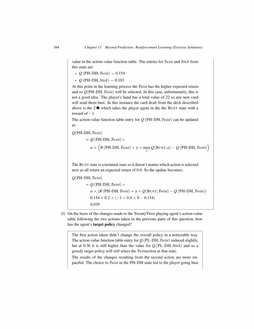
164 Chapter 11 Beyond Prediction: Reinforcement Learning (Exercise Solutions)
value in the action-value function table. The entries for Twist and Stick fromthis state are:‚ Q pPH-DH,Twistq “ 0.154
‚ Q pPH-DH, Stickq “ 0.103At this point in the learning process the Twist has the higher expected returnand so QpPH-DH,Twistq will be selected. In this case, unfortunately, this isnot a good idea. The player’s hand has a total value of 22 so any new cardwill send them bust. In this instance the card dealt from the deck describedabove is the 2♣ which takes the player agent in the the BUST state with areward of ´1.The action-value function table entry for Q pPH-DH,Twistq can be updatedas:
QpPH-DH,Twistq
ÐQ pPH-DH,Twistq`
αˆ´
R pPH-DH,Twistq ` γ ˆmaxa
QpBUST, aq ´ Q pPH-DH,Twistq¯
The BUST state is a terminal state so it doesn’t matter which action is selectednext as all return an expected return of 0.0. So the update becomes:
QpPH-DH,Twistq
ÐQ pPH-DH,Twistq`
αˆ pR pPH-DH,Twistq ` γ ˆ QpBUST,Twistq ´ Q pPH-DH,Twistqq
0.154` 0.2ˆ p´1` 0.9ˆ 0´ 0.154q
0.039
(f) On the basis of the changes made to the TwentyTwos playing agent’s action-valuetable following the two actions taken in the previous parts of this question, howhas the agent’s target policy changed?
The first action taken didn’t change the overall policy in a noticeable way.The action-value function table entry for Q pPL-DH,Twistq reduced slightly,but at 0.36 it is still higher than the value for Q pPL-DH, Stickq and so agreedy target policy will still select the Twistaction in that state.The results of the changes resulting from the second action are more im-pactful. The choice to Twist in the PH-DH state led to the player going bust

165
and reduced the action-value function table entry for Q pPH-DH,Twistq from0.154 to 0.039. This is less than the entry for Q pPH-DH, Stickq, at 0.103,and so the target policy from that state will not swap from the Twist action tothe Stick action—probably a moire sensible choice.


Bibliography
Alimoglu, Fevzi, and Ethem Alpaydin. 1996. Methods of combining multiple classifiers based on dif-ferent representations for pen-based handwritten digit recognition. In Proceedings of the fifth Turkishartificial intelligence and artificial neural networks symposium (TAINN’96).
Anguita, Davide, Alessandro Ghio, Luca Oneto, Xavier Parra, and Jorge Luis Reyes-Ortiz. 2013. Apublic domain dataset for human activity recognition using smartphones. In Proceedings of the 21stinternational European symposium on artificial neural networks, computational intelligence, andmachine learning (ESANN’13), 437–442.
Bache, K., and M. Lichman. 2013. UCI Machine Learning Repository. http://archive.ics.uci.edu/ml.
Bejar, J., U. Cortes, and M. Poch. 1991. LINNEO+: A classification methodology for ill-structured domains, Research report RT-93-10-R, Dept. Llenguatges i Sistemes Informatics, Uni-versitat Politecnica de Catalunya.
Berk, Richard A., and Justin Bleich. 2013. Statistical procedures for forecasting criminal behavior.Criminology & Public Policy 12 (3): 513–544.
Bray, Freddie, Jacques Ferlay, Isabelle Soerjomataram, Rebecca L. Siegel, Lindsey A. Torre, andAhmedin Jemal. 2018. Global cancer statistics 2018: Globocan estimates of incidence and mortalityworldwide for 36 cancers in 185 countries. CA: A Cancer Journal for Clinicians 68 (6): 394–424.doi:10.3322/caac.21492.
Cleary, Duncan, and Revenue Irish Tax. 2011. Predictive analytics in the public sector: Using datamining to assist better target selection for audit. In The proceedings of the 11th European conferenceon egovernment: Faculty of administration, University of Ljubljana, Ljubljana, Slovenia, 16–17 June2011, 168. Academic Conferences Limited.
Dua, Dheeru, and Casey Graff. 2017. UCI Machine Learning Repository. http://archive.ics.uci.edu/ml.
Fawcett, Tom. 2006. An introduction to ROC analysis. Pattern Recognition Letters 27 (8): 861–874.
Hirschowitz, Anton. 2001. Closing the CRM loop: The 21st century marketer’s challenge: Trans-forming customer insight into customer value. Journal of Targeting, Measurement and Analysis forMarketing 10 (2): 168–178.
Kansagara, Devan, Honora Englander, Amanda Salanitro, David Kagen, Cecelia Theobald, MicheleFreeman, and Sunil Kripalani. 2011. Risk prediction models for hospital readmission: A systematicreview. JAMA 306 (15): 1688–1698.

168 Bibliography
Klubicka, Filip, Giancarlo D. Salton, and John D. Kelleher. 2018. Is it worth it? Budget-relatedevaluation metrics for model selection. In Proceedings of the eleventh international conference onlanguage resources and evaluation (LREC 2018).
Kohavi, Ron. 1996. Scaling up the accuracy of Naive-Bayes classifiers: A decision-tree hybrid. InProceedings of the twenty-fifth ACM SIGKDD international conference on knowledge discovery anddata mining KDD, 202–207.
Mac Namee, B., P. Cunningham, S. Byrne, and O. I. Corrigan. 2002. The problem of bias in trainingdata in regression problems in medical decision support. Artificial Intelligence in Medicine 24 (1):51–70.
Mangasarian, Olvi L., and William H. Wolberg. 1990. Cancer diagnosis via linear programming.SIAM News 23 (5): 1–18.
Mishne, Gilad, and Natalie S. Glance. 2006. Predicting movie sales from blogger sentiment. In AAAIspring symposium: Computational approaches to analyzing weblogs, 155–158.
Osowski, Stainslaw, Linh Tran Hoai, and T. Markiewicz. 2004. Support vector machine-based expertsystem for reliable heartbeat recognition. IEEE Transactions on Biomedical Engineering 51 (4):582–589. doi:10.1109/TBME.2004.824138.
Palaniappan, Sellappan, and Rafiah Awang. 2008. Intelligent heart disease prediction system usingdata mining techniques. International Journal of Computer Science and Network Security 8 (8):343–350.
Rubin, Daniel J. 2015. Hospital readmission of patients with diabetes. Current Diabetes Reports 15(4): 17.
Siddiqi, Naeem. 2005. Credit risk scorecards: Developing and implementing intelligent credit scor-ing. Wiley.
Tsanas, Athanasios, and Angeliki Xifara. 2012. Accurate quantitative estimation of energy perfor-mance of residential buildings using statistical machine learning tools. Energy and Buildings 49:560–567.