Stressed Eye: “Know What You're Really Testing With”

Stressed Eye: “Know What You’re Really Testing With”Primer

Primer

www.tektronix.com/bertscope2

Table of ContentsAbstract...........................................................................3

Introduction.....................................................................3

Eye.Diagram.Depth.........................................................5

Eye.Opening.Metrics.in.Fibre.Channel...........................6

Eye.Opening.Metrics.in.10GbE.......................................8

So.What.Can.Go.Wrong?..............................................12

Defining.Eye.Opening.Metrics.in.BER.Terms...............13

Conclusions...................................................................16

References.....................................................................17

www.tektronix.com/bertscope 3

Stressed Eye: “Know What You’re Really Testing With”

AbstractThere are considerable differences between the way that 10 Gb/s Ethernet (10 GbE)[i] and 4x Fibre Channel (4x FC)[ii], [iii] go about defining timing and amplitude settings for receiver jitter tolerance testing. These differences can be subtle, but can have an enormous impact on the test signal, and therefore on the success of the testing. The points raised here are equally applicable to other stressed eyes, both optical and electrical.

IntroductionThe aim of receiver jitter tolerance testing of a receiver is to present a device under test with the worst possible signal it is ever likely to see. It is obviously in a device manufacturer’s interest for that signal to comply with the rules set out in the appropriate guidelines, but to be no worse than this if at all possible. The impact of under-stressing is that non-compliant devices are supplied to customers, usually with some bad consequence. Overstressing has more impact on the costs of the supplier – good devices that should pass are needlessly failed. Even more problematic is if the test signal is inconsistent between batches. As we will see, there is a big advantage in knowing exactly what test signal you are imposing, and the methods detailed in standards do not always give this information.

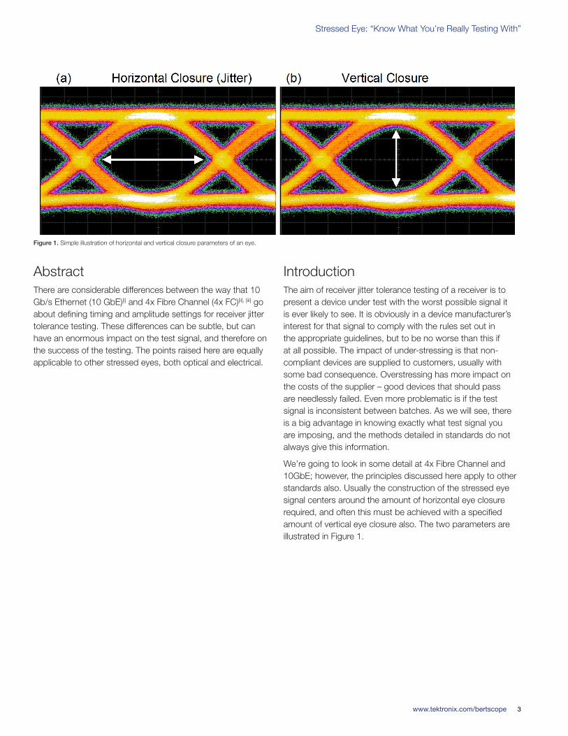
We’re going to look in some detail at 4x Fibre Channel and 10GbE; however, the principles discussed here apply to other standards also. Usually the construction of the stressed eye signal centers around the amount of horizontal eye closure required, and often this must be achieved with a specified amount of vertical eye closure also. The two parameters are illustrated in Figure 1.

Figure.1. Simple illustration of horizontal and vertical closure parameters of an eye.

Primer


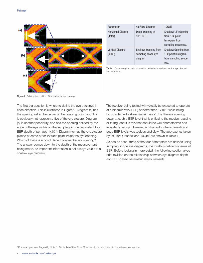
The first big question is where to define the eye openings in each direction. This is illustrated in Figure 2. Diagram (a) has the opening set at the center of the crossing point, and this is obviously not representa-tive of the eye closure. Diagram (b) is another possibility, and has the opening defined by the edge of the eye visible on the sampling scope (equivalent to a BER depth of perhaps 1x10-4). Diagram (c) has the eye closure placed at some other invisible point inside the eye opening. Which of these is a good place to define the eye opening? The answer comes down to the depth of the measurement being made, as important information is not always visible in a shallow eye diagram.

The receiver being tested will typically be expected to operate at a bit error ratio (BER) of better than 1x10-12 while being bombarded with stress impairments1. It is the eye opening down at such a BER level that is critical to the receiver passing or failing, and it is this that should be well characterized and repeatably set up. However, until recently, characterization at deep BER levels was tedious and slow. The approaches taken by 4x Fibre Channel and 10GbE are shown in Table 1.

As can be seen, three of the four parameters are defined using sampling scope eye diagrams, the fourth is defined in terms of BER. Before looking in more detail, the following section gives brief revision on the relationship between eye diagram depth and BER-based parametric measurements.

Figure.2. Defining the position of the horizontal eye opening.

Table.1. Comparing the methods used to define horizontal and vertical eye closure in two standards.

Parameter 4x Fibre Channel 10GbE

Horizontal Closure

(Jitter)

Deep: Opening at

10-12 BER

Shallow: “J”: Opening

from 10k point

histogram from

sampling scope eye.

Vertical Closure

(VECP)

Shallow: Opening from

sampling scope eye

diagram

Shallow: Opening from

10k point histogram

from sampling scope

eye.

1 For example, see 9, Note 1, Table 14 of the Fibre Channel document listed in the references section.



Figure.5. Similar looking eye diagrams with greatly differing eye closure at low BER lev-els. More information on what caused these in particular can be found in Reference vi[vi].

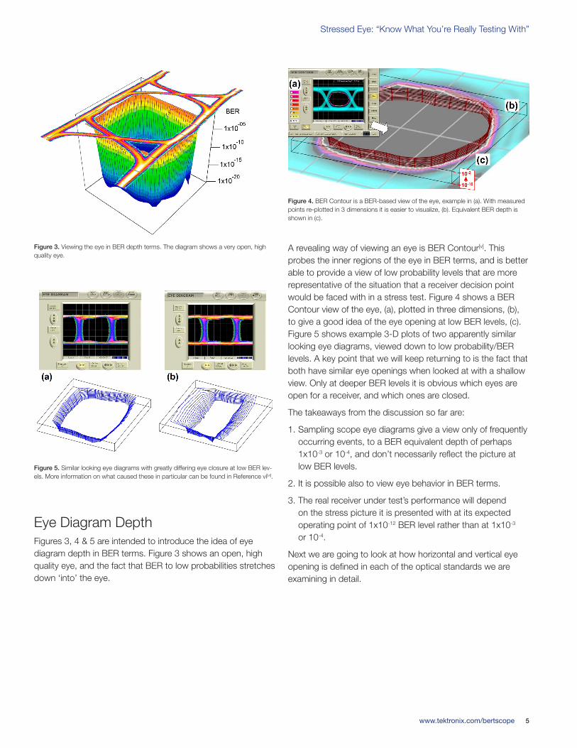
Figure.3. Viewing the eye in BER depth terms. The diagram shows a very open, high quality eye.

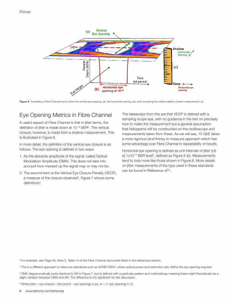
Figure.4. BER Contour is a BER-based view of the eye, example in (a). With measured points re-plotted in 3 dimensions it is easier to visualize, (b). Equivalent BER depth is shown in (c).

Eye Diagram DepthFigures 3, 4 & 5 are intended to introduce the idea of eye diagram depth in BER terms. Figure 3 shows an open, high quality eye, and the fact that BER to low probabilities stretches down ‘into’ the eye.

A revealing way of viewing an eye is BER Contour[v]. This probes the inner regions of the eye in BER terms, and is better able to provide a view of low probability levels that are more representative of the situation that a receiver decision point would be faced with in a stress test. Figure 4 shows a BER Contour view of the eye, (a), plotted in three dimensions, (b), to give a good idea of the eye opening at low BER levels, (c). Figure 5 shows example 3-D plots of two apparently similar looking eye diagrams, viewed down to low probability/BER levels. A key point that we will keep returning to is the fact that both have similar eye openings when looked at with a shallow view. Only at deeper BER levels it is obvious which eyes are open for a receiver, and which ones are closed.

The takeaways from the discussion so far are:

1. Sampling scope eye diagrams give a view only of frequently occurring events, to a BER equivalent depth of perhaps 1x10-3 or 10-4, and don’t necessarily reflect the picture at low BER levels.

2. It is possible also to view eye behavior in BER terms.

3. The real receiver under test’s performance will depend on the stress picture it is presented with at its expected operating point of 1x10-12 BER level rather than at 1x10-3 or 10-4.

Next we are going to look at how horizontal and vertical eye opening is defined in each of the optical standards we are examining in detail.

Primer


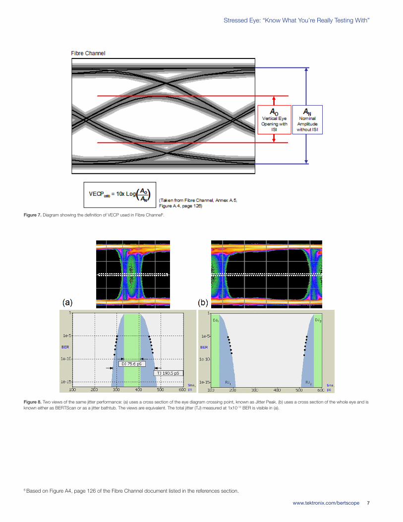
Eye Opening Metrics in Fibre ChannelA useful aspect of Fibre Channel is that in jitter terms, the definition of jitter is made down at 10-12 BER2. The vertical closure, however, is made from a shallow measurement. This is illustrated in Figure 6.

In more detail, the definition of the vertical eye closure is as follows. The eye opening is defined in two ways:

1. As the absolute amplitude of the signal, called Optical Modulation Amplitude (OMA). This does not take into account how messed up the signal may or may not be.

2. The second term is the Vertical Eye Closure Penalty (VECP), a measure of the closure observed3. Figure 7 shows some definitions4.

The takeaways from this are that VECP is defined with a sampling scope eye, with no guidance in the text on precisely how to make the measurement but a general assumption that histograms will be constructed on the oscilloscope and measurements taken from these. As we will see, 10 GbE takes a more rigorous (and finicky to measure) approach which has some advantage over Fibre Channel in repeatability of results.

Horizontal eye opening is defined as unit intervals of jitter (UI) at 1x10-12 BER level5, defined as Figure 6 (b). Measurements tend to look more like those shown in Figure 8. More details on jitter measurements of the type used in these standards can be found in Reference vii[vii].

Figure.6..Translating a Fibre Channel eye to show the vertical eye opening, (a), the horizontal opening, (b), and comparing the relative depths of each measurement, (c).

2 For example, see Page 49, Note 2, Table 14 of the Fibre Channel document listed in the references section.

3 This is a different approach to telecoms standards such as SONET/SDH, where optical power and extinction ratio define the eye opening required.

4 OMA diagrammatically looks identical to AN in Figure 7, but is defined with a particular pattern and methodology meaning there might theoretically be a slight variation between OMA and AN. The difference is not significant for this discussion.

5 Where jitter = eye closure = (bit period – eye opening) in ps, or = (1-eye opening) in UI.



Figure.8..Two views of the same jitter performance: (a) uses a cross section of the eye diagram crossing point, known as Jitter Peak. (b) uses a cross section of the whole eye and is known either as BERTScan or as a jitter bathtub. The views are equivalent. The total jitter (TJ) measured at 1x10-12 BER is visible in (a).

6 Based on Figure A4, page 126 of the Fibre Channel document listed in the references section.

Figure.7. Diagram showing the definition of VECP used in Fibre Channel6.

Primer


Before going into details for these two parameters, it is worth exploring jitter measurement on an eye diagram (“J”), as the standard uses a similar method to define this in the horizontal dimension as it does for the eye opening in the vertical dimension. It is more intuitive using jitter as a starting place. (Jitter is closely related to horizontal eye opening, with jitter being the bit period minus the horizontal eye opening.)

Jitter Histograms: For calibration of the stressed eye, the standard is written assuming that a sampling scope will be used, and that jitter histograms will be employed. As their name implies, sampling scopes sub-sample the incoming data. The example we will be looking at was made on a scope with a sample rate of 40 kHz. For a 40 kHz sampling rate, around 250 thousand bits go past unmeasured between samples at 10Gb/s. The chance of catching rare pattern sequences is very small. This leads to considerable variability in the histograms formed on sampling scopes – sequences that cause the most jitter may appear as a single outlying sample once in a while, or they may be missed entirely.

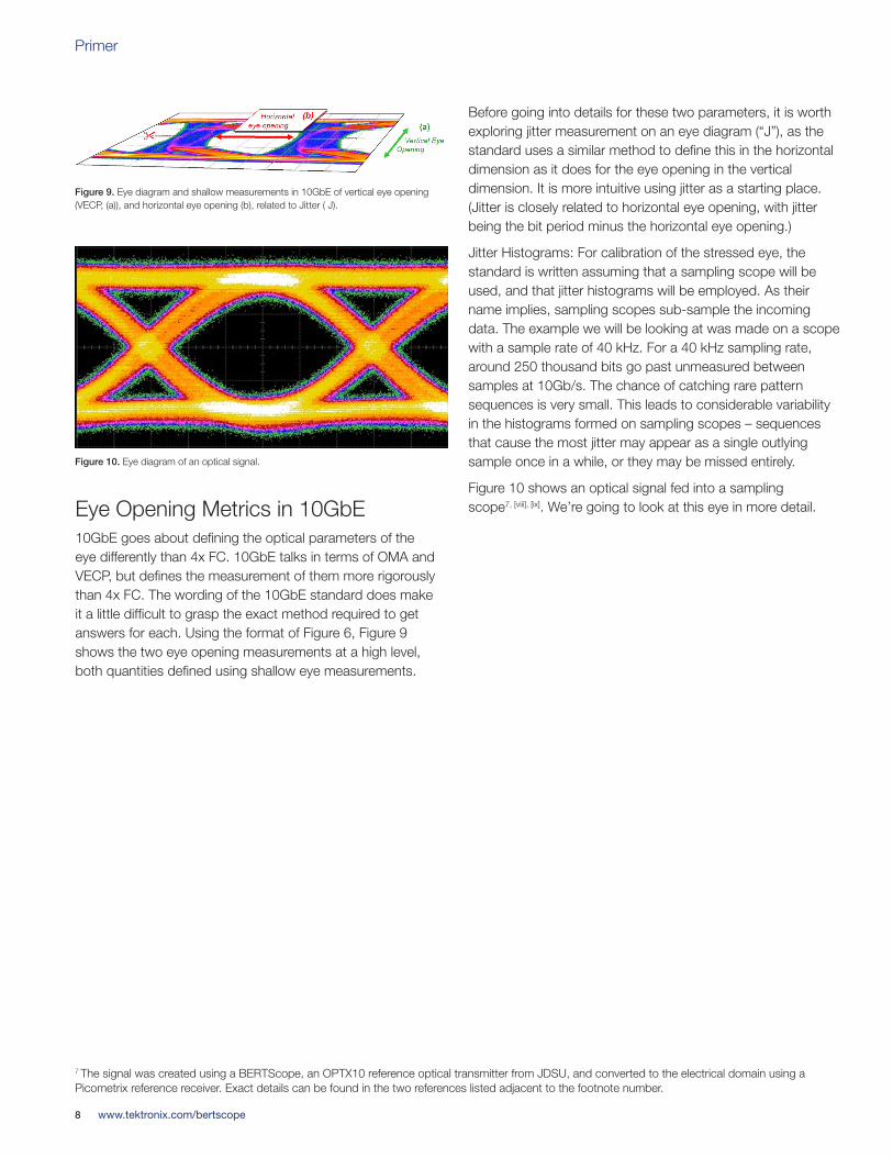
Figure 10 shows an optical signal fed into a sampling scope7, [viii], [ix]. We’re going to look at this eye in more detail.Eye Opening Metrics in 10GbE

10GbE goes about defining the optical parameters of the eye differently than 4x FC. 10GbE talks in terms of OMA and VECP, but defines the measurement of them more rigorously than 4x FC. The wording of the 10GbE standard does make it a little difficult to grasp the exact method required to get answers for each. Using the format of Figure 6, Figure 9 shows the two eye opening measurements at a high level, both quantities defined using shallow eye measurements.

Figure.9. Eye diagram and shallow measurements in 10GbE of vertical eye opening (VECP, (a)), and horizontal eye opening (b), related to Jitter ( J).

Figure.10. Eye diagram of an optical signal.

7 The signal was created using a BERTScope, an OPTX10 reference optical transmitter from JDSU, and converted to the electrical domain using a Picometrix reference receiver. Exact details can be found in the two references listed adjacent to the footnote number.



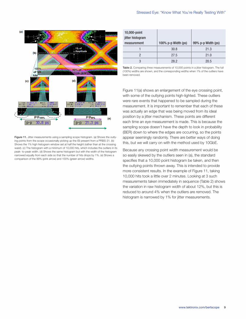
Figure 11(a) shows an enlargement of the eye crossing point, with some of the outlying points high-lighted. These outliers were rare events that happened to be sampled during the measurement. It is important to remember that each of these was actually an edge that was being moved from its ideal position by a jitter mechanism. These points are different each time an eye measurement is made. This is because the sampling scope doesn’t have the depth to look in probability (BER) down to where the edges are occurring, so the points appear seemingly randomly. There are better ways of doing this, but we will carry on with the method used by 10GbE.

Because any crossing point width measurement would be so easily skewed by the outliers seen in (a), the standard specifies that a 10,000 point histogram be taken, and then the outlying points thrown away. This is intended to provide more consistent results. In the example of Figure 11, taking 10,000 hits took a little over 2 minutes. Looking at 3 such measurements taken immediately in sequence (Table 2) shows the variation in raw histogram width of about 12%, but this is reduced to around 4% when the outliers are removed. The histogram is narrowed by 1% for jitter measurements.

Figure.11..Jitter measurements using a sampling scope histogram. (a) Shows the outly-ing points from the scope occasionally picking up the ISI present from a PRBS-31. (b) Shows the 1% high histogram window set at half the height (rather than at the crossing waist). (c) The histogram with a minimum of 10,000 hits, which includes the outliers in its peak- to-peak width. (d) Shows the same histogram but with the width of the histogram narrowed equally from each side so that the number of hits drops by 1%. (e) Shows a comparison of the 99% (pink arrow) and 100% (green arrow) widths.

Table.2. Comparing three measurements of 10,000 points in a jitter histogram. The full (100%) widths are shown, and the corresponding widths when 1% of the outliers have been removed.

10,000-point jitter histogram measurement 100% p-p Width (ps) 99% p-p Width (ps)

1 30.8 21.3

2 27.5 21.0

3 28.2 20.5

Primer


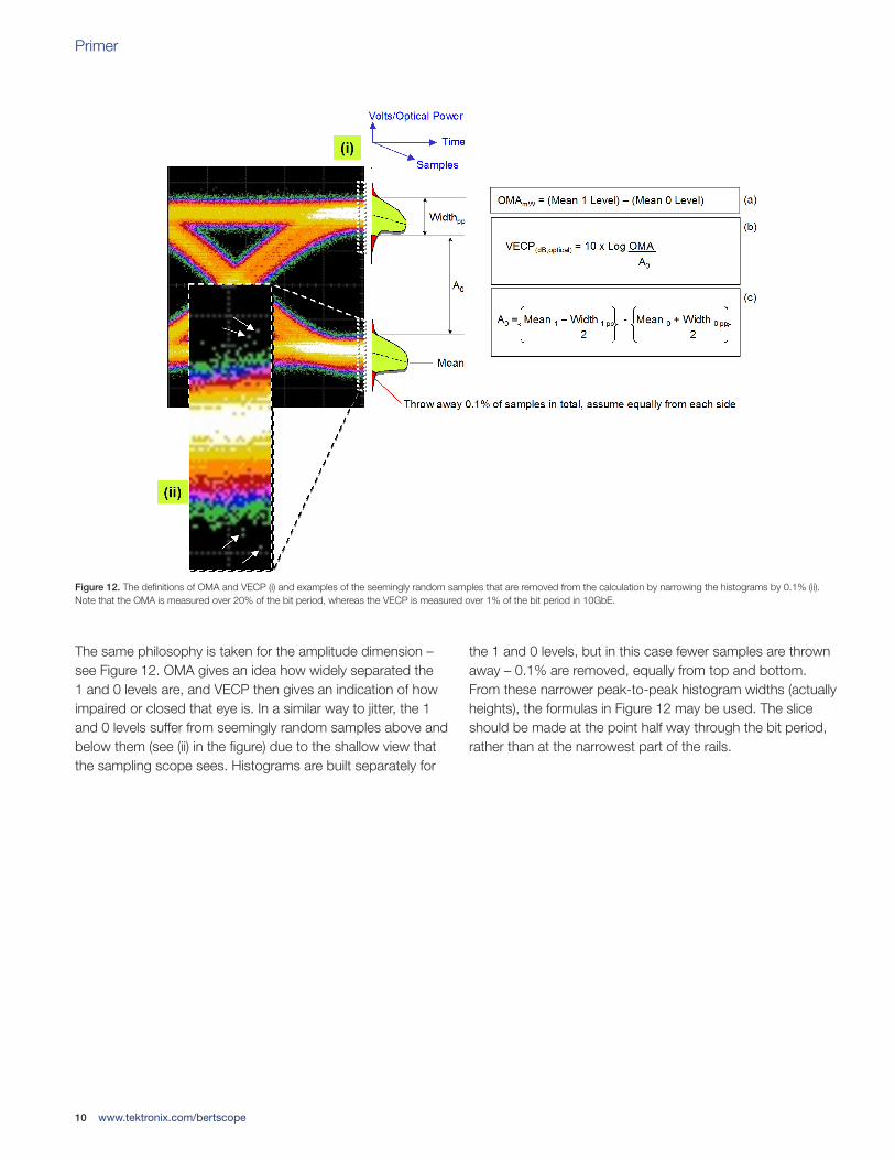
The same philosophy is taken for the amplitude dimension – see Figure 12. OMA gives an idea how widely separated the 1 and 0 levels are, and VECP then gives an indication of how impaired or closed that eye is. In a similar way to jitter, the 1 and 0 levels suffer from seemingly random samples above and below them (see (ii) in the figure) due to the shallow view that the sampling scope sees. Histograms are built separately for

the 1 and 0 levels, but in this case fewer samples are thrown away – 0.1% are removed, equally from top and bottom. From these narrower peak-to-peak histogram widths (actually heights), the formulas in Figure 12 may be used. The slice should be made at the point half way through the bit period, rather than at the narrowest part of the rails.

Figure.12..The definitions of OMA and VECP (i) and examples of the seemingly random samples that are removed from the calculation by narrowing the histograms by 0.1% (ii). Note that the OMA is measured over 20% of the bit period, whereas the VECP is measured over 1% of the bit period in 10GbE.



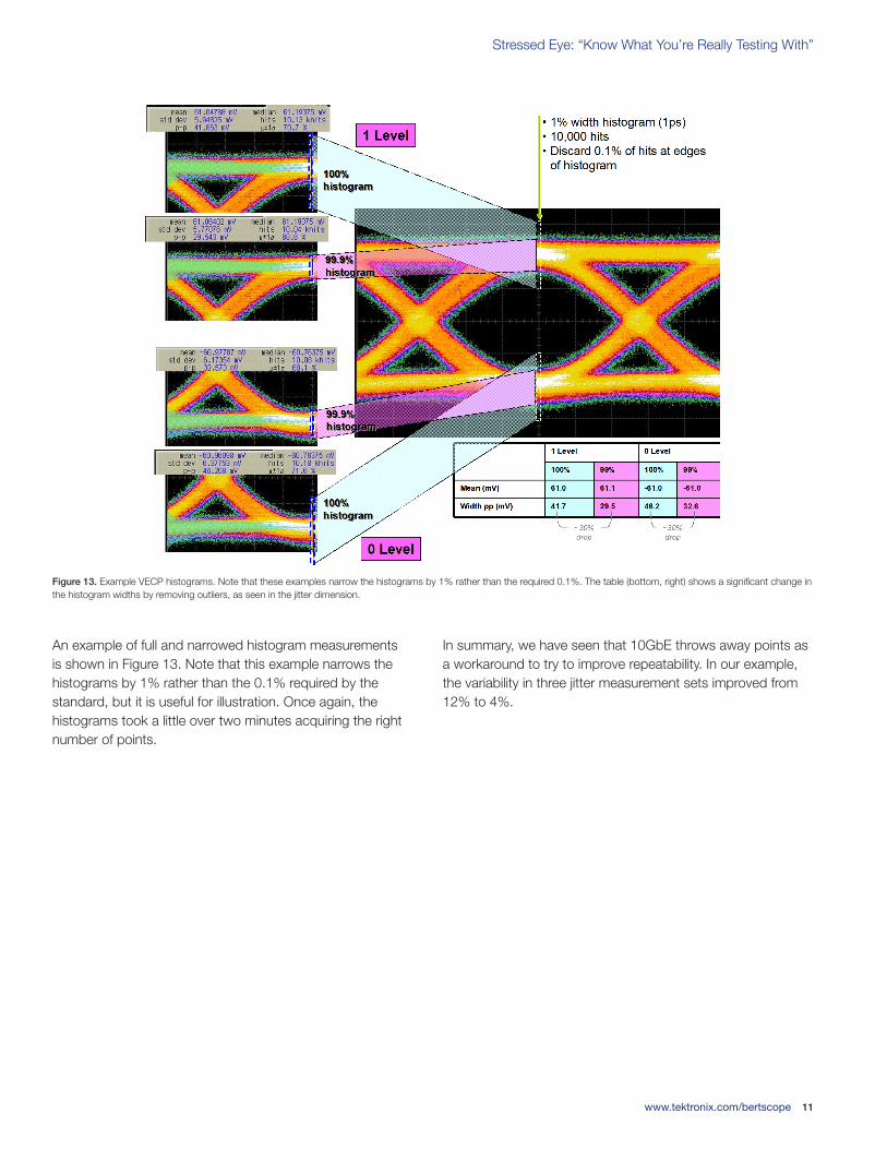
An example of full and narrowed histogram measurements is shown in Figure 13. Note that this example narrows the histograms by 1% rather than the 0.1% required by the standard, but it is useful for illustration. Once again, the histograms took a little over two minutes acquiring the right number of points.

In summary, we have seen that 10GbE throws away points as a workaround to try to improve repeatability. In our example, the variability in three jitter measurement sets improved from 12% to 4%.

Figure.13..Example VECP histograms. Note that these examples narrow the histograms by 1% rather than the required 0.1%. The table (bottom, right) shows a significant change in the histogram widths by removing outliers, as seen in the jitter dimension.

Primer


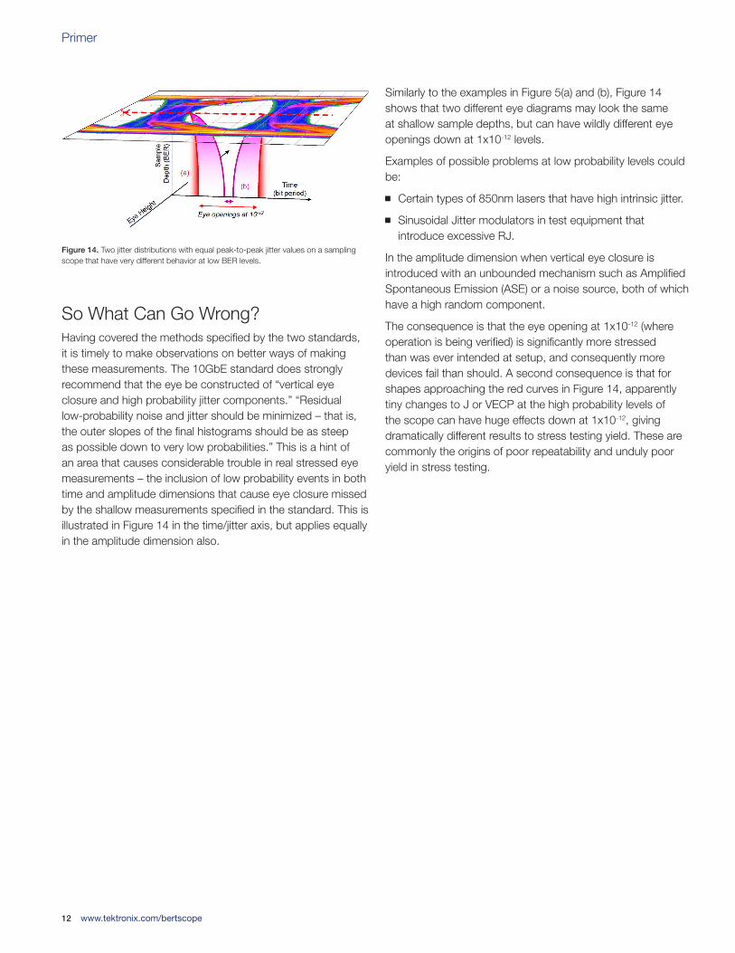
So What Can Go Wrong?Having covered the methods specified by the two standards, it is timely to make observations on better ways of making these measurements. The 10GbE standard does strongly recommend that the eye be constructed of “vertical eye closure and high probability jitter components.” “Residual low-probability noise and jitter should be minimized – that is, the outer slopes of the final histograms should be as steep as possible down to very low probabilities.” This is a hint of an area that causes considerable trouble in real stressed eye measurements – the inclusion of low probability events in both time and amplitude dimensions that cause eye closure missed by the shallow measurements specified in the standard. This is illustrated in Figure 14 in the time/jitter axis, but applies equally in the amplitude dimension also.

Similarly to the examples in Figure 5(a) and (b), Figure 14 shows that two different eye diagrams may look the same at shallow sample depths, but can have wildly different eye openings down at 1x10-12 levels.

Examples of possible problems at low probability levels could be:

Certain types of 850nm lasers that have high intrinsic jitter.

Sinusoidal Jitter modulators in test equipment that introduce excessive RJ.

In the amplitude dimension when vertical eye closure is introduced with an unbounded mechanism such as Amplified Spontaneous Emission (ASE) or a noise source, both of which have a high random component.

The consequence is that the eye opening at 1x10-12 (where operation is being verified) is significantly more stressed than was ever intended at setup, and consequently more devices fail than should. A second consequence is that for shapes approaching the red curves in Figure 14, apparently tiny changes to J or VECP at the high probability levels of the scope can have huge effects down at 1x10-12, giving dramatically different results to stress testing yield. These are commonly the origins of poor repeatability and unduly poor yield in stress testing.

Figure.14. Two jitter distributions with equal peak-to-peak jitter values on a sampling scope that have very different behavior at low BER levels.



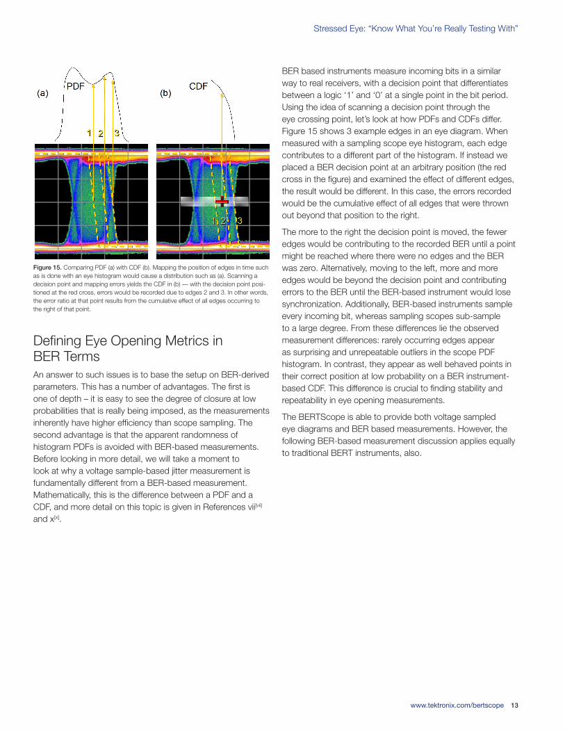
Defining Eye Opening Metrics in BER TermsAn answer to such issues is to base the setup on BER-derived parameters. This has a number of advantages. The first is one of depth – it is easy to see the degree of closure at low probabilities that is really being imposed, as the measurements inherently have higher efficiency than scope sampling. The second advantage is that the apparent randomness of histogram PDFs is avoided with BER-based measurements. Before looking in more detail, we will take a moment to look at why a voltage sample-based jitter measurement is fundamentally different from a BER-based measurement. Mathematically, this is the difference between a PDF and a CDF, and more detail on this topic is given in References vii[vii] and x[x].

BER based instruments measure incoming bits in a similar way to real receivers, with a decision point that differentiates between a logic ‘1’ and ‘0’ at a single point in the bit period. Using the idea of scanning a decision point through the eye crossing point, let’s look at how PDFs and CDFs differ. Figure 15 shows 3 example edges in an eye diagram. When measured with a sampling scope eye histogram, each edge contributes to a different part of the histogram. If instead we placed a BER decision point at an arbitrary position (the red cross in the figure) and examined the effect of different edges, the result would be different. In this case, the errors recorded would be the cumulative effect of all edges that were thrown out beyond that position to the right.

The more to the right the decision point is moved, the fewer edges would be contributing to the recorded BER until a point might be reached where there were no edges and the BER was zero. Alternatively, moving to the left, more and more edges would be beyond the decision point and contributing errors to the BER until the BER-based instrument would lose synchronization. Additionally, BER-based instruments sample every incoming bit, whereas sampling scopes sub-sample to a large degree. From these differences lie the observed measurement differences: rarely occurring edges appear as surprising and unrepeatable outliers in the scope PDF histogram. In contrast, they appear as well behaved points in their correct position at low probability on a BER instrument-based CDF. This difference is crucial to finding stability and repeatability in eye opening measurements.

The BERTScope is able to provide both voltage sampled eye diagrams and BER based measurements. However, the following BER-based measurement discussion applies equally to traditional BERT instruments, also.

Figure.15..Comparing PDF (a) with CDF (b). Mapping the position of edges in time such as is done with an eye histogram would cause a distribution such as (a). Scanning a decision point and mapping errors yields the CDF in (b) — with the decision point posi-tioned at the red cross, errors would be recorded due to edges 2 and 3. In other words, the error ratio at that point results from the cumulative effect of all edges occurring to the right of that point.

Primer


quote from the 10GbE standard is relevant here – the lower the low probability impairments can be kept, the steeper the sides of the two profiles, and the lower the real stress on the component at low BER levels.

The measurements above show that Jitter Peak and Q-Factor are revealing and repeatable views of the eye opening down where the receiver will care. However, there is the problem that compliance to each standard requires verification that jitter (10GbE) and VECP (10GbE and 4x FC) have been set and verified to the shallow levels specified in the respective standards. This can also be achieved using BER based measurements. For 10GbE, this is straightforward with the translation that a 10,000 histogram corresponds to a BER depth of 1x10-4. This is easily verified and proves true comparing experiment with measured results. 4x FC is slightly more problematic in both scope and BER domains, as the measurement depth or duration is not specified. Given that people frequently make judgments on eye diagrams after only a few seconds to a minute, it is safe to assume the range is between 10-3 and 10-4 in BER terms. The horizontal and vertical eye openings can be read off with markers at the desired BER depth with considerable accuracy and repeatability.

A related but more revealing approach is to use BER Contour to view the eye, an example of which is shown in Figure 17. As well as giving measurements of the eye width and height at specified BER depth, it also gives an idea of what the eye closure looks like all the way around the perimeter of the eye.

Jitter peak and Q factor measurements are horizontal and vertical slices through the eye respectively, made in BER terms. These are direct analogs of the jitter and VECP slices that we have been discussing. Figure 16 shows measurements of each.

Using the signal of Figures 10, 11, 12, and 13, the measurements have been made with a BER-based instrument. Figure 16 shows the Jitter Peak and the Q-Factor. In each case, a better view of the performance at low BER levels is a revealing look at what a receiver under test would really be exposed to. Also shown are the depths the 10,000 hit sampling scope histogram was achieving. Obviously the

Figure.16.

(a) Jitter Peak measurement made on the optical signal of Figures 10, 11, 12 & 13 showing a deeper view of jitter. (a1) shows the jitter peak-to-peak width at a depth of 1x10-12, 63.38 ps . Using the pruned jitter width of Figure 11, we can demonstrate the approximate depth the sampling scope was achieving (a2).

(b).The same for the amplitude dimension – Q Factor showing the deeper performance. (b1) shows the depth the measurement of Figure 13 was achieving, and (b2) show the equivalent opening at 1x10-12 BER .

Figure.17. BER Contour can give eye opening values, and also a view of the perimeter of the eye opening at a specified BER depth.



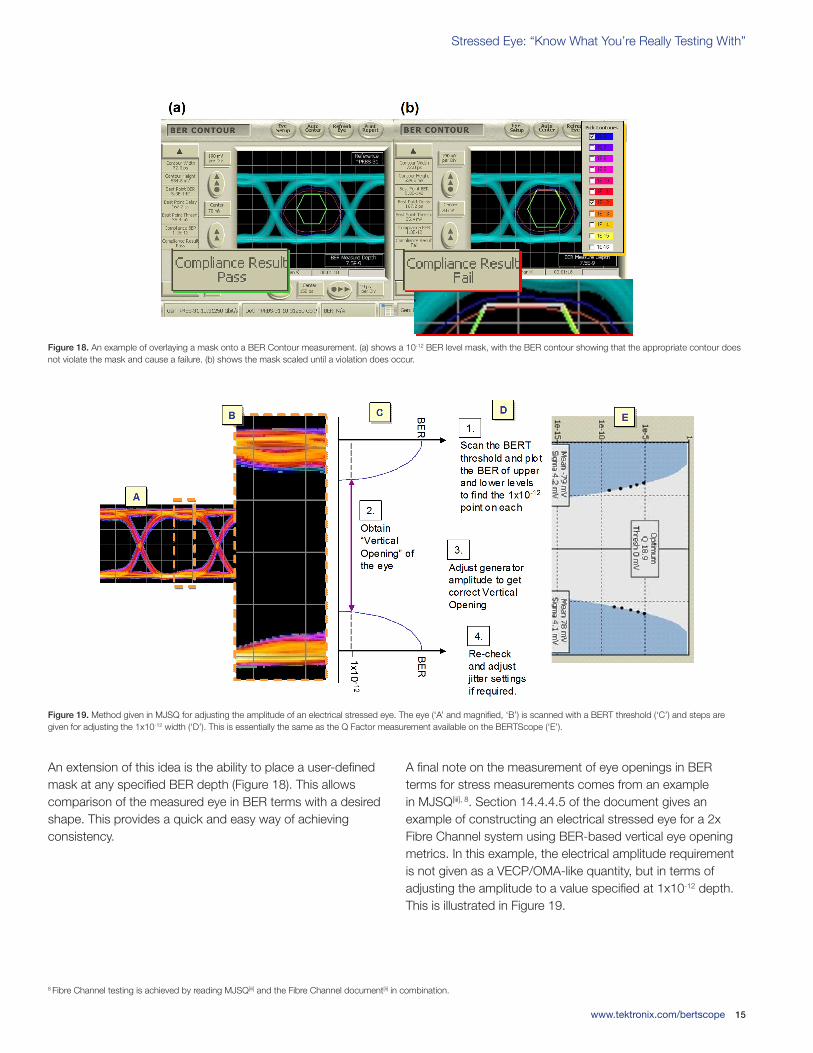
An extension of this idea is the ability to place a user-defined mask at any specified BER depth (Figure 18). This allows comparison of the measured eye in BER terms with a desired shape. This provides a quick and easy way of achieving consistency.

A final note on the measurement of eye openings in BER terms for stress measurements comes from an example in MJSQ[iii], 8. Section 14.4.4.5 of the document gives an example of constructing an electrical stressed eye for a 2x Fibre Channel system using BER-based vertical eye opening metrics. In this example, the electrical amplitude requirement is not given as a VECP/OMA-like quantity, but in terms of adjusting the amplitude to a value specified at 1x10-12 depth. This is illustrated in Figure 19.

Figure.18..An example of overlaying a mask onto a BER Contour measurement. (a) shows a 10-12 BER level mask, with the BER contour showing that the appropriate contour does not violate the mask and cause a failure. (b) shows the mask scaled until a violation does occur.

Figure.19. Method given in MJSQ for adjusting the amplitude of an electrical stressed eye. The eye (‘A’ and magnified, ‘B’) is scanned with a BERT threshold (‘C’) and steps are given for adjusting the 1x10-12 width (‘D’). This is essentially the same as the Q Factor measurement available on the BERTScope (‘E’).

8 Fibre Channel testing is achieved by reading MJSQ[iii] and the Fibre Channel document[ii] in combination.

Primer


ConclusionsMany standards specify the construction of stressed eyes by specifying the vertical and horizontal eye opening/closure. We have seen examples where the openings are given in terms of shallow eye voltage histograms, and seen that such methods lead to a lack of repeatability. We have also seen that even if they were to be repeatable, they do not necessarily give an accurate picture of the eye opening that a test receiver would see when exposed to a stressed signal. These issues can lead to yield variability in testing, and unnecessary cost to a transceiver manufacturer.

We’ve looked at an improvement in these measurements by carrying out stress calibration through measurement using BER-based analysis. We have seen that this can provide correlation to the shallow measurements specified in the standards but with increased repeatability. We have also seen that BER-based measurements can provide a better view of the stress eye opening down at the deep BER levels that the receiver will be expected to operate at when it is tested. Finally we’ve also seen that jitter is specified in BER depth terms for 4x FC, and we’ve seen an electrical example of vertical eye opening measurement from MJSQ expressed similarly



References[i] IEEE standard 802.3aeTM-2002. “Part 3: Carrier Sense

Multiple Access with Collision Detection (CSMA/CD) Access Method and Physical Layer Specifications Amendment: Media Access Control (MAC) Parameters, Physical Layers, and Management Parameters for 10 Gb/s Operation”, version worked from in this document is dated 30th August 2002, document references:

Print: SH94996, PDF: SS94996

10Gigabit Ethernet standards page: http://grouper.ieee.org/groups/802/3/ae/

10G Ethernet overview and resources page: www.ethermanage.com/ethernet/10gig.html

[ii] “Fibre Channel - Physical Interfaces (FC-PI-2)”, March 29th, 2005. dpANS NCITS.xxx-200x Global Engineering, 15 Inverness Way East, INCITS/Project 1506-D/Rev8.0, Phone: (800) 854-7179 or (303) 792-2181. Jitter reference comes from section A.1.13 Jitter Measurements - Page 120.

[iii] MJSQ: Methodologies for Jitter and Signal Quality Specification is a document written as part of the INCITS project T11.2. http://www.t11.org/index.htm. Reference made to Rev 14, 9th June 2004.

[iv] “Anatomy of an Eye Diagram – A Primer”, October 2004, SyntheSys Research, www.tektronix.com

[v] “Bridging the Gap – A BER Contour Tutorial”, October 2004, SyntheSys Research, www.bertscope.com

[vi] “Anatomy of an Eye Diagram” poster, October 2004, SyntheSys Research, www.tektronix.com

[vii] “Dual Dirac, scope histograms and BERTScan Measurements”, September 2005, SyntheSys Research, www.tektronix.com

[viii] “Constructing a 4x Fibre Channel Optical Stressed Eye”, November 2005, SyntheSys Research, www.tektronix.com

[ix] “Constructing a 10Gb/s Ethernet Optical Stressed Eye”, November 2005, SyntheSys Research, www.tektronix.com

[x] “Jitter analysis: The dual-Dirac model, RJ/DJ, and Q-scale”, White paper by Ransom Stephens, 31st December, 2004, Agilent Technologies. www.agilent.com

Primer


Contact.Tektronix:ASEAN./.Australasia..(65) 6356 3900

Austria*..00800 2255 4835

Balkans,.Israel,.South.Africa.and.other.ISE.Countries.+41 52 675 3777

Belgium*..00800 2255 4835

Brazil..+55 (11) 3759 7600

Canada..1 (800) 833-9200

Central.East.Europe,.Ukraine.and.the.Baltics..+41 52 675 3777

Central.Europe.&.Greece..+41 52 675 3777

Denmark..+45 80 88 1401

Finland..+41 52 675 3777

France*..00800 2255 4835

Germany*..00800 2255 4835

Hong.Kong..400-820-5835

India..000-800-650-1835

Italy*..00800 2255 4835

Japan..81 (3) 6714-3010

Luxembourg..+41 52 675 3777

Mexico,.Central/South.America.&.Caribbean..52 (55) 56 04 50 90

Middle.East,.Asia.and.North.Africa..+41 52 675 3777

The.Netherlands*..00800 2255 4835

Norway..800 16098

People’s.Republic.of.China..400-820-5835

Poland..+41 52 675 3777

Portugal..80 08 12370

Republic.of.Korea..001-800-8255-2835

Russia.&.CIS..+7 (495) 7484900

South.Africa. +27 11 206 8360

Spain*..00800 2255 4835

Sweden*..00800 2255 4835

Switzerland*..00800 2255 4835

Taiwan..886 (2) 2722-9622.

United.Kingdom.&.Ireland*..00800 2255 4835

USA..1 (800) 833-9200

*.If.the.European.phone.number.above.is.not.accessible,.please.call.+41.52.675.3777

Contact List Updated 25 May 2010.........

For.Further.InformationTektronix maintains a comprehensive, constantly expanding collection of application notes, technical briefs and other resources to help engineers working on the cutting edge of technology. Please visit www.tektronix.com

Copyright © 2010, Tektronix. All rights reserved. Tektronix products are covered by U.S. and foreign patents, issued and pending. Information in this publication supersedes that in all previously published material. Specification and price change privileges reserved. TEKTRONIX and TEK are registered trademarks of Tektronix, Inc. All other trade names referenced are the service marks, trademarks or registered trademarks of their respective companies.

09/10 EA/WWW 65W-26048-0

Stressed Eye: “Know What You're Really Testing With”

Documents

Transcript of Stressed Eye: “Know What You're Really Testing With”