Should more of your PROC REGs be QUANTREGS and ROBUSTREGs?
17
AA03 Should more of your PROC REGS be QUANTREGs and ROBUSTREGs? Peter L. Flom, Peter Flom Consulting, New York, NY ABSTRACT In ordinary least squares (OLS) regression, we model the conditional mean of the response or dependent variable as a function of one or more independent variables and we make assumptions about the distribution of the errors. But, just as the mean is not a full description of a distribution, so modeling the mean is not a full description of a relationship between dependent and independent variables; it may not even be an adequate one. I show how PROC QUANTREG can be used to perform quantile regression, which models the conditional quantiles, rather than the mean. I also show how both QUANTREG and ROBUSTREG can be used when the assumptions of OLS regression are violated. Keywords: quantile regression quantreg robustreg robust. INTRODUCTION In this paper, I discuss quantile regression and robust regression. I begin with descriptions and motivations for both methods, then discuss implementation in SAS with PROC QUANTREG and PROC ROBUSTREG, and then illustrate their use with examples. MOTIVATION There are at least two motivations for quantile regression and one for robust regression. First, quantile regression: Suppose our dependent variable is bimodal or multimodal that is, it has multiple humps. If we knew what caused the bimodality, we could separate on that variable and do stratified analysis, but if we dont know that, quantile regression might be good. OLS regression will, here, be as misleading as relying on the mean as a measure of centrality for a bimodal distribution. If our DV is highly skewed as, for example, income is in many countries we might be interested in what predicts the median (which is the 50th percentile) or some other quantile; just as we usually report median income rather than mean income. One more example is where our substantive interest is in people at the highest or lowest quantiles. For example, if studying the spread of sexually transmitted diseases, we might record number of sexual partners that a person had in a given time period. And we might be most interested in what predicts people with a great many partners, since they will be key parts of spreading the disease. Robust regression is designed primarily to deal with outliers of three types: • Outliers in the dependent variable • Possibly multivariate outliers in the independent variables - aka high leverage points • Outliers in both of the above Outliers and leverage points are common. Multivariate outliers can be very hard to identify, but they can have huge effects on regression. By examining the effect that leaving each subject out of the regression has on the regression, we can see if the leverage is problematic. OLS regression makes assumptions. There are various things to do when these assumptions are violated. Methods such as transforming variables or deleting outliers are often used and may sometimes be appropriate; but sometimes we do not want to transform the variable and sometimes the outliers are interesting. Here, it is interesting to note that quantile regression makes no assumptions about the distribution of the residuals and the various types of robust regression have ways to deal with them. The examples below provides additional motivation. QUANTILE REGRESSION A TINY BIT OF QUANTILE REGRESSION THEORY A quantile is ordinarily thought of as an order statistic. One type of quantile is the percentile, or 100-quantile. The pth (sample)/(population) percentile is the value that is higher than p% of all the values in the (sample)/(population). More formally, 1
-
Upload
independent -
Category
Documents
-
view
1 -
download
0
Transcript of Should more of your PROC REGs be QUANTREGS and ROBUSTREGs?
AA03Should more of your PROC REGS be QUANTREGs and ROBUSTREGs?
Peter L. Flom, Peter Flom Consulting, New York, NY
ABSTRACTIn ordinary least squares (OLS) regression, we model the conditional mean of the response or dependent variable as a functionof one or more independent variables and we make assumptions about the distribution of the errors. But, just as the meanis not a full description of a distribution, so modeling the mean is not a full description of a relationship between dependentand independent variables; it may not even be an adequate one. I show how PROC QUANTREG can be used to performquantile regression, which models the conditional quantiles, rather than the mean. I also show how both QUANTREG andROBUSTREG can be used when the assumptions of OLS regression are violated.
Keywords: quantile regression quantreg robustreg robust.
INTRODUCTIONIn this paper, I discuss quantile regression and robust regression. I begin with descriptions and motivations for both methods,then discuss implementation in SAS with PROC QUANTREG and PROC ROBUSTREG, and then illustrate their use withexamples.
MOTIVATIONThere are at least two motivations for quantile regression and one for robust regression. First, quantile regression: Suppose ourdependent variable is bimodal or multimodal that is, it has multiple humps. If we knew what caused the bimodality, we couldseparate on that variable and do stratified analysis, but if we dont know that, quantile regression might be good. OLS regressionwill, here, be as misleading as relying on the mean as a measure of centrality for a bimodal distribution.
If our DV is highly skewed as, for example, income is in many countries we might be interested in what predicts the median(which is the 50th percentile) or some other quantile; just as we usually report median income rather than mean income.
One more example is where our substantive interest is in people at the highest or lowest quantiles. For example, if studying thespread of sexually transmitted diseases, we might record number of sexual partners that a person had in a given time period.And we might be most interested in what predicts people with a great many partners, since they will be key parts of spreadingthe disease.
Robust regression is designed primarily to deal with outliers of three types:
• Outliers in the dependent variable
• Possibly multivariate outliers in the independent variables - aka high leverage points
• Outliers in both of the above
Outliers and leverage points are common. Multivariate outliers can be very hard to identify, but they can have huge effectson regression. By examining the effect that leaving each subject out of the regression has on the regression, we can see if theleverage is problematic.
OLS regression makes assumptions. There are various things to do when these assumptions are violated. Methods such astransforming variables or deleting outliers are often used and may sometimes be appropriate; but sometimes we do not want totransform the variable and sometimes the outliers are interesting. Here, it is interesting to note that quantile regression makesno assumptions about the distribution of the residuals and the various types of robust regression have ways to deal with them.
The examples below provides additional motivation.
QUANTILE REGRESSIONA TINY BIT OF QUANTILE REGRESSION THEORYA quantile is ordinarily thought of as an order statistic. One type of quantile is the percentile, or 100-quantile. The pth(sample)/(population) percentile is the value that is higher than p% of all the values in the (sample)/(population). More formally,
1
the τ th quantile of X is defined as
F−1(τ) = inf[x : F(x)> τ]
where F is the distribution function of X.
The key bit of theory, as noted by Koenker and originally developed by Fox and Rubin is that this problem of sorting can beconverted into one of optimization. Specifically, the problem is to minimize
Eρt(X− x̂) = (τ−1)∫ x̂
−∞
(x− x̂)dF(x)+ τ
∫∞
x̂(x− x̂)dF(x)
This allows relatively simple extension of the problem of ordinary least squares regression to quantile regression. For details,see Koenker.
PROC QUANTREGBASIC SYNTAX OF PROC QUANTREGHere I outline the basic syntax of PROC QUANTREG and do not go over every detail. For that, you can always see thedocumentation.
PROC QUANTREG <options> ;CLASS variables ; *SAME AS OTHER PROCS;MODEL response = independents </ options> ;OUTPUT <OUT= SAS-data-set> <options> ;PERFORMANCE <options> ;
As usual, the first statement invokes the procedure. There are also BY, ID, TEST, EFFECT and WEIGHT statements, all ofwhich operate similarly to other statistical procedures. The PROC QUANTREG statement has some options that are dissimilarto other procedures. You can choose the algorithm and the method for calculating confidence intervals, but, as usual, SAS hassensible defaults. Several of the algorithms need starting points, and you can specify these using the INEST statement. Thereare many plotting options, dealt with below.
The key statement is the model statement. The usual syntax applies, but the options are different. The key option is theQUANTILE option, the syntax of which is
QUANTILE=number-list | PROCESS
This option specifies the quantile levels for the quantile regression. You can specify any number of quantile levels in thenumber list. You can also compute the entire quantile process by specifying the PROCESS option. Only the simplex algorithmis available for computing the quantile process. The default is a median regression, which corresponds to QUANTILE=0.5.The PROCESS option calculates the entire quantile process.
ODS GRAPHICS AND PROC QUANTREGGraphics are always important evaluating models, but this is especially true in quantile regression. The volume of printedoutput can become overwhelming, because if you (for example) run quantile regressions on the .05, .10 ... .95 quantile, that is19 regressions, and there will be approximately the same amount of output as running 19 PROC GLMs. Fortunately, SAS nowoffers excellent graphics that can be obtained relatively easily. Unfortunately, you need SAS Graph to run them, and one keyword here is ‘relatively’.
PROC ROBUSTREG
QUANTILE REGRESSION EXAMPLE: BIRTH WEIGHT DATAINTRODUCTIONPredicting low birth weight is important because babies born at low weight are much more likely to have health complicationsthan babies of more typical weight. The usual approaches to this are either to model the mean birth weight as a function of
2
various factors using OLS regression, or to dichotomize or otherwise categorize birth weight and then use some form of logisticregression (either ‘normal’ or ordinal). Both these are inadequate. Modeling the mean is inadequate because, as we shallsee, different factors are important in modeling the mean and the lower quantiles. We are often interested in predicting whichmothers are likely to have the lowest weight babies, not the average birth weight of a particular group of mothers. Categorizingthe dependent variable is rarely a good idea, principally because it throws away useful information and treats people withincategories as the same. A typical cutoff value for low birth weight is 2.5 kg. Yet this implies that a baby born at 2.49 kg is thesame as a baby born at 1.0 kg, while one born at 2.51 kg is the same as one who is 4 kg. This is clearly not the case.
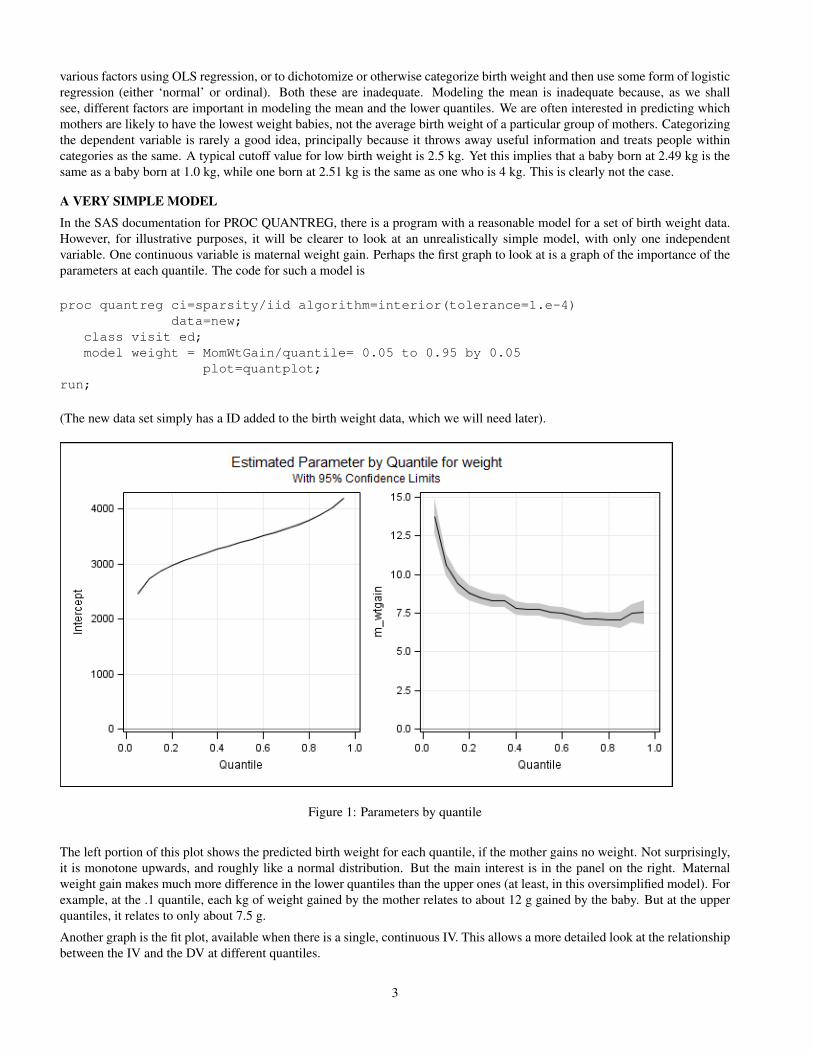
A VERY SIMPLE MODELIn the SAS documentation for PROC QUANTREG, there is a program with a reasonable model for a set of birth weight data.However, for illustrative purposes, it will be clearer to look at an unrealistically simple model, with only one independentvariable. One continuous variable is maternal weight gain. Perhaps the first graph to look at is a graph of the importance of theparameters at each quantile. The code for such a model is
proc quantreg ci=sparsity/iid algorithm=interior(tolerance=1.e-4)data=new;
class visit ed;model weight = MomWtGain/quantile= 0.05 to 0.95 by 0.05
plot=quantplot;run;
(The new data set simply has a ID added to the birth weight data, which we will need later).
Figure 1: Parameters by quantile
The left portion of this plot shows the predicted birth weight for each quantile, if the mother gains no weight. Not surprisingly,it is monotone upwards, and roughly like a normal distribution. But the main interest is in the panel on the right. Maternalweight gain makes much more difference in the lower quantiles than the upper ones (at least, in this oversimplified model). Forexample, at the .1 quantile, each kg of weight gained by the mother relates to about 12 g gained by the baby. But at the upperquantiles, it relates to only about 7.5 g.
Another graph is the fit plot, available when there is a single, continuous IV. This allows a more detailed look at the relationshipbetween the IV and the DV at different quantiles.
3
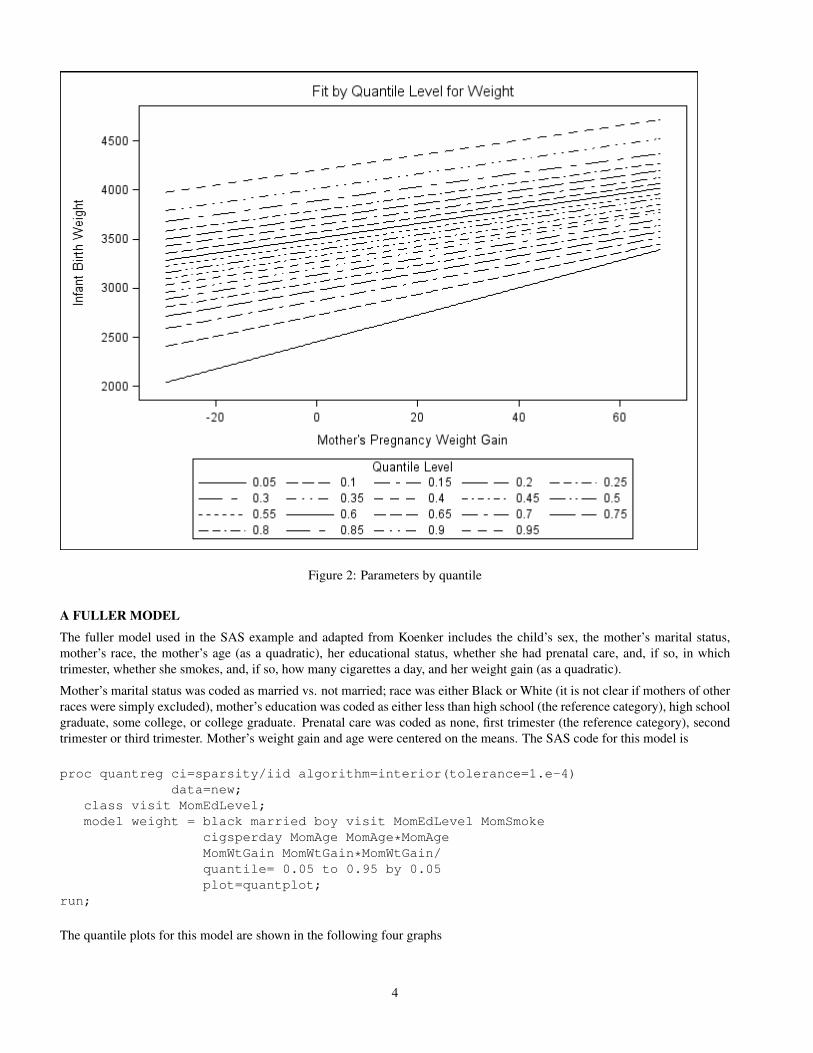
Figure 2: Parameters by quantile
A FULLER MODEL
The fuller model used in the SAS example and adapted from Koenker includes the child’s sex, the mother’s marital status,mother’s race, the mother’s age (as a quadratic), her educational status, whether she had prenatal care, and, if so, in whichtrimester, whether she smokes, and, if so, how many cigarettes a day, and her weight gain (as a quadratic).
Mother’s marital status was coded as married vs. not married; race was either Black or White (it is not clear if mothers of otherraces were simply excluded), mother’s education was coded as either less than high school (the reference category), high schoolgraduate, some college, or college graduate. Prenatal care was coded as none, first trimester (the reference category), secondtrimester or third trimester. Mother’s weight gain and age were centered on the means. The SAS code for this model is
proc quantreg ci=sparsity/iid algorithm=interior(tolerance=1.e-4)data=new;
class visit MomEdLevel;model weight = black married boy visit MomEdLevel MomSmoke
cigsperday MomAge MomAge*MomAgeMomWtGain MomWtGain*MomWtGain/quantile= 0.05 to 0.95 by 0.05plot=quantplot;
run;
The quantile plots for this model are shown in the following four graphs
4
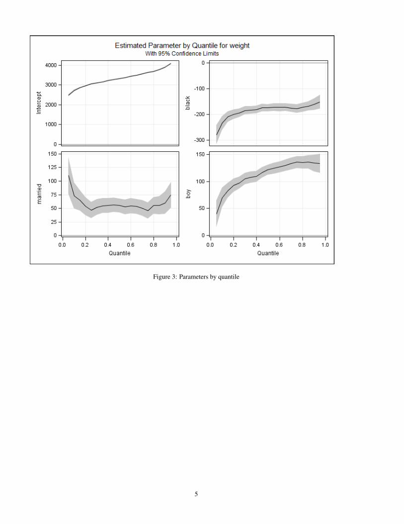
Figure 3: Parameters by quantile
5
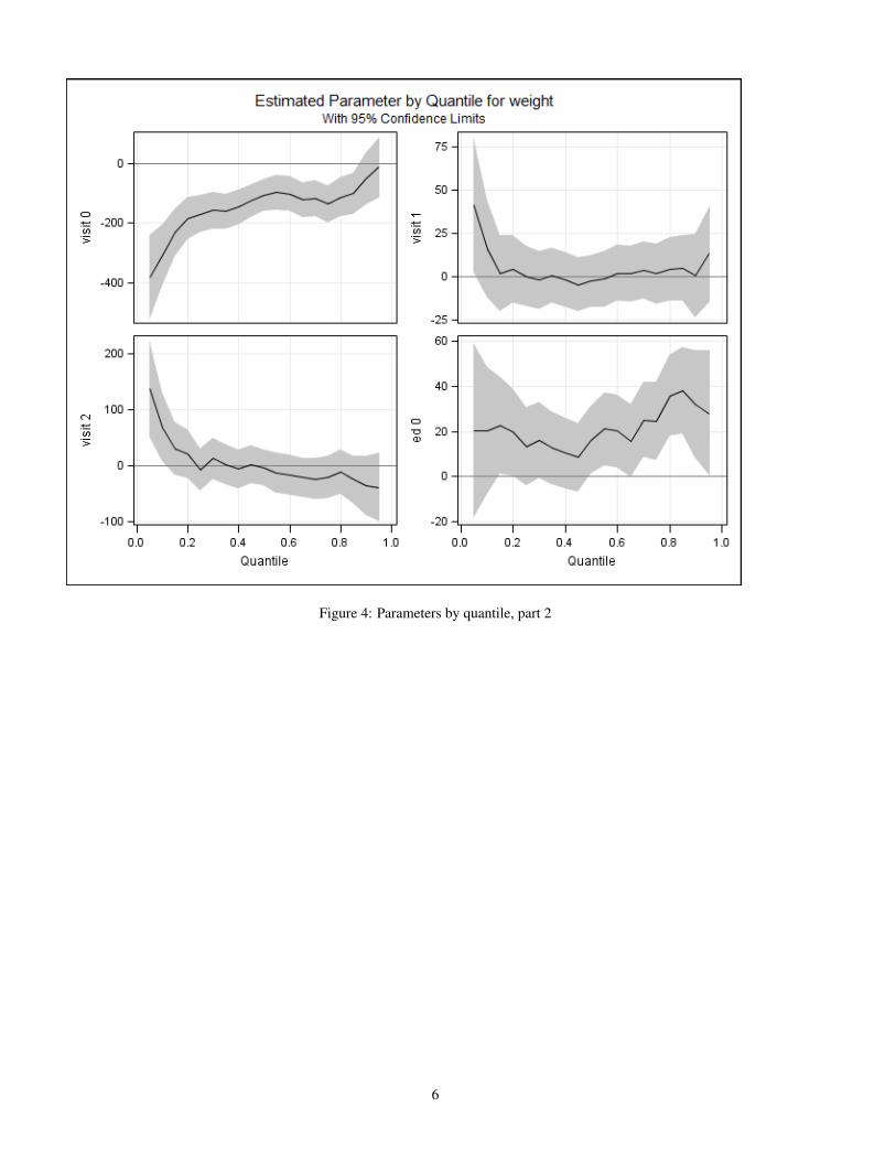
Figure 4: Parameters by quantile, part 2
6
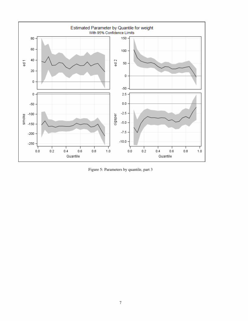
Figure 5: Parameters by quantile, part 3
7
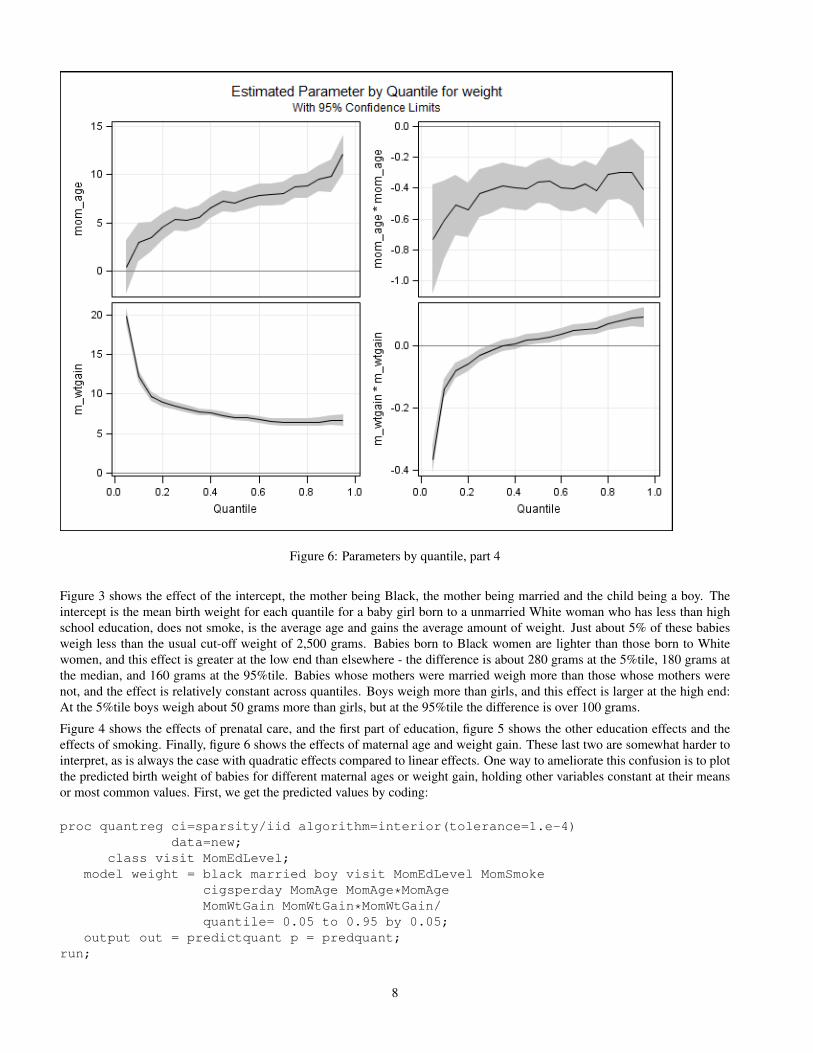
Figure 6: Parameters by quantile, part 4
Figure 3 shows the effect of the intercept, the mother being Black, the mother being married and the child being a boy. Theintercept is the mean birth weight for each quantile for a baby girl born to a unmarried White woman who has less than highschool education, does not smoke, is the average age and gains the average amount of weight. Just about 5% of these babiesweigh less than the usual cut-off weight of 2,500 grams. Babies born to Black women are lighter than those born to Whitewomen, and this effect is greater at the low end than elsewhere - the difference is about 280 grams at the 5%tile, 180 grams atthe median, and 160 grams at the 95%tile. Babies whose mothers were married weigh more than those whose mothers werenot, and the effect is relatively constant across quantiles. Boys weigh more than girls, and this effect is larger at the high end:At the 5%tile boys weigh about 50 grams more than girls, but at the 95%tile the difference is over 100 grams.
Figure 4 shows the effects of prenatal care, and the first part of education, figure 5 shows the other education effects and theeffects of smoking. Finally, figure 6 shows the effects of maternal age and weight gain. These last two are somewhat harder tointerpret, as is always the case with quadratic effects compared to linear effects. One way to ameliorate this confusion is to plotthe predicted birth weight of babies for different maternal ages or weight gain, holding other variables constant at their meansor most common values. First, we get the predicted values by coding:
proc quantreg ci=sparsity/iid algorithm=interior(tolerance=1.e-4)data=new;
class visit MomEdLevel;model weight = black married boy visit MomEdLevel MomSmoke
cigsperday MomAge MomAge*MomAgeMomWtGain MomWtGain*MomWtGain/quantile= 0.05 to 0.95 by 0.05;
output out = predictquant p = predquant;run;
8
then we subset this to get only the cases where the other values are their means or modes. First, for maternal age:
data mwtgaingraph;set predictquant;where black = 0 and married = 1 and boy = 1 and MomAge = 0 and MomSmoke = 0 and visit = 3 and MomEdLevel = 0;
run;
Then sort it:
proc sort data = mwtgaingraph;by MomWtGain;run;
Then graph it.
proc sgplot data = mwtgaingraph;title ’Quantile fit plot for maternal weight gain’;yaxis label = "Predicted birth weight";series x = MomWtGain y = predquant1 /curvelabel = "5 %tile";series x = MomWtGain y = predquant2/curvelabel = "10 %tile";series x = MomWtGain y = predquant5/curvelabel = "25 %tile";series x = MomWtGain y = predquant10/curvelabel = "50 %tile";series x = MomWtGain y = predquant15/curvelabel = "75 %tile";series x = MomWtGain y = predquant18/curvelabel = "90 %tile";series x = MomWtGain y = predquant19/curvelabel = "95 %tile";
run;
which creates figure 7.
9
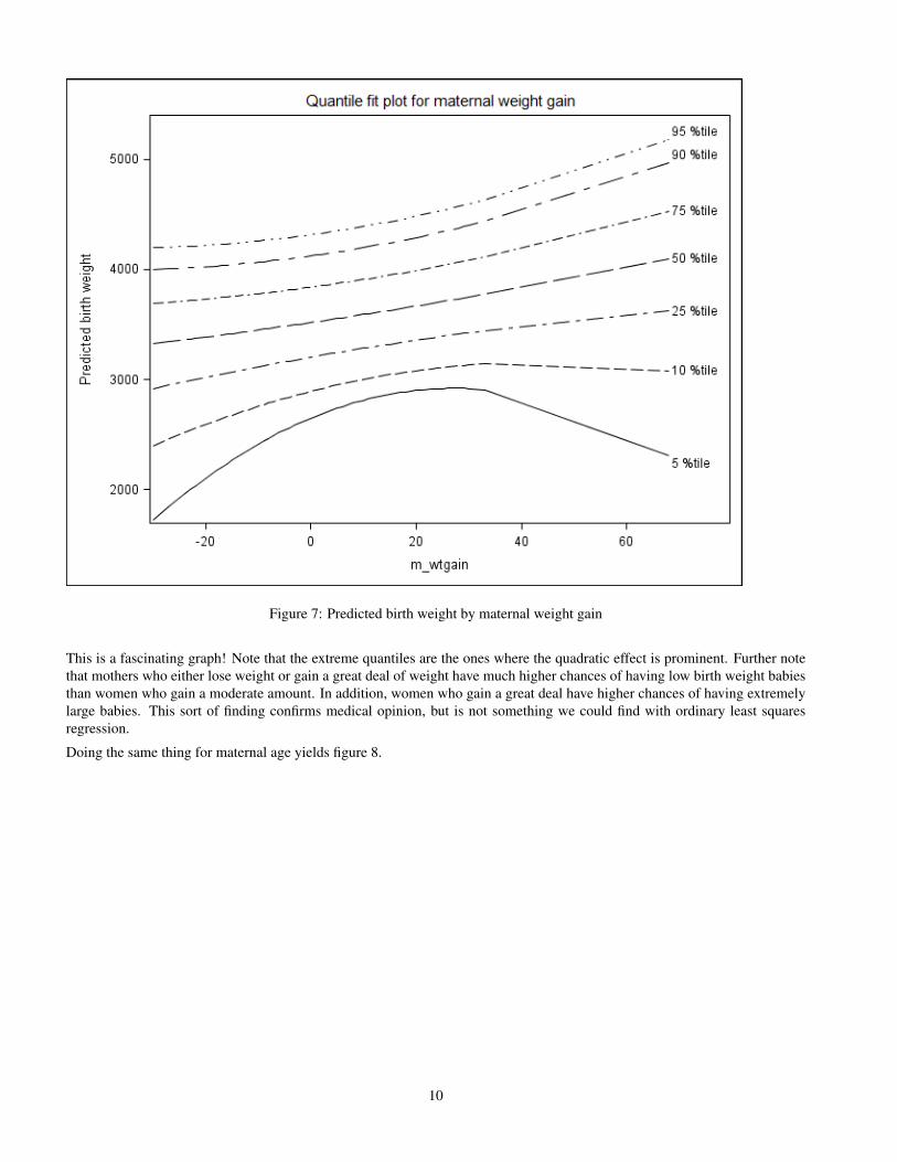
Figure 7: Predicted birth weight by maternal weight gain
This is a fascinating graph! Note that the extreme quantiles are the ones where the quadratic effect is prominent. Further notethat mothers who either lose weight or gain a great deal of weight have much higher chances of having low birth weight babiesthan women who gain a moderate amount. In addition, women who gain a great deal have higher chances of having extremelylarge babies. This sort of finding confirms medical opinion, but is not something we could find with ordinary least squaresregression.
Doing the same thing for maternal age yields figure 8.
10
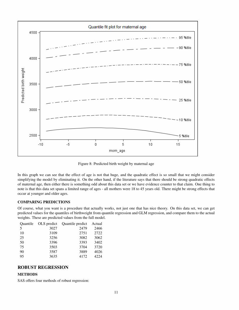
Figure 8: Predicted birth weight by maternal age
In this graph we can see that the effect of age is not that huge, and the quadratic effect is so small that we might considersimplifying the model by eliminating it. On the other hand, if the literature says that there should be strong quadratic effectsof maternal age, then either there is something odd about this data set or we have evidence counter to that claim. One thing tonote is that this data set spans a limited range of ages - all mothers were 18 to 45 years old. There might be strong effects thatoccur at younger and older ages.
COMPARING PREDICTIONSOf course, what you want is a procedure that actually works, not just one that has nice theory. On this data set, we can getpredicted values for the quantiles of birthweight from quantile regression and GLM regression, and compare them to the actualweights. These are predicted values from the full model.
Quantile OLS predict Quantile predict Actual5 3027 2479 246610 3109 2751 272225 3256 3082 306250 3396 3393 340275 3503 3704 372090 3587 3889 402695 3635 4172 4224
ROBUST REGRESSIONMETHODSSAS offers four methods of robust regression:
11
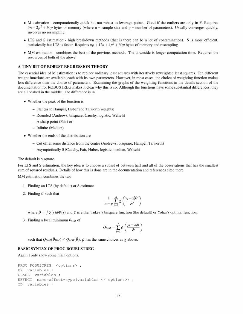
• M estimation - computationally quick but not robust to leverage points. Good if the outliers are only in Y. Requires3n+ 2p2 + 30p bytes of memory (where n = sample size and p = number of parameters). Usually converges quickly,involves no resampling.
• LTS and S estimation - high breakdown methods (that is there can be a lot of contamination). S is more efficient,statistically but LTS is faster. Requires np+12n+4p2 +60p bytes of memory and resampling.
• MM estimation - combines the best of the previous methods. The downside is longer computation time. Requires theresources of both of the above.
A TINY BIT OF ROBUST REGRESSION THEORYThe essential idea of M estimation is to replace ordinary least squares with iteratively reweighted least squares. Ten differentweight functions are available, each with its own parameters. However, in most cases, the choice of weighting function makesless difference than the choice of parameters. Examining the graphs of the weighting functions in the details section of thedocumentation for ROBUSTREG makes it clear why this is so: Although the functions have some substantial differences, theyare all peaked in the middle. The difference is in
• Whether the peak of the function is
– Flat (as in Hamper, Huber and Talworth weights)
– Rounded (Andrews, bisquare, Cauchy, logistic, Welsch)
– A sharp point (Fair) or
– Infinite (Median)
• Whether the ends of the distribution are
– Cut off at some distance from the center (Andrews, bisquare, Hampel, Talworth)
– Asymptotically 0 (Cauchy, Fair, Huber, logistic, median, Welsch)
The default is bisquare.
For LTS and S estimation, the key idea is to choose a subset of between half and all of the observations that has the smallestsum of squared residuals. Details of how this is done are in the documentation and references cited there.
MM estimation combines the two
1. Finding an LTS (by default) or S estimate
2. Finding σ̂ such that1
n− p
n
∑i=1
χ
(yi− x′iθ
′
σ̂ ′
)where β =
∫χ(s)dΦ(s) and χ is either Tukey’s bisquare function (the default) or Yohai’s optimal function.
3. Finding a local minimum θ̂MM of
QMM =n
∑i=1
ρ
(yi− xiθ
σ̂
)such that QMM(θ̂MM)≤ QMM(θ̂). ρ has the same choices as χ above.
BASIC SYNTAX OF PROC ROUBUSTREGAgain I only show some main options.
PROC ROBUSTREG <options> ;BY variables ;CLASS variables ;EFFECT name=effect-type(variables </ options>) ;ID variables ;
12
MODEL response = <effects> </ options> ;OUTPUT <OUT=SAS-data-set> keyword=name <keyword=name> ;PERFORMANCE <options> ;TEST effects ;WEIGHT variable ;
most of these are familiar from other SAS procedures. The PERFORMANCE statement offers options to track and improveperformance in terms of speed of computation. The options for the PROC ROBUSTREG statement include METHOD tospecify method and each method has many of its own options; as usual SAS has sensible defaults.
ROBUST REGRESSION EXAMPLE: CONTAMINATED WEIGHTS AND HEIGHTS
Suppose that, in stat methods 101, you want to show an example of simple linear regression. Last year, a colleague who teachesPsychology 101 did a survey of the relationship between height and weight in his class. He knew well enough to separate themen and women. But, unbeknownst to him, the football coach had recommended the class and eleven of the team had decidedto take it together. We can generate this sort of data with this code:
data a (drop=i);do i=1 to 100;
if i < 90 thendo;height = 70+rannor(1234)*3;
weight = height*2.5 + rannor(1234)*8;end;
else do;height = 78 + rannor(1234)*4;
weight = height*3.4 + rannor(1234)*8;end;
output;end;
run;
We run OLS regression on these data and get rather odd parameter estimates - the intercept is -267 and the parameter for heightis 6.35, which is not only higher than that for the 89 students who are not football players, it’s higher than that for the footballplayers as well. The diagnostics plots (figure 9) make it clear that there are high leverage points.
13
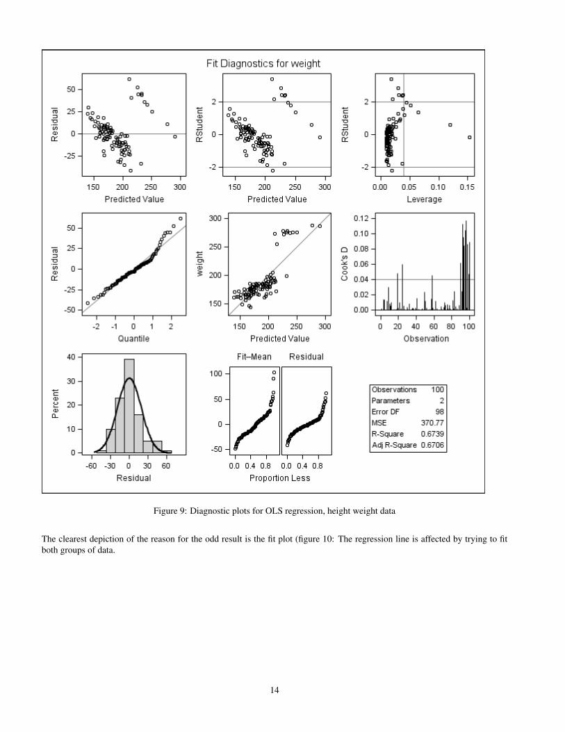
Figure 9: Diagnostic plots for OLS regression, height weight data
The clearest depiction of the reason for the odd result is the fit plot (figure 10: The regression line is affected by trying to fitboth groups of data.
14
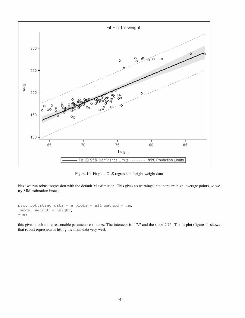
Figure 10: Fit plot, OLS regression, height weight data
Next we run robust regression with the default M estimation. This gives us warnings that there are high leverage points, so wetry MM estimation instead.
proc robustreg data = a plots = all method = mm;model weight = height;
run;
this gives much more reasonable parameter estimates: The intercept is -17.7 and the slope 2.75. The fit plot (figure 11 showsthat robust regression is fitting the main data very well.
15
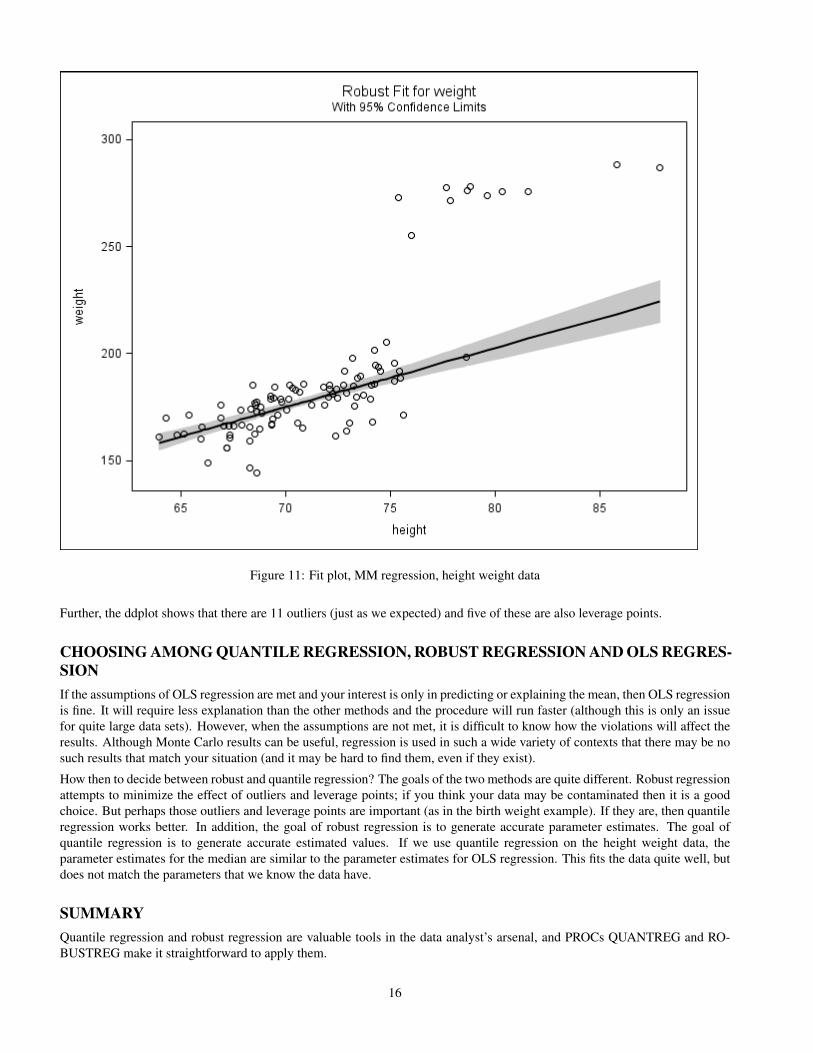
Figure 11: Fit plot, MM regression, height weight data
Further, the ddplot shows that there are 11 outliers (just as we expected) and five of these are also leverage points.
CHOOSING AMONG QUANTILE REGRESSION, ROBUST REGRESSION AND OLS REGRES-SIONIf the assumptions of OLS regression are met and your interest is only in predicting or explaining the mean, then OLS regressionis fine. It will require less explanation than the other methods and the procedure will run faster (although this is only an issuefor quite large data sets). However, when the assumptions are not met, it is difficult to know how the violations will affect theresults. Although Monte Carlo results can be useful, regression is used in such a wide variety of contexts that there may be nosuch results that match your situation (and it may be hard to find them, even if they exist).
How then to decide between robust and quantile regression? The goals of the two methods are quite different. Robust regressionattempts to minimize the effect of outliers and leverage points; if you think your data may be contaminated then it is a goodchoice. But perhaps those outliers and leverage points are important (as in the birth weight example). If they are, then quantileregression works better. In addition, the goal of robust regression is to generate accurate parameter estimates. The goal ofquantile regression is to generate accurate estimated values. If we use quantile regression on the height weight data, theparameter estimates for the median are similar to the parameter estimates for OLS regression. This fits the data quite well, butdoes not match the parameters that we know the data have.
SUMMARYQuantile regression and robust regression are valuable tools in the data analyst’s arsenal, and PROCs QUANTREG and RO-BUSTREG make it straightforward to apply them.
16

BIBLIOGRAPHYKoenker, R. “Quantile Regression”, Cambridge University Press, Cambridge, UK, 2005.
CONTACT INFORMATIONPeter L. Flom515 West End AveApt 8CNew York, NY 10024 [email protected](917) 488 7176
SAS R© and all other SAS Institute Inc., product or service names are registered trademarks ore trademarks of SAS Institute Inc.,in the USA and other countries. R© indicates USA registration. Other brand names and product names are registered trademarksor trademarks of their respective companies.
17