Semantics-Preserving DimensionalityReduction: Rough and Fuzzy-Rough-Based

ApproachesRichard Jensen and Qiang Shen

Abstract—Semantics-preserving dimensionality reduction refers to the problem of selecting those input features that are most

predictive of a given outcome; a problem encountered in many areas such as machine learning, pattern recognition, and signal

processing. This has found successful application in tasks that involve data sets containing huge numbers of features (in the order of

tens of thousands), which would be impossible to process further. Recent examples include text processing and Web content

classification. One of the many successful applications of rough set theory has been to this feature selection area. This paper reviews

those techniques that preserve the underlying semantics of the data, using crisp and fuzzy rough set-based methodologies. Several

approaches to feature selection based on rough set theory are experimentally compared. Additionally, a new area in feature selection,

feature grouping, is highlighted and a rough set-based feature grouping technique is detailed.

Index Terms—Dimensionality reduction, feature selection, feature transformation, rough selection, fuzzy-rough selection.

�

1 INTRODUCTION

MANY problems in machine learning involve high-

dimensional descriptions of input features. It istherefore not surprising that much research has been

carried out on dimensionality reduction [12], [26], [29],

[30], [31]. However, existing work tends to destroy the

underlying semantics of the features after reduction (e.g.

transformation-based approaches [13]) or require additional

information about the given data set for thresholding (e.g.

entropy-based approaches [32]). A technique that can

reduce dimensionality using information contained withinthe data set and that preserves the meaning of the features

(i.e., semantics-preserving) is clearly desirable. Rough set

theory (RST) can be used as such a tool to discover data

dependencies and to reduce the number of attributes

contained in a data set using the data alone and no

additional information [38], [41].Over the past 10 years, RST has indeed become a topic of

great interest to researchers and has been applied to many

domains. Given a data set with discretized attribute values,

it is possible to find a subset (termed a reduct) of the original

attributes using RST that are the most informative; all other

attributes can be removed from the data set with minimal

information loss. From the dimensionality reduction per-

spective, informative features are those that are most useful

in determining classifications from their values.

However, it is most often the case that the values ofattributes may be both crisp and real-valued, and this iswhere traditional rough set theory encounters a problem. Itis not possible in the original theory to say whether twoattribute values are similar and to what extent they are thesame; for example, two close values may only differ as aresult of noise, but in RST, they are considered to be asdifferent as two values of a different order of magnitude. Asa result of this, extensions to the original theory have beenproposed, for example, those based on similarity ortolerance relations [55], [61], [62].

It is, therefore, desirable to develop techniques toprovide the means of data reduction for crisp and real-value attributed data sets which utilizes the extent to whichvalues are similar. This can be achieved through the use offuzzy-rough sets. Fuzzy-rough sets encapsulate the relatedbut distinct concepts of vagueness (for fuzzy sets [70]) andindiscernibility (for rough sets), both of which occur as aresult of uncertainty in knowledge [17].

This review focuses on those recent techniques forfeature selection that employ a rough-set-based methodol-ogy for this purpose, highlighting current trends and futuredirections for this promising area. The second sectionintroduces rough set fundamentals and extensions whichenable various approaches to feature selection. Several ofthese are evaluated experimentally and compared. Section 3introduces the fuzzy extension to rough sets, fuzzy-roughsets, and details how this may be applied to the featureselection problem, with the aid of a simple example dataset. Rough set-based feature grouping is also discussed. Thereview is concluded in Section 4.

2 ROUGH SELECTION

Rough set theory [18], [37], [48], [56], [57] is an extension ofconventional set theory that supports approximations in

IEEE TRANSACTIONS ON KNOWLEDGE AND DATA ENGINEERING, VOL. 17, NO. 1, JANUARY 2005 1

. R. Jensen is with the Centre for Intelligent Systems and Their Applications,School of Informatics, The University of Edinburgh, Room 3.14, AppletonTower, Crichton Street, Edinburgh, EG8 9LE.E-mail: richjens@dai.ed.ac.uk.

. Q. Shen is with the Department of Computer Science, University of Wales,Aberystwyth, Ceredigion, SY23 3DB, Wales, UK. E-mail: qqs@aber.ac.uk.

Manuscript received 23 June 2003; revised 11 Feb. 2004; accepted 27 Apr.2004.For information on obtaining reprints of this article, please send e-mail to:tkde@computer.org, and reference IEEECS Log Number TKDE-0102-0603.

1041-4347/05/$20.00 � 2005 IEEE Published by the IEEE Computer Society

decision making. It possesses many features in common (toa certain extent) with the Dempster-Shafer theory ofevidence [54] and fuzzy set theory [39], [68]. The roughset itself is the approximation of a vague concept (set) by apair of precise concepts, called lower and upper approx-imations, which are a classification of the domain of interestinto disjoint categories. The lower approximation is adescription of the domain objects which are known withcertainty to belong to the subset of interest, whereas theupper approximation is a description of the objects whichpossibly belong to the subset. This section focuses onseveral rough set-based techniques for feature selection.Some of the techniques described here can be found inrough set systems available online [44], [45].

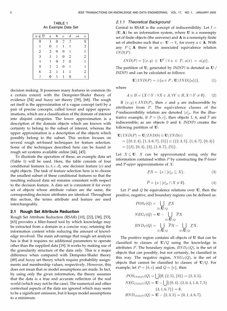
To illustrate the operation of these, an example data set(Table 1) will be used. Here, the table consists of fourconditional features (a; b; c; d), one decision feature (e) andeight objects. The task of feature selection here is to choosethe smallest subset of these conditional features so that theresulting reduced data set remains consistent with respectto the decision feature. A data set is consistent if for everyset of objects whose attribute values are the same, thecorresponding decision attributes are identical. Throughoutthis section, the terms attribute and feature are usedinterchangeably.

2.1 Rough Set Attribute Reduction

Rough Set Attribute Reduction (RSAR) [10], [22], [38], [53],[63] provides a filter-based tool by which knowledge maybe extracted from a domain in a concise way; retaining theinformation content while reducing the amount of knowl-edge involved. The main advantage that rough set analysishas is that it requires no additional parameters to operateother than the supplied data [19]. It works by making use ofthe granularity structure of the data only. This is a majordifference when compared with Dempster-Shafer theory[49] and fuzzy set theory which require probability assign-ments and membership values, respectively. However, thisdoes not mean that no model assumptions are made. In fact,by using only the given information, the theory assumesthat the data is a true and accurate reflection of the realworld (which may not be the case). The numerical and othercontextual aspects of the data are ignored which may seemto be a significant omission, but it keeps model assumptionsto a minimum.

2.1.1 Theoretical Background

Central to RSAR is the concept of indiscernibility. Let I ¼ðUU;AAÞ be an information system, where UU is a nonempty

set of finite objects (the universe) and AA is a nonempty finite

set of attributes such that a : UU ! Va for every a 2 AA. With

any P � AA there is an associated equivalence relation

INDðP Þ:

INDðP Þ ¼ fðx; yÞ 2 UU2 j 8 a 2 P; aðxÞ ¼ aðyÞg:

The partition of UU, generated by IND(P) is denoted as UU /

IND(P) and can be calculated as follows:

UU=INDðP Þ ¼ �fa 2 P : UU=INDðfagÞg; ð1Þ

where

A�B ¼ fX \ Y : 8X 2 A; 8Y 2 B;X \ Y 6¼ ;g: ð2Þ

If ðx; yÞ 2 INDðP Þ, then x and y are indiscernible by

attributes from P . The equivalence classes of the

P-indiscernibility relation are denoted ½x�P . For the illus-

trative example, if P ¼ fb; cg, then objects 1, 6, and 7 are

indiscernible; as are objects 0 and 4. IND(P) creates the

following partition of UU:

UU=INDðP Þ ¼ UU=INDðbÞ �UU=INDðcÞ¼ ff0; 2; 4g; f1; 3; 6; 7g; f5gg � ff2; 3; 5g; f1; 6; 7g; f0; 4gg¼ ff2g; f0; 4g; f3g; f1; 6; 7g; f5gg:

Let X � UU. X can be approximated using only the

information contained within P by constructing the P-lower

and P-upper approximations of X:

PX ¼ fx j ½x�P � Xg; ð3Þ

P ¼ fx j ½x�P \X 6¼ ;g: ð4Þ

Let P and Q be equivalence relations over UU, then the

positive, negative, and boundary regions can be defined as:

POSP ðQÞ ¼[

X2UU=Q

PX

NEGP ðQÞ ¼ UU�[

X2UU=Q

PX

BNDP ðQÞ ¼[

X2UU=Q

PX �[

X2UU=Q

PX:

The positive region contains all objects of UU that can be

classified to classes of UU/Q using the knowledge in

attributes P . The boundary region, BNDP ðQÞ, is the set of

objects that can possibly, but not certainly, be classified in

this way. The negative region, NEGP ðQÞ, is the set of

objects that cannot be classified to classes of UU=Q. For

example, let P ¼ fb; cg and Q ¼ feg, then

POSINDðP ÞðQÞ ¼[

f;; f2; 5g; f3gg ¼ f2; 3; 5g;NEGINDðP ÞðQÞ ¼ UU�

[ff0; 4g; f2; 0; 4; 1; 6; 7; 5g

f3; 1; 6; 7gg ¼ ;;BNDINDðP ÞðQÞ ¼ UU� f2; 3; 5g ¼ f0; 1; 4; 6; 7g:

2 IEEE TRANSACTIONS ON KNOWLEDGE AND DATA ENGINEERING, VOL. 17, NO. 1, JANUARY 2005

TABLE 1An Example Data Set

This means that objects 2, 3, and 5 can certainly be

classified as belonging to a class in attribute e, when

considering attributes b and c. The rest of the objects cannot

be classified as the information that would make them

discernible is absent.An important issue in data analysis is discovering

dependencies between attributes. Intuitively, a set of

attributes Q depends totally on a set of attributes P ,

denoted P ) Q, if all attribute values from Q are uniquely

determined by values of attributes from P . If there exists a

functional dependency between values of Q and P , then Q

depends totally on P . Dependency can be defined in the

following way:For P , Q � AA, it is said that Q depends on P in a degree

kð0 � k � 1Þ, denoted P )k Q, if

k ¼ �P ðQÞ ¼ jPOSP ðQÞjjUUj : ð5Þ

If k ¼ 1, Q depends totally on P , if 0 < k < 1, Q depends

partially (in a degree k) on P , and if k ¼ 0, then Q does not

depend on P . In the example, the degree of dependency of

attribute feg from the attributes fb; cg is:

�fb;cgðfegÞ ¼jPOSfb;cgðfegÞj

jUUj

¼ jf2; 3; 5gjjf0; 1; 2; 3; 4; 5; 6; 7gj ¼

3

8:

By calculating the change in dependency when an

attribute is removed from the set of considered conditional

attributes, a measure of the significance of the attribute can

be obtained. The higher the change in dependency, the

more significant the attribute is. If the significance is 0, then

the attribute is dispensable. More formally, given P;Q and

an attribute a 2 P ,

�P ðQ; aÞ ¼ �P ðQÞ � �P�fagðQÞ: ð6Þ

For example, ifP ¼ fa; b; cg and Q ¼ e, then

�fa;b;cgðfegÞ ¼ jf2; 3; 5; 6gj=8 ¼ 4=8

�fa;bgðfegÞ ¼ jf2; 3; 5; 6gj=8 ¼ 4=8

�fb;cgðfegÞ ¼ jf2; 3; 5gj=8 ¼ 3=8

�fa;cgðfegÞ ¼ jf2; 3; 5; 6gj=8 ¼ 4=8:

And, calculating the significance of the three attributes

gives:

�P ðQ; aÞ ¼ �fa;b;cgðfegÞ � �fb;cgðfegÞ ¼ 1=8

�P ðQ; bÞ ¼ �fa;b;cgðfegÞ � �fa;cgðfegÞ ¼ 0

�P ðQ; cÞ ¼ �fa;b;cgðfegÞ � �fa;bgðfegÞ ¼ 0:

From this, it follows that attribute a is indispensable, but

attributes b and c can be dispensed with.

2.1.2 Reduction Method

The reduction of attributes is achieved by comparing

equivalence relations generated by sets of attributes.

Attributes are removed so that the reduced set provides

the same quality of classification as the original. A reduct is

defined as a subset of minimal cardinality Rmin of the

conditional attribute set CC such that �RðDDÞ ¼ �CCðDDÞ.

R ¼ fX : X � CC; �XðDDÞ ¼ �CCðDDÞg; ð7Þ

Rmin ¼ fX : X 2 R; 8Y 2 R; jXj � jY jg: ð8Þ

The intersection of all the sets in Rmin is called the core,

the elements of which are those attributes that cannot be

eliminated without introducing more contradictions to the

data set. In RSAR, a subset with minimum cardinality is

searched for.Using the example, the dependencies for all possible

subsets of CC can be calculated as:

�fa;b;c;dgðfegÞ ¼ 8=8 �fb;cgðfegÞ ¼ 3=8�fa;b;cgðfegÞ ¼ 4=8 �fb;dgðfegÞ ¼ 8=8�fa;b;dgðfegÞ ¼ 8=8 �fc;dgðfegÞ ¼ 8=8�fa;c;dgðfegÞ ¼ 8=8 �fagðfegÞ ¼ 0=8�fb;c;dgðfegÞ ¼ 8=8 �fbgðfegÞ ¼ 1=8�fa;bgðfegÞ ¼ 4=8 �fcgðfegÞ ¼ 0=8�fa;cgðfegÞ ¼ 4=8 �fdgðfegÞ ¼ 2=8�fa;dgðfegÞ ¼ 3=8:

Note that the given data set is consistent since

�fa;b;c;dgðfegÞ ¼ 1. The minimal reduct set for this example is:

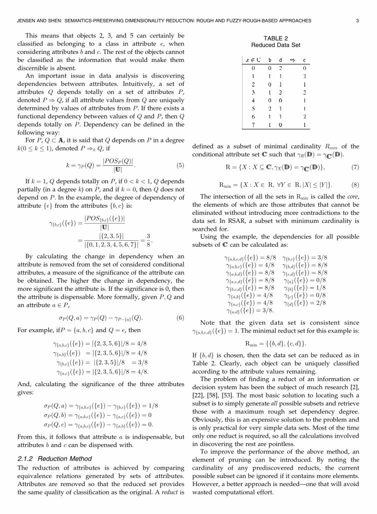
Rmin ¼ ffb; dg; fc; dgg:

If fb; dg is chosen, then the data set can be reduced as in

Table 2. Clearly, each object can be uniquely classified

according to the attribute values remaining.The problem of finding a reduct of an information or

decision system has been the subject of much research [2],

[22], [58], [53]. The most basic solution to locating such a

subset is to simply generate all possible subsets and retrieve

those with a maximum rough set dependency degree.

Obviously, this is an expensive solution to the problem and

is only practical for very simple data sets. Most of the time

only one reduct is required, so all the calculations involved

in discovering the rest are pointless.To improve the performance of the above method, an

element of pruning can be introduced. By noting the

cardinality of any prediscovered reducts, the current

possible subset can be ignored if it contains more elements.

However, a better approach is needed—one that will avoid

wasted computational effort.

JENSEN AND SHEN: SEMANTICS-PRESERVING DIMENSIONALITY REDUCTION: ROUGH AND FUZZY-ROUGH-BASED APPROACHES 3

TABLE 2Reduced Data Set

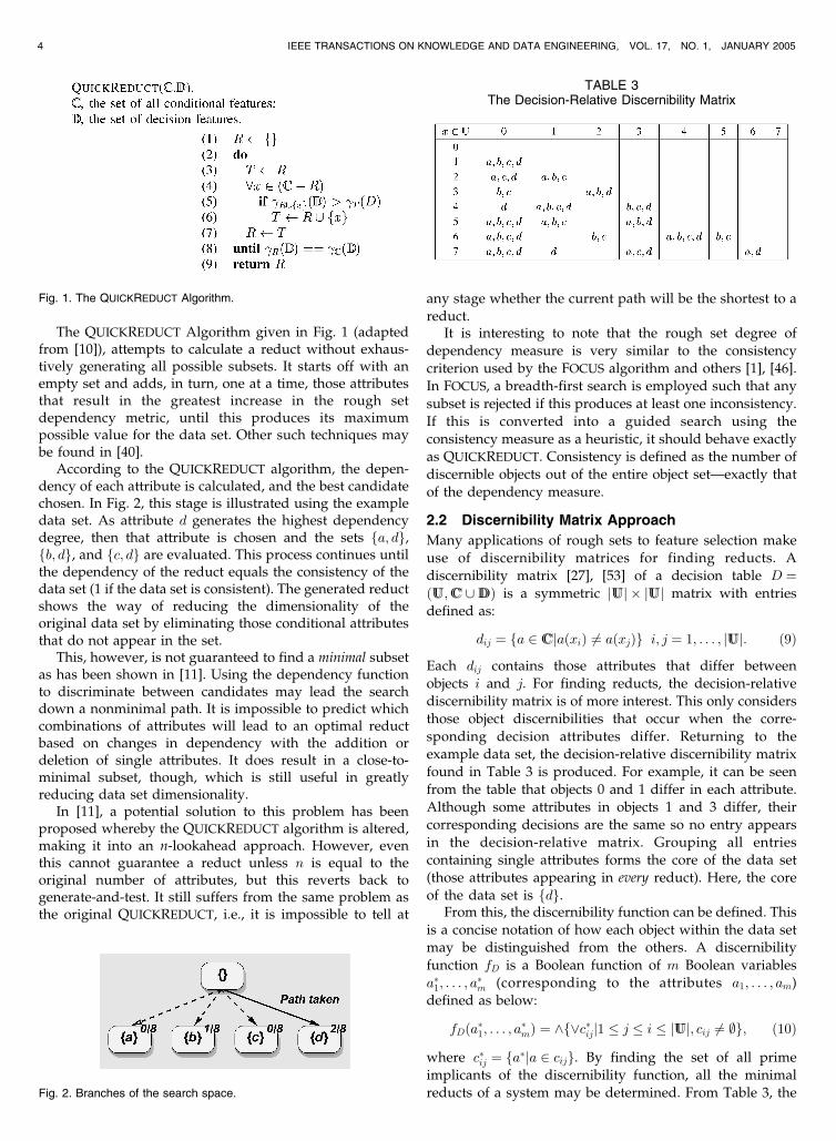
The QUICKREDUCT Algorithm given in Fig. 1 (adaptedfrom [10]), attempts to calculate a reduct without exhaus-tively generating all possible subsets. It starts off with anempty set and adds, in turn, one at a time, those attributesthat result in the greatest increase in the rough setdependency metric, until this produces its maximumpossible value for the data set. Other such techniques maybe found in [40].

According to the QUICKREDUCT algorithm, the depen-dency of each attribute is calculated, and the best candidatechosen. In Fig. 2, this stage is illustrated using the exampledata set. As attribute d generates the highest dependencydegree, then that attribute is chosen and the sets fa; dg,fb; dg, and fc; dg are evaluated. This process continues untilthe dependency of the reduct equals the consistency of thedata set (1 if the data set is consistent). The generated reductshows the way of reducing the dimensionality of theoriginal data set by eliminating those conditional attributesthat do not appear in the set.

This, however, is not guaranteed to find a minimal subsetas has been shown in [11]. Using the dependency functionto discriminate between candidates may lead the searchdown a nonminimal path. It is impossible to predict whichcombinations of attributes will lead to an optimal reductbased on changes in dependency with the addition ordeletion of single attributes. It does result in a close-to-minimal subset, though, which is still useful in greatlyreducing data set dimensionality.

In [11], a potential solution to this problem has beenproposed whereby the QUICKREDUCT algorithm is altered,making it into an n-lookahead approach. However, eventhis cannot guarantee a reduct unless n is equal to theoriginal number of attributes, but this reverts back togenerate-and-test. It still suffers from the same problem asthe original QUICKREDUCT, i.e., it is impossible to tell at

any stage whether the current path will be the shortest to a

reduct.It is interesting to note that the rough set degree of

dependency measure is very similar to the consistency

criterion used by the FOCUS algorithm and others [1], [46].

In FOCUS, a breadth-first search is employed such that any

subset is rejected if this produces at least one inconsistency.

If this is converted into a guided search using the

consistency measure as a heuristic, it should behave exactly

as QUICKREDUCT. Consistency is defined as the number of

discernible objects out of the entire object set—exactly that

of the dependency measure.

2.2 Discernibility Matrix Approach

Many applications of rough sets to feature selection make

use of discernibility matrices for finding reducts. A

discernibility matrix [27], [53] of a decision table D ¼ðUU;CC [DDÞ is a symmetric jUUj � jUUj matrix with entries

defined as:

dij ¼ fa 2 CCjaðxiÞ 6¼ aðxjÞg i; j ¼ 1; . . . ; jUUj: ð9Þ

Each dij contains those attributes that differ between

objects i and j. For finding reducts, the decision-relative

discernibility matrix is of more interest. This only considers

those object discernibilities that occur when the corre-

sponding decision attributes differ. Returning to the

example data set, the decision-relative discernibility matrix

found in Table 3 is produced. For example, it can be seen

from the table that objects 0 and 1 differ in each attribute.

Although some attributes in objects 1 and 3 differ, their

corresponding decisions are the same so no entry appears

in the decision-relative matrix. Grouping all entries

containing single attributes forms the core of the data set

(those attributes appearing in every reduct). Here, the core

of the data set is fdg.From this, the discernibility function can be defined. This

is a concise notation of how each object within the data set

may be distinguished from the others. A discernibility

function fD is a Boolean function of m Boolean variables

a�1; . . . ; a�m (corresponding to the attributes a1; . . . ; am)

defined as below:

fDða�1; . . . ; a�mÞ ¼ ^f_c�ijj1 � j � i � jUUj; cij 6¼ ;g; ð10Þ

where c�ij ¼ fa�ja 2 cijg. By finding the set of all prime

implicants of the discernibility function, all the minimal

reducts of a system may be determined. From Table 3, the

4 IEEE TRANSACTIONS ON KNOWLEDGE AND DATA ENGINEERING, VOL. 17, NO. 1, JANUARY 2005

Fig. 1. The QUICKREDUCT Algorithm.

Fig. 2. Branches of the search space.

TABLE 3The Decision-Relative Discernibility Matrix

decision-relative discernibility function is (with duplicates

removed):

fDða; b; c; dÞ ¼fa _ b _ c _ dg ^ fa _ c _ dg ^ fb _ cg^ fdg ^ fa _ b _ cg ^ fa _ b _ dg^ fb _ c _ dg ^ fa _ dg:

Further simplification can be performed by removing those

sets that are supersets of others:

fDða; b; c; dÞ ¼ fb _ cg ^ fdg

The reducts of the data set may be obtained by

converting the above expression from conjunctive normal

form to disjunctive normal form (without negations).

Hence, the minimal reducts are fb; dg and fc; dg. Although

this is guaranteed to discover all minimal subsets, it is a

costly operation rendering the method impractical for even

medium-sized data sets.For certain applications, a single minimal subset is all

that is required for data reduction. For example, dimen-

sionality reduction within text classification tends to use

only one subset to remove unnecessary keywords [25], [65].

This has led to approaches that consider finding individual

shortest prime implicants from the discernibility function.

A common method is to incrementally add those attributes

that occur with the most frequency in the function,

removing any clauses containing the attributes, until all

clauses are eliminated [35], [66]. However, even this does

not ensure that a minimal subset is found—the search can

proceed down nonminimal paths.It may also be desirable to locate several minimal subsets

for some applications [24], [67]. Once a collection of such

subsets has been found, a choice is made as to which of

these are the most informative for the application task at

hand. This decision can be made manually, or by the use of

a suitable measure such as entropy [42] to distinguish

between the subsets.

2.3 Reduction with Variable Precision Rough Sets

Variable precision rough sets (VPRS) [72] attempts to

improve upon rough set theory by relaxing the subset

operator. It was proposed to analyze and identify data

patterns which represent statistical trends rather than

functional. The main idea of VPRS is to allow objects to

be classified with an error smaller than a certain predefined

level. Let X;Y � UU, the relative classification error is

defined by:

cðX;Y Þ ¼ 1� jX \ Y jjXj :

Observe that cðX;Y Þ ¼ 0 if and only if X � Y . A degree

of inclusion can be achieved by allowing a certain level of

error, �, in classification:

X �� Y iff cðX;Y Þ � �; 0 � � < 0:5:

Using �� instead of � , the �-upper and �-lower

approximations of a set X can be defined as:

R�X ¼[

f½x�R 2 UU=Rj½x�R �� XgR�X ¼

[f½x�R 2 UU=Rjcð½x�R;XÞ < 1� �g:

Note that R�X ¼ RX for � ¼ 0. The positive, negative, and

boundary regions in the original rough set theory can now

be extended to:

POSR;�ðXÞ ¼ R�X; ð11Þ

NEGR;�ðXÞ ¼ UU�R�X; ð12Þ

BNDR;�ðXÞ ¼ R�X �R�X: ð13Þ

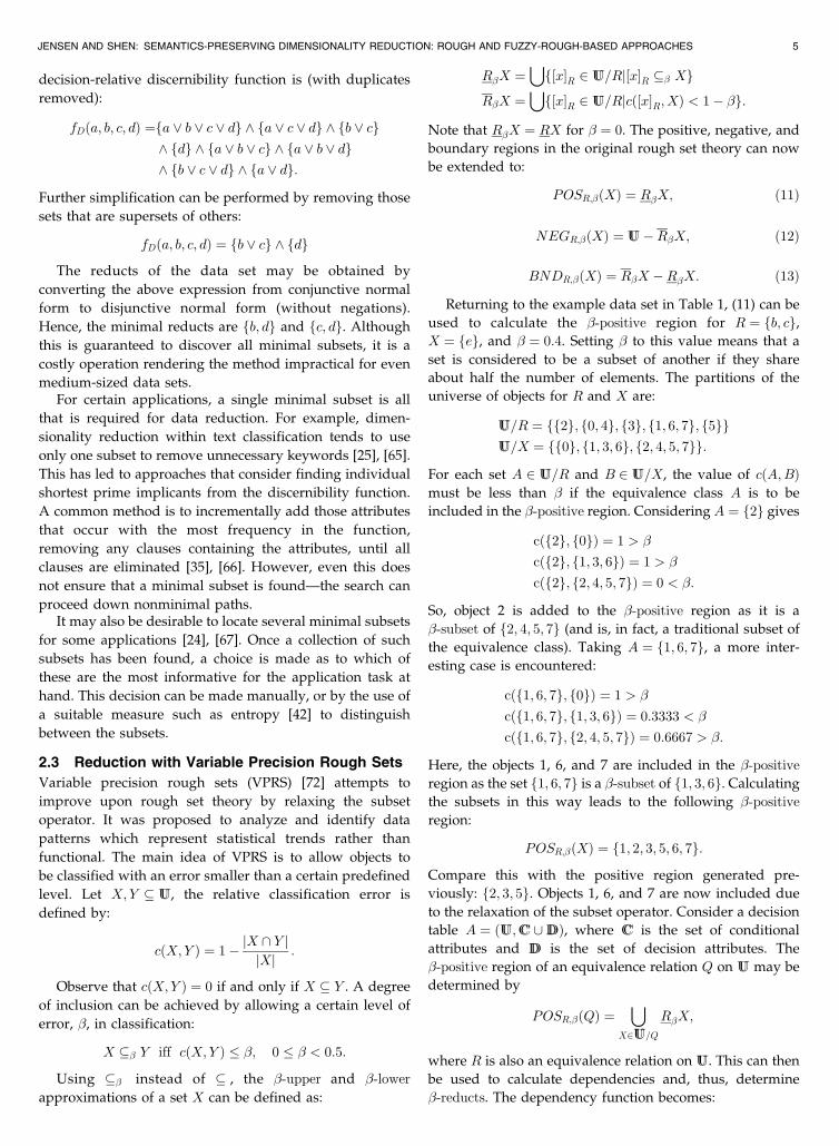
Returning to the example data set in Table 1, (11) can be

used to calculate the �-positive region for R ¼ fb; cg,X ¼ feg, and � ¼ 0:4. Setting � to this value means that a

set is considered to be a subset of another if they share

about half the number of elements. The partitions of the

universe of objects for R and X are:

UU=R ¼ ff2g; f0; 4g; f3g; f1; 6; 7g; f5ggUU=X ¼ ff0g; f1; 3; 6g; f2; 4; 5; 7gg:

For each set A 2 UU=R and B 2 UU=X, the value of cðA;BÞmust be less than � if the equivalence class A is to be

included in the �-positive region. Considering A ¼ f2g gives

cðf2g; f0gÞ ¼ 1 > �

cðf2g; f1; 3; 6gÞ ¼ 1 > �

cðf2g; f2; 4; 5; 7gÞ ¼ 0 < �:

So, object 2 is added to the �-positive region as it is a

�-subset of f2; 4; 5; 7g (and is, in fact, a traditional subset of

the equivalence class). Taking A ¼ f1; 6; 7g, a more inter-

esting case is encountered:

cðf1; 6; 7g; f0gÞ ¼ 1 > �

cðf1; 6; 7g; f1; 3; 6gÞ ¼ 0:3333 < �

cðf1; 6; 7g; f2; 4; 5; 7gÞ ¼ 0:6667 > �:

Here, the objects 1, 6, and 7 are included in the �-positive

region as the set f1; 6; 7g is a �-subset of f1; 3; 6g. Calculatingthe subsets in this way leads to the following �-positive

region:

POSR;�ðXÞ ¼ f1; 2; 3; 5; 6; 7g:

Compare this with the positive region generated pre-

viously: f2; 3; 5g. Objects 1, 6, and 7 are now included due

to the relaxation of the subset operator. Consider a decision

table A ¼ ðUU;CC [DDÞ, where CC is the set of conditional

attributes and DD is the set of decision attributes. The

�-positive region of an equivalence relation Q on UU may be

determined by

POSR;�ðQÞ ¼[

X2UU=Q

R�X;

where R is also an equivalence relation on UU. This can then

be used to calculate dependencies and, thus, determine

�-reducts. The dependency function becomes:

JENSEN AND SHEN: SEMANTICS-PRESERVING DIMENSIONALITY REDUCTION: ROUGH AND FUZZY-ROUGH-BASED APPROACHES 5

�R;�ðQÞ ¼ jPOSR;�ðQÞjjUUj :

It can be seen that the QUICKREDUCT algorithm outlinedpreviously can be adapted to incorporate the reductionmethod built upon VPRS theory. By supplying a suitable �value to the algorithm, the �-lower approximation, �-positiveregion, and �-dependency can replace the traditional calcula-tions. This will result in a more approximate final reduct,which may be a better generalization when encounteringunseen data. Additionally, setting � to 0 forces such amethod to behave exactly like RSAR.

Extended classification of reducts in the VPRS approachmay be found in [6], [7], [28]. However, the variableprecision approach requires the additional parameter �which has to be specified from the start. By repeatedexperimentation, this parameter can be suitably approxi-mated. However, problems arise when searching for truereducts as VPRS incorporates an element of imprecision indetermining the number of classifiable objects.

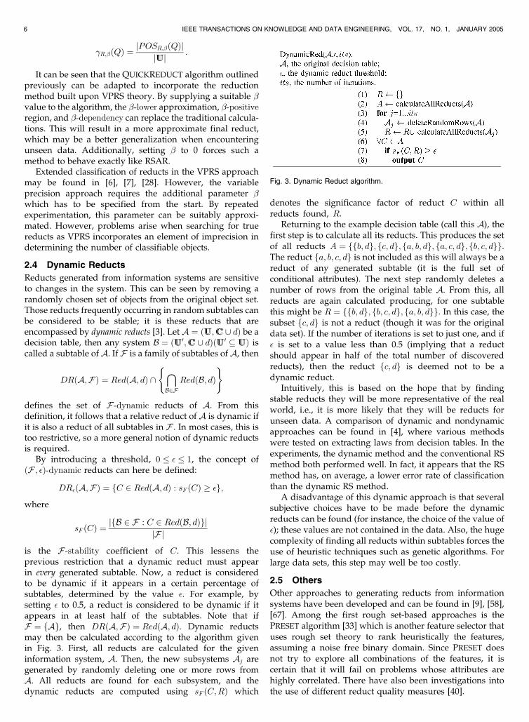
2.4 Dynamic Reducts

Reducts generated from information systems are sensitiveto changes in the system. This can be seen by removing arandomly chosen set of objects from the original object set.Those reducts frequently occurring in random subtables canbe considered to be stable; it is these reducts that areencompassed by dynamic reducts [3]. Let A ¼ ðUU;CC [ dÞ be adecision table, then any system B ¼ ðUU0;CC [ dÞðUU0 � UUÞ iscalled a subtable ofA. If F is a family of subtables ofA, then

DRðA;FÞ ¼ RedðA; dÞ \\B2F

RedðB; dÞ( )

defines the set of F -dynamic reducts of A. From thisdefinition, it follows that a relative reduct of A is dynamic ifit is also a reduct of all subtables in F . In most cases, this istoo restrictive, so a more general notion of dynamic reductsis required.

By introducing a threshold, 0 � � � 1, the concept ofðF ; �Þ-dynamic reducts can here be defined:

DR�ðA;FÞ ¼ fC 2 RedðA; dÞ : sF ðCÞ �g;

where

sF ðCÞ ¼ jfB 2 F : C 2 RedðB; dÞgjjF j

is the F -stability coefficient of C. This lessens theprevious restriction that a dynamic reduct must appearin every generated subtable. Now, a reduct is consideredto be dynamic if it appears in a certain percentage ofsubtables, determined by the value �. For example, bysetting � to 0.5, a reduct is considered to be dynamic if itappears in at least half of the subtables. Note that ifF ¼ fAg, then DRðA;FÞ ¼ RedðA; dÞ. Dynamic reductsmay then be calculated according to the algorithm givenin Fig. 3. First, all reducts are calculated for the giveninformation system, A. Then, the new subsystems Aj aregenerated by randomly deleting one or more rows fromA. All reducts are found for each subsystem, and thedynamic reducts are computed using sF ðC;RÞ which

denotes the significance factor of reduct C within allreducts found, R.

Returning to the example decision table (call this A), thefirst step is to calculate all its reducts. This produces the setof all reducts A ¼ ffb; dg; fc; dg; fa; b; dg; fa; c; dg; fb; c; dgg.The reduct fa; b; c; dg is not included as this will always be areduct of any generated subtable (it is the full set ofconditional attributes). The next step randomly deletes anumber of rows from the original table A. From this, allreducts are again calculated producing, for one subtablethis might be R ¼ ffb; dg; fb; c; dg; fa; b; dgg. In this case, thesubset fc; dg is not a reduct (though it was for the originaldata set). If the number of iterations is set to just one, and if� is set to a value less than 0.5 (implying that a reductshould appear in half of the total number of discoveredreducts), then the reduct fc; dg is deemed not to be adynamic reduct.

Intuitively, this is based on the hope that by findingstable reducts they will be more representative of the realworld, i.e., it is more likely that they will be reducts forunseen data. A comparison of dynamic and nondynamicapproaches can be found in [4], where various methodswere tested on extracting laws from decision tables. In theexperiments, the dynamic method and the conventional RSmethod both performed well. In fact, it appears that the RSmethod has, on average, a lower error rate of classificationthan the dynamic RS method.

A disadvantage of this dynamic approach is that severalsubjective choices have to be made before the dynamicreducts can be found (for instance, the choice of the value of�); these values are not contained in the data. Also, the hugecomplexity of finding all reducts within subtables forces theuse of heuristic techniques such as genetic algorithms. Forlarge data sets, this step may well be too costly.

2.5 Others

Other approaches to generating reducts from informationsystems have been developed and can be found in [9], [58],[67]. Among the first rough set-based approaches is thePRESET algorithm [33] which is another feature selector thatuses rough set theory to rank heuristically the features,assuming a noise free binary domain. Since PRESET doesnot try to explore all combinations of the features, it iscertain that it will fail on problems whose attributes arehighly correlated. There have also been investigations intothe use of different reduct quality measures [40].

6 IEEE TRANSACTIONS ON KNOWLEDGE AND DATA ENGINEERING, VOL. 17, NO. 1, JANUARY 2005

Fig. 3. Dynamic Reduct algorithm.

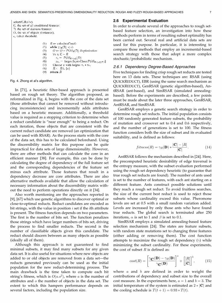
In [71], a heuristic filter-based approach is presentedbased on rough set theory. The algorithm proposed, asreformalized in Fig. 4, begins with the core of the data set(those attributes that cannot be removed without introdu-cing inconsistencies) and incrementally adds attributesbased on a heuristic measure. Additionally, a thresholdvalue is required as a stopping criterion to determine whena reduct candidate is “near enough” to being a reduct. Oneach iteration, those objects that are consistent with thecurrent reduct candidate are removed (an optimization thatcan be used with RSAR). As the process starts with the coreof the data set, this has to be calculated beforehand. Usingthe discernibility matrix for this purpose can be quiteimpractical for data sets of large dimensionality. However,there are other methods that can calculate the core in anefficient manner [38]. For example, this can be done bycalculating the degree of dependency of the full feature setand the corresponding dependencies of the feature setminus each attribute. Those features that result in adependency decrease are core attributes. There are alsoalternative methods available that allow the calculation ofnecessary information about the discernibility matrix with-out the need to perform operations directly on it [34].

Also worth mentioning are the approaches reported in[9], [67] which use genetic algorithms to discover optimal orclose-to-optimal reducts. Reduct candidates are encoded asbit strings, with the value in position i set if the ith attributeis present. The fitness function depends on two parameters.The first is the number of bits set. The function penalizesthose strings which have larger numbers of bits set, drivingthe process to find smaller reducts. The second is thenumber of classifiable objects given this candidate. Thereduct should discern between as many objects as possible(ideally all of them).

Although this approach is not guaranteed to findminimal subsets, it may find many subsets for any givendata set. It is also useful for situations where new objects areadded to or old objects are removed from a data set—thereducts generated previously can be used as the initialpopulation for the new reduct-determining process. Themain drawback is the time taken to compute each bitstring’s fitness, which is Oða:o2Þ, where a is the number ofattributes and o the number of objects in the data set. Theextent to which this hampers performance depends onseveral factors, including the population size.

2.6 Experimental Evaluation

In order to evaluate several of the approaches to rough set-based feature selection, an investigation into how thesemethods perform in terms of resulting subset optimality hasbeen carried out. Several real and artificial data sets areused for this purpose. In particular, it is interesting tocompare those methods that employ an incremental-basedsearch strategy with those that adopt a more complexstochastic/probabilistic mechanism.

2.6.1 Dependency Degree-Based Approaches

Five techniques for finding crisp rough set reducts are testedhere on 13 data sets. These techniques are: RSAR (usingQUICKREDUCT), EBR (using the same search mechanism asQUICKREDUCT), GenRSAR (genetic algorithm-based), An-tRSAR (ant-based), and SimRSAR (simulated annealing-based). Before the experiments are described, a few pointsmust be made about the later three approaches, GenRSAR,AntRSAR, and SimRSAR.

GenRSAR employs a genetic search strategy in order todetermine rough set reducts. The initial population consistsof 100 randomly generated feature subsets, the probabilityof mutation and crossover set to 0.4 and 0.6 respectively,and the number of generations is set to 100. The fitnessfunction considers both the size of subset and its evaluatedsuitability, and is defined as follows:

fitnessðRÞ ¼ �RðDDÞ � jCCj � jRjjCCj : ð14Þ

AntRSAR follows the mechanism described in [24]. Here,the precomputed heuristic desirability of edge traversal isthe entropy measure, with the subset evaluation performedusing the rough set dependency heuristic (to guarantee thattrue rough set reducts are found). The number of ants usedis set to the number of features, with each ant starting on adifferent feature. Ants construct possible solutions untilthey reach a rough set reduct. To avoid fruitless searches,the size of the current best reduct is used to reject thosesubsets whose cardinality exceed this value. Pheromonelevels are set at 0.5 with a small random variation added.Levels are increased by only those ants who have foundtrue reducts. The global search is terminated after 250iterations, � is set to 1 and � is set to 0.1.

SimRSAR employs a simulated annealing-based featureselection mechanism [24]. The states are feature subsets,with random state mutations set to changing three features(either adding or removing them). The cost functionattempts to maximize the rough set dependency (�) whileminimizing the subset cardinality. For these experiments,the cost of subset R is defined as:

costðRÞ ¼�CCðDDÞ � �RðDDÞ

�CCðDDÞ

" #a

þ jRjjCCj

� �b; ð15Þ

where a and b are defined in order to weight thecontributions of dependency and subset size to the overallcost measure. In the experiments here, a ¼ 1 and b ¼ 3. Theinitial temperature of the system is estimated as 2 � jCCj andthe cooling schedule is T ðtþ 1Þ ¼ 0:93 � T ðtÞ.

JENSEN AND SHEN: SEMANTICS-PRESERVING DIMENSIONALITY REDUCTION: ROUGH AND FUZZY-ROUGH-BASED APPROACHES 7

Fig. 4. Zhong et al’s algorithm.

The experiments were carried out on three data sets from

[43], namely m-of-n, exactly and exactly2. The remaining data

sets are from the machine learning repository [8]. Those

data sets containing real-valued attributes have been

discretized to allow all methods to be compared fairly.

2.6.2 Experimental Results

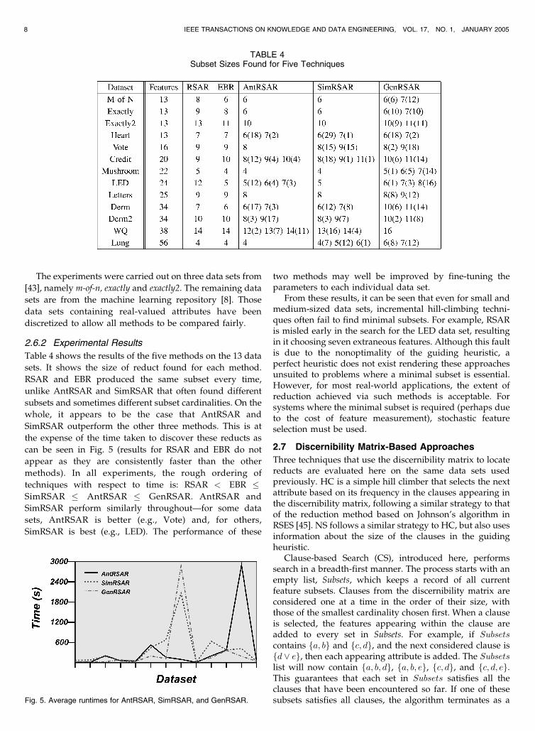
Table 4 shows the results of the five methods on the 13 data

sets. It shows the size of reduct found for each method.

RSAR and EBR produced the same subset every time,

unlike AntRSAR and SimRSAR that often found different

subsets and sometimes different subset cardinalities. On the

whole, it appears to be the case that AntRSAR and

SimRSAR outperform the other three methods. This is at

the expense of the time taken to discover these reducts as

can be seen in Fig. 5 (results for RSAR and EBR do not

appear as they are consistently faster than the other

methods). In all experiments, the rough ordering of

techniques with respect to time is: RSAR < EBR �SimRSAR � AntRSAR � GenRSAR. AntRSAR and

SimRSAR perform similarly throughout—for some data

sets, AntRSAR is better (e.g., Vote) and, for others,

SimRSAR is best (e.g., LED). The performance of these

two methods may well be improved by fine-tuning theparameters to each individual data set.

From these results, it can be seen that even for small andmedium-sized data sets, incremental hill-climbing techni-ques often fail to find minimal subsets. For example, RSARis misled early in the search for the LED data set, resultingin it choosing seven extraneous features. Although this faultis due to the nonoptimality of the guiding heuristic, aperfect heuristic does not exist rendering these approachesunsuited to problems where a minimal subset is essential.However, for most real-world applications, the extent ofreduction achieved via such methods is acceptable. Forsystems where the minimal subset is required (perhaps dueto the cost of feature measurement), stochastic featureselection must be used.

2.7 Discernibility Matrix-Based Approaches

Three techniques that use the discernibility matrix to locatereducts are evaluated here on the same data sets usedpreviously. HC is a simple hill climber that selects the nextattribute based on its frequency in the clauses appearing inthe discernibility matrix, following a similar strategy to thatof the reduction method based on Johnson’s algorithm inRSES [45]. NS follows a similar strategy to HC, but also usesinformation about the size of the clauses in the guidingheuristic.

Clause-based Search (CS), introduced here, performssearch in a breadth-first manner. The process starts with anempty list, Subsets, which keeps a record of all currentfeature subsets. Clauses from the discernibility matrix areconsidered one at a time in the order of their size, withthose of the smallest cardinality chosen first. When a clauseis selected, the features appearing within the clause areadded to every set in Subsets. For example, if Subsetscontains fa; bg and fc; dg, and the next considered clause isfd _ eg, then each appearing attribute is added. The Subsetslist will now contain fa; b; dg, fa; b; eg, fc; dg, and fc; d; eg.This guarantees that each set in Subsets satisfies all theclauses that have been encountered so far. If one of thesesubsets satisfies all clauses, the algorithm terminates as a

8 IEEE TRANSACTIONS ON KNOWLEDGE AND DATA ENGINEERING, VOL. 17, NO. 1, JANUARY 2005

TABLE 4Subset Sizes Found for Five Techniques

Fig. 5. Average runtimes for AntRSAR, SimRSAR, and GenRSAR.

reduct has been found. If not, then the process continues byselecting the next clause and adding these features. Thisprocess will result in a minimal subset, but has anexponential time and space complexity.

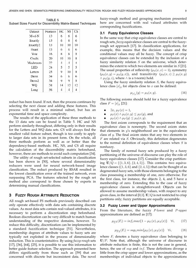
The results of the application of these three methods tothe 13 data sets can be found in Table 5. HC and NSperform similarly throughout, differing only in their resultsfor the Letters and WQ data sets. CS will always find thesmallest valid feature subset, though is too costly to applyto larger data sets in its present form. On the whole, allthree methods perform as well as or better than thedependency-based methods. HC, NS, and CS all requirethe calculation of the discernibility matrix beforehand,however, there are methods to avoid such computation [34].

The utility of rough set-selected subsets in classificationhas been shown in [50], where several dimensionalityreducers were used for neural network-based imageclassification. The reduct produced by RSAR resulted inthe lowest classification error of the trained network, evensurpassing PCA. The features selected by the rough setmethod also correspond to those chosen by experts indetermining manual classifications.

3 FUZZY ROUGH ATTRIBUTE REDUCTION

All rough set-based FS methods previously described canonly operate effectively with data sets containing discretevalues. As most data sets contain real-valued attributes, it isnecessary to perform a discretization step beforehand.Boolean discretization can be very difficult to match humanunderstanding of the respective domains, however. Toreduce this difficulty, discretization can be implemented bya standard fuzzification technique [51]. Nevertheless,membership degrees of attribute values to fuzzy sets aretypically not exploited in the process of dimensionalityreduction. This is counterintuitive. By using fuzzy-rough sets[17], [36], [64], [25], it is possible to use this information tobetter guide feature selection. The approach presented herediffers significantly from those such as [59] that areconcerned with discrete but inconsistent data. The novel

fuzzy-rough method and grouping mechanism presentedhere are concerned with real valued attributes withcorresponding fuzzifications.

3.1 Fuzzy Equivalence Classes

In the same way that crisp equivalence classes are central torough sets, fuzzy equivalence classes are central to the fuzzy-rough set approach [17]. In classification applications, forexample, this means that the decision values and theconditional values may all be fuzzy. The concept of crispequivalence classes can be extended by the inclusion of afuzzy similarity relation S on the universe, which deter-mines the extent to which two elements are similar in S [21].The usual properties of reflexivity (�Sðx; xÞ ¼ 1), symmetry(�Sðx; yÞ ¼ �Sðy; xÞ), and transitivity (�Sðx; zÞ �Sðx; yÞ^ �Sðy; zÞ, where ^ is a t-norm) hold.

Using the fuzzy similarity relation S, the fuzzy equiva-lence class ½x�S for objects close to x can be defined:

�½x�S ðyÞ ¼ �Sðx; yÞ: ð16Þ

The following axioms should hold for a fuzzy equivalenceclass F ¼ ½x�S [21]:

. 9x, �F ðxÞ ¼ 1,

. �F ðxÞ ^ �Sðx; yÞ � �F ðyÞ, and

. �F ðxÞ ^ �F ðyÞ � �Sðx; yÞ.The first axiom corresponds to the requirement that an

equivalence class is nonempty. The second axiom statesthat elements in y’s neighborhood are in the equivalenceclass of y. The final axiom states that any two elements inF are related via S. Obviously, this definition degeneratesto the normal definition of equivalence classes when S isnonfuzzy.

The family of normal fuzzy sets produced by a fuzzypartitioning of the universe of discourse can play the role offuzzy equivalence classes [17]. Consider the crisp partition-ing UU=Q ¼ ff1; 3; 6g; f2; 4; 5gg. This contains two equiva-lence classes (f1; 3; 6g and f2; 4; 5g) that can be thought of asdegenerated fuzzy sets, with those elements belonging to theclass possessing a membership of one, zero otherwise. Forthe first class, for instance, the objects 2, 4, and 5 have amembership of zero. Extending this to the case of fuzzyequivalence classes is straightforward: Objects can beallowed to assume membership values, with respect to anygiven class, in the interval [0,1].UU=Q is not restricted to crisppartitions only; fuzzy partitions are equally acceptable.

3.2 Fuzzy Lower and Upper Approximations

From the literature, the fuzzy P -lower and P -upperapproximations are defined as [17]:

�PXðFiÞ ¼ infxmaxf1� �FiðxÞ; �XðxÞg 8i; ð17Þ

�PXðFiÞ ¼ supxminf�FiðxÞ; �XðxÞg 8i; ð18Þ

where Fi denotes a fuzzy equivalence class belonging toUU=P . Note that, although the universe of discourse inattribute reduction is finite, this is not the case in general,hence, the use of sup and inf . These definitions diverge alittle from the crisp upper and lower approximations, as thememberships of individual objects to the approximations

JENSEN AND SHEN: SEMANTICS-PRESERVING DIMENSIONALITY REDUCTION: ROUGH AND FUZZY-ROUGH-BASED APPROACHES 9

TABLE 5Subset Sizes Found for Discernibility Matrix-Based Techniques

are not explicitly available. As a result of this, the fuzzylower and upper approximations are herein redefined as:

�PXðxÞ ¼ supF2UU=P

minð�F ðxÞ; infy2UU

maxf1� �F ðyÞ; �XðyÞgÞ;

ð19Þ

�PXðxÞ ¼ supF2UU=P

minð�F ðxÞ; supy2UU

minf�F ðyÞ; �XðyÞgÞ: ð20Þ

In implementation, not all y 2 UU are needed to beconsidered—only those where �F ðyÞ is nonzero, i.e., whereobject y is a fuzzy member of (fuzzy) equivalence class F .

The tuple < PX;PX > is called a fuzzy-rough set. It canbe seen that these definitions degenerate to traditionalrough sets when all equivalence classes are crisp. It is usefulto think of the crisp lower approximation as characterizedby the following membership function:

�PXðxÞ ¼1; x 2 F; F � X0; otherwise

�ð21Þ

This states that an object x belongs to the P -lower

approximation of X if it belongs to an equivalence classthat is a subset of X. The behavior of the fuzzy lowerapproximation must be exactly that of the crisp definitionfor crisp situations. This is indeed the case as the fuzzylower approximation may be rewritten as

�PXðxÞ ¼ supF2UU=P

minð�F ðxÞ; infy2UU

f�F ðyÞ ! �XðyÞgÞ; ð22Þ

where ! denotes the fuzzy implication operator. In thecrisp case, �F ðxÞ and �XðxÞ will take values from f0; 1g.Hence, it is clear that the only time �PXðxÞ will be zero iswhen at least one object in its equivalence class F fullybelongs to F but not to X. This is exactly the same as thedefinition for the crisp lower approximation. Similarly, thedefinition for the P -upper approximation can be establishedto make sense in being the generalization of the crispdefinition.

3.3 Fuzzy-Rough Reduction Process

Fuzzy RSAR (abbreviated FRAR hereafter) builds on thenotion of the fuzzy lower approximation to enable reduc-tion of data sets containing real-valued attributes. As will beshown, the process becomes identical to the traditionalapproach when dealing with nominal well-defined attri-butes. This feature selection method has been used in Webcategorization [25] and complex systems monitoring [52].

The crisp positive region in traditional rough set theoryis defined as the union of the lower approximations. By theextension principle, the membership of an object x 2 UU,belonging to the fuzzy positive region can be defined by

�POSP ðQÞðxÞ ¼ supX2UU=Q

�PXðxÞ: ð23Þ

Object x will not belong to the positive region only if theequivalence class it belongs to is not a constituent of thepositive region. This is equivalent to the crisp version whereobjects belong to the positive region only if their underlyingequivalence class does so.

Using the definition of the fuzzy positive region, the newdependency function can be defined as follows:

�0P ðQÞ ¼j�POSP ðQÞðxÞj

jUUj ¼P

x2UU �POSP ðQÞðxÞjUUj : ð24Þ

As with crisp rough sets, the dependency of Q on P is theproportion of objects that are discernible out of the entiredata set. In the present approach, this corresponds todetermining the fuzzy cardinality of �POSP ðQÞðxÞ divided bythe total number of objects in the universe.

The definition of dependency degree covers the crispcase as its specific instance. This can be easily shown byrecalling the definition of the crisp dependency degreegiven in (24). If a function �POSP ðQÞðxÞ is defined whichreturns 1 if the object x belongs to the positive region, 0otherwise, then the above definition may be rewritten as:

�P ðQÞ ¼P

x2UU �POSP ðQÞðxÞjUUj ; ð25Þ

which is identical to (24).If the fuzzy-rough reduction process is to be useful, it

must be able to deal with multiple attributes, finding thedependency between various subsets of the originalattribute set. For example, it may be necessary to be ableto determine the degree of dependency of the decisionattribute(s) with respect to P ¼ fa; bg. In the crisp case, UU=Pcontains sets of objects grouped together that are indis-cernible according to both attributes a and b. In the fuzzycase, objects may belong to many equivalence classes, so theCartesian product of UU=INDðfagÞ and UU=INDðfbgÞ mustbe considered in determining UU=P . In general,

UU=P ¼ �fa 2 P : UU=INDðfagÞg ð26Þ

Each set in UU=P denotes an equivalence class. Forexample, if P ¼ fa; bg, UU=INDðfagÞ ¼ fNa; Zag, andUU=INDðfbgÞ ¼ fNb; Zbg, then

UU=P ¼ fNa \Nb;Na \ Zb; Za \Nb; Za \ Zbg:

The extent to which an object belongs to such anequivalence class is therefore calculated by using theconjunction of constituent fuzzy equivalence classes, sayFi, i ¼ 1; 2; . . . ; n:

�F1\...\FnðxÞ ¼ minð�F1

ðxÞ; �F2ðxÞ; . . . ; �Fn

ðxÞÞ: ð27Þ

3.4 Reduct Computation

In conventional RSAR, a reduct is defined as a subset R ofthe attributes which have the same information content asthe full attribute set A. In terms of the dependency function,this means that the values �ðRÞ and �ðAÞ are identical andequal to 1 if the data set is consistent. However, in thefuzzy-rough approach, this is not necessarily the case as theuncertainty encountered when objects belong to manyfuzzy equivalence classes results in a reduced totaldependency.

A possible way of combatting this would be to determinethe degree of dependency of the full attribute set and usethis as the denominator (for normalization rather than jUUj),allowing �0 to reach 1. With these issues in mind, a newQUICKREDUCT algorithm has been developed as given in

10 IEEE TRANSACTIONS ON KNOWLEDGE AND DATA ENGINEERING, VOL. 17, NO. 1, JANUARY 2005

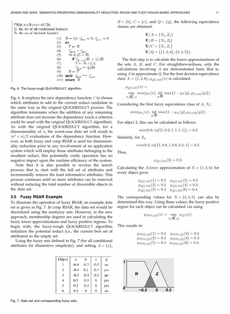
Fig. 6. It employs the new dependency function �0 to choosewhich attributes to add to the current reduct candidate inthe same way as the original QUICKREDUCT process. Thealgorithm terminates when the addition of any remainingattribute does not increase the dependency (such a criterioncould be used with the original QUICKREDUCT algorithm).As with the original QUICKREDUCT algorithm, for adimensionality of n, the worst-case data set will result inðn2 þ nÞ=2 evaluations of the dependency function. How-ever, as both fuzzy and crisp RSAR is used for dimension-ality reduction prior to any involvement of an applicationsystem which will employ those attributes belonging to theresultant reduct, this potentially costly operation has nonegative impact upon the runtime efficiency of the system.

Note that it is also possible to reverse the searchprocess; that is, start with the full set of attributes andincrementally remove the least informative attributes. Thisprocess continues until no more attributes can be removedwithout reducing the total number of discernible objects inthe data set.

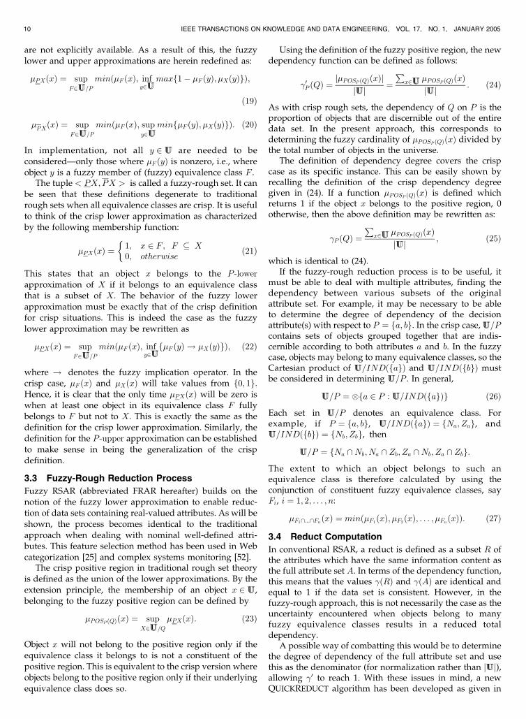
3.5 Fuzzy RSAR Example

To illustrate the operation of fuzzy RSAR, an example dataset is given in Fig. 7. In crisp RSAR, the data set would bediscretized using the nonfuzzy sets. However, in the newapproach, membership degrees are used in calculating thefuzzy lower approximations and fuzzy positive regions. Tobegin with, the fuzzy-rough QUICKREDUCT algorithminitializes the potential reduct (i.e., the current best set ofattributes) to the empty set.

Using the fuzzy sets defined in Fig. 7 (for all conditionalattributes for illustrative simplicity), and setting A ¼ fag,

B ¼ fbg, C ¼ fcg, and Q ¼ fqg, the following equivalenceclasses are obtained:

UU=A ¼ fNa; ZagUU=B ¼ fNb; ZbgUU=C ¼ fNc; ZcgUU=Q ¼ ff1; 3; 6g; f2; 4; 5gg:

The first step is to calculate the lower approximations ofthe sets A, B, and C. For straightforwardness, only thecalculations involving A are demonstrated here; that is,using A to approximate Q. For the first decision equivalenceclass X ¼ f1; 3; 6g; �Af1;3;6gðxÞ is calculated:

�Af1;3;6gðxÞ ¼sup

F2UU=A

minð�F ðxÞ; infy2UU

maxf1� �F ðyÞ; �f1;3;6gðyÞgÞ:

Considering the first fuzzy equivalence class of A, Na:

minð�NaðxÞ; inf

y2UUmaxf1� �Na

ðyÞ; �f1;3;6gðyÞgÞ:

For object 2, this can be calculated as follows:

minð0:8; inff1; 0:2; 1; 1; 1; 1gÞ ¼ 0:2

Similarly, for Za,

minð0:2; inff1; 0:8; 1; 0:6; 0:4; 1g ¼ 0:2:

Thus,

�Af1;3;6gð2Þ ¼ 0:2:

Calculating the A-lower approximation of X ¼ f1; 3; 6g forevery object gives

�Af1;3;6gð1Þ ¼ 0:2 �Af1;3;6gð2Þ ¼ 0:2�Af1;3;6gð3Þ ¼ 0:4 �Af1;3;6gð4Þ ¼ 0:4�Af1;3;6gð5Þ ¼ 0:4 �Af1;3;6gð6Þ ¼ 0:4:

The corresponding values for X ¼ f2; 4; 5g can also bedetermined this way. Using these values, the fuzzy positiveregion for each object can be calculated via using

�POSAðQÞðxÞ ¼ supX2UU=Q

�AXðxÞ:

This results in:

�POSAðQÞð1Þ ¼ 0:2 �POSAðQÞð2Þ ¼ 0:2�POSAðQÞð3Þ ¼ 0:4 �POSAðQÞð4Þ ¼ 0:4�POSAðQÞð5Þ ¼ 0:4 �POSAðQÞð6Þ ¼ 0:4:

JENSEN AND SHEN: SEMANTICS-PRESERVING DIMENSIONALITY REDUCTION: ROUGH AND FUZZY-ROUGH-BASED APPROACHES 11

Fig. 6. The fuzzy-rough QUICKREDUCT algorithm.

Fig. 7. Data set and corresponding fuzzy sets.

It is a coincidence here that �POSAðQÞðxÞ ¼ �Af1;3;6gðxÞ for thisexample. The next step is to determine the degree ofdependency of Q on A:

�0AðQÞ ¼P

x2U �POSAðQÞðxÞjUj ¼ 2=6:

Similarly, calculating for B and C gives:

�0BðQÞ ¼ 2:4

6; �0CðQÞ ¼ 1:6

6:

From this, it can be seen that attribute b will cause thegreatest increase in dependency degree. This attribute ischosen and added to the potential reduct. The processiterates and the two dependency degrees calculated are

�0fa;bgðQÞ ¼ 3:4

6; �0fb;cgðQÞ ¼ 3:2

6:

Adding attribute a to the reduct candidate causes the largerincrease of dependency, so the new candidate becomesfa; bg. Last, attribute c is added to the potential reduct:

�0fa;b;cgðQÞ ¼ 3:4

6:

As this causes no increase in dependency, the algorithmstops and outputs the reduct fa; bg (see Fig. 8). The data setcan now be reduced to only those attributes appearing inthe reduct. When crisp RSAR is performed on this data set(after using the same fuzzy sets to discretize the real-valuedattributes), the reduct generated is fa; b; cg, i.e., the fullconditional attribute set. Unlike crisp RSAR, the trueminimal reduct was found using the information ondegrees of membership. It is clear from this example alonethat the information lost by using crisp RSAR can beimportant when trying to discover the smallest reduct froma data set.

3.6 Rough Set-Based Feature Grouping

By its definition, the degree of dependency measure(whether using crisp or fuzzy-rough sets) always lies inthe range [0,1], with 0 indicating no dependency and 1indicating total dependency. For example, two subsets ofthe conditional attributes in a data set may have thefollowing dependency degrees:

�0fa;b;cgðDDÞ ¼ 0:54; �0fa;c;dgðDDÞ ¼ 0:52:

In traditional rough sets, it would be said that theattribute set fa; b; cg has a higher dependency value thanfa; c; dg and so would make the better candidate to producea minimal reduct. This may not be the case when

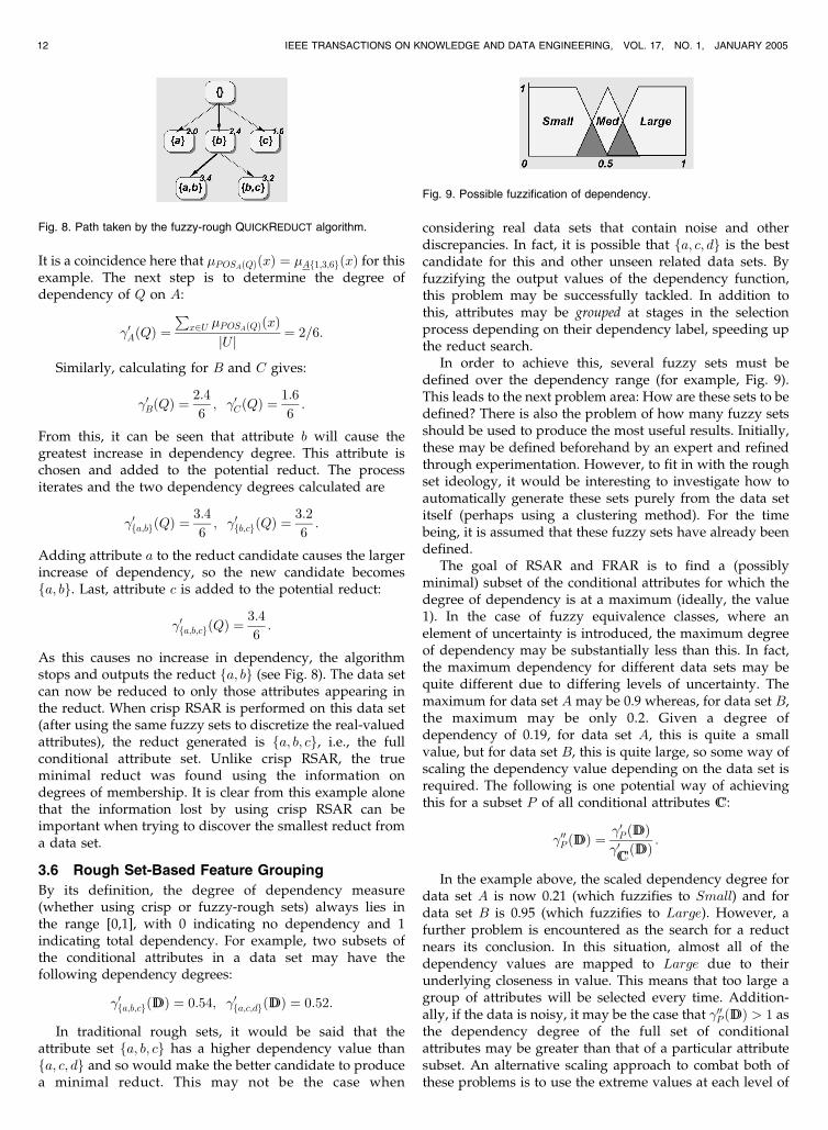
considering real data sets that contain noise and otherdiscrepancies. In fact, it is possible that fa; c; dg is the bestcandidate for this and other unseen related data sets. Byfuzzifying the output values of the dependency function,this problem may be successfully tackled. In addition tothis, attributes may be grouped at stages in the selectionprocess depending on their dependency label, speeding upthe reduct search.

In order to achieve this, several fuzzy sets must bedefined over the dependency range (for example, Fig. 9).This leads to the next problem area: How are these sets to bedefined? There is also the problem of how many fuzzy setsshould be used to produce the most useful results. Initially,these may be defined beforehand by an expert and refinedthrough experimentation. However, to fit in with the roughset ideology, it would be interesting to investigate how toautomatically generate these sets purely from the data setitself (perhaps using a clustering method). For the timebeing, it is assumed that these fuzzy sets have already beendefined.

The goal of RSAR and FRAR is to find a (possiblyminimal) subset of the conditional attributes for which thedegree of dependency is at a maximum (ideally, the value1). In the case of fuzzy equivalence classes, where anelement of uncertainty is introduced, the maximum degreeof dependency may be substantially less than this. In fact,the maximum dependency for different data sets may bequite different due to differing levels of uncertainty. Themaximum for data set A may be 0.9 whereas, for data set B,the maximum may be only 0.2. Given a degree ofdependency of 0.19, for data set A, this is quite a smallvalue, but for data set B, this is quite large, so some way ofscaling the dependency value depending on the data set isrequired. The following is one potential way of achievingthis for a subset P of all conditional attributes CC:

�00P ðDDÞ ¼ �0P ðDDÞ�0CCðDDÞ :

In the example above, the scaled dependency degree fordata set A is now 0.21 (which fuzzifies to Small) and fordata set B is 0.95 (which fuzzifies to Large). However, afurther problem is encountered as the search for a reductnears its conclusion. In this situation, almost all of thedependency values are mapped to Large due to theirunderlying closeness in value. This means that too large agroup of attributes will be selected every time. Addition-ally, if the data is noisy, it may be the case that �00P ðDDÞ > 1 asthe dependency degree of the full set of conditionalattributes may be greater than that of a particular attributesubset. An alternative scaling approach to combat both ofthese problems is to use the extreme values at each level of

12 IEEE TRANSACTIONS ON KNOWLEDGE AND DATA ENGINEERING, VOL. 17, NO. 1, JANUARY 2005

Fig. 8. Path taken by the fuzzy-rough QUICKREDUCT algorithm.

Fig. 9. Possible fuzzification of dependency.

search. As soon as the reduct candidates have beenevaluated, the highest and lowest dependencies (�0highðDDÞand �0lowðDDÞ) are used as follows to scale the dependencydegree of subset P :

�00P ðDDÞ ¼ �0P ðDDÞ � �0lowðDDÞ�0highðDDÞ � �0lowðDDÞ :

By this method, the attribute subset with the highestdependency value will have a scaled dependency (�00P ðDDÞ)of 1. The subset with the lowest will have a scaleddependency of 0. In so doing, the definition of the fuzzysets need not be changed for different data sets; onedefinition should be applicable to all.

The next question to address is how to handle thosescaled dependencies that fall at the boundaries. Forexample, a value may partially belong to both Small andMedium. A simple strategy is to choose the single fuzzylabel with the highest membership value. However, thisloses the potentially useful information of dual fuzzy setmembership. Another strategy is to take both labels asvalid, considering both possibilities within the featureselection process. If, for example, a dependency value lieswithin the labels Small and Medium then it is considered tobelong to both groups.

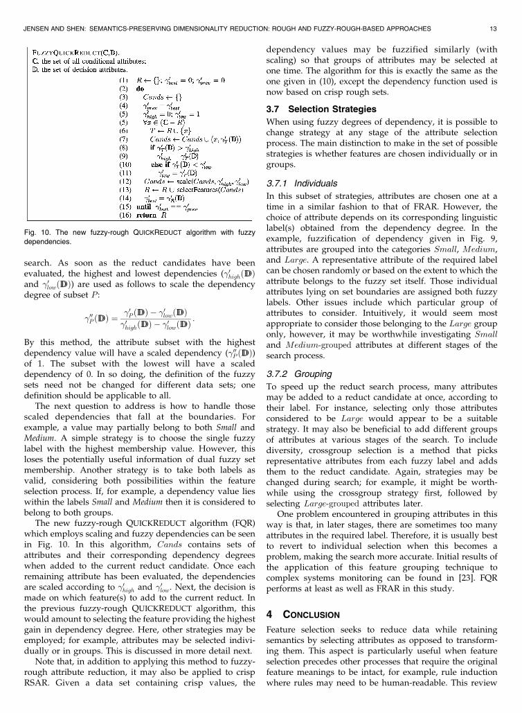
The new fuzzy-rough QUICKREDUCT algorithm (FQR)which employs scaling and fuzzy dependencies can be seenin Fig. 10. In this algorithm, Cands contains sets ofattributes and their corresponding dependency degreeswhen added to the current reduct candidate. Once eachremaining attribute has been evaluated, the dependenciesare scaled according to �0high and �0low. Next, the decision ismade on which feature(s) to add to the current reduct. Inthe previous fuzzy-rough QUICKREDUCT algorithm, thiswould amount to selecting the feature providing the highestgain in dependency degree. Here, other strategies may beemployed; for example, attributes may be selected indivi-dually or in groups. This is discussed in more detail next.

Note that, in addition to applying this method to fuzzy-rough attribute reduction, it may also be applied to crispRSAR. Given a data set containing crisp values, the

dependency values may be fuzzified similarly (withscaling) so that groups of attributes may be selected atone time. The algorithm for this is exactly the same as theone given in (10), except the dependency function used isnow based on crisp rough sets.

3.7 Selection Strategies

When using fuzzy degrees of dependency, it is possible tochange strategy at any stage of the attribute selectionprocess. The main distinction to make in the set of possiblestrategies is whether features are chosen individually or ingroups.

3.7.1 Individuals

In this subset of strategies, attributes are chosen one at atime in a similar fashion to that of FRAR. However, thechoice of attribute depends on its corresponding linguisticlabel(s) obtained from the dependency degree. In theexample, fuzzification of dependency given in Fig. 9,attributes are grouped into the categories Small, Medium,and Large. A representative attribute of the required labelcan be chosen randomly or based on the extent to which theattribute belongs to the fuzzy set itself. Those individualattributes lying on set boundaries are assigned both fuzzylabels. Other issues include which particular group ofattributes to consider. Intuitively, it would seem mostappropriate to consider those belonging to the Large grouponly, however, it may be worthwhile investigating Smalland Medium-grouped attributes at different stages of thesearch process.

3.7.2 Grouping

To speed up the reduct search process, many attributesmay be added to a reduct candidate at once, according totheir label. For instance, selecting only those attributesconsidered to be Large would appear to be a suitablestrategy. It may also be beneficial to add different groupsof attributes at various stages of the search. To includediversity, crossgroup selection is a method that picksrepresentative attributes from each fuzzy label and addsthem to the reduct candidate. Again, strategies may bechanged during search; for example, it might be worth-while using the crossgroup strategy first, followed byselecting Large-grouped attributes later.

One problem encountered in grouping attributes in thisway is that, in later stages, there are sometimes too manyattributes in the required label. Therefore, it is usually bestto revert to individual selection when this becomes aproblem, making the search more accurate. Initial results ofthe application of this feature grouping technique tocomplex systems monitoring can be found in [23]. FQRperforms at least as well as FRAR in this study.

4 CONCLUSION

Feature selection seeks to reduce data while retainingsemantics by selecting attributes as opposed to transform-ing them. This aspect is particularly useful when featureselection precedes other processes that require the originalfeature meanings to be intact, for example, rule inductionwhere rules may need to be human-readable. This review

JENSEN AND SHEN: SEMANTICS-PRESERVING DIMENSIONALITY REDUCTION: ROUGH AND FUZZY-ROUGH-BASED APPROACHES 13

Fig. 10. The new fuzzy-rough QUICKREDUCT algorithm with fuzzy

dependencies.

focused on some of the recent developments in rough set

theory for the purpose of feature selection.Several approaches to discovering rough set reducts

were experimentally evaluated and compared. The results

highlighted the shortcomings of conventional hill-climbing

approaches to feature selection. These techniques often fail

to find minimal data reductions. Some guiding heuristics

are better than others for this, but, as no perfect heuristic

exists, there can be no guarantee of optimality. From the

experimentation, it appears that the entropy-based measure

is a more useful hill-climbing heuristic than the rough set-

based one. However, the entropy measure is a more costly

operation than that of dependency evaluation which may

be an important factor when processing large data sets. Due

to the failure of hill-climbing methods and the fact that

exhaustive searches are not feasible for even medium-sized

data sets, stochastic approaches provide a promising

feature selection mechanism.Conventional rough set methods are unable to deal with

real-valued attributes effectively. This prompted research

into the use of fuzzy-rough sets for feature selection.

Additionally, the new direction in feature selection, feature

grouping, was highlighted. It was shown how fuzzifying a

particular evaluation function, the rough set dependency

degree, can lead to group and individual selection based on

linguistic labels—more closely resembling human reason-

ing. In fact, this can be applied to most FS algorithms that

use an evaluation function that returns values in ½0; 1�.Choosing grouped features instead of individuals also

decreases the time taken to reach potentially optimal

subsets.

REFERENCES

[1] H. Almuallim and T.G. Dietterich, “Learning with ManyIrrelevant Features,” Proc. Ninth Nat’l Conf. Artificial Intelligence,pp. 547-552, 1991.

[2] “Rough Sets and Current Trends in Computing,” Proc. Third Int’lConf., J.J. Alpigini, J.F. Peters, J. Skowronek, and N. Zhong, eds.,2002.

[3] J. Bazan, A. Skowron, and P. Synak, “Dynamic Reducts as a Toolfor Extracting Laws from Decision Tables,” Proc. Eighth Symp.Methodologies for Inte l l igent Systems, Z.W. Ras andM. Zemankova, eds., pp. 346-355, 1994.

[4] J. Bazan, “A Comparison of Dynamic and Non-Dynamic RoughSet Methods for Extracting Laws from Decision Tables,” RoughSets in Knowledge Discovery, L. Polkowski and A. Skowron, eds.,pp. 321-365, Physica - Verlag, 1998.

[5] T. Beaubouef, F.E. Petry, and G. Arora, “Information Measures forRough and Fuzzy Sets and Application to Uncertainty inRelational Databases,” Rough-Fuzzy Hybridization: A New Trendin Decision Making, 1999.

[6] M.J. Beynon, “An Investigation of �-Reduct Selection within theVariable Precision Rough Sets Model,” Proc. Second Int’l Conf.Rough Sets and Current Trends in Computing (RSCTC 2000), pp. 114-122, 2000.

[7] M.J. Beynon, “Reducts within the Variable Precision Rough SetsModel: A Further Investigation,” European J. Operational Research,vol. 134, no. 3, pp. 592-605, 2001.

[8] C.L. Blake and C.J. Merz UCI Repository of Machine LearningDatabases, University of California at Irvine, 1998, http://www.ics.uci.edu/~mlearn/.

[9] A.T. Bjorvand and J. Komorowski, “Practical Applications ofGenetic Algorithms for Efficient Reduct Computation,” Proc. 15thIMACS World Congress on Scientific Computation, Modelling andApplied Mathematics, A. Sydow, ed., vol. 4, pp. 601-606, 1997.

[10] A. Chouchoulas and Q. Shen, “Rough Set-Aided KeywordReduction for Text Categorisation,” Applied Artificial Intelligence,vol. 15, no. 9, pp. 843-873, 2001.

[11] A. Chouchoulas, J. Halliwell, and Q. Shen, “On the Implementa-tion of Rough Set Attribute Reduction,” Proc. 2002 UK WorkshopComputational Intelligence, pp. 18-23, 2002.

[12] M. Dash and H. Liu, “Feature Selection for Classification,”Intelligent Data Analysis, vol. 1, no. 3, 1997.

[13] P. Devijver and J. Kittler, Pattern Recognition: A Statistical Approach.Prentice Hall, 1982.

[14] J. Dong, N. Zhong, and S. Ohsuga, “Using Rough Sets withHeuristics for Feature Selection,” New Directions in Rough Sets,Data Mining, and Granular-Soft Computing, Proc. Seventh Int’lWorkshop (RSFDGrC ’99), pp. 178-187, 1999.

[15] G. Drwal and A. Mrokek, “System RClass—Software Implemen-tation of the Rough Classifier,” Proc. Seventh Int’l Symp. IntelligentInformation Systems, pp. 392-395, 1998.

[16] G. Drwal, “Rough and Fuzzy-Rough Classification MethodsImplemented in RClass System,” Proc. Second Int’l Conf. RoughSets and Current Trends in Computing (RSCTC 2000), pp. 152-159,2000.

[17] D. Dubois and H. Prade, “Putting Rough Sets and Fuzzy SetsTogether,” Intelligent Decision Support, pp. 203-232, 1992.

[18] “Rough Set Data Analysis,” I. Duntsch and G. Gediga, eds.,Encyclopedia of Computer Science and Technology, A. Kent andJ.G. Williams, eds., pp. 281-301, 2000.

[19] I. Duntsch and G. Gediga, Rough Set Data Analysis: A Road to Non-Invasive Knowledge Discovery. Bangor: Methodos, 2000.

[20] A Brief Introduction to Rough Sets, EBRSC, Copyright 1993,information available at http://cs.uregina.ca/~roughset/rs.intro.txt.

[21] U. Hohle, “Quotients with Respect to Similarity Relations,” FuzzySets and Systems, vol. 27, pp. 31-44, 1988.

[22] J. Jelonek, K. Krawiec, and R. Slowinski, “Rough Set Reduction ofAttributes and Their Domains for Neural Networks,” Computa-tional Intelligence 11, pp. 339-347, 1995.

[23] R. Jensen and Q. Shen, “Using Fuzzy Dependency-GuidedAttribute Grouping in Feature Selection,” Rough Sets, Fuzzy Sets,Data Mining, and Granular Computing, Proc. Ninth Int’l Conf.(RSFDGrC 2003), pp. 250-255, 2003.

[24] R. Jensen and Q. Shen, “Finding Rough Set Reducts with AntColony Optimization,” Proc. 2003 UK Workshop ComputationalIntelligence, pp. 15-22, 2003.

[25] R. Jensen and Q. Shen, “Fuzzy-Rough Attribute Reduction withApplication to Web Categorization,” Fuzzy Sets and Systems,vol. 141, no. 3, pp. 469-485, 2004.

[26] K. Kira and L.A. Rendell, “The Feature Selection Problem:Traditional Methods and a New Algorithm,” Proc. Ninth Nat’lConf. Artificial Intelligence, pp. 129-134, 1992.

[27] J. Komorowski, Z. Pawlak, L. Polkowski, and A. Skowron, “RoughSets: A Tutorial,” Rough-Fuzzy Hybridization: A New Trend inDecision Making, pp. 3-98, 1999.

[28] M. Kryszkiewicz, “Maintenance of Reducts in the VariablePrecision Rough Sets Model,” ICS Research Report 31/94, WarsawUniv. of Technology, 1994.

[29] P. Langley, “Selection of Relevant Features in Machine Learning,”Proc. AAAI Fall Symp. Relevance, pp. 1-5, 1994.

[30] Feature Extraction, Construction and Selection: A Data MiningPerspective (Kluwer International Series in Engineering & ComputerScience),H. Liu and H. Motoda, eds. Kluwer Academic Publishers,1998.

[31] A.J. Miller, Subset Selection in Regression. Chapman and Hall, 1990.[32] T. Mitchell, Machine Learning. McGraw-Hill, 1997.[33] M. Modrzejewski, “Feature Selection Using Rough Sets Theory,”

Proc. 11th Int’l Conf. Machine Learning, pp. 213-226, 1993.[34] S.H. Nguyen and H.S. Nguyen, “Some Efficient Algorithms for

Rough Set Methods,” Proc. Conf. Information Processing andManagement of Uncertainty in Knowledge-Based Systems, pp. 1451-1456, 1996.

[35] H.S. Nguyen and A. Skowron, “Boolean Reasoning for FeatureExtraction Problems,” Proc. Int’l Symp. Methodologies for IntelligentSystems (ISMIS), pp. 117-126, 1997.

[36] Rough-Fuzzy Hybridization: A New Trend in DecisionMaking, S.K. Paland A. Skowron, eds. Springer Verlag, 1999.

[37] Z. Pawlak, “Rough Sets,” Int’l J. Computer and Information Sciences,vol. 11, no. 5, pp. 341-356, 1982.

14 IEEE TRANSACTIONS ON KNOWLEDGE AND DATA ENGINEERING, VOL. 17, NO. 1, JANUARY 2005

[38] Z. Pawlak, Rough Sets: Theoretical Aspects of Reasoning About Data.Kluwer Academic Publishing, 1991.

[39] Z. Pawlak and A. Skowron, “Rough Membership Functions,”Advances in the Dempster-Shafer Theory of Evidence, R. Yager,M. Fedrizzi, and J. Kacprzyk, eds., pp. 251-271, 1994.

[40] “Rough Set Methods and Applications: New Developments inKnowledge Discovery in Information Systems,” Studies in Fuzzi-ness and Soft Computing, L. Polkowski, T.Y. Lin, andS. Tsumoto, eds., vol. 56, Physica-Verlag, 2000.

[41] L. Polkowski, “Rough Sets: Mathematical Foundations,” Advancesin Soft Computing, Physica Verlag, 2002.

[42] J.R. Quinlan, “C4.5: Programs for Machine Learning,” The MorganKaufmann Series in Machine Learning, Morgan Kaufmann Publish-ers, 1993.

[43] B. Raman and T.R. Ioerger, “Instance-Based Filter for FeatureSelection,” J. Machine Learning Research 1, pp. 1-23, 2002.

[44] The ROSETTA homepage, http://rosetta.lcb.uu.se/general/,2004.

[45] RSES: Rough Set Exploration System, http://logic.mimuw.edu.pl/~rses, 2004.

[46] J.C. Schlimmer, “Efficiently Inducing Determinations—A Com-plete and Systematic Search Algorithm that Uses OptimalPruning,” Proc. Int’l Conf. Machine Learning, pp. 284-290, 1993.

[47] R. Setiono and H. Liu, “Neural Network Feature Selector,” IEEETrans. Neural Networks, vol. 8, no. 3, pp. 645-662, 1997.

[48] H. Sever, V.V. Raghavan, and T.D. Johnsten, “The Status ofResearch on Rough Sets for Knowledge Discovery in Databases,”Proc. ICNPAA-98: Second Int’l Conf. Nonlinear Problems in Aviationand Aerospace, 1998.

[49] G. Shafer, AMathematical Theory of Evidence. Princeton Univ. Press,1976.

[50] C. Shang and Q. Shen, “Rough Feature Selection for NeuralNetwork Based Image Classification,” Int’l J. Image Graphics, vol. 2,no. 4, pp. 541-556, 2002.

[51] Q. Shen and A. Chouchoulas, “A Fuzzy-Rough Approach forGenerating Classification Rules,” Pattern Recognition, vol. 35,no. 11, pp. 341-354, 2002.

[52] Q. Shen and R. Jensen, “Selecting Informative Features withFuzzy-Rough Sets and Its Application for Complex SystemsMonitoring,” Pattern Recognition, vol. 37, no. 7, pp. 1351-1363,2004.

[53] A. Skowron and C. Rauszer, “The Discernibility Matrices andFunctions in Information Systems,” Intelligent Decision Support,pp. 331-362, 1992.

[54] A. Skowron and J.W. Grzymala-Busse, “From Rough Set Theoryto Evidence Theory,” Advances in the Dempster-Shafer Theory ofEvidence, R. Yager, M. Fedrizzi, and J. Kasprzyk, eds. JohnWiley &Sons, Inc., 1994.

[55] A. Skowron and J. Stepaniuk, “Tolerance Approximation Spaces,”Fundamenta Informaticae, vol. 27, no. 2, pp. 245-253, 1996.

[56] A. Skowron, J. Komorowski, Z. Pawlak, and L. Polkowski, “RoughSets Perspective on Data and Knowledge,” Handbook of DataMining and Knowledge Discovery, pp. 134-149, Oxford Univ. Press,2002.

[57] A. Skowron and S.K. Pal, “Rough Sets, Pattern Recognition, andData Mining,” Pattern Recognition Letters, vol. 24, no. 6, pp. 829-933, 2003.

[58] D. Slezak, “Approximate Reducts in Decision Tables,” Proc. SixthInt’l Conf., Information Processing and Management of Uncertainty inKnowledge-Based Systems (IPMU ’96), pp. 1159-1164, 1996.

[59] D. Slezak, “Normalized Decision Functions and Measures forInconsistent Decision Tables Analysis,” Fundamenta Informaticae,vol. 44, no. 3, pp. 291-319, 2000.

[60] Intelligent Decision Support, R. Slowinski, ed. Kluwer AcademicPublishers, 1992.

[61] R. Slowinski and D. Vanderpooten, “Similarity Relation as a Basisfor Rough Approximations,” Advances in Machine Intelligence andSoft Computing, pp. 17-33, P. Wang, ed., vol. IV, , Duke Univ. Press,1997.

[62] J. Stefanowski and A. Tsoukias, “Valued Tolerance and DecisionRules,” Rough Sets and Current Trends in Computing, pp. 212-219,2000.

[63] R.W. Swiniarski and A. Skowron, “Rough Set Methods in FeatureSelection and Recognition,” Pattern Recognition Letters, vol. 24,no. 6, pp. 833-849, 2003.

[64] H. Thiele, “Fuzzy Rough Sets versus Rough Fuzzy Sets—AnInterpretation and a Comparative Study Using Concepts of ModalLogics,” Technical Report no. CI-30/98, Univ. of Dortmund, 1998.

[65] C.J. van Rijsbergen, Information Retrieval. London: Butterworths,1979.

[66] J. Wang and J. Wang, “Reduction Algorithms Based on Discern-ibility Matrix: The Ordered Attributes Method,” J. ComputerScience and Technology, vol. 16, no. 6, pp. 489-504, 2001.

[67] J. Wroblewski, “Finding Minimal Reducts Using Genetic Algo-rithms,” Proc. Second Ann. Joint Conf. Information Sciences, pp. 186-189, 1995.

[68] M. Wygralak, “Rough Sets and Fuzzy Sets—Some Remarks onInterrelations,” Fuzzy Sets and Systems, vol. 29, pp. 241-243, 1989.

[69] Y.Y. Yao, “A Comparative Study of Fuzzy Sets and Rough Sets,”Information Sciences, vol. 109, pp. 21-47, 1998.

[70] L.A. Zadeh, “Fuzzy Sets,” Information and Control, vol. 8, pp. 338-353, 1965.

[71] N. Zhong, J. Dong, and S. Ohsuga, “Using Rough Sets withHeuristics for Feature Selection,” J. Intelligent Information Systems,vol. 16, no. 3, pp. 199-214, 2001.

[72] W. Ziarko, “Variable Precision Rough Set Model,” J. Computer andSystem Sciences, vol. 46, no. 1, pp. 39-59, 1993.

Richard Jensen is a PhD student in the Schoolof Informatics at the University of Edinburgh,working in the Approximative and QualitativeReasoning Group. His research interests includerough and fuzzy set theory, pattern recognition,information retrieval, feature selection, andswarm intelligence. He has published around10 peer-refereed articles in these areas.

Qiang Shen is a professor with the Departmentof Computer Science at the University of Wales,Aberystwyth. His research interests includefuzzy and imprecise modeling, model-basedinference, pattern recognition, and knowledgerefinement and reuse. Dr Shen is an associateeditor of the IEEE Transactions on FuzzySystems and an editorial board member of theFuzzy Sets and Systems Journal. He haspublished around 140 peer-refereed papers in

academic journals and conferences on topics within artificial intelligenceand related areas.

. For more information on this or any other computing topic,please visit our Digital Library at www.computer.org/publications/dlib.

JENSEN AND SHEN: SEMANTICS-PRESERVING DIMENSIONALITY REDUCTION: ROUGH AND FUZZY-ROUGH-BASED APPROACHES 15