Self-regulated complexity in neural networks

EYAL HULATA, VLADISLAV VOLMAN and ESHELBEN-JACOB*School of Physics and Astronomy, Raymond & Beverly Sackler Faculty of Exact Sciences,

Tel-Aviv University, Tel-Aviv, 69978, Israel (*Author for correspondence, E-mail: eshel@tamar.tau.ac.il)

Abstract. Recordings of spontaneous activity of in vitro neuronal networks reveal

various phenomena on different time scales. These include synchronized firing of neu-rons, bursting events of firing on both cell and network levels, hierarchies of burstingevents, etc. These findings suggest that networks’ natural dynamics are self-regulated to

facilitate different processes on intervals in orders of magnitude ranging from fractionsof seconds to hours. Observing these unique structures of recorded time-series give riseto questions regarding the diversity of the basic elements of the sequences, the infor-

mation storage capacity of a network and the means of implementing calculations.Due to the complex temporal nature of the recordings, the proper methods of

characterizing and quantifying these dynamics are on the time–frequency plane. Wethus introduce time-series analysis of neuronal network’s synchronized bursting events

applying the wavelet packet decomposition based on the Haar mother-wavelet. Weutilize algorithms for optimal tiling of the time–frequency plane to signify the local andglobal variations within the sequence. New quantifying observables of regularity and

complexity are identified based on both the homogeneity and diversity of the tiling(Hulata et al., 2004, Physical Review Letters 92: 198181–198104 ). These observables aredemonstrated while exploring the regularity–complexity plane to fulfill the accepted

criteria (yet lacking an operational definition) of Effective Complexity. The presentedquestion regarding the sequences’ capacity of information is addressed through applyingour observables on recorded sequences, scrambled sequences, artificial sequences pro-

duced with similar long-range statistical distributions and on outputs of neuronalmodels devised to simulate the unique networks’ dynamics.

Key words: dynamical systems, neural network, neuroinformatics, self-regulation,structural complexity, temporal organization, time–frequency analysis, wavelet packet

1. Self-regulated complexity

Diverse natural systems, biotic and abiotic alike, can exhibit self-orga-nization of complex structures and dynamics (Hubermann and Hogg,1986; Ben-Jacob and Garik, 1990; Waldrop, 1993; Gell-Mann, 1994;Horgan, 1995; Badii and Politi, 1997; Complexity, 1999; Goldenfeldand Kadanoff, 1999; Jimenez-Montano et al., 2000; Ben-Jacob and

Natural Computing (2005) 4: 363–386 � Springer 2005DOI: 10.1007/s11047-005-3668-5

Levine, 2001; Vicsek, 2002; Ben-Jacob, 2003). Higher complexity ele-vates their self-plasticity and flexibility which, in turn, impart thembetter adaptability to external stimuli and imposed tasks (Hubermannand Hogg, 1986; Gell-Mann, 1994; Ben-Jacob, 2003). It has been sug-gested that the referred biotic complexity is self-regulated and gener-ated via autonomous utilization of internal means, hence the termself-regulated complexity (Ben-Jacob, 2003). If correct, this specialnature of biotic complexity should be manifested in some observablefeatures of the dynamical behavior. This infers that in principle, withproper observables, it should be possible to distinguish between bioticand non-autonomous abiotic complexities.

Therefore, understanding this linkage and the behavioral motifs ofsuch complex adaptive systems requires understanding of complexity.However, despite the quest for an operational measure, this concept isstill blurred and intuitive, with no agreed definition (Gell-Mann, 1994;Horgan, 1995; Badii and Politi, 1997; Ben-Jacob, 1997, 2003; Golden-feld and Kadanoff, 1999; Ben-Jacob and Levine, 2001; Vicsek, 2002).This state of affairs might stem from the intermingled common use ofthe term to describe different notions (Horgan, 1995; Ben-Jacob,1997, 2003; Ben-Jacob and Levine, 2001; Vicsek, 2002). To avoid con-fusion, we adapted the distinction between structural (configurational)and operational (functional) complexity (Ben-Jacob, 1997, 2003; Ben-Jacob and Levine, 2001) and present a new measurable definition ofthe former (Hulata et al., 2004).

2. Hints about self-regulation in cultured networks

Our in vitro neuronal networks were spontaneously formed from amixture of cortex neurons and glia cells homogeneously spreadover a lithographically specified area1. Consequently, the spreadcells turned into a network by sending dendrites and axons, toform synaptic connections between neurons (Segev et al., 2002,2003, 2004). Although the above described self-wiring process isself-executed with no externally provided guiding stimulations orchemical cues, a relatively intense dynamical activity is spontane-ously generated within several days. The activity is marked by theformation of synchronized bursting events (SBEs), each in short(100–400 ms) time windows during which most of the recordedneurons participate in relatively rapid firing. For the analysis of thetemporal ordering of the events it is convenient to convert the

EYAL HULATA ET AL.364

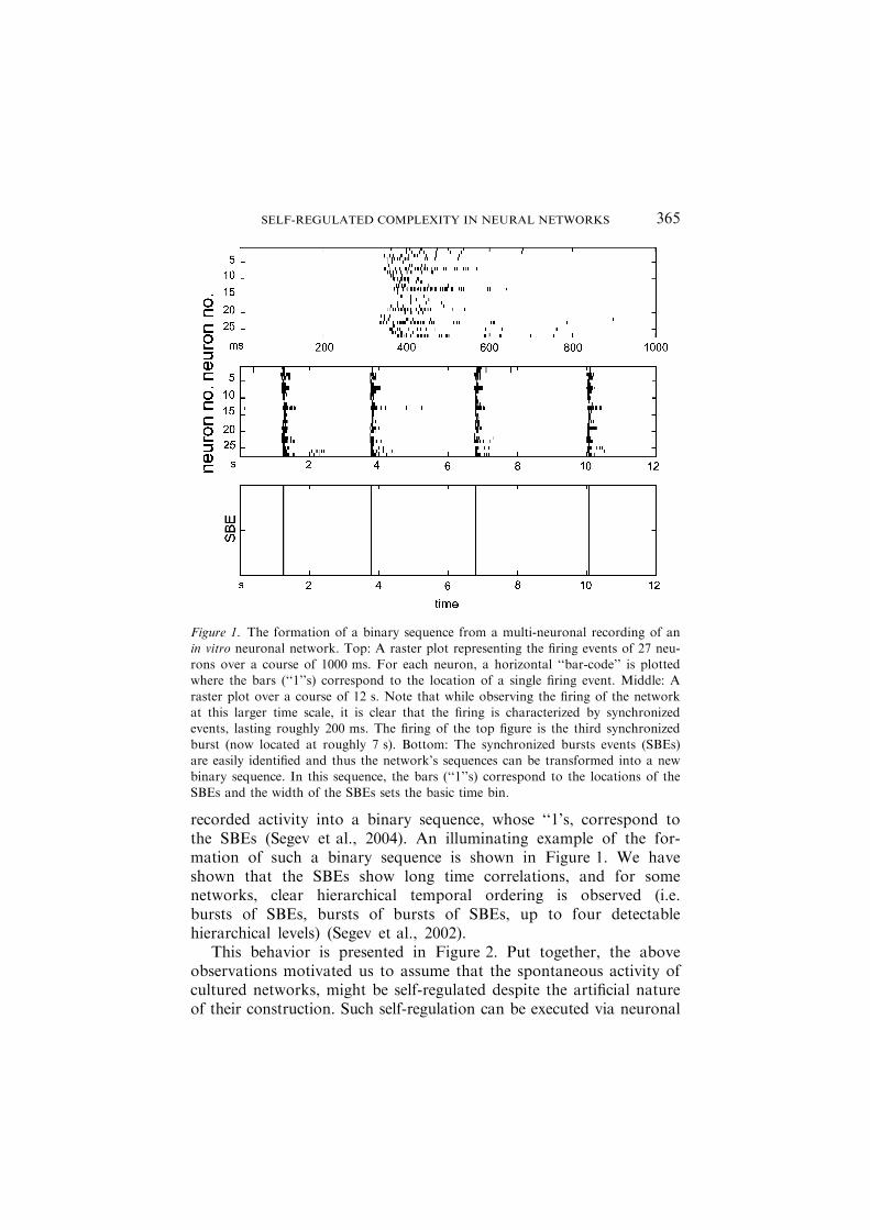
recorded activity into a binary sequence, whose ‘‘1’s, correspond tothe SBEs (Segev et al., 2004). An illuminating example of the for-mation of such a binary sequence is shown in Figure 1. We haveshown that the SBEs show long time correlations, and for somenetworks, clear hierarchical temporal ordering is observed (i.e.bursts of SBEs, bursts of bursts of SBEs, up to four detectablehierarchical levels) (Segev et al., 2002).

This behavior is presented in Figure 2. Put together, the aboveobservations motivated us to assume that the spontaneous activity ofcultured networks, might be self-regulated despite the artificial natureof their construction. Such self-regulation can be executed via neuronal

Figure 1. The formation of a binary sequence from a multi-neuronal recording of an

in vitro neuronal network. Top: A raster plot representing the firing events of 27 neu-rons over a course of 1000 ms. For each neuron, a horizontal ‘‘bar-code’’ is plottedwhere the bars (‘‘1’’s) correspond to the location of a single firing event. Middle: A

raster plot over a course of 12 s. Note that while observing the firing of the networkat this larger time scale, it is clear that the firing is characterized by synchronizedevents, lasting roughly 200 ms. The firing of the top figure is the third synchronized

burst (now located at roughly 7 s). Bottom: The synchronized bursts events (SBEs)are easily identified and thus the network’s sequences can be transformed into a newbinary sequence. In this sequence, the bars (‘‘1’’s) correspond to the locations of the

SBEs and the width of the SBEs sets the basic time bin.

SELF-REGULATED COMPLEXITY IN NEURAL NETWORKS 365

internal autonomous means which are self-activated by the neurons.Or even more likely, they are co-activated by glia cells (with theirown complementary regulatory means) which are coupled to the neu-rons (Laming et al., 2000; Stout et al., 2002; Zonta and Carmignoto,2002; Angulo et al., 2004).

3. Looking for quantified observables of self-regulated complexity

Guided by the notion of self-regulated complexity (versus abiotic-likenon-autonomous complexity), we set to develop proper observables

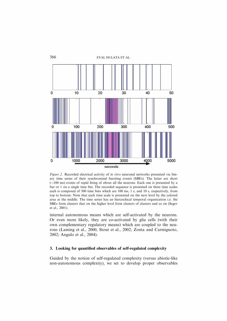
Figure 2. Recorded electrical activity of in vitro neuronal networks presented via bin-ary time series of their synchronized bursting events (SBEs). The latter are short(�100 ms) events of rapid firing of about all the neurons. Each one is presented by a

bar or 1 on a single time bin. The recorded sequence is presented on three time scaleseach is composed of 500 time bins which are 100 ms, 1 s, and 10 s, respectively, fromtop to bottom. Note that each time scale is presented on the next level by the colored

area at the middle. The time series has an hierarchical temporal organization i.e. theSBEs form clusters that on the higher level form clusters of clusters and so on (Segevet al., 2001).

EYAL HULATA ET AL.366

for distinguishing between these possibilities. To proceed, we observethe features of a recorded sequence such as presented in Figure 2. Therecorded sequence is characterized by large local and global temporalvariations. Namely, at each temporal location, there are large fre-quency (density of SBEs) variations when looking at time windows ofdifferent widths. These local variations vary from place to place alongthe sequence.

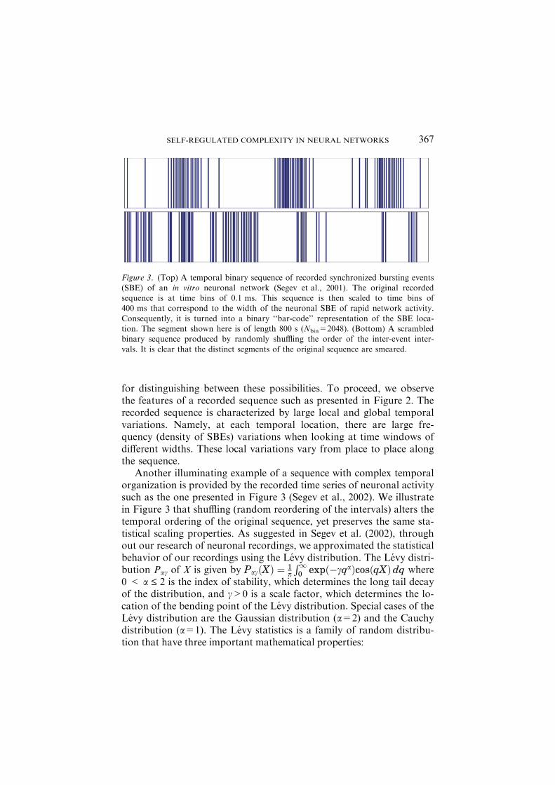
Another illuminating example of a sequence with complex temporalorganization is provided by the recorded time series of neuronal activitysuch as the one presented in Figure 3 (Segev et al., 2002). We illustratein Figure 3 that shuffling (random reordering of the intervals) alters thetemporal ordering of the original sequence, yet preserves the same sta-tistical scaling properties. As suggested in Segev et al. (2002), throughout our research of neuronal recordings, we approximated the statisticalbehavior of our recordings using the Levy distribution. The Levy distri-bution Pac of X is given by PacðXÞ ¼ 1

p

R10 expð�cqaÞcosðqXÞdq where

0 < a £ 2 is the index of stability, which determines the long tail decayof the distribution, and c>0 is a scale factor, which determines the lo-cation of the bending point of the Levy distribution. Special cases of theLevy distribution are the Gaussian distribution (a=2) and the Cauchydistribution (a=1). The Levy statistics is a family of random distribu-tion that have three important mathematical properties:

Figure 3. (Top) A temporal binary sequence of recorded synchronized bursting events(SBE) of an in vitro neuronal network (Segev et al., 2001). The original recordedsequence is at time bins of 0.1 ms. This sequence is then scaled to time bins of400 ms that correspond to the width of the neuronal SBE of rapid network activity.

Consequently, it is turned into a binary ‘‘bar-code’’ representation of the SBE loca-tion. The segment shown here is of length 800 s (Nbin=2048). (Bottom) A scrambledbinary sequence produced by randomly shuffling the order of the inter-event inter-

vals. It is clear that the distinct segments of the original sequence are smeared.

SELF-REGULATED COMPLEXITY IN NEURAL NETWORKS 367

1. These distributions are stable. That is, the sum of random vari-ables of this kind also has stable distribution.

2. The asymptotic behavior for large values of X is a power-lawbehavior. That is: PL(|X|) � |X|)(1+a) for large values of X. Themoments of the distribution are deeply affected by this property(Mantegna and Stanley, 1995). Specifically, all higher moments ofthe distribution diverge for a<2. Thus, all non-Gaussian stablestochastic processes do not have characteristic time scale due tothe fact that the variance is infinite.

3. Levy distribution resigns in the Generalized Central LimitTheorem. According to the classical Central Limit Theorem, thenormalized sum of independent and identically distributedrandom variable with a finite variance converges to a normaldistribution. The Generalized Central Limit Theorem proclaimsthat if the finite variance assumption is to be dropped, the onlypossible resulting limits are stable, i.e. Levy distributions. (Penget al., 1993; Shlesinger et al., 1993; Mantegna and Stanley, 1995;Stanley et al., 1999).

Once again, it is visualized that the temporal structure is com-posed of time segments of dense activity (bursts) separated by timeintervals of relatively sparse activity which infer local and globalvariations. These characteristic features which are not invariantunder scrambling (Figure 3) might provide the sequence a templatefor the encoding of information as we comment at the end. Theyare also the structural traits that cause their appearance to lookcomplex.

Guided by this awareness and the previously mentioned specialtemporal features of the recorded sequences, we set the followingrequirements from our observables: 1. To associate the sequenceregularity with the uniformity in the time–frequency (rates) relativeresolutions rather than with the statistics of the temporal ordering.The former refers to the relative resolution required to capturemaximal information about the observed variations. 2. To associatethe sequence complexity with the local and global variations in therequired relative resolutions, instead of the directly observed localand global frequency variations. 3. To evaluate significantly lowervalues of complexities to the recorded sequences after they areshuffled while keeping similar regularity regardless of shuffling. 4.To be able to distinguish between the dynamical behaviors of dif-ferent systems by their distinct positions on the complexity-regular-

EYAL HULATA ET AL.368

ity plane. 5. To be able to handle sequences with hierarchical tem-poral organizations.

3.1. Representation at the time–frequency plane

To retain information about both temporal locations and frequencyvariations, we first transform the sequence into a presentation in itscorresponding time–frequency domain utilizing the Wavelet PacketsDecomposition (WPD)

The WPD decomposes a signal f(t) into a set of levels, each with aunique time–frequency resolution. The packets are a set of orthogonallocalized functions. Localized, in the sense that each has a definitesupport of both the time and frequency domain. In Figure 4 we pres-ent as an example the levels of decomposition for the type of waveletpackets used for this paper – packets produced from the Haar motherwavelet (Coifman et al., 1992; Coifman and Wickerhauser, 1993; Mal-lat, 1998).

Next, we would like to extract at each temporal position (say the ithelement of the sequence) information about the activity rates (frequen-cies) for all available time windows centered around this location. Fora sequence of Nbin elements, the relevant time windows rangefrom Dtmin ” 1 (in units of the basic recording time width) toDtmax � Nbin. That is, we would like to extract information about Nbin

time windows at each of the Nbin locations of the sequences. However,such N2

bin matrix for a sequence of only Nbin elements must containredundant information (i.e. over-complete representation of therecorded sequence). In order to avoid such redundancy, only Nbin loca-tions on the time–frequency domain are allowed to be selected, subjectto the uncertainty constraint between time and frequency resolutions,Dt Df=1. Since there are also Nbin frequency bands, from Dfmin=1 toDfmax=Nbin it implies that each location can be assigned a local rela-tive resolution Dt/Df out ofNR ¼ 1þ log2ðNbinÞ possible ratios (forsimplicity, Nbin of the sequences considered here are in factors of 2).

It is convenient to illustrate both constraints as tiling of thetime–frequency domain with Nbin rectangles, each with its own aspectratio (height Df and width Dt) representing the relative resolutions intime and frequency, and equal area Dt Df=1. In other words, theWPD algorithm allows partitioning (tiling) of the domain into rectan-gles of different aspect ratios. Each possible combination of Nbin non-overlapping rectangles that geometrically covers the entire domain

SELF-REGULATED COMPLEXITY IN NEURAL NETWORKS 369

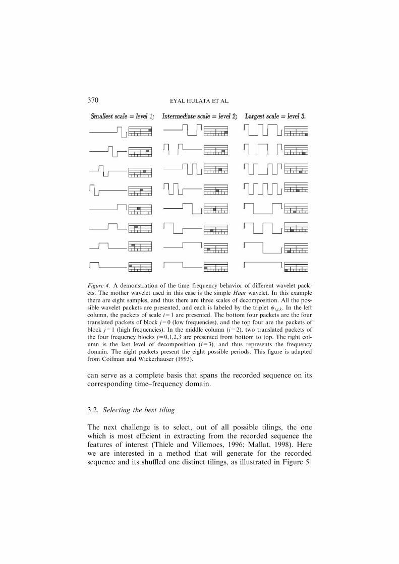
can serve as a complete basis that spans the recorded sequence on itscorresponding time–frequency domain.

3.2. Selecting the best tiling

The next challenge is to select, out of all possible tilings, the onewhich is most efficient in extracting from the recorded sequence thefeatures of interest (Thiele and Villemoes, 1996; Mallat, 1998). Herewe are interested in a method that will generate for the recordedsequence and its shuffled one distinct tilings, as illustrated in Figure 5.

Figure 4. A demonstration of the time–frequency behavior of different wavelet pack-ets. The mother wavelet used in this case is the simple Haar wavelet. In this example

there are eight samples, and thus there are three scales of decomposition. All the pos-sible wavelet packets are presented, and each is labeled by the triplet wi,j,k. In the leftcolumn, the packets of scale i=1 are presented. The bottom four packets are the fourtranslated packets of block j=0 (low frequencies), and the top four are the packets of

block j=1 (high frequencies). In the middle column (i=2), two translated packets ofthe four frequency blocks j=0,1,2,3 are presented from bottom to top. The right col-umn is the last level of decomposition (i=3), and thus represents the frequency

domain. The eight packets present the eight possible periods. This figure is adaptedfrom Coifman and Wickerhauser (1993).

EYAL HULATA ET AL.370

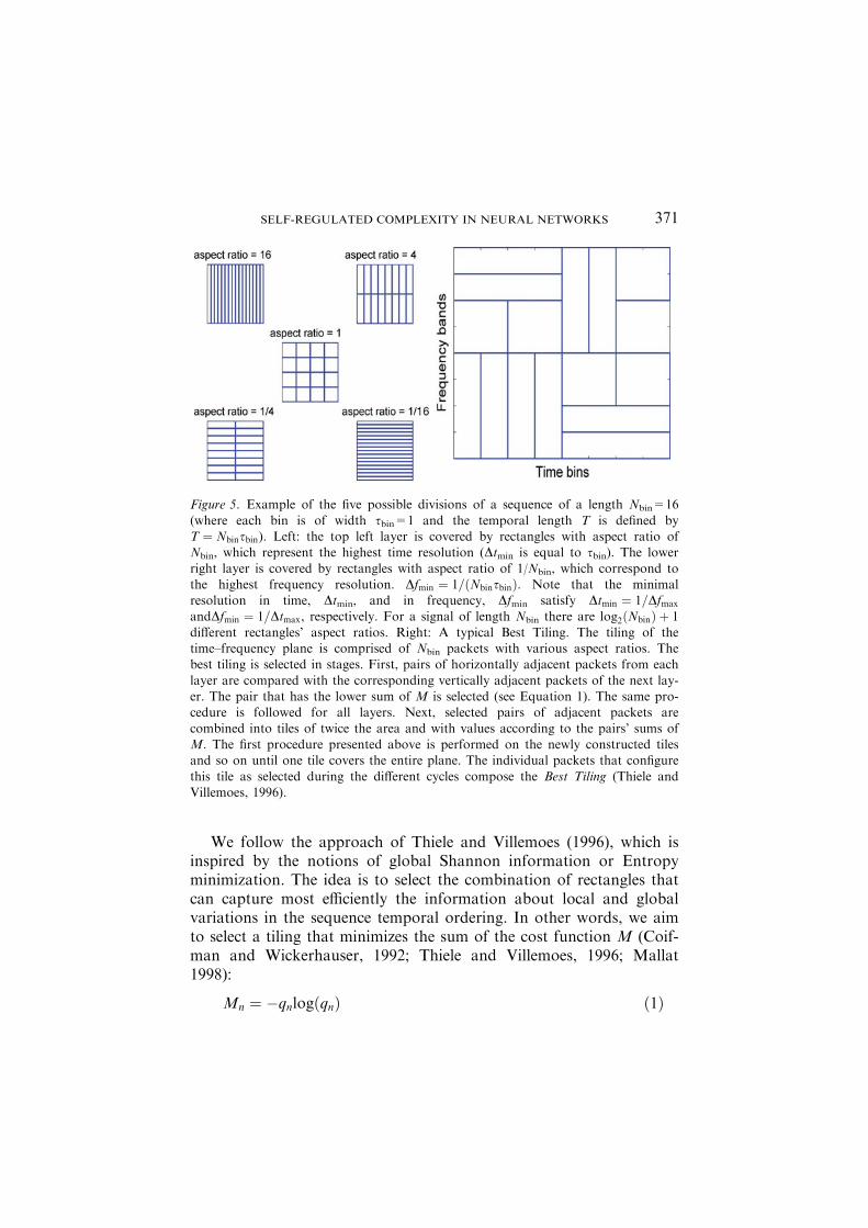
We follow the approach of Thiele and Villemoes (1996), which isinspired by the notions of global Shannon information or Entropyminimization. The idea is to select the combination of rectangles thatcan capture most efficiently the information about local and globalvariations in the sequence temporal ordering. In other words, we aimto select a tiling that minimizes the sum of the cost function M (Coif-man and Wickerhauser, 1992; Thiele and Villemoes, 1996; Mallat1998):

Mn ¼ �qnlogðqnÞ ð1Þ

Figure 5. Example of the five possible divisions of a sequence of a length Nbin=16

(where each bin is of width sbin=1 and the temporal length T is defined byT ¼ Nbinsbin). Left: the top left layer is covered by rectangles with aspect ratio ofNbin, which represent the highest time resolution (Dtmin is equal to sbin). The lower

right layer is covered by rectangles with aspect ratio of 1/Nbin, which correspond tothe highest frequency resolution. Dfmin ¼ 1=ðNbinsbinÞ. Note that the minimalresolution in time, Dtmin, and in frequency, Dfmin satisfy Dtmin ¼ 1=Dfmax

andDfmin ¼ 1=Dtmax, respectively. For a signal of length Nbin there are log2ðNbinÞ þ 1

different rectangles’ aspect ratios. Right: A typical Best Tiling. The tiling of thetime–frequency plane is comprised of Nbin packets with various aspect ratios. Thebest tiling is selected in stages. First, pairs of horizontally adjacent packets from each

layer are compared with the corresponding vertically adjacent packets of the next lay-er. The pair that has the lower sum of M is selected (see Equation 1). The same pro-cedure is followed for all layers. Next, selected pairs of adjacent packets are

combined into tiles of twice the area and with values according to the pairs’ sums ofM. The first procedure presented above is performed on the newly constructed tilesand so on until one tile covers the entire plane. The individual packets that configure

this tile as selected during the different cycles compose the Best Tiling (Thiele andVillemoes, 1996).

SELF-REGULATED COMPLEXITY IN NEURAL NETWORKS 371

where qn is the normalized energy of the signal on the nth rectan-gle. The global measure M – the summation of Mn over the Nbin rect-angles – is utilized for selecting the best tiling. The algorithmdeveloped by Thiele and Villemoes was proved to minimize M (Thieleand Villemoes, 1996).

In Figure 6 we demonstrate the concept of best tiling of thetime–frequency plain. The temporal barcode below is composed ofthree segments: In the middle, we present a sequence of SBEs from anin vitro neuronal network (Segev et al., 2002). To the left, we presentthe same sequence after we have shuffled the order of the intervals.To the right, we present a periodic signal. On top, the time–frequencyplane is presented by a set of rectangles, whose color represent theenergy content within each of the time–frequency rectangles. Thetiling of the periodic region is straight-forward: since the events are

Figure 6. A Best Tiling representation of a binary sequence. At the bottom we pres-

ent a binary signal, which is comprised of different types of signals: an artificial peri-odic sequence (at the right), a sequence from neuronal network’s SBE sequences (atthe middle) and a sequence comprised of the randomly shuffled intervals of the SBEs(at the left). Note that the middle area of interest, with a unique ordered sequence of

1 s, is tiled in a non-trivial way, i.e. a mixture of packets’ with more various aspectratios. On the other hand, in the randomly shuffled sequence adjacent tiles tend to bemore similar and the periodic segment is tiled in a very uniform and straight forward

manner.

EYAL HULATA ET AL.372

separated by equal intervals, there is a distinct energetic frequencyband, and the rest of the time–frequency plane has no energy content.The neuronal sequence in the middle has much more variety withinthe tiling. There is a mixture of rectangles with different aspect ratiosone beside the other. On the other hand, the randomly shuffled se-quence on the left has a more homogeneous tiling, where adjacenttiles tend to be similar. Further ahead, we shall define measures thatcan quantify this effect.

In Figure 7 we present the tiling of the recorded binary sequenceand the shuffled sequence of Figure 3. Note how the tilings emphasizethe differences in internal structure between the recorded sequenceand the randomly ordered one.

Figure 7. Temporal binary sequences (bottom) and their corresponding tiled time–fre-

quency planes (top). The SBE binary sequence (left) and the shuffled binary sequence(right) are correspondingly the top and bottom sequences from Figure 3. Left: Atemporal sequence of recorded synchronized bursting events (SBE) of an in vitro neu-

ronal network (Segev et al., 2001). The segment shown here is of length 800 s(Nbin=2048). In the above time–frequency plane, the horizontal axis is the timedomain and the vertical axis is the frequency domain. The color of each rectangle

represents the value of its corresponding qn. The color code ranges from white to red,the highest energy. It should be visible that the tiling of the plain follow the temporallocation of the bursting regions while creating a complex pattern with different aspectratio of tiles. Right: The corresponding scrambled sequence and its time–frequency

plane. The inter-events intervals of the neuronal sequence are randomly shuffled. It isclear that the distinct segments of the original sequence are smeared, and that a lar-ger portion of the time–frequency plane is tiled by neighboring tiles with equal aspect

ratio.

SELF-REGULATED COMPLEXITY IN NEURAL NETWORKS 373

3.3. Regularity measure of a sequence

As originally pointed out by Hubermann and Hogg (1986), in order todefine the complexity of a sequence, its regularity must first be defined.The regularity is a measure of the relative location of the sequence onthe abscissa between complete random (disordered) signals on one edge(regularity=0) and purely periodic (ordered) ones on the other edge(regularity=1). Various measures for the sequence regularity have beensuggested, such as the Algorithmic Information Content (Gell-Mann,1994; Badii and Politi, 1997). We propose that the definition of the reg-ularity should go hand in hand with the definition of the sequence struc-tural complexity, since the latter has to be a functional of the former.

The idea is to associate the sequence regularity with the uniformityof its corresponding time–frequency domain, namely, with the unifor-mity of its rectangle distribution. The latter represents the distributionof the local relative resolutions in time and frequency as selected bythe best tiling for extracting maximal information from the sequence.

From physics perspective, a tiled domain (Figures 3 and 5) can beviewed as a magnetic material with the rectangles representing its localmagnetizations. With this picture in mind, we first relate the local rela-tive resolution of each rectangle n with its aspect ratio (Dt/Df) by

Rn �log2ðDt=DfÞlog2ðNbinÞ

ð2Þ

Defined this way, Rn (the analogue of a local magnetization) isassigned positive values for rectangles with higher frequency resolution(lower Df) and negative values for those with higher time resolution.Consequently, it has the lowest average absolute values for a signal witha wide distribution of tiles and the highest values for signals with a largemajority of tiles with high aspect ratios (Figure 8). The normalizationof Rn by the logarithm of the maximal aspect ratio Nbin makes that )1 £Rn £ 1. Therefore, we propose the regularity measure RM to be definedas the average value of Rn (the analogue of the total magnetization)(Hulata et al., 2004):

RM � 1

Nbin

XNbin

n¼1Rn ð3Þ

As demonstrated in Figure 8, RM @ 0 for completely disorderedsequences, i.e. sequences with Gaussian distribution of intervals, and

EYAL HULATA ET AL.374

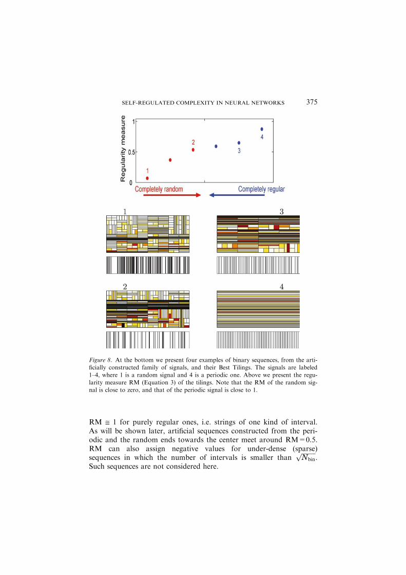
RM @ 1 for purely regular ones, i.e. strings of one kind of interval.As will be shown later, artificial sequences constructed from the peri-odic and the random ends towards the center meet around RM=0.5.RM can also assign negative values for under-dense (sparse)sequences in which the number of intervals is smaller than

ffiffiffiffiffiffiffiffiffiNbin

p.

Such sequences are not considered here.

Figure 8. At the bottom we present four examples of binary sequences, from the arti-ficially constructed family of signals, and their Best Tilings. The signals are labeled

1–4, where 1 is a random signal and 4 is a periodic one. Above we present the regu-larity measure RM (Equation 3) of the tilings. Note that the RM of the random sig-nal is close to zero, and that of the periodic signal is close to 1.

SELF-REGULATED COMPLEXITY IN NEURAL NETWORKS 375

3.4. Variation factors and structural complexity

The regularity observable represents the uniformity of the time–frequencyplane. We now set to define additional complementary observablesassociated with the local and global variability of the plane. Local vari-ability will be related to the amount of diversity within the tiling withinlocal segments of the sequence. Global variability will be related to theamount of variation between the tilings among the different segments.

Thus, we begin by segmenting the sequence into words. We quan-tify the amount of local variation within each word using anobservable named variation factor (VF). For each word l, we definethe variation factor of word to be (Hulata et al., 2004):

VFl ¼NEðlÞ �NE

NE

� �Pn;m jRn � Rmj �HðqnqmÞP

n;m HðqnqmÞð4Þ

where the sum is over all neighboring rectangles n,m. NE(l) is thenumber of events (and also intervals) detected within the lth word,and NE is an average over different words of the same length as thelth one. Q(x), is the Heaviside function; Q(0)=0 and Q (x „ 0)=1.

Finally, we quantify the global variability of the sequence usingthe variance of the variation factors between the sequence words. Fora sequence segmented into Nx words, we thus define the structuralcomplexity (SC) observable to be (Hulata et al., 2004):

SC � varðVFÞ � 1

Nx

XNx

l¼1ðVFl � VFÞ2 ð5Þ

4. Exploring the complexity plane with test Levy sequences

In order to test these definitions by relating them to a concrete exam-ple, we first devised a method to construct a family of binary timeseries, spanning from completely random (disordered) sequences topurely periodic (ordered) ones in the following manner. For the com-pletely random sequence, the intervals between the events (inter-eventintervals, or IEI) are drawn from a normal distribution (taking onlypositive increments). For the purely periodic sequence, the IEIs are allequal to the period of the signal. Next, we proceed from these twoextremes to the center. From the regular edge, we start with a verynarrow Levy distribution (Peng et al., 1993; Shlesinger et al., 1993;

EYAL HULATA ET AL.376

Mantegna and Stanley, 1995; Segev et al., 2002) of the IEI centeredaround the period of the sequence. Then, the distribution is modifiedinto a wider one and with a tail shape changing from exponential topower law decay. From the random edge, we perform the same pro-cedure but starting with a distribution centered around zero.

The statistical characteristics of the Levy distribution are con-trolled by three parameters: a controls the tail decay of the statistics,c controls the width of the distribution and d is the most probableevent. In our case, d related to the period of the sequence, while aand c relate to the variability of the sequence. In order to gain betterunderstanding of the relation between the statistical properties of thesequences (e.g. a, c and d) and their locations on the regularity–com-plexity plane, we utilized artificially constructed families of sequenceswith different Levy parameters.

The construction of an artificial sequence is as follows. We draw aset of numbers out of a Levy distribution generator with parametersa, c and d. This set is then rounded and used as intervals betweenadjacent events in a sequence. This sequence is considered a realiza-tion of the distribution. Naturally, there could be variations betweendifferent realizations of the same Levy distribution. Hence, for eachset of Levy parameters, we have constructed 10–20 realizations andcalculated RM and SC for each of them. We thus use RM and SC asthe Regularity and Structural Complexity, and the deviations betweenthe individual values as the error bars (<13%). It is important topoint out that shuffling the intervals of an artificial realization simplyproduces another realization of the same Levy distribution. We havenoticed that there was no difference between RM and SC of the origi-nal and shuffled artificial realizations (within error deviations). Ourprocedure enables us to construct families of binary sequences, suchthat each family contains sequences that cover the entire range fromdisordered to purely periodic ones, as illustrated in the characteristicsshown in Figure 9. Each family of sequences for a given a is com-posed of one branch on the random side (RM<0.5) for d=‘‘0’’(minimum of one bin separation between events). On the regular side(RM>0.5), each family has a unique branch for every d „ ‘‘0’’. Thebranches are spanned by varying c and they all meet for c >> d at alocation on the border between the random and regular sides and atrelatively higher complexity (as shown in detail in Figure 9).

As demonstrated, the above measure of complexity successfullyfulfills the commonly agreed criteria mentioned earlier (Hubermann

SELF-REGULATED COMPLEXITY IN NEURAL NETWORKS 377

and Hogg, 1986; Gell-Mann, 1994). We emphasize though that theinterpretation of the accepted criteria (Hubermann and Hogg, 1986,Gell-Mann, 1994) should be taken with caution. Not all signals canand should be fitted on a single universal curve, but rather fill the en-tire complexity plane (SC–RM plane). Only a continuous family ofsignals spanning from random to periodic (as was produced here) canresult a fully extended curve like the one shown in Figure 9. Differentfamilies of sequences will yield different curves or clusters.

5. Experimental findings: utilizing the complexity plane in search

for self-regulation in neuronal recordings

As shown, families of artificially constructed sequences exhibit veryrich characteristics on the regularity–complexity plane. These charac-teristics map can be utilized as a ‘‘grid’’ while analyzing sequences of

0 0.2 0.4 0.6 0.8 10

0.05

0.1

0.15

0.2

0.25

0.3

RM

SC

0 0.2 0.4 0.6 0.8 10

0.05

0.1

0.15

0.2

RM

SC

(b)(a)

Figure 9. Characteristics-map for families of artificially constructed sequences ofintervals with both zero mean and finite-mean symmetric Levy distributions. Numer-ous realizations were constructed for each set of Levy parameters (a, c and d), andwe present RM and SC using std(RM) and std(SC) as errorbars. Left: Three families

for a=2.0;1.6 and 1.2 on both the random and regular sides (d=0 and 20, respec-tively). The variable c is used to span each characteristic. For random ones, it spansfrom low regularity at c=1 towards higher regularity and higher complexity with

increasing c. For regular characteristics, c=1 corresponds to high regularity(RM fi 1) and increasing of c lowers the regularity while increasing the complexity.For a given a the regular branches (d „ 0) meet the random branch (d=0) at high

complexity and intermediate regularity. Right: The behavior of the regular branchesfor the same a and different d=5,10,20. For comparison, the random branch with thesame a and d=0 is also plotted. Note that all the regular branches meet together at

the same location where the random branch crosses.

EYAL HULATA ET AL.378

unknown Levy parameters or, as in our case, sequences originatingfrom a recorded biotic system.

We are now ready to identify features presumably related to self-regulation motifs of biotic systems. As stated previously, using theterm self-regulation we claim that the temporal structures of neuronalnetworks are not random or arbitrary. Rather, they originate frominternal dynamics and internally stored means of control (on individ-ual cell level, neuron-glia dynamics, global chemical and electricdynamics on the network level, etc.).

In Figure 10 we show typical examples of the evaluated regular-ity–complexity values for recorded sequences of in vitro neuronal net-works. We compare their values with those of the randomly shuffledsequences from the same recordings. Also shown are the values ofcorresponding artificially constructed sequences with matching a, cand d parameters as the recorded and shuffled sequences. While thesethree types of sequences have very similar regularity, the recordedones have significantly higher complexity then the shuffled sequences –as is clearly seen in the figure. The large circles are well above the dif-ferent shuffled segments represented by the smaller circles (30–45%higher). Moreover, the complexity of the shuffled sequences is verysimilar to that of the artificial sets with matching Levy parameters(represented by full circles) – the typical difference is within the natu-ral deviation among different realizations. Clearly, the two presentedexamples have some probability (albeit low) of being accidental.However, it is repeatedly obtained for all the recorded sequences wetested (we have tested a few tens of sequences from several differentcultured networks of different sizes and different number of neuronsfrom 50 to 1,000,000). We propose that the results described above,do provide a hint that the observed complexity is self-regulated. Inthis regard, we emphasize that for abiotic (non-autonomous) activitywe found that the recorded and shuffled sequences exhibit similar val-ues of complexities which are also similar to that of the artificiallyconstructed ones.

6. Testing the validity of the analysis on simulation sequences

We wish to further strengthen our argument regarding the ability todetect the self-regulation motifs of biotic systems. We have thus cross-compared the behavior of the neuronal sequences to the behavior of

g q

SELF-REGULATED COMPLEXITY IN NEURAL NETWORKS 379

sequences from a simulated model. These simulated sequences aretime-series of the dynamical synapse and soma model, recently intro-duced by Volman et al. (2004, 2005). The neurons in our model net-work are described by the two-variables Morris-Lecar model (Morrisand Lecar, 1981; Volman et al., 2004, 2005), which partially takesinto account the dynamics of membrane ion channels. Briefly, theequations describing the neuronal dynamics are:

_V ¼ �IionðV;WÞ þ IextðtÞ

_WðVÞ ¼ /W1ðVÞ �WðVÞ

sWðVÞð6Þ

0 0.2 0.4 0.6 0.8 10

0.05

0.1

0.15

0.2

0.25

0.3

0.35

SC

RM

Figure 10. Utilizing the complexity plane to study recorded neuronal activity and

simulated sequences. The solid black characteristics are those presented in the leftside of Figure 9. The large blue circle represent the RM and SC of different segmentsof an in vitro experiment of 10,000 neurons (over the course of an hour). The corre-

sponding errorbars represent std(SC). The smaller blue circle represent the mean val-ues assigned for different shufflings of each of the segments. The blue solid circleindicates the behavior of the artificial set of parameters that were fitted to the distri-bution of the recorded intervals (Segev et al., 2001). Note that the shuffled sequences

are repositioned very closely to the corresponding artificial sets. In red, green andpurple circles, we present similar sets for different experiments (networks of differentnumber of neurons: 50, 10,000 and 1,000,000, respectively). In brown, we present two

sets of simulations with similar time scales. The large triangles represent the RM andSC of the simulation output, and the corresponding smaller triangles represent thevalues assigned for the shuffled sequences.

EYAL HULATA ET AL.380

In the above equations, Iion(V,W) represents the contribution ofthe internal ionic Ca2+, K+ and leakage currents, with their corre-sponding channel conductivities gCa, gK and gL being constant:

IionðV;WÞ¼ gCam1ðVÞðV�VCaÞþgKWðVÞðV�VKÞþgLðV�VLÞð7Þ

The additional current Iext represents all the external current sour-ces stimulating the neuron. These might be, for example, synapse-re-lated signals received from other neurons, glia-derived currents,currents resulting from artificial stimulations, or any noise sources.The neurons in the model network exchange action potentials via theactivity-dependent synapses, as first described by Tsodyks et al.(2000).

The output of the simulation is a time-series of action potentialsfor each model-neuron, similar in form and characteristic time-scalesto our in vitro neuronal recordings (and as presented in Figure 1).Moreover, we have shown in Volman et al. (2004, 2005) that ourmodel forms SBEs and the inter-SBEs intervals follow similar Levystatistics as our in vitro neuronal recordings. Thus, the simulatedsequences are analyzed as the neuronal recording – SBEs are identi-fied and a binary sequence is formed where each bin represents aninterval of 400 ms.

Figure 10 presents the RM and SC values assigned to the simu-lated binary sequences from two different simulations. We alsopresent the values assigned for shuffled sequences, as we have donefor neuronal recording. Note that for the two simulated examplesthe simulation values are not higher that the shuffled sequences,implying that there is no hidden internal structure within thesequences.

However, we must stress that we have found larger sensitivity tothe bin width in the simulated sequences than for neuronal sequences.In other words, for bins of 800 ms we got different values with largevariation than for 400 ms. This may imply that in turn there areinternal structures in different time scales to be further studied.

7. Hierarchical structural complexity

Sequences with hierarchical organization are more complex and poseadditional challenges, especially when each level has its own specific

SELF-REGULATED COMPLEXITY IN NEURAL NETWORKS 381

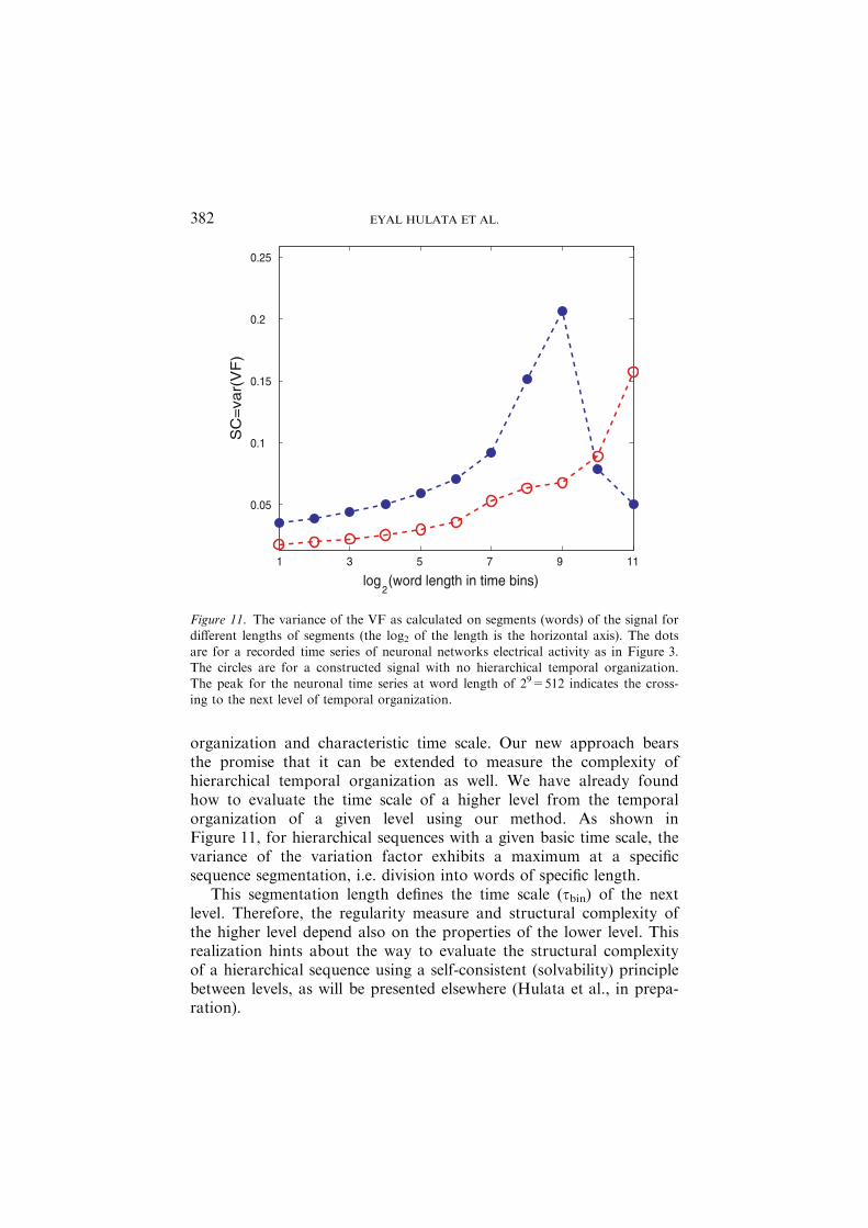
organization and characteristic time scale. Our new approach bearsthe promise that it can be extended to measure the complexity ofhierarchical temporal organization as well. We have already foundhow to evaluate the time scale of a higher level from the temporalorganization of a given level using our method. As shown inFigure 11, for hierarchical sequences with a given basic time scale, thevariance of the variation factor exhibits a maximum at a specificsequence segmentation, i.e. division into words of specific length.

This segmentation length defines the time scale (sbin) of the nextlevel. Therefore, the regularity measure and structural complexity ofthe higher level depend also on the properties of the lower level. Thisrealization hints about the way to evaluate the structural complexityof a hierarchical sequence using a self-consistent (solvability) principlebetween levels, as will be presented elsewhere (Hulata et al., in prepa-ration).

1 3 5 7 9 11

0.05

0.1

0.15

0.2

0.25

log2(word length in time bins)

SC

=va

r(V

F)

Figure 11. The variance of the VF as calculated on segments (words) of the signal fordifferent lengths of segments (the log2 of the length is the horizontal axis). The dots

are for a recorded time series of neuronal networks electrical activity as in Figure 3.The circles are for a constructed signal with no hierarchical temporal organization.The peak for the neuronal time series at word length of 29=512 indicates the cross-ing to the next level of temporal organization.

EYAL HULATA ET AL.382

8. Conclusions

We have shown that our novel observables of regularity and structuralcomplexity fulfill the following: 1. To follow the foreseen characteristicof an effective complexity measure, as presented in Hubermann andHogg (1986), Gell-Mann (1994). 2. To assign a significantly lower valueto a biotic sequence after its intervals have been shuffled. Our work wasperformed on binary sequences created from the recording of in vitroneuronal networks. We have compared the complexity values of thesesequences with the values obtained for sequences generated by shufflingthe recorded inter-event intervals. We have performed the same analysison simulated sequences produced by our model of neuronal dynamicsand on artificial sequences constructed to have the same Levy statisticsparameters. While simulated and artificial sequences have similar struc-tural complexity values regardless of shuffling, the neuronal sequencesare assigned much higher values of structural complexity than the shuf-fled sequences (Figure 10). We argue that this implies that for a bioticsequence, the order of the events bears information or provides atemplate for coding of information. By shuffling of the intervals, theinformation encoded in the order of intervals is lost or at least reduced.

We propose that the high complexity exhibited in the in vitro neu-ronal network is consistent with their free and spontaneous activity.Such isolated networks should be ready to have the full extent of pos-sible templates to sustain the different neuro-informatics tasks uponbeing connected to other networks. Therefore, complex activity isrequired to elevate their self-plasticity and flexibility that impart thembetter adaptability and efficiency to communicate with other networksand to perform imposed tasks as needed (Ben-Jacob, 2003). In thisregard, it would be important to test the complexity of linked in vitronetworks and to compare between recorded activity from differentfunctional locations of the brain.

Moreover, in upcoming work, we intend to further show that theseobservables are useful in generating curves and clusters in the regular-ity–complexity plane following the dynamics of the biotic system. Forexample, during the development of a network, the complexity valuesgrow as well as the distance between the complexities of the recordedsequences versus the shuffled sequences.

Finally, we emphasize that our new method is introduced here inconnection with binary time series (temporal sequences) merely forthe ease of presentation. Clearly this approach can be extended to

SELF-REGULATED COMPLEXITY IN NEURAL NETWORKS 383

general temporal signals and is applicable to spatial series and otherinformatic strings such as DNA sequences and written text.

Acknowledgements

We benefited from illuminating discussions with N. Tishby, R. Segev,I. Baruchi and N. Raichman. We are most thankful for collaborativework with A. Ayali, E. Fuchs and A. Robinson on application of thestructural complexity ideas to the ‘‘Contextual regularity and com-plexity of neuronal activity’’ (Ayali et al., 2004). E. Hulata thanks A.Averbuch and R. Coifman for inspiring conversations about the tilingof wavelet packets and basis selections. E. Ben-Jacob thanks S.Edwards, I. Procaccia, P. Hohenberg and W. Kohn for illuminatingconversations, especially about autonomous versus non-autonomoussystems. The studies presented here have been supported in part bythe Adams supercenter, the Kodesh institute and a grant from theIsraeli Science Foundation (ISF).

Note

1 Dissociated cultures of cortical neurons from one-day-old Charles River rats wereprepared and maintained as described previously (Segev et al., 2001, 2002). The

cultures were maintained in growth conditions at 37 � with 5% CO2 and 95%humidity prior to and during measurements. Non-invasive extracellular recordingswere taken from an array of 60 substrate-integrated micro-electrodes (MEA-chip,

Multi-Channel Systems, Germany (Egert et al., 1998)). The signal was amplified(Multi-Channel Systems) and digitized (Alpha Omega Engineering, Israel). Off-linespike-sorting of the extracellular recordings were performed by our Wavelet Pack-

ets method (Hulata et al., 2000, 2002). An average of 30 different neurons are typi-cally identified in a recording. SBEs are identified and analyzed as described inSegev et al. (2001, 2002, 2004). The typical temporal width of an SBE is 100 msand the typical temporal interval between consecutive SBEs is 1 s.

References

Angulo MC et al (2004) Glutamate released from glial cells synchronizes neuronal

activity in the hippocampus. The Journal of Neuroscience 24:(31): 6920–6927Ayali A et al (2004) Contextual regularity and complexity of neuronal activity: from

stand-alone cultures to task-performing animals. Complexity 9: 25–32

Badii R and Politi R (1997) Complexity, Hierarchical Structures and Scaling in Physics.Cambridge University Press

EYAL HULATA ET AL.384

Ben-Jacob E (1997) From snowflake formation to growth of bacterial colonies II:cooperative formation of complex colonial patterns. Contemporary Physics 38: 205

Ben-Jacob E (2003) Bacterial self-organization: co-enhancement of complexification

and adaptability in a dynamic environment. Philosophical Transactions of RoyalSociety London A 361: 1283–1312

Ben-Jacob E and Garik P (1990) The formation of patterns in non-equilibrium growth.

Nature 33: 523–530Ben-Jacob E and Levine H (2001) The artistry of Nature. Nature 409: 985–986Coifman RR et al. (1992) Wavelet analysis and signal processing. In: Wavelets and their

Applications. Jones and Barlett, Boston

Coifman RR and Wickerhauser MV (1992) Entropy-based algorithms for best basisselection. IEEE Transactions on Information Theory 38:(2): 713–718

Coifman RR and Wickerhauser MV (1993) Wavelets and adapted waveform analysis. A

toolkit for signal processing and numerical analysis. Proceedings Symposium inApplied Mathematics 47: 119–153

Complexity volume (1999). Science 284

Egert U et al (1998) A novel organotypic long-term culture of the rat hippocampus onsubstrate-integrated multielectrode arrays. Brain Research Protocols 2: 229–242

Gell-Mann M (1994) The Quark and the Jaguar. FREEMAN, N.Y.

Goldenfeld N and Kadanoff LP (1999) Simple lessons from complexity. Science 284:87–89

Horgan J (1995) From complexity to perplexity Scientific American 272: 74–79Hubermann BA and Hogg T (1986) Complexity and adaptation. Physica D 22: 376

Hulata E et al (2000) Detection and sorting neural spikes using wavelet packets PhysicalReview Letters 85: 4637–4640

Hulata E et al (2002) A method for spike sorting and detection based on wavelet packets

and Shannon’s mutual information. Journal of Neuroscience Methods 117: 1–12Hulata E et al (2004) Self-regulated complexity in cultured neuronal networks Physical

Review Letters 92: 198181–198104

Hulata E et al. Hierarchic temporal bar-codes and structural complexity in neuronalnetworks activity. in preparation

Jimenez-Montano MA et al (2000) Measures of complexity in neural spike-trains of theslowly adapting stretch receptor organs. Biosystems 58: 117–124

Laming PR et al (2000) Neuronal–glial interactions and behaviour Neuroscience andBiobehavioral Reviews 24:(3): 295–340

Mallat S (1998) A Wavelet Tour of Signal Processing. Academic Press

Mantegna RN and Stanley HE (1995) Scaling behavior in the dynamics of an economicindex. Nature 376: 46–49

Morris C and Lecar H (1981) Biophysics Journal 35: 193–213

Peng CK et al (1993) Long-range anticorrelations and non-gaussian behavior of theheartbeat. Physical Review Letters 70: 1343–1346

Segev R et al (2001) Observations and modeling of synchronized bursting in 2D neural

networks. Physical Review E 64: 11920Segev R et al (2002) Long term behavior of lithographically prepared in vitro neural

networks. Physical Review Letters 88: 1181021–1181024Segev R et al (2003) Formation of electrically active clusterized neural networks

Physical Review Letters 90: 1681011–1681014

SELF-REGULATED COMPLEXITY IN NEURAL NETWORKS 385

Segev R et al (2004) Hidden neuronal correlations in cultured neuronal networksPhysical Review Letters 92: 1181021–1181023

Shlesinger MF et al (1993) Strange kinetics Nature 363: 31

Stanley HE et al (1999) Statistical physics and physiology: monofractal and multifractalapproaches. Physica A 270: 309–324

Stout CE et al (2002) Intercellular calcium signaling in astrocytes via ATP release

through connexin hemichannels. Journal of Biological Chemistry 277: 10482–10488Thiele C and Villemoes L (1996) A fast algorithm for adapted Walsh bases. Applied and

Computational Harmonic Analysis 3: 91–99Tsodyks M et al. (2000) Synchrony generation in recurrent network with frequency-

dependent synapses, The Journal of Neuroscience 20: 1–5Vicsek T (2002) The bigger picture Nature 418: 131Volman V et al (2004) Generative modelling of regulated dynamical behavior in cul-

tured neuronal networks. Physica A 235: 249–278Volman V et al. (2005) Manifestation of function-follow-form in cultured neuronal

networks. Physical Biology 2: 98–110

Waldrop M (1993) Complexity. Simon & SchusterZonta M and Carmignoto G (2002) Calcium oscillations encoding neuron-to-astrocyte

communication. Journal of Physiology 96: 193–198

EYAL HULATA ET AL.386