Scientific Papers of the University of Pardubice, Series D, 43 ...

SCIENTIFIC PAPERS OF THE UNIVERSITY OF PARDUBICE

Series D

Faculty of Economics and Administration

No. 43 (2/2018)

Vol. XXVI

SCIENTIFIC PAPERS OF THE UNIVERSITY OF PARDUBICE

Series D

Faculty of Economics and Administration

No. 43 (2/2018)

Vol. XXVI

Registration MK ČR E 19548

ISSN 1211-555X (Print)

ISSN 1804-8048 (Online)

Contribution in the journal have been reviewed and approved by the editorial board. Contributions are not edited.

© University of Pardubice, 2018

3

ABOUT JOURNAL

Scientific Papers of the University of Pardubice, Series D journal aims to be an open platform for publication of innovative results of theoretical, applied and empirical research across a broad range of disciplines such as economics, management, finance, social sciences, law, computer sciences and system engineering with the intention of publishing high quality research results, primarily academics and researchers.

The journal is published every year since 1996 and papers are submitted to review. The paper is included in the List of reviewed non-impacted periodicals published in the Czech Republic, it is also indexed in Scopus, EBSCO Publishing, ProQuest and CNKI Scholar. The journal is published 3x per year.

CONTENTS

DIVERSE GROUPS OF SMARTPHONE USERS AND THEIR SHOPPING ACTIVITIES BACIK RADOVAN, KAKALEJCIK LUKAS, GAVUROVA BEATA ........................................................................... 5

ASSESSMENT OF TOURISM INDUSTRY CLUSTERING POTENTIAL BEZKHLІBNA ANASTASIIA, BUT TETIANA, NYKONENKO SVITLANA ............................................................ 17

REPRESENTATIVENESS HEURISTICS: A LITERATURE REVIEW OF ITS IMPACTS ON THE QUALITY OF DECISION-MAKING BÍLEK JAN, NEDOMA JURAJ, JIRÁSEK MICHAL .................................................................................................... 29

NEW TRENDS IN THE RECRUITMENT OF EMPLOYEES IN CZECH ICT ORGANISATIONS FAJČÍKOVÁ ADÉLA, URBANCOVÁ HANA, FEJFAROVÁ MARTINA .................................................................. 39

RESEARCH OF OBJECTIVE MARKET PRICE FACTORS IN THE FORMATION OF PRICES ON THE OIL MARKET FINOGENOVA YULIA Y., DOMASCHENKO DENIS V., NIKULIN EDWARD E. .................................................. 50

PROTECTION OF THE REPUTATION OF A LEGAL ENTITY AND FREEDOM OF THE EXPRESSION IN THE CONTEXT OF “MEDIA” GONGOL TOMÁŠ, MÜNSTER MICHAEL .................................................................................................................. 62

PUBLIC RESEARCH AND DEVELOPMENT IN EUROPEAN UNION COUNTRIES - EVALUATION BASED ON SELECTED INDICATORS HALÁSKOVÁ MARTINA, BEDNÁŘ PAVEL .............................................................................................................. 74

THE MEASUREMENT METHODS OF CUSTOMER VALUE AND ITS USE IN SMALL AND MEDIUM SIZED CZECH ENTERPRISES CHROMČÁKOVÁ ADÉLA, KLEPEK MARTIN, STARZYCZNÁ HALINA .............................................................. 87

OPTIMISATION OF A TRAVEL AGENCY’S PRODUCT PORTFOLIO USING A FUZZY RULE-BASED SYSTEM JADRNÁ MONIKA, MACÁK TOMÁŠ ....................................................................................................................... 100

COMPARISON OF MORTALITY CAUSED BY SERIOUS DISEASES WITHIN REGIONS OF THE CZECH REPUBLIC KOPECKÁ LUCIE ......................................................................................................................................................... 112

MEASURING THE SIZE OF THE TECHNOLOGY GAP AT A LEVEL OF CZECH REGIONS SYLVIE KOTÍKOVÁ .................................................................................................................................................... 123

SWOT ANALYSIS EVALUATIONS ON THE BASIS OF UNCERTAINTY – CASE STUDY KŘUPKA JIŘÍ, KANTOROVÁ KATEŘINA, HAILE MEAZA................................................................................... 135

4

THE CREDIBILITY OF FISCAL POLICY AND COST OF PUBLIC DEBT KUNCORO HARYO ..................................................................................................................................................... 147

FDI AND REGIONAL INCOME DISPARITY IN THE CZECH REPUBLIC MALLICK JAGANNATH, ZDRAŽIL PAVEL ............................................................................................................ 159

WHAT DETERMINES THE FISCAL CONSOLIDATION PROCESS: THE ANALYSIS WITHIN EUROPEAN MEMBER COUNTRIES MIHÓKOVÁ LUCIA, SLÁVIKOVÁ LUCIA, KMEŤOVÁ OĽGA ............................................................................. 172

SELECTED EFFICIENCY FACTORS OF AGRICULTURAL SME IN THE CZECH REPUBLIC MORAVEC LUKÁŠ, KUKALOVÁ GABRIELA, SVOBODOVÁ JITKA.................................................................. 184

OPTIMIZATION OF THE AUTOMOTIVE SERVICE CENTRE NETWORK FOR NEW ENTRANTS INTO CZECH AND SLOVAK MARKETS PEKÁREK JAN, SCHÜLLER DAVID ......................................................................................................................... 196

STATUS OF GLOBAL ECONOMIC POWERS (BRICS, EU28, JAPAN, USA): THE CASE FOR COMPETITIVENESS AND FACTORS INFLUENCING PROGRESS OR DECLINE STANÍČKOVÁ MICHAELA, FOJTÍKOVÁ LENKA .................................................................................................. 208

SHORT-TERM AND LONG-TERM RELATIONSHIPS BETWEEN GOLD PRICES AND OIL PRICES STOKLASOVÁ RADMILA .......................................................................................................................................... 221

REMUNERATION OF EMPLOYEE INVENTIONS AT CZECH UNIVERSITIES SVAČINA PAVEL, RÝDLOVÁ BARBORA, BOHÁČEK MARTIN ......................................................................... 232

IMPACT OF GENDER SEGREGATION OF BUSINESS UNIVERSITY GRADUATES ON THEIR POSITION ON THE LABOUR MARKET ŠNÝDROVÁ MARKÉTA, VNOUČKOVÁ LUCIE, ŠNÝDROVÁ IVANA ............................................................... 246

IMPACT OF INSTITUTIONAL ENVIROMENT ON THE EXISTENCE OF FAST-GROWING BUSINESS IN TIME OF ECONOMIC DISTURBANCES VALENTEOVÁ KATARÍNA, ČUKANOVÁ MIROSLAVA, STEINHAUSER DUŠAN, SIDOR JÁN .................... 256

DIVERSE GROUPS OF SMARTPHONE USERS AND THEIR SHOPPING ACTIVITIES

Radovan Bacik, Lukas Kakalejcik, Beata Gavurova

Abstract: The analysis of customers’ purchasing activities, their preferences and future potential are the subject of interest of many experts in the field of marketing. Smartphones became the common devices used during purchasing process. By examining purchasing behavior of smartphone owners, the valuable insights useful for modeling new selling strategies could be mined. The main objective of this study is to analyze different behavioral patterns of smartphone users during the pre-purchase stage of the purchase process. To achieve these goal, we analyzed the data from Consumer Barometer containg data for 56 countries and 78,920 respondents. We created 3 new latent variables – factors - while reducing the number of variables (11) entering the cluster analysis by using factor analysis. Subsequently, using the cluster analysis and the method of k-medians, we created four clusters of users. Even though there are more active and less active clusters, the most popular activities involved getting store directions and checking where to buy a certain product. Users from European countries (represented by Cluster 1 and 2) use smartphones in the pre-purchase process very little, showing conservative approach towards smartphones in these countries. On the other hand, users in Cluster 3 and 4 seem to be the most active smartphone users in terms of purchasing process.

Keywords: Smartphone User, Mobile Shopping, Mobile-first, k-medians, Cluster Analysis

JEL Classification: M31, M15.

Introduction

Scientific and technological progress in the field of digital media and devices connected to the Internet has changed the nature of the purchasing process and added to its complexity. Thus, the customer can choose from almost endless variety of choices regarding devices and media which may be used in the implementation of various activities associated with the purchase. This growing trend increases the difficulty of management decisions regarding the composition of the communications mix of companies while trying to achieve positive user experience throughout the entire duration of purchase process - from the urge to buy through the actual purchase to the customer service associated with the use of the product (Scott, 2013; Halligan and Shah, 2014; Roberge, 2015). The development in mobile devices also implies that users increasingly abandon desktops/laptops and use smartphones to consume online content. The growth in the number of user devices, as well as the process of linking online and offline environment led to the creation of a new type of user - omnichannel user. The model of omnichannel customer’s behavior assumes that the customer will interact with the company using a number of channels and devices before the actual purchase (Dorman, 2013). Deloitte (2015) states that 9% of consumers in the United States own several mobile devices (smartphone, tablets and wearable devices). Juaneda-Ayensa et al. (2016) refers to these users as 3.0 users. He states that these omnichannel users switch devices very often, which causes companies difficulties in

5

controlling customers’ purchasing processes. The issue of omnichannel users grabbed attention of companies and academics alike and a number of academics have already researched it, namely Piotrowicz and Cuthbertson (2014), Peltola et al. (2015), Lazaris et al. (2015) and others. Omnichannel users and their behavior is an issue that is beyond the scope of this study. Poushter (2016) in his study states that the amount of users owning a smartphone has increased sharply also in developing economies, but there are still significant differences when the smartphone ownership rate is compared for example with African countries. The author of the study also states a strong positive correlation between the ownership of smartphones with gross domestic product per capita. The study by Research New Zealand (2015) states that between 2013 and 2015 the share of smartphone use in New Zealand increased to 46%. In addition, the study states that daily use of other devices decreases. Deloitte (2015) pointed to the fact that most respondents use a mobile phone while doing other activities such as shopping at the store, talking to family or friends, watching TV, or while eating in a restaurant. It gives companies the opportunity to reach their target customer almost anytime and everywhere. Tossell et al. (2015) using Smartphone Addiction Measurement Instrument studied on a sample of 34 students whether the use of smartphones under the predetermined conditions affects smartphone addiction. At the end of the experiment 21 out of 34 students agreed with the statement that they are addicted to their smartphones. Report Salesforce (2014) also points out that only 85% of respondents see their mobile device as a central part of their everyday life, 90% of respondents aged between 18-24 years agreed. By becoming central part of people’s life, smartphones have also become a central part of people’s purchasing life. The following review of literature provides an evidence confirming this statement.

1 Statement of a problem

Holmes et al. (2013) pointed out that in addition to the actual shopping smartphones are also used in the process of searching for information and alternatives. Mobile devices are used more often when it comes to buying products that require a higher level of engagement. Our own study carried out by Pollák, Nastišin and Kakalejčík (2015) and the complementing study (Bucko, Kakalejčík and Nastišin, 2015) showed that 96% of respondents combine desktop and mobile devices in various ratios. Moreover, the study showed that approximately 66% of respondents purchased a product using smartphones, while the most smartphones user use their device to search for product information (76%), visit the website of a company (71%), or search for product reviews (69%). In 2015, Google announced that the number of searches on mobile devices surpassed the number of searches on desktop devices (Sterling, 2015). This finding is directly related to the study carried out by DigitasLBi (2015), which discusses the fact that customers have access to information about the product directly in the store which in turn influences their shopping behavior. The survey results showed that 77% of Internet users were influenced by a mobile device, 28% of users made their purchase via a mobile device. 55% of smartphone users think that the combination of the Internet and the smartphone has changed the way their shop at stores. Studies on the use of smartphones in the shopping process were published by the following academics and their collectives: Wang et al. (2015), Einav et al. (2014), Olivier and Treblanche (2016), Thakur (2016), Groß (2015). Based on the review of the above studies show that mobile device users cannot be overlooked when analyzing

6

the user experience and marketing. However, as there is a gap in development of particular countries, we assume this emerging trend doesn’t affect users and selling companies in the same way all around the world. By creating the similar groups of countries, companies are able to identify most critical segments of smartphone users and afterwards prioritize the optimization of the buyer journey of the smartphone users. By ignoring mobile device users we would not be able to get a whole picture of the current shopping activities of consumers and predicting their future behavior will be complicated, thus leading to poor user experience and loss of customers. As there is an assumption that mobile-first trend will continue to grow, not adjusting the buyer journey based on this trend can lead to the destruction of the companies’ client base.

2 Methods

The main objective of this study is to analyze different behavioral patterns of smartphone users during the pre-purchase stage of the purchase process based on the current knowledge. By decomposing the main objective we have arrived to the following sub-objectives:

• analyze the current state of the issue of smartphones use with a focus on their usein the buying process;

• analyze the interdependencies between the variables included in the database andorganizing factors in groups in order to reduce the number of variables;

• divide users by variables into homogeneous groups using the method of clusteranalysis;

• define the basic attributes of the previously created clusters of users and comparethese clusters.

The behavior of smartphone users from selected countries was analyzed using data obtained from the consumer research carried out by Google - Consumer Barometer (2017). Data from this consumer survey were obtained from two sources. The first was a questionnaire that focuses on online population. The second one was a consumer study that aim was to calculate the total population of adults in order to adjust the results of the first part of the questionnaire. The questionnaire was conducted between January and April 2016. The data file contains data from 56 countries - Europe (29), Asia (18), America (5), Africa (3) and Australia - a total of 78,920 respondents. The analysis posed the following question: "What kind of product research you made via your smartphone?" That question was posed to respondents in the questionnaire survey aimed at pre-purchase product research. The input variables are shown in Tab. 1.

Tab. 1: Description of input variables (in %)

Variable Min Lower

quartile Median Average

Upper quartile

Max

A. Got ideas, inspiration online 11.00 18.00 24.50 25.07 30.00 57.00

B. I found relevant brands online

12.00 17.00 21.00 21.18 23.25 40.00

C. Compared products, their features and price online

22.00 30.00 35.00 34.48 38.00 51.00

D. Sought opinions/ review/ advice online

9.00 18.00 21.50 21.96 25.00 36.00

7

E. Watched relevant videos online

4.00 8.75 10.50 10.29 12.00 16.00

F. Searched for a relevant offer online

2.00 4.00 6.00 6.96 8.00 18.00

G. Found where to buy/ product availability online

6.00 10.00 12.50 12.79 15.00 24.00

H. Get store direction/ location online

3.00 9.00 12.50 12.54 15.00 26.00

I. Made contact/ requested contact (with brands/ retailers)

3.00 4.00 6.00 5.95 7.00 12.00

J. I was looking for online financial options

0.00 1.00 2.00 2.43 3.00 7.00

K. Other information looked for online

3.00 7.00 10.00 10.52 14.00 20.00

Source: own elaboration by the authors

As can be seen in Tab. 1, the variables contained in the data files contain outliers. For this reason we also adapted the methods used. In order to analyze the data file we used the following statistical methods:

• descriptive statistics tools (tables, bar charts, line charts, box plot, mean,median, quartiles);

• factor analysis;• cluster analysis using k-medoids. Instead of the Euclidean distance this method

uses Manhattan distance because it is more accurate in respect of outliers (Cardot, 2016). During the analysis we made use of The R Project and MS Excel.

3 Problem solving

In the first step of the analysis we had to confirm that it is appropriate to use the factor analysis. Accordingly, the analysis is linked with the correlation matrix of variables.

Tab. 2: The correlation matrix of variables A B C D E F G H I J K

A 1.00 0.12 -0.39 -0.48 0.24 -0.31 -0.05 -0.10 0.20 -0.01 -0.11

B 0.12 1.00 0.40 0.00 0.33 0.13 0.33 0.16 0.40 0.46 -0.39

C -0.39 0.40 1.00 0.30 -0.06 0.40 0.20 0.32 0.07 0.10 -0.30

D -0.48 0.00 0.30 1.00 0.19 0.44 0.20 0.28 0.13 0.23 0.08

E 0.24 0.33 -0.06 0.19 1.00 0.31 0.41 0.37 0.51 0.40 -0.12

F -0.31 0.13 0.40 0.44 0.31 1.00 0.11 0.41 0.15 -0.09 -0.20

G -0.05 0.33 0.20 0.20 0.41 0.11 1.00 0.71 0.64 0.51 -0.13

H -0.10 0.16 0.32 0.28 0.37 0.41 0.71 1.00 0.51 0.30 -0.20

I 0.20 0.40 0.07 0.13 0.51 0.15 0.64 0.51 1.00 0.41 -0.28

J -0.01 0.46 0.10 0.23 0.40 -0.09 0.51 0.30 0.41 1.00 0.01

K -0.11 -0.39 -0.30 0.08 -0.12 -0.20 -0.13 -0.20 -0.28 0.01 1.00


8

The correlation matrix of variables is shown in Tab. 2. The variables are labeled with letters in accordance with Tab. 3. The correlation matrix shows small, medium and large dependencies between the analyzed variables that are color-coded. Since the correlation matrix showed a dependency between variables, we proceeded with the implementation of further tests in order to determine the appropriateness of using the factor analysis. In order to carry out Kaiser-Mayer-Olkin test we standardized the data matrix’s scale using z-scores. The total value of Kaiser-Mayer-Olkin test was 0.66, which according to Kráľ et al. (2009) represents the average adequacy of the sample data. Since, however, this value is greater than 0.50, it is suitable to carry out the factor analysis. All selected variables can be used within the analysis.

In the next step we conducted a Batlett’s sphericity test. In this test, we tested the following statistical hypotheses: H0: The correlation matrix is an identity matrix. HA: The correlation matrix is not an identity matrix.

Since the p-value was 8,853188.10-25, and thus was lower than the significance level α = 0.05, the null hypothesis was rejected. Since the correlation matrix of variables was not the identity matrix, we accept the alternative hypothesis HA.

In the next step we calculated the appropriate number of common factors. Firstly, we analyzed the principal components. The results are shown in Tab. 3. Since the value of own numbers is in the case of four components higher than 1, and the selection of these four components explains 74% of variation, the factor analysis will focus only on these 4 factors.

Tab. 3: Principal components analysis

K1 K2 K3 K4 K5 K6 K7 K8 K9 K10 K11

Standard deviation (Eigenvalues)

1.90 1.43 1.18 1.04 0.93 0.73 0.63 0.62 0.53 0.50 0.40

Cumulative variability

0.33 0.51 0.64 0.74 0.82 0.87 0.90 0.94 0.96 0.99 1.00


Since saturation of several factors under one indicator was high, we had to implement different types of rotation - orthogonal (varimax, quartimax, equamax) and oblique (oblimin, promax). The best results were obtained when using equamax rotation. With three variables the saturation was relatively high, and therefore it is impossible to assign a particular variable to a factor. Therefore, three variables with high saturation were excluded from the analysis.

After removing these variables, it is necessary to repeat the whole process again. The value of Kaiser-Mayer-Olkin statistics was again at the level of 0.66, which represents an average adequacy of sample data. In addition, Bartlett's sphericity test again rejected the null hypothesis that the correlation matrix was not the identity matrix. The achieved p-value is in fact equal to 3.729983.10-16, which is below the level of statistical significance of α = 0.05. We thus proceeded to the analysis of the principal components in order to choose the appropriate number of factors for the factor analysis. Based on Tab. 4, we chose three factors for further analysis. Since the three components are greater than 1, and the proportion of cumulative variability is 71%, we consider this selection to be correct.

9

Tab. 4: Principal components analysis K1 K2 K3 K4 K5 K6 K7 K8

Standard deviation (Eigenvalues)

1.73 1.29 1.01 0.89 0.77 0.64 0.58 0.47

Cumulative variability 0.37 0.58 0.71 0.80 0.88 0.93 0.97 1.00


After selecting factors (3), we proceeded to the factor analysis. To avoid an uncertain outcome, we performed a rotation of factors. Since it was our intention to work with uncorrelated factors, we made use only of orthogonal rotation. Using the quartimax and equamax methods we achieved excellent results - factor saturation of individual factors was really high. Although we did not arrive at the same high saturation of factors using the varimax method, we were able to eliminate the influence of a single indicator on several factors. Therefore, the varimax method was preferred. Factor saturation is shown in Tab. 5.

Tab. 5: Saturation matrix (varimax rotation) Variables (indicators) F1 F2 F3 h2 u2

A. Got ideas, inspiration online 0.18 -0.90 0.03 0.84 0.16 B. I found relevant brands online 0.31 -0.09 0.72 0.63 0.37 D. Sought opinions/ review/ advice online 0.27 0.77 -0.1 0.67 0.33 E. Watched relevant videos online 0.74 -0.17 0.05 0.59 0.41 G. Found where to buy/ product availability online 0.83 0.19 0.14 0.74 0.26 H. Get store direction/ location online 0.76 0.30 0.11 0.68 0.32 I. Request contact details/ contacted company 0.8 -0.1 0.28 0.72 0.28 K. Sought other information -0.05 0.03 -0.88 0.79 0.21


Based on the factor analysis we arrived at the following three factors: 1. Factor 1: watching relevant videos, verifying product availability, getting storedirections, contacting the brand/ store; 2. Factor 2: looking for ideas/ inspiration, reviews and opinions;3. Factor 3: searching for brands, looking for information.

The analysis of the results failed to interpret the meaning of the newly establishedfactors. Since, however, we had to reduce the number of variables due to the cluster analysis, failure to interpret factors is for us insignificant. The resulting factor saturation helped us create 3 new latent variables containing the factor scores that will be used as input data for the cluster analysis. Before we proceeded to the actual cluster analysis we had to check the presumption that there already are some dependencies between the variables.

Tab. 6: Correlation matrix of factors Factor 1 Factor 2 Factor 3

Factor 1 1.00 2.830630.10-16 -4.214035.10-16

Factor 2 2.830630.10-16 1.00 1.165143.10e-15

Factor 3 -4.214035.10-16 1.165143.10-15 1.00


10

Correlation matrix shown in Tab. 6 shows that the correlation coefficients for individual factors pairs are close to zero, which confirms that the results of orthogonal rotation are indeed uncorrelated factors. We then proceeded to the cluster analysis.

Cluster analysis offers a suitable way how to investigate relations between the explored objects. It introduces a method to combine the objects with the similar characteristics. There are the several approaches how to find out the relations between the entities. Firstly, we had to determine the appropriate number of clusters. It is determined by k-means method, whilst distance between the objects is quantified by the Euclidean distance. Y-axis in the Chart 1 represents the ratio of the sum of squares between the clusters and the total sum of squares. When choosing the number of clusters, this ratio should be, however, as high as possible. To choose the right number of clusters it is necessary to take into account the curvature of the displayed line. When choosing an appropriate number of clusters it is advisable to choose such a point at which the line breaks significantly. In Fig. 1, this condition can be monitored especially at value of 4 and 7. Due to the size of the data file and possible problems with cluster defining this study will employ k-medians method using four clusters.

Fig. 1: Selecting suitable number of clusters according to k-means method


After selecting the appropriate number of clusters we were able to proceed with the actual cluster analysis. Using the k-means method we defined 4 clusters consisting of the following countries:

• Cluster 1 (10 countries): Finland, Italy, Slovakia, Spain, Hong Kong,Indonesia, Japan, South Korea, Taiwan, Kenya;

• Cluster 2 (16 countries): Austria, Belgium, Denmark, France, Germany,Hungary, Latvia, Lithuania, Netherlands, Norway, Poland, Portugal, Sweden, Switzerland, Thailand, Nigeria;

• Cluster 3 (13 countries): Bulgaria, Croatia, Czech Republic, Estonia, Romania,Russia, Serbia, Ukraine, China, Singapore, Vietnam, Argentina, Israel;

• Cluster 4 (17 countries): Greece, Ireland, Slovenia, United Kingdom, Australia,India, Malaysia, New Zealand, Philippines, Brazil, Canada, Mexico, USA, Saudi Arabia, Turkey, United Arab Emirates, South Africa.

11

Fig. 2: Clusplot (k-medians method, 4 clusters)


Clusplot in Fig. 2 shows the division of countries into the clusters with respect to the components obtained in the factor analysis. Looking at the clusters, we can observe a kind of spatial correlation. For example, Cluster 2 contains the countries that are the neighboring European countries. Cluster 3 consists of the countries of the Eastern Europe plus China. Cluster 4 consists of the American countries, along with the English-speaking countries. Only Cluster 1 involves countries that can be considered outliers. More than a geographical representation of countries across clusters, the

12

objective of this study is to define the differences between users who use smartphones in these clusters. For this purpose, the average values of individual variables were calculated, and their comparison can be seen in the Fig. 3.

Fig. 3: Comparison of average values of the variables in the analyzed clusters (k-median)


Based on Fig. 3, it can be seen that the users belonging to Cluster 1 use their smartphone to find stores nearby, where to buy the product and to find inspiration for the potential purchase. When compared with other clusters, Cluster 1 users are way ahead when it comes to the above-mentioned activities. When it comes to other activities, Cluster 1 users are among those less active smartphone users in the buying process. Cluster 2 users use their smartphones to find inspiration, store location or check product availability. Along with Cluster 1 users they are among those less active smartphone users in the buying process. However, it should be mentioned that Cluster 2 users sought information not covered by the options of the questionnaire. Cluster 3 users use their smartphones to get store directions, check the availability of the product and for inspiration. Among all groups of users Cluster 3 users use their smartphones to get store directions, watch relevant videos and get contact details the most frequently. For those users it is the most important to have mobile-optimized videos, a contact form that is smartphone-friendly, and other smartphone-friendly features (e.g. dial phone numbers by clicking). Much like in other cases, also Cluster 4 users use their smartphones mainly to search for inspiration online, check product availability and get store directions. The first two activities are being dominated by Cluster 4 users. They

13

are also more likely to search for relevant brands online and seek views and recommendations in relation to products. Together with a Cluster 3 users they are the most active users of smartphones. We recommend companies to adjust their websites to be more smartphone-friendly just because of these users.

Generally, we can summarize the above as follows: • It is possible to create latent variables that group serveral purchasing activities

into fewer factors without missing the significant portion of the information carried by data;

• Even though there are more active and less active clusters, the most popular activities include pre-purchase activities – getting store directions and checking where to buy a certain product. Other activities are not carried out on such a large scale;

• Users in Clusters 3 and 4 use their smartphones to the largest extent possible, therefore it makes most sense to optimize websites for smartphone users mainly in these countries;

• European countries in Clusters 1 and 2 use smartphones in the pre-purchase process very little, showing conservative approach towards smartphones in these countries.

Due to uniqueness of the study, it is not possible to compare clusters of countries from our results to the clusters analyzed by other authors. However, it can be seen, that when focusing on more representative structure of respondents (juxtaposed to study by Pollák, Nastišin and Kakalejčík (2015)) it can be spotted that more general sample of users doesn’t prefer the use of smartphones in the purchasing process in the same way as more granular sample of respondents (20-28 years old). Moreover, as the execution of observed acitivities is not done solely on smartphones, we agree on existence of omnichannel users mentioned by Dorman (2013). Even though studies by Tossell et al. (2015) and Salesforce (2014) proved that smartphones are a central part of people lives, the results of our study didn’t provide clear evidence that smartphones are also major in terms of purchasing process. The areas of the future research should definitely include the analysis of the increase/decrease of this trend. In order to create more precise segmentation of smartphone users, we suggest to conduct the similar study on the individual-level data instead of country-aggregated data.

Conclusion

The use of smartphones in the buying process is becoming an increasing trend which increases the complexity of the customer journey, and makes it harder for companies to optimize it. The main objective of this study was based on the established theoretical background to analyze different behavioral patterns of smartphone users during pre-purchase stage of the purchase process. The first part of the analysis reduced the number of variables entering the subsequent cluster analysis using the factor analysis. Using k-medians we were able to create 4 clusters of countries. Users in Clusters 1 and 2 use their smartphones in the shopping process to a lesser extent than users in Cluster 3 and 4. Despite the limitations resulting from the analysis (the sample consisting of aggregated data, ambiguity of the factor analysis and uncertainty of its results, the appropriateness of the clustering methods), the results of this study are useful for companies operating in the analyzed markets.

14

References

Bucko, J., Kakalejčík, L., Nastišin, Ľ. (2015). Use of smartphones during purchasing process. In: CEFE 2015 – Central European Conference in Finance and Economics. Košice: Technická univerzita v Košiciach, pp. 91-97.

Cardot, H. (2016). Package ‘Gmedian’. [online]. Available at: <https://cran.r-project.org/web/packages/Gmedian/Gmedian.pdf> [Accessed 13.3.2017].

Consumer Barometer (2017). Methodology. [online]. Available at: <https://www.consumerbarometer.com/en/about/> [Accessed 30.3.2017].

Deloitte (2015). 2015 Global Mobile Consumer Survey: US Edition The rise of the always-connected consumer. [online] Deloitte. Available at: <https://www2.deloitte.com/content/dam/Deloitte/us/Documents/technology-media-telecommunications/us-tmt-global-mobile-executive-summary-2015.pdf> [Accessed 28.3.2017].

Digitaslbi (2015). Connected Commerce. [online]. Available at: <http://www.digitaslbi.com/Global/ConnectedCommerce2015-Deck-FINAL.pdf> [Accessed 17.1.2017].

Dorman, A. J. (2013). Omni-Channel Retail and the New Age Consumer: An Empirical Analysis of Direct-to-Consumer Channel Interaction in the Retail Industry. Claremont McKenna College.

Einav, L. et al. (2014). Growth, Adoption, and Use of Mobile E-Commerce. American Economic Review: Papers & Proceedings 2014, 104(5), pp. 489–494. DOI:10.1257/aer.104.5.489.

Groß, M. (2015). Mobile shopping: a classification framework and literature review. International Journal of Retail & Distribution Management, 43(3), pp. 221-241. DOI: doi.org/10.1108/ijrdm-06-2013-0119.

Halligan, B., Shah, D. (2014). Inbound Marketing: Get found using Google, Social Media and Blogs. New Jersey: John Wiley & Sons.

Holmes, A., Byrne, A., Rowley, J. (2013). Mobile shopping behaviour: insights into attitudes, shopping process involvement and location. International Journal of Retail & Distribution Management, 42(1), pp.25-39. DOI:10.1108/ijrdm-10-2012-0096.

Juaneda-Ayensa, E., Mosquera, A., Sierra Murillo, Y. (2016). Omnichannel Customer Behavior: Key Drivers of Technology Acceptance and Use and Their Effects on Purchase Intention. Frontiers in Psychology, 7, pp. 1-11. DOI:10.3389/fpsyg.2016.01117.

Kráľ, P. et al. (2009). Viacrozmerné štatistické metódy so zameraním na riešenie problémov ekonomickej praxe. Banská Bystrica: Univerzita Mateja Bela.

Lazaris, CH. et al. (2015). Mobile Apps for Omnichannel Retailing: Revealing the Emerging Showroom Phenomenon. In: MCIS 2015 Proceedings.

Olivier, X., Treblanche, N. S. (2016). An investigation into the antecedents and outcomes of the m-shopping experience. The Business and Management Review, 7(5), pp. 263-267.

Peltola, S., Vainio, H., Nieminen, M. (2015). Key Factors in Developing Omnichannel Customer Experience with Finnish Retailers In: International Conference on HCI in Business. Lecture Notes in Computer Science. Cham: Springer, pp. 335-346.

Piotrowicz, W., Cuthbertson, R. (2014). Introduction to the Special Issue: Information Technology in Retail: Toward Omnichannel Retailing. International Journal of Electronic Commerce, 18(4), pp. 5-16. DOI: 10.2753/jec1086-4415180400.

Pollák, F., Nastišin, Ľ., Kakalejčík, L. (2015). Analysis of the Use of Smartphones During Purchasing Process for a Selected Group of Customers within Slovak Market Conditions. Management: Science and Education, 4(1), pp. 77-79.

Poushter, J. (2016). Smartphone Ownership and Internet Usage Continues to Climb in Emerging Economies. [online] Pew Research Center. Available at:

15

<http://www.pewglobal.org/files/2016/02/pew_research_center_global_technology_report_final_february_22__2016.pdf> [Accessed 17.1.2017].

Research New Zealand (2015). A Report on a Survey of New Zealanders’ Use of Smartphones and other Mobile Communication Devices 2015. [online] Research New Zealand. Available at: <http://www.researchnz.com/pdf/special%20reports/research%20new%20zealand%20special%20report%20-%20use%20of%20 smartphones.pdf> [Accessed 17.1. 2017].

Roberge, M. (2015). The Sales Acceleration Formula: Using Data, Technology, and Inbound Selling to go from $0 to $100 Million. Hoboken: John Wiley & Sons.

Salesforce (2014). 2014 Mobile Behavior Report: Combining mobile device tracking and consumer survey data to build a powerful mobile strategy. [online] Salesforce. Available at: <https://www.marketingcloud.com/sites/exacttarget/files/deliverables/etmc- 2014mobilebehaviorreport.pdf> [Accessed 30.3.2017].

Scott, D. M. (2013). The New Rules of Marketing & PR: How to Use Social Media, Online Video, Mobile Applications, Blogs, News Releases & Viral Marketing to Reach Buyers Directly. New Jersey: John Wiley & Sons.

Sterling, G. (2015). It’s Official: Google Says More Searches Now On Mobile Than On Desktop [online]. Available at: <http://searchengineland.com/its-official-google-says-more-searches-now-on-mobile-than-on-desktop-220369> [Accessed at 18.1.2017].

Thakur, R. (2016). Understanding Customer Engagement and Loyalty: A Case of Mobile Devices for Shopping. Journal of Retailing and Consumer Services, 32, pp. 151-163. DOI: 10.1016/j.jretconser.2016.06.004.

Tossell, C. et al. (2015). Exploring Smartphone Addiction: Insights from Long-Term Telemetric Behavioral Measures. International Journal of Information Management, 9(2), pp. 37-43. DOI:10.3991/ijim.v9i2.4300.

Wang, R. J. H., Malthouse, E. C., Krishnamurthi, L. (2015). On the go: How mobile shopping affects customer purchase behavior. Journal of Retailing, 91(2), 217-234.

Contact Address

Assoc. Prof. Radovan Bacik, PhD. MBA University of Prešov, Faculty of Management, Departmnet of Marketing and International Trade Konštantínova 16, 08001, Prešov, Slovakia Email: [email protected]

Mgr. Lukas Kakalejcik Technical University of Košice Faculty of Economics, Department of Applied Mathematics and Business Informatics Němcovej 32, 040 01 Košice, Slovakia Email: [email protected]

Assoc. Prof. Beata Gavurova, PhD. MBA Technical University of Košice, Faculty of Economics, Department of Banking and Investment Němcovej 32, 040 01 Košice, Slovakia Email: [email protected]

Received: 11. 05. 2017, reviewed: 31. 01. 2018Approved for publication: 01. 03. 2018

16

ASSESSMENT OF TOURISM INDUSTRY CLUSTERING POTENTIAL

Anastasiia Bezkhlіbna, Tetiana But, Svitlana Nykonenko

Abstract: In any country the successful strategic development of the tourism industry aims at economic growth, as it helps to reduce unemployment and increase national income, as well as to make tourism attractive. Long-term experience has shown that both isolated subjects of tourist businesses and those of public administration are totally ineffective. Achieving good results requires a common development strategy with specific objectives for each of the subjects. It is for this goal that tourist clusters are created in the world community. The present study provides analysis of macro-, meso- and microenvironment to determine the potential of the tourism industry clustering in the Zaporizhzhia region, Ukraine. After making the analysis of microeconomic environment of the tourism industry in the region generally suggests that of five tourism clustering potential components, four of them have a high level (A) and one has intermediate (B), meaning that the Zaporizhzhia region possesses all the potential to create a competitive tourism cluster. The obtained data will make it possible to form a regional tourism development program, to identify gaps in infrastructure management, to do comprehensive research of whether it is effective and appropriate to establish cluster organizations on any territories.

Keywords: Tourism Industry, Tourist Cluster, Economy Growth, Macroeconomics, Microeconomics, Meso-economics, Evaluation of Clustering Potential.

JEL Classification: R58.

Introduction

In today’s global competition, the association of enterprises based on cluster approach is one of the most important priorities in tourism industry development.

The premises of the clusters theory can be found in the works of Alfred Marshall. Thus, in his book “Principles of Economics”, first published in 1890, he considers issues of external specialized spatial distribution (Marshall, 1920). The most popular, however, are the works by M. Porter. In his work “International Competition”, he gives the well-known definition of the cluster: “A cluster or industrial group is a group of geographically neighboring interconnected companies and related organizations operating in a certain area, characterized by common activities and complementary to each other” (Porter, 1990: 258).

The cluster approach founder in Ukraine, S.I. Sokolenko, offered the following definition: “Cluster is a voluntary branch and territorial association of the companies that work closely with local authorities to improve the competitiveness of its products and to ensure the economic growth of the region” (Sokolenko, 2002). Thus, the cluster concept provides a new vision of the national and regional economy; it also defines the new role of companies seeking to improve their competitiveness. Such a great importance of the clusters leads to a new management paradigm, the need for which is still underestimated.

17

Data from World Tourism Organization reports suggest a significant economic growth the tourism industry is experiencing over the past fifty years. According to UNWTO Tourism Highlights Report (UNWTO, 2015), the contribution of tourism to the global GDP is 9%, with every 11th worker engaged in tourism and services. The increase in foreign tourists’ number is a considerable amount – from 25 million in 1950 to 1,133 million in 2014 (that is more than 45 times in 64 years). The increase in foreign tourists’ number, as UNWTO predicts, could reach 1.8 billion people by 2030.


Tourism is one of the most dynamic developing industries in the world. Today the Industrial Cluster theory is, according to American scholars, the leading model of economic development. Despite this, the tourism industry has little, if any, attention in the scientific literature on the industrial cluster theory. At the same time, in the United States and around the world, those who practice tourism development do experiments with the cluster concept, sometimes innovatively, but generally haphazardly.

M. Porter’s Industrial Cluster Theory can provide meaningful and productive basis for the analysis and development of the tourism industry.

The advantages of clustering for business in particular and the economy in general are as follows:

Companies can pool their capabilities in order to reduce costs and offercompetitive market price that each of the subjects could not afford individually.

Companies can widen knowledge. This provides the supplier companies withdeeper supply chains and allow them to exploit the potential of the knowledge gained in the cooperation

Companies can enhance saving potential of scale through joint purchases ofbulk discounts and joint marketing costs.

Companies can strengthen social and other informal links that can result increating new ideas and new businesses.

Companies can improve information flows within the cluster, by, for example,recommending the cluster partners as reliable businesspersons.

Clustering is a key factor in economic growth in cities and regions. It is but the only way to stimulate regional economic growth (A Practical Guide to Cluster Development, 2006).

A group of authors T. Vereshchagina, G. Haliullina, L. Belkowa (Vereschagina, Galiullina, Belkova, 2010) proposed the methods, which have as their theoretical framework the polarized development theory, the cluster formation principles and the method of regional ranking according to statistics. The given methods can show the relationship between two potentials – region clustering and its intangible assets. The calculations based on peer assessment techniques reveal the stock, financial and raw material potential of the region that can be used to determine potential of the region industries clustering (the article studies the methods to form steel industry clusters). With the tourist industry referring to the service sector, creating additional gross domestic product in this area is significantly different, for it is formed on somewhat different principles than those in industrial areas.

18

The scheme of companies’ selection and their inclusion in the cluster, proposed in the above article (Batalova, 2013), makes it possible to determine the extent of the company and involves the need to expand the cluster organizations in order to improve competitiveness and to display this industry on an international level. Analysis of industrial clusters competitiveness (Ovcharuk, 2014) involves the definition of the analysis purposes, information evaluation and analysis of regions itself and of cluster formations in them. It is also necessary to choose the base for comparison, to establish a list of parameters to evaluate the industrial clusters competiveness, to rate competitiveness by determining the competitive of level of enterprises-participants (calculation factor of competitiveness of the enterprise). However, the issue of how to implement the cluster approach in tourism businesses and how to ensure its effectiveness, especially given the economic development of Ukraine, remains insufficiently investigated today.

The study aims to establish the potential of the tourism industry clustering by analyzing the macro-, meso- and microenvironment, with taking into account the specific conditions of the tourism industry. Achieving this goal will create a regional development program for the tourism industry in the region, to identify gaps in infrastructure management; it will provide an opportunity to conduct comprehensive studies of the efficiency and expediency of any territory cluster associations.

2 Methods

There are not so far any special methods to evaluate clustering potential. As local scientists EV Khristenko, T.V.Pulina put it: “Clustering is the presence of competitive advantages of industries, businesses, infrastructure organizations in the region territory and the possibility to combine and use these advantages in order to improve regional competitiveness” (Khrystenko, Pulina, 2015). We will assess macro-environment, that is a country’s position among global competitors in the field, by using methods of analysis, synthesis, deduction and induction. To evaluate tourism and transport infrastructure, the method of the World Economic Forum (WEF) will be applied.

To determine the potential of the tourism industry clustering potential in the Zaporizhzhia region, the methods of M. Vinokurova shall be applied (Vinokurova, 2006). The methods and techniques to estimate the leading industries potential (Pulina, 2014), that N.V. Vinokurova proposes, is to calculate coefficients of localization, implementation per person and specialization of industrial sectors.

Localization of tourist travel services in the travel industry is analyzed in different way than that in industries. Localization of tourism in the region is differentiated as defining localization of the travel agent and tour operator activities. The relevant factors are the ratio of the travel agent and tour operator’s activity share in the structure of tourism to the tour operator and travel agent’s activity regional share in the structure of the country. Coefficient of localization for tour operator activity in the region is calculated according to the above formulas by selecting the index value of travel packages, sold by travel operators, individuals and entities in the region.

Coefficient of sales per person of tourist company is calculated as the ratio of the share, that the regional tourism has in the country’s certain economic activity structure, to the proportion of the region population in the country population. The coefficient of specialization can be computed only separately for travel agency and tour operator

19

activities. The coefficient of specialization of a tour agency activity is defined as the ratio of the region travel agent share travel in the country to some of the gross regional product (GRP) in GDP of the country. The relevant formula can be used to calculate a coefficient of specialization for tour operators’ activities.

Herewith, if the calculated coefficients are close to or greater than one and tend to increase, clusters are possible to be created in these areas (Vinokurova, 2006). Currently, there are different opinions on how the obtained values of these coefficients may be interpreted. E. Bergman (Bergman, 2016) believe it is the coefficient of localization, which is more than 1.25, that signifies the specialization of the region. On identifying clusters in Sweden, Braunhelm P. and B. Karlsson (Bergman, 2016) used a coefficient with the limit value of 1.3.

For coefficients of localization for production per person and for specialization, M.V. Vinokourova offers a minimum limit value of one (Vinokurova, 2006). It is also necessary to track the dynamics of these coefficients that indicates the cluster possible growth (Khrystenko, Pulina, 2015).

To analyze what potential the microenvironment clustering of the regional tourism has, we can estimate (applying M.V. Vinokurova methods (Vinokurova, 2006)) the sources of tourism competitive advantages in the Zaporizhzhia region, namely the availability of production factors, domestic market demand, the availability of competitive industries to supply the related industries and organizations, as well as the international market competition. 300 experts were invited to evaluate microenvironment by expert assessments.

Fig. 1 shows a generalized scheme of methods and technique to assess the tourism clustering potential in the region.

Fig. 1: Technique to estimate the tourism clustering potential in the region

Source: [proposed by authors]

3 Problem solving

The study of Ukraine’s position among global competitors in the industry (World travel and tourism council, 2015) showed that international tourism spending is a key component of the contribution to GDP and amounted to 34.6 billion UAH in 2015. In 2015, the tourism industry directly supports 214,500 jobs (1.2% of total employment). Employment in tourism is expected (World travel and tourism council, 2015) to grow by 3.3% in 2016. In 2015, the tourism industry received investments in the amount of 5.4 billion UAH, or 2.0% of total investments. Expenses for travel and leisure (inbound and domestic) constitute 93.3% of total expenditure compared with 6.7% for business

Scheme to assess the tourism industry clustering potential

1. Assessment of the country’s position among global competitors in the industry

2. Evaluation of localization, production for one person and specialization for the tourism industryin the region

3. Expert assessment of the tourism industry in the region by criteria

20

travel. The cost of business travel is expected (World travel and tourism council, 2015) to grow by 2.3% in 2016. If we compare the total and direct contribution of tourism to GDP in Europe, it should be noted that Ukraine is not a leader on these indicators, that the tourism industry of our country requires improvement, development and investment.

If you compare direct and total contribution of tourism to the GDP in Ukraine and the average world and European indicators, the calculation results, shown in Tab. 1, suggest a significant lag in the tourism industry development of Ukraine, as well as its extremely low yield in comparison to that of average world and European indicators.

Tab. 1: Calculation results to indicate how the direct and total tourism contribution to GDP in Ukraine deviate from the average world and European indicators Direct contribution of tourism to GDP, in $ billion

The total contribution of tourism to GDP, in $ billion

World average 18.5 World average 55.7 European average 14.9 European average 40.3 Ukraine 1.3 Ukraine 5.1 Ukraine’s index deviation from the world average

-17.2 Ukraine’s index deviation from the world average

-50.6

Ukraine’s index deviation from the European average

-13.6 Ukraine’s index deviation from the European average

-35.2

Source: Calculated by the authors according to the data (UNWTO, 2015)

To assess quality and capacity of travel infrastructure and tourism in Europe (UNWTO, 2015) WORLD TRAVEL AND TOURISM COUNCIL widely uses the World Economic Forum (WEF) methodology, which involves evaluating territories and assigning them the rank of infrastructure development, for the development criteria of tourism infrastructure, infrastructure, air and land transport. By the tourism and transport infrastructure development Eastern Europe occupies 5th place, behind North America and Western, Northern, Southern, Central Europe.

The country is at risk of not performing the basic prediction of economic benefits due to lack of infrastructure and investment. 3.7 score of 7 indicates the need for the transport routes development and air transport reformation.

Tourism in the Zaporizhzhia region needs development, given the favorable geographical location of the region and its natural, historical and cultural values. One of the ways to increase the region competitiveness is tourism, especially with such unique natural resources – the Dnieper River and the island of Khortytsia.

The next step in assessing the clustering potential of the Zaporizhzhia region is to analyze production factor per person as well as coefficients of specialization and localization (Tab. 2).

Tab. 2: Coefficients of sales, specialization, localization per person for tourism business in the Zaporizhzhia region

Indicator 2011 2012 2013 2014 2015Coefficients of sales per person for tourism business in the Zaporizhzhia region 0,5431 0,5242 0,9731 0,5703 0,4189Coefficients of sales per person for tour agents in the Zaporizhzhia region 1,222 1,1943 1,3689 1,5027 0,7192

21

Coefficients of sales per person for tour operator activities in the Zaporizhzhia region 0,1714 0,0978 0,0712 0,0639 0,0242Coefficients of specialization for tourism businesses in the Zaporizhzhia region 0,5681 0,5288 1,0208 0,5295 0,5398Coefficients of specialization for the tour agent activity in the Zaporizhzhia region 1,2782 1,2049 1,4360 1,3951 0,9267Coefficients of specialization for tour operator activity in the Zaporizhzhia region 0,1793 0,0987 0,0747 0,0593 0,0312Coefficients of localization for tour agent activity in the Zaporizhzhia region 2,2502 2,2785 1,4067 2,6349 1,7167Coefficients of localization tour operator activity in the Zaporizhzhia region 0,3157 0,1866 0,0732 0,1120 0,0578

Source: Calculated by authors

There is a reduction in tourist flows in the Zaporizhzhia region (in 2015 by 76% compared to 2013), so the share of the industry in the production area is very small compared to other industries.

According to experts, tourism resource potential is inexhaustible in comparison of resource potential in trade and other activities, which are developing rapidly in the Zaporizhzhia region. We believe that tourism can take the lead in business in the Zaporizhzhia region, its cluster potential is average (level B).

Availability of Production Factors

Almost all tourism industry inputs listed in the Tab. 3 are available to create a cluster. The Dnieper River and the island of Khortytsia can be considered as the main among natural resources. In general, natural resources of the Zaporizhzhia region are very diverse, unique, they are not exploited enough but very attractive for tourists. In the region, there are almost 7% of Ukrainian protected areas and national parks, 8% water source reservoirs, forests 9%, 10% hydro resources of Ukraine.

Tab. 3: Availability of tourism industry inputs in the Zaporizhzhia region Production factors (resources) Rating Score

Natural Available 1 Mineral Available 1 Money Cash resources Available 1 Labor Available 1 Infrastructure: - Information infrastructure - Physical Infrastructure - Scientific and technological infrastructure - Legislation

Available Available

Unavailable Available

1 1 2 1

Total score 9 Note: Available factor is assigned a score of 1, unavailable - 2. Scale to assess the clustering potential clustering for production factors is as follows: Level A – 8-10 points (all factors available); Level B – 11-15 points (only part of the factors available) Level C – 16 points (factors unavailable in general) The level of tourism industry clustering potential in the Zaporizhzhia region for production factors is high (level A).

Source: [authors development]

In the Zaporizhzhia region, a tourism development concept was elaborated for the period up to 2018 (Stratehiia rozvytku turyzmu u misti Zaporizhzhia na 2014-2018 rr).

22

As of 01.01.2015, as many as 125 hotels operating in the Zaporizhzhia region can accommodate a total of 105,378 people (Yazina, 2015:108).

The hospitality industry (Stratehiia rozvytku turyzmu u misti Zaporizhzhi na 2014-2018 rr) in the Zaporizhzhia region has obviously the following trend: the number of hotel establishments was relatively stable for 2009-2011, but at Euro 2012 it decreased significantly, due to many inspections and failure to meet European standards. This caused fierce competition between hotel management companies. In years 2013-2014, with the number of hotels stabilized, the number of placed persons began to grow, but the current statistical information remains unstable and the hotel industry is exposed to external and internal factors, of particular importance is the political and economic situation, due to the events in the east.

Most of the restaurant industry objects (87.4%) are located in cities and urban areas. Of the total number of objects, 64.8% are located in the regional center Zaporizhzhia, only 8.3% are in the city of Berdyansk, 2.6% – in the city of Melitopol, 4.3% – in the city of Energodar and the city of Tokmak has 0,2 % (Yazina, 2015: 110). Of the total number of restaurant business objects, 52.8% are cafes, snack bars, buffets (kiosks), their number by January 1, 2015 had decreased by 10.8% and was 281 units. At the same time, there were 156 dining rooms, 55 bars, 27 restaurants and 13 ready meals supplying companies (as of January 1, 2015) (Yazina, 2015).

All this are the material resources for tourism development. Hotel and restaurant business affects the balance of payments, stimulates the development of related industries. It provides jobs for the population, mainly in the service sector, with employment in the tourism business steadily growing. There is a growing demand for specialized education. Especially popular are the universities that train specialists for the tourism industry. Infrastructure resources are also mostly available. Information about the tourism development in the Zaporizhzhia region, the types of tourism and others is located in more than 35 major Internet directories, servers, specialized firms’ sites.

The physical infrastructure of the tourism industry in the Zaporizhzhia region is presented by rail, road, water and air transport. However, presently the scientific and technological infrastructure is poorly developed, with any information on new technologies used in the tourism industry missing. The domestic demand. Evaluation of the internal demand for the tourism industry in the Zaporizhzhia region is provided in Tab. 4.

Tab. 4: Evaluation of domestic demand in the tourism industry of the Zaporizhzhia region Demand Carriers Rating Scores Zaporizhzhia region tourists Ukrainian tourists Foreign tourists The level of tourists requirements

Present present present Average

1 1 1 2

Total scores 5 Note: The presence of demand notes 1 score, its absence is 2 score. The scale of scores distribution to assess the clustering potential for the demand factor is: - Level A – 4-5 (demand interested); - Level B – 6-8 (demand varies); - Level C – 9 (demand indifferent).


23

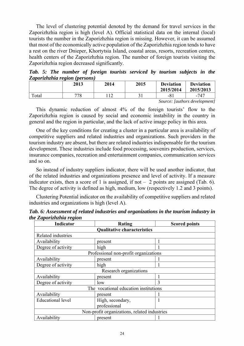
The level of clustering potential denoted by the demand for travel services in the Zaporizhzhia region is high (level A). Official statistical data on the internal (local) tourists the number in the Zaporizhzhia region is missing. However, it can be assumed that most of the economically active population of the Zaporizhzhia region tends to have a rest on the river Dnieper, Khortytsia Island, coastal areas, resorts, recreation centers, health centers of the Zaporizhzhia region. The number of foreign tourists visiting the Zaporizhzhia region decreased significantly.

Tab. 5: The number of foreign tourists serviced by tourism subjects in the Zaporizhzhia region (persons)

2013 2014 2015 Deviation 2015/2014

Deviation 2015/2013

Total 778 112 31 -81 -747 Source: [authors development]

This dynamic reduction of almost 4% of the foreign tourists’ flow to the Zaporizhzhia region is caused by social and economic instability in the country in general and the region in particular, and the lack of active image policy in this area.

One of the key conditions for creating a cluster in a particular area is availability of competitive suppliers and related industries and organizations. Such providers in the tourism industry are absent, but there are related industries indispensable for the tourism development. These industries include food processing, souvenirs production, services, insurance companies, recreation and entertainment companies, communication services and so on.

So instead of industry suppliers indicator, there will be used another indicator, that of the related industries and organizations presence and level of activity. If a measure indicator exists, then a score of 1 is assigned, if not – 2 points are assigned (Tab. 6). The degree of activity is defined as high, medium, low (respectively 1.2 and 3 points).

Clustering Potential indicator on the availability of competitive suppliers and related industries and organizations is high (level A).

Tab. 6: Assessment of related industries and organizations in the tourism industry in the Zaporizhzhia region

Indicator Rating Scored points Qualitative characteristics

Related industries Availability present 1 Degree of activity high 1

Professional non-profit organizations Availability present 1 Degree of activity high 1

Research organizations Availability present 1 Degree of activity low 3

The vocational education institutions Availability present 1 Educational level High, secondary,

professional 1

Non-profit organizations, related industries Availability present 1

24

Degree of activity average 2 Public institutions support of and assistance to companies in the tourism sector

Interest high 1 Degree high 1

Media industry organizations support to the tourism industry Availability high 1 Degree high 1 Total points 18

Note: The following scale is used to assess the clustering potential for the factor considered: Level A – 14-20 (supporting industries and organizations are present, their level is high); Level B – 21-28 (supporting industries and organization are present, but their level is average); Level C – 29-35 (industry and supporting organizations are available).


From professional organizations in the region, there are: Social and Advisory Board of Tourism, Tourist information center, Zaporizhzhia Regional Tourist Information Center; a non-profit, public organization ‘Zaporizhzhia Regional Tourist Association’ established at the initiative of individuals, whose activities affect the tourism industry, according to the Constitution of Ukraine, the Law of Ukraine “On Tourism”, the Law of Ukraine “On Public Associations” and more legislation of Ukraine.

There are no research organizations dealing with special problems of tourism in the Zaporizhzhia region. However, research is conducted in universities, the Department of Tourism Authority of the Zaporizhzhia region, and in various research institutes.

The other organizations’ level of activity is also quite high.

Evaluation results of competition in the internal market and of company strategy are given in Tab. 7

Tab. 7: Domestic market competition and companies’ strategy Indicator Rating Score

Domestic market competition Companies’ strategy

Present present

1 1

Total 2 Note:Scale to assess potential clustering by the presence of competition in the region is as follows: Level A - 2 (strong competition); Level B - 3 (weak competition); Level C - 4 (no competition). The level of clustering potential by the presence of competition in the Zaporizhzhia region is the highest (level A).


The analysis results of the tourism competitive advantage sources in the Zaporizhzhia region are given in free form in Tab. 8.

Tab. 8: Components of tourism industry clustering potential in the Zaporizhzhia region Clustering potential components Clustering potential level Indicators of production localization Production Factors Domestic market demand Competitive supplying and other related industries Competition in the market and companies’ strategy

В А А А А


25

In the Zaporizhzhia region now there are 210 travel agencies licensed for tour operator and travel agency activities. They are concentrated in three major cities in the region: Berdiansk, Melitopol, Energodar.

Of all travel companies, two-thirds are the tour operators, the rest is the travel agent companies. It is the tourist companies that directly form tourist flows and contribute to tourist attractiveness of the region.

Many tour operators have conducted international tourist activity for 5-10 year, having a long experience in the field. They are involved in promoting regional tourism products to the internal market and in expanding tourism opportunities of the Zaporizhzhia region. Many companies have a long term development strategy.

In general, of five tourism industry clustering potential components, four have a high level (A) and one has an intermediate level (B). This allows you to believe that a competitive tourism cluster may be created in the Zaporizhzhia region. All this suggests that Zaporizhzhia region has all the prerequisites for effective clusters to be created and developed, with the region competitiveness improved.

4 Discussion

The value of calculated factors characterizing the travel agencies activities is much more than one, indicating fair conditions for the tourism cluster creation.

The cited methods allow to evaluate the clustering potential by focusing on tourism development at the macro level (global) and also at the meso level (regional) and micro level (analysis of environmental factors of travel agencies activities). The methods at hand, unfortunately, do not concern any analysis of system deployment, maintenance and transport, which can also be included in the cluster and require more detailed analysis and study of statistics. The calculated coefficients of localization, specialization and sales for 1 person indicate that tourism in the Zaporizhzhia region requires establishing the scale to asses clustering potential (high, medium, low) for a clear interpretation of the calculated parameters.

These shortcomings will be addressed in subsequent studies at improving the mechanism to assess the clustering potential of tourism industry businesses in the region.

Conclusion

Thus, assessment of the clustering potential of regional tourism industry helped identify gaps in managing tourism industry development infrastructure.

Evaluation of macro-environment, that is of the country’s’ rating among global competitors in the industry indicates a significant lag in the development of the tourism industry in Ukraine, as well as its extremely low yield in comparison to world average and European average rates. The poor quality of infrastructure and lack of investment constrain revenue growth in tourism sector.

Ukraine is at risk of not performing the basic prediction of economic benefits due to lack of infrastructure and investment. Assessment 3.7 of 7 signifies the need for the transport routes development and air transport reformation.

The coefficients of localization, specialization and sales per capita, calculated on travel agency activity are significantly greater than one, which indicates good conditions for a

26

cluster creation. The above factors calculated for tour operator activities have a trend of negative dynamics reduction and indicate the need to create a complex regional tourism product, which could increase the demand for tour operator services in the region.

Expert evaluation on microeconomic environment of the tourism industry in the region generally suggests that of five tourism clustering potential components, four of them have a high level (A) and one has intermediate (B), meaning that the Zaporizhzhia region possesses all the potential to create a competitive tourism cluster.

Acknowledgement

This contribution was supported by research work of the international tourism department of the Zaporizhzhya national technical university No. 07215 "Strategic management of the hotel entities in the conditions of globalization".

References A Practical Guide to Cluster Development. (2016, december 24), from is: http://webarchive.nationalarchives.gov.uk/20090609003228/http://www.berr.gov.uk/files/file14008.pdf [in English].

Batalova, A. A. (2013). Otsenka potentsiala klasterizatsii otrasli. Internet-zhurnal «Naukovedenie». FGBOU VPO Ufimskiy gosudarstvennyiy neftyanoy tehnicheskiy universitet, 6, from is: http://naukovedenie.ru/PDF/68EVN613.pdf Ufa, [in Russian].

Bergman, E. M. (2016, december 24) Industrial and Regional Clusters: Concepts and Comparative Applications. Regional Research Institute, WVU, 1999. – from in: http://www.rri.wvu.edu/WebBook/Bergman-Feser/chapter3.htm. [in English].

Khrystenko, O. V., Pulina T. V. (2015). Otsinka peredumov stvorennia klasteru na bazi metalurhiinoho kompleksu rehionu. Efektyvna ekonomika. Elektronne naukove fakhove vydannia, 7, from: http://www.economy.nayka.com.ua/ [in Ukrainan].

Marshall, A. (1920). Principles of Economics, London. Macmillan and Co, London, (8), 687. [in English].

Ovcharuk, V. V. (2014). Konkurentospromozhnist rehionu v umovakh klasteryzatsii natsionalnoi ekonomiky: sutnist ta perspektyvy rozvytku. Ekonomichnyi prostir, 85, 72–81. [in Ukrainan].

Porter, M.E. (1990). The competitive advantage of nations. Free Press. 855. [in English].

Pulina, T. V. (2014). Vyznachennia potentsialu klasteryzatsii providnykh haluzei promyslovosti zaporizkoho rehio. Ekonomichnyi prostir, 90, 196–205. [in Ukrainan].

Sokolenko, S. I. (2002). Proizvodstvennyie sistemyi globalizatsii: seti, alyansyi, partnerstva, klasteryi. Kolos, Kyiv. 546. [in Ukrainan].

Stratehiia rozvytku turyzmu u misti Zaporizhzhi na 2014-2018 rr. (2016, december 24). from in: http://isc.biz.ua/images/HB/STZ_2014-2018_main.pdf [in Ukrainan].

UNWTO Tourism Highlights 2015 Edition. (2016, december 24), from is: http://www.e-unwto.org/doi/pdf/10.18111/9789284416899 [in English].

Vereschagina, T. A., Galiullina, G. S., Belkova, L. A. (2010). Otsenka potentsiala klasterizatsii regiona v geoekonomicheskom prostranstve. Vestnik Chelyabinskogo gosudarstvennogo universiteta, 14, 74–81. [in Russian].

Vinokurova, M. V. (2006). Konkurentosposobnost i potentsial klasterizatsii otrasley Irkutskoy oblasti. Eko, 12, 73–93. [in Russian].

World travel and tourism council. European Travel and Tourism: Where are the greatest current and future investment needs? April 2015. (2016, december 24), from is: http://www.wttc.org/research [in English].

27

Yazina, V. (2015). Ekonomichnyi analiz osoblyvostei orhanizatsii ta tendentsii rozvytku hotelno-restorannoho hospodarstva Zaporizkoi oblasti. Ekonomichnyi analiz: zb. nauk. prats. Vydavnycho-polihrafichnyi tsentr Ternopilskoho natsionalnoho ekonomichnoho universytetu «Ekonomichna dumka», Ternopil, 19,3,107–113. [in Ukrainan].

Contact Address

Anastasiia Bezkhlibna, Ph.D. assistant professor, Zaporizhzhya National Technical University, International Tourism and Management Faculty, 64,Zhukovsky Street, 69000, Zaporizhzhya, Ukraine Email: [email protected] Phone number: +380662430017

Tetiana But, Ph.D. assistant professor, Zaporizhzhya National Technical University, International Tourism and Management Faculty, 64,Zhukovsky Street, 69000, Zaporizhzhya, Ukraine Email: [email protected] Phone number: +380664940987

Svitlana Nykonenko, Ph.D. assistant professor Zaporizhzhya National Technical University, International Tourism and Management Faculty, 64,Zhukovsky Street, 69000, Zaporizhzhya, Ukraine Email: [email protected] Phone number: +380973461496

Received: 21. 05. 2017, reviewed: 31. 01. 2018 Approved for publication: 01. 03. 2018

28

REPRESENTATIVENESS HEURISTICS: A LITERATURE REVIEW OF ITS IMPACTS ON THE QUALITY OF

DECISION-MAKING

Jan Bílek, Juraj Nedoma, Michal Jirásek

Abstract: The representativeness heuristic is one of the cognitive shortcuts that simplify human decision-making. The simplicity provided by the heuristic brings advantages but also risks arising from a lack of information, leading to cognitive errors and biases. The aim of this study is to identify and evaluate the impact of biases connected to the representativeness heuristic on the quality of economic decision-making. For that purpose, a systematic literature review was conducted, and seventeen empirical studies were analyzed. The review found that the effect of the biases is indeed significant in the real world, namely in the area of business. Most of the studies analyzed the representativeness heuristics in investment and did not prove any strictly negative impact of heuristic decision-making. In fact, under certain circumstances, representativeness heuristics can be recommended. In addition to investment, we covered studies focusing on management, auditing, insurance and consulting. Although these studies show the possible impact of the heuristic on the quality of decision making, it is impossible to form general conclusions due to the lack of research in these fields. Alongside investment, further research into the use of the representativeness heuristics in various settings is recommended as well as research into the possible ways to reduce or even eliminate the negative side effects and biases of the heuristics.

Keywords: Representativeness Heuristics, Systematic Review, Bias, Management, Decision-making

JEL Classification: D21, L20, D70

Introduction People often use simple rules to make decisions because they do not have enough

time, knowledge, information or cognitive capacity to solve the problem using more sophisticated procedures that would consider all the relevant information. These simple rules of thumb are called heuristics (Tversky and Kahneman, 1974), one of them being representativeness heuristics, which is the subject of this study. The general characteristic of heuristics is that they save resources (attention, effort, etc.) at the expense of accurate decisions. The representativeness heuristics facilitate answers to questions related to the probability of the realization of random events, the future development of variables or the probability that a specific object belongs to a certain group.

The aim of this study is to investigate the impact on the quality of decision making resulting from choosing the representativeness heuristics instead of more rational models. For this purpose, the term representativeness heuristics is analyzed and defined in the Theoretical Background chapter so that it is possible to use it and its related terms in other parts of the study. After that, the study describes the methodology used and the research question which is answered in the Results chapter.

29

The possible limitations of the study, as well as several suggestions for future research, are discussed in the final part of the study.

1 Theoretical Background Heuristics are simple models that enable people to quickly find a feasible solution

(Hillier and Lieberman, 2001) while ignoring some of the information (Gigerenzer, 2008). Generally, heuristics are easy to understand, use and explain (Katsikopoulos, 2011). An important characteristic of the heuristic approach is that it seeks an acceptable (good enough) solution and not the optimal one which is associated with more complex models of decision-making (Gigerenzer, 2008). In comparison with rational models, heuristic models are advantageous in terms of saving time, information and energy; and in specific cases, they can even be as accurate as ordinary rational models (Robins and Timothy, 1974). On the other hand, heuristics – by their very definition – lead to systematic errors, biases or deviations from the objective value (Tversky and Kahneman, 1974). At this point, it is important to say that the terms heuristics and biases and their relationships are understood differently in the literature (note the famous Rationality Wars – e.g., Samuels, Stich and Bishop, 2002). For this study, heuristics represent a simplified model of decision-making and the bias is a side-effect of using this model.

There are numerous heuristics, with representativeness, availability, anchoring, and adjustment being in the prominent role. The representativeness heuristic can be understood as decision-making based on the relationship between two objects (events, processes). In general, people assign an event Y to the event X based on the degree to which Y is representative of X, i.e. how much it resembles X (Tversky and Kahneman, 1974). For example, people can deduce someone's occupation based on a brief description of the person; they perceive specific attributes that they consider to be representative of a particular occupation or of the people pursuing this occupation. Additionally, when using the representativeness heuristic, people tend to place more importance on the current information and less importance on their overall knowledge (Liu and Du, 2016), which causes deviations from rational decision-making and likely affects the quality of decisions.

The problem with using the representativeness heuristic stems from the use of the interchangeable perception of probability and similarity. This can lead to serious errors as judgments of similarity are influenced by different factors than those that affect judgments of probability (Tversky and Kahneman, 1974). People often think they see patterns in a process which is in reality only random (Luo, 2012), or make decisions based on irrelevant information while ignoring the relevant (Johnson, 1983). For example, Watson (1998) found that management consultants often provide managers with similar solutions and advice even though the clients' problems differ – the problems they have already solved seem to be similar, i.e. representative, to the problems of new clients. However, by doing so, they ignore the importance of the possible differences.

Nevertheless, the representativeness heuristic is not worthless because in some cases it can produce even better (more accurate) results than sophisticated methods (Gigerenzer, 2008). This simple model can be particularly useful in investment and

30

trading, where it provides better decisions than those made using rational decision-making (Liu, 2016).

2 Methodology This work is based on systematic review methodology, which can be defined as a

method for identifying, evaluating and interpreting all the available research related to a research question (Keele, 2007). As Jesson et al. (2013) recommended, the aim of this work, the research question, keywords, and including/excluding criteria were defined at first.

The aim of this paper is to identify possible biases emerging from decision-making based on representativeness heuristics and the general quality of the results from the use of heuristics. The research is restricted to empirical studies from the field of business. The research question is as follows:

“What are the effects of making decisions using representativeness heuristics in business?”

In accordance with the principles of a systematic review, the search string for the database was chosen as follows: ("representativeness heuristic" OR "representativeness bias") AND "empirical". The search was limited to complete English texts and reviewed articles available on the EBSCOhost database.

The search results contained 77 articles that were further shortlisted. Firstly, their relevancy to the research was assessed based on a review of abstracts. The study excluded articles that were not related to representativeness heuristics as well as those that are only theoretical or not related to business. In total, 13 articles were included during the first stage. Another 17 were set aside as being partially acceptable with the need for further review. In these cases, not only were the abstracts reviewed, but also the methods, discussion and conclusion of the studies. The authors agreed that four additional articles would be included in the research, while the rest of the articles were excluded from the research. The final list of articles reviewed is contained in Tab. 1.

3 Results Firstly, the study categorized the articles based on biases that emerge from the

representativeness heuristics as in Tversky and Kahneman (1974). They defined six possible biases that are considered to be the result of representativeness heuristics:

1. Insensitivity to prior probability of outcome

2. Insensitivity to sample size

3. Misconception of chance

4. Insensitivity to predictability

5. Illusion of validity

6. Misconception of regression

31

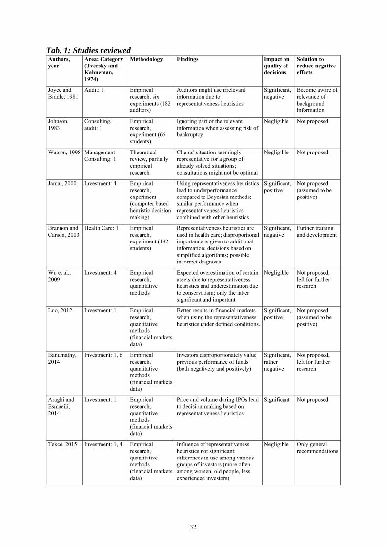
Tab. 1: Studies reviewed Authors, year

Area: Category (Tversky and Kahneman, 1974)

Methodology Findings Impact on quality of decisions

Solution to reduce negative effects

Joyce and Biddle, 1981

Audit: 1 Empirical research, six experiments (182 auditors)

Auditors might use irrelevant information due to representativeness heuristics

Significant, negative

Become aware of relevance of background information

Johnson, 1983

Consulting, audit: 1

Empirical research, experiment (66 students)

Ignoring part of the relevant information when assessing risk of bankruptcy

Negligible Not proposed

Watson, 1998 Management Consulting: 1

Theoretical review, partially empirical research

Clients' situation seemingly representative for a group of already solved situations; consultations might not be optimal

Negligible Not proposed

Jamal, 2000 Investment: 4 Empirical research, experiment (computer based heuristic decision making)

Using representativeness heuristics lead to underperformance compared to Bayesian methods; similar performance when representativeness heuristics combined with other heuristics

Significant, positive

Not proposed (assumed to be positive)

Brannon and Carson, 2003

Health Care: 1 Empirical research, experiment (182 students)

Representativeness heuristics are used in health care; disproportional importance is given to additional information; decisions based on simplified algorithms; possible incorrect diagnosis


Further training and development

Wu et al., 2009

Investment: 4 Empirical research, quantitative methods

Expected overestimation of certain assets due to representativeness heuristics and underestimation due to conservatism; only the latter significant and important

Negligible Not proposed, left for further research

Luo, 2012 Investment: 1 Empirical research, quantitative methods (financial markets data)

Better results in financial markets when using the representativeness heuristics under defined conditions.



Banumathy, 2014

Investment: 1, 6 Empirical research, quantitative methods (financial markets data)

Investors disproportionately value previous performance of funds (both negatively and positively)

Significant, rather negative

Not proposed, left for further research

Araghi and Esmaeili, 2014

Investment: 1 Empirical research, quantitative methods (financial markets data)

Price and volume during IPOs lead to decision-making based on representativeness heuristics

Significant Not proposed

Tekce, 2015 Investment: 1, 4 Empirical research, quantitative methods (financial markets data)

Influence of representativeness heuristics not significant; differences in use among various groups of investors (more often among women, old people, less experienced investors)

Negligible Only general recommendations

32

Authors, year

Area: Category (Tversky and Kahneman, 1974)

Methodology Findings Impact on quality of decisions

Solution to reduce negative effects

Shane et al., 2015

Investment: 4 Empirical research, experiment

Influence of representativeness heuristics on Technology Licensing Officer (decision on employees’ inventions); decision influenced by the assessed person's gender, country of origin, industry experience and ease of working with her or him

Significant Gaining practical knowledge

Woodland and Woodland, 2015

Investment: 6 Empirical research, quantitative methods (betting data)

Biases in football betting due to decisions based on historical (even less probable) results and ignorance of regression to the mean


Not proposed

Liu, 2016 Investment: 1 Empirical research, quantitative methods (financial markets data)

Overconfident and heuristic traders have better results than rational traders and create a more stable and efficient market



Arend et al., 2016

Management: 1 Empirical research, questionnaires and quantitative methods (102 entrepreneurs, 99 executive managers)

Entrepreneurs use heuristic decision-making more often than managers; rate of use of heuristics depends on environmental dynamics, confidence, age and education; decision-making based on representativeness heuristics is beneficial in stable environment and positive risk aversion of an entrepreneur

Significant, positive (under certain circumstan-ces)

Use representativeness heuristics only in stable environments and low risk

Croitoru, 2016

Macroeconomics: 1

Empirical research, quantitative methods (financial markets data)

Natural rate of interest and potential output overestimated in economic expansion due to representativeness heuristics, which causes problems for efficient monetary politics


Focus on input validity in predictions

Woodland and Woodland, 2016

Investment: 6 Empirical research, quantitative methods (financial markets data)

Similar to Woodland and Woodland (2015) supports the influence of representativeness heuristics and regression to the mean bias in baseball betting


Not proposed

Jaspersen and Aseervatham, 2017

Insurance industry: 3

Empirical research, experiment (272 participants)

People do not insure for situations that happened recently as they assume that they happen only once over a long time (i.e. they wrongly assess probabilities)

Significant Not proposed

Source: Authors

As Fig. 1 shows, the majority of empirical articles on representativeness heuristics is in the area of investment, followed by auditing, management, insurance and health care. Regarding the classification of Tversky and Kahneman (1974), see Fig. 1, the category of insensitivity to prior probability of outcome was identified the most often, 11 times (the individual categories were mentioned by the original authors or assigned during the review process). Insensitivity to predictability and misconception of regression were less frequent. The possible reason why illusion of validity (Category 5) is not contained in the research is probably its similarity to insensitivity to

33

predictability bias (Category 4). Overall, 13 articles support the assumption that the use of representativeness heuristics can have a serious impact on real world decision-making. This impact can be both negative and positive, depending on the decision setting and other factors. Solutions (for the reduction of negative impacts) were only proposed in five studies and, unfortunately, this was often only stated in a general theoretical form.

Fig. 1: Number of articles according to area, biases and significance of impact

102

2

3

Research Area

Investment Management

Audit Others

3

0

4

1

0

11

0 5 10 15

Category 6

Category 5

Category 4

Category 3

Category 2

Category 1

Number of Particular Categories of Bias

4

13

02468

101214

Negligible Significant

Impact of Bias

Source: Authors

Since most of the studies were related to investment (either betting or financial investment), this area was examined in greater detail. The results of the assessment are summarized in Fig. 2. In general, a congruence in the detected biases is observable. In particular, insensitivity to the prior probability of outcome and misconception of regression were considered to be biases with a significant impact (in 80% of the relevant studies for insensitivity to prior probability and in all the studies for misconception of regression).

Fig. 2: Investment Area Analysis

Source: Authors

Only Tekce (2015) stated that insensitivity to prior probability was a bias with negligible impact. Some authors considered insensitivity to prior probability as positive (Liu, 2016; Luo, 2012), and the positive characteristic of this bias was also found by Esmaeili (2014) and Banumathy (2014). Therefore, it can be concluded that if investment decision-making based on representativeness heuristics leads to insensitivity to the prior probability of outcome bias, similar or even better results can be expected in comparison to rational models.

34

From the studies in which misconception of regression bias was identified, there is the implication that investors make their decisions based on prior results and expect their recurrence in the future, meaning they ignore regression to the mean. This finding is also confirmed by Banumathy (2014), who discourages investors from investing based on previous results. As he stated, past success in investment funds does not always mean success in the future, especially when only a short period is taken into account. Similar results were also obtained in sports-betting studies (Woodland and Woodland, 2015, 2016), where betting on previously successful teams was not confirmed to be profitable. In all cases, the misconception to regression bias was considered to be negative, and therefore it is highly recommended to avoid this bias as much as possible.

Only half of the studies which considered insensitivity to predictability bias reported a significant impact on investment decisions. Taking into account the ambiguity of the results, it is difficult to support the statement that investors are making their decisions based on characteristics which they consider indicators of good investment. Nevertheless, in the studies which support the significant effect of this bias, the impact is not perceived negatively as Jamal (2000) even identified a positive impact and Shane (2015) does not exclude it.

Articles relating to management, auditing and other areas concluded that the effects of biases caused by the use of representativeness heuristics are negative. Almost each study is related to the bias of insensitivity to the prior probability of outcome. An experiment conducted by Johnson (1983) confirmed the statement that people ignore some of the relevant information when deciding about the possibility of a company's bankruptcy, which is in contrast to the other five studies. However, the author also adds the negligible impact in the conditions of the real world.

4 Discussion The main finding of the research is the fact that most of the authors rate the impact

resulting from the use of the representativeness heuristic as significant. Some authors (Liu, 2016; Luo, 2012; Jamal, 2000) argue that the impact is positive, which means that the use of heuristics brings equivalent or even better results than the rational models which consider all the available information and are more detailed and analytically oriented. This fact is in contrast with Tversky and Kahneman's (1974) findings that heuristics-based decision-making leads to systematic errors. However, this thesis can be assumed to be very general and does not deny the possibility that the heuristic model can be valuable in specific cases, an idea which is also supported by Gigerenzer (2008) and Robins and Timothy (2017).

The implications of the previous research for decision-making are particularly useful for stock-market investment. Representativeness heuristics appear to overcome the results of rational decision-making, as particular biases showed positive effects in two out of three cases. However, using representativeness heuristics is recommended only when eliminating the misconception of regression bias, which in all of the studies was related to negative results. Although the authors of the individual studies do not suggest a solution for eliminating this bias, the basic rule is not to make a decision purely on the grounds of previous results and therefore on the expectation that the same results will happen again.

35

As has already been stated, most of the studies did not offer possible solutions to prevent or at least limit the negative impacts resulting from the biases related to representativeness heuristics. Therefore, further research may explore possible ways of supporting heuristics models, making them more precise and accurate, while maintaining their simplicity. In this context, Jamal (2000) discovered that using a combination of several simple heuristic models can lead to the same results as using Bayesian-based decision making. Further research could also focus on the use of the representativeness heuristics beyond the area of investment, which has already been thoroughly examined. Finally, Johnson’s (1983) proposition – to answer the question why some information (so called “base rates”) has still been largely ignored – may benefit our understanding of decision-making.

It is necessary to mention that the findings of this study are limited by the number of studies analysed – after an evaluation of the abstracts and an application of the necessary criteria, only seventeen articles remained. Additionally, most of the authors focused on representativeness heuristics in the area of investment. This is probably due to the availability of data on the financial markets. Therefore, other areas like management or auditing were not analysed in detail in the review, and so it was impossible to draw any detailed conclusions. Considering the limitations of the studies under review, it is important to note that researchers undertaking quantitative studies need to quantify (mathematically define) heuristic decision-making. For example, for this purpose Tekce (2016) used parts of models from different researchers, while changing and reconstructing other parts to create his own model. In this context, the overall consistency of the studies analysed may be questioned. Although the findings from the studies are synthesized in this review, individual findings are based on different methods and approaches, and build on slightly different definitions. Nevertheless, this inconsistency is not considered to be a crucial problem for the review and its implications.

Conclusion By their definition (ignoring or emphasizing some aspect of the available

information), simplified decision-making models, including the representativeness heuristic, lead to systematic errors (biases). However, as this review illustrates, the results from simple decision-making rules do not have to be worse than when using a rational model; it mainly depends on the situation and context.

In the first chapter, the study focused on theoretical concepts and the definition of important terms, while taking into account different perspectives. The methodology described in the second chapter enabled the authors to answer the research question in the results section of the study. The results section consists of an analysis of seventeen empirical studies that were chosen using predefined criteria. The analysis revealed a broad scale of biases and errors that can occur when using the representativeness heuristic. The study then focused on the impact of these biases and investigated whether the impact was positive or negative. At the end of the study, several questions and problems were suggested as topics for future research.

Acknowledgements The paper was supported by the Masaryk University research project

MUNI/A/0878/2016, “Strategic behavior-performance cycle and factors influencing it”.

36

References Araghi, M., Esmaeili, B. (2014). Overreaction and representativeness heuristic in initial public offering. Management science letters, 4(2), pp. 287-294. ISSN 1923-9343.

Arend, R., Cao X., Grego-Nagel A., Im J., Yang X., Cavanati S. (2016). Looking Upstream and Downstream in Entrepreneurial Cognition: Replicating and Extending the Busenitz and Barney (1997) Study. Journal of Small Business Management, 54(4), pp. 1147-1170. ISSN 1540-627X.

Banumathy, K., Deo, M., Azhagaiah R. (2014). Investor Behaviour and The Persistence of Poorly Performing Mutual Funds: Evidence from India. International Journal of Financial Management, 4(3), pp. 43-49. ISSN 2229-5682.

Brannon, L., Carson K. (2003). Research brief: The representativeness heuristic. Applied Nursing Research, 16(3), pp. 201-204. ISSN 0897-1897.

Croitoru, L. (2016). Are We Systematically Wrong When Estimating Potential Output and the Natural Rate of Interest? Romanian Journal of Economic Forecasting, 19(2), pp. 128-151. ISSN 1582-6163.

Frederick, S., Lieberman, G. (2001). Introduction to operations research. 7th ed. Boston: McGraw-Hill.

Gigerenzer, G. (2008). Why Heuristics Work. Perspectives on Psychological Science, 3(1), pp. 20-29. ISSN 1745-6916.

Grether, D. (1980). Bayes rule as a descriptive model: The representativeness heuristic. The Quarterly Journal of Economics, 95(3), pp. 537-557. ISSN 0033-5533.

Jamal, K., Sunder S. (2001). Why do biased heuristics approximate Bayes rule in double auctions? Journal of Economic Behavior and Organization, 46(4), pp. 431-435. ISSN 0167-2681.

Jaspersen, J., Aseervatham, V. (2017). The Influence of Affect on Heuristic Thinking in Insurance Demand. Journal of Risk and Insurance, 84(1), pp. 239-266. ISSN 15396975.

Jesson, J; Matheson, L., Lacey, F. (2011). Doing your literature review: Traditional and systematic techniques. Thousand Oaks: Sage.

Johnson, W. (1983). 'Representativeness' in Judgmental Predictions of Corporate Bankruptcy. The Accounting Review, 58(1), pp. 78-97. ISSN 0001-4826.

Joyce, E., Biddle, G. (1981). Are Auditors' Judgments Sufficiently Regressive? Journal of Accounting Research, 19(2), pp. 323-349. ISSN 0021-8456.

Katsikopoulos, K. (2011). Psychological Heuristics for Making Inferences: Definition, Performance, and the Emerging Theory and Practice. Decision Analysis, 8(1), pp. 10-29. ISSN 1545-8490.

Keele, S. (2007). Guidelines for performing systematic literature reviews in software engineering. In: Technical report, Ver. 2.3 EBSE Technical Report.

Liu, H., Du, S. (2016). Can an overconfident insider coexist with a representativeness heuristic insider? Economic Modelling, 54, pp. 170-177. ISSN 0264-9993.

Luo, G. (2013). Can representativeness heuristic traders survive in a competitive securities market? Journal of Financial Markets, 16(1): 152-164. ISSN: 1386-4181.

Robbins, S., Judge, T. (2017). Organizational behavior. 17th ed. Boston: Pearson.

Samuels, R., Stich, S., Bishop M. (2002). Ending the rationality wars: How to make disputes about human rationality disappear. In: Elio, R. (ed.), Common Sense, Reasoning and Rationality, pp. 236-268. Oxford: Oxford University Press.

Shane, S., Dolmans, S., Jankowski, J., Reymen, I.Romme, A. (2015). Academic Entrepreneurship: Which Inventors Do Technology Licensing Officers Prefer for Spinoffs? Journal of Technology Transfer, 40(2), pp. 273-292. ISSN 0892-9912.

Tassoni, C. (1996). Representativeness in the market for bets on national football league games. Journal of Behavioral Decision Making, 9(2), pp. 115-124. ISSN 0894-3257.

37

Tekçe, B., Yilmaz, N., Bildik, R. (2016). What factors affect behavioral biases? Evidence from Turkish individual stock investors. Research in International Business and Finance, 37, pp. 515-526. ISSN 0275-5319.

Tversky, A., Kahneman, D. (1974). Judgment under Uncertainty: Heuristics and Biases. Science, 185(4157), pp. 1124-1131. ISSN 0036-8075.

Watson, A., Rodgers, T., Dudek, D. (1998). The Human Nature of Management Consulting: Judgment and Expertise. Managerial and Decision Economics, 19(7-8), pp. 495-503. ISSN 0143-6570.

Woodland, L., Woodland, B. (2015). The National Football League season wins total betting market: The impact of heuristics on behavior. Southern Economic Journal, 82(1), pp. 38-54. ISSN 0038-4038.

Wu, C.-H., Wu, C.-S., Liu, V. (2009). The conservatism bias in an emerging stock market: Evidence from Taiwan. Pacific-Basin Finance Journal, 17(4), pp. 494-505. ISSN 0927-538X.

Ying Luo, G. (2013). Can representativeness heuristic traders survive in a competitive securities market? Journal of Financial Markets, 16(1), pp. 152-164.

Contact Address

Ing. Jan Bílek Masaryk University Faculty of Economics and Administration, Department of Corporate Economy Lipová, 41a, 602 00, Brno, Czech Republic Email: [email protected] Phone number: +420549491710

Bc. Juraj Nedoma Masaryk University Faculty of Economics and Administration, Department of Corporate Economy Lipová, 41a, 602 00, Brno, Czech Republic Email: [email protected] Phone number: +420549491710

Ing. Michal Jirásek Masaryk University Faculty of Economics and Administration, Department of Corporate Economy Lipová, 41a, 602 00, Brno, Czech Republic Email: [email protected] Phone number: +420549491710


38

NEW TRENDS IN THE RECRUITMENT OF EMPLOYEES IN CZECH ICT ORGANISATIONS

Adéla Fajčíková, Hana Urbancová, Martina Fejfarová

Abstract: All organisations are facing the challenge of attracting and retaining employees whose skills and abilities are in line with the organisation’s needs. The plan of recruitment of human resources should be flexible, differentiate between individual categories of employees and should follow new trends in this area. The main objective of this paper is to identify the methods for the recruitment and selection of employees in Czech organisations and evaluate the differences in employee recruitment in large information and communication technology organisations (ICT) compared to other organisations active in the tertiary sector of the economy. The data was obtained through quantitative (n = 288) and qualitative (n = 34) research. Results of the survey show that organisations are starting to utilise a broader scale of methods to attract employees, in particular specialists, in ICT. Most of the organisations active in this area are struggling with the low number of job candidates on the labour market; to overcome this obstacle, they are developing and training their current staff (61.8%), changing their recruitment strategy and increasing initial salaries (50%). The research also identified 5 factors that define groups of organisations based on the methods they use to acquire new employees.

Keywords: Czech Republic, Differentiation of Employees, Human Resource Management, Information and Communication Technology, Recruitment and Selection Methods.

JEL Classification: M12, M15, O15.

Introduction

In today’s fast-changing environment, all organisations need a plan for their human resources (HR) that must be flexible and follow new trends in this area (Armstrong and Taylor, 2017). Bussin (2014), as well as Schwartz, Bersin and Pelster (2014), claim that all organisations are facing the challenge of attracting and retaining employees whose skills, knowledge, experience, competencies and values are in line with the organisation’s needs. Kociánová (2012) and Isson, Harriott and Fitz-enz (2016) also point out the necessity of changing strategies and attitudes in selecting and retaining talented staff because of the needs of Generation Y which has new requirements for their potential employers. The younger generation typically expects greater support from the employer in finding the right balance between their working and personal lives and the option of flexible working hours (Wong, Wan and Gao, 2017). This is confirmed by Dubravska and Solankova (2015) who consider this, alongside the influence of globalisation, knowledge management, talent management and changes related to compensation and benefits, to be the main trends in human resource management. According to the National Cooperative Highway Research Program (NCHRP), the workforce today increasingly often emphasises continuous feedback, professional and personal development and a clearly defined career path (NCHRP, 2012).

39


Because human resources (HR), together with their skills and knowledge, represent the essential competitive advantage of any organisation (Chunping and Xi, 2011), the struggle to find the right employees intensifies and becomes a “war for talents” (Alniacik et al., 2014). In order to attract the best, organisations have started using the principles and methods of brand building, strengthening the employer’s image in human resource management (O’Malley, 2010; Alniacik and Alniacik, 2012). Jiang and Iles (2011) see the attractiveness of an employer and the reputation of an organisation as expressions of the organisation’s ability to attract potential talents and encourage current staff to remain loyal to the organisation.

Another trend that must be mentioned as something that influences the selection of methods and techniques for selecting the right candidates is modern technology and social media (El Ourdi et al., 2016), which are part of the everyday life of Generation Y (Din et al., 2015) and play an important role in the selection of new employees in information and communication technology organisations (ICT). Nikolaou (2014) and Russell and Brannan (2016) mention the importance of the internet particularly in terms of the organisation’s presentation on social media, the use of the internet when searching for suitable candidates on job portals and when advertising jobs on its website. Despite some clear benefits in using the internet to attract talent, the traditional communication channels remain important, such as advertising, presentations in educational facilities, at conferences, workshops and job fairs, use of agency workers and more (Gogolova, Ponisciakova and Ivankova, 2015). There are many methods that can be used to attract new employees, but the specific combination used depends on the size of the organisation and its field of business.

The main objective of this paper is, therefore, to identify the methods of the recruitment and selection of employees in Czech organisations and evaluate the differences in employee recruitment in large information and communication technology organisations compared to other organisations active in the tertiary sector of the economy. The results were obtained using the methodology described below.

2 Methods

The data was obtained through two subsequent surveys. The first survey was organised from 10/2016 to 06/2017 and took the form of an electronic questionnaire. The respondents were manually selected organisations active in the tertiary sector in the Czech Republic. 288 organisations took part in the survey; the questionnaires were filled out by persons responsible for HR activities in the organisation. The questionnaire contained 12 questions, 4 of which served for identification. The survey used closed and semi-open multiple choice questions concerning the hiring of new employees.

61.8% of respondents in the quantitative survey were from the private sector and 38.2% from the public sector and the sample included organisations both large and small (40.6% under 49 employees; 59.4% over 50 employees). Most of the respondents (60.7%) are active on the national or international market; the remaining organisations are focusing on a local or regional market in the Czech Republic. Slightly less than half of the respondents (48.6%) have an HR department at their organisation. In 65.3% of organisations, the person responsible for HR activities is a member of top management and 51% of organisations are part of a larger group.

40

The data was evaluated through descriptive statistics. The results were then also evaluated with multidimensional statistical analysis. Because this particular humanities research focused on human resource management, the used methodology was factor analysis, following the recommendations of Anderson (2009) and Pecáková (2011). In order to obtain the calculations, a correlation analysis was performed first followed by an analysis of the main components and a factor analysis using the Varimax method. The Kaiser-Guttman rule was used to select significant factors (i.e. significant factors were those with variance higher than 1). In the results of the factor analysis, significant values were those with a value exceeding 0.3 (Anderson, 2009).

The research was followed up by a second qualitative survey, implemented in the period 06/2017 to 07/2017 in the form of a structured interview in person. This survey only focused on organisations active in ICT that have more than 50 employees and are the leaders in their respective field in the Czech Republic. The total number of participants was 34 and the interviewed persons were those responsible for HR activities in the organisation. The interview used both closed and open questions aiming to identify any problems in the hiring of new employees, the communication channels used in contact with potential candidates and the methods of their selection. The structured interview contained 16 questions, 4 of which served for identification. The average duration of one interview was 30 minutes.

24 organisations who took part in the survey have 50 to 249 employees (70.6%); 10 organisations have more than 250 employees (29.4%). Most of the organisations are active on the international (18; 52.9%) or national (13; 38.2%) market. Only 3 (8.9%) organisations are focusing exclusively on a local or regional market. 32.4% of the organisations (11) are part of a larger group.

The statistical software used to evaluate the data from both surveys was IBM SPSS Statistics 24.

3 Problem solving

This chapter presents the results of both surveys.

3.1 Recruitment trends in the tertiary sector

New trends in the recruitment of new employees are related to the internet. Use of the internet in the hiring of new staff is not limited to the traditional advertising of open job positions but has expanded to the full concept of how HR marketing is set up. With the development of the internet, people have started forming communities on social networks for reasons both professional and work-related as well as social. Social networks, whether global or local, are also used today, to various degrees, to look for new employees, which is a trend that’s also typical for ICT.

The surveyed organisations active in the tertiary sector typically try to fill their specialist positions from their internal resources (65.97%). 53.82% of organisations rely on the recommendation of a suitable candidate by their employees and advertise jobs on their website (52.77%) and in other media (44.79%). 23.26% of organisations try to attract new employees by actively offering a job in person and 21.87% of the organisations have their presentations in schools and educational facilities. Organisations also try to find employees by keeping records of randomly received applications (20.83%), using notice boards (18.06%), keeping records of former staff

41

(15.63%) or working with an HR agency (17.71%). Only 15.28% of organisations rely on the Labour Office when hiring specialists and a mere 3.82% use employee leasing.

Based on data analysis the research determined 5 factors (Tab. 1) influencing the methods of hiring employees in the tertiary sector. The research worked with 12 variables (Tab. 2).

Tab. 1: Variance explained by factors

Factor Total Variance Total % of Variance

Cumulative % of Variance

1 2.804 23.370 23.370 2 1.264 10.533 33.903 3 1.171 9.759 43.662 4 1.117 9.308 52.970 5 1.064 8.869 61.840

Source: Authors

The variance of factor 1 can be considered most significant (23.370). In total, the 5 identified variables explain 61.84% of the behaviour of the sample or its characteristics. The results of the factor analysis of the questionnaire are provided in Tab. 2.

Tab. 2: Resultant factors by the Varimax method Variable Factor 1 Factor 2 Factor 3 Factor 4 Factor 5

Internal resources

0.776 -0.208 0.108 0.055 0.039

Database of former employees

0.395 0.192 0.315 -0.091 0.547

Database of potential employees

0.557 0.389 0.112 -0.156 0.167

Advertising 0.286 0.542 -0.027 0.403 -0.018 Notice boards 0.223 0.236 0.165 -0.051 -0.772 Employee leasing

-0.119 0.194 -0.042 0.691 0.142

Website 0.682 0.268 0.014 0.175 -0.197 Promotion at schools

0.216 0.457 0.175 0.153 0.389

HR agency 0.196 -0.140 0.200 0.777 -0.117 Personal offers

-0.053 0.019 0.883 -0.002 0.015

Recommen-dations by employees

0.306 0.182 0.652 0.162 -0.015

Labour Office -0.069 0.793 0.117 -0.039 -0.145 Total % of Variance

23.370 10.533 9.759 9.308 8.869

Name of factor

Strategy of HR

recruitment

External HR

marketing

Personal contact and recommen-

dation

External collaboration

Internal HR

marketing

Source: Authors

42

The first group of analysed organisations emphasises hiring primarily from internal resources, particularly when planning the career of individual employees (vertical mobility). If there are suitable experts in the organisation, the management intentionally tries to manage their career path to ensure high-level management positions in ICT are staffed by experienced specialists. The same organisations try to use databases of potential employees and constantly update the news section on their website. This factor, which could be termed “Strategy of human resources recruitment”, has values ranging from 0.557 to 0.776, which can be considered a high quality of determined coefficients. These organisations can be recommended to focus on the long-term planning of the recruitment process with emphasis on gaining new talented employees. The organisations must effectively use social networks such as Twitter, LinkedIn, Facebook and others.

The surveyed organisations also focus on advertising (0.542), promotion (0.457) at schools (both secondary and tertiary) and rely on the Labour Office (0.793). These organisations emphasise the need to increase their visibility as potential employers; this factor could be called “External HR marketing”. These organisations should focus on presenting their activities at secondary and higher education institutions, cooperation on a joint project with universities for building the employer branding and gaining new, talented employees during their studies.

The third factor combines personal offers of a job position based on references (0.883), which is a typical method used for key positions in ICT (such as system consultants, system architects etc.) and direct recommendations by employees (0.652). The resulting group of surveyed organisations has been identified with the factor “Personal contact and recommendation”. These strategies are related to the emphasis on mentoring and coaching that are very important and effective learning methods for ICT organisations nowadays. The organisations can offer the possibilities of job shadowing, especially for junior positions.

The fourth factor, “External collaboration”, involves working with HR agencies (0.777) and using employee leasing (0.691). The final factor, “Internal HR marketing”, emphasises keeping records of former employees (0.547) who can still be contacted for specific jobs; these organisations, on the other hand, do not like to post jobs on notice boards, resulting in a relatively high but inversely proportional coefficient (-0.772). It is very important to stimulate current employees and give them opportunities for personal development and support the development of their competences.

Today, in a situation where there is a lack of high-quality employees particularly in technical fields, including ICT, all organisations try to improve their recruitment processes and want to have valuable analyses of the behaviour of job candidates and current staff. Knowledge of the behaviour and preferences of individual employees allows organisations to retain key current staff as well as find suitable new candidates.

3.2 Recruitment trends in ICT

The subsequent survey aimed to obtain detailed information related to hiring in ICT. The questions therefore also focused on the reasons why open positions are difficult to fill, on communication methods used to attract candidates and on the methods of their selection.

32.4% of the surveyed organisations (11) do not have an HR department responsible for HR activities in the organisation, which includes recruiting new staff and following

43

trends in this area. In 21 organisations (61.8%), the person in charge of HR is a member of top management, enabling strategic planning of the organisation’s HR needs. This, however, may be influenced by cases when power in the organisation is highly centralised and the owner also makes decisions on HR matters.

Most of the surveyed organisations (85.3%) have problems finding people for open job positions. 94.1% of respondents said the most difficult positions to hire for were specialists. Only 3 organisations reported difficulties in hiring for administrative or management positions. Detailed results are available in Fig. 1.

Fig. 1: Reasons for difficult job placement

Source: Authors

The main reason why hiring is difficult is a lack of candidates on the job market, confirmed by 85.3% of the surveyed organisations. 50% of the respondents claim that another problem is high salary demands of the candidates, insufficient knowledge of the field or insufficient education (29.4%) or a lack of work experience (20.6%). The surveyed organisations overcome this lack of workforce by developing and training their current staff (61.8% of organisations). 50% of organisations fight the issue by changing their hiring strategy and increasing initial salaries. 35.3% of respondents have been forced to lower their requirements for new staff.

Organisations active in ICT prefer modern communication channels without personal contact when communicating with potential hires. Almost all the surveyed organisations (31; 91.2%) have their own website and use job portals (30; 88.2%). In their effort to attract new employees, 29 organisations (85.3%) have a profile on social networks; the most commonly used are LinkedIn (29; 85.3%) and Facebook (22; 64.7%). Another frequently mentioned communication channels are the friends and relatives of internal employees. Less used communication channels are those that involve personal contact, such as job fairs (12; 35.3%), conferences, seminars and workshops (8; 23.5%) or doors open days (8; 23.5%).

ICT organisations agree that the main critical category in hiring new employees are specialists. Because of this, Fig. 2 shows the differences in the use of various methods for selecting specialists in organisations in the tertiary sector in general and in ICT specifically.

29

10

1

7

17

2

lack ofcandidates

insufficientknowledge or

education

lack of soft skills lack of workexperience

high salarydemands

none

Nu

mb

er o

f re

spon

den

ts

Reasons for difficult job placement

44

Fig. 2: Methods for selecting specialists

Source: Authors

Results of the research clearly show that the most commonly used methods for selecting specialists are interviews, CV analyses, use of references and proficiency tests. These methods are used most often both by large ICT organisations and by all organisations in the tertiary sector. Yet there are some differences; while the respondent ICT organisations use recruitment interviews for all of their specialist positions, the tertiary sector in general only uses this method in 83% of cases. Because of the technical nature of a specialist position in ICT, this segment much more often uses proficiency tests which are applied by almost 64.7% of the organisations, compared to less than 38.5% in the tertiary sector. Less commonly used methods for hiring in the specialist category are personality tests, intelligence tests and the use of an assessment centre. All these methods, including graphology tests, are, according to the respondents, used more often in other parts of the tertiary sector than in ICT.

4 Discussion

The decisive factor influencing the success of any organisation is its ability to find, attract and retain highly qualified employees. This field is currently experiencing major shifts caused by globalisation, changing expectations of the workforce, a dropping half-life of both skills and technical knowledge, technology and social media (Schwartz, Bersin and Pelster, 2014). In this new environment, the old ways of recruitment are no longer effective and organisations need to adapt (Bohdal-Spiegelhoff et al., 2014).

CEDEFOP (2016) has published a list of five groups of jobs which are experiencing a lack of qualified staff all across the European Union (EU), with significant impact on national economies. These groups of jobs include ICT specialists, physicians, STEM professionals (Science, Technology, Engineering and Math), nurses, midwives and teachers, with ICT specialists occupying the top spot. This was confirmed by our research which shows that 85.3% of the surveyed organisations in this field have problems finding people for open job positions. The main cause is a lack of candidates on the labour market, cited by 85.3% of organisations. 94.1% of respondents said the most difficult positions to hire for were specialist jobs because of their particularly high requirements.

85.3

58.8

100

2.98.8

64.7

0

8.8

77.4

51.7

83

8.3 11.1

38.5

2.1

10.8

CV analyses references interviews intelligencetests

personalitytests

proficiencytests

graphologytests

assessmentcentre

Sh

are

of o

rgan

isat

ion

s (%

)

Method for selecting specialists

ICT tertiary sector

45

Stephan, Brown and Erickson (2017) claim that competitive organisations must re-evaluate the way in which they promote their values among current and prospective staff. The authors also mention that campaigns created to attract potential job candidates may be just as important as advertisements aimed at customers. The research shows that organisations active in ICT prefer modern communication channels without personal contact when communicating with potential hires. Almost all the surveyed organisations try to find new employees through their website (91.2%), use job portals (88.2%) and have a profile on social media (85.3%).

On the basis of answers of respondents from the tertiary sector, we have identified 5 factors that influence the behaviour of the respondent organisations and can be used to classify them into groups based on which methods they use when hiring employees. These groups, depending on their preferences of which methods should be used, focus on the “Strategy of human resource recruitment”, “External HR marketing”, “Personal contact and experience”, “External collaboration” and “Internal HR marketing”, and each of them has different preferences for hiring in ICT. But there is one thing they all have in common: an emphasis on HR marketing, both internal and external. Taking into account the results of research by Love and Singh (2011), Martin, Gollan and Grigg (2011) and Elving et al. (2012), it seems clear that support of HR marketing and with it new trends in employee recruitment will be a key activity for all organisations. All organisations, including ICT organisations, should use modern technologies to influence talented students at universities, cooperate with them during their studies and promote knowledge sharing between junior and senior positions.

The paper is limited by survey samples. The analysed sample of organisations is adequate for obtaining the data and makes it possible for the authors to describe the probable general situation in the area of new trends in the recruitment process in the tertiary sector, but not to generalise the results to all organisations in the tertiary sector and in the Czech Republic. In ICT, only qualitative research was carried out. The research results were also not related to the characteristics of the organisations, such as its size or the organisation’s market. The limitation of the paper can also be considered the usage of a factor analysis, the main disadvantage of which is the space for the subjective opinion of the analyst when determining the groups of variables. However, this method is often used in human resource management surveys and, above all, sociologists consider it trustworthy. The follow-up research will focus on the effectiveness of used recruitment methods in predicting the future performance of employees and the link between the recruitment process and the characteristics of the organisations.

Conclusion

In the entire EU and its individual member states, there is an ever-growing gap between supply and demand of skills on the labour market, which in some groups of professionals leads to a significant lack of qualified workforce. Results of our quantitative and qualitative surveys show that this issue also affects organisations active in the tertiary sector of the economy in the Czech Republic, and particularly those in ICT. These organisations overcome this lack of specialists mainly by developing and training their current staff (61.8%), changing their recruitment strategy and increasing initial salaries (50%) or even by lowering their requirements (35.3%). In today’s highly competitive environment, organisations are also using different communication channels and methods to attract job candidates. A factor analysis identified 5 factors that

46

characterise groups of organisations based on the methods they use to acquire new employees (surveyed organisations prefer “Strategy of human resource recruitment”, “External HR marketing”, “Personal contact and experience”, “External collaboration” and “Internal HR marketing”). It has also been determined that organisations active in ICT prefer modern communication channels without personal contact when communicating with potential hires, i.e. using the internet.

Acknowledgement

This contribution was supported by the Internal Grant Agency of the Faculty of Economics and Management of the Czech University of Life Sciences Prague No. 20171006, “New Trends in Recruiting Talented Employees” and by the Internal Grant Agency of the University of Life Sciences Prague (CIGA) No. 20171001, “Assessing the quality of instruction in the selected field at the Faculty of Economics and Management of the Czech University of Life Sciences Prague”.

References

Alnıaçık, E., Alnıaçık, Ü. (2012). Identifying Dimensions of Attractiveness in Employer Branding: Effects of Age, Gender, and Current Employment Status. Procedia - Social and Behavioral Sciences, 58, pp. 1336-1343. https://doi.org/10.1016/j.sbspro.2012.09.1117

Alnıaçık, E., Alnıaçık, Ü., Erat, S. et al. (2014). Attracting Talented Employees to the Company: Do We Need Different Employer Branding Strategies in Different Cultures? Procedia - Social and Behavioral Sciences, 150, pp. 336-344. https://doi.org/10.1016/j.sbspro.2014.09.074

Anderson, V. (2009). Research Method in Human Resource Management. 2nd edition. London: Chartered Institute of Personnel Development.

Armstrong, M., Taylor, S. (2017). Armstrong’s Handbook of Human Resource Management Practice. 14th edition. London: Kogan Page.

Bohdal-Spiegelhoff, U., Barry, L., Erickson, R. et al. (2014). Talent acquisition revisited: Deploy new approaches for the new battlefield. Deloitte University Press. [online] Deloitte University Press. Available at: https://dupress.deloitte.com/dup-us-en/focus/human-capital-trends/2014/hc-trends-2014-talent-acquisition.html [Accessed 2 Aug 2016]

Bussin, M. (2014). Remuneration and talent management: strategic compensation approaches for attracting, retaining and engaging talent: a practical and informative textbook for managing the tension between talent and remuneration in organisations. Randburg, Republic of South Africa: Knowres Publishing.

CEDEFOP (European Centre for the Development of Vocational Training) (2016). Skill shortage and surplus occupations in Europe. [online] Publications and resources. Available at: http://www.cedefop.europa.eu/en/publications-and-resources/publications/9115 [Accessed 4 Aug 2016]

Chunping, Y., Xi, L. (2011). The Study on Employer Brand Strategy in Private Enterprises from the Perspective of Human Resource Management. Energy Procedia, 5, pp. 2087-2091. https://doi.org/10.1016/j.egypro.2011.03.360

Din, S. Z. M., Anuar, R. H. M., Omar, N., et al. (2015). Discovering the Use of Online Recruitment via Social Media of Student Internship. Procedia Economics and Finance, 31, pp. 856-860. https://doi.org/10.1016/S2212-5671(15)01181-8

Dubravska, M., Solankova, E. (2015). Recent Trends in Human Resources Management in Selected Industry in Slovakia and the Czech Republic. Procedia Economics and Finance, 26, pp. 1014-1019. https://doi.org/10.1016/S2212-5671(15)00924-7

Elving, W. J. L, Westhoff, J. J. C., Meeusen, K., et al. (2012). The war for talent? The relevance of employer branding in job advertisements for becoming an employer of choice. Journal of Brand Management, 20 (5), pp. 355–373.

47

El Ouirdi, M., El Ouirdi, A., Segers, J. et al. (2016). Technology adoption in employee recruitment: The case of social media in Central and Eastern Europe. Computers in Human Behavior, 57, pp. 240-249. https://doi.org/10.1016/j.chb.2015.12.043

Gogolova, M., Ponisciakova, O., Ivankova, K. (2015). The Use of External Personnel Marketing in Slovakia. Procedia Economics and Finance, 26, pp. 131-138. https://doi.org/10.1016/S2212-5671(15)00897-7

Isson, J. P., Harriott, J. S., Fitz-enz, J. (Foreword by) (2016). People Analytics in the Era of Big Data: Changing the Way You Attract, Acquire, Develop, and Retain Talent. New York: Wiley.

Jiang, T. T., Iles, P. (2011). Employer-brand equity, organizational attractiveness and talent management in the Zhejiang private sector China. Journal of Technology Management in China, 6 (1), pp. 97-110. https://doi.org/10.1108/17468771111105686

Kociánová, R. (2012). Personální řízení: východiska a vývoj. Prague: Grada Publishing.

Love, L. F., Singh, P. (2011). Workplace Branding: Leveraging Human Resources Management Practices for Competitive Advantage Through “Best Employer” Surveys. Journal of Business and Psychology, 26 (2), pp. 175-181. https://doi.org/10.1007/s10869-011-9226-5

Martin, G., Gollan, P. J., Grigg, K. (2011). Is there a bigger and better future for employer branding? Facing up to innovation, corporate reputations and wicked problems in SHRM. International Journal of Human Resource Management, 22 (17), pp. 3618-3637. https://doi.org/10.1080/09585192.2011.560880

National Cooperative Highway Research Program (2012). Attracting, Recruiting, and Retaining Skilled Staff for Transportation System Operations and Management. Washington, D. C: National Academies Press.

Nikolaou, I. (2014). Social Networking Web Sites in Job Search and Employee Recruitment. International Journal of Selection and Assessment, 22 (2), pp. 179-189. https://doi.org/ 10.1111/ijsa.12067

O’Malley, M. (2000). Creating commitment: how to attract and retain talented employees by building relationships that last. New York: Wiley.

Pecáková, I. (2011). Statistika v terénních průzkumech. Prague: Professional Publishing.

Russell, S., Brannan, M. J. (2016). “Getting the Right People on the Bus”: Recruitment, selection and integration for the branded organization. European Management Journal, 34 (2), pp. 114-124. https://doi.org/10.1016/j.emj.2016.01.001

Schwartz, J., Bersin, J., Pelster, B. (2014). Human Capital Trends 2014 survey: Top 10 findings. Deloitte University Press. [online] Human Capital Trends. Available at: https://dupress.deloitte.com/dup-us-en/focus/human-capital-trends/2014/human-capital-trends-2014-survey-top-10-findings.html [Accessed 31 Jul 2016]

Stephan, M., Brown, D, Erickson, R. (2017). Talent acquisition: Enter the cognitive recruiter. 2017 Global Human Capital Trends. Deloitte University Press [online] Human Capital Trends. Available at: https://dupress.deloitte.com/dup-us-en/focus/human-capital-trends/2017/predictive-hiring-talent-acquisition.html [Accessed 2 Aug 2016]

Wong, I. A., Wan, Y. K. P., Gao, J. H. (2017). How to attract and retain Generation Y employees? An exploration of career choice and the meaning of work. Tourism Management Perspectives, 23, pp. 140-150. https://doi.org/10.1016/j.tmp.2017.06.003

Contact Address

Ing. Adéla Fajčíková Czech University of Life Sciences Prague, Faculty of Economics and Management, Department of Management Kamýcká 129, 165 00 Prague 6 – Suchdol, Czech Republic Email: [email protected] Phone number: +420224382244

48

Ing. Hana Urbancová, Ph.D. Czech University of Life Sciences Prague, Faculty of Economics and Management, Department of Management Kamýcká 129, 165 00 Prague 6 - Suchdol, Czech Republic Email: [email protected] Phone number: +420224382026

Ing. Martina Fejfarová, Ph.D. Czech University of Life Sciences Prague, Faculty of Economics and Management, Department of Management Kamýcká 129, 165 00 Prague 6 - Suchdol, Czech Republic Email: [email protected] Phone number: +420224382037


49

RESEARCH OF OBJECTIVE MARKET PRICE FACTORS IN THE FORMATION OF PRICES ON THE OIL MARKET

Yulia Y. Finogenova, Denis V. Domaschenko, Edward E. Nikulin

Abstract: “Brent” oil prices (BOP) serves as a global standard for commodity market and it strongly influences the world economy. Forecasting BOP presents a significant and at the same time an arduous task. The main question related to “Brent” prices forecasting is the correct determination of the cause-effect relations. In order to conduct the causality analysis, we have employed adaptive-neuro fuzzy interface system based on the if-then rules and a great potential for the determination of cause-effect relations. The modeling has shown unobvious results. Despite the fundamental law, which claims that the balance of supply and demand forms the oil price, we have proved that the fundamental dependencies are not valid for “Brent” oil pricing. We have revealed that precious metals prices (Palladium, Gold, Silver and Platinum) and commodity currencies exchange rates (USD/NOK, USD/AUD, USD/CAD and USD/ZAR) serve as a signal or cause for the “Brent” price changes. Additionally, we have examined the efficiency of the forecasting model in terms of forecasting oil price trends, achieving maximum 62% of accuracy on the daily data.

Keywords: ANN, ANFIS, “Brent” Oil Prices, Causality Analysis, Fuzzy Logic, Forecasting.

JEL Classification: С12, С45,С53.

Introduction

“Brent” is considered as a global oil price standard and it has a huge impact on the global economy. Forecasting BOP is an important and at the same time a challenging task. For forecasting, the modern economic practice employs mathematical modelling. Mathematical prediction approaches can be divided into two groups: structured and unstructured models. Under the structured models we mean an approach based on the fundamental economic researches and including economics relation directly, usually, in the form of differential or difference equations. We refer to the models, whose structure does not change significantly depending on the implementation, to unstructured, this type of models is rather universal. Both approaches have advantages and disadvantages.

Structured models allow the researcher to gain a deeper understanding of the processes flowing in the modelling and of interdependencies between variables. These models provide the highest results for the scenario analysis, or, when the modeled situation is restricted, for investigation of the defined fundamental basis. In other words, the models show an appropriate performance while facing determined or low abstract tasks. However, the main issues in forecasting with the approach is a high risk of misspecification, i.e. if one of the fundamental rules is not in force for the moment, the whole model has the wrong parameterization. Moreover, these type of models requires high professionalism in both system dynamics and economics. However, as is noted in (Crookes and De Wit, 2014), there are many methodological errors caused by the lack of professionalism. Methodological errors lead to significant models misspecification.

50

For building the structured models authors have included some theoretical fundament in the models, and as we have already noted the result of the researches highly depend on the chosen basis. Structured models have served as an accurate tool since the pioneering researches were conducted by J.D. Sterman (1985, 1988) and M. K. Hubbert (1959). Concerning modern researches, the results of the models do not provide such accuracy, but still, they present a very important direction for the economic thought. For instance, in (Rafieisakhaei et al, 2015, 2016) authors proposed a system dynamic approach for BOP forecasting, they had considered BOP formation as a result of supply and demand aggregation. The analysed period was 2015, the model caught the main trend of the year. Analysis of prices for “Brent” oil in relation to supply and demand had shown quite precise results until the 2000s (Lyneis, 2000). However, there have been some deflections from this fundament since the 2000s, which was considered in the paper (Fratzscher et al, 2014). The authors conducted an analysis of the cause-effect relations between asset and oil prices. The research indicated that oil prices had been highly affected by other financial assets since the 2000s, and had reacted to changes in the financial assets immediately.

Unstructured models, oppositely, are more flexible in terms of the required information, i.e. a researcher must not characterise all variables’ dependencies. On the one hand, it raises the issue that the model, which tries to find dependencies by itself, will catch insignificant or noisy information as a base for the analysis. However, on the other hand, it gives an ability to investigate hidden dependencies and nonobvious fundamental changes. At the moment, models based on a vector autoregression are most common (VAR). C. Sims proposed the first model of vector autoregression in 1980. Significant advantages of the proposed model in comparison with models based on differential equations were the ease of identification, implementation and solution of the problem of overfitting the model. Since then, the methodology of constructing autoregressive models has been greatly advanced. The models VEC, ARIMA and Autoregressive conditional heteroskedasticity (GARCH) were developed, removing restrictions on the use of only stationary time series. These models are the most common solutions for forecasting because with the simplicity of realisation they allow to receiv fairly accurate forecasts (Zhang and Frey, 2015, Kambouroudis D. S., 2016, Corrêa J.M., 2016). For instance, in (Baumeister and Kilian, 2015) authors, applying VAR model, gained 72% of the trend forecasting accuracy on the quarterly data and 65% on the monthly data. In (Baumeister and Kilian, 2014) VAR model showed trend forecasting accuracy at the level of 57% – 69% on the monthly data.


All the models mentioned above are linear, which is a significant drawback taking into account the non-linear nature of the relationships between economic time series. To solve this problem, models based on nonlinear autoregression (NAR), proposed in (Leontaritis, 1985), are used. To implement NAR models, dynamic artificial neural networks are used, which also have a nonlinear character and show better results when working with noisy time series (Jiang and Song, 2011). For example, in (Diaconescu, 2008), a model of a nonlinear autoregressive neural network with exogenous inputs (NARX) and ARIMA models was compared. Based on the simulation results, the root-mean-square error of the NARX model is an order of magnitude smaller than the error of the ARIMA model (NARX - 0.0004, ARIMA - 0.0061). In (Chaudhuri and Ghosh,

51

2016), the superiority of the NARX model over generalised models of autoregressive conditional heteroscedasticity (GARCH, EGARCH) is shown.

Finally, it should be noted that last time unstructured models provide better results in terms of the forecasting accuracy caused partly by rapidly changing economic fundament, which gives rise to misspecification of the structured models, partly to onrush of the development of this approach, especially in the field of artificial neural network (ANN) and boosting methods.

We have two hypotheses for the BOP formation to test. First, “Brent” oil prices depend on the supply and demand. Second, “Brent” is dependent on instruments traded on world foreign exchanges. These hypotheses are contrary, hence finally we have proved one and rejected another because fundamentally oil prices should depend on the supply and demand balance and have an impact on the commodity instruments.

Thus, the purpose of this research is to determine the variables that influence the formation of BOP, to develop a model for forecasting oil prices and to test the model on historical data (back-test).

2 Methods

For the formal determination of the causality between exogenous and endogenous variable, we considered the Granger causality test. Before testing the given time series, we had examined it on the randomly generated 200-time series with 100 observations (expected value equalled zero, and standard deviation equalled one). We separated 200-time series into two groups: “cause” and “effect”, thus we gain 100 cause-effect pairs to test. We chose the following test parameters: max number of lags is 7; Alpha coefficient is 0.05.

The test showed that 40 out of 100 pairs had a cause-effect relation, which is obviously an incorrect result. Thus, we decided to use some non-linear forecasting model as an indicator of cause-effect relations. If the model shows better performance in terms of forecasting for the pair and if it shows worse performance after changing cause and effect in the pair, then there is a cause-effect relation in the given pair. We set the threshold for the minimum change in model performance on the level of 10% in trend forecasting accuracy. In addition, we should gain improvement in forecasting performance from using the exogenous time series comparing to forecasting from endogenous time series only. All of mentioned correlates with the intuitions of the Granger causality theory (Granger, 1969).

We employ BOP as an endogenous time series and the following groups of exogenous time series:

1) Prices on precious metals: Palladium, Gold, Silver and Platinum;

2) Prices on the commodity currencies exchange rates: USD/NOK, USD/AUD,USD/CAD and USD/ZAR;

3) Supply and demand balance.

2.1 Forecasting model

We employ adaptive neuro-fuzzy interface system (ANFIS) as a tool for time series forecasting since it bases on the if-then logic rules and has a huge potential for solving

52

tasks connected with the determination of the cause-effect relationships. ANFIS is an ANN based on Takagi-Sugeno fuzzy interface system (FIS). It combines advantages of both fuzzy logic and ANN. J.S.R. Jang introduces ANFIS in the paper (Jang, 1991), the author develops methods for transforming human knowledge or experience into the rule base and database of a fuzzy inference system. The model aims to solve the problem of the classical equation-based system dynamics modelling, which is connected with the uncertainties involved in the real systems (Jang, 1993). The most interesting moment is that ANFIS provides statistically estimated fuzzy if-then rules, which are observable and understandable for the human, unlike other ANN models.

The architecture of ANFIS with inputs x1and x2 is presented in fig. 1.

Fig. 1: ANFIS architecture

Source (J.S.R. Jang, 1991)

The example of Takagi-Sugeno if-then rules are presented as follows:

IF 1x is 1A AND 2x is 2B THEN 121111 rxqxpf

IF 1x is 2A AND 2x is 2B THEN 222121 rxqxpf

Where:

x1, x2 - inputs;

A1, A2, B1, B2 - the fuzzysets;

f1, f2 - the outputs within the fuzzy region by the fuzzy rules;

p1, p2, q1, q2, r1, r2 - the coefficients, which are determined by the training of ANFIS.

ANFIS architecture is defined as follows:

The first layer: every node in the layer contains membership function for the term of the corresponded linguistic variable. This layer presents fuzzification procedure for original inputs values.

For instance:

)(1iAi xO

j ki ...1 (1)

53

)(1iBi xO

j nki ...1 (2)

The second layer: every node in the layer gets membership functions from the previous layer and produces multiplication.

For instance:

)()(2iBiAii xxwO

jj (3)

3rd layer: every node in the layer normalises weights, obtained from the previous layer.

For instance:

ii

iii w

wwO3

(4)

4th layer: every node in the layer calculates the following function:

iii fwO 4(5)

5th layer: the layer contains the single node, which summarises all of the data, obtained from the previous layer.

5iO f

iii fw (6)

Fuzzy Logic Toolbox for MATLAB is the software used to design this model. Its functions provide many common methods, including fuzzy clustering and adaptive neuro fuzzy learning. We have developed ANFIS using the algorithm provided by Fuzzy C-means clustering (FCM). To clarify the developed ANFIS architecture, we provide some information about both ANFIS architecture parameters and the input parameters for the FCM function.

nCluster = 4 – the number of fuzzy clusters, Gaussian curve as membership function;

Exponent = 2 – this option controls the amount of fuzzy overlap between clusters, with larger values indicating a greater degree of overlap (the value greater than 1.0);

MaxIt = 100 – the maximum number of iterations;

MinImprovment = 1e-5 – the minimum improvement in objective function between two consecutive iterations.

The grid search was made with several nested loops which iterated through parameters (in range 2…10 with a step value 1 for the number of clusters; 1…5, step 0.2 – for the overlap option; 10, 100 and 1000 for the number of iterations).

For the training of ANFIS, we use a hybrid method, based on the error back propagation algorithm and the least squares method. The error back propagation algorithm configures the parameters of antecedent rules, i.e. membership functions. The method of least squares estimates the coefficients of the rule conclusions since they are related to the output of ANFIS linearly.

54

2.2 Back-test of the model

Concerning testing of the model forecasting ability, the first role plays correctly determined a trend, obviously, if we do not catch the trend, then it is unimportant what absolute error is, since the forecasted trend is the most significant value for practical decision making. Thus, in the scopes of the current research, we have a goal to forecast trend, but not absolute values.

The testing of the model against historical data (back-test) is done on the basis of the following algorithm:

1) The model is trained against a window of n points;

2) The forecast is built on the bases of q points;

3) Error of trend determining for each of the q points of the received forecast arecalculated;

4) The window for model training is shifted 1 point forward;

5) Procedures 2-4 are repeated until the model reaches the last points of time series;

6) The mean absolute error and the error of trend definition are calculated.

The error of trend determination is calculated the following way:

The trend for each point q of the forecast and the respective actual trend are calculated by the following formula:

)( 0aasigntrend qq (7)

where

qtrend – trend;

qa – the value of q point of forecast;

0a – the value of the last n points included into the training window (or the last actual value).

If the values of the forecasted and the actual trend do not coincide, then the variable y

qerrortrend _ is assigned the value 1; if they coincide, it is assigned the value 0.

The error of trend determining is calculated as the number of incorrectly defined trends of the point q to all the forecasts of the point q.

n

errortrenderrortrend

yq

q _

_ (8)

where

qerrortrend _ – the error of trend definition for the point q;

yqerrortrend _ – y incorrect forecast of the trend for the q point;

n – a number of forecasts.

55

The accuracy of the trend definition is expressed in the following way:

qq errortrendpricetrend _1_ (9)

3 Problem solving

For the testing of the model, we have employed 230 daily observations on trading days from 27/05/2016 to 27/04/2016. The source of the statistics is Thomson Reuters.

The model is specified with the following parameters:

forecasting points number: 5; maximum number of lags: 4; clusters number: 4; train window: 30.

The training set is determined to include 30 observations, thus the first 30 observations are used for the initial training of ANFIS and we have 200 observations remaining for the back-test.

Before forecasting, we are going to investigate cause-effect relationships between supply, demand on oil and BOP, in order to examine the hypothesis that “Brent” oil prices have no direct dependencies on supply and demand, but highly depend on the precious metals and commodity currencies exchange rates.

Supply and demand balance dynamic in comparison with BOP dynamic charts are presented in the fig. 2. Fig. 2 does not show significant cause-effect relations between supply and demand balance in the oil market and the BOP, ANFIS proves it (the difference in the trend forecasting accuracy between cause-effect and effect-cause pairs for the given time series are less than 5%, while the average accuracy does not exceed 53%).

Fig. 2: The supply and demand balance and the average annual prices of “Brent” oil

Source: Authors calculations

56

From the fig. 3, we see that precious metals have a high impact on the “Brent” prices. ANFIS proves this conclusion, showing the difference between cause-effect and effect-cause pairs in the range from 11% to 18%.

Fig. 3: Precious metals and “Brent” oil prices (normalized data)


Fig. 4 illustrates that the currencies influence the “Brent” prices. It seems that the relation between currencies and “Brent” prices is stronger than influence of the precious metals; ANFIS shows the difference between cause-effect and effect-cause pairs in the range from 15% to 26%, also it shows that we gain mean performance improvement with exogenous time series about 4-5% (see the table). It is determined that the Norwegian Krone have the most significant impact on the “Brent” prices, using only these two-time series (Norwegian Krone – exogenously and “Brent” prices – endogenously), we get from 57% to 63% trend forecasting accuracy.

Fig. 4: Commodity currencies exchange rates and “Brent” oil price (normalized data)


57

In order to gain more precise estimation of the model forecasting performance, we simulate it 5 times for each point. Results of the back-test of the model are presented in the table below. The results show that we obtain stable forecasts on the 1, 2 and 3 points.

Tab. 1: Results of the back-test Forecasting point 1 2 3 4 5

Min trend forecasting accuracy

0.57 0.55 0.51 0.48 0.48

Mean trend forecasting accuracy

0.60 0.59 0.55 0.48 0.51

Max trend forecasting accuracy

0.62 0.61 0.58 0.51 0.54

Mean trend forecasting based on the BOP only

0.56 0.53 0.48 0.39 0.41


Fig. 5 represents average dynamics of the trend forecasting accuracy of the model for BOP on the first predicted point.

Fig. 5: Average dynamic of the trend forecasting accuracy of the “Brent” oil prices


It should be noted that the accuracy of the trend forecasting does not have significant deviations from the final value, so we can consider model results as a reliable.

4 Discussion

Economists have been arguing about the mechanisms of pricing in the oil market for a long time. Some argue that supply and demand in the real market determine its dynamics. Other researchers assume that speculative sentiments prevailing in global financial markets play the leading role in pricing in the oil market. The fall of oil prices in 2014 showed the importance of speculative factors, their subsequent recovery in 2016-2017 were triggered by the OPEC + agreement that by imposing the oil supply limitation in the market stabilized the price dynamics.

58

The oil market reacts briefly to all events taking place on the global market. If we consider the long-term horizon, then the classical supply and demand in the oil market do not play a role in determining the price dynamics. It is enough to have look at oil price fluctuations during the last decade (fig. 2) to compare the strong price fluctuation of the BOP with the more stable balance of supply and demand in the world market.

The reasons for such a significant fluctuation in oil prices lie in the financial mechanisms for pricing instruments traded on world commodity exchanges, which are based on the marginal position of bidders. The marginality of the market forming the effect of leverage allows to open market positions that are many times greater than the real security, which can shift the price from the equilibrium level much more than it would be possible without this option.

However, without the marginality of the market and derivatives, there would not be an effective opportunity to hedge market risks to both real producers and oil consumers. Therefore, such fluctuations will continue and they have to be taken for granted. The question remains, which factors determine the movement of oil prices, if the fundamental reasons are in doubt? The research of the interconnectedness and synchronization of the dynamics (or cause-effect relations) of a number of sectors of the commodity and currency markets allows to answer this question.

We have concluded that fundamental factors have little effect on the dynamics of market prices (fig. 2). In any case, the relationship between the balance of supply and demand and oil prices in the long-term interval is not visible. Rather, the dynamics of the oil prices follows market prices, and not vice versa as showed by the modeling (fig. 3 and fig. 4).

Conclusion

In the framework of the current research, we conducted a study of the dependences of the prices of precious metals and commodity currencies exchange rates on “Brent” oil prices. To evaluate these dependencies and predict the BOP time series, the ANFIS model is applied.

The model was also evaluated on daytime data from 27/05/2016 to 27/04/2017 for forecasts of 5 points. The modelling confirmed that there are no obvious dependencies between the balance of supply and demand and BOP and revealed the existence of a causal relationship between prices for precious metals and BOP, as well as between commodity currencies and BOP. It should be noted that the model showed the strongest impact of Norwegian Krona on “Brent” oil prices.

The average accuracy of forecasting the trend for the price of oil: for the first point - 60.0%, for the second - 59.0%, for the third - 55%. Thus, the model showed accurate results when predicting the given time series and can be used to solve other prediction problems.

References

Atsalakis, G.S. (2016). Using computational intelligence to forecast carbon prices. Applied Soft Computing, 43, 107-116.

Azadeh, A., Asadzadeh, S.M., Ghanbari, A. (2010). An adaptive network-based fuzzy inference system for short-term natural gas demand estimation: Uncertain and complex environments. Energy Policy, 38 (3), 1529-1536.

59

Baumeister, C., & Kilian, L. (2015). Forecasting the real price of oil in a changing world: a forecast combination approach. Journal of Business & Economic Statistics, 33(3), p.338-351. DOI: 10.1080/07350015.2014.949342

Baumeister, C., & Kilian, L. (2014). What central bankers need to know about forecasting oil prices. International Economic Review, 55(3), pp. 869-889. DOI: 10.1111/iere.12074

Chaudhuri, T.D. and Ghosh, I. (2016). Artificial Neural Network and Time Series Modeling Based Approach to Forecasting the Exchange Rate in a Multivariate Framework. Journal of Insurance and Financial Management, 1 (5), pp. 92-123

Chen, D.D.; Lin, Y.C., Zhou, Y., Chen, M.S., Wen, D.X. (2017). Dislocation substructures evolution and an adaptive-network-based fuzzy inference system model for constitutive behavior of a Ni-based superalloy during hot deformation. Journal of Alloys and Compounds, 708, 938-946.

Cheng, Ch.H., Wei, L.Y., Liu, J.W., Chen, T.L. (2013). OWA-based ANFIS model for TAIEX forecasting. Economic Modelling, 30, 442-448.

Corrêa, J.M., Neto, A.C., Júnior, L.T., Franco, E.M.C. and Faria, A.E. (2016). Time series forecasting with the WARIMAX-GARCH method. Neurocomputing, 216, 5 December, pp. 805–815

Crookes, D. J., & De Wit, M. P. (2014). Is System Dynamics Modeling of Relevance to Neoclassical Economists? South African Journal of Economics, 82(2), pp.181-192 DOI: 10.1111/saje.12038

Diaconescu, E. (2008). The use of NARX neural networks to predict chaotic time series. Wseas transactions on computer research, 3(3), pp.182-191. Available at: URL http://www.wseas.us/e-library/transactions/research/2008/27-464.pdf [Accessed 2 April 2017].

Fratzscher, M., Schneider, D., & Van Robays, I. (2014 July). Oil prices, exchange rates and asset prices. European Central Bank Working Paper, 1689 pp. 1-45 Available at: URL http://www.ecb.europa.eu/pub/pdf/scpwps/ecbwp1689.pdf?06716196e143159bdcc5d65b2461f68d [Accessed 23 December 2017].

Granger, C. W. (1969). Investigating causal relations by econometric models and cross-spectral methods. Econometrica: Journal of the Econometric Society, pp.424-438. DOI: 10.2307/1912791 Available at: URL: http://www.jstor.org/stable/1912791

Hubbert, M. K. (1959, March). Techniques of prediction with application to the petroleum industry. In Published in 44th Annual Meeting of the American Association of Petroleum Geologists. Shell Development Company, Dallas, TX pp. 43

Jang, J. S. R. (1991, July). Fuzzy Modeling Using Generalized Neural Networks and Kalman Filter Algorithm. In AAAI Proceedings, Vol. 91, pp. 762-767. Available at: URL http://www.aaai.org/Papers/AAAI/1991/AAAI91-119.pdf [Accessed 10 March 2017].

Jang, J. S. (1993). ANFIS: adaptive-network-based fuzzy inference system. IEEE transactions on systems, man, and cybernetics, 23(3), pp. 665-685. DOI: 10.1109/21.256541

Jiang, C. and Song, F. (2011). Sunspot Forecasting by Using Chaotic Time-series Analysis and NARX Network. JCP, 6 (7), pp.1424-1429. DOI: 10.4304/jcp.6.7.1424-1429 ꞏ

Kambouroudis, D.S., McMillan, D.G. and Tsakou, K. (2016). Forecasting Stock Return Volatility: A Comparison of GARCH, Implied Volatility, and Realized Volatility Models. Journal of Futures Markets, 36(12), pp.1127-1163

Leontaritis, I. J., and Stephen A. Billings. (1985). «Input-output parametric models for non-linear systems part I: deterministic non-linear systems». International journal of control. 41 (2) pp.303-328. DOI: 10.1080/0020718508961130

Lyneis, J. M. (2000). System dynamics for market forecasting and structural analysis. System Dynamics Review, 16(1), pp.3-25

Rafieisakhaei, M., Barazandeh, B., Bolursaz, M., & Assadzadeh, M. (2015). Modeling dynamics of expectations on global oil price. In The 33rd International Conference of the System Dynamics Society.

60

Rafieisakhaei, M., Barazandeh, B., Moosavi, A., Fekri, M., & Bastani, K. (2016). Supply and demand dynamics of the oil market: A system dynamics approach. In The 34rd International Conference of the System Dynamics Society.

Rezaeianzadeh, M., Tabari, H., Arabi Yazdi, A., Isik, S., Kalin, L. (2014). Flood flow forecasting using ANN, ANFIS and regression models. Neural Computing and Applications, 25(1), 25-37.

Sims, C. A. (1980, January). Macroeconomics and reality. Econometrica: Journal of the Econometric Society, 48 (1), pp. 1-48 Available at URL: http://www.jstor.org/stable/1912017 [Accessed 12 March 2017].

Sterman, J. D., & Richardson, G. P. (1985). An experiment to evaluate methods for estimating fossil fuel resources. Journal of forecasting, 4(2), pp. 197-226 DOI: 10.1002/for.3980040208

Sterman, J. D., Richardson, G. P., & Davidsen, P. (1988). Modeling the estimation of petroleum resources in the United States. Technological Forecasting and Social Change, 33(3), pp. 219-249 DOI: 10.1111/saje.12038

Suparta, W., Alhasa, K.M. (2016). Modeling of Tropospheric Delays Using ANFIS, Chpt. Adaptive Neuro-Fuzzy Interference System. SpringerBriefs in Meteorology.

Zhang, X. and Frey, R. (2015). Improving ARMA-GARCH forecasts for high frequency data with regime-switching ARMA-GARCH. Journal of Computational Analysis & Applications, 18(1) p727

Contact Address

Yulia Y. Finogenova, Doctor of economics Plekhanov Russian University of economics, “Risk management, insurance and securities markets” Chair Stremianny per. 36, 115093, Moscow, Russia Email: [email protected] Phone number: + 79036142982

Denis V. Domaschenko, Ph.D Plekhanov Russian University of economics, Research laboratory “Study of the monetary system and analysis of the financial markets” Stremianny per. 36, 115093, Moscow, Russia Email: [email protected] Phone number: + 79036867163

Edward E. Nikulin Plekhanov Russian University of economics, Research laboratory “Study of the monetary system and analysis of the financial markets” Stremianny per. 36, 115093, Moscow, Russia Email:[email protected] Phone number: + 79859105275


61

PROTECTION OF THE REPUTATION OF A LEGAL ENTITY AND FREEDOM OF THE EXPRESSION IN THE CONTEXT

OF “MEDIA”

Tomáš Gongol, Michael Münster

Abstract: The article focuses on the concept of reputation (good reputation) of legal persons in respect to the legislation within civil law and media law. Interpretation of the legislation is complemented by a comprehensive analysis of the judicial case-law in this area. Attention is focused on the criteria applied for the purpose of detecting unauthorized interference to the reputation of a legal person. In particular, on distinguishing between allegations of factual statement nature and value judgements or permissible criticism.

Keywords: Reputation of Legal Person, Freedom of Expression, Permissible Criticism, Publication of a Reply, Publication of Subsequent Statement.

JEL Classification: K22, K42.

Introduction

The aim of the text is to define the concept of legal person's reputation and its protection with regard to the limits of the freedom of expression in both, printed and digital news.

The text is structured so as to give the basic definition of the concept having regard to the regulations within the new Civil Code. Then it covers other sources of law within the scope of the subject, especially the sources of media law. The differences between factual statements backed by objective reality and evaluation judgements belonging to the category of subjective statements are here considered as the key criteria for assessment of the illegitimacy of interference into legal person's reputation. Legislation on protection against interference with a legal person's reputation is also confronted with the fundamental human rights and freedoms.

1 Statement of the problem

Having regard to the economic interests of the entrepreneur, it is important to protect his reputation against injurious actions, because each such interference can cause a decrease in the market value of the business establishment. At the time of electronic means of communication, this applies all the more because it allows much faster sharing of information than it was before the massive use of the Internet. Wrongful tampering with the reputation of a legal person occurs in most cases by disclosure or publication of false, distorted or misleading factual claims. Information networks, social media or electronic dailies serve as a very good tool for spreading such pieces of information that interfere with the reputation of a legal person. Legislation applicable to print media can't be applied to such services and their providers.

It is related to constitutionally guaranteed rights and freedoms, in particular, the freedom of expression. Therefore, it is necessary to assess the illegitimacy of interference with the reputation of a legal person also in connection with the rights and

62

freedoms given by law. Based on case-law, the rights and freedoms are not considered endless. In each case, it is always necessary to examine the intensity of the alleged infringement of the rights to protection of the reputation. Such examination must be conducted in the context of the freedom of expression and requirement of proportionality with regard to the implementation of these rights and their protection.

2 Methods

The goal of a post and deficiency of specific norms applicable to legal relationships towards digital media makes it necessary to choose suitable methods enabling the right to examine the law in areas lacking the positive sources. In addition to that, it is necessary to use both, logic methods (such as induction, deduction, analysis, synthesis) and others (comparison) in each comprehensive work with legal texts.

For the purpose of such assessment, an analysis will be carried out, comparing the existing legislation to the one applied before the effectiveness of the new Civil Code. The analysis will be complemented by relevant case-law in this area.

In the context of the problem at hand, the logical interpretation argumentum per analogiam is of special significance to the interpretation of a legal norm. The logical interpretation is applied in several areas of the following text. In the absence of a specific statutory legislation, it is possible to assess the dispute at hand using such statutory legislation that shows a similar association.

3 Reputation of legal person in the Czech legal order

3.1 Generally about the reputation of a legal person

The reputation of a legal person has the nature of a personal right which is legally recognized by law and it is inalienable. In the case of an attack against the reputation of a legal person it is not considered as an attack on its name only, but basically as an attack on the rights similar to human rights (Svejkovský and Deverová, 2013: 44).

The reputation of a legal person is given by its certain attributes that express its character and its relation to society. According to decision-making practice, the reputation of a legal person is evaluated by its conduct in business relations. If the legal person fails to fulfil its obligations properly and in a timely manner, or they only rarely meet their obligations in time, it cannot be concluded that it is a legal person or an entrepreneur that enjoys a reputation at all. It is clear from the above that the reputation of a particular legal person is primarily generated on the basis of experience with its business partners, customers or other entities that come into contact with it. In accordance with the generally accepted presumption of honesty in the conduct of legal entities, it is also assumed that a legal person has a reputation until successfully proven otherwise. This means that according to this point of view, the assessment of unlawfulness of any interference to a legal person's reputation comes also into account. (Judgement of the Supreme Court from 18.03.2008, file no. 30 Cdo 1385/2006).

The reputation of a legal person arises at the time of the establishment of a legal entity and is presumed to last throughout its lifetime until it is proven that the legal person has lost the reputation.

63

The reputation of a legal person can be characterized as a certain qualitative characteristics attributed to the legal entity, which is reflected in the generally favourable reviews in society. Not only those related to its conduct in business dealings among its business partners (e.g., payment history, reliability, compliance with the contractual obligations), as could be understood from the above-mentioned Judgement of the Supreme Court, but in the context of its overall functioning in society, i.e. among its customers (e.g. quality of the provision of services, supplies, works, access to warranty claims, credibility, honesty), employees, or among the general public (e.g. fulfilment of tax and fee obligations, its relation to the environment).

3.2 The protection of the reputation of a legal person in terms of civil law

The legal regulation on the protection of the reputation of a legal person is contained in Section 135 of Act No. 89/2012 Coll., The Civil Code (hereinafter also referred to as the "Civil Code" or only "CC").

According to Section 135 (1) of the CC, a legal person affected by the impeachment of its right to a title, or who has suffered harm for an unauthorized interference with that right or which is at risk, in particular by unauthorized use of the title, may claim that this unauthorized interference should be stopped or its effect should be removed. According to Section 135 (2) of the CC, the same protection of a legal person applies against anyone who infringes on a legal person's reputation or privacy without a legitimate reason, unless it is for scientific or artistic purposes or for press, radio, television or similar news. Even such purposes, however, must not be in conflict with the legitimate interests of a legal person.

Contrary to the previous legislation, the Civil Code already uses only the term "reputation". The explanatory memorandum to the Civil Code in this context, among other things, states that it abandons the term "good reputation", because it necessarily leads to a question of which reputation is considered "good" and if, for example, a publisher of certain prints (e.g. tabloid or of an erotic character) can have a "good" reputation at all. What reputation of a legal person deserves protection must arise from the particular circumstances of the case and the logical content of the law.

Basically, there are two possible interpretations of the change in legislation. That is, the change is only (i) terminological or (ii) factual. The first case would mean the bad reputation of a legal person would not be a subject to protection and, therefore the protection would only apply to a legal person with a good reputation. So in such case, the change in legislation would only be of a formal character with no substantive impact. In the case of a factual interpretation, the subject of a protection would apply to both, good or bad reputation, when in the case of the latter the subject of protection would only apply to interferences causing further deterioration of the reputation. It means, if someone would worsen the already bad reputation by their unlawful interference, the legal person in question could seek the appropriate protection in court.

The authors of this text incline to the factual interpretation, because they believe, that from the explanatory report of the Civil Code it is clear, that the legislature took into account the fact, that it may be questionable whether certain legal persons may have a good reputation at all, in view of the subject-matter of their business or activities. However, there is no reason to exclude them from the provided legal protection. We believe that the legislator's intention was to provide reputation protection to all legal

64

persons. We therefore believe that the provision of Section 135 (2) of the CC protects any reputation of a legal person from unauthorized interference. In our opinion, this interpretation is indirectly supported in theory as well by stating the following: " In terms of the new Civil Code, each legal person that carries out a certificated (resp. legal) activity may invoke the protection of the reputation." (Lavický 2014, p. 714) In any case, the interpretation of the term "reputation" will depend on courts, because the provision in question belongs to legal norms with a relatively indefinite (abstract) hypothesis. It means such legal norms whose hypothesis is not directly established by law and thus leave the court to judge the hypothesis of the law regulation on a case-by-case basis, depend on a wide, unlimited range of circumstances.

Thus, Section 135 (2) of the CC protects the reputation of a legal person from unauthorized (unlawful) interference. The resource (the type of provider) of an injurious act against the reputation of a legal person is not significant. Thus it can be an information provided through the internet, in print, in internet discussion, etc. (Lavický, 2014: 714).

The right to protection against unauthorized interference to the reputation of a legal person acts against all subjects involved in such interventions, which unlawfully intervened (thus caused a harmful effect) to the reputation of a legal person.

This is primarily about the protection against the distribution of various untrue information about a particular legal person. According to Section 135 (2) of the CC in conjunction with paragraph 1, this protection can be implemented primarily by the claim in court by the legal person affected by the intervention, so that the unauthorized intervention is dropped or its effect (bad condition) removed. Furthermore, we believe that the legal person affected by the intervention is also entitled to demand adequate satisfaction, which can also be solved by monetary fulfilment. Similar opinion is supplied by the theory: "Legal person is entitled to claim the one who caused the interference with the reputation of the legal person to abstain from the infringement, remove the offending statement, issue the unjust enrichment (§ 2991 et seq.), bare the damage caused by the interference and provide adequate compensation of monetary or non-monetary nature" (Švestka et al, 2014: §135).

If, in the case of unauthorized interference with the reputation of a legal person occurs a loss or unjust enrichment, the affected legal person may claim a compensation for such harm or unjust enrichment. Here it should be noted that even if the legal person concerned seeks the application of all of the above-mentioned means, the court may not comply with it. According to court judicature the resolutions on the means of protection and the extent of their usage depend on reasoning of the court based on the assessment of the particular circumstances of an unlawful interference to the reputation of the legal person. According to the Judgement of the Supreme Court, there is also no obligation of the court to always impose all possible means of protection and sanctions. The use of individual means of protection and sanctions, as well as the extent of their use, lies within the court (Judgement of the Supreme Court from 09.04.2002, file no. 28 Cdo 1640/2001).

According to the decision-making practice, it is also valid, that for the imposition of civil sanctions for unauthorized interference with the reputation of a legal person the condition of the existence of a specific interference with the reputation of a legal

65

person must be fulfilled as a prerequisite condition of responsibility (from the above it is obvious that it is necessary to verify the fact that a legal person actually enjoys a certain reputation). This intervention must be unauthorized (unlawful) and there must be a causal link between intervention and unauthorization (unlawfulness) of the interference. An individual or a legal person may be held responsible for interfering with the reputation of a legal entity only if it actually triggered or caused this unauthorized interference. The obligation of the claim, the burden of argument, the burden of proof and the burden of proof in relation to the causal link is the responsibility of the concerned legal person (Judgement of the Supreme Court from 02.07.2009, file no. 30 Cdo 2448/2007).

3.3 The protection of the reputation of a legal person in terms of media law

The protection of the reputation of legal person is also the subject of the protection under special legal regulations in the field of media law, in particular according to Act No. 46/2000 Coll., On the rights and obligations of issuing periodicals and on amendments to other acts, as amended (hereinafter also referred to as the "Press Act"), and pursuant to Act No. 231/2001 Coll., On the Operation of Radio and Television Broadcasting, as amended (hereinafter also referred to as the "Radio and Television Broadcasting Act").

Both of these Acts establish the right to publish a reply and a subsequent statement, whereas, "These institutes are of a special character in relation to the protection of personality according to the Civil Code, but it is not out of the question to have been combined or complementary to each other.” (Rozehnal, 2008: 284). This conclusion is supported by the provisions of Section 10 (5) and Section 11 (3) of the Press Act, according to which the amendment of the reply and the subsequent statement do not influence the provisions of the special legal regulation of the protection of the name and reputation of the legal person (Similarly, Section 35 (5) and Section 36 (3) of the Radio and Television Broadcasting Act). In the theory, however, we can see a partly different opinion: "Legal protection under the Civil Code and just quoted special legislation can be applied independently of each other. However, if the interference with the reputation of the person has been compensated according to the special legislation, there would no longer be possible to seek a protection given by the Civil Code." (Dvořák and Švestka, 2013: 252).

According to Section 10 of the Press Act and Section 35 of the Radio and Television Broadcasting Act, if a communication containing a factual statement was published in a periodical press or in a radio or television broadcast, and such statement affects the honour, dignity or privacy of a certain individual or the name or reputation of a legal person, that person has the right to require a published reply from the publisher or the broadcaster. The publisher or broadcaster is obliged to publish the reply upon request of that person. The reply must be limited to factual claims, which correct the contested claim. The incomplete or otherwise misleading claims must be completed by previously omitted information or made overall accurate. The reply must be adequate to the extent of the contested claim, and if there is only a partial dispute, then the reply to the disputed part must indicate who is providing it. “The allegations that are untrue, incomplete or misleading are the subject to the right of reply. The reply must set the record straight in response to previously published allegations that were untrue. It must contain a complete information in those that were initially

66

provided incomplete and refine those that were misleading. The right of reply will first and foremost cover false factual claims. However, it also applies to the individual true statements that are considered incomplete or misleading." (Chaloupková, 2006: 33).

In this context, it is important to draw attention to the fact that the two legal provisions in question protect only "good reputation", not every “reputation" in the sense of protection under the Civil Code. The question is whether this was the intention or omission of the legislator. The authors of this text incline towards the fact that the legislature has failed to amend the relevant provisions in the context of the recodification of private law. Courts should therefore interpret the term "good reputation" extensively; that is, as a general "reputation" because a basic norm of private law protects every reputation and not just the "good" one. In opinion of the authors of this text, there would be an unjustified contradiction in the provision of protection consisting of the right to reply and a subsequent statement when the Press Act and the Radio and Television Broadcasting Act will protect only the "good reputation", while the "reputation” alone will be excluded from protection under the cited legislation.

In this context, the issue of Internet news becomes interesting. The theory says (Moravec, 2007), the Press Act does not apply to news provided through the Internet; given the number of authors, websites cannot be classified under the concept of printed media, as amended by the Press Act. In the case of news broadcasted through the Internet, it is therefore necessary to seek protection under the relevant provisions of the Civil Code. In the case of television broadcasting, it is different - "The definition of broadcasting extends also to data transmissions carried out through the internet or mobile phones assuming they are linear. Linear media are media, which operate on fixed schedule (resp. broadcast service provider decides on the inclusion of a specific content and the time of its broadcast).” (Rozehnal, 2011: §2)

4 Factual claims and veracity criteria of factual claims

Unlawful interference with the reputation of a legal person occurs in most cases by disclosure or publication of false, distorting or misleading factual claims. For the assessment of impact on the reputation of a legal person, it is necessary to distinguish whether the statement in question has the nature of factual claim or value judgement. (Judgement of the Supreme Court from 27.03.2013, file no. 23 Cdo 1551/2011).

While the factual claim is based on facts - an objectively existing reality that is observable by evidence (the veracity of the claim is therefore verifiable), the value judgement expresses a subjective opinion of its author, who takes a certain attitude towards the fact and he evaluates its correctness and acceptability based on his own (subjective) criteria; a value judgement cannot be proven at all, but it is necessary to examine whether it is based on truthful information, whether the form of its public presentation is adequate, whether the interference with personality rights is an inevitable side-effect of the exercise of criticism so the primary objective of criticism is not to insult and defame the person (Judgement of the Supreme Court from 29.11.2007, file no. 30 Cdo 1174/2007, Judgement of the Supreme Court from 20.01.2010, file no. 30 Cdo 2900/2008). In practice, however, there are statements that include both, factual claim and value judgment. Such statements, which combine the factual basis with the element of evaluation, are referred to as the so-called hybrid

67

statements (Kosař, 2011) or a so-called value-based judgements of a factual basis. For these hybrid statements, it is necessary to determine the extent of factual basis and whether they are exaggerated in comparison to the established facts, while taking the overall tone and circumstances of the case into account.

In the case of defamatory claims, the reason for excluding the illegitimacy of the interference is usually the fact that such claims are true (or the relevant information corresponds to the truth). However, the truth of such claims must be proven by their originator (proof of truth). It is therefore not the obligation of the plaintiff who is demanding the protection of the reputation of a legal person to prove that these claims are untrue (Judgement of the Supreme Court from 18.03.2008, file no. 30 Cdo 1385/2006, Judgement of the Supreme Court from 07.05.2015, file no. 23 Cdo 4788/2014).

In the case of defamatory claims, it is recommended to take into account the criterion of intention, goal and motive of an originator of such claims. The more obvious effort to find the truth and verify the facts (resp. professional thoroughness) there is on the part of a defamatory claim's author, the more it is needed to take into account the weight of the freedom of expression. (Bartoň, 2010: 269)

However, even the true information may result in unauthorized interference with the reputation of a legal person; according to the decision-making practice, the true information does not interfere with the right to protection of the reputation of a legal person, unless the information is presented in such a form and in such contexts, that it distorts reality or gives the impression of distortion of reality, which results in defamatory impression (Judgement of the Supreme Court from 15.06.2015, file no. 23 Cdo 975/2015).

5 Protection of the reputation of a legal person in relation to freedom of expression

According to the provisions of Section 135 (2) of the CC, the interference with the reputation of a legal person is not considered unauthorized (illegal) in the case of so-called statutory licences; the provisions are applied in the cases of interference for scientific or artistic purposes, or in the cases of press, radio, television or similar news broadcasting. Even within the scale of application of the above-mentioned statutory licences applies that the interference in question must not be in conflict with the legitimate interests of the legal person.

This includes, inter alia, constitutionally guaranteed political rights, namely the right to freedom of expression and the right to information. It is therefore necessary to assess the unlawfulness of interference with the reputation of a legal person in relation to those rights (in particular the right to freedom of expression). In each particular case, it is therefore always necessary to examine the intensity of the alleged violation of the fundamental right to the protection of the reputation of a legal person. Especially in the context of freedom of expression, the right to information and the requirement of proportionality with regard to the application of these rights (and their protection) (Lavický, 2014: 713).

The Supreme Court came to the legal conclusion that it is a generally accepted principle that freedom of expression (freedom of speech) is not an institute without

68

borders. Untrue claims, resp. claims that do not correspond to the truth can't be considered to exercise this right. (Judgement of the Supreme Court from 18.03.2008, file no. 30 Cdo 1385/2006). The alone disclosure of untrue information affecting the reputation of a legal person, basically creates unjustified interference with this reputation, however, every disclosure of untrue information may not automatically imply such interference. An interference is only considered as such when it exceeds a certain allowable intensity to an extent that can no longer be tolerated in a democratic society (Constitutional Court ruling from 08.02.2000, file no. I. ÚS 156/99).

In this context, it is also possible to refer to the Judgement of the Supreme Court (by analogy), according to which, among other things, in case of collision of the basic political right to information and dissemination with the right to protection of personality and private life (and the authors of this text consider that, by analogy, as well the right to protection of the reputation of a legal person), i.e., fundamental rights which stand on the same level, it is up to the independent courts to take careful account of the circumstances of each individual case, whether one’s right was unjustifiably given priority over the rights of others. It is, therefore, necessary to consider, on the basis of the specific circumstances of the case, whether the statement reaches such intensity that it interferes with the person's right to protection of personality or it is adequate to the situation; that is, whether in the present case to prefer the right to protection of the honour and reputation of the person concerned or to prioritize the right to freedom of expression and dissemination of information. It is then necessary to examine, among other things, whether the information provided is true, whether the form of its public presentation is reasonable and whether interference with personality rights is an inevitable side-effect, e.g. of exercising a criticism, meaning the primary objective of criticism is not the defamation and dishonour of a person. However, the publication of false or misleading information cannot be included in the public right to information and the right to freedom of expression, because the content of the right to information is the right to true objective information and the right to freedom of expression is limited by the very rights protecting other persons (Judgement of Supreme Court from 28.06.2007, file no. 30 Cdo 664/2007).

Judicial practice, however, confers a privileged position on the journalist community, resulting from the importance of its position in a democratic state. "Media shall inform about issues that are the subject of general interest, and comment on them." (Wagnerová et. al., 2012: 17). In the opinion of the Constitutional Court, it is necessary to respect the obvious specifics of the periodical press that is designed to inform the general public, in comparison to, e.g. professional publications, which, in some cases - especially with regard to the scope of individual contributions and the reader's interest - need to be made with certain simplifications, so there cannot be proclaimed without further justification, that any simplification or distortion must necessarily lead to the interference with the reputation of a legal person. Therefore, it is difficult to insist on the sheer accuracy of factual claims and to expect of the journalist to meet impossible demands, in effect. Therefore it is important that the overall tone of certain information always reflects the truth. (Constitutional Court ruling from 08.02.2000, file no. I. ÚS 156/99).

In general terms, the criterion of the truthfulness of factual claims can be concluded as follows: disclosure of true information does not, as a rule, interfere with the right to

69

protection of legal person's reputation when the information is not presented in such a way that it distorts the facts or it gives a misleading impression.

6 Limits of freedom of expression and criterion of acceptable criticism

As noted above, value judgements give expressions of subjective views which cannot be objectively reviewed or documented. The value judgements thus represent the exercise of the right of criticism, whereas it is necessary to examine whether they are based on true information, whether the form of their public presentation is adequate and whether the interference with personality rights is an inevitable accompaniment to the exercise of the right of criticism, that is, whether the primary objective of criticism is not the defamation and dishonesty of a legal entity. “Legitimate criticism must first and foremost be based on true resources upon which can be logically derived the corresponding value judgements.”

The veracity of factual resources the criticism is based on must be proven by the author of the critical value judgement.

In the case of value judgements, the criticism should be factual, specific and appropriate. Criticism (value judgement) must meet three criteria in order to be permissible by the law: it must be substantive, true (to draw the corresponding logical conclusions) and proportionate in terms of content, form and place (Melzer and Tégl, 2013: §1-117).

The value judgment must be the conclusion that can reasonably be inferred from these facts. However, it is not enough for criticism itself to be based on true facts. If the critic is not to have an unjustified interference with the reputation of the criticized, it is essential for the resources on which the evaluation is based (unless it is a fact known notoriously) to be specifically mentioned in such evaluation, so that the addressee of the court has the opportunity to review such judgment and create its own opinion and at the same time, in order to avoid any possible misconception of the facts, which served the assessors as the groundwork for the judgement (Judgement of the Supreme Court from 24.04.2013, file no. 30 Cdo 2482/2012).

The Supreme Court, in this context, points out, that criticism, as a part of freedom of expression and public awareness, is an important instrument of the scope and quality of democracy in society. At the same time, however, it stresses that freedom of expression, including the freedom to criticize, is limited in a democratic society. This limit is to consider whether the criticism is legitimate in the case of a particular critique, resp. if it is justified. In the case of permissible (legitimate) criticism, it is assumed that the limits of factual and specific criticism are not exceeded when such criticism respects the requirement of proportionality both in terms of content and form which does not go beyond the limits that are necessary to achieve the intended and, at the same time, socially recognized purpose. The factual criticism is then considered the criticism based on true backgrounds and which, at the same time, logically implies corresponding value judgments. However, if these backgrounds are not true, and if the value judgement is defamatory, criticism cannot be regarded as permissible. Criticism must be considered as a factual critique when the necessary groundwork is based on specific facts (that is, such criticism is not based only on a general judgment that is not supported by specific facts). If the permissible criticism assumes that it is reasonable

70

both in terms of content and form, it is necessary to insist that such criticism does not pursue the objective of possible dishonesty, defamation, scandal or insult of a person (Judgement of the Supreme Court from 27.09.2000, file no. 30 Cdo 964/2000).

The Constitutional Court further stated in relation to value judgements that even overstatement and exaggeration, albeit hard, do not in themselves create an illegal manifestation. Even the inadequacy of criticism from the point of view of logic and the bias of critic do not in themselves lead to the conclusion that the critic deviated from the expression that can be described as reasonable. Only in the case of criticism which lacks a substantive basis and for which no justification can be found it is necessary to consider such a criticism as inadequate. In doing so, it is always necessary to assess the criticism as a whole. There can never be assessed only a single pronounced statement or sentence (Constitutional Court ruling from 11.11.2005, file no. I. ÚS 453/03). There is also an opinion that "Sometimes, in order to achieve the purpose of criticism it is convenient to use rather harsh expressions that could otherwise be considered offensive. Especially in the attempt of drawing public attention to a significant public phenomenon. The requirement that phenomena or persons should be referred to in a moderate way leads to the lack of emotional tone of a criticism which is detrimental because such emotional tone often serves its purpose.” (Rozehnal, 2017: § 4)

If the criticism deviates from the listed limits of permissibility, resp. legitimacy, it is considered an excess, which is then evaluated as an interference with the reputation of a legal person associated with the relevant negative sanctions, in particular within the civil law. In this context, so-called "excessive excess" and so-called "intense excess" are recognized.

Excessive excess applies in the case of criticism in which the evaluation findings are based on circumstances that are at the same time being disclosed by false information or the judgements which do not have regard to the rules of logical thinking within the disclosed information. (Regional Court in Ostrava decision from 15.01.1996, file no. 23 C 96/95).

Intense excess applies in the case of criticism where there are, in a characterization of certain phenomena and persons, used expressions whose degree of expressiveness is in significant disproportion to the objectives of the criticism, resp. where the content of the criticism is wholly inadequate to the actions of the criticized, while there is clear intention to discredit or offend the criticized person (Judgement of the Supreme Court from 15.07.2005, file no. 30 Cdo 2573/2004). According to the Constitutional Court, if the published opinion does not deviate from the limits of generally accepted rules of decency in democratic society, it does not lose the character of a particular judgement (reports, commentaries) and as such usually does not fall outside the limits of constitutional protection (Constitutional Court ruling from 10.07.1997, file no. III. ÚS 359/96).

In connection with the value judgements, it is also possible to refer again to the Journalist's Code of Ethics in the Czech Republic, according to which the journalist is obliged, among other things, to "take care of distinguishing facts from personal opinions".

Conclusion

The reputation of a legal person is governed by the relevant provisions of the new Civil Code and, in comparison with the original legislation, the Civil Code no longer

71

uses the term "good reputation" but the term "reputation" only. With regard to the protection of the reputation of a legal person, the authors of this text are inclined to an extensive interpretation of the notion of “good repute" used also in the sources of media law. It is in the sense of reputation according to the relevant provisions of the new Civil Code, which protects every reputation, not just the "good" one. In the opinion of the authors there would have otherwise existed unjustified inconsistency in providing protection of the right to the publication of a reply and a subsequent statement, when the Press Act and the Radio and Television Broadcasting Act would only protect a "good reputation” so a "reputation" would be excluded from protection according to the cited legislation. In the case of Internet dailies, which do not fall under the law of the Press Act, it is necessary to apply the rules of the Civil Code in its entirety. In addition, there is a need to apply the relevant legal provisions governing the liability of the providers of Information Society Services.

In order to assess the impact on the reputation of a legal person, it is necessary to distinguish whether the judgment under consideration is of the factual claim nature or it is a value judgment. While the factual claim relies on the fact - an objectively existing reality that is detectable by evidence (the veracity of the claim is therefore verifiable), the value judgement, on the contrary, expresses the subjective opinion of its author, who takes a certain attitude towards the given fact by evaluating it in terms of correctness and acceptability. In general terms, therefore, it can be said that if the criticism is acceptable and legitimate, it must be based on truthful information, it must be factual and specific, reasonable and appropriate in terms of content, form and location; that is, it does not deviate from the limits necessary to achieve the intended and socially recognized purpose.

References

Bartoň, M. (2010). Svoboda projevu: principy, garance, meze. Prague: Leges.

Dvořák, J., Švestka, J., Zuklínová, M. a kol. (2013). Občanské právo hmotné. Svazek 1. Díl první: Obecná část. Prague: Wolters Kluwer ČR.

Chaloupková, H. (2006). Zákon o právech a povinnostech při vydávání periodického tisku (tiskový zákon ) a předpisy související. Prague: C. H. Beck.

Kosař, D. (2011). Kritika soudců v České republice. Soudní rozhledy, 2011(4), p. 118.

Lavický, P. a kol. (2014). Občanský zákoník I. Obecná část (§ 1−654). Komentář. Prague: C. H. Beck.

Svejkovský, J., Deverová, L. a kol. (2013). Právnické osoby v novém občanském zákoníku. Komentář. Prague: C. H. Beck.

Melzer, F., Tégl, P. a kol. (2013). Občanský zákoník-velký komentář. Svazek I. § 1-117. Prague: Leges.

Moravec, O. (2007). Webové stránky nejsou tiskovinou. Správní právo: odborný časopis pro oblast státní správy a správního práva, 2007(3).

Švestka, J., Dvořák, J., Fiala, J. a kol. (2014). Občanský zákoník. Komentář. Svazek I. Prague: Wolters Kluwer ČR, pp. 1736. ISBN 978-80-7478-370-8.

Rozehnal, A. (2011). Zákon o provozování rozhlasového a televizního vysílání. Komentář. 2., aktualizované vydání. Prague: Wolters Kluwer ČR.

Rozehnal, A. (2017). Tiskový zákon. Komentář. Prague: ASPI.

Rozehnal, A. (2008). Mediální zákony. Komentář. Prague: ASPI.

72

Wagnerová, E., Šimíček, V., Langášek, T., Pospíšil, I. a kol. (2012). Listina základních práv a svobod. Komentář. Prague: Wolters Kluwer ČR.

Constitutional Act No. 2/1993 Coll., Charter of Fundamental Rights and Freedoms

Act No. 89/2012 Coll., Civil Code, as amended

Act No. 46/2000 Coll., On the rights and obligations of issuing periodicals and on amendments to certain other acts, as amended

Act No. 231/2001 Coll., On the Operation of Radio and Television Broadcasting, as amended

Act No. 480/2004 Coll., on certain Information Society Services and on Amendments to other Acts

Constitutional Court ruling from 17.07.2007, file no. IV. ÚS 23/05

Constitutional Court ruling from 19.01.2016, file no. I. ÚS 750/15



Constitutional Court ruling from 10.07.1997, file no. III. ÚS 359/96

Judgement of the Supreme Court from 18.03.2008, file no. 30 Cdo 1385/2006












Regional Court in Ostrava decision from 15.01.1996, file no. 23 C 96/95

Contact Address

Mgr. Tomáš Gongol, Ph.D., Slezská univerzita v Opavě, Obchodně podnikatelská fakulta v Karviné, Univerzitní nám. 1934/3, 73340 Karviná, Czech Republic Email: [email protected] Phone number: +420553684623

Mgr. Michael Münster Slezská univerzita v Opavě, Obchodně podnikatelská fakulta v Karviné, Univerzitní nám. 1934/3, 73340 Karviná, Czech Republic Email: [email protected] Phone number: +420596398477


73

PUBLIC RESEARCH AND DEVELOPMENT IN EUROPEAN UNION COUNTRIES - EVALUATION BASED ON SELECTED

INDICATORS

Martina Halásková, Pavel Bednář

Abstract: Research, development and innovation hold a prominent position in national economies and the public sector. The aim of the paper is to evaluate the role of public research in EU countries with focus on selected indicators of research and development (R&D). The area in focus is total R&D expenditures and public R&D expenditures in years 2010 and 2015. The author also strives to analyze other R&D indicators in EU countries, pointing out the similarities and differences in the particular countries. The analysis concentrates on not only the selected indicators of public R&D, but also a comprehensive evaluation and role of public research in EU countries. EU countries are evaluated on the basis of indicators of public R&D by means of factor analysis, cluster analysis and box-plot, divided into four clusters depending on internal similarity in 2015. The most marked differences were observed in indicators of public research (R&D public expenditures as % of total R&D expenditures, researchers in public sector as % of total researchers, number of publications per 1000 researchers in the public sector, number of citable publications per 1000 researchers in the public sector) in the first cluster in comparison to the third cluster. In case of the indicator H-index (per 1000 researchers in the public sector) the most marked differences were observed in most countries of the second cluster in comparison to countries of the fourth cluster.

Keywords: Research and Development, Public R&D, R&D Public Expenditure, Indicators of R&D, EU Countries

JEL Classification: H54, H76, O32.

Introduction

Science, research, development and innovations are one of the numerous sources of economic growth and social welfare. In the European dimension, the role of public R&D is accentuated mainly with respect to the goal of the Europe 2020 strategy. To implement the strategy Europe 2020 in the field of R&D, areas to focus on are better conditions for financing research, development and innovations, where financial capabilities of the EU countries are an important prerequisite. In R&D, member states should begin investing 3% of their GDP (1% public expenditures, 2% expenditures from the private sector) by no later than 2020 (OECD, 2015; EC, 2016b).

The aim of the paper is to evaluate public research and development (R&D) in EU countries with particular focus on selected indicators, applying theoretical and empirical approach. The paper concentrates on two financial indicators (total R&D expenditures and R&D public expenditures) in 2010 and 2015, which represent the basis of the Europe 2020 strategy in R&D. The author strives to evaluate other R&D indicators in EU countries, pointing out similarities and differences in the particular countries. The analysis concentrates on not only the selected indicators of public R&D, but also a comprehensive evaluation and role of public research on the basis of the

74

selected indicators in EU countries in 2015. Compared to other analyses which observe and analyze financial indicators and indicators of financial performance in EU countries (e.g. Albu, 2011; Szarowska, Žurkova, 2017; Tkač et al., 2017), the present evaluation also makes use of indicators of efficiency and quality of public research, which enable a more objective view on the role of public R&D in the given countries. With regard to the aim, the following research question (RQ1) is tested: Is the role of public R&D more prominent in countries with lower R&D intensity (total R&D expenditure as % of GDP), or vice versa?


Research in the public sector is mainly connected with basic research and is currently focusing on the acquisition of unique information in border areas, which contribute to both general growth of knowledge and the enhancement of innovation performance as well as the maintenance of sustainable development. Public research in EU countries, according to the OECD (2015), includes activities of the government sector and higher-education sector. The government sector is connected with public research institutions carrying out R&D in most cases as their major economic activity. The higher-education sector includes R&D workplaces, mainly faculties and other places of public and state-owned universities, teaching hospitals, private universities and other research institutions of post-secondary education. According to the EC (2016 b), however, the public sector itself is quite diverse. Public research is, broadly speaking, performed in either Higher Education Institutions (HEIs) or Public Research-performing Organisations (PROs) and both of these sectors contain a very diverse range of institutions of different sizes, budgets and missions.

R&D in the European as well as international context is evaluated by means of not only individual indicators but also comprehensive indices based on a variety of selected factors of economic and social development (Halásková et al., 2016). The major indicator applied to compare the performance of innovation at the level of European countries is the Summary Innovation Index (SII). Part of the SII are also default indicators for public R&D (total R&D expenditures, R&D public expenditures or the number of publications (EC, 2016a). Innovation performance in EU countries with focus on the individual categories of innovators (Innovation Leaders, Strong Innovators, Moderate Innovators, Modest Innovators) is dealt with by Prokop, Stejskal (2017). The evaluation of R&D and key factors of innovation performance in EU countries are also addressed by other authors, e.g. Rodríguez-Pose, Crescenzi (2008).

Among the crucial indicators of a country’s competitiveness are the total expenditures allocated on R&D. It is total expenditures of public and private sphere allocated to R&D in relation to GDP of a given economy. Total expenditures on R&D (GERD) include expenditures in four sectors of R&D (business enterprise, government, higher education, and private non-profit sector). The indicator of expenditures on R&D in relation to GDP enables a view on a country's innovation capacity and allows for assessing the effort of a country in generating new knowledge and using the results of research with verifiable positive externalities (OECD, 2015).

Other input R&D indicator are researchers. Number of R&D workers is usually measured by means of two basic units: a) total number of persons who are mainly or partially employed in R&D, this includes staff employed both full-time and part-time

75

and b) the recalculated number of people employed - full-time equivalent (FTE) in R&D (OECD, 2015). Apart from the expenditures on R&D (% GDP and researchers (FTE), also output indicators of R&D can be placed in the category, such as the number of scientific publications and citable publications. The output in the public sector is associated mainly with publications. Scientific publications include reviewed paper, book, chapter in a scientific book and article in a proceedings and are usually associated with public sector and with basic research, although new information about applied research is published as well (SJR, 2017). In publication results and in terms of citation-rate, the Hirsch index (H-index) plays a significant role. The H-index represents the volume of reactions to scientific papers published by a single scientist. It is a comprehensive indicator of citing rate as opposed to a mere citing response of a particular paper (Hirsch, 2005).

Public R&D tackles topical issues in relation to the efficiency of public expenditures in R&D, the position of public institutions, or the role of national R&D policies in the individual countries (Narin et al.,1997; Chiesa, Piccaluga, 2000; Guellec, Pottelsberghe De La Potterie, 2001; Cohen et al., 2002; Mazzoleni, Nelson, 2007; Corea, 2014; Becker, 2015; Halásková, Halásková, 2015). The structure and position of public research and mutual relations of R&D indicators are addressed by, e.g. David et al. (2000); Conte et al. (2009); Radosevic, Lepori (2009) or Steen (2012).

2 Methods

The paper makes use of data in a paper available at Eurostat (Statistic database - Research and Development) and Scopus database (Scimago Journal & Country Rank). The selected group comprises 28 EU countries (Belgium-BE, Bulgaria-BG, Czech Republic-CZ, Denmark-DK, Germany-DE, Estonia-EE, Ireland- IE, Greece-EL, Spain- ES, France-FR, Croatia-HR, Italy-IT, Cyprus-CY, Latvia-LV, Lithuania-LT, Luxembourg-LU, Hungary- HU, Malta-MT, Netherlands-NL, Austria-AT, Poland-PL, Portugal-PT, Romania-RO, Slovenia-SI, Slovakia-SK, Finland-FI, Sweden-SE, United Kingdom-UK). Key methods of the scientific work are: analysis, comparison and abstraction in the theoretical and methodological framework (correlation, factor, cluster analysis) and synthesis and partial induction in drawing conclusions. The intensity of R&D (total R&D expenditures as % of GDP) and R&D public expenditures as % of total R&D expenditures was analyzed in EU countries in years 2010 and 2015.

For comparing variables with different means and standard deviations z-scores were exploited to standardize raw scores, i.e. original values, assuming standardized normal distribution N (0, 1), where population means = 0 and standard deviation of the indicators = 1. Consequently, the z-score was calculated as follows:

(1)

where: z is the z-score, x is the raw score, is the mean of the sample, s is the standard deviation of the sample.

The empirical part applies transformed variables in year 2015: 1) R&D public expenditures as % of total R&D expenditures (RDPE), 2) Researchers (FTE) in public

76

sector as % of total researchers (FTE) (RFTE), 3) Number of publications per 1000 researchers (FTE) in public sector (NPPS), 4) Number of citable publications per 1000 researchers (FTE) in public sector (NCP), 5) measurement of public research quality- H-index per 1000 researchers (FTE) in public sector (HI).

The resulting Pearson correlation coefficient clearly confirms the dependence between input and output public research indicators (RDPE, RFTE, NPPS, NCP, HI), see Tab. 1. Rigours scrutiny of the scatter plots revealed influential outliers among three EU members, namely Bulgaria, Cyprus and Malta. Consequently, these three countries were excluded from the analysis, and results of the correlation measurements among the selected variables are presented for 25 EU countries.

Tab. 1: Correlations matrix public research indicators in the EU countries (2015) RDPE RFTE NPPS NCP HI

RDPE 1

RFTE 0.837** 1

NPPS -0.711** -0.739** 1

NCP -0.693** -0.731** 0.995** 1

HI -0.168 -0.079 0.255 0.288 1 **Correlation is significant at the 0.01 level (2-tailed)

Source: Authors calculation

Hence, the explanatory factor analysis was implemented to deal with multicollinearity of these variables. Thus, the explanatory factor analysis explains the dispersion of the measured manifest variables. Factor analysis based on the correlation between a number of manifest variables determines whether some of them are close, i.e. whether they have one common factor (latent variable) or belong to another common factor (Košťál, 2013, p. 16). The results of the factor analysis detected one component (FAC1 – as public research includes RDPE, RFTE, NPPS and NCP) with standardized values employing principal factoring for estimation of factor loadings, i.e. the link between the latent factors and the original variables, and using the Cattell scree test plot and Kaiser’s criterion on eigenvalues greater than 1 to determine those components with an eigenvalue larger than the average. Moreover, the explanatory factor analysis explained 83.9 % of the total variance within RDPE, RFTE, NPPS and NCP and the Kaiser-Meyer-Olkin measure of sampling adequacy reached value of 0.712 which provided the evidence for proceeding with the factor analysis.

Similarities and differences based on indicators of public research (FC 1- public research and HI) and development in EU countries in 2015 were evaluated by means of cluster analysis. Cluster analysis is a multi-dimensional statistical method used to classify objects. It enables sorting observed units into several groups so that similar units occurred in the same group, and, in turn, so that units from other groups differed fundamentally (Everitt, et al., 2011). Cluster analysis is used for the measurement of human development in EU countries e.g. Majerová, Nevima (2017). Thus, hierarchical tree diagram (i.e. dendrogram) is widely applied for depiction of final distances between objects. The horizontal axis of the dendrogram expresses distance between clusters. The vertical axis can determine the required extent of object clustering. Clusters unite based on the shortest distance, measured either with the Euclidean distance, or another, using any method of counting distance, such as average linkage, single linkage and complete

77

linkage. In our case, complete linkage method was implemented as clustering algorithm to perform hierarchical cluster analysis between two variables, i.e. standardized values of HI and FAC1 – Public research. This algorithm was determined by applying two cluster validation assessment techniques. 1) Cophenetic Correlation Coefficient (CCC) was used, for validating hierarchy of clustering schemes by measure and 2) Delta, was applied to measure the degree of distortion where the exponent is either 0.5 or 1 and values of this index close to zero are recommended (see Tab.2).

Tab. 2: Cluster validity assessment of agglomerative hierarchical clustering algorithms Hierarchical algorithms CCC* Δ0.5** Δ1** Complete Linkage 0.79 0.35 0.39 *Cophenetic correlation coefficient; ** Delta

Source: Authors according to Halkidi et al, (2001);Mather(1976)

The EU countries were then compared using Box-plot, which is a form of graphic visualization of numerical data through their quartiles, dividing the statistical set into quarters, when 25% of items are below the values of the lower quartile Q0.25 and 75% below the upper quartile Q0.75. The middle “box” of the diagram is delineated by the third quartile from the top, the first quartile from the bottom, and between those the line defining the mean value is found. The height of the box represents an interquartile range. The lower vertical line (lower whisker) corresponds with values found beneath the box. The end of the whisker corresponds with such lowest value from the set. Similarly, the upper whisker corresponds with the highest value from the set. Apart from whiskers (below and above them) are seen points which correspond with the so-called outliers (Pavlík, 2005). The data for the analysis of public research were generated with the IBM SPSS 25 software.

3 Results - Evaluation of Public Research Based on Selected Indicators

Public R&D in EU countries is analyzed with a particular focus on two key R&D indicators (total R&D expenditures as % of GDP and R&D public expenditures as % of total R&D expenditures, including their structure), and further similarities and differences of public research in EU countries are evaluated, using the example of selected indicators.

3.1 Total R&D expenditure and R&D public expenditure in EU countries

The indicator of the ratio of total expenditures on R&D (GERD) to GDP (“R&D intensity”), used most frequently in international comparison. GERD evaluates the implementation of targets of Europe 2020 strategy and the effort of the given country to generate new knowledge and the application of the outcome of research (OECD, 2015; European Commission, 2016b). More specifically, GERD are compared in the individual EU countries in 2010 and 2015 (Tab. 3). The higher these expenditures are, the better conditions they create for the growth and strengthening of the innovation potential. In 2015, the total expenditures on R&D accounted for approximately 2% on average in the EU 28, rising in comparison to 2010 (1.93%). Among countries with the highest total expenditures on R&D (% of GDP) in 2010 and 2015 are Scandinavian countries, Austria and Germany. Conversely, the lowest total expenditures on R&D (% of GDP) are seen in Cyprus, Romania, Latvia, Malta, Greece, and Bulgaria.

78

R&D public expenditures include R&D expenditures in the government sector (GOVERD) and R&D expenditures in the higher-education sector (HERD). As has been said, public expenditures are essential for the fulfillment of the Europe 2020 strategy in R&D. In 2010, countries with the highest intensity of public expenditures on R&D (% of GDP) were mainly Sweden and Finland (1.0%), followed by Denmark, Netherlands, Germany, and Austria, with expenditures around 0.9%. In 2015, due to an increasing role of the higher education sector, also the Czech Republic (0.88%) and Slovakia (0.85%) were added to the countries with the highest intensity of public R&D expenditures. A more detailed comparison of R&D public expenditures as % of total R&D expenditures in EU countries in 2010 and 2015 is seen in Tab. 3.

Tab. 3: Comparison of total R&D expenditures and R&D public expenditures in EU countries in 2010 and 2015

Country Total R&D

expenditures as % of GDP

R&D public expenditures as %

of total R&D expenditure

R&D public expenditures (as % GOVERD and HERD)

GOVERD (%) HERD (%)

2010 2015 2010 2015 2010 2015 2010 2015 BE 2.05 2.05 31.7 27.7 26 28 74 72 BG 0.56 0.96 50 26 75 80 25 20 CZ 1.34 1.95 41.7 45 52 45 48 55

DK 2.94 3.03 32.3 38 6 6 93 94 DE 2.71 2.87 32.8 32.4 45 46 55 54 EE 1.58 1.5 48.7 52 22 21 78 79 IE 1.6 1.51 31.2 21.8 16 15 84 85 EL 0.6 0.96 58.3 65.6 40 41 60 59 ES 1.35 1.22 48.1 46.7 42 40 58 60 FR 2.18 2.23 35.3 33.1 39 39 61 61 HR 0.74 0.85 56.7 49.4 50 50 50 50 IT 1.22 1.33 42.6 42 33 32 67 68 CY 0.45 0.46 68.8 65.2 29 20 71 80 LV 0.61 0.63 62.3 74.6 37 34 63 66 LT 0.78 1.04 71.8 73 25 24 75 76 LU 1.51 1.31 33.7 48.8 63 64 37 36 HU 1.15 1.38 38.2 25.3 48 51 52 49 MT 0.62 0.77 40.3 50.6 12 33 88 67 NL 1.72 2.01 52.3 44.7 22 28 78 72 AT 2.74 3.07 31 29 17 16 83 84 PL 0.72 1 73.6 54 49 46 51 54 PT 1.53 1.28 44.4 51.5 16 12 84 88 RO 0.45 0.49 62.2 57 61 68 39 32

SI 2.06 2.21 32 24 56 56 44 44 SK 0.62 1.18 56.4 72 51 39 49 61 FI 3.73 2.9 29.5 32.7 31 25 69 75 SE 3.22 3.26 31.3 30.3 16 11 84 89 UK 1.68 1.7 36.3 32.9 26 21 74 79

EU(28) 1.93 2.03 37.3 34.9 35 65 34 66

Source: Eurostat (2017) and authors’ calculation

79

The share of public R&D resources (GOVERD+HERD) on total R&D expenditures (GERD) accounted for almost 35% in the EU 28 average in 2015, which, however, is approximately 3% less compared to 2010. Results in Tab. 3 show that in 2010 and 2015 R&D in the government sector and the higher-education sector plays an important role (accounting for no less than 40% share) in relation to total expenditure on R&D, mainly in 15 countries. Increase of R&D expenditures in the public sector in 2015, compared to 2010, is observed in eleven countries. The highest share of public expenditures as % of total R&D expenditure was observed in Poland (73.6%) and Lithuania (71.8%) in 2010, and Latvia (74.6%), Lithuania (73.0%) and Slovakia (72.0%) in 2015. The strongest position of the higher-education sector with respect to public R&D in EU countries in 2010 is seen in Denmark, Malta, Ireland, Sweden and Portugal, and in 2015 in Denmark, Ireland, Sweden, Portugal and Austria. Conversely, the public sector in terms of the public research plays a more prominent role mainly in Luxembourg, Poland, Hungary and Slovenia, mainly due to a strong position of institutions such as the academy of science, and in Bulgaria and Romania due to low R&D expenditures in the higher-education sector. Based on the results, it can be said that in the majority of the observed countries, public expenditures had increased and the role of the higher-education sector had strengthened in the structure of the public research in 2015, compared to 2010.

3.2 Evaluation of selected R&D indicators in EU countries

The R&D indicators (HI and FAC1 – Public research) were analyzed in 2015 through cluster analysis and box-plot in EU (25) countries. Out of the original 28 member states, three have been excluded from the evaluation (Bulgaria, Cyprus, Malta) on account of three outliers of R&D indicators, compared to other countries. Cyprus is the country with the highest number of publications (and citable publications) per 1000 researchers (FTE) in the public sector out of all EU countries and has also typically relatively high R&D public expenditures as % of total R&D expenditures and share of researchers (FTE) in the public sector as % of total researchers (FTE). Compared to other countries, it is a country with a low H-index value per 1000 researchers (FTE) in the public sector. Also Malta and Bulgaria have low H-index value per 1000 researchers (FTE) in the public sector. Malta and Bulgaria manifest a low number of publications per 1000 researchers (FTE) in the public sector. Bulgaria demonstrates the lowest number of citable publications per 1000 researchers (FTE) in the public sector, whereas Malta a high number of citable publications per 1000 researchers (FTE).

Results of the cluster analysis based on the indicators of public research (FAC1- Public research) and H-index in EU (25) countries divided into four clusters on the basis of internal similarity are shown in Tab. 4.

Tab. 4: Cluster membership according of indicators public R&D (2015) First cluster AT, HU, IE, NL, FI, DK, SE

Second cluster BE, CZ, DE, ES, FR, LU, RO, UK, PL, PT, IT

Third cluster EL, LV, LT, SK, HR

Fourth cluster EE, SI

Source: Authors’ calculation

80

The EU countries are further analyzed on the basis of the selected indicators of public research, by used dendrogram (Fig.1) and the box-plot (Fig. 2.). The most marked differences, by indicators of public research, are seen in the countries in the first and third cluster, and the lowest median values of the H-index (HI) are seen in the countries in the second cluster, as opposed to the countries in the fourth cluster with the highest median values (Fig. 2).

Fig. 1: Dendrogram Fig. 2: Box – plot

Source: Authors Source: Authors

On the basis of the selected indicators of R&D policy, the highest similarity between the countries in the first cluster is seen in Ireland and Denmark (mainly in the number of researchers, number of publications, namely in cited publications per 1000 researchers, and the H-index). Large differences with outliers of the H-index values are apparent in two countries of the first cluster Ireland (value Z-score 0.92) and Netherlands (value Z-score 0.04). Another similarity is observed in Hungary and Finland in terms of the number of researchers (FTE) and H-index values.

The second cluster has the highest representation (eleven countries). The countries of the second cluster are characterized by a wide dispersion indicators of R&D in public research and H-index values. The strongest similarity of R&D policy is seen mainly in the couple Czech Republic and Belgium in the indicators of public research (researchers (FTE) in the public sector, the number of publications and citable publications per 1000 researchers (FTE)). BE reaches the highest values in the H-index in the countries of the second cluster. Other similarity is seen in Poland and Portugal in the indicators of public research, mainly in R&D public expenditure as % of total expenditure and the number of citable publications per 1000 researchers (FTE). In terms of all indicators of the public research, PT shows the lowest number of publications per 1000 researchers (FTE). Another similarity was found in Spain and

81

the United Kingdom in the H-index and indicators of public research in the number of researchers (FTE) in the public sector as % of total researchers. Out of all countries in the second cluster, IT reaches the highest number of publications and citable publications per 1000 researchers (FTE).

The third cluster shows the largest similarity, according to the selected R&D indicators, in Greece and Slovakia (in particular, in researchers (FTE) in the public sector and the number of publications and citable publications per 1000 researchers (FTE)). Another similarity in the indicators of public research is seen also in Lithuania and Latvia. A strong role of the public sector in R&D is in the countries of the third cluster, which are characterized by the highest public expenditures on R&D of total R&D expenditures, but also the highest representation of researchers (FTE) in the public sector of total researchers. By contrast, a weak role of the public sector in R&D is apparent in countries of the first cluster, with the lowest R&D public expenditures of total R&D expenditures and a low representation of researchers (FTE) in the public sector of total researchers. The fourth cluster is characterized by two countries (Slovenia and Estonia), with the highest H-index from all countries observed (the value of z score 2.1 in Slovenia, and 2.6 in Estonia. A lower similarity was seen in these countries in the indicators of public research, mainly in R&D public expenditure as % of total R&D expenditure, dominated by Estonia, as opposed to the number of publications and citable publications per 1000 researchers, dominated by Slovenia.

4 Discussion

The results of the analysis of the public research showed that seven EU countries with low R&D intensity (EL, CY, LV, LT, PL, RO) have a strong role of R&D public expenditures, between 60-70%. By contrast, eight countries (BE, DK, DE, FR, AT, SI, FI, SE) with the highest R&D intensity showed a weak role of R&D public expenditures in the public sector (approximately 30%). Also in researchers (FTE) in the public sector as % of total researchers was proved a strong representation and role of the public sector in six countries (BG, EL, HR, CY, LV, RO), around 70-85%. By contrast, in countries with a high R&D intensity (SE, FI, DK, DE, AT) was proved a weak representation of researchers (FTE) in the public sector as % of total researchers (approximately 30-40%), whereby the research question was answered, namely that the role of public R&D is more prominent in countries with lower R&D intensity, and vice versa. These results are also supported by the evaluation of public research in EU countries based on the selected indicators by use of cluster analysis and the box-plot, where a strong role of the public sector was observed in R&D in public expenditures as % of total R&D expenditures in countries of the third cluster (EL, LV, LT) a strong role of public research was also proved in the number of researchers (FTE) as % of total researchers in the public sector (EL and LV). In countries of the third cluster (EL, LV, LT, SK) the lowest number of publications (also citable publications) was found per 1000 researchers (FTE) in the public sector from all EU countries. By contrast, a weak role of the public sector in R&D was found in most countries of the first cluster (FI, DK, AT, SE), in the share of R&D public expenditures as % of total R&D expenditures, but also in the representation of researchers (FTE) (SE, FI, DK, AT). These differences can be explained by different national R&D policies, including their priorities, but also the position of the public and business-enterprise sector with respect to the Europe 2020 strategy (Albu, 2011, EC, 2016b, OECD, 2015). Differences in the evaluation of R&D

82

policy indicators are associated with a varying intensity of content-related priorities in research and development, since every single country creates its own concept of national policy in R&D (in 4-6 year perspective). Also, initial conditions and potential of the given state in terms of the development of science and research and innovation-related policy, requirement of the European research area (ERA) or the target connected with the fulfillment of the Europe 2020 strategy in R&D financing (fulfilled for a long time by some countries) need to be considered as well. Other causes of a different position are then connected with the structure and extent of research. Other causes of the varying position of countries are then connected with the structure and extent of research and science and innovation potential and the possibilities of its exploitation. The most efficient country, according to R&D indicators (output), in the EU is seen in Cyprus (in the number of publications per 1000 researchers (FTE) and their citing-rate). On the other hand, a low efficiency of R&D output (in publications and cited papers per 1000 researchers FTE) was found in most countries of the third cluster (EL, LV, LT, SK), which show the lowest numbers of publications and cited publications per 1000 researchers (FTE). Countries of the second cluster (EE, SI) dominate mainly in citing-rate by the individual authors, measured through H-index per 1000 researchers (FTE). According to the Halásková, Halásková (2015); OECD (2015); EC (2016b), the number of publications in relation to FTE researchers in R&D is a rough indicator of efficiency of research, which is why the quality of the papers needs to be considered as well, i.e. their citing rate. As stated in papers and studies (Hirsch, 2005; Conte et al., 2009), from the viewpoint of the efficiency of finances, mainly specific forms of results need to be observed as well as their quality or, alternatively, their potential for application. The quality of published results can be considered by the level of the journals (key is the order of the journals and their registration in renowned world databases) and citing rate, which often indicates the use of the information from other authors in associated research and development. As regards publications results, among the most appreciated are those reaching world quality (journals with high impact factor and the citing rate, H-index, etc.).

Conclusion

For the fulfillment of the Europe 2020 strategy in R&D, the improvement of conditions for financing research, development and innovations is stressed, when it is necessary to procure an adequate volume of financial resources from the public and the business-enterprise sector. It has been shown that in the countries of the EU (in 2015, compared to 2010) experience an increase in public expenditures on R&D, and mainly of the significance of the higher-education sector in the structure of the public research. Results of the analysis of the public research in EU countries showed a significant role of the public sector in R&D in Greece, Lithuania, Latvia, Cyprus, Malta, Croatia, Slovakia (evaluated by R&D public expenditures as % of total R&D expenditures and the share of researchers (FTE) in the public sector as % of total researchers). On the other hand, among countries with a low engagement of the public sector in R&D are Scandinavian countries and Austria. Differences in scientific activities were proved in EU countries, with respect to public research in connection to the priorities defined in national R&D policies. Public research in EU countries was analyzed through the selected indicators public research (financial, human resources and results) by means of cluster analysis and box-plot in 2015. Results of the present research confirmed the

83

differences in the scientific research activity and the use of the science-research potential. In terms of the 25 evaluated countries of the EU, the most marked differences were seen in the first and the third cluster of countries. By contrast, the most considerable differences in the H-index, which is related to the quality of citing-rate of publications and authors, were found in the countries in the second and fourth cluster.

The analysis of public research in the countries was carried out only using a limited number of R&D indicators (financial, human resources and results). A more in-depth analysis, including an evaluation of efficiency and quality of public research in the respective countries, would exceed the range of this paper. Another method for the evaluation of similarities and differences between EU countries is, for instance, multi-dimensional scaling. The use of a wider variety of indicators as well as the application of other methods (e.g. DEA) for quality assessment and the evaluation of R&D efficiency can be a theme for further research.

Acknowledgement

This paper was supported within Operational Programme Education for Competitiveness (Project No. CZ. 1.07/2.3.00/20.0296).

References

Albu, N. (2011). Research and Development Spending in the EU: 2020 Growth Strategy in Perspective. Working Paper FG 1, 2011/ No. 08. Berlin: German Institute for International and Security Affairs.

Becker, B. (2015). Public R&D Policies and Private R&D Investment: A Survey of the Empirical Evidence. Journal of Economic Surveys, 29 (5), pp. 917-942. DOI: http://dx.doi.org/10.1111/joes.12074.

Cohen, W. M., Nelson, R.R., Walsh, J.P. (2002). Links and Impacts: The Influence of Public Research on Industrial R&D. Management Science, 48, (1), pp. 1-23. DOI http://dx.doi.org/10.1287/mnsc.48.1.1.14273.

Conte, A., Scweizer, P., Dierx, A. et al. (2009). An Analysis of the Efficiency of Public Spending and National Policies in the Area of R&D. Occasional papers 54. Brussels: European Commission.

Corea, P. (2014). Public Expenditure Reviews in Science, Technology, and Innovation. Washington, DC: The World Bank.

David, P. A., Hall, B. H., Toole, A. A (2000). Is Public R&D a Complement or Substitute for Private R&D? A Review of the Econometric Evidence. Research Policy, 29 (4-5), pp. 497-529. DOI: http://dx.doi.org/10.1016/S0048-7333(99)00087-6.

Everitt, B., et al. (2011). Cluster Analysis. London: John Wiley & Sons.

Eurostat (2017). Statistics Database- Research and Development. [online] Available at: http://ec.europa.eu/eurostat/data/database>. [Accessed 15.8. 2017].

EC (2016a). Innovation Union Scoreboard 2016. [online] Available at: http://ec.europa.eu/growth/industry/innovation/facts-figures/scoreboards/files/ius-2015_en.pdf>. [Accessed 23.8. 2017].

EC (2016b). Science, Research and Innovation Performance of the EU. Brussels: European Commission.

Guellec, D., Pottelsberghe De La Potterie, B. (2001). The Effectiveness of Public Policies in R&D. Revue D’Economie Industrielle, 94(1), pp. 49–68. DOI: http://dx.doi.org/10.3406/rei.2001.1780.

84

Halásková, M., Slovák, S., Halásková, R. (2016). Impact of Selected R&D Indicators on Competitiveness of the European Union Countries. In: Proceedings of the 3rd International Conference on European Integration 2016. Ostrava: VŠB- Technical University of Ostrava, pp. 309-318.

Halásková, M., Halásková, R. (2015). Research and Development Expenditure Assessment based on Selected Indicators in the EU Countries. In: Proceedings of the 7th International Scientific Conference inance and the Performance of Firms in Science, Education, and Practice. Zlín: UTB, pp. 342-357.

Halkidi, M., Batistakis, Y., Vazirgiannis, M. (2001). On Clustering Validation Techniques. Journal of Intelligent Information Systems 17(107), pp. 107-145. DOI: https://doi.org/10.1023/A:1012801612483.

Hirsch, J. E. (2005). An Index to Quantify an Individual's Scientific Research Output. PNAS, 102 (46), pp. 16569–16572. DOI: http://dx.doi.org/10.1073/pnas.0507655102.

Chiesa, V., Piccaluga, A. (2000). Exploitation and Diffusion of Public Research: The Case of Academic Spin-Off Companies in Italy. R&D Management, 30(4), pp. 329–340. DOI: http://dx.doi.org/10.1111/1467-9310.00187.

Koštál, J. (2013). Vybrané metody vícerozměrné statistiky (se zvláštním zaměřením na kriminologický výzkum). Praha: Institut pro kriminologii a sociální prevenci.

Majerová, I., Nevima, J. (2017). The measurement of human development using the ward method of cluster analysis. Journal of International Studies, 10(2), pp. 239-257. DOI: 10.14254/2071-8330.2017/10-2/17.

Mather, P. M. (1976). Computational Methods of Multivariate Analysis in Physical Geography. Chichester: John Wiley & Sons.

Mazzoleni, R., Nelson, R. (2007). Public Research Institutions and Economic Catch-up. Research Policy, 36 (10), pp. 1512–1528. DOI: http://dx.doi.org/10.1016/j.respol.2007.06.007.

Narin, F., Hamilton, K., Olivastro, D. (1997). The Linkages between US Technology and Public Science. Research Policy, 26, pp. 317 330.

OECD (2015). Frascati Manual 2015: Guidelines for Collecting and Reporting Data on Research and Experimental Development [online] Available at http://www.keepeek.com/Digital-Asset-Management/oecd/science-and-technology/frascati-manual-2015_9789264239012-en#page1>. [Accessed 10.8. 2017].

Pavlík, J. (2005). Aplikovaná statistika. Praha: Vysoká škola chemicko-technologická.

Prokop, V., Stejskal, J. (2017). Different Approaches to Managing Innovation Activities: An Analysis of Strong, Moderate, and Modest Innovators. Inzinerine Ekonomika – Engineering Economics, 28 (1), pp. 47-55. DOI: http://dx.doi.org/10.5755/j01.ee.28.1.16111.

Radosevic, S., Lepori, B. (2009). Public Research Funding Systems in Central and Eastern Europe: between excellence and relevance: introduction to special section. Science and Public Policy, 36 (9), pp. 659–666. DOI: https://doi.org/10.3152/030234209X475236.

Rodríguez-Pose, A., Crescenzi, R. (2008). Research and Development, Spillovers, Innovation Systems, and the Genesis of Regional Growth in Europe. Regional Studies, 42 (1), pp. 51–67. DOI: http://dx.doi.org/10.1080/00343400701654186.

SJR(2017). Scimago Journal & Country Rank [online] Available at: http://www.scimagojr.com/countryrank.php. [Accessed 15.8. 2017].

Steen, J. (2012). Modes of Public Funding of Research and Development: Towards Internationally Comparable Indicators. OECD Science, Technology and Industry Working Papers, No. 2012/04. Paris: OECD Publishing.

Szarowska, I., Žurkova, D. (2017). Public Expenditure on Research and Development and its Relationship with Economic Growth in the Czechia, Denmark and Slovakia. Scientific Papers of the University of Pardubice – Series D, 24 (39/1/2017)), pp. 211-222.

85

Tkač, M., Spišaková, E. D., Gontkovičová, B. (2017). Research and Development in Slovakia, Denmark and Finland from the Perspective of the Strategy Europe 2020. Scientific Papers of the University of Pardubice – Series D, 24 (39 /1/2017)), pp. 223-235.

Contact Address

doc. Ing. Martina Halásková, Ph.D. VŠB-Technical University of Ostrava, Faculty of Economics, Department of Public Economics Sokolská třída 33, 701 21, Ostrava 1, Czech Republic Email: [email protected] Phone number: +420597322315

RNDr. Pavel Bednář, Ph.D. Tomas Bata University in Zlín, Faculty of Management and Economics, Department of Regional Development Public Administration and Law Mostní 5139, 760 05, Zlín, Czech Republic Email: [email protected] Phone number: +420576032841


86

THE MEASUREMENT METHODS OF CUSTOMER VALUE AND ITS USE IN SMALL AND MEDIUM SIZED CZECH

ENTERPRISES

Adéla Chromčáková, Martin Klepek, Halina Starzyczná

Abstract: This article aims to present the research results of customers’ value measurement methods and their use in companies’ marketing management processes through the CRM databases. The starting point is a theoretical review on the issue researched. The primary research included 736 respondents from Czech small and medium sized enterprises. Logistic regression has been used to test the hypothesis about the relationship of the field of business and the most frequented methods of measurement customers’ value. The greatest part of respondents use the customers’ value in the process of price determination for individual customers, to maintain customer loyalty and for product value differentiation. Mostly, SMEs evaluated the customers according to the long-term relationship, then by sale value and the profitability of customers. Data has been divided according to the field of business. Subsequently, research findings have shown that all fields use the customers’ value in the process of price determination for individual customers. The long-term relationship has been mentioned frequently as a method for measuring customers’ value in production and services enterprises, whereas retail enterprises preferred the long-term relationship and sale value. The results of approach to measure customer value have also been compared with the previous research from 2005 showing interesting differences.

Key words: CRM, SMEs, Customer Value, Value Measurement, Logistic Regression.

JEL Classification: M3.

Introduction

The benefits of marketing and the CRM activities should be measurable. Therefore, customers’ value measurement and its use in selected business activities and the CRM processes are fundamental. Creating a positive customer relationship with company is the presumption for the long-term stability, strengthening competitiveness and profitability. There are many reasons for the implementation of the CRM system. The main reasons include efforts to efficiency improvement, reducing costs, increasing revenue through customer satisfaction and customer loyalty. The repeat purchases and increase company turnover are the consequences of customer satisfaction and customer loyalty. The benefit of customer care is also creating a positive company image and dissemination of positive references. Marketing indicators expressing the marketing productivity and efficiency of the CRM can have a varied structure. It is basically the performance metrics associated with customers and their values and performance metrics related to other interested sides (Kaplan and Norton, 1996). The studies that have already been completed confirm the benefits of successful implementation of the CRM in SMEs (Pavic, Koh, Simpson, Padmore, 2007). Companies can improve the competitive position in the market, increase the sale, improve, and extend the customer relationships. Studies also confirmed the specific barriers related to the successful operation of the CRM in SMEs. (Pavic, Koh, Simpson, Padmore, 2007), such as the lack of skills and knowledge related to IT area, limited financial and human resources,

87

concerns about ROI etc. Insufficient funds do not enable to employ the marketing specialists. SMEs also have less market power. They are dependent on a small number of customers, which makes them more uncertain (Kmieciak, 2010).

This article aims to present the research results of customers’ value measurement methods and its use in companies’ marketing management processes through the CRM databases. The results of measurements of the customer value have also been compared with the previous research in 2005. Both research areas have been considered as well the field of SMEs. There was established a hypothesis which is focused on the relationship among the size of SMEs and the most frequent method of measuring the customers’ value. The hypothesis has been verified by using the logistic regression method.

1 The issue formulation

The essence of business is to gain a loyal customer, who brings value to the company. The customer relationship management (CRM) is the key to listen to the customers, to create a feedback on their satisfaction and to support the long-term relationship. Who is a profitable customer according to Kotler and Keller? The one who represents the revenue flow of the required amount greater than it is the total cost of attracting, acquiring, and serving the customer in the same length of time (Kotler and Keller, 2013).

Kumar and Reinartz (2016) say that the creation of value has a double dimension. Firstly, the success of marketing and the strengthening of customer relationship is conditioned by creating value for a customer. A lot of studies describe the customer value (McMurrian, Matulich, 2006, Blocker, Flint, Myers, Slater, 2011, Landroguez, Castro, Cepeda-Carion, 2011). Secondly, customers give the value to company, therefore it is necessary to measure this value and integrate this aspect into customer relationship management. Lošťáková et al. (2009) claims that the value management should deal with the issue. Additionally, Simová (2007) is also interested in differentiated customer relationship management according to value. However, only a few authors deal with the customers’ value.

What are the different approaches of measuring customer value? It is not easy. There is some ambiguity how to define customer value for a company (Kräner and Burgartz, 2015). A lot of entrepreneurs measure the customer satisfaction, but only a few entrepreneurs measure the profitability by individual customers (Niraj, Gupta, Narasimhan, 2001). Nevertheless, Subramanian, Raju a Zhang (2007) suppose that a lot of companies quantify the individual customer value. It allows them to serve customers differently, to provide them with advantages, give them discounts and offer benefits with higher value. Marketers can measure the customers’ profitability not only according to the individual customers, but also according to the segments or distribution channels. These criteria allow to identify key customers. The key customer will be the source of next revenue and profit. Segmentation is a process of market dividing to customer groups (segments). The company selects one or more segments according to their contributions to company (Karlíček et al, 2013). Distribution channels can be ranked by individual subjects in the logistic chain. The emphasis is on lifecycle, not only on transaction (Reinartz and Kumar, 2003). Kotler (2012) mentions the customer lifetime value. Customer lifetime value (CLTV) describes the net present value of the future earnings expected from all purchases throughout customer life. Estimated earnings are deducted from expected cost to attract, acquire, and serve the customer. The result is discounted at appropriate discount rate. Marketers who use the CLTV

88

concept also take short-term marketing activities into account. Consequently, these activities help to increase the customer loyalty (Kotler and Keller, 2012). Is it possible to expect this sophisticated approach of customer value measurement in SMEs? Often, the discount rate is excluded from CLTV evaluation for simplification (Lošťáková, 2009, p. 112). Lošťáková (2009, p. 113) says that the result of short-term marketing activities is the basic revenue from direct transactions with customer. It is not sufficient to monitor only revenue (turnover). Improving customer care is also associated with increased costs. A company can also get indirect revenue. It often has a non-financial nature. There are customer reference value (Storbacka, Lehtinen, 2001), customer awareness value, customer loyalty value, innovative value, payment moral value and so on. The reference value means the customer’s willingness to recommend the company’s products. An informed customer uses the product better and recommends it more often. This customer is loyal and the relationship with company lasts longer. The customer’s ability to accept new products can be used to collaborate on research or product testing.

The term customer value appears in many definitions of the CRM. According to the Kumar and Reinartz (2006:15) the CRM is a strategic customer selection process, which can serve and create interaction among a company and customers. The aim is to optimize the present and future customers’ value for a company. An important task of the CRM is to create value and communicate with customers. The aim is to gain and to maintain the loyalty of customers and their satisfaction. Naidu and Babu (2016) found out that the new opportunity how to gain the customers loyalty is by the mobile CRM. The modern technologies can help to increase value especially for target customers group. The traditional form of relationship management has begun to change. Offline communication in the physical environment is converting into the social CRM - SCRM (Bachmann, Kantorová, 2016).

SMEs have the opportunity to build closer relationship with customers. This is their advantage. With this advantage, the companies can benefit by creating value for customers. Thus, it is necessary to know the customer, to analyze his behavior and specify the target customers group in an analytical part of the CRM. Current SMEs serve many local customer segments in the operational part of the CRM. The collaboration and information sharing among departments is necessary (Dohnal, 2002). The result should be to maintain value for customers and their loyalty. It is important to think about the strategic part of the CRM and the long-term relationship with customers (Starzyczná, Kauerová, Pellešová et al., 2007). The optimal balance among the CRM investments and the level of satisfying customer needs is conditional on mutual benefit for customers and the customers’ value for a company.

2 Methods

The data for research was obtained from the questionnaire distributed in the Moravian-Silesian Region in 2015. This data was inserted into a SPSS matrix which was used the SPSS program for the statistical calculations. Interviewers were instructed how to address respondents. They contacted company owners or responsible managers.

2.1 Characteristics of respondent’s sample

Respondents were selected by simple random selection. A minimum sample size was determined by the following equation (Kothari, 2004):

89

∙ ∙ (1)

, ∙ , ∙ ,

, 384, 16 (2)

Where is a sample size, is the value of the standard variate at a given confidence level, is a sample proportion (q = 1 - p) and is an acceptable error. The calculation for 95% confidence level goes as follow:

The respondent sample is larger than the minimum sample. The data is more reliable with increasing number of respondents. The respondent sample consisted of 736 companies (tab. 1). Most of them were micro-enterprises with 301 (40.9%) respondents, small businesses with 230 (31.3%), medium with 201 (27.9%) ones. The service enterprises were the largest sample (51.7%), then the retail (29.2%) and production ones (19.0%).

Tab 1: The structure of the respondent’s sample by enterprise size Enterprise Frequency Percent Microenterprise 301 40.9 Small 230 31.3 Medium 201 27.9 ∑ 736 100

Source: (author’s work)

According to the Czech Statistical Office, in 2015 there were 25 831 companies in this region. Unfortunately, the statistics are severely skewed because more than half of companies have Prague as their place of domicile although they are doing their business in other places.

2.2 Methodological approaches

There was used qualitative research focusing on frequencies. Descriptive and causal research has been used to evaluate both areas of research. The questionnaire used dichotomous and multiple answer questions. Respondents could select one or more responses (activities). They could choose the sales value, profitability, business surcharge, the long-term relationship, market position (image), and the using the ABC method. Questions have also been evaluated by the frequency and percent. For analyzing and sorting data (variables) frequencies analysis and contingency table were used. The proportions of SMEs activities have been calculated from the whole sample according to the field of business. The customer value measurement has also been compared with the research results in 2005 according to the differences in relative frequency calculated from the total number of respondents (it is expressed in percentage points).

The statistical hypothesis has been formulated. This hypothesis is focused on the relationship between the size of SMEs and the most frequent method of measurement the customers’ value. The hypothesis has been verified by using the binary logistic regression method (Valečková, 2013). The logistic regression can be used to describe the relationship among several independent variables and a dichotomous dependent variable (Kleinbaum and Klein, 2010). The aim of this method is to find out a model that describes the relationship among a dependent variable and the group of independent variables. The dependent variable is not continuous; therefore, the logistic regression has been used. The dependent dichotomous variable has the form of a categorical answer

90

yes/no on the question if company measures customer’s value according to the long-term relationship. The field of business is an independent variable.

H0 – The application method of measurement the customers’ value according to the long-term relationship is not depend in the field of business.

In the next chapter the analysis of answers, discussion of issue and evaluation are performed.

3 The analysis of problem and discussion

In the next chapter, there is the analysis of problem and discussion. These two research areas will be explored both generally from the point of view related to the whole sample as well as being differentiated by the field of business.

3.1 Use of customer value in selected company marketing activities

Use of customer value within the whole sample of SMEs in 2015

The multiple answer questions have been used. As we can see in Tab. 2 the largest part of respondents uses the customer value to determine the prices for individual customers (C, 49.6%). An optimal pricing policy focused on individual customer creates a perspective customer relationship and leads to repeated purchases (Cooper, Lane, 1999) communication with customers after their purchase. The communication with customers after their purchase (F, 39.7%) in order to maintain customer loyalty ranked in the second place. Companies are constantly trying to address valuable customers with an interesting offer. In the third place, there was the product value differentiation (B, 34.9%). The customer value in value segmentation of customers (A) is used by a relatively small part of respondents (14.8%). Segmentation is important for marketing activities. It helps with the individualization of customer relationship management, as confirmed by Lošťáková et. al. (2009: 111). Segmentation according to the regular customer asset and customer life time value can make company decision making on target markets easier. Some of the activities were surprisingly underestimated.

Tab. 2: The use of customer value in marketing activities of SMEs Used for: Yes No

Frequency % Ranking Frequency % A: a segmentation by customer value

109 14.8 6. 627 85.2

B: product value differentiation 257 34.9 3. 479 65.1C: determination of pricing for individual customers

365 49.6 1. 371 50.4

D: suggestion of distribution channels for individual customers

123 16.7 5. 613 83.3

E: using for individual customer relationship management

237 32.2 4.

499 67.8

F: to maintain customer loyalty (after-sales communication)

292 39.7 2. 444 60.3

G: to calculate customer investment 103 14.0 7. 633 86.0 Source: (author’s work)

91

Use of customer value in SMEs marketing activities in 2015 according to the field of business

The most of respondents in production sector use the customer value in determining of prices for individual customers (see Tab. 3; C, 55.1%). Product value differentiation (B, 52.9%) ranked in the second place and in the third place, there was to maintain customer loyalty (F, 51.4%) through after-sales communication to strengthen their loyalty and extend the relationships.

Service and retail businesses have been more or less balanced. Service companies also use the customer to determine prices for individual customers (C, 50.1%) similarly as production companies. The individual customer relationship management (E, 41.3%) ranked the second. It can be related to the essence of services, especially in the close customer contact (for example health care, hairdressing, cosmetic services etc.). In the third place, there was to maintaining customer loyalty (F, 39.7%).

Similarly, as other fields, the retail uses the customer value for determining of prices for individual customers (C, 42.9%). Maintaining the customer loyalty also shows great importance. This activity has taken second position (F, 33.0%). The calculation of customer investments (G, 25.5%) ranked in the third place. The retail includes retail trade and wholesale. The authors have not pursued the representation of both. Strategic decisions of companies at the level of retail trade are related to the choice of the store type, its purchasing atmosphere, and the solution of the store project and the frequency of demand. This is closely related to investments and sale costs. It has been supposed that it would also take more significant position with suggesting of distribution channels which are closely related. The wholesale is on the similar position, even if its customer is not a final consumer, but companies are operating the retail stores. These stores can differ in their needs.

In all fields of business, a segmentation of customer value (A) has low importance, which is the starting point for the placement of goods on the market (targeting) and decision making about distribution and investments to the customer.

Tab. 3: Use of customer value measurement in SMEs marketing activities in 2015 (% of the number of companies in the field of business) Used for: The field of business

Production Services Retail % Ranking % Ranking % Ranking

A: a segmentation by customer value

10.1 6. 15.7 5. 6.5 7.

B: product value differentiation 52.9 2. 32.8 4. 24.5 4. C: determination of pricing for individual customers

55.1 1. 50.1 1. 42.9 1.

D: suggestion of distribution channelfor individual customers

29.1 4. 11.2 6. 18.9 6.

E: using for individual customer relationship management 29.1 5.

41.3 2. 19.3 5.

F: to maintain customer loyalty (after-sales communication)

51.4 3. 39.7 3. 33.0 2.

G: to calculate customer investment 9.4 7. 9.9 7. 25.0 3. Source: (author’s work)

92

The value segmentation at the level of production is provided by 10% respondents. Compared to retail (16.5%) and services this means (15.7%) more use. The level of differentiation in the use of some activities in the CRM can also occur in the structure of services and retails. For example, in retail, businesses identify the key customer in a more difficult way in comparison with finance and tourism fields.

3.2 Customer value measurement in SMEs

Measuring of customer value within the whole sample of SMEs in 2015

Respondents have also marked multiple answers to this question (tab. 4). The most respondents measure the customer value according to the long-term relationships (D), 48.8%. The long-term customer loyalty and its high value can help to get loyalty programs that we can find in many fields (Kotler and Keller, 2012). To improve the customer loyalty programs several activities including after-sales communication with customer to maintain its level are used (tab. 2). A loyal customer also has a reference value for the company because it can bring other customers and to participate in the new customer relationships (Storbacka and Lehtinen, 2001). If SMEs want to use the CRM as a source of competitive advantage, it has to build long-term relationships with customers. At first the implementation process can create the CRM a decrease of short-term profit; therefore, it is necessary to perceive the CRM system in long-term viewpoint and the company can be rewarded by the existence of a stable long-term potential of increasing profit (Stoklasa et al., 2013). The measurement according to sale value (A) ranked in the second place. This method of customer evaluation is applied by 35.5% of respondents. However, the using of sales value seems insufficient regarding the customer costs. In the third place, there was the profitability (B, 31.1%). According to Honzáková and Dědková (2008) a lot of Czech companies combine the profitability with sales, sales volume, solvency, or margin. In our research, a retail margin as the method of measurement of customer value has appeared only in case of 5.3% of respondents used the retail margin. On the other hand, if the companies work with prices for individual customers (see C, tab. 2), then they should also perceive the structure of the retail margin, which has not been confirmed regarding to low participation of respondents who work with the retail margin. The retail margin also solves the costs and profit. According to Lošťáková et al. (2009: 139) the specific characteristics of the company influence the profitability. If company has more customers and a wider product portfolio, it is more difficult to measure profitability. For small and medium-sized enterprises which have close to the customer and operate rather smaller segments it is easier.

Tab. 4: The methods used to measure customer value in SMEs in 2015 The method of measurement Yes No

Frequency % Ranking Frequency %

A: according to the sales value 261 35.5 2. 475 64.5B: according to the profitability 229 31.1 3. 507 68.9C: according to the business margin 39 5.3 5. 697 94.7D: according to the long-term relationships

359 48.8 1. 377 51.2

E: according to the market position (image)

42 5.7 4. 694 94.3

F: using the ABC method 17 2.3 6. 719 97.7Source: (author’s work)

93

A very small proportion of respondents use for measuring customer value their market position (E, 5.7%) and the ABC method (F, 2.3%). The Pareto rule that divides the customers into key customer and others is used less as other studies confirm (Lošťáková et al., 2009: 131, Starzyczná, Kauerová, Pellešová et al., 2007).

Customer value measurement in SMEs in 2015 according to the field of business

Tab. 5 presents methods of customer value measurement in the field all of the SMEs. All business sectors prefer the same methods of measuring customer values. Only part of answers is different. The method of measuring customer values according to the long-term relationships (D) 71.0% respondents prefer of production field on the first position. The sales value (A) is related to 26.8% of production companies and the profitability (B) 25.4% of companies. The retail prefers the long-term relationships in 43,4 percent, similarly the sales value has been placed (A, 43.4%), on the third position there has been ranked the retail profitability (B, 36.3%). Companies in services field prefer the long-term relationships (D) in 42.1 percent. The sales value (A) has been used by34.9% and the profitability (B) has been listed by 31.2% of respondents. Other participation in all sectors have been much lower. The differentiation level of using the specific method of measuring customer value among business fields can be influenced by the specifics of the concrete field of business. For example, in tourism an attendance is a repeating problem in all regions of the Czech Republic. In this c o n t e x t , t h e r e i s a possibility how to build long-term relationships with visitors of destinations based on the CRM tools (Palatková and Zichová, 2011). Several other studies were discussing the customer long-term relationships, although they are not always related to SMEs. For example, the incentives from the research of retail trade are interesting (Najdu, Babu, 2016). New opportunities to get the customer loyalty can be provided by mobile CRM, which is considered to be an effective change tool between the seller and buyer. This mobile CRM helps to extend customer loyalty and build the long-term relationships with customer. However, Kozák (2007) is against overvaluing the role of IT in the CRM system, but it does not mean that their appropriate involvement is not beneficial for the development of CRM.

Tab. 5: Measuring customer value in SMEs in 2015 according to the field of business (in % from number of company)

The method of measurement The field of business Production Services Retail % Ranking % Ranking % Ranking

A: according to the sales value 26.8 2. 34.9 2. 43.4

1.

B: according to the profitability 25.4 3. 31.2 3. 36.3

3.

C: according to the business margin 7.2 5. 2.9 5. 8.5 4. D: according to the long-term relationships

71.0 1. 42.1 1. 43.4

2.

E: according to the market position (image)

9.4 4. 6.7 4. 1.4 6.

F: using the ABC method 3.6 6. 2.1 6. 1.9 5. Source: (author’s work)

94

The comparison of measuring customer value in SMEs in 2005 and 2015

The questions regarding the method of measurement of customer value was asked in 2005 as part of the grant project. The results have been compared as follows. In 2005 the most of respondents reported the long-term relationships (D, 46.2%) on the first position. On the second place, there was the sales value (A, 42.5%) and on the third there was the profitability (B, 27.4%). This ranking on first three places is the same as in 2015, but other items are different (see Fig 1).

The respondents, who have preferred the long-term relationships (D) as the way of measuring customer value showed more than 2,6 p. p. in 2015. Although the difference was not too large. Kotler and Keller (2012) emphasize that if the customer is more in close contact with company, the customer remains loyal. In comparison with 2005 the measuring of customers according to the turnover (A) has proved to be decreasing. The respondents applied this possibility by 7 p. p. less in 2015. Could it signal a rise of awareness about insufficiency of this method? In 2015 the profitability (B) used more respondents (3,7 p. p.) than in 2005. Again, this is positive, although of course the development cannot be generalized due to impossibility of providing identical respondents samples. Overly the parts of respondents using the ABC method for measuring customer value have not changed.

Fig. 1: The comparison of customer value measurement in 2005 and 2015 in SMEs in %


3.3 Verification of the hypothesis

H0 – the application ways of measuring customer value according to the long-term relationships are not dependent on the field of business.

Testing was performed at a 95% confidence level. The zero hypothesis is valid if:

The coefficients (parameters) of the logistic regression model are notstatistically significant, the significance is greater than 0.05, (i.e., P > 0.05).

Tab. 6 shows an estimation of the logistic regression model for SMEs size and the customer value measurement based on the long-term relationships. The maximum assurance method estimates coefficients (Pecáková, 2007). In the table there can be seen that using of this way of measurement customer value is dependent on the field of business. The coefficients are statistically significant because the significance is lower than 0,05 (the value P<0,05). We therefore accept the alternative hypothesis: H1 – the application way of measuring customer value according to the long-term relationships are dependent on the field of business.

42,5

27,4

0,1

46,2

0,1 0,1

35,531,1

5,3

48,8

5,702.I

0

10

20

30

40

50

60

A B C D E F

2005 2015

95

Tab. 6: The estimation of logistic regression for SMEs size and application of measuring customer value according to the long-term relationships

Estimate Std. Error

Wald df Sig. 95% Confidence Interval Lower Bound

Upper Bound

Threshold The long-term relationships

,924 ,182 25,879 1 ,000 ,568 1,279

Location Field of SMEs

,504 ,099 25,946 1 ,000 ,310 ,698


Conclusion

As it has already been mentioned (Kumar, Reinartz, 2016), creation of value has two perspectives in marketing. It is qualified by creation of value for the customer when the strengthening of the relationship with customer is monitored. Secondly, customers represent value for company, therefore it is necessary to measure this value and integrate this aspect into the customer relationship management. This article has presented the research results, which are concentrated on the use of customer’s value and the methods of measurement of this value in small and medium sized Czech companies. The results of measurement of the customer’s value have also been compared with research conducted in 2005.

The most of researched companies used the customer value in the process of prices determination for individual customers, then for maintaining loyalty of customers and for product value differentiation. Surprisingly, the customer value in the process of prices determination is not particularly interconnected with the segmentation of customer value. This was used by fewer respondents. Positive is also the use of value to maintain the customer loyalty. One of the goals of the CRM is to lengthen the relationship with customer related with effort to maintain the customer loyalty. Production, services, and retail companies have confirmed this. All respondents have also prioritized the customer value in the process of prices determination for individual customers. This prioritization has the greatest share of companies in production, then in services and retail.

The long-term relationship, sale value and the customer profitability are the most common methods of measuring the customer value for company. The relationship between the field of business and the method of measuring the customer value have been confirmed in the process of hypothesis testing. The field of business does determine the measurement of customer value according to the length of relationship. The production and services companies also prefer the length of relationship, which was their main factor for customer’s evaluation. Retail companies have preferred the length of relationship and the sales value.

The selection of the most used methods for measuring customer value was the same in 2005 and 2015. Each year there have been differences only in shares of respondent’s answers. All shares of responses have increased, except of the method of customer value measurement according to the sales value. What is the possible reason? We can deduce that the companies are beginning to realize that this method of customer value

96

measurement is insufficient. The absence of the costs for the CRM activities does not enable a comprehensive view of customer contributions. According to Lošťáková et al. (2009) it is necessary to observe the customer costs, not only to observe the sales. Very low shares of some activities for the use customer value and its measurement show a lower level of marketing tools usage in some SMEs.

It is generally known that SMEs have a closer relationship with customers. SMEs can profit from this customer proximity. Even with lesser number of customers and the individualization of their care, companies can better apply the CRM system, which supports the length of relationships. The customer relationship management is important for SMEs in terms of their market position and competitive ability. However, it requires better interconnection among the CRM activities and its logical continuity. Based on our research, we assume that SMEs will not use sophisticated approaches for quantifying of customer value. Practice shows that more small and medium-sized enterprises want to know their customers and customer needs. Companies are looking for the possibilities how to use their value. The goal of companies is to have loyal and long-term relationships. The use of information technologies can also contribute to this, although some studies (Pavic, Koh, Simpson, Padmore, 2007, Kmieciak, 2010), refer to specific obstacles for IT development in SMEs, for example, insufficient IT skills and knowledge and the lack of resources for the employment of professionals. Nevertheless, we want to focus the future research on the technological aspects of the CRM development in SMEs. The digital revolution contributes more interactivity to the relationships between entrepreneurs and customers.

Acknowledge

This paper was supported by the student grant competition project SGS/7/2017: “Acceptance of technology from the perspective of marketing tools.”

References

Bachmann, P., Kantorová, K. (2016). From customer orientation to social CRM. New insights from central Europe. Scientific Papers of the University of Pardubice. Series D, 23 (36), pp. 29-41.

Blocker, P., CH., Flint, D., J., Myers, M., B., Slater, S., F. (2011). Proactive customer orientation and its role for creating customer value in global market. Journal of Academy of Marketing Science, 39 (2), pp. 216–233. DOI 10.1007/s11747-010-0202-9.

Cooper, J., Lane, P. (1999). Marketingové plánování: Praktická příručka manažera. 1. vyd. Praha: Grada Publishing.

Dohnal, J. (2002). Řízení vztahů se zákazníky. 1. vyd. Praha: Grada Publishing.

Honzáková, I., Dědková, J. (2008). Měření výkonnosti podniku a ziskovosti zákazníků ve firmách zabývajících se prodejem na B2B trzích. E+M Ekonomie a Management, 2008 (3), pp. 109-115.

Kaplan, R., S., Norton, D. P. (1996). The Balanced Scorecard. 1. vyd. Boston: Harward Business School Press.

Karlíček et al. (2013). Základy marketingu. Praha: Grada Publishing.

Kärner, A., Burgartz, T. (2015). Customer Value Controlling – Combining Different Value Perspectives. Business and Management Studies. Vol. 1, No. 2; s. 11-19. ISSN 2374-5916.

Kleinbaum, D. G., Klein, M. (2010). Logistic Regression. A self-learning Text. 3. vyd. New York: Springer.

Kmieciak, R. (2010). Systemy CRM a funkcjonowanie małych i średnich przedsiębiorstw w dotychczasowych badaniach empirycznych. Konferencja Innowacje v Zarzadzaniu i Inzynierii

97

Produkcji. Zakopane: PTZP. [online]. Available at: http://www.ptzp.org.pl/s80/Konferencja_KZZ_Zakopane_2010_Artykuly. [Accessed 15. 3. 2017].

Kothari, C. R. (2004). Research Methodology: Methods and Techniques. 2nd Edition, New Delhi: New Age International Publishers.

Kotler, P., Keller, K. L. (2012). Marketing management. 14. vyd. Praha: Grada Publishing.

Kozák, V. (2007). Suggested customer relationship management (CRM) implementation for businesses. E+M Ekonomie a Management, 10 (4), pp. 113-117.

Kumar, V., Reinartz, W., J. (2016). Creating enduring customer value. Journal of Marketing, 80 (0). pp. 36-68. DOI 10.1509/JM.15.0414.

Kumar, V., Reinartz, W., J. (2006). Customer relationship management: A databased approach. 2. vyd. Hoboken: John Wiley & Sons.

Landroguez, S. M., Castro, C. B., Cepeda-Carion, G. (2011). Creating dynamic capabilities to increase customer value. Management Decision, 49 (7), pp. 1141-1159. DOI 10.1108/00251741111151181.

Lošťáková, H. (2009). Diferencované řízení vztahů se zákazníky. 1. vyd. Praha: Grada Publishing.

McMurrian, R. C., Matulich, E. (2006). Building Customer Value and Profitability with Business Ethics. Journal of Business & Economics Research, 4 (11), pp. 11-18.

Naidu, G. R., BABU, R. H. (2016). Client Relationship Through Mobile CRM in Organized Retail Outlets. International Journal of Science Engineering and Advance Technology, 4 (1), pp 100-104.

Pavic, S., Koh, S. C. L., Simpson, M., Padmore, J. (2007). Could e-business create a competitive advantage in UK SMEs? Benchmarking. An International Journal, 14 (3), pp. 320-351.

Simová, J. (2007). Způsob diferencovaného řízení vztahů se zákazníky podle jejich hodnoty pro podniky sektoru služeb. E+M Ekonomie a Management, 10 (2), pp. 118-127.

Palatková, M., Zichová, J. (2011). Ekonomika turismu. Turismus České republiky. 1. vyd. Praha: Grada Publishing.

Pecáková, I. (2007). Logistická regrese s více-kategoriální vysvětlovanou proměnou. Acta Oeconomica Pragensia, VŠE Praha, 15 (1), pp. 86 - 96.

Reinartz, W. J., Kumar, V. (2003). The Impact of Customer Realationship Characteristic on profitable Lifetime Duration. Journal of Marketing, 67 (1), pp. 77-99. DOI 10.1509/jmkg.67.1.77.18589.

Starzyczná, H., Kauerová, L., Pellešová, P. et al. (2007). Metodologie marketingu vztahů a její postavení v rámci strategického marketingu a řízení vztahů se zákazníkem (CRM) - praktické využití. Karviná: SU OPF.

Stoklasa, M., Starzyczná, H., Pellešová, P. et al. (2013). Využití vztahového marketingu v podnikání malých a středních firem. Karviná: SU OPF.

Storbacka, K., Lehtinen, J. R. (2001). Customer Relationship Management. 1. vyd. Singapore: McGraw-Hill Companies.

Subramanian, U., Raju, J. S., Zhang, Z. J. (2007). Customer Value-based Management: Competitive Implications. [online] Cloud Front. Dostupné z http://d1c25a6gwz7q5e.cloudfront.net/papers/1347.pdf. [vid. 3. února 2017].

Valečková, J. (2013). Analýza vlivu demografických faktorů na spokojenost zákazníků ve vybrané lékárně s využitím logistické regrese. Acta academica karviniensia, Slezská univerzita v Opavě, OPF Karviná, pp. 135-147.

Contact addresses

Ing. Adéla Chromčáková Silesian University in Opava, School of Business Administration in Karviná Univerzitní náměstí 1934/3, 733 40 Karviná, Czech Republic E-mail: [email protected] Phone number: +420 596 398 633

98

Ing. Martin Klepek, Ph.D. Silesian University in Opava, School of Business Administration in Karviná Univerzitní náměstí 1934/3, 733 40 Karviná, Czech Republic E-mail: [email protected] Phone number: +420 596 398 631

Doc. Ing. Halina Starzyczná, Ph.D. Silesian University in Opava, School of Business Administration in Karviná Univerzitní náměstí 1934/3, 733 40 Karviná, Czech Republic E-mail: [email protected] Phone number: +420 596 398 305


99

OPTIMISATION OF A TRAVEL AGENCY’S PRODUCT PORTFOLIO USING A FUZZY RULE-BASED SYSTEM

Monika Jadrná, Tomáš Macák

Abstract: This paper focusses on the use of a fuzzy rule-based system for the tourism area, specifically, the optimisation of production for companies operating in the tourism industry. Many travel agencies and other travel companies operate in the current market, and they not only need to win customers, but also retain them. It is necessary to include everything from the cheapest trip alternatives to expensive luxury destinations, and the best in the respective price ranges must be chosen. In this study, the fuzzy rule-based system was used to evaluate the indefinite information in tourism, which is often difficult to quantify, whether this relates to the sociopolitical situation at the destination, weather or satisfaction with the accommodation services. A correct selection of products can be complicated by the fact that consumers in tourism may intend to both satisfy the same needs and several needs by buying a service. The knowledge base includes the rules for dealing with situations of the different combinations of input criteria to achieve the optimum output. The aim of this work was to design a model for optimising the product portfolios of companies operating in the field of tourism using the fuzzy rule-based system. A further goal was determining the appropriate criteria for performing optimisation.

Keywords: Multi-criteria Analysis Options, Expert Systems, Fuzzy Rule-based System, Tourism, Portfolio, Optimisation.

JEL Classification: C02, M11, R41.

Introduction

Tourism is in constant interaction with the external environment, and it is subject to the effects of unfavourable economic development and the political and security situations of the target destinations. Tourists change their requirements according to specific criteria, often choosing holiday destinations closer to home, and their expenditures at their place of residence are declining. Travel agency clients are demanding the highest level of service and maximum satisfaction of their needs for the money they spend. Thus, service providers must continually improve, expand and adapt their offers.

The appropriate selection of products is often complicated, as the consumers may intend to both satisfy the same needs and several needs by buying a tourism service. In practice, this means that even people with different needs may seek the same services (Tangeland et al., 2013).

There are some approaches to decision making that primarily depend on the nature of the issues, time and manager capabilities. The more unique the problem is, the more the results will be affected by uncertainty. Thus, expert systems, which have become essential tools for decision making, are increasingly prominent. Expert systems represent a type of knowledge system based on the experience provided by an expert in the relevant field. The achieved decision making reaches expert-level quality. A characteristic of this is work with uncertain information, wherein categorical conclusions cannot be derived by common methods (Siler & Buckley, 2005). Fuzzy

100

modelling in the area of Balanced Scorecard was described by Pokorný, Keprt and Menšik (2013), who expressed customer satisfaction key performance indicators (KPIs) as vague fuzzy numbers and explained the usefulness of managerial decision making. Moreover, Sohrabi et al. (2012), p. 96, used fuzzy logic for the following reasons:

the selection of the most appropriate hotel entails a rather complicated decision-making process. A comprehensive hotel selection model can empower the hotel managers, the tourists, and the tourism industry to make decisions based on more effective indicators of high quality services for a higher rate of satisfaction.

This is done using computer programs with artificial intelligence, which are especially useful and necessary in situations that are not sufficiently structured, wherein the classic methods of decision-making support cannot be used (Zimmermann, 1987). Expert systems can be used to diagnose errors, faults or malfunctions (Leondes, 2002). In tourism, they offer travel agencies and tourists the possibility of finding the most appropriate set of services according to the established criteria. To accomplish this, it is first necessary to set the basic attributes that will be used to model the situations. For this reason, fundamental variables need to be specified.

1 Problem statement

As in other sectors, when making choices and decisions in the field of tourism, it is necessary to focus on a wide range of information. Because of this, choosing the right information for decision making is also more difficult.

The present article discusses the optimisation of the product portfolio of a companies that operate in the tourism market. The aim of the work is to use a fuzzy rule-based system to design a multi-criteria model of analysis for decision-making support alternatives that can optimise a travel agency’s production.

2 Problem solving

In the case of a travel agency, it is necessary for clients to set up a package of services that will be demanded, sought after and competitive on the market. Given that tourism services are similar, their quality will depend on the choice of a suitable, reliable and stable supplier that will ensure that the travel agency can provide consistent services to clients. If the task is to choose a suitable service provider, the input variables would likely be price, reliability, speed and quality of delivery, and certainly, the trendiness of the destination. In the proposed model, a quality supplier will be considered as a standard.

When creating a system, it is first necessary to select the number of input and output variables, their attributes, the membership function, and the number of rule blocks. The input variables are selected according to previous research and statistics. Research has especially focussed on destination popularity, shopping behaviour, the effects of crises on tourism and the trust of travel agency clients; the statistics have considered the traffic of individual tourism destinations.

According to the research carried out by Chang and Chang (2015), of 10 basic attributes studied, 3 had the greatest influence on the decision making of consumers in the tourism domain, namely price/costs, tourist services and information and the safety of tourist destinations. The results of this study suggest that top management

101

should include these attributes at an early stage in the decision-making process related to tourist destinations to achieve maximum efficiency with minimal resources. The UOE and ACTA (2010) research showed that when purchasing a trip, travel agency clients are most often interested in the destination, price, references and quality of hotels and accommodation.

According to Pike (2008), the destination is the basic unit of analysis in tourism, and it forms the pillar of any modelling of the tourism system. In a study by Tkaczynski et al. (2010), the authors recommended a two-step approach to choosing a destination that meets the preferences of all the interested travellers. The first step involves understanding the diversity of those interested and identifying relevant variables for segmentation. The second involves segmentation based on the variables identified in the first step. Compared with the current practices, segments derived from a two-stage segmentation approach capture the characteristics of more of the tourists visiting the area. A segmentation approach can help in identifying popular tourist destinations, maximising limited resources and focussing on more types of tourists.

The Neckermann Travel Agency (2016) stated that Bulgaria, Spain, Greece and Croatia are the bestselling destinations for Europe for the upcoming season. Moreover, eTravel (2016) stated that the premium destinations in terms of safety are Bulgaria, Croatia, Greece, Spain and Italy. According to Invia.cz’s (2016) research, the preferences of Czech tourists are constantly changing, mainly due to the unclear sociopolitical situation in the world. Travel agency clients tend to prefer European destinations. Due to terrorist attacks, for example in Turkey or in Egypt, the safety of target destinations has become an important criterion when choosing holidays; hotel complex owners see this shift as a stimulus to raise prices. The most popular current destinations include Greece (especially the islands of Crete, Rhodes, Zakynthos and Corfu), Bulgaria, Croatia, Italy and Spain.

The decision to choose a destination is almost always accompanied by a hotel selection (hotel quality), and it is therefore necessary to understand the correlation between the choice of the destination and the hotel selection. In his work, Pappa (2015) described tourists’ views of Crete as a destination. The study focussed on explaining consumers’ purchasing behaviour and consumption patterns concerning the destination and hotel choice. Pappa (2015) found that tourist preferences can vary significantly according to gender, age, education and income. The research results also indicated that younger and more informed consumers have a better overview of the destination due to their increased use of information technology. Conversely, older people primarily depend on traditional advertising methods.

Price policy is still crucial for all tourists, regardless of their financial status, and incomes play a significant role when choosing accommodations and additional services. Higher-income clients typically require a higher quality of service (Pappa, 2015).

References – information from tourists who have visited the given destination/hotel in the past – play an important role in choosing a holiday. Bigné et al.’s (2001) research focussed on the relationship between the image of the destination perceived by tourists when selecting a trip and the satisfaction gained from the holiday after it is over. The results pointed to the influence of the quality and satisfaction that tourists perceive, as well as their intention to return and willingness to recommend a destination. Referring to other relationships, it affirmed that quality has a positive

102

influence on satisfaction and intention to return, while satisfaction determines willingness to recommend a destination.

As part of their tourism consumer research, Chen and Chen (2010) summarised the views of 447 respondents, and they employed a structural equation modelling (SEM) technique to evaluate the results. The results showed direct effects of previous experience on perceived quality and satisfaction. Overall, it can be stated that an ‘experience with quality–perceived value–satisfaction → towards buying behaviour–intentions’ relationship seems to be evident.

According to Bhatia (2012), whether tourists are arriving for a longer holiday or just a short or one-day stay, their needs can be generally summarised. This concerns access to information – it is important to promote access to information before travel (references) and at the destination so that tourists can make the most of their stay. In terms of facilities (e.g. quality of the hotel, accommodations), different types of tourists look for different facility characteristics for travel. To save time, business travellers usually prefer fast check in and checkout capacity at the hotel, electronic tickets or internet availability at the hotel. Young travellers will look for accommodation where it is possible to use various student discounts, and they prefer cheap accommodation and good and cheap food and entertainment. Furthermore, Bhatia (2012) specified the importance of transport services and facilities that are not only suitable, but also safe and reliable, and primarily offer the highest quality for the invested money. According to research by the UOE and ACTA (2010), 57% of tourists check references on the internet, 33% follow their friends’ recommendations, 14% trust the travel agency employees, 20% do not check references, and 6% acquire information in a different way.

3 Methods

The fundamentals of the fuzzy logic and fuzzy sets theory, in which “how many” components relate (or do not) relate to a particular set is determined, were created by Lotfi A. Zadeh in the 1960s. Fuzzy logic is often talked about as computing with words (Martínez, Rodriguez, Herrera, 2015; Pal, Polkowski, Skowron, 2004; Zadeh, 1996). Fuzzy sets are suitable for solving tasks with an indefinite nature of input values. Whereas according to the theory of classical sets, an element either belongs or does not belong to a set (0 or 1), and there are therefore only two states. In fuzzy logic, the variable x and its affiliation to a set is labelled μ(x), and it is defined in the range 0-1; zero means complete non-membership and one full membership. The use of membership rates corresponds better in some situations than using conventional ways of including members in a set according to presence or absence. Fuzzy logic thus measures the certainty or uncertainty of the element’s affiliation to the set. Similarly, a person decides mentally and physically during activities that are not fully algorithmized. Using fuzzy logic, a solution can be found for the given case from the rules that have been defined for similar cases. The Fuzzy method overcomes the limitations of some other methods, accepts indeterminate and missing data, different types of criteria, a dependence of criteria, and complex relationships between these criteria and the overall assessment. The mathematical model is in accordance with the human method of assessing variants. The creation of the system consists of three basic steps: Fuzzification, Fuzzy inference and Defuzzification (Dostál, Rais, Sojka, 2005).

103

Fuzzification means converting real variables into language variables using about three to seven attributes of the base variable. The level of attribute membership of the variable in the set is expressed by a mathematical function. To each element u of the universe U is assigned the function of its jurisdiction of the fuzzy set F (Pokorný, 2004 in Volná, 2012):

F = {(µF(u)) / u ∈ U} (1)

Fuzzy inference defines the behaviour of the system according to certain logical rules of type <IF>, <THEN>, and conditional sentences that evaluate the status of the appropriate variable. The rules of fuzzy logic represent an expert system. Each compound of properties of variables entering the system and occurring under the condition <IF> <THEN> represents one rule. For each rule, it is necessary to determine the weight in the relevant system that can be modified during the system optimization process. The outcome of the fuzzy logic system depends to a large extent on the correct determination of the meaning of the defined rules, Tab. 5. In this paper Mamdani´s fuzzy inference method will be used. For example the first rule, Tab. 5:

IF <1.D> AND <2.L> AND<3.N> AND <4.L> THEN <out.L> (2)

To determine the fuzzy inference method for a knowledge rule block, the input aggregator and the result aggregator must be determined. By default, the MIN operator is for input aggregation and the MAX operator for the result aggregation. Aggregation of inputs is the first step of fuzzy inference and determines to what extent the IF part of the rule is met. Special operators are used for the IF assumptions degree of validity. The aggregation is calculated by Mamdami as follows:

µout (u) = max {min {α1, µ1 (u)}, min {α2, µ2 (u)}, min {α3, µ3 (u)}, min {α4, µ4 (u)}}

(3)

A completely defined block of knowledge rules requires an operator to be determined for the result of the aggregation. If there is more than one fuzzy rule in the same condition, for the aggregate result, it is necessary to define how to calculate the final result for this condition (over all rules).

The result of fuzzy inference is a language variable. In the case of placement of a product in a portfolio, the attributes may have values such as very low, low, medium, high and very high suitability to include. A degree of affiliation is used to convert the fuzzy output to a sharp value, and this conversion is known as Defuzzification.

Defuzzification converts the result of fuzzy inference realistic values so as to best represent the result of a fuzzy calculation (Dostál, Rais, Sojka 2005). Defuzzification can be done in several ways; in this case, the Center of Maximum (CoM) centre of gravity of singletons - was chosen. It replaces the functional dependence of each output term by its typical value, and it determines the sharp output variable as its centre of gravity.

(4)

where uout is the resulting value of the output variable, ai is the value of affiliation of the i term and ui is the coordinates of the output variable of the i term (Volná, 2012).

104

4 Mathematical modelling

To optimise the product portfolio of a travel agency (TA), four input variables and one output variable were selected. Moreover, 17 memberships were assigned (Tab. 1), and 81 rules were defined in one rule block (Tab. 5).

Tab. 1: Description of Input Criteria and Output Criterion Variable Name IN Type Units Min Max Default Term Names

1 TA Destination

Units 1 10 5.5 decrease

steady increase

2 TA Price

CZK 0 30000 15000 low

medium high

3 TA References

Units 0 6 3 negative

zero positive

4 TA Hotel_quality

Stars 1 5 3 low

medium high

Variable Name OUT Type Unit Min Max Default Term Names

SUITABILITY TO INCLUDE

Units 0 100 50

very_low low

medium high

very_high Source: (Authors, 2017)

‘Destination’ 1 TA is an aggregated criterion that includes both the popularity of destinations and the security of the destination country. According to the CSO statistics (2015), Neckermann (2016), Invia.cz (2016) and eTravel (2016), the countries that are most preferred for holidays are the individual destinations that are ranked and rated as shown below in the system for optimising the product portfolio (Tab. 2).

Tab. 2: Ratings of destinations Destination Units Destination Units Greece 10 b. Turkey 5 b. Bulgaria 9 b. Egypt 4 b. Croatia 8 b. Tunisia 3 b. Spain 7 b. Canary Islands 2 b. Italy 6 b. Cyprus 1 b.

Source: (Authors, 2017)

‘Price’ 2 TA expresses the amount that customers are generally willing to invest in their holidays. A price of up to 8000 CZK is considered low in the system, a price of 15 000 CZK represents the middle range and a price of 22 000 CZK and up is considered high (UOE & ACTA, 2010).

‘References’ 3 TA shows the value of the criterion based on an evaluation of hotels on the publicly accessible portal Holidaycheck.com. The rating scale is set at 0–6 points.

‘Hotel Quality’ 4 TA is derived from the number of stars of the relevant accommodation facility. Hotels are classified into five categories according to multiple

105

parameters. The lowest value is set at 1–3 three stars, and the highest value at 3–5, with the intermediate level set at 3 stars. Two- to 4-star hotels also fall under the intermediate category.

Tab. 3: Important Values for Fuzzification of the Input Variable Term IN Shape DESTINATION Definition Points (x, y)

decrease linear (1, 1) (3.25, 1) (5.5, 0) (10, 0) steady linear (1, 0) (3.25, 0) (5.5, 1) (7.75, 0) (10, 0) increase linear (1, 0) (5.5, 0) (7.75, 1) (10, 1) Term IN Shape PRICE Definition Points (x, y)

low linear (0, 1) (8000, 1) (15000, 0) (30000, 0) medium linear (0, 0) (8000, 0) (15000, 1) (22000, 0) (30000, 0) high linear (0, 0) (15000, 0) (22000, 1) (30000, 1) Term IN Shape REFERENCES Definition Points (x, y)

negative linear (0, 1) (3, 1) (4, 0) (6, 0) zero linear (0, 0) (3, 0) (4, 1) (5, 0) (6, 0) positive linear (0, 0) (4, 0) (5, 1) (6, 1) Term IN Shape HOTEL QUALITY Definition Points (x, y)

low linear (1, 1) (2, 1) (3, 0) (5, 0) medium linear (1, 0) (2, 0) (3, 1) (4, 0) (5, 0) high linear (1, 0) (3, 0) (4, 1) (5, 1)


The ‘SUITABILITY TO INCLUDE’ output variable can acquire five values (for a more detailed breakdown of the output).

Tab. 4: Important Values for the ‘SUITABILITY TO INCLUDE’ Output Variable Term OUT Shape SUITABILITY TO INCLUDE Definition Points (x, y)

very_low linear (0, 0) (16.666, 1) (33.334, 0) (100, 0) low linear (0, 0) (16.666, 0) (33.334, 1) (50, 0) (100, 0) medium linear (0, 0) (33.334, 0) (50, 1) (66.666, 0) (100, 0) high linear (0, 0) (50, 0) (66.666, 1) (83.334, 0) (100, 0) very_high linear (0, 0) (66.666, 0) (83.334, 1) (100, 0)


106

Tab. 5: Basis of the Knowledge Rules IF 1 2 3 4 DoS OUT IF 1 2 3 4 DoS OUT 1 D L N L 1.00 L 42 S M Z H 1.00 M 2 D L N M 1.00 M 43 S M P L 1.00 M 3 D L N H 1.00 M 44 S M P M 1.00 H 4 D L Z L 1.00 M 45 S M P H 1.00 H 5 D L Z M 1.00 M 46 S H N L 1.00 VL 6 D L Z H 1.00 H 47 S H N M 1.00 L 7 D L P L 1.00 H 48 S H N H 1.00 L 8 D L P M 1.00 H 49 S H Z L 1.00 L 9 D L P H 1.00 H 50 S H Z M 1.00 L 10 D M N L 1.00 L 51 S H Z H 1.00 M 11 D M N M 1.00 L 52 S H P L 1.00 M 12 D M N H 1.00 L 53 S H P M 1.00 M 13 D M Z L 1.00 L 54 S H P H 1.00 M 14 D M Z M 1.00 M 55 I L N L 1.00 M 15 D M Z H 1.00 M 56 I L N M 1.00 M 16 D M P L 1.00 M 57 I L N H 1.00 H 17 D M P M 1.00 M 58 I L Z L 1.00 H 18 D M P H 1.00 H 59 I L Z M 1.00 H 19 D H N L 1.00 VL 60 I L Z H 1.00 H 20 D H N M 1.00 VL 61 I L P L 1.00 H 21 D H N H 1.00 L 62 I L P M 1.00 VH 22 D H Z L 1.00 L 63 I L P H 1.00 VH 23 D H Z M 1.00 L 64 I M N L 1.00 L 24 D H Z H 1.00 L 65 I M N M 1.00 M 25 D H P L 1.00 L 66 I M N H 1.00 M 26 D H P M 1.00 M 67 I M Z L 1.00 M 27 D H P H 1.00 M 68 I M Z M 1.00 M 28 S L N L 1.00 M 69 I M Z H 1.00 H 29 S L N M 1.00 M 70 I M P L 1.00 H 30 S L N H 1.00 M 71 I M P M 1.00 H 31 S L Z L 1.00 M 72 I M P H 1.00 H 32 S L Z M 1.00 H 73 I H N L 1.00 L 33 S L Z H 1.00 H 74 I H N M 1.00 L 34 S L P L 1.00 H 75 I H N H 1.00 L 35 S L P M 1.00 H 76 I H Z L 1.00 L 36 S L P H 1.00 VH 77 I H Z M 1.00 M 37 S M N L 1.00 L 78 I H Z H 1.00 M 38 S M N M 1.00 L 79 I H P L 1.00 M 39 S M N H 1.00 M 80 I H P M 1.00 M 40 S M Z L 1.00 M 81 I H P H 1.00 H 41 S M Z M 1.00 M


107

Fig. 1 shows the structure of the fuzzy rule-based system. The connecting lines represent the data flow.

Fig. 1: Structure of the fuzzy rule-based system.


The assembled model can be used to optimise the travel agency’s product portfolio. The proposed methodology is verified on a realistic offer of 149 trips. With the help of the system, the offerings of all-inclusive trips in the ‘Summer by the Sea’ catalogue are optimised. The limit for inclusion in the portfolio is set at 60 points.

5 Discussion

The functionality of the system was tested on a travel agency’s product offerings. A total of 149 service packages were entered into the optimisation system. A minimum limit of 60 points was set for inclusion in the service portfolio; here, it is necessary to emphasise the role of the decision maker who sets the limit. The minimum value was not fulfilled by 34 of the included trips (22.8%) out of a total of 149. This consisted of 18 trips out of 35 for the destination of Turkey, 4 out of 56 for Greece, 3 out of 43 for Bulgaria, 3 out of 7 for Croatia, and 6 out of 8 for Spain. Turkey has long been at the top in terms of sales of trips. In most cases, the holiday packages provide accommodation at hotel complexes that offer all additional services. Compared with other destinations, the price/quality ratio is attractive for the customer, and weather stability is also ensured in Turkey. Due to the political situation in recent years, customers are increasingly inclined toward European travel, and Turkey has moved to sixth place in the sale of trips (CSO, 2015; Invia, 2016; eTravel 2016). At present, the destination of Bulgaria is attracting customers due to its good price/quality ratio, putting it in second place as a bestseller (Invia, 2016). A certain disadvantage of this country may be the weather. Within Europe, trips to Spain are in the higher price range, and according to the Invia (2016), Spain occupies the fourth position in sales; customers especially appreciate the high-quality all-inclusive programmes. Since the organising travel agency is only able to influence the price from among the set criteria (destination, price, references, hotel quality), a price is proposed for each trip that has not reached the minimum limit to achieve the required 60 points for inclusion in the portfolio.

The highest value of 81.690 points for SUITABILITY TO INCLUDE in the portfolio was achieved by the trip to Hotel Glarus Beach in Bulgaria (destination: 9, price: 8690 CZK, references: 5.1, hotel quality: 4). This trip falls into the high and very high segments of the output Suitability to Include, as evident from Fig. 2.

108

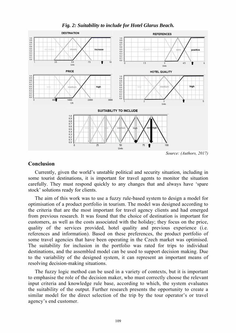
Fig. 2: Suitability to include for Hotel Glarus Beach.


Conclusion

Currently, given the world’s unstable political and security situation, including in some tourist destinations, it is important for travel agents to monitor the situation carefully. They must respond quickly to any changes that and always have ‘spare stock’ solutions ready for clients.

The aim of this work was to use a fuzzy rule-based system to design a model for optimisation of a product portfolio in tourism. The model was designed according to the criteria that are the most important for travel agency clients and had emerged from previous research. It was found that the choice of destination is important for customers, as well as the costs associated with the holiday; they focus on the price, quality of the services provided, hotel quality and previous experience (i.e. references and information). Based on these preferences, the product portfolio of some travel agencies that have been operating in the Czech market was optimised. The suitability for inclusion in the portfolio was rated for trips to individual destinations, and the assembled model can be used to support decision making. Due to the variability of the designed system, it can represent an important means of resolving decision-making situations.

The fuzzy logic method can be used in a variety of contexts, but it is important to emphasise the role of the decision maker, who must correctly choose the relevant input criteria and knowledge rule base, according to which, the system evaluates the suitability of the output. Further research presents the opportunity to create a similar model for the direct selection of the trip by the tour operator’s or travel agency’s end customer.

109

Acknowledgements

This article was prepared with the aid of research project: [No. 20171020], Designing Experiments on Manufacturing and Services, Internal Grant Agency of the Faculty of Economics and Management of the Czech University of Life Sciences Prague.

References BHATIA, A. K. (2012) The Business of Travel Agency and Tour Operations Management. Sterling Publishers Private Limited, ISBN 978-81-207-6921-2.

BIGNÉ, J. E., SÁNCHEZ, M. I., SÁNCHEZ, J. (2001) Tourism image, evaluation variables and after purchase behavior: inter-relationship. Tourism Management. 22(6): 607-616. ISSN 02615177.

CHANG, J. R., CHANG, B. (2015) The Development of a Tourism Attraction Model by Using Fuzzy Theory. Mathematical Problems in Engineering. p. 1-10, ISSN 1024-123x.

CHEN, Ch. F., CHEN, F. S. (2010) Experience quality, perceived value, satisfaction and behavioral intentions for heritage tourists. Elsevier B.V. 31(1), p. 29-31.

CSO STATISTICS. (2015) Nejoblíbenější dovolenkové destinace pro cesty trvající déle, než 4 dny.

Available at: https://www.mmr.cz/getmedia/a6e7ee4f-2a6f-46a4-ac13-099bc5477e3f/Vyjezdovy-a-

domaci-CR-rok-2015-z.pdf [Accessed 2017-01-31]

DOSTÁL, P., RAIS, K., SOJKA, Z. (2005) Pokročilé metody manažerského rozhodování. Praha: Grada Publishing, p. 168. ISBN 80-247-1338-1.

eTRAVEL, (2016) Kde je letos bezpečná dovolená. Available at: https://www.etravel.cz/novinky/276-bezpecna-dovolena-u-more [Accessed 31-08-2017].

INFORM GmbH. Professional Demo fuzzyTECH 5.81d [online] Available at: http://www.fuzzytech.com/. [Accessed 04-10-2016].

INVIA.CZ. (2016) U first minute zájezdů posílil zájem o tradiční evropské destinace, vede Bulharsko a Chorvatsko. [online] Tiskové zprávy. Available at: https://www.invia.cz/o-invia/press/tiskove-zpravy/3589-u-first-minute-zajezdu-posilil-zajem-o-tradicni-evropske-destinace-vede-bulharsko-a-chorvatsko/ [Accessed 31-01-2017].

LEONDES, C. T. (2002) Expert systems: the technology of knowledge management and decision making for the 21st century. Edition 6. San Diego: Academic Press, p. 1947. ISBN 0124438806.

Martínez, L., Rodriguez, R. M., Herrera, F. (2015) The 2-Tuple Linguistic model. New York, NY: Springer Science+Business Media. ISBN 9783319247120.

NECKERMANN CK. (2016) Nejprodávanější letní destinace pro rok 2017. [online] Available at: In: http://www.ckneckermann.cz/ [Accessed 27-12-2016].

PAL, S. K., POLKOWSKI, L., SKOWRON, A. (2004) Rough-Neural Computing Techniques for Computing with Words. Berlin, Heidelberg: Springer Berlin Heidelberg. ISBN 3642188591.

PAPPA, N. (2015) "Consumer Preferences and Key Aspects of Tourism and Hospitality Marketing on Island Destinations." Hospitality, Travel, and Tourism: Concepts, Methodologies, Tools, and Applications. IGI Global, p. 904-923.

PIKE, S. (2008) Destination Marketing: an integrated marketing communication approach. Amsterdam: Elsevier, p. 406. ISBN 978-0-7506-8649-5.

POKORNÝ, M. KEPRT, A. MENŠIK, M. (2013) Fuzzy analýza ukazatele výkonnosti zákaznické dimenze. Scientific Papers of the University of Pardubice, Series D Supply., 29, 4: 132 144.

SILER, W., BUCKLEY, J. J. (2005) Fuzzy expert systems and fuzzy reasoning. Hoboken, N.J.: Wiley.

110

SOHRABI et al. (2012). An exploratory analysis of hotel selection factors: a comprehensive survey of Tehran hotels. International Journal of Hospitality Management, 31 (1), 96 – 106.

TANGELAND, T., VENNESLAND, B., NYBAKK, E. (2013) Second-home owners' intention to purchase nature-based tourism activity products – A Norwegian case study. Tourism Management. 36, p. 364-376.

TKACZYNSKI, A.et all. (2010) Destination Segmentation: A Recommended Two-Step Approach. Journal of Travel Research. Volume 49-2, p. 139-152. p. ISSN 00472875.

VOLNÁ, E. (2012) Základy softcomputingu. ČOP: CZ.1.07. Ostrava. Vzdělávání pro konkurenceschopnost. Opatření 7.2. Oblast podpory 7.2.2. Reg. č. projektu: CZ.1.07/2.2.00/28.0245. [online] Available at: http://www1.osu.cz/~volna/Zaklady_softcomputingu.pdf [Accessed 27-01-2017].

UOE, Prague and Association of Czech Travel Agents (2010) CK Neckermann – průzkum trhu. [online]. Available at: http://kcr.vse.cz/wp-content/uploads/2009/10/Souhrná-zpráva.pdf [Accessed 01-11-2016].

ZADEH, L. A. (1996) Fuzzy logic= computing with words. IEEE transactions on fuzzy systems, 4.2: 103-111.

ZIMMERMANN, H. J. (1987) Fuzzy Sets, Decision Making, and Expert Systems. Dordrecht: Springer Netherlands. ISBN 978-940-0932-494.

Contact address

Ing. Monika Jadrná Czech University of Life Sciences Prague, Faculty of Economics and Management, Department of Management Kamycka 129, 165 21 Praha 6 – Suchdol, Czech Republic Email: [email protected] Phone number: +420608128328

doc. Ing. Tomáš Macák, Ph.D. Czech University of Life Sciences Prague, Faculty of Economics and Management, Department of Management Kamycka 129, 165 21 Praha 6 – Suchdol, Czech Republic Email: [email protected] Phone number: +420732162707


111

COMPARISON OF MORTALITY CAUSED BY SERIOUS DISEASES WITHIN REGIONS OF THE CZECH REPUBLIC

Lucie Kopecká

Abstract: The various serious diseases affect the human population all over the world. Good population health is one of the indicators of prospering country and influences economic prosperity. Oncological and cardiovascular diseases belong to the most frequently occurring causes of death in Europe but also in the Czech Republic (CR). The main aim of this article is to provide and present results of multivariate statistical methods which include correlation analysis, factor analysis, cluster analysis and multidimensional comparative analysis. We are able to provide an overview of mortality caused by oncological and cardiovascular diseases by selected indicators of mortality by using multivariate statistical methods in different regions. This information on mortality which is caused by these serious diseases is useful for the health sector to take appropriate measures against these diseases in different regions, it is also useful for insurance companies to improve offer of critical illnesses insurance and useful for revealing socio-economic situation in individual regions within the CR. Data are obtained from the database of National Health Information System of the CR (NZIS CR).

Keywords: Serious Diseases, Mortality, Correlation Analysis, Factor Analysis, Cluster Analysis, Multidimensional Comparative Analysis.

JEL Classification: C38, I15.

Introduction

Serious diseases are the most often causes of death worldwide. Oncological and cardiovascular diseases belong to the most frequently occurring causes of deaths which primarily affect the population in the developed countries such as European countries. Specifically, the Czech Republic (CR) belongs to the countries which are more vulnerable. Mortality from the cardiovascular diseases is higher than mortality from the oncological diseases, which can be caused primarily by stress and poor diets in the CR according to the website of Institute of Health Information and Statistics (ÚZIS ČR, 2016). Although the Europe belongs to the most developed parts of the world, significant socio-economic disparities exist among European countries, which influence health and mortality in Europe as demonstrates (Staníčková, 2015).

Research in this field is important because risks which result from the occurrence of these diseases influence not only the health sector but also insurance companies which offer products of critical illnesses insurance as describes (Jindrová, 2013). As in the case of European countries, significant differences in mortality can exist within regions in the CR and they are the reason for research, see (Jindrová & Kopecká, 2017; Kopecká & Jindrová, 2017). Not only socio-economic disparities can influence mortality in the individual regions but also high mortality can cause bad socio-economic environment in these regions because they create together vicious circle. These following publications deal with socio-economic situation, health care

112

and health conditions of European population, see (Clark et. al., 2017; Gavurová & Vagasová, 2016; Šoltés & Gavurová, 2014).

1. Statement of a problemThe main aim of this article is to provide and present the results of multivariate

statistical methods and to provide an overview of mortality caused by oncological and cardiovascular diseases by selected indicators of mortality in different regions in the CR.

Oncological and cardiovascular diseases belong to the most frequently occurring causes of death in Europe but also in the CR where the mortality caused by these diseases is still higher than mortality in the more developed western European countries as mentioned (Jindrová & Kopecká, 2017; Kopecká & Jindrová, 2017).

However, cardiovascular diseases are more frequently causes of deaths than oncological diseases. Development of the mortalities caused by oncological and cardiovascular diseases has a decreasing character almost in all cases with a few exceptions, for example mortalities caused by malignant neoplasm of the cervix uteri, malignant melanoma of the skin and ischemic heart diseases. It is observed from 1994 to 2015. For instance, mortalities caused by malignant neoplasms of the larynx, trachea, bronchus and lung, malignant neoplasms of colon and rectum and malignant neoplasms of female breast belong to the most common mortalities. On the other hand, mortalities associated with malignant neoplasms of lymphoid hematopoietic and related issue, malignant neoplasms of stomach and malignant neoplasms of skin belong to less frequent mortalities as demonstrates database (ÚZIS ČR, 2016).

As mentioned above, significant differences in mortality exist not only among European countries but these differences can exist within regions of these counties as well. CR is divided into 14 regions, namely Karlovarský, Plzeňský, Ústecký, Liberecký, Středočeký, Prague, Jihočeský, Královéhradecký, Pardubický, Vysočina, Olomoucký, Jihomoravský, Zlínský and Moravskoslezský as describes (ČSÚ, 2017).

We are able to measure the strength of association between and within variables, reveal the structure of the common factors, classify the regions according to similarity and finally arrange the regions by descending order from the lowest mortality due to these diseases into the highest by using multivariate statistical methods such as correlation analysis, factor analysis, cluster analysis and multidimensional comparative analysis. For example, multivariate statistical methods are described in following publications (Hebák et. al., 2007a; Hebák et. al.; 2007b, Kubanová, 2008; Řezanková et. al., 2009; Stankovičová & Vojtková, 2007). On the other hand, these methods are used within these articles, namely (Jindrová & Kopecká, 2017; Kopecká & Jindrová, 2017; Pacáková & Papoušková, 2016; Pacáková et. al., 2016; Petr et. al., 2010).

2. Methods

2.1 Data All data associated with mortality caused by oncological and cardiovascular

diseases are obtained from the database of National Health Information System CR (NZIS CR) as demonstrates (ÚZIS ČR, 2016). Each variable related to mortality is drawn for each region for the entire 14-year period (1994-2015) and they are converted to the European standard ASR (E) 2013. ASR (E) is called age-standardized

113

rate for Europe 2013. It means that this rate is created by using European Standard Population (ESP) representing European population with a standard age structure. This population age structure was updated in 2013. ASR (E) 2013 is calculated per 100 000 population. For example, this rate is often used in case of mortality which represents the proportion of deaths from a particular population during certain period. For details, see (National archives, 2016).

First, it is necessarily to compile a data matrix where the rows of this matrix are represented by 14 regions (objects) and the columns are presented by 12 quantitative indicators of mortality caused by oncological and cardiovascular diseases (variables). The variables that are intended for using multivariate statistical methods include: malignant neoplasms (X1), malignant neoplasms of lymphoid hematopoietic and related tissue (X2), malignant melanoma of the skin (X3), malignant neoplasm of the cervix uteri (X4), malignant neoplasm of the larynx, trachea, bronchus and lung (X5), malignant neoplasm of the prostate (X6), malignant neoplasm of the female breast (X7), malignant neoplasm of the colon and rectum (X8), malignant neoplasm of the stomach (X9), heart diseases, including cerebrovascular (X10), ischemic heart diseases (X11), cerebrovascular diseases (X12). All mortality variables are expressed in ASR (E) as demonstrates (ÚZIS ČR, 2016).

2.2 Correlation analysis and Kayser-Meyer-Olkin index Non-correlated variables belong to the important assumption for using cluster

analysis. The Pearson and the Spearman correlation coefficients are the correlation coefficients which measure strength of associations between variables, see (Hebák et. al., 2007a, Kopecká & Jindrová, 2017; Kubanová, 2008, Řezanková et. al., 2009). The Kayser-Meyer-Olkin index (KMO) is another way of measuring associations. This index measures associations within the group of variables. The Measure of sampling adequacy rate (MSA) is simplified and analogous rate of the KMO index. When the MSA rate points to considerable associations among variables, it is a good result for application of component analysis before using cluster analysis, see (Hebák et. al., 2007b, Kopecká & Jindrová, 2017; Stankovičová & Vojtková, 2007).

2.3 Factor analysis First, appropriate number of factors have to be determined by using eigenvalues at the

beginning of factor analysis. The main aim of factor analysis is to determine m variables by using a smaller number of common factors. For details, see (Hebák et. al., 2007b, Jindrová & Kopecká, 2017; Stankovičová & Vojtková, 2007). Relationship between variances of original and derived factor is significant result of factor analysis. Rotation of factors is the important part of factor analysis. Varimax rotation belongs to the most used rotations of factors. Next, correlations are expressed by factor loadings between the selected variables and the factors. Factor loadings point out what percentage of the variance the factor explains within the selected variables. However, factor scores are the final results of factor analysis. They assign the values of the rotated factor scores to the each object. For details, see (Pacáková & Papoušková, 2016).

2.4 Cluster analysis Cluster analysis is used to classifying the objects into group so that the objects are

the most different among the group and the most similar inside the group. Cluster analysis is based on the input data matrix. The rows of this matrix are presented by n

114

objects and the columns are presented by m selected variables. Euclidean distance is the most common distance between the objects and Ward’s method belongs to the most important and the most used hierarchical methods as describe (Hebák et. al., 2007b, Kopecká & Jindrová, 2017; Petr et. al., 2010, Řezanková et. al., 2009).

2.5 Multidimensional comparative analysis Multidimensional comparative analysis is applied because of comparing objects

which are evaluated by several variables. It is useful for arranging objects by descending order from the best into the worst. First of all, the type of each variable should be defined. The reason is that the “great” values of some variables influence analysis positively (stimulants) and “small” values of some variables influence analysis negatively (destimulants). Standardization of stimulants is expressed by formula (1) and standardization of destimulants is expressed by formula (2), see (Pacáková & Papoušková, 2016, Pacáková et. al., 2016, Stankovičová & Vojtková, 2007):

100max,

j

ijij x

xb , (1)

100min, ij

jij x

xb , (2)

where xij is value of i-th object on j-th variable, xmax,j is maximal value of j-th variable and xmin,j is minimal value of j-th variable. Finally, the score for each country is average of bij.

3. Problem solvingAll results which are presented by employing methods mentioned above are

constructed by programs EXCEL and STATISTICA in this chapter. First, associations between and among variables are determined. Then structure of common factors and similarity of the regions are found out and finally, the regions are arranged by descending order from the lowest mortality into the highest.

3.1 Results of correlation analysis and Kayser-Meyer-Olkin index Overall the MSA rate acquiring value 0.43 points to poor association among the

variables which are mentioned above, which is reason for absence of component analysis before using cluster analysis mainly because of inappropriateness of original variables for component analysis and loss of information from the variables. However, the significant associations exist between some pairs of the variables according to the Spearman correlation coefficient. For example, the considerable associations are between variables namely X1 and X4, X5, X6, X7, X8 (0.85, 0.96, 0.54, 0.70, 0.93) and next between X5 and X4, X8 (0.92, 0.81). But on the other hand, a very poor association is between X1 and X10 (0.36).

3.2 Results of factor analysis First of all, the eigenvalues are determined of the correlation matrix in Fig. 3.

115

Fig. 1: Scree plot presenting eigenvalues

Source: own

Fig. 1 shows that the top four factors are suitable for using because values of eigenvalue numbers achieve values higher than 1 and explain together more than 87 % of the original variables variability.

Now, the groups of variables are determined by employing four factors through the factor loadings after Varimax rotation in Tab. 1, which is the main aim of factor analysis.

Tab. 1: Factor loadings after the Varimax rotation Variables Factor 1 Factor 2 Factor 3 Factor 4

X1 0.96 0.04 0.16 0.19

X2 0.23 -0.53 0.62 0.21

X3 -0.07 -0.04 0.80 -0.37

X4 0.92 0.20 -0.15 -0.01

X5 0.97 0.05 0.01 0.14

X6 0.42 0.33 0.64 0.25

X7 0.71 -0.48 0.32 0.07

X8 0.84 0.12 0.29 0.24

X9 0.41 0.83 -0.09 -0.14

X10 0.25 0.71 -0.21 0.58

X11 -0.12 0.90 0.18 0.23

X12 0.20 0.06 -0.03 0.92 Source: own

Each of factors can be interpreted according to factor loadings after Varimax rotation. The factor 1 is presented by variables which provide information on mortality caused by oncological diseases, namely malignant neoplasm of the cervix uteri, malignant neoplasm of the larynx, trachea, bronchus and lung, malignant neoplasm of the female breast and malignant neoplasm of the colon and rectum. The factor 2 is described primarily by malignant neoplasm of the stomach and hearth diseases, concretely ischemic heart diseases. After that, the factor 3 is the next factor which

116

presents mortality caused by oncological diseases, namely malignant neoplasms of lymphoid hematopoietic and related tissue, malignant melanoma of the skin and malignant neoplasm of the prostate. Finally, the last factor 4 is described by cerebrovascular diseases.

The significant positive correlations exist between the original variables and the factors after Varimax rotation. It means that the high values of factor scores of individual factors indicate the high mortality caused by these diseases.

The factor 2, factor 3 and factor 4 which are described above are always presented with the factor 1 within Fig. 2, Fig. 3 and Fig. 4. The positions of the regions, associations between factors and outliers of the regions can be revealed according to these four factors through these figures.

Fig. 2: Location of the regions according to factor 1 and factor 2

Source: own


Source: own

117


Source: own

The state of mortality can be detected in individual regions based on these three figures above because the regions can be divided into 4 quadrants. The regions are situated according to factor 1 which is represented by the most frequently occurring oncological diseases and factor 2 which is described by malignant neoplasm of the stomach and hearth diseases, concretely ischemic heart diseases in Fig. 2. The worst situation is in Ústecký region. On the other hand, Královéhradecký region belongs to the regions with the lowest mortality due to these factors. The first quadrant is created by Ústecký, Karlovarský, Liberecký and Moravskoslezský regions where the situation in mortality is bad according to factor 1 and factor 2. The second quadrant contains regions such as Zlínský and Olomoucký where the situation is bad according to factor 2 and good according to factor 1. Prague, Královéhradecký, Pardubický, Vysočina, and Jihomoravský regions creates the third quadrant where the situation in mortality is the best according to the both factors. The last quadrant is created by Plzeňský, Jihočeský and Středočeský regions where the situation is worse according to factor 1 and better according to factor 2.

Next, the regions are situated according to factor 1 and factor 3 which provides information on mortality caused by less frequent oncological diseases in Fig. 3. Plzeňský and Liberecký regions belong to the regions with the highest mortality and Pardubický and Zlínský regions belong to the regions with the best situation in mortality in this case. The first quadrant includes Ústecký, Karlovarský, Plzeňský, Jihočecký and Liberecký regions where the situation in mortality is bad according to factor 1 and factor 3. The second quadrant contains regions such as Prague and Vysočina where the situation is worse according to factor 3 and better according to factor 1. Good situation in mortality is within Královéhradecký, Pardubický, Jihomoravský, Olomoucký and Zlínský regions according these factors. The last quadrant is created by Středočeský and Moravskoslezský regions.

Finally, according to factor 1 and factor 4 which represents mortality caused by cerebrovascular diseases Ústecký, Karlovarský, Plzeňský and Středočeský regions belong to the worst regions and Prague, Královéhradecký, Pardubický, Olomoucký, Jihomoravský and Zlínský regions belong to the best in Fig. 4.

118

However, the outliers include Ústecký and Karlovarský regions in all three figures. These regions belong to the regions with worse situation of mortality caused by oncological and cardiovascular diseases in all cases mentioned above.

In term of associations between these four factors the significant correlation 0.73 is detected only between factor 1 and factor 4, which can be observed in Fig. 4.

3.3 Results of cluster analysis Hierarchical Ward’s method is applied by using normalized dataset within cluster

analysis. Ward’s method classifies the regions according to similarity. The important clusters are revealed in Fig. 5.

Fig. 5: Dendrogram representing similarities within regions

Source: own

Fig. 5 shows significant three clusters at a distance which equals 6. First cluster contains regions such as Moravskoslezský, Zlínský, Pardubický, Jihomoravský, Královéhradecký, Olomoucký, Vysočina and Středočeský. These eight regions belong to the regions with lower mortality caused by malignant neoplasm of the cervix uteri, malignant neoplasm of the larynx, trachea, bronchus and lung, malignant neoplasm of the female breast and malignant neoplasm of the colon and rectum according to factor analysis. Next cluster includes only two regions, namely Ústecký and Karlovarský regions which represent regions with higher mortality caused by all diseases mentioned above. Finally, regions such as Liberecký, Plzeňský, Jihočeský and Prague create the last cluster. These regions belong to the regions where the situation in mortality is average within results of factor analysis. However, these four regions are worse in mortality caused by malignant neoplasms of lymphoid hematopoietic and related tissue, malignant melanoma of the skin and malignant neoplasm of the prostate. But situation in mortality is better in Prague than in these three remaining regions within the last cluster.

3.4 Results of multidimensional comparative analysis Multidimensional comparative analysis is useful for determining the order. It means

that the regions are arranged by descending order from the lowest mortality caused by oncological and cardiovascular diseases to the highest. The score 1 (X1-X9) describing

119

mortality caused by oncological diseases, score 2 (X10-X12) describing mortality from cardiovascular diseases and finally, score 3 (X1-X12) indicating mortality caused by both of them are displayed in Tab. 2.

Tab. 2: Ranking of the regions according to score 1, score 2 and score 3 Rank Region Score 1 Region Score 2 Region Score 3

1 Pardubický 93.41 Prague 100.00 Pardubický 91.72

2 Zlínský 92.50 Karlovarský 89.74 Prague 89.75

3 Vysočina 90.27 Královéhrad. 87.61 Zlínský 89.35

4 Jihomoravs. 89.35 Pardubický 86.62 Královéhrad. 88.75

5 Královéhrad. 89.13 Jihočeský 86.20 Jihomoravs. 88.44

6 Olomoucký 86.72 Jihomoravs. 85.73 Vysočina 87.38

7 Prague 86.33 Olomoucký 84.38 Olomoucký 86.14

8 Středočeský 84.99 Plzeňský 83.70 Středočeský 83.56

9 Jihočeský 82.24 Moravskosl. 83.56 Jihočeský 83.23

10 Moravskosl. 82.19 Liberecký 83.52 Moravskosl. 82.53

11 Plzeňský 80.12 Zlínský 79.88 Plzeňský 81.01

12 Liberecký 79.32 Středočeský 79.26 Liberecký 80.37

13 Karlovarský 75.06 Vysočina 78.69 Karlovarský 78.73

14 Ústecký 74.69 Ústecký 69.72 Ústecký 73.45 Source: own

The ranking of the regions is changing in all three cases according to Tab. 2. Pardubický region belongs to the regions with the lowest mortality. On the other hand, Ústecký region shows the highest mortality caused by these diseases. A poor association exists between score 1 and score 2 by using the Spearman correlation coefficient which takes the value 0.12. But on the other hand, a strong association is found between score 1 and score 2, namely 0.92. It is possible to see that the ranking of the regions is similar in case of score 1 and score 3 and different in case of score 2 and score 3.

Discussion The data which carry information on mortality caused by critical illnesses in the

regions within the CR were obtained based on database of NZIS CR. This information was obtained by employing multivariate statistical methods and using programs EXCEL and STATISTICA.

First, the Spearman correlation coefficients together with MSA rate revealed several significant associations, mainly between mortalities from oncological diseases and a poor association among the entire group of the selected variables.

Next, the four important factors and their structure were found out by using factor analysis. The first of them factor 1 is described by the most frequently occurring deaths caused by oncological diseases. The factor 2 represents deaths due to malignant neoplasm of the stomach and hearth diseases, concretely ischemic heart diseases which can be caused by stress. Factor 3 is determined by deaths because of less frequently occurring oncological diseases. The last factor 4 expresses deaths which are caused

120

by cerebrovascular diseases. It can be said that Ústecký and Karlovarský regions belong to the most affected regions but on the other hand, Pardubický region belongs among the least affected regions in the CR based on these factors.

After that, three significant clusters were detected based on cluster analysis. The first cluster contains Moravskoslezský, Zlínský, Pardubický, Jihomoravský, Královéhradecký, Olomoucký, Vysočina and Středočeský regions which belong to the regions with the best situation in mortality according to factor analysis. Ústecký and Karlovarský regions create the second cluster which includes the regions with the worst situation in mortality and the last cluster includes Liberecký, Plzeňský, Jihočeský and Prague regions which are considered as average in case of mortality. Finally, the results of cluster analysis are very similar to the results of multidimensional comparative analysis in case of mortality from oncological diseases but different in case of mortality from cardiovascular diseases.

Conclusion

Malignant neoplasms belong to the diseases with the high mortality within CR. On the other hand, cardiovascular diseases are the most dangerous diseases at all.

The main aim of this article was to provide and present the results of multivariate statistical methods and to provide an overview of mortality caused by oncological and cardiovascular diseases by selected indicators of mortality within different regions in the CR.

The results of multivariate statistical methods can be useful for health sector to take appropriate measures against these diseases and insurance companies to improve offer of the critical illnesses insurance within the CR. This overview of mortality brings information on significant differences in mortality situation within individual regions in CR. These differences explain one of the causes of socio-economic inequalities within regions of CR and they can lead to worsening of the situation, especially in the most affected regions.

Acknowledgement

This work was supported by SGS University of Pardubice, FEA, No. SGS_2017_022, “Ekonomický a sociální rozvoj v soukromém a veřejném sektoru”.

References

Clark, J. S., Dttrich, L. O., Stará, D., Barták, M. (2017). The Visit Fees and its Influence on Overall Health Expenditures – the Case of the Czech Republic. E&M Ekonomie a Management, 20(2), pp. 4-14. doi: 10.15240/tul/001/2017-2-001.

ČSÚ. (2017). Regionální statistiky. [online]. Available at: https://www.czso.cz/csu/czso/regiony_mesta_obce_souhrn. [accessed 10. March 2018].

Gavurová, B., Vagasová, T. (2016). Regional differences of standardised mortality rates for ischemic heart diseases in the Slovak Republic for the period 1996-2013 in the context of income inequality. Health Economics Review, 6(21). doi:10.1186/s13561-016-0099-1.

Hebák, P., Hustopecký, J., Jarošová, E., Pecáková, I. (2007a). Vícerozměrné statistické metody (1). Second edition. Praha: Informatorium.

121

Hebák, P., Hustopecký, J., Pecáková, I., Průša, M., Řezánková, H., Svobodová, A., Vlach, P. (2007b). Vícerozměrné statistické metody (3). Second edition. Praha: Informatorium.

Jindrová, P. (2013). Quantification of Risk in Critical Illness Insurance. In: Conference proceedings from 9th international scientific conference Financial Management of Firms and Financial Institutions, VŠB Ostrava pp. 298-306.

Jindrová, P., Kopecká, L. (2017). Assessment of risk factors of serious diseases in OECD countries. In: Proceedings of the 11th Professor Aleksander Zelias International Conference on Modelling and Forecasting of Socio-Economic Phenomena. Cracow: Cracow University. pp. 123-132.

Kopecká, L., Jindrová, P. (2017). Comparison of Mortality due to Critical Illnesses in the EU Countries, Proceedings of the 11th Professor Aleksander Zelias International Conference on Modelling and Forecasting of Socio-Economic Phenomena. Cracow: Cracow University. pp. 133-142.

Kubanová, J. (2008). Statistické metody pro ekonomickou a technickou praxi. Third edition. Bratislava: Statis.

National archives. (2016). Revised European Standard Population 2013. [online]. Available at: http://webarchive.nationalarchives.gov.uk/20160106020035/http://www.ons.gov.uk/ons/guide-method/user-guidance/health-and-life-events/revised-european-standard-population-2013--2013-esp-/index.html. [accessed 25. February 2018]

Pacáková, V., Jindrová, P., Zapletal, D. (2016). Comparison of Health Care Results in Public Health Systems of European Countries. European Financial Systems 2016. Vol. XIII, pp. 534-541.

Pacáková, V., Papoušková, M. (2016). Multidimensional Comparisons of Health Systems Functioning in OECD Countries. International Journal of Mathematical Models and Methods in Applied Sciences, 10, pp. 388-394.

Petr, P., Křupka, J., Provazníková R. (2010). Statistical Approach to Analysis of the Regions. International Conference on Applied Computer Science. 10, pp. 280-285.

Řezanková, H., Húsek, D., Snášel, V. (2009). Shluková analýza dat. Second edition. Praha: Professional Publishing.

Staníčková, M. (2015). Classifying the EU Competitiveness Factors Using Multivariate Statistical Methods. Procedia Economics and Finance. 23, pp. 313-320.

Stankovičová, I., Vojtková. M. (2007). Viacrozmerné štatistické metódy s aplikáciami. Bratislava: IURA Edition.

Šoltés, V., Gavurová, B. (2014). The Functionality Comparison of the Health Care Systems by the Analytical Hierarchy Process Method. E&M Ekonomie a Management, 17(3), pp. 100-117. doi:10.15240/tul/001/2014-3-009.

ÚZIS ČR. (2016). Regionální zpravodajství Národního zdravotnického informačního systému. [online]. Available at: http://reporting.uzis.cz/ [accessed 22. February 2017].

Contact Address

Ing. Lucie Kopecká University of Pardubice, Faculty of Economics and Administration, Institute of Mathematics and Quantitative Methods Studentská, 95, 532 10, Pardubice, Czech Republic E-mail: [email protected] Phone number: +420466036017


122

MEASURING THE SIZE OF THE TECHNOLOGY GAP AT A LEVEL OF CZECH REGIONS

Sylvie Kotíková

Abstract: The technology gap is one of key determinants of spillovers. This paper aims to quantify the size of the technology gap between foreign direct investments, which received investment incentives and business environment in six regions of the Czech Republic in time series of 2002-2014. The development of regional technology gap was determined by using the Shift-share analysis method - decomposition of the region's technological level into productivity, employment, and a combination of both of the effects. The main data source was the statistics issued decisions of investment incentives published by the agency CzechInvest; annual reports of foreign companies; data of the Czech Statistical Office and the OECD. The established indicator tracks the difference between the technological advancement of foreign firms and a regional business environment. The higher the value of this indicator than in other regions is, the higher the potential for technological growth the region has than regions compared. The magnitude of the value is given by the technological level of foreign companies and their share in regional employment. The best position takes the Pilsen region, which has the highest potential for spillovers in terms of the technology gap. On the contrary, the worst position has the Carlsbad region.

Keywords: Foreign Direct Investment, Foreign Presence, Investment Incentives, Productivity, Technology Gap.

JEL Classification: F23, O33.

Introduction

Foreign direct investment (FDI) is considered to be an economic phenomenon with an ambiguous interpretation of the professional public, as this type of foreign capital produces a number of effects and influences on the host business environment, the final impact of which is often contradictory. Another complication is the difficult identification and quantification of spillovers (Mišun and Tomšík, 2002), which have the character of externalities and do not have a clearly specified link to FDI. However, this kind of effects result from direct effects and the location of FDI (Pavlínek and Žížalová, 2016).

Opinions on FDI are even more divergent if the flow of capital is supported by investment incentives. Governments spend considerable volumes of public support to obtain positive effects that are considered to be self-evident but in reality, very difficult to measure. The issue is deepened while monitoring the effects or determining and evaluating of the potential for the emergence of effects at a lower regional level than the level of individual economies.


Even though the effects of FDI are under broad discussion in the literature, there are very few studies and approaches that would quantify, comprehensively evaluate and compare direct and indirect effects of FDI and their potential at lower regional levels - to identify their effects and the potential for emergence in the regional business environment. Particularly spillover effects are very difficult to measure (Blomström and Kokko, 2001). For example, it is not possible to determine whether domestic enterprises have increased productivity due to

123

competitive pressure or imitation process (Navaretti and Venables, 2013). Although contemporary literature focuses on the aspects and effects of FDI, which helps to better understanding of analyzing problematics from a microeconomic point of view, the quantification of individual effects or their determinants at the lower regional level is not dealt with at all. There is no standardized methodology to quantify the magnitude of spillover effects on the regional business environment, or whether the regional business environment has the potential to generate positive effects of spillovers.

However, the determinants of indirect positive effects of spillovers are known. These include, particularly, the size of the host market and the level of competition therein, the absorption capacity of domestic firms, the adaptability of workers, the institutional environment, foreign presence (FP) and the size of the technology gap (Görg et al., 2008).

The first to deal with research into the secondary impact of FDI on the host economy was Finlay (1978), who found out in his research that spillover effects are determined by so-called relative lagging, it means technology gap between parent and host economies. Finlay claimed in his work that the larger the technological gap, the greater the spillover effect. The author is based on the basic assumption that a foreign investor is always from a more advanced economy than the area where FDI locates.

On the other hand, Görg et al., (2011), Cantwell (2017) and Cohen and Levinthal (1990),

modify opinions on the position of the factor of the technology gap and its effect on the spillover effects. From their conclusions follows that if the technology gap is too large, domestic enterprises are unable to transfer technology both in the horizontal (for example through the imitation effect of FDI) and in the vertical direction as well. A large technological gap may lead to a crowding-out effect when local businesses are not able to compete with FDI.

As with a significant technology gap, FDI can function as so-called cathedrals in the desert. In this case, they are large production plants that use relatively advanced technology (cathedral), with a sparse number of links to the host region (desert). The cathedral in the desert is also characterized by two subordinates - both ownership and management and decision-making, as well as subordination to production where such FDI provides only a certain stage of production. FDI perspectives depend on both the efficiency of production and the commercial success of the complete product (for example a car). For successful in the dissemination of knowledge (spillover effect), can be considered such regions without the dominance of these individual actors (cathedrals), but regions with a dense network of links between entities.

In the case of a significant technology gap, the positive spillover effect does not arise. Due to the size of the technology gap, the isolation of FDI will cause workers not to disseminate their knowledge and experience, which may be due to a fundamental separation of production and conceptual processes where the branch is fully subordinated to the headquarter in the parent economy. Massey (2007) sees the solution in providing a varied structure of job functions at all skill levels. However, this also raises the question of whether the qualifications structure and the employers' demands in the host labor market are reconciled.

On the other hand, too little technology gap does not allow for learning and technology transfer. Consequently, the most likely positive spillover effect may occur with the mild technological gap.

Kokko (1994, 1996, 2014) has dealt with finding a link between the degree of foreign presence and existence of spillover effects. Based on a competition analysis of the Mexican

124

case, he came to the conclusion that this relationship does not always exist. On the one hand, he found that the spillover effect does not occur in areas where are dominant MNCs, but on the other hand, in areas where the foreign presence is up to 50% and increases over time, this effect has been identified.

The degree of foreign presence in a region or industry is an indicator that affects a variety of factors, such as product differentiation, industry specialization or the role of global networks (Benáček, 2000, 2006).

Whether or not the effects will eventually occur does not only depend on the presence of foreign firms. The FDI localization itself is only a first step, the ultimate effect is mainly dependent on the interaction between domestic and foreign enterprises. It also follows from the above that the spillover effects are also conditioned by the mutual position of the companies (Kotíková and Čuhlová, 2016).

The aim of the contribution is to quantify the size of the technological gap between FDI that received an investment incentive and entrepreneurial environment in six regions of the Czech Republic in the time series from 2002 to 2014. To contribute to the expert discussion on the FDI impact on the regional business environment to a certain extent infills a gap in current economic research to assess the impact of FDI on the business environment of lower regional levels. Given the criterion of awarding investment incentives, the conclusions may also be used in the arguments relating to this type of public support.

2 Methods

FDI effects are examined on a sample of six regions of the Czech Republic. Respectively, impacts of FDI effects are identified within the business environment of the Pilsen, Carlsbad, Ústí nad Labem, Liberec, Hradec Králové and Pardubice regions (at NUTS 3 level). The common characteristics of these regions are the border position and the neighboring of regions. These are NUTS 2 Northeast, NUTS 2 Northeast and the Pilsen region. The Pilsen region appears to be a control case in the surveyed region sample. The Pilsen region was chosen as a control case due to unique position within Czech Republic. Given its strategic position it enjoys spillovers from well-developed Bavaria that are caused by both short distance, above-average level of infrastructure with Bavaria and long-term cooperation between entrepreneur environments. In comparison with other regions, in terms of contribution to GDP, concentration of business activity and FDI inflow, as well as the firm anchoring and continuous tradition of important industries it can be concluded that the greatest results of technology gap will be quantified in the Pilsen region (Czech Statistical Office, 2017). In these circumstances is possible to expect the best position of Pilsen region in analyzed set of regions, the opposite situation could indicate anomalies in the surveyed set of regions.

It is difficult to identify the effects of all FDI because of the lack of relevant data, but it is possible to rely on resources of CzechInvest, which files projects of foreign investors – applicants for investment incentives. The main source of data was statistics issued by the CzechInvest agency on investment incentives provision (CzechInvest, 2017). A secondary source is the financial statements and annual reports of foreign companies that have received a promise of investment incentives (Ministry of Justice, 2017). From the CzechInvest evidence, were obtained a list of FDIs including information on regional location, investor's country of origin, sector, accorded investment incentives, promises of the number of newly created jobs and other information. This information was subsequently extended by data on

125

the number of employees obtained from the annual reports by the analyzed company for each year of the analyzed period.

The CzechInvest agency (2017) states that as of January 1, 2017 out of a total of 1053 projects, 536 were foreign company projects. Of which 230, i.e. 43%, of them went to the surveyed region sample.

Foreign presence (FP) is the level of foreign investment in the economy, region or industry, expressed by the share of foreign companies' employment in total employment in the economy, region or industry (Görg and Greenaway, 2004). It must be borne in mind that this indicator does not correspond with degrees of inflows of FDI. The assessment of regions' attractiveness in terms of FDI inflows has a low perceptive value as it does not provide more detailed information on foreign investment. The indicator of FDI inflow into the region does not indicate the character of the investments, Respectively, does not reflect whether and to what extent it affects the local labor market. It does not show whether the regions have fully automated production with a sparse number of workers, whether the growth of the indicator has been achieved by the entry of new investors into the local market or by only increasing the value of the investment, etc. The foreign presence is therefore measured by the formula (1), which can at least partially eliminate these shortcomings through the monitoring of the number of employees (Kotíková, 2016).

∗ 100 (1)

is the number of FDI employees who have gained investment incentives in particular regions. E are employed persons according to Czech Statistical Office classification and statistics (Czech Statistical Office, 2017).

As noted above, the size of the gap is one of the major determinants of spillover effects, along with FP. Productivity of domestic and foreign companies is mutually determined. The amount of foreign company productivity on the host market leads to growth in productivity in domestic enterprises, and productivity growth by domestic enterprises will lead to increased technology transfer and increased productivity of other firms. In professional literature, the size of the technology gap for identifying spillover effects is measured by differences in labor productivity between the country of origin of the investor and the host economy (Ferenčiková and Fifeková, 2008). However, for the quantification of the technological gap at the regional level, it is necessary to modify this approach and to come down from the observation of the technology gap at the national level in terms of the host economy to the regional level.

The "Relative Regional Technology Gap of Foreign Presence" (RRTG) focuses on the difference between the productivity (technological advancement) of foreign companies that have received investment incentives and regional business environments. Based on the development of this indicator over time, it is possible to predict the dynamics of productivity growth in the future with a high level of foreign firms compared to a region with a low representation of these companies. The indicator, along with its values and values of individual components, indicates the lagging of the region, respectively selected groups of regions, from the technological level of foreign companies and identifies where this lag is generated:

a) in the width of lagging – the degree of foreign presence,

b) in the depth of lagging – in the difference in labor productivity.

126

A technology gap’s development is calculated using the shift-share analysis method. It means decomposition of the technological level of the regions into a technological effect, the effect of employment and a combination of both effects. RRTG is calculated according to the formula (2):

∑ ∙ ∑ ∙

∑ ∙(2)

where:

is the productivity of foreign companies of the given country (OECD, 2017) (expressed as the FDI producer's country of origin) in the year n1,

is the productivity of the benchmark (expressed as the arithmetic mean of the productivity of the surveyed regions2) in the given year n,

is the share of the employees of the foreign companies of the given country and the total number of employed persons in the region in the year n,

is the benchmark of the share of employees in foreign firms in the surveyed regions in the year n (calculated as an arithmetic mean of the share of employees in the surveyed regions).

Although the size of the technological gap is usually quantified at higher regional levels (NUTS 0, NUTS 1), regarding of using of the shift-share analysis can be monitor differences in lower regional level (in this case at the level of business environment of the NUTS 3 level) and brings interesting findings about regional disparities at the lower regional level. Shift-share analysis is often used in professional literature to determine the dynamics of employment, labor productivity, or added value (Zdeněk and Střeleček, 2012). E.g. Maudos et. al. (2008) explain the changes in labor productivity through the intra sectoral effect, the static sectoral effect and the dynamic sectoral effect. This method recalls the decomposition of labor productivity changes with the rest. The authors dealt with labor productivity from 47 branches in the European Union (EU) and the United States (US). Esteban (2000), through shift-share analysis evaluates the multisectoral structure of labor productivity with regional differences at the national level of the EU.

In the Czech Republic, for example, Šimanová and Trešl (2011) used the method to pursue the development of the technology gap by decomposing the shift-share analysis into technological, sectoral and a combination of these effects. The benchmark was the productivity of the Capital City of Prague, respectively, the region with the highest productivity. Productivities of the four selected branches in the time series 1998-2008 were compared with this selected benchmark. In addition, for example, Zdeněk and Střeleček (2012) also used a method for assessing the development of labor productivity, average wage and employment in terms of regions and sectors for the period 2004-2008, when acceleration of economic growth was expected.

1 Represents the labor productivity of foreign companies reported by the OECD at constant prices in 2010, where the rate of use of labor inputs is measured by the total number of worked hours.

2 Measured in dollars; Czech National Bank exchange rate as at Dec. 31, 2010, USD / CZK = 18.751 (Czech National Bank, 2017)

127

The main advantage of the shift-share analysis method is its use at any regional level and the choice of assessed components. In the construction of formula (2) it is possible to trace its possible decomposition – respectively, it is formed as the sum of three components of the RRTG:

The first component – the productivity component – shows the extent of regional productivity lag behind the productivity of foreign firms. Given that it is a relative indicator in which construction in the denomination is the average region's productivity, the value should be understood as a relative value in the development. Specifically, this means that its reporting power is higher in the case of comparison to a selected set of regions. In the case of over-proportional growth of the average productivity of the regions (benchmark), this indicator should decrease over time, indicating a decreasing growth potential, but on the other hand a high absorption capacity of the knowledge and skills of the surveyed regions.

The second component – the employment component – is the share of the contribution of the relative difference in the technological level generated by the difference in FP size. The component shows the width of technological lag and the possibility of reducing it with the help of a high foreign presence in the region (see formula 1). If this component grows, it can be concluded that foreign firms with an investment incentive in the region collectively create a high number of jobs. The high number of jobs in these companies allows faster transfer of technological level and knowledge to the economic life of the region. However, in the context of the above mentioned, it is also necessary to bear in mind the following facts, which may help in interpreting the results of RRTG:

a) Component values may, even in excess of the over-proportional growth inproductivity of the benchmark or the region itself, decline. Such development maysignal many facts – for example: the region's lagging in the share of workers incompanies with investment incentives behind the benchmark, the presence ofcountries with low productivity in the region.

b) Employment component values may be negative, even at a relatively higher level ofthe share of employees in the region compared to other regions of the benchmark, andlower than the productivity component. In this case, the region may have relativelyhigher productivity growth but also much higher dynamics or level of employment ofcompanies with investment incentives in the region.

The third component is a combination of both the above-mentioned effects. This component summarizes the degree of interdependence of both effects. The described approach has to be taken in certain time and space with some assumptions (some are simplifying - but it cannot be fully included in the model, for example, the approach does not consider the absolute contribution of foreign companies to the region or abstracts from the interconnectedness of the regions). For final total values of the indicator, RRTG is valid:

The factor of the size of the technology gap can be understood both in the positive and the negative sense, depending on the construction of the indicator, by which the size of the technology gap is quantified. Due to the construction of the RRTG indicator, where the first member in the individual components always represents the FDI values and the values for the region are subtracted from them, it is necessary to understand the positive results of the indicator in the positive sense. The higher the value the region achieves, the higher the expected potential for creating indirect effects of spillovers. The higher the value of this indicator than in other regions, the higher the potential of technological growth (abstracted from growth constraints), compared to the comparator regions. The magnitude of the value is given by the number of foreign companies in the region, their technological level

128

(productivity of labor of their country of origin) and the share of these firms in regional employment. The amount of the RRTG is then determined by the number of newly arrived and remaining foreign companies to and in the region. More specifically, if the region has relatively more FDI with investment incentives, with a high rate of job creation (the region shows a high degree of FP) and FDI are from countries with advanced technology, then the region shows relatively higher potential for economic and technological growth than a region with low degree of FP, with a dwindling number of FDI jobs created and FDI are from countries with relatively low productivity of labor.

3 Problem solving

In this chapter attention is focused on the calculations and evaluation of the RRTG development in the selected group of regions. In terms of countries of origin, FDI investors in the analyzed regions are dominated by Germany and the United Kingdom (UK)3. Investors from these countries were represented in all regions.

The development of productivity of labor during the monitored period is shown in Tab. 1. The table shows that at the beginning of the monitored period, the Ústí nad Labem region was ranked third in the region's survey of productivity, but at the time of the increasing inflow of foreign investment with an investment incentive, it maintained a leading position along with the Pilsen region. This fact clearly confirms how vital it is for a region with economic and social problems to be able to offer investors the right conditions for doing business, for example in the form of investment incentives.

Tab. 1: Developments of labor productivity in the surveyed regions Regions 2002 2003 2004 2005 2006 2007 2008

Pilsen 14.72 16.13 17.56 17.48 19.62 20.63 20.15 Carlsbad 13.28 13.57 14.5 14.59 15.5 17.17 16.76 Ústí nad Labem 14.39 15.71 16.73 17.75 19.04 20.54 20.47 Liberec 14.36 14.17 14.84 16.57 17.88 18.58 19.18 Hradec Králové 14.21 15 16.97 17.04 18.1 19.96 20.57 Pardubice 14.84 15.56 16.46 16.94 18.82 20.13 20.53 Benchmark (AAPB) 14.3 15.02 16.18 16.73 18.16 19.5 19.61

Regions 2009 2010 2011 2012 2013 2014 Mean

Pilsen 21.4 20.75 21.2 21 21.84 24.24 19.75 Carlsbad 17.72 17.42 17.55 17.88 18.38 18.25 16.35 Ústí nad Labem 21.99 20.99 21.1 21.88 22.09 21.81 19.58 Liberec 19.28 19.42 19.82 21.5 21.59 21.75 18.38 Hradec Králové 20.73 20.96 20.91 21.02 21.79 23.86 19.32 Pardubice 20.57 20.66 21.33 20.5 20.46 20.57 19.03 Benchmark (AAPB) 20.28 20.03 20.32 20.63 21.03 21.75 18.73

Source: Our own processing based on data of the Czech Statistical Office

3 In the Pilsen region is located FDI from: Germany, France, Belgium, Switzerland, Spain, Austria, Italy, UK, Japan and from US. In the Carlsbad region from: Germany, Netherlands, UK, Switzerland, Sweden and from Japan. In the Ústí nad Labem region from: Germany, France, UK, Switzerland, Spain, Austria, Italy, Norway, Sweden, Israel, Netherlands, Luxembourg, Mexico, Japan, USA and from China. In the Liberec region from: Germany, France, Belgium, UK, Switzerland, Spain, Denmark, Japan and from US. In the Hradec Králové region from: Germany, France, Belgium, UK, Austria, Netherlands, Luxembourg and from US. In the Pardubice region from: Germany, France, UK, Switzerland, Spain, Italy, Netherlands, Denmark, India and from Japan.

129

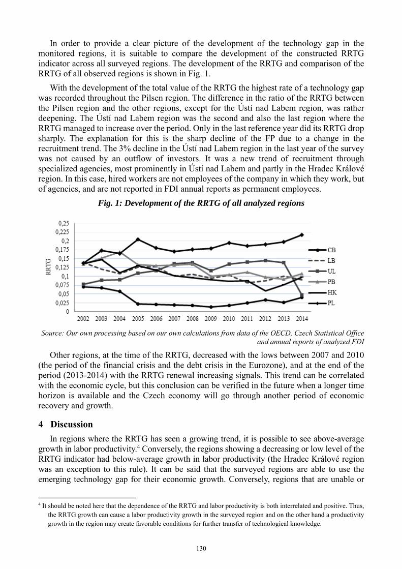
In order to provide a clear picture of the development of the technology gap in the monitored regions, it is suitable to compare the development of the constructed RRTG indicator across all surveyed regions. The development of the RRTG and comparison of the RRTG of all observed regions is shown in Fig. 1.

With the development of the total value of the RRTG the highest rate of a technology gap was recorded throughout the Pilsen region. The difference in the ratio of the RRTG between the Pilsen region and the other regions, except for the Ústí nad Labem region, was rather deepening. The Ústí nad Labem region was the second and also the last region where the RRTG managed to increase over the period. Only in the last reference year did its RRTG drop sharply. The explanation for this is the sharp decline of the FP due to a change in the recruitment trend. The 3% decline in the Ústí nad Labem region in the last year of the survey was not caused by an outflow of investors. It was a new trend of recruitment through specialized agencies, most prominently in Ústí nad Labem and partly in the Hradec Králové region. In this case, hired workers are not employees of the company in which they work, but of agencies, and are not reported in FDI annual reports as permanent employees.

Fig. 1: Development of the RRTG of all analyzed regions

Source: Our own processing based on our own calculations from data of the OECD, Czech Statistical Office and annual reports of analyzed FDI

Other regions, at the time of the RRTG, decreased with the lows between 2007 and 2010 (the period of the financial crisis and the debt crisis in the Eurozone), and at the end of the period (2013-2014) with the RRTG renewal increasing signals. This trend can be correlated with the economic cycle, but this conclusion can be verified in the future when a longer time horizon is available and the Czech economy will go through another period of economic recovery and growth.

4 Discussion

In regions where the RRTG has seen a growing trend, it is possible to see above-average growth in labor productivity.4 Conversely, the regions showing a decreasing or low level of the RRTG indicator had below-average growth in labor productivity (the Hradec Králové region was an exception to this rule). It can be said that the surveyed regions are able to use the emerging technology gap for their economic growth. Conversely, regions that are unable or

4 It should be noted here that the dependence of the RRTG and labor productivity is both interrelated and positive. Thus, the RRTG growth can cause a labor productivity growth in the surveyed region and on the other hand a productivity growth in the region may create favorable conditions for further transfer of technological knowledge.

130

unwilling to attract investors from advanced foreign countries to their region are unnecessarily losing the possibility of economic growth from the transfer of technological knowledge.

Relatively interesting facts were found in the RRTG decomposition analysis. The decomposition, as described earlier, can be divided into three components – the productivity component, the employment component, and the component of combination of both effects. For the productivity component, the surveyed regions experienced similar developments. This was caused by the construction of the formula in which an average benchmark’s productivity subtracts in the numerator and it is the denominator. Because it grew with higher dynamics than the productivity growth of companies from abroad, the component had to have a declining shape. However, this development illustrates the region's ability to absorb and exploit emerging technological gaps for its economic growth.

The development of the productivity component was, however, influenced by the different situations in the surveyed regions. E.g. while the Ústí nad Labem region generated the value of the component mainly by a high proportion of foreign-owned firms with an investment incentive, on the other hand the Hradec Králové region showed higher than the above-average values due to high labor productivity (among countries of origin of FDI the dominant and highly above-average Luxembourg).

The low values of the Carlsbad region are due to the low interest of foreign investors in the creation of new jobs in the region (the lowest share of FDI in total employment from all analyzed regions) and the composition of the investing countries (among them countries with below-average productivity compared to other developed countries – Japan, UK).

The behavior of the employment component curves for the individual surveyed regions is more varied. The shape of these curves reflects the development and shape of the RRTG curves constructed for each region (see fig. 2).

The dominance of the Pilsen region, which was able to attract enough foreign companies from highly developed countries, who were interested in creating new jobs, is quite clearly confirmed. The opposite is the Carlsbad region with a small number of FDI, which made up a small share of regional employment. A very interesting development can be seen in the Ústí nad Labem region. The region has seen a growing RRTG curve, which has had a positive effect on the region's productivity growth, among other things, thanks to the fact that there were high total employees' shares in FDI that received investment incentives recorded in the region. The employment component curve is at one of the lowest levels between the surveyed regions. This is because employment in FDI with an investment incentive in the region has been accompanied by a significant spread of foreign firms. Thus, technology transfer has gone through a significantly higher set of incoming FDI.

131

Fig. 2: Development of the RRTG employment component in the monitored regions

Source: own processing based on own calculations from data OECD, Czech Statistical Office and annual reports of analyzed FDI

In the Pilsen region, the depth of employment was formed by a small spread of companies and countries. More specifically, the growth of the RRTG in the Pilsen region is more driven by the intensity of the use of the technology gap, and the growth of the RRTG in the Ústí nad Labem region is being driven by extensive use of the technology gap brought by the FDI into the region.

Conclusion

The use of the shift-share analysis method to calculate the size of the technological gap represents to a certain extent the filling in of the missing space in the current research concerning the competitiveness of the regions and the impacts of the FDI on the business environment of the Czech Republic. Although there are known determinants that support the emergence of FDI effects, there is no general methodology to quantify which region has great potential for effects to occur. One of the key determinants for determining whether there is potential for the spillover of FDI effects in a host environment is the size of the technology gap. Using the above described methodology, it is possible to specify which region has the greatest potential for spillover effects in terms of the technology gap. At the same time, it is also possible, by using a benchmark, to compare the regions within the group. More precisely, to determine which regions are below average compared to average benchmark values and which, on the contrary, are above average benchmark values.

Going down to the level of the regions in the calculation of the size of the technology gap, results in a better presentation and evaluation of the situation in the business environment, because the chosen methodology works with data from the annual reports of concrete localized FDI. It means the evaluation of the economic level that FDI directly affected. Another advantage of the chosen approach is easy modification. The selected group of regions can be extended practically indefinitely, both in terms of the number of regions and the length of the time series. The main drawback is the time-consuming data collection, which generally involves working with annual company reports connected with each analyzed year.

In the current form of the indicator within the evaluated group of regions, the highest potential of technological growth was identified in the Pilsen region. This is not a surprising result due to the economic position of the region within the evaluated group. On the contrary, the lowest was identified in the Carlsbad region. The main reason for the overall low level of the RRTG in the Carlsbad region is above all the small representation of companies in the

-0,04

-0,03

-0,02

-0,01

0

0,01

0,02

0,03

0,04

0,05

2002 2003 2004 2005 2006 2007 2008 2009 2010 2011 2012 2013 2014

RR

TG

em

ploy

men

t co

mpo

nent

CB

LB

UL

PB

HK

PL

132

region, which is also borne by a small share of employees of foreign companies, there is low degree of the FP. In view of the fact that the level and dynamics of the development of labor productivity in the Carlsbad region (see Tab. 1) were lower than in other regions, the development of the RRTG (especially between 2002 and 2009) represents a bad signal and the finding that the region almost always lacked the opportunity of so-called "economic locomotives" in the form of benefits from the possibility of transferring technological level from more advanced foreign companies.

Acknowledgement

This contribution was supported by grant from student grant competition SGS No. 21190/2017, “Crossborder migration of labour mobility as a consequence of the international companies´ localisation”.

References

Benáček, V. (2000) Přímé zahraniční investice v české ekonomice. Politická ekonomie, 48 (1), pp. 7-22. DOI 10.18267/j.polek.100

Benáček, V. (2006). The rise of the 'grand entrepreneurs' in the Czech Republic and their contest for capitalism. Sociologický časopis, 42 (6), pp. 1151-1170.

Blomström, M., Kokko, A. (2001) Foreign direct investment and spillovers of technology. International Journal of Technology Manage bment, 22 (5-6), pp. 435-454. DOI 10.1504/IJTM.2001.002972

Cantwell, J. (2017). Innovation and international business. Industry and Innovation, 24 (1), pp. 41-60. DOI 10.1080/13662716.2016.1257422

Cohen, W. M., Levinthal, D. A. (1990) Absorptive capacity: a new perspective on learning and innovation. Administrative Science Quarterly, 35 (1), pp.128 – 152. DOI 10.2307/2393553

CzechInvest (2017). Investiční pobídky. [online]. Investiční pobídky. Available at: http://www.czechinvest.org/investicni-pobidky-czechinvest [Accessed 7. 1. 2017].

Czech National Bank (2017). Kurzy devizového trhu. [online] Česká národní banka. Available at: https://www.cnb.cz/cs/financni_trhy/devizovy_trh/kurzy_devizoveho_trhu/denni_kurz.jsp [Accessed 30. 5. 2017].

Czech Statistical Office (2017). Statistické ročenky. [online]. Katalog produktů. Available at: https://www.czso.cz/csu/czso/katalog-produktu [Accessed 7. 3. 2017].

Esteban, J. (2000) Regional convergence in Europe and the industry mix: a shift-share analysis. Regional Science and Urban Economics, 30 (3), pp. 353-364. DOI 10.1016/S0166-0462(00)00035-1

Finlay, R. (1978). Relative Backwardness, Direct Foreign Investments and the Transfer of Technology: A Simple Dynamic Model. Quarterly Journal of Economics, 92 (1), pp. 1-16. DOI 10.2307/1885996

Ferenčiková, S., Fifeková, M. (2008) Foreign Direct Investment Spillovers in Slovakia. Ekonomický časopis, 56 (9), pp. 855-872.

Görg, H. et al. (2008). Productivity spillovers through vertical linkages: Evidence from 17 OECD countries. Economics Letters, 99 (2), pp. 328-331. DOI 10.1016/j.econlet.2007.07.015

Görg, H. et al. (2011). Spillovers through backward linkages from multinationals: Measurement matters! European Economic Review, 55 (6), pp. 862-875. DOI 10.1016/j.euroecorev.2010.10.002

Greenaway, D., Görg, H. (2004) Much I do about nothing? Do domestic firms really benefit from foreign direct investment? World Bank Research Observer, 19 (2), pp. 171-197. DOI 10.1093/wbro/lkh019

Kokko, A. (1994). Technology, Market Charakteristics, and Spillovers. Journals of Development Economics, 43 (2), pp. 279-293. DOI 10.1016/0304-3878(94)90008-6

Kokko, A., Tingvall, G. P. (2014) Distance, Transaction Costs, and Preferences in European Trade. International Trade Journal, 28 (2), pp. 87-120. DOI 10.1080/08853908.2013.830941

133

Kotíková, S. (2016) T he Foreign Presence as a Determinant of Creation of Spillover Effects of Foreign Direct Investment. Ad Alta: Journal of Interdisciplinary Research, 6 (1), pp. 32 – 36. WOS 000384792600007

Kotíková, S., Čuhlová, R. (2016). Foreign Presence, Cultural Distance and Technology Gap as Indicators of Globalization in the Czech Republic. In: 16th International Scientific Conference Globalization and Its Socio-Economics Consequences. Žilina: University of Žilina, pp. 337 – 344.

Massey, D. (2007). In what sense a regional problem? Regional Studies, 41 (1), pp. 49-59. DOI 10.1080/0034300701232181

Maudos, J., Pastor, J. M., Serrano, L. (2008) Explaining the US–EU productivity growth gap: Structural change vs. intra-sectoral effect. Economics Letters, 100 (2), pp 311-313. DOI 10.1016/j.econlet.2008.02.017

Ministry of Justice (2017). Veřejný rejstřík a sbírka listin. [online]. eJustice. Available at: http://www.justice.cz [Accessed 11. 2. 2017].

Mišun, J., Tomšík, V. (2002) Does Foreign Direct Investment Crowd in or Crowd out Domestic Investment? Eastern European Economics, 40 (2), pp. 38–56.

Navaretti, G. B., Venables, A. J. (2013) Multinationals and industrial policy. Oxford Review of Economic policy, 29 (2), pp. 361 - 382. DOI 10.1093/oxrep/grt016

OECD (2017). Level of GDP and productivity. [online] OECD Statistics. Available at: http://stats.oecd.org/Index.aspx?DataSetCode=PDB_LV [Accessed 27. 5. 2017].

Pavlínek, P., Žížalová, P. (2016) Linkages and spillovers in global production networks: firm-level analysis of the Czech automotive industry. Journal of Economic Geography, 16 (2), pp. 331-363. DOI 10.1093/jeg/lbu041

Šimanová, J., Trešl, F. (2011) Vývoj průmyslové koncentrace a specializace v regionech NUTS3 České republiky v kontextu dynamizace regionální komparativní výhody. E + M Ekonomie a Management. 14 (1), pp. 38 – 52. DOI 000296411900004

Zdeněk, R., Střeleček, F. (2012) Hodnocení vývoje zaměstnanosti, průměrné mzdy a produktivity práce pomocí shift-share analýzy. E + M Ekonomie a Management, 15 (3), pp. 4 – 15.

Contact Address

Ing. Sylvie Kotíková, Ph.D. Technical University of Liberec, Faculty of Economics, Department of Economics Voroněžská, 13, 460 01, Liberec, Czech Republic Email: [email protected] Phone number: +420485352406


134

SWOT ANALYSIS EVALUATIONS ON THE BASIS OF UNCERTAINTY – CASE STUDY

Jiří Křupka, Kateřina Kantorová, Meaza Haile

Abstract: Choosing effective strategy is the main factor in running a successful enterprise, organization. The first step is to understand the organization with respect to its environment, which could be done using SWOT analysis. The main factor in performing SWOT analysis is selecting influential criteria. These criteria could be a long list and difficult to analyse depending on the organization. One way to analyse these criteria is to divide them in sub groups under strength, weakness, opportunity and threat. What is proposed in this paper is a value chain with different primary activities based on the organization, and to evaluate the each primary activity using SWOT analysis and multi criteria decision making (MCDM) to find the best strategy. The aim is to evaluate each process and the value, it is adding to the final outcome and the overall success of the organization. A tile company was analysed by dividing the processes in the company as product, promotion and customer relation using Choquet integral, Technique for Order of Preference by Similarity to Ideal Solution (TOPSIS) and fuzzy TOPSIS based on opinions of experts.

Keywords: Fuzzy Integral, Quantitative Evaluation, SWOT Analysis, TOPSIS, Value Chain, Weighted Sum Average.

JEL Classification: C02,C18, C38, C4, M10

Introduction

Strategic management is the comprehensive collection of ongoing activities and processes that corporations use to systematically coordinate and align recourses and actions with mission, vision and strategy throughout an organization (Aaker& Moorman, 2017; Alkafaji, 2003; Johnson, Whittington & Scholes, 2011). There are different models, which are used to represent strategic management process, proposed by different researchers. Hunger and Wheelen’s strategic management model has four inter connected elements: Environmental scanning, strategy formulation, implementation and evaluation and control (Hunger & Wheelen, 2011). Strategy evaluation and control is crucial to effective functioning of an organization. The success of an organization greatly depends on the effective strategies and evaluation control systems in place. Strategy evaluation should be on going in an organization. Strategic evaluation refers to a process of evaluating the effectiveness of a strategy identified and applied by business in an attempt to achieve its overall objectives and take corrective action.

While evaluating a strategy the main aspects that should be considered are evaluation of both internal and external factors that form the basis of the strategy and evaluation of its performance. SWOT analysis is a commonly used tool for analysing an organization with respect to its internal and external environment. Strength and weakness are most often viewed from the organization’s point of view whereas opportunities and threats are external environmental factors. Strength is what an organization has or what it can offer that others of its type do not. Weakness in opposite is what an organization does not have or does not offer others of its type do. Opportunities are advantages in the

135

environment that an organization could use. Threats are situations in an organization’s environment that could compromise the organization’s success (Hill & Westbrook, 1997; Humphrey, 2005; 2012; Lawrence, 2009).

The aim of the article is to propose and analyse the possibility of using the methods of MCDM with uncertainty for a quantitative evaluation of the SWOT analysis. The value chain method divides SWOT criteria into categories of processes (primary activities of value chain) based on a real-life case study, for recommendations in the selection of an ‘optimal’ strategy.

1 Problem formulation

SWOT analysis is an analysis compiles the factors of the internal and external environment and it has evolved since 1960’s. The SWOT analysis is an excellent tool for coaching, which helps to identify the most notable activities, affecting the success of business (Morison, 2016). This analysis is also a certain output, which summarizes the output from other, analyses. Frequently, PESTLE analyses, Porter’s analysis of five forces, competitive analysis, customer (ie, determining, customer lifetime, and analysis), suppliers and customers are often used for SWOT analysis input data. Internal analysis include, product analysis (Boston Consulting Group, McKinsey matrix or GE matrix, P-Q analysis or Paretto analysis, RFM (recency, frequency, monetary) analysis, …), marketing mix analyses, which, in addition to product, include communication, distribution and price manipulation. Internal analysis can be also used to analyse the internal processes of the organization, the vision, mission, goals and continuity of subsequent processes towards achieving the objectives, including control mechanisms (Grasseová, 2006).

There are following steps in the right procedure of SWOT analysis: 1st Specification for SWOT analysis; 2nd Assembling a team of specialists; 3rd Defining the internal and external environment; 4th Specifying factors in the individual quadrants of a SWOT matrix; 5th Proof of evidence to individual factors; 6th Selection of the most important factors; 7th Define key success/failures factors; 8th Selection of the SWOT strategy (Max-Max, Min-Max, ...); 9th Creating a company strategy and 10th Creating a plan to implement the strategy. The SWOT analysis includes strategically important facts that are both realistic and valid in the range of about 6 months to 2 years. Within the SWOT analysis, it is also important to look at the interrelationships between strengths and weaknesses, opportunities and strengths. This is mostly the case as part of the comparison of processed data. These synergies can be used to determine the company’s strategy and development. The SWOT analysis can be used as a tool to determine and optimize a company’s strategy, project, or decision-making to improve the current state of the organization or its individual processes. Based on the outcome of the comparison of the internal and external environment, it is possible to decide which basic strategy is most important for the investigated entity. SWOT analysis offers the following strategic options (Hanzelová, 2017; Jakubíková, 2008; Sackett, Jones & Erdley, 2005).

The organization’s success often lies in effectively managing strategic situations. Take advantage of the opportunities that come from outside, if the company has appropriate resources for them. Generates S O strategies (Max-Max). The opportunity is useful if it help eliminate the weaknesses of the company – W O (Min-Max) strategy. The organization usually chooses one of these strategies to take the opportunity. In the

136

event that an organization is seriously threatened, which the SWOT analysis may reveal, it will choose the S T (Max-Min) strategy - it will use its strengths to control threats. The W T (Min-Min) strategy is useful if it has significant problems and rescues it, it can significantly strengthen those weaknesses that are direct attack on threats. Leaders typically choose the S O strategy and benefit from opportunities based on their strengths. Average businesses often choose S T or W O strategy or a combination of these (Tomek, 2001; Molnár, 2012, pp. 101-102). The way to identify these strategy options is to weigh important criteria and evaluate a business with respect to these criteria and their weight. Nevertheless, the SWOT analysis has criticisms and limitations. The main criticism is that it relies on subjective judgments (Hindle, 2008) and other limitations are described in (Pickton & Wright, 1998), (Wasike et al, 2011), (Haile & Krupka, 2016).

Different approaches can be used for a quantitative evaluation of SWOT analysis and choice of ‘optimal’ strategy, e.g.: weighting and rating individual SWOT factors, pairwise comparison (Molnár, 2012); knowledge-based system working with a vague description of competitive strengths, weaknesses, opportunities and threats (Houben, Lenie & Vanhoof, 1999);21-24 combining qualitative evaluation with analytical hierarchy process (Santopuoli, Marchetti & Giongo, 2016; Tugrul & Cimen, 2016; Wasike et al, 2011); application of a quantification SWOT analytical method (Chang & Huang, 2006). Some authors have proposed novel methods (approaches) to quantify results of a SWOT analysis: Analytic Network Process (Yuksel & Dagdeviren, 2007), fuzzy Analytic Network Process (Sevkli et al. 2012), theory of fuzzy sets (Li & Liu, 2010; Liao, 2017), fuzzy integral and fuzzy measures (Haile & Krupka, 2016; Haile, Krupka & Mastalka, 2016), fuzzy TOPSIS (Zare, Mehri-Tekmeh & Karimi, 2015) and fuzzy ELECTRE (Gürbüz & Pardalos, 2016) etc.

2 Methods

System approach, logic methods (analysis and synthesis, induction and deduction), Value chain, Weighted sum average method (WSAM), TOPSIS, fuzzy TOPSIS, fuzzy integral, SWOT analysis and Case study method are applied in this paper.

The system approach tries to achieve application of functional analysis concept and general systems theory in management, too. It is characterized by complex view of objective reality that is assessed as a multi-dimensional organized unit. Its contribution for management development is based on inner relations management system analysis, in acceptance of importance of both mutual influences of inner factors and interaction of the system with its environment It endeavours for a complex understanding of all phenomena and deeper expression of internal and external factors (Gallopín, 2003; Coffey, 2010).

An organization is a system with interconnected departments (processes). The success or failure of departments affect other departments and the overall success of the organization. A value chain charts the path by which products and services are created and eventually sold to customers. The term value chain reflects the fact that, as each step of this path is completed, the product becomes more valuable than it was at the previous step (Ketchen & Short, 2011). Value chain analysis describes the activities within and around an organization, and relates them to an analysis of the competitive strength of the organization (Porter, 1985). Therefore, it evaluates which value each particular activity adds to the organizations products or services. This idea was built upon the

137

insight that an organization is more than a random compilation of machinery, equipment, people and money. Only if these things are arranged into systems and systematic activates it will become possible to produce something for which customers are willing to pay a price. Porter argues that the ability to perform particular activities and to manage the linkages between these activities is a source of competitive advantage. Value chains include both primary and secondary (support) activities. Their detail description is in (Porter, 1985, cited in Ketchen & Short, 2011, p. 150-151).

MCDM methods are represented by WSAM, TOPSIS and fuzzy TOPSIS. The WSAM is probably the most commonly used approach, if there are m alternatives and n criteria then the best alternative is the one that satisfies most. The assumption that governs this model is the additive utility assumption. That is the total value of the alternative is equal to the sum of the products (Panos, 2000). In this paper it was used to aggregate the total evaluation of each category of the SWOT analysis. The TOPSIS calls for ordinal information on attributes of variants as well as the criteria preference expressed in weight vector and is based on measuring distance from the ideal and negative-ideal solution. TOPSIS assumes that each attribute takes the monotonically increasing or decreasing utility. One approach is to take an alternative which has the weighted minimum Euclidean distance to the ideal solution (Panos, 2000). Since the last decade TOPSIS has been applied for analysing SWOT analysis among those the recent ones include application of TOPSIS and SWOT analysis for supplier selection and order allocation problems (Arabzad et al, 2015), a combination TOPSIS and AHP entropy in research of development strategy (Xu, Feng & Yang, 2016) and in evaluating and ranking of human resource and business strategy (Shakerian, Dehnavi & Ghanad, 2016). The fuzzy TOPSIS is an extension of TOPSIS with where fuzzy set theory is incorporated in the fuzzy set to deal with uncertainty and vagueness in data collection. The decision-maker is supposed to judge the relative importance of each pair of criteria. The elements of matrix are considered to be an estimation of importance of i-th and j-th criteria. The Saaty scale of relative importance (Saaty, 1996) is used for the proposal of the Saaty matrix that the matrix has all positive and reciprocal elements. The criteria weights or variant values are computed on the basis of eigen values and vectors or geometrical mean (Geomean) of Saaty matrix lines (Saaty, 2008) and then normalized.

Fuzzy integrals are tools used to summarize all the pieces of information provided by a function in a single value; this value could be a sort of average of the function, in terms of the underlying fuzzy measure (Haile & Krupka, 2016; Sugeno, 1977; Wei, Liou & Lee, 2008). Measure in its classic definition uses additive property, but most real world problems cannot be measured using additive measures. In most of the cases fuzzy measure has applications in many fields such as data mining, image processing and so on (Sugeno, 1974). Fuzzy integrals are integrals of a real function with respect to a fuzzy measure, by analogy with Lebesgue integral which is defined with respect to an ordinary (i.e. additive) measure. There are several definitions of fuzzy integrals, among which the most representatives are those of Sugeno fuzzy integral (Sugeno, 1974) and Choquet fuzzy integral. In this paper Choquet fuzzy integral was chosen for its unique solution (Choquet, 1953; Haile, Krupka & Mastalka, 2016).

A case study method will be used for explanation of using methods in the model and its verification. The Case study method is a common method used among researchers. Eisenhardt and Graebner (2007) recommended case study as a suitable method for

138

illuminating and extending relationships that provide understanding of complex phenomena (Eisenhardt & Graebner, 2007; Yin, 2009); this approach offers the possibility to address the dynamic interactions (Langfield-Smith, 1997) and helps maintain the validity of the obtained results (Fisher & Ziviani, 2004; Hyett, Kenny & Dickson-Swift, 2014).

3 Discussion and results

The value chain framework can be modified for different areas (Hutaibat, 2011; Normann & Ramírez, 1993; Pil & Holweg, 2006; Sison & Pablo, 2000). The approach to an analysis of value chain framework on the basis of MCDM is used in (Igbinovia & Krupka, 2017; Liao, 2014).

The value chain’s different primary activities are based on the organization and an evaluation of the each primary activity can be realized on the basis of SWOT analysis and MCDM methods that it can find the best strategy. Since the aim is to evaluate each process in primary activities and the value it is adding to the final product and over all the success of the organization. Secondary activities are not evaluated as processes. The MCDM evaluation of processes will be done on the basis of hierarchical analyses of primary activities (Fig. 1).

Fig. 1: Hierarchical analyses of primary activities

Source: Authors

For instance: ATEMIT, Ltd. takes raw material for flooring and provides customer with quality tiled floor. The main output of this business is service. To provide this service the production department as the process, has to work on providing customers quality flooring where the promotion department works to get customers attention and customer relation is another department in this business that directly provides service for customers.

The surveyed business ATEMIT, Ltd. offers services in industrial markets. It mainly focuses on wall covering and laying of floor coverings. Operates on a saturated market. It is the exclusive representative of Densit (extremely resistant cast floor). It offers its services in the building industry, the food industry and in the engineering industry. The number of employees ranges from 25 to 49. The company is very successful. It reaches high turnover, belongs to the top 10% of companies in the Czech Republic (CR). In the last period, the company has stagnated year-on-year. Process of data collection started in the end of 2015. The internal and external influences of the company were identifying during the spring and autumn 2016. During the year 2017, consultations were carrying

Process P1 Process Pn

Analysis

SP1 WP1 OP1 TP1

Process P2

SP2 WP2 OP2 TP2 SPn WPn OPn TPn

. . .

139

out with the company representatives and options for setting of qualitative assessment and performing of analyses were looking for.

It has been found to have well-engineered internal guidelines and standards, actively using communication mix tools, and building long-term relationships with customers. It primarily uses personal sales, sales promotion, and advertising. The company did not work with an analytical apparatus that would give it a wider view of the overall situation within the business with the link to its surroundings.

SWOT analysis for the ATEMIT, Ltd. was performed by external experts based on the assessment of the internal staff. These characteristics (factors) were classified into Strength (S), Weakness (W), Opportunity (O) and Threat (T) based on the values provided by experts. As discussed in the text above the aim of this paper is to show a modified application of SWOT analysis using the value chain method to sub classify characteristics in this case as Product (in the following text only P), Customer relation (only C) and Promotion (only PM) it means that the primaries activities (processes) for ATEMIT, Ltd. are P, C and PM.

The possible combination of strategic options for the company are discussed below:

Under SO strategy there are P means: Independence from Denzit’s temperaturefluctuations in conjunction with Competitors does not offer comparable quality andapplication at different temperatures. Here we do not derive from the highest valuein terms of opportunities, but from what is in relation to that strong side; C means:To take advantage of the opportunity to contact designers of new buildings toincorporate quality floor into their designs the unsatisfied market of CR in relationto Employee Orientation per customer, Network of Trained Traders; PM means:Willingness to confirm and boast a new floor in reference to the Reference Sheets

Under ST strategy there are P means: The threat of addiction to poor quality.Suppliers and Competition is achieved (in reasons no longer a competitiveadvantage); Competitiveness innovations (resin is no longer a competitiveadvantage, Denzit touches); To compensate for the development of new products;C means: Customer tries to save and crisis economies in the context of EmployeeOrientation on Customer and Personal Meetings and Customer Relationship Dealer(trained business skills plus knowledge of customer needs) In order to save costs byconvincing the customer that cheap is not necessarily the most effective

Under WO strategy there are C means: To buy a new database and that the marketis unsatisfied, it is recording that it will use larger database for the future. This willbe an important investment if the company decide to expand the marketgeographically.

The WSAM method, Saaty method, TOPSIS and fuzzy integral were used for the quantitative evaluation of SWOT analysis and recommendation for the choice of best strategy.

Based on the figure above (Fig. 1) the processes of the studied company, ATEMIT, Ltd., were divided in to three processes namely P, PM and C. Each of these processes was then evaluated using the proposed methods WSAM, fuzzy TOPSIS and fuzzy integral and TOPSIS with input data normalized by Saaty matrix.

140

The Table 1 shows the WSAM analysis of the strength of P of the tile company. The P strength is described by i-characteristic. The weight wE was suggested and discussed by the internal staff and external experts. The performance, is the status of the company, was calculated using fuzzy trapezoidal membership function of experts linguistic variables ‘not satisfactory’, ‘satisfactory’ and ‘very satisfactory’, for the Universe [1, 10], and was defuzzified.

Tab. 1: Characteristic weights wW of Strength of P on the basis of WSAM Strength i-characteristic of product SP, Ch_i wE Performance wW

Product quality (density) of exclusive representation SP, Ch_1

0.5 9.5 0.714

Development of new products SP, Ch_2 0.5 9.5 0.714

Density dependent on temperature fluctuations during application SP, Ch_3

0.6 5.5 0.86

Offers comprehensive solutions - design, applications, customer service SP, Ch_4

0.5 9.5 0.714

Weighted sum / Weighted sum average 17.55 / 8.36 Source: Authors

The results in the table (Table 1) 8.36 show the total value derived for the Strength of P process in the ATEMIT, Ltd.

The Table 2 shows the pair-wise comparison of each P characteristic (criteria) SP, Ch_1, SP, Ch_2, SP, Ch_3 and SP, Ch_4 of SWOT analysis using Saaty matrix S. The result on the basis of Saaty method is the normalized weight wi.

Tab. 2: Characteristic weights wi of Strength of P on the basis of Saaty matrix Characteristics SP, Ch_i wE S (CR is 1.65 10-16) Geomean wi

SP, Ch_1 0.5 1 1 1/3 1 0.75 0.17

SP, Ch_2 0.5 1 1 1/3 1 0.75 0.17

SP, Ch_3 0.6 3 3 1 3 2.27 0.5

SP, Ch_4 0.5 1 1 1/3 1 0.75 0.17 Source: Authors

The resulted wi was used to calculate fuzzy aggregate value that is the overall evaluation of the strength of product of the company. First the Lambda that is the combined effect of weights was calculated then the aggregate evaluation was obtained using Choquet fuzzy integral. The resulted value from this evaluation for the Strength of P was 7.489.

After analysing each category of processes P, C and PM (it means Product, Customer relation and Promotion) with respect to weights provided by experts the TOPSIS method was used to choose the best strategy using Min-Min, Min-Max, Max-Min and Max-Max.

From the results obtained using WSAM, Choquet fuzzy integral and TOPSIS experts derived a suggestion of possible strategies. The following tables show the resulted evaluation of S O, W O, S T and W T using TOPSIS and fuzzy TOPSIS.

141

Tab. 3: Possible strategies on the basis of Choquet fuzzy integral and TOPSIS S O W O

SCOC 0.325973 WCOC 0.176167

SPOP 0.325514 WPOP 0.175309

SPMOPM 0.264901 WPMOPM 0.182523

S T W T

SCTC 0.303291 WCTC 0.146453

SPTP 0.297977 WPTP 0.136871

SPMTPM 0.210666 WPMTPM 0.113021 Source: Authors

Tab. 4: Possible strategies on the basis of fuzzy TOPSIS S O W O

SCOC 0.482343 WCOC 0.219256

SPOP 0.479021 WPOP 0.225212

SPMOPM 0.42855 WPMOPM 0.216885

S T W T

SCTC 0.434633 WCTC 0.167633

SPTP 0.392687 WPTP 0.098506

SPMTPM 0.342398 WPMTPM 0.096219 Source: Authors

Based on the results (Table 3 and Table 4) from the above tables the best strategy is SCOC; that is to use the strength of customer relation to utilize the opportunity in customer relation. The conclusions summarized in Table 3 and Table 4 show that the first three positions for strategy are SCOC, SPOP and SCTC. The difference was only in the 4th and 5th positions and only in the change of their order and the other differences were reflected in other positions (namely 7th and 9th positions). However, the strategies listed in these positions are no longer included in the draft strategy. Expert with real-world knowledge had a peer-reviewed opinion and recommendations for the following company’s strategy. The expert agrees on the strategic option SCOC as discussed above so there are two options of SCOC customer relation strategy:

To take advantage of the opportunity to contact designers of new buildings toincorporate quality floor into their designs

Unsatisfied market of CR in relation to Employee orientation per customer, Networkof trained traders.

Based on the weights of these criteria the first choice of strategy option should be to take advantage of the opportunity to contact designers of new buildings to incorporate quality floor into their designs. However, the expert did agree with this choice not recommend this because of the fact that designers of new buildings are not willing to design such high-quality floors for their financial purposes for financial reasons and in this case, its advantage diminishes. We believe that this distinction has already occurred at the beginning when business representatives have erroneously identified this opportunity as being of high value.

142

This finding shows that the final calculation is always derived from the quality of the input data. Therefore, it is important, in quantification of input factors, to promptly ask the contracting authority how to determine the values. Again, the calculation must be checked and verified by an expert with real-world knowledge and cannot be ‘blindly’ implemented.

Conclusion

The aim of the article was to propose and analyse quantitative evaluation of the SWOT analysis based on a case study. The SWOT analysis works with a language description of input factors, fuzzy set theory was used to work with uncertainties, and fuzzy integrals and TOPSIS, and fuzzy TOPSIS were uses to evaluate the characteristics (criteria) of the SWOT analysis. The chosen methods were used on the information of the selected real business ATEMIT, Ltd. It offers industrial floors on the market in the CR. The underlying information was collected in cooperation with the representatives of the company.

The qualitative data acquisition approach was chosen for the case study method. In this case, this was the explanatory case study that was used to describe and explain the use of uncertainty methods for working with SWOT analysis of the real organization. The same conclusion (Table 4) to choose the above SCOC strategy was obtained from the analysis using fuzzy TOPSIS method. Although not all the strategic options rank the same way from the two analyses there is a strong correlation between the rankings of the two methods.

Based on the above analysis, it can be stated that the advantage of using fuzzy methods is the ability to work with the vagueness, the uncertainty that is a natural component present when compiling the SWOT analysis. Achieved results can have an important place when considering the choice of the final strategy. However, the results obtained using fuzzy methods are only a recommendation to decide on the choice of an appropriate strategy.

Acknowledgement

This article was supported by the grants No. SGS_2017_019 ‘Models Synthesis and Analysis for Implementation Support of Smart Cities and Regions Concept’ and No. SGS_2018_025 ‘Transparency and competitiveness of municipalities and regions within the development of the concept of smart cities and regions’ of the Ministry of Education, Youth and Sports of CR at the Faculty of Economics and Administration, University of Pardubice.

References

Aaker, D.A., Moorman, Ch. (2017). Strategic Market Management. 11th Ed. Wiley.

Alkafaji, A.F. (2003). Strategic Management Formulation, Implementation and Control in a Dynamic Environment, The Haworth Press Inc.

Arabzad S.M., Ghorbani M., Razmi J., Shirouyehzad, H. (2015). Employing fuzzy TOPSIS and SWOT for supplier selection and order allocation problem, Int J Adv Manuf Technol. 76, pp. 803-818.

Chang, H.H., Huang, W.Ch. (2006). Application of a Quantification SWOT Analytical Method, Mathematics and Computer Modelling, 43, pp. 158-169.

143

Choquet, G. (1953). Theory of capacities, Annales de l’Institut Fourier, 5, pp. 131-295.

Coffey, G. (2010). A Systems Approach to Leadership, Berlin Heidelberg: Springer-Verlag. ISBN 978-3-642-01194-8.

Eisenhardt, K., Graebner, M. (2007). Theory building from cases: opportunities and challenges, Academy of Management Journal. 50, pp. 5-32.

Fisher, I., Ziviani, J. (2004). Explanatory case studies: Implications and applications for clinical research. Australian Occupational Therapy Journal, 51, pp. 185-191.

Gallopín, G. (2003). A systems approach to sustainability and sustainable development. Santiago de Chile: United Nations Publication. ISSN 1564-4189.

Grasseová, M. (2006). Využití SWOT analýzy pro dlouhodobé plánování. Obrana a strategie, [online], [May 5, 2017]. Available at: http://www.defenceandstrategy.eu/cs/ar.

Gürbüz, F., Pardalos, P.M. (2016). Fuzzy Decision-Making of a Process for Quality Management. In: Int. Workshop on Machine Learning, Optimization and Big Data. MOD 2016: Machine Learning, Optimization, and Big Data. Springer, pp. 353-378.

Hanzelková, A., Keřkovský, M., Vykypěl, O. (2017). Strategické řízení: teorie pro praxi. 3. přepracované vydání. Praha: C.H. Beck.

Haile, M., Krupka, J. (2016). Modelling of SWOT Analysis using Fuzzy Integral, In: International Conference on Soft Science ISSC 2016, The European Proceeding of Social and Behavioural Sciences EpSBS, UK, pp. 75-82.

Haile, M., Krupka, J., Mastalka M. (2016). Evaluation of Strategic Planning Process Using Analysis of Fuzzy Integral, In: 11th International Scientific Conference on Distance Learning in Applied Informatics, Wolters Kluwer, The Netherlands, pp. 503-512.

Hyett, N., Kenny, A., Dickson-Swift, V. (2014). Methodology or method? A critical review of qualitative case study reports. International Journal of Qualitative Studies on Health and Well-being, 9, pp. 1−12. DOI: 10.3402/qhw.v9.23606.

Hindle, T. (2008). The Economist Guide to Management Ideas and Gurus. Profile Books Ltd.: London, pp. 181-182.

Hill, T., Westbrook, R. (1997). SWOT analysis: it's time for a product recall. Long Range Planning, 30 (1), pp. 46-52.

Houben, G., Lenie, K., Vanhoof, K. (1999). A knowledge-based SWOT-analysis system as an instrument for strategic planning in small and medium sized enterprises. Decision Support Systems, 26, pp. 125-135.

Humphrey, A. (2005). SWOT Analysis for Management Consulting, SRI Alumni Newsletter. Retrieved from SRI International.

Humphrey, A. (2012). Research: The Science of Team Action Management [online], [March 15, 2017], The Father of TAM, TAM UK. Available at: http://www.tamplc.com/research.htm.

Hunger, D.J, Wheelen, T.L. (2011). Strategic Management and Business Policy: Toward Global Sustainability, 13th Edition. Prentice Hall.

Hutaibat, A.K. (2011). Value Chain for Strategic Management Accounting in Higher Education, International Journal of Business and Management, 6 (11), pp. 206-218.

Igbinovia, F., Krupka, J. (2017). Product Value Chain in a Tertiary Institution: The Need for MCDM. In: 2017 IEEE European Technology and Engineering Management Summit (E-TEMS), pp. 63-68. ISBN: 978-1-5386-3721-0.

Jakubíková, D. (2008). Strategický marketing: strategie a trendy. Praha: Grada.

Johnson, G., Whittington, R., Scholes, K. (2011). Exploring strategy: text and cases. 9th Ed. Financial Times Prentice Hall.

144

Ketchen, D., Short, J. (2011). Mastering Strategic Management.: Evaluation and Execution, [online], ], [March 15, 2017], Available at: http://2012books.lardbucket.org/pdfs/strategic-management-evaluation-and-execution.pdf.

Langfield-Smith, K. (1997). Management control systems and strategy: A critical review. Accounting, Organizations and Society. 22 (2), pp. 207-232.

Lawrence, G.F. (2009). The SWOT Analysis: Using your Strength to overcome Weaknesses, Using Opportunities to overcome Threats, 1st Ed., CreateSpace Independent Publishing Platform.

Li, S., Liu, X. (2010). To Apply the Method of Multiplier-Fuzzy Synthetic Evaluation Based on SWOT Analysis to the Strategy Choice of Training Industry. In: 2010 International Conference on E-Product E-Service and E-Entertainment, pp. 1-5.

Liao, S. Ch. (2014). Using the MCDM of the Innovative Product Value Chain to Promote New Product Design. The East Asian Journal of Business Management, 4 (3), pp. 27-37.

Molnár, Z. (2012). Competitive intelligence, aneb, Jak získat konkurenční výhodu. Praha: Oeconomica.

Morrison, M.R. (2016). SWOT Analysis - Matrix, Tools, Templates and Worksheets. [online], [Oct. 12, 2016], Available at: http://rapidbi.com/created/SWOTanalysis.html#Background.

Normann, R. Ramírez, R. (1993). From value chain to value constellation: designing interactive strategy, Harv. Bus. Rev., 71, pp. 65-77.

Panos, M.P. (2000). Multi-Criteria Decision Making Methods: a Comparative Study, Kluwer Academic Publishers, The Netherlands.

Pickton, D.W., Wright, S.W. (1998). What's SWOT in strategic analysis?. Strategic Change, 7 (2), pp. 101-109.

Pil, K.F., Holweg, M. (2006). Evolving from value chain to value grid. MIT Sloan Manage. Rev. 47, pp. 72–80.

Porter. M.E. (1985). The Competitive Advantage: Creating and Sustaining Superior Performance, NY: Free Press.

Saaty, T.L. (1996). Decision Making with Dependence and Feedback: the Analytic Network Process. RWS publications. Pittsburgh.

Saaty, T.L.( 2008). Decision making with the analytic hierarchy process. Int. J. Services Sciences, 2008, 1 (1), pp. 83-98.

Sackett, K., Jones, J., Erdley, W.S. (2005). Incorporating Healthcare Informatics into the Strategic Planning Process in Nursing Education, Nurs Leadersh Forum. Spring, 9 (3), pp. 98-104.

Santopuoli, G., Marchetti, M., Giongo, M. (2016). Supporting policy decision makers in the establishment of forest plantations, using SWOT analysis and AHPs analysis. A case study in Tocantins (Brazil). Land Use Policy, 54, pp. 549-558.

Sevkli, M., Oztekin, A., Uysal, O., Torlak, G., Turkyilmaz, A., Delen, D. (2012). Development of a fuzzy ANP based SWOT analysis for the airline industry in Turkey, Expert Systems with Appl., 39, pp. 14-24.

Shakerian H., Dehnavi H.D., Ghanad S.B. (2016). The implementation of the hybrid model SWOT-TOPSIS by fuzzy approach to evaluate and rank the human resources and business strategies in organizations (case study: road and urban development organization in Yazd), Procedia Social and Behavioral Sciences, 230, pp. 307-316.

Sison, R., Pablo, C.Z. (2000). Value Chain Framework and Support System for Higher Education, In: Proceedings of the Philippine Computing Science Congress, pp. 1-6.

Sugeno, M. (1974). Theory of Fuzzy Integrals and its Applications, Tokyo Institute of Technology, Japan.

145

Sugeno, M. (1977). Fuzzy measures and fuzzy integrals—A survey, In: M.M. Gupta, G.N. Saridis, B.R. Gaines (Eds.) Fuzzy Automata and Decision Processes, Amsertdam, The Netherlands: North-Holland, pp. 89–102.

Tomek, J. (2001). Základy strategického marketingu. 2. vyd. Plzeň: Západočeská univerzita.

Tugrul, B., Cimen, S. (2016). Importance of Corporate Governance for Energy in Sustainable Development and Evaluation with Quantitative SWOT Analysis. Acta Physica Polonica A, 130 (1), pp. 87-89.

Yin, R.K. (2009). Case Study Research. Design and Methods. 4th ed. London: Sage Publications.

Yuksel, I., Dagdeviren, M. (2007). Using the Analytic Network Process (ANP) in a SWOT analysis – A case study for a textile firm, Information Sciences, 177, 3364-3382.

Wasike, Ch., Magothe, T., Kahi, A., Peters, K. (2011). Factors that influence the efficiency of beef and dairy cattle recording system in Kenya: A SWOT–AHP analysis. Tropical Animal Health and Production, 43 (1), pp. 141-152.

Wei, Ch., Liou, T.S., & Lee, K.L. (2008). An ERP performance measurement framework using a fuzzy integral approach, Journal of manufacturing technology management, 19, pp. 607-626.

Xu, J., Feng, P., Yang, P. (2016). Research of development strategy on China’s rural drinking water supply based on SWOT–TOPSIS method combined with AHP-Entropy: a case in Hebei Province, Environmental Earth Sciences, 75 (1), pp. 1-11.

Zare, K., Mehri-Tekmeh, J., Karimi, S. (2015). A SWOT framework for analyzing the electricity supply chain using an integrated AHP methodology combined with fuzzy-TOPSIS. International Strategic Management Review, 3 (1–2), pp. 66-80.

Contact Address

doc. Ing. Jiří Křupka, PhD. University of Pardubice, Faculty of Economics and Administration, Institute of System Engineering and Informatics Studentska 95, 532 10 Pardubice 2, Czech Republic Email: [email protected] Phone number: +420466036144

Ing. Kateřina Kantorová, Ph.D. University of Pardubice, Faculty of Economics and Administration, Institute of Business Economics and Management Studentska 95, 532 10 Pardubice 2, Czech Republic Email: [email protected] Phone number: +420466036666

Ing. Meaza B. Haile, Ph.D. University of Pardubice, Faculty of Economics and Administration, Institute of System Engineering and Informatics Studentska 95, 532 10 Pardubice 2, Czech Republic Email: [email protected] Phone number: +420774239248


146

THE CREDIBILITY OF FISCAL POLICY AND COST OF PUBLIC DEBT

Haryo Kuncoro

Abstract: This paper investigates the potential relationship between the credibility of fiscal policy and the cost of public debt. We analyze how a key component of fiscal governance, the ability of governments to commit the planned budget, affects the government borrowing cost. To test the hypothesis, we take the case in Indonesia over the period 2001-2013. Based on the quarterly data analysis, we found that the non-credible deficit rule tends to induce the interest rate. In contrast, the credible debt rule policy significantly reduces the borrowing cost for about 28 basis points. More interestingly, to reduce the interest cost burden of government debt, strengthening commitment to the fiscal rules is as effective as decreasing the size of debt. Those findings suggest that the credibility of fiscal policy matters to restore the fiscal burden in order to maintain fiscal sustainability in the long-run. Accordingly, improving the credibility of fiscal policy should be an integral part of the public sector reformation program in the country.

Keywords: Deficit Rule, Debt Rule, Credibility of Fiscal Policy, Implicit Interest Rate, Fiscal Sustainability

JEL Classification: G12, E43, H63

Introduction

The effectiveness of fiscal policy as a tool of macroeconomic stabilization has gone through a rise and fall both in the academic literature and the real world (Ito, et al., 2012). During global financial crisis in the late 2000s, the fiscal policy received so much attention and staged a dramatic comeback. Governments stimulated their economies by increasing spending through stimuli packages, introducing subsidies, and cutting taxes (Christiano et al., 2011). Fiscal policy then became a major thrust of international cooperation to combat the global financial crisis.

The recent sharp increase in fiscal deficits and government debt to mitigate the global financial crisis impacts raises questions regarding their effect on the key macroeconomic variables. While the effects of government debt on the economy can operate through a number of different channels, many of the recent concerns about government borrowing have focused on the potential interest rate effect. In one hand, economic theory suggests that this impact is likely to be adverse, empirical results, on the other hand, have been less clear cut.

Knowing the impact of budget deficits and debt on the interest rates is crucial. For point of view of researchers, it is an important test for the validity of classical, Keynesian, and Ricardian paradigms. Policy makers consider the impact of fiscal policy also as crucial issue. The effects of the budget deficits pass through interest rates to the major macroeconomic variables. Their immediate effects can be seen on the growth of public debt which, in turn, may produce long term effects including further rise in budget deficits due to debt serving and burden for the future generation.

147

In a bid to achieve the goal of sustainable public finances, many countries have adopted some form of fiscal rule (or a combination of fiscal rules). The governments with a strong reputation of fiscal prudence may have less need for discretionary policy action if they have flexible fiscal rules (World Bank, 2014). In the case that the condition is not met, fiscal rules are mechanisms to support fiscal credibility, fiscal sustainability, and counter-cyclical fiscal policies by removing discretionary intervention (Kopits, 2001). The concurrence of the budget deficits and debt limitation raises the question as to the nature of the relationship between the interest rates with the fiscal rules.

1 Statement of a Problem

Indonesia provides a unique opportunity to examine the nature of fiscal policy. The sharp increase in fiscal deficits and public debt induced by Asian financial crisis has raised concerns about the sustainability of public finances and highlighted the need for a significant adjustment over the medium term. According to the Law No. 17/2003, since 2004 Indonesia has been conducting a fiscal rule based on maximum deficits and debt. To meet the expenditure needs, she shifted her budget deficit financing strategy from the multilateral and bilateral foreign debt to domestic borrowing by issuing bond.

In line with the global financial crisis in 2008, the government attempted to revive economic activity through various fiscal stimulus measures. In fact, the fiscal stimulus programs have contributed substantially to Indonesia faster and stronger than expected recovery (Hur et al., 2010). After that, gradually Indonesia in 2010s is one of the largest developing countries to implement various economic liberalization reforms that produce strong economic growth (Abdurohman and Resosudarmo, 2017).

Given the significance of huge debt stock, whether the state budget can finance all spending in the long term without losing budgetary functions is a key political and economic issue. Surprisingly, the rule has not been tested, as Indonesia’s fiscal performance has been significantly better than the limits contained in the fiscal rule (Blöndal et al., 2009). The main objective of this paper is to analyze the potential impact of fiscal policy credibility on the interest cost of government debts.

2 Literature Review

The empirical study regarding the association between fiscal variables and interest rates is triggered by Plosser (1982). He found tax reduction financed by bond issues has insignificant effects on interest rate. A number studies have extended his seminal study in several ways. Evans (1985; 1987) found that tax reduction has a significant negative effect on various types of interest rates. Plosser (1987) refined his earlier work to capture the effects on real interest rate and showed no or little association between real or nominal interest rates and deficits.

Some scholars challenge those findings above (Feldstein; 1986; Elmendorf, 1993; Engen and Hubbard, 2004). They showed that the positive association between budget deficits or government debts and current interest rates exists primarily when budget deficits or government debts are anticipated. Wachtel and Young (1987), Thorbecke (1993), and Elmendorf (1996) that used “event analysis” of news reports or announcements of budget projections even support to the conclusion of significant and positive association.

148

What type of the change in deficit will be anticipated by markets in the near future is questioned by Balduzzi et al. (1997). They argue that if the anticipated change consists of spending cuts, interest rates of all maturities increase but short rates increase more than longer rates. If however there is uncertainty on the type of the fiscal policy change, the prediction of the model can be radically different: provided agents attach a positive probability to an increase in public spending, the yield curve may become steeper in anticipation of a reform.

Gale and Orszag (2003) reviewed 58 studies investigating the impact of the US fiscal deficit on the long-term interest rates and showed that only in slightly less than half of those studies was a significant positive impact defined. However, they stated that studies that use projected instead of the current fiscal deficits more often tend to show statistically significant effects of these variables. A significant effect of fiscal policy on the US long term interest rates was found in later studies as well (see, for example, Dai and Phillipon, 2005; Laubach, 2009).

In a different point of view, Caselli et al. (1998) used the primary balance to accomodate institutional factors. They found that an improvement in the primary balance is associated with a significant reduction in debt servicing costs. Other works explicitly consider institutional factors in their model. According to Campbell (1995) and Missale et al. (1997), a government committed to fiscal consolidation and debt stabilization may reduce the cost of debt servicing. Poterba and Rueben (2001) found evidence that risk premia fall with good fiscal institutions.

In an extension to the fiscal institutions, some researchers start dealing with policy credibility. Hauner et al. (2007) examined the impact of EU (a supranational entity that is generally considered to have higher policy credibility) accession on three key variables that can reflect in varying degrees of policy credibility: sovereign ratings, foreign currency spreads, and local currency yields. The results suggest that the EU new member states appear to have enjoyed higher effects of credibility on sovereign credit compared to their peers.

In emerging markets Baldacci et al. (2008) indicated that both fiscal and political factors matter for credit risk. Lower levels of political risk are associated with tighter spreads, while efforts at fiscal consolidation narrow credit spreads, especially in countries that experienced prior defaults. Alesina and Ardagna (2009) added a further channel based on agents’ expectations. A credible commitment to avoid a debt default or build-up in debt lowers agents‘expectations of interest rate levels and the risk premium on government bonds.

The possibility of isolating fiscal from non-fiscal influences can be of great importance for the conduct of fiscal policy. Taking the case of emerging markets, Žigman and Cota (2011) argue that the optimization of fiscal policy can avoid a growth in the costs of government borrowing. However, in relation to fiscal rules, Heinemann et al. (2014) found evidence that politicians and voters preferences affect sovereign bond spreads and dampen the measurable impact of fiscal rules.

While there is a growing empirical literature studying whether permanent constraints on fiscal policy reduce sovereign risk premia, the similar researches in Indonesia are rare. PPE UGM and BAF (2004) concluded that Indonesia's foreign debt has been large because the borrowing costs are cheaper than the cost of domestic debt. Kuncoro (2011) concluded that the cost of domestic debt services is

149

more expensive than that of foreign debt but the usage efficiency of domestic debt is higher than the latter.

Dealing with other domestic financial sources, Adiningsih (2009) showed that the crowding-out problem occurred. She indicates that financing budget deficit by issuing debt instruments in the financial markets has a negative impact on the private sector. Laksmi et al. (2012) pointed out that the rising interest rate as impacts of government debt issuance is evident. In short, Indonesia needs to be cognizant of specific structural and institutional features when employing fiscal policy as an economic stabilization tool (Doraisami, 2013). This brings us back to the issue of credibility of fiscal policy.

3 Research Method

By definition, the interest rate is a fee as percentage of debt that should be paid by debtor to creditor in a certain period. The implicit real interest rate (RRD) of government debt is obtained by dividing interest payments (IRP) by overall debt stock in the current period minus the inflation rate. It represents the averages interest rates of newly issued, including refinanced debt, and rates of non-maturing debt issued in the past. RRD = IRP/Debt – inflation rate (1)

Hence, the interest rate of government debt (RRD) is a function of debt stock (RD) in the previous period. The debt stock ratio is calculated by dividing the debt stock to the GDP in from of the following equation: RD = Debt/GDP (2)

When the debt is accumulated for the longer period, the interest rate of government debt in the previous period (RRDt-1) should be taken into account: RRDt = a + b1 RDt-1 + b2 RRDt-1 (3)

The lagged dependent variable is incorporated into the equation model to capture the degree of persistency where 0 b2 1 and (1- b2) is the coefficient of adjustment.

We measure the fiscal policy credibility using forecast error based on the deviation of actual outcome from the planned budget. Assume that budgetary projections are the announcements of a political target. Analogously to Naert (2011), the credibility of fiscal policy (Et) is measured as the difference between its actual budget balance in year t (At), and its most recent target for the budget balance for year t in t-1 (Pt): Et = At – Pt (4)

The positive values of Et mean a better-than-projected policy execution, yielding a higher surplus or a lower deficit. The negative values indicate that governments achieved results that were worse than projected or that forecasts were optimistic, that is, underestimations of the deficit or overestimations of the surplus.

In the similar way, we might construct the credibility of fiscal policy index (CI) as follows: CIt = At / Pt (5)

Based on this formula, the accuracy of fiscal policy is indicated by a score of 1. If the budget realization were less than what has been targeted before, the credibility index would be indicated less than 1. Meanwhile, if the budget realization exceeds the projected figures, the index will be greater than 1.

150

Furthermore, budget deficit is the difference between government revenue (REV) and government expenditure (EXP). This will be applied for the actual (subscript A) and the planned (subscript P) budgets: DEFA = REVA – EXPA (6)

DEFP = REVP – EXPP (7)

Refer to (4), the deficit rule policy is said to be credible if there is a little difference between actual and projected fiscal measures (Naert, 2011). Hence, the ratio of the actual deficit to the planned deficit represents the deficit rule policy credibility. Combining (4) and (5), we use the ratio between the actual deficit and the planned deficit:

Z1 = DefA DefP (8)

As (5), the accuracy of deficit rule policy is indicated by a score of 1. If the budget deficit realization in the current period is less than what has been targeted before, the budget deficit credibility index would be indicated less than unity. Meanwhile, if the budget deficit realization exceeds the projected figures, the index will have a greater than unity.

The similar idea is applied for debt because debt is a legacy of past deficits. Unfortunately, neither flow nor stock of the planned debt time series data is unavailable in Indonesia. Therefore, it is necessary to estimate it. Following methodology used by Akitoby et al. (2006), we suppose there is a steady-state (or long-run path) relationship between actual debt and the key macroeconomic variable given by:

Debtt = C Yt (9)

Equation (9) can also be written in the logarithmic linear form as:

Log Debtt = Log C + Log Yt + t (10)

where C and are parameter to be estimated. t is independent and identically distributed disturbance terms with mean 0 and variance 2. It also represents the forecasting error given available information of Y in period t. Hence, the difference between fitted or projected value and actual one presents the debt rule credibility:

Z2 = (Log Debtt)A (Log Debtt)P (11)

To accommodate the monetary phenomena, the relative change in foreign exchange reserve (FER) is also incorporated as a control variable. The foreign exchange reserve simply presents the central bank’s operations and traditionally is one of the possible methods of reducing variability in the exchange rate policy. In addition, Kandil and Morsy (2014) used international reserves as a measure of credibility.

Eventually, we can construct the implicit interest rate of government debt model that is a function of lagged debt stock (RDt-1), lagged interest rate (RRDt-1), deficit rule policy credibility (Z1), debt rule policy credibility (Z2), and foreign exchange reserve (FER):

RRDt = a + b1 RDt-1 + b2 RRDt-1 + c1 Z1 + c2 Z2 + c3 log FERt + e (12)

The model will be estimated with quarterly data for the period 2001–2013. The data for this study have already been available on a quarterly basis except the overall balance. The data is then interpolated linearly from annual basis in order to fit the other data in the model. In general, the data are obtained mainly from IMF, World

151

Bank, Central Bank of Indonesia, Ministry of Finance, and Central Agency of Statistics. They are reported in the cash basis.

Variables that will be used are specified as follows. Debt that is analyzed here is the central government total debt only (excluding Central Bank, state-owned enterprises, local government-owned enterprises, and local government debts). The foreign debt is denominated in US dollar and then transformed into Rupiah using mid-point official exchange rate. Inflation rate is derived from the relative change in GDP deflator at constant prices in 2000. The latest is also used to convert all variables into real values.

4 Results and Discussion

Table 1 presents the descriptive statistics covering mean, median, and extreme (maximum and minimum) values for variables of interest. The average value of the implicit real interest rate is 7.83 basis points. In addition, the implicit real interest rate is highly fluctuated ranging from 3.55 to 24 basis points. However, the low standard deviation compared to its mean value does not support to the conclusion that the movement of the real interest rate considerably varies.

Tab. 1: Descriptive Statistics RRD RD Z1 Z2 Log FER

Mean 0.0787 0.1620 0.7457 1.0007 0.0244Median 0.0656 0.1342 0.7180 0.9950 0.0305Maximum 0.2396 0.3055 3.0792 1.0929 0.1435Minimum 0.0355 0.0912 -0.4397 0.9402 -0.1106Std. Dev. 0.0426 0.0690 0.6621 0.0362 0.0603Skewness 1.6252 0.7215 0.9996 0.5660 -0.1567Kurtosis 5.7721 2.1002 5.1961 2.4695 2.5737CV 0.5410 0.4262 0.8879 0.0362 2.4760N 51 51 51 51 51

Source: own calculation

The deficit rule credibility indicates that the deviation of actual outcome from the planned deficit is substantial. The average value of Z1 suggests that the actual deficit is 75 percent lower than that of planned deficit, indicating downward deficit bias. However, when we look at the positive skewness index, most of the data locate in the right side and thus inconsistent with the earlier conclusion. Applying one-sample test proves that the mean value of Z1 significantly exceeds from unity at 95 percent confidence level. Accordingly, the deficit rule policy is not credible.

The average value of debt rule deviation from the projected one approaches to unity. The median value of Z2 is also not far enough to the mean. In addition, the maximum value is relatively close to the minimum value and standard deviation over the mean is relatively small suggesting the data series do not vary. Again, one-sample test accepts the null hypothesis that the mean value equals to unity. It supports to the conclusion that the debt rule policy is more credible than that of deficit rule.

The average value of debt ratio is greater than its median and hence the skewness value is positive; the upper tail of the distribution is thicker than the lower tail. The relative change in foreign exchange reserve is not the case. Even though the two series is normally distributed and kurtosis value is less than 3, the variability of foreign

152

exchange reserve is relatively higher. The coefficient of variation for the relative change in foreign exchange reserve is 2.5, higher than the empirical regularity.

Figure 1 presents the evolution of debt stock ratio and implicit real interest rate. There is a synchronized pattern between the two variables of interest in the same direction. It suggests that the higher interest rate burden is associated with the higher debt ratio. An exception holds in 2001. In that period, the debt ratio was high in accordance with the sharp currency depreciation following Asian financial crisis. In addition, most government external debts were due in early 2000s. As a result, the interest rate and amortization payments were about 40 percent of the total outlay (Kuncoro, 2011).

Fig. 1: Government Borrowing Cost, Debt Ratio, and Fiscal Policy Credibility Indices

.00

.05

.10

.15

.20

.25

5

10

15

20

25

30

35

01 02 03 04 05 06 07 08 09 10 11 12 13

RRD RD

-1

0

1

2

3

4

0.92

0.96

1.00

1.04

1.08

1.12

01 02 03 04 05 06 07 08 09 10 11 12 13

Z1 Z2


There is a moderate degree of positive correlation between deficit and debt rules policy credibility. An exception holds in 2009 and so forth. In those periods, the budget deficit realization exceeded from the planned deficit ratio due to the central government launched fiscal stimuli amounting 73.3 trillion Rupiah (1.7 percent of GDP) allocated to the social welfare in order to minimize the adverse impacts of global financial crisis. This trend is not likely to continue in 2012 as the government has not cut the massive energy subsidies (both fuel and electricity) that were suffering the budget imbalance.

Table 2 quantitatively measures such relationship among variables of interest. It is notable that the correlation of debt ratio and interest rate is highly positive (0.87). The relationship between deficit rule credibility index and interest rate is obtained to be positive, meanwhile the association among the debt rule credibility index and the relative change in foreign reserve with interest rate is found to be negative.

Tab. 2: Pair-wise Correlation Matrix RRD RD Z1 Z2 Log FER

RRD 1.0000 0.8665 0.1044 -0.0777 -0.0965RD 0.8665 1.0000 0.0795 0.1438 -0.1082Z1 0.1044 0.0795 1.0000 0.3957 -0.0955Z2 -0.0777 0.1438 0.3957 1.0000 -0.4106

Log FER -0.0965 -0.1082 -0.0955 -0.4106 1.0000Source: own calculation

153

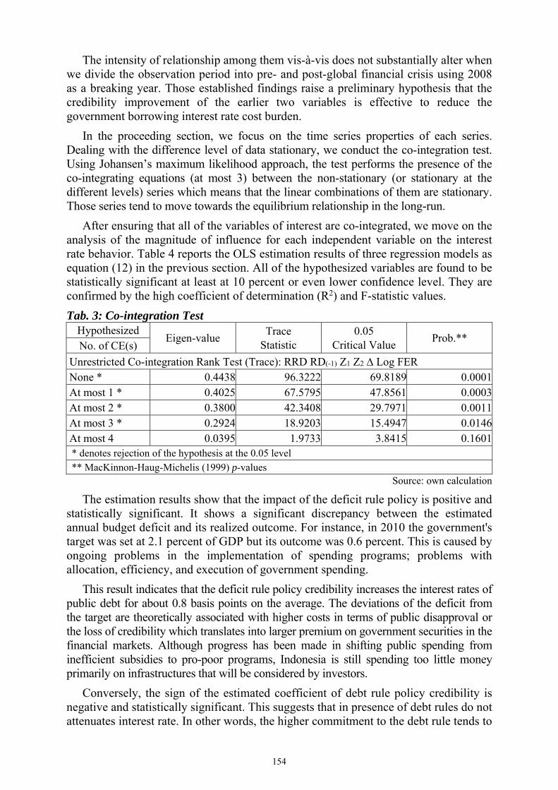
The intensity of relationship among them vis-à-vis does not substantially alter when we divide the observation period into pre- and post-global financial crisis using 2008 as a breaking year. Those established findings raise a preliminary hypothesis that the credibility improvement of the earlier two variables is effective to reduce the government borrowing interest rate cost burden.

In the proceeding section, we focus on the time series properties of each series. Dealing with the difference level of data stationary, we conduct the co-integration test. Using Johansen’s maximum likelihood approach, the test performs the presence of the co-integrating equations (at most 3) between the non-stationary (or stationary at the different levels) series which means that the linear combinations of them are stationary. Those series tend to move towards the equilibrium relationship in the long-run.

After ensuring that all of the variables of interest are co-integrated, we move on the analysis of the magnitude of influence for each independent variable on the interest rate behavior. Table 4 reports the OLS estimation results of three regression models as equation (12) in the previous section. All of the hypothesized variables are found to be statistically significant at least at 10 percent or even lower confidence level. They are confirmed by the high coefficient of determination (R2) and F-statistic values.

Tab. 3: Co-integration Test Hypothesized

Eigen-value Trace

Statistic 0.05

Critical Value Prob.**

No. of CE(s)

Unrestricted Co-integration Rank Test (Trace): RRD RD(-1) Z1 Z2 Log FER None * 0.4438 96.3222 69.8189 0.0001 At most 1 * 0.4025 67.5795 47.8561 0.0003 At most 2 * 0.3800 42.3408 29.7971 0.0011 At most 3 * 0.2924 18.9203 15.4947 0.0146 At most 4 0.0395 1.9733 3.8415 0.1601 * denotes rejection of the hypothesis at the 0.05 level ** MacKinnon-Haug-Michelis (1999) p-values


The estimation results show that the impact of the deficit rule policy is positive and statistically significant. It shows a significant discrepancy between the estimated annual budget deficit and its realized outcome. For instance, in 2010 the government's target was set at 2.1 percent of GDP but its outcome was 0.6 percent. This is caused by ongoing problems in the implementation of spending programs; problems with allocation, efficiency, and execution of government spending.

This result indicates that the deficit rule policy credibility increases the interest rates of public debt for about 0.8 basis points on the average. The deviations of the deficit from the target are theoretically associated with higher costs in terms of public disapproval or the loss of credibility which translates into larger premium on government securities in the financial markets. Although progress has been made in shifting public spending from inefficient subsidies to pro-poor programs, Indonesia is still spending too little money primarily on infrastructures that will be considered by investors.

Conversely, the sign of the estimated coefficient of debt rule policy credibility is negative and statistically significant. This suggests that in presence of debt rules do not attenuates interest rate. In other words, the higher commitment to the debt rule tends to

154

reduce the interest rate cost of government borrowing. The increase in quality of fiscal policy will lead to be lower the interest rates and then economic growth increases.

The monetary phenomena that are captured by the relative change in foreign reserve can marginally (only at 8 percent confidence level) explain the behavior of interest rates. Indeed, the short-term real interest rates reflect cyclical conditions and the stance of monetary policy. Since the corresponding coefficient is negative (-0.08), we can infer that the fluctuation of interest rate in the short-term is typically counter-cyclical against the change in foreign reserve as one of the monetary policy stances.

Tab. 4: Estimation Results of the Government Borrowing Cost Dependent Variable: RRD

(1) (2) (3) Coeff. Prob. Coeff. Prob. Coeff. Prob.

C -0.0060 0.3814 0.2163 0.0078 0.2771 0.0017Z1 - - 0.0079 0.0677 0.0085 0.0465Z2 - - -0.2299 0.0057 -0.2884 0.0013

Log FER - - - - -0.0814 0.0799

RD(-1) 0.3016 0.0000 0.3480 0.0000 0.3429 0.0000RRD(-1) 0.4377 0.0002 0.3621 0.0010 0.3649 0.0007R2 0.8037 0.8356 0.8466R2-adj 0.7955 0.8213 0.8295SEE 0.0193 0.0180 0.0176F 98.2644 58.4639 49.6605DW 1.6733 1.7369 1.7910N 51 51 51


It is widely accepted that the long-term rates are likely to raise more in response to the anticipated worsening of fiscal deficits and debt. In the case of Indonesia, that mechanism is not fully supported for several reasons. First, since 2005 the Central Bank has been focusing on the single goal, i.e. domestic currency stabilization. The change in foreign exchange reserves, therefore, is mainly intended to stabilize Rupiah in terms of exchange rates instead of interest rates. Second, the Central Bank is strictly forbidden to finance deficit. Hence, any monetary policy is independent from fiscal authority’s interventions. Third, both the deficit and debt ratios are successfully maintained below 3 and 60 percent respectively.

The negative impact of the change in international reserve on interest rate is in line with the study of Kandil and Morsy (2014). According to them, the scope for counter-cyclical policy increases with the availability of international reserves as it enhances credibility and mitigates concerns about the effect of expansionary fiscal policy on the cost of borrowing and debt service. In the case of Indonesia, the expansionary fiscal policy remains stimulating economic growth in the short-run, if fiscal easiness induce credibility so that lowers the cost of borrowing and debt service, and mitigates concerns about debt sustainability.

As expected, the coefficient of debt stock ratio in the past periods is positive. An increase of 1 percent in total debt stock ratio in the previous period tends to induce the current interest rate burden for about 30 basis points. Those are plausible results because the implementation of fiscal rules in Indonesia is in the earlier steps after

155

switching from the balance budget rule for a long time to budget deficit adoption that is financed by both domestic and foreign debts.

This result above confirms to the conventional wisdom that balanced budget rules can restrain sovereign debt and lower sovereign borrowing costs. Balanced budget rules serve as a public signal that reveals information about the government’s fiscal situation and more importantly, provides a focal point around which bond markets can coordinate. In our case, budget deficits induce interest rates. However, along with the evolution of public finance which is currently taking place continually in that country, the adoption of fiscal rules will reduce the interest rate burden.

The estimation of the lagged dependent variable gives the significant coefficients. The coefficient of lagged dependent variable is 0.4 suggesting that a change in the interest rates between quarter t-1 and t drives up the interest rate process in t only 0.4 or equivalently 60 percent partial adjustments to respond to the desired interest rates. The interest rate persistency probably due to the increase in commitment fee that should be paid if the outstanding debts are not drawn in the committed period. In principle, this supports to the results of PPE UGM and BAF (2004) and Kuncoro (2011) studies.

Conclusion

The aim of this paper was to provide direct empirical evidence on the potential relationship between fiscal rules policy and interest rates burden. To test the hypothesis, we take the case in Indonesia over the period 2001-2013. We analyzed the quarterly data on deficit and debt deviation from the planned ones and their impact on the implicit real interest rates fluctuation. The empirical study affirms that deficit rule, debt rule, the existing debt, and the relative change in foreign reserve are co-integrated implying they have a long-term relationship.

Furthermore, our pragmatic approach found that the non credible deficit rule policy significantly induces the borrowing cost for about 0.8 basis points. Meanwhile the credible debt rule policy significantly reduces the borrowing cost for about 28 basis points. Overall, the magnitude of fiscal policy credibility has the same effect for the decrease in size of debt stock to repress the interest cost. Those findings suggest that the credibility of fiscal policy matters to restore the fiscal burden in order to maintain fiscal sustainability in the long-run.

Accordingly, those findings provide some important economic implications. First, they suggest that political and institutional factors are the main obstacle in the short-run for government to effectively play an important role to the global financial market via signaling mechanism. Second, the sound and prudent fiscal policy management is necessary to avoid possible dramatic change in interest rates in the long-term in relation to the increase in persistent deficit. Third, as a consequence, they suggest that credibility of fiscal policy improvement should be an integral part of the public sector reformation programs in the country.

Acknowledgement

This paper is financially supported by Faculty of Economics, State University of Jakarta, Indonesia.

156

References

Abdurohman and Resosudarmo, B.P. (2017). “The Behavior of Fiscal Policy in Indonesia in Response to Economic Cycle”, Singapore Economic Review, 62(2), June: 377-401.

Adiningsih, S. (2009). “The Impact of Government Debt Issuance on Short-Term Interest Rates in Indonesia”, Gadjah Mada International Journal of Business, 11(3), pp. 301-318.

Akitoby, B., Clements, B., Gupta, S., and Inchauste, G. (2006). “Public Spending, Voracity, and Wagner's Law in Developing Countries”, European Journal of Political Economy, 22(4), pp. 908–924.

Alesina, A. and Ardagna, S. (2009). “Large Changes in Fiscal Policy: Taxes versus Spending”, NBER Working Paper Series, No. 15348.

Baldacci, E., Gupta, S., and Mati, A. (2008). “Is it (Still) Mostly Fiscal? Determinants of Sovereign Spreads in Emerging Markets”, IMF Working Paper No. WP/08/259, November.

Balduzzi, P., Corsetti, G., and Foresi, S. (1997). “Yield-Curve Movements and Fiscal Retrenchments”, European Economic Review, 41(9), December, pp. 1675-1685, DOI: 10.1016/S0014-2921(96)00059-1.

Blöndal, J.R., Hawkesworth, I., and Choi, H. (2009). “Budgeting in Indonesia”, OECD Journal on Budgeting, 2009/2.

Campbell, J.Y. (1995). “Some Lessons from the Yield Curve”, Journal of Economic Perspectives, 9, pp. 129-152.

Caselli F., Giovannini, A., and Lane, T. (1998). “Fiscal Discipline and the Cost of Public Debt Service: Some Estimates for OECD Countries”, IMF Working Paper, No. 98/55.

Christiano, L., Eichenbaum, M., and Rebelo, S. (2011). “When is the Government Spending Multiplier Large?”, Journal of Political Economy, 119(1), pp. 78-121.

Dai, Q. and Philippon, T. (2005). “Fiscal Policy and the Term Structure of Interest Rates”, NBER Working Papers, No. 11574.

Doraisami, A. (2013). “Fiscal Policy Challenges in Developing Countries, the Indonesian Experience in Responding to the Global Financial Crisis”, Journal of Southeast Asian Economies, 30(3): 322–333.

Elmendorf, D.W. (1993). “Actual Budget Deficit Expectations and Interest Rates”, Harvard Institute of Economic Research, May.

Elmendorf, D.W. (1996). “The Effects of Deficit Reduction Laws on Real Interest Rates”, Finance and Economics Discussion Series, No. 1996-44, Federal Reserve Board, October.

Engen, E.M. and Hubbard, R.G. (2004). “Federal Government Debt and Interest Rates”, AEI Working Paper, No. 105.

Evans, P. (1985). “Do Large Budget Deficits Produce High Interest Rates?”, American Economic Review, 75(1), pp. 68-87.

Evans, P. (1987). “Interest Rates and Expected Future Budget Deficits in the United States”, Journal of Political Economy, 95(11), pp. 32-58.

Feldstein, M. (1986). “Budget Deficits, Tax Rules, and Real Interest Rates”, NBER Working Paper, No. 1970.

Gale, W.G. and Orszag, P.R. (2003). “The Economic Effects of Long-Term Fiscal Discipline”, The Urban Institute, Discussion Paper, No. 8.

Hauner, D., Jonas, J., and Kumar, M.S. (2007). “Policy Credibility and Sovereign Credit: The Case of the New EU Member States”, IMF Working Paper WP/07/1, January.

Heinemann, F., Osterloh, S., and Kalb, A. (2014). “Sovereign Risk Premia: The Link between Fiscal Rules and Stability Culture”, Journal of International Money and Finance, 41, pp. 110-127, http://dx.doi.org/10.1016/j.jimonfin.2013.11.002.

Hur, S., Mallick, S., and Park, D. (2010). “Fiscal Policy and Crowding Out in Developing Asia”, ADB Economics Working Paper Series, No. 222, September.

157

Ito, T., Iwata, K., Mckenzie, C., and Urata, S. (2012). “Fiscal Policy and Sovereign Debt: Editors' Overview”, Asian Economic Policy Review, 7(2), December, pp. 135-156, DOI: 10.1111/j.1748-3131.2012.01244.x.

Kandil, M. and Morsy, H. (2014). “Fiscal Stimulus and Credibility in Emerging Countries”, Eastern Economic Journal, 40, pp. 420-439.

Kopits, G. (2001). “Fiscal Rules: Useful Policy Framework or Unnecessary Ornaments?”, IMF Working Paper WP/01/145.

Kuncoro, H. (2011). “The Cost of Public Debt Services, the Case of Indonesia”, International Journal of Advanced Economics and Business Management, 1(1), pp. 14-24.

Laksmi Y.D., Adiningsih, S., and Lestari, M. (2012). “The Impact of Government Debt Issuance on Lending Rate in ASEAN-5 Countries”, Final Report of an EADN Individual Research Grant Project, EADN Working Paper No. 55.

Laubach, T. (2009). “New Evidence on the Interest Rate Effects of Budget Deficits and Debt”, Journal of European Economic Association, 7, pp. 858–885, DOI: 10.1162/JEEA.2009.7.4.858.

Missale, A., Giavazzi, F., and Benigno, P. (1997). “Managing the Public Debt in Fiscal Stabilizations: the Evidence”, NBER Working Paper No. 6311.

Naert, F. (2011). “Credibility of Fiscal Policies and Independent Fiscal Bodies”, Review of Business and Economic Literature, 56(3), pp. 288-309.

Plosser, C.I. (1982). “Government Financing Decisions and Asset Returns”, Journal of Monetary Economics, 9(3), pp. 325-352.

Plosser, C.I. (1987). “Fiscal Policy and the Term Structure”, Journal of Monetary Economics, 20(2), pp. 343-367.

Poterba, J.M. and Rueben, K.S. (2001). “Fiscal News, State Budget Rules, and Tax-Exempt Bond Yields”, Journal of Urban Economics, 50, pp. 537-562, DOI:10.1006/juec.2001.2233.

PPE UGM and BAF, (2004). A Study on Internal and External Government Debt Management and Assessment to Optimal Borrowing, Research Project, Final Report.

Thorbecke, W. (1993). “Why Deficit News Affects Interest Rates”, Journal of Policy Modeling, 15(1), pp. 1-11.

Wachtel, P. and Young, J. (1987). “Deficit Announcements and Interest Rates”, American Economic Review, 77, pp. 1007-1012.

World Bank, (2014). World Development Report 2014: Risk and Opportunity Managing Risk for Development, Washington DC: World Bank.

Žigman, A. and Cota, B. (2011). “The Impact of Fiscal Policy on Government Bond Spreads in Emerging Markets”, Financial Theory and Practice, 35(4), pp. 385-412.

Contact Address

Haryo Kuncoro Faculty of Economics, State University of Jakarta Rawamangun Muka, Jakarta Timur 13220, Indonesia Email: [email protected] Phone number: +622147882651 / +62817267325


158

FDI AND REGIONAL INCOME DISPARITY IN THE CZECH REPUBLIC

Jagannath Mallick, Pavel Zdražil

Abstract: The aim of this paper is to evaluate the impact of FDI along with domestic physical investment and human capital on the regional income, and their role in the regional income convergence within the Czech economy over the periods from 1998-99 to 2013-14. The paper considers 14 regions of the Czech Republic and uses panel fixed effect regression and dynamic panel growth framework for the empirical analysis. The result finds that the role of physical capital formation and FDI along with the human capital are crucial for the regional disparity in income in the Czech Republic. There is also evidence of the convergence of per capita income at the speed of 7.8 per cent among the regions by conditioning physical investment and human capital along with FDI. This paper suggests that regional disparity in income can be reduced by the equitable allocation of investment and FDI, and equal development of human capital.

Keywords: Investment, Convergence, Regional Growth, Panel Data Methods.

JEL Classification: E22, R11, C23.

Introduction

In light of the below discussion, this paper aims at evaluating the impact of FDI along with domestic physical investment and human capital on the regional income, and their role in the regional income convergence within the Czech economy. The detailed empirical analysis of the study may suggest the policies to achieve balanced and inclusive growth, which will ensure regional convergence in terms of per capita income and spread the benefits of the growth processes among different regions of the Czech Republic. Actually, it can be suitable for many other countries that are facing similar “growth-inequality issues” like the Czech Republic. The paper is designed as follows: Section 1 introduces the problem by discussing the importance of income inequality issue in the European Union (EU) and the Czech Republic, as well as the implication of regional policy to deal with inequalities via investment and advent of human capital at most. Section 2 describes the theoretical framework to examine the factors of regional income disparity and explains the methodology for the empirical analysis and data. Section 3 discusses the results. The last section concludes the paper.

1 Income inequality issue in the European Union and the Czech Republic

The increasing disparities in development of regional economics can result in a tremendous imbalanced structure of national economics and European economy as a whole and, of course, large disparities in standards of living of inhabitants as well - the reason for such a disparities increasing rests in cumulating of pretty small differences over a long-run, that impacts the level of development significantly (Barro, Sala-i-Martin, 2004). The issue is that imbalanced economics impacts the subsequent growth and development negatively (Alesina, Rodrik, 1994). Clear evidence of such meaning can be found in works of Murphy et al. (1989) and Perotti (1993) who argue that income distribution determine the level of demand and equilibrium; hence, it impacts the

159

industrialization potential and growth. Stiglitz (2009) even claim that the rise of inequalities during last decades was one of the main causes of the economic crisis of 2008. In particular, disparities have to be seen as important reasons for tensions across nations, regions and society.

Based on the principle of solidarity, many tools to facing disparity within the EU area have been developed. In fact, the basic strategic document Europe 2020 is aimed to make growth more inclusive in terms of benefits of growth flowing to all inhabitants, especially those facing poverty or dealing with additional challenges. The strategy suggests that investment and education improvement should be the right path to achieve that goal. Besides, the main objective of last programming periods “Convergence” was designed upon solidarity between the regions - to reduce disparities at the NUTS 2 level of regions, i.e. between the regions across countries, but is not aimed at the countries themselves.

There are several studies, e.g. Geppert et al. (2008), Armstrong (1995), advocate the convergence hypothesis for EU regions. In contrast, many other studies proved that the disparities across the EU are decreasing while inner-country disparities are increasing in many EU member states (Marzinotto, 2012; Barca, 2009; Zdražil, Applová, 2016). Now, one can say, that the main objective of EU cohesion policy i.e. reducing disparities between the EU regions, is fulfilling, but the national objectives of reducing regional disparities are not achieved in many countries. An example of such a development, where regions converge towards the EU average while inner-country disparities between the regions are increasing, is the Czech Republic. The gap between the GDP per capita of the EU and the Czech average decreased from 28.1% to 15.6% between 2000 and 2014, while the disparities (measured by the coefficient of variation) among the Czech NUTS 2 regions increased from 36.3% to 39.7% during this period (Eurostat, 2016). In addition, one can say the disparities among the Czech NUTS 2 regions are pretty high, since the Czech Republic ranked 4th position among the EU countries between 2000 and 2014 (Eurostat, 2016). All those lead us to conclude that the issue of regional disparity in the Czech Republic and its determinants is demanding and calls for a deeper analysis.

The recent EU strategy is focusing investment and education improvements. This paper seeks to examine the role of both investment and education in the dynamics of economic growth in the Czech regions. Both factors can be seen as instruments to reducing disparities, but they are able to raise disparities as well (Kraftová, Kraft, 2016; Capello et al., 2011). We are focusing the role and importance of FDI due to its significant volume in a small open economy like Czech Republic, and its huge impacts on regional development as well. In fact, FDI are very important for Czech economy, since it is located in the middle of Europe – the major magnet for inward as well as the leading source of outward FDI – the Europe (Dicken, 2015). Furthermore, we are focusing the role of education, since education - as well as the technological progress - is the crucial factor of endogenous growth (Romer, 1986; Lucas, 1988; Rebelo, 1991; Barro, Sala-i-Martin, 2004).

Even repeating the well-known rule, we should point out that education and investment capability are much more interconnected than one can suggest. The well-educated population is always regarded to be the key to economic development in any region (Machlup, 1975; Graff, 1999). The evidence of that can be found in literature as follows: education is one of the main prerequisites to work (Maddison, 1994); adoption

160

of technological change requires education (Easterlin, 1981) and, at the same time, well-educated workers have comparative advantage in implementation of new technologies (Bartel, Lichtenberg, 1987); education is more productive and more stable than the level of technology factor (Nelson, Phelps, 1966; Schultz 1975); education impacts the capability to adopt innovations from foreign countries (Dowrick, Gemmel, 1991; Nelson, Phelps, 1966); and, investment is probably the best growth indicator while by considering conditions of income and education, we can get pretty solid indicator of further development (Rodrik, Chen, 1998).

In the recent study, Majeed (2017) found that FDI contribute to disparity reducing in countries with better developed human capital, while in that undeveloped FDI rather supports disparity increase. Kheng et al (2017) also found strong connections and suggest that FDI and human capital development policies, in particular spending on education and training, should be coordinated. Moreover, FDI and human capital seems to be associated with higher income in the European regions as they are positive interaction of FDI and human capital in relation to the income growth dynamics (Vollmecke et al., 2016; Jimborean, Kelber, 2017).

1.1 Regional inequalities, investment and human capital in the Czech Republic

Many recent studies conclude that the economic growth in the Czech Republic is stemming from connections between the Czech and German economics, and effects of the EU accession via the catching-up process of lesser developed regions (Crespo-Cuaresma et al., 2014). In fact, the solid performance is caused by investment inflows, technology transfer and export opportunities (Forgó, Jevčák, 2015; Dobrinsky, Havlik, 2014). Slavík (2007) suggests that the growth of the Czech Republic was slower than it should be when we consider the level of real income; still, his research is developed on EU pre-accession period (pre-2004). Considering recent data, we know the economic growth accelerated after 2004 significantly, then experienced big fall due to the economic crisis (2009) and recovery phase started in 2014 (Czech Statistical Office, 2016); hence, it is hard to offer the reliable evaluation of the current relationship between the production and income level.

According to Popescu (2014), the Czech Republic unambiguously dominates in the investment inflows with second highest FDI amount in the Central and Eastern Europe. Crespo-Cuaresma et al. (2012) developed similar conclusions when arguing that the Czech regions are among the most attracting FDI destinations in the Central and Eastern Europe, and actually currently leading FDI recipients. However, the effect of FDI on regional attractiveness from the inhabitants' point of view is ambiguous since the living standard indicators are influenced only partially and only in some of the Czech regions (Zdražil, 2015). Another study adds an additional point to this discussion when results that the gross fixed capital formation share of GDP was high in the Czech Republic during last decade, even during the crisis – at least 25% (Forgó, Jevčák, 2015). Besides, we have to consider the findings of Kraftová and Matěja (2014) who argue that industrial structure changes in Czech regions are limited due to the low qualification capability of population; and hence, this limitation is a large barrier to major long-term growth and development impulses. With all those facts, we can say that both development drivers - investment and education - play the crucial role in process of subsequent growth and development.

161

2 Theoretical framework and empirical methodology

The neoclassical growth theory has been used to understand the regional disparity in income due to its theoretical foundation (Barro and Sala-i-Martin, 2004; Baumol, 1986; Cashin, 1995; DeLong, 1988; Mankiw et al., 1992; Mallick, 2014; Mallick, 2017). This paper makes use of the theoretical framework as provided in Mankiw et al. (1992). The Cobb-Douglas production function with inputs labour, physical capital and human capital, which are paid at their marginal productivities, and with decreasing returns in accumulable factors, the production function can be specified as (1)

∝ , where, 0 λ 1 (1)

where, Yit, Ait, Kit, Hit and Lit represent output, level of technology, stock of physical capital, human capital and quantity of labour respectively, in region ‘i’ at time ‘t’. The coefficients α, λ and (1-α- λ) reflect the elasticities of output with respect to physical capital, human capital and labour. Whereas, L is assumed to grow exogenously at ‘n’ (i.e. growth of population) and A is also assumed to grow at rate ‘g’ (i.e. growth of technology). Following Mankiw et al. (1992), the human capital along with labour and physical capital as the factors of production, the natural log of per capita income (y).

ln a ln ln ln (2)

The equation (2) says that natural log of per capita income (ln y) is positively related to the natural log of physical investment rate (s) and human capital (h), and negatively to the effective depreciation rate (n+g+ ). Whereas, n+g+ is the growth rate of labour force with adjusted +g (= 0.07), Ɛit is the random disturbance term in the equation and

ln . According to Mankiw et al. (1992), based on the Solow-Swan growth model (Solow, 1956; Swan, 1956), the equation (2) can be modified to address the issue of conditional convergence of regional per capita income as follow.

ln ln ln ln ln ln (3)

where, and the convergence rate, β= (1-α-λ) (n+g+δ).

Equation (3) represents that the per capita income depends on the initial levels of per capita income (yi,0) and technology (A0), the growth of technology (g), the saving rate (sit), the growth rate of population or labour force (n), the rate of capital depreciation (δ), the rates of physical and human capital (α and λ), and the rate of convergence to the steady state (β). Thus, the equation indicates that a high investment rate is positively related to the growth in per capita income and the growth of labour force is negatively related to the growth in per capita income after being adjusted for technological progress and capital depreciation. Further, the assumption of diminishing returns to reproducible capital is the base for predicting the rate of conditional convergence. Equation (3) indicates that regions with low initial per capita income grow faster than that with higher, conditioning upon the values of s, h, n, g and . This equation is used as the framework for empirical estimation of this study under the assumption that there is common production structure in all 14 regions of the Czech economy. As the focus of the study is to evaluate the role and importance of FDI on the per capita income and long-run dynamics of economic growth, equation (3) is extended to include FDI as a factor of production.

162

The study considers all the 14 regions of the Czech Republic for the duration from 1998-99 to 2013-14. We have focused on the NUTS 3 level of regions which is below the main level where the EU cohesion policy is performed. The reason is that the NUTS 2 regions of the Czech Republic are just formally arranged units, which have been created only due to the management and funding of the EU regional policy. In fact, the Czech lower-level government is organized at the level of NUTS 3 regions. The study includes 224 numbers of observations by pooling 14 regions over 16 years. The first objective of the study used panel data method to control for individual heterogeneity of the regions with more degree of freedom and efficiency (Baltagi, 2001). There are three types of panel data methods. They are pooled regression, fixed effects regressions, and random effects regressions. There are two tests viz. Breusch and Pagan Lagrange Multiplier (LM) and the Hausman specification, which are used to diagnose the appropriate method out of above three. The significance of LM test statistics indicates that the estimation using 3rd or 2nd method is more appropriate than the 1st one. Whereas, the statistical significance of Hausman test confirms preferring estimation by using fixed effect regression over random effect regression.

The second objective of the study uses dynamic panel growth framework of Islam (1995), which is derived from the basic neoclassical growth model. The yearly time periods are too short to study regional growth convergence. The disadvantage of using annual data on per capita real income is the increasing serial correlation due to the effects of business cycle and shocks. In contrast, using a long-period average captures the changes in the steady state per capita income. We use a panel of four-year spans (i.e. τ = 4). Hence, for the period 1998–99 to 2013–14, we have four panels. With time span (τ), the equation (3) can be modified as follow.

, ∑ μ (4)

Where y is the per capita income. ln ln

1 1 1

The implied β (rate of conditional convergence) is . This analysis includes 56

numbers of observations by pooling 14 regions over four periods (each spanning a period of 4 years). Hence, the analysis of this objective uses the pooled regression.

2.1 Data

The data are based on secondary sources. The functional form of (4) has been used to evaluate the impact of FDI, physical investment and human capital on income at the regional level by using the annual data. The data on FDI are taken from the Czech National Bank (CNB) while the GDP, GFCF and population data are sourced from the Czech Statistical Office (CZSO). Human capital is expected to positively influence the income at the regional level. Human capital allows the operation of tasks that are more complicated and which produce high-skill products, thereby improving productivity. Further, Lucas (1988) argued that human capital generates positive externalities. The total number of enrolments in tertiary education, representing human capital at the regional level, is sourced from CZSO regional departments’ databases. The detailed measurements of variables and data sources are described in Tab. 1. The summary statistics of the variables are presented in table A1 of appendices.

163

Tab. 1: Variables and data sources variables measurement sources

Income Gross domestic product per capita (PGDP) at constant prices 2005 in CZK

CZSO

Domestic investment Gross fixed capital formation per capita (PGFCF) at constant prices 2005 in CZK

CZSO

Foreign direct investment

Foreign direct investment per capita (PFDI) at constant prices 2005 in CZK

CNB

Human capital The attendance of tertiary education per 1000 inhabitants (TER)

CZSO

Source: own processing

The long-run dynamics of income at the regional level is examined by using the dynamic panel growth equation (4). The annual time length’s data are very short to study growth convergence and hence the total time period from 1998–99 to 2013–14 is divided into four-year shorter time periods to estimate equation (4). The four-year periods are 1998-2001, 2002–2005, 2006–2009 and 2010-2013. The dependent variable is the natural logarithm of per capita income [ln. (PGDP)] in the estimation. The independent variables are natural log of per capita income at the beginning of the each four-year period [ln (PGDP0)], the natural log of per capita domestic investment [ln. (PGFCF)] and foreign direct investment [ln. (PFDI)], adjusted population growth rate [ln. (APG)] and human capital [ln. (TER)].

3 Problem solving and results

This section provides the patterns of income disparity and also the econometric analysis. The histogram of the regional per capita income (in tens of thousands CZK) for the latest year 2013-14 is plotted in fig. 1. This shows that the per capita income of 50 per cent of regions out of 14 lies in the range of 250000 CZK to 300000 CZK. Karlovy Vary and Prague regions are placed at the extreme left and right positions in the histogram, respectively. This indicates that there is existence of income inequality across the regions in the Czech Republic.

Fig. 1: Regional per capita income inequality in 2013-14

Sources: basic data of Czech Statistical Office (2016; 2017)

As mentioned in the literature we observe that there is a systematic relation of per capita income with the per capita FDI and physical investment, and human capital at the national level. The per capita income of Czech economy has positive trend from 1998-99 to 2013-14, which is accompanied by the positive trends of per capita FDI, per capita physical investment and human capital (see, fig. A1 in appendices). Hence we expect that these factors may be responsible for such outcome of the regional income distribution.

0

2

4

6

8

20-25 25-30 30-35 35-40 70-75

164

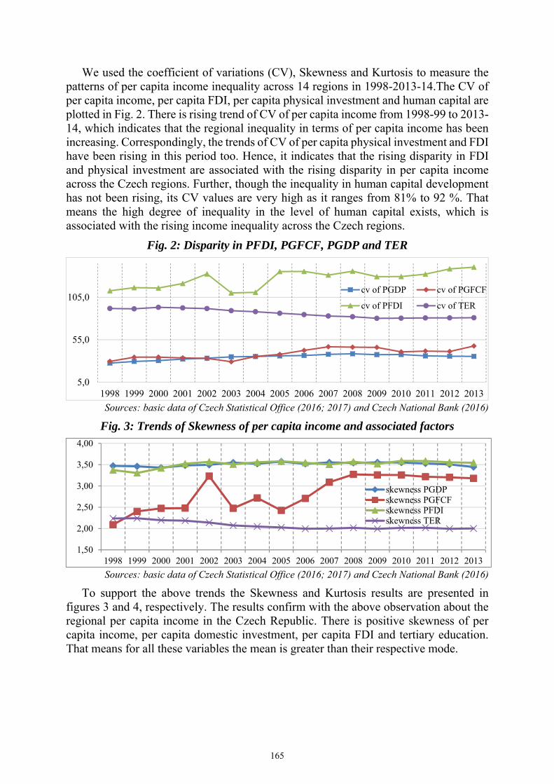
We used the coefficient of variations (CV), Skewness and Kurtosis to measure the patterns of per capita income inequality across 14 regions in 1998-2013-14.The CV of per capita income, per capita FDI, per capita physical investment and human capital are plotted in Fig. 2. There is rising trend of CV of per capita income from 1998-99 to 2013-14, which indicates that the regional inequality in terms of per capita income has been increasing. Correspondingly, the trends of CV of per capita physical investment and FDI have been rising in this period too. Hence, it indicates that the rising disparity in FDI and physical investment are associated with the rising disparity in per capita income across the Czech regions. Further, though the inequality in human capital development has not been rising, its CV values are very high as it ranges from 81% to 92 %. That means the high degree of inequality in the level of human capital exists, which is associated with the rising income inequality across the Czech regions.

Fig. 2: Disparity in PFDI, PGFCF, PGDP and TER

Sources: basic data of Czech Statistical Office (2016; 2017) and Czech National Bank (2016)

Fig. 3: Trends of Skewness of per capita income and associated factors


To support the above trends the Skewness and Kurtosis results are presented in figures 3 and 4, respectively. The results confirm with the above observation about the regional per capita income in the Czech Republic. There is positive skewness of per capita income, per capita domestic investment, per capita FDI and tertiary education. That means for all these variables the mean is greater than their respective mode.

5,0

55,0

105,0

1998 1999 2000 2001 2002 2003 2004 2005 2006 2007 2008 2009 2010 2011 2012 2013

cv of PGDP cv of PGFCF

cv of PFDI cv of TER

1,50

2,00

2,50

3,00

3,50

4,00

1998 1999 2000 2001 2002 2003 2004 2005 2006 2007 2008 2009 2010 2011 2012 2013

skewness PGDPskewness PGFCFskewness PFDIskewness TER

165

Fig. 4: Trends of Kurtosis of per capita income and associated factors


The empirical analysis started with the diagnostic tests to choose the appropriate methods of the panel data (see Tab. 2). The results show that the value of LM statistics and Hausman statistics are statistically significant in all the regressions. Hence, all the regressions are estimated using the fixed effect method. The F-statistic for the region-specific coefficients is significant at 1% in all the regressions, which indicates the significance of region-specific factors across the regions of the Czech economy.

The regression 1 includes per capita income as the function of per capita domestic investment and foreign investment. The result shows that all the coefficients have their expected sign and they are statistically significant. Further, the regression 1 is expanded to include the interaction of foreign direct investment and physical investment (PGFCF*PFDI). The finding is in confirmation with the argument made by Kay (2007), that FDI is a challenge to the domestic firms or investment. The analysis finds the negative interaction coefficient, which indicates that the FDI has crowd-out effect on the domestic investment in 1998–99 to 2013–14. This is also evidenced in the context of the developing countries like India and China (Mallick, 2017; Mallick 2015).

Further, the human capital (TER) along with the FDI and physical investment is used in the specification of regression 3. This also shows that all the included factors are statistically significant with the expected positive signs. The human capital is affecting the regional income through improving productivity. The interaction effect of FDI and physical investment is incorporated in regression 4, which also confirms the crowding out effect of FDI in the domestic investment in Czech regions. Finally, along with the three factors and the interaction terms between physical investment and FDI, the second interaction term of FDI with the human capital (PFDI*TER) is used as an additional regressor in regression 5. The result confirms the findings as obtained from the previous regressions, and also shows that there is positive interaction effect of FDI on the human capital. This indicates that the FDI has been driving the human capital across the Czech regions. The multinational investors required the skilled labour, which forces the residents to go for higher education to get a job. Consequently, FDI is affecting the human capital development across the Czech regions.

4,00

6,00

8,00

10,00

12,00

14,00

1998 1999 2000 2001 2002 2003 2004 2005 2006 2007 2008 2009 2010 2011 2012 2013

Kurtosis PGDPKurtosis PGFCFKurtosis PFDIKurtosis TER

166

Tab. 2: Impact of FDI on regional income Variables Regression 1 Regression 2 Regression 3 Regression 4 Regression 5 PGFCF 1.31 (0.14)*** 1.51 (0.12)*** 0.63 (0.11)*** 0.80 (0.11)*** 0.43 (0.12)***PFDI 0.23 (0.02)*** 0.55 (0.05)*** 0.11 (0.02)*** 0.26 (0.04)*** 0.28 (0.04)***TER 3.33 (0.23)*** 2.92 (0.24)*** 3.43 (0.24)

PGFCF*PFDI -0.000001 (0.0000001) ***

-0.000001 (0.0000001) ***

-0.000001 (0.0000003) ***

PFDI*TER 0.000003 (0.0000006) ***

F test for all u_i=0

F(13, 208) = 13.98 ***

F(13, 207) = 19.47 ***

F(13, 207) =31.63***

F(13, 206) = 29.88 ***

F(13, 205) = 37.9 ***

Over all Rsq. 0.94 0.94 0.87 0.901 0.90 Hausman test 39.99 *** 29.99 *** 15.99 *** 20.28 *** 43.97*** n 224 224 224 224 224

Note: the figures in parenthesis are the standard error of estimates. ***, ** and * represent the statistical significance at 1%, 5% and 10% level.

Source: Author’s estimation

The role and importance of physical investment, human capital and FDI in the long-run dynamics of income at the regional level is analysed by using dynamic panel growth equation (4) as suggested by Islam (1995) and Mankiw et al. (1992). The empirical result is presented in Tab. 3.

Tab. 3: Regional convergence of income Independent variables Dependent variable: LnY

LnY0 0.73 (0.09) *** LnPGFCF 0.14 (0.05) *** LnPFDI 0.02 (0.03) LnTER 0.02 (0.01) ** Ln APG - 0.05 (0.10) F test F(5, 50) = 229.89 *** Rsq. 0.96 n 56

Note: the figures in parenthesis are the standard error of estimates. ***, ** and * represent the statistical significance at 1%, 5% and 10% level. APG represents the adjusted population growth (n+g+ ).

Source: Author’s estimation

Regression includes per capita income as the function of initial per capita income, per capita domestic investment, foreign investment, human capital and population growth. The result shows that all the coefficients have their expected sign and they are statistically significant except the coefficient of adjusted population growth. The coefficient of initial income is found to be 0.73, which indicates the conditional convergence of income across the Czech regions. Hence by Islam (1995) the speed of convergence among the Czech region is 7.8%, conditioning to domestic investment, FDI and human capital in 1998–99 to 2013–14.

There is empirical evidence of conditional convergence of steady state income across the Czech regions. The FDI along with the physical investment and human capital is crucial in the regional income convergence of the Czech economy. This conclusion seems to be important for the understanding of disparities mechanism in the Czech Republic. In addition, the findings of Pinho et al. (2015) suggest that the impact of the financial aid accessed via the EU cohesion policy on regional growth are marginal,

167

moreover the impacts seem positive and significant only in regions with low levels of human capital. Hence, we have to conclude that the regional policy focused on FDI with the physical investment and human capital seems to be a much better instrument to solve the problem of imbalance in economic growth.

4 Conclusion

This paper sought to examine the role of foreign and domestic physical investment along with human capital in the regional disparity in income within the Czech economy during the period from 1998–99 to 2013–14. The preliminary analysis shows that there is existence of income inequality across the regions in the Czech economy. The results of trends of coefficient of variation, skewness and kurtosis show that such income inequality has been rising over the periods. The empirical analysis of panel fixed effect regressions concludes that FDI is crucial along with physical investment, human capital and region specific factors for the variation in per capita income in the Czech regions. This also observes that the FDI has a crowding-out effect on the domestic investment, and FDI affects positively to the development of human capital at the regional level in the Czech economy.

This paper also examined the long-run dynamics of economic growth within the regions of the Czech economy by using dynamic panel growth method as suggested by Islam (1995). The analysis concludes that there is the β-convergence of per capita income at the speed of 7.8 % by conditioning FDI, physical investment and human capital. Therefore, the equitable allocation of domestic physical investment and FDI along with the development of human capital in the low-income regions may help to mitigate the problem of imbalanced economic development within the Czech economy.

While this paper has examined the role and importance of foreign and domestic investment and human capital in the inter-regional disparity in the Czech Republic, many opportunities for extending the scope of this study remains. During this globalisation era there labour is moving from lower productivity sectors to the higher productivity sectors and also migrating from the lower wage regions to the higher wage regions. Similarly, capital as the factor of production is also reallocating from lower productivity sectors and regions to the higher productive sectors and regions. The future studies can relate such factor reallocation with regional disparity in income in the Czech Republic which will give a complete understanding of this issue.

References

Alesina, A., Rodrik, D. (1994). Distributive Politics and Economic Growth. The Quarterly Journal of Economics, 109 (2), pp. 465-490. DOI 10.2307/2118470

Armstrong, H. (1995). Convergence among Regions of the European Union. Papers in Regional Science, 74 (4), pp. 143-152. DOI 10.1111/j.1435-5597.1995.tb00633.x

Baltagi, B. (2001). Econometric Analysis of Panel Data. Chichester: John Wiley & Sons.

Baumol, W. (1986). Productivity growth, convergence and welfare: What the long-run data show. American Economic Review, 76 (5), pp. 1072–1085.

Barca, F. (2009). An Agenda for a Reformed Cohesion Policy: A place-based approach to meeting European Union challenges and expectations. Brussels: European Commision.

Barro, R., Sala-I-Martin, X. (2004). Economic Growth. 2nd edition. London: The MIT Press.

168

Bartel, A., Lichtenberg, F. (1987). The Comparative Advantage of Educated Workers in Implementing New Technology. Review of Economics and Statistics, 69 (1), pp. 1-11. DOI 10.2307/1937894

Capello, R., et al. (2011). Globalization and Regional Growth in Europe. Berlin: Springer.

Cashin, P. (1995). Economic growth and convergence across the seven colonies of Australia: 1861–1991. Economic Record, 71 (213), pp. 132–144. DOI 10.1111/j.1475-4932.1995.tb01880.x

Crespo-Cuaresma, J., et al. (2012). Drivers of Convergence in Eleven Eastern European Countries. Washington, DC: The World Bank.

Crespo-Cuaresma, J., et al. (2014). The Determinants of Economic Growth in European Regions. Regional Studies, vol. 48 (1), pp. 44-67. DOI 10.1080/00343404.2012.678824

Czech National Bank. (2016). Foreign direct investment - annual reports. [online] Available at: www.cnb.cz/en/ statistics/bop_stat/bop_publications/pzi_books/index.html [Accessed 17. 12. 2016].

Czech Statistical Office. (2016). Database of Regional Accounts. [online] Available at: apl.czso.cz/pll/rocenka/rocenka.indexnu_reg?mylang=EN [Accessed 21. 12. 2016].

Czech Statistical Office - Regional Departments. (2017). Regionální časové řady. [online] Available at: www.czso.cz/csu/czso/regionalni_casove_rady Accessed 10. 1. 2017].

DeLong, B. (1988). Productivity growth, convergence and welfare: Comment. American Economic Review, 78 (5), pp. 1138–1154.

Dicken, P. (2015). Global Shift. 7th edition. London: The Guilford Press.

Dobrinsky, R., Havlik, P. (2014). Economic Convergence and Structural Change: the Role of Transition and EU Accession. Vienna: WIIW.

Dowrick, S. Gemmell, N. (1991). Industrialisation, Catching Up and Economic Growth: A compa-rative Study Across the World’s Capitalist Economies. Economic Journal, 101 (405), pp 263-275.

Easterlin, R. (1991). Why Isn’t the Whole World Developed? Journal of Economic History, 41 (1), pp. 1-19. DOI 10.1017/S0022050700042674

Eurostat. (2016). Database. [online] Available at: ec.europa.eu/eurostat/data/database Accessed [19. 12. 2016]

Forgó, B., Jevčák, A. (2015). Economic Convergence of Central and Eastern European EU Member States over the Last Decade (2004-2014). Brussels: European Commision.

Geppert, K., et al. (2008). Regional Disparities in the European Union: Convergence and Agglomeration. Papers in Regional Science, 87 (2), pp. 193-217. DOI 10.1111/j.1435-5957.2007.00161.x.

Graff, M. (1999). Educational Imbalance, Socio-Economic Inequality, Political Freedom and Economic Development. Journal of Economic Development, 24(2), pp. 1-18.

Islam, N. (1995). Growth empirics: A panel data approach. The Quarterly Journal of Economics, 110 (4), pp. 1127–1170. DOI 10.2307/2946651

Jimborean, R., Kelber, A. (2017). Foreign Direct Investment Drivers and Growth in Central and Eastern Europe in the Aftermath of the 2007 Global Financial Crisis. Comparative economic studies, 59 (1), pp. 23-54. DOI 10.1057/s41294-016-0018-9

Kay, N. (2007). Foreign investment in the Czech Republic: a challenge for domestic firms. ECFIN Country Focus, 4 (2), pp. 1-6.

Kheng, V., et al. (2017). Foreign direct investment and human capital. Economic change and restructuring, 50 (4), pp. 341-365. DOI 10.1007/s10644-016-9191-0

Kraftová, I., Kraft, J. (2016). Regional distribution of pro-innovative sources in the Czech Republic and their linkage to performance, In: 19th international Colloquium on Regional Sciences. Conference Proceedings. Brno: Masaryk University, pp. 273-281. DOI 10.5817/CZ.MUNI.P210-8273-2016-34

Kraftová, I., Matěja, Z. (2014). Interaction of Qualified and Higher-educated Experts’ Structure and Regional Labour Market Needs. Scientific Papers of the University of Pardubice - Series D, Faculty of Economics and Administration, 21 (3), pp. 62-72.

169

Maddison, A. (1994). Explaining the Economic Performance of Nations, 1820-1989. In: Convergence of Productivity. New York: Oxford University Press, pp. 20-61.

Machlup, F. (1975). Education and Economic Growth. New York: University Press.

Majjed, M. (2017). Inequality, FDI and economic development: evidence from developing countries. Singapore economic review, 62 (5), pp. 1039-1057. DOI 10.1142/S0217590815500678

Mallick, J. (2017). Globalisation, Structural Change and Productivity Growth in India and the People’s Republic of China (PRC). ADBI Working Paper, February No-656. Tokyo: Asia Development Bank.

Mallick J. (2015). Globalisation, Structural Change and Productivity Growth in the Emerging Countries. Indian Economic Review, 50 (2), pp. 181-216.

Mallick, J. (2014). Regional Convergence of Economic Growth during Post-Reform Period in India. The Singapore Economic Review, 59 (2). pp. 1-18. DOI 1450012-1-1450012-18

Mankiw, G., et al. (1992). A contribution to the empirics of economic growth. The Quarterly Journal of Economics, 107 (2), pp. 407-437. DOI 10.2307/2118477

Marzinotto, B. (2012). The Growth Effects of EU Cohesion Policy: A Meta-analysis. Brussels: Bruegel.

Murphy, K., et al. (1989). Income Distribition, Market Size, and Industrialization. The Quarterly Journal of Economics, 104 (3), pp. 537-564. DOI 10.2307/2937810

Nelson, R. Phelps, E. (1966). Investment in Humans, Technological Diffusion, and Economic Growth. American Economic Review 65 (2), pp. 69-75.

Perotti, R., (1993). Political Equilibrium Income Distribution and Growth. Review of Economic Studies, 60 (4), pp. 755-76. DOI 10.2307/2298098

Pinho, C., et al. (2015) Under What Conditions Do Structural Funds Play a Significant Role in European Regional Economic Growth? Some Evidence from Recent Panel Data. Journal of Economic Issues, 49 (3), pp. 769-771. DOI 10.1080/00213624.2015.1072382

Popescu, G. (2014). FDI and Economic Growth in Central and Eastern Europe. Sustainability, 6 (11), pp. 8149-8163. DOI 10.3390/su6118149

Rebelo, S. (1991). Long-Run Policy Analysis and Long-Run Growth. Journal of Political Economy, 99 (3), pp. 500-521. DOI 10.1086/261764

Rodrik, D., Chen, T. (1998). TFPG Controversies, Institutions and Economic Performance in East Asia. In: International Economic Association Series. London: Palgrave Macmillan, pp. 79-105.

Romer, P. (1986). Increasing Returns and Long–Run Growth, Journal of Political Economy, 94 (5), pp. 1002-1037. DOI 10.1086/261420

Schultz, T. (1975). The Value of the Ability to Deal with Disequilibria. Journal of Economic Literature, 13 (3), pp. 827-846.

Slavík, C. (2007). Reálná konvergence Čeké republiky k Evropské unii v porovnání s ostatními novými členskými zeměmi. Politická ekonomie, 55 (1), pp. 23-40. DOI: 10.18267/j.polek.588

Solow, R. (1956). A contribution to the theory of economic growth. The Quarterly Journal of Economics, 70 (1), pp. 65-94. DOI 10.2307/1884513

Stiglitz, J. (2009). The global crisis, social protection and jobs. International Labour Review, 148 (1-2), pp. 1-13. DOI 10.1111/j.1564-913X.2009.00046.x

Swan, T. (1956). Economic growth and capital accumulation. Economic Record, 32 (2), pp. 334-361. DOI 10.1111/j.1475-4932.1956.tb00434.x

Vollmecke, D., et al. (2016). FDI, human capital and income. Economic systems, 40 (2), pp. 288-307. DOI 10.1016/j.ecosys.2015.11.001

Zdražil, P., Applová, P. (2016). Growth disparities among regions of the Visegrad group countries: an evidence of their extent and nature. E+M Economics and Management, 19 (2), pp. 37-54. DOI 10.15240/tul/001/2016-2-003

170

Zdražil, P. (2015). Do the Foreign Direct Investments Determine the Attractiveness of Czech Regions?. In: 18th international Colloquium on Regional Sciences. Conference Proceedings. Brno: Masaryk University, pp. 108-114. DOI 10.5817/CZ.MUNI.P210-7861-2015-13.

Appendix Tab. A1: summary statistics of variables

Variable Obs. Mean Std. Dev Min Max PGDP 224 294315 110470 199027 789063 PGFCF 224 81676 34667 45919 253035 PFDI 224 123043 179661 12461 1108924 TER 224 24497 21966 2093 105560


Fig. A1: Trends of PGDP, PFDI, PGFCF and TER at the national level


Contact Address

Jagannath Mallick, PhD Department of Economics, Indira Gandhi National Open University (IGNOU), New Delhi, 110067, India Email: [email protected] Phone number: +919773571990

Ing. Pavel Zdražil, Ph.D. University of Pardubice, Faculty of Economics and Administration Studentska 95, 532 10, Pardubice, Czech Republic Email: [email protected] Phone number: +420466036702


0

100000

200000

300000

1998 1999 2000 2001 2002 2003 2004 2005 2006 2007 2008 2009 2010 2011 2012 2013

PGDP PFDIPGFCF TER

171

WHAT DETERMINES THE FISCAL CONSOLIDATION PROCESS: THE ANALYSIS WITHIN EUROPEAN MEMBER

COUNTRIES

Lucia Mihóková, Lucia Sláviková, Oľga Kmeťová

Abstract: The fiscal consolidation process is determined by many factors of economic, monetary, political or fiscal environment. The paper is focused on analysis and assessment of selected determinants on the attributes of fiscal consolidation process within European Union member countries. The purpose of this paper is to study relations between macroeconomic, fiscal, political and other determinants using methods of quantitative economy. Analysis is focused on the duration, length and intensity of fiscal consolidation episodes and the quantification of their impact polarity. The paper identifies statistically significant determinants that can affect the success of a fiscal consolidation. The research results of performed panel regression analysis within time period 1995-2016 within EU member countries pointed out that macroeconomic and fiscal conditions are significant for the whole consolidation process and to all its attributes. The paper was developed within the project VEGA 1/0967/15.

Keywords: Duration, Length and Intensity of Consolidation, Fiscal Consolidation Episodes, Determinants of Consolidation, Panel Regression Model, EU Member Countries.

JEL Classification: H30, H81, H87.

Introduction

The development of public finance from the historical point of view illustrates that the fiscal consolidation has been a significant part of fiscal evolution since the 1980s (0. Over the past decades the most EU countries have performed several fiscal episodes with the aim to stabilize fiscal development, to support the economic development and to contribute to long-term sustainability of public finance (Yang, Fidrmuc and Gosh, 2015; Mirdala, 2013). The fiscal process includes some attributes (start, duration, length and the intensity of consolidation), that form the shape of consolidation and affect the overall success of consolidation process (European Commission, 2007; Guichard et al., 2007).

As Molnar (2012) state, the first important step of consolidation is the "start of consolidation" and the question what is its trigger. The start of consolidation may be considered as the year in which the effects of consolidation measures, implemented in the current or in the immediately preceding year, have taken place. The determinants of start of consolidation are the object of many researchers (e.g. Molnar, 2012; Arin, Müller and Reich, 2013; Larch and Turrini, 2001; etc.) that stated that the initial fiscal conditions and macroeconomic conditions of the country could significantly determine the start of consolidation process.

The next question, which is connected with the dynamics of the current economy, is the timing and the duration of fiscal episodes. There are many disagreements within the stated question (Agnello, Castro and Sousa, 2013). While within the Eurozone

172

countries do emphasis on the relatively short-term fiscal periods (with the assumption of sustainable economic growth and credible fiscal policy), in other countries (for example the US) a long-term fiscal consolidation is preferred (Agnello, Castro and Sousa, 2013). As research e.g. Molnar (2012) or Hernández de Cos and Moral-Benito (2012) stated, the duration of consolidation is affected by many economic, fiscal or other determinants that have a positive as well as a negative effect.

The third important question and attribute of consolidation process is the size of the consolidation, usually empirically measured by changes in the cyclically adjusted primary balance (Guichard et al., 2007; Gnangnon, 2011). The size of consolidation represents a factor that together with the type of consolidation affects its duration. As Agnello, Castro and Sousa (2013) state, from the size of the fiscal consolidation point of view, severe fiscal adjustments are generally signalling the commitment of governments to achieve long-term sustainability of public debt. Within the determining factors can be mainly fiscal conditions of the country concluded (OECD, 2007; Guichard et al., 2007).

Another attribute that is together with the duration and the size of consolidation often used to characterise the type of consolidation episodes is the intensity of consolidation (Molnar, 2012). As Guichard et al. (2007) states, despite the fact that long consolidations are characterized by a larger size, paradoxically, they tend to exhibit lower intensity. Intensive fiscal consolidation is likely to be difficult to maintain over time, due to either so-called "fatigue" or the easy-to-implement measures that are being implemented during fiscal consolidation. The intensity of consolidation depends on many factors, such as initial fiscal and monetary conditions or economic factors (OECD, 2007; Molnar, 2012).

Performed fiscal consolidation episodes will be marked as successful if the country, that is undergoing a consolidation process, has achieved pre-defined goals in the form of debt stabilization and economic performance (Alesina and Ardagna, 2012; Afonso and Jalles, 2011). Individual attributes are positively or negatively determined by many factors (e.g. Yang, Fidrmuc and Gosh, 2015; Agnello, Castro and Sousa, 2013; etc.), that can condition the success of consolidation. Therefore is the identification of individual attributes and their determinants as well as the assessment of their impact an actual and necessary.

1 Objective and research methodology

The main objective of the paper is, based on the theoretical knowledge and empirical research results about the consolidation duration, size, intensity and their determinants, to empirically assess the impact of selected consolidation determinants in European member countries during the 1995-2015 period using methods of quantitative economy.

In line with the main objective is the paper divided into two main parts. The first part of the paper is focused on the synthesis of selected theoretical knowledge of individual consolidation attributes (duration, length and intensity) and on the clarification of variety of determinants and their expected effects on attributes using a systemic review in line with the Evidence-Based Healthcare methodology (EBHC methodology). The second part of the paper is focused on the analysis and evaluation

173

of the statistically significant determinants of individual attributes and their impact using a panel regression model for the EU member states during the period 1995-2015.

From the methodological point of view is the research carried out in few steps: (i) collection of secondary scientific sources, their processing and systemisation (full-text scientific databases), (ii) creation of research review using and the summarization of knowledge, (iii) creation of a database from secondary sources (Ameco; Eurostat; ECB statistics and Norwegian Centre for Research Data (NCRD); time span: 1995-2015) and (iv) econometric analysis: model specification, quantification of model’s parameters and model verification and (iiv) research assessment and discussion.

The main research method used in the paper is analytic-synthetic method. In line with the mentioned methodology, following general methods were used: in-depth research, analysis, comparison, induction and synthesis. Mathematical and statistical methods, including graphical and numerical data description were used. As a specific econometric method was the panel regression model used. The panel regression model was selected based on the character of the model’s variables, which are a combination of cross-sectional and time series data of the 28 EU countries.

The econometric model has been designed so that it takes into account the relevant variables for a correct estimation of a causal connection between the endogenous variables tiEngV , : “duration of consolidation” tiDurC , , “size of consolidation” tiSizeC , ,

“intensity of consolidation” tiIntC , and exogenous macroeconomic ( ), fiscal

( ), political ( ) and other determinants ( ) (1).

m

k

n

ml

r

njti

s

rppujjllkkti titititi

OTHPOLFISCMACREngV1 1 1

,1

0, ,,,, (1)

During the econometric analysis four types of models were performed (Ordinary Least-Squares Regression Model (OLS), OLS model with dummy variables for countries and years, Fixed Effects Model (FEM) and Random Effects Model (REM)). The selection of the final appropriate regression model was based on statistical significance tests that were applied (F-test of the statistical significance of the individual components, Haussmann test, Panel Lagrange Multiplier test (PLM test)). The econometric verification was carried out in the form of the basic Gauss-Markov theorem verification: (i) verifying the existence of correlation between individual panels (Pesaran test) and (ii) verifying the existence of serial correlation for panel models (Breusch-Godfrey/Wooldridge test). Based on the econometric assumption’s verification showed feasibility of the model.

2 Selected theoretical aspects of individual attributes of consolidation

Dynamics of the current economy rises many questions about the proper timing and the length of fiscal adjustments that lead to cover the gaps in public finance. The wide spectrum of policies that the individual governments apply with the aim to solve existing fiscal deficits are usually in disagreements within this question. Empirical studies such as Agnello, Castro and Sousa (2013) have proven that the favourable length of the consolidation episode is less than six years. The research of these authors states that within the European countries is this period shorter than within countries outside the Europe. Countries that have introduced consolidation

174

adjustments in more than six consecutive years are more likely to be "stuck in a vicious circle of fiscal consolidations".

The size of fiscal consolidation can be from the theoretical context defined as the cumulative improvement of cyclically adjusted primary balance during the consolidation episode. Guichard et al. (2007), Hernández de Cos and Moral-Benito (2012) define the term "large scale of consolidation" that takes into account the criterion of its size (it is a significantly large reduction in the primary balance during the given period), criterion of its persistence (it is a sufficiently long time period during which the primary balance is constantly improving) or combination of both criteria. The more negative the cyclically adjusted primary balance (CAPB) indicator is, the greater the extent of the fiscal consolidation, as well as the need for a public attention about the consolidation treatment Guichard et al. (2007). In general, larger consolidation episodes take longer, and vice versa.

The intensity of fiscal consolidation can be simplistically characterized as the average annual change of CAPB indicator during the consolidation episode (Guichard et al., 2007; Molnar, 2012). Despite the fact that long consolidations are characterized by a larger range, paradoxically they tend to exhibit lower intensity. The intensive fiscal consolidation is probably difficult to perform within a long time period because of so called "fatique of adjustments" or because of easily implementable measures which are carried out during the fiscal consolidation.

3 Determinants of duration, size and intensity of consolidation

Determinants of fiscal consolidation duration, size and intensity were identified based on systematic research using EBHC methodology (Klugar, 2015). Despite the fact that EBHC methodology is primarily used for medical research, this type of methodology represents a significant and valuable type of systemic review which identifies relevant studies based on pre-selected search parameters and limitations (Klugar, 2015). Therefore the EBHC methodology was applied for this economically based research. The research was performed using a search strategy within several available full-text databases, with several indented conditions (inclusion and exclusion criteria). Resulting researches were screened and assessed using quality criteria with the aim to identify determinants of attributes and to find out their expected effects.

3.1 Theoretical aspects of determinants´ expected effects

Based on the empirical research obtained and evaluated in the review, determinants of the duration, size and intensity of consolidation and their predicted impact were identified. In line with the research evaluated such as Molnar (2012), Lassen (2010), Agnello, Castro and Sousa (2013) or Mulas-Granados (2003) are determinants divided into four main groups: macroeconomic, fiscal, political and the other factors.

(1) The first set of variables are macroeconomic determinants ( ).The macroeconomic factors used in panel regression include: real GDP growth (rGDP;%); output gap (gdpGAP;%); unemployment rate (Unempl;%); investment expenditures (Invest;% GDP); expenditures on personal consumption (S;mld.Eur), private savings, external trade (Openess;%), inflation (Infl;%), government debt interest payments

175

(Dinterest;% GDP) and short-term and long-term interest rates (STinterest, LTineterest;%)

Among the macroeconomic variables with a significant effect on the duration of consolidation can be included: real GDP growth, output gap and unemployment rate (Auerbach and Gorodnichenko, 2012). The stated determinants have the same effect on the size of consolidation. The stated above economic conditions are relevant determinants of the consolidation intensity only in case of small consolidations (Molnar, 2012). As OECD (2007) state, the duration of consolidation is positively influenced by monetary conditions in the form of inflation and short-term and long-term interest rate and by the external trade (openness) of the economy. A high initial interest rates lead to a larger consolidation (OECD, 2007; Guichard et al., 2007). On the other hand Molnar (2012) state, that the monetary conditions in the form of inflation and interest rates increase the size of consolidation only in the case of very long consolidation episodes. According to the stated author these monetary factors do positively influence also the intensity of consolidation. Authors Hernández de Cos and Moral-Benito (2012) state that the level of private savings and government debt interest payments can negatively influence the duration of consolidation. According to OECD (2007), if the economy performance is weak, it is difficult to achieve a high consolidation intensity.

(2) The second set of variables represents fiscal determinants ( ). Certain critical values of the factors in the fiscal variable group may be an incentive for a fiscal consolidation process, therefore are used in panel regression. This usually includes: public debt to GDP ratio (Debt;%GDP), deficit to GDP (Def;%GDP), cyclically adjusted balance (CAPB,%), share of expenditures on GDP (Exp;% of GDP) and share of revenues on GDP (Rev;%GDP).

The results of European Commission (2007) pointed out, that the worse the public finance situation is the higher the probability of lasting fiscal correction implementation. Hernandez de Cos and Moral-Benito (2012) and Molnar (2012) confirmed a negative effect of the share of deficit on GDP on the consolidation length. Exact size of necessary fiscal adjustments depends on individual fiscal situation in individual countries. Daniel et al. (2006) state that the size of consolidation is closely linked to initial budgetary conditions of the country, particular the primary balance indicator. The higher the value of the initial primary balance, the larger the size of consolidation episode. The indicators: share of expenditures and revenues on GDP indicate the consolidation´s composition. The research OECD (2007) shows that the size of fiscal adjustments increase if the consolidation is performed using the expenditure-based method, specifically using primary spending cuts. Molnar (2012) has confirmed that the intensity of long and big consolidation episodes probably depend on the value of deficit from previous period. According to OECD (2007) there is a direct correlation between the level of the initial deficit and the intensity of fiscal consolidation.

(3) The third group of fiscal consolidation factors are the political factors ( ).Among the political factors are considered: the electoral period (ElY, a dummy variable - the year when elections took place, value of 1, the year in which elections were held, else value of 0), the government orientation, the political rules in the EU

176

countries at different time periods, fiscal rules, or the Herfindahl index - the index of the political parties concentration in the Parliament (HI).

Among the group of political factors are several determinants with a positive effect on the consolidation duration. As Guichard et al. (2007) and Larch and Turrini (2011) state, a positive impact on the consolidation process duration can have a parliamentary election period and budgetary rules. Besides the stated variables, a positive effect on duration as well as on the size of consolidation is according to Molnar (2012) recorded for political rules of EU and other fiscal rules. Budgetary rules can have a positive impact on the intensity, but on the other hand a negative impact was recorded for the orientation of the ruling party in politics. Due to the unavailability of certain data, were in panel regression only two factors used: electoral period and Herfindahl index.

(4) Other factors ( ) that do not belong to any of the groups defined above are included in the last set of factors. Their effect on the success of fiscal consolidation can be significant. Other factors usually include: Crisis (as a dummy variable - the year with a crisis active marked 1, year without it, 0) and consolidation duration.

The length of consolidation can be affected by the presence of a crisis or the emergence of the crisis during the consolidation period. The size of consolidation is the only attribute on which the duration of consolidation (expressed in years of duration) has a positive effect. A negative effect on the consolidation size is recorded for determinants: exchange rate and political orientation of the government (Hernández de Cos and Moral-Benito, 2012).

3.2 Empirical analysis of determinants of duration, size and intensity of consolidation and discussion

The analysis of statistically significant determinants of the individual attributes was carried out using a panel regression on EU member countries data ranging 1995-2016. The basic equation was defined in the form (1). In line with the empirical research obtained and evaluated in the review (such as Molnar, 2012; Lassen, 2010; Agnello, Castro and Sousa, 2013; Mulas-Granados, 2003; etc.) assumptions A1 – A3 about the expected effects of selected determinants were formulated: A positive effect on the "duration of consolidation, size of consolidation and intensity of consolidation" is expected for the envisaged macroeconomic, fiscal, political and other determinants, with the exception of the variables: private savings, government debt interest payments and deficit.

3.2.1 Fiscal consolidation duration – analysis of its determinants

The significance of individual determinants was addressed using the assumption of the relationship A1. Within the performed models was the endogenous variable "duration of consolidation" measured in two forms: 1) binary variable (long=1, short or none=0) according to criterion: the improvement of cyclically adjusted primary balance (CAPB) by above 2%, 2) numeric variable measured by the number of consolidation years of fiscal episodes (Mihóková, Harčariková and Martinková, 2017).

Based on the tests described within the methodology, as an appropriate model was the PLM with the fixed effect for time selected. The results for both proposed models 1) and 2) with the statistically significant variables are shown in Tab. 1.

177

Tab. 1: Significant determinants of consolidation duration Variables Estimates Signif. Variables Estimates Signif.

1) duration (as binary variable) 2) duration (as numeric variable)Macroeconomic variables

gdpGAP 0.0089534 (0.013769)* rGDP -2.259854 (0.0302066)* Unemp 0.0135935 (0.009114)** gdpGAP 0.053005 (0.0039419)** Invest 0.0228794 (1.286e-05)*** LTinterest 0.128575 (2.277e-05)***

Dinterest 0.0954021 (2.2e-16)*** Dinterest -0.205811 (0.0004711)*** Fiscal variables

Exp -0.0685888 (2.2e-16)*** CAPB 0.322885 (2.2e-16)*** Rev 0.0896244 (2.2e-16)***

Political variables HI 1.1180405 (0.009299)**

Signif. codes: 0 ‘***’ 0.001 ‘**’ 0.01 ‘*’ 0.05 ‘.’ 0.1 ‘ ’ 1 Source: Author’s own elaboration

1) The results for model 1) showed that the significant determinants aremacroeconomic variables: output gap , investments, government debt interest payments and unemployment rate with the positive effect. . From the fiscal group of variables are within the significant determinants the share of expenditures (-) and revenues on GDP (+). The significant variable is also political variable: Herfindahl index.

2) The research results pointed out that the "duration of consolidation" expressed asthe number of years has been negatively influenced by macroeconomic variables: GDP growth and government debt interest payments and positively influenced by output gap as well as long-term interest rate. From the fiscal group of variables was identified as significant factor with a positive effect only one variable: cyclically adjusted primary balance.

Based on the results can be stated that the formulated assumption A1 was not confirmed. Based on the significance of both models is the interpretation of results focused on the model 1). Among the other significant macroeconomic variables are included four variables. The results are in line with the results of foreign research: as Molnar (2012) states, the economic conditions are relevant for consolidation duration. The results for output gap variable suggest that increasing gap has led to a longer duration of consolidation. As the results showed, the probability for duration increase is positively influenced by the unemployment rate, what is in line with the research Larch and Turrini (2011) or Mulas-Granados (2003) according to which the certain level of unemployment represents an impulse for longer consolidation. The effect of the government debt interest payments for the model 1) is inconsistent with the research Hernández de Cos and Moral-Benito (2012) which state, the level of government debt interest payments can negatively influence the duration of consolidation. Among the fiscal variables, the indicator Exp had a negative effect and Rev has a positive effect on duration of consolidation. As the model results show, the increasing expenditures have led to shorter consolidation. On the other hand, the results support also the success of a revenue-based consolidation OECD (2012) or Wöhlbier et al. (2014).

3.2.2 Fiscal consolidation size - analysis of its determinants

Within the panel regression analysis significant determinants of the "size of consolidation" attribute were analysed and an assumption A2 was formulated. Within

178

the performed models was the endogenous variable "size of consolidation" measured in two forms: 1) as cumulative improvement of cyclically adjusted primary balance (CAPB) within overall fiscal episode (Guichard et al., 2007) and 2) as the difference between the CAPBt+i and CAPBt-1 (t represents the start of consolidation episodes and i represents the length of fiscal episodes expressed in years) (Guichard et al., 2007; Gnangnon, 2011).

Based on performed tests, an appropriate model was the OLS model with dummy variables for countries. The results of the panel regression for both proposed models 1) and 2) with the statistically significant variables are shown in Tab. 2.

1) Within the significant determinants of the "fiscal consolidation size" can beincluded the macroeconomic variables: inflation and the long-term interest rate with a negative effect and the government debt interest payments with a positive effect. Within the fiscal variables were several determinants identified as significant: the share of expenditures (-) and revenues on GDP (+). From the group of political and other factors there were no significant determinants of the consolidation size significant.

2) Within the second model results showed that from the macroeconomic group ofvariables were factors that negatively influenced the "size of consolidation" variables: GDP growth, unemployment rate and government debt interest payments. Variables with the positive effects are output gap, inflation and long-term interest rate. Among the significant fiscal determinants with a positive effects are CAPB, deficit and the share of expenditure on GDP. The political variable Herfindahl index is the variable with a negative impact.

Tab. 2: Significant determinants of the fiscal consolidation size Variables Estimates Signif. Variables Estimates Signif.

1) size (as cumulative value) 2) size (as difference value)Macroeconomic variables

Infl -0.01643 (0.01702)* rGDP -3.29286 (3.31e-05)*** LTinterest -0.097091 (0.01956)* gdpGAP 0.02708 (0.076045). Dinterest 0.153503 (0.01793)* Unempl -0.04797 (0.024504)*

Infl 0.01329 (0.005234)** LTinterest 0.11083 (7.85e-05)*** Dinterest -0.90329 (0.000407)***

Fiscal variables Exp -0.068402 (0.02702)* CAPB 0.83865 (0.000908)*** Rev 0.121981 (0.00743)** Exp 0.98825 (0.000206)***

Rev -1.01462 (0.000152)*** Def 0.16192 (0.001612)**

Political variables HI -2.65098 (0.130464).

Signif. codes: 0 ‘***’ 0.001 ‘**’ 0.01 ‘*’ 0.05 ‘.’ 0.1 ‘ ’ 1 Source: Author’s own elaboration

Model results pointed out, that the formulated assumption A2 was not confirmed. The model results show that as a better interpretation of the CAPB was the measure based on difference and therefore is this approach used in the analysis in model 2). The greatest effect have had the selected macroeconomic and fiscal variables. The increase in GDP has a negative effect, what is in line with previous results in the consolidation duration

179

model. As Auerbach and Gorodnichenko (2012) state during an economic expansion is the probability of the duration as well as the size of consolidation lower. On the other hand, it is in line with the results of output gap variable, according to which the increasing gap leads to a consolidation of a greater size. The impact of government debt interest payments is statistically significant and negative. As Hernández de Cos and Moral-Benito (2012) state, the government debt interest payments negatively influence the consolidation process. The impact of long-term interest rates is in line with the OECD (2007) which state that the high initial interest rates lead to a larger size of consolidation. The most significant fiscal variable is the primary balance and composition of consolidation expressed as the share of expenditure and revenue on GDP. As European Commission (2007) pointed out, that the worse the public finance situation is, the higher the probability of long lasting fiscal correction implementation. The effects of fiscal components illustrate that the composition of consolidation is a significant determinant of the consolidation size. The results support the research such as Nickel, Rother and Zimmermann (2010), who state that reduction in costs (particularly with respect to government consumption and transfers), indicate a greater probability of sustainable fiscal consolidation and improved economic performance.

3.2.3 Fiscal consolidation intensity - analysis of its determinants

The intensity of consolidation is closely connected to size therefore the identification of significant determinants have been performed in two cases. The intensity of consolidation was calculated as the size of consolidation divided by the years of consolidation. The examined endogenous variables has been expressed in two forms: 1) intensity measured as the cumulative improvement of CAPB within the overall fiscal episode Chyba! Nenalezen zdroj odkazů. and 2) intensity measured as the difference between the CAPBt+i and CAPBt-1 (t represents the start of consolidation episodes and i represents the length of fiscal episodes expressed in years) Chyba! Nenalezen zdroj odkazů.Chyba! Nenalezen zdroj odkazů.. A model assumption A3 has been assumed.

The assumption was verified through four types of models and the selection of the final appropriate was based on statistical significance tests. An appropriate model was the OLS model with dummy for countries. The results of the panel regression for both models 1) and 2) with the statistically significant variables are shown in Tab. 3.

Tab. 3: Significant determinants of the intensity of consolidation Variables Estimates Signif. Variables Estimates Signif.

1) intensity (as cumulative value) 2) intensity (as difference value)Macroeconomic variables

rGDP 0.943893 (0.06002). rGDP -1.94386 (8.01e-05)*** Infl -0.005827 (0.05322). Unempl -0.02721 (0.026736)*

LTinterest -0.043907 (0.01043)* Infl 0.01069 (0.002795)** Dinterest 0.070669 (0.00980)** LTinterest 0.07496 (3.32e-05)***

Dinterest -0.46573 (0.002929)**

Fiscal variables Exp -0.023715 (0.07091). CAPB 0.42178 (0.006261)** Rev 0.055441 (0.00338)** Def 0.10037 (0.001457)**

Exp 0.52568 (0.001216)**

180

Rev -0.53950 (0.000939)*** Political variables

HI -1.985743 (0.07353). HI -1.61400 (0.138080). Other variables

Crisis -0.09167 (0.312806) Signif. codes: 0 ‘***’ 0.001 ‘**’ 0.01 ‘*’ 0.05 ‘.’ 0.1 ‘ ’ 1

Source: Author’s own elaboration

1) As significant determinants was identified macroeconomic variables thatpositively influenced the intensity of consolidation: GDP growth and government debt interest payments and variables that negatively influenced intensity: inflation and long-term interest rate. Within the other significant determinants can be included the fiscal variables: the share of expenditures (-) and revenues on GDP (+) as well as political variable: Herfindahl index (-).

2) Within the second model among significant determinants are includedmacroeconomic variables: GDP growth, output gap and government debt interest payments (negative effect) and variables: inflation and long-term interest rates (positive effect). From the group of fiscal variables are significant: CAPB, deficit and the share of expenditures and revenues on GDP. Herfindahl index is significant political variables similar as in previous models. The special determinant is the other variable: crisis that has the negative impact on the intensity.

As the model results suggest, the formulated assumption A3 was not confirmed. According to significance of the model, the more appropriate one is the model 2). Negative effect is in line with the research Auerbach and Gorodnichenko (2012). Authors state that during an economic expansion the intensity of consolidation is lower. The impact of unemployment rate ( the negative impact) on consolidation intensity is relevant only for the case of small consolidations (Molnár, 2012). The results show that the increasing unemployment rate decreases the consolidation intensity. As Hernández de Cos and Moral-Benito (2012) state, the government debt interest payments negatively influence the consolidation process. Among the fiscal variables with a positive effect on consolidation intensity are included CAPB and deficit. It is in line with the OECD research (2007) that have identified a direct correlation between the level of the initial deficit and the intensity of fiscal consolidation. The final, positive effect of expenditure suggests that the expenditure based consolidation leads to intensified consolidation that can support the probability of consolidation success (Nickel, Rother and Zimmermann, 2010).

Conclusion

The main objective of the paper was to empirically assess the impact of selected determinants on duration, size and intensity of fiscal consolidation in EU member countries. The purpose of the theoretical, as well as, empirical part of the research can be considered as fulfilled. The panel regression analysis (in the form of PLM with the fixed effect for time for the duration and OLS model with a dummy variable for countries for the size and intensity) verified formulated assumptions and quantified the polarity of determinants´ expected impact. Results suggest a similar effect of selected variables for consolidation size and intensity (the positive effect of CAPB, and the share of Exp on GDP and the negative effect of government debt interest payment,

181

Herfindahl index and the share of Rev on GDP). The mentioned variables (except CAPB) have an opposite effect in case of consolidation duration. The results confirmed the importance of initial macroeconomic and fiscal conditions. Based on the results can be assumed that the resulting (unexplained) variability of the investigated variables can be explained by random component. In addition, it needs to be noted that the final results of the individual analyses might be affected by several process-related factors such as problems with biased variables.

Acknowledgement

This contribution was supported by the Scientific Grant Agency of the Ministry of Education, Science, Research and Sport of the Slovak Republic within the project VEGA No. 1/0967/15.

References

Afonso, A., Jalles, J.T. (2011). Measuring the Success of Fiscal Consolidations. Working Papers No. 222011.

Alesina, A., Ardagna, S. (2012). The design of fiscal adjustments. In Brown, J.R. (ed.): Tax Policy and the Economy. Chicago: University of Chicago Press.

Agnello, L., Castro, V., Sousa, R.M. (2013). What determines the duration of a fiscal consolidation program?. Journal of International Money and Finance, 37, pp. 113-134.

Ameco database. Macro-economic database. © 2017. [online database]. Available at: http://ec.europa.eu/economy_finance/ameco/user/serie/SelectSerie.cfm. [Accessed 01.02.2017].

Arin, P., Müller, M., Reich, O. (2013). On the Determinants of Fiscal Consolidation Success: A Bayesian Astrroach. Work in progress.

Auerbach, A., Gorodnichenko, Y. (2012). Measuring the Output Responses to Fiscal Policy. American Economic Journal: Economic Policy, 4 (2), pp. 1-27.

Hernández de Cos, P., Moral-Benito, E. (2012). What drives a successful Fiscal Consolidation?. Applied Economic Letters, 20 (8), pp. 748-753.

Daniel, J. Davis, J., Fouad, M., Van Rijckeghem, C. (2006). Fiscal Adjustment for Stability and Growth. IMF Pamphlet Series No 55.

ECB Statistics. European Central Bank, Eurosystem. © 2017. [online database]. Available at: https://www.ecb.europa.eu/stats/html/index.en.html. [Accessed 02.04.2017].

European Commission. (2007). Public finances in EMU 2007. Belgium: Directorate-General for Economic and Financial Affairs.

Eurostat. Statistics. © 2017. [online database]. Available at: http://ec.europa.eu/eurostat/data/database. [Accessed 10.10.2017].

Gnangnon, S.K. (2011). The consequences of Fiscal Episodes in OECD Countries for Aid Sustrly. CERDI, Etudes et Documents, E 2011.22. 2011.

Guichard, S., Kennedy, M., Wurzel, E., André, C. (2007). What promotes fiscal consolidation: OECD country experiences. OECD Working Papers, 7 (5), pp. 223-245.

Klugar, M. (2015). Systematická review ve zdravotnictví. Olomouc: Univerzita Palackého v Olomouci.

Larch, M., Turrini, A. (2011). Received Wisdom And Beyond: Lessons From Fiscal Consolidation In The EU. National Institute Economic Review, National Institute of Economic and Social Research, 217 (1), pp. 1-18.

182

Lassen, D.D. (2010). Fiscal Consolidations in Advanced Industrialized Democracies: Economics, Politics, and Governance. Rastrort till Finanspolitiska rådet 2010/4.

Mihóková, L., Harčariková, M., Martinková, S. (2016). Changes in fiscal system of Europen Member Countries in the context of fiscal consolidation process (Part II). In Bezpartochnyi, M. (ed.): Organizational and economic mechanisms of development of the financial system: collective monograph. Riga, ISMA University, (pp. 8-17).

Mirdala, R. (2013). Lessons Learned from Tax vs. Expenditures Based Fiscal Consolidation in the European Transition Economies. Journal of Applied Economic Sciences, 8 (23), pp. 73-98.

Molnár, M. (2012). Fiscal Consolidation: What factors determine the success of consolidation efforts?. OECD Journal: Economic Studies, 2012(1), pp. 1-29.

Mulas-Granados, C. (2003). The political and Economic Seterminants of Budgetary Consolidation in Europe. European Political Economy Review, 1 (1), pp. 015-039.

Nickel, CH., Rother, P., Zimmermann, L. (2010). Major Public Debt Reduction: Lessons from past, lessons for the future. ECB Working paper series No. 1241, pp. 8-22.

Norwegian Centre for Research Data, © NSD. [online database]. Available at: http://www.nsd.uib.no/nsd/english/index.html. [Accessed 03.02.2017].

OECD. Fiscal Consolidation: Lessons from past experiences. OECD Economic Outlook.2007. Preliminary edition.

OECD. What are the Best Policy Instruments for Fiscal consolidation?. OECD Economics Department Policy Notes, No.12, 2012.

Wöhlbier, F., Astarita, C., Mourre, G. (2014). Consolidation on the revenue side and growth-friendly tax structures: an indicator based approach. Economic Papers 513, Belgium: European Economy.

Yang, W., Fidrmuc, J., Ghosh, S. (2015). Macroeconomic effects of fiscal adjustment: A tale of two approaches. Journal of International Money and Finance, 57, pp. 31-60.

Contact Address

Ing. Lucia Mihóková, PhD. Technical university of Košice, Faculty of Economics, Department of Finance Němcovej, 32, 04001, Košice, Slovakia Email: [email protected]

Ing. Lucia Sláviková T-Systems Slovakia, s.r.o., Žriedlová 13, 040 01, Košice, Slovakia Email: [email protected]

JUDr. Oľga Kmeťová, CSc. University of Economics in Bratislava, Faculty of Business Economics with seat in Košice, Department of Corporal Financial Management Tajovského 13, 041 30, Košice, Slovakia Email: [email protected]


183

SELECTED EFFICIENCY FACTORS OF AGRICULTURAL SME IN THE CZECH REPUBLIC

Lukáš Moravec, Gabriela Kukalová, Jitka Svobodová

Abstract: This paper identifies the influence of selected groups of factors on the efficiency of the agricultural sector represented by the Czech Small and Medium Entrepreneurs (SME). The database Amadeus was used as the primary data source. The group of data gained from the database Amadeus covers the period of years between 2005 and 2014. The group of analyzed subjects consists of more than 2000 SME agricultural companies located in the Czech Republic. The econometric models were used for identification of relationships between groups of potentially relevant factors and the efficiency. The analyzed efficiency level is represented in the econometric models by the variables EBIT and EBITDA.

Key words: Efficiency, Profit, Evaluation, SME, Agriculture, Farm, Econometric Models.

JEL classification: H 25, D 22, M 41

Introduction

The paper is focused on important participants in regional development in the Czech Republic, on the agricultural small and medium enterprises (SME). The EU regional policy aim consists of jobs creation, higher competitiveness of companies, economic growth, sustainable development and improved quality of the citizens´ life (European Commission, 2016).

As the two main groups of incentives to regional development the exogenous and endogenous concepts can be considered. Endogenous development means the utilization of the local sources and local participants from both the private and the public sector (Bernard. 2010). Small and medium agricultural enterprises can be considered as the participant in the endogenous development process of the region as they utilize the internal force of the region - its resources (land) and its capacity (local human capital).

The aim of the article is to identify the influence of the selected group of factors on the efficiency of the Czech agricultural small and medium entrepreneurs during the period of years 2005 - 2014. The analysis is based on data available in the database Amadeus using the econometric modeling approach.


The assessment of economic performance of the Czech farms can be made on the basis of various criteria. Some authors focus on technical efficiency of farms. E.g. Bojnec and Latruffe (2013) in their article assess the technical efficiency and profitability of farms in Slovenia. Technical efficiency scores, labor productivity and total factor productivity are calculated for farms of different organizational forms in Moldova (Lerman, Sutton, 2008). Vasiliev et al. (2008) evaluated the total technical, pure technical and scale efficiency of Estonian grain farms in 2000-2004. Galuzzo (2015) analyzed technical and economic efficiency on Italian smallholders’ family farms. Rezitis, Tsiboukas, Tsoukalas (2002) introduce the scale of technical efficiency of Greek farms at discrete points in time.

184

Gorton and Davidova (2004) specified the results of a study of economic performance of farms with regard to their size in six selected countries in Central and Eastern Europe. Jodkiene et al. (2013) in his article assesses the farms' economic viability of the new EU countries (EU-10), where one specific indicator was distinguished (production subsidies and the gross profit ratio).

In assessment of economic performance of agricultural enterprises are often used indicators of financial analysis and financial health. Selected indicators of financial analysis in evaluating economic performance of agricultural enterprises in the Czech Republic applies in his articles Střeleček, Lososová, Kopta et al. (2012) or Střeleček, Lososová and Zdeněk (2011). Usability of indicators of financial health assesses Kopta (2009), who in his article presents the possibilities how financial health indicators can be used both for the prediction of future value of agricultural holdings and for the prediction of the potential risk and dangers.

Kopta (2009), inter alia, argues that the explanatory power of most indicators of financial health when compared with the recommended value is limited; there are frequent extreme values of the non-standardized indicators. One of the potential problems in the economic evaluation of the performance of agricultural enterprises and the agricultural sector as a whole may be the source and veracity of data. Veveris e.g. (2008) in his study on agricultural sector in Latvia deals with assessment and possibilities of improvement of information and data sources for analysis in the agricultural sector.

2 Methods

The data for assessment was obtained from commercial database Amadeus. For performance assessment were selected Czech farms classified in categories (according to the database Amadeus) of Small companies and Medium sized companies. Companies reported in Amadeus are considered to be small (S) when they match at least one of the following conditions: Operating Revenue < 1 million EUR (1.3 million USD), Total Assets < 2 million EUR (2.6 million USD), employees < 15. Companies reported in Amadeus are considered to be medium sized when they match at least one of the following conditions: Operating Revenue < 10 million EUR (13 million USD), Total Assets < 20 million EUR (26 million USD), employees < 150. Companies with ratios Operating Revenue per Employee or Total Assets per Employee below 100 EUR (130 USD) are excluded from this category. Companies for which Operating Revenue, Total Assets and Employees are unknown but have a level of Capital comprised between 50 thousand EUR (65 thousand USD) and 500 thousand EUR (650 thousand USD) are also included in the medium sized companies’ category.

The period analyzed consists of data collected from the year 2005 to 2014 and covers approximately 2,243 agricultural subjects meeting the SME definition (both the Amadeus and generally used following the EU one), which creates file consisting of 22,366 observations for each factor (lines in the created database file analyzed).

There are specified the factors caught in the accounting of the companies which potentially influence the reported efficiency and profitability of the companies expressed as EBITDA and EBIT. Based on the available data and the expert decision process the following factors were selected as potential ones influencing the EBITDA

185

and EBIT: Gearing, Number of Employees, Total Assets and Material Costs (which means “consumption in production plus costs of goods sold minus services).

Subsequently the parameters of the econometric models are checked to verify the validity of the models or update to be realized. For the expression of dependency multi-factorial regression analysis linear model with intercept will be used for its clear interpretation and linear relationships expectation. The parameters of the models are output at the 5% level of significance. For processing the analyses the GRETL software was used as the primary tool and in some cases the IBM SPSS software was applied for verification.

3 Problem solving

3.1 EBITDA Econometric Model Description – Model No. 1

Economic model: y1 = f (x, x2, x3, x4, x5) (1)

Econometric model: y1t = γ1x1t + γ2x2t + γ3x3t + γ4x4t + γ5x5t + ut (2)

Declaration of variables: y1...EBITDA, x3…number of employees, x1…vector unit, x4…total assets, x2…gearing, x5…material costs

Tab. 1: Descriptive statistics (2005-2014) EBITDA Gearing Number of

Employees Total Asset Material

Costs Standard deviation 2596.48 6.3904 16.834 11236. 3348.2 Median 5022.00 77.750 55.000 100540 37918 Average 4943.70 76.220 52.500 104770 38022

Source: Authors based on Amadeus database

The median is the middle value that divides the data set into two parts. Dispersion is defined as the mean value of the squared deviations from the mean. Deviation from the mean value, which is of the same size as a random variable, shows the standard deviation. The standard deviation is calculated as the square root of the dispersion.

Correlation Matrix

In the correlation matrix was found multicollinearity (presence of values higher than 0.8). High values between exogenous and endogenous variables are, on the contrary, a positive aspect. To eliminate multicollinearity, we have implemented a gradual difference of variable. Total assets. Multicollinearity thus was successfully eliminated.

Tab. 2: Multicollinearity identification y1_

EBITDA X2_

Gearing X3_

No_of_emp X4_

Total_assets X5_

Material costs

1.0000 -0.3174 -0.8021 0.8190 0.7113 y1_EBITDA 1.0000 0.5041 -0.3785 -0.0768 X2_Gearing

1.0000 -0.8734 -0.4385 X3_No_of_emp 1.0000 0.7799 x4_Total_ass

1.0000 X5_Material_costs Source: Authors based on Amadeus database

186

Tab. 3: Multicollinearity reduction y1_

EBITDA X2_

Gearing X3_

No_of_emp d_X4_

Total_assets X5_

Material_costs

1.0000 -0.3174 -0.8021 0.6818 0.7113 y1_EBITDA 1.0000 0.5041 -0.6205 -0.0768 X2_Gearing

1.0000 -0.4163 -0.4385 X3_No_of_emp 1.0000 0.7791 d_x4_Total_ass

1.0000 X5_Material_costs Source: Authors based on Amadeus database

EBITDA model estimation using the common least squares method

y1t= 696.303 x1t + 505.091x2t - 162.082x3t + 0.901191x4t - 0.744746 x5t + ut (4)

All chosen parameters are statistically important.

Tab. 4: EBITDA model outputs and statistical parameters coefficient std. error t-ratio p-value

const 696.303 4044.09 0.1722 0.8717 x2_gearing 505.091 102.147 4.945 0.0078 *** x3_No_of_emp -162.082 20.9326 -7.743 0.0015 *** d_x4_Total_ass 0.901191 0.172718 5.218 0.0064 *** x5_Material_cos -0.744746 0.220145 -3.383 0.0277 **

Mean dependent var 5140.222 S.D. dependent var 2673.941 Sum squared resid 1520736 S.E. of regression 616.5907 R-squared 0.973414 Adjusted R-squared 0.946827 F(4, 4) 36.61314 P-value(F) 0.002083 Log-likelihood -66.93911 Akaike criterion 143.8782 Schwarz criterion 144.8643 Hannan-Quinn 141.7502 rho 0.028758 Durbin-Watson 1.669719

Source: Authors, Amadeus data, GRETL software

Statistical verification of the model

Coefficient of determination: R2 = 1 - (S2u / S2y) = 0.973414 (5)

Changes in EBITDA are explained by changes of JV, gearing, total asset, material costs and number of employees at 97.84 %. The Adjusted R squared on the model is 94.68 %. Test for heteroskedasticity is mentioned in Tab. 5.

Tab. 5: Heteroskedasticity of the model testing Breusch-Pagan test for heteroskedasticity

OLS, using observations 2006-2014 (T = 9)

Dependent variable: scaled uhat^2

coefficient std. error t-ratio p-value

----------------------------------------------------------------

const 1.45973 9.44719 0.1545 0.8847

x8_gearing -0.271237 0.238619 -1.137 0.3191

x11_No_of_emp 0.0440379 0.0488996 0.9006 0.4187

d_x16_Total_ass -0.000526709 0.000403477 -1.305 0.2618

x9_Material_cos 0.000511207 0.000514268 0.9940 0.3765

Explained sum of squares = 5.63556

187

Test statistic: LM = 2.817781,

with p-value = P(Chi-square(4) > 2.817781) = 0.588767

Source: Authors, GRETL software

The null hypothesis tells us that in the model is present homoscedasticity. According to Breusch Pagan-test the p-value is greater than the significance level 0.05. Thus, null hypothesis cannot be rejected. It can be said that in the model is present homoscedasticity and not heteroskedasticity.

The result of the test of autocorrelation is presented in Tab. 6 and confirms the validity of the model confirming there is not any autocorrelation of the first-grade present in the model EBITDA tested.

Tab. 6: Results of the autocorrelation test coefficient std. error t-ratio p-value

-----------------------------------------------------------------

const 85.0540 4858.89 0.01750 0.9871

x8_gearing -2.33563 123.590 -0.01890 0.9861

x11_No_of_emp -0.229779 24.4301 -0.009406 0.9931

d_x16_Total_ass -0.00516027 0.215555 -0.02394 0.9824

x9_Material_cos 0.00312149 0.258843 0.01206 0.9911

uhat_1 0.0457859 0.728469 0.06285 0.9538

Unadjusted R-squared = 0.001315

Test statistic: LMF = 0.003950,

with p-value = P(F(1,3) > 0.00395041) = 0.954

Alternative statistic: TR^2 = 0.011836,


Ljung-Box Q' = 0.0102089,



The normal distribution is confirmed by the normality test as showed in the Tab. 7.

Tab. 7: Normality test Frequency distribution for uhat23, obs 2-10

number of bins = 5, mean = 1.16213e-012, sd = 616.591

interval midpt frequency rel. cum.

< -466.64 -639.83 1 11.11% 11.11% ***

-466.64 - -120.27 -293.45 4 44.44% 55.56% ***************

-120.27 - 226.11 52.923 2 22.22% 77.78% *******

226.11 - 572.49 399.30 0 0.00% 77.78%

>= 572.49 745.68 2 22.22% 100.00% *******

Test for null hypothesis of normal distribution:

Chi-square(2) = 1.279 with p-value 0.52747


188

The null hypothesis tells us that the model has a normal distribution. According to Jarque Bera-test p-value is higher than the significance level 0.05. The null hypothesis cannot be rejected. We can say that the model has a normal distribution.

3.2 EBIT Econometric Model – Model No. 2

Economic model: y1 = f (x, x2, x3, x4, x5) (6)

Econometric model: y1t = γ1x1t + γ2x2t + γ3x3t + γ4x4t + γ5x5t + ut (7)

Declaration of variables: y1…EBIT, x3…number of employees, x1…vector unit, x4…total asset, x2…gearing, x5…material costs

Tab. 8: Descriptive statistics (2005-2014) EBIT Gearing Number of

Employees Total Asset Material Costs

Standard deviation 3346.3 6.3904 16.834 11236. 3348.2 Median 11123. 77.750 55.000 100540 37918 Average 11803. 76.220 52.500 104770 38022

Source: Authors based on Amadeus database

The median is the middle value that divides the data set into two parts. Dispersion is defined as the mean value of the squared deviations from the mean. Deviation from the mean value, which is of the same size as a random variable, shows the standard deviation. The standard deviation is calculated as the square root of the dispersion.

Correlation Matrix

In the correlation matrix was found multicollinearity (presence of values higher than 0.8) of the coefficient Total assets. High values between exogenous and endogenous variables are, on the contrary, a positive aspect. To eliminate multicollinearity, we have implemented a gradual difference of variable in Total assets. Multicollinearity thus was successfully eliminated.

Tab. 9: Multicollinearity identification and elimination Y1_

EBITX2_

gearingX3_No

_ of_emp

X4_Total

_asset

X5_Material_cos

Y1_ EBIT

X2_ gearing

X3_No_

of_emp

d_X4_ Total_asset

X5_Material_cos

1.0000 -0.3255 -0.8751 0.8916 0.7153 Y1_ EBIT

1.0000 -0.3255 -0.8751 0.6399 0.7153 Y1_ EBIT

1.0000 0.5041 -0.3785

-0.0768 X2_ gearing

1.0000 0.5041 -0.6205

-0.0768 X2_ gearing

1.0000 -0.8734

-0.4385 X3_No_ of_emp

1.0000 -0.4163

-0.4385 X3_No_ of_emp

1.0000 0.7699 X4_Total _asset

1.0000 0.7791 d_X4_ Total_ass

et1.0000 X5_Mate

rial_cos1.0000 X5_Mate

rial_cos


EBIT model estimation using the common least squares method

Final scheme of the model:

y1t= 5995.91x1t + 478.999 x2t -207.591 x3t + 0.808768 x4t - 0.582248 x5t + ut (8)

All chosen parameters are statistically important.

189

Tab. 10: EBIT model outputs and statistical parameters coefficient std. error t-ratio p-value

const 5995.91 3421.47 1.752 0.1546 x8_gearing 478.999 86.4202 5.543 0.0052 *** x11_No_of_emp -207.591 17.7098 -11.72 0.0003 *** d_x16_Total_ass 0.808768 0.146127 5.535 0.0052 *** x9_Material_cos -0.582248 0.186251 -3.126 0.0353 **

Mean dependent var 12063.89 S.D. dependent var 3439.891 Sum squared resid 3747978 S.E. of regression 865.7919 R-squared 0.960407 Adjusted R-squared 0.936651 F(3, 5) 40.42838 P-value(F) 0.000626 Log-likelihood -70.99821 Akaike criterion 149.9964 Schwarz criterion 150.7853 Hannan-Quinn 148.2940

rho -0.029302 Durbin-Watson 2.028817 Source: Authors, GRETL software

Statistical verification of the model EBIT

Coefficient of determination: R2 = 1 - (S2u / S2y) = 0.960407 (9)

Changes in EBITDA are explained by changes of JV, gearing, number of employees a total asset z 96.04 % (Adjusted R squared 93.66 %). Test for heteroskedasticity is mentioned in Tab. 11.

Tab. 11: Heteroskedasticity Breusch-Pagan test for heteroskedasticityOLS, using observations 2006-2014 (T = 9)Dependent variable: scaled uhat^2

coefficient std. error t-ratio p-value ---------------------------------------------------------------- const -3.50450 7.38049 -0.4748 0.6597 x8_gearing -0.240227 0.186418 -1.289 0.2670 x11_No_of_emp 0.0551264 0.0382021 1.443 0.2225 d_x16_Total_ass -0.000555307 0.000315211 -1.762 0.1529 x9_Material_cos 0.000568163 0.000401765 1.414 0.2302

Explained sum of squares = 7.90398

Test statistic: LM = 3.951989,with p-value = P(Chi-square(4) > 3.951989) = 0.412542


The null hypothesis tells us that in the model is present homoscedasticity. According to Breusch Pagan-test the p-value is greater than the significance level 0.05. Thus, null hypothesis cannot be rejected. It can be said that in the model is present homoscedasticity and not heteroskedasticity.

The result of the test of autocorrelation is presented in Tab. 12 and confirms the validity of the model confirming there is not any autocorrelation of the first-grade present in the model tested.

190

Tab. 12: Test of autocorrelation Breusch-Godfrey test for first-order autocorrelationOLS, using observations 2006-2014 (T = 9)Dependent variable: uhat

coefficient std. error t-ratio p-value ---------------------------------------------------------------- const 171.267 4186.96 0.04090 0.9699 x8_gearing -8.03244 119.601 -0.06716 0.9507 x11_No_of_emp 0.473911 20.7713 0.02282 0.9832 d_x16_Total_ass -0.0143641 0.205880 -0.06977 0.9488 x9_Material_cos 0.0119620 0.236166 0.05065 0.9628 uhat_1 0.0971084 0.801467 0.1212 0.9112

Unadjusted R-squared = 0.004870

Test statistic: LMF = 0.014681,with p-value = P(F(1,3) > 0.0146805) = 0.911

Alternative statistic: TR^2 = 0.043827,with p-value = P(Chi-square(1) > 0.0438271) = 0.834

Ljung-Box Q' = 0.0311195,with p-value = P(Chi-square(1) > 0.0311195) = 0.86


The null hypothesis tells us that in the model is not present first-order autocorrelation. According to Breusch Godfrey-test p-value is greater than the significance level 0.05. Thus null hypothesis cannot be rejected. We can say that in the model is not present first-grade autocorrelation. Normality tests of residuals confirms the normal distribution of the model as showed in the Tab. 13.

Tab. 13: Normality tests Frequency distribution for uhat24, obs 2-10number of bins = 5, mean = 2.72848e-012, sd = 521.661

interval midpt frequency rel. cum.

< -390.00 -533.52 1 11.11% 11.11% *** -390.00 - -102.95 -246.47 2 22.22% 33.33% ******* -102.95 - 184.10 40.575 4 44.44% 77.78% *************** 184.10 - 471.15 327.62 0 0.00% 77.78%

>= 471.15 614.67 2 22.22% 100.00% *******

Test for null hypothesis of normal distribution:Chi-square(2) = 1.030 with p-value 0.59744


The null hypothesis tells us that the model has a normal distribution of residuals. According to Jarque Bera-test the p-value is greater than the significance level 0.05. The null hypothesis cannot be rejected. We can say that the model has a normal distribution of residuals.

4 Discussion

In economic verification, we examine the direction and intensity of the effects of explanatory variables on the explained variable in the context of the logical interaction of these outcomes with the general economic laws.

191

Tab.14: Results logical and economical verification of the EBITDA model

696.303 γ1 It represents the values of the explained variable (EBITDA), when other explanatory variables are zero.

505.091 γ2 By 505.10 CZK increases EBITDA if Gearing increases by a unit (%). The intensity appears high. Direction: During growth Gearing increases EBITDA was assumed.

-162.082 γ3

By 162.10 CZK EBITDA decreases if the number of employees increases by a unit. The intensity is relatively high. Direction: During the increase of number of employees EBITDA decreases. This was expected according to the original assumptions.

0.901191 γ4 By 90.11 CZK EBITDA will increase if the Total asset increases by 100 CZK. The direction was anticipated due to the basic assumptions, intensity is adequate.

-0.744746

γ5 By 74.50 CZK EBITDA decreases when the Material Costs increase by 100 CZK. The direction and intensity were expected due to basic assumptions. The intensity is adequate.

Source: Authors

In economic verification, we examine the direction and intensity of the effects of explanatory variables on the explained variable.

Tab. 15: Results logical and economical verification of the EBIT model

5995.91 γ1 It represents the values of the explained variable (EBIT) if other explanatory variables are zero.

478.999 γ2 By 479 CZK EBIT will increase if Gearing increases by a unit (%). Direction: During growth of Gearing, EBIT increases, it was supposed. The intensity is relatively high.

-207.591 γ3 By 207.60 CZK EBIT is reduced, if the number of employees increases by a unit. The intensity is relatively high. Direction: During increase of number of employees. EBIT decreases as it was expected.

0.808768 γ4 By 80.90 CZK EBIT will increase if the Total asset increases by 100 CZK. The direction was expected due to basic assumptions. Adequate intensity.

-0.582248 γ5 By 58.20 CZK EBIT will decrease if Material Costs increase by 100 CZK. The direction was expected due to basic assumptions. Adequate intensity.

Source: Authors

As the models are based on data of the Czech Republic we must remind the high labor costs (consisting of relatively high employee taxes and social security contributions) on one hand and the relatively low level of work productivity on other hand. It probably leads to the results expressed by both models relating the number of employees and the SME efficiency relationship. Moreover, the non-flexibility of the labor market can push the companies to keep the employees even during time when the capacity of employees cannot be fully used which might be stressed by the seasonal character of the agricultural industry. Capkovicova and Hlavsa (2015) studies showed the Czech agricultural companies cannot effectively attract the employees which can multiply the above identified effects.

The relatively low quantitative influence of material costs on the EBIT/EBITDA results comparing to the can be understood both ways the companies act effectively relating the price of inputs and/or the prices of services not included in the factor can be an important and expensive part of the agricultural companies’ inputs.

192

The findings represented by the principle “the higher number of total assets the higher profitability of the company” could confirm the fact that the companies are able to use the assets effectively and increase the profit by the adequate frequency of total assets turnover. Comparing to the other countries the Czech Republic has number of companies farming on leasehold estates which should be kept in mind comparing to the other states results. Moreover the study realized by DeWulf, van Langenhove and van de Velde (2005) stated also the negative aspects of so called renewable sources devastating the agricultural land and influenced the efficiency of the sector. In fact the changes in land efficiency can be expected sooner or later as the so called renewable sources have changed the standards of the agricultural land usage and its quality with the long term influence. It is early to evaluate this impact of renewable sources in the Czech Republic; nevertheless the future research should be focused on this issue and the long term efficiency of agribusiness.

Conclusion

The article is targeted to evaluation of efficiency of agricultural companies using the EBIT and the EBITDA parameters as these profitability evaluators show the condition of the company without respect to the chosen form of financing and in case of EBITDA without respect to amount of depreciations and amortization charges of assets too.

The aspect of high labor costs discouraging effects have more negative impacts cycling the problem of whole economy, not only the agricultural industry or SME.

It can be concluded the gearing is a motivating factor for farms to put stress of efficiency.

The company must carefully decide about the employee policy due to the strong influence of labor costs on the profitability of the company, in the agricultural industry particularly. In case the company can use the benefits of higher total assets it can lead to higher efficiency. Nevertheless the system of the land ownership non-balanced structure cannot be changed easily and must be accepted as the given competiveness burden of the Czech agricultural SME, in the short run at least.

The findings of the paper complement the approach of published studies focused particularly on importance of specific profit and sector factors available about the agricultural companies. The outputs of the paper are in line with the generally declared the press of gearing towards the efficiency. Both models results expressed the relationship between the number of employees and profitability. These conclusions are in line with existing study results (Anand, 2015) stating as major problems limiting the efficiency of SME in agricultural sector the absence of adequate and timely banking finance, limited capital, access to international market and knowledge management. It could have been expected, the net profit will be lowered by the interest paid but the efficiency of the company showed to grow up with increase of the gearing. It might be concluded that the approach to the finance sources and loans helps to the agricultural SME generally, without respect to the costs consisting of interests, in the analyzed period of time.

193

Acknowledgement

This paper is a partial result of the research conducted under the CULS FEM IGA granting project No. 20171032 – Czech tax gap as a consequence of profit shifting quantification and its factors identification.

References Anand, B. (2015). Reverse Globalization by Internationalization of SME´s: Opportunities and Challenges Ahead. In: World Conference on Technology, Innovation and Entrepreneurship Location. pp. 1003-1011.

Bernard, J. (2010). Endogenous development potentials of small communities and local government. Prague: Institute of Sociology of the Academy of Sciences of the Czech Republic.

Bojnec, S., Latruffe, L. (2013). Farm size, agricultural subsidies and farm performance in Slovenia. In: Land Use Policy. Vol. 32, pp. 207-217.

Capkovicova, A., Hlavsa, T. (2015). Approaching the service-based economy: regional differentiated employment growth in Czechia. In: Studies in Agricultural Economics. Vol. 117, No. 1. pp. 10-19.

DeWulf, J., van Langenhove, H., van de Velde, B. Energy-based efficiency and renewability assessment of biofuel production. In: ENVIRONMENTAL SCIENCE AND TECHNOOGY. Vol. 39, No. 10. pp. 3878-3882.

European Comission. (2016). The EU's main investment policy. [Online] Available at: http://ec.europa.eu/regional_policy/en/policy/what/investment-policy/ [Accessed on 11 April 2017].

Gorton, M., Davidova, S. (2004). Farm productivity and efficiency in CEE applicants’ countries: a synthesis of results. In: Agricultural Economics. Vol. 30, No. 1, pp. 1-16.

Galuzzo, N. (2015). Technical and economic efficiency analysis on Italian smallholder family farms using Farm Accountancy Data Network dataset. In: Studies in Agricultural Economics. Vol. 117, No. 1, pp. 35-42.

Jodkiene, V., Savickiene, J., Slavickiene, A. (2013). The Economic Viability of the Farmer's Farms: Case of the New EU Countries. In: Asian Conference on the Social Sciences (ACSS 2013), PT 1 Book Series: Advances in Social and Behavioral Sciences. Vol. 3, pp. 102-108.

Kopta, D. (2009). Possibilities of financial health indicators used for prediction of future. In: Agricultural Economics. Vol. 55, 111-125.

Lerman, Z., Sutton, W.R. (2008). Productivity and efficiency of small and large farms in transition: Evidence from Moldova. In: Post-Soviet Affairs. Vol. 24, No. 2, pp.

Rezitis, A.N., Tsiboukas, K., Tsoukalas, S. (2002). Measuring technical efficiency in the Greek agricultural sector. In: Applied Economics. Vol. 34, No. 11, pp. 1345-1357.

Veveris, A. (2008). Improvement Possibilities of Economic Information for Analysis of the Agricultural Sector. In: Economic Science for Rural Development: Rural and Regional Development. Book Series: Economic Science for Rural Development. Vol. 15, pp. 273-279.

Střeleček, F. at al. (2012). Economic results of agricultural enterprises in 2010. In: Acta Universitatis Agriculturae et Silviculturae Mendelianae Brunensis, Vol. 60, pp. 315-328.

Střeleček, F., Lososová, J., Zdeněk, R. (2011). Economic results of agricultural enterprises in 2009. Agricultural Economics. Vol. 57, pp. 103-117.

Vasiliev, N. (2008). Efficiency of Estonian grain farms in 2000-2004. In: Agricultural and Food Science. Vol. 17, No. 1, pp. 31-40.

194

Contact Address

Ing. Lukáš Moravec, Ph.D. Czech University of Life Sciences Prague, Faculty of Economics and Management, Department of Trade and Finance Kamýcká 129, 165 21 Praha, Czech Republic Email: [email protected] Phone number: +420602821995

Ing. Gabriela Kukalová, Ph.D., MBA Czech University of Life Sciences Prague, Faculty of Economics and Management, Department of Trade and Finance Kamýcká 129, 165 21 Praha, Czech Republic Email: [email protected] Phone number: +420224382178

Ing. Jitka Svobodová Czech University of Life Sciences Prague, Faculty of Economics and Management, Department of Statistics Kamýcká 129, 165 21 Praha, Czech Republic Email: [email protected] Phone number: +420224382299


195

OPTIMIZATION OF THE AUTOMOTIVE SERVICE CENTRE

NETWORK FOR NEW ENTRANTS INTO CZECH AND SLOVAK

MARKETS

Jan Pekárek, David Schüller

Abstract: The automotive sector is the main driver of industry in both the Slovak and Czech economies. In recent years, rapid and substantive changes have been seen in the development of automotive distribution channels in the Slovak and Czech Republics and this trend can be expected in the future as well. The purpose of this paper is to present a new approach to determine the optimal location of service centres for customers of the automotive industry. The method proposed maximizes a weighted customer utility in terms of density of car-owning residents and the travel distance they need to overcome to reach the nearest station. The application of the proposed method allows automotive companies which are planning to enter new markets to create an optimal distribution network of service centres for customers in the Slovak and Czech Republics. The optimization model approximates the correct number of service centres according to evidence from other countries in the European Union and calculates their optimal spatial placing based on various criteria.

Keywords: Optimization, New Entrants into Markets, Distribution Network, Automotive Industry, Service Centres Location

JEL Classification: C61, L10, L19

Introduction The purpose of this paper is to present a new approach to determine the optimal location

of service centres for customers of the automotive industry.

In recent decades, rapid and substantive changes have been seen in channels of distribution for products and services in developed economies. (Black et al., 2002). All marketers have to decide how to provide target markets with their products. For these purposes it is necessary to use marketing channels. A marketing channel can be defined as a system designed to move products and services from producers to consumers, which consists of people and institutions supported by various facilities, devices, and information (Boveé and Thill, 1992). One of the most important issues which companies have to decide on is the kind of marketing distribution channel. According to Berman (1996), perishable goods require a short channel and non-perishable goods can use longer channels. The choice of an appropriate distribution channel on the basis of the value of the product has to be considered a crucial decision for Marketing Professionals. High value products should be distributed directly while low value products are typically distributed indirectly (Bucklin, 1966).

There are several important flows among companies and consumers or intermediates. Kotler and Armstrong (2004) identify the physical flow of products, the flow of ownership, the payment flow, the information flow and promotion flow. It is essential to know that distribution channels are not only simple collections of organizations tied together by

196

several flows. Distribution channels create complex behavioural systems where consumers and companies interact to meet their needs and accomplish their and their channels’ targets.

1 Problem formulation

1.1 Globalization and marketing channels Growing liberalization in the international marketplace and high domestic competition

has forced companies to expand into the global market. Global expansion activities are ever more significant for the growth and prosperity of modern companies. (Morgan et al., 2004). Currently companies increasingly realize that entering international marketplaces is not only an optimal opportunity but rather an urgent necessity (Mehta et al., 2005).

In global marketing four main activities should be measured and coordinated: promotional campaigns, pricing decisions, distribution activities, and after-sale services (Roth et al., 1992). These four activities are the core of the coordination and concentration dimensions in the Global Marketing Strategy Model (see Skarmeas et al., 2008). Reflecting the global environment, distribution channels consist of interdependent institutions which provide a product or service with consumers. (Coughlin et al., 2001). Management of distribution channels includes planning, organizing, coordinating, directing and controlling (Gundlach et al., 2006).

1.2 Automotive Distribution Network of Service Centres Currently automotive companies face a turbulent market with dynamic changes. The

situation in the market can be characterized by stagnating prices and decreasing sales due to high competition. Because of these challenges, the automotive industry is forced to look for new niche markets (Bihlmaier, 2009). Electromobiles may be considered one of the new opportunities for the automotive industry. Moreover, strengthening ecological movements across the whole of Europe can recently be seen emerging, as environmental awareness comes under the spotlight for European citizens. The European Union supports ecological means of transportation through its active policies and programs, such as the European Green Motion Initiative (EGVI, 2013) and its counterpart the Green eMotion Project (Green eMotion, 2015). Automotive companies are incentivized to react to these new challenges and opportunities. A functional distribution network is a basic condition for the car industry.

It is crucial to emphasize the difference between stores and service centres in the automotive industry. The main aim of car stores is to sell cars that are often tailored to consumer needs. It is obvious that customers want the ordered car as soon as possible, although they are willing to wait some time because of special requirements – colour, equipment etc. (Monden, 1993). The typical delivery time on the basis of the customer’s requirements ranges from 4 – 6 weeks (Stautner, 2001).

The situation in service centres is completely different because the primary target of these institutions is to provide the customer with immediate service - for instance, car repairmen, information support etc. However, service centres have to be regarded as a significant part of the marketing distribution network because the profit generated by after-sales service is usually higher than the one received with sales; the service market can be four or five times larger than the market for products (Bundschuh & Dezvane, 2003). Service centres can generate three times the sales of the original purchase during a given

197

product’s life-cycle (Gaiardelli et al., 2007). Nevertheless, there can exist only a limited amount of service centres, which is defined by the interaction between supply and demand in these markets. Demand refers to the amount of vehicles (customers) that are willing to use the services of service centres at a given price.

1.3 Maximization of customer satisfaction According to Frazier, management of marketing distribution channels have to be focused

on the placement of distribution centres and the allocation of resources among this marketing channel network (Frazier, 1999). The key thing is that the density of the distribution network has to be in balance with the size of demand and, moreover, distribution has to react flexibly to the changing needs of the customer. Customer satisfaction with the distribution network is a significant factor if the company wants consumers to stay loyal. When customers want to buy a new car the quality of after-sales service can play the most important role in this decision-making process. Findings from research demonstrate that satisfaction with after-sales service has a much stronger effect on a consumer’s intention to stay loyal to a distributor than satisfaction with the product itself (Homburg and Giering, 2001). Customer loyalty is primarily influenced by satisfaction with customer services (Yang and Peterson, 2004). The service centres of the cars have to provide the customer with the best possible quality for a certain price. If customers are not satisfied with the quality of the service they usually start to find some alternative service centre. If some competitor is able to offer better quality for the same or lower prices the switchover costs are usually the only barrier to customers changing distributor. An appropriate density of service centres is necessary if the company wants to prevent the customer from changing their current service centre.

To define the ideal amount of stores it is worth looking at the situation in other countries of European Union. Automotive companies which produce and sell electric vehicles will focus more on the market of Central and southern Europe in the near future. Currently there are little or no electric car stores which are able to cover customer requirements in these countries.

Tab. 1 shows the market share of electric vehicles (ratio of electric vehicles to cars with combustion engine) in the top 10 European Union countries in this field. The market share of electric vehicles is different in individual countries of the European Union.

Tab. 1. Market share of electric vehicles Country Electric Vehicle Market Share in %

Austria 1.19 France 1.14

Netherlands 1 Sweden 0.74

Denmark 0.46 United Kingdom 0.36

Belgium 0.36Portugal 0.35 Germany 0.32Lithuania 0.32

Source: (European Alternative Fuels Observatory, 2017)

198

Austria and Germany are nearest neighbour countries of the Czech and Slovak Republic that are on the list. Other countries have not developed the market to significant size yet. The market share of electric vehicles is quite different in these countries on the list. While electric vehicles in Germany contribute only 0.31% to total car market, Austria is with its 1.19 % on the top in the European Union.

The network of Tesla stores in Austria and Germany can be relevant example as the amount of stores appropriately corresponds with the population and customer requirements. There are 5 Tesla stores in Austria and 25 Tesla stores in Germany. The population of Austria is 8 611 000 and Germany has 81 413 000 inhabitants. It means that there is approximately one store per 1 720 000 inhabitants in Austria and one per 3 250 000 in Germany. The aptly amount of stores in the Czech and Slovak Republic could be similar and range between the numbers for in Austria and Germany. The mean of the numbers is 2 485 000 so it can be the appropriate quantity of people for one store. It represents 4 stores for the Czech Republic (population – 10 550 000) and 2 stores for Slovakia (5 420 000). In terms of the Slovak Republic it is reasonable to increase the number to 3 stores because this country is quite long and in case of 2 stores the customer should travel too far (The World Bank, 2017).

From the different point of view, Germany covers an area of 357 023 km² and Austria covers 83 879 km². This means roughly 14280 km² per store for Germany and 16775 km² per store for Austria. Considering equilateral hexagon as a shape of an area covered by each station, then it is possible to estimate maximal distance as a radius of that hexagon. For Germany it is 74,1 km, for Austria it is 80,3 km, which are two possible values of variable ∗.

The current or optimal cover among the countries is indeed country-specific, but at least we compare countries from the similar part of the world (EU).

2 Methods To deal with the problem of optimal service centre placement we apply problem

formulation and optimization technique of operations research methodology (Hillier, 2001), i.e. we create a mathematical formulation of the problem and then we apply proper optimization method for solving it.

2.1 Mathematical model The goal of the optimization model is to maximize a weighted customer value

(satisfaction) in terms of density of car owning residents and travel distance that they need to overcome to reach the nearest station. The constraint in this case is total number of stations, which, of course, has to be limited for economic reasons.

We assume that within the considered area (in further numerical case Czech of Slovak Republic) the service stations should be spatially distributed according to the distance from each station to the nearest customer. It follows that customers are partitioned into clusters in such way, that each customer is exactly in one cluster. The clusters are defined by the stations, specifically by the number of stations and their spatial position. Each cluster belongs to exactly one station. It follows that each customer is served by exactly one station,

199

which is also their nearest station. At this point we face the problem of data availability, since the exact spatial position of each customer is not known. We can however use aggregated data, i.e. we can work with a number of customers within certain smaller area such as district. We apply personal vehicle registration data from Czech Statistical Office (2015) to assign a number of residents to each district. District towns serve here as central points for corresponding district, i.e. all residents of the district are considered to live in district town. This simplification is necessary, because there is no additional information about vehicle owners in terms of their spatial distribution than an address of vehicle registration point. Also we take into account differences between districts, namely difference in purchase power. The purchase power was used as the relevant criterion because automotive companies are aiming to maximize their profits. Automotive companies are obviously interested in locating their service centres in regions where they suppose the high demand and high purchase power of customers. These proposed factors are reflected in following mathematical model:

(1)

min (2)

, ∗ , , ∗ 0 (3)∗ : 0

0 ∗ :∗

∗ (4)

min (5)

Equation (1) is the objective function , which is to be maximized, and it represents total customer satisfaction gained from all service stations. Variable denotes number of district central points, is distance coefficient, is district income coefficient and is number of cars in the district i. We consider a total number of all cars registered in each district regardless its type, i.e. standard vehicles with internal combustion engine are included in this number. However, the percentage of electric vehicles is derived from this total amount as a cumulative adoption rate.

Distance function is distance from each district central point to the nearest station . The nearest station is the station with minimal distance between point and all of

considered stations. From this value we calculate the distance coefficient in equations (3) and (4). It does not need to be linear, in fact, we use linear function with an assumption that customers diminish their will to travel to reach the service station linearly (with an assumption that they are not willing to travel more than ∗). It does not need to be the case, other functions may be better for simulating this behaviour, but there would have be an empirical evidence for it. Otherwise we apply simplified linear version.

200

District income coefficient is calculated as normalized average income (earnings) for each district i such that the baseline is the district with the lowest income. This means

1.

2.2 Solution via genetic algorithm solver To solve a nonlinear model we employed one of the most commonly used heuristic

algorithms in the Mathworks MATLAB software. Genetic algorithms (GA) have been used with success in many types of problems. They can solve a given problem via an iterative solution which improves over time based on several transformative operations inspired by processes in nature. This specific GA solver from MATLAB software allows us to solve an entire model when appropriate settings are used (heuristic crossover function, initial population of 300 vectors, default mutation rate). The objective function (1) requires a given number of service centres (coded as points in 2D space, i.e. defined by latitude and longitude) to place the centres in the most appropriate locations in order to minimize the total distance between the location of service centres and corresponding district towns. The number of service centres must be given in advance, since the algorithm does not have the ability to estimate the appropriate number of them on its own. These numbers for the Czech and Slovak Republics were discussed above. Since one optimization run is quite fast (it finishes within seconds), it opens up the possibility of examining scenarios with different numbers of service centres.

3 Results and Discussion

The optimization process is based on the actual physical distance from district center to the nearest service station, which is weighted by distance and income coefficients. The distance coefficient presumes that there is a distance-based effect which influences the consumer's perceived value. The further a service station is, the less a customer is satisfied. In the basic model proposed, the linear relationship is presumed in the distance coefficient calculation (4), although a more complex function dependence might also be used. The income coefficient adjusts the income differences among districts using minimum value-based normalization (5). The model works with the idea of maximal station service reach, which means there is an upper limit of distance that the customer will tolerate. So even if a customer can overcome the long distance to the station, his satisfaction level is zero, because he does not want to travel so far.

There are two problematic aspects to this approach. The first one is related to the fact that there is no difference in distance-related satisfaction beyond a certain point – service station reach (as a numeric example in the Slovak and Czech Republics, the authors work with a 50 km threshold). The authors admit that a customer can intuitively feel the difference between a station 51 km away and a station 200 km away. This issue might be solved by choosing a different type of function, for instance some kind of sigmoidal function can be employed.

The second aspect relates to the definition of ∗ . Although ∗ is considered to be a “station maximum reach”, it is actually the overall distance-related willingness of customers to travel to this station. The station itself does not have any “reach” – an enclosed area from which one cannot get out, as is the case with charging stations (Pekárek, 2015),

201

- rather it can be reached from any distance, so the question of availability is exogenous to this problem formulation. In order to properly model customer willingness to travel, a satisfaction function of distance for each customer is needed (or in terms of districts – a satisfaction function for each district’s residents). It clearly is a practically impossible issue, an aggregation and simplification would certainly be needed thus measures as an aggregated district satisfaction function would be needed. This of course would imply that not only aggregation within one district can be calculated, but also an aggregation of districts related to one station can be calculated as well. If this is carried out, the resulting aggregation would take the form of a distance-based satisfaction function for each station. And that is exactly the function (2).

The graphs below show the optimal placement of the service centres in the Czech and Slovak Republic. The data from the Czech and Slovak Statistical Office was used (Czech Statistical Office, 2015), (Statistical Office of the Slovak Republic, 2015). Four service centres in the Czech Republic and three centres in the Slovak Republic were illustratively determined as the minimum required number for the customers of approximately 1,100 cars in the Czech Republic and 550 cars in the Slovak Republic. This number is derived from the ratio between the number of service centres and the number of registered vehicles in Austria (European Automobile Manufacturers’ Association, 2017).

Fig. 1: District importance in the Czech (left) and Slovak (right) Republics

Source: (Author’s work)

202

Fig. 2: Service station location in the Czech Republic


Fig. 3: Service station location in the Slovakia


203

3.1 Limits of Suggested Method This service centre placement problem is formulated as a nonlinear optimization program

in terms of operations research (Craven, 2005). There are several constraints and one objective in the proposed version of the model. Since there are minimal distance measures to assign each node to its nearest service station, the objective cannot be considered as a simple weighted summation. The model employs several important variables, although still some simplifying assumptions were made. Those simplifications of the final objective function hold only if the underlying road network is from a high perspective connected and undirected, hence vehicles can travel through it with the same ease as they would travel through an unobstructed space. And also the travelling distance in the road network must be curved along the shortest path in the road network graph and hence be the same or greater than the linear distance, which is true for the majority of road networks.

Another simplification is the fact that the given area is considered a closed system. It might perhaps seem too much, but in fact it does not affect the results at all if a simple transformation is conducted. If there is a service demand behind an absolute border (in a case shown later the borders are country borders), the service demand projects on the border as a sum of all demand emitting nodes beyond in that direction and thus a new node is constructed. So if there is a need to consider a service demand coming from outside the selected area, this measure can simply transform that open area to a closed system.

Perhaps the most intrusive simplification used is the consideration of areas (in our example those areas are country districts) to be nodes in positions of each area-weighted centre (we take the district capital city as a district-weighted centre). That means the spatial distribution of customers within the area represented by a node is omitted. This feature is related to the limited amount of detail contained in the existing data. The database we use contains the exact number of registered vehicles for each district within a country. Even if there was a more detailed database, it still would be an aggregation for some area. The only way to really not simplify is to know each position of each vehicle exactly, but this kind of information is firstly considered to be private and secondly very hard to obtain. It follows that some level of simplification is needed anyway.

Conclusion This paper deals with the optimization of service centre distribution networks for

customers in the Czech and Slovak Republic. On the basis of the results of the method used, four service centres in the Czech Republic and three centres in the Slovak Republic were determined as the minimum required number for the customers of approximately 1,100 cars in the Czech Republic and 550 cars in the Slovak Republic. The method presented is designed to be used by car producers which want to expand into new markets. It could be used as an important and powerful tool by the automotive industry. The method allows automotive enterprises to locate their service centres on the basis of customers’ purchase power and customers’ requirements connected with the distance of the service centres. A distribution strategy designed by automotive companies has to be adapted to customer requirements and so bring them high added value. For instance, Tesla`s strategy is to create its own network of service centres for direct customers (Bresnan et al., 2015). Customers wish to be as close as possible to a service centre when they need to use its service. It means

204

that the density of service centre network should be as high as possible. An appropriate density of service centres is necessary when an automotive company wants to enter a new market or to prevent the customer from switching to another competitor. However automotive companies have to take into account limited financial and other resources. Automotive companies also have to decide how quickly they are able to create a sufficient distribution network of service centres. The suggested method is a strong tool that allows marketers of automotive companies to model optimal locations for building service centres within the Slovak and Czech Republic.

Acknowledgement The paper was supported by project no. FP-J-18-5034: The use of artificial intelligence

in entrepreneurship II.

References Berman, B. (1996). Marketing channels. New York: Wiley.

Bihlmaier, R., Koberstein, A., Obst, R. (2009). Modelling and optimizing of strategic and tactical production planning in the automotive industry under uncertainty. OR Spectrum, 31 (2), pp. 311-336.

Black, N., Lockett, A., Ennew, C., Winklhofer, H., Mckechnie, S. (2002). Modelling consumer choice of distribution channels: An illustration from financial services. International Journal of Bank Marketing, 20 (4), pp. 161-173.

Boveé, C., Thill, J. (1992). Marketing. New York: McGraw-Hill.

Bresnan, G., Rafferty, D., Pappas, D., Brady, M. (2014). Tesla Motors: The Luxury of Electricity. [online]. Available at: http://sites.psu.edu/teslammportfolio/executive-summary/ [Accessed: 14.5.2017].

Bucklin, L., California, B. (1966). A theory of distribution channel structure. Berkeley: University of California, Institute of Business and Economic Research.

Bundschuh, R. G., Dezvane, T. M. (2003). How to make after sale services pay off, The McKinsey Quarterly, (4), pp. 116–127.

Coughlin, A.T., Anderson, E., Stern, L.W. El-Ansary, A.I. (2001). Marketing Channels, Prentice-Hall, Upper Saddle River, NJ.

Craven, BD. Islam, SMN. (2005). Operations Reseach Metods: Related Production, Distribution and Inventory Management Applications. ICFAI University Press, Hyderabad, India.

Czech Statistical Office. (2016). Regional Data [online]. Available at: https://www.czso.cz/csu/czso/home [Accessed: 12. 3. 2016].

EGVI - Home. (2015): Retrieved July 6, 2015, from http://www.egvi.eu/

European Alternative Fuels Observatory. (2017). European Union: Summary. [online]. Available at: http://www.eafo.eu/eu [Accessed 14. 5. 2017].

European Automobile Manufacturers’ Association – ACEA. (2017). Consolidated Registrations - by Country [online]. ACEA - European Automobile Manufacturers' Association. Available at: http://www.acea.be/statistics/article/consolidated-figures-by-country [Accessed 14. 5. 2017].

Frazier, G. (1999). Organizing And Managing Channels Of Distribution Organizing And Managing Channels Of Distribution. Journal of the Academy of Marketing Science, 27 (2), pp. 226-240.

Gaiardelli, P., Saccani, N., Songini, L. (2007). Performance measurement of the after-sales service network - Evidence from the automotive industry. Computers in Industry, 58 (7), pp. 698-708.

205

Green eMotion. (2015). Green eMotion Project - Electromobility in Europe [online]. Available at: http://www.greenemotion-project.eu/ [Accessed: 14. 5. 2017].

Gundlach, G., Bolumole, Y., Eltantawy, R., Frankel, R. (2006). The changing landscape of supply chain management, marketing channels of distribution, logistics and purchasing. Journal of Business & Industrial Marketing, 21 (7), pp. 428-438.

Hillier, F., Lieberman, G. (2001). Introduction to Operations Research. 7th edition. New York: McGraw-Hill.

Hombugr, C., Giering, A. (2001). Personal characteristics as moderators of the relationship between customer satisfaction and loyalty? An empirical analysis. Psychology and Marketing, 18(1), pp. 43-66.

Kotler, P., Armstrong, G. (2004). Principles of marketing. 10th edition. p. 402. Upper Saddle River, NJ: Prentice Hall.

Mehta, R., Larsen, T., Rosenbloom, B., Ganitsky, J. (2005). The impact of cultural differences in U.S. business-to-business export marketing channel strategic alliances. Industrial Marketing Management, 35(2), pp. 156−165.

Monden, Y. (1993). Toyota production system: An integrated approach to just-in-time. 2nd edition. Norcross, Ga.: Industrial Engineering and Management Press.

Morgan, N., Kaleka, A., Katsikeas, C. (2004). Antecedents of Export Venture Performance: A Theoretical Model and Empirical Assessment. Journal of Marketing, 68 (1), pp. 90-108.

Roth, K. (1992). International Configuration and Coordination Archetypes for Medium-Sized Firms in Global Industries. Journal of International Business Studies, 23 (3), pp. 533-549.

Skarmeas, D., Katsikeas, C. S., Spyropouiou, S., Salehi-Sangari, E. (2008). Market and supplier characteristics driving distributor relationship quality in international marketing channels of industrial products. Industrial Marketing Management, 37 (1), pp. 23–36.

Stautner, U. (2001). Kundenorientierte Lagerfertigung im Automobilvertrieb: Ergänzende Ansätze zum Supply-chain-Management. Wiesbaden: Dt. Univ.-Verl.

Statistical Office of the Slovak Republic (2015): Regional Data [online]. Available at: http://slovak.statistics.sk/ [Accessed: 2015-10-12].

The World Bank. (2017). Population, total | Data. [online]. Available at: http://data.worldbank.org/indicator/SP.POP.TOTL [Accessed: 20.3.2016].

Wise, R., Baumgartner, R. P. (1999): Go downstream—the new profit imperative inmanufacturing, Harvard Business Review, 77 (5), pp. 133–141.

Yang, Z., Peterson, R. (2004): Customer perceived value, satisfaction, and loyalty: The role of switching costs. Psychology and Marketing, 21 (4), pp. 799-822.

Contact Address

Ing. Jan Pekárek Brno University of Technology, Faculty of Business and Management, Department of Informatics Kolejní 4, 612 00 Brno, Czech Republic Email: [email protected]

206

Ing. David Schüller, Ph.D. Brno University of Technology, Faculty of Business and Management, Department of Management Kolejní 4, 612 00 Brno, Czech Republic Email: [email protected]


207

STATUS OF GLOBAL ECONOMIC POWERS (BRICS, EU28, JAPAN, USA): THE CASE FOR COMPETITIVENESS AND

FACTORS INFLUENCING PROGRESS OR DECLINE

Michaela Staníčková, Lenka Fojtíková

Abstract: Many of the competitiveness challenges we see today stem from the aftermath of the financial crisis. Today, productivity and growth are not picking up in advanced economies, and the consequences of low and even negative productivity growth in many emerging economies are now evident. Productivity of major world economies can be seen as the source of national performance and subsequent international competitiveness. The paper deals with an application of Data Envelopment Analysis (DEA) method to multi-criteria performance evaluation of countries considered as global economic powers. The aim of the paper is to analyse development of and measure level of productive potential achieved by BRICS countries, the European Union (EU) and its members, Japan and the United States of America (USA) with the help of specialised DEA approach – the Output-Oriented Malmquist Productivity Index in reference period 2007-2016. Using of DEA is convenient due to set of different factors determining productivity, such as Global Competitiveness Index (GCI). Results confirm the constantly strong position of the post-war triad (in order of the EU, USA, and Japan) compared to rapidly developing BRICS countries. It is also evident the growing tendency and corresponding comparison of BRICS performance with traditional economic powers, i.e. triad.

Keywords: Competitiveness, DEA, Economic Power, Efficiency, Global Competitiveness Index, Malmquist Productivity Index, Productivity.

JEL Classification: C61, C67, E60, F02, F62, O11, O47.

Introduction

In the field of trade theory and policy, researchers since the time of Adam Smith debated whether openness and trade liberalisation provide the necessary ingredients for economic growth and subsequent for competitiveness. The effect of openness, trade liberalisation on economic growth as well as relationships between economic growth and competitiveness remain highly contentious issues. Openness to trade, investment and even the movement of people is vital for prosperity, peace and individual freedom. And there have been few better moments in history to reconfirm the role of trade as central to global growth, job creation and development. Today’s economic circumstances are full of challenges. Global growth remains fragile after the 2008-2009 crisis, with few bright spots in the global economy. Potential output growth has declined in recent years across developed and developing economies owing to structural factors that led to lower productivity growth (WEF, 2015). Yet it is these advanced economies that have historically been the drivers of a more globally integrated world, leading eventually to a multipolar world with changing global

208

political-economic relations1. At the same time, there are signs of new energy in global integration and when viewed from a longer perspective, this energy is not surprising, forming part of a long trend towards more closely interlinked global markets. These developments have also intensified competition in global markets, which, in turn, implies a greater need to be competitive to generate additional market opportunities and economic links in the presence of many more participants vying for the same space. Competitiveness is thus high on political agenda. Competitiveness can be defined as the set of factors – policies, institutions, strategies and processes – that determine the level of sustainable productivity of an economy, be it the world, a continent (or macro region), nation, region or even a city (WEF, 2016). Competitiveness centres on productivity – the efficiency with which an economy uses available inputs to produce outputs. It determines the rate of return on investments, which fundamentally drives economic growth. Openness to the world – through trade, investment and the movement of people – is crucial to competitiveness. But openness on its own has its limits. To reap its benefits fully, it must be combined with productivity-enhancing reforms at home. This is the rationale for pursuing reforms to advance a twin focus on trade and competitiveness (WEF, 2015). Against this backdrop, what can openness to trade and investment contribute to a sustained global recovery? How can the potential gains through global value chains be harnessed? How do countries increase competitiveness to take better advantage of the global economy?

The paper focus is efficiency measurement based on the last decade editions of Global Competitiveness Index 2007-2016 and for this purpose using the Output-Oriented Malmquist Productivity Index (OO MPI) in Data Envelopment Analysis (DEA). Global economic powers are subject to analysis (BRICS countries, the European Union (EU) members and the EU28, Japan and the United States of America (USA)) and their tendencies in competitiveness are evaluated.

1 Background of Competitiveness and Performance Concepts

In recent years, the topics about measuring and evaluating of competitiveness have enjoyed economic interest. Competitiveness remains a concept that can be understood in different ways despite widespread acceptance of its importance (Krugman, 1994). Nowadays, competitiveness is monitored characteristic of national economies which is increasingly appearing in evaluating their performance and prosperity, welfare and living standards. The need for theoretical definition of competitiveness at macroeconomic level emerged with development of globalisation process in the world economy as a result of increased competition between countries. It should be emphasised here that openness to global markets and the internationalisation of economies play an increasing role in productivity and competitiveness enhancement. Therefore, competitiveness is one of the fundamental criteria for evaluating economic performance and reflects the success of area. Territories need highly performing units in order to meet their goals, to deliver the products and services they specialised in, and finally to achieve competitive advantage. Low performance and not achieving the goals might be experienced as dissatisfying or even as a failure. Moreover,

1 Negotiations have intensified in several major groupings, including the Trans Pacific Partnership, the Transatlantic Trade and Investment Partnership between the European Union and the United States of America, the Regional Comprehensive Economic Partnership (RCEP) in Asia, the Pacific Alliance in Latin America and the Tripartite Free Trade Agreement in Africa (WEF, 2015).

209

performance, if it is recognised by others, is often rewarded by benefits, e.g. better market position, higher competitive advantages, financial condition etc. Differences in performance across territories are seen by government as important policy targets. For a number of years, government objectives have been set not only in terms of improving national productivity performance against other countries but also in creating conditions to allow less productive countries to reduce the ‘gap’ between themselves and the most productive ones.

Comparative analysis of performance in public sector is thus starting point for studying the role of efficiency/productivity and effectiveness, i.e. two aspects of performance regarding economic governance of resources utilization by public management for achieving medium/long-term objectives of economic recovery and sustainable development of national economies (Mihaiu, Opreana, Cristescu, 2010). Increasing productivity is generally considered to be the only sustainable way of improving living standards in the long term. Statistical evidence to help policy makers understand the routes to productivity growth, especially those which can be influenced by government, can help lead to better policy. Productivity is thus a central issue in analyses of economic growth, effects of fiscal policies, pricing of capital assets, level of investments, technology changes and production technology, etc. Based on Porter (1990), competitiveness is usually linked to productivity. Fig. 1 illustrates the conceptual framework of efficiency (inputs-outputs) and effectiveness (outputs-outcomes). Efficiency can be achieved under conditions of maximising results of an action in relation to resources used, and it is calculated by comparing effects (outputs) obtained in their efforts (inputs). In a competitive economy, therefore, issue of efficiency can be resolved by comparing these economic issues. Effectiveness is more difficult to assess than efficiency since the outcome is influenced by political choice and often linked to welfare or growth objectives. Drucker (2001) stated there is no efficiency without effectiveness, because it is more important to do well what you have proposed than to do well something else that was not necessarily a concern.

Based on the Institute for Management and Development (2012), competitiveness is "a field of economic knowledge, which analyses the facts and policies that shape the ability of a nation to create and maintain an environment that sustains more value creation for its enterprises and more prosperity for its people" (IMD, 2012: 502). In other words, competitiveness measures "how a nation manages the totality of its resources and competencies to increase the prosperity of its people" (IMD, 2012: 502). Understanding of competitiveness is thus closely linked with understanding of efficiency and effectiveness concepts, see Fig. 1.

Fig. 1: Performance Dimensions and their Relationship

Source: (Mandl, Dierx and Ilzkovitz, 2008)

210

2 WEF Approach to Competitiveness: World Mainstream Leader

Macroeconomic competitiveness is monitored by many institutions, however, two well-known international institutes, i.e. Institute for Management Development (IMD) and World Economic Forum (WEF) publish most reputable competitiveness reports. To compare a level of competitiveness of separated countries in the paper, we use the database performed by WEF. The first reason for choosing WEF approach is its long-term continuity and international recognition of stakeholders. Since 1979, WEF publishes Global Competitiveness Report (GCR) that produces annual Global Competitiveness Index (GCI) to rank national economies. GCR aims to serve as a neutral and objective tool for governments, the private sector, and civil society to work together on effective public-private collaboration to boost future prosperity (WEF, 2016). By benchmarking each year’s progress on different factors and institutions that matter for future growth, GCR keeps competitiveness on the public agenda, provides a focal point for the discussion of long-term competitiveness policies, and helps to keep stakeholders accountable. The ability to compare economies on a variety of indicators helps them to assess gaps and priority areas and to construct joint, public-private agendas to address them – generally, the main approach of composite indices (CI2).

The second reason for choosing WEF is its approach to perceiving competitiveness and suitability in terms of used quantitative method. In GCR, WEF defines competitiveness as the set of institutions, policies, and factors that determine level of productivity of a country. Level of productivity, in turn, sets level of prosperity that can be reached by an economy. Level of productivity also determines the rates of return obtained by investments in an economy, which in turn are the fundamental drivers of its growth rates. In other words, a more competitive economy is one that is likely to grow faster over time. This open-endedness is captured within the GCI by including a weighted average of many different components, each measuring a different aspect of competitiveness. The components are grouped into 12 categories, the pillars of competitiveness, which are not independent, they tend to reinforce each other, and a weakness in one area often has a negative impact on others (see Tab. 2, WEF, 2016). GCI pillars may be grouped according to the different dimensions (input versus output aspects) of competitiveness they describe. The terms ‘inputs’ and ‘output’ are meant to classify pillars into those which describe driving forces of competitiveness, also in terms of long-term potentiality, and those which are direct or indirect outputs of a competitive society and economy. It is not easy to make a decision on which GCI pillars are the economic drivers in terms of competitiveness (i.e. inputs) and which are the results of activities in the economy (i.e. outputs). For this purpose, we use the appropriate classification based on the EU Regional Competitiveness Index (RCI), created partly in line with GCI construction (Annoni, Kozovska, 2010), for detail see Tab. 2.

2 CIs are useful in their ability to integrate large amounts of information into easily understood formats and are valued as a communication and political tool. They are often a compromise between scientific accuracy and the information available at a reasonable cost. However, CIs construction suffers from many methodological difficulties, with the result that they can be misleading and easily manipulated, i.e. may send misleading policy messages if poorly constructed or misinterpreted; may be misused, e.g. to support a desired policy, if the construction process is not transparent and/or lacks sound statistical or conceptual principles; may disguise serious failings in some dimensions and increase the difficulty of identifying proper remedial action, if the construction process is not transparent; may lead to inappropriate policies if dimensions of performance, that are difficult to measure, are ignored.

211

3 DEA Method for Efficiency Evaluation

The main element of the paper is competitiveness at the centre of which is productivity – the efficiency with which an economy uses available inputs to produce outputs. Inthe paper, the main link in terms of theoretical background, institutional approach to data selection and methodological approach is thus productivity. In view of this, a suitable method for empirical analysis is Data Envelopment Analysis (DEA). DEA was first proposed by A. Charnes, W. W. Cooper and E. Rhodes (CCR model) in 1978 (Charnes, Cooper, Rhodes, 1978). DEA is multicriteria decision-making method and one of mathematical approaches for providing a relative efficiency assessment of a set of peer entities called Decision Making Units (DMUs), but their definition is generic and flexible. DEA is convenient to determine the efficiency of DMU, which are mutually comparable – using the same inputs, producing the same outputs, but their performances are different. Several DEA methods exist for measuring the EU efficiency and competitiveness, besides the basic DEA models, certain modifications exist (see e.g. Nurboja, Košak, 2017; Hančlová, Melecký, 2016; Melecký, Hančlová, 2015; Foddi, Usai, 2013). Recently, research effort has focused on an investigation of the causes of productivity change and its decomposition. Malmquist Productivity Index (MPI) become the standard approach in productivity measurement over time within the non-parametric research. MPI has been introduced firstly by Caves, Christensen, Diewert (1982). MPI was developed in consumer-production context, and enjoyed widespread use in territorial analysis (see e.g. Staníčková, Melecký, 2016).

In contrast to traditional DEA models which measure efficiency of a DMU, MPI enables to measure productivity change of a DMU between two time periods, t and t+1. MPI is defined as product of Catch-up and Frontier-shift terms. Catch-up or better Efficiency change term deals with degree to which a DMU improves or worsens its efficiency – technical efficiency change. Frontier-shift term shows change in efficient frontiers between two time periods – technological efficiency change. With respect to paper topic of competitiveness and orientation of policy-makers to objectives on this concept, we use output orientation of model, i.e. OO MPI measuring efficiency change in production units between successive periods t and t+1 is formulated via (1):

+1 +1, , , ,t t t tq q q q q q qMPI x y x y E P (1)

where xq represent inputs and yq represent outputs of evaluated DMUq in periods t and t+1; Eq is change in relative efficiency of DMUq in relation to other units (i.e. due to production possibility frontier) between time periods t and t+1; Pq describes the change in the production possibility frontier as a result of the technology development between time periods t and t+1. Components Eq and Pq are defined via (2) and (3) (Cooper, Seiford, Tone, 2007):

+1 +1 1,,

,

t t tq q q

q t t tq q q

x yE

x y

(2)

+1 +1

+1 +1 +1 +1

, ,

, ,

12t t t t t t

q q q q q q

q t t t t t tq q q q q q

x y x yP

x y x y

, (3)

212

where the optimum value of variable ϕq expresses the need for proportional increase of outputs to achieve DMUq efficiency in time t and t+1 corresponding to inputs xq and

outputs yq of the given period. Function ,t t tq q qx y represents the input-output

relationship of DMUq from period t and production function in time t. Function

+1 ,t t tq q qx y expresses the input-output relationship of DMUq from period t with

production function in time t+1. Function +1 +1,t t tq q qx y represents the input-output

relationship of DMUq from period t+1 with production function in period t. Function

+1 +1 +1,t t tq q qx y represents the input-output relationship of DMUq from period t+1 with

production function in period t+1.

By modification of equations (2) and (3), following MPIq equation (4) makes possible to measure change in technical efficiency and movement of frontier in terms of a specific DMUq between periods t and t+1 (Färe et al., 1994):

+1 +1 +1 +1 +1

+1 +1 +1 +1

, , ,

, , ,

12t t t t t t t t t

q q q q q q q q q

q q qt t t t t t t t tq q q q q q q q q

x y x y x yMPI ECH FS

x y x y x y

. (4)

The first term Eq on the right-hand side measures the magnitude of technical efficiency change (ECH) between time periods t and t+1. The second term Pq

measures shift in possibility frontier, i.e. technology frontier shift (FS), between time periods t and t+1. As a result, MPIq < 1 indicates deterioration in total factor productivity of DMUo from Period 1 to Period 2; result of MPIq =1 shows there is no change in total factor productivity and MPIq > 1 shows progress in total factor productivity (for more details see (Cooper, Seiford, Tone, 2007) and Tab. 1, where characteristics and trends of MPIq are shown).

Tab. 1: MPI Characteristics and Trends of Dimensions

MPI Productivity MPI Dimensions Catch-up

Frontier-shift ECH (technical change)

FS (technological change) > 1 Improving MPI > 1 Improving = 1 Unchanging Catch-up = 1 Unchanging < 1 Declining Frontier-shift < 1 Declining

Source: (own elaboration, 2017)

Suppose there are n DMUs which consume m inputs to produce s outputs. If a performance measure (input/output) is added or deleted from consideration, it will influence the relative efficiencies. Empirically, when the number of performance measures is high in comparison with the number of DMUs, then most of DMUs are evaluated efficiently. Hence, the obtained results are not reliable. There is a rough rule of thumb (Cooper, Seiford, Tone, 2007) which expresses the relation between the number of DMUs and the number of performance measures as follows (5):

3( ).n m s (5)In the paper, the rule of thumb is met, because number of DMUs equals to sum of

input and outputs, i.e. 36 3 (6 + 6), 36 3 (12), 36 36.

ArcGIS, DEA Frontier, and IBM SPSS Statistics are software used for the calculations.

213

Territorial aspect of analysis is dedicated to current global economic powers, i.e. BRICS countries (Brazil-Russia-India-China-South Africa), the EU members3 and the EU28 as a whole, and other countries from the triad to the EU, i.e. Japan and the USA. Importance of these global economic powers cannot be denied for their role in organisation of current international relations during the period of globalisation. This fact relates closely to the issue of international competitiveness and influence of these leaders on international market and business conditions. Balance of traditional world powers is thus changing and powers of the triad, i.e. the EU, Japan and the USA powers are being promoted by BRICS countries. Countries like China, India, Brazil or Russia are heard more and more often and in different contexts. The most obvious case if changed position of China. Japan has ceased to be the largest Asian economy and replaced by China. The country of rising sun in Asia is increasingly retreating. On the contrary, the "soft" or cultural power, or "hard" or economic power of China, is constantly growing. One thing is certain, distribution of powers and players on the world stage change. But what is relationship among global economic powers in challenging competitive environment?

Indicators represent twelve GCI pillars are crucial for evaluation of relationships among global economic powers via OO MPI. GCI pillars (indicators for DEA method) represent both sides of required indicators, i.e. input and output size. Indicators come from WEF database (WEF, 2017). Tab. 2 includes division of twelve GCI pillars in six inputs and six outputs, in line with time-series of analysis, i.e. years within period 2007-2016. Time period of analysis includes periods of growth dynamics and further enlargement of the EU, periods of economic downturn and stagnation, effects of the economic crisis and subsequent stagnation can be considered as the other milestones. In DEA analysis, calculations were made for year-on-year productivity changes between all years of period 2007-2016, i.e. dynamically across time. Background for DEA interpretation are results based on trend of year-on-year productivity changes in period 2007-2016 and total productivity change for the whole period.

Tab. 2: Background of Empirical Analysis by DEA GCI pillars: Inputs (I 1-6) DMUs GCI pillars: Outputs (O 1-6)

1. Institutions

Global economic powers, i.e. 36

economic entities

1. Goods market efficiency2. Infrastructure 2. Labour market efficiency

3. Macroeconomic environment 3. Financial market development4. Health and primary education 4. Market size5. Higher education and training 5. Business sophistication

6. Technological readiness 6. InnovationTime-series

GCI editions Annual changes Total period change

10 editions from GCR 2007-2008 to GCR 2016-2017

2007-2008, 2008-2009, 2009-2010, 2010-2011, 2011-2012, 2012-2013, 2013-2014, 2014-2015,

2015-2016

Total changes across years in period 2007-2016

Source: (own elaboration, 2017)

3 Belgium, Netherlands, Luxembourg, France, Italy, Germany, United Kingdom, Ireland, Denmark, Greece, Spain, Portugal, Finland, Sweden, Austria, Czech Republic, Slovak Republic, Hungary, Poland, Latvia, Lithuania, Estonia, Slovenia, Malta, Cyprus, Bulgaria, Romania, Croatia.

214

4 Application of OO MPI: Case of Global Economic Powers Performance is a major prerequisite for future development and success in broader comparison. In the paper, comparison of one dimension of performance is processed, i.e. partial efficiency changes and total productivity changes. Tab. 3 presents year-on-year efficiency changes gained by OO MPI for the whole reference period 2007-2016. Tab. 3 also shows reordered countries from the best to the worst, OO MPI scores and corresponding ranks. Results of traditional triad (EU4-Japan-USA) mark bold font and dark grey colour, results of BRICS group mark italic font and light grey colour. Based OO MPI scores, total productivity change ranges from 1.021 – the 1st position (Greece) to 0.977 – the last 36th position (Romania). Twelve countries recorded slowly positive and increasing trend in productivity change during the whole reference period (behind Greece, Cyprus, Portugal, Slovenia, Hungary, Spain, Finland, Ireland, Denmark, United Kingdom, EU28 and Netherland placed). Twenty-one countries achieved slowly negative and decreasing trend productivity change during the whole reference period (prior to Romania, they placed Luxembourg, Sweden, USA, Malta, Lithuania, Slovakia, Japan, Estonia, Austria, India, Croatia, Germany, Latvia, Czech Republic, South Africa, Brazil, China, Bulgaria, Poland and Russia). Only three countries recorded unchanging trend in productivity change during the whole reference period (France, Italy and Belgium). Differences in OO MPI scores are not large both in the case of efficient and inefficient countries. Average total change in productivity of triad countries achieves 0.998 and BRICS countries 0.986. Results thus confirm the constantly strong position of triad, but also the growing tendency BRICS performance.

Development potentials or weaknesses are inherent in the national diversity. Part of explanation of DEA efficiency results has to do with differences in competitiveness. Broader aspects enter into the overall evaluation of economics and these aspects are unnoticeable for DEA, i.e. part of qualitative evaluation in line with evaluation of overall performance. Performance is linked with respect to competitiveness sense: a good performance in the Innovation group (Input 6, Output 5-6) is expected to also be a good performance in the Efficiency group (Input 5, Output 1-2-3-4) and the Basic group (Input 1-2-3-4) as they are instrumental in increasing levels of competitiveness. The first Basic group represent the key basic drivers of all types of economies. As economy develops, other factors enter into play for its advancement in competitiveness and are grouped in the second Efficiency group of pillars. At the most advanced stage of development of economy, key drivers for improvement are pillars included in the third Innovation group. As countries move along the path of development, their socio-economic conditions change and different determinants become more important for the macroeconomic competitiveness. Thus, an economic entity in country with low level of competitiveness may not have similar opportunities as economic entity in highly competitive country. This fact remains and can be confirmed. What does it mean for efficiency? In the paper, DEA results efficiency are different from GCI results competitiveness. Why? Is a high level of competitiveness necessarily associated with a high level of efficiency and vice versa? It may not always be the case of evaluated countries, these conclusions reached also Fojtíková, Staníčková, Melecký (2017). 4 For better illustration of differences among all the EU members, Fig. 2 graphically presents results of MPI in this integration unit for the whole reference period 2007-2016. It illustrates MPI scores division among individual countries based on colour range – the highest and higher MPI score, the darker colour shade; the lowest and lower MPI score, the lighter colour shade.

215

Tab

. 3:

Res

ult

s of

OO

MP

I: A

nnu

al C

han

ges

and

Tot

al C

hang

e fo

r 20

07-2

016

Cou

ntr

y O

utp

ut-

Ori

ente

d M

alm

quis

t Pro

duct

ivit

y In

dex

Fin

al r

anki

ng

2007

-200

8 20

08-2

009

2009

-201

0 20

10-2

011

2011

-201

2 20

12-2

013

2013

-201

4 20

14-2

015

2015

-201

6 T

otal

ch

ange

R

ank

Cod

e T

otal

ch

ange

A

ustr

ia

1.00

0 0.

977

0.95

31.

012

1.02

90.

979

0.98

81.

002

1.00

00.

993

1 G

R

1.02

1 B

elgi

um

0.96

6 1.

026

1.00

50.

970

1.02

90.

989

1.00

30.

999

1.01

31.

000

2 C

Y

1.01

5 B

razi

l 0.

980

0.99

2 0.

935

0.98

30.

988

0.98

21.

000

1.02

40.

998

0.98

73

PT

1.

009

Bul

gari

a 0.

992

1.00

9 0.

892

0.99

60.

982

0.97

20.

984

0.98

91.

007

0.98

04

SI

1.00

7 C

hina

0.

933

0.99

6 0.

978

0.98

51.

010

1.01

80.

971

1.00

20.

968

0.98

45

HU

1.

004

Cro

atia

0.

974

0.97

1 0.

951

1.00

71.

023

0.99

01.

017

0.99

70.

995

0.99

26

ES

1.

004

Cyp

rus

0.99

6 1.

003

1.06

00.

963

1.08

31.

016

1.04

80.

939

1.02

41.

015

7 F

I 1.

004

Cze

ch R

epub

lic

0.99

8 1.

011

0.95

61.

022

0.98

30.

989

0.98

10.

973

1.00

10.

991

8 IE

1.

003

Den

mar

k 1.

011

1.01

2 0.

998

1.00

30.

999

0.99

60.

984

1.02

30.

995

1.00

29

DK

1.

002

Est

onia

0.

993

1.02

4 0.

951

1.01

01.

040

0.98

60.

969

0.99

20.

986

0.99

510

U

K

1.00

2 F

inla

nd

0.97

3 0.

990

1.04

01.

009

0.99

91.

010

0.98

91.

009

1.01

31.

004

11

EU

1.

001

Fran

ce

0.98

7 1.

017

0.94

61.

069

1.00

80.

957

1.01

81.

005

0.99

41.

000

12

NL

1.

001

Ger

man

y 0.

977

1.00

1 0.

953

0.98

50.

998

1.00

90.

993

1.00

70.

999

0.99

113

F

R

1.00

0 G

reec

e 1.

012

1.02

2 1.

006

1.03

81.

184

0.91

80.

981

0.98

81.

039

1.02

114

IT

1.

000

Hun

gary

0.

995

0.99

5 0.

978

1.01

01.

009

0.99

31.

009

1.00

61.

037

1.00

415

B

E

1.00

0

Indi

a 0.

980

1.00

4 0.

950

1.00

90.

998

1.00

51.

031

0.96

90.

984

0.99

216

L

U

0.99

9 Ir

elan

d 0.

986

1.01

6 0.

984

1.01

31.

115

0.97

51.

020

0.94

50.

976

1.00

317

S

E

0.99

9 It

aly

1.00

6 1.

039

0.93

81.

001

0.99

30.

997

1.03

50.

998

0.99

21.

000

18

US

A

0.99

9 Ja

pan

0.98

8 1.

037

1.00

80.

985

1.01

81.

002

1.00

80.

973

0.93

90.

995

19

MT

0.

997

Lat

via

1.01

3 1.

037

0.96

51.

001

0.99

20.

967

0.96

60.

996

0.98

20.

991

20

LT

0.

997

Lit

huan

ia

0.98

7 1.

006

0.97

71.

002

1.00

40.

990

1.01

21.

002

0.99

20.

997

21

SK

0.

996

Lux

embo

urg

0.97

1 1.

005

0.99

50.

981

1.01

00.

977

1.01

31.

016

1.02

30.

999

22

JP

0.99

5 M

alta

0.

977

1.03

9 0.

951

0.96

01.

043

1.01

71.

000

0.97

51.

011

0.99

723

E

E

0.99

5 N

ethe

rlan

ds

1.02

4 1.

000

0.97

00.

992

1.02

30.

981

1.00

41.

005

1.00

51.

001

24

AT

0.

993

Pol

and

1.01

7 1.

016

0.85

70.

975

1.00

60.

959

0.99

60.

966

1.01

30.

979

25

IND

0.

992

Por

tuga

l 0.

983

1.00

9 1.

004

1.00

71.

010

0.98

61.

062

1.01

51.

003

1.00

926

H

R

0.99

2 R

oman

ia

1.01

7 0.

998

0.84

70.

986

1.01

10.

979

0.97

11.

006

0.97

70.

977

27

DE

0.

991

Rus

sian

Fed

erat

ion

0.94

8 0.

997

0.95

00.

990

0.94

90.

980

0.98

01.

011

0.99

30.

978

28

LV

0.

991

Slo

vak

Rep

ubli

c 1.

004

1.00

2 0.

959

1.01

50.

991

1.02

10.

992

0.97

21.

006

0.99

629

C

Z

0.99

1 S

love

nia

0.97

9 1.

011

1.00

60.

984

1.03

80.

982

1.06

81.

006

0.98

71.

007

30

ZA

0.98

9 S

outh

Afr

ica

1.00

6 1.

050

0.92

91.

015

1.00

91.

028

0.94

70.

915

0.99

90.

989

31

BR

0.

987

Spa

in

0.98

9 1.

013

0.96

01.

002

1.04

91.

016

1.04

10.

984

0.97

91.

004

32

CN

0.

984

Swed

en

0.98

5 0.

989

1.01

01.

029

0.97

00.

992

1.00

11.

004

1.00

70.

999

33

BG

0.

980

Uni

ted

Kin

gdom

0.

969

1.00

5 0.

976

1.01

41.

089

0.99

90.

978

0.98

90.

998

1.00

234

P

L

0.97

9 U

nite

d St

ates

of

Am

eric

a 0.

983

1.05

2 0.

987

0.99

11.

028

1.00

31.

001

0.97

00.

973

0.99

935

R

U

0.97

8 E

urop

ean

Uni

on

0.99

3 1.

012

0.97

81.

001

1.01

80.

994

1.01

50.

997

1.00

31.

001

36

RO

0.

977

Sour

ce:

(ow

n ca

lcul

atio

n in

DE

A-F

ront

ier;

ow

n el

abor

atio

n, 2

017)

216

Fig. 2: O

O M

PI D

ivision for E

U28 C

oun

tries for 2007-2016

Source: (ow

n visualization in ArcG

IS, 2017)

Fig. 3: E

fficiency-ch

ange and F

rontier-sh

ift for 2007-2016

Source: (ow

n calculation in IBM

SPSS Statistics; ow

n elaboration, 2017)

III

IIIIV

217

Concordance of results, in GCR, e.g. country achieves lower GCI score, and in DEA higher MPI score and seems to operate more efficiently in the reference period (e.g. GR, CY, PT, and ES). Such conclusion is relevant by comparing values of inputs and outputs in DEA, and the fact that outputs are achieved with given inputs. If input-output ratio is low on both sides, countries could be considered as efficient in transformation process. These results are not linked with overall competitiveness evaluation which does not depend primarily on efficiency, but on effectiveness of whole economic processes (see Fig. 1). This fact is typical for productivity calculated by MPI and also for its two dimensions, i.e. Catch-up (technical efficiency change, ECH) and Frontier-shift (technological efficiency change, FS). Fig. 3 illustrates results of MPI dimensions, i.e. classification of countries with respect to effects of ECH and FS. Scatterplot is possible to divide via vertical axis (ECH) and horizontal axis (FS); axis mean status quo in efficiency change. Countries are placed based on ECH-FS total change during 2007-2016 in four quadrants: I: countries reached better productivity relatively to other ones, but did not notice technological shift of economy; II: countries with the best relative results; III countries positively shifted productivity; IV: countries with the worst relative results; and Border-lines placement: 1st – 4th quadrant border (countries noticed ECH equals to one but FS is lower than one), 2nd – 3rd quadrant border (countries achieved ECH equals to one but FS is higher than one).

Conclusion

The dynamics of economic, social, political and cultural change in the contemporary world are increasingly shaped by the pursuit and promotion of competitiveness. Competitiveness of economies in integrated world determines how well they convert the potential created by access to global markets into opportunities for their economic subjects. The world economy is changing in the face of growing competition as consequence of globalisation processes. These processes result in changing position of global economic powers, emergence of new powers, and thus in new distribution of global forces. It leads to importance of deeper study of factors affecting competitiveness and influencing the growth with respect to competitors and market players. As part of the follow-up research, due to the interconnectedness of world economies as a result of globalisation processes, it is desirable to analyse macroeconomic competitiveness not only for economic objectives but the other ones. Competitiveness is multifactor conditional, it is necessary to include social, environmental, institutional, etc. aspects. In reality, improving competitiveness simply means to create conditions that allow economy to allocate scarce resources where opportunities arise as external and internal conditions change. Understanding of how policies interact to affect competitiveness, at macroeconomic level is important.

Acknowledgement

This contribution was supported by Czech Science Agency project No. 17-22426S, “Law Aspects of China´s Incorporation into the Global Trade System.”

References

Annoni, A., Kozovska, K. (2010). EU Regional Competitiveness Index 2010. Luxembourg: Publication Office of the European Union.

218

Caves, D. W., Christensen, L. R., Diewert, W. E. (1982). The Economic Theory of Index Numbers and the Measurement of Input, Output, and Productivity. Econometrica, 50 (6), pp. 1393-1414.

Charnes, A., Cooper, W.W., Rhodes, E. (1978). Measuring the efficiency of decision making units. European Journal of Operation Research, 2 (6), pp. 429-444.

Cooper, W.W.,Seiford, L.M., Tone, K. (2007). Introduction to Data Envelopment Analysis and its Uses with DEA-solver Software and References. New York: Springer.

Drucker, P. (2001). The Efficiency of the Decision Makers. Bucharest: Editura Destin.

European Commission. (2006). Global Europe: Competing in the World. [online] EC. Available at: http://trade.ec.europa.eu/doclib/docs/2006/october/tradoc_130370.pdf [Accessed 06. 06. 2017].

Färe, R., Grosskopf, S., Norris, M. et al. (1994). Productivity Growth, Technical Progress and Efficiency Change in Industrialized Countries. The American Economic Review, 84 (1), pp. 66-83.

Foddi, M., Usai, S. (2013). Regional Knowledge Performance. Growth and Change. A Journal of Urban and Regional Policy, 44 (2), pp. 258-286.

Fojtíková, L., Staníčková, M., Melecký, L. (2017). Modeling of Human Capital and Impact on EU Regional Competitiveness. In: Sanchéz, L.J., de la Poza Plaza, E., Rodriguez, L.A. (eds.). Modeling Human Behavior: Individuals and Organizations. New York: Nova Science Publishers, pp. 133-163.

Hančlová, J., Melecký, L. (2016). Application of the Nonparametric DEA Meta-frontier Approach with Undesirable Outputs in the Case of EU Regions. Business Systems Research Journal, 7 (2), pp. 65-77.

IMD. (2012). IMD World Competitiveness Yearbook 2012. Lausanne: IMD.

Krugman, P. (1994). Competitiveness: A Dangerous Obsession. Foreign Affairs, 73 (2), pp. 28-44.

Mandl, U., Dierx, A., Ilzkovitz, F. (2008). The effectiveness and efficiency of public spending. Brussels: European Commission-Directorate General for Economic and Financial Affairs.

Melecký, L., Hančlová, J. (2015). Measuring Environmental Efficiency of European Regions: A Meta-frontier Approach. In: The 13th International Symposium on Operations Research SOR ´15. Ljubljana: Slovenian Society Informatika – Section of Operational Research (SOR), pp. 227-233.

Mihaiu, D.M., Opreana, A., Cristescu, M.P. (2010). Efficiency, effectiveness and performance of the public sector. Romanian Journal of Economic Forecasting, 1 (4), pp. 132-147.

Nurboja, B., Košak, M. (2017). Banking efficiency in South East Europe: Evidence for financial crises and the gap between new EU members and candidate countries. Economic Systems, 41 (1), pp. 122-138.

Porter, M.E. (1990). The competitive advantage of nations. New York: The Free Press.

Staníčková, M., Melecký, L. (2016). Using DEA for Regional Merging Zones Based on Geographic Models of the European Economy. Scientific Papers of the University of Pardubice. Series D, Faculty of Economics and Administration, 23 (36), pp. 176-186.

WEF. (2015). The Case for Trade and Competitiveness. Geneva: WEF.

WEF. (2017). Global Competitiveness Index – Competitiveness Rankings. [online] WEF. Available at: http://reports.weforum.org/global-competitiveness-index/competitiveness-rankings/ [Accessed 01. 06. 2017].

WEF. (2017). The Global Competitiveness Report 2016–2017. Geneva: WEF.

219

Contact Address

Ing. Michaela Staníčková, Ph.D. VŠB - TU Ostrava, Faculty of Economics, Department of European Integration Sokolská třída 33, 702 00 Ostrava 1, Czech Republic Email: [email protected] Phone number: +420597322237

doc. Ing. Lenka Fojtíková, Ph.D. VŠB - TU Ostrava, Faculty of Economics, Department of European Integration Sokolská třída 33, 702 00 Ostrava 1, Czech Republic Email: [email protected] Phone number: +420597322132


220

SHORT-TERM AND LONG-TERM RELATIONSHIPS BETWEEN GOLD PRICES AND OIL PRICES

Radmila Stoklasová

Abstract: This article focuses on the econometric analysis of the prices of oil and gold. The aim is to determine the degree and nature of the investigated commodity dependence in terms of short-term and long-term relationships. The work contains basic characteristics, determinants of price development and theoretical description of statistical tools used to analyze dependencies of investigated time series. In the practical part of the article there is given its own analysis and final interpretation of the development of studied commodities. There are used methods of correlation and regression analysis, Granger causality, Augmented Dickey-Fuller test of stationarity, Johansen test. With respect to Engle-Granger test the two variables have a long run equilibrium relationship. Moreover, the Granger causality test reveals that in long-term, the change in prices of gold influences the change in prices of oil, while the chance in prices of oil does not influence the future change in prices of gold. For time series analysis (monthly average commodity prices, April 1983 – December 2016) there was used computer program GRETL.

Keywords: ADF Test of Stationarity, Correlation Analysis, Granger Causality, Regression Analysis, Time Series Analysis, VECM Model.

JEL Classification: C13, C22.

Introduction

Nowadays, markets and economies of individual countries are not isolated. Globalization and deregulation have an important role in the integration process. Mutual interconnection of markets also applies to commodity markets, the important representatives of which are oil and gold. Gold and oil, as the most marketable commodities, play a significant role in shaping the economy and therefore their relationship is important.

The aim of the work is to determine the extent and nature of the interconnection between the price levels of oil and gold in terms of short and long-term relationships using statistical and econometric models. The core of the article is to determine, whether there is a long-term relationship between the commodities, namely whether the prices of gold and oil are co-integrated. Prices of gold and oil are quoted in US dollars. Co-integration tests are studied by the authors (Blake and Fomby, 1997), (Enders and Granger, 1998) and (Enders and Siklos, 2001) in their articles.

The paper is organized as follows. The next section briefly summarizes the existing literature related with the topics in this paper. Section ‘‘Characteristics of the commodities” presents commodity: gold and oil. Then, section ‘‘Analysis of the relationship between gold and oil prices’’ provides the empirical study and policy implications of this paper, which mainly includes the testing Granger causality. The next section presents testing the long-term relationship between the gold prices and oil prices. Finally, some concluding remarks are put forward in the last section.

221

1 Literature review

There is an interesting study by Radomský (2012), who argues that price levels of gold and oil are highly correlated. In his article, he examines weekly data, claiming that a higher weekly oil price level may not affect the weekly gold price level in terms of a long-term analysis. Similar results were obtained for daily, monthly and quarterly values.

Comparison of the development of oil and gold prices in the period 1968-2009 was also performed by Mielcová (2009). In her article, she states that one co-integration relationship was confirmed, which argues that changes in the price of gold affect future changes in the price of oil.

The authors (Narayan, Narayan, and Zheng, 2010) investigated long-term correlations between gold prices and oil prices. They concluded that: oil prices can be used for estimating gold prices or vice versa, at least in the analysis period (2 January 1995–3 June 2009).

Wang and Chueh (2013) dealt with the short-term and long-term dynamic interactions among interest rates, oil prices, gold prices and the U.S. dollar. The study employed the cointegration model and the error correction model for analysis covering the period between 2 January 1989 and 20 December 2007. It was seen that gold prices and crude oil prices were related positively in the short term.

Le and Chang (2012) collected data from May 1994 to April 2011 to test the effect of oil price on gold market by using vector autoregressive approach. The results performed that the appearance of oil price shocks had a significant and positive influence on real gold markets. These findings implied that the changes of oil price fluctuations can use to estimate the movements of gold price. Zhanga and Wei (2010) observed the data from 2000 to 2008 and they found that the significant coefficient which represents for the relation between the gold price and the crude oil price was 0.9295.

In another article, the authors (Baig, Shahbaz, Imran and Jabbar, 2013) examine, whether there is a long-term relationship between KSE100, gold and oil prices. KSE 100 Index was used for the analysis, which is a measure to compare prices on the Karachi Stock Exchange. The authors suggest that there is no long-term relationship between gold prices and stock market returns. Furthermore, the study argues that stock market returns are not affected by gold prices or oil prices.

In further studies, the authors explore the relationship between these commodities and other macro-economic factors. Cashin (1999) tested the dependence of seven commodities in the period from April 1960 to November 1985. The empirical results of this study show that there is a significant relationship between oil prices and gold prices.

2 Characteristics of the commodities

2.1 Characteristics and price developments of oil

The main characteristics of oil as an investment instrument are high liquidity, relatively high volatility and the possibility of profit. Classification of types of oil is based on fractional and chemical composition. The basic unit of measurement is one barrel of oil (about 159 litres). Extracted oil is compared with the regional standard (benchmark crude oil), which is used to determine the price. The standard used in the

222

United States is called West Texas Intermediate - WTI, standard for the North Sea is called Brent and standard for the Middle East is called Dubai. An important factor influencing the oil market is price, which is determined by global supply and demand.

The demand is not flexible in the short term, as there is no substitute, which would fully replace oil as a source of fuel and energy. In the long run, when considering alternatives of this commodity, the demand is more flexible. Main factors influencing the demand include: the world's population, development of the world's GDP, structural changes in the economy, changes in energy balances, climate conditions and their changes, exchange rates of importers against the US dollar, trade and political measures of importing countries, speculative and other influences. This was reported by (Baláž, 2000).

Oil supply is inflexible in the short term, mainly due to costs associated with the production of oil. Nevertheless, like oil demand, oil supply is also flexible in the long term. Investments in the oil industry and the size of the supply depend on the following factors: the size of proven global oil reserves and discoveries of new deposits, technical and technological advances in extraction and processing of oil, monetary systems in producer countries, political factors, activities of OPEC and NOPEC (Non-oil Power Exporting Countries), short-term factors: natural disasters, accidents, political and military conflicts. This was reported by (Baláž, 2000).

In the long term, the supply is determined by the size of investments in the oil processing industry. The countries of OPEC regulate oil prices by increasing or decreasing their production. In the short term there are significant fluctuations, e.g. during hurricanes and earthquakes.

There are about 30 thousand oil deposits in the world. Nearly 85% of the world reserves are stored in about 0.5% of oil deposits, as stated by (Leroen, 2002). The largest oil deposits are located in the territories of Saudi Arabia, Iraq, Iran, Kuwait and the United States. Diesel fuel experts say that the majority of technologies for oil production are already here. The technologies can be improved, but one cannot expect any major technological advance in this area.

Development of prices of this commodity from April 1983 to December 2016 is shown on the Fig. 1.

Fig. 1: Development of oil prices (in USD/Barel, April 1983 – December 2016)

Source: U.S. Energy Information Administration.

223

2.2 Characteristics and price development of gold

Gold is a safe means of payment, which maintains its value. Gold is a precious metal, which is used in jewellery, electronics, and numismatics. The classical unit of measurement used for gold is troy ounce, and the following applies: 1 troy ounce = 31.1034807 grams; 32.15 troy ounces = 1 kg. Besides weight, purity of gold is also measured.

Supply and demand is the main factor, which determines the price of gold. Like in the case of oil, gold demand is not flexible in the short term, because there is no substitute for fully replacing gold as a commodity with specific properties. In the long run, the demand is flexible. Factors, which affect the overall gold demand, include: world population, development of the world GDP, growth in living standards, economic and political situation, policy of central banks, currency exchange rates relative to the USD, technological development, speculation and other factors.

Gold supply is not flexible in the short term, mainly due to the nature of mining. Gold demand is flexible in the long term. Main factors, which affect the supply of this commodity, include: the amount of global gold reserves, recycled gold and discoveries of new deposits, technical and technological advances in gold mining, monetary system in each country, political factors, short-term factors: natural disasters, political and military conflicts.

Gold mining companies, which are mining gold on all continents, contribute to oil supply. At present, the overall level of gold production is stable. The stability of the production results from the fact that the discovered mines mostly serve for compensation of the current production and not for expansion of the global supply. Gold mining takes relatively long time, and therefore supply of gold is relatively inflexible. Gold supply is not able to respond to changing price developments in the short time. Central banks and international organizations hold almost a fifth of the world's mined gold reserves in the form of reserve assets. Each government holds an average 10% of their reserves in gold. Sale of gold is also affected by CBGA (Central Bank Gold Agreement), the aim of which is to stabilize the gold market. Price development of this commodity from April 1983 to December 2016 is shown on the Fig. 2.

Fig. 2: Development of gold prices (in USD/troy ounce, April 1983 –December 2016)

Source: World Gold Council

224

3 Analysis of the relationship between gold and oil prices

Monthly data from April 1983 to December 2016 were used to test the relationship of gold and oil. WTI crude oil price in dollars per barrel is shown as the representative of the oil market. The data are from the portal U.S. Energy Information Administration. The gold price is given in dollars per troy ounce. The data are from the World Gold Council website. Each time series includes 405 observations. Prices of these commodities have been evolving roughly in the same manner, as one can visually assess from the point chart on the Fig. 3.

Fig. 3: GOLD vs. OIL

Source: own calculations

The ratio of the gold price per troy ounce to the crude oil price per barrel is referred to as the indicator GOR. The ratio of gold to oil allows for quantification of the relationship of prices of gold and oil.

If the ratio of gold to oil is high, it means that gold is overvalued in relation to oil, so either gold is too expensive or oil is too cheap. The Tab. 1 presents descriptive statistics for the variable GOR. The mean value between the two commodities is 16.17; the standard deviation has the value of 5.76. After fluctuations, GOR values approach the average, as markets resist fluctuations, and since when the price of oil increases, the price of gold will rise as well and the value of GOR returns to the average value.

Tab. 1: Descriptive statistics GOR GOR

Mean 16.17

Minimum 6.67

Maximum 40.33

Std.Deviation 5.76 Source: program GRETL, own calculations

The value of the correlation coefficient 0.841 indicates that there is a high level of dependency between prices of oil and gold. The coefficient is statistically significant at the significance level of 0.05. However, a high value of the correlation coefficient does not yet confirm the existence of a causal relationship. The values of correlation coefficients in a shorter period are very interesting, as shown in the Tab. 2.

225

Tab. 2: The value of correlation coefficient in time Period The value of coefficient Significance

4/1983 – 12/1987 -0.249 0.061

1/1988 – 12/1992 -0.251 0.052

1/1993 – 12/1997 -0.213 0.102

1/1998 – 12/2002 -0.061 0.647

1/2003 – 12/2007 0.895 0.000***

1/2008 – 12/2012 0.288 0.025**

1/2013 – 12/2016 0.567 0.000*** ***statistical significance at the 0.01 level, ** statistical significance at the 0.05 level

Source: program GRETL, own calculations

In some periods, the correlation coefficient even becomes a negative value, so prices of gold and oil may evolve in the opposite directions, but these values are not statistically significant at the significance level of 0.05. There are values from the first four periods in the Tab. 2. The values are statistically significant only since 2003, which may be due to the fact that the development of one commodity slowed down, but did not develop in the opposite direction in the previous years, when the correlation coefficient was negative.

However, the correlation coefficient does not give information on the causal relationships between the examined commodities. Granger-causality is tested in the following text. This means that there is a correlation between the current value of one variable and past value of other variables.

3.1 Granger causality

Using linear regression, we study the relationship of a random independent variable x (oil price) and the dependent variable y (gold price). It is verified, whether time series are stationary, so that regression analysis could be used. Stationarity of time series was tested using the extended Dickey-Fuller test (ADF test), which rejects or does not reject the null hypothesis about the existence of a unit root, the so-called non-stationarity of a time series, as reported in the literature by (Hamilton, 1994) and (Černý, 2015).

Before performing the analysis, logarithms were taken with regard to both time series (LNOIL, LNGOLD). The logarithmic transformation is used to reduce heteroskedasticity and skewness. The Tab. 3 shows the results of testing stationarity using the Augmented Dickey Fuller test (ADF test). The variables LNOIL and LNGOLD for VAR model exhibit the properties of first-order non-stationarity, i.e. I(1); therefore, the long-run cointegration relationships may exist between these variables.

Tab. 3: Augmented Dickey-Fuller test Data Test Statistics Critical Value (α =0.05) Result

LNOIL -1.64 -2.89 Nonstationary TS

LNGOLD - 0.97 -2.89 Nonstationary TS

D(LNOIL) -6.15 -2.89 Stationary TS

D(LNGOLD) -3.29 -2.89 Stationary TS Source: program GRETL, own calculations

226

Changes in LNOIL Granger cause changes in LNGOLD with 1 month delay. This is a short-term causal relationship. Granger causality was not demonstrated in any direction in case of other delays, as shown in the Tab. 4.

Tab. 4: Testing Granger causality Significance

Delay 1 2 3 4 5 6

D(LNOIL)→D(LNGOLD) 0.04** 0.13 0.21 0.33 0.41 0.49

D(LNGOLD)→D(LNOIL) 0.79 0.65 0.71 0.75 0.86 0.88 ** statistical significance at the 0.05 level


4 Testing the long-term relationship

This part of the article deals with the cointegration test and elaboration of the model, which will be used to analyse the long-term relationship between oil and gold prices.

Stationarity of the time series was investigated previously (Tab. 3). Null hypothesis (H0: there is a unit root) were not rejected, indicating the presence of a unit root in both time series, therefore non-stationarity, which is a prerequisite for the cointegration test, as indicated by (Arlt, 1999) and (Artl, 2006). Stationarity was observed after the first difference, as shown in the Tab. 3.

It is also necessary to determine the order of delay of the vector autoregression (VAR) model. For example, (Ivanov and Kilian, 2005) propose using three criteria for this purpose, namely the Bayesian Information Criterion (BIC), Hannan-Quinn Information Criterion (HQN) and Akaike Information Criterion (AIC). The results in the Tab. 5 show that the optimum time of delay is one month.

Tab. 5: The order of delay Delay AIC BIC HQN

1 -5.524036* -5.461080* -5.499039*

2 -5.514790 -5.409863 -5.473129

3 -5.496508 -5.349611 -5.438184 * indicates the best (ie minimized) the value of the information criterion


To determine, whether there is a long-term relationship between variables, the cointegration tests is used, namely the Johansen test. The results of the test criterion are shown in Tab. 6.

Tab. 6: Johansen cointegration test H0: The number of cointegration vectors Track test Significance

0 15.72 0.0043***

1 0.41 0.8145 *** statistical significance at the 0.01 level


The Tab. 6 shows that the system contains one cointegration relationship in the period under review, demonstrating cointegration between the prices of gold and oil.

227

The Vector Error Correction Model (VECM) enables us to capture both long and short-term relationships between variables. The resulting VECM model was estimated with the order of delay 2. The order of delay is selected as greater by one than the delay of the VAR model in the Tab. 5.

In the first model, we test whether the change in oil prices is the cause of the change in gold prices. Results of the VEC model can be found in the Tab. 7.

Tab. 7: Model results Coefficient Std.error t-ratio Significance

Constant 0.019 0.011 1.672 0.09519

D(LNGOLD(-1)) -0.122 0.050 -2.429 0.01555**

D(LNOIL(-1)) 0.008 0.026 0.308 0.75801

EC1 -0.007 0.005 -1.431 0.15323 ** statistical significance at the 0.05 level Source: program GRETL, own calculations

0.019 0.122 ∙ 0.008 ∙ 0.007 ∙

(1)

The value of EC1 coefficient is not statistically significant, so changes in oil prices will not cause changes in gold prices in the long term.

In the second model, we test whether the change in oil prices is the cause of the change in gold prices. Results of the VEC model can be found in the Tab. 8.

Tab. 8: Model results Coefficient Std.error t-ratio Significance

Constatnt -0.055 0.021 -2.673 0.00781***

D(LNGOLD(-1)) 0.120 0.054 2.216 0.042448**

D(LNOIL(-1)) 0.323 0.048 6.706 0.00001***

EC1 0.026 0.009 2.755 0.00613***

***statistical significance at the 0.01 level, ** statistical significance at the 0.05 level Source: program GRETL, own calculations

0.055 0.12 ∙ 0.323 ∙ 0.026 ∙

(2)

Causality is captured by the statistically significant value EC1 (0.026), which indicates that this variable will be modified by 2.6% within 1 month in case of long-term instability of the price level of oil. In other words, complete elimination of instability would last approximately 38 months (1/0.026).

Regarding the statistical significance of regression coefficients in the equation (2), we find out that the price of oil is positively related to the price of gold - with a delay of one month, meaning that a growth of gold prices is followed by a growth of oil prices within one month. And of course, the oil price in a given month is related to the oil price in the previous month.

228

The Tab. 9 shows testing results of the assumptions of the model. Doornik - Hansen test is applied in order to test normality with the result of rejecting the null hypothesis. However, (Johansen, 1995) states that the assumption of normality is not essential for stability of the model. Ljung - Box test does not reject the null hypothesis of absence of autocorrelation. ARCH - LM test does not reject the null hypothesis of absence of heteroscedasticity. The tests were performed at the significance level of 0.05.

Tab. 9: The assumptions of the model Autocorrelation Heteroscedasticity Normality

Null hypothesis H0: absence of H0: absence of H0: normality of

Test Ljung – Box ARCH – LM Doornik – Hansen

Significance 0.848 0.062 0.000***

***statistical significance at the 0.01 level Source: program GRETL, own calculations

Conclusion

This paper examined two commodities: gold and oil. The aim was to determine the degree and nature of the relationship between the price levels in terms of short- and long-term relationships. First, a correlation analysis was performed. A strong correlation was confirmed between the commodities, while the correlation coefficient acquired even negative values after division into shorter time intervals, but these values were not statistically significant.

The gold to oil ratio analysis shows that the value of the average ratio is 16.17. If the ratio is higher, then gold is overvalued in relation to oil (gold is too expensive or oil is too cheap). The ratio is increasing during economic growth, the ratio is low in case of deceleration of economic activity.

Based on Granger causality testing, it was found out that a change in oil prices precedes the development of gold prices by one month. Causality was not demonstrated in the opposite direction.

The oil and gold markets are moving on the same foundations and these two commodities are important for any economy. These markets are influenced by government policy and not just by supply and demand. An important role is also played by globalization, as most markets are not isolated, but interrelated. Johansen cointegration test results confirmed the existence of cointegration relationship, and the assumption of existence of a long-term relationship between the analysed commodities was also confirmed. The used Vector Error Correction model allows for detecting of both long and short-term relationships between the examined variables. The resulting model (2) showed that there is a positive relationship between the price of oil and the price of gold – with delay of one month, meaning that a growth of gold prices is followed by a growth of oil prices within one month. Regarding the diagnostic of the model (2), then the performed tests, which found out the presence of autocorrelation or heteroscedasticity, and also the normality test demonstrate stability of the model.

Most studies, such as Narayan, Narayan, and Zheng (2010), Wang and Chueh (2013), Le and Chang (2012), Zhanga and Wei (2010), addressing this issue state that the relationship between gold and oil exists. The relationship was investigated in both short-run and long-run. In the long-time relationship, the authors found emphasized that gold

229

prices were more sensitive to rising oil prices. And it is consistent with the results of this article.

The results achieved correspond with the study of Mielcová (2009) who states that one co-integration relationship was confirmed, which argues that changes in the price of gold affect future changes in the price of oil. Conversely, Radomský (2012) argues that gold and oil price levels are indeed strongly correlated, but only in the short term. It is not the case within a long-term analysis.

Both commodities have an important role in determining prices on the commodities market, and therefore it is important to analyse their relationship. Results of the article may be useful for further analysis, which should investigate other macroeconomic factors affecting the mutual development of gold and oil prices, as suggested in their studies by the authors Baig, Shahbaz, Imran and Jabbar (2013) and Cashin (1999).

Acknowledgement

This paper was supported by the Ministry of Education, Youth and Sports Czech Republic within the Institutional Support for Long-term Development of a Research Organization in 2017.

References

Arlt, T. (1999). Moderní metody modelování ekonomických časových řad. Praha: Grada. ISBN 80-7169-539-4.

Arlt, T., Arltová, M. (2006). Ekonomické časové řady. Praha: Grada. ISBN 978-80-247-1319-9.

Baig, M. at al. (2013). Long Run Relationship between Gold Prices, Oil Prices and Karachi Stock Market. Acta Universitatis Danubius. Economica, Vol 9, No 5.

Baláž, P. ( 2000). Ropa a svetové hospodárstvo v období globalizácie. Bratislava: Sprint. ISBN 80-88848-85-7.

Blake, N., Fomby, T. (1997). Theshold cointegration. New York: R.Springer. ISBN 952-5299-79-1.

Cashin, P. (1999). Booms and slumps in world commodity prices. Reserve Bank of New Zealand Discussion Paper vol. 99 (8)

Černý, A., Kočenda, E. (2015). Element of time series econometrics: an applied approach. Prague: Charles University in Prague, Karolinum Press. ISBN 978-80-246-3199-8.

Enders, W. (1998). Unit-Root Tests and Asymmetric Adjustment With an Example Using the Term Structure of Interest Rates. In: C.W.J. GRANGER, ed. Journal of Business and Economic Statistics 16, 304 – 11.

Enders, W. (2001). Cointegration and Threshold Adjustment. In: P. SIKLOS, ed. Journal of Business & Economic Statistics, vol. 19, issue 2, pages 166-176.

Hamilton, J. (1994). Time Series Analysis. Princeton: Princeton Univ.Press. ISBN 0-691-04289-6.

Hančlová, J., Tvrdý, L. (2003). Úvod do analýzy časových řad. Ostrava: Ekonomická fakulta VŠB-TU Ostrava.

Ivanov, V. (2005). A Practitioner´s Guide to Lag-Order Selection for VAR Impulse Respone Analysis. In: L. KILIAN, ed. Studies in Nonlinear Dynamics and Econometrics.vol 9, no. 1, pp. 1219-1253.

Johansen, S. (1991). Estimation and Hypothesis Testing of Cointegration Vectors in Gaussian Vector Autoregressive Models. Econometrica, Vol. 59, No. 6, s. 1551-1580. Available at: http://www.jstor.org/stable/2938278.

230

Johansen, S. (1995). Likelihood-based Inference in Cointegrated Vector Autoregressive Models. Oxford: Oxford University Press. ISBN 9780198774501.

Le, H., Chang,Y. (2012). Oil price shocks and gold returns. International Economics.Vol.131, 71-103.

Leroen, B. V. (2002). Drops of black gold. Stavanger: Statoil. ISBN 82-991255-5-3.

Mielcová, E. (2009). Co-Integration in the Oil and Gold Prices. Acta Academica Karviniensia. Karviná: OPF SU, s.265-271. ISSN 1212-415X.

Narayan, P. K., Narayan, S., and Zheng, X. (2010). Gold and oil futures markets: Are markets efficient? Applied Energy, 87, 3299–3303.

Radomski, P. (2012). Where the Relationship between Gold and Oil Works and Where It Does Not. [Accessed. 9. 2. 2017]. Available at: http://www.sunshineprofits.com/gold-silver/free-alerts/where-relationship-between-gold-and-oil-works-and-where-it-does-not/

U.S. Energy Information Administration. [Accessed 20.1.2017]. Available at: http://www.eia.gov/dnav/pet/hist/LeafHandler.ashx?n=pet&s=rclc1&f=m Wang, Y., Chueh, Y. (2013). Dynamic transmission effects between the interest rate, the US dollar, and gold and crude oil prices. Economic Modelling, 30, 792–798.

World Gold Council. [Accessed 20.1.2017]. Available at: http://www.gold.org/statistics#group1

Zhanga, J., Wei., M. (2010). The crude oil market and the gold market: Evidence for cointegration, causality and price discovery. Resources Policy Vol.35, 168-177.

Contact Address

Mgr. Radmila Stoklasová, Ph.D. Silesian University in Opava, School of Business Administration in Karviná Department of Informatics and Mathematics Univerzitní náměstí 1934/3, 733 40 Karviná, Czech Republic Email: [email protected] Phone number: +420 604 359 524


231

REMUNERATION OF EMPLOYEE INVENTIONS AT CZECH UNIVERSITIES

Pavel Svačina, Barbora Rýdlová, Martin Boháček

Abstract: Universities have recently been facing pressure to increase the share of commercialized R&D results, as well as to manage their intellectual property rights responsibly, including the remuneration of employee-inventors. The paper brings the first overall evidence of monetary incentives and rewarding schemes for employee inventors at Czech universities. The analysis is based on the data of 15 Czech public universities, which account for 98.7% of the patenting activity of all Czech universities. We perform a content analysis of their internal guidelines, explore and discuss how they interpret and apply key categories of broad legal framework defined by the Czech patent law. We found that each university complies formally with the law and has some remuneration system for employee inventors. Most of the schemes are combined, paying employees a certain initial reward and share in income from future technology commercialization. Although there is some common ground, we found many creative approaches across the sample in particular remuneration elements.

Keywords: Employee Inventions, Monetary Incentives, Reward, Royalty-sharing, Patents.

JEL Classification: O31, O34, I23, J33, M52

Introduction

Intangible assets such as patents, trademarks, trade secrets, utility models, industrial designs copyrights and software, commonly called intellectual property rights, have become of a noticeable importance in the global marketplace in the last few decades. One of the main reasons of this phenomenon lies in a growing global competition that forces companies and individuals to look for solid competitive advantages. Investments into intangible assets (e. g. invention) could be the source of such an advantage (Lev, 2001). Intangible assets are commercially used mostly by various organizations; however, it is a result of their employees’ intellectual creativity. The World Intellectual Property Organization statistics (WIPO, 2016) show that 80-90 per cent of patent applicants are organizations (corporations, universities, research institutions). This value shows an approximate share of inventions conceived through the employee-employer relationships. In our paper, we bring an evidence of how Czech universities motivate their employee inventors by monetary rewards, and, at the same time, how they interpret the legal obligation to remunerate adequately their employee inventors. The paper is divided into the following chapters: Chapter 1 provides an overview of the literature, chapter 2 describes legal aspects of monetary incentives, explaining "employee inventions" in the Czech patent law, chapter 3 describes data and methodology, chapter 4 presents main results and discussion in relation to Czech patent law, chapter 5 concludes the paper.

232

1 Monetary incentives for university inventors

1.1 Literature review

In the last few decades, there has been a growing pressure on universities to commercialize their research and development (R&D) results (Bubela and Caulfield, 2010), as the universities can be an important supplier of discoveries to the market for innovations (Markman et al., 2009). The beginning of this trend could be dated back to 1980s’ when the United States’ (U.S.) adopted the Bayh-Dole Act. The Act provides patent rights to certain inventions arising out of government-sponsored R&D to non-profit institutions and small businesses with the expressed purpose of encouraging the commercialization of new technologies through cooperative ventures between and among the research community, small firms, and industry (Debackere and Veugelers, 2005). To bridge the gap between academic and industry, universities established technology transfer offices (TTO), giving them a responsibility for the technology transfer process (Bubela and Caulfield, 2010; Debackere and Veugelers, 2005). Hand by hand with TTOs, universities started adopting various incentive systems to motivate the academicians in producing new ideas and to be engaged in the commercialization process. This trend spread later to other countries, as well (Baldini et al., 2014; Bubela and Caulfield, 2010; Grimm and Jaenicke, 2012). The Czech Republic followed this trend mainly through the statutory unbundling of public research institutions by Act No. 341/2005. To motivate the academics, universities across the world have adopted rewarding systems. The overall picture is evidenced for the U.S. universities: Bowers and Leon (1994) made a patent policy comparison of 65 U.S. universities, later (Lach and Schankerman, 2008) provided another view on royalty-sharing schemes at U.S. universities, separately for public and private ones. Baldini et al. (2014) offer a complex picture of Italian university patent policies, Barjak et al. (2015) evidenced that most of the European universities and research institutions provide income-sharing arrangements for their employee inventors. An older evidence for United Kingdom is offered by Handscombe (1996), however, there has been a lack of papers focusing on other countries’ universities patent policies. Then, the research focused on identifying and measuring factors important for successful technology commercialization. The rewarding system was identified and measured as one of the most critical factors mostly on U.S. data (Friedman and Silberman, 2003; Lach and Schankerman, 2008; Link and Siegel, 2005; Siegel et al., 2003), the evidence pro Italy suggests positive impact of royalty-sharing arrangements on patenting and licensing activity (Baldini, 2010), the results from the Spanish and Portuguese data are not so convincing (Arqué-Castells et al., 2016).

1.2 Legal framework for monetary incentives in the Czech Republic

In addition to the incentive effect, many countries regulate the remuneration of inventions made by employees through their national patent law, calling them “employee inventions”. The law works generally as follows: The employee invents an idea, must bring it to the employer in a prescribed form and the employer decides whether he will use it or not. Eventually, the employer applies for a patent (or utility model, or keeps the idea secret) later. In many patent systems, this employee-employer transfer of rights is balanced by the legal obligation of employers to pay a reasonable reward to employee inventors. In this respect, legal frameworks and the overall

233

attitudes of the individual countries greatly differ (Peberdy and Strowel, 2010; Wolk, 2011). Moreover, in many countries there is a real controversy how what amount is reasonable (Taplin, 2008; Wolk, 2011). In the Czech Republic, the legal framework is defined in the Patent Act, No. 527/1990, par. 9-10 (‘Patent law’). The overall principle is described in Fig. 1.

Fig. 1: Czech regulatory framework for remuneration of employee inventions

Source: Compiled by the authors from the Czech patent law.

In case the Czech employer exercises this option (within 3-month period), he must pay a reasonable reward to the employee. The factors to be evaluated are: (1) technical and economical importance of the invention, (2) expected income from the invention, (3) material share of the employer and (4) extent of employee’s working duties. If the reward paid becomes visibly disproportional to the future (real) employer’s benefit obtained from exploitation or other subsequent use of the invention, the employee should get an additional compensation. Therefore, the Patent law offers only a very broad framework in this matter. More detailed framework is (or should be) specified by the internal guidelines of companies and other institutions. However, such guidelines are not legally binding. There is no overall public information whether they have or have not such guidelines. Recently, there has been a strong legal incentive in the Czech Republic to adopt such internal rules, especially for many public and private entities which support their R&D activities from public sources (Law No. 130/2002 on Public Support of Research and Development, par. 16-3). This applies to universities which use public sources on R&D in large volumes (45% of public sources for public universities in 2014 - data from Czech Statistical Office). So far, there has been no overall evidence about remuneration policies of Czech universities and other institutions. This paper tries to fill this gap.

2 Research question, data sampling and methods

Given that, (i) the inventions are one of the key sources of competitive advantage, (ii) decisive part of the inventions is created within employee-employer relationship, (iii) the Czech patent law orders remuneration of employee invention, (iv) monetary incentives matter for commercialization outputs of universities across the world, (v) Czech universities are forced to regulate appropriately handling with their intellectual properties, (vi) there is a lack of evidence from Czech universities, (v) there is a

234

“international” controversy what reward is reasonable, in our exploratory paper, we follow a simple research question:

“How do Czech universities interpret the reasonable remuneration for employee inventors?”

We search for the answers by analyzing the internal guidelines of Czech universities. Specifically, we study these internal guidelines in the context of the general regulatory framework. This framework (described in Fig. 1 above) defines a few identifiable categories that should be used to deliver “reasonable remuneration”. Such a regulatory setting enables universities using a portion of creativity in interpreting the central category and studied phenomenon “reasonable remuneration”. Such creativity is expected to be, for example, in different structuring of rewards, different defining of income, different incorporation of legal criteria, etc.

The aim of the paper is to contribute to defining the phenomenon “reasonable remuneration” in the context of Czech legal framework. Methodologically, we perform a qualitative empirical methodology – a content analysis (Krippendorff, 2004) of these internal guidelines to discuss and interpret how universities reward employee-inventors and, at the same time, how they comply with the legal obligation to adequately reward their framework employee inventors. Technically, we analyze the broad text of the guidelines, which regulate many areas related to handling with intellectual properties. We first code patterns of information attributable to the studied phenomenon, then restructure or split these categories into newly created (more detailed) ones, so that we provide a more plastic view on comparable attributes of remuneration systems across the sample. Finally, we aim at providing common or rare and creative elements constituting “reasonability” of remuneration systems, as well as address controversial issues discovered.

The key primary data for our research - internal university directives - was obtained partly from university websites, partly via e-mails addressed to the responsible persons at the universities (under a promise of anonymity). We work only with public universities as the private ones do not have a long tradition in the Czech Republic and, consequently, they do not have rich R&D activities. The whole population of public universities in the Czech Republic is 26, however, our sample of 15 represents 98.7% share of the universities’ patenting activity, measured by cumulative number of national patent applications by universities between 2002-2011 as reported by (Eliáš 2012). Therefore, the sample seems representative for the whole number of universities. Collected guidelines are dated between 2008 and 2016, some of them are actualized versions of earlier adopted rules. Other data used for interpreting purposes comes from the Czech Industrial Property Office and the Czech Statistical Office.

As a part of the analysis, we made a limited, international reasonability check of income-sharing rewards. For this reason, we gathered a convenience sample of 28 U.S., 17 U.K., 4 German and 3 Dutch universities’ remuneration systems. Unlike the key data from Czech universities, the information about foreign universities has limited role in this paper. The sources of this information were relevant available university websites (for detailed list see Reference section). When the text uses term “universities” or “institutions” without any other attribute, it is Czech universities.

235

3 Results and discussion

The key coded data are displayed in a tabulated manner (Miles et al., 2014) in Tab. 1. Analyzes are based on either 15 or 14 institutions (university 14 provided onlypartial data). The analysis revealed the following thematic categories illuminating the phenomenon of the “reasonableness” in the Czech context: (i) Existence and character of a remuneration system for employee inventions, (ii) Timing of the initial part of the reward, if any, (iii) Implementation of statutory factors in calculating the remuneration, (iv) Methods of calculating and amounts of initial reward, (v) Type of income-based systems, (vi) Share of income for inventors, (vii) Definition of income from invention, (viii) Statutory deductions from income.

3.1 Existence and character of remuneration systems

Each of the universities studied has some system for remunerating employee inventions, therefore, no university in the sample challenges the legal right of their employees. In addition, universities 4 and 10 ensure that this reward is independent of other rewards resulting from employment relationships (this fact not displayed in Tab. 1). Most universities (86%, n = 14) implemented a two-phase reward system. The first reward is a certain initial, usually fixed, amount, the second reward depends on the income from the future commercialization of the invention. Therefore, most universities interpret a reasonable remuneration basically as a two-step process. Compared internationally, foreign universities in our sample pay usually only the income-based rewards. The two-tier system at Czech universities can therefore be considered as specific, influenced by the Patent law framework.

No university offers only one initial reward remuneration. Conversely, there are two universities (14%) in the sample (2 and 13), which offer only the income-based reward. The question is whether these universities are effectively compliant with the Patent Law, since a closer look shows that university 2 has 0.7% of licensed valid patents and utility models, university 13 has no license (sample average = 4.5% see column 2 in Tab. 1). Thus, the inventor of these institutions has, on average, only a 0.4% chance of getting some reward, even if the university has legally exercised the rights to his inventions.

Almost half of the universities (six of them, 43%) offer a special reward in addition to two parts of the reward - 5 of these universities (2, 5, 6, 7, 8) offer the inventor an opportunity to acquire the invention. This option applies if the university is unable to commercialize the invention itself (3-year and 5-year periods are mentioned). 1 university (11) offers an extra fixed reward for the active participation in the commercialization process. Such a right is also used at some U.S. universities (Goswami, Armstrong, 2016).

This option can be generally considered as a valuable right, especially when Czech universities have a very low degree of commercialization of their patents and most inventions are not commercialized ever (see col. 2 in Tab. 1 for individual licensing productivity). Thus, formally, we can call these systems “three-level” (initial, income, option). However, it is doubtful how valuable this option is for an individual inventor if the university itself does not find a business partner within several years.

236

Tab. 1: Key university data Uni

Licensing

Prod’vity

Type of

scheme

Initial rewar

d value

Initial reward timing

Factors affecting reward

Specifics rights of

employees/employers

Income sharing mechan

ism

Income definitio

n

Income deductions/defi

nitions

Inventors'

share

Other reward

explanations

Health/social insurance/tax

es

1. 1.5% Combi

ned

min 10.00

0 CZK

Rights exercise

2 legal

Employer - free for non-

commercial use for not

exercised inventions.

Degressive

Net income

Direct costs

100 % up to 1 mil., min 50%

above 1 mil.

Initial called

"motivating ".

Not defined

2. 0.7% Income-based

- - - Employee -

option to buy 5Y.

Linear Net

income

Direct cost. Income =

external use. 50% - Not defined

3. 8.2% Combi

ned

5.000 CZK (per IP)

Rights grant

Not defined

(implicitly 1 legal)

Not defined Linear Net

income

Direct costs/overhead

wages 65%

Income-based called

"additional".

The reward contains all social and

health payments on

both employee and employers

side.

4. 3.8% Combi

ned

Dean's decisi

on

Not defined

Not defined

Not defined Degressi

ve Net

income

Direct costs incl subsidies.

Improvements income

cumulated together.

55 % up to 1

mil, 40 % 1-5 mil, 25

% above 5

mil.

Income-based called

"additional ".

Not defined

5. 3.8% Combi

ned

1.000-10.00

0 CZK

Rights exercise

4 legal Employee -

option to buy 5Y.

Linear Gross

income Not defined 45%

Income-based called

"additional ".

Social/health/taxes are

deducted as from common

salary.

6. 2.1% Combi

ned

100 - 1000 CZK

Rights exercise

(up to 3M) 4 legal

Employee - option to buy.

Degressive

Gross/Mixed

income

Income = incl. initial FV of

shares in spin-offs. Dividends above FV not

inc. Other income = NOT

option fees.

65 % up to 1

mil., 35 % from 1-5 mil,

25% from

above 5 mil.

Income-based called

"additional ". No

additional =

inventor gets > 5

% on Co.

No deductions from initial reward. All deductions

(social/health employee/emp

loyer, tax) from

additional reward.

Additional reward = personell

costs.

7. 1.3% Combi

ned

900 - 48000 CZK

Rights exercise

(up to 2M) 4 legal

Employee - option to buy.

Degressive

Net income

Direct costs. Income = royalties,

assigments, dividends from spin-offs, J/V.

80 % up to 1 mil., 70%

above 1 mil.

Income-based called

"additional ".

Not defined

8. 12.4% Combi

ned

min 10.00

0 CZK

Not defined

2 legal fix/2 legal considere

d for additional compensat

ion)

Employee - option to buy

3Y.

Degressive

Net Income

Direct costs + initial reward +

overhead. Income = royalties,

assignments, services etc.

70 % up to 2 mil., 35%

above 2 mil.

Initial called

"motivating".

Income-based reward called

"additional ".

Gross salary for inventor;

in case of finished

employment contract, invoiced

income. Initial reward =

salary component.

9. 5.1% Combi

ned

4.000-10.00

0 CZK

Rights exercise

4 legal Not defined Linear Net

Income Not defined 25%

Income-based called

"reward from

using".

Not defined

10. 15.2% Combi

ned

Dean's decisi

on

Not defined

Not defined

Not defined Degressi

ve Net

income

Direct costs minus subsidies.

Income = royalties and other income. Institutional or

other public subsidies not

Income. Improvements

income cumulated together.

70 % up to

100K, 55 % up

to 1 mil., 40%

above 1 mil.

Income-based called

"reward from

using", as well as

"additional ".

Not defined

237

11. 6.3% Combi

ned

max. 5.000 CZK

Not defined

Not defined

Specific reward for engagement

in the commercializati

on.

Linear Gross

income

Income = royalties and assignments

60% Not

defined

Additional reward can be paid also by

assignee, howerer Uni

guarantees the residul

payment.

12. 3.0% Combi

ned

50.000

CZK for ntl patent

+ 100.0

00 CZK for

EP/US/ JP.

Patent grant

Not defined

(implicitly 1 legal)

Not defined Progress

ive Net

income

Direct costs. Income =

Royalties and other income. Subsidies not

income. Improvements not awarded.

40 % up to

100K, 50 % up to 500

K, 70% above 500K

Income-based called

"reward from

using".

Initial reward is raised by social and

health insuarance,

reward = net money.

13. 0.0% Income-based

- - - Not defined Linear Gross

income Not defined

25% (can by changed

when reasona

ble)

Not defined

Not defined

14. 1.9% N.A. N.A. N.A. N.A. N.A. Degressi

ve Net

income N.A.

70 % up to

500K, 34%

above 500 K

N.A. N.A.

15. 2.8% Combi

ned

2-5 % of

invention

value

Rights exercise

4 legal Not defined Linear Net

income

Direct costs. Income - royalties,

assignments, J/V ets.

50%

Income-based called

"additional ".

Reward is sui generis, not viewed as

salary reward, not included in average

salary.

Source: Authorial analysis based on universities’ data

3.2 Timing of the initial reward

The Patent law states that the reasonable reward shall be paid in case the employer exercises the right to the employee invention. However, the law is not clear about the timing. As can be understood from their prevailing reward schemes, universities consider reasonable to pay one initial amount in the first stage of the remuneration process. One third of the sample does not define clearly the moment. Most universities that guarantee this reward are clear about the timing of the reward, however, two groups of universities with different approaches can be identified among them: 1) Half of the sub-sample (50%, n = 12) applies this reward without delay, practically several months after exercising the right to invention. The rest of the sub-sample (2 universities) pays the initial reward after some protection is granted.

The timing of the first reward is interesting also in terms of determining whether the reward is paid for the invention regardless of the form of protection or whether the reward is somehow related to the protection granted. From the university data, it can be concluded that mostly the inventors are remunerated, no matter what legal protection the university later chooses. This practice can have a positive effect on employees' invention disclosures (Svacina, Antosova, 2017). Two universities pay in exchange for granted patents. Such a practice is understandable from the universities’ point of view – registered patents are better (less risky) items for potential licensing (Brunsvold, O’Reilley, Kacedon 2012) or as a recognizable research result. Moreover, at this moment the employer could see much better potential benefits from the invention and estimate a reward more appropriately. On the other hand, the approach of rewarding only granted patents can be regarded as a restrictive interpretation, as the

238

Patent law lexically says that the employee inventor should be awarded if the employer exercises the rights, not if or after the protection is granted.

On the other hand, universities, which pay the initial reward only for granted patents, have (on average) substantially higher first reward this remuneration than those which pay remuneration irrespective of the patent granted (see university 12). Such a situation is logical, as it is generally possible to expect a higher benefit from granted patents.

3.3 Implementation of statutory factors in calculating the remuneration

As stated in the Patent law, the “reasonableness” of the remuneration should be tested by four factors, described in chapter 1.2. Almost 60% of the sample (n = 14) applies these factors somehow. Out of these, 6 institutions apply all four regulatory factors, one institution applies only technical and economic importance of the invention (1), leaving material share of employer and working tasks of employee out of evaluation process. Both universities who pay initial reward in exchange for granted patent (3 and 12), do not explicitly apply any of the regulatory criteria, however, they implicitly evaluate technical criterion, as patent represents a proof of world technical novelty. Therefore, the percentage of those who evaluate legal factors could raise implicitly up to 75% (from 7 to 9 universities). One university in the sample (8) applies regulatory factors differently from others. The factor of technical and economical importance is applied for the initial reward, other factors when assessing whether the initial reward is manifestly disproportionate to the real benefits from the invention and, thus, whether the additional remuneration should be paid or not.

3.4 Methods of calculating and amounts of initial rewards

Most universities indicate at least indicative amounts of the initial reward (83.3%, n = 12), others refer to the decision of the dean of the faculty. The level is from CZK 100 to CZK 48,000, depending on the legal criteria evaluated (Note: The range calculated by the authors). The average value of the initial reward can be assessed approximately at CZK 5,000-10,000. Exceptions are institutions 12 and 15. University 12 pays 50,000 CZK for granted national patents, and another 100,000 CZK for each US, EP and JP granted patent.

University 15 estimates an initial reward differently from the others. The reward is calculated as a percentage of the value of the invention at the time the employer exercises the right. However, it is not clear from the internal directive whether this is cost or market value estimate. The percentage is set somewhere between 2 and 5%, depending on the four statutory criteria being evaluated. Theoretically, this construction seems to be ideal, however, to estimate the value of an invention in such an early phase is a difficult practical task (Razgaitis, 1999). What is interesting on such a construct is, that unlike the others, university 15 implements an asset valuation methods (Reilly and Schweihs, 1999) when estimating the initial reward.

So, does the university 11, but in a different manner. As we mentioned in chapter 3.1, this university guarantees a specific (fixed) reward to the inventor for his active co-operation in the commercialization process. This remuneration is based on an agreement between the inventor and the university. In case of disagreement, the remuneration is calculated as a multiple of the average hourly wage and the number of

239

extra hours spent. This approach is, de facto, a cost approach to asset valuation (Reilly, 2012), however somewhat reduced, as the calculation is limited to the cost of labor.

3.5 Types of income-based systems

Universities differ in parameters of their income-based reward schemes, too. They use three systems: degressive, linear and progressive. In the degressive system (46.7%, n = 15), the inventor receives a higher proportion of the lower amounts and, with additional benefit’s growth, his share decreases. In the linear system (46.7%), the inventor still receives the same proportion; the progressive system (6.7% = 1 university) offers increasing income shares for inventors. As for the income shared with inventors, Net income system prevails (73%). In this system, different cost items are first deducted from commercialization revenue, then the net income is divided between the inventor, the university, and the inventor's department. The system based on Gross income (20%) divides the income from commercialization directly. One system we have called “Mixed” can be considered as a Gross income system with elements of the Net income system (will be specified in the next chapter).

Income-based schemes are also interesting from the perspective of fulfilling the legal framework. The Patent Act refers to additional compensation if the reward paid does not match the real benefits received. 7 out of 14 universities refer to the income-based reward directly as "additional compensation". 2 universities call a revenue-based reward "reward for the use of the invention". 1 university uses both terms for this reward. Thus, generally, universities define implicitly the disproportion between "reasonable reward" and "income from the invention" as the difference between situations where the invention is and is not commercially exploited.

U.S. and U.K. universities in our sample use these systems mixedly as Czech universities, Dutch universities use only Net income linear systems, German universities have only Gross income linear schemes. The German system is most likely affected by the German Employees Invention Act (ArbEG), which provides for the calculation of reward based from gross revenues (Trimborn, 2009), and, since 2002 the Act applies on university inventions, as well (Czychowski, Langfinger 2010).

3.6 Share of income for inventors

As shown in Tab. 2 in the last row, the average income share for inventors across all systems oscillates around 50%, the interquartile range is 45-70% (range calculated from the sums up to the first milestone). U.S. universities have on average lower rewards (33.3-50.0%), U.K. universities are more generous (55.0-87.5%), German universities apply all the same 30% and Dutch universities all 33.3% equally.

Generally, extraordinary values are reached in degressive systems in the lowest income category. This income category is defined by varying amounts, from CZK 100,000 to CZK 2 million, with the most frequently occurring amount of CZK 1 million. In this respect, university 1 is completely unusual, as it offers the inventor the entire income from commercialization up to CZK 1 million. As the university states in its directive, they try to involve more academics in the technology transfer process by this arrangement (they currently have the highest, 26.4%, share on patenting activity – data from Eliáš (2012), but only 1.5% licensing productivity, col. 2 in Tab. 1).

240

If we compare Net and Gross income systems, we can see an average premium of around 10 percentage points in favor of Net income systems. This difference can be explained by the effect of the deducted costs in Net income systems.

Tab. 2: Average income shares for inventors – different perspectives 1st milestone 2nd milestone 3rd milestone

Avg degressive (n=7) 72.9% 45.6% 39.9% Avg linear (n=7) 45.7% 45.7% 45.7% Avg progressive (n=1) 40.0% 50.0% 70.0% Avg Net income (n=11) 61.4% 47.6% 46.7% Avg Gross/Mixed income (n=4) 50.0% 40.0% 36.7% Avg all (n=15) 58.0% 45.9% 44.6%

Source: Calculated from the universities’ guidelines, n = 15.

3.7 Definition of income from invention

While the distinction between Gross and Net income is relatively clear, the universities are not very precise in defining the “income from the invention”. The directives most frequently mention royalties (6 cases) and income from the sale of rights (4 cases). It is rare to mention dividends from ownership interests (2 cases), and the value of these ownership interests (1 case). From the negative definition perspective, it is most common not to include in the income various subsidies and other public support. University 2 defines the income as “from external commercialization”, therefore 4 universities do not include subsidies. For example, university 6 includes into income the fair value of the ownership interests in spin-off companies, but does not include dividends from these spin-offs beyond the value of these ownership interests. This university is also a university whose system we refer to as "Mixed income" as it does not define the costs to be deducted from gross income, but at the same time it includes the fair value of the ownership, the value of which is essentially net income.

Tab. 3: Income components Included Not included

Royalties (6) Subsidies (4) Assignments (4) Part of dividends (1) Dividends (2) Option fees (1) Ownership interests (1) Services (1) Other income (3)

Source: Compiled from the universities’ guidelines, n = 14.

No university sets the maximum amount of income to be shared with the inventor. The only cap mentioned is in case 6 – the inventor gets no income share, if he gets at least 5% share on a spin-off company. From the Patent law perspective, the income-based systems allow universities to avoid situations where there would be a further disproportion between the amount already paid and the additional benefits of the invention. Similarly, foreign universities do not generally set a reward cap. From our sample, only 2 Dutch universities apply the maximum amount, namely EUR 1 million, EUR 2,5 million (Universiteit Leiden and University of Amsterdam)

Only three universities (4, 10, 12) solve the question of rewarding improvements to the original invention, moreover, differently. While universities 4 and 10 add benefits from improvements to the benefits of the original invention, University 12 does not count the benefits from improvements at all.

241

In terms of costs deducted from revenue, most universities with the Net (Mixed) income system (n = 12) work with various direct costs related to the commercialization process (9 cases). For example, fees for patent applications, patent maintenance fees, fees for consulting services, etc. are deducted. Relatively many universities (1, 2, 4, 6, 8) subtract different types of taxes. Two institutions subtract a certain part of overhead, two institutions the amount of the initial reward paid earlier.

3.8 Social/health security and taxes

A special issue that affects the amount of remuneration to be paid to inventors is deductions for social and health insurance and deduction of personal income tax (“statutory deductions”). In other words, if a remuneration such as 1 mil. CZK is paid, whether this remuneration will be reduced, like the salary of the inventor, by statutory deductions or not. In this matter, approaches are very different. 7 universities do not mention this at all, only a few universities are clearer in this matter. Universities 6 and 12 regard initial reward as a net amount, that is, without statutory deductions, on the other hand, university 6 applies all statutory payments from income-based remuneration, university 12 is silent on this part of the remuneration. Cases 3, 5 and 8 also refer to statutory deductions, but it is not always clear whether initial, income-based or both parts of the reward are meant.

Conclusions

Inventions have recently become a source of competitive advantage of organizations. Most inventions arise under employment contracts, and if the employer exercises the right on such an invention, Czech patent law orders the employer to pay the employee an appropriate remuneration. This commitment continues to be strengthened for institutions that carry out their research and development from public funds. In this article, we provided an evidence of how Czech innovative universities interpret the “reasonableness” of the remuneration.

Most analyzed institutions apply a two-stage compensation system - combination of a smaller initial reward reaching usually up to 50,000 CZK, followed by the share on the technology commercialization income, reaching on average 50 % of income. In addition to these two components, not negligible number of universities offer the inventor an option to buy back the invention after failing to commercialize it through university channels. This can be considered as a third component of the overall remuneration, however, probably not highly valuable in most cases.

A common practice is to pay an initial amount as soon as possible, however, few universities pay this reward after a patent is granted. This seems to be a controversial practice, as the law does not limit paying rewards on granted patents only. On the other hand, rewards for granted patents are much higher compared to “quick” rewards after invention disclosures.

We identified some universities offering just income-based rewards. Such a practice can be observed at foreign universities too. However, it is questionable whether pure income-based systems comply effectively with the Czech patent law. The doubts exist here due to the dramatically low rates of commercialized patents (at relevant universities and across the sample too) and, consequently no rewards for majority of disclosed inventions. Moreover, such a system can be non-motivating for invention disclosures.

242

One of the most challenging implicit legal requests of the Czech Patent law is to pay a reward that is proportionate to the benefits from the invention. In this respect, two-staged systems seem to be the best solution, as they keep the proportion by expressing the reward from commercialized patents (additional reward) as a percentage from earned benefits. The proportion of both categories is strengthened by the fact, that no university in the sample sets a cap on the reward.

Most universities apply also the statutory criteria in the rewarding process. However, it is mostly only when estimating the initial reward. As for the additional reward defined by the law, the universities mostly apply only income criterion. We identified also few patterns of asset valuation elements in estimating the initial rewards.

Czech universities use both Gross and Net income definitions (in this aspect they do not differ from foreign universities) and, across the sample, there is a lot of confusion in what Czech universities count and do not count on the revenues and costs of commercialization, and how the statutory levies are calculated for the rewards. An important finding is that there is a tendency not to include subsidies into the income from the invention.

Our efforts aimed at finding common and creative patterns in interpreting broad legal framework for remuneration of employee inventors at Czech universities. Follow-up research can further explore each university deeper, discuss and compare detailed experience with rewarding employee inventions, and work with other data using quantitative methods.

Acknowledgements

The paper was supported by Czech Science Foundation, project No. GA16-01383S.

References

Arqué-Castells, P., Cartaxo, R.M., García-Quevedo, J., Godinho, M.M., 2016. Royalty sharing, effort and invention in universities: Evidence from Portugal and Spain. Res. Policy. https://doi.org/10.1016/j.respol.2016.06.006

Baldini, N., 2010. Do royalties really foster university patenting activity? An answer from Italy. Technovation 30, 109–116. https://doi.org/10.1016/j.technovation.2009.09.007

Baldini, N., Fini, R., Grimaldi, R., Sobrero, M., 2014. Organisational Change and the Institutionalisation of University Patenting Activity in Italy. Minerva Rev. Sci. Learn. Policy 52, 27–53. https://doi.org/10.1007/s11024-013-9243-9

Barjak, F., Es-Sadki, N., Arundel, A., 2015. The effectiveness of policies for formal knowledge transfer from European universities and public research institutes to firms. Res. Eval. 24, 4–18. https://doi.org/10.1093/reseval/rvu024

Bowers, L.J., Leon, V., 1994. Patent Policies of 65 Educational Institutions: A Comparison. SRA J. Soc. Res. Adm. 25, 5–12.

Brunsvold, B.G., O’Reilley, D.P., Kacedon, D.B., 2012. Drafting patent license agreements, Seventh edition. ed. Bloomberg BNA, Arlington, VA.

Bubela, T.M., Caulfield, T., 2010. Role and reality: technology transfer at Canadian universities. Trends Biotechnol. 28, 447–451. https://doi.org/10.1016/j.tibtech.2010.06.002

Czychowski, C., Langfinger, K.D., 2010. German Law On Employees’ Inventions Regarding University Employees. Nouv. XLV, 221–226.

243

Debackere, K., Veugelers, R., 2005. The role of academic technology transfer organizations in improving industry science links. Res. Policy 34, 321–342. https://doi.org/10.1016/j.respol.2004.12.003

Eliáš, K., 2012. Seminář ČSÚ a TC: Výzkum, vývoj a inovace ve statistikách a analýzách | ČSÚ [WWW Document]. URL https://www.czso.cz/csu/czso/seminar_csu_a_tc_vyzkum_vyvoj_a_inovace_ve_statistikach_a_analyzach (accessed 5.2.17).

Friedman, J., Silberman, J., 2003. University Technology Transfer: Do Incentives, Management, and Location Matter? J. Technol. Transf. 28, 17–30. https://doi.org/10.1023/A:1021674618658

Goswami, J., Armstrong, T., 2016. Incentivizing University Faculty for Commercialization Activity.

Grimm, H.M., Jaenicke, J., 2012. What drives patenting and commerzialisation activity at East German universities? The role of new public policy, institutional environment and individual prior knowledge. J. Technol. Transf. 37, 454–477. http://dx.doi.org.zdroje.vse.cz/10.1007/s10961-010-9195-2

Handscombe, R.D., 1996. Rewards for Inventors: A Review of Current Practice in UK Universities. Ind. High. Educ. 10, 189–93.

Krippendorff, K., 2004. Content analysis: an introduction to its methodology, 2nd ed. ed. Sage, Thousand Oaks, Calif.

Lach, S., Schankerman, M., 2008. Incentives and invention in universities. RAND J. Econ. 39, 403–433. https://doi.org/10.1111/j.0741-6261.2008.00020.x

Lev, B., 2001. Intangibles: management, measurement, and reporting. Brookings Institution Press, Washington, D.C.

Link, A.N., Siegel, D.S., 2005. Generating science-based growth: an econometric analysis of the impact of organizational incentives on university–industry technology transfer. Eur. J. Finance 11, 169–181. https://doi.org/10.1080/1351847042000254211

Markman, G.D., Gianiodis, P.T., Phan, P.H., 2009. Supply-side innovation and technology commercialization. J. Manag. Stud. 46, 625–649. https://doi.org/10.1111/j.1467-6486.2009.00835.x

Miles, M.B., Huberman, A.M., Saldaña, J., 2014. Qualitative data analysis: a methods sourcebook, Third edition. ed. SAGE Publications, Inc, Thousand Oaks, Califorinia.

Peberdy, M., Strowel, A., 2010. Employee’s Rights to Compensation for Inventions - a European Perspective [WWW Document]. EU Life Sci. URL https://www.insideeulifesciences.com/2010/03/05/employees-rights-to-compensation-for-inventions-a-european-perspective/ (accessed 2.24.17).

Razgaitis, R., 1999. Early-stage technologies: valuation and pricing, Intellectual property series. Wiley, New York.

Reilly, R., 2012. Intangible Asset Valuation: Cost Approach Methods And Procedures.

Reilly, R.F., Schweihs, R.P., 1999. Valuing intangible assets. McGraw-Hill, New York.

Siegel, D.S., Waldman, D., Link, A., 2003. Assessing the impact of organizational practices on the relative productivity of university technology transfer offices: an exploratory study. Res. Policy 32, 27–48. https://doi.org/10.1016/S0048-7333(01)00196-2

Taplin, R., 2008. Japanese Intellectual Property and Employee Rights to Compensation. Asia Pac. Bus. Rev. 14, 363–378. http://www.tandfonline.com/loi/fapb20#.UcCmgtiE7xU

Trimborn, M., 2009. Employees’ inventions in Germany: a handbook for international businesses. Kluwer Law International ; Sold and distributed in North, Central, and South America by Aspen Publishers, Alphen aan den Rijn : Frederick, MD, USA.

Wolk, S., 2011. Employed Inventors’ Remuneration: Remuneration for Employee Inventors – Is There a Common European Ground? (SSRN Scholarly Paper No. ID 2019109). Social Science Research Network, Rochester, NY.

244

List of foreign universities for comparison purposes

USA: Harvard University in Cambridge, Yale University in New Haven, Drexel University, San Diego State University, University of Connecticut, The Johns Hopkins University, University of Wisconsin-Madison, Northwestern University, Stanford University, University at Buffalo, Kansas State University, Arizona State University, University of Florida, Brown University in Rhode Island, Binghamton University, University of Oregon, Tufts University, Ohio University, University of Michigan Medical School, The University of Chicago, University of Louisville, University of Cincinnati, Princeton University, The University of Georgia, Ball State University, The University of Texas at Dallas (UT Dallas), Worcester Polytechnic Institute, University of Texas Health Science Center at Houston. UK: University of Leicester, University of Bristol, University of Oxford, The University of Kentucky, The University of Nottingham, University of York, University of Glasgow, University of Cambridge, Aston University Birmingham, The University of Manchester, University of Strathclyde in Glasgow, University of Plymouth, Southampton Solent University, Harper Adams University, University of Hertfordshire, The University of Surrey, University of Liverpool. Germany: Humboldt-Universität zu Berlin, Technische Universität München (TUM), Universität des Saarlandes, University of Bremen. Netherlands: University of Amsterdam (UvA), Eindhoven University of Technology (TU/e), Leiden University.

Contact Address

Ing. Pavel Svačina, Ph.D. University of Economics Prague, Faculty of Finance and Accounting, Department of Corporate Finance and Business Valuations W. Churchill sq. 4, 130 67 Prague 3, Czech Republic Email: [email protected] Phone number: +420776047473

Ing. Barbora Rýdlová, Ph.D. University of Economics Prague, Faculty of Finance and Accounting, Department of Corporate Finance and Business Valuations W. Churchill sq. 4, 130 67 Prague 3, Czech Republic Email: [email protected] Phone number: +420224095146

Prof. JUDr. Martin Boháček, CSc. University of Economics Prague, Faculty of Finance and Accounting, Department of Corporate Finance and Business Valuations W. Churchill sq. 4, 130 67 Prague 3, Czech Republic Email: [email protected] Phone number: +420608968723


245

IMPACT OF GENDER SEGREGATION OF BUSINESS UNIVERSITY GRADUATES ON THEIR POSITION ON THE

LABOUR MARKET

Markéta Šnýdrová, Lucie Vnoučková, Ivana Šnýdrová

Abstract: This article deals with the issue of the influence of the gender segregation of graduates on finding employment on the example of the University of Economics and Management. The aim of this article is to evaluate the influence of the higher education on the role of gender within selected factors influencing employment of graduates on the labour market on the example of the University of Economics and Management. The areas of the influence of employability of graduates have been analysed using the characteristics of a position level, persistence in a studied branch, perception of a financial reward as adequate and holding a position, for which the higher education is required. The theoretical frame of the article is made of a literary search based on an analysis of scientific articles and publications dealing with the influence of gender on employment of graduates and factors influencing it. The primary research was conducted as a questionnaire survey among graduates of the University of Economics and Management from the previous 5 years. We received back 206 questionnaires from the total of 805 graduates. The results show that, although the number of higher educated women is increasing, their position on the labour market is still different compared to men. The higher education does not lead to the elimination of the gender differences on the labour market and within the working environment. These differences show in a type of employment, working positions and also wages.

Keywords: Graduate, Gender, Labour Market, Employability, Job Position

JEL Classification: I29, J21, M54.

Introduction

The higher education can be considered an excellent investment, a prerequisite for achieving a career success and preparation for highly professional positions (Wilton, 2007; Kraftová, Matěja, 2014). Kraftová and Matěja (2014) further add that the university education is now becoming a standard. However, as professional studies show, although the number of higher educated women is increasing, improving their position on the labour market, the higher education itself does not lead to the elimination of gender differences in terms of a type of employment, working positions or wages (Burchell, Hardy, Rubery, Smith, 2014, O’Reilly et al., 2015). Eurostat data (2017) shows, that there has been no significant shift in the percentage difference between wages for women and men in the previous 15 years within the European countries. Despite the antidiscrimination policy, gender differences in wages evaluation for men and women still exist in practice (Chevalier, 2007). Kaiser (2007) mentions that the different opportunities for women to access the labour market vary from one country to another and reflect also the country´s economic potential, which correlates with the participation of women in different positions on the labour market and with different satisfaction with a job and working conditions in terms of gender. The existence of the difference in financial rewards according to gender also points to

246

the fact that women often hold lower working positions than men (Mora, Ferrer-i-Carbonel, 2009). A lower percentage of women in managerial positions is thus an indicator of clear gender segregation (Mora, Ferrer-i-Carbonel, 2009). Due to the fact that only a small percentage of women work in high managerial positions, this fact affects the difference in incomes by gender minimally (García-Aracil, 2007). Researches by Mora, Ferrer-i-Carbonel (2009) show that women-graduates are less satisfied with their wages then men-graduates; however, concerning satisfaction with the content of their work in respect of required knowledge, there has not been identified any difference between men and women. Based on this fact, we can state that there still exist a “glass ceiling” for women with the higher education (De la Rica, Dolado, Llorens, 2006; Mora, Ferrer-i-Carbonel, 2009; Stier, Herzberg-Druker, 2017). Researches show that differences in financial rewards according to gender are more striking in the private sector than in the public sector (García-Aracil, 2007). Danihelová (2016) emphasizes that knowledge and skills in economics are not only a part of general education, but also a necessity for further employment.

The aim of this article is to evaluate the influence of the higher education on the role of gender within selected factors influencing employment of graduates on the labour market on the example of the University of Economics and Management.

For the purposes of the research, the employability is characterized by 4 areas: a position level, persistence in a studied branch, perception of a financial reward as adequate and holding a position, for which the higher education is required.


Current research points to several variables of demand for higher education, which include i.e. individual, social, economic, and other factors (Agbola, Cheng, 2017; Duong et al., 2017; Fürstenberg et al., 2017; Menon et al., 2017; Piróg, 2016). For students graduates, economic factors are broadly discussed as they drive their future social status and position. University graduates usually expect rates of return to higher education. But there are other additional determinates influencing the final income and social status after higher education and those are ability, gender, type of secondary school, area of residence and others. This paper focus specifically on the impact of gender on university graduates. According to Menon et al. (2017) and Guerin et al. (2017) there is a significant link between the perceived rates of return and the intention of a student to start and finish tertiary education. Also gender is strong determinant of the intention for higher education.

The dynamics of gender pay processes and career progress for men and women graduates is currently often discussed. The research by Ugarte (2017) shows that crisis generated a more gender-neutral distributional pay effect for graduates. By contrast, it also led to greater mobility. This condition suits more to men than women graduates because women tend to be more attached to their organisations (Ugarte, 2017) and tend to benefit from involvements in co-curricular activities predominated by the opposite gender (Duong et al., 2017). The author also confirmed that woman´s wage bargaining position is weaker because of genderstereotyping. Women suffer from employer prejudices constructed in reaction to preposition of family care and state support policies. Furthermore, Bunel, Guironnet (2017) found significant influence gender inequalities in higher wage penalty for women.

247

1.1 Gender segregation on the labour market

Participation of women within the higher education is steadily increasing and more women than men are being educated in some branches, as for example pedagogy, personal management, etc., (Sianou – Kyrgiou, 2012). In spite of this fact, the current education policy faces the problem of gender inequality, when women are rather discriminated at the highest levels of the education system (Šmídová, 2008; Sianou – Kyrgiou, 2012). The scholarship of today´s society is very closely linked to social mobility, i.e. the higher an individual succeeds to climb within the education system, the better job he / she should find on the labour market (Sianou – Kyrgiou, 2012; Wetterer, 2017). This correlation hypothesis, i.e. supposed relationship between a level of attained education and attained position at work applies differently for women and men (Weterer 2017). While for men, we can prove quite a high correlation between attained education and level of a position at work, the situation is different in the case of women (Weterer, 2017). Position of women on the labour market is generally associated with lower prestige, lower participation in management and decision-making process, lower wages on one hand and greater threats of attained position and higher unemployment on the other hand (Sianou – Kyrgiou, 2012; Weterer, 2017). Differences in status of men and women are smaller for lower positions, for which workers holding these positions are often requalified (Stier, Herzberg-Druker, 2017). Lower positions, for which the higher education is often not required, are hold rather by women than men. As already mentioned in the introduction of this article, these facts point to the gender segregation and „glass ceiling“, which is reflected in the limited access of women to high positions and high financial rewards (Wei, Bo, 2008; Mora, Ferrer-i-Carbonel, 2009; Stier, Herzberg-Druker, 2017). In the Czech Republic, the relation between studied branch and subsequent job selection is rather freer and graduates often seek jobs within related branches (Koucký, Zelenka, 2011). The willingness to work in other than studied branch reflects not only the relation of such graduates towards the branch they studied, but also a situation on the labour market (Trhlíková, Vojtěch, Úlovcová, 2008), as well as the different approach of men and women to the necessity of working in positions corresponding to studied branch (Wilton, 2007), when women resort to this solution more often than men. The situation is percentually lower for women and men working in economical branches than for graduates in other branches (Wilton, 2007). The Czech Republic is one of the countries with the largest difference between financial rewards for women and men (Eurostat, 2016). On the average, women have a 22% lower financial reward than men, which, according to Eurostat (2016), is probably related to a childcare, which is predominantly done by women. Differences between wages after reaching the age of 35 the best illustrate how the parental leave affects a career, when Czech men are usually working on their career growth, while women return to work after their parental leave (OECD, 2017). In addition, women work in branches with statistically lower wages and they often have lower working positions (OECD, 2017). It is interesting that despite the negative job differences within working opportunities and lower wages (even in comparable positions), women are more satisfied with their wages in the working process than men, which can be described as a gender-job satisfaction paradox (Kaiser, 2007; Kifle, Hailemariam, 2012).

248

2 Methods

The theoretical data have been processed based on the analysis of professional publications and articles. The relevant resources were searched in the databases of the Web of Science, Scopus, etc. based on key words as graduate, factors influencing the employability of graduates, employability of university graduates, gender, etc. Subsequently, there were compared opinions and points of view of quoted authors in order to process the insight into the examined issues and to create the basis for the processing of the results of the primary research.

The data was collected using primary questionnaire survey. Within the research, there were questioned all University of Economics and Management graduates from the last 5 years (i.e. 2012 – June 2017). Totally 805 graduates were contacted using e-mail correspondence (with the link to the questionnaire). Finally, 206 questionnaires returned back, i.e. 206 university graduates participated in the survey (n = 206).

Thus, the limit of the research may be that the participation of graduates in the survey was voluntary, and that most of the university graduates did not send filled the questionnaire; only interested graduates responded.

The questionnaire focused on the employability and experience of the university graduates. It contained 31 questions (of which 6 were open questions, 24 tick questions and 1 question, where respondents expressed their agreement or disagreement with statements using a five-point scale (1 strongly agree – 5 strongly disagree)). Data was collected using the CAWI method (on-li questionnaire) and subsequently entered into statistical software. Anonymity of respondents was ensured by an on-line filling questionnaire, where respondents did not mention their names or other identification data, and the used software do not allow tracing respondents back. There was always the possibility to add comments to questions add information or explain them. The respondents often used this possibility and thus provided additional information about the causes of problems or plans for the future. This information then supplemented the quantitative research and provided explanations for partial results.

The research took place from the mid May 2017 until the end of July 2017. The results of the questionnaire survey were further processed into tables, where they are presented in absolute and relative frequencies.

There was tested the gender influence on employability of graduates, which is in this case characterized by the level of the position, the persistence in the branch of study, perception of financial rewards as adequate and holding a position requiring the higher education.

On the basis of the processed theoretical data, there were formulated 4 hypotheses which tested correlation between selected variables. The zero hypothesis presumes that there is no relation between two tested variables. Rejecting a zero hypothesis means acceptation of an alternative hypothesis that there is a correlation between the components of the random variable, they are not independent.

H01: There is no correlation between the graduates´ gender and the level of working position (managerial / non-managerial).

H02: There is no correlation between the graduates´ gender and working position not requiring the higher education.

249

H03: There is no correlation between the graduates´ gender and persistence in the branch of study.

H04: There is no correlation between the graduates´ gender and the perception of financial rewards as adequate.

All the hypotheses were formulated as zero. To test the hypotheses, correlation analysis using Spearman´s correlation coefficient was employed in SPSS statistical programme. Furthermore, regression analysis and analysis of differences using the χ2 test was conducted at the significance level of 0.05.

In the questionnaire survey, there participated 65 men (31.7%) and 141 women (68.29%), which corresponds to the ratio of men and women in the total number of graduates. The age structure of respondents shows that most respondents belonged to the age group of 26 – 30 years (66 respondents, i.e. 31.7%, 40 women (19.02%) and 26 men (12.68%)), followed by the age group of 20 – 25 years (44 respondents, i.e. 21.46%, 9 men (4.39%) and 35 women (17.07%)). The third biggest group consisted of the respondents at the age of 31 – 35 years (31 respondents, i.e. 15.12%, 11 men (5.36%) and 20 women (9.75%)). The age group of 41 – 45 years (26 respondents, i.e. 12.68%, 8 men (3.9%) and 18 women (8.78%)) and the group of 36 – 40 years (22 respondents, i.e. 10.73%, 18 women (8.78%) and 4 men (1.95%)) were placed as mentioned below. The smallest number of respondents was from the age group of 51 years and more (9 respondents, i.e. 4.39%, 4 women (1.95%) and 5 men (2.43%)) and 46 – 50 years (6 respondents, i.e. 2.92%, 4 women (1.95%) and 2 men (0.97%)) and 2 respondents did not fill in their age (0.97%).

All the primary data was first evaluated using descriptive tools of statistics. Subsequently, there were processed Pivot Tables. For further data analysis, there was used linear regression, correlation analysis (Spearman´s correlation coefficient) and analysis of differences between genders and other selected characteristics using the Pearson´s chi-squared independence test (χ2 test). Those tests were performed at the significance level of 0.05. Excel 2013 and IBM SPSS Statistics was used for data processing and analysis.

3 Problem solving

This article focuses on testing and identifying the influence of the higher education on the role of gender for selected factors influencing employment of graduates on the labour market. The analysis was performed for the areas of a working position, requirement for the higher education in the branch and adequate rewards for a working position. Each of these factors was analysed and then tested separately in relation to gender differences. The Pivot Tables showing the classification of frequencies by gender for each tested factor were merged into one and the Tab. 1 shows them summarized. Absolute frequencies as well as relative frequencies are mentioned for each area in the Tab. 1. Thus there is evident the proportion of men and women separately for particular factors. As we can see, men more often than women hold managerial positions (32.3% men, 26.2% women) and also the higher education is required for positions they hold (49.2% for men, 37.6% for women). 72.3% of men and 59.6% of women work in a studied branch. As to the satisfaction with their financial rewards, the opposite ratio showed, when women (63.1%) more often consider it as adequate compared to men (53.9%). So we can state that although

250

women often hold non-managerial positions and in 40% it is in other than the studied branch, they are still more satisfied with their financial rewards. Obviously, this is associated with generally lower demands compared to men.

Tab. 1: Employment of graduates by gender Men Women Total

Managerial position 21 (32.3%) 37 (26.2%) 58 (28.2%) Non-managerial position 44 (67.7%) 104 (73.8%) 148 (71.8%) The higher education required 32 (49.2%) 53 (37.6%) 85 (41.3%) The higher education not required 33 (50.8%) 88 (62.4%) 121 (58.7%) Working in the studied branch 47 (72.3%) 84 (59.6%) 131 (63.6%) Working in other than the studied branch 18 (27.7%) 57 (40.4%) 75 (36.4%) Adequate financial rewards 35 (53.9%) 89 (63.1%) 124 (60.2%) Inadequate financial rewards 30 (46.1%) 52 (36.9%) 82 (39.8%)


As we can further see from the Tab. 1, 28% of surveyed graduates hold managerial positions. In other cases, the positions are non-managerial. Taking into account that this sample consists of graduates up to 5 years after their graduation and some of them mentioned further consequential development or practical trainings, it is quite a good development potential.

In half of the cases, the graduates also identically stated the higher education requirement for the position they hold. However, the proportion of the requirement for the higher education into the future (up to 5 years after a graduation) increases, as stated by the respondents, who planned to change their position, and who seek a new working position with the higher education requirement.

Totally 64% of graduates up to 5 years after their graduation work in the branch they studied. Again, some of them stated that they planned to change their working position soon to work in the branch they studied.

Totally 60% of respondents stated an adequate level of financial rewards. Despite the fact that many of them said that a human is never satisfied and costs increase with time and family, there is relatively a high level of satisfaction. Some graduates even stated that they consider their reward, which exceeded their expectations, as above standard. On the contrary, the table salary, that can´t be changed, was often the cause for dissatisfaction of respondents working in a state institution.

As shown in the Tab. 1, men and women are being employed or evaluate their working positions and their working conditions differently. For this reason, there were performed tests showing the extent of these differences or possible correlations, as mentioned in the methodology. The Tab. 2 shows the results of the statistical testing.

Tab. 2: Analysis of the influence of gender on graduates´ employment regression (y=ax+b)

correlation

p-value χ2 test

H1: gender - non-managerial position a -0.063 b 0.701 -0.061 0.000 H2: gender - higher education required a -0.108 b 0.727 -0.114 0.000 H3: gender - work in the studied branch a -0.116 b 0.757 -0.119 0.000 H4: gender - adequate financial rewards a 0.088 b 0.630 0.093 0.000


251

From the results shown in the Tab. 2, there are obvious statistically significant differences between men and women for all surveyed factors. Position of higher educated men and women on the labour market is statistically significantly different. On the contrary, there were not found any significant correlations between genders and observed factors. The regression coefficient is always negative, but very low, except the factor for financial rewards. This confirms the overall outcomes showing the unequal position of women on the labour market, despite their long-term study and increase of qualifications compared to the same qualified men (in the sphere of education, other factors, e.g. practices are not included).

4 Discussion

The results of the primary research showed the gender imbalance in managerial positions. The higher percentage of men – graduates of universities working in managerial positions (32.3% of men compared to 26.2% of women) is in compliance with what Weterer (2017) mentions in his research. Arulampalam, Booth, Bryan (2007) in this context mention that the gender segregation and so called “glass ceiling” appears in most European countries. From the surveyed group, 72.3% of men and only 59.6% of women work in the studied branch. A higher percentage of men (49.2%) compared to women (37.6%) hold positions requiring the higher education. The primary research showed the conformity (in the sphere of working in their branch, managerial positions and wages) with the researches by Kaiser (2007) about the gender-job satisfaction paradox, because women (63.1%) expressed their satisfaction with financial rewards more often than men (53.9%). The identified level of satisfaction with wages level within the primary research is thus in contradiction with what Mora, Ferrer-i-Carbonel (2009) mention, when they say that women-graduates are less satisfied with wages compared to men-graduates. Women more often than men hold positions in the public and non-profit sector, where financial reward is lower compared to the private sector (Wilton, 2007). On the contrary, according to Sun et al. (2017), men self-esteem correlation coefficient is 0.43 (p < 0.001), for women, it is 0.59 (p < 0.001), which is in line with current results of the presented study.

However, the results of the primary research showed that more than a quarter (28%) of all the surveyed graduates hold managerial positions, which, since the period from graduation does not exceed 5 years, shows the importance of the university education for starting a career and achieving work successes. Various authors point to the fact that the university education is a fundamental prerequisite for achieving success at work and high expertise.

The primary research generally showed that, despite the whole-European effort to overcome gender differences, there still exists a difference in the status of men-graduates and women-graduates on the labour market. Women are more likely willing to make concessions in demands on employment (branch, position, wages), which only contributes more to the existing gender segregation.

Conclusion

The article analyses assumptions about gender stereotypes in working environment. When focusing on university graduates, namely the University of Economics and Management, where the survey on graduates from 5 previous years was carried out, there was confirmed that the number of university educated women increases, but their

252

position on the labour market is still different compared to men. Therefore, we can state, in conformity with the foreign researches mentioned in the literary search, that the higher education does not lead to any elimination of gender differences. These differences show within a type of employment, working positions and wages.

On the basis of the results we can conclude that there have been proven statistically significant differences between graduates according to gender within working positions as well as working in the studied branch and perception of financial rewards of graduates as satisfactory. Men, more often than women, hold managerial positions; however, the higher education is required from men more often than in the case of women. Almost three-quarters of men work in their studied branch compared to only less than 60 % of women. Women, however, are more satisfied with their financial rewards despite these handicaps.

There does not exist any statically significant correlation among gender of graduates and a level of working position (managerial / non-managerial) as well as working position not requiring the higher education, persistence in the branch of study or perception of financial rewards as adequate. The article limit is focusing on just one university from the sphere of economics. Similarly, the results could have been distorted by a voluntary participation of graduate respondents. In spite of the mentioned limits we can state, that the results can be considered as meaningful, because the surveyed group represents a proportion of men and women at the university and it is close to the representative sample of graduates over the previous 5 years.

For further research, it is possible to focus on the comparison of results from other universities, eventually to find out the causes of negative answers of respondents for each surveyed areas, i.e. reasons for dissatisfaction with wages according to gender, self interest in managerial positions by men or women and the possibility to achieve the position.

Acknowledgement

This contribution was supported by project of Centre of Economic Studies of University of Economics and Management, grant no. GCES1117.

References

Agbola, F.W., Cheng, C. (2017). Student’s local top-up higher education choices. Studies in Continuing Education, vol. 39(3), p. 333-356.

Arulampalam,W., Booth, A.L., Bryan, M.L. (2007). Is there a glass ceiling over Europe? Exploring the gender pay gap across the wage distribution. Industrial and Labor Relations Review, vol. 60 (2), p. 163–186.

Bunel, M., Guironnet, J.-P. (2017). Income inequalities for recently graduated French workers: a multilevel modeling approach. Empirical Economics, vol. 53(2), p. 755-778.

Burchell, B., J., Hardy, V., Rubery J., Smith, M. (2014). A New Method to Understand Occupational Gender Segregation in European Labour Markets. [online] Luxembourg: Publication Office of the European Union. Available at: http://ec.europa.eu/justice/gender-equality/files/documents/ 150119_segregation_report_web_en.pdf. [5.9.2017].

Chevalier, A. (2007). Education, Occupation and Career Expectations: Determinants of the Gender Pay Gap for UK Graduates. Oxford Bulletin of Economics & Statistics, vol. 69 (6), p. 819-842.

253

Danihelková, E. (2016). Ekonomické předměty v bakalářském studijním programu sociální práce. Czech & Slovak Social Work , vol. 16 (5), p. 26-39..

De la Rica, S., Dolado, J., J., Llorens, V. (2006). Ceiling and floors: gender wage gaps by education in Spain. Discussion Paper No. 1483.

García-Aracil, A. (2007). Gender Earnings Gap among Young European Higher Education Graduates. Higher Education, vol. 53 (4), p. 431-455. DOI 10.1007/s10734-005-3864-3.

Duong, M.-Q., Wu, C.-L., Hoang, M.-K. (2017). Student inequalities in Vietnamese higher education? Exploring how gender, socioeconomic status, and university experiences influence leadership efficacy. Innovations in Education and Teaching International, (in press) p. 1-11.

Eurostat. (2016). Gender pay gap in unadjusted form. [online] Eurostat. Available at: http://ec.europa.eu/eurostat/tgm/table.do?tab=table&init=1&language=en&pcode=tsdsc340&plugin=1. [10 .9.2017].

Eurostat. (2017). Gender pay gap in unadjusted form % - NACE Rev. 2 (Structure of Earnings Survey methodology). [online] Eurostat. Available at: http://ec.europa.eu/eurostat/cache/metadata/ en/earn_gr_gpg_esms.htm. [9 .9.2017].

Fürstenberg, S., Schick, K., Deppermann, J., Kadmon, M., Harendza, S. (2017). Competencies for first year residents - Physicians' views from medical schools with different undergraduate curricula. BMC Medical Education, vol. 17(1), p. 154.

Guerin, C., Jayatilaka, A., Ranasinghe, D., McCulloch, A., Calder, P. (2017). Research degrees in Information and Communication Technology (ICT): Why so few doctoral students? Journal of Further and Higher Education, vol. 41(5), p. 625-641.

Koucký, J., Zelenka, M. (2011). Postavení vysokoškoláků a uplatnění absolventů vysokých škol na pracovním trhu 2011. [online]. Praha: Středisko vzdělávací politiky Pedagogické fakulty UK [cit. 7.6.2017]. Available at: www: <http://www.strediskovzdelavacipolitiky.info/download/ Absolventi_V%C5%A02011.pdf>. [9 .9.2017].

Kaiser, L., C. (2007). Gender‐job satisfaction differences across Europe: An indicator for labour market modernization, International Journal of Manpower, vol. 28 (1), p.75-94. DOI 10.1108/01437720710733483.

Kifle, T., Hailemariam, I. (2012). Gender differences in domains of job satisfaction: Evidence from doctoral graduates from Australian universities. Economic analysis and policy, vol. 42 (3), p. 319-338. DOI 10.1016/S0313-5926(12)50032-9.

Kraftová, I., Matěja, Z. (2014). Interakce struktury vysokoškolsky kvalifikovaných odbornéků a potřeb regionálního trhu práce (případ pardubického kraje). Scientific Papers of the University of Pardubice. Series D, vol. 21 (32), p. 62-72.

Mora, T.,Ferrer-i-Carbonel, A. (2009). The job satisfaction gender gap among young recent university graduates: Evidence from Catalonia. Journal of Socio-Economics, vol. 38, Issue (4), p. 581-589. DOI 10.1016/j.socec.2009.02.003.

Menon, M. E., Markadjis, E., Theodoropoulos, N., Socratous, M. (2017). Influences on the intention to enter higher education: the importance of expected returns. Journal of Further and Higher Education, vol. 41(6), p. 831-843.

OECD. (2017). Gender Publication - Closing The Gender Gap: Act Now. [online] OECD. Available at: http://www.oecd.org/els/family/closingthegap.htm. [9.9.2017].

O’Reilly, J., Smith, M., Deakin, S., Burchell, B. (2015). Equal pay as a moving target: International perspectives on forty-years of addressing the gender pay gap. Cambridge Journal of Economics, vol. 39, p. 299–317. DOI10.1093/cje/bev010.

Piróg, D. (2016). The impact of degree programme educational capital on the transition of graduates to the labour market. Studies in Higher Education, vol. 41 (1), p. 95–109. DOI 10.1080/03075079.2014.914916.

254

Stier, H., Herzberg-Druker, E. (2017). Running ahead or running in place? Educational expansion and gender inequality in the labor market. Social Indicators Research, vol. 130 (3), p. 1187. DOI10.1007/S11205-015-1210-4.

Sianou-Kyrgiou, E. (2012). Gender, social inequalities and the transition of graduates to the labour market under crisis conditions. Journal of Critical Studies in Business & Society, Vol. 3 (1), p.112-128.

Sun, B., Zhang, Z., Liu, X., Hu, B., Zhu, T. (2017). Self-esteem recognition based on gait pattern using Kinect. Gait and Posture, vol. 58, p. 428-432.

Šmídová, I. (2008). Muži na okraji: systémové znevýhodnění mladých mužů bez maturity. Gender, rovné příležitosti, výzkum, vol. 9 (2), p. 23-27.

Trhlíková, J., Vojtěch, J., Úlovcová, H. (2008). Připravenost absolventů Středních odborných škol na uplatnění v praxi. Praha: NUOV.

Ugarte, S. M. (2017). The gender pay implications of institutional and organisational wage-setting practices in Banking–a case study of Argentina and Chile. International Journal of Human Resource Management, vol. 28(18), p. 2594-2621.

Weterer, A. (2017). Arbeitsteilung undbGeschlechterkonstruktion „Gender at Work“ in theoretischer und historischer Perspektive Theorie und ethode, Koln: Hale.

Wei, Ch., Bo, Li. (2008). Glass ceiling or sticky floor? Examining the gender earnings differential across the earnings distribution in urban China, 1987–2004. Journal of Comparative Economics , vol. 36 (2), p. 243–263. doi 10.1016/j.jce.2007.12.001.

Wilton, N. (2007). Does a Management Degree Do the Business for Women in the Graduate Labour Market? Higher Education Quarterly. Vol. 61(4), p. 520-538. DOI 10.1111/j.1468-2273.2007.00370.

Contact Address

PhDr. Markéta Šnýdrová, PhD. University of Economics and Management, Human Resources Department Nárožní 2600/9a, 158 00 Praha 5, Czech Republic Email: [email protected]

Ing. Lucie Vnoučková, PhD. University of Economics and Management, Human Resources Department Nárožní 2600/9a, 158 00 Praha 5, Czech Republic Email: [email protected]

PhDr. Ivana Šnýdrová, CSc. University of Economics and Management, Human Resources Department Nárožní 2600/9a, 158 00 Praha 5, Czech Republic Email: [email protected]


255

IMPACT OF INSTITUTIONAL ENVIROMENT ON THE EXISTENCE OF FAST-GROWING BUSINESS IN TIME OF

ECONOMIC DISTURBANCES

Katarína Valenteová, Miroslava Čukanová, Dušan Steinhauser, Ján Sidor

Abstract: As a result of the economic crisis is the restoration of economic growth and job creation one of the main aim of economic policy. Economic growth and employment can be achieved throw the creations of conditions for increasing business competitiveness. We assume that there is a positive relationship between economic freedom, innovation, and the share of high-growing enterprises in the total number of enterprises. In this paper, we used a pair linear regression analysis between variables in which our assumptions are verified.

Keywords: Institutional Environment, Innovation, High-growing Enterprises, Small and Medium-sized Enterprises.

JEL Classification: L50, O44, L25

Introduction

A business in the form of new and high-growth enterprises is increasingly important for supporting economic growth and development (Audretsch, Thurik 2004; Barringer, Jones, Neubaum, 2005). High-growing enterprises (HGE) have a positive impact on economic growth through the competition and diversification between firms. The importance of these companies, mostly SMEs, further underlines the fact that these companies are perceived as "the engine of employment" (Audretsch, Thurik, 2004; Henrekson, Johansson, 2010).

We pay attention that despite the bad economic situation in the world, which was triggered from the global economic crisis, HGE exist and emerged. This suggests that, despite the unfavourable institutional environment, innovative enterprises have emerged. Innovative enterprises like HGEs are characterized by high employment and higher sales than others. This is mainly due to their ability to respond flexibly to changes in the environment and also to innovations.

We divide and characterize the environment in accordance with our previous work and in accordance with the new institutional economic theory on the institutional and macroeconomic environment (Steinhauser, Kittová, 2017): “The individual institutions influence other institutions, organizations and vice versa. The prosperous enterprise influences other formal and informal institutions but also other enterprises. We can expect the institutional environment with lower transaction costs has a backward effect on individual institutions and the business itself.” As institutions according Mlčoch (2005) are considered laws, but also customs, language and others. In contrast with our division authors Smit, Pennings and Bekkum (2017) divide the environment on institutional and business.

256

1 Literature review

Many studies indicate high-growth enterprises as a key source of economic growth, innovation and creation of well-being (OECD 1998, 2000, 2002). By OECD high-growth enterprises (HGE) are enterprises with 20% average annual growth and maintained it over 3 consecutive years. European Commission (2007) defines that, the growth can be observed in two areas: employment or turnover. Enterprises are HGEs if they fulfill at least one criterion. In the statistical data are expressed only HGEs, which have ten or more employees (OECD, 2015). Micro enterprises (employing less than 9) are excluded but are able to faster generate gain due to the low number of employees (Petersen, Ahmad, 2007; Dautzenberg et al., 2012). In recent studies the authors Henrekson and Johansson (2008, 2010) and Krošláková et al. (2015) are presenting HGE as young, rapidly growing businesses, which achieve stronger majority in the tertiary sector. Portuguese Instituto Nacional de Estatistica (2014) presents that the HGEs are the most representative in the service sector, but also achieves significant share in industry. According to Melikhova et al (2015) HGEs are an essential element of strategy for promoting growth in developing countries. HGE also contributes to enhancing the performance of downstream economic activities in service industries.

A quality of institutional environment is the basis for long-term development of the business activities, including HGEs and also for sustainable increase in economic performance and living standards. Experiences from previous years have shown that the systematic introduction of positive changes in environment could significantly accelerate economic development (Bacik et al. 2015). Quality of institutional environment is determinant element of business sector development (Šoltés and Gavurová, 2015). Institutional environment is influenced by public policy. Public policy supports investment in knowledge and forming the basis for enterprises growth, which become to HGE (Audretsch, Keilbach, Lehmann, 2006). The role of government in this field describes the OECD Innovation Strategy (OECD, 2015). In recent is necessary the involvement of wide range actors as: enterprise, non-profit organizations, universities, scientific institutions, public sector agencies, civil associations, consumers to work closely together (Gavurová and Šoltés, 2016).

Share HGE in service enterprises draw attention to the important role of cooperation with the public and private sectors, development of partnerships because this cooperation accumulates resources for innovation and transfer knowledge (Kubičková, Benešová, 2011). Heintel and Schienstock (2007) report that although companies rarely develop new products or renew their processes structure in isolation. But the firms do not use multilateral innovative networks and benefits from them. Strengthening of the network externalities supports HGE growth through to facilitate the creation and distribution of knowledge (Audretsch, Keilbach, Lehmann, 2006).

Support programs by OECD (2013) for HGE growth are based on their importance in turnover, employment but also qualitative characteristics such as ambition entrepreneur, management structure in the company, innovative products and services. Recommendations focus on HGE support, which mainly lead to technology sector, less healthy regions because of HGE potential to job creation. According to Warwick and Nolan (2014) reduction of barriers in regulation as bureaucratic barriers may allow the support of HGE growth. Therefore, it is necessary to point out on large

257

administrative, social and fiscal requirements, which generally increase with firm size and also increase cost of expansion.

So, we decided to deeply analyse the business - institutional environment through the Index of Economic Freedom and Innovation. World Intellectual Property Organization together with Cornell University and INSEAD publish an annual Global Innovation Index. Index is used for more than 140 economies as reference of their efforts to improve innovation and economic growth of individual countries. It focuses on five areas, including institutions, human capital and research, infrastructure, market sophistication and business. The index of Global Innovation (III) provides two output pillars as evidence of innovation action in the economy (III, 2009).

The second is the Index of Economic Freedom, which compares 42 indicators in five areas as the size of government, legal system and property right, sound money, freedom to trade internationally and regulation. Based on these areas it is compiled ranking countries according to the extent of economic freedom. Ranking focuses on comparable data available for all reviewed countries. The Economic Freedom of the World 2010 Annual Report describes a condition of individual countries for year 2009.

2 Methodology and Data

The paper analyses relationship between the proportion HGE of the total number enterprises (dependent variable) and the independent variables - economic freedom and innovation. Data were obtained from Global Innovation Index Report 2009-2010 and reflect the state of the environment for year 2009. Also, was used data from published Annual Report Index of Economic Freedom by Fraser Institute for year 2009.

The year 2009 is characterized as a year in which global, economic and financial crisis fully resulted. The crisis represents a difficult economic environment that HGEs have to adapt to.

A data of HGE were obtained from Eurostat for the year 2012. We assume that the state of the business environment in 2009 creates a favourable environment for enterprises that can be defined in three years as HGE. We applied a pair linear regression analysis between variables and correlation analysis. The data were processed in MS Excel, the estimated regression equation and correlation analysis, together with the indicators of business environment quality and the overall model has been processed by program Dell Statistica. Linear multiple regression equation has the following form (Lukáčik, Lukáčiková, Szomolányi, 2011):

HGE/Number_of_enterprices_2012=b0+b1*III_2009_2010+b2* Economic Freedom Summary Index

Our research was focused on 28 selected European countries (states of European Union without Greece and Norway). For more detailed review, we decided to use a pair linear regression analysis in graphic form by using Dell Statistica. The secondary research was based on the study and processing of numerous national and foreign theoretical and statistical sources and research studies from databases ProQuest, Ebsco Host, Scopus, Web of Knowledge, OECD, Eurostat. Our research was based on data from secondary research.

258

3 Results

For capacity reasons, we do not present source database but descriptive statistics in Tab. 1. The research sample represents 28 countries (N). Share HGE on total number of enterprises (HGE/Number_of_enterprices_2012) was used as dependent variable. Index of Economic Freedom (Economic Freedom Summary Index 2009), Global Innovation Index (III_2009_2010) and GDP per capita (GDP_p_ c_2012_current_USD) were used as independent variables.

Tab. 1: Description statistics - the output of the Excel

N Mean Median Min MaxStandard Deviation Skewness Kurtosis

GDP_p_ c_ 2012_current_USD 28 33787,30000 30778,15000 6843,30000 103267,30000 23421,40697 1,28948 1,98651III_2009_ 2010 28 4,59143 4,48500 3,79000 5,54000 0,54502 0,14696 -1,22677HGE/Number_of_ enterprices_2012 28 0,00705 0,00611 0,00000 0,01477 0,00371 0,51539 -0,28676Economic Freedom Summary Index 2009 28 7,41679 7,40000 6,79000 8,01000 0,26618 -0,08016 0,31417

Source: own processing using the program Excel. Data were obtained from Annual Report Index of Economic Freedom by Fraser Institute, Global Innovation Index Report, and Eurostat.

Tab. 2 shows the linear multiple regression analysis between the share HGE on total number of enterprises and the Global Innovation Index, Index of Economic Freedom as well as GDP p.c.

Tab. 2: Model - Linear multiple regression analyses

N=28

Regression Summary for Dependent Variable: HGE/Number_of_enterprices_2012, R= ,53475274 R2=,286 Adjusted R2= 0,19670555, F(3,24)=3,2039 p<,04122

b* Std.Err. (of b*)

b Std.Err. (of b)

t(24) p-value

Intercept -0,037980 0,018650 -2,03651 @0,052GDP_p_ c_2012_current_USD

0,368010 0,243707 0,000000 0,000000 1,51005 0,144086

III_2009_2010 -0,265679 0,276278 -0,001806 0,001879 -0,96164 0,345821Economic Freedom Summary Index 2009

0,497318 0,207215 0,006924 0,002885 2,40001 @0,025

Source: own processing using the program Dell Statistica. Data were obtained from Annual Report Index of Economic Freedom by Fraser Institute, Global Innovation Index Report, and Eurostat.

The model in Tab. 2 is statistically significant according to the F-statistics and explained 29% of observations by R-squared. Variables marked with the symbol @ were statistically significant at p <0.05000. T-statistics and p-value are estimated as statistically significant on 95% probability only for the variable Economic Freedom index and constant. With the increasing of Economic Freedom Index by 1 point is increasing the share of HGE on total number of enterprises by 0.007 points. Based on Multiple regression analysis was not identified statistical significance between variables share of HGE / Number_of_enterprices_2012 and Global Innovation Index and also GDP p.c. Therefore, we decided to use pair linear regression analysis in graphic form.

259

Fig. 1: Regression analysis share of HGE on the total number of enterprises against Index of Economic Freedom

Scatterplot of HGE/Number_of_enterprices_2012 against Economic Freedom Summary Index

economic-freedom-of-the-world-2016-data-for-researchers (1) 61v*28c

HGE/Number_of_enterprices_2012 = -0,0505+0,0078*x; 0,95 Conf.Int.

Belgium

Bulgaria

Croatia

Cyprus

Estonia

France

Germany

Ireland

Italy

Latvia

LithuaniaLuxembourg

MaltaNetherlands

Norway

Portugal

Romania

SlovakiaSlovenia

Sweden

United Kingdom

6,6 6,8 7,0 7,2 7,4 7,6 7,8 8,0 8,2

Economic Freedom Summary Index

0,002

0,004

0,006

0,008

0,010

0,012

0,014

0,016

HGE/N

umbe

r_of

_ent

erpr

ices

_201

2

Austria

Czech Republic

Denmark

HungaryPoland

Spain

Source: own processing data from the Annual Report 2010 Economic freedom Index by using the program Dell Statistica. Data were obtained from Annual Report Index of Economic Freedom by

Fraser Institute, Eurostat.

Fig. 1 shows a graphic processing of regression analysis between HGE shares on the total number of enterprises against Index of Economic Freedom. From the estimated parameters implies, that the Index of Economic Freedom is 0; the HGE share on the total number of enterprises is equal to -0.505. Theoretically, if the Index of Economic Freedom reached level 10 we expect an increase in the proportion of HGE on total number of enterprises to the level of 0.0275. The level of economic freedom of countries in the last decade will generally increase. Countries with higher economic freedom achieve higher economic performance and they are creating a favourable business environment for HGE. Based on the graphical analysis, we can identify the countries in V4 Group, which achieved similar level of economic freedom. Between the most economically freedom countries on the basis of our analysis is UK and the country with the highest proportion of HGE on total number of enterprises is Germany.

260

Fig. 2: Regression analysis share of HGE on the total number of enterprises against Global Innovation Index

Scatterplot of HGE/Number_of_enterprices_2012 against III_2009_2010

economic-freedom-of-the-world-2016-data-for-researchers (1) 61v*28c

HGE/Number_of_enterprices_2012 = -0,0054+0,0028*x; 0,95 Conf.Int.

Austria

Belgium

Bulgaria

Cyprus

Denmark

Estonia

France

Germany

Hungary

IrelandLatvia

LithuaniaLuxembourg

MaltaNetherlands

Norway

Poland

Portugal

Slovakia

Sweden

United Kingdom

3,6 3,8 4,0 4,2 4,4 4,6 4,8 5,0 5,2 5,4 5,6 5,8

III_2009_2010

0,002

0,004

0,006

0,008

0,010

0,012

0,014

0,016

HG

E/N

umbe

r_of

_ent

erpr

ices

_201

2

Croatia

Czech Republic

ItalyRomania Slovenia

Spain

Source: own processing data from the Annual Report 2010 Economic freedom Index by using the program Dell Statistica. Data were obtained from Global Innovation Index Report, Eurostat.

Graph 2 shows a graphic processing of regression analysis between HGE shares on the total number of enterprises against Summary Global Innovation Index. Estimated parameters show that the Global Innovation Index reached score 0; the HGE share in the total number of enterprises is equal to -0.0054. Theoretically, if the Index of Global Innovation reached score 10 we expected increase in the proportion of the total number of enterprises on level 0.0226. Based on the graphical analysis, we can also identify that from Visegrad countries just Czech Republic has a better innovation environment than other countries in V4 Group. Among the innovation leaders including mainly Nordic countries, the higher share HGE on total number of enterprises at the same time better innovation performance reached - UK and Germany.

4 Discussion

The country level of economic freedom in the last decade successively increases and countries with greater economic freedom achieve higher economic performance and thus create a favourable business environment for HGE. Therefore, our recommendation for the future is to monitor the impact of these variables across time, which unfortunately in the current circumstances is not possible because of lack of observation and therefore we cannot deeply determine the specific parameters for the development of HGE. Benefits from HGE are important and it is necessary to focus on reducing the barriers in legal and administrative area:

‐ Legal enforcement of contracts ‐ Legal system & property rights ‐ Impartial courts ‐ Business regulation

261

‐ Judicial independence ‐ Protection of property rights ‐ Foreign ownership / investment restrictions

These points present subindices of Index of Economic Freedom. We confirmed direct positive relationship between the index value and the HGE activity. If the institutional environment is composed of individual institutions, it is important to approach with particular importance to each single institution separately. In this way, we can step by step improve the institutional framework. High growth enterprises activity proved their resistance even in times of economic crisis. However, we assume that targeted focusing on support HGE could achieve a higher overall effect.

Therefore, it is necessary to point out on large administrative, social and fiscal requirements, which generally increase with firm size and also increase cost of expansion.

Conclusion

We recommend for the future to observe HGE in the economy related to their impact on economic growth and employment. HGE is characterized by a more flexible response to market changes through innovation. However, the basis for their long-term development, increasing economic performance and employment is a quality institutional environment. For this reason, we analysed in our paper the influence of independent variables such as Economic Freedom Index as well as the impact of the Global Innovation Index on HGEs. Results of regression and correlation analysis showed moderate linear relationship between these variables.

In our paper we chose the characteristics of the institutional environment in the crisis year 2009. This year was marked by the deteriorating economic conditions with which businesses had to deal – they had to innovate. Despite the poor economic development, enterprises achieved the status of HGE. This environment was later influenced by number of HGE and indirectly the level of GDP in year 2012. We have proven the hypothesis, that there is a direct linear dependence between the emergence of the HGE and the Economic Freedom Index. The relationship between the business class and the Global Innovation Index has not been statistically proven.

Therefore, is important to repeat that it is necessary to point out on large administrative, social and fiscal requirements, which generally increase with firm size and also increase cost of expansion. We recommend also statistical monitoring micro-enterprises because we assume, that they generate HGE indicators (employment increase and turnover increase).

References

Aepel, T. 2015. It Took the Telephone 75 Years To Do What Angry Birds Did in 35 Days. But What Does That Mean? The Wall Street Journal. Available at: <http://blogs.wsj.com/economics/2015/03/13/it-took-the-telephone-75-years-to-do-what-angry-birds-did-in-35-days-but-what-does-that-mean/>.[Accessed: 20. August 2016]

Ahmad, N. 2006. A proposed framework for business demographic statistics. Statistics Working Paper Series 3/2006. Paris, FR: OECD Publishing. Available at: <http://ina.bnu.edu.cn/docs/20140604155954882870.pdf>

Audretsch, D., 1995, ‘Innovation, growth and survival’, International Journal of Industrial Organisation,’ 13(4): p441-457.

262

Audretsch, D., Keilbach, M., 2007. Resolving the knowledge paradox: knowledge spillover entrepreneurship and economic growth, KEINS project Conference, June, Milan, Italy.

Audretsch, D., Keilbach, M., Lehmann, E., 2006. Entrepreneurship and Economic Growth. New York: Oxford University Press.

Bacik, R., Gavurova, B., Fedorko, I. (2015). The analysis of the impact of selected marketing communication factors on the online consumer behavior. In: Journal of Applied Economic Sciences, Winter 2015, 10(7): 999-1004.

Clayton, R. L., Sadeghi, A., Talan, D. M., Spletzer, J. R., 2013. High-Employment Growth Firms: Defining and Counting Them. In Monthly Labor Review, 4, 3-13. Washington, DC : The United States Department of Labor. Available at: <http://statsbls.gov/opub/mlr/2013/06/art1full.pdf>.

Dautzenberg, K. et all. 2012. Study on Fast Growing Young Companies (Gazelles) – Summary. Copenhagen, DK : Ramboll Group on behalf of the Bundesministerium fur Wirtschaft und Technologie. Available at: <https://www.bmwi.de>.

European Cluster Organization 2012. Global cluster initiative survey. Available at: <http://www.clusterobservatory.eu/common/galleries/downloads/GCIS_2012_SummaryReport.pdf>.

European Commission, 2007. Eurostat-OECD Manual on Business Demography Statistics. Paris, FR: OECD PUBLICATIONS. Available at: <http://www.oecd-ilibrary.org/economics/eurostat-oecd-manual-on-business-demography-statistics_9789264041882-en>.

European Commission, 2010. Europe 2020: A strategy for smart, sustainable and inclusive growth: Communication from the Commission. Research report.

European Commission, 2014. The role of public support in the commercialisation of innovations. Flash Eurobarometer 394. Brussel: European Commision. Available at: <http://ec.europa.eu/public_opinion/flash/fl_394_en.pdf>.

European Commission, 2015. Survey on the access to finance of enterprises. Available at: <https://www.ecb.europa.eu/stats/money/surveys>.

Eurostat – OECD, 2007. Manual on Business Demography Statistics. Luxembourg: Office for Official Publications of the European Communities. Available at: <http://ec.europa.eu/eurostat/documents/3859598/5901585/KS-RA-07-010-EN.PDF/290a71ec-7a71-43be-909b-08ea6bcdc521?version=1.0>.

Eurostat, 2014. Indicators of the EIP – entrepreneurship indicators programme (from 2008 onwards, NACE Rev. 2). Available at: <http://appsso.eurostat.ec.europa.eu/nui/print.do?print=true>.

Eurostat, 2016. Data Explorer. Available at: http://ec.europa.eu/eurostat/statistics-explained/index.php/Information_society_statistics_-_enterprises <http://appsso.eurostat.ec.europa.eu/nui/show.do?dataset=sbs_na_1a_se_r2&lang=en>.

Gavurová, B., Šoltés, M. (2016). Economic aspects of social services development in Slovakia in the context of demographic changes, In: Scientific Papers of the University of Pardubice, Series D: Faculty of Economics and Administration, 23(37): 14-25.

Heintel, P., Schienstock, G., 2007. Innovative Netzwerke, lernende Organisation und regionelle Unterstützungsstrukturen. Klagenfurt: Alpen-Adria Universität Klagenfurt. Available at: <http://www.ifz.aau.at>.

Henrekson, M., Johansson, D., 2008. Gazelles as Job Creators – A Survey and Interpretation of the Evidence. In IFN Working Paper 733/ 2008. Stockholm, SE: Research Institute of Industrial Economics. Available at: <www.ifn.se/Wfiles/wp/wp733.pdf>.

Henrekson, M., Johansson, D., 2010. Firm growth, institutions and structural transformation. In FRITSCH, M. Handbook of research on entrepreneurship and regional development: National and regional perspectives. New York: Edwar Elgar.

III. 2009. Global Innovation Index Report 2009-2010. Available at <https://www.globalinnovationindex.org/userfiles/file/GII-2009-2010-Report.pdf>.

263

Gwartney, J., Lawson, R., & Hall, J. (2010). Economic Freedom of the World: 2010 Annual Report. Available at: https://www.fraserinstitute.org/studies/economic-freedom-of-the-world-2010-annual-report.

Choi, T., Robertson, J. C., Rupasingha, A., 2013. High-Growth Firms in Georgia. In Working Paper 20. Atlanta, GA: Federal Reserve Bank of Atlanta. Available at:<https://www.frbatlanta.org/media/Documents/research/publications/wp/2013/wp1320.pdf>.

Instituto Nacional de Estatistica, 2014. High growth companies: larger and more exporting. Available at: <http://www.peprobe.com/pt/document/entrepreneurship-statistics-2009-2012-ine-2>.

KPMG, 2016. Prieskum slovenského startup ekosystému. Available at: <https://www.kpmg.com/SK/en/IssuesAndInsights/ArticlesPublications/Documents/startup-ecosystem-survey-slovakia-2016-leaflet.pdf>.

Kittová, Z., Steinhauser, D. Inštitucionálne a makroekonomické prostredie firiem. Politická ekonomie: teorie, modelování, aplikace. Praha: Vysoká škola ekonomická v Praze - Nakladatelství Oeconomica, 2017, 65(2), 234-248. ISSN 2336-8225.

Krošláková, M., Kubičková, V., Jurkovičová, L., Kubiniy, N., 2015. Dynamics of high growth enterprises – “gazelles” – in Czech Republic. In Business Perspectives, vol. 13, no. 2, 27-35. Sumy, UA: Limited Liability Company „Consulting Publishing Company. Available at: <http://businessperspectives.org/journals_free/ppm/2015/PPM_2015_02_Kroslakova.pdf>.

Kubičková, V., Benešová, D., 2011. Charakter a intenzita inovačnej aktivity v službach v Slovenskej republike a jej ekonomicky vyznam. In Ekonomický časopis : časopis pre ekonomickú teóriu, hospodársku politiku, spoločensko- ekonomické prognózovanie = journal for economic theory, economic policy, social and economic forecasting, Ekonomicky ustav SAV, Prognosticky ustav SAV, Bratislava, vol. 59, no. 4, pp. 412-427.

Lukáčik, M., Lukáčiková, A. Szomolányi, K., 2011. Ekonometrické modelovanie v programoch EViews a Gretl. Bratislava: Vydavateľstvo EKONÓM, 2011, 330 s. ISBN 978-80-225-3320-1.

Melikhova, Y., Bažó, L., Holubcová, I., Camacho, J.A., 2015. Ivana Holubcová & Trade in services and tertiarisation of the Visegrád Four economies. Post- Communist Economies, 27 (1), 1-22, DOI: 10.1080/14631377.2015.992219

Mlčoch, L. Institucionální ekonomie. 2. vyd. Praha: Univerzita Karlova v Praze. Nakladatelství Karolinum, 2005, 189 s. ISBN 80-246-1029-9.

OECD, 1998. Technology, productivity and job creation. Best policy practices. Paris: OECD.

OECD, 2000. High-growth SMEs and employment. Paris: OECD.

OECD, 2002. High-growth SMEs: Their contribution to employment and their characteristics. Paris: OECD.

OECD, 2011a. Entrepreneurship at a Glance 2011. Paris, FR: OECD Publishing. Available at: <http://dx.doi.org/10.1787/9789264097711-en>.

OECD, 2012. Entrepreneurship at a Glance 2012. Paris, FR: OECD Publishing. Available at: http://dx.doi.org/10.1787/entrepreneur_aag-2012-en.

OECD, 2013. An International Benchmarking Analysis of Public Programmes for High- Growth Firms. Paris: OECD Publishing.

OECD, 2013. Entrepreneurship at a Glance 2013. Paris, FR: OECD Publishing. Available at: <http://www.oecd-ilibrary.org/industry-and- services/enterpreneurshio- at-a- glance-2013_entrepreneur_aag-2013-en>.

OECD, 2014. Entrepreneurship at a Glance 2014. Paris, FR: OECD Publishing. Available at:<http://dx.doi.org/10.1787/entrepreneur_aag-2014-en>.

OECD, 2015a. Entrepreneurship at a Glance 2015. Paris, FR: OECD Publishing. Available at: <http://dx.doi.org/10.1787/entrepreneur_aag-2015-en>.

OECD, 2015b. The Innovative Imperative: contributing to productivity, growth and well- being.

264

OECD Publishing Paris. Available at: <http://ifuturo.org/documentacion/the%20 innovation%20imperative.pdf>.

OECD, 2015c. The Innovative Imperative in the Public Sector. OECD Publishing Paris: Available at: <http ://www.oecd.org/publications/the-innovation- imperative-in-the-public-sector-9789264236561-en.htm>.

OECD, 2015d. OECD Innovation Strategy 2015. An agenda for policy action.

Petersen, D. R., Ahmad, N., 2007. High-Growth Enterprises and Gazelles –Preliminary and Summary Sensitivity Analysis. Paris, FR: OECD-FORA. 16 p. Available at: <www.oecd.org/dataoecd/47/4/39639605.pdf>.

Smit H. – Pennings E. – Bekkum S. 2017. Real options and institutions. Journal of International Business Studies. 48 (5).

Šoltés, V., Gavurová, B. (2015). Modification of performance measurement system in the intentions of globalization trends. [Modyfikacja systemu pomiaru wyników w intencji trendów globalizacji]. In: Polish Journal of Management Studies, 11(2): 160-170.

Warwick, K. S., Nolan, A., 2014. Evaluation of industrial policy: methodological issues and policy lessons. In OECD Science, Technology and Industry Policy Papers, No. 16. OECD Publishing, Paris. Available at: <http://www.oecd.org/officialdocuments/publicdisplaydocumentpdf/?cote=DSTI/IND(2014)3/FINAL&docLanguage=En>.

Contact Address

Ing. Katarína Valenteová, PhD. University of Economics in Bratislava, Faculty of Commerce, Department of Services and Tourism Dolnozemská cesta, 1, 852 35, Bratislava, Slovak Republic Email: [email protected] Phone number: +421267291520

Ing. Miroslava Čukanová University of Economics in Bratislava, Faculty of Commerce, Department of Services and Tourism Dolnozemská cesta, 1, 852 35, Bratislava, Slovak Republic Email: [email protected] Phone number: +421267291584

Ing. Dušan Steinhauser University of Economics in Bratislava, Faculty of Commerce, Department of International Trade Dolnozemská cesta, 1, 852 35, Bratislava, Slovak Republic Email: [email protected] Phone number: +421267291260

Ing. Ján Sidor, PhD. University of Economics in Bratislava, Faculty of Commerce, Department or Institute Dolnozemská cesta, 1, 852 35, Bratislava, Slovak Republic Email: [email protected] Phone number: +421267291512


265

266

REVIEW PROCEDURE At first, each submission is assessed by executive editor and by The Editorial Board, who check whether the submission satisfies the journal requirements. If it does, they send the papers to the 2 referees. Referees elaborate evaluation reports in the form of a standard blank form (sent to referees by the executive editor). Referees evaluate the papers from content and formal point of view, a summary of comments for the author(s) is included. The referee recommendation to the editor should be one of the following: Accept for publication, accept with minor revisions, accept with major revisions, reject. The Editorial Board reserves the right to return to the authors any manuscript that in their opinion is not suitable for publication in the journal, without expressly stipulating the reasons for doing so. Accepted articles for publication do not undergo linguistic proofreading. Executive editor informs the author about the result of the review procedure.

EDITORIAL BOARD

Senior editor doc. Ing. Romana Provazníková, Ph.D.

Executive editor Ing. Filip Gyenes

Members prof. Ing. Jan Čapek, CSc. doc. Ing. Ivana Kraftová, CSc. doc. RNDr. Bohdan Linda, CSc. doc. Ing. et Ing. Renáta Myšková, Ph.D. prof. RNDr. Bohuslav Sekerka, CSc. Ing. Karel Šatera, PhD. MBA

SCIENTIFIC BOARD

prof. Dr. John R. Anchor, University of Huddersfield, England doc. Ing. Josef Brčák, CSc., Czech University of Life Sciences Prague, Czech Republic prof. Ing. Jiří Dvořák, DrSc., University of Technology Brno, Czech Republic doc. Ing. Peter Fabian, CSc., The University of Žilina, Slovak Republic prof. Ing. Mojmír Helísek, CSc., The University of Finance and Administration Prague, Czech Republic prof. Dr. Roberto Henriques, Universidade Nova de Lisboa, Portugal prof. Lazaros S. Iliadis, Democritus University of Thrace, Greece prof. Ing. Ivan Jáč, CSc., Technical university of Liberec, Czech Republic prof. Ing. Christiana Kliková, CSc., Masaryk University, Czech Republic prof. Sergey V. Kostarev, PhD., Omsk Institute of Plekhanov Russian University of Economics, Russia prof. JUDr. Jozef Králik, CSc., Pan-European University, Slovak Republic

267

prof. PhDr. Miroslav Krč, CSc., University of Defence Brno, Czech Republic prof. PhDr. Karel Lacina, DrSc., The University of Finance and Administration Prague, Czech Republic doc. Ing. Ivana Linkeová, Ph.D., Czech Technical University in Prague, Czech Republic doc. JUDr. Eleonóra Marišová, PhD., Slovak University of Agricultural in Nitra, Slovak Republic prof. dr. Ing. Miroslav Pokorný, Technical University of Ostrava, Czech Republic prof. Ing. Jiří Polách, CSc., Business School Ostrava, Czech Republic prof. univ. dr. Angela Repanovici, Universitatea Transylvania Brasov, Romania prof. dr. habil. Aleksander Sladkowski, Silesian University of Technology, Poland prof. dr. Ligita Šimanskienė, Klaipėda University, Lithuania doc. Ing. Elena Šúbertová, Ph.D., University of Economics Bratislava, Slovak Republic prof. dr. Teodoras Tamošiūnas, Šiauilai University, Lithuania doc. Ing. Miloš Vítek, CSc., Emeritus academic staff University of Hradec Králové, Czech Republic

CONTACT US University of Pardubice Faculty of Economics and Administration Studentská 95, 532 10 Pardubice, Czech Republic Email: [email protected] www.uni-pardubice.cz

Journal web page: http://www.upce.cz/en/fes/veda-vyzkum/fakultni-casopisy/scipap.html

Title Scientific Papers of the University of Pardubice, Series D Publisher University of Pardubice

Faculty of Economics and Administration Studentská 95, 532 10 Pardubice, Czech Republic

Registration number IČ 00216275 Edited by Ing. Filip Gyenes Periodicity 3 per year Volume number 26 Issue number 43 (2/2018) Place Pardubice Publication Date 23. 8. 2018 Number of Pages 268 Number of Copies 50 Edition First Printed by Printing Centre of the University of Pardubice

MK ČR E 19548 ISSN 1211-555X (Print) ISSN 1804-8048 (Online)

1804-8048 (Online)

Scientific Papers of the University of Pardubice, Series D, 43 ...

Documents

Transcript of Scientific Papers of the University of Pardubice, Series D, 43 ...