Scientific Data Analysis using Jython Scripting and Java ...
466
-
Upload
khangminh22 -
Category
Documents
-
view
1 -
download
0
Transcript of Scientific Data Analysis using Jython Scripting and Java ...


Advanced Information and Knowledge Processing
Series EditorsProfessor Lakhmi [email protected] Xindong [email protected]
For other titles published in this series, go towww.springer.com/series/4738

Sergei V. Chekanov
ScientificData Analysis usingJython Scriptingand Java

Dr. Sergei V. ChekanovArgonne National Laboratory (ANL)9700 S. Cass AveArgonne60439 IL, [email protected]
AI&KP ISSN 1610-3947ISBN 978-1-84996-286-5 e-ISBN 978-1-84996-287-2DOI 10.1007/978-1-84996-287-2Springer London Dordrecht Heidelberg New York
British Library Cataloguing in Publication DataA catalogue record for this book is available from the British Library
Library of Congress Control Number: 2010930974
© Springer-Verlag London Limited 2010Apart from any fair dealing for the purposes of research or private study, or criticism or review, as per-mitted under the Copyright, Designs and Patents Act 1988, this publication may only be reproduced,stored or transmitted, in any form or by any means, with the prior permission in writing of the publish-ers, or in the case of reprographic reproduction in accordance with the terms of licenses issued by theCopyright Licensing Agency. Enquiries concerning reproduction outside those terms should be sent tothe publishers.The use of registered names, trademarks, etc., in this publication does not imply, even in the absence of aspecific statement, that such names are exempt from the relevant laws and regulations and therefore freefor general use.The publisher makes no representation, express or implied, with regard to the accuracy of the informationcontained in this book and cannot accept any legal responsibility or liability for any errors or omissionsthat may be made.
Printed on acid-free paper
Springer is part of Springer Science+Business Media (www.springer.com)


This book is dedicated to my family


Preface
Over the course of the past twenty years I have learned many things relevant tothis book while working in high-energy physics. As everyone in this field in theyearly to mid-90s, I was analyzing experimental data collected by particle collidersusing the FORTRAN programming language. Then, gradually, I moved to C++coding following the general trend at that time. I was not too satisfied with thistransition: C++ looked overly complicated and C++ source codes were difficultto understand. With C++, we were significantly constrained by particular aspectsof computer hardware and operating system (Linux and Unix) on which the sourcecodes were compiled and linked against existing libraries. Thus, to bring the analysisenvironment outside the high-energy community to the Windows platform, used bymost people, was almost impossible.
I began serious development of ideas that eventually led to the jHepWork Javaanalysis environment in 2004, when I was struck by the simplicity and by thepower of the Java Analysis Studio (JAS) program developed at the SLAC NationalAccelerator Laboratory (USA). One could run it even on the Windows platform,which was incredible for high-energy physics applications; We never really usedWindows at that time, since high-energy physics community had wholly embracedUnix and Linux as the platform of choice, together with its build-in GNU C++ andFORTRAN compilers. More importantly, JAS running on Windows had exactly thesame interface and functionality as for Unix and Linux! It was a few months af-ter that I made the decision to focus on a simplified version of this Java frameworkwhich, I thought, should befit from Java scripting, will be simpler and more intuitive.Thus, it should be better suited for general public use. I have called it “jHepWork”(“j” means Java, “HEP” is the abbreviation for high-energy physics, and “work”means a sedentary lifestyle in front of a computer monitor).
Indeed, I was able to simplify the language and semantic of the JAS analysis en-vironment by utilizing more appropriate short names for classes and methods, whichare more suited for scripting languages. The entire project had grown tremendouslyafter inclusion of many new GNU-licensed packages and extending the functionalityof JAS in many areas, such as 3D graphics, serialized I/O and numerous numericalpackages. At present, jHepWork covers an impressive list of Java-written packages
vii

viii Preface
ranged from basic mathematical functions to neural networks and cellular automa-tion. And, eventually, a little of JAS has left inside jHepWork! One important thing,however, has remained: As JAS, jHepWork was still an open-source software thatcan be downloaded freely from the Web.
For this project, Python was chosen as the main programming language becauseit is elegant and easy to learn. It is a great language for teaching scientific compu-tation. For developers, this is an ideal language for fast prototyping and debugging.However, since the whole project was written in Java, it is Jython (Python imple-mented in Java) that was eventually chosen for the jHepWork project.
This book is intended for general audience, for those who use computing powerto make sense of surrounding us data. This book is a good source of knowledge ondata analysis for students and professionals of all disciplines. Especially, this bookis for scientists and engineers, and everyone who devoted themselves to the quest ofwhere we find ourselves in the Universe and what we find ourselves made of.
This book is also for those who study financial market; I hope it will be usefulfor them because the methods discussed in this book are undoubtedly common toany scientific research. However, I have to admit that this book may have little inter-est for a commercial use since financial-market analysts, unlike researches in basicscientific fields, could afford costly commercial products.
This book is about how to understand experimental data, how to reduce com-plexity of data, derive some meaningful conclusions and, finally, how to presentresults using Java graphical packages. It concentrates on computational aspects ofthese topics: as you will see, due to the simplicity of Python, one could catch ideasof many examples of this book just by looking at the code snippets without evenexplaining them in words. This book is also about how to simulate more or less re-alistic data samples which can mimic real situations. Such simulated data are used inthis book in order to give simple and intuitive examples of data analysis techniquesusing Java scripting.
In this book I did not go deep inside of particular statistical or physics topics,since the aim was to give concrete numeral receipts and examples using Jythonscripting language interfaced with Java numerical packages. My aim was also togive an introduction to many data-analysis subjects with sample code snippets basedon Jython and jHepWork Java libraries. In cases when I could not cover the subjectin detail, a sufficient number of relevant references was given, so the reader caneasily find necessary information for each chapter using external sources.
Thus, this book presents practical approaches for data analysis, focusing on pro-gramming techniques. Each chapter describes the conceptual and methodologicalunderpinning for statistical tools and their implementation in Java, covering essen-tially all aspects of data analysis, from simple multidimensional arrays and his-tograms to clustering analysis, curve fitting, metadata and neural networks. Thisbook includes a comprehensive coverage of various numerical and graphical pack-ages currently implemented in Java that are part of the jHepWork project.
The book was written by the primary developer of the software, and aimed topresent a reliable and complete source of reference which lays the foundation forfuture data-analysis applications using Java scripting. The book includes more than

Preface ix
200 code snippets which are directly runnable and used to produce all graphicalplots given in the text. A detailed description and several real-life data-analysisexamples which develop a genuine feeling for data analysis techniques and theirprogramming implementation are given in the last chapter of this book.
Finally, I am almost convinced myself that this book is self-contained and doesnot depend on knowledge of any computing package, Java, Python or Jython (al-though knowledge of Python and Java is desirable for professionals).
Chicago-Hamburg-Minsk Sergei V. Chekanov


Acknowledgements
Several acknowledgements are in order. Much of this project grew out of fruitfulcollaboration with many of my colleagues who devoted themselves to high energyphysics.
My scientific career in experimental high-energy physics was most influenced byProf. Dr. V.I. Kuvshinov and Prof. Dr. E.W. Kittel, who were my supervisors almostfifteen years ago. I’ve learned experimental computation in the yearly 90x fromDr. L.F. Babichev and Dr. W.J. Metzger. I’ve learned experimental physics and itscomputational aspects from Dr. M. Derrick, Prof. Dr. E. Lohrmann, Dr. J. Repond,Dr. R. Yoshida, Dr. S. Magill, Dr. C. Glasman, Prof. Dr. J. Terron, Dr. J. Proudfoot,Dr. A. Vanyashin and many others.
The author is grateful to many authors writing free scientific software for theirdedication to science and open-source analysis tools. I would like to thank many ofmy collegues for checking and debugging the jHepWork package, especially J. Dale,E. May, L. Lee, T. Johnson, P. Di Stefano and many others.
I would like to thank my parents and sister for their support, guidance, and love.Not least, I would like to express my eternal gratitude for my dear wife and childrenfor their love and patience to a husband and father who wrote this book at homeand thus was only half (mentally) present after coming from his work. Without theirpatience and understanding, this book would not have been possible.
xi


Contents
Introduction . . . . . . . . . . . . . . . . . . . . . . . . . . . . . . . . . . 1Introduction to Data Analysis and Why This Book Is Special . . . 1Who Is This Book for . . . . . . . . . . . . . . . . . . . . . . . . 2
1 Jython, Java and jHepWork . . . . . . . . . . . . . . . . . . . . . . . 31.1 Introduction . . . . . . . . . . . . . . . . . . . . . . . . . . . . . 3
1.1.1 Books You May Read Before . . . . . . . . . . . . . . . . 41.1.2 Yes, It Is Pure Java . . . . . . . . . . . . . . . . . . . . . . 41.1.3 Some Warnings . . . . . . . . . . . . . . . . . . . . . . . 51.1.4 Errors . . . . . . . . . . . . . . . . . . . . . . . . . . . . 7
1.2 Introduction to Scientific Computing . . . . . . . . . . . . . . . . 71.2.1 Book Examples and the Power of Jython . . . . . . . . . . 71.2.2 The History of jHepWork . . . . . . . . . . . . . . . . . . 81.2.3 Why Jython? . . . . . . . . . . . . . . . . . . . . . . . . . 91.2.4 Differences with Other Data-analysis Packages . . . . . . . 101.2.5 How Fast It Is? . . . . . . . . . . . . . . . . . . . . . . . . 111.2.6 Jython and CPython Versions . . . . . . . . . . . . . . . . 12
1.3 Installation . . . . . . . . . . . . . . . . . . . . . . . . . . . . . . 131.4 Introduction to the jHepWork IDE . . . . . . . . . . . . . . . . . 14
1.4.1 Source Code Editor . . . . . . . . . . . . . . . . . . . . . 151.4.2 jHepWork Java Libraries and Python Packages . . . . . . . 151.4.3 Jython and Bean Shell Consoles . . . . . . . . . . . . . . . 171.4.4 Accessing Methods of Instances . . . . . . . . . . . . . . . 191.4.5 Editing Jython Scripts . . . . . . . . . . . . . . . . . . . . 191.4.6 Running Jython Scripts . . . . . . . . . . . . . . . . . . . 191.4.7 Running a BeanShell Scripts . . . . . . . . . . . . . . . . 201.4.8 Compiling and Running Java Code . . . . . . . . . . . . . 201.4.9 Working with Command-line Scripts . . . . . . . . . . . . 211.4.10 jHepWork Code Assist . . . . . . . . . . . . . . . . . . . . 211.4.11 Other Features . . . . . . . . . . . . . . . . . . . . . . . . 22
xiii

xiv Contents
1.5 Third-party Packages and the License . . . . . . . . . . . . . . . . 231.5.1 Contributions and Third-party Packages . . . . . . . . . . 231.5.2 Disclaimer of Warranty . . . . . . . . . . . . . . . . . . . 251.5.3 jHepWork License . . . . . . . . . . . . . . . . . . . . . . 25References . . . . . . . . . . . . . . . . . . . . . . . . . . . . . . 26
2 Introduction to Jython . . . . . . . . . . . . . . . . . . . . . . . . . . 272.1 Code Structure and Commentary . . . . . . . . . . . . . . . . . . 272.2 Quick Introduction to Jython Objects . . . . . . . . . . . . . . . . 28
2.2.1 Numbers as Objects . . . . . . . . . . . . . . . . . . . . . 312.2.2 Formatted Output . . . . . . . . . . . . . . . . . . . . . . 322.2.3 Mathematical Functions . . . . . . . . . . . . . . . . . . . 332.2.4 Complex Numbers . . . . . . . . . . . . . . . . . . . . . . 34
2.3 Strings as Objects . . . . . . . . . . . . . . . . . . . . . . . . . . 342.4 Import Statements . . . . . . . . . . . . . . . . . . . . . . . . . . 35
2.4.1 Executing Native Applications . . . . . . . . . . . . . . . 362.5 Comparison Tests and Loops . . . . . . . . . . . . . . . . . . . . 37
2.5.1 The ‘if-else’ Statement . . . . . . . . . . . . . . . . . 372.5.2 Loops. The “for” Statement . . . . . . . . . . . . . . . . 382.5.3 The ‘continue’ and ‘break’ Statements . . . . . . . . 392.5.4 Loops. The ‘while’ Statement . . . . . . . . . . . . . . . 39
2.6 Collections . . . . . . . . . . . . . . . . . . . . . . . . . . . . . . 402.6.1 Lists . . . . . . . . . . . . . . . . . . . . . . . . . . . . . 402.6.2 List Creation . . . . . . . . . . . . . . . . . . . . . . . . . 412.6.3 Iteration over Elements . . . . . . . . . . . . . . . . . . . 422.6.4 Removal of Duplicates . . . . . . . . . . . . . . . . . . . . 432.6.5 Tuples . . . . . . . . . . . . . . . . . . . . . . . . . . . . 452.6.6 Functional Programming. Operations with Lists . . . . . . 462.6.7 Dictionaries . . . . . . . . . . . . . . . . . . . . . . . . . 48
2.7 Java Collections in Jython . . . . . . . . . . . . . . . . . . . . . . 502.7.1 List. An Ordered Collection . . . . . . . . . . . . . . . . . 502.7.2 Set. A Collection Without Duplicate Elements . . . . . . . 532.7.3 SortedSet. Sorted Unique Elements . . . . . . . . . . . . . 542.7.4 Map. Mapping Keys to Values . . . . . . . . . . . . . . . . 552.7.5 Java Map with Sorted Elements . . . . . . . . . . . . . . . 552.7.6 Real Life Example: Sorting and Removing Duplicates . . . 56
2.8 Random Numbers . . . . . . . . . . . . . . . . . . . . . . . . . . 572.9 Time Module . . . . . . . . . . . . . . . . . . . . . . . . . . . . . 58
2.9.1 Benchmarking . . . . . . . . . . . . . . . . . . . . . . . . 592.10 Python Functions and Modules . . . . . . . . . . . . . . . . . . . 602.11 Python Classes . . . . . . . . . . . . . . . . . . . . . . . . . . . . 63
2.11.1 Initializing a Class . . . . . . . . . . . . . . . . . . . . . . 652.11.2 Classes Inherited from Other Classes . . . . . . . . . . . . 662.11.3 Java Classes in Jython . . . . . . . . . . . . . . . . . . . . 662.11.4 Topics Not Covered . . . . . . . . . . . . . . . . . . . . . 67

Contents xv
2.12 Used Memory . . . . . . . . . . . . . . . . . . . . . . . . . . . . 672.13 Parallel Computing and Threads . . . . . . . . . . . . . . . . . . . 67
2.14 Arrays in Jython . . . . . . . . . . . . . . . . . . . . . . . . . . . 682.14.1 Array Conversion and Transformations . . . . . . . . . . . 702.14.2 Performance Issues . . . . . . . . . . . . . . . . . . . . . 70
2.15 Exceptions in Python . . . . . . . . . . . . . . . . . . . . . . . . 712.16 Input and Output . . . . . . . . . . . . . . . . . . . . . . . . . . . 72
2.16.1 User Interaction . . . . . . . . . . . . . . . . . . . . . . . 722.16.2 Reading and Writing Files . . . . . . . . . . . . . . . . . . 722.16.3 Input and Output for Arrays . . . . . . . . . . . . . . . . . 742.16.4 Working with CSV Python Module . . . . . . . . . . . . . 752.16.5 Saving Objects in a Serialized File . . . . . . . . . . . . . 772.16.6 Storing Multiple Objects . . . . . . . . . . . . . . . . . . . 772.16.7 Using Java for I/O . . . . . . . . . . . . . . . . . . . . . . 782.16.8 Reading Data from the Network . . . . . . . . . . . . . . . 79
2.17 Real-life Example. Collecting Data Files . . . . . . . . . . . . . . 802.18 Using Java for GUI Programming . . . . . . . . . . . . . . . . . . 832.19 Concluding Remarks . . . . . . . . . . . . . . . . . . . . . . . . . 84
References . . . . . . . . . . . . . . . . . . . . . . . . . . . . . . 84
3 Mathematical Functions . . . . . . . . . . . . . . . . . . . . . . . . . 853.1 Jython Functions . . . . . . . . . . . . . . . . . . . . . . . . . . . 853.2 1D Functions in jHepWork . . . . . . . . . . . . . . . . . . . . . 87
3.2.1 Details of Java Implementation . . . . . . . . . . . . . . . 893.2.2 Integration and Differentiation . . . . . . . . . . . . . . . 90
3.3 Plotting 1D Functions . . . . . . . . . . . . . . . . . . . . . . . . 913.3.1 Building a Graphical Canvas . . . . . . . . . . . . . . . . 923.3.2 Drawing 1D Functions . . . . . . . . . . . . . . . . . . . . 953.3.3 Plotting 1D Functions on Different Pads . . . . . . . . . . 973.3.4 Short Summary of HPlot Methods . . . . . . . . . . . . . 983.3.5 Examples . . . . . . . . . . . . . . . . . . . . . . . . . . . 98
3.4 2D Functions . . . . . . . . . . . . . . . . . . . . . . . . . . . . . 1003.4.1 Functions in Two Dimensions . . . . . . . . . . . . . . . . 1003.4.2 Displaying 2D Functions on a Lego Plot . . . . . . . . . . 1013.4.3 Using a Contour Plot . . . . . . . . . . . . . . . . . . . . 104
3.5 3D Functions . . . . . . . . . . . . . . . . . . . . . . . . . . . . . 1053.5.1 Functions in Three Dimensions . . . . . . . . . . . . . . . 105
3.6 Functions in Many Dimensions . . . . . . . . . . . . . . . . . . . 1053.6.1 FND Functions . . . . . . . . . . . . . . . . . . . . . . . . 1053.6.2 Drawing FND Functions . . . . . . . . . . . . . . . . . . . 106
3.7 Custom Functions Defined by Jython Scripts . . . . . . . . . . . . 1073.7.1 Custom Functions and Their Methods . . . . . . . . . . . . 1073.7.2 Using External Libraries . . . . . . . . . . . . . . . . . . . 1103.7.3 Plotting Custom Functions . . . . . . . . . . . . . . . . . 111
3.8 Parametric Surfaces in 3D . . . . . . . . . . . . . . . . . . . . . . 113

xvi Contents
3.8.1 FPR Functions . . . . . . . . . . . . . . . . . . . . . . . . 1133.8.2 3D Mathematical Objects . . . . . . . . . . . . . . . . . . 116
3.9 Symbolic Calculations . . . . . . . . . . . . . . . . . . . . . . . . 1163.10 File Input and Output . . . . . . . . . . . . . . . . . . . . . . . . 119
References . . . . . . . . . . . . . . . . . . . . . . . . . . . . . . 120
4 One-dimensional Data . . . . . . . . . . . . . . . . . . . . . . . . . . 1214.1 One Dimensional Arrays . . . . . . . . . . . . . . . . . . . . . . . 1214.2 P0D Data Container . . . . . . . . . . . . . . . . . . . . . . . . . 122
4.2.1 P0D Transformations . . . . . . . . . . . . . . . . . . . . 1254.2.2 Analyzing P0D and Summary Statistics . . . . . . . . . . . 1264.2.3 Displaying P0D Data . . . . . . . . . . . . . . . . . . . . 128
4.3 Reading and Writing P0D Files . . . . . . . . . . . . . . . . . . . 1304.3.1 Serialization . . . . . . . . . . . . . . . . . . . . . . . . . 1314.3.2 XML Format . . . . . . . . . . . . . . . . . . . . . . . . . 1314.3.3 Dealing with Object Collections . . . . . . . . . . . . . . . 133
5 Two-dimensional Data . . . . . . . . . . . . . . . . . . . . . . . . . . 1355.1 Two Dimensional Data Structures . . . . . . . . . . . . . . . . . . 1355.2 Two Dimensional Data with Errors . . . . . . . . . . . . . . . . . 136
5.2.1 Viewing P1D Data . . . . . . . . . . . . . . . . . . . . . . 1405.2.2 Plotting P1D Data . . . . . . . . . . . . . . . . . . . . . . 1425.2.3 Contour Plots . . . . . . . . . . . . . . . . . . . . . . . . 144
5.3 Manipulations with P1D Data . . . . . . . . . . . . . . . . . . . . 1455.3.1 Advanced P1D Operations . . . . . . . . . . . . . . . . . . 1465.3.2 Weighted Average and Systematical Uncertainties . . . . . 148
5.4 Reading and Writing P1D Data . . . . . . . . . . . . . . . . . . . 1515.4.1 Dealing with a Single P1D Container . . . . . . . . . . . . 1515.4.2 Reading and Writing Collections . . . . . . . . . . . . . . 153
5.5 Real-life Example I: Henon Attractor . . . . . . . . . . . . . . . . 1545.6 Real-life Example II. Weighted Average . . . . . . . . . . . . . . 155
References . . . . . . . . . . . . . . . . . . . . . . . . . . . . . . 159
6 Multi-dimensional Data . . . . . . . . . . . . . . . . . . . . . . . . . 1616.1 P2D Data Container . . . . . . . . . . . . . . . . . . . . . . . . . 161
6.1.1 Drawing P2D and HPlot3D Canvas . . . . . . . . . . . . . 1616.2 P3D Data Container . . . . . . . . . . . . . . . . . . . . . . . . . 1646.3 PND Data Container . . . . . . . . . . . . . . . . . . . . . . . . . 166
6.3.1 Operations with PND Data . . . . . . . . . . . . . . . . . 1676.4 Input and Output . . . . . . . . . . . . . . . . . . . . . . . . . . . 169
7 Arrays, Matrices and Linear Algebra . . . . . . . . . . . . . . . . . . 1717.1 Jaida Data Containers . . . . . . . . . . . . . . . . . . . . . . . . 171
7.1.1 Jaida Clouds . . . . . . . . . . . . . . . . . . . . . . . . . 1727.2 jMathTools Arrays and Operations . . . . . . . . . . . . . . . . . 174
7.2.1 1D Arrays and Operations . . . . . . . . . . . . . . . . . . 174

Contents xvii
7.2.2 2D Arrays . . . . . . . . . . . . . . . . . . . . . . . . . . 176
7.3 Colt Data Containers . . . . . . . . . . . . . . . . . . . . . . . . . 1777.4 Statistical Analysis Using Jython . . . . . . . . . . . . . . . . . . 1787.5 Matrix Packages . . . . . . . . . . . . . . . . . . . . . . . . . . . 181
7.5.1 Basic Matrix Arithmetic . . . . . . . . . . . . . . . . . . . 1837.5.2 Elements of Linear Algebra . . . . . . . . . . . . . . . . . 1847.5.3 Jampack Matrix Computations and Complex Matrices . . . 1857.5.4 Jython Vector and Matrix Operations . . . . . . . . . . . . 1867.5.5 Matrix Operations in SymPy . . . . . . . . . . . . . . . . 188
7.6 Lorentz Vector and Particle Representations . . . . . . . . . . . . 1897.6.1 Three-vector and Lorentz Vector . . . . . . . . . . . . . . 1897.6.2 Classes Representing Particles . . . . . . . . . . . . . . . 191References . . . . . . . . . . . . . . . . . . . . . . . . . . . . . . 192
8 Histograms . . . . . . . . . . . . . . . . . . . . . . . . . . . . . . . . 1938.1 One-dimensional Histogram . . . . . . . . . . . . . . . . . . . . . 193
8.1.1 Probability Distribution and Probability Density . . . . . . 1988.1.2 Histogram Characteristics . . . . . . . . . . . . . . . . . . 1988.1.3 Histogram Initialization and Filling Methods . . . . . . . . 1998.1.4 Accessing Histogram Values . . . . . . . . . . . . . . . . 2018.1.5 Integration . . . . . . . . . . . . . . . . . . . . . . . . . . 2018.1.6 Histogram Operations . . . . . . . . . . . . . . . . . . . . 2038.1.7 Accessing Low-level Jaida Classes . . . . . . . . . . . . . 2048.1.8 Graphical Attributes . . . . . . . . . . . . . . . . . . . . . 205
8.2 Histogram in 2D . . . . . . . . . . . . . . . . . . . . . . . . . . . 2058.2.1 Histogram Operations . . . . . . . . . . . . . . . . . . . . 2078.2.2 Graphical Representation . . . . . . . . . . . . . . . . . . 209
8.3 Histograms in Jaida . . . . . . . . . . . . . . . . . . . . . . . . . 2128.4 Histogram in 3D . . . . . . . . . . . . . . . . . . . . . . . . . . . 2148.5 Profile Histograms . . . . . . . . . . . . . . . . . . . . . . . . . . 214
8.5.1 Profile Histograms in 1D . . . . . . . . . . . . . . . . . . 2158.5.2 Profile Histograms in 2D . . . . . . . . . . . . . . . . . . 215
8.6 Histogram Input and Output . . . . . . . . . . . . . . . . . . . . . 2178.6.1 External Programs for Histograms . . . . . . . . . . . . . 218
8.7 Real-life Example. Analyzing Histograms from Multiple Files . . . 220References . . . . . . . . . . . . . . . . . . . . . . . . . . . . . . 221
9 Random Numbers and Statistical Samples . . . . . . . . . . . . . . . 2239.1 Random Numbers in Jython . . . . . . . . . . . . . . . . . . . . . 2239.2 Random Numbers in Java . . . . . . . . . . . . . . . . . . . . . . 2259.3 Random Numbers from the Colt Package . . . . . . . . . . . . . . 2269.4 Random Numbers from the jhplot.math Package . . . . . . . . . . 227
9.4.1 Apache Common Math Package . . . . . . . . . . . . . . 2299.5 Random Sampling . . . . . . . . . . . . . . . . . . . . . . . . . . 229
9.5.1 Methods for 1D Arrays from jhplot.math . . . . . . . . . . 230

xviii Contents
9.5.2 Methods for 2D Arrays from jhplot.math . . . . . . . . . . 2329.6 Sampling Using the Colt Package . . . . . . . . . . . . . . . . . . 233
References . . . . . . . . . . . . . . . . . . . . . . . . . . . . . . 233
10 Graphical Canvases . . . . . . . . . . . . . . . . . . . . . . . . . . . 23510.1 HPlot Canvas . . . . . . . . . . . . . . . . . . . . . . . . . . . . . 23610.2 Working with the HPlot Canvas . . . . . . . . . . . . . . . . . . . 238
10.2.1 Find USER or NDC Coordinators . . . . . . . . . . . . . . 23810.2.2 Zoom in to a Certain Region . . . . . . . . . . . . . . . . 23810.2.3 How to Change Titles, Legends and Labels . . . . . . . . . 23810.2.4 Edit Style of Data Presentation . . . . . . . . . . . . . . . 23910.2.5 How to Modify the Global Margins . . . . . . . . . . . . . 23910.2.6 Saving Plots in XML Files . . . . . . . . . . . . . . . . . 24010.2.7 Reading Data . . . . . . . . . . . . . . . . . . . . . . . . 24010.2.8 Cleaning the HPlot Canvas from Graphics . . . . . . . . . 24110.2.9 Axes . . . . . . . . . . . . . . . . . . . . . . . . . . . . . 24110.2.10Summary of the HPlot Methods . . . . . . . . . . . . . . . 24210.2.11Saving Drawings in an Image File . . . . . . . . . . . . . . 242
10.3 Labels and Keys . . . . . . . . . . . . . . . . . . . . . . . . . . . 24410.3.1 Simple Text Labels . . . . . . . . . . . . . . . . . . . . . 24410.3.2 Interactive Labels . . . . . . . . . . . . . . . . . . . . . . 24510.3.3 Interactive Text Labels with Keys . . . . . . . . . . . . . . 246
10.4 Geometrical Primitives . . . . . . . . . . . . . . . . . . . . . . . 24810.5 Text Strings and Symbols . . . . . . . . . . . . . . . . . . . . . . 24910.6 SHPlot Class. HPlot Canvas as a Singleton . . . . . . . . . . . . . 24910.7 Visualizing Interconnected Objects . . . . . . . . . . . . . . . . . 25110.8 Showing Charts . . . . . . . . . . . . . . . . . . . . . . . . . . . 25310.9 SPlot Class. A Simple Canvas . . . . . . . . . . . . . . . . . . . . 254
10.9.1 Henon Attractor Again . . . . . . . . . . . . . . . . . . . 25610.10Canvas for Interactive Drawing . . . . . . . . . . . . . . . . . . . 257
10.10.1Drawing Diagrams . . . . . . . . . . . . . . . . . . . . . . 25810.10.2SHPlotJa Class . . . . . . . . . . . . . . . . . . . . . . . . 259
10.11HPlot2D Canvas . . . . . . . . . . . . . . . . . . . . . . . . . . . 26010.123D Canvas . . . . . . . . . . . . . . . . . . . . . . . . . . . . . . 26210.13HPlot3D Canvas . . . . . . . . . . . . . . . . . . . . . . . . . . . 263
10.13.1HPlot3DP Canvas . . . . . . . . . . . . . . . . . . . . . . 26310.13.23D Geometry Package . . . . . . . . . . . . . . . . . . . . 266
10.14Combining Graphs with Java Swing GUI Components . . . . . . . 26710.15Showing Streams of Data in Real Time . . . . . . . . . . . . . . . 270
References . . . . . . . . . . . . . . . . . . . . . . . . . . . . . . 271
11 Input and Output . . . . . . . . . . . . . . . . . . . . . . . . . . . . . 27311.1 Non-persistent Data. Memory-based Data . . . . . . . . . . . . . . 27311.2 Serialization of Objects . . . . . . . . . . . . . . . . . . . . . . . 27411.3 Storing Data Persistently . . . . . . . . . . . . . . . . . . . . . . 276

Contents xix
11.3.1 Sequential Input and Output . . . . . . . . . . . . . . . . . 27611.3.2 GUI Browser for Serialized Objects . . . . . . . . . . . . . 278
11.3.3 Saving Event Records Persistently . . . . . . . . . . . . . 27911.3.4 Buffer Size for I/O Intensive Operations . . . . . . . . . . 28011.3.5 Input and Output to XML Files . . . . . . . . . . . . . . . 28111.3.6 Non-sequential Input and Output . . . . . . . . . . . . . . 282
11.4 Compressed PFile Format . . . . . . . . . . . . . . . . . . . . . . 28311.4.1 Browser Dialog for PFile Files . . . . . . . . . . . . . . . 286
11.5 Reading ROOT and AIDA Files . . . . . . . . . . . . . . . . . . . 28711.5.1 Reading ROOT Histograms . . . . . . . . . . . . . . . . . 28711.5.2 Reading ROOT Trees . . . . . . . . . . . . . . . . . . . . 28811.5.3 Plotting ROOT or AIDA Objects Using jHepWork IDE . . 290
11.6 Working with Relational SQL Databases . . . . . . . . . . . . . . 29111.6.1 Creating a SQL Database . . . . . . . . . . . . . . . . . . 29211.6.2 Working with a Database . . . . . . . . . . . . . . . . . . 29311.6.3 Creating a Read-only Compact Database . . . . . . . . . . 294
11.7 Reading and Writing CSV Files . . . . . . . . . . . . . . . . . . . 29511.7.1 Reading CSV Files . . . . . . . . . . . . . . . . . . . . . 29511.7.2 Writing CSV File . . . . . . . . . . . . . . . . . . . . . . 296
11.8 Google’s Protocol Buffer Format . . . . . . . . . . . . . . . . . . 29711.8.1 Prototyping Data Records . . . . . . . . . . . . . . . . . . 29811.8.2 Dealing with Data Using Java . . . . . . . . . . . . . . . . 29911.8.3 Switching to Jython . . . . . . . . . . . . . . . . . . . . . 30211.8.4 Adding New Data Records . . . . . . . . . . . . . . . . . 30311.8.5 Using C++ for I/O in the Protocol Buffers Format . . . . . 30311.8.6 Some Remarks . . . . . . . . . . . . . . . . . . . . . . . . 306
11.9 EFile Data Output . . . . . . . . . . . . . . . . . . . . . . . . . . 30611.10Reading DIF Files . . . . . . . . . . . . . . . . . . . . . . . . . . 30911.11Summary . . . . . . . . . . . . . . . . . . . . . . . . . . . . . . . 310
11.11.1Dealing with Single Objects . . . . . . . . . . . . . . . . . 31011.11.2Dealing with Collections of Objects . . . . . . . . . . . . . 310References . . . . . . . . . . . . . . . . . . . . . . . . . . . . . . 311
12 Miscellaneous Analysis Issues Using jHepWork . . . . . . . . . . . . 31312.1 Accessing Third-party Libraries . . . . . . . . . . . . . . . . . . . 313
12.1.1 Extracting Data Points from a Figure . . . . . . . . . . . . 31312.1.2 Cellular Automaton . . . . . . . . . . . . . . . . . . . . . 314
12.2 Downloading Files from the Web . . . . . . . . . . . . . . . . . . 31512.3 Macro Files for jHepWork Editor . . . . . . . . . . . . . . . . . . 31512.4 Data Output to Tables and Spreadsheets . . . . . . . . . . . . . . . 316
12.4.1 Showing Data in a Sortable Table . . . . . . . . . . . . . . 31612.4.2 Spreadsheet Support . . . . . . . . . . . . . . . . . . . . . 318
12.5 Accessing External Java and Jython Libraries . . . . . . . . . . . . 31812.6 Working with a jHepWork Project . . . . . . . . . . . . . . . . . . 319
12.6.1 Pure Jython Project . . . . . . . . . . . . . . . . . . . . . 319

xx Contents
12.6.2 Pure Java Project . . . . . . . . . . . . . . . . . . . . . . . 32012.6.3 Mixing Jython with Java . . . . . . . . . . . . . . . . . . . 320
12.7 Working with Images . . . . . . . . . . . . . . . . . . . . . . . . 32112.7.1 Saving Plots in External Image File . . . . . . . . . . . . . 32112.7.2 View an Image. IView Class . . . . . . . . . . . . . . . . . 32112.7.3 Analyzing and Editing Images . . . . . . . . . . . . . . . . 321
12.8 Complex Numbers . . . . . . . . . . . . . . . . . . . . . . . . . . 32212.9 Building List of Files . . . . . . . . . . . . . . . . . . . . . . . . 32212.10Reading Configuration Files . . . . . . . . . . . . . . . . . . . . . 323
12.10.1Configuration Files Using Jython . . . . . . . . . . . . . . 32312.10.2Reading Configuration Files Using Java . . . . . . . . . . 325
12.11Jython Scripting with jHepWork . . . . . . . . . . . . . . . . . . 32612.11.1Jython Operations with Data Holders . . . . . . . . . . . . 328
12.12Unwrapping Jython Code. Back to Java . . . . . . . . . . . . . . . 32912.13Embedding jHepWork in Applets . . . . . . . . . . . . . . . . . . 331
References . . . . . . . . . . . . . . . . . . . . . . . . . . . . . . 334
13 Data Clustering . . . . . . . . . . . . . . . . . . . . . . . . . . . . . . 33513.1 Data Clustering. Real-life Example . . . . . . . . . . . . . . . . . 335
13.1.1 Preparing a Data Sample . . . . . . . . . . . . . . . . . . 33613.1.2 Clustering Analysis . . . . . . . . . . . . . . . . . . . . . 33813.1.3 Interactive Clustering with JMinHEP . . . . . . . . . . . . 342References . . . . . . . . . . . . . . . . . . . . . . . . . . . . . . 342
14 Linear Regression and Curve Fitting . . . . . . . . . . . . . . . . . . 34314.1 Linear Regression . . . . . . . . . . . . . . . . . . . . . . . . . . 343
14.1.1 Data Set . . . . . . . . . . . . . . . . . . . . . . . . . . . 34314.1.2 Analyzing the Data Set . . . . . . . . . . . . . . . . . . . 344
14.2 Curve Fitting of Data . . . . . . . . . . . . . . . . . . . . . . . . 34614.2.1 Preparing a Fit . . . . . . . . . . . . . . . . . . . . . . . . 34814.2.2 Creating a Fit Function . . . . . . . . . . . . . . . . . . . 349
14.3 Displaying a Fit Function . . . . . . . . . . . . . . . . . . . . . . 35414.3.1 Making a Fit . . . . . . . . . . . . . . . . . . . . . . . . . 354
14.4 Real-life Example. Signal Plus Background . . . . . . . . . . . . . 35714.4.1 Preparing a Data Sample . . . . . . . . . . . . . . . . . . 35714.4.2 Performing Curve Fitting . . . . . . . . . . . . . . . . . . 35714.4.3 Fitting Multiple Peaks . . . . . . . . . . . . . . . . . . . . 35914.4.4 Fitting Histograms in 3D . . . . . . . . . . . . . . . . . . 362
14.5 Interactive Fit . . . . . . . . . . . . . . . . . . . . . . . . . . . . 363References . . . . . . . . . . . . . . . . . . . . . . . . . . . . . . 365
15 Neural Networks . . . . . . . . . . . . . . . . . . . . . . . . . . . . . 36715.1 Introduction . . . . . . . . . . . . . . . . . . . . . . . . . . . . . 367
15.1.1 Generating a Data Sample . . . . . . . . . . . . . . . . . . 36815.1.2 Data Preparation . . . . . . . . . . . . . . . . . . . . . . . 369

Contents xxi
15.1.3 Building a Neural Net . . . . . . . . . . . . . . . . . . . . 37115.1.4 Training and Verifying . . . . . . . . . . . . . . . . . . . . 373
15.2 Bayesian Networks . . . . . . . . . . . . . . . . . . . . . . . . . 37515.3 Self-organizing Map . . . . . . . . . . . . . . . . . . . . . . . . . 376
15.3.1 Non-interactive BSOM . . . . . . . . . . . . . . . . . . . 37815.4 Neural Network Using Python Libraries . . . . . . . . . . . . . . 379
References . . . . . . . . . . . . . . . . . . . . . . . . . . . . . . 382
16 Steps in Data Analysis . . . . . . . . . . . . . . . . . . . . . . . . . . 38316.1 Major Analysis Steps . . . . . . . . . . . . . . . . . . . . . . . . 38316.2 Real Life Example. Analyzing a Gene Catalog . . . . . . . . . . . 385
16.2.1 Data Transformation . . . . . . . . . . . . . . . . . . . . . 38616.2.2 Data Skimming . . . . . . . . . . . . . . . . . . . . . . . 38616.2.3 Data Slimming . . . . . . . . . . . . . . . . . . . . . . . . 38716.2.4 Data Sorting . . . . . . . . . . . . . . . . . . . . . . . . . 38716.2.5 Removing Duplicate Records . . . . . . . . . . . . . . . . 38916.2.6 Sorting and Removing Duplicate Records Using Java . . . 390
16.3 Using Metadata for Data Mining . . . . . . . . . . . . . . . . . . 39116.3.1 Analyzing Data Using Built-in Metadata File . . . . . . . . 39216.3.2 Using an External Metadata File . . . . . . . . . . . . . . 395
16.4 Multiprocessor Programming . . . . . . . . . . . . . . . . . . . . 39616.4.1 Reading Data in Parallel . . . . . . . . . . . . . . . . . . . 39716.4.2 Processing a Single Input File in Parallel . . . . . . . . . . 39916.4.3 Numerical Computations Using Multiple Cores . . . . . . 401
16.5 Data Consistency and Security. MD5 Class . . . . . . . . . . . . . 40316.5.1 MD5 Fingerprint at Runtime . . . . . . . . . . . . . . . . 40316.5.2 Fingerprinting Files . . . . . . . . . . . . . . . . . . . . . 404References . . . . . . . . . . . . . . . . . . . . . . . . . . . . . . 405
17 Real-life Examples . . . . . . . . . . . . . . . . . . . . . . . . . . . . 40717.1 Measuring Single-particle Densities . . . . . . . . . . . . . . . . . 407
17.1.1 Preparing a Data Sample . . . . . . . . . . . . . . . . . . 40817.1.2 Analyzing Data . . . . . . . . . . . . . . . . . . . . . . . 409
17.2 Many-particle Densities, Fluctuations and Correlations . . . . . . . 41117.2.1 Building a Data Sample for Analysis . . . . . . . . . . . . 41117.2.2 Analyzing the Data . . . . . . . . . . . . . . . . . . . . . 41517.2.3 Reading the Data and Plotting Multiplicities . . . . . . . . 416
17.3 Analyzing Macro Data: Nearby Galaxies . . . . . . . . . . . . . . 42017.4 Analyzing Micro Data: Elementary Particles . . . . . . . . . . . . 42317.5 A Monte Carlo Simulation of Particle Decays . . . . . . . . . . . 42517.6 Measuring the Speed of Light Using the Internet . . . . . . . . . . 428
17.6.1 Getting Host Names in Each Continent . . . . . . . . . . . 42917.6.2 Checking Response from Servers . . . . . . . . . . . . . . 43017.6.3 Creating Histograms with the Response Time . . . . . . . 430

xxii Contents
17.6.4 Final Measurements . . . . . . . . . . . . . . . . . . . . . 431References . . . . . . . . . . . . . . . . . . . . . . . . . . . . . . 433
Index of Examples . . . . . . . . . . . . . . . . . . . . . . . . . . . . . . . 435
Index . . . . . . . . . . . . . . . . . . . . . . . . . . . . . . . . . . . . . . 437

Conventions and Acronyms
In this book, we will use the following typographical convention: A box with a codeinside usually means interactive Jython commands typed in the Jython shell. Allsuch commands start with the symbol >>>, which is the usual invitation in Pythonto type a command. This is shown in the example below:
>>> print ’Hello, jHepWork’
Working interactively with the Jython prompt has the drawback that it is im-possible to save typed commands. In most cases, the code snippets are not so short,although they are still much shorter than in any other programming language. There-fore, it is desirable to save the typed code in a file for further modification and execu-tion. In this case, we use Jython macro files, i.e. we write a code using the jHepWork(or any other) editor, save it in a file with the extension “.py”, and run it using thekeyboard shortcut [F8] or the button “run” from the jHepWork tool bar menu. Inthe book, such code examples are also shown inside the box, but code lines do notstart with the Jython invitation symbol >>>. In such situations, the example codeswill be shown as:
print ’Hello, jHepWork’
If a code snippet should be used as a Jython module for inclusion into otherprograms, then we should write our program inside a file. A Python code alwaysimports an external module using its file name. Since the file names are important,we always indicate which exactly file name should be used on the top of the box witha code. For example, if a program code is considered as a module to be imported byanother code example, we will show it as:
Module ’hello.py’
print ’Hello, jHepWork’
xxiii

xxiv Conventions and Acronyms
with the box title indicationing the file name. For instance, we call the module aboveas:
>>> import helloHello, jHepWork
when using the Jython prompt (recall the >>> symbol!). The code imports thefile ’hello.py’ and executes it, printing the string ’Hello, jHepWork’. Inother cases, one can use any file names for the code snippets.
We use typewriter font for Jython and Java classes and methods. For filenames and directories, we also use the same font style after adding additional paren-theses.
We remind also that the directory name separators are backward slashes for Win-dows, and slashes for Linux and Mac computers. In this book, we use the latterconvention. For example, the directory with examples will be shown as:
... /macro/examples/
while for Windows computers, the same directory should be shown as:
C:...\macro\examples\
The dots in this example are used to indicate the jHepWork installation directory.This is all. We will try to avoid using abbreviations. When we use abbreviations,
we will explain their meaning directly in the text.


Introduction
Introduction to Data Analysis and Why This Book Is Special
Data analysis is a systematic process of understanding surrounding us world bymeans of several phases in a scientific research:
• Data gathering, digitization and transformation to a necessary format. Usually,data comes from experimental apparatus;
• Reduction of data volume, structuring and cleaning erroneous entries where pos-sible;
• Data description, which can usually be done via statistical analysis of data; At thisstage, producing data summaries is an important computational task to proceedfurther;
• Data mining that focuses on knowledge discovery and predictions. This stageaims to identify and classify patterns in data. The data mining is usually machine-based exploration of data;
• Comparison of data with other data sets and finding interdependence or similari-ties;
• Confronting data with numerical or analytical models. Numerical data modelingand simulation of experimental apparatus can be used if an analytical descriptionis impossible;
• Data visualization and extraction of relevant results.
As you can see, the topic of data analysis is very broad and cannot easily be coveredin a single book. We do not plan to do this.
The approach of this book is different. There are plenty of books which go intothe depth of certain data-analysis subjects. In this book, I give numerical recipes andcomplete code snippets which illustrate essentially all phases in data analysis dis-cussed above. Not only this: we will not only illustrate data-analysis computationaltechniques, but also will show how to simulate data that can be used for our analysisexamples. In addition, we perform data analysis computations using real-life dataranged from particle physics to astrophysics and biology.
Data analysis is a difficult research topic. It requires a good knowledge of notonly your specific research field, but also computer programming. On top of this,
S.V. Chekanov, Scientific Data Analysis using Jython Scripting and Java,Advanced Information and Knowledge Processing,DOI 10.1007/978-1-84996-287-2_1, © Springer-Verlag London Limited 2010
1

2 Introduction
the knowledge of mathematics and statistics is essential. To make the data analysisexamples as simple as possible from the computational point of view, I fully em-brace the scripting approach in the course of this book. This leads to short and clearanalysis codes, so one could concentrate on the logic of analysis flow rather than onlanguage-specific details.
Until now, if one needs to analyze large data volumes, most likely one has touse either C++ or FORTRAN, thus one should write some rather low-level code,compilation and execution of which require a certain computer platform. At thismoment, this is the only book which teaches how to combine the power of a high-level scripting language with Java numerical libraries, and how to make use of trulyplatform-independent and multi-threaded computational environment for data anal-ysis. I hope this book will help to unleash the tremendous potential of this newapproach and will encourage to use it by a wide audience.
The main emphasis of this book has been put on numerical methods and coddingtechniques, thus we are going to equip you with the necessary knowledge for dataanalysis from the computational point of view. In this book, you will learn howto write analysis codes, and numerous code snippets give you some ideas that caneasily be incorporated into your own research application.
Who Is This Book for
I have written this book for undergraduate and graduate students, academics, profes-sors, professionals of any field and any age. The book could be used as a textbookfor students.
I assume that the reader is not familiar with any particular programming lan-guage, but some basic understanding of statistics and mathematics would be veryhelpful to understand the material of this book. This is why I have spent so muchtime in this book showing how to write analysis codes, rather than explaining the ba-sics of statistics and data mining. Note that if the reader will decide to write his/herown Java libraries to be deployed as jar files for a new project, some experience withthe Java programming language will be required.

Chapter 1Jython, Java and jHepWork
1.1 Introduction
The data analysis approach implemented in the jHepWork data-analysis frame-work [1] and to be discussed in this book was designed for everyone who doesnot have a big desire to go into the depth of low-level hardcore programming. Yes,this book is for you, scientists, engineering and students, and the rest of us, whosebrain is already busy with professional research or hobby. jHepWork was designedto enable researches to spend their time thinking about problems and their solu-tions, rather than diving into a low-level codding using programming languages,such as C/C++ or FORTRAN, which are more oriented toward a computing ma-chine, rather than to a person who has to understand and interpret the code. jHep-Work analysis macros for data manipulations are based on Jython, an implementa-tion of the high-level language Python. Thus, one can fully benefit from variety ofprogramming possibilities offered by Python, including its syntax clarity and high-level libraries. But Jython is not prerequisite for this framework: Java can also beused to access the mathematical and graphical libraries of jHepWork.
With time, any computational framework based on a simple-to-learn program-ming language naturally gets large and difficult to handle; this is a quite inevitablefeature of the modern life. Properly chosen computation language is essential tomaintain simplicity of user communication with exponentially growing programs.And this is where Java comes to its power: Java virtual machine and its popular in-tegrated development environments can help to develop programs, tell about errorsor mistyped classes and, in general, provide a layer of intelligent activity betweena human, who writes a code or interprets its algorithmic logic, and a machine de-signed for program execution. This is rather different from low-level languages likeC/C++ or FORTRAN which are often used for numerical calculations. For suchlanguages, a researcher is usually on his own with a text editor and a programinglanguage itself which typically requires good programming skills and several man-uals on a bookshelf.
jHepWork is by no means a simple framework, although it is based on Java andhigh-level Python language. It has more than ten thousands Java classes and methods
S.V. Chekanov, Scientific Data Analysis using Jython Scripting and Java,Advanced Information and Knowledge Processing,DOI 10.1007/978-1-84996-287-2_2, © Springer-Verlag London Limited 2010
3

4 1 Jython, Java and jHepWork
designed for data manipulation, analysis and data visualization (excluding thoseprovided by the native Java API and Python itself). The jHepWork library core forstatistical and graphical analysis is based on the jHPlot library, which contains morethan 1200 Java classes and methods. However, you will be surprised to find outabout how easy to work with this program. Partially, this is because of the Pythonlanguage implemented in Java (Jython) and, partially, because of Java itself. We willexplain this point in this chapter.
1.1.1 Books You May Read Before
Generally, the text of this book is self-contained. But to understand the materialdeeper, you may need to look at other sources. First of all, there are plenty ofgood books [2–6] about Python and Jython, which are more complete for language-specific topics than the material given in this book.
Secondly, a great deal of supplementary information can be found in Java books[7–11]. These books are especially useful if you will decide to understand manyissues on much deeper level than that given in this book. The truth is that Java formsthe backbone of the jHepWork numerical and graphical libraries. This means thatone can write your data-analysis software in pure Java language using exactly thesame libraries as those used for the scripting examples in this book! Of course, inthis case, you should use the proper Java syntax.
Thirdly, as you read, you may need to look at external sources to understand thematerial better, especially when we come to statistical interpretation of data. We willsupply the reader with the necessary references, so he or she can choose the mostappropriate (and affordable) books to discover the world of data analysis and datamining.
1.1.2 Yes, It Is Pure Java
You may want to skip this section if you are not too interested in any further discus-sion of Java and C++.
Nowadays, the advantages of Java over C++ in many areas seems to be over-whelming. First of all, Java is the most popular object-oriented programing lan-guage. According to SourceForge.net and Freshmeat.net statistics, the number ofopen-source applications written in Java exceeds those written in C++. Accordingto the TIOBE Programming Community Index (http://www.tiobe.com), the popu-larity of Java in industry is at the level of 20%, while C++ has 10% popularity atthe time when this book was written.
Java retains the C++ syntax, but significantly simplifies the language. This isan incomplete list of advantages of Java over C++: (1) Java is multi-platform withthe philosophy of “write once, run anywhere”; (2) Better structured, clean, efficient,

1.1 Introduction 5
simpler (no pointers); (3) Stable, robust and well supported: Java programs written(or compiled) many years from now can be compiled (or executed) without modi-fications even today. This is true even for JAVA source code with graphic widgets.In contrast, C++ programs usually require continues time-consuming maintenancein order to follow up the development of C++ compilers and graphic desktop envi-ronment; (4) Java has the reflection technology, which is not present in C++. Thereflection allows an application to discover information about created objects, thus aprogram can design itself at runtime. In particular, this is considered to be an essen-tial feature for building integrated-development environments (IDEs); (5) Java hasseveral intelligent IDEs, which are indispensable tools for large software projects.Some of them, like Eclipse or Netbeans, are free. We probably should note thatone can also use free IDEs for C/C++, but they are not as intelligent as those forJava and usually miss many important features; (6) Automatic garbage collection.Having in hands this feature, a programmer does not need to perform a low-levelmemory management; (7) Extensive compile-time and run-time checking; (8) Javais truly multi-threaded and this significantly simplifies the development of applica-tions which should run in parallel on multi-core machines; (9) Programs written inJava can be embedded to the Web. This is important for distributed analysis envi-ronment (Java WebStart, plugins, applets), especially when data-analysis tools arenot localized in one single place but scattered over the Web (nowadays, this is themost common situation).
We will stop here assuming that you are convinced.
1.1.3 Some Warnings
We should immediately warn you: the jHepWork numerical and graphical librariescan be considered neither as most efficient nor error free. The code of jHepWorkdoes not always follow the coding recommendations for Java developers includingnaming conventions and code layout. We even admit that some parts were not de-signed with highest-possible performance for code execution in mind. The reasonis simple: it was not written by professional programmers. The numerical librarieswere written by many people at different time, most of them were students andscientists who had to develop numerical and data-visualization algorithms for theirown research programs, since commercial software companies either could not of-fer similar programs or their products were too expensive. Many contributed pack-ages were discontinued many years ago and were brought into life only recentlyafter their inclusion into jHepWork. In addition, some packages were written usingJava 1.1, and this had also some impact on the coding style of certain libraries.
Thus, a professional programmer may immediately find unprofessionally writtenpieces of code. This is true even for some examples shown in this book. The reasonfor this was not because we were not aware of such codding issues. In some cases,we did not find appealing reasons to keep very strict coding standard at the expenseof simplicity. For example, in most cases, we import all classes inside a packageusing the statement:

6 1 Jython, Java and jHepWork
>>> from PackageName import *
instead of importing only certain classes as
>>> from PackageName import class1,class2
We did not enforce the latter case to keep the examples of this book short and con-cise, so we could fit the code snippets into the pages of this book. Also, it is possiblethat you may not like to type long lists of imported classes during a code prototyp-ing (personally, I do not like this style), since this can be done at later stage duringcode deployment.
A professorial programmer might find some other odds, like why some objectcontainers are designed to store only double values (like the P1D class to be dis-cussed below), while it is more practical to store integer values when necessary.Again, the motivation was not because of omissions. The reason was that the readermay not want to dive into extra complexity of dealing with different types, sinceintegers are only a subset of float values. There are plenty of other classes which arewell suited for storing integer values (we will discuss them in this book).
The main motivation for the jHepWork project was to develop an accessible andfriendly tool to be used in scientific search, with a syntax oriented towards scientistsrather than programmers, not towards a particular operating system. The design ofthis project was mainly motivated by the simplicity: there are many programminglanguages which are required to learn for many years before starting to write usefulscientific and engineering projects. The approach discussed in this book is verydifferent: generally, the reader does not need to know any programming language tostart writing analysis codes using jHepWork libraries. However, if it happens that thereader knows either Java or Python (or both) already, he or she will find this bookalso interesting, since jHepWork is not just a simplified entry to the world of theJava and Python. The program and this book go much beyond a simple introductionto programming, as they supply with a significant amount of information on how toprofessionally analyze data.
The reader may also notice that a little attention has been paid to how to writeand use Java or Jython classes. Of course, classes are necessary for any object-oriented language. The reason for this was following: for the majority of scientificdata-analysis projects, the logic of scripting programs is linear, i.e. an analysis codetypically consists of a well-defined sequence of statements to be evaluated one byone, from the top to the bottom of the code. It is very unlikely that data-analysis logicwill contain highly parallel algorithmic branches as those for the usual graphical-user-interface (GUI) development.1 Certainly, the classes are necessary when one
1We should probably tell you that this may not be totally true in the future when multi-core ma-chines will be rather common and one will be faced with the question of how to parallelize analysiscodes to gain high performance. We will discuss this topic later on in this book.

1.2 Introduction to Scientific Computing 7
develops Java libraries to be used by a scripting language. But, in this book, wemainly concentrate on the scripting examples based on the existing Java libraries ofjHepWork, rather than discussing how to write classes for numerical computationto be deployed as external libraries.
1.1.4 Errors
This book may contain typos, omissions or even errors. jHepWork can also containbugs. If you notice any errors or if you have suggestions regarding the book andcode examples, I would be happy to hear from you. You can send your commentsto:
One can also post bug reports to the jHepWork forum accessible from the mainWeb page:
http://jwork.org/jhepwork/
1.2 Introduction to Scientific Computing
Let us say a few words about scientific analysis environment. Scripting in a scien-tific research is essential. There are plenty of programs heavily based on graphicaluser interfaces (GUI), where a researcher should go over many mouse clicks beforereaching a designed result (which, usually, is a graph or some statistical summary).Typical examples are Microsoft Excel, Origin and many other commercial products.The scripting approach is somewhat different: it requires from a developer to typeonly short commands and store them in files so one can easier reproduce the resultsby executing such macro files later. During the program development, an analysisframework should help to find a proper method for a particular class instance and tosupply with a comprehensive description of its methods which can fit to the programlogic. It should control your code while typing and correct it when needed!
In this respect, jHepWork is similar to Wolfram Research Mathematica or Maple.However, unlike these commercial products, jHepWork is significantly more dataoriented. Being Java-based, jHepWork is also more GUI oriented since all the powerof Java graphical widgets to build user interfaces is in your hands. In addition, jHep-Work uses Python, which is very popular programming language for science andengineering. Finally, jHepWork is free.
1.2.1 Book Examples and the Power of Jython
You will be surprised to know that even the most realistic data-analysis examplesgiven in this book have rather short source-code snippets. I will promise that all our

8 1 Jython, Java and jHepWork
example codes typically fit to 2/3 of the printed page of this book at most. This cameto be possible using the Python syntax and its high-level built-in data structures. Thiswas also possible due to known Python capabilities to glue different programminglanguages. In case of its Java implementation—Jython, one can seamlessly integratePython, Java and jHepWork libraries.
As you walk through the examples, you may decide to type all the listed codes inby hand, since this is the best way to get familiar with the coding techniques. But,even although Jython examples of this book are short, you may still avoid typingthem when following the book pages. The example source codes of this book (foreach section separately) can be downloaded from:
http://jwork.org/jhepwork/
or from the mirrors:
http://projects.hepforge.org/jhepwork/http://sourceforge.net/projects/jhepwork
Look at the section called “Documentation” which gives the location of the tarfile with all examples.
1.2.2 The History of jHepWork
You can easily skip this section if you are not interested in the history of this projectand jump directly to the next section.
jHepWork libraries have their roots in high-energy physics in the late 1990swhen first effort was done in accessing visibility of using Java for high-energyphysics [12]. Later, the AIDA project was formulated, with the goal to define ab-stract interfaces for common physics analysis objects, such as histograms, ntuples,fitters, input and output. The adoption of these interfaces allowed some simplifica-tion in using different tools without having to learn new interfaces or change theircode. The AIDA interface was implemented in Java and then was included into thecore of the Java Analysis Studio (JAS), which also contained a built-in editor andother software tools.
JAS has become a powerful modular application framework into which variousanalysis components can be plugged. The framework allowed to use various script-ing languages, such as Jython and Peanut. JAS and JAIDA have become the coreof the FreeHEP library [13], which was mainly aimed for future International Lin-ear Collider project. While the initial focus of this project was high-energy physics,many self-contained libraries are generic and very common in science and engineer-ing.
Being very powerful as a Java application, JAS was not ideally suited for scien-tific scripting due to long names of factories used to create objects. JAS had a ratherbasic editor without syntax highlighting, help assist and without a robust 3D supportfor data visualization. In 2005, a new project has started based on the same JAIDA

1.2 Introduction to Scientific Computing 9
libraries, with the main goal to improve graphics and to use short class names, so itwould require less typing and, naturally, can lead to a higher productivity. The maingoal was to utilize short names for Java classes, which could naturally match to theconcise syntax of the Python language. Mixing Jython and Java objects for scien-tific scripting was expected to form a natural semantic flow and could lead to shortcodes for data-analysis programs. In addition to the FreeHEP high-energy physicslibraries, the project was expected to include other freely available Java librariesaimed for statistical analysis, data mining and consequent visualization. The nameof this project was jHepWork [1].
1.2.3 Why Jython?
Python [14] became increasingly popular programming language in science andengineering [6], since it is interactive, object-oriented, high-level, dynamic andportable. It has simple and easy to learn syntax which reduces the cost of programmaintenance. Jython [15] is an implementation of Python in Java. In contrast to thestandard Python (or CPython) written in C, Jython is fully integrated with the Javaplatform, thus Jython programs can make full use of extensive built-in and third-party Java libraries. Therefore, Jython programs have even more power than thestandard Python implemented in C. Finally, the Jython interpreter is freely availablefor both commercial and non-commercial use.
jHepWork is a full-featured object-oriented data-analysis framework for scien-tists that takes advantage of the Jython language. It is truly multi-platform product,implemented 100 percent in Java.
Jython macros are used for input and output (I/O), mathematical manipulationswith data, to create histograms, visualize data, perform statistical analysis, curvefitting and so on. The program includes many tools for interactive scientific plots in2D and 3D. It can be used to develop a range of data-analysis applications focusingon analysis of complicated data sets. Data structures and data manipulation meth-ods, integrated with Java and the JAIDA FreeHEP libraries, combine a remarkablepower with a very clear syntax. It offers a full-featured, extensible multi-platformintegrated development environment (IDE) implemented in Java.
You may ask this question: what is the point in using Jython and Java if CPythonis also portable and can be installed on Linux or Windows platforms? This answeris this: CPython calls libraries implemented in C/C++ or FORTRAN, but theselibraries, by definition, should be compiled separately for each platform (in fact,as CPython itself). Thus, CPython cannot provide a genuine multi-platform frame-work. In the case of Jython, libraries developed using Java are truly multi-platformand do not require separate deployment for each computer platform.
Programs written using jHepWork are usually rather short due the simple Pythonsyntax and high-level constructs implemented in Python and in the core jHepWorklibraries. As a front-end data-analysis environment, jHepWork helps to concentrateon interactive experimentation, debugging, rapid script development and finally onwork-flow of scientific tasks, rather than on low-level programming.

10 1 Jython, Java and jHepWork
The main web pages of jHepWork are:
http://jwork.org/jhepwork/http://projects.hepforge.org/jhepwork/
These web pages contain numerous examples and documentation API.jHepWork consists of two major libraries, jeHEP (jHepWork IDE) and jHPlot
(jHepWork data-analysis library). Both are licensed under the GNU General PublicLicense (GPL).
1.2.4 Differences with Other Data-analysis Packages
How does jHepWork compare with other commercial products? Throughout theyears there have been many commercial products for data analysis, but it is impor-tant to realize that they are typically platform specific. On top of this, commercialproducts are either rather costly or do not provide a user with the source code, orboth.
We would not be too wrong in saying that it is very hard to find a commercialproduct with the same functionality in certain analysis areas, and with such varietyof methods existing in jHepWork. For example, only one single class used to build,manipulate and display an one-dimensional histogram has about eighty methods(plus dozens of methods inherited from other classes). Usually, commercial soft-ware is not competitive enough for such specialized tasks as histogramming andprocessing of large data samples. Together with a high price, this was one of thereasons why commercial products have never penetrated into the software environ-ment of high-energy physics in which the data reduction and data mining were themost important tasks. Here, we should also probably add that Linux and Unix are themost common platforms in universities and laboratories and this also has a certainimpact on the number of data-analysis packages to be used in scientific research.
Below we will compare jHepWork with another free object-oriented packagecurrently used in high-energy physics, the so-called ROOT [16, 17]. The ROOTanalysis framework is written in C++, and at the time when this book was writ-ten, ROOT was a de facto standard program in high-energy physics laboratories.Compared to ROOT, jHepWork:
• is Java-based and thus inherits the well-know robustness. For example, the sourcecode of this project developed 5 years ago can easily be compiled without anychanges even today. Even jar libraries compiled many years from now can runwithout problems on modern Java Virtual Machines. C++ programs, such asROOT, require a constant support, especially if they include a graphical interface;A typical lifetime of unsupported C++ code based on graphic widgets is severalyears on Linux-based platforms;
• being Java-based, is truly multi-platform. jHepWork does not require compilationand installation. This is especially useful for plugins distributed via the Internetin form of bytecode jar libraries;

1.2 Introduction to Scientific Computing 11
• can be integrated with the Web in form of applets or Java Web-start applications,thus it is better suited for a distributed analysis environment via the Internet. Thisis an essential feature for large scientific communities or collaborations workingon a single project;
• Java has an automatic garbage collection. This has a significant advantage overC++/C as the user does not need to perform a memory management;
• being Java-based, jHepWork is designed from the ground up to support program-ming with multiple threads. It is truly multi-threaded language. This makes par-allel programming easier and leads to a more efficient use of modern computerswith multi-core processors. Unlike C++, the Java virtual machine takes care oflow-level threads according to the host multi-core computers;
• being Java based, it comes with the reflection technology, i.e. the ability to ex-amine or modify behavior of applications at runtime. This feature is missing inC++ and, therefore, in ROOT;
• has a full-featured IDE with syntax highlighting, syntax checker, code completionand analyzer;
• is designed for calculations based on Jython, thus it is seamlessly integrated withhundreds of Java classes for advanced 2D graphics and imaging;
• is used for calculations based on Jython scripts that can be compiled into Javabytecode files and packed into jar libraries without modifications of Jythonscripts. In contrast, ROOT/CINT scripts have to be written using a proper C++syntax, without CINT shortcuts, if they will be compiled into shared libraries.This makes the ROOT/CINT scripts to be almost identical to the standard C++code with long programming statements;
• includes an advanced help system with a code completion based on the Java re-flection technology. With increasingly large number of classes and methods inROOT/C++, it is difficult to access information on classes and methods withoutadvanced IDE. Using the jHepWork IDE, it is possible to access the full descrip-tion of classes and methods while editing Jython scripts;
• essentially all jHepWork objects, including histograms, can be saved into files andrestored using Java serialization mechanism. One can store collections of objectsusing Jython maps or lists. One can even serialize dialog widgets and other GUIcomponents.
Finally, as mentioned before, Java is considered to be the most popular program-ming language. One can find more detailed information about differences betweenJava and C++ on this Web site [18].
1.2.5 How Fast It Is?
Sometime one can hear that Java is slower than C++. The subject itself is contro-versial, since the answer totally depends on the nature and the goal of an application.Nowadays, most people agree that after introduction of Just-in-Time compiler (JIT),Java is as fast as C++. Probably, in some areas, Java is still slower than C++, but

12 1 Jython, Java and jHepWork
the nature of such controversy is already a sign that the performance gap is nowquite small and there is no alarming difference in speed between Java and C++programs. And, anyway, the proper comparisons with C++ is usually unfair: Javadoes tremendous amount of run-time checks, such as array bound checking, threadsynchronization, run-time checking, garbage collection etc. to make sure that a coderuns without problems and without putting extra stress on a programmer.
The JIT compilation converts Java bytecode into a native machine code at run-time. The conversion step could be slow, but for most numerical calculations in-volving large loops over objects, this does not matter so much. With the recentdevelopment of Java engines, the speed penalty is not that significant, especially forprojects based on massively parallel processing where Java’s multi-thread supportis the strongest argument.
Secondly, while programming in C++, one can often pass objects to functions byvalue, which leads to an overhead. Java always passes references to objects insteadof objects themselves, therefore, independent of how you program in Java, yourcode will always be rather efficient.
Thirdly, Java is a process virtual machine, not a system virtual machine is usuallyused to run C/C++ applications which are difficult to run using the host comput-ers. Thus, Java avoids a significant overhead due to running non-native operatingsystems used for C/C++ or FORTRAN applications.
jHepWork is also based on Jython, not only on Java. Jython scripts are about four-five times slower than equivalent Java programs for operations on primitive datatypes (remember, all Jython data types are objects). This means that CPU intensivetasks should be moved to Java jar libraries.
One should bear in mind that jHepWork was designed for data manipulationsand visualizations in which the program speed is not essential, as it is assumedthat jHepWork scripts are used for manipulations with high-level data objects (likehistograms). For such front-end data analysis, the bottleneck is human interactionwith graphical objects using the mouse, keyboard or network latency in case ofremote data or programs.
In practice, results obtained with Jython programs can be obtained much fasterthan those designed in C++/Java, because the development is so much easier thata user often winds up with a much better algorithm based on the Jython syntax andjHepWork high-level objects than he/she would in case of C++ or Java. For CPUintensive tasks, like large loops over primitive data types, reading files etc., oneshould use high-level structures of Jython and jHepWork or user-specific librarieswhich can be developed using the jHepWork IDE. This is the basic idea. The rest ofthis book will spell it out more carefully.
1.2.6 Jython and CPython Versions
The jHepWork described in this book is based on the Jython version 2.5.1, whichsupports all language level features of CPython 2.5. This Jython release is believedto provide a much cleaner and consistent code base than the previous releases.

1.3 Installation 13
1.3 Installation
The good news is that you do not need to install anything to make all the examplesdiscussed in this book to work. But to run jHepWork, you need to have the JavaJDK (Java development kit) installed. You can also use Java Runtime Environment(JRE), which is very likely already installed on your computer but, in this case, therewill be some limitations (for example, you will not be able to compile Java sourcecodes).
Java software is available at:
http://java.sun.com/javase/downloads/
Installing the JDK or JRE is rather simple for any platform (Windows, Solaris,Mac and Linux). Once installed, check Java by typing java -version on theprompt. If Java is installed, you should see
java version "1.6.X"Java(TM) 2 Runtime Environment, Standard EditionJava HotSpot(TM) Client VM (build 1.6.X, mixed mode)
or a similar message (“X” indicates a subversion number). You will need at leastJava 1.6 or above.
jHepWork does not require installation. Download the package from the follow-ing location:
http://jwork.org/jhepwork/
or
http://projects.hepforge.org/jhepwork/http://sourceforge.net/projects/jhepwork/
The package for download has the name “jhepwork-VERSION.zip”, where“VERSION” is a version number. Unzip this file to a folder. You will see severalfiles and the directories ’lib’, ’macros’ and ’doc’. For Windows, just clickon the file ’jhepwork.bat’ which brings up the jHepWork IDE windows. ForLinux, Unix and Mac, run the script ’jhepwork.sh’.
For Mac, Linux and UNIX, one can put the file ’jhepwork.sh’ to the’$HOME/bin’ directory, so one can start jHepWork from any directory. Inthis case, one should set the variable JEHEP_HOME (defined inside the script’jhepwork.sh’) to the directory path where the file ’jehep.jar’ is located.
First time you execute the ’jhepwork.sh’ or ’jhepwork.bat’, you willsee many messages such as:
*sys-package-mgr*: processing new jar, ’jhplot.jar’*sys-package-mgr*: processing new jar, ’jminhep.jar’...................................................

14 1 Jython, Java and jHepWork
This is normal: one should wait until the end of Java libraries scan. Jython cashesthe jar libraries, i.e. it creates a new directory ’cachedir’ inside the directory’lib/jython’with the description of all classes located in jar files defined in theCLASSPATH variable. Next time when you execute the start-up script, jHepWorkIDE will start very fast as the package cache is ready (of course, if you did notmodify the Java CLASSPATH before starting the jHepWork IDE).
1.4 Introduction to the jHepWork IDE
Feel free to skip this section and jump to Chap. 2, since for the readers with someprogramming experience, this section could be too obvious. For those who arejust entering the computational world, I’ll try to explain here several tricks whichcould be useful for source code editing and execution. jHepWork comes with alight-weight integrated development environment (IDE) which includes a sourcecode editor with a code completion and a code analyzer, a Jython shell (“Jython-Shell”), a Bean shell (“BeanShell”) and a panel with the file manager. The script’jhepwork.sh’ (for Linux/UNIX/Mac) or ’jhepwork.bat’ (Windows)starts the jHepWork IDE. After initialization, you will see the jHepWork IDE witha source code editor as shown in Fig. 1.1.
It should be noted that the source-code development using the jHepWork librariescan be done using any text editor, while the execution of Jython scripts or compiled
Fig. 1.1 jHepWork IDE workbench

1.4 Introduction to the jHepWork IDE 15
Java codes can be done using a shell prompt after specifying the CLASSPATH en-vironmental variable. This part should be considered for advanced users and will bediscussed later.
The jHepWork workbench has three main windows:
• The Source Code Editor (central window);• The Tool Bar menu (above the text area);• File and code browser window (left window);• Bean-shell and Jython-shell window (bottom windows).
When jHepWork is started for the first time, it creates files with preferences lo-cated in the directory:
$HOME/.jehep
for Linux/Mac, or
$HOME\jehep.ini
for Windows. There are several preference files inside this directory: the main file,’jehep.pref’, with all source-code editor preferences, a user dictionary file,a JabRef preference file and other files. If you need to reset all settings to theirdefault values, just remove the directory with the preference files (or just the file’jehep.pref’).
1.4.1 Source Code Editor
The source code editor can be used to edit files, and it has all the features necessaryfor effective programming: syntax highlighting, syntax checker and a basic codecompletion. For bookmarks, one should click on the right margin of the source codeeditor. A blue mark should appear that tells that the bookmark is set at a given line.One can click on it with the mouse in order to jump to the bookmarked text location.
The file browser is used to display files and directories. By clicking on the se-lected file name one can open it in a new tab of the text editor. For most types of files(LaTeX, C++, Java, Python), the code browser shows the structure of the currentlyopened document.
1.4.2 jHepWork Java Libraries and Python Packages
Although this topic is probably for advances users, we feel that it is necessary todescribe the jHepWork library structure here. Generally, the program contains Javajar libraries and Python-based libraries. After the installation, the main jHepWorkdirectory contains the following subdirectories:

16 1 Jython, Java and jHepWork
• ’lib’—contains Java libraries. When you start jHepWork, this directory isscanned by jHepWork and all libraries inside this directory are put to the JavaCLASSPATH environmental variable. The directory lib contains several sub-directories with jar files: freehep—contains only FreeHEP Java libraries; thedirectory ’jython’ contains Jython libraries; system contains libraries nec-essary to run jHepWork, including third-party libraries. User-specific libraries canbe put under the user directory (which will also be scanned by the jHepWorkstartup script).
• ’python’—contains Python libraries. By default, they are not imported byPython modules, so it is up to you to import them into your programs. There areseveral ways to do this: (1) put the directory name in the file ’registry’located in the directory ’lib/jython’. You should define the variablepython.path as:
python.path=[dir]/python/packages
where [dir] is the installation directory (it should contain the file’jehep.jar’). Or, alternatively, one can set the location of Python libraries atthe beginning of your Jython code as:
import syssys.path.append(’[dir]/python/packages’)
If you run a Jython module inside the jHepWork IDE, one can specify the currentinstallation directory using the variable SystemDir which always points to theinstallation directory. Thus the line above will look as:
import syssys.path.append(SystemDir+’/python/packages’)
I will come back to this point later in the text where several Python-based scien-tific libraries will be discussed.
• ’macros’—contains Python modules necessary to run jHepWork. It alsocontains examples in the sub-directory ’examples’. When you start jHep-Work, the directory ’macros/system’ is put inside the Jython class pathautomatically by the script ’sysjehep.py’ located inside the subdirectory’system’.
A user can put new macros in the ’macros/user’ directory. There are alreadyseveral macros in this directory: For example, one can replace a string with anotherstring in the current text just by calling the method replace(str1,str2),where str1 and str2 are input strings; In fact, all user macros are rather
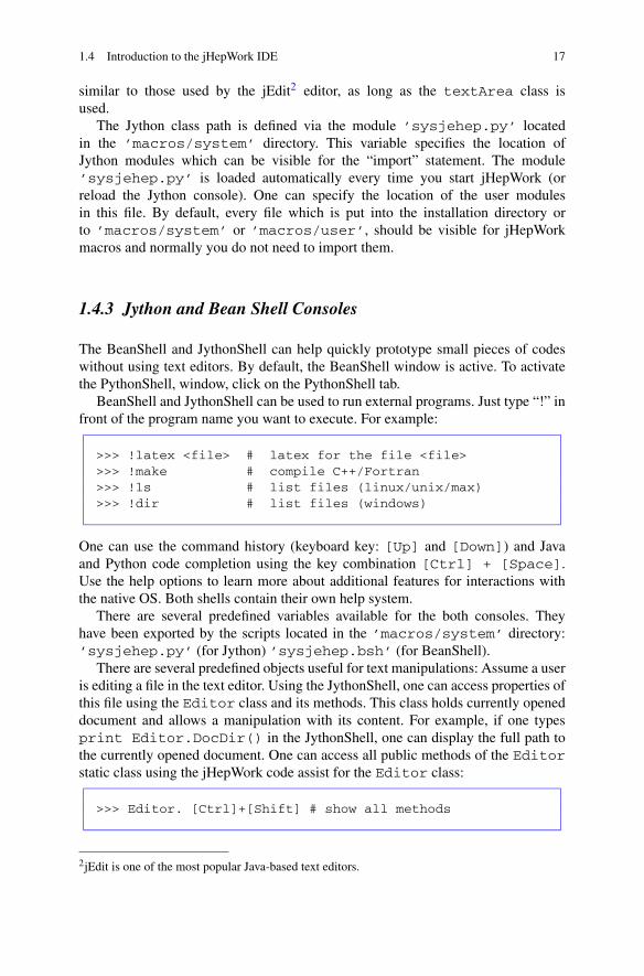
1.4 Introduction to the jHepWork IDE 17
similar to those used by the jEdit2 editor, as long as the textArea class isused.
The Jython class path is defined via the module ’sysjehep.py’ locatedin the ’macros/system’ directory. This variable specifies the location ofJython modules which can be visible for the “import” statement. The module’sysjehep.py’ is loaded automatically every time you start jHepWork (orreload the Jython console). One can specify the location of the user modulesin this file. By default, every file which is put into the installation directory orto ’macros/system’ or ’macros/user’, should be visible for jHepWorkmacros and normally you do not need to import them.
1.4.3 Jython and Bean Shell Consoles
The BeanShell and JythonShell can help quickly prototype small pieces of codeswithout using text editors. By default, the BeanShell window is active. To activatethe PythonShell, window, click on the PythonShell tab.
BeanShell and JythonShell can be used to run external programs. Just type “!” infront of the program name you want to execute. For example:
>>> !latex <file> # latex for the file <file>>>> !make # compile C++/Fortran>>> !ls # list files (linux/unix/max)>>> !dir # list files (windows)
One can use the command history (keyboard key: [Up] and [Down]) and Javaand Python code completion using the key combination [Ctrl] + [Space].Use the help options to learn more about additional features for interactions withthe native OS. Both shells contain their own help system.
There are several predefined variables available for the both consoles. Theyhave been exported by the scripts located in the ’macros/system’ directory:’sysjehep.py’ (for Jython) ’sysjehep.bsh’ (for BeanShell).
There are several predefined objects useful for text manipulations: Assume a useris editing a file in the text editor. Using the JythonShell, one can access properties ofthis file using the Editor class and its methods. This class holds currently openeddocument and allows a manipulation with its content. For example, if one typesprint Editor.DocDir() in the JythonShell, one can display the full path tothe currently opened document. One can access all public methods of the Editorstatic class using the jHepWork code assist for the Editor class:
>>> Editor. [Ctrl]+[Shift] # show all methods
2jEdit is one of the most popular Java-based text editors.

18 1 Jython, Java and jHepWork
or
>>> dir(Editor) # show all methods’DocDir’, ’DocMasterName’, ’DocMasterNameShort’,’DocName’, ’DocStyle’ ..
(below we print only a few first methods). As you can see, having in hand this class,one can access a broad variety of methods for text manipulation. More informationabout this class can be found using the code assist to be discussed in Sect. 1.4.10.
Below we give several examples of how to access the information about anopened file using several predefined variables. Use the Jython shell to type the fol-lowing commands:
>>> print ’Java classpath’,ClassPath>>> print ’File name=’,DocName ->>> print ’Directory=’,DocDir>>> print ’File separator=’,fSep>>> print ’Name with complete path’,DocMasterName>>> print ’Name without extension’,DocMasterNameShort
All these variables are automatically imported by the IDE.But how one can find the predefined variables available in jHepWork while work-
ing with Jython macros files? This should be easy: Click on JythonShell and typethe following command:
>>> dir()[ClassPath’, ’DicDir’, ’DocDir’, ’DocMasterName’,’DocMasterNameShort’, ’DocName’, ’DocStyle’,’Editor’, ’ObjectBrowser’, ’ProjDir’, ’SetEnv’,’SystemDir’, ’SystemMacrosDir’, ’UserMacrosDir...
(again I show only a few first variables). The best approach to learn about themis just to print them out. Analogously, one can print all such variables using theBeanShell commands (but using the BeanShell syntax).
It is useful in many cases to clean up messages from the interactive consoles.To reload either the File Browser or Jython/Bean shell, one should use theReload buttons located directly on the small blue tabs of the console windows.
jHepWork uses the following aliases for the BeanShell macros:
[CLASSPATH] java class path;[FILE_SHORT] returns the filename without the extension;[FILE_SHORT_NODIR] returns the file name without the extension and the path;[FILE] returns the full name of the file including the path;[FILE_NODIR] returns the full name of the file excluding the path;

1.4 Introduction to the jHepWork IDE 19
[DIR_FILE] returns file directory;[DIR_SYS] returns system directory.
For example, typing print [FILE] prints the name of the currently openedfile. Such substitutions can be used in macros. For example, if a macro contains[FILE], it will be automatically replaced by the current file name.
1.4.4 Accessing Methods of Instances
A user can view the available methods by typing obrowser in the BeanShell. Thiswill open an object browser window with all objects. If one needs to add someobject, one should type obrowser.add(obj), where “obj” is an instance of aJava class.
>>> obrowser>>> obj=new JLabel(’OK’)>>> obrowser.add(obj)
For a similar task in the JythonShell prompt, a user should use the code assist,see Sect. 1.4.10, or the Python dir(’obj’) method. The jHepWork code assistcannot be used in BeanShell. In this case, one should use the obrowser class.
One can manually execute the obrowser class by running the script’obrowser.bsh’ or ’obrowser.py’ from the directory macros/system.
1.4.5 Editing Jython Scripts
First, a new file with the extension ’.py’ should be created. There are sev-eral ways to do this: (1) Select [File]-[New]-[jHPlot script] in themain menu. A new template Jython script should appear; (2) Use the menu[File]-[New]-[Text document]. Then, save it as a Jython file with theextension ’.py’; (3) Click on any Jython file with the extension ’.py’ in the FileBrowser.
If a script with the user analysis program is ready, one should save it. But beforethis, you may check for syntax errors without actual execution of the macro file.Look at the menu [Run] and [Check Jython syntax]. In the case of errors,the IDE will point to a line with an error. For the syntax checker, it is impossible toidentify run-time errors, i.e. errors which may happen during the execution of thescript. Once you know that there are no errors, save the file again using the menu[File].
1.4.6 Running Jython Scripts
To run a Jython script, use the [run] button from the main tool-bar of jHepWork.One can also use the keyboard key [F8] for fast script execution. In case of an

20 1 Jython, Java and jHepWork
error, the jHepWork main editor will move the cursor to the appropriate line withthe detected error. Press any key to remove the line highlighting (red color). One canalso execute a Jython file line-by-line using the [run] menu of the main tool-bar.
During the execution, all program outputs will be redirected to the JythonShellwindow. It is appropriate mention here one feature: JythonShell is not designedfor very heavy output, it is mainly a debugging tool. If you want to print a lot ofmessages, then you should be careful: you may wipe out significant resources bydoing this and your code execution will be rather slow. For example, consider asimple Jython program: printing integer values:
for i in range(1000000):print ’Test=’,i
Save these lines in the file ’test.py’. Then open it in the jHepWork editor andrun it by clicking on the button [run]. You will immediately see that the memorymonitor in the right corner of the IDE will show an increase in the memory usage.So, try to avoid such situations. If you need to debug loops like this, use a smallnumber of iterations. If you still want to run the loop over many iterations, youshould not print many debugging messages for every single iteration inside a loop.For example, one can print a status line every 100 iteration as:
for i in range(1000000):if i%100 == 0: print ’Test=’,i
As you may guess, % means a remainder of i/100, which should be 0 for printingthe string ’Test=’,i.
1.4.7 Running a BeanShell Scripts
One can run BeanShell scripts and Java source codes in the same way. However,jHepWork has much less advanced error handling in this case. As in the Jythoncase, the [F8] key can be used fast execution of a BeanShell script.
During the execution, the output from the scripts will be redirected to the Bean-Shell window.
1.4.8 Compiling and Running Java Code
Java files can be edited in the same way. Java source code can be compiled intobytecodes using the menu from the [Run] tool-bar menu as [Run]-[Javaccurrent file]. Similarly, one can also compile all Java source codes locatedin the same directory or build a jar library.

1.4 Introduction to the jHepWork IDE 21
1.4.9 Working with Command-line Scripts
For advanced users, we should be more specific about how to run Jython scripts fromjHepWork without the main text editor. For this, one can set the ’CLASSPATH’variable to the libraries located in the ’lib’ directory. One can find an examplebash script ’a_run.sh’ in the directory macros/examples. To run a Jythonfile, say file.py, run the command:
bash#: a_run.sh file.py
from the Linux/UNIX or Mac prompt.It is however more convenient to use the ANT tool [19], since it is a multi-
platform Java program. It reads a configuration file ’build.xml’ to run and com-pile programs using the command line. jHepWork has a special ’build.xml’file which allows to run and compile Jython macros from the command line with-out the main text editor. Go to the directory ’macros/cmd’ and type ant. If theANT tool is installed, one should see command-line options to run or compile thescripts. For example, to run the ’file.py’ script without the main text editorusing Linux, Unix or Mac, type:
bash#: ant run -DM file
If you want to compile this script into a jar library, type:
bash#: ant jarpy -DM file
If one needs to compile standard Java source files with the purpose of creating ajar library, one should put the source files to the ’src’ directory and execute thecommand ’ant jarjava’.
In all such cases, it is assumed that a user is working in the ’cmd’ directory. Ifone needs to work in some other directory, modify the variable jhepwork in the’build.xml’ file.
1.4.10 jHepWork Code Assist
If a user is working with the Jython shell, all methods associated with a particularobject are shown in a drop down menu after typing a dot after the name of an objectand pressing [Space] after holding down the [Ctrl] key. For example, if aJython or Java object obj was instantiated, type:
>>> obj. # press [Ctrl]+[Space] for the help
to bring up a table with all methods associated with a class instance obj.
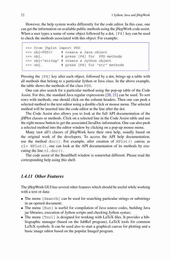
22 1 Jython, Java and jHepWork
However, the help system works differently for the code editor. In this case, onecan get the information on available public methods using the jHepWork code assist.When a user types a name of some object followed by a dot, [F4] key can be usedto check the methods associated with this object. For example:
>>> from jhplot import P0D>>> obj=P0D() # create a Java object>>> obj. # press [F4] for P0D methods>>> obj="string" # create a Jython object>>> obj. # press [F4] for "str" methods
Pressing the [F4] key after each object, followed by a dot, brings up a table withall methods that belong to a particular Jython or Java class. In the above example,the table shows the methods of the class P0D.
One can also search for a particular method using the pop-up table of the CodeAssist. For this, the standard Java regular expressions [20, 21] can be used. To sortrows with methods, one should click on the column headers. Then one can push aselected method to the text editor using a double-click or mouse menu. The selectedmethod will be inserted into the code editor at the line after the dot.
The Code Assist also allows you to look at the full API documentation of thejHPlot classes or methods. Click on a selected line in the Code Assist table and usethe right mouse button to get the associated JavaDoc information. One can also pusha selected method into the editor window by clicking on a pop-up mouse menu.
Many (not all!) classes of jHepWork have their own help, usually based onthe original work of the developers. To access the API help documentation,use the method doc(). For example, after creation of HPlot() canvas asc1= HPlot(), one can look at the API documentation of its methods by exe-cuting the line c1.doc().
The code assist of the BeanShell window is somewhat different. Please read thecorresponding help using this shell.
1.4.11 Other Features
The jHepWork GUI has several other features which should be useful while workingwith a text or data:
• The menu [Search] can be used for searching particular strings or substringsin an opened document;
• The menu [Run] is useful for compilation of Java source codes, building Javajar libraries, execution of Jython scripts and checking Jython syntax;
• The menu [Tool] is designed for working with LaTeX files. It provides a bib-liographic manager (based on the JabRef program), LaTeX tools for commonLaTeX symbols. It can be used also to start a graphical canvas for plotting and abasic image editor based on the popular ImageJ program.

1.5 Third-party Packages and the License 23
It is worth exploring the menu toolbar of the IDE. Especially, if you wouldlike to see jHepWork examples, look at the menu [Tool] and select [jHPlotexamples]. This brings up a dialog with the list of available Jython examples.One can run the example macro files to get a clue on how to use the jHPlot packagewith numerical and graphical libraries.
Before jumping to the data analysis sections, I would like to give one advice.The jHepWork IDE is only an experimental tool and, probably, it was not tested ascareful as any other professional IDE. It was designed as a light-weight source-codeeditor with IDE-like features to help for new users to get started. Therefore, if youare not too satisfied with the jHepWork IDE, you are likely to be a professional pro-grammer. In this case, use ether Eclipse or NetBeans (well, if you are a professionalprogrammer, you must know about them!). Both Eclipse and Netbean can be usedfor editing jHepWork scripts if you will set the $CLASSPATH to the jHepWork jarlibraries inside the directory ’lib’ (again, I do not need to explain this to advancedusers).
Finally, you may even use popular code editors, like jEdit, Emacs or VI (Linuxand Windows) or Notepad (Windows). How to run the jHepWork scripts in a consolewithout using the IDE has been described before.
1.5 Third-party Packages and the License
1.5.1 Contributions and Third-party Packages
Note that some third-party libraries are not licensed by the GPL license but freeonly for non-commercial purposes. Therefore, generally, you can safely use the en-tire software for non-commercial purposes only. If you will use it for commercialpurposes, you should contact the authors.
jHepWork is based on several reused classes that have been rewritten and adoptedfor the use together in jHepWork. This book has numerous references on other third-party packages if the discussed package contains or relies on a particular library.The author apologize in advance if some reference is missing; such omissions werewholly unintentional.
All packages listened below are subject to their licenses (as well as the packagescited in the following sections). The vast majority of the included packages areGNU-licensed or have very permissive open-source licenses.
Many projects from the list given below are not supported any longer by theoriginal authors, but they were very useful at the time when jHepWork was underheavy development. jHepWork (version 2.2) contains:
• FreeHEP java librarieshttp://java.freehep.org;
• jEdit TextArea components (from the jEdit 2003 version, written by SlavaPestov);

24 1 Jython, Java and jHepWork
• some classes from the jMySpell projecthttp://jmyspell.javahispano.net/en/index.html by DreamTagnerine;
• classes from early versions of JabRef projecthttp://jabref.sourceforge.net/;
• classes for color syntax highlighting taken from the Jext projecthttp://www.jext.org/;
• LatexTools Beanshell macro developed for jEdit (this is still a test version);• Debuxter package
http://dexter.sourceforge.net/;• classes from the JyConsole project by Artenum
http://www.artenum.com;• some classes of the jpEdit project
http://www.jpedit.co.uk/;• drawing classes from jPlot
http://www.cig.ensmp.fr/~vanderlee/jplot/ by Jan van der Lee;• the Surface Plotter package
http://www.fedu.uec.ac.jp/~yanto/java/surface/ by Yanto Suryono;• a rewrite of the Browser3d package (I could not identify its developers);• a rewrite of the popular JaxoDraw package
http://jaxodraw.sourceforge.net/;• the Jakart Common Math library
http://jakarta.apache.org/commons/math/;• self-contained mathematics and statistics components addressing the most com-
mon problems. In addition, T. Flanagan’s Java Libraryhttp://www.ee.ucl.ac.uk/~mflanaga/java/updates.html;
• a self-contained framework for clustering analysis by S.Chekanov, the JMinHEPpackagehttp://hepforge.cedar.ac.uk/jminhep/;
• the core engine of the JOONE package http://www.jooneworld.com/ and theEncoghttp://code.google.com/p/encog-java/;
• the JGraph package and the JGrapht packagehttp://www.jgraph.com/http://jgrapht.sourceforge.net/;
• the jFreeChart packagehttp://www.jfree.org/;
• the classes from the ObjectBrowser project by J. Hrivnac;• jHepWork includes the GlobalDocs program
http://globaldocs.zeevbelkin.com/;• the Colt package
http://dsd.lbl.gov/~hoschek/colt/;• refactored classes from the PTPlot 5.6
http://ptolemy.berkeley.edu/java/ptplot/;• several classes from the high performance jMathTools package
http://jmathtools.sourceforge.net/;

1.5 Third-party Packages and the License 25
• look and feel based upon Liquidlnf and JGoodies and therefore subject to theirlicense;
• the Protocol Buffers libraryhttp://code.google.com/p/protobuf/;
• VLJTable table class from VLsolutionshttp://www.vlsolutions.com;
• classes from the ImageJ java programhttp://rsb.info.nih.gov/ij/;
• the package Sympy, a Python library for symbolic mathematicshttp://code.google.com/p/sympy/;
• several icons are from Gnome and Eclipse and therefore subject to their licenses;• 3D-XplorMath project by the 3D-XplorMath Consortium
http://3d-xplormath.org/.
1.5.2 Disclaimer of Warranty
jHepWork is not commercial product, although it is professionally written and manylibraries have been tested by a large scientific community. I cannot guarantee that itis fault free in all possible foreseeable situations. Therefore, you use this package atyour own risk.
The author and publisher make no warranties, express or implied, that the pro-grams contained in this book are free of errors, or are consistent with any particularstandard of merchantability. They should not be relied on for solving a problemwhose incorrect solution could result in injury to a person or loss of property. If youdo use the program in such a manner, it is at your own risk. The authors and pub-lisher disclaim all liability for direct or consequential damages resulting from youruse of the programs.
1.5.3 jHepWork License
jHepWork is licensed by the GNU General Public License (GPL). However, it con-tains some third-party libraries integrated to jHepWork which are free for non-commercial purposes.
Here is the GNU License:Copyright (C) 2006 S. Chekanov. The jHepWork project.This program is free software; you can redistribute it and/or modify it under
the terms of the GNU General Public License as published by the Free SoftwareFoundation; either version 2 of the License, or any later version.
This program is distributed in the hope that it will be useful, but without anywarranty; without even the implied warranty of merchantability or fitness for a par-ticular purpose. See the GNU General Public License for more details.

26 1 Jython, Java and jHepWork
You should have received a copy of the GNU General Public License along withthis program; if not, write to the Free Software Foundation, Inc., 59 Temple Place—Suite 330, Boston, MA 02111-1307, USA.
References
1. Chekanov, S.: HEP data analysis using JHEPWORK and JAVA. In: Proceedings of theHERA-LHC workshop (CERN-DESY) 2007–2008 (2008), p. 763. URL http://arxiv.org/abs/0903.3861
2. Pilgrim, M.: Dive into Python. Apress, New York (2004)3. Guzdial, M.: Introduction to Computing and Programming in Python. A Multimedia Ap-
proach. Prentice Hall, New York (2005)4. Martelli, A.: Python in a Nutshell (In a Nutshell (O’Reilly)). O’Reilly Media, Sebastopol
(2006)5. Lutz, M.: Learning Python, 3rd edn. O’Reilly Media, Sebastopol (2007)6. Langtangen, H.: Python Scripting for Computational Science. Springer, Berlin/Heidelberg
(2008)7. Richardson, C., Avondolio, D., Vitale, J., Schrager, S., Mitchell, M., Scanlon, J.: Professional
Java, JDK 5th edn. Wrox, Birmingham (2005)8. Arnold, K., Gosling, J., Holmes, D.: Java(TM) Programming Language, 4th edn. Java Series.
Addison-Wesley, Reading (2005)9. Flanagan, D.: Java in a Nutshell, 5th edn. O’Reilly Media, Sebastopol (2007)
10. Eckel, B.: Thinking in Java, 4th edn. Prentice Hall PTR, Englewood Cliffs (2006)11. Bloch, J.: Effective Java, 2nd edn. The Java Series. Prentice Hall PTR, Englewood Cliffs
(2008)12. Johnson, A.: A Java based analysis environment JAS (1996)13. FreeHEP Java Libraries. URL http://java.freehep.org/14. Python Programming Language. URL http://www.python.org/15. The Jython Project. URL http://www.jython.org/16. Brun, R., Rademakers, F., Canal, P., Goto, M.: Root status and future developments. ECONF
C0303241 (2003) MOJT00117. Brun, R., Rademakers, F.: ROOT: An object oriented data analysis framework. Nucl. Instrum.
Methods A 389, 81 (1997). URL http://root.cern.ch/18. Wikipedia, Comparison of Java and C++. URL http://en.wikipedia.org/wiki/Comparison_of_
Java_and_C19. The Apache Ant. URL http://ant.apache.org/20. Java regular expressions, ReGex package. URL http://java.sun.com/j2se/1.6.0/docs/api/21. Stubblebine, T.: Regular Expression Pocket Reference: Regular Expressions for Perl, Ruby,
PHP, Python, C, Java and .NET (Pocket Reference (O’Reilly)). O’Reilly Media, Sebastopol(2007)

Chapter 2Introduction to Jython
In this chapter, we will give a short introduction to the Jython programming lan-guage. We have already pointed out that Jython is an implementation of the Pythonprogramming language, unlike CPython which is implemented in C/C++.
While these implementations provide almost identical a Python-language pro-gramming environment, there are several differences. Since Jython is fullyimplemented in Java, it is completely integrated into the Java platform, so onecan call any Java class and method using the Python-language syntax. Thishas some consequences for the way you would program in Jython. Duringthe execution of Jython programs, the Jython source code is translated to Javabytecode that can run on any computer that supports the Java virtual machine.
We cannot give a comprehensive overview of Jython or Python in this chapter:This chapter aims to describe a bare minimum which is necessary to understand theJython language, and to provide the reader with sufficient information for the fol-lowing chapters describing data-analysis techniques using the jHepWork libraries.
2.1 Code Structure and Commentary
As for CPython, Jython programs can be put into usual text files with the extension‘.py’. A Jython code is a sequence of statements that can be executed normally,line-by-line, from the top to the bottom. Jython statements can also be executedinteractively using the Jython shell (the tab ‘JythonShell’ of the jHepWork IDE).
Comments inside Jython programs can be included using two methods: (1) Tomake a single-line comment, put the sharp “#” at the beginning of the line; (2) Tocomment out a multi-line block of a code, use a triple-quoted string.
It is good idea to document each piece of the code you are writing. Documenta-tion comments are strings positioned immediately after the start of a module, class
S.V. Chekanov, Scientific Data Analysis using Jython Scripting and Java,Advanced Information and Knowledge Processing,DOI 10.1007/978-1-84996-287-2_3, © Springer-Verlag London Limited 2010
27

28 2 Introduction to Jython
or function. Such comment can be accessed via the special attribute __doc__. Thisattribute will be considered later on when we will discuss functions and classes.
Jython statements can span multiple lines. In such cases, you should add a backslash at the end of the previous line to indicate that you are continuing on the nextline.
2.2 Quick Introduction to Jython Objects
As for any dynamically-typed high-lavel computational language, one can useJython as a simple calculator. Let us use the jHepWork IDE to illustrate this. Startthe jHepWork and click on the “JythonShell” tab panel. You will see the Jythoninvitation “>>>” to type a command. Let us type the following expression:
>>> 100*3/15
Press [Enter]. The prompt returns “20” as you would expect for the expression(100*3)/15. There was no any assignment in this expression, so Jython assumesthat you just want to see the output. Now, try to assign this expression to somevariable, say W:
>>> W=100*3/15
This time, no any output will be printed, since the output of the expression fromthe right side is assigned directly to the variable W. Jython supports multiple assign-ments, which can be rather handy to keep the code short. Below we define threevariables W1, W2 and W3, assigning them to 0 value:
>>> W1=W2=W3=0
One can also use the parallel assignments using a sequence of values. In the examplebelow we make the assignment W1=1, W2=2 and W3=3 as:
>>> W1,W2,W3=1,2,3
At any step of your code, you can check which names in your program are de-fined. Use the built-in function dir() which returns a sorted list of strings
>>> dir()[’W’,’W1’,’W2’,’W3’,’__doc__’, ’__name__’ ...

2.2 Quick Introduction to Jython Objects 29
(we have truncated the output in this example since the actual output is rather long).So, Jython knows about all our defined variables including that defined using thecharacter W. You will see more variables in this printed list which are predefined byjHepWork.
One can print out variables with the print() method as:
>>> print W11
One can also append a comment in front:
>>> print ‘The output =’,W1The output = 1
You may notice that there is a comma in front the variable W1. This is because‘The output’ is a string, while ‘W1’ is an integer value, so their types are distinctand must be separated in the print statement.
How do we know the variable types? For this we can use the type() methodwhich determines the object type:
>>> type(W1)<type ’int’>
The output tells that this variable holds an integer value (the type “int”).Let us continue with this example by introducing another variable, ‘S’ and by
assigning a text message to it. The type of this variable is “str” (string).
>>> S=’The output =’>>> type (S)<type ’str’>
So, the types of the variables ’W1’ and S are different. This illustrates the factthat Jython, as any high-level language, determines types based on assigned valuesduring execution, i.e. a variable may hold a binding to any kind of object. Thisfeature is very powerful and the most useful for scripting: now we do not needto worry about defining variable types before making assignments to a variable.Clearly, this significantly simplifies program development.
Yet, the mechanics behind such useful feature is not so simple: the price to payfor such dynamical features is that all variables, even such simple as ‘W1’ and ‘S’ de-fined before, are objects. Thus, they are more complicated than simple types in otherprogramming languages, like C/C++ or FORTRAN. The price to pay is slower ex-ecution and larger memory consumption. On the other hand, this also means thatyou can do a lot using such feature! It should also be noted that some people use

30 2 Introduction to Jython
the word “value” when they talk about simple types, such as numbers and strings.This is because these objects cannot be changed after creation, i.e. they are im-mutable.
First, let us find out what can we do with the object ‘W1’. We know that it holdsthe value 10 (and can hold any value). To find out what can be done with any objectsin the JythonShell window is rather simple: Type ‘W1’ followed by a dot and pressthe [Space] key by holding down [Ctrl]:
>>> W1. [Ctrl]-[Space]
You will see a list of methods attributed to this object. They usually start as__method__, where ’method’ is some attribute. For example, you will see themethod like __str__, which transforms an object of type integer to a string. So,try this
>>> SW=str(W1); type(SW)<type ’str’>
Here we put two Jython statements on one line separated by a semi-column. This,probably, is not very popular way for programming in Jython, but we use it to il-lustrate that one can this syntax is also possible. In some cases, however, a programreadability can significantly benefit from this style if a code contains many similarand short statements, such as a1=1; a2=2. In this case, the statements have cer-tain similarity and it is better to keep them in one single logical unit. In addition, wewill use this style in several examples to make our code snippets short.
The last expression in the above line does not have “=”, so Jython assumes thatwhat you really want is to redirect the output to the interactive prompt. The methodtype() tells that “SW” is a string. As before, you may again look at the methodsof this object as:
>>> SW. [Ctrl]-[Space]
This displays a list of the methods attributed to this object. One can select a neces-sary method and insert it right after the dot.
In addition to the JythonShell help system, one can discover the attributes of eachJython object using the native Jython method dir():
>>> dir(SW)
In the following sections we will discuss other methods useful to discover at-tributes of Java objects.

2.2 Quick Introduction to Jython Objects 31
2.2.1 Numbers as Objects
Numbers in Jython are immutable objects called values, rather than simple typesas in other programming languages (C/C++, Fortran or Java). There are two maintypes: integers (no fractional part) and floats (with fractional part). Integers can berepresented by long values if they are followed by the symbol ‘L’. Try this:
>>> Long=20L<type ’long’>
The only limit in the representation of the long numbers is the memory of Javavirtual machine.
Let us take a look again at the methods of a real number, say “20.2” (withoutany assignment to a variable).
>> 20.2. [Ctrl]-[Space]
or, better, you can print them using the method “dir()”
>>> dir(20.2)
Again, since there is no any assignment, Jython just prints the output of the dir()method directly to the same prompt. Why they are needed and what you can do withthem? Some of them are rather obvious and shown in Table 2.1.
Table 2.1 A short overview of the Jython operators for values
Jython operators for values
abs(x) __abs__ absolute value
pow(x, y) or y**x __pow__ raise x to the power y
−x,+x __neg__, __pos__ negative or positive
+, - __radd__, __rsub__ add or subtract
∗, / __rmul__, __rdiv__ add or subtract
x < y, x > y __com__ less or larger. Returns 0 (false) or 1 (true)
cmp(x, y) __com__ compare numbers. Returns 0 (false) or 1 (true)
x <= y, x >= y – comparison: less (greater) or equal
x == y, x! = y – comparison: equal or not equal
str(x) __str__ convert to a string
float(x) __float__ convert to float
int(x) __int__ convert to integer
long(x) __long__ convert to long

32 2 Introduction to Jython
There are more methods designed for this object, but we will not go into furtherdiscussion. Just to recall: any number in Jython is an object and you can manipulatewith it as with any object to be discussed below. For example, Jython integers areobjects holding integer values. This is unlike C++ and Java where integers areprimitive types.
Is it good if simple entities, such as numbers are, have properties of objects? Forinteractive manipulation with a code and fast prototyping, probably we do not careso much, or even can take advantage of this property. But, for numerical libraries,this feature is unnecessary and, certainly, is too heavy for high-performance calcu-lations. We will address this issue later in the text.
2.2.2 Formatted Output
In the above examples we have used the print command without setting controlover the way in which printed values are displayed. For example, in the case of theexpression “1.0/3.0”, Jython prints the answer with 17 digits after the decimalplace!
Obviously, as for any programming language, one can control the way the valuesare displayed: For this, one can use the % command to produce a nicely formattedoutput. This is especially important of one needs to control the number of deci-mal places the number is printed to. For example, one can print 1.0/3.0 to threedecimal places using the operator %.3f inside the string:
>>> print ’The answer is %.3f’%(1.0/3)The answer is 0.333
As you can see, Jython replaces the character “f” with the variable value that fol-lows the string. One can print more than one variable as shown in the examplebelow:
>>> print ’The answer is %.3f and %.1f’% (1.0/3, 2.0/3)The answer is 0.333 and 0.7
One can also use the operator % to control the width of the displayed number,so one can make neatly aligned tables. For example, the string “10.1f” forces thenumber to be printed such that it takes up to ten characters. The example belowshows how to do this using the new-line character to print the second number on anew line. As one can see, we align this second number with that printed on the firstline:
>>> print ’The answer: %.3f \n %13.1f’% (1.0/3, 2.0/3)The answer: 0.333
0.7

2.2 Quick Introduction to Jython Objects 33
2.2.3 Mathematical Functions
To perform mathematical calculations with values, one should use the Jython mathmodule which comes from the standard specification of the Python programminglanguage. Let us take a look at what is inside of this module. First, we have toimport this module using the “import math” statement:
>>> import math
Use the usual approach to find the methods of this module:
>>> dir(math)[’acos’, ’asin’, ’atan’, ’atan2’, ’ceil’,’classDictInit’, ’cos’, ’cosh’, ’e’, ’exp’,’fabs’, ’floor’, ’fmod’, ’frexp’, ’hypot’,’ldexp’, ’log’, ’log10’, ’modf’, ’pi’, ’pow’,’sin’, ’sinh’, ’sqrt’, ’tan’, ’tanh’]
Most of us are familiar with all these mathematical functions that have the samenames in any programming language. To use these functions, type the module namemath followed by the function name. A dot must be inserted to separate the moduleand the function name:
>>> math.sqrt(20)4.47213595499958
As before for JythonShell, one can pick up a necessary function as:
>>> math. [Ctrl]-[Space]
It should be noted that, besides functions, the math module includes a few well-known constants: π and e:
>>> print "PI=", math.piPI= 3.141592653589793>>> print "e=", math.ee= 2.718281828459045
If you have many mathematical operations and want to make a code shorter byskipping the “math” attribute in front of each function declaration, one can explic-itly import all mathematical functions using the symbol “*”:

34 2 Introduction to Jython
>>> from math import *>>> sqrt(20)4.47213595499958
2.2.4 Complex Numbers
Python has a natural support for complex numbers. Just attach “J” or “j” for theimaginary part of a complex number:
>>> C=2+3j>>> type(C)<type ’complex’>
Once a complex number is defined, one can perform mathematical manipulations aswith the usual numbers. For example:
>>> 1j*1j(-1+0j)
Mathematical operations with complex numbers can be performed using the’cmath’ module, which is analogous to the ’math’ module discussed above.The example below demonstrates how to calculate hyperbolic cosine of a complexvalue:
>>> import cmath>>> print cmath.cosh( 2+3j )(-3.724+0.511j)
The output values for the real and imaginary part in the above example were trun-cated to fit the page width.
2.3 Strings as Objects
Strings are also treated as values since they are immutable. To define a string, oneshould enclose it in double (”) or single (’) quote. The escape character is a back-slash, so one can put a quote character after it. The newline is given by n directlyafter the backslash character. Two strings can be added together using the usual “+”operator.
As mentioned above, an arbitrary value, val, can be converted into a string us-ing the method str(val). To convert a string into int or float value, use the

2.4 Import Statements 35
methods int(str) or float(str). Below we illustrate several such conver-sions:
>>> i=int(’20’)>>> type(i)<type ’int’>>>> f=float(’20.5’)>>> type(f)<type ’float’>
As before, all the methods associated with a string can be found using [Ctrl]-[Space] or the dir() method:
>>> dir(’s’)...’capitalize’, ’center’, ’count’,’decode’,’encode’, ’endswith’, ’expandtabs’, ’find’,’index’, ’isalnum’, ’isalpha’, ’isdecimal’,’isdigit’, ’islower’, ’isnumeric’, ’isspace’...
(we display only a few first methods). Some methods are rather obvious and donot require explanation. All methods that start from the string “is” check for aparticular string feature.
Below we list more methods:
len(str) gives the number of characters in the string strstring.count(str) counts the number of times a given word appears in a
stringstring.found(str) numeric position of the first occurrence of word in the
stringstr.lower() returns a string with all lower case lettersstr.upper() returns a string with all upper case letters
Strings can be compared using the standard operators: ==, !=, <, >, <=,and >=.
2.4 Import Statements
There are several ways that can be used to import a Java or Python package. Onecan use the ’import’ statement followed by the package name. In case of Python,this corresponds to a file name without the extension ’.py’. The import statementexecutes the imported file, unlike lower-level languages, like C/C++, where theimport statement is a preprocessor statement. The consequence of this is that theimport statement can be located in any place of your code, as for the usual exe-cutable statement. We have seen already how to import the Python package “math”.

36 2 Introduction to Jython
Here is an example illustrating how to import the Java Swing package (usually usedto build a GUI):
>>> from javax.swing import *
In the above example we use the wildcard character “*” to import all packagesfrom Java Swing. In this book, you will see that we use “*” wildcard almost forevery example, since we what to keep our examples short. This is often consideredas a bad style since it “pollutes” the global namespace. However, if you know thatthe code is not going to be very long and complicated, we should not worry toomuch about this style.
Let us give another example showing how to import of a Java class. We remindthat the code below works only for Python implemented in Java (Jython):
>>> from javax.swing import JFrame
This time we have imported only a single class (JFrame) from Java, unlike theprevious example with the “polluted” namespace.
Another way to import classes is to use the ’import’ statement without thestring ’from’. For example:
>>> import javax.swing
In this case, we should use the qualified names, i.e.:
>>> f=javax.swing.JFrame(’Hello’)
Although it takes more typing, we have avoided polluting the global namespace ofour code.
2.4.1 Executing Native Applications
In Sect. 1.4.3 we have shown that native applications can be run using JythonShellby appending “!” in front of an external command. In addition, one can also useJython ’os.system’ package to run an external program.
The code below shows how to run an external command. In this example, webring up the Acroread PDF file viewer (it should be found on the current PATH ifthis program installed on your system):
>>> import os>>> rc=os.system(’acroread’)

2.5 Comparison Tests and Loops 37
>>> if rc == 0:>>> ... print ’acroread started successfully’
The statement ’if’ checks whether the execution has succeeded or not. We willdiscuss the comparison tests in the next section. The same operation will look like!acroread when using the Jython shell.
2.5 Comparison Tests and Loops
2.5.1 The ‘if-else’ Statement
Obviously, as in any programming language, one can use the ’if-else’ state-ment for decision capability of your code. The general structure of comparison testsis
if [condition1]:[statements to execute if condition1 is true]
elif [condition2]:[statements to execute if condition2 is true]
....
else:[rest of the program]
The text enclosed in square brackets represents some Jython code. After the linewith the statement ’if’, the code is placed farther to the right using white spacesin order to define the program block. Either space characters or tab characters (oreven both!) are accepted as forms of indentation. In this book, we prefer two spacesfor indentation. It should also be noted that the exact amount of indentation doesnot matter, only the relative indentation of nested blocks (relative to each other) isimportant.
The indentation is good Python feature: The language syntax forces to use theindentation that you would have used anyway to make your program readable. Thuseven a lousy programmer is forced to write understandable code!
Now let us come back to the comparison tests. The [condition] statementhas several possibilities for values ’a’ and ’b’ values as shown in Table 2.2:
Let us illustrate this in the example below:
>>> a=1; b=2;>>> if a*b>1:>>> .. print "a*b>1">>> else:>>> .. print "a*b<=1"

38 2 Introduction to Jython
Table 2.2 Most popularJython comparison tests Comparison tests
a == b a is equal to b
a! = b a is not equal to b
a > b a is greater than b
a >= b a is greater than or equal to b
a < b a is less than b
a <= b a is less than or equal to b
a == b a is equal to b
a! = b a is not equal to b
In case if you will need more complex comparisons, use the boolean operatorssuch as ’and’ and ’or’:
>>> a=1; b=0>>> if a>0 and b=0:>>> ..print ’it works!’
One can also use the string comparisons = (equal) or != (not equal). The com-parison statements are case sensitive, i.e. ’a’ == ’A’ is false.
2.5.2 Loops. The “for” Statement
The need to repeat a statement or a code block is essential feature of any numericalcalculation. There is, however, one feature you should be aware of: Python should beviewed as an “interface” type of language, rather than that used for heavy repeatedoperations like long loops over values. According to the author’s experience, if thenumber of iterations involving looping over values is larger than several thousands,such part of the code should be moved to an external library to achieve a higherperformance and a lower memory usage compared to the Python code operatingwith loops over objects. In case of Java, such libraries should be written in Java.
In this section we will be rather short. One can find more detailed discussionabout this topic in any Python textbook.
The simplest loop which prints, say, 10 numbers is shown below:
>>> for i in range(10):>>> ... print i
This ’for’ loop iterates from 0 to 9. Generally, you can increment the counter byany number. For example, to print numbers from 4 to 10 with the step 2, use thisexample:

2.5 Comparison Tests and Loops 39
>>> for i in range(4,10,2):>>> ... print i
2.5.3 The ‘continue’ and ‘break’ Statements
The loops can always be terminated using the ’break’ statement, or some itera-tions can be skipped using the ’continue’ statement. All such control statementsare rather convenient, since help to avoid various ’if’ statements which makes thePython code difficult to understand. This is illustrated in the example bellow:
>>> for i in range(10):>>> ... if (i == 4): continue>>> ... if (i == 8): break>>> ... print i
In this loop, we skip the number 6 and break the loop after the number 8:
2.5.4 Loops. The ‘while’ Statement
One can also construct a loop using the ’while’ statement, which is more flexiblesince its iteration condition could be more general. A generic form of such loop isshown below:
while CONDITION:... <Code Block as long as CONDITION is true>
Let us give a short example which illustrates the while loop:
>>> a=0>>> while a<10:>>> ... a=a+1
The while loop terminates when a=10, i.e. when the statement after the’while’ is false. As before, one can use the control statements discussed aboveto avoid overloading the execution block with various “if” statements.
One can also create an infinite loop and then terminate it using the “break”statement:

40 2 Introduction to Jython
>>> a=0>>> while 1:>>> ... print "infinite loop!">>> ... a=a+1;>>> ... if a>10:>>> break>>> ... print i
In this example, the ’break’ statement together with the ’if’ condition controlsthe number of iterations.
2.6 Collections
Data-analysis computations are usually based on object collections, since they havebeing designed for various repetitious operations on sequential data structures—exactly what we mostly do when analyzing multiple measurements. In addition, atypical measurement consists of a set of observations which have to be stored in adata container as a single unit.
Unlike to other languages, we consider Python collections to be useful mainlyfor storing and manipulation with other high-level objects, such as collections witha better optimized performance for numerical calculations. In this book, we will usethe Jython collections to store sets of jHepWork histograms, mathematical func-tions, Java-based data containers and so on.
Of course, one can use Jython collections to keep numerical values, but this ap-proach is not going to be very efficient: An analysis of such values requires Pythonloops which are known to be slow. Secondly, there are no too many pre-build Jythonlibraries for object manipulation.
Nevertheless, in many parts of this books we will use collections which containnumerical values: this is mainly for pedagogical reasons. Besides, we do not care toomuch about the speed of our example programs when analyzing tens of thousandsevents.
2.6.1 Lists
As you may guess, a list is an object which holds other objects, including values.The list belongs to a sequence, i.e. an ordered collection of items.

2.6 Collections 41
2.6.2 List Creation
An empty list can be created using squared brackets. Let us create a list and checkits methods:
>>> list=[]>>> dir(list) # or list. + [Ctrl]+[Space]
One can also create a list which contains integer or float values during the initial-ization:
>>> list=[1,2,3,4]>>> print list[1, 2, 3, 4]
The size of this list is accessed using the len(list) method. The minimum andmaximum values are given by the min(list) and max(list) methods, respec-tively. Finally, for a list which keeps numerical values, one can sum-up all list ele-ments as sum(list).
One can create a mixed list with numbers, strings or even other lists:
>>> list=[1.0,’test’,int(3),long(2),[20,21,23]]>>> print list[1.0, ’test’, 3, 2L, [20, 21, 23]]
One can obtain each element of the list as list[i], where ’i’ is the elementindex, 0<i<len(list). One can select a slice as list[i1:i2], or even selectthe entire list as list[:]. A slice which selects index 0 through ’i’ can be writ-ten as list[:i]. Several lists can be concatenated using the plus operator ’+’,or one can repeat the sequence inside a list using the multiplication ’*’.
As before, one can find the major methods of the list using [Ctrl]+[Space]keys. Some methods are rather obvious:
To add a new value, use the method append():
>>> list.append(’new string’)
A typical approach to fill a list in a loop would be:
>>> list=[]>>> for i in range(4,10,2):>>> ... list.append(i)
(here, we use a step 2 from 4 to 10). The same code in a more elegant form lookslike:

42 2 Introduction to Jython
>>> list=range(4, 10, 2)>>> print list[4, 6, 8]
If one needs a simple sequence, say from 0 to 9 with the step 1, this code can besimplified:
>>> list=range(10)>>> print ’List from 0 to 9:’,listList from 0 to 9: [0,1,2,3,4,5,6,7,8,9]
One can create a list by adding some condition to the range statement. Forexample, one create lists with odd and even numbers:
>>> odd =range(1,10)[0::2]>>> even=range(1,10)[1::2]
Another effective “one-line” approach to fill a list with values is demonstratedbelow:
>>> import math>>> list = [math.sqrt(i) for i in range(10)]
Here we created a sequence of sqrt(i) numbers with i = 0..9.Finally, one can use the ’while’ statement for adding values in a loop. Below
we make a list which contains ten zero values:
>>> list=[]>>> while len(list)<10:>>> ... list.append(0)
2.6.3 Iteration over Elements
Looping over a list can be done with the ’for’ statement as:
>>> for i in list:>>> ...print i
or calling its elements by their index ’i’:

2.6 Collections 43
>>> for i in range(len(list)):>>> ...print list[i]
2.6.3.1 Sorting, Searches, Removing Duplicates
The list can be sorted with the sort() method:
>>> list.sort()>>> print list[1.0, 2L, 3, [20, 21, 23], ’new string’, ’test’]
To reverse the list, use the method reverse().To insert a value, use the insert(val) method, while to remove an element,
use the remove(val) method. Finally, one can delete either one element of alist or a slice of elements. For example, to remove one element with the index i1of a list use this line of the code: ’del list[i1]’. To remove a slice of ele-ments in the index range i1-i2, use ’del list[i1:i]’. To empty a list, use’del list[:]’. Finally, ’del list’ removes the list object from the com-puter memory.
It should be noted that the list size in the computer memory depends on thenumber of objects in the list, not on the size of objects, since the list contains pointersto the objects, not objects themselves.
Advanced statistical analysis will be considered in Sect. 7.4, where we will showhow to access the mean values, median, standard deviations, moments and etc. ofdistributions represented by Jython lists.
Jython lists are directly mapped to the Java ordered collection List. For exam-ple, if a Java function returns ArrayList<Double>, this will be seen by Jythonas a list with double values.
To search for a particular value ’val’, use
>>> if val in list:>>> ...print ’list contains’, val
For searching values, use the method index(val), which returns the indexof the first matching value. To count the number of matched elements, the methodcount(val) can be used (it also returns an integer value).
2.6.4 Removal of Duplicates
Often, you may need to remove a duplicate element from a list. To perform thistask, use the-called dictionary collection (will be discussed below). The example to

44 2 Introduction to Jython
be given below assumes that a list object has been created before, and now wecreate a new list (with the same name) but without duplicates:
>>> tmp={}>>> for x in list:>>> ...tmp[x] = x>>> list=tmp.values()
This is usually considered to be the fastest algorithm (and the shortest). However,this method works for the so-called hashable objects, i.e. class instances with a“hash” value which does not change during their lifetime. All Jython immutablebuilt-in objects are hashable, while all mutable containers (such as lists or dictio-naries to be discussed below) are not. Objects which are instances of user-definedJython or Java classes are hashable.
For unhashable objects, one can first sort objects and then scan and comparethem. In this case, a single pass is enough for duplicate removal:
>>> list.sort()>>> last = list[-1]>>> for i in range(len(list)-2, -1, -1):>>> ...if last==list[i]:>>> del list[i]>>> ...else:>>> last=list[i]
The code above is considered to be the second fastest method after that based on thedictionaries. The method above works for any type of elements inside lists.
2.6.4.1 Examples
Lists are very handy for many data-analysis applications. For example, one can keepnames of input data files which can be processed by your program in a sequentialorder. Or, one can create a matrix of numbers for linear algebra. Below we will givetwo small examples relevant for data analysis:
A matrix. Let us create a simple matrix with integer or float numbers:
>>> mx=[... [1, 2],... [3, 4],... [5, 6],... ]
One can access a row of this matrix as mx[i], where ’i’ is a row index. One canswap rows with columns and then access a particular column as:

2.6 Collections 45
>>> col=[[x[0] for x in mx], [x[1] for x in mx]]>>> print col[[1, 3, 5], [2, 4, 6]]
In case of an arbitrary number of rows in a matrix, use the map container for thesame task:
>>> col=map(None,*mx)>>> print col[[1, 3, 5], [2, 4, 6]]
Advanced linear-algebra matrix operations using a pure Jython approach will beconsidered in Sect. 7.5.4.
Records with measurements. Now we will show that the lists are very flexiblefor storing records of data. In the example below we create three records that keepinformation about measurements characterized by some identification string, a timestamp indicating when the measurement is done and a list with actual numericaldata:
>>> meas=[]>>> meas.append([’test1’,’06-08-2009’,[1,2,3,4]])>>> meas.append([’test2’,’06-09-2009’,[8,1,4,4,2]])>>> meas.append([’test3’,’06-10-2009’,[9,3]])
This time we append lists with records to the list holding all event records. We maynote that the actual numbers are stored in a separate list which can have an arbitrarylength (and could also contain other lists). To access a particular record inside thelist meas use its indexes:
>>> print meas[0]>>> [’test1’, ’06-08-2009’, [1, 2, 3, 4]]>>> print meas[0][2][1, 2, 3, 4]
2.6.5 Tuples
Unlike lists, tuples cannot be changed after their creation, thus they cannot growor shrink as the lists. Therefore, they are immutable, similar to the values. As theJython lists, they can contain objects of any type. Tuples are very similar to the listsand can be initiated in a similar way:

46 2 Introduction to Jython
>>> tup=() # empty tuple>>> tup=(1,2,"test",20.0) # with 4 elements
Of course, now operations that can change the object (such as append()), cannotbe applied, since we cannot change the size of this container.
In case if you need to convert a list to a tuple, use this method:
>>> tup=tuple([1,2,3,4,4])
Below we will discuss more advanced methods which add more features to ma-nipulations with the lists and tuples.
2.6.6 Functional Programming. Operations with Lists
Functional programming in Jython allows to perform various operations on datastructures, like lists or tuples. For example, to create a new list by applying theformula:
b[i] − a[i]b[i] + a[i] (2.1)
for each element of two lists, a and b, you would write a code such as:
>>> a=[1,2,3]>>> b=[3,4,5]>>> c=[]>>> for i in range(len(a)):>>> ... c.append( b[i]-a[i] / (a[i]+b[i]) )
To circumvent such unnecessary complexity, one can reduce this code to a singleline using functional programming:
>>> a=[1.,2.,3.]>>> b=[3.,4.,5.]>>> c= map(lambda x,y: (y-x)/(y+x),a,b)>>> print c[0.5, 0.33, 0.25]
The function map creates a new list by applying (2.1) for each element of the inputlists. The statement lambda creates a small anonymous function at runtime whichtells what should be done with the input lists (we discuss this briefly in Sect. 2.10).
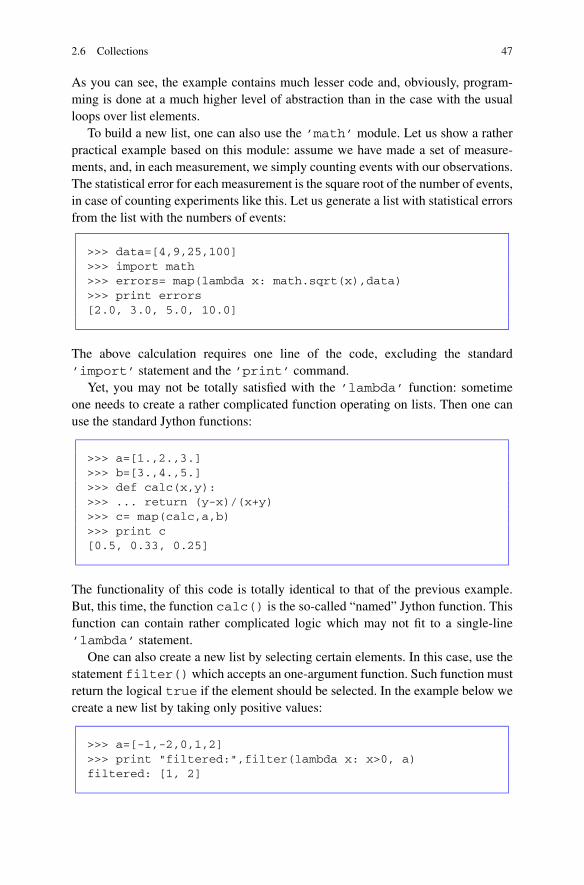
2.6 Collections 47
As you can see, the example contains much lesser code and, obviously, program-ming is done at a much higher level of abstraction than in the case with the usualloops over list elements.
To build a new list, one can also use the ’math’ module. Let us show a ratherpractical example based on this module: assume we have made a set of measure-ments, and, in each measurement, we simply counting events with our observations.The statistical error for each measurement is the square root of the number of events,in case of counting experiments like this. Let us generate a list with statistical errorsfrom the list with the numbers of events:
>>> data=[4,9,25,100]>>> import math>>> errors= map(lambda x: math.sqrt(x),data)>>> print errors[2.0, 3.0, 5.0, 10.0]
The above calculation requires one line of the code, excluding the standard’import’ statement and the ’print’ command.
Yet, you may not be totally satisfied with the ’lambda’ function: sometimeone needs to create a rather complicated function operating on lists. Then one canuse the standard Jython functions:
>>> a=[1.,2.,3.]>>> b=[3.,4.,5.]>>> def calc(x,y):>>> ... return (y-x)/(x+y)>>> c= map(calc,a,b)>>> print c[0.5, 0.33, 0.25]
The functionality of this code is totally identical to that of the previous example.But, this time, the function calc() is the so-called “named” Jython function. Thisfunction can contain rather complicated logic which may not fit to a single-line’lambda’ statement.
One can also create a new list by selecting certain elements. In this case, use thestatement filter() which accepts an one-argument function. Such function mustreturn the logical true if the element should be selected. In the example below wecreate a new list by taking only positive values:
>>> a=[-1,-2,0,1,2]>>> print "filtered:",filter(lambda x: x>0, a)filtered: [1, 2]

48 2 Introduction to Jython
As before, the statement ’lambda’may not be enough for more complicated logicfor element selection. In this case, one can define an external (or named) functionas in the example below:
>>> a=[-1,-2,0,1,2]>>> def posi(x):>>> ... return x > 0>>> print "filtered:",filter(posi, a)filtered: [1, 2]
Again the advantage of this approach is clear: we define a function posi(), whichcan arbitrary be complicated, but the price to pay is more codding.
Finally, one can use the function reduce() that applies a certain function toeach pair of items. The results are accumulated as shown below:
>>> print "accumulate:",reduce(lambda x, y: x+y,[1,2,3])>>> accumulate: 6
The same functional programming methods can be applied to the tuples.
2.6.7 Dictionaries
Another very useful container for analysis of data is the so-called dictionary. If oneneeds to store some objects (which, in turn, could contain other objects, such asmore efficiently organized collections of numbers), it would be rather good idea toannotate such elements. Or, at least, to have some human-readable description foreach stored element, rather than using an index for accessing elements inside thecontainer as for lists or tuples. Such a description, or the so-called “key”, can beused for fast element retrieval from a container.
Dictionaries in Jython (as in Python) are designed for one-to-one relationshipsbetween keys and values. The keys and the corresponding values can be any objects.In particular, the dictionary value can be a string, numerical value or even othercollection, such as a list, a tuple, or other dictionary.
Let us give an example with two keys in form of strings, ’one’ and ’two’,which map to the integer values ‘1’ and ‘2’, respectively:
>>> dic={’one’:1, ’two’:2}>>> print dic[’one’]1
In this example, we have used the key ’one’ to access the integer value ‘1’. Onecan easily modify the value using the key:

2.6 Collections 49
>>> dic[’one’]=10
It should be noted that the keys cannot have duplicate values. Assigning a valueto the existing key erases the old value. This feature was used when we removedduplicates from the list in Sect 2.6.3.1. In addition, dictionaries have no concept oforder among elements.
One can print the available keys as:
>>> print dic.keys()
The easiest way to iterate over values would be to loop over the keys:
>>> for key in dic:>>> ... print key, ’corresponds to’, dic[key]
Before going further, let us rewrite the measurement example given in the previ-ous section when we discussed the lists. This time we will use record identificationsas keys for fast retrieval:
>>> meas={}>>> meas[’test1’]=[’06-08-2009’,[1,2,3,4]]>>> meas[’test2’]=[’06-09-2009’,[8,1,4,4,2]]>>> meas[’test3’]=[’06-10-2009’,[9,3]]>>> print meas[’test2’][’06-09-2009’, [8, 1, 4, 4, 2]]
In this case, one can quickly access the actual data records using the keys. In ourexample, a single data record is represented by a list with the date and additional listwith numerical values.
Let us come back to the description of the dictionaries. Here are a few importantmethods we should know about:
dic.clear() clean a dictionary;dic.copy() make a copy;has_key(key) test, is a key present?;keys() returns a list of keys;values() returns a list of values in the dictionary.
One can delete entries from a dictionary in the same way as for the list:
>>> del dic[’one’]

50 2 Introduction to Jython
One can sort the dictionary keys using the following approach: convert them intoa list and use the sort() method for sorting:
>>> people = {’Eve’:10, ’Tom’: 20, ’Arnold’: 50}>>> list = people.keys()>>> list.sort()>>> for p in list:>>> ... print p,’is ’,people[p]Arnold is 50Eve is 10Tom is 20
2.7 Java Collections in Jython
It was already said that the concept of collections is very important for any dataanalysis, since “packing” multiple records with information into a single unit is avery common task.
There are many situations when it is imperative to go beyond the standardPython-type collections implemented in Jython. The strength of Jython is in its com-plete integration with Java, thus one can call Java collections to store data. Yes, thepower of Java is in your hands!
To access Java collections, first you need to import the classes from the packagejava.util. Java collections usually have the class names started with capitalletters, since this is the standard convention for class names in the Java programminglanguage. With this observation in mind, there is a little chance for mixing Pythoncollections with Java classes during the code development. In this section, we willconsider several collections from the Java platform.
2.7.1 List. An Ordered Collection
To build an ordered collection which contain duplicates, use the class List fromthe Java package java.util. Since we are talking about Java, one can check whatis inside of this Java package as:
>>> from java.util import *>>> dir()[ .. ’ArrayList’,’Currency’,’Date’,List,Set,Map]
Here we printed only a few Java classes to fit the long list of classes to the pagewidth. One can easily identify the class ArrayList, a class which is usually used

2.7 Java Collections in Jython 51
to keep elements in a list. One can check the type of this class and its methods usingeither dir() or the JythonShell code assist:
>>> from java.util import *>>> jlist=ArrayList()>>> type(jlist)<type ’java.util.ArrayList’>>>> dir(jlist):[... methods ...]>>> jlist. # [Ctrl]+[Space]
As you can see, the type() method indicates that this is a Java instance, so wehave to use the Java methods of this instance for further manipulation. Let us addelements to this list and print them:
>>> e=jlist.add(’test’)>>> e=jlist.add(1)>>> jlist.add(0,’new test’)>>> e=jlist.add(2)>>> print jlist[new test, test, 1, 2]>>> print jlist.get(0)new test>>> print jlist.toArray()array(java.lang.Object,[’new test’, ’test’, 1, 2])
You may notice that when we append an element to the end of this list, we assign theresult to the variable ’e’. In Jython, it returns ‘1’ for success (or true for Java).We also can add an object obj at the position characterized with the index i usingthe method add(i,obj). Analogously, one can access elements by their integerpositions. For example, one can retrieve an object back using the method get(i).The list of elements can be retrieved in a loop exactly as we usually do for the Jythonlists. Let us show a more complete example below:
Java list example
from java.util import *
jlist=ArrayList()# append integersfor i in range(100):
jlist.add(i)print jlist.size()
# replace at 0 positionjlist.set(0,100)s=jlistprint type(s)

52 2 Introduction to Jython
# range between 0-50newlist=jlist.subList(0,50)for j in newList:
print j
Run the above code and make sense of its output.Probably, there are not too strong reasons to use Java List while working with
Jython, since the native Jython list discussed in the previous section should be suffi-cient for almost any task. However, it is possible that you will need to use Java listsin order to integrate your application natively into the Java platform after movingyour code into a pure Java codding.
2.7.1.1 Sorting Java Lists
One can do several manipulations with the List using the Java Collectionclass. Below we show how to sort a list using the natural ordering of its elements,and how to reverse the order:
>>> from java.util import *>>> jlist=ArrayList()>>> jlist.add(’zero’); jlist.add(’one’); jlist.add(’two’)>>> Collections.sort(jlist)>>> print jlist>>> [one, two, zero]>>> Collections.reverse(jlist)>>> print jlist>>> [zero, two, one]
The next question is how to sort a list with more complicated objects, using someobject attribute for sorting. Consider a list containing a sequence of other lists as inthe case shown below:
>>> from java.util import *>>> jlist=ArrayList()>>> jlist.add([2,2]); jlist.add([3,4]); jlist.add([1,1])>>> print jlist[[2, 2], [3, 4], [1, 1]]
Here there is a small problem: how can we tell to the method sort() that we wantto perform a sorting using a first (or second) item in each element-list? Or, moregenerally, if each element is an instance of some class, how can we change orderingobjects instantiated by the same class?
One can do this by creating a small class which implements the Comparatorinterface. We will consider Jython classes in Sect. 2.11, so at this moment just accept

2.7 Java Collections in Jython 53
this construction as a simple prescription that performs a comparison of two objects.The method compare(obj1,obj2) of this class compares objects and returnsa negative value, zero, or a positive integer value depending on whether the objectis less than, equal to, or greater than the specified object. Of course, it is up toyou to define how to perform such object comparison. For the example above, eachobject is a list with two integers, so one can easily prototype a function for objectcomparison. Let us write a script which orders the list in increasing order using thefirst element of each list:
Sorting Java lists
from java.util import *
jlist=ArrayList()jlist.add([2,2]); jlist.add([3,4]); jlist.add([1,1])
class cmt(Comparator):def compare(self, i1,i2):
if i1[0]>i2[0]: return 1return 0
Collections.sort(jlist,cmt())print jlist
After running this script, all elements will be ordered and the print method displays[[1, 1],[2, 2],[3, 4]].
We will leave the reader here. One can always find further information about theJava lists from any Java textbook.
2.7.2 Set. A Collection Without Duplicate Elements
The Set container from the package java.util is a Java collection that cannotcontain duplicate elements. Such set can be created using general-purpose imple-mentations based on the HashSet class:
>>> from java.util import *>>> s=HashSet()>>> e=s.add(’test’)>>> e=s.add(’test’)>>> e=s.add(1)>>> e=s.add(2)>>> print s[1, 2, test]
As you can see from this example, the string ’test’ is automatically removedfrom the collection. Operations with the Java sets are exactly the same as those with
54 2 Introduction to Jython
the ArrayList. One can loop over all elements of the set collection using thesame method as that used for the ArrayList class, or one can use a method bycalling each element by its index:
>>> for i in range(s.size()):>>> ...print s[i]
As in the case with the Java lists, you may face a problem when go beyondsimple items in the collection. If you want to store complicated objects with certainattributes, what method should be used to remove duplicates? You can do this aswell but make sure that instances of the class used as elements inside the Java setuse hash tables (most of them do). In case of the example shown in Sect. 2.7.1.1, youcannot use HashSet since lists are unhashinable. But with tuples, it is different:Tuples have hash tables, so the code snippet below should be healthy:
>>> from java.util import *>>> s=HashSet()>>> e=s.add( (1,2) )>>> e=s.add( (2,4) )>>> e=s.add( (1,2) )>>> print s[(2, 4), (1, 2)]
As you can see, the duplicate entry (1,2) is gone from the container. In case ifyou need to do the same with Python lists, convert them first into tuples as shown inSect. 2.6.5.
2.7.3 SortedSet. Sorted Unique Elements
Next, why not to keep all our elements in the Java set container in a sorted order,without calling an additional sorting method each time we add a new element? Theexample below shows the use of the SortedSet Java class:
>>> from java.util import *>>> s=TreeSet()>>> e=s.add(1)>>> e=s.add(4)>>> e=s.add(4)>>> e=s.add(2)>>> print s[1, 2, 4]
the second value “4” is automatically removed and the collection appears in thesorted oder.

2.7 Java Collections in Jython 55
2.7.4 Map. Mapping Keys to Values
As it is clear from the title, now we will consider the Java Map collection whichmaps keys to specific objects. This collection is analogous to a Jython dictionary,Sect. 2.6.7. Thus, a map cannot contain duplicate keys as we have learned from theJython dictionaries.
Let us build a map collection based on the HashMap Java class:
>>> from java.util import *>>> m=HashMap()>>> m.put(’a’, 1)>>> m.put(’b’, 2)>>> m.put(’c’, 3)>>> print m{b=2, c=3, a=1}
Now you can see that Java maps have the same functionality as the Jython dictionar-ies. As for any Java collection, the size of the Map is given by the method size().One can access the map values using the key:
>>> print m[’a’]1
Similar to the lists, one can print all keys in a loop:
>>> for key in m:>>> ... print key, ’corresponds to’, m[key]b corresponds to 2c corresponds to 3a corresponds to 1
Here we print all keys and also values corresponding to the keys.
2.7.5 Java Map with Sorted Elements
This time we are interested in a map with sorted keys. For this one should use theclass TreeMap and the same methods as for the HashMap class discussed before:
>>> from java.util import *>>> m=TreeMap()>>> m.put(’c’, 1)>>> m.put(’a’, 2)

56 2 Introduction to Jython
>>> m.put(’b’, 3)>>> print m{a=2, b=3, c=1}
Compare this result with that given in the previous subsection. Now the map issorted using the keys.
2.7.6 Real Life Example: Sorting and Removing Duplicates
Based on the Java methods discussed above, we can do something more compli-cated. In many cases, we need to deal with a sequence of data records. Each record,or event, can consist of strings, integer and real numbers. So we are dealing withlists of lists. For example, assume we record one event and make measurements ofthis event by recording a string describing some feature and several numbers char-acterizing this feature. Such example was already considered in Sect. 2.6.4.1.
Assume we make many such observations. What we want to do at the end of ourexperiment is to remove duplicates based on the string with a description, and thensort all the records (or observations) based on this description. This looks like a realproject, but not for Jython! The code below does everything using a several lines ofthe code:
Sorting and removing duplicates
from java.util import *
data=ArrayList()data.add( ["star",1.1,30] )data.add( ["galaxy",2.2,80] )data.add( ["galaxy",3.3,10] )data.add( ["moon",4.4,50] )
map=TreeMap()for row in data:
map.put(row[0],row[1:])
data.clear()for i in map:
row=map[i]row.insert(0,i)data.add(row)
print data
Let us give some explanations. First, we make a data record based on the list’data’ holding all our measurements. Then we build a TreeMap class and usethe first element to keep the description of our measurement in form of a “key”.
2.8 Random Numbers 57
The rest of our record is used to fill the map values (see row[1:]). As you alreadyknow, when we fill the TreeMap object, we remove duplicate elements and sort thekeys automatically. Once the map is ready, we remove all entries from the list andrefill it using a loop over all the keys (which are now ordered). Then we combine thekey value to form a complete event record. The output of the script is given below:
[[’galaxy’,3.3,10],[’moon’,4.4,50],[’star’,1.1,30]]
We do not have extra record with the description ‘galaxy’ and, expectedly, all ourrecords are appropriately sorted.
2.8 Random Numbers
A generation of random numbers is an essential phase in scientific programming.Random numbers are used for estimating integrals, generating data encryption keys,data interpretation, simulation and modeling complex phenomena. In many exam-ples of this book, we will simulate random data sets for illustrating data-analysistechniques.
Let us give a simple example which shows how to generate a random floatingpoint number in the range [0,1] using the Python language:
>>> from random import *>>> r=Random()>>> r.randint(1,10) # a random number in range [0.10]
Since we do not specify any argument for the Random() statement, a random seedfrom the current system time is used. In this case, every time you execute this script,a new random number will be generated.
In order to generate a random number predictably for debugging purpose, oneshould pass an integer (or long) value to an instance of the Random() class. Forthe above code, this may look as: r=Random(100L). Now the behavior of thescript above will be different: every time when you execute this script, the methodrandint(1,10) will return the same random value, since the seed value is fixed.
Random numbers in Python can be generated using various distributions depend-ing on the applied method:
>>> r.random() # in range [0.0, 1.0)>>> r.randint(min,max) # int in range [min,max]>>> r.uniform(min,max) # real number in [min,max]>>> r.betavariate(a,b) # Beta distribution (a>0,b>0)>>> r.expovariate(lambda) # Exponential distribution>>> r.gauss(m,s) # Gaussian distribution>>> r.lognormvariate(m,s) # Log normal distribution

58 2 Introduction to Jython
>>> r.normalvariate(m,s) # Normal distribution>>> r. gammavariate(a, b) # Gamma distribution.>>> r.seed(i) # set seed (i integer or long)>>> state=r.getstate() # returns internal state>>> setstate(state) # restores internal state
In the examples above, ’m’ denotes a mean value and ’s’ represents a standarddeviation for the output distributions.
Random numbers are also used for manipulations with Jython lists. One canrandomly rearrange elements in a list as:
>>> list=[1,2,3,4,5,6,7,8,9]>>> r.shuffle(list)>>> print list[3, 4, 2, 7, 6, 5, 9, 8, 1] # random list
One can pick up a random value from a list as:
>>> list=[1,2,3,4,5,6,7,8,9]>>> r.choice(list) # get a random element
Similarly, one can get a random sample of elements as:
>>> list=[1,2,3,4,5,6,7,8,9]>>> print r.sample(list,4) # random list>>> [4, 2, 3, 6]
Of course, the printed numbers will be different in your case.
2.9 Time Module
The time module is rather popular due to several reasons. First, it is always a goodidea to find our the current time. Secondly, it is an essential module for more serioustasks, such as optimization and benchmarking analysis programs or their parts. Letus check the methods of the module time:
>>> import time>>> dir(time) # check what is inside[’__doc__’, ’accept2dyear’, ’altzone’, ’asctime’,’classDictInit’, ’clock’, ’ctime’, ’daylight’,’gmtime’, ’locale_asctime’, ’localtime’, ’mktime’,’sleep’, ’strftime’, ’struct_time’, ’time’,’timezone’, ’tzname’]

2.9 Time Module 59
You may notice that there is a method called __doc__. This looks like a methodto keep the documentation for this module. Indeed, by printing the documentationof this module as
>>> print time.__doc__
you will see a rather comprehensive description. Let us give several examples:
>>> time.time() # time in seconds since the Epoch>>> time.sleep() # delay for a number of seconds>>> t=time.time()>>> print t.strftime(’4-digit year: %Y, 2-digit year: \
%y, month: %m, day: %d’)
The last line prints the current year, the month and the day with explanatory anno-tations.
To find the current day, the easiest is to use the module datetime:
>>> import datetime>>> print "The date is", datetime.date.today()>>> The date is 2008-11-14>>> t=datetime.date.today()>>> print t.strftime("4-digit year: \
%Y, 2-digit year: %y, month: %m, day: %d")
To force a program to sleep a certain number of seconds, use the sleep()method:
>>> seconds = 10>>> time.sleep(seconds)
2.9.1 Benchmarking
For tests involving benchmarking, i.e. when one needs to determine the time spentby a program or its part on some computational task, one should use a Jython mod-ule returning high-resolution time. The best is to use the module clock() whichreturns the current processor time as a floating point number expressed in seconds.The resolution is rather dependent on the platform used to run this program but, forour benchmarking tests, this is not too important.
To benchmark a piece of code, enclose it between two time.clock() state-ments as in this code example:

60 2 Introduction to Jython
>>> start = time.clock(); \[SOME CODE FOR BENCHMARKING]; \end = time.clock()
>>> print ’The execution of took (sec) =’, end-start
Let us give a concrete example: We will benchmark the creation of a list with integernumbers. For benchmarking in an interactive mode, we will use the exec() state-ment. This code benchmarks the creation of a list with the integer numbers from 0to 99999.
>>> code=’range(0,100000)’>>> start=time.clock();List=exec(code);end=time.clock()>>> print ’Execution of the code took (sec)=’,end-startExecution of the code took (sec) = 0.003
Alternatively, one can write this as:
>>> List=[]>>> code=’for x in range(0,100000): List.append(x)’>>> start=time.clock();exec(code);end=time.clock()>>> print ’Execution of the code took (sec)=’,end-start
2.10 Python Functions and Modules
Jython supports code reuse via functions and classes. The language has many built-in functions which can be used without calling the import statement. For example,the function dir() is a typical built-in function. But how one can find out whichfunctions have already been defined? The dir() itself cannot display them. How-ever, one can always use the statement dir(module) to get more informationabout a particular module. Try to use the lines:
>>> import __builtin__>>> dir(__builtin__)...’compile’, ’dict’, ’dir’, ’eval’ ..
This prints a rather long list of the built-in functions available for immediate use(we show here only a few functions).
Other (“library”) functions should be explicitly imported using the importstatement. For example, the function sqrt() is located inside the package’math’, thus it should be imported as ’import math’. One can always list

2.10 Python Functions and Modules 61
all functions of a particular package by using the dir() function as shown inSect. 2.2.3.
It is always a good idea to split your code down into a series of functions, each ofwhich would perform a single logical action. The functions in Jython are declaredusing the statement def. Here is a typical example of a function which returns(a-b)/(a+b):
>>>def func(a,b):>>> ... "function">>> ... d=(a-b)/(a+b)>>> ... return d>>>print func(3.0,1.0)0.5>>> print func.__doc__function
To call the function func(), a comma-separated list of argument values is used.The ’return’ statement inside the function definition returns the calculatedvalue back and exits the function block. If no return statement is specified, then’None’ will be returned. The above function definition contains a string comment’function’. A function comment should always be on the first line after the defattributed. One can print the documentation comment with the method __doc__from a program from which the function is called.
One can also return multiple values from a function. In this case, put a list ofvalues separated by commas; then a function returns a tuple with values as in thisexample:
>>>def func(a,b,c=10):>>> ... d1=(a-b)/(a+b)>>> ... d2=(a*b*c)>>> ... return d1,d2>>>print func(2,1)(0, 20)>>> >print func(2.,1.0)(0.5, 30.0)
The example shows another features of Jython functions: the answer from thefunction totally depends on the type of passed argument values. The statementfunc(2,1) interprets the arguments as integer values, thus the answer for(a-b)/(a+b) is zero (not the expected 0.5 as in case of double values). Thus,Jython functions are generic and any type can be passed in.
One can note another feature of the above example: it is possible to omit a pa-rameter and use default values specified in the function definition. For the aboveexample, we could skip the third argument in the calling statement, assuming c=10by default.

62 2 Introduction to Jython
All variable names assigned to a function are local to that function and existonly inside the function block. However, you may use the declaration ’global’to force a variable to be common to all functions.
>>>def func1(a,b):>>> ... global c>>> ... return a+b+c>>>def func2(a,b):>>> ... global c>>> ... c=a+b>>>>>>print func2(2,1)None>>>print func1(2,1)6
Thus, once the global variable ’c’ is assigned a value, this value is propagatedto other functions in which the ’global’ statement was included. The secondfunction does not have the ’return’ statement, thus it returns ’None’.
We should note that a function in Jython can call other functions, including itself.In Jython, one can also create an anonymous function at runtime, using a con-
struct called ’lambda’ discussed in Sect. 2.6.6. The example below shows twofunction declarations with the same functionality. In one case, we define the functionusing the standard (“named”) approach, and the second case uses the “lambda”anonymous declaration:
>>> def f1 (x): return x*x>>> print f1(2)4>>> f1=lambda x: x*x>>> print f1(2)4
Both function definitions, f1 and f2 do exactly the same operation. However, the“lambda” definition is shorter.
It is very convenient to put functions in files and use them later in your programs.A file containing functions (or any Jython statement!) should have the extension’.py’. Usually, such file is called a “module”. For example, one can create a file’Func.py’ and put these lines:
File ’Func.py’
def func1(a,b):"My function 1"global creturn a+b+c
def func2(a,b):

2.11 Python Classes 63
"My function 2"global cc=a+b
This module can be imported into other modules. Let us call this module fromthe JythonShell prompt with the following commands:
>>> import Func>>>print Func.func2(2,1)None>>>print Func.func1(2,1)6
We can access functions exactly as if they are defined in the same program, since theimport statement executes the file ’Func.py’ and makes the functions availableat runtime of your program.
Probably, we should remind again that one can import all functions with thestatement ’from Func import *’, as we usually do in many examples of thisbook. In this case, one can call the functions directly without typing the modulename.
Another question is where such modules should be located? How can we tellJython to look at particular locations with module files? This can be done by using apredefined list sys.path from the ’sys’ module. The list sys.path containsstrings that specify the location of Jython modules. One can add an additional mod-ule location using the append() method: In this example, we added the location’/home/lib’ and printed out all directories containing Jython modules:
>>> import sys>>> sys.path.append(’/home/lib’)>>> print sys.path
Here we have assumed that we put new functions in the directory ’/home/lib’.Now we are equipped to go further. We would recommend to read any book about
Python or Jython to find more detail about Jython modules and functions.
2.11 Python Classes
As for any object-oriented language, one can define a Jython class either inside amodule file or inside the body of a program. Moreover, one can define many classesinside a single module.
Classes are templates for creation of objects. Class attributes can be hidden, soone can access the class itself only through the methods of the class. Any Pythonbook or tutorial should be fine in helping to go into the depth of this subject.

64 2 Introduction to Jython
A Jython class is defined as:
>>> class ClassName[args]:>>> ... [code block]
where [code block] indicates the class body and bounds its variables and meth-ods.
The example below shows how to create a simple class and how to instantiateit:
>>> class Func:>>> ... ’My first class’>>> ... a=’hello’; b=10>>>>>> c=Func()>>> print c.a, c.bhello 10
The class defined above has two public variables, a and b. We create an instance ofthe class ’Func’ and print its public attributes, which are just variables of the typestring and integer. As you can see, the class instance has its own namespace whichis accessible with the dot. As for functions and modules, classes can (and should)have documentary strings.
The created instance has more attributes which can be shown as a list using thebuilt-in function dic(): Try this line:
>>> dir(Func)[’__doc__’, ’__module__’, ’a’, ’b’]
The command displays the class attributes and the attributes of its class base. Notethat one can also call the method dir(obj), where ’obj’ is an instance of theclass (c in our example), rather than explicitly using the class name.
But what about the attributes which start from the two leading underscores? Inthe example above, both variables, a and b, are public, so they can be seen by aprogram that instantiates this class. In many cases, one should have private vari-ables seen by only the class itself. For this, Jython has a naming convention: onecan declare names in the form __Name (with the two leading underscores). Suchconvention offers only the so-called “name-mangling” which helps to discourageinternal variables or methods from being called from outside a class.
In the example above, the methods with two leading underscores are privateattributes generated automatically by Jython during class creation. The variable__doc__ keeps the comment line which was put right after the class definition,

2.11 Python Classes 65
and the second variable __module__ keeps a reference to the module where theclass is defined.
>>> print c.__doc__My first class>>> print c.__module__None
The last call returns ’None’ since we did not put the class in an external modulefile.
2.11.1 Initializing a Class
The initialization of a Jython class can be done with the __init__ method, whichtakes any number of arguments. The function for initialization is called immediatelyafter creation of the instance:
>>> class Func():>>> ’My class with initialization’>>> def __init__(self, filename=None):>>> self.filename=filename>>> def __del__(self):>>> # some close statement goes here>>> def close(self):>>> # statement to release some resources
Let us take a closer look at this example. You may notice that the first argument ofthe __init__ call is named as self. You should remember this convention: everyclass method, including __init__, is always a reference to the current instance ofthe class.
In case if an instance was initialized and the associated resources are allocated,make sure they are released at the end of a program. This is usually done withthe __del__ method which is called before Jython garbage collector deallocatesthe object. This method takes exactly one parameter, self. It is also a good prac-tice to have a direct cleanup method, like close() shown in this example. Thismethod can be used, for example, to close a file or a database. It should be calleddirectly from a program which creates the object. In some cases, you may wish tocall close() from the __del__ function, to make sure that a file or database wasclosed correctly before the object is deallocated.

66 2 Introduction to Jython
2.11.2 Classes Inherited from Other Classes
In many cases, classes can be inherited from other classes. For instance, if you havealready created a class ’exam1’ located in the file ’exam1.py’, you can use thisclass to build a new (“derived”) class as:
>>> from exam1 import exam1>>> class exam2(exam1):>>> ... [class body]
As you can see, first we import the ancestor class ’exam1’, and then the ances-tor of the class is listed in parentheses immediately after the class name. The newclass ’exam2’ inherits all attributes from the ’exam1’ class. One can change thebehavior of the class ’exam1’ by simply adding new components to ’examp2’rather than rewriting the existing ancestor class. In particular, one can overwritemethods of the class ’exam1’ or even add new methods.
2.11.3 Java Classes in Jython
The power of Jython, a Java implementation of the Python language, becomes clearwhen we start to call Java classes using Python syntax. Jython was designed as alanguage which can create instances of Java classes and has an access to any methodof such Java class.
This is exactly what we are going to do while working with the jHepWorklibraries. The example below shows how to create the Java Date object fromjava.util and use its methods:
>>> from java.util import Date>>> date=Date()>>> date.toGMTString()’09 Jun 2009 03:48:17 GMT’
One can use the code assist to learn more about the methods of this Java class (Type)the object name followed by a dot and use [Ctrl]+[Space] in JythonShell forhelp. Similarly, one can call dir(obj), where obj is an object which belongs tothe Java platform. For jHepWork IDE code editor, use a dot and the key [F4].
In this book, we will use Java-based numerical libraries from jHepWork, thusmost of the time we will call Java classes of this package. Also, in many cases, wecall classes from the native Java platform. For example, the AWT classes ’Font’and ’Color’ are used by many jHepWork objects to set fonts and colors. Forexample, Sect. 3.3.1 shows how to build a Java instance of graphical canvas basedon the Java class HPlot.

2.12 Used Memory 67
2.11.4 Topics Not Covered
In this book, we will try to avoid going into the depths of Python classes. We cannotcover here many important topics, such as inheritance (the ability of a class to in-herit propertied from another class) and abstract classes. We would recommend anyPython or Jython textbook to learn more about classes.
As we have mentioned before, we would recommend to develop Java librariesto be linked with Jython, rather than building numerical libraries using pure-Jythonclasses; for the latter approach, you will be somewhat locked inside the Pythonlanguage specification, plus this may result in slow overall performance of yourapplication. Of course, you have to be familiar with the Java language in order todevelop Java classes.
2.12 Used Memory
To know how much memory used by the Java virtual machine for an application isimportant for code debugging and optimization. The amount of memory currentlyallocated to a process can be found using the standard Java library as in the examplebelow:
>>> from java.lang import Runtime>>> r=Runtime.getRuntime()>>> Used_memory = r.totalMemory() - r.freeMemory()>>> ’Used memory in MB = ’, Used_memory/(1024*1024)
We will emphasize that this only can be done in Jython, but not in CPython whichdoes not have any knowledge about the Java virtual machine.
We remind that if you use the jHepWork IDE, one can look at the memory mon-itor located below the code editor.
2.13 Parallel Computing and Threads
A Jython program can perform several tasks at once using the so-called threads.A thread allows to make programs parallelizable, thus one can significantly boosttheir performance using parallel computing on multi-core processors.
Jython provides a very effective threading compared to CPython, since JAVAplatform is designed from the ground up to support multi-thread programming.A multi-threading program has significant advantage in processing large data sets,since one can break up a single task into pieces that can be executed in parallel.At the end, one can combine the outputs. We will consider one such example inSect. 16.4.

68 2 Introduction to Jython
To start a thread, one should import the Jython module ’threading’. Typi-cally, one should write a small class to create a thread or threads. The class shouldcontain the code to be executed when the thread is called. One can also put an ini-tialization method for the class to pass necessary arguments. In the example below,we create ten independent threads using Jython. Each thread prints integer numbers.We create instances of the class shown above and start the thread using the methodstart() which executes the method run() of this class.
A thread example
from threading import Thread
class test(Thread):def __init__ (self,fin):Thread.__init__(self)self.fin = fin
def run(self):print ’This is thread No=’+str (self.fin)
for x in xrange ( 10 ):current=test(x)current.start()print ’done!’
Here we prefer to avoid going into detailed discussion of this topic. Instead,we will illustrate the effectiveness of multi-threading programs in the followingchapters when we will discuss concrete data-analysis examples.
2.14 Arrays in Jython
This is an important section: Here we will give the basics of objects which can beused for effective numerical calculations and storing consecutive values of the sametype.
Unfortunately, the Java containers discussed in Sect. 2.7 cannot be used in allcases. Although they do provide a handy interface for passing arrays to Java andjHepWork objects to be discussed later, they do not have sufficient number of built-in methods for manipulations.
Jython lists can also be used for data storage and manipulation. However, theyare best suited for general-purpose tasks, such as storing complex objects, especiallyif they belong to different types. They are rather heavy and slow for numerical ma-nipulations with numbers.
Here we will discuss Python/Jython arrays that can be used for storing a sequenceof values of a certain type, such as integers, long values, floating point numbers etc.Unlike lists, arrays cannot contain objects with different types.
The Jython arrays directly mapped to Java arrays. If you have a Java functionwhich returns an array of double values, and declared as double[] in a Java code,this array will be seen by Jython as an array.

2.14 Arrays in Jython 69
Table 2.3 Characters used tospecify types of the Jythonarrays
Jython array types
Typecode Java type
z boolean
c char
b byte
h short
i int
l long
f float
d double
To start working with the arrays, one should import the module jarray. Then,for example, an array with integers can be created as:
>>> from jarray import *>>> a=array([1,2,3,4], ’i’)
This array, initialized from the input list [1,2,3,4], keeps integer values, see theinput character ’i’ (integer). To create an array with double values, the character’i’ should be replaced by ’d’. Table 2.3 shows different choices for array types.The length of arrays is given by the method len(a).
Arrays can be initialized without invoking the lists. To create an array containing,say, ten zeros, one can use this statement:
>>> a=zeros(10, ’i’)
here, the first argument represents the length of the array, while the second specifiesits type.
A new value ’val’ can be appended to the end of an array using theappend(val) method if the value has exactly the same type as that used dur-ing array creation. A value can be inserted at a particular location given by theindex ’i’ by calling the method insert(i,val). One can also append a list tothe array by calling the method fromlist(list).
The number of occurrences of a particular value ’val’ in an array can be givenby the method count(val). To remove the first occurrence of ’val’ from anarray, use the remove(val) method.
70 2 Introduction to Jython
2.14.1 Array Conversion and Transformations
Many Java methods return Java arrays. Such arrays are converted to Jython arrayswhen Java classes are called from a Jython script.
Very often, it is useful to convert arrays to Jython list for easy manipulation. Usethe method tolist() as below:
>>> from jarray import *>>> a=array([1,2,3,4], ’i’)>>> print a.tolist()[1, 2, 3, 4]
One can reverse all elements in arrays using the reverse() method. Finally, onecan also transform an array into a string applying the tostring() method.
There are no too many transformations for Jython arrays: in the following chap-ters, we will consider another high-level objects which are rather similar to theJython arrays but have a large number of methods for numerical calculations.
2.14.2 Performance Issues
We have already noted that in order to achieve the best possible performance fornumerical calculations, one should use the built-in methods, rather than Python-language constructs.
Below we show a simple benchmarking test in which we fill arrays with onemillion elements. We will consider two scenarios: In one case, we use a built-infunction. In the second case, we use a Python-type loop. The benchmarking testwas done using the time module discussed in Sect. 2.9. The only new component inthis program is the one in which we format the output number: here we print onlyfour digits after the decimal point.
Benchmarking Jython arrays
import timefrom jarray import *
start=time.clock()a=zeros(1000000, ’i’)t=time.clock()-startprint ’Build-in method (sec)= %.4f’ % t
start=time.clock()a=array([], ’i’)for i in range(0,1000000,1):
a.append(0)

2.15 Exceptions in Python 71
t=time.clock()-startprint ’Python loop (sec) %.4f’ % t
Run this small script by loading it in the editor and using the “[run]” button. Theperformance of the second part, in which integers are sequentially appended to thearray, is several orders of magnitudes slower than for the case with the built-in arrayconstructor zeros().
Generally, the performance of Jython loops is not so dramatically slow. For mostexamples to be discussed later, loops are several times slower than equivalent loopsimplemented in built-in functions.
2.15 Exceptions in Python
Exception is an unexpected error during program execution. An exception is raisedwhenever an error occurs.
Jython handles the exceptions using the “try”-“except”-“else” block. Let us givea short example:
>>> b=0>>> try:>>> ... a=100/b>>> except:>>> ... print "b is zero!"
Normally, if you will not enclose the expression a=100/b in the “try”-“except”block, you will see the message such as:
>>> a=100/bTraceback (innermost last):
File "<input>", line 1, in ?ZeroDivisionError: integer division or modulo by zero
As you can see, the exception in this case is ZeroDivisionError.Another example of the exceptions is “a file not found” which happens while
attempting to open a non-existing file (see the next chapter describing Jython I/O).Such exception can be caught in a similar way:
>>> try:>>> ... f=open(’filename’)>>> except IOError, e:>>> ... print e

72 2 Introduction to Jython
This time the exception is IOError, which was explicitly specified. The variablee contains the description of the error.
Exceptions can be rather different. For example, NameError means unknownname of the class or a function, TypeError means operation for incompatibletypes and so on. One can find more details about the exceptions in any Pythonmanual.
2.16 Input and Output
2.16.1 User Interaction
A useful feature you should consider for your Jython program is interactivity, i.e.when a program asks questions at run-time and a user can enter desired values orstrings. To pass a value, use the Jython method input():
>>> a=input(’Please type a number: ’)>>> print ’Entered number=’,a
In this example, the input() method prints the string ‘Please type a number:’ andwaits for the user response.
But what if the entered value is not a number? In this case, we should handle anexception as discussed in Sect. 2.15.
If you want to pass a string, use the method raw_input() instead ofinput().
The above code example works only for the stand-alone Jython interpreter, out-side the jHepWork IDE. For the jHepWork IDE, this functionality is not supported.In fact, you do not need this feature at all: When working with the IDE, you arealready working in an interactive mode. However, when you run Jython using thesystem prompt, the operations input() or raw_input() are certainly very use-ful.
2.16.2 Reading and Writing Files
File handling in Jython is relatively simple. One can open a file for read or writeusing the open() statement:
>>> f=open(FileName, option)
where ’FileName’ represents a file name including the correct path, ’option’is a string which could be either ’w’ (open for writing, old file will be removed),’r’ (open for reading) or ’a’ (file is opened for appending, i.e. data written to itis added on at the end). The file can be closed with the close() statement.

2.16 Input and Output 73
Let us read a file ’data.txt’with several numbers, each number is positionedon a new line:
>>> f=open(’data.txt’,’r’)>>> s=f.readline()>>> x1=float(s)>>> s=f.readline()>>> x2=float(s)>>> f.close()
At each step, readline() reads a new line and returns a string with the number,which is converted into either a float or integer.
The situation is different if several numbers are located on one line. In the sim-plest case, they can be separated by a space. For such file format, we should splitthe line into pieces after reading it. For example, if we have two numbers separatedby white spaces in one line, like ‘100 200’, we can read this line and then split it as:
>>> f=open(’data.txt’, ’r’)>>> s=f.readline()>>> x=s.split()>>> print s[’100’,’200’]
As you can see, the variable ’x’ is a list which contains the numbers in form ofstrings. Next, you will need to convert the elements of this list into either float orinteger numbers:
>>> x1=float( x[0] )>>> x2=float( x[1] )
In fact, the numbers can also be separated by any string, not necessarily by whitespaces. Generally, use the method split(str), where ’str’ is a string used tosplit the original string.
There is another powerful method: readlines(), which reads all lines of afile and returns them as a list:
>>> f=open(’data.txt’)>>> for l in f.readlines():>>> ... print l
To write numbers or strings, use the method write(). Numbers should be co-erced into strings using the str() method. Look at the example below:
>>> f=open(’data.txt’, ’w’)>>> f.write( str(100)+’\n’ )

74 2 Introduction to Jython
>>> f.write( str(200) )>>> f.close()
here we added a new line symbol, so the next number will be printed on a new line.One can also use the statement ’print’ to redirect the output into a file. This
can be done with the help of the >> operator. (Note: by default, this operator printsto a console.). Let us give one example that shows how to print ten numbers fromzero to nine:
>>> f=open(’data.txt’, ’w’)>>> for i in range(10):>>> ... print >> f, i>>> f.close()
One can check the existence of the file using the Jython module ’os’:
>>> import os>>> b=os.path.exists(fileName)
where ’b=0’ (false in Java) if the file does not exist, and ’b=1’ (true in Java) inthe opposite case.
2.16.3 Input and Output for Arrays
Jython arrays considered in the previous section can be written into an external(binary) file. Once written, one can read its content back to a new array (or appendthe values to the existing array).
>>> from jarray import *>>> a=array([1,2,3,4],’i’)>>> f=open(’data.txt’,’w’)>>> a.tofile(f) # write values to a file>>> f.close()>>> # read values>>> f=open(’data.txt’,’r’)>>> b=array([],’i’)>>> b.fromfile(f,3) # read 3 values from the file>>> print barray(’i’,[1, 2, 3])
It should be noted that the method fromfile() takes two arguments: the fileobject and the number of items (as machine values).

2.16 Input and Output 75
2.16.4 Working with CSV Python Module
The CSV (“Comma Separated Value”) file format is often used to store data struc-tured in a table. It is used for import and export in spreadsheets and databases and toexchange data between different applications. Data in such files are either separatedby commas, tabs, or some custom delimiters.
Let as write a table consisting of several rows. We will import Jython csv fileand write several lists with values using the code below:
Writing a CSV file
import csv
w=csv.writer(open(’test.csv’, ’w’),delimiter=’,’)w.writerow([’London’, ’Moscow’, ’Hamburg’])w.writerow([1,2,3])w.writerow([10,20,30])
Execute this script and look at the current directory. You will see the file’test.csv’ with the lines:
London,Moscow,Hamburg1,2,310,20,30
This is expected output: each file entry is separated by a comma as given in thedelimiter attribute specified in our script. One can put any symbol as a delim-iter to separate values. The most popular delimiter is a space, tab, semi-columnand the symbol ’|’. The module also works for quoted values and line endings,so you can write files that contain arbitrary strings (including strings that containcommas). For example, one can specify the attribute quotechar=’|’ to separatefields containing quotes.
In the example below we read a CSV file and, in case of problems, we print anerror message using the Jython exception mechanism discussed in Sect. 2.15:
Reading a CSV file
import csv
r = csv.reader(open(’test.csv’, ’rb’), delimiter=’,’)try:
for row in r:print row
except csv.Error, e:print ’line %d: %s’ % (reader.line_num,e)
Let us convert our example into a different format. This time we will use a doublequote (useful when a string contains comma inside!) for each value and tab for value

76 2 Introduction to Jython
separations. The conversion script is based on the same Jython csvmodule and willlook as:
Converting CSV file
import csv
reader=csv.reader(open(’test.csv’,"rb"),delimiter=’,’)writer=csv.writer(open(’newtest.csv’,"wb"),\
delimiter=’\t’,\quotechar=’"’, quoting=csv.QUOTE_ALL)
for row in reader:writer.writerow(row)
The output file will look as:
"London" "Moscow" "Hamburg""1" "2" "3""10" "20" "30"
But what if we do not know which format was used for the file you want toread in? First of all, one can always open this file in an editor to see how it lookslike, since the CSV files are human readable. One can use the jHepWork editor byprinting this line in the JythonShell prompt:
>>> view.open(’newtest.csv’, 0 )
which opens the file ’newtest.csv’ in the IDE. Alternatively, one can deter-mine the file format automatically using the Sniffer method for safe opening ofany CSV file:
Reading a CSV file using sniffer
import csv
f=open(’newtest.csv’)dialect = csv.Sniffer().sniff(f.read(1024))f.seek(0)reader = csv.reader(f, dialect)for row in csv.reader(f, dialect):
print row
This time we do not use the exception mechanism, since it is very likely that yourfile will be correctly processed.
We will come back to the CSV file format in the following chapters when wewill discuss Java libraries designed to read the CSV files.

2.16 Input and Output 77
2.16.5 Saving Objects in a Serialized File
If you are dealing with an object from the Python-language specification, you maywant to store this object in a file persistently (i.e. permanently), so another applica-tion can read it later. In Jython, one can serialize (or pickle) an object as:
>>> import pickle>>> f=open(’data.pic’,’w’)>>> a=[1,2,3]>>> pickle.dump(a,f)>>> f.close()
One can restore the object back as:
>>> import pickle>>> f=open(’data.pic’,’r’)>>> a=pickle.load(f)>>> f.close()
In this example, we save a list and then restore it back from the file ’data.pic’.One cannot save Java objects using the same approach. Also, any object which hasa reference to a Java class cannot be saved. We will consider how to deal with suchspecial situations in the following chapters.
2.16.6 Storing Multiple Objects
To store one object per file is not too useful feature. In many cases, we are dealingwith multiple objects. Multiple objects can be stored in one serialized file using theshelve module. This Jython module can be used to store anything that the picklemodule can handle.
Let us give one example in which we store two Jython objects, a string and a list:
>>> import shelve>>> sh=shelve.open(’data.shelf’)>>> sh[’describe’]=’My data’>>> sh[’data’]=[1,2,3,4]>>> sh.close()
The example above creates two files, ‘data.shelf.dir’ and ‘data.shelf.dat’. The firstfile contains a “directory” with the persistent data. This file is in a human-readableform, so if you want to learn what is stored inside of the data file, one can open itand read its keys. For the above example, the file contains the following lines:

78 2 Introduction to Jython
’describe’, (0, 15)’data’, (512, 22)
The second file, ‘data.shelf.dat’, contains the actual data in a binary form.One can add new objects to the “shelf” file. In the example below, we add a
Jython map to the existing file:
>>> import shelve>>> sh=shelve.open(’data.shelf’)>>> sh[’map’]={’x1’:100,’x2’:200}>>> sh.close()
Let us retrieve the information from the shelve storage and print out all savedobjects:
>>> import shelve>>> sh=shelve.open(’data.shelf’)>>> for i in sh.keys():>>> ...print i, ’ = ’,sh[i]>>> sh.close()
The output of this code is:
describe = My datadata = [1, 2, 3, 4]map = {’x2’: 200, ’x1’: 100}
Finally, one can remove elements using the usual del method.As you can see, the “shelve” module is very useful since now one can create a
small persistent database to hold different Jython objects.
2.16.7 Using Java for I/O
In this section, we show how to write and read data by calling Java classes. Letus give an example of how to write a list of values into a binary file using theDataOutputStream Java class. In the example below we also use the Java classBufferedOutputStream to make the output operations to be more efficient. Inthis approach, data are accumulated in the computer memory buffer first, and areonly written when the memory buffer is full.
Writing data using Java
from java.io import *

2.16 Input and Output 79
fo=FileOutputStream(’test.d’)out=DataOutputStream(BufferedOutputStream( fo ))
list=[1.,2.,3.,4]for a in list:
out.writeFloat(a)
out.close()fo.close()
The output of this example is binary data. The DataOutputStream class al-lows to write any of the basic types of data using appropriate methods, suchas boolean (writeBoolean(val)), double (writeDouble(val)), integers(writeInt(val)), long (writeLong(val)) and so on.
Now let us read the stored float numbers sequentially. We will do this in an in-finite loop using the ’while’ statement until we reach the end of the file (i.e.until the “end-line” exception is thrown). Then, the break statement exits the in-finite loop. Since we know that our data are a sequence of float numbers, we usethe method readFloat(). One can play with other similar methods, such asreadInt() (read integer values), readDouble() (read double values).
Reading data using Java
from java.io import *
fo=FileInputStream(’test.d’)inf=DataInputStream(BufferedInputStream(fo))
while 1:try:
f=inf.readFloat()print f
except:print ’end of file’break
inf.close()fo.close()
We will continue the discussion of high-level Java classes for I/O which allow usto store objects or sequences of objects in Chap. 11.
2.16.8 Reading Data from the Network
Files with data may not be available from a local file storage, but exist in network-accessible locations. In this case, one should use the module ’urllib2’ that can

80 2 Introduction to Jython
read data from URLs using HTTP, HTTPS, FTP file protocols. Here is an exampleof how to read the HTML Jython web page with Jython news:
>>> from urllib2 import *>>> f = urlopen(’http://www.jython.org/Project/news.html’)>>> s=f.read()>>> f.close()>>> print s
This code snippet is very similar to the I/O examples shown above, with the onlyone exception: now we open a file using the urlopen statement. The web accessis an unauthenticated. One can always check the response headers as f.info(),while the actual URL can be printed using the string f.geturl(). As usual, onecan also use the method readlines() to put all HTML-page lines into a Jythonlist.
One can also use a jHepWork module for downloading files from the Web. It hasone advantage: it shows a progress bar during file retrievals. This will be discussedin Sect. 12.2.
If authentication is required during file access, a client should retry the requestwith the appropriate name and password. The module ’urllib2’ also providessuch functionality, but we will refrain from further discussion of this advanced topic.
2.17 Real-life Example. Collecting Data Files
Here we will consider a rather common data-analysis task: we collect all files lo-cated in a file system, assuming that all such files have the extension ’.dat’. Thefiles will be located in the root directory ’/home’, which is the usual user-homedirectory on the Linux/UNIX platform. Our files contain numbers, each of which ispositioned on a new line. We will persuade the following task: we will try to sum upall numbers in the files and calculate the sum of all numbers inside these files.
A snippet of a module ’walker.py’ which returns a list of files is given be-low. The module accepts two arguments: the root directory for scanning and theextension of the files we are interested in. The function builds a list of files with theappended full path. We will call the function walk() recursively until all directo-ries are identified:
File ’walker.py’
import os
def walker (dir,extension):files=[]def walk( dir, process):for f in os.listdir( dir ):fpath = os.path.join( dir, f)if os.path.isdir(fpath) and not os.path.islink(fpath):

2.17 Real-life Example. Collecting Data Files 81
walk( fpath, process )if os.path.isfile( fpath ):
if fpath.endswith(extension):files.append(fpath)
walk(dir,files)return files
Let us test this module. For this, we will write a small program which: (1) importsthe module ’walker.py’; (2) lists all descendant files and subdirectories underthe specified directory and fills the file list with all files which have the extension’.dat’; (3) then it loops over all files in the list and reads the numbers positionedon every new line; (4) Finally, all numbers are summed up. The code which does allof this is given below:
File collector
import osfrom walker import *
files= walker(’/home/’,’.dat’)
sum=0lines=[]for file in files:
ifile = open(file,’r’)lines=lines+ifile.readlines()ifile.close()for i in range(len(lines)):
sum=sum+float(lines[i])print "Sum of all numbers=", sum
The described approach is not the only one. The module which lists all filesrecursively can look much sorter using the os.walk function:
Building a file list
def getFileList(rootdir):fileList = []for root, subFolders, files in os.walk(rootdir):for f in files:
fileList.append(os.path.join(root,f))return fileList
print getFileList(’/home/’)
This code builds a list of files in the directory “/home/”.

82 2 Introduction to Jython
In Sect. 12.9 we will show another efficient code based on the jHepWork Javaclass which can also be used in pure-Java applications. As in the example above, itbuilds a list of files recursing into all subdirectories.
The above code can significantly be simplified if we know that all input files arelocated inside a single directory, thus there is no need for transversing all subdirec-tories.
>>> list=[]>>> for f in os.listdir(’/home/’):>>> if not file.endswith(’.dat’): continue>>> list.append(f)
Finally, there is a simpler approach: import the module ’glob’ and scan allfiles:
>>> import glob>>> list=glob.glob(’/home/*.dat’)
The asterisk (*) in this code indicates that we are searching for a pattern match, soevery file or directory with the extension ’.dat’ will be put into a list, without re-cursing further into subdirectories. One can specify other wildcard characters, suchas ’/home/data?.dat’, that matches any single character in that position in thename starting from ’data’. Another example: ’/home/*[0-9].dat’ stringconsiders all files that have a digit in their names before the extension ’.dat’.
Often, in order to process data stored in many files, it is useful to divide a listwith file names into several lists with equal number of files in each list. In this way,one can process files in parallel using multiple computers or multiple processors.This task can easily be achieved with the code given below:
File list splitter
def splitlist(seq, size):newlist = []splitsize = 1.0/size*len(seq)for i in range(size):
k1=round(i*splitsize)k2=round((i+1)*splitsize)newlist.append(seq[int(k1):int(k2)])newlist.append(seq[k])
return newlist
The code accepts a list of files and an integer size which specifies how many listsneed to be generated. The function returns a new list in which each entry representsa list of files. The number of entries in each sublist is roughly equal.

2.18 Using Java for GUI Programming 83
2.18 Using Java for GUI Programming
Undoubtedly, the major strength of Jython is in its natural integration with Java, alanguage used to build Jython. This opens infinite opportunities for a programmer.Assuming that you had already a chance to look at one of these Java books [1–5],you can start immediately use Java libraries to write a Jython code.
Below we show a small example of how to write a graphical user interface whichconsists of a frame, a button and a text area. While the code still uses the Pythonsyntax, it calls classes from the Java platform.
Swing GUI using Jython
from java.awt import *from javax.swing import *
fr = JFrame(’Hello!’)pa1 = JPanel()pa2 = JTextArea(’text’,6,20)
def act(event):pa2.setText(’Hello, jHepWork’)
bu=JButton(’Hello’, actionPerformed=act)pa1.add(bu)
fr.add(pa1,BorderLayout.SOUTH)fr.add(pa2,BorderLayout.NORTH)fr.setDefaultCloseOperation(JFrame.DISPOSE_ON_CLOSE)fr.pack()fr.setVisible(1)
In this example, we call Java swing components directly, like they are usual Pythonclasses. The main difference with Python is in the class names: Java classes alwayshave names starting with capital letters.
When comparing this code with Java, one should note several important differ-ences: there is no need to use the ’new’ statement when creating Java objects. Also,there is no need to put a semicolon at the end of each Java method or class declara-tion. We should also recall that Java boolean values are transformed into either “1”(true) or “0” (false) in Jython programs.
So, let us continue with our example. Create a file, say, ’gui.py’, copy thelines from the example below and run this file in the jHepWork editor. You willsee a frame as shown in Fig. 2.1. By clicking on the button, the message “Hello,jHepWork” should be shown.
In the following chapters, we try to follow our general concept: a Jython macrois already a sufficiently high-level program style, so we will avoid detailed discus-sion of GUI-type of program development. In this book, we aim to show how todevelop data analysis programs for which GUI-type of features are less frequent,
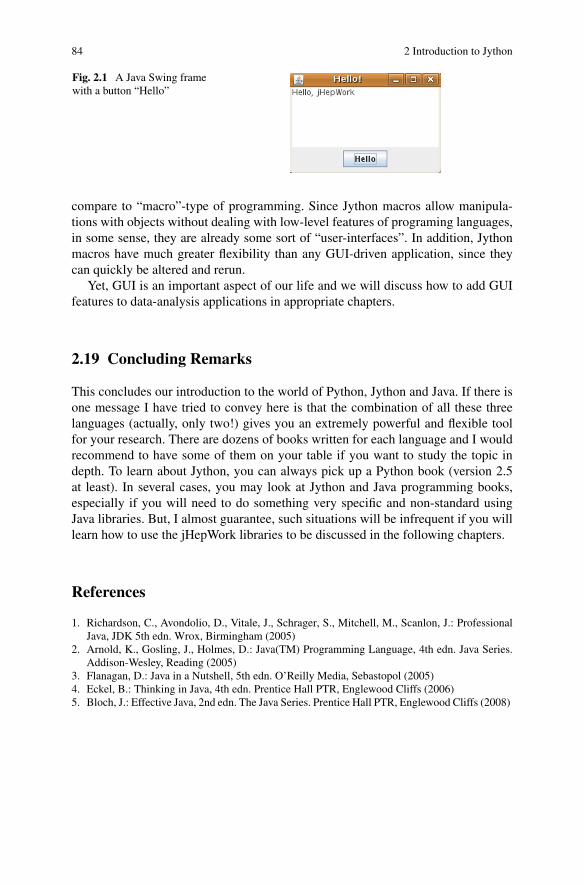
84 2 Introduction to Jython
Fig. 2.1 A Java Swing framewith a button “Hello”
compare to “macro”-type of programming. Since Jython macros allow manipula-tions with objects without dealing with low-level features of programing languages,in some sense, they are already some sort of “user-interfaces”. In addition, Jythonmacros have much greater flexibility than any GUI-driven application, since theycan quickly be altered and rerun.
Yet, GUI is an important aspect of our life and we will discuss how to add GUIfeatures to data-analysis applications in appropriate chapters.
2.19 Concluding Remarks
This concludes our introduction to the world of Python, Jython and Java. If there isone message I have tried to convey here is that the combination of all these threelanguages (actually, only two!) gives you an extremely powerful and flexible toolfor your research. There are dozens of books written for each language and I wouldrecommend to have some of them on your table if you want to study the topic indepth. To learn about Jython, you can always pick up a Python book (version 2.5at least). In several cases, you may look at Jython and Java programming books,especially if you will need to do something very specific and non-standard usingJava libraries. But, I almost guarantee, such situations will be infrequent if you willlearn how to use the jHepWork libraries to be discussed in the following chapters.
References
1. Richardson, C., Avondolio, D., Vitale, J., Schrager, S., Mitchell, M., Scanlon, J.: ProfessionalJava, JDK 5th edn. Wrox, Birmingham (2005)
2. Arnold, K., Gosling, J., Holmes, D.: Java(TM) Programming Language, 4th edn. Java Series.Addison-Wesley, Reading (2005)
3. Flanagan, D.: Java in a Nutshell, 5th edn. O’Reilly Media, Sebastopol (2005)4. Eckel, B.: Thinking in Java, 4th edn. Prentice Hall PTR, Englewood Cliffs (2006)5. Bloch, J.: Effective Java, 2nd edn. The Java Series. Prentice Hall PTR, Englewood Cliffs (2008)

Chapter 3Mathematical Functions
Functions allow programming code reuse, and thus are essential in any program-ming language. We have already discussed how to define general-purpose functionsin the Python language in Sect. 2.10. Now we will turn to the question of how tobuild mathematical functions. First, we will remind how to construct mathematicalfunctions in Jython and then we will discuss Java implementations of mathemat-ical functions in jHepWork. At the end of this chapter, we will discuss symbolicmanipulations with functions.
For many examples of this chapter, we will “glue” Python-type statements withJava libraries. Therefore, we will stop using the word Python1 when refer to the codesnippets, and will switch to the word “Jython” as the main programming languageused throughout this book.
3.1 Jython Functions
As we already know, Jython functions can be declared with the def() statement.In case of mathematical functions, it is very likely you will need to import the mod-ule ’math’ before or during creation of Jython functions, so a general form of afunction definition would be:
>>> def FunctionName( arg1, arg2, .. ) :>>> ... import math>>> ... -- math statements -->>> ... return value
In this example, arg1, arg2 etc. is a comma-separated list of arguments. Thearguments could be values, lists, tuples, strings or any Jython object.
1This usually implies the CPython implementation of the Python programming language.
S.V. Chekanov, Scientific Data Analysis using Jython Scripting and Java,Advanced Information and Knowledge Processing,DOI 10.1007/978-1-84996-287-2_4, © Springer-Verlag London Limited 2010
85
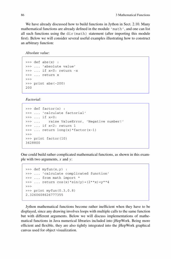
86 3 Mathematical Functions
We have already discussed how to build functions in Jython in Sect. 2.10. Manymathematical functions are already defined in the module ’math’, and one can listall such functions using the dir(math) statement (after importing this modulefirst). Below we will consider several useful examples illustrating how to constructan arbitrary function:
Absolute value:
>>> def abs(x) :>>> ... ’absolute value’>>> ... if x<0: return -x>>> ... return x>>>>>> print abs(-200)200
Factorial:
>>> def factor(x) :>>> ... ’calculate factorial’>>> ... if x<0:>>> ... raise ValueError, ’Negative number!’>>> ... if x<2: return 1>>> ... return long(x)*factor(x-1)>>>>>> print factor(10)3628800
One could build rather complicated mathematical functions, as shown in this exam-ple with two arguments, x and y:
>>> def myfun(x,y) :>>> ... ’calculate complicated function’>>> ... from math import *>>> ... return cos(x)*sin(y)+(2**x)+y**4>>>>>> print myfun(0.3,0.8)2.3260608626777355
Jython mathematical functions become rather inefficient when they have to bedisplayed, since any drawing involves loops with multiple calls to the same functionbut with different arguments. Below we will discuss implementations of mathe-matical functions in Java numerical libraries included into jHepWork. Being moreefficient and flexible, they are also tightly integrated into the jHepWork graphicalcanvas used for object visualization.

3.2 1D Functions in jHepWork 87
3.2 1D Functions in jHepWork
For one-dimensional (1D) functions, we have to deal with a dependence of onevalue, say y, on another, usually called x. jHepWork includes the F1D class todescribe, evaluate and display such functions. A 1D function can be instantiatedas:
>>> from jhplot import *>>> f1=F1D(’definition’)
where the string ’definition’ should be replaced by a mathematical formula.This string can contain any combinations of +, -, *, / operations, parenthesis ()and predefined mathematical functions. For numerical values, the scientific nota-tions “e”, “E”, “d”, “D” can be used. The only independent variable should be spec-ified as x. The function definition can contain predefined mathematical functionslistened in Tables 3.1 and 3.2, as well as the constants given in Table 3.3.
To evaluate a function at a fixed point, use the eval(x) method. For evaluationof a list of numerical values, pass a Jython list instead. In this case, the eval(x)method returns an array of values y calculated at specific values x from the inputlist.
Table 3.1 Mathematicalfunctions used to build theF1D objects
Function Defined as
xy Power
∗∗ as before
exp(x) Exponential
sqrt(x)√
x
log(x) Natural Logarithm
log10(x) Logarithm base 10
cos(x) Cosine
sin(x) Sine
tan(x) Tangent
cosh(x) Hyperbolic cosine
sinh(x) Hyperbolic sine
tanh(x) Hyperbolic tangent
acos(x) Arc Cosine
asin(x) Arc Sine
atan(x) Arc Tangent
acosh(x) Hyperbolic Arc Cosine
asinh(x) Hyperbolic Arc Sine
atanh(x) Hyperbolic Arc Tangent
rem(x) Reminder
atan2(x,y) Arc Tangent (2 parameters)

88 3 Mathematical Functions
Table 3.2 Special functions that can be included into the F1D definition
Function Defined as
j0 Bessel function of order 0 of the argument
j1 Bessel function of order 1 of the argument
jn Bessel function of order n of the argument
y0 Bessel function of the 2nd kind of order 0
y1 Bessel function of the 2nd kind of order 1
yn Bessel function of the 2nd kind of order n
fac(x) factorial x!gamma(x) the Gamma function
erf(x) the Error function
erfc(x) the complementary Error function
normal(x) the normal function
poisson(k,x) sum of the first k terms of the Poisson distribution
poissonc(k,x) the sum of the terms k + 1 to infinity of the Poisson distribution
igam(a,x) incomplete Gamma function
igamc(a,x) complemented incomplete i Gamma function
chisq(d,x) area under the left hand tail (from 0 to x) of the χ2 probability densityfunction with “d” degrees of freedom
chisqc(d,x) area under the right hand tail (from x to infinity) of the Chi squareprobability density function with “d” degrees of freedom
Let us give one example which makes this feature clear:1D function
from jhplot import *f1=F1D(’x^2+pi*sqrt(x)’)print f1.eval(20)a=f1.eval([10,20,30])print a.tolist()
The execution of this script gives:
414.049629462[109.934, 414.049, 917.207]
As you may note, since eval(d) returns an array, we converted this array into alist using the tolist() method for shorter printout (still we truncated the outputnumbers to fit them to the page width).
In many situations, it is useful to create a “parsed” function object to pass it tosome method or class inside a long loop. This can significantly boost performancesince the string parsing is done outside loops. This example illustrates how to printten numbers evaluated by the function x ∗ exp(x):

3.2 1D Functions in jHepWork 89
Table 3.3 Constants used to define the F1D functions
Constants Defined as
pi PI
e E
k Boltzman Constant: 1.3807e-16
ec Elementary Charge: 4.8032e-10
me Electron Mass. Units g: 9.1095e-28
mp Proton Mass. Units g: 1.6726e-24
gc Gravitational Constant. Units dyne-cm2/g2: 6.6720e-08
h Planck constant. Units erg-sec: 6.6262e-27
c Speed of Light in a Vacuum. Units cm/sec: 2.9979e10
sigma Stefan-Boltzman Constant. Units erg/cm2-sec-deg4: 5.6703e-5
na Avogadro Number. Units 1/mol: 6.0220e23
r Gas Constant. Units erg/deg-mol: 8.3144e07
g Gravitational Acceleration at the Earths surface. Units cm/sec2: 980.67
>>> from jhplot import *>>> f=F1D(’x*exp(x)’)>>> p=f.getParse()>>> for i in range(10):>>> ... print p.getResult(i)
Of course, one can also print the numbers using the eval() method (since thestring parsing is done during creation of the F1D object). However, there are manysituations in which a “parsed” function (i.e. the object “p” in this example) can beused as an argument for methods inside loops.
One can find all the methods associated with this class as explained inSect. 1.4.10.
3.2.1 Details of Java Implementation
The object created in the above examples is an instance of the F1D Java class, thusit does not belong to the Python programming language, although we call it us-ing the Python syntax. When we instantiate the object of the class F1D, we callthe Java library package jhplot stored in the file jhplot.jar located in the’lib/system’ directory. How can we check this? As usual, call the methodtype():
>>> from jhplot import *>>> f=F1D(’x*exp(x)’)
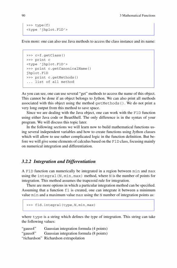
90 3 Mathematical Functions
>>> type(f)<type ’jhplot.F1D’>
Even more: one can also use Java methods to access the class instance and its name:
>>> c=f.getClass()>>> print c<type ’jhplot.F1D’>>>> print c.getCanonicalName()jhplot.F1D>>> print c.getMethods()... list of all method
As you can see, one can use several “get” methods to access the name of this object.This cannot be done if an object belongs to Jython. We can also print all methodsassociated with this object using the method getMethods(). We do not print avery long output from this method to save space.
Since we are dealing with the Java object, one can work with the F1D functionusing either Java code or BeanShell. The only difference is in the syntax of yourprogram. We will discuss this topic later.
In the following sections we will learn now to build mathematical functions us-ing several independent variables and how to create functions using Jython classeswhich will allow to use rather complicated logic in the function definition. But be-fore we will give some elements of calculus based on the F1D class, focusing mainlyon numerical integration and differentiation.
3.2.2 Integration and Differentiation
A F1D function can numerically be integrated in a region between min and maxusing the integral(N,min,max) method, where N is the number of points forintegration. This method assumes the trapezoid rule for integration.
There are more options in which a particular integration method can be specified.Assuming that a function f1 is created, one can integrate it between a minimumvalue min and a maximum value max using the N number of integration points as:
>>> f1d.integral(type,N,min,max)
where type is a string which defines the type of integration. This string can takethe following values:
“gauss4” Gaussian integration formula (4 points)“gauss8” Gaussian integration formula (8 points)“richardson” Richardson extrapolation

3.3 Plotting 1D Functions 91
“simpson” using Simpson’s rule“trapezium” trapezium rule
The code below tests different integration algorithms using the methods shownabove. We also benchmark the code (see Sect. 2.9.1) by printing the time spent byeach algorithm (in milliseconds):
Integration of a function
from jhplot import *import time
f1=F1D(’sin(1.0/x)*x^2’)methods=[’gauss4’, ’gauss8’, ’richardson’,\
’simpson’,’trapezium’]for m in methods:
start = time.clock()d=f1.integral(m,10000,1,10)t = time.clock()-startprint m+’ =’,d,’ time (ms)=’,t*1000
The result of code execution is given below:
gauss4 = 49.1203116758 time (ms)= 42.245gauss8 = 49.1203116758 time (ms)= 32.382richardson = 49.1203116758 time (ms)= 12.162simpson = 49.1203116758 time (ms)= 14.173trapezium = 49.1203116663 time (ms)= 4.234
While the time needed for the integration could be different for your tests (clearly,this depends on many factors), it appears that the fastest algorithm is that based onthe trapezium method.
A function can numerically be differentiated using the method:
>>> a=f1d.differentiate(N,min,max)
The method returns an array with the result of differentiation. The size of this arrayis set using an integer value N .
In Sect. 3.9, we will again discuss the topic of integration and differentiationusing symbolic mathematical calculations.
3.3 Plotting 1D Functions
The remaining issue is how to visualize the F1D functions. Below we will learn howto build a canvas suited for plotting F1D objects and discuss the main options fortheir visualization.

92 3 Mathematical Functions
3.3.1 Building a Graphical Canvas
To plot the 1D functions, first we need to create a graphical canvas. This can be doneby instantiation of a canvas object of the HPlot class:
>>> from jhplot import *>>> c1=HPlot(’Canvas’)
This creates a default canvas with the title ‘Canvas’ and with the default frame sizeof 600 × 400 pixels. To display the canvas in a pop-up frame, execute the statement:
>>> c1.visible(1)
It should be reminded that “1” means boolean “true”, while “0” means “false”. Onecan also use the shortcut visible() instead of visible(1). If you do notwant to pop-up the canvas frame and want to keep it in the computer memory, setthe argument of the method visible() to zero.
There are more constructors for this class. For example, one can customize theframe size with the method:
>>> c1=HPlot(’Canvas’,800,600)
which creates a canvas with the frame size of 800 by 600 pixels. One can also resizethe canvas using the mouse.
The created canvas can be divided into several plot regions (or “pads”). In thiscase, use the following initialization:
>>> c1=HPlot(’Canvas’,600,400,iX,iY)
which again creates a canvas of the size 600 by 400 pixels, but, in addition, the lasttwo numbers are used to make two plot regions inside the canvas frame. The firstinteger number after 400 tells that we need iX plot regions in X, and the secondnumber is used to set the number of pads in Y . For example, after setting iX=2 andiY=1, the above constructor creates two pads positioned horizontally.
A function can be plotted inside the canvas using the draw(obj) method,where obj is an instance of the F1D class. One can navigate to the current re-gion using the method cd(i1,i2), where i1 and i2 specify the pad in X and Y .For example, if one needs to plot a function inside the first pad, use:
>>> c1.cd(1,1)>>> c1.draw(f1d)

3.3 Plotting 1D Functions 93
where f1d represents an object of the F1D function. If the function should be shownon the second region, use
>>> c1.cd(1,2)>>> c1.draw(f1d)
By default, the HPlot canvas has the range between 0 and 1 for the X or Y axis.One should specify the necessary range using the method:
>>> c1.setRange(x1,x2,y1,y2)
where x1 is a minimum value in X, x2 is a maximum value in X, and y1 and y2are the same but for the Y -axis. Alternatively, one can set “auto-range” using themethod c1.setAutoRange().
Before plotting a function, one can show a global title of the entire canvas. Thiscan be done by using the method setGTitle(str), where str represents astring. In the simplest case, it accepts one argument: a string with the title text. Onecan customize the text color and/or the font size as will be shown later. As usual,use the code assist (see Sect. 1.4.10) to learn about possible choices.
In addition to the global title, one can set titles for each drawing pad using themethod setName(s), with “s” being a string with some text. We can also anno-tate X and Y axes. The methods for this are setNameX(s) and setNameY(s),where “s” is an annotation string.
Let us give a more concrete example. First, import the Color class from theJava AWT library and then set appropriate annotations:
>>> from java.awt import Color>>> from jhplot import *>>>>>> c1.setGTitle(’GlobalTitle’,Color.red)>>> c1.setNameX(’X axis’)>>> c1.setNameY(’Y axis’)>>> c1.setName(’Pad title’)>>> c1.visible() # make it visible>>> c.setAutoRange() # set autorange for X and Y
All the entries above are self-explanatory. One may add a background color for thecanvas using:
>>> c1.setBackgroundColor(c)
where ’c’ stands for the Java AWT color. Colors can be set using any of the staticmethods shown in Table 3.4.
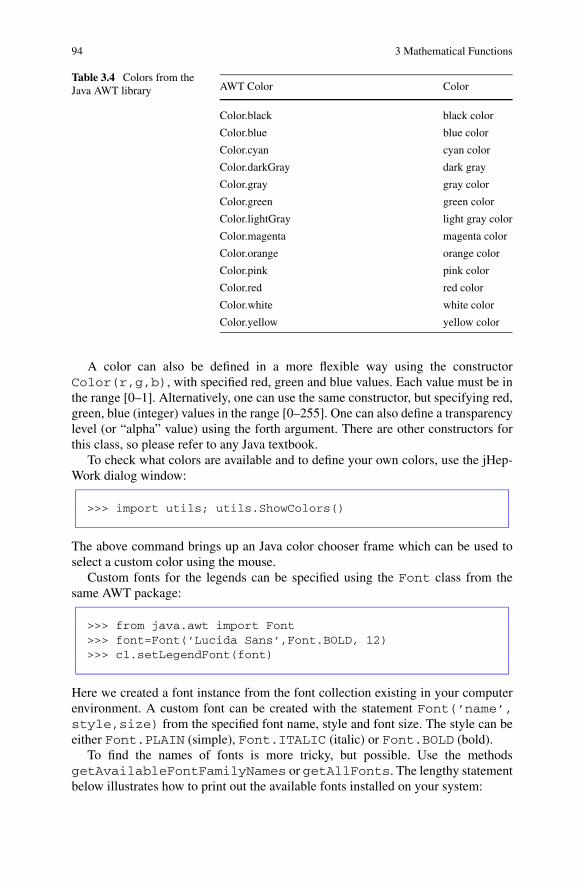
94 3 Mathematical Functions
Table 3.4 Colors from theJava AWT library AWT Color Color
Color.black black color
Color.blue blue color
Color.cyan cyan color
Color.darkGray dark gray
Color.gray gray color
Color.green green color
Color.lightGray light gray color
Color.magenta magenta color
Color.orange orange color
Color.pink pink color
Color.red red color
Color.white white color
Color.yellow yellow color
A color can also be defined in a more flexible way using the constructorColor(r,g,b), with specified red, green and blue values. Each value must be inthe range [0–1]. Alternatively, one can use the same constructor, but specifying red,green, blue (integer) values in the range [0–255]. One can also define a transparencylevel (or “alpha” value) using the forth argument. There are other constructors forthis class, so please refer to any Java textbook.
To check what colors are available and to define your own colors, use the jHep-Work dialog window:
>>> import utils; utils.ShowColors()
The above command brings up an Java color chooser frame which can be used toselect a custom color using the mouse.
Custom fonts for the legends can be specified using the Font class from thesame AWT package:
>>> from java.awt import Font>>> font=Font(’Lucida Sans’,Font.BOLD, 12)>>> c1.setLegendFont(font)
Here we created a font instance from the font collection existing in your computerenvironment. A custom font can be created with the statement Font(’name’,style,size) from the specified font name, style and font size. The style can beeither Font.PLAIN (simple), Font.ITALIC (italic) or Font.BOLD (bold).
To find the names of fonts is more tricky, but possible. Use the methodsgetAvailableFontFamilyNames or getAllFonts. The lengthy statementbelow illustrates how to print out the available fonts installed on your system:

3.3 Plotting 1D Functions 95
>>> from java.awt import *>>> e = GraphicsEnvironment.getLocalGraphicsEnvironment()>>> print e.getAllFonts()>>> print e.getAvailableFontFamilyNames()
When using jHepWork, call the predefined command which lists the availablefonts:
>>> import utils; utils.ShowFonts()
Use the above approach to find out necessary fonts to be used in Jython scrips tosetup graphical options for drawing of titles, and other labels. In addition, one canuse the GUI-dialogs of the HPlot canvas. For example, double-click on the globaltitle to bring up a setup dialog used to change the global text, fonts and colors. In asimilar way one can edit the margins of the pads.
3.3.2 Drawing 1D Functions
Once a canvas is ready, one can plot a 1D function discussed in Sect. 3.2 as:
>>> from jhplot import *>>>>>> c1=HPlot("Canvas")>>> c1.visible()>>> c1.setAutoRange()>>> f1=F1D(’2*exp(-x*x/50)+sin(pi*x)/x’, -2.0,5.0)>>> c1.draw(f1)
Obviously, −2.0 and 5.0 specify the range for the abscissa. There is an importantdifference with respect to the function definition given in Sect. 3.2: now we explic-itly tell what abscissa range should be used for evaluation and drawing. One can setthe range for the function later using the methods:
>>> f1.setMin(min)>>> f1.setMax(max)
where min and max are a minimum and a maximum value for the abscissa. Natu-rally, the corresponding “getter” methods getMin() and getMax() return thesevalues back. It should be noted that the specified abscissa range does not affect themethod eval(x) which determines the value of a function at a certain x value.

96 3 Mathematical Functions
Finally, you may need to determine the plotting resolution. By default, a func-tion is evaluated at 500 points in the specified abscissa range. One can find thisusing the getPoints() method. One can change this value using the methodsetPoints(i), where ’i’ is an integer number (should be sufficiently large).For a very large number, the price to pay is a larger memory consumption and slowerplotting.
In order to plot several functions on the same canvas, simply repeat thedraw(obj) statement for each function.
>>> f1=F1D(’2*exp(-x*x/50)+sin(pi*x)/x’, -2.0,5.0)>>> f2=F1D(’exp(-x*x/10)+cos(pi*x)/x’, -2.0,5.0)>>> c1.draw(f1)>>> c1.draw(f2)
It should be noted that the method draw(obj) can also be used to visualize aJython list of F1D functions as in the example below:
>>> from jhplot import *>>>>>> c1=HPlot(’Canvas’)>>> c1.visible()>>> c1.setAutoRange()>>> f1=F1D(’2*exp(-x*x/50)+sin(pi*x)/x’, -2.0,5.0)>>> f2=F1D(’2*sqrt(x)’)>>> c1.draw([f1,f2])
For all these examples, the color used for drawing is the same, thus it is difficultto separate the plotted functions visually. One can draw the functions using variouscolors after importing the Color class from the Java AWT package as discussedbefore. Moreover, one can define the line width as:
>>> from java.awt import Color>>> from jhplot import *>>>>>> f1=F1D(’2*exp(-x*x/50)+sin(pi*x)/x’, -2.0,5.0)>>> f2=F1D(’exp(-x*x/10)+cos(pi*x)/x’, -2.0,5.0)>>> f1.setPenWidth(2)>>> f1.setColor(Color.green)>>> f2.setColor(Color.red)>>> c1.draw(f1)>>> c1.draw(f2)
where the method setPenWidth(i) accepts an integer number for the line widthin terms of the number of pixels. To draw dashed lines, use the setPenDash()method. One can change the dashed line length by specifying an integer value be-tween 0 and 40. One can also use the update() method to redraw the plot.

3.3 Plotting 1D Functions 97
Table 3.5 The most important methods for graphical representations of the F1D class. For themethods shown in this table, “b” indicates a boolean value (0 for true and 1 for false), while “i” isan integer parameter. The notation “d” indicates a float value. The attributes “c” and “f” correspondto the Color and Font classes of Java AWT. “text” represents a string
Methods Definitions
setColor(c) set line color
setPenWidh(i) width of the line
setPenDash(i) dashed style with “i” being the length
setLegend(b) set (b=1) or not (b=0) the legend
setTitle(text) set title text
The example above shows that a F1D function contains several methods fordrawing. Some most important graphical options are listed in Table 3.5.
As mentioned before, instead of using all these graphical methods in Jythonscripts, for function drawing, one can also edit function attributes using a GUI-driven dialog: Navigate the mouse to the pad with the graph and select [Editsettings] with the mouse button. Then select [Y item] and you will see apop-up window with various attributes. In a similar way one can edit the global titleand margins of the pads.
3.3.3 Plotting 1D Functions on Different Pads
To plot two or more functions on different plot regions, one should construct anappropriate canvas. Before calling the method draw(obj), the current plottingpad has to be changed using the cd(i1,i2) method. In the example below wemake a canvas with two pads and then navigate to the necessary pad when we needto plot a function:
>>> from java.awt import Color>>> from jhplot import *>>>>>> c1=HPlot(’Canvas’,600,400,1,2)>>> c1.visible()>>> c1.setAutoRange()>>> f1=F1D(’2*exp(-x*x/50)+sin(pi*x)/x’, -2.0, 5.0)>>> f2=F1D(’exp(-x*x/10)+cos(pi*x)/x’, -2.0, 5.0)>>> f1.setColor(Color.green)>>> c1.draw(f1)>>> c1.cd(1,2) # go to the second pad (1,2)>>> c1.draw(f2)

98 3 Mathematical Functions
3.3.4 Short Summary of HPlot Methods
Table 3.6 shows the major methods of the HPlot class. Note that there are morethan 300 methods associated with this class, which are divided into the “getter” (theystart from the “get” string) and “setter” (starting from “set”) groups of methods.
One can learn about the methods of the HPlot canvas using the jHepWork codeassist, i.e. typing c1. and pressing [F4] key, where c1 is an instance of the HPlotclass. One can also use the method dir(c1) to print the methods.
We will discuss the HPlot canvas in Sect. 10.2 in more detail. In addition, wecan show how to use other graphical tools to display functions in Chap. 10.
3.3.5 Examples
Let us show a complete script example for visualization of several 1D functionsusing two plot regions. Save these lines in a file, say ’test.py’, load this file intothe jHepWork editor and click on the “[run]” button (or press [F8]) to executethe script.
Using HPlot canvas
from java.awt import Colorfrom jhplot import *
c1 = HPlot(’Canvas’,600,400,2,1)c1.visible()c1.setGTitle(’F1D Functions’,Color.red)c1.setNameX(’X axis’)c1.setNameY(’Y axis’)
c1.cd(1,1)c1.setAutoRange()c1.setName(’Local title’)f1 = F1D(’2*exp(-x*x/50)+sin(pi*x)/x’,-2.0,5.0)f1.setPenDash(4)c1.draw(f1)f1 = F1D(’exp(-x*x/50)+pi*x’,-2.0,5.0)f1.setColor(Color(10,200,50))f1.setPenWidth(3)c1.draw(f1)
c1.cd(2,1)c1.setAutoRange()f1 = F1D(’20*x*cos(x)’,-0,5.0)f1.setColor(Color.red)f1.setPenWidth(3)c1.draw(f1)

3.3 Plotting 1D Functions 99
Table 3.6 Most important methods of the HPlot class. For the methods shown in this table, “b”indicates a boolean value (0 or 1), while “a” is an integer parameter indicating axis (a=0 meansX-axis, a=1 means Y -axis). The notation “d” indicates a float value. The attributes “c” and “f”correspond to the Color and Font classes of Java AWT. “text” represents a string
Methods Definitions
destroy() clean and destroy the canvas frame
draw(o) draw some object, like F1D etc.
clear() clean the current region
cd(X,Y) go to a current region in X and Y
clear(X,Y) clean one region given by X and Y
clearAll() clean all regionsclearData() clean data from the current region all graph
settings are keptclearAllData() clean data from all regions all graph
settings are kept
visible(b) make canvas visible (b=1) or invisible (b=0)
visible() make canvas visible
setAutoRange() set autorange for all axes
setAutoRange(b) set autorange (b=1) or not (b=0) for all axes
setAutoRange(a,b) set (b=1) or not set (b=1) autorange for axis
setAxesColor(c) set color for axes
setBox(b) set or not a bounding box around the graph
setBoxOffset(d) offset of the bounding box
setBoxFillColor(c) fill color of the bounding box
setBoxColor(c) color of the bounding box
setBackgroundColor(c) background color of the graph
setGrid(a,b) show grid (b=1) or not (b=1) for axis
setGridColor(c) grid color
setGridToFront(b) grid in front of drawing (b=1) or behind (b=0)
update() update current plot defined by cd()
updateAll() update plots in all regions
setGTitle(text,f,c) set attributes for global title
setLegend(b) set legend (b=1) or not (b=0)
setLegendFont(f) set legend font
setLogScale(a,b) set (b=1) or not set (b=0) log scale for axis
setLegendPosition(a,pos) set legend position given by pos value
setTicsMirror(a,b) set (b=1) or not set (b=0) mirror ticks for axis
setGrid(a,b) show grid (b=1) or not (b=1) for axis
setRange(a,min,max) min and max for axis
setRange(minX,maxX,minY,maxY) min and max range for X and Y
setAntiAlias(b) set (b=1) or not set antialiase for graphics
removeAxes() remove all axesexport(FileName) export to an image (png, eps, ps)
Image format is given by the file extension
update() update the current plot

100 3 Mathematical Functions
Fig. 3.1 Several F1D functions plotted on two pads of the same HPlot canvas
f1 = F1D(’10*sqrt(x)+20*x’,0,5.)f1.setColor(Color.blue)f1.setPenWidth(3)c1.draw(f1)
f1 = F1D(’15*sqrt(x)+20*x*x’,0,5.)f1.setColor(Color.blue)f1.setPenDash(3)c1.draw(f1)
The execution of this script creates a canvas with several plotted functions as shownin Fig. 3.1.
3.4 2D Functions
3.4.1 Functions in Two Dimensions
By considering functions with more than one independent variable, we are nowbeginning to venture into high-dimensional spaces. To build a two-dimensional (2D)function, jHepWork has the F2D class. It is defined in the same way as F1D. Theonly difference - it takes two independent variables, x and y.

3.4 2D Functions 101
>>> from jhplot import *>>> f1=F2D( ’definition’)
where ’definition’ is a string that must be replaced by the actual mathematicalformula with two independent variables, x and y. As for the F1D class, the func-tion definition can contain any combination of predefined operators, functions andconstants listened in Tables 3.1, 3.2 and 3.3.
To evaluate a 2D function at a fixed point (x, y), use the eval(x,y) method.One can evaluate a function for lists with x and y values using the methodeval(x[],y[]) as in the example below:
>>> from jhplot import *>>> f2=F2D(’sqrt(x)*sin(y)/x + y^3’)>>> f2.eval(2,0.1)0.07>>> f2.eval([1,2],[2,4])array([D,[array(’d’,[8.9,63.2]),array(’d’,[8.6,63.4])])
The output numbers below are truncated to fit them to the width of this page.As for the F1D function, use a “parsed” object if you need to pass it to some
method inside long loops. Get it using the method getParse() which returns anobject for evaluation.
The F2D functions can numerically be integrated for a region betweenminX-maxX (for x) and between minY-maxY (for y) using the method:
>>> f2.integral(N,minX,maxX,minY,maxY)
where N is the number of points for integration for each abscissa. The method as-sumes the trapezoid rule for integration.
3.4.2 Displaying 2D Functions on a Lego Plot
The F2D functions can be shown using a three-dimensional HPlot3D canvas. Thiscanvas has very similar methods as those for the HPlot canvas, but allows to drawobjects in 3D. What we should remember is that we have to prepare the function fordrawing beforehand, which means one should specify the ranges for x and y axesduring the initialization (or after, but before drawing).
During the initialization step, one can set the ranges as:
>>> from jhplot import *>>> f2=F2D(’sqrt(x)*sin(y)/x + y^3’,minX,maxX,minY,maxY)

102 3 Mathematical Functions
so the function will be plotted for x in the interval [minX-maxX], and in theinterval [minY-maxY] for the y independent variable.
After the initialization, one can set the range using the setMinX(min),setMinX(max) methods for x, and analogously for y. The number of points forthe evaluation can be set using setPoints(n) methods (the default number ofpoints is 500).
Here is a typical example which shows how to plot either a single function ortwo functions on the same lego plot:
Plotting 2D functions
from java.awt import Colorfrom jhplot import *
c1 = HPlot3D(’Canvas’,600,700, 2,2)c1.visible()c1.setGTitle(’F2D examples’)
f1=F2D(’cos(x*y)*(x*x-y*y)’, -2.0, 2.0, -2.0, 2.0)f2=F2D(’cos(x+y)*x’, -2.0, 5.0, -2.0, 5.0)f3=F2D(’sin(4*x)+x^2’, -2.0, 2.0, -2.0, 2.0)f4=F2D(’x^2+y^2’, -2.0, 2.0, -2.0, 2.0)
c1.cd(1,1)c1.setScaling(8)c1.setRotationAngle(30)c1.draw(f1)
c1.cd(2,1)c1.setAxesFontColor(Color.blue)c1.setColorMode(3)c1.setScaling(8)c1.setElevationAngle(30)c1.setRotationAngle(35)c1.draw(f2)
c1.cd(1,2)c1.setColorMode(4)c1.setLabelFontColor(Color.red)c1.setScaling(8)c1.setRotationAngle(40)c1.draw(f3)
c1.cd(2,2)c1.setColorMode(1)c1.setScaling(8)c1.setElevationAngle(30)c1.setRotationAngle(35)c1.draw(f4,f2)

3.4 2D Functions 103
Fig. 3.2 F2D functions shown using the HPlot3D canvas in several regions
The resulting figure is shown in Fig. 3.2.This example features one interesting property of the HPlot3D canvas: Instead
of plotting one function as c1.draw(f1), we plot both functions on the samepad after passing two functions as arguments (see the last line). This is somewhatdifferent from the HPlot behavior, where we could pass any number of functionsin a form of the list. For the HPlot3D canvas, one can plot two functions at most.Also, the class does not accept lists of functions. Later we will show that one canplot 2D histograms or even mixing histograms with functions using the methoddraw(obj1,obj2).
For the three-dimensional canvas, the presentation style can be changed us-ing setColorMode(i) method, where i=0 for wireframe, i=1 for hidden,i=2 for color spectrum, i=3 for gray scale, i=4—for dualshades. The methodssetScaling(), setElevationAngle() and setRotationAngle() areself-explanatory. The plots can be rotated with the mouse and the title can be mod-ified using exactly the same way as for the HPlot canvas. We will return to theHPlot3D canvas in Sect. 10.12.

104 3 Mathematical Functions
3.4.3 Using a Contour Plot
The 2D functions can also be shown using a contour (density) style. Thiscan be done with the help of the same HPlot3D canvas but adding the linec1.setContour() after the definition of the c1 object. This is shown bellow:
Contour plot
from java.awt import Colorfrom jhplot import *
c1 = HPlot3D(’Canvas’,600,600)c1.setNameX(’X’)c1.setNameY(’Y’)c1.setContour()c1.visible()f1=F2D(’x^2+y^2’, -2.0, 2.0, -2.0, 2.0)c1.draw(f1)
The execution of this script leads to the plot shown in Fig. 3.3. The color barfrom the right indicates the density levels used for drawing in color. They can beredefined using several methods of this canvas.
However, it is more practical to show the F2D functions using the canvas basedon the class HPlot2D. As we will discuss in Sect. 10.11, this class has significantly
Fig. 3.3 A contour representation of the function x2 + y2 using the HPlot3D canvas

3.5 3D Functions 105
more options to display the contour and density plots since it was designed mainlyfor such types of plots.
3.5 3D Functions
3.5.1 Functions in Three Dimensions
You may already have guessed that for tree-dimensional (3D) functions, jHepWorkhas the F3D class. It is defined in the same way as F1D and F2D, the only differenceis it can take up to three independent variables: x, y and z.
>>> from jhplot import *>>> f3=F3D(’definition’)
where ’definition’ is a string that should be replaced by the actual formula. Asfor the F1D and F2D classes, the function definition can be constructed from a com-bination of operators, mathematical functions and constants, as given in Tables 3.1,3.2 and 3.3.
To evaluate a 3D function at a fixed value (x, y, z), use the usual methodeval(x,y,z):
>>> from jhplot import *>>> f3=F3D(’sqrt(x)*sin(y)/x + z^3’)>>> f3.eval(2,0.1,4) # calculate for x=2, y=0.1, z=40.07159288589999416
Probably, we can stop here and will not go into the drawing part of this section.We have to be creatures leaving in four-dimensional space in order to be interestedin how to draw such functions (actually, if such a creature is reading this bookand is still interested in this option, please contact me—we may discuss how toplot such functions). One can also project 3D functions into a 2D space by fixingsome independent variables and then using the F2D and HPlot3D to display suchprojections.
Below we will discuss more flexible classes for dealing with multidimensionalfunctions.
3.6 Functions in Many Dimensions
3.6.1 FND Functions
jHepWork supports functions with arbitrary number of independent variables usingthe FND class. This class is more complicated and has its roots in the known JEPJava package [1].
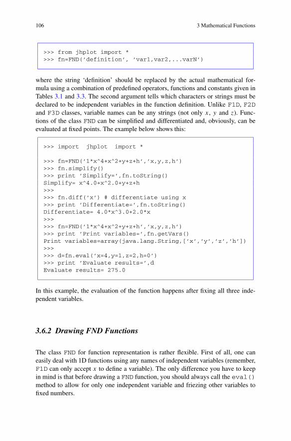
106 3 Mathematical Functions
>>> from jhplot import *>>> fn=FND(’definition’, ’var1,var2,...varN’)
where the string ‘definition’ should be replaced by the actual mathematical for-mula using a combination of predefined operators, functions and constants given inTables 3.1 and 3.3. The second argument tells which characters or strings must bedeclared to be independent variables in the function definition. Unlike F1D, F2Dand F3D classes, variable names can be any strings (not only x, y and z). Func-tions of the class FND can be simplified and differentiated and, obviously, can beevaluated at fixed points. The example below shows this:
>>> import jhplot import *
>>> fn=FND(’1*x^4+x^2+y+z+h’,’x,y,z,h’)>>> fn.simplify()>>> print ’Simplify=’,fn.toString()Simplify= x^4.0+x^2.0+y+z+h>>>>>> fn.diff(’x’) # differentiate using x>>> print ’Differentiate=’,fn.toString()Differentiate= 4.0*x^3.0+2.0*x>>>>>> fn=FND(’1*x^4+x^2+y+z+h’,’x,y,z,h’)>>> print ’Print variables=’,fn.getVars()Print variables=array(java.lang.String,[’x’,’y’,’z’,’h’])>>>>>> d=fn.eval(’x=4,y=1,z=2,h=0’)>>> print ’Evaluate results=’,dEvaluate results= 275.0
In this example, the evaluation of the function happens after fixing all three inde-pendent variables.
3.6.2 Drawing FND Functions
The class FND for function representation is rather flexible. First of all, one caneasily deal with 1D functions using any names of independent variables (remember,F1D can only accept x to define a variable). The only difference you have to keepin mind is that before drawing a FND function, you should always call the eval()method to allow for only one independent variable and friezing other variables tofixed numbers.

3.7 Custom Functions Defined by Jython Scripts 107
Let us consider an example with two independent variables. In this case, weshould set the second variable to some value since we want to plot an one-dimensional function:
Drawing a FND function
from jhplot import *
c1=HPlot()f2=FND(’sqrt(var1)*sin(var2)’,’var1,var2’)f2.eval("var1",1,100,’var2=2’) # var1 in range 1-100c1.visible()c1.setAutoRange()c1.draw(f2)
In the example above, first we evaluate the function in the range between 1 and 100and fixing var2 to 2 before calling the draw(obj) method.
Below is the example for a function with three independent variables. After fixingtwo variables, we plot this function in 1D:
Drawing a FND function
from jhplot import *
c1 = HPlot(’Example’,600,400)c1.setGTitle(’FND function’)c1.visible()c1.setAutoRange()f2=FND(’x*x+y+20+z’,’x,y,z’)f2.eval(’x’,-2,10,’y=2,z=100’)c1.draw(f2)
Now we have fixed two variables, y and z, and plotted the function in terms of theindependent variable x between −2 and 10. It should be noted that the variables tobe fixed are separated by a comma in the eval() statement.
3.7 Custom Functions Defined by Jython ScriptsBuilding a custom mathematical function using Jython scripts makes sense whenthe logic of the mathematical expression is so complicated that it’s better to define itin a separate code block rather than to use a string and pass it during the instantiationof the function. In this way one can build infinitely complicated functions in manydimensions and evaluate them using jHepWork Java libraries.
3.7.1 Custom Functions and Their Methods
For constructing functions in this section, we will use the package shplot pro-vided by jHepWork. Let us build a simple second-order polynomial function,
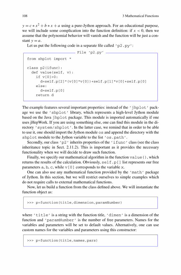
108 3 Mathematical Functions
y = c ∗ x2 + b ∗ x + a using a pure-Jython approach. For an educational purpose,we will include some complication into the function definition: if x < 0, then weassume that the polynomial behavior will vanish and the function will be just a con-stant y = a.
Let us put the following code in a separate file called ’p2.py’:
File ’p2.py’
from shplot import *
class p2(ifunc):def value(self, v):if v[0]>0:
d=self.p[2]*(v[0]*v[0])+self.p[1]*v[0]+self.p[0]else:
d=self.p[0]return d
The example features several important properties: instead of the ’jhplot’ pack-age we use the ’shplot’ library, which represents a high-level Jython modulebased on the Java jhplot package. This module is imported automatically if oneuses jHepWork. If you are using something else, one can find this module in the di-rectory ’system/shplot’. In the latter case, we remind that in order to be ableto use it, one should import the Jython module os and append the directory with theshplot module to the Jython variable to the list ’os.path’.
Secondly, our class ’p2’ inherits properties of the ’ifunc’ class (see the classinheritance topic in Sect. 2.11.2). This is important as it provides the necessaryfunctionality when we will decide to draw such function.
Finally, we specify our mathematical algorithm in the function value(), whichreturns the results of the calculation. Obviously, self.p[] list represents our freeparameters a, b, c, while v[0] corresponds to the variable x.
One can also use any mathematical function provided by the ’math’ packageof Jython. In this section, but we will restrict ourselves to simple examples whichdo not require calls to external mathematical functions.
Now, let us build a function from the class defined above. We will instantiate thefunction object as:
>>> p=function(title,dimension,paramNumber)
where ’title’ is a string with the function title, ’dimen’ is a dimension of thefunction and ’paramNumber’ is the number of free parameters. Names for thevariables and parameters will be set to default values. Alternatively, one can usecustom names for the variables and parameters using this constructor:
>>> p=function(title,names,pars)

3.7 Custom Functions Defined by Jython Scripts 109
where ’name’ and ’pars’ are lists of strings defining the names for independentvariables and parameters names (this overwrites the default names).
Let us come back to our example and instantiate the second-order polynomialfunction given in the module ’p2.py’. We will create a function by assigning thetitle ’p2’, dimension of this function (1) and the number of parameters (3 param-eters).
Building a custom function
from p2 import *
p=p2(’p2’,1,3)print p.title()print p.dimension()print p.numberOfParameters()print p.parameterNames()print p.variableNames()print p.variableName(0)
The execution of this script gives:
p213array(java.lang.String, [u’par0’, u’par1’, u’par2’])array(java.lang.String, [u’x0’])x0
Let us discuss the output in more detail: We print out the title of this functionwith the method title() and the dimension with the method dimension().The number of parameters is given by the method numberOfParameters().The method parameterNames() returns the parameter names. Since we didnot assign any custom names, it prints the default names, ’par0’, ’par1’,’par2’. Then we print the variable name (the default is ’x0’).
Now let us evaluate this function at several points. But before, let us assign somenumerical values to our free parameters. One can set a single value by calling theparameter name, or setting it at once in form of list. Then we will evaluate thefunction at x = 10 and x = −1:
Setting parameters
from p2 import *
p=p2(’p2’,1,3)p.setParameter(’par0’, 10)p.setParameter(’par1’, 20)p.setParameter(’par2’, 30)
# set all parameters in one go

110 3 Mathematical Functions
p.setParameters([10,20,30])
print "Value at x=10 =", p.value([10])print "Value at x=-1 =", p.value([-1])
Note how this was done: first we pass a list to the function, and then return it with themethod value(). As you may guess, this is necessary in case if you have severalvariables to pass to a function. Executing the above script gives:
Value at x=10 = 3210.0Value at x=-1 = 10.0
Now, let us assign custom names for the parameters. This time will instantiate itusing the second constructor as:
Setting parameters
from p2 import *
p=p2(’p2’,[’x’],[’a’,’b’,’c’])print p.parameterNames()print p.variableNames()p.setParameter(’a’, 10)p.setParameter(’b’, 20)p.setParameter(’c’, 30)
print "Value at x=10 =", p.value([10])print "Value at x=-1 =", p.value([-1])
As you can see, we assign the names ’a’, ’b’, ’c’. We also set the variable nameto the convenient ’x’. One can see this from the output shown below:
array(java.lang.String, [u’a’, u’b’, u’c’])array(java.lang.String, [u’x’])Value at x=10 = 3210.0Value at x=-1 = 10.0
More advanced users can look at the methods of the object ’p’. They will findout that this object is constructed from the AIDA class IFunction and containsmany other methods which have not been discussed here.
3.7.2 Using External Libraries
Previously we have shown a rather simple example illustrating how to constructa mathematical function. But we are not restricted here with constructions from

3.7 Custom Functions Defined by Jython Scripts 111
Jython: since our codding is based on Java, one can call a function or library fromJava API, or Java-based external library. We can direct you, for example, to theColt Java library [2] (included into jHepWork) which provides a large set of specialfunctions and functions commonly used for probability densities.
To build a function, you will need first to import necessary classes from third-party libraries and replace parameters with self.p[], while variables should bereplaced with v[] in the method value(). Let us show how to make a simpleJython module containing a Bessel function and Beta function:
Calling Java libraries. Module ’special.py’
from shplot import *
class bessel(ifunc):def value(self, v):
from cern.jet.math import Besselreturn Bessel.i0e(v[0])
class beta(ifunc):def value(self, v):
from cern.jet.stat.Probability import betareturn beta(self.p[0],self.p[1],v[0])
First, we import the Java package ’cern.jet.math’ from the Colt library men-tioned above and use this library to construct the Bessel and Beta functions. Pleaselook at the Java API of the Colt library to learn about such functions. We will savethese lines in a module called ’special.py’.
Calling both functions from the module ’special.py’ is trivial. Just importthis module and take care of the number of parameters you pass to such functionswhen calling them:
Calling special functions
from special import *
b1=beta(’Beta function’,1,2)b2=bessel(’Bessel order 0’,1,0)
One can evaluate the functions at any allowed value ’x’ after specifying values forfree parameters. In case of the Bessel function, we do not have free parameters andthe evaluation of such function is straightforward.
3.7.3 Plotting Custom Functions
Now we know how to build function objects from a script. Next, we will show howto manipulate with such custom functions and plot them.

112 3 Mathematical Functions
First thing you probably will need to do is to convert a function to F1D or F2Dobjects for plotting. Below we show how to convert IFunction to the standardF1D, using the function Bessel defined in the previously constructed module’special.py’.
Conversion to F1D
from special import *from jhplot import *
p=bessel(’Bessel’,1,0)f=F1D(p)print f.eval([0.1,0.2,0.5])
so, it looks easy: just pass the custom function to the constructor of the F1D func-tion. In the above example, we evaluate this function at several points using a listof x values. The execution of this script prints the output list of y values, [0.9071,0.8269, 0.6450].
One can return the object IFunction back as getIFunction(), a handymethod of the F1D function. We will see that the IFunction class is very impor-tant when dealing with curve fitting in Sect. 14.2.
Probably you have already realized how to plot our Bessel function. The scriptbelow plots this function in the range [0–100]:
Conversion to F1D
from special import *from jhplot import *
p=bessel(’Bessel’,1,0)f1=F1D(p,1,100)c1 = HPlot()c1.visible()c1.setAutoRange()c1.draw(f1)
Plotting 2D functions is as easy as in the 1D case. First build a custom functionfrom the script using two variables. Then pass it to the F2D constructor exactly as inthe above example. Always pay attention to free parameters: they have to be definedbeforehand by passing the function object to the F2D constructor.
We will return to the subject of custom functions when we will discuss the classIFunction in Sect. 14.2, which will be used for fitting experimental data. Youwill also learn how to access predefined functions or create functions of the classIFunction from a string.
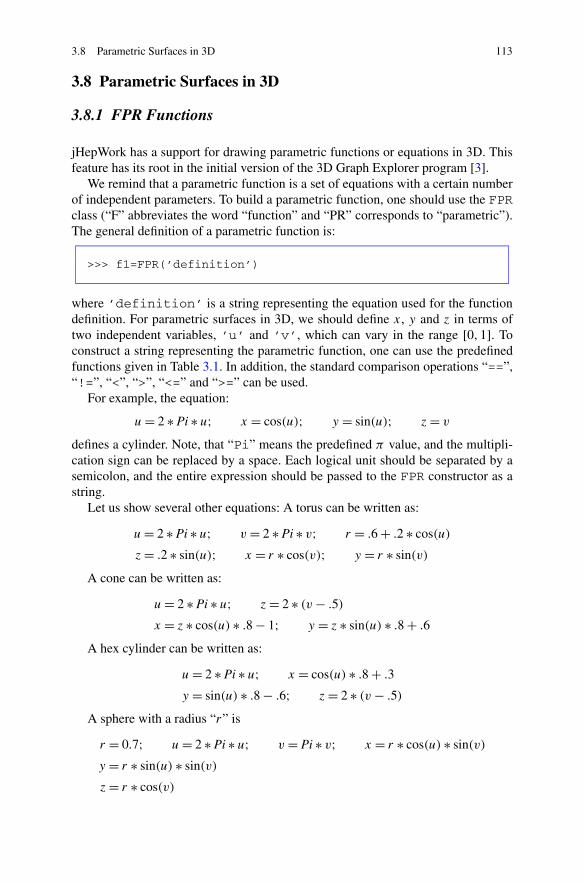
3.8 Parametric Surfaces in 3D 113
3.8 Parametric Surfaces in 3D
3.8.1 FPR Functions
jHepWork has a support for drawing parametric functions or equations in 3D. Thisfeature has its root in the initial version of the 3D Graph Explorer program [3].
We remind that a parametric function is a set of equations with a certain numberof independent parameters. To build a parametric function, one should use the FPRclass (“F” abbreviates the word “function” and “PR” corresponds to “parametric”).The general definition of a parametric function is:
>>> f1=FPR(’definition’)
where ’definition’ is a string representing the equation used for the functiondefinition. For parametric surfaces in 3D, we should define x, y and z in terms oftwo independent variables, ’u’ and ’v’, which can vary in the range [0,1]. Toconstruct a string representing the parametric function, one can use the predefinedfunctions given in Table 3.1. In addition, the standard comparison operations “==”,“!=”, “<”, “>”, “<=” and “>=” can be used.
For example, the equation:
u = 2 ∗ Pi ∗ u; x = cos(u); y = sin(u); z = v
defines a cylinder. Note, that “Pi” means the predefined π value, and the multipli-cation sign can be replaced by a space. Each logical unit should be separated by asemicolon, and the entire expression should be passed to the FPR constructor as astring.
Let us show several other equations: A torus can be written as:
u = 2 ∗ Pi ∗ u; v = 2 ∗ Pi ∗ v; r = .6 + .2 ∗ cos(u)
z = .2 ∗ sin(u); x = r ∗ cos(v); y = r ∗ sin(v)
A cone can be written as:
u = 2 ∗ Pi ∗ u; z = 2 ∗ (v − .5)
x = z ∗ cos(u) ∗ .8 − 1; y = z ∗ sin(u) ∗ .8 + .6
A hex cylinder can be written as:
u = 2 ∗ Pi ∗ u; x = cos(u) ∗ .8 + .3
y = sin(u) ∗ .8 − .6; z = 2 ∗ (v − .5)
A sphere with a radius “r” is
r = 0.7; u = 2 ∗ Pi ∗ u; v = Pi ∗ v; x = r ∗ cos(u) ∗ sin(v)
y = r ∗ sin(u) ∗ sin(v)
z = r ∗ cos(v)

114 3 Mathematical Functions
In the above examples, we set the constants defining geometrical sizes to arbitraryvalues for simplicity.
As it can be seen, to vary the parameters u and v over a different range than[0,1], one should scale and shift them by a certain value. For example, if oneneeds to change the range of u to [5,15], use this transformation: u = u ∗(15 − 5) + 5.
The parametric functions can be shown using the HPlot3DP class (extra “P” inits name means “parametric”). This class provides a canvas for drawing parametricfunctions and can be used for interactive work with these functions (zooming androtations). One can draw a surface using the usual draw(obj) method, whereobj represents an object of the class FPR. One can make drawing pads as usualand navigate to the pads using the cd(i1,i2) method. One can draw severalparametric functions on the same pad by repeating the draw(obj) method. Thisis seen from this example:
Drawing parametric functions
from java.awt import Colorfrom jhplot import *
c1 = HPlot3DP(’Canvas’,700,600,2,1)c1.setGTitle(’Parametric surfaces’)c1.visible()
f1=FPR(’r=0.7; u=2 Pi u; v=Pi v; \x=r cos(u) sin(v); y=r sin(u) sin(v); z=r cos(v)’)
f1.setDivisions(50,50)f1.setLineColor(Color.blue);
f2=FPR(’u=2 Pi u; v=2 Pi v; r=.7+.2cos(u); \z=.2 sin(u)-0.5; x=r cos(v); y=r sin(v)’)
f2.setFillColor( Color(20,170,170) )
f3=FPR(’ang=atan2(y,x); r2=x*x+y*y;\z=sin(5(ang-r2/3))*r2/3’)
c1.draw(f1)c1.draw(f2)
c1.cd(2,1)c1.setCameraPosition(-1.0)c1.setFog(0)c1.draw(f3)
In this example, the lengthy strings which define the functions were broken to fit thepage width. Figure 3.4 shows the resulting plot.
Let us discuss several graphical methods for the FPR functions. First of all, onecan set colors for the lines and for the filled area, as well as the line width as:

3.8 Parametric Surfaces in 3D 115
Fig. 3.4 Several parametric functions displayed using the HPlot3DP canvas
>>> f1.setFilled(b)>>> f1.setFillColor(c)>>> f1.setLineColor(c)>>> f1.setPenWidth(i) # set line width "i"
where b is ether 0 (not filled area) or 1 (Java true) if the object has to be filled. ’c’is the usual Java AWT Color class used to fill a surface. One can set the width ofthe lines as setPenWidth(i), where “i” is an integer value. Finally, all abovegraphical attributes can be obtained using the corresponding “getter” methods.
One can add a transparency level to the filled color by setting the so-called alphavalue for the AWT Color class. For example,
>>> f1.setFillColor( Color(0.1,0.9,0.7,0.5)
sets the transparency level for filled color to 50% (see the last argument 0.5).The numbers of divisions for “u” and “v” independent variables are given by the
method:
>>> f1.setDivisions(divU, divV)

116 3 Mathematical Functions
where divU and divV are the numbers of divisions (21 is the default value).The larger number of the divisions, the smoother surface is. However, this requiresmore computer resources, especially during an interactive work, such as rotations orzooming. One can also include the number of divisions during the construction of aparametric function:
>>> f1=FPR(’definition’,divU,divV)
We will discuss several methods associated with the class HPlot3DP inChap. 10. One can also look at the corresponding API documentation of this class.
3.8.2 3D Mathematical Objects
In addition, jHepWork contains the 3D-XplorMathJ package [4] as a third-party li-brary which allows to view various parametric functions in 3D. A user can specifyand draw any function using the menu of this program. The package contains an im-pressive catalog of pre-build interesting mathematical objects, ranging from planarand space curves to polyhedra and surfaces to differential equations and fractals.
The 3D-XplorMathJ can be started using [Tools]→ [3DXplorMath] fromthe Tool bar menu the jHepWork IDE.
3.9 Symbolic Calculations
Symbolic calculations can be performed using the SymPy library for symbolicmathematics [5]. This library is implemented in Python and included as a third-party package in the directory ’python/packages’. When working with thejHepWork IDE, this directory is automatically imported by Jython, so you do notneed to worry about how to install the SymPy library.
The SymPy library can perform differentiation, simplification, Taylor-series ex-pansions, integration. It can be used to solve algebraic and differential equations,as well as systems of equations. The complete list of features can be found on theSymPy Web page [5]. Below we will show several examples illustrating how tointegrate this package with the jHepWork graphics libraries.
But, first of all, let us give several examples illustrating how to use this packagefor analytic functions. We will start from the example illustrating how to perform aseries expansion of the expression x2/ cos(x).
Series expansion
from sympy import *
x = Symbol(’x’)func=x**2/cos(x)

3.9 Symbolic Calculations 117
s=func.series(x, 0, 10)
print sprint latex(s)pprint(s)
The statement ’Symbol()’ is rather important: in this package, symbolic vari-ables have to be declared explicitly. The output of this example is printed in thestandard (“Python”) format when using the print command:
x**2 + x**4/2 + 5*x**6/24 + ..
(we have truncated the output). In addition, the example shows how to print a nicely-formatted output using the pprint() method, close to that used in papers andbooks. In addition, one can transform the output to the LaTeX format which is verypopular within the scientific community.
We should note that, as for the jHepWork functions, all mathematical defini-tions given in Table 3.1 can be used to build SymPy functions as well. The func-tions can be in any dimensions. For example, if you have a second independentvariable, y, in your mathematical formula, specify this variable using the methody=Symbol(’y’).
Below we show a code snippet that gives you some feeling about what mathemat-ical operations can be performed with the SymPy library. The names of the methodsshown below are self-explanatory, so we will be rather brief here:
SymPy examples
from sympy import *
x=Symbol(’x’)f=x*sin(x)print ’Differential=’,diff(f, x)print ’Integral=’,integrate(f,x)print ’Definite integral=’,integrate(f,(x,-1,1))print ’Simplify=’,S(f/x, x)print ’Numerical simplify’,nsimplify(pi,tolerance=0.01)print ’Limit x->0=’,limit(f/(x*x), x, 0)print ’Solve=’,solve(x**4 - 1, x)y=Symbol(’y’)z=Symbol(’z’)print ’Combine together=’,together(1/x + 1/y + 1/z)

118 3 Mathematical Functions
The output of this script is given below:
Differential= x*cos(x) + sin(x)Integral= -x*cos(x) + sin(x)Definite integral= -2*cos(1) + 2*sin(1)Simplify= sin(x)Numerical simplify 22/7Limit x->0= 1Solve= [-1, I, 1, -I]Combine together= (x*y + x*z + y*z)/(x*y*z)
The jHepWork libraries can be used for visualization of the symbolic calculationsperformed by the SymPy program. Use the jHepWork functions, F1D and F2D, andHPlot or HPlot3D (for 2D functions) for graphical canvases. For the conversionbetween Java and SymPy Python objects, you will need to use the str() methodthat moves SymPy objects into strings.
Below we show how to differentiate a function and show the result on the HPlotcanvas, together with the original function:
Function differentiation
from java.awt import Colorfrom jhplot import *
c1 = HPlot(’Canvas’)c1.setGTitle(’Example’, Color.red)c1.setName(’Differential’)c1.visible()c1.setAutoRange()
func=’2*exp(-x*x/50)+sin(pi*x)/x’f1 = F1D(func, 1.0, 10.0)
# now symbolic calculationsfrom sympy import *x = Symbol(’x’)d=diff(S(func), x)
f2 = F1D(str(d), 1.0, 10.0)f2.setTitle(’Differential’)f2.setColor(Color.green)c1.draw([f1,f2])
The only non-trivial place of this code is when we moved the result from the dif-ferentiation into a string using the str() method. For convenience, we also usedthe simplify method, ’S()’, which converts the string representing F1D functioninto the corresponding SymPy object. The rest of this code is rather transparent. Theresult of the differentiation will be shown with the green line.
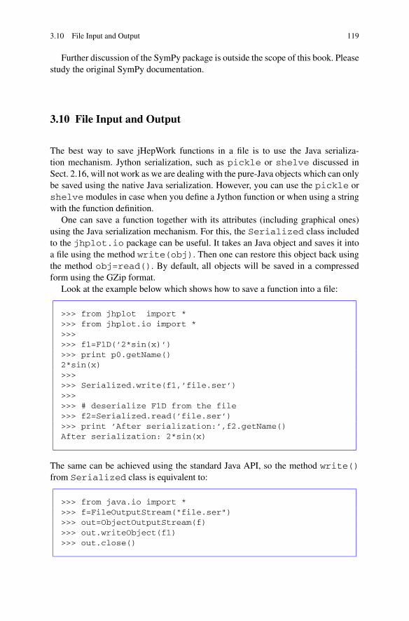
3.10 File Input and Output 119
Further discussion of the SymPy package is outside the scope of this book. Pleasestudy the original SymPy documentation.
3.10 File Input and Output
The best way to save jHepWork functions in a file is to use the Java serializa-tion mechanism. Jython serialization, such as pickle or shelve discussed inSect. 2.16, will not work as we are dealing with the pure-Java objects which can onlybe saved using the native Java serialization. However, you can use the pickle orshelve modules in case when you define a Jython function or when using a stringwith the function definition.
One can save a function together with its attributes (including graphical ones)using the Java serialization mechanism. For this, the Serialized class includedto the jhplot.io package can be useful. It takes an Java object and saves it intoa file using the method write(obj). Then one can restore this object back usingthe method obj=read(). By default, all objects will be saved in a compressedform using the GZip format.
Look at the example below which shows how to save a function into a file:
>>> from jhplot import *>>> from jhplot.io import *>>>>>> f1=F1D(’2*sin(x)’)>>> print p0.getName()2*sin(x)>>>>>> Serialized.write(f1,’file.ser’)>>>>>> # deserialize F1D from the file>>> f2=Serialized.read(’file.ser’)>>> print ’After serialization:’,f2.getName()After serialization: 2*sin(x)
The same can be achieved using the standard Java API, so the method write()from Serialized class is equivalent to:
>>> from java.io import *>>> f=FileOutputStream("file.ser")>>> out=ObjectOutputStream(f)>>> out.writeObject(f1)>>> out.close()

120 3 Mathematical Functions
while the method read() from the Serialized class is equivalent to:
>>> file = File(’file.ser’)>>> fin = ObjectInputStream(FileInputStream(file))>>> f2 =fin.readObject()>>> fin.close()
One can also write a list of functions, instead of a single function:Serialization of functions
from jhplot import *from jhplot.io import *
f1=F1D(’x*x+2’)f2=F2D("x*y+10")# make lista=[f1,f2]
# write list to a fileSerialized.write(a,’file.ser’)
# read functions from the file:list=Serialized.read(’file.ser’)
f1=list[0]f2=list[1]print ’After serialization:\n’print f1.getName()print f2.getName()
At this moment, the serialization mechanism is not implemented for FND. How-ever, generally, the jHepWork functions are relatively simple entities, therefore, onecan just serialize or write a string with the function definition into a file and then useit to instantiate a new object of this function.
In Chap. 11 we will discuss the input-output (I/O) issues in more detail. We willlearn how to save an arbitrary mix of various jHepWork and Java objects, includ-ing lists of functions, histograms and arrays. For example, one can write a largesequence of functions persistently using the HFile class to be discussed later.
References
1. Funk, N.: A Java library for mathematical expressions. URL http://sourceforge.net/projects/jep/2. The Colt Development Team: The COLT Project. URL http://acs.lbl.gov/~hoschek/colt/3. Bose, A.: 3D Graph Explorer.4. T.D.-X. Consortium: The 3D-XPLORMATHJ project. URL http://3d-xplormath.org/5. SymPy Development Team: SYMPY: Python library for symbolic mathematics. URL http://
www.sympy.org
Chapter 4One-dimensional Data
4.1 One Dimensional Arrays
Numerical computations based on repetitive tasks with values are not too efficientin Jython, since loops over objects are slow. This has already been illustrated usingJython arrays in Sect. 2.14.2. In most cases, what we really what is to manipulatewith primitive data types, such as floats or integers, rather than with immutableobjects used for representation of numbers in Jython. Therefore, our strategy forthis book will be the following:
Jython will be viewed as “interface” type of language, i.e. a language designedto link and manipulate with high-level Java classes that implement repetitiveoperations with primitive types.
In the following chapters, we will discuss objects used for data storage andmanipulation—building blocks from which a typical Java or Jython program canbe constructed. Unlike Jython classes, the objects to be discussed below will bederived from pure Java classes and imported from the Java libraries of jHepWork.
In this chapter, we will discuss one-dimensional data, i.e. a data set representedby a sequence of double-precision floating-point real values, N1, N2, . . . ,Nmax. Thisis a rather common case for almost any data analysis. Each number can represent,for example, a value obtained from a single measurement. Below we will discusshow to build objects which can be used for: (1) generation of one-dimensional datasets; (2) storing numerical values in containers; (3) writing to or reading from files;(4) performing numerical analyzes and producing statistical summaries; (5) finally,for visualization and comparisons with other data sets.
As we are progressing deeper into analysis of one-dimensional (1D) data, youmay be unsatisfied with the simplicity of JythonShell when typing a short codesnippets. We will remind that, in this case, one should write code in files with theextension ’.py’ and execute such macros using the key [F8] or the [run] buttonas described in Sect. 1.4.
S.V. Chekanov, Scientific Data Analysis using Jython Scripting and Java,Advanced Information and Knowledge Processing,DOI 10.1007/978-1-84996-287-2_5, © Springer-Verlag London Limited 2010
121

122 4 One-dimensional Data
4.2 P0D Data Container
The P0D class is among the simplest classes of jHepWork: it does not have anygraphical attributes. This class is designed to keep a sequence of real numbers. It issimilar to the Java ArrayList class, but keeps only double-precision real valuesrepresented with 64 bit accuracy. In some extent, the class P0D is also similar to theJython list which keeps a sequence of objects.
For integer values, use the class P0I which has exactly the same methods asP0D. For the P0I arrays, you may benefit from a lower memory usage and smallerfile size when writing this array into files. Below we will discuss only the P0D class.
Let us construct a P0D object to keep an one-dimensional data set. It is advisableto annotate it, so we can easily obtain its attribute later:
>>> from jhplot import *>>> p0=P0D(’measurement’)
where ’measurement’ is a string representing the dataset title.Let us remind again how we can learn about all methods associated with jHep-
Work objects, like the p0 object described above. Here is the list of various methodsto learn about this object:
• If you are using the JythonShell prompt, type ’p0.’ and press [Ctrl]-[Space];
• If you are using JythonShell or jHepWork source-code editor, use the methoddir(p) to print its methods;
• If you are using the jHepWork source-code editor, type ’p0.’ and press [F4].You will get a detailed description of all methods in a pop-up frame. One canselect a necessary method and check its description using the mouse. In addition,one can copy the selected method to the editor area as described in Sect. 1.4.10;
• If you are using Java instead of Jython and working with Eclipse or NetBeansIDE, use the code assist of these IDEs. The description of these IDEs is beyondthe scope of this book.
In all cases, you might be impressed by the significant number of methods associatedwith the P0D class. But let us go slowly and first discuss its most important methods.
One can obtain the title by calling the method getTitle():
>>> print p0.getTitle()measurement
One can reassign a new title with the method:
>>> p0=P0D()>>> p0.setTitle(’new measurement’)

4.2 P0D Data Container 123
Once the p0 object is created, one can add numbers to this container. In practice,one-dimensional data can be filled from a file or some external sources (this will bediscussed later). Here we show how can add a value to the container:
>>> p0.add(1) # add an integer>>> p0.add(-4.0) # add a float>>> p0.add(-4E12) # add a float>>> p0.set(2,200) # insert the value at the 2nd position
One can obtain the value at a specific index ’i’ using the method get(i).It should be noted that all values are converted into “double” representation inside
the P0D. The size of the container can be found using the method size(). One canremove all elements from the container using the method clear():
>>> print p0.size() # size of the data3>>> p0.clear() # clean up the container>>> print p0.size() # again print the size0
Data from the p0 instance can be obtained in a form of the Jython arrays dis-cussed in Sect. 2.14:
>>> array=p0.getArray() # array with double numbers>>> array=p0.getArrayInt() # array with integer numbers
If you want to return a list, instead of arrays, you can call the methodgetArrayList() method. One can convert the array into a list using the methodtolist().
A P0D container can be initialized from a Jython list as:
>>> p0.setArray([1,2,3,4])
It should be noted again that, for scripting with Jython, one should use thesetArray() and getArray() methods which are optimized for the speed.They are much faster than pieces of codes with the methods add() or set()called inside Jython loops.
One can fill the current P0D from a file (see below), generate a sequence ofnumbers or fill the P0D with random numbers. For example, to fill a P0D containerwith a sequence of real numbers between 0 and 100, use:
>>> from jhplot import *>>> p0=P0D(’sequence’)>>> p0.fill(101,0,100) # numbers from 0-100 (step 1)

124 4 One-dimensional Data
A P0D container can be instantiated from the Jython list:
>>> p0=P0D(’title’,[1,2,3,4]) # with title>>> p0.P0D([1,2,3,4]) # without title
P0D objects can also be filled with random numbers using a few built-in methods.For example, uniformly-distributed numbers can be filled as:
>>> p0= P0D(’Uniform distribution’)>>> p0.randomUniform(1000,0.0,1.0)
The first argument is the number of values to be filled, while the second and thirdspecify the range for random numbers. One can also generate an array with randomnumbers in accordance with a Gaussian (normal) distribution with the mean 0 andthe standard deviation equals one as:
>>> p0= P0D(’Normal distribution’)>>> p0.randomNormal(1000, 0.0, 1.0)
As before, 1000 is the total number of entries.We will consider how to fill the P0D class with many other random distributions
in Sect. 9.5. In particular, we will explain how to fill a P0D with random numbersusing various functional forms of probability distributions in Sect. 9.6.
To print a P0D on the screen, use the method toString() that converts theP0D object into a string representation:
>>> p0=P0D(’measurement’)>>> p0.add(1); p0.add(2); p0.add(3);>>> print p0.toString()1.02.03.0
In some cases, it is convenient to show data as a table in a separate frame, so onecan sort and search for a particular value. In this case, use
>>> p0.toTable()
This line brings up a table with filled values. Finally, one can use the print()method for printing using Java System.out.
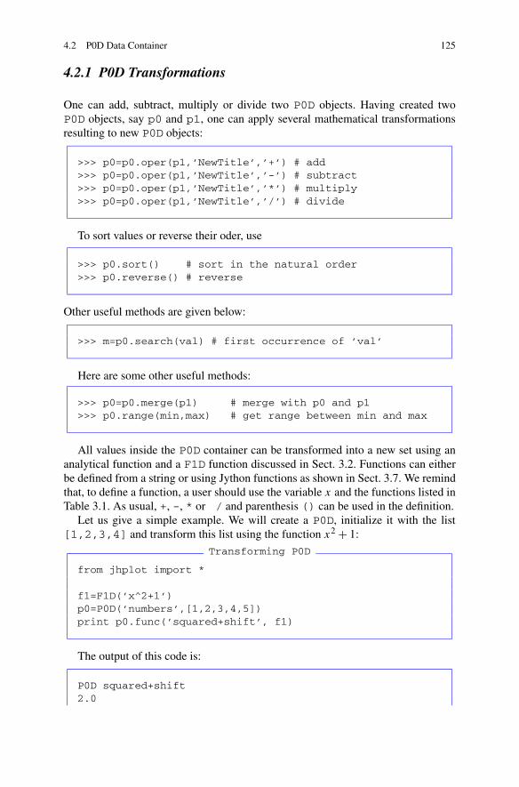
4.2 P0D Data Container 125
4.2.1 P0D Transformations
One can add, subtract, multiply or divide two P0D objects. Having created twoP0D objects, say p0 and p1, one can apply several mathematical transformationsresulting to new P0D objects:
>>> p0=p0.oper(p1,’NewTitle’,’+’) # add>>> p0=p0.oper(p1,’NewTitle’,’-’) # subtract>>> p0=p0.oper(p1,’NewTitle’,’*’) # multiply>>> p0=p0.oper(p1,’NewTitle’,’/’) # divide
To sort values or reverse their oder, use
>>> p0.sort() # sort in the natural order>>> p0.reverse() # reverse
Other useful methods are given below:
>>> m=p0.search(val) # first occurrence of ’val’
Here are some other useful methods:
>>> p0=p0.merge(p1) # merge with p0 and p1>>> p0.range(min,max) # get range between min and max
All values inside the P0D container can be transformed into a new set using ananalytical function and a F1D function discussed in Sect. 3.2. Functions can eitherbe defined from a string or using Jython functions as shown in Sect. 3.7. We remindthat, to define a function, a user should use the variable x and the functions listed inTable 3.1. As usual, +, -, * or / and parenthesis () can be used in the definition.
Let us give a simple example. We will create a P0D, initialize it with the list[1,2,3,4] and transform this list using the function x2 + 1:
Transforming P0D
from jhplot import *
f1=F1D(’x^2+1’)p0=P0D(’numbers’,[1,2,3,4,5])print p0.func(’squared+shift’, f1)
The output of this code is:
P0D squared+shift2.0

126 4 One-dimensional Data
5.010.017.026.0
Note that, in all cases, the objects remain to be the same, only the values will bemodified. If one needs a copy of a P0D object, use the method copy().
One can obtain a new P0D object with all elements smaller, larger or equal of aspecified value. Assuming that p0 is an object with filled values, this can be doneusing the following method:
>>> p1=p0.get(d,str)
The method returns a new array with values smaller, larger or equal to an inputvalue d. The type of operation is specified using a string (shown as str in theabove example), which can be equal to “<”, “>” or “=”, respectively.
4.2.2 Analyzing P0D and Summary Statistics
One can obtain several useful characteristics of the P0D class. First of all, let usconsider the most simple methods, which return double values with certain charac-teristics of a p0 object of the class P0D:
>>> m=p0.size() # size of P0D>>> m=p0.getMin() # min value>>> m=p0.getMax() # max value>>> m=p0.getMinIndex() # index of min value>>> m=p0.getMaxIndex() # index of max value>>> m=p0.mean() # mean value.>>> m=p0.correlation(p1) # correlation coefficient p1>>> m=p0.covariance(p1) # covariance>>> m=p0.getSum() # sum of all values
In the above examples, p1 is another P0D object used to find correlations betweenp0 and p1 arrays.
One can also perform a search for a specific value inside the P0D arrays. Themethod contains(val) returns true if a value val is found. One can also findan index of the first occurrence of the specified element inside a P0D array usingthe method find(d).
The second set of methods is more elaborate, but it requires execution of themethod getStat(). This method returns a string charactering the entire data set.Such a summary contains a very comprehensive statistical characteristics of one-dimensional data set:
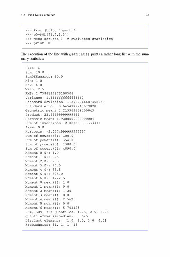
4.2 P0D Data Container 127
>>> from jhplot import *>>> p0=P0D([1,2,3,3])>>> m=p0.getStat() # evaluates statistics>>> print m
The execution of the line with getStat() prints a rather long list with the sum-mary statistics:
Size: 4Sum: 10.0SumOfSquares: 30.0Min: 1.0Max: 4.0Mean: 2.5RMS: 2.7386127875258306Variance: 1.6666666666666667Standard deviation: 1.2909944487358056Standard error: 0.6454972243679028Geometric mean: 2.213363839400643Product: 23.99999999999999Harmonic mean: 1.9200000000000004Sum of inversions: 2.083333333333333Skew: 0.0Kurtosis: -2.0774999999999997Sum of powers(3): 100.0Sum of powers(4): 354.0Sum of powers(5): 1300.0Sum of powers(6): 4890.0Moment(0,0): 1.0Moment(1,0): 2.5Moment(2,0): 7.5Moment(3,0): 25.0Moment(4,0): 88.5Moment(5,0): 325.0Moment(6,0): 1222.5Moment(0,mean()): 1.0Moment(1,mean()): 0.0Moment(2,mean()): 1.25Moment(3,mean()): 0.0Moment(4,mean()): 2.5625Moment(5,mean()): 0.0Moment(6,mean()): 5.70312525%, 50%, 75% Quantiles: 1.75, 2.5, 3.25quantileInverse(median): 0.625Distinct elements: [1.0, 2.0, 3.0, 4.0]Frequencies: [1, 1, 1, 1]

128 4 One-dimensional Data
Once the method getStat() is called, one can access the following characteris-tics:
>>> m=p0.variance() # variance>>> m=p0.stddeviation() # standard deviation>>> m=p0.standardError() # standard error>>> m=p0.kurtosis() # kurtosis>>> m=p0.skew() # skewness>>> m=p0.median() # median>>> m=p0.moment(k,c) # k-th order moment
The above methods are quite self-explanatory. The last method returns k-th ordermoment of the distribution defined as
∑i=0((x[i] − mean)k)/size().
4.2.3 Displaying P0D Data
There is only one way to show a P0D array: project it into a histogram. This topicis extensively covered in Sect. 8.1. Here we will briefly point out that a histogramis a chart of rectangles drawn on the x-axis whose areas are proportional to thefrequency of a range of variables.
One can build a histogram from a P0D using the two methods:
>>> h=p0.getH1D(bins)>>> h=p0.getH1D(bins, min, max)
The first method creates a histogram with a given number of bins (bins is an integernumber). The minimum and the maximum values of the X range are determinedautomatically. In the second case, one can explicitly specify the number of bins andthe minimum (min) and maximum (max) values.
One question you may ask is this: assume we have two P0D objects. One objectrepresents x values, the second represents y values. We already know how to checkcorrelations between these object - use the method correlation() as shown inSect. 4.2.2. But how one can display pairs (x, y) on X–Y plots? Below we showhow to do this:
Plotting P0D
from jhplot import *
c1 = HPlot(’Canvas’,600,400)c1.setGTitle(’X Y plot’)c1.visible()c1.setAutoRange()

4.2 P0D Data Container 129
p1=P0D(’numbers’,[1,2,3,4,5])p2=p1.copy()
f1=F1D(’x^2’)p2.func(’squared’, f1)pp=P1D(p1,p2)c1.draw(pp)
You may notice that we made an extra step by creating an object P1D from two P0D
arrays. We will discuss this object in Sect. 5.1.
Below is an example which shows how to generate random numbers and trans-
form them using the F1D class. The output is shown as a histogram on the HPlot
canvas:
Plotting P0D
from java.awt import Colorfrom jhplot import *
# build a canvasc1 = HPlot(’Canvas’,600,400)c1.setGTitle(’Example of P0D data array’, Color.blue)c1.visible()c1.setAutoRange()p0= P0D(’Random normal distribution’)p0.randomNormal(1000, 0.0, 1.0)
# make a copy and transform to a functionf1=’x*cos(x)+2’p01=p0.copy(f1)p01.func(F1D(f1))
f2=’exp(x)-2’ # make a new copy and transformp02=p0.copy(f2)p02.func(F1D(f2))
h1=p0.getH1D(20) # histogram with 20 binsc1.draw(h1)
h1=p01.getH1D(100) # histogram with 100 binsc1.draw(h1)
h1=p02.getH1D(200) # show againc1.draw(h1)
Run this script and try to make sense of it. If it is not easy, skip this section since we
will return to a very detailed discussion of the histograms in Sect. 8.1.

130 4 One-dimensional Data
4.3 Reading and Writing P0D Files
To fill a P0D object from a ASCII file, assuming that each number is on a new line,use the method read(). For such files, use # or * for comments at the beginningof each line.
>>> p0=P0D(’data from ASCII file’)>>> p0.read(’FileName’)
where ’FileName’ is a string with the file name (the full path should be included).Data can also be read from a compressed (“zipped”) file as:
>>> p0=P0D(’data from a ZIP file’)>>> p0.readZip(’FileName’)
or from a gzipped format:
>>> p0=P0D(’data from a GZIP file’)>>> p0.readGZip(’FileName’)
In all these cases, the methods read(), readZip() and readGZip() returnzero in case of success. Error code 1–2 means that the file not found and 3 indicatesa parse error.
To build a P0D from an ASCII file, use this constructor:
>>> p0=P0D(’measurement’, ’FileName’)
(in this case, GZIP and ZIP form is not supported).To write a p0 back to an ASCII file, use:
>>> p0.toFile(’FileName’)
Data can be written to a binary file using the so-called big endian format as:
>>> p0.writeBinary(’FileName’)
To read data from an existing binary file, use
>>> p0.readBinary(’FileName’)
In this case, the old content of the p0 object will be erased.

4.3 Reading and Writing P0D Files 131
4.3.1 Serialization
One can save and restore a P0D object containing data and other attributes using theJava object serialization. jHepWork has a short command for this:
>>> p0.writeSerialized(’FileName’)
The object p0 will be saved in a file with the name ’FileName’ using a com-pressed format. The method returns zero in case of success. One can restore theobject from the file as:
>>> p1=p0.readSerialized(’FileName’)
where p1 is a new object restored from the input file.Now let us show an example of how to write a P0D object into an external file
in a serialized form and then how to restore the object back using a handy staticmethod write(obj) of the class Serialized. To read a P0D object from thefile, use the method read() of the same class. The example below shows this:
Serialized I/O
from jhplot import *from jhplot.io import *
p0=P0D(’test’)p0.add(20)p0.add(12)print p0.toString()
# write to a fileSerialized.write(p0,’file.ser’)
# deserialize P0D from the filep0s=Serialized.read(’file.ser’)print ’After serialization:’,p0s.toString()
The method write(obj) in this example writes a compressed object obj into afile. In Sect. 11.2, we will show how to deal with the case when no compression isused. Often, a program can benefit from the use of uncompressed objects since, inthis case, the CPU time wasted for uncompressing files is avoided.
4.3.2 XML Format
In some cases, it is convenient to write an object to a human-readable XML file, soone can open it using any editor and look at its structure as well as written data. For

132 4 One-dimensional Data
the XML format, one should use the following methods from the class Serial-ized of the package jhplot.io:
writeXML(obj,’FileName’) writes a Java object (obj) into a file with thename FileName;
readXML(’FileName’) reads a file with the name FileName and re-turns a stored object.
Try to replace the corresponding lines in the above examples and check how theoutput was written.
It should be noted that the XML-style is not recommended if there is a lot of datato be stored, since XML tags increase the file size dramatically. In addition, thisapproach may not work for all jHepWork classes.
For your convenience, the package ’jhplot.io’ provides two other importantmethods. An object can easily be converted into a XML string using the methodstoXML(obj) and fromXML(str) of the Serialized class. Below we illus-trate how to print an object in a XML form and then read it back:
>>> from jhplot import *>>> from jhplot.io.Serialized import *>>>>>> p0=P0D(’data’)>>> str=toXML(p0)>>> print str>>> p0=fromXML(str)
To make the code shorter, we imported all methods from the class Serialized.It should be noted that the serialization can be done using the native Java API.
Below we rewrite the example discussed above using the standard Java serializationclass:
Java serialized I/O
from jhplot import *from java.io import *
p0=P0D("test")p0.add(20)p0.add(12)print p0.toString()
# serialize P0D into a filef=FileOutputStream("filename.ser")out =ObjectOutputStream(f)out.writeObject(p0)out.close()
# Deserialize P0D from the filefile = File(’filename.ser’)

4.3 Reading and Writing P0D Files 133
fin = ObjectInputStream(FileInputStream(file))p0s =fin.readObject();fin.close();print ’After serialization:\n’,p0s.toString()
4.3.3 Dealing with Object Collections
The next question is how to write many P0D objects to a single file. This can easilybe done using Jython lists. The example below writes two P0D objects into a singlefile:
Writing multiple P0D objects
from jhplot import *from jhplot.io import *
p1=P0D(’p1’)p1.add(10)p1.add(12)
p2=P0D(’p2’)p2.add(1000)p2.add(2000)
# make lista=[p1,p2]
# write to a fileSerialized.write(a,’file.ser’)print ’Ready!’
We can restore all objects from the file as:
Reading multiple P0D objects
from jhplot import *from jhplot.io import *
# deserialize list from the filef=Serialized.read(’file.ser’)
p1=f[0]p2=f[1]print "After serialization:\n"print p1.toString()print p2.toString()

134 4 One-dimensional Data
Similarly, one can write objects and read them back using the methodswriteXML(obj) and readXML() discussed before. Finally, one can use Jythondictionaries for convenient access to the data using the keys.
The serialization can be used for almost any jHepWork class. In Sect. 5.4 we willshow how to use Jython dictionaries to store various objects in a serialized file andfetch them later using the keys.
To write huge sequences of P0D arrays, the best approach would be to use theclass HFile which will be discussed in Chap. 11 dedicated to input and output ofJava objects.

Chapter 5Two-dimensional Data
In the previous chapter we have considered the simplest possible data holder thatkeeps information about an one-dimensional array of numbers. More frequently,two-dimensional (or bivariate) data are necessary to consider, when each data pointon the (X,Y ) plane is represented by two variables, x and y. Such bivariate arraysare ideal to show a relationship between two sets of measurements.
5.1 Two Dimensional Data Structures
The P1D class is among the central classes designed for data manipulations in twodimensions (2D). The name of the P1D class is similar to that of the class F1D usedto construct functions.
The declaration of a P1D object is rather similar to that considered for the P0Dclass. However, this time, the container should be filled with at least two numbersusing the method add(x,y):
>>> from jhplot import *>>> p1=P1D(’x-y points’)>>> p1.add(10,20)>>> p1.add(20.,40.)
In this short example we declare the object P1D with the title ’x-y points’ andthen fill it with two points using the method add(x,y). Each point is representedby two numbers (either integer or float).
As it has been stated before, the method add(x,y) is not the most optimal,especially when it is used inside Jython loops. To avoid performance penalty, usehigh-level methods of this class for passing containers with numbers, rather thannumbers themselves. In the example shown below, we fill a P1D from two P0Darrays which, in turn, can also be filled using high-level methods as discussed in theprevious chapter:
S.V. Chekanov, Scientific Data Analysis using Jython Scripting and Java,Advanced Information and Knowledge Processing,DOI 10.1007/978-1-84996-287-2_6, © Springer-Verlag London Limited 2010
135

136 5 Two-dimensional Data
>>> from jhplot import *>>> p1=P1D(’x-y points’)>>> p01=P0D(’px’); p02=P0D(’py’)>>> ax=p01.randomNormal(100,1.0,0.5)>>> ay=p02.randomNormal(100,10.0,1.0)>>> p1.fill(ax,ay)
In the above example, we fill two P0D arrays with random numbers in accordancewith the normal distributions and use these arrays to fill a P1D object. The codeabove can be shortened, since the P0D arrays can also be passed to the P1D con-structor as:
>>> p1=P1D(’x-y points’,p01,p02)
Of course, make sure that the sizes of the input arrays are the same.Having filled the array P1D, one can replace data points using the method
set(i,x,y), where ’i’ denotes a position (index) of the (x, y) point insidethe array. The array can be cleaned up with the method clear(), while the arraysize can be found using the method size().
Finally, one can extract data points using the methods getX(i) and getY(i)(0 ≤ i < size()). Or, one can get arrays for x and y values without looping over allelements inside the container as:
>>> from jhplot import *>>> p1= P1D(’x-y points’)>>> p1.add(10,20)>>> p1.add(20,50)>>> ax=p1.getArrayX() # get all X values as array>>> ay=p1.getArrayY() # get all Y values as array
One can also initialize a P1D from an external file as:
>>> p1= P1D(’data from file’,’data.d’)
The format of the input file is rather simple: each pair of numbers should be on anew line. To include comments, use ’#’ at the beginning of each line. Later we willdiscuss the I/O topics in more detail.
5.2 Two Dimensional Data with Errors
A P1D object is not as simple as it first may look like—it can also hold informationon errors on x and y values.

5.2 Two Dimensional Data with Errors 137
Fig. 5.1 An illustration of aP1D array characterized byten numbers: two numbersrepresent positions of a datapoint on the (x, y) plane,while other eight represent1st and 2nd leveluncertainties (see the text).The figure displays severalmethods to access theinformation on a single datapoint defined by an index i
There are two different types of errors: one type comes from the fact that thereis always inherent statistical uncertainty in counting random events. Usually, suchuncertainties are called statistical or random errors. Also, we will call such errors“1st-level errors” when discussing various technical aspects.
The second type of uncertainties are called “systematical errors”, which mainlyoriginate from instrumental mistakes. For the P1D, we will call such uncertainties“2nd-level errors”.
Thus, a single point at a position (x, y) is characterized by ten double-precisionnumbers: two numbers give the central position in (x, y) and other eight numbersspecify its errors. A single point with 1st and 2nd errors is illustrated in Fig. 5.1,together with the “getter” methods used to access all characteristics of a P1D object.
Why do we need this complication when dealing with 2D data? Is it not enoughto represent a relationship between two sets of data with two arrays? For example,a P1D can contain information on a set of points representing positions of particlesin two dimensions: Each particle will be characterized by the position on the (x, y)
surface, while the total number of particles will be given by the size of the P1Darray. Well, in this case, you do not need indeed extra information to be stored inthis data holder. Probably, you would not need even such a data holder, since one canuse the usual Jython or Java arrays or the PND class to be discussed in the followingchapters. However, there are many situations when each data point represents manymeasurements. In this case, one should store possible uncertainties associated withthe measurements, which can have either statistical or systematical nature (or both).And this is why P1D becomes really handy, since this class is optimized exactly forsuch tasks.
Let us give a simple example. Assume we measure the average number of carsparked per week day on some parking spot. If the measurements are done duringone month, there should be seven measurements for each day of the week. We cal-culate the average for each week day, and represent the entire measurement withseven numbers. Each number has a statistical uncertainty, which is assumed to besymmetric. The measurements can be represented by a single P1D container which,for example, can be filled for two week days as:
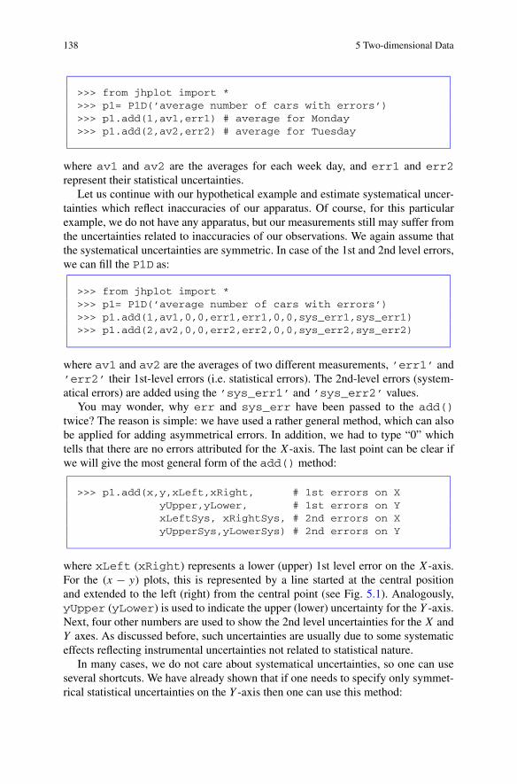
138 5 Two-dimensional Data
>>> from jhplot import *>>> p1= P1D(’average number of cars with errors’)>>> p1.add(1,av1,err1) # average for Monday>>> p1.add(2,av2,err2) # average for Tuesday
where av1 and av2 are the averages for each week day, and err1 and err2represent their statistical uncertainties.
Let us continue with our hypothetical example and estimate systematical uncer-tainties which reflect inaccuracies of our apparatus. Of course, for this particularexample, we do not have any apparatus, but our measurements still may suffer fromthe uncertainties related to inaccuracies of our observations. We again assume thatthe systematical uncertainties are symmetric. In case of the 1st and 2nd level errors,we can fill the P1D as:
>>> from jhplot import *>>> p1= P1D(’average number of cars with errors’)>>> p1.add(1,av1,0,0,err1,err1,0,0,sys_err1,sys_err1)>>> p1.add(2,av2,0,0,err2,err2,0,0,sys_err2,sys_err2)
where av1 and av2 are the averages of two different measurements, ’err1’ and’err2’ their 1st-level errors (i.e. statistical errors). The 2nd-level errors (system-atical errors) are added using the ’sys_err1’ and ’sys_err2’ values.
You may wonder, why err and sys_err have been passed to the add()twice? The reason is simple: we have used a rather general method, which can alsobe applied for adding asymmetrical errors. In addition, we had to type “0” whichtells that there are no errors attributed for the X-axis. The last point can be clear ifwe will give the most general form of the add() method:
>>> p1.add(x,y,xLeft,xRight, # 1st errors on XyUpper,yLower, # 1st errors on YxLeftSys, xRightSys, # 2nd errors on XyUpperSys,yLowerSys) # 2nd errors on Y
where xLeft (xRight) represents a lower (upper) 1st level error on the X-axis.For the (x − y) plots, this is represented by a line started at the central positionand extended to the left (right) from the central point (see Fig. 5.1). Analogously,yUpper (yLower) is used to indicate the upper (lower) uncertainty for the Y -axis.Next, four other numbers are used to show the 2nd level uncertainties for the X andY axes. As discussed before, such uncertainties are usually due to some systematiceffects reflecting instrumental uncertainties not related to statistical nature.
In many cases, we do not care about systematical uncertainties, so one can useseveral shortcuts. We have already shown that if one needs to specify only symmet-rical statistical uncertainties on the Y -axis then one can use this method:

5.2 Two Dimensional Data with Errors 139
p1.add(x,y,err) # fills X,Y and symmetric error on Y
where err is a statistical error on the y value, assuming that it is equal toyUpper=yLower. All other errors are set to zero. If the error on Y is asymmetric,use this method:
p1.add(x,y,err_up, err_down)
where err_up and err_down are symmetric upper and lower error on y. If thereare only 1st-level errors, then one can fill a P1D as:
p1.add(x,y,xLeft,xRight,yUpper,yLower)
while the 2nd level errors are set to zero.Table 5.1 lists the main “setter” methods associated with the P1D class.Occasionally, it is convenient to reset all errors to zero. For this, use the method:
>>> p1.setErrToZero(a) # set 1st level errors to 0>>> p1.setErrAllToZero(a) # set 1st and 2nd error to 0>>> p1.setErrSysToZero(a) # set 2nd level error to 0
where a=0 for x values and a=1 for y values.In addition, you may need to generate new errors from the numbers of counted
events, when statistical uncertainty for each y value is the squared root of countednumbers [1]. If y represents the counted number of events, its statistical error is
√y
(upper and lower). One can build a new P1D by assigning the 1st level errors for x
and y separately:
>>> p1.setErrSqrt(a) # set 1st level errors
Errors are set on x (y) when a=0 (a=1).Table 5.2 gives “getter” methods used to access characteristics of this object.To get index with either minimum or maximum value, use:
>>> p1=p1.getMinIndex(a) # index with min>>> p1=p1.getMaxIndex(a) # index with max
where a=0 for x values and a=1 for y values.Finally, one can use the method integral(i1,i2) that returns the integral
between two indexes, i1 and i2 of a P1D data. For this operation, the integration isa sum over all y values, so it is rather similar to the integration of one-dimensionalfunctions.

140 5 Two-dimensional Data
Table 5.1 Some methods used to fill a P1D container. In the methods shown in this table, “b”indicates a boolean value (1 for true and 0 for false), while “i” is an integer parameter
Methods Definitions
add(x,y) add (X,Y ) (all errors are 0)
add(x,y,err) add (X,Y ) and 1st level error on Y
add(x,y,up,down) add (X,Y ) and asymmetric 1st level errors on Y
add(x,y,left,right,up,down) add (X,Y ) and asymmetric 1st level errors on X
and Y
add(x,y,left,right,upper,lower,leftSys,rightSys,upperSys,lowerSys)
add (X,Y ) and asymmetric 1st and 2nd levelerrors on X and Y insert (X,Y ) at position i (allerrors are 0)
set(i,x,y,err) insert (X,Y ) and 1st level error on Y
set(i,x,y,up,down) add (X,Y ) and asymmetric 1st level errors on Y
set(i,x,y,left,right,up,down) insert (X,Y ) and asymmetric 1st level errors onX and Y
set(i,x,y,left,right,upper,lower,leftSys,rightSys,upperSys,lowerSys)
insert (X,Y ) and asymmetric 1st and 2nd levelerrors on X and Y
replace(i,x,y) replace (X,Y ) at position i (all errors are 0)
replace(i,x,y,err) replace (X,Y ) and 1st level error on Y
replace(i,x,y,up,down) replace(X,Y ) and asymmetric 1st level errorson Y
replace(i,x,y,left,right,up,down) replace (X,Y ) and asymmetric 1st level errors onX and Y
replace(i,x,y,left,right,upper,lower,leftSys,rightSys,upperSys,lowerSys)
replace (X,Y ) and asymmetric 1st and 2nd levelerrors on X and Y
fill(arrayX,arrayY) fills from 2 arrays
fill(arrayX,arrayY,arrayE) fills from 3 arrays with errors
fill(arrayX,arrayY,arrayUP,arrayDOWN) fills from 4 arrays with errors
fill(arrayX,arrayY ..+ 8 arrays with errors) fills from 10 arrays with full sets of errors
fill(P0D,P0D) fills from 2 P0D arrays
fill(P0D,P0D,P0D) fills from 3 P0D arrays with errors
setTitle(‘text’) set a title
5.2.1 Viewing P1D Data
In addition to the Java serialization mechanism used to store the P1D containers,which will be discussed in detail later, one can store entries from a P1D in a human-readable format. For example, one can write data in ASCII files using the method:
>>> p1.toFile(’newfile.d’)

5.2 Two Dimensional Data with Errors 141
Table 5.2 Some methods for accessing information about a P1D object. In the methods shown inthis table, “b” indicates a boolean value (“1” is false, “0” is true), while “a” is an integer parameterindicating the axis (a=0means X-axis, a=1means Y -axis). The notation “d” denotes a float value,while ‘text’ represents a string
Methods Definitions
copy() copy to new P1D
size() size of the data
getMin(a) min value for axis
getMax(a) max value for axis
getMaxIndex(a) get index of max value for axis
getMinIndex(a) get index of min value for axis
mean() mean value
integral(i1,i2) sum up all Y -values between i1 and i2
updateSummary() update summaries after adding a value
getArrayX() get array with all X values
getArrayY() get array with all Y values
getArrayXleft() get array with all left X-errors
getArrayXright() get array with all right X-errors
getArrayXleft() get array with all left X-errors
getArrayXrightSys() get array with all right X-2nd level errors
getArrayXleftSys() get array with all left X-2nd level errors
getArrayYlower() get array with all lower Y -errors
getArrayYupper() get array with all upper Y -errors
getArrayYlowerSys() get array with all lower 2nd-level Y -errors
getArrayYupperSys() get array with all upper 2nd-level Y -errors
getTitle() get title
getX(i) X value at index i
getY(i) Y value at index i
getXleft(i) left error on X at index i
getXright(i) right error on X at index i
getXleftSys(i) left 2nd error on X at index i
getXrightSys(i) right 2nd error on X at index i
getYupper(i) upper error on Y at index i
getYlower(i) lower error on y at index i
getYupperSys(i) upper 2nd error on Y at index i
getYlowerSys(i) lower 2nd error on Y at index i

142 5 Two-dimensional Data
where ’newfile.d’ is the name of the output file. One can also export data intoa LaTeX table as
>>> from java.text import DecimalFormat>>> format=DecimalFormat("##.####E00")>>> p1.toFileAsLatex("Output.tex",xformat,xformat)
One should specify an appropriate format for the numbers to be stored the LaTeXtable. We remind that the class DecimalFormat is used to format decimal num-bers in the Java platform. The pound sign (’#’) denotes a digit, and the dot is aplaceholder for the decimal separator. Please refer to the Java API documentationsof this class.
Also, one can print a P1D container on the console as
>>> p1.print()
To print the stored values on the JythoShell prompt, convert the p1 object into astring and print it using the standard print method:
>>> print p1.toString()
In some cases, it is convenient to show data as a table in a separate frame, so onecan sort and search for a particular value. In this case, use the statement:
>>> p1.toTable()
which brings up a frame showing the data inside a table. The method calls theclass HTable to be discussed in Sect. 12.4. Analogously, data can be exportedto a spreadsheet as discussed in Sect. 12.4.
5.2.2 Plotting P1D Data
In oder to display a P1D representing a set of bivariate data, the usual HPlot can-vas discussed in Sect. 3.3 can be used. To plot data, follow the same steps as fordrawing F1D functions: first, create a canvas and then use the draw(obj) methodto display a P1D object on a scatter plot:
>>> from jhplot import *>>> c1=HPlot(’Canvas’)>>> c1.visible()>>> c1.setAutoRange()>>> p1=P1D(’x-y points’, ’data.d’)>>> c1.draw(p1)

5.2 Two Dimensional Data with Errors 143
Table 5.3 The most important methods for graphical representation of a P1D. “b” indicates aboolean value (1 for true and 0 for false), while “i” is an integer parameter. The notation “d”indicates a float value. The attributes “c” and “f” correspond to the Color and Font classes ofJava AWT, while ‘text’ represents a Jython string
Methods Definitions
setStyle(‘text’) set as symbols (“p”) or line (“l”)
setSymbolSize(i) symbol size
setSymbol(i) symbol type i=0-12:
0: not filled circle
1: not filled square
2: not filed diamond
3: not filled triangle
4: filled circle
5: filled square
6: filed diamond
7: filled triangle
8: plus (+)
9: cross as (x)
10: star (*)
11: small dot (.)
12: bold plus (+)
setColor(c) set the line color
setPenWidh(i) width of the line
setPenDash(i) dashed style with “i” being the length
setLegend(b) set (b=1) or not (b=0) the legend
setTitle(‘text’) set a title
In this example, we first create a P1D object from an ASCII input file, and then wedisplay data as a collection of points on the (x, y) plane.
Table 5.3 shows the most important graphical attributes associated with the P1Dclass.
It should be noted that one can edit the plot using a pop-up menu Edit whichallows to change some attributes. Click on the right mouse button to access a GUI-driven dialog with the menu.
There are many methods which come together with the P1D data holder to dis-play error bars, assuming that error values have been filled before. To display errors,use the methods:
>>> p1.setErr(1) # show 1st level errors>>> p1.setErrSys(1) # show 2nd level errors
which should be set before drawing the p1 object on the canvas.

144 5 Two-dimensional Data
Table 5.4 The most important methods for a graphical representation of the P1D errors. “b” in-dicates a boolean value (1 for true and 0 for false), while “i” is an integer parameter. The notation“d” indicates a float value. The attributes “c” and “f” correspond to the Color and Font classesof Java AWT, while ‘text’ represents a Jython string
Methods Definitions
setErrAll(b) set all errors (1st and 2nd level)
setErrX(b) set error on X or not
setErrY(b) ser error on Y or not
setErrColorX(c) color used for X error bars
setErrColorY(c) color used for Y error bars
setPenWidthErr(i) line width for 1st level errors
setPenWidthErrSys(i) line width for 2nd level errors
setErrSysX(b) set or not 2nd level error on X
setErrSysY(b) set or not 2nd level error on Y
setErrFill(b) fill or nor the area covering errors
setErrFillColor(c) fill color
setErrFillColor(c,d) fill color + transparency level “d”
setErrSysFill(b) fill or not 2nd level errors
setErrSysFillColor(c) fill color
setErrSysColor(c,d) as before + transparency level “d”
Table 5.4 shows various methods for controlling the attributes of the errors bars.As you can see, there are two separate methods to modify the horizontal and verticalerror bars. The “getter” methods are similar, but start with the “get” string insteadof “set”.
5.2.3 Contour Plots
The HPlot canvas can be used to display P1D data in a form of a contour plot.For such type of plots, we draw colored regions which show the density population,instead of showing separate particles. It is required to bin a (x, y) plane in x and y:the smaller the bin size is, the more chances to resolve a fine structure for the plotteddensity distribution.
To set up the canvas HPlot for showing contour plots, use the methodsetContour(1). Table 5.5 shows some methods to setup a contour plot.
It should be noted that there is a special canvas, called HPlot2D, which is de-signed to show the contour plots and has more options for manipulations. Pleaseread Sect. 10.11 for more details.
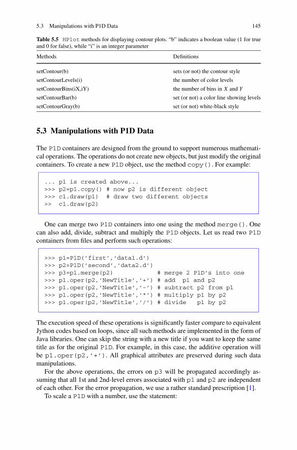
5.3 Manipulations with P1D Data 145
Table 5.5 HPlot methods for displaying contour plots. “b” indicates a boolean value (1 for trueand 0 for false), while “i” is an integer parameter
Methods Definitions
setContour(b) sets (or not) the contour style
setContourLevels(i) the number of color levels
setContourBins(iX,iY) the number of bins in X and Y
setContourBar(b) set (or not) a color line showing levels
setContourGray(b) set (or not) white-black style
5.3 Manipulations with P1D Data
The P1D containers are designed from the ground to support numerous mathemati-cal operations. The operations do not create new objects, but just modify the originalcontainers. To create a new P1D object, use the method copy(). For example:
... p1 is created above...>>> p2=p1.copy() # now p2 is different object>>> c1.draw(p1) # draw two different objects>> c1.draw(p2)
One can merge two P1D containers into one using the method merge(). Onecan also add, divide, subtract and multiply the P1D objects. Let us read two P1Dcontainers from files and perform such operations:
>>> p1=P1D(’first’,’data1.d’)>>> p2=P1D(’second’,’data2.d’)>>> p3=p1.merge(p2) # merge 2 P1D’s into one>>> p1.oper(p2,’NewTitle’,’+’) # add p1 and p2>>> p1.oper(p2,’NewTitle’,’-’) # subtract p2 from p1>>> p1.oper(p2,’NewTitle’,’*’) # multiply p1 by p2>>> p1.oper(p2,’NewTitle’,’/’) # divide p1 by p2
The execution speed of these operations is significantly faster compare to equivalentJython codes based on loops, since all such methods are implemented in the form ofJava libraries. One can skip the string with a new title if you want to keep the sametitle as for the original P1D. For example, in this case, the additive operation willbe p1.oper(p2,’+’). All graphical attributes are preserved during such datamanipulations.
For the above operations, the errors on p3 will be propagated accordingly as-suming that all 1st and 2nd-level errors associated with p1 and p2 are independentof each other. For the error propagation, we use a rather standard prescription [1].
To scale a P1D with a number, use the statement:

146 5 Two-dimensional Data
>>> p1.operScale(a, scaleFactor)
where scaleFactor is a double or an integer number. If a=0 (Java boolean‘false’), the scaling is applied for x, if a=1, the scaling is applied for y. The ti-tle is optional for this operation. It is important to know that the factor ’scale-Factor’ scales the 1st and 2nd levels uncertainties as well. If you need to scaleonly errors, use:
>>> p1.operScaleErr(a, scaleFactor)
which scales only the 1st-level errors for either X (a=0) or Y (a=1) axis. If oneneeds to scale also the 2nd-level errors, use:
>>> p1.operScaleErrSys(a, scaleFactor)
which works exactly as the method operScaleErr(), but this time it is appliedfor the 2nd-level errors.
Finally, to extract a range of P1D points from the original data container, use
>>> p1=p1.range(min,max)
where min and max are integer numbers denoting the range.
5.3.1 Advanced P1D Operations
5.3.1.1 Operations with Correlations
The operations considered above assume that there are no correlations between twodata holders. In reality, data from different measurements can correlate, so do P1Dcontainers corresponding to such measurements. In this case, one can also specifya correlation coefficient and use it for mathematical operations. A correlation coef-ficient should be represented with an additional P1D container used for the actualmathematical manipulations. The correlation coefficients should be added using theadd() method and included at the positions of errors (statistical or systematical).Look at the example below where we assume that there is a 50% correlation betweentwo data sets:
Adding data with correlations
from jhplot import *

5.3 Manipulations with P1D Data 147
# fill data set 1 points with 2 pointsp1= P1D(’data1’)# use only 1st-level errors on Yp1.add(10,100,5,5)p1.add(20,50,5,5)
# fill data set 2 with 2 pointsp2= P1D(’data2’)# use only statistical errors on Yp2.add(10,40,5,5)p2.add(20,40,5,5)
# add with 50% correlationscorr=P1D(’correlation coefficients’)corr.add(0,0,0.5,0.5)corr.add(0,0,0.5,0.5)# add them. Do not do anything with Xp50=p1.copy()p0=p1.copy()p50.oper(p2,’added with 50% corr.’,’+’,’Y’,corr)print p50.toString()p0.oper(p2,’added with 0% corr.’,’+’)print p0.toString()
The output of this script shows that the (x, y) values remain to be the same, but thestatistical errors are different for the case with 50% correlations and without anycorrelations.
Analogously, one can include correlations for the 2nd-level errors (see the APIdescription for this method). The same feature is supported for any operation, suchas subtraction, multiplication and division.
5.3.1.2 Functional Transformation
One can also transform a P1D data using a mathematical function. The error prop-agation is done for x or y components (or for both). The following functions aresupported: “inverse” (1/y), square (y ∗ y) “sqrt” (square root), “exp” (exponential),“log” (log10(y)) and all trigonometrical functions. The example given below illus-trates a generic usage of this functional transformation:
>>> p1=p1.move(’function’, ’a’ )
where ’function’ is a string defining a function used for the transformation, and’a’ is a string indicating the axis, which can either be “X” (apply the transforma-tion for x values), “Y ” (apply the transformation for y values) or “XY ” (transformboth x and y). For example:

148 5 Two-dimensional Data
>>> p1=p1.move(’log’, ’Y’ )
transforms all y values to log10(y). Errors for the p1 container will be transformedappropriately.
5.3.1.3 Smoothing
For some situations, you may be interested in smoothing P1D values. This can bedone by averaging over a moving window of a size specified by the method param-eter: if the value of the parameter is “k” then the width of the window is 2 ∗ k + 1. Ifthe window runs off the end of the P1D only those values which intersect are takeninto account. The smoothing may optionally be weighted to favor the central valueusing a “triangular” weighting. For example, for a value of “k” equal to 2 the centralbin would have weight 1/3, the adjacent bins 2/9, and the next adjacent bins 1/9.Errors are kept to be the same.
All of this can be achieved using the command:
>>> p2=p1.operSmooth(a,b,k)
where “a” defines the axis to which the smoothing is applied, i.e. it can be eithera=0 (for the “X” axis) or a=1 (for the “Y ” values). When b=1 (boolean “true”) thenx or y values are weighted using a triangular weighting scheme favoring bins nearthe central bin, and “k” is the smoothing parameter which must be non-negative. Ifzero, the original P1D object will be returned with no smoothing applied.
One can also convert a P1D into a Gaussian smoothed container in which eachband of the original P1D is smoothed by discrete convolution with a kernel approxi-mating a Gaussian impulse response with the specified standard deviation. This canbe done using the command:
>>> p2=p1.operSmoothGauss(a,sDev)
where “sDev” is the standard deviation of the Gaussian smoothing kernel (must benon-negative).
5.3.2 Weighted Average and Systematical Uncertainties
When there are several different measurements with different values xi and knownerrors σi (or variance, σ 2
i ), then it is reasonable to combine the measurements usingthe so-called weighted average method. In this case, the value x for best estimateand its variance are given by
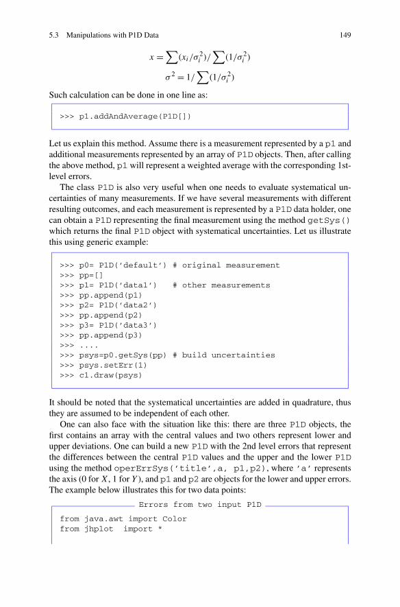
5.3 Manipulations with P1D Data 149
x =∑
(xi/σ2i )/
∑(1/σ 2
i )
σ 2 = 1/∑
(1/σ 2i )
Such calculation can be done in one line as:
>>> p1.addAndAverage(P1D[])
Let us explain this method. Assume there is a measurement represented by a p1 andadditional measurements represented by an array of P1D objects. Then, after callingthe above method, p1 will represent a weighted average with the corresponding 1st-level errors.
The class P1D is also very useful when one needs to evaluate systematical un-certainties of many measurements. If we have several measurements with differentresulting outcomes, and each measurement is represented by a P1D data holder, onecan obtain a P1D representing the final measurement using the method getSys()which returns the final P1D object with systematical uncertainties. Let us illustratethis using generic example:
>>> p0= P1D(’default’) # original measurement>>> pp=[]>>> p1= P1D(’data1’) # other measurements>>> pp.append(p1)>>> p2= P1D(’data2’)>>> pp.append(p2)>>> p3= P1D(’data3’)>>> pp.append(p3)>>> ....>>> psys=p0.getSys(pp) # build uncertainties>>> psys.setErr(1)>>> c1.draw(psys)
It should be noted that the systematical uncertainties are added in quadrature, thusthey are assumed to be independent of each other.
One can also face with the situation like this: there are three P1D objects, thefirst contains an array with the central values and two others represent lower andupper deviations. One can build a new P1D with the 2nd level errors that representthe differences between the central P1D values and the upper and the lower P1Dusing the method operErrSys(’title’,a, p1,p2), where ’a’ representsthe axis (0 for X, 1 for Y ), and p1 and p2 are objects for the lower and upper errors.The example below illustrates this for two data points:
Errors from two input P1D
from java.awt import Colorfrom jhplot import *
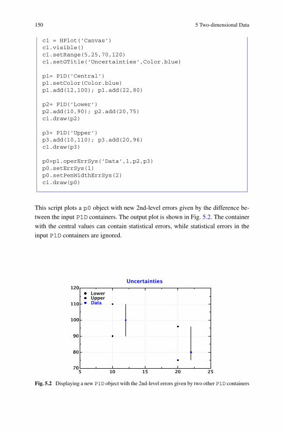
150 5 Two-dimensional Data
c1 = HPlot(’Canvas’)c1.visible()c1.setRange(5,25,70,120)c1.setGTitle(’Uncertainties’,Color.blue)
p1= P1D(’Central’)p1.setColor(Color.blue)p1.add(12,100); p1.add(22,80)
p2= P1D(’Lower’)p2.add(10,90); p2.add(20,75)c1.draw(p2)
p3= P1D(’Upper’)p3.add(10,110); p3.add(20,96)c1.draw(p3)
p0=p1.operErrSys(’Data’,1,p2,p3)p0.setErrSys(1)p0.setPenWidthErrSys(2)c1.draw(p0)
This script plots a p0 object with new 2nd-level errors given by the difference be-
tween the input P1D containers. The output plot is shown in Fig. 5.2. The container
with the central values can contain statistical errors, while statistical errors in the
input P1D containers are ignored.
Fig. 5.2 Displaying a new P1D object with the 2nd-level errors given by two other P1D containers

5.4 Reading and Writing P1D Data 151
5.4 Reading and Writing P1D Data
5.4.1 Dealing with a Single P1D Container
The P1D containers can be saved into a file and restored later. As for the P0D class,one can fill a P1D container from a text ASCII file using the method read(). Weremind that each (x, y) pair should be on a separate line, and x and y should beseparated by a space. One can use the characters # or * at the beginning of each linefor comments:
>>> p0=P1D(’data from ASCII file’)>>> p0.read(’FileName’)
In this example, ’FileName’ is a string with the file name (the full path shouldbe included). One can use a shorter version of the code above by passing a file namedirectly to the constructor:
>>> p0=P1D(’data from ASCII file’, ’FileName’)
as was illustrated before. Data can also be read from a compressed (Zip) file:
>>> p0=P1D(’data from a ZIP file’)>>> p0.readZip(’FileName’)
or from a file in the Gzip format:
>>> p0=P1D(’data from a GZIP file’)>>> p0.readGZip(’FileName’)
In all cases, the methods read(), readZip() and readGZip() return zero incase of success. The error code 1 or 2 tells that the file not found. If a parse erroroccurs, the reaGZip() method returns 3.
To write a P1D data into an ASCII file, use the following method:
>>> p0.toFile(’FileName’)
There is another handy method: one can store data in the LaTeX format as:
>>> from java.text import DecimalFormat>>> format=DecimalFormat(’##.####E00’)>>> p0.toFileAsLatex(’FileName’, format, format)

152 5 Two-dimensional Data
where ’format’ is an instance of the DecimalFormat class from the Javapackage java.text. We passed the object ’format’ twice, one for x valuesand one for y values.
It should be pointed out that, for the above examples, we could only write (read)data. All graphical attributes are completely lost after saving the data in ASCII files.But there is another more elegant way to save a P1D object: As for any jHepWorkobject, one can save and restore P1D data and other attributes (including those usedfor graphical representation) using the Java serialization mechanism.
To serialize the entire P1D object into a file, use the method below:
>>> p0.writeSerialized(’FileName’)
which writes the object p0 including their graphical attributes into a file with thename ’FileName’. The method returns zero in case of no I/O problem occurs.One can restore the object from this file as:
>>> p1=p0.readSerialized(’FileName’)
where p1 is a new object from the file.The example below shows how to write a P1D into an external file in a serialized
form and then restore the object back:
P1D serialization
from jhplot import *from jhplot.io import *
p1=P1D(’x-y data’)p1.add(10,20)p1.add(12,40)print p1.toString()
# write to a fileSerialized.write(p1,’file.ser’)
# deserialize P1D from the filep1s=Serialized.read(’file.ser’)
print ’After serialization:’,p1s.toString()
The serialization to the XML format can be achieved using the writeXML()and readXML() methods of the same Serialization class. This class alsoallows to convert the container into XML strings using the toXML() method.

5.4 Reading and Writing P1D Data 153
5.4.2 Reading and Writing Collections
One can write any number of P1D objects into a single file using the serializationmechanism. The idea is simple: put all P1D objects into a list and then serialize theentire list in one step. Of course, one can use Jython tuples or dictionaries insteadof using lists.
Below we show how to save two different objects, P0D and P1D, into one fileand then restore them later:
Serialization of multiple containers
from jhplot import *from jhplot.io import *
p1=P1D(’p1 data’)p1.add(10,20); p1.add(12,40)print p1.toString()
p2=P0D(’p2 data’)p2.add(1000); p2.add(2000)print p2.toString()
a=[p1,p2] # make a list
# write to a fileSerialized.write(a,’file.ser’)
# deserialize list from the filelist=Serialized.read(’file.ser’)
p1,p2 = list[0], list[1]print ’After serialization:\n’print p1.toString()print p2.toString()
We should note again that one can also use the standard Java for the serializationmechanism as shown in Sect. 4.3.
It is more convenient to use Jython dictionaries to store different objects, sincethere will be no need for memorizing the order of objects in the list or tuple holdingother objects. We remind that, in case of dictionaries, we have one-to-one relation-ship between the keys and the corresponding values. Below we write three objectsinto a file, P1D, P0D and F2D, using the keys for easy retrieval:
Serialization using dictionaries
from jhplot import *from jhplot.io import *
hold = {} # create empty dictionary
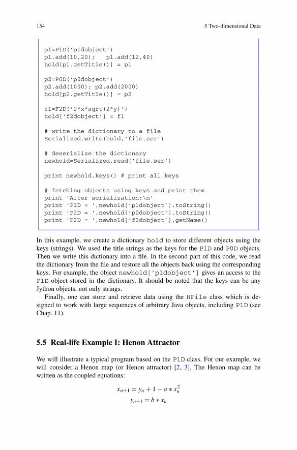
154 5 Two-dimensional Data
p1=P1D(’p1dobject’)p1.add(10,20); p1.add(12,40)hold[p1.getTitle()] = p1
p2=P0D(’p0dobject’)p2.add(1000); p2.add(2000)hold[p2.getTitle()] = p2
f1=F2D(’2*x*sqrt(2*y)’)hold[’f2dobject’] = f1
# write the dictionary to a fileSerialized.write(hold,’file.ser’)
# deserialize the dictionarynewhold=Serialized.read(’file.ser’)
print newhold.keys() # print all keys
# fetching objects using keys and print themprint ’After serialization:\n’print ’P1D = ’,newhold[’p1dobject’].toString()print ’P2D = ’,newhold[’p0dobject’].toString()print ’F2D = ’,newhold[’f2dobject’].getName()
In this example, we create a dictionary hold to store different objects using thekeys (strings). We used the title strings as the keys for the P1D and P0D objects.Then we write this dictionary into a file. In the second part of this code, we readthe dictionary from the file and restore all the objects back using the correspondingkeys. For example, the object newhold[’p1dobject’] gives an access to theP1D object stored in the dictionary. It should be noted that the keys can be anyJython objects, not only strings.
Finally, one can store and retrieve data using the HFile class which is de-signed to work with large sequences of arbitrary Java objects, including P1D (seeChap. 11).
5.5 Real-life Example I: Henon Attractor
We will illustrate a typical program based on the P1D class. For our example, wewill consider a Henon map (or Henon attractor) [2, 3]. The Henon map can bewritten as the coupled equations:
xn+1 = yn + 1 − a ∗ x2n
yn+1 = b ∗ xn
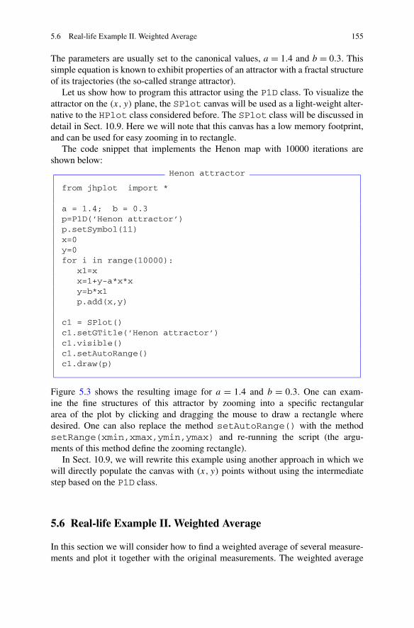
5.6 Real-life Example II. Weighted Average 155
The parameters are usually set to the canonical values, a = 1.4 and b = 0.3. Thissimple equation is known to exhibit properties of an attractor with a fractal structureof its trajectories (the so-called strange attractor).
Let us show how to program this attractor using the P1D class. To visualize theattractor on the (x, y) plane, the SPlot canvas will be used as a light-weight alter-native to the HPlot class considered before. The SPlot class will be discussed indetail in Sect. 10.9. Here we will note that this canvas has a low memory footprint,and can be used for easy zooming in to rectangle.
The code snippet that implements the Henon map with 10000 iterations areshown below:
Henon attractor
from jhplot import *
a = 1.4; b = 0.3p=P1D(’Henon attractor’)p.setSymbol(11)x=0y=0for i in range(10000):
x1=xx=1+y-a*x*xy=b*x1p.add(x,y)
c1 = SPlot()c1.setGTitle(’Henon attractor’)c1.visible()c1.setAutoRange()c1.draw(p)
Figure 5.3 shows the resulting image for a = 1.4 and b = 0.3. One can exam-ine the fine structures of this attractor by zooming into a specific rectangulararea of the plot by clicking and dragging the mouse to draw a rectangle wheredesired. One can also replace the method setAutoRange() with the methodsetRange(xmin,xmax,ymin,ymax) and re-running the script (the argu-ments of this method define the zooming rectangle).
In Sect. 10.9, we will rewrite this example using another approach in which wewill directly populate the canvas with (x, y) points without using the intermediatestep based on the P1D class.
5.6 Real-life Example II. Weighted Average
In this section we will consider how to find a weighted average of several measure-ments and plot it together with the original measurements. The weighted average
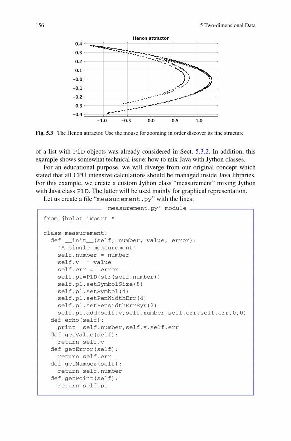
156 5 Two-dimensional Data
Fig. 5.3 The Henon attractor. Use the mouse for zooming in order discover its fine structure
of a list with P1D objects was already considered in Sect. 5.3.2. In addition, thisexample shows somewhat technical issue: how to mix Java with Jython classes.
For an educational purpose, we will diverge from our original concept whichstated that all CPU intensive calculations should be managed inside Java libraries.For this example, we create a custom Jython class “measurement” mixing Jythonwith Java class P1D. The latter will be used mainly for graphical representation.
Let us create a file “measurement.py” with the lines:"measurement.py" module
from jhplot import *
class measurement:def __init__(self, number, value, error):"A single measurement"self.number = numberself.v = valueself.err = errorself.p1=P1D(str(self.number))self.p1.setSymbolSize(8)self.p1.setSymbol(4)self.p1.setPenWidthErr(4)self.p1.setPenWidthErrSys(2)self.p1.add(self.v,self.number,self.err,self.err,0,0)
def echo(self):print self.number,self.v,self.err
def getValue(self):return self.v
def getError(self):return self.err
def getNumber(self):return self.number
def getPoint(self):return self.p1
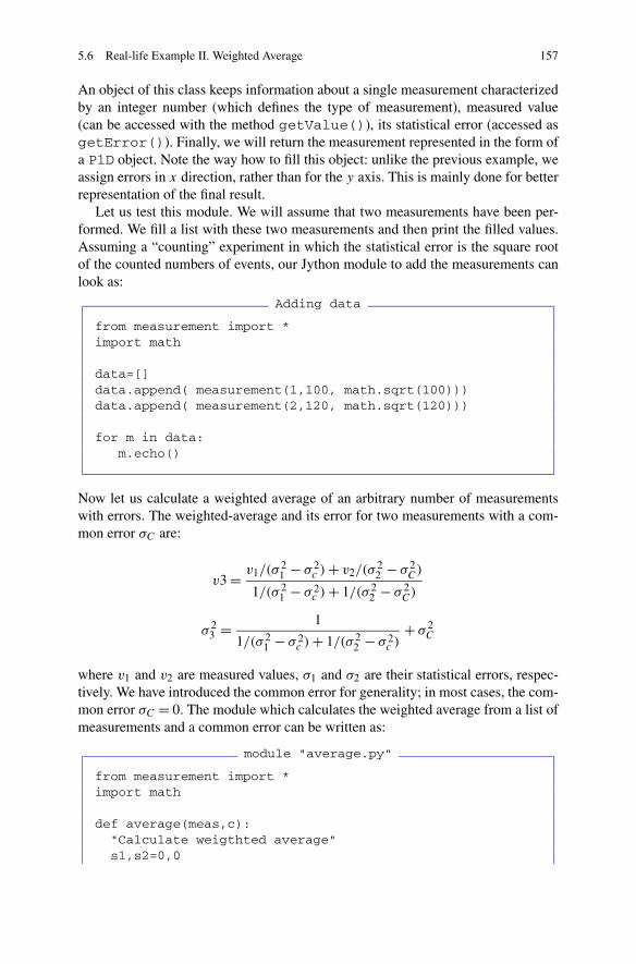
5.6 Real-life Example II. Weighted Average 157
An object of this class keeps information about a single measurement characterizedby an integer number (which defines the type of measurement), measured value(can be accessed with the method getValue()), its statistical error (accessed asgetError()). Finally, we will return the measurement represented in the form ofa P1D object. Note the way how to fill this object: unlike the previous example, weassign errors in x direction, rather than for the y axis. This is mainly done for betterrepresentation of the final result.
Let us test this module. We will assume that two measurements have been per-formed. We fill a list with these two measurements and then print the filled values.Assuming a “counting” experiment in which the statistical error is the square rootof the counted numbers of events, our Jython module to add the measurements canlook as:
Adding data
from measurement import *import math
data=[]data.append( measurement(1,100, math.sqrt(100)))data.append( measurement(2,120, math.sqrt(120)))
for m in data:m.echo()
Now let us calculate a weighted average of an arbitrary number of measurementswith errors. The weighted-average and its error for two measurements with a com-mon error σC are:
v3 = v1/(σ21 − σ 2
c ) + v2/(σ22 − σ 2
C)
1/(σ 21 − σ 2
c ) + 1/(σ 22 − σ 2
C)
σ 23 = 1
1/(σ 21 − σ 2
c ) + 1/(σ 22 − σ 2
c )+ σ 2
C
where v1 and v2 are measured values, σ1 and σ2 are their statistical errors, respec-tively. We have introduced the common error for generality; in most cases, the com-mon error σC = 0. The module which calculates the weighted average from a list ofmeasurements and a common error can be written as:
module "average.py"
from measurement import *import math
def average(meas,c):"Calculate weigthted average"s1,s2=0,0

158 5 Two-dimensional Data
for m in meas:e=m.getError()*m.getError()-c*cw1= 1.0/ew2= m.getValue()*w1s1=s1+w1s2=s2+w2
err=math.sqrt((1.0/s1)+c*c)return measurement(len(meas)+1,s2/s1,err)
Put these lines into a file with the name “average.py”.Now let us use this module and plot the original measurements as well as the
weighted average (for which we used a different symbol). This time, we will use theclass HPlotJa which has very similar methods as for the HPlot canvas, but canbe used for an interactive drawing with the mouse, as discussed in Sect. 10.10.
A weighted average
from measurement import *from average import *import math
c1 = JaPlot(’Canvas’)c1.removeAxes()c1.showAxis(0)c1.setGridAll(0,0)c1.setGridAll(1,0)c1.setRange(50,150,0,5)c1.setNameX(’Measurements’)c1.visible()
data=[]data.append( measurement(1,100, math.sqrt(100)))data.append( measurement(2,120, math.sqrt(120)))
p=average(data,1.)for m in data:
c1.draw(m.getPoint())
p1=p.getPoint()p1.setSymbol(5)c1.draw(p1)
Figure 5.4 presents the result. Two filled circles show the original measure-ments, while the third point shows their weighted average calculated by the module“average.py”.

References 159
Fig. 5.4 A weighted average (marked by the filled square and labeled as “3”) of two independentmeasurements (indicated using the keys “1” and “2”)
References
1. Taylor, J.: An Introduction to Error Analysis: The Study of Uncertainties in Physical Measure-ments. University Science Books, Herdon (1997)
2. Henon, M.: Numerical study of quadratic area-preserving mappings. Q. Appl. Math. 27, 291–312 (1969)
3. Gleick, J.: Chaos: Making a New Science. Penguin Books, New York (1988)


Chapter 6Multi-dimensional Data
6.1 P2D Data Container
Now let us discuss how to deal with data in dimensions larger than two. A naturalextension of the P1D class for 3-dimensional data is the class P2D. It is rather sim-ilar to the P1D, the only difference is that it keeps data in 3D phase space (x, y, z).Also, it has less options for drawing and, in addition, statistical and systematicalerrors are not supported. In Jython, one can add values to this container in the sameway as for P1D, only this time the method add(x,y,z) takes three arguments.In the example below we create a P2D object and append a single point with thecomponents (1,2,3):
>>> from jhplot import *>>> p2= P2D(’x-y-z points’)>>> p1.add(1,2,3)
Table 6.1 shows the main methods of this class. We will not discuss in detailsince the P2D arrays are similar to P1D, and one can always look at the Java APIdocumentation to learn about this data holder.
6.1.1 Drawing P2D and HPlot3D Canvas
To draw a P2D, one should use the 3D canvas based on the HPlot3D class. Thisclass was discussed in Sect. 3.4.2 and used to draw F2D functions. In the examplebelow we draw two data sets shown in blue and red colors:
Drawing P2D data in 3D
from jhplot import *from java.awt import Color
c1 = HPlot3D(’Canvas’)
S.V. Chekanov, Scientific Data Analysis using Jython Scripting and Java,Advanced Information and Knowledge Processing,DOI 10.1007/978-1-84996-287-2_7, © Springer-Verlag London Limited 2010
161

162 6 Multi-dimensional Data
Table 6.1 The main P2Dmethods. In this table, “b”denotes a boolean value (1 forJava “true” and 0 for “false”),while “i” is an integerparameter. “a” indicates theaxis (a=0,1,2)
Methods Definitions
add(x,y,z) add (x, y, z)
set(i,x,y,z) insert (x, y, z) at position i
fill(arrayX, arrayY, arrayZ) fills from 3 arrays
setTitle(“text”) set title
getTitle() get title
size() get size
clear() clean from data
copy() copy to a new P2D
getArrayX() get arrays with X
getArrayY() get array with Y
getArrayZ() get array with Z
getX(i),getY(i),getZ(i) get points at index i
getMax(a) get max for axis
getMin(a) get min for axis
mean(a) get mean for axis
toTable() show in a table
merge(p2d) merge with another P2D
c1.visible()c1.setNameX(’X axis’)c1.setNameY(’Y axis’)c1.setRange(-5,10,-5,5,-10,20)
h1= P2D(’blue data’)h1.setSymbolSize(6)h1.setSymbolColor(Color.blue)h1.add(1,2,3)h1.add(4,4,5)h1.add(3,2,0)c1.draw(h1)
h1= P2D(’red data’)h1.setSymbolSize(6)h1.setSymbolColor(Color.red)for i in range(10):
h1.add(0.1*i, 0.2*i, 0.5*i)c1.draw(h1)
Table 6.2 lists several most important methods used to draw P2D data on the3D canvas. The number of methods is not very large, since many drawing methodsbelong to the actual 3D canvas, rather then attributed to the P2D object itself. Wewill discuss the HPlot3D methods in Sect. 10.12.

6.1 P2D Data Container 163
Table 6.2 Graphicalmethods for displaying P2Ddata. In the methods shown inthis table, “c” denotes theJava Color class, while “i”is used to indicate an integerparameter
Methods Definitions
setSymbolColor(c) Set symbol color
setSymbolSize(i) Set symbol size
getSymbolColor() Get symbol color
getSymbolSize() Get symbol size
We will remind that the HPlot3D canvas is a rather similar to HPlot: One candisplay several plots on the same canvas and change the plotted regions using thecd(i1,i2) method:
>>> from jhplot import *>>> c1=HPlot3D(’Canvas’,600,400,2,2) # 2x2 pads>>> c1.visible() # set visible>>> c1.cd(1,1) # go to the 1st pad... draw some object ..>>> c1.cd(1,2) # go to the 2nd pad
As for the HPlot canvas, first two integers in the constructor HPlot3D define thesize of the canvas (600 × 400 pixels for this example), while two other integersdefine how many drawing regions (pads) should be shown (2 regions in X and 2regions in Y ).
Let us give a more concrete example of how to work with the P2D:
Graphical options for drawing P2D
from java.util import Randomfrom java.awt import Colorfrom jhplot import *
c1 = HPlot3D(’Canvas’)c1.setGTitle(’Interactive 3D’)c1.setNameX(’X’)c1.setNameY(’Y’)c1.visible()c1.setRange(-5,10,-5,5,-10,30)
p1= P2D(’3D Gaussian 1’)p1.setSymbolSize(6)p1.setSymbolColor(Color.blue)
rand = Random()for i in range(200):
x=1+rand.nextGaussian()y=1+0.5*rand.nextGaussian()z=10+4.5*rand.nextGaussian()p1.add(x,y,z)

164 6 Multi-dimensional Data
Fig. 6.1 Two P2D objectsdisplayed using theHPlot3D canvas
p2= P2D(’3D Gaussian 2’)p2.setSymbolSize(10)p2.setSymbolColor(Color.red)
for i in range(50):x=2+2*rand.nextGaussian()y=4+0.5*rand.nextGaussian()z=6+1.5*rand.nextGaussian()p2.add(x,y,z)
c1.draw(p1)c1.draw(p2)
In this script, we fill two P2D containers with 3D Gaussian numbers and plotthem on the same canvas. The result of this script is shown in Fig. 6.1. Note that themost efficient way to fill the containers is to fill P0D with Gaussian numbers usingthe methods of the P0D class, and use three P0D containers for the input of the P2Dconstructor.
6.2 P3D Data Container
You may wonder, what could be shown with the object called P3D, since by anal-ogy, it must contain points in a 4-dimensional space. The P3D container, by design,still can be used to show 3-dimensional data, but this time, points can have someextension in 3D space. All methods of the P3D are very similar to that of P2D, the

6.2 P3D Data Container 165
only difference is that each data point in x, y, z, has an additional parameter rep-resenting an extension of the point in the corresponding direction. As before, thecanvas HPlot3D should be used for drawing such objects. To fill a P3D container,one should use the method add(x,dx,y,dy,z,dz) which takes exactly 6 argu-ments, with dx, dy and dz being the extensions in corresponding direction.
Here we will stop the discussion of this class since it has a limited use for math-ematical manipulations. Rather, we will show a simple example of how to use theP3D to draw various shapes (lines, cubes and surfaces):
Working with P3D
from jhplot import *from java.util import Randomfrom java.awt import Color
c1 = HPlot3D(’Canvas’)c1.setGTitle(’3D plot with P3D objects’)c1.setNameX(’X’)c1.setNameY(’Y’)c1.visible()
c1.setRange(-5,10,-4,10,0,20)# build P3D shapeh1 = P3D(’3D form in blue’)h1.setPenColor(Color.blue)# build a 3D cubeh1.add(4.0,1.0,8.0,2.0,3.0,4.0)
# build 2D panel (Z extension is 0)h1.add(5.0,2.0,3.0,1.0,8.0, 0.0)
# build 1D linesh1.add(5.8,0.0,3.0,0.0,10.0, 3.0)h1.add(-1.2,4.0,-2.0,0.0,10.0, 0.0)h1.add(-1.2,0.0,-2.0,2.0,10.0, 0.0)
# build a 3D cubeh2 = P3D(’3D form in red’)h2.setPenColor(Color.red)h2.add(-0.5,3.0,-1.0,2.0,6.0,2.0)
c1.draw(h1)c1.draw(h2)
Figure 6.2 shows the resulting plot.We should note that the P3D class was not designed for complicated drawings
in 3D. You may find more appropriate to visualize geometrical shapes using theHView3D class discussed in Sect. 10.13.2 or the class HPlot3DP discussed inSect. 10.12.

166 6 Multi-dimensional Data
Fig. 6.2 P3D objectsdisplayed using theHPlot3D canvas
6.3 PND Data Container
The PND class can be used to store data in many dimensions (this explains theappearance of the “N” in its name). As usual, “D” in the class name means that theobject stores double values. Use the class PNI to store integer values.
Unlike other classes discussed so far, this class does not have any graphical at-tributes, since it is mainly designed for data manipulations. To be able to visualizemultidimensional data, one should always project such data into a lower dimension,or use the P1D or P2D classes for drawing.
Below we will discuss the class PND, since its clone for integer values, PNI, hasexactly the same methods.
As usual, one should first initialize a PND object and then fill it. This can be doneby appending lists with numbers using the method add(list). The lists can haveany size. The example below shows how to create and fill a PND:
>>> from jhplot import *>>>>>> p0=PND(’example’) # build a PND object>>> p0.add([1,2,3]) # append some values>>> p0.add([2,3,4])>>> p0.add([2,3,4,3,4]) # append more columns>>> p0.add([2,3]) # append less columns>>> print p0.getDimension()2>>> print p0.toString()PND: example1.0 2.0 3.02.0 3.0 4.0
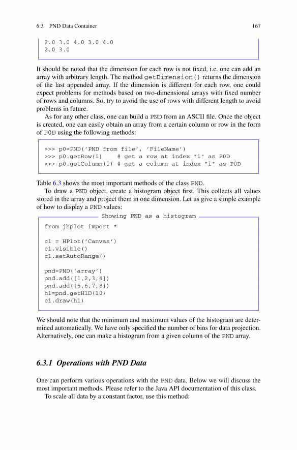
6.3 PND Data Container 167
2.0 3.0 4.0 3.0 4.02.0 3.0
It should be noted that the dimension for each row is not fixed, i.e. one can add anarray with arbitrary length. The method getDimension() returns the dimensionof the last appended array. If the dimension is different for each row, one couldexpect problems for methods based on two-dimensional arrays with fixed numberof rows and columns. So, try to avoid the use of rows with different length to avoidproblems in future.
As for any other class, one can build a PND from an ASCII file. Once the objectis created, one can easily obtain an array from a certain column or row in the formof P0D using the following methods:
>>> p0=PND(’PND from file’, ’FileName’)>>> p0.getRow(i) # get a row at index "i" as P0D>>> p0.getColumn(i) # get a column at index "i" as P0D
Table 6.3 shows the most important methods of the class PND.To draw a PND object, create a histogram object first. This collects all values
stored in the array and project them in one dimension. Let us give a simple exampleof how to display a PND values:
Showing PND as a histogram
from jhplot import *
c1 = HPlot(’Canvas’)c1.visible()c1.setAutoRange()
pnd=PND(’array’)pnd.add([1,2,3,4])pnd.add([5,6,7,8])h1=pnd.getH1D(10)c1.draw(h1)
We should note that the minimum and maximum values of the histogram are deter-mined automatically. We have only specified the number of bins for data projection.Alternatively, one can make a histogram from a given column of the PND array.
6.3.1 Operations with PND Data
One can perform various operations with the PND data. Below we will discuss themost important methods. Please refer to the Java API documentation of this class.
To scale all data by a constant factor, use this method:

168 6 Multi-dimensional Data
Table 6.3 Some methods of the PND class. “i” and “j” denote integer indexes
Methods Definitions
setTitle() set title
clear() clean from entries
get(i) returns row “i” as array
get(i,j) returns value at row “i” and column “j”
toString() convert data to a string
getColumn(i) get P0D from column at index “i”
getRaw(i) get P0D from row at index “i”
getDimension() get dimension (last added entry)
getArrayList() get data in form of array list
getArray() get double array
getH1D(bins) get H1D histogram with “bins”
add(P0D) add P0D as row
add(array[]) add array
set(i,P0D) set P0D at index i
set(i,array[]) set array at index i
setArray(array[][]) set from double array
remove(i) remove a row at index i
getMin() get minimum value
getMax() get minimum value
size() get the size
copy(‘text’) new copy with a title ‘text’
standardize() convert each column to (xi − x̄)/σ
rescale(i) rescale each column to [0,1] (i=0) or [-1,1] (i=1)
>>> p0.operScale(scale)
where ’scale’ is a number used to scale all elements.A PND can be rescaled to the range [−1,1] or [0,1] with the rescale()
method. Another operation is the so-called standardize(), which is useful forthe neural-network studies to be discussed in Sect. 15.1.1.
One can add, subtract, multiply and divide two PND arrays. Assuming p0 andp1 are objects of the PND class, this can be done as:
>>> p2=p0.oper(p1,’NewTitle’,operation)
where ’operation’ is a string which can either be “+”, “/”, “*” or “/” (they areself-explanatory). Finally, ’NewTitle’ is an optimal title which can be dropped.

6.4 Input and Output 169
6.4 Input and Output
All the containers discussed before, P2D, P3D and PND, can be serialized and re-stored back in exactly the same way as discussed in Sect. 5.4.
In addition, one can write and read ASCII files with the instances pn of the classPND using the methods:
>>> pn.toFile(’FileName’) # write to a file>>> pn.write(’FileName’)>>> pn.read(’FileName’) # read from files:
In case if a multidimensional collection of data must be stored in a single file,the most convenient way would be to populate a Jython list or a dictionary with thePND objects and serialize it to a file as shown in Sects. 4.3.3 and 5.4.
We will come back to the I/O methods in Chap. 11.


Chapter 7Arrays, Matrices and Linear Algebra
jHepWork contains many types of arrays that can be used to hold data in the formof primitive numbers. Typically, they come from third-party Java libraries.
One should not consider such external arrays as being completely independent ofthe native jHepWork containers which come with the package jhplot. There aremany ways to convert the third-party arrays into the P0D, P1D and PND objects formanipulation and graphical representation.
7.1 Jaida Data Containers
First, we will start from the Jaida library which is included to the jHepWork packageby default.
To keep data points with errors, one can use the Measurement class. It keepsinformation on a single measurement with its errors. There are several constructorsfor this class:
>>> from hep.aida.ref.histogram import *>>> m=Measurement(d)>>> m=Measurement(d,err)>>> m=Measurement(d,errMinus, errPlus)
where ’d’ is a central measurement represented by a double value, ’err’ is itserror. ’errMinus’ and ’errPlus’ can be used to add asymmetric uncertainties(i.e. a lower and an upper error).
To retrieve the measurement value and its errors, one should call the followingmethods:
value() to obtain the measurement valueerrorMinus() to obtain a lower errorerrorPlus() to obtain upper error
S.V. Chekanov, Scientific Data Analysis using Jython Scripting and Java,Advanced Information and Knowledge Processing,DOI 10.1007/978-1-84996-287-2_8, © Springer-Verlag London Limited 2010
171

172 7 Arrays, Matrices and Linear Algebra
One should note that this class is conceptually rather similar to the P1D container.A measurement can also be kept in a more general container, called Data-
Point. It has the following constructors:
>>> from hep.aida.ref.histogram import *>>> DataPoint(d[])>>> DataPoint(d[], err[])>>> DataPoint(d[], errMinus[], errPlus[])
In contrast to the class Measurement, the DataPoint object can hold valuesand their errors in many dimensions. One can access the values as:
dimension() get the data dimensionlowerExtent(i) the lower value at “i”upperExtent(i) the upper value at “i”
Jaida has a special container to hold data represented by the class DataPoint,called DataPointSet. It was designed for holding a set of DataPoint objects.Below we give two most popular constructors:
>>> from hep.aida.ref.histogram import *>>> DataPointSet(name,title, int dim)>>> DataPointSet(name,title, int dim, int capacity)
The strings ’name’ and ’title’ are self-explanatory, dim is the dimension (in-teger) and capacity is the default capacity (integer). Once the DataPointSetobject is created, one can add a DataPoint using the method addPoint(p),where ’p’ is a data point represented by a DataPoint object.
A DataPointSet object can be translated into the usual P1D object discussedin Sect. 5.1 and used for visualization using the jHepWork canvas. What one needsto do is to build a P1D object passing a DataPointSet as argument:
>>> from hep.aida.ref.histogram import *>>> from jhplot import *>>> #.. create dp using DataPointSet class>>> p1=P1D(dp) # convert to P1D
In this operation, only 1st-level errors of the P1D array will be filled. Table 7.1 listssome methods of this container.
7.1.1 Jaida Clouds
Jaida cloud is a set of data points. These objects are rather similar to P0D, P2D etc.containers of the jHepWork library.

7.1 Jaida Data Containers 173
Table 7.1 Some methods ofthe DataPointSet fromthe Jaida library
Methods Definitions
addPoint(p) add a DataPoint
clear() clear the array
dimension() returns the dimension
point(i) returns DataPoint at index ‘i’
removePoint(i) removes point at index ‘i’
scale(d) scales by a factor ‘d’
scaleValues(d) scales values by a factor ‘d’
scaleErrors(d) scales errors by a factor ‘d’
upperExtent(i) get a lower extent at index ‘i’
lowerExtent(i) get an upper extend at index ‘i’
To create a cloud in 1D, the following constructor should be used:
>>> from hep.aida.ref.histogram import *>>> c=Cloud1D()
Once the cloud object has been initialized, one can fill it using two methods:
>>> c.fill(d)>>> c.fill(d,w)
The second method fills a cloud with a value ’d’ which has a weight ’w’ (bothnumbers are double). The notion of the weight is rather similar to that to be dis-cussed in the section devoted to histograms (see the following chapter). In simplewords, the number ’w’ represents importance of a data point in the data set. Bydefault, the first method assumes w=1. To display a cloud, one needs to convert itinto a histogram. Table 7.2 shows some most important methods of the clouds:
A cloud can be created in 2D using the Cloud2D constructor:
>>> from hep.aida.ref.histogram import *>>> c=Cloud2D()
which can be filled with two numbers (say, x, y):
>>> c.fill(x,y)>>> c.fill(x,y,w)
As before, one can specify a weight ’w’ for each 2D point (x, y) (the default weightis 1). The methods for this cloud are the same as those shown in Table 7.2, but thistime there are more methods since we have two values, instead of one. Therefore,

174 7 Arrays, Matrices and Linear Algebra
Table 7.2 Some methods ofthe class Cloud1D from theJaida library. ‘d’ indicates adouble value and ‘i’ is aninteger index
Methods Definitions
fill(d) fill with data point ‘d’
fill(d,w) fills with ‘d’ and a weight ‘w’
histogram() create a histogram
lowerEdge() cloud’s lower edge
mean() the mean value
entries() the number of entries
rms() the standard deviation
scale(d) scale with a factor ‘d’
upperEdge() get the upper edge
value(i) get a value at the index ‘i’
weight(i) get a weight at the index ‘i’
each method characterizing the Coud1D class has extra “X” or “Y ” string at theend of each method name. For example, meanX() denotes the mean value in x,meanY() is the mean value in y.
Similarly, one can build a cloud in 3D using the constructor Cloud3D(). Wewill leave the reader here as it is rather easy to guess how to fill and how to accessvalues of such cloud, reminding that one single point now is represented by threenumbers, (x, y, z).
7.2 jMathTools Arrays and Operations
Another package which is incorporated into jHepWork is jMathTool[1]. It contains acollection of Java classes designed for engineering and general scientific computingneeds.
7.2.1 1D Arrays and Operations
Let us first create an one-dimensional array with double numbers as:
>>> from jhplot.math.DoubleArray import *>>> a=one(N,d)
This example instantiates a 1D array with ’N’ numbers, all of which have thesame double value ’d’. Check the type which corresponds to the object ’a’ astype(a). You will see that the object ’a’ is <type ’array.array’>. Onecan find all the methods which could be used for manipulation with this object usingthe code assist.

7.2 jMathTools Arrays and Operations 175
One can also build an array with numbers incremented by some value:
>>> a=increment(N,begin,val)
again, ’N’ is the total number of values, ’begin’ is an initial value, and’val’ represents a double value used to increment it, x[0]=begin, x[n]=x[n-1]+val. Below we describe some important methods for the 1D arrays (de-noted by ’a’):
copy(a) returns a copymin(a) the minimum value for arraymax(a) the maximum values for arrayminIndex(a) get index of the minimum valuemaxIndex(a) get index of the maximum valuesum(a) sums of all values,
∑Ni=0 xi
cumSum(a) array with the cumulative sum, bk = ∑ki=0 xi
product(a) product of all values,∏N
i=0 xi
cumProduct(a) array with the cumulative product, bk = ∏ki=0 xi
sort(a) sorts arrayinsert(a1,i,a2) inserts an array a2 to array a1 starting from index “i”increment(N,d,p) initializes an array with size N , x[i] = d + i ∗ p
deleteRange(a,i,j) deletes range from ‘i’ to ‘j’delete(a,i) deletes the range starting from ‘i’random(i) creates an array of the size ‘i’ with random numbersrandom(i,min,max) creates an array of size ‘i’ with random numbers be-
tween min and max
One can print the 1D array using the io.ArrayString method. Here is ancomplete example of how to create an array, print it and sum-up its values:
>>> from jhplot.math.DoubleArray import *>>> from jhplot.math.io.ArrayString import *>>> a=increment(10,0,1)>>> print ’Array=’+printDoubleArray(a)Array=0.0 1.0 2.0 3.0 4.0 5.0 6.0 7.0 8.0 9.0>>> sum(a)45
We remind that one can learn more about this type of arrays using the methoddir(obj). For the DoubleArray static Java class, call this lines:
>>> from jhplot>>> dir(jhplot.math.DoubleArray)

176 7 Arrays, Matrices and Linear Algebra
7.2.2 2D Arrays
DoubleArray class can be used to build 2D arrays almost in the same way as itfor the 1D case above. Such arrays are ideal for storing matrix values. To initializea 2D array, the following class can be used:
>>> from jhplot.math.DoubleArray import *>>> a=one(i1,i2,d)
where ’d’ is a number to be assigned for the entire matrix with the number ’i1’of rows and the number ’i2’ of columns.
>>> from jhplot.math.DoubleArray import *>>> from jhplot.math.io.ArrayString import *>>> a=one(2,5,1)>>> print printDoubleArray(a)1.0 1.0 1.0 1.0 1.01.0 1.0 1.0 1.0 1.0
Below we give a list of the most important methods of this class, where ’a’ indi-cates an input array.
copy(a) returns exact copymin(a) minimum value for arraymax(a) maximum values for arrayminIndex(a) an index of the minimum valuemaxIndex(a) an index of the maximum valuesum(a) sums of all values,
∑Ni,j=0 ai,j
cumSum(a) array with cumulative sum, bk =∑ki,j=0 ai,j
product(a) product of all values,∏N
i,j=0 ai,j
cumProduct(a) array with cumulative product, bk =∏ki,j=0 ai,j
increment(i,j, b[], p[]) initialize array ixj as a[i][j ] = b[j ] +i ∗ p[j ]
getSubMatrixRangeCopy(a,i1,i2,j1,j2) get submatrix using rangesi1–i2 (rows) and j1–j2 (columns)
getColumnsRangeCopy(a,i1,i2) get columns between ‘i1–i2’getColumnCopy(a,i) obtains a column ‘i’getColumnsRangeCopy(a,i1,i2) obtains columns between ‘i1–i2’getRowsRangeCopy(a,i1,i2) obtains rows between ‘i1–i2’getRowCopy(a,i) obtains a row at ‘i’getColumnDimension(a,i) the dimension of column at ‘i’insertColumns(a1, a2, i) inserts a2[][] to a1[][] at column ‘i’insertColumn(a1, a2, i) inserts a2[] to a1[][] at column ‘i’

7.3 Colt Data Containers 177
insertRows(a1, a2, i) inserts a2[][] to a1[][] at row ‘i’insertRow(a1, a2, i) inserts a2[] to a1[][] at row ‘i’deleteColumnsRange(a,i1,i2) deletes columns between ‘i1’ and ‘i2’deleteRowRange(a,i1,i2) deletes rows between ‘i1’ and ‘i2’sort(a) sorts the arrayrandom(i) creates a 2D array of size ‘i’ with ran-
dom numbersrandom(i,min,max) creates a 2D array of the size ‘i’ with
random numbers between min and max
7.3 Colt Data Containers
The Colt package [2] provides several enhanced data containers to store primitivevalues and to perform manipulations with them. The arrays support quick access toits elements which is achieved by non-bounds-checking methods. There are severalclasses used to build the Colt arrays:
• IntArrayList• DoubleArrayList• LongArrayList
We will consider the DoubleArrayList container for further examples sinceall these classes are very similar.
>>> from cern.colt.list import *>>> a=DoubleArrayList() # empty list>>> a=DoubleArrayList(d[]) # with elements d[]>>> a=DoubleArrayList(initialCapacity)
The constructors above illustrate various ways to initialize the arrays. Try to lookat the methods of this class with the code assist. Table 7.3 lists some of the mostimportant methods of the DoubleArrayList class.
The data stored in the DoubleArrayList array can be analyzed using theDynamicBin1D class from the same package:
>>> from cern.colt.list import *>>> from hep.aida.bin import *>>> a=DoubleArrayList()>>> bin=DynamicBin1D()>>> bin.addAllOf(a);>>> print bin.toString()
This example prints a comprehensive statistical summary of the array. One shouldalso note that one can build a P0D from the DoubleArrayList object as:

178 7 Arrays, Matrices and Linear Algebra
Table 7.3 Methods for the DoubleArrayList. (IntegerArrayList and LongArrayList have the samemethods)
Methods Definitions
add(d) add a double value
size() get the size
copy() returns a DoubleArrayList copy
elements() returns elements as list
get(i) get double value at index ‘i’
getQuick(i) get double at index ‘i’ without checking
set(i,d) set double ‘d’ at index ‘i’
reverse() reverses the order
shuffleFromTo(i1,i2) randomly permutes from index ‘i1’ to ‘i2’
contains(d) returns true (1) if “d” exists
delete(d) deletes first element ‘d’
addAllOf(a) appends an array ‘a’
indexOf(d) returns index of the first occurrence
quickSortFromTo(i1,i2) Sorts the range [i1–i2] into ascending numerical order
toList() returns ArrayList
clear() clear the array
>>> from cern.colt.list import *>>> from jhplot import *>>> a=DoubleArrayList()>>> p0=P0D(a)>>> print p0.getStat()
File-based input/output can be achieved through the standard Java built-in serializa-tion mechanism.
The Colt package also includes the class ObjectArrayList, which is similarto the Java list discussed in the previous sections.
7.4 Statistical Analysis Using Jython
In addition to the Java libraries provided by jHepWork, one can also use third-partylibraries implemented using the Python language. The Python/Jython third-partypackages are located in the directory python/packages. There are several ad-vantages in using programs implemented in Jython: (1) one can directly access thecode with the implemented numerical algorithms. (2) One can reuse the libraries inCPython programs.

7.4 Statistical Analysis Using Jython 179
We remind that the directory ’python/packages’ is imported automaticallywhen using the jHepWork IDE, so there is no need to worry about appending thisdirectory location to the ’sys.path’ variable. If one uses another editor, makesure that Jython looks at the directory ’python/packages’ to import the third-party packages. For example, you can do it as:
>>> import sys>>> sys.path.append(SystemDir+’/python/packages’)
where SystemDir is the directory with the installed jHepWork. Below we assumethat the reader uses the jHepWork IDE and does not need to specify this directory.
Here we will consider the module ’stats’ which provides basic statisticalfunctions for Jython collections. It allows calculations of simple characteristics froma Jython list, such as the mean value and the standard deviation:
>>> from statlib.stats import *>>> a = [1,2,3,4,5,6,7,8,10 ]>>> print ’Mean=’,mean(a)Mean= 5.1111>>> print ’Standard deviation=’,stdev(a)Standard deviation= 2.93446
Analogously, one can calculate other statistical characteristics, such as the me-dian, variation, skewness, kurtosis and moments. Let us give their definitions: A mo-ment of an order n for a list with N elements is given as
Mn = 1
N
N∑
i
(list(i) − mean)n
A skewness is defined via the moments, M3/(M2)1.5, while the kurtosis is
M4/(M2)2. A variation is given as the ratio of the biased standard deviation to
the mean. All such statistical characteristics can be assessed in one line of the codeusing the describe(list) function:
>>> a = [1,2,3,4,5,6,7,8,10]>>> stat=describe(a)>>> print ’N=’,stat[0]N= 9>>> print ’tuple=’,stat[1]tuple= (1, 10)>>> print ’mean=’,stat[2]mean= 5.1111>>> print ’standard deviation=’,stat[3]standard deviation= 2.93>>> print ’skewness=’,stat[4]

180 7 Arrays, Matrices and Linear Algebra
skewness= 0.199>>> print ’kurtosis=’,stat[5]kurtosis= 2.00
The output values have been truncated to fit the page width.In the next example, we will extend this code snippet by including calculations
of various characteristics of a list with 100 numbers. Moments about the mean forthis list will be calculated in a loop (up to the order nine):
Statistical analysis of lists
from statlib.stats import *
a=range(100)print ’geometric mean=’,geometricmean(a)print ’median=’,median(a)print ’variation=’,variation(a)print ’skew=’,skew(a)print ’kurtosis=’,kurtosis(a)for n in range(2,10):
print ’moment order ’+str(n)+’:’,moment(a,n)
The output of this code snippet is given below:
geometric mean= 0.0median= 49.005variation= 58.315skew= 0.0kurtosis= 1.799moment order 2: 833moment order 3: 0.0moment order 4: 1249moment order 5: 0.0moment order 6: 2230moment order 7: 0.0moment order 8: 4.335+12moment order 9: 0.0075
Again, we have reduced the precision of the output numbers to fit the page width.The module allows calculations of correlation coefficients between two lists. Let
us generate two correlated lists using a Gaussian distribution and estimate their cor-relations using several tests:
Correlation coefficients
from statlib.stats import *
from random import *ran=Random()
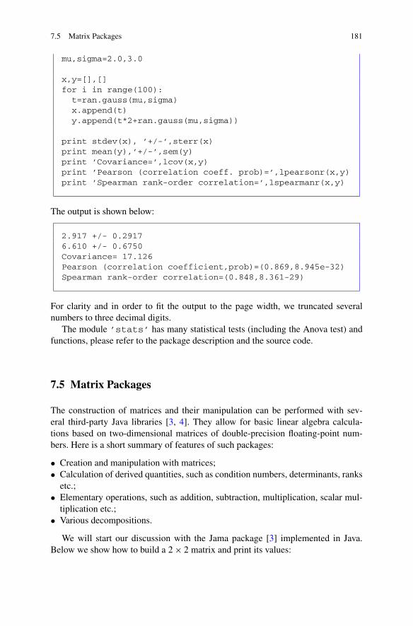
7.5 Matrix Packages 181
mu,sigma=2.0,3.0
x,y=[],[]for i in range(100):
t=ran.gauss(mu,sigma)x.append(t)y.append(t*2+ran.gauss(mu,sigma))
print stdev(x), ’+/-’,sterr(x)print mean(y),’+/-’,sem(y)print ’Covariance=’,lcov(x,y)print ’Pearson (correlation coeff. prob)=’,lpearsonr(x,y)print ’Spearman rank-order correlation=’,lspearmanr(x,y)
The output is shown below:
2.917 +/- 0.29176.610 +/- 0.6750Covariance= 17.126Pearson (correlation coefficient,prob)=(0.869,8.945e-32)Spearman rank-order correlation=(0.848,8.361-29)
For clarity and in order to fit the output to the page width, we truncated severalnumbers to three decimal digits.
The module ’stats’ has many statistical tests (including the Anova test) andfunctions, please refer to the package description and the source code.
7.5 Matrix Packages
The construction of matrices and their manipulation can be performed with sev-eral third-party Java libraries [3, 4]. They allow for basic linear algebra calcula-tions based on two-dimensional matrices of double-precision floating-point num-bers. Here is a short summary of features of such packages:
• Creation and manipulation with matrices;• Calculation of derived quantities, such as condition numbers, determinants, ranks
etc.;• Elementary operations, such as addition, subtraction, multiplication, scalar mul-
tiplication etc.;• Various decompositions.
We will start our discussion with the Jama package [3] implemented in Java.Below we show how to build a 2 × 2 matrix and print its values:
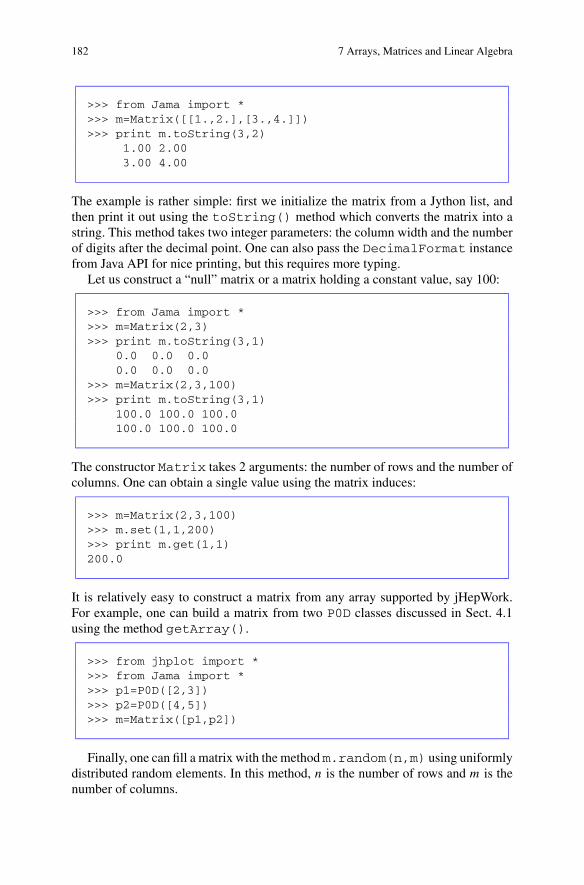
182 7 Arrays, Matrices and Linear Algebra
>>> from Jama import *>>> m=Matrix([[1.,2.],[3.,4.]])>>> print m.toString(3,2)
1.00 2.003.00 4.00
The example is rather simple: first we initialize the matrix from a Jython list, andthen print it out using the toString() method which converts the matrix into astring. This method takes two integer parameters: the column width and the numberof digits after the decimal point. One can also pass the DecimalFormat instancefrom Java API for nice printing, but this requires more typing.
Let us construct a “null” matrix or a matrix holding a constant value, say 100:
>>> from Jama import *>>> m=Matrix(2,3)>>> print m.toString(3,1)
0.0 0.0 0.00.0 0.0 0.0
>>> m=Matrix(2,3,100)>>> print m.toString(3,1)
100.0 100.0 100.0100.0 100.0 100.0
The constructor Matrix takes 2 arguments: the number of rows and the number ofcolumns. One can obtain a single value using the matrix induces:
>>> m=Matrix(2,3,100)>>> m.set(1,1,200)>>> print m.get(1,1)200.0
It is relatively easy to construct a matrix from any array supported by jHepWork.For example, one can build a matrix from two P0D classes discussed in Sect. 4.1using the method getArray().
>>> from jhplot import *>>> from Jama import *>>> p1=P0D([2,3])>>> p2=P0D([4,5])>>> m=Matrix([p1,p2])
Finally, one can fill a matrix with the method m.random(n,m) using uniformlydistributed random elements. In this method, n is the number of rows and m is thenumber of columns.

7.5 Matrix Packages 183
One can insert a sub-matrix of a matrix with the method:
>>> m.setMatrix(int[] r, int[] c, X)
where r is an array of row indexes and c is an array of column indexes. X is theactual sub-matrix defined as A(r(:),c(:)).
Now let us consider the question of extraction of the information about a matrix.First, one can access 2D array of a matrix using the method getArray(). To geta single value, use the usual method get(i1,i2), where i1 is the row numberand i2 is the column number. One can return the entire matrix object or only a sub-matrix using getMatrix(i1,i2,j1,j2), where i1 is the initial row index,i2 is the final row index, j1 is the initial column index and j2 is the final columnindex. One can also learn about other methods by looking at the corresponding APIdocumentation.
A matrix or a group of matrices can be saved into dictionaries or lists and se-rialized into a file as any jHepWork object discussed in Chap. 11. This is possiblebecause the class Matrix implements the Java Serializable interface.
7.5.1 Basic Matrix Arithmetic
Assuming that you have two matrices, “A” and “B”, one can perform the followingoperations:
B.minus(A) subtract matrix A from BA.timesEquals(d) multiply a matrix by a scalar “d”, A =
d ∗ AB.times(A) Linear algebraic matrix multiplication,
A ∗ BB.plus(A) C = A + BA.plusEquals(B) A = A + BA.minusEquals(B) A = A − BA.minus(B) C = A − BA.arrayRightDivide(B) Element-by-element right division, C =
A./BA.arrayRightDivideEquals(B) Element-by-element right division in
place, A = A./BA.arrayLeftDivide(B) Element-by-element left division, C =
A. divide BA.arrayLeftDivideEquals(B) Element-by-element left division in place,
A = A. divide BA.arrayTimes(B) Element-by-element multiplication, C =
A. ∗ B

184 7 Arrays, Matrices and Linear Algebra
A.arrayTimeEquals(B) Element-by-element multiplication, A =A. ∗ B
A.uminus() unary minus, i.e. −A
Finally, one can use the inverse()method to inverse all elements. One can obtainthe basic normalization methods, such as:
norm1() the maximum column sum, i.e. summing up absolute values of allcolumn numbers
normInf() the maximum row sum, i.e. summing up absolute values of all rownumbers
7.5.2 Elements of Linear Algebra
The Jama package provides more advanced operations with matrices than those dis-cussed above. The determinant of a matrix can be obtained with the method det(),while one can access its rank as rank().
There are several basic matrix decompositions:
• Cholesky Decomposition of symmetric, positive definite matrices;• QR Decomposition of rectangular matrices;• LU Decomposition of rectangular matrices;• Singular Value Decomposition of rectangular matrices;• Eigenvalue Decomposition of both symmetric and non-symmetric square matri-
ces.
The decompositions are accessed by the class Matrix to compute solutions ofsimultaneous linear equations, determinants and other matrix functions.
Let us give a small example illustrating the power of the Jama package:
Solving a linear system
from Jama import *
A=Matrix([[2.,2.,3],[4.,5.,6.],[7.,8.,4.]])print ’Determinant’,A.det()B=Matrix([[7.,8.,1],[1.,7.,0.],[4.,1.,9.]])X = A.solve(B)print X.toString(1,2)R = A.times(X).minus(B)print ’normInf=’,R.normInf()
print ’EigenvalueDecomposition:’Eig=A.eig()D=Eig.getD()V=Eig.getV()print ’D=’,D.toString(1,3), ’V=’,V.toString(1,3)

7.5 Matrix Packages 185
The output is shown below:
Determinant -13.014.77 8.85 4.23-13.00 -9.00 -2.001.15 2.77 -1.15
normInf= 1.50990331349e-14EigenvalueDecomposition:D=13.765 0.000 0.0000.000 0.307 0.0000.000 0.000 -3.072
V=0.291 0.761 -0.3190.627 -0.675 -0.4810.722 0.021 0.860
7.5.3 Jampack Matrix Computations and Complex Matrices
The package Jampack (Java Matrix PACKage) [4] is a complementary package.Unlike the previous package, it supports complex matrices. In fact, it supports onlycomplex matrices, since the design proceeded from a more general case to the lessgeneral. The package has all basic linear algebra operations and many decomposi-tion methods:
• The Pivoted LU decomposition;• The Cholesky decomposition;• The QR decomposition;• The eigendecompostition of a symmetric matrix;• The singular value decomposition;• Hessenberg form;• The Schur Decomposition;• The eigendecompostition of a general matrix.
In this package, a complex number is represented by the class Z(a,b), wherea represents a real part while b is an imaginary part of a complex number. One canperform several simple arithmetical operations as shown below:
>>> from Jampack import *>>> z1=Z(10,6)>>> z2=Z(8,1)>>> z1.Minus(z2)>>> print ’Real part=’,z1.re, ’ Imaginary part=’,z1.im

186 7 Arrays, Matrices and Linear Algebra
The print statement is used to print real and imaginary parts of the complex num-ber. Below we will give an example to help to get started with the complex matrices:
Complex matrices
from Jampack import *
# initializes real and imaginary partsA=Zmat([[1,2],[3,4]], [[3,4],[5,6]])print Print.toString(A,4,3)
# Frobenius normalizationnrm = Norm.fro(A)# then productA=Times.o(H.o(A), A)print Print.toString(A,4,3)
One should look at the API documentation of this package or use the jHepWorkhelp assist to learn about the package.
7.5.4 Jython Vector and Matrix Operations
In addition to the Java-based packages for matrix operations, jHepWork also con-tains pure Jython packages for vector, matrix, and table math operations. Theseoperations are based on the Jython package ’statlib’ which is located in the’python/packages’. We remind that this directory is imported by the jHep-Work IDE during the startup. More details on how to import Jython libraries havebeen discussed in Sect. 1.4.2.
The ’statlib’ package provides many basic vector operations. Below we willshow an example of how to call this library and perform a few basic operations withtwo vectors, ’a’ and ’b’:
Vector operations
from statlib.matfunc import Vec
a = Vec( [ 4, -2, 5 ] )b = Vec( [ 3, 10, -6 ] )print a.dot(b) # the dot product of ’a’ and ’b’print a.norm() # length of the vectorprint a.normalize() # length 1print a.cross(b) # cross product of ’a’ and ’b
One can learn more about the methods of this package using the code assist orby calling the statement dir(obj) (obj represents an object of the class Vec).Another option is to look at the module directly. Just open the Jython modulematfunc.py in the directory ’python/packages/statlib’.

7.5 Matrix Packages 187
Let us consider several examples of how to work with Jython-implemented ma-trices. A matrix can be defined from a list of lists as in this example:
>>> from statlib.matfunc import *>>> m=Mat( [[1,2,3], [4,5,1,], [7,8,9]] )>>> print m1 2 34 5 17 8 9>>> print ’eigs:’, m.eigs()eigs: 2.692799 -0.846943 13.154144>>> print ’det(m):’, m.det()det(m): 30.0
The class Mat has many useful methods, such as tr() (for transpose), star()(for Hermetian adjoints), diag(), trace(), and augment(). All such methodshave their usual mathematical meaning. Matrix multiplications are accomplished bythe method mmul(), and matrix division by solve(b).
Let us give a more detailed example:Vector operations
from statlib.matfunc import *
C = Mat( [[1,2,3], [4,5,1,], [7,8,9]] )print C.mmul( C.tr())print C ** 5print C + C.tr()A = C.tr().augment( Mat([[10,11,13]]).tr() ).tr()q, r = A.qr()print ’q:\n’, q, ’\nr:\n’,rq.mmul(r) == Aprint ’\nQ.tr()&Q:\n’, q.tr().mmul(q)print ’\nQ*R\n’, q.mmul(r)b = Vec([50, 100, 220, 321])x = A.solve(b)print ’x: ’, xprint ’b: ’, bprint ’Ax: ’, A.mmul(x)inv = C.inverse()print ’inverse=\n’,invprint ’C * inv(C):\n’, C.mmul(inv)
Because of the lengthy output, we will not show it in this book. Try to make sense ofall these operations. They are well documented in the file ’matfunc.py’ insidethe directory ’python/packages/statlib’.

188 7 Arrays, Matrices and Linear Algebra
7.5.5 Matrix Operations in SymPy
Another package designed for matrix operations, including operations with sym-bols, is SymPy [5]. It was already discussed in Sect. 3.9. We remind that this libraryis implemented in Python and included as a third-party package in the directory’python/packages’.
Let us build a matrix using the SymPy package. Our matrix can contain numbersas well as symbols which have to be declared with the statement Symbol():
>>> from sympy import *>>> Matrix([[1,2], [3,4]])[1, 2][3, 4]>>> x = Symbol(’x’)>>> Matrix([[1,x], [2,3]])[1, x][2, 3]
There are several ways to construct predefined matrices based on the statementseye (the identity matrix), zeros and ones:
>>> from sympy import *>>> eye(2)[1, 0][0, 1]>>> zeros((2, 3))[0, 0, 0][0, 0, 0]
One can use the standard mathematical operations, like *, /, -, + as shown inthe example:
>>> from sympy import *>>> M1=Matrix(([1,2,3],[4,5,6]))>>> M2=Matrix(([1,1,1],[2,2,2]))>>> M3=M1-M2>>> M3[0, 1, 2][2, 3, 4]
A few linear-algebra operations are shown below:
>>> from sympy import *>>> M1 = eye(3)>>> M1.det()
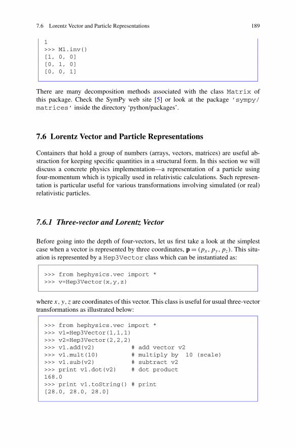
7.6 Lorentz Vector and Particle Representations 189
1>>> M1.inv()[1, 0, 0][0, 1, 0][0, 0, 1]
There are many decomposition methods associated with the class Matrix ofthis package. Check the SymPy web site [5] or look at the package ’sympy/matrices’ inside the directory ‘python/packages’.
7.6 Lorentz Vector and Particle Representations
Containers that hold a group of numbers (arrays, vectors, matrices) are useful ab-straction for keeping specific quantities in a structural form. In this section we willdiscuss a concrete physics implementation—a representation of a particle usingfour-momentum which is typically used in relativistic calculations. Such represen-tation is particular useful for various transformations involving simulated (or real)relativistic particles.
7.6.1 Three-vector and Lorentz Vector
Before going into the depth of four-vectors, let us first take a look at the simplestcase when a vector is represented by three coordinates, p = (px,py,pz). This situ-ation is represented by a Hep3Vector class which can be instantiated as:
>>> from hephysics.vec import *>>> v=Hep3Vector(x,y,z)
where x, y, z are coordinates of this vector. This class is useful for usual three-vectortransformations as illustrated below:
>>> from hephysics.vec import *>>> v1=Hep3Vector(1,1,1)>>> v2=Hep3Vector(2,2,2)>>> v1.add(v2) # add vector v2>>> v1.mult(10) # multiply by 10 (scale)>>> v1.sub(v2) # subtract v2>>> print v1.dot(v2) # dot product168.0>>> print v1.toString() # print[28.0, 28.0, 28.0]

190 7 Arrays, Matrices and Linear Algebra
Next, a four-momentum of a particle can be represented by four numbers: three-momentum p = (px,py,pz) and energy e. Similarly, a position of particle in spaceand time can be represented with four coordinates, (x, y, z, t), where t is time.This means that either position, in the momentum space or space-time, can bedescribed by four numbers. A class which can be used for such description isHepLorentzVector:
>>> from hephysics.vec import *>>> hp=HepLorentzVector(px,py,pz,e)
or, in the case of space-time:
>>> hp=HepLorentzVector(x,y,z,t)
There is a number of useful methods implemented for this class. First of all, onecan perform the standard arithmetic operations as with the usual three-vector. Onecan access angles and perform transformations as with any other vector representa-tion. Let us give a few examples:
>>> from hephysics.vec import *>>> # (px,py,pz,energy)=(10,20,30,100)>>> hp=HepLorentzVector(10,20,30,100)>>> print hp.mag() # magnitude of 3-vector>>> print hp.phi() # azimuthal angle>>> print hp.perp() # transverse momenta.>>> print hp.m() # invariant mass>>> print hp.theta() # polar angle>>> h.add(HepLorentzVector(1,2,3,10)) # add a new vector
The transverse momentum is calculated as√
px2 + py2, while the invariant mass is√e2 − px2 − py2 − pz2. Please refer to the corresponding API to find more meth-
ods of this class.Now let us show how to visualize an object of the HepLorentzVector class.
One natural way to do this is to use the 3D canvas HPlot3D, and show a Lorentzvector as a point with a symbol size proportional to the forth component (eitherenergy or time) as show below:
Visualizing a Lorenz vector
from jhplot import *from hephysics.vec import *
hp=HepLorentzVector(10,20,30,10)
c1 = HPlot3D("Canvas",600,400)c1.setGTitle("Lorenz Particle")

7.6 Lorentz Vector and Particle Representations 191
c1.setRange(0,100,0,100,0,100)c1.setNameX(’pX’); c1.setNameY(’pY’); c1.setNameZ(’pZ’)c1.visible()
p= P2D(’LorenzParticle’)p.setSymbolSize(int(hp.e()))p.add(hp.px(),hp.y(),hp.z())c1.draw(p)
7.6.2 Classes Representing Particles
A particle in the package hephysics can be represented by the two classes,LParticle (a “light-weight” class which is a direct extension of the classHepLorentzVector) and HEParticle. The latter contains not only the basicLorentz-type coordinates, but also can be characterized by a spin, parity and othercharacteristics which are typically used in particle physics. For simplicity, below wewill concentrate on the LParticle class.
The class LParticle can hold information about four-momentum, particlename and even another LParticle object representing a parent particle. Let uscreate a particle with the name “proton” and with a known mass (in MeV units):
>>> from hephysics.particle import *>>> p1=LParticle(’proton’,939.5)>>> p1.setPxPyPzE(10,20,30,300)
The second line of this code sets the three-momentum and energy. One can alsoset charge of this particle via the method setCharge(c). One can access theinformation about this particle using various “getter” methods which can be foundeither using the code assist or the class API.
As for any other Jython/ or Java object, one can create a list of particles and storethem in a file. In case of Java, use the ArrayList class, in case of Jython, one canuse a Jython list:
>>> from hephysics.particle import *>>> p1=LParticle(’proton’,939.5)>>> p1.setPxPyPzE(10,20,30,300)>>> p2=LParticle(’photon’,0.0)>>> p2.setPxPyPzE(1,2,3,30)>>> list=[p1,p2] # keep them in a list
The object list (as well as the objects of type LParticle) can be serialized intoa file as any other Java object to be discussed in Chap. 11. Particles can be visualized

192 7 Arrays, Matrices and Linear Algebra
in exactly the same way as shown for the HepLorentzVector class, since theclass LParticle is an extension of the class HepLorentzVector.
We will give detailed examples of how to work with the LParticle class inSect. 17.5 where we will discuss a simple Monte Carlo model for simulation ofparticle decays.
References
1. JMATHTOOLS Java Libraries. URL http://jmathtools.berlios.de2. The Colt Development Team: The COLT Project. URL http://acs.lbl.gov/~hoschek/colt/3. Hicklin, J., et al.: Jama, a Java Matrix Package. URL http://newcenturycomputers.net/projects/
dif.html4. Stewart, G.: Jampack, a Java package for matrix computations. URL ftp://math.nist.gov/pub/
Jampack/Jampack/5. SymPy Development Team: SYMPY: Python library for symbolic mathematics. URL http://
www.sympy.org

Chapter 8Histograms
A histogram is an elegant tool to project multidimensional data to lower dimensions,a tool which is designed for graphical representation and visual inspection.
A histogram is a summary graph showing counts of data points falling intovarious ranges, thus it gives an approximation of the frequency distribution ofdata.
The histogram shows data in the form of a bar graph in which the bar heightsdisplay event frequencies. Events are measured on the horizontal axis, X, which hasto be binned. The larger number of bins, the higher chances that a fine structure ofdata can be resolved. Obviously, the binning destroys the fine-grain information oforiginal data, and only the histogram content can be used for analysis.
In this respect, the histogram representation is useful if one needs to create astatistical snapshot of a large data sample in a compact form. Let us illustrate this:Assume we have N numbers, each representing a single measurement. One can storesuch data in a form of Java or Jython arrays. Thus, one needs to store 8 × N bytes(assuming 8 bytes to keep one number). In case of a large number measurements, weneed to be ready to store a very big output file, as the size of this file is proportionalto the number of events. Instead, one can keep for future use only the most importantstatistical summary of data, such as the shape of the frequency distribution and thetotal numbers of events. The information which needs to be stored is proportionalto the number of bins, thus the file storage has nothing to do with the size of theoriginal data.
8.1 One-dimensional Histogram
To create a histogram in one dimension (1D), one needs to define the number ofbins, Nbins, and the minimum (Min) and the maximum (Max) value for a certainvariable. The bin width is given by (Max-Min)/Nbins. If the bins are too wide
S.V. Chekanov, Scientific Data Analysis using Jython Scripting and Java,Advanced Information and Knowledge Processing,DOI 10.1007/978-1-84996-287-2_9, © Springer-Verlag London Limited 2010
193

194 8 Histograms
(Nbins is small), important information might get lost. On the other hand, if thebins are too narrow (Nbins is large), what may appear to be meaningful informa-tion really may be due to statistical variations of data entries in bins. To determinewhether the bin width is set to an appropriate size, different bin sizes should betried.
jHepWork histograms are designed on the bases of the JAIDA FreeHEP li-brary [1]. For an one-dimensional histogram, use the class H1D. To initialize anempty histogram, the following constructor can be used:
>>> from jhplot import *>>> h1=H1D(’data’, 100, 0, 20)
This creates a 1D histogram with the title ’data’, the number of bins Nbins=100, and the range of axis X to be binned, which is defined by the minimum andthe maximum values, Min=0 and Max=20. Thus, the bin width of this histogramis fixed to 0.2. The bin size and the number of bins are given by the followingmethods:
>>> d=h1.getBinSize()>>> i=h1.getBins()
We should note that a fixed-size binning is used. In the following sections, we willconsider a more general case when the histogram bin size is not fixed to a singlevalue.
The method fill(d) fills a histogram with a single value, where ’d’ is adouble number. The histograms can be displayed on the HPlot canvas using thestandard draw(h1) method.
We will discuss the main methods of the histogram class in the following section.Here, to illustrate the methods discussed before, we give a complete example of howto fill three histograms with Gaussian random numbers and then display them ondifferent pads.
Plotting histograms
from java.awt import Colorfrom java.util import Randomfrom jhplot import *
c1 = HPlot(’Canvas’,600,400,2,1)c1.visible()
h1 = H1D(’First’,20,-2.0,2.0)h1.setFill(1)h1.setFillColor(Color.green)
h2 = H1D(’Second’,100,-2.5,2.5)
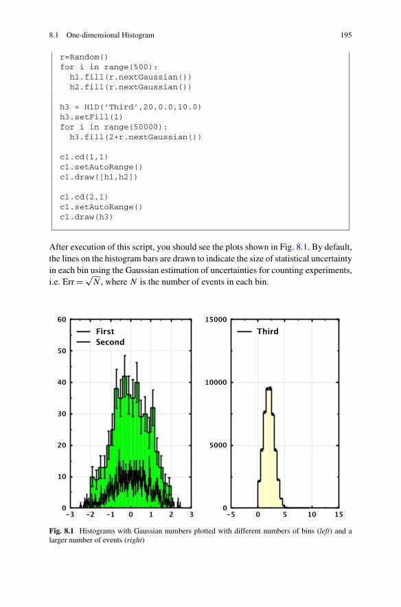
8.1 One-dimensional Histogram 195
r=Random()for i in range(500):
h1.fill(r.nextGaussian())h2.fill(r.nextGaussian())
h3 = H1D(’Third’,20,0.0,10.0)h3.setFill(1)for i in range(50000):
h3.fill(2+r.nextGaussian())
c1.cd(1,1)c1.setAutoRange()c1.draw([h1,h2])
c1.cd(2,1)c1.setAutoRange()c1.draw(h3)
After execution of this script, you should see the plots shown in Fig. 8.1. By default,the lines on the histogram bars are drawn to indicate the size of statistical uncertaintyin each bin using the Gaussian estimation of uncertainties for counting experiments,i.e. Err = √
N , where N is the number of events in each bin.
Fig. 8.1 Histograms with Gaussian numbers plotted with different numbers of bins (left) and alarger number of events (right)
196 8 Histograms
In the above script, we have used two new methods of the H1D class. Due to theirimportance, we will discuss them here:
setFill(b) fill a histogram area when b=1 (b=0 means the area is notfilled)
setFillColor(c) color for filling (Java AWT class)
As before, ’c’ denotes the Java Color class discussed in details in Sect. 3.3.1.The example above illustrates the following important features:
• The height of bins depends on the bin size. Even when the number of entries isthe same, histograms are difficult to compare in shape when the histogram binsare different, see Fig. 8.1 (left).
• Relative size of errors decreases with increasing the number of entries.
Below we will show a few basic manipulations useful for examining the shapesof histograms, assuming that the underlaying mechanism for occurrence of eventsreveals itself in shapes of event distributions, rather than in the overall statisticsor chosen bin size. The shape of the distributions is very important as it conveysinformation about the probability distribution of event samples.
First of all, let us get rid of the bin dependence. To do this, we will divide eachbin height by the bin size. Assuming that ’h1’ represents a histogram, this can bedone as:
>>> width=h1.getBinSize()>>> h1.scale(1/width)
After this operation, all histogram entries (including statistical uncertainties) will bedivided by the bin width. You may still want to keep a copy of the original histogramusing the method h2=h1.copy(), so one can come back to the original histogramif needed.
Different histograms can contain different normalization. In case if we are in-terested in the shapes only, one can divide each bin height by the total number ofhistogram entries. This involves another scaling:
>>> entries=h1.allEntries()>>> h1.scale(1/entries)
Obviously, both operations above can be done using one line:
>>> h1.scale(1/(h1.getBinSize()*h1.allEntries()))
The second step in comparing our histograms would be to shift the bins of thethird histogram. Normally, we do not know the exact shift (what should be donin this case will be considered later). At this moment, for the sake of simplicity,we assume that the shift is known and equals to −2. There is a special histogramoperation which does such shift:
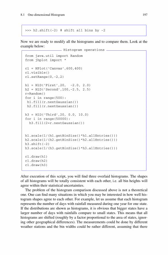
8.1 One-dimensional Histogram 197
>>> h2.shift(-2) # shift all bins by -2
Now we are ready to modify all the histograms and to compare them. Look at theexample below:
Histogram operations
from java.util import Randomfrom jhplot import *
c1 = HPlot(’Canvas’,600,400)c1.visible()c1.setRange(0,-2,2)
h1 = H1D(’First’,20, -2.0, 2.0)h2 = H1D(’Second’,100,-2.5, 2.5)r=Random()for i in range(500):h1.fill(r.nextGaussian())h2.fill(r.nextGaussian())
h3 = H1D(’Third’,20, 0.0, 10.0)for i in range(50000):
h3.fill(2+r.nextGaussian())
h1.scale(1/(h1.getBinSize()*h1.allEntries()))h2.scale(1/(h2.getBinSize()*h2.allEntries()))h3.shift(-2)h3.scale(1/(h3.getBinSize()*h3.allEntries()))
c1.draw(h1)c1.draw(h2)c1.draw(h3)
After execution of this script, you will find three overlaid histograms. The shapesof all histograms will be totally consistent with each other, i.e. all bin heights willagree within their statistical uncertainties.
The problem of the histogram comparison discussed above is not a theoreticalone. One can find many situations in which you may be interested in how well his-togram shapes agree to each other. For example, let us assume that each histogramrepresents the number of days with rainfall measured during one year for one state.If the distributions are shown as histograms, it is obvious that bigger states have alarger number of days with rainfalls compare to small states. This means that allhistograms are shifted (roughly by a factor proportional to the area of states, ignor-ing other geographical differences). The measurements could be done by differentweather stations and the bin widths could be rather different, assuming that there

198 8 Histograms
is no agreement between the weather stations about how the histograms should bedefined. Moreover, the measurements could be done during different time intervals,therefore, the histograms could have rather different numbers of entries. How onecan compare the results from different weather stations, if we are only interestedin some regularities in the rainfall distributions? The answer to this question is inthe example above: all histograms have to be: (1) normalized; (2) shifted; (3) a bindependence should be removed.
The only unclear question is how to find the horizontal shifts, since the normal-ization issue is rather obvious and can be done with the method discussed above.This problem will be addressed in the following chapters when we will discuss astatistical test that evaluates the “fit” of a hypothesis to a sample.
8.1.1 Probability Distribution and Probability Density
The examples above tell that there are several quantities which can be derived froma histogram. One can extract a probability distribution by dividing histogram entriesby the total number of entries. The second important quantity is a probability den-sity, when the probability distribution is divided by the bin width, so that the totalarea of the rectangles sums to one (which is, in fact, the definition of the probabilitydensity).
Both the probability distribution and the density distribution can be obtained afterdevisions of histogram entries as discussed above. However, these two characteris-tics can be obtained easier by calling the following methods:
>>> h2=h1.getProbability()>>> h2=h1.getDensity()
which return two new H1D objects: the first represents the probability distributionand the second returns the probability density. In addition to the obvious simplicity,such methods are very useful for variable-bin-size histograms, since this case istaken into account automatically during the devisions by bin widths.
Also note the following: one can save computation time in case of the calculationof the probability distributions if you know the total number of events (or entries)Ntot beforehand. In this case, one can obtain the probability distribution by usingthe weight w1 = 1.0/Ntot in the method fill(x,w1), without subsequent callto the method getProbability(). After the end of the fill, the histogram willrepresent the probability distribution normalized to unity by definition. In addition,one can remove the bin dependence by specifying the weight as w2 = 1.0/BinSize.Finally, the density distribution can be obtained using the weight w3 = w1 ∗ w2.
8.1.2 Histogram Characteristics
In this subsection we will continue to discuss the most important characteristics ofthe H1D histogram class.

8.1 One-dimensional Histogram 199
The most popular characteristics of a histogram are the median and the standarddeviations (RMS). Assuming that h1 represents a H1D histogram, both (double)values can be obtained as:
>>> d=h1.mean()>>> d=h1.rms()
We already know that one can obtain the number of entries with the methodallEntries(). However, some values could fall outside of the selected rangeduring the fill() method. Luckily, the histogram class has the following list ofmethods to access the number of entries:
>>> i=h1.allEntries() # all entries>>> i=h1.entries() # number entries in the range>>> i=h1.extraEntries() # under and overflow entries>>> i=h1.getUnderflow() # underflow entries>>> i=h1.getOverflow() # overflow entries
All the methods above return integer numbers.Another useful characteristics is the histogram entropy. It is defined to be the
negation of the sum of the products of the probability associated with each bin withthe base-2 log of the probability. One can get the value of the entropy with themethod:
>>> print ’Entropy=’,h1.getEntropy()
8.1.3 Histogram Initialization and Filling Methods
In this subsection we will consider the major histogram methods used for histograminitialization and filling. Previously, it has been shown how to initialize a histogramwith fixed bin sizes. One can also create a histogram using a simpler constructor,and then using a sequence of methods to set histogram characteristics:
>>> h1=H1D(’Title’)>>> h1.setMin(min)>>> h1.setMax(max)>>> h1.setBins(bins)
which are used to set the minimum, maximum and the number of bins. These meth-ods can also be useful to redefine these histogram characteristics after the histogramwas created using the usual approach.

200 8 Histograms
One can also build a variable bin-size histogram by passing a list with the binedges as shown in this example:
>>> bins=[0,10,100,1000]>>> h1=H1D(’Title’,bins)
This creates a histogram with three bins. The bin edges are given by the input list.This constructor is handy when a data is represented by a bell-shaped or fallingdistribution; in this case it is important to increase the bin size in certain regions(tails) in order to reduce statistical fluctuations.
As we already know, to fill a histogram with numbers, use the method fill(d).More generally, one can assign a weight “w” to each value as
>>> h1.fill(d, w)
where ’w’ is any arbitrary number representing a weight for a value ’d’. Theoriginal method fill(d) assumes that all weights are 1.
But why do we need weights? We have already discussed in Sect. 8.1.1 that theweights are useful to reduce the computational time when the expected final answershould be either a probability distribution or density distribution. There are alsoother cases when the weights are useful. We should note again that a histogramobject stores the sum of all weights in each bin. This sum runs over the number ofentries in a bin only when the weights are set to 1. Events may have smaller weightsif they are relatively unimportant compared to other events. It is up to you to makethis decision, this depends on a concrete situation.
The method fill(d) is slow in Jython when used inside loops, therefore, it ismore efficient to fill a histogram at once using the method fill(list), wherelist is an array with the numbers passed from another program or file. As be-fore, fill(list, wlist) can be used to fill a histogram from two lists. Eachnumber in list has an appropriate weight given by the second argument.
Instead of Jython (or Java) lists, one can pass a P0D array discussed in Sect. 4.2.3:
>>> h1.fill(p0d)
where p0d represents an object of the P0D class.Analogously, one can fill a histogram by passing a PND multidimensional ar-
ray discussed in Sect. 6.3. This can be done again with the method fill(pnd),where pnd is an array with any size or dimension. One can specify also weights inthe form of an additional PND object passed as a second argument to the methodfill(pnd, w).
Histograms can be filled with weights which are inversely proportional to the binsize—as it was shown in the previous section, removing the bin size dependence isone of the most common operations:

8.1 One-dimensional Histogram 201
>>> h1.fillInvBinSizeWeight(d)
It should be noted that this method works even when histograms have irregularbinning.
Finally, one can set the bin contents (bin heights and their errors) from an externalsource as shown below:
>>> h1.setContents(values, errors)>>> h1.setMeanAndRms(mean,rms)
where values and errors are input arrays. Together with the settings for the bincontent, the second line of the above example shows how to set the global histogramcharacteristics, such as the mean and the standard deviation. There are more meth-ods dealing with external arrays; advanced users can find appropriate methods in theAPI documentation of the class H1D or using the code assist.
8.1.4 Accessing Histogram Values
One-dimensional histograms based on the H1D class can easily be viewed using thefollowing convenient methods designed for visual inspection:
toString() convert a H1D histogram into a stringprint() print a histogramtoTable() show a histogram as a table
Once we know that a histogram is initialized and filled, the next question is toaccess the histogram values. We will be brief in this section, since most methods areobvious. Table 8.1 shows the most important H1D methods.
It should be noted that the bin heights and the numbers of entries are the samewhen histogram weights used to fill histogram are set to one, i.e. when the methodfill(d) is used.
Finally, one can view the H1D histograms using already known toTable()method. This method passes all histogram attributes to a pop-up table for easy visualinspection.
8.1.5 Integration
Histogram integration is similar to the F1D functions considered in the previouschapters: We simply sum up all bin heights. This can be done using the methodintegral(). More often, however, it is necessary to sum up heights in a certainbin region, say between a bin ’i1’ and ’i2’. Then use this method:
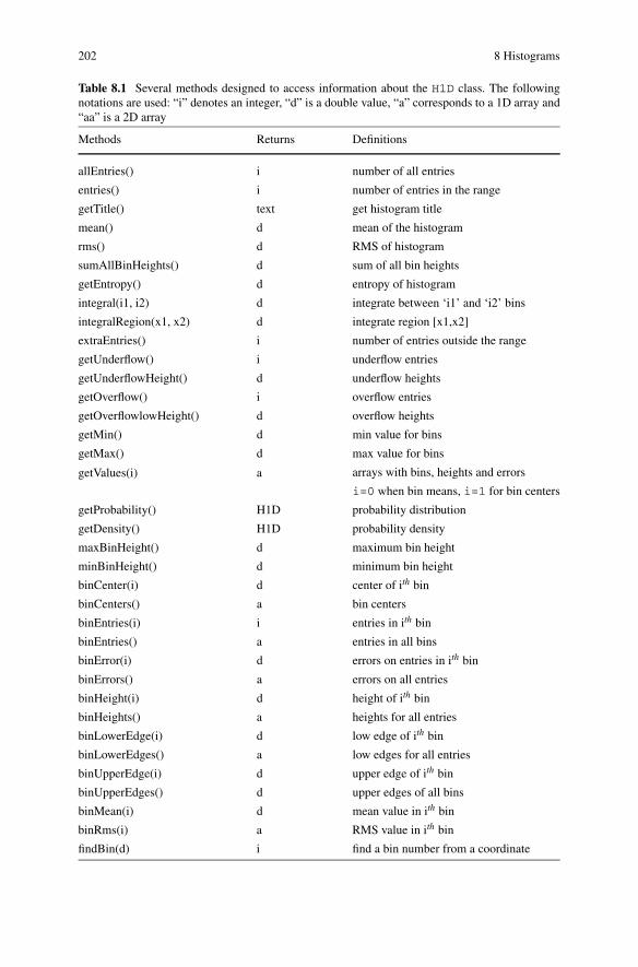
202 8 Histograms
Table 8.1 Several methods designed to access information about the H1D class. The followingnotations are used: “i” denotes an integer, “d” is a double value, “a” corresponds to a 1D array and“aa” is a 2D array
Methods Returns Definitions
allEntries() i number of all entries
entries() i number of entries in the range
getTitle() text get histogram title
mean() d mean of the histogram
rms() d RMS of histogram
sumAllBinHeights() d sum of all bin heights
getEntropy() d entropy of histogram
integral(i1, i2) d integrate between ‘i1’ and ‘i2’ bins
integralRegion(x1, x2) d integrate region [x1,x2]
extraEntries() i number of entries outside the range
getUnderflow() i underflow entries
getUnderflowHeight() d underflow heights
getOverflow() i overflow entries
getOverflowlowHeight() d overflow heights
getMin() d min value for bins
getMax() d max value for bins
getValues(i) a arrays with bins, heights and errors
i=0 when bin means, i=1 for bin centers
getProbability() H1D probability distribution
getDensity() H1D probability density
maxBinHeight() d maximum bin height
minBinHeight() d minimum bin height
binCenter(i) d center of ith bin
binCenters() a bin centers
binEntries(i) i entries in ith bin
binEntries() a entries in all bins
binError(i) d errors on entries in ith bin
binErrors() a errors on all entries
binHeight(i) d height of ith bin
binHeights() a heights for all entries
binLowerEdge(i) d low edge of ith bin
binLowerEdges() a low edges for all entries
binUpperEdge(i) d upper edge of ith bin
binUpperEdges() d upper edges of all bins
binMean(i) d mean value in ith bin
binRms(i) a RMS value in ith bin
findBin(d) i find a bin number from a coordinate

8.1 One-dimensional Histogram 203
>>> sum=h1.integral(i1,i2)
We should note that the integral is not just the number of events between these twobins: the summation is performed using the bin heights. However, if the weightsfor the method fill() are all set to one, then the integral is equivalent to thesummation of numbers of events.
The integration shown above does include multiplication by a bin width. If oneneeds to calculate an integral over all bins by multiplying the bin content by the binwidth (which can be either fixed or variable), use the method:
>>> sum=h1.integral(i1,i2,1)
where the last parameter should be set to 1 (or to ‘true’ in case of Java codding).The next question is how to integrate a region in X by translating X-coordinates
into the bin indexes. This can be done by calling the method findBin(x), whichreturns an index of the bin corresponding to a coordinate X. One can call thismethod every time when you need to identify the bin index before calling the methodintegrate(). Alternatively, this can be done in one line as:
>>> sum=integralRegion(xmin,xmax,b)
The method returns a value of the integral between two coordinates, xmin andxmax. The bin content will be multiplied by the bin width if the boolean value b isset to 1 (boolean ‘true’ in Java).
8.1.6 Histogram Operations
Histograms can be added, subtracted, multiplied and divided. Assuming that wehave filled two histograms, h1 and h2, all operations can be done using the follow-ing generic method:
>>> h1.oper(h2,’NewTitle’,’operation’)
where ’operation’ is a string which takes the following values: “+” (add), “-”(subtract), “*” (multiply) and “/” (divide). The operations are applied to the his-togram h1 using the histogram h2 as an input. One can skip the string with a newtitle if one has to keep the same title as for the original histogram. In this case, theadditive operation will look as h1.oper(h1,’+’)
To create an exact copy of a histogram, use the method copy(). Previously, wehave already discussed the scale(d) and shift(d) operations.
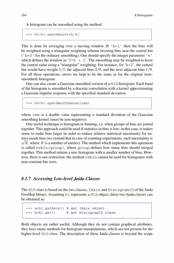
204 8 Histograms
A histogram can be smoothed using the method:
>>> h1=h1.operSmooth(b,k)
This is done by averaging over a moving window. If ’b=1’ then the bins willbe weighted using a triangular weighting scheme favoring bins near the central bin(’b=0’ for the ordinary smoothing). One should specify the integer parameter ’k’which defines the window as ‘2*k + 1’. The smoothing may be weighted to favorthe central value using a “triangular” weighting. For instance, for ‘k=2’, the centralbin would have weight 1/3, the adjacent bins 2/9, and the next adjacent bins 1/9.For all these operations, errors are kept to be the same as for the original (non-smoothed) histogram.
One can also create a Gaussian smoothed version of a H1D histogram. Each bandof the histogram is smoothed by a discrete convolution with a kernel approximatinga Gaussian impulse response with the specified standard deviation.
>>> h2=h1.operSmoothGauss(rms)
where rms is a double value representing a standard deviation of the Gaussiansmoothing kernel (must be non-negative).
One useful technique is histogram re-binning, i.e. when groups of bins are joinedtogether. This approach could be used if statistics in bins is low; in this case, it makessense to make bins larger in order to reduce relative statistical uncertainty for en-tries inside bins (we remind that in case of counting experiments, such uncertainty is√
N , where N is a number of entries). The method which implements this operationis called rebin(group), where group defines how many bins should mergedtogether. This method returns a new histogram with a smaller number of bins. How-ever, there is one restriction: the method rebin cannot be used for histograms withnon-constant bin sizes.
8.1.7 Accessing Low-level Jaida Classes
The H1D class is based on the two classes, IAxis and Histogram1D of the JaidaFreeHep library. Assuming h1 represents a H1D object, these two Jaida classes canbe obtained as:
>>> a=h1.getAxis() # get IAxis object>>> h=h1.get() # get Histogram1D class
Both objects are rather useful. Although they do not contain graphical attributes,they have many methods for histogram manipulations, which are not present for thehigher-level H1D class. The description of these Jaida classes is beyond the scope
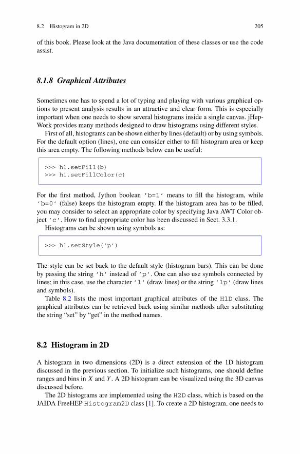
8.2 Histogram in 2D 205
of this book. Please look at the Java documentation of these classes or use the codeassist.
8.1.8 Graphical Attributes
Sometimes one has to spend a lot of typing and playing with various graphical op-tions to present analysis results in an attractive and clear form. This is especiallyimportant when one needs to show several histograms inside a single canvas. jHep-Work provides many methods designed to draw histograms using different styles.
First of all, histograms can be shown either by lines (default) or by using symbols.For the default option (lines), one can consider either to fill histogram area or keepthis area empty. The following methods below can be useful:
>>> h1.setFill(b)>>> h1.setFillColor(c)
For the first method, Jython boolean ’b=1’ means to fill the histogram, while’b=0’ (false) keeps the histogram empty. If the histogram area has to be filled,you may consider to select an appropriate color by specifying Java AWT Color ob-ject ’c’. How to find appropriate color has been discussed in Sect. 3.3.1.
Histograms can be shown using symbols as:
>>> h1.setStyle(’p’)
The style can be set back to the default style (histogram bars). This can be doneby passing the string ’h’ instead of ’p’. One can also use symbols connected bylines; in this case, use the character ’l’ (draw lines) or the string ’lp’ (draw linesand symbols).
Table 8.2 lists the most important graphical attributes of the H1D class. Thegraphical attributes can be retrieved back using similar methods after substitutingthe string “set” by “get” in the method names.
8.2 Histogram in 2D
A histogram in two dimensions (2D) is a direct extension of the 1D histogramdiscussed in the previous section. To initialize such histograms, one should defineranges and bins in X and Y . A 2D histogram can be visualized using the 3D canvasdiscussed before.
The 2D histograms are implemented using the H2D class, which is based on theJAIDA FreeHEP Histogram2D class [1]. To create a 2D histogram, one needs to

206 8 Histograms
Table 8.2 Methods for graphical representation of the H1D histograms. The following notationsare used: “i” means an integer, “d” means a double value, “b” corresponds to a boolean (“b=1”means Java true and “b=0” means false), “c” is Java AWT Color class
Methods Definitions
setStyle(“text”) “p”—show symbols, “l”—show lines
“lp”—lines and symbols, “h”—as histogram bars
setPenWidthErr(i) line width
setPenDash(i) dashed line style,
“i” is the length of dashed line
setColor(c) set color for drawing
setFill(b) b=1—fill histogram area (b=0 not fill)
setFillColor(c) set AWT Java color for fill area
setFillColorTransparency(d) set the transparency (0 ≤ d ≤ 1)
setErrX(b) show or not errors on X
setErrY(b) show or not errors on Y
setErrColorX(c) set Java color for errors on X
setErrColorY(c) set Java color for errors on Y
setSymbol(i) symbol type: 0: circle;
1: square; 2: diamond;
3: triangle; 4: filled circle;
5: filled square; 6: filed diamond;
7: filled triangle; 8: plus (+);
9: cross; 10: star; 11: small dot;
12: bold plus;
setSymbolSize(i) set symbol size “i”
define the number of bins for X and Y axis, and the minimum and the maximumvalues for each axis. Then the histogram can be initialized as:
>>> from jhplot import *>>> h2= H2D(’Title’,binsX,minX,maxX,binsY,minY,maxY)
where binsX(binsY) is the number of bins for X (Y ), minX(minY) andmaxX(maxY) are the minimum and the maximum values for the X (Y ) axis, re-spectively.
In addition to the fixed-bin-size case, one can create histograms with variable binsizes. One should call the constructor below which allows to pass lists with the binedges:
>>> from jhplot import *>>> h2= H2D(’Title’,[1,2,3],[1,2,4,8])

8.2 Histogram in 2D 207
This constructor shows how to define the bin edges in X (the first input list) and Y
(the second input list).To fill a 2D histogram, the method fill(x,y) should be used, where ’x’ and
’y’ values for the X and Y axis. It should be noted that the bin heights and thenumbers of entries are the same when weights used to fill the histogram are set toone. Non-unity weights ’w’ can be specified in the method fill(x,y,w).
Table 8.3 shows the main methods of the H2D histogram class. Unlike the H1Dhistogram, the H2D class has the setter and getter methods for each axis, X and Y .For example, getMeanX() returns the mean value in X, while getMeanY()returns the mean value in Y .
You may find that the methods given above are not enough for some com-plicated operations. We should remind that the H2D class is based on the Jaidaclasses, IAxis and Histogram2D, which are located in the Jaida packagehep.aida.ref.histogram.*. As a consequence, one can build H2D his-tograms by creating the object of the class IAxis , which represents the axis inone dimension, and then pass it to the H2D constructor.
>>> from hep.aida.ref.histogram import *>>> from jhplot import *>>> xAx=FixedAxis(10,0.0,1.0)>>> yAy=FixedAxis(20,0.0,1.0)>>> h2=H2D(’Title’,xAx,yAy)
Again, as for the one-dimensional case, both Jaida classes can be obtained as:
>>> aX=h2.getAxisX() # get IAxis object for axis X>>> aY=h2.getAxisY() # get IAxis object for axis Y>>> h=h2.get() # get Histogram2D class
assuming that h2 represents a H2D object. We will return to the Jaida histogrampackage in Sect. 8.3.
8.2.1 Histogram Operations
All histogram operations are exactly the same as for the H1D class discussed inSect. 8.1.6. The H2D histograms can be added, subtracted, multiplied and dividedusing the generic method:
>>> h1=h1.oper(h2,’NewTitle’,’operation’)
where ’operation’ is a string which can have the following values: “+” (add),“-” (subtract), “*” (multiply) and “/” (divide) histograms, and h1 and h2 are ob-jects of the class H2D. The histograms can be scaled using the method scale(d).

208 8 Histograms
Table 8.3 Some methods of the H2D class. The table uses the following notations: “i” indicatesan integer value, “d” means a double value, “a” corresponds to a 1D array, “aa” denotes a 2Darray
Methods Returns Definitions
fill methods
fill(x,y) – fill x and y
fill(x,y,w) – fill x and y with weight w
clear() – clean from all entries
getter methods
copy() H2D exact copy
getMeanX() d get the mean value in X
getMeanY() d get the mean value in Y
getRmsX() d get RMS in X
getRmsY() d get RMS in Y
getMinX() d get min value in X
getMaxX() d get max value in Y
getMinY() d get min value in Y
getMaxY() d get max value in Y
getBinsX() i number of bins in X
getBinsY() i number of bins in Y
allEntries() i number of all entries
entries() i number of entries in the range
getTitle() text get histogram title
sumAllBinHeights() d sum of all bin heights
extraEntries() i number of entries outside the range
getUnderflowX() i underflow entries in x
getUnderflowHeightX() d underflow heights in x
getUnderflowY() i underflow entries in y
getUnderflowHeightY() d underflow heights in y
getOverflowX() i overflow entries in x
getOverflowlowHeightX() d overflow heights in x
getOverflowY() i overflow entries in y
getOverflowlowHeightY() d overflow heights in y
binEntries(ix,iy) i entries in bins (ix,iy) bin
binError(ix,iy) d errors on a (ix,iy) bin
binHeight(ix,iy) d height of a (ix,iy) bin
getDensity() H2D density distribution
getProbability() H2D probability distribution
integral(i1,i2,j1,j2) d integral in the range
integralRegion(d1,d2,d1,d2) d integral in the range (coordinates)

8.2 Histogram in 2D 209
Table 8.3 (Continued)
Methods Returns Definitions
setter methods
setContents(d[][], e[][]) set heights and errors (double arrays)
setBinError(ix,iy,d) set the bin error for (ix,iy) bin
setMeanX(d) set the mean value for X
setMeanY(d) set the mean value for Y
setRmsX(d) set RMS for X
setRmsY(d) set RMS for Y
The probability and density distributions can be obtained as discussed inSect. 8.1.1:
>>> h2=h1.getProbability()>>> h2=h1.getDensity()
Finally, one can obtain the sum of the bin contents in the range defined in termsof the bin indexes or coordinate values using the methods shown in Sect. 8.1.5.
Finally, one can calculate an integral of histogram entries using theintegral() method. A histogram region can be integrated by passing bin in-dexes.
8.2.2 Graphical Representation
The 2D histograms should be plotted using the three-dimensional canvas HPlot3Dwhich has been used before to plot F2D functions. One can find more details inSect. 3.4. The example below shows how to fill and display a H2D histogram:
Filling 2D histogram
from jhplot import *from java.util import Randomc1 = HPlot3D(’Canvas’)c1.visible()c1.setNameX(’X axis’)c1.setNameY(’Y axis’)h1=H2D(’2D Test’,30,-3.0, 3.0, 30, -3.0, 3.0)r=Random()for i in range(1000):
h1.fill(r.nextGaussian(),r.nextGaussian())c1.draw(h1)
Here we fill a 2D histogram with Gaussian random numbers and then plot it us-ing exactly the same draw(obj) method (with obj being an object for drawing)method as for the F2D functions.

210 8 Histograms
Below we show a more complicated example. We will fill several histogramsusing Gaussian numbers after shifting the means for the sake of better illustration.In addition, we show how to: (1) plot two histograms on the same plot; (2) plot ahistogram and a 2D function on the same plot. In both cases, we use the methoddraw(obj1,obj2), where obj1 and obj2 could be either H2D or F2D object.
Multiple 2D histograms
from java.awt import Colorfrom java.util import Randomfrom jhplot import *
c1 = HPlot3D(’Canvas’,600,700, 2,2)c1.visible()c1.setGTitle(’H2D drawing options’)
h1=H2D(’H2D Test1’,30,-4.5,4.5,30,-4.0, 4.0)h2=H2D(’H2D Test 2’,30,-3.0, 3.0, 30, -3.0, 3.0)f1=F2D(’8*(x*x+y*y)’, -3.0, 3.0, -3.0, 5.0)
r=Random()for i in range(10000):
h1.fill(r.nextGaussian(),0.5*r.nextGaussian())h2.fill(1+0.5*r.nextGaussian(),-2+0.5*r.nextGaussian())
c1.cd(1,1)c1.setScaling(8)c1.setRotationAngle(30)c1.draw(h1)
c1.cd(1,2)c1.setScaling(8)c1.setColorMode(2)c1.setRotationAngle(30)c1.draw(h1,h2)
c1.cd(2,1)c1.setColorMode(4)c1.setLabelFontColor(Color.red)c1.setScaling(8)c1.setRotationAngle(40)c1.draw(f1,h2)
c1.cd(2,2)c1.setColorMode(1)c1.setScaling(8)c1.setElevationAngle(30)c1.setRotationAngle(35)c1.draw(h1)

8.2 Histogram in 2D 211
Fig. 8.2 H2D and F2D objects shown on the HPlot3D canvas using different styles
The resulting plots are shown in Fig. 8.2. One can see that the default drawingoption for the H2D is histogram bars. The 2D functions are usually shown using asurface-type representation.
We should note that, at the moment when this book was written, there was nosupport for drawing 2D histograms with variable bin sizes.
The 2D histograms (as well as 2D functions) can be shown as a contour (ordensity) plot, an alternative graphical method when each region in X and Y is rep-resented by different color, depending on the density population of each area withdata points. To show such plot, one can use the method setContour(). The smallcode snippet below illustrates this:
2D Contour histogram
from jhplot import *from java.util import Random
c1 = HPlot3D(’Canvas’,600,600)c1.setNameX(’X’)c1.setNameY(’Y’)

212 8 Histograms
Fig. 8.3 A H2D histogram shown as a contour plot
c1.setContour()c1.visible()
h1 = H2D(’Contour’,30,-3.0,3.0,30,-3.0,3.0)rand = Random()for i in range(100):
h1.fill(0.5*rand.nextGaussian(),rand.nextGaussian())c1.draw(h1)
The execution of this script brings up a window with the contour plot shown inFig. 8.3.
As for the F2D and P1D objects, one can use the canvas HPlot2D for showingH2D histograms. This canvas class was specifically designed to show the densityand contour plots as will be discussed in Sect. 10.11.
8.3 Histograms in Jaida
We have already mentioned that there is a way to access the so-called Jaida his-tograms from the FreeHep scientific library. Essentially, every histogram class injHepWork is a derivative of the corresponding Jaida class.
The Jaida histograms can be created after importing the Java packagehep.aida.ref.histogram. Generally, one can use the so-called Java fac-

8.3 Histograms in Jaida 213
tories to create the Jaida histograms. In this section, however, we will concentrateon a more basic histogram construction using Jaida.
Before building a Jaida histogram, first you have to define the “axis” object,which can either contain fixed or variable size bins. The example below shows howto create an one-dimensional Jaida histogram from the class Histogram1D:
>>> from hep.aida.ref.histogram import *>>> ax=FixedAxis(bins,min,max)>>> h1=Histogram1D(’name’,’title’,ax)
where ’bins’ represents the number of bins, ’min’ and ’max’ is the minimumand the maximum value for the X range. The code above builds a 1D Jaida his-togram using fixed-size bins. One should also specify the histogram name and itstitle. They may not need to be the same. The passed name is used for the internalJaida purpose, so one can just set it to the histogram title.
Using the code assist, try to check the available methods of the object h1. Youmay notice that they are rather similar to those of the H1D class. The only differenceis that the Histogram1D does not have any graphical attributes.
Analogously, one can build a Jaida histogram using a variable bin size. The codeis essentially the same, with the only one difference: the axis should be replaced bythe line with axis=VariableAxis(edges) with edges being an array withthe bin edges.
A two-dimensional Jaida histogram, Histogram2D can be constructed in asimilar way:
>>> from hep.aida.ref.histogram import *>>> ax=FixedAxis(binsX,minX,maxX)>>> ay=FixedAxis(binsY,minY,maxY)>>> h1=Histogram2D(’name’,’title’,ax,ay)
Again, to make a 2D histogram with variable bin sizes, use the VariableAxis()instead of FixedAxis.
To add graphical attributes to these Jaida classes, we have to move them to thefull-featured jHepWork histograms, H1D or H3D. One can do this rather easily byusing these constructors:
>>> from hep.aida.ref.histogram import *>>> from jhplot import *>>> h1d=H1D(h1) # build H1D from Jaida histogram>>> h2d=H2D(h2) # build H2D from Jaida histogram
One can retrieve the Jaida histograms back as:

214 8 Histograms
>>> h1=h1d.get() # get Histogram1D object>>> h2=h2d.get() # get Histogram2D object
But why do we need to use the Jaida histograms, if the jHepWork histogramsare direct derivatives of the corresponding Jaida classes? The answer is simple:jHepWork does not map every single method of the Jaida histogram classes. Inmost cases, jHepWork histograms inherent only the most common methods (andadd extra methods not present in Jaida). Therefore, if you find that jHepWork his-tograms do not have necessary methods, try to access the IAxes, Histogram1Dand Histogram2D objects that may have the methods you need for your work.
8.4 Histogram in 3D
Histograms in three dimensions are a bit tricky. One cannot use them for a graphicalrepresentation, therefore, jHepWork does not add extra features compared to thosepresent in the Jaida Histogram3D class.
In jHepWork, 3D histograms are implemented using the H3D class. In case of afixed-size binning, these histograms can be defined by building three axes in X, Y
and Z, and passing them to the histogram constructor:
>>> from jhplot import *>>> from hep.aida.ref.histogram import *>>> ax=FixedAxis(binsX,minX,maxX)>>> ay=FixedAxis(binsY,minY,maxY)>>> az=FixedAxis(binsZ,minZ,maxZ)>>> h3=H3D(’title’, ax, ay, az)
The methods of the H3D class are rather similar to those discussed for H2D.The only difference is this: now we should take care of the additional Z axis.For example, to fill this histogram with weights, one needs to use the methodfill(x,y,z). We remind again that this type of histograms does not haveany graphical attributes—essentially, it is the exact mapping of the correspondingHistogram3D Jaida class.
8.5 Profile Histograms
A profile histogram is used to show the mean value in each bin of a second variable.The errors on the bin heights usually represent statistical uncertainties on the meanvalues or data spreads (i.e. standard deviations) of event distributions inside bins.
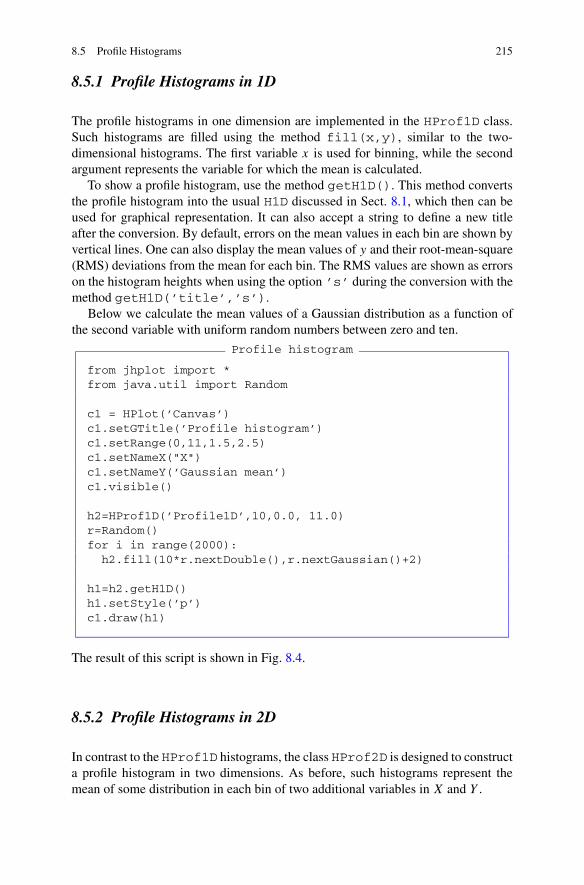
8.5 Profile Histograms 215
8.5.1 Profile Histograms in 1D
The profile histograms in one dimension are implemented in the HProf1D class.Such histograms are filled using the method fill(x,y), similar to the two-dimensional histograms. The first variable x is used for binning, while the secondargument represents the variable for which the mean is calculated.
To show a profile histogram, use the method getH1D(). This method convertsthe profile histogram into the usual H1D discussed in Sect. 8.1, which then can beused for graphical representation. It can also accept a string to define a new titleafter the conversion. By default, errors on the mean values in each bin are shown byvertical lines. One can also display the mean values of y and their root-mean-square(RMS) deviations from the mean for each bin. The RMS values are shown as errorson the histogram heights when using the option ’s’ during the conversion with themethod getH1D(’title’,’s’).
Below we calculate the mean values of a Gaussian distribution as a function ofthe second variable with uniform random numbers between zero and ten.
Profile histogram
from jhplot import *from java.util import Random
c1 = HPlot(’Canvas’)c1.setGTitle(’Profile histogram’)c1.setRange(0,11,1.5,2.5)c1.setNameX("X")c1.setNameY(’Gaussian mean’)c1.visible()
h2=HProf1D(’Profile1D’,10,0.0, 11.0)r=Random()for i in range(2000):
h2.fill(10*r.nextDouble(),r.nextGaussian()+2)
h1=h2.getH1D()h1.setStyle(’p’)c1.draw(h1)
The result of this script is shown in Fig. 8.4.
8.5.2 Profile Histograms in 2D
In contrast to the HProf1D histograms, the class HProf2D is designed to constructa profile histogram in two dimensions. As before, such histograms represent themean of some distribution in each bin of two additional variables in X and Y .

216 8 Histograms
Fig. 8.4 A profile histogramshowing the mean values as afunction of a second variable
A HProf2D histogram can be created by specifying the number of bins in X andY , as well as the minimum and maximum values for each axis. Alternatively, one canpass arrays with the bin edges, if the bin sizes should not be fixed to a constant value.The HProf2D histograms should be converted to H2D histograms (see Sect. 8.1) forgraphical representation. The conversion can be done by either calling the methodgetH2D() (error on the mean in each bin) or getH2D(’title’,’s’) (errorscorrespond to RMS in each bin). Obviously, the HPlot3D canvas should be usedfor plotting.
Below we show a simple example of how to display the mean of a Gaussiandistribution in two dimensions.
2D profile histogram
from jhplot import *from java.util import Random
c1 = HPlot3D(’Canvas’)c1.setGTitle(’Gaussian mean’)c1.setRange(0,10,0.0,5)c1.setNameX(’X’)c1.setNameY(’Y’)c1.visible()
h2=HProf2D(’Profile2D’,10,0.0,10.0,10,0.0,5.0)r=Random()for i in range(5000):
x=10*r.nextDouble()y=5*r.nextDouble()z=r.nextDouble()+2h2.fill(x,y,z)
c1.draw( h2.getH2D() )

8.6 Histogram Input and Output 217
8.6 Histogram Input and Output
All the histograms discussed above can be written into files and restored later. Asexample, one can use the method toFile() to write a histogram into a file. Asfor any jHepWork object, one can save collections of histograms using Jython lists,tuples or dictionaries. Alternatively, one can use the Java containers, such as arrays,sets or maps.
In case of Jython lists, one should always remember the order that was used tostore histograms inside the lists. In case of Jython dictionaries or Java maps, onecan use a human-readable description as the key for each histogram entry. Belowwe illustrate how to use a Jython dictionary to store several histograms (includingtheir graphical attributes) in a serialized file: The code below writes a collection ofhistograms filled with random numbers into the file ’file.ser’:
Writing histograms
from jhplot import *from jhplot.io import *from java.awt import Colorfrom java.util import Random
hold = {} # define a dictionary
h1=H1D(’Simple1’,20,-2.0,2.0)h1.setFill(1)h1.setFillColor(Color.green)h2=H2D(’Simple2’,20,-3.0, 3.0, 20, -3.0, 3.0)h3=HProf1D(’Profile1D’,10,0.0, 11.0)
r=Random()for i in range(1000):
h1.fill(r.nextGaussian())h2.fill(r.nextDouble(),r.nextGaussian())h3.fill(10*r.nextDouble(),r.nextGaussian()+50)
# put all objects in a dictionary with descriptionhold[’describe’]=’Collection of histograms’hold[’h1’]=h1hold[’h2’]=h2hold[’h3’]=h3
# write the collection into a fileSerialized.write(hold,’file.ser’)
Next, we will restore the histograms from the written file. First, we will read thedictionary and then will fetch all the histograms from the file using their keys:

218 8 Histograms
Reading histograms
from jhplot import *from jhplot.io import *
c1 = HPlot(’Canvas’)c1.visible()c1.setAutoRange()
# deserialize dictionary objecthold=Serialized.read(’file.ser’)
# print all keysprint hold.keys()print ’Description: ’+hold[’describe’]
# draw two 2D histogramsc1.draw(hold[’h1’])c1.draw(hold[’h3’].getH1D())
In this example, we draw two histograms retrieved from the serialized file, H1D andHProf1D. The latter histogram has to be converted to a H1D object for visualiza-tion. We will remind that, in order to draw the H2D histogram, we will need a 3Ddrawing canvas, HPlot3D.
Serializations into XML files can be done using the writeXML() andreadXML() methods from the same Serialization class. In addition, onecan convert a histogram into a XML string using the toXML() method.
Finally, we recall that one can store and retrieve multiple objects, including jHep-Work histograms, using the class HFile. It is designed to work with a large se-quence of any Java objects (see Chap. 11 for detail). In addition, one can use a GUIbrowser to look at all stored objects inside the files created with the class HFileand then plot them.
8.6.1 External Programs for Histograms
8.6.1.1 CFBook Package
Histograms can be filled by an external C++ or FORTRAN program. For this,use the CFBook [2] or CBook [3] packages. The first package can be used to fillhistograms from a C++ or FORTRAN program, and write them into specially de-signed XML files (which are optimized for storing numerical data). The secondpackage is based on compressed records constructed using the Google’s ProtocolBuffers. This approach will be discussed in Sect. 11.4.
The package CFBook package generates two static libraries: libcbook.a (tobe linked with C++) or libfbook.a (to be linked with FORTRAN). Histograms

8.6 Histogram Input and Output 219
filled by the CFBook library can be retrieved and visualized using the HBook class.Let us give one example. We assume that histograms are filled by a C++ externalprogram and are kept in the ’cpp.xml’. One can read and retrieve histogramsfrom this file as:
>>> from jhplot import *>>>>>> hb = HBook() # create HBook instance>>> hb.read(’cpp.xml’) # read input XML file>>> print hb.listH1D() # list all histograms>>> h1 = hb.getH1D(10) # get H1D histogram with ID=10>>> c1.draw(h1) # draw it
In the code above, ’c1’ represents an instance of the HPlot class.The HBook class can also be used to save histograms or other objects into XML
files. In this case, one should use its method write():
>>> from jhplot import *>>>>>> hb = HBook(’hbook’)>>> h3=H1D(’test’,2,0.0,1.)>>> h4=H2D(’test’,5,0.0,1.,4,0.,1.)>>> hb.add(30,h3) # add to HBook with ID=30>>> hb.add(40,h3) # add to HBook with ID=40>>> p1=P1D(’test") # create P1D objects>>> hb.add(10,p1) # add to HBook with ID=10>>> print hb.listH1D() # list all histograms>>> h1 = hb.getH1D(30) # get H1D histogram with ID=30>>> ...>>> hb.write(’out.xml’) # write to an XML file
This example illustrates that one can insert the histogram H1D, H2D or even thecontainers like P1D into the HBook holder using some identification numbers(10,20,30). These numbers can be used later for object retrieval. Also, we showhow to write all such objects into an external XML file.
8.6.1.2 ROOT Package
jHepWork can also read histograms saved into ROOT files [4, 5]. One can readROOT histograms using Jython scripts or using a GUI browser in order to navigateto a certain histogram object inside the ROOT files. These topics will be discussedin Sect. 11.5.1.
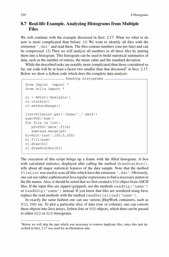
220 8 Histograms
8.7 Real-life Example. Analyzing Histograms from MultipleFiles
We will continue with the example discussed in Sect. 2.17. What we what to donow is more complicated than before: (1) We want to identify all files with theextension ’.dat’ and read them. The files contain numbers (one per line) and canbe compressed. (2) Then we will analyze all numbers in all these files by puttingthem into a histogram. This histogram can be used to build statistical summaries ofdata, such as the number of entries, the mean value and the standard deviation.
While the described tasks are notably more complicated than those considered sofar, our code will be at least a factor two smaller than that discussed1 in Sect. 2.17.Below we show a Jython code which does the complete data analysis:
Reading histograms
from jhplot import *from utils import *
c1 = HPlot(’Analysis’)c1.visible()c1.setAutoRange()
list=FileList.get(’/home/’,’.dat$’)sum=P0D(’sum’)for file in list:
p0=P0D(’data’,file)sum=sum.merge(p0)
h1=H1D(’test’,100,0,200)h1.fill(sum)c1.draw(h1)c1.drawStatBox(h1)
The execution of this script brings up a frame with the filled histogram. A boxwith calculated statistics, displayed after calling the method drawStatBox(),tells about all major statistical features of the data sample. Note that the methodFileListwas used to scan all files which have the extension ’.dat’. Obviously,one can use rather sophisticated Java regular expressions to find a necessary patten inthe file names. Also, it should be noted that we first created a P0D object from ASCIIfiles. If the input files are zipped (gzipped), use the methods readZip(’name’)or readGZip(’name’) instead. If you know that files are serialized using Java,replace the read methods with the method readSerialized(’name’).
In exactly the same fashion one can use various jHepWork containers, such asP1D, PND etc. To plot a particular slice of data (row or column), one can convertthese objects into Java arrays, Jython lists or P0D objects, which then can be passedto either H1D or H2D histograms.
1Below we will skip the part which was necessary to remove duplicate files, since this task de-scribed in Sect. 2.17 was used for an illustration only.

References 221
References
1. FreeHEP Java Libraries. URL http://java.freehep.org/2. Chekanov, S.: CFBOOK histogram library. URL http://jwork.org/jhepwork/cbook3. Chekanov, S.: CBOOK histogram library. URL http://jwork.org/jhepwork/cbook4. Brun, R., Rademakers, F., Canal, P., Goto, M.: Root status and future developments. ECONF
C0303241 (2003) MOJT0015. Brun, R., Rademakers, F.: ROOT: An object oriented data analysis framework. Nucl. Instrum.
Methods A 389, 81 (1997). URL http://root.cern.ch/


Chapter 9Random Numbers and Statistical Samples
A random number, i.e. a number chosen by chance from a specified distribution, isan essential concept for many scientific areas, especially for simulations of physicalsystems using Monte Carlo methods.
For a set with random numbers, no individual number can be predicted fromknowledge of any other number or group of numbers. However, sequences of ran-dom numbers in a computer simulation eventually contain repeated numbers aftergeneration of many millions of random numbers. Thus, it is only a good approxi-mation to say that the numbers are random, and the definition “pseudo-random” ismore appropriate.
Another notion which is usually associated with a sequence of random numbersis the so-called “seed” value. This is a number that controls whether the randomnumber generator produces a new set of random numbers after the code executionor repeats a certain sequence.
For debugging of programs, it is often necessary to start generating exactly thesame random number sequence every time you start the program. In this case, oneshould initialize a random number generator using the same seed number.
The seed must be changed for each run if you want to produce completely dif-ferent sets of random numbers every time the program is executed. Usually, this canbe done by generating a new seed using the current date and time, converted to aninteger value.
9.1 Random Numbers in Jython
This section is going to be very short, since we have discussed this topic in Sect. 2.8.The standard Jython (as well as CPython) module that implements a random num-ber generator is called ’random’. It must be imported using the usual statementimport.
As before, it is advisable to use the standard jHepWork libraries to create arrayswith random numbers where possible, instead of filling lists with random valuesusing Jython loops. There are two reasons for this: (1) less chances that a mistake
S.V. Chekanov, Scientific Data Analysis using Jython Scripting and Java,Advanced Information and Knowledge Processing,DOI 10.1007/978-1-84996-287-2_10, © Springer-Verlag London Limited 2010
223

224 9 Random Numbers and Statistical Samples
can be made; (2) programs based on the standard Java libraries are significantlyfaster. Look at the examples below: the first program is rather inefficient (and long),while the second code snippet is a factor five faster (and shorter). Both programs fillhistograms with random numbers in the range between 0 and 100 and show them ina canvas.
Jython random numbers
from java.util import Randomfrom jhplot import *from time import clock
start=clock()h1 = H1D(’Uniform distribution’,100, 0.0, 100.0)
rand = Random()for i in range(2000000):
h1.fill(100*rand.nextDouble())
c1 = HPlot(’Canvas’)c1.visible()c1.setAutoRange()
c1.draw(h1)send=clock()print ’Time elapsed = ’,send-start,’ seconds’
The program below does the same, but it is faster by a factor seven:
jHepWork random numbers
from jhplot import *from time import clockfrom jhplot.math.StatisticSample import randUniform
start=clock()# fill histogram with random numbersh1 = H1D(’Uniform distribution’,100, 0.0, 100.0)h1.fill( randUniform(2000000,0.0,100.0) )
c1 = HPlot(’Canvas’)c1.visible()c1.setAutoRange()c1.draw(h1)send=clock()print ’Time elapsed = ’, send-start,’ seconds’
Here we recall that the method fill() of the class H1D accepts not only separatevalues, but also arrays of different type—in this case, we build such array on-flyusing the method randUniform().

9.2 Random Numbers in Java 225
Below we will discuss in more detail how to use pre-build libraries from jHep-Work and third-party libraries. But first will discuss the most common classes togenerate random numbers in Java.
9.2 Random Numbers in Java
Random numbers provided by Java API have already been used in the previoussections. Let us remind that the class Random can be used to generate a singlerandom number. Below we check the methods of this class:
>>> from java.util import *>>> r=Random() # seed from the system time.>>> r=Random(100L) # user defined seed=100L>>> dir(r)[.. ’nextDouble’, ’nextFloat’, ’nextGaussian’,...’nextInt’, ’nextLong’ ..]
In the first definition, the default seed comes from the computer system time. Inthe second example, we initiate the random sequence from an input value to obtainreproducible results for every program execution.
Below we describe the most common methods to generate random numbers: Asusual, ’i’ denotes an integer, ’l’ represents a long integer, ’d’ means a doublevalue while ’b’ corresponds to a boolean value.
i=r.nextInt(n) random int ≥ 0 and ≤ n
i=r.nextInt() random int (full range)l=r.nextLong() random long (full range)d=r.nextDouble() random double ≥ 0.0 and ≤ 1.0b=r.nextBoolean() random boolean, true (1) or false (0)d=r.nextGaussian() double from a Gaussian distribution with mean 0.0 and
standard deviation 1
To build a list containing random numbers, invoke a Jython loop. For example,this code typed using JythonShell builds a list with Gaussian random numbers:
>>> from java.util import *>>> r=Random()>>> g=[]>>> for i in range(100):>>> ... g.append(r.nextGaussian())
It was already discussed before that Jython loops are not particularly fast, therefore,it is recommended to use the predefined jHepWork methods to build lists. This isalso not the only problem: using the predefined methods to build collections withrandom numbers grantees that the code is sufficiently short and free of errors.

226 9 Random Numbers and Statistical Samples
9.3 Random Numbers from the Colt Package
The Colt package provides a comprehensive list of methods to create ran-dom numbers. The classes necessary to build random numbers come from thepackage cern.jet. As example, let us consider a generation of reproduciblerandom numbers using the MersenneTwister class from the sub-packagerandom.engine. The macro below creates an array P0D with random numbersand then prints the statistical summary of a Gamma distribution:
Colt random numbers
from cern.jet.random.engine import *from cern.jet.random import *engine = MersenneTwister()alpha=1lamb=0.5gam=Gamma(alpha,lamb,engine)from jhplot import P0Dp0=P0D()for i in range(100):
p0.add(gam.nextDouble())print p0.getStat()
Here we used the so-called “Mersenne-Twister” algorithm, which is one of thestrongest uniform pseudo-random number generators. We did not specify any ar-gument for the engine, therefore, the seed is set to a constant value and the output istotally reproducible. One can use the current system date for a seed to avoid repro-ducible random numbers:
>>> import java>>> engine=MersenneTwister(new java.util.Date())
Learn about all possible methods of this package as usual:
>>> import cern.jet.random>>> dir(cern.jet.random)
The above command prints the implemented distributions:
Beta, Binomial, BreitWigner, BreitWignerMeanSquare,ChiSquare, Empirical, EmpiricalWalker, Exponential,ExponentialPower, Gamma, Hyperbolic, HyperGeometric,Logarithmic, NegativeBinomial, Normal, Poisson,PoissonSlow, StudentT, Uniform, VonMises, Zeta
All these classes operate on a user supplied uniform random number generator.
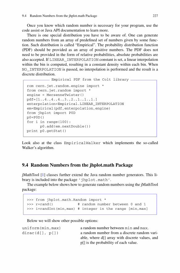
9.4 Random Numbers from the jhplot.math Package 227
Once you know which random number is necessary for your program, use thecode assist or Java API documentation to learn more.
There is one special distribution you have to be aware of. One can generaterandom numbers from an array of predefined set of numbers given by some func-tion. Such distribution is called “Empirical”. The probability distribution function(PDF) should be provided as an array of positive numbers. The PDF does notneed to be provided in the form of relative probabilities, absolute probabilities arealso accepted. If LINEAR_INTERPOLATION constant is set, a linear interpolationwithin the bin is computed, resulting in a constant density within each bin. WhenNO_INTERPOLATION is passed, no interpolation is performed and the result is adiscrete distribution.
Empirical PDF from the Colt library
rom cern.jet.random.engine import *from cern.jet.random import *engine = MersenneTwister()pdf=[1.,4.,4.,4.,3.,2.,1.,1.,1.]enterpolation=Empirical.LINEAR_INTERPOLATIONem=Empirical(pdf,enterpolation,engine)from jhplot import P0Dp0=P0D()for i in range(100):
p0.add(em.nextDouble())print p0.getStat()
Look also at the class EmpiricalWalker which implements the so-calledWalker’s algorithm.
9.4 Random Numbers from the jhplot.math Package
jMathTool [1] classes further extend the Java random number generators. This li-brary is included into the package ’jhplot.math’.
The example below shows how to generate random numbers using the jMathToolpackage:
>>> from jhplot.math.Random import *>>> r=rand() # random number between 0 and 1>>> i=randInt(min,max) # integer in the range [min,max]
Below we will show other possible options:
uniform(min,max) a random number between min and max.dirac(d[], p[]) a random number from a discrete random vari-
able, where d[] array with discrete values, andp[] is the probability of each value.

228 9 Random Numbers and Statistical Samples
normal(m,s) a random number from a Gaussian (Normal)distribution with the mean (‘m’) and the stan-dard deviation (‘s’).
chi2(i) a random number from a ξ2 random variablewith ‘i’ degrees of freedom.
logNormal(m,s) a LogNormal random variable with the mean(‘m’) and the standard deviation (‘s’).
exponential(lam) a random number from an exponential distribu-tion (mean = 1/lam, variance = 1/lam**2).
triangular(min,max) a random number from a symmetric triangulardistribution.
triangular(min,med,max) a random number from a non-symmetric trian-gular distribution (“med” means a value of therandom variable with max density).
beta(a,b) a random number from a Beta distribution. ‘a’and ‘b’ is the first and second parameter of theBeta random variable.
cauchy(med,s) a random number from a Cauchy distribution(Mean = Inf, and Variance = Inf). ‘med’ isa median of the Weibull random variable, ‘s’is the second parameter of the Cauchy randomvariable.
weibull(lam,c) a random number from a Weibull distribution.“lam” is the first parameter of the Weibull ran-dom variable, ‘c’ is the second parameter of theWeibull random variable.
Finally, one can generate a random number from an analytical function usingthe known rejection method. This requires building a F1D function first and thenpassing its parsed object to the rejection() method. Below we show how thiscan be done:
>>> from jhplot import *>>> from jhplot.math.Random import *>>> f=F1D(’x*exp(x)’,1,2)>>> p=f.getParse()>>> print rejection(p,15,1,2)1.4
The method rejection() takes three arguments: a parsed function, a maximumvalue of the function (15 in this case) and a minimum and a maximum value forthe abscissa. The method returns a random number between 1 and 2, since thesenumbers have been specified in the rejection() method.

9.5 Random Sampling 229
9.4.1 Apache Common Math Package
Random numbers can also be generated using the Apache common math package.A random generator can be initialized using the RandomDataImpl() class. Then,call its methods to generate a random number. The code below shows how to gen-erate a single random number from different distributions:
>>> from org.apache.commons.math.random import *>>> r=RandomDataImpl()>>> dir(r) # check all methods>>> d=r.nextUniform(0,1) # a random number in [0,1]>>> d=r.nextExponential(1) # Exponential with the mean 1>>> d=r.nextGaussian(0,1) # Gaussian (mean=0 and sigma=1)>>> d=r.nextPoisson(1) # Poisson with mean 1>>> s=r.nextHexString(10) # hex string of length len
Check the corresponding API documentation for more options. One can reseed therandom numbers using the reSeed() method (it sets the seed of the generator tothe current computer time in milliseconds). One can also reseed the random numbergenerator with the supplied seed using the method reSeed(i), where ’i’ is anarbitrary integer number.
There are also the so-called “secure” methods, much are slower than those givenabove. A secure random sequence has the additional property that knowledge of val-ues generated up to any point in the sequence does not make it any easier to predictsubsequent values. Such values are useful for a cryptographically secure random se-quence. As an example, check the method nextSecureHexString(10) whichgenerates a “secure” random string of size ten.
9.5 Random Sampling
When one needs to create a large array with random numbers obeying some prob-ability distribution, it is inconvenient (and slow!) to create data containers usingJython loops as shown at the beginning of this chapter. Instead, one should use theJava libraries implementing generations of arrays with random numbers.
We have already discussed in Sect. 4.1 how to build a P0D and populate it withrandom numbers:
>>> from jhplot import *>>> p0= P0D()>>> p0.randomUniform(1000,0.0,1.0) # Uniform distribution>>> p0.randomNormal(1000,0.0,1.0) # Gaussian distribution

230 9 Random Numbers and Statistical Samples
In both cases we will fill an array with 1000 numbers populated by either a uniformrandom generator (in the range [0–1]) or a Gaussian generator with the mean zero,and with the standard deviation equals unity.
Below we will consider more options that specify how to fill the P0Dwith customrandom numbers.
9.5.1 Methods for 1D Arrays from jhplot.math
Static methods of the package ’jhplot.math’ can also be useful to generatearrays with random numbers. We remind that the package is based on the originalclass of jMathTools [1].
We will start from a simple example of how to create an array of size 10 withrandom integer numbers distributed between 0 and 100. After creation, we print outthe array:
>>> from jhplot.math.StatisticSample import *>>> a=randomInt(10,0,100)>>> print aarray(’i’,[93, 19, 70, 36, 55, 43, 52, 50, 67, 38])
Analogously, randUniform(N,min,max) generates ’N’ random numbersuniformly distributed between ’min’ and ’max’.
Below we show a list of methods designed to generate arrays with random num-bers:
randomDirac(N,d[],p[]) a random array from a discrete randomvariable, where d[] array with discretevalues and p[] is the probability of eachvalue.
randomNormal(N,m,s) a Gaussian (Normal) random numberswith the mean (“m”) and standard devi-ation (“s”).
randomChi2(N,i) a random array with ξ2 random numberswith ‘i’ degrees of freedom.
randomLogNormal(N,m,s) a random array with a LogNormal ran-dom numbers.
randomExponential(N,lam) an array with an exponential random vari-able (mean = 1/lam, variance = 1/lam2).
randomTriangular(N,m1,m2) an array with symmetric triangular ran-dom variable in the range [m1,m2].
randomTriangular(N,m1,m,m2) an array from a non-symmetric triangularrandom distribution in the range [m1,m2](‘m’ indicates a value of the random vari-able with the maximal density).

9.5 Random Sampling 231
randomBeta(N,a,b) an array with Beta distribution, “a” and“b” are first and second parameter of theBeta random variable.
randomCauchy(N,m,s) an array from a Cauchy random distribu-tion (Mean = Inf, and Variance = Inf).‘m’ is the median of the Weibull randomvariable, ‘s’ is second parameter of theCauchy random variable.
randomWeibull(N,lam,c) an array with Weibull random variable.‘lam’ is the first parameter of the Weibullrandom variable (‘lam’), ‘c’ is the secondparameter of the Weibull random vari-able.
In all cases, the names of the methods are exactly the same as those shown inSect. 9.4. The only difference now is in the extra argument “N” which specifies howmany random values should be generated in the output arrays.
Obviously, once a sequence of random numbers is generated, the next step wouldbe to verify it. This can be done as following:
• Convert the random array into a P0D object;• Display accumulated statistics with the method getStat() or convert it to aH1D histogram for visualization.
As example, let us generate an array with log-normal distribution, print statisticsand plot log-normal distribution in a form of histogram:
Checking random numbers
from jhplot import *from jhplot.math.StatisticSample import *
a=randomLogNormal(1000,0,10)p0=P0D(a)print p0.getStat()
h=H1D(’LogNormal’,40,-50,50)h.fill(a)
c1 = HPlot(’Show histogram’)c1.setGTitle(’LogNormal’)c1.visible()c1.setAutoRange()c1.draw(h)
By running this script you will see a very detailed statistical summary of the log-normal distribution, plus a histogram with random numbers from this distribution.
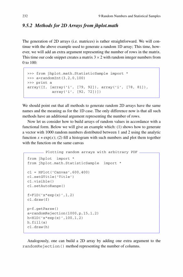
232 9 Random Numbers and Statistical Samples
9.5.2 Methods for 2D Arrays from jhplot.math
The generation of 2D arrays (i.e. matrices) is rather straightforward. We will con-tinue with the above example used to generate a random 1D array; This time, how-ever, we will add an extra argument representing the number of rows in the matrix.This time our code snippet creates a matrix 3×2 with random integer numbers from0 to 100:
>>> from jhplot.math.StatisticSample import *>>> a=randomInt(3,2,0,100)>>> print aarray([I, [array(’i’, [79, 92]), array(’i’, [78, 81]),
array(’i’, [92, 72])])
We should point out that all methods to generate random 2D arrays have the samenames and the meaning as for the 1D case. The only difference now is that all suchmethods have an additional argument representing the number of rows.
Now let us consider how to build arrays of random values in accordance with afunctional form. Below we will give an example which: (1) shows how to generatea vector with 1000 random numbers distributed between 1 and 2 using the analyticfunction x ∗ exp(x); (2) fill a histogram with such numbers and plot them togetherwith the function on the same canvas
Plotting random arrays with arbitrary PDF
from jhplot import *from jhplot.math.StatisticSample import *
c1 = HPlot(’Canvas’,600,400)c1.setGTitle(’Title’)c1.visible()c1.setAutoRange()
f=F1D(’x*exp(x)’,1,2)c1.draw(f)
p=f.getParse()a=randomRejection(1000,p,15,1,2)h=H1D(’x*exp(x)’,100,1,2)h.fill(a)c1.draw(h)
Analogously, one can build a 2D array by adding one extra argument to therandomRejection() method representing the number of columns.

9.6 Sampling Using the Colt Package 233
9.6 Sampling Using the Colt Package
We have already considered how to generate separate random numbers using theColt random engine in Sect. 9.3. Now we will learn how to use this package tocreate 1D and 2D random arrays.
First, let us discuss how to fill a P0D container with random numbers using theColt package. Consider the code below:
Statistical summary of the Binomial PDF
from cern.jet.random.engine import *from cern.jet.random import *from jhplot import *engine=MersenneTwister()n,p=10,0.5gam=Binomial(n,p,engine)a=P0D()a.random(100,gam)print a.getStat() # print statistics
If you need to look at the actual numbers, just append the line ’printa.toString(). The method applied to populate the P0D with random numbersis rather powerful since many predefined distributions are available. In addition,one can build an empirical distribution without making any assumptions about thefunctional form of the population distribution that the data come from. See the classEmpirical() discussed in Sect. 9.3 for detail.
Analogously, one can fill the native Colt array called DoubleArrayList. Thisis exactly what we will do in the next example: we change the random generatorengine, fix the seed value to 99 and then create an array with the random numbers:
Generating a Gamma PDF
from cern.jet.random.engine import *from cern.jet.random import *from cern.colt.list import *engine=DRand(99)alpha,lamb = 1, 0.5gam=Gamma(alpha,lamb,engine)a=DoubleArrayList()a.fillRandom(100,gam)print a
Similarly, one can populate the array IntArrayList with integer random num-bers.
References
1. jMathTools Java Libraries. URL http://jmathtools.berlios.de


Chapter 10Graphical Canvases
In this chapter we will step back from the numerical computations and discuss some-what technical issues about how to present numerical results in a graphical form,what graphical canvas should be used to plot data points, histograms, functions andother objects.
The task of choosing the right graphical canvas may look daunting at first. It isfurther complicated by large choice of canvases and large number of objects whichhave to be visualized for numerical calculations. Below we summarize the canvasesincluded to jHepWork:
HPlot 2D canvas and contour plots for P1D, F1D, H1D and other graphicalprimitives;
HPlotJa 2D canvas with interactive editor for drawing diagrams. Support forthe H1D, P1D, F1D, graphical primitives and Feynman diagrams;
SPlot a light-weight 2D canvas, supports H1D, P1D and arrays;HPlot2D contour (or density) plots in 2D for classes P1D, H2D and F2D;HPlot3D interactive 3D plots, P2D, P3D, H2D and F2D;HPlot3DP interactive 3D surfaces for parametric and non-parametric functions
(FPR);HChart 2D charts. Support for P1D, X–Y charts, area, bar, histogram, pie
charts;HGraph interactive interconnected graphs.
Usually, all such canvases originate from different base classes and created for dif-ferent visualization tasks. Most of these canvas are also implemented as Java sin-gleton classes (see our discussion later). In the following sections we will describethese canvases and help to identify the most appropriate canvas for representationof your results.
We should remind that jHepWork is a graphics-intensive program, and the burdenof plotting graphs on various canvas on the CPU could be immense. The advise is tobuild graphical canvas after performing all CPU-consuming numerical calculations.In this book, we do not always use this rule since our examples are not too CPUconsuming. But, in real situations, one should consider to reorganize analysis codessuch that creation of graphical canvas goes after numerical calculations.
S.V. Chekanov, Scientific Data Analysis using Jython Scripting and Java,Advanced Information and Knowledge Processing,DOI 10.1007/978-1-84996-287-2_11, © Springer-Verlag London Limited 2010
235

236 10 Graphical Canvases
10.1 HPlot Canvas
In Sect. 3.3.1 we have already discussed the HPlot class. We will remind that itcan be used to show F1D, P1D and H1D objects on X–Y plane. In this section wewill discuss this canvas in more detail.
First, we will remind how to build this canvas and make it visible:
>>> from jhplot import HPlot>>> c1=HPlot(’Canvas’)>>> c1.visible(1)
If the canvas should not be shown, use the method visible(0) for Jython—inthis case it will be created in the computer memory. We remind that, Jython “1”means Java ‘true’ and “0” corresponds to Java ‘false’. One can use also the methodvisible() instead of visible(1).
The size of the canvas on the screen can be customized as:
>>> c1=HPlot(’Canvas’,600,400)
This creates an initial canvas of the size 600 by 400 pixels (explicitly defined). Onecan resize the canvas frame later by dragging the edges of the canvas frame withthe mouse. Most objects, such as titles, labels, symbols, lines etc. should be resizedproportional to the canvas size.
The constructor:
>>> c1=HPlot(’Canvas’,600,400,1,2)
also creates a canvas of the size 600 by 400 pixels. In addition, the last two numberstell that two plot regions (or pads) will be created inside the same canvas. If the lasttwo numbers are, say 3 × 2, then 6 pads are created (3 pads are in X direction and 2pads are in Y direction). One can navigate to the current pad using the cd(i1,i2)method, where i1 is the location of the pad in X, and i2 is the location in Y . Forexample, if one needs to plot a jHepWork object obj on the first pad, use:
>>> c1.cd(1,1)>>> c1.draw(obj)
where obj could either be F1D, P1D or H1D. It should be also noted that one canplot a list of objects at once:
>>> a=[]>>> a.append(f1) # add first F1D

10.1 HPlot Canvas 237
>>> a.append(f2) # add second F1D>>> c1.draw(a) # draw all functions in the list
One can navigate to the second pad using the method cd(). For example, if anobject obj should be shown on the second pad, use
>>> c1.cd(1,2)>>> c1.draw(obj)
By default, the HPlot canvas has the range between 0 and 1 for the X or Y axis.One should specify a necessary range using the method
>>> c1.setRange(Xmin,Xmax,Ymin,Ymax)
where Xmin (Xmax) and Ymin (Ymax) are the minimum (maximum) ranges forX and Y axes. Alternatively, one can set “auto”-range mode using the methodsetAutoRange(). After calling this method, the minimum and maximum val-ues for the X-axis range will be determined automatically.
One can change color for many attributes of the canvas, as well as to annotate thecanvas. First, one should import the classes Color or Font from the Java AWTlibrary. How to use the class Color and Font has been discusses in Sect. 3.3.1.How to set user-defined annotations is shown in the example below:
>>> from java.awt import Color>>> c1.setGTitle(’Global canvas title’,Color.red)>>> c1.setNameX(’X axis title’)>>> c1.setNameY(’Y axis title’)>>> c1.setName(’Current pad title’)>>> c1.visible()>>> c.setAutoRange()
All the statements above are self-explanatory. One may add a background color tothe canvas as:
>>> c1.setBackgroundColor(Color.yellow)
or one can specify custom fonts for the legends as:
>>> from java.awt import Font>>> font=Font(’Lucida Sans’,Font.BOLD, 12)>>> c1.setLegendFont(font)
Read the Java documentation of the HPlot class [1].

238 10 Graphical Canvases
Finally, you can edit pad titles and titles of the axes using the mouse. Simplydouble click on the area with the text. We will discuss this in more detail in thefollowing section.
10.2 Working with the HPlot Canvas
There are several important operations you should know while working with theHPlot canvas frame:
10.2.1 Find USER or NDC Coordinators
To determine the coordinate of the mouse in the USER coordinate system (i.e. de-termined by the range of X or Y axis) or the NDC (a user-independent, given bythe actual size of the canvas on the screen) coordinate system, click on the middlemouse button. The mouse pointer should be located inside the area with the drawingpad. The located coordinates will be displayed at the bottom of the canvas frame.
10.2.2 Zoom in to a Certain Region
To zoom in, use the middle mouse button. The mouse location should be below theX-axis or on the left side of the Y -axis. Drag the mouse holding the middle button.A red line indicating a zoom region in X (or Y ) will be shown. After releasing themiddle mouse button, you will see an updated HPlot canvas with the new axisrange. To set the axis range to the default, use the right mouse button and select apop-up menu “Default axis range”.
One can also click-and-drag the mouse pointer to create a zoom rectangle. To per-form a zoom to rectangle, press the middle mouse button, hold, and drag the mouseto draw a rectangle. Release the middle mouse button to complete the rectangle.
10.2.3 How to Change Titles, Legends and Labels
If one needs to change titles, legends and labels, select the appropriate object anddouble click on the right mouse button. This brings up a window with all graph set-tings. One can change the location of a selected object by dragging it while holdingthe mouse button.
10.2 Working with the HPlot Canvas 239
10.2.4 Edit Style of Data Presentation
Click on the right mouse button. You should see a pop-up menu with several sub-menu options. Click on “Edit” and this will bring up a new window which allows tomake necessary changes. In particular, one can change:
• axis ranges, set auto-range, logarithmic or linear scales;• ticks size, numbers of ticks, colors, axis colors etc.;• labels, legends, title, the names of X and Y ranges;• the presentation style of data points or a histograms. One can select the fill style,
points, lines, colors for points. One can also remove (or add) statistical or system-atical error bars. Refresh the canvas to update drawn graphics.
Of course, all these attributes can be changed using Jython macros. Read the APIdocumentation of the HPlot class. We remind that one can access API documen-tation by calling the method doc() of the HPlot class (or any class).
10.2.5 How to Modify the Global Margins
To change the global title, which can be set using the setGTitle() method,navigate the mouse to the title location at the very top of the frame, and click onthe right mouse button. A new pop-up menu will appear. Using this menu, one canincrease or decrease the divider location, make the divider invisible, change fontsand colors.
One can edit left, right and bottom margins of the main frame using exactly thesame approach: navigate to the frame border and use the mouse pop-up menu. Onecan access all attributes of the margins using this method:
>>> c1.panel()
This method returns the GHPanel class (an extension of the swing JPanel) whichkeeps attributes of all four margins. Here are several operations associated with thisclass (all sizes are given in pixels):
>>> # set margins as some location>>> c1.setMarginSizeLeft(50)>>> c1.setMarginSizeRight(20)>>> c1.setMarginSizeBottom(50)>>> c1.setMarginSizeTop(50)>>>>>> # get the margin size>>> a=c1.getMarginSizeLeft()>>> a=c1.getMarginSizeRight()>>> a=c1.getMarginSizeBottom()

240 10 Graphical Canvases
>>> a=c1.getMarginSizeTop()>>>>>> # set text of the global margins>>> c1.setTextBottom(’This is X’)>>> c1.setTextLeft(’This is Y’)>>> c1.setTextTop(’This is X’) # same as setGTitle()>>> c1.setTextBottom(’This is Y’)>>> # set global margin background>>> c1.setMarginBackground(Color color)>>> # returns JPanel of the global margins>>> c1.getMarginPanelLeft()>>> c1.getMarginPanelRight()>>> c1.getMarginPanelTop()>>> c1.getMarginPanelBottom()
Look at the jHPlot API documentation for more details.
10.2.6 Saving Plots in XML Files
One can save all drawings shown on the HPlot canvas into external files usingthe File menu. The plots can be restored later using the same menu. This worksfor most of the plotted objects, like HLabel, Primitives and other graphicsattributes to be discussed below.
The output files have the extension *.jhp and contain a XML file which keepsall attributes of the HPlot canvas and the data files necessary to recreate figureswithout running Jython macros. Look inside of this file after unzipping it (below weshow how to do this using a Linux/UNIX prompt):
>>> unzip [file].jhp
This creates the directory with the name [file] with [file].xml, where[file] is the specified file name and several data files. The general form of the filenames is: plotXY-dataZ.d, where X are Y are the positions of the pads insidethe HPlot canvas and Z indicates the data set number.
It should be noted that all data files are just the outputs from P1D objects (seeChap. 5). Therefore, one can easily read such files using the methods of the P1Dclass. This is useful in case if the automatic procedure from the File menu fails,and the user wants to re-plot the data using a different macro.
10.2.7 Reading Data
One can open a serialized (the extension ser) or PFile (the extension pbu) file forbrowsing Java objects stored inside this file using the menu [File] and [Read

10.2 Working with the HPlot Canvas 241
data] of the HPlot canvas. This file should be created using the class HFileas discussed in Sect. 11.3 (using the default compression). Select a file with theextension “ser” or “pbu” and open it. You will see a dialog with all objects insidethe file. Select an object and click on the “Plot” button. If the object can be plotted,you will see it inside the canvas. Most objects can be visualized on the HPlotcanvas, such as P0D, P1D , H1D histograms, functions and Java strings. The latterare converted into a HLabel object on the fly for drawing inside the HPlot canvas.In addition, one can store GUI dialogs based on the JFrame class of the Java swinglibrary.
We remind that the browser is based on the HFileBrowser andPFileBrowser classes which can be called from the scrips. See Sects. 11.3.2and 11.4.
10.2.8 Cleaning the HPlot Canvas from Graphics
All graphs on the same HPlot canvas can be removed using several methods. Ifone needs to clean canvas from plotted objects (histogram, function etc.), use themethod cleanData(). Note: in this case, only the current plot defined by thecd(i1,i2) method will be updated. If one needs to remove all objects from allplots on the same HPlot canvas, use cleanAllData().
It is also useful in many cases to remove all user settings from a certain graph, aswell as to remove input objects. In this case, use the method clear(). One can alsouse the method clear(i1,i2) to remove graphics on any arbitrary pad, sincei1 and i2 specify the pad location. The method clearAll() removes drawingson all pads, but keeps the main canvas frame untouched. The method close()removes the canvas frame and disposes the frame object.
10.2.9 Axes
The axis range can be set automatically by calling:
>>> c1.setAutoRange()
This method tells that the canvas determines the X and Y ranges automatically fromthe objects passed to the method draw(obj).
A user can specify the X–Y range manually by calling the method:
>>> c1.setRange(xMin,xMax,yMin,yMax)
One can remove all drawn axes using:
>>> c1.removeAxes()

242 10 Graphical Canvases
If only one axis should be drawn instead of all four, first remove all axes and thencall the method:
>>> c1.setAxisY() # show only Y axis>>> c1.setAxisX() # show only X axis
One can draw a small arrow at the end of axes as:
>>> c1.removeAxes()>>> c1.setAxisX()>>> c1.setAxisArrow(1) # arrow type 1>>> c1.setAxisArrow(2) # another arrow type 2
If no mirror axes should be drawn, use these methods:
>>> c1.setAxisMirror(0,0) # no mirror axis on X>>> c1.setAxisMirror(1,0) # no mirror axis on Y
If no ticks should be drawn, use:
>>> c1.setTickLabels(0,0) # no mirror axis on X>>> c1.setTickLabels(1,0) # no mirror axis on Y
Finally, call the method update() to redraw the canvas.
10.2.10 Summary of the HPlot Methods
Table 10.1 shows the major methods of the HPlot class. This list is incomplete,therefore, use the code assist or the Java API documentation to find more methods.
10.2.11 Saving Drawings in an Image File
One can export a graph shown on the HPlot canvas (including all its pads) intoan image using the method export(’FileName’), where ’FileName’ is astring representing the file name. With this method, the graphs can be saved to avariety of vector graphics formats as well as bitmap image formats.
The export() statement should always be at the end of your script, when allobjects have been drawn with the draw(obj) method or after the update()statement.
In the example below:

10.2 Working with the HPlot Canvas 243
Table 10.1 The main methods of the HPlot class. The following notations are used: ‘i’ denotesan integer value, ‘d’ means a double value, ‘b’ corresponds to a boolean (‘b=1’ means true and‘b=0’ means false), ‘c’ is Java AWT color, ‘f’ is the Java AWT class. Finally, ‘axis’ defines axis:‘axis = 0’ for X and ‘axis = 1’ for Y
Methods Definitions
visible(b) makes it visible (b=1) or not (b=0)
visible() sets to visible
setAutoRange() sets auto-range
cd(i1,i2) navigates to a specific region (i1 × i2)
update() updates a region defined by cd(i1,i2)
updateAll() updates all regions
drawStatBox( H1D ) draws statistical box for a histogram
setMargineTitle(i) defines the region size for the global title
showMargineTitle(b) do not show the global title
setGTitle(string,f,c) sets the global title with Font and Color
viewHisto(b) shows Y starting from 0 (for histograms)
setLegendFont(f) sets the legend font
setLegend(b) draws the legend when b=1 (if b=0, do not draw it)
setLegendPosition(axis,d) sets legend for axis
setLogScale(axis,b) sets log scale (b=1) or not (b=0) for axis
setTicsMirror(axis,b) sets ticks (b=1) or not (b=0) for axis
setGrid(axis,b) shows grid (b=1) or not (b=0) for axis
setGridColor(c) sets grid color
setGridToFront(b) grid in front of drawing (b=1) or not (b=0)
setBox(b) bounding box around the graph (b=1) or not (b=0)
setBoxOffset(d) offset of the bounding box
setBoxFillColor(c) fill color of the bounding box
setBoxColor(c) color of the bounding box
setBackgroundColor(c) background color of the graph
setRange(axis,min,max) set the range for axis (axis = 0,1)
setRange(minX,maxX,minY,maxY) ranges for X and Y
setAutoRange(axis, b) sets auto-range for axis
setAutoRange(b) sets auto-range for X and Y
setLabel(string,f,c) sets a label at random position
>>> c1.export(’file.ps’)
we export drawings on the canvas HPlot (c1 represents its instance) into aPostScript image file. One can also export it into PNG, JPEG, EPS, PDF etc. formatsusing the appropriate extension for the output file name. Here are more examples:
244 10 Graphical Canvases
>>> c1.export(’file.eps’) # create an EPS file>>> c1.export(’file.png’) # create an PNG file>>> c1.export(’file.jpg’) # create a JPG file>>> c1.export(’file.pdf’) # create a PDF file>>> c1.export(’file.svg’) # create a SVG file>>> ...
If you are not too sure which extension to use, look at the [File]-[Export]menu which can give you some ideas about the supported graphics formats. Onecan use this menu for exporting graphs into images without calling the methodexport() inside your scripts.
It is also useful to create an image file using the same name as that of your script,and in the same directory where the script itself is located. In this case, type:
>>> c1.export(Editor.DocMasterName()+’.ps’)
where the method Editor.DocMasterName() accesses the file name of thecurrently opened script.
It is also possible to save the HPlot canvas to an image file with a pop-up dialog.One should use the method exportDialog(file) for this task.
10.3 Labels and Keys
10.3.1 Simple Text Labels
Labels can be shown on the HPlot canvas using the Text class. It is impossible tointeract with such simple labels using the mouse, since this class is based on the stan-dard Java 2D graphics. However, due to a low memory consumption, such labels canbe rather useful. The Text class is located in the Java package jhplot.shapes.The example below shows how to access such labels:
Text label example
from jhplot.shapes import Textfrom jhplot import *c1=HPlot(’Canvas with a text’)c1.visible()lab=Text(’Label in USER system’, 0.5, 0.2)c1.add(lab)c1.update()
You may notice that, instead of the draw() method, we use the add() andupdate() methods. This could be rather handy since now we can add many ob-

10.3 Labels and Keys 245
jects to the same canvas and then trigger update of the canvas to display all added ob-jects at once. The text label will be drawn in the USER coordinate system at X = 0.5and Y = 0.2. For the NDC system, use the method setPosCoord(’NDC’).
>>> lab=Text(’Text in the NDC system’, 0.5, 0.2)>>> lab.setPosCoord(’NDC’)>>> lab=Text(’Text in USER system’, 0.5, 0.2)>>> lab.setPosCoord(’USER’)>>> c1.add(lab) # add to HPlot canvas>>> c1.update() # update the canvas
As before, one can set the text fonts, color and transparency level usingsetFont(f) and setColor(c) methods, where ’f’ and ’c’ are Java AWTFont and Color classes, respectively. The transparency level can be set using thesetTransparency(d) method (0 < d < 1, with d = 1 for completely transpar-ent objects).
10.3.2 Interactive Labels
Once a HPlot is initialized, one can insert an interactive text label, which is signif-icantly more memory consuming object than objects created using the Text class.Such labels are created using the HLabel class. One can drag this label using themouse, adjust its position and edit the text using a GUI dialog after double clickingon the label text. As before, use the method add(obj), and then make it visibleby calling the update() method. Here is a typical example:
>>> lab=HLabel(’HLabel in NDC’, 0.5, 0.2)>>> c1.add(lab) # add it to HPlot object>>> c1.update() # trigger update
In the code above, the HLabel object is inserted at the position 0.5 and 0.2 in theUSER coordinate system of the HPlot canvas. One can observe this by clickingon the middle mouse button and by looking at text message at the bottom of theHPlot frame. The status panel at the bottom of the frame should indicate the mouseposition in the USER system.
Alternatively, one can set the label location in the user-independent coordinatesystem (“NDC”). We remind that this coordinate system is independent of the win-dow size and is defined with two numbers in the range from 0 to 1. Again, one canstudy this coordinate system by clicking on the middle mouse button.
The same label in the NDC system should be created as:
>>> lab=HLabel(’HLabel in NDC’,0.5,0.2,’NDC’)

246 10 Graphical Canvases
One can modify the label attributes using the usual setFont(f), as well assetColor(c) method.
The position of the label can be adjusted using the mouse. A double click on thelabel brings up a label property window.
One can also show a multi-line interactive label on the HPlot canvas using theHMLabel class. It is very similar to HLabel, however, instead of a string, it takesa list of strings. Each element of such list will be shown on a new line. We will showa relevant example in Sect. 10.5.
It should be noted that to show a legend, global title or title for an axis, theHLabel class is not necessary; one should use the special methods of the HPlotcanvas, such as setGTitle(), setNameX() and setNameY().
10.3.3 Interactive Text Labels with Keys
Unlike the HLabel class, the HKey class creates an interactive label with a text anda key describing the shown data. It should be noted that it behaves differently thanthe legend which is automatically shown with the corresponding data set. The HKeyobject is not related to any data set and can be shown even if no data are plotted.This class is rather similar to HLabel and has all the methods which the HLabelclass has. To make it visible, call the update() method. Here is a typical exampleusing the Jython shell:
>>> ... create c1 canvas>>> h1 =HKey(’key type=32’,55,62) # key at x=55 and y=62>>> h1.setKey(32,7.0,Color.blue) # key of type 32,size=7>>> h1.setKeySpace(4.0) # space between a key and text>>> c1.add(h1)>>> c1.update()
Various key types are shown in Fig. 10.1. This figure was generated by the scriptshown below:
Keys and their descriptions
from java.awt import Font,Colorfrom jhplot import *
c1=HPlot(’Canvas’,600,550)c1.visible()c1.setGridAll(0,0)c1.setGridAll(1,0)c1.setGTitle(’HKey types’)c1.removeAxes()c1.setRange(0,100,0,100)
for j in range(1,13):

10.3 Labels and Keys 247
title=’key type=’+str(j)hh=HKey(title,15,97-7*j)c=Color(0,65 + j*10,0)hh.setKey(j,2.0,c)hh.setKeySpace(4.0)c1.add(hh)
h=HKey(’key type=20’,55,90)h.setKey(20,7.0,Color.blue)h.setKeySpace(4.0)c1.add(h)
h1=HKey(’key type=21’,55,83)h1.setKey(21,7.0,Color.blue)h1.setKeySpace(4.0)c1.add(h1)
h1 =HKey(’key type=30’,55,76)h1.setKey(30,7.0,Color.blue)h1.setKeySpace(4.0)c1.add(h1)
h1 =HKey(’key type=31’,55,69)h1.setKey(31,7.0,Color.green)h1.setKeySpace(4.0)c1.add(h1)
h1 =HKey(’key type=32’,55,62)h1.setKey(32,7.0,Color.red)h1.setKeySpace(4.0)c1.add(h1)
c1.update()
Fig. 10.1 Various types ofthe keys used by thesetKey() method

248 10 Graphical Canvases
10.4 Geometrical Primitives
The package jhplot.shapes can be used to display several (non-interactive)geometrical primitives, including the text label discussed before:
Arrow(x1,y1,x2,y2) shows an arrow from (x1,y1) to (x2,y2)Circle(x1,y1,R) inserts a circle with the radius REllipse(x1,y1,rX,rY) inserts an ellipse with the radius rX (rY for Y axis)Text(’text’,x1,y1) inserts a text labelLine(x1,y1,x2,y2) inserts a line from (x1,y1) to (x2,y2)Picture(x1,y2,file) inserts a PNG or JPG figureRectan(x1,y1,w,h) rectangle with the width ’w’ and height ’h’
In all cases, the objects will be drawn in the USER coordinate system. But onecan also insert the primitives in the NDC system using the usual methodsetPosCoord(’NDC’) to be applied to the objects above. As before, the methodsetPosCoord(’USER’) sets the user coordinates.
To show all such graphical primitives on a canvas, use the add() method andexecute update() when you want all objects to be shown. To add a different coloror a line width, use additional arguments for the constructor. For example:
>>> from java.awt import Font,BasicStroke>>> from jhplot.shapes import *>>> stroke= BasicStroke(1.0)>>> c=Circle(x1,y1,R,stroke,Color.red)
or, alternatively, one can use several “setter” methods:
>>> c=Circle(x1,y1,R)>>> c.setFill(1)>>> c.setColor(Color.red)>>> c.setStroke( BasicStroke(1.0) )>>> c.setDashed(3.0)>>> c.setTransparency(0.5)
The last line in the above code makes the circle filled with red color and sets itstransparency to 50%.
The arrow lines can be of two different types depending on the arrow style.The style can be set using the setType(i) method, where i=1,2,3. Thelength and the width of the arrows can be set as setEndLength(d) andsetEndWidth(d), where ’d’ is a double value.
To fill the primitives with a certain color, use the method setFill(1). Thecolor and the transparency level is set by the setColor(c) and setFont(f)methods, respectively.

10.5 Text Strings and Symbols 249
10.5 Text Strings and Symbols
In the previous section, we have discussed several important classes to add anno-tations to the HPlot plots. In many occasions, you would need to shows specialsymbols on HKey, HLabel, Text labels or HPlot methods designed to showglobal titles and axis names.
The text attributes can be set manually or via the label property dialog. Subscriptsand superscripts in the text should be included as for the standard LaTeX text files,i.e. use the “underscore” symbol (_) to show subscripts and the “hat” symbol toshow superscript. To indicate over-line, use the reserved word #bar{symbol}.
Below we give a small code example which makes a label with several specialsymbols:
Special symbols
from jhplot import *c1=HPlot()c1.visible()s1=’ω,F^{2},F_{2},γ→e^{+} e^{-}’s2=’g → q#bar{q}’s=[s1,s2]lab=HMLabel(s,0.3,0.7)c1.add(lab)c1.update()
This creates a multi-line label with the text:
ω,F 2,F2, γ → e+e−, g → qq̄
Symbols for the jHepWork labels must be encoded in HTML using the entityreference notation of the ARENA project [2]. For instance, use ω symbolto show the Greek letter ω. Figures 10.2 and 10.3 for lists of symbols supported byjHepWork. These figures are generated by the example macros ’symbols1.py’and ’symbols2.py located in the directory ’macros/examples’.
10.6 SHPlot Class. HPlot Canvas as a Singleton
During the debugging stage, it is often necessary to execute a script (using the key[F8]) and then manually close the HPlot canvas. If you do not close the HPlotcanvas, a new instance of the canvas will be created next time you execute the same(or different) script. It will overlay on the existing canvas, but the worst thing is thatit will consume the computer memory.

250 10 Graphical Canvases
Fig. 10.2 Symbols for jHepWork strings (Set I)
Several HPlot frames shown on the same desktop is useful in certain situations,for example, when one necessary to compare plots generated by different Jythonscripts. But in many cases, the last thing you want is to create a new HPlot objectand manually dispose it in order to prepare for the next script execution.
One can avoid the creation of new canvas frame by using the SHPlot class:
>>> from jhplot import *>>> c=SHPlot.getCanvas()>>> c.visible()>>> c.setAutoRange()
Here ’c’ represents a SHPlot object, which is a Java singleton extension of theHPlot class. You can work with this class exactly as with the HPlot canvas. Forexample, to set the overall size of the canvas to 600 × 400 pixels and to create 2 × 2plotting pads, just type:

10.7 Visualizing Interconnected Objects 251
Fig. 10.3 Symbols forjHepWork strings (Set II).Some symbols could not beavailable for someplatforms—this case is shownas open squares
>>> c=SHPlot.getCanvas(’Canvas’,600,400,2,2)
When you create the canvas using SHPlot.getCanvas method, the HPlotframe is instantiated only once, and only once. If the canvas frame already existsfrom the previous run, it will be cleared and then a new graph will be drawn on thesame canvas. In this case, you do not close the canvas frame manually.
10.7 Visualizing Interconnected Objects
To visualize interconnected objects, one should use the HGraph class. It is verysimilar to HPlot, since it also extends on the GHFrame class used as a basis for

252 10 Graphical Canvases
the HPlot frame. This means that one can set titles, margins and plotting pads inexactly the same way as for the HPlot canvas. The example below shows how tobuild interconnected objects:
A graph with interactive objects
from java.awt import Colorfrom jhplot import *
c1 = HGraph(’Canvas’)c1.setGTitle(’Connected objects’)c1.visible()
v1,v2,v3,v4 =’v1’,’v2’,’v3’,’v4’c1.addVertex( v1 )c1.addVertex( v2 )c1.addVertex( v3 )c1.addVertex( v4 )
# set positionsc1.setPos( v1, 130, 40 )c1.setPos( v2, 60, 200 )c1.setPos( v3, 310, 230 )c1.setPos( v4, 380, 70 )
# set edgesc1.addEdge( v1, v2 )c1.addEdge( v2, v3 )c1.addEdge( v3, v1 )c1.addEdge( v4, v3 )
The plot is fully interactive: one can drag the connected objects using the mouse tomodify their locations and even edit their attributes. Figure 10.4 shows the result ofthe above script.
Fig. 10.4 Using the HGraph canvas to show interconnected objects
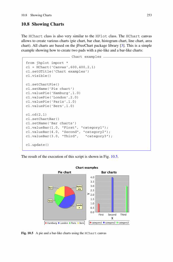
10.8 Showing Charts 253
10.8 Showing Charts
The HChart class is also very similar to the HPlot class. The HChart canvasallows to create various charts (pie chart, bar char, histogram chart, line chart, areachart). All charts are based on the jFreeChart package library [3]. This is a simpleexample showing how to create two pads with a pie-like and a bar-like charts:
Chart examples
from jhplot import *c1 = HChart(’Canvas’,600,400,2,1)c1.setGTitle(’Chart examples’)c1.visible()
c1.setChartPie()c1.setName(’Pie chart’)c1.valuePie(’Hamburg’,1.0)c1.valuePie(’London’,2.0)c1.valuePie(’Paris’,1.0)c1.valuePie(’Bern’,1.0)
c1.cd(2,1)c1.setChartBar()c1.setName(’Bar charts’)c1.valueBar(1.0, "First", "category1");c1.valueBar(4.0, "Second", "category2");c1.valueBar(3.0, "Third", "category3");
c1.update()
The result of the execution of this script is shown in Fig. 10.5.
Fig. 10.5 A pie and a bar-like charts using the HChart canvas
254 10 Graphical Canvases
When the HChart canvas is created, one can set the following types of charts:
>>> c1.setChartXY() # create a XY chart>>> c1.setChartPie() # create a Pie chart>>> c1.setChartPie3D() # create a Pie chart in 2D>>> c1.setChartLine() # create a line chart>>> c1.setChartAre() # create an area chart>>> c1.setChartBar() # create a bar chart>>> c1.setChartBar3D() # create a 2D bar chart>>> c1.setChartHistogram() # create a histogram
Then one can add values using the value+ChartName() method. For example,to add a value to the bar chart use valueBar() method. Check the HChart APIdocumentation for details. Finally, to display a chart, execute the usual update()method.
One can access many jFreeChart components via several “getter” methods. Forexample, c1.getChar() will return the JFreeChart class for further manipu-lations.
10.9 SPlot Class. A Simple Canvas
For simple tasks involving drawings of X–Y plots, which do not require plottingmany graphical objects, or interaction with a canvas using the mouse, one can use alight-weight canvas based on SPlot class (“S” originates from the word “simple”).The class SPlot is based on the PTPlot package [4] which was originally designedto make scatter plots on (x–y) planes and simple histograms.
The methods of the SPlot canvas are similar to those of the HPlot class, butthe number of such methods is not too large. However, this canvas requires muchless computer memory and thus is better suited for applets or to show streams ofdata at runtime.
One can build the SPlot canvas as:
>>> from jhplot import SPlot>>> c1=SPlot(’Canvas’)>>> c1=visible()
This creates a default 600 × 400 canvas using the SPlot class. Now one can showthe names for X and Y axes as:
>>> c1.setNameX(’X’)>>> c1.setNameY(’Y’)>>> c1.setAutoRange()
Both axes can be set to an auto-range mode, so you do not need to worry aboutsetting proper axis ranges:

10.9 SPlot Class. A Simple Canvas 255
>>> c1.setAutoRange()
To set the ranges, use the method setRange(xmin,xmax,ymin,ymax),where the arguments define the ranges for the X and Y axes.
To add a single point at a location (x, y), use the method:
c1.addPoint(0,x,y, b)
Usually, “b=0” (Java false) if points are not connected by lines. When “b=1”(Java value true), then the point should be connected to the next one plot-ted by calling the addPoint() method again. The data set is characterizedwith an integer number (0 in the above example). Finally, the methodsetMarksStyle(’various’) tells that each new dataset will be shown withdifferent symbols.
To add an error bar for a point at the location (x, y), use the method:
>>> addPointErr(dataset,x,y,yLow,yHigh,con)
where dataset is an integer number, yLow and yHigh are the lower and uppererrors for the Y axis, and con is a boolean value defining whether the points areconnected (= 1) or not (= 0).
After filling the data points in a loop, one should call update() to make datavisible on the canvas.
The method addPoint() adds a single point to the canvas and, as we alreadyknow, to call methods inside a loop in Jython is CPU and memory consuming. How-ever, as for the HPlot canvas, one can also use the method draw(obj) to drawJava high level objects, such as histograms (H1D), data containers (P1D) or simplyarrays of numbers with x and y values. Data can be shown with symbols connectedby the lines if setConnected(1,set) is called with the first argument 1 (orboolean true for Java), where set specifies the data set identification number (in-teger). There is no need to call the update method after calling the draw(obj)method, since the plot will be updated automatically.
The plot can be zoomed into a specific rectangular area by clicking and dragging,to draw a rectangle where desired; this feature is also different from the HPlotcanvas where you can rescale axis ranges one at the time. Finally, one can savethe plot into an image using the usual export(file) method. Look at all othermethods associated with this class using the code assist.
Below we give a small example showing how to plot two different sets of datapoints:
SPlot example
from java.util import Randomfrom jhplot import *
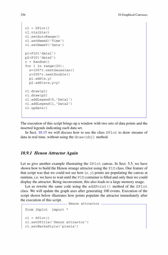
256 10 Graphical Canvases
c1 = SPlot()c1.visible()c1.setAutoRange()c1.setNameX(’Time’)c1.setNameY(’Data’)
p1=P1D(’data1’)p2=P1D(’data2’)r = Random()for i in range(20):
x=100*r.nextGaussian()y=200*r.nextDouble()p1.add(x,y)p2.add(x+x,y+y)
c1.draw(p1)c1.draw(p2)c1.addLegend(0,’Data1’)c1.addLegend(1,’Data2’)c1.update()
The execution of this script brings up a window with two sets of data points and theinserted legends indicating each data set.
In Sect. 10.15 we will discuss how to use the class SPlot to draw streams ofdata in real time, without using the draw(obj) method.
10.9.1 Henon Attractor Again
Let us give another example illustrating the SPlot canvas. In Sect. 5.5, we haveshown how to build the Henon strange attractor using the P1D class. One feature ofthat script was that we could not see how (x, y) points are populating the canvas atruntime, i.e. we have to wait until the P1D container is filled and only then we coulddisplay the attractor. Being inconvenient, this also leads to a large memory usage.
Let us rewrite the same code using the addPoint() method of the SPlotclass. We will update the graph axes after generating 100 events. Execution of thescript shown below illustrates how points populate the attractor immediately afterthe execution of this script.
Henon attractor
from jhplot import *
c1 = SPlot()c1.setGTitle(’Henon attractor’)c1.setMarksStyle(’pixels’)

10.10 Canvas for Interactive Drawing 257
c1.setConnected(0, 0)c1.setNameX(’x’)c1.setNameY(’y’)c1.visible()a = 1.4; b = 0.3x=0; y=0for i in range(100000):
x1=xx=1+y-a*x*xy=b*x1c1.addPoint(0,x,y,1)if i%1000==0: c1.update()
We will leave the reader here for more experimentation.
10.10 Canvas for Interactive Drawing
For complicated tasks which involve drawing diagrams together with the usual data-driven plots, one should use the HPlotJa canvas. From the point of view of dis-playing functions, arrays and histograms, this canvas is rather similar to the HPlotclass, i.e. one can use the same method draw(obj) to display instances of lists,F1D, H1D and P1D objects. Yet, it has many advanced features such as:
• plots are more interactive. One can easily manipulate with different pads, makeinserts, overlays etc.;
• one can open ROOT or AIDA files in an object editor described in Sect. 11.5.3;• one can draw diagrams using Jython scripts or using the object editor.
One should emphasize that this canvas is very easy to use for making insetplots, i.e. showing one pad inside the other. This is technically impossible for theHPlot canvas, in which each pad is built using the JPanel Java class. In case ofHPlotJa, the pads are located inside a single panel.
The HPlotJa canvas is based on the JaxoDraw package [5] designed to drawFeynman diagrams used in high-energy physics. The original package was signifi-cantly modified by adding the possibility to plot the standard jHepWork objects andadding vector graphics capabilities.
To build an instance of the HPlotJa canvas, use the following code snippet:
>>> from jhplot import *>>> c1=HPlotJa(’Canvas’)>>> c1=visible()
The methods associated with the HPlotJa canvas are similar to those of theHPlot class and we will not repeat them here. The largest difference with the

258 10 Graphical Canvases
HPlot is that there are many methods related to drawing axes which cannot becalled directly, but only via the method getPad() as shown in this example:
>>> from java.awt import Color>>> from jhplot import *>>> c1=HPlotJa(’Canvas’,1,2)>>> c1=visible()>>> c1.cd(1,2)>>> pad=c1.getPad() # get current pad>>> pad.setRange(0,0,1) # set axis range [0,1] on X>>> pad.setFillColor(Color.red) # new color>>> pad. + [F4] # check other methods
As for the original JaxoDraw package, the HPlotJa canvas has a completegraphical user interface that allows to carry out all actions in a mouse click-and-drag fashion. To bring up the graphical editor, go to the [Option] menu and select[Show editor]. Now you can create and edit the graph objects using the mouseclicks. One can draw many graphical objects, lines, circles etc. One can remove,drag and resize all plotted objects, including the pad regions. Finally, one can editproperties of all plotted objects.
10.10.1 Drawing Diagrams
Once an object of the HPlotJa canvas is created, one can draw diagrams using Jax-oDraw mouse click-and-drag fashion. To do this, you have to select the [Editor]option from the [Option] menu.
The power of Jython scripting allows to draw diagrams interactively or usingJython macro files. This will require importing the static methods of the Diagramclass from the package jhplot.jadraw. Below we show a typical example ofhow to draw “gluon” and “fermion” lines typically used for representation of Feyn-man diagrams:
"gluon" and "fermion" lines
from jhplot import *from jhplot.jadraw import *
c1=HPlotJa(’Canvas’,500,400,1,1,0)c1.visible()c1.showEditor(1)
# draw text boxgl=Diagram.TextBox("Gluons and fermions",0.25,0.15)c1.add(gl)
# gluon line in NDC coordinates
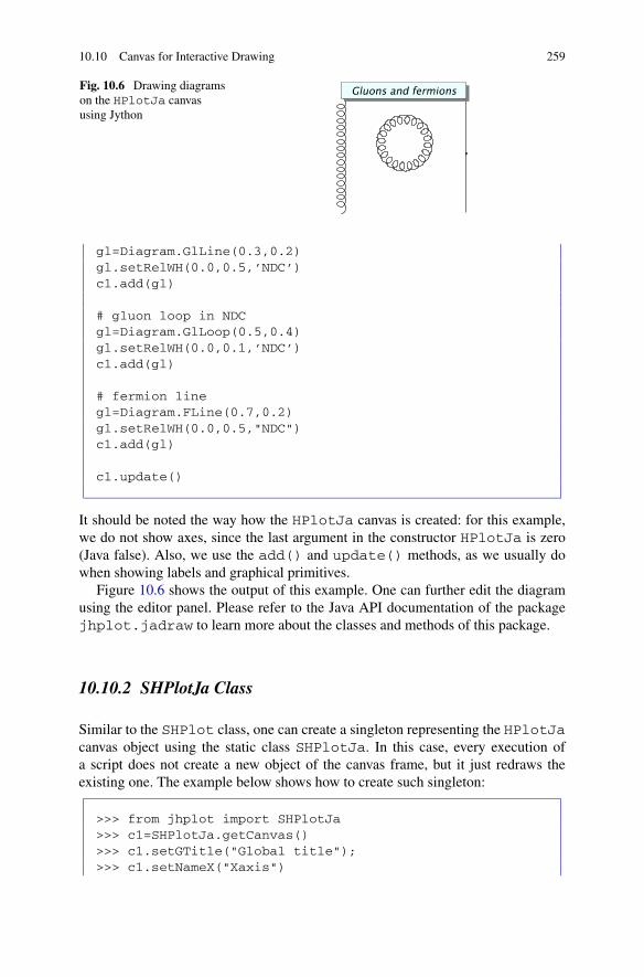
10.10 Canvas for Interactive Drawing 259
Fig. 10.6 Drawing diagramson the HPlotJa canvasusing Jython
gl=Diagram.GlLine(0.3,0.2)gl.setRelWH(0.0,0.5,’NDC’)c1.add(gl)
# gluon loop in NDCgl=Diagram.GlLoop(0.5,0.4)gl.setRelWH(0.0,0.1,’NDC’)c1.add(gl)
# fermion linegl=Diagram.FLine(0.7,0.2)gl.setRelWH(0.0,0.5,"NDC")c1.add(gl)
c1.update()
It should be noted the way how the HPlotJa canvas is created: for this example,we do not show axes, since the last argument in the constructor HPlotJa is zero(Java false). Also, we use the add() and update() methods, as we usually dowhen showing labels and graphical primitives.
Figure 10.6 shows the output of this example. One can further edit the diagramusing the editor panel. Please refer to the Java API documentation of the packagejhplot.jadraw to learn more about the classes and methods of this package.
10.10.2 SHPlotJa Class
Similar to the SHPlot class, one can create a singleton representing the HPlotJacanvas object using the static class SHPlotJa. In this case, every execution ofa script does not create a new object of the canvas frame, but it just redraws theexisting one. The example below shows how to create such singleton:
>>> from jhplot import SHPlotJa>>> c1=SHPlotJa.getCanvas()>>> c1.setGTitle("Global title");>>> c1.setNameX("Xaxis")
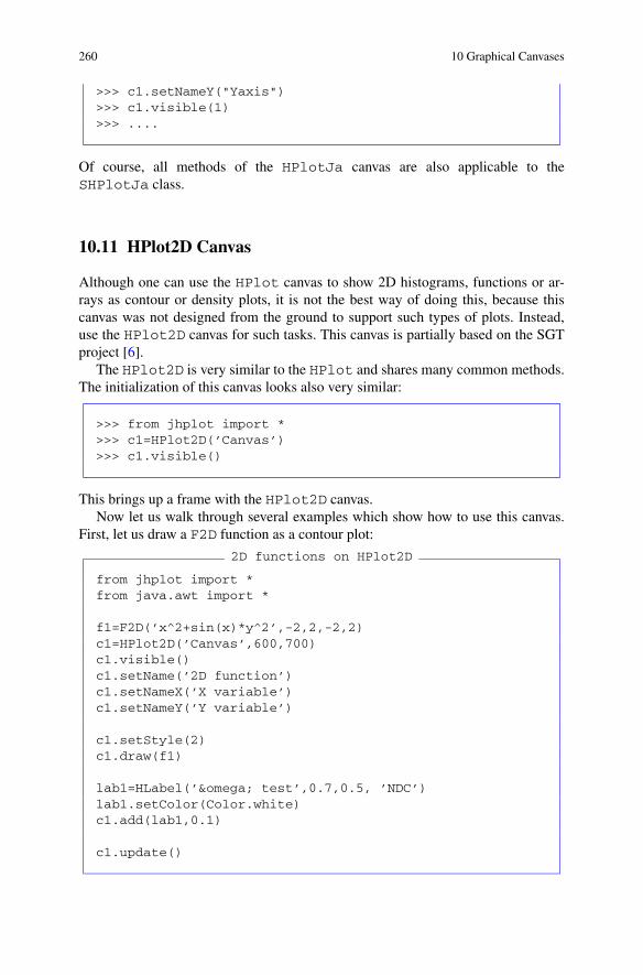
260 10 Graphical Canvases
>>> c1.setNameY("Yaxis")>>> c1.visible(1)>>> ....
Of course, all methods of the HPlotJa canvas are also applicable to theSHPlotJa class.
10.11 HPlot2D Canvas
Although one can use the HPlot canvas to show 2D histograms, functions or ar-rays as contour or density plots, it is not the best way of doing this, because thiscanvas was not designed from the ground to support such types of plots. Instead,use the HPlot2D canvas for such tasks. This canvas is partially based on the SGTproject [6].
The HPlot2D is very similar to the HPlot and shares many common methods.The initialization of this canvas looks also very similar:
>>> from jhplot import *>>> c1=HPlot2D(’Canvas’)>>> c1.visible()
This brings up a frame with the HPlot2D canvas.Now let us walk through several examples which show how to use this canvas.
First, let us draw a F2D function as a contour plot:
2D functions on HPlot2D
from jhplot import *from java.awt import *
f1=F2D(’x^2+sin(x)*y^2’,-2,2,-2,2)c1=HPlot2D(’Canvas’,600,700)c1.visible()c1.setName(’2D function’)c1.setNameX(’X variable’)c1.setNameY(’Y variable’)
c1.setStyle(2)c1.draw(f1)
lab1=HLabel(’ω test’,0.7,0.5, ’NDC’)lab1.setColor(Color.white)c1.add(lab1,0.1)
c1.update()

10.11 HPlot2D Canvas 261
Fig. 10.7 2D function shownas a density plot
The resulting plot is shown in Fig. 10.7. The methods used for the canvas object c1are rather similar to the methods of the HPlot canvas. The only new feature is thatwhen we add a text label, we use the method add(obj,d), where ’d’ specifiesthe label height.
We should mention that the HPlot2D canvas is fully interactive. One can moveand edit labels, click-and-drag the mouse pointer to create a zoom rectangle. Onecan edit axis attributes by clicking on an axis (this pops-up a dialog where all mod-ifications can be made).
There are several options for showing an object inside the canvas. They are con-trolled with the method seStyle(style), where
style=0 draws data using a raster style;style=1 draws using a contour style;style=2 combined style (raster and contour);style=3 draws data using filled areas.
One can access several objects for modifications inside Jython scripts. First, onecan obtain the axis object as getAxis(axis), where axis is either 0 (for X)or 1 (for Y ). Using the methods of this axis object, one can make necessary mod-ifications, like setting new fonts, redefine colors etc. One can also access the colorbar-key as getColorBar(), which also has several useful methods.
One important method you should keep in mind is
>>> setRange(axis,min,max,bins)
which sets the range for X (axis = 0), Y (axis = 1) and Z (axis = 2). The variablebins specifies how many divisions between min and max values should be used.In case of the Z-axis, the variable bins specifies how many contour levels to draw.
Let us give another example. This time we will plot data using different styles.We display a histogram and 2D array. In case of the histogram, we change the rangefor X and Y axes using the setRange() method. We note that the last argumentfor this method, which usually defines the number of bins between the minimumand maximum values, does not do anything. This is because we plot the histogram

262 10 Graphical Canvases
which has its own binning, and this cannot be changed when the histogram is shown.
2D data on HPlot2D
# HPlot2D. Showing H2D,P1D and 2D function# S.Chekanov
from jhplot import *from java.util import *
h1=H2D(’Data’,30,-3.0, 3.0, 30,-3.0, 3.0)p1=P1D(’Data’)
r=Random()for i in range(1000):
x=r.nextGaussian()y=r.nextGaussian()h1.fill(0.6*x-0.5, y)p1.add(0.4*x+1, y+0.5)
c1=HPlot2D(’Canvas’,600,400,3,1)c1.visible()
c1.cd(1,1)c1.setName(’H2D histogram’);c1.setStyle(0)c1.draw(h1)
c1.cd(2,1)c1.setName(’H2D range’)c1.setStyle(1)c1.setRange(0,-2.0,2.0,50)c1.setRange(1,0.0,1.0,50)c1.draw(h1)
c1.cd(3,1)c1.setName(’2D array’)c1.setStyle(1)c1.draw(p1)
The output of this script is shown in Fig. 10.8.
10.12 3D Canvas
We have already discussed canvases for 3D graphics in Sects. 3.4.2, 6.1.1 and 8.2.Here we remind that one should use the classes HPlot3D and HPlot3DP for a 3Drepresentation of mathematical functions and data. The first class is used for plotting

10.13 HPlot3D Canvas 263
Fig. 10.8 2D data shown using different styles and ranges
H2D, P2D and F2D objects, while the second one for parametric equations based onthe FPR class, see Sect. 3.8.
10.13 HPlot3D Canvas
This canvas is used for visualization of H2D, P2D and F2D objects, which can bedrawn with the same draw(obj) method as for the 2D case. In case if two objectsshould be shown, say obj1 and obj2, on the same canvas, one should call themethod draw(obj1,obj2). Table 10.2 lists the most important methods of theHPlot3D Java class:
We should remind that if you are debugging a script and do not want to createmany pop-up windows with canvas frames after each script execution, you may wantto instantiate a singleton using the class SHPlot3D. In this case, every new macroexecution redraws the existing canvas, instead of creating a new canvas object. Onecan build a singleton as usual:
>>> c1=SHPlot3D.getCanvas(’3D’,600,400,2,2)
This creates four plotting pads inside a 3D canvas of the size 600 × 400.
10.13.1 HPlot3DP Canvas
The second 3D canvas, HPlot3DP, is used to draw surfaces defined by an analyticparametric or a non-parametric function of the type FPR, as shown in Sect. 3.8.
The HPlot3DP canvas can be constructed exactly in the same way as theHPlot3D class. Specifically, one can define the frame size during object instan-tiation and set any number of drawing pads. The major difference with HPlot3Dis following: if several objects should be shown on the same pad, then one can use

264 10 Graphical Canvases
Table 10.2 The main methods of the HPlot3D class. “b” indicates a boolean value (1 for trueand 0 for false), while “i” is an integer value. The notation “d” denotes a float value. The attributes“c” and “f” correspond to the Color and FontAWT Java classes. “text” represents a string value.The character “a” is a shortcut to “axis” (a=0 for X, a=1 for Y , a=2 for Z)
Methods Definitions
setRotationAngle(i) set rotation angle to ‘i’ degrees
getRotationAngle() get rotation angle
setScaling(i) set scaling factor to ‘i’ (default is 12)
getScaling() get scaling
setElevationAngle(i) set elevation angle to ‘i’ degrees
getElevationAngle() get elevation angle
setAxesFontColor(c) set fonts for axes labels
setColorMode(i) set color mode (from 1 to 4)
0: wire-frame
1: hidden
2: color spectrum 3: gray scale
4: dual shades
setDistance(d) set distance to objects
getDistance() get distance from object
setLabelFontColor(c) set color for labels
setPenWidthAxes(i) set line width for axes
getPenWidthAxes() get pen with for axes
setNameX(“text”) set name for axis X
setNameY(“text”) set name for axis Y
setNameZ(“text”) set name for axis Z
setLabelFont(f) set fonts for labels
setLabelFont(f) set fonts for axes numbers
setLabelColor(c) set label color
setTicFont(f) set fonts for ticks
setTicOffset(d) set ticks offset
setRange(Xmin,Xmax,Ymin,Ymax) set plot ranges
setRangeZ(Zmin,Zmax) set range for Z
cd(iX,iY) go to the pad (iX,iY)
clear() clean the current region
clear(iX,iY) clean the pad (iX,iY)
clearAll() clean all pads
quite() remove frame
update(iX,iY) update the pad (iX,iY)
updateData(iX, iY) update data shown in the pad (iX,iY)
updateData() update data on the current pad
updateAll() update all pads
getLabelOffset(a) get label offset for axis
draw(obj) draw an object (P2D, F2D..)

10.13 HPlot3D Canvas 265
Table 10.3 The mainmethods of the HPlot3DPclass. “b” denotes a booleanvalue (1 for true and 0 forfalse), while “i” is an integervalue. The notation “d”indicates a float value. Theattributes “c” and “f”correspond to the Color andFont AWT Java classes
Methods Definitions
setFog(b) sets the fog style for 3D
setAxes(b) shows or not axes
setAxes(b1,b2,b3) shows axes for X, Y , Z
setAxesColor(c) axes color
setBackgColor(c) background color
setNameX(text) text for X axis
setNameY(text) text for Y axis
setNameZ(text) text for Z axis
setCameraPosition(d) set camera position
zoom in for positive “d”
zoom out for negative “d”
setEyePosition(x,y,z) set eye positions
clear(object) clear the frame
cd(i1,i2) navigates to a i1 × i2 pad
update() updates the canvas
draw(obj) draws an object (FPR)
the draw(obj) methods several times, one after other. The main methods of thiscanvas are given in Table 10.3.
One can zoom in the pad area using the right mouse button. In macro files, onecan zoom in and zoom out using the following method:
>>> c1.setCameraPosition(d)
where d is a double value, which should be positive for zooming in, and negativefor zooming out. One can change the location of axes and the object position usingthe method setEyePosition(x,y,z). The graphs can be edited using the GUIdialog and the [Edit] menu by clicking on the mouse button.
Below we show the use of several methods of the HPlot3DP class:HPlot3DP canvas
from java.awt import Colorfrom jhplot import *
c1 = HPlot3DP(’Canvas’,600,600)c1.setGTitle(’HPlot3DP examples’)c1.visible()
f1=FPR(’u=2*Pi*u; x=cos(u); y=sin(u); z=v’)c=Color(0.5,0.2,0.5,0.5) # color+transparencyf1.setFillColor(c)f1.setLineColor(Color.green)

266 10 Graphical Canvases
Fig. 10.9 HPlot3DP canvasand its graphical methods
f2=FPR(’u=2 Pi u; v=2 Pi v; r=0.6+.2cos(u); \z=.8 sin(u); x=r cos(v); y=r sin(v)’)
f2.setFillColor(Color.blue)f2.setFilled(1)
c1.setFog(0)c1.setAxes(1)c1.setNameX("X axis")c1.setNameY("Y axis")c1.setAxesColor(Color.gray)c1.setAxesArrows(0)
print c1.getEyePosition()print c1.getCameraPosition()c1.setCameraPosition(-1.2) #zoom outc1.draw(f2)c1.draw(f1)
The above code brings up a frame with the image of a cylinder and a torus as shownin Fig. 10.9. One can rotate objects and zoom into certain area using the mousebutton. In addition, one can further edit the figure using the [Edit] menu.
10.13.2 3D Geometry Package
The HView3D class also allows to draw 3D objects (cubes, shapes cylinders etc.)which are already predefined Java classes, thus there is no need to define them usingparametric equations. Look at the Java API of the jhplot.v3d package. This is atypical example of how to draw 3D shapes:

10.14 Combining Graphs with Java Swing GUI Components 267
Creating 3D objects
from java.awt import Colorfrom jhplot import *from jhplot.v3d import *
c1 = HView3D(’Canvas’,400,400)c1.visible(1)c1.setGTitle("3D objects in HView3D")
o=Cube(c1.getModel(),40) # a cube of the size 40o.setRot(45,45,45) # rotatec1.draw(o)
o=Sphere(c1.getModel(),30.,80,80) # a sphere eithr=30o.setTrans(40,-20,10) # move itc1.draw(o);
o=Cone(c1.getModel(), 30, 100, 50)o.setTrans(-20, 30, 0)o.setColor(Color.red)c1.draw(o);
o=Cylinder(c1.getModel(), 40, 100, 2)o.setTrans(-1, 0, 0)o.setRot(0, 60, 0)o.setColor(Color.yellow)c1.draw(o)
c1.update() # draw all objects
The execution of this script brings up a window with 3D objects using their attributespassed to the constructors.
10.14 Combining Graphs with Java Swing GUI Components
In Sect. 2.18 we have shown how easy to use the Java Swing components in Jython.Jython scripting allows a creation of graphical user interfaces (GUI) using the JavaGUI widgets, such as windows, menus, buttons, etc. One can make them to respondto physical events (keyboard, mouse etc.) with a few lines of Jython code. This isan important when it is necessary to make “control panels” or “graphical user inter-faces” for applications in order to manipulate with Java programs at run time. Suchapplications can be deployed as self-contained programs in jar files after compilingJython codes into the Java bytecodes, the machine language of the Java virtual ma-chine. But how one can use the jHepWork canvas together with such components?We will briefly discuss such topic in this section.

268 10 Graphical Canvases
Numerous methods of the canvases described in the previous sections are so richthat one can always find a necessary method suited for your GUI application. Themost important method for the GUI development is that which returns the SwingJFrame object holding the entire canvas panel. In the example of Sect. 2.18, aninstance of the Java class JFramewas created using the standard constructor. Whenyou are working with the jHepWork canvases, there is no need to do this. What youwill need is to use the getFrame() method which returns an appropriate JFrameinstance:
>>> c1 = HPlot(’GUI’)>>> jframe=c1.getFrame()
Once you have retrieved the frame object, you can add the necessary Swing GUIcomponents (menu, buttons, sliders etc.) to control the displayed data.
Let us show an extensive example in which we illustrate how to attach a panelwith two Swing JButton buttons and a TextArea component directly to theHPlot canvas object. One button will be used to generate a histogram populatedwith Gaussian numbers. The second will be used to erase graphs from the canvas.The text area displays a short message about what happens when you press thesebuttons.
Combining HPlot canvas with Swing components
from java.awt import *from javax.swing import *from java.util import *from jhplot import *
c1 = HPlot(’GUI’)c1.setGTitle(’Plot area with GUI’)c1.visible(1)c1.setAutoRange()fr=c1.getFrame()
h1 = H1D(’Histogram’,20, -2.0, 2.0)h1.setFill(1)h1.setFillColor(Color.blue)
pa0 = JPanel(); pa1 = JPanel()pa2 = JTextArea(’GUI test’,6,20)pa2.setBackground(Color.yellow)
def act1(event):r=Random()for i in range(100):
h1.fill(r.nextGaussian())c1.draw(h1)pa2.setText(’Generated 100 Gaussian numbers’)

10.14 Combining Graphs with Java Swing GUI Components 269
def act2(event):c1.clearData()pa2.setText(’Clear plot’)
pa0.setLayout(BorderLayout());bu1=JButton(’Gaussian’, actionPerformed=act1)pa0.add(bu1,BorderLayout.NORTH)bu2=JButton(’Clear’, actionPerformed=act2)pa0.add(bu2,BorderLayout.SOUTH)pa0.add(pa2,BorderLayout.WEST)fr.add(pa0,BorderLayout.EAST)fr.pack()
After execution of this script, you will see the HPlot canvas with an attached panelwith the Swing components, see Fig. 10.10. Press the buttons to see the output ofthis program.
By examining the script, you may wonder why do we need the method pack()at the very end of this script. We call this method to avoid changes in the size ofthe HPlot canvas, so the extra panel just extends the canvas without distorting itsdefault size (which is 600 × 400 pixels). If you will want to append extra canvas bykeeping the same size of the entire frame, remove the method pack() and, call anymethod which updates the frame (calling setVisible(1) can do this).
Fig. 10.10 HPlot canvas together with a Swing control panel

270 10 Graphical Canvases
10.15 Showing Streams of Data in Real Time
Showing streams of data in real time is very often situation. Instead of collectingdata in some container, such as Java or Jython array, and plotting data at once usingthe draw(obj) method, one can plot a fraction of data samples without waitinguntil all data set become available and populate a data holder to be used for drawing.
In this section, we will show how to fill histograms or data holders and update thecanvas after each such operation. Let us illustrate this by using the Jython sleep()function: we will fill a histogram and update the plot after each random Gaussiannumber. Thus we will see how the histogram is filled at runtime. At the end of theloop, we will clean up the canvas and then re-plot the final histogram. How to cleanthe canvas from plotted data has been discussed in Sect. 10.2.8.
HPlot data stream
from java.awt import Colorfrom java.util import Randomfrom jhplot import *
c1 = HPlot(’Canvas’)c1.setGTitle(’data stream’)c1.visible()c1.setLegend(1)c1.setAutoRange()
h1 = H1D(’Updated histogram’,20,-2.0,2.0)h1.setFill(1)h1.setErrX(0)h1.setErrY(1)h1.setFillColor(Color.blue)h1.setColor(Color.blue)
r = Random()import timefor i in range(1000):
h1.fill(r.nextGaussian())time.sleep(1)c1.clearData()c1.draw(h1)
c1.drawStatBox(h1)time.sleep(2)c1.draw(h1)
c1.clearData()time.sleep(2)c1.setLegend(1)c1.draw(h1)
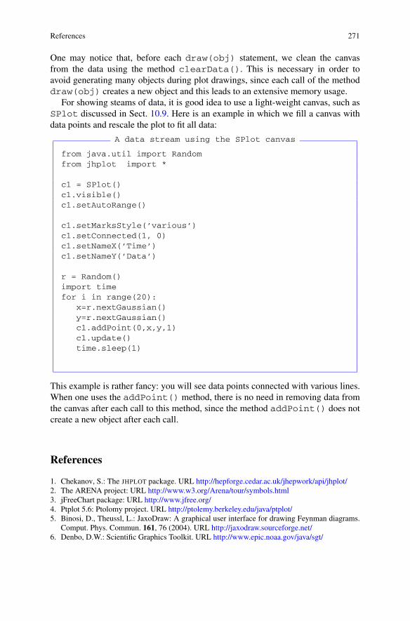
References 271
One may notice that, before each draw(obj) statement, we clean the canvasfrom the data using the method clearData(). This is necessary in order toavoid generating many objects during plot drawings, since each call of the methoddraw(obj) creates a new object and this leads to an extensive memory usage.
For showing steams of data, it is good idea to use a light-weight canvas, such asSPlot discussed in Sect. 10.9. Here is an example in which we fill a canvas withdata points and rescale the plot to fit all data:
A data stream using the SPlot canvas
from java.util import Randomfrom jhplot import *
c1 = SPlot()c1.visible()c1.setAutoRange()
c1.setMarksStyle(’various’)c1.setConnected(1, 0)c1.setNameX(’Time’)c1.setNameY(’Data’)
r = Random()import timefor i in range(20):
x=r.nextGaussian()y=r.nextGaussian()c1.addPoint(0,x,y,1)c1.update()time.sleep(1)
This example is rather fancy: you will see data points connected with various lines.When one uses the addPoint() method, there is no need in removing data fromthe canvas after each call to this method, since the method addPoint() does notcreate a new object after each call.
References
1. Chekanov, S.: The JHPLOT package. URL http://hepforge.cedar.ac.uk/jhepwork/api/jhplot/2. The ARENA project: URL http://www.w3.org/Arena/tour/symbols.html3. jFreeChart package: URL http://www.jfree.org/4. Ptplot 5.6: Ptolomy project. URL http://ptolemy.berkeley.edu/java/ptplot/5. Binosi, D., Theussl, L.: JaxoDraw: A graphical user interface for drawing Feynman diagrams.
Comput. Phys. Commun. 161, 76 (2004). URL http://jaxodraw.sourceforge.net/6. Denbo, D.W.: Scientific Graphics Toolkit. URL http://www.epic.noaa.gov/java/sgt/


Chapter 11Input and Output
jHepWork has a large choice for file input and output (I/O) for efficient data storageand processing. There are several mechanisms for I/O:
• streams to write or read data using the native JAVA platform. The Java libraries forI/O are located in the java.io package which can be imported using the usual’import’ statement. We will not discuss the Java I/O streams in this book asthey are described in detail in any Java book [1–5]. We have already discussedthe class DataOutputStream in Sect. 2.16 in context of writing and readingdata using Java called from Jython;
• native Python I/O discussed in Sect. 2.16;• libraries included into the jHepWork Java package jhplot.io. In this chapter,
we will discuss these libraries in more detail;• third-party Python libraries. We will discuss the package DIF from these libraries
in Sect. 11.10;• third-party Java libraries included into the jHepWork. As example, we will dis-
cuss the Apache Derby relational database in Sect. 11.6.
File I/O, data streaming and format conversions are essential for any stage ofdata analysis. Unfortunately, in the standard manuals and tutorials, details of fileI/O seem to be buried at the back. In this book, we will discuss this topic in greatdetail, focusing on I/O libraries included into the jHepWork program.
11.1 Non-persistent Data. Memory-based Data
In simple words, non-persistent objects contain data that are kept in the computermemory and cannot be restored after the end of the program execution. In contrast,persistent objects are stored in files and can be restored at any moment.
Most scripts discussed in this books hold objects in a non-persistent way. Forexample, when you create a histogram or an array with random numbers as:
S.V. Chekanov, Scientific Data Analysis using Jython Scripting and Java,Advanced Information and Knowledge Processing,DOI 10.1007/978-1-84996-287-2_12, © Springer-Verlag London Limited 2010
273

274 11 Input and Output
>>> from jhplot import *>>> p=P0D(’test’)>>> p.randomUniform(100000,0,1)
the object ’p’ is created in the computer memory. Watch out the memory-statusmonitor at the bottom right corner of the jHepWork editor: you will see a notableincrease in the used memory. By increasing the number of random numbers in theabove example, one can eventually run out of memory, and an OutOfMemory-Error message will be thrown.
Thus, you are very limited by the available memory of your computer (and avail-able memory assigned to the virtual machine). The memory assigned to store objectscan be released manually: in Jython, to remove an object, say ’p’, call the state-ment ’del p’. In addition, the Jython garbage collector takes care of reclamationof memory space in an automatic mode. One can also invoke the Jython garbagecollector manually as:
>>> del p>>> import gc>>> gc.collect()
After calling the statement above, you will see a decrease in the used memory (again,look at the bottom right corner of the jHepWork IDE).
The computer memory is like the work table. It is fine to work on it using smallportions of data because it is fast and effective. But in order to handle large piecesof data, you have to put data on “a shelf”, i.e. copy them to a real file storage on adisk. Below we will discuss how to store jHepWork data in files and how to bringthem back into the computer memory for fast operation.
11.2 Serialization of Objects
Before we have already discussed how to save separate objects into files. Most ob-jects, like P1D or H1D, contain methods for writing them into files, which can beeither text files or binary files.
These objects have also the methods to instantiate themselves from files. Look atthe previous sections: Sect. 3.10 discusses this topic for functions, while Sects. 4.3,5.4 and 6.4 for P0D, P1D and PND arrays, respectively. Section 8.6 describes thehistogram I/O operations. In all these sections, we have illustrated how to save andrestore all such objects using the standard Java serialization, including the serializa-tion into a human-readable XML file format.
We also should remind that jHepWork objects can be saved into Jython lists, dic-tionaries or Java collection classes using the Serialized class. This is a genericexample of how to save objects as lists:

11.2 Serialization of Objects 275
>>> from jhplot.io import *>>> list=[]>>> list.append(object1)>>> list.append(object2)...# write to a file>>> Serialized.write(list,’file.ser’)...# deserialize the list from the file>>> list=Serialized.read(’file.ser’)
Similarly, one can use Jython dictionaries with the keys which are rather handy toextract objects:
>>> from jhplot.io import *>>> map={}>>> map[’object1’]=object1>>> map[’object2’]=object2...>>> # write to a file>>> Serialized.write(map,’file.ser’)...>>># de-serialize the map from the filemap=Serialized.read(’file.ser’)
The class Serialized compresses data using the GZip format. One can also saveand read objects without compression using the following methods:
>>> Serialized.write(obj,’file.ser’,compression)>>> obj=Serialized.read(’file.ser’,compression)
where a boolean compression should be set to zero (‘false’ for Java) if no com-pression is applied.
One can also use a XML format for all such output files. This format is im-plemented using the methods writeXML(obj) and readXML() from the sameSerialization class. However, this is not the most economic approach, sincestring parsing is a CPU intensive and the XML files are significantly larger than fileswith binary data.
In all such approaches, there was a significant drawback: we write data at the endof numerical computations, so first we put the entire collection in a non-persistentstate, and then move it into a persistent state. This can only work if the data are nottoo large and one can fit them in the computer memory.

276 11 Input and Output
Below we will discuss how to avoid such problems by writing objects with datadirectly into files sequentially, without building collections of objects first and thenwriting them using the Serialized class.
11.3 Storing Data Persistently
11.3.1 Sequential Input and Output
To load all data into a Jython or Java container and write it at once into a file usingthe Serialized() class is not the only approach. One can also write or readselected portions of data, i.e. one can sequence through data by writing or readingsmall chunks of data that are easier to handle in the computer memory.
This time we are interested in truly persistent way of saving objects: insteadcollecting them in the collections before dumping them into a file, we will writeeach object separately into a file. In this case, one can write and read back huge datasets to/from the disk.
The Java serialization mechanism for objects could be slower than the standardJava I/O for streaming primitive data types. As usual, there is a trade-off betweenconvenience and performance and, in this book, we usually prefer convenience. Incase of the Java serialization, restored objects carry their types, and such “self-description” mechanism is very powerful and handy feature as there is no need toworry about what exactly data have been retrieved from a file.
If the serialization is slow for your particular tasks, one can always use the I/Omethods of jHepWork objects which are not based on the Java serialization. See, forexample, Sects. 4.3 and 5.4 for such examples.
To write objects sequentially into a file and read them back, one can use theHFile class. A general call to create an instance of this class is:
>>> f=HFile(FileName,option,compression,buffersize)
where FileName is a string with the file name, ’option’ is a string which canbe either ’w’ (write into file) or ’r’ (read from a file). If the boolean variable’compression’ is set to zero (‘false’ in Java), objects inside the file will not becompressed. An integer value, ’buffersize’, specifies the buffer size. The classHFile is constructed such that it writes data chunks to a memory buffer first, beforerecording them on the disk. This dramatically increases the speed of I/O operations,compare to the situations when writing one byte at a time. Selecting a correct buffersize is important; typically this number should be multiples of 1024 bytes. If thedata chunks to be written are large, consider to increase the buffer size. This pointwill be illustrated in more detail later.
The following shortcuts for creation of a HFile object can be useful:

11.3 Storing Data Persistently 277
>>> f=HFile(FileName,option,compression)>>> f=HFile(FileName,option)>>> f=HFile(FileName)
In all these initializations, the buffer size is set to 12 kilobytes (KB). The second con-structor assumes data compression, while the third assumes that the file is openedfor reading objects only.
Let us give an example of how to store several Java objects in a file persistently.The example below shows how to create an output file with several Java objects.Some of them (like P1D) can contain data:
Writing Java objects
from jhplot.io import *from jhplot import *from javax.swing import JFrame
# create a lsit with objectslist=[]list.append(P0D(’title’))list.append(P1D(’title’))list.append(H1D(’histogram’,100,-5,5))list.append(F1D(’x*x’,1,5))list.append(’String’)list.append(JFrame(’Frame’))
f=HFile(’output.ser’,’w’)for i in list:
f.write(i)f.close()
As we have mentioned before, data from the serialization contain a self-description. Let us read the file from the above example and check the types ofthe retrieved objects. In one case, we will use the Jython type(obj) method, insecond we will use the Java-oriented type of check:
Reading Java objects
from jhplot.io import *from jhplot import *
f=HFile(’output.ser’)while 1:
obj=f.read()if obj == None:
breakprint ’Type=’,type(obj)
f.close()

278 11 Input and Output
The output of this script is:
Type= <type ’jhplot.P0D’>Type= <type ’jhplot.P1D’>Type= <type ’jhplot.H1D’>Type= <type ’jhplot.F1D’>Type= <type ’unicode’>Type= <type ’javax.swing.JFrame’>
In case if an object belongs to a Java class, one can also access the informationabout this object using the getClass() method from the native Java API. Thishas already been discussed in Sect. 3.2.1, but here we will remind how to do thisagain:
>>> try:>>> cla=obj.getClass()>>> print ’Java=’,cla.getCanonicalName()>>> except:>>> print ’Non-Java class’;
11.3.2 GUI Browser for Serialized Objects
If a serialized file has been created with the help of the HFile class using its defaultattribute (i.e. GZip compression), one can browser objects inside such file usinga specially-designed GUI browser. Start the jHepWork IDE and select [Tools]and then [HPlot] menu, which brings up an empty HPlot canvas. Then select[Read data] using the menu [File] from the tool bar. This opens an objectbrowser which will be discussed in more detail in Sect. 10.2.7.
In this section, we would rather show how to look at the serialized objects usingJython scripting. In our next example, we create a canvas and open a HFile filein the HFileBrowser dialog. You will see a list of objects stored in the file (to-gether with their titles). One can select an object and plot it on the HPlot canvas.The selected object can be either a F1D function, a H1D histogram, P0D or P1D)array. This code snippet opens the file ’output.ser’ created before in the objectbrowser:
Java object browser
from jhplot.io import *from jhplot import *
c=HPlot(’canvas’)c.visible()

11.3 Storing Data Persistently 279
f=HFile(’output.ser’)HFileBrowser(c,f,1)f.close()
Select an entry, say “String” (which, obviously, means “Java String” object) andpush the button “Plot”. You will see the plotted text on the canvas. In exactly thesame way, one can bring up a serialized JFrame (note that we did not set the sizeof this frame, so you will see only a small box). One can also plot other objects(histograms, jHepWork arrays) stored in the file ’output.ser’.
11.3.3 Saving Event Records Persistently
Now let us come to the question of how to store large data sets in a sequential form.The passed argument obj to the method write(obj) can be rather complex sinceit can keep a data record with various types of containers and their graphical at-tributes.
Below we will show a simple example of how to write 10000 events into a se-rialized file. Each event is a list with the event identification information (a string),P0D array with random numbers and a histogram H1D. We print a debugging in-formation after each 100 events, showing how the file is growing after inserting thedata.
Writing event records
from jhplot.io import *from jhplot import *
def makeEvent(entry):’event with 3 objects’label=’Event=’+str(entry)p=P0D(label)p.randomUniform(10,0,1)h=H1D(label,10,-1,1)h.fill(i)return [label,p,h]
f=HFile(’output.ser’,’w’)for i in range(10000):
ev=makeEvent(i)if (i%100 == 0):
print ev[0]+’ size=’,os.path.getsize(file)f.write(ev)
f.close()
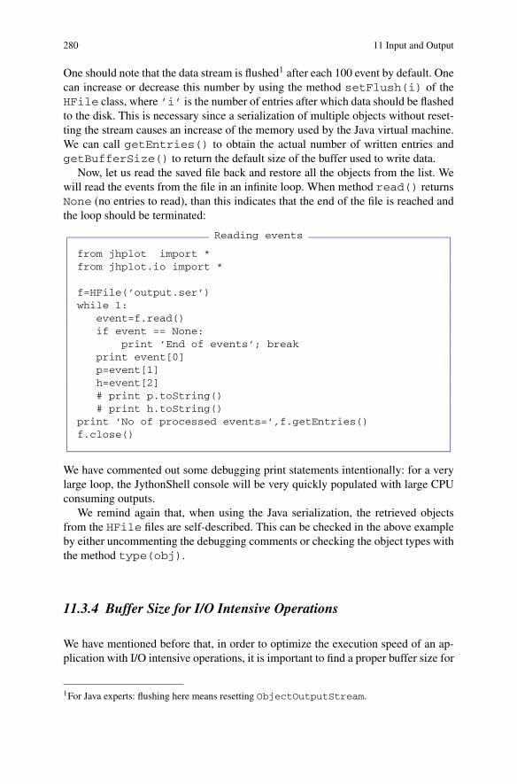
280 11 Input and Output
One should note that the data stream is flushed1 after each 100 event by default. Onecan increase or decrease this number by using the method setFlush(i) of theHFile class, where ’i’ is the number of entries after which data should be flashedto the disk. This is necessary since a serialization of multiple objects without reset-ting the stream causes an increase of the memory used by the Java virtual machine.We can call getEntries() to obtain the actual number of written entries andgetBufferSize() to return the default size of the buffer used to write data.
Now, let us read the saved file back and restore all the objects from the list. Wewill read the events from the file in an infinite loop. When method read() returnsNone (no entries to read), than this indicates that the end of the file is reached andthe loop should be terminated:
Reading events
from jhplot import *from jhplot.io import *
f=HFile(’output.ser’)while 1:
event=f.read()if event == None:
print ’End of events’; breakprint event[0]p=event[1]h=event[2]# print p.toString()# print h.toString()
print ’No of processed events=’,f.getEntries()f.close()
We have commented out some debugging print statements intentionally: for a verylarge loop, the JythonShell console will be very quickly populated with large CPUconsuming outputs.
We remind again that, when using the Java serialization, the retrieved objectsfrom the HFile files are self-described. This can be checked in the above exampleby either uncommenting the debugging comments or checking the object types withthe method type(obj).
11.3.4 Buffer Size for I/O Intensive Operations
We have mentioned before that, in order to optimize the execution speed of an ap-plication with I/O intensive operations, it is important to find a proper buffer size for
1For Java experts: flushing here means resetting ObjectOutputStream.
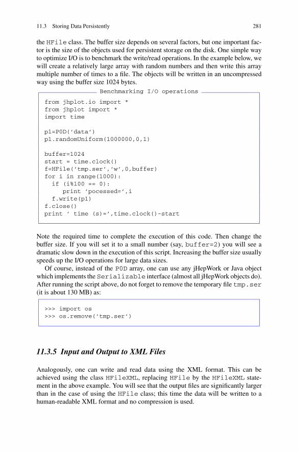
11.3 Storing Data Persistently 281
the HFile class. The buffer size depends on several factors, but one important fac-tor is the size of the objects used for persistent storage on the disk. One simple wayto optimize I/O is to benchmark the write/read operations. In the example below, wewill create a relatively large array with random numbers and then write this arraymultiple number of times to a file. The objects will be written in an uncompressedway using the buffer size 1024 bytes.
Benchmarking I/O operations
from jhplot.io import *from jhplot import *import time
p1=P0D(’data’)p1.randomUniform(1000000,0,1)
buffer=1024start = time.clock()f=HFile(’tmp.ser’,’w’,0,buffer)for i in range(1000):
if (i%100 == 0):print ’pocessed=’,i
f.write(p1)f.close()print ’ time (s)=’,time.clock()-start
Note the required time to complete the execution of this code. Then change thebuffer size. If you will set it to a small number (say, buffer=2) you will see adramatic slow down in the execution of this script. Increasing the buffer size usuallyspeeds up the I/O operations for large data sizes.
Of course, instead of the P0D array, one can use any jHepWork or Java objectwhich implements the Serializable interface (almost all jHepWork objects do).After running the script above, do not forget to remove the temporary file tmp.ser(it is about 130 MB) as:
>>> import os>>> os.remove(’tmp.ser’)
11.3.5 Input and Output to XML Files
Analogously, one can write and read data using the XML format. This can beachieved using the class HFileXML, replacing HFile by the HFileXML state-ment in the above example. You will see that the output files are significantly largerthan in the case of using the HFile class; this time the data will be written to ahuman-readable XML format and no compression is used.

282 11 Input and Output
11.3.6 Non-sequential Input and Output
Data can also be written in a non-sequential order using a database-type approach.The database can be build using the HDataBase class.
A typical database associates a key of type string with each written record.This has some similarity with Jython dictionaries, but this time we are dealing withtruly persistent approach. A data record can consist of only one “blob” of binarydata. The file can grow and shrink as records are inserted and removed. The databaseoperations do not depend on the number of records in the file, i.e. they will beconstant in time with respect to file accesses. The index is small enough to be loadedinto memory for efficiency.
Let us give a short example of how to create a small database. This will be asimple address book with two entries. First, we will create a binary database file,inserting two entries with the names of people as keys. Then we read the databaseagain, check the number of entries and print all entries inside the file using the keys:
An object database: an address book
from jhplot.io import *from java.util import *
# open a database for writingf=HDataBase(’addressbook.db’,’w’)f.insert(’steve’, ’Chicago’)f.insert(’alexey’,’Minsk’)f.close()
# open database for readingf=HDataBase(’addressbook.db’,’r’)print ’Number of records=’,f.getRecords()print ’Is record exists?’, f.isExists(’alexey’)keys=f.getKeys()while keys.hasMoreElements():
next = keys.nextElement()print ’key=’,next,’ obj=’,f.get(next)
The output of this script is shown below:
Number of records= 2Is record exists? Truekey= steve obj= Chicagokey= alexey obj= Minsk
The same approach can be used to store more complicated objects and associatethem with the keys in form of strings. The example below shows how to build afile (’data.db’) with object database which could be useful for writing arbitraryevent records:

11.4 Compressed PFile Format 283
An object database: Event records
from jhplot import *from jhplot.io import *import os.path
# build event from 3 objectsdef makeEvent(entry):
label=’Event=’+str(entry)p=P0D(label)p.randomUniform(10,0,1)h=H1D(label,10,-1,1)h.fill(i)return [label,p,h]
# write events into a databasef=HDataBase(’data.db’,’w’)Events=1000for i in range(Events):
event=makeEvent(i)if (i%100 == 0):
print event[0]+’ size=’,os.path.getsize(’data.db’)f.insert(str(i),event)
f.close()
f=HDataBase(’data.db’,’r’) # read the databaseprint ’extract event 26’; event=f.get(’26’)print ’=== ’+event[0]+’====’print event[1].toString()print event[2].toString()f.close()
Let us comment on this code. As before, for each insert(key,obj) method,we used the key defined by a string. Each string represents an event number but, ofcourse, it can be any non-unique string. We access the event record No. 26 using therandom access feature of this database and then print its objects.
One can always remove an object from the file with the remove(key) methodor update an entry with the update(ob,key) method. Look at the Java APIdocumentation of this class.
11.4 Compressed PFile Format
Despite the power of the Java serialization mechanism, it is important to note severalits features when making decisions about input and output of numerical data:

284 11 Input and Output
• Java serialization can be slower in comparison with the usual I/O approach. It isgood approach for storing complex objects, but it has unnecessary overhead fornumerical data streams;
• It is not intended to be platform neutral. One cannot write or read data using otherprogramming languages (such as C++);
• The size of the files created by the Java serialization can be larger than expected(even after compression). In fact, what we really need in many data-analysis ap-plications is simply to write or read numerical values, rather than objects with allassociated graphical attributes.
This poses a certain trade-off between the power of being able to write essentiallyany Java object into a Java serialized file and the shortcomings listened above. IfJava serialization is too heavy approach for numerical calculations, consider an al-ternative I/O approach using the class called PFile. The methods of this classallow to write and read compressed data records constructed using the Google’sProtocol Buffers package [6] (which gives the origin of the first letter “P” in theclass name PFile). The Protocol Buffers program encodes structured data in aplatform-neutral format, similar to XML. But, unlike XML, the Protocol Buffersapproach is faster, simpler and the output file is smaller. This will be discussed inmore detail in Sect. 11.8.
There are several advantages in using the class PFile: it is faster for writingcompared to HFile and output data files generated by HFile are smaller. But,more importantly, one can use external programs to write and read files as long as aProtocol Buffers file which specifies data format is provided (again, see Sect. 11.8for details). The class PFile is designed to keep data without their graphical at-tributes, which leads to smaller output files. However, only a limited set of objectsis supported; at present, only objects from the package jhplot can be dealt byPFile.
In the previous section, we have considered constructors of the HFile class.An object of the class PFile can be created in a similar way. Below we list themajor constructors to open a file ’data.pbu’:
>>> f=PFile(’data.pbu’,’w’) # open for writing>>> f=PFile(’data.pbu’,’r’,map) # open for reading and map>>> f=PFile(’data.pbu’,’r’) # as above with map=1>>> f=PFile(’data.pbu’) # as above with map=1
The file extension of the file is ’pbu’, which originates from the underlying Proto-col Buffers format. The only difference from the HFile class is additional booleanattribute ’map’. If this attribute is set to 1 (“true” in Java), we will create an associ-ation between a numerical record position and an object name which can usually beset using the setTitle() method. This is rather handy since one can retrieve anobject by using its name (which can be obtained using the method getTitle()),rather than using its position in the PFile file. The price to pay is that it takes moreresources in case of large files, since the constructor must pre-process records inorder to make a map between object names and positions.

11.4 Compressed PFile Format 285
Let us give a detailed example. Below we generate two 1D arrays with 100 num-bers and then create a two-dimensional array. We write all arrays in a compressedfile:
Writing jHepWork objects in PFile files
from jhplot.io import *from jhplot import *
f=PFile(’data.pbu’,’w’)x=P0D(’X’)x.fill(100,0,1); f.write(x)y=P0D(’Y’)y.fill(100,0,1); f.write(y)
xy=P1D(’XY’,x,y); f.write(xy)f.close()
Now let us read the objects from this file. As usual, we will open the file and checkwhat is inside:
Reading jHepWork objects
from jhplot.io import *from jhplot import *
f=PFile(’data.pbu’)print f.listEntries()print ’No of entries=’,f.getNEntries()
for i in range(f.getNEntries()):a=f.read(i+1)print ’entry=’,i+1,type(a)
f.close()
We open the file in the read-only mode using the “name-mapping” option whichwill allow us to retrieve objects by calling their names. We also print all entriestogether with the record sizes using the method listEntries(). Finally, weread all records in a sequential order and verify their types:
1 -> X --> 8092 -> Y --> 8093 -> XY --> 1613No of entries= 3entry= 1 <type ’jhplot.P0D’>entry= 2 <type ’jhplot.P0D’>entry= 3 <type ’jhplot.P1D’>
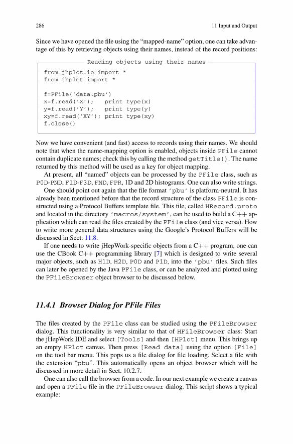
286 11 Input and Output
Since we have opened the file using the “mapped-name” option, one can take advan-tage of this by retrieving objects using their names, instead of the record positions:
Reading objects using their names
from jhplot.io import *from jhplot import *
f=PFile(’data.pbu’)x=f.read(’X’); print type(x)y=f.read(’Y’); print type(y)xy=f.read(’XY’); print type(xy)f.close()
Now we have convenient (and fast) access to records using their names. We shouldnote that when the name-mapping option is enabled, objects inside PFile cannotcontain duplicate names; check this by calling the method getTitle(). The namereturned by this method will be used as a key for object mapping.
At present, all “named” objects can be processed by the PFile class, such asP0D-PND, F1D-F3D, FND, FPR, 1D and 2D histograms. One can also write strings.
One should point out again that the file format ’pbu’ is platform-neutral. It hasalready been mentioned before that the record structure of the class PFile is con-structed using a Protocol Buffers template file. This file, called HRecord.protoand located in the directory ’macros/system’, can be used to build a C++ ap-plication which can read the files created by the PFile class (and vice versa). Howto write more general data structures using the Google’s Protocol Buffers will bediscussed in Sect. 11.8.
If one needs to write jHepWork-specific objects from a C++ program, one canuse the CBook C++ programming library [7] which is designed to write severalmajor objects, such as H1D, H2D, P0D and P1D, into the ’pbu’ files. Such filescan later be opened by the Java PFile class, or can be analyzed and plotted usingthe PFileBrowser object browser to be discussed below.
11.4.1 Browser Dialog for PFile Files
The files created by the PFile class can be studied using the PFileBrowserdialog. This functionality is very similar to that of HFileBrowser class: Startthe jHepWork IDE and select [Tools] and then [HPlot] menu. This brings upan empty HPlot canvas. Then press [Read data] using the option [File]on the tool bar menu. This pops us a file dialog for file loading. Select a file withthe extension “pbu”. This automatically opens an object browser which will bediscussed in more detail in Sect. 10.2.7.
One can also call the browser from a code. In our next example we create a canvasand open a PFile file in the PFileBrowser dialog. This script shows a typicalexample:
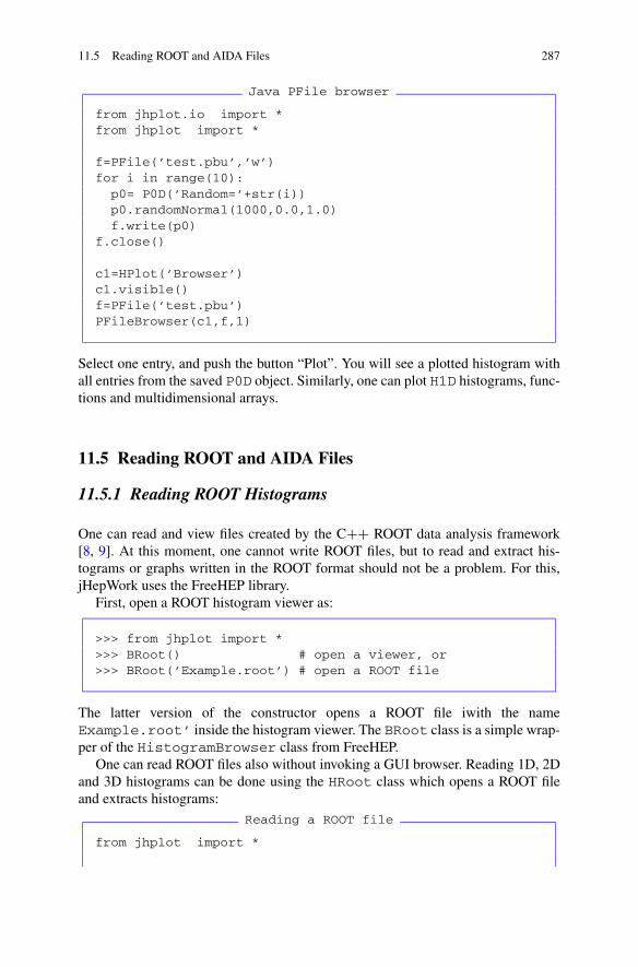
11.5 Reading ROOT and AIDA Files 287
Java PFile browser
from jhplot.io import *from jhplot import *
f=PFile(’test.pbu’,’w’)for i in range(10):
p0= P0D(’Random=’+str(i))p0.randomNormal(1000,0.0,1.0)f.write(p0)
f.close()
c1=HPlot(’Browser’)c1.visible()f=PFile(’test.pbu’)PFileBrowser(c1,f,1)
Select one entry, and push the button “Plot”. You will see a plotted histogram withall entries from the saved P0D object. Similarly, one can plot H1D histograms, func-tions and multidimensional arrays.
11.5 Reading ROOT and AIDA Files
11.5.1 Reading ROOT Histograms
One can read and view files created by the C++ ROOT data analysis framework[8, 9]. At this moment, one cannot write ROOT files, but to read and extract his-tograms or graphs written in the ROOT format should not be a problem. For this,jHepWork uses the FreeHEP library.
First, open a ROOT histogram viewer as:
>>> from jhplot import *>>> BRoot() # open a viewer, or>>> BRoot(’Example.root’) # open a ROOT file
The latter version of the constructor opens a ROOT file iwith the nameExample.root’ inside the histogram viewer. The BRoot class is a simple wrap-per of the HistogramBrowser class from FreeHEP.
One can read ROOT files also without invoking a GUI browser. Reading 1D, 2Dand 3D histograms can be done using the HRoot class which opens a ROOT fileand extracts histograms:
Reading a ROOT file
from jhplot import *

288 11 Input and Output
r=HRoot(’Example.root’)print ’number of histograms=’,r.getNKeys()print ’ROOT version=’,r.getVersion()print ’List histograms=’,r.toString()
h1=r.getH1D(’mainHistogram’) # fetch a H1Dc1=HPlot(’ROOT’)c1.setGTitle(’ROOT histogram’)c1.visible()c1.setAutoRange()c1.draw(h1)
Here we first read the key of the ROOT histogram and then convert it into the H1Dhistogram. Then, the object h1 can be plotted in the usual way using the draw(h1)method of the HPlot class.
One can also use the class RootFileReader to do the same (but it takes moretyping):
Reading a ROOT file
from jhplot import *from hep.io.root import *
r=RootFileReader(’Example.root’)print ’Number of histograms=’,r.nKeys()print ’ROOT version=’,r.getVersion()
key=r.getKey(’mainHistogram’) # read the keyhis1=key.getObject()h1=H1D(his1) # convert ROOT histogram to H1D
c1=HPlot(’ROOT’)c1.setGTitle(’ROOT histogram’)c1.visible(1)c1.setAutoRange()c1.draw(h1)
11.5.2 Reading ROOT Trees
The FreeHEP library contains a mechanism to read arbitrary ROOT objects, aswell as the so-called ROOT trees. A ROOT tree can contain a list of independentbranches, each can have its own definition. The RootIO package from the FreeHEPlibrary allows to read ROOT files which can contain user defined objects [10]. Thelibrary is still under development and was tested with the ROOT 3.00 version. TheRootIO package is included into the jHepWork library in a slightly redesigned style.

11.5 Reading ROOT and AIDA Files 289
The topic of reading ROOT tree is rather common for high-energy physics, wheredata in the form of objects are stored sequentially in a machine independent way.Readers who are not familiar with this field can skip this section. For others, wewill give a step-by-step instruction of how to read a file with ROOT trees containinguser-defined objects (for example, particle tracks).
There are several steps in reading a ROOT file. First of all, one should look insidethe file using the BRoot() method described above. This can help to understandthe structure of the file.
Next, one should generate a Java interface library for the user-defined objectscontained in a ROOT file. This interface library pre-processes a ROOT file and gen-erates classes with the description of ROOT objects. We will illustrate this by usingthe ROOT file ’Event.root’ which is located in
http://projects.hepforge.org/jhepwork/examples/data/orhttp://jwork.org/jhepwork/examples/data/
One can also find this file as well as the ROOT source file used to generate this filein [10].
Once the data file has been copied to a local directory, one should generate sourcefiles for our interface library by using this ROOT file. This can be done by executingthe following code inside the jHepWork IDE:
Building an interface library
from hep.rootio.util import *
a=InterfaceBuilder(’Event.root’)print a.message()
This script creates a directory ’hep’ with all necessary Java files. These files needto be compiled into bytecode. There are many ways to do this. In case of jHepWork,one can compile all files in this directory as: (1) Navigate to the directory ’hep’using the project file menu, i.e. click on the button below the file menu (bottom leftof the IDE) and select the directory ’hep’. Then, from the tool bar menu, select[Run] and [Javac all files]. You will see a message saying that all Javafiles have been compiled (check the existence of the files with the extension classin the directory ’hep’).
Now you are ready to write a code which reads this ROOT file. Below we showhow to access the ROOT tree and its branches inside the file ’Event.root’.Then we will plot squared transverse momenta of all particles (in this case, chargedtracks).
Reading a ROOT tree with user-defined objects
from hep.rootio.interfaces import *from hep.rootio import *from jhplot import *

290 11 Input and Output
reader = RootFileReader(’Event.root’)tree = reader.get(’T’)branch = tree.getBranch(’event’)n = branch.getNEntries()print ’entries=’,n
h1=H1D(’Pt2’,100,0,10)for i in range(n):
e = branch.getEntry(i)l = e.getTracks()print ’No=’,i,’ NTracks=’,e.getNtrack(),’ ’,l.size()it = l.iterator()while(it.hasNext()):
t = it.next()px=t.getPx()py=t.getPy()h1.fill(px*px+py*py)
c1=HPlot(’Canvas’)c1.visible()c1.setAutoRange()c1.draw(h1)
The example reads all stored events, accesses tracks and extract their momenta.Then it plots squared transverse momenta of all stored tracks in the form of a 1Dhistogram.
We will not discuss this example further, since everyone who knows ROOT willnot have any problems to understand it. We only note that one can also do all theabove steps using a shell prompt. Look at the example in ’RootIO’ stored in the’example’ directory.
11.5.3 Plotting ROOT or AIDA Objects Using jHepWork IDE
On can use the jHepWork IDE to read data files written in the ROOT or AIDAformat in a GUI-driven fashion. One can do this as:
• Start the jHepWork IDE.• Select the menu [Tools] and then [HPlotJa canvas]. You will see a new
window which can be used for data visualization (based on the class HPlotJa).The HPlotJa class is described in Sect. 10.10.
• In the HPlotJa frame, go to the menu [Option] and select [Add pads].You will see a sub-menu to build various pads (plotting regions), such as 1 × 1,1 × 2, 2 × 1, 2 × 2. To create, for example, 4 plotting pads with X–Y axes, selectthe sub-menu [pad 2x2].

11.6 Working with Relational SQL Databases 291
• Open a data file using the [File] menu and sub-menu [Open data] of theHPlotJa window. The file extension should be ’*.root’ or ’*.aida’. Youwill see an object browser from the right side of the HPlotJa frame. Using themouse, locate some entry and then plot it using the right mouse button, whichshows different choices of the pads where the object should be shown. One canplot data points either on one pad by overlaying the points from different objects,or one can plot data points on different pads.
One can do the same from a Jython script as:
>>> from jhplot import HPlotJa>>> c1=HPlotJa(’Canvas’)>>> c1.visible()>>> c1.showBrowser(’file.root’)>>> c1.showEditor(1) # open an object editor
Once the script is executed, you should see a browser (on the left of the main can-vas) listing all objects inside the file. If one clicks on an entry of this list, a his-togram or data set will be plotted. One can also plot data on different pads using themouse pop-up menu. One can learn more about how to read ROOT or AIDA files inSect. 11.5.1.
11.6 Working with Relational SQL Databases
We cannot avoid the discussion of relational databases based on the SQL standard,since such databases are reality of our life.
So far we have discussed a “flat file” approach in which a binary or text file usu-ally contains one record per line. A SQL-relational database has several advantages:one can implement a server-client mode, scalability (indexing of records), and con-currency when one needs to synchronize multiple updates at the same time.
However, I should warn you: in many cases you do not need such SQL databasesat all. For data analysis, we often read data sequentially, i.e. we read data recordsfrom the top to the bottom all the way through. We are in less degree worry abouta random access, concurrency or client-server mode as it is implemented in manyrelational databases. Straight file access is usually faster than executing a SQL queryand less memory consuming.
Thus, in terms of performance, a data-analysis code may not benefit from switch-ing to the SQL databases. Using a SQL database may or may not be worthwhile.Your decision should be based on complexity of the data access, where a databasesoftware needs to be installed, and many other factors.
Below will consider the Apache (“Derby”) open-source relational database.More detail about Java implementation of this database can be found elsewhere [11].

292 11 Input and Output
11.6.1 Creating a SQL Database
First of all, let us prepare a module which keeps common information about our SQLdatabase. This module will be necessary for creation and retrieval information in ourfurther examples. We will consider an embedded Derby database i.e. a database fora simple single-user Java application. In this mode, only a single application canaccess the database at the time and no network access is required.
Let us prepare a file ’openDB.py’ with the information necessary for creationof database, such as drivers, protocol, name of database table. The name of ourdatabase will be ’derbyDB’, which will keep a single table with the name “loca-tion”. We also set a user name and a password for this database. Below is a scriptwhich has all necessary information:
Common module: ’openDB.py’
from java.sql import *from java.lang import Classfrom java.util import Properties
framework = ’embedded’driver = ’org.apache.derby.jdbc.EmbeddedDriver’protocol = ’jdbc:derby:’dbName=’derbyDB’table=’location’
Class.forName(driver).newInstance()props = Properties();props.put(’user’, ’jhepwork’)props.put(’password’, ’secret’)
This file will be imported for all Jython modules to be discussed below.Now let us create a database called “derbyDB”. Here we will use the Jython
syntax to create a database and to insert several SQL statements into the table’location’, which will keep information about the street name (type string) andhome number (integer).
The script below does the following: (1) loads the JDBC Java driver in order tostart-up the Derby database. (2) Creates a table inside the database, first checkingwhether this table is already created. If it does exist, we remove it (see the statement’drop table’+table. (3) Then we insert a few records with addresses.
Creating a SQL database
from openDB import *
scon=protocol+dbName+’;create=true’conn = DriverManager.getConnection(scon, props)s = conn.createStatement()
try:

11.6 Working with Relational SQL Databases 293
s.execute(’drop table ’+table)except SQLException:
print ’no need to remove table’
s.execute(’create table ’+table+\’(num int, addr varchar(40))’)
s.execute(’insert into ’+table+\’ values (1956,\’Webster St.\’)’)
s.execute(’insert into ’+table+\’ values (1910,\’Union St.\’)’)
s1=’update ’+table+’ set num=?, addr=? where num=?’ps = conn.prepareStatement(s1)ps.setInt(1,180)ps.setString(2, ’Grand Ave.’)ps.setInt(3, 1956)ps.executeUpdate()print ’Updated 1956 Webster to 180 Grand’s.close()conn.commit()
try:DriverManager.getConnection(’jdbc:derby:;shutdown=true’)
except SQLException:print ’all done’
This example shows how to use two alternative methods to insert and update thedatabase: (1) one is based on the standard SQL statements, and the second using aprepared statement based on the method prepareStatement() for fast query.
It is important to close the database properly using the line:
’jdbc:derby:;shutdown=true’.
The DriverManager should raise only one exception : SQLException. Thedatabase should be shut down so it can perform a checkpoint and releases its re-sources.
After the execution of the script above, you will see a database directoryderbyDB with the stored information.
11.6.2 Working with a Database
Now let us read the database entries. As before, we will use exactly the same com-mon module ’openDB.py’. This time, however, we will set create=false forthe argument of DriverManager.getConnection. Using two SQL queries,

294 11 Input and Output
we will print all database records and will search for a record with the string’Union St.’. Finally, we close the database:
Reading database
from openDB import *
scon=protocol+dbName+’;create=false’conn = DriverManager.getConnection(scon,props)s = conn.createStatement()
s1=’SELECT num, addr FROM ’+table+’ ORDER BY num’rs = s.executeQuery(s1)while rs.next():
print ’sorted=’+rs.getString(1),rs.getString(2)
s2 = ’SELECT * FROM ’+table+’ WHERE addr=\’Union St.\’’rs = s.executeQuery(s2)while rs.next():
print ’Found=’,rs.getString(1),rs.getString(2)s.close()conn.commit()
try:DriverManager.getConnection(’jdbc:derby:;shutdown=true’)
except SQLException:print ’all done’
11.6.3 Creating a Read-only Compact Database
Sometimes it is useful to create a read-only database and compress it into a jar file.This allows a database to be distributed as a single file instead of multiple fileswithin a directory. In this case, we will not be able to modify it, since the databasewill be represented by a single self-contained file.
The operation discussed above can easily be done with the Jython module os.This module will be used to create the file ’derbyDB.jar’ with the databasedirectory by calling the external jar command (it comes with the Java installation):
Compacting a database to a jar file
import oscmd=’jar cMf derbyDB.jar derbyDB’print os.system(cmd)
Now, how can we read the file ’derbyDB.jar’? This can be done in same spiritas shown in Sect. 11.6.2: use the same script, but add the extra line shown below:

11.7 Reading and Writing CSV Files 295
protocol = ’jdbc:derby:jar:(’+dbName+’.jar)’
after the import statement. Try to execute the corrected script. After this, youshould be able to read the database stored in this jar file.
11.7 Reading and Writing CSV Files
The comma separated value files, CSV, are used to store information in a form oftables. This format is especially popular for import and export in spreadsheets. Datain such files are either separated by a comma or a tab, or by any other customdelimiter.
We have already considered how to read and write the CSV files using the Jythonmodule csv (see Sect. 2.16.4). Below we will consider high-performance Java li-braries to work with such files.
11.7.1 Reading CSV Files
jHepWork supports reading the CSV files as well as writing data into such files. Letus create a typical CSV file using any text editor:
File ’table.csv’
Sales, Europe, Russia, USAJanuary, 10, 20, 20February, 30, 20, 50March, 10, 40, 100April, 80, 7, 30May, 300, 400, 90June, 50, 10, 70
Dealing with CSV format couldn’t be much easier when using the jHepWorkJava classes—just open a CSV file using the class CSVReader and iterate over allits entries as shown in the example below:
Reading table.csv file
from jhplot.io.csv import *
r=CSVReader(’table.csv’,’,’)while 1:
line= r.next()if line == None: breakprint line
r.close()

296 11 Input and Output
As one can see, the method next() returns a list of strings for each line of theCSV file. File reading stops when the end of the file is detected. If you want toread arrays of lists, use the method readNext() instead. One can easily convertstrings inside the list representing each row to floats and integers, as float(str)(returns a float value) or int(str) (returns an integer).
One can read all entries at once, instead of looping over all rows. This can bedone using the methods:
l=r.readList() read all elements into a 2D list;l=r.readAll() read all elements into list, each row is represented as an array.
Let us take a closer look into the CSVReader class. It has several constructors:
>>> CSVReader(file, separator, quotechar, line)>>> CSVReader(file, separator, quotechar)>>> CSVReader(file, separator)>>> CSVReader(file)
where file is the string with a file name, separator is the character used forseparating entries in each row, quotechar is the character to use for quoted el-ements. Finally, line is an integer number representing the line number to skipbefore start reading. When no separator is given, then the default separation isdone using a comma. If no quotechar is given, the default escaping quotes is [”],and if no line is given, the default end of line is the new line symbol.
Finally, one can display a CSV file in a spreadsheet using the SPsheet classdiscussed in Sect. 12.4.2. Once CSVReader object has been created, just pass it tothe SPsheet object as:
Showing entries from ’table.csv’ file
from jhplot import *from jhplot.io.csv import *r=CSVReader(’table.csv’,’,’)SPsheet(r)
Now let us move to the next subject where we will discuss how to write data intothe CSV files.
11.7.2 Writing CSV File
To write data to CSV files is as easy as reading them. Instead of the CSVReaderclass, one should use the CSVWriter class. It has the following constructors:
>>> CSVWriter(file, separator, quotechar, line)>>> CSVWriter(file, separator, quotechar)

11.8 Google’s Protocol Buffer Format 297
>>> CSVWriter(file, separator)>>> CSVWriter(file)
Here, file is an output file name, and other arguments are exactly as for theCSVReader class.
Let us show an example illustrating how to write lists of objects line by line:Writing ’out.csv’ file
from jhplot.io.csv import *
w=CSVWriter(’out.csv’,’,’)
w.writeNext( [’Test1’,’20’,’30’] )w.writeNext( [’Test2’,’100’,’50’] )w.writeNext( [’Test3’,’200’,’100’] )
w.close()
Check the output file. It has the following structure:
"Test1","20", "30""Test2","100","50""Test3","200","100"
One can write the entire file at once using the writeAll(list) method.
11.8 Google’s Protocol Buffer Format
Many situations require an analyzer to write structural data into a format whichcan be understood by variety of programming languages. Imagine an experimentalapparatus producing a data stream. It is very likely that its code for data I/O is writtenin C/C++, since most hardware drivers are implemented in this system language.But, at the end of the day, this is a user who should analyze the data and whomay prefer a human-friendly language (like Java or Jython) for final analysis code.Therefore, we should find a way to read structural data produced by experimentsusing these higher-level languages. Or, imagine an opposite situation: an analyzerproduces data using Java or Jython, and an application implemented using a lower-level language should read this data during communication with a hardware.
One way to deal with such kind of problems is to use a self-described file format,such as XML. But there are several problems with this format when dealing withlarge data volumes: (1) programs are slow for loading; (2) there is a significantpenalty on program’s performance; (3) data files are large due to tags overhead.
Taking into account that the XML format is too cumbersome to use as an encod-ing method for large data files, one can use the ROOT format as an alternative. This

298 11 Input and Output
may seem to be rather heavy approach (installed ROOT takes several hundreds ofmegabytes!), and to read most recent ROOT files in Java is not too easy: in fact,the ROOT framework was not designed from the ground to be friendly for otherprogramming languages.
The Google team has recently released the Protocol Buffers package [6] whichdeals with serializing structured data in a platform-neutral format. This data-interchange format is used by Google for persistent storage of data in a varietyof storage systems. It is also well tested on many platforms. The Protocol Buffersis self-describing format, which is equally well supported by C++, Java, Pythonand by other languages using third-party packages. In comparison with the XMLformat, the Protocol Buffers files are up to a factor 100 times faster to read, andfile sizes are significantly smaller due to a built-in compression. This format is alsovery promising due to the offered backwards compatibility: new fields created bynew protocol versions are simply ignored during data parsing.
Even more. The Protocol Buffers helps to abstract from a language-specific de-scription of data structures. More specifically, this means that an analyzer only needsto produce a file describing his/her data records, and then the Protocol Buffers pro-gram generates a C++ or Java code for automatic encoding and parsing data struc-tures.
Below we will discuss the Protocol Buffers in more detail. The program isincluded into jHepWork; look at the library protobuf.jar in the directorylib/system. To develop applications in C++, the reader is assumed to installthe Protocol Buffers (at least version 2.2) from the official web site [6].
11.8.1 Prototyping Data Records
For our next example, we will assume the following experiment. We perform N
measurements, each measurement is characterized by an identification number, astring (name) and arbitrary array with some other data. In each measurement, itis assumed that we observe n number of particles. This number is not fixed, andcan vary from measurement to measurement. Finally, for each particle, we measureparticle’s energy and electric charge. We also assign a string with particle name.
Let us prototype an event record using the Protocol Buffers syntax, which is thencan be used to generate a C++ or Java code. The code is shown below:
Data prototype. File ’experiment.proto’
package proto;option java_package = "proto";option java_outer_classname = "Observations";
message Event {required int64 id = 1;required string name=2;repeated double data = 3 [packed=true];

11.8 Google’s Protocol Buffer Format 299
message Particle {required string name=1;required sint32 charge=2;required double energy=3;
}repeated Particle particle = 4;
}message Experiment {
repeated Event event = 1;}
This file contains the description of all objects in self-described platform-indepen-dent way, so later one can read or write data from a variety of languages. As one cansee, the class Event envelops the entire data. Instead of using the class name, theProtocol Buffers uses the word “message”. Each event has 4 records, id (integer),name (string), data (list of doubles) and the class Particle. Each such record (or“message”) has numbered fields (in this example, running from 1 to 4). Such integervalues are unique “tags” used in the binary encoding.
The value types can be numbers, booleans, strings or other message types, thusdifferent messages can hierarchically be nested. The required field tells that suchfield should always be present. One can also set the default value using the line[default=value], where value is a given default value. The message fieldcan have other two types: optional—a message can have zero or one of thisfield (but not more than one), and repeated—a message can be repeated anynumber of times, preserving the order of the repeated values. The fields can includeenumerators for tight association of a specific value to a variable name.
In the above example, the message data can be repeated (similar to alist), so we can append any number of double values in each record. The field[packed=true] is used for a more efficient encoding of multiple data entries.Finally (and this is very important), the message of the Particle type can also berepeated, since we can have multiple number of particles in events.
As you may already have guessed, the message Particle keeps informationabout a single particle, such as its name, charge and energy. This message is con-structed in exactly the same way as the outer messages. The only difference is thatnow we should specify the fields which are the most appropriate for defining particleproperties.
A scalar message field can have one of the following types shown in Table 11.1.More types are given in [6].
11.8.2 Dealing with Data Using Java
Now let us generate a Java code using the above prototype file. Assuming that thePrototype Buffer is properly installed, and assuming that we are working in theUnix/Mac environment, we generate the Java code as:

300 11 Input and Output
Table 11.1 Scalar valuetypes used in .proto filesand their Java and C++equivalents
Scalar message field types
int int (Java and C++)
double double (Java and C++)
int int (Java and C++)
bool boolean (Java) and bool (C++)
string String (Java) and string (C++)
fixed32 int (Java) and int32 (C++)
fixed64 long (Java) and int64 (C++)
Generating Java code
protoc --java_out=. experiment.proto
This creates a directory ’proto’ with the Observations.java file. The–java_out option tells to generate Java classes to be used for data encoding. Simi-lar options are provided for other supported languages. The dot after this option tellsto generate the output in the current directory. The output of this command is theJava file Observations.java located in the directory proto, as specified inthe original experiment.proto file (see the Java-package statement).
Let us write a test code which generates 100 events with 10 particles in eachevent. We will create the file WriteData.java and copy it into the directory’proto’ together with recently generated file Observations.java:
Writing data into a file. ’WriteData.java’ file
package proto;import proto.Observations.Experiment;import proto.Observations.Event;import java.io.FileOutputStream;
class WriteData {public static void main(String[] args) throws Exception {
Experiment.Builder exp = Experiment.newBuilder();FileOutputStream output =
new FileOutputStream("data.prod");for (int e=0; e<100; e++){
Event.Builder ev = Event.newBuilder();ev.setId(e); ev.setName("collision");ev.addData(1); ev.addData(2);
for (int i=0; i<10; i++){Event.Particle.Builder p =
Event.Particle.newBuilder();p.setName("proton");p.setCharge(1); p.setEnergy(1);ev.addParticle(p);
};

11.8 Google’s Protocol Buffer Format 301
exp.addEvent(ev); } ;
exp.build().writeTo(output);output.close();}
}
Next we need to compile all Java files and build a jar library. For this, we definean environmental variable JHEP as a directory with the installed jHepWork and thencompile and build a jar library.
Compiling Java code
javac -1.6 -cp $JHEP/lib/system/protobuf.jar proto/*.javajar -cf proto.jar proto/*
This produces the file proto.jar with the compiled classes.Let us test the above code. We will run the WriteData class in the usual Java
fashion.
Running WriteData program
java -cp $JHEP/lib/system/protobuf.jar:proto.jar \proto.WriteData
The result of this command is the output file ’data.prod’ with our structuraldata written in a binary form. Let us verify what is written by adding the codeReadData.java into the directory ’proto’.
Reading data. ’ReadData.java’ file
package proto;import proto.Observations.Experiment;import proto.Observations.Event;import java.io.FileInputStream;
class ReadData {
public static void main(String[] args) throws Exception {Experiment exp=Experiment.parseFrom(new FileInputStream("data.prod"));for (Event ev: exp.getEventList()) {
System.out.println("Event id:" +ev.getId());System.out.println("Event name:" +ev.getName());
for (Event.Particle p: ev.getParticleList()) {System.out.println(p.getName());System.out.println(p.getEnergy());
} }} }
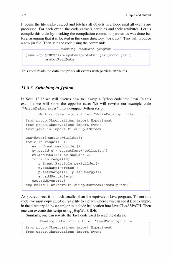
302 11 Input and Output
It opens the file data.prod and fetches all objects in a loop, until all events areprocessed. For each event, the code extracts particles and their attributes. Let uscompile this code by invoking the compilation command javac as was done be-fore, assuming that it is located in the same directory ’proto’. This will producea new jar file. Then, run the code using the command:
Running ReadData program
java -cp $JHEP/lib/system/protobuf.jar:proto.jar \proto.ReadData
This code reads the data and prints all events with particle attributes.
11.8.3 Switching to Jython
In Sect. 12.12 we will discuss how to unwrap a Jython code into Java. In thisexample we will show the opposite case: We will rewrite our example code’WriteData.java’ into a compact Jython script:
Writing data into a file. ’WriteData.py’ file
from proto.Observations import Experimentfrom proto.Observations import Eventfrom java.io import FileOutputStream
exp=Experiment.newBuilder()for e in range(100):
ev = Event.newBuilder()ev.setId(e); ev.setName(’collision’)ev.addData(1); ev.addData(2)for i in range(10):
p=Event.Particle.newBuilder()p.setName(’proton’)p.setCharge(1); p.setEnergy(1)ev.addParticle(p)
exp.addEvent(ev)exp.build().writeTo(FileOutputStream(’data.prod’))
As you can see, it is much smaller than the equivalent Java program. To run thiscode, we must copy proto.jar file to a place where Java can see it (for example,in the directory lib/user) or to include its location into Java CLASSPATH. Thenone can execute this script using jHepWork IDE.
Similarly, one can rewrite the Java code used to read the data as:
Reading data into a file. ’ReadData.py’ file
from proto.Observations import Experimentfrom proto.Observations import Event

11.8 Google’s Protocol Buffer Format 303
from java.io import FileInputStream
exp=Experiment.parseFrom(FileInputStream(’data.prod’));for e in exp.getEventList():
print e.getId()print e.getName()for p in e.getParticleList():
print p.getName(),p.getEnergy();
Again, run this code and you will see exactly the same output as in the case of Java.
11.8.4 Adding New Data Records
Now let us illustrate how to add a new event record to the existing file. To make ourcodding shorter, we will use Jython and add an event (but without any particle) as:
Adding new records. ’AddData.py’ file
from proto.Observations import Experimentfrom proto.Observations import Eventfrom java.io import FileOutputStreamfrom java.io import FileInputStream
exp=Experiment.newBuilder()try:
input=FileInputStream(’data.prod’)exp.mergeFrom(input); input.close()
except FileNotFound, e:print ’The file was not found, going to backup file’
ev = Event.newBuilder() # add new eventev.setId(99); ev.setName(’new entry’)exp.addEvent(ev)
output=FileOutputStream(’data.prod’)exp.build().writeTo(output)output.close()
In this example we simply read the file and then write a new file with the additionalevent.
11.8.5 Using C++ for I/O in the Protocol Buffers Format
Now we come to the main issue of how to generate the same file using a C++program, so we can read it using Java, Jython or any other language. Of course,

304 11 Input and Output
we also need to test the opposite situation when reading the Java-generated file’data.prod’ by a C++ program.
Below we will show the necessary steps to produce a C++ code which generatesexactly the same data file as that shown in the previous section, and then how toread this file (or the file generated by the Java code above). We will use the sameprototype file ’experiment.proto’ as before. Let us generate a C++ code tobe used for data encoding:
Generating C++ code
protoc --cpp_out=. experiment.proto
Note the option cpp which tells to generated the C++ encoding code. Afterexecution of this line, we should find two files, experiment.pb.cc andexperiment.pb.h in the same directory. As in case of Java, they contain thenecessary information to be used for data serialization.
Let us write a small test program which creates the output file.
Writing data into a file. ’write_test.cc’ file
#include <iostream>#include <fstream>#include <string>#include "experiment.pb.h"using namespace std;
int main(int argc, char **argv){
GOOGLE_PROTOBUF_VERIFY_VERSION;proto::Experiment exp;
for (int e=0; e<100; e++){proto::Event* ev = exp.add_event();ev->set_id(e); ev->set_name("collision");ev->add_data(1); ev->add_data(2);
for (int i=0; i<10; i++) {proto::Event::Particle* p=ev->add_particle();p->set_name("proton");p->set_energy(1); p->set_charge(1);} };
cout << "Write data.prod" << endl;fstream output("data.prod",
ios::out | ios::trunc | ios::binary);if (!exp.SerializeToOstream(&output)) {
cerr << "Failed to write address book." << endl;return -1; }
output.close();google::protobuf::ShutdownProtobufLibrary();

11.8 Google’s Protocol Buffer Format 305
return 0;}
For those who know C++ this code should look rather simple. Moreover, the codelogic is rather similar to that of the Java code. Since we declared the package protoin the prototype file, one should use the corresponding C++ namespace for theclass declarations. The first statement in the main() method verifies that we havenot accidentally linked against the library which is incompatible with the version ofthe headers.
Next, we will need to compile all these files. For this, we use GNU gcc compilerinstalled by default on Unix/Linux systems
Compiling the source codes
gcc write_test.cc experiment.pb.cc \-o write_test ‘pkg-config --cflags --libs protobuf‘
Finally, try to execute the program write_test. We will see the created file’data.proto’. Check its size. It should have the same size as in the case ofJava example. Surely, this is a good sign, since it likely indicates that the new file iscorrectly produced and, in fact, is totally identical to that generated previously usingJava.
Let us move on and write a C++ code which will read the data from this file.
Reading data from a file. ’read_test.cc’ file
#include <iostream>#include <fstream>#include <string>#include "experiment.pb.h"using namespace std;
int main(int argc, char **argv){GOOGLE_PROTOBUF_VERIFY_VERSION;proto::Experiment exp;
fstream input("data.prod", ios::in | ios::binary);if (!exp.ParseFromIstream(&input)) {cerr << "Failed to parse data file" << endl;return -1; }
for (int i = 0; i < exp.event_size(); i++) {const proto::Event& ev = exp.event(i);cout << " ID: " << ev.id() << endl;cout << " Name: " << ev.name() << endl;
for (int j = 0; j < ev.particle_size(); j++) {const proto::Event::Particle& p = ev.particle(j);

306 11 Input and Output
cout << " - name: " << p.name() << endl;cout << " - energy: " << p.energy() << endl;
} }google::protobuf::ShutdownProtobufLibrary();return 0;
}
The file reads the data and loops over all event entries. We can compile all sourcefiles as usual:
Generating C++ code
gcc read_test.cc experiment.pb.cc \-o read_test ‘pkg-config --cflags --libs protobuf‘
and run the executable program as read_test. We will see the print messagesincluded for debugging.
As a final exercise, try to use the Java or Jython code developed in the previoussubsection for reading file created by our C++ program.
11.8.6 Some Remarks
The Protocol Buffers is easy-to-use format to organize sequential data in a platform-independent way. It is a good format for handling individual messages within a largedata set which consists of large number of small pieces. Each piece can also be astructural data in the form of “messages”.
We have already discussed that the class PFile (see Sect. 11.4) is com-pletely based on the Protocol Buffers format. Each record is compressed us-ing the ZIP file format. The records are implemented using the Protocol Buffersfile HRecord.proto located in the directory ’macros/system’. The fileHRecord.proto can be used to construct applications in C++ which can readand write files generated by the PFile Java class.
11.9 EFile Data Output
The usage of the Protocol Buffers encoding is simplified by the class EFile de-signed to deal with stacking Protocol Buffers messages into compressed files. Eachmessage is written independently, which allows to write and read large data volumesorganized in separate data records.
The data structure of each data record is based on the file HEvent.proto lo-cated in the directory macros/system. Since this file is rather short, we willshow it here:
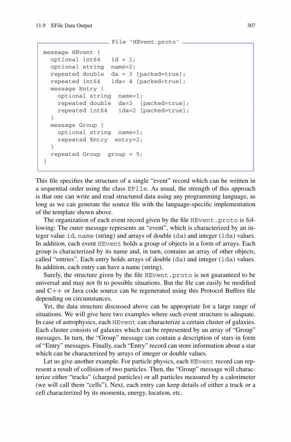
11.9 EFile Data Output 307
File ’HEvent.proto’
message HEvent {optional int64 id = 1;optional string name=2;repeated double da = 3 [packed=true];repeated int64 ida= 4 [packed=true];message Entry {optional string name=1;repeated double da=3 [packed=true];repeated int64 ida=2 [packed=true];
}message Group {optional string name=1;repeated Entry entry=2;
}repeated Group group = 5;
}
This file specifies the structure of a single “event” record which can be written ina sequential order using the class EFile. As usual, the strength of this approachis that one can write and read structured data using any programming language, aslong as we can generate the source file with the language-specific implementationof the template shown above.
The organization of each event record given by the file HEvent.proto is fol-lowing: The outer message represents an “event”, which is characterized by an in-teger value id, name (string) and arrays of double (da) and integer (ida) values.In addition, each event HEvent holds a group of objects in a form of arrays. Eachgroup is characterized by its name and, in turn, contains an array of other objects,called “entries”. Each entry holds arrays of double (da) and integer (ida) values.In addition, each entry can have a name (string).
Surely, the structure given by the file HEvent.proto is not guaranteed to beuniversal and may not fit to possible situations. But the file can easily be modifiedand C++ or Java code source can be regenerated using this Protocol Buffers filedepending on circumstances.
Yet, the data structure discussed above can be appropriate for a large range ofsituations. We will give here two examples where such event structure is adequate.In case of astrophysics, each HEvent can characterize a certain cluster of galaxies.Each cluster consists of galaxies which can be represented by an array of “Group”messages. In turn, the “Group” message can contain a description of stars in formof “Entry” messages. Finally, each “Entry” record can store information about a starwhich can be characterized by arrays of integer or double values.
Let us give another example. For particle physics, each HEvent record can rep-resent a result of collision of two particles. Then, the “Group” message will charac-terize either “tracks” (charged particles) or all particles measured by a calorimeter(we will call them “cells”). Next, each entry can keep details of either a track or acell characterized by its momenta, energy, location, etc.

308 11 Input and Output
Let us come to a specific example which illustrates a concrete program imple-mentation of this approach. In case of jHepWork, the generated class from the aboveprototype is called PEventFile. Using this class and the class EFile whichimplements an I/O layer for each HEvent, one can create a file holding multiplerecords as shown in this example:
Writing events into a file
from jhplot.io import *from jhplot.io.PEventFile import *
f=EFile(’tmp.nbu’,’w’)for i in range(1000):
ev = HEvent.newBuilder()ev.setName(’collision’)ev.setId(i); ev.addDa(1)
tracks = HEvent.Group.newBuilder()tracks.setName(’tracks’)for j in range(20):
track=HEvent.Entry.newBuilder()track.setName(’pion’+str(i))track.addDa(1); track.addDa(2)tracks.addEntry(track)
ev.addGroup(tracks)
cells = HEvent.Group.newBuilder()cells.setName(’cells’)for j in range(20):
cell=HEvent.Entry.newBuilder()cell.setName(’cell’+str(i))cell.addDa(1);cell.addIda(1)cells.addEntry(cell)
ev.addGroup(cells)
f.write(ev) # write eventf.close()
As the reader may notice, we use the second example from particle physics. Foreach collision, we write two groups of objects, “tracks” and “cells”. Then we filled“entries” characterized by one double and one integer number. Of course, nothingprevents us from adding more groups, more entries or more primitive values foreach object. By convention, we will create an output file with the extension ’nbu’.
Now let us read this file. This part is rather simple:
Reading events
from jhplot.io import *from jhplot.io.PEventFile import *

11.10 Reading DIF Files 309
f=EFile(’tmp.nbu’)print f.getVersion()
for i in range(1,f.size()):ev = f.read()print ’Read =’,ev.getId(),ev.getName()# get groups
for j in range(ev.getGroupCount()):g=ev.getGroup(j)print g.getName()# get entriesfor k in range(g.getEntryCount()):
e=g.getEntry(k)print e.getDa(0)
f.close()
The above example shows how to loop over all HEvent entries, retrieve groupsand then entries from each group. The method getVersion() checks the versionof EFile implementation used to generate the file. The total number of HEventmessages is given by the method size().
As was already said, Java and Jython allow to write arbitrary structural data vol-umes in a simple and transparent way using their own classes and methods. Butthe strength of the above approach is that data files can also be generated by otherprogramming languages using the Protocol Buffers template. More specifically, incase of C++, the CBook [7] library can be used to write data structures using theHEvent.proto prototype file implemented in C++. Therefore, one can generatedata using a C++ code and read data using the EFile Java class exactly as shownin the previous example.
11.10 Reading DIF Files
The DIF (“Data Interchange Format”) format has a limited support in jHepWork.Files in this format have the extension ’.dif’ and can be used to import or exportspreadsheets between various applications.
The current implementation of this package [12] is only for read-only mode.There is no possibility for saving data into this file. To read such files, one shouldimport the module dif located in the ’macros/system’ directory. In the ex-ample below, we read the file ’nature.dif’, extract all information into Jythontuples and print the entries:
Reading the file nature.dif
import dif
f=open(’nature.dif’,’r’)d = dif.DIF(f)

310 11 Input and Output
print d.headerprint d.vectorsprint d.data
Below we give some explanation:
d.header dictionary of header entities, with names shifted to lowercase for easeof handling
d.data list of tuples with datad.vectors list of vector names (or, better, column names)
Read more information about Python implementation of this module in [12].
11.11 Summary
It may well be that you get confused by the significant number of I/O formats sup-ported by jHepWork. Below we will summarize the jHepWork I/O and give someguiding tips about what exactly to use in certain situations.
11.11.1 Dealing with Single Objects
If we need to save one object at the time (like a histogram, function or a P-typearray), use their native methods. For example, to write an object into a file, usethe toFile() method, see Sects. 5.4 and 8.6. For reading data, one can use thecorresponding constructors which accept the name of the file with input data forobject initialization. This also includes a compression mechanism, see the methodreadGZip() in Sect. 5.4. The good thing about this approach is that: (1) it isfast; (2) data can be produced using other programming languages, as long as ourcodding strictly follows the native jHepWork format.
A slower approach would be to use Java serialization, i.e. serializing separateobjects with the method writeSerialized(). By default, files will be com-pressed. One can also write and read data stored in XML files using the methodwriteXML() and readXML(). This will be the slowest approach, but the ad-vantage is that the XML files are human-readable and human-editable. Finally, it israther easy to read such files using applications implemented in other programminglanguages.
11.11.2 Dealing with Collections of Objects
To read and save collections of jHepWork objects, use the serialization methodwriteSerialized() or readSerialized(). This can be done “in one go”,

References 311
if all Java objects are put either in a list or map. This approach also allows to dealwith the XML-type formats. As we have already mentioned, this is human-readable,self-describing and platform-neutral protocol.
For large and complicated data structures, it makes sense to use the HFile class,see Sect. 11.3. In most cases, objects can be viewed using a GUI browser. Data insuch files are compressed by default. As before, one can serialize data in XML usingthe class HFileXML.
An arbitrary collection of structural data can also be written using the Google’sProtocol Buffer format discussed in Sect. 11.8. It is a compact way of encoding datain a binary format. The main advantage of this format is that data can be processedby programs implemented in other programming languages.
If we are interested in the jHepWork objects only, use the class PFile. Thisapproach has several advantages compared to the Java serialization as discussed inSect. 11.4. The class PFile writes data in a form of compressed records basedthe Google’s Protocol Buffer format. This approach encodes high-level jHepWorkobjects (like histograms) in a platform-independent way. This means that data canbe generated by C++ programs using the package CBook [7] and processed usingthe PFile class.
Similarly, one can use the class EFile (see Sect. 11.9) which deals with a ratherbroad range of data structured in “events” and “records”. Both PFile and EFilecan be used to read a particular event or record, without uncompressing the wholefile. This feature is particularly useful for reading data in parallel using multi-coreprocessors (this will be discussed in Sect. 16.4).
Similarly, one can use the class HBook and the CFBook package, see Sect. 8.6.1,which are mainly designed for XML-type outputs (but more optimized to keep largedata sets, removing unnecessary tags for arrays). No compression is used.
As discussed in this chapter, if one needs to find an association between a keyand a data object, one can use databases. In the simplest, non-persistent case, useJython dictionaries or Java maps. For storing information in a persistent state, onecan use a database based on the class HDataBase, see Sect. 11.3.6. Note that onecan use a similar database approach using the PFile class. As discussed earlier, itcan also be used for a direct association between a stored object inside a file and itstextual key (which is just object title). For complicated input queries, one can usethe Apache Derby SQL-type databases, see Sect. 11.6.
The format CSV is only useful for keeping data in simple tables. The only ad-vantage of this approach is that it is simple and data can easily be converted by aspreadsheet-like application.
Finally, one can use a pure-Python approach or calling Java classes, seeSect. 2.16. The pure-Python method is generally not recommended for large datafiles, but it is very useful when it comes to the simplicity.
References
1. Richardson, C., Avondolio, D., Vitale, J., Schrager, S., Mitchell, M., Scanlon, J.: ProfessionalJava, JDK 5th edn. Wrox, Birmingham (2005)

312 11 Input and Output
2. Arnold, K., Gosling, J., Holmes, D.: Java(TM) Programming Language, 4th edn. Java Series.Addison-Wesley, Reading (2005)
3. Flanagan, D.: Java in a Nutshell, 5th edn. O’Reilly Media, Sebastopol (2005)4. Eckel, B.: Thinking in Java, 4th edn. Prentice Hall, Englewood Cliffs (2006)5. Bloch, J.: Effective Java, 2nd edn. The Java Series. Prentice Hall, Englewood Cliffs (2008)6. Google Protocol Buffers project. URL http://code.google.com/p/protobuf/7. Chekanov, S.: CBOOK histogram library. URL http://jwork.org/jhepwork/cbook8. Brun, R., Rademakers, F., Canal, P., Goto, M.: Root status and future developments. ECONF
C0303241 (2003) MOJT0019. Brun, R., Rademakers, F.: ROOT: An object oriented data analysis framework. Nucl. Instrum.
Methods A 389, 81 (1997). URL http://root.cern.ch/10. Johnson, T.: FreeHEP RootIO. URL http://java.freehep.org/freehep-rootio/11. Apache Derby: URL http://db.apache.org/derby/12. Gonnerman, C.: Navy DIF file handler. URL http://newcenturycomputers.net/projects/dif.html

Chapter 12Miscellaneous Analysis Issues Using jHepWork
In this chapter, we will consider several third-party libraries and classes which, be-sides being educational, are shown to be very helpful for working with data and theiruse directly translates to an increased productivity.
This chapter encompasses miscellaneous topics, such as how to retrieve filesfrom the web, extract data points from images, display tables and spreadsheets,mixing Java and Jython codes in one program and many other.
12.1 Accessing Third-party Libraries
12.1.1 Extracting Data Points from a Figure
jHepWork includes a remastered Dexter package. This is a tool for extraction ofdata points from figures in raster formats (GIF, JPEG or PNG). To start this program,run the commands:
>>> from debuxter import *>>> a=JDebux(FileName)
As before, the FileName indicates the file name of a GIF, PNG or JPEG figure.If you are lucky to have a PDF, EPS or PS figure, enlarge it as much as possiblebefore converting it to the raster formats. There are plenty of tools around whichcan be used for such transformation. For example, for Linux/Unix, use the commandconvert.
After execution of the above lines, a frame with the Dexter program pops upwith the inserted figure. After calibration of the X and Y axes, one can locate datapoints with the mouse and print their (x, y) values. Read the documentation of thistool which can accessed by clicking on the help menu.
S.V. Chekanov, Scientific Data Analysis using Jython Scripting and Java,Advanced Information and Knowledge Processing,DOI 10.1007/978-1-84996-287-2_13, © Springer-Verlag London Limited 2010
313
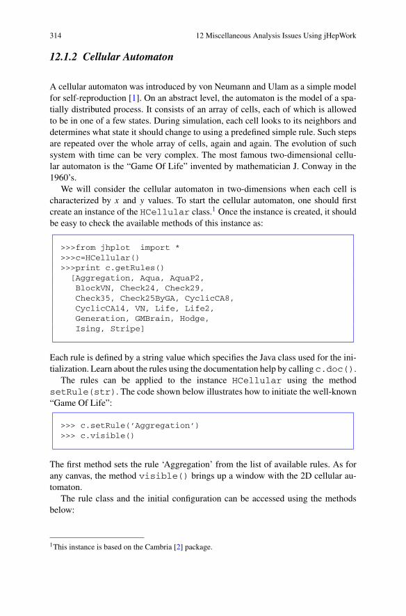
314 12 Miscellaneous Analysis Issues Using jHepWork
12.1.2 Cellular Automaton
A cellular automaton was introduced by von Neumann and Ulam as a simple modelfor self-reproduction [1]. On an abstract level, the automaton is the model of a spa-tially distributed process. It consists of an array of cells, each of which is allowedto be in one of a few states. During simulation, each cell looks to its neighbors anddetermines what state it should change to using a predefined simple rule. Such stepsare repeated over the whole array of cells, again and again. The evolution of suchsystem with time can be very complex. The most famous two-dimensional cellu-lar automaton is the “Game Of Life” invented by mathematician J. Conway in the1960’s.
We will consider the cellular automaton in two-dimensions when each cell ischaracterized by x and y values. To start the cellular automaton, one should firstcreate an instance of the HCellular class.1 Once the instance is created, it shouldbe easy to check the available methods of this instance as:
>>>from jhplot import *>>>c=HCellular()>>>print c.getRules()
[Aggregation, Aqua, AquaP2,BlockVN, Check24, Check29,Check35, Check25ByGA, CyclicCA8,CyclicCA14, VN, Life, Life2,Generation, GMBrain, Hodge,Ising, Stripe]
Each rule is defined by a string value which specifies the Java class used for the ini-tialization. Learn about the rules using the documentation help by calling c.doc().
The rules can be applied to the instance HCellular using the methodsetRule(str). The code shown below illustrates how to initiate the well-known“Game Of Life”:
>>> c.setRule(’Aggregation’)>>> c.visible()
The first method sets the rule ‘Aggregation’ from the list of available rules. As forany canvas, the method visible() brings up a window with the 2D cellular au-tomaton.
The rule class and the initial configuration can be accessed using the methodsbelow:
1This instance is based on the Cambria [2] package.

12.2 Downloading Files from the Web 315
>>> print c.getRule()>>> print c.getInitString()
One can change the initial configuration for a cellular automation with thesetInitString(str). The most convenient way is to write a configurationto an external file and then read it using Jython as discussed in Sect. 2.16.
12.2 Downloading Files from the Web
In this section, we will show how to download files from the Web and display themin the jHepWork IDE (of course, in case of simple textual files). This can be done us-ing the Jython module ’web.py’ located in the directory ’macros/system’.Essentially, it is rather similar to the well-known “wget” program available on theLinux and Unix platforms, but it is much simplified and implemented using Jython(thus it does not have platform dependencies). In case of the HTTP protocol, a filecan be downloaded using the Jython prompt as:
>>> from web import *>>> wget(’http://www.jython.org/Project/news.html’)
This command retrieves the file ’news.html’ from the server to the current di-rectory and shows the progress status during the download.
12.3 Macro Files for jHepWork Editor
To show a text file in the jHepWork editor, one can use JythonShell of the IDE.Simply type the line:
>>> view.open(’news.html’,0)
which opens the file “news.html” (downloaded using the previous example) in anew tab of the editor. The object view represents an “editor” text component of thejHepWork IDE. This instance is imported by default during the IDE startup. Onecan find the methods of this editor instance using the dir(view) method.
In order to find what can be done with the object view, run the program “test”using JythonShell. It illustrates the major operations with the text editor and how tomanipulate with the example text loaded to the editor using various macros.
Let us show an example of how to work with text files using the object view.Assuming that a file is loaded into the editor, use these commands from JythonShell:
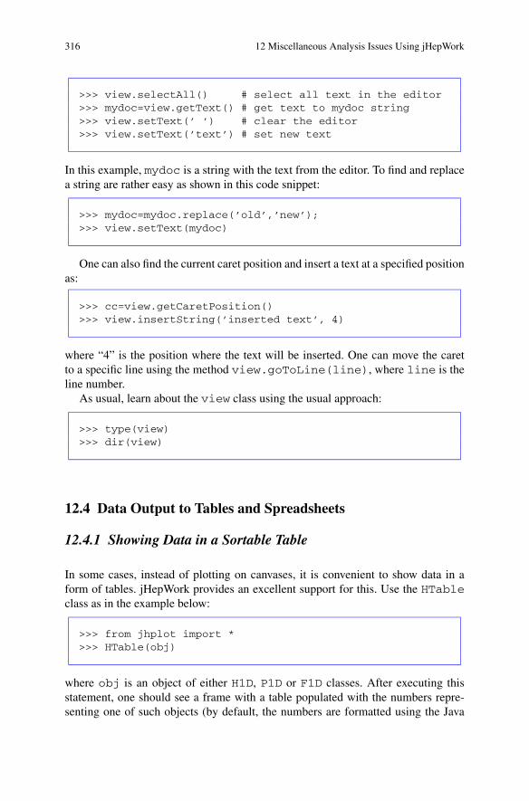
316 12 Miscellaneous Analysis Issues Using jHepWork
>>> view.selectAll() # select all text in the editor>>> mydoc=view.getText() # get text to mydoc string>>> view.setText(’ ’) # clear the editor>>> view.setText(’text’) # set new text
In this example, mydoc is a string with the text from the editor. To find and replacea string are rather easy as shown in this code snippet:
>>> mydoc=mydoc.replace(’old’,’new’);>>> view.setText(mydoc)
One can also find the current caret position and insert a text at a specified positionas:
>>> cc=view.getCaretPosition()>>> view.insertString(’inserted text’, 4)
where “4” is the position where the text will be inserted. One can move the caretto a specific line using the method view.goToLine(line), where line is theline number.
As usual, learn about the view class using the usual approach:
>>> type(view)>>> dir(view)
12.4 Data Output to Tables and Spreadsheets
12.4.1 Showing Data in a Sortable Table
In some cases, instead of plotting on canvases, it is convenient to show data in aform of tables. jHepWork provides an excellent support for this. Use the HTableclass as in the example below:
>>> from jhplot import *>>> HTable(obj)
where obj is an object of either H1D, P1D or F1D classes. After executing thisstatement, one should see a frame with a table populated with the numbers repre-senting one of such objects (by default, the numbers are formatted using the Java

12.4 Data Output to Tables and Spreadsheets 317
scientific format). Using this table, one can sort data by clicking at the top of eachcolumn or search for a particular value or string. Note: it is impossible to mod-ify the data as the class HTable was designed only for examining data contain-ers.
One can pass a boolean value telling how you expect the data to be formatted. Ifthe data have to be shown as formatted strings using the Java scientific format, usethis constructor:
>>> HTable(obj,1)
If data values should not be formatted, set “0” (Java false) instead of “1”.One can call the HTable object differently: if a data container is created, one
can use the toTable() method. For example, to display a H1D histogram, onecan use:
>>> HTable(h1) # where h1 is H1D histogram
or, alternatively,
>>> h1.toTable()
As before, if toTable() is used with the argument “0”, the numbers will notbe formatted using the scientific format.
The HTable viewer can be filled by the standard Java Vector class. In thiscase, it accepts three arguments:
>>> HTable(’name’, nameVector, fillVector)
where nameVector is a vector with column names (string type) andfillVector with input data. Let us give an example illustrating this:
Table with particles
from java.util import Vectorfrom jhplot import *
v1=Vector()v1.add(’Name’)v1.add(’Mass’)v1.add(’Error’)
vv=Vector()vv.add(’Electron’)vv.add(0.5109)vv.add(4.0E-8)
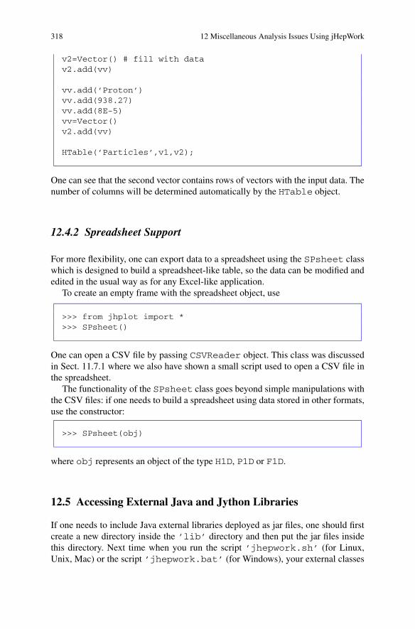
318 12 Miscellaneous Analysis Issues Using jHepWork
v2=Vector() # fill with datav2.add(vv)
vv.add(’Proton’)vv.add(938.27)vv.add(8E-5)vv=Vector()v2.add(vv)
HTable(’Particles’,v1,v2);
One can see that the second vector contains rows of vectors with the input data. Thenumber of columns will be determined automatically by the HTable object.
12.4.2 Spreadsheet Support
For more flexibility, one can export data to a spreadsheet using the SPsheet classwhich is designed to build a spreadsheet-like table, so the data can be modified andedited in the usual way as for any Excel-like application.
To create an empty frame with the spreadsheet object, use
>>> from jhplot import *>>> SPsheet()
One can open a CSV file by passing CSVReader object. This class was discussedin Sect. 11.7.1 where we also have shown a small script used to open a CSV file inthe spreadsheet.
The functionality of the SPsheet class goes beyond simple manipulations withthe CSV files: if one needs to build a spreadsheet using data stored in other formats,use the constructor:
>>> SPsheet(obj)
where obj represents an object of the type H1D, P1D or F1D.
12.5 Accessing External Java and Jython Libraries
If one needs to include Java external libraries deployed as jar files, one should firstcreate a new directory inside the ’lib’ directory and then put the jar files insidethis directory. Next time when you run the script ’jhepwork.sh’ (for Linux,Unix, Mac) or the script ’jhepwork.bat’ (for Windows), your external classes
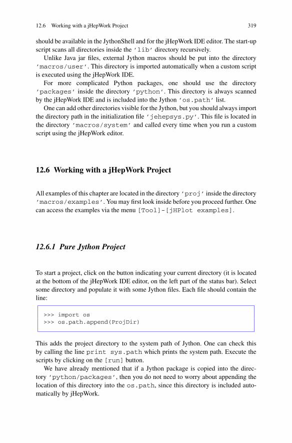
12.6 Working with a jHepWork Project 319
should be available in the JythonShell and for the jHepWork IDE editor. The start-upscript scans all directories inside the ’lib’ directory recursively.
Unlike Java jar files, external Jython macros should be put into the directory’macros/user’. This directory is imported automatically when a custom scriptis executed using the jHepWork IDE.
For more complicated Python packages, one should use the directory’packages’ inside the directory ’python’. This directory is always scannedby the jHepWork IDE and is included into the Jython ’os.path’ list.
One can add other directories visible for the Jython, but you should always importthe directory path in the initialization file ’jehepsys.py’. This file is located inthe directory ’macros/system’ and called every time when you run a customscript using the jHepWork editor.
12.6 Working with a jHepWork Project
All examples of this chapter are located in the directory ’proj’ inside the directory’macros/examples’. You may first look inside before you proceed further. Onecan access the examples via the menu [Tool]-[jHPlot examples].
12.6.1 Pure Jython Project
To start a project, click on the button indicating your current directory (it is locatedat the bottom of the jHepWork IDE editor, on the left part of the status bar). Selectsome directory and populate it with some Jython files. Each file should contain theline:
>>> import os>>> os.path.append(ProjDir)
This adds the project directory to the system path of Jython. One can check thisby calling the line print sys.path which prints the system path. Execute thescripts by clicking on the [run] button.
We have already mentioned that if a Jython package is copied into the direc-tory ’python/packages’, then you do not need to worry about appending thelocation of this directory into the os.path, since this directory is included auto-matically by jHepWork.

320 12 Miscellaneous Analysis Issues Using jHepWork
12.6.2 Pure Java Project
In case of a pure Java project, use the example located inside the directory proj.Click on the project button again (look at the bottom of the jHepWork IDE), andselect the directory proj using the file browser. Then open the main class fileexample_java.java by double clicking using the mouse button. This is asimple Java program which calls the external library, Calc.java, located in the’example2’ directory.
First, build Java library files located inside the proj/example* directories. Todo this, select [Compile and jar] project files from the [Run] menu. Afterexecuting it, a jar file ’classes.jar’ will appear in the main project directory.It contains all the classes built from the source files located in the project librarydirectories.
If example_java.java is already opened in the jHepWork IDE, press[Run] (or [Run java]) using the tool bar. You will see the output from theclass Calc in the BeanShell prompt.
One can further adjust the class path of external libraries by modifying the Bean-Shell scrips in run_java* files in the director ’macros/user’.
12.6.3 Mixing Jython with Java
One can mix Jython and Java codes for CPU intensive tasks, such as large loops overprimitive data types, reading large files and so on. Such tasks must be implementedin Java to achieve the best possible performance. Jython scripts can be used as aglue language for various Java libraries with the source files located inside the mainproject directory.
First, build a jar file which contains the byte-codes of Java classes. Again, forthis example, set proj as your project directory and select the menu [Compileand jar] project files from the [Run] tool-bar menu. After executing it, a jar fileclasses.jar appears in the main project directory, which contains the classes ofthe source files located in the project directory.
Then, open the Jython file ’example_java.py’. This script calls the classCalc and prints its output. Execute this Jython script by clicking on the [Run]button on the tool-bar menu. The output result will be the Calc class located in thedirectory example2/Calc.java.
One can modify the file example2/Calc.java and recompile the projectagain using the sub-menu [javac all files] from the [Run]menu. One canalso rebuild the jar library. Note that, to trigger changes, you will need to reload theBeanShell console using the small reload button on the BeanShell tab. Then run theexample_java.py again. You should see a different output from the class Calc.

12.7 Working with Images 321
12.7 Working with Images
12.7.1 Saving Plots in External Image File
We should remind that in order to export a canvas into an image file, one can use theexport(FileName)method after calling draw(obj) or update()methods.This was discussed in Sect. 10.2.11. Below we will continue with this example.
12.7.2 View an Image. IView Class
If an image is saved in JPG, GIF or PNG format, one can view it using the IViewclass. Below we will show how to use it.
Assume we have created a script which plots a histogram or any other object onthe HPlot canvas (or any other canvas). We assume that the instance of this canvasis c1. If you want to create an image file and open it immediately after creation inthe IView frame, put these lines at the end of your Jython script:
>>> file=Editor.DocMasterName()+’.png’>>> c1.export(file) # export to a PNG file>>> IView(file) # view the image
where the method Editor.DocMasterName() accesses the file name of thecurrently opened script. Execution of this file brings up a frame with the PNG imageinside.
12.7.3 Analyzing and Editing Images
If an image is saved in one of the raster formats, such as JPG, GIF, PNG, one canedit it (crop, resize, add a text, etc.) using the IEditor class. This class is builton the top of the ImageJ program [3], which is of the most advanced image editorimplemented in Java.
Let us show a typical example when a canvas, like HPlot or HPlot3D, is firstsaved in an image file and then the IEditor class is used to edit and analyze thecreated image:
>>> file=Editor.DocMasterName()+’.png’ # file name based>>> c1.export(file) # export to a PNG file>>> IEditor(file) # edit the created image
where c1 is a canvas object and Editor.DocMasterName() is the name of thecurrently opened document in the IDE. The example shows how the image createdby the c1 object is redirected to the IEditor program for further editing.

322 12 Miscellaneous Analysis Issues Using jHepWork
12.8 Complex Numbers
We already know that Jython has support for complex numbers which comes fromthe Python language specification, see Sect. 2.2.4. We remind that one can define acomplex number in Jython as x+yj, where j indicates an imaginary part.
In addition, jHepWork libraries provide a comprehensive support for usualcomplex-number arithmetic operators and necessary standard mathematical func-tions. Unlike Jython, the complex numbers and operations are implemented in Java,thus one can use these libraries in pure Java projects.
Complex numbers in jHepWork are based on the class Complex from theJava package jhplot.math. Unlike Jython, the imaginary part is denoted bythe conventional character ’i’. A complex number is defined by the constructorComplex(real,img), where real is a real part and img is an imaginary partof a complex number. Either part can be zero.
Below we show a simple example of how to deal with the complex numbersusing the Java jhplot.math package:
>>> from jhplot.math import *>>>>>> a=Complex(10,2)>>> print a.toString()10.0 + 2.0i>>> b=Complex(20,1)>>> cc=a.minus(b)print cc.toString()-10.0 + 1.0i>>> cc=a.times(b)>>> print cc.toString()198.0 + 50.0i
There is a large number of methods associated with the class Complex. Look atthe API description of the class Complex or use the jHepWork code assists whileworking with this class.
12.9 Building List of Files
Let us come back to the example given in Sect. 2.17 where we wrote a small Jythonscript to transverse all subdirectories in order to collect files with a given file exten-sion. This time, the jHepWork Java library will be used which significantly simpli-fies the code, essentially reducing it to a single-line statement.
Instead of creating the function wolk() shown in Sect. 2.17, one can use a staticclass from jHepWork called FileList as in this example:
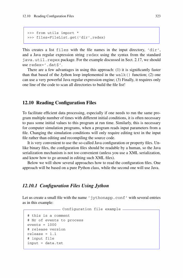
12.10 Reading Configuration Files 323
>>> from utils import *>>> files=FileList.get(’dir’,redex)
This creates a list files with the file names in the input directory, ’dir’,and a Java regular expression string redex using the syntax from the standardjava.util.regex package. For the example discussed in Sect. 2.17, we shoulduse redex=’.dat$’.
There are a few advantages in using this approach: (1) it is significantly fasterthan that based of the Jython loop implemented in the walk() function; (2) onecan use a very powerful Java regular expression engine; (3) Finally, it requires onlyone line of the code to scan all directories to build the file list!
12.10 Reading Configuration Files
To facilitate efficient data processing, especially if one needs to run the same pro-gram multiple number of times with different initial conditions, it is often necessaryto pass some initial values to this program at run time. Similarly, this is necessaryfor computer simulation programs, when a program reads input parameters from afile. Changing the simulation conditions will only require editing text in the inputfile rather than editing and recompiling the source code.
It is very convenient to use the so-called Java configuration or property files. Un-like binary files, the configuration files should be readable by a human, so the Javaserialization mechanism is not too convenient (unless you use a XML serialization,and know how to go around in editing such XML files).
Below we will show several approaches how to read the configuration files. Oneapproach will be based on a pure Python class, while the second one will use Java.
12.10.1 Configuration Files Using Jython
Let us create a small file with the name ’jythonapp.conf’ with several entriesas in this example:
Configuration file example
# this is a comment# Nr of events to processevents = 1000# release versionrelease = 1.1# input fileinput = data.txt

324 12 Miscellaneous Analysis Issues Using jHepWork
This configuration file has the format: ‘name = value’. White spaces between theseelements are ignored during reading such files. A configuration file can contain com-ments: by default, the ‘#’ character at the start of each line with a comment text.
How would you read such files in Jython? We will use a small Jython modulebased on the package ConfReader [4] for this purpose. This code reads the con-figuration file, parses all text lines and prints the input values and their types:
Reading configuration file
from Conf import *try:
config = ConfReader(’jythonapp.conf’)except IOError:
print ’Cannot read configuration file’
config.set(’release’, post=float)config.set(’events’, post=int)config.set(’input’, default=’/tmp’)
try:config.parse()
except ConfigMissingError, why:print ’Missing config’, why
except ConfigPostError, why:print ’Postprocessing Error’, why
print config.release, type(config.release)print config.events, type(config.events)print config.input, type(config.input)
The parameters of the configuration file are retrieved with the help of theset(str,option) function. It takes two arguments. The first argument is astring which contains a parameter name. The second, option, should be in theform post=value (to be discussed below). The example contains several excep-tion statements which have briefly been discussed in Sect. 2.15.
Running the script shown above prints:
1.1 <type ’float’>1000 <type ’int’>data.txt <type ’str’>
As you can see, the program correctly identifies the input values and their type.Let us come back to the set(str,option) function. As mentioned, the sec-
ond argument of this function should be in the form post=value, where the at-tribute value can have the following values:
default the value returned if the config is not foundpost post-processing function to use; can be a lambda form or any function

12.10 Reading Configuration Files 325
required set to 1 if config is requiredlist set to 1 if config should always be returned as list. Multiple entries will
be appended to the list, if this is not a list but a set; otherwise, the last entrywill be used
The above example is based on the module ’Conf.py’, which is located in thedirectory ’system’ inside the ’macro’ directory. The module is rather flexible:you can change the default syntax of your configuration file rather easily.
Optionally, the configuration file can be arranged in sections of data, which canbe used to organize references to multiple resources. Please read the documentationgiven in the file ’Conf.py’
12.10.2 Reading Configuration Files Using Java
One can also read the configuration files using the Properties class from theJava package java.util. The Properties can be used to save a property filein a stream. Each key and its corresponding value in the property list is a string.
Below we show an example of how to read the configuration file created in theprevious section. We will use the strings ’release’, ’events’ and ’input’as the keys. Then we print the loaded strings in the ISO 8859-1 character encoding.Since we expect ’events’ to be an integer number, we convert it to the integertype and modify its value. Finally, we set a new property using ’events’ as thekey and save it to a file with the optional comment ‘New settings’ (one can use also‘None’ in case of no comments).
Reading a configuration file
from java.util import Propertiesfrom java.io import *
p=Properties()
# read property filep.load(FileInputStream("jythonapp.conf"))print p.getProperty("release")print p.getProperty("input")print p.getProperty("events")
# save new file with x10 more eventsev=int(p.getProperty("events"))ev=10*evp.setProperty("events",str(ev))p.store(FileOutputStream("new.conf"),"New settings");
One should note that, in case of Java, the file extension of the property files is’properties’ by convention, rather than that given in this example.

326 12 Miscellaneous Analysis Issues Using jHepWork
12.11 Jython Scripting with jHepWork
Throughout the book, we have considered a programming style with the directJython calls to the jHPlot Java classes. Java, however, does not support operatoroverloading, which is one of important features of object-oriented programming.We will remind that “operator overloading” means that one can define custom typesand operations. For example, one can redefine operators like “+” or “-” dependingon the types for which these operators are used.
The operator overloading is useful since this feature can significantly simplify aprogram and makes it more concise and readable. One can easily see a problem ifone wants to do a lot of elementary mathematical operations with objects, like toadd them, subtract etc. In this case, one should call Java methods which, usually,have long names. For the simplest mathematical operations, such as addition andsubtraction, it is more convenient to use + and -.
jHepWork allows to use the operator overloading by calling the correspondingJython classes, which are directly mapped to the Java jHPlot classes. Such Jythonclasses inherit all methods of the Java jHPlot classes. At the same time, the mostcommon arithmetical operators are overloaded. The package which allows to do thisis called shplot (where the first letter “s” means “scripted” or “simple” hplot), incontrast to name jhplot (“Java j-hplot”)
Below is an example of how to build Jython histograms and to perform somecommon operations:
Jython scripting with an operator overloading
from java.util import Randomfrom shplot import *
c1=hplot(’scripting’,1,2)c1.visible()c1.setAutoRange()
h1=h1d(’histogram1’,200,-5,5)h2=h1d(’histogram2’,200,-5,5)
r=Random()for i in range(500):
h1.fill(r.nextGaussian())h2.fill(0.2*r.nextGaussian())
h1=h1+h2 # add 2 histogramsc1.draw(h1) # drawh1=h1*2 # scale by a factor 2c1.draw(h2)
c1.cd(1,2) # go to the next plotc1.setAutoRange()h1=h1-h2 # subtract 2 histogramsh1=h1/h2 # divide 2 histograms

12.11 Jython Scripting with jHepWork 327
h1=h1*10 # scale by factor 10h1=h1/100 # divide by 100c1.draw(h1)
One should note that all Jython classes which inherit Java jHPlot classes have ex-actly the same names as the corresponding Java classes from the jhplot package.The only difference is that Jython classes have to be typed in lower case. This meansthat the statement such as:
>>> from jhplot import *>>> c1=HPlot(’scripting’)
creates an instance of the Java class HPlot. However, when one uses the lower casefor the same class name, the corresponding Jython instance of this object is created:
>>> from shplot import *>>> c1=hplot(’scripting’)
In this case, the major arithmetical operators are overloaded since ’c1’ is a pureJython object.
Analogously, one can look at the Jython equivalent of the Java H1D class:
>>> from shplot import *>>> h1=h1d(’test’,200,-5,5)>>> h1. # press [F4] to see all methods
One may notice that all jHPlot Java methods are inherited by the Jython classh1d. Thus, even if you write a code using Jython shplot classes, one can easilyaccess the Java classes:
>>> from shplot import *>>> h1=h1d(’test’,200,-5,5) # build a Jython histogram>>> h1.setFill(1) # accesses a Java method
In the above example, setFill(1) was applied directly to the Java class H1D. Ifone needs to subtract, add, divide, scale the data, use -, +, /, * or *factor, insteadof the long oper(obj) or operScale(obj) statements of the Java H1D class.
One can go even further in redesigning the Jython coding. When plotting anobject on a canvas, like a histogram, one can say that a histogram was added to thecanvas. So, why not, instead of the usual draw(obj) method, use the operation +?Yes, this is also possible: Here is a code which shows how to draw three histogramson the same canvas using a single line:

328 12 Miscellaneous Analysis Issues Using jHepWork
>>> c1+h1+h2+h3
Of course, the same operation can be done with any other class, like H1D or P1D,which can also be drawn on the canvas. Note: subtraction of objects (which maycorrespond to the removal of objects from the canvas) is not implemented for thehplot Jython class.
In the same spirit, data can be shown in a table. Below we display histogramvalues in a pop-up table:
>>> htable()+h1
where the Jython htable class is a direct mapping of the HTable Java class.As before, one should use the jHepWork code assist to learn more about
Jython/Java methods. This time, the code assist will be applied to Jython objects,rather than to Java ones.
Note that not all Java classes have been mapped to the corresponding Jythonclasses. Please look at the directory ’macros/shplot’ to find out which Jythonmodules are available. In the same directory, one can find several useful examples(their names contain the string _test).
12.11.1 Jython Operations with Data Holders
In case of Jython scripting, all major operations for P0D, P1D and PND are over-loaded as well:
>>> from shplot import *>>> p1=p1d(’test1’) # a Jython p1d based on P1D>>> p2=p1d(’test2’)>>> p1=p1+p2 # all values are added
Note that, for the latter operation, all y-values are added (and errors are propagatedrespectively), while x values remain to be the same. This operation cannot appendarrays, instead, use the merge() method.
Here are some other examples:
>>> p1=p1+p2 # all values are added>>> p1=p1-p2 # subtraction>>> p1=p1*p2 # multiplication>>> p1=p1/p2 # division>>> p1=2*p1 # scale by 2>>> p1=p1/10 # scale by 0.1

12.12 Unwrapping Jython Code. Back to Java 329
To draw objects on a canvas, use “+” as before:
>>> c1+p1 # add p1d object to a canvas
Similarly, one can work with one-dimensional (P0D) or multidimensional (PND)arrays.
12.12 Unwrapping Jython Code. Back to Java
In most cases, jHepWork libraries are just Java libraries deployed as jar files, so youmay choose to write a Java code instead of Jython scrips.
One can develop Java codes using the jHepWork IDE exactly as when workingwith Jython scripts. Any Java IDE, such as Eclipse or NetBeans, is also good forsuch task. Applications based on the jHepWork libraries can be converted to a Javajar file and deployed together with other jar libraries which come with jHepWork.
For a Java application, you should remember to create the main() method,which must be encapsulated into a class with the same name as the file name. UnlikeJython, you should explicitly declare all variables and put the Java new operatorwhen instantiating a class. Do not forget changes to be made for loops. Lastly, putsemicolons at the end of each statement. Our next example illustrates the differencebetween the Jython and Java syntax. In the case of Jython scripting, let us write ourexample code as:
>>> p0=P0D(’test’)>>> for i in range(5):
... p0.add(i)
... print i
The same code snippet in Java looks like:
P0D p0 = new P0D(’test’);for ( i=1; i<5; i++ ) {
p0.add(i);System.out.println(i);}
One should put these lines into a file (with the same name as the class name), com-pile it using javac compiler and run it as any Java application. One can also put thisJava bytecode into a jar file. Comment lines should start from the usual Java com-ment symbols instead of the symbol “#”. If you are using an external Java IDE, donot forget to add the directory ’lib’ from the jHepWork installation into CLASS-PATH, so all jHepWork libraries should be visible for Java.

330 12 Miscellaneous Analysis Issues Using jHepWork
Let us show a more detailed example. In Sect. 8.1 we have considered how toplot three histograms using Jython. Now we will rewrite this code in Java:
File ’Example.java’
import java.awt.Color;import java.util.Random;import jhplot.*;
class Example{public static void main(String[] args){
HPlot c1 = new HPlot("Canvas",600,400,2,1);c1.visible(true);c1.setAutoRange();H1D h1 = new H1D("First",20, -2.0, 2.0);h1.setFill(true);h1.setFillColor(Color.green);H1D h2 = new H1D("Second",100, -2.5, 2.5);Random r = new Random();
for (int i=0; i<500; i++) {h1.fill(r.nextGaussian());h1.fill(r.nextGaussian()); }
H1D h3 = new H1D("Third",20, 0.0, 10.0);h3.setFill(true);for (int i=0; i<50000; i++)
h3.fill(2+r.nextGaussian());
c1.cd(1,1);c1.setAutoRange();c1.draw(h1);c1.draw(h2);
c1.cd(2,1);c1.setAutoRange();c1.draw(h3);
}}
Save these lines into the file ’Example.java’ and open it inside the jHepWorkIDE. Now you can: (1) Compile and run the program by pressing the [Run] button.(2) Or one can just compile the file loaded to the editor into bytecode using themenu [Run] → [Javac current file]. Then you can run the compiledcode as: [Run] → [Run Java]. As you will see, the output will be identical tothat shown in Fig. 8.1 of Sect. 8.1.
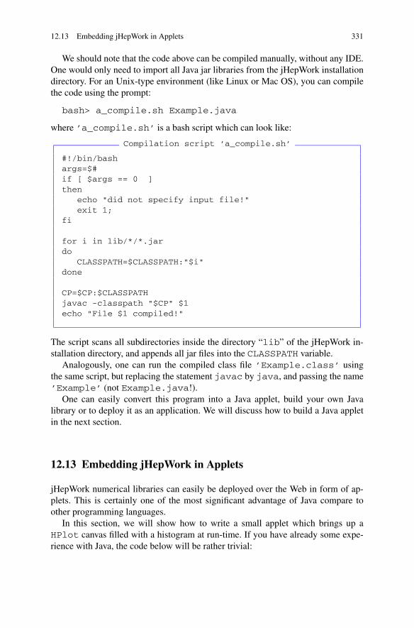
12.13 Embedding jHepWork in Applets 331
We should note that the code above can be compiled manually, without any IDE.One would only need to import all Java jar libraries from the jHepWork installationdirectory. For an Unix-type environment (like Linux or Mac OS), you can compilethe code using the prompt:
bash> a_compile.sh Example.java
where ’a_compile.sh’ is a bash script which can look like:
Compilation script ’a_compile.sh’
#!/bin/bashargs=$#if [ $args == 0 ]then
echo "did not specify input file!"exit 1;
fi
for i in lib/*/*.jardo
CLASSPATH=$CLASSPATH:"$i"done
CP=$CP:$CLASSPATHjavac -classpath "$CP" $1echo "File $1 compiled!"
The script scans all subdirectories inside the directory “lib” of the jHepWork in-stallation directory, and appends all jar files into the CLASSPATH variable.
Analogously, one can run the compiled class file ’Example.class’ usingthe same script, but replacing the statement javac by java, and passing the name’Example’ (not Example.java!).
One can easily convert this program into a Java applet, build your own Javalibrary or to deploy it as an application. We will discuss how to build a Java appletin the next section.
12.13 Embedding jHepWork in Applets
jHepWork numerical libraries can easily be deployed over the Web in form of ap-plets. This is certainly one of the most significant advantage of Java compare toother programming languages.
In this section, we will show how to write a small applet which brings up aHPlot canvas filled with a histogram at run-time. If you have already some expe-rience with Java, the code below will be rather trivial:
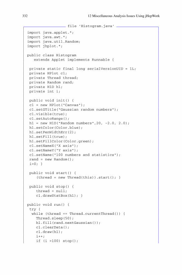
332 12 Miscellaneous Analysis Issues Using jHepWork
file ’Histogram.java’
import java.applet.*;import java.awt.*;import java.util.Random;import jhplot.*;
public class Histogramextends Applet implements Runnable {
private static final long serialVersionUID = 1L;private HPlot c1;private Thread thread;private Random rand;private H1D h1;private int i;
public void init() {c1 = new HPlot("Canvas");c1.setGTitle("Gaussian random numbers");c1.visible(true);c1.setAutoRange();h1 = new H1D("Random numbers",20, -2.0, 2.0);h1.setColor(Color.blue);h1.setPenWidthErr(2);h1.setFill(true);h1.setFillColor(Color.green);c1.setNameX("X axis");c1.setNameY("Y axis");c1.setName("100 numbers and statistics");rand = new Random();i=0; }
public void start() {(thread = new Thread(this)).start(); }
public void stop() {thread = null;c1.drawStatBox(h1); }
public void run() {try {while (thread == Thread.currentThread()) {Thread.sleep(50);h1.fill(rand.nextGaussian());c1.clearData();c1.draw(h1);i++;if (i >100) stop();

12.13 Embedding jHepWork in Applets 333
}} catch (Exception e) {} }
}
Although it is a bit lengthy (it is not a Jython script!), the code itself is rather simple:We create the usual HPlot and H1D objects and set some attributes. Then we filla histogram with random numbers in a thread. We animate the canvas, i.e., we plotrandom numbers in a loop with a time delay. After the number of entries reaches100, we stop filling the canvas and display the statistics.
Compile this code as discussed in the previous section, either inside the jHep-Work IDE or with the help of the compilation script discussed in the previous sec-tion:
bash> a_compile.sh Histogram.java
After compilation, you should see the file ’Example.class’. The next step isto embed it into a HTML file or a PHP script which can be used for a Web browser.
Our preference is to use a PHP script which is more flexible as it allows automaticscanning of all jar files inside a directory. First, copy the library directory ’lib’with the jHepWork jar libraries to a location which can be accessible by the webserver. Then, write a script:
PHP script ’applet.php’
<?phprequire("list_files.php");$list=list_files("lib/system/") . ", " .
list_files("lib/freehep/");$html_body = "";$html_body .= <<<EOT<html><body><h1>Histogram example</h1><APPLET
CODE="Histogram.class"WIDTH=0 HEIGHT=0 ARCHIVE="$list">Please use a Java-enabled browser.
</APPLET></body></html>EOT;
print $html_body?>
This PHP script creates the necessary HTML file with our applet “on-the fly”. Theonly unusual variable is $list which is a comma-separated list of jar files fromthe directory ’lib’. This list is created by the function ’list_files.php’,which returns a list of files in a certain directory. This function is shown here:

334 12 Miscellaneous Analysis Issues Using jHepWork
PHP script ’list_files.php’
<?phpfunction list_files($dir){$list="";if ($handle = opendir($dir)) {
while (false !== ($file = readdir($handle))) {if ($file != "." && $file != "..") {
$ff= $dir . $file;$list .= $ff . ", ";
}}closedir($handle);
}return $list;}?>
Now you are ready. Copy the three files above:
applet.php, list_files.php, Example.class
into a Web-server accessible directory. Make sure that this directory contains thedirectory ’lib’ from the jHepWork installation directory (one can also make alink to this directory). Consider to remove unnecessary jar files, if they are not usedto run the applet (this will make the execution faster). Then, point a Web browser tothe file ’applet.php’. The PHP module ’list_files.php’will scan all jarfiles inside the directory ’lib’ and will pass it to the ’applet.php’ file. Thisfile will build a proper HTML file to be displayed inside a Web browser. You shouldsee a HPlot frame with filled histogram entries. After 100 entries, the animationwill stop and you will see the statistics for the filled histogram.
References
1. von Neumann, J.: The General and Logical Theory of Automata (1963), p. 2882. Suzudo, T.: Cambria package3. ImageJ Java library. URL http://rsb.info.nih.gov/ij/4. Nottingham, M.: Confreader—Configuration File Reading Class (1998)
Chapter 13Data Clustering
13.1 Data Clustering. Real-life Example
Clustering algorithms are important tools for an unsupervised classification of data(compared to a “supervised” classification which will be discussed in the followingchapter). The main idea is to classify a given data set through a certain numberof clusters by minimizing distances between objects inside each cluster. A detaileddiscussion of a clustering analysis can be found, for example, in several books [1–3],but many details could also be found from many other (less costly) sources.
The data clustering in jHepWork is based the jMinHEP Java library [4] and in-cludes:
• The K-means algorithm (single and multi-pass), when classification is done byminimizing the sum-of-square distances between data points and the so-calledgeometric centroids assuming that the number of clusters is fixed a priory. Theclustering is done in a single pass starting from seed centroids positioned at ran-dom location. The algorithm assigns each object to a group of objects that havethe closest centroid, and then it recalculates the positions of new centroids. Thenthis step is repeated until the centroids no longer move.
This algorithm has the disadvantage that it depends on the initial conditions,thus jMinHEP has also an option to re-run the algorithm multiple number of timesuntil a stable solution is found. Typically, you will need to define a number ofexpected clusters, a maximum number of iterations and/or a precision with whichthe clustering is done. To get started, you may rely on the default values for theprecision and the maximum number of iterations.
• The C-means (fuzzy) algorithm. Unlike the K-means approach, this method ofclustering allows data points to belong to two or more clusters. The algorithmusually uses a “fuzziness” coefficient (typically, it is set to 2) and an accuracy ofthe calculations.
It is always a hard task to plot such clusters, since each point has a member-ship probability to belong to a particular cluster. However, one could supply someprobability (say, 0.7) to illustrate data points which have a membership probabil-ity above the specified value.
S.V. Chekanov, Scientific Data Analysis using Jython Scripting and Java,Advanced Information and Knowledge Processing,DOI 10.1007/978-1-84996-287-2_14, © Springer-Verlag London Limited 2010
335

336 13 Data Clustering
• The agglomerative hierarchical clustering algorithm. In this case, no a predeter-mined number of clusters is set. The algorithm tries to determine the so-called“natural grouping”. The clustering continues until all points are clustered into asingle cluster.
The clustering can be done with the package jminhep.algorithms. Oneshould follow these steps to perform the clustering:
• Create a data container using the class DataHolder. This data holder keepsdata in a multidimensional phase space, i.e. each data point can be characterizedby an arbitrary number of values.
• Each point is represented by the DataPoint class from the packagejminhep.cluster. Data points can be defined in a multidimensional phasespace. One should fill this data holder from an external source, or fill it on-the-flyby simulating events. We will show how to do this in the example below.
• Create and initialize a clustering algorithm class and pass it the DataHolder()constructor.
• Run the algorithm in a loop and retrieve the output.
Then one can print or plot the retrieved centroids of clusters by projecting multi-dimensional space into X–Y plane, and optionally, one can plot the original pointsused for the clustering.
13.1.1 Preparing a Data Sample
First, let us learn how to fill data into a DataHolder container. Once this dataholder is ready, we will save it into a file, and then we will read this file in order toillustrate the clustering analysis.
One single point should be represented by a DataPoint object. For example,a point with five components can be filled as:
>>> from jminhep.cluster import *>>> p=DataPoint([1,2,3,4,5])>>> print p.getDimension()>>> print p.toString()
Then one should add each point represented by the DataPoint class to theDataHolder container. Below we add two data points:
>>> from jminhep.cluster import *>>> d=DataHolder(’data’)>>> p=DataPoint([1,2,3,4,5])>>> d.add(p)>>> p=DataPoint([5,6,7,8,9])>>> d.add(p)
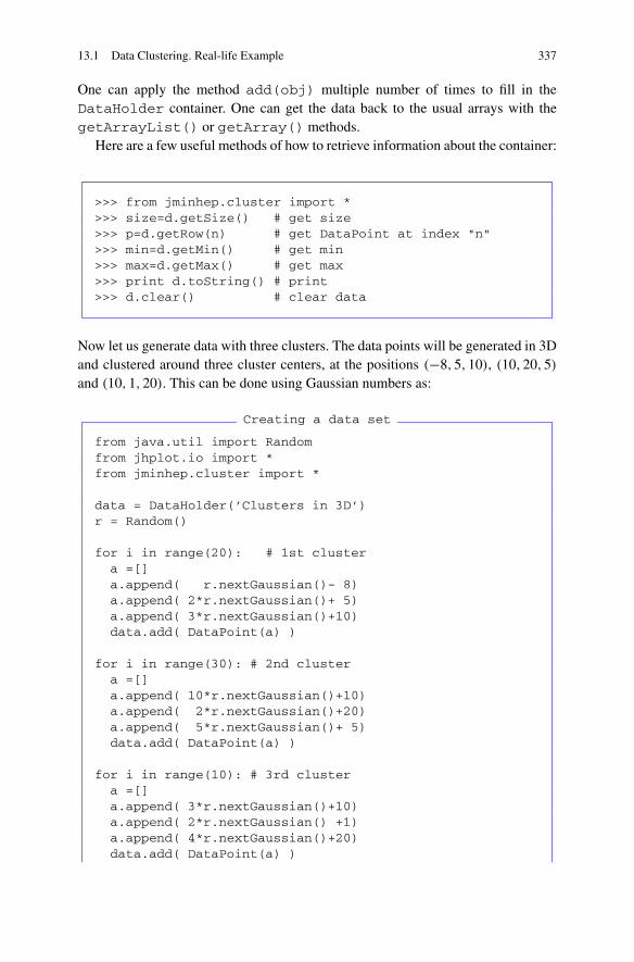
13.1 Data Clustering. Real-life Example 337
One can apply the method add(obj) multiple number of times to fill in theDataHolder container. One can get the data back to the usual arrays with thegetArrayList() or getArray() methods.
Here are a few useful methods of how to retrieve information about the container:
>>> from jminhep.cluster import *>>> size=d.getSize() # get size>>> p=d.getRow(n) # get DataPoint at index "n">>> min=d.getMin() # get min>>> max=d.getMax() # get max>>> print d.toString() # print>>> d.clear() # clear data
Now let us generate data with three clusters. The data points will be generated in 3Dand clustered around three cluster centers, at the positions (−8,5,10), (10,20,5)
and (10,1,20). This can be done using Gaussian numbers as:
Creating a data set
from java.util import Randomfrom jhplot.io import *from jminhep.cluster import *
data = DataHolder(’Clusters in 3D’)r = Random()
for i in range(20): # 1st clustera =[]a.append( r.nextGaussian()- 8)a.append( 2*r.nextGaussian()+ 5)a.append( 3*r.nextGaussian()+10)data.add( DataPoint(a) )
for i in range(30): # 2nd clustera =[]a.append( 10*r.nextGaussian()+10)a.append( 2*r.nextGaussian()+20)a.append( 5*r.nextGaussian()+ 5)data.add( DataPoint(a) )
for i in range(10): # 3rd clustera =[]a.append( 3*r.nextGaussian()+10)a.append( 2*r.nextGaussian() +1)a.append( 4*r.nextGaussian()+20)data.add( DataPoint(a) )

338 13 Data Clustering
Serialized.write(data,’data.ser’)
We should note that the sizes of the clusters are different—this is given bythe scaled factors used to multiply the random values generated by the methodr.nextGaussian(). The second cluster is rather broad—its radius spans 10(arbitrary) units.
We have written the data in a compressed serialized file. One can also try touse the writeXML() method to write data into a XML file for easy viewing.We should remind: if you need to write a lot of data, the best way to do thisis to use the HFile or HFileXML classes, see Sect. 11.3. We can write eachDataPoint object persistently in a loop. This can be done rather straightfor-wardly, since DataPoints objects can be serialized. As explained before, thisapproach allows to create rather large files since we do not store all data in thecomputer memory before writing them to a disk.
So, the data are filled with the help of the DataPoint class in three dimensions.But how one can display such data, especially in cases when there are more thanthree dimensions? One can project the DataHolder into a P1D array and plot itusing the standard HPlot class. For example, if our data are represented by a filledDataHolder object, one can view 1st and 2nd components as:
>>> from jhplot import *>>> c1=HPlot()>>> c1.setAutoRange()>>> c1.visible()>>> p1=P1D(data,0,1) # fill 1st and 2nd component>>> HTable(p1) # show data in a table>>> c1.draw(p1) # draw 1st and 2nd component
13.1.2 Clustering Analysis
Assume we have prepared an object data of the type DataHolder. Now one canperform a realistic clustering analysis. Generally, to run any clustering algorithm,one needs to follow these steps:
>>> from jminhep.algorithms import *>>> alg = [Algorithm]Alg(data)>>> alg.setClusters(NumberOfClusters)>>> alg.setOptions(some options)>>> .. more options ..>>> alg.run() # run over the data>>> print ’algorithm: ’ + pat.getName()>>> .. get results

13.1 Data Clustering. Real-life Example 339
In the above example, ’[Algorithm]’ is the name of clustering algorithm whichcould be:
KMeansAlg(data) the standard K-Means cluster algorithm;KMeansExchangeAlg(data) K-Means cluster algorithm using the exchange
mode;FuzzyCMeansAlg(data) Fuzzy (C-means) cluster algorithm;HierarchicalAlg(data) an agglomerative hierarchical clustering algo-
rithm.
Then one should set the expected number of clusters and other options. For ex-ample, for the C-means algorithm, one should set the number of expected clusters,the numerical precision of clustering and a fuzziness parameter. It is also possible toset the maximum number of iterations to stop clustering if no appropriate solutioncan be found. It is also useful to set the probability association if you need to knowwhich points belong to which cluster (this is not necessary for the K-means algo-rithm). The description of each mode can be found with the method getName().
To run the algorithm over the data, call the method run(). This method shouldbe invoked for a fixed number of clusters. One may also consider to use the runBest()method. In this case, the program will attempt to determine the number of clustersby re-running the algorithm many times over the same data set. Then it calculates themost optimal solution by minimizing the so-called “compactnesses” of the clusterconfiguration. The smaller compactness is, the higher chance that a particular clustersolution is the most optimal.
After the clustering (i.e. after running the method run()), one can find the“compactness” of the cluster configuration by calling getCompactness(). Thecentroid positions can be retrieved with the method getCenters() and the datapoint association can be obtained using several built-in methods.
We now have all the machinery to perform a clustering analysis and below weshow a detailed example. Let us read the prepared data and run the K-means algo-rithm over this data. First, we prepare a function printAnswer() designed toprint all relevant information about the cluster configuration. Then we will run theK-means algorithm for: (1) one-pass using three clusters; (2) 10 passes with differ-ent random seed locations. The algorithm returns the cluster configuration with thesmallest compactness; (3) Running the K-means algorithm using multiple numberof passes, and determining the best possible configuration with the smallest com-pactness.
Running the K-means algorithm
from jhplot.io import *from jminhep.algorithms import *
data=Serialized.read(’data.ser’)
def printAnswer(alg):print ’Name=’+alg.getName()print ’No of final clusters:’ +str(alg.getClusters())

340 13 Data Clustering
print ’No of points: ’ +str(alg.getNumberPoints())print ’Compactness: ’ +str(alg.getCompactness())centers = alg.getCenters()print centers.toString()
alg=KMeansAlg(data) # run K-means algorithmalg.setClusters(3)alg.setOptions(1000,0.001)alg.run()printAnswer(alg)
alg.run(10) # run 10 times with different seedsprintAnswer(alg)
alg=KMeansExchangeAlg(data)alg.setEpochMax(200)alg.runBest() # find smallest compactnessprintAnswer(alg)
The clustering results will be printed by the printAnswer() function. The short-ened output from execution of the above example is given below:
Name=kmeans algorithm fixed cluster modeNo of final clusters:3No of points: array(’i’, [30, 13, 17])Compactness: 1.4870 (-2.55, 3.93, 12.75)[0]1 ( 2.40, 19.69, 6.22)[0]2 (16.76, 19.80, 4.99)[0]
Name=kmeans algorithm for multiple iterationsNo of final clusters:3No of points: array(’i’, [21, 10, 29])Compactness: 0.8910 (-8.24, 6.0, 8.23)[0]1 ( 8.70, 1.09, 20.40)[0]2 (11.23, 19.78, 5.91)[0]
Name=K-means clustering for best estimateNo of final clusters:5No of points: array(’i’, [15, 10, 5, 20, 10])Compactness: 0.8430 (17.52,19.77,4.36)[0]1 (6.57, 19.27,9.48)[0]2 (-2.46,20.64,1.11)[0]3 (-8.18,5.36, 8.92)[0]4 (8.700,1.09, 20.40)[0]

13.1 Data Clustering. Real-life Example 341
One may immediately see that the answers from all three algorithms are different.This is not too surprising—the clustering analysis is an inherently ambiguous task,especially when dealing with overlapping clusters.
Try to make some modifications to the input data to reduce the cluster overlaps.One can simply set all multiplicative factors for the method r.nextGaussian()to a smaller value (say, 1), see the code snipped given in Sect. 13.1.1. This reducesthe cluster size, and thus overlaps between the clusters. After re-running the abovecode with the K-means clustering, you will see that all three algorithms give thesame answer.
Now let us visualize the clustering results. In the code below, we will read thedata prepared in the previous subsection, and plot them (only 1st and 2nd columns).This time, however, we will run the C-means algorithm with a fixed number ofexpected clusters.
C-means algorithm and visualization
from java.awt import Colorfrom jhplot import *from jhplot.io import *from jminhep.algorithms import *
data=Serialized.read(’data.ser’)
c1=HPlot()c1.visible()c1.setAutoRange()p1=P1D(data,0,1) # 1st and 2nd componentc1.draw(p1)
alg = FuzzyCMeansAlg(data)alg.setClusters(3)alg.setOptions(1000, 0.001, 1.7)alg.setProb(0.7)alg.run()print ’algorithm: ’ + alg.getName()print ’Compactness: ’ + str(alg.getCompactness())print ’No of final clusters:’ + str(alg.getClusters())centers=alg.getCenters()print ’No of points in cluster=’,alg.getNumberPoints()p2=P1D(centers,’Centroids’,0,1)p2.setColor(Color.red)p2.setErrAll(0)p2.setSymbol(9)p2.setSymbolSize(15)c1.draw(p2)
The resulting plot is shown in Fig. 13.1. The figure displays the input data projectedin 2D (black dotes) and the crosses show the centers of three clusters. You maywonder: why the cluster centers are shifted from the visually expected positions?
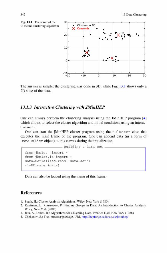
342 13 Data Clustering
Fig. 13.1 The result of theC-means clustering algorithm
The answer is simple: the clustering was done in 3D, while Fig. 13.1 shows only a2D slice of the data.
13.1.3 Interactive Clustering with JMinHEP
One can always perform the clustering analysis using the JMinHEP program [4]which allows to select the cluster algorithm and initial conditions using an interac-tive menu.
One can start the jMinHEP cluster program using the HCluster class thatexecutes the main frame of the program. One can append data (in a form ofDataHolder object) to this canvas during the initialization.
Building a data set
from jhplot import *from jhplot.io import *data=Serialized.read(’data.ser’)c1=HCluster(data)
Data can also be loaded using the menu of this frame.
References
1. Spath, H.: Cluster Analysis Algorithms. Wiley, New York (1980)2. Kaufman, L., Rousseeuw, P.: Finding Groups in Data: An Introduction to Cluster Analysis.
Wiley, New York (2005)3. Jain, A., Dubes, R.: Algorithms for Clustering Data. Prentice Hall, New York (1988)4. Chekanov, S.: The JMINHEP package. URL http://hepforge.cedar.ac.uk/jminhep/

Chapter 14Linear Regression and Curve Fitting
Very often, an empirical data set has to be explained using a model based on amathematical equation. To find a proper function and adjust free parameters of thisfunction that most closely match the data is the primary goal of curve fitting.
We start this chapter with the simplest linear case and then consider curve fittingusing arbitrary functions. The section below discusses the elements of the linearregression which models a relationship between two variables by fitting a linearequation to observed data. Then, in the following sections, we will discuss non-linear regression.
14.1 Linear Regression
Linear regression is a method of finding a linear correspondence between two datasets. The method is based on fitting a collection of data points by a simple linearform, Y = A+BX. The variable X is considered to be an explanatory variable, andthe other, Y , is considered to be a dependent variable. Sometime, the variable A iscalled the intercept, and B is the slope of the line.
Before going into the heart of the matter, it is useful to remind that it is alwaysa good practice to visualize a data set before attempting to fit it using the linearfunction. For example, in case of two-dimensional data, one can make a contourplot (see Sect. 5.2.3) in order to determine the strength of the relationship betweentwo variables.
14.1.1 Data Set
First, let us create a data set in order to illustrate a linear regression analysis. Weassume that an explanatory variable X is distributed in accordance with a Gaus-sian distribution. We also assume that the “dependent” variable is a function of theexplanatory variable and an additional “noise” simulated using random Gaussiannumbers. Look at this code:
S.V. Chekanov, Scientific Data Analysis using Jython Scripting and Java,Advanced Information and Knowledge Processing,DOI 10.1007/978-1-84996-287-2_15, © Springer-Verlag London Limited 2010
343

344 14 Linear Regression and Curve Fitting
Creating a data set
from jhplot import *from jhplot.io import *from java.util import Random
p1=P1D(’data’)r = Random()for i in range(100):
x=10*r.nextGaussian()y=20*x +200*r.nextGaussian()+50.0p1.add(x,y)
Serialized.write(p1,’data.ser’)
In the example above, we fill a P1D using random values x and y (the latter dependson x) and store it in a serialized file for the use in the next section.
14.1.2 Analyzing the Data Set
For the linear regression analysis of the created data, we will use the class LinRegfrom the package jhplot.stat which provides all necessary tools for the linearregression fits. To initialize the linear regression calculation, we should pass ourdata in the form of P1D to the LinReg() constructor:
>>> from jhplot.stat import *>>> r=LinReg(p1d)
We should note that one can also use the usual Java arrays or Jython lists for X andY values for the input, but here we will concentrate only on the P1D case.
After calling the constructor LinReg with the input P1D object, the calculationis already done and the next step is to extract the linear regression results. First ofall, we are interested in the intersect and the slope values of the fit. Both values, in-cluding their statistical uncertainties, can be extracted using the following methods:
>> print r.getIntercept(), ’+/-’,r.getInterceptError()>> print r.getSlope(),’+/-’,r.getSlopeError()
Next, we could be interested in how to display the fitted values. This can be doneusing the method getResult(), which returns a F1D function with the results ofthe linear regression.
>>> f=r.getResult()

14.1 Linear Regression 345
Next, the prediction and the confidence levels of the linear regression can beextracted as:
>>> d=r.getCorrelation()>>> p1d=r.getResiduals()
The first method returns the usual correlation coefficient,
ρ = cov(X,Y )
σXσY
where cov(X,Y ) is the covariance and σ is the standard deviation. We remind thatthe correlation coefficient varies from −1 to +1, with −1 being for a perfect nega-tive correlation between X and Y , and +1 for a perfect positive correlation.
The second method returns a P1D with the residuals, i.e. the vertical distances ofeach point from the regression line.
In addition, one can also calculate the 95% confidence interval for the regressionline given by the method getResult(). This band encloses the true best-fit linearregression line, leaving a 5% chance that the true line is outside the confidenceinterval boundaries. The confidence interval is the area that has a 95% chance ofcontaining the true regression line. This typically means that many points could befar away from the confidence-interval band.
Finally, we can calculate the 95% prediction interval. The prediction interval isthe area in which you should expect 95% of all data points to fall. As we would ex-pect, the prediction interval is further away from the best-fit line than the confidencebands.
Both the prediction and the confidence intervals can be obtained using the fol-lowing two methods:
>>> a1=r.getPrediction()>>> a2=r.getConfidence()
These two methods return two P1D objects representing the lowest and the highestlevel for the prediction and the confidence level. We remind than one can easilyplot them with the method c1.draw(obj), where obj is either a1 or a2, sincethis method can be used for displaying lists of P1D objects. There are several otherconvenient methods which can be found by reading the API documentation of thispackage.
Now let us illustrate how to analyze the data set generated in the previous section.First, we read the data from the serialized file. Then we plot the data, the linearregression fit result, the confidence interval and, finally, the predictions:
Linear regression analysis
from jhplot.io import *from jhplot import *from jhplot.stat import *

346 14 Linear Regression and Curve Fitting
from java.awt import Color
p1=Serialized.read(’data.ser’)
c1 = HPlot(’Canvas’,700,500,2,1)c1.visible()c1.setGTitle(’Linear regression’)c1.setAutoRange()
r = LinReg(p1)print r.getIntercept(), ’+/-’,r.getInterceptError()print r.getSlope(),’+/-’,r.getSlopeError()print ’Correlation=’,r.getCorrelation()
c1.cd(1,1)c1.draw(p1)c1.draw( r.getResult() )c1.draw( r.getConfidence() )
c1.cd(2,1)c1.setAutoRange()c1.draw(p1)c1.draw( r.getResult() )c1.draw( r.getPrediction() )
The output of the script is shown below:
Intercept= 48.041 +/- 17.578Slope= 20.248 +/- 1.728Correlation= 0.76383
(as before, the output numbers are shown here with a reduced precision). At thesame time, the script generates two plots shown in Fig. 14.1.
14.2 Curve Fitting of Data
Now let us come to a non-linear case, when the relationship between X and Y valuescannot be explained by the linear behavior. In this case, we need to fit data pointsusing an arbitrary curve.
Moreover, each data point can represent a group of events or measurements, thuspoints can have statistical (and systematical) errors. Obviously, the latter situationmust be considered in a different way, since points should not have the same statisti-cal weight during the fit: points with larger errors should be taken into account witha smaller weight.
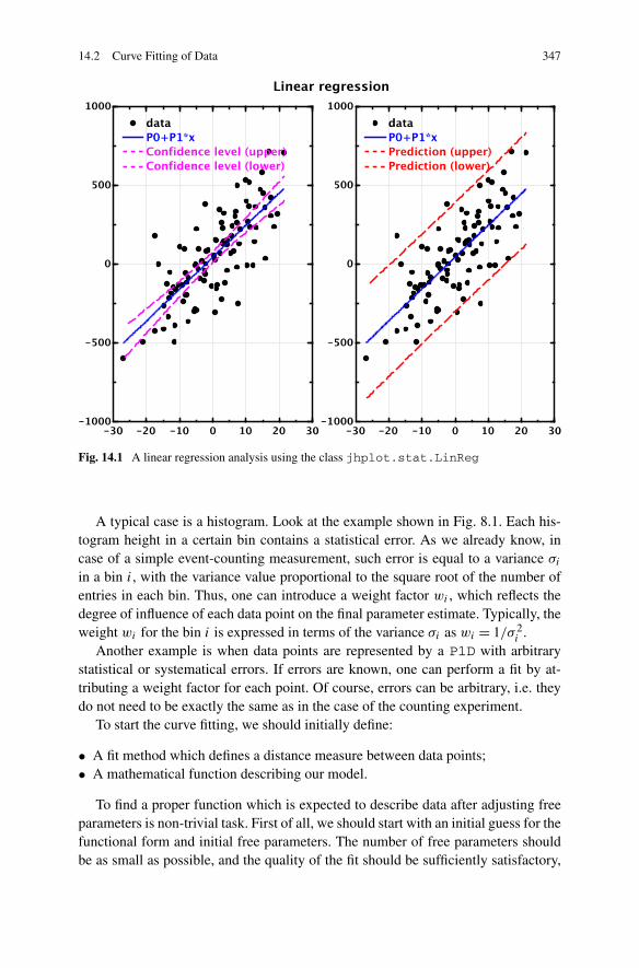
14.2 Curve Fitting of Data 347
Fig. 14.1 A linear regression analysis using the class jhplot.stat.LinReg
A typical case is a histogram. Look at the example shown in Fig. 8.1. Each his-togram height in a certain bin contains a statistical error. As we already know, incase of a simple event-counting measurement, such error is equal to a variance σi
in a bin i, with the variance value proportional to the square root of the number ofentries in each bin. Thus, one can introduce a weight factor wi , which reflects thedegree of influence of each data point on the final parameter estimate. Typically, theweight wi for the bin i is expressed in terms of the variance σi as wi = 1/σ 2
i .Another example is when data points are represented by a P1D with arbitrary
statistical or systematical errors. If errors are known, one can perform a fit by at-tributing a weight factor for each point. Of course, errors can be arbitrary, i.e. theydo not need to be exactly the same as in the case of the counting experiment.
To start the curve fitting, we should initially define:
• A fit method which defines a distance measure between data points;• A mathematical function describing our model.
To find a proper function which is expected to describe data after adjusting freeparameters is non-trivial task. First of all, we should start with an initial guess for thefunctional form and initial free parameters. The number of free parameters shouldbe as small as possible, and the quality of the fit should be sufficiently satisfactory,

348 14 Linear Regression and Curve Fitting
so one can claim that the analytical model describes the data. The degree of the fitquality is usually characterized by the χ2 value:
χ2 =N∑
i=0
[yi − f (xi)
σi
]2
(14.1)
where fi(x) is a given function with free parameters that should be found after thefitting procedure, yi is a data value in Y , σi is the data point variance (i.e. error in abin) in the bin i. The fitting procedure tries to find the values of free parameters ofthe input function, so the χ2 has the minimum possible value.
As mentioned before, it is usually a good idea to plot data first to see how the fitfunction may look like and what initial parameter values may have sense to producethe desired result.
14.2.1 Preparing a Fit
First of all, let us initialize the curve fitting package by creating an instance of theHFitter class.
>>> from jhplot import *>>> f=HFitter()>>> print f.getFitMethod()[’chi2’,’cleverchi2’,’uml’,’bml’,’leastsquares’]
The example shows how to print the available methods of the HFitter class. Themost popular method is the so-called chi2. This method, which is based on theminimization of (14.1), is the default method used by the HFitter() class if it in-stantiated without passing any arguments. The χ2 method works the best if data arerepresented by discrete points with Gaussian uncertainties. The main assumption isthat the points yi are normally distributed around a function f (xi), uncorrelated andhave a variances σi . If the number of events in each bin is larger than a certain min-imum number (say, several hundred entries), then the distribution of the expectedevents per bin is approximately Gaussian.
Next, the cleverchi2 method does not include the variance of experimentaldata points. It is based on the minimization of the following function:
χ2 =N∑
i=0
[(yi − f (xi))
2
|f (xi)|]
(14.2)
As before, yi is the data-point value (or the height of the bin i), xi is the center ofthe ith bin, f (xi) is the value of the function calculated in the ith bin.
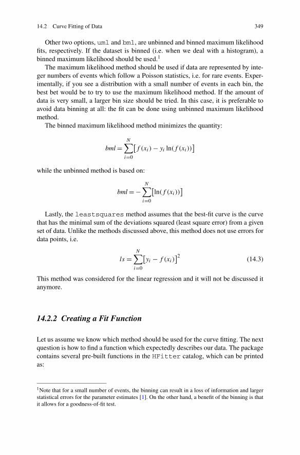
14.2 Curve Fitting of Data 349
Other two options, uml and bml, are unbinned and binned maximum likelihoodfits, respectively. If the dataset is binned (i.e. when we deal with a histogram), abinned maximum likelihood should be used.1
The maximum likelihood method should be used if data are represented by inte-ger numbers of events which follow a Poisson statistics, i.e. for rare events. Exper-imentally, if you see a distribution with a small number of events in each bin, thebest bet would be to try to use the maximum likelihood method. If the amount ofdata is very small, a larger bin size should be tried. In this case, it is preferable toavoid data binning at all: the fit can be done using unbinned maximum likelihoodmethod.
The binned maximum likelihood method minimizes the quantity:
bml =N∑
i=0
[f (xi) − yi ln(f (xi))
]
while the unbinned method is based on:
bml = −N∑
i=0
[ln(f (xi))
]
Lastly, the leastsquares method assumes that the best-fit curve is the curvethat has the minimal sum of the deviations squared (least square error) from a givenset of data. Unlike the methods discussed above, this method does not use errors fordata points, i.e.
ls =N∑
i=0
[yi − f (xi)
]2 (14.3)
This method was considered for the linear regression and it will not be discussed itanymore.
14.2.2 Creating a Fit Function
Let us assume we know which method should be used for the curve fitting. The nextquestion is how to find a function which expectedly describes our data. The packagecontains several pre-built functions in the HFitter catalog, which can be printedas:
1Note that for a small number of events, the binning can result in a loss of information and largerstatistical errors for the parameter estimates [1]. On the other hand, a benefit of the binning is thatit allows for a goodness-of-fit test.

350 14 Linear Regression and Curve Fitting
Table 14.1 The list ofimplemented fit functions ofthe HFitter class
Name Definitions
e Exponential
g Gaussian
g2 Double Gaussian
lorenzian Lorenzian
moyal Moyal
landau Landau
pow power-law, a ∗ (b − x)c
P0 y = a
P1 y = a + b ∗ x
P2 y = a + b ∗ x + c ∗ x2
Pn polynomial of nth order
>>> from jhplot import *>>> f=HFitter()>>> print f.getFuncCatalog()[’e’, ’g’, ’g2’, ’lorentzian’, ’moyal’,’p0’, ’p1’, ’p2’, ’p3’, ’p4’, ’p5’,’p6’, ’p7’, ’p8’, ’p9’, ’landau’, ’pow’]
This command prints the names of the implemented fit functions as described inTable 14.1.
There are several ways to create a function object to be used for the actual fit.The simplest approach would be to pick up a predefined function from the catalog.Alternatively, one can use a simple script to define any custom function (see later).
Generally, there is no need to include a custom function to the catalog using themethod addFunc(name,func), where func is a function of the type IFunc-tion which was briefly discussed in Sect. 3.7. To use this method is rather straight-forward when working with Java: One needs to implement a function class using theexamples located in jhplot.fit package. We will discuss this later.
14.2.2.1 Using Built-in Fit Functions
Let us create a Gaussian function using the predefined key ’g’ and print all at-tributes of this function:
>>> f.setFunc(’g’)>>> func=f.getFunc()>>> print funcBaseModelFunction: Title=g, name=g

14.2 Curve Fitting of Data 351
Dimension: 1, number of parameters: 3Codelet String: codelet:g:catalogVariable Names: x0,Parameters: amplitude=1.0, mean=0.0, sigma=1.0,Provides Gradient:true,Provides Parameter Gradient:trueProvides Normalization: false
One may find this information a bit cryptic, but the important information can stillbe found: This function is implemented in one dimension, has three free parame-ters (amplitude, mean, sigma). One can also see the initial values assigned to thisfunction during the initialization.
It should be noted that the object func, which is returned by the methodgetFunc(), belongs to the class IFunction. Let us illustrate some of them:
print ’Metatype and implementation:’,func.codeletString()print ’Parameter names:’,func.parameterNames()print ’List parameters’, func.parameters()print ’No of free parameters’,func.numberOfParameters()print ’Function title:’, func.title()print ’Function value:’, func.value([1])
The last method is rather important: It accepts a list of values at which the func-tion is evaluated. In case of an one-dimensional function, the list contains only onevalue. Usually, the printed information is sufficient to understand the function im-plementation. If you are not sure how the function is implemented, evaluate it at afixed value.
One can also set free parameters to certain values. For example, one can set themean of a Gaussian to ten using this method:
>>> func.setParameter(’mean’,10)
One can also set all three parameters by using a list:
>>> func.setParameters([100,10,1])
which sets the amplitude, the mean and the sigma to 100, 10, 1, respectively.The real power of the pre-built fit functions comes when one needs to go beyond
the simple functions already existing in the catalog. One can easily construct newfunctions using simple operations. For example, one can build a Gaussian functionplus a second-order polynomial using the string ’g+p2’, i.e.:
>>> f.setFunc(’g+p2’)>>> func=f.getFunc()

352 14 Linear Regression and Curve Fitting
>>> print func.title()+’ has: ’,func.parameterNames()’amplitude’, ’mean’, ’sigma’, ’p0’, ’p1’, ’p2’
Now you can add this function to the catalog as discussed above:
>>> from jhplot import *>>> f=HFitter()>>> f.setFunc(’g+p2’)>>> func=f.getFunc()>>> f.addFunc(’g+p2’,func)>>> print f.getFuncCatalog()array(java.lang.String, [ ... ’g+p2’ ..])
14.2.2.2 Building Functions from a String
One can also generate a custom IFunction object using an analytical expres-sion, function dimension and the list of parameters. Let us illustrate how to build aparabolic function from a string:
>>> f.setFunc(’parabola’,1,’a*x[0]*x[0]+b*x[0]+c’,’a,b,c’)>>> func=f.getFunc()>>> print func.title()+’ has: ’, func.parameterNames()parabola has: [’a’, ’b’, ’c’]>>> print func.codeletString()parabola:verbatim:jel:1:a*x[0]*x[0]+b*x[0]+c:a,b,c:
The setFunc() method takes several arguments: the function title, the number ofdimensions, a string representing the function, and the names of the free parameters.The only independent variable of this function is ’x[0]’. In case of 2D functions,one can add a second variable ’x[1]’. The method codeletString() printsthe implementation details of this function.
14.2.2.3 Building Functions from a Script
Finally, one can build a IFunction using Jython scripts as discussed in Sect. 3.7.In this case, one can include any logic you want into its definition (like if-elsestatements), or even call external Java libraries to access special functions. We willremind that one should create a custom class which is based on ifunc. This canlook as:
>>> from shplot import *>>> class [name](ifunc):

14.2 Curve Fitting of Data 353
>>> def value(self, v):>>> [equation]>>> return [value]
where [name] is the function name, [equation] its functional form. The pur-pose of the method value() is to return the calculated function value. Then onecan instantiate an object of this class which now will have all properties of theIFunction class. This object can be used for the fits as usual.
14.2.2.4 Preparing a Fit Function
During the fit procedure, the fit optimization program tries to find the best pos-sible parameters of the function which is expected to describe input data. Itstarts fitting with some initial values. It is always a good practice to set ini-tial values to some sensible numbers. This can be done using two methodsdiscussed before, either the method setParameters(list) or the methodsetParameter(name,v), where ’v’ is an input value. One can also useshorter names, like setPar(name,v) of the class HFitter (there should beno any confusion here, since only one function is allowed for the fit).
>>> f.setPar(’mean’,10)
This sets the parameter ’mean’ to the value 10, assuming that setFunc(’g’)has been called first as shown previously (i.e. ’f’ represents an instance of a Gaus-sian function).
During the minimization, one can restrict parameter variations to a certain range:
>>> f.setParRange(’mean’, -10, 10)
This sets the range [−10,10] for the Gaussian mean.Finally, in some situations, one may constrain certain fit parameters. Let us give
an example by creating a double-Gaussian function. During the fit, we want to keepthe mean of the first Gaussian exactly to be the same as for the second one:
>>> f.setFunc(’gauss2’,1,N*( a*exp(-0.5*(mean0-x[0])\>>> *(mean0-x[0])/(s0*s0))+(1-a)*exp(-0.5*(mean1-x[0])\>>> *(mean1-x[0])/(s1*s1) ))’,\>>> ’N,a,mean0,s0,mean1,s1’)>>> f.setParConstraint(’mean0=mean1’)
The method setParConstraint() does the trick. Make sure that you have cor-rectly assigned the names of the parameters during function creation.
354 14 Linear Regression and Curve Fitting
14.3 Displaying a Fit Function
Once the function is defined, one can display it in the usual way. This can be doneusing either F1D or F2D functions, after passing an IFunction object to the func-tion constructor:
>>> ff=F1D(f.getFunc(),min,max)>>> c1.draw(ff)
where c1 is a HPlot canvas. How to display a F1D function was discussed inSect. 3.3. Analogously, one can build and display functions in 2D.
14.3.1 Making a Fit
Next, we will fit our data with the prepared function. This part is easy: if you haveP1D, H1D, H2D or PND containers filled with data, simply execute the methodfit(obj), where the obj is one of the objects mentioned above:
>>> f.fit(obj)
In case of 1D data, you may also restrict the fitting range with the methodsetRange(min,max) applied to the object f. After the fit, one can get the re-sulting function after the minimization as:
>>> func=f.getFittedFunc()
The method returns a IFunction function with the parameters determined by thefit minimization.
Another way to retrieve the results is to use this method:
>>> result=f.getResult()
The object result is a rather sophisticated as it keeps essentially everything youneed to retrieve the fit results. Below we list the most important methods of thisclass and comment some of them:
>>> result.fittedParameters()>>> result.errors()>>> result.constraints()>>> result.covMatrixElement(0,1)>>> result.engineName()>>> result.errors() # parabolic errors

14.3 Displaying a Fit Function 355
>>> result.errorsMinus() # error ->>> result.errorsPlus() # error +>>> result.fitMethodName()>>> result.fitStatus()>>> result.fittedFunction()>>> result.fittedParameter("mean")>>> result.fittedParameterNames()>>> result.fittedParameters()>>> result.ndf() # number of degrees of freedom>>> result.quality() # chi2/ndf for Chi2 method
We should point out that the quality of the fit can be obtained via the methodquality(), which represents the χ2 per degree of freedom. The smaller its valueis, the better the fit minimization.
It is time now to give a small example before going any further. Below we gen-erate a Gaussian distribution and then we fit it with a Gaussian function.
Gaussian fit
from jhplot import *from java.util import Random
f=HFitter()f.setFunc(’g’)f.setPar(’amplitude’,50)
h1 = H1D(’Data’,50, -4, 4)h1.setPenWidthErr(2)h1.setStyle(’p’)h1.setSymbol(4)h1.setDrawLine(0)
r = Random()for i in range(1000):
h1.fill(r.nextGaussian())
c1 = HPlot(’Canvas’)c1.visible()c1.setAutoRange()c1.draw(h1)
f.setRange(-4,4)f.fit(h1)ff=f.getFittedFunc()
r=f.getResult() # get fitted resultsPars = r.fittedParameters()Errors = r.errors()Names = r.fittedParameterNames()

356 14 Linear Regression and Curve Fitting
print ’Fit results:’for i in range(ff.numberOfParameters()):
print Names[i]+’ : ’+str(Pars[i])+’ +- ’+str(Errors[i])
mess=’χ^{2}/ndf=’+str(round(r.quality()*r.ndf()))mess=mess+’ / ’+str(r.ndf())lab=HLabel(mess, 0.12, 0.69, ’NDC’)c1.add(lab)
f2 = F1D(’Gaussian’,ff,-4,4)f2.setPenWidth(3)c1.draw(f2)print ’Quality=’,r.quality(), ’ NDF=’,r.ndf()
The output of this program is shown below:
Fit results:amplitude : 62.578 +- 2.465mean : -9.484E-4 +- 0.032sigma : 0.986 +- 0.023Quality= 0.990 NDF= 34
In addition, the script generates Fig. 14.2 and shows the χ2/ndf value inside theinteractive label.
Fig. 14.2 Curve fitting example using a Gaussian function

14.4 Real-life Example. Signal Plus Background 357
14.4 Real-life Example. Signal Plus Background
With the curve fitting class in hand, now we will give a rather realistic example ofhow to perform a fit of data using a Gaussian plus a background function. As usual,we will divide the example into two parts: In one part, we will generate a histogramwith data, and in the second part, we will read this histogram and perform a fit.
14.4.1 Preparing a Data Sample
Let us prepare our input for the curve fitting, which will consists of two histograms,H1D and H2D. The 1D histogram is filled with two Gaussian random numbers, oneis for a signal and the second is for background. The signal distribution is modeledalso by a Gaussian distribution by setting its width to some large value. Also, wefill a 2D histogram with Gaussian numbers, but this time, we shifted their meansfrom zero and increased the widths. We will store these histograms in a dictionary,in which a string will be used as a key. Then, we write the dictionary into a XMLfile:
Histograms for curve fitting
from java.util import Randomfrom jhplot import *from jhplot.io import *
h1 = H1D(’Data’,50, -7, 7)h2 = H2D(’Data 3D’,40,-10,10,40,-10,10)
r= Random()for i in range(10000):
if (i<5000): h1.fill(r.nextGaussian())h1.fill(5*r.nextGaussian()+5)h2.fill(2*r.nextGaussian(),2*r.nextGaussian()+3)
d={’h1’:h1,’h2’:h2,’description’:’Gaussian+background’}Serialized.writeXML(d,’data.xml’)
Later we will read the ’data.xml’ file and will use the keys ’h1’ and ’h2’ toretrieve the histograms from the dictionary.
14.4.2 Performing Curve Fitting
Let us now to fit the data prepared by the above script. After reading the serializedfile, we will retrieve the histograms and fit them using a Gaussian function with afirst-order polynomial describing the background under the signal peak:

358 14 Linear Regression and Curve Fitting
Signal+background fit
from jhplot import *from java.util import Randomfrom java.awt import Colorfrom jhplot.io import *
d=Serialized.readXML(’data.xml’)h1=d[’h1’]; name=d[’description’]
f=HFitter()print f.getFuncCatalog()f.setFunc(’g+p1’)f.setPar(’p0’,10); f.setPar(’amplitude’,100)
c1 = HPlot(’Canvas’)c1.visible()c1.setAutoRange()
h1.setPenWidthErr(2)h1.setStyle(’p’)h1.setSymbol(4)h1.setDrawLine(0)
c1.draw(h1)f.setRange(-7,7)f.fit(h1)
ff=f.getFittedFunc()r=f.getResult()fPars = r.fittedParameters()fErrs = r.errors()fNames = r.fittedParameterNames()print ’Fit results:’for i in range(ff.numberOfParameters()):
print(fNames[i]+’:’+str(fPars[i])+’ +- ’+str(fErrs[i]))print ’Chi2/Ndf=’,r.quality()*r.ndf(),’/’,r.ndf()
f2 = F1D(’Gaussian’,ff,-7,7)f2.setColor(Color.blue)f2.setPenWidth(3)c1.draw(f2)
This code snippet prints the fit results:
Fit results:amplitude : 570.3 +- 11.3mean : 0.08 +- 0.02
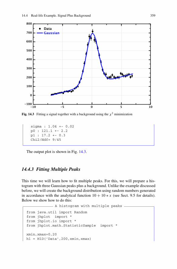
14.4 Real-life Example. Signal Plus Background 359
Fig. 14.3 Fitting a signal together with a background using the χ2 minimization
sigma : 1.04 +- 0.02p0 : 121.1 +- 2.2p1 : 17.2 +- 0.3Chi2/Ndf= 9/45
The output plot is shown in Fig. 14.3.
14.4.3 Fitting Multiple Peaks
This time we will learn how to fit multiple peaks. For this, we will prepare a his-togram with three Gaussian peaks plus a background. Unlike the example discussedbefore, we will create the background distribution using random numbers generatedin accordance with the analytical function 10 + 10 ∗ x (see Sect. 9.5 for details).Below we show how to do this:
A histogram with multiple peaks
from java.util import Randomfrom jhplot import *from jhplot.io import *from jhplot.math.StatisticSample import *
xmin,xmax=0,20h1 = H1D(’Data’,200,xmin,xmax)
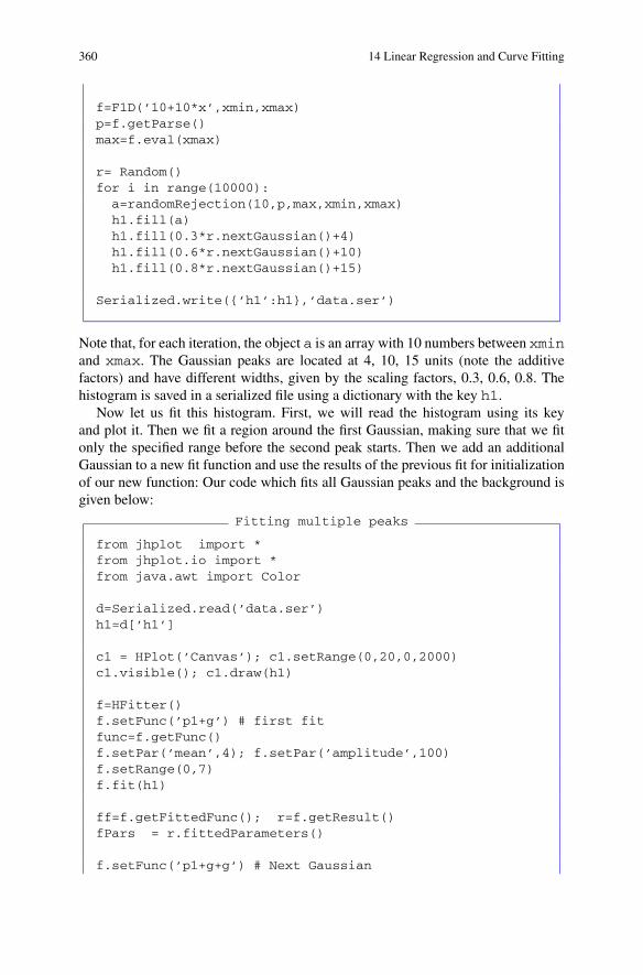
360 14 Linear Regression and Curve Fitting
f=F1D(’10+10*x’,xmin,xmax)p=f.getParse()max=f.eval(xmax)
r= Random()for i in range(10000):
a=randomRejection(10,p,max,xmin,xmax)h1.fill(a)h1.fill(0.3*r.nextGaussian()+4)h1.fill(0.6*r.nextGaussian()+10)h1.fill(0.8*r.nextGaussian()+15)
Serialized.write({’h1’:h1},’data.ser’)
Note that, for each iteration, the object a is an array with 10 numbers between xminand xmax. The Gaussian peaks are located at 4, 10, 15 units (note the additivefactors) and have different widths, given by the scaling factors, 0.3, 0.6, 0.8. Thehistogram is saved in a serialized file using a dictionary with the key h1.
Now let us fit this histogram. First, we will read the histogram using its keyand plot it. Then we fit a region around the first Gaussian, making sure that we fitonly the specified range before the second peak starts. Then we add an additionalGaussian to a new fit function and use the results of the previous fit for initializationof our new function: Our code which fits all Gaussian peaks and the background isgiven below:
Fitting multiple peaks
from jhplot import *from jhplot.io import *from java.awt import Color
d=Serialized.read(’data.ser’)h1=d[’h1’]
c1 = HPlot(’Canvas’); c1.setRange(0,20,0,2000)c1.visible(); c1.draw(h1)
f=HFitter()f.setFunc(’p1+g’) # first fitfunc=f.getFunc()f.setPar(’mean’,4); f.setPar(’amplitude’,100)f.setRange(0,7)f.fit(h1)
ff=f.getFittedFunc(); r=f.getResult()fPars = r.fittedParameters()
f.setFunc(’p1+g+g’) # Next Gaussian
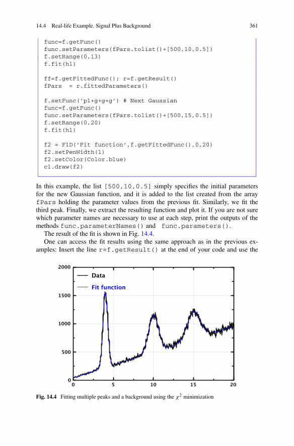
14.4 Real-life Example. Signal Plus Background 361
func=f.getFunc()func.setParameters(fPars.tolist()+[500,10,0.5])f.setRange(0,13)f.fit(h1)
ff=f.getFittedFunc(); r=f.getResult()fPars = r.fittedParameters()
f.setFunc(’p1+g+g+g’) # Next Gaussianfunc=f.getFunc()func.setParameters(fPars.tolist()+[500,15,0.5])f.setRange(0,20)f.fit(h1)
f2 = F1D(’Fit function’,f.getFittedFunc(),0,20)f2.setPenWidth(1)f2.setColor(Color.blue)c1.draw(f2)
In this example, the list [500,10,0.5] simply specifies the initial parametersfor the new Gaussian function, and it is added to the list created from the arrayfPars holding the parameter values from the previous fit. Similarly, we fit thethird peak. Finally, we extract the resulting function and plot it. If you are not surewhich parameter names are necessary to use at each step, print the outputs of themethods func.parameterNames() and func.parameters().
The result of the fit is shown in Fig. 14.4.One can access the fit results using the same approach as in the previous ex-
amples: Insert the line r=f.getResult() at the end of your code and use the
Fig. 14.4 Fitting multiple peaks and a background using the χ2 minimization
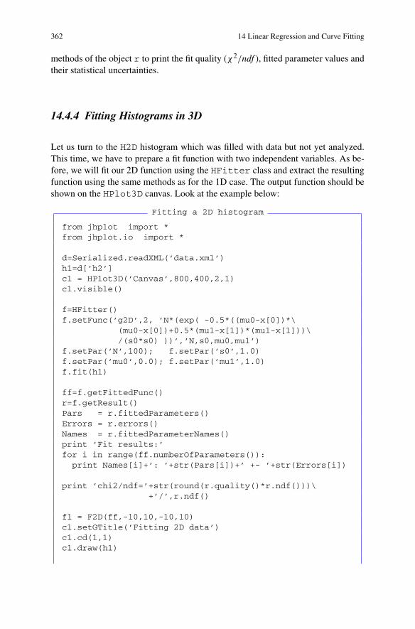
362 14 Linear Regression and Curve Fitting
methods of the object r to print the fit quality (χ2/ndf ), fitted parameter values andtheir statistical uncertainties.
14.4.4 Fitting Histograms in 3D
Let us turn to the H2D histogram which was filled with data but not yet analyzed.This time, we have to prepare a fit function with two independent variables. As be-fore, we will fit our 2D function using the HFitter class and extract the resultingfunction using the same methods as for the 1D case. The output function should beshown on the HPlot3D canvas. Look at the example below:
Fitting a 2D histogram
from jhplot import *from jhplot.io import *
d=Serialized.readXML(’data.xml’)h1=d[’h2’]c1 = HPlot3D(’Canvas’,800,400,2,1)c1.visible()
f=HFitter()f.setFunc(’g2D’,2, ’N*(exp( -0.5*((mu0-x[0])*\
(mu0-x[0])+0.5*(mu1-x[1])*(mu1-x[1]))\/(s0*s0) ))’,’N,s0,mu0,mu1’)
f.setPar(’N’,100); f.setPar(’s0’,1.0)f.setPar(’mu0’,0.0); f.setPar(’mu1’,1.0)f.fit(h1)
ff=f.getFittedFunc()r=f.getResult()Pars = r.fittedParameters()Errors = r.errors()Names = r.fittedParameterNames()print ’Fit results:’for i in range(ff.numberOfParameters()):
print Names[i]+’: ’+str(Pars[i])+’ +- ’+str(Errors[i])
print ’chi2/ndf=’+str(round(r.quality()*r.ndf()))\+’/’,r.ndf()
f1 = F2D(ff,-10,10,-10,10)c1.setGTitle(’Fitting 2D data’)c1.cd(1,1)c1.draw(h1)

14.5 Interactive Fit 363
Fig. 14.5 Fitting a 2D histogram (left) and showing the fit result (right)
c1.cd(2,1)c1.draw(f1)
The output figure is shown in Fig. 14.5.
14.5 Interactive Fit
One can fit 1D data (H1D histograms or P1D arrays) using an interactive dialogbased on the HFit class. Assuming that c1 represents the HPlot canvas and h1is a H1D histogram, one can start this fitter dialog as:
>>>a=HFit(c1,’c1’,h1,’h1’)
The execution of this line brings up a fit dialog where one can select the necessaryanalytical function (it must exist in the catalog). Note that we pass not only theobjects, but also the variable names for the HPlot and H1D class. This is necessaryif one needs to generate the JAIDA source code automatically. One should mentionthat one can also pass a P1D object instead of the histogram.
The fit panel allows a user to add custom functions, fit methods and perform thefit. One can also set up the initial parameters for the selected fit function using the[Settings] button. Once the fit is acceptable, one can generate the output fitparameters, which will be inserted directly to the editor in a form of Jython code.One can also automatically generate the JAIDA source code which corresponds tothe fit. Once inserted, it can further be corrected using the editor. Then, HFit()statement can be removed and the generated JAIDA code can be run manually.
One can also specify a user-defined 1D function and add it to the HFit dialog.This is an example of how to insert a first order polynomial function to be used forthe curve fitting:
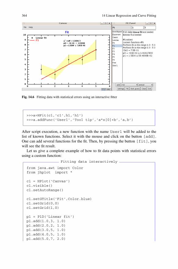
364 14 Linear Regression and Curve Fitting
Fig. 14.6 Fitting data with statistical errors using an interactive fitter
>>>a=HFit(c1,’c1’,h1,’h1’)>>>a.addFunc(’User1’,’Tool tip’,’a*x[0]+b’,’a,b’)
After script execution, a new function with the name User1 will be added to thelist of known functions. Select it with the mouse and click on the button [add].One can add several functions for the fit. Then, by pressing the button [fit], youwill see the fit result.
Let us give a complete example of how to fit data points with statistical errorsusing a custom function:
Fitting data interactively
from java.awt import Colorfrom jhplot import *
c1 = HPlot(’Canvas’)c1.visible()c1.setAutoRange()
c1.setGTitle(’Fit’,Color.blue)c1.setGrid(0,0)c1.setGrid(1,0)
p1 = P1D(’Linear fit’)p1.add(1.0,3, 1.0)p1.add(2.0,2, 1.0)p1.add(3.0,5, 1.0)p1.add(4.0,5, 1.0)p1.add(5.0,7, 2.0)
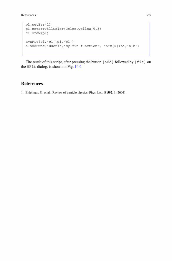
References 365
p1.setErr(1)p1.setErrFillColor(Color.yellow,0.3)c1.draw(p1)
a=HFit(c1,’c1’,p1,’p1’)a.addFunc(’User1’,’My fit function’, ’a*x[0]+b’,’a,b’)
The result of this script, after pressing the button [add] followed by [fit] onthe HFit dialog, is shown in Fig. 14.6.
References
1. Eidelman, S., et al.: Review of particle physics. Phys. Lett. B 592, 1 (2004)


Chapter 15Neural Networks
15.1 Introduction
A neural network is a powerful tool for data classification: if we know a sourcewith input data, and also have knowledge of how the output data looks like, one canobtain a relationship between inputs and outputs. This can be done totally numeri-cally, without using any predefined function as in the case of curve fitting discussedbefore. Once such a relationship is established, one can perform predictions basedon the input, assuming that the data set has the same characteristics as those usedfor determination of the relationship during the so-called “training” step. Here wewill recommend several books [1, 2] with detailed information about the neural net-works. Below we will touch only the basics of this subject.
But what exactly should be used to perform such classification of inputs? The en-tire concept of the neural-network approach tries to capture the essence of biologicalneural systems. In particular, it tries to simulate the brain’s way of processing infor-mation. A neural network consists of a number of interconnected “neurons” in oderto simulate biological neural systems. We should remind that a human brain consistsof a very large number of interconnected neurons. Each neuron has an input and abranching output structure. When a neuron is activated, it sends an electrochemicalsignal via the synapses to other neurons which may, in turn, fire signals to inputs ofother neurons. The strength of the propagated signal depends on the efficiency ofthe synapses.
Mathematically, a neural network consists of a set of interconnected units, callednodes. Each node accepts a weighted set of inputs and responds with an output.Each input has an associated weight representing the strength of that particular con-nection. A multilayer network with several layers of units is rather popular. For suchnetworks, the output from one layer serves as input to the next.
Below we will consider a feedforward neural network, in which the data frominput to output units is strictly feedforward. For this type of network, no feedbackconnection exists. This is the most popular network in many practical applications.
The number of neurons in the input layer depends on the number of inputs, whilethe number of neurons in the output layer depends on the number of desired outputs.
S.V. Chekanov, Scientific Data Analysis using Jython Scripting and Java,Advanced Information and Knowledge Processing,DOI 10.1007/978-1-84996-287-2_16, © Springer-Verlag London Limited 2010
367

368 15 Neural Networks
The number of hidden layers and the number of neurons in each such layer must bedefined empirically.
Each neuron performs accumulation of incoming pulses from its inputs usingweights. All weights are sum up and the sum is passed into a non-liner activationfunction. We will use the most popular sigmoid activation function, S(x) = 1/(1 +e−x). The output of such neutron is formed by applying the sigmoid function as:S(d+∑N
i=0 xiwi), where xi are the input values from other neurons, wi characterizethe weights for input connections and d is a real number called the threshold. Thisnumber characterizes the neutron as whole.
The neural net should be trained to adjust wi and d parameters. Once the inputunits have received the signal from outside and from output units with the result-ing signal, one can adjust the weights in interconnected neurons such that one canperform predictions. During the learning process, the output vector of numbers iscompared to the expected output. If the difference is not zero, the (“epoch”) erroron the prediction is calculated. The idea is to adjust the weights to minimize thedifference between the neural-net output and the expected output. In this case, suchnetworks can learn arbitrary associations between the input vector and the output.
15.1.1 Generating a Data Sample
Let us sketch a typical task which can be solved using the neural-net approach.Assume we have many events with the input vector of numbers. We also knowsome events in which the input vector produces a specific output. How to makepredictions in case when only the input is available?
We will start with the preparation of a data sample, so later we will use it forour neural network studies. Let us assume that we have five variables generated inaccordance with some distributions. We generate a new variable from the inputsusing some functions. The vector with inputs and outputs will be stored persistentlyin a serialized file as shown below:
Creating a data set
from java.util import Randomfrom jhplot import *from jhplot.io import *
input=PND(’Data’)out=PND(’Output’)r= Random()for i in range(1000):
x1=10*r.nextDouble()x2=2**(10*r.nextDouble())x3=1/(r.nextDouble()+0.0001)x4=10*r.nextDouble()+0.0001input.add([x1,x2,x3,x4])out.add([x1/x4-x2+x3])
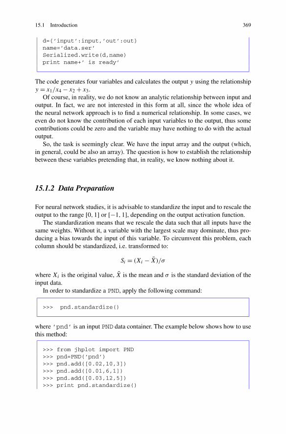
15.1 Introduction 369
d={’input’:input,’out’:out}name=’data.ser’Serialized.write(d,name)print name+’ is ready’
The code generates four variables and calculates the output y using the relationshipy = x1/x4 − x2 + x3.
Of course, in reality, we do not know an analytic relationship between input andoutput. In fact, we are not interested in this form at all, since the whole idea ofthe neural network approach is to find a numerical relationship. In some cases, weeven do not know the contribution of each input variables to the output, thus somecontributions could be zero and the variable may have nothing to do with the actualoutput.
So, the task is seemingly clear. We have the input array and the output (which,in general, could be also an array). The question is how to establish the relationshipbetween these variables pretending that, in reality, we know nothing about it.
15.1.2 Data Preparation
For neural network studies, it is advisable to standardize the input and to rescale theoutput to the range [0,1] or [−1,1], depending on the output activation function.
The standardization means that we rescale the data such that all inputs have thesame weights. Without it, a variable with the largest scale may dominate, thus pro-ducing a bias towards the input of this variable. To circumvent this problem, eachcolumn should be standardized, i.e. transformed to:
Si = (Xi − X̄)/σ
where Xi is the original value, X̄ is the mean and σ is the standard deviation of theinput data.
In order to standardize a PND, apply the following command:
>>> pnd.standardize()
where ’pnd’ is an input PND data container. The example below shows how to usethis method:
>>> from jhplot import PND>>> pnd=PND(’pnd’)>>> pnd.add([0.02,10,3])>>> pnd.add([0.01,6,1])>>> pnd.add([0.03,12,5])>>> print pnd.standardize()

370 15 Neural Networks
0.0 0.21 0.0-1.0 -1.09 -1.00.99 0.87 1.0
In contrast, a normalization or rescaling means that each column is transformedsuch that all column values are either between [0,1] or [−1,1], depending on therange of the activation function. To normalize a PND, use the rescale() method.One should pass “0” as an argument in case if the rescaling should be done for therange [0,1]:
Si = (Xi − Xmin)/(Xmax − Xmin)
In case of the range [−1,1], one should apply this transformation:
Si = 2 ∗ (Xi − midrange)/(Xmax − Xmin), midrange = 0.5(Xmax + Xmin)
which is implemented for the PND class using the method rescale(1). Thismethod returns an array which then is used to transform the PND back to the originalform. In this case, the output of the rescale method should be passed as an input tothe rescale(obj) method. Consider the example:
>>> from jhplot import PND>>> pnd=PND(’pnd’)>>> pnd.add([0.02,10,3])>>> pnd.add([0.01,6,1])>>> pnd.add([0.03,12,5])>>> a=pnd.rescale(0)>>> print pnd0.5 0.66 0.50.0 0.0 0.01.0 1.0 1.0
>>> pnd.rescale(a)>>> print pnd0.02 10.0 3.00.01 6.0 1.00.03 12.0 5.0
One can see that the rescale method has restored the original array, once you havepassed the output from the first rescale(0) call which converts each columnto the range [0,1]. Analogously, if the rescale(i) method is called with theargument “1”, all values will be moved to the range [−1,1], and the conversionback will be done in exactly the same way as before.
In the next example we read the saved containers, standardize the input and nor-malize the output. Then we save the resulting container into a dictionary. We alsosave the array keeping the scaling factors, which can be used to restore the outputlater.

15.1 Introduction 371
Standardizing data
from jhplot.io import *
d=Serialized.read(’data.ser’)input=d[’input’]out=d["out"]
input.standardize()scale=out.rescale(0)
d={’input’:input,’out’:out,’scale’:scale}name=’data_scaled.ser’Serialized.write(d,name)print name+’ is ready’
It should be noted that the standardization should be approached with cautionbecause it discards certain information. Generally, there are no ‘rules of thumb’ thatapply to all possible cases.
Now we are ready to use a fraction of the rescaled data for training of our neuralnetwork. But before, let us discuss the machinery behind the construction of a neuralnet.
15.1.3 Building a Neural Net
First, let us discuss how to build and visualize a neural network. In case of jHep-Work, a neural net can be constructed using the class HNeuralNet which is basedon the Encog project [3]. In order to illustrate its usage, we will build a feedforwardneural network with an input layer, two hidden layers and one output layer. The in-put layer will contain four neurons, two hidden layers will have five neurons each,and the output layer will have a single neuron:
>>> from jhplot import *>>> net = HNeuralNet()>>> net.addFeedForwardLayer(4)>>> net.addFeedForwardLayer(5)>>> net.addFeedForwardLayer(5)>>> net.addFeedForwardLayer(1)
The code above simply adds layers, staring from input to the output, passing in-teger arguments and specifying the number of interconnected neutrons in eachlayer.
The next step is to reset all neuron thresholds to some (random) values. Thisshould be done with the method reset().

372 15 Neural Networks
Fig. 15.1 A representation of a neural network with two hidden layers. The threshold values forthe activation matrix is shown for each neutron. In this example, they are random numbers gener-ated with the reset() method
The constructed network can be visualized with the method showNetwork().Below we show how to initialize the network and display it on the screen:
>>> net.reset()>>> net.showNetwork()
The result of the last line is a pop-up window which displays the structure of thenetwork. This window is shown in Fig. 15.1. Each layer has the following notations:“I” is the input layer, “H” is the hidden layer and “O” is the output layer.
Once the network is created, we should set the input and the output data fortraining. This can be done with the method setData(input,output), whereinput and output are data holders of the type PND. One can look at the data bycalling the editData() method which opens an editor with the neural-net inputand output.
Next, the created network should learn how to adjust the weights and the neuronthresholds. This is done by applying the method:
>>> net.trainBackpopogation(b,max,learnRate,mom,err)

15.1 Introduction 373
where:
b is 1 (Java true) if a dialog window is required to show the learningrate and its errors. The smaller error on Y , the higher chances that thelearning is successful. Make sure that the error value does not changewith iteration (or epoch) number. If b is Java false (“0” in Jython),one cannot monitor the learning rate and error.
max is the maximal number of epochs for learning. The learning contin-ues until max is reached, but only if the epoch error is larger thanerrEpoch. If we reach a maximum count of iterations or epochs,this will mean that the training was not successful.
learnRate is the rate at which the weight matrix will be adjusted based on learn-ing (the so-called learning rate); This number is usually between 0.1and 0.2.
mom is the influence that previous iteration’s training deltas will have onthe current iteration. Usually it is set to 0.1–0.4.
err is the “epoch” error for training at which the learning should bestopped. If the specified error is not reached during the learning, theprogram stops the learning after reaching “max” number of events.
It should be noted that the epoch error can also be obtained with the methodnet.getEpochError() without opening the control window.
It is always a good idea to call the showNetwork() method to look at the newthreshold values. Once the network was trained, one can save the network in a file,so one can restore it later. This can be done as:
>>> net.save(’test.eg’,’trainedNN’,’My trained NN’)
The first string is the output file name (’test.eg’ in this example), the secondis the name of the network (’rainedNN’) and the third argument is used for thenetwork description.
One can restore the saved network at any time by calling the method:
>>> net.read(’test.eg’,’trainedNN’);
where ’test.eg’ is an input file with the neural network.
15.1.4 Training and Verifying
The data after the standardization of the inputs and rescaling the outputs are readyfor the next step—training. We will create a neural net with four neutrons in theinput layer. The output layer will contain one neuron. Our hidden layer will containseven neurons. After creating the net, we will reset all inputs and load the first halfof our data (500 rows). The training will be done using 2000 epoches. During thetraining, we will open a frame displaying the value of the epoch error. Once the
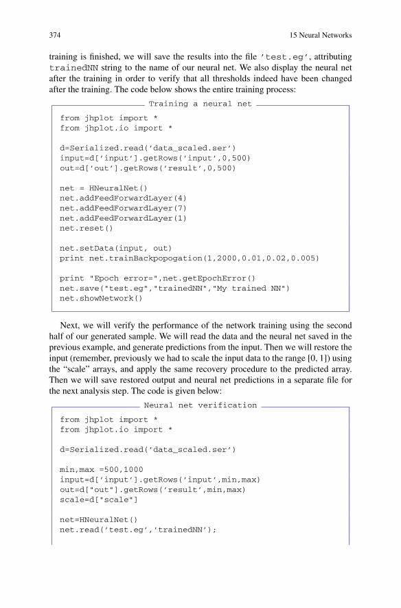
374 15 Neural Networks
training is finished, we will save the results into the file ’test.eg’, attributingtrainedNN string to the name of our neural net. We also display the neural netafter the training in order to verify that all thresholds indeed have been changedafter the training. The code below shows the entire training process:
Training a neural net
from jhplot import *from jhplot.io import *
d=Serialized.read(’data_scaled.ser’)input=d[’input’].getRows(’input’,0,500)out=d[’out’].getRows(’result’,0,500)
net = HNeuralNet()net.addFeedForwardLayer(4)net.addFeedForwardLayer(7)net.addFeedForwardLayer(1)net.reset()
net.setData(input, out)print net.trainBackpopogation(1,2000,0.01,0.02,0.005)
print "Epoch error=",net.getEpochError()net.save("test.eg","trainedNN","My trained NN")net.showNetwork()
Next, we will verify the performance of the network training using the secondhalf of our generated sample. We will read the data and the neural net saved in theprevious example, and generate predictions from the input. Then we will restore theinput (remember, previously we had to scale the input data to the range [0,1]) usingthe “scale” arrays, and apply the same recovery procedure to the predicted array.Then we will save restored output and neural net predictions in a separate file forthe next analysis step. The code is given below:
Neural net verification
from jhplot import *from jhplot.io import *
d=Serialized.read(’data_scaled.ser’)
min,max =500,1000input=d[’input’].getRows(’input’,min,max)out=d["out"].getRows(’result’,min,max)scale=d["scale"]
net=HNeuralNet()net.read(’test.eg’,’trainedNN’);

15.2 Bayesian Networks 375
pred=net.predict(input)pred.rescale(scale)out.rescale(scale)
d={’predicted’:pred,’expected’:out}Serialized.write(d,’data_verify.ser’)
Finally, we can look at the outputs and the predicted values. We will print thevalues and also calculate the ratio of the predicted outputs to the original outputs.We will create a histogram with this ratio as shown below:
Neural network predictions
from jhplot import *from jhplot.io import *
d=Serialized.read(’data_verify.ser’)predicted=d[’predicted’]expected=d[’expected’]ratio=predicted.copy(’ratio’)ratio.oper(expected,’/’)
c1=HPlot()c1.visible()c1.setAutoRange()
h=H1D(’ratio’,50,-3,3.)h.fill(ratio)c1.draw(h)c1.drawStatBox(h)
for i in range(100): # check first 100p=predicted.getRow(i)x=expected.getRow(i)d1=p.get(0)d2=x.get(0)print ’predicted=’,d1,’ expected=’,d2
The script generates a canvas with the filled histogram. One can see that the his-togram has a peak at unity as expected. The distribution has long tails indicatingthat, for some rear events, the predictions could still be far away from the originalvalues.
15.2 Bayesian Networks
A Bayesian network (or “belief” network) is a graphical model for manipulatingprobabilistic relationships among variables of interest, and building decision scenar-

376 15 Neural Networks
ios requiring reasoning under uncertainty. Such networks are widely used in man-aging uncertainty in science, engineering, business and medicine [4, 5].
The Bayesian network is included into the jHepWork libraries using theJavaBayes package [6]. It calculates marginal probabilities and expectations, pro-duces explanations and performs robustness analysis. In addition, it allows a user toimport, create, modify and export networks.
The network editor can be called using the HBayes class:
>>> from jhplot import *>>> HBayes()
This brings up the Bayesian-network editor and a console window. A user can followthe step-by-step instruction given in the console. The JavaBayes network is ratherwell documented and will not be discussed here further.
15.3 Self-organizing Map
In addition to the neural network algorithms which require a “learning” procedure,there is a class of unsupervised learning algorithms which attempt to find the mostappropriate topological description of input data. Below we will consider a Bayesianself-organizing map (BSOM), which represents a method for estimating a probabil-ity distribution from input data on the basis of a Bayesian stochastic model. For thismodel, the data recognition algorithm tries to find relationships in high-dimensionaldata and converts this knowledge into a simple relationship using low-dimensions.
We will consider an example which can help to make the BSOM explanationmore illustrative. For this, we will use the class HBsom based on the BSOM program[7].
The code below fills a histogram, converts it to a P1D container which is thenused for the algorithm input. We use 30 interconnected units to analyze the topolog-ical shape in 2D, see the method setNPoints. The last line of the code brings upa window with visualized data points and interconnected units. Also, we save thegenerated input data (see the method toFile()), so we can use the same data forthe example to be shown in the next subsection.
Interactive self-organizing map
from java.util import Randomfrom jhplot import *
h1 = H1D(’Data’,20,-100.0, 300.0)r = Random()for i in range(2000):
h1.fill(100+r.nextGaussian()*100)
p1d=P1D(h1,0,0)

15.3 Self-organizing Map 377
p1d.toFile(’data.txt’)
bs=HBsom()bs.setNPoints(30)bs.setData(p1d)bs.visible()
To start the algorithm, one should set up the values α and β . Then press the but-ton “learn”. Initially the BSOM units are positioned randomly, then the algorithmcalculates the most optimal positions for interconnected units. The resulting plot isshown in Fig. 15.2.
The BSOM model parameters, α and β , represent the strength of topologicalconstraint and the noise level expected in data, respectively. α and 1/β correspond tothe temperature of a physical system. For α � 0, topological constraint on the unitsis not imposed and BSOM can be viewed as a data clustering based on a spherical
Fig. 15.2 The BSOM algorithm in action using an interactive mode

378 15 Neural Networks
Fig. 15.3 Using the BSOM algorithm in a non-interactive mode
Gaussian mixture model. When β is infinitely large, BSOM is very similar to theK-means algorithm.
Running this algorithm will help to find an optimal configuration for data de-scription. Usually, one should start learning from a high value of α and a low valueof β . One should note that BSOM can automatically search for the optimal val-ues of the parameters by pressing the ‘auto’ button. The ‘density’ button shows theestimated data density.
15.3.1 Non-interactive BSOM
It is more practical to run the BSOM program in a non-interactive mode. Thiscan be done by removing the line with the visible() method and insertingthe line run(). The results of the algorithm can be retrieved with the methodgetResult() with the output in the form of P1D array. Then we plot the resultsas in the code below:
Non-interactive BSOM
from jhplot import *from java.awt import Color
c1 = HPlot("Canvas")c1.setGTitle("Bayesian Self-Organizing Map")c1.visible()c1.setAutoRange()
p1d=P1D("data","data.txt")p1d.setErrToZero(1)bs=HBsom()bs.setNPoints(30)bs.setData(p1d)

15.4 Neural Network Using Python Libraries 379
bs.run()result=bs.getResult()result.setStyle("pl")result.setColor(Color.blue)c1.draw(p1d)c1.draw(result)
One should note that we set all statistical errors of the input P1D to zero. Theresulting P1D is shown with symbols connected with the lines. The result of theabove script is shown in Fig. 15.3.
Let us give more details about the use of the HBsom in the non-interactive mode.The method run() executes the learning algorithm. The learning stops if topolog-ical changes between each step are smaller than some parameter, which can be setvia the method setDelta(). One can get the total number of iterations using themethod getNiterations().
For more complicated topologies of data in 2D, it is important to adjust the initialα and β values using the method setAlphaBeta(a,b).
15.4 Neural Network Using Python Libraries
jHepWork packaged several libraries for neural-network studies implemented inPython. In particular, one can use the PyANN program [8] which was initially writ-ten for CPython. As you already know, numerical programs implemented in Pythonare slow. Therefore, we will not gain anything in terms of execution performancewhile running this package using Jython, compare to native Java or C++ libraries.But there are several other advantages in using the Jython approach: (1) The codeis fully “transportable” and can be run using CPython; (2) There is a direct accessto the original code if one needs to understand it and make necessary modifications;(3) Finally, you will get all benefits of the Python programming language, includingits interactivity for easy debugging.
In this section, we will illustrate how to use the PyANN library using jHep-Work. The corresponding library is located inside the directory pyann in python/packages. If you are using the jHepWork IDE, this directory is imported automat-ically. Below we will learn how to run a multilayer algorithm, which implements afeedforward, supervised algorithm for data classification.
As in the previous section, we will divide our work in several steps: (1) we willprepare a common module, to make our codding compact; (2) we will create fileswith input data for training and verifications. We will use the shelve module dis-cussed in Sect. 2.16.6; (3) then we will build a neural net and train it. Finally, wewill verify the performance of this algorithm.
Let us first make a common module which imports the necessary libraries fromthe PyANN package. Here we will also define several global parameters, as well

380 15 Neural Networks
functions for input and output. The example code is given below:
Common module "NNpython.py"
import sys,math,random,shelve
import pyann.mlpfrom pyann.mlp.layer import *from pyann.mlp.monitoring import *from pyann.mlp.training import *from pyann.mlp.training.backprop import *
WINDOW, MIN_VALUE, MAX_VALUE = 10,-1,1
def writeData(data,valid,pattern):sh=shelve.open(’data.shelf’)sh[’data’]=datash[’validate’]=validsh[’pattern’]=patternsh.close()
def readData():return shelve.open(’data.shelf’)
Next, using the module above, we will create a file with the input data. We will usesin(i) as an engine to generate our data. The data will have 73 rows, 63 will beused for training and 12 for validation. Each row of data will be in a form of tuplewith 10 inputs, while we will have only one output (also in the form of tuple butwith one value).
Creating a data set
from NNpython import *
data = [] # Build data setfor i in range(-360, 361, 10):
data.append(math.sin(i))print len(data)
start = len(data)-WINDOW-1pattern=[] # Build patternwhile len( data[start : start+WINDOW] ) == WINDOW:
input = tuple(data[start : start+WINDOW])output = (data[start+WINDOW],)pattern.append(pyann.mlp.Pattern(input, output))start -= 1
valid = [] # validation pattern. 20% of datafor i in range(int(len(pattern)*0.2)):valid.append(pattern.pop(random.randrange(len(pattern))))

15.4 Neural Network Using Python Libraries 381
writeData(data,valid,pattern)
In the above example, use the method type() for debugging which helps to un-derstand what the above code is doing. All data will be saved into a file.
Now we come to the training. First, we build a neural net with 10 inputs, 5 nodesfor the hidden layer and one output node. Then we read the data and train the net us-ing rather self-explanatory methods. The script prints the training (“epoch”) errors.Finally, we will verify the net using our verification sample.
Neural network training and predictions
from NNpython import *
layers = (SigmoidInputLayer(WINDOW),\SigmoidLayer(5),\SigmoidOutputLayer(1,minValue=MIN_VALUE,maxValue=MAX_VALUE))
net = pyann.mlp.Network( layers )
sh=readData()data=sh[’data’]validation=sh[’validate’]patterns=sh[’pattern’]
monitor = VerboseMonitor()stopOnMaxIter =MaxIterationsStopCondition(500)stopOnMinError =MinErrorStopCondition(0.01)stopOnVMinError =MinValidationErrorStopCondition(0.005)
trainer =BackpropagationTrainer(net, monitor)trainer.setLearningRate(0.7)trainer.setMomentum(0.5)trainer.setRandomize(True)trainer.setStopConditions((stopOnMaxIter,\
stopOnMinError,stopOnVMinError),\joiner = ’or’)
trainInfo = trainer.train(patterns, validation)print """Epochs: %(epoch)sFinal error: %(error)sValidation set error: %(validationError)s""" % { ’epoch’: trainInfo.getIterationNumber(),
’error’: trainInfo.getError(),’validationError’: trainInfo.getValidationSetError()}
for i in range(370, 725, 10):start = len(data) - WINDOW

382 15 Neural Networks
predicted = net.classify( tuple(data[start:]) )[0]data.append(predicted)print ’sin(%s) = %s’ % (i, predicted)
Run this code to see the result of the training. The code snippet prints out the pre-dicted values, which are rather close to the true values of the sin(i) function.
References
1. Beale, R., Jackson, T.: Neural Computing: An Introduction. Institute of Physics Publishing,Bristol (1990)
2. Bharath, R., Drosen, J.: Neural Network Computing. McGraw-Hill, New York (1994)3. Heaton, J.: Contributions: The ENCOG project. URL http://code.google.com/p/encog-java/4. Neapolitan, R.E.: Learning Bayesian Networks. Prentice Hall, New York (2003)5. Jensen, F.V., Nielsen, T.D.: Bayesian Networks and Decision Graphs, 2nd edn. Information
Science and Statistics. Springer, Berlin (2007)6. Cozman, F.G.: Javabayes: Bayesian networks in Java. URL http://www.cs.cmu.edu/~
javabayes/7. Utsugi, A.: Neural Comput. 9, 623 (1997)8. PyANN, a Python framework to build artificial neural networks. URL http://sourceforge.net/
projects/pyann

Chapter 16Steps in Data Analysis
In this chapter, we will consider rather common analysis techniques used to pro-cess and analyze data before final visualization. We will gain insight into how totransform data, reject unnecessary records or add additional information, removeduplicate records, sort data and many other common operations. We will also learnhow to process data in parallel using multiple processors.
From the programming point of view, our discussion is heavily based on theknowledge collected in the previous chapters.
16.1 Major Analysis Steps
A first step towards understanding of a general analysis strategy is to abstract froma particular type of data and focus on generic steps for data processing, which canconsist of
Measurement A determination of numerical values of some observables andcollection of experimental results into data files. A group ofmeasured values forms an “event record”, or simply, “events”.Each event can contain a set of records, each consisting of a setof objects (strings, values, multi-dimensional arrays, histogramsetc.). The event record may represent various characteristics ofa single observation.
Transformation Transformation of the event records into the most appropriateformat for further manipulation. This can be done at any analysisstep, depending on a concrete situation. If event records are toobig for disk storage, they can be converted into a more compactformat. But keep in mind that we may pay for this later witha lower processing speed during data analysis. If data requiresa lot of processing and the file storage is not an issue, one cankeep data in a less compact format.
S.V. Chekanov, Scientific Data Analysis using Jython Scripting and Java,Advanced Information and Knowledge Processing,DOI 10.1007/978-1-84996-287-2_17, © Springer-Verlag London Limited 2010
383
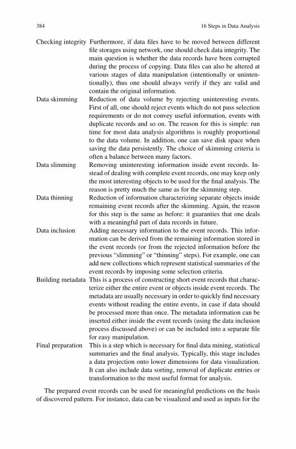
384 16 Steps in Data Analysis
Checking integrity Furthermore, if data files have to be moved between differentfile storages using network, one should check data integrity. Themain question is whether the data records have been corruptedduring the process of copying. Data files can also be altered atvarious stages of data manipulation (intentionally or uninten-tionally), thus one should always verify if they are valid andcontain the original information.
Data skimming Reduction of data volume by rejecting uninteresting events.First of all, one should reject events which do not pass selectionrequirements or do not convey useful information, events withduplicate records and so on. The reason for this is simple: runtime for most data analysis algorithms is roughly proportionalto the data volume. In addition, one can save disk space whensaving the data persistently. The choice of skimming criteria isoften a balance between many factors.
Data slimming Removing uninteresting information inside event records. In-stead of dealing with complete event records, one may keep onlythe most interesting objects to be used for the final analysis. Thereason is pretty much the same as for the skimming step.
Data thinning Reduction of information characterizing separate objects insideremaining event records after the skimming. Again, the reasonfor this step is the same as before: it guaranties that one dealswith a meaningful part of data records in future.
Data inclusion Adding necessary information to the event records. This infor-mation can be derived from the remaining information stored inthe event records (or from the rejected information before theprevious “slimming” or “thinning” steps). For example, one canadd new collections which represent statistical summaries of theevent records by imposing some selection criteria.
Building metadata This is a process of constructing short event records that charac-terize either the entire event or objects inside event records. Themetadata are usually necessary in order to quickly find necessaryevents without reading the entire events, in case if data shouldbe processed more than once. The metadata information can beinserted either inside the event records (using the data inclusionprocess discussed above) or can be included into a separate filefor easy manipulation.
Final preparation This is a step which is necessary for final data mining, statisticalsummaries and the final analysis. Typically, this stage includesa data projection onto lower dimensions for data visualization.It can also include data sorting, removal of duplicate entries ortransformation to the most useful format for analysis.
The prepared event records can be used for meaningful predictions on the basisof discovered pattern. For instance, data can be visualized and used as inputs for the

16.2 Real Life Example. Analyzing a Gene Catalog 385
supervised or unsupervised learning algorithms discussed in the previous chapters.Finally, the selected data should be compared with a certain theory.
The data skimming, slimming and thinning are not new concepts in data analysis.However, in recent years, there has been growing interest in such analysis techniquesduring preparation to data taking at the Large Hadron Collider to be constructed bythe international community in Geneva (Switzerland), where such concepts havebeen reshaped and refined [1].
In this book, our approach will remain to be the same: Instead of being abstract,we will illustrate the above analysis techniques using numerical examples.
16.2 Real Life Example. Analyzing a Gene Catalog
In this section will analyze a published gene catalog of human chromosome 11 andillustrate most of the analysis steps discussed above. Other aspects of data analysiswill be discussed in the following sections.
Of course, we cannot discuss the actual measurement of the gene catalog; instead,we will copy the available data from a public domain and then perform necessaryoperations using Jython scripting. The analyzed data file can be copied from a webpage given in [2]. For easy manipulation, we have transformed the original file intoa CSV file (one can do this with any spreadsheet program).
Let us download a CSV file with the gene catalog and display it in the CSVbrowser.
Getting the data
from jhplot.io.csv import *from jhplot import *
http=’http://projects.hepforge.org/jhepwork/’file=’nature04632-s16-2.csv’wget(http+’examples/data/’+file)r=CSVReader(file,’,’)SPsheet(r)
As for the previous chapters, if the above web page location fails, use a mirrorsite by replacing the http address with the string:
http=’http://jhepwork.sourceforge.net/’orhttp=’http://jwork.org/jhepwork/’
The above code brings up a spreadsheet filled with the data from the gene catalog.A visual study of this file reveals that each gene symbol is characterized by severalrecords. In fact, each row representing a gene can be considered an “event record”using the terminology adopted above. Each gene has its symbol, name, category,location, length and so on. We will use this file as a starting point for our examples.

386 16 Steps in Data Analysis
16.2.1 Data Transformation
Now we will show how to transform the gene event records into a machine-readableform. For many practical applications, this is necessary in order to save disk spacewhile storing the data, or for best performance while reading data.
In the example below we illustrate how to read the CVS file (see Sect. 11.7.1)and convert the event records, line by line, into a compressed serialized file (seeSect. 11.3):
Transforming data records
from jhplot.io.csv import *from jhplot.io import *
r=CSVReader(’nature04632-s16-2.csv’,’,’)f=HFile(’nature.ser’,’w’)
i=0while 1:
line= r.next()if line == None: breakif (i%100 == 0): print if.write(line)i +=1
f.close()r.close()
The code seemed very simple: We loop over all rows in the CSV file and serializethem into the file ’nature.ser’ which keeps data in a compressed form. Thesize of the output file is typically three times smaller than the original file size.
16.2.2 Data Skimming
Let us turn to the skimming stage during which the data volume is reduced afterrejecting uninteresting event records. For our example, we assume that some rowsconvey no useful information for further analysis. In particular, we would like toskip all genes with undefined gene names (“symbol”). By examining the CSV fileusing a spreadsheet, one can find that a gene symbol entry is not defined if the firstcolumn has the string ’undef’. So, let us rewrite the file by rejecting such entries:
Skimming data records
from jhplot.io import *
f1=HFile(’nature.ser’,’r’)f2=HFile(’nature_skim.ser’,’w’)

16.2 Real Life Example. Analyzing a Gene Catalog 387
while 1:row=f1.read()if row == None: breakif row[0] == ’undef’ or len(row)<18: continuef2.write(row)
f1.close()f2.close()
The output will be saved into the file ’nature_skim.ser’. In the above code,we included a simple check which verifies the correct length (18) for the processedrows.
16.2.3 Data Slimming
This time we are not interested in storing all information withing each event record.For example, we would like to remove two last columns for each row, which donot convey any useful information for us, but keeping the same number of rows asbefore. It takes only a few lines of the code to perform this manipulation:
Slimming data records
from jhplot.io import *
f1=HFile(’nature_skim.ser’,’r’)f2=HFile(’nature_slim.ser’,’w’)
while 1:row=f1.read()if row == None: breaks=len(row)del row[s-1]del row[s-2]f2.write(row)
f1.close()f2.close()
16.2.4 Data Sorting
Next, we would like to sort the event records using some arbitrary criteria. Ourevent records are not very simple because they are constructed from several objects.Therefore, the standard use of the sort() method for Jython lists will not work: Incase if each row contains several records, the sorting of rows should be done using

388 16 Steps in Data Analysis
values stored in a certain column, thus we should use the standard Jython methodsort() in a somewhat different way.
Sorting of data will be performed in a computer memory to make the entire pro-cess fast. For this example, we will sort the records based on the first column. Wewill read data into a list and use the sort()method together with the cmp() func-tion which provides a sorting algorithm. After the sorting, we will write the eventrecords into a new file:
Sorting records
from jhplot.io import *
f1=HFile(’nature_slim.ser’,’r’)f2=HFile(’nature_sorted.ser’,’w’)
data=[]while 1:
row=f1.read()if row == None: breakdata.append(row)
f1.close()
def cmp1(a,b): return cmp(a[0],b[0])
data.sort(cmp1)for k in data:
f2.write(k)f2.close()
In our example, the sort() method uses a custom cmt1() function, whichcalls the standard Python cmt() function. However, one can build totally customcmp1(). For example, one can construct the cmp1() function used in the aboveexample as:
A custom sorting function
def cmp1(a,b):if a[0]<b[0]: return -1if a[0]==b[0]: return 0if a[0]>b[0]: return 1
One can define the function cmt1() before the sort() command, and includeany logic for sorting.
We do not need always to use the Python-type objects. One can also use pure-Java collections to store and sort elements. In Sect. 2.7 we have shown how to usethe List class to store data and how to sort records using the Collection class.

16.2 Real Life Example. Analyzing a Gene Catalog 389
16.2.5 Removing Duplicate Records
Removal of duplicate event records requires a small preparation step. First, let uswrite a simple function which accepts a list containing other lists and sorts the listin accordance with an input index. Then, we scan from the end of the list, deletingduplicate entries based on the input index as we go:
Module ’unique.py’
def unique(s,inx):def cmp1(a,b): return cmp(a[inx],b[inx])s.sort(cmp1)last = s[-1]for i in range(len(s)-2, -1, -1):
if last[inx] == s[i][inx]:del s[i]
else:last = s[i]
return s
The function returns a list of elements without duplicate entries. We pass a variableinx which defines the column number used for the duplicate removal.
Now we should make a test of this function. Assume we have a list in which eachelement is another list. We will remove duplicate entries based on the first index (0),and then remove duplicates based on the second index:
Testing module
from unique import *
L=[[1,2],[’a’,10],[’a’,100],[’b’,1],[’c’,2]]print unique(L,0)print unique(L,1)
The output of this code is given below:
[[1, 2], [’a’, 100], [’b’, 1], [’c’, 2]][[’b’, 1], [’c’, 2], [’a’, 100]]
As you can see, after the first call, we have removed [’a’,10] (based on the firstindex), while the element [1,2] was rejected after the second call based on thesecond index.
Now we are ready to remove duplicate records in our example of the gene cata-log. We will remove duplicate rows based on the second column (index = 1):
Removing duplicate entries
from jhplot.io import *from unique import *

390 16 Steps in Data Analysis
f1=HFile(’nature_sorted.ser’,’r’)f2=HFile(’nature_unique.ser’,’w’)data=[]while 1:
row=f1.read()if row == None: breakdata.append(row)
f1.close()
unique(data,1)for k in data:
f2.write(k)f2.close()
16.2.6 Sorting and Removing Duplicate Records Using Java
We should also remind that there is no need for the Python-type approach for re-moving duplicate objects while working with Jython. On can always convert datainto the Java collection Set discussed in Sect. 2.7. We have shown that one canuse the class HashSet implementation of the interface Set which, by construc-tion, cannot contain duplicates. Moreover, one can use the class SortedSet thatalways maintains its elements in ascending order, so there is no need to worry aboutsorting and removing duplicates.
So, plan the analysis beforehand: if you think that the final data output should notcontain the same elements in the output container, just find appropriate container tokeep data records.
In the following subsections we will show two examples of how to work withevent records using pure Java collections.
16.2.6.1 Processing Big Event Sample
You may find yourself in a typical situation: One needs to read a huge data sampleand remove duplicate records based on some value. One cannot store all recordsin the computer memory, but one can still store values used for duplicate removal.In this case, there is no need for loading a full event into the computer memory:just read the file and write the event back as you go. Use the class HashSet to skipevent records with exactly the same description (in our case, this is the first element).When you add a description into the HashSet object, it returns ‘1’ (success) if noduplicate is found and ‘0’ if a duplicate is found. Using this approach one should beable to process big data files without too much load on the computer memory.

16.3 Using Metadata for Data Mining 391
16.2.6.2 Sorting and Removing Duplicate Records
In the next example we show how to sort and remove duplicate records using Javaclasses. In particular, the class TreeMap will be used for sorting and removing du-plicate objects at the same time. This example is similar to that shown in Sect. 2.7.6.The only difference is that now we read and fill a file with the data using the Listclass to decouple the first record with the description from the rest of the eventrecord. We use the description of genes as the keys for the TreeMap object whichremoves duplicates and sorts the keys as we fill it in. Finally, we loop over all sortedkeys and restore the event records by combining keys with the key value.
Sorting and removing duplicates
from jhplot.io import *from java.util import *
f1=HFile(’nature_slim.ser’,’r’)map=TreeMap()while 1:
row=f1.read()if row == None: breakln=row.size()r=row.subList(1,ln)map.put(row[0], row.subList(1,ln))
f1.close()
f2=HFile(’sorted_unique.ser’,’w’)for i in map:
row=map[i]row.set(0,i)print rowf2.write(row)
f2.close()
At this stage, we cannot use the gene catalog for our further examples. Our re-maining gene records are not sophisticated enough to perform thinning or buildinga metadata file. The latter techniques will be illustrated using an appropriate datasample.
16.3 Using Metadata for Data Mining
We will continue with our discussion of data analysis techniques by diving into thenotion of metadata. For this section, we cannot use the previous data sample as itlacks the necessary volume and complexity with which we usually have to deal withwhen the metadata records become necessary. The metadata is especially useful forlarge, data-intensive tasks in which one observation (or event) contains many datarecords.

392 16 Steps in Data Analysis
As mentioned before, the metadata is a short record which captures the basiccharacteristics of the entire event or objects inside each event record. These char-acteristics appear to be useful when one needs to find a necessary record as fast aspossible, without reading the entire data records.
The metadata concept is essential when one needs to find a few rear events, sothere is no too much sense in reading the data again and again if one single pro-cessing can build a metadata file which can be used for searching. Especially, onecan gain a lot in terms of a program performance when a multiple data processing isrequired. For example, one can benefit from the use of the metadata if data recordshave to be analyzed by many users.
The reason why the metadata can be useful for multiple processing is simple:in this approach, a program reads only a small (“metadata”) record. Usually, this isneither IO nor CPU consuming. Of course, the metadata records should be first con-structed using a priory knowledge about which data characteristics are important forfuture analysis. We should also note that the process of construction of the metadatafiles can be rather CPU consuming.
In this chapter we will illustrate the metadata concept using a few short codesnippets and Jython scripting.
16.3.1 Analyzing Data Using Built-in Metadata File
First, let us create event records for our examples. Each event will consist of a string,representing the record number, and two arrays of the type P0D. The size of botharrays is not fixed: it is determined by a Poisson distribution with the mean 500.One array is filled with a uniform random numbers, while the second array is filledwith random numbers in the range between 0 and 1. We write 10,000 events into aserialized compressed file ’data.ser’
Building a data file
from jhplot.io import *from jhplot import *
ps=math.Poisson(500)def makeEvent(entry):
p1,p2=P0D(’a’),P0D(’b’)p1.randomUniform(ps.next(),0,1)p2.randomNormal(ps.next(),0,1)return [str(entry),p1,p2]
f=HFile(’data.ser’,’w’)for i in range(10000):
ev=makeEvent(i)if (i%100 == 0):
print ’pocessed=’,ev[0]

16.3 Using Metadata for Data Mining 393
f.write(ev)f.close()
When the output file is ready, one question we may to ask themselves is this: howcan we find events in which the sum of all elements inside both arrays is above somevalue cut? Of course, this can be any other data mining task. We just have pickedup this one as it is simple to implement and, at the same time, it well captures theidea of using the metadata.
The code which reads the data file and counts all data records with the sum of allelements above cut=320 inside both arrays can look like this:
Analyzing data
from jhplot import *from jhplot.io import *import time
f=HFile(’data.ser’)start = time.clock()i=0; cut=320while 1:
event=f.read()if event == None:
print "End of events"break
if int(event[0])%1000 == 0:print ’processed=’,event[0]
p1,p2=event[1],event[2]v=p1.getSum()+p2.getSum()if v>cut:
i+=1t = time.clock()-startprint ’Nr above ’+str(cut)+’ =’,i, ’ after time (s)=’,tf.close()
The above code also performs a very basic benchmarking. The output is listed be-low:
End of eventsNr above 320 = 30 after time (s)= 10
Of course, the number of selected events and the execution time can be different foryour test.
Now, let us assume that we need to process the generated data file many timesusing different values of the variable cut for the event selection. This means thatwe should build a metadata by constructing an additional event record with the sumof all elements inside the arrays.
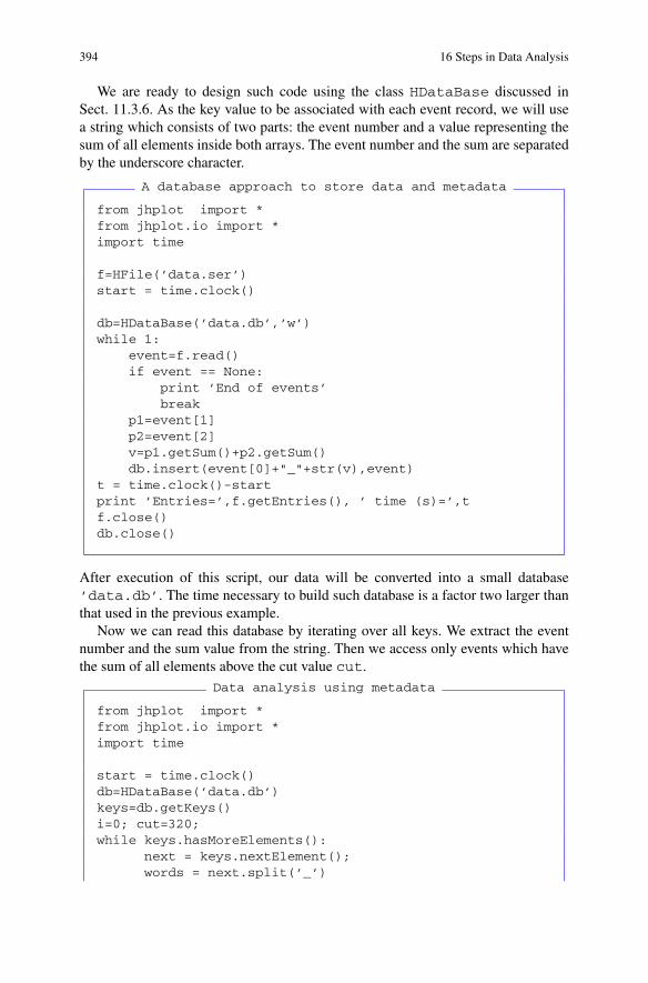
394 16 Steps in Data Analysis
We are ready to design such code using the class HDataBase discussed inSect. 11.3.6. As the key value to be associated with each event record, we will usea string which consists of two parts: the event number and a value representing thesum of all elements inside both arrays. The event number and the sum are separatedby the underscore character.
A database approach to store data and metadata
from jhplot import *from jhplot.io import *import time
f=HFile(’data.ser’)start = time.clock()
db=HDataBase(’data.db’,’w’)while 1:
event=f.read()if event == None:
print ’End of events’break
p1=event[1]p2=event[2]v=p1.getSum()+p2.getSum()db.insert(event[0]+"_"+str(v),event)
t = time.clock()-startprint ’Entries=’,f.getEntries(), ’ time (s)=’,tf.close()db.close()
After execution of this script, our data will be converted into a small database’data.db’. The time necessary to build such database is a factor two larger thanthat used in the previous example.
Now we can read this database by iterating over all keys. We extract the eventnumber and the sum value from the string. Then we access only events which havethe sum of all elements above the cut value cut.
Data analysis using metadata
from jhplot import *from jhplot.io import *import time
start = time.clock()db=HDataBase(’data.db’)keys=db.getKeys()i=0; cut=320;while keys.hasMoreElements():
next = keys.nextElement();words = next.split(’_’)
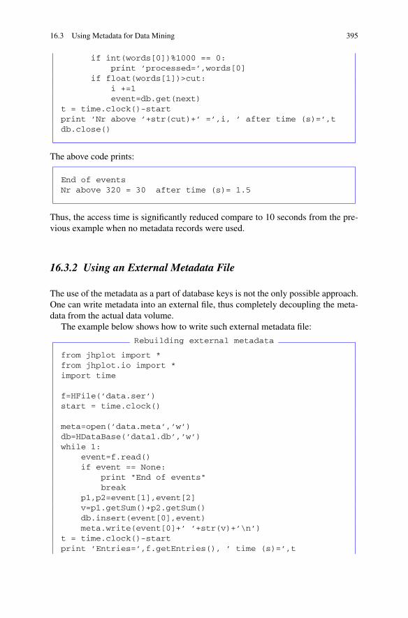
16.3 Using Metadata for Data Mining 395
if int(words[0])%1000 == 0:print ’processed=’,words[0]
if float(words[1])>cut:i +=1event=db.get(next)
t = time.clock()-startprint ’Nr above ’+str(cut)+’ =’,i, ’ after time (s)=’,tdb.close()
The above code prints:
End of eventsNr above 320 = 30 after time (s)= 1.5
Thus, the access time is significantly reduced compare to 10 seconds from the pre-vious example when no metadata records were used.
16.3.2 Using an External Metadata File
The use of the metadata as a part of database keys is not the only possible approach.One can write metadata into an external file, thus completely decoupling the meta-data from the actual data volume.
The example below shows how to write such external metadata file:
Rebuilding external metadata
from jhplot import *from jhplot.io import *import time
f=HFile(’data.ser’)start = time.clock()
meta=open(’data.meta’,’w’)db=HDataBase(’data1.db’,’w’)while 1:
event=f.read()if event == None:
print "End of events"break
p1,p2=event[1],event[2]v=p1.getSum()+p2.getSum()db.insert(event[0],event)meta.write(event[0]+’ ’+str(v)+’\n’)
t = time.clock()-startprint ’Entries=’,f.getEntries(), ’ time (s)=’,t
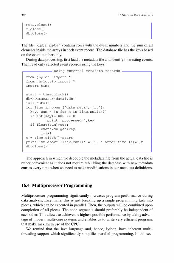
396 16 Steps in Data Analysis
meta.close()f.close()db.close()
The file ’data.meta’ contains rows with the event numbers and the sum of allelements inside the arrays in each event record. The database file has the keys basedon the event number only.
During data processing, first load the metadata file and identify interesting events.Then read only selected event records using the keys:
Using external metadata records
from jhplot import *from jhplot.io import *import time
start = time.clock()db=HDataBase(’data1.db’)i=0; cut=320for line in open (’data.meta’, ’rt’):
key, sum = [x for x in line.split()]if int(key)%1000 == 0:
print ’processed=’,keyif float(sum)>cut:
event=db.get(key)i=i+1
t = time.clock()-startprint ’Nr above ’+str(cut)+’ =’,i, ’ after time (s)=’,tdb.close()
The approach in which we decouple the metadata file from the actual data file israther convenient as it does not require rebuilding the database with new metadataentries every time when we need to make modifications in our metadata definitions.
16.4 Multiprocessor Programming
Multiprocessor programming significantly increases program performance duringdata analysis. Essentially, this is just breaking up a single programming task intopieces, which can be executed in parallel. Then, the outputs will be combined uponcompletion of all pieces. The code segments should preferably be independent ofeach other. This allows to achieve the highest possible performance by taking advan-tage of modern multi-core systems and enables us to write very efficient programsthat make maximum use of the CPU.
We remind that the Java language and, hence, Jython, have inherent multi-threading support which significantly simplifies parallel programming. In this sec-

16.4 Multiprocessor Programming 397
tion, we will illustrate how to write analysis programs that contain two or more partsthat can run concurrently.
16.4.1 Reading Data in Parallel
One can achieve a better performance of a program using multiple threads when I/Obandwidth is not a bottleneck. This, obviously, depends on hardware and the actualcalculations. Typically, numerical calculations can benefit from the use of parallelcores when the time necessary for processing events is larger than the time neededto access events from a file storage.
Let us illustrate the idea behind the parallel processing of data by looking at someconcrete examples. As usual, first we will prepare two data samples to work withusing a single thread. Both files contain a sequence of event records. Each event isrepresented by a P0D array with 20 random numbers:
Generating data files
from jhplot.io import *from jhplot import *
f1=HFile(’random1.ser’,’w’)f2=HFile(’random2.ser’,’w’)for k in range(100000):
p=P0D()p.randomUniform(20,0,1.)f1.write(p)p.randomUniform(20,0,1.)f2.write(p)if k%1000==0: print ’done=’, k
f1.close()f2.close()
Next, we will create a small class which reads the files ’random1.ser’ and’random2.ser’. This class should accept a string with the file name, open thisfile and read the file record-by-record. We refill the records, constructed from singleP0D arrays, with 200 random numbers distributed in accordance with the normaldistribution. We will use the Jython threads discussed in Sect. 2.13 to perform thistask:
Module ’readthread.py’
from jhplot.io import *from jhplot import *from threading import Thread
class testit(Thread):def __init__ (self,fin):

398 16 Steps in Data Analysis
Thread.__init__(self)self.fin = finself.k =0
def run(self):f1=HFile(self.fin,’r’)self.k=0while 1:
row=f1.read()if row == None: breakif self.k%10000==0:
print self.fin+" done=",self.krow.sort()row.getStat()self.k=self.k+1
f1.close()
Our new class inherits the Thread class, i.e. we sub-classing the Thread interfaceand overwrite its initialization and the method run(). In the method run(), weopen the file to read its records. Then we sort the 1D array and evaluate its statisticalcharacteristics.
In the example below we will read two data files using two independent threads.Then we perform a simple benchmarking by printing the total number of processedevents and the timing.
Reading data in two threads
from readthread import *import time
print ’Start at’,time.ctime()list=[’random1.ser’,’random2.ser’]# list=[’random1.ser’]t1 = time.clock()tlist = []for f in list:
cu=testit(f)tlist.append(cu)cu.start()
for t in tlist:t.join()print ’From ’,t.fin,’ processed: ’,t.k
t2=time.clock()-t1print ’calculation takes’,int(t2),’ sec’
The code reads two files at the same time. But you can always read only one fileby removing one file name from the list (we have commented out this case). If yourcomputer has several computational cores, then what likely you will see is that the
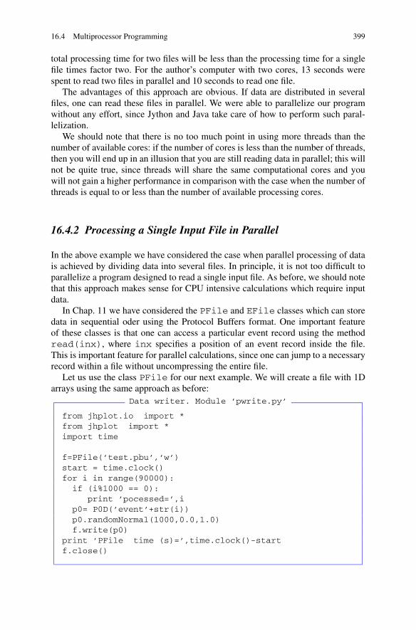
16.4 Multiprocessor Programming 399
total processing time for two files will be less than the processing time for a singlefile times factor two. For the author’s computer with two cores, 13 seconds werespent to read two files in parallel and 10 seconds to read one file.
The advantages of this approach are obvious. If data are distributed in severalfiles, one can read these files in parallel. We were able to parallelize our programwithout any effort, since Jython and Java take care of how to perform such paral-lelization.
We should note that there is no too much point in using more threads than thenumber of available cores: if the number of cores is less than the number of threads,then you will end up in an illusion that you are still reading data in parallel; this willnot be quite true, since threads will share the same computational cores and youwill not gain a higher performance in comparison with the case when the number ofthreads is equal to or less than the number of available processing cores.
16.4.2 Processing a Single Input File in Parallel
In the above example we have considered the case when parallel processing of datais achieved by dividing data into several files. In principle, it is not too difficult toparallelize a program designed to read a single input file. As before, we should notethat this approach makes sense for CPU intensive calculations which require inputdata.
In Chap. 11 we have considered the PFile and EFile classes which can storedata in sequential oder using the Protocol Buffers format. One important featureof these classes is that one can access a particular event record using the methodread(inx), where inx specifies a position of an event record inside the file.This is important feature for parallel calculations, since one can jump to a necessaryrecord within a file without uncompressing the entire file.
Let us use the class PFile for our next example. We will create a file with 1Darrays using the same approach as before:
Data writer. Module ’pwrite.py’
from jhplot.io import *from jhplot import *import time
f=PFile(’test.pbu’,’w’)start = time.clock()for i in range(90000):
if (i%1000 == 0):print ’pocessed=’,i
p0= P0D(’event’+str(i))p0.randomNormal(1000,0.0,1.0)f.write(p0)
print ’PFile time (s)=’,time.clock()-startf.close()
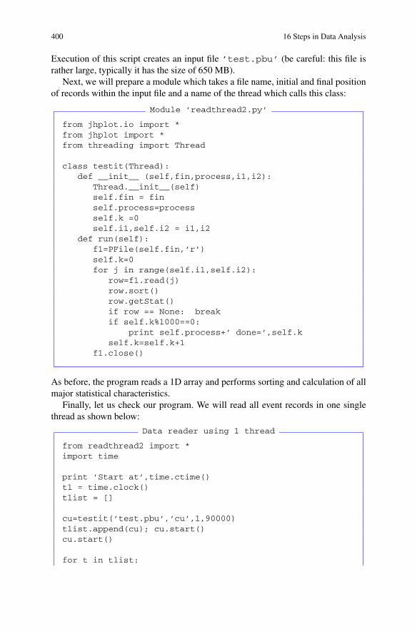
400 16 Steps in Data Analysis
Execution of this script creates an input file ’test.pbu’ (be careful: this file israther large, typically it has the size of 650 MB).
Next, we will prepare a module which takes a file name, initial and final positionof records within the input file and a name of the thread which calls this class:
Module ’readthread2.py’
from jhplot.io import *from jhplot import *from threading import Thread
class testit(Thread):def __init__ (self,fin,process,i1,i2):
Thread.__init__(self)self.fin = finself.process=processself.k =0self.i1,self.i2 = i1,i2
def run(self):f1=PFile(self.fin,’r’)self.k=0for j in range(self.i1,self.i2):
row=f1.read(j)row.sort()row.getStat()if row == None: breakif self.k%1000==0:
print self.process+’ done=’,self.kself.k=self.k+1
f1.close()
As before, the program reads a 1D array and performs sorting and calculation of allmajor statistical characteristics.
Finally, let us check our program. We will read all event records in one singlethread as shown below:
Data reader using 1 thread
from readthread2 import *import time
print ’Start at’,time.ctime()t1 = time.clock()tlist = []
cu=testit(’test.pbu’,’cu’,1,90000)tlist.append(cu); cu.start()cu.start()
for t in tlist:

16.4 Multiprocessor Programming 401
t.join()print ’From ’,t.fin,’ processed: ’,t.k
t2=time.clock()-t1print ’calculation takes’,int(t2),’ sec’
For calculations in parallel on multiple cores, we will create three threads. Eachthread will read a fraction of data, such the total number of processed events will beexactly as in the single-thread example:
Data reader using 3 threads
from readthread2 import *import time
print ’Start at’,time.ctime()t1 = time.clock()tlist = []
cu = testit(’test.pbu’,’cu1’,1,30000)tlist.append(cu); cu.start()
cu = testit(’test.pbu’,’cu2’,30001,60000)tlist.append(cu); cu.start()
cu = testit(’test.pbu’,’cu3’,60001,90000)tlist.append(cu); cu.start()
for t in tlist:t.join()print ’From ’,t.fin,’ processed: ’,t.k
t2=time.clock()-t1print ’calculation takes’,int(t2),’ sec’
Run this code and compare the answers. For a computer with four cores, the sec-ond program with three threads is typically 40% faster. This is not due to faster diskI/O (which is still the same!), but due to the fact that the program can perform calcu-lations in parallel. One can easily check this by removing our 1D array calculationsfrom the file ’readthread2.py’.
16.4.3 Numerical Computations Using Multiple Cores
Now let us move on and consider calculation-intensive programs which do not re-quire access to data. Thus, instead of reading and processing objects using extensiveI/O, we will perform numerical calculations without any input data.
Again, we will prepare a class which inherits the properties of the Thread class.This time, we pass a two-dimensional function F2D discussed in Sect. 3.4. We cal-

402 16 Steps in Data Analysis
culate the sum of all values in a double loop from 0 to 2000 inside the methodrun():
Module ’functhread.py’
from jhplot.io import *from jhplot import *from threading import Thread
class functhread(Thread):def __init__ (self,func):
Thread.__init__(self)self.func = funcself.sum=0
def run(self):for i in range(2000):
for j in range(2000):self.sum += self.func.eval(i,j)
Next we will perform numerical evaluations of both input functions in parallel:Parallel numerical computations
from functhread import *import time
print "Start at",time.ctime()
f1=F2D(’cos(x*y)*x+y’)f2=F2D(’cos(x*y)*y-x’)list=[f1,f2]# list=[f1]t1 = time.clock()tlist = []for f in list:
current = functhread(f)tlist.append(current)current.start()
for t in tlist:t.join()print ’From ’,t.func.getTitle(),’ processed: ’,t.sum
t2=time.clock()-t1print ’calculation takes=’,int(t2),’ sec’
Run this script using two functions specified in the Jython list as given in this exam-ple. Then, make a new test: Uncomment the line with the list containing only onefunction. You will see that, for two functions, the calculation time is rather close tothe time necessary to evaluate a single function. Again, this can be seen if one usesa computer with multiple cores.

16.5 Data Consistency and Security. MD5 Class 403
The conclusion of this section is simple: take advantage of multiple cores thatmake maximum use of your computer. First, you should think about how to split upyour program into independent segments to increase efficiency of your calculations.Then, write a custom class based on the Thread class and use the run() methodto include the necessary calculations.
16.5 Data Consistency and Security. MD5 Class
While your data analysis code grows, one may start to worry about consistencyand integrity of data objects which are either stored in the computer memory (non-persistent data) or saved in files (stored persistently). Surely, any data containercan easily be modified inside an analysis code. In order to prevent deliberate (oraccidental) modifications of data, one should find fingerprints of the objects thatkeep data, and compare them with those generated during object initializations. Thisshould be done at runtime, i.e. during the code execution.
More importantly, it is often necessary to check integrity of data files, to makesure that files have not been modified by someone after posting them on the Web.Again, what you will need is a fingerprint or some sort of unique signatures for suchfiles.
16.5.1 MD5 Fingerprint at Runtime
Maintaining data consistency is not too difficult: what you really need to do is touse the well known MD5 algorithm. The usual procedure is following: a publishershould provide a MD5 signature of an object or a file. A user confirms it by calculat-ing the signature again and comparing it to the one provided by the publisher. If thesignatures do not match, then this will indicate that the object or the file was alteredsince it was created.
Below we will generate a MD5 hash of a P1D object at runtime. This is simply astring with a hexadecimal number which reflects the counts of each byte of your ob-ject. Any recreation or modification of this object at runtime leads to a modificationof this string.
We use the class MD5 which accepts any Java object as an argument. After gen-erating a MD5 string, we regenerate it again after modifying the P1D container byadding a row of data:
>>> from jhplot.security import *>>> from jhplot import *
>>> p1=P1D(’test’)>>> p1.add(10,20)>>> md5=MD5(p1)

404 16 Steps in Data Analysis
>>> print md5.get()da14f51d302dd6756457f16f989b8eb9
>>> # modify a object and check MD5>>> p1.add(20,30)>>> md5=MD5(p1)>>> print md5.get()c5671fff0834bcc09489798ec1f3f752
The method get() returns a hex-string representing the array of bytes of the inputobject. It should be noted that the printed strings in your case could be rather differ-ent from those shown here, since every new creation of objects leads to a differentfingerprint. The important thing to remember is that they do not change at runtime.
One can perform a similar fingerprint using the Jython module md5. This ap-proach works in case of jHepWork objects which are convertible into strings (usu-ally, this means that the method toString() is implemented for such objects).The syntax is somewhat different since now we pass strings to the md5 instance:
>>> from jhplot import *>>> import md5>>>>>> p1=P1D(’test’)>>> p1.add(10,20)>>> # check MD5>>> m=md5.new()>>> m.update(p1.toString())>>> print m.hexdigest()c5671fff0834bcc09489798ec1f3f752
As before, the string returned by the method hexdigest() can be rather differentin your case.
16.5.2 Fingerprinting Files
Analogously, one can calculate a MD5 checksum for any file using the class MD5. Incase of files, a publisher should provide a MD5 signature and a user must confirmit by calculating the signature again and comparing it to the one provided by thepublisher. If the signatures do not match then this will indicate that the file wasaltered after it was published.
This time the fingerprint string is exactly the same as long as a file is not modifiedon the file system. Below we calculate a MD5 checksum for the file ’file.txt’and print it.

References 405
>>> from jhplot.security import *>>> from java.io import *>>>>>> md5=MD5( File("file.txt") )>>> print md5.get()
The string returned by the method get() is unique and can be used for detectingfile corruptions or deliberate modifications, since the chances of accidentally havingtwo files with identical MD5 checksums are very small.
References
1. Cranshaw, J., et al.: A data skimming service for locally resident analysis data. J. Phys. (Conf.Ser.) 119, 072011 (2008)
2. Taylor, T., et al.: Human chromosome 11 DNA sequence and analysis including novel geneidentification. Nature 440, 495 (2006)


Chapter 17Real-life Examples
Now we have all the machinery that is necessary to perform a realistic data analysis.Unlike the previous chapters with the programming recipes, this chapter featuresextensive real-research examples based on Java scripting.
Here we will learn how to simulate data and how to use data from the real world.We will show how to perform a full-scale data analysis to make a first step in extrac-tion of knowledge about the underlying nature of data. The self-contained examplesgiven in the following sections can provide the basis to conduct your own research.
17.1 Measuring Single-particle Densities
In this chapter, we will analyze particle distributions, starting from a single-particledistribution and then moving towards studies of multi-particle densities, correlationsand fluctuations.
As usual, before doing actual analysis, first we should prepare an event sampleto be used for our research. We will create it in almost exactly the same way asscientists usually do when they need to model real-world data: we will simulatea data sample using some mathematical principles. The simulated samples usuallyhelp us to understand and explain the underlying dynamics in the observed data,especially if there are missing data or data distorted by experimental apparatus. Inthis book, the simulated data will serve for an illustration of programming aspectsof data analysis.
We will consider the following experiment: Particles created or observed in anexperiment are counted in certain phase-space intervals. “Particles” could be realelementary particles produced by an accelerator machine or by cosmic rays, photonsproduced by a light source and so on. We do not need to go into such details, as wellas details of the underlaying particle production mechanism: We will use this notionin a very generic way. For example, one can think about particles as people comingto a store during a certain time interval, cars entering a highway, telephone calls pertime unit and so on.
S.V. Chekanov, Scientific Data Analysis using Jython Scripting and Java,Advanced Information and Knowledge Processing,DOI 10.1007/978-1-84996-287-2_18, © Springer-Verlag London Limited 2010
407
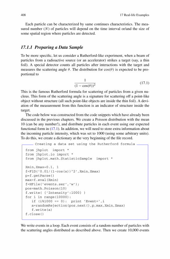
408 17 Real-life Examples
Each particle can be characterized by same continues characteristics. The mea-sured number (N ) of particles will depend on the time interval or/and the size ofsome spatial region where particles are detected.
17.1.1 Preparing a Data Sample
To be more specific, let us consider a Rutherford-like experiment, when a beam ofparticles from a radioactive source (or an accelerator) strikes a target (say, a thinfoil). A special detector counts all particles after interactions with the target andmeasures the scattering angle θ . The distribution for cos(θ) is expected to be pro-portional to
1
(1 − cos(θ))2 (17.1)
This is the famous Rutherford formula for scattering of particles from a given nu-cleus. This form of the scattering angle is a signature for scattering off a point-likeobject without structure (all such point-like objects are inside the thin foil). A devi-ation of the measurement from this function is an indicator of structure inside thetarget.
The code below was constructed from the code snippets which have already beendiscussed in the previous chapters. We create a Poisson distribution with the mean10 (can be any number!), and distribute particles in each event using our expectedfunctional form in (17.1). In addition, we will need to store extra information aboutthe incoming particle intensity, which was set to 1000 (using some arbitrary units).To do this, we create a dictionary at the very beginning of the file record.
Creating a data set using the Rutherford formula
from jhplot import *from jhplot.io import *from jhplot.math.StatisticSample import *
Xmin,Xmax=0.1, 1f=F1D(’0.01/(1-cos(x))^2’,Xmin,Xmax)p=f.getParse()max=f.eval(Xmin)f=HFile(’events.ser’,’w’);pos=math.Poisson(10)f.write( {’Intensity’:1000} )for i in range(10000):
if (i%1000 == 0): print ’Event=’,ia=randomRejection(pos.next(),p,max,Xmin,Xmax)f.write(a)
f.close()
We write events in a loop. Each event consists of a random number of particles withthe scattering angles distributed as described above. Then we create 10,000 events

17.1 Measuring Single-particle Densities 409
in a loop, writing each event into a file. In this form, our program is well scalablesince we do not leave any objects in the computer memory, unlike the case whenfirst we create a list of events and then write such list into a file.
17.1.2 Analyzing Data
Now we come to an analysis of the event sample generated in the previous section.We remind that the file ’events.ser’ contains everything we need: the intensityof the incoming beam of particles and the event records for multiple observations.Each event contains a certain number of particles characterized by one-dimensionalquantity (in our example, this is the cosine of the scattering angle).
Our task is to read all information from the data file and plot what is called adifferential cross section calculated as:
dσ
dθ= N
Δ · Lwhere L is the intensity of the incoming particles and Δ is the width of the histogrambin where particles are counted. As you can see, the distribution above is nothingbut a probability density discussed in Sect. 8.1.1 scaled by the intensity value.
The distribution above conveys information about: (1) the shape of the particledistribution. Note that the distribution itself does not depend on the chosen bin sizesince we divide the counted number of particles in each bin by the bin size; (2) theintensity with which events are happening. This is due to the scaling of the densitydistribution by the intensity number, L.
Integration of the distribution must give a total cross section or a total rate of in-teractions, σ , which is simply σ = Ntot/L, where Ntot is the total number of countedparticles after the interaction.
The code below shows how to extract the differential distribution and then visu-alize it:
Analyzing a particle distribution
from jhplot import *from jhplot.io import *
f=HFile(’events.ser’)a=f.read()Intensity=a[’Intensity’]print ’Intensity=’,Intensityh=H1D("Rutherford Scattering",40,0.1,1)while(1):
p=f.read()if p == None:
print ’End of events’break
n=f.getEntries();

410 17 Real-life Examples
ntot=len(p)if (n%1000 == 0):
print ’Event=’,n, ’ particles=’,ntoth.fill(p)
f.close()
c1 = HPlot(’Scattering’)c1.visible()c1.setAutoRangeAll()c1.setLogScale(1,1)c1.setNameX(’cos θ [rad]’)c1.setNameY(’dσ / d cos θ’)h.scale(1/(h.getBinSize()*Intensity))h.setFill(1)c1.draw(h)
The code reads the data file and then extracts the intensity of the beam L usingthe known key. Then we read the event records one by one, using the loop over allentries until the end of the file is reached. For each event, we extract the array ofnumbers representing the particle angles and then use this array to fill a histogram.Note that the method fill(obj) accepts arrays (not single values!). Then wescale the histogram using the bin width and the intensity value. The resulting plot isshown in Fig. 17.1.
Fig. 17.1 A differential cross section extracted from a Java serialized file

17.2 Many-particle Densities, Fluctuations and Correlations 411
One can use the methods of the H1D class (see Sect. 8.1) to access a detailedinformation about this distribution or even perform a fit as discussed in Sect. 14.2 tomake sure that we indeed observe the famous scattering-angle cross section givenin (17.1).
17.2 Many-particle Densities, Fluctuations and Correlations
Now we will discuss correlations between particles. The notion of correlations isdirectly related to the question of fluctuations inside small intervals [1], and bothphenomena ultimately imply the existence of forces between particles.
In the previous example we distributed particles independent of each other, ig-noring the fact that this may not be true in real situations. This time, our plan is tomodel a data sample by introducing interdependence between particles. Then, us-ing this simulation, we will try to measure the strength of correlations/fluctuataionsusing several statistical tools included in jHepWork.
17.2.1 Building a Data Sample for Analysis
We will assume that each particle can be characterized by a continues value y. Forexample, this can be a particle velocity, or a momentum, or the time at which aparticle is detected. First, we will consider a sample without any correlations in thevariable y, and then we will introduce correlations between particles.
17.2.1.1 Independently Produced Events
In the simplest case, we assume that the total number of particles falling into themeasured interval Δy = ymax − ymin is distributed in accordance with a Poissondistribution:
Pn = λn exp(−λ)
n!where λ defines the average number of particles in the counting interval, Δy. Thisdistribution naturally arises when the number of occurrences of rare events is mea-sured in a long series of trials. Inside the interval Δy, particles are distributed inde-pendent of each other.
Let us prepare such data sample and write it to an output file:
Creating a data set I
from jhplot import *from jhplot.io import *from cern.jet.random.engine import *from cern.jet.random import *

412 17 Real-life Examples
Ymin,Ymax=0,1file=HFile(’sample1.ser’,’w’)ps=Poisson(50,MersenneTwister() )for i in range(10000):
if (i%1000 == 0): print ’Event=’,ip=P0D(’Event=’+str(i))ntot=ps.nextInt()p.randomUniform(ntot,Ymin,Ymax)p.sort()file.write(p)
print ’Entries written =’, file.getEntries()file.close()
This script assumes 10000 generated events. Each event record contains a certainnumber of particles arriving inside the interval [0,1]. The global distribution isgiven by a Poisson with the average 50. We distribute particles uniformly insidethe interval [0,1] using the method randomUniform(). Each event is put into aP0D array which is then written into a serialized file.
To understand what is written, it is instructive to write the data into a XML fileusing the HFileXML() class, instead of HFile(). One can view such XML fileusing any favorite editor, but to store such file is not recommended since its size isa factor eight larger than in the case of the compressed serialized file.
17.2.1.2 Including Interactions Between Particles
So far we have considered an idealized situation when particles are produced totallyindependent of each other. For each event, particles produces at certain region donot know anything about the presence of other particles.
Actually, this almost never happens in reality: there are always interactions be-tween particles which can be detected by looking at particle correlations at any givenevent. For example, for particle or cosmic-ray physics, each particles can interactwith other particles in accordance with some underlying dynamics.
Let us consider another example from the real life. Assume that our particles areshop customers counted in certain time intervals. Usually, people come to storesin groups of relatives and friends, thus customers are never independent of eachother. Of course, such bunching of people in certain time intervals is due to a socialmechanism which can be studied using various statistical tools.
There are two types of interactions: one type is attraction which can be charac-terized by a positive correlation. In fact, this is the most frequent situation in ourexample with the number of visitors per time interval. The second type of inter-action is a repulsion, which features anti-correlations. Probably, you have alreadyguessed what does it mean: this corresponds to a hypothetical town where everyonehates each other and people avoid meeting with other people in public places.

17.2 Many-particle Densities, Fluctuations and Correlations 413
Now let us introduce interactions between particles. Positive correlations will bemodeled by shifting particles closer to each other, while in case of anti-correlation,we will increase the distance between particles. Before doing this, let us determinethe distribution of distances between particles. This can be done with this modifiedcode:
Distances between particles
from jhplot import *from cern.jet.random.engine import *from cern.jet.random import *
Ymin,Ymax = 0,1h=H1D(’delta’,100,0,0.2)ps=Poisson(50,MersenneTwister() )for i in range(10000):
if (i%1000 == 0): print ’Event=’,ip=P0D(’Event=’+str(i))ntot=ps.nextInt()p.randomUniform(ntot,Ymin,Ymax)p.sort()for j in range(p.size()-1):
delta=p.get(j+1)-p.get(j)h.fill(delta)
c1 = HPlot(’Delta’)c1.visible()c1.setAutoRange()c1.draw(h)c1.drawStatBox(h)
The code above calculates the distances between particles in an event and plots thecorresponding histogram, see Fig. 17.2. The distribution has exponentially fallingshape with the mean (and RMS) being around 0.02.
Try to fit this histogram using the method discussed in Sect. 14.5. This can bedone in the above code snippet by appending the lines:
a=HFit(c1,’c1’,h,’h’)a.addFunc(’User1’, ’Tooltip’, ’b* exp(-a*x[0])’,’a,b’)
and rerun the script. You will see a dialog window for interactive curve fitting. Selectwith the mouse the “User1” function (left list), and click on the “Add” button. Thenclick on the “Fit” button. You will see that the histogram with the distances is welldescribed by the function:
1.8 · 104 · x31
Here we did not discover anything new: the exponential distributions are knownto describe distances between events with the uniform distribution in time or space.

414 17 Real-life Examples
Fig. 17.2 The distribution of distances between any two particles
The distribution above is proportional to λ exp(−nλ), with the mean 1/λ and vari-ance 1/λ2. It is obvious that λ depends on the full phase-space and on the averagenumber of particles per event.
Our task is not to go into the details of this distribution, but try to introduce inter-actions between particles by either shifting them closer to each other (correlations),or moving them away from each other (anti-correlations).
Let us write a small function for this operation. We assume that the input forsuch function is a P0D object which keeps the information about the original parti-cle locations in an event. The output is a new P0D with a modified distance betweenparticles. We define R as a radius of interactions and will modify the distance be-tween particles only if the size between any two particles is smaller than R. In thiscase, we will set a new inter-particle distance as:
Creating a data set II
from jhplot import *from jhplot.io import *from cern.jet.random.engine import *from cern.jet.random import *
Ymin,Ymax=0,1file=HFile(’sample2.ser’,’w’)ps=Poisson(50,MersenneTwister() )R=0.01for i in range(10000):
if (i%1000 == 0): print ’Event=’,i
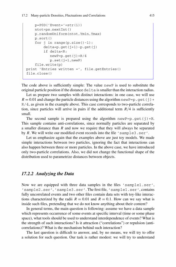
17.2 Many-particle Densities, Fluctuations and Correlations 415
p=P0D(’Event=’+str(i))ntot=ps.nextInt()p.randomUniform(ntot,Ymin,Ymax)p.sort()for j in range(p.size()-1):
delta=p.get(j+1)-p.get(j)if delta<R:
newP=p.get(j)+R/4p.set(j+1,newP)
file.write(p)print ’Entries written =’, file.getEntries()file.close()
The code above is sufficiently simple: The value newP is used to substitute theoriginal particle position if the distance delta is smaller than the interaction radius.
Let us prepare two samples with distinct interactions: in one case, we will useR = 0.01 and change the particle distances using the algorithm newP=p.get(j)+R/4, as given in the example above. This case corresponds to two-particle correla-tion, since particles will arrive in pairs if the additional term R/4 is sufficientlysmall.
The second sample is prepared using the algorithm newP=p.get(j)+R.This sample contains anti-correlations, since normally particles are separated bya smaller distance than R and now we require that they will always be separatedby R. We will write our modified event records into the file ’sample3.ser’.
Let us emphasize again that the examples above are just toy models. We madesimple interactions between two particles, ignoring the fact that interactions canalso happen between three or more particles. In the above case, we have introducedonly two-particle correlations. Also, we did not change the functional shape of thedistribution used to parametrize distances between objects.
17.2.2 Analyzing the Data
Now we are equipped with three data samples in the files ’sample1.ser’,’sample2.ser’, ’sample3.ser’. The first file, ’sample1.ser’, containsfully uncorrelated events and two other files contain data sets with toy-like interac-tions characterized by the radii R = 0.01 and R = 0.1. How can we say what isinside such files, pretending that we do not know anything about their content?
In general terms, the main question is following: assume we have a data samplewhich represents occurrence of some events at specific interval (time or some phasespace), what tools should be used to understand interdependence of events? What isthe strength of such interactions? Is it attraction (“correlations”) or repulsion (anti-correlations)? What is the mechanism behind such interaction?
The last question is difficult to answer, and, by no means, we will try to offera solution for such question. Our task is rather modest: we will try to understand

416 17 Real-life Examples
whether events are independent or not. If we will find that events are heavily inter-dependent, then we will try to determine the type of such dependence (attraction orrepulsion). Furthermore, we will try to estimate the strength of interdependence.
We should also add that we are not going to offer a universal and comprehensiveapproach to deal with such kind of problems. Our task is to illustrate what can bedone using Java scripting and the tools included in the jHepWork package.
17.2.3 Reading the Data and Plotting Multiplicities
First, let us read the prepared data files and plot a few basic distributions. We haveall necessary equipment for doing this. The code below shows how to read the datafiles and plot multiplicity distributions inside a small region [0–0.5]. We remind thatour original points are distributed inside the phase space window [0–1]:
Multiplicity distributions
from jhplot import *from jhplot.io import *from java.awt import Colorimport os
Ymax=0.5h=[]files=[’sample1.ser’,’sample2.ser’,’sample3.ser’]
for f in range(len(files)):name=files[f]if os.path.exists(name):
file=HFile(name)print ’Open: ’+nameh.append(H1D(name,25,0,50))while(1):
p=file.read()if p == None:
print ’End of events’; breaki=file.getEntries();if (i%1000 == 0): print ’Event=’,in=0for j in range(p.size()):
if p.get(j)<Ymax: n=n+1h[f].fill(n)
file.close()c1 = HPlot(’Multiplicity’)c1.visible()c1.setAutoRange()
for i in range(len(h)):

17.2 Many-particle Densities, Fluctuations and Correlations 417
h[i].setFill(1)color=Color.getHSBColor(0.3*i, 1.0, 1.0);h[i].setColor(color)
h[1].setPenDash(2)h[2].setPenDash(6)c1.draw(h)
Running this script will bring a canvas with three distributions, each of them hasa Poisson-like shape. They are all very similar, so there is no way to say aboutthe difference we have introduced for two-particle distances. So, we should find abetter solution to tackle the problem of correlations. One solution would be to studyfluctuations inside small phase space windows.
Since we have introduced two-particle correlations, we should expect that themultiplicity distributions inside small regions should deviate from a Poisson distri-bution: in case of interactions, it should be broader than the standard Poisson (largefluctuations). In case of repulsion between particles, the distribution should be nar-rower.
When fluctuations of separate particles are measured, it is convenient to trans-form a multiplicity distribution Pn(δ) inside a region δ to the following observables:
BP: ηq(δ) = q
q − 1
Pq(δ)Pq−2(δ)
P 2q−1(δ)
(17.2)
NFM: Fq(δ) = [n(δ)]−q∞∑
n=q
n!(n − q)!Pn(δ) (17.3)
where the abbreviations denote the bunching parameters (BP) or the normalizedfactorial moments (NFM). The parameter q defines the order of the BP or NFM.Note that the experimental definitions of the BPs [2, 3] and the NFM [4, 5] aredifferent from those given above since, in reality, one should scan all phase spaceregions to increase statistics when looking into ever smaller regions.
These two quantities measure deviations of a multiplicity distribution Pn(δ) froma Poisson distribution for which Fq(δ) = ηq(δ) = 1. Note that such deviations aremeasured differently by these three methods (for a review see [1]).
Uncorrelated particle production inside δ leads to the Poisson statistics, thus de-viations of the NFM and BP from unity indicate correlations (interactions) betweenparticles leading to dynamical fluctuations (i.e. non-Poisson type of statistics). Ifηq(δ) or Fq(δ) are larger than one, one can say about positive correlations. Thiscase is expected for the first sample generated without including the toy interac-tions. In contrast, if both quantities are smaller than unity for ever smaller δ regions,one can say about anti-correlations (this, naturally, should be the case for our secondsample with defined repulsion).
jHepWork contains a Java library for calculations of both ηq(δ) and Fq(δ). Wewill consider the class called BunchingParameters, and also a similar classFactorialMoments from the package jhplot.stat.
We can initialize our calculations as:
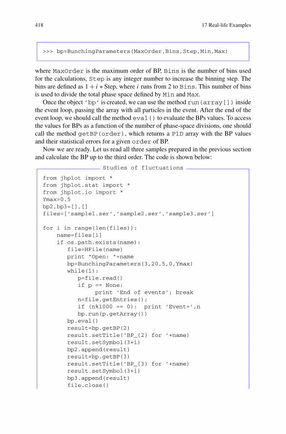
418 17 Real-life Examples
>>> bp=BunchingParameters(MaxOrder,Bins,Step,Min,Max)
where MaxOrder is the maximum order of BP, Bins is the number of bins usedfor the calculations, Step is any integer number to increase the binning step. Thebins are defined as 1 + i ∗ Step, where i runs from 2 to Bins. This number of binsis used to divide the total phase space defined by Min and Max.
Once the object ’bp’ is created, we can use the method run(array[]) insidethe event loop, passing the array with all particles in the event. After the end of theevent loop, we should call the method eval() to evaluate the BPs values. To accessthe values for BPs as a function of the number of phase-space divisions, one shouldcall the method getBP(order), which returns a P1D array with the BP valuesand their statistical errors for a given order of BP.
Now we are ready. Let us read all three samples prepared in the previous sectionand calculate the BP up to the third order. The code is shown below:
Studies of fluctuations
from jhplot import *from jhplot.stat import *from jhplot.io import *Ymax=0.5bp2,bp3=[],[]files=[’sample1.ser’,’sample2.ser’,’sample3.ser’]
for i in range(len(files)):name=files[i]if os.path.exists(name):
file=HFile(name)print "Open: "+namebp=BunchingParameters(3,20,5,0,Ymax)while(1):
p=file.read()if p == None:
print ’End of events’; breakn=file.getEntries();if (n%1000 == 0): print ’Event=’,nbp.run(p.getArray())
bp.eval()result=bp.getBP(2)result.setTitle(’BP_{2} for ’+name)result.setSymbol(3+i)bp2.append(result)result=bp.getBP(3)result.setTitle(’BP_{3} for ’+name)result.setSymbol(3+i)bp3.append(result)file.close()

17.2 Many-particle Densities, Fluctuations and Correlations 419
c1 = HPlot(’BP’,800,400,2,1)c1.visible()c1.setAutoRangeAll()c1.cd(1,1)c1.draw(bp2)c1.cd(2,1)c1.draw(bp3)
As you can see, we do this rather complicated calculations using a few lines of thecode. We build two lists which keep the results for η2 and η3 for all three processedsamples and then run over each of this sample. The result of this code is shownin Fig. 17.3. As expected, the BPs for the sample without interactions are indeedindependent of δ = (Ymin − Ymax)/Bins and they are all equal to unity (“Pois-son statistics”). The sample with the interactions, when particles arrive in bunches,has a sharp increase for the calculated η2(δ) with decreasing δ. The η3(δ) does notshow too much variations with the number of bins, indicating that we are dealingwith two-particle correlations. For the third sample, η2(δ) decreases with δ (anti-correlations) and stays constant when δ reaches some δmin, which roughly corre-sponds to anti-correlation radius in our code (the parameter “R”).
Now, let us calculate the NFMs. This can be done by replacing the class nameBunchingParameters with the name FactorialMoments. To retrieve theresults, we should call getNFM() instead of getBP(). The resulting plot is shownin Fig. 17.4. One can see a similar result as that shown on Fig. 17.3. The only notabledifference is that F3 for the sample with interactions still shows some increase withthe bin size. This is not totally surprising since F3 reflects not only three-particle
Fig. 17.3 Bunching parameters η2 (left) and η3 (right) as functions of the number of bins usedto divide the total phase space [0–0.5]. The calculations were done for three data samples: withno correlations (’sample1.ser’) with correlations (’sample2.ser’) and with anti-correla-tions (’sample3.ser’)

420 17 Real-life Examples
Fig. 17.4 The normalized factorial moments F2 (left) and F3 (right) as functions of the numberof bins used to divide the total phase space. The calculations were done for the three data sam-ples: with no correlations (’sample1.ser’), with correlations (’sample2.ser’) and withanti-correlations (’sample3.ser’)
correlations but also contains a contribution from two-particle correlations which(we know!) have been included when the sample was generated. One can find moredetails about the use and properties of BP or NFM in the review [1].
At the very end, you may still wonder why not just to look at the distribution ofdistances between two particles if we want to know how particles are distributedwith respect to each other. We know that inter-particle distances should be dis-tributed in accordance with the exponential distribution in case of the Poisson statis-tics. In principle, this can be done as well, but then we should find a method to com-pare such distributions with a reference distribution which is known to have exactlythe same properties (multiplicities, shapes of single-particle distributions) but with-out any correlations between particles. This is not too easy and is outside the scopeof our example: the use of the BPs, NFMs or other tools is very handy since they donot require construction of any reference sample [1].
17.3 Analyzing Macro Data: Nearby Galaxies
In this section, we give another real-life example: this time we plan to analyze dataon nearby galaxies. Our intention is not to be too scientific, nor to discuss in de-tail topics which require special knowledge. What we want to do is to illustratethe power of scientific scripting: in a few lines of the code we will perform almostcomplete data analysis. It will consist of reading a data file, fetching necessary datarecords and plotting one type of values against another. The readers who are inter-ested in science will immediately find areas where the discussed code snippets can

17.3 Analyzing Macro Data: Nearby Galaxies 421
be reused for their own research or even to make a detailed study of the data filediscussed in this section.
What we are going to do now is to analyze the catalog of Southern spirals galax-ies (Mathewson+ 1996) publicly accessible from the Astronomical Data server [6].To simplify our task, we have prepared a file with the catalog to be used for thistutorial.
Let us first copy the catalog with the galaxy’s data and open it in the jHepWorkeditor in order to understand its format:
Getting data from the web
http=’http://projects.hepforge.org/jhepwork/’file=’Mathewson1996.tsv’wget(http+’examples/data/’+file)view.open(file, 0 )
The script above fetches the file ’Mathewson1996.tsv’ and opens it in a neweditor tab. If you are using this script outside jHepWork, do not forget to importwebustils package from the directory macros/system.
If the script above fails, try several other mirrors by replacing the http valuewith the string:
http=’http://jhepwork.sourceforge.net/’orhttp=’http://jwork.org/jhepwork/’
By looking at the file structure, one can see that each entry in the row is separatedby a space. Thus, if we want to read this file line by line, one should find a way tosplit each line of this file. Also, one can see that comment lines always start with thesymbol “#”. Such lines have to be ignored. Finally, we split the strings into piecesand convert such sub-strings into float values.
We are dealing with a typical CSV file discussed in Sect. 2.16.4, thus it can beopened using the class CSVReader. This class may not be flexible ehough, but thegood thing is that to write a small Jython code which parses a CSV file is very easy,perhaps as easy as when using a ready-to-go third-party library!
So, let us write a small Jython code which reads a CSV file and performs thenecessary conversions. Our module will be designed for the following task: It splitsa string into n-size pieces using an arbitrary string as the delimiter and ignores thelines which start from the symbols “#” or “*” (this will be necessary for our nextexample). Finally, we will need to prepare a function which converts a string into anumber. Normally, this can be done with the float()method (in case if we expecta real number). But we should take care of the situations when we need to convertthe strings such as “1/2”, “2/3” etc. into float values.
Let us create a Jython module file called ’reader.py’ with the followingcode:
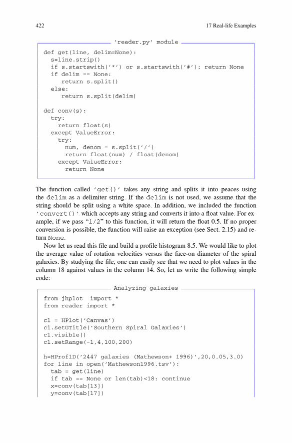
422 17 Real-life Examples
’reader.py’ module
def get(line, delim=None):s=line.strip()if s.startswith(’*’) or s.startswith(’#’): return Noneif delim == None:
return s.split()else:
return s.split(delim)
def conv(s):try:return float(s)
except ValueError:try:
num, denom = s.split(’/’)return float(num) / float(denom)
except ValueError:return None
The function called ’get()’ takes any string and splits it into peaces usingthe delim as a delimiter string. If the delim is not used, we assume that thestring should be split using a white space. In addition, we included the function’convert()’ which accepts any string and converts it into a float value. For ex-ample, if we pass “1/2” to this function, it will return the float 0.5. If no properconversion is possible, the function will raise an exception (see Sect. 2.15) and re-turn None.
Now let us read this file and build a profile histogram 8.5. We would like to plotthe average value of rotation velocities versus the face-on diameter of the spiralgalaxies. By studying the file, one can easily see that we need to plot values in thecolumn 18 against values in the column 14. So, let us write the following simplecode:
Analyzing galaxies
from jhplot import *from reader import *
c1 = HPlot(’Canvas’)c1.setGTitle(’Southern Spiral Galaxies’)c1.visible()c1.setRange(-1,4,100,200)
h=HProf1D(’2447 galaxies (Mathewson+ 1996)’,20,0.05,3.0)for line in open(’Mathewson1996.tsv’):
tab = get(line)if tab == None or len(tab)<18: continuex=conv(tab[13])y=conv(tab[17])

17.4 Analyzing Micro Data: Elementary Particles 423
Fig. 17.5 A dependence of the rotational velocities on the galaxy size
if x != None and y!=None: h.fill(x,y)
c1.setNameX(’Face-on diameter [arcmin]’)c1.setNameY(’< Rotation velocity [km/s] >’)h1=h.getH1D()h1.setStyle(’p’)c1.draw(h1)
The example shows how to open a CVS file and read it line by line. We split eachline and make sure that we have the correct number of pieces (18). Then we fill theprofile histogram.
The resulting image is shown in Fig. 17.5. As we can see, there is rather obviousdependence of the average velocity on the galaxy radius. I am sure some readerswill find this plot familiar and will connect it to some physics phenomena. If thereader is not one of them, then this would be your entry to the world of science.
17.4 Analyzing Micro Data: Elementary Particles
In this section we plan to study elementary particles from the Particle Data Book [7].A typical size of the galaxies analyzed in the previous example is 1020 meters, whilethe proton size is 10−15 meters, so the examples in this book span more than 35orders of magnitude in distances! Sure, the universe we leave in is a big place, andwe have to find a way to study it.
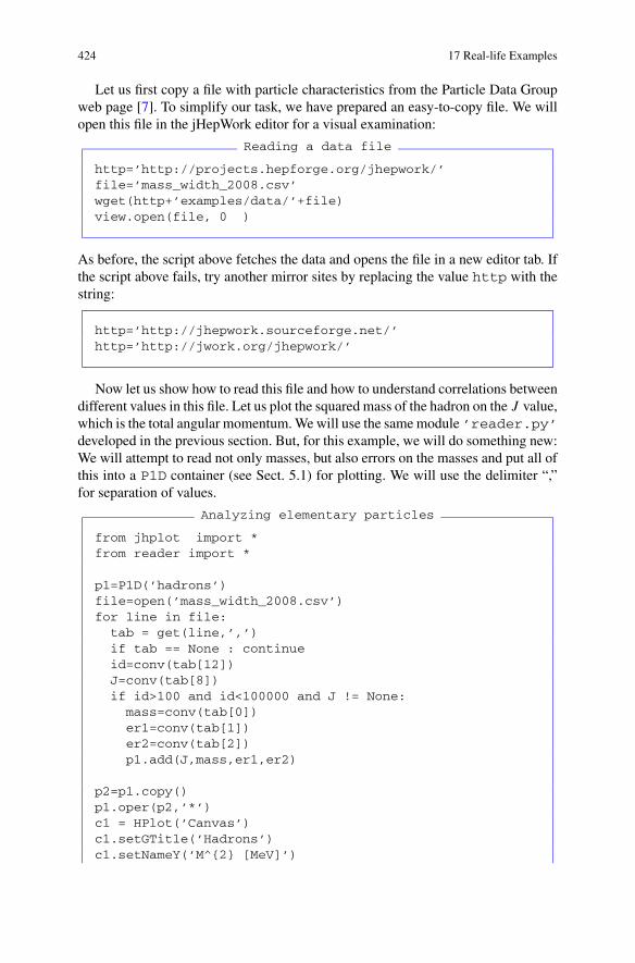
424 17 Real-life Examples
Let us first copy a file with particle characteristics from the Particle Data Groupweb page [7]. To simplify our task, we have prepared an easy-to-copy file. We willopen this file in the jHepWork editor for a visual examination:
Reading a data file
http=’http://projects.hepforge.org/jhepwork/’file=’mass_width_2008.csv’wget(http+’examples/data/’+file)view.open(file, 0 )
As before, the script above fetches the data and opens the file in a new editor tab. Ifthe script above fails, try another mirror sites by replacing the value http with thestring:
http=’http://jhepwork.sourceforge.net/’http=’http://jwork.org/jhepwork/’
Now let us show how to read this file and how to understand correlations betweendifferent values in this file. Let us plot the squared mass of the hadron on the J value,which is the total angular momentum. We will use the same module ’reader.py’developed in the previous section. But, for this example, we will do something new:We will attempt to read not only masses, but also errors on the masses and put all ofthis into a P1D container (see Sect. 5.1) for plotting. We will use the delimiter “,”for separation of values.
Analyzing elementary particles
from jhplot import *from reader import *
p1=P1D(’hadrons’)file=open(’mass_width_2008.csv’)for line in file:
tab = get(line,’,’)if tab == None : continueid=conv(tab[12])J=conv(tab[8])if id>100 and id<100000 and J != None:mass=conv(tab[0])er1=conv(tab[1])er2=conv(tab[2])p1.add(J,mass,er1,er2)
p2=p1.copy()p1.oper(p2,’*’)c1 = HPlot(’Canvas’)c1.setGTitle(’Hadrons’)c1.setNameY(’M^{2} [MeV]’)

17.5 A Monte Carlo Simulation of Particle Decays 425
Fig. 17.6 A dependence of the hadron masses on the angular momenta
c1.setNameX(’J’)c1.visible()c1.setRange(-1,5,0,5000)c1.draw(p2)
Figure 17.6 shows the result.As you can see, there is a correlation between M2 and J . In fact, what we have
discovered here using a few lines of the code is a reflection of the well-known ob-servation that hadrons from the same family lie on special trajectories (the so-calledChew-Frautschi conjecture [8–10]). Such a relationship between J and M2, alsoknown as the principle of exchange degeneracy, is usually interpreted as a manifes-tation of the linear potential of the strong forces between constituent quarks insidethe proton. One can see clear regularities using a rigorous linear regression fit andthe most recent data in this articles [11, 12].
Here we will stop discussing any further scientific issues: the example above isjust an invitation to science via the offered Java scripting and the jHepWork pro-gram.
17.5 A Monte Carlo Simulation of Particle Decays
In this section we will build a simple Monte Carlo simulation of particle de-cays based on the class HepLorentzVector discussed in Sect. 7.6. We willconsider two-body decays of a particle with a mass M which can be written as

426 17 Real-life Examples
M → M1 + M2, where M1 and M2 are masses of daughter particles. When a par-ticle decays, one should keep in mind the usual four-momentum conservation. Thecalculation itself can be organized in two steps: (1) a calculation of decays in center-of-mass frame of daughter particles and; (2) transformation of four-momenta ofdaughter particles to the laboratory frame using the Lorentz transformation.
In our numerical calculation we will be interested in the distribution of the max-imum angle between daughter particles with respect to the initial particle. We willlook at this on a statistical bases by introducing some randomness of decay anglesin the center-of-mass frame of the original particle.
First, we define an initial particle to be a “top” quark, while daughter particleswill be called W and b. It should be said that this corresponds to quite realisticsituation in particle physics when a top quark decays into a W boson and b quarks.At this stage, however, we will be more interested in the program implementationof our task, rather than in physics interpretation of our results.
Let us take a look at the code below:
Particle decays
from jhplot import *from java.awt import Colorfrom java.util import Randomfrom hephysics.particle import *from math import *
P=100Top=LParticle(’Top quark’,170)Top.setV3( 0,0,P )W,b =LParticle(’W’,80),LParticle(’b’,5)
r = Random()h1 = H1D("Θ_{max} angle",50, 0,3)for i in range(10000):
if (i%1000==0): print ’event=’,iTop.twoBodyDecay(W, b,1);theta =acos(2.0*r.nextDouble()-1.0 )phi =6.28*r.nextDouble()Top.setThetaPhiP(theta,phi,P)W.boost( Top ); b.boost( Top )p=P0D(’max angle’)p.add(Top.angle(W))p.add(Top.angle(b))pmax=p.getMax()h1.fill(pmax)
c1 = HPlot(’Canvas’)c1.setGTitle(’Max angle t → W b’)c1.visible()c1.setAutoRange()c1.setNameX(’Θ_{max} [rad]’)

17.5 A Monte Carlo Simulation of Particle Decays 427
c1.setNameY(’Events’)h1.setFill(1)h1.setFillColor(Color.yellow)c1.draw(h1)
Let us make some comments. First, we have defined three particles using theLParticle class discussed in Sect. 7.6. The particles have the masses 170, 80,5, respectively (using some arbitrary units). We have assumed that the total mo-mentum (P ) of the original particle is 100 (again, in arbitrary units). Then we havegenerated 10,000 events, introducing a randomness in the azimuthal (φ) and polar(θ ) angle, since angles defined in the center-of-mass frame can have any values cov-ering the full solid angle. The line 6.28*r.nextDouble() simply randomizesthe azimuthal angle in the range [0,2π]. We redefine four-momenta of the originalparticle using the input φ and θ . Then we have performed the Lorentz boost andcalculated angles between the original particle and the daughter particles. Finally,we have determined the maximum angle for each decay and filled a histogram.
Run this code and look at its output shown in Fig. 17.7. We can do the followingsimple experiment with this code: change the initial momentum from 100 to a highervalue. We will see that the shape of this distribution will change depending on thisvalue.
Fig. 17.7 A distribution of angles between daughter particles and the original parent particle

428 17 Real-life Examples
17.6 Measuring the Speed of Light Using the Internet
Yes, this is correct. What we going to do now is to measure the speed of light. It isnot going to be the most precise measurement, probably it will be the most impre-cise among other imprecise measurements, but it still be a measurement which cangive you ideas about this fundamental physical constant, and the way how it can beextracted. At least, we guarantee that the value of the speed obtained in this chapterwill be of the same order of magnitude as the established value, 299,792 km/c. Thegood thing about this measurement is that we do not need to have any apparatus:a home computer with a reasonable Internet bandwidth should be sufficient for ourpurpose.
We will only warn you before going into details of this experiment: for our mea-surement, Linux or Mac computers are best suited as they usually have the “ping”command. The program to be discussed below was tested using Ubuntu Linux, acommunity developed Linux-based operating system. But one can use any operat-ing system with the “ping” program, as long as it is installed. We will use jHepWorkin a combination with the ping program.
Now let us come to the main idea. The “ping” command is usually used fortesting connectivity and response time over networks. For example, when one typesping -c1 www.google.com, it will test the response of the Google server.The execution of this program prints the time necessary for a package to reach aserver and return to your PC.
We know that the signal in a vacuum travels with the speed of light, which ap-pears to be very important physical constant with a value of 299,792 kilometers persecond. It travels a little bit slower in fiber optics, but we will ignore this for the mo-ment since we are not too interested in such precision. The distance, between twosufficiently separated points, say between Chicago and Berlin, is around 7,000 km.Thus, if one pings a server in Berlin from Chicago, we should get the response atleast in 2 ∗ 23 milliseconds, where the factor two is introduced to take into accountthe round signal trip. In the real word, the response time will be longer than 46 ms,since the Internet signal does not travel along a straight line, and various switchesand routers slow down the transfer speed. If the signal is transported by a fiber, itbounces around along the path. Therefore, it is a reasonable assumption that thesignal needs 40–50% more time to travel.
Now we can try to get a rough estimate of the speed of light on a statistical basis.We will ping few servers in Europe, USA and Asia. Then we will make histogramswith the response time for each continent. Depending on the location, one can es-timate an approximate distance between continents by analysing the histograms. Ifyou know what is the distance between the continents, one can measure the speedof light with a certain precision.
Below we will develop the necessary modules to perform our measurement. Theexample we are going to show is rather informative: we will illustrate how to useJython lists, how to call an external program, how to process data and use a randomnumber generator. Finally, the example will help you to develop a genuine feelingfor the quantities and concepts involved.

17.6 Measuring the Speed of Light Using the Internet 429
17.6.1 Getting Host Names in Each Continent
First, we should obtain the lists of hosts in each continent. For this, we will use againthe Web site of Ubuntu with a list of mirror servers located in different parts of theworld. We will use the same method as in the previous examples: to make thingseasier, we will download three prepared files containing the computer host names ina HTML form:
Getting data from the web
http=’http://projects.hepforge.org/jhepwork/’list=[’ubuntu_usa.html’,\
’ubuntu_europe.html’,\’ubuntu_asia.html’]
for file in list:wget(http+’examples/data/’+file)
We remind that the script above fetches files from the Web. If you are using thisscript outside jHepWork, do not forget to import webustils package from the di-rectory macros/system. If the script above fails, try another mirror by replacingthe http value with the strings:
http=’http://jhepwork.sourceforge.net/’orhttp=’http://jwork.org/jhepwork/’
Upon download completion, open one of such files in the jHepWork editor. Youwill see that this is a HTML file with the server names. Our task is to make a smallJython module which reads the names of the servers from such files. The namesusually start with the string http://, and end after a quotation mark. We want tomake a list of servers from each file, and pick up only several random servers fromeach list.
Getting host names. The module ’get_host.py’
from random import *
def get_host(file,number):r=Random()f = open(file)list=[]for line in f.readlines():
inx1=line.find(’//’)if inx1>0:
ss=line[inx1+2:len(line)]ss=ss[0:ss.find("/")]list.append(ss)
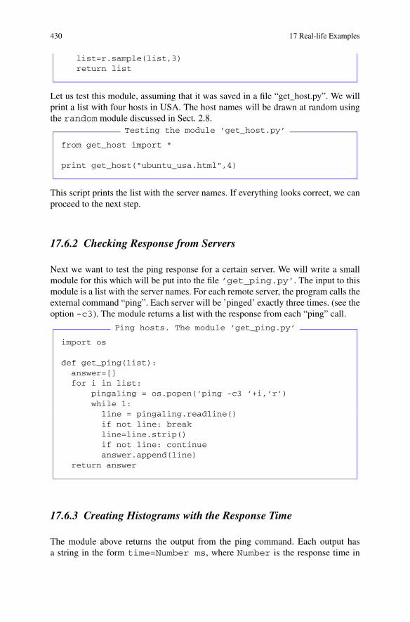
430 17 Real-life Examples
list=r.sample(list,3)return list
Let us test this module, assuming that it was saved in a file “get_host.py”. We willprint a list with four hosts in USA. The host names will be drawn at random usingthe random module discussed in Sect. 2.8.
Testing the module ’get_host.py’
from get_host import *
print get_host("ubuntu_usa.html",4)
This script prints the list with the server names. If everything looks correct, we canproceed to the next step.
17.6.2 Checking Response from Servers
Next we want to test the ping response for a certain server. We will write a smallmodule for this which will be put into the file ’get_ping.py’. The input to thismodule is a list with the server names. For each remote server, the program calls theexternal command “ping”. Each server will be ’pinged’ exactly three times. (see theoption -c3). The module returns a list with the response from each “ping” call.
Ping hosts. The module ’get_ping.py’
import os
def get_ping(list):answer=[]for i in list:
pingaling = os.popen(’ping -c3 ’+i,’r’)while 1:
line = pingaling.readline()if not line: breakline=line.strip()if not line: continueanswer.append(line)
return answer
17.6.3 Creating Histograms with the Response Time
The module above returns the output from the ping command. Each output hasa string in the form time=Number ms, where Number is the response time in

17.6 Measuring the Speed of Light Using the Internet 431
milliseconds for each server. We should identify this number using the standardPython string method (like the method find() and plot each number on a graph.
Our next module will be called “get_h1d.py”. It accepts the list with the servernames from the previous example, and identifies the response time. Then, a his-togram with the response time will be filled for further investigation. We will alsopass the color for this histogram and the title for better visualization. Once the his-togram is filled, the module will return the filled histogram.
Getting H1D using ’get_h1d.py’
from jhplot import H1D
def get_h1d(answer,title,color):h1=H1D(title,50,0,500)h1.setFill(1)h1.setFillColor(color)h1.setColor(color)for m in answer:inx1=m.find(’time=’)if inx1>0:
ss=m[inx1+5:len(m)]ss=ss[0:ss.find(’ms’)]d=float(ss)h1.fill(d)
return h1
17.6.4 Final Measurements
Now we are ready to collect all pieces together. First, we will import all functionsfrom the files we created so far. Then, we will prepare a list with the input files fromwhich the server names will be taken. Then, for each file, we will build a list with theservers, ping at random several servers from each continent and fill the histogramswith response time. In addition, we will print the mean values of the server responsefor each continent. This can be done using the method mean(). Here is our codeexample:
Response-time measurement
from get_host import *from get_ping import *from get_h1d import *from jhplot import *from java.awt import Color
sites=[’europe’,’usa’,’asia’]colors=[Color.red,Color.blue,Color.green]

432 17 Real-life Examples
all=[]for i in range(len(sites)):
list=get_host(’ubuntu_’+sites[i]+’.html’,4)answer=get_ping(list)h1d=get_h1d(answer,sites[i],colors[i])all.append(h1d)print sites[i],’ mean=’,h1d.mean()
c1 = HPlot(’Canvas’)c1.setGTitle(’Response time (ms)’)c1.visible(1)c1.setRange(0.0,300,0,10)c1.draw(all)
The execution of this script prints the mean values and brings up a canvas with threefilled histograms. Each histogram is shown with different color and has appropriateannotations.
For the author’s computer, the execution of the above script prints:
europe mean= 142.0usa mean = 54.1asia mean = 252.8
Let us try to make sense from these numbers: The author of this book is in USA,and the average response time to a random server inside USA is 54 ms. The averagetravel time to European servers is 142 ms. The signal needs to travel in one directionroughly (142 − 54)/2 = 44 ms. This is a upper limit, since it does not take intoaccount how much time is lost in European servers, assuming that 54 ms is the timewhich was lost in USA servers.
So, a lower limit on the speed of light is 159,090 km/s. It is twice lower thanexpected, since we did not take into account many factors discussed above (serverresponse time, travel of light inside fibers rather than in a vacuum, large geographi-cal spread of servers). But we kept our promise: we are close to the correct answer,at least the order of magnitude for the extracted speed is correct.
Let us give a final comment: we would not recommend to increase the numberof servers and/or the number of pings for each server. This will not help you toincrease the precision of the measurement. If you really want to do this measurementwith a high precision, one should pick up a certain server and assess all the effectsdiscussed above. To do this is not easy. But what we can say is this: all such effectsare minimal if the ping test is done over very long distances. So, the advice is tocome back to this approach when you will be a scientist or seriously interested inthis type of measurements. Or, when you will be able to ping Internet servers on theMoon or Mars from your home (in not too distant future!).

References 433
References
1. De Wolf, E.A., Dremin, I.M., Kittel, W.: Scaling laws for density correlations and fluctuationsin multiparticle dynamics. Phys. Rep. 270, 1–141 (1996)
2. Chekanov, S.V., Kuvshinov, V.I.: Bunching parameter and intermittency in high-energy colli-sions. Acta Phys. Pol. B 25, 1189 (1994)
3. Chekanov, S.V., Kittel, W., Kuvshinov, V.I.: Generalized bunching parameters and multiplicityfluctuations in restricted phase-space bins. Z. Phys. C 74, 517 (1997)
4. Bialas, A., Peschanski, R.B.: Moments of rapidity distributions as a measure of short rangefluctuations in high-energy collisions. Nucl. Phys. B 273, 703 (1986)
5. Bialas, A., Peschanski, R.B.: Intermittency in multiparticle production at high-energy. Nucl.Phys. B 308, 857 (1988)
6. ADC, Astronomical data center, access to astronomy data and catalogs. URL http://adc.astro.umd.edu/
7. Eidelman, S., et al.: Review of particle physics. Phys. Lett. B 592, 1 (2004)8. Chew, G.F., Frautschi, S.C.: Principle of equivalence for all strongly interacting particles
within the s matrix framework. Phys. Rev. Lett. 7, 394–397 (1961)9. Chew, G.F., Frautschi, S.C.: Regge trajectories and the principle of maximum strength for
strong interactions. Phys. Rev. Lett. 8, 41–44 (1962)10. Frautschi, S.: Regge Poles and S-Matrix Theory. Benjamin, New York (1968)11. Anisovich, V., et al.: Quark Models and High Energy Collisions. World Scientific, Singapore
(2004)12. Chekanov, S.V., Levchenko, B.B.: Regularities in hadron systematics, Regge trajectories and
a string quark model. Phys. Rev. D 75, 014007 (2007)

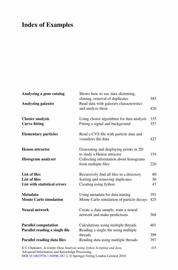
Index of Examples
Analyzing a gene catalog Shows how to use data skimming,sliming, removal of duplicates 385
Analyzing galaxies Read data with galaxies characteristicsand analyze them 420
Cluster analysis Using cluster algorithms for data analysis 335Curve fitting Fitting a signal and background 357
Elementary particles Read a CVS file with particle data andvisualizes the data 423
Henon attractor Generating and displaying points in 2Dto study a Henon attractor 154
Histogram analyzer Collecting information about histogramsfrom multiple files 220
List of files Recursively find all files in a directory 80List of files Sorting and removing duplicates 56List with statistical errors Creating using Jython 47
Metadata Using metadata for data mining 391Monte Carlo simulation Monte Carlo simulation of particle decays 425
Neural network Create a data sample, train a neuralnetwork and make predictions 368
Parallel computation Calculations using multiple threads 401Parallel reading a single file Reading a single file using multiple
threads 399Parallel reading data files Reading data using multiple threads 397
S.V. Chekanov, Scientific Data Analysis using Jython Scripting and Java,Advanced Information and Knowledge Processing,DOI 10.1007/978-1-84996-287-2, © Springer-Verlag London Limited 2010
435

436 Index of Examples
Single particle density studies How to generate and analyze particledensities 407
Study of fluctuations Calculations of factorial moments andbunching parameters 411
The speed of light Approximately determine the speed oflight using the Internet 428
Weighted average Weighted average of several measurements 155

Index
__builtin__, 60__del__, 65__doc__, 65__init__, 65__module__, 653D-XplorMathJ package, 116
AAlgorithms, FuzzyCMeansAlg, 339Algorithms, HierarchicalAlg, 339Algorithms, KMeansAlg, 339Algorithms, KMeansExchangeAlg, 339Applets, 331ArrayList, Java, 50Arrays, 68Arrays of random numbers, 230Attractor, Henon, 154, 256
BBash compilation script, 331Bayesian network, 375Bayesian self-organizing map, 376BeanShell, 15Benchmarking program, 59BRoot class, 287BunchingParameters class, 417
CCBook library, 218, 286Cellular automaton, 314CFBook library, 218Cloud2D, 173Cloud3D, 174Clustering, 342cmath module, 34
Code assist in jHepWork, 21Code assist in jHPlot, 22Code assist in JythonShell, 21Code assist using doc(), 22Coefficient of correlations, 345Color AWT, 93Complex matrices, 185Complex numbers, 185, 322Configuration files, 323Contour plot, 144Contour plot, F2D, 104csv, read and write, 295csv files, Jython, 75CSVWriter class, 296Curve fitting, 346CVSReader class, 295
DData streams, 270Database, relational SQL, 291DataHolder class, 336DataOutputStream, Java, 78DataPoint, 172DataPoint class, 336DataPointSet, 172Derby database, 291Dexter program, 313Diagram class, 258dic(), 64dif, file format, 309Differentiation, F1D, 91Differentiation, SymPy, 118dir(), 28, 30, 60Distribution Beta, 226Distribution Binomial, 226
S.V. Chekanov, Scientific Data Analysis using Jython Scripting and Java,Advanced Information and Knowledge Processing,DOI 10.1007/978-1-84996-287-2, © Springer-Verlag London Limited 2010
437

438 Index
Distribution Breit-Wigner, 226Distribution Breit-Wigner-MeanSquare, 226Distribution Chi-Square, 226Distribution Empirical, 226Distribution EmpiricalWalke, 226Distribution Gamma, 226Distribution Hyper-Geometric, 226Distribution Hyperbolic, 226Distribution Logarithmic, 226Distribution Negative Binomial, 226Distribution Normal, 226Distribution Poisson, 226Distribution Student, 226Distribution Uniform, 226Distribution VonMises, 226DoubleArrayList, 177Downloading files from the web, 79DynamicBin1D, 177
EEclipse, 23Editor class, 17EFile class, 306
FF1D class, 87F2D class, 100F3D class, 105FactorialMoments class, 417FileList class, 322FND class, 105Font class, Java, 94FPR class, 113fromXML(), 132Functional programming, 46Functions, in Jython, 60Functions, mathematical, 85, 107
GGarbage collection, Jython, 274getClass(), Java, 89getStat(), P0D, 126GHFrame class, 251GHPanel, 239Glob, Jython, 82Google structured data, 297GUI programming, Jython, 83
HH1D class, 194H2D class, 205
H3D class, 214HashMap, Java, 55HashSet, Java, 53HBayes class, 375HBook class, 218HBsom class, 376HCellular class, 314HChart class, 253HCluster class, 342HDataBase class, 282Henon map, 154, 256Hep3Vector class, 189HepLorentzVector class, 190HFile class, 276HFileBrowser dialog, 278HFileXML class, 281HFit class, 363HFitter class, 348HGraph class, 251Histogram1D, 213Histogram1D, Jaida, 204Histogram2D, 213Histogram3D, 214HistogramBrowser class, 287Histograms, Jaida, 212HKey class, 246HLabel class, 245HMLabel, 246HNeuralNet class, 371HPlot canvas, 236HPlot class, 92HPlot2D canvas, 260HPlot3D, 161HPlot3D class, 101, 262HPlot3DP class, 114, 262HPlotJa class, 158, 257HProf1D class, 215HProf2D class, 215HTable class, 316HView3D class, 266
II/O buffer size, 280IAxis, 207IAxis, Jaida, 204IDE, jHepWork, 14IDE, running Jython scripts, 19IEditor class, 321If-else statement, 37

Index 439
IFunction, 110, 351Installation, 13IntArrayList, 177Integral, H1D, 201Integral, F1D, 90Integral, F2D, 101Integral, P1D, 139Integration, SymPy, 118IView class, 321
JJaida, 212Jampack package, 185Java, converting Jython, 329Java classes, 66JDebux class, 313JFreeChart class, 254jhepwork.bat, 13jhepwork.sh, 13JMinHEP, 342Jython class, 63Jython classpath, 17Jython input and output (I/O), 72Jython multiple object persistently, 77Jython pickle module, 77Jython urllib2 module, 79JythonShell, 15JythonShell, redirection, 20
KKurtosis, Jython, 179
LLambda, Jython, 46, 62Linear algebra, 184Linear-algebra calculation, 181List, Jython, 40List, removing duplicates, 43List of files, 322listdir, Jython, 80LongArrayList, 177Loops, 38Lorentz vector, 189LParticle class, 191
MMath module, 33Matrix operations, Java, 181Matrix operations, Jython, 186
MD5 Class, 403md5 module, Jython, 404Mean, Jython, 178Measurement, 171Menu ‘Run’, 22Menu ‘Search’, 22Menu ‘Tool’, 22Metadata, 391Moments, Jython, 179
NNetbean, 23Neural network, Python, 379
OObjectArrayList, 178Operator overloading, 326os.path.exists(), 74os.system, 36Output, formated, 32
PP0D class, 122P0D.add(), 123P0D.getArray(), 123P0D.random(), 233P0I class, 122P1D class, 135P1D.toFile(), 151P1D.toFileAsLatex(), 152P2D, 161P3D, 164Parametric function, 113PFile class, 283PFileBrowser class, 286PND class, 166PNI class, 166Probability density, 198Probability distribution, 198Prodbuf, 297Properties class, Java, 325
RRandom number, 223Random numbers, Jython, 57Random numbers, seed, 223Random.beta, 228Random.cauchy, 228Random.chi2, 228Random.dirac, 227

440 Index
Random.exponential, 228Random.logNormal, 228Random.normal, 228Random.rand, 227Random.randInt, 227Random.rejection, 228Random.triangular, 228Random.uniform, 227Random.weibull, 228randomBeta(N,a,b), 231randomCauchy(N,m,s), 231randomChi2(N,i), 230RandomDataImpl, 229randomDirac(N,d[],p[]), 230randomExponential(N,lam), 230randomLogNormal(N,m,s), 230randomNormal(N,m,s), 230randomRejection, 232RandomTriangular(N,m1,m2), 230RandomTriangular(N,m1,med,m2), 230RandomWeibull(N,lam,c), 231Re-binning, H1D, 204Readline(), 73Readlines(), 73Removing duplicates, 390Removing duplicates, Java, 390ROOT files, reading, 287ROOT trees, reading, 288
SSaving plots in an image, 242Scatter plot, 142Serialization, Java, 131Serialization in Jython, 77Serialized class, 119, 274Serialized.read, 131Serialized.readXML(), 132Serialized.write, 131Serialized.writeXML(), 132Set, Java, 53setGTitle(), 93setName, 93setNameX, 93setNameY, 93shapes.Arrow, 248shapes.Circle, 248shapes.Ellipse, 248shapes.Line, 248shapes.Picture, 248
shapes.Rectan, 248shapes.Text, 248Shelve module, 77SHPlot class, 249Shplot package, 107SHPlot3D, 263SHPlotJa class, 259Simplification, SymPy, 118Skewness, Jython, 179Sort and remove duplicate, 55SortedSet, Java, 54, 55Sorting and removing duplicates, 56Sorting Java lists, 52Sorting lists, Java, 390SPlot class, 254SPsheet class, 296, 318SQL, Derby database, 291Standard deviation, Jython, 178Statistical error, 136Statistical functions, Jython, 178Statistical uncertainty, 195Symbolic calculations, 118SymPy package, 118sys.path, 63Systematical errors, 137
TText class, 244Text symbols, 249Third-party libraries, Jython, 178Threads, Jython, 67Time, Jython, 59Time module, Jython, 58toXML(obj), 132
VVector, Jython, 186
Wwalk(), Jython, 80web.wget, 80Weight, histogram, 200Weighted average, 149, 155Weighted average, P1D, 148wget, downloading files, 315Wildcard, pattern matches, 82
ZZoom in, 238