SAMUEL OLATUNDE OREKOYA

i

TRANSMISSION MECHANISM OF MONETARY

POLICY IN NIGERIA

By

SAMUEL OLATUNDE OREKOYA (Matriculation Number: 118305)

Bachelor of Science in Economics (O. A. U., Ile-Ife)

Master of Science in Economics (U.I., Ibadan)

A Thesis in the Department of Economics, submitted to the Faculty of the Social Sciences in

partial fulfilment of the requirements for the award of the degree of

DOCTOR OF PHILOSOPHY

of the

UNIVERSITY OF IBADAN

NOVEMBER 2011

ii

ABSTRACT

The Central Bank of Nigeria (CBN) has pursued, among other goals, low and stable domestic

price level and output growth using various monetary policy instruments. Despite these efforts,

output growth rate averaged 1.32% between 1980 and 1989 and 2.87% between 1990 and 1999.

Also, the monetary authority’s inflation rate target of 5.00% in 1992 and 31.00% in 1995

escalated into 44.59% and 72.81% respectively. There has been limited attempt to investigate the

channels through which monetary policy affects output and prices in Nigeria. This study,

therefore, empirically investigated monetary policy transmission mechanism and sought to

establish the relative effectiveness of various monetary policy instruments in Nigeria.

A Monetary Transmission Mechanism (MTM), predicated on Mishkin framework, that captures

the impact of monetary policy in an economy was employed. The MTM focused on bank

lending, exchange rate and interest rate channels that are evident in most developing economies

like Nigeria. A Structural Vector Autoregressive (SVAR) model, based on monetary policy

transmission dynamics, which identified the magnitude and impact of structural shocks, was

developed to test the importance of these channels. Generic, composite and separate models

including the impulse responses of the channels were estimated. Variance decomposition was

also conducted to determine the magnitude of fluctuation attributable to different shocks. With

quarterly data from 1970 to 2008, the time series properties of the models’ variables were

ascertained using the Augmented Dickey-Fuller and Phillips-Perron tests.

The effectiveness of Reserve Money (RM) as a monetary policy instrument over Interest Rate

(IR) was evident as a marginal increase of 0.15% in RM precipitated output and prices decline

by 0.20% and 0.60% respectively. The weakness of interest rate (IR) as a policy instrument was

shown with an increase of 2.02% in IR yielding no significant response from output and prices.

Bank lending declined from 0.89% in the first quarter to 0.23% below the baseline in the second

quarter following a marginal increase of 0.05% in RM. Output declined consequently below the

baseline by 0.12% and 0.15% while prices rose by 0.15% and 0.10% in the second and third

quarters respectively. By implication, the weak response of exchange rate to similar increases in

IR of 2.02% and RM of 0.15% suggests that this channel did not capture MTM in Nigeria. Also,

output and prices’ non-response to increase in IR of 2.02% and RM of 0.15% suggested that

interest rate channel is weak. Bank lending channel remained the existing MTM in Nigeria,

while the impact of monetary policy shock on output and prices occurred only after a time-lag of

6years.

Reserve Money was a potent policy instrument with output responding more to policy variations

than prices. Bank lending remained a significant channel for propagating policies to target

variables. The CBN should therefore focus more on the use of RM as a policy instrument rather

than a hybrid of reserve money and interest rate. There should also be emphasis on price level

stability since this has the tendency of fostering output growth.

Key words: Output, Price level, Monetary policy, Monetary transmission mechanism,

Structural vector autoregressive.

Word count: 492

iii

DEDICATION

This doctoral thesis is dedicated to my Lord and King; El Elohim Israel.

He is the GOD of all Glory, the Author and Giver of knowledge.

iv

ACKNOWLEDGEMENTS

My GOD and my Father; this is thanking You for making good your promise to be with

me at every stage of this doctoral journey both at home and abroad. You sent men who stood out

as gems among their peers to mould me into what you desire me to be. To these chosen treasures

who laboured on me during the core-courses and electives stages in the University of Ibadan and

at the JFE in Arusha Tanzania: Professors Akin Iwayemi, Sam Olofin, Olawale Ogunkola,

Adeola Adenikinju, Oluwole Owoye, S.I Ilori, Festus Egwaikhide, Tomson Ogwang, Tafa

Edokat, Drs Fidelis Ogwumike, Thompson Ekanem, Adam Mugume, Eugene Kouassi and Sanni

Badayi, I pray God’s unending favour upon all the fruits of their loins

My profound appreciation to Professor Ademola Oyejide, my thesis committee chair, for

taking the pains to read through the various drafts as well as providing the needed

encouragement and guidance at different stages of the work. Honestly, you are a true father. Sir,

even though I am and will always remain greatly indebted to you, I can only trust God to fully

repay you. I also appreciate in no small measure the effort of my other supervisors; Professor

Wale Ogunkola for the unrestricted access you offered me to reach you for counsel, advice and

even the tweaking. Honestly, Uncle Wale, you are just unique to me and I will forever appreciate

knowing you. Also Dr Abiodun Folawewo for your understanding and the assistance you gave

when the initial work needed direction and focus. I pray God of all glory to perfect all that

concerns you. With deep gratitude, I acknowledge the contribution of all the other lecturers in

the Department of Economics, University of Ibadan; Drs Remi Ogun, Lanre Olaniyan, Biodun

Bankole, Adeolu Adewuyi, Omo Aregbeyen, Yinka Lawanson, Alarudeen Aminu, Tunji

Babatunde, Babajide Fowowe, my dear friend Bimbo Oyinlola (“Clean Thing”) and Elisa

Olubusoye of Statistics Department. Your comments during my “several” seminar presentations

and personal interactions helped a lot in improving the quality of the work.

There are several other administrative staff of the department deserving a place in this

work. Mrs Paulina Okebugwu (Aunty P) remains outstanding in terms of her response to distress

calls both at home and from abroad. You are just too wonderful. May His Grace ever abound in

your life. My sincere gratitude to the departmental IT technocrat, Mrs Ojebode, for her

invaluable assistance right from the master’s degree period together with her brother Tay. Aside

from your readiness to help even when it is glaringly inconvenience, your approachable

v

disposition and smiles were encouraging. Mrs Adeosun’s warm smile and reception provided the

needed comfort at a crucial stage of the programme. May the favour of God always locate you

and all that are yours.

I also want to appreciate the encouragement of my dear friends and some colleagues: Drs

Eric Ogunleye (Cantona), Tosin Adeniyi (Saino), Jemilat Yaqub, Ibrahim Kargbo (BIB),

William Bekeo, Idowu Olayinka (Double Mayor), Dayo Olutade (D1), Henry Hundjo (Baleco),

Toyin Fashae and Messrs Abidemi Abiola, Ayoola Omojolaibi, Olusegun Omisakin, Afolabi

Olowookere, Kilishi Abdulhakeem, Babatunde Ekundayo (Noble), Biola Oresajo, Riskat

Balogun, Anthonia Odeleye, Felix Adekunjo, Sunkanmi Odubunmi, Dele Ogunbayo (Doexy),

Gbenga and Funke Olamigoke, Funmi Odubiyi, Akeem and Banke Adepoju, Damilola

Akinbami, Pere Benson, Tosin Ogunrounbi, Femi Ibrahim, Wunmi Obembe, Bolaji Oyewole,

Bunmi Ibigbami, Itoro Akpan, Doyin Ariyo-Adeniyi, Salmat Saibu,Taiwo Ayantunji, Ayo

Adigun and Temilade Faleti. Thanks for all the support.

To my very dear students some of who are already my junior colleagues; Adefolajuwon

Adekoya, Omotilewa Jaiyeola Lawal, Ifeoluwakiitan Jeje, Oluwatoyin Fashua, Oyindamola

Adejumo, Tobi, George Igiehon, Babatunde Akinmoladun, Fadekemi Ajakaiye, Bukola

Babatunde, Yinka Otesile, Bamise Oyewole, Joshua David Oduntan, Akintola Akinola and those

of you outside the “dy/dx” unit like Ige Babatunde, Maryam Adefuyi, Okemute Ogbeni, Onyiye,

I challenge you to “seek not yet repose”.

To my fellow Balewites and colleagues in this dynamic struggle especially Mrs Mercy

Koroyin (and my family viz Preye, Tare, Tj, MamaB and Dise Fiepere), Dr Anarado, Aunty

Meg, Gloriah Momoh, Krystal Strong, Patrick and Ada Chieze, Esenowo Kokoete, Colman Goji,

Daddy Odeseye, Waheed Ashagidigbi, Dr Ijeoma Egeonu, Dr Justina Porbeni, Dr Marie Octavie,

Joyce Tondo, Blessing Eboigbe Oligbi, Subulade Olaniyan, Anna Tizhe, Mohammed Shaibu,

Sam Omenka, Foluke Olorunfemi, IfeOluwa Kayode, Comrade Olutusin, Clement Meseko, and

so many others that I cannot cover for want of space. I love and appreciate you all.

To you all for providing support when all hopes seems gone; Sesan Ajala (My Prof.),

Olumuyiwa Akinola Ajayi (for the laptops), Dr Akanni Akinyemi, Dr Victor Ola-Akande, Ebun

Odeniyi, Ambrose Oke, Osborne Iweka, Tunde Ogundele, Dele Olaitan, Biodun Awodipe, Mike

Smith and Tope Adeniyi. May the pillar of support in your live never disappear.

vi

My family in The Latter House, Ibadan; Pastors Yomi & Funke Odeleye and their

wonderful children (Bunmi, Moyo, Adeniran and Saino) for being there at all times as a true

family and making their abode a home for me, Pastors Niyi & Deborah Olorunkosebi and my

team in the house (Prof, Kemogxy and G.O.K) for the financial and moral supports, Pastors

Segun & Bisi Ajayi (and their children Miye, Toyo and Tooni) for your prayers, Prophet

Adegbola Adeniyi for standing by me, Pastors Akindolani & Aralola Olusuyi (not forgetting my

dear Oluwafeyisayo) for being a source of encouragement and Pastors Ayodeji & Funlola

Olorunda. I pray God for multiple rewards for all you have done during this travail. Also to my

wonderful friends and families God brought across my path in the house; My Mother in the

house - Prof. (Mrs) Longe, my very dear friend Seyi Akanbi (and her wonderful kids Tobi and

Tomi), Elder Bode and Mrs Bose Oyewole, Pastors Wale Adeyemo, Jide Adeniran and Taiwo

Joseph (and their wonderful families), Mr Oyewole and Mrs Toyin Adegoke (and my baby girl

Oluwatooni), Bro Tunde & Dr Boladale Adebowale, Bro. Lolu & Sis. Ronke Oyelami, Mr &

Mrs Adekunle (and Dr Yinka), Mrs Onajide and her family (Gbenga and Dammy), Sis. Sola

Ogungbade, Bro George, Sis Bisi & Maranatha Opiah, Seye Awopegba, Oyeyemi Oyegbola,

Justin Maurice, Friday Azoro, Solomon, Michael Toriola, Paul Ayide, Jorge Oyewole, and so

many others. I pray God to ever meet you at your point of need.

I owe a lot to my CPP 2008 cum “Ibadan School” classmates for a season of splendid

scholarly interaction Dr Afees Salisu (Adebare1), Dr Ibrahim Adeleke, Benard Ishioro, Peter

Sede, David Umoru, Dr Williams Ohenmeng, I learnt some lessons from you all. And to all my

colleagues at the JFE; Seedwell Hove, Thresa Mtenga, Mpofu Sehliselo, George Mutasa, Telim

Kasile, Oswald Mugune, Martins Odhiambo, I appreciate and will never forget the team-spirit

that binds us throughout that regimented period. You all really influenced me during the CPP

Joint Facility for Electives (JFE) at Lush Garden, Arusha, Tanzania between July and November

2008.

The thesis grant offered me by the African Economic Research Consortium (AERC),

Nairobi is gratefully acknowledged. Comments from participants of the bi-annual conferences

organised by this institution where earlier draft of this study was presented have tremendously

improved the quality of the final output. My profound gratitude to the chair and resource persons

of the thematic group B: Macroeconomic Policies, Investment and Growth. My gratitude to

Professors S. Ibi Ajayi, Akpan Ekpo and the CPP resource person for their contributions and

vii

suggestions. Also, I remain grateful to the teeming staff of the AERC secretariat for their

assistance and prompt response to matters especially Lynnette Onyango, Mukwanason Hyua,

Emma Rono and Paul Mburu. May God abundantly reward you all.

This section is specially reserved for my loving mother, Mrs Grace Modupe Orekoya, in

recognition of all the personal sacrifices she made to see me accomplish my academic goals. You

backed your confidence and trust in me with givings that cannot be quantified. Again, on behalf

of Late Michael Olatunde Orekoya, accept my profound gratitude for your selfless sacrifice.

Now that rest has finally come, may you live long in good health to eat the fruit of your labour.

My sincere appreciation for the support and encouragement received from my sisters –

Olayinka, Bolanle and Opeyemi, my nieces – Tokunbo and Temiloluwa as well as my cousin –

Bola Taiwo; I say a very big thank you for your love and understanding. I cannot forget you my

love, Grace Oluwatosin Babalola, just that this is where you belong – a part of my family.

Thanks for accommodating my many demands, for the precious time and labour you sacrificed

for me as the rigours of this Ph.D come to an end. Hoping you will be there to walk the rest of

the journey. Yeah! We can now jointly sing praises and thanks to God because we eventually

saw the end together.

There are so many others who contributed in diverse ways towards bringing this thesis to

reality but whose names are missing. Honestly, words cannot express my heartfelt gratitude to

you all.

I still remain your loved one,

Samuel OREKOYA

Department of Economics

Faculty of the Social Sciences

University of Ibadan,

Ibadan, Nigeria.

November, 2011

viii

CERTIFICATION

We, the undersigned, hereby certify that this work was carried out by Samuel Olatunde

OREKOYA under our supervision in the Department of Economics, Faculty of the Social

Sciences, University of Ibadan, Nigeria.

----------------------------------------------------------------------

Professor T. Ademola Oyejide

Chairman, Thesis Supervising Committee

B.Sc (Econ) (Ibadan), M.Sc (Econ) (London), M.A., Ph.D (Princeton)


University of Ibadan

Nigeria

----------------------------------------------------------------------

Professor E. Olawale Ogunkola

Member, Thesis Supervising Committee

B.Sc (Econ), M.Sc, Ph.D. (Ibadan)



Nigeria

----------------------------------------------------------------------

Dr Abiodun Folawewo

Member, Thesis Supervising Committee

B.Sc (Econ) (Ogun), M.Sc, Ph.D (Ibadan)



ix

TABLE OF CONTENTS

TITLE PAGE………………..……………………………………………………………………i

ABSTRACT………………………………………………………………………………………ii

DEDICATION…………………….……………………………………………...……………..iii

ACKNOWLEDGEMENTS…….…………………………………………………..……………iv

CERTIFICATION………………………………………………………………….…………..viii

TABLE OF CONTENTS…………………….…..………………………………….…………..ix

LIST OF TABLES…………………………………………..……………………….…………xiii

LIST OF FIGURES…………………………………………….…………………….…………xiv

CHAPTER ONE: INTRODUCTION

1.1 Problem Statement………………………..……………………………………………….1

1.2 Objectives of the Study………………….……………………………......……………….3

1.3 Justification for the Study…………………………………………………………………4

1.4 Scope of the Study…………………………………………………………...……………6

1.5 Outline of the Study……………………………………………………………………….6

CHAPTER TWO: BACKGROUND TO THE STUDY

2.1 Overview of the Nigerian Economy………………………………………………………7

2.2 Conduct of Monetary Policy in Nigeria………………………………..…….…………..14

2.3 Monetary Policy Techniques …………………………………...……………………….16

2.3.1 Objectives, Instruments and Phases of Monetary Policy in Nigeria…………………..…18

2.3.2 Open Market Operations……………………………………………………..…………..22

2.3.3 Reserve Requirements……………………………………...……………………………23

2.3.4 Discount Rate…………………………...………………………………………………..23

x

2.4 Analysis of Money Supply Process…………….………………………………………..24

2.4.1 The Central Bank of Nigeria…………………….………….……………………………24

2.4.2 The Government…………………………………………………………………………25

2.4.3 The Deposit Money Banks (DMBs) or Commercial banks……………………….…….26

2.4.4 The Non-Banking Public Sector…………………………………………………………26

2.4.5 External sector…………………………………………………………..……………….27

2.5 Monetary Policy and Macroeconomic Performance …………………………………...28

2.5.1 Review of Monetary Policy in Nigeria…………………………………………..………28

2.5.2 Monetary Policy Formulating Procedure in Nigeria…………………………………….29

2.5.3 Monetary Policy and Real GDP Growth……………………………………………..30

CHAPTER THREE: LITERATURE REVIEW

3.1 Introduction…………………………………………………………………..…………..32

3.2 Theoretical Review………………………………………………………………………32

3.2.1 Channels of Monetary Transmission…………………………………………………….33

3.3 Methodological Review………………………………………………………………….44

3.3.1 Descriptive Analysis Approach……………………………………………………….…44

3.3.2 The Big Macro-Econometric Model Approach………………………………………….45

3.3.3 The Small Macro-Econometric Model Approach……………………………………….46

3.3.4 The Dynamic Stochastic General Equilibrium Approach……………………….………47

3.3.5.1 The Vector Auto-regressive Approach………………………………………….48

3.3.5.2 The Structural Vector Autoregressive Approach……………………………..…51

3.4 Empirical Review…………………………………………………………….………….52

xi

CHAPTER FOUR: THEORETICAL FRAMEWORK AND METHODOLOGY

4.1 Theoretical Framework…………………………………………………….…………….68

4.1.1 Credit (Bank Lending) Channel……………………………………………………….…69

4.1.2 Exchange Rate channel……………………………………………………………….….70

4.1.3 The interest rate channel…………………………………………………………………70

4.2 Methodology………………………………………….…………………………………71

4.2.1 Model Specification………………………………….…………………………………..71

4.2.2 Key variables……………………….……………………………………………………72

4.2.3 Data Sources and Type………………………………………………………………….73

4.2.4 Estimation Techniques…………..……………………………………………………….73

4.2.5 Estimation Procedures……..…………………………………………………………….76

4.2.6 Analysis ……..…………………………………………………………………………..79

4.2.7 Generic Model .………………………………………………………………………….80

4.2.7.1 Channels of Monetary Transmission…………………………….………………………80

4.2.7.2 Bank Lending Channel…………………………………………….………….…80

4.2.7.3 The Exchange Rate Channel……………………………………………………..81

4.2.7.4 The Interest Rate Channel…………………….………………………………….82

4.2.7.5 The Composite Model…………………………………...……………………….82

4.2.8 Error Correction model…………………………………………..………………………83

xii

CHAPTER FIVE: ANALYSIS OF EMPIRICAL RESULT

5.1. Statistical Properties of the Variables……………………………………………………85

5.2. Stationarity Tests……………………………………………………..………………….86

5.3 The Impulse Responses for the Generic Model………………………………………….90

5.3.1 Variance Decomposition for The Generic Model………………………………………..93

5.4 Channels of Monetary Transmission ……………………………………………………95

5.4.1 Bank Lending Model…………………………………………………………………….96

5.4.2 Exchange Rate Model……………………………………………………………..……..98

5.4.3 Interest Rate Model…………………….………………………………………..…….100

5.5 The Composite Model…………………………………………………………………..102

5.5.1 Impulse Response for the Composite Model…………………………………………..102

5.5.2 Variance Decomposition: Composite Model…………………………………………...104

5.6 Contemporaneous Model Analysis……………………………………………………..114

5.7 Error Correction Model…………………………………………………………………116

5.8 A Synthesis of Empirical Results and the Study Objectives…………………………...116

CHAPTER SIX: SUMMARY, CONCLUSION AND LESSONS FOR POLICY

6.1 Summary of Findings ………………………………………………………………… 118

6.2 Policy Implication of Findings and Recommendations……………………….……..…122

6.3 Conclusions ………………………………………..……………………………………123

6.4 Limitations of the Study and Suggestions for Further Research ……………..…….…124

REFERENCES……...…………………………………………………………………………124

APPENDICES………..…………………..……………………………………………………134

xiii

LIST OF TABLES

Table 2.1 Phases of Monetary policy in Nigeria……………………………….….……….21

Table 5.1: Summary statistics of Variables…………………………………………………85

Table 5.2Unit root test result using Augmented Dickey-Fuller Test (AIC)…..…………..87

Table 5.3 Unit root test result using Augmented Dickey-Fuller Test (SIC)…………….…88

Table 5.4Unit root test result using Phillips-Perron……………………………………….89

Table 5.5A: Variance Decomposition for the Generic Model: RGDP……………………….93

Table 5.5b: Variance Decomposition for the Generic Model: CPI…………………..…..…94

Table 5.5c: Variance Decomposition for the Generic Model: IR…………………………...94

Table 5.5d: Variance Decomposition for the Generic Model: RM………………………….94

Table 5.6(A) Variance Decomposition for the Composite Model: RGDP…………………..105

Table 5.6(B) Variance Decomposition for the Composite Model: CPI…………………..…106

Table 5.6(C) Variance Decomposition for the Composite Model: CPS……………………..108

Table 5.6(D) Variance Decomposition for the Composite Model: NEER…………………..109

Table 5.6(E) Variance Decomposition for the Composite Model: IR……………………….110

Table 5.6(F) Variance Decomposition for the Composite Model: M2…………….………..112

Table 5.6(G) Variance Decomposition for the Composite Model: RM……………………..113

Table 5.7: Estimated Coefficients of Contemporaneous Variables……………………….115

xiv

LIST OF FIGURES

Figure 2.1: Percentage Contribution of Agriculture, Industry and Trade+ Services to GDP... 8

Figure 2.2: M2 Growth and Inflation……………………………………………………..….10

Figure 2.3: Inflation, Growths of Real GDP and M2………………………………………...11

Figure 2.4: Monetary Control Framework………………………………………………..….20

Figure 3.1: Stylized representation of the Transmission Mechanism………………………..43

Figure 5.1 The Impulse responses of Interest rate & Reserve Money: The Generic Model...90

Figure 5.2: The Impulse responses of Output & Consumer prices: The Generic Model…….91

Figure 5.3: Impulse Response for the Bank Lending Model……………………………...…96

Figure 5.4: Impulse Response for Exchange Rate Model…………………………………....99

Figure 5.5: Impulse Response for Interest Rate Model…………………………………..…101

Figure 5.6: Impulse Response for the Composite Model…………………………………...103

1

CHAPTER ONE

INTRODUCTION

1.1 Problem Statement

Money plays a pivotal role in the correct functioning of the economy in all countries of

the world. Thus, to preserve this important role of money, the Nigerian government reposed the

task of designing an appropriate monetary policy to maintain a stable price level, among other

important functions, with the Central Bank of Nigeria (CBN) as contained in the Act of 1958

(now CBN Act 2007). However, the impact of the policies designed by the central bank on the

economy as a whole, especially the channels through which they affect prices and output among

other macroeconomic variables, has remained a key issue in macroeconomic theory and policy.

The challenges confronting the central bank, aside from knowing the appropriate

monetary policy instrument to choose for attaining a desired macroeconomic objective, include

understanding the existence of lag between this monetary policy action and the subsequent

response from the economy. Expediency therefore requires that the central bank has a proper

knowledge and sound understanding of the consequences of its actions on first, the non-

financial agents and ultimately on macroeconomic aggregates for its policies to be successful.

The central bank’s choice of instruments for attaining its desired objectives at any particular

time would be determined mainly by the structure of the economy, the state of development of

the money and capital markets and the institutional and legal frameworks within which the

financial system operates.

Of course, there exist some controversies among the schools of thought concerning the

appropriate instrument of monetary policy to choose in achieving a desired macroeconomic

objective. The monetarists are of the opinion that the choice of the monetary policy instrument

should be set such that it targets the growth of money supply or some monetary aggregates

while the effectiveness of such instrument is best gauged by observing its impact on the desired

macroeconomic variables. However, the Keynesians argued that the choice of the monetary

policy instrument should be set so as to target the interest rate while the effectiveness of such an

2

instrument should be judged in terms of its impact on the desired macroeconomic variables

(Vonnak, 2005).

In Nigeria, between 1959 and 1967, the main instrument of monetary policy was the

exchange rate which was fixed at par between the Nigerian naira and the British pound. Due to

the CBN’s apprehension that devaluing the naira would raise the price of imports without any

appreciable impact on exports, given the huge resources gulped by the civil war, the CBN

became circumspect choosing rather to maintain the existing exchange rate and ultimately peg

the currency to the US dollar. However, following the international financial crisis of the early

1970s which affected the US dollar, this rate was abandoned for the status quo until 1973 when

it was again pegged to the US dollar. Ultimately in 1978, the naira was pegged to a basket of 12

currencies of Nigeria’s major trading partners.

With the dominance of Nigeria’s foreign currency revenue by proceeds from crude oil

export to as much as 57.6 percent in 1970 and 96 percent in 1980, the conduct of monetary

policy changed to monetary targeting i.e. controlling the monetary aggregates (Nnanna, 2001).

This involved the use of market (indirect) and non-market (direct) instruments. Thus, in pursuit

of the government’s goals of promoting rapid and sustainable economic growth, the CBN rather

than allow the interest rate to be determined by the market forces imposed quantitative interest

rate which was below its determined minimum rediscount rate. Additionally, it placed credit

ceilings on the banks deposit using the instrument of setting targets for aggregate credit.

The adoption of the Structural Adjustment Programme (SAP) in 1986, however, ushered

in a regime of financial sector reforms characterized by the free entry and exit of banks and the

dominance of indirect instruments for monetary control (Sanusi, 2002). With the operational

framework of market instrument, only the operating variables, the monetary base or its

components are targeted while the market is left to determine interest rates and allocate credit.

In adopting the indirect market approach, the CBN’s instruments for monetary control thus

became open market operations (OMO), reserve requirements, CBN securities as well as moral

suasion.

However, the poor performance of Nigeria’s real sector and the changing structure of the

economy have remained major challenges in the formulation and implementation of an

appropriate monetary policy by the CBN. Thus, while the monetary authority grew the

3

economy’s broad money (M2) at an average of 36.5 per cent and 18.8 per cent between 1975-

1979 and 1980-84 respectively, the corresponding growth in the economy’s output (GDP) for

this same period stood at 17.5 per cent and 7.55 per cent. At this same period, inflationary

response was as high as 20.3 per cent and 20.5 per cent. Furthermore, while the CBN tinkered

with monetary instruments to achieve a desired inflationary rate of 5 per cent, 25 per cent and 7

per cent in 1992, 1993 and 2001, the actual inflation rate in the economy was as high as 44.6 per

cent, 57.2 per cent and 18.8 per cent respectively. These discrepancies between target and actual

rate only go to confirm that the monetary authority is yet to have a full grasp of the appropriate

instrument to use in achieving a desired policy target as well as when to “accelerate or slam the

brake” in its pursuit of a stated goal.

Some policy related questions emerging from these are: How are monetary policy

shocks propagated through the economy? What is the appropriate monetary instrument for

achieving the CBN’s objective? Which of the monetary transmission channels of monetary

policy is in existence in Nigeria? How long does it take for a change in monetary policy to

affect output and prices? Addressing these and other related issues constitute the main thrust of

this study.

1.2 Objectives of The Study

The broad objective of this study is to establish the major channel(s) through which

monetary policy impact some macroeconomic variables (especially inflation and output) and

how long it takes for this impact to affect the real sector. To effectively capture this broad

objective, the specific objectives are divided into three and these are to:

a) determine the more effective policy instrument(s) to be used by the central bank;

b) identify the channel(s) through which monetary policy variation affects output and price

level in Nigeria; and

c) determine the time lag between monetary policy variations and the effect on domestic

price level and output (i.e. the speed with which monetary impulses are transmitted)

4

1.3 Justification for The Study

The transmission mechanisms of monetary policy work through various channels,

affecting different variables and markets at various speeds and intensities. Identifying these

transmission channels is important because they not only determine the most effective set of

policy instruments but also the timing of policy changes. Understanding the transmission

process will as well help the CBN design and implement appropriate monetary policy since the

lags with which monetary policy operates are not only long, but also varies depending on the

extent of the economy’s development. Policy makers would therefore like to know the exact

channel(s) through which monetary policy variations affect output and prices as well as the

corresponding lags associated with monetary shocks. In the light of the uncertainties associated

with the transmission channels of monetary policy initiatives to aggregate demand and inflation,

the study of these intricate links between policy instruments and key economic variables is

crucial to ensure that correct policy measures are taken at any time to achieve a desired outcome

in the future.

In Nigeria however, in spite of the conspicuous importance given to monetary policy as

a process of attaining macroeconomic objectives, the transmission mechanism of monetary

policy is yet to be fully understood perhaps due to paucity of studies that rigorously and

exhaustively investigate its importance. A consequence of this scantiness of empirical studies

on the monetary transmission mechanism in Nigeria is the fuzzy perception of the channels of

monetary influence by the CBN. This vagueness has remained a clog in the appropriate design

and effective implementation of monetary policy, which more often than not, has subjected the

monetary regulating authority to the option of basing their policy decisions mainly on untested

received theories, hunches and at best, the “experience of technocrats” (Soyibo and Adekanye,

1992).

Some of the earlier attempts at investigating monetary policy transmission mechanism in

Nigeria include Jimoh’s (1990) work on the demand for money in Nigeria which only examined

the relevance and role of interest rate sensitivity in the demand for money as a means of

explaining the channels of monetary influence. Uchendu (1996) also attempted identifying the

monetary transmission channel in Nigeria but rather than use basic econometric techniques for

5

model specification and estimation, he opted for historical and descriptive analysis which does

not capture the transmission channel of monetary policy on output and inflation. Oyaromade’s

(2004) approach seems to assume, a priori, the existence of credit rationing hence his work only

focus on establishing the significance of credit rationing in Nigeria’s financial system. He

therefore extrapolated from his findings, without any specific test, that interest rate and credit

channels of monetary transmission mechanism play a significant role in the transmission of

monetary impulse to the real sector in Nigeria. His conclusion that a particular channel is

important is difficult to rely on since he fails to test this channel against other channels to

determine its strength while also not establishing the lag that could help monetary authority to

determine when to apply the shock towards determining a desired policy goal or objective.

Other related studies on the relationship between monetary aggregates and the real

sector rather focused their searchlight on examining the direction of causation with none

seeking to establish the appropriate transmission channel of monetary policy in Nigeria.

(Odedokun, 1989; Ajayi, 1983; Adewunmi, 1981).Thus, to confirm Wane’s (1999) assertion

that “the research area of understanding monetary policy transmission channels has not been

effectively documented in Africa”, establishing the channel through which monetary policy

variations affects the real sector of the economy eluded most of these researchers’ attention.

Thus, using a time-tested econometric tool of analysis that conforms with economic

theory, the overriding objectives of this study shall be to establish the exact channel through

which monetary policy propagates to output and price level. Such an econometric analysis of

the monetary transmission mechanisms will help us produce estimates of the lag structure

involved between the change in the monetary policy instrument and its effect on output and

price level. Additionally, identifying the active channels of monetary transmission will provide

an inference about the important intermediate variables that should be closely monitored by the

monetary authority to control inflation and stabilize output fluctuations. Finally, understanding

the feedback mechanisms between the different channels will help the CBN avoid adopting an

excessively expansionary (or contractionary) policy stance.

6

1.4 Scope of The Study

The study focused on monetary policy and the transmission mechanism in Nigeria for

the period 1970 to 2008. The choice of this period is informed by the availability of uniform

time series data on the variables that are relevant to the study. Quarterly time series data is

employed to conduct the investigation.

1.5 Outline of The Study

The rest of the thesis is organized into five chapters. Following this introductory chapter

is chapter two which provides the background to the study. This chapter, aside from presenting

details of macroeconomic performance in Nigeria, also traces the monetary history of Nigeria

from the inception of the Central Bank of Nigeria and the various policies adopted by the

monetary authority over time. Chapter three, taking cognizance of the divergent views among

economist and policy makers about how monetary impulses are transmitted to the real sector,

provides an in-depth review of the relevant literature. For clarity of exposition, this chapter is

organized into theoretical, methodological and empirical literature with each treated in turn.

Contained in chapter four, however, is the theoretical basis for the research and analytical

framework employed in the study. The model is specified here and the sources of data

indicated. Chapter five presents the model estimation and evaluation as well as reports the result

of the estimation and their implications for monetary policy. We concluded the thesis in Chapter

six by summarizing the major findings, highlighting the lessons for policy and offering

conclusion.

7

CHAPTER TWO

BACKGROUND TO THE STUDY

2.1 Overview of the Nigerian Economy

Within the first decade of Nigeria’s attainment of independence, precisely between 1960

and 1970, the annual growth rate of the Gross Domestic Product stood at 3.1per cent. The

agricultural sector, among the various sectors of the economy, stood out as the mainstay of the

economy providing food for domestic consumption as well as the foreign exchange required for

importing raw materials and capital goods. Its contribution to the total GDP figure, despite the

low commodity prices prevailing at that time, was 64 per cent in 1960, 62 per cent in 1963, 59

per cent in 1964, 52 per cent in 1968 while the average contribution of the Industrial sector

during this period of 1960-1970 remained as low as 10.5 per cent. Capital formation in the

economy within this same period was not satisfactory with Gross Domestic Investment as a

percentage of GDP standing at 16.3 per cent while the average inflation rate stood at 5.1 per

cent for the same period.

However, with the discovery of crude oil in commercial quantity in 1956 and the oil

boom resulting from the Arab oil embargo on the USA in 1973, the industrial (oil) sector lured

labour away from the agricultural sector as people attempted to reap the windfall from oil. Thus

in addition to the predominance of subsistence agricultural production, ill-adapted technology,

inappropriate policy and weak institutional capabilities; the oil factor further compounded the

woes of the agricultural sector as production for both consumption and exportation declined

unabated. Thence, agricultural sector’s contribution to the economy’s GDP, as can be seen in

Figure 2.1 below, began to ebb from 44.7 per cent in 1970 to 34 per cent in 1973 and further to

as low as 20.1 per cent in 1979. The industrial or, put more aptly, oil sector at this time had

gradually began to show some promising future; contributing 19.4 per cent, 24.8 per cent and

36.3 per cent to GDP in 1970, 1972 and 1979 respectively. Its contribution to exports ballooned

from an average of 10.5 per cent between 1960 and 1970 to 73 per cent, 83 per cent and 93 per

cent in 1971, 1973 and 1976 respectively.

8

Source: Calculated by the author from CBN Statistical Bulletin 2009

9

The advent of this oil boom brought in its trail two fundamental developments that had

serious implications for the economy’s macroeconomic management. These were the heavy

dependence of the economy on the oil sector - to the detriment of the agricultural sector- as the

main source of foreign exchange earnings and government revenue, and the extraordinary

expansion of the public sector, and the unsustainable growth in government expenditure arising

from the massive investments in social, physical and economic infrastructure. Another factor

that exacerbated the growth in government expenditure was the need to, as a matter of urgency,

finance post-war developments which further compounded and intensified the inflationary

pressures.

An additional but one of the very important multi-fractured wounds attendant to this oil

discovery was shortage in food production. This became a problem as production could not

match the pace of population growth hence a nation which used to be a large net exporter of

food to the industrialized nations gradually metamorphosed into a net importer of basic foods.

Encouraged by the then prevailing exchange rate regime, the Federal Government’s move to

counter the consequent increase in prices of foodstuff was therefore to utilize huge amount of

foreign exchange earnings from crude oil sales to import basic foods. To further worsen the

problem precipitated by this measure, the government also began to adopt and execute various

ad-hoc and ill-conceived policies such as the Udoji award of 1975 and other non-productive

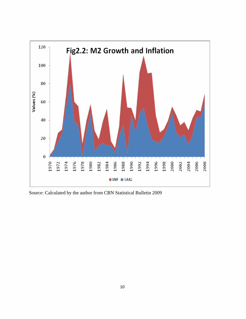
jamboree like the “FESTAC 77”. Thus, as shown in Figure 2.2 below, as money supply growth

begin to move from a single digit of 6.5 per cent in 1971 to double digits of 16.6 per cent in

1972, 54.5 per cent in 1974 and 80.3 per cent in 1975, the rate of inflation fuelled by federal

government’s expenditure also began to grow from single digit of 1.8 per cent in 1970 and 4.6

per cent in 1973 to 13.5 per cent in 1974 and further rose to 33.9 per cent in 1975.

10


11


12

Even though the data available, as captured by Figure 2.3 above, showed that the

economy at this time recorded a relatively high GDP growth rate of 10.9 per cent for 1976 and

8.2 per cent for 1977; these were considered unimpressive and misleading as they are adjudged

to be a product of the boom in the oil sector. This made Ekpo and Umoh (2009) to caution that

such growth rate must be interpreted circumspectly because industrialization which ordinarily

should “imply the process of developing the capacity of a country to master and locate the

whole production process within its border are lacking in this case”.

Since this era, the country has been going through an austere economic period which has

brought the nations per capita GNP from US$830.00 in 1983 to US$370.00 in 1988 and

US$250.00 in October 1990 (Nwankwo, 1992). Furthermore by 1978, a country which had

thought that foreign exchange was not a constraint on development went borrowing on the

Euro-dollar market at exorbitant rates. This act turned the country into a debtor nation with a

huge portion of the nation’s GDP being spent annually on debt-servicing and pay-back. This

bleak and grim economic situation has had serious implications for the nation in terms of the

crime rate, civil and political unrest which are still prevalent in the society as consequences of

the worsening socio-economic situation in the country. Consequently, the need to chart and

adopt an enduring and pragmatic developmental agenda that could help curtail or forestall these

problems remain irresistible.

Successive administrations have therefore come up with different kinds of economic

reforms aimed at returning the economy to the path of recovery. Beginning with the Shagari

regime, stabilization measures which were demand-management in content were adopted with

emphases on exchange controls, abolition of tax exemptions and increase in import duties as

means of reducing demand for imports. However, while the economy was still grappling with

this measure, the military came on board and introduced the idea of pruning down the

government’s expenditure, reducing the size of the public sector and counter-trade measures to

reduce foreign exchange requirements in foreign transactions. These led to massive

retrenchment which further compounded the unemployment problem in the country.

Following the failure of these measures, the country adopted the Structural Adjustment

Programmes (SAP) in 1986 in an attempt to alter and restructure the consumption pattern of the

economy, remove price distortions and heavy dependence on crude oil export. The SAP mainly

13

focused on exchange rate, fiscal and monetary policy management, foreign trade liberalization

and external debt management among others. The fiscal policy management has to do with the

size of the public sector, public expenditure, the budget deficits and taxation while the monetary

policy management is targeted at reviewing the restraint placed on domestic credit and interest

rate liberalization. The main thrust of the exchange rate management under this programme was

to make the exchange rates market-determined. With the adoption of this programme, the Naira

was floated and the two-tier exchange rate system was introduced with the hope that the rates

would converge over time. Consequently, it was expected that the demand for imports would be

curtailed, non-oil exports would be boosted, capital inflows would be encouraged, distortions

imposed by the import licensing system would be eliminated and a realistic exchange rate

would be attained.

With the floating of the Naira at the foreign exchange market, foreign trade was equally

liberalized so as to gain the full benefits of liberalization. In that light, import prohibitions were

eased and the import licensing system and import surcharges were abolished. Customs and

excise tariffs were restructured to reduce the average nominal rate of protection. In addition to

this, a more comprehensive tariff structure with a definite but longer-term horizon was

introduced alongside export policy reforms to support the growth and diversification of the

export structure. External debt management under the reform also considered the issue of debt

refinancing, rescheduling and deferment of obligations, debt buy-back and conversion.

The implementation of these policy reforms was unable to achieve its stated objectives

because of its short time frame, poor sequencing of the prescribed reform measures, poor policy

implementation, policy instability and lack of political will (Ekpo and Umoh, 2009). This made

the problems of the economy to persist well into subsequent administrations and as it eventually

turned out, the general economic situation continued to deteriorate.

Despite the various measures put in place by the monetary authority towards achieving

some lofty macroeconomic objectives, the impact of the deposit money banks has not been felt

in terms of providing the much needed long term financial needs of the real sector. Thus, apart

from depositors demanding outrageous returns on their investment, another factor accounting

for this is the short-term nature of their deposit liabilities and the inappropriateness of using

such deposit base to support long term lending. Deposit money banks, at the expense of the real

14

sector, therefore have to lend short at exorbitant rates in order to sustain their rent-seeking habit.

The banking sector reform was therefore embarked upon so that deposit money banks can give

priority to and make available, cheap and competitive credits to the real sector in a bid to

accelerate the economy’s growth.

The banking sector reform package was anchored on a 13-point programme. A major

point being to increase the minimum capital base requirement of the banks from N2billion to

N25billion so that big banks will emerge that would be able to support the growth of the real

sector and compete in the international arena. The resultant appearance of these mega banks

with robust capital and asset-base on the national economic landscape, it was expected, would

provide the spring board for launching the economy to greater sustainable heights and in the

process achieve the long term goals of reducing the level of poverty in the system, providing

employment in the wider economy and creating wealth for all. Other key points in the

programme include consolidating the banking institutions through mergers and acquisitions and

the establishment of an Asset Management Company as an important vehicle for banking

system distress resolution to purchase the non-performing risk assets of the banks (Soludo,

2004).

A ballpark assessment of the deposit money banks’ performance since the

implementation of these packages reveals that contrary to its predictions, the reform has not

been able to unlock and make available alternative funding scheme to support the emergence

and growth of local private investment in the core economic sector. Also, it has failed to provide

a platform for accelerating the growth of the economy’s real sector.

2.2 Conduct of Monetary Policy in Nigeria

Monetary policy, a major economic stabilization tool, refers to the combination of

measures designed by the monetary authority (the Central Bank of Nigeria) to regulate and

control the volume, cost, availability and direction of money and credit in the economy in order

to achieve some specific macroeconomic policy objectives. It can be described as a deliberate

effort by the monetary authority, in consonance with the level of economic activities, to control

the money supply and credit conditions for the purpose of achieving certain broad economic

15

objectives. However, monetary policy objectives, as designed by the CBN, over the years have

remained the attainment of internal and external balance while emphasis on

techniques/instruments to achieve these objectives has been changing over the years.

Under the colonial government, monetary policy conduct in Nigeria was largely dictated

by the prevailing economic conditions in Britain. Thus the instrument of monetary policy at that

time was the exchange rate, which was fixed at par between the Nigerian pound and the British

pound. This was very convenient, as fixing the exchange rate provided a more effective

mechanism for the maintenance of balance of payments viability and for control over inflation

in the Nigerian economy. This fixed parity lasted until 1967 when the British pound was

devalued.

Despite the Nigerian civil war that broke out in the later part of this period, the monetary

authorities did not consider it expedient to devalue the Nigerian pound in sympathy with the

British pound. This was partly because a considerable proportion of the country’s resources was

being diverted to finance the civil war and also due to the apprehension that the devaluation of

the Nigerian pound would only raise the domestic price of imports without any appreciable

impact on exports. The monetary authorities, rather than devalue, then decided to peg the

Nigerian currency to the US dollar but imposed severe restrictions on imports via strict

administrative controls on foreign exchange.

Following the devaluation of the US dollar because of the international financial crisis

of the early 1970s, Nigeria abandoned the dollar peg and once again kept faith with the pound

until 1973 when the Nigerian currency was once again pegged to the US dollar. However, these

developments brought to the fore, the severe drawbacks of pegging the Nigerian currency

(naira) to a single currency thus establishing firmly the need to independently manage the naira

exchange rate. Hence, in 1978 Nigeria pegged her currency to a basket of 12 currencies of her

major trading partners.

Due to these developments, the monetary policy emphasis shifted in 1974 to monetary

targeting which involve the use of market (indirect) and non-market (direct) instruments. This

consequently made the focus of monetary policy to be predicated mainly on controlling the

monetary aggregates with the belief that inflation is essentially a monetary phenomenon.

Between this period and 1992, the monetary policy objective became that of accelerating the

16

pace of rapid and sustainable economic growth and development, maintaining domestic price

stability as well as a healthy balance of payments position. Also, during this period and up until

the adoption of the SAP in 1986, the conduct of monetary policy in Nigeria relied mainly on

direct control measures, involving the imposition of aggregate credit ceilings and selective

sectoral control, interest rate controls, cash reserve requirements, exchange rate control and call

for special deposits. The use of market-based instruments such as open market operations was

not feasible because of the under-developed structure of the financial market, characterized by

limited menu of money market instruments, fixed and inflexible interest rates, and restricted

participation in the market.

Beginning from September 1993, selective removal of all credit ceilings for some banks

was carried out by the monetary authority. Series of amendment to the Central Bank’s Act was

also carried out to reduce the influence exerted by the Ministry of Finance on the conduct of

monetary policy. With the amendment granting more autonomy and discretion to the CBN in

the conduct of monetary policy, the focus of monetary policy shifted significantly from growth

and development objectives to price stability. Under the operational framework of market

(indirect) instruments; only the operating variables, the monetary base or its components are

targeted while the market is left to determine the interest rates and credit allocation.

2.3 Monetary Policy Techniques

Techniques of monetary policy can be classified broadly into two viz:

i. The Direct techniques of monetary policy and

ii. The Indirect (also known as market-based) techniques of monetary policy.

i) Direct techniques

The direct techniques set or limit the desired quantities of monetary variables. They

include interest rate ceilings and administrative determination of interest rates, quantitative

restrictions on bank credit expansion, mandatory holdings of government securities and sectoral

allocation of credit. The use of these techniques was abandoned in the 1980s when it became

obvious that it resulted in substantial misallocation of resources, because prices did not reflect

their true value, thus sending wrong signals to investors and savers.

17

ii) Indirect (or market-based) techniques

The indirect (or market-based) techniques focus on the demand for and supply of

financial assets thus relying mainly on market forces to transmit their effects to the economy.

These techniques, unlike the direct techniques which focus on the balance sheet of deposit

money banks, target the balance sheet of the central bank. Thus in line with the policy of

financial sector liberalization that accompanied the Structural Adjustment Programme (SAP) in

the second half of the 1980s, the CBN embarked on the transition process from direct to indirect

techniques of monetary management. The adoption of the indirect mechanism required interest

rate policy to become the most important instrument of monetary management, aimed at

regulating the cost of credit by deposit money banks, with the minimum rediscount rate (MRR)

as the nominal anchor for all money market interest rates. The purpose of varying the interest

rate is to alter the demand for and supply of financial assets in the direction that is consistent

with the overall objectives of monetary policy, including output growth and inflation.

Quantity based instruments, mainly reserve money and other monetary aggregates, are

chosen as intermediate targets for the purpose of achieving desired policy objectives. Most of

them affect the availability (and also cost) of funds and, therefore, the decisions of economic

agents. The quantity instruments operate mainly through Open Market Operations (OMO),

where treasury bills purchases (or sales) increase (or decrease) the stock of reserve money,

defined as the deposits, which banks keep with the central bank. Variable cash reserve ratio, the

ratio of cash to deposit liabilities that a bank must hold, liquidity ratio, the ratio of liabilities to

be held in liquid assets, and discount window operations are sometimes used to enhance the

effectiveness of open market intervention, particularly in a relatively underdeveloped financial

market environment. The effect of changes in any of these variables eventually impact on the

real sector. Thus, in pursuance of the goals of price stability, the central bank is always mindful

of the fact that its actions have important repercussions on the real sector.

However, a caveat here is that monetary policy works best where financial markets are

efficient and well developed, and market participants are committed to the achievement of

overall national economic goals. Thus, in the absence of a well-structured financial market; the

conduct of market-based monetary policy is problematic and often produces perverse results or

truncates the transmission mechanisms of monetary policy. Taking the earlier argument as an

18

example; raising interest rates in a liberalized financial market could increase the savings rate,

the marginal productivity of capital and possibly, the rate of investment, as more financial

resources are available to be channelled from savers to investors. However, this outcome

cannot be taken for granted in an imperfect and oligopolistic financial market. In such

circumstances, high interest rates may actually not only discourage investments and thereby

slow economic growth, but could possibly precipitate financial sector crisis. Financial crises

become unavoidable when financial intermediaries finance high-risk quick-return projects with

low value-added (e.g. merchandise trading) rather than more productive long-term economic

activities.

Similarly, monetary policy cannot achieve much in a situation where there is fiscal

dominance and/or where the central bank is turned into a “printing press” for financing large

government budgetary deficits. By the same token, financial intermediaries that are conscious of

short-term gains or whose horizons are too short would always make choices that render

monetary policy objectives difficult and sometimes, impossible to achieve in the long run.

One other important but very serious limitation to monetary policy is the degree of

autonomy enjoyed by the central bank. Although central banks are ultimately responsible for the

creation of money, the process is largely influenced by government’s fiscal operations, in terms

of the size and pattern of spending, while responding to political questions of: “who gets what,

when and how”. An independent central bank ensures that the power to spend money is

separated from the power to create money. It is encouraging to say that in Nigeria, the central

bank currently enjoys instrument and operational independence and has exercised the power for

the general good of the economy and people of Nigeria (Donli, 2004).

2.3.1 Objectives, Instruments and Phases of Monetary Policy in Nigeria

There is a close relationship between objectives and the posture of monetary policy in all

economies of the world. This means that the stance of monetary policy is strongly influenced by

the monetary policy macroeconomics objectives set for a particular period and vice versa. For

instance, if excess liquidity is perceived within an economic system, monetary policy would

most likely be restrictive with the main objective of attaining price stability. This order can be

reversed in policy analysis with the setting of the objective of containing inflationary pressure

19

thereby making monetary policy stance to be restrictive. The choice of instruments for attaining

stated objectives at any particular time would be determined by the structure of the economy,

the state of development of the money and capital markets and the institutional and legal

frameworks within which the financial system is operating. Based on the objectives and

instruments of monetary policy, and the changing macroeconomic environment in Nigeria, it is

feasible to identify various regimes of monetary policy.

In Nigeria, the main objectives of monetary policy since the inception of the CBN in

July 1959 have remained broadly the same; attaining price stability, full employment, achieving

balance of payment equilibrium and ensuring economic growth and development. However,

fluctuations in the fortunes of the national economy and unexpected internal and external

shocks have necessitated changes in emphasis among these objectives and in some cases the

inclusion of some specific sectoral objectives of monetary policy. These changes in economic

conditions have also led to variation in the posture of monetary policy. From a review of the

annual reports of the CBN, monetary policy circulars to the banks and previous studies such as

Ajayi and Ojo, 1981; Teriba, 1978; and Falegan, 1987, a quantitative assessment of changes in

monetary policy resulted in the various dating of the monetary policy in Nigeria between 1959

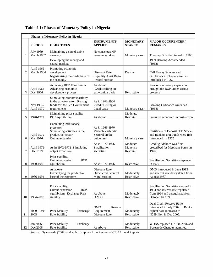
and 2000. Overall, twelve regimes were identified and these monetary policy phases are

summarised in Table 2.1 below.

20

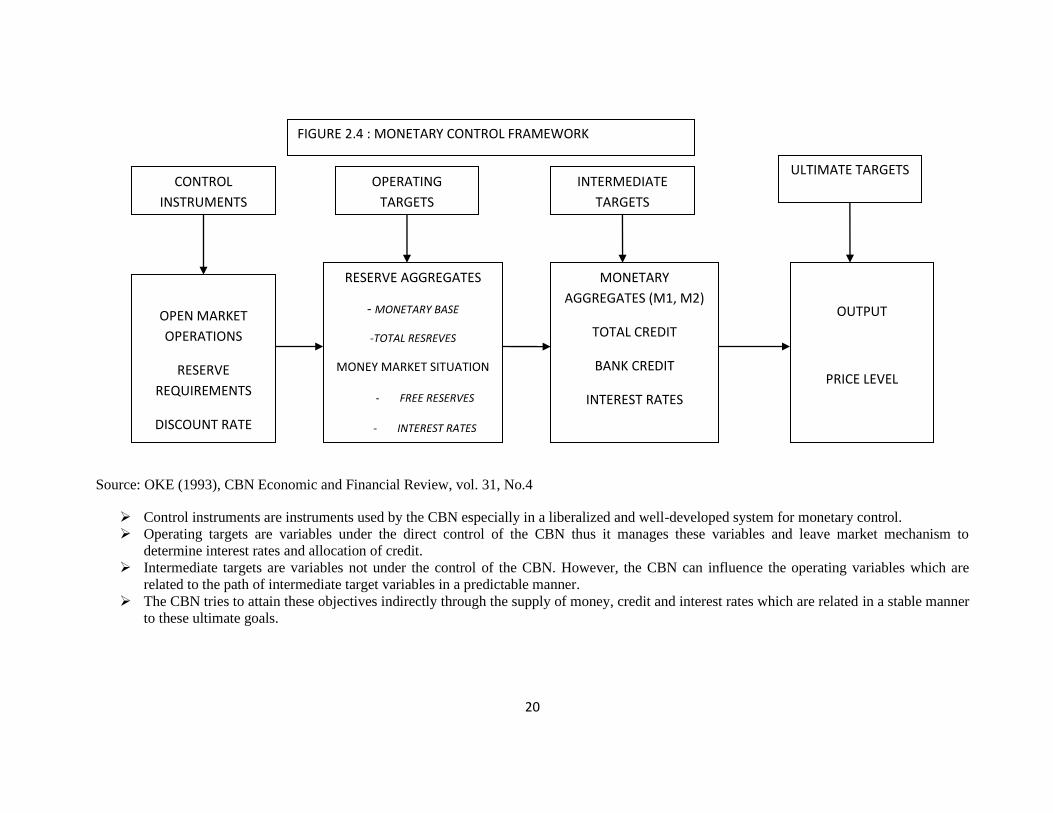
Source: OKE (1993), CBN Economic and Financial Review, vol. 31, No.4

➢ Control instruments are instruments used by the CBN especially in a liberalized and well-developed system for monetary control.

➢ Operating targets are variables under the direct control of the CBN thus it manages these variables and leave market mechanism to

determine interest rates and allocation of credit.

➢ Intermediate targets are variables not under the control of the CBN. However, the CBN can influence the operating variables which are

related to the path of intermediate target variables in a predictable manner.

➢ The CBN tries to attain these objectives indirectly through the supply of money, credit and interest rates which are related in a stable manner

to these ultimate goals.

RESERVE AGGREGATES

- MONETARY BASE

-TOTAL RESREVES

MONEY MARKET SITUATION

- FREE RESERVES

- INTEREST RATES

OUTPUT

PRICE LEVEL

MONETARY

AGGREGATES (M1, M2)

TOTAL CREDIT

BANK CREDIT

INTEREST RATES

OPEN MARKET

OPERATIONS

RESERVE

REQUIREMENTS

DISCOUNT RATE

CONTROL

INSTRUMENTS

ULTIMATE TARGETS INTERMEDIATE

TARGETS

OPERATING

TARGETS

FIGURE 2.4 : MONETARY CONTROL FRAMEWORK

21

Table 2.1: Phases of Monetary Policy in Nigeria

Phases of Monetary Policy in Nigeria

PERIOD OBJECTIVES

INSTRUMENTS

APPLIED

MONETARY

STANCE

MAJOR OCCURENCES /

REMARKS

1

July 1959-

March 1962

Maintaining a sound stable

currency

No conscious MP

were undertaken Monetary ease Treasury Bills first issued in 1960

Developing the money and

capital markets

1959 Banking Act amended

(1962)

2

April 1962-

March 1964

Promoting economic

development Discount Rate Passive Call Money Scheme and

Nigerianising the credit base of

the economy

Liquidity Asset Ratio

- Moral suasion

Bill Finance Scheme were first

introduced in 1962

3

April 1964-

Oct 1966

Achieving BOP Equilibrium

Advancing economic

development process

As above

-Credit ceiling on

exhortation basis Restrictive

Previous monetary expansion

brought the BOP under serious

pressure

4

Nov 1966-

April 1970

Stimulating economic activity

in the private sector Raising

funds for the Fed Government

requirements

As in 1962-1964

-Credit Ceiling on

Legal basis Monetary ease

Banking Ordinance Amended

(1968)

5 1970-1972

Maintaining price stability -

BOP equilibrium As above

Moderate

Restraint Focus on economic reconstruction

6

April 1972-

Mar 1976

Containing inflationary

pressures

Stimulating activities in the

productive sector

Output expansion

As in 1966-1970

Variable cash ratio

Sectoral credit

guidelines Monetary ease

Certificate of Deposit, ED Stocks

and Bankers unit Funds were first

introduced in 1975

7

April 1976-

Dec 1979

As in 1972-1976 Stimulating

output expansion

As in 1972-1976

Stabilisation

securities

Moderate

Monetary

Restraint

Credit guidelines was first

prescribed for Merchant Banks in

1976

8 1980-1985

Price stability,

Output expansion BOP

equilibrium As in 1972-1976 Restrictive

Stabilisation Securities suspended

in 1979

9 1986-1994

As above

Diversifying the productive

base of the economy

Discount Rate

Direct credit control

Moral suasion

Moderately

Restrictive

OMO introduced in June 1993

and interest rate deregulated from

August 1987

10 1994-2000

Price stability,

Output expansion BOP

equilibrium Exchange Rate

stability

As above

O M O

Moderately

Restrictive

Stabilisation Securities stopped in

1994 and interest rate regulated

from 1994 and deregulated from

October 1st 1996

11

2000- Dec

2005

Price Stability Exchange

Rate Stability

OMO Reserve

Requirement

Discount Rate

Moderately

Restrictive

Dual Credit Reserve Ratio

introduced in July 2002. Banks

capital base increased to

N25billion in Dec 2005.

12

Jan 2006 -

Dec 2008

Price Stability Exchange

Rate Stability As Above

Moderately

Restrictive

WDAS replaced DAS in 2006 and

Bureau de Change's admitted.

Source: Oyaromade (2004) and author’s update from Review of CBN Annual Reports.

22

2.3.2 Open Market Operations

These are short-term instruments introduced at the end of June 1993 and conducted

wholly on Nigerian Treasury Bills (NTBs) including repurchase agreements (repos). These

entails the sale or purchase of eligible government bills or securities in the open market by the

CBN for the purpose of influencing deposit money banks’ reserve balances, the level of base

money and consequently the overall level of monetary and financial conditions. In this

transaction, banks subscribing to the offer, through the discount houses, draw on their reserve

balances at the CBN thereby reducing the overall liquidity of the banking system and the banks’

ability to create money via credit. This development has greatly facilitated the conduct of

monetary policy thus allowing the CBN to effectively control money supply and monitor trends

in the financial indicators. Thus for an economy with well developed money and capital markets,

OMO can be a potent weapon of monetary control by the central bank to achieve the objectives

of curbing inflation and sustaining economic growth.

For its implementation, the CBN’s Research Department advises its trading desk at the

Banking Operations Department on the level of excess or shortfall in bank reserves. Thereafter,

the trading desk decides on the type, rate and tenor of the securities to be offered and notifies the

discount houses 48 hours ahead of the bid date. The highest bid price (lowest discount rate

quoted) for sales and the lowest price offered (highest discount offer) for purchases, with the

desired size or volume, is then accepted by the CBN. The amount of securities sold at the OMO

weekly sessions since the inception of the indirect monetary policy in 1993 has risen over a

hundred-fold to N0.2 billion in 1994. Despite the slump in sales recorded in 1995, statistics for

1996 show an increase of 45.5 per cent in the amount sold at OMO over the 1995 sales. The

open market operations activities have been on the increase ever since, with average OMO sales

increasing by over 300 percentage points to N7.73 billion in 2000 and astronomically to N989.9

billion and N1,808.4 billion in 2005 and 2006 respectively. This stupendous growth rate

recorded during these last two periods could be attributable to: the attractive rates offered at the

open market, the supply shortage of long tenured instruments offered at the primary market and

the injection into the economy of N570.0 billion excess crude oil proceeds (Sanusi 2002).

23

2.3.3 Reserve Requirements

The CBN require the deposit money banks to maintain certain (or a minimum) reserve

requirements in order to control their liquidity and influence their credit operations. These

reserve requirements are usually expressed as a percentage of customers’ deposits and can be

manipulated by the CBN to vary the ability of commercial banks to make loans to the public by

simply increasing the ratios. In this regard, they serve as instrument for; liquidity management,

ensuring the solvency of the banking system and prudential regulation. Thence, the CBN

complements the use of open market operation with a reserve requirement. The reserve

requirements are:

i) The Cash Reserve Ratio (CRR)

The statutory Cash Reserve Ratio (CRR) is defined as a proportion of the total demand,

savings and time deposits which banks by law are expected to keep as deposits with the central

bank. This requirement works in the direction of raising or reducing the liquidity of commercial

banks thus impacting their credit creation ability. A higher cash reserve ratio reduces the ability

of the banks to create credit since it reduces the amount of credit banks can give out to the

private sector and government. This affects investment negatively and results in a decline in

economic growth. On the other hand, a low cash reserve ratio increases the credit creation ability

of banks as they are now free to lend their excess reserve to both the private sector and

government. This in turn increases investment opportunities and thereby raises economic growth.

ii) The Liquidity Ratio (LR).

The CBN often impose upon deposit money banks a minimum liquidity ratio and varies it

according to the situation. It is thus designed to enhance the ability of commercial banks to meet

cash withdrawals on them by their customers. Such liquidity ratio stands for a proportion of

specified liquid assets (such as cash, bills and government securities) in the total assets of a bank.

That is, a proportion of banks’ liquid assets to their total deposit liabilities. The CBN has varied

the CRR and LR at various times to its desired objectives.

2.3.4 Discount Rate

The CBN discount window facilities were established strictly in line with the “lender of

last resort” role that the central bank is expected to play. It is the rate of interest the central bank

24

charges the commercial banks on loans extended to them. It is also the official minimum rate at

which the central bank would rediscount what is regarded as eligible bills. Accordingly, the CBN

has continued to provide loans of a short-term nature (overnight) to banks in need of liquidity.

The facilities are collateralized by the borrowing institution’s holding of government debt

instruments and any other instrument approved by the CBN and subject to a maximum quota.

This implies therefore that the effectiveness of this policy is a function of the ability of

commercial banks to have access to liquid assets and must not keep excess reserves. The

Minimum Rediscount Rate (MRR) is the nominal anchor, which influences the level and

direction of other interest rates in the domestic money market. Its movements are generally

intended to signal to market operators the monetary policy stance of the CBN. For example, the

discount rate was reviewed upwards by the CBN from 16.5 per cent to 18.5 per cent in June 2001

in order to contain the rapid monetary expansion arising from an expansionary fiscal policy.

2.4 Analysis of Money Supply Process

Under this section, we shall discuss the sources through which the activities of the

various players in the money supply process ultimately affect the domestic money stock. There

are five key players in the money supply process in Nigeria namely: the Central Bank of Nigeria,

the Governments, the deposit money banks, non-bank private sector and the external sector.

2.4.1 The Central Bank of Nigeria

The supply of high-powered money in any economy is generally perceived to be

determined by the central bank. The operational procedures commonly deployed by this agent to

manipulate the stock of high-powered money are through the acquisition of assets using open

market operations, rediscount operations and foreign exchange operations. The CBN, under the

OMO, embarks on the sale or purchase of securities from the deposit money banks and non-bank

public with a view to achieve some desired level of money stock. In some instances, the CBN

uses the OMO to meet some public sector borrowing requirement. The OMO may be used for

expansionary or contractionary policies depending on whether the CBN wants to increase or

decrease the amount of money in circulation. Whichever policy is being pursued, there exist

some parallelism between the policy and the money stock.

25

The CBN can also influence the amount of money in circulation through the discount

window by varying the discount rate. Thus a decrease in the discount rate is normally considered

as an expansionary monetary policy since it induces commercial banks to borrow more while an

increase is regarded as a contractionary monetary policy. The effectiveness of this operation as a

monetary policy tool depends on the market rate of interest vis-à-vis the discount rate charged by

the CBN. The reason simply being that; if the market interest rate was lower than the discount

rate, commercial banks would not turn to the central bank for loans hence the purpose of using

this policy to reduce money supply would be defeated.

Another means through which the central bank can influence the money supply is the

foreign exchange operation which involves the sale and purchase of foreign currencies. The

exchange rate regime in existence determines the effectiveness of this method to influence the

money supply. The central bank, under a fixed exchange rate regime, normally intervenes by

purchasing domestic currency in exchange for foreign currency when there is excess supply of

domestic currency in order to prevent excessive devaluation of the domestic currency, a situation

referred to as sterilization. This results in a decline in the amount of money in circulation. When

there is excess demand for domestic currency on the other hand, the central bank also intervenes

by selling domestic currency in exchange for foreign currency thus resulting in an increase in

money supply. The essence of sterilization is to maintain the fixed exchange rate regime. This

policy measure has serious policy implications on the economy. Under a floating exchange rate

regime, the nominal exchange rate is allowed to gain its equilibrium level through the forces of

demand and supply.

2.4.2 The Government

Proceed from crude oil exports has remained the largest source of the federal

government’s revenue while non-oil revenue such as VAT accounts for a smaller percentage of

the total annual government revenue. Disbursing and expending these federally-collected

revenue among the three tiers of government has remained one major source of money supply in

the economy. This is due to the incessant increase in the recurrent expenditure of these tiers of

government coupled with the fiscal autonomy of the lower tiers of government which often made

it difficult for the monetary authority to synchronize their expenditure pattern. Additionally, the

governments accumulate huge fiscal deficits which are financed through various means such as

26

sale of government bonds, borrowing from the CBN (credit creation/printing of money), running

down of reserve/asset among others. All of these have monetary implications as it increases the

stock of high-powered money in circulation thereby fuelling inflation in the economy.

2.4.3 Deposit Money Banks (DMBs) or Commercial banks

The deposit money banks’ main function is that of financial intermediation which simply

means receiving money from depositors and channelling them to those in need of funds. The

DMBs pays interest on deposit and receives interest on loans they give out to borrowers. The

spread between the deposit and lending rate indicates the profitability of the intermediation

process which has some monetary implications. The DMBs ability to create bank money requires

that they acquire enough funds to satisfy the demand for credit. The rate of profit on assets held

by DMBs, in addition to the size of money markets and the instruments they offer, sets a limit on

credit creation.

From the money multiplier approach to money supply analysis, the channel through

which the activities of commercial banks influence the money supply can be traced through the

total reserve ratio.

2.4.4 Non-Banking Public Sector

This basically comprises of the surplus spending units and deficit spending units who,

due to mismatch in their respective needs, gives the deposit money banks the opportunity to

carry on their intermediation activities, which in turn affects the domestic money supply. The

divergence between the needs of the surplus spending units and the deficits spending units is due

to the fact that the former usually consists of a large number of small individual savers who only

need to invest small amounts of money. The deficit spending units on the other hand consist

largely of firms with great need for large amount of funds. This situation provides a platform for

the deposit money banks to receive money from the surplus spending units and make them

available to the deficit spending units. This role of the deposit money banks is then referred to as

financial intermediation. Thus the channel through which the behaviours of the non-bank public

impact on the money supply can be traced through the currency deposit ratio (currency ratio) and

/or interest rate on deposit.

27

The relationship existing between the currency ratio and the money multiplier and hence

money can be said to be negative. An increase in the currency ratio therefore implies that loans

granted by the deposit money banks will generate a lower value of deposits since agents are

holding more of their money in currency. With decrease in the deposit money banks liability or

public deposit, the banking systems ability to create money is hindered and so does the money

supply decreases. Persistent increase in the currency ratio normally leads to intermediation in the

banking sector, which may result in a fall in investment and ultimately a decline in economic

growth. There is also the believe that too much money in the hands of non-public may lead to

excess liquidity which might eventually set in motion an inflationary spiral.

2.4.5 External sector

As an open economy, the impact of trade on the domestic money supply in the Nigerian

economy cannot be ignored. Nigeria exports crude oil, agricultural commodities and others to

some countries while it also imports capital and consumer goods into the country. The proceeds

from these exports constitute a source of money supply into the economy. For instance, if there is

an increase in the price of crude oil over the anticipated price, this will result in excess revenue

and lead to an inflow of foreign currency. If such an inflow is monetized, it will lead to an

increase in the domestic money supply.

Also, the inflow of foreign currency into the domestic economy in the form of remittance

to family and relatives (through Western Union Money Transfer or MoneyGram) or as foreign

investments equally affects the amount of money supply in the domestic economy. When these

remittances are channelled through the banking sector, they are converted into domestic currency

and paid to the beneficiaries in local currencies or invested locally thus affecting the amount of

money supply.

Aside from those mentioned above, another veritable external source of money supply is

the donations from bodies such as the World Bank, IMF, ADB, etc. Donations from these bodies

come in the form of financial assistance for budgetary support programmes to the receiving

country and often serve to improve the Net Foreign Asset (NFA) position and hence increase the

money supply. However, Nigeria has not benefited much from these in recent times.

28

2.5 Monetary Policy and Macroeconomic Performance

This section discusses the developments in monetary, fiscal and exchange rate policies as

well as inflation and other macroeconomic variables. Given the CBN mandate of promoting

macroeconomic stability through the conduct of monetary policy, it is pertinent to examine how

far monetary policy has faired vis-à-vis the attainment of its mandated objectives of domestic

price stability as a necessary condition for promoting high output and employment growth and a

healthy balance of payments position. This will provide a clear and better picture on the link and

relationships amongst the variables of interest.

2.5.1 Review of Monetary Policy in Nigeria

Since the establishment of the CBN, monetary policy has been conducted under varying

macroeconomic conditions and the stance of monetary policy has been dictated by the prevailing

economic situation and the period’s objectives. Overall, the administration of monetary policy in

Nigeria since 1959 can be broadly grouped into phases/periods based on the specific objectives

and posture of monetary policy. The early years of the emergence of the CBN was characterized

by monetary ease based on the relatively stable macroeconomic environment, and the monetary

objectives of developing the local money and capital markets, and promoting economic

development through the process of ‘Nigerianising” the credit base of the economy. The

substantial increase in capital formation and domestic output in the early 1970s made monetary

management less challenging. However, the growing involvement of the public sector in

economic activities that are traditionally restricted to the private enterprise in a mixed economy,

as well as the overdependence of the economy on the external sector, increasingly put greater

pressure on monetary management in the 1970s. In the early 1980s, a tremendous trauma was

imposed on the conduct of monetary policy, as the period was inundated with a wide array of

economic misfortunes culminating in the inevitable introduction of economic adjustment

programmes under which monetary policy appeared to have borne a relatively heavy share of the

burden of adjustment (Ojo, 1992).

Given that monetary actions originates in the monetary sector and the initial impact of

monetary policy is felt in the financial markets, most especially the money market, a review of

development and growth of the financial markets will ultimately shed more light on the

knowledge of the breadth, resilience and depth of these markets in Nigeria. This trend analysis of

29

the financial markets is also important as the particular monetary instrument(s) to be put in place

for achieving a set of macroeconomic objectives are strongly influenced by the state of

development of the money and capital markets.

2.5.2 Monetary Policy Formulating Procedure in Nigeria.

In compliance with the varying legislative framework, the procedure for formulating

monetary policy in Nigeria has changed over the years. The monetary policy-making relationship

between the Central Bank of Nigeria and the Federal Government (the Ministry of Finance) has

been dictated mainly by the prevailing enactment governing the CBN operations. The CBN,

prior to 1968, was exclusively responsible for the formulation and implementation of monetary

and financial policy. From 1968 to 1988, the Federal Ministry of Finance was mandated to

approve the monetary policy proposals and such proposals are to be sent to the Federal Executive

Council for approval in the case of disagreement with the CBN. This operating arrangement was

unambiguously contained in the 1968 CBN (Amendment) Decree. Teriba (1978) aptly describe

this arrangement as a situation whereby the Federal Executive Council, the Federal Ministry of

Finance and the CBN constitutes ‘the monetary authority’.

The CBN amendment decree of 1991 formalized this arrangement that subsist between

1988 and 1996, in which monetary policies are sent directly to the President by the CBN. From

January 1997 to December 1998, the CBN was required to send its proposals to the Government

through the Minister of Finance. Overall, between 1968 and 1997, the monetary and banking

policy measures approved by government became a part of the annual budget and formed the

basis of CBN’s monetary and credit guidelines. Ajayi and Ojo (1981) while frowning at this

arrangement noted that “no one denies that a Central Bank cannot be fully independent of

government, but it is equally objectionable to make a central bank an arm of government”. The

Central Bank for the country, according to them, should be autonomous while the responsibility

for the overall economic policy should be assigned to the government to ensure sustainable

development. The major consequences of the CBN being under the control of the Ministry of

Finance identified by Falegan (1987) include: first the possibility of the CBN being stifled of

initiative and innovation thus confining it to the routine functions of exchange control

administration and humdrum credit control operations and second the day-to day monitoring of

30

monetary tools and operations might be turned into an annual budgetary affair thus glossing over

prompt remedies to emerging problems arising therefrom. However, reprieve from the control by

the Ministry of Finance came the way of the CBN in December 1998 when it was granted

instrument autonomy in the formulation and implementation of monetary and financial policies.

Regarding the factors given consideration in the formulation of monetary policy, the

CBN begins its monetary management with a comprehensive review of the economic conditions

as well as the observed and anticipated problems. Computation is also made of the optimum

quantity of demand for money stock that is consistent with predetermined targets for GDP

growth, inflation rate and level of external reserves. The economy’s absorptive capacity is thus

derived from the optimum level of money and external reserves computed. This allows the CBN

to use the monetary policy instruments at its disposal to keep money supply in line with optimal

demand (CBN, 2000).

Monetary Policy and Real GDP growth.

The effect of monetary policy on output, as gleaned from the literature, shows that there

is a direct and positive relationship between these two variables. However, the channels through

which the effect of monetary policy impact on output differs based on the structure of the

particular economy under review. In the case of Nigeria, there has been a sustained decline in the

growth rate of real GDP since the early 1970s as it fell from 18.2 per cent in 1971 to 2 per cent in

1973 and further to as low as -3.2 per cent in 1975. A proximate factor for the growth rate in

GDP in the year 1971 and 1972 was partly due the huge government expenses on financing post

war reconstruction. The rate of growth in money supply also reflects this as it grows from 6.4 per

cent in 1971 to 15.5 per cent in 1972 and 25.2 per cent in 1973. The growth of M2 in the

subsequent year (1974) by 81 per cent, perhaps a fallout of the windfall from the Arab oil war,

reflects the increase in the economy’s activity as the real GDP grew in that same year by 12 per

cent.

As the real GDP growth rate nosedived in 1977 from 8.2 per cent to -7.4 per cent in 1978,

M2 growth rate also deepened to -3.7 per cent in 1978 from the previous year’s figure of 33.7 per

cent. Though, economic activity began to pick up shortly after a civilian government came into

31

power as shown in the growth rate of M2 by 46.1 per cent in 1980 which was accompanied by a

growth of real GDP by 5.3 per cent in that same year. However, this was short-lived as the real

GDP growth rate between 1981 and 1984 remained in the negative region ranging between -0.3

and -8.5 per cent even when M2 was growing at an average of 10.25 per cent per year.

Even though the poor economic performance of the civilian government remained the

leeway for the military interruption in 1984; economic performance for the sixteen (16) years of

military intervention and governance was not any better. While the average growth rate of M2

for the sixteen (16) years stood as high as 25.3 per cent, economic performance as reflected by

the average growth rate of real GDP for the same period stood as low as 3.17 per cent. Even the

adoption of the Structural Adjustment Programme in 1986 could not help the economy’s

misfortune that was characterized by an abysmally poor annual real GDP growth rate. Only two

post-SAP annual real GDP, that is 1988 and 1990, exhibits some meaningful growth in economic

activity. Given the challenges of the SAP such as short time frame, poor sequencing of the

prescribed reform measures, poor policy implementation, policy instability and lack of political

will; one is not surprised of its failure.

However, there has been resurgence in economic activity since the advent of democratic

system of government in 1999 with average real GDP growth rate of 9.03 per cent between the

fiscal year 2000 and 2008. Even though a spike was observed in 2002 with real GDP growth

peaking at 21.3 per cent, this was partly due to the last round of increase in crude oil prices and

the difficulty of performing sterilization operations by the CBN in a democratic setting where the

lower tiers of government embarked on expansionary fiscal policies. This was occasioned by the

rapid monetization of the proceeds of excess crude earnings (Sanusi 2002). However, economic

performance in the subsequent years remained moderately stable at 10.2 and 10.5 per cents in

2003 and 2004 reflecting the politically stable environment prevalent in the economy. Thereafter,

real GDP growth has remained stable at an average of 6.3 per cent between 2005 and 2008

despite a seemingly high growth rate in M2 from 24.4 per cent in 2003 to 44.2 per cent and 57.8

per cent in 2007 and 2008 respectively.

32

CHAPTER THREE

LITERATURE REVIEW

3.1 Introduction

The conventional wisdom that immediately followed the Great Depression of the 1930s

and Keynes’ classic thesis was that money does not matter. However after World War II, the re-

emergence of monetarism led to the consensus that monetary policy can significantly affect real

economic activity, at least, in the short run. The general agreement of monetary policy’s potency

notwithstanding, the precise nature of the causal links between monetary and real aggregates

remains a bone of contention (Laidler, 1978). Observers have therefore painstakingly weighed

differently the various specific channels through which monetary policy works. The weights

attached to each of the channels of monetary transmission mechanism differ in the emphasis

placed on money, credit, interest rates, exchange rates, asset prices or the role of deposit money

banks and other financial institutions (Taylor, 1995). Divergent views and opinions exist as well

about the monetary transmission process in individual industrialized nations while in the

developing nations, the process still remains hazy and uncertain.

This chapter therefore reviews the plethora of literature on the monetary transmission

mechanism particularly highlighting the theoretical, methodological and empirical literature on

the various channels through which monetary impulses are transmitted to the real sector of the

economy. The review of different works also attempts emphasizing the modelling techniques and

methodology used by the authors and compare the empirical results emanating therefrom.

3.2 Theoretical Review

Various transmission mechanisms through which monetary policy can affect economic

activity have long been established by theory and evidence. Given its complexity, however,

tagging the monetary transmission mechanism as ‘black box’ seems accurate since there are not

one but many channels through which monetary policy simultaneously operates. Also, depending

on the state of payments system and the money (especially financial) markets, the relative

strength of the various channels vary from country to country. Thus, beginning with the

33

transmission of Open Market Operations (OMOs) to money market interest rates, the process

passes through the reserves market or more broadly to market interest rate through the supply

and demand for money.

Even though the operating procedures, instruments and targets of monetary policy may

vary across countries, monetary transmission remains the mechanism identified in the literature

as the medium through which monetary policy actions of the central bank impact real economic

activity. Macroeconomic theories and empirical studies have therefore, over the time, developed

a great many approaches that explains how such links actually works. However, one common

feature among these links is that a change in monetary policy stance caused by central bank’s

action somehow translates into a change in aggregate demand that affects real output and

domestic prices. Thus, there have been variations across countries on the operation of monetary

transmission channels due to differences in the extent of financial intermediation, the size,

concentration and health of the banking system, the development of capital markets and

structural economic conditions (Cecchetti, 1999). Monetary transmission has therefore come to

be referred to as “black box” because of these numerous channels through which monetary

policy operates simultaneously. In an attempt to unearth this “black box”, economists have come

up with some channels of monetary transmission that provides some explanations on how this

translation occurs and what eventually drives aggregate demand as well as output and prices up

or down.

3.2.1 Channels of Monetary Transmission

The literature on the monetary transmission mechanism advocates a transmission process

through which monetary policy decisions are converted into changes in real output and inflation

(Baksh and Craigwell, 1997). Even though monetary actions originate in the monetary sector, the

Central Bank’s target variables -output, prices and full employment- are in the real sector of the

economy. Thus the way or channel through which the actions in the monetary sector affect the

real sector is referred to as the Transmission Mechanism. In essence, it is the link between the

monetary and the real sector of the economy. But while Meltzer (1995) referred to a transmission

process as describing the economy’s response to an impulse, Pierce and Tysome (1985) in

34

differentiating between a monetary transmission mechanism and a channel of monetary

influence posited that; the monetary transmission mechanism refers to the general conceptual

framework within which the analysis of monetary disturbances may be undertaken while the

channel of monetary influence refers to the route through which these monetary disturbances

influence the general variables. Thence they conclude that it is possible for a number of channels

of monetary influence to co-exist within the same monetary transmission mechanism.

The financial structure of a country and its macroeconomic environment determines the

relative importance of the different channels of monetary transmission. The financial system’s

structure - which includes the degree of competition in the banking sector - determines the

linkage between an instrument under the direct control of the central bank (e.g. reserve

requirements) and the variables that drive the conditions in the non-financial sector (e.g. loan and

deposit rate, asset prices and the exchange rate). In turn, the macroeconomic environment (e.g.

the degree of financial leverage and competition in different sectors, currency denomination of

liabilities, openness of the economy, etc) determines the link between the financial conditions

and spending as well as investment decisions among households and firms (Kamin, Turner and

Van’t dack, 1998).

The work of Mishkin (1995) titled “symposium on the transmission mechanism”

identified; interest rate, exchange rate, bank credit and asset prices as the main channels of

monetary transmission in the literature. The common trend that can be found in all of these

channels is that fluctuation in the level of money supply resulting from variation in monetary

policy stance – through the use of OMO or reserve requirement – essentially affects real

economic variables (prices and output) through aggregate demand or aggregate supply. The

various channels identified in the literature are thus analyzed in what follows.

i) Interest Rate Channel

The interest rate channel which lies at the heart of the traditional Keynesian textbook IS-

LM model was originated by Hicks (1937) but also associated with the works of Taylor(1995),

Cotarelli and Courelis (1994) and Clarida, Gali & Gertler (2000). According to this theory, all

agents in the economy hold only two types of assets namely money and bonds as a superficial

35

collection of all other financial assets. A monetary expansion through an open market purchase

of bonds, the theorists claim, will lead to an excess supply of money thus making economic

agents hold more money and fewer bonds. Therefore for equilibrium to exist in the assets

market, short term interest rate should fall to make economic agents accept extra money

holdings. This fall in interest rate will lead to an increase in investment spending (due to

decrease in the capital cost of financing investment) which will ultimately cause an increase in

aggregate demand and output.

Also, such an increase in money which raises households real money balances for a given

interest rate implies an excess of cash in the perception of households. It is predicted that when

households begin to increase their bondholding in a bid to reduce their real balances, interest rate

will reduce thus lowering the cost of capital and consequently causing an increase in investment

spending, aggregate demand and output as well as price level. The increase in aggregate demand

may lead to an increase in the general price level. The reverse scenario occurs for a

contractionary monetary policy. This scenario is presented schematically below:

Expansionary Monetary Policy=> Interest Rate↓=> Investment↑=> Output↑

However, two conditions should be satisfied for the theory above to hold. First is that the

central bank must have influence over the short and long run real interest rates. This can be the

case when there is slow responsiveness of inflation in the economy. Second is that the

components of aggregate demand should be interest rate sensitive.

ii) Exchange Rate Channel

The second contribution of the Keynesians to the monetary transmission debate is the

Exchange rate channel. This examines the relationship between net private capital inflows and

monetary policy and how an alteration of the interest rate alters the attractiveness of a country’s

currency. This channel posits that an increase in the domestic currency’s attractiveness will cause

foreign investors to shift part of their investment to financial assets denominated in this currency.

36

The currency, due to this, appreciates and lowers the competitiveness of the domestic industry

which ultimately results in a decline in net exports (Kuttner et al, 2002).

The exchange rate channel is an important element in conventional open-economy

macroeconomic models. Though effective only under a flexible exchange rate regime, it works

through both aggregate demand and supply effects, the chain of transmission being from the

interest rate to the exchange rate via the uncovered interest rate parity condition (which relates

the interest rate differentials to expected exchange rate movements). Thus, a decrease in the

domestic interest rate relative to the foreign interest rates would lead to a weaker currency and an

increase in both net exports and in the overall level of aggregate demand.

The exchange rate channel also involves interest rate effects (Mishkin, 1995). On the

demand side, an expansionary monetary policy lowers domestic interest rate. The fall in interest

rate causes deposit in the domestic currency and credit in foreign currency to become less

attractive thus bringing about a real depreciation of the domestic currency. This in turn leads to

higher net export and a stronger aggregate demand (Obstfeld and Rogoff, 1995). On the supply

side, the real depreciation that results from monetary expansion raises the domestic prices of

imported goods thus raising inflation directly. In addition, the higher price of imported inputs

contracts aggregate supply, reduces output and increases inflation. Thus, an expansionary

monetary policy that results to a fall in domestic interest rate, according to this channel, will

cause an outflow of capital. The outflow of capital puts pressure on the exchange rate and this

leads to a depreciation of the domestic currency. Depreciation makes the foreign price of exports

cheaper and the domestic price of imports expensive. This expands export and reduces import

hence an increase in net exports. The increase in net exports leads to an increase in aggregate

demand and output. Also, the depreciation of the domestic currency together with the increase in

aggregate demand results in an increase in domestic price level. On the other hand, a

contractionary monetary policy stance will increase interest rate and hence cause an appreciation

of the exchange rate. Exchange rate appreciation will increase import and decrease export,

thereby resulting to a fall in net exports and hence a fall in aggregate demand, output and price

level. This scenario is presented schematically below:

37

Contractionary Monetary Policy => Interest Rate↑ => Exchange rate↑ => Net Exports↓ =>

Output ↓

The Mundell-Fleming theorem of a floating exchange rate regime, aided by an elastic

balance of payments, remains the premise upon which the exchange rate as a key variable in the

monetary policy transmission is anchored (Baksh and Craigwell, 1997). According to Mundell

(1962), capital mobility implies an important relationship between short term interest rate and

exchange rate. This parity relationship states that the interest rate differential between any two

countries is equal to the expected rate of change in the exchange rate between these two

countries. If this relationship is violated, then capital would flow into the country with the higher

returns until expected returns in both countries became equal. By this process, the interest rate

parity relationship transmits monetary impulse through the effect of exchange rate changes on

net exports to the real sector of the economy.

Contrasting the situation with what obtains under a fixed exchange regime; an

expansionary monetary policy initially lowers the domestic interest rate and raises income thus

resulting in capital outflows as well as current account deficit. The government’s attempt to

increase the money supply fails because its acquisition of domestic bonds is offset by its losses

of foreign exchange reserves thus leading to a constraint in conducting monetary policy. Flowing

from the aforementioned, Taylor (1995) and Obstfeld & Rogoff (1995) emphasize that a

framework for the conduct of monetary policy must be inherently international in scope.

iii) Credit Channel

The credit channel of monetary policy transmission operates as an accelerator of the

mechanism and is closely linked to the interest rate channel in a way that further extends the

effects of monetary policy. Unlike the interest rate channel, it shows an indirect impact of

monetary policy on the real economy. Its emphasis is on how imperfect information and other

“frictions” in the credit market work as an important channel of monetary policy. Due to

information asymmetry in the credit market and enforcement cost, Bernanke and Gertler (1995)

argued that, principal-agent problems arise in the financial market and create an external finance

38

premium1. They therefore postulate that: variations in monetary policy stance alter the external

finance premium facing borrowers and that; smaller firms which rely more on bank credit and

have more limited access to external funds than larger ones could be expected to be more

affected by an increase in interest rate (Gertler and Gilchrist, 1993, 1994; Bernanke, Gertler, and

Gilchrist, 1996; Clements, Kontolemis and Levy, 2001). The strength of this effect however

depends on the health of the banking system and the degree to which it can react to policy

changes. Following the problems facing the credit markets, this channel is further decomposed

into two basic channels of monetary transmission. These are the Bank lending channel and the

Balance sheet channel.

The Bank lending channel postulates that banks play an important role in an economy

both by issuing liabilities (bank deposits) that contributes to the broad monetary aggregates and

by holding assets (bank loan) which scarcely has any substitute. The proponents of this channel

therefore emphasized that for many banks; deposit represent the principal source of funds for

lending and that for many firms, bank loans represents the principal source of funds for

investment. Thus, variation in monetary policy stance then affects the external finance premium

through the shifts in the supply of intermediated credits especially the quantity of loans supplied

by the banking institutions to the credit markets. The main presumption of this argument is that

monetary policy significantly alters the supply of bank loans which is the asset side of the banks’

balance sheet. However, there is need to note the fact that the problem of asymmetric

information is prevalent more with small firms.

To apply the bank lending channel, consider an expansionary monetary policy which

increases the aggregate volume of banks’ reserves and deposits as well as the amount of credit

available. Given that banks play a special role of lending to different classes of borrowers, this

increase in loan will cause investment spending to rise as well as aggregate demand and output.

This may eventually put an upward pressure on the general price level. The schematic

presentation of the above story is shown below:

1 External finance premium is the difference in cost between funds raised externally by issuing equity or debt and

the opportunity cost of funds generated internally by retaining earnings.

39

Expansionary Monetary Policy=> Bank reserve↑=> Bank Loan↑=> Investment↑=>

Output↑ .

For the bank lending channel to work, however, bank dependent borrowers must exist

and the central bank must be able to significantly affect the supply of intermediated bank loans

by altering the amount of loans available to the deposit money banks.

The Balance Sheet Channel even though operates via the net worth of business firms

(Bernanke and Blinder, 1988) rests on the notion of asymmetric information in credit markets

and emphasizes the role of collateral in reducing moral hazards. Business firms with lower net

worth clearly signal to the lenders that there is less collateral for their loans, and so lenders are

weary that losses from adverse selection may be higher. Therefore, a lower net worth raises the

adverse selection problem thus leading to decreased lending to finance investment spending.

Additionally, lower net worth of business firms increases the moral hazard problem because it

means that owners have a lower equity stake in their firms, giving them more incentive to engage

in risky investment projects. Since taking on riskier investment projects makes it more likely that

lenders will not be paid back, a decrease in business firms’ net worth leads to a decrease in

lending and hence in investment spending (Mishkin, 1995). A contractionary monetary policy

stance which causes a fall in equity prices reduces the networth of firms and so leads to lower

investment spending and aggregate demand because of the increase in adverse selection and

moral hazard problems. The contractionary monetary policy together with the decrease in

aggregate demand reduces the domestic price level. Schematically, this is shown below:

Contractionary Monetary Policy => Equity Prices↓ => Adverse Selection↑ => Moral

Hazard↑ => Bank Loans↓ => Investment↓ => Output↓.

iv) Asset Price Channel

The Keynesian paradigm for analyzing monetary policy effects on the economy was

strongly objected to by the Monetarist on the ground that it focuses on only one relative asset

price and the interest rate (Mishkin, 1995 and Meltzer, 1995). The classical monetarist model

40

emphasizes the role of monetary aggregates in determining asset, goods and factor prices. They

argue that monetary policy actions impact on prices simultaneously across a wide variety of

markets for financial assets and durable goods especially in the market for equities and real

estates. In essence, this channel reflects the impact of monetary policy on the prices of bonds,

shares, real estate, and other domestic assets. It operates through changes in firms’ market value

and in household wealth. The former alters the relative price of new equipment, affecting

investment spending, while the latter affects household consumption and the availability of

collateral for borrowing. Two monetary transmission channels namely Tobin’s q theory of

investment and the wealth effects on consumption emerged from this monetarist argument

Tobin’s q2 theory provides a mechanism through which monetary policy affects the

economy via its effects on the valuation of equities. According to Tobin (1969), a high q implies

that the market price of firms is high relative to the replacement cost of capital thus investment

spending will rise while a low q implies that firms will reduce investment because the market

value of firms is low relative to the cost of capital.

The monetary channel emphasized that a link exists between Tobin’s q and investment

spending through the price of equity. An expansionary monetary policy through decrease in

discount rate or decrease in reserve requirement ratio will increase money supply. This leaves the

public with more money than it desires. Thus, a veritable means for the public to rid such excess

is in the stock market by increasing the demand for equities which will correspondingly increase

their prices. A rise in the price of equities will lead to a higher q, and thus increase investment

spending. This results in an increase in aggregate demand and an increase in output, which then

triggers an increase in the price level. The scenario analysed above is presented schematically

below:

Expansionary Monetary Policy => Equity Prices↑ => Tobin’s q↑ => Investment↑ =>

Output↑.

The second mechanism according to the monetarist for transmission through equity

prices is the wealth effect on consumption. According to the life cycle model of Modigliani

2 Tobin (1969) defines q as the ratio of the market value of firms to the replacement cost of capital.

41

(1971), consumption spending is determined by the consumer’s life time resources which consist

of human and real capital plus financial wealth (mainly common stocks). The monetarists posit

therefore that an expansionary monetary policy will increase the demand for stocks which will

cause their prices to rise. When this happens, the value of individual consumers’ financial wealth

increases consequently increasing their lifetime resources and consumption. This increase in

consumption impacts positively on aggregate demand, output as well as price level. The schema

below portrays this story:

Expansionary Monetary Policy => Equity Prices↑ => Financial Wealth↑ => Consumption↑

=> Output↑.

v) Cash Flow Channel

There also exists another channel of transmission through which monetary policy affects

the real sector and this is known as the Cash Flow channel. Here also, the same logic with

asymmetric information applies. In this mechanism, the changes in intensity of adverse selection

and moral hazard are rooted in improvement/deterioration of the firm’s cash flow. For instance,

if an expansionary monetary policy first lowers short-term nominal interest rates, then the firm

may find it much easier to service its short-term debt because interest payments are now lower.

This implicitly improves the firm’s cash flow and comforts the lender that the loan granted to

this firm will be serviced and repaid when due. Consequently, moral hazard and adverse

selection problems diminish, engineering new lending and thus increasing investment spending

and output and causing price to increase through an increase in investment spending and output.

The picture is painted by the schema below:

Expansionary Monetary Policy => Nominal Interest Rate↓ => Cash Flow↑ => Adverse

Selection↓=> Moral Hazard↓=> Bank Loans↑=> Investment↑=> Output↑.

In spite of the above analysis of the various channels, establishing the existence of a

particular lending channel in any country may not be as simple as explained above for two

reasons. First, changes in interest rates usually occur in response to changes in economic

42

conditions, which makes it difficult to recover from the data the pure effect of the interest rate

change on economic activity. Second, all channels of monetary transmission tend to work at the

same time, which complicates their separate identification. Following an interest rate increase,

for instance, bank credit may decline due to either lower demand for loans (the interest rate

channel and, possibly, the balance sheet channel), or reduced supply of loans (the bank lending

channel), or both (Brooks, 2007).

Also, the operation of monetary transmission channels varies systematically across

countries due to differences in the extent of financial intermediation; the size, concentration, and

health of the banking system; the development of capital markets; and structural economic

conditions (Checetti 1999). The depth, breadth, and structure of the financial system determines

the link between the monetary policy instruments under the control of the central bank (short-

term interest rate, reserve requirements) and the variables that drive the conditions in the non-

financial sector (e.g., loan and deposit rates; asset prices; and the exchange rate). The

macroeconomic environment as well as structural features of the economy (e.g., degree of

monetization and dollarization; cash-based payments system; size of the informal sector;

openness of the economy; and inflows of private and official financing resources) in turn

determine the link between financial conditions and spending/investment decisions among

households and firms.

43

FIGURE 3:1 STYLIZED REPRESENTATION OF THE TRANSMISSION MECHANISM

MONETARY POLICY

INTEREST RATE CHANNEL

EXCHANGE RATE CHANNEL

CREDIT CHANNEL

ASSET PRICE CHANNEL

CASH FLOW CHANNEL

AGGREGATE

DEMAND/ OUTPUT

GAP

INFLATION

AND OUTPUT

SOURCE: AUTHOR

44

3.3 Methodological Review

From the plethora of economic literature reviewed, we discover that various

methodologies have been explored and applied by researchers to identify the transmission

mechanisms and effects of monetary policy on inflation and output. These methodologies can

be classified into five main categories namely: the descriptive analysis approach, the big

macro-econometric models approach, the small macro-econometric models approach, the

Dynamic Stochastic General Equilibrium (DSGE) approach which is also called the New

Open Economy Macroeconomics (NOEM) and the variants of Vector Autoregressive (VAR)

models such as the Structural Vector Autoregressive (SVAR) and the Vector Error

Correction Models (VECM) approach.

3.3.1 Descriptive Analysis Approach

The earliest approach is the descriptive analysis which observes and compares

relevant economic variables to make inference about monetary transmission mechanism.

Even though this methodology is purely descriptive and very simple to handle, it is marred

with some fundamental shortcomings. The most notable of these is that studies conducted

using this methodology do not make use of basic econometric techniques to perform any

empirical analysis and as such model specification and estimations are ignored. Since

empirical results are lacking, it thus implies that conclusions made from such studies may not

have any economic interpretations. Also, being descriptive in nature, it may not be suitable

for our present study because it does not capture the direct and indirect effect of monetary

policy on inflation and output as well as trace the transmission mechanism. Empirical works

using this approach include Jimoh’s (1990) work on demand for money in Nigeria which

examined the relevance and role of interest rate sensitivity in the demand for money as a

means of explaining the channels of monetary influence. Uchendu (1996) also explore this

methodology in his attempt to identify the monetary transmission channel in Nigeria and

came to a conclusion that the credit channel of monetary transmission exist and is more

relevant to the Nigerian economy.

45

3.3.2 The Big Macro-Econometric Model Approach

The second approach is the big macro-econometric models which usually specify all

the most important relationships in the economy and link the different markets together so

that monetary policy transmission mechanism can be identified. Most of the studies on

macro-econometric model used Ordinary Least Square (OLS) estimation techniques in

arriving at the parameter estimates. However, despite the advantages associated with OLS in

terms of its simplicity and the best linear unbiased estimator (BLUE) property, it fails to

capture the direct and indirect effect of monetary policy on domestic price and output. Also,

empirical analyses using this type of methodology are known to require a large data for

specific variables which is often not available. This data-hurdle may seriously affect the

estimation process. These aside, the approach has further been found to be lacking in

transparency due to the theoretical assumptions underlying the different interrelated sectors

which may eventually lead to the problem of misspecification (Tarawalie, 2008).

In exploring this methodology, Aron and Muellbauer (2000) developed a big macro-

econometric model to forecast the effect of interest rate change on output for South Africa.

They cited the presence of structural breaks from political and policy regime as a justification

for its forecasting superiority over recursive forecasting from vector autoregressive model.

They noted the inclusion of important monetary policy regime shifts, which altered the

output response to interest rates, and the control for other structural changes (e.g., trade

liberalization), to have addressed the Lucas critique in forecasting output growth. They

observe further that there are important and persistent effects of high real interest rates,

which significantly constrained growth in the 1990s and potential growth benefits from fiscal

discipline. Allen and Robinson (2004) empirical works further explores this methodology by

constructing an aggregated macroeconomic model to simulate the behavior of the Jamaican

economy under different policy rules. The model provides them a platform to note the

existence of a direct transmission from interest rate to exchange rates through portfolio

substitution as well as to observe the impact of monetary policy on inflation in the second

quarter after an innovation.

46

3.3.3 The Small Macro-Econometric Model Approach

The third approach which specifies the most important relationships that address

specific channels of monetary transmission mechanism in the economy is the use of small

macro-econometric models. Unlike the big macro-econometric models, this approach is not

data-intensive and requires fewer variables. Formulating its model is anchored on sound

economic theory whose parameter estimates are known to have salient economic

interpretations. Aside from being easier to handle in terms of model specification and

estimation, the model also provides linkages within and across equations in order to capture

the direct and indirect effect of the monetary transmission mechanism. Fanelli and Paruolo

(1999) explore this methodology for Italy and other members of the European Union

countries before the adoption of the stage III of EMU while Brooks (2007) also designed

something similar in a study of monetary transmission mechanism for Turkey. He built the

model for quarterly data on some financial variables such as the Liquidity, size, capitalization

of firms as well as dummies to proxy ownership status and stock market participation. His

model was designed to test the effective propagation channel of monetary policy by the

banking sector, depending on their liquidity position.

Modelling this approach for a Sub-Saharan country, Tarawalie (2008) did the same

for Sierra Leone by building a small macro-econometric model in the form of a system of

equations to study the transmission mechanism of monetary policy in the country. His

empirical work used quarterly data on some macroeconomic variables such as real exchange

rate, inflation, real GDP, interest rate, Treasury Bill rate, private sector credit, broad money

(M2) among others for the period of 1990 to 2006 to establish the channel through which

monetary policy propagates to the real sector.

From the literature surveyed so far, most researches conducted using the second and

third approaches above tend to adopt the Ordinary Least Square (OLS) estimation technique

in arriving at the parameter estimates. However, despite its simplicity and “best linear

unbiased estimator” property, using OLS to estimate the coefficients of macro-econometric

models may be inappropriate since it tends to overestimate the coefficients. Also, macro-

econometric models for monetary policy analysis are often designed with the intent of

describing the interactions of key macroeconomic variables over the medium term. Their

47

main purpose, in any case, is not to produce a forecast understood as best guess of the values

of the main variables. Thus in reality, these models do not produce the forecast rather

economists do. What such models can do, at best, is to provide a coherency check on the

judgment that produces the main forecast. These models only allow for systematic analysis of

risks to the forecast, including sensitivity to various assumptions, shocks, and policy

responses as well as provide a framework that can help to ask the right questions.

3.3.4 The Dynamic Stochastic General Equilibrium Approach

The fourth approach which is recently being used everywhere by modellers is the

dynamic stochastic general equilibrium (DSGE) model. The DSGE model, though emerging,

is also called the New Open Economy Macroeconomics (NOEM). It is actually based on the

New Keynesian thinking which merges Keynes ideas - that markets can fail - with the

classical economics of rational human beings (Canova and Sala, 2005). The model follows

the earlier rational expectations models of Lucas (1972) and Sargent and Wallace (1975) by

stressing the role of expectations in the monetary transmission mechanism. As emphasized

by Kimball (1995), by deriving these expectation forms for the IS and Phillips curves from

completely spelled-out descriptions of the optimizing behavior of households and firms, the

New Keynesian model takes advantage of the powerful microeconomic foundations

introduced into macroeconomics through Kydland and Prescott’s (1982) real business cycle

model (Ireland, 2005). The DSGE model has the advantage of offering coherent frameworks

for structuring policy discussions. However, a major problem with the use of this

methodology is how to empirically validate its findings. The other challenge is how to

effectively communicate the features of the methodology and the implications of its findings

to policy makers and the general public. Overall, at their current stage these important

limitations of DSGE are yet to be resolved. Rotemberg and Woodford (1997), Smets and

Wouters (2003), Ireland (2004, 2005), Canova (2004), Canova and Sala (2005), Rubio and

Rabanal (2005), Gali and Rabanal (2005) and Fernández-Villaverde, (2009) are among the

authors who have explored this methodology.

48

3.3.5.1 The Vector Auto-regressive Approach

Vector auto-regressive (VAR) models and its variants are the fifth methodology

known to have been extensively explored by various researchers in the developed,

developing as well as quasi-emerging market economies of the world in their attempt at

resolving the monetary transmission mechanism of their respective economies. The

consideration and popularity of VAR as benchmarks in econometric modelling of monetary

policy transmission followed the groundbreaking work of Sims (1980) and a sort of widely

accepted notion that this class of models provide a certain mix between a mere “data-driven”

approach and an approach coherently based on economic theory (Fry and Pagan, 2005; Borys

and Horvath, 2007; Ngalawa, 2009).

In this widely acclaimed work, Sims (1992) estimates separate VARs for Japan,

Germany, France, the United Kingdom and the United States of America using monthly data.

His variables include industrial production, consumer prices, and short-term interest rate as

measure of monetary policy, a measure of money supply, an exchange rate index and an

index of commodity prices. He makes the identifying restriction that the interest rate variable

potentially affects other variables contemporaneously, while the interest rate is not affected

by innovations in any of the other variables. Also similar to the identifying assumption of

Sims (1992) such that monetary policy is predetermined, Bernanke and Blinder (1992) did a

study on the credit channel in the United States, using the US federal funds rate,

unemployment rate, logarithm of consumer price index (CPI), deposits, loans and securities.

They were able to establish that both the conventional money demand and the credit

mechanisms operate in the economy. They also established the time-lag between when a

positive shock to the federal funds rate affects the volume of deposit held by institutions.

While making similar identifying assumptions as Sims (1992) and explicitly

including commodity prices to avoid the price puzzle, Christiano, Eichenbaum and Evans

(1996) used US quarterly data to test the effect of monetary policy shocks. Variables used for

their analysis include real GDP, the GDP deflator, commodity prices, U.S. federal fund rate,

non-borrowed reserves, total reserves and net funds raised through financial markets.

Alternating between two policy variables, the federal funds rate and non-borrowed reserves,

they establish the effect of a shock to US federal funds rate on the business sector as well as

49

its lag and duration. However, Weber, Gerke and Worms (2009), also exploring the VAR

methodology, conducted a study of the Euro area to investigate if there has been any

significant change in the overall transmission of monetary policy to inflation and output. The

study used a few variables such as real GDP, domestic nominal short term interest rate, GDP

deflator and real housing wealth on quarterly data between 1980:1-2006:4. Their study

provides a clear link between variation in monetary policy and the long-run responses of real

output and inflation in the Euro area countries. They however cautioned that monetary policy

should neither concentrate on too narrow a set of indicators nor ignore important

explanations or models for inflation when judging the monetary policy stance or making

monetary policy decisions.

Bonci and Columba (2008) followed the work of Christiano, Eichenbaum and Evans

(1999) by adopting a recursive vector auto regression (VAR) approach on quarterly data for

the period of 1980 to 2002 to identify the impacts of monetary policy shocks on the Italian

economy. The variables for their model consist of industrial production index, the consumer

price index, the import price of raw materials, the nominal exchange rate of the Italian lira

vis-à-vis the German mark, a policy interest rate, namely the repo rate and a monetary

aggregate (M2). All the variables, except exchange rate and interest rate are seasonally

adjusted. The variables were ordered from the most exogenous (starting from the left) to the

most endogenous, reflecting their identifying assumption that policy shocks (i.e. shocks to

interest rate) have only lagged effects on the first four variables in their equation.

Additionally, they include four lags in the VAR model, which is driven by established

criteria selection approach.

Motivated by the vast literature, they also explored different specifications of the

VAR model. In particular, they considered different interest rates, such as the three month

interest rate, the overnight interest rate and different averages of these rates and of the repo

rate, as policy rate. They also considered GDP measures as an alternative to industrial

production. Moreover, they went further by attempting to use other monetary aggregates in

place of M2, such as M1 and M3 measured with simple or moving averages, and different

definitions of each aggregate. Alternative measures of inflation (the GDP deflator) and of

commodities prices (including or excluding oil) and a number of definitions of the exchange

rate were also used: effective, vis-à-vis the German mark, vis-à-vis the US dollar, real or

50

nominal. An attempt was also made at controlling for the exogeneity of commodity prices,

but they detected a worsening in the quality of the response of the monetary aggregate

without observing improvements in the response of the other variables and therefore prefer to

assume commodity prices are endogenous. Finally, even if the focus of the study was not

concerned with structural parameters, the researchers excluded the last four years of the

sample to account for a possible change in the monetary policy regime at the start of the

single currency area and detected no significant changes in results.

In order to explain the Belarusian economy’s response to unexpected changes in

monetary policy and exogenous variables, Horvath and Maino (2006) conducted an

investigation also exploring a VAR model on monthly data from 1995 to 2005. Their study

made use of variables such as real GDP, consumer price index, real exchange rate, inter-bank

rate, US federal funds rate and monetary aggregate. The research provides a link between

exchange rate pass-through and prices as well as between interest rate policy variations and

the financial market developments or sophistication. Their work highlighted the extent

towards which fiscal dominance and government intervention in the financial markets to

control the exchange rate, the direction, size and terms of credit can affect monetary policy

transmission in an economy.

Using VAR model on variables of interest such as real effective exchange rate, real

output, foreign exchange reserves, US Federal Funds rate, interest rate, 3-month CD rates,

retail spread for quarterly data from 1996:Q1 to 2005:Q1 to examine the transmission

mechanism of monetary policy in Jordan; Poddar, Sab and Khachatryan (2006) provided a

link between the current operating target of monetary policy, the spread between 3-month

CD rates as well as the influence of the US federal funds rate on bank retail rates and foreign

exchange reserves. The short term period of their data, which precludes them from making

any strong statements about long-run relationships between variables and the structural

reforms of unprecedented magnitude that occurred during the period of analysis, remains a

strong caveat to the reliability of their results.

Kuijs (2002) carried out an empirical investigation of monetary policy transmission

mechanism and inflation in Slovak using VAR model. Monthly data series between 1993 and

2000 were used for some unique variables such as changes in foreign prices, the wage costs,

51

modest effect of aggregate demand and the exchange rate. His research work, apart from

providing a link between monetary policy variation and price, also establish the lag between

policy variation and economic variables. Also a similar study of monetary transmission

mechanism in Egypt, Al-Mashat and Billmeier (2007), using VAR model, confirm the

existence of a monetary policy propagating channel to real variables and added that the

introduction of interest corridor bodes well for the country’s adoption of inflation targeting

over the medium term.

3.3.5.2 The Structural Vector Autoregressive Approach

In terms of monetary policy analysis, the VAR methodology has further been

extended by various authors such as Sims (1986), Bernanke (1986) and Blanchard and

Watson (1986), Shapiro and Watson (1988) and Blanchard and Quah (1989), Gerlach and

Smets (1995); Leeper, Sims and Zha (1996); and Christiano, Eichenbaum and Evans (1998).

Using structural VAR – a variant of VAR – for analysis has the advantage that the necessary

restrictions on the estimated reduced form model, required for identification of the

underlying structural model, can be provided by economic theory. These restrictions can be

either contemporaneous or long-run in nature depending on whether the underlying

disturbances are considered to be temporary or permanent in nature. Once the identification

is achieved it is possible to recover the structural shocks. These shocks can then be used to

generate impulse response and variance decomposition functions to assess the dynamic

impact of shocks on different economic variables. Additionally, these functions can be used

to test whether such shocks affect the economic variables as economic theory would predict

thus providing a check on the theory.

Angeloni, Kashyap, Mojon and Terlizzese (2003) among other authors have applied

this SVAR methodology for the developed countries while Borys and Horváth (2007) have

also used it to examine the effects of Czech monetary policy on the economy within the

VAR, structural VAR, and factor-augmented VAR frameworks. They used variables such as

GDP, consumer price index, net price index, nominal exchange rate, inter-bank interest rate

and real-time output gap instead of GDP for their analyses. Their rationale for using the real-

time output gap instead of current GDP growth is that using the former results in much more

precise estimates. Regarding prices at the sectoral level, tradables adjust faster than non-

52

tradables, which is in line with microeconomic evidence on price stickiness. There is no price

puzzle, as our data come from a single monetary policy regime. There is a rationale in using

the realtime output gap instead of current GDP growth, as using the former results in much

more precise estimates. The results indicate a rather persistent appreciation of the domestic

currency after a monetary tightening, with a gradual depreciation afterwards.

Some other authors have also explored this approach for some sub-Saharan African

countries. This include Mugume (2009) who deploy the SVAR model for MTM in Uganda

using variables such as GDP, broad money, consumer price index, interest rate, nominal

effective exchange rate, lending rate and credit to the private sector employed monthly data

series. He confirm the capability of monetary policy to influence economic activity and

inflation. At about the same period, Ngalawa (2009) conducted an empirical study of

monetary transmission mechanism in Malawi using the structural VAR methodology. With

the aid of monthly data for the period of 1988:1 – 2005:12 on a good number of

macroeconomic variables such as gross domestic product (GDP), broad money (M2),

consumer price index (CPI), bank rate, exchange rate, reserve money and credit to private

sector. His study provides a veritable link between monetary policy and some key economic

variables.

3.4 Empirical Review

Various studies have been conducted by researchers to establish the transmission

mechanism of monetary policy and the effects of monetary policy shocks on output and

inflation. While most of these studies were done using various econometric tools of analysis,

it is interesting to note that the empirical debate still remains inconclusive. For instance,

establishing the existence of a lending channel in any country may not be as easy as the

panoply of econometric tools available may want to predict. This may either be due to;

changes in interest rates which usually occur in response to changes in economic conditions

thus making it difficult to recover the pure effect of the interest rate change on economic

activity from the data or because all channels of monetary transmission tend to work at the

same time, which complicates their separate identification (Brooks, 2007). The

aforementioned challenges notwithstanding, this section still documents a review of some

53

empirical works carried out in both the developed and developing economies towards

explaining the existing transmission channels of monetary policy.

i) Interest Rate Channel

The interest rate channel works through the effect of real interest rate developments

on aggregate demand. The traditional Keynesian view postulates that monetary policy can

influence the real cost of borrowing by setting nominal short-term interest rates. Owing to

price rigidities, nominal interest rate changes lead to corresponding real interest rate changes,

which have an impact on business, inventory investment as well as on consumer durable

spending. Seemingly to establish this, Sims (1992) conducted an investigation of the

transmission channel of monetary policy in France, Japan, Germany, the U.K. and the United

States of America. His evidence on the effects of monetary policy in these five OECD

countries shows that in all the countries under study, there are significant negative responses

of output to positive innovation in interest rates. He makes the identifying restriction that the

interest rate variable potentially affects other variables contemporaneously, while the interest

rate is not affected by innovations in any of the other variables. He went on to conclude that

the response of output to interest rate innovations is similar in all the countries examined

while output has a hump shaped response to monetary policy shocks.

In order to explain the Belarusian economy’s response to unexpected changes in

monetary policy and exogenous variables, Horvath and Maino’s (2006) study shows a

significant exchange rate pass-through to prices, and interest rate policy following, instead of

leading, the financial market developments. Their study also reveal that the transmission

mechanism is significantly affected by the economy’s financial structure—the sophistication

of financial markets, the financial condition of the banking system, the degree of

dollarization (widespread domestic use of foreign currencies for transactional purposes and

as a store of value), balance sheet heterogeneity—and by the macroeconomic environment. A

remarkable conclusion from their findings is that an important issue regarding the

effectiveness of monetary policy transmission in Belarus is the extent of fiscal dominance

and of government intervention in the financial markets which was aimed at controlling the

exchange rate, and the direction, size, and terms of bank lending.

54

Also using a VAR framework for the period 1997-2000 to examine the monetary

transmission mechanism in Mexico, Martinez, Sanchez and Werner (2001) corroborate the

above findings. The result of their research shows that interest rate, in addition to its effect

through the exchange rate, has significant effects on aggregate demand and ultimately on the

price level. Even though they find a high pass-through of changes in the exchange rate to

prices in Mexico, they concluded their findings with a note that interest rate significantly

influence the lending-deposit rate spread, which in turn has a significant impact on output.

However, using similar techniques for Slovak republic, Kuijs (2002) observes clearly that

monetary policy variation affect inflation significantly. Using data of higher frequency on a

different set of economic variables; the researcher concludes that interest rate is the

transmission channel of monetary policy in Slovak Republic. Further in the researcher’s

opinion, change in the money supply seems to have a modest but rapid impact on prices

while the measured effect of interest rate changes on output and price level is modest and

gradual but appears to have become more important in recent years.

While most studies reviewed focus their attention on measuring the effects of

monetary policy on output, Clements, Kontolemis and Levy (2001) focuses their attention on

determining the relative strength of the different channels through which monetary policy

affects output. Thus, deviating from the common trend, they carried out a study of ten (10)

euro area countries to unravel the strength of the various channels through which monetary

policy is propagated to macroeconomics variables especially price level and output. They

found out, like Ehrmann (2000) and Mojon (2000) did, that the interest rate channel rather

than the credit and exchange rate channels explains the lion’s share of the observed channel

through which macroeconomic variables respond to monetary policy shock across the euro

area countries. According to them, (Clements et al (2001)), “the assessment of the reasons

behind differences in the strength of the transmission mechanism revealed that the interest

rate channel was by far the dominant factor easily over-shadowing the effects of the

exchange and credit channels in most countries”. Some years later, Weber, Gerke and

Worms (2009) conducted a study on some countries in the same euro area. Though with a

different focus, they claim they could not ascertain the existence of any channel of monetary

transmission and came to the conclusion that changes in the transmission process have not

altered the long run responses of real output and inflation to monetary policy.

55

Also investigating the transmission mechanism of monetary policy in Czech

Republic, Borys and Horváth (2007) included real-time output gap instead of GDP. Their

rationale for using the realtime output gap instead of current GDP growth is that using the

former results in much more precise estimates. They find that a contractionary monetary

policy shock has a negative effect on the degree of economic activity and the price level,

both with a peak response after one year or so. Their results also indicate a rather persistent

appreciation of the domestic currency after a monetary tightening, with a gradual

depreciation afterwards. Regarding prices at the sectoral level, tradables adjust faster than

non-tradables, which is in line with microeconomic evidence on price stickiness but there is

no evidence of price puzzle as the data were obtained from a single monetary policy regime.

However, prior to the study above, in a separate investigation carried by Arnostova

and Hurnik (2005) on Czech Republic for a sample period of 1998-2004 - after the adoption

of inflation targeting – a different result was obtained. They find that prices respond with a

peak after around five (5) to six (6) quarters from the time of shock, albeit, there is some

evidence for a price puzzle in the first two quarters after the shock. They also observe that

output falls after monetary contraction with a peak after one year or so but there is a delayed

overshooting in the exchange rate, as it depreciates only after some four (4) to five (5)

quarters after the monetary policy innovation. Also similar to the findings of Christiano,

Eichenbaum and Evans (1996) and Bernanke and Gertler (1995) where prices only respond

to monetary policy after seven (7) to eight (8) quarters; Clements et al (2001) observed in

their study that for between eight (8) and twelve (12) quarters, - the period of peak output

response in most countries - the interest rate channels in most countries under investigation

accounts for about 80 percent of the effects of monetary policy. Flowing from this, Clements

et al (2001) proceed to warn that while the credit channel appears important in a few

countries of the euro-area, the over-arching importance of differences in the strength of the

interest rate channel should not be forgotten.

The work of Cheng (2006) which examine the impact of a monetary policy shock on

output, prices and the nominal effective exchange rate for Kenya further lend support to the

interest rate channel. From the conclusions of his findings, he extrapolates that an exogenous

increase in short term interest rate leads to a fall in prices and an appreciation of the nominal

56

exchange rate but with insignificant impact on output. His empirical findings further suggest

that Kenya’s nominal exchange rate is highly susceptible to monetary policy given its

appreciation following an increase in the short term interest rates. He drew a conclusion from

his findings that this probably reflects the mobility of capital associated with interest rate

differentials vis-à-vis other countries. Furthermore, his findings also reveal that variations in

the short-term interest rate account for significant fluctuations in the nominal exchange rate

and prices while accounting little for output fluctuations. Mugume (2009) conduct a similar

investigation for Uganda using the same methodology, data set but adding credit to the

private sector as well as lending rate to replace the variables representing the economy’s

openness i.e. oil price and U.S. Federal funds rate. He also confirms that interest rate is the

transmission channel through which monetary policy is propagated to the real sector.

However, he was quick to add that the capability of monetary policy to influence economic

activity and inflation is still limited and also that this channel remains weak even though

there is some evidence of transmission to prices of changes in treasury bills rate.

Notably, the results from several studies comparing the monetary transmission

mechanism in euro-area countries were found to have varied considerably even though “they

share a few common threads” (Britton and Whitely, 1997). Gerlach and Smets (1995) in a

study of some Euro area countries conclude that while the effects of monetary policy shocks

on output and inflation were not vastly different across countries, they were somewhat larger

in Germany than in France or Italy. Dornbusch, Favero and Giavazzi (1998), however, found

that the effects of changes in the short term interest rates on output- holding the intra euro

area exchange rate constant- was about twice as large in Italy as in Germany and France, and

about three times as large as in Spain. Ramaswamy and Sloek (1998) however found that the

full effect of an unanticipated contraction in MP on output in Austria, Belgium, Finland,

Germany, and the Netherlands took twice as long to occur and was twice as deep as in

France, Italy, Portugal and Spain.

Following the findings in the above studies, among others, that part of the differences

in the response of economic activity to monetary policy during the pre-EMU period reflect

differences in monetary policy reaction functions rather than different transmission

mechanisms; Clements, Kontolemis and Levy (2001) did some investigation in their study to

57

identify the differences in the monetary policy transmission mechanism across the countries

in the euro area. They construct an empirical model on the basis of common reaction

functions and their result confirm that even when a common monetary policy is

implemented, its effects on economic activity are likely to differ across EMU countries. They

also construct an aggregate measure of the effect of monetary policy on prices and output to

examine the relative strength of the credit, exchange rate and interest rate channels of

monetary transmission. From this, they conclude that the interest rate channel rather than the

credit and exchange rate channels explains the lion share of the observed differences in the

transmission mechanism across countries. Additionally, they conclude that the heterogeneous

response only reflects the differences in reaction functions across countries and the relative

importance countries attached to achieving low inflation. Also that inflation is likely to

assume a more prominent role in the European Central Bank’s objective function than it had

for many countries during the Exchange Rate Mechanism (ERM) period. In summarizing

their findings, they noted that the timing and depth of the response to interest rate shocks

varies markedly among countries, suggesting that, in the absence of other off-setting policies

(e.g. fiscal policy), a common monetary policy could still further exacerbate divergences in

cyclical positions.

In sum, we find interest rate, like the other monetary transmission channels to remain

largely ineffective in the face of underdeveloped financial intermediation and only

rudimentary capital markets and non-bank financial institutions. Most pertinent however is

the fact that the effectiveness of the monetary transmission channel may be constrained in

Nigeria as in most other transition and developing economies by a number of factors. Two

among which include the fact that generally; the transmission of policy interest rates to

market interest rates may be incomplete, and because spending and investment decisions may

be insensitive to the availability and cost of credit. Both of these factors seriously hamper the

effectiveness of monetary policy in emerging and developing economies.

ii) Exchange Rate Channel

Empirical evidence has shown that, although the interest rate channel is the most

important transmission channel in industrial countries with developed financial markets, the

exchange rate channel is generally the dominant channel of monetary policy transmission in

58

transition economies (Coricelli, Ếgert, and MacDonald, 2005; Al-Mashat and Billmeier, 2007

and Dabla-Norris and Floerkemeier, 2006). Likewise, the exchange rate channel is

particularly important in small open or developing economies with flexible exchange rates.

The channel assumes that changes in the monetary policy stance are directly reflected in the

exchange rate as it exert influence on the external position through changes in aggregate

demand and aggregate supply, and, ultimately, output. Thus, compared to other transmission

channels, this mechanism seems to generally constitute the most important channel of

monetary policy transmission, especially in countries with underdeveloped financial markets.

In the light of this, Saizar and Chalk (2008) employ the VAR model to carry out a

study examining how monetary policy can transmit its effects to the real economy when

credit is low. Their findings reveal that monetary policy relies on the belief that, by changing

the interest rate in money markets, they can impact the cost of credit to households and firms

and thus affect overall economic activity and inflation through this channel. However,

empirical evidence from the data available to them suggests that the effectiveness of changes

in policy interest rates in influencing the path of inflation appear to be unrelated to the level

of credit and that, instead, the willingness to allow exchange rate flexibility is a far more

important determining factor. Thus, when controlling for the exchange rate regime, it is clear

that allowing for exchange rates to move flexibly is a far more important factor in ensuring

that monetary policy can influence domestic inflation.

In a similar attempt at unraveling the transmission mechanism of monetary policy for

Armenia by Dabla-Norris and Floerkemeier (2006), they found out that the capability of

monetary policy to influence economic activity and inflation remains limited since the

important channels of monetary transmission are not fully functional. Their study found out

that, as in other emerging and transition economies with a high degree of dollarization, the

exchange rate channel has a strong impact on the inflation rate. Also that the interest rate

channel in particular remains weak, even though there is some evidence of transmission to

prices of changes in the repo rate.

Lyziak (2001), in an attempt to explain the transmission mechanism for Poland, also

undertook a thorough overview of the relative importance of different monetary policy in

Poland using the Bernanke and Blinder (1988) model. His finding reveals that the exchange

rate channel is the quickest way to affect inflation, and that the real appreciation of the

59

exchange rate constituted an important pillar of the Polish dis-inflationary process. However,

Al-Mashat and Billmeier (2007), also using a VAR model, did an evaluation of the monetary

transmission mechanism in Egypt and came to a conclusion that the exchange rate channel

plays a strong role in propagating monetary shocks to both output and prices and that other

channels such as bank lending and asset price are rather weak. They, however discover from

their findings, that the interest rate channel is underdeveloped even though it appears to be

strengthening with the introduction of the interest rate corridor since 2005. All these

conclusions confirm Durevall and Ndung’u’s (1999) earlier finding, using Kenya data from

1974 to 1996, that exchange rate has long-term effects on prices while interest rates and

money supply have short-term effects.

Contrary to the opening paragraph claim that “the exchange rate channel is generally

the dominant channel of monetary policy transmission in transition economies”, the presence

of an independent exchange rate channel is controversial. Friedman (1980) denies a role of

the exchange rate in the transmission of monetary policy, arguing that monetary policy

affects output and prices through changes in asset portfolios and in investment decisions. He

argued further that the movements in the exchange rate are only a consequence of these on

output and prices, either domestically or abroad. Thus, even if one is ready to accept the

existence of an exchange rate channel, as described by the asset theory of the exchange rate,

the issue arises whether this latter is independent from the interest rate channel. In fact, one

could argue that the capital inflows that generate a worsening of the terms of trade and a

reduction of net exports are induced by the same increased differential in domestic and

foreign interest rates that generates lower investment.

iii) Credit Channel

There are two versions of the credit channel. One version is the bank lending channel

which relies on the dual nature of banks as holders of reserve-backed deposits and as

originators of loan. The second version is the balance sheet channel which focuses on the

supply of funds from all financial intermediaries and markets and has no special role for the

banks. It arises from the presence of asymmetric information problems in credit markets.

The empirical evidence in support of a bank lending channel, in most countries, is

mixed. Bernanke and Blinder (1992) did a study on the credit channel in the U.S.A. and find

60

that both the conventional money demand and the credit mechanisms are in operation. Also

that a positive shock to the federal funds rate reduces the volume of deposits held by

institutions immediately after the shock and peaks after nine months. Additionally after a

period of two years, the entire long run impact of the decline in deposits is reflected in loans.

They conclude that their findings support the operation of a credit channel. Christiano,

Eichenbaum and Evans (1996) used VAR estimation techniques for US quarterly data to test

the effect of monetary policy shocks on macroeconomic variables. They make similar

identifying assumptions as Sims (1992) and explicitly included commodity prices to avoid

the price puzzle. The policy variables used alternately were the federal funds rate and non-

borrowed reserves. Their results show that the initial effect of a positive shock to the federal

funds rate is to increase net funds raised by the business sector for almost a year, which

declines thereafter.

In the United States, Kashyap and Stein (2000) find that small and illiquid banks are

more responsive to monetary policy actions. Kishan and Opiela (2000) establish that small

banks with low-capital base tend to contract their lending during monetary contractions by

more than other banks. Ashcraft (2006) argues that though bank loans are special for small

firms, they are not special enough to make the lending channel important for monetary

transmission in the United States. However, in the euro area, results vary across time and

countries. In a case study, Favero, Gavazzi and Flabbi (1999) find no evidence for the bank

lending channel following the tightening of monetary conditions in 1992 in France,

Germany, Italy and Spain. Liquidity appears to be an important factor in determining the

effects of monetary policy in most euro countries, except Finland and Portugal (Erhmann, et

al., 2001). Bank size is found to make a difference in Greece (Brissimis, Kamberoglou, and

Simigiannis, 2001) and the Netherlands. In addition, loan supply of well-capitalized banks is

less responsive to monetary policy shock in the Netherlands and Portugal (Erhmann, et al.,

2001).

For emerging market countries, there seems to be more support for the bank lending

channel. Poddar, Sab and Khachatryan (2006) in a study of monetary transmission

mechanism in Jordan observe that monetary policy has been successful in influencing

reserves as well as in driving bank deposit and lending rates. They proceed to conclude

further that monetary policy has been less successful in influencing aggregate activity with

61

little evidence found for the claim that the operating target of the central bank has an impact

on output. They also do not find any evidence of monetary policy significantly affecting

economic activity as aggregate activity responds very little to changes in bank lending rates.

Brooks’ (2007) study of monetary transmission mechanism of Turkey however found out

that bank liquidity has a significant effect on loan supply. This suggests that the effect of

monetary policy can be propagated by the banking sector, depending on its liquidity position.

Additional evidence also emerge from the work of Ahmed, Shah, Agha and Mubarik (2005)

for Pakistan to establish that bank lending channel is the mechanism through which monetary

policy propagates its effects on aggregate spending and price.

An earlier attempt at explaining the monetary transmission mechanism in Nigeria was

provided by Uchendu (1996) wherein he found out that the credit channel of monetary policy

exists and is more relevant to the Nigerian economy. Uanguta and Ikhide (2002) conducted

an investigation of monetary transmission mechanism for Namibia and came out with a result

showing that a tightening of monetary policy, as evidenced by an increase in the repo or bank

rate, causes lending rates to increase in the domestic economy leading to a decrease in private

investment and hence a decrease in output. Their finding further lends credence to the

importance of the bank lending channel. In another study of the monetary transmission

channel in Sierra Leone, Tarawalie (2008) established bank lending channel as the means

through which monetary policy are propagated to the real sector in the economy.

These empirical findings notwithstanding, review of literature show that two key

conditions must be satisfied for the bank lending channel to operate. The first essential

element is that banks should not be able to fully shield their loan portfolios from changes in

monetary policy. The presumption here is that banks cannot offset completely the decline in

liquid funds - due to restrictive monetary policy - by resorting to alternative sources of

funding without incurring additional costs. The second crucial element is that there should be

a substantial group of borrowers, firms or consumers, that cannot insulate their spending

from the reduction in bank credit else, they will depress real investment and consumption

(Bernanke and Blinder, 1988; Bernanke and Gertler, 1995; Farinha and Marques, 2001).

Brooks’ (2007) empirical study indicates that banks can play a role in monetary transmission

mechanism and that bank liquidity has a significant effect on loan supply. This suggests that,

62

depending on its liquidity position, the effect of monetary policy can be propagated by the

banking sector.

iv) Asset Price Channel

Empirical findings of Fillardo (2004) reveal that there are at least two reasons for

considering the stock price channel as irrelevant in Hungary. First, there is no empirical

evidence that monetary policy affects stock prices since only estimates for the instantaneous

impact of monetary policy decisions on the Hungarian stock market index are available.

Rezessy (2005) found no effect, which is in contrast with Rigobon and Sack (2004), who

detected significant decreases in major US stock market indices after an unexpected

tightening. Taking into account the ability of stock markets to absorb news quickly, it is hard

to imagine that monetary policy shocks have only a delayed effect on equity prices. Second,

shares play a minor role in Hungarian households’ financial wealth amounting typically to

approximately 10% of all financial assets during the past 10 years. The same is true for other

securities, like government bonds. Their amount has never exceeded 10% of total assets.

Even households’ financial wealth itself is not as large as in more developed countries. At the

end of 2004, total financial assets excluding items that are not supposed to play a role in the

asset price channel (cash, deposits, insurance technical reserves) amounted to 40% of the

country’s annual GDP.

According to the findings of Egert and MacDonald (2006), in a study of monetary

transmission channel on the economies of some Central and Eastern Europe countries, the

asset price channel is still of limited importance and is probably going to remain a low profile

transmission channel. Stock and bond markets matter little to investment and consumption

decisions through the wealth and income effects, given that these markets are dominated

massively by foreign investors rather than by domestic ones. As a consequence, price

movements on these markets have limited impact on the domestic economy via these two

effects. Even though the effect of monetary policy via the property market appears to be not

very important for the time being, this channel may grow more powerful in the future with

the dynamic development of borrowing related to housing.

Housing wealth may play a more important role in the asset price channel, as its

market value is more than three times larger than household financial assets. Kiss and Vadas

63

(2005) estimated the effect of an interest rate increase on house prices. Feeding their results

into the consumption function of the country’s central bank quarterly projection model, they

obtained an estimate that combines the asset price channel with the credit channel, as the

consumption function cannot distinguish between the two mechanisms. They also detected a

significant effect of the interest rate on private consumption and housing investments through

house prices. However, comparing the result to other macro-level estimates like Vonnák

(2005) and taking into account the relative size of the interest rate shock, we can conclude

that even the housing market is unable to explain the effect of monetary policy.

The above notwithstanding, if market valuation is believed to play a role in

investment decisions, large fluctuations in asset prices unrelated to fundamentals, which lead

to over- or undervaluation of asset prices, can cause over- or under-investment. This raises

the question of whether monetary policy should respond to asset price bubbles. A question

which is all the more relevant since asset price booms and busts are observed to occur on a

regular basis. On this, Bernanke and Gertler (2000) opined that monetary policy should react

to asset prices only if they influence expected future inflation. It is also argued that reacting

to asset prices may induce increased inflation volatility. However, Alexandre (2002)

demonstrates that reacting to non-fundamental shocks to asset prices leads not only to more

stability in inflation and asset prices, but also to more stable investment and thus, ultimately,

to more stable output. Filardo (2004) argues that monetary policy should step in only in the

event that an asset price bubble has macroeconomic implications (macroeconomic asset price

bubble). Although it may prove tricky to identify and to react to such bubbles, Cecchetti et

al. (2000) consider uncertainty not to exceed that prevailing for other parts of the monetary

transmission mechanism.

v) Cash Flow Channel

Attempting to confirm the existence of cash flow channel in their country, Christiano,

Eichenbaum and Evans (1996) conducted a study of the effects of monetary policy shocks on

the economy of the United States of America. They found out that net funds raised by the

business sector rises for roughly a year after a contractionary monetary policy shocks.

Thereafter, as the recession induced by the policy shocks takes hold, net funds raised by the

business sector declines. They thus conjecture that the initial rise in net funds raised reflects a

64

deterioration in firms’ cash flow due to a fall in sales, an initially unchanged level in

production and a rise in inventories.

Bonci and Columbia (2008) concluded from their empirical findings that the result for

the main macroeconomic aggregates are consistent with the literature and do not seem to be

affected by the empirical puzzles that have plagued a number of works. Moreover, new

features of the transmission of monetary policy shocks are provided through the flow-of-

funds responses. Non-financial firms were observed to have decreased both their acquisition

of new financial assets and their issuance of liabilities up to a year after the shock; there is no

strong evidence in favour of financial frictions that would prevent firms from adjusting their

nominal expenditures promptly. In the first quarter after the shock, households increase their

short-term liabilities, diminish the acquisition of liquid assets and shares and increase the

amount of securities in their portfolio. The public sector increases net borrowing (the public

deficit rises) until almost two years after the shock. However, financial corporations decrease

the funds borrowed up to three quarters, while during the same period the foreign sector

increases the amount of borrowed funds (i.e. Italy’s net external position improves).

On the time lag between when monetary policy actions are taken and when the

impacts are transmitted to the real sector of the economy, Borys and Horváth (2007)

observed specifically that in Czech, the degree of economic activity falls after a

contractionary monetary policy shock with a bottom after about one year (11-14 months).

This seems to be similar, in terms of persistence of responses of economic variables to

monetary shocks, to the transmission in more developed countries, including the euro zone

(see e.g. Mojon and Peersman, 2001). Their results points to the usefulness of monthly data,

as opposed to quarterly data, in cases where the time span under study is relatively short.

According to the authors, using the monthly data enable them to obtain the results that are in

line with economic theory. A finding which contrasts some previous empirical studies on the

Czech Republic that have employed the quarterly data.

While Kuijs (2002) observes that it takes around 10 months for changes in monetary

policy to impact macroeconomic variables in Slovak, Bernanke and Blinder (1992) used

monthly data to test whether tight money reduces bank lending in the USA. They find that

after a monetary contraction, banks’ holdings of deposits and securities dropped

immediately, while bank loans fell only after six months. They interpret this lagged response

65

of loans as either supporting or refuting a bank-lending channel and argue further that this

evidence supports bank-lending effects, since there is a persistent decline in loans. Additional

empirical analyses of monetary transmission in the USA by Cecchetti (1994) also establish

that output growth is significantly correlated with money growth at lags of up to ten years.

They however maintain that there are several possible interpretations of these findings, but

that they strongly suggest that monetary shocks have something to do with aggregate real

fluctuations

Findings from the composite model of Ngalawa (2009) indicate that the bank rate is a

more effective tool of monetary policy than reserve money. According to him, while bank

rate shocks account for 4.8 percent of the fluctuations in output after 6 months, 7.8 percent

after a year, 5.8 percent after 2 years and 6 percent after five years, reserve money shocks

account for 0.6 percent of the output fluctuations after 6 months, 3.5 percent after a year, 8

percent after 2 years and 4.1 percent after five years. He interpret this to mean that interest

rate shocks account for a larger proportion of the fluctuations in output up to a year and,

thereafter, reserve money shocks accounts for most of the variations in output. Reserve

money shocks is found to account for only 0.9 percent of the fluctuations in consumer prices

after 6 months, 1.1 percent after two years and 0.5 percent after 4 years while bank rate

shocks account for 0.7 percent of the fluctuations in consumer prices after 6 months, 3.7

percent after 2 years and 7.7 percent after 4 years, illustrating that the bank rate accounts for

most of the consumer price variations given the two operating targets.

The bank lending model of Ngalawa (2009) also shows that Bank lending responds to

a 2.2 percent sudden increase in the bank rate with a decline, bottoming at 1.7 percent below

baseline after 2 years. He found this response to be significant between 12 and 30 months.

M2 is also observe to respond to the shock with an instantaneous decline of 0.8 percent,

before rising in the next 6 months and declining thereafter. The response is marginally

significant between 16 and 24 months. Also, an unanticipated 5.7 percent increase in bank

lending causes output to rise, peaking at 1.3 percent above baseline after 15 months while a

sudden 5.8 percent increase in M2 also causes output to rise, peaking at 1.6 percent above

baseline after 5 months.

66

Overall, he conclude by claiming that output fluctuations are largely attributed to M2

up to about a year, exchange rates at about 2 years and bank lending from about 3 years and

beyond. Collectively, bank lending, exchange rates and M2 account for 8.12 percent of the

fluctuations in output after a year, 19.4 percent after 2 years, 28 percent after three years and

36.9 percent after 5 years. Excluding own shocks, variations in consumer prices are mostly

accounted for by exchange rates up to about 3 years and by bank lending thereafter.

All the above notwithstanding, various literature search reveals that the transmission

mechanism of monetary policy is not only affected by an economy’s financial structure—the

sophistication of financial markets, the financial condition of the banking system, the degree

of dollarization, balance sheet heterogeneity—but also by the macroeconomic environment.

Needless, therefore, to say that a key component for the effectiveness of monetary policy

transmission is the extent of fiscal dominance and of government intervention in financial

markets aimed at controlling the exchange rate, and the direction, size, and terms of bank

lending. Thus, given the over-reliance of the Nigerian economy on crude oil revenue and its

role in determining the government’s expenditure, fiscal dominance remains an important

factor to consider in conducting any study to determine the transmission mechanism of

monetary policy in Nigeria.

Also in dollarized economies, it is critical - especially for monetary policy

formulation - to take a close examination of the economy from a balance sheet perspective

with an emphasis on currency, maturity, and capital structure mismatches. The balance sheets

of banks, firms, and households in many emerging and developing economies have liabilities

mostly denominated in foreign currency, while assets are largely denominated in domestic

currency. This is a clear case of currency mismatch which exposes them to exchange rate

risk. Maturity mismatches of liabilities and liquid assets expose balance sheets to roll-over or

liquidity risk, and to interest rate risk. Finally, capital structure mismatches stem from

relying on debt rather than equity to finance investment. This leads to a decline in dividends

when income falls while at the same time debt service remains unchanged, claiming a larger

portion of income.

Flowing from the foregoing, there is no doubt that there exists various channels

through which monetary policy shock is transmitted to output and inflation while the

literature also reveal that different policy instruments have different effects on output and

67

prices. Another important observation from the review of literature is that; most of the

empirical works carried out on developing countries conclude with exchange rate, interest

rate and bank lending channels as the monetary transmission channels in operation in the

country under study. This review is thus concluded with a note that, the importance of any

given channel depends on the structure and development of the economy under study.

68

CHAPTER FOUR

THEORETICAL FRAMEWORK AND METHODOLOGY

This chapter presents the theoretical framework for the research. Specifically, the

theoretical relationship between monetary policy shocks and economic variables is presented.

Following this, the empirical model, estimation techniques and procedure are examined.

Aside from considering the types and sources of data used for the empirical analysis, this

chapter concludes by presenting the error correction model.

4.1 Theoretical Framework

For several years, empirical investigations of the channels through which the effects

of monetary policy are transmitted to the real sector were conducted based on the IS-LM

model. Hence general discussion and analysis of the transmission mechanism and its

theoretical framework has remained rooted mainly in the IS-LM framework – a model

introduced by Hicks (1937) which relate money and the interest rate to aggregate income or

output. The proposition of Hicks (1937) in his analysis is that, if the monetary authority

decides to embark on contractionary monetary policy, then the interest rate will rise. The

resultant increase of the interest rate, for instance, on the cost of borrowing is to reduce both

consumption and investment spending so that aggregate spending fluctuates in tandem with

changes in money stock. And since aggregate spending, output and income are the same in a

closed economy, output and spending change together.

Following a detailed and exhaustive analysis of empirical research works conducted

to unravel the propagation mechanism of monetary policy to the real sector of the economies

of some developed and developing countries, the channels of monetary policy transmission

deemed to be operational in Nigeria are mainly the Interest Rate Channel, Exchange Rate

Channel and the Credit (Bank Lending) Channel. In line with this, we therefore provide a

detailed analysis of the framework for each of these channels, establishing the link between

monetary policy shocks and macroeconomic aggregates separately below.

69

4.1.1 Credit (Bank Lending) Channel

The bank lending model is a component of the credit channel of monetary

transmission. The underlying argument in the credit channel is that asymmetric information

and costly enforcement of contracts create agency problems in financial markets (Bernanke

& Gertler, 1995). Two mechanisms explain this process: balance sheet and bank lending. The

balance sheet model operates through the net worth of business firms (Mishkin, 1995) and

transmission occurs either through equity prices or interest rates and firms‟ cash-flows.

These affect the severity of adverse selection and moral hazard problems, which in turn

impact on lending, investment and output. Owing to data constraints, the balance sheet

channel is not pursued further in this study.

The credit channel operates via the influence of monetary policy on the supply of

money and bank loans, that is, the quantity rather than the price of credit. A contractionary

monetary shock reduces bank reserves and therefore the total amount of bank credit

available, leading to a fall in investment by bank-dependent borrowers and possibly in

consumer spending. In essence, the impact of a contractionary shock on the policy rate will

be to significantly raise the bank lending interest rates. The effect of this shock on private

sector credit will then be to cause a rise in inflation due to decline in investment and output.

Thence, for the workings of credit channel in Nigeria, a monetary policy tightening

by the authority will effectively limit commercial banks’ ability to supply loans by reducing

bank reserves. Thus, a reduction in the amount of excess reserves and the commercial banks’

inability to substitute bank reserves with alternative sources of investment funds could make

Nigerian banks to respond speedily to any restrictive policy measures. Equally important is

the extent to which economic agents are dependent on bank financing. Even though

substantial inflows of remittances via money transfers could serve as leverage to firms’

sources of finance for business and real estate investment in Nigeria, the impact of this has

not been sufficient to inhibit the effectiveness of the credit market. Finally, even though there

exists the informal sector which operates in the shadow economy and relies on cash for

transactions, the magnitude of this is not sufficient to be a constraint to the effectiveness of

the credit channel in the Nigerian economy.

70

4.1.2 Exchange Rate channel

Monetary policy can influence the exchange rate through interest rates (via the risk-

adjusted uncovered interest rate parity), direct intervention in the foreign exchange market, or

inflationary expectations. Changes in the exchange rates could affect aggregate demand and

the price level through their influence on (1) the cost of imported goods; (2) the cost of

production and investment; (3) international competitiveness and net exports; and (4) firms’

balance sheets in the case of high-liability dollarization. There are several reasons to expect

the nominal exchange rate to have an important influence on inflation and aggregate demand

in Nigeria. First, the effect of exchange rate changes on inflation may be significant due to

the relatively high share of imports in GDP (estimated to be around 25 percent in 2008).

Second, there is a significant amount of foreign currency cash in Nigerians’ portfolios, and

Nigerian aggregate demand is substantially affected by the development of remittance flows

from abroad. Consequently, any appreciation or depreciation of the local currency can result

in a wealth effect with a potential impact on consumption spending. Third, changes in the

real exchange rate have implications for the international competitiveness of exports and

import-competing goods.

4.1.3 The interest rate channel

The interest rate channel works through the effect of real interest rate developments

on aggregate demand. As postulated by the traditional Keynesian view, monetary policy will

influence the real cost of borrowing by setting nominal short-term interest rates. Thus, owing

to price rigidities, nominal interest rate changes will lead to corresponding real interest rate

changes, which will have an impact on business, housing, and inventory investment as well

as on consumer durable spending. In the Nigerian case therefore, aggregate demand should

respond to changes in bank lending rates, though at an indeterminable rate, given the levels

of monetization and financial intermediation in the economy. From our understanding of the

Nigerian economy, even though there are handfuls of foreign currency-denominated loans to

the private sector and the multinational companies, the magnitude of these has not in any way

impacted the responsiveness of borrowers to domestic interest rate movements. Market

segmentation alongside with competition among banks cannot be said to have any

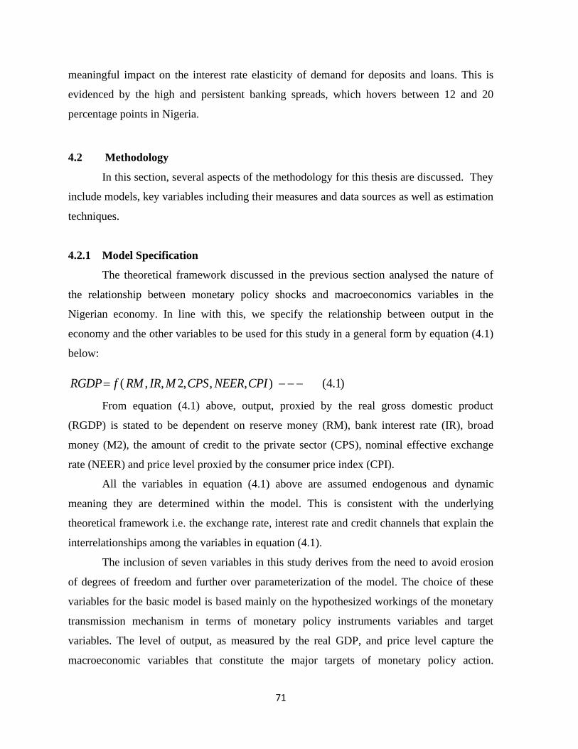
71

meaningful impact on the interest rate elasticity of demand for deposits and loans. This is

evidenced by the high and persistent banking spreads, which hovers between 12 and 20

percentage points in Nigeria.

4.2 Methodology

In this section, several aspects of the methodology for this thesis are discussed. They

include models, key variables including their measures and data sources as well as estimation

techniques.

4.2.1 Model Specification

The theoretical framework discussed in the previous section analysed the nature of

the relationship between monetary policy shocks and macroeconomics variables in the

Nigerian economy. In line with this, we specify the relationship between output in the

economy and the other variables to be used for this study in a general form by equation (4.1)

below:

( , , 2, , , ) (4.1)RGDP f RM IR M CPS NEER CPI= − − −

From equation (4.1) above, output, proxied by the real gross domestic product

(RGDP) is stated to be dependent on reserve money (RM), bank interest rate (IR), broad

money (M2), the amount of credit to the private sector (CPS), nominal effective exchange

rate (NEER) and price level proxied by the consumer price index (CPI).

All the variables in equation (4.1) above are assumed endogenous and dynamic

meaning they are determined within the model. This is consistent with the underlying

theoretical framework i.e. the exchange rate, interest rate and credit channels that explain the

interrelationships among the variables in equation (4.1).

The inclusion of seven variables in this study derives from the need to avoid erosion

of degrees of freedom and further over parameterization of the model. The choice of these

variables for the basic model is based mainly on the hypothesized workings of the monetary

transmission mechanism in terms of monetary policy instruments variables and target

variables. The level of output, as measured by the real GDP, and price level capture the

macroeconomic variables that constitute the major targets of monetary policy action.

72

Contextually, the macroeconomic objectives to be targeted in this study are twofold;

increasing output and minimizing inflationary tendency in the economy. The analysis of the

SVAR model places strong emphasis on identifying the channels through which monetary

policies are propagated to the real sector of the economy.

4.2.2 Key variables

Bank interest rate ( )tIR which is also called the minimum rediscount rate (MRR) is

defined as the rate at which the central bank provides short term loans to commercial banks

and discount houses in its function as a lender of last resort. The choice of this rate hinges on

the fact that it represents the anchor for the determination of other rates. In our preliminary

analysis, experimentations with other forms of interest rates, especially the lending rate,

show that there is no significant difference between the empirical results emanating from the

use of different rates. This is because the various interest rates move in tandem throughout

this period of the analysis. The variable enters the estimable model as an instrument target of

monetary policy. Reserve money ( )tRM is also employed as an instrument target of

monetary policy in the model. Components of ( )tRM are identified as total cash reserves

held by the central bank, vault cash in commercial banks and currency held by the non-bank

public. The variable, credit to the private sector ( tCPS ) captures commercial bank loans and

advances to the private sector and it enters the SVAR as an intermediate target of monetary

policy. Similarly, exchange rate ( )tNEER enters the model as an intermediate target of

monetary policy. Nominal effective exchange rates of the Nigerian naira (N) vis-à-vis the

United States Dollar (US$) as reported by the Central Bank of Nigeria adjusted for relative

movements in general prices of Nigeria and its major trading partner are used as a proxy for

( )tNEER . Aggregate money supply is measured by the sum of currency in circulation,

demand deposits plus savings and time deposits (M2). The use of broad money as proxy for

money supply has become popular in the literature on research conducted in the developed

and developing countries alike, even though their money and capital market is still

developing. This is mainly because the line of division between the narrow and broad money

is waning out by the day. This variable also enters the model as an intermediate target of

monetary policy. Consumer prices ( )tCPI are measured by the all items national composite

73

consumer price index. The variable enters the model as a monetary policy goal. A measure of

output ( )tRGDP enters the model as a monetary policy goal as well.

4.2.3 Data Sources and Type

The study employs quarterly time series data for the period 1970:Q1 to 2008:Q4 from

the annual series available for the period. The starting and the cut-off dates correspond to the

date when the latest data on all variables of interest was available. In our empirical analysis,

we also took the natural logarithm of the real GDP, broad money, consumer price level,

nominal effective exchange rate, credit to the private sector and reserve money. Apart from

aiding interpretation and compactness of results presentation, this form of transformation

tend to reduce heteroskesdasticity significantly (Enders, 1996). The major source of data for

this study is the Central Bank of Nigeria statistical bulletin of 2008.

4.2.4 Estimation Techniques

Given that a simultaneous equation system models the dynamic relationship between

the endogenous and exogenous variables, a vector representation of the Structural Vector

Autoregression (SVAR) system can therefore be given by the equation below:

1( ) (4.2)t t tAx C L x Dz−= + −−−

where A is an invertible ( )n n matrix of variable coefficients describing contemporaneous

relations among the variables. The elements of the square matrix, A, are the structural

parameters on the contemporaneous endogenous variables and ( )C L is a kth degree matrix

polynomial in the lag operator L. D is an ( )n n matrix whose non-zero off–diagonal

elements allow for direct effects of some shocks on more than one endogenous variable in

the system. The vector Z above is assumed to consist of unobservable variables which are

interpreted as disturbances to the structural equations while tx and t

z are vectors with length

equal to the number of structural equations in the model3.

3 If observable exogenous variables exist, they are included as explanatory variables in the VAR.

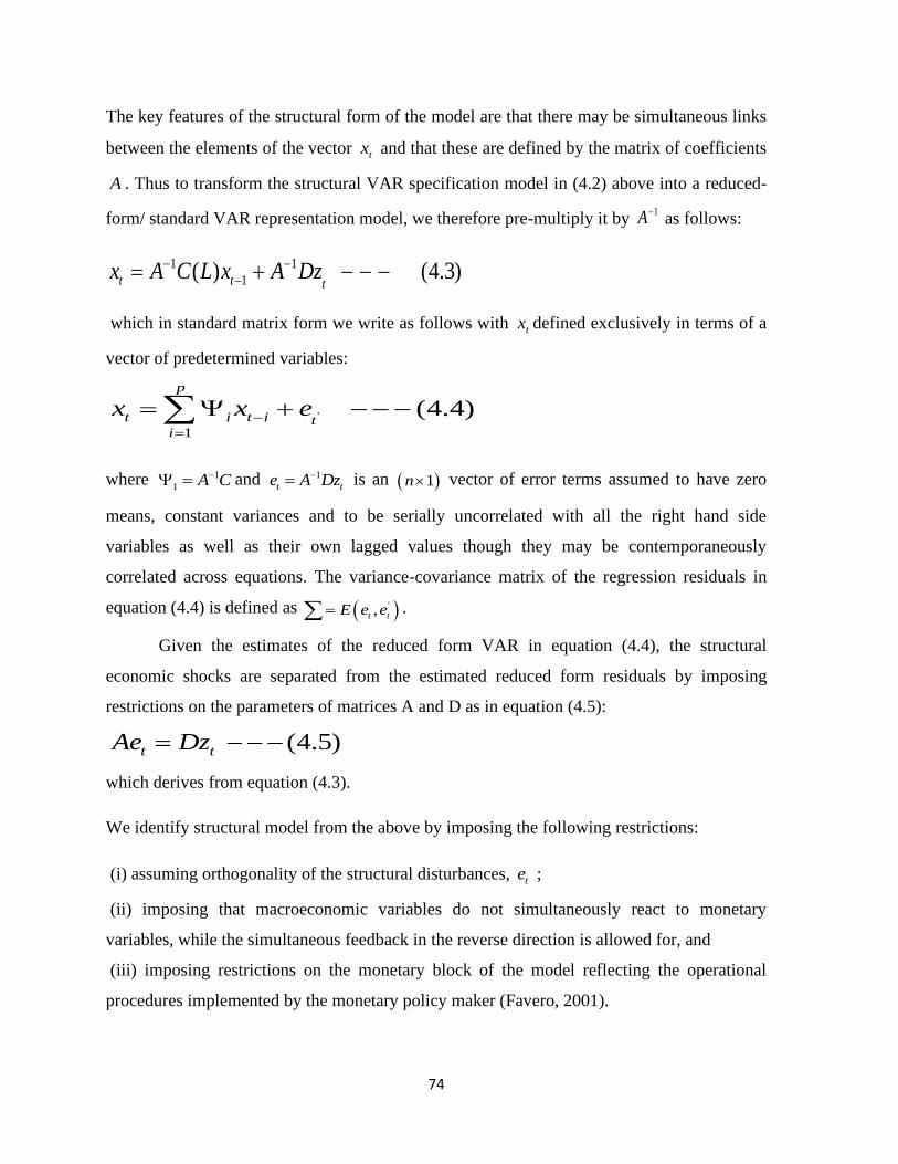
74

The key features of the structural form of the model are that there may be simultaneous links

between the elements of the vector tx and that these are defined by the matrix of coefficients

A . Thus to transform the structural VAR specification model in (4.2) above into a reduced-

form/ standard VAR representation model, we therefore pre-multiply it by 1A− as follows:

1 1

1( ) (4.3)t t tx A C L x A Dz− −

−= + − − −

which in standard matrix form we write as follows with tx defined exclusively in terms of a

vector of predetermined variables:

'

1

(4.4)p

t i t i ti

x x e−

=

= + −−−

where 1

1 A C− = and 1

t te A Dz−= is an ( )1n vector of error terms assumed to have zero

means, constant variances and to be serially uncorrelated with all the right hand side

variables as well as their own lagged values though they may be contemporaneously

correlated across equations. The variance-covariance matrix of the regression residuals in

equation (4.4) is defined as ( )',t tE e e= .

Given the estimates of the reduced form VAR in equation (4.4), the structural

economic shocks are separated from the estimated reduced form residuals by imposing

restrictions on the parameters of matrices A and D as in equation (4.5):

(4.5)t tAe Dz= −−−

which derives from equation (4.3).

We identify structural model from the above by imposing the following restrictions:

(i) assuming orthogonality of the structural disturbances, te ;

(ii) imposing that macroeconomic variables do not simultaneously react to monetary

variables, while the simultaneous feedback in the reverse direction is allowed for, and

(iii) imposing restrictions on the monetary block of the model reflecting the operational

procedures implemented by the monetary policy maker (Favero, 2001).

75

The orthogonality assumption of the structural innovations i.e. ( )', 1t tE z z = , and the

constant variance-covariance matrix of the reduced-form equation residuals i.e. ( )',t tE e e =

impose identifying restrictions on A and D as presented below in equation (4.6):

The matrix is the variance/covariance of the estimated residuals, te , of the standard VAR.

' '' 1 ' ' 1 1 ' 1 (4.7)e t t t tE e e A DE z z D A A D D A− − − − = = = −−−

Given

1

1

t t

t t t

e A Dz

E e e

− =

=

where E is the unconditional expectations operator, and e is the covariance matrix for the

shocks.

(0, )(4.8)

(0, )

t

t t

z N

e N

− − −

An ordinary least squares estimate of the VAR provides an estimate of e which can then be

used with equation (4.8) to obtain estimates of A, D and .

Since matrices A and D are both ( )n n , a total of 22n unknown elements can be

identified upon which ( 1) / 2n n+ restrictions are imposed by equation (4.6). To identify A

and D, therefore, at least 22 ( 1) / 2n n n− + or (3 1) / 2n n− additional restrictions are required.

These restrictions can be imposed in a number of ways. We use the Sims’ (1980) recursive

factorization approach based on a Cholesky decomposition of matrix A which assumes that

elements of matrix A are recursively related and are, therefore, lower triangular. The

implication of this relationship is that identification of the structural shocks is dependent on

the ordering of variables, with the most endogenous variable ordered last (Favero, 2001).

Thus, with a given ordering, the first variable has no contemporaneous relationships with all

other variables in the model, indicating that its reduced form shock is identical to its

structural shock; the second variable has contemporaneous interactions only with its own and

' ' (4.6)A A DD = −−−

76

the first structural shock; the third variable is contemporaneously affected by its own and the

first two structural shocks; and so on. However in this framework, the system is just (exactly)

identified. The exactly identified or just identified condition is obtained when the number of

information is equal to the number of parameter to be estimated. It is only under the exactly

or just identified and over-identified conditions that the estimation process can take place.

4.2.5 Estimation Procedures

Thus, the procedure for operating a straightforward SVAR involves a number of

discrete steps. First, we need to determine the order of integration of the variables. The next

step involves estimating the reduced form VAR, ensuring that enough lags are incorporated

to ensure no serial correlation in the residuals. An important aspect in specification of the

VAR is the determination of the lag order of the autoregressive lag polynomial since all

inference in the VAR model depends on the correct model specification. We therefore use

established information criterion to determine the optimal lag length, that is, seeking to

measure the closeness of an estimated model to the true data-generating process over the

domain of the regressand. There are various other test procedures for the determination of the

lag length but the commonly used ones are the Akaike, the Schwartz and the Hannan-Quinn

information criteria.

In several contributions, the effect of lag length selection has been demonstrated. Lutkepohl

(1991) indicates that selecting a higher order lag length than the true lag causes an increase in

the mean square forecast errors of the VAR and that under-fitting the lag length often

generates auto-correlated errors. Braun and Miinik (1993) show that impulse response

functions and variance decompositions are inconsistently derived from the estimated VAR

when the lag length differs from the true lag length. Johansen (1991) and Gonzalo (1994)

point out that VAR order selection may affect proper inference on cointegrating vector and

rank. After the reduced form VAR is estimated we then impose sufficient restrictions to

identify the structural parameters of the model.

For the purpose of this study, seven variables are included in the SVAR namely,

Output and consumer prices which enter as policy goals or the ultimate targets; reserve

money and bank lending rate as operating targets; and commercial bank loans to the private

77

sector, exchange rates and broad money as intermediate targets. The structural shocks in

equation (4.6) are identified according to the following scheme:

21

31 32 34 35 36 37

41 42

251 52 56

64 66

73 74 75 76

11

22

33

1 0 0 0 0 0 0

1 0 0 0 0 0

1

0 1 0 0 0 ;

0 0 1 0

0 0 0 0 0

0 0 1

0 0 0 0 0 0

0 0 0 0 0 0

0 0 0 0

RGDP

t

CPI

t

CPS

t

NEER

t t

M

t

IR

t

RM

t

e

a e

a a a a a a e

A a a e e

a a a e

a a e

a a a a e

d

d

d

D

= =

= 44

255

66

77

0 0

0 0 0 0 0 0 ; (4.9)

0 0 0 0 0 0

0 0 0 0 0 0

0 0 0 0 0 0

RGDP

t

CPI

t

CPS

t

NEER

t t

M

t

IR

t

RM

t

z

z

z

d z z

d z

d z

d z

= − − −

The non-zero coefficients ija and

ijd in matrices A and D, respectively, show that any

residual j in matrices te and tz , in that order, has an instantaneous impact on variable i . The

first two equations suggest that output and consumer prices are sluggish in responding to

shocks to monetary variables in the economy. This scheme is based on the observation that

most types of real economic activity may respond only with a lag to monetary variables

because of inherent inertia and planning delays (Karame and Olmedo, 2002). Proposed by

Bernanke and Mihov (1995), the validity of this argument has been supported by a number

studies (Cheng, 2006; Berkelmans, 2005; Vonnak, 2005; Karame and Olmedo, 2002).

Commercial bank loans and advances to the private sector are postulated to be

contemporaneously affected by all variables in the system. Blundell-Wignall and Gizycki

(1992) argue that expectations of future activity form an important determinant of credit

demand by economic agents. Assuming current output, price level, exchange rates, interest

78

rates, and money supply give some indication of what is expected in the future (Berkelmans,

2005) and that economic agents are indeed forward looking, bank lending may respond

contemporaneously to all variables in the system.

Modelling contemporaneous responses of exchange rates to other variables in a

SVAR is relatively standard across studies. Becklemans (2005) uses a real trade-weighted

exchange rate index in a study of Australia and assumes that the index responds

instantaneously to all variables in the system. Borys and Horvath (2007) in a study of the

Czech Republic and Piffanelli (2001) in a study of Germany assume all variables in the

system affect exchange rates instantaneously. In a study of Kenya, Cheng (2006) employs a

nominal effective exchange rate and maintains that the exchange rate responds

contemporaneously to all variables in the SVAR. Thus, given the depth of Nigeria’s financial

sector; while the exchange rate may respond contemporaneously to changes in the level of

output and consumer prices, there is reason to believe that it may also respond

contemporaneously to monetary variables as well.

Some studies include variables that specifically capture external price shocks, most

common of which are oil price shocks. Oil price disturbances are usually singled out among

the oil price shocks. Other studies also incorporate international financial market interest rate

shocks and the Federal Reserve Bank Funds Rate has been widely used as a proxy for these

shocks. This study, however, does not explicitly model the external shocks for two reasons.

One of which is the fact that, it is expected that any disturbances in the external sector will be

captured by the exchange rate variable. The other very important reason is that, the complete

SVAR analysed in this study has seven variables, which is already large by SVAR standards.

Increasing the number of variables without proper justification, therefore, is likely to

decrease the power of the model without making meaningful additions.

The fifth equation in (4.9) above is a standard money demand function. The equation

postulates that money demand behaviour in the country makes aggregate money supply

respond contemporaneously to changes in consumer prices, output and interest rates but not

to other variables in the system, akin to Sims and Zha (1998). The last two equations

constitute the monetary policy feedback rule. While the Central Bank of Nigeria’s tacit desire

is to target inflation via reserve money, there is reason to believe that the monetary authority

79

also target short term interest rates. The study, therefore, assumes that the country employs

hybrid operating procedures, with the bank rate and reserve money as operating targets. In

this framework, both interest rates and reserves are expected to contain information about

monetary policy (Bernanke, 1996). The country’s effective operating target, accordingly, is

determined empirically.

The monetary policy feedback rule is drawn on the assumption that information

delays impede policymakers to react within the present to economic activity and price level

developments (Karame and Olmedo, 2002). Both the bank rate and reserve money, therefore,

do not respond contemporaneously to output and consumer prices. The bank rate,

specifically, responds contemporaneously to exchange rates only. While exchange rate data

is available real-time, data on other variables including bank loans and monetary aggregates

is usually available to the monetary authorities with a lag. Reserve money, on the other hand,

is assumed to respond contemporaneously to all monetary variables because by its definition,

this information is inherent in the monetary aggregate.

4.2.6 Analysis

Analysis of the SVAR is carried out in three modular experiments. First, a generic

model comprising the country’s monetary policy goals and operating targets is estimated.

Output and price level enter the model as policy goals while bank rate and reserve money go

in as operating targets. The rationale for estimating the generic model is to establish how the

two monetary policy goals respond to each of the operating targets and to find out if

monetary authorities react to changes in the policy goals. In addition, the estimated generic

model is used to determine which of the two monetary policy operating-targets has a greater

impact on the policy goals. At the second level of analysis; bank lending, exchange rates and

interest rate, representing three different transmission processes, are separately appended to

the generic model and estimated. At the third and final level of analysis, all variables found

to hold important information in the country’s monetary transmission process are pooled and

a composite SVAR is estimated.

80

4.2.7 Generic Model

Investigation of the monetary transmission process commences with a simple four variable

generic model. The vector of endogenous variables included in the model is presented in

equation (4.10):

[ , , ] (4.10)t t t tRGDP f CPI IR RM= − − − −

Following the identification scheme in system of equations (4.10), the equation separating

structural economic shocks from the estimated reduced form residuals for the generic model

is presented as:

11

21 22

33

0 01 0 0

1 0 0 0 (4.11)

0 0 1 0 0

CPI CPI

t t

IR IR

t t

RM RM

t t

de z

a e d z

de z

= − − −−

4.2.7.1 Channels of Monetary Transmission

In line with our outlined objective, we move the analysis further from the generic model to

examination of more specific transmission channels for the purpose of establishing the

monetary transmission process. The three channels deemed to exist in Nigeria are therefore

considered, viz., bank lending, exchange rates and interest rate channels, with particular

attention to measuring the importance of each channel in the transmission process.

4.2.7.2 BANK LENDING CHANNEL

The bank lending model is a component of the credit channel of monetary transmission. The

underlying argument in the credit channel is that asymmetric information and costly

enforcement of contracts create agency problems in financial markets (Bernanke & Gertler,

1995). Two mechanisms explain this process: balance sheet and bank lending. The balance

sheet model operates through the net worth of business firms (Mishkin, 1995) and

transmission occurs either through equity prices or interest rates and firms‟ cash-flows.

These affect the severity of adverse selection and moral hazard problems, which in turn

impact on lending, investment and output. Owing to data constraints, the balance sheet

channel is not pursued further in this study.

The bank lending model, on the other hand, operates through quantity rather than price of

credit. A monetary policy shock is assumed to be transmitted through changes in bank

reserves, the total amount of available bank credit, and bank lending. The channel presumes

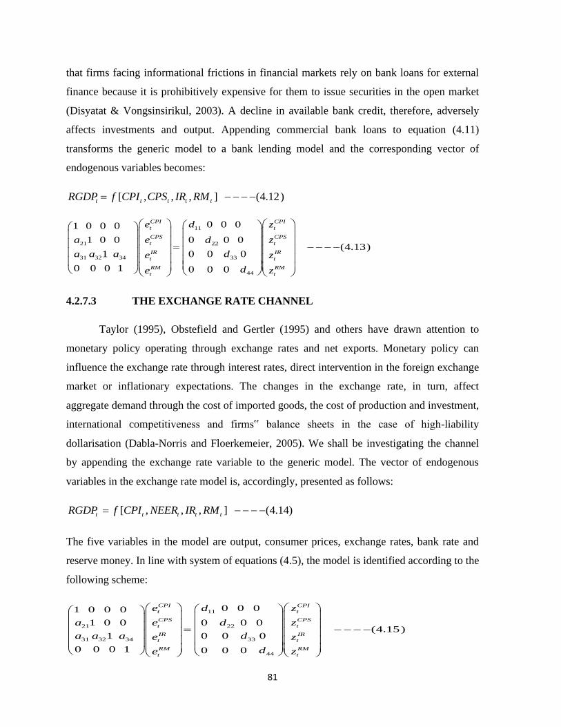
81

that firms facing informational frictions in financial markets rely on bank loans for external

finance because it is prohibitively expensive for them to issue securities in the open market

(Disyatat & Vongsinsirikul, 2003). A decline in available bank credit, therefore, adversely

affects investments and output. Appending commercial bank loans to equation (4.11)

transforms the generic model to a bank lending model and the corresponding vector of

endogenous variables becomes:

[ , , , ] (4.12)t t t t tRGDP f CPI CPS IR RM= − − − −

11

21 22

31 32 34 33

44

0 0 01 0 0 0

1 0 0 0 0 0(4.13)

1 0 0 0

0 0 0 1 0 0 0

CPI CPI

t t

CPS CPS

t t

IR IR

t t

RM RM

t t

e zd

e za d

a a a de z

de z

= − − − −

4.2.7.3 THE EXCHANGE RATE CHANNEL

Taylor (1995), Obstefield and Gertler (1995) and others have drawn attention to

monetary policy operating through exchange rates and net exports. Monetary policy can

influence the exchange rate through interest rates, direct intervention in the foreign exchange

market or inflationary expectations. The changes in the exchange rate, in turn, affect

aggregate demand through the cost of imported goods, the cost of production and investment,

international competitiveness and firms‟ balance sheets in the case of high-liability

dollarisation (Dabla-Norris and Floerkemeier, 2005). We shall be investigating the channel

by appending the exchange rate variable to the generic model. The vector of endogenous

variables in the exchange rate model is, accordingly, presented as follows:

[ , , , ] (4.14)t t t t tRGDP f CPI NEER IR RM= − − − −

The five variables in the model are output, consumer prices, exchange rates, bank rate and

reserve money. In line with system of equations (4.5), the model is identified according to the

following scheme:

11

21 22

31 32 34 33

44

0 0 01 0 0 0

1 0 0 0 0 0(4.15)

1 0 0 0

0 0 0 1 0 0 0

CPI CPI

t t

CPS CPS

t t

IR IR

t t

RM RM

t t

e zd

e za d

a a a de z

de z

= − − − −

82

4.2.7.4 THE INTEREST RATE CHANNEL

An alternative channel of monetary transmission is the traditional Keynesian view

which postulates that monetary policy can influence the real cost of borrowing by setting

nominal short-term interest rates. The channel emphasizes the role of interest rates in the

transmission mechanism, elevating the process to a direct link between changes in aggregate

money supply and absorption (Bolnick, 1991). According to this view, owing to price

rigidities, nominal interest rate changes lead to corresponding real interest rate changes,

which have an impact on business, housing, and inventory investment as well as on consumer

durable spending. These occur primarily because of the existence of a time lag between

observing the impulses and being able to distinguish between permanent and transitory

impulses and real and nominal shocks. Appending to the generic model, the vector of

endogenous variables in the interest rate model is presented as:

[ , , 2 , ] (4.16)t t t t tRGDP f CPI IR M RM= − − − −

where the five variables in the model are output, consumer prices, bank rate, M2 and reserve

money. Following the identification scheme in system of equations (4.5), the model is

identified as:

11

2 2

21 22

31 32 34 33

44

0 0 01 0 0 0

1 0 0 0 0 0(4.17)

1 0 0 0

0 0 0 1 0 0 0

CPI CPI

t t

M M

t t

IR IR

t t

RM RM

t t

e zd

e za d

a a a de z

de z

= − − − −

4.2.7.5 THE COMPOSITE MODEL

The possibility that bank lending, exchange rate and interest rate channels may

contain important additional information for the country’s monetary transmission process

from the analysis carried out in the previous section cannot be ruled out. In the light of this, a

composite model of monetary transmission in Nigeria can be drawn with the following

vector of endogenous variables:

[ , , , 2 , , ] (4.18)t t t t t t tRGDP f CPI CPS NEER M IR RM= − − − −

83

which is identified according to system of equations (4.6). Impulse responses for the

consolidated model over some period of years shall then be carried out. This will help

establish the most important channels of monetary transmission in the Nigerian economy.

Following this, a general identification scheme based on short run restrictions

developed in system of equations (4.9) will then be used for identifying structural shocks in

each of the models. Analysis in the study shall be carried out only for the short run to

conform with the subject matter under investigation. In essence, since there is a general

consensus among economists that monetary policy affects only the price level in the long

run, there shall be little or no need in extending the investigation of the monetary

transmission process to cover the long run.

ERROR CORRECTION MECHANISM (ECM)

If the variables in our empirical model have unit roots from the Augmented Dickey-

Fuller (1979) and Phillips-Perron (1988) tests conducted, then we can capitalise on the

likelihood of co-movements in their behaviour hence the possibilities that they trend together

towards a long-run equilibrium. Using Granger representation theorem (Engle and Granger

1987), (which states that if two variables are cointegrated, then the relationship between the

two can be expressed as ECM) the error correction model is specified as follows:

1 1 1

1 1 1

1

1

2 2(4.19)

N M P

t i t i t j t j t k t k

i j k

Q R S

t l t l t h t h t f t f

l h f

V

t g t g t t

g

RGDP RGDP CPI CPI RM RM

IR IR CPS CPS M M

NEER NEER Z

− − −

= = =

− − −

= = =

− −

=

= + + + + + +

+ + + + + +− −−

+ + +

where , , , , , , , , , , , , , , are the parameter estimates, denotes the

first difference operator and t is a random error term.

84

Equation (4.19) implies that the first differences of the variables are explained by lagged

differences and the lagged stationary linear relationship, 1tZ − .

Thus, the nature of the error correction term is what determines the nature of the

cointegration relationships among the variables (Engsted and Bentzen, 2001). If the

cointegrating relations (equilibrium conditions) are imposed, the error correction models

describe the way output will adjust towards their equilibrium state in each time period. In the

short-run, deviation of output from their long-run equilibrium path will feed back on their

future changes in order to force their movement towards the long-run equilibrium state since

the variables are supposed to be cointegrated. The cointegration term is known as the error

correction term since the deviation from long-run equilibrium is corrected gradually through

a series of partial short-run adjustments. The cointegrating vectors from which the error

correction terms are derived are each indicating an independent direction where a stable,

meaningful long-run equilibrium exists. The coefficients of the error correction terms,

however, represent the proportion by which the long-run disequilibrium in the dependent

variable is corrected in each short-term period.

85

CHAPTER FIVE

ANALYSIS OF EMPIRICAL RESULTS

The preoccupation of this chapter is to investigate the time series properties of the

SVAR model variables of this study and present its empirical findings. Specifically, the

statistical and time series properties of the variables are discussed in order to explicitly

establish compatibility of the series with the inherent characteristics of the models vis-à-vis

the estimation techniques employed.

5.1. Statistical Properties of the Variables

The characteristics of the annual time series data used in the regression analysis are

presented in the summary statistics table below. It provides information about the means,

medians, standard deviations as well as the skewness and Jarque-Bera statistics of each

variable. As indicated by the various statistics in Table 5.1 below, the variables are not

haphazardly distributed. The mean values of the natural log of real gross domestic product

(RGDP) and the natural log of consumer price index (CPI) are 11.77 and 1.86 respectively

while the mean of values of bank rate of interest (IR) and natural log of reserve money (RM)

stood at 14.67 and 10.14 respectively also. The summary of statistics table also provides

information on other explanatory variables such as the natural logs of amount of credit to the

private sector, nominal effective exchange rate (NEER) and broad money (M2).

Table 5.1: Summary Statistics of Variables

Sample: 1970:I - 2008:IV

RGDP CPI NEER CPS M2 IR RM

Mean 11.77 1.86 3.22 10.70 11.25 14.67 10.14

Median 12.37 1.70 4.60 10.30 10.76 16.50 9.38

Maximum 13.42 5.26 4.73 15.88 16.03 29.80 14.14

Minimum 8.35 -1.47 -1.61 5.86 6.89 6.00 5.96

Std. Dev. 1.49 2.30 2.04 2.75 2.59 6.66 2.56

Skewness -1.12 0.06 -1.09 0.06 0.07 0.25 -0.01

Kurtosis 2.97 1.49 2.76 1.99 1.94 2.01 1.68

Jarque-Bera 32.44 14.85 31.54 6.73 7.37 7.95 11.30

Probability 0.00 0.00 0.00 0.03 0.03 0.02 0.00

Observations 156 156 156 156 156 156 156

86

Additionally, the skewness and standard deviation statistics show that the variances of

the variables are not unnecessarily large while the Jarque-Bera statistics of each variable

accepts the null hypothesis of normality at one (1) per cent level of significance. Also, given

the time scope of the study (1970:I to 2008:IV) and the frequency of the data (quarterly), all

the variables have 156 observations.

5.2. Stationarity Tests

Rather than the exception, it is the rule in time series analysis to investigate the

stationarity of macroeconomic variables before they are used in regressions. The reason for

this is that estimation with non-stationary variables results in bias and inconsistency of the

estimates of coefficient standard errors thus increasing the likelihood of drawing false

inferences. Due to this and Enders’ (1995) suggestion that “it is safer to use two types of unit

root tests”, the variables for our analysis are subjected to two types of unit root tests to

determine whether they are stationary series or non-stationary series. If the results from these

unit root tests reinforce each other, then we can have confidence in the results. The tests

employed are the Augmented Dickey-Fuller test (ADF) and the Phillips-Perron test (PP). For

both the ADF and the PP tests, two models are considered: with drift as well as with drift and

trend. The null hypothesis in both the ADF and PP tests is the presence of unit root.

The results of the unit root test as presented, based on the PP and the ADF test

statistic using both the Akaike and Schwarz information criteria, indicate that all the

variables under consideration exhibit unit roots at different critical levels. However, none of

the variables was found stationary in levels. The variables are only found stationary after

differencing once. This implies that the variables are integrated of order one (I(1)). The unit

root results are presented in Tables 5.2, 5.3 and 5.4 below.

Appendix 2 also provides a graph showing the trends of the data in the variables of

the model to be estimated.

87

Table 5.2: Unit Root Test Result Using Augmented Dickey-Fuller

Variable ADF using (AIC) Decision

With Drift With Drift &

Trend

RGDP Level -2.134051 1.975052

I(1)

∆Level -12.7485 -12.8803

M2 Level 0.277984 -2.386134

I(1)

∆Level -3.522293 -3.548122

RM Level -0.724024 -2.833557

I(1)

∆Level -3.752137 -3.750775

IR Level -1.45827 -1.430317

I(1)

∆Level -9.803652 -9.813752

CPI Level -0.604036 -2.067708

I(1)

∆Level -3.647734 -3.627714

NEER Level -1.607933 -1.428179

I(1)

∆Level -12.32883 -12.33341

CPS Level 0.77461 -1.88318

I(1)

∆Level -3.46324 -3.54105

CRITICAL VALUES

1% 5%

(i) Auxilliary Regression with Drift -3.472813 -2.880088

(ii) Auxilliary Regression with Drift and Trend -4.018748 -3.439267

(iii) ∆ represents first difference operator

88

Table 5.3: Unit Root Test Result Using Augmented Dickey-Fuller

Variable ADF using (SIC) Decision


Trend

RGDP Level -2.134051 -1.975052

I(1)

∆Level -12.7485 -12.8803

M2 Level 0.277984 -2.386134

I(1)

∆Level -3.522293 -3.548122

RM Level -0.724024 -2.833557

I(1)

∆Level -3.752137 -3.750775

IR Level -1.45827 -1.430317

I(1)

∆Level -9.803652 -9.813752

CPI Level -0.604036 -2.067708

I(1)

∆Level -3.647734 -3.627714

NEER Level -1.607933 -1.428179

I(1)

∆Level -12.32883 -12.33341

CPS Level 0.70444 -1.82612

I(1)

∆Level -3.81777 -3.88376

CRITICAL VALUES

1% 5%




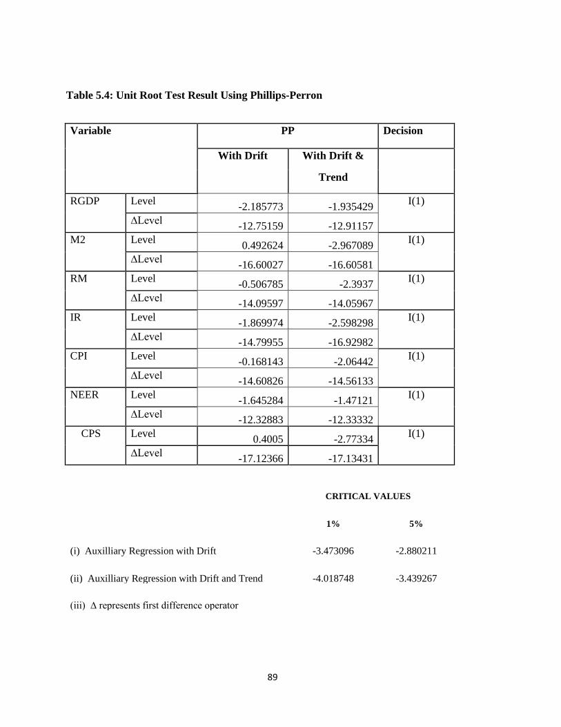
89

Table 5.4: Unit Root Test Result Using Phillips-Perron

Variable PP Decision


Trend

RGDP Level -2.185773 -1.935429

I(1)

∆Level -12.75159 -12.91157

M2 Level 0.492624 -2.967089

I(1)

∆Level -16.60027 -16.60581

RM Level -0.506785 -2.3937

I(1)

∆Level -14.09597 -14.05967

IR Level -1.869974 -2.598298

I(1)

∆Level -14.79955 -16.92982

CPI Level -0.168143 -2.06442

I(1)

∆Level -14.60826 -14.56133

NEER Level -1.645284 -1.47121

I(1)

∆Level -12.32883 -12.33332

CPS Level 0.4005 -2.77334

I(1)

∆Level -17.12366 -17.13431

CRITICAL VALUES

1% 5%




90

5.3 The Impulse Responses of Bank Interest rate and Reserve Money: The Generic

Model

We begin our empirical analysis by looking at the response of the central bank to

shocks in the policy goals. Figure 5.1 below presents the impulse responses of the bank rate

and reserve money to structural one standard deviation innovations in output and consumer

prices over a three-year horizon. Impulse responses of output and consumer prices to own

shocks are also presented in the same figure. The time scale measured on the primary

horizontal axis is in quarters and the dashed red lines are analytic confidence intervals

obtained from variance-covariance matrices after the final iteration.

Figure 5.1: The Impulse Responses of Interest Rate and Reserve Money: The Generic Model

-.4

-.2

.0

.2

.4

.6

1 2 3 4 5 6 7 8 9 10 11 12

Response of D(IR) to D(RGDP)

-.4

-.2

.0

.2

.4

.6

1 2 3 4 5 6 7 8 9 10 11 12

Response of D(IR) to D(CPI)

-.08

-.04

.00

.04

.08

.12

1 2 3 4 5 6 7 8 9 10 11 12

Response of D(RM) to D(RGDP)

-.08

-.04

.00

.04

.08

.12

1 2 3 4 5 6 7 8 9 10 11 12

Response of D(RM) to D(CPI)

91

An output shock corresponding to an unanticipated 0.18 percent variation in output

and a supply shock equivalent to an unexpected 0.108 percent rise in consumer prices in the

first quarter triggers significant responses by the central bank. This shows that the monetary

authorities in Nigeria are concerned with both inflation and economic growth in accordance

with its objectives as contained in the CBN Act of 2007. The monetary authority’s response

to output shock is to loosen monetary policy through a decrease in the bank rate so as to

further boost the growth of output. In response to price shock, monetary policy is tightened

by raising the bank rate to arrest the increase in the consumer prices. The central bank’s

response with regard to reserve money shows their determination to address any observed

macroeconomic imbalance. Following the sudden decrease in output, as shown in Figure 5.1

above, reserve money declines by -0.11 percent while the unexpected rise in consumer prices

triggers an increase in reserve money by 0.87 percent.

Figure 5.2: The Impulse Responses of Output and Consumer Prices: The Generic Model

-.04

-.02

.00

.02

.04

1 2 3 4 5 6 7 8 9 10 11 12

Response of D(RGDP) to D(IR)

-.04

-.02

.00

.02

.04

1 2 3 4 5 6 7 8 9 10 11 12

Response of D(RGDP) to D(RM)

-.03

-.02

-.01

.00

.01

.02

1 2 3 4 5 6 7 8 9 10 11 12

Response of D(CPI) to D(IR)

-.03

-.02

-.01

.00

.01

.02

1 2 3 4 5 6 7 8 9 10 11 12

Response of D(CPI) to D(RM)

92

Next, we analyse how monetary policy goals are affected by shocks to the operating

targets. To do this, we plot the impulse responses of output and consumer prices to structural

one standard deviation shocks in the bank rate and reserve money. Figure 5.2 above reveals

that a monetary policy shock corresponding to an unanticipated increase in the bank rate of

about 2.02 percent leads to output declining to a permanent position on the baseline

throughout the first four quarters. The response of price level to the monetary tightening of

interest rate was found to be exactly similar to that of output maintaining a baseline position

throughout the first eight quarters of the year.

Figure 5.2 above also shows that an contractionary monetary shock equivalent to a

0.105 percent sudden increase in reserve money in the first quarter causes a decrease in

output from the baseline position in the first quarter to -0.02 percent in the second and third

quarters. However, there was a 0.03 percent increase in output in the fourth quarter, which

returned to the baseline from the fifth quarter and remained even till the ninth quarter.

Consumer prices response to a 0.105 percent unexpected increase in reserve money by the

monetary authority is a -0.06 percent decrease in prices which only oscillate back to baseline

and changed into a 0.03 percent rise in price in the fourth quarter. However, from the fifth

quarter to the twelfth, it stabilizes on the baseline. Overall, shocks to one of the monetary

policy operating targets, reserve money, attract significant output and consumer price

responses. The implication of this is that, even though interest rate does not seem to have

much impact, monetary factor via reserve money remains a primary determinant of price

level and output in Nigeria. In essence, we can infer from this that reserve money remains the

most effective policy instruments at the disposal of the monetary authority.

93

5.3.1 Variance Decomposition for The Generic Model

To determine the relative importance of each structural innovation in explaining

fluctuations of the variables in the generic model, Table 5.5 presents variance

decompositions for each variable in the model over a two-year forecast horizon. Given the

two policy goals, fluctuations in both the bank rate and reserve money witnessed a mixed

response from the target variables. Consumer prices as well as some magnitude of output

seem to be more responsive towards reserve money variation than interest rate connoting that

the former impacts more on our target variables than the latter. The observed response of

consumer prices to reserve money can therefore be interpreted to mean that the principal

objective of monetary policy in the country is price stability. Table 5.5(C) shows that shocks

to both the consumer prices and output account for less than one percent of the bank rate

fluctuations after the first four quarters of the first year but consumer prices accounts for

approximately 1 percent throughout the four quarters of the second year. However, Table

5.5(D) shows that shocks to consumer prices account for 19 percent of the reserve money

fluctuations after the first quarter, 19.4 percent after the second quarter, 19.8 and 20.1 percent

after the third and fourth quarters respectively. Shocks to output, on the other hand, account

for less 1 percent of reserve money fluctuations throughout the four quarters of the first year

but accounts for 6.4 percent throughout the four quarters of the second year. This indicates

that price level and output are responsive to reserve money.

Table 5.5A: VARIANCE DECOMPOSITION FOR THE GENERIC MODEL: RGDP

A VARIANCE DECOMPOSITION OF RGDP

QUARTER D(RGDP) D(CPI) D(IR) D(RM)

1 100.0000 0.000000 0.000000 0.000000

2 99.87899 0.100709 0.000825 0.019475

3 99.78116 0.182125 0.001491 0.035219

4 99.70204 0.247974 0.002031 0.047952

5 93.80694 0.736720 0.085440 5.370904

6 93.63168 0.844534 0.085547 5.438235

7 93.48879 0.932654 0.085637 5.492917

8 93.37221 1.004722 0.085712 5.537354

94

Table 5.5B: VARIANCE DECOMPOSITION FOR THE GENERIC MODEL: CPI

B VARIANCE DECOMPOSITION OF CPI


1 0.252269 99.74773 0.000000 0.000000

2 0.295289 99.62139 0.003385 0.079932

3 0.329811 99.52001 0.006101 0.144075

4 0.357566 99.43850 0.008285 0.195644

5 0.234557 84.77592 0.012724 14.97680

6 0.279652 84.56691 0.014783 15.13865

7 0.315948 84.39955 0.016446 15.26805

8 0.345253 84.26513 0.017792 15.37183

Table 5.5C: VARIANCE DECOMPOSITION FOR THE GENERIC MODEL: IR

C VARIANCE DECOMPOSITION OF IR


1 0.067726 0.006849 99.92543 0.000000

2 0.067799 0.007531 99.92454 0.000132

3 0.067858 0.008083 99.92382 0.000239

4 0.067905 0.008531 99.92324 0.000325

5 0.092759 0.878481 97.07482 1.953941

6 0.092766 0.878498 97.07473 1.954009

7 0.092772 0.878510 97.07465 1.954064

8 0.092777 0.878520 97.07459 1.954110

Table 5.5D: VARIANCE DECOMPOSITION FOR THE GENERIC MODEL: RM

D VARIANCE DECOMPOSITION OF RM


1 0.211812 18.98898 1.034370 79.76483

2 0.273852 19.43464 1.031197 79.26031

3 0.323424 19.79074 1.028661 78.85717

4 0.363143 20.07606 1.026630 78.53417

5 6.388835 18.27278 1.049633 74.28875

6 6.369428 18.63976 1.041203 73.94961

7 6.353957 18.93570 1.034435 73.67591

8 6.341587 19.17511 1.028986 73.45432

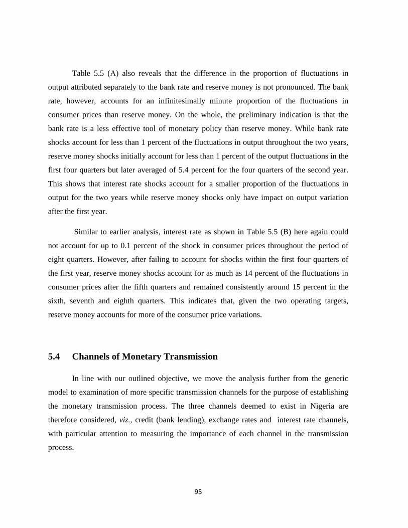
95

Table 5.5 (A) also reveals that the difference in the proportion of fluctuations in

output attributed separately to the bank rate and reserve money is not pronounced. The bank

rate, however, accounts for an infinitesimally minute proportion of the fluctuations in

consumer prices than reserve money. On the whole, the preliminary indication is that the

bank rate is a less effective tool of monetary policy than reserve money. While bank rate

shocks account for less than 1 percent of the fluctuations in output throughout the two years,

reserve money shocks initially account for less than 1 percent of the output fluctuations in the

first four quarters but later averaged of 5.4 percent for the four quarters of the second year.

This shows that interest rate shocks account for a smaller proportion of the fluctuations in

output for the two years while reserve money shocks only have impact on output variation

after the first year.

Similar to earlier analysis, interest rate as shown in Table 5.5 (B) here again could

not account for up to 0.1 percent of the shock in consumer prices throughout the period of

eight quarters. However, after failing to account for shocks within the first four quarters of

the first year, reserve money shocks account for as much as 14 percent of the fluctuations in

consumer prices after the fifth quarters and remained consistently around 15 percent in the

sixth, seventh and eighth quarters. This indicates that, given the two operating targets,

reserve money accounts for more of the consumer price variations.

5.4 Channels of Monetary Transmission

In line with our outlined objective, we move the analysis further from the generic

model to examination of more specific transmission channels for the purpose of establishing

the monetary transmission process. The three channels deemed to exist in Nigeria are

therefore considered, viz., credit (bank lending), exchange rates and interest rate channels,

with particular attention to measuring the importance of each channel in the transmission

process.

96

5.4.1 Bank Lending Model

The SVAR under investigation in equation (4.12) and (4.13) comprises of five

variables, which include output, consumer prices, commercial bank loans to the private

sector, bank interest rate and reserve money. Thus, Figure 5.3 presents impulse responses of

output, consumer prices and bank loans to innovations in the bank rate, reserve money and

bank lending.

Figure 5.3 below shows that a shock equivalent to an unanticipated marginal increase

in the bank rate of about 0.001 percent and a 0.04 percent increase in the reserve money

causes credit to the private sector to decline from 0.89 percent in the first quarter to negative

0.23 percent below baseline after the second quarter and remains significant even till the

third quarter. The response of output to the shock in commercial bank lending shows a

negative 0.12 percent reduction in output for the second quarter and negative 0.08 percent for

the third quarter. Output response further shows some slight fluctuations, in tandem with

bank lending variations, between the fifth and sixth quarters before returning to baseline in

the seventh quarter.

The same Figure 5.3 also shows the response of consumer prices at a time

corresponding to the period of variation in commercial bank lending. Following a shock in

bank lending, consumer prices fall to -0.15 percent and -0.10 percent in the second and third

quarters respectively, increasing slightly when bank lending returned to baseline before

normalizing from the seventh quarter. The inference from this is that variation in bank

lending impacts both price levels and output in the economy.

97

Figure 5.3: Impulse Response for the Bank Lending Model

-.08

-.04

.00

.04

.08

.12

1 2 3 4 5 6 7 8 9 10 11 12

Response of D(CPS) to D(CPS)

-.08

-.04

.00

.04

.08

.12

1 2 3 4 5 6 7 8 9 10 11 12

Response of D(CPS) to D(IR)

-.08

-.04

.00

.04

.08

.12

1 2 3 4 5 6 7 8 9 10 11 12

Response of D(CPS) to D(RM)

-.06

-.04

-.02

.00

.02

.04

1 2 3 4 5 6 7 8 9 10 11 12

Response of D(RGDP) to D(CPS)

-.06

-.04

-.02

.00

.02

.04

1 2 3 4 5 6 7 8 9 10 11 12


-.06

-.04

-.02

.00

.02

.04

1 2 3 4 5 6 7 8 9 10 11 12


-.04

-.03

-.02

-.01

.00

.01

.02

1 2 3 4 5 6 7 8 9 10 11 12

Response of D(CPI) to D(CPS)

-.04

-.03

-.02

-.01

.00

.01

.02

1 2 3 4 5 6 7 8 9 10 11 12


-.04

-.03

-.02

-.01

.00

.01

.02

1 2 3 4 5 6 7 8 9 10 11 12


98

5.4.2 Exchange Rate Model

Investigating the exchange rate channel under the SVAR analysis as defined in

equation (4.14) and (4.15) requires five variables, which include output, consumer prices,

nominal effective exchange rate, bank interest rate and reserve money. Following this, Figure

5.4 below presents impulse responses of exchange rate to own, bank interest rate and reserve

money shocks and responses of output and consumer prices to innovations in exchange rate,

bank lending rate and reserve money.

As shown in Figure 5.4 below, a monetary tightening corresponding to an unexpected

2.02 percent increase in the bank interest rate leads to no change in the exchange rate causing

it to remain on the baseline throughout the first to the twelfth quarter. In line with theoretical

expectations, the exchange rate does not respond to shock in the reserve money equivalent to

a 1.05 percent sudden increase hence also remaining on the baseline throughout the twelve

quarters. In the same light, an exchange rate shock equivalent to a depreciation of the

domestic currency by 0.55 percent was found to attract no response in both the output in the

domestic economy as well as the consumer price level. Consumer prices as well as output

response remains stable on the baseline beginning from the first to the twelfth quarter. The

implication of this result is that variations in exchange rate, precipitated by shock in the

reserve money or interest rate, does not in any way affect both the output and price level in

the domestic economy of Nigeria.

99

Figure 5.4: Impulse Response for Exchange Rate Model

-.2

.0

.2

.4

.6

.8

1 2 3 4 5 6 7 8 9 10 11 12

Response of D(NEER) to D(NEER)

-.2

.0

.2

.4

.6

.8

1 2 3 4 5 6 7 8 9 10 11 12

Response of D(NEER) to D(IR)

-.2

.0

.2

.4

.6

.8

1 2 3 4 5 6 7 8 9 10 11 12

Response of D(NEER) to D(RM)

-.04

-.02

.00

.02

.04

1 2 3 4 5 6 7 8 9 10 11 12

Response of D(RGDP) to D(NEER)

-.04

-.02

.00

.02

.04

1 2 3 4 5 6 7 8 9 10 11 12


-.04

-.02

.00

.02

.04

1 2 3 4 5 6 7 8 9 10 11 12


-.03

-.02

-.01

.00

.01

.02

1 2 3 4 5 6 7 8 9 10 11 12

Response of D(CPI) to D(NEER)

-.03

-.02

-.01

.00

.01

.02

1 2 3 4 5 6 7 8 9 10 11 12


-.03

-.02

-.01

.00

.01

.02

1 2 3 4 5 6 7 8 9 10 11 12


100

5.4.3 Interest Rate Model

Investigating the Interest rate channel under the SVAR analysis as defined in equation

(4.16) and (4.17) requires five variables, which include output, consumer prices, bank

interest rate, broad money and reserve money. Based on this, Figure 5.5 presents impulse

responses of bank interest rate to own, broad money and reserve money shocks and responses

of output and consumer prices to bank interest rate shocks.

Impulse Response for Interest Rate Model

A marginal tightening in monetary policy equivalent to a 0.01 percent unexpected

increase in the reserve money between the first and second quarter leads to a significant

increase in interest rate of 2.0 percent between the same period. However, this sudden

innovation in the reserve money triggers an insignificant response in M2 of 0.001 percent. A

possible explanation for this occurrence is the dominance of commercial banks in the trading

of government securities. Variations in reserve money arising from OMO transactions

changes bank reserves proportionately without significantly affecting currency and, term and

demand deposits, except for the interest component in maturing securities. Accordingly,

aggregate money supply is insignificantly affected by the reserve money shock.

Quite surprisingly, both output and consumer prices show no response to unexpected

changes in interest rate. An unanticipated 2.03 percent increase in interest rate does not elicit

any significant response in both output and consumer prices. However, both consumer prices

and output shows a significant response to innovations in broad money and reserve money. A

shock in broad money supply from a positive value of 0.085 percent in the first quarter to -

0.021 percent in the second quarter elicit a marginal decline in output from the baseline

position in the first quarter to -0.011 percent in the second quarter. Also, a positive shock of

0.072 percent to reserve money resulted in an increase in consumer prices from the baseline

position in the first quarter to 0.007 percent in the second quarter, declining to -0.004 in the

fourth quarter and thereafter hovering around the baseline in the remaining quarters.

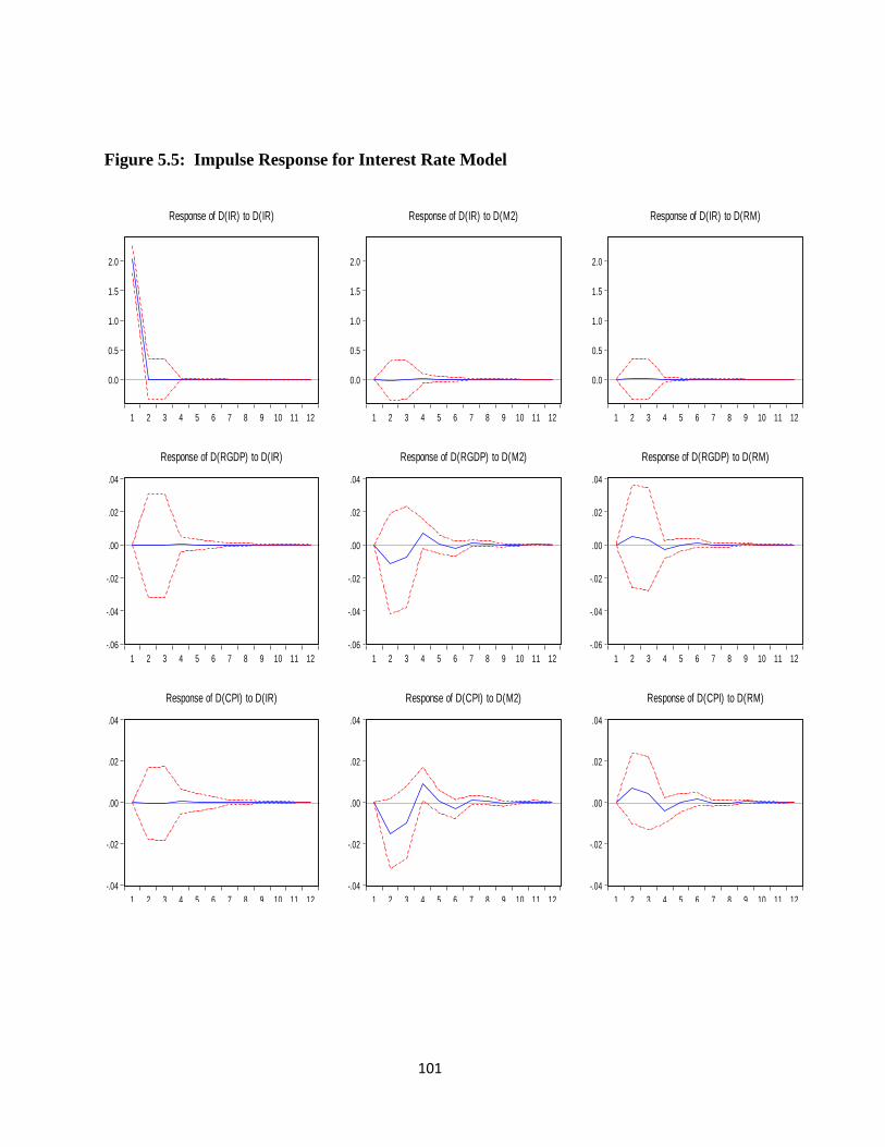
101

Figure 5.5: Impulse Response for Interest Rate Model

0.0

0.5

1.0

1.5

2.0

1 2 3 4 5 6 7 8 9 10 11 12

Response of D(IR) to D(IR)

0.0

0.5

1.0

1.5

2.0

1 2 3 4 5 6 7 8 9 10 11 12

Response of D(IR) to D(M2)

0.0

0.5

1.0

1.5

2.0

1 2 3 4 5 6 7 8 9 10 11 12

Response of D(IR) to D(RM)

-.06

-.04

-.02

.00

.02

.04

1 2 3 4 5 6 7 8 9 10 11 12


-.06

-.04

-.02

.00

.02

.04

1 2 3 4 5 6 7 8 9 10 11 12

Response of D(RGDP) to D(M2)

-.06

-.04

-.02

.00

.02

.04

1 2 3 4 5 6 7 8 9 10 11 12


-.04

-.02

.00

.02

.04

1 2 3 4 5 6 7 8 9 10 11 12


-.04

-.02

.00

.02

.04

1 2 3 4 5 6 7 8 9 10 11 12

Response of D(CPI) to D(M2)

-.04

-.02

.00

.02

.04

1 2 3 4 5 6 7 8 9 10 11 12


102

5.5 THE COMPOSITE MODEL

Preliminary indications from the preceding section suggest that bank lending,

exchange rate and interest rate channels contain important additional information for the

country’s monetary transmission process. A composite model of monetary transmission in

Nigeria is therefore drawn from the resulting vector of endogenous variables as shown in

equation (4.18).

5.5.1 Impulse Response for the Composite Model

For the composite model, the impulse responses over a three year period are

presented in Figure 5.6 below. The figure illustrates that bank lending channel (credit to the

private sector) alone is the important channel of monetary transmission in Nigeria even

though appearing somewhat weak. Among the three intermediate policy targets, only bank

lending channel responds marginally to reserve money shocks while the interest rate and

exchange rate channels shows no significant response. The exchange rate and interest rate

channels does not respond to a decrease in reserve money shock from 0.072 percent in the

first quarter to 0.033 percent in the second quarter while the same shock elicit an increase of

0.011 percent in bank lending in the second quarter from the baseline position of the first

quarter.

Figure 5.6 also shows that aside from the marginal response of the bank lending

channel, both interest rate and exchange rate channels do not elicit any response to sudden

shocks in broad money supply. A reduction in the shock to broad money from 0.058 percent

in the first quarter down to 0.012 resulted in a marginal increase in bank lending from the

baseline position in the first year to 0.009 percent in the second quarter. Further decrease in

the shock to broad money supply within the precinct of positive and negative 0.005 percent

between the third and sixth quarters however only resulted in 0.005 percent increase in bank

lending within the same period after which it stabilized along the baseline.

103

Figure 5.6: Impulse Response for the Composite Model

-.1

.0

.1

.2

.3

2 4 6 8 10 12

Res pons e of D (RGDP) to D (RGDP)

-.1

.0

.1

.2

.3

2 4 6 8 10 12

Res pons e of D (RGDP) to D (CPI)

-.1

.0

.1

.2

.3

2 4 6 8 10 12

Res pons e of D (RGDP) to D (CPS)

-.1

.0

.1

.2

.3

2 4 6 8 10 12

Res pons e of D (RGDP) to D (NEER)

-.1

.0

.1

.2

.3

2 4 6 8 10 12

Res pons e of D (RGDP) to D (IR )

-.1

.0

.1

.2

.3

2 4 6 8 10 12

Res pons e of D (RGDP) to D (M2)

-.1

.0

.1

.2

.3

2 4 6 8 10 12

Res pons e of D (RGDP) to D (RM)

-.05

.00

.05

.10

.15

2 4 6 8 10 12

Res pons e of D (CPI) to D (RGDP)

-.05

.00

.05

.10

.15

2 4 6 8 10 12

Res pons e of D (CPI) to D (CPI)

-.05

.00

.05

.10

.15

2 4 6 8 10 12

Res pons e of D (CPI) to D (CPS)

-.05

.00

.05

.10

.15

2 4 6 8 10 12

Res pons e of D (CPI) to D (NEER)

-.05

.00

.05

.10

.15

2 4 6 8 10 12

Res pons e of D (CPI) to D (IR )

-.05

.00

.05

.10

.15

2 4 6 8 10 12

Res pons e of D (CPI) to D (M2)

-.05

.00

.05

.10

.15

2 4 6 8 10 12

Res pons e of D (CPI) to D (RM)

-.08

-.04

.00

.04

.08

.12

2 4 6 8 10 12

Res pons e of D (CPS) to D (RGDP)

-.08

-.04

.00

.04

.08

.12

2 4 6 8 10 12

Res pons e of D (CPS) to D (CPI)

-.08

-.04

.00

.04

.08

.12

2 4 6 8 10 12

Res pons e of D (CPS) to D (CPS)

-.08

-.04

.00

.04

.08

.12

2 4 6 8 10 12

Res pons e of D (CPS) to D (NEER)

-.08

-.04

.00

.04

.08

.12

2 4 6 8 10 12

Res pons e of D (CPS) to D (IR )

-.08

-.04

.00

.04

.08

.12

2 4 6 8 10 12

Res pons e of D (CPS) to D (M2)

-.08

-.04

.00

.04

.08

.12

2 4 6 8 10 12

Res pons e of D (CPS) to D (RM)

.0

.4

.8

2 4 6 8 10 12

Res pons e of D (NEER) to D (RGDP)

.0

.4

.8

2 4 6 8 10 12

Res pons e of D (NEER) to D (CPI)

.0

.4

.8

2 4 6 8 10 12

Res pons e of D (NEER) to D (CPS)

.0

.4

.8

2 4 6 8 10 12

Res pons e of D (NEER) to D (NEER)

.0

.4

.8

2 4 6 8 10 12

Res pons e of D (NEER) to D (IR )

.0

.4

.8

2 4 6 8 10 12

Res pons e of D (NEER) to D (M2)

.0

.4

.8

2 4 6 8 10 12

Res pons e of D (NEER) to D (RM)

-1

0

1

2

3

2 4 6 8 10 12

Res pons e of D (IR ) to D (RGDP)

-1

0

1

2

3

2 4 6 8 10 12

Res pons e of D (IR ) to D (CPI)

-1

0

1

2

3

2 4 6 8 10 12

Res pons e of D (IR ) to D (CPS)

-1

0

1

2

3

2 4 6 8 10 12

Res pons e of D (IR ) to D (NEER)

-1

0

1

2

3

2 4 6 8 10 12

Res pons e of D (IR ) to D (IR )

-1

0

1

2

3

2 4 6 8 10 12

Res pons e of D (IR ) to D (M2)

-1

0

1

2

3

2 4 6 8 10 12

Res pons e of D (IR ) to D (RM)

-.10

-.05

.00

.05

.10

2 4 6 8 10 12

Res pons e of D (M2) to D (RGDP)

-.10

-.05

.00

.05

.10

2 4 6 8 10 12

Res pons e of D (M2) to D (CPI)

-.10

-.05

.00

.05

.10

2 4 6 8 10 12

Res pons e of D (M2) to D (CPS)

-.10

-.05

.00

.05

.10

2 4 6 8 10 12

Res pons e of D (M2) to D (NEER)

-.10

-.05

.00

.05

.10

2 4 6 8 10 12

Res pons e of D (M2) to D (IR )

-.10

-.05

.00

.05

.10

2 4 6 8 10 12

Res pons e of D (M2) to D (M2)

-.10

-.05

.00

.05

.10

2 4 6 8 10 12

Res pons e of D (M2) to D (RM)

-.08

-.04

.00

.04

.08

.12

2 4 6 8 10 12

Res pons e of D (RM) to D (RGDP)

-.08

-.04

.00

.04

.08

.12

2 4 6 8 10 12

Res pons e of D (RM) to D (CPI)

-.08

-.04

.00

.04

.08

.12

2 4 6 8 10 12

Res pons e of D (RM) to D (CPS)

-.08

-.04

.00

.04

.08

.12

2 4 6 8 10 12

Res pons e of D (RM) to D (NEER)

-.08

-.04

.00

.04

.08

.12

2 4 6 8 10 12

Res pons e of D (RM) to D (IR )

-.08

-.04

.00

.04

.08

.12

2 4 6 8 10 12

Res pons e of D (RM) to D (M2)

-.08

-.04

.00

.04

.08

.12

2 4 6 8 10 12

Res pons e of D (RM) to D (RM)

104

While output shows no response to sudden shocks in exchange and interest rate in the

figure above, we observe some marginal responses to bank lending within the first four

quarters. An unanticipated decrease in the credit to the private sector from 0.102 percent in

the first quarter to -0.023 percent in the second quarter causes output to fall from the baseline

position in the first quarter to -0.002 percent in the second quarter. A further increase in the

shock to 0.014 percent in the fourth quarter expectedly elicits a marginal response in output

to 0.004 percent in the same quarter. However, consumer prices respond to shocks from bank

lending with a decrease of -0.016 percent in the second quarter from the baseline position in

the first quarter.

5.5.2 Variance Decomposition: Composite Model

In a bid to examine the interactions among all the variables over the impulse response

horizon, the results of the forecast error variance decomposition is presented in this section.

This helps to determine the proportion of fluctuations in a given variable that is caused by the

different shocks to all the variables in the model. Table 5.6 below reports the variance

decomposition of the first twelve period horizons into the future.

The output variance decomposition analysis in Table 5.6(A) above shows that in the

first period, variations in output are wholly explained by own shocks. This implies that

variations in output are hardly affected by other variables in the first quarter. The table also

shows that the contributions of other variables are insignificant throughout the other periods.

In essence, beside own contributions, output fluctuations can only be attributed marginally to

variations in the consumer prices beginning from the second quarter through to the twelfth

quarter maintaining a seemingly constant trend. Collectively, bank lending, exchange rate

and interest rate were found not to account for fluctuation in output until the second quarter

when their aggregate contribution was observed to be less than 1 percent.

105

Table 5.6(A) VARIANCE DECOMPOSITION FOR THE COMPOSITE MODEL: RGDP

VARIANCE DECOMPOSITION OF D(RGDP)

QUARTER D(RGDP) D(CPI) D(CPS) D(NEER) D(IR) D(M2) D(RM)

1 100.000 0.000 0.000 0.000 0.000 0.000 0.000

2 98.738 0.735 0.390 0.003 0.001 0.053 0.080

3 98.257 1.015 0.539 0.004 0.002 0.073 0.110

4 97.800 1.282 0.680 0.005 0.002 0.092 0.139

5 97.800 1.282 0.680 0.005 0.002 0.092 0.139

6 97.735 1.320 0.700 0.005 0.002 0.095 0.143

7 97.726 1.325 0.703 0.005 0.002 0.095 0.143

8 97.722 1.327 0.704 0.005 0.002 0.095 0.144

9 97.719 1.329 0.705 0.005 0.002 0.095 0.144

10 97.719 1.329 0.705 0.005 0.002 0.095 0.144

11 97.718 1.330 0.705 0.005 0.002 0.095 0.144

12 97.718 1.330 0.705 0.005 0.002 0.095 0.144

106

Table 5.6(B) VARIANCE DECOMPOSITION FOR THE COMPOSITE MODEL: CPI

VARIANCE DECOMPOSITION OF D(CPI)


1 2.662 97.338 0.000 0.000 0.000 0.000 0.000

2 3.228 93.889 2.135 0.016 0.006 0.289 0.435

3 3.426 92.688 2.880 0.022 0.008 0.389 0.587

4 3.605 91.597 3.555 0.027 0.010 0.481 0.725

5 3.605 91.597 3.555 0.027 0.010 0.481 0.725

6 3.630 91.444 3.650 0.028 0.011 0.494 0.744

7 3.633 91.424 3.662 0.028 0.011 0.495 0.747

8 3.634 91.415 3.668 0.028 0.011 0.496 0.748

9 3.636 91.407 3.672 0.028 0.011 0.497 0.749

10 3.636 91.407 3.672 0.028 0.011 0.497 0.749

11 3.636 91.406 3.673 0.028 0.011 0.497 0.749

12 3.636 91.406 3.673 0.028 0.011 0.497 0.749

107

Table 5.6(B) above shows clearly that the forecast-error variance explained by own

innovations (consumer prices) in the first quarter amount to 97.34 percent while the

remaining 2.66 percent is explained by variations in the level of output. Over time, however,

the variation in consumer prices accounted for by own shock diminished. Aside from own

variation accounting for 91.59 percent of the shock in the fourth quarter, the contribution of

shock to output variation also increased to 3.61 percent while credit to the private sector

joined to contribute 3.55 percent in the second quarter. Even though own variations retains a

high percentage of the explanations for variations in consumer prices, the contributions of

both output and bank lending towards explaining the variations in price level increased over

time and stabilized at an average of 3.6 percent from the fourth quarter to the twelfth.

Variations to other variables in the model does not account for any significant percent in the

variations to consumer prices.

Also, just like the addition of broad and reserve money, the collective contribution of

the three channels was observed to be less than 1 percent implying that they do not account

for variation in price level in the economy.

From the variance decomposition of bank lending (credit to the private sector) in

Table 5.6(C) below, we observe that more than half of the variations to bank lending in the

first quarter is attributed to own shock while consumer prices and output variations accounts

for the remaining 36.7 and 7.6 percent respectively. The explanatory power of bank lending

to own shock diminish to 52.71 and 51.72 in the second and third quarters while that of

consumer prices increased to 38.39 and 38.95 percents and that of output to 7.86 and 7.95

percents in the second and third quarters respectively. In the following quarters, variations in

bank lending as accounted for by own shock stood approximately at 50.7 percent while

variations in output and consumer prices also explained approximately 8.03 and 39.5 percent

throughout this remaining nine quarters. Aside from variations in reserve money which

accounts marginally for an average of 1.0 percent, all the other variables in the model

provide no meaningful contribution to variation in bank lending.

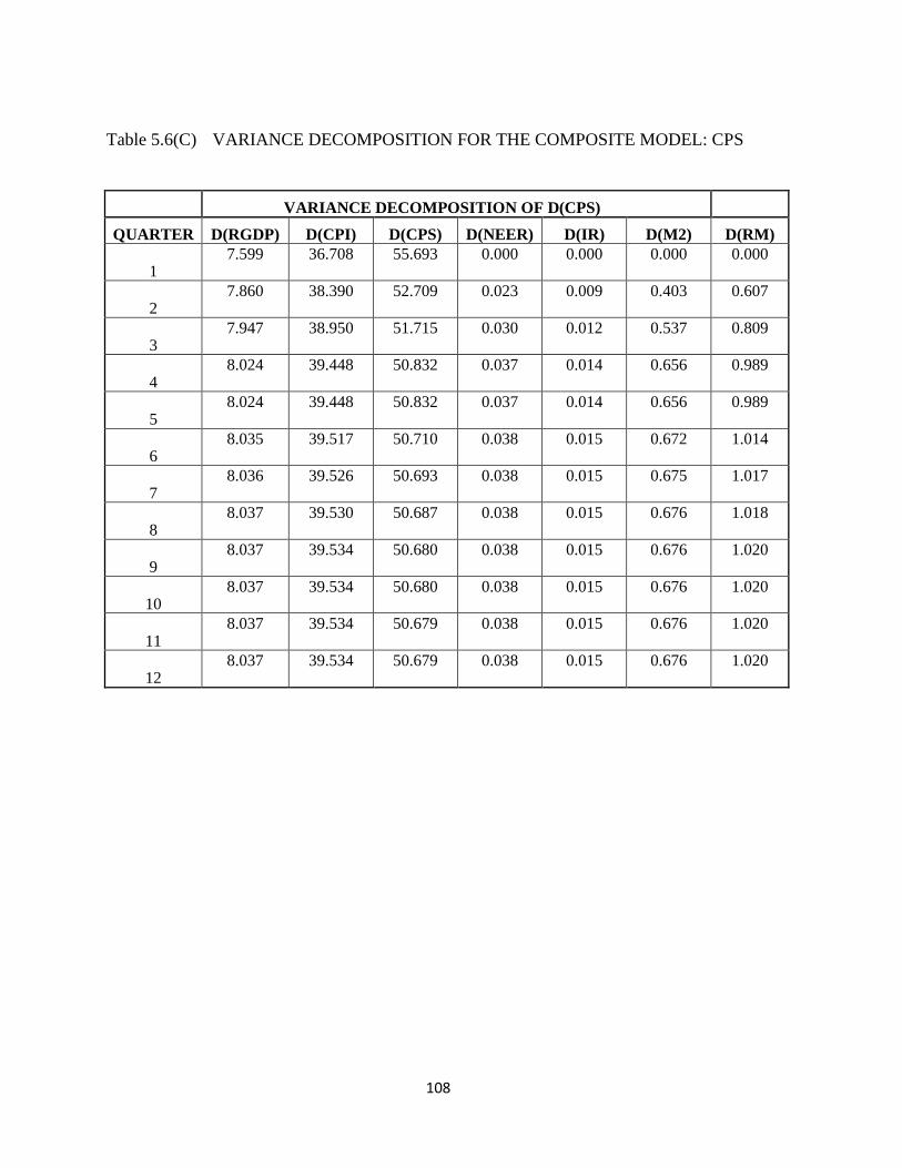
108

Table 5.6(C) VARIANCE DECOMPOSITION FOR THE COMPOSITE MODEL: CPS

VARIANCE DECOMPOSITION OF D(CPS)


1 7.599 36.708 55.693 0.000 0.000 0.000 0.000

2 7.860 38.390 52.709 0.023 0.009 0.403 0.607

3 7.947 38.950 51.715 0.030 0.012 0.537 0.809

4 8.024 39.448 50.832 0.037 0.014 0.656 0.989

5 8.024 39.448 50.832 0.037 0.014 0.656 0.989

6 8.035 39.517 50.710 0.038 0.015 0.672 1.014

7 8.036 39.526 50.693 0.038 0.015 0.675 1.017

8 8.037 39.530 50.687 0.038 0.015 0.676 1.018

9 8.037 39.534 50.680 0.038 0.015 0.676 1.020

10 8.037 39.534 50.680 0.038 0.015 0.676 1.020

11 8.037 39.534 50.679 0.038 0.015 0.676 1.020

12 8.037 39.534 50.679 0.038 0.015 0.676 1.020

109

Table 5.6(D) VARIANCE DECOMPOSITION FOR THE COMPOSITE MODEL: NEER

VARIANCE DECOMPOSITION OF D(NEER)


1 0.142 0.314 2.015 97.530 0.000 0.000 0.000

2 0.142 0.314 2.015 97.530 0.000 0.000 0.000

3 0.142 0.314 2.015 97.530 0.000 0.000 0.000

4 0.142 0.314 2.015 97.530 0.000 0.000 0.000

5 0.142 0.314 2.015 97.530 0.000 0.000 0.000

6 0.142 0.314 2.015 97.530 0.000 0.000 0.000

7 0.142 0.314 2.015 97.530 0.000 0.000 0.000

8 0.142 0.314 2.015 97.530 0.000 0.000 0.000

9 0.142 0.314 2.015 97.530 0.000 0.000 0.000

10 0.142 0.314 2.015 97.530 0.000 0.000 0.000

11 0.142 0.314 2.015 97.530 0.000 0.000 0.000

12 0.142 0.314 2.015 97.530 0.000 0.000 0.000

The variance decomposition of exchange rate as shown in Table 5.6 (D) below

reveals that a significant percentage of the observed variance is accounted for by own

variation which amount to 97.5 percent in the first quarter while bank lending accounts for

2.02 percent of the remaining variation. The table also shows that all the other variables do

not account for variation in the exchange rate. This pattern was maintained by all the

variables in the model throughout the twelve quarters under observation.

110

Similar to the observed pattern of exchange rate decomposition, interest rate variance

decomposition as shown in Table 5.6 (E) below shows that a significant percentage of the

observed variance is only accounted for by own variation. This amounts to 97.78 percent in

the first quarter while exchange rate accounts for 1.23 percent of the remaining variation.

Unlike the exchange rate decomposition, here, while broad and reserve money do not

account for variation in interest rate, credit to the private sector account for less than 1

percent of the variation. The observed trend in the percentage of variation in interest rate

accounted for by own and exchange rate was also shown in the table to remain the same all

through the twelve quarters. The other variables in the model were found, consistently, to

have accounted for an insignificant percentage of the variation in interest rate.

Table 5.6(E) VARIANCE DECOMPOSITION FOR THE COMPOSITE MODEL: IR

VARIANCE DECOMPOSITION OF D(IR)


1 0.000 0.135 0.853 1.234 97.777 0.000 0.000

2 0.004 0.155 0.863 1.234 97.741 0.001 0.002

3 0.006 0.162 0.867 1.234 97.726 0.002 0.003

4 0.007 0.170 0.871 1.234 97.713 0.002 0.004

5 0.007 0.170 0.871 1.234 97.713 0.002 0.004

6 0.007 0.171 0.871 1.234 97.711 0.003 0.004

7 0.007 0.171 0.871 1.234 97.710 0.003 0.004

8 0.007 0.171 0.871 1.234 97.710 0.003 0.004

9 0.007 0.171 0.871 1.234 97.710 0.003 0.004

10 0.007 0.171 0.871 1.234 97.710 0.003 0.004

11 0.007 0.171 0.871 1.234 97.710 0.003 0.004

12 0.007 0.171 0.871 1.234 97.710 0.003 0.004

111

Looking at the variance decomposition of broad money in Table 5.6 (F) below, it is obvious

that both consumer prices and credit to the private sector accounts for a greater percentage of

the shock. In the first quarter, while variations to consumer prices and credit to the private

sector account for 38.76 and 27.07 percent respectively, own shock of broad money only

accounts for 24.43 percent. However, while credit to the private sector maintained the

magnitude of its contribution in the subsequent quarters, the percentage of consumer prices

explanation to broad money variation increased from 40 percent in the second and third

quarter to approximately 41 percent throughout the remaining quarters. In all of these, own

explanation to variation in broad money declined from 22 and 21 percents in the second and

third quarters to a stable 20.7 percent in the following quarters.

Surprisingly, however, while output and interest rate shock accounts for 6.66 and 2.96

percents of the variations in broad money in the first quarter, reserve money provides none.

In the subsequent quarters, while output variation gained and maintained a marginal increase

in its account to 7 percent, interest rate variation maintained an average of 2.45 percent but

variation in reserve money remained approximately 1 percent.

112

Table 5.6(F) VARIANCE DECOMPOSITION FOR THE COMPOSITE MODEL: M2

VARIANCE DECOMPOSITION OF D(M2)


1 6.660 38.760 27.070 0.121 2.964 24.426 0.000

2 7.014 40.193 27.148 0.130 2.661 22.259 0.595

3 7.132 40.672 27.175 0.134 2.560 21.534 0.794

4 7.238 41.098 27.198 0.136 2.470 20.889 0.971

5 7.238 41.098 27.198 0.136 2.470 20.889 0.971

6 7.252 41.157 27.201 0.137 2.458 20.800 0.995

7 7.254 41.165 27.201 0.137 2.456 20.788 0.998

8 7.255 41.168 27.202 0.137 2.456 20.783 1.000

9 7.256 41.171 27.202 0.137 2.455 20.779 1.001

10 7.256 41.171 27.202 0.137 2.455 20.779 1.001

11 7.256 41.172 27.202 0.137 2.455 20.778 1.001

12 7.256 41.172 27.202 0.137 2.455 20.778 1.001

113

Table 5.6(G) VARIANCE DECOMPOSITION FOR THE COMPOSITE MODEL: RM

VARIANCE DECOMPOSITION OF D(RM)


1 5.139 37.074 17.242 0.226 0.025 13.872 26.422

2 5.440 38.018 17.892 0.225 0.028 13.251 25.146

3 5.547 38.354 18.124 0.225 0.030 13.029 24.692

4 5.645 38.662 18.336 0.225 0.031 12.826 24.275

5 5.645 38.662 18.336 0.225 0.031 12.826 24.275

6 5.659 38.706 18.366 0.225 0.031 12.797 24.216

7 5.661 38.712 18.370 0.225 0.031 12.794 24.208

8 5.662 38.714 18.372 0.225 0.031 12.792 24.205

9 5.662 38.716 18.373 0.225 0.031 12.791 24.202

10 5.662 38.716 18.373 0.225 0.031 12.791 24.202

11 5.663 38.717 18.373 0.225 0.031 12.790 24.201

12 5.663 38.717 18.374 0.225 0.031 12.790 24.201

Variance decomposition of reserve money as shown in Table 5.6(G) reveals that all

the variables in the model exhibit a uniform trend throughout the quarters following quarter

one. The table also shows that consumer prices provide more explanation (37 percent) to

variation in reserve money than own shock (26 percent) and broad money (13.8 percent).

Bank lending and output provides further explanation for variation in reserve money. All the

variables in the model were found to retain the percentage of their explanatory power

throughout the remaining the quarters.

114

5.6 Contemporaneous Model Analysis

From the Structural VAR estimation, the restrictions placed on the models based on

economic theory are as follows:

RGDP=@e1=C(1)*@u1

CPI=@e2=C(2)*@e1 + C(3)*@U2

CPS=@e3=C(4)*@e1 +C(5)*@e2 +C(6)*@u3

NEER=@e4=C(7)*@e1 +C(8)*@e2 +C(9)*@e3 + C(10)*@u4

IR=@e5=C(11)*@e1 + C(12)*@e2 + C(13)*@e3 + C(14)*@e4 + C(15)*@u5

M2=@e6=C(16)*@e1 + C(17)*@e2 + C(18)@e3 + C(19)*@e4 +C(20)*@e5 + C(21)*@u6

RM=@e7=C(22)*@e1+C(23)*@e2+C(24)*@e3+(25)*@e4+C(26)*@e5+C(27)*@e6+C(28)*

@u7

Thus, Table 5.7 below provides the results of the contemporaneous model generated from

using the restrictions from above economic theory. The log-likelihood ratio test statistic for

null hypothesis of over-identifying restrictions does not reject the restrictions implying that

they are statistically valid.

The coefficient in the consumer prices (CPI) specification with output (RGDP) shows

that it has positive impact in the short run. This implies that any change in the price level will

impact output along the same direction. Also in line with theory, the credit to the private

sector equation shows a positive sign to both output (RGDP) and consumer prices (CPI).

Here also, we interpret the result to mean that a positive variation in the amount of credit to

the private sector will cause output as well as price level to increase. A plausible explanation

for the increase in price level could be that the resultant increase in aggregate demand

outstrips that of output.

In the exchange rate equation (NEER), the coefficient is both positive on output

(RGDP) and the amount of credit to the private sector (CPS) while it is negative on consumer

prices (CPI) specification. The impact of this on output and the amount of credit to the

private sector could be interpreted to mean that an appreciation of the exchange rate will lead

to increase in domestic production and the amount of credit to the private sector and result in

a fall in price level.

115

Table 5.7: Estimated Coefficients of Contemporaneous Variables

Coefficient

Standard

Error z-Statistic Prob.

C(2) 0.089487 0.043745 2.045655 0.0408

C(4) 0.119354 0.041597 2.869280 0.0041

C(5) 0.761654 0.075846 10.04216 0.0000

C(7) 0.040116 0.246189 0.162947 0.8706

C(8) -0.937839 0.563240 -1.665079 0.0959

C(9) 0.828603 0.466100 1.777738 0.0754

C(11) -0.313226 0.914382 -0.342555 0.7319

C(12) -1.168021 2.110638 -0.553397 0.5800

C(13) 2.345366 1.748795 1.341132 0.1799

C(14) -0.417256 0.300244 -1.389721 0.1646

C(16) 0.017762 0.026114 0.680193 0.4964

C(17) 0.213657 0.060314 3.542381 0.0004

C(18) 0.672980 0.050217 13.40146 0.0000

C(19) -0.011596 0.008625 -1.344455 0.1788

C(20) -0.009944 0.002308 -4.308634 0.0000

C(22) 0.004450 0.032518 0.136845 0.8912

C(23) 0.194651 0.078007 2.495297 0.0126

C(24) 0.000105 0.092058 0.001142 0.9991

C(25) 0.022185 0.010787 2.056569 0.0397

C(26) 0.007867 0.003039 2.588942 0.0096

C(27) 0.900923 0.100520 8.962650 0.0000

C(1) 0.187861 0.010739 17.49286 0.0000

C(3) 0.101651 0.005811 17.49286 0.0000

C(6) 0.095364 0.005452 17.49286 0.0000

C(10) 0.549808 0.031430 17.49286 0.0000

C(15) 2.041885 0.116727 17.49286 0.0000

C(21) 0.058291 0.003332 17.49286 0.0000

C(28) 0.072477 0.004143 17.49286 0.0000

The coefficients of interest rate specification have heterogeneous signs with output,

price level and exchange rate showing negative correlation while credit to the private sector

has a positive sign. Expectedly, increase in the rate of interest will dampen investment as

cost of production will increase thus impacting negatively on consumer prices and leaving its

ripple effect on exchange rate.

116

In the broad money equation, the coefficients have varied signs. Output, price level

and credit to the private sector have positive signs while exchange rate and interest rate have

negative signs. The expected response of output, price level and private sector credit to

increase in broad money supply is a corresponding increase while the response of exchange

rate and interest rate were also expected to fall with an increase in broad money supply.

Positive signs were noticed in the reserve money coefficients for all the variables.

However, this sign was expected only for exchange and interest rates but not for output,

consumer prices, private sector credit and broad money supply. The positive sign for interest

and exchange rates means that an increase in the monetary authority’s reserve money will

cause both interest rate and exchange rate to increase. However, the expected signs for

output, consumer prices, private sector credit and broad money supply are negative. In

essence, we expect variation in reserve money to negatively impact output, consumer prices,

bank lending and broad money.

5.7 Error Correction Model

Following the ECM specification in equation (4.19), the over-parameterised model

was specified for the variables in the study’s estimable model. To this end, the variables were

differenced and lagged by three years while the error correction term was lagged once. The

parsimonious model below was however arrived at after the lagged values of some variables

were pruned as the result shows that their probability value were insignificant.

D(RGDP(-2)) D(CPI(-1) D(M2(-1)) ECT(-1)

𝑎: 0.018 -0.159 -0.238 0.535 -0.044

(0.378) (0.043) (0.169) (0.018) (0.081)

The coefficient of the ECT shown above provides the speed of adjustments of the

target variables to policy variations. From this coefficient of the error correction term, we can

infer that policy variations impacts on target variables after twenty four (24) quarters (six

years precisely).

5.8 A Synthesis of Empirical Results and the Study Objectives

Attempt is made in this section to relate the findings of the study with the specific

objectives set forth at the beginning of the thesis.

117

Objective 1: To determine the more effective policy instrument(s) to be used by the

central bank.

To achieve this objective, we analyse the impulse response function to determine the

magnitude of output and price response to variation in interest rate and reserve money. The

result showed that reserve money is a more effective policy instrument given that a 0.11

percent increase in reserve money results in output and prices declining, even though

marginal, by 0.02 percent and 0.06 percent respectively. In contrast, an increase in bank

interest rate of 2.02 percent does not elicit any significant response from both output and

prices.

Objective 2: To identify the channel(s) through which monetary policy variation affects

output and price level in Nigeria.

From the estimation of the generic model, the results emanating from impulse

response function showed that after a marginal increase in bank interest rate and reserve

money of about 0.001percent and 0.04 percent respectively, bank lending declined from 0.89

percent in the first quarter to - 0.23 percent after the second quarter. This reduction in bank

lending caused output to decline to -0.12 percent and -0.15 percent while prices rose by 0.15

percent and 0.10 percent in the second and third quarters respectively. We conclude from this

that bank lending channel is a potent monetary transmission mechanism in Nigeria. Further

findings showed that an increase in interest rate of 2.02 percent and reserve money of 1.05

percent caused no change in exchange rate while a 2.03 percent increase in interest rate

elicited no response in output and prices. This signified that both exchange and interest rates

are impotent channels for transmitting monetary policy in Nigeria.

Objective 3: To determine the time lag between monetary policy variations and the

effect on domestic price level and output (i.e. the speed with which monetary

impulses are transmitted)

To ascertain the length of time it takes for monetary policy variation to have impact

on prices and output in the Nigerian economy, the result from the estimation of the error

correction model (ECM) of this study helps to realize this objective. The ECM estimation

establishes that the time lag for policy impact on prices and output in the Nigerian economy

is twenty four (24) quarters which translates into six (6) years.

118

CHAPTER SIX

SUMMARY, CONCLUSIONS AND POLICY RECOMMENDATIONS.

In this chapter, the key findings of this study are summarized followed by policy

implications of findings and recommendations. Conclusions are drawn here and the

limitations encountered during the study are also presented.

6.1 Summary of Findings

Recognizing the important role played by monetary policy in a well-functioning

economy, the Nigerian government established the Central Bank of Nigeria and saddled it

with the responsibility of designing an appropriate monetary policy to maintain stable price

level output growth among others. The impact of the policies designed by the central bank on

the economy as a whole, especially the channels through which monetary policy variations

affect prices and output among other macroeconomic variables, has over time attracted the

attention of policy makers.

One startling revelation in the course of literature review for this study is the large

and widening disparity between monetary policy instruments and target variables on one

hand and between monetary target and actual on the other. For instance, while broad money

(M2) grew at an average of 37 percent between 1975 and 1979, the corresponding growth in

GDP and inflation rate were 7 percent and 20 percent respectively. Similar trend was also

observed between 1980 and 1984 when a 19 percent growth in broad money supply was

matched correspondingly by a mere 4 percent growth in output and 12 percent growth in

inflation. Another alarming discrepancy was also observed between desired policy targets

and actual. For instance, while the monetary authority targeted 5 percent, 31 percent, 7

percent, 12 percent and 11 percent inflation rate for the years 1992, 1995, 2002, 2004 and

2005 respectively, the resulting inflation rate stood as high as 45 percent, 73 percent, 12

percent, 22 percent and 24 percent for the same period.

Thus, expediency requires that the CBN have a quick and proper understanding of the

consequences of their actions on non-financial agents and macroeconomic aggregates for a

successful policy design and implementation. However, the Central Bank of Nigeria’s choice

of instruments for attaining any desired objectives at a particular time would be determined

119

mainly by the structure of the economy, the level of development in the money and capital

markets among others.

Nigeria’s adoption of the Structural Adjustment Programme (SAP) in 1986 ushered in

a regime of financial sector reforms characterized by the free entry and exit of banks and the

dominance of indirect instruments for monetary control. With the operational framework of

market instrument, only the operating variables, the monetary base or its components are

targeted while the market is left to determine interest rates and allocate credit. The unfolding

poor performance of Nigeria’s real sector after several measures remained a major challenge

in the formulation and implementation of an appropriate policy by the Central Bank Nigeria.

It is against this backdrop that this study sought to provide answers to the following

policy related questions:

(i) What is the appropriate monetary instrument for achieving the CBN’s objective?

(ii) Which of the transmission channels of monetary policy is in existence in Nigeria?

(iii)How long does it take for a change in monetary policy to affect output and prices?

In attempting to provide answers to the above questions, the study employed the

econometric tool of structural vector autoregressive (SVAR) model on quarterly data

obtained from the CBN annual statistical bulletin for the period between 1970 and 2008.

Structural analysis of the monetary transmission mechanism was captured by the impulse

response functions and the forecast error variance decomposition. They were both used to

identify the dynamic interrelationships between policy variables/instruments and policy goals

(e.g. price level and output). Impulse response functions allow the study of the time path of

each endogenous variable in reaction to a structural shock (innovation) in a certain variable

or group of variables and thus allow comparison of projected performance according to the

estimated model with what the theory implies. Furthermore, forecast error variance

decomposition allows inference about the relative importance of the existing monetary policy

transmission channels. Additionally, contemporaneous model analysis of the restrictions

placed on the models, based on economic theory, was interpreted while an error correction

mechanism was estimated to establish the time lag of policy implementation.

A number of salient findings were obtained during the course of this research. The

generic model clearly established that, above all other goals, the monetary authorities in

120

Nigeria are concerned with both inflation and economic growth in accordance with its

objectives. Also, that the CBN employs a hybrid of monetary policy instruments to achieve

its desired goal of price stability and output growth in the economy. It also established further

that, of the two instruments, namely reserve money and interest rate, the former is a more

effective policy instrument deployed by the CBN. However, the core finding of the model is

that both price level and output respond to monetary policy variation even though output

seems to respond more to shocks emanating from reserve money.

The study, expectedly, found out that the monetary authority’s response to output

shock was to loosen monetary policy through a decrease in the bank rate so as to further

boost the growth of output. However, the authority responded to price shock via a monetary

policy tightening by raising the bank rate to arrest the increase in consumer prices. The

central bank’s response with regard to reserve money showed their determination to address

any observed macroeconomic imbalance.

The study also found out that output will decrease in response to a contractionary

monetary shock especially via an increase in reserve money. Also that shocks to one of the

monetary policy operating targets, reserve money, attracted significant response from output

and consumer price. This implied that, even though interest rate does not seem to have much

impact, monetary factor via reserve money remains a primary determinant of price level and

output in Nigeria. In essence, we inferred from this that reserve money remains the most

effective policy instruments at the disposal of the monetary authority.

Variance decompositions for each variable in the model to determine the relative

importance of each structural innovation showed that consumer prices as well as some

magnitude of output are more responsive towards reserve money variation than interest rate.

The finding from this is that the former impacted more on target variables than the latter.

Hence we interpreted the observed response of consumer prices to reserve money to mean

that price stability is the principal objective of monetary policy in the country. In essence, the

observed magnitude of explanation by prices and output to variation in reserve money

showed that price level and output are responsive to reserve money. On the whole, we found

bank rate a less effective tool of monetary policy than reserve money.

Further findings from the study, while analysing the separate SVAR models under the

bank lending, showed that contractionary monetary policy via a marginal increase in the

121

reserve money caused credit to the private sector to decline. Output response showed some

fluctuations in tandem with bank lending variation while prices declined significantly. This

confirmed further that variation in bank lending impacts both price level and output in the

economy.

The study also found out under the exchange rate model, that exchange rate had an

insignificant response to variations in both bank rate and reserve money. Consequently,

exchange rate shocks precipitated by variations in bank rate and reserve money had no effect

on both output and price level. A plausibly possible explanation to justify this is the “round –

tripping” activities of the operators in the financial sector. Findings under the interest rate

model was not significantly difference as a monetary policy tightening via an increase in

reserve money, and not broad money, explained the observed significant increase in interest

rate. And similar to our finding under the exchange rate model, both output and consumer

prices showed no response to unexpected changes in interest rate.

The finding of the study from the impulse response of the composite model

comprising both the generic and separate models confirms the above result. The forecast

error variance decomposition showed no significant difference from what obtained under the

generic model. Variations in output, interest rate and exchange rate were found not to be

affected by other variables in the model throughout the quarters as their collective impact

accounts for less than three percent. Price level also accounted for a very high percentage of

own variations while the combined explanation of output and bank credit is marginal.

From the bank lending variance decomposition, we found own explanatory power

accounting for an average of fifty percent throughout the period under review while price

level provided an average of forty percent of the variations. This we interpreted to mean that

variations in prices significantly influence the amount of bank lending to the private sector.

One significant result from both the reserve money and broad money (M2) forecast

error variance decomposition is the fact that, price level remains the major determining factor

of their variations. In the case of broad money; bank credit to the private sector and own

explanation, in that order, accounts for variation while in the case of reserve money; own

explanation, bank credit to the private sector and broad money accounts for its variation.

Upon analyzing the contemporaneous model, our findings conform with a priori

expectation that any change in price level will impact output along the same direction.

122

Further findings also revealed that the positive sign of variation in the amount of credit to the

private sector on output and prices could be interpreted to mean an increase in the level of

output and prices. While the positive coefficient of exchange rate on output and private

sector credit was taken to mean an in domestic production and bank lending, the negative

coefficient of consumer prices was assumed to imply a fall in price level. We found the

interest rate coefficient on output, prices and exchange rate to have a dampening effect on

investment due to its incremental impact on the cost of production.

6.2 Policy Implication of Findings and Recommendations

Several policy lessons can be drawn from the findings of this study. Following the

findings that monetary target variables respond more to variations in reserve money than

interest rate, the monetary authority in Nigeria need to shift from hybrid operating procedures

to a scalar indicator of policy. The recommendation is for the Central Bank of Nigeria to

embrace the use of reserve money as a measure of monetary policy rather than the less

effective bank rate. Flowing from the evidence in our findings that the Central Bank of

Nigeria also targets output growth alongside price stability, we also suggest that the authority

concentrates primarily on the latter as this has the propensity of fostering output growth in

the economy.

Findings indicate that the capability of monetary policy to influence economic

activity and prices are still limited, as important channels of monetary transmission are not

effective. In particular, the interest rate and exchange rate channels remain weak. To the

extent that supervising and monitoring Nigeria’s financial sector activity remained weak,

monetary policy effectiveness will remain illusory. Thus, we suggest the financial sector’s

supervisory and regulatory authorities device a superior investigative method of auditing

deposit money bank financial report and enforcing compliance.

While empirical evidence showed that the central bank’s means of influencing

economic activity remains the bank lending channel, a major challenge to this channels’

having any meaningful impact is the large activity of the informal (lending) sector and the

shadow economy which are yet to be fully integrated into the formal economy. Apart from

firms and individuals who majorly rely on cash for transactions, Nigeria has a large shadow

economy that does not rely on the formal financial sector. This significantly diminishes the

123

potential deposit base of the banking system and the market for products offered by banks

and other financial institutions—thereby precluding any effects of monetary policy on

activity and prices in the informal economy. In order to foster the assimilation of the informal

sector into the formal economy, the authorities need to create incentives for formalization so

as to deepen financial intermediation and financial sector efficiency.

6.3 Conclusions

This study provides a description of monetary policy transmission mechanisms which

is concerned with the relationships between changes in the money supply and the level of

real income (output and prices). Several channels through which the changes in money

supply affect output exist prominent among which are the interest rate channel, credit (bank

lending) channel and exchange rate channel among others. This study investigates the

channels through which monetary policy shocks are propagated in Nigeria so that policy

makers can interpret movements in financial variables with precision and make accurate

predictions from their choice instruments.

Reserve money rather than interest rate was found to be a more potent monetary

policy instrument of the Central Bank of Nigeria as both prices and output respond to shocks

emanating therefrom hence we recommend its use rather than a hybrid. Among the perceived

channels of monetary transmission mechanism in the less developed countries, bank lending

channel was found to be the existing channel of monetary policy in Nigeria. To this end,

bank lending channel should be bolstered by tightening creditworthiness standards;

strengthening accounting standards, corporate governance and creditor rights; improving

bank credit assessment capabilities; and strengthening the judicial system to improve banks’

ability to enforce on collateral. A number of legislative and judicial reforms designed to

simplify and reduce the cost of foreclosure and strengthen creditor rights should also be put

in place by the financial sector supervisory and regulatory authorities.

124

6.4 Limitations of the Study and Suggestions for Further Research

The model estimated in this study offered a reasonable framework within which the

effects of monetary policy on some target variables can be analysed. Notwithstanding this,

there is still room for further research. The data on the key variables of the model employed

for this study are not available in higher frequency. This has implication for the result of our

study as some palpable impacts of monetary policy shocks on macroeconomic variables are

better studied with monthly data.

Similar to the above constrain, any study on the response of the real sector to

monetary impulse should consider it expedient to include data on employment as this signify

the absorption and utilization capacity in the entire economy. Notwithstanding the identified

shortcomings, the information in this thesis remains valid, reliable, and can be used for

generalisation.

For the purpose of future research, the role of the non-bank financial institutions in

the supply of domestic credit and in the transmission channel should be looked into as this

constitute a veritable source of credit in the informal sector. Additional insights into the

channels through which the effects of monetary policy are transmitted to the real sector may

be provided when non-bank financial institutions are included in the monetary transmission

mechanism.

125

REFERENCES

Adewunmi, W. (1981) Money Matter in Economic Development: Some Tentative Empirical

Evidence in Nigeria. Savings and Development vol 5(2), pp 155-171.

Ahmed, N., Shah, H., Agha, A. I. and Mubarik, Y. A., (2005). Transmission Mechanism of

Monetary Policy in Pakistan. State Bank of Pakistan Working papers, no. 9

Ajayi, S.I (1983). On the Causality between Money and Prices. Nigerian Journal of Economics and

Social Studies Vol. 25, No. 3, pp319-326

Ajayi, S.I and Ojo, O.O.(1981). Money and Banking: Analysis and Policy in the Nigerian

context. George Allen and Unwin Publishers Ltd, London .

Allen, C. and Robinson, W., (2004). Monetary Policy Rules and the Transmission Mechanism in

Jamaica. Bank of Jamaica Working Paper.

Al-Mashat, R. and Billmeier, A. (2007). The Monetary Transmission Mechanism in Egypt. IMF

Working Paper WP/07/285. Washington DC.

Angeloni, I, A Kashyap, B Mojon and D Terlizzese (2003): The output composition puzzle: A

difference in the monetary transmission mechanism in the euro area and U.S., Journal of

Money Credit and Banking, no 35 (6, Part 2).

Arnostova, K. and Hurnik, J.(2005) The Monetary Transmission Mechanism in the Czech

Republic( Evidence from VAR Analysis). Czech National Bank, Working Paper Series 4.

Aron, J. and J. Muellbauer (2000). Inflation and output forecasts for South Africa: Monetary

Transmission implications. CSAE Working paper Series WPS/2000. 23

Ashcraft, A. B., (2006). New Evidence on the Lending Channel. Journal of Money, Credit and

Banking 38, 751–775.

Baksh, S. and R.C Craigwell (1997), The monetary transmission mechanism in small open

economies: A case study of Barbados. Savings and Development Journal Vol. 21(2)

pp179-193.

Becklelmans, L. (2005). Credit and Monetary Policy: An Australian SVAR. Reserve Bank of

Australia Research Discussion Paper 2005-06 , 2005 (September), 1-29.

Bernanke, B. (1983). Non-Monetary Effects of the Financial Crisis in the Propagation of the Great

Depression, American Economic Review, vol.73, (3).

Bernanke, B. (1986). Alternative Explanations of the Money-Income Correlation. NBER Working

Paper Series (NBER Working Paper Number 1842), 1-62.

Bernanke, B. (1996). What Does the Bundesbank Target? NBER Working Paper Series (WP 5764),

1-42.

126

Bernanke, B., & Gertler, M. (1995). Inside the Black Box: The Credit Channel of Monetary Policy

Transmission. Journal of Economic Perspectives , 9 (4), 27-48.

Bernanke, B., Gertler, M. and Gilchrist, S.(1996). The Financial Accelerator and the Flight to

Quality. The Review of Economics and Statistics, Vol. 78, No. 1, pp. 1-15.

Bernanke, B., & Mihov, I. (1995). Measuring Monetary Policy. National Bureau of Economic

Research Working Paper WP-97-7 .

Bernanke, B. S. and Blinder, A. S. (1992). The Federal funds rate and the channels of monetary

transmission. American Economic Review, 82, 901-902.

Bernanke, B.S. and Blinder, A.S. (1988). Credit, Money and Aggregate Demand. American

Economic Review 78: 435–439.

Blanchard O.J. and M.W. Watson (1986). Are Business Cycles All Alike?, in R. Gordon (ed) The

American Business Cycle: Continuity and Change, NBER and University of Chicago Press,

pp 123-156.

Blanchard, O.J. (1989), A Traditional Interpretation of Macroeconomic Fluctuations. American

Economic Review, December ed., pp 1146-64.

Blanchard, O.J. and D. Quah, (1989): The Dynamic Effects of Aggregate Demand and Supply

Disturbances, American Economic Review, Vol. 79, pp 655-73.

Blinder, A. S. and Stiglitz, J. E. (1983). Money, Credit Constraints and Economic Activity,

American Economic Review – Papers and Proceedings vol.73, (2), May.

Blundell-Wignall, A., & Gizycki, M. (1992). Credit Supply and Demand and the Australian

Economy. Reserve Bank of Australia Discussion Papers (Discussion paper No. 9208).

Borys, M. M., and Horvath, R. (2007). The Effects of Monetary Policy in the Czech Republic: An

Empirical Study. CERGE-EI Working Paper Series (339), 1-26.

Braun P.A. and Mittnik, S., (1993) Misspecifications in VAR and Their Effects on Impulse

Responses and Variance Decompositions. Journal of Econometrics, 59, 319-41.

Bredin, D. and O’Reilly G.,(2004). An Analysis of transmission mechanism of monetary Policy in

Ireland. Journal of Applied Economics, 36, 49-58

Brissimis, S., Kamberoglou, N. and Simigiannis, G., (2001). Is There A Bank Lending Channel of

Monetary Policy in Greece: Evidence from Bank Level Data, ECB Working Paper 104,

Frankfurt: European Central Bank.

Britton, E. and Whitely, J. (1997). Comparing the Monetary Transmission Mechanism in France,

Germany and the United Kingdom: Some issues and Results, Bank of England Quarterly

Bulletin, May, pp. 152-62.

Brooks, P.K. (2007), Does the Bank Lending Channel of Monetary Transmission Work in Turkey?

IMF Working Paper, WP/07/272. Washington DC.

127

Brunner, K. A. and Meltzer, A. (1988), Money and Credit in the Monetary Transmission Process,

American Economic Review – Papers and Proceedings, Vol. 78 (May).

Canova, F. (2004) Structural changes in the US economy, www.econ.upf.edu/crei/canova.

Canova, F. and Sala, L. (2005) Back to square one: identification issues in DSGE models, ECB

Working Paper.

CBN (2000), The Changing Structure of the Nigerian Economy and Implications for Development.

Realm Communications Ltd., for CBN

Cecchetti, S. G. (1995). Distinguishing Theories of the Monetary Transmission Mechanism.

Federal Reserve Bank of St. Louis Review. 77/3: 83-97.

Cecchetti, S. G. (1999). Legal Structure, Financial Structure, and the Monetary Policy

Transmission Mechanism, Economic Policy Review, Federal Reserve Bank of New

York, July, 5(2), pp.9-28.

Central Bank of Nigeria Statistical Bulletin (2009). Abuja

Cheng, K.C. (2006). A VAR analysis of Kenya’s monetary policy transmission mechanism:

How does the Central Bank’s REPO rate affect the economy? IMF Working Paper

WP/06/300, Washington D.C

Christiano, L. J., Eichenbaum, M. and Evans C. (1996). The Effects of Monetary Policy shocks:

Evidence from the Flow of Funds. The Review of Economics and Statistics, vol. 78,

No.1,pp16-34.

Christiano, L., Eichenbaum, M., & Evans, C. (1998). Monetary Policy Shocks: What have we

Learned and to What End? NBER Working Paper Series (Working Paper Number

6400), 1-77.

Clarida, R., Gali, J. and Gertler, M. (2000) Monetary Policy Rules and Macroeconomic Stability:

Evidence and Some Theory, Quarterly Journal of Economics 115, 147-80.

Clements, B., Kontolemis, Z.G. and Levy, J., (2001). Monetary Policy Under EMU: Differences in

the Transmission Mechanism. IMF working paper WP/01/102. Washington DC

Cooley, T.F. and S.F. Le Roy (1985): Atheoretical Macroeconomics: A Critique, Journal of

Monetary Economics, pp 283-308.

Cottarelli, C. and A. Kourelis (1994). Financial Structure, Bank lending rates, and

transmission Mechanism of monetary policy. IMF staff papers, p 587-628.

Dabla-Norris, E., & Floerkemeier, H. (2006). Transmission Mechanisms of Monetary Policy in

Armenia: Evidence from VAR Analysis. IMF Working Paper WP/06/248 , 1-26.

Disyatat, P., & Vongsinsirikul, P. (2003). Monetary Policy and the Transmission Mechanism in

Thailand. Journal of Asian Economies , 2003 (14), 389-418.

http://www.econ.upf.edu/crei/canova

128

Donli, J. G. (2004). An Overview of Nigeria’s Economic Reforms. CBN executives’ seminar at

Midway International Hotels, Ilorin Kwara State.

Dornbusch R., Favero, C. and F. Giavazzi (1998), The immediate challenges for the European

Central Bank, Economic Policy, No.26, 17-64.

Durevall, D. and Ndung’u, N.S (1999). A dynamic model of inflation for Kenya 1974-1996 IMF

Working Paper WP/99/97., Washington, D.C.: IMF

Ehrmann M. (2000), Comparing monetary policy transmission across European countries,

Weltwirtschaftliches Archiv, No. 136(1), 58-83.

Erhmann, M., Gambacorta, L., Martines-Pages, J., Sevestre, P. and Worms, A., (2001), Financial

Systems and the Role of Banks in Monetary Transmission in the Euro Area, ECB Working

Paper 105, Frankfurt: European Central Bank.

Ekpo, A. H. and Umoh, 0. J. (2009). An Overview of The Nigerian Economic Growth and

Development, http://www.onlinenigeria.com/economics/January 19, 2010.

Enders, W. (2004). Applied Econometric Time Series. Hoboken: John Wiley & Sons, Inc.

Engle, R.F. and Granger, C.W.J. (1987), Cointegration and Error Correction: Representation,

Estimation and Testing. Econometrica March 1987, pp 251-76.

Falegan, S. B. (1987), Redesigning Nigeria’s Financial System. University Press Ltd, Ibadan.

Fahrer, T. and Rohling, D., (1990). Financial Deregulation and the Monetary Transmission

Mechanism. Reserve Bank of Australia Research Discussion Paper, November.

Fanelli, L. and Paruolo, P. (1999), New Evidence on the Transmission Mechanisms of Monetary

Policy in Italy before Stage III of European Monetary Union. Mimeo, Universita di

Bologna.

Farinha, L., and Marques, C. R., (2001), The Bank Lending Channel of Monetary Policy:

Identification and Estimation Using Portuguese Micro Bank Data, ECB Working Paper

102, Frankfurt: European Central Bank.

Favero, C. A. (2001). Applied Macroeconometrics. New York: Oxford University Press Inc.

Favero, C., Gavazzi, F. and Flabbi, L., (1999), The Transmission Mechanism of Monetary Policy in

Europe: Evidence from Banks’ Balance Sheets, NBER Working Paper 7231, Cambridge:

National Bureau of Economic Research.

Fernandez-Villaverde, J. (2009). The Econometrics of DSGE Models. NBER Working Paper Series,

working paper 14677.

Friedman, M. (1968). The Role of Monetary Policy, American Economic, Vol. 58 (1), March.

Fry, R. and Pagan, A. (2005) Some Issues in Using VARs for the Macroeconometrics Research,

CAMA Working Papers Series No 19/2005, The Australian National University.

Fuller, W. A. (1976). Introduction to statistical Time Series. New York: Wley.

129

Gali, J. (1992). “How well does the IS-LM Model fits postwar US data?”. Quarterly Journal of

Economics 10:152-231.

Gali, J. and Rabanal, P. (2005) Technology shocks and aggregate fluctuations: How well does the

RBC model fit Postwar US data?, NBER Macroeconomic Annual, 20.

Garcia, C. Garcia, P. Magendzo, I. and Restrepo, J (2003). “The Monetary Transmission mechanism

in Chile: A Medium sized macro econometric model”. Central bank of Chile Working paper,

WP 254

Gerlach, S., and Smets, F. (1995), .The monetary transmission mechanism: Evidence from the G-7

countries,. In Financial Structure and the Monetary Policy Transmission Mechanism, Basel,

Switzerland: Bank for International Settlements, March, No. C.B. 394.

Gonzalo, J., 1994. "Five alternative methods of estimating long-run equilibrium relationships,"

Journal Of Econometrics, vol. 60 (1-2), pp. 203-233.

Hicks, J. R. (1937), Mr Keynes and the ‘Classic’: A Suggested Interpretation. Econometrica, April,

vol. (5) pp258-78.

Hoover, K. D. and Perez, S. J. (1994). Post Hoc Ergo Propter Hoc Once More: An Evaluation of

“Does Monetary Policy Matter” in the Spirit of James Tobin. Journal of Monetary

Economics.

Horvath, B. and Maino, R. (2006). Monetary transmission Mechanism in Belarus IMF Working

Paper WP/06/246

Ireland, P.N. 2004. Money’s Role in the Monetary Business Cycle. Journal of Money, Credit, and

Banking 36, 969-983.

Ireland, P (2005): The monetary transmission mechanism, Boston College Working Papers in

Economics, no 628, Boston College Department of Economics.

Jimoh, A. (1990). The Demand for Money and the Channels for Monetary Shocks Transmission in

Nigeria. Nigerian Journal of Economics and Social Studies. Vol. 32(1) pp 91-103.

Johansen, S. (1991), Estimation and Hypothesis Testing of Cointegration Vectors in Gaussian

Vector Autoregressive Models. Econometrica, vol. 59, pp 1551-80.

Kamin, S., Turner, P., & Van't dack, J. (1998). The Transmission Mechanism of Monetary

Policy in Emerging Market Economies: An Overview. BIS policy paper, No.3, 5-65.

Karame, F., & Olmedo, A. (2002). The Assymetric Effects of Monetary Policy shocks: A

Non- Linear Structural VAR Approach. Unpublished Manuscript , 1-28.

Kashyap, A. K., and Stein, J. C. and Wilcox, D. W. (1993). Monetary Policy and Credit Conditions:

Evidence from the Composition of External Finance. American Economic Review, vol. 83.

Kashyap, A. K., and Stein, J. C. (1999). What do a million observations on banks have to say

about the transmission of monetary policy?, American Economic Review,

Keating, J.W. (1992): Structural Approached to Vector Autoregression, Federal Reserve Bank of St.

Louis Review, Vol. 74, No. 5, pp 37-57.

130

Keating, J.W. (1990): Identifying VAR Models under Rational Expectations, Journal of Monetary

Economics, June, pp 453-76.

Kim, S., & Roubini, N. (2000). Exchange Rate Anomalies in the Industrial Countries: A Solution

with a Structural VAR Approach. A Journal of Monetary Economics , 45 (3), 561-586.

Kimball, M.S. 1995. The Quantitative Analytics of the Basic Neomonetarist Model. Journal of

Money, Credit, and Banking 27, 1241-1277.

King, S. R.. (1986). Monetary Transmission: Through Bank Loans or Bank Liabilities. Journal of

Money, Credit and Banking. Vol. 18 (3) August.

King, R.G. and Plosser, C.I., (1984). Money, Credit and Prices in a Real Business Cycle. American

Economic Review, Vol. 74 (3) June.

King, R.G., Plosser, C.I., Stock, J.H. and Watson, M.W. (1991), Stochastic Trend and Economic

Fluctuations. American Economic Review September

Kishan, R. P. and Opiela, T. P., (2000). Bank Size, Bank Capital, and the Bank Lending Channel.

Journal of Money, Credit and Banking 32, 121–141.

Kuijs, L. (2002), Monetary Policy Transmission Mechanisms and the Inflation in the Slovakia

Republic. IMF Working Papers WP/02/80.

Kuttner, K.N. and Mosser, P. (2002), The Monetary Transmission Mechanism: Some Answers and

Further Questions. Economic Policy Review, Federal Reserve Bank, vol. 8, No.1.

Kydland, F.E. and Prescott, E.C. 1982. Time to Build and Aggregate Fluctations. Econometrica 50,

1345- 1370.

Laidler, D. (1978), Money and Money Income: An Essay on the Transmission Mechanism. Journal

of Monetary Economics vol. 4, (April) pp. 151-91.

Leeper, E. M., Sims, C. A., & Zha, T. (1996). What Does Monetary policy Do. Brookings Papers on

Economic Activity , 1996 (2), 1-78.

Luca, F. and Paruolo, P. (1999). “New Evidence on the Transmission Mechanisms of Monetary

Policy in Italy before Stage III of European Monetary union. Ricerche quantitative per la

politica Economica.

Lucas Jr., R.E. 1972. Expectations and the Neutrality of Money. Journal of Economic Theory 4,

103-124.

Lutkepokl H., 1991, Introduction to Multiple Time Series Analysis, Springer, New York.

Lütkepohl, H and M Krätzig (2004) (eds.), Applied Time Series Econometrics, Cambridge

University Press, Cambridge.

Martinez, L. Sanchez, O. and Werner, A. (2001). Monetary Policy and the transmission mechanism

in Mexico. Papers presented at Banco de Mexico’s 75th

Anniversary Seminar Mexico City

Nov 14-15, 197-261

131

McCallum, J. (1991). Credit rationing and the Monetary Transmission Mechanism. American

Economic Review, vol. 81

McCoy, D.(1997), How Useful is Structural VAR Analysis for Irish economies? Central Bank of

Ireland Technical Paper, 2/RT/97

Meltzer, A. (1995). Money, Credit and (Other) Transmission Processes: A Monetarist Perspective.

The Journal of Economic Perspectives , 19 (4), 49-72.

Mishkin, F. (1995). Symposium on the monetary transmission mechanism. Journal of Economic

Perspective, vol 9, No.4, pp3-10

Modigliani, F. (1971). Monetary Policy and Consumption. In Consumer spending and Monetary

Policy: the linkages: Boston. Federal Reserve Bank of Boston, 9-84

Mojon, B.,( 2000). Financial structure and the interest rate channel of ECB monetary policy.

Working paper 40. European Central Bank.

Montiel, P. (1991). The Transmission Mechanism for Monetary Policy in Developing Countries.

IMF Staff Papers , 38 (1), 83-108.

Morris, C. S. and Sellon, G. H. (1995). Bank Lending and Monetary Policy: Evidence on a Credit

Channel. Economic Review, Federal Reserve Bank of Kansas City, Vol. 80 (2).

Morsink, J., & Bayoumi, T. (2001). A Peek Inside the Black Box: The Monetary Transmission

Mechanism in Japan. IMF Staff Papers , 48 (1), 22-57.

Mugume, A. (2009) Monetary Transmission Mechanism in Uganda, African Economic research

Consortium, Nairobi

Mundell, R.A. (1962), The Appropriate of Monetary and Fiscal Policy for Internal and External

Stability, IMF Staff Papers vol.9.

Ngalawa, H.P.E.(2009), Dynamic Effects of Monetary Policy Shocks in Malawi. African

Econometrics Society Annual Conference, Abuja, Nigeria.

Nnanna, O.J. (2001) Monetary Policy Framework in Africa: The Nigerian Experience. CBN.

Nwankwo, U.(1992), Economic Agenda for Nigeria, Centrist Productions Limited, Lagos.

Obstfeld, M. and Rogoff, K. (1995). “Exchange Rate Dynamics Redux”. Journal of Political

economy 103,624-660

Odedokun, M.O. (1989) Causalities between Financial Aggregates and Economic Activities

in Nigeria. Savings and Development vol.13(1) pp101-110.

Ojo M.O. (1992), Monetary Policy in Nigeria in the 1980s and Prospect in the 1990s, Economic and

Financial Review, CBN vol. 30(1)

Oke, B. A. (1993), CBN Economic and Financial Review, vol. 31, No.4

Oyaromade, R (2004) Credit Rationing and the Transmission Mechanism of Monetary Policy in

Nigeria. PhD Thesis, Economics Department, University of Ibadan, Ibadan.

Phillips, P and P. Perron(1988). Testing for a unit root time series regression. Biometrika 75, 333- 46.

132

Pierce, D.G.and Tysome, P.J. (1985), Monetary Economics, Theories, Evidence and Policy.

Butterwood, London.

Piffanelli, S. (2001). The Instrument of Monetary Policy in Germany. A Structural VAR Approach.

United Nation Department of Economic and Social Affairs (DESA) Working paper Series

(DESA Discussion Paper No. 19), 1-6.

Poddar, T., Sab, R. and Khachatryan, H. (2006). The Monetary Transmission Mechanism in

Jordan. IMF Working Paper, WP/06/48

Rabanal, P. and Rubio-Ramirez, J (2005) Comparing New-Keynesian Models of the Business

Cycle: A Bayesian Approach, Journal of Monetary Economics, 52, 1150-1162.

Ramasawamy, R. and Sloek, T., (1998). The Real Effects of Monetary policy in the European

Union: What Are the Differences?. IMF Staff Papers vol. 45, No. 2. Washington DC.

Runkle, D.E. (1987), Vector Autoregressions and Reality. Journal of Business and Economics

Statistics, October ed., pp437-42.

Romer, C. and D. Romer (1990). New Evidence of the monetary transmission mechanism.

Brookings Papers on Economic Activity, 1, 149-213

Rotemberg, J.J and M Woodford (1997), An Optimization-Based Econometric Framework for the

Evaluation of Monetary Policy, NBER Macroeconomics Annual 199. pp. 69–104.

Saizar, A. C. and Chalk, N. ( 2008) Is Monetary Policy Effective When Credit is Low? IMF

Working Paper 08/288. IMF Washington DC.

Sanusi, .J (2002), Nigeria’s Macroeconomic Position: Controlling the Money supply being a paper

presented to the Honorary Presidential Advisory Council on Investment in Nigeria

(HPACI) at Hilton Hotel, Park Lane, London, UK.

Sargent, T.J. and Wallace, N. “Rational” Expectations, the Optimal Monetary Instrument, and the

Optimal Money Supply Rule. Journal of Political Economy 83, 241-254.

Sealey, C. W. Jnr (1979). Credit Rationing in The Commercial Loan Market: Estimates of a

Structural Model Under Conditions of Disequilibrium. Journal of Finance, Vol. 34 (June).

Shapiro, M. D. and M.W. Watson (1988): Sources of Business Cycles Fluctuations, NBER

Macroeconomics Annual, pp 111-148.

Sims, C. (1980). Macroeconomics and Reality. Econometrica , 48 (January 1980), 1-49.

Sims, C. A. (1992). Interpreting the Macroeconomic Time Series facts: the effects of Monetary

Policy. European Economic Review, 36, 975-1000

Sims, C. A., & Zha, T. A. (1998). Does Monetary Policy Generate Recessions? Federal Reserve

Bank of Atlanta Working Paper Series , Federal Reserve Bank of Atlanta Working Paper 98-

12 (July 1998), 1-61.

Sims, C., Stock, J., & Watson, M. (1990). Inference in Linear Time series Models with Some Unit

Roots. Econometrica , 58 (1), 113-144.

133

Sims. C. A.(1986). Are Forecasting Models Usable for Policy Analysis? Federal Reserve Bank of

Minneapolis Quarterly Review , 10 (1), 2-16.

Smets, F and R Wouters (2003), An Estimated Dynamic Stochastic General Equilibrium Model of

the Euro Area, Journal of the European Economic Association, vol 1, pp 1123–75.

Soludo, C. C. (2004), Consolidating the Nigerian Banking Industry to meet the Development

Challenges of the 21st Century, Being an Address to the Special Meeting of Bankers

Committee, Held on July 6, 2004 at CBN HQ, Abuja.

Soyibo, A. and Adekanye, F. (1992). The Financial System Regulation, Deregulation and Savings

Mobilisation in Nigeria, AERC Research Paper (No.11).

Stock, J.H, and Watson, M. (1991), A Simple Estimator of Cointegration Vectors in Higher Order

Integrated Systems. Federal Reserve Bank of Chicago Working Paper WP91-4

Tarawalie, A.B. (2008), Monetary Policy and the Transmission Mechanism in Sierra Leone. An

Unpublished PhD Thesis, Department of Economics, University of Ibadan, Nigeria.

Taylor, J.B (1995). The monetary Transmission Mechanism: An Empirical Framework. Journal of

Economic perspective, 9/4, 11-26

Teriba, O.(1978), Instruments of Monetary Control: The Nigerian Experience. In O.Teriba and

V.P.Diejomaoh, eds., Money, Finance and Nigerian Economic Development: Essays in

Honour of Obasanmi Olakanpo. University of Ibadan Press, Ibadan.

Tobin, James (1969). A General Equilibrium Approach to Monetary Theory. Journal of Money,

Credit and Banking No1,15-29

Tushar, P., Sab, R., and Khachatryan, H., (2006). The Monetary transmission mechanism In

Jordan. IMF working papers WP/06/04

Uanguta, E. and Ikhide S. (2002). Monetary policy transmission mechanism in Namibia, Bank of

Namibia working paper, No. 2/02

Uchendu, O.A (1996). The Transmission of Monetary Policy in Nigeria. Economic and Financial

Review CBN, vol 34(2), 606-625

Vonnák, B (2005): Estimating the effect of Hungarian Monetary Policy within a structural VAR

framework, MNB Working Paper, no 2005/1.

Wane, A. A. (1999). Monetary Policy, Financial Imperfections and the Credit Channel in the

WAEMU: An Empirical Investigation. A Revised AERC Research proposal, May.

Weber, A. A., Gerke, R. and Worms, A. (2009). Has the monetary transmission process in the

euro area changed? Evidence based on VAR estimates. BIS Working Papers No 276.

West, K.D. (1990), The Sources of Fluctuations in Aggregate Inventories and GNP. Quarterly

Journal of Economics November ed., pp 939-71

Zellner, A. (1962), An Efficient Method of Estimating Seemingly Unrelated Regressions and

Tests for Aggregation Bias. Journal of the American Statistical Association June ed.,

pp348-68.

134

Author Country / Data Type Methodology/

Channel

Variables Used Findings

Kuijs (2002)

Slovak Republic /

Monthly data (1993-

2000)

VAR/

Interest Rate channel

Price level, Real Interest

Rate, GDP, M2, Real

Effective Exchange Rate,

Unit of labour costs.

The main direct determinants of inflation are

exchange rate, foreign prices, aggregate demand

and wage cost but no direct impact of either

monetary aggregates or interest rate.

Dabla-Norris and

Floerkemeier

(2006)

Armenia /

Monthly data (2000:5-

2005:12)

VAR/

Exchange rate

channel

M1, repo rate (for short term

interest rate), real GDP, CPI

and nominal effective

exchange rate.

Exchange rate channel has a strong impact on the

inflation rate and that the capability of monetary

policy to influence economic activity and

inflation is limited, as important channels of

monetary transmission are not fully functional.

Hovarth and

Maino (2006)

Belarus /


2005:10)

VAR/

Exchange rate

channel

RGDP, CPI, real effective

exchange rate, M1, interbank

rate and US Fed. Fund Rate

(for interest rate parity).

There exists a significant exchange rate pass-

through to prices. Interest rate policy is

following, rather than leading, financial market

developments.

Poddar, Sab and

Khachatryan

(2006)

Jordan/

Quarterly data

(1996:1-2005:1)

VAR/

Not Stated

RGDP, foreign reserve,

spread btw 3months CD rates,

US Fed. Fund rate, Real

effective exchange rate, real

credit and real lending rates.

That monetary policy has been successful in

influencing reserves as well as driving bank

deposit and lending rates. However, they do not

find any evidence of monetary policy

significantly affecting economic activity.

Brooks (2007)

Turkey /

Quarterly data

Small macro-

econometrics model.

Bank Lending

channel

Liquidity, size, capitalization

and dummies for ownership

status and stock market

participation.

Bank liquidity has a significant effect on loan

supply. This suggests that the effect of monetary

policy can be propagated by the banking sector,

depending on its liquidity position.

Borys and

Horvarth (2007)

Czech Republic /


2006:5)

VAR and SVAR /

Not stated

GDP, real-time output gap,

net price index, nominal

exchange rate, interbank

interest rate and CPI

That a contractionary monetary policy shock has

a negative effect on the degree of economic

activity and the price level, both with a peak

response after one year or so.

135

Saizar and Chalk

(2008)

Asia and Latin America

/ Monthly data (1996-

2007)

VAR/

Exchange Rate

channel

Change in industrial

production, consumer price

inflation, wholesale food and

oil price inflation, interest

rate, growth of m1 and

nominal effective exchange

rate.

When controlling for the exchange rate regime it

is clear that allowing for exchange rates to move

flexibly is an important factor in ensuring that

monetary policy can influence domestic inflation.

Countries with floating exchange rates have no

evidence that the level of private sector credit

meaningfully impact economic aggregate.

Sims (1992) France, Germany,

Japan, the U.S.A. and

the U.K./


1964:1

VAR/

Interest rate channel

Industrial production, M1,

interest rate, consumer price,

commodity price and

exchange rate indexes

That the interest rate variable potentially affects

other variables contemporaneously, while the

interest rate is not affected by innovations in any

of the other variables.

Bernanke and

Blinder (1992)

U.S.A/

Monthly data (1959:7

– 1989:12)

VAR/

Credit channel

U.S. Federal Funds rate,

monetary aggregates, CPI,

industrial productions, CP

Bill, loans and securities

A positive shock to the federal funds rate reduces

the volume of deposits held by institutions

immediately after shock and peaks after nine

months That their findings support the operation

of a credit channel.

Christiano,

Eichenbaum and

Evans (1996)

U.S.A./

Quarterly data

(1960:Q1 – 1992: Q4)

VAR/

Cash Flow channel

RGDP, the GDP deflator,

commodity prices, Federal

Fund rate, total reserves, non-

borrowed reserves and

aggregate production activity.

The initial effect of a positive shock to the

federal funds rate is to increase net funds raised

by the business sector for almost a year and

thereafter decline.

Clements,

Kontolemis and

Levy (2001)

10 Euro area /

Quarterly data (1983:1-

1988:4)

Macro-econometrics

model and VAR/


Real GDP, CPI, short term

domestic interest rate, M2,

effective exchange rate, and

credit to private sector.

That interest rate channel rather than the credit

and exchange rate channels explains the lion’s

share of the observed differences.

136

Weber, Gerke and

Worms (2009)

Euro area /

Quarterly data (1980:1 -

2006:4)

VAR/

Not stated

RGDP, GDP deflator, real

housing wealth, domestic

nominal short term IR.

Changes in the transmission process have not

altered the long-run responses of real output and

inflation to monetary policy.

Ahmed, Shah,

Agha and Mubarik

(2005)

Pakistan/

Monthly data

(1996:July-

2004:March)

VAR /

Bank Lending

Channel

TB rate, Private Sector credit,

real effective exchange rate,

consumer price index,

industrial production index as

proxy for GDP

Monetary tightening leads to a fall in investment

demand financed by bank lending, which

translates into a gradual reduction in price

pressures that eventually reduces the overall price

level with a significant lag.

Cheng (2006)

Kenya /

Monthly data (1997-

2005)

SVAR/

Interest rate

Nominal effective exchange

rate, GDP, short term interest

rate, CPI, M2, oil price and

Federal Funds rate.

Increase in interest rate leads to a fall in prices

and an appreciation of exchange rate, but

accounting little for output fluctuation.

Mugume (2009)

Uganda /

Monthly data 1993:6-

2009:3

SVAR/


GDP, M2, CPI, interest rate,

nominal effective exchange

rate, lending rate and credit to

the private sector.

The capability of monetary policy to influence

economic activity and inflation is still limited.

Also, the interest rate channel remains weak,

even though there is some evidence of

transmission to prices of changes in the TB rate.

Uanguta and

Ikhide (2002)

Namibia/

Monthly data 1997:1-

1998:12

VAR/

Credit and Interest

rate channels.

M2, credit to private sector,

lending rate, private

investment and CPI

Both credit and interest rate channels are

effective. However, the intensity of both channels

is difficult to gauge from the results.

Ngalawa (2009)

Malawi /

Monthly data (1988:1 –

2005:12)

SVAR/

Not stated

GDP, M2, CPI, bank rate,

exchange rate, reserve money

and credit to private sector.

The role of exchange rates became more

conspicuous than before although its impact was

weakened; and the importance of aggregate

money supply and bank lending in transmitting

monetary policy impulses was enhanced.

Tarawalie (2008) Sierra Leone/ Small Macro- Real exchange rate, inflation,

real GDP, interest rate, M2,

Bank lending channel was found to be the most

effective channel through which MP actions

137

Quarterly data (1990:1

– 2006:4)

econometric model /

Bank lending channel

TB rate, private sector credit, affects inflation and output.

Oyaromade

(2004)

Nigeria/

Quarterly data (1970:1

– 1999:4)

VAR/

Interest rate and

Credit channels

Real GDP, M2, lending rate,

private sector credit, TB rate,

real exchange rate, expected

rate of inflation, interest rate,

real investment and demand

deposit.

That credit rationing significantly exist and

financial deepening has the tendency of reducing

its propensity to persist. The interest rate and

credit channels play a significant role in the

transmission of monetary impulse to the real

sector in Nigeria.

Adebiyi (2006) Nigeria/

Monthly data series

(interpolated from

annual data series of pre

and post banking

reform era).

VAR/

Credit channel

TB rate, nominal exchange

rate, lending rate, credit to the

private sector, RGDP, CPI,

monetary aggregates and

liquidity ratio.

Credit channel seems to be the most important

for developments in prices before the reforms

while lending rate, bank credit, and M2 are most

important after the reforms. However, for

developments in output, Treasury bill rate is the

important channel before the reforms.

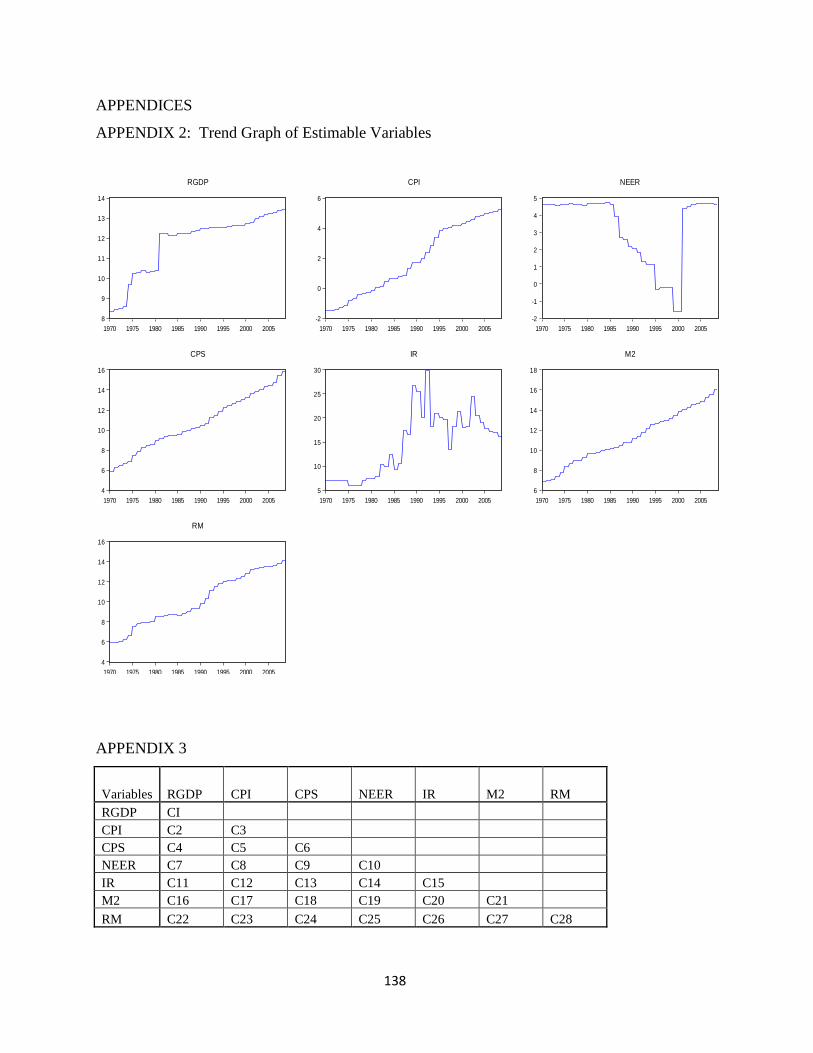
138

APPENDICES

APPENDIX 2: Trend Graph of Estimable Variables

APPENDIX 3

Variables RGDP CPI CPS NEER IR M2 RM

RGDP CI

CPI C2 C3

CPS C4 C5 C6

NEER C7 C8 C9 C10

IR C11 C12 C13 C14 C15

M2 C16 C17 C18 C19 C20 C21

RM C22 C23 C24 C25 C26 C27 C28

8

9

10

11

12

13

14

1970 1975 1980 1985 1990 1995 2000 2005

RGDP

-2

0

2

4

6

1970 1975 1980 1985 1990 1995 2000 2005

CPI

-2

-1

0

1

2

3

4

5

1970 1975 1980 1985 1990 1995 2000 2005

NEER

4

6

8

10

12

14

16

1970 1975 1980 1985 1990 1995 2000 2005

CPS

5

10

15

20

25

30

1970 1975 1980 1985 1990 1995 2000 2005

IR

6

8

10

12

14

16

18

1970 1975 1980 1985 1990 1995 2000 2005

M2

4

6

8

10

12

14

16

1970 1975 1980 1985 1990 1995 2000 2005

RM

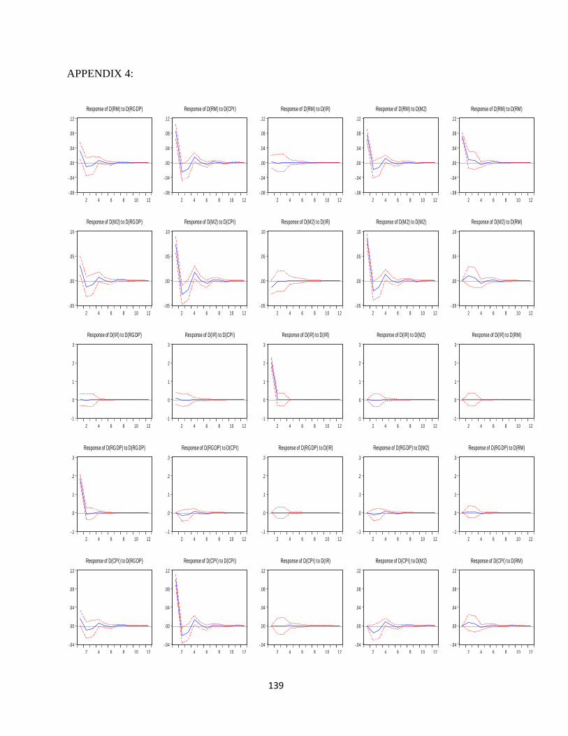
139

APPENDIX 4:

- .08

-.04

.00

.04

.08

.12

2 4 6 8 10 12

Response of D(RM) to D(RGDP)

- .08

-.04

.00

.04

.08

.12

2 4 6 8 10 12

Response of D(RM) to D(CPI)

- .08

-.04

.00

.04

.08

.12

2 4 6 8 10 12

Response of D(RM) to D(IR)

- .08

-.04

.00

.04

.08

.12

2 4 6 8 10 12

Response of D(RM) to D(M2)

- .08

-.04

.00

.04

.08

.12

2 4 6 8 10 12

Response of D(RM) to D(RM)

- .05

.00

.05

.10

2 4 6 8 10 12

Response of D(M2) to D(RGDP)

- .05

.00

.05

.10

2 4 6 8 10 12

Response of D(M2) to D(CPI)

- .05

.00

.05

.10

2 4 6 8 10 12

Response of D(M2) to D(IR)

- .05

.00

.05

.10

2 4 6 8 10 12

Response of D(M2) to D(M2)

- .05

.00

.05

.10

2 4 6 8 10 12

Response of D(M2) to D(RM)

-1

0

1

2

3

2 4 6 8 10 12

Response of D(IR) to D(RGDP)

-1

0

1

2

3

2 4 6 8 10 12

Response of D(IR) to D(CPI)

-1

0

1

2

3

2 4 6 8 10 12

Response of D(IR) to D(IR)

-1

0

1

2

3

2 4 6 8 10 12

Response of D(IR) to D(M2)

-1

0

1

2

3

2 4 6 8 10 12

Response of D(IR) to D(RM)

- .1

.0

.1

.2

.3

2 4 6 8 10 12

Response of D(RGDP) to D(RGDP)

- .1

.0

.1

.2

.3

2 4 6 8 10 12

Response of D(RGDP) to D(CPI)

- .1

.0

.1

.2

.3

2 4 6 8 10 12


- .1

.0

.1

.2

.3

2 4 6 8 10 12

Response of D(RGDP) to D(M2)

- .1

.0

.1

.2

.3

2 4 6 8 10 12


- .04

.00

.04

.08

.12

2 4 6 8 10 12

Response of D(CPI) to D(RGDP)

- .04

.00

.04

.08

.12

2 4 6 8 10 12

Response of D(CPI) to D(CPI)

- .04

.00

.04

.08

.12

2 4 6 8 10 12


- .04

.00

.04

.08

.12

2 4 6 8 10 12

Response of D(CPI) to D(M2)

- .04

.00

.04

.08

.12

2 4 6 8 10 12


SAMUEL OLATUNDE OREKOYA

Documents

Transcript of SAMUEL OLATUNDE OREKOYA