Research Field: Finance

TITLE: RELATIONSHIP BETWEEN DOWNSIDE RISK

MEASURES AND RETURN IN THE BRAZILIAN

MARKET

Abstract

Recent research shows that distortions of distributional properties of emerging markets

returns may impact the effectiveness of conventional asset pricing models. Last years a

mean-semivariance framework has been proposed as an alternative approach to portfolio

analysis since different investors assign a lower weight to positive deviations from the

mean than to negative ones. The present work aims to investigate empirically the

relationship between risk and return in a downside risk framework and in a regular risk

framework by utilizing daily returns of securities trades on the Sao Paulo Stock Exchange.

Using individual equities from Brazilian market we separately examine conditional returns

in upturn and downturn periods in order to indentify the potential contribution of downside

risk measures to explain asset pricing in both states of economy. The results reveal that for

downturn periods, downside risk measures are better in explaining risk returns than the

regular risk measures. The paper also concludes that both co-skewness and downside beta

are priced by investors, and they may capture different aspects of downside risk.

Keywords: Asset Pricing, Downside risk, Downside Beta, Co-skewness.

2

1. Introduction

The cost of capital is one of the most important factors to assess any project or company.

For an investor point of view, it represents the lowest required return to provide and

allocate resources at the firm. Thus, this cost of equity should be equal to the expected rate

of return on alternative investments with similar risk characteristics within the capital

market.

One of the main problems of addressing investment portfolio management in emerging

capital markets is to quantify expected return and risk, and also how to assess accurately

the risk-return relationship. The Capital Asset Pricing Model (CAPM) (Sharpe, 1965;

Lintner, 1966 & Black, 1972) like others market equilibrium models of capital assets

pricing, tries to capture the relationship between the systematic risk of an asset, measured

as the equity´s beta, and the expected rate of return on that asset. The most common

application of the CAPM is to estimate the expected return to equity, which is used among

others, for pricing financial assets and business valuation, capital budgeting and portfolios

performance simulations.

There exists a lot of empirical evidence that the traditional model of CAPM has some

flaws and does not capture all risk factors. Despite CAPM has been widely and strongly

criticized during the last 40 years, most practitioners and analysts continue using the

traditional CAPM construction. Accordingly to Graham & Harvey (2009) and Brounen et.

al (2004), 75% of US CFO´s and 45% in Europe use CAPM to assess cost of capital. This

widely utilization is based on its simplicity in a low cost and relative high effectiveness

process, keeping CAPM more popular among analysts than both arbitrage and multi-factor

models.

The CAPM assumes a normal distribution of returns, and the model´s underlying

assumption is that the perception of risk is attributed by the dispersion on both sides of the

mean. Estrada (2000, 2002) criticized the use of variance and therefore also the standard

deviation as a measure of risk and he proposed to measure it by the semi-standard deviation

of the distribution. He argued that the variance is a good measure of risk only when return’s

distribution is both symmetrical and normal and he points out that empirical evidence

contradicts these both underlying requirements. Estrada (2000) highlights three pros in

using semi-variance as a measure of risk: a) it captures the preference of investors upside

risk b) is more useful than variance when distribution is asymmetric c) semi-variance gives

the same information than variance and skewness and therefore is more efficient for use in

asset pricing. Ang et al. (2006) tested cross sectional asset pricing and demonstrated that

investors are willing to incorporate a premium for downside risk. The rationale behind this

theory is that measures that incorporate only the semi-standard deviation are more useful

when dealing with asymmetric distributions as these factors are more sensible capturing the

volatility that affects downside returns. From an investor point of view, this is could be

explained by saying that investors are mainly interested in the risk of losses rather in the

“risk” of gains (represented the latter by the right side of the normal distribution curve).

This investor´s concern about the preference for positive skewness of asset returns has been

already addressed by the literature, deriving in some interesting researches about higher

moment’s behaviors. The evidence shows that the risk premium of assets will depend on

their co-skewness, with investors preferring assets with positive co-skewness (Huan &

Litzenberger, 1988).

3

2. Review of Empirical Literature

The CAPM, attributed to Sharpe (1965); Lintner (1966) & Black (1972), is based on

Markowitz´ modern portfolio theory of Markowitz (1952), involving that the risk and

return of investments are effectively measured by variance and mean of the expected return

from the investment. Throughout this concept CAPM arrives to the conclusion that on

efficient portfolios there exist a linear risk-return relationship represented by the Capital

Market Line (CML).

From the early seventies vast empirical evidence reinforced CAPM as a robust model.

The most significant research in this area was conducted by Black, Jensen and Scholes

(1972). They tested CAPM since 1926 to 1966 using NYSE market data and examining

whether intercepts comes to zero on market beta for cross sectional and time series

regressions of excess return. They found positive relationship between market beta and

expected return. In other relevant studies, Hamada (1972) found linkage between

systematic risk and leverage and Fama & MacBeth (1973) provided evidence that linear

relationship between the average return and beta still holds even when data covers a long

time period.

Markowitz (1952,1959), who initially proposed the mean variance framework on the

development of modern portfolio theory, suggested in his seminal work the use of semi-

variance as better measure of risk. Due to lack of resources at that time, Markowitz (1959)

stays with the mean variance measure meaning that deviation both below and above mean

equally contribute towards the risk perceived by investors. In the very beginning of the

model Roy (1952), argues that investor cares from disaster and his main concern is to avoid

it, in other words, he holds the theory of the “safety-first rule”. Lybby & Fishburn (1977),

support this theory, suggesting that investors are more concerned with deviation of returns

below the mean. Gul (1991), who develop rational Disappointment Aversion (DA) utility

function, points out that investors display a larger aversion to losses relative to the

attraction for gains. Hence investor seems to be loss averse, not risk averse.

Hogan & Warren (1974), and later Bawa & Lindenberg (1977), developed an asset

pricing model based on expected return semi-variance, presenting the return of the security

as a linear function of its downside beta computed with respect to the market portfolio.

Price et al. (1982) tested returns on the US stock over a sample period from 1927 to

1968 and found that the semi-variance risk estimators of risk differ from the variance based

risk measures. Furthermore, they suggested that measuring risk using the standard CAPM

(mean variance approach) leads to overestimate the risk of high beta stocks and

underestimate the risk of low beta stocks. Due to these findings and the hypothesis of

borrowing and lending at the risk free rate, it would be expected that return and downside

risk share positive and linear relationship, meaning that downside risk beta is a complete

measure of risk.

Harlow & Rao (1989) provided evidence that the Mean Semi-variance CAPM seems to

capture better the cross-section of stock returns than the Mean Variance- CAPM. They

found a measure of downside risk, named the generalized mean lower partial moment

(MLPM), based on downside deviations below the mean of returns of an asset i and the

market portfolio. Thus, this brings a sensibility measure of the security´s returns (below and

above average returns) to changes in market returns below mean.

Ang et al. (2001) analyze daily US stock data from 1964 to 1999 and within DCAPM

framework shed some light to explain momentum effect. Additionally, Ang et al. (2006)

provide a detailed empirical examination of the explanatory power of downside beta for

individual shares in the US market. They showed that the shares which co-vary strongly

with the market during market downturns do have higher average returns, reporting a 6%

risk premium for downside risk.

4

The case in emerging markets merits separate examination, as there is vast evidence

that asset returns exhibit very high volatility and are not normally distributed. Beakert &

Harvey (1997) indentified significant skeweness and kurtosis in emerging market returns,

with persistence of skewness over time.

3. Background theory and research question.

As explained before, the underlying fundamentals behind the development of downside

CAPM models in emerging markets is that CAPM baseline requirements, concerning

distributional properties of symmetry and normality of expected stock returns, are not

achieved, thus investors should be clearly rewarded for exposure to downside risk

measures.

3.1 Downside Beta A notable contribution within the issue of downside risk in emerging markets came from

Estrada (2000). Estrada (2000) and later Pereiro (2006), suggested to use the downside beta

( -), a sensitivity measure defined as the ratio between the semi-deviation of returns with

respect to the mean in market i and the semi-deviation of returns with respect to the mean

in the world market. This measure of risk is empirically supported as it explained the

variations in the cross section of stock returns in emerging markets. Estrada (2002) uses

market indices to provide evidence on the explanatory power of downside beta. Using a

coefficient that results from the comparison of securities returns and market portfolio

returns, when each variable is below their respective means, the conventional beta

coefficient is not as good to explain the returns of individual assets as the downside beta. In

other words, Estrada (2002) shows that mean returns are more sensitive to changes in

downside beta than to equal changes in conventional beta. Using this approach, Pereiro

(2006) found some empirical explanatory power in DCAPM for Argentinean market. With

all this emerging markets evidence for non normality and investor´s preference for

downside risk, DCAPM seems to be a good substitute to CAPM, (and therefore downside

beta a great alternate to conventional beta), both for theoretical and empirical grounds.

3.2 Co-skewness If stock prices exhibit non normality properties, then the importance of skewness

cannot be overlooked. Kraus & Litzenberger (1976) extend the CAPM to incorporate the

effect of skewness in asset pricing. They show that investors, with decreasing marginal

utility of wealth and non-increasing absolute risk aversion, prefer positive skewness

portfolios (more right skewed). Hence, assets that decrease a portfolio’s skewness (i.e., that

make the portfolio returns more left skewed) are less desirable and should command higher

expected returns. Similarly, assets that increase a portfolio’s skewness should have lower

expected returns (Harvey & Siddique, 2000).This suggests that investors value higher

moments and this fact leads us into the study of the third and fourth moments to explain

better the results in future markets. Ang & Chua (1979) demonstrated that ignoring the

third moment would generate a bias in performance evaluation. To date, most emphasis has

been placed on the impact on co-skewness on asset prices, rather than skewness, to reflect

the argument that investors are not compensated for diversifiable skewness in equilibrium

(Ingersoll, 1975) and recent research deal with this higher co-moment measure. Kraus &

Litzenberger (1976) early introduce the definition of co-skewness of an asset. They stated

that the co-skewness of a security represents the marginal contribution of the security to the

skewness of a broader portfolio. According Harvey & Siddique (2000), a negative co-

skewness measure means that, when incorporated into a portfolio, the security is adding

negative skewness, and investors dislike this fact because their results yield an amplified

5

high average stock returns for low co-skewness stocks, fact that increases the probability of

obtaining undesirable extreme values.

3.3 Research question Downside beta is not to be mixed up with co-skewness in the sense that the downside

market movements should be captured by downside beta in a conditional and inter-

temporal manner, while co-skewness should not show any changes for asymmetrical

properties for down and up markets even though co-skewness may vary over time.

However according to the literature, co-skewness may capture some aspects of downside

covariation that are not included in downside beta premium, so we believe that co-

skewness and downside beta should capture different aspects of downside risk. As a matter

of fact, Galagedera & Brooks (2007) include downside co-skewness to downside beta to

asses and compare the performance of downside risk with and without co-skewness. They

conclude that co-skewness has to be included in a complementary way to the downside risk

premiums.

The purpose of this paper is to test both downside beta and co-skewness in a downside

framework approach for the Brazilian equity market and therefore to examine the linkage

between the risk/reward relationships between these two measures and others systematic

measures of risk.

We believe that the main advantage of using downside beta for the Brazilian market

relies on the fact that it does not require compliance with the symmetry and normality of

the distribution, uncommon properties in emerging markets. Moreover, Brazilian investor

should really be concerned of negative volatility of returns.

In the other side, the main benefit of using co-skewness is that the asset pricing

models, when supported by higher moments, allow researchers to focus on investor

preferences over particular features of the underlying stock return distribution (Dittmar,

2002; Kraus & Litzenberger, 1976)

In his paper we aim to test if investors of Brazilian market are rewarded for exposure to

both co-skewness and downside beta. As we showed before, to date existing asset pricing

literature points out the convenience of using these both downside risk measures in which

investors are compensated for holding, in a semi–variance environment, systematic and co-

skewness risk. Therefore, the major contribution of this paper is to provide empirical

evidence about the role of downside beta and co-skewness in Brazilian market securities

returns.

Regarding this asset pricing issue in Emerging Markets and specifically focusing in the

Brazilian case, we decided to state the following main research question:

Would the analysis of systematic downside deviation help to receive a more

adequate relation between market risk and return in Brazil?

4. The Data

The research will be based on daytime data of exchange auctions of financial assets that

compound around the 85% of the capitalization of the Brazilian market index Ibovespa.

The source of the daily returns is provided by Economatica database. The Ibovespa Index is

a gross total return index weighted by traded volume and is comprised of the most liquid

stocks traded on the Sao Paulo Stock Exchange. It is the most widely used index in the

Brazilian equity market and it is composed of 66 stocks (BMF BOVESPA, 2013). An

obvious concern is that, since there are large numbers of small thinly traded shares in the

Brazilian Market, an accurate estimation of their risk attributes will not be possible.

Although there are 66 stocks comprising the index, we limit our investigation only to the

most representative ones in terms of market capitalization. A further selection criterion is

6

employed as some emerging market companies may suffer a lack of liquidity (Feldman &

Kumar, 1995). For all shares we estimate the proportion of days with zero returns, and we

exclude those shares recording a proportion of zero daily returns above 50%. These

selection criteria result in a substantial reduction of the sample that remains in 49 stocks.

The study covers the period from June 1st 2006 to July 3

th 2013, which means a window

of 1849 observations per share. As will be explained later, for estimating purposes and

better forecasting explanatory power we divide this entire period in some sub periods

because the model should test both upturn and downturn market periods.

5. Methodology

Our research proposal is to test both the viability and strength of Coskewness and

Downside Beta when estimating expected returns for Brazilian Market Stocks. Due to the

continuous nature of information and compounded return rates, in order to calculate the

daily return of the stocks we use the following equation:

(1)

With all the data we form two sub-samples, one containing company returns during

one semester periods of downturn and one for those semesters of upturns. A downturn

period is defined as a semester in which overall market returns are below the market risk

free rate. For this analysis, this market excess return is calculated by the nominal

IBOVESPA return “rm” minus the nominal daily inter-bank CD rate “rf“(compounded

monthly). A semester in which market returns exceed their risk-free rates is designated as

an upturn period. An examination of our data indicates that approximately 57 % of all

periods are upturns and 43% are downturns.

The present study considers four risk measures. Co-skewness of returns is our primary

measure of downside risk. Harvey (1995) defines co-skewness as the component of an

asset´s skewness related to the market porfolio´s skewness. Using individual share data,

Harvey & Siddique (2000) find that co-skewness has explanatory power for share returns,

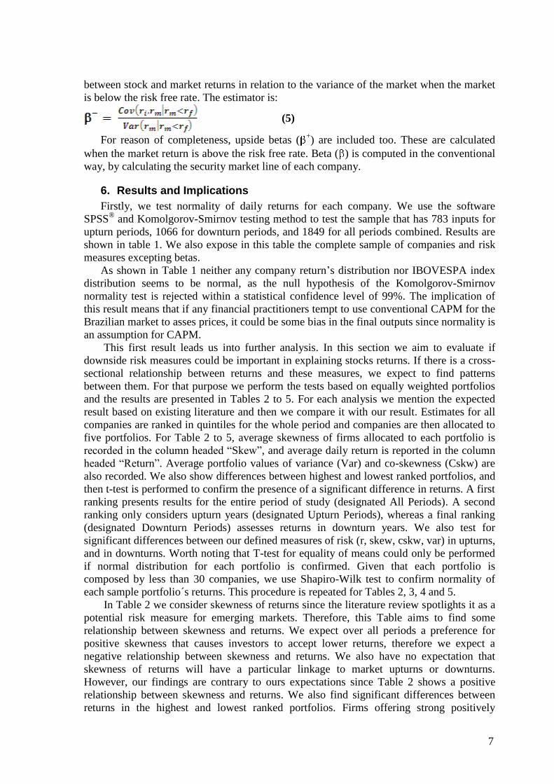
after allowing for other established explanatory factors. Our empirical estimator for co-

skewness is as follows:

(2)

In all cases is daily return on share I and is average return. Ibovespa index returns

are indicated by m, so that is its daily return and is average market return. For

comparison purposes we also consider two related idiosyncratic measures of risk, the

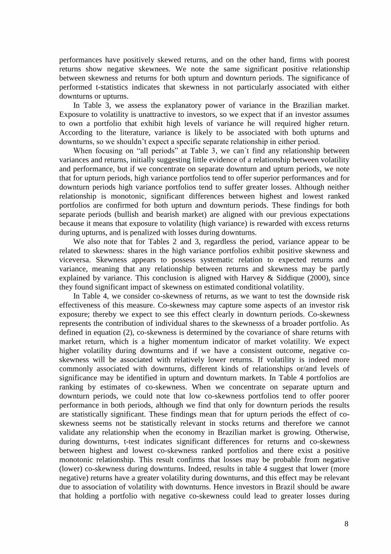
skewness (Skew) of returns, and the variance of returns (Var). Our empirical estimator for

skewness of returns is the adjusted Fisher-Pearson standardized moment coefficient:

(3)

The estimator for volatility is the variance of returns, calculated as:

(4)

Downside beta (-) is a further indicator of downside risk. Ang et al. (2006a) provide a

detailed empirical examination of the explanatory power of downside beta for individual

shares in the US market. We could define downside beta (-) as an indicator of negative

sensibility to market risk and it should be computed when the market return is below the

risk free rate (Petengill et al. 1995). Therefore, downside beta measures the covariance

7

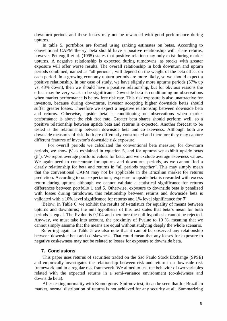
between stock and market returns in relation to the variance of the market when the market

is below the risk free rate. The estimator is:

(5)

For reason of completeness, upside betas (+) are included too. These are calculated

when the market return is above the risk free rate. Beta ( ) is computed in the conventional

way, by calculating the security market line of each company.

6. Results and Implications

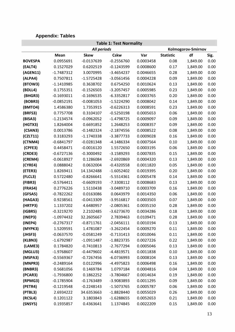
Firstly, we test normality of daily returns for each company. We use the software

SPSS® and Komolgorov-Smirnov testing method to test the sample that has 783 inputs for

upturn periods, 1066 for downturn periods, and 1849 for all periods combined. Results are

shown in table 1. We also expose in this table the complete sample of companies and risk

measures excepting betas.

As shown in Table 1 neither any company return’s distribution nor IBOVESPA index

distribution seems to be normal, as the null hypothesis of the Komolgorov-Smirnov

normality test is rejected within a statistical confidence level of 99%. The implication of

this result means that if any financial practitioners tempt to use conventional CAPM for the

Brazilian market to asses prices, it could be some bias in the final outputs since normality is

an assumption for CAPM.

This first result leads us into further analysis. In this section we aim to evaluate if

downside risk measures could be important in explaining stocks returns. If there is a cross-

sectional relationship between returns and these measures, we expect to find patterns

between them. For that purpose we perform the tests based on equally weighted portfolios

and the results are presented in Tables 2 to 5. For each analysis we mention the expected

result based on existing literature and then we compare it with our result. Estimates for all

companies are ranked in quintiles for the whole period and companies are then allocated to

five portfolios. For Table 2 to 5, average skewness of firms allocated to each portfolio is

recorded in the column headed “Skew”, and average daily return is reported in the column

headed “Return”. Average portfolio values of variance (Var) and co-skewness (Cskw) are

also recorded. We also show differences between highest and lowest ranked portfolios, and

then t-test is performed to confirm the presence of a significant difference in returns. A first

ranking presents results for the entire period of study (designated All Periods). A second

ranking only considers upturn years (designated Upturn Periods), whereas a final ranking

(designated Downturn Periods) assesses returns in downturn years. We also test for

significant differences between our defined measures of risk (r, skew, cskw, var) in upturns,

and in downturns. Worth noting that T-test for equality of means could only be performed

if normal distribution for each portfolio is confirmed. Given that each portfolio is

composed by less than 30 companies, we use Shapiro-Wilk test to confirm normality of

each sample portfolio´s returns. This procedure is repeated for Tables 2, 3, 4 and 5.

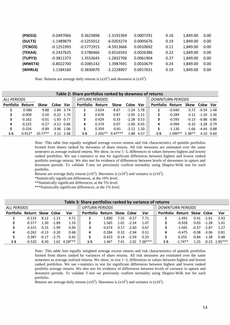
In Table 2 we consider skewness of returns since the literature review spotlights it as a

potential risk measure for emerging markets. Therefore, this Table aims to find some

relationship between skewness and returns. We expect over all periods a preference for

positive skewness that causes investors to accept lower returns, therefore we expect a

negative relationship between skewness and returns. We also have no expectation that

skewness of returns will have a particular linkage to market upturns or downturns.

However, our findings are contrary to ours expectations since Table 2 shows a positive

relationship between skewness and returns. We also find significant differences between

returns in the highest and lowest ranked portfolios. Firms offering strong positively

8

performances have positively skewed returns, and on the other hand, firms with poorest

returns show negative skewnees. We note the same significant positive relationship

between skewness and returns for both upturn and downturn periods. The significance of

performed t-statistics indicates that skewness in not particularly associated with either

downturns or upturns.

In Table 3, we assess the explanatory power of variance in the Brazilian market.

Exposure to volatility is unattractive to investors, so we expect that if an investor assumes

to own a portfolio that exhibit high levels of variance he will required higher return.

According to the literature, variance is likely to be associated with both upturns and

downturns, so we shouldn’t expect a specific separate relationship in either period.

When focusing on “all periods” at Table 3, we can´t find any relationship between

variances and returns, initially suggesting little evidence of a relationship between volatility

and performance, but if we concentrate on separate downturn and upturn periods, we note

that for upturn periods, high variance portfolios tend to offer superior performances and for

downturn periods high variance portfolios tend to suffer greater losses. Although neither

relationship is monotonic, significant differences between highest and lowest ranked

portfolios are confirmed for both upturn and downturn periods. These findings for both

separate periods (bullish and bearish market) are aligned with our previous expectations

because it means that exposure to volatility (high variance) is rewarded with excess returns

during upturns, and is penalized with losses during downturns.

We also note that for Tables 2 and 3, regardless the period, variance appear to be

related to skewness: shares in the high variance portfolios exhibit positive skewness and

viceversa. Skewness appears to possess systematic relation to expected returns and

variance, meaning that any relationship between returns and skewness may be partly

explained by variance. This conclusion is aligned with Harvey & Siddique (2000), since

they found significant impact of skewness on estimated conditional volatility.

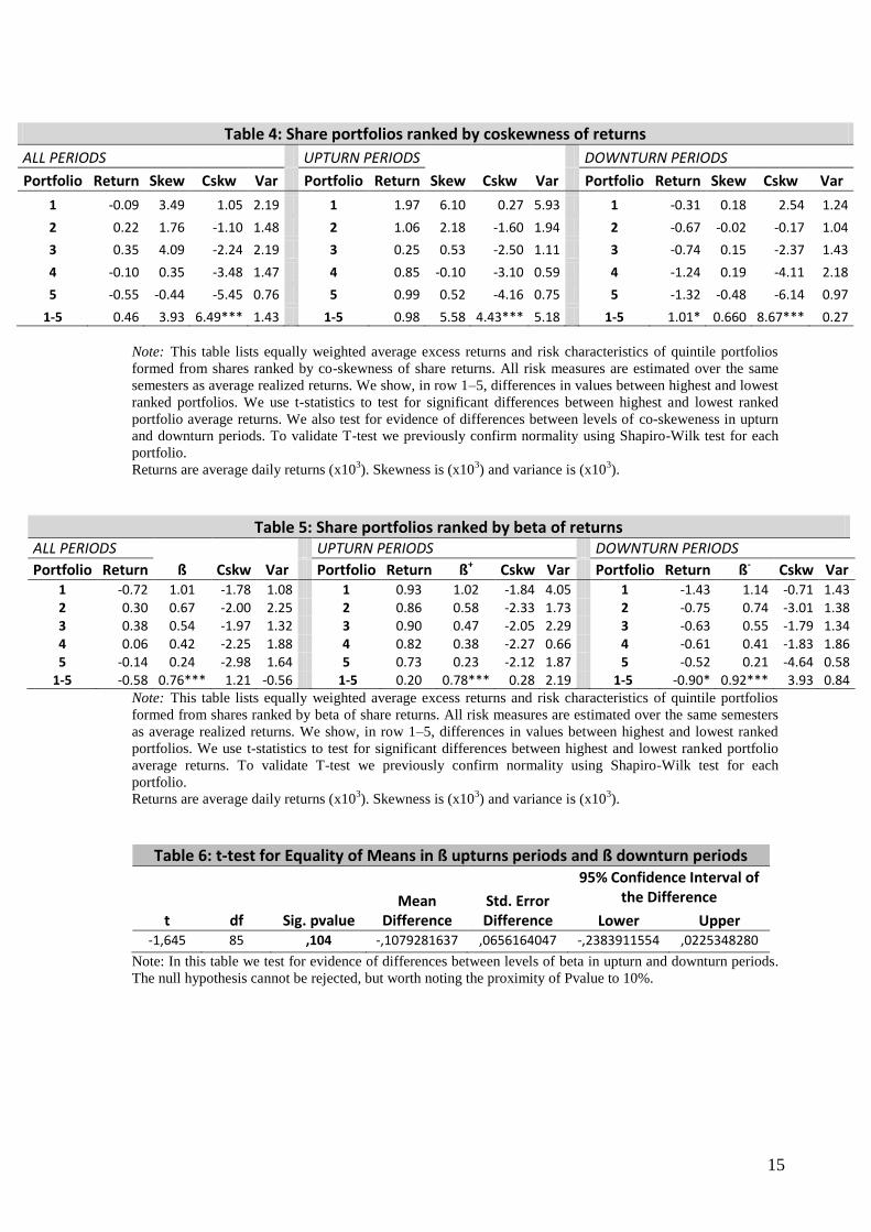
In Table 4, we consider co-skewness of returns, as we want to test the downside risk

effectiveness of this measure. Co-skewness may capture some aspects of an investor risk

exposure; thereby we expect to see this effect clearly in downturn periods. Co-skewness

represents the contribution of individual shares to the skewnesss of a broader portfolio. As

defined in equation (2), co-skewness is determined by the covariance of share returns with

market return, which is a higher momentum indicator of market volatility. We expect

higher volatility during downturns and if we have a consistent outcome, negative co-

skewness will be associated with relatively lower returns. If volatility is indeed more

commonly associated with downturns, different kinds of relationships or/and levels of

significance may be identified in upturn and downturn markets. In Table 4 portfolios are

ranking by estimates of co-skewness. When we concentrate on separate upturn and

downturn periods, we could note that low co-skewness portfolios tend to offer poorer

performance in both periods, although we find that only for downturn periods the results

are statistically significant. These findings mean that for upturn periods the effect of co-

skewness seems not be statistically relevant in stocks returns and therefore we cannot

validate any relationship when the economy in Brazilian market is growing. Otherwise,

during downturns, t-test indicates significant differences for returns and co-skewness

between highest and lowest co-skewness ranked portfolios and there exist a positive

monotonic relationship. This result confirms that losses may be probable from negative

(lower) co-skewness during downturns. Indeed, results in table 4 suggest that lower (more

negative) returns have a greater volatility during downturns, and this effect may be relevant

due to association of volatility with downturns. Hence investors in Brazil should be aware

that holding a portfolio with negative co-skewness could lead to greater losses during

9

downturn periods and these losses may not be rewarded with good performance during

upturns.

In table 5, portfolios are formed using ranking estimates on betas. According to

conventional CAPM theory, beta should have a positive relationship with share returns,

however Pettengill et al. (1995) states that positive relation may only exist during market

upturns. A negative relationship is expected during turndowns, as stocks with greater

exposure will offer worse results. The overall relationship in both downturn and upturn

periods combined, named as “all periods”, will depend on the weight of the beta effect on

each period. In a growing economy upturn periods are more likely, so we should expect a

positive relationship. In our case of study, we have slightly more upturns periods (57% up

vs. 43% down), then we should have a positive relationship, but for obvious reasons the

effect may be very weak to be significant. Downside beta is conditioning on observations

when market performance is below free risk rate. This risk exposure is also unattractive for

investors, because during downturns, investor accepting higher downside betas should

suffer greater losses. Therefore we expect a negative relationship between downside beta

and returns. Otherwise, upside beta is conditioning on observations when market

performance is above the risk free rate. Greater beta shares should perform well, so a

positive relationship between upside beta and returns is expected. Another forecast to be

tested is the relationship between downside beta and co-skewness. Although both are

downside measures of risk, both are differently constructed and therefore they may capture

different features of investor’s downside risk exposure.

For overall periods we calculated the conventional beta measure; for downturn

periods, we show - as explained in equation 5, and for upturns we exhibit upside betas

(+). We report average portfolio values for beta, and we exclude average skewness values.

We again need to concentrate for upturns and downturns periods, as we cannot find a

clearly relationship for beta and returns in “all periods together”. This may simply mean

that the conventional CAPM may not be applicable in the Brazilian market for returns

prediction. According to our expectations, exposure to upside beta is rewarded with excess

return during upturns although we cannot validate a statistical significance for returns

differences between portfolio 1 and 5. Otherwise, exposure to downside beta is penalized

with losses during turndowns, this relationship between returns and downside beta is

validated with a 10% level significance for returns and 1% level significance for - .

Below, in Table 6, we exhibit the results of t-statistics for equality of means between

upturns and downturns; the null hypothesis of this test states that beta’s mean for both

periods is equal. The Pvalue is 0,104 and therefore the null hypothesis cannot be rejected.

Anyway, we must take into account, the proximity of Pvalue to 10 %, meaning that we

cannot simply assume that the means are equal without studying deeply the whole scenario.

Referring again to Table 5 we also note that it cannot be observed any relationship

between downside beta and co-skewness. That could mean that any losses for exposure to

negative coskewness may not be related to losses for exposure to downside beta.

7. Conclusions

This paper uses returns of securities traded on the Sao Paulo Stock Exchange (SPSE)

and empirically investigates the relationship between risk and return in a downside risk

framework and in a regular risk framework. We aimed to test the behavior of two variables

related with the expected returns in a semi-variance environment (co-skewness and

downside beta).

After testing normality with Komolgorov-Smirnov test, it can be seen that for Brazilian

market, normal distribution of returns is not achieved for any security at all. Summarizing

10

the results, it can be observed some strong evidence that there exists a relationship between

downside risk measures and returns to portfolios in Brazilian market. Thus, we found that

for equally weighted portfolios, the downside risk measures are better in explaining mean

returns than variance, skewness and conventional beta. During upturn markets, we cannot

conclude about the superiority of the downside risk measures since, even after showing

tendencies of direct relationship with returns, t-tests don´t show statistical significance in

difference of means between returns for high and low ranked portfolios. Otherwise, for

downturn markets, results reveal that both downside beta and co-skewness are priced in

downfalls for equity markets. These results are perfectly aligned with Harvey & Sidiqque

(2000) and Estrada (2002) since the latter showed that downside beta is more sensitive than

conventional beta during downturns and the former demonstrated the importance of the

inclusion of co-skewness in the asset pricing platform to help in explaining the variation of

equity returns.

Our most interesting finding is that co-skewness seems to possess more interesting

features than downside beta from a Brazilian investor point of view, since negative co-

skewness is related to greater losses during turndowns and these losses would not be

rewarded by greater earnings during upturns. Therefore, an investor would be willing to

avoid Brazilian stocks with negative co-skewness of returns within their portfolios. This

result is consistent, among others, with Huan & Litzenberger (1988) and Harvey &

Siddique (2002), since both papers demonstrated that investors should dislike adding stocks

with negative co-skewness into their portfolios, because these stocks would make the

portfolio returns more left skewed and finance literature recognize the investor´s preference

for positive skewness.

Finally, we found that in downfalls both measures of downside risk (co-skewness and

downside beta) independently seem to capture different aspects of downside risk, because

both have explanatory power over returns, but they don’t show any direct relationship

between each other.

References

Ang, A., Chen, J. and Xing, Y. (2001). Downside Risk and the Momentum Effect. Working Paper

8643, National Bureau of Economic Research, Massachusetts.

Ang, A., Chen, J., Xing, Y., (2006). Downside risk. The Review of Financial Studies 19, 1191–

1239.

Ang, J.S., Chua, J.H., (1979). Composite measures for the evaluation of investment performance.

Journal of Financial and Quantitative Analysis 14, 361–384.

Bawa, V. and Lindenberg, E. (1977). Capital Market Equilibrium in a Mean-Lower Partial Moment

Framework. Journal of Financial Economics, 5(2), 189-200.

Banz, Rolf W. (1981), The Relationship between Return and Market Value of Common Stocks.

Journal of Financial Economics, 9(1), 3–18.

Bekaert, G., Erb, C. and C.H. Harvey, (1997), What matters for emerging equity market

investments? Emerging Markets Quarterly, 17 - 46.

Bekaert, G. and C.H. Harvey,(1998), Emerging equity market volatility, Journal of Financial

Economics 43, 29 - 78.

Black, Fischer (1972), Capital Market Equilibrium with Restricted Borrowing. The Journal of

Business, 45(3), 444–455.

11

Black, F., Jensen, M, Scholes, M. (1972), The capital asset pricing model: some empirical tests.

Studies in the Theory of Capital Markets, Praeger, New York, NY, 79-124.

BMF BOVESPA (2013) ; http://www.bmfbovespa.com.br/ capitalizacaobursatil /

ResumoBursatilDetalhado. (accessed December 23, 2013)

Borch, Karl (1969). A Note on Uncertainty and Indifference Curves. Review of Economic Studies,

1969, vol. 36, issue 105, pages 1-4

Bovespa (2008), Índice Bovespa Definição e Metodologia. São Paulo: Bovespa. Available at

http://www.bmfbovespa.com.br/Indices/download/IBovespa.pdf (accessed June 25, 2013)

Brounen, D., De Jong, A., Koedijk, C.G., (2004). Corporate Finance in Europe: Confronting Theory

with Practice, Financial Management 33, 71-101.

Bruner, R.F., Conroy, R.M., Li, W., O’Halloran, E.F. and Lleras, M.P. (2003), Investing in

emerging markets, The Research Foundation, The Association for Investment Management and

Research, Charlottesville.

Dittmar, R.F., (2002). Nonlinear Pricing Kernels, Kurtosis Preference, and Evidence from the

Cross Section of Equity Returns. Journal of Finance 57, 369-403.

Doan, P., Lin, C., Zurbruegg R., (2009). Pricing assets with higher moments: Evidence from the

Australian and US stock markets. Int.Fin.Markets, Inst. and Money 20, 51 67.

Estrada, J., (2000). The cost of equity in emerging markets: a downside risk approach, Emerging

Markets Quarterly, 19 - 30.

Estrada, J. (2002). Systematic risk in emerging markets: the D-CAPM. Emerging Markets Review

3, 365–379.

Fama. Eugene F. and James Macbeth. (1973). Risk Return and Equilibrium: Empirical Tests,

Journal of Political Economy 81. 607-636.

Feldman, R., Kumar, M., (1995). Emerging equity markets: growth, benefits, and policy concerns.

The World Bank Research Observer 10, 181–200.

Galagedera, D., Brooks, R.D., (2007). Is co-skewness a better measure of risk in the downside than

downside beta? Evidence in emerging market data. Journal of Multinational Financial

Management 17, 214–230.

Graham, John and Campbell Harvey, (2001) The Theory and Practice of Corporate Finance:

Evidence from the Field, Journal of Financial Economics, LX, 187-243.

Graham, John; Campbell Harvey, (2009) Equity risk premium; Evidence from the Global CFO

Outlook survey 2009. The CFO Global Business Outlook: 1996-2009.

Gul, F.(1991). A theory of disappointment aversion. Econometrica 59, 667–686.

Hamada, R.S. (1972) “The Effect of the Firm's Capital Structure on the Systematic Risk of

Common Stocks,” The Journal of Finance, 27(2):435-452

Harvey, C.H., Siddique, A., (2000). Conditional skewness in asset pricing tests. Journal of Finance

60, 1263–1295.

Harvey, C.H. (1995), Predictable risk and returns in emerging markets, Review of Financial Studies,

773 - 816.

Hogan, W. & Warren, J. (1974). Towards the Development of an Equilibrium Capital-Market

Model Based on Semivariance. Journal of Financial & Quantitative Analysis, 9(1), 1-11.

Huang, C-F., Litzenberger, R., (1988). Foundations for Financial Economics. North- Holland, New

York.

12

Ingersoll, J., (1975). Multidimensional security pricing. Journal of Financial and Quantitative

Analysis 10, 785-798.

Kraus, A., Litzenberger, R.H., (1976). Skewness preference and the valuation of risk assets. Journal

of Finance 31, 1085–1100

Libby, R. and Fishburn, P. (1977). Behavioral Models of Risk Taking in Business Decisions: A

Survey and Evaluation. Journal of Accounting Research, 15, 272-292.

Lintner, John (1965). The Valuation of Risky Assets and the Selection of Risky Investments in

Stock Portfolios and Capital Budgets. The Review of Economics and Statistics, 47(1), 13–37.

Markowitz, H.M. (1959). “Portfolio Selection: Efficient Diversification of Investments”, New

York: John Wiley & Sons.

Nantell T.J., Price K. and Price B. (1982). Mean-Lower Partial Moment Asset Pricing Model: Some

Empirical Evidence. The Journal of Finance Vol. 37, No. 3 (Jun., 1982), pp. 843-855

Pettengill, G.N., Sundaram, S., Mathur, I., (1995). The conditional relation between beta and

returns. Journal of Financial and Quantitative Analysis 30, 101–116.

Pereiro, L. (2002). Valuation of companies in emerging markets: a practical approach, Wiley, New

York.

Pereiro, L. (2006) The Practice of Investment Valuation in Emerging Markets: Evidence from

Argentina, Journal of Multinational Financial Management, No.16, pp.160-183.

Ross, S., Westerfield, R. & Jaffe, J. (2003) Corporate Finance, Sixth Edition, The McGraw−Hill

Companies.

Roy, A. D. (1952) "Safety-First and the Holdings of Assets", Econornetrica 20, 431

Sharpe, Willian F. (1964), Capital Asset Prices: A Theory of Market Equilibrium under Conditions

of Risk. The Journal of Finance, 19(3), 425–442.

Tobin, J. (1958), "Liquidity preference as behavior towards risk", Review of Economic Studies, Vol.

26 pp.65-86.

Tsiang, S.C (1972). The Rationale of the Mean-Standard Deviation Analysis, Skewness Preference,

and the Demand for Money. The American Economic Review, Vol. 62, No. 3 (Jun., 1972), pp. 354-

371

13

Appendix: Tables

Table 1: Test Normality All periods Kolmogorov-Smirnov

Mean Skew Cskw Var Statistic df Sig.

BOVESPA 0.0955691 -0.0137639 -0.2556760 0.0003458 0.08 1,849.00 0.00

(EALT4) 0.1527029 0.6202519 -0.1243599 0.0008600 0.17 1,849.00 0.00

(AGEN11) -1.7487312 3.0070995 -3.4654237 0.0046655 0.28 1,849.00 0.00

(ALPA4) 0.7507811 -1.5725428 -3.0561456 0.0004228 0.09 1,849.00 0.00

(BTOW3) -1.1410985 0.3638702 0.6754250 0.0010624 0.13 1,849.00 0.00

(BDLL4) 0.1755351 -0.1526503 -3.2057457 0.0005985 0.23 1,849.00 0.00

(BHGR3) -0.1693011 -0.1696535 -6.3352817 0.0003765 0.20 1,849.00 0.00

(BOBR3) -0.0852191 -0.0081053 -1.5224290 0.0008042 0.14 1,849.00 0.00

(BMTO4) 1.4586380 1.7353915 -0.6226313 0.0008591 0.23 1,849.00 0.00

(BRFS3) 0.7757708 0.3104107 -0.5250198 0.0005653 0.06 1,849.00 0.00

(BISA3) -1.2134574 -0.0962052 -1.4798725 0.0009097 0.09 1,849.00 0.00

(HGTX3) 1.8264004 0.6691852 1.2648253 0.0008357 0.09 1,849.00 0.00

(CSAN3) 0.0013786 -0.1482324 -2.1874556 0.0008522 0.08 1,849.00 0.00

(CZLT11) 0.3183293 -1.1740338 -3.3877733 0.0009028 0.16 1,849.00 0.00

(CTNM4) -0.6841797 -0.0281348 -4.1486334 0.0007564 0.10 1,849.00 0.00

(CPFE3) 0.4458471 -0.0016120 1.5572650 0.0003195 0.06 1,849.00 0.00

(CRDE3) -0.6727136 -0.3000492 -3.1589293 0.0007835 0.15 1,849.00 0.00

(CREM4) -0.0618927 0.1286084 -2.6920869 0.0004320 0.13 1,849.00 0.00

(CYRE4) 0.0888042 0.0632004 -0.4320558 0.0011820 0.05 1,849.00 0.00

(ETER3) 1.8269411 14.1342488 -1.6052402 0.0019395 0.20 1,849.00 0.00

(FLCL3) 0.5722480 -0.8266641 -5.5514361 0.0005478 0.14 1,849.00 0.00

(FIBR3) -0.5764411 -0.6609193 -7.3308112 0.0008683 0.13 1,849.00 0.00

(FRAS4) 0.2776226 1.5110438 -3.0489710 0.0003709 0.16 1,849.00 0.00

(GFSA5) -0.7822262 0.0163086 0.0643979 0.0014350 0.06 1,849.00 0.00

(HAGA3) 0.9238561 -0.0413309 -3.9516817 0.0003503 0.07 1,849.00 0.00

(HRTP3) 1.1337202 4.6480957 -2.0805361 0.0035150 0.28 1,849.00 0.00

(IGBR5) -0.3219270 2.2102485 -3.6273670 0.0034286 0.18 1,849.00 0.00

(INEP3) -1.0974432 32.2605667 2.7839463 0.0109471 0.28 1,849.00 0.00

(INEP4) -0.2767317 -0.8711761 -2.0456111 0.0010194 0.13 1,849.00 0.00

(MYPK3) 1.5209591 1.4781087 -3.2622454 0.0009270 0.11 1,849.00 0.00

(JHSF3) -0.0637570 -0.0581249 -0.7131413 0.0010046 0.11 1,849.00 0.00

(KLBN3) -1.6792987 -1.0911487 -1.8823735 0.0027226 0.22 1,849.00 0.00

(LAME3) 0.1784820 -0.7410813 -2.7677294 0.0005046 0.13 1,849.00 0.00

(MGLU3) -1.9768607 -0.4479602 -4.4819571 0.0011838 0.10 1,849.00 0.00

(MSPA3) -0.5569367 -0.7267456 -6.0736993 0.0008104 0.13 1,849.00 0.00

(MNPR3) -0.2489164 0.0122996 -4.4975823 0.0006498 0.16 1,849.00 0.00

(BNBR3) 0.5681056 0.1469784 1.0797184 0.0004816 0.04 1,849.00 0.00

(PCAR3) -1.7936800 0.1862252 -3.7804667 0.0014634 0.19 1,849.00 0.00

(RPMG3) -0.1785904 -0.1763489 -3.9083893 0.0011295 0.09 1,849.00 0.00

(PETR4) -0.1219548 -0.2248143 -1.5073765 0.0005787 0.06 1,849.00 0.00

(PTBL3) 2.6934222 34.6353663 -1.8828440 0.0055029 0.26 1,849.00 0.00

(RCSL4) 0.1201122 3.1803843 -1.6288655 0.0052653 0.21 1,849.00 0.00

(SNSY5) 0.1935857 0.4363641 1.1374845 0.0022209 0.15 1,849.00 0.00

14

(PSEG3) -0.0497066 0.3623898 -1.3192369 0.0007291 0.16 1,849.00 0.00

(SULT3) -1.1489879 -0.5255012 -6.0203274 0.0005676 0.19 1,849.00 0.00

(TCNO3) -0.1251993 -0.5771915 -4.5913666 0.0010692 0.11 1,849.00 0.00

(TEKA4) -0.2437625 0.5780466 0.6516543 0.0026386 0.22 1,849.00 0.00

(TUPY3) -0.3811373 1.3553645 -1.2832706 0.0061904 0.27 1,849.00 0.00

(MWET4) -0.8022700 -0.2085142 1.3987691 0.0010679 0.24 1,849.00 0.00

(WHRL4) 1.1184160 -0.3830670 -2.2228907 0.0017631 0.19 1,849.00 0.00

Note: Returns are average daily returns is (x103) and skewness is (x10

3)

Table 2: Share portfolios ranked by skewness of returns ALL PERIODS

UPTURN PERIODS

DOWNTURN PERIODS

Portfolio Return Skew Cskw Var Portfolio Return Skew Cskw Var Portfolio Return Skew Cskw Var 1 0.586 9.88 -1.84 3.74 1 2.624 8.67 -1.24 5.78 1 -0.040 0.72 -0.54 1.48 2 -0.009 0.50 -0.22 1.70 2 0.678 0.87 -2.05 2.21 2 -0.289 0.12 -1.20 1.36 3 -0.162 -0.01 -1.93 0.77 3 0.429 0.33 -2.28 0.53 3 -0.593 -0.13 -0.88 0.86 4 -0.225 -0.27 -3.12 0.86 4 0.374 0.07 -2.00 0.65 4 -0.999 -0.33 -3.28 0.79 5 -0.326 -0.89 -3.96 1.06 5 0.359 -0.81 -3.12 1.20 5 -1.130 -1.66 -4.64 0.88

1-5 0.912* 10.77** 2.12 2.68 1-5 2.265** 9.47*** 1.88 4.57 1-5 1.090** 2.38** 4.10 0.60

Note: This table lists equally weighted average excess returns and risk characteristics of quintile portfolios

formed from shares ranked by skewness of share returns. All risk measures are estimated over the same

semesters as average realized returns. We show, in row 1–5, differences in values between highest and lowest

ranked portfolios. We use t-statistics to test for significant differences between highest and lowest ranked

portfolio average returns. We also test for evidence of differences between levels of skeweness in upturn and

downturn periods. To validate T-test we previously confirm normality using Shapiro-Wilk test for each

portfolio.

Returns are average daily returns (x103). Skewness is (x10

3) and variance is (x10

3).

*Statistically significant differences, at the 10% level.

**Statistically significant differences, at the 5% level.

***Statistically significant differences, at the 1% level.

Table 3: Share portfolios ranked by variance of returns ALL PERIODS UPTURN PERIODS DOWNTURN PERIODS

Portfolio Return Skew Cskw Var Portfolio Return Skew Cskw Var Portfolio Return Skew Cskw Var 1 -0.133 8.12 -1.13 4.71 1 1.890 7.55 -0.57 7.71 1 -1.491 0.41 -1.61 2.43 2 -0.377 1.30 -1.89 1.33 2 1.565 1.01 -2.24 1.07 2 -0.928 0.03 -1.28 1.41 3 0.315 0.15 -1.99 0.90 3 0.674 0.17 -2.60 0.67 3 -1.045 -0.37 -2.87 1.27 4 -0.262 -0.13 -3.20 0.68 4 0.284 0.32 -2.94 0.51 4 -0.475 -0.08 -3.06 0.81 5 0.387 -0.17 -2.75 0.42 5 0.423 0.14 -2.59 0.33 5 0.255 -0.84 -1.38 0.48

1-5 -0.520 8.30 1.62 4.28*** 1-5 1.46* 7.41 2.02 7.38*** 1-5 -1.74** 1.25 -0.23 1.95***

Note: This table lists equally weighted average excess returns and risk characteristics of quintile portfolios

formed from shares ranked by variances of share returns. All risk measures are estimated over the same

semesters as average realized returns. We show, in row 1–5, differences in values between highest and lowest

ranked portfolios. We use t-statistics to test for significant differences between highest and lowest ranked

portfolio average returns. We also test for evidence of differences between levels of variance in upturn and

downturn periods. To validate T-test we previously confirm normality using Shapiro-Wilk test for each

portfolio. Returns are average daily returns (x10

3). Skewness is (x10

3) and variance is (x10

3).

15

Table 4: Share portfolios ranked by coskewness of returns

ALL PERIODS UPTURN PERIODS

DOWNTURN PERIODS

Portfolio Return Skew Cskw Var Portfolio Return Skew Cskw Var Portfolio Return Skew Cskw Var

1 -0.09 3.49 1.05 2.19 1 1.97 6.10 0.27 5.93 1 -0.31 0.18 2.54 1.24

2 0.22 1.76 -1.10 1.48 2 1.06 2.18 -1.60 1.94 2 -0.67 -0.02 -0.17 1.04

3 0.35 4.09 -2.24 2.19 3 0.25 0.53 -2.50 1.11 3 -0.74 0.15 -2.37 1.43

4 -0.10 0.35 -3.48 1.47 4 0.85 -0.10 -3.10 0.59 4 -1.24 0.19 -4.11 2.18

5 -0.55 -0.44 -5.45 0.76 5 0.99 0.52 -4.16 0.75 5 -1.32 -0.48 -6.14 0.97

1-5 0.46 3.93 6.49*** 1.43 1-5 0.98 5.58 4.43*** 5.18 1-5 1.01* 0.660 8.67*** 0.27

Note: This table lists equally weighted average excess returns and risk characteristics of quintile portfolios

formed from shares ranked by co-skewness of share returns. All risk measures are estimated over the same

semesters as average realized returns. We show, in row 1–5, differences in values between highest and lowest

ranked portfolios. We use t-statistics to test for significant differences between highest and lowest ranked

portfolio average returns. We also test for evidence of differences between levels of co-skeweness in upturn

and downturn periods. To validate T-test we previously confirm normality using Shapiro-Wilk test for each

portfolio. Returns are average daily returns (x10

3). Skewness is (x10

3) and variance is (x10

3).

Table 5: Share portfolios ranked by beta of returns ALL PERIODS

UPTURN PERIODS DOWNTURN PERIODS

Portfolio Return ß Cskw Var Portfolio Return ß+ Cskw Var Portfolio Return ß- Cskw Var 1 -0.72 1.01 -1.78 1.08 1 0.93 1.02 -1.84 4.05 1 -1.43 1.14 -0.71 1.43 2 0.30 0.67 -2.00 2.25 2 0.86 0.58 -2.33 1.73 2 -0.75 0.74 -3.01 1.38 3 0.38 0.54 -1.97 1.32 3 0.90 0.47 -2.05 2.29 3 -0.63 0.55 -1.79 1.34 4 0.06 0.42 -2.25 1.88 4 0.82 0.38 -2.27 0.66 4 -0.61 0.41 -1.83 1.86 5 -0.14 0.24 -2.98 1.64 5 0.73 0.23 -2.12 1.87 5 -0.52 0.21 -4.64 0.58

1-5 -0.58 0.76*** 1.21 -0.56 1-5 0.20 0.78*** 0.28 2.19 1-5 -0.90* 0.92*** 3.93 0.84 Note: This table lists equally weighted average excess returns and risk characteristics of quintile portfolios

formed from shares ranked by beta of share returns. All risk measures are estimated over the same semesters

as average realized returns. We show, in row 1–5, differences in values between highest and lowest ranked

portfolios. We use t-statistics to test for significant differences between highest and lowest ranked portfolio

average returns. To validate T-test we previously confirm normality using Shapiro-Wilk test for each

portfolio. Returns are average daily returns (x10

3). Skewness is (x10

3) and variance is (x10

3).

Table 6: t-test for Equality of Means in ß upturns periods and ß downturn periods

t df Sig. pvalue Mean

Difference Std. Error Difference

95% Confidence Interval of the Difference

Lower Upper -1,645 85 ,104 -,1079281637 ,0656164047 -,2383911554 ,0225348280

Note: In this table we test for evidence of differences between levels of beta in upturn and downturn periods.

The null hypothesis cannot be rejected, but worth noting the proximity of Pvalue to 10%.