ts âôo

REGIONAL BIODIVERSITY MANAGEMENT STRATEGY:

CASE STUDY ON THE FLINDERS RANGES

By

Batbold Dorigurhem Otgoid

B.Sc.Agric. (Odessa, Ukraine)

This thesis is submitted in fulfilment of the

requirements for the

Degree of Master of Applied Sciences

In

The University of Adelaide

Faculty of Agricultural and Natural Resource Sciences

Department of Applied and Molecular Ecology

Australia

+1

Iuty 7999

TABLE OF CONTENTS

ACKNOWLEDGMENTSPREFACEABSTRACT ............

CHAPTER 1

GENERAL INTRODUCTION 1

CHAPTER 2

SAMPLING THE BIODIVERSITY ...............6

2.2.BTODIVERSITY - A BACKGROUND

2.2.L. G enetic diversity2.2.2. Sp ecies diversity .....

2.2.3. Eco system diversity

2.3. WHY MANAGE FOR THE CONSERVATION OF BIODIVERSITY?

2.4. SPECIES - A TARGET FOR BIODIVERSITY MANAGEMENT

2.4.1, Indicator species2.4.2 U rnbrella sp ecies2.4.3Flagship species2.4.4Keystone species

2.5. CONCLUSTON .......14

CHAPTER 3

THEORETICAL NOTIONS OF BIODIVERSITY MANAGEMENTON A REGIONAL BASIS ..........15

3.1. INTRODUCTION 15

3.2. THE IMPORTANCE OF MANAGING BIODIVERSITY ON AREGIONAL BASIS .......15

tv.vv1

6

7

8

8

9

lL

12121313

ll

3.2.1 Protected areas in practice..3.2.2 OÊÊ-reserve conservation3.2.3 Conclusion ...........

3.3. REGIONAL BIODIVERSITY MANAGEMENT PRACTICES

3.3.1 Biosphere reserve ......

3.3.2 Bioregionalism.

3.4. THE FLINDERS RANGES AS A CASE STUDY..............

CHAPTER 4BIOCLIMATIC ANALYSIS OF SOUTH AUSTRALIAN DISTRIBUTIONoF THE YELLOW-FOOTED ROCK WALLABY PETROGALEXANTHOPUS

4.1. INTRODUCTION4.2. P. XANTHOPUS DISTRIBUTION IN SOUTH AUSTRALIA...............

4.2.-J.. P ast distribution4.2.2. Present distribution .......

4.3. CLIMATIC CONDITIONS OVER THE KNOWN DISTRIBUTION OFP. XANTHOPUS

4.4. BIOCLIMATIC PREDICTION SYSTEM: A TOOL FOR RAPIDASSESSMENT OF THE SPECIES DISTRIBUTION.

4.4.1. Bioctimatic prediction system within ANUCLIM package'4.4.2. Cllrnate surfaces .................

4.4.3. Bioclimatic p arameters and climatic prof iie4.4.4. Prediction of species distlibution ...

4.5. STATISTICAL MODELLING ........... ........50

1.6

1822

23

2425

28

37

32

JJ

34

39

40

40424346

4.5.1. Logistic regression ..................4.5.2. Multivariate analysis

.............51

.............54

55

5565

69

70

4.6.1. Bioclimatic range of P. xønthopus distrLbution.........4.6.2. Otlner statistical approaches for the assessment of climatic factors4.6.3. Summaty of results...

4.7. DISCUSSION AND CONCLUSION ............

lll

CHAPTER 5

POPULATION VIABILITY ANALYSIS OF THE YELLOW-FOOTEDROCK WALLABY P. XANTHOPUS IN SOUTH AUSTRALIA:MANAGEMENT OPTIONS FOR SPECIES PERSISTENCE

5.1. INTRODUCTION

5.2. POPULATION VIABILITY ANALYSIS: A TOOL FOR ASSESSINGPOPULATIONS EXTINCTION AND MANAGEMENT......

5.2.1 ALEX: a model for population viability analysis

5.3. BACKGROUND INFORMATION ON THE YELLOW-FOOTED ROCKWALLABY P. XANTHOPUS.......

5.3.1. Life-history.........5.3.2. Threats to YRW pelsistence.....

5.4. METHODS USED FOR MODELLING THE METAPOPULATIONVIABILITY OF P. XANTHOPUS

5.4.1. Study area..............5.4.2. Inltr.al population si2e...............5.4.3. Movement between habitat patches...........5.4.4. Other parameters input to ALEX....5.4.5. Catastrophe and environmental variable ..

5.5. SCENARIOS AND RESULTS.

5.6. DISCUSSION

CHAPTER 6

GENERAL DISCUSSION ..........1.04

REFERENCES 107

APPENDICES ............118

73

76

7B

84

8486

86

8689909092

93

99

lv

ACKNOWLEDGMENTS

I sincerely thank my principal supervisor Prof. Hugh Possingham,

for his guidance, interest, invaluable discussions, and encouragement

and for his valuable advice and support during the supervision of

this project.

I would also like to thank my co-supervisor Dr. Desmond Coleman

for his support, and encouragement during my candidature'

Support and assistance from people in the Department of Applied

and Molecular Ecology wefe offered without hesitation. I would

especially like to thank Greg van Gaans for his assistance in complex

mapping procedure. I am also indebted to Dr. Drew Tyre for his

willingness to answer my questions and careful editing of drafts.

The statistical analysis would not have been possible without the

help of Michelle Lorimer. Her assistance and enthusiasm was greatly

appreciated.

I would also like to acknowledge, with thanks, the financial support

I received from AusAID through the Government of Mongolia, which

enabled me to undertake and complete this study and my employer,

the Ministry f or Nature and the Environment of Mongolia f or

granting me the study leave.

Finally, and most important, I express my deepest gratitude to my

wife Oyunbileg for her help, patience and moral support throughout

my study and also to my boys Chintogtoh (7 yrs old) and Togtohtur

(4 yrs old) for their understanding and joy they brought to me during

these years.

v

iI

I

I

I

i,

PREFACE

This thesis contains no material which has been accepted for the

award of any other degree or diploma in any University, and to the

best of my knowledge and belief, contains no material previously

published or written by anothef pelson, except where due reference

has been made in the text.

I give consent to this copy of my thesis, when deposited in the

University Library, being available f or loan and photocopying,

provided that acknowledgment is made of any reference to work

therein.

Signed Date 24..m#.çh.., ..?uoÕ

III

I

T

I

VI

d

ti

ABSTRACT

This thesis examines the rationale for managing biological diversity

on a regional basis and develops recommendations for the use of two

computational methods in regional biodiversity management

planning by conducting a case study in the Flinders Ranges, centred

on the Yellow-footed Rock Wallaby Petrogøle xønthopus.

The research was conductedby a combination of literature review on

the importance and practices of managing biodiversity on a regional

basis, bioclimatic analysis on the distribution of P. xnnthopus in

South Australia, using bioclimatic prediction system (BIOCLIM), and

an application of Population Viability Analysis (PVA) for the long-

term management strategy of P. xønthopus, using computer

simulation package ALEX.

BIOCLIM

The primary objective of this analysis was to identify priority area in

the bioregion by predicting the distribution of P. xønthopus.

Three types of distribution (extant, extinct and all-time) were

predicted using BIOCLIM. These analyses suggest that climate

determines the general distributional pattern of P. xønthopus in South

Australia.

As a controversy, the actual distributional pattern will not always

coincide with the predicted ones. This situation is probably caused

by the factors other than climatic variables. The other factors may

include such hypotheses as predation by exotic carnivores and

Wedge-tailed Eagle and competition with again exotic species as

goat. This hypothesis is supported by the prediction of possible

extinct distribution. The bioclimatic signatures of the predicted and

actual regions wet'e identical. If the climate was a factor that forces

the species extinction we must have a completely different result.

Flowever', our result suggests that the climatic variables are not the

II

!

¡l

tÍ

vu

major determinant of the Yellow-footed Rock Wallaby extinction in

South Australia.

BIOCLIM does not predict the distribution of the species, rather itpredicts the area climatically suitable f or a particular species

distribution. If, the climatically suitable area supports preferred

habitats of P. xønthopus with shelter sites, then it could be considered

as an af ea to have a high probability of f inding additional

populations of the species ot more realistically specimens.

PVA:

The main objective of this analysis was to minimise the chance of

extinction of P, xønthopus.

In this paft of the thesis, the hypothesis that arised by BIOCLIM

analysis is tested. The predation by exotic carnivores and

competition with introduced herbivores afe considered to be the

major threats to P. xønthopus decline in South Australia.

The result of the analysis demonstrated that there is a high

probability of extinction amongst populations of P. xønthopus in a set

of small patches of <60 ha. Similarly, single patch of <360 ha does

not have significant effect on the species persistence.

Set of 5 or more patches, each of >100 ha in size,located within 10-15

km from each other was that most likely to support P' xønthopus

populations and these areas make the greatest contribution to the

persistence of the species in the Flinders Ranges.

Increase of mortality rates of all ages reduced the median time to

extinction drastically. The highest probability of extinction occurs

with an increase in the moltality rate of adult wallaby. The results of

the analyses suggest that reducing the mortality rate of adult female

wallabies would be a highly successful option for the conservation of

P. xønthopzs colonies.I

t

vlll

Conclusion

Cooperative efforts of identifying priority areas for the biodiversity

management and setting priorities for the actions in the area are the

crucial fesponses for the development of biodiversity management

strategy in a particular af ea. For this task BIOCLIM and PVA

appeared to be powerful tools if the target species has been chosen

correctly. F{owever, the selection of 'right' species is a very

demanding task. Therefore, for the development of such strategy, it

might be wise to select several species with different backgrounds of

life-history and distributions.

ï

CHAPTER 1.

GENERAL INTRODUCTION

The quality of human life in the next century will depend largely on

developing a healthy relationship between people and nature.

Human life depends on other organisms for fulfilment of major needs

like food, clothing and medicines. Both total and per capita human

consumption of natural resouïces increased dramatically in the few

centuries since the industrial revolution began in Europe. This

pïocess has brought humanity to the point where loss of natural

resoulces is a serious conceln. The species of plants, animals, and

microorganisms, their genetic makeup, and the ecosystems of which

they are integral parts that provide these needs can be summarised

with one word: biodiversit]¡ (Wilson 1985).

A healthy relationship between people and nature mandates the

pfopel management of biodiversity. This thesis afgues the case for

conducting biodiversity management on a bioregional basis, by

conducting a case study of in the Flinders Ranges of South Australia,

centred on the Yellow-footed Rock Wallaby Petrogale xønthopus.

For a long time, concerns about biodiversity have f ocused on

threatened and endangered species, but these represent only one

aspect of the larger issue: conservation and management of the full

variety of life, flom genetic variation in species population to the

full richness of ecosystems on Earth (szaro 1,996). This new

perspective includes both the management and sustainability of

natural ecosystems and their enrichment in terms of species, size and

numbers. With more intensive use of natural resources there is

increasing concern about the influence of management practices.

Three main types of processes lead to loss of species, and therefore

the diminution of biodiversity: loss of degradation of habitat,

2

overexploitation of harvested species, and the introduction of exotic

species (Primack 1.995). The major threat to biodiversity is loss of

habitat, and theref ore the most important means of protecting

biodiversity is habitat preservation or restoration. Global climate

change and increased variation within local climates may increase

the susceptibility of species to habitat loss (McNeely 1'988, Leemans

et øl. 1,996). Habitat destruction, generally through human

exploitation, reduces the total amount of habitat. This is especially

common in regions of high human population density. The habitat

that remains intact is often also fragmented, or broken into small,

isolated pieces. Fragmented habitats, with their barriers to dispersal

and colonization, experience accelerated loss of species (Soule 1'986)'

Environmental pollution from excessive use of pesticides of

fertilizers, contamination of water sources with industrial wastes,

and air pollution, deglades habitat and can directly eliminate

sensitive species from biological communities'

Species that are harvested for economic gain can become fare of

extinct through overexploitation. Globalization of the world economy

and increasingly ef f icient methods of hunting and harvesting

encouïage the overexploitation of many species, eg. saiga antelope

(Milner-Gulland et ø1. 1'999).

Introduced exotic species contribute to species losses through

incr.eased competition (eg. Rabbit Oryctoløgus cuniculus in Australia

compete with small herbivorous mammals), predation (eg. Feral Cat

Felis cøtus in Australia), or the spread of disease (eg. Possums spread

Bovine TB in New Zealand).

Researchers have discussed a variety of methods to protect

biodiversity. Such methods include monitoring endangered species

and implementing captive breeding and release progf ams,

developing protected areas and corridors, changing land use patterns

of the local community, managing the landscape within limits to

J

protect biodiversity (Government of Mongolia L996), and pest control

measures

afea

FIowever, the maintenance of biodiversity requires much more than

protecting species by conselving their habitats. It also requires the

rational use of biological resources and safeguarding the life-support

systems on earth (ANZECC 1,996). Economically sustainable

development requires new approaches such as the sustainable use of

natural resoufces, the use of environmentally safe and renewable

eneïgy, and strict pollution control (Government of Mongolia 1'996).

In order to achieve this goal, development and management

activities must be kept within the environmental capabilities of an

The National Strategy for the Conservation of Australia's Biological

Diversity (ANZECC 1,996) adopted bioregional planning as a

framework within which to manage biodiversity. This framework

integrates conservation values into land management. While there is

no internationally agreed def inition of a bioregion, the Global

Biodiversity Strategy (WRI, IUCN, UNEP 1,992) provides a starting

point for regions where coordinated management practices are going

to occur.

' A bioregion is a land and water territory whose limitsare defined not by political boundaries, but by thegeographic limits of human communities andecological systems. Such a region must be large enoughto maintain the integrity of the region's biologicalcommunities, habitats and ecosystems..' It must besmall enough for local residents to consider it home'..'.

Conf ronted by the complex issues surrounding biodiversity

management, it often seems impossible to find a general focus for

conserving biodiversity, particularly one that is positive and

proactive. However, the overall vision of bioregions unifies different

backgrounds into one general PuIpose. It presents an idea of

thinking in whole landscapes, f rom a human settlement to a

4

wilderness area. A landscape has repeatable patterns of habitats,

physical features and human influences. It's patterns result from

both enduring, slow-changing features of nature such as soil, climate

and topography and more dynamic patterns of biotic communities,

ecological processes and disturbances (Salwassef et ø1.1,996).

On the other hand, conservation and management of all biodiversity

components is not a realistic option in the near future. In the first

place, most species, let alone genetic varieties, have not yet been

described and named. Furthermore, the ecological knowledge

required to determine if the integrity of a region's ecosystems will be

maintained is generally not available. It is only possible to protect

and manage a sample of biodiversity. For these reasons, conservation

efforts have generally focussed on representative species as

indicators of ecosystem functions, oÍ as umbrellas under which many

other species will be Protected.

I selected the Ftinders Ranges of South Australia as a case study site

for the development of biodiversity management planning for two

1'easons. First, an outstanding characteristic of the region is the

diversity of habitats to be found there (Greenwood et nl. 1'989), a

product of the region's geological history. Second, a wide range of

land uses from agricultural to tourism to conservation co-exist there,

creating on-going conflicts and opportunities f or innovative

solutions. I selected the Yellow-f ooted Rock Wallaby Petrogale

xanthopus as an overall representative of biodiversity in the Flinders

Ranges, given its permanent existence in the region over thousands

of yeaïs, and its status as a charismatic and widely recognised

symbol of conservation in South Australia (eg' emblem of the Nature

Conservation Society of SA).

This thesis examines the rationale for managing biological diversity

on a regional basis and develops recommendations for the use of two

computational methods in regional biodiversity management

5

planning. The thesis consists of six chapters. Chapter 2 introduces

the conceptual background of biodiversity and highlights the species

level of biodiversity as a target for the management and conservation

of biodiversity. Chapter 3 outlines the importance of regionally

based management of biological diversity and describes ongoing

appfoaches to regional biodiversity management, concentrating on

rhe Biosphere Program (UNESCO '1.995a, 1,995b & Gadgil 1'996) and

bioregionalism (Berg L995 &. McCloskey 1'996).

Chapters 4 and. 5 focus on using two tools to aid the Yellow-footed

Rock Wallaby management. Knowledge of the distribution and

abundance of a region's biodiversity, or at least the distribution and

abundance of representative species, is crucial to the development of

biodiversity management planning. Chapter 4 describes the Yellow-

f ooted Rock Wallaby distribution in South Australia f rom both

historical and predictive perspectives. Potential distributions were

predicted using BIOCLIM, a BIOCLIMatic prediction system (Busby

'l,gg1.), generalised linear models, and discriminant analyses. Chapter

5 begins with a brief review of the role of Population Viability

Analysis (PVA) in legional biodiversity management planning, along

with a short summary of aspects of the biology and ecology of the

Yellow-footed Rock Wallaby. Then I develop baseline predictions of

the Yellow-footed Rock Wallaby population dynamics within suitable

habitats, and investigate the consequences of predator, habitat

competition and drought for the Yellow-footed Rock Wallaby

populations using the computer simulation model ALEX (Possingham

& Davies 1,995). Finally, Chapter 6 integrates the results of the

analyses described in Chapters 4 and 5, and makes fecommendations

f or the use of these computational techniques in regional

biodiversity management planning.

6

CHAPTER 2

SAMPLING THE BIODIVERSITY

2.1.. INTRODUCTION

Biodiversity is the collection of genes, species, ecosystems and the

processes connecting these levels in the biosphere. It is logistically

impossible to completely describe this gigantic combination of

resoulces. This chapter briefly describes biodiversity and pfoposes

the species level of biodiversity as the most practical unit of

biodiversity to deal with.

2.2. BIODIVERSITY-ABACKGROUND

The pf ocess of evolution by natural selection (Darwin 1859) is

widely accepted as one of the means by which new species arise. The

wealth of life on earth today is the product of hundreds of millions

of years of evolutionary history. Evolution is a dynamic process, and

can lead to both increases and decreases in biological diversity.

Biological diversity increases when new genetic variation is

produced, a new species is created oI a novel ecosystem formed; it

decleases when the genetic variation within a species decreases, a

species becomes extinct oI an ecosystem complex is lost. The concept

of biodiversity emphasises the interrelated nature of the living world

and its processes.

Biological diversity is both very familiar to üs, and yet largely

unknown because of the millions of undescribed sPecies in the

world. The UN Convention on Biological Diversity formally defines

biological diversity, ot biodiversity, as'the variability among living

organisms from all sources including terrestrial, marine and other

aquatic ecosystems and the ecological complexes of which they are

part; this includes diversity within species, between species and of

7

ecosystems' (UNEP 1,992). This formal definition breaks the concept

of biodiversity down into three hierarchical categories: genes/

species and ecosystems. I describe each of these categories in more

detail below.

2.2.1. Genetic diversity

Genetic diversity ref ers to the variety of genetic inf ormation

contained in all individual plants, animals and microorganisms.

Genetic diversity occuls within and between Poplllations of species

as well as between species. This coveïs distinct populations of the

same species, such as the thousands of traditional rice varieties in

India, or genetic variation within a population which is very high

among Indian rhinos (WRI 1,999), and vely low among cheetahs

(O'Brien et ø1. 1985). The measulement of genetic diversity within a

particular group of organisms is a straightforward and quantitative

process that is well def ined and understood. Until recently,

measurements of genetic diversity wef e applied mainly to

domesticated species and populations held in zoos or botanic

gardens, but increasingly the techniques are being applied to wild

species (WRI 1,999).

The genetic content in dif f erent species varies between about 1'

million and 10 million base-pairs, and with an estimated 10 million

species on earth, the genetic database holds about 1015 bits of

inf ormation (Mattick et ø1. 1,992), Genetic diversity should be

conserved for at least three biological reasons. First, loss of genetic

diversity within a population could impair adaptive change in

response to environmental challenges. Second, individual fitness

increases with genetic variation within individuals, measured as

heterozygosity. High heterozygosity has been related to increased

survivorship, improved disease resistance and faster growth rates.

Third, the genetic variation contained in an ofganism's DNA may be

likened to a library of inf ormation. The global pool of genetic

diversity contains all the information for all biological resources on

the planet (Mattick et aL 1992).

8

2.2.2. Species diversity

The measurement of species level diversity is complicated by the

necessity of first defining which individuals constitute a species.

One generally accepted definition is that a species is a grouP of

individuals that can potentially interbreed with one another to

produce viable offspring, but cannot interbreed with individuals

from any othef gïoup. At the global scale, species diversity is the

total number of species found on earth. At the regional scale, species

diversity can be measured in many ways, and scientists have not

settled on a single best method. The number of species in a region -

its species 'tichness' - is one often-used measure. A more precise

measuïement,'taxonomic diversity,' also considers the relationship

of species to each other. For example, an island with two species of

birds and one species of lizard has greater taxonomic diversity than

an island with three species of birds but no lízards. Thus, even

though there may be more species of beetles on earth than all other

species €tloups combined, they do not account for the greater part of

species diversity because they are relatively closely related (WRI

1.eee).

2.2.3. Ecosystem diversity

Ecosystem diversity is harder to measure than species of genetic

diversity because the 'boundaries' of communities - associations of

species - and ecosystems at'e elusive. Nevertheless, ecosystem

diversity relates to the variety of habitats, biotic communities, and

ecological processes, as well as the tremendous diversity present

within ecosystems in terms of habitat differences and the variety of

ecological processes.

Ecological processes, including the cycling of chemicals and enelgy

f lows aIe essential f or the evolution and development of all

organisms. Ecosystem diversity is therefore required in order to have

species and genetic diversity.

9

2.3. WHY MANAGE FOR THE CONSERVATION OF BIODIVERSITY?

Robert May (1,973) first investigated systematically the possibility

that ecosystems rich in species diversity are more resilient and are

theref ore able to ïecoveï mole readily f rom natural and

anthropogenic stresses. When ecosystems afe diverse, there is a

ïange of pathways for primary production and ecological processes

such as nutrient cycling, so that if one is damaged or destroyed, an

alternative pathway rr.ay be used and the ecosystem can continue

functioning at its normal level. IÍ biological diversity is greatly

diminished, the functioning of ecosystems is put at risk (Grumbine

1,994). In contrast, the species-redundancy hypothesis contends that

many species are so similar that ecosystem f unctioning is

independent of diversity if major functional groups aÍe present

(Walker 1,992).

There is some experimental evidence, although these experiments are

fraught with technical problems (Huston '1.997), that the beliefs of the

former assumption afe correct. For example, in a long-term study of

grasslands, the primary productivity in mole diverse plant

communities is mo1'e resistant to, and fecovefs mole fully ftom, a

major drought (Tilman & Downingl'99\'

The presence of a large number of fauna and flora species is also

recognised as being important for the well-being of humans (Patrick

1997). Because their physiological diff erences provide various

soutces of benefits, such as food, clothing, shelter and medicine.

Therefore, the plesence of large number of species form one of the

most important bases of life for humans throughout our planet.

Genetic diversity enables breeders to tailor clops to new climatic

conditions, while the Earth's biota is likely to hold still

undiscovered cures for known and emerging diseases.

10

Since biodiversity is itself a complex issue, it is impossible to

describe separately the values of genes, species and ecosystem- A

multiplicity of genes, species, and ecosystems is a resource that can

be tapped as human needs change.

Apart f rom humanities needs f or biodiversity, there are other

important aspects of biodiversity (Patrick 1,997). These aspects are

well described by Spellerberg (1,992) as ethical and moral values,

enjoyment and aesthetic values, and maintenance of the

environment. The ethical and moral values of biodiversity include

intrinsic value of nature and value as a human heritage, while

enjoyment and ae sthetic values cover leisure and sp orting

activities, value by way of seeing, hearing and touching wildlife, and

enjoyment of nature depicted in art.

Another important aspect of biodiversity is its role in maintaining

the CO2-O2 balance, water cycles and water catchments, in

absorbing waste materials, in determining the nature of world,

regional and micro-climates, as an indicator of environmental change

and f inally as a protector f rom harmful weather conditions

(Spellerb erg 1.992).

Finally, there is another value of bîodiversity - unknown to human

function value. If we would imagine that biodiversity is a building

made out of bricks, then for maintaining the building we must care

for every brick. Pulling out one brick may not show much visible

effects to us, yet we do not know what is happening inside the

building and when it will collapse. Consequently, there is a need to

maintain biodiversity for its function that is unfamiliar to us'

There is possibly no single particular argument which on its own

provides sufficient grounds for attempting to maintain all existing

biological diversity. A more general and pragmatic approach,

howevet, r'ecognises that different but equally valid arguments -

ïesource values, precautioîary values, ethics and aesthetics, attd

11

simple self-interest - apply in different cases, and between them

provide an ovefwhelmingly powerful and convincing case for the

conservation of biological diversity.

2.4. SPECIES - A TARGET FOR BIODIVERSITY MANAGEMENT

A complete inventory of biodiversity is not a realistic option in the

neal future. In the first place, most species, let alone genetic

varieties, have not been described and named. Even if they wefe/

knowing their distribution patterns and functions in nature would be

a impossible demand on the resources available. The only feasible

option is to measute and record a sample of biodiversity. The

problem then is to design a strategy for biodiversity consel'vation on

the basis of the incomplete information gained through sampling

(Biodiversity Working Party 1991')'

The species concept occupies a central position in the biodiversity

hierarchy. For example, ecosystems can be degraded and reduced in

area, but as long as all of the original species survive/ ecosystems

still have the potential to recover. Similarly, genetic variation within

a species will be reduced as population size is lowered, but species

can regain genetic variation through mutation and natural selection.

Consequently, conserving species diversity both protects ecosystem

and genetic diversity , arrd Plesefves the ability of all types of

diversity to recover. from natural and anthropogenic stress.

Therefore, a key element of a strategy for biodiversity management

within a particular region is the choice of one ol mole

representative species for monitoring. This sample of species must

be carefully chosen so that managing the environment for their

benefit will lead to the preservation of biodiversity in the whole

r.egion. It is not necessarily true that threatened species should be

chosen as targets for biodiversity management. Several approaches

12

to the choice of representative species have been proposed: indicator

species, flagship species, umbrella species, and keystone species'

2.4.1, Indicator species

The most quoted of the approaches is that of the indicator species.

Landres et al. (1988) noted that indicator species are used for two

different reasons. Typ" I indicator species are chosen because their

presence and population fluctuations are believed to reflect those of

other species in the community. Type II indicator species ale chosen

because they are believed to reflect chemical or physical changes in

the environment.

Simberlof f (1998) recommended avoiding the second type of

indicator species and restricted attention to the species that indicate

the health of the system. Further, Simberloff (1998) suggested that

species like the large vertebrates could be good indicators for other

species that require massive, continuous tracts of habitat, although

they may not be good indicators of species that require fragmented

landscapes.

Graul and Miller (198a) identified the strengths and weaknesses of

various management approaches such as the management-indicator,

the ecological-indicator, the habitat-diversity and the special-

f eatures approaches in terms of the risk of not maintaining all

species, while retaining practicality f or f ield application. They

suggested the latter should be used with an overall community

perspective, in conjunction with other approaches.

2.4.2 Umbrella species

An umblella species has such demanding habitat requirements,

particularly in terms of area, that saving it will automatically save

many other species. Usually the atea occupied by such species

supports large numbers of other species. Wide ranging vertebrate

species such as the Florida black bear Ursus ømericanus floridønus,

13

could pluy the role of 'coarse filters'and is suggested their

conservation would save entire ecosystems (Wilcove 1993).

For example, Cox et ø1. (1,994) suggested that proposed conservation

aÍeas for the Florida black bear include about half of the threatened

vertebrate species and many threatened plants in Florida.

2.4.3 Flagship species

Often vertebrate species are chosen for protection simply because

they are charismatic and capture public attention, have symbolic

value, or are crucial to ecotourism. However, if they are selected

cautiously, flagship species can also serve as indicators or umbrella

species. For example, an attractive bird that symbolises the beauty of

the forest, the northern spotted owl, was chosen by the US Forest

Service as 'management indicator species' for the Pacific Northwest

Region (Simberloff 1,998). The owl is extremely dependent on old-

growth rain forest. The amount of this habitat has been drastically

reduced by Iogging, and other species requiring this habitat are

likely to be threatened also. FIowever, only the owl is studied

enough to recommend further management actions, because of itscharm. In the process of protecting the owl, whole communities are

likely to be also protected, thus making it an'umbrella species'.

2.4.4 Keystone species

The keystone species concept (Paine 1,995) suggests that, at least in

many ecosystems, certain species have significant impacts on many

others. Protecting keystone species ís a priority for conservation

efforts because if a keystone species is lost from a conservation area,

numerous other species might be lost as well. Top predators such as

Grey wolf Cønis lupus are among the most obvious keystone species,

because they are important in controlling herbivore populations

(Redford 1.992). When predators are eliminated, populations of prey

species often explode, potentially driving herbaceous species extinct.

14

The loss oÍ these plants is in turn detrimental to other species

including insects.

2.5. CONCLUSION

In this chapter I have argued that targeting management efforts at

preserving individual species can ef ficiently approximate the

'maintain biodiversity' goal. Choosing a species to target f or

management of regional biodiversity must be approached cautiously

using the full range of existing approaches. Graul and Miller (198a)

noted that no single management approach suits all regions, and

thus every particular region requires different management options

as well as different target species. In the next chapter I elaborate on

the need for tailoring biodiversity management to the regional level.

15

CHAPTER 3

THEORETICAL NOTIONS OF BIODIVERSITY MANAGEMENTON A REGIONAL BASIS

3.1.. INTRODUCTION

This chapter explofes some key technical and policy implications of a

paradigm shift concept in biodiversity management and it briefly

reviews several management practices on a regional scale, including

biosphere reseïves and bioregionalism. It proposes that managing

biological diversity on a regional basis using natural boundaries is

critical to the success of biodiversity consef vation. Finally, itjustifies the selection of the Yellow-f ooted Rock Wallaby as a

ïepïesentative species of the overall biodiversity in the Flinders

Ranges of South Australia.

3.2. THE IMPORTANCE OF MANAGING BIODIVERSITY ON AREGIONAL BASIS

For the continued survival of species and natural communities, all

three inter-linked components of biodiversity, genetic, species, and

ecosystem diversity, are necessaly, The diversity of species provides

people with lesources and resource alternatives that can be used for

food, shelter and medicine. Genetic diversity is needed by species in

order to maintain reproductive vitality, resistance to disease, and the

ability to adapt to a changing environment. Ecosystem level

diversity represents the collective response of species to different

environmental conditions (Primack 1995).

It is generally agreed (Myers 'l'982, 1'990; Primack 'l'993; UNESCO

1995a and McCloskey 1996) that conservation of species in their

natural habitat is the most effective way of conserving biodiversity.

A system of national parks and reserves, as a means of preserving

1.6

natural habitat, has become an increasingly important category of

wildlands management ever since the initiation of the international

park movement. The international park movement started late in the

eighteenth century in the USA, when Yellowstone was dedicated as

the modern world's first National Park. Founded in '1,872,

Yellowstone National Park was established with objectives f or

'protecting wild nature' and for the 'benefit and enjoyment of the

people' (Bekele 1980).

Following Yellowstone in the USA, Royal National Park near Sydney

was dedicated in 1,879; while in South Australia the Forests Board

was empowered to protect forests in 1875 (Fox 1991). In Mongolia,

protected ateas have a long history. The Bogdkhan Mountain Strictly

Protected Area was officially protected in L778, predating western

examples by at least a century (Government of Mongolia 1'996).

3.2.1, Protected areas in practice

One of the most critical steps in protecting biological resources is

establishing legalty designated protected areas (Primack 1,995).

While legislation will not by itself ensure habitat preservation, it

represents an important starting point. Protected af eas can be

established in different ways with different objectives. They can be

established by public organizations such as local and national

governments, and also by non-government organizations such as The

Nature Conservancy (USA), Royal Society for Protection of Birds

(UK), and Birds Australia. Objectives of the protected areas vary

from strict conservation of biological resoutces, to controlled

commefcial use. FIowever, all these different approaches share the

objective of conservation and sustainable use of natural resources. At

the same time, another dilemma f acing protected areas is how

effective they are.

In certain circumstances, the eff ectiveness of protected aleas of

limited extent, eg. in terms of representing samples of each species,

is very high. Sayer and Stuart (1938) observed that in most of the

17

large tropical African countries, the majority of the native bird

species have populations inside protected areas. For example, Zaire

has over 1000 bird species, and 89% of them occur in the 3.9% of the

land area under protection. Similarly, 85% of Kenya's birds are

protected in the 5.4% of the land area included in parks. F{owevet, as

Primack (1,995) noted the long-term future of many species in these

reserves remains in doubt. The real value of the protected area must

be in its ability to support viable long-term populations of all species

in isolation.

From a conseïvation biology perspective, protected areas should be

designed to maintain viable populations of species and functioning

of its environments in natural patterns of distribution and abundance

over the long term.

National parks and special protected afeas historically have been

established to protect wildlife or unique natural features from human

disruption. The philosophy of this approach (Myers 1'982) is one of

'pristine nature versus contaminating man'. Such an exclusionary

approach may have worked during a time when the human

population was much smaller, but in most of today's world,

reserving land strictly for nature conservation is often not an option.

Although biodiversity conservation can, up to a certain level, rely on

protected areas, its management cannot rest entirely on protected

areas (Government of Mongolia 1.996), because it is rare to find a

protected area large enough to be capable of maintaining viable

populations of all species.

Wildlife biologist john Craighead is generally credited with focusing

current attention on the management of viable populations.

Craighead conducted twelve yeafs population resealch on gtizzly

bear (l,lrsus ørctos) and determined that the beats' needs could not be

met solely within the borders of Yellowstone National Park

(Craighea d 1,979). He suggested that the Yellowstone population of

18

grízzly bear required at least two million hectares of protected

habitat, while the park is less than one million ha.

Protected areas themselves are of ten an artificial division of the

landscape. Most of the territory of most countries will always be

outside protected aLeas, and thus require diff erent management

principles. A report of World Conservation Monitoring Centre

(WCMC 1,999) stated that as of '1.996, a total of 9,869 protected aleas

had been designated worldwide, covering a total of 9,31-7,874 ktn2.

Despite this impressive figure, it represents slightly more t}:.an 6% of

the Earth's land surface. Moreover, only 3.5% of the total land

surface of the Earth is in the strictly protected categories (IUCN-Ia,

Ib and II) of scientific resefves and national parks. The proportion of

land in protected areas various among countries, f rom 32'2

%(Denmark) to 0.1 %(Lrbya) (WCMC 1'999). It is unlikely that

protected aleas will ever covel 30 % of the whole Earth's land

surface, as in Denmark, due to the perceived needs of human society

for access to natural lesources. Areas off-reserves ate also needed for

long-term conservation of biodiversity.

3.2.2 Off-reserve conservation

Biodiversity does not recognize any administrative boundaries and itoccufs everywhere from wilderness afeas to suburban backyards.

Humanity f aces a problem to protect and eff ectively manage

biodiversity wherever it is found. Administrative boundaries lead to

communities relying on their national parks and other special

protected areas to protect and preserve the diverse life forms found

in their local aIeas. Conservation and management activities

intended to be implemented in aÍeas immediately adjacent to

protected ateas are often disregarded. But people see an increasing

need fol off-reselve biodiversity management (Reid 1'996)'

i

19

Australia's biological diversity and the threats to it extend across

tenure and administrative boundaries. At present more than two-

thirds of Australian terrestrial land is managed by private

landholders, while about 40 million hectares (about 5% of country's

territory) are within the terrestrial reserve system (ANZECC 1'996).

Moreover, there are many different regional boundaries established

for administrative and planning pufPoses. The current relationship

between administrative zoning and biodiversity conservation was

well described by Senator John Faulkner (1.996).

'You only have to fly over Australia to realize thatthese administrative boundaries bear little relationshipto the distribution of our biological diversity acrossthe landscape. The fact is, while our biodiversitydoesn't fit neatly within State or regional boundaries,the environment is generally managed as though thatwere the case.'

Biodiversity is managed according to the rules eff ective f or that

administrative unit of land. However, the biodiversity distribution

does not fit neatly within the administrative boundaries of a region.

As a result, within reserves, most of which wele established to

prevent oï revelse declines of population and natural beauty, the

biodiversity is theoretically protected but not managed. In addition,

some protected areas were established initially for the conservation

of a single species and have not been developed to deal with new

ideas about the ecology and management of biodiversity. So we are

reaching a stage where ouf reliance f or protection of biological

diversity through the traditional strategy of parks and reserves is

diminished (Myer s 1,997).

As an option, a wide range of off -reserve measures must be

considered (Possingham 1996). As defined by Caughley and Gunn

(1,996), off -reserve areas are considered as managed lands where

conservation is not the principle priority, but control of specific

activities protects some habitat. This control can succeed both on

private and public land through legal means. Off reserve areas of

ür!

rII

*

}fJ

20

value to conservation can be roughly classified into three categories:

land linking individual reserves to form a reserve network, land

surrounding reserves to buffer them from other land uses , alld multi-

use land where conservation of biodiversity is a secondary objective.

The concept of an off-r'eserve system to support and buffer existing

protected areas was promoted in the 1980s and represented a step

forward (Caughley & Gunn 1,996). However, Wells & Brandon (1'992)

observed that off reserve conservation has struggled with

administrative and legislative problems. The struggle is compounded

by difficulties of determining what constitutes sustainable use. As

the first category of off-reserve management represents corridors

between individual reserves mainly f or migration, detailed

knowledge of the ecology and behaviour of a species is the only

certain way to determine the necessary size and location of such

corridors (Brooker et al. 1,999).

Theoretically, corridors should be established as mobile units

according to the seasonality of movements of the species, which is

often an impossible task flom a legislative point of view. For the two

latter types of off-reserve conservation, objectives have to be clearly

defined and the ecology of the species within buffer and multi-use

zones has to be well enough known to ensure that the off-reserve

areas are suitable f or maintaining the species and ecological

processes concerned.

Pressey (1996) emphasizes that off-reserve protection measures do

not necessarily meet biodiversity planning objectives. Pressey (1'996)

cites an example flom north-eastern New South Wales, Australia,

where off-reserve conservation measures have been applied to steep

and unf ertile areas rather than to environments vulnerable to

clearing. Thus, it is possible that off-reselve protection measures are

not always applied in the best place f or achieving regional

objectives. This could be a simple failure of decision makers to take

into account the need for biodiversity management at a regional level

I

TI

þ

21.

of because habitats that are useful to people are always going to be

exploited. Thus, the off-reserve protection zones in this instance are

in fact the left-overs from development.

Therefore , àf option that should be considered to address the

problem is to shift management and administration to a bioregional

of ecosystem scale, utllizing off-reserve principles. As previously

stated, the result of Craighead's (1,979) research on gtizzly bear

populations suggested a fundamental criteria for defining greater

ecosystems: the aïea must provide the primary habitat necessary to

sustain the largest carnivore in a region. Later Newmark (1-985)

reinforced Craighead's conclusions, analyzing and comparing the

legal and biological boundaries of various protected areas in western

North Amelica.

Land management and planning has traditionally occurred using a

cadastral base. This division of land into ownership parcels, usually

without any ecological context, is a planning legacy that strongly

impacts upon humans' ability to plan biodiversity management in an

effective way.Equally, until recently, the landscape scale has been

the poor relation of biodiversity as it has been much overshadowed

by the fixation of attention at the species and genetic levels

(Bridgewatet et ø1. 1.996). Effective, long-term land management that

will conserve ecological processes, crucial to the capacity of the land

to sustain human communities, needs a'patadigm shift'.

The traditional paradigm in ecology, with its emphasis on the stable

state, its suggestion of natural systems as closed and self regulating,

and its resonance with the nonscientific idea of the balance of nature

can no longer serve as an adequate foundation for conservation. The

new ecological paradigm, with its recognition of episodic events,

openness of ecological systems, and multiple approaches is a more

realistic basis for conselvation planning and management (Pickett ef

nl. 1.992).

ilJl,¿

I

tÌI

!

I

rII

22

3.2.3 Conclusion

The paradigm shift for biodiversity conservation and management is

to set objectives on a bioregional basis. The starting point, as

previously defined, is that a bioregion is '... a land and water

territory whose limits are defined not by political boundaries, but by

the geographic limits of ... ecological systems. Such a region must be

large enough to maintain the integrity of the region's biological

communities, habitats and ecosystems... It must be small enough for

local residents to consider it home...'(WRI, IUCN, UNEP 1'992).

A major advantage of the bioregion is its comparatively large size.

Management of small units of area tend to be labor intensive and

largely subject to external influences. Inter-relationship of

biodiversity elements and ecological health are difficult to maintain

in small aIeas. Instead large units of afea, extend the available

management options to maintain biological integrity and ecological

health. It also allows ïoom to mend possible management mistakes,

which are often difficult to fix in smaller areas.

Conservation cannot continue to be guided by the belief that people

are the problem and not the solution. People are both. It follows

then, that the issue is not how shall we manage nature, but rather,

how shall we manage ourselves? Since residents of a bioregion

consider it a home, local participation in the conservation and

management of biological communities will be increased. It is

preposterous to have a strategy to manage biodiversity without the

local citizens' participation and support.

Thus, today' s emphasis on conservation efforts is on the management

of biological diversity of an entire region with the broad

participation of local residents. Consequently, a regionally based

I

23

strategy in which environmental characteristics are a principal

determinant of boundaries is considered to be of major importance ifbiological diversity management and conservation is to succeed

(ANZECC 1,996). In addition, such a biodiversity management

strategy should ensure that ecologically sustainable development is

to occur in an area. The purpose of such a strategy is to set priorities

for biodiversity management in the region.

3.3. REGIONALBIODIVERSITYMANAGEMENTPRACTICES

Biodiversity management on a regional scale is a fesPonse to today's

deepening biodiversity crisis (Grumbine 1,994). Flowever, at1 idea of

biodiversity management on an entire ecosystem basis is not new. A

few visionary ecologists from -1,920s had the foresight to argue for

specific elements of the present ecosystem discussion. According to

Grumbine (1,994), besides the well-known contributions of Aldo

Leopold in conservation science and philosophy, there are several

other considerable efforts on this issue. The Ecological Society of

America's Committee for the Study of Plant and Animal

Communities recognized in '1,932 that a comprehensive US nature

sanctuary system must protect ecosystems as well as particular

species of concern, rePfesent wide lange of ecosystem types/ manage

for natural disturbances, and employ a cofe /búfet zoîe approach.

Grumbine Q99\ also noted in his work, that biologists Wright &

Thompson observed that parks were not fully functional ecosystems

by their virtue of boundary and size limitations, and accordingly

there even was lobby for increasing the size of parks by redrawing

their boundaries to reflect biological requirements of large mammals.

Early attempts for regionally-based resoufce management were not

always successful. Whitelock (1985) pointed out that 'the ambivalent

attitude of Government to the precarious leserves was soon put to

the test'. Under pressure from a land boom due to rapid development

of wheat and wool industries in the early 1950s the State Government

24

of South Australia reassessed the large flora and fauna reserves/

especially on Eyre Peninsula. The result was that between 1954 and

1,960 a total of 'L6,903 hectares of the land from different reserves

wel'e resumed for farming.

3.3.1 Biosphere reserve

Despite the significant increase in the total number of managed areas

in various countries during the L950s and L960s, the concept of

managed areas remained as diverse as the countries themselves

(Bekele 1980), consequently there was no general agleement on land

management practices for biodiversity conservation. But by the late

1980s an ecosystem approach to land management was being

supported by many scientists and managefs. According to Grumbine

(1,994), proposals focused on specific regions such as Yellowstone

and the North Cascades of Washington State.

Several other approaches wete tried around the world for better

management of biological diversity on a regional basis (Grumbine-l,gg4, Caughley & Gunn L996, Miller 1.996). Two notable approaches

are the Biosphere Program of United Nations Educational, Scientific

and Cultural Organization's (UNESCO) Man and Biosphere Program

(MAB) (UNESCO, 1995a) and bioregionalism (Berg 'l'995, Kasperzyk

L996, Mazza L996 e. McCloskey 1'996).

The Biosphere Reserves concept (UNESCO 1995a) originated in 1'973

in a Task Force of UNESCO's Man and the Biosphere Program.

UNESCO assigned the Expert Panel to address the subject of

'conservation of natural af eas and of the genetic material they

contain' (Bekele 1980). After almost twenty years, the conclusions of

the task force were brought to the attention of the world's leaders by

the United Nations Conference on Environment and Development in

a new shape of sustainable development, in the World Summit.

The biosphere l'eseIVe concept is a key component for achieving

MAB's objective of striking a balance between the apparently

conflicting goals of conserving biodiversity, promoting economic and

25

social development, and maintaining associated cultural values.

Biosphere Reserves are conceived as sites where this objective is to

be tested, refined, demonstrated and implemented'

Biosphere Reserves are recognized afeas of representative

environments which have been internationally designated for their

value to conservation through providing the scientific knowledge,

skills and values to support sustainable development. Biosphere

Reserves aÍe nominated by national governments but must meet

agreed criteria and adhere to a minimum set of agreements before

being admitted to the worldwide network.

According to UNESCO (1995a), each Biosphere Reserve is intended to

fulfil three basic functions; a conservation function that contributes

to the conservation of landscapes, ecosystems, species and genetic

variation; a development function to fostel economic and human

development which is socio-culturally and ecologically sustainable;

and a losistic function to support tesearch, monitoring, education

and information exchange related to local, national and global issues

of conservation and development.

International treaties such as Agenda 2L, Conventions on Biological

Diversity and Climate Change and Desertification, wele agreed upon

to show the way f orward towards sustainable development,

incorporating cale of the environment, living from the interests of

the land without depleting its capital, with greater social equity,

including respect f or rural communities and their accumulated

wisdom. The proceedings of the International Conf erence on

Biosphere Reserves (UNESCO 1.995b) confirmed that Biosphere

Reserves offer such examples.

3.3.2 Bioregionalism

Bioregionalism, initiated by local groups in the US, f ocuses on

emphasizing the human role in nature or human participation in the

26

life-cycle of a particular bioregion. It concentrates on two main

processes that are signif icant f or the conservation of biological

diversity: reinhabitation of humanity's life places, and restoration of

natural systems (McClosk ey 1'995).

As Berg (1995) stated the bioregions are geographic areas common in

characteristics of soil, watershed, climate, native plants and animals.

A bioregion refers both to geographical terrain and a terrain of

awareness - to a place and the ideas that have developed about how

to live in that place. Although a bioregion can be determined

initially by use of natural sciences, the final boundaries of a region

are best described by the people who have lived within it, through

human recognition of the realities of living-in-place. Further, Berg

(1995) added that 'there is a distinctive tesonance among living

things and the factors that influence which occurs specifically within

each separate place on the planet. Discovering and describing that

resonance is a way to describe a bioregion'.

In the absence of bioregional planning, mainline environmental

movements are running a hospital with only an emergency ward.

According to McCloskey (1.996), the bioregional concept moves

beyond 'saving what's left', to the restoration of natural systems.

There are two main challenges that must be addressed. First,

maintaining the vitality of natural ecosystems on a regional scale and

second achieving sustainability of the regional economy and society

as a whole.

There are several individual attempts such as an Interim

Biogeographic Regionalisation for Australia (IBRA) (Thackway &

Cresswell 1,994) to develop an agreed biogeographic regionalisation

to provide a cooperative approach to the identif ication and

management of a national reserves system and a basis f or

establishing common criteria f or identifying def iciencies in the

existing protected areas system. Synthesizing these various

27

approaches leads to answers of critical questions: How do we define

a bioregion? what do we do there?

As stated previously biodiversity is primarily managed through the

actions of administrative or political regions. The development of an

ecologically meaningful regionalisation for Australia was initiated

by the Australian Nature Conservation Agency in 1'992. A

biogeographic approach was chosen as the f ramework f or this

interim biogeographic regionalisation for Australia.

IBRA (Thackway & Cresswell 1,994) identif ies 80 regions to

summarise and integrate the complex array of data and information

about Australia's ecosystems, which is held by dif f erent nature

conservation agencies within their respective administrative

jurisdictions. Planning on the basis of these regions offers an

approach to managing the environment, without attempting the

impossible task of redrawing all the administrative boundaries. By

defining regions primarily on the basis of environmental

chalacteristics, ecosystems can be managed more eff iciently and

eff ectively. However, the development f unction of the Biosphere

Reserve approach, the social context of the problem, is left out in

this scientific approach to bioregional management.

Despite the fact that the general principles of bioregionalism in the

USA, and biogeographic regions in Australia are mostly similar, the

idea of bioregionalism was introduced by local communities,

concerned about their homeland, while biogeographic regionalisation

was initiated by the Government.

Apart f rom the approaches described above, there are many

individual bioregional projects, implemented or in the

implementation phase, mainly in the developing world. These have

arisen in recent years as a lesult of agreements on a environmentally

sound sustainable development concept for the 'common future'

(Government of Mongolia 1'996).

28

3.4. THE FLINDERS RANGES AS A CASE STUDY

Miller (1,996) synthesized the various approaches described

previously into a genefal framework for bioregional management.

Biodiversity management on a regional basis should be implemented

in a large, self-contained aÍea, that featufes one or mofe cole zones

or protected areas and interconnecting colfidors, all lying within a

matrix of mixed land use and ownelship. Management actions afe

specified in a plan which is socially acceptable. Moreover, research

and monitoring activities aIe geared to support decision making

functions , arld to shifting technologies and practice towards

sustainability. A strong emphasis is placed on restoration of

impoverished habitats. In addition, a Iegional biodiversity

management strategy requires coordination and integration of public

and government agency plograms, capacities and budgets.

With mysterious wild deserts, majestic mountain ranges and coastal

al.eas, South Australia is rich in ecosystem diversity and it harbors

many species adapted to its different climates from Mediterranean

style south-east to red, hot north. The Flinders Ranges form a natural

colridor between these two exttemes, because of the anomalously

high and effective rainfall in the region (Schwerdtfeger & Gurran

1,996). This natural corridor changed dramatically in the last forty

yeaïs as a ïesult of increased inland settlement (Greenwood et ø1.

1,989). Howevet, the Flinders Ranges, by virtue of not only their

splendid sceneïy but also their diverse biological communities

remain an afea of great scientific interest and under the IBRA the

Flinders ranges and adjacent Olary Hills have been defined as a

bioregion.

29

The Flinders Ranges extend from about 33" to 30"S and 138" to

140'E. with the highest point of 1165 m at St. Mary Peak, and 900 m

peaks well distributed over the entire ranges. FIowever, the

surrounding terrain is only about 100 m above sea level and south

western margin of the ranges extends almost to the shores of Spencer

Gulf (Davies ¿f ø1. 1.996). This unique location makes the Flinders

Ranges a climatic bridge between the Mediterranean Mount Lofty

Ranges and arid Simpson desert.

At present the Flinders Ranges is known to support 36 taxa of tare,

threatened or vulnerable plant species at the national level (DENR

1996). It also support 283 bird species (Reid et ø1. 1'996),86 species of

reptiles, and 10 species of amphibians (Hutchinson & Tyler 1'996).It

is believed that bef ore European arrival fifty native mammalian

species lived in the Flinders Ranges, comprised of one egg-laying

mammal, twenty-six marsupials, thirteen rodents and ten bats (Smith

1996). FIowever, almost half of these native mammalian species are

now extinct in the Flinders Ranges. Furthermore, the survival of a

species to the present does not mean that its continued existence is

assured.

I selected the Yellow-footed Rock Wallaby Petrogøle xønthopus, one of

the most beautiful of Australia's twenty-three species of wallabY, as

a Type I indicator species f or biodiversity management in the

Flinders Ranges. The rationale is that the wallaby is closely tied to

rocky mountainous areas, and the quality of this habitat has been

changing due to human influence. Other species requiring this

habitat are likely to be threatened also, and the population dynamics

of the wallaby should be representative of this suite of species.

In addition, the Yellow-footed Rock Wallaby is arguably the flagship

species of the Flinders Ranges of South Australia - a species that is

symbolic of an entire conservation campaign. It is identified with the

Flinders Ranges and has been used as a poster animal in public

30

campaigns for different conservation objectives. The wallaby has

been studied in enough detail for us to know how threatened they

are, because it is so charismatic. The Yellow-footed Rock Wallaby

requires rocky outcrops in the mountainous region for its survival

and shelter, and saving enough of this habitat for the wallaby would

almost sulely save enough of it for other species. Thus, the Yellow-

footed Rock Wallaby would serve not only as an indicator species but

also as an umbrella species. Given the Flinders Ranges, for its

biodiversity management, I could not find more suitable species that

can represent the region, than the Yellow-footed Rock Wallaby.

Conservation of species diversity in situ requires networks of areas

for conservation management. Several methods for selecting areas of

high value f or biodiversity conservation have been advocated

including the system based on climatic f actors to delineate the

species distribution. Once the area of high value is identified, the

next action is to hightight a need for special management actions for

the species consetvation and setting priorities for the actions. PVA

and various related forms of population modelling have been used

widely in the development of conservation strategies for threatened

species (Lindenmayer & Possingharn 1'994).

I completed two different analyses, first, to identify an area of high

value for the conservation of the Yellow-footed Rock Wallaby using

the climatic predictive model BIOCLIM, second, to set priorities for

management actions to minimise the chance of extinction of the

species. These analyses are described in the following Chapters 4 and

5.

31.

CHAPTER 4

BIOCLIMATIC ANALYSIS OF SOUTH AUSTRALIAN DISTRIBUTIONOF THE YELLOW-FOOTED ROCK WALLABY PETROGALE

XANTHOPUS

4.I. INTRODUCTION

Successful management of a species depends on knowledge of the

geographical distribution of the species. Until recently, most

distributional studies ("g. Copley L983, Moutlon & Pimm 1983,

Brown 1.984, Sievert & Keith 1985) focused on finding the actual

distribution of the species by trapping, observation, and reviewing

historical records. In addition, these studies often single out one

factor as limiting the species distribution. Examples of such factors

include predation (Sievert & Keith 1,985), resoutce limitation (Brown

1984), and behavioul and interrelations with other organisms

(Moutlon & Pimm 1983). An alternative approach is to predict the

potential species distribution using biophysical variables (Nix 1,986).

According to Krebs (1985), one of the major factors limiting a species

distribution is climate. Furthermore, Smith et ø1. (1,994) noted that

climatic variables inf luence the distribution of vegetation, and

vegetation and climate in combination influence the distribution of

mammals.

This chapter predicts the potential Yellow-footed Rock Wallaby P.

xønthopus distribution in South Australia using three sets of data: all-

time, extinct, and extant records. The bioclimatic prediction system

BIOCLIM was used to model the response of the species to climatic

valiables. For this particular application of BIOCLIM, it is important

to choose a study species that represents a stable distributional

pattern over relatively long period, because climate is a long-term

process (Stokes 1,997).

32

The objective of this chapter has two purposes. Having done an

analysis of range sites, we have both scientific documentation of

potential reintroduction sites, and clues to the factors that have

caused the species to decline.

In chapter 5 we go beyond the broad distribution of the species and

simulate the viability of the Yellow-footed Rock Wallaby on a local

scale to set priorities for the species consetvation and management.

Past and present distribution records of the Yellow-footed Rock

Wallaby are described in section 4.2. Clirnatic conditions over the

known distribution of the species are outlined in section 4.3. Section

4.4 introduces the BIOCLIMatic prediction system in detail and

explains how the system pledicts the range of a particular species.

Section 4.5 outlines the statistical methods used to identify which

bioclimatic variables have the most influence on the presence and

absence of the species. The results of this analysis are given in

section 4.6 in two parts: first, the predicted distribution from the

BIOCLIM package, and second, the statistical analyses. Finally, a

general conclusion and review of what we have learnt is given in

section 4.7.

4.2. P. XANTHOPUS DISTRIBUTION IN SOUTH AUSTRALIA

In addition to the Flinders Ranges described earlier in chapter 3, the

Yellow-footed Rock Wallaby occurs in the Olary Hills and the

Gawler ranges of northern Eyre Peninsula (Copley 1983) (see

Appendix 1). The Olary Hills are situated between about 3L' 50' to

32" 15' S and 140' to 'L41.." E, including Boolcoomata - a site where the

only substantiated records of P. xønthopus were collected. Eyre

Peninsula is a prominent tliangular coastal projection of South

Australia. This area is bounded by the open waters of the Great

Australian Bight and Southern Ocean toward the southwest, Spencer

JJ

Gulf to the southeast and the interior of the Australian continent inthe north (Davies et ø1.1985).

There is a general consensus on the distribution of the Yellow-footedRock Wallaby (Copley L9B'J., Copley & Robinson 1983, Lirn et ø1.

1,987). This section describes the past and present distributionrecords of the Yellow-footed Rock Wallaby in South Australia for use

in the subsequent analyses.

4.2.1,. Past distribution

Before the 'J,970s the Yellow-footed Rock Wallabies were widelyrecorded in the Flinders Ranges, Gawler Ranges, Olary Hills and

Willouran Ranges (Copley 1983). Additionally, there are several

other unconfirmed reports of the Yellow-footed Rock Wallaby in the

Andamooka Ranges, the south-western hills of Lake Torrens and the

Mt. Lofty Ranges.

The first Europeans that reached the Flinders Ranges recorded thatrock wallabies were widespread throughout the Ranges (Copley

1983). Explorers such as Eyre (1,84'1,, in Copley 1983) and Hawker

(1843, in Copley 1983) noted that many wallabies were present on

Mt. Aroona and Mt. Chambers (Figure 4.1). Rock wallabies were also

numel'ous on Pekina and Aroona sheep stations between the 1850 and

1860s (Hayward -1,928, also quoted in Copley 1983).

Many people from naturalist to native resident have noted that rock

wallabies of the Flinders Ranges were extensively hunted (Copley'1.981, 1983; Lim et ø1. 1987). In fact, during the early years of

colonization the hunting of rock wallabies was encouraged by the

government and high prices were paid for rock wallaby skins. By the

early 1900s the decline of rock wallabies must have been evident. As

a result the South Australian Parliament passed the Animals

Protection Act in 1912, prohibiting the killing of rock wallabies and

the sale of their skins (Lim et ø1.1,987).

34

The history of rock wallaby in the other parts of the State, however,

was different.

P. xønthopus was first recorded in the Gawler Ranges in1857 by Hack

(Forrest 1,972, quoted in Lim et aI. 1,987) and several others noted

presence of wallabies in the Ranges. None of these reports

(Warburton 1858, Bonnin 1908 and Redding, all quoted in Lim et ø1.

1,957) commented on the abundance of the rock wallabies at sites

where it was observed. In the later accounts, Aitken (1,978)

mentioned that the Yellow-footed Rock Wallaby is known from only

two places in the Gawler Ranges - Scrubby Peak and Coralbignie

Rocks (Figure 4.3). F{owever Lirn et ø1. (1,987) suggested that the

second record is based on misinformation and probably the Yellow-

footed Rock Wallaby has never been observed there. Lirnet ø1. (1'987)

noted that the species used to occur on the ridges adjacent to

Kondoolka homestead at least until 'l'965.

The other important patt of the range of the Yellow-footed Rock

Wallaby is the Olary Hills. According to Lim et ø1. (1,987) Dr. Stirling

collected twenty-six specimens of the species from Boolcoomatta in

1924 for the South Australian Museum. The museum has in its

collection one P. xønthopus specimen collected in the Willouran

Ranges by Finlayson (1936, quoted in Lim et ø1. 1,987), which is the

only other recorded account of the species' Presence in South

Australia.

Besides these confirmed recotds, there are anecdotal reports of the

Yellow-footed Rock Wallaby in the hilly country to the south - west

01' west of Lake Torrens, south of Carriewerloo and the Gawler

Ranges, north-east of Burta, and only 85 km north of Adelaide.

However, no specimens were collected from these sites.

4.2.2. Present distribution

By the rníd 1.970s the Yellow-footed Rock Wallaby was considered to

be 1'a1'e and possibly in danger of becoming extinct. This idea

35

probably alose from lack of information on this species in the

IUCN Red Data Book it was classified as 'inadequately known'

(IUCN 1,966). Therefore, the South Australian National Parks and

Wildlife Service committed itself to a study of the Yellow-footed

Rock Wallaby in 1975 with several aims. One primary aim was to

suïvey the distribution of the Yellow-footed Rock Wallaby in South

Australia.

According to Copley (1983), the Yellow-footed Rock wallaby still

occuïs oveï most of its f ormer Iange in South Australia. It is

widespread in the Flinders Ranges, whete 1.87 extant colonies ale

known and spread throughout the Ranges (Fig'4.L and 4.2).

Elsewhere, the species are known from the Gawler Ranges with six

colonies (Fig. 4.3) and Olary Hills with seven colonies (Fig.a. ).

Another single colony is known from Carriewerloo Station west of

Port Augusta (Fig. 4.4).

These sufveys determined only the presence of wallabies. FIowever,

Copley (1983) noted that the number of wallabies varied

considerably between colonies. One of the many reasons for variation

in numbers between colonies is the diversity of microhabitats. The

prefer.r.ed habitats of wallabies are rock outcrops that provide shelter

from predators and extremes of climate, and suitable feed during

times of drought (copley 1981 and Litn et ø1. 1.987). Sites that do not

provide all of these may not support large numbers of wallabies.

%

Ml Nor Wertao Witchotu

t

t/a{[ Chambers

JO km

,/1\/alloo¡¡walana

z'-

-+-J \ a

a

L

Free.frg Heþhts

.ti ooa ^l,ll Parls

OOa-¡ ,z'I Ârkarooùr Yiãa1e /o¡ . ')-,r'

- a; -. a,'- /o ¡ tl. € (' ,=r'

--.-ì|¡{ SerÞ e¡¡¡ ucKntayt!/'a --\.--.- /'-'a! \

LSIGH CREEK

cortel--Vt Aroom r 7/ a

(/1

o\I

aa;a(

I

I

aaa

VIaac Hack^a

ooa

¡t¡

aa

It^p"r"å*t" ?¡ 3I

Lakø fo¡rens

oz/

\I

a

Mt Falkland o!c

a

¡O

a.a

Wiþena

ÀaMt Alecko o

-?-/co

o

HÂWKER

>.Martins r'Yerl

[:)

LiI

I

I

IJ

I

I1 a

O AnmaE se€fl ihB sweyI Faecsl Jel€ts lhe rßeya Reponed slg.Í¡ìçs 19€O - 1980I Repdred sitÍirgs ,re 1960

Distribution of P. xanthoPus ln the northern Flinders Ranges(Source: Copley, 1983)

Figure 4.1 :

37

a

a

aa

a

oa

aaa

II

I

\\

)

a

o'WKEÊ

aa

oa

o

a

)

cc'o-.-

)(

PORT Âa

Mt Brown

ckraooMa

Mekose

/lC TERAONOUGH

!O ¡il

spencer Gull

o

a .\nmab seen thts s¡ra€Y

o Faecal P#s tlÈ s¡voy¡ Repori€d ri¡lrilgs 1960 - 1980

o Roport€d si¡Hhçs Pre t96o

S Sk€lstâ¡ ront¡1s

oaThe Bþll

ao

Figure 4.2: Distribution of P. ranthopus in the southern Flinders Ranges(Source: CopleY, 1983)

38

MffiEF

I vt r¡tt

m r5rla

t-a - \

v ¡s""rr '\ \ \

uarrqæ

aa

. (üMy É.Saa

--<8.úra HS.

---lc'l aalota

\

a

I(

(

I

laì ,/--

a

\q¿.m tsa

dl

II

I

I: Añ¡a¡ñ¿ l'll

I .. 'l- -:scPcLca

P¿øa ''t

a Ariúr¡ ñ l}. sryo Fæ¡l9a¡t! lE !Úoya Ræd.d ti,rhs l9€o - lgao

O R@r.d !¡QrlñgÊ rt 1960

I Skoatt¡l iñis

< -lgæ

-/'lcee

Scruo þ y aø¿t a/,'l

I cocat¡ trll

Figure 4.3: Distribution of P. xanthoPus in the Olary Hills region(Source: Copley, 1983)

tI

v.rtb¡noð r¡ll l -)

t t'í*.o"o j-r :;-

^{\

a \¡6¡13 tado:nrs ìurvðY

I F¡ec¿l o.ll6tt :hr. ¡ur'reY

t Ræorrc¿ !¡qñlhg! :3õo - l98o

I R.oortad t4ñ1n9. tc - lt60S 5l.trt¡t rñ!¡s

\-..--rYr!\

PENß¡SI,JLA

a C¿.rD.d r¡ll

ð.m

I

EYFEo

T

ù"d

.t$

Figure 4.4: Distribution of P. xanthoPils on northern Eyre Peninsula(Source: CoPleY, 1983)

39

4.3. CLIMATIC CONDITIONS OVER THE KNOWN DISTRIBUTIONOF P. XANTHOPUS

According to Lim et ø1. (1,987), the data f rom selected weather

stations show that the Yellow-footed Rock Wallaby extends from a

relatively reliable winter rainfall zorle in the southern Flinders

Ranges to a much more unreliable zone of essentially summel

rainfall in the northern parts of its range. All areas however aIe

characterised by very high summef temperature. The wallabies are

generally distributed in semi-arid country receiving an avelage of

150 to 250 mm of rain annually. Several colonies in the southeln

Flinders Ranges receive up to 450 mm Per annum (Copley 1'983). Here

I will discuss the climate of the region in what the Yellow-footed

Rock Wallaby occuf in turn.

The Flinders Ranges and Olary Hills: Schwerdtfeger and Curran

(1996) noted that the annual regime of mean temperature is

influenced by local topography and proximity to the sea. Mean

monthly maximum temperatules valy from 31-36'C in January to 13-

17"C in July. The mean monthly minimum temperatules vafy from 3-

7"C in July to 1,9-22"C in January ovel the entire ranges. The general

trend is for temperatures to increase toward the north. Mean annual

rainfall over the entire aïea fanges between less than 200 mm and

600 mm in high areas tike Mt. Remarkable' According to

Schwerdtfeger and Curran (1,996), the Flinders Ranges has moÍe

lainf all, than the surrounding aIea. There is a clear correlation

between the areas of higher altitude and precipitation.

Northern Eyre Peninsula: According to Schwerdtfeger (1985), the

region is semi-arid. Mean monthly maximum temperature in the

central Eyre Peninsula fanges between 1,7 to 18'C in winter months

and more than 32'C in January. At the same spot, mean monthly

minimum temperatures are between 4.5"C in Ittly and 16"C in

January. Mean annual rainfall in the northern Eyre Peninsula ranges

fitl

,l'

40

from 250 mm in the Whyalla area to 300 mm in the Gawler Ranges

are a

4.4. BIOCLIMATIC PREDICTION SYSTEM: A TOOL FOR RAPIDASSESSMENT OF THE SPECIES DISTRIBUTION

The concept behind the bioclimatic prediction system originated with

Nix (1986) and the first program was the outcome of a collaborative

pr.oject between Nix (1986) and Busby (1986). The system was further

developed by Hutchinson (1'991').

The system has two main functions implemented in two separate

progfams, BIOCLIM and BIOMAP. These functions ale 1) to calculate

values of bioclimalic parameters at either nominated points or on

regular grids, and 2) to predict the spatial distributions of species

based on limited 'occutrence-only' survey data.

4.4.'1.. Bioclimatic prediction system within ANUCLIM package

Although BIOCLIM and BIOMAP programs together constitute the

bioclimatic prediction system, it is essential to understand their

functions in the framework of the ANUCLIM package (McMahon eú

nl. 1.995). The latest velsion of the BIOCLIMatic prediction systern is

designed to work with the ANUCLIM package which permits

systematic interrogation of the f itted climate surf aces - essential

components of the prediction system.

The full ANUCLIM package consists of BIOCLIM, BIOMAP, and four

additional FORTRAN programs. The main function of this package is

to provide a means of systematically accessing the climate surfaces

and to predict the spatial distributions of biological processes related

to climate variation.

tI

;

r

41.

BIOMAP

ESOCLIM GROCLIMBIOCLIM

ANUCLIM

ADDSURFsurflist file

,Iu',i.i

,I

Figure 4.5: The ANUCLIM package(source: The Australian BioRap Consortiurr.,'l'996).

The central pathway from ADDSURF to BIOMAP in the diagram

(Figure 4.5) shows how the data flows for a species prediction and itis described in more detail in the later sections. The main drivers of

Lhe package are the ADDSURF and ANUCLIM programs, because

they ale essential to access the information needed and to create

command files.

The pïogram ADDSURF is used to add specifications of climate

surfaces to the SURFLIST file. This file acts as a'climate surface data

base'. It contains inf ormation on each stored climate surf ace to

permit systematic access to the climate surfaces by other programs in

the ANUCLIM package. Fol each climate surface the SURFLIST file

describes the file name, geographic location and the type of climate

variable.

The ANUCLIM ploglam itself acts as a user friendly front end to the

main three climate interrogation programs in the package, ESOCLIM,

BIOCLIM and GROCLIM. ANUCLIM creates command files to be

submitted to these plograms and it makes direct use of the SURFLIST

file.

tI

j

!

ii,i

42

The ESOCLIM and GROCLIM pfograms were developed to calculate

estimates of long term monthly mean values of climate variables and

generalised growth model of crop resPonse to light, thermal and

water regimes, respectively. I do not describe these plogfams further

as their use is beyond the scope of my reseatch.

Busby (1,991,) noted that the most appropriate use of the BIOCLIMatic

prediction system is in the planning stages of surveys, to determine

the geographical and climatic stratif ication of the af ea to be

surveyed, and in reviewing the geographic covelage of existing

survey data. The system can also map the distribution of any species,

and provide climate analyses and predicted distributions specific for

that species. This capacity of the system facilitates focussing of effort

on aïeas predicted to have a high probability oÍ finding additional

populations for the species, or to confirm predicted boundaries of its

distribution.

As noted above, the two main functions of BIOCLIMatic prediction

system are the calculation of values of bioclimatic parameters at

nominated points and on regular grids and the prediction of the

spatial distributions of species based on limited 'occurrence-only'

sufvey data. A flow chart indicating both the functions of BIOCLIM

and BIOMAP, the two ploglams it consists of, is shown in Figure 4.6.

The starting point of the two functions is climate surfaces.

4.4.2. Climate surf aces

The core of BIOCLIM is the climate surfaces, which are stored as files

of surface variables Busby (1,991,). These surface coefficient files are

produced from irregular networks of actual meteorological variables

from weathel stations, such as maximum and minimum temperature,

rainf all, radiation and evaporation, using the ANUSPLIN

interpolation programs (Hutchinson 1.991.). The interpolation

progf ams calculate sutf aces, using the thin plate surf ace f itting

technique described by Wahba (1,979). The idea of this technique is to

I

t

43

minimise the predictive errors of the surface. In the latest version

(McMahon et ø1. 1,996), the number of available climate surfaces has

increased to five: mean maximum and mean minimum temperatures/

mean monthly precipitation, radiation and evaporation.

error detection

Figule 4.6 The main data flows for BIOCLIM and BIOMAP(source: The Australian BioRap Consortiurn, 1'996)

4.4.3. Bioclimatic parameters and climatic profile

BIOCLIM acts on a set of bioclimatic parameters. BIOCLIM can

calculate up to thirty-five bioclimatic parameters if all five surface

coefficient files are used (Table 4.1).

BIOCLIM predicts a species distribution in two steps. First, climate

surf aces aïe applied to calculate regular grids of the bioclimatic

parameters. In this case the grids afe determined by directing

BIOCLIM to calculate values of the f itted elevation dependant

surfaces, as outlined in the SURFLIST file, at each point on an

underlying Digital Elevation Model (DEM) (right-hand pathway of

the flow chart in Figure 4.6).

Mappins Tool

BIOMAP

ProfileBioclimatic

Grids of BioclimaticParameters

BIOCLIMBIOCLIM

Species Site DataDigital Elevation

ModelClimate Surfaces

l¡I

44

No Parameter Unit

1.

2

J

4

5

6

7

8

9

101.1

TEMPERATUREAnnual mean temperatureMean diurnal rangeIsothermalityTemperature seasonalityMaximum temperature of warmest periodMinimum temperature of coldest periodTemperature annual rangeMean temperature of wettest quarterMean temperature of driest quarterMean temperature of warmest quarterMean temperature of coldest quarterPRECIPITATIONAnnual precipitationPrecipitation of wettest periodPrecipitation of driest periodPrecipitation seasonalityPlecipitation of wettest quarterPrecipitation of driest quarterPrecipitation of warmest quarterPrecipitation of coldest quarterRADIATIONAnnual mean radiationHighest period radiationLowest period radiationRadiation seasonalityRadiation of wettest quarterRadiation of driest quarterRadiation of warmest quarterRadiation of coldest quarterMOISTUREAnnual mean moisture indexHighest period moisture indexLowest period moisture indexMoisture index seasonalityMean moisture index of highest quarterMean moisture index of lowest quarterMean moisture index of warmest quarterMean moisture index of coldest quarter

OC

OC

OC

OC

OC

OC

OC

OC

OC

"COC

mmmmmm

mmmmmmmm

1.2

1.3

14151.6

1.7

1819

2021.

222324252627

28293031JZJJ3435

MMMMMMMMj

IJ

Table 4.1 The standard set of 35 bioclimatic parameters(Source: McMahon et nl.1'996)

The first nineteen bioclimatic parameters are based on monthly mean

temperature and precipitation. These parameters constitute the basic

set of environmental data to be used f or rapid assessment of

biodiversity (Hutchinson et ø1. 1'996).

45

The number and type of bioclimatic parameters calculated by

BIOCLIM depend on the selection of climate surfaces (Table 4.2). For

example, having climate surfaces for only mean maximum and mean

minimum temperatures, it is possible to calculate only nine

bioclimatic parameters (the first nine parameters in Table 4'1).

Table 4.2 The numbers of the bioclimatic parameters(Source: Centre for Resource and Environmental Studies,ANU, 1,996)

In the second step the values of bioclimatic parameters are calculatecl

at each site where a palticular species has been observed. This

requires the longitude, latitude and altitude of each site together

18666Rainfall, RadiationandEvaporation

1.266Rainfall andEvaporation

1,26(,Rainfall andRadiation

358I811Max. ancl MintemperaturesRainf allRadiationEvaporation

278811Max. and MintemperaturesRainf allRadiation

1569Max. and Min.temperatures andl{adiation

1981.1Max. and Min.temperatures andRainf all

99Max. and Mintemperatures

noneEvaporation44Radiation66Rainf allnoneMin. temperaturenoneMax. temperature

TotalMoistureparamet-ers Index

Radia-tionpata-meters

Rainf allpafa-meters

Tempera-tureparameters(max/min)

Clirnate surfaces

46

with the climate surfaces. For a species locality records as input data

BIOCLIM produces two files - first, the list of bioclimatic parameters

estimated for each of the locality records oÍ a given species and

frequency graphs for each bioclimatic parameters and, second - the

bioclimatic profile of the species (left-hand pathway in Figure 4.6).

This consists of a collection of empirical distribution functions

(EDF), one for each bioclimatic parameter. Each distribution function

is constructed from the set of values across all sites of the associated

bioclimatic parameter. The values from all the sites in each data set

are ranked into numerical order and the minimum, S,'10,25,50,75,

90, 95 percentiles and maximum values determined. These EDF

collectively constitute the climate profile (see Appendix 3).

For DEM as input data, BIOCLIM produces one file in the form of a

table that contains, for each location of the surveyed atea, the

coordinates of the location and bioclimatic parameters dependent on

the number and type of the surface coefficient files chosen. This

output file is combined with the climate profile to predict the species

distribution.

4.4.4. Prediction of species distribution

The program BIOMAP matches the values of the bioclimatic

parameters at each grid point to the bioclimatic profiles calculated

fr.om the distribution records. At each location, for each of the

bioclimatic parameters present in the profile, BIOMAP tests the

bioclimatic parameter value to see if it f alls within one of the

statistical limits of the profile, eg. between 5 and 95 or between 10

and 90. The expected distribution is determined by the numbel of

bioclimatic parameters that fall within specified limits of the species'

climate profile.

The 'possible' spatial distribution is all grid points with bioclimatic

parameter values within the ranges (ie. between the minimum and

maximum observed values) of the corresponding empirical

47

distribution functions. The 'marginal' distribution is all grid points

with bioclimatic parameter values within some nominated percentile

limits of the corresponding empirical distribution functions. The 5-95

percentile range is chosen. The'rantge'distribution is all grid points

with bioclimatic parameter values within the ranges (ie. between 10

and 90 percentile observed values) of the colresPonding empirical

distribution functions. Finally, the 'core' distribution is all grid

points with bioclimatic parameter values within some nominated

percentile limits of the corresponding empirical distribution

functions. The 25-75 percentile range is chosen.

If alt selected bioclimatic parameters for a given location fall within

the profile limits f or all variables then the coordinates of that

location are written as a final output of BIOMAP or BIOCLIMatic

prediction system, together with a user selected symbol. The

lecommended symbols are:

1=all parameter values falt within the minimum and maximum limits

for every selected parameter,

Z=all parameter values fall within the 5 and 95 percentile limits for

every selected parameter,

3=all parameter values fall within the 10 and 90 percentile limits for

every selected parameter, and

A=all parametel values f all within the 25 and 75 percentile limits f or

every selected parameter.

Finally, the results can be submitted to the Mapping Tool for storage

and display.

I applied BIOCLIM to the distribution records of the Yellow-footed

Rock Wallaby P. xønthopus in South Australia. This particular study

was designed to predict those areas with a high probability of

additional sightings of the Yellow-footed Rock Wallaby in South

Australia.

48

The prediction system was used as a component of ANUCLIM

package, because the SURFLIST file which describes the geographic

location and the type of climate variable was available in ANUCLIM

package. Moreover, it produces an input command file f or a

BIOCLIM run.

For BIOCLIM runs I used three climate surfaces: mean maximum,

mean minimum temperatules, and precipitation f or the set of

nineteen bioclimatic parameters. In order to use BIOCLIM as a

predictive system, two separate runs of the BIOCLIM program are

ïequired and for each run it uses different data as input file.

A computer generated plot of the species input files were created

using locational data supplied by the Department of Environment

and Aboriginal Affairs (DEHAA) and review of previously published

records (see example in Appendix 2a).

The species distributional records were organised in three files, such

as extant, extinct and all-time distributions (Appendix 2) of the

Yellow-footed Rock Wallaby in South Australia. Howevet, only

known extinction records in South Australia, obtained from Lin:- et ø1.

(1987) are considered to be substantial. The coordinates of the

locality records of P. xønthopus, obtained from DEHAA were in

northings and eastings and in some cases were missing. In addition,

the papers pïesented by Copley (1933) and Lim et al. (1987) on the

distributional status of the species gave the approximate location of

the species occurïence rather than the precise locational records of P.

xønthopus occulïence. The coordination of DEHAA records were

transformed to decimal degrees, and missing records were deleted.

Combining these three soulces, in total I was able to use only 228

recolds, of which 30 were extinct and 198 are extant populations. No

extant records wef e available from the Olary Hills aÍea, although we

know the area still supports the Yellow-footed Rock Wallaby.

I considered the extant records of the species simply as the records

except the extinct ones and all-time records as the combination of

extinct and extant records.

49

As a third independent variable, the elevation for all records were

taken from topographic maps of various scales. Because, not all the

records weïe located in l-:50,000 scale Ír'ap, therefore I used the other

but as much as possible fine scale maps'

For the calculation of regular grids of bioclimatic parameters, I used

a digital elevation model supplied by AUSLIG. I selected 6 sheets of

the DEM between 1,32" and L44" East Longitude and -24" and -36"

South Latitude. This adequately covers the expected distribution of

YRW based on our previous understanding of the distribution and

general biology of the species.

The species locational data was submitted to BIOCLIM to calculate

the bioclimatic profile of the Yellow-footed Rock Wallaby (Appendix

3). Besides the bioclimatic profile, this run of BIOCLIM produced

bioclimatic parameters for each location (see example in Appendix 4)

where the species has been observed as well as the line printer

f r.equency plots of the bioclimatic parameters (Appendix 5).

BIOCLIM was also ïun to calculate a gtid of the full set of 1'9

temperature and precipitation bioclimatic parameters overlying the

DEM for the selected area in South Australia'

The distribution prediction is completed by submitting the climatic

profile from the first run and the grids of bioclimatic parameters

from the second run to BIOMAP. The BIOMAP ploglam predicted the

occuïrence and absence of the species across the selected DEM sheets

(see example in Appendix 6). Four selection clitelia wele used for

this prediction. First, possible distribution, denoted by L, was

predicted using all values calculated f rom the climate profile,

including the extreme maximum and minimum values. If values for

any parameter fell outside the possible distribution, the climate was

considered'unsuitable'. Second, a'rnatgirtal' distribution, denoted

by 2,was predicted within the range of 5-95 percentile of the climatic

profile. Third, a 'range' distribution, denoted by 3, was predicted

50

within the range of 10-90 percentile of the climatic profile. Finally, a

'coïe' distribution, denoted by 4, was predicted within the range of

25-75 percentile of the climatic profile.

I repeated this process for each of the three sets of locational data,

namely extant, extinct and all together.

Finally, I used ARCVIEW software to visualise the species

distribution. The output of BIOMAP includes spatial referencing (XY

coordinates) to allow the information to be mapped. This facilitates

visual interpretation and presentation and gives more flexibility to

manage the result produced by the modelling software'

Having estimated the bioclimatic parameters f or each of

distributional records of P. xønthopus in South Australia (Appendix

7), we used statistical analyses to identify the most inf luential

climatic parameters fol presence or absence for the species'

4.5. STATISTICAL MODELLING

Statistics is a tool in the study of variability in empirical data. The

formalisation of this variability, as an approximation to reality, is

known as a statistical model (Lindsey 1'995).

Methods of statistical analysis depend on the measurement scales of

the response and explanatory variables. The aim of this statistical

study was to identify which bioclimatic variables have the most

influence on the presence of absence of the Yellow-footed Rock

Wallaby P. xønthopus. In the analysis we used the list of bioclimatic

parameters estimated for each distributional locality records of P.

xønthopus (an output fite with extension of .bio from BIOCLIM first

run - Appendix 7).

I excluded temperature seasonality and precipitation of driest period

from the analysis because these variables have zero vaniation (see

columns 4 and 14 respectively in Appendix 7). This left seventeen

51

bioclimatic parameters in the statistical analysis. I also included

longitude, latitude and elevation of each specific site, making twenty

variables in all. The response variable was binary, either the Yellow-

footed Rock Wallabies were present (denoted by a 1) oI wefe absent

(denoted by a 0) at the observed grid co-ordinates. In the remainder

of this section I describe two commonly used statistical methods for

the analysis of distributional data.

4.5.1,. Logistic regression

Generalised linear models provide a unified theoretical and

conceptual framework f or many of the most commonly used

statistical methods: simple and multiple regression, t-tests, analysis

of variance and covatiance, logistic regression, 1og-linear models for

contingency and several others (Dobson 1,990). All of these statistical

models share a number of properties including linearity (McCullagh

& Nelder 1983). These common properties unify generalised linear

models in a single class, rather than an unrelated collection of

special topics.

As mentioned previously, binary variables can take only two

different values. For example, the fesponses may be alive or dead, or

present or absent.'Present'and'absent'are used as generic terms for

the two categories. We define the binary random variable:

Z = f. if the outcome is a present,

Z = 0 if the outcome is a absent

with Pr(Z= 1) = nandPr(Z= 0) = L - n. If there aÍen suchrandom

variables 21,....,2,, which are independent with Pr(Zi = 1) = ni, t}":.en

their joint probability is

I ¿ F 7r i) : *rlf ,'",(i¡* i r"g(r - ùl(Dobson 1990). The probabilities n,can be modelled as

Tx1

p: :

Tx,N

52

S(o,)= Xi B where x, is a vector of explanatory variables, þ is a

vector of parameters

and g is a monotone, differentiable function called the link function

The superscript T is used for matrix transpose.

The simplest case is the linear model, o = xT þ' This has some

practical applications but it has the disadvantage that the f itted

values xrp rnay be outside the interval [0, 1], blut tr is a probability.

A cumulative probability distribution is used for modelling to ensure

that n is restricted to the interval [0, 1].

/î = s 1(. B) = f-f {t¡ot

where f(s)>0 and f*f!)dt = 1. The probability density function f(s)

is called a tolerance distribution.

One of the first uses of regression-like models for binomial data to

explain bioassay results (Dobson 1,990). Responses wef e the

proportions oI percentages of 'stlccesses'. The aim is to describe the

probability of 'success', lr , as a function of the dose, x, fot example

g(tr):þt+þzx.If the tolerance distribution f(s) is the uniform distribution on the

interval lcL, c2l

1

,f(r) :

then

if c, < s'1cz

otherwise

cz-ct0

f f(s)ds = x-c' for c, 1x 1c,cz-ct

This is of the form

n: þt + þzx

53

where þr : a u',,d þ,cz-ct

The tolerance distribution is

SO

o = I f(s\ds - ex9(þ' + þ'x)

!-"'' I+exp(þ,+þrx)

This function links the dependant probability to the independent

variable X, as

^t(:): þ, t þzx

The logistic model is widely used f or binomial data and is

implemented in many statistical programs (Dobson 1990).

In our case, a generalised linear model assuming a binomial

distribution with a logit link was used to model the probability that

the Yellow-footed Rock Wallabies occur at each grid location. This is

also known as logistic regression.

The full model was of the form

t"r(+- r)

= þo * B,Long+ BrLat+ BrFjlev + poTemp+ B,Diumal+ Bulsothermal

+8, WTem p + B rCT emp + P s ArrrtTemp + B, o WetTemp + B' DryTemp

+ p rrMeanW + p,rMeanC + B roPrecip + p,, RainWP + pru RainS

+B,rRainWQ + B,rRainDQ + p,nRainWarm + BroRainCold

where

p is the probability that a P. xønthopus is present

and, p1'þr,.....'þro are the estimable parameters

Backward elimination was used to determine the most appropriate

model with the f ewest number of parameters to explain the

occurïenc e of P. xnnthopus. This technique involves fitting the full

54

model and removing the term that makes the least contribution. The

model is then re-f itted and the process repeated. An alternative

statistical approach to logistic regression is discriminant analysis.

4.5.2. Discriminant analysis

The most basic concept in multivariate analysis is the idea of a

multivariate probability distribution (Chatfield & Collins 1980). A

wide variety of multivariate techniques are available. The choice of

the most appropriate method depends on the kind of data, the type

of problem, and the f eason of purpose f or the analysis. The

underlying theme of much discriminant analysis is simplification'

One fundamental distinction of many techniques is that some

analyses aIe primarily concerned with relationships between

variables, while others are primarily concerned with relationships

between individuals (Chatfield & Collins 1980). One of the most

commonly used techniques and an alternative statistical approach to

logistic regression is discriminant analysis. Discriminant analysis is

used to classify individuals into one of a number of groups on the

basis of observations. The objective of this descriptive technique is

to form a new variable which is a linear function of the observed

variables. In this thesis i wish to find a linear combination of

bioclimatic variables that most efficiently separate the presence and

absence of the Yellow-footed Rock Wallaby. The classifying rule is

based on one or more discriminant functions'

The number of discliminant functions is calculated using the rule:

min(no. of groups-L, no. of variables). In ouI case, the number of

discriminant functions is 1,

rnin(2-L,1,7) = 1

where 2 is a number of groups, and 1,7 is the number of bioclimatic

variables in the analysis. So, for the Yellow-footed Rock Wallaby

d.ata, only one discriminant function can be obtained. From the

discr.iminant function a score can be calculated for each observation,

known as the discriminant score. This score can be used to estimate

the probability that a rock wallaby is present oI absent at that

55

location. To check how well the discriminant function separates

observations into the two groups the misclassification frequency (ie.

the number of times a location is placed in the wrong group) is

examined.

4.6. RESULTS

The key results of this Chapter are discussed in two parts: firstly,

results gained using BIOCLIM, secondl/, a statistical analysis of the

significance of diff erent variables.

4.6.1,. Bioclimatic range of P. x.ønthopus distribution

I determined the distributional status of the Yellow-footed Rock

wallaby using three sets of locational data (see column P / A of

Appendix 7: 0 denoted extinct, 1 denoted extant) - locations with

extant colonies, locations with extinct colonies and all locations

taken together.

Distributional status is classified in four categories-core area, fange

area, possible habitat and not suitable for the Yellow-footed Rock

Wallaby.

Present distribution

The Yellow-footed Rock Wallaby present distribution maP of South

Australia was generated f rom the extant locality records (see

Appendix 7, Figure 4.7). The predicted core distribution of the

Yellow-footed Rock Wallaby is restricted primarily to the Flinders

Ranges and Olary Hills. In addition, the system predicted a small

core alea west of Lake Torrens.

The predicted geographic distribution of the Yellow-footed Rock

Wallaby in the Flinders Ranges is generally continuous, rather than

patchy. When compared to the actual distribution described by

Copley (1983), predicted coïe aleas extended ovel recorded sites

56

from Mount Remarkable in the southern Flinders Ranges to

Yudnamutanna Hill in the northefn most tip of the Gammon Ranges

National Park. In addition, the sufveys conducted in the early 1980s

(Copley 1983) identified colonies in a corridor like area along the

Flinders Ranges from Port Pirie to Moolawatana (Fig.4.1 and 4.2).

The predicted distribution has a similar feature (Fig. a.7). However,

the predicted distribution (Fig. a.\ extends to the east from line

connecting Quorn and Hawker, f orming triangular shaped alea

between Quorn, Hawker and Carrieton. This area supports high hill

country with an abundance of water sources. This shows that the

system predicts an a1'ea climatically suitable for wallaby habitat

rather than actual colonies of the Yellow-footed Rock Wallaby' As

Busby (1,991,) suggested this facilitates focussing of effort on the

predicted area to have a high probabitity of finding additional

populations or specimens of the species.

Another signif icant core al'ca is predicted to the south west of

Flinders Ranges National Park, including Chace and Druid Ranges in

the nolth and sevelal other hills such as Yacko Hill, Weira Hill and

Wilyerpa Hill in the south. The actual distributional records support

the prediction of the Yellow-f ooted Rock Wallaby only in the

northern part of this area, namely in Chace Range.

A third coïe area stretches from Brachina and Wilkawillina Gorges in

the Flinders Ranges National Park right through to the Gammon

Ranges National Park covering hilly countries between the two

national parks. The survey of 1980s (Lim et ø1. 1,987) fully support

this area in the south. Flowever, the north of this area shows less

probability of occurrence of the species neaf Freeling heights as

compared with significant number of colonies observed during the

survey. A possible explanation is the diff erence in elevations

between the Freeling area and the rest of the Flinders Ranges' The

aveïage altitude of this area is 300-400 m while in other parts of the

Flind.ers Ranges there ale many aleas over 500 m. The lower hill

country does not fully support the preferred habitat for the species -

57

focky outcfops, as compafed with high countries of the Flinders

Ranges.

Another major cofe afea predicted in the Flinders Ranges is east of

Leigh Creek (Fig. a.7).

Note that there are always possibilities of coincidental rather than

causal explanations for the results of analyses such as I have carried

out, particularly when it is impossible to test separately the effects of

two or more correlated variables. For example, the temperature

characteristics of the domain preferred by the YFRW may not be

absolute temperature preferences for the species, but may simply

reflect the fact that all the rocky habitat that the species requires, is

situated at relatively high altitudes. If this was the case the species

may have a much wider temperature tolerance in terms of food

availability or physiology but will be limited to a certain thermal

domain because that is the only domain in which the requirements

for rocky outcrops and shelter are provided.

Figure 4.7 : Biæ.limatic predictionsystem predicted distribution ofP. xanthopus in SA using knownslantrecords (n=198)

Flinders Ranges NPSouth Australian Coastline

from Present dishibution.shpnot zuibablepossible habitâtrange aleacorle area

wtñ

ff** &ffi

&

tlLi:.-i.-lffiII

.tN

S

E

xn o m 40oKilomehrsll

:i:.. .. ... ..1. ..' .,.

59

The situation in the Olary Hills fully support the actual situation

presented by Copley (1.983), which stretched horizontally from

Ethiudna to Bimbowrie Hills, though there were no locational

records of P. xanthopus available for this application of BIOCLIM.

The predicted distribution in the Olary Hills stretched between the

two hills as well with small north and southward expansions in

accordance with topographic relief of the area.

Another small cofe alea is predicted 40-50 km west of Lake Torrens

in Andamooka Ranges. Interestingly, the predicted cofe afeas do not

always overlap with extant locality records. For instance, no records

weïe available from this area to use for the analysis (see Appendix

2). Despite this ract, BIOCLIM predicted the Yellow-footed Rock

Wallabies existence in the area. This result in its turn confirms Jones

(1,924 quoted in Lim et ø1. 1,987) statement that says'a rock wallaby

was abundant not very long ago in hilly country to the west of Lake

Tortens'.

The predicted range distribution of the Yellow-footed Rock Wallaby

extends throughout the Flinders Ranges and Olary Hills. These areas

mainly surround the core af eas described above and represent

continuous distribution. Atthough the predicted distribution (core

and range) is generally continuous, BIOCLIM calculated an

interesting sector north of the Flinders Ranges National Park

(approximately 50 km from the northern boundary of the park),

which does not support neither cole nor Iange habitat of the Yellow-

f ooted Rock wallaby. It is east of Beltana and is only possible

habitat for rock wallabies.

ü

r

60

Extinct distribution

It was interesting to produce a fange map based only on extinction

fecords, to compare with earlier produced distribution map based

extant records. For example, if the distributional map of the Yellow-

footed Rock Wallaby based on extinct records is different than the

map based on extant records, then we may say that the major threat

to the Yellow-footed Rock Wallaby extinction were climatic factors.

In general, the result may give us information about the cause of

extinction of the Yellow-footed Rock Wallaby in regard to climatic

condition.

The range map of the Yellow-footed Rock wallaby was produced

separately using the known extinctions (Lim et al. 1,987) of the

Yellow-f ooted Rock Wallaby colonies in South Australia since

European settlement (Fig.a.B). If climate was a contributing factor to

the extinctions at these sites, then this map predicts areas where

Yellow-footed Rock Wallaby will be extinct (Figure 4.8). Of course/

climate can be mediated through the other f actors such as

competition oï predator. But at this stage of my study, I calculated

the distribution of the Yellow-footed Rock Wallaby based only on

climatic factors, because the assessment of the other factors will be

discussed in the following chapter. For convenience and comparison

we classified the distributional status in four categories same as the

present distribution. FIowever, this map should be read in

descending order, in other words the core aleas represent the areas

with highest possibility for extinction and so on, because we used

only the extinction locality records alone for BIOCLIM calculations.

If the extinct locations have a different bioclimatic signature to the

extant records, then it is at least possible that climatic factors

contributed to local extinction of wallaby colonies.

67

FIowever, the distribution predicted from extinct sites overlaps the

distribution predicted from extant sites. The extinct sites appear to

have roughly the same biophysical space as the present population.

,.I

II,i

rÌ

Ì

,a-

Figure 4.8: BIOCLIM calculatedpossible extinction of P. xanthopusin SA using known extinctíonrecords (n=30)

Flinders Ranges NPSouth Aushalian C-oastline

from Extinctl.shpnot suitablepossible habitatrange areacore areà

n#

*

a"

l, lmII

.âdelâids N

S

é +\ry E

63

,'IÊl

,r

I{r

Predicted distribution calculated usins both extant and extinct

rec ords

The Yellow -footed Rock Wallaby all-time distribution map of South

Australia was generated on the basis of known to us records of the

species, including extant and extinct distributions (total 228

records). The all-time predicted distribution of the Yellow-footed

Rock Wallaby is shown in Figure 4.9. Tk.e main aim of this test is to

draw a general picture of the Yellow-f ooted Rock Wallaby

distribution in South Australia before European settlement.

As expected, due to its known localities in South Australia, its extent

includes Flinders Ranges, Gawler Ranges, Olary Hills and the

northern Mt. Lofty Ranges.

The distributional pattern predicted from all records together is very

similar to that predicted from the extant records only. With the

additional support from the extinct distribution records, the all time

distribution covers wider areas than the distribution predicted from

extant records only. For instance, the area north of the Flinders

Ranges National Park that is classified as unsuitable by the extant

distribution, now supports range areas for the Yellow-footed Rock

Wallaby. In addition, the Gawler Ranges support extensive range

aïeas.

Range habitat areas predicted everywhere else in the Flinders

Ranges and Olary Hills. Another interesting addition to the tange

habitat is in the northern Mount Lofty Ranges. Although there is

only one record from 1.904 by J. Smith (Lim ef al. 1'987) between

Rhynie and Salter Springs, the predicted area is quite large

almost the size of the Olary Hills sector.

I

. .:i

:: r:a .. I

:l ' ',:::':

:

:::,, , t::' ::: ):

: i ':i

',1

,,'l :

i',,:

Figure 4.9: Bioclimatic predictionsystem calculated all-timedistribution of P. xanthoPus in SA

(n=?28)

Flinders Ranges NPSouth Australian Coastline

from All-time distribution. shP

not suitablepossible habitatrange afeacofe afea

rII

E

N

s

t' .r

ll

.,ì, ,'

i ttat .,,

0600 Kilometers

65

The extant distribution records do not occur in all areas predicted to

be coÍe habitat. This suggests that factors other than bioclimatic

processes have restricted the present distribution'

4.6.2. Other statistical approaches for the assessment of climatic

factors

Losistic reqression

We used a genef alised linear model with a binomial ef f ol

distribution, ie. the variables can take only two variables, and a logit

link to model the probability that the Yellow-footed Rock Wallabies

occur at each grid location. In this case the responses were present or

absent. The residual deviance obtained from the full model is 28'77

on 207 degrees of f reedom. To be conf ident that there ale no

inadequacies with the model the ratio of the residual deviance to its

degrees of freedom should be approximately L' This data is clearly

underdispersed since the estimated dispersion parameter is 0.139.

Underdispersion in this data may be due to the following:

1. There are 198 occul'ïences where the Yellow-footed Rock Wallabies

occur and only 30 where they are absent.

2. Factors other than bioclimatic variables could inf luence the

extinction of the Yellow-footed Rock Wallaby at a particular location,

such as a predator or competitor in terms of habitat selection.

Note that this analysis is comparing sites at which the Yellow-footed

rock wallabies are extant with sites flom which the species is known

to have become extinct. The logistic regression theref ore models

persistence vs non-pelsistence according to climatic variables, rather

than presence vs (current and historical) absence.

From the full model described in 4.3.L, precipitation of coldest

quarter appears to have the least influence on the persistence of the

Yellow-footed Rock Wallaby (t = -0.068) . This term was pelmanently

removed and the model refitted. Subsequent models indicated that

66

mean diurnal range of tempelature, precipitation of wettest quarter

and mean temperature of warmest quarter could be permanently

removed since they all appeared to have a minimal influence on the

persistence of the Yellow-footed Rock Wallaby. The models fitted are

summarised in Table 4.3.

odelM TelmsFu111-RainCold2-Diurnal3-RainWQ4-MeanW

Residual Deviance (DF).28.77046(207)28.77502(208)28.8e657 (209)2e.00e46(21.0)27 .77 41.2 21.1

t-value

-0.06790.3499-0.3395-0.8463

1.

2õJ

45*DF = degrees of freedom; **Final model

Tabie 4.3: The summary of models fitted

The estimates and standard eÍIoIS from the final model, Model 5 are

summarised in TabIe 4.4.

0.54031.474RainWarm0.5236-1..091RainDQ0.596-'t.233RainS4.0389.723RainWP0.1.107-0.223Precip38.968-105.070MeanC2.02965.662DryTemp0.8604-2.233WetTemp1.7 .87 6-47.027AnnTemp31.80967.055Ctemp22.1.3455.304Wtemp345.5781.029.891.Isothermal17.66637.346Temperature0.0930.233Elevation1.6.1.2532.1.49Latitude4.66312.954Longitude704.045-171.6.559(intercept)Standard ErrorEstimateTerm

Table 4.4: Estimates and Standard elrols from final model

The estimates above show that isothermality and the mean

temperature in the coldest quarter have the greatest influence on

whether rock wallabies ale cuïïently present or absent at a particular

67

location. In general, the probability of persistence is lower when

isothermality is higher', and the probability of non-persistence is

higher when the mean temperature in coldest quarter is lower for the

Yellow-footed Rock Wallaby. High isothermality indicates a low

variation in temperature throughout the yeaf . Warm temperatures in

the coldest quarter will tend to increase isothermality, and so these

two variables may be predicting the same fesponse: an avoidance of

extreme low temperatures.

riminant An

Using this analysis, I wish to find a linear combination of bioclimatic

variables that most ef f iciently separate the persistence and non-

persistence of the species in the study area between the townships of

Quorn and Hawker.

The linear discriminant function is given by the following equation,

LD1 = -326.5-1,.00(Long) -1..024(Lat)+0.019(Elev)+2.955(Temp)-

0 . 07 7 (D ittr nal) + 5 9 .7 9 3( I s o th e r m al) + 7 .53 5( WT e mp ) + 2.7 5 0 (CT e mp ) -

1. .23 4 (AnnT e mp ) -0. 0 1 2 (We tT emp ) + 0. 3 93 ( D ryT emp ) -4' 5 95 ( M e anw) -

3 .91,8(MeanC) -0. 044 (PIecip ) + g. 75 (RainWP) -0. 08 1 (RainS) +

0.07 1.(RainwQ) -0. 082 (RainDQ) + 0.161.(RainWarm) + 0. 003 (Raincold)

This function enables us to find discriminant scores and these have

been used to illustrate the separation between the two groups with a

histogram (Figure 4.10).

68

1 00

80

60

40

20

0

Group I (present)

group 0 (absent)

-4-3-2-101234

1 0080604020

0

-4-3-2-101234Discriminant scores

Figure 4.10: The separation between the two grouPs

There is some degree of overlap or misclassif ication. Table 4.5

illustrates the number of observations that have been correctly

classified and those that have been incorrectly classified. In total 1'2

observations have been mis-classified. We have a 94.7 % chance of

rock wallabies being colrectly predicted from this equation.

LD1: The Yellow-footed Rock Walla P. xøntho US

P. xnntho US Total30L98228

Table 4.5: The number of observations classified correctly andincorrectly

Ideally, the discriminant function would be calculated from a smaller

subset of variables. Determining the best subset of variables from the

twenty available is very subjective and time consuming.

0

1.

1atoT 19830

246

6

1.92

L0

69

4.6.3. Summary of results

Having predicted possible distributions of the Yellow-footed Rock

Wallaby using three sets of records-namely extant, extinct and both,

and identifying the presence oI absence of the same species using

statistical methods, I conclude in that climatic factors as a whole are

not the major cause for the Yellow-footed Rock Wallaby extinction in

South Australia. As Krebs (1985) noted that the direct influence of

climate on species decline is usually small, but it also acts indirectly

to the distribution of a species through its effects on competitive

ability, disease resistance and predation.

The distributional patterns of the Ye11ow-f ooted Rock Wallaby

calculated by BIOCLIMatic prediction system shows no indication

that extinct distribution any different from extant distribution.

The results from the logistic regression showed that isothermality

and the mean temperature in the coldest quarter apPear to have the

most influence on the persistence oI non-persistence of the Yellow-

f ooted Rock Waltaby. F{owever, the model was severely

underdispersed, due to the ratio of presence (n=198) and absence

(n=30) data, proximity of these data in terms of geographic location

and factors other than bioclimatic variables, so the accuracy of these

results is questionable.

Flom the discriminant analysis all twenty variables have been

included and although we can be fairly confident (over 90%) of

correctly classifying the persistence and non-persistence of the

Yellow-footed Rock Wallaby, this technique should be used on a

smaller subset of variables.

Overall these results show that climate is a major determinant for the

extent of the distribution of the Yellow-f ooted Rock Wallaby.

However, climate is not a major contributing factor towards local

extinctions within the geographic extent.

The logistic regression indicated that it might be possible to separate

sites where wallabies had become extinct from sites where they

70

pelsisted, on climatic variables but the model was vely complex and

there is no clear interpretation of the results in terms of climate

variables favouring persistence was possible. In addition, some of

the variables included in the analysis afe not independent ( for

example, elevation and temperature variables). Such analysis

nevertheless illustrates a potentially useful approach to investigation

of distlibution patterns, current or historical, and if sample sizes

weïe higher, could be used to indicate whether populations in

specific patch of a species' range definable by climate variables are

nrote or less likely to suffer extinction from causes such as hunting

or habitat alteration.

4.7. DISCUSSION AND CONCLUSION

The present study suggests that climate determines the general

distribution of the Yellow-footed Rock Wallaby in South Australia.

The BIOCLIMatic prediction system predicted a large core area in the

Olary Hills regardless of lack of extant locational records from the

area. Even though many authors (Lim et ø1.'1.987, Copley 1983 ) noted

that there aïe 6 known colonies in the Olary Hills atea, only the

occullence records available to me (198 records from the Flinders

and Gawler Ranges - see Appendix 2) wefe used to predict the

species present distribution. However, the BIOCLIMatic prediction

system predicted a big cofe alea in the Olary Hills, suggesting that

this area is climatically suitable for the distribution of the Yellow-

f ooted Rock Wallaby, which corresponds well with these other

observations (Fig. 4.7).

Similarly, the predicted cole alea in the Andamooka Ranges

identifies a site where further survey is required.

The actual distributional pattern will not always coincide with the

predicted ones. This situation is probably caused by the factors other

than climatic variables. The other factors may include things like

predation by exotic carnivores and wedge-tailed Eagle and

71.

competition with exotic species as goat. A. Robinson noted (pers.

comm.) that predation, especially by the Red fox vulpes uulpes, could

be a possible reason for moving Yellow-footed Rock wallaby away

from its original distribution.

This hypothesis is supported by the prediction of the distribution of

extinctions. The possible extinct distribution of the Yellow-footed

Rock Wallaby was predicted using known extinction records

throughout the state of South Australia. I found that the bioclimatic

signatures of the extinct and extant distributions were similar. If

climate was a factor contributing to local extinction I would have

found different result. My results suggest that climatic variables are

not the major determinant of Yellow-footed Rock Wallaby extinction

in South Australia.

Current inf ormation on the biology and ecology of the species

implies topographic compiexity is another determinant of

distribution.

Although BIOCLIM predicts a continuous distributional pattern for

the Yellow-footed Rock Wallaby, the fact is that the populations of

this species occur in discrete colonies rather than evenly distributed

throughout the whole of their geographic range. This fact suggests

that the distribution of Yellow-footed Rock Wallaby populations

should be viewed within a metapopulation context (Sharp 1,997a). So,

what is the problem with climate that determines the distribution of

the species in regard to the area that is not occupied by the

wallabies. Probably climatic variables restrict the species

d.istribution to varying degrees. In this instance, microclimatic effect

on distribution of the Yellow-f ooted Rock Wallaby should be

considered mole thoroughly. Many f actors combine to create

microclimate, including components of suitable habitats of the

Yellow-footed Rock Wallaby. The Yellow-footed Rock Wallaby

prefers structurally complex sites (Coptey 1,983, Gordon et ø1. 1'978).

72

Thus, suitable sites for Yellow-footed Rock Wallaby colony appears

to be linked to the ptesence of large boulders, rock piles, and caves.

This topographic complexity provides microclimatic conditions

guaranteeing cooler summel lefuges for the wallabies (Lim et al.

1,987). The statistical analyses in this chapter support this hypothesis

to some degree as temperature parameters have moÍe influence on

rock wallabies plesence and absence than precipitation parameters.

BIOCLIM does not predict the exact distribution of the species,

rather it bounds the area climatically suitable for a particular species

distribution. If the climatically suitable af ea supports pref erred

habitats of the Yellow-footed Rock Wallaby with shelter sites, then it

could be considered as an afea with a high probability of finding

additional populations of the species, or suitable for reintroduction.

On the question of local extinctions of the Yellow-footed Rock

Wallaby, again it is not acceptable to ignore climatic variables,

completely. While it is true that the direct influence of climate on the

extinction of animals is usually small, it can have an indirect

influence through the plant community, the food soufce for most

animals, and the Yellow-footed Rock Wallaby predators. Even in this

instance, the plant community in the cliffs that sheltered from direct

sunlight, in other words being dependent on micro-climate

conditions, provide enough food supply for the wallabies (Lim et al'

1,987). If we approach the debate concerning the causes of local

extinction from a slightly different point of view, say, the effects of

sevele climatic conditions, probably we will see a different picture.

In the semi-arid legions of South Australia, when a long period of

dr.ought occut's, many species are threatened with extinction. In 1865

Hughes (quoted in Mincharn 1,996) described the shocking state of

wildlife'...This year the terrible drought has been as fatal to those

animals as it has been to the sheep and cattle for the squatters.

Wallabies, eutos and kangaf oos are lying dead in all directions...'.

73

The BIOCLIMatic prediction system proved itself to be a powerful

tool for identifying new potential distribution aleas lor a species, by

predicting the present distribution of the species in Olary Hills atea,

where extant records were not available.

Having determined the distribution of the Yellow-f ooted Rock

Wallaby in South Australia and identified the necessity of a cautious

approach to the problem of extinction, especially relating to the

occurrence of drought, in the next chapter I will apply Population

Viability Analysis to the Yellow-footed Rock Wallaby in its principal

habitat aÍeas.

74

CHAPTER 5

POPULATION VIABILITY ANALYSIS OF THE YELLOW.FOOTEDROCK WALLABY P. XANTHOPUS IN SOUTH AUSTRALIA:

MANAGEMENT OPTIONS FOR SPECIES PERSISTENCE

5.1. INTRODUCTION

One of the primary goals of biodiversity conservation is to prevent

the extinction of threatened species. Achieving this goal requires a

variety of strategies, including techniques to assess how different

management options affect the long-term persistence of the target

species. Assessing the risk of species extinction involves complex

interactions between a variety of Processes that aIe not easily

understood without mathematical analysis.

This chapter ranks various conservation management options for the

Yellow-footed Rock Wallaby in terms of the likely persistence of the

species over a 200 year time frame in the area between the townships

of Quorn and Hawker. The fecommendations ale based on the

biology of the Yellow-footed Rock Wallaby and a Population

Viability Analysis (PVA) applied to the species.

The primary pulpose of this chapter is to assist the development of

biodiversity management strategy on a regional basis. Managing a

single species is not a solution to the biodiversity management

problem fol an entire region. FIowever, Wagner (1'977) demonstrated

that single-value decisions based on single-species management can

achieve ecosystem management objectives. Thus, appropriate

management practices for a species that requires particular habitat

will assist the survival of other fauna dependent on that particular

habitat.

The Yellow-footed Rock Wallaby was first described scientifically by

J.E. Gary, the famous taxonomist and director of the British Museum

75

of Natural History. It is still found over most of its former range in

South Australia. Colonies have become locally extinct in northern

Eyre Peninsula and in parts of the Olary Hills, but it is widespread

in the Flinders Ranges and locally common in areas of the Flinders

Ranges and olary Hills (Copley 1983) (see previous chapter for

details of distribution). The Yellow-f ooted Rock Wallaby, is a

stockily built, herbivorous hopping marsupial in the f amily of

Macropodidae with head-body tength -75 crn and tail length -60cm.

Adult males weigh up to 11 kg and females up to 9 kg (Copley 1981).

Its taxonomy, morphology, skull characteristics, diet, social structure

and distribution status have been studied by several scientists

including Nicholls (1'972), Hornsby (1,973, 'l'975, 'l'980, 1'997), Copley

(1.981., 1983), Copley & Robinson (1983), Lim et ø1. (1'987)' Copley &

Alexander (1.997) and Sharp (1'997a,1,997b).

Many of these investigations, notably Lirn et ø1. (L978) and Hornsby

(1,997) suggested that the causes of the species' decline are predation

and competition. Lirrr et ø1. (1,987) have suggested that the long-term

conservation of the species will depend on the conservation of

habitat ateas, the elimination of the causes of decline and the

protection of key colonies. Flowever, these fecommendations ale

based on the ecologists' intuition and there has been no f ormal

assessment of the eff iciency and ef f ectiveness of alternative

management options. McCallum (1'997) suggested identification of

threats and actions for reduction of the threats should be based on

scientific assessments.

The primary objective of this study was to generate scientifically-

based inf olmation useful f or the development of the long-term

conservation strate gy fot the Yellow-footed Rock Wallaby. I predict

the response of the Yellow-footed Rock Wallaby population dynamics

to a range of possible threats over the next 200 years. Habitat loss

and predation by introduced carnivores are the two factors most

responsible for the Yellow-footed Rock Wallaby's current decline.

76

Section 5.2 gives a brief overview of Population Viability Analysis

and its role in decision making f or wildlif e conservation. I also

describe the computel simulation model ALEX in this section.

ALEX's strengths and weaknesses with fespect to the intended

investigation are also given in this section. Section 5.3 contains a

summaïy of the biology and ecology of the Yellow-footed Rock

W allaby, and describes habitat requirement of the species. The

rationale for the management scenarios examined is also explained in

this section. Details of the input parameters to ALEX are described in

section 5.4. Results from population simulation study are presented

in section 5.5 for each management scenario and include the baseline

probability of persistence, contribution of patches of different sizes

and population behaviour concerning predation and competition.

Finally, section 5.6 discusses dif f erent management options f or

r.ecovering the Yellow-footed Rock Wallaby and reasons why it may

be in decline.

5.2. POPULATION VIABILITY ANALYSIS: A TOOL FOR ASSESSINGPOPULATIONS EXTINCTION AND MANAGEMENT

In a world with limited funding sources, priorities must be

established for biological diversity and most importantly, individual

species (Primack 1,995). The study of the ways in which habitat loss,

environmental uncertainty, and demographic stochasticity interact to

determine extinction probability f or individual species has been

termed population viability analysis (Soule 1,987). Population

viability analysis is the quantitative evaluation of all factors and

their interactions that inf luence on population persistence and

contribute to their decline or extinction (Lindenmayel et nl. 1,995).

PVA and various related forms of population modelling have been

widely used in the development of conservation strategies f or

threatened species, including invertebrates, fish, reptiles, birds and

mammals (Lindenmayer & Possingharn 1,994). Once a species has

77

been identified as threatened, there are several tasks that need to be

completed simultaneously within a programme for its recovery; 1)

assessing existing information on the species; 2) listing and costing

management options; 3) ranking management options; 4) testing,

ranking and guiding future l'esearch; and 5) implementing the best

options (Possingharn et ø1. 1993).

At the same time, PVA can produce outcomes such as explicit

statements of the biolo gy and ecology of a target taxon; identifying

major threatening processes; highlighting a need for management

and setting goals for conservation policy; providing an objective

framework for decision making and setting targets for research and

management; and giving a background f or integrating research

r.esults with on-ground management activities that correspond with

most of these tasks (Lindenmayer & Possingharnl'994).

The evaluation of population viability could be achieved by various

means such as likelihood of global or local extinction of target taxa

and the probability of population sizes dropping below low, but non-

zero, thresholds, ie. quasi-extinction (Burgman et ø1. 1,993). For

example, Lindenmayer & Possinghatn (1,994) simulated the dynamics

of metapopulations of Leadbeater's Possum in four afeas separately

(local extinction) with the quasi-extinction threshold set to 2

individuals.

The types of data used in PVA vafy between species. Viability

analysis for cheet dns Acinonyx jubøtus lnas f ocused on the genetic

risks, because cheetah populations show a lack of genetic variation

(O'Brien et ø1.1985), and therefore management planning for cheetah

conselvation must consider gene flow among isolated populations of

cheetahs. Possingharn et ø1. (1.99\ applied PVA to the Greater Glider

Petøuroides aoløns focusing on the habitat and landscape issues,

because the species exists not as a single population but many

subpopulations in a dynamic landscape. Moreover, the area to which

Greater Gliders af e restricted is managed f or multiple uses and

78

contains timber and pulpwood lesoulces. Consequently, the species'

survival will depend on the availability of suitable habitat and its

stze.

In regard to the Yellow-footed Rock Wallaby, I have focused on

f actors, such as predation by introduced carnivores and suitable

habitat size, that are believed to influence the species decline (Lim ef

ø1. 1.987 , Hornsby 1,997).

The assessment of the viability of populations of a particular taxon

usually involves mathematical models and currently there are several

programs available for viability analysis - these include: GAPPS

(Harris et ø1.'1.986), VORTEX (Lacy 1993), RAMAS/age/stage/space

(Akcakaya & Ferson L992), and ALEX (Possinghatn et ø1. 'l'994)'

The choice of the most appropriate model will vary depending on the

objectives of the study, lif e-history parameters of the species

examined and model's capacity to implement the tasks. For example,

if gene flow effects are significant, VORTEX has the capacity to

model the impacts of changes in genetic variation (Lacy 1'993)'

The computer simulation model ALEX was selected for this study for

its ability to rapidly simulate spatially distributed populations, and

to allow the user to model two different types of animal movement.

The Yellow-footed Rock Wallaby exists not as a single population but

many sub-populations. This discontinuous nature of the colonies

suggest that populations of the species should be viewed within a

metapopulation context (Sharp 1,997a). A metapopulation is a group

of local populations interconnected by dispersing individuals (den

Boer 1990).

5.2.1. ALEX: a model for population viability analysis

Assessing the risk of population extinction involves complex

interactions between a variety of plocesses that aIe not easily

combined without mathematical analysis (Possingharn et ø1. 1,993).

79

ALEX (Analysis of the Likelihood of EXtinction) is a PVA model and

was used to complete the risk assessment study of the Yellow-footed

Rock Wallaby. ALEX has both strengths and weaknesses, and differs

from other PVA models in a number of ways. ALEX is a

metapopulation model, which means the entire population is

assumed to exist in set of habitat patches, each with dif f erent

properties including a unique set of spatial co-ordinates and an area.

Moreover these patches may differ in their quality as habitat for the

target taxon. ALEX incorporates a dynamic habitat variable that may

influence the fecundity of animals in a given patch.

The model allows animals to move between patches by'migration' or

'diffusion'. These movements can be used to model habitat selection,

dispersal mortality, density related movement, and the ef f ects of

habitat corridors on population dynamics. In addition, ALEX

simulates comparatively large populations very quickly

(Lindenmayer & Possingharn -l'994).

As described by Possingham & Davies (1.995), the major weaknesses

of ALEX aïe associated with the simulation of very small

populations. The model counts only one sex and includes no genetic

component. In our case, only females are simulated because they are

likely to be the limiting sex in most populations of the Yellow-footed

Rock Wallaby. To minimise limitations of the latter assumption/ we

set a quasi-extinction threshold of 5 adult female wallabies. It is

worth noting that even with mof e detailed inf ormation, oul

undelstanding of small population biology is very poor.

Model description

ALEX simulates an annual cycle of events (Figure 5.1) for a given

taxon using the Monte Carlo method. This is a technique f or

estimating the probability of an event (eg. extinction) by means of an

artificial sampling experiment. The importance of this method arises

pr.imarily from the fact that natural processes are too complicated to

solve by analytical methods alone. Each scenario of events must be

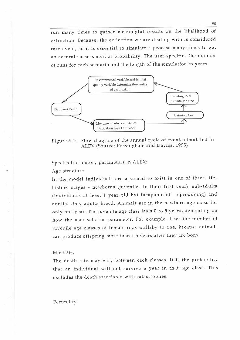
80

lun many times to gathel meaningful results on the likelihood of

extinction. Because, the extinction we ale dealing with is considered

1.are event, so it is essential to simulate a pr.ocess many times to get

an accurate assessment of probability. The user sPecifies the number

of runs for each scenario and the length of the simulation in years'

Figure 5.1: Flow diagram of the annual cycle of events simulated inALEX (Source: Possingham and Davies, 1'995)

Species life-history parameters in ALEX:

Age structure

In the model individuals are assumed to exist in one of three life-

history stages - newborns (juveniles in their first year), sub-adults

(individuals at least 1 yeat old but incapable of reproducing) and

adults. Only adults breed. Animals are in the newborn age class for

only one yeaf. The juvenile age class lasts 0 to 5 years, depending on

how the user sets the parameter. For example, I set the number of

juvenile age classes of female rock wallaby to one, because animals

can produce offspring more than 1,.5 years after they are born.

MortalityThe death rate may vafy between each classes. It is the probability

that an individual will not survive a year in that age class. This

excludes the death associated with catastrophes.

Movemeut between patches

Migration then Diffu sion

Catastrophes

Birth and Death

Limiting totalpopulation size

Environmental variable and habitat

quality variable determine the quality

of each patch

Fecundity

:i

HI

81

The birth rate is the probability that any adult female gives birth to

0, L,2,3, ... other females in a good year under ideal conditions. The

separate pïogIam BIRTH accompanies ALEX for calculation of the

birth rates from data on the sex ratio at birth, litter size, an:.d number

of litters pef year All subpopulations in the metapopulation have

the same demographic parameters.

ALEX focuses on species in which populations are restricted to more

or less isolated patches that are connected by dispersing individuals.

Each patch has different attributes: location and atea, A¡

Environmental stochasticity in each patch is modelled as a normally

distributed random variable with patch-specific mean and standard

deviation. Each patch gets a new value at the beginning of each yeaf .

These may be fully, partially correlated, oI uncorrelated between

patches. For example, if a patch has a correlation coefficient of L, its

envitonmental variable is perfectly correlated with patch 'J., if 0 then

its environmental variable is uncorrelated with patch 1-.

The impact of the annually selected environment on the number of

breeding females is modelled using an environmental rnodiÍier, M¡.

The user sets an environmental value above which breeding is

unaffected, M¡=L, and a lower value below which breeding cannot

take a place, M¡:0. In ouf analyses, all patches were completely

correlated, because drought usually affects the entire area used in

this investigation. I assume drought is the only catastrophic event

for the Yellow-footed Rock Wallaby survival.

ALEX allows the quality of the patch, Q¡(t) to be determined by

habitat state variable and parameters of the patch. However, in out

case the quality of each patch is determined only by an

environmental modifier, thus Q¡(t) = Mi.

!

.¡

ryl

82

The patch quality in its turn determines the maximum number of

females that can breed in the patch, X¡(t),

AX,(t¡: O,G); where

R is the minimum home range size of a breeding female.

Catastrophes:

ALEX can model up to three types of catastrophes at once. These

have a direct impact on the population size in the year they occur,

and can also influence habitat suitability and hence breeding success

in following years. The frequency of catastrophes can be specified as

an annual probability of occullence and it may depend on the

number of the animals in the patch ("g. disease), oI the habitat

quality ("g. drought), or neither. Catastrophes may act

independently in each patch (local) or simultaneously in all patches

(gtobal).

Movement between patches:

Two types of movement can be modelled in ALEX. These are called

'diffusion' when individuals move to adjacent patches where there is

no increased risk of mortality, and 'migration' in which individuals

move to a more distant patch associated with a substantial decrease

in survivorship.

Diffusion only occurs between patches that afe connected by user

specified corridors and it is intended to allow movement associated

with a change of territory position. The maximum number of

individuals that can diffuse between patches is the corridor width

divided by the squafe root of the minimum breeding area. There is

no probability of mortality associated with the diffusion.

Migration occurs when the density of individuals in a particular

patch exceeds a given proportion of its carrying capacity. The mean

distance an animal can fnove before it dies is specified by the user.

I

I

TI

t

83

Each emigrant moves in a randomly chosen direction from its source

patch (Fig.5.2). The probability that it reaches another patch, P, is a

function of the distance between the source and target patches and

the size of the target patch.

P:a dm

where d is the distance between the two patches, ø

is probability that a line drawn in a random direction from the centre

of the soufce patch strikes the target patch, and m is the mean

expected migration distance.

ø is calculated using the formula

(r\a=arctanl-ll.r, ford>r\d/ø=0.5 ford<rwhere r is the radius of the target patch.

I

Figure 5.2: Schematic diagram of migration in ALEX

Migrants move out from the centre of the source patch and die at a

constant rate as they move outwards unless they strike another patch

before dying. In the example shown in Figure 5.2 two animals

successfully migrated to another patch and'l'2 died.

Limitation of total population size:

The user sets a minimum living area for a given species, L, in order

to stop the population becoming excessively large. This reflects a

limit on density in a given patch. In this case the carrying capacity of

a patch is A¡/L.If the population in a patch has risen above A¡/L then

T

I

Source

patch

Ì

84

individuals are removed until the population is equal to the carrying

capacity.

Output:

Output from ALEX includes the probability of quasi-extinction (in

our case a chance that metapopulation falls to 5), the mean, median,

f irst, and third quartile time to extinction and the number of

simulation time steps during which each habitat patch was

unoccupied.

Besides the type of model used in population simulation, there is

little doubt that the success of PVA depends largely on the quality

and quantity of information on the biology, ecology and life-history

parameters of the target species.

5.3. BACKGROUND INFORMATION ON THE YELLOW-FOOTED ROCKWALLABY P. XANTHOPUS

Some of the key aspects of the biology and ecology of the Yellow-

footed Rock Wallaby relevant to our simulation wele taken from a

literature review of population studies of the species (Poole et al-

1.g85; Nicholls 1,972; Copley 198L, '1,983; Copley & Robinson 1983;

Lirn et ø1. 1,987; Robinson et ø1. 1,994 and Hornsby 1,997). FIere I

discuss the relevant information on the Yellow-footed Rock Wallaby

and explicitly parameterise the model.

5.3.1 . Lif e-history

Social structure:

Because of the patchiness of their preferred habitat the Yellow-footed

Rock wallaby is found in colonies ranging in síze from '1,0-1.2

wallabies to over 100 individuals and are comprised of one or several

gfoups of wallabies separated from nearby groups by stretches of

unsuitable habitat (Lim et aI. 1987). Each gloup typically comprises

several females, an older male and several younger males. Females

are able to defend important refuge areas more effectively than males

I

85

and femain in similar size home fanges during both winter and

summer seasons.

Fecundity:

The Yellow-footed Rock Wallaby is capable of breeding throughout

the year (Poole et nl., 1.985, Lirn et al., 1.987) and the individuals of

both sexes attain sexual maturity when they are 18 months old (Poole

et ø1. 1985). Lim et ø1. (1987) recofded sixty-eight pouch young from

twenty-seven mothers during the three and half year study in the

Middle Gorge area.

Sex ratio:

The sex ratio of pouch young (Robinson et al. 1,994) is not

significantly different from 1:1. However, detailed observation (Lim

et aI. 1987) suggests that older females might have a greater tendency

to produce male offspring. Moreover, Robinson et ø1. (1'994) noted

that this unbalanced sex ratio has also been observed by Rix in the

captive colony at the Adelaide Zoo.

Mortality:There is a general lack of definitive information on mortality for the

Yellow-footed Rock Wallaby. Ltrn et ø1. (1'987) suggested that female

Yellow-footed Rock Wallaby survival rate on the Middle Gorge study

area through the study period is on avelage 92.4 pet cent per year in

the absence of catastrophes. In addition, Lirn et ø1. (1,987) note that

newborn mortality rates are likely to be higher than juvenile or adult

mortality rates. They claim that the potential of foxes preying on the

Yellow-footed Rock Wallaby, particularly the young which are left

unattended f or considerable periods of time, should not be

completely discounted'

Records of copley (1981) and Lirn et ø1. (1,987) suggest that the

Yellow-footed Rock Wallaby may live in captivity as long as 15 years

and in the wild it may live at least 8 years.

86

5.3.2. Threats to the Yellow-footed Rock wallaby persistence

The Yellow-f ooted Rock Wallaby suff ered a major decline in

abundance since European settlement, having become extinct locally

throughout its Iange. Hunting for skins, competition with introduced

herbivores for food and shelter and predation by foxes seem to be the

major reasons for this decline (Copley 1,983, Lítn et ø1. 1.987, Hornsby

1,997). However, the species was afforded legislative protection in

South Australia in 1,9'1,2 and since that time there has been no

commelcial hunting and very few reports of illegal shooting of the

Yellow-footed Rock Wallaby (Lim et ø1. 1987). At present, therefore

the two remaining factors could be considered major causes for the

species decline. In fact, fox baiting and goat control have enabled the

species recovely in the Flinders Ranges National Park in 'operation

bounce back'

5.4. METHODS USED FOR MODELLING THE METAPOPULATIONVIABILITY OF P. XANTHOPUS

In this section, I describe how each parameter relevant to our study

was estimated, including patch structure, catastrophes, and lif e-

history parametels for the Yellow-footed Rock Wallaby'

5.4.1.. Study area

I selected the area between the towns of Quorn and F{awker, South

Australia to caïIy out a metapopulation viability analysis of the

Yellow-footed Rock Wallaby. The total afea of the study site is

approximately L10,000 ha and it is dominated by mountainous high

land with rocky outcrops and numefous gorges. The area is managed

by landholders for multiple use and it was selected for the most

detailed Yellow-footed Rock Wallaby population study that was

conducted in this area.

Suitable habitat for the Yellow-footed Rock Wallaby is abundant in

the southern Flinders Ranges, and reasonable inf ormation exists

about the colonies in the alea. However, there aIe no precise

I

87

locational record for the colonies. I identified forty-two patches by

combining three diff erent inf ormation sources; 1) approximate

locational records of the colonies in the area (see Figute 4.2), 2)

locational data supplied by DEHAA (see Appendix 1), and 3)

topographic maps (1:50,000) of the area.

I identified the locations of the preferred habitat of the Yellow-

f ooted Rock Wallaby, rocky outcrops. Theref ore, the basis f or

selecting the patches location was the whereabouts of suitable rocky

outcrops between Quorn and Hawker (Figure 5.3). The patches are

distributed in an area of approximately 1600 km2 and range from L0

to 360 ha (Table 5.L).

only 1,2 patches afe 30 ha or less, which is close to minimum

breeding afea size. All other patches are large enough to

accommodate the Yellow-footed Rock Wallaby.

88

îet5 I

t

D

nUru 3

7Hawker

i5

{

5

0t9

10ll

00

6

t1

20

2r,

Quorn

ê¿2L ln

0232o- 24

/ 25

26

2E

/utt

l3s

37

il ,,

û39

Dto s'\¡t- 0km Þ r0

ù{1

{l,

Figure 5.3: The patch structure used for analyses of the persistenceof P.xønthopus poprJ lation in the area between the townships ofQuorn and Hawker.

89

0.867240420.8923021

0.7 65470410.89923020

0.771,160400.799J601.9

0.706J60390.812J5018

0.3410't 95380.7344801.7

0.06218360J/0.7394801.6

0.5946125360.73648015

0.708480350.8 912301.4

0.58871.40340.549714013

0.753470JJ0.95611012

0.894230320.9521.101.1.

0.78IJ60310.9341,1510

0.808J50300.9431.159

0.5827140290.765J508

0.779J60280.235132607

0.815J50270.38101.906

0.831J50260.842305

0.946115250.54761.204

0.6876110240.24812250J

0.902230230.6364802

0.903230220.66951001

Probab-ility ofbeingempty

Meaninitialpopul-ationsize

Area(hu)

PatchID

Probab-ility ofbeingempty

Meaninitialpopul-ationsize

Area(hu)

PatchID

Table 5.1: The area, initial population size and probability of beingempty in the baseline simulation for 42 patches in the area betweenthe townships of Quorn and Hawker in Southern Flinders Ranges.

5.4.2. Initial population size

Each patch is given ârr initial population size of 40 % of its

maximum. The maximum population size is found by estimation how

many f emales live in a particular patch in accordance with its

minimum living atea pel individual. For example, a 250 ha patch will

start with 12 females, and be given a 13th with a probability of 50%,

in the simulation. So, initial population size in this patch (see Patch

No. 3 in Table 5.1) is 0.4.(250 /8):1.2.5'

90

5.4.3. Movement between habitat patches

In relation to the Yellow-footed Rock WallabY, only the migration

pattern was used to simulate the dispersal of juvenile females from

their natal home ïanges. The probability of migration varies between

age classes and the density of animals in any given soulce patch. In

our model, when a patch is more than 50% occupied, each sub-adult

female wallaby has 50% chance of leaving. Each migrating animal

travels an exponentially distributed distance before dying, and if the

migrant reaches another patch in that distance, then a successful

disper.sal is recorded. Although there is not much information about

the extent of movement between colonies, Lirn et ø1. (1'987) suggested

that a reasonable level of gene f low between populations occtlf s

because a lack a genetic differentiation throughout the widespread

range. Lirn et ø1. (1,987) noted that all rock wallaby colonies examined

have been within 5 km of a water soufce. Therefofe we set mean

migration distance bef ore death as three times mole than that

necessary for quenching of thiïst - 15 km (see Table 5.3)'

5.4.4. Other parameters inPut to ALEX

The results of a population study conducted in the southern Flinders

Ranges between Decembet'1.978 and March 19S3 by Lim et ø1. (1'987)

and other relevant studies (Copley 1.98L, Poole et ø1. 1985) wele used

to derive the values for life history parameters for ALEX (Table 5.2).

Breeding:

Individuals of both sexes of the Yellow-footed Rock Wallaby attain

sexual matulity at 1.5 yeaÍs (Poole et ø1.1985), so I set pre-adult age

classes as 2 years. This means individuals are newborns for a yeat,

then juveniles for a second yeaf . From the third year they are mature

enough to produce offspring.

As noted by Robinson ef al. (1,99\, sex ratio at birth in the Yellow-

footed Rock Wallaby is approximately -L:'l,,bu-t amongst older females

91

where consecutive births were recorded sex ratio was closer to 2:1 in

favour of males. Therefore, we assume that the sex ratio is between

0.4 and 0.5. Given the above sex ratio at birth (0.45), average number

of litters peï yeaf (0.5), and size of litters (1 young) I calculated the

probability of a number of offspring using the program BIRTH. The

probability of 0 female offspring is 0.595 and L female offspring is

0.405 (see Table 5.2).

Survival:

Little is known about the mortality rates of the Yellow-footed Rock

Wallaby, so I assume that the mortality rate of young wallabies is

higher than the mortality rate of adult wallaby (see Table 5.2) for the

following reasons:

1. Lim et ø1. (1,987) suggest that fox predation on the Yellow-footed

Rock Wallaby, particularly unattended young, should not be

completely discounted.

2. Hornsby (1,997) suggests that 57% of the wallaby cafcasses found

and analysed for mortality causes wele adults, 30% were immature,

and the remainin g 13% wele classified as unknown. Howevef , on

one occasion Hornsby (1,997) did not count the pouch young as an

individual. During the examination of the f inal caf cass, 'When

found, only the lower half (complete) of the body remained. This

included the pouch which contained a very small live young.'

This fact shows an indication that sometimes the young animals are

discounted unwillingly during investigation.

I assume that the mortality rate of young wallabies is higher than the

value suggested by Hornsby (1,997) and I set it to 35 percent for the

newborns, 20 percent for the juveniles and 0.12 percent for the adult

wallabies.

Population density:

The population size in the 4.5 km2 Middle Gorge study area was

estimated to be between 103 and 131 rock wallabies (Lim et ø1. 1'987).

Therefore, the estimated density of the Yellow-footed Rock Wallaby

92

in this preferred habitat is between 22.8 and.29.L individuals per km2

(Lim et ø1. 1,987). This translates to about 4 ha per individual in

general. Theref ore, I assume that each f emale, representing both

sexes, needs 8 ha as a minimum requirement.

Analyses of the home fange size and activity cofes suggested that

female wallaby concentrate their activity in an area of less than 30 ha

(Lim et ø1. 1,987). Moreover, behavioural observations show that the

mating period overlaps with feeding and foraging periods, in other

words with most active periods of the day. Therefore, I suggest that

female lock wallabies require a minimum area for breeding that is

slightly smaller than its active core area, ie' 25 },.:.a.

Pre-adult age classesProbability of death

New born)uvenileAdult

Population extinction thresholdAnnual probability of 0 female young per femaleAnnual probability of 1 female young per female

Annual probability of female babYMax. number of litters per yearMax. number of young per litterProb. of 0 litter per yearProb. of 1 litter per yearPlob. of 0 young per litterProb. of 1 young per litter

Minimum living area for femaleMinimum breeding area for femaleMean migration distance for juvenile

2

0.350.20.1.25

0.5950.4050.451.

1

0.10.90.10.98ha25 ha15 km20%Po ulation densi before mi ation

Table 5.2:ALEX

Values for life-history parameters of P. xanthopus for

5.4.5. Catastrophe and environmental variable

I include drought as the only catastrophic phenomena affecting the

survival of the Yellow-footed Rock Wallaby. The drought frequency

in the Flinders Ranges is described by Schwerdtfeger & Gurran

93

(1,996) and I estimate flom their data that the probability of a

drought condition in the Flinders Ranges in any year is 10% (ie. once

every 10 years on average). Drought eff ects all patches

simultaneously. I assume that in each patch, total biomass is reduced

by 10-60o/o, àrtd 10-40% of Yellow-footed Rock Wallaby population die

due to drought condition.

5.5. SCENARIOS AND RESULTS

The dynamics of populations of the Yellow-footed Rock Wallaby

were calculated over 200 years by combining data on the life-history

attributes (Table 5.2) and spatial location and size of the patches in

the study area (Figure 5.3). Each scenario is simulated 200 times. The

standard deviation of extinction probabilities for 200 runs is 3.5%

(Lindenmayer & Possingh arn 1'994).

Scenario L. General probability of persistence

In this scenario, the probability of persistence of the Yellow-footed

Rock Wallaby in the study area was examined with the baseline input

parameters (Table 5.2). The baseline median time to extinction is 121

yeaïs. The cumulative probability of extinction at intervals of 20

years is shown in Figure 5.4.

0.8

0.7

0.6

0.5

0.4

0.3

0.2

0.1

0

80 100 120 140 160 180 200

years

oocxoo

='õ(ú

.c¡oLCL

20 40 60

94

Figure 5.4: The cumulative probability of extinction of the Yellow-footed Rock Waltaby in the Flinders Ranges National Park for thebaseline parameter set

The annual probability that each patch is empty while the population

as a whole is extant is also shown in Table 5.1. Patches of the same

size show different levels of occupancy depending on their spatial

relationships with other patches. For example, patch numbers 2 and

L6 have the same patch size (80 ha), but the levels of occupancy are

different, 0.636 and 0.739 respectively. In this instance, patch 2 is

empty about 64% of the time because it is approximately L km away

from patch 3, which is much larger. In contrast, patch 16 is isolated

from all other patches by between 10-15 km (Fig.5.5). This baseline

scenario provides reference values for comparison with the result of

subsequent analyses.

Scenario 2. Examining contribution of patches of different sizes to

population viabilityIn this scenario, firstly,I calculated the probability of extinction of

the Yellow-footed Rock Wallaby in each patch separately. Figure 5'5

shows the results of the analyses of the probability of persistence of

populations of the Yellow-footed Rock Wallaby in a single isolated

patches oÍ 3-360 ha and further up to 470 ha. These results show that

the increase of patch size reduced the probability of extinction of

Yellow-footed Rock Wallaby populations in the patch. Howevel/ even

the largest patch (patch 37) in our study site does not contribute

much to the persistence of the Yellow-footed Rock Wallaby alone. It

gives a median time to extinction of only 68 yeats, which is about

half of the result of the baseline scenario.

95

200

ooExoooE

c.g!toE

80

60

40

20

100

80

60

40

20

0oooooooooooco99e=+ñõc.l@orNr¡¡!qrS\Cat9 (\ôlô¡Í)c)a"sfts

patch siz

Figure 5.5: The relationship between the size of a single patch andthe median time to extinction of a population of the Yellow-footedRock Wallaby in the patch.

Secondly, I examined the contribution of different sets of patches to

the persistence of Yellow-f ooted Rock Wallaby population. All

patches smaller than 30, 60, L00 and 140 ha in the Quorn-Hawker

atea weïe deleted in this order and the simulations repeated' This

procedure simulates the eff ects of f urther habitat losses f rom

intensive utilization of land in this paft of the Flinders Ranges. In

other word, it tells us about patch value - which patches should have

highest priority for protection, particularly from habitat competitor

like goat. The baseline simulation with aIl 42 patches has a median

time to extinction of l2l years (Scenario 1).

If I remove all patches smaller than 30 ha, the median time to

extinction is 118 years. Given the 3.5% standard deviation of

extinction probabilities, I conclude that the 12 patches smaller than

30 ha play no significant role in terms of persistence of the species in

this part of the Flinders Ranges. Next, I deleted all patches smaller

than 60 ha, leaving a totai of L9 patches and re-ran the simulations.

In this case the median time to extinction is 110 years indicating that

patches of 30-60 hectares in size contribute more to persistence than

the smallest patches, but still not a substantial amount. Deleting a

further.seven patches less than 100 ha in size does not further reduce

the median time to extinction. FinaIIy, a simulation with only the

96

largest 5 patches (all greater than 1.40 hu) the median time to

extinction drops to 101 years, suggesting that patches larger than

100 ha make the biggest contribution to the Yellow-footed Rock

Wallaby population viability.

In the next test I deleted patches not only by their size but also by

position, because I expected some sort of correlation between the

probability of persistence and distance between patches.

Therefore, I deleted a set of large patches (patches 3, 6 and 7: aÍea

sizes 250, 1.90 and 260 ha respectively) and re-ran the model with

only two patches (patches 37 and 38 with the sizes of 360 and 195

ha, respectively). Then I deleted the latter two patches and ran the

model with the other three patches (patches 3, 6 and 7). Because the

patches in each set were different in distance from each other within

the set. The patches in the first set (patches 37 and 38) wele isolated

from each other by apploximately 2 km and the other patches

(patches 3,6 andT) were apart from each other by 3-4 km.

The median time to extinction was 83 years with only two patches

(patches 37 and 38) and 65 yeafs with the other three patches

(patches 3,6 and 7), suggesting that the distance of the patches in a

set plays reverse role in population persistence of the Yellow-footed

Rock Wallaby.

From the above simulations, I conclude that the contribution of

single patches to the population persistence of the Yellow-footed

Rock Wallaby is not signif icant, theref ore the species' survival

depends only on the set of patches.

Note that a set of small patches with an alea of up to 100 ha appears

to be insuf f icient f or persistence of the population and that the

results indicated an insignif icant ef f ect on time to extinction by

excluding such patches. Flowever, it must be remembered that small

patches could potentially serve a useful conservation function during

catastrophic events and it would be premature to base conservation

strategies on the culrent analysis without further investigation of the

97

costs and benefits of concentration of effort on a minimum set of

habitat patches.

Scenario 3. Impact of predators

In this scenatio, I varied mortality rates because predation,

especially on the youngest wallabies, is considered to be important

factor influencing the Yellow-footed Rock Wallaby populations. The

impact of predators on the persistence of the metapopulation is

explored by examining different mortality rates in each of the three

age classes.

The mortality rate was increased by 30% and 50% of the initial

mortality rate for each age class (Table 5.3). Increasing the death rate

of adult female wallaby by 30 and 50 percent reduces the median

time to extinction to 61. and 40 yeals respectively. Increased

mortality in the new-born age class has a smaller effect on the

persistence of the Yellow-footed Rock Wallaby population than the

adult age class. Increases in the sub-adult mortality rate have the

smallest effect on the persistence of the population as compared with

the other two age classes.

The results of the above simulations suggest that the most effective

option to deal with the persistence of the Yellow-f ooted Rock

Wallaby is to reduce mortality rate of adult female wallabies. The

mortality sources of the Yellow-footed Rock Wallaby could be quite

variable, such as disease, drought and predation. Hornsby (1'997)

examined the possible causes of mortality in the Yellow-footed Rock

Wallaby and concluded that the predation is a major cause of

wallaby death and amongst predators the Red Fox, an introduced

predator is the principal predator of the Yellow-f ooted Rock

Wallaby.

Theref ore, the elimination of potential predators of the Yellow-

footed Rock Wallaby, particularly the Red fox, is the most essential

action to reduce the mortality of the Yellow-footed Rock Wallaby

population. The predation is the most easily manageable cause of

98

mortality of the Yellow-footed Rock Wallaby, besides being the major

cause for the death of the wallabies.

decreaseby 50%

>200 >200 >200

decreaseby 50%

110 >200 >200

decreaseby 50%

>200 >200 >200

decreaseby 30%

17-l >200 >200

decreaseby 30%

86 154 >200

decreaseby 30%

>200 >200 >200

lncreaseby50%

34 50 68

rncrease 44 69 109by 50%

lncr e as e 30 40 57by 50%

lncreaseby 30%

43 74 105

lncreaseby 30%

47 76 125

rncr e as e

by 30%37 61 86

B aseline0.35

(deatho.2

rate)0.1.2 71. 727 188

New born Sub-adult AdultFirst

quartileextinction

(vtr)

Mediantime to

extinction(vts)

Thirdquartileextinction (yrs)

Table 5.3: The effect of different mortality rates to the pef sistenceof the Yellow-footed Rock Wallaby P.xanthopzs metapopulation in thesouthern Flinders Ranges.

Decreasing the mortality rate by 50% and 30% for all age classes

increases the probability of persistence of the Yellow-footed Rock

Wallaby dramatically. Thus , for all age classes the median time to

extinction is rnoïe than 200 yeafs, except for a 30% decrease in

mortality rate in the sub-adult age class (Figure 5.5).

99

200

180

160

---o- Adults

--Ð- Newborns

---r- Subadults

Median Time to Extinction

40

100

80

60

40

20

-60 -40 -20 0 20

Relative Change in MortalitY

40 60

Figure 5.5: Median tirne to extinction of the Yellow-footed RockWallaby P.xanthopus in relation to relative changes in mortality ratefor thlee age classes

Scenario 4. Impact of drought

one major catastrophe af f ecting Yellow-f ooted Rock wallaby

population size is drought. I examined the impact of drought

increasing the frequency of drought by 50% or 1'00% relative to the

baseline of f. in 10 years frequency. I also decreased the frequency by

50% and 1,00% (ie. no drought).

Frorn the previous results in regard to patch size and structure we

found out that the persistence of the Yellow-footed Rock Wallaby

depends on a set of large patches connected with corridors.

A sensitivity analysis of drought frequency has a very substantial

impact on the meclian time to extinction. Increasing drought

frequerrcy by 50% (1in 7.5 years) increases the extinction rate trlr

almost l-ralf. Drought flecluency inclease by L00% or once every 5

years clecreases the rneclian time to extinction from 107 to 2B years.

5.6. DISCUSSION

Any PVA model operates on a set of a static population parameters

to deterrnine how long the population will persist. Given this genelal

100

assumption, the results of this study show that there is a high

probability of extinction of the Yellow-footed Rock Wallaby within

100-150 yeafs in the southern part of the Flinders Ranges. Here I will

first discuss a number of potentially important factors that were not

examined in the analyses.

The analyses completed in this study are restricted to very simple

patch structures without habitat variables and do not examine the

impacts of habitat state variable, which could be assigned to each

patch, on the quality of the patch and hence fecundity of the species.

I used only the population density in a given patch as a factor

determining migration out of the source patch.

Other limitations include: 1) possible effects of genetic structure on

population viability, 2) simplicity of the movement model in ALEX

and 3) adequate information on patch data.

The impacts of patch sîze and number on the probability of

persistence of the Yellow-f ooted Rock Wallaby

The results reveal that there is a high probability of 1ocal extinction

amongst populations of the Yellow-footed Rock Wallaby in srnall

isolated patches particularly patches smaller than 60 ha. A set of 5

oï moïe patches, each larger than 100 ha connected by corridors of

located within 5-10 km from each othel was that most likely to make

the greatest contribution to the persistence of the Yellow-footed Rock

Watlaby in the Flinders Ranges.

Since the contribution of single patch even of area 360 ha alone to the

persistence of the species is very small (median time to extinction is

only 55 yeaïs), it is not appropriate to manage just one single patch

as a habitat for the Yellow-footed Rock population. My analyses

suggest that several patches in combination could play major role in

the Yellow-footed Rock Wallaby persistence.

However, the size of these patches must be larger than 100 ha each to

support populations of the Yellow-footed Rock Wallaby for greater

1l

ili

than 100 year period. In this instance, the actions that could

the effects of competition, particularly with feral goats shoul

taken into account. Lim et ø1. (1,987) observed that there is no

evidence that active competition between feral goat and the Yellow-

footed Rock Wallaby has lead to any loca1 extinctions of the latter.

However, it is essential to gather more information regarding the

impact of feral goats and gtazing pressufe on the distribution and

density of plant communities and the Yellow-footed Rock Wallaby

populations, because goats are accepted as a major contributor to

desertification in the Middle East and in Africa (Freudenberger

1992). Additional actions that could support the movement of

animals between the patches (improve connectivity) should be taken

into account. These could include elimination of possible predators

in the area, restriction of human activities between patches.

Given the size of a single patch and the structure of a set of patches,

it is meaningless to look af ter a patch not greater than 360 ha

individually, and any set of patches, where all patches ale less than

60 }:.a.

Taking into account that the structure and location of patches, and

size of the patches used in this study are not exact, it is wise to

cond.uct further investigation on this matter collecting detailed data

on the suitable habitat for the species.

The Yellow-footed Rock Wallaby is still common in places

throughout the Flinders Ranges. My analysis suggests it is most

important to preserve these areas and keep them free of both natural

and introduced competitors.

r

:

ü

r

102

The impact of predators on the Yellow-footed Rock Wallaby

survivalI explored the impacts of predators on the persistence of the Yellow-

footed Rock Waltaby by varying the mortality rates. These results

indicate that both increases and decreases of mortality rates in the

Yellow-footed Rock Wallaby have a dramatic effect on the species

persistence. The highest probability of extinction occurs with an

increase in the mortality rate of adult wallabies. Adults are the

r.eproductive members of the population, and so shorter adult

lifespans mean fewer offspring, and therefore a lower population

glowth rate.

Interestingly, changing the mortality rate in the subadult age class

has the smallest impact on the persistence of the species. Given that

only juveniles move between patches in search for another habitat,

probably, juveniles are the most successful amongst all age-classes of

the Yellow-footed Rock Wallaby. This analysis suggests that reducing

the mortality rate of adult female wallabies would be a highly

successful option for the conservation of the colonies. This result

may be sensitive to the death rate data used as an input to the model.

Although Hornsby (1,997) suggested that the mortality rate of adult

wallabies is higher than the youngeï ones, I used the data that is of

revelse nature ie. death rate of young wallabies is higher than the

adults. My initial hypothesis in this matter was reducing the

mortality rate of young wallabies will increase the probability of the

persistence of the species more than that of adult wallabies.

FIowever, the results of these simulations did not support this

hypothesis.

The accuracy of the predictions from population models such as used

in this analysis depend of course on the reliability of the data used in

the model. Here I have relied largely on data from three studies

made in the 1,970' s and 1980's to determine life-histoly pafameters.

Lif e-history characteristics vaïy ovel time and between sites,

according to environmental conditions and interpretation of theI

t

1,t

üI

103

fesults of PVA's must always be made with cafe. In some cases I had

to set arbitrary values for certain life-history parameters-useful for

the analysis but the source of potential errors in interpretation of the

results. Nevertheless, the PVA performed here for the yellow-footed

rock wallaby had some important conclusions that should be checked

through further work.

Caughley & Gunn (1,996) noted that one problem for applícation of

PVA is that the detailed information needed as input is almost never

available for an endangered species.'FIence the user often gets fed

with guesses or consensus views of experts f amiliar with the

species'. This is a fault not of the software but of the user.

The impact of drought condition on the Yellow-f ooted Rock

Wallaby survivalAlthough drought has large eff ect on the Yellow-f ooted Rock

Wallaby population persr.stence, it is not that factof we can manage

effectively. So, this application has little practical importance.

I examined the impact of drought on the Yellow-footed Rock Wallaby

survival and found that drought is one factor that can make a major

contribution to the decline of the species. However, given the fact

that drought is a natural process, controlling the f requency of

drought is a not realistic option. As an alternative it may be better to

seek an indirect means to reduce the impact of drought on the

species persistence. This may include the elimination of potential

habitat competitols during and immediately af ter the drought

season. For example, the number of the Yellow-footed Rock Wallaby

lecovered to pre-drought levels within 1-.5 years after drought in a

colony where feral goat numbers were controlled (Lim et al.1'987).In

contrast, the Yellow-f ooted Rock Wallaby numbers remained

depressed in the area where goat numbers were not controlled.

tI

t

104

ïI

CHAPTER 6

GENERAL DISCUSSION

Thr.oughout the thesis I have sought a genef al solution to the

development of a biodiversity management strategy. Biodiversity is

managed most efficiently at a bioregional scale - small enough that

the people living there call it home, and yet large enough to support

its biological communities and ecological processes. Managing

biodiversity at the bioregional scale can be problematic, because a

bioregion comprises a large number of entities and complex

ecological processes about which there is little information, even

about what they are and where they occul"

The maintenance and recovely of threatened and endangered species

is the most urgent step toward biodiversity conservation in a

managed landscape (Szaro 1,996). Therefore, one feasible alternative

is to develop a management plan for one or several biodiversity

entities that must be protected. The representative or representatives

of overall biodiversity must be chosen carefully, so that management

actions for the good of the representative species ensure reasonable

management for the rest or at least most of the biodiversity in the

bioregion. In this thesis, I considered a variety of rationales for

choosing representative species, and I examined how two common

conservation tools, BIOCLIMatic Analysis of distribution and

Population Viability Analysis, can contribute to the process of

developing management recommendations for a single species.

I selected the Yellow-Footed Rock Wallaby in the Flinders Ranges

bioregion as a case study species. The Yellow-footed Rock Wallaby

are a threatened species with a high public profile, and may be a

good f lagship species. Howevet, the species' pref erred habitat is

r.ocky outcrops, which comprises only a small portion of the

bioregion, reducing the importance of the Ye11ow-f ooted Rock

Wallaby' s contribution to legional ecological processes. If targeting

r

105

management fof a flagship species does not adequately achieve the

goal of overall biodiversity management in the Flinders Ranges, what

alternatives aïe there? I suggest identifying another species with a

preferred habitat different than the Yellow-footed Rock Wallaby's,

possibly at lower altitudes in the bioregion. This species need not be

an endangeled species, but needs to somehow be indicative of the

state of the ecosystem. It could even be the rabbít, which must be

thoroughly managed if native biodiversity conservation is to

succeed. Since the introduced species usually destroys native species,

then in order to restore the balance it is essential to eliminate the

cause. FIowever, not all introduced species cause problems if

managed correctly. Conservation and management are different

things. Usually, when we talk about introduced species it is

management, and it is conservation when we deal with native

species. These ideas need to be approached with caution.

Once a target or flagship species has been selected, two problems

remain. First, we need to know where we should concentrate

management activities within the bioregion. Second, what actions

should be taken there. Generally, the distributional range of the

selected species is the site whele managers should concentrate their

activities. I tested the utility of BIOCLIM software for identifying the

distribution of a given species. BIOCLIM predicts an afea that is

climatically suitable f or a given species rather than the actual

distribution of the species. Therefote, the interpretation of BIOCLIM

output depends on the intended purpose. For example, to focus

survey effort on aïeas predicted to have a high probability of finding

additional populations of a given entity, oI to confirm predicted

boundaries of its distribution, the interpretation of the output is

straightforward. But fol the intended management actions it should

be double checked using other methods such as direct survey of the

predicted area.

1.06

Following the definition of the management site, the second step is

to rank management options. For this purpose, I used the software

package ALEX to perform a Population viability Analysis of the

Yellow-footed Rock Wallaby. Population viability analysis uses the

extinction probability of threatened and endangered vertebrates to

rank management options f or their survival (Goldingay &

Possingham 1,995). While this approach deals with a particular

species, oul overall goal is to consef ve and manage biological

entities as well as functioning ecosystems. Therefore, consideration

must be given to actions that will enhance functioning ecosystems in

the bioregion. This idea must influence the application of PVA, eg.

selecting possible causes f or a species decline and developing

scenarios. This analysis revealed that habitat restoration, elimination

of predators and decreasing drought are major determinants of the

success of YRW management and conservation. However, drought is

a natural pf ocess and possible actions ale limited to mitigation.

For this particular species all predators are introduced, including the

dingo (Copley 1997). How would we proceed if the major predator

was a native species, and introduced predators af e of minor

importance? For the sake of this particular species survival it is

essential to eliminate major predators immediately and this option

was be ranked highly. However, from the overall biodiversity point

of view, I suggest first eliminating introduced predators, and then

later assess the effects of native predators.

The application of the two conventional methods BIOCLIM and PVA

are only a smal1 part of large amount of work related to biodiversity

management strategy. The application of these methods will help the

development of such a plan, provided consideration is given to other

ecological communities and Processes.

107

REFERENCES

Akcakaya, H.R. and Ferson, 5.,'l'992, RAMAS/space: SpatiallyStluctured Population Models for Conservation Biology, Version1,.3, Applied Biomøthemntics, New York

Aitken, P.F.,1978, Ring-tailed Rock Wallaby, Petrogale XanthoPus'South Austrølian Pørks ønd Conseruøtion, 'l', 17

ANZECC, L996, Nøtionøl Strøtegy for the Conseraation of Austrøliø'sBiologicøl Diuersity, Department of Environment, Sport andTerritories, Canberra

Australian BioRap Consortiurn, 1996, BioRap - Rapid assessment ofbiodiversity,Yol.2 - Spatial modelling tool, ANU, Canberra

Bekele, E., L980,Islønd Biogeogrøphy and guidelines for the selection ofconserantion units for lørge mømntøls, Ph.D. dissertation, lJniversityMicrofilms Intelnational, Ann Arbor, Michigan

Betg, P.,1,995, Putting "Bio" in Front of "Regional" ,lOnline, accessed27 F eb. -1,9971, URL:http : / / www.tnews.com:80 / text / berg.html

Biodiversity Working Party (BWP), '1,991., Report: The conseraøtion ofbiodiuersity øs it reløtes to ecologicølly sustøinable deaelopment

Bridgewater, P.8., Cresswell, I.D. and Thackway, R.,'L996, A regionalframework for planning a national system of protected areas, In:R. Breckwoldt (ed), Approøches to Bioregionøl Plønning, Pørt L,

Paper No. 10, Biodiuersity Series, Department of Environment,Sport and Territories, Canberra, PP.67-72

Brooker, L., Brooker, M. and Cale, P.,'l'999, Animal dispersal infr.agmented habitat: measuring habitat connectivity, corridor use,and dispersal mortality. Conseraation Ecology [Online] 3, 4

Brown, J. H., 7984, On the relationship between abundance anddistlibution of species, Americøn N øturnlist, 124, 255-279

Burgman, M.4., Ferson, S. and Akcakaya, H.R., 'l'993, Risk øssessmentin conseraøtion biology, Chapman and Ha11, London

Busby, J.R., 1986, Bioclimate Prediction System (BIOCLIM), IJser'sManual Version 2.0, Austrøliøn BiologicøI Study Leøflet

108

Busby, 1.R.,1.991., BIOCLIM-A Bioclimate Analysis and PredictionSystem, In: C.R. Margules and M.P' Austin (eds), Nøtureconseraation: cost effectiue biologicøl suraeys ønd døta ønøIysis,CSIRO, Canberra , pp. 64-68

Caughley, G. and Gunn, A.,1996, Conseruøtion Biology in Theoty øndPrøctice, Cambridge, Blackwell Science, Massachusetts

Chatfield, C. and collins, 4.J., 1980, Introduction to MultiaøriateAnalysis, Chapman and Hall, London

Copley, P.8., 1981, Distribution and status of the Yellow-footed RockWallaby, Petrogale Xanthopus in the Flinders Ranges, SouthAustralia , A Report to World Wildlife Fund for Austrøllø, NatureConservation Society of South Australia

Copley, P.B. 1983, Studies on the Yellow-footed Rock Wallaby,Petrogale Xanthopus Gray (Marsupialia: Macropodidae) 1.

Distribution in south Australia, Austrøliøn wildlife Reseatch,10, 47-61.

Copley, P.B. and Robinson, A.C., L983, Studies of the Yellow-footedRock Wallaby Petrogale xanthopus (Gray), II. Diet of the Yellow-f ooted Rock Wallaby at Middle Gorge, South Australia, AustralinnWildlife Reseørch, 1'0, 63-77

Copley, P.B. and Alexandet,PJ.,1.997, Overview of the status of rockwallabies in South Australia, Australiøn Mømmølogy, 19,153-1.62

Cox, J., Kantz, R., Maclaughlin, M. and Gilbert, T. L994, Closing the

Gøps in Floridø's wildlife Høbitøt Conseraøtion system, FloridaGame and Fresh water Fish Commission, Tallahassee, Fl0rida

Craighea d, 8., 1,979, Track of the grizzly, Sierra Club Books, SanFrancisco, California

Davies, M., Twidale, C.R. and Tyler, M.J., L985, Nøturøl History ofEyre Peninsulø, Royal Society of South Australia, Adelaide

Davies, M., Twidale, C.R. and Tyler, M'J., 1'996, Naturøl History of the

Flinders Ranges, Royal Society of South Australia, Adelaide

Darwin, C., L859, The origin of species, [Online, accessed 24 Mar'19991 The University of Adelaide L|btaty,URL: http: / / www.Itbrary.adelaide.edu. au f etext f d / d22o /

109

den Boer, P.J.,1.990, The survival value of dispersal in terrestrialarthropod s, Biological Conserantion, 54,'l'75-1'92

Department of Environment & Natural Resources (DENR) ,'l-996,South Austrøliøn Threøtened Plønt Species Døtø Bøse, Department ofEnvironment & Natural Resources, Adelaide

Dobson, A.J.,1,990, An introduction to Generølized Linear Models,Chapman and Hall, London

Faulkner, J.P.,1996, OÍficial opening address, In: R. Breckwoldt (ed)Approaches to bioregional plønning, Pørt 1, Ptoceedings of the

Conference, 30 Oct-l Noa, Melbourne, Pøpet No. 10 BiodiaersitySeries, Department of Environment, Sport and Territories,Canberra , pp. 7-8

Fox, 4., 1.99L, Centenøry Field Guide of Møior Pøtks and Reseraes ofsouth Austrølin, National Parks and wildlife service, Adelaide

Freudenbergef , D.(ed), 1.992, , Proceedings of the Nøtional zuorkshop on

Ferøl goøt mønøgement: Plønning for Action, Commonwealth ofAustralia, Dubbo

Gadgil, M., L996, Managing biodiversity, In: K.J.Gaston

çea¡,nioaiuersity: A biology of Numbers ønd Difference, BlackwellScience, Oxford, pp.345-366

Goldingay, R. and PossinghaÍL, lH',1995, Area requirements forviable populations of the Australian gliding rnarsuP ial Petaurusaustlalis , Biological Conseruøtion, 73, 16'l'-L67

Gordon, G., McGreevy, D.G. and Lawrie, B'C.,'l'978, The Yellow-footed Rock wallaby, Petrogale xønthopus Gray (Macropodidae) inQueensla nd, Austrølictn Wildlife Resenrch, 5, 295-297

Government of Mongolia , 1,996, Biodiuersity Conseraøtion Action Pløn,Ministry for Nature and the Environment, Ulaanbaatar, Mongolia

Greenwood, G., Pitts, B. and Mitchell, L.,1'989, Flinders Rønges

Mønøgement Reaietu Inaestigation Report, Department ofEnvironment and Planning, Adelaide

Groombridge, B. (ed.), 1.992, Globøl biodiuersity: støtus of the Enrth'sliaing resources, A Report compiled by the world ConservationMonitoring Center, Chapman and Hall, London

Graul, W.D., and Miller, G.C.,1'984, Strengthening ecosystemmanagement approaches, Wildlife Society Bulletin, 1'2(3)

Grumbine, B. 8., 'l-994, What is Ecosystem Management?, ConseraøtionBiology, B:27-38

110

F{arris, R.8., Metzger, L.H. and Bevin, C.D., L986, GAPPS Version 3.0,Montana Co-operative Research Unit, Uni. Montana, Missoula,Montana

Hornsby, P.8.,1,973, Some preliminary findings from the study of thebehaviour of South Australian Rock Wallabies: The Yellow-footedRock Wallaby Petrogale xanthopus and the Pearson's Island RockWallaby P. penicillata pearsonü, 45th ANZAAS Congress, Perth,Section II, Zoology

Hornsby, P.8.,1,975, Dominance and territoriality in Rock Wallabies,46th ANZAAS Congress, CanbeÍta, Section II, Zoology

Hornsby, P.E., 1980, A History of Rock wallabies, Petrogale spp inthe Adelaide Zoo, InternøtionøI Zoo Yearbook, 20,1'54-1'60.

Hornsby, P., L997, Possible causes of mortality in the Yellow-footedRock-walIaby, Petrogøle xønthopus Gray (Marsupialia:Macropodidae), Australiøn Mømmalogy, 19, 245-248 -

F1uston, M.4., '1.997, Hidden treatrrients in ecological experiments: re-evaluating the ecosystem function of biodiversity, oecologiø,1,1,0,449-460

Hutchinson, M.N. and Tyler, M.j.,'l'996, Reptiles and amphibians, In:M.Davies, C.R. Twidale and M.J.Tyler (eds) Nnturøl History of the

Flinders Rønges, Royal Society of South Australia, Adelaide,pp.1.49-L58

Hutchinson, M.F., '1'99'!', The application of thin plate smoothingsplines to continent-wide data assimilation, In J'D. Jasper ("d),Døtø Assimiløtion systems, Bureau of Meteorology Res. Rep. No.27,Bureau of Meteor ology, Melbourne, pp.1'04-11'3

IUCN., 1966, The Red Data Book, Volume I: Mammalia, H.A.Goodwin and C.W. Holloway (eds), lnternøtionøl Union forConseraation of Nøture, Morges, Switzerland

Kasperzyk, D., L996, Bioregionøl design ønd plønning: A neu ciuicprocess to chnllenge chøotic ønd consuming grou)th, [Online, accessed27 Feb.1,9971. URL: http: / /www.tnews.com:80/text/ bioregional.design. plannin.html

Krebs, c.,1.985, Ecology: The Experimental Analysis of Distribution øndAbundønce, Harper Collins, New York

Lacy, R.C., 1,ggg, voRTEX- a model for use in population viabilityanalysis, Wildlife Reseørch, 20, 45-65

111.

Landres, P.8., Verner, J. and Thomas, I.W',1'988, Ecological uses ofvertebrate indicator species: a critique, Conseraøtion Biology,2,316-328

Leemans, R., Gramer, W. and van Minnen, J.G','l'996, Prediction ofglobal bíome distribution using bioclimatic equilibrium models,in Melillo, J.M. and Breymeyer, A, (ed) Effects of Globøl Chønge inConiferous Forests ønd Grøsslønd, New York: Wiley

Lirn, L., Robinson, 4.C., Copley, P.8., Gordon, G., Canty, P.D' andReimer, D., L987, The conseraøtion ønd mønagement of the Yellozu-

footed Rock Wallaby, Perrogale Xanthopus Grøy, L854, Dept'Environment and Planning, South Australia, D.J.Woolman,Adelaide

Lindenmayer, D.B. and Possingham, H.P., 1994, The risk of extinctron:Rønking mønagement options for Leødbeøter's Possum usingPopuløtion Viøbitity Anølysis, CRES, ANU, Canberra

Lindenmayer, D.8., Burgman, M.A', Akcakaya, H.R, Lacy, R'C' andPossingham, H.P., 1'995, A review of the generic computerptogta-r ALEX, RAMAS/space and VORTEX for modelling the

"iuUitlty of wildlife populations, Ecologicøl modelling, 82,'l'61-1'74

Lindsey, J.K., 1995, Introductory Støtistics: A modelling øpproøch,

Clarendon Press, Oxford

Mattick, J.S., Ablett, E.M. and Edmonson, D.L.,'L992, The genelibrary and analysis of genetic diversity In Australasia, in Adams,R.P. and Adams, I. E. (eds) Consert¡øtion of plønt 7enes, DNABønleing ønd in aitro Biotechnology, Academic Press Inc', California

Mazza, P., L995, An Orgønizing Principle for Politicøl ActionT-Thinkingin whole Løndscapes; Møking Ecologicøl Pløns, [online, accessed 27

Feb. 1.9971. URL: http: / f www. tnews.com:8O / text/ org. pol'act.html

May, R., L973, Stnbility ønd complexity in model ecosystems, PrincetonUniversity Press, Princeton, New Jersey

McCallum, H.L, 1'997, Rock Wallaby biology and management:Synthesis and directions for future research, AustrølianMømmølo gy, 19, 31'9-324

McCloske y , D ., L996, Ecology ønd community: The Bioregionøl visionI Online, accessed 1.2 F eb.1997] URL:http: / /www.tnews.com:80/text mc closkey2.html

McCullagh, P. and Nelder, J.4., 1983, Generølized Lineør Models,Chapman and Hall, London

112

McMahon, J.R., Hutchinson, M.F., Nix, H.A. and Ord, K'D.,'1996,ANUCLIM Version L,L Llser Guide, Centre for Resource andEnvironmental Studies, ANU, Canberra

McNeely, J.4., 1988 , Economics ønd Biologicøl diuersity: Deaeloping and

using Economic incentiaes to consetae Biologicøl Resources, IUCN,Gland, Switzerland

Miller, K.R., L996, Balancing the Scales: Guidelines for increasingbiodiversity's chances through bioregional management, In:R.Breckwoldt (ed), Approøches to Bioregionøl Plønning, Pørt L, Pøper

No. 10, Biodiaersity Series, Department of Environment, Sport andTerritories, Canberra, PP. 9-20

Milner-Gulland, E.J., Shea, K., Possingham, H., Coulson, T' andwilcox, c., 1.999, Competing hørcesting strntegies in øsimulatedpopulntion under uncertainty, (in press)

Ministry for Nature and Environment, Mongolia; 1.996, Mongoliø'sWild Heritøge, Avery Press, Ulaanbaatar

Moutlon, M.P. and Pimm, S'L-, L983, The introduced Hawaiianavifauna: Biogeographic evidence for competitiott, AmericønN atur ølist, L2L, 669 -690

Myers, N., 1982, Eternal values of the Parks Movement and theMonday Morning World, In: A'J'McNeely and K'R'Miller(eds),Nøf ionøl Parks, conseraøtion ønd Deaelopment: the role ofprotected areas in sustøining society. Proceedings of the worldCongress on Nøtionøl Pørks, Bøli lndonesia 11-22 October,Smithsonian Institution Press, Washington. DC

Myers, N., L990, The biodiversity challenge: expanded hot spotanalysis, Enuironmentalist, vol' 10, pp'243-256

Myers, N.,1-997, The Rich Diversity of Biodiversity Issues, In:M.L.Reaka-Kudla, D.E.Wilson, and E.o.wilson (eds), BiodiaersityII Llnderstønding nnd Protecting our Biologicøl Resources, JosephHenry Ptess, Washington, DC, pp.1'25-1'38

Newmar.k, w.D., 1985, Legal and biotic boundaries of western NorthAmerican national parks: a problem of congruence, Biologicølconseraøtion, 33, 'l'97 -208

Nicholls, C.,1.972, A study of the behaviour and social organizationof the Yellow-footed Rock Wallaby (Petrogale xanthopus),BA(Hons) Thesis, Dept. Psychology, Uni. Adelaide

113

Nix, H., L986, A biogeographic analysis of Australian elapid snakes,In: R. Longmore (ed) Atløs of Austrøliøn Eløpid Snnkes, Bureau ofFlora and Fauna, Canberra, pp. 4-L5

O'Brien, S., Roelke, M., Marker, L., Newman, 4., Winkler, C.,Meltzer, D., Colly, L., Evermann, J., Bush, M. and Wildt, D.,1985,Genetic basis for species vulnerability in the cheetah, Science,227, 1428-1.434.

Paine, R.T., 1.995, A conversation on refining the concept of keystonespecies, Conseruøtion Biology, 9, 962-964.

Patrick, R.,1997, Biodiversity: Why is it impottant?,In: M.L.Reaka-Kudla, D.E.Wilson and E.O.Wilson (eds), Biodiaersity IILlnderstønding ønd Protecting Our Biologicøl Resources, josephHenry Ptess, Washington, DC, pp. L5-24

Pickett, S.T.A., Parker, V.T. and Fiedler, P.L.,1992, The NewParadigm in Ecology: Implications for Conservation BiologyAbove the Species Level, In: P.L.Fiedler and S'K.Jain (eds),Conseraation Biology: The Theory ønd Prøctice of Nature ConseraøtionPreseraøtion ønd Mønøgement, Clnapman and Hall, New York andLondon

Poole, W.E., Merchant,I.C., Carpenter, S.M. and Calaby,I.H.,1'985,Reproduction, growth and age determination in the Yellow-footedRock Wallaby Petrogale xønthopus Gray, in captivity, AustraliønWildlife Research, 1'2, 127-1'36

Possingham, H. P., Lindenmayer, D. B. and Norton, T. W. 1'993, Aframework for the improved management of threatened speciesbased on Population Viability Analysis (PVA), Pacific ConseruationBiology, 1., 39-45.

Possingham, H.P., Lindenmayer,D.B., Norton, T.W. and Davies, I.,L994, Metapopulation viability analysis of the Greater GliderPetøuroides aoløns in a wood production area, BiologicøICon seru ntion, 7 0, 227 -236

Possingham, H.P. and Davies, I. 1'995, ALEX: A population viabilityanalysis model for spatially structured populations, BiologicalCon seru øtion, 7 3, 143-150

Possingham, FI. P. L996,'Biodiversity Management andRehabilitation for Bioregions" In Breckwoldt R. (ed), Approøches to

Bioregionøl Plønning, Pørt 1, Pøper No. 10, Biodiaersity Series,Department of Environment, Sport and Territories, Canberra,pp.179-1.81.

11.4

Powell, J.M., 1,996, Bioregional planning in Australia-past to present,In: R.Breckwoldt (ed),Approøches to Bioregionøl Plønning, Pørt L,

Pøper No, 10, Biodiuersity Series, Department of Environment,Sport and Territories, Canberra, pp.21'-31'

Pressey, 8., L996, Bioregional Planning for the Conservation ofBiodiversity - Putting Theory into Practice, In: R.Breckwoldt (ed),Approøches to Bioregionøl Plønning, Pørt '1., Pøper No. 10, BiodiuersitySeries, Department of Environment, Sport and Territories,Canberra, pp.99-1'07

Primack, R.8., L995, A Primer of Conseruation Biology, SinauerAssociates Inc., Sunderland, Massachusetts

Redford, K.H., '1,992, The empty forest, Bioscience, 42, 41'2-422

Reid, J.R.W., Carpenter, G.A. and Pedlet, L.P',1-996, Birds, In:M.Davies, C.R. Twidale and M.J.Tyler (eds) Nøturøl Histoty of theFlinders Rønges, Royal Society of South Australia, Adelaide,pp.1.32-1.48

Reid, W.V., 7996, Beyond protected areas: Changing perceptions ofecological management objectives, In; Szaro, R.C. and Johnston,D.W. (eds) Biodiuersity in Mønaged Landscøpe: Theory ønd Practice,Oxford University Press, Oxford, pp.442-453

Robinson , A.C., Leong, L., Canty , P.D.,Jenkins, R.B. and Macdonald,C.4., 1.994, Studies of the Yellow-footed Rock Wallaby Petrogølexønthopus Gray (Marsupialia: Macropodidae): Population studiesat Middle Gorge, South Australia, Wildlife Research, 2-l', 473-481

SalwasseÍ, H., Caplan, J.4., Cartwright, C.W., Doyle, 4.T., Kessler,W.8., Marcot, B.G. and Stritch, L., 1'996, Conserving biodiversitythrough Ecosystem Management, In: R.C. Szaro and D.W.Johnston, (eds) Biodiuersity in Mnnøged Løndscnpe: Theory øndPrøctice, Oxford University Press, Oxford, pp.548-573

Sayer, J.A. and Stuart, S., L988, Biological diversity and tropicalf orests, Enaironmentøl conseruøtion, L5, 1'93-1'94

Schwerdtfeger, P., -l-985, Climate of Eyre Peninsula, In: M' Davies,C.R. Twidale and M.J. Tyler (eds), Naturøl History of EyrePeninsulø. Royal Society of South Australia, Adelaide, pp '63-75

Schwerdtfeger, P. and Curran, 8.,'l'996, Climate of the FlindersRanges, In: M.Davies, C.R. Twidale and M.J.Tyler (eds) NøturølHistory of the Flinders Rønges, Royal Society of South Australia,Adelaide , pp.63-75

115

Sharp, A.,'1.997a, Insights into the dispersal patterns of Yellow-footed Rock Wallabies, Petrogøle xønthopus, Austrøliøn Mømmølogy,1.9,229-238

Sharp, A.,1997b, The use of shelter sites by Yellow-footed RockWallabies , Petrogale xønthop'tts, i11 central western Queensland,Austrøliøn Mømmølogy, L9, 239-244

Sievert, P.R. and Keith, L.8., 1985, Survival of snowshoe hares at a

geographic range boundary, lournøl of Wildlife Manøgement, 49,854-866

Simberloff, D., 1,998, Flagships, umbrellas, and keystones: Is single-species management passe in the landscape era?, BiologicøIConseruøtion, 83, 247 -257

soule, M.E. (ed) ,1,986, Conseraøtion biology: the science of scørcity anddioersity, Sinauer Press, Sunderland, Massachusetts

soule, M.E. (ed) ,1987, Viable Populations for conseruøtion, CambridgeUniversity Press, New York

Smith, M.J., 1.996, Mammals of the Flinders Ranges, In: M'Davies,C.R. Twidale and M.J.Tyler (eds) Nøturøl History of the FlindersRønges, Royal Society of South Australia, Adelaide, pp. 1'27-1'31'

Smith, F.D.M., May, R.M. and Harvey, P.FL, 1'994, GeographicalRanges of Australian Mammals, loutnal of Animøl Ecology,63, 441.-450

Speller.berg, LF., L994, Eaøluøtion ønd øssessment for conseraation,Cambridge University Press, Cambridge

stokes, D.J., 1,997, Climøtic Anølysis of Biogeogrøphic Pøtterning of the

Genus Mølurus in Austrølia, BA(Hons) Thesis, Dept. ES&M, Uni.Adelaide

szaro, R.c.,-L996, Biodiversity in Managed Landscapes: Principles,Plactices, and Policies, In: R.C. Szaro and D.W. Johnston (eds),Biodiaersity in Manøged Løndscape: Theory ønd Prøctice, Ox|otdUniversity Press, Oxford, pp.727-770

Thackway, R. and Cresswel, I.D. (eds), 'l'994, An Interim biogeogrøphicregionølizøtion for Austrøliø: ø frømework for estøblishing the nøtionalsystem of reseroes, Australian Nature Conservation Agency,Canberra

11.6

Tilman, D. and Downing,I.A.,1'994, Biodiversity and stability ingrassland s, N øture, 367, 363-365

UNEP, 1992, Conoention on Biologicøl Diuersity, UNEP document No.92-5509, Nairobi, Kenya

UNESCO , L995a, The seaille strøtegy for Biosphere Reserae [online:accessed 27 Feb 1,9971,URL:http : f / www.unesco.or g/ rr.ab / home/stry.html

UNESCO,1gg5b, The Vision from Seaille for the 21-st Century: The

Seoille strøtegy for biosphere reseraes, United Nations Educationand Scientific and Cultural Otganization, Paris

Wagner, F.H., L977, Species vs ecosystem management: concepts andpractices , Trøns. N. Am. Wildl. ønd Nat. Resour. Conf ', 42,14-24

wahba, G., 1979, How to smooth curves and surfaces with splinesand crossvalidation, Proc. 24th Conference on the Design ofExperiments, US Army Research Office, No' 792, ResearchTriangle Park, NC, 1'671'92

Walker, 8.H., 1992, Biodiversity and ecological redundancy,Conseraøtion Biology, 6, 1'8-23

Wells, M. and Brandon, K.,1'992, People ønd pnrks: Linking protectedareø manøgement ruith locøl communities, Tlne World Bank,Washington, DC

Whitelock, D., 1,985, Conquest to conseruntion: History of humøn impøcton the South Austrøliøn Enaironment, Wakefield Ptess, Netley,South Australia

wilcove, D., L993, Getting ahead of the extinction curve, EcologicalApplications, 3, 21'8-220

wilson, E.O., 1,985, The biological diversity crisis, Bioscience, 35:700-706

World Resource Institute (WRI), World Conservation Union (IUCN)and United Nations Environment Program (UNEP), L992, Globøl

Biodiaersity Strøtegy, WRI, Washington DC; IUCN, GlandSwitzerland; UNEP, Nairobi, Kenya

world Resource Institute (wRI), United Nations EnvironmentProgram (UNEP), & United Nations Development Program(UNDP), 1.994, World Resources L994-95, Oxford University Press,New York

117

World Resources Institute (WRI), -J.999, Biologicøl Diaersity: Whøt it isønd Why it is lmportønt, [Online assessed on 25 April 1'9991http: / / www.econet.apc. org/ wrí/biodiv /biodiv.html

World Conservation Monitoring Centre (WCMC), 1999, ProtectedAreas Information, [On-line assessed:'J.7 Mat., 1999]URL http : / / www.iucn.org/themes/themes.html

118

APPENDICES

lr9

Appendix 1

Pit¡mt¡.t¡r. brl

Cw PuJy

Gawler Ranges

L¡rh

L.,¡rF CrF¿(

Ð30

dg

49

0 1æ 200 300 aoo

rcbil.lm

Olaty

Ito{¡t

Approximate location of traditional p. xanthopus habitat areain South Australia:Flinders Ranges, Cawler Ranges and Olary Hills

Eyn Pm¡wh

,i

)rrl

I

r

--1'tf

RR

å

Rmb¿Lua

#Wollary.

tr lsaúW ht,1be1

Çr".enu i''

ulhtdbev

yD t s E R r,?¿

ó,t {onncn

o I t:ê.

\"nii r

os€nf

fhonæ L Shortellrf'ltnerct'

l -td

s

Ltloorong;.

Mabel

,lf0\ns¿t e

+

5'Y¡'''"

R

Hopc

$0

^_sUreSory

ord

ugh

Lacepode 8.

ñ"€

\tM?

R[,

t"

Yl'8ritto,\g Appendix 1a

'+l'Crombl¿ C lt:5-4 rr ó a

II,.\NTJATJARA.LANOSfurnduSoltPu

i;e. f"iiu¡¿ R q

,vtLL

ÀBOR G NAL LÂNO

A

o4

iAi

iiiik¿n"Ytie La*es "1,-- '

T

rT

LI

.-i.vuø-o;,"-E ,:5---r:'-7 S 10

WOOMERA

ÞROHIBITEO ?AFÊA sL Phr//,Pscc

.'i ûl*¡rron ¿olu Iü Sc".Hil:"rùl

L AnthonY -,L Snag - t.i

¿L tldt$lmnma

tf'd'ntølfould L

Mr f¡nketteaf'

Mooi n c-bø Roc*ls

o

t æ

rlane

,(J

è

Ls

an)I

B/GHT

8at

)n,<ious

Fl¡nder-s /

lnrcs LtTa tor

't¿usan tL

Nrr,vts

lJ of Sfrøcis:lltæ1.EAT

A /'lC

I(

Rrù()

cCorny

C Carnob

5/e¿

/n ve st i ia tor Strait

(,

$

E

Mour\tC lort

iVs

YREooþe

G

Ran

ô

o

L

f" Mulk¡o

o.L--h

ú.lvf.E¡m

,4.

Mynlc

creeLI

A LSùBtr

B

boo BooP

eS

.\g1É

Gøt-hwme

t2t

Appendix 2.

Locational records of the Yellow-footed Rock Wallaby Petrogale xønthopusin South Australia

Presence/Absence

1.

1.

1.

1,

1.

1.

1.

1,

1,

1.

1.

1.

1

1.

1.

1

1

1,

1,

1.

1.

0

0

0

0

0

0

0

0

0

0

0

0

0

0

0

00

0

0

0

Long.

138.15138.1s137.59137.59137.58138.11138.07138.05138.05138.03138.05138.09138.11138.01138.03138.01138.01138.02138.02138.19138.17138.13138.33

138138.25138.37138.07138.12135.1,

135.21135.32137.26137.28137.07140.051.40.07

1,40

1,40.17

140.191,40.22

1,40.12

-32.02-32.05-32.25-32.19-32.2-31.52-31..59

-31..59

-31.55-32.06-32.09-32.05-32.04-32.04-32.01.

-32.1.4

-32.09-32.08-32.12-31.53-31.58-30.27-30.31-32.25-32.24-32.44-32.58-33.21,

-32.1,6

-32.37-32.3-32.5-32.45-32.4-32.03-32.05-32.1,

-32.06-32.04-32.04-32.43

Lat. Elev. Place name

Hut HillKanyaka HillDevil's peakDutchmans Stern CliffsRichman RangeMt OrkoloEast Stephen CliffsMt StephenSteep HillBuck-Mid. GorgeRagless RangeDrakes Nob PeakThe Dyke RidgeWyacca Bluff CliffsBuckaringa HillThe Bluff CliffsWarren HannimansHannimans-Buck. GorgeMt BenjaminMt. Elm-Yappala PeakYappala South RidgeMyrtle SpringsRed GorgeDevils PeakMoockraOrrorooGermein GorgeCrystal BrookPerenning BluffNear Paney H.S.Pondanna BluffMt WhyallaRed RockNear Corunna HillBirnbowie StationNear Doughboy CreekWeekeeroo StationWallaby RocksBinberrie HillMeningie GorgeAnabarna Hill

¡,1

'5,l

400250310560700260265390110300390220200450280470400290420470480185

370660740420280135

17013025011090

390250350300270

300270330

I

t

122

üI

139.37139.12138.38138.46138.47138.47137.58137.58137.58138.44138.41,

138.26138.28137.58137.58137.56138.45138.47138.07138.07138.08138.09138.09137.55137.56138.04138.04138.02

138138.21.

138.23138.2-1.

138.29138.25135.18135.22135.22135.21.

139.17139.19139.2

139.21,

139.23139.27139.25139.26139.25

-32.58-33.18-34.11.

-31,.4

-31,.47

-32-32.42-32.43-32.26-30.32

-30.32

-31.44-31.39

-32.22-32.18-32.19-30.42-30.42

-33.04-33.01-33.07-33.09-33.05-32.18-32.25-32.45-32.44-32.44-32.31.

-32.24-31..57

-31.51-31.31

-31,.49

-32.3-32.34-32.33-32.33-30.11-30.1-30.1

-30.1-30.04-30.1

-30.09-30.11-30.11

550380255450640540230285680

520580320550610700420850640180210300350240230390460480420850530480330600

550310300275205650550550

525510260490250270

Pualco WestMt PullenBetw Rhynie & Salter SpringsChace RangeBlack RangeGood Friday CavesDavenport MapDavenport MapPort Augusta MapGoddard MapGoddard MapElder RangeMt AleckPort Augusta MapPort Augusta MapPort Augusta MapMocatoona HillAngepena HillC.Davis-NelshabyTelowie GorgePirie MapNapperby GorgeBig Broad CreekSouth CreekSaltia HillMRNP-8 TerraceMRNP Alligator GorgeMRNP Gullet CkMt BrownHorseshoe RangeYourumbulla PeakYappala WatersReggie nobWonoka HillMt WallabyPaney HS NearbyPondanna BluffScrubby Peak NthPetalinka waterfallCapraCk waterfallNear Wheal Frost MineBalancing Rock GorgeMt Shanahan mineHot Springs CkFreeling Hgts EscarpmentYudnamutana Gorge EastYudnamutana Gorge

II

I

l

123

,'}

lrt

ï

139.23139.21.139.19139.22139.22139.21,

139.2139.19139.17139.17139.24139.24139.2

139.21.

139.27139.22139.17139.2139.22139.24139.21

139.22139.22139.21.

139.03139.12139.09139.1,4

138.49138.5138.5138.51138.52138.56

139138.58139.05138.3139.1,

139.08139.09139.06139.09139.1,

139.1.

139.12139.13

-30.12-30.1.4

-30.13-30.13-30.12

-30.06-30.17-30.18-30.17-30.1,6

-30.18-30.2-30.18-30.17

-30.19

-30.19-30.27-30.19

-30.2

-30.18-30.17

-30.1.6

-30.2

-30.28

-30.1,6

-30.23-30.27-30.29-30.19-30.17

-30:t6-30.22-30.23-30.24-30.24

-30.26-30.07-31..07

-30.34

-30.27

-30.26-30.28-30.27-30.34

-30.32-30.38-30.43

3307506706004105603404454404002103003403701.40

31044045032020539030026020049060053027035030030041,0

390680

600

750350570300550670

680

840270340235260

Box CanyonMt PainterRadium RidgeSplit RockArmchair CkGreenhil WellArkaroola waterholeThe PinnaclesGreenwood HillNooldoonooldoonaBarraranna GorgeKingmill GorgeSir Mark Oliphant HillDinnertime HillArkaroola SpringsSinan's FallsMt McTaggartGriselda HillArkaroola HomesteadStubbs waterholeSwitch backMundoo oopinnaKingsmill fallsNepouie springWilkindinna springMainwater springIllinawortina mapHells gateFrome Crk-Moosha BoreFrome CrkVeldemartyWNW Voca vocanaVoca vocanaMount RoseCammon CrkArcoona BluffYerelina SpringsMt SamuelItalowie GapItalowie CreekBunyip GorgeRover rockholeMt John RobertsDr Chewings CkMt McKinlay SpringsErragoona HillStirrup Iron Range

I

r

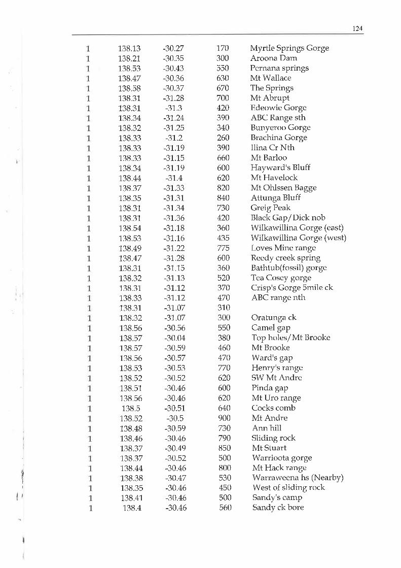
124

138.13138.21,

138.53138.47138.58138.31138.31138.34138.32138.33138.33L38.33138.34138.44138.37138.35138.31138.31138.54138.53138.49138.47138.31138.32138.31138.33138.31138.32138.56138.57138.57138.56138.53138.52138.51138.56138.5138.52138.48138.46138.37138.37138.44138.38138.35138.41138.4

-30.27-30.35-30.43-30.36-30.37-31,.28

-31.3-31,.24

-31.25-31,.2

-31..19

-31.15-31..19

-31.4-31.33-31.31-31,.34

-31..36

-31.18-31,.1.6

-31..22

-31.28-31.15-31.13-31..12

-31..12

-31,.07

-31..07

-30.56-30.04-30.59-30.57-30.s3-30.52-30.46-30.46-30.51-30.5-30.59-30.46

-30.49-30.52

-30.46

-30.47-30.46-30.46-30.46

170300550630670700420390340260390660600620820840730420360435775

600360520370470310300550380460470770

620600620640900

730790850500800s30450s00560

Myrtle Springs GorgeAroona DamPernana springsMt WallaceThe SpringsMt AbruptEdeowie GorgeABC Range sthBunyeroo GorgeBrachina GorgeIlina Cr NthMt BarlooHayward's BluffMt HavelockMt Ohlssen BaggeAttunga BluffGreig PeakBlack Gap/Dick nobWilkawillina Gorge (east)

Wilkawillina Gorge (west)Loves Mine rangeReedy creek springBathtub(fossil) gorgeTea Cosey gorgeCrisp's Gorge 5mile ckABC range nth

Oratunga ckCamel gapTop holes/Mt BrookeMt BrookeWard's gapHenry's rangeSW Mt AndrePinda gapMt Uro rangeCocks combMt AndreAnn hillSliding rockMt StuartWarrioota gorgeMt Hack rangeWarraweena hs (Nearby)West of sliding rockSandy's campSandy ck bore

II

I

125

138.36138.43138.15139.1,5

139.17139.1.4

139.1.5

138.01138.03138.03138.01138.02138.02138.1138.09138.02138.02138.03138.03138.03138.04138.03138.01138.01138.02138.01138.02138.02138.03138.04138.05138.07138.1138.03137.57138.02138.05138.08

138134.51,

134.44134.45134.29135.08136.1.6

137.42

-30.35-30.32-32.02-30.57-30.51-30.58-30.57

-32.28-32.27-32.28-32.04-32.03-32.02-32.04-32.05-32.46-32.48-32.47-32.5

-32.49-32.48-32.48-32.15-32.11,

-32.12-32.09-32.07-32.06-32.06-32.05-31..57

-31..59

-31..49

-32-32.13-32.48-32.59-32.02-32.12-31..59

-31,.57

-31.55-33.04-33.15-33.25-29.58

380510500250140350215440600

450620340290190220440250500

170280240340420360500

3803s0270

280290120420400200320240240180380350280220120100300450

Red gorgePatsy springHut HillChambers gorgeOutouie HillMt ChambersNear Mt ChambersWaukarie fallQourn mapCaltuchie gorgeWyacca bluffBuckaringa hillPettana gorgeThe DykeDrakes nobMRNP-1MRNP-4MRNP-Battery NthMelrose mapMelrose mapMRNP-S Alligator CkMRNP-7 Hidden gorgeThe BluffWarren gorgeMt BenjaminSouth gorgeBuckaringa gorgeMiddle gorge (West)Middle gorge (east)North Middle gorgeTP4Mt Stephen Range southMt EyreMarachowie gorgeDepot CreekMRNP-Mambray CkPort Germein GorgeWillochra CkBlue Range GorgeMt WallabyYarlbrinda HillKondoolkaMt HatCocata HillCarappee HillNear Mt. Nor West

Note: 1 denotes to presence and 0 denotes to absence

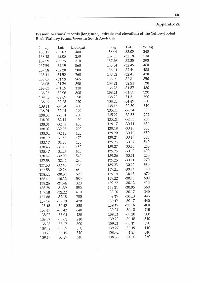
t26

Appendix 2a

Present locational records (longitude, latitude and elevation) of the Yellow-footedRock Wallaby P. xønthopøs in South Australia

Long.138.15138.15137.59737.59137.58138.11138.07138.05138.05138.03138.05138.09138.11138.01138.03138.01138.01138.02138.02138.19138.17138.46138.47138.47137.58137.58137.58138.44138.41.

138.26138.28137.58137.58137.56138.45138.47138.07138.07138.08138.09139.22139.17

Lat.-32.02-32.05-32.25-32.19-32.20-31..52

-31..59

-31..59

-31.55-32.06-32.09-32.05-32.04-32.04-32.01-32.1.4

-32.09-32.08-32.12-31.53-31.58-31.40-31.47-32.00-32.42-32.43-32.26-30.32-30.32-31..44

-31..39_2,')'))

-32.18-32.19-30.42-30.42-33.04-33.01-33.07-33.09-30.19-30.27

400250310560700260265390110300390220200450280470400290420470480450640540230285680520580320550610700420850640180210300350310440

Long.138.09137.55137.56138.04138.04138.02138.00138.21.

138.23138.21.

138.29138.25135.18135.22135.22135.21.

139.!7139.19139.20139.21.

139.23139.27139.25139.26139.25139.23139.21139.19139.22139.22139.21.

139.20139.19139.17139.\7139.24139.24139.20139.21.

139.27138.32138.33

Lat.-33.05-32.18-32.25-32.45-32.44-32.44-32.31.-32.24-31..57

-31.51-3L.31.-31..49-32.30-32.34-32.33-32.33-30.11-30.10-30.10-30.10-30.04-30.10-30.09-30.11-30.11

-30.12-30.1.4

-30.13-30.13-30.12-30.06-30.17-30.18-30.17-30.16-30.18-30.20-30.18-30.17-30.19-31..25

-31..20

240230390460480420850530480330600550310300275205650550550525510260490250270

3307506706004105603404454404002103003403701.40

340260

ElevmElev ( m)(

Bioctimatic profile of the Yellow-footed Rock Wallaby, consisting of empirical distribution functions,one for each bioclimatic parameters.

Appendix 3

20

1.4.3

0.49

97

36.75.3

31..6

27.223.4

27.6

72.1.

5861943

22478

92223

1 Annual Mean Temperature 77.1'

2 Mean Diurnal Range(Mean(period max-min)) 13.6

3 Isotherrnallq 2/7 0.45

4 Temperature Seasonality (C of V) 97

5 Max Temperature of Warmest Period 33.6

6 Min Temperature of Coldest Period 3.6

7 Temperature Annual Range (5-6) 29-9

8 Mean Temperature of Wettest Quarter 1'6.8

9 Mean Temperature of Driest Quarter 17.1

10 Mean Temperature of Warmest Quarter 24.3

71, Mean Temperature of Coldest Quarter 9.9

12 Annual Precipitation 265

13 Precipitation of Wettest Period 7

15 Precipitation Seasonality(C of V) 24

1,6 Precipitation of Wettest Quarter 87

17 Precipitation of Driest Quarter 51

18 Precipitation of Warmest Quarter 67

19 Precipitation of Coldest Quarter 78

PARAMETER

the time period for this profile is weeks

user input file : prsnt-dist.txtDate of this run: Mon Aug 1712:30:241999

mean S.D. 5% 10% 25% 50% 75% 90% 95% max min

1..27

4340.0L

0.071..45

0.91

1..17

7.673.931.5

1.05

77.1.

2.264.9827.6

13.3

9.5

35.1

15.112.9

0.4497

31.32

28.1.

8

10.922.1.

I151

5

1753275231

15.513.10.44

97

31..7

2.4

28.3

9

11.522.4

8.4

7645

17

5631

5535

1.6.2

13.40.44

97

32.5J

28.9

9.8

13

23.2

9.2205

6

19

66

39

61.

45

17.713.6

0.4597

33.53.730.1

1'1..9

18.1

24.1.

10

2627

23

8255

6775

18

13.8

0.4797

34.64.431.

25

20.3

25.4

10.8

3109

28

103

61.

/J

101

19.3

1.4.1.

0.4797

36.25

31.5

26.822.727

11..6

39511.

3213470

86138

1.4

720.497

301..4

27

7

9.221.

7

138

41.6

500

4328

19

1.4

0.5

97

364.8

3'1.

26

2227

11

358

10

31

11967

81

121

t2l

t28

Appendix 4

A listing of the bioclimatic parameters for first 18 locationsof the present distribution records of P. xønthopus

BIOCLIM - The BIOCLIMatic Prediction System************tr******************************

Version 3.6 };4ay 1995Writtenby J.McMahonCRES - ANU - CANBERRA O2OO - AUSTRALIA

Date of this run: Mon Aug 1712:30:21.1998

user input 111" = prsnt-dist.txtthe time period for this run is weeks

19 = the number of bioclimatic parameters and they are:

1. Annual Mean Temperature2. Mean Diurnal Range(Mean(period max-min))3. Isothermalfty 2/74. Temperature Seasonality (C of V)5. Max Temperafure of Warmest Period6. Min Temperature of Coldest Period7. Temperature Annual Range (5-6)

8. Mean Temperature of Wettest Quarter9. Mean Temperature of Driest Quarter10. Mean Temperature of Warmest Quarter11. Mean Temperature of Coldest QuarterL2. Annual Precipitation13. Precipitation of Wettest Period14. Precipitation of Driest Period15. Precipitation Seasonality(C of V)16. Precipitation of Wettest Quarter17. Precipitation of Driest Quarter18. Precipitation of Warmest Quarter19. Precipitation of Coldest Quarter

ident 138.1500 -32.0200 400. 1,6.40 13.50 0.47 97.00 32.60 3.70

29.00 9.80 20.70 23.30 9.70 307.00 9.00 0.00 24.00 101.00

59.00 68.00 101.00ident 138.1500 -32.0500 250. 17.50 13.60 0.47 97.00 33.60 4.50

29.10 10.90 21..70 24.30 10.70 274.00 8.00 0.00 23.00 89.00

54.00 61.00 88.00ident 137.5900 -32.2500 310. 16.80 13.50 0.47 97.00 32.90 4.30

28.60 10.50 19.50 23.50 10.20 285.00 7.00 0.00 21.00 88.00

57.00 65.00 87.00ident 137.5900 -32.1900 560. 15.30 13.10 0.46 97.00 31.50 2.90

28.50 8.70 18.80 22:1.0 8.70 342.00 9.00 0.00 23.00 110.00

66.00 78.00 109.00

ident 137.5800 -32.2000 700. 1'4.60 12.70 0.45 97.00 30.70 2.30

129

28.50 7.90 18.10 21..50 7.90 375.00 10.00 0.00 24.00 121..00

7-t.00 86.00 121.00

ident 138.1100 -31,.5200 260. 17.90 13.80 0'46 97'00 34.40 4.50

29.90 11..40 20.60 25.00 10.80 248.00 7.00 0.00 20.00 77.00

53.00 61.00 75.00ident 138.0700 -3]'5900 265. 17.80 13.80 0'46 97.00 34.30 4.50

29.80 11.30 20.50 24.90 't0.80 252.00 7.00 0.00 20.00 79.00

53.00 61.00 77.00

ident 138.0500 -31.5900 390. 17.00 13.70 0.46 97.00 33'40 3.80

29.60 10.20 19.60 24.00 10.00 280.00 7.00 0.00 21..00 89.00

57.00 68.00 88.00ident 138.0500 -31.5500 110. 18.80 13.80 0.46 97.00 34.90 5.20

29.80 12.70 20.50 25.70 11..70 213.00 6.00 0.00 19.00 64.00

47.00 53.00 61.00ident 138.0300 -32.0600 300. 171'0 13.60 0'47 97'00 33.30 4.30

29.00 10.60 2'1,.40 23.90 10.30 289.00 8.00 0.00 23.00 94.00

56.00 64.00 93.00

ident 138.0500 -32.0900 390. 1'6.40 13.50 0.47 97'00 32.60 3.70

28.90 9.80 20.70 23.20 9.70 313.00 9.00 0.00 24.00 103.00

59.00 68.00 102.00

ident 138.0900 -32.0500 220. 17.70 13.60 0'47 97-00 33'80 4.70

29.20 11.10 21'90 2450 1.0.90 268.00 8.00 0.00 22.00 86.00

53.00 59.00 85.00

ident 138.1100 -32.0400 200. 17.80 13.60 0.47 97'00 34.00 4.80

29.20 11.30 22.1.0 24.60 11.00 262.00 7.00 0.00 22.00 84.00

52.00 58.00 83.00

ident 138.0100 -32.0400 450. 1'6.10 13.40 0.47 97.00 3230 3'40

28.90 9.40 19.60 22.90 9.40 322.00 9.00 0.00 24.00 1.06.00

61.00 71.00 105.00

ident 138.0300 -32.0100 280. 17.30 13.60 0'47 97'00 33.50 4.40

29.1.0 10.80 21..60 241.0 10.50 280.00 8.00 0.00 23.00 90.00

55.00 63.00 89.00ident 138.0100 -32.1.400 470. 15.90 13.40 0.47 97.00 32.00 3.30

28.70 9.30 20.10 22.70 9.20 337.00 9.00 0.00 25.00 112.00

63.00 72.00 11'1..00

ident 138.0100 -32.0900 400. 1'6.40 13.50 0.47 97.00 3250 3.70

28.90 9.70 20.60 23.20 9.60 316.00 9.00 0.00 24.00 104.00

60.00 69.00 103.00

ident 138.0200 -32.0800 290. 17.20 13.60 0.47 97.00 33'30 4.30

29.00 '1,0.70 21..40 24.00 '1.0.40 289.00 8.00 0.00 23.00 93.00

56.00 63.00 93.00

130

Appendix 5Line printer frequency plots of the first 4 bioclimatic parameters

00-

75-

1

+

+

50-

PERCENTILE

++

+

+

0- 1--+--+---1---------1.---------1.13.7 15.8 17.9 20.0

1. Annual Mean Temperature

100- 1

1+1+1.

1"

P75- 1 +E1.R1.c1.E1+N50- 1.

T1.I1L1El+1.

'1.

1+1

1+0- l--+--+--+1---------1.---------'1.

12.3 72.9 13.6 14.3

2. Mean Diurnal Range

100-

L

7

1.

1.

L

L

L

1

1.

1.

1.

1.

1.

1.

1.

1.

1

1

1

1

25-25-+

+

00-1

75-

25-

1.

1.

1.

1.

1.

1.

1

1'1.

1

L

1.

1

1.

1

1

1

1

1

1

1

0

J

++++1.

1.

1.

1.

1

1

'1.

1.

1.

1.

1.

1.

1.

1.

1.

1.

1

1.

1.

+++++++

E

+

50-

PERCENTILE

++75-

50-

25-

P1.

RCENTILE

++

- - + ----- -'t - - -- - - -- -1.- - - -- - - - -1.

.43 0.45 0.47 0.49

. Isothermallty 2/7

0- 1,---------1,--------1.---------797+ 97 97 97

4. Temperature Seasonality (C ofv)

0-

131

Appendix 6

Example of output file from BIOMAP for Adelaide region, where column 1 islongitude, column 2 is latitude and column 3 is the symbol for grid matching(shown only first 20 and last 20 records)

138.00125 -32.001251.138.1.0126 -32.00125 3

138.20125 -32.00125 3

138.30125 -32.00125 3

138.40125 -32.00125 3

138.50125 -32.00125 4138.60126 -32.00125 3

138.701.25 -32.00125 2

138.80125 -32.00125 3

138.901.25 -32.00125 3

139.00125 -32.00125L139.10126 -32.001251.139.20125 -32.001251139.30125 -32.00125 3

139.40125 -32.00125 2

139.501.25 -32.00125 3

139.60126 -32.00125 2

139.70125 -32.00125 3

139.80125 -32.00125 3

139.90125 -32.001251.

1,42.00125 -35.901251142.10126 -35.9012511. 42.201.25 -35.9 0125 1.

1.42.30125 -35.901251142.401.25 -35.90125 1.

142.501.25 -35.90125 1.

1.42.601.26 -35.90125 1.

1.42.7 0125 -35.90125 1.

1.42.80125 -35.90125 1.

1.42.901.25 -35.90125 3

143.00125 -35.90125 3

1.43.10126 -35.90125 31.43.20125 -35.90125 3

143.30125 -35.90125 3

1.43.40125 -35.90125 3

1.43.50125 -35.90125 3

1.43.60126 -35.90125 2

1.43.70125 -35.90125 21.43.80125 -35.90125 2

1.43.901.25 -35.90125 2

Appendix 7

Presence or absence, location, elevation, place name and the list of bioclimatic parameters estimated foreach of distributional locality records of P. xanthopus

No.1

23

45

67

I9

1011

1213

1415161718

192021

222324252627282930

3 29.5I 31.54 31.3

23 10020 51

18 5927 13326 13025 10033 13535 14838 8740 97

P/A Long.1 138.1s1 138.151 137.591 137.591 137.581 138.111 138.071 138.051 138.051 138.031 138.051 138.091 138.111 138.011 138.031 138.011 138.011 138.021 138.021 138.191 138.170 138.130 138.330 1380 138.250 138.370 138.070 138.120 135.10 135.21

Lat. EIev Place name-32.02 400 Hut Hill-32.05 250 Kanyaka Hill-32.25 310 Devil's Peak-32.19 560 Dutchmans Stern Cliffs-32.2 700 Richman Range

-31.52 260 Mt Orkolo-31.59 265 East Stephen Cliffs-31.59 390 Mt StePhen-31.55 1 10 Steep Hill-32.06 300 Buck-Mid. Gorge-32.09 390 Ragless Range-32.05 220 Drakes Nob Peak-32.04 200 The Dyke Ridge-32.04 450 Wyacca Bluff Cliffs-32.01 280 Buckaringa Hill-32.14 470 the Bluff Cliffs-32.09 400 Warren Hannimans-32.08 290 Hannimans-Buck. Gorg-32.12 420 Mt Benjamin-31.53 470 Mt. Elm-Yappala Peak-31.58 480 Yappala South Ridge-30.27 185 Myrtle SPrings-30.31 370 Red Gorge-32.25 660 Devils Peak-32.24 740 Moockra-32.44 420 Orroroo-32.58 280 Germein Gorge-33.21 135 Crystal Brook-32.16 170 Perenning Bluff-32.37 130 NearPaneY H.S.

1

16.417.516.815.314.617.917.8

1718.8't7.1

16.417.717.816.1

17.315.916.417.216.216.516.419.618.414.714.315.816.717.217.817.9

213.513.613.513.1

12.713.813.813.713.813.613.513.613.613.413.613.413.513.613.513.613.514.314.1

12.812.613.313.312.713.9

14

3

0.470.470.470.460.450.460.460.460.460.470.470.470.470.470.470.470.470.470.470.460.460.450.450.450.440.470.470.47

0.50.5

I20.721.719.518.818.1

20.620.519.620.521.420.721.922.119.621.620.1

20.621.420.419.1

19

13.712.6

1917.820.722.923.322.723.6

10

23.324.323.522.121.5

2524.9

24

24.122.723.2

2423

23.623.527.1

2621.621.322.s23.223.4

2423.9

11

9.710.710.28.77.9

10.810.8

11

9.410.59.29.6

10.49.59.59.4

11.810.7

8.1

7.69.3

10.311.1

11.s11.6

12307274285342375248252280213289313268262322280337316289323300304165195391

385306385423235255

13 14 15 16

24 10123 8921 8823 11024 12120 7720 7921 8919 64

17 18

59 6854 61

57 6566 7871 8653 61

53 61

57 6847 53

19

101

8887

10912175778861

97 336 45 291 1

97 32.9 4 3 28.6 1

97 31.5 2.9 28.597 307 2.3 28597 344 45 299 1

97 343 45 298 1

97 33.4 3 8 29.6 1

97 34.9 5 2 29.8 1

97 33.3 4.3 29 1

97 326 3.7 28.997 33 8 4.7 29.2 'l

97 34 48 292 1

97 32.3 34 28997 33.5 4.4 29j 1

97 32 3.3 28.797 325 3.7 28997 33.3 43 29 1

97 31.8 3.5 28 397 32.6 44 282 1

97 32.3 54 269 1

456797 326 37 29

97 32.4 3.6 28.897 33 3.4 29.697 328 3.

97 364 4.

97 35397 30.9 2.4 28 597 30.5 2 28 4

97 33.4 5.4 28 1

97 33.3 5.5 27.8 1

I9.80.90.58.77.91.41.30.22.70.69.8'1.1

1.39.40.89.39.70.79.69.79.62726

8.1

7.69.30.41.41.51.6

56 64 9359 68 10253 59 8552 58 8361 71 10555 63 8963 72 11160 69 10356 63 9361 70 10661 71 9761 72 9934 51 3942 59 4871 82 13271 83 13056 63 10061 64 13459 60 14737 38 8738 39 97

94103

8684

10690

112104

9310798

2324222224232524232523

90807090

10 0707070608090807090809090809080805050

11 0

11 080

11 01207080

1011.710.3

9.710.9

25.723.923.224.524.622.9

132

31 0

32033034035036037038039040041 0

42043044045 1

46 1

47 1

48 1

49 1

50 1

51 1

s2 1

53 1

54 1

55 1

56 1

57 1

58 1

59 1

60 1

61 1

62 1

63 1

64 1

65 1

66 1

13s.32137.26137.28137.07140.05140.07

140140.17140.19140.22140.12139.37139.12138.38138.46138.47138.47137.58137.58137.58138.44138.41

138.26138.28137.58137.58137.56138.45138.47138.07138.07138.08138.09138.09137.55137.56

-32.3-32.5

-32.45-32.4

-32.03-32.05

-32.1-32.06-32.04-32.04-32.43-32.58-33.18-34.11

-31.4-31.47

-32-32.42-32.43-32.26-30.32-30.32-31.44-31.39-32.22-32.18-32.19-30.42-30.42-33.04-33.01

-33.07-33.09-33.05-32.18-32.25

5.35.43.94.74.14.4

27.927.927.928.228.828.728.728.728.728.728.4

11

12.1

12.69.8

24.323.623.9

23.78.9

11.310.2

9.98.68.911

10.6I

24.924.5

11

9.38.47.99.6

22.724

11.1

10.9

10.1

9.510.511.4

9.8

23.524.224.322.724.924.124.424.724.s24.823.721.92t.721.223.522.722.623.823.421.524.924.s24.723.321.821.522.822.7

2423.323.1

22.321.822.824.122.9

258 I235 6197 6

262 7

229 6224 6234 6205 5

206 5

202 5

194 5

277 7255 ô472 14299 I344 10

316 I274 7

292 I377 11

2'19 6

231 6261 7

312 I356 10

373 10305286247449470549586

0340 19

0 18

0 19

0 19

0 19

0 19

0 19

0 19

0 19

0 18

0140170370250270240200210240 18

0 18

0200230240240220 19

0 18

0350360410430380 19

022

93 4471 4856 4377 5568 4868 4669 4961 41

62 41

61 4056 4079 61

75 52167 66101 61

120 68105 6284 5691 58

123 71

67 4971 51

83 55103 63115 ô8121 7196 6088 6275 55

157 63167 65

206 69224 71

182 6677 s395 60

250110

90390250350300270300270330550380255450640540230285680520580320550610700420850640180210300350240230390

Pondanna BluffMt WhyallaRed RockNear Corunna HillBirnbowie StationNear Doughboy CreekWeekeeroo StationWallaby RocksBinberrie HillMeningie GorgeAnabarna HillPualco WestMt PullenBetw Rhynie & Salter SChace RangeBlack RangeGood Friday CavesDavenport MapDavenport MapPort Augusta MapGoddard MapGoddard MapElder RangeMt AleckPort Augusta MapPort Augusta MapPort Augusta MapMocatoona HillAngepena HillC.Davis-NelshabyTelowie GorgePirie MapNapperby GorgeBig Broad CreekSouth CreekSaltia Hill

17.317.9

18

16.217.8

1717.417.717.s17.716.8

15

15.315.516.81s.615.617.316.814.617.4

1717.616.2

1514.616.1

15.316.5

1716.9

16

15.616.617.516.3

13.613.313.313.313.1

13

13.1

13

13

13

13

12.813.1

1213.613.213.213.413.412.813.813.713.813.4

13

12.713.413.1

13.612.9

13

13

13.1

13

13.613.4

0.490.480.480.470.450.450.450.450.450.450.460.460.480.480.460.450.460.470.470.450.450.440.460.450.460.450.470.430.440.470.470.480.480.470.470.47

31

30.9

31.833.132.830.834.333.834.1

22.222.622.717.1

11.910.811.511.411.211.410.717.6

17

21.120.319.1

18.221.4

21

18.1

11.616.620.318.818.518.118.814.816.1

23.223

22.221.822.820.1

18.9

11

1',|.5

11.69.7

10.710.1

10.410.610.410.6

108.49.1

109.78.58.8

10.710.3

I9.89.5

10.59.1

8.47.99.57.99.1

10.810.6

9.99.5

10.410.8

9.7

97 32.997 33.297 33.397 32j97 33.597 32.897 33.197 33.397 33.197 33.397 32.5

5.1 46 9353 6950 5266 7764 53ô6 51

65 5560 4561 4559 4456 4467 7858 73

24.224.324.5

6461

4.

4.

4.4.2.3.

5.

3.2.

9797979797979797979797979797979797979797

9797979797

3033.3

32

8 28.25 27.51255 29.85 29.5

2.9 28.928.428.328.4

31

30.929.929.728.s28.528.630.330.727.327.427.227.227.328.828.5

66 16769 10078 11971 10562 8365 9085 12367 5571 5864 81

7s 10281 11586 12071 9588 7475 6364 15s66 165

70 20572 223

4.74.42.43.22.94.2

3

2.72.33.61.62.65.1

4.94.33.94.84.73.8

32.731.230.832.331.933.332.432.331.531.1

3233.532.4

II6

13

14

'17

1967 18061 7570 94

500 15

254 7302 I

133

6768697071

7273747576

777879808l82838485868788899091

9293949596979899

100101

102

-32.45-32.44-32.44-32.31-32.24-31.57-31.51-31.31-31.49-32.3

-32.34-32.33-32.33-30.11

-30.1-30.1-30.1

-30.04-30.1

-30.09-30.11-30.11-30.12-30.14-30.13-30.13-30.12-30.06-30.17-30.18-30.'17

-30.16-30.18

-30.2-30.18-30.17

460480420850530480330600550310300275205650550550525510260490250270330750670600410560340445440400210300340370

31.331.131.331.231.231.231.531.331.331.3

24.425.724.726.1

25.425.42s.726.926.426.1

25.9

26.623.624.224.6

2625

26.425.725.7

2627.226.726.426.2

1 138.04I 138.041 138.021 1381 138.211 138.231 138.211 138.291 138.251 135.181 135.221 '135.22

1 135.211 139.171 139.191 139.21 139.211 139.231 139.271 139.251 139.261 139.251 139.231 139.211 139.191 139.221 139.221 139.211 139.21 139.191 139.171 139.171 139.241 139.241 139.21 139.21

MRNP-8 TerraceMRNP Alligator GorgeMRNP Gullet CkMt BrownHorseshoe RangeYourumbulla PeakYappala WatersReggie nobWonoka HillMt WallabyPaney HS NearbyPondanna BluffScrubby Peak NthPetalinka waterfallCapra Ck waterfallNear Wheal Frost MineBalancing Rock GorgeMt Shanahan mineHot Springs CkFreeling Hgts EscarpmYudnamutana Gorge EYudnamutana GorgeBox CanyonMt PainterRadium RidgeSplit RockArmchair CkGreenhilWellArkaroola waterholeThe PinnaclesGreenwood HillNooldoonooldoonaBarraranna GorgeKingmill GorgeSir Mark Oliphant HillDinnertime Hill

9.1

I9.3

78.89.6

10.69.1

9.310.6

30 13530 13530 131

27 14726 11724 10221 8522 102

15.ô15.515.813.715.416.417.5

16

16.1

16.916.917.1

17.516.817.417.417.617.819.417.919.419.318.916.1

16.617.1

18.417.418.818.1

18.1

18.419.6

1918.818.6

13.313.213.312.313.213.513.713.313.413.4

13.413.513.713.613.713.713.813.8

1413.814.1

1414

13.313.513.613.913.713.913.813.913.914.1

1413.913.9

0.470.470.470.430.460.460.460.450.450.480.480.490.490.440.440.440.440.440.450.440.450.45o.440.440.440.440.440.440.450.440.440.440.450.450.45o.44

20.420.320.7

18

19.719.920.1

18.619.622.922.923.123.410.4

11

11

11.211.312.911.4

13

12.812.4

9.810.310.711.9

11

12.411.711.7

1213.1

12.612.312.2

9.1

I9.3

78.89.4

10.48.8

I10.6

10.610.811.29.29.89.89.910

11.510.1

11.s11.411.1

8.6I

9.510.69.711

10.310.410.611.711.2

11

10.8

389 11

390 12

380 11

434 13

347 10

306 9

267 7315 I317 9272 8

275 I270 I260 I219 7

201 6201 6197 6193 6153 5

193 6152 5

155 5

165 5

240 7

224 7

212 7179 5

202 6168 5

187 6185 6177 5148 5

165 5169 5

174 s

67 7367 7466 7278 9264 7361 71

s6 64ô5 78

97 31.697 31.597 31.897 29.897 31.597 32.897 33.997 32.597 32.597 32.597 32.597 32.797 33.197 33.597 34.297 34.297 34.497 34.697 36.197 34.697 36.297 36.197 35.797 32.897 33.497 33.897 35.197 34.297 35.597 34.897 34.997 35.297 36.497 35.897 3s.597 35.3

3.33.23.51.5

3

3.34.1

2.73

4.84.8

5

5.32.63.1

3.1

3.33.44.63.54.74.64.32.22.52.93.9

10.610.811.324.224.724.824.92s.126.725.226.826.626.323.523.9

28.228.228.328.328.529.529.829.729.627.727.727.727.830.931.1

31.1

31.1

31.231.531.231.531.531.430.630.8

31

22.222.122.520.722.223.524.623.223.223.1

23.223.323.724.3

2525

25.225.4

2725.527.1

27

0

0

0

0

0

0

0

0

00

0000

0

0

0

0

0

000000

0

0

0

0

0

0

0

00

00

24 106 64 7534 99 47 48

135135131147117101

84102105

99

101

99964641

41

404031

3931

323451

474336423538383730333536

3.1

4.23.73.73.94.84.44.24.1

34 101 47 4835 99 45 4737 97 42 4325 7s 41 7427 70 37 6927 70 37 7027 70 36 6928 68 35 6830 55 27 5529 69 35 6830 55 27 5430 55 27 5529 59 30 5826 83 46 8226 77 42 7627 75 39 7429 64 32 6327 71 37 7029 60 30 5928 66 34 6527 65 34 6427 62 32 61

30 53 26 51

30 60 29 5929 60 31 5929 62 31 62

134

103 1

104 1

105 1

106 1

107 1

108 ',l

109 1

110 1

111 1

112 1

113 1

114 1

11s 1

116 1

117 1

118 1

119 1

120 1

121 1

122 1

123 1

124 1

12s 1

126 1

127 1

128 1

129 1

130 1

131 1

132 1

133 1

134 1

135 1

136 1

137 1

138 1

139.27139.22139.17

139.2139.22139.24139.21139.22139.22139.21139.03139.12139.09139.14138.49

138.5138.5

138.51138.52138.56

139138.58139.05

138.3139.1

139.08139.09139.06139.09

139.1

139.1139.12139.13138.13138.21138.53

-30.19-30.19-30.27-30.19

-30.2-30.18-30.17-30.16

-30.2-30.28-30.16-30.23-30.27-30.29-30.19-30.17-30.16-30.22-30.23-30.24-30.24-30.26-30.07-31.07-30.34-30.27-30.26-30.28-30.27-30.34-30.32-30.38-30.43-30.27-30.35-30.43

140310440450320205390300260200490600530270350300300410390680600750350570300550670680840270340235260170300550

18.519.1

19.319.617.8

1717.419.1

18.719

19

18.218.416.5

1716

18.816.418.917.316.516.415.419.1

18.619.319.1

19.618.817.1

14.214

13.813.813.914.1

13.91414

14.1

13.813.613.7

1414.1

14.1

14.1

1414

13.513.613.4

1413.513.913.713.513.513.1

1413.9

1413.914.314.1

13.7

34.235.935.635.9

3635.135.333.233.732.735.6

3335.6

3433.233.1

27.226.325.325.326.226.925.826.426.626.825.324.324.726.426.326.626.625.825.923.924.423.526.49.4

26.224.623.923.922.826.425.926.526.327.126.324.6

14.1

12.s11.611.612.513.2

1212.612.813.1

11.410.6

11

12.712.813.1

13.1

12.412.s

1610.615.612.9

18

12.s10.910.210.1

9.22.72.22.92.7

27.626.625.625.626.527.326.126.726.927.225.424.s

2526.726.326.626.625.825.923.924.523.526.523.626.524.8

24

12.1

11.1

10.310.311.1

11.710.711.211.411.710.1

9.49.8

11.310.911.211.210.510.6

8.99.48.511

9.1

11.1

9.79

8.9I

11.310.911.511.311.911.1

9.6

138165192189168147178162157152189211203162181

171171192189241213255158287170206227230263165176162171163187229

Arkaroola SpringsSinan's FallsMt McTaggartGriselda HillArkaroola HomesteadStubbs waterholeSwitch backMundoo oopinnaKingsmillfallsNepouie springWilkindinna springMainwater springlllinawortina mapHells gateFrome Crk-Moosha BorFrome CrkVeldemartyWNW Voca vocanaVoca vocanaMount RoseCammon CrkArcoona BluffYerelina SpringsMt SamuelItalowie GapItalowie CreekBunyip GorgeRover rockholeMt John RobertsDr Chewings CkMt McKinlay SpringsErragoona HillStirrup lron RangeMyrtle Springs GorgeAroona DamPernana springs

20l91818

18.919.6

0.45 970.45 970.44 970.44 970.45 970.45 970.44 970.45 970.45 970.45 970.44 970.44 970.44 970.45 970.45 970.45 970.45 970.45 970.45 970.44 970.44 970.44 970.45 970.45 970.45 970.44 970.44 970.44 970.43 970.45 970.45 970.45 970.45 970.45 970.45 970.45 97

5.1 31.54.4 31.33.7 31.1

3.7 31.1

4.3 31.34.9 31.54 31.2

4.4 31.44.6 31.44.9 31.43.4 31.1

2.9 30.93.2 30.9

36.735.734.834.835.636.435.235.8

405060605040605050506070605050505050507060705070506070708050505050505060

31 50 048 2830 60 30 59 3428 68 35 67 39

29 64 32 63 3629 58 29 57 33

36.334.633.7

29 68 34 66 3830 61 30 60 3430 53 26 51 30

30 56 28 56 323630 54 27 53 31

19 58 40 58 46

19 80 56 80 6325 52 30 52 36

19 87 61 76 8626 58 32 58 3624 68 38 67 4423 74 43 74 4922 75 45 75 5022 88 54 87 59

26 56 31 56 3s26 60 33 59 3727 56 30 55 3427 59 32 58 3620 50 33 50 39

23 62 36 61 41

24 70 39 69 4424 67 38 67 4327 56 30 56 34

19 55 38 55 4420 52 35 52 41

20 52 35 s2 41

19 59 41 59 47

4.6 31.34.1 31.54.4 31.64.4 31.63.8 31.33.9 31.32.5 30.82.9 30.92.1 30.64.2 31.52.9 30.1

4.4 31.23.1 30.92.5 30.72.5 30.71.7 30.34.6 31.24.2 31.24.7 31.24.6 31.1

5 31.54.4 31.43.1 30.8

3235.835.4

363s.736.535.833.9

19 75 53 75 6022 69 41 68 47

1

1

1

1

1

23922926726226826627 1

264246

3.813

1619 57 40 57 4618 69 51 69 58

135

139 1

140 1

141 1

142 1

143 1

144 1

145 1

146 1

147 1

148 1

149 1

150 1

151 1

152 1

153 1

154 1

155 1

156 'l

157 1

158 1

159 1

160 1

161 1

162 1

163 1

164 1

165 1

166 1

167 1

168 I169 1

170 1

171 1

172 1

173 1

174 1

138.47138.58138.31138.31138.34138.32138.33138.33138.33138.34138.44138.37138.35138.31138.31

138.54138.53138.49138.47138.31138.32138.31138.33138.31138.32138.56138.57138.57138.56138.53138.52138.51138.56

138.5'138.52

138.48

-30.36-30.37-31.28-31.3

-31.24-31.25

-31.2-31.19-31.15-31.19

-31.4-31.33-31.31-31.34-31.36-31 .18-31.16-31.22-31.28-31.15-31 .13-31.12-31.12-31.07-31.07-30.56-30.04-30.59-30.57-30.53-30.52-30.46-30.46-30.51

-30.5-30.59

16.716.415.417.1

17.317.718.317.415.816.1

15.814.714.61s.2

1717.617.1

1516

17.616.617.616.918.1

18.1

1718.617.517.515.716.616.816.616.514.915.8

13.613.513.1

13.713.713.813.913.813.313.413.212.812.7

13

13.713.813.712.913.313.813.613.813.713.913.913.714.1

13.813.813.213.613.613.613.512.913.3

0.440.440.440.460.460.460.460.460.440.450.450.430.430.440.460.460.450.440.450.460.450.460.450.460.460.450.450.450.450.440.440.440.440.440.430.44

30

29.829.929.629.429.429.529.930.230.129.629.830.330.130.330.130.430.530.731.630.830.830.330.630.730.7

24.123.9

8.410.1

10.610.911.510.7

8.89.1

8.77.67.58.2

10.1

10.810.47.99.1

10.99.6

10.810.211.211.324.426.2

2525

23.1

2424.224.1

16.316

18

19.720

20.318.6

1917.418.719.317.317.217.819.619.518.917.618.619.318.219.318.618.418.516.612.716.416.315.316.216.416.31ô.1

14.516.4

24.123.922.624.324.624.925.524.6

2323.322.921.921.822.424.224.924.422.323.224.923.924.924.225.32s.424.426.2

2525

23.1

2424.224.123.922.323.2

9.28.98.39.9

10.1

10.411

10.28.68.98.77.67.58.1

9.910.3

9.97.98.9

10.49.4

10.39.7

10.710.8

9.510.8

l010

8.39.1

9.39.2I

7.58.5

241

246332276265253229260312305334357358342281255270341318249283249271231229238178223224277249241244252299275

60609070706060708080

10 0

10 0

10 0

10 0

70607090906070607060606050606070606060708070

18 7418 7622 10720 8719 8218 7716 6718 7920 9821 9726 11423 11623 11623 11221 91

18 7819 8422 10923 10517 7419 8717 7418 8316 6716 6ô17 71

21 5517 6617 6618 8317 7418 7318 7417 7619 91

18 82

630 Mt Wallace670 The Springs700 Mt Abrupt420 Edeowie Gorge390 ABC Range sth340 Bunyeroo Gorge260 Brachina Gorge390 llina Cr Nth660 Mt Barloo600 Hayward's Bluff620 Mt Havelock820 Mt Ohlssen Bagge840 Attunga Bluff730 Greig Peak420 Black Gap/Dick nob360 Wilkawillina Gorge (eas435 Wilkawillina Gorge (wes775 Loves Mine range600 Reedy creek spring360 Bathtub(fossil) gorge520 Tea Cosey gorge370 Crisp's Gorge Smile ck470 ABC range nth310300 Oratunga ck550 Camel gap380 Top holes/Mt Brooke460 Mt Brooke470 Ward's gap

770 Henry's range620 SW Mt Andre600 Pinda gap620 Mt Uro range640 Cocks comb900 Mt Andre730 Ann hill

97 33.5 2.7 30.897 33.2 2.5 30.797 31.9 2.3 29.6

53 7455 7668 8359 6957 6855 6552 6257 6865 81

64 7867 7872 8972 9069 8459 6955 6658 6970 8766 7755 6660 7455 6659 71

52 6351 6353 71

37 5550 6650 6661 8355 7454 73s4 7456 7665 91

60 82

1

61

62078680756477979613161511

897682090472867281

64636243585873656262667974

97 33.697 33.997 34.297 34.897 3497 32.397 32.697 32.297 31.1

97 31

97 31.797 33.597 34.297 33.797 31.597 32.597 34.297 33.297 34.297 33.597 34.797 34.897 33.797 35.697 34.397 34.397 32.397 33.397 33.597 33.497 33.297 31.597 32.5

30.6 23.930.1 22.330.3 23.2

30.130.230.330.2

3.63.84.1

4.53.82.52.82.61.71.62.1

3.64

3.61.92.7

4

1

1

1

1

1

1

3.23.93.44.34.33.1

43.53.5

22.72.82.72.61.42.2

136

175176177178179180181

18218318418s186187188189190191

192193194195196197198199200201202203204205206207208209210

1

1

1

1

1

1

1

1

1

1

1

1

1

1

1

1

1

1

1

1

1

1

1

1

1

1

1

1

'l

1

1

1

1

1

1

1

138.46138.37138.37138.44138.38138.35138.41

138.4138.36138.43138.15139.1s139.17"t39.14

139.15138.01138.03138.03138.01138.02138.02

138.1138.09138.02138.02'138.03

138.03138.03138.04138.03138.01138.01138.02138.01138.02138.02

-30.46-30.49-30.52-30.46-30.47-30.46-30.46-30.46-30.35-30.32-32.02-30.57-30.51-30.58-30.57-32.28-32.27-32.28-32.04-32.03-32.02-32.04-32.05-32.46-32.48-32.47

-32.5-32.49-32.48-32.48-32.15-32.11-32.12-32.09-32.07-32.06

790850500800530450500560380510500250140350215440600450620340290190220440250500170280240340420360500380350270

15.615.217.315.517.217.717.4

17

18.317.515.8

1919.718.319.215.9

15

15.815.1

16.817.217.917.715.717.1

15.317.616.817.1

16.416.216.615.716.516.717.3

13.213

13.813.213.813.913.813.7

14

13.813.313.9

1413.813.913.4

13

13.313

13.613.613.613.613.313.413.213.313.413.413.413.413.513.313.513.613.6

2322.624.822.924.725.224.924.525.8

259.1

26.226.92s.626.4

9.38.4

9.610

9.1

9.910.1

10.8

15.214.817.91s.117.816.6

2322.624.822.924.725.224.924.525.8

2522.726.527.225.926.722.621.822.522.123.7

2424.724.522.323.6

2224.223.423.722.922.923.422.523.323.524.1

8.27.89.88.1

9.710.2

9.99.5

10.69.99.1

11.312

10.711.s

9.38.49.28.4

10.1

10.411.1

10.99.2

10.58.8

11.1

10.310.6

9.99.59.9

9

9.810

10.5

278 7

292 8

229 6280 I231 6217 6225 6

236 6198 5

218 6328 I178 6155 5

197 6172 5

351 10

381 11

352 10

358 10

296 8

283 I260 7

268 I389 11

347 10

402 12310 I360 10

Sliding rockMt StuartWarrioota gorgeMt Hack rangeWarraweena hs (NearbWest of sliding rockSandy's campSandy ck boreRed gorgePatsy springHut HillChambers gorgeOutouie HillMt ChambersNear Mt ChambersWaukarie fallQourn mapCaltuchie gorgeWyacca bluffBuckaringa hillPettana gorgeThe DykeDrakes nobMRNP-1MRNP-4MRNP-Battery NthMelrose mapMelrose mapMRNP-5 Alligator CkMRNP-7 Hidden gorgeThe BluffWarren gorgeMt BenjaminSouth gorgeBuckaringa gorgeMiddle gorge (West)

0.43 970.43 970.45 970.43 970.45 970.45 970.45 970.45 970.45 970.45 970.46 970.45 970.45 970.45 970.45 970.47 970.46 970.47 970.45 970.47 970.47 970.47 970.47 970.47 970.47 970.47 970.47 970.47 970.47 970.47 970.47 970.47 970.46 970.47 970.47 970.47 97

32.331.834.232.2

3434.634.233.835.234.3

3235.636.3

3535.8

3231.1

31.931.433.133.4

3433.831.732.931.333.432.7

3332.332.332.831.932.732.933.5

42I3

30303030

19163319

20.420.9

2020.7

21

21.6

343374327308341311302282

30 13529 11730 14026 10130 12329 11631 12925 10824 10125 11424 10224 9923 91

7277607360555861

4955

10938324337

118129118119

9691

8285

13511614099

122115129108100113101

9790

0

0

0

0

0000

0

0

0

0

000

0

0

0

0

0

00

0

0

0

000000

0

0

0

0

0

60 8463 8951 6861 8552 6948 6550 6752 71

43 6048 6662 7234 6028 5339 6632 5863 7269 7964 7267 8057 6655 6352 5853 5967 7360 6569 7555 5962 6760 6564 6961 7059 6764 7459 6858 6655 62

18 8419 8917 ô819 8518 6918 6518 6718 71

18 6018 6625'11026 61

28 5425 6726 5927 11827 13027 11925 11923 9623 91

22 8322 86

16.217.612.511.719.313.313.912.613.520.1

19.320

18.621.121.522.121.920.522.420.223.422.222.521.8

9.28.4

10.210.711.311.19.2

10.68.8

11.310.410.7

10

3.2 30.83.6 31

3.3 30.93 30.84 31.2

3.3 31

3.2 28.94.6 31

5.1 31.24.1 30.84.8 31

3.4 28.52.7 28.43.4 28.52.6 28.8

4294.3 29j4.8 29.24.7 29.23.4 28.24.6 28.43.1 28.2

5 28.44.4 28.34.6 28.44 28.3

3.6 28.73.9 28.93.2 28.73.8 28.94 28.9

4.4 29.1

1011

II

10

9

II

137

211 1

212 1

213 1

214 1

215 1

216 1

217 1

218 1

219 1

220 1

221 1

222 0

223 0224 0225 0226 0

227 0

228 0

138.03138.04138.05138.07

138.1138.03137.57138.02138.05138.08

138134.51134.44134.45134.29135.081 36.1 6

137.42

-32.06-32.05-31.57-31.59-31.49

-32-32.13-32.48-32.59-32.02-32.12-31.59-31.57-31.55-33.04-33.15-33.25-29.58

21.5 24j

19.

22.23.22.20.22.22.22.22.22.21.

1

0.5 284 I0.4 286 I1.7 216 69.8 287 8

9.9 278 7

11 260 70.2 276 7

0.6 343 100.6 369 11

1257 7

8314 I7265 7

1257 75246 76 438 18

5 372 143 369 127209 6

29 11631 12722 8224 10325 8827 8728 8362 20754 16438 13625 72

55 6356 6348 5458 6957 6852 5956 6560 6560 6351 5759 6852 5549 5245 4840 4041 41

55 5644 72

280 Middle gorge (east)

290 North Middle gorge120 TP4420 Mt Stephen Range sout400 Mt Eyre200 Marachowie gorge

320 Depot Creek240 MRNP-Mambray Ck240 Porl Germein Gorge180 Willochra Ck380 Blue Range Gorge350 Mt Wallaby280 Yarlbrinda Hill220 Kondoolka120 Mt Hat100 Cocata Hill300 Carappee Hill450 Near Mt. Nor West

33.4 433.4 434.9 5

33.2 3

21.420.419.419.722.1

17.317.218.716.8

1717.916.917.1

1718

16.517.317.617.916.917.1

16.1

18.5

13.613.613.813.613.713.613.613.413.313.613.513.513.613.712.713.312.614.3

0.47o.470.460.460.460.470.47o.470.47o.47o.470.470.480.484.520.520.480.44

979797979797979797979797979797979797

33.5343333

32.834.1

32.633.1

33.333.430.531.330.935.7

29.228.828.428.2

10.710.712.2

10

10.211 .3

10.510.710.711.49.9

10.7

91

926391

8781

84115126

80102

888683

203163136

47

43

1

67

I266.9 29.2.8 28.8.5 28.6.9 28.4.2 28.36 24.5.7 25.65 25.9

291291298296298

23 9223 9219 6622 9221 8822 8320 85

2425232424232323242323

7

8

1

7

67

5

8

27

00

0000

000

0

0

0

0

0

0

0

0

0

3

444443

445

5

65

227

47I1

5

9

24.22.22.21.

.1

.5

.8

.6

.3

.2

11

11

11

11

10

24

2 26.2 10

21

5

9

1.

9.

0.

1.

1.

1.

1.

0.

1

1

1

1

1

1

3.7 321 26

138