RECOMMENDATIONS IN MOBILE AND PERVASIVE BUSINESS ...

RECOMMENDATIONS IN MOBILE AND PERVASIVE

BUSINESS ENVIRONMENTS

by

YONG GE

A Dissertation submitted to the

Graduate School-Newark

Rutgers, The State University of New Jersey

in partial fulfillment of the requirements

for the degree of

Doctor of Philosophy

Graduate Program in Management

written under the direction of

Dr. Hui Xiong

and approved by

Newark, New Jersey

May 2013

c© Copyright 2013

Yong Ge

All Rights Reserved

ABSTRACT OF THE DISSERTATION

RECOMMENDATIONS IN MOBILE AND PERVASIVE BUSINESS

ENVIRONMENTS

By YONG GE

Dissertation Director: Dr. Hui Xiong

Advances in mobile technologies have allowed us to collect and process massive

amounts of mobile data across many different mobile applications. If properly ana-

lyzed, this data can be a source of rich intelligence for providing real-time decision

making in various mobile applications and for the provision of mobile recommenda-

tions. Indeed, mobile recommendations constitute an especially important class of

recommendations because mobile users often find themselves in unfamiliar environ-

ments and are often overwhelmed with the ”new terrain” abundance of unfamiliar

information and uncertain choices. Therefore, it is especially useful to equip them

with the tools and methods that will guide them through all these uncertainties by

providing useful recommendations while they are ”on the move.”

In this dissertation, we aim to address the unique challenges of recommendations

in mobile and pervasive business environments from both theoretical and practical

perspectives. Specifically, we first develop an energy-efficient mobile recommender

system which is to recommend a sequence of potential pick-up points for taxi drivers

by handling the complex data characteristics of real-world location traces. The de-

veloped mobile recommender system can provide effective mobile sequential recom-

mendation and the knowledge extracted from location traces can be used for coaching

ii

drivers and lead to the efficient use of energy. The experimentations on real-world

spatio-temporal data demonstrate the efficiency and effectiveness of our methods.

Moreover, we introduce a focused study of cost-aware collaborative filtering that is

able to address the cost constraint for travel tour recommendation. Specifically, we

present two ways to represent user’s latent cost preference and different cost-aware

collaborative filtering models for travel tour recommendations. We demonstrate that

the cost-aware recommendation models can consistently and significantly outperform

several existing latent factor models. In addition, we introduce a Tourist-Area-Season

Topic (TAST) model. This TAST model can represent travel packages and tourists

by different topic distributions, where the topic extraction is conditioned on both the

tourists and the intrinsic features (i.e. locations, travel seasons) of the landscapes.

Then, based on this topic model representation, we present a cocktail approach to

generate the lists for personalized travel package recommendation. When applied

to real-world travel tour data, the TAST model can lead to better performances of

recommendation. Finally, we introduce the collective training to boost collaborative

filtering models. The basic idea is that we compliment the training data for a particu-

lar collaborative filtering model with the predictions of other models. And we develop

an iterative process to mutually boost each collaborative filtering model iteratively.

iii

ACKNOWLEDGEMENTS

I would like to express my great appreciation to all the people who provided me

tremendous support and help during my Ph.D. study.

First, I would like to express my deep gratitude to my advisor, Prof. Hui Xiong, for

his continuous support, guidance and encouragement, which are necessary to survive

and thrive the graduate school and the beyond. I thank him for generously giving me

motivation, support, time, assistance, opportunities and friendship; for teaching me

how to identify key problems with impact, present and evaluate the ideas. He helped

making me a better writer, speaker and scholar.

I also sincerely thank my other committee members: Prof. Alexander Tuzhilin,

Prof. Vijay Atluri and Prof. Xiaodong Lin. All of them not only provide constructive

suggestions and comments on my work and this thesis, but also offer numerous sup-

port and help in my career choice, and I am very grateful for them. Prof. Alexander

Tuzhilin has been a great professor to me over the past three years. His experience

and vision in recommender systems, data mining and personalization has inspired me

a lot to solve the challenging problems in my research, and I have learned a great deal

from the collaboration with him on many exciting projects. I learned current database

systems and information security technology from Prof. Vijay Atluri’s courses, and I

was provided lots of useful feedback and suggestions from him during my PhD study.

iv

Prof. Xiaodong Lin has provide many exciting discussions for my research and career

development and friendship during my PhD study.

Special thanks are due to Prof. Shashi Shekhar at department of computer science

at University of Minnesota, Prof. Wenjun Zhou at University of Tennessee and Dr.

Ramendra Sahoo at Citi helping with my job search and career development. Thanks

are also due to Dr. Guofei Jiang, Dr. Ming Li, Dr. Milind Naphade, Dr. K.C. Lee,

Prof. Enhong Chen, Dr. Qi Liu, Prof. Zhi-hua Zhou, and Dr. Min Ding. It was a

great pleasure working with all of them. I also owe a hefty amount of thanks to my

colleagues and friends Zhongmou Li, Keli Xiao, Chuanren Liu, Hengshu Zhu, Yanchi

Liu, Chunyu Luo, Zijun Yao, Yanjie Fu, Konstantin Patev, Jingyuan Yang, Xue Bai,

Liyang Tang, Chang Tan, for their help, friendship and valuable suggestion.

I would like to acknowledge the Department of Management Science and Infor-

mation Systems (MSIS) and Center for Information Management, Integration and

Connectivity (CIMIC) for supplying me with the best imaginable equipment and

facilities that helped me to accomplish much of this work.

Finally, I would like to thank my wife, my daughter, my parents, and my brother

for their love, support and understanding. Without their encouragement and help,

this thesis would be impossible.

v

TABLE OF CONTENTS

ABSTRACT . . . . . . . . . . . . . . . . . . . . . . . . . . . . . . . . . . . . . . . . . . . . . . . . . . . . . . . . . . . . . . . . . . . ii

ACKNOWLEDGEMENTS . . . . . . . . . . . . . . . . . . . . . . . . . . . . . . . . . . . . . . . . . . . . . . . . . . . . . iv

LIST OF TABLES . . . . . . . . . . . . . . . . . . . . . . . . . . . . . . . . . . . . . . . . . . . . . . . . . . . . . . . . . . . . . x

LIST OF FIGURES. . . . . . . . . . . . . . . . . . . . . . . . . . . . . . . . . . . . . . . . . . . . . . . . . . . . . . . . . . . . xi

CHAPTER 1. INTRODUCTION . . . . . . . . . . . . . . . . . . . . . . . . . . . . . . . . . . . . . . . . . . . . . 1

1.1 Background and Preliminaries . . . . . . . . . . . . . . . . . . . . . . . . . . . . . . . . . . . . . . . 2

1.2 Mobile Recommender Systems . . . . . . . . . . . . . . . . . . . . . . . . . . . . . . . . . . . . . . . 5

1.3 Research Motivation. . . . . . . . . . . . . . . . . . . . . . . . . . . . . . . . . . . . . . . . . . . . . . . . 6

1.4 Research Contributions . . . . . . . . . . . . . . . . . . . . . . . . . . . . . . . . . . . . . . . . . . . . . 8

1.5 Overview . . . . . . . . . . . . . . . . . . . . . . . . . . . . . . . . . . . . . . . . . . . . . . . . . . . . . . . . . 11

CHAPTER 2. MOBILE SEQUENTIAL RECOMMENDATION. . . . . . . . . . . . . . . 13

2.1 Introduction . . . . . . . . . . . . . . . . . . . . . . . . . . . . . . . . . . . . . . . . . . . . . . . . . . . . . . 14

2.2 Problem Formulation . . . . . . . . . . . . . . . . . . . . . . . . . . . . . . . . . . . . . . . . . . . . . . . 17

2.2.1 A General Problem Formulation . . . . . . . . . . . . . . . . . . . . . . . . . . . . . . . . 17

2.2.2 Analysis of Computational Complexity . . . . . . . . . . . . . . . . . . . . . . . . . . 20

2.2.3 The MSR Problem with Constraints . . . . . . . . . . . . . . . . . . . . . . . . . . . . 21

2.3 Recommending Point Generation . . . . . . . . . . . . . . . . . . . . . . . . . . . . . . . . . . . . . 22

2.3.1 High-Performance Drivers . . . . . . . . . . . . . . . . . . . . . . . . . . . . . . . . . . . . . 23

2.3.2 Clustering Based on Driving Distance . . . . . . . . . . . . . . . . . . . . . . . . . . . 23

2.3.3 Probability Calculation . . . . . . . . . . . . . . . . . . . . . . . . . . . . . . . . . . . . . . . 24

2.4 Sequential Recommendation . . . . . . . . . . . . . . . . . . . . . . . . . . . . . . . . . . . . . . . . . 24

2.4.1 The Potential Travel Distance Function . . . . . . . . . . . . . . . . . . . . . . . . . 25

2.4.2 The LCP Algorithm . . . . . . . . . . . . . . . . . . . . . . . . . . . . . . . . . . . . . . . . . 27

2.4.3 The SkyRoute Algorithm . . . . . . . . . . . . . . . . . . . . . . . . . . . . . . . . . . . . . 29

2.4.4 Obtaining the Optimal Driving Route . . . . . . . . . . . . . . . . . . . . . . . . . . . 33

2.4.5 The Recommendation Process . . . . . . . . . . . . . . . . . . . . . . . . . . . . . . . . . 33

vi

2.5 Experimental Results . . . . . . . . . . . . . . . . . . . . . . . . . . . . . . . . . . . . . . . . . . . . . . . 36

2.5.1 The Experimental Setup . . . . . . . . . . . . . . . . . . . . . . . . . . . . . . . . . . . . . . 36

2.5.2 An Illustration of Optimal Driving Routes . . . . . . . . . . . . . . . . . . . . . . . 37

2.5.3 An Overall Comparison . . . . . . . . . . . . . . . . . . . . . . . . . . . . . . . . . . . . . . . 38

2.5.4 A Comparison of Skyline Computing . . . . . . . . . . . . . . . . . . . . . . . . . . . . 41

2.5.5 Case: Multiple Evaluation Functions . . . . . . . . . . . . . . . . . . . . . . . . . . . . 42

2.6 CONCLUDING REMARKS . . . . . . . . . . . . . . . . . . . . . . . . . . . . . . . . . . . . . . . . . 43

CHAPTER 3. COST-AWARE COLLABORATIVE FILTERING FOR TRAVEL

TOUR RECOMMENDATIONS. . . . . . . . . . . . . . . . . . . . . . . . . . . . . . . . 46

3.1 Introduction . . . . . . . . . . . . . . . . . . . . . . . . . . . . . . . . . . . . . . . . . . . . . . . . . . . . . . 47

3.2 Related Work . . . . . . . . . . . . . . . . . . . . . . . . . . . . . . . . . . . . . . . . . . . . . . . . . . . . . 51

3.2.1 Collaborative Filtering . . . . . . . . . . . . . . . . . . . . . . . . . . . . . . . . . . . . . . . . 51

3.2.2 Travel Recommendation . . . . . . . . . . . . . . . . . . . . . . . . . . . . . . . . . . . . . . . 53

3.2.3 Cost/Profit-based Recommendation . . . . . . . . . . . . . . . . . . . . . . . . . . . . 54

3.3 Cost-aware PMF Models . . . . . . . . . . . . . . . . . . . . . . . . . . . . . . . . . . . . . . . . . . . . 55

3.3.1 The vPMF Model . . . . . . . . . . . . . . . . . . . . . . . . . . . . . . . . . . . . . . . . . . . . 55

3.3.2 The gPMF Model . . . . . . . . . . . . . . . . . . . . . . . . . . . . . . . . . . . . . . . . . . . . 59

3.3.3 The Computational Complexity . . . . . . . . . . . . . . . . . . . . . . . . . . . . . . . . 62

3.4 Cost-aware LPMF Models . . . . . . . . . . . . . . . . . . . . . . . . . . . . . . . . . . . . . . . . . . . 63

3.4.1 The LPMF Model . . . . . . . . . . . . . . . . . . . . . . . . . . . . . . . . . . . . . . . . . . . . 63

3.4.2 The vLPMF Model . . . . . . . . . . . . . . . . . . . . . . . . . . . . . . . . . . . . . . . . . . . 65

3.4.3 The gLPMF Model . . . . . . . . . . . . . . . . . . . . . . . . . . . . . . . . . . . . . . . . . . . 66

3.5 Cost-aware MMMF Models . . . . . . . . . . . . . . . . . . . . . . . . . . . . . . . . . . . . . . . . . 68

3.5.1 The MMMF Model . . . . . . . . . . . . . . . . . . . . . . . . . . . . . . . . . . . . . . . . . . . 68

3.5.2 The vMMMF Model . . . . . . . . . . . . . . . . . . . . . . . . . . . . . . . . . . . . . . . . . . 69

3.5.3 The gMMMF Model . . . . . . . . . . . . . . . . . . . . . . . . . . . . . . . . . . . . . . . . . . 70



3.6.2 Collaborative Filtering Methods . . . . . . . . . . . . . . . . . . . . . . . . . . . . . . . . 73

3.6.3 The Details of Training . . . . . . . . . . . . . . . . . . . . . . . . . . . . . . . . . . . . . . . 74

3.6.4 Validation Metrics . . . . . . . . . . . . . . . . . . . . . . . . . . . . . . . . . . . . . . . . . . . . 75

3.6.5 The Performance Comparisons . . . . . . . . . . . . . . . . . . . . . . . . . . . . . . . . . 77

3.6.6 The Performances with Different Values of α and D . . . . . . . . . . . . . . 84

3.6.7 The Performances on Different Users . . . . . . . . . . . . . . . . . . . . . . . . . . . . 86

3.6.8 The Learned User’s Cost Information . . . . . . . . . . . . . . . . . . . . . . . . . . . 88

3.6.9 An Efficiency Analysis . . . . . . . . . . . . . . . . . . . . . . . . . . . . . . . . . . . . . . . . 92

vii

3.7 Conclusion and Discussion . . . . . . . . . . . . . . . . . . . . . . . . . . . . . . . . . . . . . . . . . . 93

CHAPTER 4. A COCKTAIL APPROACH FOR TRAVEL PACKAGE REC-

OMMENDATION . . . . . . . . . . . . . . . . . . . . . . . . . . . . . . . . . . . . . . . . . . . . . 99

4.1 Introduction . . . . . . . . . . . . . . . . . . . . . . . . . . . . . . . . . . . . . . . . . . . . . . . . . . . . . . 100

4.2 Concepts and Data Description . . . . . . . . . . . . . . . . . . . . . . . . . . . . . . . . . . . . . . 103

4.3 The TAST Model . . . . . . . . . . . . . . . . . . . . . . . . . . . . . . . . . . . . . . . . . . . . . . . . . . 106

4.3.1 Topic Model Representation . . . . . . . . . . . . . . . . . . . . . . . . . . . . . . . . . . . 107

4.3.2 Model Inference . . . . . . . . . . . . . . . . . . . . . . . . . . . . . . . . . . . . . . . . . . . . . . 110

4.3.3 Area/Seasons Segmentation . . . . . . . . . . . . . . . . . . . . . . . . . . . . . . . . . . . 111

4.3.4 Related Topic Models . . . . . . . . . . . . . . . . . . . . . . . . . . . . . . . . . . . . . . . . . 112

4.4 Cocktail Recommendation Approach . . . . . . . . . . . . . . . . . . . . . . . . . . . . . . . . . 113

4.4.1 Seasonal Collaborative Filtering for Tourists . . . . . . . . . . . . . . . . . . . . . 115

4.4.2 New Package Problem . . . . . . . . . . . . . . . . . . . . . . . . . . . . . . . . . . . . . . . . 116

4.4.3 Collaborative Pricing . . . . . . . . . . . . . . . . . . . . . . . . . . . . . . . . . . . . . . . . . 117

4.4.4 Related Cocktail Recommendations . . . . . . . . . . . . . . . . . . . . . . . . . . . . . 120

4.5 The TRAST Model . . . . . . . . . . . . . . . . . . . . . . . . . . . . . . . . . . . . . . . . . . . . . . . . 121



4.6.2 Season Splitting and Price Segmentation . . . . . . . . . . . . . . . . . . . . . . . . 128

4.6.3 Understanding of Topics . . . . . . . . . . . . . . . . . . . . . . . . . . . . . . . . . . . . . . 129

4.6.4 Recommendation Performances . . . . . . . . . . . . . . . . . . . . . . . . . . . . . . . . 131

4.6.5 The Evaluation of the TRAST Model . . . . . . . . . . . . . . . . . . . . . . . . . . . 135

4.6.6 Recommendation for Travel Groups . . . . . . . . . . . . . . . . . . . . . . . . . . . . . 138

4.7 Concluding Remarks . . . . . . . . . . . . . . . . . . . . . . . . . . . . . . . . . . . . . . . . . . . . . . . 140

CHAPTER 5. COLLABORATIVE FILTERING WITH COLLECTIVE TRAIN-

ING . . . . . . . . . . . . . . . . . . . . . . . . . . . . . . . . . . . . . . . . . . . . . . . . . . . . . . . . . . . 141

5.1 Introduction . . . . . . . . . . . . . . . . . . . . . . . . . . . . . . . . . . . . . . . . . . . . . . . . . . . . . . 142

5.2 Related Work . . . . . . . . . . . . . . . . . . . . . . . . . . . . . . . . . . . . . . . . . . . . . . . . . . . . . 144

5.3 Collective Training . . . . . . . . . . . . . . . . . . . . . . . . . . . . . . . . . . . . . . . . . . . . . . . . . 145

5.3.1 The Bi-CF Algorithm . . . . . . . . . . . . . . . . . . . . . . . . . . . . . . . . . . . . . . . . . 146

5.3.2 The Tri-CF Algorithm . . . . . . . . . . . . . . . . . . . . . . . . . . . . . . . . . . . . . . . . 150


5.5 Concluding Remarks . . . . . . . . . . . . . . . . . . . . . . . . . . . . . . . . . . . . . . . . . . . . . . . 153

CHAPTER 6. CONCLUSIONS AND FUTURE WORK . . . . . . . . . . . . . . . . . . . . . . 156

viii

BIBLIOGRAPHY. . . . . . . . . . . . . . . . . . . . . . . . . . . . . . . . . . . . . . . . . . . . . . . . . . . . . . . . . . . . . . 158

VITA . . . . . . . . . . . . . . . . . . . . . . . . . . . . . . . . . . . . . . . . . . . . . . . . . . . . . . . . . . . . . . . . . . . . . . . . . . 166

ix

LIST OF TABLES

1.1 An Example of Item-User Rating Matrix . . . . . . . . . . . . . . . . . . . . . . . . . . . 4

2.1 Some Acronyms. . . . . . . . . . . . . . . . . . . . . . . . . . . . . . . . . . . . . . . . . . . . . . . . 39

2.2 A Comparison of Search Time (Second) between BFS and LCPS . . . . . 41

3.1 Some Characteristics of Travel Data . . . . . . . . . . . . . . . . . . . . . . . . . . . . . . . 72

3.2 The Notations of 9 Collaborative Filtering Methods . . . . . . . . . . . . . . . . . 73

3.3 A Performance Comparison (10D Latent Features & α = 0.1) . . . . . . . . . 78


3.5 A Performance Comparison in terms of RMSE. . . . . . . . . . . . . . . . . . . . . . 80



3.8 The Performances on Different Users (10D Latent Features & α = 0.1) . 96

3.9 Performances with Tail Users/Packages (30D Latent Features & α = 0.1) 97

3.10 A Comparison of Variance . . . . . . . . . . . . . . . . . . . . . . . . . . . . . . . . . . . . . . . 97

3.11 A Comparison of the Model Efficiency (10D Latent Features) . . . . . . . . . 98

4.1 Mathematical notations. . . . . . . . . . . . . . . . . . . . . . . . . . . . . . . . . . . . . . . . . . 107

4.2 The description of the training and test data. . . . . . . . . . . . . . . . . . . . . . . 126

4.3 A performance comparison: DOA(%). . . . . . . . . . . . . . . . . . . . . . . . . . . . . . 131

4.4 User study ratings. . . . . . . . . . . . . . . . . . . . . . . . . . . . . . . . . . . . . . . . . . . . . . 134

4.5 Experimental results for K-means clustering. . . . . . . . . . . . . . . . . . . . . . . . 136

4.6 The recall results for Leave-Out-Rest (%). . . . . . . . . . . . . . . . . . . . . . . . . . 137

4.7 Group recommendation results: DOA(%). . . . . . . . . . . . . . . . . . . . . . . . . . . 139

5.1 A Sample Data Set. . . . . . . . . . . . . . . . . . . . . . . . . . . . . . . . . . . . . . . . . . . . . . 143

5.2 RMSE Comparisons on MovieLens . . . . . . . . . . . . . . . . . . . . . . . . . . . . . . . . 154

x

LIST OF FIGURES

2.1 An Illustration Example. . . . . . . . . . . . . . . . . . . . . . . . . . . . . . . . . . . . . . . . . 18

2.2 Some Statistics of the Cab Data. . . . . . . . . . . . . . . . . . . . . . . . . . . . . . . . . . 23

2.3 A Recommended Driving Route. . . . . . . . . . . . . . . . . . . . . . . . . . . . . . . . . . . 25

2.4 Illustration: the Sub-route Dominance. . . . . . . . . . . . . . . . . . . . . . . . . . . . . 28

2.5 Illustration of the Circulating Mechanism. . . . . . . . . . . . . . . . . . . . . . . . . . . 35

2.6 Illustration: Optimal Driving Routes. . . . . . . . . . . . . . . . . . . . . . . . . . . . . . 38

2.7 A Comparison of Search Time. . . . . . . . . . . . . . . . . . . . . . . . . . . . . . . . . . . . 40

2.8 The Pruning Effect . . . . . . . . . . . . . . . . . . . . . . . . . . . . . . . . . . . . . . . . . . . . . 40

2.9 A Comparison of Search Time (L = 3) on the Synthetic Data set. . . . . . 42

2.10 A Comparison of Skyline Computing . . . . . . . . . . . . . . . . . . . . . . . . . . . . . . 43

2.11 A Comparison of Search Time for Multiple Optimal Driving Routes . . . 44

3.1 The Cost Distribution. . . . . . . . . . . . . . . . . . . . . . . . . . . . . . . . . . . . . . . . . . . 49

3.2 Graphical Models. . . . . . . . . . . . . . . . . . . . . . . . . . . . . . . . . . . . . . . . . . . . . . . 61

3.3 A Performance Comparison in terms of CD (10D Latent Features). . . . . 81

3.4 A Local Performance Comparison in terms of CD (10D Latent Features). 82

3.5 A Performance Comparison in terms of CD (30D Latent Features). . . . . 83

3.6 A Local Performance Comparison in terms of CD (30D Latent Features). 84

3.7 Performances with Different α (10D Latent Features). . . . . . . . . . . . . . . . 87

3.8 Performances with Different D (α = 0.1). . . . . . . . . . . . . . . . . . . . . . . . . . . 88

3.9 The Performances on Different Users (10D Latent Features). . . . . . . . . . 89

3.10 An Illustration of User Financial Cost. . . . . . . . . . . . . . . . . . . . . . . . . . . . . 90

3.11 An Illustration of the Gaussian Parameters of User Cost. . . . . . . . . . . . . 91

3.12 An Illustration of the Convergence of RMSEs (10D Latent Features). . . 93

4.1 An illustration of the chapter contribution. . . . . . . . . . . . . . . . . . . . . . . . . . 102

4.2 An example of the travel package, where the landscapes are represented

by the words in red. . . . . . . . . . . . . . . . . . . . . . . . . . . . . . . . . . . . . . . . . . . . . . 103

4.3 TAST: A graphical model. . . . . . . . . . . . . . . . . . . . . . . . . . . . . . . . . . . . . . . . 109

4.4 The three related topic models. . . . . . . . . . . . . . . . . . . . . . . . . . . . . . . . . . . . 111

xi

4.5 The cocktail recommendation approach. . . . . . . . . . . . . . . . . . . . . . . . . . . . 114

4.6 The TRAST model and its two sub-models. . . . . . . . . . . . . . . . . . . . . . . . . 118

4.7 Season splitting and price segmentation. . . . . . . . . . . . . . . . . . . . . . . . . . . . 128

4.8 The correlation of topic distributions between different price ranges

(Left)/different areas (Center)/different seasons(Right). Darker shades

indicate lower similarity. . . . . . . . . . . . . . . . . . . . . . . . . . . . . . . . . . . . . . . . . . 129

4.9 A performance comparison based on Top-K. . . . . . . . . . . . . . . . . . . . . . . . . 131

4.10 The runtime results for different algorithms. . . . . . . . . . . . . . . . . . . . . . . . . 135

4.11 The precision results for Leave-Out-Rest (%). . . . . . . . . . . . . . . . . . . . . . . 137

5.1 RMSEs at Different Iterations. . . . . . . . . . . . . . . . . . . . . . . . . . . . . . . . . . . . 154

xii

- 1 -

CHAPTER 1

INTRODUCTION

Advances in sensor, wireless communication, and information infrastructure such as

GPS, WiFi, and mobile phone technology have enabled us to collect and process

massive amounts of location traces from multiple sources but under operational time

constraints. These location traces are fine-grained, sufficiently information-rich, and

have global road coverage, and thus provide unparallel opportunities for people to un-

derstand mobile user behaviors and generate useful knowledge, which in turn deliver

intelligence for real-time decision making in various fields, including that of mobile

recommendations. For example, recent years have witnessed a revolution in mobile

phone technology, which is driven by the development of the mobile Internet. Accord-

ing to the Telephia Mobile Internet Report, US had 34.6 million mobile web users as

of June, 2006. While this is only 17% of total wireless phone subscribers, the penetra-

tion rate has been steadily increasing. As the mobile Internet keeps evolving, there

are clear signs that mobile pervasive recommendation will have huge demand, and

therefore,mobile application awareness continues to grow among mobile users. Mobile

pervasive recommendation is promised to provide mobile users access to personalized

recommendations anytime, anywhere. In order to keep this promise, an immediate

need is to understand the unique features that distinguish mobile recommendation

systems from classic recommender systems. Indeed, the objective of this disserta-

- 2 -

tion is to exploit the hidden information in location traces collected from multiple

application domains for developing mobile recommender systems.

1.1 Background and Preliminaries

Recent years have witnessed an increased interest in recommender systems (Hofmann,

1999; Resnick, Iacovou, Suchak, Bergstrom, & Riedl, 1994), especially after these

technologies were popularized by Amazon and Netflix, as well as after the establish-

ment of $1,000,000 Netflix Prize Competition that attracted over 45,000 contestants

from 180 countries. A lot of works have done both in the industry and academia on

developing new approaches to recommender systems over the last decade. In its most

common formulation, the recommendation problem is simplified to the problem of

estimating ratings for items that have not been rated by users. Intuitively, this esti-

mation is usually based on the ratings given by this user to other items, the ratings

by other users to the same item and soem other information(features) of the items.

Once we can estimate ratings for the unknown ratings, we can simply recommend to

the user the item(s) with the highest rating(s).

More formally, the recommendation problem can be formulated as follows. Let C

be the set of all users and let S be the set of all possible items that can be recom-

mended, such as books, movies, or restaurants. The space S of possible items can be

very large, ranging in hundreds of thousands or even millions of items in some appli-

cations, such as recommending books or CDs. Similarly, the user space can also be

very large-millions in some cases. Let u be a utility function that measures usefulness

of item s to user c, i.e., u: CXS → R, where R is a totally ordered set. Then for each

- 3 -

user c ∈ C, we want to choose such item s′ ∈ S that maximizes the user’s utility.

More formally:

∀c ∈ C, s′c = argmaxs∈Su(c, s) (1.1)

In recommender systems the utility of an item is usually represented by a rating,

which indicates how a particular user liked a particular item.

The central problem of recommender systems lies in that utility u is usually not

defined on the whole C×S space, but only on some subset of it. This means u needs to

be extrapolated to the whole space C×S. In recommender systems, utility is typically

represented by ratings and is initially defined only on the items previously rated by the

users. For example, in a movie recommendation application, users initially rate some

subset of movies that they have already seen. An example of a user-item rating matrix

for a movie recommendation application is presented in Table 1.1, where ratings are

specified on the scale of 1 to 5. The ”NaN” symbol for some of the ratings in table

1.1 means that the users have not rated for the movies. Then, the recommendation

engine should be able to estimate/predict the ratings of the unknown ratings and

decide appropriate recommendations based on these predictions.

Extrapolations from known to unknown ratings are usually done by specific heuris-

tics that can exploit the known ratings for prediction and optimize certain perfor-

mance criterion, such as the mean square error. Once the unknown ratings are es-

timated, actual recommendations of an item to a user are made by selecting the

highest rating among all the estimated ratings for that user according to formula 1.1.

Alternatively, we can recommend N best items to a user or a set of users to an item.

- 4 -

Table 1.1. An Example of Item-User Rating Matrix

Alice Bob Cindy David

RainMan NaN NaN 2 3

TheX − Files 1 2 NaN 2

Batman 2 4 2 4

TheGodfather 1 2 NaN 2

Note: NaN indicates unknown rating.

The new ratings of the unknown ratings can be estimated in many different ways

using the methods from machine learning, approximation theory and various heuris-

tics. Recommender systems are usually classified according to their approach to rating

estimation. In the following, we will present a classification that was proposed in the

literature. The commonly accepted formulation of the recommendation problem was

first stated in (Resnick et al., 1994; Shardanand & Maes, 1995; Hill, Stead, Rosen-

stein, & Furnas, 1995) and this problem has been studied extensively since then.

Moreover, recommender systems are usually classified into the following categories,

based on how recommendations are made:

• Content-based recommendations: the user is recommended items similar to the

ones the user preferred in the past;

• Collaborative recommendations: the user is recommended items that people

with similar mind liked in the past;

• Hybrid approaches: these methods combine collaborative and content-based

- 5 -

methods.

In addition to recommender systems that predict the absolute values of ratings

that individual users would give to the unseen items, there has been work done

on preference-based filtering, i.e., predicting the relative preferences of users (Iyer,

Jr., Karger, & Smith, 1998). For example, in a movie recommendation application

preference-based filtering techniques would focus on predicting the correct relative

order of the movies, rather than their individual ratings.

1.2 Mobile Recommender Systems

Recommender systems in the mobile environments become a promising area with the

advanced development of mobile device, such as GPS and WiFi, and the increasing

demand of users for mobile applications, such as travel planning and location-based

shopping. A lot of works have already done both in the industry and academia on

developing new systems and applications in recent years. Typically, mobile recom-

mender systems are systems that provide assistance/guidance to users as they face

decisions ’on the go’, or, in other words, as they move into new, unknown environment.

And different from traditional recommendation techniques, mobile recommendation is

unique in its location-aware capability. Mobile computing adds a relevant but mostly

unexplored piece of information- the users physical location-to the recommendation

problem. For example, a mobile shopping recommender system could analyze the

shopping history of users at different locations and the current position of users to

make recommendation for particular user. Another example would be recommenda-

tion for tourists or traveler. This kind of mobile recommender system could analyze

- 6 -

the historical data of variant tourists or travelers to recommend traveling route to

meet the demand/preference of particular user.

1.3 Research Motivation

However, the development of personalized recommender systems in mobile and per-

vasive environments is much more challenging than developing recommender systems

from traditional domains due to the complexity of spatial data and intrinsic spatio-

temporal relationships, the unclear roles of context-aware information, the lack of user

rating information, and the diversified location-sensitive recommendation tasks. As a

matter of fact, recommender systems in the mobile environments have been studied

before. For instance, the work in targets the development of mobile tourist guides.

Also, Heijden et al. have discussed some technological opportunities associated with

mobile recommendation systems. In addition, Averjanova et al. have developed a

map-based mobile recommender system that can provide users with some personal-

ized recommendations. However, this prior work is mostly based on user ratings and

is only exploratory in nature, and the problem of leveraging unique features distin-

guishing mobile recommender systems remains pretty much open.1 Indeed, there are

a number of technical and domain challenges inherent in designing and implementing

an effective mobile recommend system in pervasive environments. First, the het-

erogeneous and noisy nature of mobile environments makes the data more complex

than traditional commercial item data, such as the Movie data. Location traces are

spatio-temporal data in nature. Spatial data have spatial autocorrelation and follow

the first law of geography - everything is related to everything else, but the nearby

- 7 -

things are more related than distant things. The challenge lies in how to effectively

extract recommendable knowledge from location traces not being affected by these

data characteristics. Second, traditional recommender systems usually rely on the

user ratings for validation. However, in mobile application domains, the user rat-

ings are usually not conveniently available. Therefore, it becomes a real challenge

to develop alternative evaluation metrics and recommendation techniques for mobile

recommender systems. Third, recommendation techniques developed in traditional

recommendation systems may only be tangentially applicable to mobile recommender

systems and a new set of methods needs to be developed instead. In addition, it is

not clear that whether the mobile recommendation techniques developed in one ap-

plication domain can be easily adapted for building a mobile recommender system in

a different application domain. Therefore, it is important to identify the commonality

and diversity among different types of mobile recommender systems. Fourth, in tradi-

tional recommender systems, it is usually not necessary to consider the corresponding

cost to take a recommendation. For instance, the cost for watching a recommended

movie is usually not a concern for any user. However, in mobile recommender systems

for tourists, the users may have various time and price constraints to select among

different recommended travel plans. Finally, the recommended items in traditional

recommender systems usually have a stable value. However, in many mobile recom-

mender systems, the values of the items to be recommended can be depreciated over

time. Moreover, some mobile items have life cycle. For instance, a tour package can

only last for a certain period. The travel agents need to actively create new tour

packages to replace old tour packages based on the interests of the customers.

- 8 -

1.4 Research Contributions

In this dissertation, we study the unique characteristics of mobile recommender sys-

tems and demonstrate how to develop mobile recommender systems in different ap-

plication domains. Generally, the proposed research has the following major thrusts:

• Investigating the impact of the unique characteristics of mobile data on the de-

velopment of mobile recommender systems. To this end, we will exploit mobile

data from different application domains and develop two mobile recommender

systems, an energy-efficient mobile recommender system and a mobile recom-

mender system for targeting tourists. In addition, as an unique challenge to

the development of mobile recommender systems, the issues related to location

privacy will also be taken into the consideration.

• Development of novel approaches to mobile recommender systems that work for

the applications and data described above. Since these applications and data

are significantly different from each other, we also plan to understand common-

ality and diversity across different mobile recommendation techniques. The goal

is to demonstrate the design and implementation issues of mobile recommender

systems in different application settings. In particular, we will also design and

evaluate the effective evaluation metrics for mobile recommender systems. Al-

though the key differences between traditional recommender systems and mobile

recommender systems are known, we will explore them further and at a deeper

level in this project.

- 9 -

Specifically, we first provide a focused study of extracting energy-efficient trans-

portation patterns from location traces. Specifically, we have the initial focus on a

sequence of mobile recommendations. As a case study, we develop a mobile recom-

mender system which has the ability in recommending a sequence of pick-up points

for taxi drivers or a sequence of potential parking positions. The goal of this mobile

recommendation system is to maximize the probability of business success. Along

this line, we provide a Potential Travel Distance (PTD) function for evaluating each

candidate sequence. This PTD function possesses a monotone property which can be

used to effectively prune the search space. Based on this PTD function, we develop

two algorithms, LCP and SkyRoute, for finding the recommended routes. Experi-

mental results show that the proposed system can provide effective mobile sequential

recommendation and the knowledge extracted from location traces can be used for

coaching drivers and leading to the efficient use of energy.

Second we provide another focused study of cost-aware travel tour recommenda-

tion. We first propose two ways to represent user’s cost preference. One way is to

represent user’s cost preference by a 2-dimensional vector. Another way is to con-

sider the uncertainty about the cost that a user can afford and introduce a Gaussian

prior to model user’s cost preference. With these two ways of representation of user’s

cost preference, we develop different cost-aware latent factor models by incorporating

the cost information into the Probabilistic Matrix Factorization (PMF) model, the

Logistic Probabilistic Matrix Factorization (LPMF) model, and the Maximum Mar-

gin Matrix Factorization (MMMF) model respectively. When applied to real-world

travel tour data, all the cost-aware recommendation models consistently outperform

- 10 -

existing latent factor models with a significant margin.

Third we introduce a Tourist-Area-Season Topic (TAST) model to address more

challenges of travel package recommendations. This TAST model can represent travel

packages and tourists by different topic distributions, where the topic extraction is

conditioned on both the tourists and the intrinsic features (i.e. locations, travel sea-

sons) of the landscapes. Then, based on this topic model representation, we propose

a cocktail approach to generate the lists for personalized travel package recommenda-

tion. Furthermore, we extend the TAST model to the Tourist-Relation-Area-Season

Topic (TRAST) model for capturing the latent relationships among the tourists in

each travel group. Finally, we evaluate the TAST model, the TRAST model, and

the cocktail recommendation approach on the real-world travel package data. Ex-

perimental results show that the TAST model can effectively capture the unique

characteristics of the travel data and the cocktail approach is thus much more effec-

tive than traditional recommendation techniques for travel package recommendation.

Also, by considering tourist relationships, the TRAST model can be used as an effec-

tive assessment for travel group formation.

Finally, we introduce a collective training paradigm to address the sparseness issue

of recommendations by automatically and effectively augmenting the training ratings.

Essentially, the collective training paradigm builds multiple different Collaborative

Filtering (CF) models separately, and augments the training ratings of each CF model

by using the partial predictions of other CF models for unknown ratings. Along this

line, we develop two algorithms, Bi-CF and Tri-CF, based on collective training. For

Bi-CF and Tri-CF, we collectively and iteratively train two and three different CF

- 11 -

models via iteratively augmenting training ratings for individual CF model. We also

design different criteria to guide the selection of augmented training ratings for Bi-

CF and Tri-CF. The experimental results show that Bi-CF and Tri-CF algorithms

can significantly outperform baseline methods, such as neighborhood-based and SVD-

based models.

1.5 Overview

Chapter 2 addresses the computation challenge embedded in mobile sequential rec-

ommendation with GPS data. Two types of algorithms are introduced to efficiently

search the optimal drive route and recommend it to users.

Chapter 3 presents different types of cost-aware collaborative filtering models for

travel package recommendation. Two different ways are introduced to represent the

user’s cost preference. Probabilistic Matrix Factorization (PMF) model, Logistic

Probabilistic Matrix Factorization (PMF) model, and Maximum Margin Matrix Fac-

torization (MMMF) model are considered and extended with the cost information.

Experimental results with real world data are presented to validate the effectiveness

of cost-aware models.

Chapter 4 presents two types of topic models (i.e., TAST and TRAST) based on

the LDA model to address the analytical challenges of travel package data. A hybrid

recommendation framework is presented based on the topic models to produce the

recommendation results. Empirical comparisons with real world data are presented

show the performances of different recommendation methods.

Chapter 5 presents a collective training paradigm to address the sparseness issue

- 12 -

of recommendation. This collective training compliments the training data for one

collaborative filtering model by effectively leveraging the predictions of other models.

And an iterative process is introduced to mutually compliment the training data for

each collaborative filtering model.

- 13 -

CHAPTER 2

MOBILE SEQUENTIAL RECOMMENDATION

The increasing availability of large-scale location traces creates unprecedent oppor-

tunities to change the paradigm for knowledge discovery in transportation systems.

A particularly promising area is to extract energy-efficient transportation patterns

(green knowledge), which can be used as guidance for reducing inefficiencies in en-

ergy consumption of transportation sectors. However, extracting green knowledge

from location traces is not a trivial task. Conventional data analysis tools are usually

not customized for handling the massive quantity, complex, dynamic, and distributed

nature of location traces. To that end, in this chapter, we provide a focused study of

extracting energy-efficient transportation patterns from location traces. Specifically,

we have the initial focus on a sequence of mobile recommendations. As a case study,

we develop a mobile recommender system which has the ability in recommending a

sequence of pick-up points for taxi drivers or a sequence of potential parking posi-

tions. The goal of this mobile recommendation system is to maximize the probability

of business success. Along this line, we provide a Potential Travel Distance (PTD)

function for evaluating each candidate sequence. This PTD function possesses a

monotone property which can be used to effectively prune the search space. Based on

this PTD function, we develop two algorithms, LCP and SkyRoute, for finding the

recommended routes. Finally, experimental results show that the proposed system

- 14 -

can provide effective mobile sequential recommendation and the knowledge extracted

from location traces can be used for coaching drivers and leading to the efficient use

of energy.

2.1 Introduction

Advances in sensor, wireless communication, and information infrastructures such as

GPS, WiFi and RFID have enabled us to collect large amounts of location traces (tra-

jectory data) of individuals or objects. Such a large number of trajectories provide

us unprecedented opportunity to automatically discover useful knowledge, which in

turn deliver intelligence for real-time decision making in various fields, such as mobile

recommendations. Indeed, a mobile recommender system promises to provide mo-

bile users access to personalized recommendations anytime, anywhere. To this end,

an important task is to understand the unique features that distinguish pervasive

personalized recommendation systems from classic recommender systems.

Recommender systems (Adomavicius & Tuzhilin, 2005) address the information

overloaded problem by identifying user interests and providing personalized sugges-

tions. In general, there are three ways to develop recommender systems. The first one

is content-based (Mooney & Roy, 1999). It suggests items which are similar to those

a given user has liked in the past. The second way is based on collaborative filtering.

In other words, recommendations are made according to the tastes of other users that

are similar to the target user. Finally, a third way is to combine the above and have

a hybrid solution (Pazzani, 1999). However, the development of personalized recom-

mender systems in mobile and pervasive environments is much more challenging than

- 15 -

developing recommender systems from traditional domains due to the complexity of

spatial data and intrinsic spatio-temporal relationships, the unclear roles of context-

aware information, and the increasing availability of environment sensing capabilities.

Recommender systems in the mobile environments have been studied before (Abowd,

Atkeson, & al, 1997; Averjanova, Ricci, & Nguyen, 2008; Cena et al., 2006; Chev-

erst, Davies, & al, 2000; Miller, Albert, & al, 2003; Tveit, 2001; Heijden, Kotsis,

& Kronsteiner, 2005). For instance, the work in (Abowd et al., 1997; Cena et al.,

2006) targets the development of mobil tourist guides. Also, Heijden et al. have

discussed some technological opportunities associated with mobile recommendation

systems (Heijden et al., 2005). In addition, Averjanova et al. have developed a

map-based mobile recommender system that can provide users with some personal-

ized recommendations (Averjanova et al., 2008). However, this prior work is mostly

based on user ratings and is only exploratory in nature, and the problem of leverag-

ing unique features distinguishing mobile recommender systems remains pretty much

open.

In this chapter, we exploit the knowledge extracted from location traces and de-

velop a mobile recommender system based on business success metrics instead of

predictive performance measures based on user ratings. Indeed, the key idea is to

leverage the business knowledge from the historical data of successful taxi drivers for

helping other taxi drivers improve their business performance. Along this line, we

provide a pilot feasibility study of extracting business-success knowledge from loca-

tion traces by taxi drivers and exploiting this business information for guiding taxis’

driving routes. Specifically, we first extract a group of successful taxi drivers based on

- 16 -

their past performances in terms of revenue per energy use. Then, we can cluster the

pick-up points of these taxi drivers for a certain time period. The centroids of these

clusters can be used as the recommended pick-up points with a certain probability of

success for new taxi drivers in these areas. This problem can be formally defined as

a mobile sequential recommendation problem, which recommends sequential pick-up

points for a taxi driver to maximize his/her business success. Essentially, a key chal-

lenge of this problem is that the computational cost can be dramatically increased

as the number of pick-up points increases, since this is a combinatorial problem in

nature.

To that end, we provide a Potential Travel Distance (PTD) function for evaluating

each candidate route. This PTD function possesses a monotone property which can be

used to effectively prune the search space and generate a small set of candidate routes.

Indeed, we have developed a route recommendation algorithm, named LCP , which

exploits the monotone property of the PTD function. In addition, we observe that

many candidate routes can be dominated by skyline routes (S.Borzsonyi, K.Stocker,

& D.Kossmann, 2001), and thus can be pruned by skyline computing. However,

traditional skyline computing algorithms are not efficient for querying skyline of all

candidate routes because it leads to an expensive network traversal process. Thus,

we propose a SkyRoute algorithm to compute the skyline for candidate routes. An

advantage of searching optimal drive route through skyline computing is that it will

save the total online processing time when we try to provide different optimal drive

routes defined by different business needs.

Finally, the extensive experiments on real-world location traces of 500 taxi drivers

- 17 -

show that both LCP and SkyRoute algorithms outperform the brute-force method

with a significant margin. Also, SkyRoute has a much better performance than

traditional skyline computing methods (S.Borzsonyi et al., 2001). Moreover, we show

that, if there is an online demand for different evaluation criteria, SkyRoute results

in better performances than LCP . However, if there is only one evaluation criterion,

the performance of LCP is the best.

2.2 Problem Formulation

In this section, we formulate the problem of mobile sequential recommendation (MSR).

2.2.1 A General Problem Formulation

Consider a scenario that a large number of GPS traces of taxi drivers have been

collected for a period of time. In this collection of location traces, we also have the

information when a cab is empty or occupied. In this data set, it is possible to

first identify a group of taxi drivers who are very successful in business. Then, we

can cluster the pick-up points of these taxi drivers for a certain time period. The

centroids of these clusters can be used as the recommended pick-up points with a

certain probability of success for new taxi drivers in these areas. Then, a mobile

sequential recommendation problem can be formulated as follows.

Assume that a set of N potential pick-up points, C={C1, C2, · · · , CN}, is available.

Also, the estimated probability that a pick-up event could happen at each pick-up

point is known as P (Ci), where P (Ci)(i = 1, · · · , N) is assumed to be independently

distributed. Let P = {P (C1), P (C2), · · · , P (CN)} denote the probability set. In

addition, let−→R = {−→R1,

−→R2, · · · ,

−→RM} be the set of all the directed sequences (potential

- 18 -

driving routes) generated from C and |−→R| = M is the size of−→R - the number of

all possible driving routes. Note that the pick-up points in each directed sequence

are assumed to be different from each other. Next, let L−→Ri

be the length of route

−→Ri(1 ≤ i ≤ M), where 1 ≤ L−→

Ri≤ N . Finally, for a directed sequence

−→Ri, Let P−→

Ribe

the route probability set which are the probabilities of all pick-up points containing

in−→Ri, where P−→

Riis a subset of P .

C1

T

C4

P(C1)

P(C4)

D(C4−>C3)

D1

PoCab

C3

P(C3)

C2

P(C2)

D4

Figure 2.1. An Illustration Example.

The objective of this MSR problem is to recommend a travel route for a cab driver

in a way such that the potential travel distance before having customer is minimized.

Let F be the function for computinging the Potential Travel Distance (PTD) before

having a customer. The PTD can be denoted as F(PoCab,−→R,P). In other words, the

computation of PTD depends on the current position of a cab (PoCab), a suggested

sequential pick-up points (−→R〉), and the corresponding probabilities associated with

all recommended pick-up points.

Based on the above definitions and notations, we can formally define the problem

as:

- 19 -

The MSR Problem

Given: A set of potential pick-up points C with |C| = N , a probability set

P = {P (C1), P (C2), · · · , P (CN)}, a directed sequence set−→R with |−→R| = M

and the current position (PoCab) of a cab driver, who needs the service.

Objective: Recommending an optimal driving route−→R (

−→R ∈ −→R). The goal

is to minimize the PTD:

min−→Ri∈−→R

F(PoCab,−→Ri,P−→Ri

) (2.1)

The MSR problem involves the recommendation of a sequence of pick-up points

and has combinatorial complexity in nature. However, this problem is practically

important and interesting, since it helps to improve the business performances of taxi

companies, the efficient use of energy, the productivity of taxi drivers, and the user

experiences.

The MSR problem is different from traditional Traveling Salesman Problem (TSP)

(Applegate, Bixby, & al, 2006), which finds a shortest path that visits each given

location exactly once. The reason is that TSP evaluates a combination of exact N

given locations. In other words, all N locations have to be involved. In contrast,

the proposed MSR problem is to find a subset locations of given N locations for

recommendation. Also, the MSR problem is different from the traditional scheduling

problem (Dell’Amico, Fischetti, & Toth, 1993; Portugal, Lourenc4o, & Paixao, 2009),

which selects a set of duties for vehicle drivers. The reason is that all these duties

- 20 -

are determined in advance, such as delivering the packages to determined locations,

while the MSR problem consists of uncertain pick-up jobs among several locations.

Figure 2.1 shows an illustration example. In the figure, for a cab T, the closest pick-

up point is C1. However, we cannot simply recommend C1 as the first stop in the

recommended sequence even if the probability of having a customer at C1 is greater

than C4 which is the second closest to T. The reason is that there is still probability

that this cab drive cannot find a customer at C1 and then it will cost much more to

go to a next pick-up point. Instead, if T goes to C4 first, T might be able to exploit

a sequence of pick-up opportunities.

For the MSR problem, there are two major challenges. First, how to find reliable

pick-up points from the historical data and how to estimate the successful probability

at each pick-up point? Second, there is a computational challenge to search an optimal

route.

2.2.2 Analysis of Computational Complexity

Here, we analyze the computational complexity of the MSR problem. A brute-force

method for searching the optimal recommended route has to check all possible se-

quences in−→R. If we assume the cost for computing the function F once is 1 (

Cox(F) = 1), the complexity of searching a given set C with N pick-up points is as

follows.

Lemma 1 Given a set of pick-up points C, where |C| = N , 1 ≤ L−→Ri≤ N and

Cox(F) = 1, the complexity of searching an optimal directed sequence from−→R is

O(N !)

- 21 -

Proof The complexity of searching an optimal sequence is equal to the total num-

ber M of all possible sequences generated from C. Since every directed sequence is

actually a permutation of pick-up points which form the subset of C, we decompose

the checking process into two steps: enumeration of non-empty subset B from C and

the permutation of pick-up points belonging to the subset B. For a subset B with

i different pick-up points, there are totally(

Ni

)different subsets. And the range of

integer i is 1 ≤ i ≤ N . For each subset B of i different element, there are totally

i! different permutations. Thus the total number of all possible directed sequences

generated from C is M =∑N

i=1

(Ni

) · i! < N !(1+ 1+1/2) = 52·N !. Thus, we can have

2 · N ! < M < 52· N !. Therefore, the complexity of search optimal directed sequence

is O(N !).

2.2.3 The MSR Problem with Constraints

As illustrated above, it is computationally prohibited to search for the optimal so-

lution of the general MSR problem. Therefore, from a practical perspective, we

consider a simplified version of the MSR problem. Specifically, we put a constraint

on the length of a recommended route L−→Ri

. In other words, the length of a recom-

mended route is set to be a constant; that is, L−→Ri

= L. To simplify the discussion,

let−→RL

i denote the recommended route with a length of L. Based on this constraint,

we can simplify the original objective function of the MSR problem as follows.

- 22 -

The MSR Problem with a Length Constraint

Objective: Recommending an optimal sequence−→RL(

−→RL ∈ −→R). The goal is to

minimize the PTD:

min−→RLi ∈

−→R

F(PoCab,−→RL

i ,P−→RLi

)

The computational complexity of this simplified MSR problem is analyzed as

follows.

Lemma 2 Given |C| = N ,L−→Ri

= L and Cox(F) = 1, the computational complexity

of searching an optimal directed sequence with a length of L from−→R is O(NL)

Proof Since the length of the recommended route has been fixed, the computational

complexity can actually be obtained through modifying equation in proof of Lemma

1 as M =(

NL) · L!, where M is the number of all the sequences with a length as L. M

can be transformed as N(N−1) · · · (N−L+1). Thus, the computational complexity

of this problem is O(NL).

The above shows that the computational cost of this simplified MSR problem will

dramatically increase as the number of pick-up points N increases. In this chapter,

we focus on studying the MSR problem with a length constraint.

2.3 Recommending Point Generation

In this section, we show how to generate the recommending points and compute the

probability of pick-up events at each recommending point from location traces of cab

drivers.

- 23 -

2.3.1 High-Performance Drivers

In real world, there are always high-performance experienced cab drivers, who typ-

ically have sufficient driving hours and higher customer occupancy rates - the per-

centage of driving time with customers. For example, Figure 2.2 (a) and (b) show

the distributions of driving hours and occupancy rates of more than 500 drivers in

San Francisco over a period of about 30 days. In the figure, we can clearly see that

the drivers have different performances in terms of occupancy rates. Based on this

observation, we will first extract a group of high-performance drivers with sufficient

driving hours and high occupancy rates. The past pick-up records of these selected

drivers will be used for the generation of potential pick-up points for recommendation.

0 100 200 300 400 5000

5

10

15

20

25

30

35

40

45

50

Driving Hours

Fre

qu

en

cy o

f D

riv

ing

Ho

urs

s

(a) Driving Hours

0 0.1 0.2 0.3 0.4 0.5 0.6 0.70

10

20

30

40

50

60

70

80

90

Occupancy Rate

Fre

quen

cy o

f Occ

upan

cy R

ates

(b) Occupancy Rates

Figure 2.2. Some Statistics of the Cab Data.

2.3.2 Clustering Based on Driving Distance

After carefully observing historical pick-up points of high-performance drivers, we

notice that there are relative more pick-up events in some places than others. In other

words, there are the cluster effect of historical pick-up points. Therefore, we propose

- 24 -

to cluster historical pick-up points of high-performance drivers into N clusters. The

centroids of these clusters will be used for recommending pick-up points. For this

clustering algorithm, we use driving distance rather than Euclidean distance as the

distance measure. In this study, we perform clustering based on driving distance

during different time periods in order to have recommending pick-up pointers for

different time periods. Another benefit of clustering historical pick-up points is to

dramatically reduce the computational cost of the MRS problem.

2.3.3 Probability Calculation

For each recommended pick-up point (the centroid of historical pick-up cluster), the

probability of a pick-up event can be computed based on historical pick-up data. The

idea is to measure how frequent pick-up events can happen when cabs travel across

each pick-up cluster. Specifically, we first obtain the spatial coverage of each cluster.

Then, let #T denote the number of cabs which have no customer before passing a

cluster. For these #T empty cabs, the number of pick-up events #P is counted in this

cluster. Finally, the probability of pick-up event for each cluster (each recommended

pick-up point) can be estimated as P (Ci)1≤i≤N = #P

#T, where #P and #T are recorded

for each historical pick-up cluster at different time periods.

2.4 Sequential Recommendation

In this section, we design mobile sequential algorithms for searching the optimal route

for recommendation.

- 25 -

C1

C2

C3

C4D1

D2

D3

D4

P(C1)

P(C2)

P(C3)

P(C4)

PoCab

Figure 2.3. A Recommended Driving Route.

2.4.1 The Potential Travel Distance Function

First, we introduce the Potential Travel Distance (PTD) function, which will be

exploited for algorithm design. To simplify the discussion, we illustrate the PTD

function via an example. Specifically, Figure 2.3 shows a recommended driving route

PoCab → C1 → C2 → C3 → C4 for the cab PoCab, where the length of suggested

driving route L = 4.

When a cab driver follows this route−→RL, he/she may pick up customers at each

pick-up point with a probability P (Ci). For example, a pick-up event may happen

at C1 with the probability P (C1), or at C2 with the probability P (C1)P (C2), where

P (Ci) = 1 − P (Ci) is the probability that a pick-up event does not happen at Ci.

Therefore, the travel distance before a pick-up event is discretely distributed. In

addition, it is possible that there is no pick-up event happening after going through

the suggested route. This probability is P (C1) ·P (C2) ·P (C3) ·P (C4). In this chapter,

since we only consider the driving routes with a fixed length, the travel distance

beyond the last pick-up point is set to be D∞ equally for all suggested driving routes.

Formally, we represent the distribution of the travel distance before next pick-up event

- 26 -

with two vectors: D−→RL

=〈D1, (D1+D2), (D1+D2+D3), (D1+D2+D3+D4), D∞〉 and

P−→RL

=〈P1, P (C1) ·P (C2), P (C1) ·P (C2) ·P (C3), P (C1) ·P (C2) ·P (C3) ·P (C4), P (C1) ·

P (C2) · P (C3) · P (C4)〉. Finally, the Potential Travel Distance (PTD) function F is

defined as the mean of this distribution as follows.

F = D−→RL· P−→

RL(2.2)

where · is the dot product of two vectors.

From the definition of the PTD function, we know that the evaluation of a sug-

gested drive route is only determined by the probability of each pick-up point and

the travel distance along the suggested route, except the common D∞. These two

types of information associated with each drive route−→RL

i can be represented with one

2L-dimensional vector DP = 〈DP1, · · · , DPl, · · ·DP2L〉. Let us consider the example

in Figure 2.3, where L = 4. The 8-dimensional vector DP for this specific driving

route is DP = 〈D1, P (C1), D2, P (C2), D3,

P (C3), D4, P (C4)〉.

However, to find the optimal suggested route, if we use a brute-force method, we

need to compute the PTD for all directed sequences with a length L. This involves

a lot of computation. Indeed, many suggested routes can be removed without com-

puting the PTD function, because all pick-up points along these routes are far away

from the target cab. Along this line, we identify a monotone property of the Function

F as follows.

Lemma 3 The Monotone Property of the PTD Function F . The PTD Func-

tion F(DP) is strictly monotonically increasing with each attribute of vector DP,

- 27 -

which is a 2L-dimensional vector.

Proof A proof sketch is as follows. By the definition of the function F in Equation

2.2, we can first derive the polynomial form of F . From the polynomial form of F ,

we can observe that the degree of each variable is one. Also, D∞ is assumed to be

one big enough constant. To prove the monotonicity of F , it is equally to prove that

the coefficient of each variable is positive. This is easy to show. The proof details are

omitted due to the space limit.

2.4.2 The LCP Algorithm

In this subsection, we introduce the LCP algorithm for finding an optimal driving

route. In LCP , we exploit the monotone property of the PTD function and two

other pruning strategies, Route Dominance and Constrained Subroute Dominance,

for pruning the search space.

Definition 1 Route Dominance. A recommended driving route−→RL, associated

with the vector DP, dominates another route−→RL, associated with the vector DP, iff

∃1 ≤ l ≤ 2L, DPl < DP l and ∀1 ≤ l ≤ 2L, DPl ≤ DP l. This can be denoted as

−→RL °

−→RL.

By this definition, if a candidate route A is dominated by a candidate route B,

A cannot be an optimal route. Next, we provide a definition of constraint sub-route

dominance.

Definition 2 Constrained Sub-route Dominance. Consider that two sub-routes

−→R sub and

−→R′

sub with an equal length (the number of pick-up points) and the same

- 28 -

source and destination points. If the associated vector of−→R sub dominates the associ-

ated vector of−→R′

sub, then−→R sub dominates

−→R′

sub, i.e.−→R sub °

−→R′

sub.

C2

C3

C′3

C4

D′3

D4D3

D’4

P(C3)

P(C4)

P(C′3)

Figure 2.4. Illustration: the Sub-route Dominance.

For example, as shown in Figure 2.4,−→R sub is C2 → C3 → C4 and

−→R′

sub is C2 →

C ′3 → C4. The associated vectors of

−→R sub and

−→R′

sub areDPsub = 〈D3, P (C3), D4, P (C4)〉

and DP ′sub = 〈D′3, P (C ′

3), D′4, P (C4)〉 respectively. Then the dominance of

−→R sub over

−→R′

sub is determined by the dominance of these two vectors. Here, we have the con-

straints that two routes have the same length as well as the same source and desti-

nation. The constrained sub-route dominance enables us to prune the search space

in advance. This is shown in the following lemma.

Lemma 4 LCP Pruning. For two sub-routes A and B with a length L, which in-

cludes only pick-up points, if sub-route A is dominated by sub-route B under Definition

2, the candidate routes with a length L which contain sub-route A will be dominated

and can be pruned in advance.

- 29 -

Let us study the example in Figure 2.4. If L = 3 and−→R sub (C2 → C3 → C4)

dominates−→R′

sub(C2 → C ′3 → C4), the candidate PoCab → C2 → C3 → C4 dominates

the candidate PoCab → C2 → C ′3 → C4 by Definition 1. Thus we can prune the

candidate contains−→R′

sub in advance before online recommendation. Specifically, the

LCP algorithm will enumerate all the L-length sub-routes, which include only pick-

up points, and prune the dominated sub-routes by Definition 2 offline. This pruning

process could be done offline before the position of a taxi driver is known. As a result,

LCP pruning will save a lot of computational cost since it reduces the search space

effectively.

2.4.3 The SkyRoute Algorithm

In this subsection, we show how to leverage the idea of skyline computing for iden-

tifying representative skyline routes among all the candidate routes. Here, we first

formally define skyline routes.

Definition 3 Skyline Route. A recommended driving route−→RL is a skyline route

iff ∀−→RLi ∈

−→R,−→RL

i cannot dominate−→RL by Definition 1. This is denoted as

−→RL

i 1−→RL.

The skyline route query retrieves all the skyline routes with a length of L. For-

mally, we use−→RSkyline to represent the set of all the skyline routes.

Lemma 5 Joint Principle of Skyline Routes and the PTD Function F . The

optimal driving route determined by the PTD function F should be a skyline route.

This is denoted as−→RL ∈ −→RSkyline

- 30 -

Proof(Proof Sketch.) This lemma can be proved by contradiction. Assume that−→RL1

is an optimal driving route and is not a skyline route. By Definition 3,−→RL1 must

be dominated by some driving route denoted as (−→RL

i ), which is a skyline route. By

Definition 1, each attribute of the vector associating with−→RL1 should be not smaller

than the corresponding attribute of the vector associating with−→RL

i . Also, there must

be one attribute, for which the value of vector associating with−→RL1 is bigger than

that of vector associating with associating with−→RL

i . Then, by Lemma 3, the function

F value of the vector associating with−→RL

i should be less than that of the vector

associating with−→RL1 . Therefore,

−→RL1 should not be the optimal drive route.

With the joint principle of skyline routes and the PTD function F in Lemma 5,

it is possible to first find skyline routes and then search for the optimal driving route

from the set of skyline routes. This way can eliminate lots of candidates without

computing the PTD function F . Next, we show how to compute skyline routes.

Indeed, skyline computing, which retrieves non-dominated data points, has been

extensively studied in the database literature (D.Papadias, Y.Tao, & B.Seeger, 2005;

J.Chomicki, P.Godfrey, & D.Liang, 2003; Kian-Lee, Pin-Kwang, & Ooi, 2001). How-

ever, most of these algorithms cannot be directly used to find skyline routes in

the MSR problem, because vectors associated with suggested routes are generated

through an expensive cluster network traversal process. In Particular, the perfor-

mances of traditional skyline computing algorithms degrade significantly when the

network size increases or the length of suggested driving route is increased. Also, there

are a large memory requirement for storing these vectors during the traditional skyline

- 31 -

computing process. Moreover, for real-world applications, the position of empty cab

is dynamic. Therefore, the recommended driving routes are dynamic in a real-time

fashion. This means that we cannot have the indices for the multi-dimensional data

points(vector DP) in advance, which is desired for many traditional skyline comput-

ing algorithms (Tian, C.K.Lee, & Lee, 2009). To this end, we design a SkyRoute

algorithm for computing skyline routes by exploiting the unique properties of skyline

routes for the purpose of efficient computation.

The basic idea of the SkyRoute algorithm is to prune some candidate routes,

which are comprised of the dominated sub-routes and cannot be skyline routes, at

a very early stage. This idea is based on the observation that any recommended

driving routes are composed of sub-routes and different routes can cover the same sub-

routes. The search space will be significantly reduced, since lots of candidate routes

containing the dominated sub-routes will be discarded from further consideration as

skyline routes. In the following, we first introduce two lemmas for candidate routes

pruning based on dominated sub-routes.

Lemma 6 Backward Pruning. If a sub-route R1 from PoCab to an intermediate

pick-up point Ci is dominated by another sub-route R2 from PoCab to Ci under the

sub-route dominance By Definition 2, all the candidate routes−→RL3R1, which have

R1 as a precedent sub-route will be dominated by the candidate routes−→RL3R2. The

only different between−→RL3R1 and

−→RL3R2 is from PoCab to Ci. Thus, those candidate

routes−→RL3R1 can be pruned in advance.

- 32 -

Lemma 7 Forward Pruning. If a sub-route R1 from one pick-up point Ci to an-

other pick-up point Cj is dominated by another sub-route R2 from Ci to Cj under

the sub-route dominance by Definition 2, then all the candidate routes−→RL3R1, which

contain R1 as sub-route will be dominated by the candidate routes−→RL3R2. The only

difference between−→RL3R1 and

−→RL3R2 is from Ci to Cj, Therefore, those candidate

routes−→RL3R1 can be pruned in advance.

With the lemma of Backward Pruning, it is possible to decide some dominated

sub-routes and discard some candidate routes which contain these dominated sub-

routes. Also, the benefit of the lemma of Forwarding Pruning is the ability to prune

some dominated sub-routes as well as some candidate routes offline, since both prob-

abilities and distances between pick-up points can be obtained before any online

recommendation of driving routes. Note that only sub-routes with a length less than

L need to be considered in the above discussion.

Figure 2.4.3 shows the pseudo-code of the SkyRoute algorithm. As can be seen,

during offline processing, SkyRoute checks the dominance of sub-routes with a length

L by Definition 2 and prunes the ones dominated by others. This process is also

applied in the LCP algorithm. In addition, SkyRoute can also prune sub-routes with

different lengths with Forward Pruning in lemma 7. During online processing, results

of offline processing are used as candidate routes. From line 2 to line 5, SkyRoute

iteratively checks the sub-routes with PoCab as the source node and prunes the

candidate routes containing dominated sub-routes with Backward Pruning in lemma

6. Then, in line 6, the candidate set is obtained after all the pruning process. Finally,

- 33 -

a skyline query (S.Borzsonyi et al., 2001) is conducted on this candidate set to find

skyline routes. Please note that the online search time of the optimal driving route

should include the time of online process of SkyRoute and the search time on the set

of skyline routes.

2.4.4 Obtaining the Optimal Driving Route

For both LCP and SkyRoute algorithms, after all the pruning process, we will have

a set of final candidate routes for a given taxi driver. To obtain the optimal driving

route, we can simply compute the PTD function F for all the remaining candidate

routes with a length L. Then, the route with the minimal PTD value is the optimal

driving route for this given taxi driver.

2.4.5 The Recommendation Process

Even though we can find the optimal drive route for a given cab with its current

position, it is still a challenging problem about how to make the recommendation for

many cabs in the same area. In this section, we address this problem and introduce

a strategy for the recommendation process in the real world.

A simple way is to suggest all these empty cabs to follow the same optimal drive

route, however there is naturally an overload problem, which will degrade the per-

formance of the recommender system. To this end, we employ load balancing tech-

niques (Grosu & Chronopoulos, 2004) to distribute the empty cabs to follow multiple

optimal drive routes. The problem of load balancing has been widely used in dis-

tributed systems for the purpose of optimizing a given objective through finding

allocations of multiple jobs to different computers. For example, the load balancing

- 34 -

Input: C: set of cluster nodes with central positions; P : probability set for all

cluster nodes; Dist: pairwise drive distance matrix of cluster nodes; L:

the length of suggested drive route; PoCab: the position of one empty

cab

Output:−→R Skyline: list of skyline drive routes.

Online Processing: Enumerate all candidate routes by connecting PoCab1

with each sub-route of RLsub obtained in step 10 during Offline Processing

for i = 2 : L − 1 do2

Decide dominated sub-routes with ith intermediate cluster and prune the3

corresponding candidates by using lemma 6

Update the candidate set by filtering the pruned candidates in step 34

end5

Select the remained candidate routes with length of L from the loop above6

Final typical skyline query to get−→R Skyline from those candidate routes in step 67

Offline Processing(LCP ): Enumerate all sub-routes with length of L from C8

Prune and maintain dominated Constrained Sub-routes with length of L using9

lemma 7

Maintain the remained non-dominated sub-routes with length of L, denoted as10

RLsub

Algorithm 1: The SkyRoute Algorithm

- 35 -

NO.1

NO.2 NO.3

NO.kNO.k-1

NO.i

Multiple Empty Cabs

K drive routesNO.1

NO.kNO.k-1

NO. i

Figure 2.5. Illustration of the Circulating Mechanism.

mechanism distributes requests among web servers in order to minimize the execu-

tion time. For the proposed mobile recommendation system, we can treat multiple

empty cabs as jobs and multiple optimal drive routes as computers. Then, we can

deal with this overload problem by exploiting existing load balancing algorithms.

Specifically, in this study, we apply the circulating mechanism for the recommender

systems by exploiting a Round Robin algorithm (Xu & Huang, CS213 Univ. of Cali-

fornia,Riverside), which is a static load balancing method.

Under the circulating mechanism, to make recommendation for multiple empty

cabs, a round robin scheduler alternates the recommendation among multiple optimal

drive routes in a circular manner. As shown in Figure 2.5, we could search k optimal

drive routes and recommend the NO.1 route to the first coming empty cab. Then, for

the second empty cab, the NO. 2 drive route will be recommended. Assume there are

more than k empty cabs, recommendations are repeated from NO. 1 route again after

the kth empty cab. In practice, to achieve this, one central dispatch (processor) is

needed to maintain the empty cabs and assignments among the top-k driving routes.

Note that the load balancing techniques are not the focus of this dissertation.

- 36 -

2.5 Experimental Results

In this section, we evaluate the performances of the proposed two algorithms: LCP

and SkyRoute.

2.5.1 The Experimental Setup

Real-world Data. In the experiments, we have used real-world cab mobility traces,

which are provided by the Exploratorium - the museum of science, art and human

perception through the cabspotting project (http://cabspotting.org/ , n.d.). This data

set contains GPS location traces of approximately 500 taxis collected around 30 days

in the San Francisco Bay Area. For each recorded point, there are four attributes:

latitude, longitude, fare identifier and time stamp. In the experiments, we select the

successful cab drivers and generate the cluster information as follows. Specifically,

we select cab drivers with total driving hours over 230 and occupancy rates greater

than 0.5. In total, we obtain 20 cab drivers and their location traces. Based on

this selected data, we generate potential pick-up points and the pick-up probability

associated with each pick-up point for different time periods. In the experiments, we

focus on two time periods: 2PM -3PM and 6PM -7PM . For these two time periods,

we obtain 636 and 400 historical pick-up points respectively. After calculating the

pairwise driving distance of pick-up points with the Google Map API, we use Cluto

(Karypis, n.d.) for clustering. All default parameters are used in the clustering process

except for ”-clmethod=direct”. Please note that, since the driving distance measured

by the Google Map API depends on the driving direction, we use the average to

estimate the distance between each pair of pick-up points. Finally, we group the

- 37 -

historical pick-up points into 10 clusters. The traveling distances between clusters

are measured between centroids of clusters with the Google Map API.

Synthetic data. To enhance validation, we also generate synthetic data for

the experiments. Specifically, we randomly generate potential pick-up points within

a specified area and generate the pick-up probability associated with each pick-up

point by a standard uniform distribution. In total, we have 3 synthetic data sets

with 10, 15 and 20 pick-up points respectively. For this synthetic data, we use the

Euclidean distance instead of the driving distance to measure the traveling distance

between pick-up points. Also, for both real-world and synthetic data, we randomly

generate the positions of the target cab for recommendation.

Experimental Environment. The algorithms were implemented in Matlab2008a.

All the experiments were conducted on a Windows 7 with Intel Core2 Quad Q8300

and 6.00GB RAM. The search time for the optimal driving route and the skyline

computing time are two main performance metrics. All the reported results are the

average of 10 runs.

2.5.2 An Illustration of Optimal Driving Routes

Here, we show some optimal driving routes determined by the PTD function F on

real-world data.

In Figure 2.6, we plot the potential pick-up points within the time period 6PM -

7PM and the assumed position of the target cab for recommendation. During this

time period, the optimal drive routes evaluated by the PTD function are PoCab →

C1 → C3 → C2, PoCab → C1 → C3 → C2 → C7 and PoCab → C4 → C1 →

- 38 -

C3 → C2 → C7 for L = 3, L = 4 and L = 5 respectively.

C1C4

C3

C2

C6

C5C8

C9

C7

C10

PoCab

Figure 2.6. Illustration: Optimal Driving Routes.

2.5.3 An Overall Comparison

In this subsection, we show an overall comparison of computational performances of

several algorithms.

First, in SkyRoute, after the pruning process proposed in this chapter, we ap-

ply some traditional skyline computing methods to find the skylines from the re-

mained candidate set. Here, we employ two skyline computing methods, BNL and

D&C (S.Borzsonyi et al., 2001). In this experiment, all acronyms of evaluated algo-

- 39 -

Table 2.1. Some Acronyms.

BFS: Brute-Force Search .

LCPS: Search with LCP

SR(BNL)S: Search via Skyline Computing

algorithm SkyRoute + BNL.

SR(D&C)S: Searching via Skyline Computing

Algorithm SkyRoute + D&C.

rithms are given in Table 2.1. Note that, for BFS, we only compute the PTD value

for all candidate routes one by one and find the maximum value as well as the opti-

mal driving route. Also, most information, such as the locations of potential pick-up

points and the pick-up probability, can be known in advance. The online computa-

tions are the distance from the target cab to pick-up points and PTD function.

Figure 2.7 shows the online search time of optimal driving routes evaluated by

the PTD function for different values of L on both synthetic data and real-world

data. The search time shown here includes all the time for online processing. As

can be seen, LCPS outperforms BFS and SR(D&C)S with a significant margin for

all different lengths of the optimal drive route on both synthetic and real data. The

reason why searching via skyline computing takes longer time than LCPS or BFS is

that skyline computing is partially online processing and takes a lot of time. Although

we only show the results of the time period 6PM − 7PM , a similar trend has also

been observed in other time periods.

In terms of the pruning effect, both LCP and SkyRoute can prune the search

space significantly as shown in Figure 2.8, where we show the pruning ratios of LCP

and Skyroute. Note that the pruning ratio is the number of pruned candidates divided

- 40 -

3 5

0

1

2

3

4

5

6

7

8

Length of Driving Route(L)

Sea

rch

Tim

e (S

ec)

3 4 50

10

20

30

40

50

60

Length of Driving Route(L)

Sea

rch

Tim

e (S

ec)

BFSLCPSSR(D&C)S

(b) Comparisons on Synthetic Data (10 Clusters)(a) Comparisons on Real Data (6−7PM)

BFSLCPSSR(D&C)S

4

Figure 2.7. A Comparison of Search Time.

3 4 5

Length of Driving Route (L)

Pru

ning

Per

cent

age

10 15 20

Number of Pick−up Points

Pru

ning

Per

cent

age

LCPSSkyline

(a) The Pruning Effect on Real Data (6−7PM) (b) The Pruning Effect on Synthetic Data (L=3)

1

0.4

0.6

0.8

0.65

0.75

0.85

0.95

LCPSSkyline

Figure 2.8. The Pruning Effect

by the original number of all the candidates.

In addition, for LCPS, the pruning process can be done in advance. This saves

a lot of time for online search. In particular, Table 2.2 shows a comparison of online

search time between BFS and LCPS across different numbers of pick-up points and

different lengths of driving routes on both synthetic and real-world data. As can be

seen, LCPS always outperforms BFS with a significant margin.

Finally, Figure 2.9 shows the online search time of optimal driving routes (L = 3)

- 41 -

Table 2.2. A Comparison of Search Time (Second) between BFS and LCPS

10 Synthetic Pick-up Clusters

L = 3 L = 4 L = 5

BFS 0.051643 0.300211 2.000949

LCPS 0.043750 0.165401 0.803290

15 Synthetic Pick-up Clusters

BFS 0.142254 1.925054 23.517042

LCPS 0.095364 0.611193 4.322053

Real Data (2-3PM)

BFS 0.045933 0.297187 1.991507

LCPS 0.036736 0.141536 0.622932

across different numbers of pick-up points on synthetic data. In the figure, a similar

trend of performances can be observed as in Figure 2.7.

2.5.4 A Comparison of Skyline Computing

In this subsection, we evaluate the performances of different skyline computing algo-

rithms.

This experiment was conducted across different numbers of pick-up points and

different lengths of recommended driving routes on both synthetic and real-world

data. As shown in Figure 2.10, SkyRoute with BNL or D&C can lead to better

efficiency compared to traditional skyline computing methods. The above indicates

that SkyRoute is an effective method for computing Skyline routes.

Furthermore, we have observed that the computation cost of BNL or D&C varies

on different data sets with the same size of candidate routes. The reason is that BNL

or D&C has different computation complexity for the best and worse cases. Therefore,

even with the same number of pick-up points and the same length of driving routes,

the running time of SkyRoute(BNL), (SkyRoute(D&C) or SR(D&C)S) is different as

- 42 -

10 12 14 16 18 200

0.5

1

1.5

2

2.5

3

3.5


Sea

rch

Tim

e (S

ec)

BFSLCPS

SR(D&C)SSR(BNL)S

Figure 2.9. A Comparison of Search Time (L = 3) on the Synthetic Data set.

shown in Figure 2.10 and Figure 2.7

2.5.5 Case: Multiple Evaluation Functions

Here, we show the advantages of searching optimal driving routes through skyline

computing. Specifically, we evaluate the following business scenario. When there

are business needs for different ways to define optimal driving routes, which can be

measured by different evaluation functions.

As can be seen in Figure 2.7 and Figure 2.9, the search of an optimal driving route

via skyline computing does not outperform LCPS or BFS, because it takes the most

part of total online processing time for computing skylines. However, for a target cab

and fixed potential pick-up points, we only need to compute skylines once. And the

search space can be pruned drastically as shown in Figure 2.8. In other words, if the

goal is to provide multiple optimal driving routes based on different business needs

- 43 -

10 15 200

2

4

6


Sky

line

Com

putin

g Ti

me

(Sec

)

3 4 5

0

40

80

120

Length of Driving Route (L)

Sky

line

Com

putin

g Ti

me

(Sec

)

BNLD&CSkyRoute(BNL)SkyRoute(D&C)

(a) Comparisons on Synthetic Data (L=3) (b) Comparisons on Real Data (6−7PM)

BNLD&CSkyRoute(BNL)SkyRoute(D&C)

Figure 2.10. A Comparison of Skyline Computing

at the same time. Skyline computing will have an advantage.

To illustrate this benefit of skyline computing, we design 5 different evaluation

functions (including PTD) to select 5 corresponding optimal drive routes. Note that

all these evaluation functions have the monotonicity Property as stated in lemma

3. Due to the space limitation, we omit the details of these evaluation functions.

Then, we search five different optimal driving routes simultaneously with the methods

shown in Table 2.1 on both synthetic data and real-world data. Figure 2.11 shows the

comparisons of computational performances with L = 3. As can be seen, SR(D&C)S

outperforms LCPS and BFS with a significant margin.

2.6 CONCLUDING REMARKS

In this chapter, we developed an energy-efficient mobile recommender system by

exploiting the energy-efficient driving patterns extracted from the location traces of

Taxi drivers. This system has the ability to recommend a sequence of potential pick-

up points for a driver in a way such that the potential travel distance before having

- 44 -

0

0.05

0.1

0.15

0.2

0.25

Sea

rch

Tim

e w

ith M

ultip

le E

valu

atio

n F

unct

ions

(S

ec)

Comparisons on Synthetic Data (L=3, 10 Clusters)Comparisons on Real Data (L=3, 6−7PM)

SR(D&C)S

LCPS

BFS

BFS

LCPSSR(D&C)S

Figure 2.11. A Comparison of Search Time for Multiple Optimal Driving Routes

customer is minimized. To develop the system, we first formalized a mobile sequential

recommendation problem and provided a Potential Travel Distance (PTD) function

for evaluating each candidate sequence. Based on the monotone property of the

PTD function, we proposed a recommendation algorithm, named LCP . Moreover,

we observed that many candidate routes can be dominated by skyline routes, and

thus can be pruned by skyline computing. Therefore, we also proposed a SkyRoute

algorithm to efficiently compute the skylines for candidate routes. An advantage of

searching an optimal route through skyline computing is that it can save the overall

online processing time when we try to provide different optimal driving routes defined

by different business needs.

Finally, experimental results showed that the LCP algorithm outperforms the

brute-force method and SkyRoute with a significant margin when searching only one

optimal driving route. Moreover, the results showed that SkyRoute leads to better

performances than brute-force and LCP when there is an online demand for different

- 45 -

optimal drive routes defined by different evaluation criteria.

- 46 -

CHAPTER 3

COST-AWARE COLLABORATIVE FILTERING FOR TRAVEL TOUR

RECOMMENDATIONS

Advances in tourism economics have enabled us to collect massive amounts of travel

tour data. If properly analyzed, this data can be a source of rich intelligence for

providing real-time decision making and for the provision of travel tour recommen-

dations. However, tour recommendation is quite different from traditional recom-

mendations, because the tourist’s choice is directly affected by the travel cost, which

includes both financial and time cost. To that end, in this chapter, we provide a

focused study of cost-aware tour recommendation. Along this line, we first propose

two ways to represent user’s cost preference. One way is to represent user’s cost pref-

erence by a 2-dimensional vector. Another way is to consider the uncertainty about

the cost that a user can afford and introduce a Gaussian prior to model user’s cost

preference. With these two ways of representation of user’s cost preference, we de-

velop different cost-aware latent factor models by incorporating the cost information

into the Probabilistic Matrix Factorization (PMF) model, the Logistic Probabilistic

Matrix Factorization (LPMF) model, and the Maximum Margin Matrix Factoriza-

tion (MMMF) model respectively. When applied to real-world travel tour data, all

the cost-aware recommendation models consistently outperform existing latent factor

models with a significant margin.

- 47 -

3.1 Introduction

Recent years have witnessed an increased interest in data-driven travel marketing.

As a result, massive amounts of travel data have been accumulated, and thus provide

unparallel opportunities for people to understand user behaviors and generate useful

knowledge, which in turn deliver intelligence for real-time decision making in various

fields, including that of travel tour recommendation.

Recommender systems address the information overloaded problem by identifying

user interests and providing personalized suggestions. In general, there are three

ways to develop recommender systems (Adomavicius & Tuzhilin, 2005). The first

one is content-based. It suggests the items which are similar to those a given user

has liked in the past. The second way is based on collaborative filtering (Ge, Xiong,

Tuzhilin, & Liu, 2011; Q. Liu, Chen, Xiong, & Ding, 2010; N. N. Liu, Zhao, Xiang, &

Yang, 2010). In other words, recommendations are made according to the tastes of

other users that are similar to the target user. Finally, a third way is to combine the

above two approaches and lead to a hybrid solution (Xu & Huang, CS213 Univ. of

California,Riverside). However, the development of recommender systems for travel

tour recommendation is significantly different from developing recommender systems

in traditional domains, since the tourist’s choice is directly affected by the travel cost

which includes the financial cost as well as various other types of costs, such as time

and opportunity costs.

In addition, there are some unique characteristics of travel tour data, which dis-

tinguish the travel tour recommendation from the traditional recommendation, such

- 48 -

as movie recommendation. First, the prices of travel packages can vary a lot. For

example, by examining the real-world travel tour logs collected by a travel company,

we can find that the prices of packages can range from $50 to $10000. Second, the

time cost of packages also varies very much. For instance, while some travel packages

take less than 3 days, other packages may take more than 10 days. In traditional

recommender systems, the cost for consuming a recommended item, such as a movie

or music, is usually not a concern for the customers. However, the tourists usually

have the financial and time constraints for selecting a travel package. In fact, Figure

3.1 shows the cost distributions of some tourists. In the figure, each point corresponds

to one user. As can be seen, both the financial and time costs vary a lot among dif-

ferent tourists. Therefore, for the traditional recommendation models, which do not

consider the cost of travel packages, it is difficult to provide the right travel tour rec-

ommendation for the right tourists. For example, traditional recommender systems

might recommend a travel package to a tourist who cannot afford it because of the

price or time.

To address the above challenge, in this chapter, we study how to incorporate the

cost information into traditional latent factor models for travel tour recommendation.

The extended latent factor models aim to learn user’s cost preferences and user’s

interests simultaneously from the large scale of travel tour logs. Specifically, we

introduce two types of cost information into the traditional latent factor models. The

first type of cost information refers to the observable costs of a travel package, which

include both financial cost and time cost of the travel package. For example, if a

person goes on a trip to Cambodia for 7 days and pays $2000 for the travel package j,

- 49 -

0 2 4 6 8 100

1000

2000

3000

4000

5000

6000

7000

8000

Time Cost (Day)

Fin

an

cia

l Co

st (

RM

B)

Figure 3.1. The Cost Distribution.

then the observed costs of this travel package are denoted as a vector CVj= (2000, 7).

The second type of cost information refers to the unobserved financial and time cost

preference of a user. We propose two different ways to represent the unobserved user’s

cost preference. First, we represent the cost preference of user i with a 2-dimensional

cost vector CUi, which denotes both financial and time costs. Second, since there is

still some uncertainty about the financial and time costs that a user can afford, we

further introduce a Gaussian priori G(CUi), instead of the cost vector CUi

, on the cost

preference of user i to express the uncertainty.

Given the above item cost information and two ways of representation of user’s

cost preference, we have introduced two cost-aware Probabilistic Matrix Factoriza-

tion (PMF) (Salakhutdinov & Mnih, 2008) models in (Ge, Liu, Xiong, Tuzhilin, &

Chen, 2011). These two cost-aware Probabilistic Matrix Factorization models are

- 50 -

based on the Gaussian noise assumption over observed implicit ratings. However,

in this chapter, we further argue that it may be better to assume noise term as bi-

nomial, because over 60% implicit ratings of travel packages are 1. Therefore, we

further investigate two more latent factor models, i.e., Logistic Probabilistic Matrix

Factorization (LPMF) (Yang et al., 2011) and Maximum Margin Matrix Factorization

(MMMF) (Srebro, Rennie, & Jaakkola, 2005) models, and propose new cost-aware

models based on them in this chapter. Compared with Probabilistic Matrix Factor-

ization model studied in (Ge, Liu, et al., 2011), these two latent factor models are

based on different assumptions and have different mathematical formulations. We

have to develop different techniques to incorporate the cost information into these

two models in this chapter. Furthermore, for both Logistic Probabilistic Matrix Fac-

torization and Maximum Margin Matrix Factorization models, we need to sample

negative ratings, which were not considered in (Ge, Liu, et al., 2011), to learn the

latent features. In sum, we develop cost-aware extended models by using two ways of

representation of user’s cost preference for each of PMF, LPMF and MMMF models.

In addition to the unknown latent features, such as the user’s latent features, the

unobserved user’s cost information (e.g., CU or G(CU)) is also learned by training

these extended cost-aware latent factor models. Particularly, by investigating and ex-

tending the above three latent factor models, we expect to gain more understanding

about which model works the best for travel tour recommendations in practice and

how much improvement we may achieve by incorporating the cost information into

the different models. Finally, we provide efficient algorithms to solve the different

objective functions in these extended models.

- 51 -

Finally, with real-world travel data, we provide very extensive experimentation in

this chapter, which is much more than that in (Ge, Liu, et al., 2011). Specifically, we

first show that the performances of PMF, LPMF and MMMF models for tour rec-

ommendation can be improved by taking the cost information into the consideration,

especially when active users have very few observed ratings. The statistical signifi-

cance test shows that the improvement of cost-aware models is significant. Second,

the extended MMMF and LPMF models lead to a better improvement of performance

than the extended PMF models in terms of Precision@K and MAP for travel tour

recommendations. Third, we demonstrate that the sampled negative ratings have

interesting influence on the performance of extended LPMF and MMMF models for

travel package recommendations. Finally, we demonstrate that the latent user’s cost

information learned by extended models can help travel companies with customer

segmentation.

3.2 Related Work

Related work can be grouped into three categories. The first category includes the

work on collaborative filtering models. In the second category, we introduce the

related work about travel recommendation. Finally, the third category includes the

work on cost/profit-based recommendation.

3.2.1 Collaborative Filtering

Two types of collaborative filtering models have been intensively studied recently:

memory-based and model-based approaches. Memory-based algorithms (Deshpande

& Karypis, 2004; Koren, 2008; Bell & Koren, 2007) essentially make rating prediction

- 52 -

by using some other neighboring ratings. In the model-based approaches, training

data are used to train a predefined model. Different approaches (Hofmann, 2004;

N. N. Liu, Xiang, Zhao, & Yang, 2010; Xue et al., 2005; B. Marlin, 2003; Ge, Xiong,

et al., 2011) vary due to different statistical models assumed for the data. In partic-

ular, various matrix factorization (Srebro et al., 2005; Salakhutdinov & Mnih, 2008;

Agarwal & Chen, 2009) methods have been proposed for collaborative filtering. Most

MF approaches focus on fitting the user-item rating matrix using low rank approxi-

mation and use the learned latent user/item features to predict the unknown ratings.

PMF model (Salakhutdinov & Mnih, 2008) was proposed by assuming Gaussian noise

to observed ratings, and applying Gaussian prior to latent features. Via introduc-

ing Logistic function to the loss function, PMF was also extended to address binary

ratings (Yang et al., 2011). Recently, instead of constraining the dimensionality of

latent factors, Srebro et al. (Srebro et al., 2005) proposed the MMMF model via

constraining the norms of user and item feature matrices. Finally, more sophisticated

methods are also available to consider user/item side information (Adams, Dahl, &

Murray, 2010; Gu, Zhou, & Ding, 2010), social influence (Ma, King, & Lyu, 2009),

and context information (Adomavicius, Sankaranarayanan, Sen, & Tuzhilin, 2005)

(e.g., temporal information (Liang Xiong, 2010) and spatio-temporal context (Lu,

Agarwal, & Dhillon, 2009)). However, most of the above methods were developed

for recommending traditional items, such as movie, music, articles, and webpages. In

these recommendation tasks, financial and time costs are usually not essential to the

recommendation results and are not considered in the models.

- 53 -

3.2.2 Travel Recommendation

Travel-related recommendations have been studied before. For instance, in (Hao et

al., 2010), one probabilistic topic model was proposed to mine two types of topics,

i.e., local topics (e.g., lava, coastline) and global topics (e.g., hotel, airport), from

travelogue on the website. Travel recommendation was performed by recommend-

ing a destination, which is similar to a given location or relevant to a given travel

intention, to a user. (Cena et al., 2006) presented UbiquiTO tourist guide for in-

telligent content adaptation. UbiquiTO used a rule-based approach to adapt the

content of the provided recommendation. A content adaptation approach (Yu et

al., 2006) was developed for presenting tourist-related information. Both content and

presentation recommendations were tailored to particular mobile devices and network

capabilities. They used content-based, rule-based and Bayesian classification methods

to provide tourism-related mobile recommendations. (Baltrunas, Ricci, & Ludwig,

2011) presented a method to recommend various places of interest for tourists by us-

ing physical, social and modal types of contextual information. The recommendation

algorithm was based on the factor model that is extended to model the impact of the

selected contextual conditions on the predicted rating. A tourist guide system COM-

PASS (Setten, Pokraev, Koolwaaij, & Instituut, 2004) was presented to support many

standard tourism-related functions. Finally, other examples of travel recommenda-

tions proposed in the literature are also available in (Cheverst et al., 2000; Ardissono,

Goy, Petrone, Segnan, & Torasso, 2002; Carolis, Mazzotta, Novielli, & Silvestri, 2009;

M.-H. Park, Hong, & Cho, 2007; Woerndl, Huebner, Bader, & Vico, 2011; Baltrunas,

- 54 -

Ludwig, Peer, & Ricci, 2011; Jannach & Hegelich, 2009), and (Kenteris, Gavalas, &

Economou, 2011) provided an extensive categorization of mobile guides according to

connectivity to Internet, being indoor or outdoor, etc. In this chapter, we focus on

developing cost-aware latent factor models for travel package recommendation, which

is different from the above travel recommendation tasks.

3.2.3 Cost/Profit-based Recommendation

Also, there are some prior works (Hosanagar, Krishnan, & Ma, 2008; Das, Mathieu, &

Ricketts, 2010; Chen, Hsu, Chen, & Hsu, 2008; Ge et al., 2010) related to profit/cost-

based recommender systems. For instance, (Hosanagar et al., 2008) studied the

impact of firm’s profit incentives on the design of recommender systems. In particular,

this research identified the conditions under which a profit-maximizing recommender

recommends the item with highest margins and those under which it recommends

the most relevant item. It also explored the mismatch between consumers and firm

incentives, and determined the social costs associated with this mismatch. (Das et

al., 2010) studied the question of how a vendor can directly incorporate profitability

of items into the recommendation process so as to maximize the expected profit while

still providing accurate recommendations. The proposed approach takes the output

of a traditional recommender system and adjusts it according to item profitability.

However, most of these prior travel-related and cost-based recommendation studies

did not explicitly consider the expense and time cost for travel recommendation. Also,

in this chapter, we focus on travel tour recommendation.

Finally, in our preliminary work on travel tour recommendation (Ge, Liu, et al.,

- 55 -

2011), we developed two simple cost-aware PMF models for travel tour recommenda-

tion. In this chapter, we provide a comprehensive study of cost-aware collaborative

filtering for travel tour recommendation. Particularly, we investigate how to incorpo-

rate the cost information into different latent factor models and evaluate the design

decisions related to model choice and development.

3.3 Cost-aware PMF Models

In this section, we propose two ways to represent user’s cost preferences, and introduce

how to incorporate the cost information into the PMF (Salakhutdinov & Mnih, 2008)

model by designing two cost-aware PMF models: vPMF and gPMF models.

3.3.1 The vPMF Model

vPMF is a cost-aware probabilistic matrix factorization model which represents user

and item costs with 2-dimensional vectors as shown in Figure 3.2 (b). Suppose we

have N users and M packages. Let Rij be the rating of user i for package j, Ui and

Vj represent D-dimensional user-specific and package-specific latent feature vectors

respectively (both Ui and Vj are column vectors in this chapter). Also, let CUiand

CVjrepresent 2-dimensional cost vectors for user i and package j respectively. In

addition, CU and CV simply denote the sets of cost vectors for all the users and

all the packages respectively. The conditional distribution over the observed ratings

R ∈ RN×M is:

p(R|U, V, CU , CV , σ2) =N∏

i=1

M∏j=1

[N (Rij|f(Ui, Vj, CUi, CVj

), σ2)]Iij , (3.1)

- 56 -

where N (x|µ, σ2) is the probability density function of the Gaussian distribution with

mean µ and variance σ2, and Iij is the indicator variable that is equal to 1 if user

i rates item j and is equal to 0 otherwise. Also U is a D × N matrix and V is a

D ×M matrix. The function f(x) is to approximate the rating for item j by user i.

We define f(x) as:

f(Ui, Vj, CUi, CVj

) = S(CUi, CVj

) · UTi Vj , (3.2)

where S(CUi, CVj

) is a similarity function to measure the similarity between user cost

vector CUiand item cost vector CVj

. Several existing similarity/distance functions

can be used here to perform this calculation, such as Pearson coefficient, the cosine

similarity or Euclidean distance. CV can be considered to be known in this chapter

because we can directly obtain the cost information for tour packages from the tour

logs. CU is the set of user cost vectors which is going to be estimated. Moreover, we

also apply zero-mean spherical Gaussian prior (Salakhutdinov & Mnih, 2008) on user

and item latent feature vectors:

p(U |σ2U) =

N∏i=1

N (Ui|0, σ2UI),

p(V |σ2V ) =

M∏j=1

N (Vj|0, σ2V I).

As shown in Figure 3.2, in addition to user and item latent feature vectors, we

- 57 -

also need to learn user cost vectors simultaneously. By a Bayesian inference, we have

p(U,V, CU |R,CV , σ2, σ2U , σ2

V )

∝ p(R|U, V, CU , CV , σ2)p(U |σ2U)p(V |σ2

V )

=N∏

i=1

M∏j=1

[N (Rij|f(Ui, Vj, CUi, CVj

), σ2)]Iij

×M∏i=1

N (Ui|0, σ2UI)×

N∏j=1

N (Vj|0, σ2V I). (3.3)

U ,V and CU can be learned by maximizing this posterior distribution or the log of the

posterior distribution over user cost vectors, user and item latent feature vectors with

fixed hyperparameters, i.e., the observation noise variance and prior variances. By

Equation (3.3) or Figure 3.2, we can find that vPMF is actually an enhanced general

model of PMF by taking the cost information into consideration. In other words, if

we limit S(CUi, CVj

) as 1 for all pairs of user and item, vPMF will be a PMF model.

The log of the posterior distribution in Equation (3.3) is:

ln p(U, V, CU |R, CV , σ2, σ2U , σ2

V ) =

− 1

2σ2

N∑i=1

M∑j=1

Iij(Rij − f(Ui, Vj, CUi, CVj

))2

− 1

2{(

N∑i=1

M∑j=1

Iij) ln σ2 + ND ln σ2U + MD ln σ2

V }

− 1

2σ2U

N∑i=1

UTi Ui − 1

2σ2V

M∑j=1

V Tj Vj + C, (3.4)

where C is a constant that does not depend on the parameters. Maximizing the log of

the posterior distribution over user cost vectors, user and item latent feature vectors

is equivalent to minimize the sum-of-squared-errors objective function with quadratic

- 58 -

regularization terms:

E =1

2

N∑i=1

M∑j=1

Iij(Rij − S(CUi, CVj

) · UTi Vj)

2

+λU

2

N∑i=1

||Ui||2F +λV

2

M∑j=1

||Vj||2F , (3.5)

where λU = σ2/σ2U , λV = σ2/σ2

V , and || · ||2F denotes the Frobenius norm. From the

objective function, i.e., Equation (3.5), we can also see that vPMF model will be

reduced to PMF model if S(CUi, CVj

) = 1 for all pairs of user and item.

Since the dimension of cost vectors is small, we use the Euclidean distance for

the similarity function as S(CUi, CVj

) = (2 − ||CUi− CVj

||2)/2. Since two attributes

of the cost vector have significantly different levels of scale, we utilize the Min-Max

Normalization technique to preprocess all cost vectors of items. Then the value of

attribute of cost vectors is scaled to fit in the specific range [0, 1]. Subsequently,

the value of the above similarity function also locates in the range [0, 1]. Then, a

local minimum of the objective function given by Equation (3.5) can be obtained by

performing gradient descent in Ui, Vj and CUias:

∂E

∂Ui

=M∑

j=1

Iij

(S

(CUi

, CVj

) · UTi Vj −Rij

) · S (CUi

, CVj

)Vj + λUUi

∂E

∂Vj

=N∑

i=1

Iij

(S

(CUi

, CVj

) · UTi Vj −Rij

) · S (CUi

, CVj

)UT

i + λV Vj

∂E

∂CUi

=M∑

j=1

Iij

(S

(CUi

, CVj

)UT

i Vj −Rij

) · UTi VjS

′ (CUi, CVj

), (3.6)

where S ′ (CUi, CVj

)is the derivative with respect to CUi

.

- 59 -

3.3.2 The gPMF Model

In the real world, the user’s expectation on the financial and time cost of travel pack-

ages may vary within a certain range. Also, as shown in Equation (3.5), overfitting

can happen when we perform the optimization with respect to CUi(i = 1 · · ·N).

These two observations suggest that it might be better if we could use a distribution

to model the user’s cost preference, instead of representing it as a 2-dimension vec-

tor. Therefore, we propose to use a 2-dimensional Gaussian distribution to model the

user’s cost preference in the gPMF model as:

p(CUi|µCUi

, σ2CU

) = N (CUi|µCUi

, σ2CU

I). (3.7)

In Equation (3.7), µCUiis the mean of the 2-dimensional Gaussian distribution for

user Ui. σ2CU

is assumed to be the same for all the users for simplicity.

In gPMF model, since we use a 2-dimensional Gaussian distribution to represent

the user’s cost preference, we need to change the function for measuring the simi-

larity/match between the user’s cost preference and the package cost information.

Considering each package’s cost is represented by a constant vector and the user’s

cost preference is characterized via a distribution, we measure the similarity between

the user’s cost preference and the package’s cost as:

SG(CVj,G(CUi

)) = N (CVj|µCUi

, σ2CU

I), (3.8)

where we simply use G(CUi) to represent the 2-dimensional Gaussian distribution of

user Ui. Note that CUiin equations 3.8 and 3.7 represents the variable of the user’s

cost distribution G(CUi), instead of a user cost vector. Along this line, the function

- 60 -

for approximating the rating for item j by user i is defined as:

fG(Ui, Vj,G(CUi), CVj

) = SG(CVj,G(CUi

)) · UTi Vj

= N (CVj|µCUi

, σ2CU

I) · UTi Vj . (3.9)

With this representation of user’s cost preference and the similarity function, a similar

Bayesian inference as Equation (3.3) can be obtained:

p(U, V, µCU|R, CV , σ2, σ2

U , σ2V , σ2

CU)

∝ p(R|U, V, µCU, CV , σ2, σ2

CU)p(CV |µCU

, σ2CU

)p(U |σ2U)p(V |σ2

V )

=N∏

i=1

M∏j=1

(N (Rij|fG

(Ui, Vj,G(CUi

), CVj

), σ2

))Iij

×N∏

i=1

M∏j=1

N (CVj|µCUi

, σ2CU

I)Iij

×N∏

i=1

N (Ui|0, σ2UI)×

M∏j=1

N (Vj|0, σ2V I), (3.10)

where µCU= (µCU1

, µCU2, · · · , µCUN

), which denotes the set of means of all users’ cost

distributions. p(CV |µCU, σ2

CU) is the likelihood given the parameters of all users’ cost

distributions. Given the known ratings of a user, the costs of packages rated by this

user can be treated as observations of this user’s cost distribution. This is why we

represent the likelihood over CV , i.e., the set of package’s cost. Then we are able to

derive the likelihood asN∏

i=1

M∏j=1

N (CVj|µCUi

, σ2CU

I)Iij in Equation 3.10.

Maximizing the log of the posterior over the means of all user’s cost distributions,

user and item latent features is equivalent to minimize the sum-of-squared-errors

objective function with quadratic regularization terms with respect to U , V and

- 61 -

σUσV σUσV

σ σ

j=1, ... ,Mi=1, ... ,N

Vj Ui

R ij

(a) PMF

j=1, ... ,M

Vj Ui

R ij

i=1, ... ,N

(b) vPMF (c) gPMF

CUi

CV σ

σV σU

UiVj

R ij

i=1, ... ,Nj=1, ... ,M

σCU

μCU iCVj

Figure 3.2. Graphical Models.

µCU= (µCU1

, µCU2, · · · , µCUN

):

E =1

2

N∑i=1

M∑j=1

Iij

(Rij −N (CVj

|µCUi, σ2

CUI) · UT

i Vj

)2

+λU

2

N∑i=1

||Ui||2F +λV

2

M∑j=1

||Vj||2F

+λCU

2

N∑i=1

M∑j=1

Iij||CVj− µCUi

||2, (3.11)

where λCU= σ2/σ2

CU, λU = σ2/σ2

U , and λV = σ2/σ2V . As we can see from Equation

(3.11), the 2-dimensional Gaussian distribution for modeling user’s cost preference

leads to one more regularization term to the objective function, thus easing the over-

fitting. gPMF model is also an enhanced general model of PMF, because the objective

function, i.e., Equation (3.11), is reduced to that of PMF if σ2CU

is limited to be in-

finite. A local minimum of the objective function given by Equation (3.11) can be

identified by performing gradient descent in Ui, Vj and µCUi. For the same reason,

we also utilize the Min-Max Normalization to preprocess all the cost vectors of items

before training the model.

In this chapter, instead of using Equation (3.2) and Equation (3.9), which may

- 62 -

have predictions out of the valid rating range, we further apply the logistic function

g(x) = 1/(1 + exp(−x)) to the results of Equation (3.2) and Equation (3.9). The

applied logistic function bounds the range of predictions as [0, 1]. Also, we map the

observed ratings from the original range [1, K] (K is the maximum rating value) to

the interval [0, 1] using the function t(x) = (x − 1)/(K − 1), thus the valid rating

range matches the range of predictions by our models. Eventually, to get the final

prediction for an unknown rating, we restore the scale of predictions from [0, 1] to

[1,K] by using the inverse transformation of function t(x) = (x− 1)/(K − 1).

3.3.3 The Computational Complexity

The main computation of gradient methods is to evaluate the object function and

its gradients against variables. Because of the sparseness of matrices R, the compu-

tational complexity of evaluating the object function (3.5) is O(ηf), where η is the

number of nonzero entries in R and f is the number of latent factors. The computa-

tional complexity for gradients ∂E∂U

, ∂E∂V

and ∂E∂CU

in Equation (3.6) is also O(ηf). Thus,

for each iteration, the total computational complexity is O(ηf). Thus, the computa-

tional cost of vPMF model is linear with respect to the number of observed ratings in

the sparse matrix R. Similarly, the overall computational complexity of gPMF model

is also O(ηf), because the only difference between gPMF and vPMF is that we need

to compute the cost similarity with the 2-dimensional Gaussian distribution, instead

of the Euclidean distance involved in vPMF. This complexity analysis shows that the

proposed cost-aware models are efficient and can scale to very large data. In addition,

instead of performing batch learning, we divide the training set into sub-batches and

- 63 -

update all latent features after sub-batch in order to speed-up training.

3.4 Cost-aware LPMF Models

In this section, we first briefly introduce the LPMF model, and then propose the cost-

aware LPMF models to incorporate the cost information. Note that, in this section

and section 3.5, all notations, such as CUiand µCUi

, have the same meaning as in

section 3.3 unless specified otherwise.

3.4.1 The LPMF Model

LPMF (Yang et al., 2011) generalizes the PMF model via applying the Logistic func-

tion as the loss function. Given binary ratings, Rij follows a Bernoulli distribution,

instead of Normal distribution. Then Logistic function is used to model the rating

as:

P (Rij = 1|Ui, Vj) = σ(UTi Vj) =

1

1 + e−UTi Vj

P (Rij = 0|Ui, Vj) = 1− P (Rij = 1|Ui, Vj) =1

1 + eUTi Vj

= σ(−UTi Vj) ,

where Rij = 1 means Rij is a positive rating and Rij = 0 indicates Rij is a nega-

tive rating. Given the training set, i.e., all observed binary ratings, the conditional

likelihood over all available ratings can be calculated as:

p(R|U, V ) =N∏

i=1

M∏j=1

((P (Rij = 1))Rij(1− P (Rij = 1))1−Rij

)Iij, (3.12)

where (P (Rij = 1))Rij(1−P (Rij = 1))1−Rij is actually the Bernoulli probability mass

function. Also Iij is the indicator variable that is equal to 1 if user i rates item j as

either positive or negative and is equal to 0 otherwise.

- 64 -

To avoid overfitting via Maximum Likelihood Estimation (MLE), we also intro-

duce Gaussian priors onto U and V and find a Maximum A Posteriori (MAP) es-

timation for U and V . The log of the posterior distribution over U and V is given

by

ln p(U, V |R, σ2U , σ2

V )

=N∑

i=1

M∑j=1

Iij

(Rij ln σ(UT

i Vj) + (1−Rij) ln σ(−UTi Vj)

)

− 1

2σ2U

N∑i=1

UTi Ui − 1

2σ2V

M∑j=1

UTj Vj

− 1

2(ND ln σ2

U + MD ln σ2V ) + C, (3.13)

where C is a constant that does not depend on the parameters. By maximizing the

objective function, i.e., Equation 3.13, U and V can be estimated.

However, in our travel tour data set, the original ratings are not binary, but or-

dinal. Thus, we need to binarize the original ordinal ratings before training LPMF

model. In fact, some research works (Pan et al., 2008; Yang et al., 2011) have shown

that the binarization can yield better recommendation performances in terms of rel-

evance and accuracy (Herlocker, Konstan, Terveen, John, & Riedl, 2004). We are

interested in investigating this potential for our travel recommendations. Specifically,

a rating Rij is considered as positive if it is equal to or greater than 1. However, in

our travel tour data set, there are no negative ratings available. Actually, in many

recommendation applications, such as YouTube.com and Epinions.com, negative rat-

ings may be extremely few, or completely missed because users are much less inclined

to give negative ratings for items they dislike than positive ratings for items they

- 65 -

like, as illustrated in (B. M. Marlin & Zemel, 2009, 2007). To this end, we adopt the

User-Oriented Sampling approach in (Pan et al., 2008; Pan & Scholz, 2009) to get

the negative ratings. Basically, if a user has rated more items (travel packages) with

positive ratings, those items that she/he has not rated positively could be rated as

negative with higher probability. Overall, we control the number of sampled negative

ratings by setting the ratio of the number of negative ratings to the number of positive

ratings, i.e., α. For example, α = 0.1 means that the number of negative ratings we

sample is 10% of the number of positive ratings.

3.4.2 The vLPMF Model

Similar to the vPMF model, we first represent the user’s cost preference with a 2-

dimensional vector. Then we incorporate the cost information into LPMF model

as:

P (Rij = 1|Ui, Vj) = S(CUi, CVj

) · σ(UTi Vj) =

S(CUi, CVj

)

1 + e−UTi Vj

(3.14)

P (Rij = 0|Ui, Vj) = 1− P (Rij = 1|Ui, Vj) =1 + eUT

i Vj − S(CUi, CVj

)

1 + eUTi Vj

. (3.15)

Here the similarity S(CUi, CVj

) needs to be set within the range [0, 1] in order to main-

tain that the conditional probability is within the range [0, 1]. Thus, the similarity

function defined in subsection 3.3.1, i.e., S(CUi, CVj

) = (2− ||CUi− CVj

||2)/2, is also

applicable here.

Given the above formulation, we can get the log of posterior distribution over U ,

V and CU as:

- 66 -

ln p(U, V |R, σ2U , σ2

V , CV , σ2)

=N∑

i=1

M∑j=1

Iij{Rij ln(S(CUi, CVj

)σ(UTi Vj))

+ (1−Rij) ln(1− S(CUi, CVj

)σ(UTi Vj))}

− 1

2σ2U

N∑i=1

UTi Ui − 1

2σ2V

M∑j=1

V Tj Vj

− 1

2(ND ln σ2

U + MD ln σ2V ) + C. (3.16)

We search the local maximum of the objective function, i.e., Equation 3.16, by per-

forming gradient ascent in Ui (1 ≤ i ≤ N), Vj (1 ≤ j ≤ M) and CUi(1 ≤ i ≤ N). To

save space, we omit the details of partial derivatives.

3.4.3 The gLPMF Model

With the 2-dimensional Gaussian distribution for modeling the user’s cost preference,

i.e., Equation 3.8, we update Equations 3.14 and 3.15 as:

P (Rij = 1|Ui, Vj) = SG(CVj,G(CUi

)) · σ(UTi Vj) =

SG(CVj,G(CUi

))

1 + e−UTi Vj

,

P (Rij = 0|Ui, Vj) = 1− P (Rij = 1|Ui, Vj) =1 + eUT

i Vj − SG(CVj,G(CUi

))

1 + eUTi Vj

,

where SG(CVj,G(CUi

)) is defined in Equation 3.8. Here we also constrain the similarity

SG(CVj,G(CUi

)) to be within the range [0, 1]. To apply such a constraint, we limit

the common variance, i.e., σ2CU

in Equation 3.8, to a specific range, which will be

discussed in section 5.4.

- 67 -

Then the log of posterior distribution over U , V and µCUcan be updated as:

lnp(U, V, µCU|R, σ2

U , σ2V , σ2

CU, σ2, CV )

=N∑

i=1

M∑j=1

Iij[Rij ln SG(CVj,G(CUi

))σ(UTi Vj)

+ (1−Rij) ln(1− SG(CVj,G(CUi

))σ(UTi Vj))]

− 1

2σ2CU

N∑i=1

M∑j=1

Iij(CVj− µCUi

)T (CVj− µCUi

)

− 1

2σ2U

N∑i=1

UTi Ui − 1

2σ2V

M∑j=1

V Tj Vj − 1

2[(

N∑i=1

M∑j=1

Iij) ln σ2

+ (N∑

i=1

M∑j=1

Iij) ln σ2CU

+ ND ln σ2U + MD ln σ2

V ] + C . (3.17)

Finally we search the local maximum of the objective function, i.e., Equation 3.17, by

performing gradient ascent in Ui (1 ≤ i ≤ N), Vj (1 ≤ j ≤ M) and µCUi(1 ≤ i ≤ N).

To predict an unknown rating, e.g., Rij, as positive or negative with LPMF,

vLPMF or gLPMF model, we compute the conditional probability P (Rij = 1) with

the learned Ui, Vj, CUior µCUi

. If P (Rij = 1) is greater than 0.5, we predict Rij as

positive, otherwise we predict Rij as negative. In practice, we can also rank all items

based on the probability of being positive for a user and recommend the top items to

the user.

The computational complexity of LPMF, vPMF or gPMF is also linear with the

number of available ratings for training. We also divide the training set into sub-

batches and update all latent features sub-batch by sub-batch.

- 68 -

3.5 Cost-aware MMMF Models

In this section, we propose the cost-aware MMMF models after briefly introducing

the classic MMMF model. For the MMMF model and its cost-aware extensions, we

also take binary ratings as input.

3.5.1 The MMMF Model

MMMF (Srebro et al., 2005; Rennie & Srebro, 2005) allows an unbound dimensional-

ity for the latent feature space via limiting the trace norm of X = UT V . Specifically,

given a matrix R with binary ratings, we minimize the trace norm 1 matrix X and

the hinge loss as:

||X||∑ + C∑ij

Iijh(XijRij), (3.18)

where C is a trade-off parameter and h(·) is the smooth hinge loss function (Rennie

& Srebro, 2005) as:

h(z) =

12− z if x ≤ 0

12(1− z)2 if 0 < x < 1

0 if x ≥ 1 .

Note that for the MMMF model, we denote the positive rating as 1, and the negative

rating as −1, instead of 0. By minimizing the objective function, i.e., Equation 3.18,

we can estimate U and V . In addition, we adopt the same methods as described in

subsection 3.4.1 to binarize the original ordinal ratings and obtain negative ratings.

1Also known as the nuclear norm and the Ky-Fan n-norm

- 69 -

3.5.2 The vMMMF Model

To incorporate both user and item cost information into MMMF model, we extend

the smooth hinge loss function with the 2-dimensional user’s cost vector as:

h(Xij, CUi, CVj

, Rij) = h(S(CUi

, CVj)XijRij

). (3.19)

Then we can update the objective function, i.e. Equation 3.18, as:

||X||∑ + C∑ij

Iijh(S(CUi

, CVj)XijRij

). (3.20)

Here we can have different similarity measurements for S(CUi, CVj

), but we need to

constrain the similarity S(CUi, CVj

) to be non-negative, because otherwise the symbol

of XijRij may be changed by S(CUi, CVj

). To this end, we still use the similarity

function defined in subsection 3.3.1 to compute the similarity.

To solve the minimization problem in Equation 3.20, we adopt the local search

heuristic as suggested in (Rennie & Srebro, 2005), where it was shown that the

minimization problem in Equation 3.20 is equivalent to

G =1

2(||U ||2Fro + ||V ||2Fro) +

C∑ij

Iijh(S(CUi

, CVj)(UT

i Vj)Rij

). (3.21)

In other words, instead of searching over X, we search over pairs of matrices (U, V ),

as well as the set of user cost vectors CU = {CU1 , · · · , CUN} to minimize the objective

function, i.e., Equation 3.21. Finally we turn to the gradient descent algorithm to

solve the optimization problem in Equation 3.21 as used in (Rennie & Srebro, 2005).

- 70 -

3.5.3 The gMMMF Model

Moreover, we extend the smooth hinge loss function with the 2-dimensional Gaussian

distribution, i.e., Equation 3.8, as:

h(Xij,G(CUi), CVj

, Rij) = h(N (CVj

|µCUi, σ2

CUI)XijRij

). (3.22)

Here, N (CVj|µCUi

, σ2CU

I) is positive naturally because it is a probability density func-

tion. Then, similar to Equation 3.21, we can derive a new objective function:

G =1

2(||U ||2Fro + ||V ||2Fro) +

C∑ij

Iijh(N (CVj

|µCUi, σ2

CUI)(UT

i Vj)Rij

). (3.23)

To solve the above problem, we also adopt the gradient descent algorithm as used for

vMMMF model.

To predict an unknown rating, such as Rij, with MMMF, we compute UTi Vj.

If UTi Vj is greater than a threshold, Rij is predicted as positive, otherwise Rij is

predicted as negative. With vMMMF and gMMMF, we predict an unknown rating

as positive or negative by thresholding S(CUi, CVj

)UTi Vj or N (CVj

|µCUi, σ2

CUI)UT

i Vj in

the same way. Of course, there are other methods (Rennie & Srebro, 2005; Srebro et

al., 2005) to decide the final predictions. But we adopt the above simple way because

this is not the focus of this chapter.

The computational complexity of MMMF, vMMMF or gMMMF is also linear

with the number of available ratings for training. Here, we adopt the same strategy

to speed up the training processing.

- 71 -


In this section, we evaluate the performances of the cost-aware collaborative filtering

methods on real-world travel data for travel tour recommendation.


Experimental Data. The travel tour data set used in this chapter is provided by a

travel company. In the data set, there are more than 200,000 expense records starting

from the beginning of 2000 to October 2010. In addition to the Customer ID and

travel Package ID, there are many other attributes for each record, such as the cost

of the package, the travel days, the package name and some short descriptions of

the package, and the start date. Also, the data set includes some information about

the customers, such as age and gender. From these records, we are able to obtain

the information about users (tourists), items (packages) and user ratings. Moreover,

we are able to know the financial and time cost for each package from these tour

logs. Instead of using explicit rating (e.g., scores from 1 to 5) which is actually not

available in our travel tour data, we use the purchasing frequency as the implicit

rating. Actually, the purchasing frequency has been widely used for measuring the

utility of an item for a user (Panniello, Tuzhilin, Gorgoglione, Palmisano, & Pedone,

2009) in the transaction-based recommender systems (Panniello et al., 2009; Huang,

Chung, & Chen, 2004; Pan et al., 2008; Huang, Li, & Chen, 2005). Since a user may

purchase the same package multiple times for her/his family members and many local

travel packages are even consumed multiple times by the same user, there are still a

lot of implicit ratings larger than 1, while over 60% of implicit ratings are 1.

- 72 -

Table 3.1. Some Characteristics of Travel Data

Statistics User Package

Min Number of Rating 4 4

Max Number of Rating 62 1976

Average Number of Rating 5.94 24.57

The tourism data is naturally much sparser than the movie data. For instance, a

user may watch more than 50 movies each year, while there are not many people who

will travel more than 50 times every year. In fact, many tourists only have three or

five travel records in the data set. To reduce the challenge of sparseness, we simply

ignore users, who have traveled less than 4 times, as well as packages which have been

purchased for less than 4 times. After this data preprocessing, we have 34007 pairs

of ratings with 1384 packages and 5724 users. Thus the sparseness of this data is still

higher than the famous Movielens data set 2 and Eachmovie 3 data set. Finally,

some statistics of the item-user rating matrix of our travel tour data are summarized

in Table 3.1.

Experimental Platform. All the algorithms were implemented in Matlab2008a.

All the experiments were conducted on a Windows 7 with Intel Core2 Quad Q8300

and 6.00GB RAM.

2http://www.cs.umn.edu/Research/GroupLens.3HP retired the EachMovie dataset

- 73 -

3.6.2 Collaborative Filtering Methods

We have extended 3 different collaborative filtering models with two ways of rep-

resentation of user’s cost preference. Thus, we totally have 9 collaborative filtering

models in this experiment. Also, we compare our extended cost-aware models with

Regression-based Latent Factor Models (RLFM) (Agarwal & Chen, 2009), which take

the cost information of packages as item features and incorporate such features into

matrix factorization framework. In (Agarwal & Chen, 2009), two versions of RLFM

were proposed for both Gaussian and Binary response. In the experiment of this

chapter, both of them are used as additional baseline methods. To present the ex-

perimental comparisons easily, we denote these methods with acronyms in Table 3.2.

Table 3.2. The Notations of 9 Collaborative Filtering Methods

PMF Probabilistic Matrix Factorization

vPMF PMF + Vector-based Cost Representation

gPMF PMF + Gaussian-based Cost Representation

RLFM Regression-based Latent Factor Model for Gaussian response

LPMF Logistic Probabilistic Matrix Factorization

vLPMF LPMF + Vector-based Cost Representation

gLPMF LPMF + Gaussian-based Cost Representation

LRLFM Regression-based Latent Factor Model for Binary response

MMMF Maximum Margin Matrix Factorization

vMMMF MMMF + Vector-based Cost Representation

gMMMF MMMF + Gaussian-based Cost Representation

- 74 -

3.6.3 The Details of Training

First, we train the PMF model and its extensions with the original ordinal ratings. For

the PMF model, we empirically specify the parameters as: λU = 0.05 and λV = 0.005.

For vPMF and gPMF models, we use the same values for λU and λV , together with

λCU= 0.2 for the gPMF model. We specify σ2

CU= 0.09 for the gPMF model in

the following. Also, we remove the global effect (Q. Liu et al., 2010) by subtracting

the average rating of the training set from each rating before performing PMF-based

models. Moreover, we initialize the cost vector (e.g., CUi) or the mean of the 2-

dimensional Gaussian distribution (e.g., µCUi) for a user with the average cost of

all items rated by this user, while user/item latent feature vectors are initialized

randomly.

Second, we train LPMF, MMMF and their extensions with the binarized ratings.

We set different values for the ratio α in order to empirically examine how the ratio

affects the performances of LPMF, MMMF and their extensions. For the LPMF-

based models, the parameters are empirically specified as σ2U = 0.85 and σ2

V = 0.85. In

addition, σ2CU

is set as 0.3 for the gLPMF model in order to constrain SG(CVj,G(CUi

))

to be within the range [0,1] as mentioned in subsection 3.4.3. For the MMMF-based

approaches, the parameters are empirically specified as C = 1.8, and σ2CU

= 0.09 for

gMMMF. The cost vectors or the means of the 2-dimensional Gaussian distribution

of users, and the user/item latent feature vectors are initialized in the same way as

PMF-based approaches.

Finally, we use cross-validation to evaluate the performances of different methods.

- 75 -

We split all original ratings or positive ratings to two parts with split ratio 90/10.

90% of original or positive ratings are used for training and 10% of them are used for

testing. For each user-item pair in the testing set, the item is considered relevant to

the user in this experiment. After getting the 90% of positive ratings, we sample the

negative ratings with the set ratio α. We conduct the splitting 5 times independently

and show the average results on 5 testing sets for all comparisons. In addition, we stop

the iteration of each approach via limiting the same maximum number of iterations,

which is set as 60 in this experiment.

3.6.4 Validation Metrics

We adopt Precision@K and Mean Average Precision (MAP) (Herlocker et al., 2004)

to evaluate the performances of all competing methods listed in subsection 3.6.2.

Moreover, we use Root Mean Square Error (RMSE) and Cumulative Distribution

(CD) (Koren, 2008) to examine the performances of the PMF-based methods from

different perspectives, while both RMSE and CD are less suitable for the evaluation

of LPMF-based and MMMF-based models with the input of binary ratings.

Precision@K is calculated as:

Precision@K =

∑Ui∈U |TK(Ui)|∑Ui∈U |RK(Ui)| , (3.24)

where RK(Ui) is the top-K items recommended to user i, TK(Ui) denotes all truly

relevant items among RK(Ui), and U represents the set of all users in a test set. MAP

is the mean of average precision (AP) over all users in the test set. AP is calculated

as:

APu =

∑Ni=1 p(i)× rel(i)

number of relevant items, (3.25)

- 76 -

where i is the position in the rank list. N is the number of returned items in the list.

p(i) is the precision of a cut-off rank list from 1 to i and rel(i) is an indicator function

equaling 1 if the item at position i is a relevant item, 0 otherwise. The RMSE is

defined as:

RMSE =

√∑ij (rij − rij)

2

N, (3.26)

where rij denotes the rating of item j by user i, rij denotes the corresponding rating

predicted by the model, and N denotes the number of tested ratings.

CD (Koren, 2008) is designed to measure the qualify of top-K recommendations.

CD measurement could explicitly guide people to specify K in order to contain the

most interesting items in the suggested top-K set with certain probability. In the

following, we briefly introduce how to compute CD with the testing set(more details

about this validation method can be found in (Koren, 2008)). First, all highest ratings

in the testing set are selected. Assume that we haveM ratings with the highest rating.

For each item i with the highest rating by user u, we randomly select C additional

items and predict the ratings by u for i and other C items. Then, we order these C+1

items based on their predicted ratings in a decreasing order. There are C+1 different

possible ranks for item i, ranging from the best case where none(0%) of the random

C items appearing before item i, to the worst case where all (100%) of the random C

items appearing before item i. For each of those M ratings, we independently draw

the C additional items, predict the associated ratings, and derive a relative ranking

(RR) between 0% and 100%. Finally, we analyze the distribution of overall M RR

observations, and estimate the cumulative distribution (CD). In our experiments, we

- 77 -

specify C = 200 and obtain 761 RR observations in total.

3.6.5 The Performance Comparisons

In this subsection, we present comprehensive experimental comparisons of all the

methods with four validation measurements.

First, we examine how the incorporated cost information boosts different models

in terms of different validation measurements. Table 3.3 shows the comparisons of

all methods in terms of Precision@K and MAP. In Table 3.3, the dimension of latent

factors (e.g., Ui, Vj) is specified as 10 and the ratio α is set as 0.1 for the sampling of

negative ratings. Performances in terms of Precision@K are evaluated with different

K values, i.e., K = 5 and K = 10. For example, Precision@5 of vPMF and gPMF is

increased by 7.54% and 13.58% respectively. MAP of vPMF and gPMF is increased by

4.21% and 17.71% respectively. Similarly, vLPMF (gLPMF) and vMMMF (gMMMF)

outperform LPMF and MMMF models in terms of Precision@K and MAP. Also,

vPMF (gPMF) and vLPMF (gLPMF) result in better performances than RLFM

and LRLFM. In addition, we can observe that MMMF, LPMF and their extensions

produce much better results than PMF and its extensions in terms of Precision@K

and MAP. There are two main reasons why LPMF-based methods and MMMF-

based methods perform better than PMF-based methods. First, the lost functions

of LPMF and MMMF are more suitable for the travel package data, because over

60% of known ratings are 1. Second, sampled negative ratings are helpful because

the unknown ratings are actually not missed at random. For example, if one user has

not consumed one package so far, this probably tells us that this user does not like

- 78 -

Table 3.3. A Performance Comparison (10D Latent Features & α = 0.1)

Precision@5 Precision@10 MAP

PMF 0.0265 0.0154 0.0689

RLFM 0.0271 0.0167 0.0695

vPMF 0.0285 0.0181 0.0718

gPMF 0.0301 0.0193 0.0811

LPMF 0.0482 0.0339 0.1385

LRLFM 0.0486 0.0338 0.1394

vLPMF 0.0497 0.0342 0.1420

gLPMF 0.0501 0.0351 0.1460

MMMF 0.0545 0.0408 0.1571

vMMMF 0.0552 0.0411 0.1606

gMMMF 0.0558 0.0413 0.1629

this package. The sampled negative ratings somehow leverage this information and

contribute to the better performance of LPMF-based and MMMF-based methods.

Then we make the parallel comparisons in Table 3.4, where the dimension of latent

factors is specified as 30 and α = 0.1. By comparing Table 3.4 with Table 3.3, we

can find that increasing the dimension of latent factors could generally boost the

performance of all 9 methods. Furthermore, in both Table 3.4 and Table 3.3, the 2-

dimensional Gaussian distribution for modeling user’s cost preference leads to better

results than the cost vector. All the above results show that it is helpful to consider

the cost information for travel recommendations and the way of representation of

- 79 -



PMF 0.0271 0.0167 0.0704

RLFM 0.0280 0.0175 0.0714

vPMF 0.0291 0.0184 0.0752

gPMF 0.0309 0.0194 0.0813

LPMF 0.0485 0.034 0.1355

LRLFM 0.0489 0.0341 0.1397

vLPMF 0.0498 0.0343 0.1423

gLPMF 0.0503 0.0354 0.1468

MMMF 0.0618 0.0472 0.1723

vMMMF 0.0629 0.0480 0.1737

gMMMF 0.0638 0.0487 0.1750

user’s cost preference may influence the performance of cost-aware models.

For PMF-based methods, we also adopt RMSE and CD to evaluate their perfor-

mances because they produce numerical predictions for unknown ratings. A perfor-

mance comparison of PMF, vPMF and gPMF with 10-dimensional and 30-dimensional

latent features is shown in Table 3.5. Also, we compare the performances of PMF-

based models using the CD metric introduced in subsection 3.6.4. Figure 3.3 shows

the cumulative distribution of the computed percentile ranks for the three models

over all 761 RR observations. Note that we use 10-dimensional latent features in Fig-

ure 3.3. As can be seen, both vPMF and gPMF models outperform the competing

- 80 -

Table 3.5. A Performance Comparison in terms of RMSE

PMF RLFM vPMF gPMF

10D Latent Features

RMSE 0.4981 0.4963 0.4951 0.4932

30D Latent Features

RMSE 0.4960 0.4928 0.4933 0.4913

model, i.e., PMF model. For example, considering the point of 0.1 on x-axis, the

CD value for gPMF at this point suggests that, if we recommend top-20 ones from

randomly-selected 201 packages, approximately at least one package matches user’s

interest and cost-expectation with a probability as 53%. Since people are usually

more interested in top-5 or even top-3 ones, out of 201 packages, we zoom in on the

head of the x-axis, which represents top-K recommendation in a more detailed way.

As shown in Figure 3.4, a more clear difference can be observed. For example, gPMF

model has a probability of 0.5 to suggest a highest-rated package before other 198

packages. In other words, if we use gPMF to recommend top-2 packages out of 201

packages, we can match user’s needs with a probability of 0.5. This outperforms

PMF with over 60% percentage. Also, vPMF leads to better performance than PMF.

In addition, we show more comparisons in Figures 3.5 and 3.6 with 30-dimensional

latent features, where a similar trend can be observed.

Furthermore, we conduct statistical significance test to show whether the perfor-

mance improvement of cost-aware latent factor models is statistically significant. We

do the statistical significance test based on the results in Tables 3.3, 3.4, 3.6 and 3.7.

- 81 -

0 0.2 0.4 0.6 0.8 10

0.1

0.2

0.3

0.4

0.5

0.6

0.7

0.8

0.9

1

Relative rank

Cu

mu

lati

ve

dis

trib

uti

on

gPMF

vPMF

PMF

Figure 3.3. A Performance Comparison in terms of CD (10D Latent Features).

Specifically, we first get the difference between the performance measurement of one

cost-aware model (e.g., vPMF or gPMF) and the performance measurement of the

corresponding original model (i.e., PMF, LPMF or MMMF). For example, from Ta-

ble 3.3, we get the difference between Precision@5 of vPMF and Precision@5 of PMF,

which is 0.0285 - 0.0265 = 0.002, and the different between Precision@5 of gPMF and

Precision@5 of PMF, which is 0.0301 - 0.0265 = 0.0036. Along this line, from Ta-

ble 3.3, we get 18 samples of difference between the performance measurements of

cost-aware models and those of original models (i.e., PMF, LPMF, and MMMF). And

from Tables 3.3, 3.4, 3.6 and 3.7, we get total 60 samples of difference between the

performance measurements of cost-aware models and those of original models. While

half of these samples are for cost-aware models with vector-based cost representation,

half of them are for cost-aware models with Gaussian-based cost representation. The

- 82 -

0 0.01 0.02 0.03 0.04 0.050

0.1

0.2

0.3

0.4

0.5

0.6

0.7

Relative rank

Cu

mu

lati

ve

dis

trib

uti

on

gPMF

vPMF

PMF

Figure 3.4. A Local Performance Comparison in terms of CD (10D Latent Features).

statistical significance test is conducted for each half of these 60 samples separately

in order to examine the different statistical significance of improvement by different

cost representations in cost-aware latent factor models. More specifically, the null

hypothesis of each test is there is no significant difference between the mean of sam-

ples of difference and zero. For the 30 samples of difference for vector-based cost

representation, the sample mean is around 0.0015; the sample standard deviation is

around 0.0016. Then, we can derive that the one-tailed p-value is less than 0.0001.

Thus, we can conclude that we should reject the null hypothesis, and the mean of

samples of difference is significantly larger than zero at the significance level of 0.01.

For the another half of 60 samples for Gaussian-based cost representation, we gain

the same conclusion.

In addition, we further conduct similar statistical significance test by using the

- 83 -

0 0.2 0.4 0.6 0.8 10

0.1

0.2

0.3

0.4

0.5

0.6

0.7

0.8

0.9

1

Relative rank

Cu

mu

lati

ve

dis

trib

uti

on

gPMF

vPMF

PMF

Figure 3.5. A Performance Comparison in terms of CD (30D Latent Features).

relative difference between performance measurements of cost-aware models and those

of original models. For example, from Table 3.3, we get the relative difference between

Precision@5 of vPMF and Precision@5 of PMF as (0.0285 - 0.0265)/0.0265 = 0.07547.

After obtaining all 60 samples of such relative difference, we conduct the similar

statistical test on each half of these samples. The null hypothesis of each test is

there is no significant difference between the mean of samples of relative difference

and µ0. µ0 is the assumed population mean of relative difference of performance

measurements. For the vector-based cost representation, the conclusion is that the

mean of relative difference is significantly larger than 0.018 at the significance level

of 0.05. For the Gaussian-based cost representation, the conclusion is that the mean

of relative difference is significantly larger than 0.037 at the significance level of 0.05.

- 84 -

0 0.01 0.02 0.03 0.04 0.050

0.1

0.2

0.3

0.4

0.5

0.6

0.7

Relative rank

Cu

mu

lati

ve

dis

trib

uti

on

gPMF

vPMF

PMF

Figure 3.6. A Local Performance Comparison in terms of CD (30D Latent Features).

3.6.6 The Performances with Different Values of α and D

As we mentioned in subsection 3.6.3, the ratio α may influence the results of LPMF

and MMMF-based methods. To examine this point, we set the ratio α as α =

0.3, and produce another set of results by LPMF and MMMF-based methods as

shown in Table 3.6, where the dimension of latent factors is set as 10. By comparing

with Table 3.3, we can observe that increasing α from 0.1 to 0.3 actually causes

the performances of LPMF and MMMF-based methods to generally decrease. A

similar trend can be observed in Table 3.7, where the dimension of latent factors

is 30. This is probably caused by that the increased negative ratings by sampling

are noisy, or not accurate. Though more accurate training ratings should generally

yield better results, more noisy or inaccurate negative ratings may lead to biased

parameter estimations and worse predictions. On the contrary, fewer but accurate

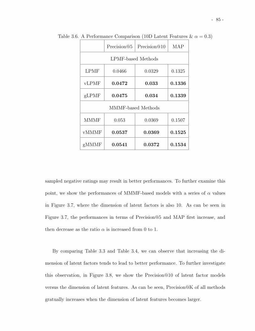
- 85 -



LPMF-based Methods

LPMF 0.0466 0.0329 0.1325

vLPMF 0.0472 0.033 0.1336

gLPMF 0.0475 0.034 0.1339

MMMF-based Methods

MMMF 0.053 0.0369 0.1507

vMMMF 0.0537 0.0369 0.1525

gMMMF 0.0541 0.0372 0.1534

sampled negative ratings may result in better performances. To further examine this

point, we show the performances of MMMF-based models with a series of α values

in Figure 3.7, where the dimension of latent factors is also 10. As can be seen in

Figure 3.7, the performances in terms of Precision@5 and MAP first increase, and

then decrease as the ratio α is increased from 0 to 1.

By comparing Table 3.3 and Table 3.4, we can observe that increasing the di-

mension of latent factors tends to lead to better performance. To further investigate

this observation, in Figure 3.8, we show the Precision@10 of latent factor models

versus the dimension of latent features. As can be seen, Precision@K of all methods

gratually increases when the dimension of latent features becomes larger.

- 86 -



LPMF-based Methods

LPMF 0.0496 0.0340 0.1418

vLPMF 0.0497 0.0341 0.1422

gLPMF 0.0502 0.0355 0.1430

MMMF-based Methods

MMMF 0.0557 0.0376 0.1555

vMMMF 0.0563 0.0378 0.1585

gMMMF 0.0565 0.0379 0.1588

3.6.7 The Performances on Different Users

For most collaborative filtering models, the prediction performances for users with

different number of observed ratings usually vary a lot. Particularly, the performances

on users with very few ratings may be quite bad for traditional collaborative filtering

models. However, the user and item cost information play as an effective constraint

to tune the prediction via the similarity weight. Thus, our extended models with

cost information are expected to perform better on users with few ratings than the

traditional models. In order to examine this potential, we first group all users based on

the number of observed ratings in the training set, and then compare the performances

of different methods over different user groups. Specifically, users are grouped into 5

classes: ”1-5”, ”6-10”, ”11-20”, ”21-30” and ” > 30”. For example, the group of ”1-5”

denotes that the number of observed ratings per user in the training set is between 1

- 87 -

0 0.1 0.2 0.3 0.4 0.5 0.6 0.7 0.8 0.90.038

0.04

0.042

0.044

0.046

0.048

0.05

0.052

0.054

0.056

Pre

cis

ion

@5

MMMF

vMMMF

gMMMF

0 0.1 0.2 0.3 0.4 0.5 0.6 0.7 0.8 0.90.135

0.14

0.145

0.15

0.155

0.16

0.165

MA

P

vMMMF

MMMF

gMMMF

(a) (b)

Figure 3.7. Performances with Different α (10D Latent Features).

and 5.

Table 3.8 shows the performances of different methods in terms of Precision@K

and MAP. In Table 3.8, the dimension of latent factors is 10 and the ratio α is 0.1. As

can be seen in Table 3.8, our extended models with the incorporated cost consistently

outperform the traditional methods. For example, for the group of ”1-5”, MAP of

gPMF, gLPMF and gMMMF is increased by 13.26% on average. In addition, the

comparisons of RMSE among PMF-based methods are shown in Figure 3.9, where

the dimension of latent factors is also 10 and the RMSE is the value of final iteration

for each method.

Performances with Tail Packages and Users. In Table 3.9, we demonstrate

the performances of different methods with all tail users and packages. Tail users are

those who have consumed less than 4 different travel packages. Tail packages are those

which have been purchased by less than 4 different users. These tail users or packages

usually contribute a lot to the high sparseness of recommendation data (Y.-J. Park

& Tuzhilin, 2008), and eventually cause the average performances of collaborative

- 88 -

0 50 100 1500.015

0.02

0.025

0.03

0.035

0.04

Dimension of Latent Factors

Pre

cisi

on

@1

0

PMF

vPMF

gPMF

LPMF

vLPMF

gLPMF

Figure 3.8. Performances with Different D (α = 0.1).

filtering methods to decrease (Y.-J. Park & Tuzhilin, 2008). As shown in Table 3.9,

Precision@K or MAP are generally lower than those in Table 3.4. While the long tail

is a general and important topic in the recommender systems field, it is not the focus

of this chapter.

3.6.8 The Learned User’s Cost Information

By training cost-aware latent factor models, we can not only produce better recom-

mendation results as shown in subsections 3.6.7 and 3.6.5, but also learn the latent

user’s cost information. In the following, we illustrate the user’s cost information

learned by our models and demonstrate that the learned user’s cost information can

help travel companies with the customer clustering or segmentation.

Since we normalize the package cost vectors into [0, 1] before feeding into our

models, the learned user’s cost features (CU and µCU) via our models have the similar

- 89 -

0.485

0.49

0.495

0.5

0.505

0.51

0.515

Number of Observed Ratings

RM

SE

gPMFvPMFPMF

1-5 5-10 10-20 20-30 >30

Figure 3.9. The Performances on Different Users (10D Latent Features).

scale as normalized package cost vectors. To visualize the learned CU , we first restored

the scale of user’s cost features (CU and µCU) by using the inverse transformation

of MinMax normalization. Figure 3.10 shows the financial cost feature of CU by the

vPMF model for randomly-selected 40 users, where each user corresponds to a column

of vertically-distributed points. For example, for the most right vertical points, the

star represents the learned user financial cost feature and the dots represent the

financial cost of packages, which are rated by this specific user in the training set.

As we can see, the learned user’s financial cost feature is relatively representative.

However, there is still obvious variance among the cost features of packages by some

users. That is why we apply the Gaussian distribution to model user’s cost preference.

In Figure 3.11, we visualize the learned µCUby gPMF for randomly-selected 12 users.

For each subfigure of Figure 3.11, we directly plot the learned 2-dimensional µCUi

- 90 -

0

2000

4000

6000

8000

10000

12000

User

Fin

an

cia

l C

ost

(RM

B)

Figure 3.10. An Illustration of User Financial Cost.

(without inverse transformation) for individual user and all normalized 2-dimensional

cost vectors of packages, which are rated by the user in the training set. And µCUiis

represented as the star and the dot represents the package cost vector.

The learned user’s latent features, e.g., Ui, with PMF, LPMF or MMMF models

can be used to group users or customers. We argue that the learned user’s cost infor-

mation, in addition to the user’s latent features, can improve the customer clustering

or segmentation. In order to show this effect, we first cluster users with the latent

features learned by PMF via representing each user with her/his latent feature vector.

We use K-means algorithm to perform the clustering and denote the clustering result

as Clu. Then, with the same clustering method we cluster users with both user’s

latent features and user’s cost information, i.e., CU or µCU, learned by vPMF and

gPMF. Now each user is represented by a vector containing her/his latent features

- 91 -

0 0.02 0.040

0.2

0.4

Financial costT

ime

co

st

0 0.050

0.2

0.4

Financial cost

Tim

e c

ost

0 0.05 0.10

0.2

0.4

Financial cost

Tim

e c

ost

0 0.05 0.10

0.2

0.4

Financial cost

Tim

e c

ost

0 0.05 0.10

0.2

0.4

Financial cost

Tim

e c

ost

0 0.1 0.20

0.2

0.4

Financial cost

Tim

e c

ost

0 0.02 0.040

0.05

0.1

Financial cost

Tim

e c

ost

0 0.1 0.20

0.2

0.4

Financial cost

Tim

e c

ost

0 0.05 0.10

0.5

Financial cost

Tim

e c

ost

0 0.1 0.20

0.2

0.4

Financial cost

Tim

e c

ost

0 0.050

0.2

0.4

Financial cost

Tim

e c

ost

0 0.1 0.20

0.2

0.4

Financial cost

Tim

e c

ost

Figure 3.11. An Illustration of the Gaussian Parameters of User Cost.

and cost vector CUior µCUi

. We denote this clustering result as Clu+. However, there

is no available benchmark to evaluate these two clustering results with traditional ex-

ternal clustering validation measurements (Wu, Xiong, & Chen, 2009). To this end,

we leverage the explicit cost information of items to make the comparisons between

these two clustering results. Specifically, for each user within a cluster, we can get

the average financial/time cost of all travel packages, which are consumed by this

user. After obtaining the average financial/time cost of each user of one cluster, we

can get the variances of such average financial/time cost of all users for this cluster.

Table 3.10 shows the comparisons of these two clustering results in terms of such

variance. Here the number of clusters is specified as 5 for K-means algorithm and

- 92 -

C1 indicates cluster 1. Also in Table 3.10, Clu+ is obtained via using µCUlearned

by gPMF in addition to the user’s latent features. As can be seen from Table 3.10,

the average variance over 5 clusters of Clu+ is much less than that of Clu. From this

perspective, we can see that the learned user’s cost information improve the results

of customer clustering or segmentation.

3.6.9 An Efficiency Analysis

As stated in subsection 3.3.3, the computational complexity of the proposed ap-

proaches is linear with respect to the number of ratings. This indicates that the

extended models are theoretically scalable for very large data. Here, we would like

to show the efficiency of all the methods in this experiment. Table 3.11 shows the

training time of all 9 models. Here, we used the 10-dimensional latent features. Since

there is some additional cost for computing the similarity functions and updating

cost vectors or the parameters of Gaussian distribution for the 6 cost-aware models,

more time is required for these 6 models, e.g., vMMMF and gMMMF. In addition,

the Gaussian distribution causes more time than the 2-dimensional vector, because

there is one more regularization item caused by the Gaussian prior in the objective

functions. But, the computing time of cost-aware models is still linearly increasing

as the number of observed ratings increases as discussed in subsection 3.3.3. In addi-

tion, we show the convergence of RMSEs on the test set for PMF-based methods in

Figure 3.12. As can be seen, vPMF and gPMF can quickly converge to relatively low

RMSEs after the first 25 rounds of iterations.

- 93 -

0 5 10 15 20 25 300.495

0.5

0.505

0.51

0.515

0.52

0.525

Epochs

RM

SE

gPMF

vPMF

PMF

Figure 3.12. An Illustration of the Convergence of RMSEs (10D Latent Features).

3.7 Conclusion and Discussion

In this chapter, we studied the problem of travel tour recommendation by analyzing

a large amount of travel logs collected from a travel agent company. One unique

characteristic of tour recommendation is that there are different financial and time

costs associated with each travel package. Different tourists usually have different

affordability for these two aspects of cost. Thus, we explicitly incorporated observ-

able and unobservable cost factors into the recommendation models. Specifically,

we first proposed two ways to model user’s cost preference. With these two ways

of representation of user’s cost preference, we incorporated the cost information into

three classic latent factor models for collaborative filtering, including the Probabilistic

Matrix Factorization (PMF) model, the Logistic Probabilistic Matrix Factorization

(LPMF) model, and the Maximum Margin Matrix Factorization (MMMF) model.

- 94 -

When applied to real-world travel tour data, the extended PMF, LPMF and MMMF

models showed consistently better performances for travel tour recommendation than

classic PMF, LPMF and MMMF models which do not consider the cost information.

Furthermore, the extended MMMF and LPMF models lead to a better performance

improvement than the extended PMF models. Finally, we have demonstrated that

the latent user’s cost information learned by these models can help to do customer

segmentation for travel companies.

Discussion. People may argue that some dimensions of learned latent factors

of users/packages might somehow capture the cost factors implicitly. However, it is

hard to identify which dimensions correspond to these cost factors. At the same time,

in our application (and in many others), the cost information of is given explicitly,

and it is every natural to incorporate it into the model(s), that is what we do in

this chapter. Furthermore, through extensive experimentation, we showed that this

addtional information, indeed, boosts the performance of the collaborating filtering

methods that do not take this cost information into account.

As shown Table 3.9, tail users/packages result in lower performances for different

collaborative filtering methods. Since the long tail is a major challenge in the rec-

ommendation field, and is not the focus of this chapter, we would like to study this

topic for travel package recommendations in the future.

Like cost information, time sensitivity is another important factor for travel pack-

age recommendations. For example, Orlando trips may be more attractive to people

in Northeast of US during winter. However, since the focus of the chapter is on incor-

porating economic indicators, such as costs, into recommendation models, we would

- 95 -

like to work on time sensitivity as a topic of future research.

- 96 -

Table 3.8. The Performances on Different Users (10D Latent Features & α = 0.1)

Groups ”1-5” ”6-10” ”11-20” ”21-30” ”>30”

PMF

Precision@5 0.0211 0.0295 0.0482 0.072

MAP 0.0586 0.0784 0.0902 0.0958 0.0054

vPMF

Precision@5 0.0223 0.0306 0.0498 0.096

MAP 0.0573 0.0865 0.0959 0.1228 0.005

gPMF

Precision@5 0.0259 0.0308 0.053 0.096

MAP 0.0752 0.086 0.0937 0.1154 0.0045

LPMF

Precision@5 0.036 0.0488 0.0738 0.1419 0.0857

MAP 0.1109 0.1466 0.1836 0.2118 0.1722

vLPMF

Precision@5 0.0386 0.0496 0.0744 0.1419 0.0857

MAP 0.1186 0.1471 0.1863 0.2120 0.2613

gLPMF

Precision@5 0.0391 0.0500 0.0748 0.1426

MAP 0.1191 0.1479 0.1869 0.2128 0.2621

- 97 -

Table 3.9. Performances with Tail Users/Packages (30D Latent Features & α = 0.1)


PMF 0.0253 0.0148 0.0644

vPMF 0.0254 0.0157 0.0658

gPMF 0.0265 0.0164 0.0663

LPMF 0.043 0.0305 0.1286

vLPMF 0.0441 0.0324 0.1292

gLPMF 0.0462 0.0339 0.1315

MMMF 0.0553 0.0416 0.1651

vMMMF 0.0561 0.0431 0.1668

gMMMF 0.0578 0.0454 0.1683

Table 3.10. A Comparison of Variance

Results on Clu

C1 C2 C3 C4 C5 Average

Financial Variance 0.00091 0.00102 0.00079 0.00086 0.00114 0.000944

Time Variance 0.0292 0.0012 0.0321 0.0093 0.0125 0.0169

Results on Clu+

C1 C2 C3 C4 C5 Average

Financial Variance 0.00073 0.00105 0.00047 0.00090 0.00035 0.00070

Time Variance 0.0193 0.0009 0.0214 0.0098 0.0133 0.0129

- 98 -

Table 3.11. A Comparison of the Model Efficiency (10D Latent Features)

PMF vPMF gPMF

Training Time (Sec) 3.411 4.894 10.878

LPMF vLPMF gLPMF


MMMF vMMMF gMMMF


- 99 -

CHAPTER 4

A COCKTAIL APPROACH FOR TRAVEL PACKAGE RECOMMENDATION

Recent years have witnessed an increased interest in recommender systems. Despite

significant progress in this field, there still remain numerous avenues to explore. In-

deed, this chapter provides a study of exploiting online travel information for person-

alized travel package recommendation. A critical challenge along this line is to address

the unique characteristics of travel data, which distinguish travel packages from tra-

ditional items for recommendation. To that end, in this chapter, we first analyze

the characteristics of the existing travel packages and develop a Tourist-Area-Season

Topic (TAST) model. This TAST model can represent travel packages and tourists

by different topic distributions, where the topic extraction is conditioned on both the

tourists and the intrinsic features (i.e. locations, travel seasons) of the landscapes.

Then, based on this topic model representation, we propose a cocktail approach to

generate the lists for personalized travel package recommendation. Furthermore, we

extend the TAST model to the Tourist-Relation-Area-Season Topic (TRAST) model

for capturing the latent relationships among the tourists in each travel group. Finally,

we evaluate the TAST model, the TRAST model, and the cocktail recommendation

approach on the real-world travel package data. Experimental results show that the

TAST model can effectively capture the unique characteristics of the travel data and

the cocktail approach is thus much more effective than traditional recommendation

- 100 -

techniques for travel package recommendation. Also, by considering tourist relation-

ships, the TRAST model can be used as an effective assessment for travel group

formation.

4.1 Introduction

As an emerging trend, more and more travel companies provide online services. How-

ever, the rapid growth of online travel information imposes an increasing challenge for

tourists who have to choose from a large number of available travel packages for satis-

fying their personalized needs. Moreover, to increase the profit, the travel companies

have to understand the preferences from different tourists and serve more attractive

packages. Therefore, the demand for intelligent travel services is expected to increase

dramatically.

Since recommender systems have been successfully applied to enhance the quality

of service in a number of fields (Adomavicius & Tuzhilin, 2005; Ge et al., 2010), it

is natural choice to provide travel package recommendations. Actually, recommen-

dations for tourists have been studied before (Abowd et al., 1997; Averjanova et al.,

2008; Cena et al., 2006), and to the best of our knowledge, the first operative tourism

recommender system was introduced by Delgado et al. (Delgado & Davidson, 2002).

Despite of the increasing interests in this field, the problem of leveraging unique fea-

tures to distinguish personalized travel package recommendations from traditional

recommender systems remains pretty open.

Indeed, there are many technical and domain challenges inherent in designing and

implementing an effective recommender system for personalized travel package recom-

- 101 -

mendation. First, travel data are much fewer and sparser than traditional items, such

as movies for recommendation, because the costs for a travel are much more expen-

sive than for watching a movie (Ge, Liu, et al., 2011). Second, every travel package

consists of many landscapes (places of interest and attractions), and thus has intrinsic

complex spatio-temporal relationships. For example, a travel package only includes

the landscapes which are geographically co-located together. Also, different travel

packages are usually developed for different travel seasons. Therefore, the landscapes

in a travel package usually have spatial-temporal autocorrelations. Third, traditional

recommender systems usually rely on user explicit ratings. However, for travel data,

the user ratings are usually not conveniently available. Finally, the traditional items

for recommendation usually have a long period of stable value, while the values of

travel packages can easily depreciate over time and a package usually only lasts for

a certain period of time. The travel companies need to actively create new tour

packages to replace the old ones based on the interests of the tourists.

To address these challenges, in our preliminary work (Q. Liu, Ge, Li, Xiong, &

Chen, 2011), we proposed a cocktail approach on personalized travel package recom-

mendation. Specifically, we first analyze the key characteristics of the existing travel

packages. Along this line, travel time and travel destinations are divided into differ-

ent seasons and areas. Then, we develop a Tourist-Area-Season Topic (TAST) model,

which can represent travel packages and tourists by different topic distributions. In

the TAST model, the extraction of topics is conditioned on both the tourists and the

intrinsic features (i.e. locations, travel seasons) of the landscapes. As a result, the

TAST model can well represent the content of the travel packages and the interests

- 102 -

Figure 4.1. An illustration of the chapter contribution.

of the tourists. Based on this TAST model, a cocktail approach is developed for

personalized travel package recommendation by considering some additional factors

including the seasonal behaviors of tourists, the prices of travel packages, and the cold

start problem of new packages. Finally, the experimental results on real-world travel

data show that the TAST model can effectively capture the unique characteristics of

travel data and the cocktail recommendation approach performs much better than

traditional techniques.

In this chapter, we further study some related topic models of the TAST model,

and explain the corresponding travel package recommendation strategies based on

them. Also, we propose the Tourist-Relation-Area-Season Topic (TRAST) model,

which helps understand the reasons why tourists form a travel group. This goes be-

yond personalized package recommendations and is helpful for capturing the latent

relationships among the tourists in each travel group. In addition, we conduct sys-

tematic experiments on the real-world data. These experiments not only demonstrate

- 103 -

Niagara Falls Discovery

Figure 4.2. An example of the travel package, where the landscapes are represented

by the words in red.

that the TRAST model can be used as an assessment for travel group automatic for-

mation but also provide more insights into the TAST model and the cocktail recom-

mendation approach. In summary, the contributions of the TAST model, the cocktail

approaches and the TRAST model for travel package recommendations are shown in

Fig. 4.1, where each dashed rectangular box in the dashed circle identifies a travel

group and the tourists in the same travel group are represented by the same icons.

4.2 Concepts and Data Description

In this section, we first introduce the basic concepts, and then describe the recom-

mendation scenario of this study. Finally, we provide the detailed information about

the unique characteristics of travel package data.

Definition 4 A travel package is a general service package provided by a travel

company for the individual or a group of tourists based on their travel preferences. A

package usually consists of the landscapes and some related information, such as the

price, the travel period, and the transportation means.

Specifically, the travel topics are the themes designed for this package, and the

- 104 -

landscapes are the travel places of interest and attractions, which usually locate in

nearby areas.

Following Definition 4, an example document for a package named “Niagara

Falls Discovery” from the STA Travel 1 is shown in Fig. 4.2. It includes the travel

topics (tour style), travel days, price, travel area (the northeastern U.S.), and land-

scapes (e.g., Niagara Falls) etc. Note that different packages may include the same

landscapes and each landscape can be used for multiple packages. Meanwhile, for

some reasons, the tourists for each individual package are often divided into differ-

ent travel groups (i.e., traveling together). In addition, each package has a travel

schedule and most of the packages will be traveled only in a given time (season) of

the year, i.e., they have strong seasonal patterns. For example, the “Maple Leaf

Adventures” is usually meaningful in Fall.

In this chapter, we aim to make personalized travel package recommendations for

the tourists. Thus, the users are the tourists and the items are the existing packages,

and we exploit a real-world travel data set provided by a travel company in China for

building recommender systems. There are nearly 220, 000 expense records (purchases

of individual tourists) starting from January 2000 to October 2010. From this data

set, we extracted 23, 351 useful records of 7, 749 travel groups for 5, 211 tourists from

908 domestic and international packages in a way that each tourist has traveled at

least two different packages. The extracted data contain 1, 065 different landscapes

located in 139 cities from 10 countries. On average, each package has 11 different

landscapes, and each tourist has traveled 4.4 times.

1STA Travel, URL:http://www.statravel.com/

- 105 -

As illustrated in our preliminary work (Q. Liu et al., 2011), there are some unique

characteristics of the travel data. First, it is very sparse, and each tourist has only a

few travel records. The extreme sparseness of the data leads to difficulties for using

traditional recommendation techniques, such as collaborative filtering. For example,

it is hard to find the credible nearest neighbors for the tourists because there are very

few co-traveling packages.

Second, the travel data has strong time dependence. The travel packages often

have a life cycle along with the change to the business demand, i.e., they only last

for a certain period. In contrast, most of the landscapes will still be active after

the original package has been discarded. These landscapes can be used to form

new packages together with some other landscapes. Thus, we can observe that the

landscapes are more sustainable and important than the package itself.

Third, landscape has some intrinsic features like the geographic location and the

right travel seasons. Only the landscapes with similar spatial-temporal features are

suitable for the same packages, i.e., the landscapes in one package have spatial-

temporal auto-correlations and follow the first law of geography–everything is related

to everything else, but the nearby things are more related than distant things (Cressie,

1991). Therefore, when making recommendations, we should take the landscapes’

spatial-temporal correlations into consideration so as to describe the tourists and the

packages precisely.

Fourth, the tourists will consider both time and financial costs before they accept

a package. This is quite different from the traditional recommendations where the

cost of an item is usually not a concern. Thus, it is very important to profile the

- 106 -

tourists based on their interests as well as the time and the money they can afford.

Since the package with a higher price often tends to have more time and vice versa,

in this chapter we only take the price factor into consideration.

Fifth, people often travel with their friends, family or colleagues. Even when two

tourists in the same travel group are totally strangers, there must be some reasons

for the travel company to put them together. For instance, they may be of the same

age or have the same travel schedule. Hence, it is also very important to understand

the relationships among the tourists in the same travel group. This understanding

can help to form the travel group.

Last but not least,few tourist ratings are available for travel packages. However,

we can see that every choice of a travel package indicates the strong interest of the

tourist in the content provided in the package.

In summary, these characteristics bring in three major challenges. First, how to

compare the interests of tourists and the content of the travel package; Second, how

to make package recommendations for each tourist; Third, how to capture the tourist

relationships to form a travel group. As a result, it is necessary to develop more

suitable approaches for travel package recommendation.

4.3 The TAST Model

In this section, we show how to represent the packages and tourists by a topic model,

like the methods in (Blei, Ng, Jordan, & Lafferty, 2003) based on Bayesian networks,

so that the similarity between packages and tourists can be measured. Table 4.1 lists

some mathematical notations in this chapter.

- 107 -

Table 4.1. Mathematical notations.

Notation Description

U = {U1, U2, ..., UM} the set of tourists

S = {S1, S2, ..., SJ} the set of seasons

P = {P1, P2, ..., PN} the set of packages

T = {T1, T2, ..., TZ} the set of topics

A = {A1, A2, ..., AO} the set of different areas

P′= {P ′

1, P′2, ..., P

′D} packages for travel logs

P′′

= {P ′′1 , P

′′2 , ..., P

′′

D′} packages for travel group logs

LAi= {LAi1 , ..., LAi|Ai|

} landscape set for area Ai

LP′i

= {LP′i 1

, ..., LP′i |P ′

i|} landscapes for the package P

′i

LP′′i

= {LP′′i 1

, ..., LP′′i |P ′′

i|} landscapes for the package P

′′i

4.3.1 Topic Model Representation

When designing a travel package, we assume that people in travel companies often

consider the following issues. First, it is necessary to determine the set of target

tourists, the travel seasons, and the travel places. Second, one or multiple travel

topics ( e.g., “The Sunshine Trip”) will be chosen based on the category of target

tourists and the scheduled travel seasons. Each package and landscape can be viewed

as a mixture of a number of travel topics. Then, the landscapes will be determined

according to the travel topics and the geographic locations. Finally, some additional

information (e.g., price, transportation, and accommodations) should be included.

According to these processes, we formalize package generation as a What-Who-When-

Where(4W ) problem. Here, we omit the additional information and each W stands

for the travel topics, the target tourists, the seasons and the corresponding landscape

- 108 -

located areas, respectively. These four factors are strongly correlated.

Formally, we reprocess the generation of a package in a topic model style, where we

treat it mainly as a landscape drawing problem. These landscapes for the package are

drawn from the landscape set one by one. For choosing a landscape, we first choose a

topic from the distribution over topics specific to the given tourist and season, then

the landscape is generated from the chosen topic and travel area. We call our model

for package representation as the TAST (Tourist-Area-Season Topic) model. Please

note that, a topic mentioned in TAST is different from a real topic, where the former

one is a latent factor extracted by topic model, while the latter one is an explicit

travel theme identified in the real world, and latent topics are used to simulate real

topics. Without loss of generality, we use travel topic and topic to stand for the real

and latent topic, respectively.

Mathematically, the generative process corresponds to the hierarchical Bayesian

model for TAST is shown in Fig. 4.3, where shaded and unshaded variables indi-

cate observed and latent variables respectively. The TAST model follows the similar

Dirichlet distribution assumptions as (Blei et al., 2003), and here landscapes are the

“tokens” for topic modelling. In TAST model, the notation P′d is different from Pd,

where Pd is the ID for a package in the package set while P′d stands for the pack-

age ID of one travel log, and each travel log can be distinguished by a vector of

three attributes 〈P ′d, Ud, timestamp〉, where the timestamp can be further projected

to a season Sd and P′d=〈LP

′d, Ad, price2 〉. Specifically, in Fig. 4.3, each package

P′d is represented as a vector of |LP

′d| landscapes where landscape l is chosen from

2The price factor will be considered later.

- 109 -

Figure 4.3. TAST: A graphical model.

one area a and a ∈ Ad (Ad includes the located area(s) for P′d) and (Ud,Sd) is the

specific tourist-season pair. t is a topic which is chosen from the set T with Z top-

ics. θ and φ correspond to the topic distribution and landscape distribution specific

to each tourist-season pair and area-topic pair respectively, where α and β are the

corresponding hyperparameters.

The distributions, such as θ and φ, can be extracted after inferring this TAST

model (“invert” the generative process and “generate” latent variables). The general

idea is to find a latent variable (e.g., topic) setting so as to get a marginal distribution

of the travel log set P′:

p(P′|α, β, U, S, A) =

∫∫ M∏m=1

J∏j=1

p(θmj|α)O∏

o=1

Z∏k=1

p(φok|β)D∏

d=1

|LP′d

|∏i=1

Z∑tdi=1

(p(tdi|θUdSd)

∑adi∈Ad

(p(adi|Ad)p(ldi|φaditdi)))dφdθ

- 110 -

4.3.2 Model Inference

While the inference on models in the LDA family cannot be solved with closed-form

solutions, a variety of algorithms have been developed to estimate the parameters of

these models. In this chapter, we exploit the Gibbs sampling method (Griffiths &

Steyvers, 2004), a form of Markov chain Monte Carlo, which is easy to implement and

provides a relatively efficient way for extracting a set of topics from a large set of travel

logs. During the Gibbs sampling, the generation of each landscape token for a given

travel log depends on the topic distribution of the corresponding tourist-season pair

and the landscape distribution of the area-topic pair. Finally, the posterior estimates

of θ and φ given the training set can be calculated by:

ˆθmjt =αt + nmjt

ΣZk=1(αk + nmjk)

, ˆφokl =βl + mokl

Σ|Ao|q=1(βq + mokq)

(4.1)

where |Ao| is the number of landscapes in area Ao, nmjt is the number of landscape

tokens assigned to topic Tt and tourist-season pair (Um, Sj), and mokl is the number

of tokens of landscape Ll assigned to area-topic pair (Ao, Tk). Let us take the topic

assignment for “Central Park” as an example, in each iteration, the topic assignment

of one “Central Park” token depends on not only the topics of the landscapes traveled

by the tourist in the given season but also the topics of the other landscapes located

nearby. Meanwhile, many other posterior probabilities can also be estimated, e.g.,

the topic distribution of tourist Ui and package Pi:

ϑUij =

αj + ΣJs=1nisj

ΣZk=1(αk + ΣJ

s=1nisk), ϑP

ij =αj + hij

ΣZk=1(αk + hik)

(4.2)

- 111 -

(a) The TT model. (b) The TAT model. (c) The TST model.

Figure 4.4. The three related topic models.

where hij is the number of the landscape tokens in package Pi and these tokens are

assigned to topic Tj.

After Gibbs sampling, all the tourists and packages are represented by the Z

entry topic distribution vectors (Z, the number of topics, is usually in the range

of [20,100]). For example, a tourist, who traveled “Tour in Disneyland, Hongkong”

and “Christmas day in Hongkong”, may have high probabilities on the entries that

stand for the topics such as “amusement parks” and “Hongkong”. By computing

the similarity of the topic distribution vectors, we can find the similarity between

the corresponding tourists and packages. There are also many other benefits of the

TAST model, e.g., we can learn the popular topics in each season and find the popular

landscapes for each topic.

4.3.3 Area/Seasons Segmentation

There are two extremes for the coverage of each area Ai and each season Si: we can

view the whole earth as an area and the entire year as a season, or we can view

each landscape itself as an area and each month as a different season. However, the

first extreme is too coarse to capture the spatial-temporal auto-correlations, and we

- 112 -

will face the overfitting issue for the second extreme and the Gibbs sampling will be

difficult to converge.

To this end, we divide the entire location space in our data set into 7 big areas

according to the travel area segmentations provided by the travel company, which

are South China (SC), Center China (CC), North China (NC), East Asia (EA),

Southeast Asia (SA), Oceania (OC) and North America (NA), respectively.To make

more reasonable season splitting, we assume that most packages are seasonal, and

we use an information gain based method (Fayyad & Irani, 1993) to get the season

splits.The information entropy of the season SP is Ent(SP )=−∑|SP |i=1 pilog(pi) , where

|SP | is the number of different packages in SP and pi is the proportion of package

Pi in this season. Initially, the entire year is viewed as a big season and then we

partition it into several seasons recursively. In each iteration, we use the weighted

average entropy (WAE) to find the best split:

WAE(i; SP ) =|SP

1 (i)||SP | Ent(SP

1 (i)) +|SP

2 (i)||SP | Ent(SP

2 (i))

where SP1 (i) and SP

2 (i) are two sub-seasons of season SP when being splitted at

the i-th month. The best split month induces a maximum information gain given by

4E(i) which is equal to Ent(SP )−WAE(i; SP ) .

4.3.4 Related Topic Models

While the generation processes in TAST are similar to those in the text modelling

problems for both documents (Blei et al., 2003), the TAST model is quite different

from these traditional ones (e.g., LDA, AT, and ART models). The TAST model

- 113 -

has a crucial enhancement by considering the intrinsic features (i.e., location, travel

seasons) of the landscapes, and thus it can effectively capture the spatial-temporal

auto-correlations among landscapes. The benefit is that the TAST model can describe

the travel package and the tourist interests more precisely, because the nearby land-

scapes or the landscapes preferred by the same tourists tend to have the same topic.

In addition, the text modelling has the assumption that the words in an email/ar-

ticle are generated by multiple authors, while we assume that the landscapes in the

package are generated for the specific tourist of this travel log. Therefore, each single

text is considered only once in the text models. However, each package may appear

many times in the TAST model according to their records in the travel logs.

Indeed, as shown in Fig. 4.4, there are three related topic models. The first one

(Fig. 4.4(a)) is the Tourist Topic (TT) model, which does not consider the travel

area and travel season factors. The second one (Fig. 4.4(b)) is the Tourist-Area

Topic (TAT) model, which only considers the travel area. The third one (Fig. 4.4(c))

is the Tourist-Season Topic (TST) model , which only considers the travel season.

All these methods can also be used for package and tourist representation. Finally,

note that the graphical representations of TT and TST are similar to the AT model

and ART model, respectively. However, their differences have been discussed.

4.4 Cocktail Recommendation Approach

In this section, we propose a cocktail approach on personalized travel package recom-

mendation based on the TAST model, which follows a hybrid recommendation strat-

egy (Burke, 2007) and has the ability to combine many possible constraints that exist

- 114 -

Figure 4.5. The cocktail recommendation approach.

in the real-world scenarios. Specifically, we first use the output topic distributions of

TAST to find the seasonal nearest neighbors for each tourist, and collaborative filter-

ing will be used for ranking the candidate packages. Next, new packages are added

into the candidate list by computing similarity with the candidate packages generated

previously. Finally, we use collaborative pricing to predict the possible price distri-

bution of each tourist and reorder the packages. After removing the packages which

are no longer active, we will have the final recommendation list.

Fig. 4.5 illustrates the framework of the proposed cocktail approach, and each

step of this approach is introduced in the following subsections. We should note that,

the major computation cost for this approach is the inference of the TAST model.

As the increase of travel records, the computation cost will increase. However, since

the topics of each landscape evolves very slowly, we can update the inference process

periodically offline in real-world applications. At the end of this section, we will

describe many similar cocktail recommendation strategies based on the related topic

- 115 -

models of TAST.

4.4.1 Seasonal Collaborative Filtering for Tourists

In this subsection, we describe the method for generating the personalized candidate

package set for each tourist by the collaborating filtering method. After we have

obtained the topic distribution of each tourist and package by the TAST model, we can

compute the similarity between each tourist by their topic distribution similarities.

Intuitively, based on the idea of collaborative filtering, for a given user, we rec-

ommend the items that are preferred by the users who have similar tastes with her.

However, as we explained previously, the package recommendation is more complex

than the traditional ones. For example, if we make recommendations for tourists

in winter, it is inappropriate to recommend “Maple Leaf Adventures”. In other

words, for a given tourist, we should recommend the packages that are enjoyed by

other tourists at the specific season. Indeed, we have obtained the seasonal topic

distribution for each tourist from the TAST model. Multiple methods can be used to

compute these similarities, such as matrix factorization (Koren & Bell, 2011; Koren,

2008) and graphical distances (Fouss, Pirotte, Renders, & al, 2007). Alternatively,

a simple but effective way is to use the Correlation coefficient, and the similarity

between tourist Um and Un in season Sj can be computed by:

SimSj(Um, Un) =

∑Zk=1(θmjk − θmj)(θnjk − θnj)√∑Z

k=1(θmjk − θmj)2

√∑Zk=1(θnjk − θnj)2

(4.3)

where θmj is the average topic probability for the tourist-season pair (Um, Sj)3

3If tourist Um has never traveled in season Sj , then her total topic distribution ϑUm is used as an

alternative throughout this chapter.

- 116 -

, For a given tourist, we can find his/her nearest neighbors by ranking their sim-

ilarity values. Thus, the packages, favored by these neighbors but have not been

traveled by the given tourist, can be selected as candidate packages which form a

rough recommendation list, and they are ranked by the probabilities computed by

the collaborative filtering.

4.4.2 New Package Problem

In recommender systems, there is a cold-start problem, i.e., it is difficult to recommend

new items. As we have explored in Section 4.2, travel packages often have a life cycle

and new packages are usually created. Meanwhile, most of the landscapes will keep

in use, which means nearly all the new packages are totally or partially composed

by the existing landscapes. Let us take the year of 2010 as an example. There are

65 new packages in the data and only 2 of them are composed completely by new

landscapes. Thus, for most of the new packages P new, their topic distributions can

be estimated by the topics of their landscapes:

ϑP new

ij =αj +

∑l∈P new

iolj

ΣZk=1(αk +

∑l∈P new

iolk)

(4.4)

where olj is the number of times that landscape l is assigned to topic Tj in the

travel logs, and the seasonal topic distribution of the new packages can be computed

in the similar way. The following question is how to recommend new packages. One

way to address this issue is to recommend the new packages that are similar to

the ones already traveled by the given tourist (i.e., via the content based method).

However, if the recommender systems just deal with the current interest of the given

- 117 -

tourist, we will suffer from the overspecialization problem (Adomavicius & Tuzhilin,

2005). Thus, we propose to compute the similarity between the new package and

the given number (e.g. 10) of candidate packages in the top of the recommendation

list. The new packages which are similar to the candidate packages are added into

the recommendation list and their ranks in the list based on the average probabilities

of the similar candidate packages. It is expected that this method can not only deal

with the cold-start problem but also avoid the overspecialization problem. Please note

that, in real applications, new travel package recommendation list can be separated

from the general list. However, in this chapter, for better illustration and evaluation,

we insert the new packages into the general recommendation list as an alternative.

Since there is no effective method to learn the topics of the new packages whose

landscapes are not included in the training set, we can use the topic distributions of

their located areas on the given travel season as an estimation. Luckily, there are few

such packages.

4.4.3 Collaborative Pricing

In this subsection, we present the method to consider the price constraint for devel-

oping a more personalized package recommender system. The price of travel packages

may vary from $20 to more than $3, 000, so the price factor influences the decision

of tourists. Along this line, we propose a collaborative pricing method in which we

first divide the prices into different segments. Then, we propose to use the Markov

forecasting model to predict the next possible price range for a given tourist.

In the first phase, we divide the prices of the packages based on the variance of

- 118 -

(a) The TRAST model. (b) The TRAST1 model.

(c) The TRAST2 model.

Figure 4.6. The TRAST model and its two sub-models.

- 119 -

prices in the travel logs. We first sort the prices of the travel logs, and then partition

the sorted list PL into several sub-lists in a binary-recursive way. In each iteration,

we first compute the variance of all prices in the list. Later, the best split price having

the minimal weighted average variance (WAV) defined as:

WAV (i; PL) =|PL1(i)||PL| V ar(PL1(i)) +

|PL2(i)||PL| V ar(PL2(i))

where PL1(i) and PL2(i) are two sub-lists of PL split at the i-th element and V ar

represents the variance. This best split price leads to a maximum decrease of 4V (i),

which is equal to V ar(PL)−WAV (i; PL).

In the second phase, we mark each price segment as a price state and compute the

transition probabilities between them. Specifically, at first, if a tourist used a package

with price state a before traveling a package with price state b, then the weight of

the edge from a to b will plus 1. After summing up the weights from all the tourists,

we normalize them into transition probabilities, and all the transition probabilities

compose a state transition matrix. From the current price state of a given tourist

(i.e. the current price distribution normalized from his/her previous travel records),

we predict the next possible price state by the one-step Markov forecasting model

based on random walk. Finally, we obtain the predicted probability distribution of

the given tourist on each state, and use these probabilities as weights to multiply

the probabilities of the candidate packages in the rough recommendation list so as to

reorder these packages. After removing the packages which are no longer active, we

have the final recommendation list.

- 120 -

4.4.4 Related Cocktail Recommendations

The previous cocktail recommendation approach (Cocktail) is mainly based on the

TAST model and the collaborative filtering method. Indeed, another possible cock-

tail approach is the content based cocktail, and in the following, we call this method

TASTContent. The main difference between TASTContent and Cocktail is that in

TASTContent the content similarity between packages and tourists are used for rank-

ing packages instead of using collaborative filtering. Since TASTContent can only

capture the existing travel interests of the tourists, thus it may also suffer from the

overspecialization problem.

As there are many related topic models for the TAST model, it is also possible

to design the similar cocktail recommendation approaches based on these models.

Actually, it is quite straightforward to replace the TAST model by TT, TAT and

TST models in the cocktail approach to get the new recommendations. For example,

in the experimental section, the notation TTER stands for the cocktail approach that

is based on the TT model.

In Cocktail we use the price factor as an external constraint to measure package

ranks. To some extent, the package prices may also directly influence the interests of

the tourists. Thus, it can be included in the topic model representation. If we replace

the season token Sd in Fig. 4.3 by (Sd, Cd) pair, where Cd is the price segment of this

package log, and update the previous 4W assumptions, the price factor can be well

incorporated into the topic model. In this way, the topic preference of the packages

in each price segment can also be inferred. What’s more, this topic model shares

- 121 -

the same inference process with the TAST model, and in the following, we call the

cocktail recommendation approach based on this model as Cocktail-.

In summary, both Cocktail and the above related approaches follow the idea of

hybrid recommendations, which exploit multiple recommendation techniques, such

as collaborative filtering and content-based approaches, for the best performances.

Indeed, hybrid recommender systems are usually more practical and have been widely

used (Burke, 2007; Lai, Xiang, Diao, Liu, & al, 2011). For instance, seven different

types of hybrid recommendation techniques have been discussed in (Burke, 2007).

In fact, the cocktail recommendation is a combined exploitation of several hybrid

approaches. Specifically, the seasonal collaborative filtering based on topic modelling

is a “Feature Augmentation”, where the new features of latent topics are generated

as the better input to enhance the existing algorithm. Second, the insertion of new

packages is a “Mixed” strategy, where recommendations from different sources are

combined. At last, the collaborative pricing is similar to a “Cascade” strategy, where

the secondary recommender refines the decisions made by a stronger one.

4.5 The TRAST Model

In this section, we extend the current TAST model and propose a novel Tourist-

Relation-Area-Season Topic (TRAST) model to formulate the tourist relationships in

a travel group.

In the TAST model, we do not consider the information of the travel group.

However, as noted in Section 4.2, each package has usually been used by many groups

of tourists, and the tourists belong to different travel groups. Thus, if two tourists

- 122 -

have taken the same package but in different travel groups, we can only say these

two tourists have the same travel interest, but we cannot conclude that they share

the same travel profile. However, if these two tourists are in the same group, they

may share some common travel traits, such as similar cultural interests and holiday

patterns. In the future, they may also want to travel together. Also, they may be

family and always travel together during the holiday season. In this chapter, we

use the notation relationship to measure these commonalities and connections in

tourists’ travel profiles. Please also note that there are multiple tourist relationships

simultaneously.

Based on the above understanding, we incorporate into the TAST model a new set

of variables, with each entry indicating one relationship, and we consider the tourist

relationships in each travel group. This novel topic model is named as the TRAST

model, as shown in Fig. 4.6(a), where each tourist has a multinomial distribution

over G relationships, and each relationship has a multinomial distribution over Z

topics. Other assumptions are similar to those in the TAST model. However, in the

TRAST model, the purchases of the tourists in each travel group are summed up as

one single expense record and thus it has more complex generative process. We can

understand this process by a simple example. Assume that two selected tourists in

a travel group (U′′d ) are u1 and u2, who are young and dating with each other. Now,

they decide to travel in winter (Sd) and the destination is North America (Ad). To

generate a travel landscape (l), we first extract a relationship (r, e.g., lover), and

then find a topic (t) for lovers to travel in the winter (e.g., skiing). Finally, based on

this skiing topic and the selected travel area (e.g., Northeast America), we draw a

- 123 -

landscape (e.g., Stowe, Vermont).

Thus, in the TRAST model, the notation U′′d stands for a group of tourists and

P′′d is the corresponding package ID for this travel group log. θ and Λ correspond

to the topic distribution and relationship distribution specific to each relationship-

season pair and tourist, respectively, where η is a new hyperparameter. The marginal

distribution of the travel group set P′′

can be computed as:

p(P′′ |α, β, η, U, S, A) =

∫∫∫ M∏i=1

p(Λi|η)G∏

i=1

J∏j=1

p(θij|α)O∏

i=1

Z∏j=1

p(φij|β)D′∏

d=1

|LP′′d

|∏i=1

(p(u1, u2|U ′′d )

M∑rdi=1

(p(rdi|u1, u2)Z∑

tdi=1

(p(tdi|θrdiSd)

∑adi∈Ad

(p(adi|Ad)p(ldi|φaditdi)))))dφdθdη

To perform the inference, the Gibbs sampling formulae can be derived in a similar

way as the TAST model, but the sampling procedure at each iteration is significantly

more complex. To make inference more efficient and easier for understanding, we

instead perform it in two distinct parts. We first split TRAST model into two sub-

models, as shown in Fig. 4.6(b) and 4.6(c). The first sub-model TRAST1 is just

like the TAST model, except for the two tourists are latent factors and some of the

notations are with different meanings here. By this model, we use a sample to obtain

topic assignments and tourist pair assignments for each landscape token. Then, in the

second sub-model TRAST2, we treat topics and tourist pairs as known, and the goal

is to obtain relationship assignments. In the following, let us introduce the inference

- 124 -

of these two models, one by one.

If we directly transfer the results that we get from the TAST model to assign a

topic for each landscape token in the TRAST1 model, we need to compute n(u1,u2)st

for each (u1, u2) pair, which is the number of landscape tokens that are assigned to

topic t, and have been co-traveled by tourists (u1, u2) in season s. In this way, we

have to compute and store each n(u1,u2)st, an entry in a M ∗M ∗ J ∗Z matrix. Thus,

the cost will be too expensive (actually, most of the entries should be 0). Instead, we

use the following strategy as a simulation.

p(adi , tdi , (udi1 , udi2)|...) ∝

αtdi+nudi1

sdtdi+nudi2

sdtdi−1

ΣZk=1(αk+nudi1

sdk+nudi2sdk)−1

βldi+maditdildi

−1

Σ|Ai|k=1(βldi

+maditdik)−1(4.5)

where “...” refers to all the known information such as the area (a¬di), topic (t¬di

)

and tourist pair ((u1, u2)¬di) information of other landscape tokens, and the hyperpa-

rameters α, and β. By the above equation, we only have to keep a M ∗ J ∗ Z matrix

for storing each nust.

We can see that the TRAST2 model is similar to the TST model (Fig. 4.4(c)),

except for the location of Sd and the pair of tourists. Similar to the inference of the

TRAST1 model, when inferring this model, for each relationship assignment, we use

the following equation:

p(rdi |...) ∝ηrdi

+nu1rdi+nu2rdi

−1

ΣGk=1(ηk+nu1rk

+nu2rk)−1

αtdi+mrdiSdtdi

−1

ΣZt=1(αt+mrdiSdt)−1

(4.6)

- 125 -

After Gibbs sampling, each tourist’s travel relationship preference can be esti-

mated by the following equation, and each entry of θ and φ can be computed simi-

larly.

Λir =ηt + nir

ΣGk=1(ηk + nik)

(4.7)

Actually, this TRAST model can be easily extended for computing relationships

among many more tourists. However, the computation cost will also go up. To

simplify the problem, in this chapter, each time we only consider two tourists in a

travel group as a tourist pair for mining their relationships. By this TRAST model,

all the tourists’ travel preferences are represented by relationship distributions. For

a set of tourists, who want to travel the same package, we can use their relationship

distributions as features to cluster them, so as to put them into different travel groups.

Thus, in this scenario, many clustering methods can be adopted. Since choosing

clustering algorithm is beyond the scope of this chapter, in the experiments, we refer

to K-means, one of the most popular clustering algorithms.

Thus, the TRAST model can be used as an assessment for travel group automatic

formation. Indeed, in real applications, when generating a travel group, some more

external constraints, such as tourists’ travel date requirements, the travel company’s

travel group schedule should also be considered. Please note that, it is possible to use

the topics mined by TRAST1 to represent the latent relationships directly. However,

in this way, the topics will represent both landscape topics and latent relationships,

it would be hard for interpretation.

- 126 -


In this section, we evaluate the performances of the proposed models on real-world

data, and some of previous results (Q. Liu et al., 2011) are omitted due to the space

limit. Specifically, we demonstrate: (1) the results of the season splitting and price

segmentation, (2) the understanding of the extracted topics, (3) a recommendation

performance comparison between Cocktail and benchmark methods, (4) the evalua-

tion of the TRAST model, and (5) a brief discussion on recommendations for travel

groups.


The data set was divided into a training set and a test set. Specifically, the last

expense record of each tourist in the year of 2010 was chosen to be part of the test

set, and the remaining records were used for training. The detailed information is

described in Table 4.2 4 . Note that there are 65 new packages traveled by 269

tourists in the test set. However, only two of these packages are composed completely

by new landscapes, and there are 11 new landscapes.

Table 4.2. The description of the training and test data.

Data Split #Tourists #Packages #Landscapes #Records #Groups

Training set 5,211 843 1,054 22,201 7,083

Test set 1,150 908 1,065 1,150 666

Benchmark Methods. To compare the fitness of the TAST model, we compare

4Since the data is very sparse and to ensure that each method can get a meaningful result, wechoose a comparably small test set.

- 127 -

it with three related models: TAT model, TST model and TT model, which do not

take the season, area, and both season and area factors into consideration, respec-

tively. The perplexity (an evaluation metric for measuring the goodness of fit of a

model) comparison result illustrated in (Q. Liu et al., 2011) shows that TAST model

has significantly better predictive power than three other models.

For the recommendation accuracies of the Cocktail approach, we compare it with

the following benchmarks:

• Three methods based on topic models including TTER, TASTContent and

Cocktail- as described in Section 4.4.4.

• A content-based recommendation (SContent) based on co-traveled landscapes.

• For the memory based collaborative filtering, we implemented the user based

collaborative filtering method (UCF).

• For the model based collaborative filtering, we chose Binary SVD (BSVD) (Lai

et al., 2011).

• Since UCF and BSVD only use the package-level information, to do a fair

comparison, we implemented two similar methods based on landscapes (i.e.,

LUCF, LBSVD).

• One graph-based algorithm, LItemRank (Gori & Pucci, 2007), where a land-

scape correlation graph is constructed, and the packages are ranked by the

expected average steady-state probabilities on their landscapes.

- 128 -

(a) (b)

Figure 4.7. Season splitting and price segmentation.

In the following, we choose the fixed Dirichlet distributions, and these settings are

widely used in the existing works (Griffiths & Steyvers, 2004). For instance, we set

β=0.1 and α = 50/Z for the TAST model.

4.6.2 Season Splitting and Price Segmentation

In this subsection, we present the results of season splitting and price segmentation as

shown in Fig. 4.7. For better illustration, in Fig. 4.7(a), we only show the travel logs

with prices lower than $1, 500. In the figure, different price segments are represented

with different grayscale settings, and seasons are split by the dashed lines among

months. In total, we have 4 seasons (i.e., spring, summer, fall, and winter), and 5

price segments (i.e., very low, low, medium, high and very high). Since almost all

the tourists in the data are from South China, this season splitting has well captured

the climatic features there. Another interesting observation is that the peak times for

travel in China include February (around the Spring Festival), July and August (the

summer for students) and the beginning of October (National Day holiday).

- 129 -

Figure 4.8. The correlation of topic distributions between different price ranges

(Left)/different areas (Center)/different seasons(Right). Darker shades indicate lower

similarity.

Fig. 4.7(b) describes the relationship between the percentage of the travel packages

and the number of scheduled travel seasons. In Fig. 4.7(b), we can see that most of

the packages are only traveled in one season during a year, and less than 6% packages

are scheduled in the entire year. At last, note that we do not give the illustration of

relationship between each travel package and the number of its located areas. The

reason is that almost all the packages in the data located in only one of the 7 travel

areas. These statistical results reflect the fact that landscapes in most packages have

spatial-temporal auto-correlations, and the travel area and travel season segmentation

methods are reasonable and effective.

4.6.3 Understanding of Topics

To understand the latent topics extracted by TAST, we focus on studying the rela-

tionships between topics and their landscapes’/packages’ intrinsic characteristics.

In (Q. Liu et al., 2011) we have demonstrated that TAST can capture the spatial-

temporal correlations among landscapes, and these landscapes, which are close to each

- 130 -

other or with similar travel seasons, can be discovered. Meanwhile, the TAST model

retains the good quality of the traditional topic models for capturing the relation-

ships between landscapes locating in different areas and has no special travel season

preference. Similarly, the topic distributions on each package can be also computed.

Based on the price-spatial-temporal correlations of packages (for many interpreta-

tions, there may contain some noise), all the topics can now be classified into eight

types, which are noted from 1-1-1 (packages have price, spatial and temporal cor-

relations) to 0-0-0 (packages have none of these correlations). Another interesting

observation is that, the top travel packages in many topics are actually quite similar

with each other, even though they are with different package IDs. For example, all

the packages in topic 43 are about the Kunming-Dali-Lijiang tour. This finding once

again demonstrates that, in addition to capture the intrinsic characteristics of the

travel data, the TAST model still holds the capability of traditional models, such as

the property of clustering documents (packages) (Blei et al., 2003).

In addition, we show the Pearson Correlations of the topic distributions for differ-

ent prices/areas/seasons in Fig. 4.8 where different prices/areas/seasons are assigned

with different topic distributions. From the left matrix, it is very interesting to ob-

serve that the topic distribution of the very low price segment and the very high price

segment are quite different from three other price ranges. In the center matrix, for

most area pairs, there are no obvious topic correlations, except for East Asia (EA)

and North China (NC), which locate nearby and are with similar latitude. The differ-

ent types of topic relationships between seasons are more clear as shown in the right

matrix, the most different two pairs of seasons are (winter, summer) and (summer,

- 131 -

Figure 4.9. A performance comparison based on Top-K.

fall), while (summer, spring) have the most similar latent topic distributions.

Table 4.3. A performance comparison: DOA(%).

Alg. SContent UCF BSVD LUCF LBSVD

DOA(%) 62.41 69.96 68.77 88.44 87.67

Alg. TTER TASTContent Cocktail- Cocktail

DOA(%) 89.82 80.00 92.44 92.56

4.6.4 Recommendation Performances

Since there are no explicit ratings for validation, we use the ranking accuracy instead.

We adopt the widely used Degree of Agreement (DOA) (Q. Liu, Chen, Xiong, Ding,

& Chen, 2012) and Top-K (Koren, 2008) as the evaluation metrics. Also, a simple

user study was conducted and volunteers were invited to rate the recommendations.

For comparison, we recorded the best performance of each algorithm by tuning their

parameters, and we also set some general rules for fair comparison. For instance,

- 132 -

for collaborative filtering based methods, we usually consider the contribution of the

nearest neighbors with similarity values larger than 0.

DOA measures the percentage of item pairs ranked in the correct order with

respect to all pairs (Gori & Pucci, 2007). Let NWUi = P − (FUi ∪EUi) denote the set

of packages that do not occur in the training set (FUi) nor the test set (EUi

) for Ui,

and PRPjdenote the predicted rank of package Pj in the recommendation list, and

define check orderUi(Pj, Pk) as 1 if PRPj

≥ PRPkotherwise 0. Then the individual

DOA for tourist Ui is defined as:

DOAUi =

∑j∈EUi

,k∈NWUicheck orderUi(Pj , Pk)

|EUi | × |NWUi |

For instance, an ideal(a random) ranking corresponds to a 100%( an average 50%)

DOA, and we use DOA to stand for the average of each individual DOA. Under this

metric, the ranking performance of each method is shown in Table 4.3, where we

can see that Cocktail outperforms the benchmark methods. By integrating the price

factor into the TAST model, Cocktail- performs nearly as well as Cocktail, and both

of them perform better than TTER. Also, the methods that consider landscape infor-

mation (i.e., LUCF, LBSVD, LItemRank, TTER, TASTContent, Cocktail) usually

outperform those do not use such information (i.e., UCF, BSVD). As mentioned pre-

viously, it is harder to find the credible nearest neighbor tourists (and latent interests)

only based on the co-traveling packages. Furthermore, TASTContent performs bet-

ter than SContent, and TTER performs better than LUCF and LBSVD, and these

demonstrate the effectiveness of modelling latent topics. Meanwhile, unlike watch-

- 133 -

ing movies, most of the tourists seldom travel the packages that are similar to the

ones that they have already traveled (e.g., have too many identical landscapes), thus

content based methods (i.e., SContent and TASTContent) perform worse than col-

laborative filterings (e.g., LUCF and Cocktail).

Top-K indicates the recall value of the recommended top-K percent of packages.

Since there is only 1 relevant package for each test tourist (i.e., |EUi| = 1), we define

Top−KUi=#hit, where #hit equals to 1 or 0. Then, the average of individual Top-Ks

are used for comparing the performances of the algorithms as shown in Fig. 4.9. We

can see that Cocktail still outperforms other methods and the Top-K result is very

similar to the DOA result, except that BSVD/LBSVD are evaluated better now.

User Study. Since it is now impossible for us to directly ask the test tourists to

rate the recommendation results, we conducted another type of user study. Specif-

ically, we first gave the package information that one tourist had traveled and the

season that he/she was planing a new trip, then we showed the top ranked recom-

mendations from each algorithm (i.e., LUCF, LBSVD, TTER, TASTContent, and

Cocktail). Finally, some volunteers were invited to blindly review the recommen-

dations on a 5-point Likert scale ranging from 1 (Meaningless) to 5 (Excellent). In

total, we collected 2,580 ratings for these 5 algorithms (i.e., 516 for each) from 17

volunteers (all of them are the undergraduate and graduate students from the Univer-

sity of Science and Technology of China). The final mean ratings and the standard

deviations (SD) are shown in Table 4.4. We can see that the rating for Cocktail

is slightly higher than others, and LBSVD outperforms both LUCF and TASTCon-

tent. By applying z-test, we find that the differences between the ratings obtained

- 134 -

Table 4.4. User study ratings.

LUCF LBSVD TTER TASTContent Cocktail

Mean 3.22 3.30 3.46 3.20 3.55

SD 0.74 0.75 0.81 0.94 0.76

by Cocktail and the other algorithms are statistically significant with |z|≥ 2.58 and

thus p≤ 0.01 (except for the comparison with TTER, where |z| = 1.53 and p = 0.06).

Another interesting observation is that the SD value for TASTContent is extremely

high, which means this content based algorithm makes very distinguishable and con-

troversial recommendations.

In summary, Cocktail performs better than other methods for all the evalua-

tion metrics, and Cocktail-/TTER have the second best performances. Due to the

unique characteristics of the travel data, the traditional collaborative filtering meth-

ods (UCF and BSVD) do not perform well, and they cannot recommend new packages

for tourists. Since different metrics characterize the recommendations from different

perspectives, some “controversial results” have also been observed (e.g., the different

performances of LBSVD). In general, the methods, which consider additional useful

information in a proper way, tend to have better performances. During the user study

where the users are exposed to many different recommendations simultaneously, we

also noticed that it is often hard for them to directly judge two recommendation

results from different algorithms. This indicates the issue: the ways of exposing the

recommendations and interacting with the users are also very important for success-

fully deploying a system.

- 135 -

Figure 4.10. The runtime results for different algorithms.

Computational Performances. Also, we compare the computational perfor-

mances of the algorithms. We run all the algorithms on the same platform 5 .

Fig. 4.10 shows the execution time (i.e., the time used for building the model and

making final recommendations for all the test tourists). We can see that many al-

gorithms (e.g., LItemRank, TASTContent, Cocktail- and Cocktail) have the similar

runtime. Among all the algorithms, BSVD and LBSVD are the most efficient, and

Cocktail- has the worst computational performance. Specifically, for the topic model

based methods, TTER does not have to consider the seasonal topic similarities of the

tourists, thus it is the most efficient.

4.6.5 The Evaluation of the TRAST Model

Since we have little information about tourists, it is hard to interpret the identified

relationships. However, we can test the effectiveness of the TRAST model from an

alternative perspective; that is, the mined relationships will be used as features to

help automatically form travel groups. We conduct two types of experiments. The

first experiment is to use K-means clustering for grouping given tourists, and the

second one is to find the tourists who would like to travel with given tourist.

5For the topic model based algorithms, we set Gibbs sampling run 100 iterations, since similarresults are already observed.

- 136 -

Table 4.5. Experimental results for K-means clustering.HHHHHHHHHHHHFeatures

Metrics Cosine Euclidean distance

MI (↑) V Dn (↓) MI (↑) V Dn (↓)

Groups 0.7570 0.4453 0.7659 0.4233

Landscapes 0.7640 0.4727 0.7714 0.4619

Topics 0.7556 0.4227 0.7459 0.4440

Relationships 0.7972 0.4012 0.7804 0.4161

To this end, we use 7, 083 travel groups to train the TRAST model. For testing,

we select 76 packages from the original test set (shown in Table 4.2) to ensure that

each selected package has more than 2 travel groups. In total, there are 167 travel

groups traveled by 570 tourists. In the experiments, we fix the number of topics and

relationships to be 100 and 20, and set parameters η, α, β the same as the TAST

model.

For the clustering experiment, given the set of tourists (i.e., objects for clustering)

and the number of travel groups (K) of each test package, we run K-means to cluster

these tourists into K groups, and here the relationship serves as the feature for clus-

tering. We compare this clustering result with three other clustering results, which

are the K-means results by using group logs (i.e., if two tourists often traveled in

the same groups, then they will have similar travel preferences), traveled landscapes

and topics (mined by TAST model) as features, respectively. Thus, the better the

selected features, the better clustering results should be observed. Indeed, K-means

clustering validation has been carefully studied before, and we choose two recognized

- 137 -

(a) Cosine. (b) Euclid dis-

tance.

Figure 4.11. The precision results for Leave-Out-Rest (%).

Table 4.6. The recall results for Leave-Out-Rest (%).HHHHHHHHHHHHFeatures

MetricsCosine Euclidean distance

Groups 37.10 53.31

Landscapes 59.28 50.27

Topics 53.26 53.07

Relationships 60.18 56.23

validation measures, MI (mutual information) and V Dn(normalized van Dongen cri-

terion), where MI is a widely used measure and V Dn is the most suitable validation

measure identified. The corresponding experimental results are shown in Table 4.5.

We can see that, regardless of the similarity measures, the K-means results based on

relationships always perform much better than the clustering results based on other

features for each evaluation metric.

Meanwhile, we evaluate the identified relationships from each tourist’s point of

view. Specifically, we randomly select a tourist from each travel group, and then we

- 138 -

rank all the rest tourists (including the ones from other groups) of this travel package

for this tourist (i.e., Leave-Out-Rest). Here, the ranking list is generated based on

the candidates’ similarities with the given tourist computed by the travel relationship

distributions (or co-traveled groups, or landscapes, or topic distributions). Ideally,

the tourists who are in the same travel group with the given tourist should appear

earlier in the list. To evaluate these ranking lists, we choose “precision” and “recall”

as the metrics, and the corresponding results are shown in Fig. 4.11 and Table 4.6.

We can see that the ranking lists based on relationships are still better than those

based on other features.

From the above analysis, we know that the relationships identified by TRAST

can be better used for clustering tourists and help to find the most possible co-travel

tourists for a given tourist. Thus, compared to co-traveled groups, landscapes and

topics, it is more suitable for travel companies to choose relationships as an assessment

for travel group automatic formation.

4.6.6 Recommendation for Travel Groups

The evaluations in previous sections are mainly focused on the individual (personal-

ized) recommendations. Since there are tourists who frequently travel together, it is

interesting to know whether the latent variables (e.g., the topics of each individual

tourist and the relationships of a travel group) as well as the cocktail approaches are

useful for making recommendations to a group of tourists. To this end, we performed

an experimental study on group recommendations.

Similar to the evaluation for the personalized recommendation, we recommended

- 139 -

for the 666 travel groups existing in the test set (shown in Table 4.2). Specifically, each

recommendation algorithm simply views a group of tourists as an “individual tourist”

and all the previous travel/expense records of these tourists are used for training,

and then generates a single recommendation list for each test group (tourists in this

group) using the training set (training groups). According to their performances

in Section 4.6.4, we chose five typical recommendation algorithms for comparison

including LUCF, LBSVD, TTER, the two Cocktails based on the topics extracted

by the TAST model and based on the relationships extracted by the TRAST model.

We chose DOA as the evaluation metric due to its simplicity in interpretation. The

experimental results are shown in Table 4.7, where we can see that Cocktails still

outperform other algorithms, and in addition to modelling each individual tourist,

the relationships can also be used for making recommendations. Meanwhile, we

observe that both LUCF and LBSVD perform much better with more training records

comparing to the results in Table 4.3.

Table 4.7. Group recommendation results: DOA(%).

Alg. LUCF LBSVD TTER Cocktail(Topics) Cocktail(Relationships)

DOA(%) 90.86 88.77 89.60 92.29 92.10

It is worth noting that the differences between group recommendation and indi-

vidual recommendation are more subtle and complex than we could imagine at the

first glance (Jameson & Smyth, 2007). While the detailed discussion is beyond the

scope of this chapter, we hope there are more future studies on travel group recom-

- 140 -

mendations.

4.7 Concluding Remarks

In this chapter, we present study on personalized travel package recommendation.

Specifically, we first analyzed the unique characteristics of travel packages and de-

veloped the Tourist-Area-Season Topic (TAST) model, a Bayesian network for travel

package and tourist representation. The TAST model can discover the interests of the

tourists and extract the spatial-temporal correlations among landscapes. Then, we

exploited the TAST model for developing a cocktail approach on personalized travel

package recommendation. This cocktail approach follows a hybrid recommendation

strategy and has the ability to combine several constraints existing in the real-world

scenario. Furthermore, we extended the TAST model to the TRAST model, which

can capture the relationships among tourists in each travel group. Finally, an empiri-

cal study was conducted on real-world travel data. Experimental results demonstrate

that the TAST model can capture the unique characteristics of the travel packages,

the cocktail approach can lead to better performances of travel package recommenda-

tion, and the TRAST model can be used as an effective assessment for travel group

automatic formation. We hope these encouraging results could lead to many future

work.

- 141 -

CHAPTER 5

COLLABORATIVE FILTERING WITH COLLECTIVE TRAINING

Rating sparsity is a critical issue for collaborative filtering. For example, the well-

known Netflix Movie rating data contain ratings of only about 1% user-item pairs.

One way to address this rating sparsity problem is to develop more effective methods

for training rating prediction models. To this end, in this chapter, we introduce a

collective training paradigm to automatically and effectively augment the training

ratings. Essentially, the collective training paradigm builds multiple different Col-

laborative Filtering (CF) models separately, and augments the training ratings of

each CF model by using the partial predictions of other CF models for unknown

ratings. Along this line, we develop two algorithms, Bi-CF and Tri-CF, based on

collective training. For Bi-CF and Tri-CF, we collectively and iteratively train two

and three different CF models via iteratively augmenting training ratings for individ-

ual CF model. We also design different criteria to guide the selection of augmented

training ratings for Bi-CF and Tri-CF. Finally, the experimental results show that

Bi-CF and Tri-CF algorithms can significantly outperform baseline methods, such as

neighborhood-based and SVD-based models.

- 142 -

5.1 Introduction

Recommender systems (Adomavicius & Tuzhilin, 2005) provide personalized sugges-

tions by identifying user interests from user behavior data. As a major recommenda-

tion technique, collaborative filtering (CF) aims at predicting the preference of a user

by using available ratings or taste information from many users. Specifically, given

N users, M items and a M ×N preference matrix R, CF is typically to predict the

unknown ratings in R by using the available training ratings. Many CF algorithms,

which can usually be categorized into two groups: memory-based and model-based

methods (Adomavicius & Tuzhilin, 2005), have been proposed to address this predic-

tion problem.

The prediction performance of most CF methods strongly depends on the avail-

able training ratings. In other words, better prediction can usually be expected if

more training ratings become available. However, rating data are usually very sparse

because it is expensive to obtain more training ratings from users or experts. Con-

sequently, the unknown ratings usually significantly outnumber the available ratings.

Then, the question is whether it is possible to leverage the abundant unknown ratings

in addition to training ratings to improve the performance of CF methods. Through

the sample data in Table 5.1, we demonstrate the feasibility to exploit unknown

ratings to improve CF methods.

In Table 5.1, we have an item-user matrix (R), where there are 7 items and 5

users. For example, with an item-oriented KNN method (iKNN) (Adomavicius &

Tuzhilin, 2005), we can predict the rating R(4, 3) and R(2, 3) as around 1. Note

- 143 -

Table 5.1. A Sample Data Set.

User1 User2 User3 User4 User5

Item1 NaN NaN 2 3 NaN

Item2 1 2 NaN 2 3

Item3 2 4 2 4 5

Item4 1 2 NaN 2 3

Item5 1 2 1 NaN 4

Item6 1 2 NaN 5 7

Item7 NaN NaN 5 NaN NaN

Note: NaN indicates unknown rating.

that KNN is the acronym of K-Nearest Neighbors and is also known as neighborhood

method (Adomavicius & Tuzhilin, 2005). With these two predictions, we can better

measure the similarity between User3 and User5, thus we can better predict rat-

ing R(1, 5) via using user-oriented KNN method (uKNN) (Adomavicius & Tuzhilin,

2005). In contrast, if we only use known ratings to predict R(1, 5) with user-oriented

KNN method (Adomavicius & Tuzhilin, 2005), we are not able to obtain reliable

similarity value among User3 and User5 because the support (i.e., the number of

common ratings by User3 and User5) is too low. Therefore we are not able to predict

R(1, 5) well. Through this illustrative study, we show that the performance of one

CF model can be improved by leveraging partial predictions of other CF models for

unknown ratings.

To that end, in this chapter, we introduce the collective training paradigm to im-

- 144 -

prove CF methods. Essentially, the collective training paradigm iteratively augments

the training ratings of one model by using the partial predictions of other CF models,

then re-trains all CF models again. Along this line, we first develop a Bi-CF algo-

rithm based on collective training among two CF models, which iteratively augments

the training ratings for one model by leveraging the partial predictions of the other

model, and re-trains the two CF models and re-makes predictions. The final predic-

tion is based on the ensemble of the two CF models. Furthermore, to exploit the

advantage of different CF models, we collectively train three CF models and develop

a Tri-CF algorithm. For both Bi-CF and Tri-CF algorithm, one essential challenge

is how to select augmented training ratings. In this chapter, we design two different

criteria to guide the selection for Bi-CF and Tri-CF. Finally, the experimental results

on MovieLens data show that both Bi-CF and Tri-CF models could result in better

performance than several traditional methods, such as KNN and SVD methods.

5.2 Related Work

First, the idea of collective training has been studied for classification and regres-

sion problems (Ghamrawi & McCallum, 2005; Sen et al., 2008; Zhou & Li., 2005)

in machine learning community. But, in this chapter, we adapt collective training to

collaborative filtering and propose two algorithms to deal with the arisen challenge,

which is how to iteratively augment the training set for individual CF method. Sec-

ond, in the field of collaborative filtering (Ge, Liu, et al., 2011; Q. Liu et al., 2010),

there are some research papers (Jin & Si, 2004; Boutilier, Zemel, & Marlin, 2003;

Harpale & Yang, 2008), which have already explored unknown ratings to improve

- 145 -

collaborating filtering methods and are known as active collaborative filtering. How-

ever, most of these methods need to query users with a small amount of unknown

ratings. Then these supplemental training samples are included and used to build

the CF models again together with original training samples. In other words, user’s

or expert’s interaction is still needed to exploit the unknown ratings. In addition,

Zhang and Pu (Zhang & Pu, 2007) introduced a specific recursive method to itera-

tively use some predicted ratings for predictions of other unknown ratings. However,

this method is specifically designed for the user-based CF approach. In contrast,

our collective training is developed to automatically exploit unknown ratings without

user’s interaction and collectively train and boost different CF approaches.

5.3 Collective Training

In the context of collaborative filtering, collective training is to boost one CF model

by the predictions of other CF models. The diversity of these CF models is needed

for collective training because the estimations of unknown ratings by these CF meth-

ods will be the same if all these CF models are identical. Then, the mutual boost

effect among these CF models will disappear. With different CF methods, different

algorithms can be developed to perform collective training. The methods to select

augmented training ratings may also vary among different algorithms.

Though collective training can be generally adapted to various combinations of

multiple CF methods, we focus on three CF methods, i.e., uKNN (Bell & Koren,

2007), iKNN (Bell & Koren, 2007) and SVD (Paterek, 2007), and develop two specific

examples of collective training among them. Specifically, we design Bi-CF and Tri-CF

- 146 -

algorithms based on these three CF models. Before introducing Bi-CF and Tri-CF,

we briefly review these three CF methods.

Suppose we have N users and M items, and a set of available ratings. To esti-

mate the unknown rating rji to item j by user i, item-oriented KNN method makes

the prediction for rji as: rji =∑

v∈N(j) svjrvi∑v∈N(j) svj

. N(j) is a set of neighboring items that

are also rated by user i. svj is similarity between item j and item v, which is often

computed with traditional correlation measurement, e.g. Pearson Correlation or Co-

sine Correlation. The analogous user-oriented KNN make the prediction for rji as:

rji =∑

u∈N(i) suirju∑u∈N(i) sui

, where N(i) is a set of neighboring users who also rate item j. sui

is similarity between user u and user i. SVD models a user’s preference to a item

as dot product of the user latent factor and the item latent factor (Paterek, 2007).

Given observed training rates, user and item latent factors are learned by minimizing

the objective function as:

E =1

2

N∑i=1

M∑j=1

Iji(rji − UTi Vj)

2 + αU

N∑i=1

||Ui||+ αV

M∑j=1

||Vj||,

where Iji is 1 if rji is observed, and 0 otherwise. αU and αV are parameters.

5.3.1 The Bi-CF Algorithm

Bi-CF algorithm is based on two different CF methods: SVD and user-oriented KNN

(uKNN). Specifically, we provide the pseudo code of Bi-CF as shown in Figure 5.3.1.

As we can see, we first make prediction for the unknown ratings by using uKNN and

SVD methods (step 2-3). Secondly we select partial predictions yielded by individual

model (step 6-7). Then we re-predict the unknown ratings by uKNN model (SVD-

based model) with the selected predictions by SVD-based model(neighborhood-based

- 147 -

model) in addition to the original training ratings (step 8-10). This process is itera-

tively performed until a stop criterion is satisfied, which is that both SVD and uKNN

models do not change much. Specifically, the changing of SVD model is reflected by

U and M in latent feature space. And the changing of uKNN can be reflected by the

predictions for unknown ratings.

Furthermore, instead of selecting the augmented ratings from all unknown ratings,

we select these augmented ratings from a pool of unknown ratings for each iteration

(step 4 and 11). This strategy can significantly decrease the probability that the same

set of predicted ratings is selected at different steps of iteration. And this mechanism

could save much time for the selection, which is actually quite time-consuming due

to the large number of unknown ratings. Also the selected augmented predictions

(H1 and H2) are put back into W after each iteration. After all iterations, we make

predictions for unknown ratings by combining the results of uKNN and SVD models

(step 15). Also note that, Θ in Algorithm 5.3.1 represents all parameters for uKNN

and SVD, including the number of neighbors for uKNN, the number of latent factor

and penalty parameters for SVD.

Confidence Measurement. One critical challenge of Bi-CF algorithm is how

to effectively and efficiently select the partial predictions from all unknown ratings.

On one hand, if many inaccurate predictions are augmented, the CF model may be

degraded, but not boosted. On the other hand, the overall iteration will be very time-

consuming if the selection takes much time. To this end, we propose one criterion to

efficiently estimate the confidence of prediction.

Since there is no benchmark for an unknown rating, we turn to consulting available

- 148 -

Input: R: the set of known ratings W : the set of unknown ratings T : the set

of testing ratings Θ: the set of parameters K: the number of

augmented ratings

Output: Pt: the predictions on testing set.

R1 ← R; R2 ← R1

Make prediction for W with uKNN and R12

Make prediction for W with SVD and R23

Generate pool W by randomly selecting from W4

while a stopping criterion is not satisfied do5

Select K predictions (denoted as H1) from all predictions for W by uKNN6

Select K predictions (denoted as H2) from all predictions for W by SVD7

R1 ← R1 ∪H2; R2 ← R2 ∪H18



Generate W by randomly selecting from W11

end12

Get the predictions P 1t for test set T with uKNN13

Get the predictions P 2t for test set T with SVD14

Output: Pt ← Average(P 1t , P 2

t );15

Algorithm 2: The Bi-CF Algorithm

- 149 -

ratings, which are neighboring to the unknown rating in terms of users or items, to

estimate the confidence of prediction for the unknown rating. For the prediction of

one unknown rating, if these neighboring available ratings are predicted well with

the CF model, we think the prediction of this unknown rating is high-confident.

Thus, the average/overall deviation between ground truth ratings and predictions of

these neighboring available ratings should be evaluated first. Specifically, given one

unknown rating rji, we first find a set of items (N(j)), which are neighboring to item

j and rated by user i. Also we find a set of users (N(i)), who are neighboring to

user i and rate item j. With N(j) and user i, we have a set of known ratings {rvi},

v ∈ N(j). And we have a set of known ratings {rju}, u ∈ N(i), with item j and N(i).

We still can get the prediction for each one in these two sets of known ratings with

CF models. Accordingly we denote these two sets of predictions as {pvi} and {pju}.

Note that elements in {pvi} ({pju}) have one-to-one correspondence with elements

in {rvi} ({rju}). Then we use RMSE (Root Mean Squared Error) to evaluate the

average deviation between ground truth ratings and predictions as follows:

√∑u∈N(i)(rju − pju)2 +

∑v∈N(j)(rvi − pvi)2

|N(i)|+ |N(j)| (5.1)

|N(i)| or |N(j)| is the number of neighboring users or item. We specify this parameter

as the same as the number of neighbors in KNN methods. Since the confidence of

prediction for rij is inversely proportional to RMSE, we select top-K predictions,

which are associated with lowest RMSE in equation 5.1, for each iteration.

- 150 -

5.3.2 The Tri-CF Algorithm

In this subsection, we introduce Tri-CF algorithm, which is based on item-oriented

KNN (iKNN), uKNN and SVD and boosts one CF model with the augmented ratings

generated from the predictions of the other two CF models. As shown in Figure 5.3.2,

Tri-CF has a similar interactive process as Bi-CF. But different from Bi-CF model,

Tri-CF evaluate the confidence of predictions for each unknown rating via analyzing

the consistency of predictions by two models. In other words, if two CF motheds make

consistent predicitons for one unknown rating, the predictions are considered as high-

confident and will be added to the training set for the third CF model. Specifically,

for one unknown rating, we can obtain three predictions p1, p2 and p3 by uKNN, SVD

and iKNN respectively. The consistency and confidence of two predictions p1 and p2

are inversely proportional to |p1 − p2|. Thus, among all unknown ratings, we select

top-K unknown ratings, which are associated with lowest values of p1 − p2. And for

each selected unknown rating, we calculate the average of p1 and p2, and add it into

the training set for iKNN. For uKNN and SVD we use the same way to obtain the

augmented training ratings.

However, the consistent predictions by two models (e.g., uKNN and SVD) still

may be inaccurate, and consequently will degrade the third model (e.g., iKNN) if such

predictions are augmented into training set of the third model (e.g., iKNN). Thus,

inspired by (Zhou & Li., 2005), we heuristically put a constraint condition in order

to select effective predictions and overcome the argmented noisy ratings. Specifically,

we first evaluate the confidence of the predictions for each known rating with the the

- 151 -

same method as in the above paragraph. Note that we consider the two predictions

p1 and p2 as confident if |p1−p2| is lower than 0.5 in the experiment. Then, we count

the number (denoted as c) of confident predictions for the known ratings. Among

these c confident predictions, we count the number (denoted as c′) of predictions,

which are almost the same as the ground truth ratings. Finally we estimate the noise

rate of the found high-confident estimations as c−c′c . This noise rate is estimated for

the augmented rating of individual CF model. Therefore, during each iteration, we

estimate the noise rate of potential augmented ratings for each CF model. And we

augment the training rating, if it is lower than certain threshold Nr. In addition, we

use some other procedures for Tri-CF as mentioned in section 5.3.1, such as stopping

criterion.


In this section, we empirically validate the performances of the proposed Bi-CF and

Tri-CF models.

The Experiment Setup. We validate the proposed Bi-CF and Tri-CF models on

the MovieLens dataset 1 which contains 100000 discrete ratings (on a 1-5 scale) from

943 users for 1682 movies. In this chapter, 80% of known ratings are used as training

ratings and 20% are used as the testing set. The parameters for SVD are specified

as αU = 0.05, αV = 0.05, and the learning rate γ = 0.003 as suggested in (Paterek,

2007). And we represent the number of neighbors for KNN and equation 5.1 as Nei,

the number of latent factors as f . In our experiments, we show the performance with

1http://www.grouplens.org/node/73

- 152 -

Input: R: the set of known ratings W : the set of unknown ratings T : the set

of testing ratings Θ: the set of parameters K: the number of top-K

confident predictions Nr: the noise rate threshold

Output: Pt: the predictions on testing set.

R1 ← R; R2 ← R; R3 ← R1



Make prediction for W with iKNN and R34

Generate pool W by randomly selecting from W5

while a stopping criterion is not satisfied do6

If Noise rate for iKNN is lower than Nr. Then Select Top-K confident7

predictions H12 from W by uKNN and SVD; R3 ← R3 ∪H12

If Noise rate for uKNN is lower than Nr. Then Select Top-K confident8

predictions H23 from Wby SVD and iKNN; R1 ← R1 ∪H23

If Noise rate for SVD is lower than Nr. Then Select Top-K confident9

predictions H13 from Wby uKNN and iKNN; R2 ← R2 ∪H13



Make prediction for W with iKNN and R312

Regenerate W by randomly selecting from W13

end14

Get the predictions P 1t (P 2

t , P 3t ) for test set T with CF1 (CF2, CF3)15

Output: Pt ← Average(P 1t , P 2

t , P 3t );16

- 153 -

different values of Nei and f . Also the number of augmented ratings during each

iteration is set as K = 500. The noise rate threshold is set as Nr = 0.1. Finally,

we use the RMSE (Bell & Koren, 2007; Adomavicius & Tuzhilin, 2005) metric to

evaluate different methods.

In Table 5.2, we show the performances of different methods with different values

of Nei and f . Particularly, we also directly ensemble SVD and uKNN by averaging

the final predictions of these two models. We represent this method as Ensemble.

As can be seen, Bi-CF and Tri-CF models can outperform the competing methods,

including KNN, SVD and Ensemble, in the most cases. The results of Bi-CF and

Tri-CF are obtained after a stop criterion is satisfied.

To further study and compare the proposed two models, we compare the RMSEs

on the testing set at different steps of iteration in Figure 5.1, where we obtain the

RMSEs at each step of iteration by averaging the predictions of the two/three basic

CF models. In Figure 5.1, we specify the number of neighbors as Nei = 40 and f = 40.

As can be seen, the RMSEs of both Bi-CF and Tri-CF decrease significantly after

several initial iterations. Also, the Tri-CF results show a little better performance

during these iteration. Note that it takes much more steps to converge for both Bi-CF

and Tri-CF models, but here we only show the first 10 iterations.

5.5 Concluding Remarks

In this chapter, we exploited the well-known concept of collective training for collab-

orative filtering and demonstrated its effectiveness for recommendation. Essentially,

the collective training paradigm builds multiple collaborative filtering models, and

augments the training rating for one collaborative filtering model by leveraging the

- 154 -

Table 5.2. RMSE Comparisons on MovieLens

Nei f uKNN SVD Ensemble Bi-CF Tri-CF

10 10 1.0401 0.987 0.9702 0.9581 0.9522

20 20 1.0207 1.0022 0.9702 0.9590 0.9535

30 30 1.0183 1.0162 0.9750 0.9600 0.9535

40 40 1.0181 1.0298 0.9795 0.9609 0.9580

1 2 3 4 5 6 7 8 9 100.95

0.955

0.96

0.965

0.97

0.975

0.98

0.985

Iterations

RM

SE

Bi−CFTri−CF

Figure 5.1. RMSEs at Different Iterations.

predictions of other collaborative filtering models. To demonstrate the usefulness

and practicality of this powerful idea, we developed two specific examples of collec-

tive training of multiple CFs, i.e., Bi-CF and Tri-CF. Two different criteria are also

designed to guide the selection of augmented training ratings. Finally, experimental

results on the MovieLen data showed the advantages of both Bi-CF and Tri-CF by

comparing with some baseline methods, such as KNN and SVD. As a future work, we

would like to explore other possible combinations of collective training, in addition to

Bi-CF and Tri-CF, and identify the most powerful combination methods. In addi-

- 155 -

tion, one limitation of Bi-CF and Tri-CF is that it takes many iterations before a stop

criterion is satisfied. In the future, we will study the convergence of the iterations.

- 156 -

CHAPTER 6

CONCLUSIONS AND FUTURE WORK

In this dissertation, we address the unique and intractable analytical challenges of mo-

bile recommendations by effectively modeling and efficiently computing with various

mobile data, such as GPS data and travel package data.

First we developed an energy-efficient mobile recommender system by exploit-

ing the energy-efficient driving patterns extracted from the location traces of Taxi

drivers. This system has the ability to recommend a sequence of potential pick-up

points for a driver in a way such that the potential travel distance before having cus-

tomer is minimized. To develop the system, we first formalized a mobile sequential

recommendation problem and provided a Potential Travel Distance (PTD) function

for evaluating each candidate sequence. Based on the monotone property of the PTD

function, we proposed a recommendation algorithm, named LCP . Moreover, we ob-

served that many candidate routes can be dominated by skyline routes, and thus can

be pruned by skyline computing. Therefore, we also proposed a SkyRoute algorithm

to efficiently compute the skylines for candidate routes. An advantage of searching

an optimal route through skyline computing is that it can save the overall online

processing time when we try to provide different optimal driving routes defined by

different business needs.

Second we developed different cost-aware collaborative filtering models to address

- 157 -

the cost constraint of travel tour recommendation. And we empirically investigated

which model can lead to the best improvement by incorporating the cost information

and which one can work the best in practice. We demonstrate the performance

comparisons among all methods with different evaluation metrics.

Third we developed the Tourist-Area-Season Topic (TAST) model, a Bayesian

network for travel package and tourist representation. The TAST model can discover

the interests of the tourists and extract the spatial-temporal correlations among land-

scapes. Then, we exploited the TAST model for developing a cocktail approach on

personalized travel package recommendation. This cocktail approach follows a hybrid

recommendation strategy and has the ability to combine several constraints existing

in the real-world scenario. Furthermore, we extended the TAST model to the TRAST

model, which can capture the relationships among tourists in each travel group. Ex-

perimental results demonstrate that the TAST model can capture the unique charac-

teristics of the travel packages, the cocktail approach can lead to better performances

of travel package recommendation, and the TRAST model can be used as an effective

assessment for travel group automatic formation.

- 158 -

BIBLIOGRAPHY

Abowd, G., Atkeson, C., & al et. (1997). Cyber-guide: A mobile context-aware

tour guide. Wireless Networks , 3(5), 421-433.

Adams, R. P., Dahl, G. E., & Murray, I. (2010). Incorporating side information in

probabilistic matrix factorization with gaussian processes. In Computing research

repository - corr.

Adomavicius, G., Sankaranarayanan, R., Sen, S., & Tuzhilin, A. (2005). Incorpo-

rating contextual information in recommender systems using a multidimensional

approach. ACM Transactions on Information Systems , 23 (1), 103-145.

Adomavicius, G., & Tuzhilin, A. (2005). Toward the next generation of recom-

mender systems: A survey of the state-of-the-art and possible extensions. IEEE

TKDE , 17 (6), 734-749.

Agarwal, D., & Chen, B. C. (2009). Regression-based latent factor models. In

Proceedings of the acm sigkdd international conference on knowledge discovery and

data mining (p. 19-28).

Applegate, D. L., Bixby, R. E., & al et. (2006). The traveling salesman problem:

A computational study. Princeton University Press.

Ardissono, L., Goy, A., Petrone, G., Segnan, M., & Torasso, P. (2002). Ubiquitous

user assistance in a tourist information server. In Proceedings of international

conference on adaptive hypermedia and adaptive web based systems (p. 14-23).

Averjanova, O., Ricci, F., & Nguyen, Q. N. (2008). Map-based interaction with

a conversational mobile recommender system. In The 2nd int’l conf on mobile

ubiquitous computing, systems, services and technologies.

Baltrunas, L., Ludwig, B., Peer, S., & Ricci, F. (2011). Context-aware places

of interest recommendations for mobile users. In Proceedings of the international

conference on human-computer interaction (p. 531-540).

- 159 -

Baltrunas, L., Ricci, F., & Ludwig, B. (2011). Context relevance assessment

for recommender systems. In Proceedings of the 2011 international conference on

intelligent user interfaces.

Bell, R. M., & Koren, Y. (2007). Scalable collaborative filtering with jointly

derived neighborhood interpolation weights. In Ieee icdm (p. 43-52). Omaha NE,

US.

Blei, D. M., Ng, A. Y., Jordan, M. I., & Lafferty, J. (2003). Latent dirichlet

allocation. Journal of Machine Learning Research, 3 , 2003.

Boutilier, C., Zemel, R. S., & Marlin, B. (2003). Active collaborative filtering. In

Acm sigir.

Burke, R. (2007). Hybrid web recommender systems. In The adaptive web (p. 377-

408).

Carolis, B. D., Mazzotta, I., Novielli, N., & Silvestri, V. (2009). Using common

sense in providing personalized recommendations in the tourism domain. In Pro-

ceedings of workshop on context-aware recommender systems.

Cena, F., Console, L., Gena, C., Goy, A., Levi, G., Modeo, S., et al. (2006). Inte-

grating heterogeneous adaptation techniques to build a flexible and usable mobile

tourist guide. AI Communication, 19 (4), 369–384.

Chen, L.-S., Hsu, F.-H., Chen, M.-C., & Hsu, Y.-C. (2008). Developing recom-

mender systems with the consideration of product profitability for sellers. Infor-

mation Sciences , 178(4), 1032-1048.

Cheverst, K., Davies, N., & al et. (2000). Developing a context-aware electronic

tourist guide: some issues and experiences. In the sigchi conference on human

factors in computing systems (p. 17-24).

Cressie, N. A. C. (1991). Statistics for spatial data (ISBN:0471843369 ed.). Wiley

and Sons.

Das, A., Mathieu, C., & Ricketts, D. (2010). Maximizing profit using recommender

systems. In Proceedings of the international conference on world wide web.

Delgado, J., & Davidson, R. (2002). Knowledge bases and user profiling in travel

and hospitality recommender systems. In Enter (p. 1-16).

- 160 -

Dell’Amico, M., Fischetti, M., & Toth, P. (1993). Heuristic algorithms for the

multiple depot vehicle scheduling problem. Management Science, 39(1), 115-125.

Deshpande, M., & Karypis, G. (2004). Item-based top-n recommendation. In Acm

transactions on information systems (Vol. 22, p. 143-177).

D.Papadias, Y.Tao, G., & B.Seeger. (2005). Progressive skyline computation in

database systems. ACM TODS , 30(1), 43-82.

Fayyad, U. M., & Irani, K. B. (1993). Multi-interval discretization of continuous-

valued attributes for classification learning. In Ijcai (p. 1022-1027).

Fouss, F., Pirotte, A., Renders, J.-M., & al et. (2007). Random-walk compu-

tation of similarities between nodes of a graph with application to collaborative

recommendation. IEEE TKDE , 19 (3), 355-369.

Ge, Y., Liu, Q., Xiong, H., Tuzhilin, A., & Chen, J. (2011). Cost-aware travel

tour recommendation. In Proceedings of the acm sigkdd international conference

on knowledge discovery and data mining (p. 983-991).

Ge, Y., Xiong, H., Tuzhilin, A., & Liu, Q. (2011). Collaborative filtering with

collective training. In Proceedings of the acm conference on recommender systems

(p. 281-284).

Ge, Y., Xiong, H., Tuzhilin, A., Xiao, K., Gruteser, M., & Pazzani, M. J. (2010).

An energy-efficient mobile recommender system. In Proceedings of the acm sigkdd

international conference on knowledge discovery and data mining (p. 899-908).

Ghamrawi, N., & McCallum, A. (2005). Collective multi-label classification. In

Acm cikm.

Gori, M., & Pucci, A. (2007). Itemrank: A random-walk based scoring algorithm

for recommender engines. In Ijcai (p. 2766-2771).

Griffiths, T., & Steyvers, M. (2004). Finding scientific topics. PNAS , 101 , 5228-

5235.

Grosu, D., & Chronopoulos, A. T. (2004). Algorithmic mechanism design for load

balancing in distributed systems. IEEE TSMC-B , 34(1), 77-84.

Gu, Q., Zhou, J., & Ding, C. H. Q. (2010). Collaborative filtering weighted non-

negative matrix factorization incorporating user and item graphs. In Proceedings

of the siam international conference on data mining (p. 199-210).

- 161 -

Hao, Q., Cai, R., Wang, C., Xiao, R., Yang, J.-M., Pang, Y., et al. (2010). Equip

tourists with knowledge mined from travelogues. In Proceedings of the international

conference on world wide web.

Harpale, A. S., & Yang, Y. (2008). Personalized active learning for collaborative

filtering. In Acm sigir.

Heijden, H. van der, Kotsis, G., & Kronsteiner, R. (2005). Mobile recommendation

systems for decision making ’on the go’. In Icmb.

Herlocker, J. L., Konstan, J. A., Terveen, L. G., John, & Riedl, T. (2004). Eval-

uating collaborative filtering recommender systems. ACM Transactions on Infor-

mation Systems , 22 , 5-53.

Hill, W., Stead, L., Rosenstein, M., & Furnas, G. (1995). Recommending and

evaluating choices in a virtual community of use. In Proceedings of the sigchi

conference on human factors in computing systems (1995) (p. 194-201).

Hofmann, T. (1999). Probabilistic latent semantic analysis. In Proceedings of the

fifteenth conference on uncertainty in artificial intelligence (p. 289-296). Stock-

holm, Sweden.

Hofmann, T. (2004). Latent semantic models for collaborative filtering. ACM

Transactions on Information Systems , 22(1), 89-115.

Hosanagar, K., Krishnan, R., & Ma, L. (2008). Recommended for you: The impact

of profit incentives on the relevance of online recommendations. In Proceedings of

the international conference on information systems. Paris.

http://cabspotting.org/. (n.d.).

Huang, Z., Chung, W., & Chen, H. (2004). A graph model for e-commerce rec-

ommender systems. Journal of the American Society for Information Science and

Technology , 55 , 259-274.

Huang, Z., Li, X., & Chen, H. (2005). Link prediction approach to collaborative

filtering. In In proceedings of the joint conference on digital libraries (p. 141-142).

Iyer, R. D., Jr., Karger, D. R., & Smith, A. C. (1998). An efficient boosting

algorithm for combining preferences. In Proceedings of the fifteenth international

conference on machine learning.

- 162 -

Jameson, A., & Smyth, B. (2007). Recommendation to groups. In The adaptive

web (p. 596-627).

Jannach, D., & Hegelich, K. (2009). A case study on the effectiveness of rec-

ommendations in the mobile internet. In Proceedings of the acm conference on

recommender systems (p. 205-208).

J.Chomicki, P.Godfrey, J., & D.Liang. (2003). Skyline with presorting. In Icde

(p. 717- 719).

Jin, R., & Si, L. (2004). A bayesian approach toward active learning for collabo-

rative filtering. In Uai.

Karypis, G. (n.d.). Cluto: http://glaros.dtc.umn.edu/gkhome/views/cluto.

Kenteris, M., Gavalas, D., & Economou, D. (2011). Electronic mobile guides: a

survey. Personal and Ubiquitous Computing , 15 (1).

Kian-Lee, T., Pin-Kwang, E., & Ooi, B. C. (2001). Efficient progressive skyline

computation. In Vldb.

Koren, Y. (2008). Factorization meets the neighborhood: a multifaceted collab-

orative filtering model. In Proceedings of the acm sigkdd international conference

on knowledge discovery and data mining (p. 426-434).

Koren, Y., & Bell, R. (2011). Advances in collaborative filtering. In Recommender

systems handbook (p. 145-186).

Lai, S., Xiang, L., Diao, R., Liu, Y., & al et. (2011). Hybrid recommendation

models for binary user preference prediction problem. In Kdd cup.

Liang Xiong, T.-K. H. J. S. J. G. C., Xi Chen. (2010). Temporal collaborative

filtering with bayesian probabilistic tensor factorization. In Proceedings of the siam

international conference on data mining (p. 211-222).

Liu, N. N., Xiang, E., Zhao, M., & Yang, Q. (2010). Unifying explicit and implicit

feedback for collaborative filtering. In Proceedings of the 19th acm conference on

information and knowledge management.

Liu, N. N., Zhao, M., Xiang, E. W., & Yang, Q. (2010). Online evolutionary col-

laborative filtering. In Proceedings of the acm conference on recommender systems

(p. 95-102).

- 163 -

Liu, Q., Chen, E., Xiong, H., Ding, C., & Chen, J. (2012). Enhancing collaborative

filtering by user interests expansion via personalized ranking. IEEE TSMC-B ,

42 (1), 218-233.

Liu, Q., Chen, E., Xiong, H., & Ding, C. H. Q. (2010). Exploiting user interests for

collaborative filtering: interests expansion via personalized ranking. In Proceedings

of the acm conference on information and knowledge management (pp. 1697–1700).

Liu, Q., Ge, Y., Li, Z., Xiong, H., & Chen, E. (2011). Personalized travel package

recommendation. In Icdm (p. 407-416).

Lu, Z., Agarwal, D., & Dhillon, I. S. (2009). A spatio-temporal approach to col-

laborative filtering. In Proceedings of the acm conference on recommender systems

(p. 13-20).

Ma, H., King, I., & Lyu, M. R. (2009). Learning to recommend with social trust

ensemble. In Research and development in information retrieval (p. 203-210).

Marlin, B. (2003). Modeling user rating profiles for collaborative filtering. In

Neural information processing systems.

Marlin, B. M., & Zemel, R. S. (2007). Collaborative filtering and the missing at

random assumption. In Proceedings of the conference on uncertainty in artificial

intelligence (p. 267-275).

Marlin, B. M., & Zemel, R. S. (2009). Collaborative prediction and ranking with

non-random missing data. In Proceedings of the acm conference on recommender

systems (p. 5-12).

Miller, B. N., Albert, I., & al et. (2003). Movielens unplugged: Experiences with

a recommender system on four mobile devices. In International conference on

intelligent user interfaces.

Mooney, R. J., & Roy, L. (1999). Content-based book recommendation using

learning for text categorization. In Workshop recom. sys.: Algo. and evaluation.

Pan, R., & Scholz, M. (2009). Mind the gaps: weighting the unknown in large-

scale one-class collaborative filtering. In Proceedings of the acm sigkdd international

conference on knowledge discovery and data mining (p. 667-676).

- 164 -

Pan, R., Zhou, Y., Cao, B., Liu, N. N., Lukose, R., Scholz, M., et al. (2008). One-

class collaborative filtering. In Proceedings of the ieee international conference on

data mining (p. 502-511).

Panniello, U., Tuzhilin, A., Gorgoglione, M., Palmisano, C., & Pedone, A. (2009).

Experimental comparison of pre- vs. post-filtering approaches in context-aware rec-

ommender systems. In Proceedings of the acm conference on recommender systems

(p. 265-268).

Park, M.-H., Hong, J.-H., & Cho, S.-B. (2007). Location-based recommendation

system using bayesian user’s preference model in mobile devices. In Proceedings of

the international conference on ubiquitous intelligence and computing.

Park, Y.-J., & Tuzhilin, A. (2008). The long tail of recommender systems and how

to leverage it. In Proceedings of the acm conference on recommender systems.

Paterek, A. (2007). Improving regularized singular value decomposition for collab-

orative filtering. In Kdd cup and workshop.

Pazzani, M. (1999). A framework for collaborative, content-based, and demo-

graphic filtering. Artificial Intelligence Review .

Portugal, R., Lourenc4o, H. R., & Paixao, J. P. (2009). Driver scheduling problem

modelling. Public Transport , 1(2), 103-120.

Rennie, J. D. M., & Srebro, N. (2005). Fast maximum margin matrix factorization

for collaborative prediction. In In proceedings of the international conference on

machine learning (pp. 713–719).

Resnick, P., Iacovou, N., Suchak, M., Bergstrom, P., & Riedl, J. (1994). Grouplens:

An open architecture for collaborative filtering of netnews. In Proceedings of the

1994 acm conference on computer supported cooperative work (pp. 175–186). ACM

Press.

Salakhutdinov, R., & Mnih, A. (2008). Probabilistic matrix factorization. In

Neural information processing systems.

S.Borzsonyi, K.Stocker, & D.Kossmann. (2001). The skyline operator. In Icde

(p. 421-430).

Sen, P., Namata, G., Bilgic, M., Getoor, L., Gallagher, B., & Eliassi-rad, T. (2008).

Collective classification in network data articles. In Ai magazine.

- 165 -

Setten, M. V., Pokraev, S., Koolwaaij, J., & Instituut, T. (2004). Context-aware

recommendations in the mobile tourist application compass. In Proceedings of

international conference on adaptive hypermedia and adaptive web-based systems

(p. 235-244).

Shardanand, U., & Maes, P. (1995). Social information filtering: Algorithms for

automating ”word of mouth”. In In proceedings of acm CHI’95 conference on

human factors in computing systems (pp. 210–217). ACM Press.

Srebro, N., Rennie, J., & Jaakkola, T. (2005). Maximum margin matrix factoriza-

tions. In Neural information processing systems.

Tian, Y., C.K.Lee, K., & Lee, W.-C. (2009). Finding skyline paths in road net-

works. In Gis (p. 444-447).

Tveit, A. (2001). Peer-to-peer based recommendations for mobile commerce. In

the 1st international workshop on mobile commerce.

Woerndl, W., Huebner, J., Bader, R., & Vico, D. G. (2011). A model for proac-

tivity in mobile, context-aware recommender systems. In Proceedings of the acm

conference on recommender systems.

Wu, J., Xiong, H., & Chen, J. (2009). Adapting the right measures for k-means

clustering. In Proceedings of the acm sigkdd international conference on knowledge

discovery and data mining (p. 877-886).

Xu, Z., & Huang, R. (CS213 Univ. of California,Riverside). Performance study of

load balancing algorithms in distributed web server systems. In Tr.

Xue, G., Lin, C., Yang, Q., Xi, W., Zeng, H., Yu, Y., et al. (2005). Scalable

collaborative filtering using cluster-based smoothing. In Proceeding of the interna-

tional acm sigir conference on research and development in information retrieval

(p. 114-121).

Yang, S.-H., Long, B., Smola, A. J., Sadagopan, N., Zheng, Z., & Zha, H. (2011).

Like like alike: joint friendship and interest propagation in social networks. In

Proceedings of the international conference on world wide web (p. 537-546).

Yu, Z., Zhou, X., Zhang, D., Chin, C.-Y., Wang, X., & Men, J. (2006, July). Sup-

porting context-aware media recommendations for smart phones. IEEE Pervasive

Computing , 5 (3), 68–75.

- 166 -

Zhang, J., & Pu, P. (2007). A recursive prediction algorithm for collaborative

filtering recommender systems. In Acm recsys.

Zhou, Z.-H., & Li., M. (2005). Tri-training: Exploiting unlabeled data using three

classifiers. IEEE TKDE , 17 (11), 1529-1541.

- 167 -

VITA

Yong Ge

1982 Born January in Xuzhou, Jiangsu Province, China.

2001 Graduated from Suining High School, Xuzhou, Jiangsu Province,

China.

2001-05 Attended Xi’an Jiao Tong University, Xi’an, China; majored in Infor-

mation Engineering.

2005 B.S., Xi’an Jiao Tong University.

2005-08 Graduate study in Signal and Information Processing, University of

Science and Technology of China, Hefei, China.

2008 M.S., University of Science and Technology of China.

2008-13 Graduate study in Information Technology, Rutgers University,

Newark, New Jersey, U.S.A.

2008-12 Teaching Assistantship, Department of Management Science and In-

formation Systems.

2011-12 Instructor in Management Information Systems and Data Mining for

Business Intelligence, Rutgers University.

2011 Article: “ Multi-focal Learning for Customer Problem Analysis,” ACM

Transaction on Intelligent Systems and Technology, vol. 2, no. 3

2012 Article: “ A Cocktail Approach for Travel Package Recommendation,”

IEEE Transactions on Knowledge and Data Engineering, accepted

2013 Ph.D., Rutgers University.

RECOMMENDATIONS IN MOBILE AND PERVASIVE BUSINESS ...

Documents

Transcript of RECOMMENDATIONS IN MOBILE AND PERVASIVE BUSINESS ...