NBER WORKING PAPER SERIES

A MULTICOUNTRY ECONOMETRIC MODEL

Ray C. Fair

Working Paper No. 414R

NATIONAL BUREAU OF ECONOMIC RESEARCH1050 Massachusetts Avenue

Cambridge MA 02138

May 1981

The research reported here is part of the NBER's research programsin Economic Fluctuations and International Studies. Any opinionsexpressed are those of the author and not those of the NationalBureau of Economic Research.

NBER Working Paper #414RMay 1981

A Multicountry Econometric Model

ABSTRACT

A multicountry econometric model is presented in this paper. Thetheoretical basis of the model is discussed in Fair (l979a), and thepresent paper is an empirical extension of this work. The model isquarterly and contains estimated equations for 44 countries. Most ofthe equations have been estimated by two stage least squares. The basicestimation period is 19581—19801 (89 observations). For equations thatare relevant only when exchange rates are flexible, the basic estimationperiod is 197211—19801 (32 observations). The trade matrix containsdata for 64 countries. The U.S. part of the model is the model describedin Fair (1976, 1980b).

The model differs from previous models in a number of ways.(1) Linkages among countries with respect to exchange rates, interestrates, and prices appear to be more important in the model than they arein previous models. (2) There is no natural distinction in the modelbetween stock—market and flow—market determination of the exchange rate.(3) The number of countries is larger than usual, and the data are allquarterly. (4) I alone have estimated small models for each country andthen linked them together, rather than, as Project LINK has done, takemodels developed by others and link them together. The advantage of thisapproach is that the person constructing the individual models knows fromthe beginning that they are to be linked together, and this may lead tobetter specification of the linkages.

The paper contains (1) a review of the theoretical basis of themodel, (2) a description of the econometric model, including presentationand discussion of all the estimated equations, (3) a comparison of thepredictive accuracy of the model to that of a fourth order autoregressivemodel, and (4) a brief discussion of the properties of the model. A muchmore detailed examination of the properties of the model is presented inFair (1981).

Ray C. FairCowles FoundationDepartment of EconomicsBox 2125 Yale Station

Ydle UniversityNew Haven, CT 06520

(203) 436—0244

A MIJLTICOUNTRY ECONOMETRIC MODEL*

by

Ray C. Fair

I. Introduction

A multicountry econometric model is presented in this paper. The

theoretical basis of the model is discussed in Fair (l979a), and the

present paper is an empirical extension of this work. Quarterly data

have been collected or constructed for 64 countries, and the model con-

tains estimated equations for 44 countries. The basic estimation period

is 19581—19801 (89 observations). For equations that are relevant only

when exchange rates are flexible, the basic estimation period is 197211-

19801 (32 observations). Most of the equations have been estimated by

two stage least squares. The U.S. part of the model is the model described

in Fair (1976, 1980b).

The model differs from previous models in a number of ways. First,

linkages among countries with respect to exchange rates, interest rates,

and prices appear to be more important in the present model than they

are in previous models. Previous models have been primarily trade link-

age models. The LINK model (Ball 1973), for example, is of this kind,

although some recent work has been done on making capital movements

endogenous in the model)

*The research described in this paper was financed by grant S0C77—03274from the National Science Foundation.

2

Second, the theory upon which the model is based differs somewhat

from previous theories. The theoretical model in Fair (1979a) is one

in which stock and flow effects are completely integrated. There is no

natural distinction in this model between stock—market and flow—market

determination of the exchange rate, a distinction that is important in

recent discussions of the monetary approach to the balance of payments.2

The theoretical model also allows for the possibility of price linkages

among countries, something which has generally been missing from previous

theoretical work.

Third, the number of countries in the model is larger than usual,

and the data are all quarterly. Considerable work has gone into the

construction of quarterly data bases for all the countries. Some of the

quarterly data had to be interpolated from annual data, and a few data

points had to be guessed. The collection and construction of the data

bases are discussed in the Appendix.

Finally, there is an important difference between the approach taken

in this study and an approach like that of Project LINK. I alone have

estimated small models for each country and then linked them together,

rather than, as Project LINK has done, take models developed by others

and link them together. The advantage of the LINK approach is that larger

models for each country can be used. It is clearly not feasible for one

person to construct medium— or large—scale models for each country. The

1See Hickman (1974, p. 203) for a discussion of this. See also Berneret al. (1976) for discussion of a five—country econometric model in whichcapital flows are endogenous.

2See, for example, Frenkel and Johnson (1976), Dornbusch (1976), Frenkeland Rodriguez (1975), and Kouri (1976),

3

advantage of the present approach, on the other hand, is that the person

constructing the individual models knows from the beginning that they

are to be linked together, and this may lead to better specification of

the linkages. It is unlikely, for example, that the specification of the

exchange rate and interest rate linkages in the present model would develop

from the LINK approach. Whether this possible gain in the linkage speci-

fication outweighs the loss of having to deal with small models of each

country is, of course, an open question.

The theoretical basis of the model is reviewed in Section II. Be-

cause of data limitations, not all versions of the theoretical model in

Fair (l979a) can be estimated, and the primary purpose of Section II is

to present the version of the theoretical model that the econometric model

most closely approximates. The econometric model is presented and dis-

cussed in Section III. The predictive accuracy of the model is then

examined in Section IV, and the properties of the model are discussed in

Section V. Section VI contains a brief conclusion.

II. The Theoretical Basis of the Model

Data limitations usually make the transition from a theoretical model

to an empirical model less than straightforward. This is certainly true

In the present case, where much of the International data that one would

like to have are of poor quality or do not exist. The transition from

the theoretical models in Fair (1974, 1979a) to the present econometric

model Is discussed in this section. The theoretical models will first

be reviewed, and then the modifications needed for the empirical work will

be discussed.

The basic theoretical model that has guided my empirical work is

4

presented in Fair (1974). Individual agents in this model derive their

decisions from the solutions of multiperiod maximization problems: house-

holds maximize utility and firms maximize profits. The variables that

explain the decision variables are the ones that affect these solutions.

These problems require that agents form expectations of the future values

of a number of variables. Even though the model is deterministic, agents

make expectation errors. They do not know the complete structure of the

model and must form their expectations are the basis of a limited set of

information (usually only the past history of a few variables). These ex-

pectation errors lead at times to hldisequilibriumt! in the labor, goods,

and financial markets, and much of the modeling is concerned with the

effects of disequilibrium. Another important feature of the modeling

is making sure that all flows of funds among the agents are accounted for.

The idea for the two—country model in Fair (l979a) came from consider-

ing how one would link the above theoretical model, which is a single—

country model, to a model just like it. One way in which the two—country

model is distinguished from previous models is in the determination of

the exchange rate. The distinction between the stock—market and f low—

market determination of the exchange rate, which has played an important

role in the literature on the monetary approach to the balance of payments,

is not relevant in the model. The exchange rate, like the price level,

the wage rate, and the interest rate, is merely one endogenous variable

out of many, and in no rigorous sense can it be said to be "the" variable

that clears a particular market. Because of the accounting for all flows

of funds, the model is one in which stock and flow effects are completely

integrated.

There are a number of versions of the two—country model, depending

5

(1) on whether there are fixed or flexible exchange rates, (2) on whether

the bonds of the two countries are perfect substitutes, (3) on the level

of aggregation of the sectors in the countries, (4) on whether reaction

functions of the monetary authorities with respect to interest rates and

the exchange rate are postulated, and (5) on the treatment of the forward

rate. Before considering the transition to the empirical model, it will

be necessary to outline some of these versions.

Consider first the case in which there are two sectors per country:

private (p) and government (g) . In what follows capital letters de-

note variables for country 1; lower case letters denote variables for

country 2; and an asterisk (*) on a variable denotes the other

country's holdings of the variable. Each country has its own money

(M,m) and its own bond (B,b) . The bonds are one—period securities.

Negative values of B and b denote liabilities. The interest rate on

B is R and on b is r • e is the price of country 27s currency

in terms of country l's currency, and F is the (one—period) forward

price of country Vs currency. Each country holds a positive amount of

the international reserve (Q,q), which is denominated in the currency

of country 1.

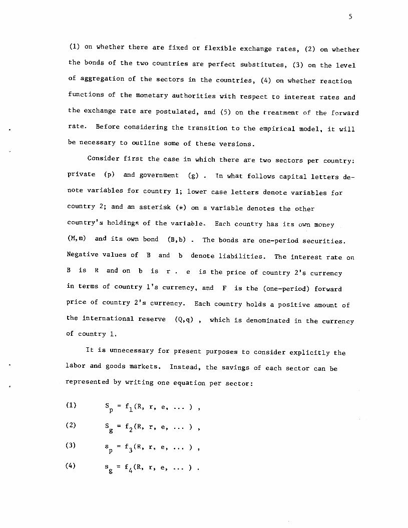
It is unnecessary for present purposes to consider explicitly the

labor and goods markets. Instead, the savings of each sector can be

represented by writing one equation per sector:

(1) S = f1(R, r, e, •.. )

(2) Sg = f2(R, r, e,

(3) s = f3(R, r, e, •.. )

(4)Sg

=f4(R, r, e,

6

S and s denote savings, the difference between a sector's revenue and

its expenditures. In the complete model the savings variables are deter-

mined by definitions, where many of the right hand side variables in these

definitions are determined in the labor and goods markets. Almost every

variable in the model has at least an indirect effect on savings, and

so the argument list in the above functions is long. The two interest

rates and the exchange rate have been listed explicitly in the functions

only for emphasis.

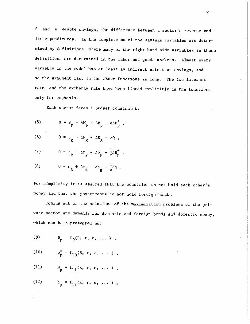
Each sector faces a budget constraint:

(5) 0S —AM —AB _eAb*,p p p p

(6) O=S +AM —AB —AQ,g g g

(7) Os —Am —Abp p p e p

(8) 0s +Am —Ab —-Aq.g g g e

For simplicity it is assumed that the countries do not hold each other's

money and that the governments do not hold foreign bonds.

Coming out of the solutions of the maximization problems of the pri-

vate sector are demands for domestic and foreign bonds and domestic money,

which can be represented as:

(9) B =f9(R, r, e, ... )

(10) b* =f10(R, r, e, ... )

(11) N =f11(R, r, e, ... )

(12) b =f12(R, r, e, ... )

7

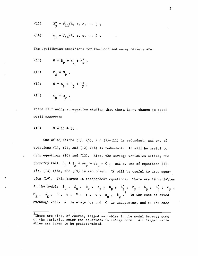
(13) B* =f13(R, r, e, )

(14) m =f14(R, r, e, ... )

The equilibrium conditions for the bond and money markets are:

(15) 0=B +B +B*p g p

(16) M =Mg p

(17) 0=b +b +b*,p g p

(18) in mg p

There is finally an equation stating that there is no change in total

world reserves:

(19) 0LQ+q

One of equations (1), (5), and (9)—(ll) is redundant, and one of

equations (3), (7), and (12)—(l4) is redundant. It will be useful to

drop equations (10) and (13). Also, the savings variables satisfy the

property that +Sg

+ es + esg = 0 , and so one of equations (1)—

(8), (15)—(l8), and (19) is redundant. It will be useful to drop equa-

tion (19). This leaves 16 independent equations. There are 19 variables

inthemodel: S , S , s , s , B , b*, M , b , B*, in

Mg mg, Pq , R , r, e

Bg bgIn the case of fixed

exchange rates e is exogenous and Q is endogenous, and in the case

3There are also, of course, lagged variables in the model because someof the variables enter the equations in change form. All lagged vari-ables are taken to be predetermined.

8

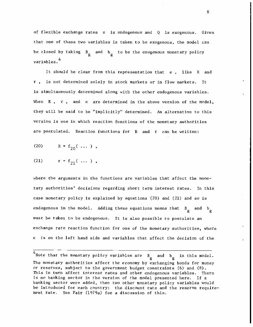
of flexible exchange rates e is endogenous and Q is exogenous. Given

that one of these two variables is taken to be exogenous, the model can

be closed by taking Bg and bg to be the exogenous monetary policy

variables .

It should be clear from this representation that e , like R and

r , is not determined solely in stock markets or in flow markets. It

is simultaneously determined along with the other endogenous variables.

When R , r , and e are determined in the above version of the model,

they will be said to be "implicitly" determined. An alternative to this

version is one in which reaction functions of the monetary authorities

are postulated. Reaction functions for R and r can be written:

(20) R = f20( ... )

(21) r = f21( ... )

where the arguments in the functions are variables that affect the mone-

tary authorities' decisions regarding short term interest rates. In this

case monetary policy is explained by equations (20) and (21) and so is

endogenous in the model. Adding these equations means that Bg and bg

must he taken to be endogenous. It is also possible to postulate an

exchange rate reaction function for one of the monetary authorities, where

e is on the left hand side and variables that. affect the decision of the

4Note that the monetary policy vriahles are Bg and bg in this model.

The monetary authorities affect the economy by exchanging bonds for moneyor reserves, subject to the government budget constraints (6) and (8).This in turn affect interest rates and other endogenous variables. Thereis no banking sector in the version of the model presented here. If abanking sector were added, then two other monetary policy variables wouldbe introduced for each country: the discount rate and the reserve require-ment rate. See Fair (1979a) for a discussion of this.

9

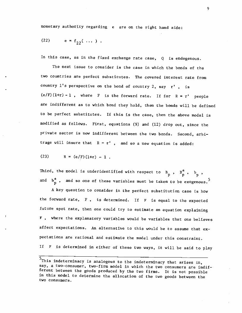
monetary authority regarding e are on the right hand side:

(22) e = f22(

In this case, as in the fixed exchange rate case, Q is endogenous.

The next issue to consider is the case in which the bonds of the

two countries are perfect substitutes. The covered interest rate from

country l's perspective on the bond of country 2, say r' , is(elF) (l+r) — 1 , where F is the forward rate. If for R = r' people

are indifferent as to which bond they hold, then the bonds will be defined

to be perfect substitutes. If this is the case, then the above model is

modified as follows. First, equations (9) and (12) drop out, since the

private sector is now indifferent between the two bonds. Second, arbi-

trage will insure that R = r' , and so a new equation is added:

(23) R = (e/F)(l-i-r) — 1

Third, the model is underidentified with respect to B, B* , b

and b* , and so one of these variables must be taken to be exogenous.5

A key question to consider in the perfect substitution case is how

the forward rate, F , is determined. If F is equal to the expected

future spot rate, then one could try to estimate an equation explaining

F , where the explanatory variables would be variables that one believes

affect expectations. An alternative to this would be to assume that ex-

pectations are rational and estimate the model under this constraint.

If F is determined in either of these two ways, it will be said to play

5This indeterminacy is analogous to the indeterminacy that arises in,say, a two—consumer, two—firm model in which the two consumers are indif-ferent between the goods produced by the two firms. It is not possiblein this model to determine the allocation of the two goods between thetwo consumers.

10

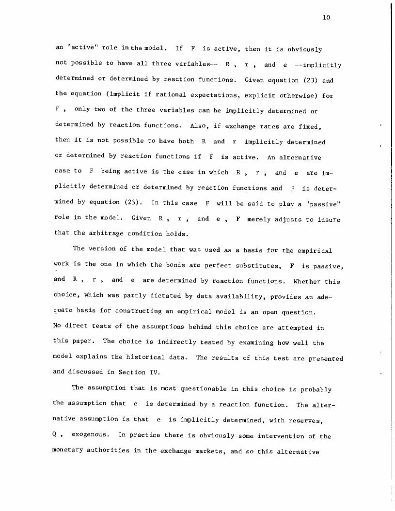
an "active" role inthemodel. If F is active, then it is obviously

not possible to have all three variables—— R, r , and e ——implicitly

determined or determined by reaction functions. Given equation (23) and

the equation (implicit if rational expectations, explicit otherwise) for

F , only two of the three variables can be implicitly determined or

determined by reaction functions. Also, if exchange rates are fixed,

then it is not possible to have both R and r implicitly determined

or determined by reaction functions if F is active. An alternative

case to F being active is the case in which R, r , and e are im-

plicitly determined or determined by reaction functions and F is deter-

mined by equation (23). In this case F will be said to play a "passive"

role in the model. Given R, r , and e , F merely adjusts to insure

that the arbitrage condition holds.

The version of the model that was used as a basis for the empirical

work is the one in which the bonds are perfect substitutes, F is passive,

and R , r , and e are determined by reaction functions. Whether this

choice, which was partly dictated by data availability, provides an ade-

quate basis for constructing an empirical model is an open question.

No direct tests of the assumptions behind this choice are attempted in

this paper. The choice is indirectly tested by examining how well the

model explains the historical data. The results of this test are presented

and discussed in Section IV.

The assumption that is most questionable in this choice is probably

the assumption that e is determined by a reaction function. The alter-

native assumption is that e is implicitly determined, with reserves,

Q , exogenous. In practice there is obviously some intervention of the

monetary authorities in the exchange markets, and so this alternative

11

assumption is also questionable. The assumption that e is determined

by a reaction function means that intervention is complete: the monetary

authority has a target e each period and achieves this target by appro-

priate changes in Q . This assumption may not be, however, as restrictive

as it first sounds. The monetary authority is likely to be aware of the

market forces that are operating on e in the absence of intervention

(i.e., the forces behind the determination of e when e is implicitly

determined), and it may take these into account in setting its target

each period. If some of the explanatory variables in the reaction function

are in part measures of these forces, then the estimated reaction function

may provide a better explanation of e than one would otherwise have

thought. Similar arguments apply to the assumption that R and r are

determined by reaction functions.

The assumption that F is passive means that the forward market

imposes no "discipline" on the monetary authority's choice of the exchange

rate. Again, if the monetary authority takes into account market forces

operating on e in the absence of intervention, including market forces

in the forward market, and if the explanatory variables in the reaction

function for e are in part measures of these forces, then the estimated

reaction function for e may not be too bad an approximation. Given

this assumption and given that F does not appear as an explanatory vari-

able in any of the equations, F plays no role in the empirical model.

For each country it is determined by an estimated version of the arbitrage

condition, equation (23), but the predictions from these equations have

no effect on the predictions of any of the other variables in the model.

The assumption that F is passive is not sensible in the case of

fixed exchange rates: for most observations F is equal to or very close

12

to e when e is fixed. A different choice was thus made for the fixed

rate case. This choice was designed to try to account for the possibility

that the bonds of the different countries are not perfect substitutes as

well as for the fact that F is not passive. The procedure that was

followed in the fixed rate case is as follows. The U.S. was assumed to

be the "leading" country with respect to the determination of interest

rates. Assume in the above model that the U.S. is country 1. Consider

the determination of r , country 2's interest rate. If exchange rates

are fixed, bonds are perfect substitutes, and F is equal to e , then

r is determined by equation (23) and is equal to R . In other words,

country Vs interest rate is merely country l's interest rate: country

1 sets the one world interest rate and country 2's monetary authority has

no control over country 2's rate. If the bonds are not perfect substi-

tutes, then equation (23) does not hold and country 2's monetary authority

can affect its rate. If, however, the bonds are close to being perfect

substitutes, then very large changes in bg will be needed to change

r very much. In the empirical work interest rate reaction functions

were estimated for each country, but with the U.S. interest rate added

as an explanatory variable to each equation. If the bonds are close to

being perfect substitutes, then the U.S. rate should be the only significant

variable in these equations and have a coefficient estimate close to 1.0.

If the bonds are not at all close substitutes, then the coefficient esti-

mate should be close to zero and the other variables should be significant.

The in—between case should correspond to both the U.S. rate and the other

variables being significant.

The above discussion about the U.S. rate in the interest rate reac-

tion functions does not pertain to the flexible exchange rate case. One

13

would thus not expect the interest rate reaction functions to be the same

in the fixed and flexible rate cases, and so in the empirical work separate

interest rate reaction functions were estimated for each country for the

fixed and flexible rate periods. Note that the U.S. rate may still be

an explanatory variable in the reaction functions for the flexible rate

period. This would be, however, because the U.S. rate is one of the vari-

ables that affects the monetary authority's interest rate decision, not

because the U.S. rate is being used to try to capture the degree of sub-

stitutability of the bonds. It should finally be noted in this regard

that the interest rate reaction function for the U.S. was estimated over

the entire sample period. This procedure is consistent with the above

assumption that the U.S. is the interest rate leader in the fixed rate

period. If it is the leader, then it is not constrained as the other

countries are, and so there is no reason on this account to expect the

function to be different in the fixed and flexible rate periods.

The next issue to consider in the transition to the empirical model

is the level of aggregation of the sectors. In the empirical model the

private and government sectors are aggregated together, and so there is

only one sector per country. In this case the budget constraint for country

1 is the sum of equations (5) and (6):

(24) 0 = S — — eLb* —

S is equal to S + S , tB is equal to LB + B , and the p sub-p g p g

script has been dropped from b* since it is now unnecessary. The budget

constraint for country 2 is similarly the sum of equations (7) and (8):

(25) 0s—b—4B*_Aq.

14

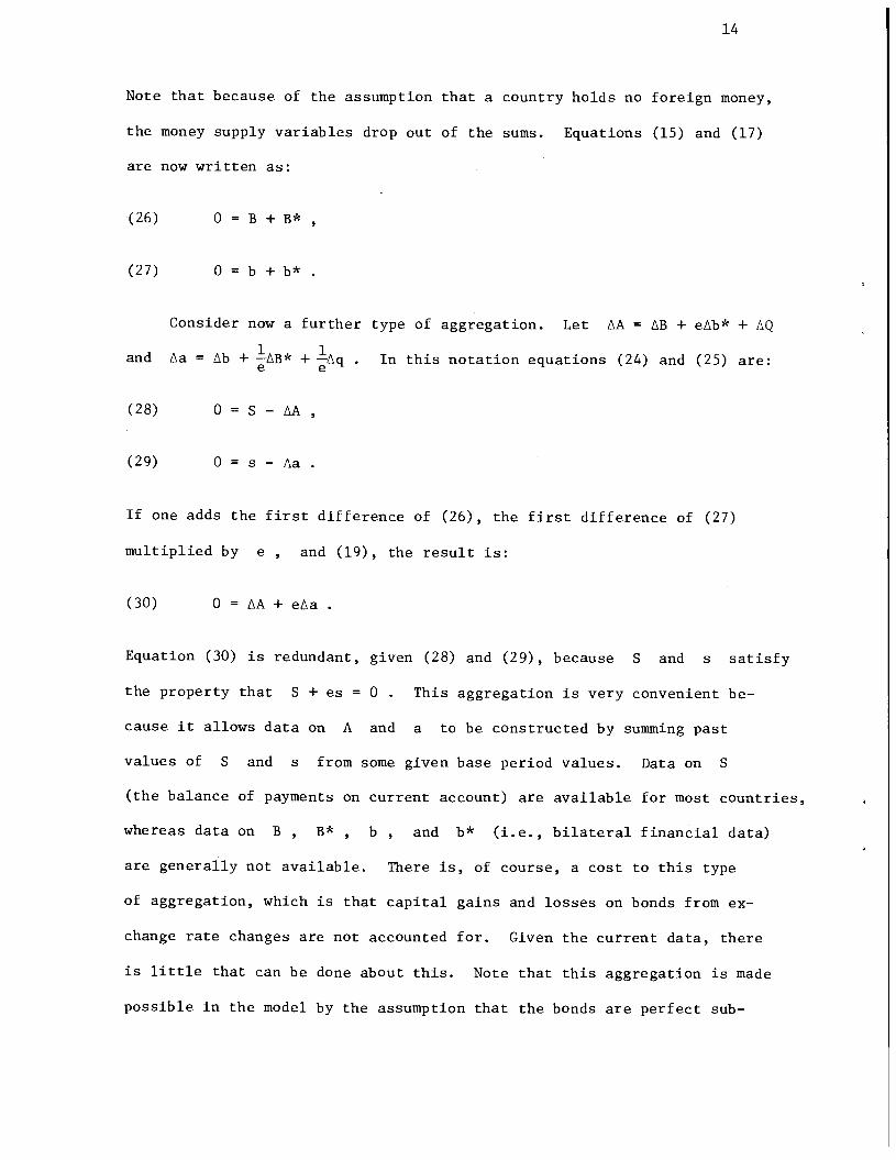
Note that because of the assumption that a country holds no foreign money,

the money supply variables drop out of the sums. Equations (15) and (17)

are now written as:

(26) 0=B+B*

(27) 0=b+b*

Consider now a further type of aggregation. Let AA AB + eAb* + LQ

and a = b + B* + -Aq . In this notation equations (24) and (25) are:

(28) 0=S—AA

(29) Os—isa

If one adds the first difference of (26), the first difference of (27)

multiplied by e , and (19), the result is:

(30) 0 = LA+ eAa

Equation (30) is redundant, given (28) and (29), because S and s satisfy

the property that S + es = 0 . This aggregation is very convenient be-

cause it allows data on A and a to be constructed by summing past

values of S and s from some given base period values. Data on S

(the balance of payments on current account) are available for most countries,

whereas data on B , B* , b , and b* (i.e., bilateral financial data)

are generally not available. There is, of course, a cost to this type

of aggregation, which is that capital gains and losses on bonds from ex-

change rate changes are not accounted for. Given the current data, there

is little that can be done about this. Note that this aggregation is made

possible in the model by the assumption that the bonds are perfect sub—

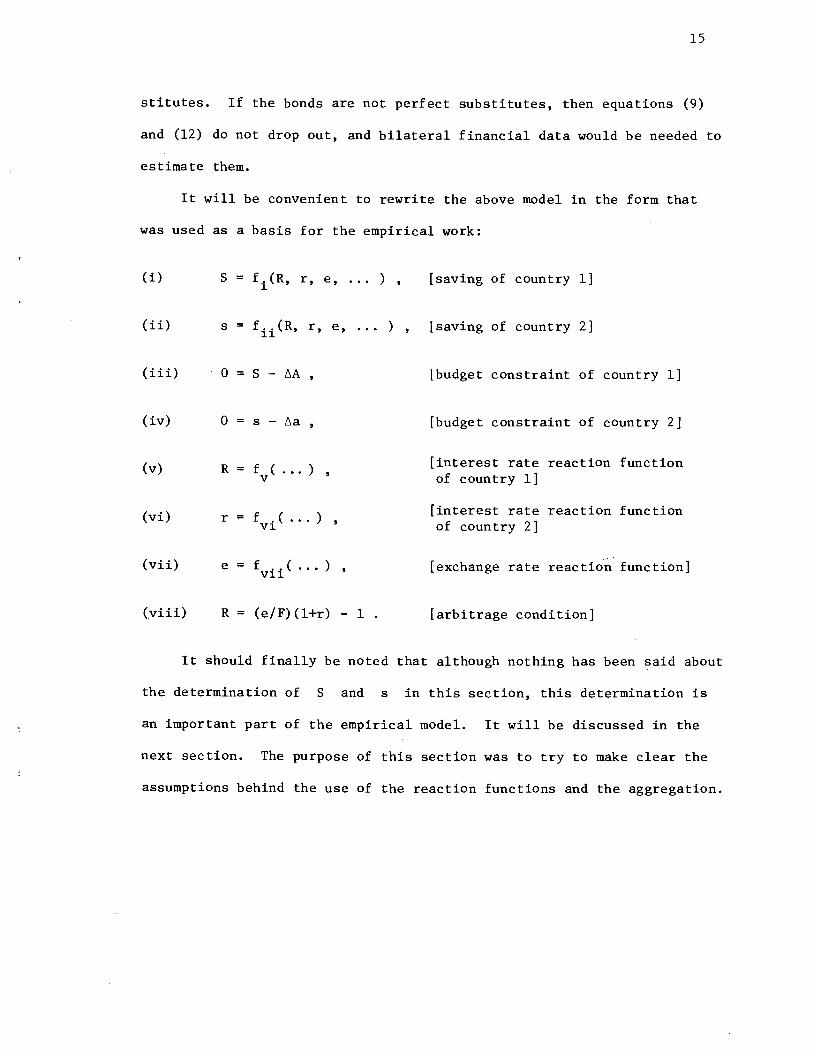
15

stitutes. If the bonds are not perfect substitutes, then equations (9)

and (12) do not drop out, and bilateral financial data would be needed to

estimate them.

It will be convenient to rewrite the above model in the form that

was used as a basis for the empirical work:

(1) S = f(R, r, e, ... ) , [saving of country 1]

(1) = r, e, ... ) , [saving of country 2]

(iii) 0 = S — AA , [budget constraint of country 1]

(iv) 0 = s — Aa , [budget constraint of country 2]

[interest rate reaction function(v) R=f(...)V of country 1]

[interest rate reaction function(vi) vi of country 2]

(vii) e = f..( ... ) , [exchange rate reaction function]

(viii) R = (e/F)(1+r) — 1 . [arbitrage condition]

It should finally be noted that although nothing has been said about

the determination of S and s in this section, this determination is

an important part of the empirical model. It will be discussed in the

next section. The purpose of this section was to try to make clear the

assumptions behind the use of the reaction functions and the aggregation.

16

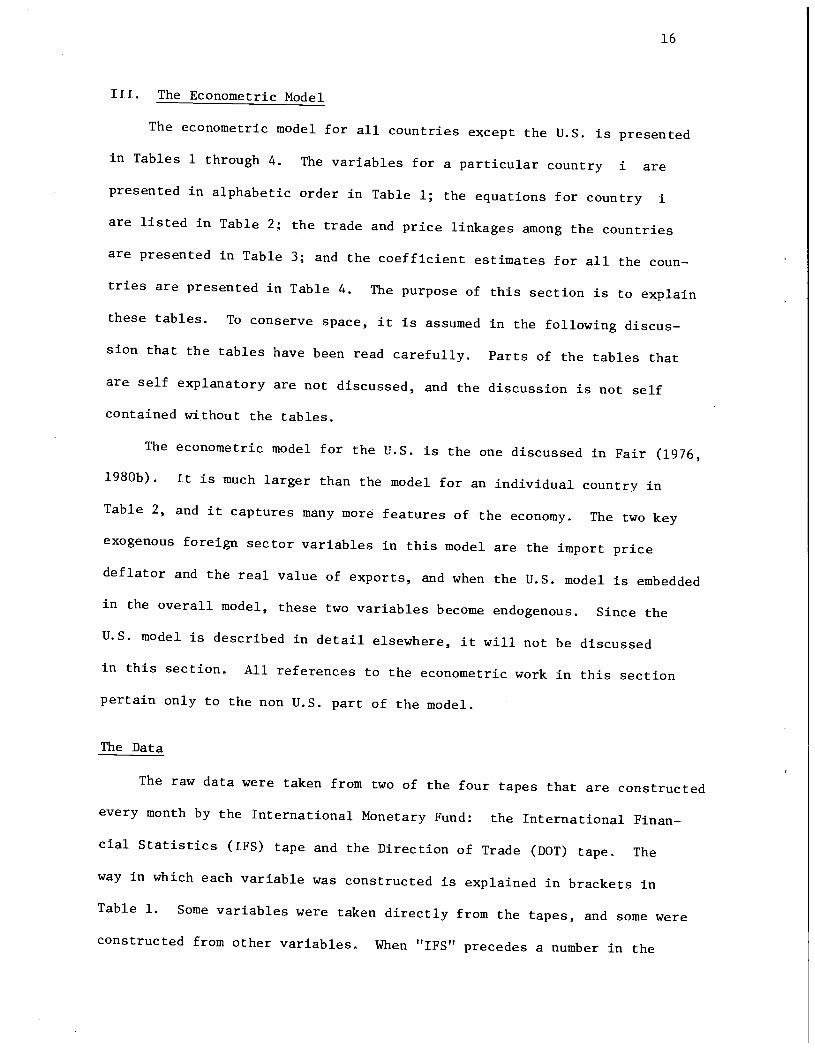
III. The Econometric Model

The econometric model for all countries except the U.S. is presented

in Tables 1 through 4. The variables for a particular country i are

presented in alphabetic order in Table 1; the equations for country i

are listed in Table 2; the trade and price linkages among the countries

are presented in Table 3; and the coefficient estimates for all the coun-

tries are presented in Table 4. The purpose of this section is to explain

these tables. To conserve space, it is assumed in the following discus-

sion that the tables have been read carefully. Parts of the tables that

are self explanatory are not discussed, and the discussion is not self

contained without the tables.

The econometric model for the U.S. is the one discussed in Fair (1976,

1980b). It is much larger than the model for an individual country in

Table 2, and it captures many more features of the economy. The two key

exogenous foreign sector variables in this model are the import price

deflator and the real value of exports, and when the U.S. model is embedded

in the overall model, these two variables become endogenous. Since the

U.S. model is described in detail elsewhere, it will not be discussed

in this section. All references to the econometric work in this section

pertain only to the non U.S. part of the model.

The Data

The raw data were taken from two of the four tapes that are constructed

every month by the International Monetary Fund: the International Finan-

cial Statistics (IFS) tape and the Direction of Trade (DOT) tape. The

way in which each variable was constructed is explained in brackets in

Table 1. Some variables were taken directly from the tapes, and some were

constructed from other variables. When "IFS" precedes a number in the

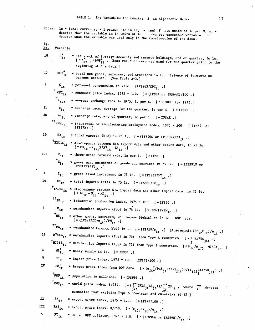
TABLE 1. The Variables for Country i in Alphabetic Order 17

Notes: ic local currency; all prices are in ic; e and F are units of ic per an *denotes that the variable is in units of le. t denotes exogenous variable. ttdenotes that the variable was used only In the construction of the data.

Eq.No. ________

18 At— net stock of foreign security and reserve holdings, end of quarter, In ic.+ BOPt . Base value of zero was used for the quarter prior to the

beginning of the data.)17 BOP total net goods, services, and transfers in Ic. Balance of Payments on

current account. [See Table A—3.]

personal consumption in 751c.[IFS96F/cP11 .]

consumer price index, 1975 1.0. [ (1FS64 or 1FS64X)/lOO .]

average exchange rate in 1975, ic per $. [ = IFSRF for 1975.1

exchange rate, average for the quarter, ic per $. [ IFSRF . 1

exchange rate, end of quarter, ic per $. [ IFSAE .

industrial or manufacturing employment index, 1975 = 100. [ 1FS67 orIFS67EY .1

— total exports (NIA) in 75 lc. ( (IFS9Oc or IFS9ON)/PX .1

discrepancy between NIA export data and other export data, in 75 ic.[_EXjt_ej75X75$i_XS1 .1

lObFit

— three—month forward rate, ic per $. [=IFSB .J

government purchases of goods and services in 75 ic. ( (IFS91F orIFS91FF)/py1 1

gross fixed investment in 75 lc.(1Fs93E/pY1 .1

14IMj total imports (NIA) in 75 lc. [ IFS98C/PMi .1

discrepancy between NIA import data and other Import data, in 75 ic.[IMj_Mj_r.is .1

tflp industrial production index, 1975 100. [ 1FS66 .1

• merchandise imports (fob) in 75 lc. [ IFS71V/PMit .

1MS other goods, services, and income (debit) in 75 ic. BOP data.(IFS77ADD.e)/pM .1

— merchandiseimports (fob) in $. NIFS71v/e .) [Alsoequais (PM1M1)/e— merchandise imports (fob) In 75$ from Type A countries.

I XX75$ .)ut— merchandise imports (fob) in 75$ from Type Bcountries. NMjt/ei75_5$A1

= money supply in ic. [—1F534 .1

import price index, 1975 1.0. [1FS75/100 .]

•import price index from DOT data.

['(ejt(PX$J XX75$)}/{exx75$— population In millions. ('IFs99z .]

— world price index, $/75. [_{*(px$ where r denotesj1i i ji jsuation that excludes Type B countries and countries 26—35.]

— export price index, 1975 1.0. [1FS74/jOO .1— export price index, $/75$. [= (e17PX)/e .1

— GNP or GD? deflator, 1975 — 1.0. 1 (1FS94A or 1FS99g)/y .]

Variable

2Cit

tttcPIit

e175

9b ej20 ee

15 EXj

1•EXDIS

it19

M7S$Aj

tM75$B

6

VPMIt

IV

Ipopit

f.Pw$it

11 PxIII

pX$1

5PYit

1 7a

TABLE 1 (continued)

Eq.No. Varib1e

7a,7b rj three—month interest rate, percentage points. NIFS6O, IFS6OB, or IFS6OC .]

8Rit long—term interest rate, percentage points. [ = IFS61 or IFS61A .]

16sit final sales in 75 ic. [=Yi_Vj .]

•t•SDIS discrepancy in real NIA data (in 75 ic) due to use of different deflators.

[=sjt_cjt_Ii_G1_Exj+IMj .]= total net transfers in lc. [See Table A—3.]

12 inventory investment in 75 ic. HIFS93I/PYj .]

13Vit: stock of inventories, end of quarter, in 75 lc. [ V_1 + . Base value

of zero was used for the quarter prior to the beginning of the data.]

other goods, services, ahd income (credit) in 75 ic. BOP data.N (IFS77ACD.e1)/pX. .]

= merchandise exports (fob) in $. [IFSlO/ei .]

merchandise exports (fob) from i to j in $. [DOT tape.] [XX$i6s=x$—

OC$t andXX$65it=M$it_xx$Jit .] if i = i .1

= merchandise exports (fob) from i to j in 75$. [ (ejXX$j)/(ej75PXj)if I is a Type A country; 0 if i is a Type B country.]

II X75$ merchandise exports (fob) in 75$. [=XX75$j .1 [Also equals X$1/PX$1 .1j -'

[Equals 0 and Is not used if I is a Type B country.]

— real GNP or GDP in 75 ic. [=IFS99AP,. IFS99FP, 1FS99AR, or IFS99BR .]

= share of i's total merchandise imports from Type A countries importedfrom j in 75$. [ = Oc7s$ji/M75$Ai .]

11it ((eejt+eeji)/2)/e

'1'21t — PMi/PM

Notes: 1. For countries with no PM data, PMjt was taken to be PM (so that 2it=1and was taken to be [ej(PX$jtXX75$j1))/PM . For these countries it

it not the case that M$j (PMjMi)/ej because the summation (PX$j)CC75$jj)

is only over Type A countries. M$j pertains to all countries.

2. For the oil exporting countries (countries 26—35), CPI was used In place of PYto deflate IFS9IF or IFS91FF (for G1 ) , IFS93E (for I ), and 1FS931(for ).

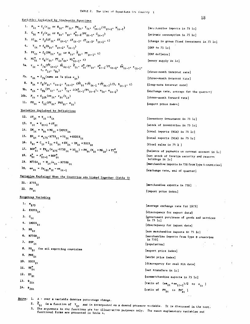
TABLE 2. The List of Eqiast ions in Count ry t

1. — f1(ri or Rj, n. PMi. Yit A _1/fl1_1, Mji)2. Cit — or Ri. . At_j/PYit ,3. — f3'fit, 'iti' a''it_2. t)4. Yi — f4(S1,5. I'Y — f5(PM, or R1, fl t)6. Mi7

— fi(ri, M1I! t)

75. r1 a 17ait—i' it—l' '' At/PYi , A1/FYi i, it—l'

t, r, rae)7b. — as 7a plus e)

8. — f8(ri. nt1. (P'fit+P'Yit..i+*i2)/3, R_1. t)9b. e1 — 9b0'it' r. '' 1/PYi e&.

lOb. = flObei, ri/r1)11 Px1 — it' ei)

Variables Expjned by Definitions

12. — l' —

13. Vi — Viti+AVi14. lMi — Mi+NSit+IMnrsi15. EX — ei7s7S$i+x5i+EX1IS16. —

Cit+tit+Cit+EXit_Thit+sDIs17. BOP PXi(eiis.X75$ + it — it(Mit +flsi) ÷"t18. — At..i+5OP19. M75$A Mit/ei_M75$BO. ee1 — 2*ieft —

Variables Explained When the Countries are Linked Together (Table 3)

21. X75$i

22. PMit

xpgnous Variables

1. e15

2. EXDISit

3. cit

4. flWIs

NSit

M75$Bit

popit

PX1 for oil exporting countries

pW$it

sDIsit

xsit

18

[merchandise imports in 75 Ic]

(private consumption in 75 id

(change in grnss fixed investment in 75 lc]

[cNP in 75 ic]

[CNP deflator]

[money supply in lc]

[three—month interest rate]

[three—month interest rate]

[long—term interest rate]

[exchange rate, average for the quarter)

[three—month forvard rate]

[export price index]

[inventory investment in 75 ic]

(stock of inventories in 75 ic]

[total imports (NIA) in 75 lc]

[total exports (NrA) in 75 lc]

(final sales in 75 1

(balance of paymenta on current account in lcj

[net stock of foreign security and reserveholdings in lc]

[merchandise imports in 75$ frcmTypeAcountries]

[exchange rate, end of quarter]

[merchandise exports in 75$]

[import price index]

[average exchange rate for 1975]

[discrepancy for export data]

[government purchases of gonds and servicesin 75 lc]

[discrepancy for import data]

[non merchandise imports in 75 ic][merchandise imports from Type B countriesin 75$][population]

[export price index]

[world price index]

[discrepancy for real NIA data]

[net transfers in lc]

[nonmerchandise exports in 75 lc]

(ratio of (eeit+eei1)/2 to eft[ratio of PMi to

5.

6.

7.

8.

9.

10.

11.

12.

13.

14.

*lit

*2it

Notes: 1. A • over e varIable denotes percentage change.

2. is s function of and is interpreted as a dcm.ind pressure variable. It is discussed in the text.3. The arguments in the functions are tor illustrative

purposes only. The exact explanatory varishles andfunctional forms are presented in Table 4.

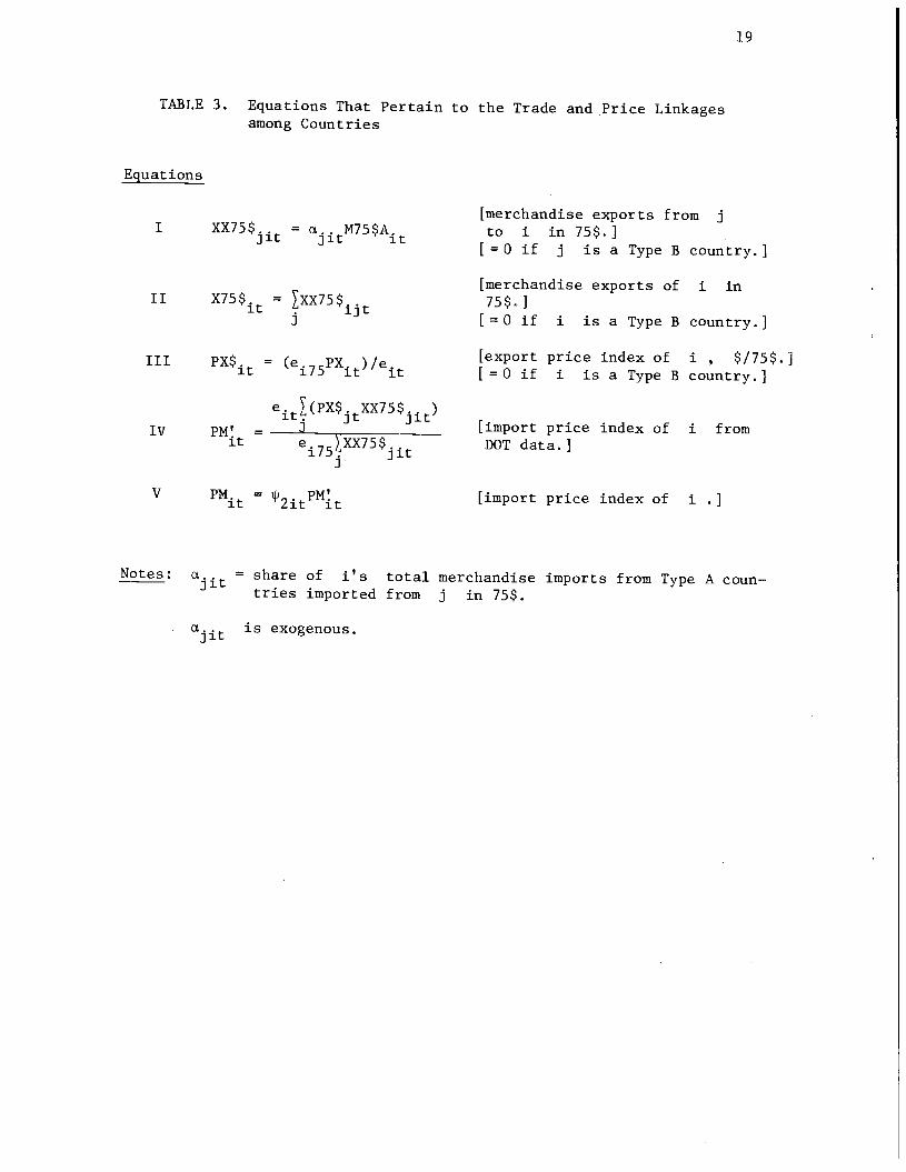
19

TABLE 3. Equations That Pertain to the Trade and Price Linkagesamong Countries

Equations

[merchandise exports from jI XX75$.. = ci.. M75$A. to I in 75$.]Jit Jit it .[= 0 if j is a Type B country. I

[merchandise exports of i inII X75$. = I

j [0 if i is a Type B country.]

III PX$ = (e PX )/e [export price index of i , $/75$.jit i75 it it [=0 if i is a Type B country.]

e.j(PX$.Xx75$..).

IV PM' — __________________ [import price index of i fromit

—

e.75XX75$.. DOT data.]

V PM.t = 2itPMIt [import price index of i .]

Notes: = share of i's total merchandise imports from Type A coun—tries imported from j in 75$.

is exogenous.

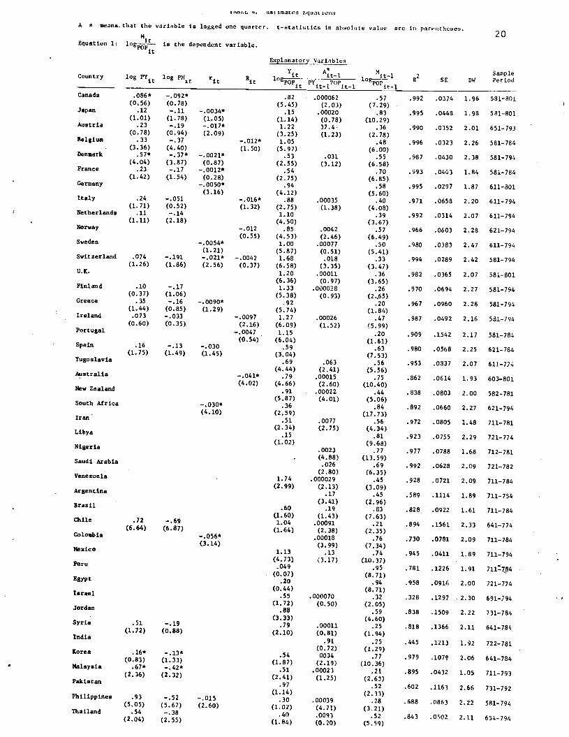
LIn.c '. r.at tmatea MeaL Lone

A * means that the varieble ie lagged one quarter. t—atatiettcs in ahaolute value arc in par.nthesea.20

EquatIon 1: 105L. is the dependent variable.

Expianatory Variables

1 2 SampleCountry log PMt R1 log.!— --,----—.j_____ 1ogt_ R SE 0W Period

Canada .086* _.092* .82 .000062 .57 .992 .0374 1.96 581—801(0.56) (0.78) (5.45) (2.03) (7.29)

Japan .12 —.11 _.0Ø34* .15 .00020 .83 .995 .0448 1.98 581—801(1.01) (1.78) (1.05) (1.14) (0.78) (10.29)

Austria .23 —.19 —.017* 1.22 37.4 .36 .990 .0352 2.01 651—793(0.78) (0.94) (2.09) (3.25) (1.23) (2.78)

Belgium .33 —.37 _.012* 1.05 .48 .996 .0323 2.26 581—784(3.36) (4.40) (1.50) (5.97) (6.00)

Denmark •57* _•37* _.0021* .53 .031 .55 .987 .0430 2.38 581—794(4.04) (3.87) (0.87) (2.55) (3.12) (6.58)

France .23 —.17 _.0012* .54 .70 .993 .0463 1.84 581—784(1.42) (1.54) (0.28) (2.75) (6.85)

Germany _.0050* .94 .58 .995 .0297 1.87 611—801(3.16) (4.12) (5.60)

Italy .24 —.051 _.016* .88 .00035 .40 .971 .0658 2.20 611—794(1.71) (0.52) (1.32) (2.75) (1.38) (4.08)

Netherlands .11 —.14 1.10 .39 .992 .0314 2.07 611—794(1.11) (2.18) (4.50) (3.67)

Norway —.012 .85 .0042 .57 .966 .0603 2.28 621—794(0.55) (4.53) (2.46) (6.49)

Sweden _.0054* 1.00 .00077 .50 .980 .0383 2.47 611—794(1.21) (5.87) (0.51) (5.41)

Switzerland .074 —.191 _.021* —.0042 1.68 .018 .33 .994 .0289 2.42 581—794(1.26) (1.86) (2.56) (0.37) (6.58) (3.35) (3.47)

U.K. 1.20 .00011 .36 .982 .0365 2.07 581—801(6.36) (0.97) (3.65)

Finland .10 —.17 1.33 .000028 .26 .970 .0694 2.27 581—794(0.37) (1.06) (5.38) (0.93) (2..65)

Greece .35 —.16 _.0090* .92 .20 .967 .0960 2.28 581—794(1.44) (0.85) (1.29) (5.74) (1.84)

Ireland .073 —.033 —.0097 1.27 .00026 .47 .987 .0492 2.16 581—794(0.60) (0.35) (2.16) (6.09) (1.52) (5.99)

Portugal —.0047 1.15 .20 .909 .1542 2.17 581—784(0.54) (6.04) (1.61)

Spain .16 —.13 —.030 .59 .63 .980 .0568 2.25 621—784(1.75) (1.49) (1.45) (3.04) (7.53)

Yugoslavia .69 .063 .56 .953 .0837 2.07 611—774(4.44) (2.41) (5.56)Australia _.041* .79 .00015 .75 .862 .0614 1.93 603—801

(4.02) (4.66) (2.60) (10.40)New Zealand .91 .00022 .44 .838 .0803 2.00 582—781(5.87) (4.01) (5.06)South Africa _.030* .36 .84 .892 .0660 2.27 621—794

(4.10) (2.59) (17.73)Iran .51 .0077 .56 .972 .0805 1.48 711—781(2.34) (2.75) (4.34)

Libya .15 .81 .923 .0755 2.29 721—774(1.02) (9.68)

Nigeria .0023 .77 .977 .0788 1.68 712—781(4.88) (13.59)Saudi Arabia.026 .69 .992 .0628 2.09 721—782

(2.80) (6.35)Venezuela 1.74 .000029 .45 .928 .0721 2.09 711—784(2.99) (2.13) (3.09)

Argentina .17 .45 .589 .1114 1.89 711—754(3.41) (2.96)Brazil .60 .19 .83 .828 .0922 1.61 711—784

(1.60) (1.43) (7.63)Chile .72 —.69 1.04 .00091 .21 .894 .1561 2.33 641—774(6.64) (6.87) (1.64) (2.38) (2.35)Colombia _.056* .00018 .76 .730 .0781 2.09 711—784

(3.14) (3.99) (7.34)Maxico 1.13 .13 .74 .945 .0411 1.89 711—794(4.73) (3.17) (10.37)Peru .049 .95 .781 .1226 1.91 7l1784(0.07) (8.71)

Egypt .20 .94 .958 .0916 2.00 721—774(0.44) (8.71)Israel .55 .000070 .32 .328 .1297 2.30 691—794(1.72) (0.50) (2.05)Jordan .88 .59 .838 .1509 2.22 731—784(3.33) (4.60)

Syria .51 —.19 .79 .00011 .25 .818 .1366 2.11 641—784(1.72) (0.88) (2.10) (0.81) (1.94)India

.91 .25 .445 .1213 1.92 722—781(0.72) (1.29)Korea .16* _.l3* .54 0034 .77 .979 .1079 2.06 641—784(0.83) (1.33) (1.87) (2.19) (10.36)Malaysia .67* _.42* .51 .00023 .21 .895 .0432 1.05 711—793(2.36) (2.32) (2.41) (1.25) (2.63)Pakistan

.97 .52 .602 .1163 2.66 731—792(1.14) (2.33)Philippines .93 —.52 —.015 .30 .00039 .28 .688 .0863 2.22 581—794(5.05) (5.67) (2.60) (1.02) (4.21) (3.21)Thailand .54 —.38 .40 .0093 .52 .843 .0502 2.11 656—794(2.04) (2.55) (1.84) (0.20) (5.59)

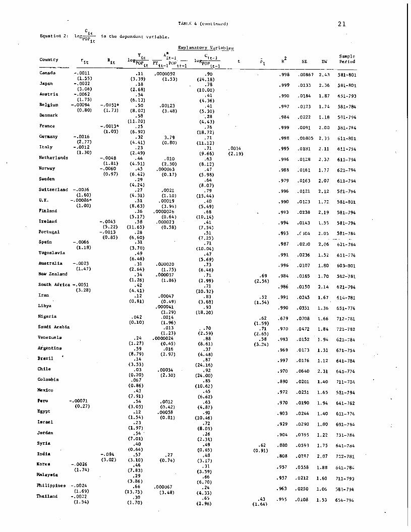
TAJII,E 4 (coot mcd) 21

Equation 2 1ogj7ft_- ía the dependunt vuriuble.

p1anatory VariabLes

________ 1 2 SampleCountry

—nt Rft log!-_ t RSE DW Period

Canada —.0011 .11 .0000092 .90 .998 .00867 2.43 581—801(1.55) (3.39) (1.53) (24.18)

Japan —.0022 .18 .78 .999 .0133 2.36 581—801(3.06) (2.68) (10.00)

Austria —.0062 .54 .41 .990 .0184 1.87 651—793(1.75) (6.13) (4.36)

Belgium —.00094 _.0052* .50 .00123 .41 .997 .0123 1.74 581—784(0.80) (1.73) (8.02) (3.48) (5.30)

Denmark .58 .28 .984 .0222 1.18 581—794(11.20) (4. 43)

France _.0013* .25 .76 .999 .0091 2.03 581—784(1.03) (6.92) (18.72)

Germany —.0016 .32 3.79 .71 .998 .00805 2.33 611—801(2.77) (4.41) (0.80) (11.12)

Italy —.0012 .23 .71 .0014 .995 .0181 2,11 611—794(1.30) (2.49) (9.66) (2.19)

Netherlands —.0048 .44 .010 .63 .996 .0128 2.32 611—794(1.81) (4.51) (2.50) (8.12)

Norway —.0060 .45 .000063 .47 .988 .0161 1.77 621—794(0.97) (6.42) (0.17) (5.98)

Sweden .29 .64 .979 .0163 2.07 611—794(4.24) (8.07)

SwItzerland —.0036 .27 .0021 .79 .996 .0121 2.12 581—794(1.60) (4.31) (1.10) (15.44)

U.K. _.00086* .51 .00019 .40 .990 .0123 1.72 581—801(1.00) (8.63) (3.94) (5.49)

Finland .36 .0000026 .68 . .993 .0238 2.19 581—794(5.17) (0.64) (10.14)Ireland —.0043 .58 .000023 .41 .994 .0143 1.55 581—794

(5.22) (11.65) (0.58) (7.54)Portugal —.0013 .28 .51 .993 .( 3C4 2.05 581—784

(0.85) (6.60) (7.25) -Spain —.0066 .31 .71 .987 .02,0 2.06 621—784

(1.18) (3.70) (10.04)Yugoslavia •49 .47 .991 .0236 1.52 611—774

(6.48) (5.69)Australia —.0023 .31 .030020 .73 .996 .0107 1.80 603—801

(1.47) (2.64) (1.75) (6.46)New Zealand .34 .000057 .71 .69 .984 .01.65 1.70 582—781.

(1.26) (1.86) (2.99) (2.58)South Africa —.0051 .42 .71 .986 .0150 2.14 621—794

(3.28) (4.41) (10.32)Iran .12 .00047 .83 .52 .991 .0245 1.67 514—781

(0.81) (0.49) (3.68) (1.54)Libya .000041 .93 .990 .0351 1.36 651—774

(1.29) (18.20)Nigeria .042 .0014 .62 .679 .0708 1.66 712—781

(0.10) (1.96) (1.59)Saudi Arabia .013 . .70 .71 .970 .0472 1.84 721—782

(1.23) (2.59) (2.65)Venezuela .24 .0000024 .88 .58 .993 .0152 1.94 621—784

(1.27) (0.45) (8.61) (3.24)Argentina .59 .016 .37 .969 .0173 1.31 671—754

(8.79) (2.97) (4.48)Brazil •.14 .87 .997 .0176 1.12 641—784

(3.53) (24.16)Chile .03 .00034 .92 .970 .0640 2.31 641—774(0.20) (2.30) (24.00)

Colombia .067 .85 .890 .0201 1.40 711—734(0.86) (10.62)

Mexico .43 .45 .972 .0251 1.65 581—794(7.91) (6.62)

Peru —.00071 .54 .0012 .63 .970 .0190 1.94 641—782(0.27) (3.05) (0.42) (4.87)Egypt .12 .00058 .90 .903 .0244 1.40 611—774

(1.54) (0.81) (10.46)Israel .23 .72 .929 .0290 1.80 691—794

(1.97) (8.05)Jordan .54 .26 .904 .0395 1.22 731—784

(7.01) (2.31.)Syria .40 .49 .62 .880 .0593 1.75 641—7d4

(0.64) (0.65) (0.91)India —.094 .57 .27 .48 .808 .0287 2.07 722—781

(3.02) (3.10) (0.74) (3,17)Korea —.0026 .46 .31 .957 .0558 1.88 641—784

(1.74) (7.83) (3.59)Malaysia . .29 .66 .957 .0212 1.60 711—793

(3.86) (6.70)Philippines —.0024 .66 .000067 .24 .963 .0250 1.06 781—794(1.69) (13./5) (3.48) (4.33)Thailand —.0022 .30 .6 .43 .995 .0108 1.53 654—794(1.54) (1.70) (2.96) (1.64)

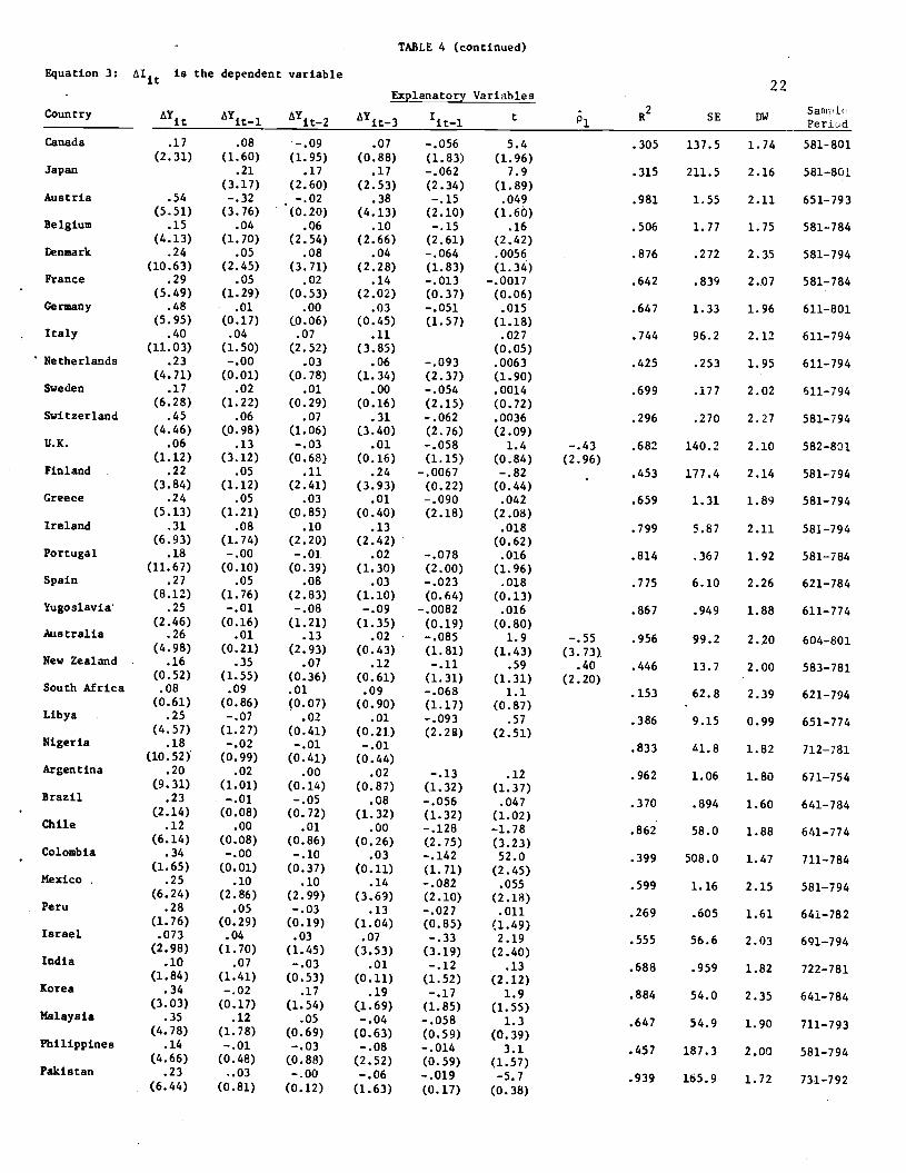
- TABLE 4 (continued)

Equation 3: is the dependent variable22

Explanatory Variables

Country it it—l it—2 it—3 1it—l p1SE DW

—_________

Canada .17 .08 —.09 .07 —.056 5.4 .305 137.5 1.74 581—801(2.31) (1.60) (1.95) (0.88) (1.83) (1.96)

Japan .21 .17 .17 —.062 7.9 .315 211.5 2.16 581—801(3.17) (2.60) (2.53) (2.34) (1.89)

Austria .54 —.32 —.02 .38 —.15 .049 .981 1.55 2.11 651—793(5.51) (3.76) (0.20) (4.13) (2.10) (l.6O)

Belgium .15 .04 .06 .10 —.15 .16 .506 1.77 1.75 581—784(4.13) (1.70) (2.54) (2.66) (2.61) (2.42)

enmark .24 .05 .08 .04 —.064 .0056 .876 .272 2.35 581—794(10.63) (2.45) (3.71) (2.28) (1.83) (1.34)

France .29 .05 .02 .14 —.013 —.0017 .642 .839 2.07 581—784(5.49) (1.29) (0.53) (2.02) (0.37) (0.06)

Germany .48 .01 .00 .03 —.051 .015 .647 1.33 1.96 611—801(5.95) (0.17) (0.06) (0.45) (1.57) (1.18)

Italy .40 .04 .07 .11 .027 .744 96.2 2.12 611—794(11.03) (1.50) (2.52) (3.85) (0.05)

Netherlands .23 —.00 .03 .06 —.093 .0063 .425 .253 1.95 611—794(4.71) (0.01) (0.78) (1.34) (2.37) (1.90)

Sweden .17 .02 .01 .00 —.054 .0014 .699 .177 2.02 611—794(6.28) (1.22) (0.29) (0.16) (2.15) (0.72)

Switzerland .45 .06 .07 .31 —.062 .0036 .296 .270 2.27 581—794(4.46) (0.98) (1.06) (3.40) (2.76) (2.09)

U.K. .06 .13 —.03 .01 —.058 1.4 —.43 .682 140.2 2.10 582—801(1.12) (3.12) (0.68) (0.16) (1.15) (0.84) (2.96)

Finland .22 .05 .1]. .24 —.0067 —.82 .453 177.4 2.14 581—794(3.84) (1.12) (2.41) (3.93) (0.22) (0.44)

Greece .24 .05 .03 .01 —.090 .042 .659 1.31 1.89 581—794(5.13) (1.21) (0.85) (0.40) (2.18) (2.08)

Ireland .31 .08 .10 .13 .018 .799 5.87 2.11 581—794(6.93) (1.74) (2.20) (2.42) (0.62)

Portugal .18 —.00 —.0] .02 —.078 .016 .814 .361 1.92 581—784(11.67) (0.10) (0.39) (1.30) (2.00) (1.96)

Spain .27 .05 .08 .03 —.023 .018 .775 6.10 2.26 621—784(8.12) (1.76) (2.83) (1.10) (0.64) (0.13)

Yugoslavia' .25 —.01 —.08 —.09 —.0082 .016 .867 .949 1.88 611—774(2.46) (0.16) (1.21) (1.35) (0.19) (0.80)Australia .26 .01 .13 .02 —.085 1.9 —.55 .956 99.2 2.20 604—801(4.98) (0.21) (2.93) (0.43) (1.81) (1.43) (3.73)

New Zealand .16 .35 .07 .12 —.11 .59 .40 .446 13.7 2.00 583—781(0.52) (1.55) (0.36) (0.61) (1.31) (1.31) (2.20)South Africa .08 .09 .01 .09 —.068 1.1 .153 62.8 2.39 621—794

(0.61) (0.86) (0.07) (0.90) (1.17) (0.87)Libya .25 —.07 .02 .01 —.093 .57 .386 9.15 0.99 651—774

(4.57) (1.27) (0.41) (0.21) (2.2) (2.51)Nigeria .18 —.02 —.01 —.01 .833 41.8 1.82 712—781

(10.52) (0.99) (0.41) (0.44)Argentina .20 .02 .00 .02 —.13 .12 .962 1.06 1.80 671—754

(9.31) (1.01) (0.14) (0.87) (1.32) (1.37)Brazil .23 —.01 —.05 .08 —.056 .047 .370 .894 1.60 641—784

(2.14) (0.08) (0.72) (1.32) (1.32) (1.02)Chile .12 .00 .01 .00 —.128 —1.78 .862 58.0 1.88 641—774

(6.14) (0.08) (0.86) (0.26) (2.75) (3.23)Colombia .34 —.00 -.10 .03 —.142 52.0 .399 508.0 1.47 711—784

(1.65) (0.01) (0.37) (0.11) (1.71) (2.45)Mexico .25 .10 .10 .14 —.082 .055 .599 1.16 2.15 581—794

(6.24) (2.86) (2.99) (3.69) (2.10) (2.18)Peru .28 .05 —.03 .13 —.027 .011 .269 .605 1.61 641—782

(1.76) (0.29) (0.19) (1.04) (0.85) (1.49)Israel .073 .04 .03 .07 —.33 2.19 .555 56.6 2.03 691—794

(2.98) (1.70) (1.45) (3.53) (3.19) (2.40)India .10 .07 —.03 .01 —.12 .13 .688 .959 1.82 722—781

(1.84) (1.41) (0.53) (0.11) (1.52) (2.12)Korea .34 —.02 .17 .19 —.17 1.9 .884 54.0 2.35 641—784

(3.03) (0.17) (1.54) (1.69) (1.85) (1.55)Malaysia .35 .12 .05 —.04 —.058 1.3 .647 54.9 1.90 711—793

(4.78) (1.78) (0.69) (0.63) (0.59) (0.39)Philippines .14 —.01 —.03 —.08 —.014 3.1 .457 187.3 2.00 581—794

(4.66) (0.48) (0.88) (2.52) (0.59) (1.57)Pakistan .23 ..03 —.00 —.06 —.019 —5.7 .939 15.9 1.72 731—792

(6.44) (0.81) (0.12) (1.63) (0.17) (0.38)

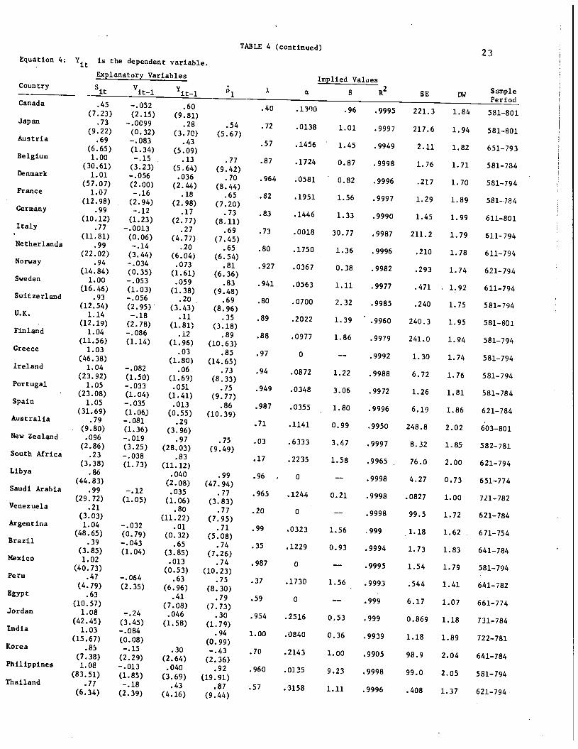
Equation 4: is the dependent variable.

!p1anatory Variables

Country - S1 V1 '1—1

TABLE 4 (continued)23

Canada .45 —.052 .60

A

liedB

Values

SE SamplePer iod

(7.23) (2.15) (9.81)

.40 .13'O .96 .9995 221.3 1.84 581—801Japan •73

(9.22)

—.0099

(0.32)

.28

(3.70).54 .72 .0138 1.01 .9997 217.6 1.94 581—801

Austria .69

(6.65)

—.083

(1.34)

.43

(5.09)

(5.67).57 .1456 1.45 .9949 2.11 1.82 651—793

Belgium i.oo

(30.61)—.15

(3.23)

.13

(5.64)

.77 .87 .1724 0.87 .9998 1.76 1.71 581—784nmark 1.01

(57.07)—.056

(2.00).036

(2.44).70 .964 .0581 0.82 .9996 .217 1.70 581—794

France 1.07

(12.98)

-.16

(2.94)

.18

(2.98)

.65 .82 .1951 1.56 .9997 1.29 1.89 581-784Germany .99

(10.12)

—.12

(1.23)

.17

(2.77)

.73

(8.11).83 .1446 1.33 .9990 1.45 1.99 611—801

Italy .77 —.0013 .27 .69.(11.81) (0.06) (4.77) (7.45)

.0018 30.77 .9987 211.2 1.79 611-794Netherlands .99

(22.02)

—.14

(3.44)

.20

(6.04)

.65

(6.54)

.80 .1750 1.36 .9996 .210 1.78 611—794Norway .94

(14.84)

—.034

(0.35).073

(1.61).81 .927 .0367 0.38 .9982 .293 1.74 621—794

Sweden i.oo

(16.46)—.053

(1.03)

.059

(1.38)

.83 .941 .0563 1.11 .9977 .471 1.92 611—794Switzerland .93

(12.54)

—.056

(2.95)

.20

(3.43).69 .80 .0700 2.32 .9985 .240

.

1.75 581—794U.K. 1.14 —.18 .11

(8.96)

. (12.19) (2.78) (1.81)

.35 .89 .2022 1.39 .9960 240.3 1.95 581—801Finland 1.04

(11.56)—.086

(1.14)

.12

(1.96).89

(10.63)

.88 .0977 1.86 .9979 241.0 1.94 581—794Greece 1.03

(46.38).03

(1.80).85

(14.65)

.97 0 —- .9992 1.30 1.74 581-794Ireland 1.04

(23.92)

—.082

(1.50)

.06

(1.69)

.73

(8.33)

.94 .0872 1.22 .9988 6.72 1.76 581—794Portugal 1.05 —.033 .051 .75

(23.08) (1.04) (1.41) (9.77).949 .0348 3.06 .9972 1.26 1.81 581—784

Spain 1.05

(31.69)

—.035

(1.06J

.013

(0.55).86

(10.39).987 .0355 1.80 .9996 6.19 1.86 621—784

AustralIa .79

(9.80)

—.081

(1.36)

.29

(3.96).71 .1141 0.99 .9950 248.8 2.02

.603—801

New Zealand .096

(2.86)—.019

(3.25)

.97

(28.03).75

(9.49)

.03 .6333 3.47 .9997 8.32 1.85 582—781South Africa .23

(3.38)

—.038

(1.73).83

(11.12).17 .2235 1.58 .9965 76.0 2.00 621—794

Libya .86

(44.83).040

(2.08)

.99

(47.94).96 0 —— .9998 4.27 0.73 651—774

Saudi Arabia .99

(29.72)

—.12

(1.05)

.035

(1.06).77

(3.83).965 .1241. 0.21 .9998 .0827 1.00 721—782

Venezuela .zi

(3.03).80

(11.22).77

(7.95)

.20 0 —— .9998 99.5 1.72 621—784Argentina 1.04

(48.65)—.032

(0.79).01

(0.32)

.71

(5.08).99 .0323 1.56 .999 1.18 1.62 671—754

Brazil .39

(3.85)—.043

(1.04)

.65

(3.85).74

(7.26)

.35 .1229 0.93 .9994 1.73 1.83 641—784Mexico 1.02

(40.73).013

(0.53)

.74

(10.23).987 0 —— .9995 1.54 1.79 581—794

Peru .47

(4.79)

—.064

(2.35)

.63

(6.96).75

(8.30)

.37 .1730 1.56.

.9993 .544 1.41 641—782Egypt .63

(10.57).41

(7.08).79

(7.73)

.59 0 —— .999 6.17 1.07 661—774Jordan 1.08

(42.45)

—.24

(3.45)

.046

(1.58)

.30

(1.79)

.954 .2516 0.53 .999 0.869 1.18 731—784India 1.03

(15.67)

—.084

(0.08).94

(0.99)

1.00 .0840 0.36 .9939 1.18 1.89 722—781Korea .85

(7.38)

—.15

(2.29)

.30

(2.64)

—.43

(2.36)

.70 .2143 1.00 .9905 98.9 2.01. 641—784Philippines 1.08

(83.51)

—.013

(1.85)

.040

(3.69)

.92

(19.91)

.960 .0135 9.23 .9998 99.0 2.05 581—794ThaIland .77

(6.34)

—.18(2.39)

.43

(4.16)

.87 .57 .3158 1.11 .9996 .408 1.37 621—794

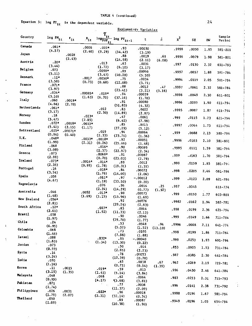
TABLE 4 (continued)

Equation 5:

Country

log PY1 is the dependent variable.

Variables

log PM1t rj .Rit log—-- log PY_1 t

24

SampleSE DW Period

Canada .061* .0026 .022* .93(4.57) (2.40) (9.29) (54.42)

.00030 .9998 .0050 1.95 581—801

Japan .0028 .88(3.19)

(2.43) (14.98)

.0019 .69 .9996 .0079 1.98 581—801

Austria .20*

(3.44).013

(1.72).63

(2.11).0031

(6.08).997 .0130 2.32 651—793

Belgium .073

(5.11).0098*

(3.47)

.89

(40.20)

(3.17).00096 .9997 .0057 1.88 581—784

Denmark .11*

(3.58).0017

(0.73)

.0050*

(0.68).75

(12.08)

(5:50).0034 .9994 .0119 2.05 581—794

France .071*

(3.97).88

(23.41)

(3.71).0012 .47 .9997 .006]. 2.32 581—784

Germany .034*

(3.10).00085*

(1.63).019*

(6.70)

.94

(37.16)

(3.21).00039

(5.16).9996 .0049 2.30 611—801

Italy .060

(4.66).0019*

(2.70).91

(51.83)

(1.70).00080 .9996 .0099 1.90 611—794

Netherlands .061*

(3.17).012

(2.30)

.83

(14.89)

(4.32).0022 .9995 .0087 1.87 611—794

Norway .18

(5.47).013*

(2.85).47

(6.41)

(2.87).0061 .999 .0115 1.23 621—794

Sweden .072*

(5.42)

.0018*

(2.15)

.QQ33*

(1.17).85

(27.29)

(7.98).0013 .9997 .0064 1.73 611—794

Switzerland .025*

(0.94).00071*

(0.40).019

(2.33).94

(23.76)

(5.12).00064 .999 .0088 2.13 581—794

U.K. .048*

(1.99).0033*

(2.31)

.0018*

(0.26).92

(25.66)

(1.36).00051 .9996 .0103 2.10 581—801

Finland .068

(3.08).016*

(2.37).90

(22.97)

(1.48).00089 .9995 .0111 1.59 581—794

Greece .073

(2.99)

..0068*(0.70)

.91

(23.03)

(2.34).00087 .999 .J163 1.70 581—794

Ireland .073*

(2.35).0014*

(0.99)

.014*

(1.78).89

(19.31)

(2.79).0012 .999 .0159 1.85 581—794

Portugal .16

(3.54).018*

(1.76)

.84

(14.00)

(2.31).00072 .998 .0205 2.46 -581—784

SpaIn .058

(4.67).011*

(1.19)

.97

(33.50)

(2.06)—.00012 .999 .0123 2.09 621—784

Yugoslavia

Australia .046

(1.48).0052

(1.69)

.076

(2.24).013*

(1.15)

.96

(14.29).90

(15.96)

(0.20).0016

(0.77).00073

.25

(1.92)

.997

.999

.0345

.0150

.

1.77

611—774

603—801

New Zealand

South Africa

.056*

(2.83).12*

(2.61).027*

(1.92)

.92

(29.24).83

(11.33)

(1.69).00076

(2.83).0014

.9982

.998

.0162

.0199

1.94

2.36

582—781

621—794Brazil .058

(1.97).90

(29.70)

(2.13).0046 .999 .0149 1.66 711—784

Chile .24

(6.95).53

(5.52)

(1.77).0548 .94 .9996 .0668 2.11 641—774

Colombia .068

(1.46).73

(7.58)

(1.52).0103

(13.10).998 .0199 1.86 711—784

Israel .088

(1.83) ..032*

(1.34)

.95

(13.30)

(1.88)—.00040 .999 .0253 1.93 691—794

Jordan .073

(0.59).50

(2.85)

(0.22).014 .853 .0905 1.53 731—784

Syria .14

(3.24).78

(12.39)

(2.23).00053 .987 .0385 2.30 641—784

India .070

(1.16).43

(0.75)

(0.70).0038 .67 .962 .0269 2.19 722—781

Korea .11

(3.15)

.0015

(1.35).019*

(1.43)

.59

(6.14)

(0.54).013

(1.39).996 .0430 2.46 641—784

Malaysia .048

(0.95).068

(4.17)

.62

'(5.68)

(3.84).0064 .983 .0253 2.31 711—793

Pakistan .071

(2.74)

..77

(11.37)

(3.81).0036 .996 .0141 2.38 731—792

PhIlippines .026

(1.79)

.0031

(2.07).022*

(2.31)

.96

(32.14)

(2.09).00018 .9988 .0196 1.67 581—794

Thailand .050

(1.09).89

(0.34).00087 .9949 .0196 1.05 654—794

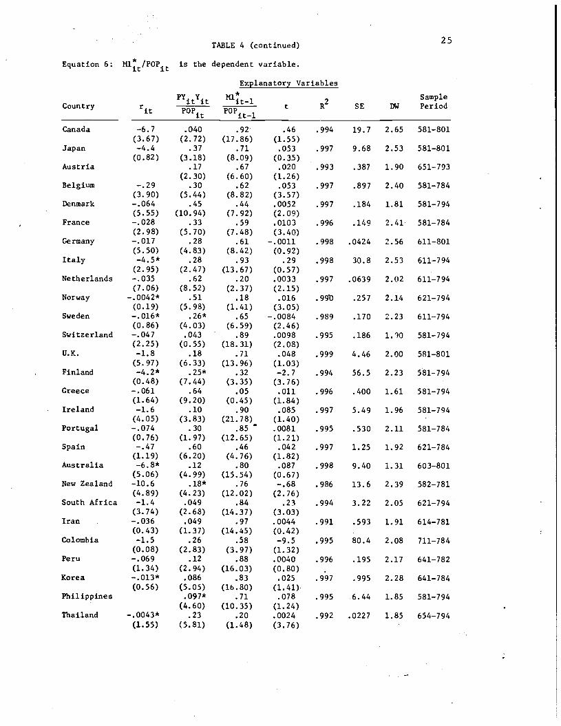
TABLE 4 (continued)25

Equation 6: M]./P0Pjt is the dependent variable.

Explanatory Variables

Ml1_1 2 SampleCountry ri

— t R SE DW Period

______________ it it—l

Canada —6.7 .040 .92 .46 .994 19.7 2.65 581—801(3.67) (2.72) (17.86) (1.55)

Japan —4.4 .37 .71 .053 .997 9.68 2.53 581—801(0.82) (3.18) (8.09) (0.35)

Austria .17 .67 .020 .993 .387 1.90 651—793(2.30) (6.60) (1.26)

Belgium —.29 .30 .62 .053 .997 .897 2.40 581—784(3.90) (5.44) (8.82) (3.57)

Denmark —.064 .45 .44 .0052 .997 .184 1.81 581—794(5.55) (10.94) (7.92) (2.09)

France —.028 .33 .59 .0103 .996 .149 2.41 581—784(2.98) (5.70) (7.48) (3.40)

Germany —.017 .28 .61 —.0011 .998 .0424 2.56 611—801(5.50) (4.83) (8.42) (0.92)

Italy _4•5* .28 .93 .29 .998 30.8 2.53 611—794(2.95) (2.47) (13.67) (0.57)

Netherlands —.035 .62 .20 .0033 .997 .0639 2.02 61l794(7.06) (8.52) (2.37) (2.15)

Norway _.0042* .51 .18 .016 .990 .257 2.14 621—794(0.19) (5.98) (1.41) (3.05)

Sweden _.0l6* .26* .65 —.0084 .989 .170 2.23 611—794(0.86) (4.03) (6.59) (2.46)

Switzerland —.047 .043 .89 .0098 .995 .186 1.30 581—794(2.25) (0.55) (18.31) (2.08)

U.K. —1.8 .18 .71 .048 .999 4.46 2.00 581—801(5.97) (6.33) (13.96) (1.03)

Finland _4.2* .25* .32 —2.7 .994 56.5 2.23 581—794(0.48) (7.44) (3.35) (3.76)

Greece —.061 .64 .05 .011 .996 .400 1.61 581—794(1.64) (9.20) (0.45) (1.84)

Ireland —1.6 .10 .90 .085 .997 5.49 1.96 581—794(4.05) (3.83) (21.78) (1.40)

Portugal —.074 .30 .85 .0081 .995 .530 2.11 581—784(0.76) (1.97) (12.65) (1.21)

Spain —.47 .60 .46 .042 .997 1.25 1.92 621—784(1.19) (6.20) (4.76) (1.82)

Australia _6.8* .12 .80 .087 .998 9.40 1.31 603—801(5.06) (4.99) (15.54) (0.67)

New Zealand —10.6 .18* .76 —.68 .986 13.6 2.39 582—781(4.89) (4.23) (12.02) (2.76)

South Africa —1.4 .049 .84 .23 .994 3.22 2.05 621—794(3.74) (2.68) (14.37) (3.03)

Iran —.036 .049 .97 .0044 .991 .593 1.91 614—781(0.43) (1.37) (14.45) (0.42)

Colombia —1.5 .26 .58 —9.5 .995 80.4 2.08 711—784(0.08) (2.83) (3.97) (1.32)

Peru —.069 .12 .88 .0040 .996 .195 2.17 641—782(1.34) (2.94) (16.03) (0.80)

Korea _.013* .086 .83 .025 .997 .995 2.28 641—784(0.56) (5.05) (15.80) (1.41)

Philippines .097* .71 .078 .995 6.44 1.85 581—794(4.60) (10.35) (1.24)

Thailand _.0043* .23 .20 .0024 .992 .0227 1.85 654—794(1.55) (5.81) (1.48) (3.76)

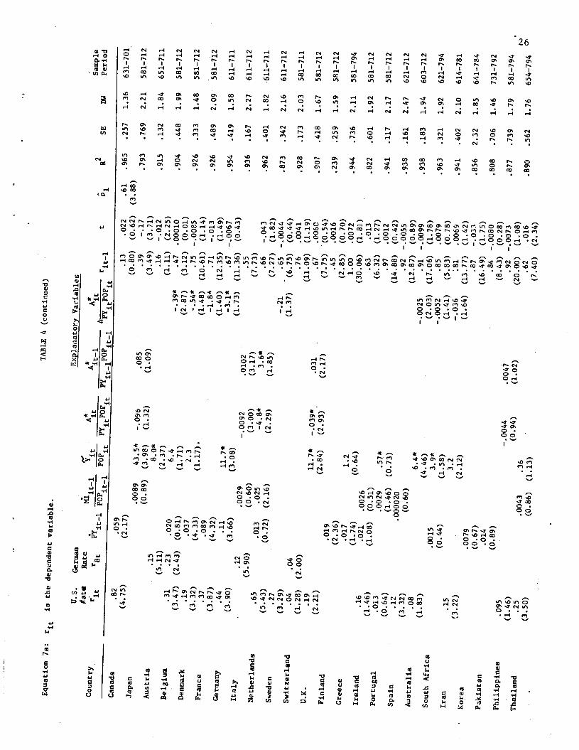
Equation la: rj is the dependent variable.

TABLE 4 (continued)

atory V

ariables

atg

Rate

Cou

ntry

r

iti

it

A*

A

___

it ti

it

It

r8

*ft_l

po1

PY

_1P

0Pj

rii

2

Sample

R

SE

DW

Period

Canada

.82

.059

(4.75)

(2.17)

.13

.022

.61

.965

.257

1.

36

631—701

Japan

(0.80)

(0.62)

(3.88)

.0089

43.5*

—.09o

.085

.39

.17

.793

.769

2.21

581—712

Austria

(0.89)

(3.98)

(1.32)

(1.09)

(3.49)

(3.71)

.15

8.0*

(5.11)

(2.37)

.16

—.012

.915

.132

1.84

651—711

Belgium

.31

.23

.020

6.4

(1.11)

(2.25)

(3.47)

(2.43)

(0.81)

(1.71)

_39*

.47

.00010

.904

.448

1.99

581—712

Denmark

.19

.037

2.3

(2.87)

(3.12)

(0.01)

(3.32)

(4.33)

(1.17).

_54*

.75 —.oo&s

.926

.333

1.48

581—712

France

.37

.089

(1.48)

(10.61)

(1.14)

(3.87)

(4.32)

_1.8*

.71

—.013

.926

.489

2.09

581—712

Germany

.44

.11

11.7*

(1.40)

(12.35)

(1.49)

(3.90)

(3.66)

(3.08)

_3.1*

.67 —.0067

.954

.419

1.58

611—711

Italy

.12

.0029

—.0092

.0102

(1.73)

(11.36)

(0.43)

.55

.936

.167

2.27

611—712

(5.90)

(0.60)

(3.00)

(3.17)

(7.73)

Nether1ds

.65

.013

.025

-4.8*

3.6*

.66

—.043

.962

.401

1.82

611—711

(5.43)

(0.72)

(2.16)

(2.29)

(1.85)

(7.27)

(1.82)

Sweden

.27

(3.29)

—.21

.65 —.0044

.873

.342

2.16

611—712

Switzerland

.04

.04

(1.37)

(6.75)

(0.64)

(1.28)

(2.00)

.76

.0041

.928

.173

2.03

581—711

U.K.

.19

(11.09)

(1.19)

11.7*

—.039*

.031

.67

.0060

.907

.418

1.67

581—712

(2.21)

Finland

(2.84)

(2.93)

(2.17)

(7.75)

(0.54)

.019

Greece

(2.36)

.45

.0016

.239

.259

1.59

581—712

.017

1.2

(2.85)

(0.70)

Ireland

.16

(1.74)

(0.64)

1.00

.0072

.944

.736

2.11

581—794

.021

.0026

(30.06)

(1.81)

(1.46)

(1.08)

(0.51)

.63

.013

.822

.601

1.92

581—712

Portugal

.013

.0029

•57*

(6.32)

(1.27)

(0.64)

(1.46)

(0.73)

.97

.0012

.941

.117

2.17

581—712

Spain

.12

.000020

(14.88)

(0.42)

(3.32)

(0.60)

.92 —.0055

.933

.161

2.47

621—712

Australia

.08

6.4*

(12.87)

(0.89)

(1.83)

(4 46)

—.0025

.91 —.0099

.938

.183

1.94

603—712

South Africa

.0015

39*

(2.03) (1

7.06

) (1

.78)

(0

.44)

(1.58)

—.0052

.85

.0079

.963

.321

1.92

621—794

Iran

.15

3.2

(1.41)

(5.83)

(0.78)

(3.22)

2 12)

—.0

36

81

.006

9 .941

.402

2.10

614—781

Korea

t .0

079

(1.64)

(13.77)

(1.42)

(0.67)

.87

—.033

.856

2.

32

1.85

641—784

Pakistan

.014

(16.49)

(1.75)

Philippines

.095

(0.89)

.84 —.0080

.808

.706

1.46

731—792

(8.43)

(0.28)

(1.46)

—.0044

.0047

.92 —.0073

.877

.739

1.79

581—794

Thailand

.25

(0.94)

(1.02)

(20.00)

(1.08)

0043

.36

(3.50)

(0.86)

(1.13)

.62

.016

.890

.562

1.76

654—794

°'

(7.4

0)

(2.34)

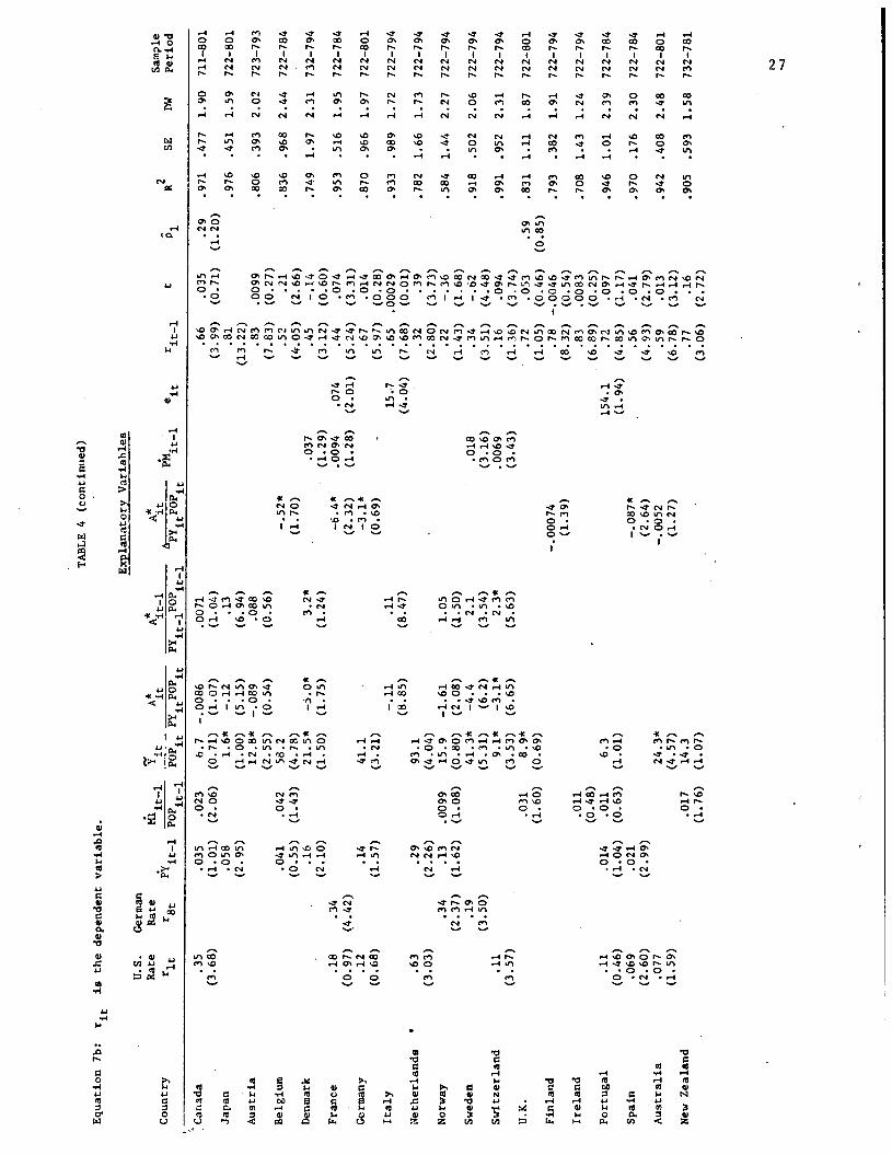
TABLE 4 (continued)

Equation 7b: nt is the dependent variable.

Explanatory Variables

U.S.

German

Rat

e R

ate

A

A*

A*

Sample

_____

t it

jtl

it

Country

ri

rBt

it—i 01'it1

PYitlPiil

PM

e

r

t

p1

R2

SE

OW

Period

it—i

it

it—i

Canada

.35

.035

.023

6.7

—.0086

.0071

.66

.035

.29

.971

.477 1.90

711—801

(3.68)

(1.01)

(2.06)

(0.71)

(1.07)

(1.04)

(3.99)

(0.71)

(1.20)

Japan

.058

1.6*

—.12

.13

.81

.976

.451 1.59

722—80].

(2.95)

(1.00)

(5.15)

(6.94)

(13.22)

Austria

12.8* —.089

.088

.83

.0099

.806

.393 2.02

723—793

(2.55)

(0.54)

(0.56)

(7.83)

(0.27)

Belgium

.041

.042

58.2

_.52*

.52

.21

.836 .968 2.44 722—784

(0.55)

(1.43)

(4.78)

(1.70)

(4.05)

(2.66)

Denmark

.16

21.5*

.i.0*

3.2*

-

.037

.45

—.14

.749 1.97 2.31 732—794

(2.10)

(1.50)

(1.75)

(1.24)

(1.29)

(3.12)

(0.60)

France

.18

.34

_6.4*

.0094

.074

.44

.074

.953

.516

1.95 722—784

(0.97)

(4.42)

(2.32)

(1.28)

(2.01)

(5.24)

(3.31)

Germany

.12

.14

41.1

_3.l*

.67

.014

.870

.966

1.97 722—801

(0.68)

(1.57)

(3.21)

(0.69)

(5.97)

(0.28)

Italy

—.11

.11

15.7

.65

.00029

.933 .989 1.72 722—794

(8.85)

(8.47)

(4.04)

(7.68)

(0.01)

Netherlands

•

.63

.29

93.1

.32

.39

.782 1.66 1.73 722—794

(3.03)

(2.26)

(4.04)

(2.80)

(3.73)

Norway

.34

.13

.0099

15.9

—1.61

1.05

.22

—.36

.584 1.44 2.27 722—794

(2.37)

(1.62)

(1.08)

(0.80)

(2.08)

(1.50)

(1.43)

(1.68)

Sweden

.19

41.3*

—4.4

2.1

.018

.34

—.62

.918

.502

2.06 722—794

(3.50)

(5.31)

(6.2)

(3.54)

(3.16)

(3.51)

(4.48)

Switzerland

.11

9.1*

3.1*

2.3*

.0069

.16

.094

.991

.952 2.31 722794

(3.57)

(3.53)

(6.65)

(5.63)

(3.43)

(1.36)

(3.74)

U.K.

.031

8.9*

.72

.053

.59

.831

1.11 1.87 722—801

(1.60)

(0.69)

(1.05)

(0.46)

(0.85)

Finland

—.00074

.78 —.0046

.793 .382 1.91 722—794

(1.39)

(8.32)

(0.54)

Ireland

.011

.83

.0083

.708 1.43 1.24 722—794

(0.48)

.

(6.8

9)

(0.25)

Portugal

.11

.014

.011

6.3

154.1

.72

.097

.946 1.01 2.39 722—784

(0.46)

(1.04)

(0.63)

(1.01)

(1.94)

(4.85)

(1.17)

Spain

.069

.021

_.087*

.56

.041

.970 .176 2.30

722—784

(2.60)

(2.99)

(2.64)

(4.93)

(2.79)

Australia

.077

24.3*

—.0052

.59

.013

.942 .408 2.48 722—801

(1.59)

(4.57)

(1.27)

(6.78)

(3.12)

New Zealand

.017

14.3

.77

.16

.905 .593 1.58 732—781

(1.76)

(1.07)

(3.06)

(2.72)

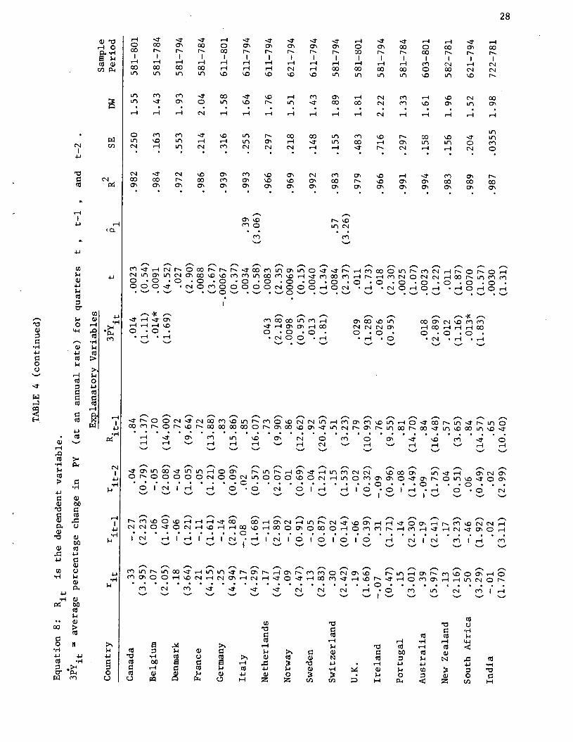
TABLE 4 (continued)

Equation 8:

is the dependent variable.

= av

erag

e percentage change in

PY

(at an annual rate) for quarters

t

,

t—l

,

and

t—2

Explanatory Variables

2

Sample

Country

r.

r.1

r.2

R.ti

t

R

SE

DW

Period

Canada

.33

—.27

.04

.84

.014

.0023

.982

.250

1.55

581—801

(3.95)

(2.23)

(0.79)

(11.37)

(1.11)

(0.54)

Belgium

.07

.06

—.05

.70

.014*

.0091

.984

.163

1.43

581—784

(2.05)

(1.40)

(2.08)

(14.00)

(1.69)

(4.52)

Denmark

.18

—.06

—.04

.72

.027

.972

.553

1.93

581—794

(3.64)

(1.21)

(1.05)

(9.64)

(2.90)

France

.21

—.11

.05

.72

.0088

.986

.214

2.04

581—784

(4.15)

(1.61)

(1.21)

(13.88)

(3.67)

Germany

.25

—.14

.00

.83

—.00067

.939

.316

1.58

611—801

(4.94)

(2.18)

(0.09)

(15.86)

(0.37)

Italy

.17

—.08

.02

.85

.0034

.39

.993

.255

1.64

611—794

(4.29)

(1.68)

(0.57)

(16.07)

(0.58)

(3.06)

Netherlands

.17

—.11

.05

.73

.043

.0083

.966

.297

1.76

611—794

(4.41)

(2.89)

(2.07)

(9.90)

(2.18)

(2.35)

Norway

.09

—.02

.01

.86

.0098

.00069

.969

.218

1.51

621—794

(2.47)

(0.91)

(0.69)

(12.62)

(0.95)

(0.15)

Sweden

.13

—.05

—.04

.92

.013

.0040

.992

.148

1.43

611—794

(2.83)

(0.87)

(1.21)

(20.45)

(1.81)

(1.34)

Switzerland

.30

—.02

.15

.51

.0084

.57

.983

.155

1.89

581—794

(2.42)

(0.14)

(1.53)

(3.23)

(2.37)

(3.26)

U.K.

.19

—.06

—.02

.79

.029

.011

.979

.483

1.81

581—801

(1.66)

(0.39)

(0.32)

(10.93)

(1.28)

(1.73)

Ireland

—.07

.31

—.09

.76

.026

.018

.966

.716

2.22

581—794

(0.47)

(1.71)

(0.96)

(9.55)

(0.95)

(2.30)

Portugal

.15

.14

—.08

.81

.0025

.991

.297

1.33

581—784

(3.01)

(2.30)

(1.49)

(14.70)

(1.07)

Australia

.39

—.19

—.09

.84

.018

.0023

.994

.158

1.61

603—801

(5.97)

(2.41)

(1.75)

(16.48)

(2.89)

(1.22)

New Zealand

13

.17

.04

.57

.012

.011

.983

.156

1.96

582—781

(2.16)

(3.23)

(0.51)

(3.65)

(1.16)

(1.87)

South Africa

.50

—.46

.06

.84

.013*

.0070

.989

.204

1.52

621—794

(3.29)

(1.92)

(0.49)

(14.57)

(1.83)

(1.57)

India

—.01

.02

.02

.65

.0030

.987

.0355

1.98

722—781

(1.70)

(3.11)

(2.99)

(10.40)

(1.31)

TA

BL

E

4 (c

ontin

ued)

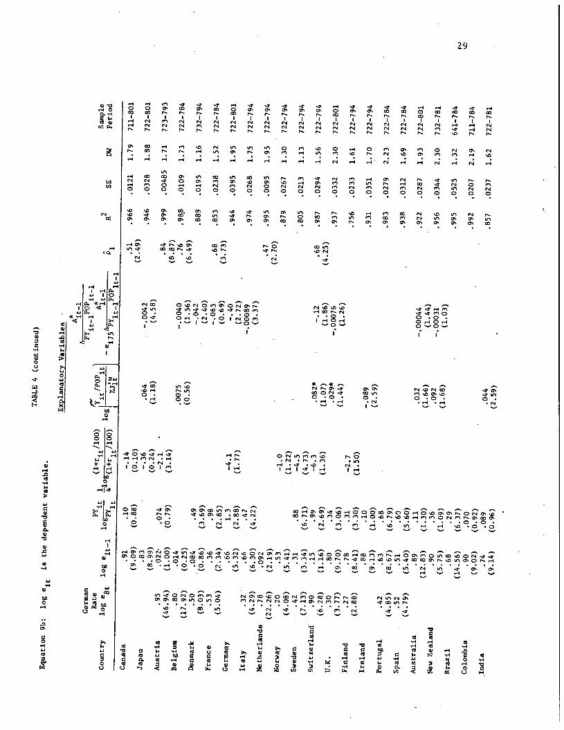
Equation 9b:

log e1

is the dependent variable.

natory Va

riables

A

German

Rat

e it

1

(l+r1/lOO)

•t'ft

A1

2

Sample

Country

log e8

log ejt_l 1og— 4lO&+/l00) 1og

U

—

e175

A

______

R

SE

DW

Period

Canada

.91

.10

—.14

.51

.966

.0121

1.79

711—801

(9.09)

(0.88)

(0.10)

(2.49)

Japan

.83

—.36

.064

—.0042

.946

.0328

1.88

722—801

(8.99)

(0.24)

(1.18)

(4.58)

Austria

.95

.022

.074

—2.1

.84

.999

.00485

1.71

723—793

(46.94)

(1.00)

(0.79)

(3.14)

(8.87)

Belgium

.80

.014

.0075

—.0040

.76

.988

.0109

1.73

722—784

(17.92)

(0.25)

(0.56)

(1.56)

(6.49)

Denmark

.50

.084

.49

—.042

.889

.0195

1.16

732—794

(8.03)

(0.86)

(3.69)

(2.40)

France

.53

.36

.98

—.063

.68

.853

.0238

1.52

722—784

(5.04)

(2.34)

(2.85)

(0.69)

(3.73)

Germany

.66

1.3

—4.1

—.40

.944

.0395

1.95

722—801

(5.32)

(2.88)

(1.77)

(2.72)

Italy

.32

.66

.47

—.00089

.974

.0268

1.75

722—794

(4.29)

(6.30)

(4.22)

(3.37)

Netherlands

.78

.092

.47

.995

.0095

1.95

722—794

(22.26)

(2.19)

(2.70)

Norway

.20

.53

—1.0

.879

.0267

1.30

722—794

(4.08)

(5.41)

(1.22)

Sweden

.42

.31

.88

—4.5

.805

.0213

1.13

722—794

(7.13)

(3.34)

(6.71)

(4.73)

Switzerland

.90

.15

.99

—6.3

.082*

—.12

.68

.987

.0294

1.56

722—794

(6.28)

(1.16)

(2.69)

(1.36)

(1.07)

(1.86)

(4.25)

U.K.

.30

.80

.34

.029*

—.00076

.937

.0332

2.30

722—801

(3.77)

(9.70)

(3.06)

(1.44)

(1.26)

Finland

.27

.78

.31

—2.7

.756

.0233

1.61

722—794

(2.88)

(8.41)

(3.30)

(1.50)

Ireland

.88

.10

—.089

.931

.0351

1.70

722—794

(9.13)

(1.00)

(2.59)

Portugal

.42

.63

.68

.983

.0279

2.23

722—784

(4.85)

(8.67)

(6.79)

Spain

.52

.51

.60

.938

.0312

1.69

722—784

(4.79)

(5.40)

(5.60)

Australia

.89

.11

.032

—.00044

.922

.0287

1.93

722—801

(12.83)

(1.30)

(1.66)

(1.44)

New Zealand

.90

.36

.092

—.00031

.956

.0344

2.30

732—781

(5.75)

(1.09)

(1.68)

(1.03)

Brazil

.68

.29

.995

.0525

1.32

641—784

(14.56)

(6.37)

Colombia

.90

.070

.992

.0207

2.19

711—784

(9.02)

(0.92)

-

Indi

a .74

.089

.044

.857

.0237

1.62

722—781

(9.14)

(0.96)

(2.59)

30

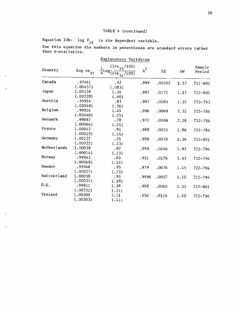
TABLE 4 (continued)

Equation lOb: log F.t is the dependent variable.

For this equation the numbers in parentheses are standard errors ratherthan t—statistjcs.

planatory Variables

SampleSE DW PeriodCountry log ee

it1104

jt'l+ri/l00)

R2

Canada .97461

(.00457)

.92

(.083).999 .00202 1.57 711—801

Japan 1.00128

(.00228)

1.34

(.40)

.987 .0172 1.17 722—801

Austria .99954

(.00048)

.83

(.36)

.997 .0083 1.35 723—793

Belgium .99924

(.00040)

1.45

(.25)

.996 .0069 2.32 722—784

Denmark .99887

(.00064)

.78

(.24)

.972 .0108 2.28 732—794

France 1.00042

(.00019)

.91

(.14)

.998 .0033 1.86 722—784

Germany 1.00137

(.00025)

.25

(.23)

.998 .0078 1.36 722—801

Netherlands 1.00038

(.00014)

.82

(.13)

.999 .0046 1.92 722—794

Norway .99843

(.00068)

.65

(.52)

.951 .0176 2.43 722—794

Sweden .99946

(.00027).95

(.23)

.979 .0076 1.45 722—794

Switzerland 1.00058

(.00032)

.93

(.18)

.9996 .0057 1.25 722—794

U.K. .99911

(.00232)

1.38

(.21)

.998 .0060 1.33 722—801

Finland 1.00509

(.00203)

2.11

(.41)

.950 .0116 1.50 722—794

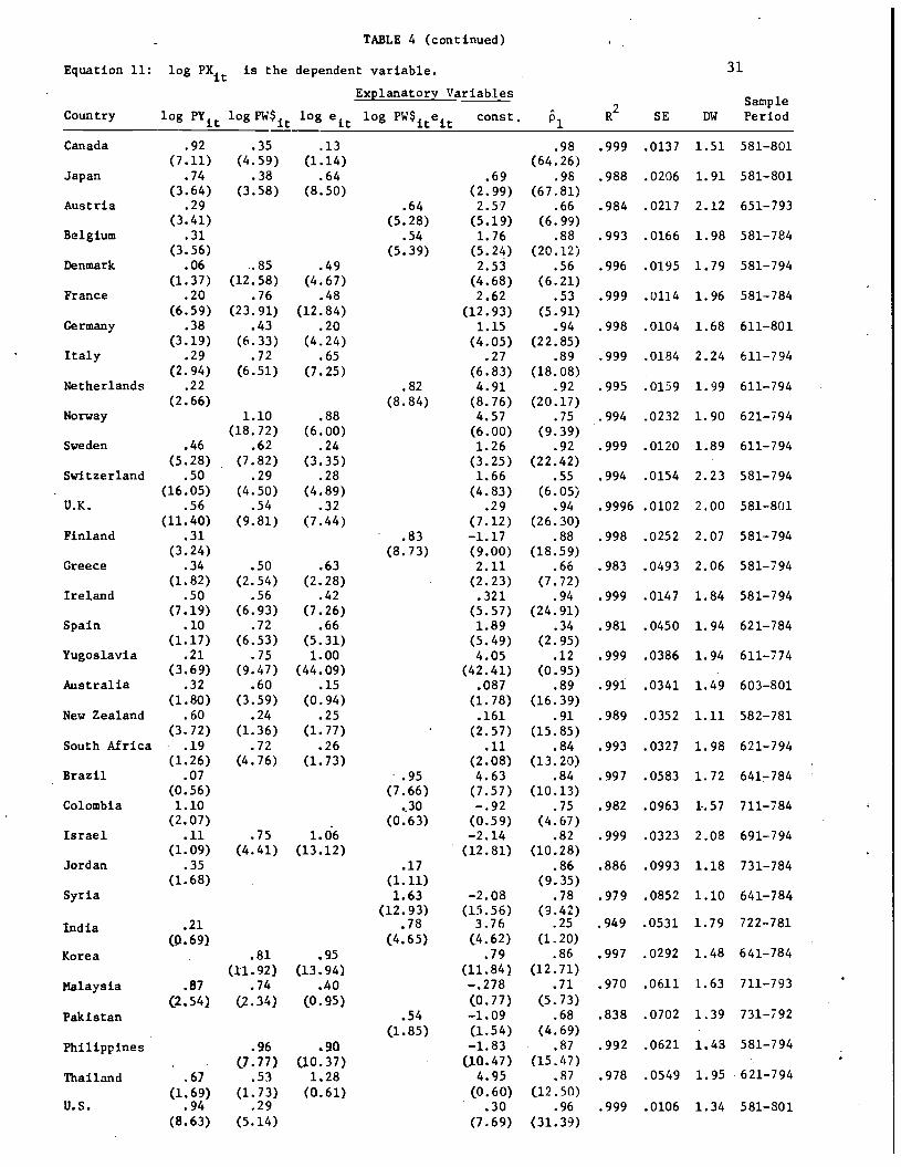
TABLE 4 (continued)

Equation 11: log PX is the dependent variable. 31

Explanatory Variables2 Sample

Country log PY1 logPW$i log ej log PW$jej Const. R SE DW Period

Canada .92 .35 .13 .98 .999 .0137 1.51 581—801(7.11) (4.59) (1.14) (64.26)

Japan .74 .38 .64 .69 .98 .988 .0206 1.91 581—801(3.64) (3.58) (8.50) (2.99) (67.81)

Austria .29 .64 2.57 .66 .984 .0217 2.12 651—793(3.41) (5.28) (5.19) (6.99)

Belgium .31 .54 1.76 .88 .993 .0166 1.98 581—784(3.56) (5.39) (5.24) (20.12)

Denmark .06 .. 85 .49 2.53 .56 .996 .0195 1.79 581—794(1.37) (12.58) (4.67) (4.68) (6.21)

France .20 .76 .48 2.62 .53 .999 .0114 1.96 581—784(6.59) (23.91) (12.84) (12.93) (5.91)

Germany .38 .43 .20 1.15 .94 .998 .0104 1.68 611—801(3.19) (6.33) (4.24) (4.05) (22.85)

Italy .29 .72 .65 .27 .89 .999 .0184 2.24 611—794(2.94) (6.51) (7.25) (6.83) (18.08)

Netherlands .22 .82 4.91 .92 .995 .0159 1.99 611—794(2.66) (8.84) (8.76) (20.17)

Norway 1.10 .88 4.57 .75 .994 .0232 1.90 621—794(18.72) (6.00) (6.00) (9.39)

Sweden .46 .62 .24 1.26 .92 .999 .0120 1.89 611—794(5.28) (7.82) (3.35) (3.25) (22.42)

Switzerland .50 .29 .28 1.66 .55 .994 .0154 2.23 581—794(16.05) (4.50) (4.89) (4.83) (6.05)

U.K. .56 .54 .32 .29 .94 .9996 .0102 2.00 581—801(11.40) (9.81) (7.44) (7.12) (26.30)

Finland .31 .83 —1.17 .88 .998 .0252 2.07 581—794(3.24) (8.73) (9.00) (18.59)

Greece .34 .50 .63 2.11 .66 .983 .0493 2.06 581—794(1.82) (2.54) (2.28) (2.23) (7.72)

Ireland .50 .56 .42 .321 .94 .999 .0147 1.84 581—794(7.19) (6.93) (7.26) (5.57) (24.91)

Spain .10 .72 .66 1.89 .34 .981 .0450 1.94 621—784(1.17) (6.53) (5.31) (5.49) (2.95)

Yugoslavia .21 .75 1.00 4.05 .12 .999 .0386 1.94 611—774(3.69) (9.47) (44.09) (42.41) (0.95)

Anstralia .32 .60 .15 .087 .89 .991 .0341 1.49 603—801(1.80) (3.59) (0.94) (1.78) (16.39)

New Zealand .60 .24 .25 .161 .91 .989 .0352 1.11 582—781(3.72) (1.36) (1.77) (2.57) (15.85)

South Africa .19 .72 .26 .11 .84 .993 .0327 1.98 621—794(1.26) (4.76) (1.73) (2.08) (13.20)

Brazil .07 .95 4.63 .84 .997 .0583 1.72 641—784(0.56) (7.66) (7.57) (10.13)

Colombia 1.10 .30 —.92 .75 .982 .0963 1.57 711—784(2.07) . (0.63) (0.59) (4.67)

Israel .11 .75 1.06 —2.14 .82 .999 .0323 2.08 691—794(1.09) (4.41) (13.12) (12.81) (10.28)

Jordan .35 .17 .86 .886 .0993 1.18 731—784(1.68) (1.11) (9.35)

Syria 1.63 —2.08 .78 .979 .0852 1.10 641—784(12.93) (15.56) (9.42)

India .21 .78 3.76 .25 .949 .0531 1.79 722—781

(0.69) (4.65) (4.62) (1.20)

Korea .81 .95 .79 .86 .997 .0292 1.48 641—784(11.92) 0.3.94) (11.84) (12.71)

Malaysia .87 .74 .40 —.278 .71 .970 .0611 1.63 711—793

(2.54) (2.34) (0.95) (0.77) (5.73)Pakistan .54 —1.09 .68 .838 .0702 1.39 731—792

(1.85) (1.54) (4.69)

Philippines .96 .90 —1.83 .87 .992 .0621 1.43 581—794

(7.77) (10.37) (10.47) (15.47)Thailand .67 .53 1.28 4.95 .87 .978 .0549 1.95 621—794

(1.69) (1.73) (0.61) (0.60) (12.50)U.S. .94 .29 .30 .96 .999 .0106 1.34 581—301

(8.63) (5.14) (7.69) (31.39)

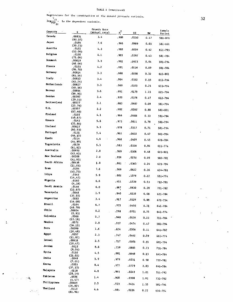
TA8LE 4 (contlned)

Rercito.s for tie constructin 01 tIo dcfl.IFl(l prssure v.rldb1.lng1— is the dependent variable.it

32

Count tGrowth Rate(annual rate) 2

R SESample

DVCanada .00831 3.4

(80. 57).986 .0250 0.17 581—801

Japan .0184 7.6(50.23)

.966 .0889 0.03 581—101

Austria .0105 4.3(53. 06)

.982 .0259 0.42 651—793

Belgium .oioo 4.1(75.06)

.985 .0297 0.43 581—784

Denmark .00819 3.3(46. 06)

.961 .0423 0.81 581—794

Prance .0103

(96.70).99]. .0236 0.09 581—784

Germany .00814 3.3(61.56)

.980 .0258 0.32 611—801

Italy .00833 3.4(45.24)

.964 .0352 0.15 611—794

Netherlands .00827 3.3(48.56)

.969 .0325 0.25 611—794

Norway .00884 3.6(86.90)

.991 .0179 1.23 621—794

Sweden .00585

(29.53).920 .0378 0.27 612—794

Switzerland .00527

(25. 76)

2.1 .883 .0487 0.09 581—794

U.K. .00557

(67. 40).982 .0200 0.88 581—801

Finland .0102 4.1(49.67)

.966 .0488 0.33 581—794

Greece .0143(55.80)

.973 .0611 0.78 581—794

Ireland .00812 3.3(60.93)

.978 .0317 0.71 581—794

Portugal .0131 5.4(46.15)

.962 .0632 0.47 581—784

Spain .0114 4.6(44.99)

.968 .0409 0.45 621—784

Yugoslavia .0129 5.3(61.82)

.963 .0338 0.84 611—774

Australia .00690 2.8(45. 63)

.969 .0306 0.48 603—801

New Zealand .00508 2.0.

.

South Africa

Iran

Libya

Nigeria

Saudi Arabia

Venezuela•

Argentina

Brazil

Chile

(41.85).00436

(21.05).0184

(45.73).0145

(14.47).0160

(4.39).0146

(12.97).0048

(32.55).ooas

(16.08).0164(48. 79).00054

1.8

7.6

5.9

6.6

6.0

1.9

3.4

6.7

0.2

.956 .025)

.861 .0365

.969 .0622

.802 .1079

.411 .1539

.867 .0430

.940 .0239

.917 .0329

.975 .0450

0.09

0.24

0.16

0.22

0.53

0.28

0.08

0.88

0.21

582—781

621—794

614—781

651—774

712—781

721—782

621—784

671—754

641—784

Colombia

Mexico

(0.93).0068

(22.18).0072

2.7

2.9

.298 .0701

.940 .0159

0.75

0.23

641—774

711—784

Peru

Egypt

(36. 15)

.00399

(16.48).0057

1.6

2.3

.937 .0474

.824 .0308

0.47

0.11

581—794

641—782

Israel

Jordan

Syria

(11.87).00631(10.47).0212

(8.04).0110

2.5

8.8

4.5

.747 .0462

.717 .0505

.73 .0885

0.09

0.55

0.73

661—774

691—794

731—784

.

India(21.02).0048 1.9

.881 .0698 0.13 641—784

Korea(7.01).0203 8.4

.979 .0231 0.98 722—781

Malaysia(37. 33).0118 4.8

.977 .0729 2.83 641—784

(28.19).961 .0249 1.01 711—793

. •k Pakistan

Philippines

.0036(4.47)

.00609

1.4

2.5

.908 .0308 1.81 731—792

Thailand(34.82).0113 4.6

.933 .0416 1.35 581—794

.985 .0226 0.22 654—794

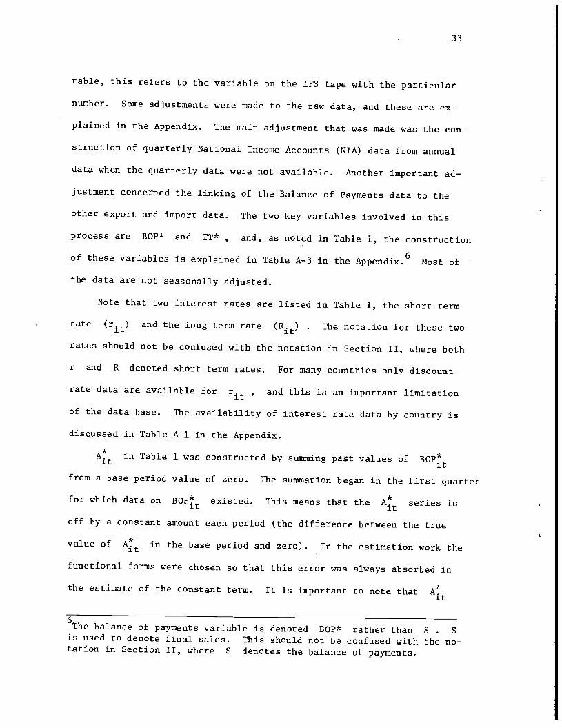
33

table, this refers to the variable on the IFS tape with the particular

number. Some adjustments were made to the raw data, and these are ex-

plained in the Appendix. The main adjustment that was made was the con-

struction of quarterly National Income Accounts (NIA) data from annual

data when the quarterly data were not available. Another important ad-

justment concerned the linking of the Balance of Payments data to the

other export and import data. The two key variables involved in this

process are BOP* and TT* , and, as noted in Table 1, the construction

of these variables is explained in Table A—3 in the Appendix.6 Most of

the data are not seasonally adjusted.

Note that two interest rates are listed in Table 1, the short term

rate (r.) and the long term rate (R) . The notation for these two

rates should not be confused with the notation in Section II, where both

r and R denoted short term rates. For many countries only discount

rate data are available for r. , and this is an important limitation

of the data base. The availability of interest rate data by country is

discussed in Table A—i in the Appendix.

in Table 1 was constructed by summing past values of BOPfrom a base period value of zero. The summation began in the first quarter

for which data on BOP existed. This means that the A series isit it

off by a constant amount each period (the difference between the true

value of At in the base period and zero). In the estimation work the

functional forms were chosen so that this error was always absorbed in

the estimate of the constant term. It is important to note that

6The balance of payments variable is denoted BOP* rather than S . Sis used to denote final sales. This should not be confused with the no-tation in Section II, where S denotes the balance of payments.

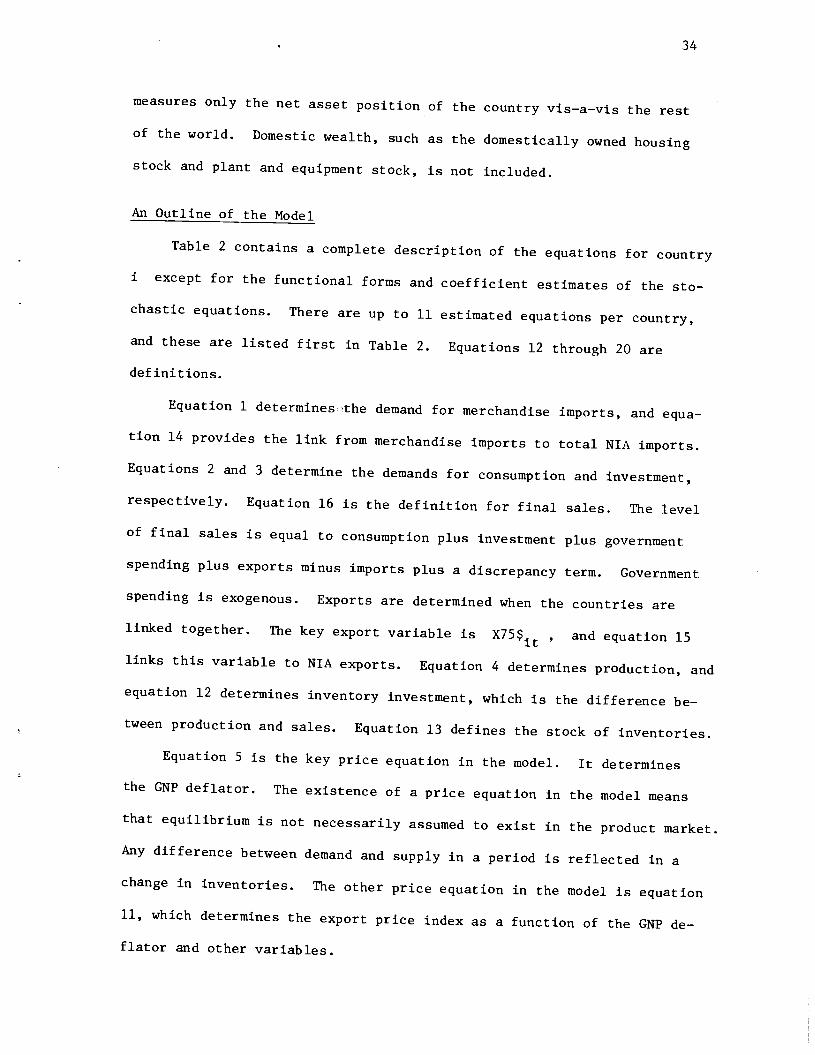
34

measures only the net asset position of the country vis—a—vis the rest

of the world. Domestic wealth, such as the domestically owned housing

stock and plant and equipment stock, is not included.

An Outline of the Model

Table 2 contains a complete description of the equations for country

i except for the functional forms and coefficient estimates of the sto-

chastic equations. There are up to 11 estimated equations per country,

and these are listed first in Table 2. Equations 12 through 20 are

definitions.

Equation 1 determines 'the demand for merchandise imports, and equa-

tion 14 provides the link from merchandise imports to total NIA imports.

Equations 2 and 3 determine the demands for consumption and investment,

respectively. Equation 16 is the definition for final sales. The level

of final sales is equal to consumption plus investment plus government

spending plus exports minus imports plus a discrepancy term. Government

spending is exogenous. Exports are determined when the countries are

linked together. The key export variable is X75$. , and equation 15

links this variable to NIA exports. Equation 4 determines production, and

equation 12 determines inventory investment, which is the difference be-

tween production and sales. Equation 13 defines the stock of inventories.

Equation 5 is the key price equation in the model. It determines

the GNP deflator. The existence of a price equation in the model means

that equilibrium is not necessarily assumed to exist in the product market.

Any difference between demand and supply in a period is reflected in a

change in inventories. The other price equation in the model is equation

11, which determines the export price index as a function of the GNP de-

flator and other variables.

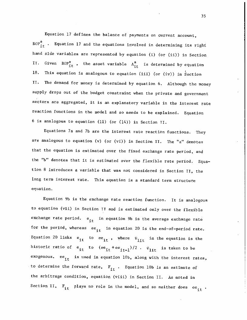
35

Equation 17 defines the balance of payments on current account,

B0Pt . Equation 17 and the equations involved in determining its right

hand side variables are represented by equation (i) (or (ii)) in Section

II. Given B0Pt , the asset variable At is determined by equation

18. This equation is analogous to equation (iii) (or (iv)) in Section

II. The demand for money is determined by equation 6. Although the money

supply drops out of the budget constraint when the private and government

sectors are aggregated, it is an explanatory variable in the interest rate

reaction functions in the model and so needs to be explained. Equation

6 is analogous to equation (11) (or (14)) in Section II.

Equations 7a and 7b are the interest rate reaction functions. They

are analogous to equation Cv) (or (vi)) in Section II. The "a" denotes

that the equation is estimated over the fixed exchange rate period, and

the "b" denotes that it is estimated over the flexible rate period. Equa-

tion 8 introduces a variable that was not considered in Section II, the

long term interest rate. This equation is a standard term structure

equation.

Equation 9b is the exchange rate reaction function. It is analogous

to equation (vii) in Section II and is estimated only over the flexible

exchange rate period. e± in equation 9b is the average exchange rate

for the period, whereas ee. in equation 20 is the end—of—period rate.

Equation 20 links eit to ee. , where 1it in the equation is the

historic ratio of e. to (ee. +ee. )/2 . . is taken to beit it it—l lit

exogenous. ee. is used in equation lOb, along with the interest rates,

to determine the forward rate, Fit . Equation lOb is an estimate of

the arbitrage condition, equation (viii) in Section II. As noted in

Section II, F.t plays no role in the model, and so neither does ee.

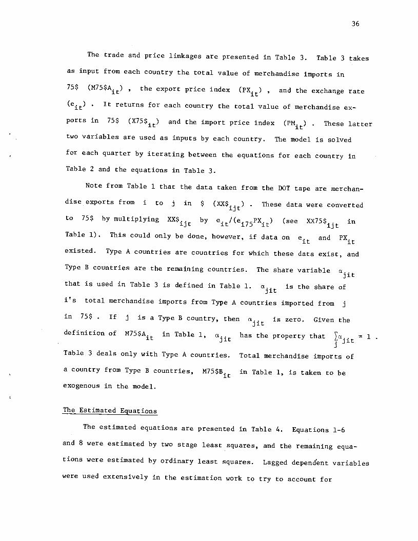
36

The trade and price linkages are presented in Table 3. Table 3 takes

as input from each country the total value of merchandise imports in

75$ (N75$A.) , the export price index (Px.) , and the exchange rate

(e.) . It returns for each country the total value of merchandise ex-

ports in 75$ (X75$.) and the import price index (PM.t) . These latter

two variables are used as inputs by each country. The model is solved

for each quarter by iterating between the equations for each country in

Table 2 and the equations in Table 3.

Note from Table 1 that the data taken from the DOT tape are merchan-

dise exports from i to j in $ (XX$..) . These data were converted

to 75$ by multiplying XX$.. by e./(ej75PX.) (see 75ijt in

Table 1). This could only be done, however, if data on e. and PXexisted. Type A countries are countries for which these data exist, and

Type B countries are the remaining countries. The share variable

that is used in Table 3 is defined in Table 1. a. is the share of'lit

i's total merchandise imports from Type A countries imported from j

in 75$ . If j is a Type B country, then is zero. Given the

definition of M75$A1 in Table jit has the property that cti

Table 3 deals only with Type A countries. Total merchandise imports of

a country from Type B countries, M75$B. in Table 1, is taken to be

exogenous in the model.

The Estimated Equations

The estimated equations are presented in Table 4. Equations 1—6

and 8 were estimated by two stage least squares, and the remaining equa-

tions were estimated by ordinary least squares. Lagged dependent variables

were used extensively in the estimation work to try to account for

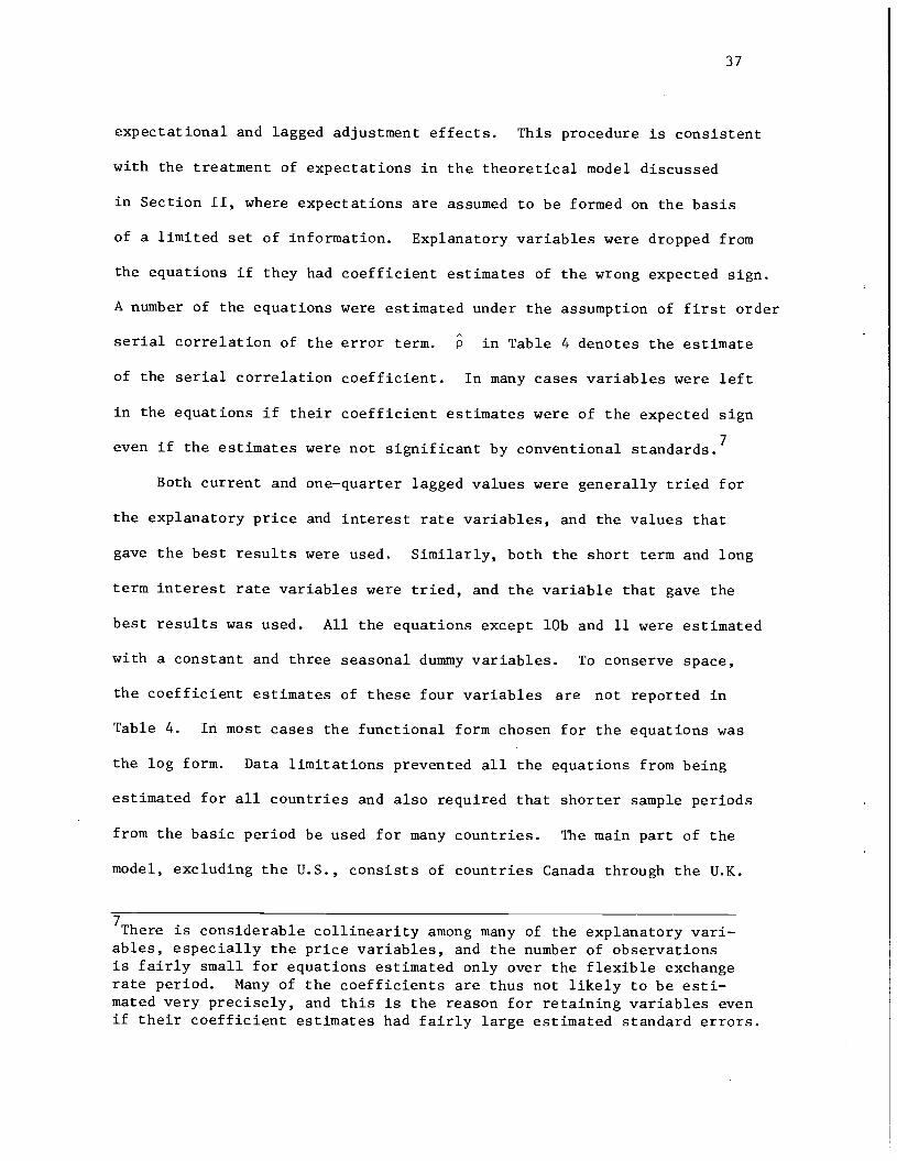
37

expectational and lagged adjustment effects. This procedure is consistent

with the treatment of expectations in the theoretical model discussed

in Section II, where expectations are assumed to be formed on the basis

of a limited set of information. Explanatory variables were dropped from

the equations if they had coefficient estimates of the wrong expected sign.

A number of the equations were estimated under the assumption of first order

serial correlation of the error term. in Table 4 denotes the estimate

of the serial correlation coefficient. In many cases variables were left

in the equations if their coefficient estimates were of the expected sign

even if the estimates were not significant by conventional standards.7

Both current and one—quarter lagged values were generally tried for

the explanatory price and interest rate variables, and the values that

gave the best results were used. Similarly, both the short term and long

term interest rate variables were tried, and the variable that gave the

best results was used. All the equations except lOb and 11 were estimated

with a constant and three seasonal dummy variables. To conserve space,

the coefficient estimates of these four variables are not reported in

Table 4. In most cases the functional form chosen for the equations was

the log form. Data limitations prevented all the equations from being

estimated for all countries and also required that shorter sample periods

from the basic period be used for many countries. The main part of the

model, excluding the U.S., consists of countries Canada through the U.K.

7There is considerable collinearity among many of the explanatory vari-ables, especially the price variables, and the number of observationsis fairly small for equations estimated only over the flexible exchangerate period. Many of the coefficients are thus not likely to be esti-mated very precisely, and this is the reason for retaining variables evenif their coefficient estimates had fairly large estimated standard errors.

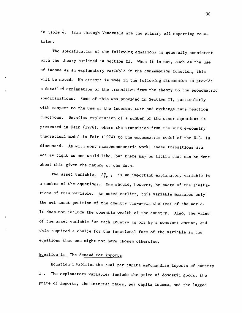
38

in Table 4. Iran through Venezuela are the primary oil exporting coun-

tries.

The specification of the following equations is generally consistent

with the theory outlined in Section II. When it is not, such as the use

of income as an explanatory variable in the consumption function, this

will be noted. No attempt is made in the following discussion to provide

a detailed explanation of the transition from the theory to the econometric

specifications. Some of this was provided in Section II, particularly

with respect to the use of the interest rate and exchange rate reaction

functions. Detailed explanation of a number of the other equations is

presented in Fair (1976), where the transition from the single—country

theoretical model in Fair (1974) to the econometric model of the U.S. is

discussed. As with most macroeconometrjc work, these transitions are

not as tight as one would like, but there may be little that can be done

about this given the nature of the data.

The asset variable,, is an important explanatory variable in

a number of the equations. One should, however, be aware of the limita-

tions of this variable. As noted earlier, this variable measures only

the net asset position of the country vis—a—vis the rest of the world.

It does not include the domestic wealth of the country. Also, the value

of the asset variable for each country is off by a constant amount, and

this required a choice for the functional form of the variable in the

equations that one might not have chosen otherwise.

Equation 1: The demand for imports

Equation 1 explains the real per capita merchandise imports of country

I . The explanatory variables include the price of domestic goods, the

price of imports, the interest rates, per capita Income, and the lagged

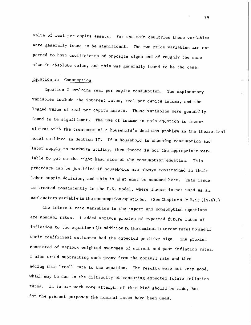
39

value of real per capita assets. For the main countries these variables

were generally found to be significant. The two price variables are ex-

pected to have coefficients of opposite signs and of roughly the same

size in absolute value, and this was generally found to be the case.

uation 2: Consumption

Equation 2 explains real per capita consumption. The explanatory

variables include the interest rates, real per capita income, and the

lagged value of real per capita assets. These variables were generally

found to be significant. The use of income in this equation is incon-

sistent with the treatment of a household's decision problem in the theoretical

model outlined in Section II. If a household is choosing consumption and

labor supply to maximize utility, then income is not the appropriate var-

iable to put on the right hand side of the consumption equation. This

procedure can be justified if households are always constrained in their

labor supply decision, and this is what must be assumed here. This issue

is treated consistently in the U.S. model, where income is not used as an

expianatoryvariabie in the consumption equations. (See Chapter 4 in Fair (1976).)

The interest rate variables in the import and consumption equations

are nominal rates. I added various proxies of expected future rates of

inflation to the equations (in addition to th.e nominal interest rate) to see if

their coefficient estimates had the expected positive sign. The proxies

consisted of various weighted averages of current and past inflation rates.

I also tried subtracting each proxy from the nominal rate and then

adding this "real" rate to the equation. The results were not very good,

which may be due to the difficulty of measuring expected future inflation

rates. In future work more attempts of this kind should be made, but

for the present purposes the nominal rates have been used.

40

ation 3: Investment

Equation 3 explains the change in gross investment. It is based on

the following three equations:

(31) I = + a2_1 + a3i_2 + 4it—3* n*

(32) 'it = lit + DEP.

(33) = A(I —1it—l , 0 < A < 1

Combining the three equations yields:

it = ljt + 2it—l + 3lt—2 + 4it—3 — it-l ÷ itEquation (31) states that desired net investment (I?) is a function

of past changes in output. Thepast output variables are taken to be

proxies for expected future output. Desired gross investment (I)

in equation (32) is equal to desired net investment plus depreciation

(DEP.t) . Equation (33) states that actual gross investment partially

adjusts to desired gross investment each period. Data on DEP.t are not

available, and for the empirical workDEPt was approximated by a con-

stant and linear time trend: DEP.t = o + . The investment equation

thus cOnsists of a regression ofthe change in gross investment on current

and past changes in output, lagged gross investment, a constant, and time.

One would expect the output coefficients to be positive, the coefficient

for lagged gross investment to be negative, and the coefficient for time

to be positive. This is generally the case in Table 4. In many cases

not all of the output coefficientestimates are significant, which is

not surprising given the likelycollinearity among the output variables.

41

The investment equation estimated here is similar to the investment

equation estimated in the U.S. model, with two important exceptions.

For the U.S. model a capital stock series and an "excess" capital series

were constructed. Desired net investment was assumed to be a function of

the amount of excess capital on hand as well as of the output changes.

Also, depreciation was assumed to be proportional to the capital stock.

This introduces two new explanatory variables into the estimated equation

——the amount of excess capital on hand and the measure of depreciation

——and subtracts one variable——time. (See Chapter 5 in Fair (1976) for

further discussion.)

Equation 4: Production

Equation 4 explains the level of production. It is based on the

following three equations:

(35)

(36) St + ct(V_Vi)

(37) —"—i.

=

Combining the three equations yields:

(38) = A(1+c)S — +(l—X)Y1

Equation (35) states that the desired level of inventories is proportional

to current sales. Equation (36) states that the desired level of produc-

tion is equal to sales plus some fraction of the difference between the

desired level of inventories and the level on hand at the end of the previous

period. Equation (37) states that actual production partially adjusts

42

to desired production each period. The implied values of A, a , and

are presented in Table 4 along with the actual coefficient estimates.

The values of A are less than one, and it is generally the case that

A is greater than a for a given country. In a few cases the original

estimates implied a negative value of a , and in these cases

was dropped as an explanatory variable. First order serial correlation

of the error term is quite pronounced in most of the equations.

Equation 5: The GNP deflator

Equation 5 explains the GNP deflator. It is the key price equation

in the model for each country. The explanatory variables include the

price of imports, interest rates, and a demand pressure variable,

It is clear from the results that import prices have an im-

portant effect on domestic prices for most countries. The estimated

coefficient of the demand pressure variable is also significant for a

number of countries, and at least some slight effect of interest rates

on prices has been estimated for some countries.

The demand pressure variable was constructed as follows.

Log(Y./POP.) was first regressed on a constant, time, and three seasonal

dummy variables, and the estimated standard error, SE, and the fitted

values, log('/pop) , from this regression were recorded. (The re-

sults from these regressions are presented last in Table 4.) A new series,

was then constructed, where

1\(39) y1p0p = exP[log(Y1/PoP. ) +4.SE]

Y /POP. was taken to be:it it

43

Yit/PoPit(40) Y. /POP. = _______ — 1

it it

The demand pressure variable in equation (40) is equal to zero when the

actual value of log(Y./PoP.) is 4 standard errors greater than the

value predicted by the above mentioned regression and is less than zero

otherwise.8 Given that the log of the demand pressure variable is used

in the price equation, and assuming that this variable has the expected

positive coefficient estimate, this treatment means that as the actual

value of real per capita output approaches Y/P0P. , the predicted

price level approaches plus infinity. Given the other equations in the

model, this would never be a solution of the overall model, and so this

treatment bounds the output of the country from above. This is a way

with limited data of putting supply constraints into the model.

There are a number of theoretical arguments that can be made for

the inclusion of import prices in the domestic price equation, and given

the seeming empirical significance ofimport prices on domestic prices,

some of these should perhaps be mentioned here. In this discussion of

the U.S. model in Fair (1976), it is argued that import prices may affect

a firm's expectations of other firms' pricing behavior, which may in turn

affect its own price decision. This "expectational" justification is

consistent with the profit maximizing model of firm behavior in Fair (1974).

On a more practical level, if some wages and prices in a country are in-

dexed and if the index in part includes import prices, them import prices

8Thjs is assuming that the actual value of log(Y./POP.) is never more

than 4 standard errors greater than the value predicted by the regression.For no country was the actual value greater than 4 standard errors fromthe predicted value in any quarter.

44

may directly or indirectly (through a wage effect on prices) affect domes-

tic prices.

Another implication of the profit maximizing model in Fair (1974)

is that interest rates should have a positive effect on prices. This, as

noted above, was found to be true for some countries. This was also found

to be true for the U.S.

qation 6: The demand for money

Equation 6 explains the per capita demand for money. Both the in-

terest rate and the incomevariables are generally significant in this

equation. For all countries except Austria and the Philippines the esti-

mated coefficient of the interest rate was of the expected negative sign.

Equations 7a and 7b: The interest rate reaction functions

The candidates for inclusion as explanatory variables in the interest

rate reaction functions are variables that one believes may affect the

monetary authority's decision regarding short term interest rates. In

addition, the U.S. interest rate may be an important explanatory variable

in the equations estimated over the fixed exchange rate period if bonds

are close substitutes. The variables that were tried include the lagged

rate of inflation, the lagged rate of growth of the money supply, the

demand pressure variable, the change in assets, the lagged rate of change

of import prices, the exchange rate (equation 7b only), and the German

interest rate. The form of the asset variable that was tried is

At/(PYjPOPj) . Except for division by 1'°"1 , the change in

this variable is the balance of payments on current account. For some

countries, depending on the Initial results, the current and one period

lagged values were entered separately. It may be that the monetary

45

authorities respond in part to the level of assets and in part to the

change, and entering the current and lagged values separately will pick

this up.

Although equations 7a and 7b are estimated over fairly small numbers

of observations because of the breaking up of the sample periods, a num-

ber of significant coefficient estimates were obtained. The estimates

vary considerably across countries, but in general it does seem that

monetary authorities in other countries "lean against the wind." This

conclusion is consistent with the results for the U.S., where the Fed

is also estimated to lean against the wind. (See Fair (1978).) The U.S.

rate, as expected, is a more important explanatory variable in the fixed

exchange rate period than it is in the flexible rate period.

qation 8: The long term interest rate

Equation 8 is a standard term structure equation. The current and

lagged short term interest rates and the rate of inflation term are meant

to be proxies for expected future short term interest rates. Many of

the current and lagged short term rates are significant. The rate of

inflation term is in general not very important.

Equation 9b: The exchange rate reaction function

Equation 9b explains the spot exchange rate. Candidates for inclu-

sion as explanatory variables in this equation are variables that one

believes affect the monetary authority's decision regarding the exchange

rate. If, as mentioned in Section II, a monetary authority takes into

account market forces in choosing its exchange rate target, then variables

measuring these forces should be included in this equation. The variables

that were tried include the price level of country i relative to the

46

U.S. price level, the short term interest rate of country i relative

to the U.S. rate, the demand pressure variable of country I relative

to the demand pressure variable In the U.S. model (ZJ), the one—

quarter lagged value of the change in real per capita net foreign assets

of country I relative to the change in the same variable for the U.S.,

and the German exchange rate.

As was the case for the interest rate reaction functions, the results

vary considerably across countries, but in general significant effects

of these variables appear to be found. (Remember that these estimates,

like the estimates for the interest rate reaction functions, are based

on a relative small number of observations.) The German exchange rate

has an important positive effect on the exchange rates of the other

European countries. The signs of the effects of the other variables,

when they are operating, are (all changes are relative to the U.S.):

an increase in a country's price level or demand pressure variable has

a positive effect on its exchange rate (a depreciation), and an increase

in a country's short term interest rate or change in assets has a negative

effect (an appreciation). The change in asset variable,

Al/(PY.1Pop11)) , is the per capita balance of payments of the

country in 1975 local currency. When subtracting from this variable the

similar variable for the U.S., the U.S. variable must be multiplied by

the 1975 exchange rate (e.75) to make the units comparable.

Equation lOb: The forward rate

Equation lOb is the estimated arbitrage condition. Although this

equation plays no role In the model, it is of Interest to see how close

the quarterly data match the arbitrage condition. If the condition were

47

(l+r.t/100)met exactly, the coefficient estimates of log ee. and -lo(11/100)

would be 1.0 and the fit would be perfect. As can be seen, the results

do indicate that the data are consistent with the arbitrage condition,

especially considering the poor quality of some of the interest rate data.

Equation 11: The export price index

Equation 11 provides a link from the GNP deflator to the export price

index. Export prices are needed when the countries are linked together

(see Table 3). If a country produced only one good, then the export price

would be the domestic price and only one price equation would be needed.

In practice, of course, a country produces many goods, only some of which

are exported. If a country is a price taker with respect to its exports,

then its export prices would just be the world prices of the export goods.

To try to capture the in between case where a country has some affect on

its export prices, but not complete control over every price, the export

price index was regressed on the GNP deflator and a world price index.

The world price index (PW$.) is defined in Table 1. It is a

weighted average of the export prices (in dollars) of the individual coun-

tries. Type B countries and oil exporting countries (countries 26 through

35) are excluded from the calculations. The weight for each country is

the ratio of its total exports to the total exports of all the countries.

The world price index differs for different countries because the individual

country is excluded from the calculations for itself.

Since the world price index is in dollars, it needs to be multiplied

by the exchange rate to convert it into local currency before being used

as an explanatory variable in the export price equation for a given country.

(The export price index explained by equation 11 is in local currency.)

48

For some countries, depending on the initial results, this was done, but

for others the world price index in dollars and the exchange rate were

entered separately. The results in Table 4 show, as expected, that ex-

port prices are in part linked to domestic prices and in part to world

prices.

It should be stressed that equation 11 is meant only as a rough

approximation. If more disaggregated data were available, one would want

to estimate separate price equations for each good, where some goods'

prices would be strongly influenced by world prices and some would not.

This type of disaggregation is beyond the scope of this study.

As noted above, equation 11 is used to link the export price index

to the GNP deflator. The world price index is added to the equation to

try to lessen the bias of the coefficient estimate of the GNP deflator.

The world price index is not meant to be an endogenous variable. Although

it is measured as a weighted average of the export price indices of the

individual countries, which are endogenous, its use in equation 11 is

merely as a control variable. The export price index of one country is

indirectly affected by the export prices of other countries through the

effect of import prices on the GNP deflator in equation 5 and the effect

of the GNP deflator on the export price index in equation 11. It would

be (in a loose sense) double counting to have the export price index of

a country also be affected by the export prices of other countries through

their effect on the world price index. Again, this treatment, which at

best provides only a rough approximation to the truth, is dictated by

the use of the aggregated data.

49

Summary

This completes the discussion of the estimated equations. Given the

poor quality of much of the data, especially for the non industrial coun-

tries, the results do not seem too bad. The least precise estimates in

terms of t—statistics are those for the interest rate and exchange rate

reaction functions, which are based on relatively few observations. Even

for these equations, however, the results do not seem unreasonable. In

particular, it is encouraging that a number of explanatory variables were

found to be significant (by conventional standards) in the exchange rate

equations aside from the lagged dependent variable and the German exchange

rate.

IV. The Predictive Accuracy of the Model

The evaluation of macroeconometric models is a difficult problem.

Any model is likely to be only an approximation to the true structure

of the economy, and one would like to choose that model that provides

the best approximation. The problem is deciding what one means by best

approximation. It is difficult to compare the fit of one model to the

fit of another because models differ in the number and types of variables

that are taken to be exogenous. Also, there is a serious danger of data

mining with macro time series data, and it is not easy to control for

this. A model may be poorly specified (i.e., a bad approximation to the

true structure) but fit the data well because of data mining.

I have recently proposed a method (Fair (l980a)) that I think can

be used in the long run to compare alternative models. The method pro-

vides estimates of forecast error variances that take into account the

four main sources of uncertainty: uncertainty due to the error terms,

50

the coefficient estimates, the exogenous—variable forecasts, and the pos-

sible misspecificatlon of the model. It puts each model on an equal

footing and so allows comparisons to be made across models. The method

is unfortunately expensive to use, since it is based on successive re—

estimation and stochastic simulation of the model, and it is beyond the

computer budget for this project to apply it to the model.

Because this method has not been used, this paper provides no rigorous

comparison of the present model to other models. What was done instead

is the following. Three eight—quarter prediction periods were chosen:

a fixed exchange rate period, 19701—l9711v, and two flexible rate periods,

19741—19751v and 19761—l977IV. For each of these periods both static

and dynamic predictions were generated using the actual values of the

exogenous variables.9 Root mean squared errors (RNSEs) were computed

for each endogenous variable for each run. The same procedure was followed

for what will be called the "autoregressive" model. For the autoregres-

sive model each of the variables on the left hand side of a stochastic

equation in the regular model is regressed on a constant, time, three

seasonal dummy variables, and the first four lagged values of the left

hand side variable. The autoregressive model consists of a set of com-

pletely unrelated equations. The predictions and errors in one equation

have no effect on any of the other equations. The same estimation periods

were used for this model as were used for the regular model. The variables

9The model was solved using the Fair—Parke (1981) program, which usesthe Gauss—Seidel technique. Iteration occurs for a given quarter bothwithin the countries (the Table 2 part of the model) and among countries(the Table 3 calculations). Convergence was generally quite rapid, re-quiring between about 3 and 7 Table 3 calculations per quarter. Theapproximate time on the IBM 370—158 at Yale for one eight—quarter simu-lation of the complete model (including the U.S. model) was 3.5 minutes.

51

explained by definitions in the regular model are not part of the auto-

regressive model.

The results are presented in Tables 5, 6, and 7. For the results

in Table 5 a weighted average of the RNSEs across all countries except

the U.S. was taken for each variable. The RI1SEs were weighted by the

ratio of the country's real GNP (in 75$ ) in the last (i.e., eighth)

quarter of the prediction period to the total real GNP of all the coun-

tries. This provides a summary measure of the overall fit of the model

with respect to each variable. The RNSEs of the individual countries

are presented in Table 6 for one run, the dynamic simulation for the

period l9741—l975IV. This is the period of the large increase in the

price of oil by OPEC and is not a particularly easy period to explain.

The RMSEs for the U.S. are presented in Table 7.

Each number in parentheses in Tables 5 and 6 is the ratio of the ENSE

to the corresponding RMSE for the autoregressive model. Two of the variables

in the tables, PM and X75$ , are explained by definitions in the regular

model, and so no RMSEs from the autoregressive model are available for these.

Each number in parentheses in Table 7 is the ratio of the RNSE to the corres-

ponding EMSE when the rest of the world is taken to be exogenous from the

point of view of the U.S.

The following general conclusions can be drawn from Table 5. (1) The

model is the same as or less accurate than the autoregressive model for

GNP and its two major components, consumption and investment. It is the

same as or more accurate than the autoregressive model for the GNP de-

flator, the two interest rates, the exchange rate, imports, and the price

of exports. The two models are about the same for the money supply.

(2) The best period for the accuracy of the model relative to that for

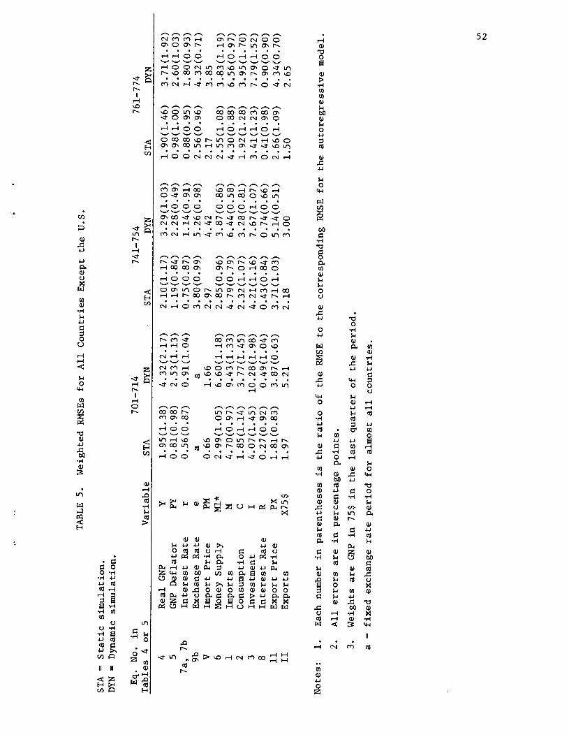
STA = S

tatic

simulation.

DYN =

Dyn

amic

simulation.

TABLE 5.

Weighted RMSEs for All Countries Except the U.S.

Notes:

1.

Each number in parentheses is the ratio of the RMSE to the corresponding RMSE for the autoregressive model.

2.

All errors are in percentage points.

3.

Weights are GNP in

75$ in the last quarter of the period.

a = fix

ed exchange rate period for almost all countries.

Lri

Eq. No. in

Tables 4 or 5

Variable

STA

DYN

701—714

741—754

STA

DYN

STA

DYN

761—774

4

Real GNP

Y

1.95(1.38)

4.32(2.17)

2.10(1.17)

3.29(1.03)

1.90(1.46)

3.71(1.92)

5

GNP Deflator

PY

0.81(0.98)

2.53(1. 13)

1.19(0.84)

2.28(0.49)

0.98(1.00)

2.60(1.03)

7a, 7b

Interest Rate

r

0.56(0.87)

0.91(1.04)

0.75(0.87)

1.14(0.91)

0.88(0.95)

1.80(0.93)

9b

Exchange Rate

e

a

a

3.80(0.99)

5.26(0.98)

2.56(0.96)

4.32(0.71)

V

Import Price

PM

0.66

1.66

2.97

4.42

2.17

3.85

6

Money Supply

Ml*

2.99(1.05)

6.60(1.18)

2.85(0.96)

3.87(0.86)

2.55(1.08)

3.83(1.19)

1

Imports

M

4.70(0.97)

9.43(1.33)

4.79(0.79)

6.44(0.58)

4.30(0.88)

6.56(0.97)

2

Consumption

C

1.85(1.14)

3.77(1.45)

2.32(1.07)

3.28(0.81)

1.92(1.28)

3.95(1.70)

3

Investment

I

4.07(1.45) 10.28(1.98)

4.21(1.16)

7.67(1.07)

3.41(1.23)

7.79(1.52)

8

Interest Rate

R

0.27(0.92)

0.49(1.04)

0.43(0.84)

0.74(0.66)

0.41(0.98)

0.90(0.90)

11

Export Price

PX

1.81(0.83)

3.87(0.63)

3.71(1.03)

5.14(0.51)

2.66(1.09)

4.34(0.70)

II

Exports

X75$

1.97

5.21

2.18

3.00

1.50

2.65

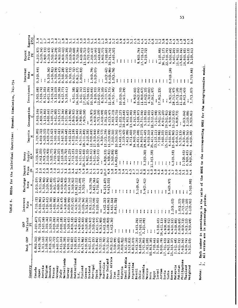
TABLE 6. RNSEs for the Individual Countries: Dynamic S

imul

atio

n, 741—754

GNP

interest

Exchange Import

Money

Interest

Export

Real GNP

Deflator

Rate

Rate

Price

Supply

Imports Consumption Investment

Rate

Price

Exports

Country

Y

PY

r

e

PM

Ml*

M

C

I

R

PX

X75$

Canada

0.8(0.56) 2.0(0.67) 0.7(0.72)

2.0(1.07) 3.4

3.1(0.98)

3.7(0.80) 0.9(0.59)

3.0(1.03)

0.5(0.69) 6.2(0.87)

7.9

Japan

3.6(0.78)

0.7(0.27) 0.5(0.96)

3.2(1.04)

2.6

2.4(1.05)

4.0(0.21)

2.8(0.32)

7.5(0.74)

——

4.1(

0.34

) 2.7

Austria

3.3(1.16)

2.5(0.58)

1.6(1.91)

5.7(0.96)

2.5

3.9(1.42)

4.3(0.52)

3.1(1.84)

8.2(1.55)

——

2.9(

0.33

) 1.7

Belgium

1.5(0.54)

2.3(0.34)

1.2(0.62)

5.1(0.94)

2.8

2.5(0.93)

2.6(0.23)

1.6(0.66)

6.0(1.29) 0.3(0.56) 4.2(0.43) 2.1

Denmark

1.8(0.32)

1.3(0.33)

1.4(0.30)

4.5(0.85)

3.8

5.3(0.77)

5.5(0.42)

4.3(0.71)

7.4(0.56)

1.4(0.81) 3.5(0.44) 3.3

France

1.3(0.72)

1.0(0.26)

1.4(0.98)

8.0(1.07)

7.0

3.7(0.94)

4.3(0.46)

1.4(1.00)

3.1(1.03)

0.7(0.59) 2.9(0.29) 1.8

Germany

1.6(

0.57

) 0.7(0.26)

1.7(1.34)

4.6(0.91) 3.5

1.8(0.52)

3.3(0.51)

1.5(3.57)

6.3(0.59) 0.5(0.47) 4.9(0.55) 2.7

Italy

2.5(1.16) 2.0(0.18) 1.9(0.47) 6.4(0.82) 4.1

2.1(0.19)

5.6(0.36) 1.2(0.34)

9.4(2.77)

0.5(0.28) 4.8(0.41) 1.9

Netherlands

0.9(0.39) 1.0(0.31) 1.4(0.68) 5.2(0.92) 3.1

3.2(0.70)

4.0(0.48) 2.5(1.09)

5.3(0.61)

0.7(0.64) 4.1(0.39)

1.8

Norway

1.9(0.95)

1.3(0.45) 2.0(0.99) 6.0(1.14) 1.6

6.4(1.23)

5.6(1.21) 2.1(0.96)

——

0.3(

0.73

) 2.1(0.21)

3.1

Sweden

3.9(1.60) 1.8(0.52) 2.0(2.45)

5.5(0.91) 3.4

7.7(2.15)

6.2(1.19) 2.8(0.92)

4.5(1.38) 0.5(1.71) 6.0(0.68)

3.1

Switzerland

5.5(0.83) 3.4(1.82) 1.4(1.36) 12.9(2.11) 8.1

4.0(0.53)

77(0.46)

3.9(0.64)

14.3(0.80) 0.8(1.27) 3.7(0.56)

2.4

U.K.

2.7(1.16)

5.4(0.63)

0.5(0.74)

5.5(1.09)

7.8

6.1(1.62)

6.5(1.34)

2.9(0.89)

5.4(1.34) 2.0(0.83) 5.6(0.60)

3.0

Finland

8.4(3.96)

6.9(0.82)

0.1(0.34)

3.3(0.72)

5.9 16.5(1.60) 18.1(1.88) 7.9(3.28)

17.0(2.13)

13.1(0.71) 3.0

Greece

4.5(0.58)

4.2(0.88)

3.3(1.56)

——

3.9

9.9(2.32)

8.1(0.58)

——

27.7

(0.9

3)

——

4.7(

0.43

) 2.0

Ireland

5.4(2.27)

4.7(0.92)

1.0(1.11)

4.3(0.79)

5.1

3.5(0.51) 11.0(0.69) 5.3(0.97)

10.3(0.66) 1.9(0.79)

2.2(0.43)

5.1

Portugal

8.9(1.25) 2.5(0.44) 0.7(0.59)

7.6(1.36)

5.3

4.5(1.46) 17.1(0.64) 4.6(0.92)

9.1(0.93)

0.1(0.07)

2.5(0.44)

3.4

Spain

5.8(1.84)

1.6(1.37)

0.2(0.65) 6.7(0.87) 4.3

5.9(2.22) 10.5(2.59) 3.7(1.19)

12.6(2.34)

——

5.4(

0.60

) 2.9

Yugoslavia

3.7(2.25)

9.3(1.90)

—-

——

4.

5 ——

4.3(

0.57

) 3.4(0.99)

8.5(1.10)

——

5.9(

0.77

) 1.3

Australia

3.0(1.76) 6.6(1.02) 1.4(2.21) 8.2(3.63) 10.0 .4.8(0.53) 12.1(1.28) 2.0(1.22)

5.7(3.37)

1.0(2.42)

3.7(0.69)

3.0

New Zealand

0.7(1.04) 4.1(0.82) 0.6(0.96) 9.6(3.05) 9.9

4.3(0.81) 11.2(0.69) 4.2(3.47)

11.8(0.77) 0.4(0.96) 20.7(1.76) 4.4

South Africa 5.8(1.81) 3.4(2.36)

1.6(2.14)

——

3.8

3.3(0.89)

7.5(0.51)

3.9(2.23)

14.5(l.33) 1.0(1.76) 2.4(0.32) 2.2

Iran

3.5(0.99)

——

0.6(

1.25

) ——

3.9

14.0(1.29) 10.5(0.56) 3.4(0.75)

——

—

—

2.5

Libya

5.5(0.60)

——

——

—

—

3.8

——

14.6

(1.1

3) 1

1.2(1.17)

10.0(0.70) ——

——

3.

9 Nigeria

7.8(0.81)

——

——

—

—

3.4

5.1(0.42) 10.2(0.68)

16.4(1.29) ——

——

4.

6 Saudi Arabia

3.4(1.18)

——

——

—

—

3.7

7.6(1.89)

9.9(1.62)

——

——

—

—

3.2

Venezuela

3.5(2.83)

——

——

—

—

4.5

8.5(1.40) 13.0(0.99)

——

——

—

—

5.2

-

Arg

entin

a 8.8(2.03)

——

——

—

—

2.7

14.9(0.70) 8.2(2.39)

8.9(2.61) —

——

2.

5 BrazIl.

5.4(1.16) 2.4(1.26)

——

5.1(

0.41

) 2.2

14.6(1.08) 5.5(0.97)

10.6(2.04) ——

9.8(

0.76

) 2.8

Chile

8.1(0.54) 17.3(0.21) ——

——

3.

1 ——

24.8

(0.2

7) 1

0.7(1.04)

11.8(0.67) ——

17.7

(0.2

1)

4.4

Colombia

5.7(1.86) 2.2(1.09)

——

5.4(

1.41

) 8.8

5.5(0.50) 19.8(1.42) 3.1(0.95)

12.6(2.32) ——

9.2(

0.72

) 4.5

Mexico

2.3(1.08)

——

——

—

—

5.1

——

6.0(

0.53

) 5.5(1.03)

4.3(2.01)

——

——

7.

4 Peru

10.8(3.38) —

——

—

—

4.0

11.5(1.58) 25.4(1.04) 11.5(2.45)

37.0(1.97)

——

0.8

Egypt

2.7(0.46)

——

——

—

—

3.0

——

23.1

(2.1

1)

7.1(1.98)

——

——

—

—

1.2

Israel

5.7(0.95)

6.5(0.65)

——

——

4.

5 ——

7.7(

0.86

) 5.0(1.16)

17.8(1.23) —

6.1(

0.88

) 3.2

Jordan

9.0(0.79) 16.4(1.13)

——

——

3.

6 ——

7.4(

0.33

) 8.9(1.10)

——

——

36

.7(i.

17)

3.8

Syria

17.7(1.63) 6.9(0.46)

——

——

4.

0 —--

15.7

(1.2

5) 2

9.5(1.91)

——

——

22

.5(0

.79)

0.8

India

6.9(2.84) 4.8(0.91)

——

3.4(

0.97

) 4.4

——

6.6(

0.99

) 6.9(0.89)

5.9(1.04)

0.0(0.18)

4.0(0.49)

2.4

Korea

15.3(3.37) 6.4(0.51) 1.1(1.02)

——

3.7

4.6(0.58) 15.6(0.90) 13.1(2.83)

28.2(1.97)

——

9.0(

1.20

) 4.5

Malaysia

2.1(1.48) 4.2(0.88)

——

——

2.

0 ——

6.0(

0.51

) 4.8(0.73)

13.7(1.18)

——

11.9

(1.3

5) 2.8

Pakistan

2.4(

1.21

) 2.0(0.69) 1.0(1.27)

——

2.6

——

5.7(

1.13

) ——

11.1

(1.2

3) —

13.8

(2.2

4)

1.9

Philippines

7.4(1.54) 4.0(0.72) 2.7(1.20)

——

3.1

2.1(0.45)

8.3(

1.38

) 6.0(1.04)

24.6(1.45)

——

19.8

(0.9

3) 6.8

Thailand

3.4(0.74) 3.6(1.22)

0.7(1.10)

——

3.0

2.3(0.45)

6.0(0.34)

3.1(0.88)

——

——

9.

6(1.

13)

2.3

Weighted

3.3(1.03)

2.3(0.49)

1.1(0.91)

5.3(0.98)

4.4

3.9(0.86)

6.4(0.58)

3.3(0.81)

7.7(1.07)

0.7(0.66)

5.1(0.51)

3.0

Notes:

1.

Each number in parentheses is the ratio of the R

}ISE to the corresponding RMSE for the autogregreesive model.

2.

All errors are in percentage points.

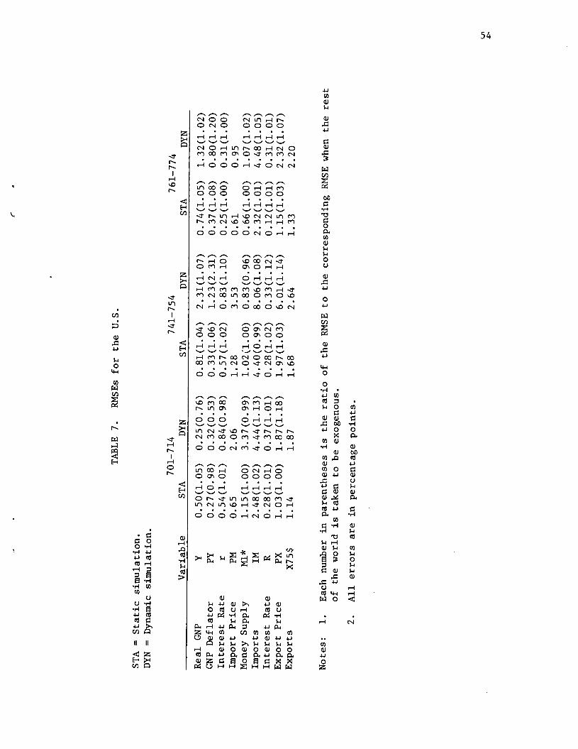
STA = S

tatic

simulation.

DYN =

Dyn

amic

simulation.

TABLE 7.

RMSEs for the U.S.

Notes:

1.

Each number in parentheses is the ratio of the RMSE to the corresponding RMSE when the rest

of the world is taken to be exogenous.

2.

All errors are in percentage points.

U,

701—714

741—754

761—774

Variable

STA

DYN

STA

DYN

STA

DYN

Real GNP

Y

0.50(1.05) 0.25(0.76)

0.81(1.04) 2.31(1.07)

0.74(1.05) 1.32(1.02)

GNP Deflator

PY

0.27(0.98) 0.32(0.53)

0.33(1.06) 1.23(2.31)

0.37(1.08) 0.80(1.20)

Interest Rate

r 0.54(1.01) 0.84(0.98)

0.37(1.02) 0.83(1.10)

0.25(1.00) 0.31(1.00)

Import Price

PM

0.65

2.06

1.28

3.53

0.61

0.95

Money Supply

M1*

1.15(1.00) 3.37(0.99)

1.02(1.00) 0.83(0.96)

0.66(1.00)

1.07(1.02)

Imports

IM

2.48(1.02) 4.44(1.13)

4.40(0.99) 8.06(1.08)

2.32(1.01) 4.48(1.05)

Interest Rate

R

0.28(1.01) 0.37(1.01)

0.28(1.02) 0.33(1.12)

0.12(1.01) 0.31(1.01)

Export Price

PX

1.03(1.00) 1.87(1.18)

1.97(1.03) 6.01(1.14)

1.15(1.03) 2.32(1.07)

Exports

X75$

1.14

1.87

1.68

2.64

1.33

2.20

55

the autoregressive model is l9741—19751V. (3) In going from a static

simulation to a dynamic simulation, the accuracy of the model improves

relative to that for the autoregressive model for the 19741—l9751V period.

The relative accuracy worsens for the 19701—l97lIV period. It is about

the same for the 19761—19771v period.

The RI4SEs in Table 6 give a general idea of how well the model ex—

plains the individual countries. The RNSEs are generally larger for the

smaller countries, which is as expected given, among other things, the

poor quality of much of the data for the smaller countries.

The main conclusion to be drawn from the results for the U.S. in

Table 7 is that the fit of the U.S. model is not very sensitive to whether

or not the U.S. model is included in the overall model, i.e., to whether

or not the rest of the world is taken to be exogenous in the U.S. model.

Note also that the U.S. RNSEs for a given variable are generally much

smaller than the corresponding RNSEs for the other countries in Table 5.

Although the results in this section give one a general idea of the

accuracy of the model, they do not, as mentioned above, provide a test

of the model. It is unclear how the model would compare to the autore—

gressive model if the method in Fair (1980a) were used.

This method takes into account exogenous variable uncertainty, whereas

the procedure followed in this section does not, which biases the current

results against the autoregressive model. The autoregressive model has

no non trivial exogenous variables. The important exogenous variables in

the regular model are the government spending variable (G.e) and the

price of exports of the oil exporting countries. On the other hand, the

10The U.S. model is compared to an autoregressive model in Fair (1980a),and so no comparisons of this kind are presented here.

56

autoregressive model may be more misspecified than the regular model,

which would bias the current results, which are all within sample,

against the regular model. The method has been used to compare the

U.S. model and an autoregressive model (Fair (l9SOa)), and the results

in general indicate that the autoregressive model is more misspecified.

In future work it will be of interest to use the method to compare

the present model not only to the autoregressive model but also to

other structural models.

V. The Properties of the Model

A useful way of examining the properties of the model is to consider

the effects of changing government policy variables. The results of one

experiment are reported In this section: an increase in the purchase of

U.S. goods by the U.S. government. This experiment was performed in both

a fixed exchange rate period (l9701—197l1v) and a flexible rate period

(l9761—19771v). The results of other experiments are reported in a

sequel to this paper, Fair (1981). This paper provides much mote dis-

cussion of the properties of the model than space limitations allow in

this section.

Before discussing the results of the experiment, it will be useful

to explain some of the ceteris aribus effects in the model. In what

follows a variable is said to have a "direct" effect on another variable

if it appears on the right hand side of the equation (either a stochastic

equation or a definition) explaining the other variable. Most endogenous

variables have at least an Indirect effect on the other endogenous

variables——either contemporaneously or with a lag of one quarter. Because

of this, it is difficult to explain the properties of the model in a

57

systematic way. The following discussion is designed to try to give a

general idea of the properties of the model without going into every

possible indirect effect. The experiment, of course, takes all effects

into account, and so the experimental results provide a check on the less

rigorous discussion of the properties.

It should also be kept in mind in the following discussion that not

all of the effects operate for all countries. To conserve space, no dis-

tinction is made across countries. Each effect is discussed as if it

applied to all countries. All interest rates referred to in the discus-

sion are short term interest rates unless otherwise noted.

Trade Effects Among Countries

There is a standard trade multiplier effect in the model. An auto-

nomous increase in GNP in country I increases its demand for imports,

which increases the exports of other countries and thus their GNP and

demand for imports, which then increases the exports of country i and

thus its GNP. In short, exports affect imports and vice versa.

Price Effects Among Countries

There is also a price multiplier effect in the model. An autonomous

increase in country i's domestic price level increases its export prices,

which increases the import prices of other countries, which increases

their domestic prices, including their export prices, which then increases

country i's import prices and thus its domestic and export prices. In

short, export prices affect import prices and vice versa.

58

Direct Interest Rate Effects Among Countries

The U.S. short term interest rate appears as an explanatory variable

in the interest rate reaction functions of a number of countries. The

U.S. rate is more important in the fixed exchange rate period than it

Is in the flexible rate period, but even in the flexible rate period It

has an effect on some countries. This means that an increase in the U.S.

interest rate directly increases other countries' rates. The German in-

terest rate appears as an explanatory variable In the interest rate reaction

functions of a few other European countries, and so an Increase In the

German interest rate also directly increases other countries' rates.

Direct Exchange Rate Effects Among Countries

The German exchange rate appears as an explanatory variable in the

exchange rate equations of the other European countries. The German

exchange rate thus directly affects other exchange rates. All exchange

rates are relative to the U.S. dollar, and so each explanatory variable

in the exchange rate equations (other than the lagged dependent variable

and the German exchange rate) is the particular variable of the country

relative to the same variable for the U.S. This means that the following

U.S. variables appear as explanatory variables in the exchange rate equa-

tions: the GNP deflator, the short term interest rate, the demand pressure

variable, and the change In net foreign assets.

Direct Effects Within a Country

The short term interest rate directly affects the long term rate

(equation 8). The short term rate or the long term rate has a direct

negative effect on imports and consumption (equations 1 and 2) and a

direct positive effect on the GNP deflator (equation 5). The short term

59

rate has a direct negative effect on the demand for money and the exchange

rate (equations 6 and 9b). (Remember that an increase in the exchange

rate is a depreciation of the country's currency.)

The asset variable, which is a measure of the net asset position

of the country vis—a—vjs the rest of the world, has a direct positive

effect on imports and consumption (equations 1 and 2) and a direct nega-

tive effect on the short term interest rate and the exchange rate (equa-

tions 7a, 7b, and 9b).

The exchange rate has a direct positive effect on the price of im-

ports and the price of exports, both of which are in units of the local

currency (equations V and 11). It also has a direct negative effect on

the price of exports in dollars (because the coefficient estimate of the

log of the exchange rate in equation 11 is less than 1). It has a direct

positive effect on the short term interest rate for three countries (equa-

tion 7b).

The price of imports has a direct negative effect on imports (equa-

tion 1), a direct positive effect on the GNP deflator (equation 5), a

direct negative effect on the asset variable (equations 17 and 18), and

a direct positive effect on the short term interest rate for four coun-

tries (equation 7b). The price of exports has a direct positive effect

on the asset variable (equations 17 and 18). The GNP deflator has direct

positive effects on imports, the demand for money, the short term and

long term interest rates, the exchange rate, and the price of exports

(equations 1, 6, 7a, 7b, 8, 9b, and 11).

The level of imports has a direct negative effect on final sales

and the asset variable, and the level of exports has a direct positive

effect on these two variables (equations 16, 17, and 18). The level of

60

final sales has a direct positive effect on GNP (equation 4). Any devi-

ation of GNP from final sales in a period is absorbed by a change in in-

ventories (equation 12). The stock of inventories has a direct negative

effect on production (equation 4).

GNP or the demand pressure variable (which is a nonlinear function

of GNP) has a direct positive effect on imports, consumption, investment,

the GNP deflator, the demand for money, the short term interest rate,

and the exchange rate.

Some Indirect Effects Within a Country

It should be clear that there are very few unambiguous indirect ef-

fects in the model with respect to sign. The signs depend on the relative

sizes of the coefficient estimates. It will nevertheless be useful to

consider the likely signs of some indirect effects, even though these signs

are not necessarily logical consequences of the model.

Consider first the Indirect effect of the exchange rate on GNP.

The main direct effect of the exchange rate is on the price of imports,

at least in the short run. The price of imports has a direct negative

effect on imports, and the level of imports has a direct positive effect

on GNP. In other words, an increase in the price of imports causes sub-

stitution from imports to domestically produced goods, which raises GNP.

The exchange rate thus has an indirect positive effect on GNP through

this channel (i.e., depreciation increases GNP).

Depreciation also lowers the dollar price of exports, which lowers the

import price indices of countries that import from the given country,

which in turn increases the demand for the given country's exports. There-

fore, depreciation also increases GNP through this channel.

61

Depreciation is likely to have a negative indirect effect on GNP

through a third channel. The likely initial effect of a depreciation

on the balance of payments is negative. Depreciation raises the local

currency price of imports more than it does the local currency price of

exports, which, other things being equal, has a negative effect on the

balance of payments. Depreciation also lowers imports and raises exports,

which has a positive effect on the balance of payments. This latter effect

is, however, likely to be smaller initially than the price effect, and

so the initial net effect is likely to be negative. (This is, of course,

the " J curve" effect.) A decrease in the balance of payments decreases

net foreign assets, which directly decreases imports and consumption and

directly increases the short term interest rate. Although the decrease

in imports raises GNP, the decrease in consumption and the increase in

the interest rate lower GNP, and the net effect is likely to be negative.

Depreciation is thus likely to have an initial indirect negative effect

on GNP through this "assett' effect channel.

Depreciation has two main indirect effects on the GNP deflator, one

positive and one ambiguous. The positive effect is through the price

of imports, which has a direct positive effect on the GNP deflator. The

second effect is through GNP. If the net effect of depreciation on GNP

is positive, this will have a positive effect on the GNP deflator through

the direct positive effect of the demand pressure variable on the GNP

deflator. If the net effect of depreciation on GNP is negative, the in-

direct effect on the GNP deflator is negative.

There are three main effects of the short term interest rate on GNP,

one negative, one ambiguous, and one positive. The negative effect is

through consumption. An increase in the short term rate increases the

62

long term rate. An increase in the short term rate or the long term rate

decreases consumption, which lowers GNP. The ambiguous effect Is through

the exchange rate. An increase in the short term rate has a negative

effect on the exchange rate (an appreciation), which has an ambiguous

effect on GNP. The positive effect is through imports. An increase in

the short term or long term rate lowers imports, which, other things being

equal, raises GNP. The consumption effect is likely to be the dominant

one, and so the net effect of the short term rate on GNP Is likely to

be negative.

An increase in interest rates has three main effects on the GNP de-

flator, one positive and two negative. The positive effect is a direct

one: interest rates appear as explanatory variables in the price equa-

tion (equation 5). The first negative effect is the negative Indirect

effect of interest rates on GNP and thus on the demand pressure variable.

The other negative effect is the effect on the exchange rate: the exchange

rate appreciates, which lowers the price of imports, which lowers the

GNP deflator.

The Results of the Experiment

The effects of increasing U.S. government expenditures on some of

the key variables in the model are presented in Tables 8 and 9 for the

main countries. Each number in the tables is the percentage difference

between the two— or six—quarter—ahead predicted value of the variable

before and after the change divided by the percentage change in autonomous

income. For these results the estimated residuals were added to the

stochastic equations and treated as exogenous. This means that when the

model is simulated us1g the actual values of the exogenous variables,

a perfect tracking solution is obtained. The base path before the change

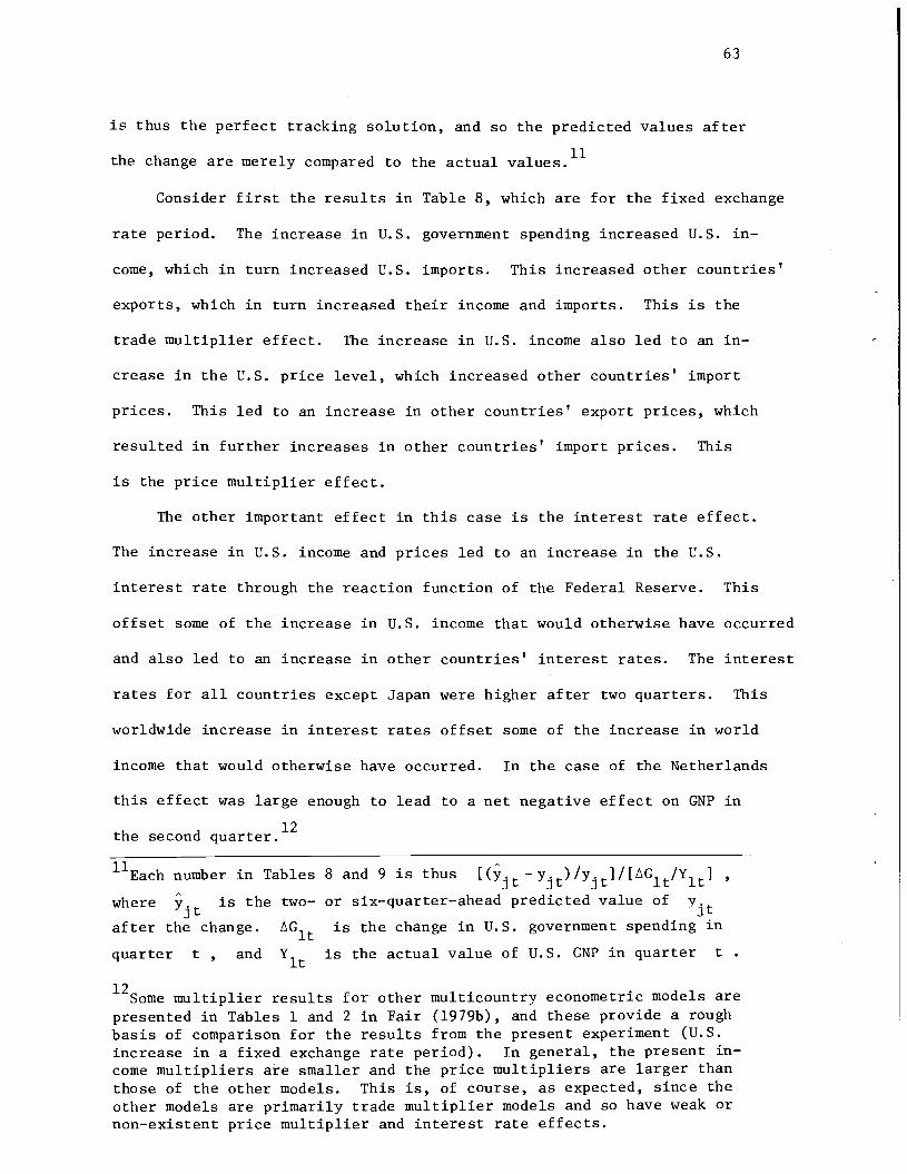
63

is thus the perfect tracking solution, and so the predicted values after

the change are merely compared to the actual values.11

Consider first the results in Table 8, which are for the fixed exchange

rate period. The increase in U.S. government spending increased U.S. in-

come, which in turn increased U.S. imports. This increased other countries'

exports, which in turn increased their income and imports. This is the

trade multiplier effect. The increase in U.S. income also led to an in-

crease in the U.S. price level, which increased other countries' import

prices. This led to an increase in other countries' export prices, which

resulted in further increases in other countries' import prices. This

is the price multiplier effect.

The other important effect in this case is the interest rate effect.

The increase in U.S. income and prices led to an increase in the U.S.

interest rate through the reaction function of the Federal Reserve. This

offset some of the increase in U.S. income that would otherwise have occurred

and also led to an increase in other countries' interest rates. The interest

rates for all countries except Japan were higher after two quarters. This

worldwide increase in interest rates offset some of the increase in world

income that would otherwise have occurred. In the case of the Netherlands

this effect was large enough to lead to a net negative effect on GNP in

the second quarter.12

11Each number in Tables 8 and 9 is thus_Yt)IYI/L\cltIY1tI

where is the two— or six—quarter—ahead predicted value of

after the change. AG1t is the change in U.S. government spending in

quarter t , and is the actual value of U.S. GNP in quarter t

'2Some multiplier results for other multicountry econometric models arepresented in Tables 1 and 2 in Fair (1979b), and these provide a roughbasis of comparison for the results from the present experiment (U.S.increase in a fixed exchange rate period). In general, the present in-come multipliers are smaller and the price multipliers are larger thanthose of the other models. This is, of course, as expected, since theother models are primarily trade multiplier models and so have weak ornon—existent price multiplier and interest rate effects.

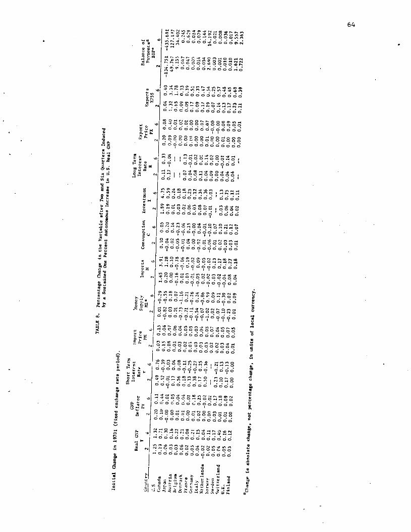
TA

EL

B 8

. Percentage Change in the V

aria

ble

after Two

and

Six

Q

uart

ers

indu

ced

by a S

ustained One

Per

cent

Autonomous Increase in U.S. Real GNP

Initi

al QLange in 19701 (fixed exchange rate period).

Short Term

Long Term

CNP

Inte

rcqt

Import

lony

Interest

Export

Balance of

Real GNP

f1at

or

Rate

Price

Supply

Imports

Consumption Investment

Rate

Price

Exports

Pntsa

Y

P1

r

PM

Ml*

M

c R

PX

X

75$

gop*

6

2

6

2

6

2

6

2

6

2

6

2

6

1.25

1.32

0.20

0.11

0.49 0.76

0.03

0.15

0.01 —0.29

1.65

3.91

0.10 0.05

1.89 4.75

0.11 0.33

0.20 0.08

0.04 0.40

—134.751 —435.691

'inada

0.19 0.71

0.10

0.44

0.52 —0.39

0.15 0.04 -0.82 -0.55

0.20

1.28 —0.04 0.20

0.19 0.59

0.17 —0.04

0.09 0.40

L32

3.34

49.77

127.17

Japan

0.06 0.30 —0.00 0.01 —0.01 0.03

0.05 0.07

0.03 0.18

0.00 0.10

0.02 0.14

0.01

0.24

0.00 0.01

0.65

1.78

9.155

34.602

Autria

0.03 0.16

0.00 0.05

0.17

0.04

0.01

0.06

0.01 0.07 -0.16 —0.78 —0.05 —0.23

0.03

0.18

-—

-—

0.00

0.02

0.09

0.13

0.047

0.245

Bclgium

0.03

0.22

0.01 0.04

0.56 0.08

0.03

0.04 -0.23 -1.16

0.01 -0.06

—0.01 -0.04

0.02 0.18

0.07 0.13

0.00

0.01

0.09 0.39

0.047

0.629

0.06 0.21

0.01 0.04

0.13 —0.11

0.02 0.05 —0.21 0.21

0.03

0.19

0.04

0.15

0.06

0.25

0.04 -0.01

0.00 0.00

0.17 0.51

O.OOS

0.014

France

0.02 0.08

0.00 0.01

0.33 -0.25

0.03 0.05 —0.11 -0.26

—0.01 —0.02

0.00 —0.00

0.03

0.12

0.08 0.02

0.00 0.00

0.09 0.33

0.014

0.079

Grany

0.05

0.21

0.01 0.18

0.38 -0.27

0.03 0.03 —0.54 0.24

—0.05 0.09 —0.02 0.04

0.08 0.34

0.11 0.01

0.00 0.07

0.17

0.67

0.054

0.144

Italy

0.04

0.15

0.02 0.25

0.17

0.25

0.03 0.04 —0.07 —0.86

0.02 —0.05

0.01 —0.01

0.07 0.36

0.04 0.14

0.01

0.07

0.19

0.54

2.690

14.192

Sther1ands

—0.02 0.04

0.00 —0.02

0.50 -0.36

0.03 0.05 —1.02 0.59 —0.02 -0.02 —0.06 —0.10 —0.01 0.03

0.09 0.02

0.00 —0.00

0.07 0.25

0.003

0.021

Norway

0.02 0.11

0.00 0.02

—-

-—

0.02

0.07

0.02 0.09

0.03 0.13

0.01

0.07

—-

——

0.

00 0.00

0.00 —0.00

0.14 0.57

0.001

0.008

Swede:,

0.05 0.17

0.03 0.17

0.23 —0.21

0.02 0.04 —0.07 0.11 —0.02 0.17

0.02 0.10

0.03 0.13

0.04 —0.01

0.01 0.08

0.13 0.48

0.010

0.036

SwItzerland

o e4 0.40

0.01 0.18

0.10

0.13

0.03 0.05 —0.10 —0.39 —0.04 0.18

-0.03 0.21

0.06 0.75

0.04 0.14

0.00 0.09

0.17

0.45

0.010

0.017

U.K.

0.05

0.

16

0.01

0.

09

0.17

-0.

13

0.04

0.

07

-0.2

3 0.

02

0.08

0.

27

0.03

0.

12

0.04

0.

11

0.04

0.

01

0.00

0.

05

0.23

0.

68

1.62

1 9.

557

Fin

land

0.03 0.12

0.00 0.02

0.00 0.00

0.01

0.05

0.01 0.09

0.04 0.18

0.01

0.07

0.02 0.11

—-

——

0.

00

0.01

0.

11

0.39

0.

722

2.36

3 8C

?an8

e is

abo

1ute

change,

not p

erce

ntag

e ch

ange

, in

un

ite

of

loca

l currency.

a'

.c.

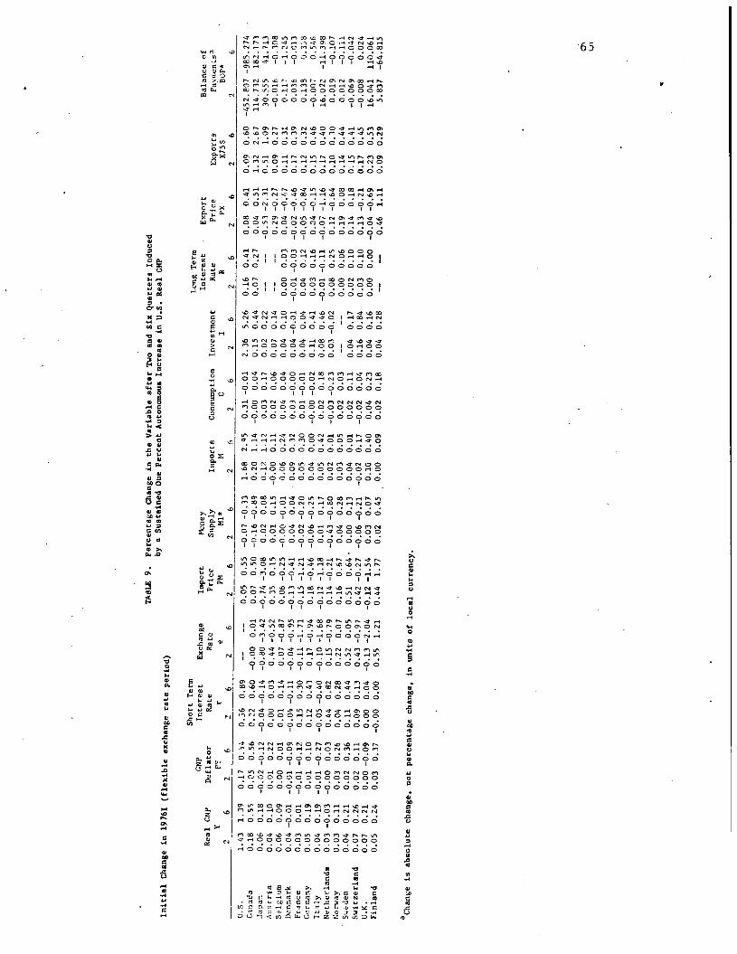
TA8LE 9. Percentage Change in the Variable after Two a

nd Six Quarters

Induced

by a Sustained One Percent Autonomous In

crea

se in U.S. Real GNP

Initi

al Change in 19761 (flexible exchange rate period)

Short Term

Long Term

GM?

Interest

Exchange

Import

Money

Interest

Export

Ealance of

Real CNP

Deflator

Rate

Rato

Price

Supply

Imports

Consumption

Investment

Rate

Price

Exports

Payments5

Y

PY

r

e

PM

M1*

H

C

I

8

PX

X75$

B0P*

2

6

2

6 26

2

6 26

2

6

2

6

2

6

2

6

2

6

2

6

2

6

2

6

u.S.

1.43 1.39

0.17 0.4

0.36

0.89

——

——

0.

05 0.55 —0.07 —0.33

1.68 2.55

0.31 —0.01

2.36 5.26

0.16 0.41

0.08 0.41

0.09 0.60 —452.P07 —985.274

C.-inada

0.18 0.55

0.05 0.56

0.22

0.60 —0.00 0.01

0.07 0.50 —0.16 —0.89

0.20 1.14 —0.00 0.04

0.15 0.44

0.07 0.27

0.04 0.51

1.32 2.67

114.732 182.173

Ja7ar

0.06

0.18 —0.02 —0.12 —0.04 —0.14 —0.80 —3.42 —0.74 —3.08

0.02 0.08

0.12 1.12

0.03 0.17

0.02 0.22

'.31

0.51 1.09

30.555

41.713

Atria

0.04 0.10

0.01 0.22

0.00 0.03

0.44 —0.52

0.35

0.15

0.01 0.15

—0.00 0.11

0.02 0.06

0.07 0.14

——

——

0.

29 —

0.27

0.09 0.27

—0.016

—0.308

Belgium

0.06

0.

09

0.00

0.

01

0.01

0.

14

0.07

—0.

87

0.06

—

0.25

—

0.00

—0.

01

0.06 0.24

0.04 0.04

0.04 0.10

0.00 0.03

0.04 —0.47

0.11

0.31

0.117

—1.245

Denmark

0.04 —0.01 —0.01 —0.09 —0.04 —0.11 —0.04 —0.95 —0.13 —0.41

0.04

0.04

0.09 0.32

0.03 —0.00

0.04 —0.01 —0.01 —0.03 —0.02 —0.46

0.17

0.39

0.036

—0.013

France

0.03 0.01 —0.01 —0.17

0.15 0.30

—0.11 —1.71 —0.15 —1.21 —0.02 —0.20

0.05 0.30

0.01 —0.01

0.04 0.04

0.04

0.12 —0.05 —0.84

0.12 0.32

0.138

0.358

Germany

0.05

0.19

0.

01 0.10

0.12 0.43

0.17 —0.94

0.18 —0.46 —0.06 —0.25

0.04 0.00 —0.00 —0.02

0.11 0.41

0.03 0.16

0.04 —0.15

0.15

0.46

—0.007

0.546

Italy

0.04 0.19 —0.01 —0.27 —0.05 —0.40 —0.10 —1.68 —0.12 —1.18

0.01

0.17

0.05 0.42

0.02 0.18

0.08 0.46 —0.01 —0.11 —0.07 —1.16

0.17

0.40

16.022 —11.358

Netherlands

0.03 —0.03 —0.00 0.03

0.44 0.82

0.15 —0.79

0.14 —0.21 —0.43 —0.60

0.02 0.01 —0.03 —0.23

0.03 —0.02

0.08

0.25

0.12 —0.64

0.10 0.30

0.019

—0.107

Norway

0.03 0.11

0.03

0.26

0.04 0.28

0.22

0.07

0.16 0.67

0.04

0.28

0.03 0.05

0.02

0.03

——

——

0.

00

0.06

0.

19

0.08

0.

14

0.44

0.

012

—0.

111

5'.r

den

0.04 0.21

0.02 0.36

0.11 0.44

0.52

0.05

0.51

0.

64

0.00

0.

13

0.04

0.

01

0.02

0.

11

0.04

0.

17

0.02

0.

10

0.14

0.

18

0.15

0.

41

0.06

9 —

0.04

2 Sw

itzer

land

0.

07

0.26

0.

02

0.11

0.

09

0.13

0.

43 —

0.97

0.

42 —

0.27

—

0.06

—

0.21

—

0.02

0.

17

—0.

02

0.04

0.

16

0.84

0.

03

0.10

0.

13 -

0.21

0.

17

0.45

—

0.00

8 0.

024

u.K

. 0.

07

0.21

0.

00 —

0.09

0.

00

0.04

—

0.13

—2.

04

—0.

12 —

1.54

0.

03

0.07

0.

10

0.40

0.

04

0.23

0.

04

0.16

0.

00

0.00

—

0.04

—0.

69

0.23

0.

53

16.0

41

110.

061

Finl

and

0.05 0.24

0.03 0.37 —0.00 0.00

0.55

1.21

0.44 1.77

0.02 0.45

-

0.00

0.

09

0.02

0.

18

0.04

0.

28

—

—

0.46

1.11

0.09

0.29

5.

837

—64

.815

is

abso

lute

ch

ange

, no

t pe

rcen

tage

ch

ange

, in

un

its

of

loca

l currency.

J1

66

The U.S. increase had a negative effect on the U.S. balance of pay-

ments and a positive effect on the other countries' balance of payments.

This has, other things being equal, a negative effect on other countries'

interest rates. For some of the countries the net effect on the interest

rate after six quarters was negative. This reverses at least part of

the initial negative effect of the world wide increase in Interest rates

on world income.

Although GNP Increased for all countries except the Netherlands,

imports declined for some countries. This is due in part to the effects

of higher Initial interest rates and in part to the fact that import

prices increased more initially than domestic prices. An increase in

import prices relative to domestic prices leads to a substitution away

from imported goods.

Note finally with respect to Table 8 that the money supply decreased

for many countries. Although income was higher, interest rates were also

higher, and In many cases the negative Interest rate effect dominated.

The results in Table 9 are for the flexible exchange rate period.

One key difference between the fixed and flexible rate periods is that

the U.S. interest rate has smaller direct effects on other countries'

interest rates. The changes in the other countries' interest rates after

two quarters are smaller in Table 9 than in Table 8. This means that

there is less initial offset to the trade multiplier effect from higher

interest rates in the flexible rate period.

There are four main effects of the U.S. spending

rates, three negative and one positive. The spending

U.S. output and prices relative to those of the other

of which have a negative effect on other

increase on exchange

increase raised

countries, both

countries' exchange rates (an

67

appreciation). The U.S. balance of payments fell relative to those of

the other countries (the balance of payments of other countries generally

rose), and this also has a negative effect on exchange rates. The posi-

tive effect is the interest rate effect. The U.S. short term interest

rate rose relative to other countries' rates, and this has a positive

effect on exchange rates (a depreciation). As can be seen in Table 9,

the net effect can go either way. For some countries, such as Germany,

there is a depreciation after two quarters (the interest rate effect

dominating) and an appreciation after six quarters.

The changes in the price of imports are much higher in the flexible

rate period. This is, of course, due to the fact that exchange rate

changes are no longer zero. The changes in the price of exports are

also higher for the same reason. Thechanges in import prices are nega--

tive for countries whose exchange rate appreciates. For most of these

countries the fall in import prices led to a fall in the GNP deflator.

In other words, the U.S. expansion generally led to a fall in inflation

rates in those countries whose exchange rates appreciated. This is con-

trary to the case in Table 8, where the U.S. expansion led to an increase

in almost all countries' inflation rates.

The balance of payments fell for some countries in Table 9, contrary

to the case in Table 8. If a country's exchange rate depreciates in

response to the U.S. expansion (the interest rate effectdominating),

then, as noted above, the initial effect on the balance of payments is

likely to be negative (the J curve effect).

The rest of the results in Table 9 should beself explanatory given

the above discussion. As a final comment, it would be possible, as some

people have suggested to me to compare the properties of the present model

68

to the properties of Model A in Fair (1979a). Model A is a "quasi—

empiricalt' two—country model obtained by linking the U.S. model to a

model exactly like it. Model A has the advantage of allowing more ver-

sions of the theoretical model to be analyzed. This may be of interest

in future work, but In general I look on Model A as merely an intermed-

iate step between the theoretical model and the present econometric

model.

VI. Conclusion

The econometric model presented in this paper provides quantitative

estimates of the trade, price, and interest rate linkages among countries.

Some information on these linkages is presented in Section V. Much more

information is presented in a sequel to this paper, Fair (1981).

It is clear from the results in Tables 8 and 9 that there are important

quantitative differences between the fixed and flexible rate periods,

which shows the importance of trying to model exchange rates accurately.

The models of the individual countries can be easily replaced by al-

ternative models within the context of the overall model, and it is hoped

that this study will induce work of this kind)3 It will be interesting

to see how sensitive the properties of the overall model are to the re-

placement of individual models. As more observations become available

under flexible exchange rates, it should be possible to get more precise

estimates of the interest rate and exchange rate reaction functions, and

it will also be interesting to see how sensitive the properties of the

model are to the new estimates. Another important area for future work

131t is quite easy in the Fair—Parke program, which estimates and solvesthe model, to replace one individual country model with another.

69

is estimating the responsiveness of the trade shares (thejit

to

changes in relative prices.

In the more distant future the overall model will need to be tested

using a method like the one in Fair (l980a). A method like this should

help decide which version of the model is the best and how this version

compares to alternative models. In the meantime, the results from the

model must be interpreted with considerable caution.

70

DATA APPENDIX

The collection of the data for the U.S. model is described in Fair

(1976, l980b), and this discussion will not be repeated here. The data

for all the other countries were obtained from the International Financial

Statistics (IFS) tape (October 1980) and the Direction of Trade (DOT)

tape (October 1980). The following steps were involved in the construc-

tion of the data base:

1. A program was written to read the IFS tape and create for each

country all the variables in Table 1 except the variables for

which DOT data are needed: M75$A., M75$B. , PM

XX$ XX75$ . and 2it • Most of the work in

constructing the data base was writing this program. No two

countries were exactly alike with respect to the availability

of the data, and so separate subroutines were written for each

country.1 The individual treatment of the countries is discussed

below. The output from this program was stored by country on a

tape called IFS1.

2. A program was written to read the DOT tape and create the XX$..

data (the bilateral trade data). The output from this program

was stored by country on a tape called DOT1.

3. The IFS1 and DOT1 tapes were sorted to store the data by quarter.

'Before these subroutines were written, a program was written to printthe IFS data in a convenient format. The information needed to writethe individual subroutines was taken from this printout. I am indebtedto William Parke for help in writing the initial program that read thetape.

71

The sorted tapes were then used together to create the variables

mentioned in step 1. This completed the construction of the

data base.

The individual treatment of the data for each country is outlined

in Table A—i. The comments in the tablediscuss any special treatment

of the country. If no comments appear for a particular country, then

all the data were available andnothing special needed to be done. Two

standard procedures were followed for all the countries, and it is neces-

sary to discuss these before considering the comments in Table A—i.

First, if no quarterly National Income Accounts (NIA) data were available,

then quarterly data were interpolated from annual data using quarterly

data on the industrial production index(IP). If quarterly data on IP

were not available, then the procedure in Table A—2 was used to create

the quarterly data. One can thus tell from Table A—i how the quarterly

NIA data were constructed (if theywere constructed) by noting whether

or not IP data were available.

The second standard procedure concerns the construction of the Balance

of Payments (BOP) data, and this procedure is presented in Table A—i.

The key variable that is created in this process is BOP , the balance

of payments on current account. It is used in the construction of the

asset variable, At , for each country. Quarterly BOP data do not gen-

erally begin as early as the other data, and the procedure in Table A—3

allows data on BOP to be constructed as far back as the beginning

of the data for merchandise imports and exports ( M$. and

When all data are available, the procedure is a way of linking the BOP

and non—BOP data.

Most of the comments in Table A—i are self explanatory. Data for

80

Frenkel, Jacob A. and Harry G. Johnson, eds. The Monetary Approach tothe Balance of Payments. Toronto: University of Toronto Press,1976.

Frenkel, Jacob A. and Carlos A. Rodrigues. "Portfolio Equilibrium andthe Balance of Payments: A Monetary Approach." The AmericanEconomic Review. 65 (September 1975): 674—88.

Hickman, Bert G. "International Transmission of Economic Fluctuationsand Inflation." In International Aspects of Stabilization Policies,edited by Albert Ando, Richard Herring, and Richard Martson. Boston:Federal Reserve Bank of Boston, 1974.

Kouri, Penti J. K. "The Exchange Rate and the Balance of Payments in theShort Run and in the Long Run." Scandinavian Journal of Economics.2 (May 1976): 280—304.

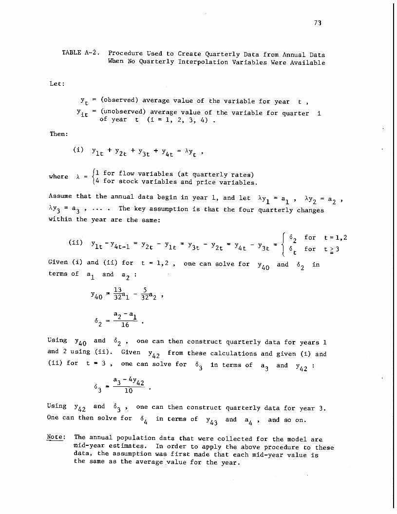
73

TABLE A—2. Procedure Used to Create Quarterly Data from Annual Data

When No Quarterly Interpolation Variables Were Available

Let:

= (observed) average value of the variable for year t= (unobserved) average value of the variable for quarter I1 of year t ( = 1, 2, 3, 4)

Then:

(i) + + 3t + =

h = fi for flow variables (at quarterly rates)w ere4 for stock variables and price variables.

Assume that the annual data begin in year 1, and let Ày1 = a1 , Ày2 a2Ày3 = a3 The key assumption is that the four quarterly changes

within the year are the same:

I 2 for t1,2(ii) lt4t—l = 2t — lt = - 2t = 4t — 3t =

for t>3

Given (i) and (ii) for t = 1,2 , one can solve for y40 and

terms of a1 and a2

13 5y40 = —

= a2—a1

Using y40 and 2 one can then construct quarterly data for years 1

and 2 using (ii). Given y42 from these calculations and given (i) and

(ii) for t = 3 , one can solve for 53 in terms ofa3 and y42

— a3—

10

Using y42 and 63 , one can then construct quarterly data for year 3.

One can then solve for in terms of y43 and a4 , and so on.

Note: The annual population data that were collected for the model aremid—year estimates. In order to apply the above procedure to thesedata, the assumption was first made that each mid—year value isthe same as the average value for the year.

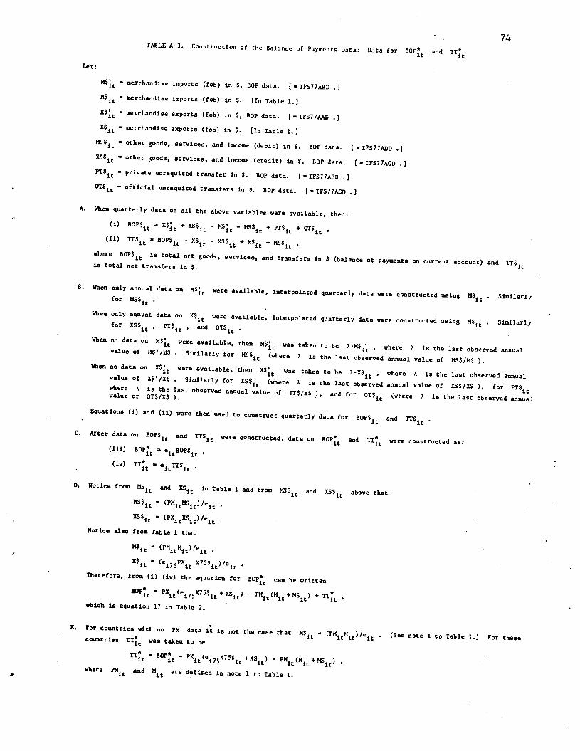
74TABLE A—I. Construction of the Balance of Payments Data: Data for

B0P7 and TTt

Let:

M$it— merchandise imports (fob) in $, 80? data. [ — IFS77ABD

M$jt — merchandise imports (fob) in $. [In Table 14

— merchandise exports (fob) in $, SOP data. [—IFS77Mz 4— merchandise exports (fob) in $. [In Table 1.

it — othergoods, services, and income (debit) in$. SOP data. NIFS77ABD

.1

— othergoods, services, and income (credit) in $. SOP data. [ — IFS77ACD .

PT$J— private unrequited transfer in $. SOP data. [ • IFS77AEO .

— official unrequited transfers in $. SOP data. [—IFS77AGO .]

A. When quarterly data on all the above variableswere available, then:

(i) + xs$ — — it + +(ii) 501t — X$ — XS$ + M$i + it

where 50 is total net goods, services, and transfers in $ (balance of payments on current account) and TT$iis total net transfers in $.

S. When only annual data onwere available, interpolated quarterly data were constructed using M$i . Similarlyfor it

When only annual data on X$ were available,interpolated quarterly data were constructed using

M$it . Similarlyfor XS$ , PT$it , andOT$it

When nn data on M$it were available, thenM$j was tsken to be A.M$i , where A is the last observed annual

value of M$'/hl$ . Similarly for it (where A is the last observed annual value of MS$/M$ ).When no data on X$h were available, then X$k was taken to be A.x$1 , where A is the last observed annual

value of X$'/x$ . Similarly for XS$ (where A is the last observed annual value of XS$/X$ ), forPT$itwhere A is the last observed annual value of

PT$/X$ ), and for OT$1 (where A is the last observed annualvalue of OT$/X$ ). tEquations (i) and (ii) were then used to construct

quarterly data for SOP$t and

C. After data on SOP$iand fl$ were constructed, data on BOP7 and 17 were constructed as:

(iii) 50t a

(iv) TT — ein$11).

Notice from MS1 and it in Table 1 end fromMS$i

and above that— (PMM5)/e

it • (Pxitxsit)/eiNotice also from Table 1 that

—(PNitMit)/ei

X$1—

(ei7sPxi X75$it)/ei

Therefore, from (i)—(iv) the equation for SOP can be written

SOP — PX(e75x75$ +XS) — it(Mit+MSit) +

which is equation 17 in Table 2.-

K. For countriea with no PM data it is not the case that M$it(PKitHi)/ei . (See note 1 to Table 1.) For these

countries TTt was taken to be

—SOP

—PXi (ei75X7c$ +1(5) — PMit(Hi+M5)

where PM and M are defined in note 1 to Table 1.

75

a variable were "made up" if there were a relatively small gap in an

otherwise good series. In these cases the data were usually made up by

linearly interpolating between the closest two available observations.

In a few cases quarterly data on the consumer price index (CPI) were used

for quarterly interpolations of annual data, and for France and Switzer-

land quarterly data on employment (ENPL) rather than on industrial pro-

duction were used for the quarterly interpolation of the NIA data. For

many countries only discount rate data were available for the short term

interest rate (r) , and these cases are mentioned in the table. For

a few countries the NIA year began other than January 1, and this had

to be taken into account in the quarterly interpolations. These cases

are also mentioned in the table. For a few countries data on real GNP

(Y) were not available, but data on the nominal NIA variables were.

In these cases, as indicated in the table, CPI data were used for the

GNP deflator. Real GNP was then taken to be nominal GNP divided by the

GNP deflator.

Quarterly population data were not available for any country, and

the procedure in Table A—2 was used to construct quarterly from annual

data. See in particular the note at the bottom of the table.

Quarterly DOT data began only in 19701, and no attempt was made to

construct DOT data before this quarter. Instead, the variables in the

model were constructed In such a way (with one exception noted below)

that no DOT data were needed in the estimation of the model. In other

words, no DOT data were used for the estimates in Table 4. This allowed

the estimation periods for most countries to be much longer than would

otherwise be the case. The DOT data are needed, of course, for the solu-

tion of the model, and so the earliest quarter for which the model can

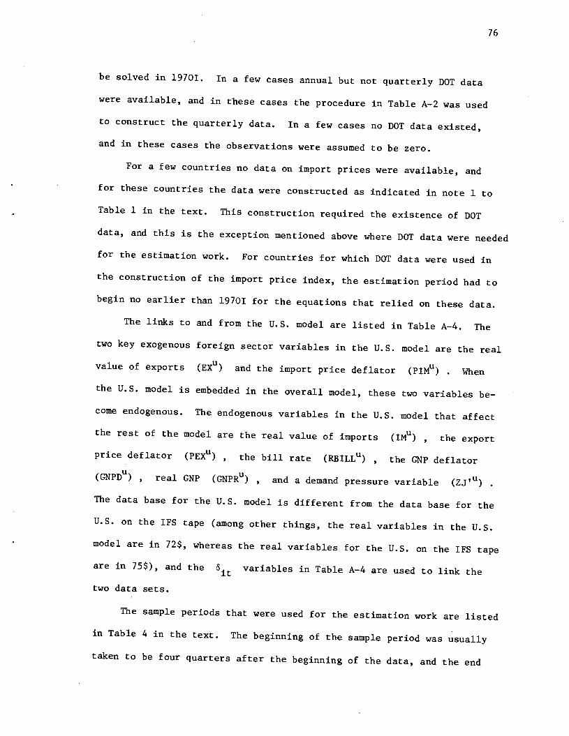
76

be solved in 19701. In a few cases annual but not quarterly DOT data

were available, and in these cases the procedure in Table A—2 was used

to construct the quarterly data. In a few cases no DOT data existed,

and in these cases the observations were assumed to be zero.

For a few countries no data on import prices were available, and

for these countries the data were constructed as indicated in note 1 to

Table 1 in the text. This construction required the existence of DOT

data, and this is the exception mentioned above where DOT data were needed

for the estimation work. For countries for which DOT data were used in

the construction of the import price index, the estimation period had to

begin no earlier than 19701 for the equations that relied on these data.

The links to and from the U.S. model are listed in Table A—4. The

two key exogenous foreign sector variables in the U.S. model are the real

value of exports (EX") and the import price deflator (PIN") . When

the U.S. model is embedded in the overall model, these two variables be-

come endogenous. The endogenous variables In the U.S. model that affect

the rest of the model are the real value of imports (IM") , the export

price deflator (PEX') , the bill rate (RBILLU) , the GNP deflator

(GNPD") , real GNP (GNPRu) , and a demand pressure variable (ZJu)

The data base for the U.S. model is different from the data base for the

U.S. on the IFS tape (among other things, the real variables in the U.S.

model are in 72$, whereas the real variables for the U.S. on the IFS tape

are in 75$), and the variables in Table A—4 are used to link the

two data sets.

The sample periods that were used for the estimation work are listed

in Table 4 in the text. The beginning of the sample period was usually

taken to be four quarters after the beginning of the data, and the end

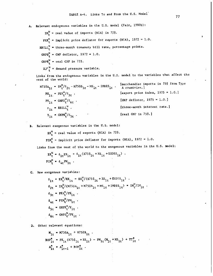
TABLE A—4. Links To and From the U.S. Model77

A. Relevant endogenous variables in the U.S. model (Fair, 1980b):

IM real value of imports (NrA) in 72$.

PEX implicit price deflator for exports (NIA), 1972 1.0.

RBILL= three—month treasury bill rate, percentage points.

GNPD'= GNP deflator, 1972 = 1.0.

GNPR= real GNP in 72$.

ZJ' = demand pressure variable.

Links from the endogenous variables in the U.S. model to the variables that affect the

rest of the world:

M75$Ai IM/62_M75$Bit_MSit_IMDISlt .[merchandis:imports in 75$ from Type

PXi PEX/t53 . [export price index, 1975 = 1.0.]

GNPD/S6 . [GNP deflator, 1975 1.0.]

nt RBILL' . [three—month interest rate.]

CNPR/S5 . [real GNr in 75$.]

B. Relevant exogenous variables in the U.S. model:

EX real value of exports (NIA) in 72$.

PIM' = implicit price deflator for imports (NIA), 1972 1.0.

Links from the rest of the world to the exogenous variables in the U.S. model:

EX = óiEXi =S1(X75$i+XSi+EXDIS1t)

PIN = 64PMit

C. New exogenous variables:

EX'/EX1 = EX/(X75$i+XSit+EXDIS1)

2t IM/(M75$Ai+M75$Bit+MSi+IMDISlt) = IM'/IMi

PEX/PXi

PIM'/P4t t M1.

5t GNPR/Yit

6 CNPDU/PY6t t ltD. Other relevant equations:

Mit M75$Ai + M75$B1

BOP — PXi(Xl5$i+XSit) — PMi(M+MSi) +

* A* +B0P*Ai it—i it

78

of the sample period was usually taken to be the last quarter of the data.

One can thus tell from Table 4 approximately how much data are available

for each country.

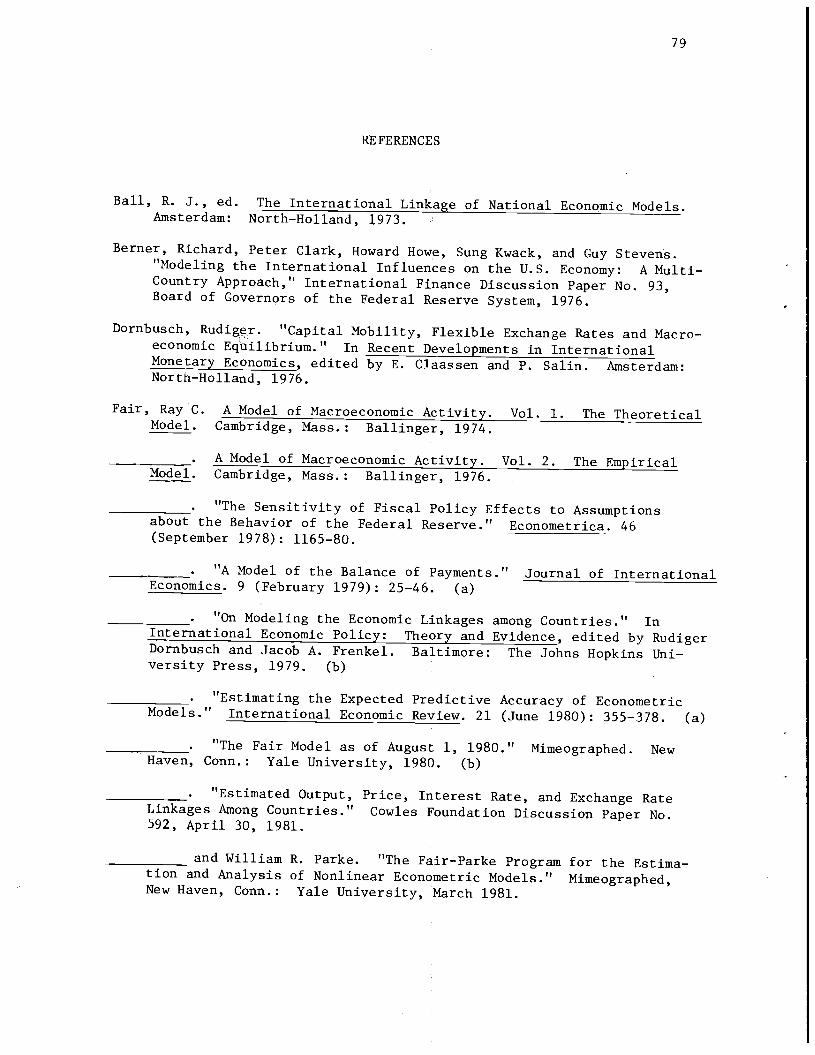
79

REFERENCES

Ball, R. J., ed. The International Linkage of National Economic Models.Amsterdam: North—Holland, 1973.

Berner, Richard, Peter Clark, Howard Howe, Sung Kwack, and Guy Stevens."Modeling the International Influences on the U.S. Economy: A Multi—Country Approach," International Finance Discussion Paper No. 93,Board of Governors of the Federal Reserve System, 1976.

Dornbusch, Rudiger. "Capital Mobility, Flexible Exchange Rates and Macro-economic Equilibrium." In Recent Developments in InternationalMonetary Economics, edited by E. Claassen and P. Salin. Amsterdam:North—Holland, 1976.

Fair, Ray C. A Model of Macroeconomic Activity. Vol. 1. The TheoreticalModel. Cambridge, Mass.: Ballinger, 1974.

__________ A Model of Macroeconomic Activity. Vol. 2. The EmpiricalModel. Cambridge, Mass.: Ballinger, 1976.

___________ "The Sensitivity of Fiscal Policy Effects to Assumptionsabout the Behavior of the Federal Reserve." Econometrica. 46(September 1978): 1165—80.

__________ "A Model of the Balance of Payments." Journal of InternationalEconomics. 9 (February 1979): 25—46. (a)

__________ "On Modeling the Economic Linkages among Countries." InInternational Economic Policy: Theory and Evidence, edited by RudigerDornbusch and Jacob A. Frenkel. Baltimore: The Johns Hopkins Uni-versity Press, 1979. (b)

"Estimating the Expected Predictive Accuracy of EconometricModels." International Economic Review. 21 (June 1980): 355—378. (a)

__________ "The Fair Model as of August 1, 1980." Mimeographed. NewHaven, Conn.: Yale University, 1980. (b)

__________ "Estimated Output, Price, Interest Rate, and Exchange RateLinkages Among Countries." Cowles Foundation Discussion Paper No.92, April 30, 1981.

___________ and William R. Parke. "The Fair—Parke Program for the Estima-tion and Analysis of Nonlinear Econometric Models." Mimeographed,New Haven, Conn.: Yale University, March 1981.

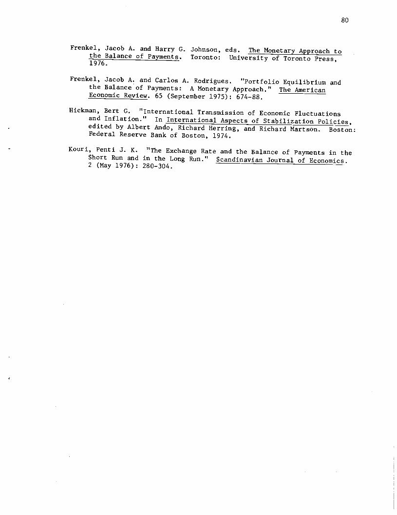
80

Frenkel, Jacob A. and Harry G. Johnson, eds. The Monetary Approach tothe Balance of Payments. Toronto: University of Toronto Press,1976.

Frenkel, Jacob A. and Carlos A. Rodrigues. "Portfolio Equilibrium andthe Balance of Payments: A Monetary Approach." The AmericanEconomic Review. 65 (September 1975): 674—88.

Hickman, Bert G. "International Transmission of Economic Fluctuationsand Inflation." In International Aspects of Stabilization Policies,edited by Albert Ando, Richard Herring, and Richard Martson. Boston:Federal Reserve Bank of Boston, 1974.

Kouri, Penti J. K. "The Exchange Rate and the Balance of Payments in theShort Run and in the Long Run." Scandinavian Journal of Economics.2 (May 1976): 280—304.