Charles University in PragueFaculty of Mathematics and Physics

MASTER THESIS

Martin Svoboda

Processing of Incorrect XML Data

Department of Software Engineering

Supervisor: RNDr. Irena Mlynkova, Ph.D.

Study Program: Software Systems

2010

I would like to thank my supervisor RNDr. Irena Mlynkova, Ph.D. for providedadvices, reviews of thesis working versions and text corrections.

Rad bych podekoval me vedoucı RNDr. Irene Mlynkove, Ph.D. za poskytnuterady, pripomınky k pracovnım verzım prace a textove korektury.

I hereby declare that I have elaborated this master thesis on my own and listedall used references. I agree with making this thesis publicly available.

Prohlasuji, ze jsem svou diplomovou praci napsal samostatne a vyhradne s pou-zitım citovanych pramenu. Dale souhlasım se zapujcovanım teto prace a jejımzverejnovanım.

In Prague on July 1, 2010 Martin SvobodaV Praze dne 1. srpna 2010

2

Contents

1 Introduction 6

2 Preliminaries 102.1 Extensible Markup Language . . . . . . . . . . . . . . . . . . . 10

2.1.1 Model of Documents . . . . . . . . . . . . . . . . . . . . 112.1.2 Schema Languages . . . . . . . . . . . . . . . . . . . . . 14

2.2 Regular Expressions . . . . . . . . . . . . . . . . . . . . . . . . 152.2.1 Glushkov Automaton . . . . . . . . . . . . . . . . . . . . 16

2.3 Regular Tree Grammars . . . . . . . . . . . . . . . . . . . . . . 192.3.1 Data Trees Validity . . . . . . . . . . . . . . . . . . . . . 202.3.2 Grammar Classes . . . . . . . . . . . . . . . . . . . . . . 21

2.4 Document Type Definition . . . . . . . . . . . . . . . . . . . . . 222.4.1 Schema Translation . . . . . . . . . . . . . . . . . . . . . 22

2.5 XML Schema . . . . . . . . . . . . . . . . . . . . . . . . . . . . 242.5.1 Schema Translation . . . . . . . . . . . . . . . . . . . . . 25

3 Analysis 313.1 General Aspects . . . . . . . . . . . . . . . . . . . . . . . . . . . 313.2 Existing Implementations . . . . . . . . . . . . . . . . . . . . . 353.3 Theoretical Research . . . . . . . . . . . . . . . . . . . . . . . . 36

3.3.1 Incremental Validation and Correction . . . . . . . . . . 363.3.2 Validity Sensitive Querying . . . . . . . . . . . . . . . . 413.3.3 Correctors for XML Data . . . . . . . . . . . . . . . . . 433.3.4 Repairs and Consistent Answers . . . . . . . . . . . . . . 443.3.5 Repairing Documents using Chase . . . . . . . . . . . . . 45

4 Corrections 464.1 Framework Concept . . . . . . . . . . . . . . . . . . . . . . . . . 464.2 Edit Operations . . . . . . . . . . . . . . . . . . . . . . . . . . . 50

4.2.1 Edit Operations for Nodes . . . . . . . . . . . . . . . . . 524.2.2 Edit Operations for Attributes . . . . . . . . . . . . . . . 564.2.3 Costs and Sequences of Operations . . . . . . . . . . . . 57

4.3 Update Operations . . . . . . . . . . . . . . . . . . . . . . . . . 594.3.1 Elementary Update Operations . . . . . . . . . . . . . . 604.3.2 Complex Update Operations . . . . . . . . . . . . . . . . 614.3.3 Costs and Sequences of Operations . . . . . . . . . . . . 65

3

4.4 Correction Intents . . . . . . . . . . . . . . . . . . . . . . . . . . 684.4.1 Grammar Context . . . . . . . . . . . . . . . . . . . . . 694.4.2 Repairing Instructions and Repairs . . . . . . . . . . . . 714.4.3 Correction of Data Trees . . . . . . . . . . . . . . . . . . 74

4.5 Correction Multigraphs . . . . . . . . . . . . . . . . . . . . . . . 834.5.1 Exploration Multigraph . . . . . . . . . . . . . . . . . . 834.5.2 Correction Multigraph . . . . . . . . . . . . . . . . . . . 864.5.3 Repairing Multigraph . . . . . . . . . . . . . . . . . . . . 874.5.4 Repairs Construction . . . . . . . . . . . . . . . . . . . . 89

4.6 Repairs Presentation . . . . . . . . . . . . . . . . . . . . . . . . 904.6.1 Repairs for Nodes and Attributes . . . . . . . . . . . . . 914.6.2 Repairs for Sequences and Intents . . . . . . . . . . . . . 94

4.7 Correction Algorithms . . . . . . . . . . . . . . . . . . . . . . . 984.7.1 Naive Correction Algorithm . . . . . . . . . . . . . . . . 994.7.2 Dynamic Correction Algorithm . . . . . . . . . . . . . . 1034.7.3 Caching Correction Algorithm . . . . . . . . . . . . . . . 1034.7.4 Incremental Correction Algorithm . . . . . . . . . . . . . 106

5 Conclusion 120

A Content of CD 124

4

Nazev prace: Zpracovanı nekorektnıch XML datAutor: Bc. Martin SvobodaKatedra: Katedra softwaroveho inzenyrstvıVedoucı diplomove prace: RNDr. Irena Mlynkova, Ph.D.E-mail vedoucıho: irena.mlynkova@ksi.mff.cuni.cz

Abstrakt:XML dokumenty a technologie reprezentujı siroce akceptovany standard

pro spravu a vymenu semistrukturovanych dat. Prekvapive vysoky pocet XMLdokumentu vsak obsahuje chyby dobre formovanosti, strukturalnı validity nebonekonzistence dat. Cılem teto prace je analyza existujıcıch prıstupu vedoucık navrhu noveho korekcnıho systemu. Predstaveny model zahrnuje opravyelementu a atributu vuci jednotypovym stromovym gramatikam. Pruchodemstavoveho prostoru automatu na rozpoznavanı regularnıch vyrazu jsme vzdyschopni nalezt vsechny minimalnı opravy. Tyto opravy jsou kompaktne repre-zentovany rekurzivnımi multigrafy, ktere se dajı prelozit do konkretnıch se-kvencı editacnıch operacı modifikujıcıch datove stromy. Navrzeny byly ctyrikonkretnı algoritmy doplnene o prototypovou implementaci a experimentalnıvysledky. Nejvıce efektivnı algoritmus heuristicky sleduje pouze perspektivnısmery oprav a branı jakymkoli opakovanym vypoctum.

Klıcova slova: XML, validita, opravy.

Title: Processing of Incorrect XML DataAuthor: Bc. Martin SvobodaDepartment: Department of Software EngineeringSupervisor: RNDr. Irena Mlynkova, Ph.D.Supervisor’s e-mail address: irena.mlynkova@ksi.mff.cuni.cz

Abstract:XML documents and related technologies represent widely accepted stan-

dard for managing and exchanging semi-structured data. However, surprisinglyhigh number of XML documents is affected by well-formedness errors, struc-tural invalidity or data inconsistencies. The aim of this thesis is the analysisof existing approaches resulting to the proposal of a new correction frame-work. The introduced model involves repairs of elements and attributes withrespect to single type tree grammars. Via the inspection of the state space ofan automaton recognising regular expressions, we are always able to find allminimal repairs. These repairs are compactly represented by recursively nestedmultigraphs, which can be translated to particular sequences of edit operationsaltering data trees. We have proposed four particular algorithms and providedthe prototype implementation supplemented with experimental results. Themost efficient algorithm heuristically follows only perspective repair directionsand avoids repeated computations using the caching mechanism.

Keywords: XML, validity, corrections.

5

Chapter 1

Introduction

XML documents [18] and related technologies constitute without any doubtan integral part of the contemporary Word Wide Web. They are used for datainterchange, sharing knowledge, other means of communication or for storingsemi-structured data. The Web is already not only an extensive repository forunstructured pages, it is a web of data, web of services and its slowly movingtowards semantic web or a web of linked data.

Technologies around the XML format are often treated as a standard fordevelopment of outlined directions of the web growth. As a consequence, we canbe witnessing the XML usage explosion. However, this process is automaticallyattended with the presence of various forms of incorrect or damaged XML data.

We can detect several miscellaneous reasons causing these unwanted situa-tions and according to [37], the number of documents with errors is surprisinglyhigh. These errors can cause the given documents are not well formed, they donot conform to the required structure or have inconsistencies in data values.

Anyway these errors represent at least obstructions and may completelyprevent successful processing. Generally we can modify existing algorithmsto cope with these problems, or we can introduce a framework for proposingsuitable corrections.

Problem Specification

This thesis focuses on the problem of the structural invalidity of XML docu-ments. This means that we assume the inspected documents are well formedand constitute trees. However, these trees do not conform to the structuredeclared by a provided schema written in DTD [18] or XML Schema [53] lan-guages.

Schema languages have generally different abilities and expressive power torestrict structure of data trees. Although there exist other languages like RelaxNG [43] or Schematron [45], we will work only with schemata at the level ofsingle type tree grammars [38].

These grammars are able to describe allowed XML trees by specifying per-mitted nesting of elements, their content via regular expressions or requiredpresence of attributes.

6

The overall purpose of this work is the proposal of a correction frameworkcapable to detect validity violations and propose suitable repairs close to theoriginal trees.

Thesis Objectives

The proposed correction framework is based especially on two existing ap-proaches presented in papers [14, 48].

The former one deals with the incremental correction problem, which isextended by finding local structural corrections. Suppose that we are provideda valid XML document which is later on updated by a sequence of edit op-erations. The resulting tree may not be valid, thus the proposed algorithmprocesses the tree in a bottom up manner and whenever it comes across alocally invalid node, it attempts to propose its corrections.

These repairs are gathered during the dynamic traversal of the state spaceof a finite automaton for recognising words of the language defined by a pro-vided regular expression describing an allowed content model. However, thisinvolves the inefficient generation of word by word, repeatedly invoked identicalcomputations and the inability to find any repair under not rare circumstances.

The latter named paper works with the similar concept of local corrections,however, its primary purpose is to introduce a framework for querying poten-tially invalid XML databases. Contrary to the previous approach authors donot generate words successively, but statically construct a restoration graphdescribing all possible suitable repairs at once in a compact structure. Al-though we can efficiently represent repairs as shortest paths, the introducedset of operations is not sufficient and there are several other related problems.

Considering these two existing approaches we will harness their interestingideas and deal with determined disadvantages.

We attempt to introduce a correction algorithm that will be always able toefficiently find repairs, will consider higher class from the hierarchy of regulartree grammars and, finally, that will have wider set of allowed trivial trans-forming operations.

Approach Concept

We consider the class of single type tree grammars. Therefore, we are able toprocess not only a DTD schema as do both presented existing approaches, butwe can also encompass nearly all constructs from XML Schema language. As aconsequence we have decided to process the provided invalid XML documentfrom its root towards leaf nodes. This way brings the transparent working withcontexts. Furthermore, we take attribute corrections into account too.

Tree modifications are realised via elementary edit operations, throughwhich we can add a new leaf or internal node into a tree, remove an existing oneor change a label of a node. Composing these edit operations into sequenceswe can define more complex update operations for insertions of new subtrees,deletions of existing ones, pushing sibling nodes one level lower or pulling them

7

one level higher. Each of these transformations is assigned a non-negative costand using it we can measure distances between trees and grammars.

For each node in a tree we construct a repairing multigraph, which containsall found repairs with a minimal cost. These repairs are compactly representedin a form of shortest paths. However, there are several ways how we can con-struct these multigraphs. Thus we have introduced four correction algorithms,starting with the naive one and ending with the most efficient one.

As a consequence, we actually do not need to consider all possible correctionintents in each situation, but we directly follow only those directions, whichseem to be perspective in each moment of the algorithm execution. This meansthat we are not forced to fully evaluate all possible ways of correction andeven more. Using the introduced mechanism of caching we are never forcedto compute any repair repeatedly. The algorithm behaves lazily even to thedepth, meaning that we are able to incrementally give precision to estimatedcosts of repairs and follow only the perspective ways starting by the correctionof the root node and moving towards leaf nodes.

Finally, the presented approach is able under any circumstances computeall minimal repairs, in which we differ to approach in [14].

Related Work

As a key aspect of any correction framework we can probably determine theselection of operations, through which we are able to transform invalid treesinto valid. This problem has a rather close connection to measuring similaritiesbetween XML documents or between a document and a schema. The formercase is presented in [42, 23], for the latter case there exist papers [41, 49, 54].

We have already listed the most common schema languages for restrictingcontent of XML documents. However, a schema may not always be consistent,for example it may enforce an infinite recursion. This problem is discussed in[4, 35]. Having a consistent schema we can represent it and detect validity usingseveral theoretical models. The most common are probably tree automata[40, 38], or we can choose from automata for extended context free grammars[33] or visibly pushdown automata [2].

The problem of detecting validity is studied for example in [47, 20, 34, 46].All these papers especially focus on the problem of validating streaming XMLdata. The special category of validation is the incremental validation, dealingwith originally valid documents that are partially updated by the user [5, 12,15]. Similarly we can put attention to attributes validation as authors in [11]or to validate keys and foreign keys [13].

Authors in [19, 16] extended the incremental validation by proposing repairsfor locally invalid nodes and thus introduced the framework for structuralrepairs. Another work on correcting validity is presented in [44, 9]. Correctionsof integrity constraints such as functional dependencies, keys and foreign keysare discussed in [27, 28, 51, 52].

The purpose of correction frameworks, however, needs not be only thegeneration of suitable repairs. Authors in [48] attempted to extend the standard

8

model of query evaluation in order to retrieve more information from invaliddocuments. Finally, we can mention work [1], where the authors introduced amodel for working with partially incomplete or missing XML data.

Thesis Organization

Chapter 2 introduces the essential formal definitions for modelling XML trees,working with regular expressions and characterisation of regular tree gram-mars with introduction of their classes. Finally, we will provide mechanism fortranslation of DTD or XML Schema constructs into tree grammars.

In Chapter 3 we first discuss several general aspects and questions thatare crucial for proposing frameworks working with incorrect XML data. Next,we will shortly introduce existing software projects for correction of HTMLdocuments. The last section of this chapter concerns on the detailed discussionof existing theoretical approaches for correcting structural validity or integrityconstraints in XML documents.

The main part of this thesis is represented by Chapter 4, where we com-pletely introduce the formal framework and correction algorithms proposed inthis work. The attention will be first put on sets of permitted elementary editoperations and then complex update operations, which are used for XML treestransformations. Next sections will be dedicated to the detailed description ofcorrection strategies represented by correction intents and ways of finding,gathering and composing best suitable repairs using multigraphs model andshortest paths in them. Finally, we will in detail present four correction algo-rithms with different level of reached efficiency.

Chapter 5 concludes this thesis giving a brief overview of advantages anddisadvantages of the proposed framework including potential directions of thefuture work.

9

Chapter 2

Preliminaries

The primary goal of this work is to propose a correction routine for XML doc-uments capable of suggesting repairs for such documents, that do not conformto the structural restrictions given by a provided schema written in DTD orXML Schema languages.

Therefore our main interest during the inspection of a provided XML doc-ument lies in studying the structure of a tree, the given document represents.We are also interested in the presence of compulsory or optional attributes,but our goal is not to manipulate textual values of elements or attributes. Ourgeneral view of XML documents is significantly simplified and we ignore everyallowed construct, which is not directly connected with our approach to thecorrection.

The first section of this chapter presents this adjusted notion of XML docu-ments. In order to provide a formal framework for our proposal, we then followwith two sections providing required knowledge from the domain of regular ex-pressions and regular tree grammars. The chapter is concluded by two anothersections, which describe the most important steps of DTD or XML Schematranslation into our concept of single type tree grammars.

2.1 Extensible Markup Language

XML documents [17, 18] play without any doubt an important role in the datainterchange especially over the Internet. However, we can find several causes,which can lead to various types of damages.

Our main intent is to inspect provided XML documents as trees that shouldbe valid with respect to a given set of structural restrictions. These constraintsare in our case defined by tree grammars. Since we are not interested in a plentyof technical details of the XML specification, we will simplify the model of thesetrees in order to provide more suitable framework adjusted to our concern.

10

2.1.1 Model of Documents

The main idea of the construction of our XML trees is based on the prefixnumbering schema over the set of non-negative integers. Trees themselves arein fact not trees, but sets of nodes. These nodes are numbered by the mentionedschema and thus we can sense the tree itself implicitly due to the numbering.Before we can formally introduce this notion, we first need to define severalrequired string operations and relations.

Processing of Strings

The following definition introduces the concatenation and Kleene star opera-tions over strings.

Definition 2.1 (String Operations). Let u = u1.u2 . . . um and v = v1.v2 . . . vnbe two words over an alphabet X, i.e. ui ∈ X for ∀i ∈ N, 1 ≤ i ≤ m and vj ∈ Xfor ∀j ∈ N, 1 ≤ j ≤ n and some m,n ∈ N0. We suppose that ϵ is considered tobe a special symbol for the empty word.

We define string concatenation by u.v = u1 . . . um.v1 . . . vn.Assume that S ⊆ X is a set of symbols from an alphabet X. Given S0 =

{ϵ} and inductively Si+1 = {v.s | v ∈ Si and s ∈ S} for i ∈ N0, we define S∗

=∪

i∈N0Si as a set of all words over symbols from S.

Let L be a set of words over an alphabet X. Given L0 = {ϵ} and induc-tively Li+1 = {v.s | v ∈ Li and s ∈ L} for i ∈ N0, we analogously define L∗

=∪

i∈N0Li as the smallest set which contains ϵ and which is closed under the

string concatenation operation.

In order to easily work with our model of XML trees, we need to definetwo essential relations. The first one will be used to implicitly construct thestructure of XML trees and the second one orders nodes of such trees builtover the prefix numbering schema.

Definition 2.2 (Prefix Relation). Let L be a language over an alphabet X, i.e.L is a set of words over X. We define prefix relation ≼ as a binary relationin L. For u, v ∈ L we say that u ≼ v if u.w = v for some w ∈ L.

A set D ⊆ L is closed under prefixes, if for ∀u, v ∈ L such that u ≼ v,v ∈ D implies u ∈ D.

The relation ≼ is reflexive, antisymmetric and transitive.

Definition 2.3 (Partial order relation). Assume that u = u1.u2 . . . um, v =v1.v2 . . . vn ∈ N∗

0 for some m, n ∈ N0. We define the partial order relation≤ for words over an alphabet N0 this way: u ≤ v if and only if ∃c ∈ N0,0 ≤ c ≤ min(m,n), ∀k ∈ N, 1 ≤ k ≤ c: uk = vk and uc+1 ≤ vc+1 in case ofc < min(m,n) or m ≤ n if c = min(m,n).

11

Underlying Trees

The underlying tree, simply called a tree, is a structure, which formally corre-sponds to a set of words over an alphabet of non-negative integers, but usingthe prefix relation we can implicitly view such set as an ordinary tree with onedesignated node called root.

Definition 2.4 (Tree). Let N∗0 be the set of all finite words over the set of

non-negative integers N0. A set D ⊂ N∗0 is a tree, if both following conditions

hold:

• D is closed under prefixes.

• For ∀u ∈ N∗0 and ∀j ∈ N0, if u.j ∈ D then for ∀i ∈ N0, 0 ≤ i ≤ j, also

u.i ∈ D.

Elements of D are called nodes and references also as positions or ad-dresses. We say that D is an empty tree, if D = ∅. Otherwise the given treemust contain at least the root node, i.e. node ϵ.

The set of leaves of D is defined as LeafNodes(D) = {u | u ∈ D and¬∃i ∈ N0 such that u.i ∈ D}.

Given a node u ∈ D we define a fan-out of node u (fanOut(u)) as n ∈N0 such that u.(n− 1) ∈ D and ¬∃n′ ∈ N, n′ > n− 1 such that u.n′ ∈ D. Ifu.0 /∈ D, we put n = 0.

Finally, we define depth of a node to be a function D → N such thatdepth(ϵ) = 1 and for ∀u ∈ D, u = ϵ, u = v.i for some v ∈ N∗

0 and i ∈ N0:depth(u) = depth(v) + 1.

For technical reasons we also need to introduce the notion of a subtree, sinceit is not true, that using the previous definition we can follow the widespreadidea automatically considering a subtree as a tree. This problem can be easilyrectified by trimming addresses of nodes.

Definition 2.5 (Subtree). Let D be a tree and p ∈ D its node. We denote byDp the subtree whose root is at position p, i.e. Dp = {r | r ∈ D and ∃s ∈ N∗

0 :r = p.s}. Node p stands for a root of the given subtree.

Since Dp is not a tree, we define Dtreep as a tree resulting from corresponding

subtree Dp. Formally Dtreep = {s | s ∈ N∗

0 and p.s ∈ Dp}.

Data Trees for Modeling XML

We consider XML documents as trees that are ordered and unranked. Thesetrees are constituted from nodes representing elements and nodes represent-ing data values located in elements. Constructs like processing instructions,namespaces, entities or notations are completely ignored in our framework.Attributes are modelled using a function over element nodes, thus attributesdo not directly influence the structure of a tree.

12

We assume that names for elements and attributes, as well as data values ofattributes and textual values of elements, do not play an important role in ourcorrection approach, thus we will always suppose, that we have three specialdomains E, A and V. The former one is a set of all names for elements, thelatter one stands for a set of all attribute names and, finally, the last domainis a set of all data values for both attributes and data nodes.

Definition 2.6 (Data Tree). Let D be a tree, V a domain for data values, E adomain of element labels (i.e. set of distinct element names) and analogouslyA a domain of attribute names.

Tuple T = (D, lab, val, att) is a data tree, if all following conditions aresatisfied:

• lab is a labelling function D → E ∪ {data}, where data /∈ E is a specialsymbol for labelling data nodes.

– Data nodes are those nodes p ∈ D, for which lab(p) = data.

– If p is a data node, then p ∈ LeafNodes(D).

– The set of all data nodes in D is denoted by DataNodes(D).

• val is a partial function D → V ∪ {⊥} assigning values to data nodes,where ⊥ /∈ V is a special symbol for marking an undefined value. Thisfunction is not defined on nodes that are not data nodes.

• att is a partial function assigning a set of pairs of the form (name, value)to p ∈ D, where name ∈ A and value ∈ V ∪ {⊥}.

– This function is not defined on data nodes. In other cases the func-tion is defined, but the set of pairs may be empty.

– Whenever (n1, v1), (n2, v2) ∈ att(p) for n1, n2 ∈ A, v1, v2 ∈ Vand any p ∈ D, then either n1 = n2 or concurrently n1 = n2 andv1 = v2.

Finally, we define functions labelsDomain and attsDomain returning ac-tive domains for node labels and attribute names used in a given data tree.Formally labelsDomain(D) = {e | e ∈ E and ∃p ∈ D, lab(p) = e} andattsDomain(D) = {a | a ∈ A and ∃p ∈ D, ∃v ∈ V, (a, v) ∈ att(p)}.

XML documents are modelled using data trees. Each data tree is in factan ordinary underlying tree with the prefix numbering, which is enriched bythree functions representing labels of element nodes, values of data nodes andsets of existing attributes assigned to particular element nodes.

Definition 2.7 (Data Subtree). Given a data tree T = (D, lab, val, att) anda node p ∈ D, we define Tp = (Dp, labp, valp, attp) to be a data subtree of thetree T , where:

• Dp is a subtree of D rooted at position p,

13

• for each function f ∈ {lab, val, att}: if f(p.u) is defined, then fp(p.u) =f(p.u), where u ∈ N∗

0.

Analogously to the underlying subtrees, we define T treep = (Dtree

p , labtreep ,valtreep , atttreep ) to be a data tree resulting from the data subtree Tp, where:

• Dtreep is a tree resulting from the subtree Dtree

p ,

• for each function f ∈ {lab, val, att}: if fp(p.u) is defined, then f treep (u)

= fp(p.u), where u ∈ N∗0.

The definition of the data subtree directly follows the idea of the subtreeof its underlying tree.

Definition 2.8 (Data Trees Equivalence). Assume that T1 = (D1, lab1, val1,att1) and T2 = (D2, lab2, val2, att2) are two data trees. We define a relationequivalence ≡ on data trees: T1 ≡ T2 if and only if D1 = D2, lab1 = lab2, val1= val2 and att1 = att2. In such case we say, that T1 and T2 are equivalent.

Two data trees are equivalent, if all their components are equivalent. It isnot surprising, that the relation ≡ on data trees is reflexive, symmetric andtransitive.

Data Trees Construction

In our correction model we suppose, that XML documents to be corrected arewell formed. This generally means, that we can assume the well-formedness asit is defined in [18], but we can relax it only on constructs, that are accountedin our model. Thus we only consider restrictions on elements, attributes andgenerally on the structure of an XML tree.

Having such XML document, we can easily construct its data tree usingfor example a SAX parser [36] or parsers based on [25]. Processing the treefrom top to down, we create for each element a new node in a constructed datatree. Derived functions over nodes are easy to define and all other content ofthe given XML document is ignored.

2.1.2 Schema Languages

We start with a short overview of a several languages for creating specificationsof schemata the given XML documents should conform to.

• Document Type Definition [18]. The specification of this language isan integral part of the XML specification itself. It provides basic wayshow to restrain the structure of documents, describing especially theallowed nesting of elements or sets of compulsory or optional attributes.

• XML Schema [53]. This schema language can be considered as an ex-tension of DTD. Ignoring constructs that we do not handle in this the-sis, we have for example better possibilities to define content model of

14

elements. The expressive power is approximately at the level of singletype tree grammars. The own schema is written as an ordinary XMLdocument, which can be concurrently treated as an advantage and dis-advantage.

• Relax NG [43]. Another example of a schema language for XML, whichis based on patterns. It introduces an XML syntax and a compact syntax,has an extended support for restriction of element content and can beused in conjunction with data types from XML Schema.

• Schematron [45]. This framework allows creating schemata, that arenot built on tree grammars. Its concept is based on finding patterns inparsed documents and using two main constructs assert and report, wecan specify restrictions the given documents should respect.

In this thesis only DTD an XML Schema languages will be considered andeven only on the level of single type tree grammars, as it will be explainedlater in this chapter.

2.2 Regular Expressions

The basic way how we can restrain structure of an XML tree is to enforce onlyallowed sequences of child nodes for nodes in a tree. This can be done usingregular expressions.

Definition 2.9 (Regular Expression). Let Σ be a finite nonempty alphabet andS = {∅, ϵ, |, ., ∗, (, )} are special symbols such that Σ ∩ S = ∅. We inductivelydefine a regular expression over Σ as a word in alphabet Σ ∪ S:

• Each of the following is a primitive regular expression:

– ∅– ϵ

– x for ∀x ∈ Σ

• Assume that r1 and r2 are regular expressions that have already beendefined. Then each of the following is a compound regular expression:

– (r1|r2)– (r1.r2)

– r1∗

The set of all regular expressions over Σ is denoted by RE(Σ).Having an expression r = r1, . . . , rn as a word over Σ∪S for some n ∈ N0,

we define symbols to be a function RE(Σ) → P(Σ) such that symbols(r) ={ri | ri ∈ Σ for i ∈ N0, 1 ≤ i ≤ n}.

15

In order to simplify the notation of regular expressions, we usually adoptseveral conventions. We can for example omit outer parentheses or parenthe-ses around . and | due to the associativity. Sometimes we omit . and definepriorities of operators.

Sometimes it is useful to extend the basic set of operators with ? or +. Theformer one stands for r? = (r|ϵ), the latter one r+ = (r.r∗). In our approachwe will not integrate these operators into the regular expression definition andif needed, we will translate these operators into the basic set using providedformulae.

Definition 2.10 (Regular Expression Evaluation). Let r be a regular expres-sion over an alphabet Σ. We define the value of r as a regular language L(r)inductively:

• Evaluation of primitive regular expressions:

– If r ≡ ∅, then L(r) = ∅– If r ≡ ϵ, then L(r) = {ϵ}– If r ≡ x for x ∈ Σ, then L(r) = {x}

• Evaluation of compound regular expressions:

– If r ≡ (r1|r2), then L(r) = L(r1) ∪ L(r2)

– If r ≡ (r1.r2), then L(r) = L(r1).L(r2)

– If r ≡ r1∗, then L(r) = (L(r1))

∗

Each regular expression thus represents a regular language over a givenalphabet. Both DTD and XML Schema use regular expressions to limit allowedsequences of child nodes in XML trees. If the sequence of child nodes belongs tothe language defined by a provided regular expression called content model, it istreated as an allowed sequence. The only problem is that we cannot generallybuild these words and expressions over an alphabet of element names. Thistopic will be in detail discussed in Section 2.3.

2.2.1 Glushkov Automaton

We have already defined regular expressions and their value. Now we will focusthe problem of recognising words of a language generated by a given regularexpression. Assume that a schema for a given XML document defines a contentmodel for a specified node, i.e. we are provided a regular expression and wehave to decide, whether the word created from the sequence of child nodesbelongs to the language of such regular expression.

For this purpose we can utilise finite automata. The nondeterministic vari-ant is used for example in [48], the deterministic variant in [5, 20]. In our workwe have chosen the Glushkov automaton. States of this automaton correspondto positions of a given regular expression and transitions connect those posi-tions that can be consecutive in words generated by that expression.

16

Before we can introduce the notion of the Glushkov automaton, we needto define positions in a regular expression. This auxiliary notion allows us todefine 1-unambiguous regular expressions and we will also need it in order toconstruct the required automaton.

Definition 2.11 (Marked Regular Expression). Let r be a regular expressionover an alphabet Σ. We define marked regular expression r′ as a regular ex-pression over an alphabet Σ′, where:

• Σ′ = {xi | ∀x ∈ Σ and ∀i ∈ N, 1 ≤ i ≤ count(r, x), xi is a symbol xwith a subscript i}, where count(r, x) is the overall number of symbol xoccurrences in the expression r.

• Items of Σ′ are called marked symbols. We define sym(x′) as a functionΣ′ → Σ by the formula sym(xi) = x.

• We define r′ to be the adjusted expression r, where all occurrences ofsymbol x are replaced by xi for ∀x ∈ Σ and some xi ∈ Σ′ only ensuring,that whenever xj, xk ∈ Σ′ are two different occurrences in the expressionr′, necessarily j = k.

If we have a regular expression, a corresponding marked regular expressionis derived from the original one by adding subscripts to all occurrences ofsymbols from the original alphabet in order to distinguish occurrences of thesame original symbols. This is in other words the last condition in the previousdefinition.

Although the particular algorithm of indexing symbols is not presented, weonly have to ensure uniqueness of all symbols. One way how to add such sub-scripts to symbols is to create a continuous numbering sequence from naturalnumbers for each original symbol separately, marking that symbols from theleft to the right.

It is easy to see, that a marked regular expression can be seen as a regularexpression over a marked alphabet.

Definition 2.12 (1-unambiguous Regular Expressions). Assume that r is aregular expression over an alphabet Σ and r′ is a derived marked regular ex-pression over an alphabet Σ′. We say that r is 1-unambiguous if and only iffor all words u, v, w ∈ (Σ′)∗ and all marked symbols x, y ∈ Σ′ such that x = ywhenever u.x.v, u.y.w ∈ L(r′), then sym(x) = sym(y).

If a regular expression is 1-unambiguous, the processed input string, whichis to be recognised, can be uniquely matched only with a look ahead of onecharacter.

Definition 2.13 (Glushkov Automaton). The Glushkov automaton for a reg-ular expression r over an alphabet Σ is a nondeterministic finite automatonAr = (Q, Σ, δ, q0, F ), where

• Q = Σ′ ∪ {q0} is a set of states,

17

• Σ is the original alphabet standing for input symbols,

• δ is a partial transition function Q× Σ→ P(Q) such that:

– δ(q0, a) = {x | x ∈ first(r) and sym(x) = a} for ∀a ∈ Σ,

– δ(q, a) = {x | x ∈ follow(r, q) and sym(x) = a} for ∀q ∈ Σ′ and∀a ∈ Σ,

• q0 ∈ Q is the initial state,

• F ⊆ Q is a set of output states such that:

– if ϵ ∈ L(r) then F = last(r) ∪ {q0},– otherwise F = last(r).

Having the transition function δ we can define an extended transition func-tion δ∗: Q× Σ∗ → P(Q), where ∀w ∈ Σ∗ we define δ∗(q, w) to be:

• If w = ϵ, then δ∗(q, w) = {q}.

• If w = a.v for a ∈ Σ and v ∈ Σ∗, then δ∗(q, w) =∪

q′∈δ(q,a) δ∗(q′, v).

For each q ∈ Q we define reachable(q) = {q′ | ∃w ∈ Σ∗, q′ ∈ δ∗(q, w)} tobe a set of all states reachable from q.

Auxiliary functions first, follow and last are defined as follows:

• first is a function RE(Σ)→ P(Σ′) assigning a set of all marked symbols,that can appear as the first symbol in some word in language L(r′) for agiven regular expression r,

• follow is a function RE(Σ)× Σ′ → P(Σ′) assigning a set of all markedsymbols, that can appear immediately after a given symbol in some wordin language L(r′),

• last is a function RE(Σ) → P(Σ′) assigning a set of all marked symbols,that can appear as the last symbol in some word in language L(r′).

It can be shown, that a language recognised by the Glushkov automatonconstructed for a given regular expression corresponds to the language of suchregular expression. Moreover the Glushkov automaton is deterministic if andonly if the given regular expression is 1-unambiguous. Therefore, if we have 1-unambiguous regular expression, the transition function of the correspondingautomaton assigns to each state and symbol pair at most one state.

18

2.3 Regular Tree Grammars

Although XML documents are naturally represented as ordinary strings, weshould rather comprehend this form of representation only as a serialisationof an XML tree. This is because XML data in fact stand for semi structureddata, not a monolithic string.

From the same point of view we should use tree grammars to describeallowed XML trees instead of using context free grammars. However, this stringapproach is frequently used for example by [47, 5, 33]. Similarly another stringapproach is based on visibly pushdown languages and automata [2, 34, 46] aswell as we can find papers using regular hedge grammars [54].

The purpose of this section is to introduce a notion of a regular tree gram-mar and its derived classes. Even though we can base our definitions on [38],the provided formal system is modified in order to support also description ofattributes.

Definition 2.14 (Regular Tree Grammar). A regular tree grammar is a tupleG = (N, T,A, S, P ), where:

• N is a finite set of nonterminal symbols,

• T is a finite set of terminal symbols,

• S is a set of starting symbols, where S ⊆ N

• T is a finite set of production rules of the form [a, C, O, r → n], where

– a ∈ T is a terminal symbol,

– C ⊆ A is a set of required attributes,

– O ⊆ A is a set of optional attributes,

– r is a 1-unambiguous regular expression over an alphabet N ,

– n ∈ N is nonterminal symbol.

If [a1, C1, O1, r1 → n] and [a2, C2, O2, r2 → n] are two production rules,then necessarily a1 = a2.

Without loss of generality, we assume that no two production rules from agiven grammar have concurrently the same terminal symbol a and the samenonterminal symbol n on the right-hand side of the rule. This restriction isexpressed by the last condition in the definition. If there should be such twoconsistent rules, they can be merged together into a single rule.

Informally let us have a data tree and a regular tree grammar to which thegiven tree should conform. In order to verify this conformity, we can processthe tree in a top-down manner, i.e. a selected node is processed after its parentis already processed. The regular expression restricts the suitable sequencesof children whereas sets of attributes enforce the presence of attributes. If allconditions are satisfied and a label of a given node corresponds to a terminal

19

symbol, the given node can be assigned with a nonterminal symbol from usedproduction rule.

Probably a more frequent formalism for XML schemata are variations oftree automata. This approach is used for example by [12, 15, 16], the basicoverview of tree automata can be found in [40]. Approaches using tree au-tomata are in fact very close to our grammars. Since we cannot directly usethe mechanism of an automaton and we need to modify validation algorithmitself, we have chosen the grammar approach, although we will use productionrules rather for validation than generation purposes.

2.3.1 Data Trees Validity

Now we will define the validity of a data tree with respect to a given regulartree grammar. The first step of this effort is an interpretation tree notion.

Definition 2.15 (Interpretation Tree). Let T = (D, lab, val, att) be a datatree and G = (N, T,A, S, P ) is a regular tree grammar. An interpretation treeof a tree T against grammar G is a tuple N = (D, int), where

• D is the original underlying tree,

• int is a function D → N mapping nodes to nonterminals and satisfyingthe following conditions:

– For each node e ∈ D and its child nodes e1, . . . , ei for some i ∈ N0,there exists a rule [a, C, O, r → n] in the set of production rules Psuch that:

· int(e) = n,

· lab(e) = a,

· ∀t ∈ C, ∃(t, v) ∈ att(e) for some v ∈ V,· ∀(t, v) ∈ att(e), t ∈ C or t ∈ O, where v ∈ V,· int(e0).int(e1) . . . int(ei) ∈ L(r).

– If e is the root node, then int(e) ∈ S.

Given data tree is valid with respect to a provided grammar, if there existsat least its one interpretation.

Definition 2.16 (Data Tree Validity). We say that a data tree T = (D, lab,val, att) is valid against a regular tree grammar G = (N , T , A, S, P ), if thereexists at least one interpretation N of T against G.

A set of trees is a regular tree language, if all trees in this set are validagainst some regular tree grammar and no other trees are valid.

The goal of our correction algorithm is to correct a provided data tree inorder to acquire another not too distant data tree that is valid against a givenschema. This algorithm works step by step through the original data tree, thuswe can use the following definition of local validity to gracefully describe thelocal working of our algorithm.

20

Definition 2.17 (Local Validity). Assume that T = (D, lab, val, att) is a datatree, p ∈ D is a node and G = (N, T,A, S, P ) is a regular tree grammar. Wesay, that p is locally valid, if T tree

p is valid with only one exception, that ifp = ϵ, we do not insist on the last partial condition of validity, thus we do notrequire that int(ϵ) ∈ S.

2.3.2 Grammar Classes

The main problem of validation against regular tree grammars is caused bycompeting nonterminal symbols.

Definition 2.18 (Competing Nonterminals). Let G = (N, T,A, S, P ) be aregular tree grammar and n1, n2 ∈ N , n1 = n2 are two different nonterminalsymbols. We say that n1 and n2 are competing with each other, if there existtwo production rules [a, C1, O1, r1 → n1] and [a, C2, O2, r2 → n2] sharing thesame terminal symbol a.

Assume that we have a data tree and its node e with lab(e) = a. This labelcorresponds to an equivalent terminal symbol (a), but if there are competingnonterminal symbols having this terminal on their left-hand sides, we do notknow, which of these rules to chose and, therefore, which unique nonterminalsymbol should be assigned to the given node.

We will next introduce two classes of regular tree grammars with limitednonterminals competition. The local tree grammar is the most restricted one,the single type tree grammar is less restricted. In [38] or other papers we canalso find the definition of restrained competition tree grammar as another class,but for our purposes this class is not relevant.

Definition 2.19 (Local Tree Grammar). A regular tree grammar is a localtree grammar, if it has no competing nonterminal symbols. A set of trees is alocal tree language, if all trees in this set are valid for some local tree grammarand no other trees are valid.

Definition 2.20 (Single Type Tree Grammar). A regular tree grammar G =(N , T , A, S, P ) is a single type tree grammar, if both following conditionshold:

• For each production rule [a, C, O, r → n] all nonterminal symbols in rdo not compete with each other,

• Starting nonterminal symbols in S do not compete with each other.

A set of trees is a single type tree language, if all trees in this set are validfor some single type tree grammar and no other trees are valid.

Any local tree grammar is necessarily a single type tree grammar. This im-plies directly from the given classes definitions. Providing particular examplesit could be proven, that some regular tree grammars are not single type and

21

analogously that some single type tree grammars are not local ones. Similarconclusions can be derived for corresponding tree languages classes.

In other words local tree grammars have strictly less expressive power thansingle type tree grammars and these grammars have strictly less expressivepower than regular tree grammars.

Following the propositions presented in [38], any data tree has at leastone interpretation against a local tree grammar or against a single type treegrammar. As a consequence, if a given data tree is valid with respect to somegrammar of those two types, there exists right one interpretation of a givendata tree.

2.4 Document Type Definition

A Document Type Definition [18], abbreviated as a DTD, is a simple schemalanguage for restricting content of XML documents. Its specification was in-troduced as a direct part of the Extensible Markup Language recommendationand this tight binding also results in a fact, that a DTD schema can be anintegral part of a given XML document.

A DTD schema language allows describing the structure of an XML docu-ment, focusing in particular on nesting of elements and presence of attributes.Although this language can declare as well other types of constraints and dec-larations, e.g. notations, we are interested only in elements and attributes,since our model of XML documents is simplified too.

As shown in [38] the expressive power of a DTD is at the level of a localtree grammar. The detailed description of schema translation into a grammarwill be shown in the next subsection. The basic idea is however hidden ina fact that element names directly correspond to their nonterminal symbols.Thus there can be no competing nonterminal symbols and thus the derivedgrammar is a local tree grammar.

2.4.1 Schema Translation

Inspired by [11] we will now show how constructs from a DTD schema can betranslated into a grammar rules from Definition 2.14.

Formally we want to derive G = (N, T,A, S, P ) grammar, therefore we needto define individual sets of symbols and the set of production rules.

Root Element

In order to simplify our notation, we will not bother with precise white spacesnotion and we will only use simple blank character. Each DTD schema there-fore has the form:

<!DOCTYPE RootElement [ ListOfSpecifications ] >

22

Item RootElement represents the name of the outermost element, i.e. the labelof the root element of an XML document conforming to a given DTD. Be-cause no other outermost element names are not allowed, we can define S ={RootElement}.

Item ListOfSpecifications contains individual specifications for element andattributes definitions. Both of them are discussed in the following paragraphs.

Element Declarations

An element declaration has the following form:

<!ELEMENT ElementName(EMPTY | ANY | ElementContent | MixedContent) >

Item ElementName defines the name of an element the given declaration de-scribes. There are generally four different types of content, which is permittedin a given element. In our work we will only consider ElementContent, EMPTYand #PCDATA, which is the simpliest case of MixedContent.

For each element declaration in a given DTD we insert ElementName intoa set N of nonterminals and also into a set T of terminals. This correspondencebetween terminal and nonterminal symbols causes the resulting grammar tobe a local tree grammar as discussed earlier.

Model ElementContent allows specifying a regular expression describingpermitted sequences of child elements, the processed element can have nestedinside. Since these expressions may contain in addition to standard operatorsalso ? and + operators, we translate them first. All regular expressions have tobe 1-unambiguous.

For an element declaration with element content, we add a production ruleof the form

[ElementName, ∅, ∅, r → ElementName]

into a set P . In this case r is a adjusted regular expression corresponding toElementContent.

For an element declaration with only a textual content, i.e. #PCDATA as thecase of MixedContent, we add a production rule of the form

[ElementName, ∅, ∅, data → ElementName]

into a set P . Symbol data is a special distinct nonterminal symbol for datanodes, as introduced in Definition 2.6. Hence, we need to insert it both in Nand T sets of symbols and also we need to add rule of the form

[data, ∅, ∅, ∅ → data]

into a set P . Using this rule we are able to recognise data nodes.

23

Attribute Declarations

An attribute declaration has the following form:

<!ATTLIST ElementName SetOfAttributes >

It declares a set of attributes, that can appear inside an ElementName element.If a given DTD has no specification for ElementName element itself, we canignore such attribute declaration.

Each individual attribute declaration in SetOfAttributes has the form:

AttributeName AttributeType AttributeDefaults

Item AttributeName defines an attribute name and AttributeType chooses oneof the allowed attribute types from the predefined set or represents an enumer-ation of values defined by the user. Since we are not interested in attributestyping, we only need to discuss AttributeDefaults, which tailors the presenceof attributes themselves inside elements.

Let [ElementName, C, O, r → ElementName] be a production rule fromP corresponding to ElementName. In case of #REQUIRED we add AttributeNameinto a set C and in case of #IMPLIED, #FIXED or in case with specified attributedefault value we add AttributeName into a set O.

In all cases we also add AttributeName into a set A of all attribute namesdefined in a given DTD.

Other Declarations

Declarations of entities or notations are ignored, because we are only interestedin structural schema constraints on elements nesting and presence of attributes.

2.5 XML Schema

An XML Schema language proposed in [26, 53, 6] is another example of rep-resentative language for writing schemata for XML documents. Its expressivepower is mainly within the single type tree grammar class, but some constructsviolate restrictions of this class. As in [38] we will ignore these constructs and,therefore, we are not forced to use the most general form of validation algo-rithm for regular tree grammars.

The considered constructs are especially element, attribute, attribute-Group, complexType, simpleType, group, all, choice and sequence. On theother hand we will ignore constructs like annotation, any, anyAttribute orintegrity constraints like keys.

The essential difference between DTD and XML Schema is that in XMLSchema nonterminal and terminal symbols do not correspond to each other.Therefore we gained more possibilities how to express structural constraintson elements and attributes.

We will however not discuss all constructs in detail, since it would be outof the scope of this work. The purpose of this section is thus not to provide

24

a complete and formal framework for XML Schema translation into a treegrammar.

2.5.1 Schema Translation

Our goal is to transform a given XML Schema document into a G = (N , T ,A, S, P ) grammar. This involves definition of listed sets of symbols and a theset of production rules.

Although we will not specify any prefix for names in the following examples,we expect that names of schema components are from the standard XMLSchema namespace.

Element Declarations

A declaration of element can appear directly in schema or nested somewherein complexType, i.e. under a particular all, choice or sequence construct.The former case represents globally defined elements, the latter locally definedelements.

As discussed previously, content model of elements depends on a context,i.e. terminal and nonterminal symbols are not equivalent and cannot be directlyderived from only element names themselves.

A type of a given element is declared either by a specification of namedtype in a type property, or by an anonymous type declaration using nestedsimpleType or complexType.

<elementname="ElementName"type="ElementType"ref="ElementReference"minOccurs="MinOccurs"maxOccurs="MaxOccurs"

>(simpleType|complexType)

</element>

Declarations of complexType are either named explicitly by the user or weassume that the anonymous ones can be associated with a unique name usingsome provider. These names can be based for example on sequential numberingor an adoption and adjustment of names of superior element declarations.

For each element declaration we define corresponding nonterminal sym-bol as ElementNonterminal = ElementName.@.ContextName, where Con-textName is equal to global for globally defined elements and TypeName ofcorresponding complexType for locally defined ones, whether this name wasdefined explicitly or automatically assigned. We only suppose that @ is a char-acter not allowed in names of XML Schema components and that global

cannot conflict with remaining names TypeName.

25

We are now ready to formulate required production rule for a given elementdeclaration. We first add ElementName into a set T of terminal symbols andElementNonterminal into a set N of nonterminal symbols. Finally, we add arule of the form

[ElementName, C, O, r → ElementNonterminal]

into a set P of production rules. Sets of attributes C and O are initialized toempty sets and content model r is derived from an element type. Mechanismsof all these derivations will be the subject of the following paragraphs.

If ref is present, we adopt target element declaration of name Elemen-tReference. In this case we use target ElementName as a terminal symbol, butfor the derivation of a nonterminal symbol we use the local context, not targetcontext.

Root Elements

Any element that is globally declared in a schema may be used as a rootelement of an XML document valid with respect to a given schema.

<schema><element name="ElementName" .../>. . .

</schema>

Since ElementName.@global is a nonterminal symbol associated with suchelement with name ElementName, we add this nonterminal symbol into a setS of starting symbols of the grammar.

Attribute Declarations

An attribute declaration can appear either in attributeGroup or complex-Type. Each of these constructs in fact represents a set of such attribute decla-rations and via an anonymous or named type this set is finally associated toan element declaration.

Hence, let [ElementName, C, O, r → ElementNonterminal] be a cor-responding production rule from the set P of the grammar. ElementNamerepresents a name (terminal symbol) for a processed element and Element-Nonterminal a corresponding nonterminal symbol. Now we are provided a setof attribute declarations. Each of them is of the form:

<attributename="AttributeName"ref="AttributeReference"use="AttributeUsage"

>(simpleType)?

</attribute>

26

We first add AttributeName into a set A of attribute names. If AttributeUsageis equal to required, then this attribute is required and we therefore addAttributeName into a set C. If it is optional, we extend a set O. Otherwisewe do nothing, since we do not handle prohibited alternative.

If the declaration contains ref property, we simply adopt the referencedattribute declaration, i.e. globally declared attribute with a name AttributeRef-erence. Properties type, default, fixed and others are not interesting for ourwork.

Attribute Groups

As described ealier, attributeGroup directly or indirectly represents a setof attribute declarations. These declarations are finally associated with aparticular element declaration.

<attributeGroupname="GroupName"ref="GroupReference"

>(attribute|attributeGroup)∗

</attributeGroup>

If a property ref is present, we simply adopt referenced attribute group,i.e. globally declared group with a name corresponding to GroupReference.

Simple and Complex Types

A declaration of complexType can appear as a global definition in schema orlocally within element declaration.

<complexTypename="TypeName"mixed="MixedContent"

>(simpleContent) | (complexContent) | (

(group|all|choice|sequence)?,(attribute|attributeGroup)∗

)</complexType>

The only thing we need to do is to gather a content model specification anda set of attribute declarations from subordinated constructs. When a particulartype is assigned to an element declaration, all required steps are performedto translate declarations into a grammar rule.

If we are processing complexType, we propagate a regular expression overnonterminal symbols. This expression is composed from subordinated group,all, choice and sequence constructs.

27

In case of simpleType declaration, we propagate data as the only nonter-minal symbol of the content model. In order to recognize data elements, wefinally need to add a special rule

[data, ∅, ∅, ∅ → data]

into a set P of production rules. The symbol data is a special distinct nonter-minal symbol for data nodes, as introduced in Definition 2.6. Hence, we needto insert it both in N and T sets of symbols.

Restriction and Extension

Constructs extension and restriction are used within simpleContent andcomplexContent declarations. The particular usage conditions depend on thecontext. Since we are not interested in simple types and we treat data values asnot distinguished data nodes, we only need to gather and later on propagateuntouched declarations of attributes or in latter case a content model as well.

<simpleContent|complexContent>(restriction|extension)

</simpleContent|complexContent>

Model Groups

At first we need to create a mechanism for the translation of values minOccursand maxOccurs into appropriate operators and subexpressions of regular ex-pressions describing content models.

Let r be a regular expression corresponding to the nested constructs suchas element, group, all, choice or sequence.

If maxOccurs is equal to unbounded and if minOccurs is equal to i ∈ N0,then the resulting regular expression is equal to (r)i.r

∗, where (r)i is the con-catenation of i times repeated r.

If maxOccurs is equal to j ∈ N0 and minOccurs to i ∈ N0, then the resultingexpression is equal to (r)i.(r|ϵ)(j−i). We assume that i and j represents a validrange.

<groupname="GroupName"ref="GroupReference"minOccurs="MinOccurs"maxOccurs="MaxOccurs"

>(all|choice|sequence)?

</group>

If a ref is used, we adopt target declarations of a group with name Group-Reference. The resulting regular expression for a group content model is ad-justed from nested all, choice or sequence by minOccurs and maxOccurs

properties.

28

<allminOccurs="MinOccurs"maxOccurs="MaxOccurs"

>(element)∗

</all>

In case of all the XML Schema requires that all nested element declara-tions have restricted domains for minOccurs and maxOccurs properties, suchthat each individual element can appear either 0 or 1 times.

Let P = {p1, . . . , pn} be a set of content model expressions from all nestedelement constructs for some n ∈ N. The initial idea of creating the result-ing expression can be based on the alternation and the Cartesian productof items in P . However, we have to ensure, that the resulting expression is1-unambiguous.

<choiceminOccurs="MinOccurs"maxOccurs="MaxOccurs"

>(element|group|choice|sequence)∗

</choice>

Let p1, . . . , pn be expressions of content models from all nested element,group, choice or sequence constructs for some n ∈ N. We first prepare a reg-ular expression for the alternation defined by (p1| . . . |pn) and after it we createthe resulting expression by adjusting the alternation expression by minOccurs

and maxOccurs properties.

<sequenceminOccurs="MinOccurs"maxOccurs="MaxOccurs"

>(element|group|choice|sequence)∗

</sequence>

Let p1, . . . , pn be expressions of content models from all nested element,group, choice or sequence constructs for some n ∈ N. We first prepare aregular expression for the concatenation defined by (p1. . . . .pn) and after it wecreate the resulting expression by adjusting the concatenation expression byminOccurs and maxOccurs properties.

<elementname="ElementName"type="ElementType"ref="ElementReference"minOccurs="MinOccurs"maxOccurs="MaxOccurs"

>

29

(simpleType|complexType)</element>

Assume that an element declaration is nested directly or indirectly in somecomplexType and let ElementNonterminal be a nonterminal symbol corre-sponding to a given element. The resulting regular expression of this elementis equal to the nonterminal symbol adjusted by minOccurs and maxOccurs

properties.

30

Chapter 3

Analysis

Since the processing of incorrect XML data not only involves proposing struc-tural corrections focused in this work, this section will provide overview ofexisting theoretical approaches and discussion of general aspects of correctionframeworks for XML documents.

Generally we can classify errors in XML documents primarily into threelevels, starting with well-formedness violation, continuing with structural in-validity and ending with data inconsistency. However, we do not need only tofind corrections for incorrect data, we can also leave the invalid data untouchedand extend possibilities of querying over them or we can treat such data asincomplete or unreliable.

There are also several aspects that need to be clearly answered in order tocreate meaningful correction framework that could be able to find fulfilmentin practise. In the last part of this chapter we will discuss five basic theoreticalapproaches for correcting structural invalidity or integrity constraints violationin XML documents.

3.1 General Aspects

Except the correction possibilities themselves, we need to at least take intoaccount several aspects that may radically influence the possibilities and be-haviour of the proposed correction framework. We will successively discuss themost important of them and we will also outline several interesting alternativeapproaches not attempting to provide repairs of incorrect documents.

Errors Classification

As we have already outlined, we can determine essentially three basic levelsof incorrectness that can be found in XML documents. The first fundamentalquestion is the inspection of well-formedness of documents. If a given documentis not well formed, we cannot view it as a tree. Once we have a well formed treewe can focus on its validity. This means we can detect violations of its structure,

31

which is defined by a tree grammar. Finally, having a valid document, we areable to solve questions about correctness of data values contained in it.

This classification can naturally be simplified or extended, but the mainidea will probably be preserved. This principle stands on the fact that it isquite reasonable to first ensure the given document is well formed, then validand, finally, consistent. The inverse order would probably not lead to goodresults or transparent frameworks.

However, another question is, whether we are able to use some sort ofhelping knowledge from latter levels within the prior ones. For example, if weare provided a not well formed document, we can harness the knowledge ofthe structure defined by the tree grammar and directly use it in order to findmore suitable repairs of formedness. Similarly we can utilise the type of datavalues to find more suitable structural corrections.

At the level of structural repairs we can generally focus on allowed contentmodels, order of sibling nodes, labels of elements, correct nesting or presenceof attributes. Particularly we can refer to [19, 16, 54, 44, 9]. At the level of dataconsistency we can consider corrections with respect to integrity constraints,functional dependencies, keys or foreign keys, type checking or consistencyof ID and IDREF/S values of attributes. Papers discussing this level are forexample [27, 28, 51, 52].

Correction Objectives

When proposing a new approach for corrections, we first need to answer severalprincipal questions. It is apparent that we can generally achieve probably muchbetter corrections, if we are not limited by space or time complexity. The morecomplex and interesting correction strategies, the higher probability of findingsuitable repairs is. Otherwise we can limit ourselves and then we are forced tosettle for worse results.

We can also study the characteristics of documents to be corrected. Itseems that at least two basic groups can be distinguished. Some documents aretextual designated especially to human readers, other documents have strictlydata nature, are precisely structured and created especially for programs.

The former group puts an attention probably on data values, the latter oneon correct structure or consistency. Even the given documents may not havespecified explicit schema, applications processing them nearly always assumethe schema at least implicitly. For these reasons it is a good idea to introducea framework capable at least to achieve well-formedness and validity, leavingother questions to particular applications. Only they can perfectly master thesemantics that cannot be caught in the schema even if it is provided.

If we know what we need to correct, we also need to know the allowedrange of errors. For example, an approach discussed in [44, 9] assumes onlydocuments that are not too far from their explicitly provided schema.

32

Processing Strategies

Without any doubt the better correction results can be achieved in situations,when we can work with the entire data tree loaded into the system memory.This approach is represented by parsers [25]. We can walk through the treewithout limitations, we can inspect the tree from the global context, performextensive or distant repairs, but we are probably limited in the size of a doc-ument that can be processed this way. On the other hand, we can propose aframework which can dynamically fetch only required portions of data fromhard disk and thus facilitate correction of huge documents.

For streaming XML documents we can use for example parser [36]. How-ever, it is a question whether this approach would at all allow at least somecorrection strategies.

Finally, we can discuss one special problem connected with the incrementalvalidation of XML documents. Anyway we do not always need to process andcorrect entire trees, but we can only inspect smaller parts of documents, assum-ing that the rest of them is valid. This efficient way of revalidation connectedwith correction proposals is introduced in [16, 14].

In this case we can harness one interesting idea that is based on refusingthose suitable local corrections, which are too close to the original document.If the user once decided to modify it, proposing backward repairs would notbe a good idea.

Edit Operations

Probably one of the crucial aspects of any correction framework is the setof permitted operations used for transforming trees in order to correct them.Generally we can distinguish three basic strategies. First we can insert newinformation into a tree, next we can modify the existing information and,finally, we can delete it from the tree.

When deleting, we obviously lose some portion of the information thatwas originally stored in a tree. It is a question, whether we should performdeletions in situations, in which we are in fact not sure about the absolutelyfitting repair and we only do it because it seems that no better solution canbe found. However, this can only mean, that we are not able to find a bettersolution, not that it cannot generally exist.

Therefore, some papers work with the idea of keeping incorrect informationin a tree and marking it as not reliable. This approach is presented in [27].

Anyway the correction framework needs the definition of comparison offound repairs in order to decide, what repairs are better than others. Havinga set of proposed elementary operations, for example an addition or deletionof a leaf node and a node label rename, we can base this comparison on a costfunction that assigns to each operation some non-negative cost. The lower cost,the better repair. This idea is generally used, but we can name for example[16]. Another alternative based on a greatest lower bound of all found repairscan be found in [51].

33

The introduced model of measuring distances between trees can easily beextended to the notion of distance between a tree and a grammar. The problemof document correction with respect to a given schema, therefore, can be viewedas finding those repairs that have minimal distance to such grammar.

Alternative Approaches

Having incorrect XML data, we not only need to correct them. In the area ofquerying we are not forced to correct the data, we can as well adjust preparedquery statements to deal with incorrectness or we can harness errors to providemore extensive answers.

The latter named approach is presented for example in [48, 27, 28]. We canprocess the potentially invalid XML documents and propose their corrections.The goal is, however, not to find the best repair and its consequent application,but we consider several suitable repairs together concurrently. Then we are ableto introduce notions of possible and certain answers with the meaning that apossible answer is involved at least in one considered repair and a certainanswer in all repairs.

Following this extended way of querying and query evaluation we are ableto access potentially damaged documents and retrieve more information.

Furthermore, we can find another alternative approaches that directly donot propose corrections. For example the framework presented in [1] main-taining the incomplete information. The purpose of this work is to introducestorage for XML documents that need not be complete. Thus the authorsestablished a simple mechanism for the description of missing or incompletevalues. Similar strategies can be used in the context of corrections too.

Interactivity and Learning

There are essentially two options how the best suitable repair can be chosenfrom the set of all found suitable ones. We have already outlined the possibili-ties of cost functions, but these do not solve the problem definitely. If we needto find best corrections, we had better interact with the user. The algorithmthen attempts to find repairs, it orders them using the defined mechanism ofcomparison and then yields the final decision up to the user.

In this approach the algorithm should probably be able not only providethe minimal repairs, but also some other ones, since we cannot assume thatthe cost function can be defined perfectly to fit expectations of the user. Whenthere is no interaction, the algorithm can select the right one best repair on itsown and in this case the algorithm obviously can automatically throw awayall candidates with not minimal cost.

Finally, we can discuss the question of learning possibilities of the correctionframework. From the first point of view it would be interesting, if the correctionalgorithm would be able to gather experiences from already proposed repairsconfirmed by the user, but the problem is quite more complicated.

34

The learning itself would only be useful, if the algorithm would be ableto derive new knowledge from already learnt situations and apply it undercircumstances that are not equal to that learnt. Otherwise the learning wouldbring the advantage only if we could apply learnt situations repeatedly, thus theinput document must repeatedly provide these situations. However, in thesecases it seems better to even manually find the suitable correction and thenmassively apply it using standard XML transformations tools like XSLT [21].The expressive power of such tools obviously exceeds the scope of a correctionframework itself.

3.2 Existing Implementations

Except the prototype implementations from some theoretical research papersdealing with corrections of XML, there not exists any complex tool for cor-recting XML documents in a way related to structural corrections focused inthis thesis.

However, we can find several tools correcting HTML [29]. Although theyprocess primarily HTML documents, there is a clear connection to XML. Sincethese tools do not have a solid theoretical background and they have manyconstructs firmly associated only with a schema for HTML, we will providetheir short listing with brief descriptions.

HtmlCleaner

HtmlCleaner [31] is an HTML parser available as a Java [32] library or acommand line tool. Its original motivation was to correct existing HTML doc-uments in order to acquire valid XML documents prepared for querying usingXPath [22], XQuery [7] or XSLT [21].

However, it primarily serves for transforming provided HTML documentsinto well formed ones. The parser is for example able to reorder individualelements, correct invalid attributes or nesting of elements and is also partiallyconfigurable allowing a custom tags filtering and balancing functionality.

NekoHTML

NekoHTML [39] is another example of a tool for correcting HTML documents,which in fact produces valid XML trees. It represents a simple scanner and tagbalancer, generating documents capable to be processed via standard XMLinterfaces.

It is particularly able for example to add missing parent elements, auto-matically close elements or can handle mismatched inline element tags.

HTML Tidy

HTML Tidy [30] is the last example of an existing implementation for correc-tions of HTML documents and, moreover, it is able to directly process XML

35

documents as well. Users are again provided with a library and a commandline utility.

In case of HTML documents this tool is able to correct their well-formednessand propose other repairs based on the most common coding errors. Usually itis used for transforming HTML documents into valid XML. When processingnative XML documents, HTML Tidy is able to correct them in a way of pro-ducing well formed documents, but the question of validity is not considered.

3.3 Theoretical Research

In this section we will discuss existing papers related to the correction of XMLdocuments. First three approaches pursue structural correction to achieve validdocuments with respect to a given local tree grammar. The remaining twopapers focus the problem of repairing documents against a set of integrityconstraints.

The major attention is put only to first two approaches, since the correctionframework presented in this thesis adopts several aspects right from these twostudies.

3.3.1 Incremental Validation and Correction

Suppose that we have an XML document valid with respect to a given schemaand the user modifies it. In order to verify validity of the resulting document,we are not necessarily forced to validate the entire document, but we can focusonly on its modified parts. This problem is discussed for example in papers[5, 12, 15].

Authors of these papers later on attempted to enrich the concept of incre-mental validation by correction proposals in [19, 16] and, finally, they sum-marised the proposed incremental correction framework in [14]. This paperrepresents one of two crucial starting points of this thesis.

Incremental Correction

Let us first return to the problem of the incremental validation. At the begin-ning we have a valid document, which is subsequently updated by the user.This means that the user performs a sequence of trivial modifications like aleaf node insertion or an element label renaming. This sequence can be viewedusing the paradigm of transactions. We are naturally not interested in theirproceeding, but at the end we need to obtain a document, which is again validwith respect to a provided schema.

Since the user probably did not perform radical modifications, it seems tobe more efficient only to focus on those local parts of the tree, which have beenaffected by realised updates. Anyway, if the resulting document is not valid,we can prompt the user for corrections. Or we can as well attempt to guess

36

some suitable corrections and offer them. The user thus can easier find outwhat is wrong and he/she is even provided by some suitable solutions.

The proposed correction algorithm processes the updated tree from leavestowards the root node, i.e. we are inspecting a given node only after all itschild nodes are already inspected. Whenever we find out that the given nodehas not its child nodes matching the allowed content model, we invoke thelocal correction routine, whose purpose is to locally repair these invalid childnodes.

The corrections are based on a consecutive generation and inspection ofwords in the language defined by the regular expression restricting the contentmodel of a given locally invalid node. We dynamically generate all possiblesequences of child nodes, bypassing not perspective ways and propose suitablecorrections. The authors, however, only considered a DTD schema belongingto the class of local tree grammars with no competing nonterminal symbolsand identical sets of terminals and nonterminals.

Formal Model of XML Trees

XML documents are modelled using unranked ordered labelled trees. The un-derlying tree is composed from a set of nodes numbered using the prefix num-bering schema over non-negative integers, thus the tree itself is defined onlyimplicitly via this numbering schema as in the approach proposed in this the-sis. However, attributes are completely ignored. Not only that they are notconsidered in the tree model, but they are not involved in corrections too.

The validity of data trees is based on the definition of unranked tree au-tomaton, similarly to our grammars. The validation algorithm starts the pro-cessing of the tree at leaf nodes and if there exists the transition with cor-responding element label and the child nodes sequence matches the regularexpression, the automaton assigns the inspected node its state and then con-tinue towards the root node. If the root matches any of the final states, then thedocument is valid. Whenever we cannot use any transition rule, we attemptto correct the given node and then continue with the rest of the validationtraversal.

Edit and Update Operations

Both the correction routine and the user express the required document changesusing the provided edit operations, which are composed together to form morecomplex update operations.

The purpose of discussed papers was not to propose the set of most suitableoperations, thus only three elementary edit operations were introduced. Theyare the removal of an existing leaf node, insertion of a new leaf node and alabel renaming of an existing node in a tree.

Each of these edit operations is assigned a unit cost and the framework itselfdoes not discuss other variants, even though it is clear that less restrained costswould be also acceptable.

37

Update operations represent possibilities the correction routine can choosefrom in order to correct provided sequence of nodes. The first update operationis the insertion of a subtree. Because the schema generally allows the recursionand even via Kleene star operation in regular expressions we can be threatenby potentially infinite trees, the insertion operation only allows the insertionof minimal trees.

The deletion update operation is intended for the complete removal ofexisting subtrees. Finally, the replace operation may change the label of agiven node and then recursively attempts to process the sequence of all itschild nodes and subtrees in order to correct them using any of introducedthree update operations. We generally attempt to find those repairs that areas close to the original tree as it is possible.

This distance is measured using the introduced cost function, which isextended to update operations too. Since we can view update operations likesequences of edit operations, cost of an update operation is simply the sum ofcosts of all its component edits.

Correction Routine

Suppose that we are traversing the updated tree and we failed to validatesome node. There are essentially two reasons why the local validation couldfail. First the label of a given node may not be defined by the provided schemaand thus we have no transition rule to even take into account. Although thedescribed formal framework explicitly does not handle these situations, we cansimply move forward one level up and then correct this unknown node as anordinary node in a certainly not valid sequence of nodes.

The second and probably more common reason is that we have a regularexpression describing the content model, but the sequence of child nodes doesnot conform to it. The proposed correction routine attempts to rectify thissituation by finding those sequences that are suitable and also with minimaldistance.

Note, however, that the problem is composed of two orthogonal dimen-sions. First we horizontally step by step generate words from the languageof a given regular expression. These words are over the alphabet of elementnames, since we do not need to distinguish between terminal and nonterminalsymbols. However each of these symbols in a generated word represents theentire subtree. As a consequence we also need to proceed vertically.

At the horizontal level our goal is to generate words of element names, i.e.new possible sequences of child nodes. For this purpose we use the Glushkovautomaton, whose state space we traverse to the depth following defined tran-sitions. Although the algorithm processes dynamically, suppose now that wehave generated some suitable word. Using the standard Levenshtein distancemodel we resolve the distance between the original invalid word and the gen-erated one.

The Levenshtein metric considers a symbol insertion, deletion or replace-ment. In our case we have update operations, which follow the same idea, only

38

these operations involve also nested subtrees and costs are not trivial. Whenwe decide to insert a new node in the horizontal plan, we not only need to adda new leaf node using the corresponding edit operation, but we also need toinsert all its potential child nodes in order to ensure the given newly insertedsubtree will be locally valid.

Distance Matrix and Threshold

It is easy to see that the algorithm would be significantly inefficient if it wouldreally first generate a word and only then inspect its distance to the originalinvalid one. Therefore, authors use the general concept of dynamic program-ming and via the edit distance matrix we successively generate words andconcurrently we straight away compute the distance to the original one.

Having any cell of this distance matrix, the row represents the numberof processed symbols from the original invalid word and the column numberstands for the size of the generated word. The first column of the matrixcontains values∞ standing for very great costs and the second column containscosts of the original subtrees deletions. Similarly the first row again containsinfinite values, the second one costs representing subtrees insertions.

At the beginning we are provided the original word and the generated wordis so far empty. Therefore, we initialize only the first two technical columnsof the matrix. During the algorithm execution, we successively try suitable al-lowed symbols, thus we extend the matrix with new columns and incrementallycompute the distance.

Each cell is computed from three nearest neighbouring cells located to theleft and top including the diagonal one. These three options represent possibleactions that can be taken into account at a given position. We can ignore thenext symbol and first rather insert a new subtree, or we can delete the existingone or, finally, we can repair the existing one in the connection to the newlygenerated symbol. All cheapest possibilities win.

If we reach the accepting state of the Glushkov automaton, we have gener-ated allowed sequence of nodes and the value located in the last column andthe last row represents the distance of this sequence to the original invalidone. The cells not only contain cost values, but also particular sequences ofaccounted operations, which are of the minimal cost and through which wecan completely repair the original tree.

However, the authors had to introduce the concept of pruning, becausedue to recursive tree grammars or Kleene star operation, the algorithm mightnever stop and incessantly generate longer and longer words. Therefore, at thebeginning we specify the fixed constant with the meaning of threshold andwhenever during the traversal we exceed this value, we treat the inspecteddirection as not perspective, we backtrack and attempt to choose some otherdirection.

39

Repairs Gathering and Merging

Whenever the algorithm reaches the accepting state of the automaton andthe distance does not exceed the allowed threshold, we have found a suitablecorrection. The horizontal generation of words continue until the entire statespace of the automaton is examined. All successively found corrections aregathered.

The local correction routine finally terminates and we continue process-ing the original tree towards the root node. Whenever we discover anotherinvalid node which is the ancestor of some previously corrected node, we canencompass already found corrections and do not need to compute them again.

Finally, when the tree is completely processed, we locate isolated areas ofthe tree and combine proposed solutions for their local correction into theaggregated global correction proposals.

Approach Assessment

Even though the set of introduced update operations and the model of correc-tions itself is sufficient to enable basic XML trees correction, we can identifyseveral problematic aspects and disadvantages.

First there is a problem in the way, how the algorithm processes the entiretree. Whenever we have processed all sibling nodes and enter their parent node,we only correct this parent, if it is not locally valid. If so, we can only workwith its child nodes, but we cannot change the label of the parent node itself.Assume a situation when we have explored such node and we have attemptedto repair it, thus find another sequence of child nodes that is suitable and withthe minimal distance. Suppose that the grandparent node is locally valid, thusthere is no way how to change the label of the original parent. But potentiallythere may exist other labels, which would perfectly fit either the context ofthis renamed parent and also the grandparent. Since the proposed model doesnot permit this technique, we can throw away potentially very cheap repairs.

However, there are more crucial disadvantages. The algorithm ensures thatwe always find all minimal corrections and also some other non minimal ones.Unfortunately always does not mean really always. We are only assured to findcorrections in situations, when there exists some correction with cost at mostequal to the threshold value. Since the threshold is a constant, there can alwaysexist some invalid data tree, which could not be repaired, since all promisingdirections during the horizontal and vertical generation are pruned too earlydue to the exceeded cost. As a consequence the algorithm may not be able tofind local corrections and, in addition to this disadvantage, the problem itselfis not formally discussed in the paper.

It seems that we can set the threshold value high enough. And in fact wereally can and probably there might also exist a formal calculation of neededvalue for each input tree. However, high threshold values bring other difficultiesand thus do not solve the problem itself.

The reason is quite simple, because the algorithm prunes unpromising di-

40

rections only using the idea of exceeding the given threshold. The higher valuefor threshold, the more time the algorithm will spend inspecting ways thatobviously do not lead to the minimal corrections. Just consider the situationwhen we are processing a sequence of nodes with respect to the regular expres-sion for example (a|b)∗. We will be forced to generate the enormous number ofevidently non perspective words over symbols a and b using the insertion up-date operation, without any opportunity to stop this hopeless working earlier.

And, moreover, we can find another disadvantage connected with this prob-lem, namely repeated computations. Each symbol a or b in the previous ex-ample may represent a nontrivial subtree, which need to be repeatedly con-structed. The same problem can be detected in any update operation whereverin the original tree. Generally we not only need to generate suitable sequencesof nodes dynamically, but we are forced to repeatedly execute the same com-putations.

3.3.2 Validity Sensitive Querying

The problem of querying potentially invalid XML documents with respect toDTD schemata is focused in [48]. Although the main goal of this paper is theframework for querying, its integral part is also the model for proposing repairsfor structurally invalid documents.

Users querying databases of XML documents usually formulate their querieswith at least some knowledge of a schema, the given documents conform to.If documents are not valid, standard queries evaluation may not provide assufficient answers as they could be returned, if the evaluation algorithm alsoattempts to propose some corrections of invalid data.

The main idea adopted by this thesis from the querying framework is thenotion of a trace graph, which is capable to compactly represent all repairs ofa sequence of child nodes of a given inspected node.

Edit and Update Operations

XML documents are modelled similarly to the previously discussed papers viaunranked ordered labelled trees including the fact that attributes are com-pletely ignored. However, the numbering schema is not the integral part oftrees and we only use it for determining positions of nodes.

A DTD schema is viewed as a function assigning to each declared elementname the allowed content model, thus a regular expression over element names.Similarly the mixed content is not handled and since only a local tree grammaris considered, we do not need to distinguish between terminal and nonterminalsymbols.

Having a locally invalid node in a tree, we can use two basic macro op-erations for correcting its child nodes. These operations are analogous to up-date operations from the previous work and they are again composed fromsequences of elementary edit operations. These are, however, only a leaf nodeinsertion and removal at the level of edit operations and thus a new subtree

41

insertion, an existing subtree deletion or recursive repairing at the level of up-date operations. The recursive repairing however does not permit a node labelmodification.

The authors remark that it would be possible to extend the set of intro-duced operations with a rename label edit operation, but the paper does notwork with it.

Each edit operation is assigned a unit cost, the cost of macro operationsis derived as a sum of costs of all edit operations in a given sequence. Thedistance between two trees and between a tree and a schema is based on thiscost function.

Restoration Graph

The provided XML tree is processed in a bottom up manner. Starting withleaves we continue towards the root node and for each locally invalid nodewe construct the restoration graph capable to compactly represent all possiblerepairs.

The main idea of sibling nodes correction is once again based on the ex-ploration of the automaton for detecting words of the language defined by aprovided content model regular expression. However, we do not dynamicallygenerate word by word, but we statically construct the restoration graph andstore all allowed corrections within it.

It is worth noting that the notion of this graph has a very close connectionto the edit distance matrix presented in [14]. Vertices of this graph are dividedinto disjoint sets called columns and have a connection to rows of the distancematrix, thus represent the range of original sequence of nodes already involvedinto the correction. Each column is comprised from all states of the automatonfor the recognition of the given regular expression. If the original sequence hasn nodes, then the graph has n+ 1 columns.

Edges between these vertices represent macro operations that can be per-formed. Between vertices inside a column we define edges representing inser-tions of new subtrees and between two adjacent columns we define edges rep-resenting deletions of existing subtrees or recursive repairs, depending on thecorrespondence of automaton transitions and node labels from the sequence tobe processed.

Having constructed such restoration graph and assigned costs to all itsedges, we can transform the problem of finding corrections to the problem offinding shortest paths in this graph. Each path starting in the first column atthe initial state of the automaton and ending in the last column at any accept-ing state of the automaton represents the correction proposal. The shortestpaths logically stand for corrections with the minimal cost.

Approach Assessment

The essential advantage of this approach lies in avoiding the dynamical traver-sal of the automaton state space and the generation of word by word. We can

42

directly focus the attention on processing only those directions of correctionthat seem perspective. We even do not need to construct the entire restora-tion graph, because we can use for example standard Dijkstra’s algorithm andconstruct only the required parts of the graph.

Another advantage is that we can compactly represent all found correctionsin a form of the trace graph, thus the subgraph of the restoration graph withonly the shortest paths.

Finally, the processing is not limited by any threshold or pruning. Underany circumstances the algorithm is able to find corrections, which particularlymeans that it returns all corrections with the minimal cost. However, the in-troduced set of edit operations is obviously not sufficient to fulfil expectationsof rational correction possibilities.

3.3.3 Correctors for XML Data

Authors in the series of papers [44, 9, 10] adopt the idea of correctors used inthe theory of algorithm verification and use it in the context of XML documentscorrection. This approach represents the last analysed one, which pursues theproblem of structural corrections of well formed but not valid documents.

A corrector is a function that transforms a provided potentially invalidXML document into a valid one, however, only under the condition that theoriginal tree is not too far from the schema. Depending on a particular pre-sented algorithm with the connection to permitted edit operations this distanceneeds to be constant or at most linear according to the particular schema.

An associated tester is capable to detect the approximate distance of a pro-vided document to a schema with high probability in constant time, however,only under the same condition.

XML documents are represented using ranked ordered labelled trees, whichare based on a set of nodes and associated relations for catching the structureof trees. Once again the paper only considers a DTD schema, modelled asa function returning content model regular expressions for declared elementnames.

The authors presented different models of allowed edit operations used fortrees transformations and corrections. The first model is based on elementaryoperations for inserting a leaf node, deleting a leaf node and renaming anexisting node. The second model is enriched by an operation for an atomic moveof entire subtrees. Anyway, by the combination of these elementary operationswe can acquire complex operations for inserting or deleting whole subtrees.

The measuring distances between trees are derived from the standard treeedit distance counting number of renamed labels and inserted or deleted nodesand edges.

The correction algorithm works in two basic phases. We first traverse thetree from leaves towards the root node in order to mark all nodes that are notlocally valid. These nodes are marked using symbol ∗ behaving similarly as awildcard. Other nodes are marked by their labels, since only a DTD schema

43

is taken into account.During the second phase we process the tree from the root node towards

leaves and recursively attempt to correct the neighbourhood of nodes markedwith ∗. These corrections are based on finding new suitable labels for the invalidnode and for each such label we attempt to locally correct the sequence of childnodes using introduced set of operations. We finally select such alternative,where the regular expression is the closest to the original sequence of nodes,and then we select the particular transformation with the lowest cost.

Although the authors provided a prototype implementation available at[8], the entire framework for corrections is not sufficiently transparent andespecially the main disadvantage lies in the restriction that only documentswith small number of errors can be corrected.

3.3.4 Repairs and Consistent Answers

Authors of [27, 28] proposed a framework for repairing XML documents withrespect to a given set of integrity constraints. In these papers we, therefore,assume that provided documents are well formed and also valid with respect toa tree grammar, but we focus on functional dependencies between data valuesstored in a tree.

Proposed repairs are based on two combined concepts. First we can replacevalues of attributes or elements and second we can use the boolean functionstating the reliability of nodes in a tree.

The functional dependencies are derived from the notion of tree tuplesand paths. A path is a sequence of element and attribute names, which canbe derived from the provided schema in a way of potential occurrence in adocument valid with respect to this schema. Each path starts with a nameof an element that is allowed to become the root node of a tree. All adjacentpairs in a path must conform to declarations of elements and attributes and,finally, we end in an attribute or element with only empty model permitted.

Now assume that we have a set of all paths that can be derived from aprovided schema. A tree tuple is a maximal subtree such that for every existingpath there exists at most one element in a given XML tree. The notion of thetree tuple can be used for determining elementary data components for whichwe can define functional dependencies.

These dependencies are again based on paths and we can use them toexpress demands on data values equalities. Generally we prefer marking incor-rect data as unreliable rather than removing them permanently, because thedeletion leads to the loss of information originally stored in such tree.

Having a particular functional dependency and incorrect values, we canchange these values in case we are sure of the right correction, we can use thespecial symbol for unknown values or, finally, we can mark nodes as unreliable.Whenever a given node becomes unreliable, all descendant nodes in its subtreeare automatically treated as unreliable too.

The algorithm successively processes all provided functional dependencies,

44

propose local repairs and merge these repairs into global ones. Having foundall repairs we can extend the concept of the standard querying by the notionsof possible and certain answers. Possible answers are those answers, which areinvolved at least in one possible repair, certain answers have to be located inall found repairs.

3.3.5 Repairing Documents using Chase

Similarly to the approach presented in the previous subsection authors in[51, 52] introduced a framework for repairing well formed and valid XML doc-uments with respect to a given set of integrity constraints. These constraints,however, have wider expressive possibilities.

More particularly using them we are able to introduce constraints based onfunctional dependencies, keys and multivalued dependencies. The constraintsthemselves are structured expressions over variables and simple paths derivedfrom the schema similarly to the previous approach.

In the first phase we construct a mend for the provided inconsistent XMLdocument. Processing each provided constraint we inspect the tree and removeall conflicting data. This means that we can change values of nodes in a tree,replace constant values with variables and also delete nodes.

During the second phase we add new information into the prepared mend.We can change values of nodes, replace variables by other variables or byconstants and, finally, we can insert new nodes. The resulting tree representsa repair.

It is easy to see that the algorithm can find more possible repairs. In thesecases we select such repair that represents the greatest lower bound of all foundrepairs.

Authors of these papers also demonstrated that the strategy based on thesuccessive creation of mends and only then repairs is not worse than a strat-egy producing fixes, thus the strategy that can mix all introduced operationswithout limits. Not only removal operations in the first phase and insertion inthe second one.

45

Chapter 4

Corrections

Having discussed advantages and disadvantages of existing theoretical ap-proaches especially for structural corrections of XML documents, we can moveforward and focus on the detailed introduction of proposed correction frame-work.

First we will informally outline the entire model of corrections and in the re-maining sections we will formally define all aspects of this model and proposedalgorithms.

4.1 Framework Concept

The correction framework proposed in this thesis is capable to generate localstructural repairs for locally invalid elements. These repairs are motivated bythe classic Levenshtein metric for strings. For each node in a given XML treeand its sequence of child nodes we attempt to efficiently inspect new sequencesthat are allowed by the corresponding content model and that can be derivedusing the extended concept of measuring distances between strings. However,in our case we do not handle ordinary strings, but sequences of nodes, whichin fact are not only labels, but also entire subtrees.

We pursue corrections for attributes and elements, however, only sepa-rately, i.e. we do not permit switching of attributes and elements mutually. Allcorrections are proposed in order to achieve valid documents with respect to aprovided schema at the level of the single type tree grammar class. Althoughthe framework primarily serves for the correction of the whole data trees, thereis no problem using it in the context of the incremental validation for repairingonly updated subtrees.

The correction algorithm starts processing at the root node and recursivelymoves towards leaf nodes. We assume that we have the complete data treeloaded into the system memory and, therefore, we have access to all its parts.Under all conditions the algorithm is able to find all minimal repairs, i.e. repairswith the minimal distance to the grammar and the original data tree accordingto the introduced cost function. Even though the algorithm does not considerany interaction with the user, it is possible to modify it.

46

In the following paragraphs we will shortly discuss all important aspects ofthe formal framework and correction algorithms. All these models and notionswill be in detail described and formally defined in the remaining sections ofthis chapter.

Edit Operations

Edit operations are elementary transformations that are used for altering in-valid data trees into valid ones. They behave as deterministically defined func-tions, performing small local modifications with a provided data tree. Despitethe correction algorithm does not directly generate sequences of these editoperations, we can in the end acquire them using a translation of generatedrepairs, as it will be explained later.

For correcting attributes we have proposed edit operations for a new at-tribute insertion and an existing attribute deletion or rename. For nodes ina data tree there are operations capable to insert a new leaf node, delete anexisting one, rename a label of a node, push a group of adjacent sibling nodeslower under a newly inserted internal node and, finally, an edit operation thatpulls all sibling nodes one level higher deleting their original parent node.

Note that these operations are designed to correct attributes and elementsseparately.

Update Operations

Edit operations can be put together into sequences. And if these sequencesfulfil certain qualities, they can be classified as update operations. We haveproposed an insertion, deletion and repair elementary update operations forcorrecting attributes and a new subtree insertion, an existing subtree deletion,recursive repair of a subtree with an option of changing a label of its rootnode and, finally, push and pull operations based on corresponding edit oper-ations. Update operations for transforming nodes are called complex updateoperations.

Anyway, the purpose of each update operation is to correct a local partof a data tree in order to achieve its local validity. Unfortunately the correc-tion algorithm does not generate these operations. The algorithm generatesrepairs based on repairing instructions, which are subsequently translated intosequences of edit operations. And this is the reason, why update operations arenot defined deterministically similarly to edit operations. Having a particularsequence of edit operations, we can inspect its segments and if all required con-ditions are satisfied, the given sequence can be viewed as an update operationof a corresponding type.

Repairing Instructions

Assume that we are in a particular node in a data tree and our goal is to locallycorrect the given node, which, passing over attributes, especially involves the

47

correction of the sequence of its child nodes.Our objective is to find all minimal repairs for this inspected node. Since

the introduced model for measuring distances uses only non-negative valuesfor the cost function, in order to acquire the global optimum, we can simplyfind minimal combinations of local optimums, meaning minimal repairs for allsubtrees of original child nodes of the inspected one.

However, we need to find all minimal repairs and because edit operationsrequire particular positions in a current data tree to be specified, we cannot usethem to describe all repairs. Assume for example that we have several optionshow to correct the first child node. If we delete it, all positions of nodes tothe right must be shifted by one to the left, but if we accept the first childnode, original positions preserve. Thus we are not able to use edit operationsfor describing multiple different repairing sequences.

The problem with the continuously changing numbers of positions is solvedby the model of repairing instructions. We have exactly one instruction foreach edit operation and these instructions represent the same transformingideas, however, do not include particular positions to be applied on. Havinga particular sequence of repairing instructions, we can easily translate it intothe corresponding sequence of edit operations.

Correction Intents

Being in a particular node and repairing its sequence of child nodes, the correc-tion algorithm generally has many ways to achieve the local validity proposingrepairs for all these involved nodes. As already outlined, these actions followthe model of measuring distances between ordinary strings. The Levenshteinmetric is defined as the minimal number of required elementary operations totransform one string into another. These operations are an insertion of onenew symbol, deletion of an existing one and also replacement of an existingsymbol with a new one.

We follow the same model, however, we have edit and update operationsrespectively and sequences of nodes. It is easy to see that the given sequencecan be viewed as an ordinary string over labels of its nodes. For example, aninsertion of a new subtree at a given position stands for the insertion of itslabel into the corresponding string of labels and of course recursive processingof such new subtree.

The algorithm attempts to examine all suitable new words that are in thelanguage of the provided regular expression restraining the content model ofthe inspected parent node. We do not generate word by word, but we attemptto inspect all these words statically using a notion of an exploration and otherderived multigraphs.

Anyway suppose that the algorithm has already processed first few nodesfrom the inspected sequence of sibling nodes, thus all nodes from the corre-sponding prefix of the original sequence are already involved into corrections.Now the algorithm must consider all possible actions that can be selected

48

in order to involve at least one next node from the original sequence. Thesepossibilities are formally modelled using the notion of correction intents.

In other words, the correction algorithm in each parent node has a varietyof options how to achieve its validity and particular steps performed with itschild nodes are called correction intents. Intents because we always examineone possible action from more permitted ones.

Repairing Multigraphs

All existing correction intents in the context of a given node can be modelledusing an exploration multigraph. Suppose that we need to process a sequenceof child nodes with n nodes. This means that the graph will have n+1 strata,numbered from 0 to n. Being on a stratum with number i, we have alreadyprocessed right i first nodes from this sequence.

Except one small exception, which can be ignored for this moment, eachstratum is constructed from the Glushkov automaton for recognising the pro-vided regular expression restricting the given sequence. This means that thereare vertices corresponding to states of the automaton and directed edges re-flecting the transition function in each stratum. Each such edge represents anew tree insertion operation. Similarly, we can define edges between strata torepresent other allowed operations.

In other words, the exploration multigraph represents all correction intentsthat can be derived for this sequence. And more precisely, each intent is rep-resented by some edge in this multigraph. However, there can be intents thatare represented by more edges.

In order to find best repairs for a provided sequence of nodes, we need tofind all shortest paths in this multigraph, assuming that every edge is ratedwith an overall cost of corresponding nested correction intent associated withsuch edge. However, to resolve these costs, we need to fully evaluate associatedintents. And this represents nontrivial nested recursive computations. Anyway,we require that each edge can be evaluated in a finite time, otherwise we wouldobviously not be able to find required shortest paths.

Repairs Construction

Each correction intent can essentially be viewed as an assignment to the nestedrecursive processing. This model in fact has a transparent relation with astructure of an underlying tree itself and its processing from the root nodetowards leaves. The entire correction of a provided data tree is initiated as aspecial starting correction intent for root node and processing of every intentalways involves the construction of at least the required part of the introducedmultigraph with other nested intents.

Therefore, we continuously invoke recursive computations of nested intents.When we reach the bottom of the recursion, we start backtracking, whichinvolve gathering of found repairs. This means that after we have found the

49

desired shortest paths at a given level, we encapsulate them in a form of a repairstructure and pass it one level up, towards the starting correction intent.

Having found shortest paths in the repairing multigraph for the startingintent, we have found repairs for the entire data tree. Each intent repair con-tains encoded shortest paths and related repairing instructions. Now we needto generate particular sequences of repairing instructions and translate theminto standard sequences of edit operations. Having one such edit sequence, wecan apply it on the original data tree and we obtain its valid correction witha minimal distance.

Correction Algorithms

Now we have completely outlined the model of the proposed correction frame-work. However, there are several related efficiency problems that would causesignificantly slow behaviour, if we would strictly follow the formal model.Therefore, we will introduce four correction algorithms. They all produce thesame repairs, but there are key differences in their efficiency.

First we start with a naive algorithm strictly following the formal model.Later on we will introduce a dynamic algorithm, which is able to directlysearch for shortest paths inside each intent computation and does not needthe entire multigraphs to be constructed. The next improvement is based oncaching already computed repairs, which causes that a caching algorithm nevercomputes the same thing twice. The final extension is represented by an in-cremental algorithm, which is able to compute lazily even to the depth of therecursion.

4.2 Edit Operations

The first essential step in the description of proposed corrections approach is anintroduction of transformations that can be used in order to correct provideddata trees with respect to given schemata. The model of these modificationsperformed on data trees is based at two different levels of abstraction. Thefirst level stands for elementary operations, whereas the second level representssome sort of macro operations.

The former type of operations is called edit operations, the latter one updateoperations. As already sketched, edit operations are elementary operationswhich represent basic alterations with a local impact. Formally, we define editoperations as partial functions, which are capable to transform the source datatree into another data tree.

On the other hand, update operations are more complex and representtransformations with potentially great and global impact on data trees. Whileedit operations are exactly defined, update operations are in fact only macrooperations, i.e. complex operations that are composed from sequences of editoperations.

50

Auxiliary Sets of Nodes

Before we will formally define the set of proposed edit operations, we need tointroduce several auxiliary sets of nodes. Doing it, we can make edit operationsa little bit more readable.

Definition 4.1 (Auxiliary Sets of Nodes). Given an underlying tree D, wedefine PosNodes as an auxiliary set of nodes:

• PosNodes(D) = {u.i | i ∈ N0, u.i /∈ D, u ∈ D and either i = 0 or i > 0and u.(i− 1) ∈ D}.If D is an empty tree, then PosNodes(D) = {ϵ}.

Given a tree D and a position p ∈ D, p = ϵ, p = u.i, u ∈ N∗0, i ∈ N, we define

ExpNodes, IncNodes and DecNodes as sets of nodes:

• ExpNodes(D, p) ={u.k.v | k ∈ N0, i ≤ k < fanOut(u), v ∈ N∗

0, u.k.v ∈ D}.

• IncNodes(D, p) ={u.(k + 1).v | k ∈ N0, i ≤ k < fanOut(u), v ∈ N∗

0, u.k.v ∈ D}.

• DecNodes(D, p) ={u.(k − 1).v | k ∈ N0, i+ 1 ≤ k < fanOut(u), v ∈ N∗

0, u.k.v ∈ D}.

Given a tree D, s ∈ N0 and a position p ∈ D, p = ϵ, p = u.i, u ∈ N∗0, i ∈ N,

we define ShlNodes, ShrNodes, PshNodes and PulNodes as sets of nodes:

• ShlNodes(D, p, s) ={u.(k − s).v | k ∈ N0, i < k < fanOut(u), v ∈ N∗

0, u.k.v ∈ D}.

• ShrNodes(D, p, s) ={u.(k + s).v | k ∈ N0, i < k < fanOut(u), v ∈ N∗

0, u.k.v ∈ D}.

• PshNodes(D, p, s) ={u.i.k.v | k ∈ N0, 0 ≤ k ≤ s, v ∈ N∗

0, u.(i+ k).v ∈ D}.

• PulNodes(D, p) ={u.(i+ k).v | k ∈ N0, 0 ≤ k < fanOut(p), v ∈ N∗

0, u.i.k.v ∈ D}.

For a given data tree, PosNodes stands for a set of all positions, wherewe can perform insertion of a new leaf node. These positions correspond to allexisting nodes in a tree, positions after the last child of each node and, finally,positions for the first child node in current leaf nodes.

When we are inserting a new subtree at a given position in a data tree,we need to shift all original subtrees of sibling nodes located to the right fromthe insertion position by one to the right. Analogously when we are deleting asubtree, we need to shift all these sibling subtrees by one to the left. Obsoletepositions for these shifts are defined in ExpNodes, new positions after shiftingare in IncNodes and DecNodes respectively.

51

Sets ShlNodes and ShrNodes stand for sets of analogously shifted posi-tions, but in this case we do not include the original base position and theshifting itself has a variable size. The last two sets PshNodes and PulNodestogether with both previously described sets are used in conjunction with in-sertions or deletions of internal nodes, where group of nodes are lifted up orpressed down.

Edit Operations Model

We are now ready to formally introduce the set of proposed edit operations. Tomake the situation clearer, these operations are divided into two disjoint sets.One set is for operations over attributes, the second one contains operationsfor nodes.

In order to simplify the following definitions, we use a special notation ofthe form f1(p1)← f0(p0), where f1, f0 are functions and p1, p0 are values fromcorresponding domains, with this meaning: if f0(p0) is defined, then we definef1(p1) = f0(p0), else f1(p1) remains undefined.

Definition 4.2 (Edit Operations). An edit operation e is a partial functionthat transforms a given data tree T0 = (D0, lab0, val0, att0) into a new datatree T1 = (D1, lab1, val1, att1), shortly denoted by T0

e−→ T1.For each edit operation we define impactedNodes(e) as a function returning

a subset of N∗0 representing a set of directly impacted nodes.

Before we continue, we have to emphasise that edit operations are functions,which are not generally defined for all data trees. If the provided prerequisitesare not satisfied, the corresponding operation is undefined. We will start withoperations for nodes and continue with operations for attributes. Anyway wewill not consider any other operations than those defined in the followingsubsections.

4.2.1 Edit Operations for Nodes

We are going to define addLeaf , removeLeaf , renameLabel, addNode andremoveNode edit operations for nodes. They represent insertion of a new leafinto a given data tree, deletion of an existing leaf node, changing the label of anexisting node, insertion of an internal node and, finally, deletion of an internalnode. Since the majority of these operations are little bit complicated, we willusually describe operations on the root node position separately to increaselegibility.

The first two operations are also introduced in the correction approach pro-posed in [48], whereas authors in [14] append also the third named operation.We have adopted these operations, but since we have significantly differentformal model for data trees, the corresponding definitions had to be adjusted.

52

Formal Model of Operations

Definition 4.3 (Node Edit Operations). Given data trees T0 and T1 fromDefinition 4.2, we define the following node edit operations:

• e = addLeaf(p, n) for p ∈ D0 ∪ PosNodes(D0), p = ϵ and n ∈ E asa node label (not necessarily n ∈ attsDomain(D0)). We assume thatp = u.i, where u ∈ N∗

0 and i ∈ N0. We require that u /∈ DataNodes(D0).

– D1 = [D0 \ ExpNodes(D0, p)] ∪ IncNodes(D0, p) ∪ {p}.– ∀w ∈ D0 \ ExpNodes(D0, p):

· f1(w)← f0(w) for f ∈ {lab, val, att}.– For a position p we define:

· lab1(p) = n.

· If lab1(p) = data, then val1(p) = ⊥.· If lab1(p) = data, then att1(p) = ∅.

– ∀(u.(k + 1).v) ∈ IncNodes(D0, p) with appropriate k, v:

· f1(u.(k + 1).v)← f0(u.k.v) for f ∈ {lab, val, att}.– impactedNodes(e) = {p}.

• e = addLeaf(p, n) for p = ϵ, n a node label, D0 = ∅.

– D1 = {p}.– lab1(p) = n.

– If n = data, then val1(p) = ⊥, else val1 is undefined.

– att1 is undefined.

– impactedNodes(e) = {p}.

• e = removeLeaf(p) for p ∈ LeafNodes(D0), p = ϵ. We assume thatp = u.i, where u ∈ N∗

0 and i ∈ N0. We require att0(p) = ∅.

– D1 = [D0 \ ExpNodes(D0, p)] ∪ IncNodes(D0, p).

– ∀w ∈ D0 \ ExpNodes(D0, p)

· f1(w)← f0(w) for f ∈ {lab, val, att}.– ∀(u.(k − 1).v) ∈ DecNodes(D0, p) with appropriate k, v:

· f1(u.(k − 1).v)← f0(u.k.v) for f ∈ {lab, val, att}.– impactedNodes(e) = {p}.

• e = removeLeaf(p) for p = ϵ, p ∈ LeafNodes(D0). We require thatatt0(p) = ∅.

– D1 = ∅.– lab1, val1, att1 are not defined anywhere.

53

– impactedNodes(e) = {p}.

• e = renameLabel(p, n) for p ∈ D0 and n ∈ E as a node label (notnecessarily n ∈ attsDomain(D0)), supposing that n = lab0(p).

– D1 = D0.

– ∀w ∈ [D0 \ {p}]:· f1(w)← f0(w) for f ∈ {lab, val, att}.

– For a position p we define:

· lab1(p) = n.

· If lab1(p) = data, then val1(p) = ⊥.· If lab1(p) = data and lab0(p) = data, then att1(p) = ∅.· If lab1(p) = data and lab0(p) = data, then att1(p) = att0(p).

– impactedNodes(e) = {p}.

• e = addNode(p1, p2, n) for p1, p2 ∈ D0, p1, p2 = ϵ, p1 = u.i, p2 = u.j,where u ∈ N∗

0 and i, j ∈ N0, i ≤ j. Next n ∈ E, n = data is a node label(not necessarily n ∈ attsDomain(D0)).

– D1 = [D0 \ ExpNodes(D0, p1)] ∪[ShlNodes(D0, p2, j − i) ∪ PshNodes(D0, p1, j − i].

– ∀w ∈ [D0 \ ExpNodes(D0, p1)]:

· f1(w)← f0(w) for f ∈ {lab, val, att}.– For a newly added node on position p1:

· lab1(p1) = n

· If lab1(p1) = data, then val1(p1) = ⊥· If lab1(p1) = data, then att1(p1) = ∅

– ∀(u.i.k.v) ∈ PshNodes(D0, p, j − i) with appropriate k, v:

· f1(u.i.k.v)← f0(u.(i+ k).v) for f ∈ {lab, val, att}.– ∀(u.(k − s).v) ∈ ShlNodes(D0, p, s− 1) with appropriate k, v:

· f1(u.(k − s).v)← f0(u.k.v) for f ∈ {lab, val, att}.– impactedNodes(e) = {u.k | k ∈ N0, i ≤ k ≤ j}.

• e = addNode(p1, p2, n) for p1, p2 = ϵ, ϵ ∈ D0 and n ∈ E, n = data is anode label (not necessarily n ∈ attsDomain(D0)).

– D1 = {0.w | w ∈ D0} ∪ {ϵ}.– ∀w ∈ D0:

· f1(0.w)← f0(w) for f ∈ {lab, val, att}.– For a newly added root node:

· lab1(ϵ) = n.

54

· att1(ϵ) = ∅.– impactedNodes(e) = {ϵ}.

• e = removeNode(p) for p ∈ D0, p /∈ LeafNodes(D0), p = ϵ. We assumethat s = fanOut(p) and p = u.i, where u ∈ N∗

0 and i ∈ N0.

– D1 = [D0 \ ExpNodes(D0, p)] ∪[ShrNodes(D0, p, s− 1) ∪ PulNodes(D0, p)].

– ∀w ∈ [D0 \ ExpNodes(D0, p)]:

· f1(w)← f0(w) for f ∈ {lab, val, att}.– ∀(u.(i+ k).v) ∈ PulNodes(D0, p) with appropriate k, v:

· f1(u.(i+ k).v)← f0(u.i.k.v) for f ∈ {lab, val, att}.– ∀(u.(k + s).v) ∈ ShrNodes(D0, p, s− 1) with appropriate k, v:

· f1(u.(k + s).v)← f0(u.k.v) for f ∈ {lab, val, att}.– impactedNodes(e) = {p}.

• e = removeNode(p) for p = ϵ, p ∈ D0, p /∈ LeafNodes(D0). We requirethat fanout(p) = 1.

– D1 = {v | 0.v ∈ D0, v ∈ N∗0}.

– ∀(0.v) ∈ D0 with appropriate v:

· f1(v)← f0(0.v) for f ∈ {lab, val, att}.– impactedNodes(e) = {p}.

Description of Defined Operations

The first defined operation addLeaf inserts a new leaf node at a position, thatallows such insertion. We require, that we do not nest this new leaf under adata node, since data nodes cannot be internal nodes. The label of a new nodecan be equal to some already known name, it can be either a newly introducedname or, finally, it can be a special name data, that is used for data nodes.In this case, the value is set to the undefined value ⊥, since we are actuallynot interested in values themselves in our XML trees model and correctionapproach.

The removeLeaf operation deletes the existing leaf node from the datatree. Before we can apply such operation, the given node cannot have anydefined attribute. These attributes have to be removed before.

The third operation renameLabel lies in the replacement of a node label.If we want to apply this operation, we really have to change the label. It isnot allowed to replace it with the same original value. Furthermore we haveto follow the condition for data nodes, since this operation as a consequenceallows also changing the type of a node from a data node to an element nodeand vice versa.

55

The last but one operation addNode stands for the insertion of a newinternal node. For doing it, we have to specify the valid range of sibling nodes,which will be moved one level lower and later on will be nested under a newlyadded internal node with a specified label. Since it is expected that this rangeis not empty, this label cannot be equal to data. The insertion of an internalnode with no descendants, i.e. specification of an empty range, is not permitted,because it would lead to the standard leaf node insertion.

Finally, we will shortly describe the removeNode operation. It causes thedeletion of an internal node and later on the relocation of all its original childnodes by one level upwards between sibling nodes of the former parent. Thisoperation requires, that the base node is really an internal node, otherwise itwould take the same effect as a simple remove leaf node operation. To makethe description complete, before the node is deleted, all attributes must beremoved.

4.2.2 Edit Operations for Attributes

The second type of edit operations are those for manipulation with attributes.Their definition is the subject of this subsection.

Formal Model of Operations

Definition 4.4 (Attribute Edit Operations). Given data trees T0 and T1 fromDefinition 4.2, we define the following attribute edit operations.

Furthermore we define a function impactedAtts assigning to each attributeedit operation e a set of names of impacted attributes.

• e = addAttribute(p, a) for p ∈ D0, p /∈ DataNodes(D0) and a ∈ A isan attribute name. We require that (a, v) /∈ att0(p) for some appropriatev ∈ V.

– D1 = D0.

– ∀w ∈ [D0 \ p]:· f1(w)← f0(w) for f ∈ {lab, val, att}.

– For a position p we define:

· lab1(p) = lab0(p).

· att1(p) = att0(p) ∪ {(a,⊥)}.– impactedNodes(e) = {p}.– impactedAtts(e) = {a}.

• e = removeAttribute(p, a) for p ∈ D0, p /∈ DataNodes(D0) and a ∈ A isan attribute name. We require that (a, v) ∈ att0(p) for some appropriatev ∈ V.

– D1 = D0.

56

– ∀w ∈ [D0 \ p]:· f1(w)← f0(w) for f ∈ {lab, val, att}.

– For a position p we define:

· lab1(p) = lab0(p).

· att1(p) = att0(p) \ {(a, v)}.– impactedNodes(e) = {p}.– impactedAtts(e) = {a}.

• e = renameAttribute(p, a0, a1) for p ∈ D0, p /∈ DataNodes(D0), a0,a1 ∈ A, a0 = a1 are attribute names. We require that (a0, v0) ∈ att0(p)and (a1, v1) /∈ att0(p) for some appropriate v0, v1 ∈ V.

– D1 = D0.

– ∀w ∈ [D0 \ p]:· f1(w)← f0(w) for f ∈ {lab, val, att}.

– For a position p we define:

· lab1(p) = lab0(p).

· att1(p) = [att0(p) \ {(a0, v0)}] ∪ {(a1, v0)}.– impactedNodes(e) = {p}.– impactedAtts(e) = {a0, a1}.

Description of Defined Operations

Edit operations for attributes are quite simpler than operations for nodes. Thisis first of all because we do not change the structure of a given data tree, whenwe apply attribute edit operations. We only affect the set of pairs composedby attribute names and their values.

The first operation addAttribute inserts a new distinct attribute, opera-tion removeAttribute deletes the existing attribute and, finally, the operationrenameAttribute changes the name of some existing attribute. We are notforced to use only established words for new attribute names and generally weare not interested in data values of attributes. Thus we preserve them as longas they can be preserved and for newly added attributes we use a special value⊥ similarly to nodes themselves and their values.

4.2.3 Costs and Sequences of Operations

Our main goal is to find repairs of data trees that are as close to original treesas they can be. Thus we need to introduce some method of measuring thesedistances and a model for construction of more complex operations.

57

Sequences of Operations and Segmentation

The following definition sets up the notion of a sequence of edit operations,which can be understood as a next step towards update operations, which arebuilt by a composition of edit operations.

Definition 4.5 (Sequence of Edit Operations). Given some n ∈ N0, let T0, . . . ,Tn be data trees and e1, . . . , en edit operations, such that ∀i ∈ N0, 0 ≤ i < n:

Tiei+1−−→ Ti+1.

We say that T0e1−→ T1 . . . Tn−1

en−→ Tn, simply denoted by T0S−→ Tn for S

= ⟨e1, . . . , en⟩, is a sequence of edit operations transforming T0 into Tn. Asequence is empty, if n = 0.

Let k0, k1 ∈ N0, 1 ≤ k0 ≤ k1 ≤ n. Then a sequence ⟨ek0, . . . , ek1⟩ is asubsequence of the sequence S.

It will be shown in the next subsection, that update operations are in factthose sequences of edit operations that satisfy some restrictions. The notion ofsequences segmentation helps us to describe such restrictions.

Definition 4.6 (Sequence Segmentation). Let S = ⟨e1, . . . , en⟩ be a non-empty sequence of edit operations transforming T0 into Tn, let s ∈ N and1 = i0, i1, . . . , is−1, is = n+ 1, ∀k ∈ N0, 0 ≤ k < s: ik ≤ ik+1.

We say, that P = ⟨P1, . . . , Ps⟩ is a segmentation of the sequence S, if ∀k,0 ≤ k < s: Pk = ⟨ei(k−1)

, . . . , e(ik)−1⟩ is a subsequence called segment. Positivenumber s represents the number of segments.

If S is an empty sequence, then P = ⟨⟩ or the segmentation can lead toany number of empty segments.

Segments of edit operations are therefore ordinary subsequences of editsequences. For technical reasons we also admit empty segments.

Costs of Operations and Sequences

Authors in [51, 52] based their idea of measuring edit distance on a definitionof partial ordering of data trees, which is derived from the structure of treesthemselves. This approach may be interesting from the theoretical point ofview, but we have inclined to the model used for example in [14], i.e. a modelbased on costs assigned to performed operations.

Definition 4.7 (Edit Operations Costs). Given an edit operation e, we definecost(e) to be a function assigning to an operation e its non-negative cost.

The only restriction we put on the cost function is the non-negative rangeof values. We allow zero value, but negative values could potentially triggerproblems in a phase of data tree correction. Thus we prohibit them.

It can be expected, that prospective implementations would pay nontrivialattention on searching the ideal configuration of the cost function. Moreover

58

they can also provide configurable environment, leaving the final adjustmentup to the user.

The cost function can generally assign different values for different opera-tions. However, it is a good idea to follow for example cost(renameLabel) ≤cost(addLeaf) + cost(removeLeaf) restriction. In our approach we assume,that the cost function always returns value 1. The formal framework howeverdoes not assume this simplification. Having the cost function defined on singleoperations, we can extend this idea to sequences of edit operations.

Definition 4.8 (Cost of edit operations sequence). Assume that S = ⟨e1, . . . ,en⟩ is a sequence of edit operations transforming a data tree T0 into a data treeTn. We define a cost of a sequence of edit operations to be a function cost(S)=

∑ni=1 cost(ei). If n = 0, we define cost(S) = 0.

The cost of a sequence of edit operations is therefore equal to the sum ofcosts of all operations in such sequence.

4.3 Update Operations

Whereas edit operations are deterministic functions with a local impact ondata trees, update operations are sequences of these primitive operations. Butnot each sequence can be treated as an update operation. We say, that thegiven sequence is an update operation of corresponding type, if that sequencefulfils all conditions that the definition of such update operation requires.

Assume that we have, for example, an update operation insertTree, whichinserts a subtree into a data tree. Informally, any sequence doing this taskcorrectly, is treated as an update operation insertTree. As a consequence,there can be many those sequences.

In order to restrain some strange behaviour, we restrict the description ofseveral update operations more than it could be expected from the first pointof view. For example it is not possible to use repeatedly nested operationfor deleting internal nodes to achieve the deletion of the complete originalsubtree, because the same effect can be reached using the standard operationfor deleting whole subtrees.

Definition 4.9 (Update Operations). Let U = ⟨e1, . . . , en⟩ be a sequence ofedit operations transforming a given data tree T0 = (D0, lab0, val0, att0) into

a new data tree Tn = (Dn, labn, valn, attn), thus in other words T0U−→ Tn. We

generally admit empty sequences to be update operations.The sequence U is an update operation o, if it satisfies conditions of some

elementary update operation or complex update operation.Furthermore we define baseNode(o) to be a function, that assigns exactly

one value from N∗0 to each update operation o.

We have two basic types of update operations. We will start with updateoperations for attributes. Their purpose is to provide transformations capable

59

of the complete correction of attributes in a given node. The second typerepresents complex update operations which perform structural modificationsand which automatically involve invocation of potentially required elementaryupdate operations for attributes.

Even the following definitions do not explicitly recall this fact, it is alwaysrequired that a given sequence of edit operations is correctly defined. Thismeans that each operation in a chain must be feasible, thus all prerequisitesare correctly fulfilled in each step of the chain.

4.3.1 Elementary Update Operations

The first type of update operations represents elementary operations for ma-nipulating attributes in a selected node. We have three basic strategies, thatwe can use depending on the initial conditions and with the connection tocomplex update operations in order to correct attributes.

Formal Model of Operations

Definition 4.10 (Elementary Update Operations). Given a sequence U = ⟨e1,. . . , en⟩ and data trees T0 and Tn from Definition 4.9, we define the followingelementary update operations o:

• o = insertAttributes(p) for p ∈ N∗0:

– p ∈ D0.

– ∀k ∈ N, 1 ≤ k ≤ n: ek = addAttribute(p, ak) for some ak ∈ A asan attribute name (optionally ak ∈ attsDomain(Dk−1)).

– baseNode(o) = {p}.

• o = deleteAttributes(p) for p ∈ N∗0:

– p ∈ D0.

– ∀k ∈ N, 1 ≤ k ≤ n: ek = removeAttribute(p, ak) for some ak as anattribute name, (ak, v) ∈ att(p).

– baseNode(o) = {p}.

• o = repairAttributes(p) for p ∈ N∗0:

– p ∈ D0.

– ∀k ∈ N, 1 ≤ k ≤ n: ek satisfies one of the following:

· ek = addAttribute(p, ak) for some ak ∈ A as an attribute name(not necessarily ak ∈ attsDomain(Dk−1)).

· ek = removeAttribute(p, ak) for some existing attribute nameak ∈ attsDomain(Dk−1).

60

· ek = renameAttribute(p, (a0)k, (a1)k) for some attribute names(a0)k such that ((a0)k, v) ∈ att(p) and (a1)k ∈ A not necessarilyfrom attsDomain(Dk−1).

– Sequence U is without redundancies, i.e. ∀i, j ∈ N, 1 ≤ i < j ≤ n:impactedAtts(ei) ∩ impactedAtts(ej) = ∅.

– baseNode(o) = {p}.

Description of Defined Operations

If we have inserted a completely new node into a data tree, we need to addall required attributes as well, in order to achieve local validity of this node.This is the meaning of the first update operation called insertAttributes. Con-versely, the operation deleteAttributes removes all existing attributes from agiven node. This operation has to be invoked before the given node itself canbe removed from a tree. Finally, the operation repairAttributes attempts tocorrect the existing node, thus add missing and remove invalid attributes.

It is important to say that the particular implementation of these strategiesis up to the correction routine. We have said that the operation deleteAttributeswill be used in situations, when we need to delete all attributes from a givennode, but the definition do not mention this demand.

Furthermore the definition also does not handle the order of such attributeedit operations in a sequence. It is easy to find out, that since attributes aremodelled using a set paradigm, ordering is not relevant. Multiple sequences cantherefore exist and bring the same effect applied on a node. We only requirethat we do not manipulate with one attribute repeatedly. This demand isbroadly legitimate, because one edit operation on an attribute would canceloutcome of the previously performed one.

4.3.2 Complex Update Operations

Whereas elementary update operations handle only attributes, complex up-date operations manipulate both with the structure of a data tree and withattributes. The following definition gives the enumeration of all proposed com-plex operations. It is suitable to recall, that sequences of update operationscan generally be empty.

Formal Model of Operations

Definition 4.11 (Complex Update Operations). Given a sequence U = ⟨e1,. . . , en⟩ and data trees T0 and Tn from Definition 4.9, we define the followingcomplex update operations o:

• o = insertSubtree(p) for p ∈ N∗0:

– p ∈ D0 ∪ PosNodes(D0).

– ∃P = ⟨P1, . . . , Ps⟩ segmentation of U for s ≥ 2 such that:

61

· P1 = ⟨e1⟩ and e1 = addLeaf(p, l) for some appropriate nodelabel l ∈ E.· P2 = insertAttributes(p), where P2 can be empty.

· ∀k ∈ N, 3 ≤ k ≤ s: Pk = insertSubtree(p.(k − 3)).

– baseNode(o) = {p}.

• o = deleteSubtree(p) for p ∈ N∗0:

– p ∈ D0.

– ∃P = ⟨P1, . . . , Ps⟩ segmentation of U for s ≥ 2 such that:

· ∀k ∈ N, 1 ≤ k ≤ (s− 2): Pk = deleteSubtree(p.0).

· Ps−1 = deleteAttributes(p), where Ps−1 can be empty.

· Ps = ⟨en⟩ and en = removeLeaf(p).

– baseNode(o) = {p}.

• o = repairSubtree(p) for p ∈ N∗0:

– p ∈ D0.

– ∃P = ⟨P1, . . . , Ps⟩ segmentation of U for s ≥ 1 such that:

· P1 = repairAttributes(p), where P1 can be empty.

· ∀k ∈ N, 2 ≤ k ≤ s: Pk is one of the following update operationsfor some appropriate uk, vk ∈ N0 \ {ϵ}:· insertSubtree(p.uk), deleteSubtree(p.uk),

· repairSubtree(p.uk), renameSubtree(p.uk),

· pushSiblings(p.uk, p.vk) or pullSiblings(p.uk).

· ∀k ∈ N, 2 ≤ k < s: baseNode(Pk) ≤ baseNode(Pk+1).

– baseNode(o) = {p}.

• o = renameSubtree(p) for p ∈ N∗0:

– p ∈ D0.

– ∃P = ⟨P1, . . . , Ps⟩ segmentation of U for s ≥ 2 such that:

· P1 = ⟨e1⟩ and e1 = renameLabel(p, l) for some appropriatenode label l ∈ E.· P2 = repairAttributes(p), where P2 can be empty.

· ∀k ∈ N, 3 ≤ k ≤ s: Pk is one of the following update operationsfor some appropriate uk, vk ∈ N0:

· insertSubtree(p.uk), deleteSubtree(p.uk),

· repairSubtree(p.uk), renameSubtree(p.uk),

· pushSiblings(p.uk, p.vk) or pullSiblings(p.uk).

· ∀k ∈ N, 3 ≤ k < s: baseNode(Pk) ≤ baseNode(Pk+1).

– baseNode(o) = {p}.

62

• o = pushSiblings(p1, p2) for p1, p2 ∈ N∗0:

– p1, p2 ∈ D0. Either p1, p2 = ϵ or p1 = p.i, p2 = p.j for some p ∈ N∗0

and i, j ∈ N0, i ≤ j.

– ∃P = ⟨P1, . . . , Ps⟩ segmentation of U for s ≥ 2 such that:

· P1 = ⟨e1⟩ and e1 = addNode(p1, p2, l) for some appropriatenode label l ∈ E.· P2 = repairAttributes(p1), where P2 can be empty.

· ∀k ∈ N, 3 ≤ k ≤ s: Pk is one of the following update operationsfor some appropriate uk, vk ∈ N0:

· insertSubtree(p.uk), deleteSubtree(p.uk),

· repairSubtree(p.uk), renameSubtree(p.uk),

· pushSiblings(p.uk, p.vk) or pullSiblings(p.uk).

· ∀k ∈ N, 3 ≤ k < s: baseNode(Pk) ≤ baseNode(Pk+1).

– baseNode(o) = {p1}.

• o = pullSiblings(p) for p ∈ N∗0, p = ϵ, p = u.i for some u ∈ N∗

0 andi ∈ N0:

– p ∈ D0, p /∈ LeafNodes(D0).

– ∃P = ⟨P1, . . . , Ps⟩ segmentation of U for s ≥ 3 such that:

· P1 = deleteAttributes(p)

· P2 = ⟨ej⟩ and ej = removeNode(p) for some j ∈ N.· ∀k ∈ N, 3 ≤ k ≤ s: Pk is one of the following update operationsfor some appropriate jk ∈ N0:

· insertSubtree(u.jk), deleteSubtree(u.jk),· repairSubtree(u.jk), renameSubtree(u.jk),

· pullSiblings(u.jk).· Let f0 = fanOut(u) in D0 and fn = fanOut(u) in Dn. Then∀jk from the previous condition the following formula i ≤ jk ≤i+ (fn − f0)− 1 must hold.

· ∀k ∈ N, 3 ≤ k < s: baseNode(Pk) ≤ baseNode(Pk+1).

– baseNode(o) = {p}.

• o = pullSiblings(p) for p = ϵ:

– p ∈ D0, p /∈ LeafNodes(D0).

– ∃P = ⟨P1, . . . , Ps⟩ segmentation of U for s = 3 such that:

· P1 = deleteAttributes(p).

· P2 = ⟨ej⟩ and ej = removeNode(p) for some j ∈ N.· P3 is one of the following update operations:

· repairSubtree(p), renameSubtree(p),

· pullSiblings(p).– baseNode(o) = {p}.

63

Description of Defined Operations

The first update operation is insertSubtree. It causes the insertion of a wholesubtree on a given suitable position of the original data tree. The first step isalways the addition of a root node of such subtree using the edit operation foradding leaf nodes. After it we optionally insert required attributes to this nodeand then we can continue in a top-down and left to right manner, recursivelyprocessing the rest of the tree to be inserted.

The operation deleteSubtree removes the entire subtree on a given positionfrom a data tree. This deletion is performed in a left to right and bottom-upmanner. Sibling nodes are thus removed from the left and we cannot remove anode before all its child nodes are already removed. The last but one step at agiven level is therefore the removal of attributes and the last step deletes thenode itself.

Operations renameSubtree and repairSubtree are practically identical, ex-cept that the former one invokes the rename label edit operation on a givenposition, whereas the latter one does not allow this modification. Either waythe next step is the correction of attributes using the repair attributes elemen-tary operation. Child nodes of the given node are always processed in a leftto right manner and in case of these two operations we are not limited, whichoperations can be used recursively.

The operation pushSiblings selects the non-empty subsequence of siblingnodes, pushes them one level lower and inserts a new internal node into thetree on the former position of the first node in such sequence. This new nodebecomes a new parent node for these pushed siblings. The first step is alwaysthe insertion of a new parent followed by the insertion of attributes. All pushednodes are subsequently processed recursively in a left to right manner allowingall defined update operations to be used.

Finally, the operation pullSiblings represents the deletion of an internalnode followed by lifting up its original child nodes one level higher. First weneed to remove potentially existing attributes and then we remove such internalnode from a tree using the remove node edit operation. The next step representsprocessing of all fetched former child nodes. We handle them from left to rightand we only cannot use nested pushSiblings operation. This restriction is quitestrict, since the problem is in fact hidden in the consecutive application of thepush siblings operation on the whole sequence of pulled nodes, not its propersubsequence.

General Problems of Update Operations

At first we recall once again, that all edit operations in a sequence must becorrectly defined. Thus restrictions in the previous definition are only generaland have to be respectively extended.

An update operation is by the definition a sequence of edit operations. Hav-ing some sequence, we can inspect it and declare it to be the correspondingupdate operation, if all declared conditions are fulfilled. The goal of update

64

operations is of course to provide the mechanism for corrections. Therefore,it is better to insight update operations as transactions. The consistency re-quirements are satisfied at the end, bud we cannot guarantee them inside thetransaction.

Our model of update operations is mainly derived from the approach pre-sented in [14] and related papers, but there is a significant difference. Updateoperations in this paper are defined deterministically in a way, how the pre-sented correction algorithm works. Contrary to this attitude, our correctionroutine generates repairing instructions, which are mapped to defined updateoperations later on.

As already sketched in the previous paragraphs, we can permit modalitiesin some of the introduced operations. Moreover we can also provide the config-urable environment to the user, letting up to him which operations should beused. But it is easy to see, that we need at least some minimal set of operationsto be allowed, in order to ensure the correction routine will always find repairs.

Another problem lies in the computation of repairs, i.e. finding sequencesreflecting introduced update operations. Both insertSubtree and pushSiblingsallows generation of potentially infinite subtrees. The correction routine itselfmust restrict the semantics of these two operations and provide some sort ofmechanism preventing recursion without the bottom. Other update operationsdo not cause this problem, since they only handle the existing finite informationstored in a given data tree.

4.3.3 Costs and Sequences of Operations

Analogously to edit operations and their sequences we can introduce the notionof a sequence of update operations. Since updates are sequences of edit oper-ations, sequences of update operations in fact represent ordinary sequences ofedit operations.

Sequences and Cost

Definition 4.12 (Sequence of Update Operations). Given some n ∈ N0, let T0,. . . , Tn be data trees and o1, . . . , on are update operations, such that ∀i ∈ N0,

0 ≤ i < n: Tioi+1−−→ Ti+1. We say that T0

o1−→ T1 . . . Tn−1on−→ Tn, simply

denoted by T0U−→ Tn for U = ⟨o1, . . . , on⟩, is a sequence of update operations

transforming T0 into Tn.

Now we are able to easily extend the cost function notion to the cost ofsequences of update operations.

Definition 4.13 (Cost of Update Sequence). Assume that U = ⟨o1, . . . , on⟩ isa sequence of update operations o1, . . . , on transforming a data tree T0 into adata tree Tn. We define a cost of a sequence of update operations as a functioncost(U) =

∑ni=1 cost(oi). If n = 0, we define cost(U) = 0.

65

Sequences Equivalence

It has already been outlined, that there can exist different update sequencesleading to the same target data tree. The first reason is hidden in the elemen-tary update operations for attributes, because the nature of their occurrencein elements is based on sets and sets are not ordered contrary to sequences.We have therefore more possibilities how to arrange required attribute editoperations into one segment representing an elementary update operation, butthe result will be the same.

However, we can obtain the same target data tree even if we use differentcomplex update operations. For example using the pullSiblings operation wecan achieve the complete subtree removal, but this removal can be done directlyvia deleteSubtree. Although the result is in both cases the same, it is not agood idea to treat such sequences as equivalent, since the correction intentis not the same. In fact not only formally, but these two sequences of editoperations can have different costs and thus they should be both considered.

The following definition introduces the update sequences equivalence rela-tion reflecting the discussed opposing interests.

Definition 4.14 (Update Operations Equivalence). Two update operations e= ⟨e1, . . . , en⟩ and f = ⟨f1, . . . , fn⟩ are equivalent, e ≡ f , if they are of thesame type, the same length n ∈ N0 and all the following conditions hold for agiven case of the update operation type.

For complex update operations we assume that Pe = ⟨Pe1 , . . . , Pe

s ⟩ is thesegmentation for e and analogously Pf = ⟨Pf

1 , . . . , Pfs ⟩ for f , where both Pe

and Pf conform to Definition 4.11.

• e = insertAttributes(pe) and f = insertAttributes(pf ):e = deleteAttributes(pe) and f = deleteAttributes(pf ):e = repairAttributes(pe) and f = repairAttributes(pf ):

– pe = pf .

– ∃j1, . . . , jn ∈ N permutation of indices 1, . . . , n such that ∀i ∈ N,1 ≤ i ≤ n: ei = fji.

• e = insertSubtree(pe) and f = insertSubtree(pf ):

– pe = pf .

– e1 = f1 = addLeaf(pe, l) for some appropriate l ∈ E.– Pe

2 ≡ Pf2 .

– ∀k ∈ N, 3 ≤ k ≤ s: Pek ≡ P

fk inductively.

• e = deleteSubtree(pe) and f = deleteSubtree(pf ):

– pe = pf .

– ∀k ∈ N, 1 ≤ k ≤ (s− 2): Pek ≡ P

fk inductively.

66

– Pes−1 ≡ P

fs−1.

– en = fn = removeLeaf(pe).

• e = repairSubtree(pe) and f = repairSubtree(pf ):

– pe = pf .

– Pe1 ≡ P

f1 .

– ∀k ∈ N, 2 ≤ k ≤ s: Pek ≡ P

fk inductively.

• e = renameSubtree(pe) and f = renameSubtree(pf ):

– pe = pf .

– e1 = f1 = renameLabel(pe, l) for some appropriate l ∈ E.– Pe

2 ≡ Pf2 .

– ∀k ∈ N, 3 ≤ k ≤ s: Pek ≡ P

fk inductively.

• e = pushSiblings(pe1, pe2) and f = pushSiblings(pf1 , p

f2):

– pe1 = pf1 and pe2 = pf2 .

– e1 = f1 = addNode(pe1, pe2, l) for some appropriate l ∈ E.

– Pe2 ≡ P

f2 .

– ∀k ∈ N, 3 ≤ k ≤ s: Pek ≡ P

fk inductively.

• e = pullSiblings(pe) and f = pullSiblings(pf ):

– pe = pf .

– Pe1 ≡ P

f1 .

– Assuming Pe2 = (ej) and Pf

2 = (fj) for some j ∈ N:ej = fj = removeNode(pe).

– ∀k ∈ N, 3 ≤ k ≤ s: Pek ≡ P

fk inductively.

Our correction algorithm attempts to produce only mutually not equiva-lent update sequences. Internally we in fact do not store completely unrolledsequences of particular edit operations during the processing of provided datatree, but we use compact data structures called repairs, which are not unrolleduntil the phase of presenting found corrections.

Generated update sequences also do not contain redundancies, i.e. uselessoperations which have no effect due to some another subsequent edit oper-ations. For example at a given position in a data tree we can insert a com-pletely new subtree and then immediately remove it. It is probable, that thecost function would prevent these strange correction intents, but nonethelessour definition of update operations do not allow these redundancies, becausewe need always to process the tree from left to right. Once a new subtree isinserted, there is no chance to remove it later on.

67

Data Tree Distance

Having completely introduced the model of update operations, we can definethe way, how distances between data trees and a data tree to tree languageare measured.

Definition 4.15 (Data Tree Distances). Assume that T1 and T2 are two datatrees and S is a set of all sequences of update operations capable to transformT1 to T2. We define distance of T1 and T2 to be dist(T1, T2) = minS∈S cost(S).

Given a regular tree grammar G and the corresponding regular tree lan-guage L(G), we define the distance between a tree T1 and language L(G) asdist(T1, L(G)) = minT2∈L(G) dist(T1, T2).

The general idea is obviously to find those repairs of an invalid data treethat are as close as possible to the original tree. However, the proposed cor-rection algorithm is not able to produce all potentially existing repairs andthen choose the cheapest ones using the cost function, since for example thesubtree insertion connected with a recursive grammar or grammar with Kleenestar can lead to unlimited number of locally valid subtrees. This case can besolved by the appropriately configured cost function, but the problem withpushSiblings is more complicated.

As a consequence, the correction algorithm is generally not able to alwaysfind repairs conforming to the distance of a given tree and provided grammar.

4.4 Correction Intents

Our correction algorithm is based on the top down processing of a provideddata tree. We start at the root node and using the general concept of divideet impera we walk through the data tree towards individual leaf nodes. Thisis the basic difference to the approach presented in [14], where only local treegrammars are considered, but we also have another way how to generate re-pairs.

Although the processing is motivated by the top down traversal, we actuallyonly invoke the correction routine at a given level of tree and then we needto wait until repairs at descendant levels are evaluated. Hence, suppose thatwe are in some node of a data tree. We first need to correct this node (e.g. bychanging its label), then we optionally need to correct its attributes (e.g. addmissing compulsory or remove not allowed ones) and then recursively processall its child nodes.

Suppose that we have computed repairs for this sequence of child nodes,then we combine these repairs with attribute repairing instructions and, finallyand optionally, with an instruction manipulating a given node itself. Then wecan encapsulate this repair and return it to the ascendant level of the recursion.

These repairs cannot be expressed directly using introduced edit or updateoperations, since these operations generally require specifying a particular po-sition in a tree. Our algorithm however attempts to generate at once all possible

68

closest repairs, and thus it is impossible to know exact positions that wouldbe valid for all found repairs.

In order to solve this problem, we will introduce repairing instructions.They are connected to introduced edit operations, but do not contain explicitlyspecified positions. Having one particular sequence of repairing instructions,we can derive these positions implicitly. Therefore we are able to translate suchsequence into a standard sequence of edit operations that can be offered to theuser or immediately used to modify the source tree.

As already outlined, the correction algorithm starts the processing at theroot node and then recursively invokes the correction of descendant levels.Being at a particular level, we can generally choose from more possible actionslooking forward to find the right repair. These actions are called correctionintents and can be compared with update operations.

The correction approach in [14] tries to dynamically generate repairs fora sequence of sibling nodes one by one, recursively invoking the processing oftheir subtrees. In contrast we generate at each level a correction multigraph,which is able to statically describe all possible repairs. Then we only need tofind the shortest paths in this multigraph according to the given cost function.

4.4.1 Grammar Context

The purpose of the grammar context notion is to provide an encapsulation ofconditions from a single type tree grammar, that should be respected by nodesin a data tree.

Local Context of Tree Grammar

Having a single type tree grammar, we are assured that starting nonterminalsymbols do not compete with each other and also that nonterminal symbols ina regular expression of each production rule do not compete with each other.As a consequence, if we are in a given node of a data tree and we have alreadydecided, that this node and its child nodes should conform to one particularproduction rule, we are able to uniquely assign a nonterminal symbol to eachchild node, i.e. to its label viewed as a terminal symbol. Therefore we areable to choose right one production rule that should be used to restrict thegiven child node content. The only problem is that there can be a node withlabel, which is not permitted in a given context. Then we need to use specialnonterminal symbol and later on we will be forced to correct such node.

Definition 4.16 (Grammar Context). Let G = (N , T , A, S, P ) be a singletype tree grammar and R = [aR, CR, OR, rR → nR] be a production rule fromthe set P . We define CR to be a general context of the grammar G for the ruleR as a tuple CR = (aR, nR, Nc, Pc, map, r, C, O) such that:

• aR is equal to ⊥ or to a terminal symbol from R.

• nR is equal to ⊥ or to a nonterminal symbol from R.

69

• Nc ⊆ N is a set of allowed nonterminal symbols, whereNc = {n | n ∈ symbols(rR)}.

• Pc ⊆ P is a set of active production rules, wherePc = {U | U = [aU , CU , OU , rU → nU ] and nU ∈ Nc}.

• map is a partial function T → Nc ∪ {⊥} such that ∀ U ∈ Pc, U = [aU ,CU , OU , rU → nU ] we define map(aU) = nU and for all other aX ∈ Twe define map(aX) = ⊥ supposing that ⊥ /∈ N is a special symbol.

• r = rR, C = CR and O = OR.

Next, we define a starting context to be C• = (⊥, ⊥, Nc, Pc, map, r•, ∅,∅), where Nc = S and both Pc and map are defined in the same way as fora general context. Expression r• is a starting regular expression and is equalto (n1| . . . |ns), where s = |S|, ∀i ∈ N, 1 ≤ i ≤ s, ni ∈ S and ∀i, j ∈ N,1 ≤ i < j ≤ s, ni = nj.

Finally, we define an empty context to be C∅ = (⊥, ⊥, ∅, ∅, map, r∅, ∅,∅), where r∅ = ∅ and map is defined in the same way as for a general context,i.e. ∀aX ∈ T we define map(aX) = ⊥.

The purpose of the grammar context is to encapsulate conditions, whichshould be used in order to validate a given node of a data tree. The contextcontains a set of allowed nonterminal symbols, mapping function from nodelabels to these nonterminals and, finally, a subset of production rules to beused for child nodes.

Due to the last restriction in Definition 2.14, there cannot be two pro-duction rules in a given grammar with the same terminal and concurrentlynonterminal symbol. As a consequence each grammar context is uniquely de-termined by the pair of a terminal aR and nonterminal symbol nR. Using thispair we can uniquely determine one particular production ruleR in a grammarand thus to derive its context CR.

For technical reasons we have defined two special grammar contexts. Thestarting context describes the context for a root node of a data tree and the cor-responding regular expression represents the alternation of all allowed startingnonterminals. The empty context is used e.g. in situations, when we need todelete whole subtrees, that can generally contain unknown labels, thus terminalsymbols for which we cannot known the mapping to corresponding nontermi-nals and production rules.

Node Sequence Imprint

Having defined the function for mapping terminal labels to nonterminal sym-bols of the grammar, we can use it for sequences of nodes.

Definition 4.17 (Imprint of a Sequence of Nodes). Let T = (D, lab, val, att)be a data tree and u = ⟨u1, . . . , un⟩ a sequence of nodes for some n ∈ N0 suchthat ∀i ∈ N, 1 ≤ i ≤ n, ui ∈ D.

70

Given a general, starting or empty context C = (aR, nR, Nc, Pc, map, r,C, O) of a grammar G, we define an imprint of a sequence u of nodes in thecontext C, denoted by imprint(u), to be a word over an alphabet Nc such thatimprint(u) = m1, . . . , mn, where mi = map(lab(ui)).

Given a grammar context and a sequence of nodes, usually sequence of allsibling nodes of a given parent node, the imprint of this sequence represents aword from nonterminal symbols mapped from element labels.

Finally, we will shortly describe the meaning of ⊥ symbol. It is a specialnonterminal symbol and it is used in situations, when we are not able to mapa given node label to nonterminal symbol, since this label is not allowed bythe schema itself, or is only not allowed in a given context.

4.4.2 Repairing Instructions and Repairs

Suppose that the correction algorithm at a given level of recursive processingfinds the best suitable repairs. It has been explained, that the goal of ouralgorithm is to find all these repairs, but the problem is, that applying eachindividual found repair, we can obtain a subtree with a different fan-out. Thusit is impossible to elegantly describe explicit positions for all operations infound repairs. And we even do not need them.

On that account we use repairing instructions, which always assume theprocessing of a given sequence of nodes from left to right, and, therefore, canbe later on easily translated into the already introduced set of edit or updateoperations respectively.

Repairing Instructions

Having addAttribute, removeAttribute and renameAttribute edit operationsfor attributes and addLeaf , removeLeaf , renameLabel, addNode and remove-Node edit operations for nodes, we can introduce the corresponding set of re-pairing instructions. Their meaning is equivalent to that defined in the contextof edit operations.

Definition 4.18 (Repairing Instructions). We define the following attributerepairing instructions, for some appropriate a, a0 and a1 ∈ A:

• (addAttribute, a).

• (removeAttribute, a).

• (renameAttribute, a0, a1).

Next, we define the following node repairing instructions, for some appro-priate n ∈ E and i ∈ N:

• (addLeaf, n).

• (removeLeaf).

71

• (renameLabel, n).

• (addNode, n, i).

• (removeNode).

For each repairing instruction we define cost to be a function returning thesame value as the cost function of corresponding edit operation.

Even though we did not mention it explicitly, we need to be able to translatethese instructions into valid edit operations, therefore the correction algorithmmust consider prerequisites defined for edit operations in order to produce onlysuitable repairs.

Definition 4.19 (Sequences of Instructions). Having a sequence of repairinginstructions s = ⟨s1, . . . , sn⟩ for some n ∈ N0, we define cost of a sequenceof repairing instructions to be a function cost(s) =

∑nk=1 cost(sk).

Two sequences of attribute repairing instructions are equivalent, if we canreorder their items and obtain the identical sequences. This notion follows theidea of equivalence of edit sequences.

Definition 4.20 (Equivalence of Attribute Instruction Sequences). Let s =⟨s1, . . . , sn⟩ and t = ⟨t1, . . . , tn⟩ be two sequences of attribute repairing in-structions for some n ∈ N0. We say that s and t are equivalent, s ≡ t, if ∃j1,. . . , jn ∈ N permutation of indices 1, . . . , n such that ∀i ∈ N, 1 ≤ i ≤ n: si =tji.

Repairs for Attributes

When we are inserting a new node into a data tree, we need to add all compul-sory attributes. Analogously when we are deleting a node, we need to removeall its attributes. In a situation we are correcting an existing node, we needto add those compulsory attributes, which are missing, and remove those at-tributes, that are not allowed.

Definition 4.21 (Attribute Repairs). Assume that C, O ⊂ A are sets ofnames of required and optional attributes respectively and that P is a set ofexisting attributes, i.e. pairs of the form (a, v), a ∈ A, v ∈ V conforming tothe specification of the att function in Definition 2.6.

If P is provided, we derive E = {a | ∃v ∈ V, (a, v) ∈ P}. We define thefollowing attribute repairs as pairs (R,A), where R, A ⊂ A and:

• insertAttributes(C) represents (∅, C).

• deleteAttributes(P ) represents (E, ∅).

• repairAttributes(P,C,O) represents (E \ (C ∪O), C \ E).

72

Assuming that ca is the cost of addAttribute, cr of removeAttribute andcn of renameAttribute repairing instruction, we define a cost to be a functionreturning the minimal cost of all sequences of attribute repairing instructionscapable to correct attributes of a given node:

• If cn < ca + cr, then cost = max(0, |R| − |A|) ∗ cr +max(0, |A| − |R|) ∗ ca + min(|R|, |A|) ∗ cn.

• If cn > ca + cr, then cost = |R| ∗ cr + |A| ∗ ca.

• If cn = ca+cr, then we can define cost using any of two previous formulae,since the returned values will always be the same.

Repair containers are generally data structures that are capable to store allcorrections, thus sequences of repairing instructions, subsequently translatedto sequences of edit operations. This however does not mean, that we need tostore all these sequences explicitly, we only need to store the information, fromwhich we can later on produce such sequences.

In case of repairs for attributes we can therefore store only two sets of at-tributes. This is useful, because especially repairAttributes can produce ratherlarge number of possible sequences.

Repairs for Nodes

A repair for a node represents a simple data structure, that only stores oneoptional repairing instruction meeting the criteria of corresponding correctionintent.

Definition 4.22 (Node Repairs). If relevant, assume that n ∈ E and i ∈ N.We define the following node repairs as sequences of repairing instructions:

• insertSubtree(n) represents ⟨(addLeaf, n)⟩.

• deleteSubtree() represents ⟨(removeLeaf)⟩.

• repairSubtree() represents ⟨⟩.

• renameSubtree(n) represents ⟨(renameLabel, n)⟩.

• pushNodes(n, i) represents ⟨(addNode, n, i)⟩.

• pullNodes() represents ⟨(removeNode)⟩.

Furthermore, we define a cost to be a function returning the overall costof a node repair, i.e. for a node repair R = ⟨r1, . . . , rn⟩ we define cost(R) =∑n

k=1 cost(rk).

73

Repairs for Trees

We have already introduced repairs for attributes and nodes, now we are firstgoing to discuss repairs for sequences of nodes and after it repairs for correctionintents. The only problem is that we currently do not have defined all requirednotions. Thus the following definitions will be tentative and will be elaboratedlater on with the knowledge of formally introduced correction intents.

A repair of a sequence of nodes stores the information describing all poten-tial sequences of repairing instructions capable to correct a given sequence ofnodes into a locally valid data tree.

Definition 4.23 (Node Sequence Repair). We tentatively define a node se-quence repair to be a structure, that is capable to store repairs for a givensequence of nodes. It will be shown that this structure corresponds to a repair-ing multigraph.

Each intent repair corresponds to particular correction intent and encap-sulates sequences of repairing instructions correcting the inspected node andits entire subtree.

Definition 4.24 (Correction Intent Repair). We tentatively define a repairfor a given correction intent to be a structure containing a node repair, anattribute repair and optionally a node sequence repair.

Depending on the type of the associated intent, we define a cost to be afunction returning the overall cost of all involved repairs.

The correction algorithm starts at the root node and proceeds subtrees ofits child nodes recursively. When we move one level lower towards leaf nodes,we follow the idea of selected correction intents. When we are backtracking, wegather proposed corrections and in a form of a repair we pass it back towardsthe root node.

4.4.3 Correction of Data Trees

Being at a particular level of recursion, beside other we are given a sequenceof nodes to process. Usually this sequence corresponds to all child nodes of agiven parent node. But in case of the pull update operation, we can fetch allgrandchild nodes and pull them at the level of their former parent.

Generally we can say that we have to process a given sequence with someother restrictions in order to find the best suitable repairs, thus sequences ofrepairing instructions capable to achieve a valid tree. We do not generate thesesequences directly, but we choose a suitable action, which can be performedwith a given node or a sequence of nodes, and then recursively repair its subtreeor subtrees respectively.

These possible actions are called correction intents and their model is for-mally introduced in the following definition. Except the correct, they allcorrespond to already introduced update operations. Even their purpose is the

74

same, formally there are a few differences. First of all, correction intents aremore assignment to the recursive subproblem rather than the particular speci-fication of a sequence of operations. The subproblem is described, then solvedand only then we are able to provide via repair structures particular sequencesof operations. And in fact not operations, but repairing instructions, whichfirst need to be translated, as already sketched.

Model of Correction Intents

First, we will provide the general description of correction intents. They can beseen from two levels of adjacent recursion levels differently in a way that eachintent is represented by a tuple from which the first few parameters describethe situation at a level that decided to create that intent and the remain-ing parameters describe the subproblem to be solved at the nested level ofrecursion.

Definition 4.25 (Correction Intents). Let us consider all the following as-sumptions:

• T = (D, lab, val, att) is a data tree.

• u = ⟨u1, . . . , un⟩ is a sequence of nodes for some n ∈ N0 such that∀i ∈ N, 1 ≤ i ≤ n, ui ∈ D.

• G = (N , T , A, S, P ) is a single type tree grammar.

• C = (aR, nR, Nc, Pc, map, r, C, O) is a general, starting or emptycontext of the grammar G.

• Ar = (Q, Nc, δ, q0, F ) is the Glushkov automaton for r.

Next, assume that Y = {correct, insert, delete, repair, rename, push,pull} is a set of correction intent types. The first one is a starting intent, allremaining are recursive intents.

We define a correction intent to be any tuple I = (y, RN , RA, sI , qI ,sE, QE, u

′, d′, C ′, f ′S, f

′T , q

′S, Q

′T , Y

′a) which generally fulfils all the following

conditions:

• Items describing the correction intent:

– y ∈ Y is a type of the correction intent I.– RN is a node repair.

– RA is an attribute repair.

– sI ∈ N0, sI ≤ n is an initial stratum.

– qI ∈ Q is an initial state in sI .

– sE ∈ N0, sE ≤ n is an ending stratum.

– QE ⊆ Q is a set of ending states in sE.

75

Only if y = correct, items RN , RA, sI , qI , sE and QE may not bedefined.

• Items describing the recursive processing:

– u′ = ⟨u′1, . . . , u

′n′⟩ is a sequence of nodes to be processed for some

n′ ∈ N0 such that ∀i ∈ N, 1 ≤ i ≤ n′, ui ∈ D.

– d′ ∈ N is a reached depth in a new data tree.

– C ′ = (a′R, n′R, N

′c, P

′c, map′, r′, C ′, O′) is a general, starting or

empty context of the grammar G. Then let Ar′ = (Q′, N ′c, δ

′, q′0,F ′) be the Glushkov automaton for r′.

– f ′S ∈ {expanded, collapsed} indicates how to start.

– f ′T ∈ {aggregated, separated} indicates how to terminate.

– q′S ∈ Q′ is a source state.

– Q′T ⊆ Q′ is a set of target states.

– Y ′a ⊂ Y is a set of allowed nested correction intent types.

If r′ = ∅, then we require that Q′T = {q′0}. If f ′

T = separated, then QE

= Q′T , and if f ′

T = aggregated, then |QE| = 1.

Particular restrictions for all introduced correction intent types are the subjectof two following definitions.

Correction intents in fact define the behaviour and possibilities of the cor-rection algorithm itself. The tuple of the particular intent can be treated asthe assignment for the nested problem and the solution from this subproblemis returned upwards in a form of an intent repair structure. The correction al-gorithm processes the given sequence of nodes from left to right and attemptsto create new nested correction intents in the way the definition permits. Re-turned repair structure should represent those sequences of repairing instruc-tions, that can be translated into sequences of edit operations correspondingto associated update operations.

Starting Correction Intent

Before we can define the set of recursive correction intents, we need to introducethe special intent, called starting correction intent. This intent describes theinitiation of data trees correction.

Definition 4.26 (Starting Correction Intent). Let T = (D, lab, val, att) bea data tree and G = (N , T , A, S, P ) a single type tree grammar.

Assume that C• is the starting context of the grammar G and that Ar =(Q, Nc, δ, q0, F ) is the Glushkov automaton for r.

We define I• = (correct, RN , RA, sI , qI , sE, QE, u′, d′, C ′, f ′

S, f′T , q

′S,

Q′T , Y

′a) to be a starting correction intent, where:

76

• RN , RA, sI , qI , sE and QE are not defined.

• If D is not empty, then u′ = ⟨ϵ⟩, else u′ = ⟨⟩.

• d′ = 1.

• C ′ = C• = (a′R, n′R, N

′c, P

′c, map′, r′, ∅, ∅) for introduced a′R, n

′R, N

′c,

P ′c, map′ and r′. Then let Ar′ = (Q′, N ′

c, δ′, q′0, F ′) be the Glushkovautomaton for r′.

• fS = expanded.

• fT = aggregated.

• qS = q′0.

• QT = F ′.

• Ya = Y \ {correct}.

Since this correction intent starts the entire processing of a data tree, firstsix items in the tuple are not relevant, because there is no other recursion levelbefore this one.

Recursive Correction Intents

Although the definition of the Glushkov automaton supposes the nondeter-ministic finite automaton, we require 1-unambiguous regular expressions forcontent models of elements and thus the Glushkov automaton is deterministic.We will harness this fact in the following definition of the allowed recursivecorrection intents.

Definition 4.27 (Recursive Correction Intents). Let T = (D, lab, val, att)be a data tree and G = (N , T , A, S, P ) a single type tree grammar.

Assume that I = (y, RN , RA, sI , qI , sE, QE, u, d, C, fS, fT , qS, QT , Ya)is an already defined correction intent, where u = ⟨u1, . . . , un⟩ is a sequenceof nodes of a tree D for some n ∈ N0, C = (aR, nR, Nc, Pc, map, r, C, O) is ageneral, starting or empty context and Ar = (Q, Nc, δ, q0, F ) is the Glushkovautomaton for r.

Furthermore, let m = imprint(u) = m1, . . . , mn be the imprint of thesequence u in the context C.

Under the specified constraints we recursively define the following correctionintents:

• insert. ∀k ∈ N0, 0 ≤ k ≤ n in case of fS = expanded or 1 ≤ k ≤ n incase of fS = collapsed, ∀qs ∈ Q, ∀x ∈ Nc such that δ(qs, x) is defined,qt = δ(qs, x), we define a correction intent I ′ = (insert, R′

N , R′A, s

′I ,

q′I , s′E, Q

′E, u

′, d′, C ′, f ′S, f

′T , q

′S, Q

′T , Y

′a), where:

– s′I = k, q′I = qs, s′E = k and Q′

E = {qt}.

77

– u′ = ⟨⟩.– d′ = d+ 1.

– C ′ = CR = (a, x, N ′c, P

′c, map′, r′, C ′, O′) for a production rule

R ∈ Pc such that R = [a, C ′, O′, r′ → x] for map(a) = x, someappropriate C ′, O′, r′ and derived N ′

c, P′c, map′. There is always

right one such R. Then let Ar′ = (Q′, N ′c, δ

′, q′0, F′) be the Glushkov

automaton for r′.

– f ′S = expanded.

– f ′T = aggregated.

– q′S = q′0.

– If r′ = ∅, then Q′T = F ′, else Q′

T = {q′0}.– Y ′

a = {insert}.– RN = insertSubtree(a).

– RA = insertAttributes(C ′).

Suppose that I1, . . . , Ij is the maximal chain of correction intents forsome j ∈ N0, such that ∀i ∈ N, 1 ≤ i < j, yi = insert, I i invokesI i+1 and, finally, Ij = I, yj = insert. We do not allow the previouslydescribed correction intent I ′, if ∃i, 1 ≤ i ≤ j: aiR = a and ni

R = x,where aiR and ni

R are terminal and nonterminal symbols from context Cirespectively. In other words we do not allow repeated nesting of insertioncorrection intents with the same context.

• delete. ∀k ∈ N0, 0 ≤ k < n in case of fS = expanded or 1 ≤ k < n incase of fS = collapsed, ∀qs ∈ Q and concurrently in addition for qs =qI and k = 0 in case that fs = collapsed, we define a correction intentI ′ = (delete, R′

N , R′A, s

′I , q

′I , s

′E, Q

′E, u

′, d′, C ′, f ′S, f

′T , q

′S, Q

′T , Y

′a),

where:

– s′I = k, q′I = qs, s′E = k + 1 and Q′

E = {qs}.– u′ = ⟨uk+1.0, . . . , uk+1.(fanOut(uk+1)− 1)⟩.– d′ = d+ 1.

– C ′ = C∅ = (⊥, ⊥, ∅, ∅, map′, r∅′, ∅, ∅) for introduced map′ and

r∅′. Then let Ar′ = (Q′, N ′

c, δ′, q′0, F

′) be the Glushkov automatonfor r′.

– f ′S = expanded.

– f ′T = aggregated.

– q′S = q′0.

– Q′T = {q′o}.

– Y ′a = {delete}.

– RN = deleteSubtree().

78

– RA = deleteAttributes(att(uk+1)).

• repair. ∀k ∈ N0, 0 ≤ k < n in case of fS = expanded or 1 ≤ k < n incase of fS = collapsed, ∀qs ∈ Q and concurrently in addition for qs =qI and k = 0 in case that fs = collapsed; if mk+1 = ⊥, δ(qs,mk+1) isdefined and qt = δ(qs,mk+1), we define a correction intent I ′ = (repair,R′

N , R′A, s

′I , q

′I , s

′E, Q

′E, u

′, d′, C ′, f ′S, f

′T , q

′S, Q

′T , Y

′a), where:

– s′I = k, q′I = qs, s′E = k + 1 and Q′

E = {qt}.– u′ = ⟨uk+1.0, . . . , uk+1.(fanOut(uk+1)− 1)⟩.– d′ = d+ 1.

– C ′ = CR = (lab(uk+1), mk+1, N′c, P

′c, map′, r′, C ′, O′) for a pro-

duction rule R ∈ Pc such that R = [lab(uk+1), C′, O′, r′ → mk+1]

for some appropriate C ′, O′, r′ and derived N ′c, P

′c, map′. There is

always right one such R. Then let Ar′ = (Q′, N ′c, δ

′, q′0, F′) be the

Glushkov automaton for r′.

– f ′S = expanded.

– f ′T = aggregated.

– q′S = q′0.

– If r′ = ∅, then Q′T = F ′, else Q′

T = {q′0}.– If r′ = ∅, then Y ′

a = Y \ {correct}, else Y ′a = {delete}.

– RN = repairSubtree().

– RA = repairAttributes(att(uk+1), C′, O′).

• rename. ∀k ∈ N0, 0 ≤ k < n in case of fS = expanded or 1 ≤ k < n incase of fS = collapsed, ∀qs ∈ Q and concurrently in addition for qs =qI and k = 0 in case that fs = collapsed; if mk+1 = ⊥ or δ(qs,mk+1)is not defined, then ∀x ∈ Nc such that δ(qs, x) is defined, qt = δ(qs, x),we define a correction intent I ′ = (rename, R′

N , R′A, s

′I , q

′I , s

′E, Q

′E, u

′,d′, C ′, f ′

S, f′T , q

′S, Q

′T , Y

′a), where:

– s′I = k, q′I = qs, s′E = k + 1 and Q′

E = {qt}.– u′ = ⟨uk+1.0, . . . , uk+1.(fanOut(uk+1)− 1)⟩.– d′ = d+ 1.

– C ′ = CR = (a, x, N ′c, P

′c, map′, r′, C ′, O′) for a production rule

R ∈ Pc such that R = [a, C ′, O′, r′ → x] for map(a) = x, someappropriate C ′, O′, r′ and derived N ′

c, P′c, map′. There is always

right one such R. Then let Ar′ = (Q′, N ′c, δ

′, q′0, F′) be the Glushkov

automaton for r′.

– f ′S = expanded.

– f ′T = aggregated.

– q′S = q′0.

79

– If r′ = ∅, then Q′T = F ′, else Q′

T = {q′0}.– If r′ = ∅, then Y ′

a = Y \ {correct}, else Y ′a = {delete}.

– RN = renameSubtree(a).

– RA = repairAttributes(att(uk+1), C′, O′).

• push. ∀k ∈ N0, 0 ≤ k < n in case of fS = expanded or 1 ≤ k < n incase of fS = collapsed, ∀qs ∈ Q and concurrently in addition for qs =qI and k = 0 in case that fs = collapsed; ∀j ∈ N, k < j < n, ∀x ∈ Nc

such that δ(qs, x) is defined, qt = δ(qs, x) we define a correction intent I ′= (push, R′

N , R′A, s

′I , q

′I , s

′E, Q

′E, u

′, d′, C ′, f ′S, f

′T , q

′S, Q

′T , Y

′a), where:

– s′I = k, q′I = qs, s′E = j + 1 and Q′

E = {qt}.– u′ = ⟨uk+1, . . . , uj+1⟩.– d′ = d+ 1.

– C ′ = CR = (a, x, N ′c, P

′c, map′, r′, C ′, O′) for a production rule

R ∈ Pc such that R = [a, C ′, O′, r′ → x] for map(a) = x, someappropriate C ′, O′, r′ and derived N ′

c, P′c, map′. There is always

right one such R. Then let Ar′ = (Q′, N ′c, δ

′, q′0, F′) be the Glushkov

automaton for r′. We require that r′ = ∅.

– f ′S = expanded.

– f ′T = aggregated.

– q′S = q′0.

– Q′T = F ′.

– Y ′a = Y \ {correct}.

– RN = pushNodes(a, (j + 1)− (k + 1) + 1).

– RA = insertAttributes(C ′).

Suppose that I1, . . . , Ij is the maximal chain of correction intents forsome j ∈ N0, such that ∀i ∈ N, 1 ≤ i < j, yi = push, I i invokes I i+1,ni = n′ and, finally, Ij = I, n = n′, yj = push. We do not allow thepreviously described correction intent I ′, if ∃i, 1 ≤ i ≤ j: aiR = a andniR = x, where aiR and ni

R are terminal and nonterminal symbols fromcontext Ci respectively. In other words we do not allow repeated nestingof push correction intents with the same context and same sequence ofnodes.

• pull. ∀k ∈ N0, 0 ≤ k < n in case of fS = expanded or 1 ≤ k < n incase of fS = collapsed, ∀qs ∈ Q and concurrently in addition for qs =qI and k = 0 in case that fs = collapsed; if fanOut(uk+1) > 0 andreachable(qs) = ∅, then we define a correction intent I ′ = (pull, R′

N ,R′

A, s′I , q

′I , s

′E, Q

′E, u

′, d′, C ′, f ′S, f

′T , q

′S, Q

′T , Y

′a), where:

– s′I = k, q′I = qs, s′E = k + 1 and Q′

E = reachable(qs).

80

– u′ = ⟨uk+1.0, . . . , uk+1.(fanOut(uk+1)− 1)⟩.– d′ = d.

– C ′ = C.– f ′

S = collapsed.

– f ′T = separated.

– q′S = qs.

– Q′T = reachable(qs).

– Y ′a = Y \ {correct, push}.

– RN = pullNodes().

– RA = deleteAttributes(att(uk+1)).

Each of the previously introduced correction intent of whatever type I ′ =(y′, R′

N , R′A, sI , qI , sE, QE, u

′, d′, C ′, f ′S, f

′T , q

′S, Q

′T , Y

′a) is only defined if

y′ ∈ Ya.We declare intents(I) to be a set of all correction intents I ′, that can be

derived from I using the above descriptions.Finally, for correction intents I ′ having type y′ ∈ {delete, repair, rename,

push, pull} we define baseNode(I ′) = uk+1.

Basic Description of Intents

Now we will describe the semantics of items in a tuple of a given correctionintent. The first parameter y represents the type of the correction intent andmust be equal to one of the defined intents.

Parameters RN and RA stand for a node repair and an attribute repairrespectively. These repairs define instructions that have to be performed at agiven node in order to follow selected intent on invoked levels of recursion.

Item sI is the number of the stratum and qI the state of the Glushkovautomaton in this stratum, where the given intent has been generated. Thismeans that after sI processed nodes from the input sequence of nodes and inthe corresponding state of automaton, the algorithm allows to perform a newcorrection intent with the following node and its subtree or nodes and theirsubtrees.

The correction algorithm in fact can be described as a simulation of thetraversal of the state space of the corresponding Glushkov automaton. Forexample, if we choose repair intent, we accept the next node of a sequence,recursively initiate correction of descendant subtrees and then appear backin sE stratum, i.e. one stratum to the right from sI , and in a new state ofautomaton qE ∈ QE, since we have accepted and used the transition in theGlushkov automaton from state qI to state qE via given nonterminal symbol.Item sE describes the number of the target stratum and QE set of states in it.

All the previous items were describing the circumstances, from which thegiven correction item has been generated. The remaining items describe theparameters for the processing of the next level of recursion.

81

The first of them u stands for the sequence of nodes to be processed. Asalready explained, this sequence does not need to always conform to the se-quence of all sibling nodes of a given parent node. Item d is the depth in a datatree. Usually we increase this depth by 1 whenever we enter the next recursionlevel, but this not holds always. In a pull intent we pull some nodes up by onelevel and continue their processing in the same depth of the tree.

Item C ′ is the grammar context to be used at a nested level. It conforms tothe terminal and nonterminal symbol assigned to a given parent node (fromthe point of view of the nested level).

If the flag fS is equal to collapsed, then the stratum with a number 0 ofthe nested level is collapsed into only one state qS and we do not allow insertcorrection intent in that zeroth stratum. Otherwise if it is equal to expanded,the zeroth stratum is defined completely. The former variant is only used bypull, since we can perform any required insertion in the original depth beforewe decide to invoke this intent.

Flag fT influences the way of aggregating found repairs at a given level. Ifit is equal to aggregated, which is the usual variant, we are trying to find allrepairs and finish at the last stratum in any state qT ∈ QT . We do not need toknow in which state we have really finished, because all found repairs are worththe same. Conversely, if this flag is equal to separated, we are interested inparticular target states and we need to return repairs separately.

The last parameter of each correction item Ya is a set of correction intenttypes, that are allowed in the nested level. For example if we have once decidedto insert a new subtree using insert, we really cannot use any other way ofcorrection, since there would be nothing to correct.

Recursion Termination

The main idea of the correction algorithm is based on the recursive processing,therefore we need to explicitly define conditions, under which we stop furthernesting. It is easy to determine, that the processing will certainly be stopped insuch correction intents that to not allow any nested content and concurrentlythat should process only empty sequence of input nodes. We will call this typeof correction intent as a terminating correction intent.

Definition 4.28 (Terminating Correction Intent). Assume that I = (y, RN ,RA, sI , qI , sE, QE, u, d, C, fS, fT , qS, QT , Ya) is a correction intent and C= (aR, nR, Nc, Pc, map, r, C, O) a grammar context.

We say that I is a terminating correction intent, if the following conditionsconcurrently hold:

• u = ⟨⟩ is an empty sequence of nodes.

• r = r∅ = ∅ is an empty regular expression.

Each terminating intent only has one stratum with only one state. Thisstate is a source state, but there are no target states, i.e. the correspondingGlushkov automaton accepts only an empty language.

82

The essential problem is caused by the mechanism of correction intentsevaluation. We process the tree from top to down, but in order to completethe processing at a given level of recursive nesting, we first need to evaluate allinvoked nested correction intents. If we ensure, that each nesting must finishin finite time reaching some terminating correction intent, the recursion itselfwill be certainly finite.

The problem is therefore hidden only in the way, how we generate nestedintents. And, in fact, only insert and push correction intents are really prob-lematic. All other intents are safe, because they always handle only existingnodes and move one level lower towards leaves. Since data trees are finite, wemust reach some terminating correction intent sooner or later.

In case of the insert intent, there are two constructs causing potentialinfinity of trees to be inserted. The first cause is Kleene star operation in con-tent models. We can avoid this repeated generation of subtrees in a way, thatwe prohibit repeated walking through cycles in the corresponding Glushkovautomaton. The second problem with insert is caused by recursive tree gram-mars. Because we consider only consistent grammars, there must always be away in content models, how to bypass this recursion. Therefore, we can avoidthis behaviour by forbidding repeated nested invocations of such insertion in-tent.

The similar situation is as well around the push correction intent, since wecan insert new internal nodes without limits, if the provided tree grammar isrecursive. The proposed solution is analogous to the insert intent.

4.5 Correction Multigraphs

The previous chapter introduced the notion of the correction intents. Theirpurpose is to describe one possible step of the correction algorithm in a wayof a local action with usually one or exceptionally more sibling nodes followedusually by the processing of their child nodes.

We will successively introduce three levels of multigraph abstractions, start-ing with an exploration multigraph for description of all possible nested correc-tion intents, then derived correction multigraph having all nested correctionintents evaluated and, finally, a repairing multigraph compactly storing allfound repairs.

4.5.1 Exploration Multigraph

The correction algorithm itself can be at each level of the recursion describedby the exploration multigraph. Its vertices are separated into strata, whichcorrespond to the size of processed subsequence of the input sequence of nodes,and its edges correspond to generated intents, yet without repairs passed fromnested levels.

The notion of this multigraph is the subject of this subsection. Furthermore,this multigraph not only abstracts the working of the correction algorithm, but

83

in order to find all suitable repairs efficiently, we really need to construct it,or at least its required subgraph.

Vertices and Edges

At first we start with the notion of vertices and edges for the explorationmultigraph.

Definition 4.29 (Exploration Vertex). Assume that I = (y, RN , RA, sI , qI ,sE, QE, u, d, C, fS, fT , qS, QT , Ya) is a correction intent, n length of u andQ the set of states of the Glushkov automaton Ar for r from C.

An exploration vertex is a tuple v = (s, q) where:

• s ∈ N0, 0 ≤ s ≤ n is a number of a stratum,

• q ∈ Q is a state of the Glushkov automaton Ar.

An exploration vertex is a vertex of the exploration multigraph. Each vertexis defined by a number of a stratum and a state of the Glushkov automaton,which is constructed for a regular expression describing allowed content for aprocessed element node.

Since we are going to define the exploration multigraph, not only an or-dinary graph, we have decided to formally introduce edges as special objects.Thus each directed exploration edge has its source and target vertex appendedby the reference to the particular correction intent. We have to emphasise thatcorrection intents usually produce only one exploration edge, but pull intentcan generally produce more edges. This means that there can be more edgeswith the same associated intent under the circumstance |QE| > 1.

All exploration edges only describe the assignment for the nested recursivecomputations, but later on we will append to these edges also repair structurespassed from the nested levels. This is the reason why pull generally need moreedges, although from the nested level only one common repair structure isreturned.

Definition 4.30 (Exploration Edge). Assume that I and I ′ are two correctionintents. An exploration edge is a tuple e = (v1, v2, i) where:

• v1 and v2 are exploration vertices derived from I,

• i = I ′ ∈ intents(I).

Exploration Multigraph Notion

In other words the exploration multigraph describes all ways of correcting agiven sequence of nodes. This structure is static and we will show that we needto find all shortest paths to some specified vertices in order to find correctionsclosest to the original data tree. This is one of the main differences to theapproach presented in [14]. The main idea of a graph abstraction itself isadopted from [48].

84

Definition 4.31 (Exploration Multigraph). Given a data tree T = (D, lab,val, att) and a single type tree grammar G = (N , T , A, S, P ), assume thatI = (y, RN , RA, sI , qI , sE, QE, u, d, C, fS, fT , qS, QT , Ya) is a correctionintent, where u = ⟨u1, . . . , un⟩ is a sequence of nodes, C = (Nc, Pc, map, r, C,O) a grammar context and Ar = (Q, Nc, δ, q0, F ) the corresponding Glushkovautomaton.

Let intents(I) be a set of all correction intents I ′, that can be derived fromI using Definition 4.27.

We define an exploration multigraph for I to be a directed multigraph E(I)= (V,E), where V is a non empty set of exploration vertices derived from I,E is a set of exploration edges derived from I and both V and E satisfies thefollowing conditions:

• If fS = expanded, then:V = {(k, q) | k ∈ N0, 0 ≤ k ≤ n, q ∈ Q}.

• If fS = collapsed, then:V = {(k, q) | k ∈ N, 1 ≤ k ≤ n, q ∈ Q} ∪ {(0, qS)}.

• Starting with E = ∅, we add for ∀ I ′ ∈ intents(I), I ′ = (y′, s′I , q′I ,s′E, Q

′E, u

′, d′, C ′, f ′S, f

′T , q

′S, Q

′T , Y

′a), ∀q′E ∈ Q′

E an exploration edge((s′I , q

′I), (s

′E, q

′E), I ′) into E.

A stratum s of an exploration multigraph (V,E) for some s ∈ N is a set Vs

of exploration vertices such that Vs = {v | v ∈ V , v = (s, q) for some q ∈ Q}.

Having an exploration multigraph, all its vertices can be divided into dis-joint strata. Vertices in each stratum correspond to states of the Glushkovautomaton, that is used to recognise sequences of nodes, which conforms tothe allowed content model. Being in the stratum with a number k, exactly knodes from the input sequence have already been processed.

Moreover all edges except that for insert intents start in some vertexof one stratum and always have to end in some vertex of a stratum withstrictly higher number. This means that these edges follow the processing ofthe sequence from left to right.

Conversely, edges for insert intents only start and end in the same stra-tum. And there are even no other edges than for insertion intents inside anystratum. The reason is simple, because the purpose of this intent is to inserta new subtree, thus we insert it, but do not touch the next waiting node fromthe input sequence.

Edges between strata are oriented only from left to right, thus from stratumwith a lower number to a stratum with a strictly higher number. In a givennon-collapsed stratum, edges directly correspond to transition function of theGlushkov automaton. Thus there can generally be cycles, because Kleene staroperator causes them.

85

4.5.2 Correction Multigraph

The naive algorithm statically constructs the whole exploration multigraph andthen evaluates all its edges in order to find all repairs. It will be shown, thatwe do not actually need to evaluate the complete multigraph, but the notionof the correction multigraph from theoretical reasons assumes the completeevaluation.

Correction Edges

First we will extend the notion of an exploration edge to enable storing ofevaluated nested intent repairs directly in the structure of correction edges.

Definition 4.32 (Correction Edge). Given an exploration edge (v1, v2, I ′) inan exploration multigraph E(I) = (V,E), where v2 = (s2, q2) and I ′ = (y′,R′

N , R′A, s

′I , q

′I , s

′E, Q

′E, u

′, d′, C ′, f ′S, f

′T , q

′S, Q

′T , Y

′a), we define a correction

edge to be a tuple (v1, v2, I ′, RI′, c) such that:

• RI′ is a repair corresponding to the correction intent I ′.

• If f ′T = aggregated, then c = cost(RI′).

• If f ′T = separated, then c = cost(RI′ , q2).

Each correction edge is derived from the corresponding exploration edgeby adding the repair structure returned from the nested level of recursiveprocessing and the corresponding value of cost function. Its computation willbe introduced later on.

Correction Multigraph Notion

The correction multigraph itself comes out from the exploration multigraphand only contains all its edges evaluated.

Definition 4.33 (Correction Multigraph). Given an exploration multigraphE(I) = (V,E), we define a correction multigraph to be a pair C(I) = (V,E ′),where:

• V is equivalent to the original set of exploration vertices.

• E ′ = {(v1, v2, I ′, RI′, c) | (v1, v2, I ′) ∈ E} is a set of correction edges.

Paths in Correction Multigraphs

It has been already outlined, that all corrections we want to find, are encoded inthe shortest paths in the correction multigraph. We will first formally introducepaths in these multigraphs as sequences of distinct edges with no repeatedvertices.

86

Definition 4.34 (Path and Shortest Path). Let C(I) = (V,E) be a correctionmultigraph. Given vS, vT ∈ V , we define a path to be a sequence pvS ,vT = ⟨e1,. . . , en⟩ of correcting edges, where n ∈ N0 is a length of the sequence and:

• ∀k ∈ N, 1 ≤ k ≤ n, ek = (vk1 , vk2 , i

k, Rkik, ck).

• If n > 0, then v11 = vS and vn2 = vT .

• ∀k ∈ N, 1 ≤ k < n: vk2 = vk+11 .

• ¬∃j, k ∈ N, 1 ≤ j < k ≤ n: vj1 = vk1 , vj2 = vk2 or vj1 = vj2.

If vS = vT , then pvS ,vT = ⟨⟩ is an empty sequence. Vertices vS, vT are calledsource and target respectively. By PvS ,vT we denote a set of all paths from vSto vT . Next, we define a cost of the path to be a function defined by formulacost(pvS ,vT ) =

∑nk=1 c

k.We say that pvS ,vT is the shortest path from source vS to target vT , if and

only if ¬∃p′vS ,vT such that cost(p′vS ,vT ) < cost(pvS ,vT ). By PminvS ,vT

we denote aset of all shortest paths from vS to vT .

Let m = minvT∈VTcost(pvS ,vT ) for some VT ⊆ V . Then we define Pmin

vS ,VTto

be a set of all paths from vS to any vT ∈ VT with cost equal to m, i.e. PminvS ,VT

= {p | ∀vT ∈ VT , ∀p ∈ PminvS ,vT

such that cost(p) = m}.Finally, given a path pvS ,vT we define a function vertices returning a set

of vertices on a given path, i.e. vertices(pvS ,vT ) = {v | ∃k ∈ N, 1 ≤ k ≤ n,vk1 = v or vk2 = v}.

Shortest paths are computed using the concept of the cost function, firstintroduced for edit operations and then adopted by repairing instructions. It isimportant to recall that we only consider paths with distinct edges and vertices.This avoids involving whole cycles of the multigraph as parts of paths. Since wehave presented that the correction multigraph can only contain cycles inside astratum in the connection with insert intents, we can show that if the cost ofaddLeaf edit operation is strictly greater then 0, then the shortest path wouldnever involve whole cycles even if paths with repeated edges or vertices wouldbe allowed. According to this finding we can justify the restriction for simplepaths.

4.5.3 Repairing Multigraph

We present two modifications of the repairing multigraph. The first one is ded-icated to correction intents, that should return separated corrections for eachindividual target state in the last stratum, and the second one aggregate allfound corrections to any specified target state into only one common repair. Inboth cases, the repairing multigraph is a subgraph of the corresponding cor-rection multigraph. Its purpose is to therefore prune the correction multigraphand store only the required portion of information needed to encode foundcorrections.

87

Separated Repairing Multigraph

Definition 4.35 (Separated Repairing Multigraph). Let C(I) = (V,E) be acorrection multigraph for some correction intent I = (y, RN , RA, sI , qI , sE,QE, u, d, C, fS, fT , qS, QT , Ya), where fT = separated and u = ⟨u1, . . . ,un⟩ for some n ∈ N0.

Assume that vS ∈ V is a source vertex such that vS = (0, qS) and VT ⊆ V ,VT = {vT | vT = (n, qT ), qT ∈ QT} is a set of target vertices.

We define RS(I) to be a separated repairing multigraph, where RS(I) =(V ′, E ′, pathPrev, pathCost, termCost) is a directed subgraph of C(I) suchthat:

• V ′ = {v | ∀vT ∈ VT , ∀p ∈ PminvS ,vT

: v ∈ vertices(p)}.

• E ′ = {e | ∀vT ∈ VT , ∀p ∈ PminvS ,vT

, ∀k ∈ N, 1 ≤ k ≤ n: e = ek}.

• pathPrev is a partial function V ′ → P(V ′) assigning to a vertex v ∈ V ′

a set of vertices preceding v on any of the shortest paths from vS to v,i.e. pathPrev(v) = {w | ∃p ∈ Pmin

vS ,v, p = ⟨e1, . . . , en⟩, en = (w, v, i, Ri, c)

for some intent i, repair Ri and cost c}.

• pathCost is a partial function V ′ → R+0 assigning to a vertex v ∈ V ′ the

cost of the shortest path from vS to v, i.e. pathCost(v) = cost(p) for anyp ∈ Pmin

vS ,v.

• termCost is a function VT → R+0 such that ∀vT ∈ VT : termCost(vT ) =

pathCost(vT ).

The separated repairing multigraph contains all shortest paths to each in-dividual target vertex separately, thus there can be paths with different costs,but whenever there is a path to a selected target vertex, then it is the shortestpath to this vertex. Conversely, the aggregated repairing multigraph containsall shortest paths to any of the target vertices, but all of these paths are of thesame and minimal cost.

Aggregated Repairing Multigraph

Definition 4.36 (Aggregated Repairing Multigraph). Let C(I) = (V,E) be acorrection multigraph for some correction intent I = (y, RN , RA, sI , qI , sE,QE, u, d, C, fS, fT , qS, QT , Ya), where fT = aggregated and u = ⟨u1, . . . ,un⟩ for some n ∈ N0.

Assume that vS ∈ V is a source vertex such that vS = (0, qS) and VT ⊆ V ,VT = {vT | vT = (n, qT ), qT ∈ QT} is a set of target vertices.

We define RA(I) to be an aggregated repairing multigraph, where RA(I) =(V ′, E ′, pathPrev, pathCost, termCost) is a directed subgraph of C(I) suchthat:

• V ′ = {v | ∀p ∈ PminvS ,VT

: v ∈ vertices(p)}.

88

• E ′ = {e | ∀p ∈ PminvS ,VT

, ∀k ∈ N, 1 ≤ k ≤ n: e = ek}.

• pathPrev and pathPrev are partial functions defined in the same way ascorresponding functions in Definition 4.35.

• termCost is a constant such that termCost = cost(pmin) for some pmin ∈PminvS ,VT

.

The former repairing multigraph is used only for pull intent, the latterone is used for all other correction intents. This can also be explained by afact, that in the first case we continue processing at the same depth of a datatree, even though we have entered the next level of recursion. Thus we do notwant to end at accepting states in the last stratum, but we need to carry thecomputed information up to the previous level of recursion and then resumeand continue the processing from corresponding states.

4.5.4 Repairs Construction

Finally, having formally introduced the notion of the repairing multigraph, wecan complete the definition of repairs for sequences of nodes and repairs forintents, which have tentatively been introduced in the Subsection 4.4.2.

Repairs of Node Sequences

Definition 4.37 (Node Sequence Repair). A node sequence repair for a cor-rection intent I is a repairing multigraph RS(I) or RA(I) depending on thetype of the correction intent.

The previous definition directly follows expectations and we only note thatthe node sequence repair structure can be seen only as an encapsulation forthe corresponding repairing multigraph.

Repairs for Correction Intents

Now we need to precisely define the overall repair for a correction intent.The correction algorithm processes the provided data tree from top to down,attempting to consider all correction ways derivable using introduced modelof correction intents. During the backtracking, we gather the found solutions,encapsulate them in a compact data structure and pass them one level uptowards the original root node.

Definition 4.38 (Correction Intent Repair). Assume that I = (y, R′N , R

′A,

sI , qI , sE, QE, u, d, C, fS, fT , qS, QT , Ya) is a correction intent, where u =⟨u1, . . . , un⟩ for some n ∈ N0.

We define a repair for correction intent I to be a tuple RI = (RN , RA,RS, cost), where:

• RN = R′N is a node repair.

89

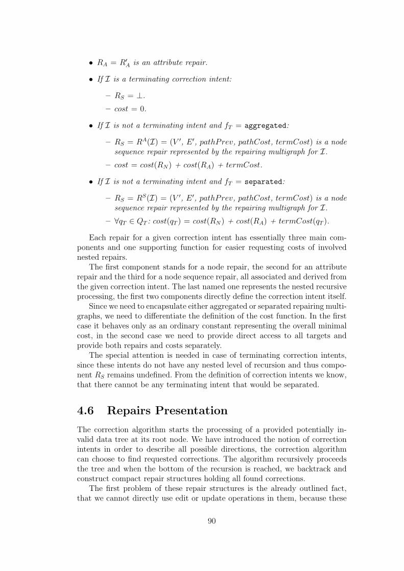
• RA = R′A is an attribute repair.

• If I is a terminating correction intent:

– RS = ⊥.– cost = 0.

• If I is not a terminating intent and fT = aggregated:

– RS = RA(I) = (V ′, E ′, pathPrev, pathCost, termCost) is a nodesequence repair represented by the repairing multigraph for I.

– cost = cost(RN) + cost(RA) + termCost.

• If I is not a terminating intent and fT = separated:

– RS = RS(I) = (V ′, E ′, pathPrev, pathCost, termCost) is a nodesequence repair represented by the repairing multigraph for I.

– ∀qT ∈ QT : cost(qT ) = cost(RN) + cost(RA) + termCost(qT ).

Each repair for a given correction intent has essentially three main com-ponents and one supporting function for easier requesting costs of involvednested repairs.

The first component stands for a node repair, the second for an attributerepair and the third for a node sequence repair, all associated and derived fromthe given correction intent. The last named one represents the nested recursiveprocessing, the first two components directly define the correction intent itself.

Since we need to encapsulate either aggregated or separated repairing multi-graphs, we need to differentiate the definition of the cost function. In the firstcase it behaves only as an ordinary constant representing the overall minimalcost, in the second case we need to provide direct access to all targets andprovide both repairs and costs separately.

The special attention is needed in case of terminating correction intents,since these intents do not have any nested level of recursion and thus compo-nent RS remains undefined. From the definition of correction intents we know,that there cannot be any terminating intent that would be separated.

4.6 Repairs Presentation

The correction algorithm starts the processing of a provided potentially in-valid data tree at its root node. We have introduced the notion of correctionintents in order to describe all possible directions, the correction algorithmcan choose to find requested corrections. The algorithm recursively proceedsthe tree and when the bottom of the recursion is reached, we backtrack andconstruct compact repair structures holding all found corrections.

The first problem of these repair structures is the already outlined fact,that we cannot directly use edit or update operations in them, because these

90

operations need specifying of explicit positions, i.e addresses of nodes in theunderlying tree. Since we store different corrections together, there is no sim-ple way how to determine the required positions already during the recursiveprocessing.

Thus we use repairing instructions, which only define actions to be per-formed, but the particular position is omitted. Since we restricted processingof each sequence of nodes only in a left to right manner, we can retrospectivelytranslate found repairs and obtain standard sequences of edit operations.

The purpose of this section is to first describe the mechanisms, how weunroll compact repairs into individual sequences of repairing instructions, andthen how we perform the mentioned translation to update sequences.

The outlined problem also relates to a way, how we plan to present foundcorrections. The algorithm proposed in this thesis assumes that there is nointeraction with the user and thus we only need to find the best correctionsand directly apply them in order to gain a valid data tree. On that accountwe will describe the mechanism for creating monolithic edit sequences for rootnodes, capable of correcting the entire original data tree.

On the other hand, we can also traverse the given data tree to the depthand find isolated locations, where corrections to errors are proposed. Then wecan independently offer these local corrections to the user.

4.6.1 Repairs for Nodes and Attributes

Node repairs are very simple and since they contain only trivial sequencesof repairing instructions, their evaluation and translation is easy. Attributerepairs are simple data structures too, however we first need to generate allsuitable sequences of repairing instructions.

Attribute Repairs Translation

The problem with repairing sequences for attributes of a selected node in adata tree is hidden in the very quickly increasing number of combinations de-pending on the number of attributes to be removed or added. The prospectiveimplementation of the correction algorithm should therefore consider to sug-gest repairs for attributes completely independently on corrections of the treestructure itself. However, we will follow the introduced formal model of editoperations.

As a consequence, we first need to generate all sequences of repairing in-structions, that are capable to correct attributes with respect to given sets ofrequired and optional attributes from the grammar context for a given node,thus with respect to given sets of invalid existing attributes and required miss-ing attributes.

Definition 4.39 (Evaluation of Attribute Repairs). Assume that a tuple RA =(R,A) is an attribute repair as introduced in Definition 4.21, where R, A ∈ Aare sets of attributes to be removed and added respectively.

91

We define a value of an attribute repair RA to be a set seq(RA) of mu-tually not equivalent sequences of repairing instructions having the minimalcost, without redundancies and correcting attributes with respect to given setsof required and optional attributes.

For ∀m ∈ N0, 0 ≤ m ≤ min(|R|, |A|) we put:

• rm = |R| −m and am = |A| −m.

• R′m = {N | N ∈ P(R) and |N | = m}.

• A′m = {N | N ∈ P(A) and |N | = m}.

• Xm = R′m × A′

m is the Cartesian product of R′m and A′

m.

For each selection of m source and target attributes to be involved in the at-tribute renaming procedure, i.e. ∀xm = (NR, NA) ∈ Xm, we define sequence smto be any sequence of the form:

⟨(renameAttribute, nS1 , n

T1 ), . . . , (renameAttribute, n

Sm, n

Tm),

(removeAttribute, nD1 ), . . . , (removeAttribute, n

Drm),

(addAttribute, nI1), . . . , (addAttribute, n

Iam)⟩

and satisfying the following conditions:

• ∀i ∈ N, 1 ≤ i ≤ m: nSi ∈ NR, n

Ti ∈ NA.

• ∀i, j ∈ N, 1 ≤ i < j ≤ m: nSi = nS

j , nTi = nT

j .

• ∀i ∈ N, 1 ≤ i ≤ rm: nDi ∈ R \NR.

• ∀i, j ∈ N, 1 ≤ i < j ≤ rm: nDi = nD

j .

• ∀i ∈ N, 1 ≤ i ≤ am: nIi ∈ A \NA.

• ∀i, j ∈ N, 1 ≤ i < j ≤ am: nIi = nI

j .

For ∀m we define Sm to be a set of all such sequences sm described above.In other words Sm represents a set of all sequences, where exactly m attributepairs are corrected using the renameAttribute operation and all other usingthe appropriate addAttribute or removeAttribute.

Assuming cn = cost(renameAttribute), cr = cost(removeAttribute) andca = cost(addAttribute), we define seq(RA) depending on the definition of thecost function:

• If cn < ca + cr, then seq(RA) = Smin(|R|,|A|).

• If cn = ca + cr, then seq(RA) =∪min(|R|,|A|)

m=0 Sm.

• If cn > ca + cr, then seq(RA) = S0.

92

We only consider those sequences that are not equivalent. Since all thesesequences modify only one particular node, their translation into edit sequencesis simple. For technical reasons we will always use 0 as a base address fortranslations. This idea will be kept in all other translations too.

Note as well, that each sequence of repairing instructions generated usingthe previous definition has a cost corresponding to the minimal cost requestedby Definition 4.21. We only need to discuss different relations between costs ofindividual edit operations and as a consequence to choose the minimal, what-ever or maximal number of pairs of attributes to be involved in the renamingoperation.

Definition 4.40 (Translation of Attribute Instructions). Given a sequence SA

= ⟨s1, . . . , sn⟩ of attribute repairing instructions for some n ∈ N0, we define atranslation of this sequence to be a sequence of attribute edit operations fix(SA)= ⟨f1, . . . , fn⟩ such that ∀k ∈ N, 1 ≤ k ≤ n:

• If sk = (addAttribute, a),then fk = addAttribute(0, a).

• If sk = (removeAttribute, a),then fk = removeAttribute(0, a).

• If sk = (renameAttribute, a0, a1),then fk = renameAttribute(0, a0, a1).

We assumed that a, a0 and a1 ∈ A were attribute names.Having a set S of sequences of attribute repairing instructions, we define

fix(S) = {fix(SA) | SA ∈ S}.

Node Repairs Translation

Since a node repair contains only one sequence of repairing instructions, theevaluation simply encapsulates this sequence into a set with one element.

Definition 4.41 (Evaluation of Node Repairs). For a given node repair RN

we define seq(RN) = {RN} to be a value of the node repair RN .

Each particular node repairing instruction is translated in a way presentedin the following definition. We keep the concept of a base address equal to 0.One of the reasons to do it is connected with addNode edit operation. Fromthe first point of view, address ϵ seems to be more suitable, but this would leadto inability to represent mentioned operation. The better idea is therefore totreat all base nodes as a sequence of nodes numbered from 0.

Definition 4.42 (Translation of Node Instructions). Given a sequence SN

= ⟨s1, . . . , sn⟩ of node repairing instructions for some n ∈ N0, we define atranslation of this sequence to be a sequence of node edit operations fix(SN)= ⟨f1, . . . , fn⟩ such that ∀k ∈ N, 1 ≤ k ≤ n:

93

• If sk = (addLeaf, n), then fk = addLeaf(0, n).

• If sk = (removeLeaf), then fk = removeLeaf(0).

• If sk = (renameLabel, n), then fk = renameLabel(0, n).

• If sk = (addNode, n, i), then fk = addNode(0, 0 + i, n).

• If sk = (removeNode), then fk = removeNode(0).

We assumed that n ∈ E was an element name and i ∈ N0.Having a set S of sequences of node repairing instructions, we define fix(S)

= {fix(SN) | SN ∈ S}.

4.6.2 Repairs for Sequences and Intents

Now we will focus the problem of generation and translation of sequences forrepairs of node sequences and intents. Contrary to the previously discussedrepairs, these two are not isolated only within one level of recursion and weneed to introduce an inductive definition. At the bottom of the recursion,we construct repairing sequences only from repairs of nodes and attributes.Backtracking towards the root of a processed data tree, we need to inspectrepairing multigraphs depending on particular intent types.

Auxiliary Translation Functions

Before we can continue, we need to introduce three auxiliary functions, whichwill be used for manipulating addresses of nodes occurring in edit operations.The first function calledmodPre prepends specified non-negative integer beforeaddresses of all nodes, function modAlt modifies the first number in addressesto a new number and, finally, function modCut truncates the first number inaddresses.

Definition 4.43 (Auxiliary Translation Functions). Assume that SE = ⟨s1,. . . , sn⟩ is a sequence of edit operations for some n ∈ N0. We define modPre,modAlt and modCut to be functions transforming SE into S ′

E = ⟨s′1, . . . , s′n⟩such that ∀k ∈ N, 1 ≤ k ≤ n:

• If sk = addAttribute(u, a),then s′k = addAttribute(f(u), a).

• If sk = removeAttribute(u, a),then s′k = removeAttribute(f(u), a).

• If sk = renameAttribute(u, a0, a1),then s′k = renameAttribute(f(u), a0, a1).

• If sk = addLeaf(u, n), then s′k = addLeaf(f(u), n).

94

• If sk = removeLeaf(u), then s′k = removeLeaf(f(u)).

• If sk = renameLabel(u, n), then s′k = renameLabel(f(u), n).

• If sk = addNode(u0, u1, n), then s′k = addLeaf(f(u0), f(u1), n).

• If sk = removeNode(u), then s′k = removeNode(f(u)).

We have assumed that u, u0, u1 ∈ N∗0, a, a0, a1 ∈ A, n ∈ E and that function f

is defined depending on modPre, modAlt and modCut alternatives this way:

• For modPre(SE, c), where c ∈ N0, we define f(u) = c.u.

• For modAlt(SE, c), where c ∈ N0, we furthermore assume that u = i.vfor some i ∈ N0, v ∈ N∗

0, and then we define f(u) = (i+ c).v.

• For modCut(SE), we furthermore assume that u = i.v for some i ∈ N0,v ∈ N∗

0, and then we define f(u) = v.

Having a set S of sequences of edit operations, we analogously define:

• modPre(S, c) = {modPre(SE, c) | SE ∈ S},

• modAlt(S, c) = {modAlt(SE, c) | SE ∈ S} and

• modCut(S) = {modCut(SE) | SE ∈ S}.

Node Sequence Repairs Translation

Having a particular repairing path in the repairing multigraph, we can generateall repairing sequences by combining repairs associated with edges of such path.

Our goal is however not only to generate all sequences of repairing instruc-tions, we also need to translate them. For one particular path this translationis easy, because we need only to monitor correction intents along the processedpath and determine the number of nodes the given intents involve at their toplevel.

Definition 4.44 (Translation of Node Sequence Repairs). Assume that RS isa node sequence repair corresponding to a repairing multigraph R(I) = (V ′,E ′, pathPrev, pathCost, termCost) for a correction intent I = (y, RN , RA,sI , qI , sE, QE, u, d, C, fS, fT , qS, QT , Ya), where u = ⟨u1, . . . , un⟩ for somen ∈ N0.

We define fix(RS) or fix(RS, qT ) to be a translation of a node sequence re-pair RS, where fix(RS) is a set of all sequence mends for shortest paths in thegiven aggregated repairing multigraph for correction intent I and fix(RS, qT )for ∀qT ∈ QT a set of all sequence mends for shortest paths to state qT in thelast stratum in the given separated repairing multigraph.

A sequence mend for a particular shortest path is a pair (S, shift), where Sis a corresponding sequence of edit operations derived from the path and shiftis a number of processed nodes as defined subsequently.

95

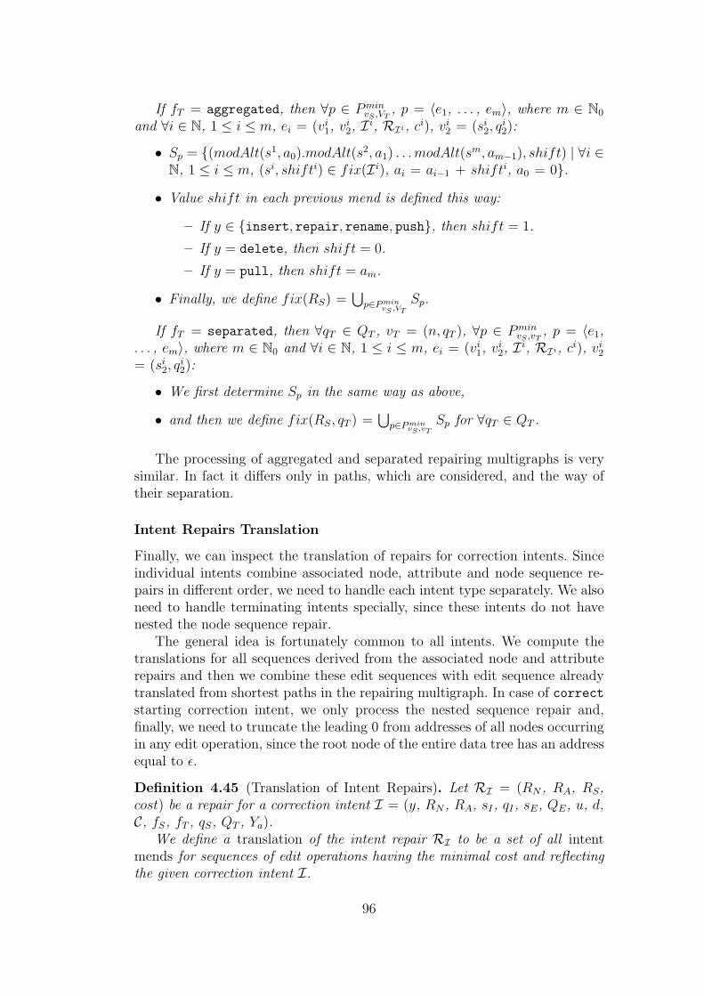
If fT = aggregated, then ∀p ∈ PminvS ,VT

, p = ⟨e1, . . . , em⟩, where m ∈ N0

and ∀i ∈ N, 1 ≤ i ≤ m, ei = (vi1, vi2, I i, RIi, ci), vi2 = (si2, q

i2):

• Sp = {(modAlt(s1, a0).modAlt(s2, a1) . . .modAlt(sm, am−1), shift) | ∀i ∈N, 1 ≤ i ≤ m, (si, shifti) ∈ fix(I i), ai = ai−1 + shifti, a0 = 0}.

• Value shift in each previous mend is defined this way:

– If y ∈ {insert, repair, rename, push}, then shift = 1.

– If y = delete, then shift = 0.

– If y = pull, then shift = am.

• Finally, we define fix(RS) =∪

p∈PminvS,VT

Sp.

If fT = separated, then ∀qT ∈ QT , vT = (n, qT ), ∀p ∈ PminvS ,vT

, p = ⟨e1,. . . , em⟩, where m ∈ N0 and ∀i ∈ N, 1 ≤ i ≤ m, ei = (vi1, v

i2, I i, RIi, ci), vi2

= (si2, qi2):

• We first determine Sp in the same way as above,

• and then we define fix(RS, qT ) =∪

p∈PminvS,vT

Sp for ∀qT ∈ QT .

The processing of aggregated and separated repairing multigraphs is verysimilar. In fact it differs only in paths, which are considered, and the way oftheir separation.

Intent Repairs Translation

Finally, we can inspect the translation of repairs for correction intents. Sinceindividual intents combine associated node, attribute and node sequence re-pairs in different order, we need to handle each intent type separately. We alsoneed to handle terminating intents specially, since these intents do not havenested the node sequence repair.

The general idea is fortunately common to all intents. We compute thetranslations for all sequences derived from the associated node and attributerepairs and then we combine these edit sequences with edit sequence alreadytranslated from shortest paths in the repairing multigraph. In case of correctstarting correction intent, we only process the nested sequence repair and,finally, we need to truncate the leading 0 from addresses of all nodes occurringin any edit operation, since the root node of the entire data tree has an addressequal to ϵ.

Definition 4.45 (Translation of Intent Repairs). Let RI = (RN , RA, RS,cost) be a repair for a correction intent I = (y, RN , RA, sI , qI , sE, QE, u, d,C, fS, fT , qS, QT , Ya).

We define a translation of the intent repair RI to be a set of all intentmends for sequences of edit operations having the minimal cost and reflectingthe given correction intent I.

96

If I is an aggregated correction intent, we denote this translation by fix(RI),otherwise for a separated intent we define a translation for ∀qT ∈ QT separatelyby fix(RI, qT ).

• If y = correct:

– fix(RI) = {(modCut(rS),⊥) | (rS, shift) ∈ fix(RS)}.

• If y = insert:

– If I is a terminating intent, then fix(RI) = {(rN .rA, 0) |rN ∈ fix(seq(RN)), rA ∈ fix(seq(RA))}.

– Otherwise fix(RI) = {(rN .rA.modPre(rS, 0), shift) |rN ∈ fix(seq(RN)), rA ∈ fix(seq(RA)),(rS, shift) ∈ fix(RS)}.

∀f ∈ fix(RI): f = insertSubtree(0) update operation.

• If y = delete:

– If I is a terminating intent, then fix(RI) = {(rA.rN , 0) |rN ∈ fix(seq(RN)), rA ∈ fix(seq(RA))}

– Otherwise fix(RI) = {(modPre(rS, 0).rA.rN , shift) |rN ∈ fix(seq(RN)), rA ∈ fix(seq(RA)),(rS, shift) ∈ fix(RS)}

∀f ∈ fix(RI): f = deleteSubtree(0).

• If y = repair, then:

– If I is a terminating intent,then fix(RI) = {(rA, 0) | rA ∈ fix(seq(RA))}.

– Otherwise fix(RI) = {(rA.modPre(rS, 0), shift) |rA ∈ fix(seq(RA)), (rS, shift) ∈ fix(RS)}.

∀f ∈ fix(RI): f = repairSubtree(0).

• If y = rename, then:

– If I is a terminating intent, then fix(RI) = {(rN .rA, 0) |rN ∈ fix(seq(RN)), rA ∈ fix(seq(RA))}.

– Otherwise fix(RI) = {(rN .rA.modPre(rS, 0), shift) |rN ∈ fix(seq(RN)), rA ∈ fix(seq(RA)),(rS, shift) ∈ fix(RS)}.

∀f ∈ fix(RI): f = renameSubtree(0).

97

• If y = push:

– fix(RI) = {(rN .rA.modPre(rS, 0), shift) |rN ∈ fix(seq(RN)), rA ∈ fix(seq(RA)),(rS, shift) ∈ fix(RS)}.

∀f ∈ fix(RI): f = pushSiblings(0, sE − sI − 1).

• If y = pull, then for ∀qT ∈ QT :

– fix(RI , qT ) = {(rA.rN .rS, shift) | rN ∈ fix(seq(RN)),rA ∈ fix(seq(RA)), (rS, shift) ∈ fix(RS, qT )}.

∀f ∈ fix(RI , qT ): f = pullSiblings(0).

Note that addresses of nodes are reconstructed in a bottom up way andwe do not use any direct knowledge about positions from the original datatree. Moreover performing an edit operation we can achieve changes in ad-dresses of former or newly subordinated nodes, thus we need to be aware ofthis addressing variability.

The previous definition also declares the connection of correction intentsand update operations. Once having a particular sequence of repairing in-structions translated into a sequence of edit operations, we can classify suchsequence using definitions for update operations. As already outlined, the cor-rection algorithm is not able to generate all potentially existing sequences thatwould conform to introduced update operations. But the algorithm is alwaysable to find corrections and these can be viewed via updates.

4.7 Correction Algorithms

The purpose of the previous section was to completely introduce the correc-tion capabilities of the proposed correction algorithm. We have abstracted theproceeding of the algorithm using multigraphs. Their purpose was to staticallydescribe all repairs that can be generated in the limits of introduced correctionintents.

The basic idea of these multigraphs originates from the complete traversalof the state space of the Glushkov automaton, which is derived from the regularexpression restricting the element content of a given node in a data tree. Weare generally able to perform this processing dynamically, or we can constructthe multigraph and then inspect all possible repairs statically. This has alsoanother advantage, because multigraphs not only record the algorithm flow,but also store the computed results in a form of the shortest paths to somespecified vertices, usually corresponding to the accepting output states of theautomaton itself.

In this section we will describe four different versions of the correctionalgorithm. Starting with the naive correction algorithm we will directly followintroduced formal framework of multigraphs. Next, we will discuss dynamic

98

algorithm, which directly constructs only the required portion of the repairingmultigraph. The last but one algorithm stands for caching correction algorithmcapable to avoid repeated computations of identical intents. Finally, we willpresent incremental algorithm, which is able to work efficiently even to thedepth of recursively invoked intents.

4.7.1 Naive Correction Algorithm

The first presented algorithm strictly follows the idea of defined multigraphs.Therefore, the naive correction algorithm really first constructs the completeexploration multigraph, then it evaluates all its edges by invoking the compu-tations of recursively nested correction intents and, finally, it constructs therepairing multigraph, which can be simply turned into the repair for the givenintent.

Algorithm Description

The correction starts by the invocation of the recursive routine with the start-ing context I•. At each level of the recursion we first prepare the entire explo-ration multigraph with its all vertices and edges.

The second step represents the evaluation of all nested intents. This meansthat we compute all generated correction intents and bind returned repairsto corresponding edges in the correction multigraph. The last but one steprepresents the searching for all shortest paths, since these paths involve allfound suitable repairs, which are as close to the original data tree as the notionof correction intents admits.

The following enumeration gives an overview of all input and output pa-rameters, which are passed into and from the correction routine respectively:

• The problem defining input parameters: data tree T = (D, lab, val, att)and single type tree grammar G = (N , T , A, S, P ).

• The intent description input parameters: correction intent type y, noderepair RN and attribute repair RA, initial stratum number sI and stateqI in sI , ending stratum number sE and set of ending states in sE.

• The intent assignment input parameters: sequence of nodes u = ⟨u1, . . . ,un⟩ to be processed, depth d of processed nodes in a new tree, grammarcontext C = (aR, nR, Nc, Pc, map, r, C, O), flags fS and fT , startingstate qS of Ar, set of terminating states QT of Ar and set of allowedcorrection intent types Ya.

• The output parameter: repair structure RI = (RN , RA, RS, cost).

99

Main Procedure Definition

The main procedure presented in Algorithm 1 reflects the sequence of stepsthat should be executed. First we prepare the exploration multigraph, thenwe compute the correction multigraph, derive the repairing multigraph and,finally, encapsulate the found repairs into the repair structure.

Algorithm 1: naiveCorrectionAlgorithm

Input : Data tree T , single type tree grammar G, intent I.Output: Repair RI for correction intent I.

1 E(I) ← createExplorationMultigraph(T , G, I);2 C(I) ← createCorrectionMultigraph(T , G, I, E(I));3 R(I) ← createRepairingMultigraph(T , G, I, C(I));4 RI ← composeIntentRepair(I, R(I));5 return RI

Procedure for Exploration Multigraph Creation

The procedure introduced in Algorithm 2 for the exploration multigraph con-struction starts with an empty multigraph and then successively adds newvertices and edges following Definition 4.27 of recursive correction intents.

Algorithm 2: createExplorationMultigraph

Input : Data tree T , single type tree grammar G, intent I.Output: Exploration multigraph E(I).

1 E(I) = (VE, EE) ← (∅, ∅);2 VE ← {(0, qS)};3 NewV ertices ← {(0, qS)};4 while ∃v1 ∈ NewV ertices, v1 = (s, q) do5 foreach correction intent I ′ = (y′, R′

N , R′A, s

′I , q

′I , s

′E, Q

′E, u

′, d′,C ′, f ′

S, f′T , q

′S, Q

′T , Y

′a) defined in stratum s and state q do

6 foreach q′E ∈ Q′E do

7 v2 ← (s′E, q′E);

8 if v2 /∈ VE then9 Add vertex v2 into VE and NewV ertices;

10 Add edge (v1, v2, I ′) into EE;

11 Remove v1 from NewNodes;

100

Procedure for Correction Multigraph Creation

The purpose of Algorithm 3 is to derive the corresponding correction multigrapfrom a provided and fully constructed exploration multigraphh. Thus the maintask is to invoke the recursive computations of prepared correction intents andthen store returned repairs inside edges of the correction multigraph.

Algorithm 3: createCorrectionMultigraph

Input : Data tree T , single type tree grammar G, correction intent I,exploration multigraph E(I) = (VE, EE).

Output: Correction multigraph C(I).1 C(I) = (VC , EC) ← (VE, ∅);2 foreach v1 ∈ VC, v1 = (q, s) do3 foreach correction intent I ′ = (y′, R′

N , R′A, s

′I , q

′I , s

′E, Q

′E, u

′, d′,C ′, f ′

S, f′T , q

′S, Q

′T , Y

′a) defined in stratum s and state q do

4 repair ← naiveCorrectionRoutine(T , G, I ′);5 foreach q′E ∈ Q′

E do6 v2 ← (s′E, q

′E);

7 if f ′T = aggregated then c ← cost(repair);

8 else c ← cost(repair, q′E) ; f′T = separated

9 Add correcting edge (v1, v2, I ′, repair, c) into EC ;

Procedure for Repairing Multigraph Creation

The repairing multigraph is a subgraph of the correction multigraph with onlythose vertices and edges that are involved in the found shortest paths to thegiven set of target vertices.

Its construction is presented in Algorithm 4, where we have just followedthe idea of standard Dijkstra’s algorithm [24] for searching shortest paths ingraphs.

We start the processing of the multigraph in the source vertex specified bythe correction intent itself. Then we step by step walk through the multigraphand in each step, we first select the previously reached vertex, which has theminimal pathCost between all reached vertices. The algorithm ensures thatthis cost becomes final for this vertex, since it cannot be improved any more.

If we need to generate an aggregated repair, we have already closed thefirst target vertex and if the current path cost has strictly greater value thanthe cost of the target vertex that has been wiped as the first item from theworking set of target vertices, we can stop the loop. Analogously if we need togenerate separated repair, we are forced to operate until the last vertex fromthe set of target vertices is marked as closed and then wait until the currentcost exceeds the fixed value from the last wiped target vertex.

101

Algorithm 4: createRepairingMultigraph

Input : Data tree T , single type tree grammar G, correction intent I= (y, RN , RA, sI , qI , sE, QE, u, d, C, fS, fT , qS, QT , Ya),correction multigraph C(I) = (VR, ER).

Output: Repairing multigraph R(I).1 R(I) = (VR, ER, pathPrev, pathCost, termCost) ← (VR, ER, ∅, ∅,⊥);2 vS ← (0, qS); pathCost(vS) ← 0; pathPrev(vS) ← ∅;3 reachedV ertices ← {vS}; closedV ertices ← ∅;4 targetV ertices ← {(n, qT ) | qT ∈ QT};5 while reachedV ertices = ∅ do6 m ← minv∈reachedV erticespathCost(v);7 v1 = (s, q) for some v1 ∈ reachedV ertices, pathCost(v1) = m;8 if [(targetV ertices = {v1}) or (fT = aggregated and

v1 ∈ targetV ertices)] and [finalCost is not defined] then9 finalCost ← pathCost(v1);

10 Remove v1 from reachedV ertices and targetV ertices;11 Add v1 to closedV ertices;12 if finalCost is defined and finalCost < pathCost(v1) then13 break

14 foreach e ∈ ER, e = (v1, v2, i, Ri, c) do15 c′ ← pathCost(v1) + c;16 if pathCost(v2) is defined and pathCost(v2) = c′ then17 pathPrev(v2) ← pathPrev(v2) ∪ {v1};18 if pathCost(v2) is not defined or pathCost(v2) > c′ then19 pathCost(v2) ← c′; pathPrev(v2) ← {v1};20 if v2 /∈ closedV ertices and v2 /∈ reachedV ertices then21 Add v2 to reachedV ertices;

22 if fT = aggregated then termCost ← finalCost;23 else ∀vT ∈ VT termCost(vT ) ← pathCost(vT ) ; fT = separated

Otherwise we process all outgoing edges from the current vertex and if weare able to reach the given ending vertex with the same or better path cost,we change it and update the set of preceding vertices. Thus we are able tobacktrack and reconstruct all shortest paths.

Finally, we need to clean the multigraph from unnecessary vertices andedges. This step is easy and is not included in Algorithm 4.

102

4.7.2 Dynamic Correction Algorithm

The main disadvantage of the naive correction algorithm is that we usuallyuselessly construct the entire exploration multigraph and later on in orderto create the derived creation multigraph, we evaluate all prepared nestedcorrection intents. It is easy to see, that we can propose an algorithm, thatdirectly attempts to search for all shortest paths and during this search itconstructs only the required part of the multigraph. This can lead to timesavings, since we do not need to compute all correction edges.

Suggested improvements are considered in Algorithm 5. It does not work inthe consecutive steps based on the exploration, correction and repairing multi-graphs construction, but it straightforwardly builds the repairing multigraph,which at the end only needs to be cleaned from vertices and edges, that arenot located at any of the found shortest paths.

Although we now evaluate only those nested intents, that we need to inspectduring the procedure of searching shortest paths, there still remains otherproblems causing significant inefficiency. We will thus attempt to make twomore improvements.

4.7.3 Caching Correction Algorithm

During the computation of the naive or dynamic correction algorithm, weare quite often forced to compute the same information, as we have alreadycomputed probably many times before.

Suppose that we are in some of the nodes of a given data tree and wehave decided for example to change its label. This means that we consequentlyneed to recursively process all its child nodes in a few alternative ways, one foreach pair of allowed terminal and nonterminal symbol used for renaming. It ishighly probable that the processing of these nodes and all their subtrees willbe similar. In other words there would be chance for any type of correctionintent to be evaluated repeatedly.

As a particular example we can name for example the deletion intent. Itis easy to sea, that there can be various different chains of nested intents, butwhenever we decide to delete a subtree on a given position in the original datatree, the deletion will always proceed identically, since only the data subtreeitself defines the generation of nested deletion intents and thus correspondingrepair.

Similarly whenever we decide to insert a subtree with a specified terminalsymbol as a label for a new root node and nonterminal symbol describing thecontext to be used, the proceeding of this insert correction intent will alwaysbe the same.

To harness this finding and in order to introduce much more efficient algo-rithm, we are going to introduce the model of caching. Its main purpose is toprovide the environment, where nothing already computed is forgotten, sinceit can be reused again.

103

Algorithm 5: dynamicCorrectionRoutine

Input : Data tree T , single type tree grammar G, intent I = (y, RN ,RA, sI , qI , sE, QE, u, d, C, fS, fT , qS, QT , Ya).

Output: Repair RI for intent I.1 R(I) ← ({(0, qS)}, ∅, ∅, ∅,⊥);2 vS ← (0, qS); pathCost(vS) ← 0; pathPrev(vS) ← ∅;3 reachedV ertices ← {vS}; targetV ertices ← {(n, qT ) | qT ∈ QT};4 while reachedV ertices = ∅ do5 m ← minv∈reachedV erticespathCost(v);6 v1 = (s, q) for some v1 ∈ reachedV ertices, pathCost(v1) = m;7 if [(targetV ertices = {v1}) or (fT = aggregated and

v1 ∈ targetV ertices)] and [finalCost is not defined] then8 finalCost ← pathCost(v1);

9 if finalCost is defined and finalCost < pathCost(v1) then10 break

11 foreach correction intent I ′ = (y′, R′N , R

′A, s

′I , q

′I , s

′E, Q

′E, u

′, d′,C ′, f ′

S, f′T , q

′S, Q

′T , Y

′a) defined in stratum s and state q do

12 repair ← dynamicCorrectionRoutine(T , G, I ′);13 foreach q′E ∈ Q′

E do14 v2 ← (s′E, q

′E);

15 if f ′T = aggregated then c ← cost(repair);

16 else c ← cost(repair, q′E) ; f′T = separated

17 if v2 /∈ VE then Add v2 into VE and reachedV ertices;18 Add correcting edge (v1, v2, I ′, repair, c) into ER;19 c′ ← pathCost(v1) + c;20 if pathCost(v2) is defined and pathCost(v2) = c′ then21 pathPrev(v2) ← pathPrev(v2) ∪ {v1};22 if pathCost(v2) is undefined or pathCost(v2) > c′ then23 pathCost(v2) ← c′; pathPrev(v2) ← {v1};

24 Remove v1 from reachedV ertices and targetV ertices;

25 if fT = aggregated then termCost ← finalCost;26 else ∀vT ∈ VT termCost(vT ) ← pathCost(vT ) ; fT = separated

27 return RI ← composeIntentRepair(I, R(I));

Signatures of Correction Intents

Our goal is to describe correction intents, which certainly lead to the samerepairs, i.e. intents with the identical assignment for a nested recursion levelof processing. Having a particular type of a correction intent, the notion of anintent signature solves our problem.

104

Definition 4.46 (Correction Intent Signature). Assume that T = (D, lab,val, att) is a data tree and I = (y, RN , RA, sI , qI , sE, QE, u, d, C, fS, fT ,qS, QT , Ya) is a correction intent where C = (aR, nR, Nc, Pc, map, r, C, O)is a grammar context and u = ⟨u1 . . . un⟩ is a node sequence of length n.

We define a signature S(I) of a correction intent to be a tuple, which fulfilsthe following conditions:

• If y = correct, then S(I) = (correct).

• If y = insert, then S(I) = (insert, nR, aR).

• If y = delete, then S(I) = (delete, baseNode(I)).

• If y = repair, then S(I) = (repair, baseNode(I), nR).

• If y = rename, then S(I) = (rename, baseNode(I), nR, aR).

• If y = push, then S(I) = (push, baseNode(I), n, nR, aR).

• If y = pull, then S(I) = (pull, baseNode(I), nR, aR, qS).

The insert correction intent is only described by the terminal symboland a production rule to be used. This rule uniquely implies the nonterminalsymbol. In case of delete intent, we only need to specify the position in theoriginal data tree.

Correction intents repair and rename are similar, but the former one doesnot need to specify the terminal symbol, because this symbol equals to thenode label in the original data tree.

The push intent needs to be described by the range of sibling nodes thatshould be pushed one level lower. The label and nonterminal symbol of theirnew parent node uniquely defines the nested processing. Finally, the pull

intent is described by a pair of terminal and nonterminal symbol again, butthese symbols belong to the original grandparent of pulled nodes, thus theirnew parent to whose context they should now conform. The source state isrequired too, since it influences the set of reachable target states.

Caching Repository Model

Now we can introduce the notion for a caching repository, which serves for stor-ing already computed repairs. The caching version of the correction algorithmfirst attempts to ask this cache and only if the specified correction intent hasnot yet been computed, we invoke its computation. Otherwise we can accessthe cached repair we need.

Definition 4.47 (Caching Manager). A caching manager is a data structureacting as a partial function, which is able to assign a corresponding repair to agiven signature of an intent I , denoted by cacheRepair(signature(I)) = RI.

105

At the beginning of the correction algorithm the caching repository is emptyand this means, that the internal cache function is not defined for any signa-ture. During the recursive processing, whenever we finish computation of agiven level and thus have evaluated a repair for a given correction intent, weextend this function, i.e. insert newly computed repair into the cache.

Algorithm Description

The newly presented caching Algorithm 6 is almost identical to the dynamiccorrection algorithm. We only need to modify the code near the place of thenested recursion level invocation. We first attempt to fetch the already com-puted repair from the caching repository and only if we are not successful, weinvoke its computation.

Algorithm 6: cachingCorrectionRoutine

Input : Data tree T , single type tree grammar G, intent I.Output: Repair for correction intent I.// Lines 1 to 11 from Algorithm 5

// Adjusted line 12 from Algorithm 5

1 if cache(signature(I)) is defined then2 repair ← cacheRepair(signature(I));3 else4 repair ← cachingCorrectionRoutine(T , G, I ′);5 cacheRepair(signature(I)) ← repair;

// Lines 13 to 27 from Algorithm 5

4.7.4 Incremental Correction Algorithm

The dynamic correction algorithm efficiently processes each level of recursion,because it only invokes evaluation of those edges that need to be inspectedin order to find all required shortest paths. Therefore, we are able to avoidprocessing of those directions in a given partial repairing multigraph, whichseem not to be perspective. The main problem however remains. Althoughwe ignore some edges, whenever we decide to evaluate one edge, we need toinspect the entire recursion hidden in this single edge. Even if this edge wouldnot be the good direction to acquire the shortest path, we need to evaluate itcompletely.

The idea of the incremental correction algorithm is to work efficiently evenwith the recursion. Suppose that we are at the top level, thus we are processingthe starting correction intent and we need to find the shortest paths to correctthe entire tree. This means that we still need to follow standard Dijkstra’salgorithm, but we can act lazily. This means that whenever we need to evaluate

106

a correction intent associated with a given edge, we only initiate the processof its incremental computation. The algorithm will work in steps, permanentlyattempting to give more precision to partially evaluated intents. Step by stepwe will obtain more precise estimations of edge costs and dynamically followonly directions, which seem to be the most promising.

Tasks Model

The main difference to all previously introduced correction algorithms is thefact that we cannot directly use nested calls of the correction routine. We needto introduce the model, where we only tell what to compute and the particularcomputations will be controlled by some manager. This also means that weneed a data structure with ability to store the complete context describing thestate of elaboration for each single correction intent.

Definition 4.48 (Intent Computation Task). Assume that I = (y, RN , RA,sI , qI , sE, QE, u, d, C, fS, fT , qS, QT , Ya) is a correction intent. We definea task for I to be a tuple KI = (I, R(I), state, stamp, Vreached, Ereached,Edelayed, VT , creached, cfixed, WA, WD), where:

• I is the correction intent.

• R(I) is the partially evaluated repairing multigraph for I. This meansthat the multigraph is not complete and function or constant termCostreturns only estimated values.

• state ∈ {suspended, blocked, activated, signalled}

• stamp ∈ N0 is a timestamp of the last incremental processing.

• Vreached ⊆ VC is a set of reached vertices.

• Ereached ⊆ EC is a set of reached edges.

• Edelayed ⊆ EC is a set of delayed edges.

• VT ⊆ VC is a set of opened target vertices.

• creached is a value of reached cost.

• cfixed is a value of fixed cost or ⊥.

• WA is a set of correction tasks waiting for KI.

• WD is a set of correction tasks for which KI is waiting.

It is easy to see that we have in principle only encapsulated local variablesfrom Algorithm 5. These are especially items Vreached for storing reached andnot yet closed vertices, VT representing a set of not yet closed target vertices,creached for reached cost of the inspected node and also cfixed for storing the

107

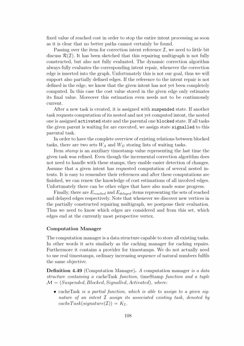
fixed value of reached cost in order to stop the entire intent processing as soonas it is clear that no better paths cannot certainly be found.

Passing over the item for correction intent reference I, we need to little bitdiscuss R(I). It has been sketched that this repairing multigraph is not fullyconstructed, but also not fully evaluated. The dynamic correction algorithmalways fully evaluates the corresponding intent repair, whenever the correctionedge is inserted into the graph. Unfortunately this is not our goal, thus we willsupport also partially defined edges. If the reference to the intent repair is notdefined in the edge, we know that the given intent has not yet been completelycomputed. In this case the cost value stored in the given edge only estimatesits final value. Moreover this estimation even needs not to be continuouslycurrent.

After a new task is created, it is assigned with suspended state. If anothertask requests computation of its nested and not yet computed intent, the nestedone is assigned activated state and the parental one blocked state. If all tasksthe given parent is waiting for are executed, we assign state signalled to thisparental task.

In order to have the complete overview of existing relations between blockedtasks, there are two sets WA and WD storing lists of waiting tasks.

Item stamp is an auxiliary timestamp value representing the last time thegiven task was refined. Even though the incremental correction algorithm doesnot need to handle with these stamps, they enable easier detection of changes.Assume that a given intent has requested computation of several nested in-tents. It is easy to remember their references and after these computations arefinished, we can renew the knowledge of cost estimations of all involved edges.Unfortunately there can be other edges that have also made some progress.

Finally, there are Ereached and Edelayed items representing the sets of reachedand delayed edges respectively. Note that whenever we discover new vertices inthe partially constructed repairing multigraph, we postpone their evaluation.Thus we need to know which edges are considered and from this set, whichedges end at the currently most perspective vertex.

Computation Manager

The computation manager is a data structure capable to store all existing tasks.In other words it acts similarly as the caching manager for caching repairs.Furthermore it contains a provider for timestamps. We do not actually needto use real timestamps, ordinary increasing sequence of natural numbers fulfilsthe same objective.

Definition 4.49 (Computation Manager). A computation manager is a datastructure containing a cacheTask function, timeStamp function and a tupleM = (Suspended,Blocked, Signalled, Activated), where:

• cacheTask is a partial function, which is able to assign to a given sig-nature of an intent I assign its associated existing task, denoted bycacheTask(signature(I)) = KI.

108

• timeStamp provider is a function returning values from N serving astimestamps. Whenever this function is called, it returns a value equal tothe previously returned value increased by 1.

• Suspended is a set of tasks having state = suspended.

• Blocked is a set of tasks having state = blocked.

• Signalled is a set of tasks having state = aignalled.

• Activated is a set of tasks having state = activated.

All existing tasks are cached within the computation manager in four dis-joint sets separated by task states. We actually only need the direct access tosets of Signalled and Activated, because the main correction routine works ina cycle and in each step it invokes the computation of some task correspondingone of these two states.

Whenever we first encounter a correction intent, we create a task encapsu-lating this intent and we put this task structure into the cache of tasks in thecomputation manager. After its computation is fully finished, we destroy thetask structure and put the intent repair into the standard caching repositoryfor repairs.

Main Correction Routine

The main routine of the incremental correction algorithm is presented in Al-gorithm 7. Its purpose is to create the starting intent for correction of theentire tree, start up its processing, continuously manage it and, finally, fetchthe repair structure with corrections for the data tree itself.

The life cycle of each task begins in the state suspended. This is quite im-portant, because this means that the given task cannot be passed to processinguntil some running task explicitly requests this. In a such situation there is aclear relation between the requesting task and the requested tasks.

The main loop continually fetches prepared and requested tasks and in-vokes their incremental computation. Note that there is at most one runningtask in each moment. Although we could probably extend the incremental cor-rection algorithm to multithreaded environment with parallel computations,this version only works task by task.

After the execution of activated task is started, we attempt to do thebest in order to complete its mission, i.e. to find repair for a sequence ofnodes, thus to find shortest paths in the constructed repairing multigraph.But we need to manage this effort and therefore only the starting intent hasno limitations. All other tasks have only one opportunity to request the furthersteps of nested intents computation. This stands for the explanation of the lastboolean parameter in the procedure invoked in the loop.

109

Algorithm 7: incrementalCorrectionRoutine

Input : Data tree T , single type tree grammar G.Output: Repair RI• for correction intent I•.

1 M = (Suspended,Blocked, Signalled, Activated) ← (∅, ∅, ∅, ∅);2 cacheTask ← ∅;3 createCorrectionTask(I•);4 activateCorrectionTask(⊥, I•);5 while ∃KI ∈M.Signalled ∪M.Activated do6 switch KI .state do7 case signalled

8 creative ← (I = I•);9 processCorrectionStep(T , G, KI, creative);

10 case activated

11 processCorrectionStep(T , G, KI, true);

12 R(I•) ← cacheRepair(signature(I•));13 return RI•;

Incremental Correction Step

The main principle of the incremental algorithm is to compute progressivelyinto the depth. This means that at each level of the nested intents we first needto follow the idea of the shortest paths searching, but concurrently we need tosuppress excessive activity to really achieve the comfortable behaviour insidethe top intent. Thus whenever the particular intent task is requested for thenext headway, we need to create a mechanism for its well-timed interruption.

Each activated intent except the top one is able to process without limitsuntil it first requests computation of some not yet fully computed tasks. Thiscondition seems rather strict, but after there are already some intents finishedand their repairs cached, there is a chance to go through larger parts of themultigraph.

Suppose that we have selected the most perspective vertex from the setof reached vertices. The dynamic version of the correction algorithm does thesame, but now we cannot automatically declare this vertex as fully defined,since we only have the estimation of costs of edges leading to this vertex. Eventhough it now seems the given node is the best one, further computations mayreverse this state. Thus in order to declare the given candidate vertex as final,there must be at least one fully evaluated ingoing edge to this vertex fromthe set of reached edges and all other not yet fully evaluated edges must havestrictly greater cost estimation.

Only under these conditions we can declare the given perspective vertexas final, terminate its processing and explore other probably not yet explored

110

vertices beyond it. If we cannot close the given candidate, we need to refine allits ingoing edges that have not yet been fully evaluated. We therefore requestcomputation of these tasks and then we end in order to wait until these nestedintents bring progress to edges in constructed multigraph.

Algorithm 8: processCorrectionStep

Input : Data tree T , single type tree grammar G, correction task KI= (I, R(I), state, stamp, Vreached, Ereached, Edelayed, VT ,creached, cfixed, WA, WD), boolean creative.

1 foreach e ∈ KI .Ereached do2 renewEdgeRatings(e, KI .stamp);

3 foreach v ∈ KI .Vreached do4 renewVertexRatings(R(I), KI, v);

5 while KI .Vreached = ∅ do6 v1 ← selectBestCandidate(R(I), KI .Vreached);7 KI .creached ← pathCost(v1);8 if [(KI .VT = {v1}) or (I.fT = aggregated and v1 ∈ KI .VT )] and

[KI .cfixed is not defined] then KI .cfixed ← KI .creached;9 if KI .cfixed is defined and KI .cfixed < KI .creached then

10 KI .Vreached ← ∅; break11 if resolveVertexCompleteness(R(I), KI, v1) then12 processCompleteVertex(T , G, I, R(I), v1);13 else14 if creative then15 processIncompleteVertex(KI, v1);

16 break

17 if KI .Vreached = ∅ and KI .Edelayed = ∅ and creative then18 processDelayedEdges(R(I), KI);

19 renewRepairRatings(I, R(I), KI);20 KI .stamp ← timeStamp();

21 if KI .Vreached = ∅ and KI .Edelayed = ∅ then22 repair ← composeIntentRepair(I, R(I));23 cacheRepair(signature(I)) ← repair;24 signalCorrectionTask(KI);25 destroyCorrectionTask(KI);

26 else27 if creative then blockCorrectionTask(KI);28 else signalCorrectionTask(KI);

111

Structuring Algorithm 8 into main parts, we can start with the initial re-newing of the knowledge about the acquired progress in nested intents, thenthe main loop of processing reached vertices and, finally, the code for taskprocessing termination. This ending essentially consists of the intent repairstructure composition in case we have successfully completed the entire pro-cessing of a given task, or blocking and signalling requests in case we need towait for nested executions or, conversely, inform ascendent tasks respectively.

Vertices Processing Routines

Now we will present procedures for processing vertices believed to be perspec-tive candidates in the main loop of each step of task proceeding. First, we willput attention to Algorithm 9 describing the processing of vertices that can bedeclared as final, thus satisfying the outlined conditions of existence of somefully evaluated ingoing edge having the cost better than all other estimationsfrom only partially evaluated edges.

Algorithm 9: processCompleteVertex

Input: Data tree T , single type tree grammar G, correction intent I,partial multigraph R(I), task KI , vertex v1 = (s1, q1)

1 Remove v1 from KI .Vreached and KI .VT ;2 Remove ∀e′ = (v′1, v

′2, I ′, R′, c′), v′2 = v1 from KI .Ereached;

3 foreach I ′ ∈ intents(I), (I ′.sI , I ′.qI) = v1 do4 s′ ← signature(I ′);5 if cacheTask(s′) is not defined and cacheRepair(s′) is not defined

then createCorrectionTask(I ′);6 foreach q′E ∈ I ′.QE do7 v2 ← (I ′.sE, q′E); e ← (v1, v2, I ′, ⊥, ⊥);8 if v2 /∈ R(I).VR then9 Add v2 into R(I).VR and KI .Vreached;

10 if v2 ∈ KI .Vreached then11 Add correcting edge e into R(I).ER and KI .Ereached;

12 else13 Add correcting edge e into R(I).ER and KI .Edelayed;

14 renewEdgeRatings(e, 0);15 renewVertexRatings(R(I), KI, v2);

Similarly to the original dynamic algorithm we need to inspect all outgoingedges and newly discovered vertices terminating these edges.

In Algorithm 10 we present the processing of vertices that cannot be closed,since we have not yet computed enough to be sure we can do it. In order to

112

achieve better estimations, we request further processing of all edges ingoingto the vertex currently declared as the perspective one.

Algorithm 10: processIncompleteVertex

Input: Correction task KI , vertex v1 = (s1, q1).

1 foreach e = (v′0, v′1, I ′, R′, c′) ∈ KI .Ereached, v

′1 = v1 do

2 if e.R′ = ⊥ then3 activateCorrectionTask(KI, I ′);

During the process of searching for the shortest paths we sometimes comeacross edges leading from the vertex being closed to some other already closedone. It is easy to see that we do not need to evaluate these edges immediately,because they cannot influence the traversal itself. However, we need to eval-uate them at least partially in order to eliminate the possibility they can beinvolved in other shortest paths. In our correction algorithm we have decidedto postpone their computation until we know that some superior task reallyneeds to terminate such intent. In Algorithm 11 we present the procedure ofdeferred processing of these edges.

Algorithm 11: processDelayedEdges

Input: Partial multigraph R(I), task KI .

1 foreach e = (v1, v2, I ′, R, c) ∈ KI .Edelayed do2 renewEdgeRatings(e, KI .stamp);3 c′ ← pathCost(v1) + e.c;4 if c′ > pathCost(v2) then5 Remove e from KI .Edelayed;

6 else7 if e.R′ = ⊥ then8 activateCorrectionTask(KI, I ′);9 else

10 pathPrev(v2) ← pathPrev(v2) ∪ {v1};11 Remove e from KI .Edelayed;

Selection of Perspective Vertices

The candidate vertex regarded as the best vertex to work on is selected in a waypresented in Algorithm 12. Similarly to basic algorithms we again only selectsuch vertex from the set of reached vertices that have the lowest estimationof cost. Although the presented function does not contain it, we can extend

113

this selection criterion in a way that we prefer those vertices with lowest cost,which have also some already closed ingoing edge. This choice increases theprobability of the candidate termination.

Algorithm 12: selectBestCandidate

Input : Partial multigraph R(I), set of vertices V ⊆ R(I).VR.Return: Selected perspective vertex vm.

1 m ← minv∈V [R(I).pathCost(v)];2 vm = (s, q) for some vm ∈ V , R(I).pathCost(vm) = m;

3 return vm;

Algorithm 13 introduces the evaluation of condition the perspective candi-date vertex should satisfy in order it can be treated as fully completed. Notethat an ordinary vertex in the exploration multigraph usually has more ingoingedges, thus there is a chance that some edges need not to be fully evaluatedand only the lowest ones win and cause earlier progress in the shortest pathsearching goal.

Algorithm 13: resolveVertexCompleteness

Input : Partial multigraph R(I), task KI , vertex v2 = (s2, q2).Return: true for completed vertex, false otherwise.

1 InputEdges ← {e | e ∈ KI .Ereached and e.v2 = v2};2 ClosedEdges ← {e | e ∈ InputEdges and e.R = ⊥};3 OpenedEdges ← {e | e ∈ InputEdges and e.R = ⊥};4 if InputEdges = ∅ then return true;

5 if ∃e = (v1, v2, I ′, R, c) ∈ ClosedEdges then6 m ← mine∈ClosedEdges(pathCost(e.v1) + e.c);7 Let e0 be any edge from ClosedEdges corresponding to m;8 if ∀e ∈ OpenedEdges, pathCost(e.v1) + e.c > m then return

true; else return false;

9 else return false;

Updates of Constructed Multigraph

Although the original purpose of Algorithm 14 was to renew values of estimatedcosts in all reached edges that have showed some progress during the givenintent task was waiting blocked, we can also use it to correctly resolve valuesfor edges newly reached during the processing of candidate vertices.

114

Algorithm 14: renewEdgeRatings

Input: Edge e = (v′1, v′2, I ′, R′, c′) ∈ R(I).ER, v

′2 = (s′2, q

′2), timestamp

stamp of the last performed update of e.

1 if e.R′ = ⊥ then2 if cacheTask(signature(I ′)) is defined then3 K′ ← cacheTask(signature(I ′));4 if K′.stamp > stamp then5 if I ′.fT = aggregated then6 e.c′ ← K′.R(I ′).termCost;

7 else I ′.fT = separated

8 e.c′ ← K′.R(I ′).termCost(q′2);

9 else10 e.R′ ← cacheRepair(signature(I ′));11 if I ′.fT = aggregated then e.c′ ← cost(e.R′);12 else e.c′ ← cost(e.R′, q′2) ; I ′.fT = separated

Whereas the purpose of the previous procedure was only to update recordsstored in the structure of the correction edge, Algorithm 15 introduces themechanism of updating the pathPrev and pathCost functions of the con-structed repairing multigraph.

Algorithm 15: renewVertexRatings

Input: Partial multigraph R(I) = (VR, ER, pathPrev, pathCost,termCost), task KI , vertex v to be updated.

1 if v ∈ KI .Vreached then2 pathCost(v) ← ∞; pathPrev(v) ← {};3 foreach e = (v1, v2, I, R, c) ∈ R(I).ER, v2 = v do4 c′ ← pathCost(v1) + c;5 if pathCost(v) = c′ then6 pathPrev(v) ← pathPrev(v) ∪ {v1};7 if pathCost(v) > c′ then8 pathCost(v) ← c′; pathPrev(v) ← {v1};

9 else10 foreach e = (v1, v2, I, R, c) ∈ R(I).ER, v2 = v do11 c′ ← pathCost(v1) + c;12 if pathCost(v) = c′ then13 pathPrev(v) ← pathPrev(v) ∪ {v1};

115

The mechanism of updating vertices is different to basic correction algo-rithms, since we need for each vertex inspect all its ingoing edges. In Algorithm16 we renew the record about estimated cost for the entire intent repair we areattempting to construct in a given correction task.

Algorithm 16: renewRepairRatings

Input: Correction intent I, partial repairing multigraph R(I) = (VR,ER, pathPrev, pathCost, termCost) and task KI .

1 if I.fT = aggregated then2 if KI .cfixed is defined then termCost ← KI .cfixed;3 else termCost ← KI .creached;

4 else I.fT = separated

5 foreach qT ∈ I.QT do6 vT ← (n, qT );7 if vT ∈ KI .VT then termCost(qT ) ← KI .creached;8 else termCost(qT ) ← pathCost(vT );

Tasks Managing Procedures

Finally, we will introduce five auxiliary procedures serving for management oftasks processing. Their precise introduction is relatively important, since thereare some crucial aspects, which may not be obvious from the first point ofview.

Algorithm 17: createCorrectionTask

Input : Correction intent I.1 vS ← (0, qS);

2 R(I) = (VR, ER, pathPrev, pathCost, termCost);3 R(I) ← ({vS}, ∅, ∅, ∅, ⊥);4 pathCost(vS) ← 0; pathPrev(vS) ← ∅;5 Vreached ← {vS}; Ereached ← ∅; Edelayed ← ∅;6 VT ← {(n, qT ) | qT ∈ QT};7 if fT = aggregated then termCost ← 0;8 else foreach qT ∈ QT do termCost(qT ) ← 0 ; fT = separated

9 KI ← (I, R(I), suspended, timeStamp(), Vreached, Ereached, Edelayed,VT , 0, ⊥, ∅, ∅);

10 M.Suspended ←M.Suspended ∪ {KI};11 cacheTask(signature(I)) ← KI ;

116

In Algorithm 17 we start with a new task creation routine. First a newlycreated task is not automatically activated. This is because new tasks are usu-ally constructed during the closure of perspective vertices when exploring newparts of the multigraph, but in this step we do not invoke their computation.Next, we need to initialize all task internal records.

When the correction routine processes the candidate vertex which needsto be refined before its termination can be accounted, we need to requestthe execution of all not yet fully computed ingoing edges and thus associatedcorrection tasks. For this purpose we use Algorithm 18.

Algorithm 18: activateCorrectionTask

Input: Parental intent task KI or ⊥, nested intent I ′.1 KI′ ← cacheTask(signature(I ′));2 formerState ← KI′ .state;

3 if formerState ∈ {activated, blocked, signalled} then4 if KI = ⊥ then KI′ .WA ← KI′ .WA ∪ {KI};

5 if formerState = suspended then6 KI′ .state ← activated;7 if KI = ⊥ then KI′ .WA ← {KI};8 M.Suspended ←M.Suspended \ {KI′};9 M.Activated ←M.Activated ∪ {KI′};

10 if KI = ⊥ then KI .WD ← KI .WD ∪ {KI′};

Note that we also need to handle situations, when we want to activate atask that has already been activated, or even executed. These situations canreally arise, since there can be other tasks pursuing the same aims. After wehave requested computations of all suitable ingoing edges, we also need toblock the original task. This functionality is offered by Algorithm 19.

Algorithm 19: blockCorrectionTask

Input: Intent task KI to be blocked.

1 formerState ← KI .state;2 KI .state ← blocked;

3 if formerState = activated then4 M.Activated ←M.Activated \ {KI};5 if formerState = signalled then6 M.Signalled ←M.Signalled \ {KI};7 M.Blocked ←M.Blocked ∪ {KI′};

117

The given task remains blocked until all its required nested tasks are notexecuted. After this situation arises, the computation manager can executethis task once again, but this time we can only continue its processing via can-didate vertices that can be immediately finalised. Another recursive requestsare not allowed, otherwise we would not be able to achieve determined efficientbehaviour at the top level, thus in the starting intent. On the other hand wecan easily imagine minor modifications that would for example allow repeatingthe requesting phase for some predefined number of attempts.

Anyway at the end we need to inform all superior tasks that have originallyrequested the computation of this newly interrupted task. For this purpose weuse procedure presented in Algorithm 20.

Algorithm 20: signalCorrectionTask

Input: Intent task KI to announce signal.

1 formerState ← KI .state;

2 KI .state ← suspended;3 M.Suspended ←M.Suspended ∪ {KI};4 if formerState = activated then5 M.Activated ←M.Activated \ {KI};

6 if formerState = signalled then7 M.Signalled ←M.Signalled \ {KI};

8 foreach K′ ∈ KI .WA do9 K′.WD ← K′.WD \ {KI};

10 if K′.WD = ∅ then11 K′.state ← signalled;12 M.Blocked ←M.Blocked \ {K′};13 M.Signalled ←M.Signalled ∪ {K′};

14 KI .WA ← ∅;

Finally, we will present Algorithm 21, which is called after the given taskhas fulfilled its mission. Such task is removed from all structures of the com-putation manager and then we instantly insert composed repair structure intothe caching repository.

Algorithm 21: destroyCorrectionTask

Input: Intent task KI to be destroyed.

1 M.Suspended ←M.Suspended \ {KI};2 cacheTask(signature(I)) ← ⊥;

118

Incremental Algorithm Summary

Having introduced all component routines of the incremental correction al-gorithm, we can shortly discuss several questions. First the presented algo-rithm does not directly allow the multithreaded environment and it is notsure, whether the necessary overhead would be suppressed by acquired advan-tages. On the other hand we can also modify the heuristic we use for detectingperspective vertices when attempting to find shortest paths. It is easy to seethat we may not follow the standard Dijkstra’s algorithm too strictly, allowmore latitude in the multigraph exploration and in these cases there is higherprobability of the contribution of such parallel enabled algorithm.

119

Chapter 5

Conclusion

We have presented the framework for correcting structurally invalid XML doc-uments with respect to single type tree grammars. Proposed repairs of elementsare based on finding new suitable sequences of their child nodes that conformto corresponding content model, using efficient traversal and inspection of thestate space of associated finite automaton for recognising words from a lan-guage of a regular expression.

Under any circumstances our framework is able to find all minimal repairsaccording to the introduced cost function assigning to each edit operation anon-negative cost. Using these elementary operations we are able to insert ordelete a leaf or internal node or rename a label of an existing node.

In order to compute repairs efficiently, we have presented four correctionalgorithms. The most extended one is capable to incrementally evaluate onlypromising directions from all possible corrections.

Approach Advantages

The first contribution of our framework lies in the consideration of the singletype tree grammar class. All studied approaches assumed only schemata inDTD, thus at the level of the local tree grammar class. Although not all con-structs from XML Schema in fact meet criteria for single type tree grammars,this classification is widely accepted.

The advantage of our correction model is the fact that we are able togenerate repairs under any circumstances. Correction algorithms in [14, 44]are able to find repairs only if the original data tree is not too far from thegrammar, i.e. if it does not contain too many errors. Our algorithm does notneed any form of threshold or pruning, we always find all minimal repairs.

Next, we have wider set of elementary and complex operations, throughwhich we can attempt to correct provided potentially invalid data trees. It iseasy to see that the set of proposed operations is the key factor of correctionframework abilities. Finally, it is worth saying that all proposed complex up-date operations can be implemented using the same mechanism, we do not needto introduce, for example, different routines for inserting or deleting subtrees.All correction intents are handled in the same way.

120

The last proposed incremental correction algorithm is able to search forrepairs efficiently, ignoring directions that do not seem perspective. And we donot only find shortest paths representing minimal repairs using this heuristic,but we are able to evaluate repairs only partially, estimate their costs andharness these estimations in the process of finding repairs for the entire datatree. Moreover, the algorithm itself never computes any local repair repeatedly,since all completed computations are cached.

Approach Disadvantages

The main disadvantage of the proposed set of edit and update operations isthe fact that they do not allow local transpositions within a sequence of siblingnodes. This is a rather significant deficiency, since we can assume that localmoves would probably solve typical errors in content models with fixed orderof elements.

Moreover we only produce local corrections. Even though we have proposedoperations for pushing or pulling groups of sibling nodes connected with aninternal node insertion or deletion respectively, we are not able to suggest, forexample, moves of subtrees between distant parts of a data tree.

Another disadvantage is that we consider only corrections of attributes andelements separately and do not permit their mutual switching.

Approaches Comparison

In contrast to the approach presented in [48], we have presented a wider setof update operations. Although this extension can be seen only as a minorimprovement, in fact the situation is rather more complicated. It is becausethis work only assumed operations for a subtree insertion, deletion and a re-cursive repair without an option to rename a label. All these operations can beimplemented very efficiently and thus authors do not need to deal with relatedproblems.

Comparing to the approach presented in [14], we have wider set of opera-tions too, but, first of all, we are able to return repairs under all conditions,not only if the original data tree has small number of errors. In that casethis algorithm is able to return at least some repairs, it returns all minimalrepairs and also some other non-minimal. However, not all non-minimal. Ourcorrection algorithm returns always all minimal but only minimal repairs.

Our correction algorithm is also able to propose new suitable labels forparental nodes with invalid sequence of their child nodes, which the discussedapproach is only able under certain conditions. Finally we have presented muchmore efficient correction algorithm, which not only caches computed repairs,but also behaves lazily.

121

Performance Experiments

Although we have introduced four different correction algorithms followingthe same formal model, for practical applications are suitable only the cachingalgorithm and especially the incremental one.

Having a simple recursive tree grammar and trees with even only a rootnode, the naive correction algorithm may not be able to compute any repair,terminating unexpectedly on the lack of memory. This behaviour is causedby an enormously high number of pointlessly repeated computations. Eventhough the dynamic algorithm directly constructs only the shortest paths, thesame problem remains.

Whilst these basic algorithms have problems with units of nodes in a datatree, the incremental algorithm is able to process under the same tree grammarhundreds of thousands nodes in a time less than a second. Not only that thisalgorithm does not need to evaluate all intents, it seems that only units ofpercents of reached edges in constructed repairing multigraphs are required tobe fully evaluated.

Possible Extensions

Except dealing with already named disadvantages, we can propose severalother interesting extensions that could improve the correction framework as ithas been introduced in this thesis.

It has already been sketched that we can attempt to find not only allminimal repairs, but also some non-minimal or even all non-minimal repairswithin a certain threshold. This extension would first need to slightly extendthe model of multigraph edges in order to enable representation of repairs withdifferent costs. However, we would consequently need to significantly modifythe concept of finding paths. More paths bring more intents evaluation and,moreover, we can lose the advantages based on introduced efficiency concepts.

Next, we can propose new edit and associated update operations. For ex-ample, with the connection to presented existing implementations correctingwell-formedness of both HTML and XML documents, there would obviouslybe interesting an operation dealing with potentially badly closed or openedelements that originally had omitted closing or opening tags respectively. Thementioned correction algorithm may not propose right locations for their plac-ing and thus we can attempt to rectify these misses. An operation capable tolift up a prefix or postfix of a sequence of sibling nodes one level up before orbehind their parent respectively and next an operation capable to press downa sequence of sibling nodes preceding or following a given node under this nodeas a prefix or postfix respectively seem sufficient for solving these situations.

Although we have ended with a presentation of the incremental correctionalgorithm, there is an option of its further improvement based on enablingparallel computations by more threads concurrently. On this account we canprobably relax the proposed heuristic for finding shortest paths and permitmore requested computations at once, not only working on edges ingoing to

122

the most perspective vertex in a multigraph.Another extension can be introduced in a way how found repairs are pre-

sented to the user. Passing over an already outlined option of interactivity withthe user having the veto for choosing the best local repairs, we can separaterepairs for attributes and elements. First we can establish the final structureof a data tree and later on we can walk through nodes and repair attributes.

Future Work

The main direction of our future work around introduced correction frameworkis its integration into the Analyzer project [50, 3], robust framework designedfor massive parallel analyses of especially XML related documents. Althoughit is able to provide an environment for computing miscellaneous analyses overany types of documents, we will focus on the problem of processing structurallyinvalid XML documents.

We will encapsulate the proposed correction algorithm into a plugin andthen use it for computing characteristics of real-world XML documents andtheir degree and forms of invalidity.

123

Appendix A

Content of CD

The enclosed CD contains:

• PDF version of this thesis.

• Source files of the prototype implementation.

• Generated JavaDoc documentation.

• Performed experiments data.

124

Bibliography

[1] Abiteboul, Serge and Segoufin, Luc and Vianu, Victor. Representing andQuerying XML with Incomplete Information. ACM Trans. Database Syst.,31(1):208–254, 2006.

[2] Alur, Rajeev and Madhusudan, P. Visibly Pushdown Languages. InSTOC ’04: Proceedings of the 36th annual ACM symposium on Theoryof computing, pages 202–211, New York, NY, USA, 2004. ACM.

[3] Analyzer 1.0. http://urtax.ms.mff.cuni.cz/anaxml/.

[4] Arenas, Marcelo and Fan, Wenfei and Libkin, Leonid. On Verifying Con-sistency of XML Specifications. In PODS ’02: Proceedings of the 21stACM SIGMOD-SIGACT-SIGART symposium on Principles of DatabaseSystems, pages 259–270, New York, NY, USA, 2002. ACM.

[5] Barbosa, Denilson and Mendelzon, Alberto O. and Libkin, Leonid andMignet, Laurent and Arenas, Marcelo. Efficient Incremental Validationof XML Documents. In ICDE ’04: Proceedings of the 20th InternationalConference on Data Engineering, pages 671–682. IEEE Computer Society,30 2004.

[6] Biron, P. V. and Malhotra, A. XML Schema Part 2: Datatypes (SecondEdition), 2004. http://www.w3.org/TR/xmlschema-2/.

[7] Boag, Scott and Chamberlin, Don and Fernandez, Mary F. and Florescu,Daniela and Robie, Jonathan and Simeon, Jerome. XQuery 1.0: An XMLQuery Language, 2007. http://www.w3.org/TR/xquery/.

[8] Boobna, Utsav and Rougemont, Michel de. Prototype Implementation ofCorrectors for XML Data. http://www.lri.fr/ mdr/xml/.

[9] Boobna, Utsav and Rougemont, Michel de. Correctors for XML Data. InDatabase and XML Technologies, volume 3186/2004 of Lecture Notes inComputer Science, pages 69–96. Springer-Verlag Berlin Heidelberg, 2004.

[10] Boobna, Utsav and Rougemont, Michel de. Correctors for Ranking XMLDocuments, 2008.

125

[11] Bouchou, B. and Duarte, D. and Halfeld, M. and Alves, Ferrari and Lau-rent, D. Extending Tree Automata to Model XML Validation under El-ement and Attribute Constraints. In ICEIS 2003, Proceedings of the 5thInternational Conference on Enterprise Information Systems, pages 184–190, 2003.

[12] Bouchou, Beatrice and Alves, Mirian Halfeld Ferrari. Updates and Incre-mental Validation of XML Documents. In Database Programming Lan-guages, volume 2921/2004 of Lecture Notes in Computer Science, pages139–140. Springer-Verlag Berlin Heidelberg, 2004.

[13] Bouchou, Beatrice and Alves, Mirian Halfeld Ferrari and Musicante, Mar-tin A. Tree Automata to Verify XML Key Constraints. In WebDB: In-ternational Workshop on Web and Databases, pages 37–42, 2003.

[14] Bouchou, Beatrice and Cheriat, Ahmed and Alves, Mirian Halfeld Ferrariand Savary, Agata. Integrating Correction into Incremental Validation.In BDA, 2006.

[15] Bouchou, Beatrice and Cheriat, Ahmed and Ferrari, Mirian Halfeld andMusicante, Martin. Incremental Constraint Validation of XML Docu-ments under Multiple Updates. Technical report, Universite Francois-Rabelais de Tours, 2006.

[16] Bouchou, Beatrice and Cheriat, Ahmed and Ferrari, Myrian Halfeld andSavary, Agata. XML Document Correction: Incremental Approach Ac-tivated by Schema Validation. Database Engineering and ApplicationsSymposium, International, pages 228–238, 2006.

[17] Bray, Tim and Paoli, Jean and Sperberg-McQueen, C. M. and Maler, Eveand Yergeau, Francois. Extensible Markup Language (XML) 1.0 (FifthEdition), 2008. http://www.w3.org/XML/.

[18] Bray, Tim and Paoli, Jean and Sperberg-McQueen, C. M. and Maler, Eveand Yergeau, Francois and Cowan, John. Extensible Markup Language(XML) 1.1 (Second Edition), 2006. http://www.w3.org/XML/.

[19] Cheriat, Ahmed and Savary, Agata and Bouchou, Beatrice and Alves,Mirian Halfeld Ferrari. Incremental String Correction: Towards Correctionof XML Documents. In Stringology: Proceedings of the Prague StringologyConference, pages 201–215. Department of Computer Science and Engi-neering, Faculty of Electrical Engineering, Czech Technical University,2005.

[20] Chitic, Cristiana and Rosu, Daniela. On Validation of XML Streams usingFinite State Machines. InWebDB ’04: Proceedings of the 7th InternationalWorkshop on the Web and Databases, pages 85–90, New York, NY, USA,2004. ACM.

126

[21] Clark, James. XSL Transformations (XSLT) Version 1.0, 1999.http://www.w3.org/TR/xslt.

[22] Clark, James and DeRose, Steve. XML Path Language (XPath) Version1.0, 1999. http://www.w3.org/TR/xpath/.

[23] Cobena, Gregory and Abiteboul, Serge and Marian, Amelie. DetectingChanges in XML Documents. In ICDE ’02: Proceedings of the 18th Inter-national Conference on Data Engineering, pages 41–52, Washington, DC,USA, 2002. IEEE Computer Society.

[24] Dijkstra, E. W. A Note on Two Problems in Connexion with Graphs.Numerische Mathematik, 1(1):269–271, 1959.

[25] Document Object Model (DOM). http://www.w3.org/DOM/.

[26] Fallside, David C. and Walmsley, Priscilla. XML Schema Part 0: Primer(Second Edition), 2004. http://www.w3.org/TR/xmlschema-0/.

[27] Flesca, Sergio and Furfaro, Filippo and Greco, Sergio and Zumpano, Ester.Repairs and Consistent Answers for XML Data with Functional Depen-dencies. In Database and XML Technologies, volume 2824/2003 of LectureNotes in Computer Science, pages 238–253. Springer-Verlag Berlin Hei-delberg, 2003.

[28] Flesca, Sergio and Furfaro, Filippo and Greco, Sergio and Zumpano, Ester.Querying and Repairing Inconsistent XML Data. In WISE ’05: Proceed-ings of the 6th International Conference on Web Information SystemsEngineering, volume 3806/2005 of Lecture Notes in Computer Science,pages 175–188. Springer-Verlag Berlin Heidelberg, 2005.

[29] HTML 4.01 Specification, 1999. http://www.w3.org/TR/html401/.

[30] HTML Tidy. http://tidy.sourceforge.net/.

[31] HtmlCleaner 2.1. http://htmlcleaner.sourceforge.net/.

[32] Java 6 Standard Edition. http://java.sun.com/javase/6/.

[33] Klarlund, Nils and Schwentick, Thomas and Suciu, Dan. XML: Model,Schemas, Types, Logics, and Queries. In In Logics for Emerging Applica-tions of Databases, pages 1–41. Springer, 2003.

[34] Kumar, Viraj and Madhusudan, P. and Viswanathan, Mahesh. VisiblyPushdown Automata for Streaming XML. In WWW ’07: Proceedings ofthe 16th International Conference on World Wide Web, pages 1053–1062,New York, NY, USA, 2007. ACM.

127

[35] Lu, Shiyong and Sun, Yezhou and Atay, Mustafa and Fotouhi, Farshad.A Sufficient and Necessary Condition for the Consistency of XML DTDs.In ER (Workshops), volume 2814 of Lecture Notes in Computer Science,pages 250–260, 2003.

[36] Megginson, David. SAX 2.0. http://www.saxproject.org/.

[37] Mlynkova, Irena and Toman, Kamil and Pokorny, Jaroslav. StatisticalAnalysis of Real XML Data Collections. In Proceedings of the 13th Inter-national Conference on Management of Data, 2006.

[38] Murata, Makoto and Lee, Dongwon and Mani, Murali and Kawaguchi,Kohsuke. Taxonomy of XML Schema Languages using Formal LanguageTheory. ACM Trans. Internet Technol., 5(4):660–704, 2005.

[39] NekoHTML Parser 1.9.14. http://nekohtml.sourceforge.net/.

[40] Neven, Frank. Automata Theory for XML Researchers. SIGMOD Rec.,31(3):39–46, 2002.

[41] Ng, Patrick K. L. and Ng, Vincent T. Y. Structural Similarity betweenXML Documents and DTDs. In Computational Science — ICCS 2003,volume 2659/2003 of Lecture Notes in Computer Science, pages 412–421.Springer-Verlag Berlin Heidelberg, 2003.

[42] Nierman, Andrew and Jagadish, H. V. Evaluating Structural Similarityin XML Documents. In WebDB ’02: Proceedings of the 5th InternationalWorkshop on the Web and Databases, pages 61–66, 2002.

[43] RELAX NG. http://www.relaxng.org/.

[44] Rougemont, Michel de. The Correction of XML Data. In ISIP ’03: FirstFranco-Japanese Workshop on Information Search, Integration and Per-sonalization, 2003.

[45] Schematron. http://www.schematron.com/.

[46] Schewe, Klaus Dieter and Thalheim, Bernhard and Wang, Qing. Vali-dation of Streaming XML Documents with Abstract State Machines. IniiWAS ’08: Proceedings of the 10th International Conference on Informa-tion Integration and Web-based Applications & Services, pages 147–153,New York, NY, USA, 2008. ACM.

[47] Segoufin, Luc and Vianu, Victor. Validating Streaming XML Documents.In PODS ’02: Proceedings of the 21st ACM SIGMOD-SIGACT-SIGARTsymposium on Principles of Database Systems, pages 53–64, New York,NY, USA, 2002. ACM.

128

[48] Slawomir Staworko, Jan Chomicky. Validity-Sensitive Querying of XMLDatabases. In Current Trends in Database Technology – EDBT 2006,2nd International Workshop on Database Technologies for Handling XMLInformation on the Web (DataX’06), volume 4254/2006 of Lecture Notesin Computer Science, pages 164–177. Springer-Verlag Berlin Heidelberg,2006.

[49] Suzuki, Nobutaka. Finding an Optimum Edit Script between an XMLDocument and a DTD. In SAC ’05: Proceedings of the 2005 ACM sym-posium on Applied computing, pages 647–653, New York, NY, USA, 2005.ACM.

[50] Svoboda, Martin and Starka, Jakub and Sochna, Jan and Schejbal, Jiriand Mlynkova, Irena. Analyzer: A Framework for File Analysis. In Bench-marX ’10: Proceedings of the 2nd International Workshop on Benchmark-ing of Database Management Systems and Data-Oriented Web Technolo-gies of DASFAA ’10: 15th International Conference on Database Systemsfor Advanced Applications, Lecture Notes in Computer Science. Springer-Verlag, 2010.

[51] Tan, Zijing and Wang, Wei and Xu, Jian Jun and Shi, Baile. RepairingInconsistent XML Documents. In Knowledge Science, Engineering andManagement, volume 4092/2006 of Lecture Notes in Computer Science,pages 379–391. Springer-Verlag Berlin Heidelberg, 2006.

[52] Tan, Zijing and Zhang, Zijun and Wang, Wei and Shi, Baile. ComputingRepairs for Inconsistent XML Document Using Chase. In Advances inData and Web Management, volume 4505/2007 of Lecture Notes in Com-puter Science, pages 293–304. Springer-Verlag Berlin Heidelberg, 2007.

[53] Thompson, H. S. and Beech, D. and Maloney, M. and Mendel-sohn, N. XML Schema Part 1: Structures (Second Edition), 2004.http://www.w3.org/TR/xmlschema-1/.

[54] Xing, Guangming and Malla, Chaitanya R. and Xia, Zhonghang andVenkata, Snigdha Dantala. Computing Edit Distances between an XMLDocument and a Schema and its Application in Document Classification.In SAC ’06: Proceedings of the 2006 ACM symposium on Applied com-puting, pages 831–835, New York, NY, USA, 2006. ACM.

129