Probabilistic analysis of stress intensity factor (SIF ... - SciELO
20
2025 Abstract The stress intensity factor (SIF) and the degree of bending (DoB) are among the crucial parameters in evaluating the fatigue reliability of offshore tubular joints based on the fracture mechanics (FM) approach. The value of SIF is a function of the crack size, nominal stress, and two modifying coefficients known as the crack shape factor (Yc) and geometric factor (Yg). The value of the DoB is mainly determined by the joint geometry. These three para- meters exhibit considerable scatter which calls for greater emphasis in accu- rate determination of their governing probability distributions. As far as the authors are aware, no comprehensive research has been carried out on the probability distribution of the DoB and geometric and crack shape factors in tubular joints. What has been used so far as the probability distribution of these factors in the FM-based reliability analysis of offshore structures is mainly based on assumptions and limited observations, especially in terms of distribution parameters. In the present paper, results of parametric equations available for the computation of the DoB, Yc, and Yg have been used to propose probability distribution models for these parameters in tubular K- joints under balanced axial loads. Based on a parametric study, a set of samples were prepared for the DoB, Yc, and Yg; and the density histograms were generated for these samples using Freedman-Diaconis method. Ten dif- ferent probability density functions (PDFs) were fitted to these histograms. The maximum likelihood (ML) method was used to determine the parame- ters of fitted distributions. In each case, Kolmogorov-Smirnov test was used to evaluate the goodness of fit. Finally, after substituting the values of esti- mated parameters for each distribution, a set of fully defined PDFs were proposed for the DoB, crack shape factor (Yc), and geometric factor (Yg) in tubular K-joints subjected to balanced axial loads. Keywords Tubular K-joint; degree of bending (DoB); stress intensity factor (SIF); geo- metric factor; crack shape factor; probability density function (PDF); Kol- mogorov-Smirnov goodness-of-fit test. Probabilistic analysis of stress intensity factor (SIF) and degree of bending (DoB) in axially loaded tubular K-joints of offshore structures Hamid Ahmadi a Amirreza Ghaffari b a,b Faculty of Civil Engineering, University of Tabriz, Tabriz 5166616471, Iran Corresponding author: a [email protected] b [email protected] http://dx.doi.org/10.1590/1679-78251698 Received 15.11.2014 Accepted 30.05.2015 Available online 07.07.2015
-
Upload
khangminh22 -
Category
Documents
-
view
3 -
download
0
Transcript of Probabilistic analysis of stress intensity factor (SIF ... - SciELO

2025
Abstract
The stress intensity factor (SIF) and the degree of bending (DoB) are among the crucial parameters in evaluating the fatigue reliability of offshore tubular joints based on the fracture mechanics (FM) approach. The value of SIF is a function of the crack size, nominal stress, and two modifying coefficients known as the crack shape factor (Yc) and geometric factor (Yg). The value of the DoB is mainly determined by the joint geometry. These three para-meters exhibit considerable scatter which calls for greater emphasis in accu-rate determination of their governing probability distributions. As far as the authors are aware, no comprehensive research has been carried out on the probability distribution of the DoB and geometric and crack shape factors in tubular joints. What has been used so far as the probability distribution of these factors in the FM-based reliability analysis of offshore structures is mainly based on assumptions and limited observations, especially in terms of distribution parameters. In the present paper, results of parametric equations available for the computation of the DoB, Yc, and Yg have been used to propose probability distribution models for these parameters in tubular K-joints under balanced axial loads. Based on a parametric study, a set of samples were prepared for the DoB, Yc, and Yg; and the density histograms were generated for these samples using Freedman-Diaconis method. Ten dif-ferent probability density functions (PDFs) were fitted to these histograms. The maximum likelihood (ML) method was used to determine the parame-ters of fitted distributions. In each case, Kolmogorov-Smirnov test was used to evaluate the goodness of fit. Finally, after substituting the values of esti-mated parameters for each distribution, a set of fully defined PDFs were proposed for the DoB, crack shape factor (Yc), and geometric factor (Yg) in tubular K-joints subjected to balanced axial loads.
Keywords
Tubular K-joint; degree of bending (DoB); stress intensity factor (SIF); geo-metric factor; crack shape factor; probability density function (PDF); Kol-mogorov-Smirnov goodness-of-fit test.
Probabilistic analysis of stress intensity factor (SIF) and
degree of bending (DoB) in axially loaded tubular
K-joints of offshore structures
Hamid Ahmadia
Amirreza Ghaffarib
a,bFaculty of Civil Engineering, University of Tabriz, Tabriz 5166616471, Iran Corresponding author: [email protected] [email protected] http://dx.doi.org/10.1590/1679-78251698
Received 15.11.2014 Accepted 30.05.2015 Available online 07.07.2015
2026 H. Ahmadi and A.R. Ghaffari / Probabilistic analysis of stress intensity factor (SIF) and degree of bending (DoB) in axially loaded tubular
Latin American Journal of Solids and Structures 12 (2015) 2025-2044
1 INTRODUCTION
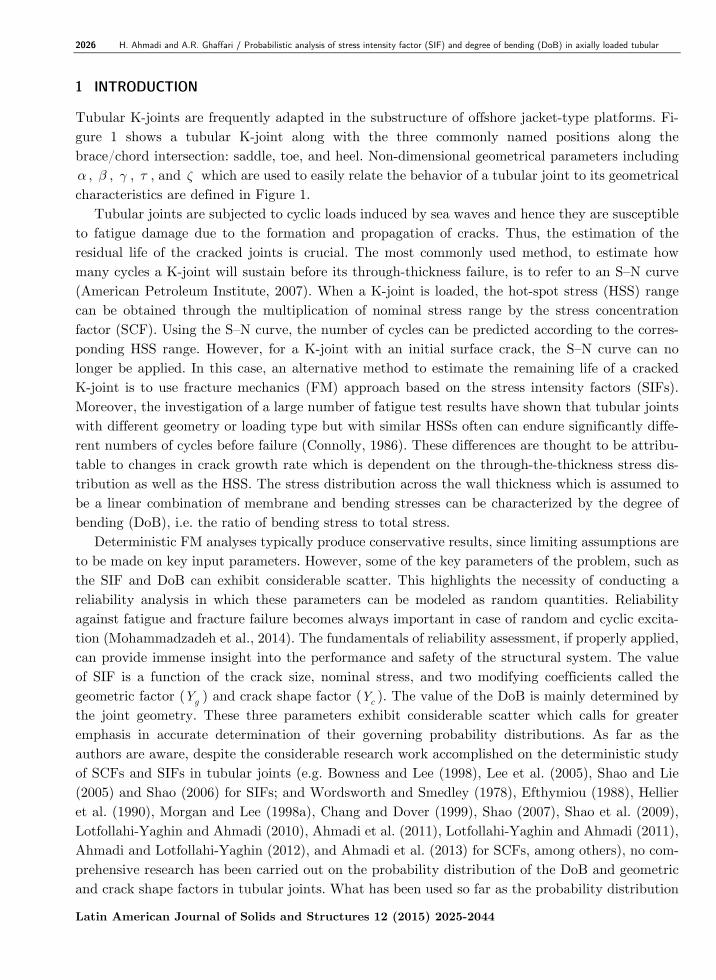
Tubular K-joints are frequently adapted in the substructure of offshore jacket-type platforms. Fi-gure 1 shows a tubular K-joint along with the three commonly named positions along the brace/chord intersection: saddle, toe, and heel. Non-dimensional geometrical parameters including α , β , γ , τ , and ζ which are used to easily relate the behavior of a tubular joint to its geometrical characteristics are defined in Figure 1. Tubular joints are subjected to cyclic loads induced by sea waves and hence they are susceptible to fatigue damage due to the formation and propagation of cracks. Thus, the estimation of the residual life of the cracked joints is crucial. The most commonly used method, to estimate how many cycles a K-joint will sustain before its through-thickness failure, is to refer to an S–N curve (American Petroleum Institute, 2007). When a K-joint is loaded, the hot-spot stress (HSS) range can be obtained through the multiplication of nominal stress range by the stress concentration factor (SCF). Using the S–N curve, the number of cycles can be predicted according to the corres-ponding HSS range. However, for a K-joint with an initial surface crack, the S–N curve can no longer be applied. In this case, an alternative method to estimate the remaining life of a cracked K-joint is to use fracture mechanics (FM) approach based on the stress intensity factors (SIFs). Moreover, the investigation of a large number of fatigue test results have shown that tubular joints with different geometry or loading type but with similar HSSs often can endure significantly diffe-rent numbers of cycles before failure (Connolly, 1986). These differences are thought to be attribu-table to changes in crack growth rate which is dependent on the through-the-thickness stress dis-tribution as well as the HSS. The stress distribution across the wall thickness which is assumed to be a linear combination of membrane and bending stresses can be characterized by the degree of bending (DoB), i.e. the ratio of bending stress to total stress. Deterministic FM analyses typically produce conservative results, since limiting assumptions are to be made on key input parameters. However, some of the key parameters of the problem, such as the SIF and DoB can exhibit considerable scatter. This highlights the necessity of conducting a reliability analysis in which these parameters can be modeled as random quantities. Reliability against fatigue and fracture failure becomes always important in case of random and cyclic excita-tion (Mohammadzadeh et al., 2014). The fundamentals of reliability assessment, if properly applied, can provide immense insight into the performance and safety of the structural system. The value of SIF is a function of the crack size, nominal stress, and two modifying coefficients called the geometric factor (
gY ) and crack shape factor (cY ). The value of the DoB is mainly determined by
the joint geometry. These three parameters exhibit considerable scatter which calls for greater emphasis in accurate determination of their governing probability distributions. As far as the authors are aware, despite the considerable research work accomplished on the deterministic study of SCFs and SIFs in tubular joints (e.g. Bowness and Lee (1998), Lee et al. (2005), Shao and Lie (2005) and Shao (2006) for SIFs; and Wordsworth and Smedley (1978), Efthymiou (1988), Hellier et al. (1990), Morgan and Lee (1998a), Chang and Dover (1999), Shao (2007), Shao et al. (2009), Lotfollahi-Yaghin and Ahmadi (2010), Ahmadi et al. (2011), Lotfollahi-Yaghin and Ahmadi (2011), Ahmadi and Lotfollahi-Yaghin (2012), and Ahmadi et al. (2013) for SCFs, among others), no com-prehensive research has been carried out on the probability distribution of the DoB and geometric and crack shape factors in tubular joints. What has been used so far as the probability distribution

H. Ahmadi and A.R. Ghaffari / Probabilistic analysis of stress intensity factor (SIF) and degree of bending (DoB) in axially loaded tubular 2027
Latin American Journal of Solids and Structures 12 (2015) 2025-2044
of these parameters in the FM-based reliability analysis of offshore structures is mainly based on assumptions and limited observations, especially in terms of distribution parameters. In the present paper, results of parametric equations available for the computation of the DoB,
gY , and cY have been used to propose probability distribution models for these parameters in
tubular K-joints under balanced axial loads. Based on a parametric study, a set of samples were prepared for the DoB,
gY , and cY ; and the density histograms were generated for these samples
using Freedman-Diaconis method. Ten different probability density functions (PDFs) were fitted to these histograms. The maximum likelihood (ML) method was used to determine the parameters of fitted distributions; and in each case, Kolmogorov-Smirnov test was utilized to evaluate the goodness of fit. Finally, the best-fitted distributions were selected and are introduced in the present paper. The proposed PDFs can be adapted in the FM-based fatigue reliability analysis of tubular K-joints commonly found in offshore jacket structures.
Figure 1: Geometrical notation for an axially loaded tubular K-joint.
2 THE FORMULATION OF SIF IN TUBULAR K-JOINTS SUBJECTED TO BALANCED AXIAL LOADS
The SIF can be calculated as follows:
nomSIF g cYY aσ π= (1)
where nomσ is the nominal stress, a is the crack size,
gY is the geometric factor, and cY is the crack
shape factor. Both gY and
cY are dimensionless quantities.
Toe
Toe
Saddle
Chord
Heel
Weld toe
0º
90º
180º
270º
Definition of
Geometry Loading

2028 H. Ahmadi and A.R. Ghaffari / Probabilistic analysis of stress intensity factor (SIF) and degree of bending (DoB) in axially loaded tubular
Latin American Journal of Solids and Structures 12 (2015) 2025-2044
In a tubular K-joint subjected to balanced axial loads, the nominal stress is computed as:
( )
nom 22
4
2
P
d d t
σ
π
= − −
(2)
where P , d , and t are defined in Figure 1. Geometric factor for a tubular K-joint subjected to balanced axial loads can be calculated using following equation (Shao and Lie, 2005):
( )( )( )0.43577
0.2193661 21.557 0.131486 0.42659 0.8275 0.42414 1.489
12gY
γτ θ θ β−
= + + − + (3)
where 1θ and 2θ should be inserted in radians. The expression for crack shape factor is (Shao and Lie, 2005):
0.141 0.36
/ 5c
a cY
T a
− = (4)
where T is the thickness of the chord; and a and c are crack dimensions illustrated in Figure 2. The validity ranges for the application of Eqs. (3) and (4) are as follows:
1 2 1 2
1 2
;
2 12, 30 ; 0.3, 0.6 ; 0.25, 1.0
5, 8 ; 0.1, 0.7
30 , 60 ; 30 , 60 ; 0
t t t d d d
D T d D t T
c a a T
e
γ β τ
θ θ
= = = =
= ∈ = ∈ = ∈ ∈ ∈
∈ ∈ =
(5)
Figure 2: Crack dimensions a and c through the chord thickness T .

H. Ahmadi and A.R. Ghaffari / Probabilistic analysis of stress intensity factor (SIF) and degree of bending (DoB) in axially loaded tubular 2029
Latin American Journal of Solids and Structures 12 (2015) 2025-2044
3 THE FORMULATION OF DoB IN AXIALLY LOADED TUBULAR K-JOINTS
As mentioned earlier, the degree of bending (DoB) is the ratio of bending stress over total stress expressed as:
DoB B B
T B M
σ σ
σ σ σ= =
+ (6)
where
Bσ is the bending stress component, Tσ is the total stress on the outer tube surface, and
Mσ is the membrane stress component (Figure 3).
Figure 3: Through-the-thickness stress distribution in a tubular joint.
Morgan and Lee (1998b) proposed a set of equations for the calculation of DoBs in tubular K-joints subjected to balanced axial loads (Eqs. (7)−(12)). In Eq. (7), DoBch stands for the DoB at the position of the maximum SCF. In Eqs. (8)−(12), DoBch0, DoBch45, DoBch90, DoBch135, and DoBch180 denote the DoB on the chord at θ = 0˚, 45˚, 90˚, 135˚, and 180˚, respectively; where θ is the polar angle around the weld toe shown in Figure 1.
0.017 0.092 2 0.166Ch
0.077 0.042
1.97 0.921 max m in
DoB (1.34 0.01 0.228 )sin
[0.504 0.547 arctan(0.194 )]
τ γ β β θ
θ θβ τ ζ
θ θ
−−
= + +
−
(7)
0.22 2
Ch0
0.635 0.007 0.444
DoB 0.135 (3.954 2.765 2.023 )
sin [2.987 14.751 arctan(0.013 )] ( )f
γ β β
θτ β ζ α
−
− −
= − +
− (8)
0.03 2
Ch45
0.193 0.025 0.661
DoB 0.467 (1.021 0.592 0.325 )
sin [1.382 1.39 arctan(0.063 )]
γ β β
θτ β ζ−
= + −
− (9)
1.052 2
Ch90
13.809 3.016 0.45 0.117 0.02 0.128
DoB 1.704 ( 2.222 3.466 15.522 )
sin [4.325 24.963 arctan(1.605 )] [ (0.027 0.892) ]
γ β β
θτ β ζ β γ τ θ
−
−
= − − +
− + + (10)
2030 H. Ahmadi and A.R. Ghaffari / Probabilistic analysis of stress intensity factor (SIF) and degree of bending (DoB) in axially loaded tubular
Latin American Journal of Solids and Structures 12 (2015) 2025-2044
min max
0.044 2 0.281Ch135
0.02 1.205
0.03 0.13 [39.582( / ) 23.887]
max min
min
0.142 0.2
DoB 0.359 (1.797 0.251 0.015 )sin
[0.81 0.13 arctan(0.244 )]
( )
1.395( )
f
f
β β
γ β β θ
τ β ζ
θ θ ββ
θ θ β
θ τβ
−
−
− −
−
= + −
+
=01
max min for cases where 1, 60 and
1 for all other cases
β θ θ θ = < =
(11)
0.002 2Ch180
0.215 0.021 0.002
DoB 0.795 (0.755 0.266 0.083 )
sin [1.453 0.479 arctan(1.342 )]
γ β β
θτ β ζ
−= + −
− (12)
The validity ranges for the application of Eqs. (7)−(12) are as follows:
1 2 1 2 1 2 ; ;
2 10, 40 ; 0.3, 1 ; 0.2, 1
30 , 90 ; 0.1, 0.8 ; 6, 40
t t t d d d
D T d D t T
θ θ θ
γ β τ
θ ζ α
= = = = = =
= ∈ = ∈ = ∈
∈ ∈ ∈
(13)
4 PREPARATION OF THE SAMPLE DATABASE
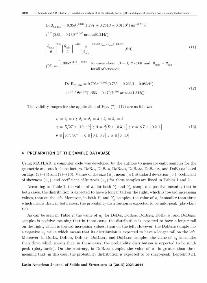
Using MATLAB, a computer code was developed by the authors to generate eight samples for the geometric and crack shape factors, DoBch, DoBch0, DoBch45, DoBch90, DoBch135, and DoBch180 based on Eqs. (3)−(5) and (7)−(13). Values of the size (n ), mean (µ ), standard deviation (σ ), coefficient of skewness ( 3a ), and coefficient of kurtosis ( 4a ) for these samples are listed in Tables 1 and 2.
According to Table 1, the value of 3a for both cY and
gY samples is positive meaning that in both cases, the distribution is expected to have a longer tail on the right, which is toward increasing values, than on the left. Moreover, in both
cY and gY samples, the value of 4a is smaller than three
which means that, in both cases, the probability distribution is expected to be mild-peak (platykur-tic).
As can be seen in Table 2, the value of 3a for DoBch, DoBch0, DoBch45, DoBch135, and DoBch180 samples is positive meaning that in these cases, the distribution is expected to have a longer tail on the right, which is toward increasing values, than on the left. However, the DoBch90 sample has a negative 3a value which means that its distribution is expected to have a longer tail on the left. Moreover, in DoBch, DoBch0, DoBch45, DoBch135, and DoBch180 samples, the value of 4a is smaller than three which means that, in these cases, the probability distribution is expected to be mild-peak (platykurtic). On the contrary, in DoBch90 sample, the value of 4a is greater than three meaning that, in this case, the probability distribution is expected to be sharp-peak (Leptokurtic).
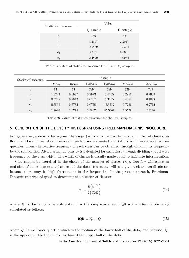
H. Ahmadi and A.R. Ghaffari / Probabilistic analysis of stress intensity factor (SIF) and degree of bending (DoB) in axially loaded tubular 2031
Latin American Journal of Solids and Structures 12 (2015) 2025-2044
Statistical measure Value
cY sample gY sample
n 400 32 µ 4.2347 2.2017
σ 0.6859 1.3384
3a 0.2851 0.5331
4a 2.4820 1.9964
Table 1: Values of statistical measures for cY and gY samples.
Statistical measure
Sample
DoBch DoBch0 DoBch45 DoBch90 DoBch135 DoBch180
n 64 64 729 729 729 729 µ 1.2243 0.9937 0.7973 0.4765 0.2856 0.7904
σ 0.5705 0.2942 0.0707 2.3265 0.4054 0.1098
3a 0.5538 0.5782 0.0758 -8.3512 0.7266 0.2712
4a 1.8080 2.6714 2.3867 85.5309 1.5559 2.3190
Table 2: Values of statistical measures for the DoB samples.
5 GENERATION OF THE DENSITY HISTOGRAM USING FREEDMAN-DIACONIS PROCEDURE
For generating a density histogram, the range (R ) should be divided into a number of classes/ce-lls/bins. The number of occurrences in each class is counted and tabulated. These are called fre-quencies. Then, the relative frequency of each class can be obtained through dividing its frequency by the sample size. Afterwards, the density is calculated for each class through dividing the relative frequency by the class width. The width of classes is usually made equal to facilitate interpretation. Care should be exercised in the choice of the number of classes (
cn ). Too few will cause an omission of some important features of the data; too many will not give a clear overall picture because there may be high fluctuations in the frequencies. In the present research, Freedman-Diaconis rule was adapted to determine the number of classes:
( )( )
1/3
2 IQRc
R nn = (14)
where R is the range of sample data, n is the sample size, and IQR is the interquartile range
calculated as follows: 3 1IQR Q Q= − (15)
where 1Q is the lower quartile which is the median of the lower half of the data; and likewise, 3Q is the upper quartile that is the median of the upper half of the data.
2032 H. Ahmadi and A.R. Ghaffari / Probabilistic analysis of stress intensity factor (SIF) and degree of bending (DoB) in axially loaded tubular
Latin American Journal of Solids and Structures 12 (2015) 2025-2044
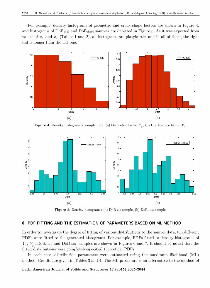
For example, density histograms of geometric and crack shape factors are shown in Figure 4; and histograms of DoBch45 and DoBch180 samples are depicted in Figure 5. As it was expected from values of 3a and 4a (Tables 1 and 2), all histograms are platykurtic; and in all of them, the right tail is longer than the left one.
(a) (b)
Figure 4: Density histogram of sample data: (a) Geometric factor gY , (b) Crack shape factor cY .
(a) (b)
Figure 5: Density histograms: (a) DoBch45 sample, (b) DoBch180 sample.
6 PDF FITTING AND THE ESTIMATION OF PARAMETERS BASED ON ML METHOD
In order to investigate the degree of fitting of various distributions to the sample data, ten different PDFs were fitted to the generated histograms. For example, PDFs fitted to density histograms of
cY , gY , DoBch45, and DoBch180 samples are shown in Figures 6 and 7. It should be noted that the
fitted distributions were completely-specified theoretical PDFs. In each case, distribution parameters were estimated using the maximum likelihood (ML) method. Results are given in Tables 3 and 4. The ML procedure is an alternative to the method of
0.65 0.7 0.75 0.8 0.85 0.9 0.950
1
2
3
4
5
6
7
8
Data
De
nsit
y
(DoB)ch45 Data
0.6 0.65 0.7 0.75 0.8 0.85 0.9 0.95 1 1.050
0.5
1
1.5
2
2.5
3
3.5
4
4.5
5
Data
Den
sit
y
(DoB)ch180 Data

H. Ahmadi and A.R. Ghaffari / Probabilistic analysis of stress intensity factor (SIF) and degree of bending (DoB) in axially loaded tubular 2033
Latin American Journal of Solids and Structures 12 (2015) 2025-2044
Figure 6: PDFs fitted to the density histogram of sample data:
(a) Crack shape factor cY , (b) Geometric factor gY .
moments. As a means of finding an estimator, statisticians often give it preference. For a random variable X with a known PDF, ( )Xf x , and observed values 1x , 2x , . . . ,
nx , in a random sample of size n , the likelihood function of θ , where θ represents the vector of unknown parameters, is defined as:
( )1
( ) n
X ii
L f xθ θ=
= ∏ (16)
The objective is to maximize ( )L θ for the given data set. This is easily done by taking m partial derivatives of ( )L θ , where m is the number of parameters, and equating them to zero. We then find the maximum likelihood estimators (MLEs) of the parameter set θ from the solutions of the equations. In this way the greatest probability is given to the observed set of events, provided that we know the true form of the probability distribution.
(a)
(b)

2034 H. Ahmadi and A.R. Ghaffari / Probabilistic analysis of stress intensity factor (SIF) and degree of bending (DoB) in axially loaded tubular
Latin American Journal of Solids and Structures 12 (2015) 2025-2044
(a)
(b)
Figure 7: PDF fitted to the density histograms: (a) DoBch45 sample, (b) DoBch180 sample.
Fitted PDF Estimated parameters
Crack shape factor ( cY ) sample Geometric factor ( gY ) sample
Birnbaum-Saunders β γ
4.17957 0.16243
1.81261 0.655245
Extreme value µ
σ
4.58519 0.700136
2.88914 1.34837
Gamma a b
38.39 0.110308
2.72621 0.807614
Generalized extreme value k σ µ
-0.183782 0.635822 3.96276
---
Inverse Gaussian µ
λ 4.23471 159.455
2.20173 4.63102
Log-logistic β
a
1.43185 0.0956718
0.594767 0.396898
Logistic β
a
4.21602 0.401737
2.09946 0.7954
Lognormal µ
σ
1.43023 0.162227
0.594767 0.648587
Nakagami µ
Ω
9.78083 18.402
0.847615 6.58296
Normal (Gaussian) µ
σ
4.23471 0.685854
2.20173 1.33841
Weibull a b
--- 2.48872 1.77255
Table 3: Estimated parameters of PDFs fitted to the density histograms of cY and gY samples.
H. Ahmadi and A.R. Ghaffari / Probabilistic analysis of stress intensity factor (SIF) and degree of bending (DoB) in axially loaded tubular 2035
Latin American Journal of Solids and Structures 12 (2015) 2025-2044
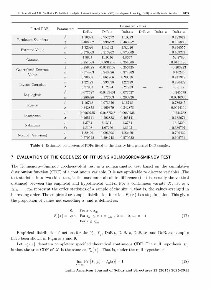
Fitted PDF Parameters Estimated values
DoBch DoBch0 DoBch45 DoBch90 DoBch135 DoBch180
Birnbaum-Saunders β γ
1.10323 0.468852
0.952592 0.293792
1.10323 0.468852
--- ---
0.782877 0.138833
Extreme Value µ
σ
1.52026 0.570069
1.14692 0.313862
1.52026 0.570069
0.846555 0.109227
Gamma a b
4.8647 0.251668
11.9476 0.0831714
4.8647 0.251668
52.2789 0.0151193
Generalized Extreme Value
k σ µ
0.256425 0.374963 0.90638
-0.0379108 0.240826 0.861266
0.256425 0.374963 0.90638
-0.203823 0.10245 0.747919
Inverse Gaussian µ
λ 1.22429 5.27933
0.993698 11.2694
1.22429 5.27933
0.790422 40.8117
Log-logistic β
α
0.077527 0.280926
-0.0499401 0.172563
0.077527 0.280926
-0.245578 0.0816333
Logistic β
α
1.16748 0.342878
0.973626 0.169379
1.16748 0.342878
0.786245 0.0644169
Lognormal µ
σ
0.0960735 0.465141
-0.0487548 0.293833
0.0960735 0.465141
-0.244782 0.138674
Nakagami µ
Ω
1.3734 1.8193
3.13911 1.07266
1.3734 1.8193
13.2329 0.636797
Normal (Gaussian) µ
σ
1.22429 0.570522
0.993698 0.294248
1.22429 0.570522
0.790422 0.109754
Table 4: Estimated parameters of PDFs fitted to the density histograms of DoB samples.
7 EVALUATION OF THE GOODNESS OF FIT USING KOLMOGOROV-SMIRNOV TEST
The Kolmogorov-Smirnov goodness-of-fit test is a nonparametric test based on the cumulative distribution function (CDF) of a continuous variable. It is not applicable to discrete variables. The test statistic, in a two-sided test, is the maximum absolute difference (that is, usually the vertical distance) between the empirical and hypothetical CDFs. For a continuous variate X , let x(1), x(1), … , x(n) represent the order statistics of a sample of the size n, that is, the values arranged in increasing order. The empirical or sample distribution function ( )nF x is a step function. This gives the proportion of values not exceeding x and is defined as:
( )
(1)
( ) ( 1)
( )
0, For
, For , 1, 2, ..., 1
1, For n k k
n
x x
F x k n x x x k n
x x
+
<= ≤ < = − ≥
(17)
Empirical distribution functions for the
cY , gY , DoBch, DoBch0, DoBch45, and DoBch180 samples
have been shown in Figures 8 and 9. Let ( )0F x denote a completely specified theoretical continuous CDF. The null hypothesis 0H is that the true CDF of X is the same as ( )0F x . That is, under the null hypothesis:
0lim Pr ( ) ( ) 1nn
F x F x→∞
= = (18)

2036 H. Ahmadi and A.R. Ghaffari / Probabilistic analysis of stress intensity factor (SIF) and degree of bending (DoB) in axially loaded tubular
Latin American Journal of Solids and Structures 12 (2015) 2025-2044
Figure 8: Empirical cumulative distribution functions of sample data:
(a) Crack shape factor cY , (b) Geometric factor gY .
Figure 9: Empirical distribution functions:
(a) DoBch sample, (b) DoBch0 sample, (c) DoBch45 sample, (d) DoBch180 sample.
(a) (b)
0.6 0.8 1 1.2 1.4 1.6 1.8 2 2.2 2.40
0.1
0.2
0.3
0.4
0.5
0.6
0.7
0.8
0.9
1
Data
Cu
mu
lati
ve p
rob
ab
ilit
y
(DoB)ch Data
0.6 0.8 1 1.2 1.4 1.60
0.1
0.2
0.3
0.4
0.5
0.6
0.7
0.8
0.9
1
Data
Cu
mu
lati
ve p
rob
ab
ilit
y
(DoB)ch0 Data
0.65 0.7 0.75 0.8 0.85 0.9 0.950
0.1
0.2
0.3
0.4
0.5
0.6
0.7
0.8
0.9
1
Data
Cu
mu
lati
ve p
rob
ab
ilit
y
(DoB)ch45 Data
0.6 0.65 0.7 0.75 0.8 0.85 0.9 0.95 10
0.1
0.2
0.3
0.4
0.5
0.6
0.7
0.8
0.9
1
Data
Cu
mu
lati
ve p
rob
ab
ilit
y
(DoB)ch180 Data
(a) (b)
(c) (d)

H. Ahmadi and A.R. Ghaffari / Probabilistic analysis of stress intensity factor (SIF) and degree of bending (DoB) in axially loaded tubular 2037
Latin American Journal of Solids and Structures 12 (2015) 2025-2044
The test criterion is the maximum absolute difference between ( )nF x and ( )0F x , formally defined as:
0sup ( ) ( )n n
x
D F x F x= − (19)
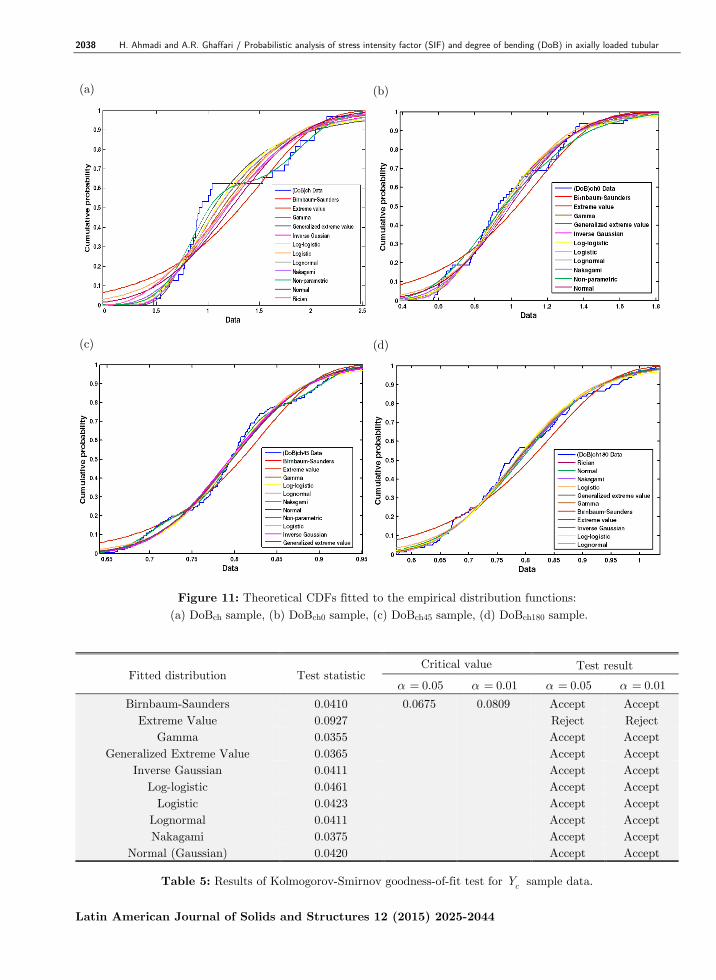
Theoretical continuous CDFs fitted to the empirical distribution functions of the
cY , gY , DoBch,
DoBch0, DoBch45, and DoBch180 samples have been shown in Figures 10 and 11.
A large value of this statistic (nD ) indicates a poor fit. So critical values should be known. The
critical values ,nD α for large samples, say n >35, are (1.3581 n ) and (1.6276 n ) for a = 0.05 and 0.01, respectively (Kottegoda and Rosso, 2008).
Results of Kolmogorov-Smirnov test for cY ,
gY , DoBch, DoBch0, DoBch45, and DoBch180 sample data are given in Tables 5−10, respectively. It should be noted that, according to the results of Kolmogorov-Smirnov test, none of considered continuous CDFs was acceptably fitted to the DoBch90 and DoBch135 samples. Hence, no table is provided here for these two samples.
It is evident in Tables 5 and 6 that Gamma and Birnbaum-Saunders distributions have the smallest values of test statistic for
cY and gY sample data, respectively. Hence, it can be concluded
that Gamma and Birnbaum-Saunders distributions are the best probability models for the crack shape factor (
cY ) and geometric factor (gY ) in tubular K-joints under balanced axial loads, respec-
tively.
According to Tables 7−10, that Generalized Extreme Value, Gamma, Log-logistic, and Birnbaum-Saunders distributions have the smallest values of test statistic for DoBch, DoBch0, Do-Bch45, and DoBch180 samples, respectively. Hence, it can be concluded that Generalized Extreme Value, Gamma, Log-logistic, and Birnbaum-Saunders distributions are the best probability models for DoBch, DoBch0, DoBch45, and DoBch180 in axially loaded tubular K-joints, respectively.
Figure 10: Theoretical continuous CDFs fitted to the empirical distribution function of sample data:
(a) Crack shape factor cY , (b) Geometric factor gY .
(a) (b)
2038 H. Ahmadi and A.R. Ghaffari / Probabilistic analysis of stress intensity factor (SIF) and degree of bending (DoB) in axially loaded tubular
Latin American Journal of Solids and Structures 12 (2015) 2025-2044
Figure 11: Theoretical CDFs fitted to the empirical distribution functions:
(a) DoBch sample, (b) DoBch0 sample, (c) DoBch45 sample, (d) DoBch180 sample.
Fitted distribution Test statistic Critical value Test result
α = 0.05 α = 0.01 α = 0.05 α = 0.01
Birnbaum-Saunders 0.0410 0.0675 0.0809 Accept Accept Extreme Value 0.0927 Reject Reject
Gamma 0.0355 Accept Accept Generalized Extreme Value 0.0365 Accept Accept
Inverse Gaussian 0.0411 Accept Accept Log-logistic 0.0461 Accept Accept
Logistic 0.0423 Accept Accept Lognormal 0.0411 Accept Accept Nakagami 0.0375 Accept Accept
Normal (Gaussian) 0.0420 Accept Accept
Table 5: Results of Kolmogorov-Smirnov goodness-of-fit test for cY sample data.
(c) (d)
(a) (b)

H. Ahmadi and A.R. Ghaffari / Probabilistic analysis of stress intensity factor (SIF) and degree of bending (DoB) in axially loaded tubular 2039
Latin American Journal of Solids and Structures 12 (2015) 2025-2044
Fitted distribution Test statistic Critical value Test result
α = 0.05 α = 0.01 α = 0.05 α = 0.01
Birnbaum-Saunders 0.1433
0.2343 0.2809 Accept Accept
Extreme Value 0.1904
Gamma 0.1695
Weibull 0.1776
Inverse Gaussian 0.1451
Log-logistic 0.1446
Logistic 0.1810
Lognormal 0.1438
Nakagami 0.1854
Normal (Gaussian) 0.2001
Table 6: Results of Kolmogorov-Smirnov goodness-of-fit test for gY sample data.
Fitted distribution Test statistic Critical value Test result
α = 0.05 α = 0.01 α = 0.05 α = 0.01
Birnbaum-Saunders 0.1751
0.1669 0.2003
Reject Accept
Extreme Value 0.2750 Reject Reject
Gamma 0.2029 Reject Reject
Generalized Extreme Value 0.1550 Accept Accept
Inverse Gaussian 0.1718 Reject Accept
Log-logistic 0.1590 Accept Accept
Logistic 0.2168 Reject Reject
Lognormal 0.1736 Reject Accept
Nakagami 0.2288 Reject Reject
Normal (Gaussian) 0.2516 Reject Reject
Table 7: Results of Kolmogorov-Smirnov goodness-of-fit test for DoBch simple.
8 PROPOSED PROBABILITY MODELS
Based on the results of Kolmogorov-Smirnov goodness-of-fit test, Gamma and Birnbaum-Saunders distributions are the best probability models for
cY and gY , respectively (Tables 5 and 6). Moreo-
ver, Based on the results of Kolmogorov-Smirnov goodness-of-fit test (Tables 7−10), Generalized Extreme Value, Gamma, Log-logistic, and Birnbaum-Saunders distributions are the best probabi-lity models for DoBch, DoBch0, DoBch45, and DoBch180, respectively. The PDFs of these distributions are given by the following equations:
1 /1( )
( )
a x bX af x x e
b a
− −=Γ
Gamma distribution (20)
( )2
2
/ / / /1( ) exp
222X
x x x xf x
x
β β β β
γγπ
− + = −
Birnbaum-Saunders distribution (21)

2040 H. Ahmadi and A.R. Ghaffari / Probabilistic analysis of stress intensity factor (SIF) and degree of bending (DoB) in axially loaded tubular
Latin American Journal of Solids and Structures 12 (2015) 2025-2044
Fitted distribution Test statistic Critical value Test result
α = 0.05 α = 0.01 α = 0.05 α = 0.01
Birnbaum-Saunders 0.0941
0.1669 0.2003
Accept Accept Extreme Value 0.1482 Accept Accept
Gamma 0.0881 Accept Accept Generalized Extreme Value 0.0997 Accept Accept
Inverse Gaussian 0.0944 Accept Accept Log-logistic 0.1032 Accept Accept
Logistic 0.1010 Accept Accept Lognormal 0.0937 Accept Accept Nakagami 0.0882 Accept Accept
Normal (Gaussian) 0.1046 Accept Accept
Table 8: Results of Kolmogorov-Smirnov goodness-of-fit test for DoBch0 sample.
Fitted distribution Test statistic Critical value Test result
α = 0.05 α = 0.01 α = 0.05 α = 0.01
Birnbaum-Saunders 0.0666
0.0501 0.0600
Reject Reject Extreme Value 0.1338 Reject Reject
Gamma 0.0613 Reject Reject Generalized Extreme Value 0.0736 Reject Reject
Inverse Gaussian 0.0666 Reject Reject Log-logistic 0.0561 Reject Accept
Logistic 0.0637 Reject Reject Lognormal 0.0665 Reject Reject Nakagami 0.0657 Reject Reject
Normal (Gaussian) 0.0707 Reject Reject
Table 9: Results of Kolmogorov-Smirnov goodness-of-fit test for DoBch45 sample.
Fitted distribution Test statistic Critical value Test result
α = 0.05 α = 0.01 α = 0.05 α = 0.01
Birnbaum-Saunders 0.0557
0.0501 0.0600
Reject Accept Extreme Value 0.1190 Reject Reject
Gamma 0.0645 Reject Reject Generalized Extreme Value 0.0596 Accept Accept
Inverse Gaussian 0.0557 Reject Accept Log-logistic 0.0580 Reject Accept
Logistic 0.0715 Reject Reject Lognormal 0.0558 Reject Accept Nakagami 0.0728 Reject Reject
Normal (Gaussian) 0.0809 Reject Reject
Table 10: Results of Kolmogorov-Smirnov goodness-of-fit test for DoBch180 sample.
1
1/ 11
( ) exp 1 1
kk
X
x xf x k k
µ µ
σ σ σ
− − − − − = − + + Generalized Extreme Value distribution (22)

H. Ahmadi and A.R. Ghaffari / Probabilistic analysis of stress intensity factor (SIF) and degree of bending (DoB) in axially loaded tubular 2041
Latin American Journal of Solids and Structures 12 (2015) 2025-2044
( )( )
( )( )
1
2
/ /( )
1 /X
xf x
x
β
β
β α α
α
−
=
+
Log-logistic distribution (23)
where ( )aΓ is the Gamma function defined as follows:
1
0( ) t aa e t dt
∞ − −Γ = ∫ (24)
After substituting the values of estimated parameters from Table 3, following probability density functions are proposed for the crack shape factor (
cY ) and geometric factor (gY ) in tubular K-
joints under balanced axial loads, respectively.
7 37.39 /0.110308( ) (1.0019 10 ) x
X
c
f x x e
Y
− −= × (25)
( )2/ 1.81261 1.81261 / / 1.81261 1.81261 /1
( ) exp0.85869 1.310492
X
g
x x x xf x
x
Y
π
− + = −
(26)
After substituting the values of estimated parameters from Table 4, following probability density functions are proposed for DoBch, DoBch0, DoBch45, and DoBch180 in axially loaded tubular K-joints, respectively.
3.8998 4.8998
ch
1 0.9064 0.9064( ) exp 1 0.2564 1 0.2564
0.3750 0.3750 0.3DoB
750X
x xf x
− − − − = − + + (27)
( )5 10.9476 /0.08
h
3
0
17
c
( ) 2.2803 10
B
xXf x x e−= ×
(28)
( )
( )( )
0.9225
20.0775
ch45
27
0.27597 / 0.2809( )
1 / 0.2809B
X
xf x
x
−
=
+ (29)
( )
ch 8
2
1 0
/ 0.78288 0.78288 / / 0.78288 0.78288 /( ) 0.3989 exp
0.03855 0.
D
27767
oB
X
x x x xf x
x
− + = − (30)
These proposed PDFs, shown in Figures 12 and 13, can be adapted in the FM-based fatigue reliability analysis of axially loaded tubular K-joints which are commonly found in offshore jacket structures.

2042 H. Ahmadi and A.R. Ghaffari / Probabilistic analysis of stress intensity factor (SIF) and degree of bending (DoB) in axially loaded tubular
Latin American Journal of Solids and Structures 12 (2015) 2025-2044
Figure 12: PDFs proposed for cY and gY :
(a) Crack shape factor cY − Gamma distribution, (b) Geometric factor gY − Birnbaum-Saunders distribution.
Figure 13: Proposed PDFs for the DoB:
(a) DoBch − Generalized extreme value distribution. (b) DoBch0 − Gamma distribution. (c) DoBch45 − Log-logistic distribution. (d) DoBch180 − Birnbaum-Saunders distribution.
(a) (b)
0 0.5 1 1.5 2 2.50
0.1
0.2
0.3
0.4
0.5
0.6
0.7
0.8
0.9
1
Data
Den
sit
y
(DoB)ch Data
Generalized extreme value
0.4 0.6 0.8 1 1.2 1.4 1.6 1.80
0.2
0.4
0.6
0.8
1
1.2
1.4
1.6
Data
Den
sit
y
(DoB)ch0 Data
Gamma
0.65 0.7 0.75 0.8 0.85 0.9 0.950
1
2
3
4
5
6
7
8
Data
Den
sit
y
(DoB)ch45 Data
Log-logistic
(a) (b)
(c) (d)

H. Ahmadi and A.R. Ghaffari / Probabilistic analysis of stress intensity factor (SIF) and degree of bending (DoB) in axially loaded tubular 2043
Latin American Journal of Solids and Structures 12 (2015) 2025-2044
9 CONCLUSIONS
In the present paper, results of parametric equations available for the computation of the DoB, Yg, and Yc were used to propose probability distribution models for these parameters in axially loaded tubular K-joints. Based on a parametric study, a set of samples were prepared for the DoB, Yg, and Yc; and the density histograms were generated for these samples using Freedman-Diaconis method. Ten different PDFs were fitted to these histograms. The ML method was used to determine the parameters of fitted distributions; and in each case, Kolmogorov-Smirnov test was utilized to eva-luate the goodness of fit. It was concluded that Gamma and Birnbaum-Saunders distributions are the best probability models for Yc and Yg, respectively; and Generalized Extreme Value, Gamma, Log-logistic, and Birnbaum-Saunders distributions are the best probability models for DoBch, Do-Bch0, DoBch45, and DoBch180, respectively. Finally, after the substitution of estimated parameters, a set of fully defined PDFs were proposed which can be used in the FM-based fatigue reliability analysis of axially loaded tubular K-joints.
References Ahmadi, H., Lotfollahi-Yaghin, M.A., Aminfar, M.H., (2011). Geometrical effect on SCF distribution in uni-planar tubular DKT-joints under axial loads. Journal of Constructional Steel Research 67: 1282–91.
Ahmadi, H., Lotfollahi-Yaghin, M.A., (2012). Geometrically parametric study of central brace SCFs in offshore three-planar tubular KT-joints. Journal of Constructional Steel Research 71: 149–61.
Ahmadi, H., Lotfollahi-Yaghin, M.A., Shao, Y.B., (2013). Chord-side SCF distribution of central brace in internally ring-stiffened tubular KT-joints: A geometrically parametric study. Thin-Walled Structures 70: 93−105.
American Petroleum Institute (API), (2007). Recommended practice for planning, designing and constructing fixed offshore platforms: Working stress design: RP2A-WSD. 21st Edition, Errata and Supplement 3, Washington DC, US.
Bowness, D., Lee, M.M.K., (1998). Fatigue crack curvature under the weld toe in an offshore tubular joint. Inter-national Journal of Fatigue 20(6): 481–90.
Chang, E., Dover, W.D., (1999). Parametric equations to predict stress distributions along the intersection of tu-bular X and DT-joints. International Journal of Fatigue 21: 619–35.
Connolly, M.P.M., (1986). A fracture mechanics approach to the fatigue assessment of tubular welded Y and K-joints. PhD Thesis, University College London, UK.
Efthymiou, M., (1988). Development of SCF formulae and generalized influence functions for use in fatigue analysis. OTJ 88, Surrey, UK.
Hellier, A.K., Connolly, M., Dover, W.D., (1990). Stress concentration factors for tubular Y and T-joints. Interna-tional Journal of Fatigue 12: 13–23.
Kottegoda, N.T., Rosso, R., (2008). Applied statistics for civil and environmental engineers. 2nd Edition, Blackwell Publishing Ltd, UK.
Lee, C.K., Lie, S.T., Chiew, S.P., Shao, Y.B., (2005). Numerical models verification of cracked tubular T, Y and K-joints under combined loads. Engineering Fracture Mechanics 72: 983–1009.
Lotfollahi-Yaghin, M.A., Ahmadi, H., (2010). Effect of geometrical parameters on SCF distribution along the weld toe of tubular KT-joints under balanced axial loads. International Journal of Fatigue 32: 703–19.
Lotfollahi-Yaghin, M.A., Ahmadi, H., (2011). Geometric stress distribution along the weld toe of the outer brace in two-planar tubular DKT-joints: parametric study and deriving the SCF design equations. Marine Structures 24: 239–60.

2044 H. Ahmadi and A.R. Ghaffari / Probabilistic analysis of stress intensity factor (SIF) and degree of bending (DoB) in axially loaded tubular
Latin American Journal of Solids and Structures 12 (2015) 2025-2044
Mohammadzadeh, S., Ahadi, S., Nouri, M., (2014). Stress-based fatigue reliability analysis of the rail fastening spring clip under traffic loads. Latin American Journal of Solids and Strucutres 11(6): 993-1011.
Morgan, M.R., Lee, M.M.K., (1998a). Parametric equations for distributions of stress concentration factors in tu-bular K-joints under out-of-plane moment loading. International Journal of Fatigue 20: 449–61.
Morgan, M.R., Lee, M.M.K., (1998b). Prediction of stress concentrations and degrees of bending in axially loaded tubular K-joints. Journal of Constructional Steel Research 45(1): 67–97.
Shao, Y.B., (2006). Analysis of stress intensity factor (SIF) for cracked tubular K-joints subjected to balanced axial load. Engineering Failure Analysis 13: 44–64.
Shao, Y.B., (2007). Geometrical effect on the stress distribution along weld toe for tubular T- and K-joints under axial loading. Journal of Constructional Steel Research 63: 1351–60.
Shao, Y.B., Du, Z.F., Lie, S.T., (2009). Prediction of hot spot stress distribution for tubular K-joints under basic loadings. Journal of Constructional Steel Research 65: 2011–26.
Shao, Y.B., Lie, S.T., (2005). Parametric equation of stress intensity factor for tubular K-joint under balanced axial loads. International Journal of Fatigue 27: 666–79.
Wordsworth, A.C., Smedley, G.P., (1978). Stress concentrations at unstiffened tubular joints. Proceedings of the European Offshore Steels Research Seminar, Paper 31, Cambridge, UK.