9

A New Load Adjustment Approach for Job-Shops

Zied Bahroun1, Mourad Fendouli1 and Jean-Pierre Campagne2 1Laboratory LIP2, Faculty of Sciences of Tunis,

2Laboratory LIESP, University of Lyon, INSA-Lyon, 1Tunisia

2France

1. Introduction This chapter presents a middle-term new load adjustment approach by overlapping for a set of jobs in a job-shop context, guaranteeing the existence of a limited capacity schedule without scheduling under the assumption of pre-emptive tasks. The proposed approach is based on the exploitation of the tasks scheduling time segments overlapping and on the distribution of the job’s margins between tasks in a just in time context. First, we present a literature review concerning load adjustment approaches. Second, we introduce the overlapping load adjustment approach. Third, we present an original heuristic to use this approach in the case of job-shops organized firms. After that, we present the associated scheduling approach. Finally, we will discuss a more general use of this approach and the possible extensions. Generally, the production planning is made in a hierarchical way in two planning and scheduling decision levels. In the first step, we decide which products to supply, in which quantities and delays, in the second step, we adjust load to the capacity and schedule the tasks on the machines. There are three main and classical load adjustment approaches. First of all, we have the placement. This approach consists in calculating a detailed tasks schedule. A new task is integrated in the planning if we find a hole in the planning which is bigger than the duration of this task. This approach estimates only one schedule which can be destroyed by any disturbance. The second approach is the periodic and cumulative approach. It consists in calculating the cumulative load and capacity for a latest loading and for each period. This approach does not guarantee the existence of a scheduling solution because it does not take into consideration the ready dates constraints. The third approach is the periodic and non- cumulative approach. It consists in assigning tasks to periods and comparing period by period the available and the required capacities. This method estimates only the solutions in which the tasks are fixed in a specific period. The problem of sequencing decisions in production planning and scheduling was studied by (Dauzere-Peres & Laserre, 1999). They think that it is better in some cases to integrate the scheduling decision level in the lot sizing decision level and propose an iterative approach for planning and scheduling production. Some researchers integrated the scheduling and capacity constraints in their lot sizing model (see for example, Fleishmann & Meyr, 1997).

Advances in Robotics, Automation and Control

152

We can also find a survey on lot sizing and scheduling in (Drexl & Kimms, 1997). Nevertheless, a single machine is generally considered in most of these works which are difficultly applicable in a real situation. (Hillion & Proth, 1994) and (Gunther, 1987) studied the problem of finite capacity planning. (Hillion & Proth, 1994) considered the problem of a finite capacity flow control in a multi-stage/multi-product environment. (Gunther, 1987) developed two heuristics for the lot sizing in the context of finite capacity. (Néron et al., 2001) developed an approach for solving hybrid flow shop problem using energetic reasoning. This approach has some similarities in the concept with our approach. The problem of finite capacity planning in MRP based systems has also been studied. In order to obtain capacity-based production plans, (Pandey et al., 2000; Wuttipornpun & Yenradee, 2004) proposed a finite capacity material requirement planning system. (Grubbström & Huynh, 2006) considered multi-level, multi-stage capacity-constrained production-inventory systems in a MRP context. In comparison with all these approaches, the overlapping load adjustment approach allows to distinguish two main phases. The first phase consists in establishing a long or mid-term production planning where the feasibility is ensured without scheduling and tasks placement, which allows us to characterize a set of feasible scheduling solutions. The scheduling will be done only in the second phase.

2. The overlapping load adjustment approach The time scale is divided into time periods. Each task of a job has got a processing time, requires one or more resources and has to be realized during a scheduling time segment associated with one or more consecutive periods. The scheduling time segments of consecutive tasks of the same job cannot overlap. From now on and throughout this paper a lapse of time called here lapse, designates a succession of a number of n consecutive periods. Let (a,b) be a lapse composed of a succession of periods which are limited by the periods a and b including them. The shortest lapses are composed of only one period, for instance (a,a). Such a lapse (a,a) is called a basic lapse. The longest lapse is noted (1,H) in which number 1 is associated with the first period of the planning time frame and the letter H the last one. From such a planning time frame, the total number of different lapses is equal to H*(H+1)/2.This number is of course to be multiplied by the number of existing processors. The sub-lapse of a lapse is a subset of one or more consecutive periods of this lapse. For instance, the sub-lapses of [1,3] are [1,1], [2,2], [3,3], [1,2] and [2,3]. Every lapse containing a lapse [a,b] is called the over-lapse of [a,b]. For instance, [1,3] is an over-lapse of [1,1]. Each lapse is characterized by: - An accumulated capacity: sum of the capacities of each period included in this lapse. - A direct capacity requirement: sum of the capacities required by the tasks whose

scheduling time segment is exactly equal to this lapse. - An accumulated capacity requirement: sum of the capacities required by the tasks

whose scheduling time segment is fully included in this lapse. It is the sum of the direct capacity requirements of this lapse and its sub-lapses.

(Dillenseger, 1993) sets the following proposition out: for any lapse, its accumulated capacity requirement must be equal or smaller than its accumulated capacity. He proves that it is a necessary and sufficient condition for the existence of a loading solution of the set of tasks (within the limits of their scheduling time segments and considering the capacity levels), according to pre-emptive possibility.

A New Load Adjustment Approach for Job-Shops

153

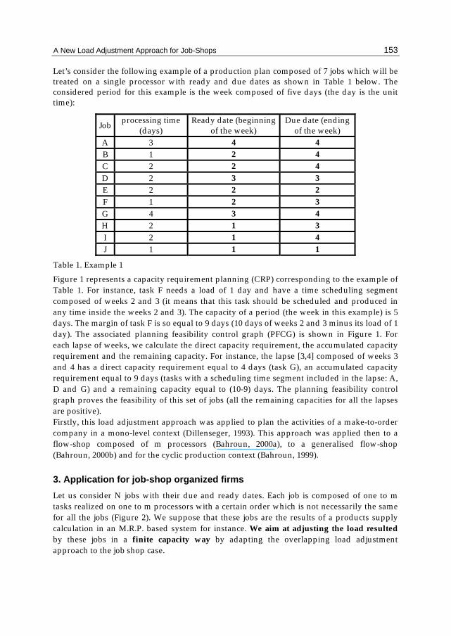
Let’s consider the following example of a production plan composed of 7 jobs which will be treated on a single processor with ready and due dates as shown in Table 1 below. The considered period for this example is the week composed of five days (the day is the unit time):

Job processing time (days)

Ready date (beginning of the week)

Due date (ending of the week)

A 3 4 4 B 1 2 4 C 2 2 4 D 2 3 3 E 2 2 2 F 1 2 3 G 4 3 4 H 2 1 3 I 2 1 4 J 1 1 1

Table 1. Example 1

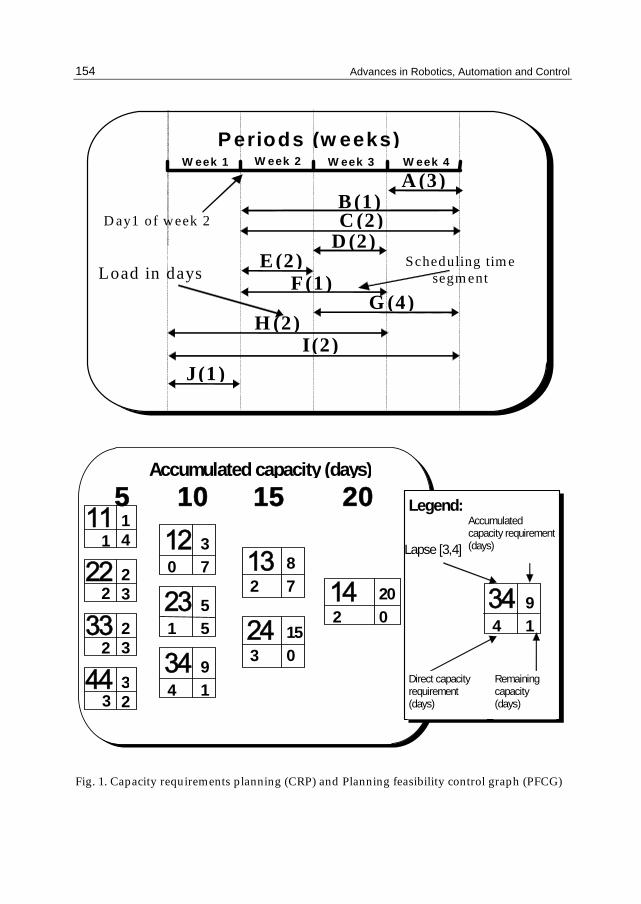
Figure 1 represents a capacity requirement planning (CRP) corresponding to the example of Table 1. For instance, task F needs a load of 1 day and have a time scheduling segment composed of weeks 2 and 3 (it means that this task should be scheduled and produced in any time inside the weeks 2 and 3). The capacity of a period (the week in this example) is 5 days. The margin of task F is so equal to 9 days (10 days of weeks 2 and 3 minus its load of 1 day). The associated planning feasibility control graph (PFCG) is shown in Figure 1. For each lapse of weeks, we calculate the direct capacity requirement, the accumulated capacity requirement and the remaining capacity. For instance, the lapse [3,4] composed of weeks 3 and 4 has a direct capacity requirement equal to 4 days (task G), an accumulated capacity requirement equal to 9 days (tasks with a scheduling time segment included in the lapse: A, D and G) and a remaining capacity equal to (10-9) days. The planning feasibility control graph proves the feasibility of this set of jobs (all the remaining capacities for all the lapses are positive). Firstly, this load adjustment approach was applied to plan the activities of a make-to-order company in a mono-level context (Dillenseger, 1993). This approach was applied then to a flow-shop composed of m processors (Bahroun, 2000a), to a generalised flow-shop (Bahroun, 2000b) and for the cyclic production context (Bahroun, 1999).

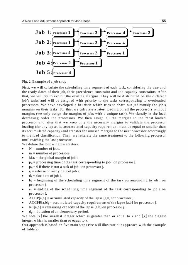
3. Application for job-shop organized firms Let us consider N jobs with their due and ready dates. Each job is composed of one to m tasks realized on one to m processors with a certain order which is not necessarily the same for all the jobs (Figure 2). We suppose that these jobs are the results of a products supply calculation in an M.R.P. based system for instance. We aim at adjusting the load resulted by these jobs in a finite capacity way by adapting the overlapping load adjustment approach to the job shop case.

Advances in Robotics, Automation and Control

154

Periods (w eeks)W eek 1

A (3)

G (4)

C (2)D (2)

E (2)F(1)

B (1)

Load in days Scheduling tim e

segm ent

W eek 2 W eek 3 W eek 4

D ay1 of week 2

H (2)I(2)

J(1)

11

22

33

44

12

23

34

13

2414

1 1 4

2 2 3

2 2 3

3 3 2

3 0 7

5 1 5

9 4 1

8 2 7

153 0

202 0

Accumulated capacity (days)5 10 15 20 Legend:

34 9 4 1

Accumulated capacity requirement (days) Lapse [3,4]

Direct capacity requirement (days)

Remaining capacity (days)

Fig. 1. Capacity requirements planning (CRP) and Planning feasibility control graph (PFCG)

A New Load Adjustment Approach for Job-Shops

155

Processor 1 Processor 3 Processor 4

Processor 4 Processor 2 Processor 1

Processor 2 Processor 1

Processor 4

Job 1: Processor 1 Processor 3 Processor 4 Processor 2

Job 2:

Job 3:

Job 4:

Job 5:

Fig. 2. Example of a job shop

First, we will calculate the scheduling time segment of each task, considering the due and the ready dates of their job, their precedence constraint and the capacity constraints. After that, we will try to exploit the existing margins. They will be distributed on the different job’s tasks and will be assigned with priority to the tasks corresponding to overloaded processors. We have developed a heuristic which tries to share out judiciously the job’s margins on their tasks. For this, we calculate a latest loading on all the processors without margins (we only assign the margins of jobs with a unique task). We classify in the load decreasing order the processors. We then assign all the margins to the most loaded processor and after that we keep only the necessary margins to validate the processor loading (for any lapse, its accumulated capacity requirement must be equal or smaller than its accumulated capacity) and transfer the unused margins to the next processor accordingly to the load classification. Then, we reiterate the same treatment to the following processor until reaching the last processor. We define the following parameters: • N = number of jobs. • m = number of processors. • Mai = the global margin of job i. • pij = processing time of the task corresponding to job i on processor j. • pij = 0 if there is not a task of job i on processor j. • ri = release or ready date of job i. • di = due date of job i. • bij = beginning of the scheduling time segment of the task corresponding to job i on

processor j. • eij = ending of the scheduling time segment of the task corresponding to job i on

processor J. • ACCP[a,b]j = accumulated capacity of the lapse [a,b] for processor j. • ACCPR[a,b]j = accumulated capacity requirement of the lapse [a,b] for processor j. • RC[a,b]j = remaining capacity of the lapse [a,b] on processor j. • dp = duration of an elementary period. We note ⎡x⎤ the smallest integer which is greater than or equal to x and ⎣x⎦ the biggest integer which is smaller than or equal to x. Our approach is based on five main steps (we will illustrate our approach with the example of Table 2):

Advances in Robotics, Automation and Control

156

Job Processingorder

Process. time

on proc. 1 (day)

Process. time

on proc. 2 (days)

Process. time

on proc. 3 (days)

ready date (beginning of

the period)

due date (ending of

the period)

Global margins

in periods (weeks)

A P1→P2→P3 3 2 2 1 6 3

B P1→P2→P3 2 3 1 1 5 2

C P1 3 0 0 3 5 2

D P2 0 2 0 2 4 2

E P3 0 0 2 4 6 2

F P3→P2→P1 3 3 2 2 5 1

G P3→P2→P1 1 1 1 2 6 2

H P3→P1→P2 2 2 2 3 5 0

I P3→P1→P2 1 2 2 3 5 0

J P2→P1 3 3 0 2 5 2

K P2→P3 0 3 4 3 6 2

L P3→P1 2 0 3 4 6 1

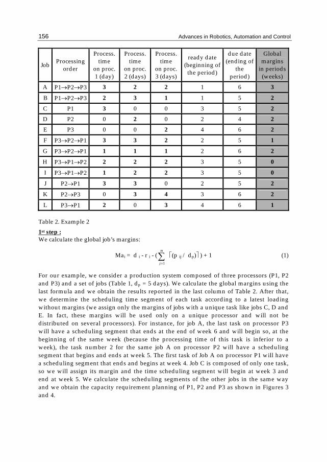
Table 2. Example 2 1st step : We calculate the global job’s margins:

Mai = d i - r i - (j

m

=∑

1

⎡(p ij / dp)⎤ ) + 1 (1)

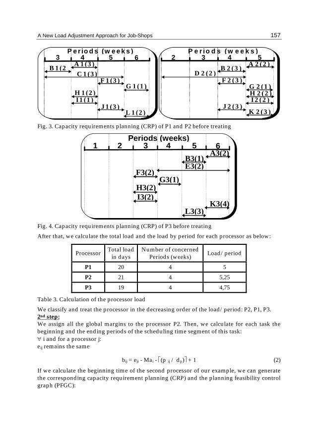
For our example, we consider a production system composed of three processors (P1, P2 and P3) and a set of jobs (Table 1, dp = 5 days). We calculate the global margins using the last formula and we obtain the results reported in the last column of Table 2. After that, we determine the scheduling time segment of each task according to a latest loading without margins (we assign only the margins of jobs with a unique task like jobs C, D and E. In fact, these margins will be used only on a unique processor and will not be distributed on several processors). For instance, for job A, the last task on processor P3 will have a scheduling segment that ends at the end of week 6 and will begin so, at the beginning of the same week (because the processing time of this task is inferior to a week), the task number 2 for the same job A on processor P2 will have a scheduling segment that begins and ends at week 5. The first task of Job A on processor P1 will have a scheduling segment that ends and begins at week 4. Job C is composed of only one task, so we will assign its margin and the time scheduling segment will begin at week 3 and end at week 5. We calculate the scheduling segments of the other jobs in the same way and we obtain the capacity requirement planning of P1, P2 and P3 as shown in Figures 3 and 4.

A New Load Adjustment Approach for Job-Shops

157

P e r io d s (w e e k s )3 4 5

A 1 (3 )

F 1 (3 )G 1 (1 )

H 1 (2 )I1 (1 )

J 1 (3 )L 1 (2 )

6B 1 (2

C 1 (3 )

P e r io d s (w e e k s ) 2 3 4 5

A 2 (2 )

F 2 (3 )G 2 (1 ) H 2 (2 ) I 2 (2 )

J 2 (3 )K 2 (3 )

B 2 (3 )D 2 (2 )

Fig. 3. Capacity requirements planning (CRP) of P1 and P2 before treating

Periods (weeks)1 2 3 4 5

A3(2)

F3(2)G3(1)

H3(2)I3(2)

K3(4)L3(3)

6B3(1)E3(2)

Fig. 4. Capacity requirements planning (CRP) of P3 before treating

After that, we calculate the total load and the load by period for each processor as below:

Processor Total load in days

Number of concerned Periods (weeks) Load/period

P1 20 4 5

P2 21 4 5,25

P3 19 4 4,75

Table 3. Calculation of the processor load

We classify and treat the processor in the decreasing order of the load/period: P2, P1, P3. 2nd step: We assign all the global margins to the processor P2. Then, we calculate for each task the beginning and the ending periods of the scheduling time segment of this task: ∀ i and for a processor j: eij remains the same

bij = eji - Mai - ⎡(p ij / dp)⎤ + 1 (2)

If we calculate the beginning time of the second processor of our example, we can generate the corresponding capacity requirement planning (CRP) and the planning feasibility control graph (PFGC):

Advances in Robotics, Automation and Control

158

Periods (weeks)2 3 4 5

A2(2)

F2(3)G2(1)

H2(2)I2(2)J2(3)

K2(3)

B2(3)D2(2)

22

33

44

55

23

34

45

24

3525

0 0 5

0 0 5

0 0 5

4 4 1

0 0 10

3 3 7

4 0 6

118 4

114 4

212 -1

Accumulated capacity (days)

5 10 15 20Legend:

24 11 8 4

Accumulated capacity requirement

Lapse [2,4]

Direct capacity requirement

Remaining capacity

66 0

0 5

56 4 0 6

46 4 0 11

36 110 9

26 210 4

25

Fig. 5. CRP and PFCG of the processor P2 after assigning all the margins 3rd Step: We then check the feasibility condition. If we find problems in certain lapses (even with all available margins), we should lengthen the scheduling time segment of some tasks. If for a lapse [a, b] in the processor j, the validation condition is not verified: - We consider in the duration increasing order all the tasks that bij ≥ a et eij= b. - In this list, we begin to treat the first task in the kth position in the list with a load equal

or superior to the overloading in the lapse which allows us to delay the minimum number of tasks.

- We proceed progressively to the lengthening of the scheduling time segment of these tasks, period by period until the verification of the feasibility condition or arrival to the end of the list.

- If we arrive to the end of the list we try with tasks positioned in the (k-1)th, (k-2)th … position until the verification of the feasibility condition.

In our example (Figure 5), we remark that we have an overloading in the lapse [2,5] which obliges us to delay of one period, one of the tasks included in this lapse and which finishes in

A New Load Adjustment Approach for Job-Shops

159

period 5 (A2, G2, H2, I2 or K2 as we can see in CRP of Figure 5). We choose in this example to lengthen the scheduling time segment of task G2 from the lapse [3,5] to the lapse [3,6]. Remark: If we do not accept to delay jobs, the lapses with negative remaining capacity indicate where we must increase the capacity by using for example overtime or interims. We can also introduce the notion of jobs priority for choosing which tasks must be delayed. 4th Step: Now, we will try to regain margins. We begin with the tasks corresponding to jobs with weak global margins. Tasks of jobs without margins are assigned to the elementary lapses ([1,1], [2,2] etc.), those corresponding to jobs with one period margin are assigned to the lapses of the second column of the feasibility control graph, those corresponding to jobs with k periods margins are assigned to the column number k etc. Our treatment begins with the lapses of the second column because the corresponding jobs have only one period global margin and we must preserve these precious margins to validate the other processors and use the margins from jobs that have important global margins. A transfer of a task from the lapse [a,b] to the lapse [a+w,b], adds load to all the over-lapses of [a+w,b] which are not initially over-lapses of [a,b]. The transferred load must be equal or smaller than the remaining capacity on these lapses for maintaining the validation condition. The proposed approach for this transfer tries to transfer the maximum number of tasks and tries to match in the best way the transferred load in regard to the remaining capacity. Consequently, we construct the set of tasks which can be transferred, and we classify this set in the increasing order of their load. We transfer the tasks one by one in this order while the sum of their load is smaller than the remaining capacity. Then, we take the last task transferred and we try to change it by another task from the remaining tasks of the set and which matches better the remaining capacity. If two tasks have the same load we can choose for example the task corresponding to a product with a greater carrying cost. If we take the example of PFCG in Figure 5, we begin with the lapses of the second column. If we try, for instance, to regain margins from the tasks corresponding to the lapse [3,4], we should transfer the maximum number of tasks to the lapse [4,4]. We can transfer task F2 because the minimum of the remaining capacity of the over-lapses of [4,4] which are not over-lapses of [3,4] (the lapses [4,4], [4,5] and [4,6]) is 5 and it is greater than the load of the task F2. Then, we pass to lapses [4,5], [5,6], and next to the lapses of the third column (for the task G2, we succeed to regain 2 periods, the scheduling time is shortened from the lapse [3,6] to lapse [5,6]). We reiterate this treatment until arriving to the last column. We obtain after treatment of the processor P2 the capacity requirement planning of Figure 6.

Periods (w eeks)1 2 3 4 5

A 2(2)

F 2(3)G 2(1H 2(2I2(2)

J2(3)K 2(3

6

B 2(3)D 2(2)

Fig. 6. C.R.P. of processor P2 after treatment

Advances in Robotics, Automation and Control

160

We can generalize this step for a processor j: ∀ the lapse [x,y] / x= a and y= a+w with 1 ≤ w ≤ H and 1 ≤ a ≤ H-w : - Construct the set A = {set of tasks / b ij = a and e ij = a+ w} (The set of tasks that their

scheduling time segment can be shortened, this set will be ordered in the increasing order of their load).

- Iterate then for f = w -1 → 0 Cap = Min ( RC j [a+1+z, a+w+n] ) For n = 0 → H - a - w, z = f → 0 (we calculate the

maximum load that can be transferred). Transfer the maximum number of tasks from A (using the approach described in

the precedent page) that the sum of their processing times is inferior or equal to Cap. Let C be the set of these tasks transferred and Q the sum of their processing time: ∀ the task ij ∈ C, we put b ij = a+1 + f For n = 0 → H - a - w and for z = f → 0, we do: RC j [a+1+z, a+w+n] = RC j [a+1+z, a+w +n ] – Q (We update the new time scheduling segment of the tasks and the remaining capacity of the concerned lapses).

- We update the beginning and the ending of the scheduling time segments of the other tasks on the other processors as follow:

If a task u precedes task j of the same job i on the processor j, we move its scheduling time segment in a manner that the ending time becomes equal to the beginning time of the task j. We effectuate the same treatment until arriving to the first task.

If a task u follows task j of the same job i on the processor j, we update in a symmetrical manner the scheduling time segment of this task and all the other tasks up to the last one.

5th step: We assign all the unused margins to the next processor (in this case the processor P1). We calculate the scheduling time segments of the tasks corresponding to this processor using the following formulae: ∀ i, for a processor j :

bji = eji – M’ai - ⎡(p ij / dp)⎤ + 1 (3)

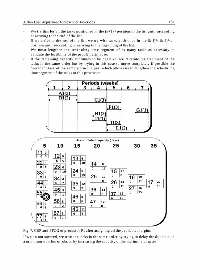
Where M’ai is the remaining margin. We can assign margins for a task i on a processor j only if the precedent tasks of the same job are not already treated. We obtain the C.R.P. and the control feasibility graph of the processor P1 of figure 7. We check then the feasibility condition. If for a lapse [a,b] in the processor j, the validation condition is not verified, we should lengthen the scheduling time segment of the tasks as below: - We consider in the duration increasing order the list of all the tasks included in the

lapse [a,b] and that bij = a or eij= b. - In order to treat the minimum number of tasks, we begin to treat in this list the first task in

the kth position in the list which has a load equal or superior to the overloading in the lapse. - We try to regain a margin for this task by shortening the scheduling time segment of the

precedent task of the same job in a processor already treated.

A New Load Adjustment Approach for Job-Shops

161

- We try this for all the tasks positioned in the (k+1)th position in the list until succeeding or arriving to the end of the list.

- If we arrive to the end of the list, we try with tasks positioned in the (k-1)th, (k-2)th … position until succeeding or arriving to the beginning of the list.

- We must lengthen the scheduling time segment of as many tasks as necessary to validate the feasibility of the problematic lapse.

- If the remaining capacity continues to be negative, we reiterate the treatment of the tasks in the same order but by trying in this case to move completely if possible the precedent task of the same job in the past which allows us to lengthen the scheduling time segment of the tasks of this processor.

Periods (weeks)

1 2 3 4 5A1(3)

F1(3) G1(1)H1(2)I1(1)

J1(3)L1(2)

6

B1(2) C1(3)

7

22

33

44

55

23

34

45

24

3525

0 0 5

0 0 3

3 3 2

6 6 -1

0 0 10

3 0 7

9 0 1

0 0 15

123 3

120 8

Accumulated capacity (days)

5 10 15 20

66 0

0 5

56 8 2 2

46 9 0 6

36 140 6

26 140 11

2511

0 0 5 12 5

5 13 5 0 10 14 8

0 12

47 120 8

77 1

1 4

67 1 0 9

46 110 4

37 150 10

15 170 8

27 150 15

16 190 11 17 20

0 15

30 35

5

Fig. 7. CRP and PFCG of processor P1 after assigning all the available margins

If we do not succeed, we treat the tasks in the same order by trying to delay the due date on a minimum number of jobs or by increasing the capacity of the incriminate lapses.

Advances in Robotics, Automation and Control

162

Periods (weeks)1 2 3 4 5

A1(3)

F1(3)G1(1)

H1(2)I1(1)

J1(3)L1(2)

6

B1(2)C1(3)

7

Periods (weeks)2 3 4 5

A3(2)

F3(2)G3(1)

H3(2)I3(2)

K3(4)L3(3)

6

B3(1)E3(2)

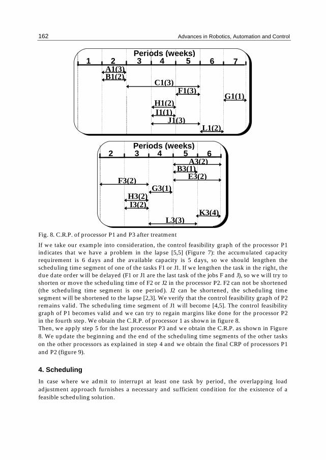
Fig. 8. C.R.P. of processor P1 and P3 after treatment

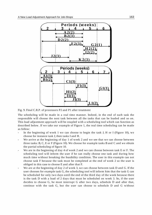
If we take our example into consideration, the control feasibility graph of the processor P1 indicates that we have a problem in the lapse [5,5] (Figure 7): the accumulated capacity requirement is 6 days and the available capacity is 5 days, so we should lengthen the scheduling time segment of one of the tasks F1 or J1. If we lengthen the task in the right, the due date order will be delayed (F1 or J1 are the last task of the jobs F and J), so we will try to shorten or move the scheduling time of F2 or J2 in the processor P2. F2 can not be shortened (the scheduling time segment is one period). J2 can be shortened, the scheduling time segment will be shortened to the lapse [2,3]. We verify that the control feasibility graph of P2 remains valid. The scheduling time segment of J1 will become [4,5]. The control feasibility graph of P1 becomes valid and we can try to regain margins like done for the processor P2 in the fourth step. We obtain the C.R.P. of processor 1 as shown in figure 8. Then, we apply step 5 for the last processor P3 and we obtain the C.R.P. as shown in Figure 8. We update the beginning and the end of the scheduling time segments of the other tasks on the other processors as explained in step 4 and we obtain the final CRP of processors P1 and P2 (figure 9).

4. Scheduling In case where we admit to interrupt at least one task by period, the overlapping load adjustment approach furnishes a necessary and sufficient condition for the existence of a feasible scheduling solution.

A New Load Adjustment Approach for Job-Shops

163

P eriods (w eeks)2 3 4 5

A 2(2)

F 2(3) G 2(1)H 2(2)I2(2)

J2(3) K 2(3)

6

B 2(3)D 2(2)

Periods (weeks)2 3 4 5

A1(3)

F1(3)G1(1)

H1(2)I1(1)

J1(3)L1(2)

6

B1(2) C1(3)

7

Fig. 9. Final C.R.P. of processors P2 and P1 after treatment

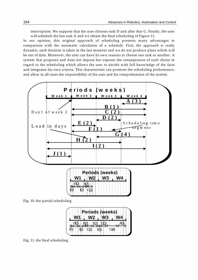
The scheduling will be made in a real time manner. Indeed, in the end of each task the responsible will choose the next task between all the tasks that can be loaded and so on. This load adjustment approach will be coupled with a scheduling tool which can function as described below. If we take our example of Figure 1, the real time scheduling can be made as follow: - In the beginning of week 1 we can choose to begin the task J, H or I (Figure 10), we

choose for instance task J, then tasks I and H. - We arrive at the beginning of day 1 of week 2 and we see that we can choose between

three tasks: B, C, E or F (Figure 10). We choose for example tasks B and C and we obtain the partial scheduling of figure 10.

- We are in the beginning of day 4 of week 2 and we can choose between task E or F. The scheduling tool will inform the user if he can really choose one task and during how much time without breaking the feasibility condition. The user in this example can not choose task F because the task must be completed at the end of week 2 so the user is obliged in this case to choose E and after that F.

- We are at the beginning of day 2 of week 3, we can choose between task D and G. If the user chooses for example task G, the scheduling tool will inform him that the task G can be scheduled for only two days until the end of the third day of the week because there is the task D with a load of 2 days that must be scheduled on week 3. So, if the user decides to choose G, he must interrupt G after two days, schedule D and after that, continue with the task G, but the user can choose to schedule D and G without

Advances in Robotics, Automation and Control

164

interruption. We suppose that the user chooses task D and after that G. Finally, the user will schedule the last task A and we obtain the final scheduling of Figure 11.

In our opinion, this original approach of scheduling presents many advantages in comparison with the automatic calculation of a schedule. First, the approach is really dynamic, each decision is taken in the last moment and we do not produce plans which will be out of date. Moreover, the user can have its own reasons to choose one task or another. A system that proposes and does not impose but exposes the consequences of each choice in regard to the scheduling which allows the user to decide with full knowledge of the facts and integrates his own criteria. This characteristic can promote the scheduling performance, and allow in all cases the responsibility of the user and his comprehension of the system.

P e r i o d s ( w e e k s )W e e k 1

A ( 3 )

G ( 4 )

C ( 2 )D ( 2 )

E ( 2 )F ( 1 )

B ( 1 )

L o a d i n d a y s S c h e d u l i n g t i m e

s e g m e n t

W e e k 2 W e e k 3 W e e k 4

D a y 1 o f w e e k 2

H ( 2 )I ( 2 )

J ( 1 )

Periods (weeks)

W1 W2 W3 W4

I(2) H(2)

J(1) C(2) B(2)

Fig. 10. the partial scheduling

Periods (weeks)W1 W2 W3 W4

A(3) E(2)G(4) I(2)

H(2) J(1) C(2)

B(2) F(1)

D(2)

Fig. 11. the final scheduling

A New Load Adjustment Approach for Job-Shops

165

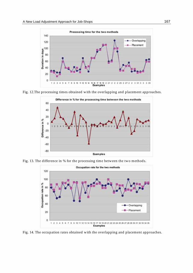
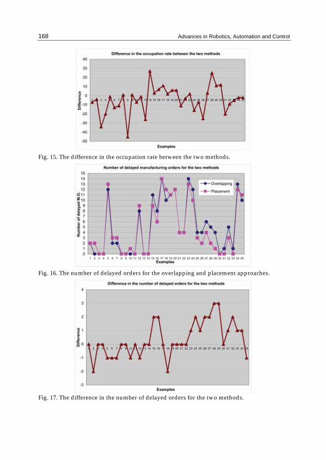
5. Experimentation An experimentation has been carried out on a set of examples. We will describe the conditions and the results of this experimentation. We have constructed 35 examples in a job shop context where we have varied the number of jobs (6 to 16), the number of processors (2 to 4) and the size of the period (4 to 7 days). The total load is always near or superior to the capacity. We compared our approach with the classic approach of placement. For each example, we apply our approach and the placement approach. This placement is applied in two steps: first an earliest placement to determine the earliest due dates and second a latest placement using job’s due dates as the maximum between the requested due dates and the earliest ones. The results of the experimentation are summarized in Table 4. We will use for this these notations: NMO: Number of Manufacturing Orders. NPr: Number of processors. PS: Period size in days. NPe: Number of periods. PTO: Processing time of the overlapping approach which represents the duration in days between the beginning of the first task of the M.O. until the ending of the last task of the last M.O. PTP: Processing time of the placement approach which represents the duration in days between the beginning of the first task of the M.O. until the ending of the last task of the last M.O for the placement approach. DPT: Difference in % for the processing time between the two approaches. ORO: Occupation rate of the processors in % for the overlapping approach. It is in fact an average of the occupation rate of all the processors. ORP: Occupation rate of the processors in % for the placement approach. DOR: Difference in % for the occupation rate between the two approaches. NDO: Number of delayed orders for the overlapping approach. NDP: Number of delayed orders for the placement approach. DDO: difference in the delayed orders between the two approaches. First, we have compared the two approaches in terms of processing times (figures 12 and 13). We call the processing time the duration in days between the beginning of the first task on the first processor and the end of the last task on the last processor. The difference is about 4.5 % between the two approaches. Second, we have compared the two approaches in terms of occupation rate (figures 14 and 15). We remark that there is a difference of about -4.3 % in the occupation rate for the two approaches. This fact is normal because with the first approach we try to keep the maximum of freedom in a middle term without giving a detailed production schedule. Third, we have compared the two approaches in terms of number of delayed jobs (figures 16 and 17). The average number of delayed jobs with the overlapping approach is about 5.1 whereas it is equal to 4.7 with the placement approach. We observe that the results given by the two approaches are very close even if the placement gives only one scheduling solution when the overlapping approach gives a set of scheduling solutions.

Advances in Robotics, Automation and Control

166

All these facts prove really the efficiency of our approach. However, we should experiment and compare our approach with other approaches and with a biggest number of examples. Example NMO NPr PS NPe PTO PTP DPT ORO ORP DOR NDO NDP DDO

1 12 3 5 6 30 28 7 80 87 -7 2 2 0 2 14 4 5 7 30 25 17 70 74 -4 0 2 -2 3 9 3 5 6 25 13 48 54 88 -34 0 0 0 4 6 2 5 7 25 20 20 57 77 -20 0 0 0 5 16 3 5 14 70 59 16 91 92 -1 12 13 -1 6 6 3 5 8 40 40 0 78 91 -13 2 3 -1 7 6 3 4 9 36 40 -11 87 98 -11 2 3 -1 8 12 3 7 6 28 28 0 79 78 1 0 0 0 9 14 4 7 7 42 27 36 48 93 -45 0 0 0 10 6 3 6 7 30 40 -33 93 92 1 0 1 -1 11 6 2 7 7 35 26 26 47 54 -7 0 0 0 12 16 3 7 10 70 59 16 91 92 -1 8 9 -1 13 6 3 7 7 42 40 5 67 93 -26 0 0 0 14 8 3 7 7 28 44 -57 84 57 27 0 0 0 15 12 3 5 14 70 71 -1 87 84 3 11 9 2 16 12 3 7 10 70 71 -1 91 84 7 8 6 2 17 16 3 5 18 90 96 -7 100 89 11 14 14 0 18 16 3 7 14 98 96 2 92 90 2 10 12 -2 19 12 3 5 23 110 112 -2 85 79 6 11 11 0 20 12 3 7 16 112 112 0 85 79 6 12 12 0 21 6 2 5 12 60 55 8 89 100 -11 4 4 0 22 6 2 7 9 63 60 5 87 90 -3 4 4 0 23 14 4 5 22 125 100 20 70 68 2 14 13 1 24 14 4 7 13 91 101 -11 72 88 -16 12 10 2 25 9 3 5 7 35 31 11 78 85 -7 4 3 1 26 9 3 7 7 49 31 37 60 85 -25 4 2 2 27 10 3 5 10 45 46 -2 76 73 3 6 4 2 28 10 3 7 8 56 46 18 100 75 25 5 2 3 29 8 3 4 8 28 36 -29 84 73 11 4 1 3 30 8 3 6 7 30 36 -20 90 78 12 0 0 0 31 14 4 4 7 28 24 14 69 89 -20 1 0 1 32 12 3 4 7 28 26 7 79 88 -9 5 3 2 33 12 3 6 6 30 29 3 77 82 -5 1 0 1 34 16 3 4 16 64 59 8 90 92 -2 13 12 1 35 16 3 6 16 66 59 11 90 92 -2 10 11 -1

Average 10,9 3,0 5.7 10,2 53,7 51,0 4,5 79,3 83,7 -4,3 5,1 4,7 0,4

Table 4. Results of the experimentation

A New Load Adjustment Approach for Job-Shops

167

Fig. 12.The processing times obtained with the overlapping and placement approaches.

Fig. 13. The difference in % for the processing time between the two methods.

Fig. 14. The occupation rates obtained with the overlapping and placement approaches.

Advances in Robotics, Automation and Control

168

Fig. 15. The difference in the occupation rate between the two methods.

Fig. 16. The number of delayed orders for the overlapping and placement approaches.

Fig. 17. The difference in the number of delayed orders for the two methods.

A New Load Adjustment Approach for Job-Shops

169

6. Conclusion The most common approach used in production planning remains MRP II (Manufacturing Resource Planning). The proposed approach in this paper constitutes an alternative to the traditional load adjustment approaches used in the CRP (Capacity Requirement Planning) modules in software based on MRP II philosophy. The new heuristic presented in this paper, in comparison with the usual middle and/or long-term planning and scheduling approaches, has the following advantages: - not setting a long-term tasks scheduling to assure that the planning can be properly

carried out; - exploiting and distributing judiciously the job’s margins on their tasks and trying to

respect the just-in-time principles; - permitting the postponement of the final scheduling job’s problems until the short term

at the order release phase and/or the scheduling phase; - delaying, if necessary, the due dates of some jobs or increasing the capacity in some

lapses for guaranteeing in every case the feasibility of the production planning. We can extend and improve our work by studying the possibility of introducing the overlapping of the scheduling time segments of consecutive tasks. We can also improve our heuristic in order to use it in the case where the tasks are not preemptive.

7. References Bahroun, Z., Jebali, D., Baptiste, P. & Campagne, J-P. & Moalla, M. (1999). Extension of the

overlapping production planning and application for the cyclic delivery context, in IEPM ‘99 Industrial Engineering and Production Management, Glasgow.

Bahroun, Z., Campagne, J-P. & Moalla, M. (2000a). The overlapping production planning: A new approach of a limited capacity management. International Journal of Production Economics, 64, 21-36.

Bahroun, Z., Campagne, J-P. & Moalla, M. (2000b). Une nouvelle approche de planification à capacité finie pour les ateliers flow-shop. Journal Européen des Systèmes Automatisés, 5, 567-598.

Dauzere-Peres, S., & Lassere, J-B. (2002). On the importance of scheduling decisions in production planning and scheduling. International Transactions in Operational Research, 9, 6, 779-793.

Dillenseger, F. (1993). Conception d'un système de planification à moyen terme pour fabrications à la commande. PhD thesis, INSA Lyon, France.

Drexl, A. & Kimms, A. (1997). Lot sizing and scheduling - Survey and extensions. European Journal of Operation Research, 99, 221-235.

Fleischmann, B. & Meyr, H. (1997). The general lot sizing and scheduling problem. Operation Research Spektrum, 19, 1, 11-21.

Grubbström, R.W. & Huynh, T.T.T. (2006). Multi-level, multi-stage capacity-constrained production-inventory systems in discrete time with non-zero lead times using MRP theory. International Journal of Production Economics, 101, 53-62.

Gunther, H.O. (1987). Planning lot sizes and capacity requirements in a single stage production system. European Journal of Operational Research, 31, 1, 223-231.

Hillion, H. & Proth, J-M. (1994). Finite capacity flow control in a multi-stage/multi-product environment. International Journal of production Research, 32, 5, 1119-1136.

Advances in Robotics, Automation and Control

170

Néron, E., Baptiste, P. & Gupta, J.N.D. (2001). Solving Hybrid Flow Shop problem using energetic reasoning and global operations. Omega, 29, 501-511.

Pandey, P.C., Yenradee, P. & Archariyapruek, S. (2005). A finite capacity material requirement planning system. Production Planning & Control, 2, 113-121.

Wuttipornpun, T. & Yenradee, P. (2004). Development of finite capacity material requirement planning system for assembly operations. Production Planning & Control, 15, 534-549.