1

Immanent Reasoning or Equality in Action

A Dialogical Study

Shahid Rahman♣ Nicolas Clerbout♦, Ansten Klev●,

Zoe McConaughey♣, Juan Redmond♦1

♦ Instituto de Filosofía, Universidad de Valparaíso. ● Academy of Sciences of the Czech Republic. ♦ Instituto de Filosofía, Universidad de Valparaíso. The results of the present work have been developed in the frame of the Project: Fondecyt Regular N° 1141260. ♣ Univ. Lille, CNRS, UMR 8163 - STL - Savoirs Textes Langage, F-59000 Lille, France, ADA-MESH (NpdC).

2

To all of the present and past members of the team of Dialogicians of Lille and beyond

3

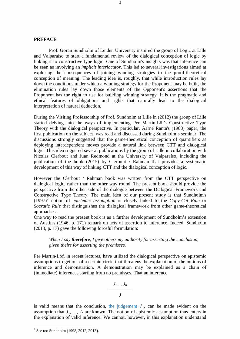
PREFACE Prof. Göran Sundholm of Leiden University inspired the group of Logic at Lille and Valparaíso to start a fundamental review of the dialogical conception of logic by linking it to constructive type logic. One of Sundholm's insights was that inference can be seen as involving an implicit interlocutor. This led to several investigations aimed at exploring the consequences of joining winning strategies to the proof-theoretical conception of meaning. The leading idea is, roughly, that while introduction rules lay down the conditions under which a winning strategy for the Proponent may be built, the elimination rules lay down those elements of the Opponent's assertions that the Proponent has the right to use for building winning strategy. It is the pragmatic and ethical features of obligations and rights that naturally lead to the dialogical interpretation of natural deduction. During the Visiting Professorship of Prof. Sundholm at Lille in (2012) the group of Lille started delving into the ways of implementing Per Martin-Löf's Constructive Type Theory with the dialogical perspective. In particular, Aarne Ranta's (1988) paper, the first publication on the subject, was read and discussed during Sundholm’s seminar. The discussions strongly suggested that the game-theoretical conception of quantifiers as deploying interdependent moves provide a natural link between CTT and dialogical logic. This idea triggered several publications by the group of Lille in collaboration with Nicolas Clerbout and Juan Redmond at the University of Valparaíso, including the publication of the book (2015) by Clerbout / Rahman that provides a systematic development of this way of linking CTT and the dialogical conception of logic. However the Clerbout / Rahman book was written from the CTT perspective on dialogical logic, rather than the other way round. The present book should provide the perspective from the other side of the dialogue between the Dialogical Framework and Constructive Type Theory. The main idea of our present study is that Sundholm's (1997)2 notion of epistemic assumption is closely linked to the Copy-Cat Rule or Socratic Rule that distinguishes the dialogical framework from other game-theoretical approaches. One way to read the present book is as a further development of Sundholm’s extension of Austin's (1946, p. 171) remark on acts of assertion to inference. Indeed, Sundholm (2013, p. 17) gave the following forceful formulation:

When I say therefore, I give others my authority for asserting the conclusion, given theirs for asserting the premisses.

Per Martin-Löf, in recent lectures, have utilized the dialogical perspective on epistemic assumptions to get out of a certain circle that threatens the explanation of the notions of inference and demonstration. A demonstration may be explained as a chain of (immediate) inferences starting from no premisses. That an inference

J1 ... Jn —————

J is valid means that the conclusion, the judgement J , can be made evident on the assumption that J1, …, Jn are known. The notion of epistemic assumption thus enters in the explanation of valid inference. We cannot, however, in this explanation understand

2 See too Sundholm (1998, 2012, 2013).

4

'known' in the sense of demonstrated, for then we are explaining the notion of inference in terms of demonstration, whereas demonstration has been explained in terms of inference. Martin-Löf suggests that we here understand 'known' in the sense of asserted, so that epistemic assumptions are judgements others have made, judgements for which others have taken the responsibility; that the inference is valid then means that, given that others have taken responsbility for the premisses, I can take responsibility for the conclusion:

The circularity problem is this: if you define a demonstration to be a chain of immediate inferences, then you are defining demonstration in terms of inference. Now we are considering an immediate inference and we are trying to give a proper explanation of that; but, if that begins by saying: Assume that J1, …, Jn have been demonstrated – then you are clearly in trouble, because you are about to explain demonstration in terms of the notion of immediate inference, hence when you are giving an account of the notion of immediate inference, the notion of demonstration is not yet at your disposal. So, to say: Assume that J1, …, Jn have already been demonstrated, makes you accusable of trying to explain things in a circle. The solution to this circularity problem, it seems to me now, comes naturally out of this dialogical analysis. […]

The solution is that the premisses here should not be assumed to be known in the qualified sense, that is, to be demonstrated, but we should simply assume that they have been asserted, which is to say that others have taken responsibility for them, and then the question for me is whether I can take responsibility for the conclusion. So, the assumption is merely that they have been asserted, not that they have been demonstrated. That seems to me to be the appropriate definition of epistemic assumption in Sundholm's sense.3

One of the main tenets of the present study is that the further move of relating the

Socratic Rule rule with judgemental equality provides both a simpler and more direct way to implement the constructive type theoretical approach within the dialogical framework. Such a reconsideration of the Socratic Rule, roughly speaking, amounts to the following.

1. A move from P that brings-forward a play object in order to defend an elementary proposition A can be challenged by O.

2. The answer to such a challenge, involves P bringing forward a definitional equality that expresses the fact that the play object chosen by P copies the one O has chosen while positing A. For short, the equality expresses at the object-languaje level that the defence of P relies on the authority given to O to be able to produce the play objects she brings forward.

More generally, according to this view, a definitional equality established by P and brought forward while defending the proposition A, expresses the equality between a play object (introduced by O) and the instruction for building a play object deployed by O while affirming A. So it can be read as a computation rule that indicates how to compute O's instructions. Let us recall that from the strategic point of view, O's moves correspond to elimination rules of demonstrations. Thus, the dialogical rules that prescribe how to introduce a definitional equality – correspond – at the strategic level – to the definitional equality rules for CTT as applied to the selector-functions involved in the elimination rules. So, what we are doing here is extending the dialogical interpretation of Sundholm's epistemic assumption to the rules that set up the definitional equality of a type.

3 Transcription by Ansten Klev of Martin-Löf's talk in May 2015.

5

The present work is structured in the following way:

• In the Introduction we state the main tenets that guide our book • Chapter II contains a brief overview of Constructive Type Theory penned by

Ansten Klev with exercises and their solutions. • Chapter III offers a novel presentation of the dialogical conception of logic. In

fact, the first two sections of the chapter provide an overview of standard dialogical logic – including solved exercises, slightly adapted to the content of the present volume. The rest of the sections develop a new dialogical approach to Constructive Type Theory.

• Chapters IV and V contain the main body of our study, namely the relation between the Socratic Rule, epistemic assumptions, and equality. The chapter provides the reader with thoroughly worked out examples with comments.

• The final chapter develops some remarks on material dialogues, including two main examples, namely, the set Bool and the set of natural numbers Our also text includes four appendices (i) Abrief outline of Per Martin-Löf's informal presentation of the demonstration

of the axiom of choice. (ii) Two examples of a tree-shaped graph of an extensive strategy. (iii)An appendix containing an overview of main rules and notation for the new

formulation of dialogical approach to constructive type theory developed in the book;

(iv) An appendix containing the main notation of the CTT-framwork

Acknowledgments:

Many thanks to Mark van Atten (Paris1), Giuliano Bacigalupo (Zürich), Charles Zacharie Bowao (Univ. Ma Ngouabi de Brazzaville , Congo), Christian Berner (Lille3), Michel Crubellier (Lille3), Pierre Cardascia (Lille3), Oumar Dia (Dakar), Marcel Nguimbi ((Univ. Marien Ngouabi de Brazzaville, Congo), Adjoua Bernadette Dango (Lille3 / Alassane Ouattara de Bouaké, Côte d'Ivoire), Steephen Rossy Eckoubili (Lille3), Johan Georg Granström (Zürich) , Gerhard Heinzmann (Nancy2), Muhammad Iqbal (Lille3), Matthieu Fontaine (Lille3), Radmila Jovanovic (Belgrad), Hanna Karpenko (Lille3), Laurent Keiff (Lille3), Sébastien Magnier (Saint Dennis, Réunion), Clément Lion (Lille3), Gildas Nzokou (Libreville), Fachrur Rozie (Lille3), Helge Rückert (Mannheim), Mohammad Shafiei (Paris1), and Hassan Tahiri (Lisbon), for rich interchanges, suggestions on the main claims of the present study and proof-reading of specific sections of the text. Special thanks to Gildas Nzokou (Libreville), Steephen Rossy Eckoubili (Lille3) and Clément Lion (Lille3), with whom a Pre-Graduate Textbook in French on dialogical logic and CTT is in the process of being worked out – during the visiting-professorship in 2016 of the former. Eckoubili is the author of the sections on exercises for dialogical logic, Nzokou cared of those involving the development of CTT-demonstrations out of winning-strategies. Special thanks also to Ansten Klev (Prague) for helping with technical details and conceptual issues on CTT, particularly so as author of the chapter introducing CTT.

6

We are very thankful too to our host institutions that fostered our researches in the frame of specific research-programs. Indeed, the results of the present work have been developed in the frames of

• the transversal research axe Argumentation (UMR 8163: STL), • the research project ADA at the MESHS-Nord-pas-de-Calais and • the research-projects: ANR-SÊMAINÔ (UMR 8163: STL) and • Fondecyt Regular N° 1141260 (Chile).

Shahid Rahman♣ Nicolas Clerbout♦, Ansten Klev●,

Zoe McConaughey♣, Juan Redmond♦4

♦ Instituto de Filosofía, Universidad de Valparaíso. ● Academy of Sciences of the Czech Republic. ♦ Instituto de Filosofía, Universidad de Valparaíso. The results of the present work have been developed in the frame of the Project: Fondecyt Regular N° 1141260. ♣ Univ. Lille, CNRS, UMR 8163 - STL - Savoirs Textes Langage, F-59000 Lille, France, ADA-MESH (NpdC).

7

I. Introduction The question about the nature of the notion of identity is an old and venerable one and, in the western tradition the history of its written sources takes us from Parmenides’ famous poem and its challenge by Heraclitus, to the discussions of Plato and Aristotle, up to the puzzles of Frege and Wittgenstein,5 and the introduction of the notation “ = “ for it by Robert Recorde in 1557:

And to avoide the tediouse repetition of these woordes : is equalle to : I will sette as I doe often in woorke use, a paire of paralleles, or Gemowe lines of one lengthe, thus : =, bicause noe 2 thynges, can be moare equalle. 6

From the very start different pairs of concepts were linked to identity and puzzled the finest minds, such as numerical (or extensional) identity – qualitative identity (or intensional), ontological principle – logical principle, real-definition – nominal definition and on top of these pairs the relation between sign and object. The following puzzling lines of Plato’s Parmenides contain already the core of many of the discussions that took place long after him:

If the one exists, the one cannot be many, can it? No, of course not [… ].Then in both cases the one would be many, not one.” “True.” “Yet it must be not many, but one.” “Yes.” (Plato (1997), Parmenides, 137c-d)7

Hegel takes the tension between the one and many mentioned by Plato as constitutive of the notion of identity. Moreover, Hegel defends the idea that the concept of identity, conceived as the fundamental law of thought, if it should express more than a tautology, must be understood as a principle that comprehends both the idea of identical (that expresses reflexive cases of the principle) and the idea of different (that expresses non-reflexive cases). Hegel points out that expressions such as A = A have a “static” character empty of meaning – presumably in contrast to expressions such as A = B:

In its positive formulation [as the first law of thought] , A = A, this proposition is at first no more than the expression of empty tautology. It is rightly said, therefore, that this law of thought is without content and that it leads nowhere. It is thus to an empty identity that they cling, those who take it to be something true, insisting that identity is not difference but that the two are different. They do not see that in saying, “Identity is different from difference,” they have thereby already said that identity is something different. And since this must also be conceded as the nature of identity, the implication is that to be different belongs to identity not externally, but within it, in its nature. – But, further, inasmuch as these same individuals hold firm to their unmoved identity, of which the opposite is difference, they do not see that they have thereby reduced it to a one-sided determinateness which, as such, has no truth. They are conceding that the principle of identity only expresses a one-sided determinateness, that it only contains formal truth, truth abstract and incomplete. – Immediately implied in this correct judgement, however, is that the truth is complete only in the unity of identity and difference, and, consequently, that it only consists in this unity . (Hegel (2010), 1813, Book 2, Vol. 2, II.258, 2nd remark, p. 358).8

5 Quite often Plato's dialogue Theaetetus (185a) (in Plato (1997)) is mentioned as one of the earliest explicit uses of the principle. 6 Recorde (1577). There are no page numbers in this work, but the quoted passage stands under the heading “The rule of equation, commonly called Algebers Rule” which occurs about three quarters into the work. The quote has been overtaken from Granström (2011), p. 33. 7 In the present study we shall use the standard conventions for referring to Aristotle’s or Plato’s texts. The translations we used are those of J. Barnes (1984) for Aristotle and J. M. Cooper (1997) for Plato. 8 Der Satz der Identität [als das erste Denkgesetz] in seinem positiven Ausdrucke A=A, ist zunächst nichts weiter, als der Ausdruck der leeren Tautologie. Es ist daher richtig bemerkt worden, daß dieses Denkgesetz ohne Inhalt sey und nicht weiter führe. So ist die leere Identität, an welcher diejenigen festhangen bleiben, welche sie als solche für etwas Wahres nehmen und immer vorzubringen pflegen, die Identität sey nicht die Verschiedenheit, sondern die Identität und die Verschiedenheit seyen verschieden.

8

What Hegel is going after, is that the clue for grasping a conceptually non-empty notion of identity lies in the understanding the links of the reflexive with the non-reflexive form and vice-versa. More precisely, the point is understand the transition from the reflexive to its non-reflexive form.9 The history of studies involving this interplay, before and after Hegel, is complex and rich. Let us briefly mention in the next section the well-known “linguistic” approach to the issue that followed from the work of Gottlob Frege and Ludwig Wittgenstein, that had a decisive impact in the logical approach to identity. I.1 Equality at the propositional level:

One of the most influential studies of the relation between sign and object as involving the (dyadic) equality-predicate expressed at the propositional level was the one formulated in 1892 by Gottlob Frege in his celebrated paper Über Sinn und Bedeutung. The paper starts by asking the question: Is identity a relation? If it is a relation, is it a relation between objects, or between signs of objects. To take the notorious example of planet Venus, the morning star = the morning star is a statement very different in cognitive value from the morning star = the evening star. The former is analytically true, while the second records an astronomical discovery. If we were to regard identity as a relation between a sign and what the sign stands for it would seem that if a = b is true, then a = a would not differ form a = b. A relation would thereby be expressed of a thing to itself, and indeed one in which each thing stands to itself but to no other thing. (Frege, Über Sinn und Bedetung, pp. 40-42). On the other hand if every sentence of the form a = b really signified a relationship between symbols, it would not express any knowledge about the extra-linguistic world. The equality morning star = the evening star would record a lexical fact rather than an astronomical fact. Frege’s solution to this dilemma is the famous difference between the way of presentation of an object, called its sense (Sinn) and the reference (Bedeutung) of that object. In the equality the morning star = the evening star the reference of the two expressions at each side of the relation is the same, namely the planet Venus, but the sense of each is different. This distinction entitles Frege the following move: a statement of identity can be informative only if the difference between signs corresponds to a difference in the mode of presentation of the object designated (Frege, Über Sinn und Bedeutung, p. 65): that is why, according to Frege, a = a is not informative but a = b is. In the Tractatus Logico-Philosophicus Ludwig Wittgenstein (1922), who could be seen as addressing Hegel’s remark quoted above, adds another twist to Frege’s analysis:

5.53 Identity of object I express by identity of sign; and not by using a sign for identity. Difference of objects I express by difference of signs.

5.5301 Obviously, identity is not a relation between objects […]. Sie sehen nicht, daß sie schon hierin selbst sagen, daß die Identität ein Verschiedenes ist; denn sie sagen, die Identität sey verschieden von der Verschiedenheit; indem dieß zugleich als die Natur der Identität zugegeben werden muß, so liegt darin, daß die Identität nicht äußerlich, sondern an ihr selbst, in ihrer Natur dieß sey, verschieden zu seyn. - Ferner aber indem sie an dieser unbewegten Identität festhalten, welche ihren Gegensatz an der Verschiedenheit hat, so sehen sie nicht, daß sie hiermit dieselbe zu einer einseitigen Bestimmtheit machen, die als solche keine Wahrheit hat. Es wird zugegeben, daß der Satz der Identität nur eine einseitige Bestimmtheit ausdrücke, daß er nur die formelle eine abstrakte, unvollständige Wahrheit enthalte. - In diesem richtigen Urtheil liegt aber unmittelbar, daß die Wahrheit nur in der Einheit der Identität mit der Verschiedenheit vollständig ist, und somit nur in dieser Einheit bestehe. (Hegel (1999), 1813, Teil 2, Buch II; II.258, pp. 29-30). 9 Mohammed Shafiei pointed out that the point of Hegel’s passage is to stress how the same object, that is equal to itself enters into a dynamic with something that is, in principle, different.

9

5.5303 By the way, to say of two things that they are identical is nonsense, and to say of one thing that it is identical with itself is to say nothing at all.

(L. Wittgenstein (1922). Wittgenstein’s proposal is certainly too extreme: a language that provides a different sign to every different object will make any expression of equality false and thus the use of equations, such as arithmetical ones, will be impossible. Unsurprisingly, Wittgenstein’s proposal was not followed, particularly not by either logicians or mathematicians. In fact, in standard first-order logic, it is usual to introduce an equality-predicate for building propositions that express numerical equality. Moreover, numerical equality is seen as a special case of qualitative equality. Indeed, qualitative identities or equivalences are relations which are reflexive, symmetric and transitive and structure the domain into disjoint subsets whose members are regarded as indiscernible with respect to that relation. Identity or numerical identity is the smallest equivalence relation, so that each of the equivalence classes is a singleton, i.e., each contains one element

I.2 Equality in action and the dialogical turn I.2.1 The dialogical turn and the operative justification of intuitionistic logic

Interesting is the fact that the origins of the dialogical conception of logic were motivated by the aim of finding a way to overcome some difficulties specific to Paul Lorenzen’s (1955) Einführung in die Operative Logik und Mathematik which remind us of Martin-Löf’s circularity puzzle mentioned above. Let us briefly recall the main motivations that lead Lorenzen to turn the normative perspectives of the operative approach into the dialogical framework as presented by Peter Schröder-Heister’s thorough (2008) paper on the subject.10 In the context of the operative justification of intuitionistic logic the operative meaning of an elementary proposition is understood as a proof of it's derivability in relation to some given calculus. Calculus is here understood as a general term close to the formal systems of Haskell B. Curry (1951, 1956) that includes some basic expresssions, and some rules to produce complex expressions from the basic ones. More precisely, Lorenzen starts with elementary calculi which allow generating words (strings of signs) over an arbitrary (finite) alphabet.

The elements of the alphabet are called atoms, the words are called sentences (“Aussagen”).

A calculus K is specified by providing certain initial formulas

(“Anfänge”) A and rules A1, . . . , A1 ⇒ A, where an initial formula is the limiting case of a rule (for n = 0), i.e, an initial formula might be thought has the rule ⇒ A.

Since expressions in K are just strings of atoms and variables, Lorenzen starts with an arbitrary word structure rather than the functor-argument structure common in logic. This makes his notion of calculus particularly general. 10 See too Lorenz's (2001) study of the origins of the dialogical approach to logic.

10

Logic is introduced as a system of proof procedures for assertions of admissibility of rules11: a rule R is admissible in a calculus K if its addition to the primitive rules of K – resulting in an extended calculus K + R – does not enlarge the set of derivable sentences. If ⊢K A denotes the derivability of A in K, then R is admissible in K if

⊢K+R A implies ⊢K+R A

for every sentence A. Now, since implication is explained by the notion of admissibility, admissibility cannot be explained via the notion of implication. In fact, Lorenzen (1955, chapter 3) endowes admissibility an operative meaning by reference to the notion of an elimination procedure. According to this view, R is admissible in K, if every application of R can be eliminated from every derivation in K+R. The implicational expressed above is reduced to the insight that a certain procedure reduces any given derivation in K+R in such a way that the resulting derivation does no longer use R. According to Lorenzen, this is the sort of insight (evidence) on which constructive logic and mathematics is based. It goes beyond the formalistic focus on derivability, what provides meaning is the insight won by the notion of adimissibility. Lorenzen’s theory of implication is based on the idea that an implicational sentence A ⇒ B expresses the admissibility of the rule A ⇒ B, so the assertion of an implication is justified if this implication, when read as a rule, is admissible. In this sense an implication expresses a meta-statement about a calculus. This has a clear meaning as long as there is no iteration of the implication sign. In order to cope with iterated implications, Lorenzen develops the idea of finitely iterated meta-calculi. In fact, as pointed out by Schröder-Heister (2008, p. 235 ) the operative approach has its own means to draw the distinction between direct and indirect inferences, that triggered the puzzle mentioned by Martin-Löf quoted in the preface of our work. Indeed, the implication A ⇒ B can be asserted as either (i) a direct derivation in a meta-calculus MK, based on a demonstration of the admissibility in K of the rule A ⇒ B, or (ii) an indirect derivation by means of a formal derivation in MK using axioms and rules already shown to be valid. So, in the context of operative logic, direct knowledge or canonical inference of the implication A ⇒ B is the gathered by the demonstration of the admissibility in K of the rule A ⇒ B, and indirect knowledge or non-canonical inference results from the derivation of A ⇒ B by means of rules already established as admissible/ However, this way out has the high price that it does not allow to characterize the knowledge required for showing that a reasoner masters the meaning of an implication. More precisely, as pointed out by Schröder-Heister (2008, p. 236) in a Gentzen-style introduction rule for implication the conclusion prescribes that there is a derivation of the consequent from the antecedent, independently of the validity of the hypothetical derivation itself, quite analogously to the fact that the introduction rule for a conjunction prescribes that A ∧ B can be inferred, from the inference of A and the inference of B, and this prescription can be formulated independently of the validity of the inferences that yield A and B.

11 As pointed out by Schröder-Heister (2008, p. 218) the notion of admissibility, a fundamental concept of nowadays proof-theory was coined by Lorenzen.

11

This motivated Lorenzen to move to the dialogical framework where the play-level cares of issues of meaning and strategies are associated to validity features: a proof of admissibility amounts in this context to show that some specific sequence of plays yield a winning strategy – in fact in the first writings of Lorenzen and Lorenz winning strategies were shaped in the form of a sequent-calculus (see Lorenzen/Lorenz 1978). Moreover, in such a framework one can distinguish formal-plays at the play level that are different to the formal inferences of the strategic level. Formal-plays, so we claim, are intimately linked to a dynamic perspective on equality. I.2.2 The dialogical perspective on equality

In fact, when introducing equations in the way we are used to in mathematics there are two main different notions at stake. On the one hand we use equality when introducing both nominal definitions (that establish a relation between linguistic expressions – such a relation yields abbreviations) and real definitions (that establish a relation between objects within a type – this relation yields equivalences in the type). But definitions are neither true nor false, though real definitions can make propositions true. For example, the following equalities are not propositions but certainly constitute an assertion:

a + 0 and a are equal objects in the set of numbers Which we can write – using the notation of chapter 2 – as: a + 0 = a : number Since it is an assertion we can formulate the following inference rule: a : number ———————— a + 0 = a : number Once more, a real definitional equality is a relation between objects, it does not express a proposition. In other words, it is not the dyadic-predicate as found in the usual presentation of first-order logic. However in mathematics, we do have, and even need, an equality predicate. For example when we assert that a + b = b + a. In fact, we can prove it: we prove it by induction. It is proving the proposition that expresses the commutativity of equality. Thus equality expresses here a dyadic predicate.12

• Since we do not have much to add to the subject of nominal definitions, in the following, when we speak of definitional equality we mean those equalities that express a real definition. In the last chapter of our study we will sketch how to combine nominal with real definitions.

It is the Constructive Type Theory of Per Martin-Löf that enabled us to express these different forms of equality in the object language. From the dialogical point of view, these distinctions can be seen as the result of the different forms that a specific kind of dynamic process can take when (what we call) formal plays of immanent reasoning are deployed. Such a form of immanent reasoning is the reasoning where the speaker endorses his responsibility of grounding the thesis by

12 For a thorough discussion on this issue see Granström (2011, pp. 30-36, and pp. 63-69).

12

rooting it in the relevant concessions made by the antagonist while developing his challenge to that thesis. In fact the point of such a kind of reasoning is that the speaker accepts the assertions brought forward by the antagonist and he has now the duty to develop his reasoning towards the conclusion based on this acceptance. We call this kind of reasoning immanent since there is no other authority that links concessions (premisses) and main thesis (conclusion) beyond the intertwining of acceptance and responsibility during the interaction. In the context of CTT Göran Sundholm (1997, 1998, 2012, 2013) called such premisses epistemic assumptions, since with them we assume that the proposition involved is known, though no demonstration backing the assumption has been (yet) produced.13 In the preface we quoted some excerpts of a talk on ethics and logic by Per Martin-Löf (2015) where he expressed by means of a deontic language14 one of the main features of the dialogical framework:

the Proponent is entitled to use the Opponent’s moves in order to develop the defence of his own thesis.15

According to this perspective the Proponent takes the assertions of the Opponent as epistemic assumptions (to put it into Sundholm’s happy terminology), and this means that the Proponent trusts them only because of its force, just because she claims that she has some grounds for them. The main aim of the present study is to show that in logical contexts the Π- and Σ-rules of definitional equality can be seen as highlighting the dialogical interaction between entitlements and duties mentioned above. Under this perspective the standard monological presentation of these rules for definitional equality encodes implicitly an underlying process – by the means of which the Proponent “copies” some of the Opponent’s choices – that provides its dialogical and normative roots. Moreover, this can be extended to the dialogical interpretation of the equality-predicate. We are tracing back, in other words, the systematic origins of the dialogical interpretation recently stressed by Göran Sundholm and Per Martin-Löf. This journey to the origins also engages us to study the whole process at the level of plays, that is, the stuff which winning-strategies (the dialogical notion of demonstration) are made of. In fact, as discussed further on, the dialogical framework distinguishes the strategy level from the play level. While a winning strategy for the Proponent can be seen as linked to a CTT-proof with epistemic assumptions, the play-level constitute a level where it is possible to 13 It is important to recall that in the context of CTT a distinction must be drawn between open assumptions, that involve hypothetical judgements, judgements that are true, that involve categorical judgements, and epistemic assumptions. What distinguishes open assumptions from true judgements is that open judgements contain variables,: we do not know the proof-object that corresponds to the hypothesis. Open assumptions are different from epistemic assumptions, since with the former we express that we do not know the hypothesis to be true, while the latter we express that we take it to be true. Moreover, epistemic assumptions are not part of a judgement. It is a whole judgement that is taken to be true. A hypothetical judgement; can be object of an epistemic assumption. This naturally leads to think of epistemic assumptions as related to the way to handle the force of a given judgement. 14 Let us point out that one of the main philosophical assumptions of the constructivist school of Erlangen was precisely the tight interconnection between logic and ethics, see among others: Lorenzen (1969) and Lorenzen/Schwemmer (1975). In a recent paper, Dutilh Novaes (2015) undertakes a philosophical discussion of the normativity of logic from the dialogical point of view. 15 In fact, Martin-Löf’s discussion is a further development of Sundholm’s (2013, p. 17) proposal of linking some pragmatist tenets with inferentialism. According to this proposal those links emerge from the following insight of J. L Austin (1946, p. 171):

If I say "S is P" when I don't even believe it, I am lying: if I say it when I believe it but am not sure of it, I may be misleading but I am not exactly lying. When I say "I know" ,I give others my word: I give others my authority for saying that "S is P".

13

define some kind of plays that despite the fact of being formal do not reduce to formality in the sense of logical truth (the latter amounts to the existence of a winning strategy) and some other kind plays called material that do not reduce to truth-functional games (such as in Hintikka’s Game-theoretical Semantics). What characterizes the play-level are speech-acts of acceptance that lead to games where the Proponent, when he wins a play, he might do so because he follows one of the following options determined by different formulations of the Copy-cat or Formal Rule – nowadays called by Marion / Rückert (2015) more aptly the Socratic Rule:16

a) he responds to the challenge on A (where A is elementary) by grounding his move on a move where O posits A. He accepts O’s posit of A including the play object posited in that move (without questioning that posit). In fact, the formulation of the Socratic Rule allows the Proponent to over-take not only A but also the play objects brought forward by the Opponent while positing A. This defines formal dialogues of immanent reasoning and leads to the establishment of pragmatic-truth, if we wish to speak of truth.

b) he responds to the challenge on A (where A is elementary) by an endorsement based on a series of actions specific to A prescribed by the Socratic Rule. More generally, what the canonical play objects are, as well as what equal canonical play objects for A are, is determined by those actions prescribed by the Socratic Rule as being specific for A. This defines material dialogues of immanent reasoning and leads to the notion of material-truth.

We call both forms of dialogues immanent since the rules that settle meaning in general and the Socratic Rule in particular (the latter settles the meaning of elementary expressions) ensue that the defence of a thesis relies ultimately on the moves conceded by the Opponent while challenging it. The strategy level is a level where, if the Proponent wins, he wins whatever the Opponent might posit as a response to the thesis.17 Our study focuses on formal plays of immanent reasoning, where, as mentioned above, the elementary propositions posited by O and the play objects brought forward by such posits are taken to be granted, without requiring a defence for them. Grounded claims of material dialogues provide the most basic form of definitional equality, however, a thorough study of them will be left for future work, though in the last chapter of our study we will provide some insights into their structure. More generally, the conceptual links between equality and the Socratic Rule, is one of the many lessons Plato and Aristotle left us concerning the meaning of expressions taking place during an argumentative process. Unfortunately, we cannot

16 In previous literature on dialogical logic this rule has been called the formal rule. Since here we will distinguish different formulations of this rule that yield different kind of dialogues we will use the term Copy-Cat Rule when we speak of the rule in standard contexts – contexts where the constitution of the elementary propositions involved in a play is not rendered explicit. When we deploy the rule in a dialogical framework for CTT we speak of the Socratic Rule. However, we will continue to use the expression copy-cat move in order to characterize moves of P that overtake moves of O. 17 Zoe McConaughey suggests that one other way to put the difference between the play and the strategic level, is that at the play-level we might have real concrete players, and that the strategic level only considers an arbitrary idealized one. McConaughey (2015) interpretation stems from her dialogical reading of Aristotle. According to this reading, while Aristotle‘s dialectics displays the play level the syllogistic, displays the strategy level.

14

discuss here the historical source which must also be left for future studies.18 What we will deploy here are the systematic aspects of the interaction that links equality and immanent reasoning. Let us formulate it with one main claim:

• Immanent reasoning is equality in action.

I.3 The ontological and the propositional levels revisited: Per Martin-Löfs Constructive Type Theory (CTT) allows a deep insight of the interplay between the propositional and the ontological level. In fact, within CTT judgement rather proposition is the crucial notion. The point is that CTT endorses the Kantian view that judgement is the minimal unit of knowledge and other sub-sentential expressions gather their meaning by their epistemic role in such a context. According to this view an assertion (the linguistic expression of a judgement) is constituted by a proposition, of which it is asserted that it is true, say, the proposition “that Lille is in France” and the proof-object (or in another language, the truth-maker) that makes the proposition true (for instance the geographical fact that makes true that Lille is in France). The CTT notation yields the following expression of this assertion

b : Lille is in France (Lille is in France is the proposition made true by the fact b)

Because of the isomorphism of Curry-Howard (where propositions can be seen as types and as sets), this could also be seen as expressing that the proposition-type Lille is in France, is instantiated by the (geographical) fact b. Now let us have the assertion that expresses that a = b are elements of the same type. For example, a is the same kind of human as b:

a = b : Human-Being It is crucial to see that, within the frame of CTT, the equality at the left of the colon is not a proposition: the assertion establishes that a and b express qualitatively equal objects in relation to the type Human-Being. It is very different to the assertion for example that it is true that there is at least one human being such that it is equal to a and to b

c : (∃x : Human-Being) x = a ∧ x = b Indeed at the right of the colon, we have a proposition that is made true by the proof-object c, whereas the equality at the left of the colon is not bearer of truth (or falsity) but it is what instantiates the type Human being. In other words, when an equality is placed at the left of the colon such as in a = b : Human-Being it involves the ontological level (it expresses an equivalence relation within a type). In contrast, the equality at the right involves the propositional level: it is a dyadic predicate. Accordingly, identity-expressions can be found at both sides of a judgement. This follows from a general and fundamental distinction: in a judgement we would like to distinguish what makes a proposition true from the proposition judged to be true. Let us now study the issue in the context of a whole structure of judgements. In fact, as pointed out by Robert Brandom (1994, 2000), if judgements provide indeed the minimal 18 For an excellent study on how Aristotle's notion of category relates to types in CTT see Klev (2014).

15

unit of meaning, the entire scope of the conceptual meaning involved is rendered by the role of a judgement in a structure deployed by games of giving and asking for reasons. The deployment of such games is what Brandom calls an inferential process and is what leads him to bring forward his own pragmatist inferentialism.19 I.4 Identity expressions and their dialogical roots Given the context above, the task is to describe those moves in the context of games of giving and asking for reasons that ground both the ontological and the propositional expressions of identity mentioned above. Only then, so we claim, can we understand within a structure of concepts the written form as rendering explicit those acts of judgement that involve identity.20 In fact, the main claim of the present paper is that both the ontological and the propositional level of identity can be seen as rooted in a specific form of dialogical interaction ruled by what in the literature on game-theoretical approaches to meaning has been called the Copy-Cat Rule or Fomal Rule move or (more recently) Socratic Rule. The leading idea is that explicit forms of intensional identity expressed in a judgement are, at the strategic level, the result of choices of the Proponent, who copies the choices of his adversary in order to introduce a real definition based on the authority P grants to O of producing the play objects for elementary propositions at stake. On this view, identity expressions stand for a special kind of argumentative interaction. The usual propositional identity predicate of first order logic is introduced, systematically seen, at a later stage and it results from the identity established at the ontological level. In fact, if the ontological and the propositional level are kept tight together an intensional propositional equality-predicate results. The introduction of an extensional propositional predicate is based on a weak link between the ontological and the propositional levels: in fact, the extensional predicate displays the loosest relation between both levels. To put it bluntly: whereas Constructive Type Theory contributes to elucidate the crucial difference between the ontological and the propositional level, the dialogical frame adds that the ontological level is rooted on argumentative interaction. According to this view, expressions of identity make explicit the argumentative interaction that grounds the ontological and the propositional levels. These points structure already the following main sections of our paper: we will start with a brief introduction to CTT and then we present the contribution that, according to our view, the dialogical analysis provides. Before we start our journey towards a dynamic perspective on identity, let us briefly introduce to Constructive Type Theory

19 For the links between the dialogical framework and Brandom's inferentialism see Marion (2006, 2009, 2010) and Clerbout/Rahman (2015, i-xiii). 20 Let us point out that Brandom’s approach only has one way to render explicit an act of judgement, namely, the propositional level. In our context this is a serious limitation of Brandom’s approach since it fails to distinguish between those written forms that render explicit the ontological from those concerning the propositional level.

16

II A brief introduction to constructive type theory

By Ansten Klev

Martin-Löf’s constructive type theory is a formal language developed in order to reason constructively about mathematics. It is thus a formal language conceived primarily as a tool to reason with rather than a formal language conceived primarily as a mathematical system to reason about. Constructive type theory is therefore much closer in spirit to Frege’s ideography and the language of Russell and Whitehead’s Principia Mathematica than to the majority of logical systems (“logics”) studied by contemporary logicians. Since constructive type theory is designed as a language to reason with, much attention is paid to the explanation of basic concepts. This is perhaps the main reason why the style of presentation of constructive type theory differs somewhat from the style of presentation typically found in, for instance, ordinary logic textbooks. For those new to the system it might be useful to approach an introduction such as the one given below more as a language course than as a course in mathematics. II.1 Judgements and categories

Statements made in constructive type theory are called judgements. Judgement is thus a technical term, chosen because of its long pedigree in the history logic (cf. e.g. Martin- Löf 1996, 2011 and Sundholm 2009). Judgement thus understood is a logical notion and not, as it is commonly understood in contemporary philosophy, a psychological notion. As in traditional logic, a judgement may be categorical or hypothetical. Categorical judgements are conceptually prior to hypothetical judgements hence we must begin by explaining them. II.1.1 Forms of categorical judgement

There are two basic forms of categorical judgement in constructive type theory:

a : C a = b : C

The first is read “a is an object of the category C ” and the second is read “a and b are identical objects of the category C ”. Ordinary grammatical analysis of a : C yields a as subject, C as predicate, and the colon as a copula. We thus call the predicate C in a : C a category. This use of the term ‘category’ is in accordance with one of the original meanings of the Greek katēgoria, namely as predicate. It is also in accordance with a common use of the term ‘category’ in current philosophy.21 We require, namely, that any category C occurring in a judgement of constructive type theory be associated with

• a criterion of application, which tells us what a C is; that a meets this criterion is precisely what is expressed in a : C;

21 See, in particular, the definition of category given by Dummett (1973, pp. 75–76), a definition that has been taken over by, for instance, Hale and Wright (2001).

17

• a criterion of identity, which tells us what it is for a and b to be identical C’s; that a and b together meet this criterion is precisely what is expressed in a = b : C.

What the categories of constructive type theory are will be explained below. In constructive type theory any object belongs to a category. The theory recognizes something as an object only if it can appear in a judgement of the form a : C or a = b : C . Since with any category there is associated a criterion of identity, we can recover Quine’s precept of “no entity without identity” (Quine, 1969, p. 23) as

no object without category + no category without a criterion of identity.

Thus we derive Quine’s precept from two of the fundamental principles of constructive type theory. We shall have more to say later about the treatment of identity in constructive type theory. Neither semantically nor syntactically does a : C agree with the basic form of statement in predicate logic:

F(a)

In F(a) a function F is applied to an argument a (in general there may be more than one argument). The judgement a : C , by contrast, does not have function–argument form. In fact, the ‘a : C’-form of judgement is closer to the ‘S is P’-form of traditional, syllogistic logic than to the function–argument form of modern, Fregean logic. Since we have required that the predicate C be associated with criteria of application and identity, the judgement a : C can, however, be compared only with a special case of the ‘S is P’-form, for no such requirement is in general laid on the predicate P in a judgement of Aristotle’s syllogistics—it can be any general term. To understand the restriction that P be associated with criteria of application and identity in terms of traditional logic, we may invoke Aristotle’s doctrine of predicables from the Topics. A predicable may be thought of as a certain relation between the S and the P in an ‘S is P’-judgement. Aristotle distinguishes four predicables: genus, definition, idion or proprium, and accident. That P is a genus of S means that P reveals a what, or a what-it-is, of the subject S; a genus of S may thus be proposed in answer to a question of what S is. The class of judgements of Aristotelian syllogistics to which judgements of the form a : C may be compared is the class of judgements whose predicate is a genus of the subject. Provided the judgement a : C is correct, the category C is namely an answer to the question of what a is; we may thus think of C as the genus of a. Aristotle’s other predicables will not concern us here. Being a natural number is in a clear sense a what of 7. The number 7 is also a prime number; but being prime is not a what of 7 in the sense that being a natural number is, even though 7 is necessarily, and perhaps even essentially, a prime number. Following Almog (1991) we may say that being prime is one of the hows of 7. This difference between the what and the how of a thing captures quite well the difference in semantics between a judgement a : C of constructive type theory and a sentence F(a) of predicate logic. In the predicate-logical language of arithmetic we do not express the fact that 7 is a number by means of a sentence of the form F(a). That the individual terms of the language of arithmetic denote numbers is rather a feature of the interpretation of the

18

language that we may express in the metalanguage.22 We do, however, say in the language of arithmetic that 7 is prime by means of a sentence of the form F(a), for instance as Pr(7). It is therefore natural to suggest that by means of the form of statement F(a) we express a how, but not the what, of the object a. The opposite holds for the form of statement a : C — by means of this we express the what, but not the how, of the object a. Thus, in constructive type theory we do say that 7 is a number by means of a judgement, namely as 7 : ℕ, where ℕ is the category of natural numbers; but we do not say that 7 is prime by means of a similar judgement such as 7 : Pr. Precisely how we express in constructive type theory that 7 is prime will become clear only later; it will then be seen that we express the primeness of 7 by a judgement of the form

p : Pr(7) where Pr(7) is a proposition and p is a proof of this proposition. The proposition Pr(7) has function–argument form, just as the atomic sentences of ordinary predicate logic. II.1.2 Categories

The forms of judgement a : C and a = b : C are only schematic forms. The specific forms of categorical judgement employed in constructive type theory are obtained from these schematic forms by specifying the categories of the theory. There is then a choice to be made, namely between what may be called a higher-order and a lower-order presentation of the theory. The higher-order presentation results in a conceptually somewhat cleaner theory, but for pedagogical purposes the lower-order presentation is preferable, both because it requires less machinery and because it is the style of presentation found in the standard references of Martin-Löf (1975b, 1982, 1984) and Nordström et al. (1990, chs. 4–16). We shall therefore follow this style of presentation. The categories are then the following. There is a category set of sets in the sense of Martin-Löf; and for any set A, A itself is a category. We therefore have the following four forms of categorical judgement:

A : set A = B : set

and for any set A,

a : A a =b : A

In the higher-order presentation the categories are type and α, for any type α. The higher-order presentation in a sense subsumes the lower-order presentation, since we have there, firstly, as an axoim set : type, hence set itself is a category; and secondly, there is a rule to the effect that if A : set, then A : type, hence also any set A will be a category. The higher-order presentation can be found in (Nordström et al., 1990, chs. 19–20) and (Nordström et al., 2000). We have so far only given names to our categories. To justify calling set as well as any set A a category we must specify the criteria of application and identity of set and of A, for any set A. Thus we have to explain four things: what a set is, what identical sets are, what an element of a set A is, and what identical elements of a set A are. By giving these explanations we also explain the four forms of categorical judgement A : set, A = B : set,

22 Compare Carnap’s treatment of what he calls Allwörter (‘universal words’ in the English translation) in §§ 76, 77 of Logische Syntax der Sprache (Carnap, 1934).

19

a : A, and a = b : A. Our explanations follow those given by Martin-Löf (1984, pp. 7–10). We explain the form of judgement A : set as follows. A set A is defined by saying what a canonical element of A is and what equal canonical elements of A are. (Instead of ‘canonical element’ one can also say ‘element of canonical form’.) What the canonical elements are, as well as what equal canonical elements are, of a set A is determined by the so-called introduction rules associated with A. For instance, the introduction rules associated with the set of natural numbers ℕ are as follows.

0 : ℕ 0 = 0 : ℕ n : ℕ n = m : ℕ ——— —————— s(n) : ℕ s(n) = s(m) : ℕ

By virtue of these rules 0 is a canonical element of ℕ, as is s(n) provided n is a ℕ, which does not have to be canonical. Moreover, 0 is the same canonical element of ℕ as 0, and s(n) is the same canonical element of ℕ as s(m) provided n = m : ℕ. It is required that the specification of what equal canonical elements of a set A are renders this relation reflexive, symmetric, and transitive. The form of judgement A = B : set means that from a’s being a canonical element of A we may infer that a is also a canonical element of B, and vice versa; and that from a and b’s being identical canonical elements of A we may infer that they are also identical canonical elements of B, and vice versa. Thus we have given the criteria of application and identity for the category set. Suppose that A is a set. Then we know how the canonical elements of A are formed as well as how equal canonical elements of A are formed. The judgement a : A means that a is a programme which, when executed, evaluates to a canonical element of A. For instance, once one has introduced the addition function, +, and the definitions 1 = s(0) : ℕ and 2 = s(1) : ℕ, one can see that 2 + 2 is an element of ℕ, since it evaluates to s(2 + 1), which is of canonical form. A canonical element of a set A evaluates to itself; hence, any canonical element of A is an element of A. The judgement a = b : A presupposes the judgements a : A and b : A. Hence, if we can make the judgement a = b : A, then we know that both a and b evaluate to canonical objects of A. The judgement a = b : A means that a and b evaluate to equal canonical elements of A. The value of a canonical element a of a set A is taken be a itself. Hence, if b evaluates to a, then we have a = b : A. Thus we have given the criteria of application and identity for the category A, for any set A. A note on terminology is here in order. ‘Set’ is the term used by Martin-Löf from (Martin-Löf, 1984) onwards for what in earlier writings of his were called types.23 A set in the sense of Martin-Löf is a very different thing from a set in the sense of ordinary axiomatic set theory. In the latter sense a set is typically conceived of as an object belonging to the cumulative hierarchy V. It is, however, this hierarchy V itself rather

23 This older terminology is retained for instance in Homotopy Type Theory (The Univalent Foundations Program, 2013); what is there called a set (ibid., Definition 3.1.1) is only a special case of a set in Martin- Löf’s sense, namely a set over which every identity proposition has at most one proof.

20

than any individual object belonging to V that should be regarded as a set in the sense of Martin-Löf. A set in the sense of Martin-Löf is in effect a domain of individuals, and V is precisely a domain of individuals. That was certainly the idea of Zermelo in his paper on models of set theory (Zermelo, 1930): he there speaks of such models as Mengenbereiche, domains of sets. And Aczel (1978) has defined a set in the sense of Martin-Löf that is “a type theoretic reformulation of the classical conception of the cumulative hierarchy of types” (ibid. p. 61). It is in order to mark this difference in conception that we denote a set in the sense of Martin-Löf with boldface type, thus writing ‘set’.24 II.1.3 General rules of judgemental equality

Recall that it is required when defining a set A that the relation of being equal canonical elements then specified be reflexive, symmetric, and transitive. From the explanation of the form of judgement a = b : A it is then easy to see that the relation of so-called judgemental identity, namely the relation expressed to hold between a and b by means of the judgement a = b : A, is also reflexive, symmetric, and transitive. Thus the folllowing three rules are justified.

a : A a = b : A a = b : A b = c : A ———— ———— ——————————— a = a : A b = a : A a = c : A

The explanation of the form of judgement A = B : set justifies the same rules at the level of sets.

A : set A = B : set A = B : set B = C : set ————— ————— ——————————— A = A : set B = A : set A = C : set

They also justify the following two important rules.

a : A A = B : set a = b : A A = B : set ——————————— ———————————

a : B a = b : B II.1.4 Propositions

The notion of proposition has already been alluded to above; and it is reasonable to expect that a system of logic should give some account of this notion. In constructive type theory there is a category prop of propositions. The reason this category was not explicitly introduced above is that it is identified in constructive type theory with the category set. Thus we have

prop = set

The identification of these two categories25 is the manner in which the so-called Curry– 24 For more discussion of the difference between Martin-Löf’s and other notions of set, see Granström(2011, pp. 53–63) and Klev (2014, pp. 138–140). 25 In the higher-order presentation this identification can be made in the language itself, namely as the judgement prop = set : type.

21

Howard isomorphism (cf. Howard, 1980) is implemented in constructive type theory. This “isomorphism” is one of the fundamental principles on which the theory rests. When regarding A as a proposition, the elements of A are thought of as the proofs of A. Thus proof is employed as a technical term for elements of propositions. A proposition is, accordingly, identified with the set of its proofs. That a proposition is true means that it is inhabited. By the identification of set and prop the meaning explanation of the four basic forms of categorical judgement carries over to the explanation of the similar forms

A : prop A = B : prop a : A a = b : A

To define a prop one must lay down what are the canonical proofs of A and what are identical canonical proofs of A. That the propositions A and B are identical means that from a’s being a canonical proof of A we may infer that it is also a canonical proof of B, and vice versa; and that from a and b’s being identical canonical proofs of A we may infer that they are also identical canonical proofs of B, and vice versa. Thus, by the identification of set and prop we get for free a criterion of identity for propositions. That a is a proof of A means that a is a method which, when executed, evaluates to a canonical proof of A. That a and b are identical proofs of A means that a and b evaluate to identical canonical proofs of A. Thus we have provided a criterion of identity for proofs. Let us illustrate the concept of a canonical proof in the case of conjunction. A canonical proof of A ∧ B is a proof that ends in an application of ∧-introduction

D1 D2 A B ————————

A ∧ B

where D1 is a proof of A and D2 a proof of B. An example of a non-canonical proof is therefore

D1 D2 C ⊃ A ∧ B C ———————————

A ∧ B where D1 is a proof of C ⊃ A ∧ B and D2 a proof of C. The proofs occurring in the above illustration are in tree form. Proofs in the technical sense of constructive type theory are not given in tree form, but rather as the subjects a of judgements of the form a : A, where A is a prop. Proofs in this sense are in effect terms in a certain rich typed lambda-calculus and they are often called proof objects (this term was introduced by Diller and Troelstra, 1984). We may introduce a new form of judgement ‘A true’ governed by the following rule of inference

22

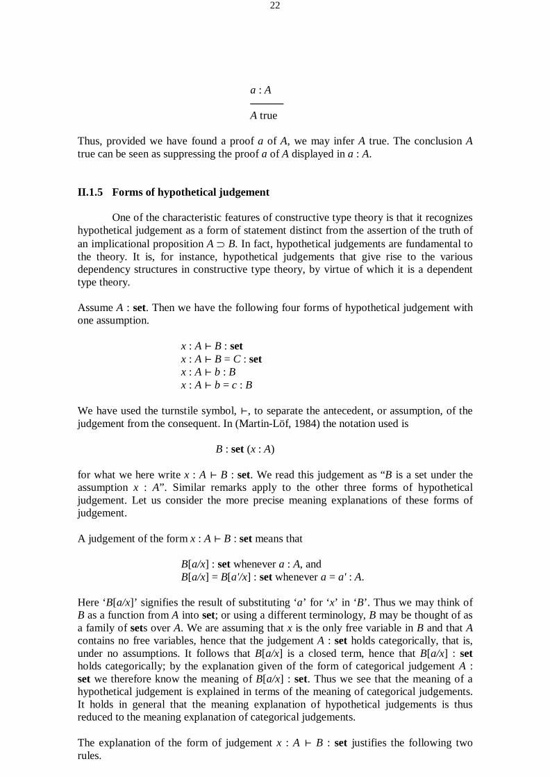
a : A ——— A true

Thus, provided we have found a proof a of A, we may infer A true. The conclusion A true can be seen as suppressing the proof a of A displayed in a : A. II.1.5 Forms of hypothetical judgement

One of the characteristic features of constructive type theory is that it recognizes hypothetical judgement as a form of statement distinct from the assertion of the truth of an implicational proposition A ⊃ B. In fact, hypothetical judgements are fundamental to the theory. It is, for instance, hypothetical judgements that give rise to the various dependency structures in constructive type theory, by virtue of which it is a dependent type theory.

Assume A : set. Then we have the following four forms of hypothetical judgement with one assumption.

x : A ⊢ B : set x : A ⊢ B = C : set x : A ⊢ b : B x : A ⊢ b = c : B

We have used the turnstile symbol, ⊢, to separate the antecedent, or assumption, of the judgement from the consequent. In (Martin-Löf, 1984) the notation used is

B : set (x : A) for what we here write x : A ⊢ B : set. We read this judgement as “B is a set under the assumption x : A”. Similar remarks apply to the other three forms of hypothetical judgement. Let us consider the more precise meaning explanations of these forms of judgement. A judgement of the form x : A ⊢ B : set means that

B[a/x] : set whenever a : A, and B[a/x] = B[a'/x] : set whenever a = a' : A.

Here ‘B[a/x]’ signifies the result of substituting ‘a’ for ‘x’ in ‘B’. Thus we may think of B as a function from A into set; or using a different terminology, B may be thought of as a family of sets over A. We are assuming that x is the only free variable in B and that A contains no free variables, hence that the judgement A : set holds categorically, that is, under no assumptions. It follows that B[a/x] is a closed term, hence that B[a/x] : set holds categorically; by the explanation given of the form of categorical judgement A : set we therefore know the meaning of B[a/x] : set. Thus we see that the meaning of a hypothetical judgement is explained in terms of the meaning of categorical judgements. It holds in general that the meaning explanation of hypothetical judgements is thus reduced to the meaning explanation of categorical judgements. The explanation of the form of judgement x : A ⊢ B : set justifies the following two rules.

23

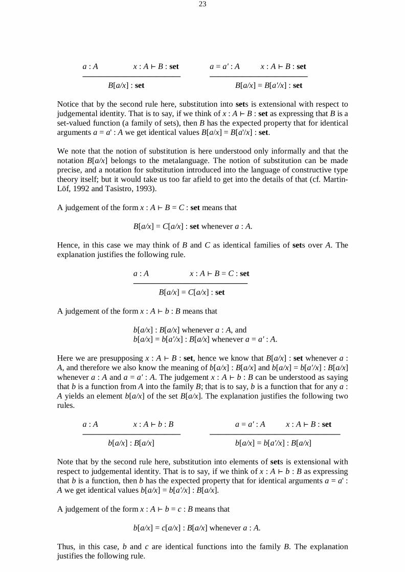
a : A x : A ⊢ B : set a = a' : A x : A ⊢ B : set

———————————— ———————————— B[a/x] : set B[a/x] = B[a'/x] : set

Notice that by the second rule here, substitution into sets is extensional with respect to judgemental identity. That is to say, if we think of x : A ⊢ B : set as expressing that B is a set-valued function (a family of sets), then B has the expected property that for identical arguments a = a' : A we get identical values B[a/x] = B[a'/x] : set. We note that the notion of substitution is here understood only informally and that the notation B[a/x] belongs to the metalanguage. The notion of substitution can be made precise, and a notation for substitution introduced into the language of constructive type theory itself; but it would take us too far afield to get into the details of that (cf. Martin-Löf, 1992 and Tasistro, 1993). A judgement of the form x : A ⊢ B = C : set means that

B[a/x] = C[a/x] : set whenever a : A. Hence, in this case we may think of B and C as identical families of sets over A. The explanation justifies the following rule.

a : A x : A ⊢ B = C : set ——————————————

B[a/x] = C[a/x] : set A judgement of the form x : A ⊢ b : B means that

b[a/x] : B[a/x] whenever a : A, and b[a/x] = b[a'/x] : B[a/x] whenever a = a' : A.

Here we are presupposing x : A ⊢ B : set, hence we know that B[a/x] : set whenever a : A, and therefore we also know the meaning of b[a/x] : B[a/x] and b[a/x] = b[a'/x] : B[a/x] whenever a : A and a = a' : A. The judgement x : A ⊢ b : B can be understood as saying that b is a function from A into the family B; that is to say, b is a function that for any a : A yields an element b[a/x] of the set B[a/x]. The explanation justifies the following two rules.

a : A x : A ⊢ b : B a = a' : A x : A ⊢ B : set ———————————— ————————————————

b[a/x] : B[a/x] b[a/x] = b[a'/x] : B[a/x] Note that by the second rule here, substitution into elements of sets is extensional with respect to judgemental identity. That is to say, if we think of x : A ⊢ b : B as expressing that b is a function, then b has the expected property that for identical arguments a = a' : A we get identical values b[a/x] = b[a'/x] : B[a/x]. A judgement of the form x : A ⊢ b = c : B means that

b[a/x] = c[a/x] : B[a/x] whenever a : A. Thus, in this case, b and c are identical functions into the family B. The explanation justifies the following rule.

24

a : A x : A ⊢ b = c : B —————————————

b[a/x] = c[a/x] : B[a/x]

II.1.6 Assumptions and other speech acts

All the three notions of proposition, categorical judgement and hypothetical judgement can be seen to be presupposed by what is arguably the most natural interpretation of natural deduction derivations (cf. Sundholm, 2006). Consider the following natural deduction proof sketch:

A D1

B D2 ——— A ⊃ B A ————————

B Here D1 is a proof of B from A, and D2 is a closed proof of A. Let us regard this natural deduction proof sketch as a representation of an actual mathematical demonstration and let us consider which speech acts the individual formulae here then represent. The topmost A represents an assumption, namely the assumption that the proposition A is true. The formula A that is the conclusion of D2 is the conclusion of a closed proof; this formula therefore represents the categorical judgement, or assertion, that A is true; the same considerations apply to A ⊃ B and to the final conclusion B. The B that is the conclusion of D1 represents neither an assumption nor a categorical assertion; it rather represents a hypothetical judgement, namely the judgement that B is true on the hypothesis that A is true. Let us also note the formula A occurring as a subformula in A ⊃ B. In the given proof sketch this formula A represents neither an assumption nor a categorical assumption nor a hypothetical judgement. It rather represents a proposition that is a part of a more complex proposition A ⊃ B, which in the given proof is asserted categorically to be true. Thus we see that in order to make the semantics of natural deduction derivations explicit we should employ a notation that is able to distinguish not only propositions from judgements, but also categorical judgements from hypothetical judgements, and perhaps also assumptions from all of these. Assumptions can, however, be subsumed under hypothetical judgements, since we may regard the assumption of some categorical judgement J as the assertion of J on the hypothesis that J. In particular, the assumption of a : A and the assumption that the proposition A is true may be analyzed as

a : A ⊢ a : A and A true ⊢ A true respectively. In constructive type theory one can therefore make the semantics of the above natural deduction proof sketch explicit as follows

A true ⊢ A true D1

A true ⊢ B true D2

25

——————— A ⊃ B true A true ————————————————

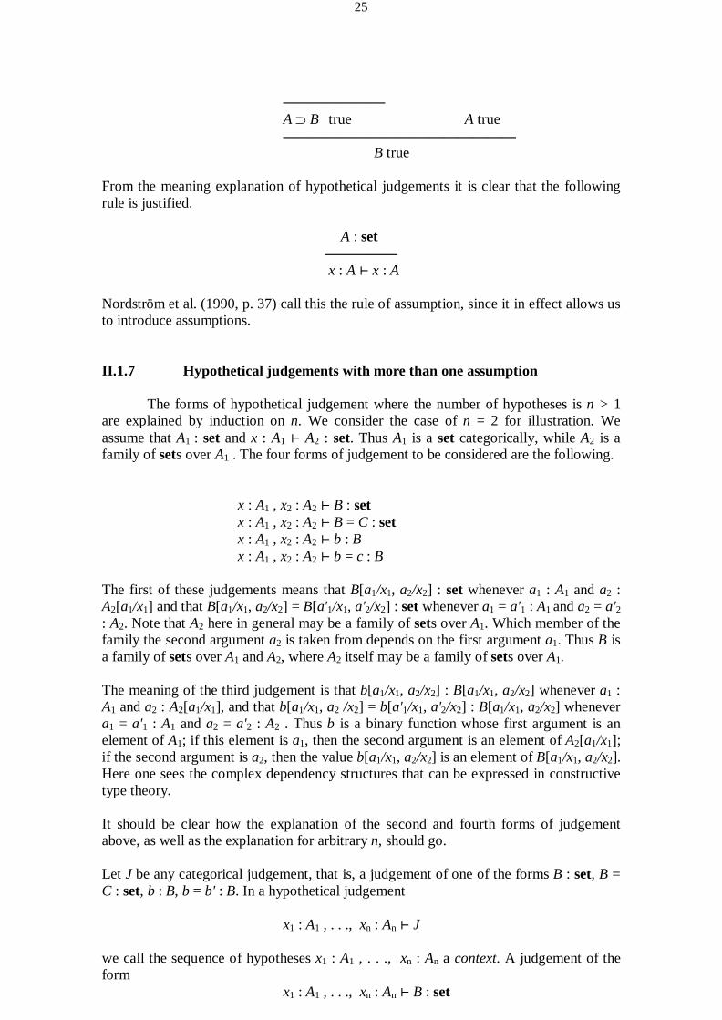
B true From the meaning explanation of hypothetical judgements it is clear that the following rule is justified. A : set

————— x : A ⊢ x : A

Nordström et al. (1990, p. 37) call this the rule of assumption, since it in effect allows us to introduce assumptions. II.1.7 Hypothetical judgements with more than one assumption

The forms of hypothetical judgement where the number of hypotheses is n > 1 are explained by induction on n. We consider the case of n = 2 for illustration. We assume that A1 : set and x : A1 ⊢ A2 : set. Thus A1 is a set categorically, while A2 is a family of sets over A1 . The four forms of judgement to be considered are the following.

x : A1 , x2 : A2 ⊢ B : set x : A1 , x2 : A2 ⊢ B = C : set x : A1 , x2 : A2 ⊢ b : B x : A1 , x2 : A2 ⊢ b = c : B

The first of these judgements means that B[a1/x1, a2/x2] : set whenever a1 : A1 and a2 : A2[a1/x1] and that B[a1/x1, a2/x2] = B[a'1/x1, a'2/x2] : set whenever a1 = a'1 : A1 and a2 = a'2 : A2. Note that A2 here in general may be a family of sets over A1. Which member of the family the second argument a2 is taken from depends on the first argument a1. Thus B is a family of sets over A1 and A2, where A2 itself may be a family of sets over A1. The meaning of the third judgement is that b[a1/x1, a2/x2] : B[a1/x1, a2/x2] whenever a1 : A1 and a2 : A2[a1/x1], and that b[a1/x1, a2 /x2] = b[a'1/x1, a'2/x2] : B[a1/x1, a2/x2] whenever a1 = a'1 : A1 and a2 = a'2 : A2 . Thus b is a binary function whose first argument is an element of A1; if this element is a1, then the second argument is an element of A2[a1/x1]; if the second argument is a2, then the value b[a1/x1, a2/x2] is an element of B[a1/x1, a2/x2]. Here one sees the complex dependency structures that can be expressed in constructive type theory. It should be clear how the explanation of the second and fourth forms of judgement above, as well as the explanation for arbitrary n, should go. Let J be any categorical judgement, that is, a judgement of one of the forms B : set, B = C : set, b : B, b = b' : B. In a hypothetical judgement

x1 : A1 , . . ., xn : An ⊢ J we call the sequence of hypotheses x1 : A1 , . . ., xn : An a context. A judgement of the form

x1 : A1 , . . ., xn : An ⊢ B : set

26

may thus be expressed by saying that B is a set in the context x1 : A1 , . . ., xn : An. Let Γ be a context. From the meaning explanation of hypothetical judgements one sees that rules of the following kind are justified.

Γ ⊢ J Γ ⊢ B : set ————————————

Γ, y : B ⊢ J These rules may be called rules of weakening, in accordance with the terminology used in sequent calculus. With the general hypothetical form of judgement explained we may introduce a notion of category in a wider sense, in effect what is called a category in (Martin-Löf, 1984, pp. 21–23). Let us write the four general forms of judgement in the style of Martin-Löf, namely as follows.

B : set (x1 : A1 , . . ., xn : An) B = C : set (x1 : A1 , . . ., xn : An) b : B (x1 : A1 , . . ., xn : An) b = c : B (x1 : A1 , . . ., xn : An)

In a grammatical analysis of the first of these it is natural to view not only set but everything that is to the right of the colon, namely

set (x : A1 , . . ., xn : An) as the predicate. The relation between the notions of predicate and category thus suggests that we may regard this as a category. Indeed, this may be regarded as the category of families of sets in n variables ranging over the sets or families of sets A1 , . . ., An, among which there may be dependency relations as explained for the case of n = 2 above. Likewise we may regard

B (x : A1 , . . ., xn : An) as a category. It is the category of n-ary functions from A1 , . . ., An into the family B (again keeping dependency relations in mind). Thus we may extend the notion of category to include not only set and A for any set A, but also n-ary families of sets and n-ary functions into a set A. Note that these are indeed categories in the present sense since they are associated with criteria of application and identity, namely through the explanation of the general forms of hypothetical judgement. II.2 Rules

So far we have only the frame of a language, namely an explanation of its basic forms of statement as well as explanations of the basic notions of set, proposition, element of a set, and proof of a proposition. The frame is filled by the introduction of symbols signifying sets, operations for forming sets, and operations for forming elements of sets. These symbols are not explained one by one, but rather in groups. The meaning of the symbols in a given group is determined by rules of four kinds:

• Formation rules

27

• Introduction rules • Elimination rules • Equality, or computation, rules

The inclusion of formation rules in the language itself is a distinctive feature of constructive type theory. The introduction- and elimination rules are like those of Gentzen (1933), though generalized to the syntax of constructive type theory so as also to cover the construction of proof objects. The equality rules correspond to the reduction rules of Prawitz (1965). The best way of getting a grip on these notions is by looking at concrete examples, which we now proceed to do. In the following we shall in most cases write A[b, c] and a[b, c], etc., instead of A[b/x, c/y] and a[b/x, c/y], etc. That is, for ease of readability we shall usually omit to mention the variables for which b, c, etc. are substituted in A, a, etc. Which variables are replaced will usually be clear from the context. Although variables are not mentioned, square brackets will still stand for substitution and not for function application. II.2.1 Cartesian product of a family of sets

Given a set A and a family B of sets over A we can form the product of B over A. That is the content of the Π-formation rule:

A : set x : A ⊢ B : set

(Π-form) ———————————— (Πx : A)B : set

This rule lays down the conditions for when we can judge that (Πx : A)B is a set. There is a second Π-formation rule that lays down the conditions for when we can judge that two sets of the form (Πx : A)B are identical:

A = A' : set x : A ⊢ B = B' : set —————————————————

(Πx : A)B = (Πx : A') B' : set All formation-, introduction-, and elimination rules are paired with identity rules of this kind, but we shall state these rules explicitly only in the present case of Π. The conclusion of Π-formation says that (Πx : A)B is a set. Since we have the right to judge that C is a set only if we can say what the canonical elements of C are as well as what equal canonical elements of C are, we see that the rule of Π-formation requires justification. The required justification is provided by the Π-introduction rules:

x : A ⊢ b : B x : A ⊢ b = b' : B (Π-intro) ——————— ——————————

λx.b : (Πx : A)B λx.b = λx.b' : (Πx : A)B According to this rule a canonical element of (Πx : A)B has the form λx.b, where b[a] : B[a] whenever a : A. Note that such a b is of a category different from the category of λx.b. Namely, b is of category B [x : A] whereas λx.b is of category (Πx : A)B. It was noted above that we may regard such a b as a function from A into the family B. We may think

28

of λx.b as an individual that codes this function. The λ-operator is thus similar to Frege’s course-of-values operator (cf. e.g. Frege, 1893, § 9) which, given a function f(x), yields an individual άf(α). Note, however, that λx.b belongs to a separate set (Πx : A)B and not to the domain A of the function b; whence we cannot make sense of applying the function b to λx.b, hence a contradiction along the lines of Russell’s Paradox cannot be derived. The role of the elements of (Πx : A)B as codes of functions is made clear by the Π-elimination rule:

c : (Πx : A)B a : A c = c': (Πx : A)B a = a': A (Π-elim) ————————— —————————————

ap(c, a) : B[a] ap(c, a) = ap(c', a') : B[a]

The conclusion of this rule asserts that ap(c, a) is an element of the set B[a]. Since we have the right to judge that c is an element of a set C only if we can specify how to compute c to a canonical element of C, we see that the rule of Π-elimination requires justification. The required justification is provided by the rule of Π-equality, which specifies how ap(c, a) is computed in the case where c is of canonical form, namely λx.b.

x : A ⊢ b : B a : A (Π-eq) ————————————

ap(λx.b, a) = b[a]: B[a] We can now justify Π-elimination as follows. By the assumption c : (Πx : A)B we know how to evaluate c to canonical form λx.b, where x : A ⊢ b : B; thus we have c = λx.b : (Πx : A)B. But then also ap(c, a) = ap(λx.b, a) : B[a], so ap(c, a) = b[a] : B[a], whence the value of ap(c, a) is equal to the value of b[a]; by the assumption x : A ⊢ b : B we know how to find this value. From the Π-equality rule we see that ap is an application operator; as such it is similar to the function x ͡ y, satisfying the equation Δ ͡ άf(α) = f(Δ), defined by Frege (1893, § 34). We have now seen that the Π-introduction rules make possible the justification of the Π-formation rule and that the Π-equality rule makes possible the justification of the Π-elimination rule. These relations of justification hold in general and not only in the case of Π. The advantage of the higher-order presentation of constructive type theory is most readily seen when we ask about the categories of Π, λ, and ap. Intuitively we may think of Π as a certain higher-order function that takes a set A and a family of sets B over A and yields a set (Πx : A)B. But we have no means of naming the category of such a function in the language frame introduced here. In the higher-order presentation such a name is easily constructed; indeed we then express the category assignment of Π by means of the judgement Π : (X : set)((X )set)set. Similar remarks apply to λ and ap, and in fact to all of the various symbols that we are now in the process of introducing into the language (apart from the constant sets ℕn and ℕ to be introduced below — these are of category set). II.2.2 The logical interpretation of the cartesian product

29

Recall that prop = set. Hence we may regard a family B of sets over a set A as a family of propositions over A. A family of propositions over A is a function from A into the category of propositions; it is thus a propositional function. Let us consider B as a propositional function over A and (Πx : A)B as a proposition, and let us ask what a canonical proof of this proposition looks like. Such a canonical proof has the form λx.b, where x : A ⊢ b : B, and is in effect a code of the function b. This function b takes an element a of A and yields a proof b[a] of the proposition B[a]. Keeping in mind the Brouwer–Heyting–Kolmogorov interpretation of the logical connectives (cf. e.g. Troelstra and van Dalen, 1988, pp. 9–10), we see thus that (Πx : A)B, when regarded as a proposition, is the proposition (∀x : A)B, which intuitively says that all elements of A have the property B. Note that this proposition is not written ∀xB as in ordinary predicate logic; rather, the domain of quantification, A, is explicitly mentioned. On the understanding of Π as ∀, we can recover the rule of ∀-introduction from the rule of Π-introduction by employing the form of judgement ‘C true’ as follows.

x : A ⊢ B true —————— (∀x : A)B true

That is to say, if B[a] is true whenever a : A, then (∀x : A)B is true. Let us also consider the version of ∀-introduction where the proof objects have not been suppressed:

x : A ⊢ b : B ———————— λx.b : (∀x : A)B

Here we should think of b as an open proof of B, a proof depending on a parameter x : A. For instance, A may be the natural numbers, ℕ, and B may be the propositional function that for any element n of ℕ yields the proposition that n is either even or odd; b is then a proof of the proposition that x is either even or odd, where x is a generic or arbitrary natural number. By binding x we get a proof λx.b of (∀x : A)B where x is no longer free; if x is the only free variable in b, then λx.b is a closed proof of (∀x : A)B. Since the domain of quantification is explicitly mentioned in (∀x : A)B, it also has to be mentioned in the ∀-elimination rule:

(∀x : A)B true a : A ———————————

B[a] true Making the proof-objects explicit yields the following ∀-elimination rule.

c : (∀x : A)B a : A ————————————

ap(c, a) : B[a] The rule says that if c is a proof of (∀x : A)B and a : A, then ap(c, a) is a proof of B[a]. The Π-equality rule can now be seen to correspond to the ∀-reduction of Prawitz (1965, p. 37) at the level of proof objects. We shall illustrate this in the case of ⊃, to which we

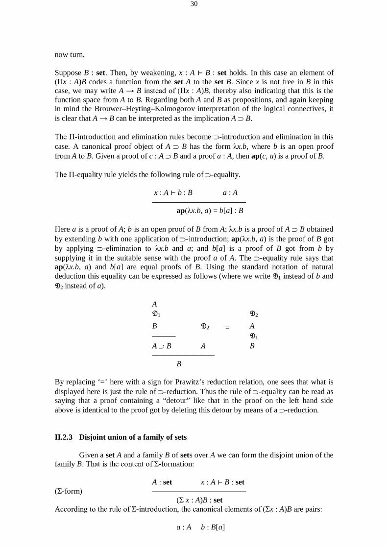
30

now turn. Suppose B : set. Then, by weakening, x : A ⊢ B : set holds. In this case an element of (Πx : A)B codes a function from the set A to the set B. Since x is not free in B in this case, we may write A → B instead of (Πx : A)B, thereby also indicating that this is the function space from A to B. Regarding both A and B as propositions, and again keeping in mind the Brouwer–Heyting–Kolmogorov interpretation of the logical connectives, it is clear that A → B can be interpreted as the implication A ⊃ B. The Π-introduction and elimination rules become ⊃-introduction and elimination in this case. A canonical proof object of A ⊃ B has the form λx.b, where b is an open proof from A to B. Given a proof of c : A ⊃ B and a proof a : A, then ap(c, a) is a proof of B. The Π-equality rule yields the following rule of ⊃-equality.

x : A ⊢ b : B a : A ————————————

ap(λx.b, a) = b[a] : B Here a is a proof of A; b is an open proof of B from A; λx.b is a proof of A ⊃ B obtained by extending b with one application of ⊃-introduction; ap(λx.b, a) is the proof of B got by applying ⊃-elimination to λx.b and a; and b[a] is a proof of B got from b by supplying it in the suitable sense with the proof a of A. The ⊃-equality rule says that ap(λx.b, a) and b[a] are equal proofs of B. Using the standard notation of natural deduction this equality can be expressed as follows (where we write D1 instead of b and D2 instead of a).

A D1 D2

B D2 = A

——— D1 A ⊃ B A B ————————

B By replacing ‘=’ here with a sign for Prawitz’s reduction relation, one sees that what is displayed here is just the rule of ⊃-reduction. Thus the rule of ⊃-equality can be read as saying that a proof containing a “detour” like that in the proof on the left hand side above is identical to the proof got by deleting this detour by means of a ⊃-reduction. II.2.3 Disjoint union of a family of sets

Given a set A and a family B of sets over A we can form the disjoint union of the family B. That is the content of Σ-formation:

A : set x : A ⊢ B : set

(Σ-form) ———————————— (Σ x : A)B : set

According to the rule of Σ-introduction, the canonical elements of (Σx : A)B are pairs:

a : A b : B[a]

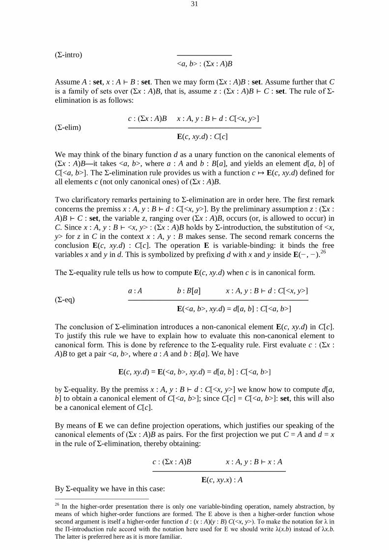
31

(Σ-intro) ——————— <a, b> : (Σx : A)B Assume A : set, x : A ⊢ B : set. Then we may form (Σx : A)B : set. Assume further that C is a family of sets over (Σx : A)B, that is, assume z : (Σx : A)B ⊢ C : set. The rule of Σ-elimination is as follows:

c : (Σx : A)B x : A, y : B ⊢ d : C[<x, y>] (Σ-elim) —————————————————

E(c, xy.d) : C[c] We may think of the binary function d as a unary function on the canonical elements of (Σx : A)B—it takes <a, b>, where a : A and b : B[a], and yields an element d[a, b] of C[<a, b>]. The Σ-elimination rule provides us with a function c ↦ E(c, xy.d) defined for all elements c (not only canonical ones) of (Σx : A)B. Two clarificatory remarks pertaining to Σ-elimination are in order here. The first remark concerns the premiss x : A, y : B ⊢ d : C[<x, y>]. By the preliminary assumption z : (Σx : A)B ⊢ C : set, the variable z, ranging over (Σx : A)B, occurs (or, is allowed to occur) in C. Since x : A, y : B ⊢ <x, y> : (Σx : A)B holds by Σ-introduction, the substitution of <x, y> for z in C in the context x : A, y : B makes sense. The second remark concerns the conclusion E(c, xy.d) : C[c]. The operation E is variable-binding: it binds the free variables x and y in d. This is symbolized by prefixing d with x and y inside E(−, −).26 The Σ-equality rule tells us how to compute E(c, xy.d) when c is in canonical form.

a : A b : B[a] x : A, y : B ⊢ d : C[<x, y>] (Σ-eq) ———————————————————————

E(<a, b>, xy.d) = d[a, b] : C[<a, b>] The conclusion of Σ-elimination introduces a non-canonical element E(c, xy.d) in C[c]. To justify this rule we have to explain how to evaluate this non-canonical element to canonical form. This is done by reference to the Σ-equality rule. First evaluate c : (Σx : A)B to get a pair <a, b>, where a : A and b : B[a]. We have

E(c, xy.d) = E(<a, b>, xy.d) = d[a, b] : C[<a, b>]

by Σ-equality. By the premiss x : A, y : B ⊢ d : C[<x, y>] we know how to compute d[a, b] to obtain a canonical element of C[<a, b>]; since C[c] = C[<a, b>]: set, this will also be a canonical element of C[c]. By means of E we can define projection operations, which justifies our speaking of the canonical elements of (Σx : A)B as pairs. For the first projection we put C = A and d = x in the rule of Σ-elimination, thereby obtaining:

c : (Σx : A)B x : A, y : B ⊢ x : A —————————————————

E(c, xy.x) : A By Σ-equality we have in this case: 26 In the higher-order presentation there is only one variable-binding operation, namely abstraction, by means of which higher-order functions are formed. The E above is then a higher-order function whose second argument is itself a higher-order function d : (x : A)(y : B) C(<x, y>). To make the notation for λ in the Π-introduction rule accord with the notation here used for E we should write λ(x.b) instead of λx.b. The latter is preferred here as it is more familiar.

32

E(<a, b>, xy.x) = x[a/x, b/y] = a : A

We may therefore define the first projection fst as follows.

c : (Σx : A)B ⊢ fst(c) = E(c, xy.x) For the second projection we put C = B[fst(z)] and d = y in the rule of Σ-elimination:

c : (Σx : A)B x : A, y : B ⊢ y : B[fst(<x, y>)] ——————————————————————

E(c, xy.y) : B[fst(c)] The second premiss here is valid since x : A, y : B ⊢ B[fst((<x, y>)] = B[x] = B : set holds. By Σ-equality we have

E(<a, b>, xy.y) = y[a/x, b/y] = b : B[fst(<a, b>)] But fst(<a, b>) = a : A, hence

B[fst(<a, b>)] = B[a] : set We therefore define the second projection by

c : (Σx : A)B ⊢ snd(c) = E(c, xy.y) The following four rules are then justified

c : (Σx : A)B a : A b : B[a] —————— ———————— fst(c) : A fst(<a, b>) = a : A c : (Σx : A)B a : A b : B[a] ——————— ————————— snd(c) : B[fst(c)] snd(<a, b>) = b : B[a]

II.2.4 The logical interpretation of the disjoint union of a family of sets

If we regard B as a propositional function over A, then (Σx : A)B can be regarded as the existentially quantified proposition (∃x : A)B. A canonical proof of (∃x : A)B is a pair <a, b> where a : A and b : B[a]; that is to say, a is a witness and b is a proof that a indeed has the property B. When suppressing proof objects and employing the form of judgement D true, the rule of Σ-elimination becomes ∃-elimination:

(∃x : A)B true x : A, B true ⊢ C true ——————————————————

C true In ordinary natural deduction the assumption x : A in the second premiss is usually not made explicit. If B : set holds categorically, then the rules for Σ yield rules for ordinary cartesian

33

product. On the logical interpretation, the cartesian product becomes conjunction. Indeed the Σ-formation and introduction rules then become:

A : prop B: prop a : A b : B —————————— ———————— A ∧ B : prop <a, b> : A ∧ B

The Σ-elimination rule, with and without proof objects, becomes:

A ∧ B true A true, B true ⊢ C true ———————————————————

C true c : A ∧ B x : A, y : B ⊢ d : C[<a, b>]; —————————————————————

E(c, xy.d) : C[c]

This is a generalization of the ordinary rules of ∧-elimination also found in Schroeder-Heister (1984, p. 1294). The ordinary rules are obtained as a special case by letting C be A or B. We remark that in the higher-order presentation a generalized elimination rule in this sense can also be given for Π (cf. Nordström et al., 1990, pp. 51–52); using this generalized elimination rule instead of the rule of Π-elimination presented above in fact yields a strictly stronger theory, as shown by Garner (2009). II.2.5 Disjoint union of two sets

Given two sets we may form their disjoint union. That is content of the rule of +- formation.

A : set B: set (+-form) —————————————

A + B : set A canonical element of A + B is an element of A or an element of B together with the information that it comes from A or B respectively. Thus there are two rules of +-introduction:

a : A b : B (+-intro) ————— —————

i(a) : A + B j(b) : A + B

Assume A : set, B : set, and z : A + B ⊢ C : set. The rule of +-elimination is:

c : A + B x : A ⊢ d : C[i(x)] y : B ⊢ e : C[j(y)] (+-elim) ———————————————————————

D(c, x.d, y.e) : C[c] The rule can be glossed as follows. Assume that C is a family of sets over A + B and that we are given a function d which takes an a : A to an element d[a] of C[i(a)] and a function e which takes a b : B to an element e[b] of C[j(b)]. Then C[c] is inhabited for any c : C, namely by D(c, x.d, y.e). How to compute D(c, x.d, y.e) is determined by the +-equality rules. Since there are two +-introduction rules, there are also two +-equality rules.

34

a : A x : A ⊢ d : C[i(x)] y : B ⊢ e : C[j(y)] (+-eq) ——————————————————————

D(i(a), x.d, y.e) = d[a] : C[i(a)]

b : B x : A ⊢ d : C[i(x)] y : B ⊢ e : C[j(y)] ———————————————————————

D(j(b), x.d, y.e) = e[b] : C[j(b)] In the logical interpretation + becomes disjunction ∨. II.2.6 Finite sets

We have introduced operations for constructing sets from other sets or families of sets; but so far we have no basic sets to start from. We shall now provide a scheme of rules which, when specified for any particular natural number n, gives us a set with n canonical elements.

In the following n is a generic natural number. There is a set ℕn: (ℕn-form) ℕn : set The set ℕ has n canonical elements, each introduced by its own introduction rule; thus ℕn has n introduction rules: (ℕn -intro) m1 : ℕn , . . . , mn : ℕn The ℕn-elimination rule can be seen as a principle of proof by n cases. We assume that C is a family of sets over ℕn ; that is, we assume z : ℕn ⊢ C : set. m : ℕn c1 : C[m1] . . . cn : C[mn] (ℕn -elim) ————————————————————

casen(m, c1 , . . . , cn ) : C[m] Thus, assume that for each canonical mk : ℕn we have an element ck : C[mk]. The ℕn-elimination rule allows us to infer that for any m : ℕn there is an element, namely casen(m, c1 , . . . , cn ), in C[m]. How to compute casen(m, c1 , . . . , cn ) to canonical form is determined by the ℕn-equality rules. Since there are n ℕn-introduction rules, there are also n ℕn -equality rules, one for each introduction rule. We state the rule for a generic k ≤ n.

c1 : C[m1] . . . cn : C[mn] (ℕn -eq) ————————————————

casen(mk , c1 , . . . , cn) = ck : C[mk ] On the basis of this rule we may explain how to compute casen(m, c1 , . . . , cn) : C[c]. Evaluate m : ℕn , thereby obtaining a canonical element mk : ℕn. Since m = mk : ℕn , we have both casen(m, c1 , . . . , cn) = casen(mk, c1 , . . . , cn) : C[mk] and C[mk] = C[m] : set. Therefore, casen(m, c1 , . . . , cn) = ck : C[m], by ℕn -equality. Hence the value of casen(m, c1 , . . . , cn) equals the value of ck, which we know how to compute by the premiss ck : C[mk].

35

We may give ℕ2 the name bool; the canonical elements of ℕ2 the names t and f; and the expression case2(m, c1, c2) may be written if m then c1 else c2. Let C be a family of sets over bool; that is, assume z : bool ⊢ C : set. We have the following two rules of bool-elimination, which we here state as one rule with two conclusions:

c : C[t] d : C[f] ——————————— if t then c else d = c : C[t] if f then c else d = d : C[f]

The set ℕ0 has 0, that is no, introduction rules; but it does have an elimination rule:

m : ℕ0 ——————— case0(m) : C[m]

Thus, in particular, if we are given C : set and m : ℕ0, then we may infer that C is inhabited, namely by case0(m). Since there is no ℕ0-introduction rule, neither is there a ℕ0-equality rule. The justification of ℕ0-elimination is therefore different in character from the justification of the other elimination rules. A rule of inference is justified if we can make the conclusion of the rule evident on the assumption that its premisses are known (cf. e.g. Sundholm, 2012). Since ℕ0 has no introduction rule and therefore no canonical elements, the premiss m : ℕ0 of ℕ0-elimination cannot be known. The rule of ℕ0-elimination is therefore vacuously justified, for the assumption that its premiss is known cannot be fulfilled. In the logical interpretation ℕ0 becomes absurdity ⊥. In constructive type theory absurdity is thus the proposition that by definition has no introduction rule. The rule of ⊥-elimination is the principle of ex falso quodlibet:

⊥ true ——— C true

We define the negation of a proposition A to be the proposition A ⊃ ⊥:27

A : prop ⊢ ¬A = A ⊃ ⊥ The following rules are then derivable.

A : prop x : A ⊢ b : ⊥ b : ¬A a : A ———— ————— ——————— ¬A : prop λx.b : ¬A ap(b, a) : C

II.2.7 The natural numbers We shall not need the natural numbers in later chapters, but it may nevertheless be useful 27 In the higher-order presentation ¬ may be defined in the empty context, namely as follows.

¬ = [A]A ⊃ ⊥: (prop)prop Thus, ¬ is a function which takes a prop A as argument and yields a prop ¬A as value. Similar considerations apply to the definitions of fst and snd above as well as to the definitions given below pertaining to ℕ.

36

to see that the primitive notions of arithmetic can be introduced by Gentzen–Prawitz style rules. (ℕ-form) ℕ : set The canonical elements of ℕ are 0 and s(n), where n is any ℕ, not necessarily of canonical form: (ℕ-intro) 0 : ℕ n : ℕ ———— s(n) : ℕ The rule of ℕ-elimination is simultaneously a principle of definition by recursion and proof by mathematical induction. Assume that C is a family of sets over ℕ; that is, assume z : ℕ ⊢ C : set.

n : ℕ d : C[0] x : ℕ, y : C[x] ⊢ e : C[s(x)] (ℕ-elim) ———————————————————————

R(n, d, xy.e) : C[n] We are given an element d : C[0] together with a function e that takes k : ℕ and c : C[k] and yields e[k, c] : C[s(k)]. The rule tells us that for an arbitrary n : ℕ the set C[n] is then inhabited, namely by R(n, d, xy.e). To see that ℕ-elimination encapsulates the ordinary principle of proof by induction over the natural numbers, assume that C is a propositional function over ℕ. Then d is a proof of the base case C[0] and e is a proof of the induction step; that is, e is an open proof from C[k] to C[s(k)]. The conclusion of ℕ-elimination says that C[n] is inhabited, that is, true, for an arbitrary n : ℕ. The rule of ℕ-equality tells us how to compute R(n, d, xy.e) when n is of canonical form. Since there are two ℕ-introduction rules, there are also two ℕ-equality rules, which we here state more simply without the premisses R(0, d, xy.e) = d : C[0] (ℕ-eq) R(s(n), d, xy.e) = e[n, R(n, d, xy.e)] : C[s(n)] Thus, to compute R(m, d, xy.e) first evaluate m to get either 0 or s(n). In the first case output d, in the second case continue by computing e[n, R(n, d, xy.e)]. As the reader may check, we can define addition and multiplication as follows.

a : ℕ, b : ℕ ⊢ a + b = R(b, a, xy.s(x)) : ℕ a : ℕ, b : ℕ ⊢ a × b = R(b, 0, xy.(y + a)) : ℕ

II.2.8 Propositional identity

In the language developed so far we can express identities by means of judgements a = b : C . Judgements can, however, not be operated on by the propositional operators, that is, for instance by conjunction or universal quantification. Since we want to be able to operate on identity statements with the propositional operations, it is clear that we need identity propositions. Thus, for each set A we wish to introduce a binary

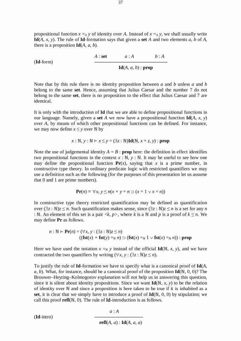
37

propositional function x =A y of identity over A. Instead of x =A y, we shall usually write Id(A, x, y). The rule of Id-formation says that given a set A and two elements a, b of A, there is a proposition Id(A, a, b).

A : set a : A b : A (Id-form) ———————————————

Id(A, a, b) : prop Note that by this rule there is no identity proposition between a and b unless a and b belong to the same set. Hence, assuming that Julius Caesar and the number 7 do not belong to the same set, there is no proposition to the effect that Julius Caesar and 7 are identical. It is only with the introduction of Id that we are able to define propositional functions in our language. Namely, given a set A we now have a propositional function Id(A, x, y) over A, by means of which other propositional functions can be defined. For instance, we may now define x ≤ y over ℕ by

x : ℕ, y : ℕ ⊢ x ≤ y = (∃z : ℕ)Id(ℕ, x + z, y) : prop Note the use of judgemental identity A = B : prop here: the definition in effect identifies two propositional functions in the context x : ℕ, y : ℕ. It may be useful to see how one may define the propositional function Pr(x), saying that x is a prime number, in constructive type theory. In ordinary predicate logic with restricted quantifiers we may use a definition such as the following (for the purposes of this presentation let us assume that 0 and 1 are prime numbers).

Pr(n) ≡ ∀x, y ≤ n(x × y = n ⊃ (x = 1 ∨ x = n)) In constructive type theory restricted quantification may be defined as quantification over (∃z : ℕ)z ≤ n. Such quantification makes sense, since (∃z : ℕ)z ≤ n is a set for any n : ℕ. An element of this set is a pair <k, p>, where k is a ℕ and p is a proof of k ≤ n. We may define Pr as follows.

n : ℕ ⊢ Pr(n) = (∀x, y : (∃z : ℕ)z ≤ n) ((fst(x) × fst(y) =ℕ n) ⊃ (fst(x) =ℕ 1 ∨ fst(x) =ℕ n)) : prop

Here we have used the notation x =ℕ y instead of the official Id(ℕ, x, y), and we have contracted the two quantifiers by writing (∀x, y : (∃z : ℕ)z ≤ n). To justify the rule of Id-formation we have to specify what is a canonical proof of Id(A, a, b). What, for instance, should be a canonical proof of the proposition Id(ℕ, 0, 0)? The Brouwer–Heyting–Kolmogorov explanation will not help us in answering this question, since it is silent about identity propositions. Since we want Id(ℕ, x, y) to be the relation of identity over ℕ and since a proposition is here taken to be true if it is inhabited as a set, it is clear that we simply have to introduce a proof of Id(ℕ, 0, 0) by stipulation; we call this proof refl(ℕ, 0). The rule of Id-introduction is as follows.

a : A (Id-intro) ——————————

refl(A, a) : Id(A, a, a)

38

Thus, provided a : A, we stipulate that there is a proof refl(A, a) : Id(A, a, a). We here emphasize the aspect of stipulation, but in fact, all introduction rules are purely stipulatory in nature. An introduction rule stipulates that the canonical elements of the set under consideration look such and such. The Id-introduction rule is therefore no different from other introduction rules in this regard. The Id-introduction rule is different from other introduction rules in that it does not immediately yield an answer to the question of what is a canonical element of Id(A, a, b), that is, of a set of the form introduced by Id-formation. It yields an answer only to the question of what is a canonical element of Id(A, a, a). Since no introduction rule has Id(A, a, b) as the predicate C of its conclusion c : C , it is clear that the only way in which we can come to judge that c is a canonical element of Id(A, a, b) is on the basis of an identity judgement of the form C = Id(A, a, b) : prop, where c : C is the conclusion of an application of an introduction rule. It is, moreover, clear that any such C must have the form Id(A', a', a'), where A = A' : set, a = a': A and b = a' : A. A canonical element of Id(A, a, b) is therefore of the form refl(A', a') where A = A' : set, a = a' : A and b = a' : A. Martin-Löf (1971), in a paper concerned with natural deduction rather than type theory, provided a general scheme of introduction- and elimination rules as well as reduction procedures for so-called inductively defined predicates. The rules provided above for ℕn and ℕ follow this scheme, although generalizing the rules to the syntax of constructive type theory. Also the identity predicate of ordinary predicate logic is covered by this rule scheme (Martin-Löf, 1971, p. 190). The ordinary binary identity predicate, which Martin-Löf designates by E , is the predicate that has the introduction rule

Exx with no premisses. It should be clear how the rule of Id-introduction above generalizes this rule to the syntax of constructive type theory. Martin-Löf’s scheme yields the following elimination rule for E:

Etu C[z/x, z/y] —————————

C[t/x, u/y] Here C is any formula of the language, and C[z/x, z/y] is the result of substituting the variable z for both x and y in C. If we assume that x and y are all and only the free variables in C, then we may think of C as defining a binary relation over the underlying domain. That we can prove C[z/x, z/y] means that the relation defined by C is reflexive. The E-elimination rule allows us to infer that the relation defined by C is true of t and u provided we have a derivation of Etu. Thus the rule says in effect that E is the smallest reflexive relation over the underlying domain. The rule of Id-elimination generalizes the E-elimination rule to the syntax of constructive type theory; it generalizes the E-elimination rule also in allowing the relation C occurring in the minor premiss to include as argument a proof object of the identity proposition being eliminated. Assume A : set, a : A, b : A, and x : A, y : A, u : Id(A, x, y) ⊢ C : set.

p : Id(A, a, b) z : A ⊢ d : C[z, z, refl(A, z)] (Id-elim) ——————————————————————

J(p, z.d) : C[a, b, p]

39

Thus, if we have a proof p of the proposition Id(A, a, b) and a function d taking any a' of A to a proof that the ternary relation C holds of the triple a', a', refl(A, a'); then Id-elimination allows us to infer that there is a proof J(p, z.d) of C[a, b, p]. The rule of Id-equality tells us how to compute J(p, z.d) when p is of canonical form, refl(A, a). (Id-eq) J(refl(A, a), z.d) = d[a] : C[a, a, refl(A, a)] The rule of Id-elimination can now be justified as follows. To evaluate J(p, z.d) first evaluate p to get a canonical element of Id(A, a, b). As noted above, such a canonical element has the form refl(A', a'), where A = A' : set, a = a' : A and b = a' : A. Hence,

J(p, z.d) = J(refl(A', a'), z.d) = d[a'] : C[a', a', refl(A', a')]. By the assumption z : A ⊢ d : C[z, z, refl(z)] we know how to evaluate d[a'] to canonical form. It remains then only to see that C[a', a', refl(A', a')] = C[a, b, p] : set, but this follows from the judgemental identities

A = A' : set; a = a' : A; b = a' : A; p = refl(A', a') : Id(A, a, b) together with the extensionality of substitution into sets with respect to judgemental identity. In many applications of Id-elimination the family C in its minor premiss does not depend on the set Id(A, a, b) of its major premiss. Thus, C will then be a set already in the context x : A, y : A; that is, C will then be a binary relation over A. What is required then for an application of Id-elimination is that we have a function d witnessing that C is a reflexive relation over A; more precisely, that d[a] is a proof of C[a, a] for any a : A. We shall now demonstrate how Id-elimination is used in practice by showing that the relation Id(A, x, y) is symmetric and transitive, and by showing that if F[a] and Id(A, a, b) are true, then so is F[b], that is, by showing the indiscernibility of elements related by Id(A, x, y). The main task in each case is to find a suitable C and a suitable function d taking a : A and yielding a proof of C[a, a]. For symmetry let C be Id(A, y, x). It is clear that z : A ⊢ refl(A, z) : Id(A, z, z), so we let d be refl(A, z). If we insert these data into Id-elimination we get:

p : Id(A, a, b) z : A ⊢ refl(A, z) : Id(A, z, z) ———————————————————

J(p, z.refl(A, z)) : Id(A, b, a) Hence, from a proof p : Id(A, a, b) we get a proof J(p, z.refl(A, z)) : Id(A, b, a). For transitivity we let C be Id(A, y, c) ⊃ Id(A, x, c) for an arbitrary c : A. We have λu.u : Id(A, z, c) ⊃ Id(A, z, c), so we let d be λu.u. Inserting these data into Id-elimination yields:

p : Id(A, a, b) z : A ⊢ λu.u : Id(A, z, c) ⊃ Id(A, z, c) ——————————————————————

J(p, λu.u) : Id(A, b, c) ⊃ Id(A, a, c)

40

Hence, from a proof p : Id(A, a, b) and a proof q : Id(A, b, c), we get a proof ap(J(p, λu.u), q) : Id(A, a, c). Note that λu.u does not depend on z : A, hence no variable gets bound by this application of Id-elimination. For the inidiscernibility of elements a, b for which Id(A, a, b) is true, let F be a propositional function over A, that is x : A ⊢ F : prop. Let C be F[x] ⊃ F[y]. Again we have λu.u : F[z] ⊃ F[z], hence Id-elimination yields:

p : Id(A, a, b) z : A ⊢ λu.u : F[z] ⊃ F[z] ——————————————————

J(p, λu.u) : F[a] ⊃ F[b]

Hence, from a proof p : Id(A, a, b) and a proof q : F[a], we get a proof ap(J(p, λu.u), q) : F[b]. The second Id-formation rule, the rule that governs when two sets of the form Id(A, a, b) are identical, is as follows.

A = A' : set a = a' : A b = b' : A ———————————————————

Id(A, a, b) = Id(A', a', b') : set Employing this rule together with the general rules governing judgemental identity, one sees that the following rule is derivable:

a = b : A ————————— refl(A, a) : Id(A, a, b)

The rule of identity elimination employed in (Martin-Löf, 1984) lays down that one can also go the other way:

p : Id(A, a, b) ——————

a = b : A In the literature this rule is sometimes called extensional identity elimination, whereas the rule of Id-elimination is called intensional. Subsequent metamathematical work has shown that this extensional rule has several undesirable consequences, perhaps the strongest of which is that in the presence of this rule judgements of the form a = b : A become undecidable in general (Hofmann, 1995, Theorem 3.2.1). From the normalization theorem of Martin-Löf (1975b) for the system employing the intensional Id-elimination rule it follows that judgements of the form a = b : A are decidable in this system. For this and other reasons,28 most presentations of constructive type theory therefore prefer the intensional system. It follows from Martin-Löf’s normalization theorem that if p : Id(A, a, b) is demonstrable in the empty context, then so is a = b : A; hence if one can construct a

28 In Homotopy Type Theory the main reason to prefer the intensional Id-elimination rule is that it does not entail

(∀p,q : Id(A, a, b))Id(Id(A, a, b), p, q) true for arbitrary A and a, b : A, a result that was established by Hofmann and Streicher (1998).

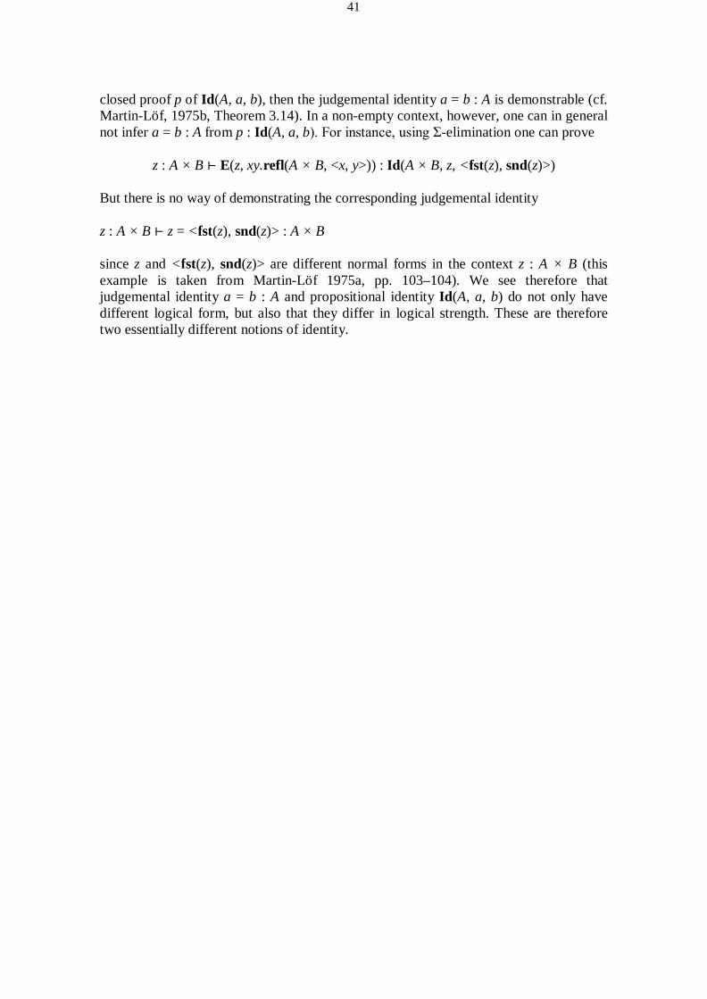
41

closed proof p of Id(A, a, b), then the judgemental identity a = b : A is demonstrable (cf. Martin-Löf, 1975b, Theorem 3.14). In a non-empty context, however, one can in general not infer a = b : A from p : Id(A, a, b). For instance, using Σ-elimination one can prove

z : A × B ⊢ E(z, xy.refl(A × B, <x, y>)) : Id(A × B, z, <fst(z), snd(z)>) But there is no way of demonstrating the corresponding judgemental identity z : A × B ⊢ z = <fst(z), snd(z)> : A × B since z and <fst(z), snd(z)> are different normal forms in the context z : A × B (this example is taken from Martin-Löf 1975a, pp. 103–104). We see therefore that judgemental identity a = b : A and propositional identity Id(A, a, b) do not only have different logical form, but also that they differ in logical strength. These are therefore two essentially different notions of identity.

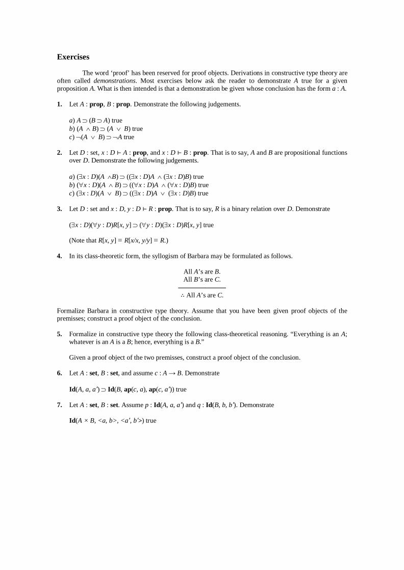
Exercises

The word ‘proof’ has been reserved for proof objects. Derivations in constructive type theory are often called demonstrations. Most exercises below ask the reader to demonstrate A true for a given proposition A. What is then intended is that a demonstration be given whose conclusion has the form a : A. 1. Let A : prop, B : prop. Demonstrate the following judgements.

a) A ⊃ (B ⊃ A) true b) (A ∧ B) ⊃ (A ∨ B) true c) ¬(A ∨ B) ⊃ ¬A true

2. Let D : set, x : D ⊢ A : prop, and x : D ⊢ B : prop. That is to say, A and B are propositional functions

over D. Demonstrate the following judgements. a) (∃x : D)(A ∧B) ⊃ ((∃x : D)A ∧ (∃x : D)B) true b) (∀x : D)(A ∧ B) ⊃ ((∀x : D)A ∧ (∀x : D)B) true c) (∃x : D)(A ∨ B) ⊃ ((∃x : D)A ∨ (∃x : D)B) true

3. Let D : set and x : D, y : D ⊢ R : prop. That is to say, R is a binary relation over D. Demonstrate

(∃x : D)(∀y : D)R[x, y] ⊃ (∀y : D)(∃x : D)R[x, y] true (Note that R[x, y] ≡ R[x/x, y/y] ≡ R.)

4. In its class-theoretic form, the syllogism of Barbara may be formulated as follows.

All A’s are B. All B’s are C.

——————— ∴ All A’s are C.

Formalize Barbara in constructive type theory. Assume that you have been given proof objects of the premisses; construct a proof object of the conclusion. 5. Formalize in constructive type theory the following class-theoretical reasoning. “Everything is an A;

whatever is an A is a B; hence, everything is a B.”

Given a proof object of the two premisses, construct a proof object of the conclusion.

6. Let A : set, B : set, and assume c : A → B. Demonstrate

Id(A, a, a') ⊃ Id(B, ap(c, a), ap(c, a')) true

7. Let A : set, B : set. Assume p : Id(A, a, a') and q : Id(B, b, b'). Demonstrate

Id(A × B, <a, b>, <a', b'>) true

43

Solutions 1. In the solutions to these exercises we will include all the details. Each demonstration begins from the

judgements A : prop and B : prop. These judgements could also be included in the demonstration as hypotheses, namely by placing them to the left of ⊢. Here we rather choose to regard these judgements as given. We may think of an interlocutor who has taken responsibility for these judgements, A : prop and B : prop, and view it is our task to make evident each of A ⊃ (B ⊃ A) true. 29

a)

A : prop B : prop ———— —————— x : A ⊢ x : A x : A ⊢ B : prop ————————————————

x : A, y : B ⊢ x : A ——————— x : A ⊢ λy.x : B ⊃ A ——————— λx.λy.x : A ⊃ (B ⊃ A)

b)

A : prop B : prop ———————————

A ∧ B : prop ——————————— x : A ∧ B ⊢ x : A ∧ B ——————————— x : A ∧ B ⊢ fst(x) : A ——————————— x : A ∧ B ⊢ i(fst(x)) : A ∨ B ——————————— λx.i(fst(x)) : (A ∧ B) ⊃ (A ∨ B)

There is a similar demonstration having as conclusion

λx.j(snd(x)) : (A ∧ B) ⊃ (A ∨ B).

c)

A : prop B : prop ——————————

A ∨ B : prop A : prop —————————— ————

¬(A ∨ B) : prop x : A ⊢ x : A —————————— ——————— y : ¬(A ∨ B) ⊢ y : ¬(A ∨ B) x : A ⊢ i(x) : A ∨ B ———————————————————————

y : ¬(A ∨ B), x : A ⊢ ap(y, i(x)) : ⊥ ———————————————

y : ¬(A ∨ B) ⊢ λx.ap(y, i(x)) : ¬A ———————————————

λy.λx.ap(y, i(x)) : ¬(A ∨ B) ⊃ ¬A

29 This dialogical view on demonstration has been developed in some recent lectures of Per Martin-Löf. This proposal, as communicated by Prof. Sundholm to the group of dialogicians at Lille, is one of the main motivations for the research documented in the following chapters of this book.

44

2. Here we shall use the natural deduction style of presenting demonstrations. That means that we shall not exhibit the hypotheses, but take these to be implicitly understood. The reader may want to supply the missing hypotheses. a)

y : (∃x : D)(A ∧ B) y : (∃x : D)(A ∧ B) ——————— ———————

y : (∃x : D)(A ∧ B) q(y) : (A ∧ B)[p(y)] y : (∃x : D)(A ∧ B) q(y) : (A ∧ B)[p(y)] ——————— ———————— ————————————————————

p(y) : D p(q(y)) : A[p(y)] p(y) : D q(q(y)) : B[p(y)] ——————————————— ———————————————————— <p(y), p(q(y))> : (∃x : D)A <p(y), q(q(y))> : (∃x : D)B ———————————————————————————————

<<p(y), p(q(y))>, <p(y), q(q(y))>> : (∃x : D)A ∧ (∃x : D)B

b)

z : (∀x : D)(A ∧ B) x : D z : (∀x : D)(A ∧ B) x : D ————————————— ————————V—————

ap(z, x) : A ∧ B ap(z, x) : A ∧ B ——————— ———————— fst(ap(z, x)) : A snd(ap(z, x)) : B

——————————— ——————————— λx.fst(ap(z, x)) : (∀x : D)A λx.snd(ap(z, x)) : (∀x : D)B ——————————————————————————————

<λx.fst(ap(z, x)), λx.snd(ap(z, x))> : (∀x : D)A ∧ (∀x : D)B —————————————————————————————————— λz.<λx.fst(ap(z, x)), λx.snd(ap(z, x))> : (∀x : D)(A ∧ B) ⊃ ((∀x : D)A ∧ (∀x : D)B)

c) In the solution to this exercise we use both Σ-elimination and +-elimination. To save space we define Dis = (∃x : D)A ∨ (∃x : D)B : prop.

x : D v : A x : D w : B ———————— ——————— <x, v> : (∃x : D)A <x, w> : (∃x : D)B ——————— ————————

y : A ∨ B i(<x, v>) : Dis j(<x, w>) : Dis ——————————————————————————

z : (∃x : D)(A ∨ B) D(y, v.i(<x, v>), w.j(<x, w>)) : Dis ——————————————————————————————————

E(z, xy.D(y, v.i(<x, v>), w.j(<x, w>))) : Dis —————————————————————————

λz.E(z, xy.D(y, v.i(<x, v>), w.j(<x, w>))) : (∃x : D)(A ∨ B) ⊃ Dis • Note that, since A and B are propositional functions over D, the judgement v : A is made in the context x : D, v : A; the judgement w : B is made in the context x : D, w : B; and the judgement y : A ∨ B is made in the context x : D, y : A ∨ B. The variables w and v get bound by the application of D, whereas x and y get bound by the application of E. 3. Again we use the natural deduction style of presenting demonstrations.

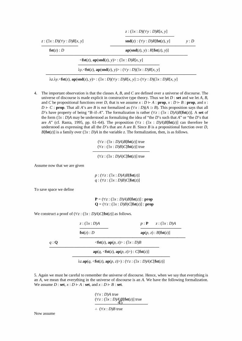
45

z : (∃x : D)(∀y : D)R[x, y] ————————————

z : (∃x : D)(∀y : D)R[x, y] snd(z) : (∀y : D)R[fst(z), y] y : D ————————— —————————————————————

fst(z) : D ap(snd(z), y) : R[fst(z), y)] ——————————————————————————————————

<fst(z), ap(snd(z), y)> : (∃x : D)R[x, y] ———————————————————— λy.<fst(z), ap(snd(z), y)> : (∀y : D)(∃x : D)R[x, y]

————————————————————————————————————— λz.λy.<fst(z), ap(snd(z), y)> : (∃x : D)(∀y : D)R[x, y] ⊃ (∀y : D)(∃x : D)R[x, y]

4. The important observation is that the classes A, B, and C are defined over a universe of discourse. The

universe of discourse is made explicit in constructive type theory. Thus we let D : set and we let A, B, and C be propositional functions over D, that is we assume x : D ⊢ A : prop, x : D ⊢ B : prop, and x : D ⊢ C : prop. That all A’s are B is not formalized as (∀x : D)(A ⊃ B). This proposition says that all D’s have property of being “B–if–A”. The formalization is rather (∀z : (∃x : D)A)B[fst(z)]. A set of the form (∃x : D)A may be understood as formalizing the idea of “the D’s such that A” or “the D’s that are A” (cf. Ranta, 1995, pp. 61–64). The proposition (∀z : (∃x : D)A)B[fst(z)] can therefore be understood as expressing that all the D’s that are A are B. Since B is a propositional function over D, B[fst(z)] is a family over (∃x : D)A in the variable z. The formalization, then, is as follows.

(∀z : (∃x : D)A)B[fst(z)] true (∀z : (∃x : D)B)C[fst(z)] true

—————————————— (∀z : (∃x : D)A)C[fst(z)] true

Assume now that we are given

p : (∀z : (∃x : D)A)B[fst(z)] q : (∀z : (∃x : D)B)C[fst(z)]

To save space we define

P = (∀z : (∃x : D)A)B[fst(z)] : prop Q = (∀z : (∃x : D)B)C[fst(z)] : prop

We construct a proof of (∀z : (∃x : D)A)C[fst(z)] as follows.

z : (∃x : D)A p : P z : (∃x : D)A ——————— —————————— fst(z) : D ap(p, z) : B[fst(z)] ——————————————————————————

q : Q <fst(z), ap(p, z)> : (∃x : D)B ———————————————————————————

ap(q, <fst(z), ap(p, z)>) : C[fst(z)] ————————————————————————

λz.ap(q, <fst(z), ap(p, z)>) : (∀z : (∃x : D)A)C[fst(z)] 5. Again we must be careful to remember the universe of discourse. Hence, when we say that everything is an A, we mean that everything in the universe of discourse is an A. We have the following formalization. We assume D : set, x : D ⊢ A : set, and x : D ⊢ B : set.

(∀x : D)A true (∀z : (∃x : D)A)B[fst(z)] true ————————————— ∴ (∀x : D)B true

Now assume

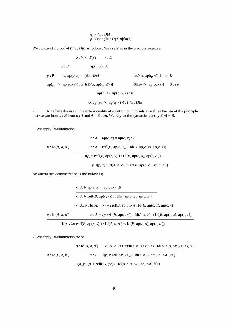
46

q : (∀x : D)A p : (∀z : (∃x : D)A)B[fst(z)]

We construct a proof of (∀x : D)B as follows. We use P as in the previous exercise.

q : (∀x : D)A x : D —————————

x : D ap(q, x) : A —————————————

p : P <x, ap(q, x)> : (∃x : D)A fst(<x, ap(q, x)>) = x : D —————————————————— ————————————— ap(p, <x, ap(q, x)>) : B[fst(<x, ap(q, x)>)] B[fst(<x, ap(q, x)>)] = B : set ————————————————————————————————————

ap(p, <x, ap(q, x)>) : B —————————————

λx.ap( p, <x, ap(q, x)>) : (∀x : D)B • Note here the use of the extensionality of substitution into sets as well as the use of the principle that we can infer a : B from a : A and A = B : set. We rely on the syntactic identity B[x] ≡ B. 6. We apply Id-elimination.

x : A ⊢ ap(c, x) = ap(c, x) : B —————————————————————

p : Id(A, a, a') x : A ⊢ refl(B, ap(c, x)) : Id(B, ap(c, x), ap(c, x)) ———————————————————————————————

J(p, x.refl(B, ap(c, x))) : Id(B, ap(c, a), ap(c, a')) —————————————————————————

λp.J(p, x) : Id(A, a, a') ⊃ Id(B, ap(c, a), ap(c, a'))

An alternative demonstration is the following.

x : A ⊢ ap(c, x) = ap(c, x) : B ————————————————————— x : A ⊢ refl(B, ap(c, x)) : Id(B, ap(c, x), ap(c, x)) —————————————————————————— x : A, p : Id(A, x, x) ⊢ refl(B, ap(c, x)) : Id(B, ap(c, x), ap(c, x))

——————————————————————————————— q : Id(A, a, a') x : A ⊢ λp.refl(B, ap(c, x)) : Id(A, x, x) ⊃ Id(B, ap(c, x), ap(c, x)) ——————————————————————————————————————

J(q, x.λp.refl(B, ap(c, x))) : Id(A, a, a') ⊃ Id(B, ap(c, a), ap(c, a')) 7. We apply Id-elimination twice.

p : Id(A, a, a') x : A, y : B ⊢ refl(A × B,<x, y>) : Id(A × B, <x, y>, <x, y>) ———————————————————————————————

q : Id(B, b, b') y : B ⊢ J(p, x.refl(<x, y>)) : Id(A × B, <a, y>, <a', y>) ———————————————————————————————————

J(q, y.J(p, x.refl(<x, y>)) : Id(A × B, <a, b>, <a', b'>)

47

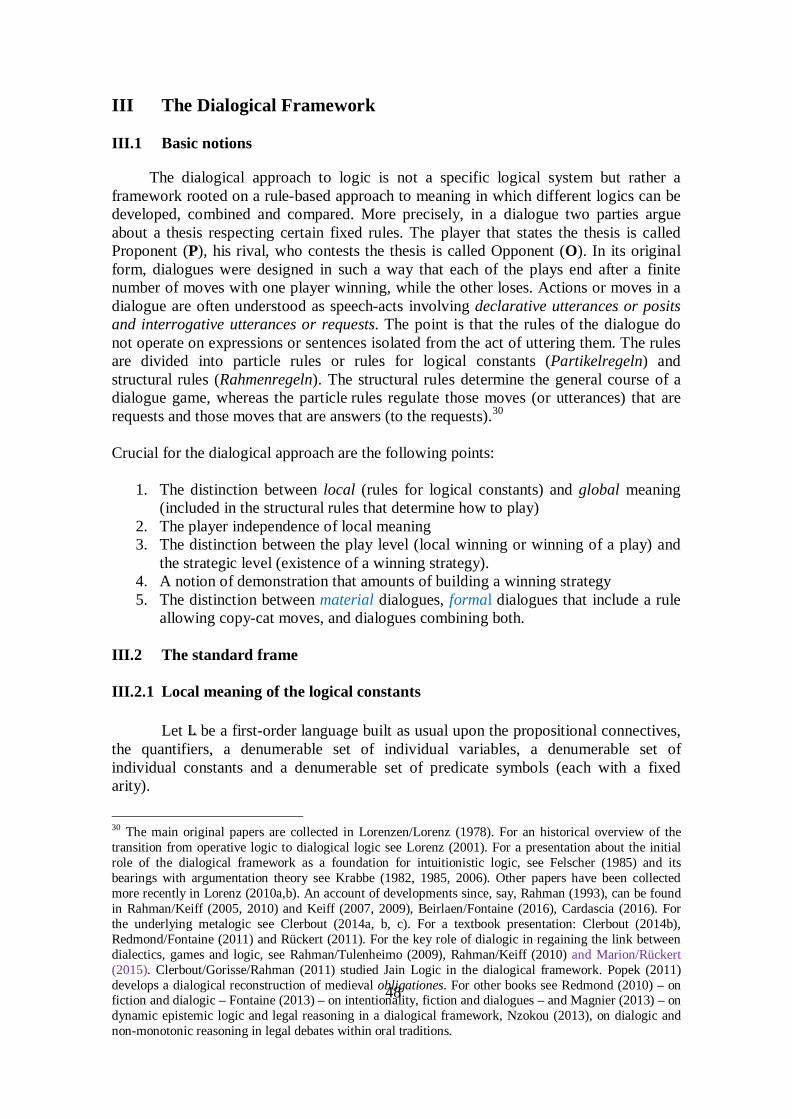
48

III The Dialogical Framework III.1 Basic notions

The dialogical approach to logic is not a specific logical system but rather a framework rooted on a rule-based approach to meaning in which different logics can be developed, combined and compared. More precisely, in a dialogue two parties argue about a thesis respecting certain fixed rules. The player that states the thesis is called Proponent (P), his rival, who contests the thesis is called Opponent (O). In its original form, dialogues were designed in such a way that each of the plays end after a finite number of moves with one player winning, while the other loses. Actions or moves in a dialogue are often understood as speech-acts involving declarative utterances or posits and interrogative utterances or requests. The point is that the rules of the dialogue do not operate on expressions or sentences isolated from the act of uttering them. The rules are divided into particle rules or rules for logical constants (Partikelregeln) and structural rules (Rahmenregeln). The structural rules determine the general course of a dialogue game, whereas the particle rules regulate those moves (or utterances) that are requests and those moves that are answers (to the requests).30 Crucial for the dialogical approach are the following points:

1. The distinction between local (rules for logical constants) and global meaning

(included in the structural rules that determine how to play) 2. The player independence of local meaning 3. The distinction between the play level (local winning or winning of a play) and

the strategic level (existence of a winning strategy). 4. A notion of demonstration that amounts of building a winning strategy 5. The distinction between material dialogues, formal dialogues that include a rule

allowing copy-cat moves, and dialogues combining both. III.2 The standard frame

III.2.1 Local meaning of the logical constants

Let L be a first-order language built as usual upon the propositional connectives,

the quantifiers, a denumerable set of individual variables, a denumerable set of individual constants and a denumerable set of predicate symbols (each with a fixed arity).

30 The main original papers are collected in Lorenzen/Lorenz (1978). For an historical overview of the transition from operative logic to dialogical logic see Lorenz (2001). For a presentation about the initial role of the dialogical framework as a foundation for intuitionistic logic, see Felscher (1985) and its bearings with argumentation theory see Krabbe (1982, 1985, 2006). Other papers have been collected more recently in Lorenz (2010a,b). An account of developments since, say, Rahman (1993), can be found in Rahman/Keiff (2005, 2010) and Keiff (2007, 2009), Beirlaen/Fontaine (2016), Cardascia (2016). For the underlying metalogic see Clerbout (2014a, b, c). For a textbook presentation: Clerbout (2014b), Redmond/Fontaine (2011) and Rückert (2011). For the key role of dialogic in regaining the link between dialectics, games and logic, see Rahman/Tulenheimo (2009), Rahman/Keiff (2010) and Marion/Rückert (2015). Clerbout/Gorisse/Rahman (2011) studied Jain Logic in the dialogical framework. Popek (2011) develops a dialogical reconstruction of medieval obligationes. For other books see Redmond (2010) – on fiction and dialogic – Fontaine (2013) – on intentionality, fiction and dialogues – and Magnier (2013) – on dynamic epistemic logic and legal reasoning in a dialogical framework, Nzokou (2013), on dialogic and non-monotonic reasoning in legal debates within oral traditions.

49

We extend the language L with two labels O and P, standing for the players of the game, and the two symbols `!' and `?'. When the identity of the player does not matter, we use variables X or Y (with X≠Y). A move M is an expression of the form `X-e', where e is either of the form '!ϕ' (that reads: the player X posits ϕ or X claims that ϕ holds), for some sentence ϕ of L or of one of the forms specified by the particle rules. In dialogical logic, the particle rules are said to state the local semantics: what is at stake is only the request and the answer corresponding to the utterance of a given logical constant, rather than the whole context where the logical constant is embedded. • The standard terminology makes use of the terms challenge or attack and defence.

However let us point out that at the local level (the level of the particle rules) this terminology should be devoid of strategic underpinning.

The particle (or local) rules for standard dialogical games are given in the following table:

Previous move X ! ϕ ∧ ψ X ! ϕ ∨ ψ X ! ϕ ⊃ ψ X ! ¬ ϕ

Challenge Y ?L or Y ?R Y ? ∨ Y ! ϕ Y ! ϕ

Defence X ! ϕ resp. X ! ψ

X ! ϕ or X ! ψ X ! ψ – –

Previous move X ! ∀xϕ X ! ∃xϕ

Challenge Y ?[ ! ϕ(x / ai)] Y ? ∃

Defence X ! ϕ(x / ai) X ! ϕ(x / ai) with 1≤ i ≤n

In this table, the ais are individual constants and ϕ(x / ai) denotes the formula obtained by replacing every free occurrence of x in ϕ by ai. When a move consists in a question on a disjunction or an existential quantifier, the defender chooses one formula among ϕ1,..., ϕn and plays it. We thus distinguish conjunction from disjunction and universal quantification from existential quantification in terms of which player chooses. With conjunction and universal quantification, the challenger chooses which formula he asks for. With disjunction and existential quantification, it is the defender who can choose between various formulas. Notice that there is no defence in the particle rule for negation.

Particle rules provide an abstract description of how the game can proceed locally: they

50

specify the way a formula can be challenged and defended according to its main logical constant. In this way the particle rules govern the local level of meaning. Strictly speaking, the expressions occurring in the table above are not actual moves because they feature formula schemata and the players are not specified. Moreover, these rules are indifferent to any particular situations that might occur during the game. For these reasons we say that the description provided by the particle rules is abstract. Since the players' identities are not specified in these rules, particle rules are symmetric: the rules are the same for the two players. It would not be reasonable to base a game-theoretical approach to the meaning of logical constants where they have different meaning when played by different players. This would make any interaction senseless: since each player means something else. The local meaning being symmetric (in this sense) is one of the greatest strengths of the dialogical approach to meaning. It is in particular the reason why the dialogical approach is immune to a wide range of trivializing connectives such as Prior's tonk.31

The expressions occurring in particle rules are all move schematas. The words ``challenge" and ``defence" are convenient to name certain moves according to their relation with other moves which can be defined in the following way.

• Let σ be a sequence of moves. The function ρσ assigns a position to each move in σ, starting with 0.

• The function Fσ assigns a pair [m, Z] to certain moves M in σ, where m denotes a position smaller than ρσ(M) and Z is either C or D, standing respectively for ``challenge" and ``defence". That is, the function Fσ keeps track of the relations of challenge and defence as they are given by the particle rules.

III.2.2 Global meaning:

As mentioned above global meaning is defined by means of structural rules that determine the general development of the plays, by specifying who starts, what are the allowed moves and in which order, when does a play end and who wins. The structural rules include the following:

• P may not utter an elementary proposition unless O uttered it first. Elementary propositions cannot be challenged.

This, rule is one of the most salient characteristics of dialogical logic. As discussed by Marion / Rückert (2016), it can be traced back to Aristotle’s reconstruction of the Platonic Dialectics: the main idea is that, when an elementary proposition is challenged then, from the purely argumentative point of view – that is, without making use of an authority beyond the moves brought forward during an argumentative interaction-, the only possible response is to appeal to the concessions of the challenger. In fact, one could see the Copy-Cat Rule as allowing moves such as:

31 See Rahman et al.(2009) and Redmond/Rahman (2016).

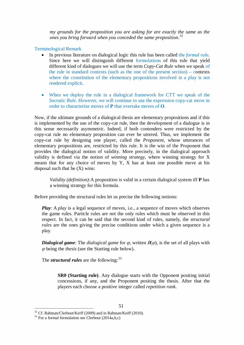
51

my grounds for the proposition you are asking for are exactly the same as the ones you bring forward when you conceded the same proposition.32

Terminological Remark

• In previous literature on dialogical logic this rule has been called the formal rule. Since here we will distinguish different formulations of this rule that yield different kind of dialogues we will use the term Copy-Cat Rule when we speak of the rule in standard contexts (such as the one of the present section) – contexts where the constitution of the elementary propositions involved in a play is not rendered explicit.

• When we deploy the rule in a dialogical framework for CTT we speak of the

Socratic Rule. However, we will continue to use the expression copy-cat move in order to characterize moves of P that overtake moves of O.

Now, if the ultimate grounds of a dialogical thesis are elementary propositions and if this is implemented by the use of the copy-cat rule, then the development of a dialogue is in this sense necessarily asymmetric. Indeed, if both contenders were restricted by the copy-cat rule no elementary proposition can ever be uttered. Thus, we implement the copy-cat rule by designing one player, called the Proponent, whose utterances of elementary propositions are, restricted by this rule. It is the win of the Proponent that provides the dialogical notion of validity. More precisely, in the dialogical approach validity is defined via the notion of winning strategy, where winning strategy for X means that for any choice of moves by Y, X has at least one possible move at his disposal such that he (X) wins:

Validity (definition):A proposition is valid in a certain dialogical system iff P has a winning strategy for this formula.

Before providing the structural rules let us precise the following notions:

Play: A play is a legal sequence of moves, i.e., a sequence of moves which observes the game rules. Particle rules are not the only rules which must be observed in this respect. In fact, it can be said that the second kind of rules, namely, the structural rules are the ones giving the precise conditions under which a given sequence is a play.

Dialogical game: The dialogical game for ϕ, written D(ϕ), is the set of all plays with ϕ being the thesis (see the Starting rule below). The structural rules are the following:33

SR0 (Starting rule). Any dialogue starts with the Opponent positing initial concessions, if any, and the Proponent positing the thesis. After that the players each choose a positive integer called repetition rank.

32 Cf. Rahman/Clerbout/Keiff (2009) and in Rahman/Keiff (2010). 33 For a formal formulation see Clerbout (2014a,b,c)

52

• The repetition rank of a player bounds the number of challenges he can play in reaction to a same move.

SR1c (Classical Development rule). Players move alternately. After the repetition ranks have been chosen, each move is a challenge or a defence in reaction to a previous move and in accordance with the particle rules. SR1i (Intuitionisitic Development rule). Players move alternately. After the repetition ranks have been chosen, each move is a challenge or a defence in reaction to a previous move and in accordance with the particle rules. Players can answer only against the last non-answered challenge by the adversary.34

SR2 (Copy-Cat Rule). P may not utter an elementary proposition unless O uttered it first. Elementary propositions cannot be challenged. Remark: This formulation of the rule has the problem that elementary propositions cannot be set as thesis of a dialogical game. This motivated to use the following rule that will a main subject of our discussion on equality.

Special Copy-Cat Rule. O's elementary sentences cannot be challenged. However, O can challenge a P-elementary move. The challenge and correspondent defence is ruled by the following table.

Posit Challenge Defence

P ! A

(for elementary A)

O ? P sic (n)

(P indicates that O posited A at move n)

The last structural rule requires some additional terminology:

• Terminal play: A play is called terminal when it cannot be extended by further moves in compliance with the rules.

• X-terminal: We say it is X-terminal when the play is terminal and the

last move in the play is an X-move.

SR3 (Winning rule). Player X wins the play ζ only if it is X-terminal. Consider for example the following sequences of moves:

P-Q(a) ⊃ Q(a), O-n:=1, P-m:=12, O- Q(a), P- Q(a) This sequence constitutes a play in D(P- Q(a) ⊃ Q(a)). We often use a convenient table 34 This last clause is known as the Last Duty First condition, and is the clause making dialogical games suitable for Intuitionistic Logic, hence the name of this rule.

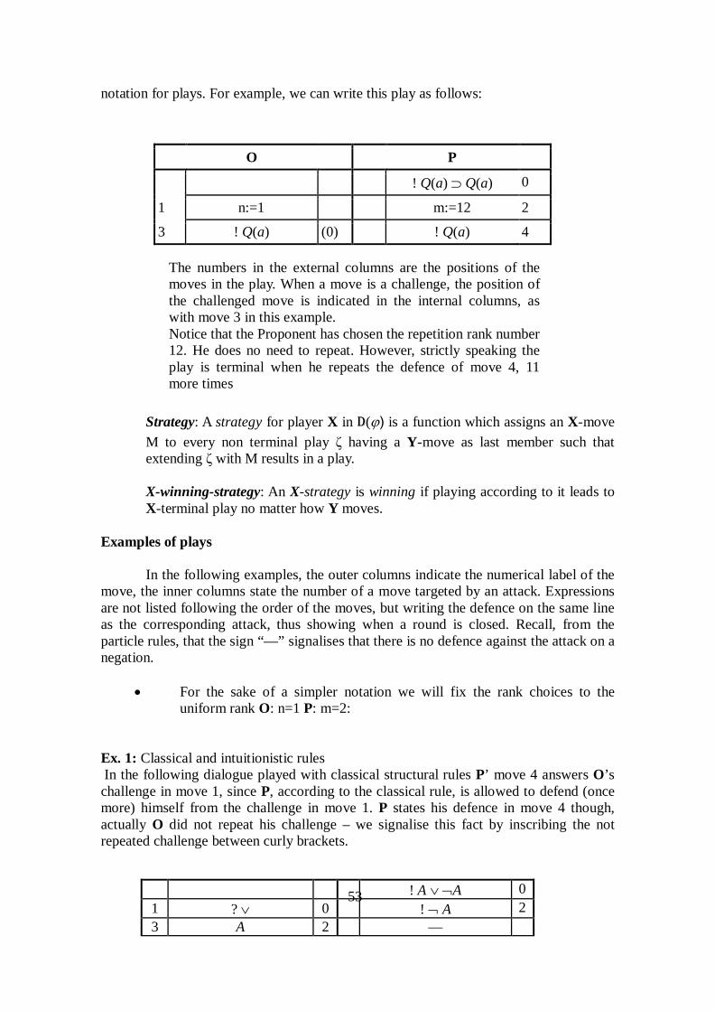
53

notation for plays. For example, we can write this play as follows:

O P

! Q(a) ⊃ Q(a) 0

1 n:=1 m:=12 2

3 ! Q(a) (0) ! Q(a) 4

The numbers in the external columns are the positions of the moves in the play. When a move is a challenge, the position of the challenged move is indicated in the internal columns, as with move 3 in this example. Notice that the Proponent has chosen the repetition rank number 12. He does no need to repeat. However, strictly speaking the play is terminal when he repeats the defence of move 4, 11 more times

Strategy: A strategy for player X in D(ϕ) is a function which assigns an X-move M to every non terminal play ζ having a Y-move as last member such that extending ζ with M results in a play. X-winning-strategy: An X-strategy is winning if playing according to it leads to X-terminal play no matter how Y moves.

Examples of plays

In the following examples, the outer columns indicate the numerical label of the move, the inner columns state the number of a move targeted by an attack. Expressions are not listed following the order of the moves, but writing the defence on the same line as the corresponding attack, thus showing when a round is closed. Recall, from the particle rules, that the sign “—” signalises that there is no defence against the attack on a negation.

• For the sake of a simpler notation we will fix the rank choices to the uniform rank O: n=1 P: m=2:

Ex. 1: Classical and intuitionistic rules In the following dialogue played with classical structural rules P’ move 4 answers O’s challenge in move 1, since P, according to the classical rule, is allowed to defend (once more) himself from the challenge in move 1. P states his defence in move 4 though, actually O did not repeat his challenge – we signalise this fact by inscribing the not repeated challenge between curly brackets.

! A ∨ ¬A 0 1 ? ∨ 0 ! ¬ A 2 3 A 2 —

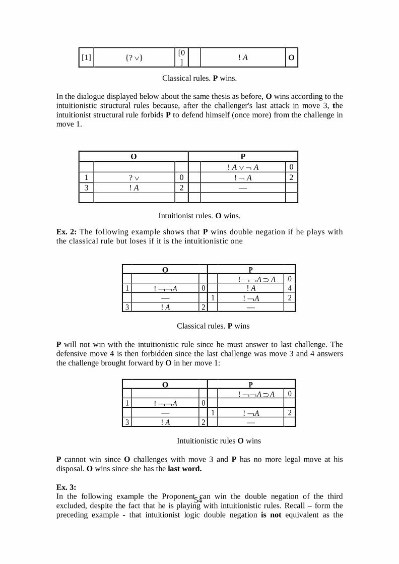
54

[1] {? ∨} [0] ! A O

Classical rules. P wins.

In the dialogue displayed below about the same thesis as before, O wins according to the intuitionistic structural rules because, after the challenger's last attack in move 3, the intuitionist structural rule forbids P to defend himself (once more) from the challenge in move 1.

O P ! A ∨ ¬ A 0 1 ? ∨ 0 ! ¬ A 2 3 ! A 2 —

Intuitionist rules. O wins.

Ex. 2: The following example shows that P wins double negation if he plays with the classical rule but loses if it is the intuitionistic one

O P ! ¬¬A ⊃ A 0 1 ! ¬¬A 0 ! A 4

— 1 ! ¬A 2 3 ! A 2 —

Classical rules. P wins

P will not win with the intuitionistic rule since he must answer to last challenge. The defensive move 4 is then forbidden since the last challenge was move 3 and 4 answers the challenge brought forward by O in her move 1:

O P ! ¬¬A ⊃ A 0 1 ! ¬¬A 0

— 1 ! ¬A 2 3 ! A 2 —

Intuitionistic rules O wins

P cannot win since O challenges with move 3 and P has no more legal move at his disposal. O wins since she has the last word. Ex. 3: In the following example the Proponent can win the double negation of the third excluded, despite the fact that he is playing with intuitionistic rules. Recall – form the preceding example - that intuitionist logic double negation is not equivalent as the

55

positive version of expression. Here P makes use of the repetition rank 2. That he is allowed to challenge twice the same move of his antagonist.

O P ! ¬¬(A ∨ ¬A) 0 1 ! ¬( A ∨ ¬A) 0 —

- 1 ! A ∨ ¬A 2 3 ? ∨ 2 ! ¬A 4 5 ! A 4 —

1 ! A ∨ ¬A 6 7 ? ∨ 6 ! A 8

In the following example. we displayed two possible plays triggered by the rank 1 of the Opponent. Since she cannot defend twice in the same place, each alternative will lead to a new play:

Ex. 4:

O P ! ((A ∨ B) ∧ ¬A) ⊃ B 0

1 ! ((A ∨ B) ∧ ¬A) 0 3 ! ¬A 1 ?R 2 5 ! A ∨ B 1 ?L 4

5 ? ∨ 6

Play 1

O P ! ((A ∨ B) ∧ ¬A) ⊃ B 0

1 ! ((A ∨ B) ∧ ¬A) 0 ! B 8 3 ! ¬A 1 ?R 2 5 ! A ∨ B 1 ?L 4 7 ! B 5 ? ∨ 6

Intuitionistic rules P wins

Play 2

O P ! ((A ∨ B) ∧ ¬A) ⊃B 0

1 ! ((A ∨ B) ∧ ¬A) 0 3 ! ¬A 1 ?R 2 5 ! A ∨ B 1 ?L 4 7 ! A 5 ? ∨ 6 — 3 ! A 8

Intuitionistic rules P wins

56

In fact, when we want to consider several plays together – for example when building a strategy – such tables are not that perspicuous. So we do not use them to deal with dialogical games for which we prefer another perspective.

Extensive form of a dialogical game: The extensive form E(ϕ) of the dialogical game D(ϕ) is simply the tree representation of it, also often called the game-tree. Nodes are labelled with moves so that the root is labelled with the thesis, paths in E(ϕ) are linear representations of plays and maximal paths represent terminal plays in D(ϕ).

The extensive form of a dialogical game is thus an infinitely generated tree where each branch is of finite length. Many dialogical game metalogical results are obtained by leaving the level of rules and plays to move to the level of strategies. Significant among these results are the ones concerning the existence of winning strategies for a player.

Strategy: A strategy for player X in D(ϕ) is a function which assigns an X-move M to every non terminal play ζ having a Y-move as last member such that extending ζ with M results in a play. X-winning-strategy: An X-strategy is winning if playing according to it leads to X's victory no matter how Y plays.

Also, strategies can be considered from the perspective of extensive forms:

Extensive form of an X-strategy: The extensive form of an X-strategy s in D(ϕ) is the tree-fragment Sϕ =(Ts,ls,Ss) of Eϕ such that: i) The root of Sϕ is the root of Eϕ, ii) Given a node t in Eϕ labelled with an X-move, we have t'∈Ts and tSst' whenever tSt'. iii) Given a node t in Eϕ labelled with a Y-move and with at least one t' such that tSt', we have a unique s(t) in Ts with tSss(t) and s(t) is labelled with the X-move prescribed by s.

Definition 4 Let sx be a strategy of player X in D(ϕ) of extensive form E(ϕ). The extensive form of sx is the fragment Sx of E(ϕ) such that:

1. The root of E(ϕ) is the root of Sx , 2. For any node t which is associated with an X-move in E(ϕ), any immediate successor of t in E(ϕ) is an immediate successor of t in Sx , 3. For any node t which is associated with a Y-move in E(ϕ), if t has at least an immediate successor in E(ϕ) then t has exactly one immediate successor in Sx namely the one labelled with the X-move prescribed by sx .

57

Here are some results pertaining to the level of strategies:35

- Winning P-strategies and leaves. Let w be a winning P-strategy in D(ϕ). Then every leaf in the extensive form Wϕ of w is labelled with a P elementary sentence. - Determinacy. There is a winning X-strategy in D(ϕ) if and only if there is no

winning Y-strategy in D(ϕ). - Soundness and Completeness of Tableaux. Consider first-order tableaux and first-order dialogical games. There is a tableau proof for ϕ if and only if there is a winning P-strategy in D(ϕ). The fact that existence of a winning P-strategy coincides with validity (there is a winning P-strategy in D(ϕ) if and only if ϕ is valid) follows from the soundness and completeness of the tableau method with respect to model-theoretical semantics.

Extensive forms of strategies have key parts in those results: one of the parts of a winning strategy, called the core of the strategy, is actually that on which one works when considering translation algorithms such as the procedures. The basic idea behind the notion of core is to get rid of redundant information (for example, different orders of moves) which we find in extensive forms of strategies (see Clerbout and Rahman (2015). Let us motivate the introduction of a core. Consider once more the example of the thesis

((A ∨ B) ∧ ¬A) ⊃ B

However, we are interested in defining the dialogical game for it. That is all the possible plays, without assuming, as we did before that the number of the repetition rank has been fixed.

1) After setting the thesis the first move that follows is the choice of the repetition ranks. This already generates an infinity of plays constituting a dialogical game, namely, each of those plays generated by the players choices: O chooses 1, P can choose from 1 …n , O chooses 2, P can again choose from 1 to n, etc.

2) After one of the choices for the repetition rank has been fixed, P can choose to challenge first the left of the right part of the conjunction.

3) After this choice of P, O can choose the left and the right side of the thesis. It is clear that we need some kind of heuristic procedure that help us mastering such kind of arborescence. In the section where we develop some of the metalogical results relevant for dialogical games for CTT, we discuss in detail the motivations and the rationale that leads to the core. For the moment we will make use of the metalogical results achieved in order to design such an algorithm. III.2.3 Developing a dialogical demonstration

35 These results are proven, together with others, in Clerbout (2014a).

58

• Using some metalogical results from the previous literature

1. Repetition rank

1.1 We assume that the number of repetition rank for O is 1.36 1.2 As for the Proponent’s rank allows P to win the first play. After the first

play there is a device in procedure that allows P to choose once the repetition rank for a new play.37

We also assume that 2. when O has to choose an individual constant she will always choose a new

one.38 3. when O can challenge a move where P has several defensive options, O will

launch the challenge before carrying out other moves.39

• O-Decisions

Suppose then that we have a play ℘n won by P where O played according to the assumptions mentioned above.

Preliminaries. We say that O takes a decision in ℘1 in the following cases:

(i) She challenges a conjunction: the decision involves choosing which side to ask for.

(ii) She defends a disjunction: the decision involves choosing one of the sides of the disjunction

(iii) She defends an implication, the decision involves choosing either defending or launching a counter-attack.

(iv) She defends an existential: the decision involves choosing a (new) constant.

(v) She challenges a universal: the decision involves choosing a (new) constant.

• The method only takes into consideration kind of decisions i), ii), and iii).40

• We say that a decision does not use up the available options in the play when, because of rank 1, O decided for one of the two choices and the second decision has

36 The point is that, since O is not restricted by the copy-cat rule in any of its forms (including the Socratic Rule), she can always choose the move that is the best for her own interests – and as implemented in the method above, even if in a play she makes a bad choice, she can correct it in a new play. Thus, rank 1 is sufficient. 37 Finding the precise P-rank for the thesis at stake is part of the objectives of the development of a demonstration 38 The reason is pretty straight-forward: it is the best possible choice for O. Indeed, since P is restricted by the Copy-cat rule, he needs to rely on O's choices in order to apply a copy-cat move. In such a context, the only way to (try to) block the use of the copy-cat move is by choosing always a new constant, whenever a choice is possible. 39 The reason is similar to the previous one: it is better for O to force P to makes his choice as soon as possible. 40 Notice that, because we assume that O always chooses a new constant (prescription 2) and also because of prescription 3 those O-moves will never be unused. Thus, we can also leave out the cases where O defends an existential or challenges a universal.

59

not been taken before. The second choice is the one that remains unused.

• We say that a decision used up the available options iff this decision results from taking one of the two available decisions, while the other decision has already been taken.

• Moreover, we say that a move M depends on the move M' if there is a chain of

applications of game (particle) rules that leads from M' to M.

• We use the following notational convention for the last decision– bottom up in the relation to the flow of the moves – taken by O in a play m such that this decision does not use up all of the two available options: We speak of left-decision in the case that

O decides to defend the left side of a disjunction O decides to challenge the left side of a conjunction (while defending an implication) O decides for a counterattack-decision.

We speak of right-decision in the case that

O decides to defend the right side of a disjunction O decides to challenge the right side of a conjunction (while defending an implication) O decides for a defence-decision.

At the right, of a move where a decision has been taken for a disjunction or a conjunction we write one of the following expressions: either [δn, …] or […δn]:

[δn, …] indicates that the left decision has been taken in play 3 – whereas the right option has not been yet chosen, […,δn] indicates similar for the right decision

The under-script m indicates the number of the play in which the decision δ has been taken. Thus, [δ3, …] indicates that the left decision has been taken in play 3 – whereas the right option has not been yet chosen, Furthermore, [δm, δn] indicates that both of the available choices have been used up such that the first choice has been taken in play m and the second choice in play n.

When O takes a decision for an implication in the play ℘n, she can open two new subplays ℘n.L and ℘n.R, one after the other such that

℘n.L indicates the play were O decides to counterattack. ℘n.R indicates the play were O decides to defend.

Each of the subplays, starts with the move that responds to the challenge. So if the implication was challenged in move n of play ℘n , then both ℘n.L and ℘n.R start with move n+1. The first move of the play ℘n.R, is the defence to the challenge. The challenge itself will be rewritten but, because it has been already counterattacked in ℘n.L, and

60

because of rank 1, it cannot be counterattacked in ℘n.L. Notice that O’s response in ℘n.R might allow P to make a move in the upper play ℘n. In such a case, the move imported into the upper play will be provided with an indication of its origin, (e.g. 12, ℘n.R). • ℘n is P-terminal iff each of the paths that start with the thesis and continue by

℘n.L and ℘n.R (including further possible subplays) are P-terminal

• ℘n is O-terminal iff one of the paths is. Remark: The procedure prescribes to start with the subplay involving the counterattack. Once the counterattack of the antecedent has been launched, the repetition rank 1 has been used-up. Thus, in the second subplay involving the defence, a challenge to the antecedent of the implication is no more available. This shows that, that the two sub-plays are only a graphical device to present both options within the same (main) play. 41 The notation [δm, δn] indicates that both of the available choices for a conjunction or a disjunction have been used up such that the first choice has been taken in play m and the second choice in play n. We say that that both of the available choices for an implication has been used up if both of the subplays have been opened.

Procedure. 0. The process starts with a P-terminal play ℘1. We assume that the number of repetition rank for O is 1. The Proponent’s rank allows P to win the first play. 1. If there is no (remaining) unused decision to be taken by O in ℘n

then go to step 4. Otherwise go to the next step. 2. Take the last (bottom up in the relation to the flow of the moves)

not yet used up decision taken by O in ℘n (label it [δn, …] or [δn, …], if it has not been labelled yet) and, depending on the case, apply one of the steps described below to open a new play. Repeat them until all the decisions have been used up and go then to Step 3. When a new play is opened P has the chance to change the repetition-rank once. 2.1. If δn is a challenge against a conjunction, then open a new play ℘m=n+1 with a challenge to the other side of the conjunction and label it as [δm, δn] or [δn, δm] to indicate that it used up both of the available decision-options. The new play then proceeds as

41 In fact the opening of two subplays called in Rahman/Keiff (2004, pp. 273-275) branching-rule, has a strategic motivation not a play level one. The reason is that here we are after the development of a demonstration. It is also possible to develop a notation where both responses, counterattack and defence are in the same play, but this comes with a heavy notation. Moreover, in the context of the presente paper, where we deploy repetition-ranks, the rank 1 of the Opponent blocks from the branch involving the defence of the implication the problematic second counterattack upon P's-challenge (for a discussion of this problem see Rahman/Clerbout/Keiff, section 1.6 ). This shows that the subplays are really two options in the same (main-)play.

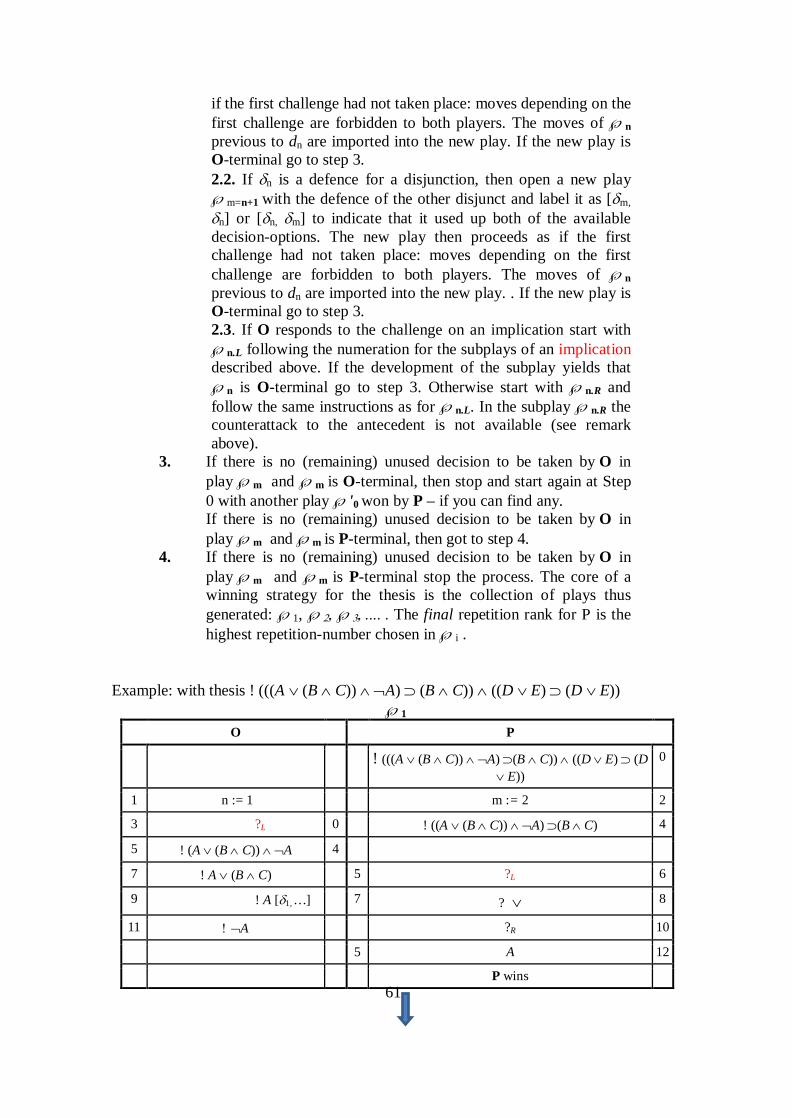
61

if the first challenge had not taken place: moves depending on the first challenge are forbidden to both players. The moves of ℘n previous to dn are imported into the new play. If the new play is O-terminal go to step 3. 2.2. If δn is a defence for a disjunction, then open a new play ℘m=n+1 with the defence of the other disjunct and label it as [δm,

δn] or [δn, δm] to indicate that it used up both of the available decision-options. The new play then proceeds as if the first challenge had not taken place: moves depending on the first challenge are forbidden to both players. The moves of ℘n previous to dn are imported into the new play. . If the new play is O-terminal go to step 3. 2.3. If O responds to the challenge on an implication start with ℘n.L following the numeration for the subplays of an implication described above. If the development of the subplay yields that ℘n is O-terminal go to step 3. Otherwise start with ℘n.R and follow the same instructions as for ℘n.L. In the subplay ℘n.R the counterattack to the antecedent is not available (see remark above).

3. If there is no (remaining) unused decision to be taken by O in play ℘m and ℘m is O-terminal, then stop and start again at Step 0 with another play ℘'0 won by P – if you can find any. If there is no (remaining) unused decision to be taken by O in play ℘m and ℘m is P-terminal, then got to step 4.

4. If there is no (remaining) unused decision to be taken by O in play ℘m and ℘m is P-terminal stop the process. The core of a winning strategy for the thesis is the collection of plays thus generated: ℘1, ℘2, ℘3, .... . The final repetition rank for P is the highest repetition-number chosen in ℘i .

Example: with thesis ! (((A ∨ (B ∧ C)) ∧ ¬A) ⊃ (B ∧ C)) ∧ ((D ∨ E) ⊃ (D ∨ E))

℘1 O P

! (((A ∨ (B ∧ C)) ∧ ¬A) ⊃(B ∧ C)) ∧ ((D ∨ E) ⊃ (D ∨ E))

0

1 n := 1 m := 2 2

3 ?L 0 ! ((A ∨ (B ∧ C)) ∧ ¬A) ⊃(B ∧ C) 4

5 ! (A ∨ (B ∧ C)) ∧ ¬A 4

7 ! A ∨ (B ∧ C) 5 ?L 6

9 ! A [δ1, …] 7 ? ∨ 8

11 ! ¬A ?R 10

5 A 12

P wins

62

Now the last decision (move 9 : ) has not been used up. We labellize it and O can now open a new play where he will choose the right side of the disjunction this time.

℘2

O P

! (((A ∨ (B ∧ C)) ∧ ¬A) ⊃(B ∧ C)) ∧ ((D ∨ E) ⊃ (D ∨ E))

0

1 n : = 1 m:= 2 2

3 ?L 0 ! ((A ∨ (B ∧ C)) ∧ ¬A) ⊃(B ∧ C) 4

5 ! (A ∨ (B ∧ C)) ∧ ¬A 4 ! B ∧ C 10

7 ! A ∨ (B ∧ C) 5 ?L 6

9 ! B ∧ C [δ1, δ2,] 7 ? ∨ 8

11 ?L [δ2, ...] 10 ! B 14

13 ! B 9 ?L 12

P wins

Now, all the decisions in relation to the disjunction have been taken: the available decision have been used up. Now the last decision [δ2, …] (move 11 : ) has not been used up so O can now open a new play where he will choose the challenge the right side of the conjunction so we replace move 11 with ?R, delete all the moves that depend upon ?L (of mover 11 of the precedent play) and start the process again

℘3 O P

! (((A ∨ (B ∧ C)) ∧ ¬A) ⊃ (B ∧ C)) ∧ ((D ∨ E) ⊃ (D ∨ E))

0

1 n : = 1 m:= 2 2

3 ?L [δ3, ...] 0 ! ((A ∨ (B ∧ C)) ∧ ¬A) ⊃(B ∧ C) 4

5 ! (A ∨ (B ∧ C)) ∧ ¬A 4 ! B ∧ C 10

7 ! A ∨ (B ∧ C) 5 ?L 6

9 ! B ∧ C [δ1, δ2,] 7 ? ∨ 8

11 ?R [δ2, δ3] 10 C 14

13 C 9 ?R 12

P wins

Now, all the available challenges of the conjunction have been used up. Nevertheless, the Opponent does not give up, he realizes, that there is still an available challenge since there is still an unused decision, namely, move 3 is the last not yet used up decision of

63

play 3 – we indicate this fact by adding the expression [δ3, ...] to the move 3. Accordingly it is possible to launch a new play that challenges the right of the main conjunction that constitutes the thesis.

℘4 O P

! (((A ∨ (B ∧ C)) ∧ ¬A) ⊃(B ∧ C)) ∧ ((D ∨ E) ⊃ (D ∨ E))

0

1 n: = 1 m:= 2 2

3 ?R [δ3, δ4] 0 ! (D ∨ E) ⊃ (D ∨ E) 4

5 ! D ∨ E 4 ! D ∨ E 6

7 ? ∨ 6 ! D 10

9 ! D [δ4, …] 5 ? [D, E] 8

P wins

The next play is the last one. Indeed, O can still try out defending the right side of the disjunction, but then all have been tried out and defeat must be acknowledged:

℘5 O P

! (((A ∨ (B ∧ C)) ∧ ¬A) ⊃(B ∧ C)) ∧ ((D ∨ E) ⊃ (D ∨ E))

0

1 n : = 1 m:= 2 2

3 ?R [δ3, δ4] 0 ! (D ∨ E) ⊃ (D ∨ E) 4

5 ! D ∨ E 4 ! D ∨ E 6

7 ? ∨ 6 ! E 10

9 ! E [δ4, δ5] 7 ? ∨ 8

P wins

The procedure stops. Each of the plays are won by P. The graphic presentation of the core corresponds to a tree where the nodes are constituted by the moves of the players displayed as a vertical sequence of dialogical P- and O- steps, and where the branches are triggered by the decisions that yield the plays ℘1 to ℘4.

However in the tree-shape presentation the building up starts from the first decision of the first play – not the last decision as in the heuristic method displayed above.

64

More precisely P's move m that triggered the first decision of O, is the start of two branches, such that

one branch copies the moves of the first play after m (including the first decision) and the other branch those of the second play after m (including the second decision).

Thus, m and the moves before m, common to both plays, yield the main trunk from which the branching starts.

In order to facilitate the reading of the tree and make it independent of the plays originating them we will introduce the following notation • at the left of each node we record the number of the move • at the right of each challenge we add the indication [? n], which expresses that the

move is a challenge to move n • at the right of each defence we add the indication [!, n], which expresses that the

move is a response to the challenge launched at move n

0 P ! (((A ∨ (B ∧ C)) ∧ ¬A) ⊃(B ∧ C)) ∧ ((D ∨ E) ⊃ (D ∨ E))

1 O?L [δ3, …] [?, 0] 1 O?R [δ3, δ4] [?0] 2 P ! ((A ∨ (B ∧ C)) ∧ ¬A) ⊃(B ∧ C) [!, 1] 2 P !(D ∨ E) ⊃ (D ∨ E) [!, 1] 3 O ! (A ∨ (B ∧ C)) ∧ ¬A [?, 2] 3 O ! D ∨ E [?, 2] 4 P?L [?, 3] 4 P ! D ∨ E [! 3] 5 O ! A ∨ (B ∧ C) [!, 4] 5 O? ∨ [?, 4] 6 P? ∨ [?, 5] 6 P? ∨ [?, 3]

7 O ! A [δ1, …] [!, 6] 7 O ! (B ∧ C) [δ1, δ2] [!, 6] 8 P?R [?, 3] 8 P! (B ∧ C) [!, 3] 7 O ! D [δ4, …] [!, 6] 7 O ! E [δ4, δ5] [!, 6] 9 O ! ¬A [!, 8] 8 P ! D [!, 5] 8 P ! E [!, 5] 10 P ! A [!, 9]

9 O?L [δ2, …] [?, 8] 9 O?R [δ2, δ3] [?, 8]

10 P?L [?, 7] 10 P?R [?, 7] 11 O ! B [!, 10] 11 O ! C [!, 10] 12 P ! B [!, 9] 12 P ! C [!, 9]

It should clear that one could develop the whole demonstration directly in the shape of the tree, and skip the more cumbersme tableau presentation. In fact, in metalogical contexts the tree-shaped structure produces a more direct way to link dialogical strategies with CTT-demonstrations. However, the tableau presentation highlights the dialogical background from which the strategy emerges.

65

One simple way to skech the procedure for the development of such a tree (with the notation described above) is the following:

1. The root of the tree is the thesis 2. The next step proceeds by O either challenging the thesis or by positing the

required initial concessions 3. The tree develops as a vertical sequence of dialogical P- and O- steps, until the

first O-decission occurs. 4. When the first decision occurs split the tree in two branches and explore one of

them (recall that if the decision involved an O-implication we start with the counterattack option (if possible))

5. If the end of the branch ends with a O-move (other than giving up), then O won and the procedure finishes.

6. Otherwise, start exploring the second main branch and so on until the end For the development of the tree we continue to assume the strategic shorts-cuts mentioned above, such as repetition rank 1 for O, O’s predilection for new constants, etc.

66

III.3 Dialogues with play objects.

Recent developments in dialogical logic show that the CTT approach to meaning is very natural to those game-theoretical approaches where (standard) metalogical features are explicitly displayed at the object language-level.42 Thus, in some way, this vindicates, albeit in quite of a different manner, Hintikka’s plea for the fruitfulness of game-theoretical semantics in the context of epistemic approaches to logic, semantics and the foundations of mathematics.43 In fact, from the dialogical point of view, those actions that the local rules associate with the use of logical constants, such as choices, are a crucial element of its full-fledged (local) meaning. Indeed, if meaning is conceived as being constituted during interaction, then all of the actions involved in the constitution of the meaning of an expression should be rendered explicit. They should all be part of the object language. The roots of this perspective are based on Wittgenstein’s Unhintergehbarkeit der Sprache – one of the tenets of Wittgenstein that Hintikka explicitly rejects.44 According to this perspective of Wittgenstein language-games are purported to accomplish the task of displaying this “internalist feature of meaning”. Furthermore, one of the main insights of Kuno Lorenz’ interpretation of the relation between the so-called first and second Wittgenstein is based on a thorough criticism of the metalogical approach to meaning Lorenz (1970, pp. 74-79).45 If we recall Hintikka’s (1996b) extension of van Heijenoort (1967) distinction of a language as the universal medium and language as a calculus, the point is that the dialogical approach shares some tenets of both conceptions. Indeed, on one hand the dialogical approach shares with universalists the view that we cannot place ourselves outside our language, on the other it shares with the anti-universalists the view that we can develop a methodical of local truth. Similar criticism to the metalogical approach to meaning has been raised by G. Sundholm (1997, 2001) who points out that the standard model-theoretical semantic turns semantics into a meta-mathematical formal object where syntax is linked to meaning by the assignation of truth values to uninterpreted strings of signs (formulae). 42 Cf. Clerbout/Rahman (2015), Dango (2014, 2015, 2016), Jovanovic (2013), Jovanovic (2015), Rahman/Clerbout (2013, 2015), Rahman/Clerbout/Jovanovic (2014), Rahman/Clerbout/McConaughey (2014). 43 Cf. Hintikka (1973, 1996a). 44 Hintikka (1996b) shares this rejection with all those who endorse model-theoretical approaches to meaning. 45 In this context Lorenz writes :

Also propositions of the metalanguage require the understanding of propositions, […] and thus cannot in a sensible way have this same understanding as their proper object. The thesis that a property of a propositional sentence must always be internal, therefore amounts to articulating the insight that in propositions about a propositional sentence this same propositional sentence does not express anymore a meaningful proposition, since in this case it is not the propositional sentence that it is asserted but something about it. Thus, if the original assertion (i.e., the proposition of the ground-level) should not be abrogated, then this same proposition should not be the object of a metaproposition, […]. Lorenz (1970, p.75) – translated from the German by S.R. While originally the semantics developed by the picture theory of language aimed at determining unambiguously the rules of “logical syntax” (i.e. the logical form of linguistic expressions) and thus to justify them […] – now language use itself, without the mediation of theoretic constructions, merely via “language games”, should be sufficient to introduce the talk about “meanings” in such a way that they supplement the syntactic rules for the use of ordinary language expressions (superficial grammar) with semantic rules that capture the understanding of these expressions (deep grammar). Lorenz (1970, p.109) – translated from the German by S.R.

67

Language does not any more express content but it is rather conceived as a system of signs that speaks about the world - provided a suitable metalogical link between signs and world has been fixed. Moreover, Sundholm (2016) shows that the cases of quantifier-dependences that motivate Hintikka’s IF-logic can be rendered in the frame of CTT. What we add to Sundholm’s remark is that even the game-theoretical interpretation of these dependences can be given a CTT formulation, provided this is developed within a dialogical framework. In fact, Ranta (1988) was the first in relating game-theoretical approaches with CTT. Ranta took Hintikka's (1973) Game-Theoretical Semantics as a case study, though his point does not depend on that particular framework: in game-based approaches, a proposition is a set of winning strategies for the player positing the proposition.46 In game-based approaches, the notion of truth is at the level of such winning strategies. Ranta's idea should therefore let us safely and directly apply to instances of game-based approaches methods taken from constructive type theory. But from the perspective of game-theoretical approaches, reducing a game to a set of winning strategies is quite unsatisfactory, especially when it comes to a theory of meaning. This is particularly clear in the dialogical approach in which different levels of meaning are carefully distinguished. There is thus the level of strategies which is one of the possible levels of meaning analysis, but there is also a level prior to the strategic level which is usually called the level of plays. The role of the latter level for developing a meaning explanation is crucial according to the dialogical approach, as pointed out by Kuno Lorenz in his 2001 paper:

Fully spelled out it means that for an entity to be a proposition there must exist a dialogue game associated with this entity, i.e., the proposition A, such that an individual play of the game where A occupies the initial position, i.e., a dialogue D(A) about A, reaches a final position with either win or loss after a finite number of moves according to definite rules: the dialogue game is defined as a finitary open two-person zero-sum game. Thus, propositions will in general be dialogue-definite, and only in special cases be either proof-definite or refutation-definite or even both which implies their being value-definite. Within this game-theoretic framework [ … ] truth of A is defined as existence of a winning strategy for A in a dialogue game about A; falsehood of A respectively as existence of a winning strategy against A. Lorenz (2001), p. 258).

Given the distinction between the play- and the strategic level and, if we are looking to deploy within the dialogical frame the CTT-explicitation programme that expresses at the object-language level the proposition and that what makes it true, it seems natural to distinguish between play object and strategic objects (only the latter correspond to the proof-objects of CTT). Thus, in this context, Ranta's work on proof-objects and strategies is the end, not the beginning, of the dialogical approach to CTT. In order to implement such a project we enriched the language of the dialogical frame with expressions of the form “p : ϕ” , where at the left of the colon there is what we call an argumentative play-element or play object and at the right a proposition (or set)). 47 The meaning of such expressions results from the local and structural rules that describe the way to analyse and compose within a play the suitable play objects and provide their 46 That player can be called Player 1, Myself or Proponent. 47 See: Clerbout/Rahman (2015), Rahman/Clerbout (2013, 2014, 2015).

68

canonical argumentation form. The most basic contribution of a play object is its contribution to a material dialogue involving an elementary proposition. Informally:

If the player P endorses the elementary proposition A, stating such an endorsement presupposes that there is something, what we call the play object p, that can be brought forward, in order to defend A, following a series of actions specific to A prescribed by the Socratic Rule. More generally, what the canonical play objects for A are, as well as what equal canonical play objects (with A) are is determined by the actions prescribed by the Socratic Rule as specific for A. This defines material dialogues of immanent reasoning and leads to material-truth.

Thus, we can say that play objects prefigure a material dialogue that display the content of the proposition involved in such a claim. However, our study focuses on formal plays of immanent reasoning. The development of material dialogues will be left for future work, though in the last chapter of the book we will provide some insights into their structure. In formal dialogues the formulation of the Socratic Rule allows the Proponent to over-take not only A but also the play objects brought forward by the Opponent while positing A. The proponent grants the O not only A but the play objects brought forward during the play. Thus, since, the play objects for the elementary expressions are left to authority of O, what we need now is to describe the canonical argumentation play objects of the logical constants. As we will discuss below the standard local-rules of the dialogical frame provide the relevant information needed in order to describe the play objects specific to the (dialogical) meaning of each of these constants. Before starting to enrich the language of the standard dialogic frame with play objects for logical constants let us discuss how to implement a dialogical notion of formation rules. III.3.1 Local meaning I: The formation rules It is presupposed in standard dialogical systems that the players use well-formed formulas. The well formation can be checked at will, but only with the usual meta reasoning by which the formula is checked to indeed observe the definition of a wff. We want to enrich the system by first allowing players to enquire on the status of expressions and in particular to ask if a certain expression is a proposition. We thus start with dialogical rules explaining the formation of propositions. These rules are local rules which we are added to the particle rules giving the local meaning of logical constants (see next section). Some preliminary remarks:

1) Because the dialogical theory of meaning is based on argumentative interaction, dialogues feature expressions which are not only posits of sentences. They also feature requests, used for challenges, as the formation rules below and the particle rules in the next section illustrate. Because of the no entity without type principle, it seems at first glance that we should specify the type of these actions

69

during a dialogue: the type ``formation-request". It turns out we should not: an expression such as ``?F: formation-request'' is a judgement that some action ?F is a formation-request, which should not be confused with the actual act of requesting. We also consider that the force symbol ?F makes the type explicit. Hence the way requests are written in rules and dialogues in this work.

2) Recall, from our section on standard dialogical logic, that a move is an

expression of the form `X-e', where e is either of the form '!ϕ' (that reads: the player X posits ϕ or X claims that ϕ holds), for some sentence ϕ of L or of one of the forms specified by the particle rules. In the context of the dialogical conception of CTT we also have expressions of the form

X ! π(x1, …, xn) [xi : Ai]

where "π" stands for some posit in which (x1, …, xn) ocurr, and where [xi : Ai] stands for some conditions under which the posit π(x1, …, xn) has been brought forward). Thus, the expression reads,

X claims that π(x1, …, xn) holds, under the condition that the antagonist concedes xi : Ai.

We call expressions of the form [xi : Ai] that condition a claim, required concessions. The challenge, assumes then that the antagonist accept to bring forward such concessions. The concessions of the thesis are called initial concessions.

3) A crucial feature of formation rules is that they enable the displaying of the syntactic and semantic presuppositions of a given thesis which can thus be examined by the Opponent before running the actual dialogue on the thesis. For instance if the thesis amounts to positing ϕ, then before launching an attack, the Opponent can ask for its formation. Defending on the formation of ϕ might bring the Proponent to posit that ϕ is a proposition, provided that A, for instance, is a set is conceded. In this situation the Opponent might concede A is a set, but only after the constitution of A has been established. Now, as already mentioned what the canonical play objects for A are, is determined by the actions prescribed by the Socratic Rule specific to the kind of play in which A has been posited. If the play is material, the Socratic Rule will describe a kind of actions specific to A. If the dialogue is formal, as assumed in our study, the Socratic Rule will allow O to bring forward the relevant canonical play objects during the development of the play. The point is that in formal dialogues, the Opponent’s challenge on a thesis assumes that it is well-formed up to the logical constants, and that the formation of the elementary expressions is displayed during the development of a dialogue. So in both cases, the formation rule for elementary expressions, does not really take place at the level of local meaning but at level of the developments rules. The formation rule below makes this explicit.

The formation rules are given in following table. Notice that a posit `⊥ : prop' cannot be challenged: this is the dialogical account of the fact that the falsum ⊥ is by definition a proposition.

70

Posit Challenge Defence

X ! Γ : set(prop) Y ? can Γ X ! Socratic Rule-Γ 48

X ! ϕ : prop

Y ?F∨1 X ! ϕ : pro

X ! ϕ ∨ ψ : prop Or

Y ?F∨2 X ! ψ : prop

Y ?F∧1 X ! ϕ : pro

X ! ϕ ∧ ψ : prop Or

Y ?F∧2 X ! ψ : prop

Y ?F ⊃ 1 X ! ϕ : pro

X ! ϕ ⊃ ψ : prop Or

Y ?F ⊃ 2 X ! ψ : prop

Y ?F∀1 X ! A : set

X ! (∀x : A) ϕ(x) : prop Or

Y ?F∀2 X ! ϕ(x) : prop [x : A]

Y ? ∃1 X ! A : set

X ! (∃x : A) ϕ(x) : prop Or

Y ?F∃2 X ! ϕ(x) : prop [x : A]

X ! ⊥ : prop _ _

Example of a formation-play By way of illustration, here is an example where the Proponent posits the thesis (∀x : A)(B(x) ⊃ C(x)) : prop given that A : set, B(x) : prop [x : A] and C(x) : prop [x : A], where the three provisos appear as initial concessions by the Opponent.49 Normally we should give all the rules of the game before giving an example, but we make an exception here because the standard structural rules are enough to understand the following plays. We can focus this way on illustrating the way formation rules can be used.

O P

I ! A : set

II ! B(x) : prop [x : A]

III ! C(x) : prop [x : A]

! (∀x : A) B(x) ⊃ C(x) : prop 0

1 n := 1 m := 2 2

3 ?F∀1 0 ! A : set 4

Explanations: - I to III: O concedes that A is a set and that B(x) and C(x) are propositions provided x is an element of A, - Move 0: P posits that the main sentence, universally quantified, is a proposition (under the concessions made by O),

48 There is no general way to specify a set. The specification of a set leads to material dialgoues that will require extending the structural-rules with a set of definitions implemented by the Socratic Rule – see the last chapter of the present study. 49 The example stems from Ranta (1994, p.31).

71

- Moves 1 and 2: the players choose their repetition ranks,50 - Move 3: O challenges the thesis by asking the left-hand part as specified by the formation rule for universal quantification, - Move 4: P responds by positing that A is a set. This has already been granted with the concession I so even if O were to challenge this posit, the Proponent could refer to this initial concession. Later on, we will introduce the structural rule SR3 to deal with this phenomenon. Thus O has no further possible move, the dialogue ends here and is won by P. Obviously, this dialogue does not cover all the aspects related to the formation of (∀x : A) B(x) ⊃ C(x) : prop. Notice however that the formation rules allow an alternative move for the Opponent's move 3.51 Hence another possible course of action for P arises.

O P

I ! A : set

II ! B(x) : prop [x : A]

III

! C(x) : prop [x : A]

! (∀x : A) B(x) ⊃ C(x) : prop 0

1 n := 1 m := 2 2

3 ?F∀2 0 ! B(x) ⊃ C(x) : prop [x : A] 4

5 ! x : A 4 ! B(x) ⊃ C(x) : prop 6

7 ?F ⊃ 1 6 ! B(x) : prop 10

9 ! B(x) : prop II ! x : A 8

Explanations: The second play starts like the first one until move 2. Then: - Move 3: This time O challenges the thesis by asking for the right-hand part, - Move 4: P responds, positing that B(x) ⊃ C(x) is a proposition provided x : A, - Move 5: O challenges the preceeding move by both granting the proviso and asking P to respond (this kind of move is ruled by a posit-substitution rule to be specified in the next section), - Move 6: P responds by positing that B(x) ⊃ C(x) is a proposition, - Move 7: O then challenges move 6 by asking the left-hand part as specified by the formation rule for material implication. To defend this P needs to make an elementary move. But since O has not played it yet, P cannot defend it at this point. Thus: - Move 8: P launches a counterattack against assumption II by granting the proviso x : A (that has already been conceded by O in move 5) making use of the same kind of posit-substitution rule deployed in move 5, - Move 9: O answers to move 8 and posits that B(x) is a proposition, - Move 10: P can now defend in reaction to move 7 and win this dialogue. Then again, there is another possible path for the Opponent because she has another possible choice for her move 7, namely asking the right-hand part. This yields a dialogue similar to the one above except that the last moves are about C(x) instead of B(x). By displaying these various possibilities for the Opponent, we have entered the strategical level. This is the level at which the question of the good formation of the thesis gets a definitive answer, depending on whether the Proponent can always win – i.e., whether he has a winning strategy. The basic notions related to this level are to be found in our presentation of standard dialogical logic.

50 The repetition rank of a player bounds the number of challenges he can play in reaction to a same move. See Clerbout (2014a,b,c) for detailed explanations on this notion. 51 As a matter of fact increasing her repetition rank would allow her to play the two alternatives for move 3 within a single play. But increasing the Opponent's rank usually yields redundancies (Clerbout (2014a,b)) making things harder to understand for readers not familiar with the dialogical approach. Hence our choice to divide the example into different simple plays.

72

Now that the dialogical account of formation rules has been clarified, we may further develop our analysis of plays by introducing play objects. III.3.2 Local meaning II

Play objects, canonical argumentation form and argumentation form. III.3.2.1 Play objects and canonical argumentation form

Besides the formation rules, the rules described by the local meaning for some posit π indicate those moves that display the canonical argumentation form of the play object specific to the proposition/set at stake in π. Different to non-dialogical frameworks, the canonical argumentation form includes the indication of the player committed to the posit or request prescribed by the local rule. Thus, the canonical argumentation form for the implication p : ϕ ⊃ ψ posited by X (X ! p : ϕ ⊃ ψ) indicates

a) that the challenger Y posits the antecedent by providing a play object for it and

requests the defender X to posit the consequent (with a suitable play object) – that is, Y ! p1 : ϕ, ? ! ψ . 52

b) that the defender must respond to the request by positing the requested consequent and bringing forward a play object for it – that is, X ! p2 : ψ .

If we collect the three interactive steps together the canonical argumentation form for the implication X ! p : ϕ ⊃ ψ is the following

Posit: X ! p : ϕ ⊃ ψ Challenge: Y ! p1 : ϕ, ? ! ψ

Defence: X ! p2 : ψ The canonical argumentation of a negation follows the one of implication. Though, as discussed further on, it requests the defender to give-up, once the antecedent has been posited. In the dialogical framework; the player who makes the move ! ⊥, gives up. :

Posit: X ! p : ϕ ⊃ ⊥ Challenge: Y ! p1 : ϕ, ? ! ⊥

Defence: X ! ⊥ More generally, the canonical argumentation form of a play object as determined by the local rules is given by the triple Posit by X Challenge by Y Defence by X

52 The notation follows the one developped by Keiff (2004, section 2.3.4 ) and Clerbout (2014, p. 17), adapted to a framework with play-objects.

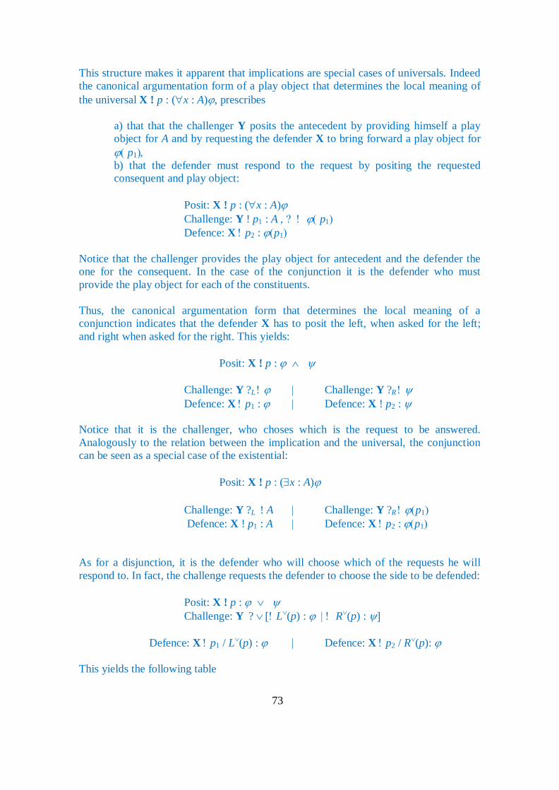
73

This structure makes it apparent that implications are special cases of universals. Indeed the canonical argumentation form of a play object that determines the local meaning of the universal X ! p : (∀x : A)ϕ, prescribes

a) that that the challenger Y posits the antecedent by providing himself a play object for A and by requesting the defender X to bring forward a play object for ϕ( p1), b) that the defender must respond to the request by positing the requested consequent and play object:

Posit: X ! p : (∀x : A)ϕ Challenge: Y ! p1 : A , ? ! ϕ( p1) Defence: X ! p2 : ϕ(p1)

Notice that the challenger provides the play object for antecedent and the defender the one for the consequent. In the case of the conjunction it is the defender who must provide the play object for each of the constituents. Thus, the canonical argumentation form that determines the local meaning of a conjunction indicates that the defender X has to posit the left, when asked for the left; and right when asked for the right. This yields:

Posit: X ! p : ϕ ∧ ψ

Challenge: Y ?L ! ϕ | Challenge: Y ?R ! ψ Defence: X ! p1 : ϕ | Defence: X ! p2 : ψ

Notice that it is the challenger, who choses which is the request to be answered. Analogously to the relation between the implication and the universal, the conjunction can be seen as a special case of the existential:

Posit: X ! p : (∃x : A)ϕ Challenge: Y ?L ! A | Challenge: Y ?R ! ϕ(p1) Defence: X ! p1 : A | Defence: X ! p2 : ϕ(p1)

As for a disjunction, it is the defender who will choose which of the requests he will respond to. In fact, the challenge requests the defender to choose the side to be defended:

Posit: X ! p : ϕ ∨ ψ Challenge: Y ? ∨ [! L∨(p) : ϕ | ! R∨(p) : ψ]

Defence: X ! p1 / L∨(p) : ϕ | Defence: X ! p2 / R∨(p): ϕ

This yields the following table

74

Canonical argumentation form

Posit Challenge Defence

Y ?L ! A X ! p1 : A

X ! p : (∃x : A)ϕ Or Respectively

Y ?R ! ϕ

X ! p2 : ϕ(p1)

Y ?L ! A X ! p1 : A

X ! p : {x : A | ϕ}

Or Respectively

Y ?R ! ϕ(p1)

X ! p2 : ϕ(p1)

Y ?L ! ϕ X ! ! p1 : ϕ

X ! p : ϕ ∧ ψ Or respectively

Y ?R ! ψ

X ! p2 : ψ

X ! p : (∀x : A)ϕ Y ! p1 : A , ? ! ϕ X ! p2 : ϕ(p1)

X ! p : ϕ ⊃ ψ

Y ! p1 : ϕ, ? ! ψ X ! p2: ψ

X ! p : ¬ϕ also expressed as X ! p : ϕ ⊃ ⊥

Y ! ! p1 : ϕ, ? ! ⊥

X ! ⊥ (Player X gives up)

X ! p1 : ϕ

X ! p : ϕ ∨ ψ Y ? ∨ [! L∨(p) : ϕ | ! R∨(p) : ψ] Or

X ! p2 : ψ

The canonical argumentation form as displayed by the table above expresses both the prescription and the result of carrying out the prescription involved in that posit. However, we can also determine the local meaning by means of isolating the prescriptive level. This level, stresses the commitments and the entitlements that characterize the meaning of the posit at stake: it makes explicit its bare argumentation form. In order to settle the bare argumentation form, we introduce instructions, such as L ∨ (p), R∧ (p), and so on. E.g. the argumentation form of the disjunction p : φ ∨ ψ indicates that its defence includes expressions such as L ∨ (p) and R ∨ (p) called the left and right instruction of the disjunction. Their respective interpretations are produce – at your choice - the left (right) component of the play object for that disjunction. In fact, the development of a dialogue determined by immanent reasoning includes four phases:

1) Displaying the argumentation form.The explicit display of the instructions that makes the argumentation form of the thesis manifest.

75

2) Resolution of instructions. Carrying out the prescriptions indicated by the argumentation form, by bringing forward the play objects that solve those instructions indicated by the argumentation form.

3) Establishing the canonical argumentation form. Showing by means of explicit equalities that the resolution of the instructions achieved at step 2 describes the play objects indicated by the canonical argumentation form.

4) Producing the strategic object. Bringing forward the strategic object specific to the winning-strategy specific to the thesis that launched the dialogue. It amounts to produce the strategic object out of the play objects produced in step 3.

Whereas the first two steps requires settling the local meaning, step 3 concern the development or structural rules and step 4 requires describing how to produce a winning strategy. Let us tackle each of the steps one by one starting with step 1 III.3.2.2 Instructions and Argumentation form

The instructions prescribed by the local meaning for some posit π indicate those moves that display the intertwining of commitments and entitlements specific to the argumentation form of the play object of that posit. Thus, the argumentation form for the implication amounts to the following sequence of moves:

Posit: X ! p : ϕ ⊃ ψ Challenge: Y ! L ⊃ (p) : ϕ Defence: X ! R ⊃ (p) : ψ

If we collect the three interactive steps together the form of the play object p in X ! p : ϕ ⊃ ψ is the following

(L ⊃ (p), R ⊃ (p)) : ϕ ⊃ ψ However, this does not show the contribution of each player to the production of p. In fact, since the dialogical framework is procedural by nature, the argumentation form is also procedurally displayed, namely as the concatenation of posit, challenge, defence, mentioned in the preceding section. Notice that the sequence (L ⊃ (p), R ⊃ (p)) does not show that the second-play object produced when carrying out R ⊃ (p) is a response of the defender to the challenger’s posit L ⊃ (p) : ϕ , brought forward as an attack against ϕ ⊃ ψ. However, if we display the sequent of moves as described by the argumentation form the instructions help us to design the winning strategy that produces the required strategic object. For example, given the play object p : A ∧ B ⊃ A posited by X the canonical argumentation form of the play object for the implication prescribed by the rules for local meaning is :

the challenge Y ! L⊃ (p) : A ∧ B and the defence X ! R⊃ (p) : A

If we display the inner structure of the play objects, we have

76

Y ! (L ∧ (L⊃ (p)), R∧ (L⊃ (p))) : A ∧ B X ! R⊃ (p) : A

Though wining a play is not part of the local rules, the instructions already prefigure the strategic object to be produced in order to assert successfully the posit π. Indeed, while carrying out the instruction R⊃(p), the defender of the implication must produce a play object that is the same as whatever play object produces Y while carrying out the instruction L ∧(L⊃ (p) : A. – how this is precisely achieved is determined by the winning strategy built out of the relevant plays prescribed by the structural rules. Thus, in our example the strategic object – to be discussed further on – is the following

P ! L∧(L⊃(p)) = R⊃(p) = pi : A ∧ B ⊃ Α If we leave out the result of the operations prescribed by the instructions:

P ! L ∧(L⊃(p)) = R⊃ (p) = pi : A ∧ B ⊃ Α The reader familiar with CTT might associate instructions with the operators of the elimination rules. However, though there is some similarity, let us point out that instructions occur both at the play and at the strategic levels. At the play-level instructions do not correspond to application-operators since instructions do not operate on proof-objects but on play objects. We will come back to this distinction further on. Let us not put all together into a table

Argumentation form

Posit Challenge Defence

Y ?L X ! L∃(p) : A

X ! p : (∃x : A)ϕ Or Respectively

Y ?R

X ! R∃(p) : ϕ(L∃(p))

Y ?L X ! L{...}(p) : A

X ! p : {x : A | ϕ} Or Respectively

Y ?R

X ! R{...}(p) : ϕ(L{...}(p))

Y ?L X ! L∧(p) : ϕ

X ! p : ϕ ∧ ψ Or respectively

Y ?R X ! R∧(p) : ψ

X ! p : (∀x : A)ϕ Y ! L∀(p) : A X ! R∀(p) : ϕ(L∀(p))

X ! p : ϕ ⊃ ψ

Y ! L ⊃(p) : ϕ X ! R⊃(p) : ψ

X ! p : ¬ϕ also expressed as X ! p : ϕ ⊃ ψ

Y ! L¬(p) : ϕ Y ! L⊃(p) : ϕ

X ! R¬(p) : ⊥ X ! R ⊃ (p) : ⊥

X ! L∨(p) : ϕ

X ! p : ϕ ∨ ψ Y ? ∨ Or

77

X ! R∨(p) : ψ

Posit-substitution53

X ! π(x1, …, xn) [xi : Ai]

Y ! τ1 : A1, …, τn : An (where τi is a play object either of the form ai : A or of the form xi : A)

X ! π( [τ1 … τ n]

Transmission of definitional equality I

X ! b(x) : B(x) [x : A] Y ! a = c : A X ! b(a) = b(c) : B(a)

X ! b(x) = d(x) : B(x) [x : A] Y ! a : A X ! b(a) = d(a) : B(a) X ! B(x) : type [x : A] Y ! a = c : A X ! B(a)=B(c) : type

X ! B(x)=D(x) : type [x : A]

Y !1B(x)=D(x) a : A

or Y ?2

A=D a = c : A

X ! B(a)=D(a) : type X ! B(a)=D(c) : type

X ! A = B : type

Y !1B(x)=D(x) a : A

or Y ?2

A=D a = c : A

X ! a : B X ! a = c : B

Transmission of definitional equality II

X ! A : type Y ?type- refl X ! A = A : type X ! A = B : type Y ?B- symm X ! B = A : type X ! A = B : type X ! B = C : type

Y ?A- trans

X ! A = C : type

X ! a : A Y ?A- refl X ! a = a : A X ! a = b : A Y ?b- symm X ! b = a : A

X ! a = b : A X ! b = c : A

Y ?a- trans

X ! a = c : A

"type" stands for prop or set

Remarks: 1 Quantifier rules: There are two distinct moments in the meaning of quantifiers, brought out by dialogical semantics: choosing a suitable substitution term for the bound variable, and instantiating the formula after replacing the bound variable with the chosen substitution term. However the standard dialogical approach tends to presuppose a unique and global collection of objects on which the quantifiers range. Things are different with the explicit language borrowed from CTT. Quantification is always relative to a set, and there are sets of many different kinds of objects (for example: sets of individuals, sets of pairs, sets of functions, etc). Owing to the instructions we can give a general form for the particle rules, and the object is specified in a third and later moment, when instructions are ``resolved" by means of the structural rule to be described in the next section. Constructive type theory clearly shows the basic similarity there is between conjunction and existential quantifier on the one hand and material implication and universal quantifier on the other hand, as soon as propositions are thought of as sets. Briefly, the point is that they are formed in similar ways and their elements are generated by the same kind of operations. In our approach, this similarity manifests itself in the fact that a play object for an existentially quantified expression is of the same form as a play object for a conjunction. Similarly, a play object for a universally quantified expression is of the same form as one for a material implication

53 This is the dialogical version - at the play level - of the CCT-substitution rules for hypothetical judgements described by Martin-Löf (1984, pp. 9-11). See too Nordström/Petersson/Smith (1990, p. 38-39) and Ranta (1994, p.30).

78

Subset-Separation: The particle rule just before the one for universal quantification is a novelty in the dialogical approach. It involves expressions commonly used in Constructive Type Theory to deal with separated subsets. The idea is to understand those elements of A such that ϕ as expressing that at least one element L{...}(p) of A witnesses ϕ(L{...}(p)). The same correspondence that linked conjunction and existential quantification now appears. This is not surprising since such posits actually have an existential aspect: in {x : A | ϕ} the left part ``x : A" signals the existence of a play object. 54 Posit-substitution: A particular case of posit-substitution is when the challenger simply chooses the same play objects that occur in the concession of the initial posit. This is particularly useful in the case of formation plays (see example of a formation-play above). Notice that this rule covers cases such as the following: Posit Challenge Defence X ! b(x) : B(x) [x : A] Y ! a : A X ! b(a) : B(a) X ! B(x) : type [x : A] Y ! a : A X ! B(a) : type (where "type" stands for prop or set) Transmission rules: These rules will be discussed after we introduced definitional equality. In these rules we considered the case with only one assumption. The rules can be generalized for provisos featuring multiple assumptions

The use of instructions requires

1) a rule we call resolution of instructions, which sets out how to attack an instruction and how to defend it by choosing a play object; and

2) a second rule called substitution of instructions, which ensures that once a given instruction has been resolved by the choice of play object, say, b, then every time the same instruction again occur, the same instruction will always be replaced with the same play object b.

This shows that in fact instructions are pre-defined functions: both rules deploy the dialogical take on functions. Indeed, within the dialogical framework, functions are rules of correspondence such that; if a player brings forward some element of an underlying domain then the antagonist must relate it to its image so that the relation satisfies the usual value-unicity. In the particular case of instructions, the antagonist Y will ask to resolve the instruction, say R ∨ (p), for some argument, in our case, p and the defender X, must carry out the computation: we call this action resolving an instruction. Now in order to assure the unicity of the value, the defender might be recalled during the development of a play, that if the function R ∨ (p) has been once resolved with, say p1, then whenever it occurs again, R ∨ (p) must be always substituted in the same way. namely with p1. For short the combination of the rule for the resolution of instructions with the rule for their substitution deploy the dialogical way to deal with functions. Thus, if we adopt the notation often used for the computation of functions in CTT the following ensues55: 54 Indeed as pointed out in Martin-Löf (1984), subset separation is a notational variant for the Σ operator. See in particular p.53:

Let A be a set and B(x) a proposition for x∈A. We want to define the set of all a∈A such that B(a) holds (which is usually written {x∈A : B(x)}). To have an element a∈A such that B(a) holds means to have an element a∈A together with a proof of B(a), namely an element b∈B(a). So the elements of the set of all elements of A satisfying B(x) are pairs (a,b) with b∈B(a), i.e., elements of (Σx∈A)B(x). Then the Σ-rules play the role of the comprehension axiom (or the separation principle in ZF).

55 For such a notation see Thompson (1999).

79

L ∧ (p) p1, (where, p : ϕ ∧ ψ, p1 : ϕ, and p1 has been chosen by the defender) R ∧ (p) p2, (where, p : ϕ ∧ ψ, p2 : ψ, and p2 has been chosen by the defender ) L∃(p) p1, (where, p : (∃x : A)ϕ, p1 : A, and p1 has been chosen by the defender) R∃(p) p2, (where, p : (∃x : A)ϕ, p2 : ϕ[ p1/ L∃(p)], and p2 has been chosen by the defender) L ∨ (p) p1, (where, p : ϕ ∨ ψ , p1 : ϕ, and p1 has been chosen by the defender) R ∨ (p) p2, (where, p : ϕ ∨ ψ , p2 : ψ, and p2 has been chosen by the defender) L ⊃ (p) p1, (where, p : ϕ ⊃ ψ, p1 : ϕ, and p1 has been chosen by the challenger) R ⊃ (p) p2, (where, p : ϕ ⊃ ψ, p1 : ϕ, and p2 has been chosen by the defender) L∀(p) p1, (where, p : (∀x : A)ϕ, p1 : A, and p1 has been chosen by the challenger) R∀(p) p2, (where, p : (∀x : A)ϕ, p2 : ϕ[ p1/ L∀(p)], and p2 has been chosen by the

defender) Let us now present both, the resolution and the substitution rules. But first some terminology:

We say that the instruction Iκ(p) commits player X with κ (where "I", stands for an instruction, " κ" stands for a specific expression included in the table for local meaning, and " p" is some play object) ; iff

a. Iκ(p) is of the form L∀(p) (or L⊃(p)) and, according to the setting of the play, X has the task to challenge a universal (or an implication) the play object of which is p.

b. Iκ(p) is of one of the other forms recorded in the table for local meaning and, according to the setting of the play, X has the task to defend the proposition the play object of which is p.

SR3.1 (Resolution of instructions).

(1) Instructions Iκ(p) can be requested to be replaced by a suitable play object. (2) When the replacement has been carried out we say that the instruction has been

solved. (3) If the instruction Iκ(p) commits player X with κ and the resolution-request is

launched by Y, then it has the form ? --- / Iκ(p)

(4) If π[Iκ(p)] has been posited by Y, but the instruction Iκ(p) commits player X with κ, then the resolution-request launched by X, has the form

? - b - / Iκ(p) where b is chosen by X

(5) Solving an instruction π[Iκ(p)] amounts replacing it with a suitable play object b and obtain

π[b] (6) If the instruction Iκ(p) commits player X with κ, then it is he who chooses the

play object that resolves the instruction. (7) In the case of embedded instructions I1(...(Ik)...), the resolutions are thought of as

being carried out from Ik to I1: first resolve Ik with some play object bk following the indication (6), then Ik-1 etc. until I1.

provisos: resolution-requests do not apply to instructions solved already once resolution-requests do not apply to definitional equalities

80

Remarks. • Here we assume that the instructions to be resolved have been introduced. If

exactly the same instruction, say Iκ(p), has been resolved once, a further occurrence of it that is not a new introduction is handled by the next rule, called substitution of instructions.

• If the instruction already solved occurs within a equality, then the rules on equality to be discussed below apply.

A special case:

• Instructions involving a posit such ⊥ are resolved by giving-up. .

X ! R¬(p) : ⊥ Y ! Iκ : α X ! ⊥

… … … Y ? --- / R¬(p) X ? --- / Iκ -------------------- Resolution⊥1 -----------------------------------Resolution⊥2

X ! ⊥ (n) Y ! X-gives-up (n): α

The idea behind is that when X posits ⊥ in move n, he gives up. This allows the antagonist to answer to every pending challenge, you just gave up in move n!. In practice, in order to shorten the development of a play we implemented in the structural rules the indication to stop the play when X ! ⊥ occurs, and declare Y to be the winner of the play. SR3.2 (Substitution of instructions).

i. If the play object b has been chosen in order to resolve for the first time an instruction Iκ(p), then the players have the right to ask this instruction to be replaced with b whenever Iκ occurs again in the same play

Provisos: substitution-requests do not apply to definitional equalities. The substitutions within those equalities are ruled by the rules for the transmission of equality.

Remarks. The idea is that the resolution of an instruction yields a certain play object for some substitution term, and therefore the same play object can be assumed to result from any other occurrence of the same substitution term (provided the instruction has not been freshly introduced) while the rule for the resolution of instructions is part of the commitments of a player, the rule for the substitution of instructions is about taking the fulfilment of such commitments to be consistent. More generally, once an instruction has been resolved (or even substituted) before in some way by any player, the substitution has to be carried on in a uniform manner all over that play. SR3.3 (Resolution and substitution of functions).

81

Functions: Since, functions have the form of universal quantification, the rule for the resolution of functions such as a f(a), where a : A and f(a) : B, where a : A, is exactly the rule for the resolution and substitution of instructions involving universal quantifiers. In the dialogical frame functions are conceived as rules of correspondence as emerging from interaction. Indeed, given the function f(x), where x : A and f(x) : B, the challenger will choose one element of A, say a, and then the defender is committed to the posit f(a) : B. Moreover, the defender is committed to substitute f(a) with a suitable element of B. In other words, for any element of A chosen by the challenger, the defender must bring up a suitable element of B. Thus, the resolution and substitution of functions are general cases of the rules SR3.1 and SR3.2. A dialogic frame enriched with play objects makes it apparent that the point of a copy-cat move triggered by the Socratic Rule does not only amount copying the proposition of the Opponent but also overtaking the reason underlying the asserted proposition. Another way to see the copy-cat move is that it provides the dynamic expression of reflexivity. This leads us to the next section and the main subject of our study.

82

IV The Dialogical Roots of Equality As already mentioned one of the most salient features of dialogical logic is the so-called, Socratic Rule, that establishes:

• The Proponent can play an elementary sentence only if the Opponent has played it previously.

The Socratic Rule is one of the characteristic features of the dialogical approach: other game-based approaches do not have it. With this rule the dialogical framework comes with an internal account for elementary sentences: an account in terms of interaction only, without depending on metalogical meaning explanations for the non-logical vocabulary. More prominently, this means that the dialogical account does not rely – contrary to Hintikka's GTS games – on the model-theoretical approach to meaning for elementary propositions.

The rule has a clear Platonist and Aristotelian origin and sets the terms for what it means to deploy a formal argument: for instance in Plato’s Gorgias (472b-c) we find a clear formulation of it that amounts to the following:

• there is no better grounding of an assertion within an argument that indicating that it has been already conceded by the Opponent or it follows from these concessions. 56

What we would like to stress here are the following two points:

1) formality is understood as a kind of interaction. 2) formal reasoning should not be understood here as devoid of content and reduced

to a purely syntactic move. Both points are important in order to understand the criticism often raised against formal reasoning in general and logic in particular. It is only quite late in the history of philosophy that formal reasoning is being reduced to syntactic manipulation – presumably the first explicit occurrence of the syntactic view of logic is Leibniz’s “pensée aveugle” (though Leibniz’s notion was not a reductive one). Plato’s and Aristotle’s notion of formal reasoning is – to make use of Hegel’s words quoted in the introduction, neither “static” nor “empty of meaning”: the point is that one of the players (namely, the one who is trying to show that to deny an assertion posited by himself involves a contradiction) is allowed to point out that the justification of the assertion under discussion has already been conceded by the antagonist, and that he can simply overtake it. The idea underlying this form of interaction is that the meaning and justification of an assertion is the result of what has been brought forward during that (argumentative) interaction. Actually, even some former interpretations of standard dialogical logic understood the Socratic Rule as described as a purely syntactic move. This is mainly due to the fact that 56 Recent work by Crubellier (2014, pp. 11-40) and McConaughey/ Rahman/ Crubellier (2016) claim that this rule is central to the interpretation of dialectic as the core of Aristotle's logic. Neither Ian Lukasiewicz’s (1957) famous reconstruction of Aristotle’s syllogistic nor the Natural deduction approach of Kurt Ebbinghaus (1964) and John Corcoran (1974) deploys this rule, but Marion and Rückert (2015) showed that it displays Aristotle's view on universal quantification..

83

the standard version of the framework does not have the means to express meaning at the object-language level in terms of asking and giving reasons for elementary sentences. As a consequence, the standard formulation simply relies on a syntactic understanding of copy-cat moves which amounts to entitle P to copy-cat the elementary sentences brought forward by O ignoring its content. The dialogical approach to CTT provides an answer to express the contentual aspects of copy-cat moves. Indeed, since a posit in such a frame is constituted by both the propositional and the ontological grounds for it (the play object), the copy-cat applies to both levels: while the Proponent copies an elementary sentence he is also overtaking the ontological grounds for it. That is what the Socratic Rule is about. By now is should be clear what it is the interactive root of the so trivial-looking expression A = A that expresses that the proposition A is equivalent to itself. It is by no means an empty-tautology: this expression, when posited in a dialogue, is to be understood as expressing at the object-language level the use of copy-cat moves applied to the elementary sentence A. Hence, A = A, expresses from the dialogical point of view the fact that if the antagonist posits A, the defender can do the same, and on the same grounds that provide the meaning and justification of A. This is the dialogical solution to Hegel’s challenge. Now this only explains a quite simple form of equality, but it does not deal yet with the finer-grain distinctions discussed above. This is the subject of the next sections. In order to engage in the discussion mentioned in the title of the present section we need to have a closer look at the notion of instruction:57

Let us recall that according the local rules for quantifiers, there are two distinct moments in the constitution of their meaning, namely:

• Choosing a suitable substitution term for the bound variable • Instantiating the predicate after replacing the bound variable with the chosen

substitution-term. The first action relates to the ontological level and the second to the propositional level. The substitution of the bound variable for the term chosen displays the interdependence of the ontological and the propositional level. Now, we can present these two moments as involving two different instructions, one related to the left component of the quantified expression, the ontological side, and one related to the right component, the propositional. This makes it patent, as displayed by the table of the precedent section, that conjunction- and existential-posits share the same dialogical structure (since it is the challenger who chooses which component of the posit will be played first) and so does the universal- and the implication-posit. The difference between the propositional and the quantified counterparts lies in the fact that the challenge-defence moves for the latter specify that within the second component of the quantified expression the variable will be substituted by the instruction specified by the first component: Let us now deploy the process by the means of which definitional equality is made explicit:

57 For a thorough study on the role of instructions for building a strategy and their relation to selectors in demonstrations see Clerbout/Rahman (2015).

84

Assume that the Proponent brings forward the thesis that if the Opponent concedes the conjunction, say A ∧ B, he (the Proponent) will be able to successfully defend the assertion B ∧ A, that is, that P has a winning strategy for the commutative transformation of the conjunction. Let us present informally the dialogical development of this thesis:

1. O ! p : A ∧ B (concession) 2. P ! q : B ∧ A 3. O ?L (the Opponent launches his challenge asking for the left component) 4. P ! L ∧ (q) : B 5. O L ∧ (q)? (O asks P to resolve the instruction by picking out one play object) 6. Since we are focusing on a winning strategy we will assume that P makes the

smartest move, and this is certainly to launch a counter-attack: the idea is to force O to choose a play object first and then copy-cat it, before he goes on to answer the challenge of move 5: P ?R

7. O ! R ∧ (p) : B 8. P R ∧ (q)? (P asks O to carry out the instruction by picking out one play object

for the right side of the conjunction) 9. O ! b : B ( O carries out the instruction by choosing the play object b) 10. Now the Proponent has the information he needed, and copies the Opponents

choice to answer O’s challenge launched at move 5: P ! b : B (It should be clear that a similar end will happen if O starts by challenging the right component of the conjunction-posit)

Now, let us try to make explicit what happened:

• From the strategical point of view the Proponent is in fact considering that the play object for the right part of p as definitionally equal to the left part of q. More precisely, the point is that the winning strategy for B ∧ A is constituted by the pair (b, a) such that b is definitionally equal to the right part of A ∧ B and a to its left part. If we were to make explicit this move, the following will come out:

(R ∧ (p), L ∧ (p)) : B ∧ A R ∧ (p) = b : B L ∧ (p) = a : A

So that, whatever play object O might choose for the right part of the conjunction, P will copy-cat it when he solves the instruction L ∧ (q).

• From the more fundamental level of the plays, one can put it in the following

way: If O solves R ∧ (p),with the play object, say, b, and P solves the instruction L ∧ (q), with the same play object, then P is not only positing b : B but he does so by choosing as play object for B the same play object that O has chosen for the resolution of R ∧ (p). Thus, when P's posit b : B is challenged, then he will be able to bring forward the definitional equality R ∧ (p) = b : B. More precisely, we might have a variant of what Marion / Rückert (2015) call the Socratic Rule, such that given an

85

elementary assertion O might ask P about the identity of the play object occurring in that assertion, and then P will introduce a suitable definitional equality. The strategic point of view is only a generalization of the procedure that takes place at the play-level. Thus, our informal presentation will take the following form (we start with move 10 since the precedent moves remain unchanged)

9. O ! b : B ( O carries out the instruction by choosing the play object b) 10. :P ! b : B 11. O ? = b 12. P ! R ∧ (p) = b : B

The influence of the definitional equality on the propositional level is exemplified at its best in the case of quantifiers. Take for instance, the thesis that there is a P-winning strategy for p : (∃x : A)B(x) if the Opponent concedes q : (∀x : A)Bx . The play-level that leads to the constitution of a winning strategy (for a non-empty A) is based on the fact that P can choose for the resolution of the instruction for the first component of the existential a play object, say a, that is definitionally equal to the one that solves the instruction of the first component of the universal. The explicit formulation of this process amounts to P making use of the equality L∀(q) = a : A. Now, since the resolution of L∀(q) will spread to B(L∀(q)), we will have as a result that B(L∀(q)) and B(a) are equal propositions, i.e. L∀(q) = B(a) : prop. In other words, in our example, when the choice for his resolution is being challenged, P must be able to bring forward both, the equality L∀(q) = a : A and the equality L∀(q) = B(a) : prop. At the strategic level, this should be the case for whatever a will O chose. We achieve such a generality by expressing the required equalities making use of instructions. In our case this yields L∃(p) = L∀(q) : B and B(L∀(q)) = B(L∃(p)) : prop. In this context, the usual copy-cat move of the standard formulation of the rule allowing such moves can be seen as encoding two different cases, namely:

• non-reflexive cases – they result from uses of copy-cat moves in order to resolve different instructions

• reflexive cases - result from P deploying copy-cat moves for the resolution of either the same instruction or from P' chosing a play object posited by O (though O's posit it not the result of a resolution).

The rules discussed below only deal with those definitional equalities introduced by P. Certainly, both players might posit expressions containing definitional equalities. However, what we are discussing now is how the definitional equalities are introduced before they have been explicitly expressed in a given posit. Once they have been introduced, the usual rules of reflexivity, transitivity, symmetry and substitution hold on explicit expressions of equality. As already discussed, the copy-cat move is known in the standard dialogical literature as formal move, but for reasons already discussed, it is important to notice, that according to our reading formal should not be understood as a kind of reasoning that involves expressions without content.

86

So, dialogues where immanent formal reasoning takes place assume

1. The formation up to the logical constants has been carried out before the claim involving the thesis is challenged.

2. The formation of the elementary constituents, including those of sets, is developed during the dialogue. In fact it is part of the epistemological assumption that characterizes immanent formal reasoning that it is the Opponent who provides the formation of those constituents while bringing forward his objections to the thesis.

Moreover,

3. The start of a formal dialogue is a move by the means of which P brings forward a thesis, possibly under some conditions called initial concessions. The start of a play presupposes that O accepting those concessions (if there are any, if there are no conditions O starts challenging the thesis). If the aim of the game is to develop a winning-strategy then P must show that he can build a strategic object out of the concessions. If the set of concessions is empty (and the aim is the same as before) then P must show that he can build a strategic object out of the play object brought forward by the proposition involved in the thesis.

IV.1. The Socratic Rule and definitional equality

The precedent considerations lead us to a reformulation of the Socratic Rule that, roughly, amounts to the following.

• A move from P that brings-forward a play object in order to defend an

elementary proposition A can be challenged by O.

• The answer to such a challenge, involves P bringing forward a definitional equality that expresses the fact that the play object chosen by P copies the one O has chosen while bringing forward A. For short, the equality expresses at the object-language level that the defence of P relies on the authority given to O.

• If the answer amounts to P choosing the play object p in order to substitute the same instruction that O resolved before with p, or if O has simply posited p, then the result is reflexivity. Otherwise definitional equality between an instruction and the play object p obtains.

More generally, according to this view, a definitional equality established by P and brought forward while defending the proposition A, expresses the equality between a play object (introduced by O) and the instruction for building a play object deployed by O while affirming A. So it can be read as a rule that indicates how to compute O's instructions. Let us recall that from the strategic point of view, O's moves correspond to elimination rules of demonstrations. Thus, the dialogical rules for definitional equality as emerging from the Socratic Rule – while building a winning strategy for P – correspond to the definitional equality rules for CTT as applied to the selector-functions involved in the elimination rules. So, what we are doing here is extending the dialogical

87

interpretation of Sundholm's epistemic assumption to the rules that set up the definitional equality of a type. Let us now implement this in two series of tables, one for the non-reflexive and one for the reflexive cases. However, the tables do no cover cases of transmission of equality, this will be handled separately. The cases covered by the Socratic Rule I (the non-reflexivity-cases) are:

a) The Proponent can defend a challenge on a play object – that resolved an instruction/function i (or that is not the result of resolving an instruction) – at the left of the colon, with the equality of that play object with a different instruction/function k • if the Opponent already conceded such an equality • if the Opponent resolved before the instruction/function k with exactly that

play object (the equality at stake is at the left of the colon)

b) The Proponent can defend a challenge on a play object occurring at the right of the colon with either a propositional or a set/prop equality (depending on the formation of the expression at the right of the colon)

The cases ruled by the Socratic Rule II (the reflexivity-cases) are a variation of the cases ruled by the Socratic Rule I are, where the instruction resolved by the Proponent is either exactly the same as the one resolved by the Opponent or the Opponent has conceded exactly the same play object though not as the result of a resolution: Since we will use the same rule for functions and instructions, we make use of the following notational conventions:

• The notation “ɠ” (read: funcstrion), 58 stands for either an instruction or a function – other than those associated with the identity or equality predicate (these will be handled separately).

• Each line in the rule is the result of a move. The vertical order indicates the order of the moves in the play.

• The expressions above the line set the conditions required by the P- move below the arrow. Those conditions are divided in two sets, the left, the challenge-conditions, describe the challenge and the preceding moves that lead to the challenge. The right set, the reply-conditions, describes the move of O on the grounds of which P replies to the challenge by bringing forward the definitional equality prescribed by that rule – this reply of P is the move specified below the arrow.

• The notation “Y ! a / ɠ : A” stands for the condition: “Y replaced ɠ with a in A” • The expression type in “α : type” stands for set or prop. • The expression ɠi ≠ ɠk indicates that those funcstrions are syntactically different,

e.g. L∀(p) and L∃(p) • “A” and “A(a)” stand for elementary expressions. The resolution of the funcstrion

occurring in A(ɠ) yields and elementary expression. " φ " stands for an elementary proposition of one of the forms just described.

58 The term funcstrion has been suggested by Zoe Mc Conaughey.

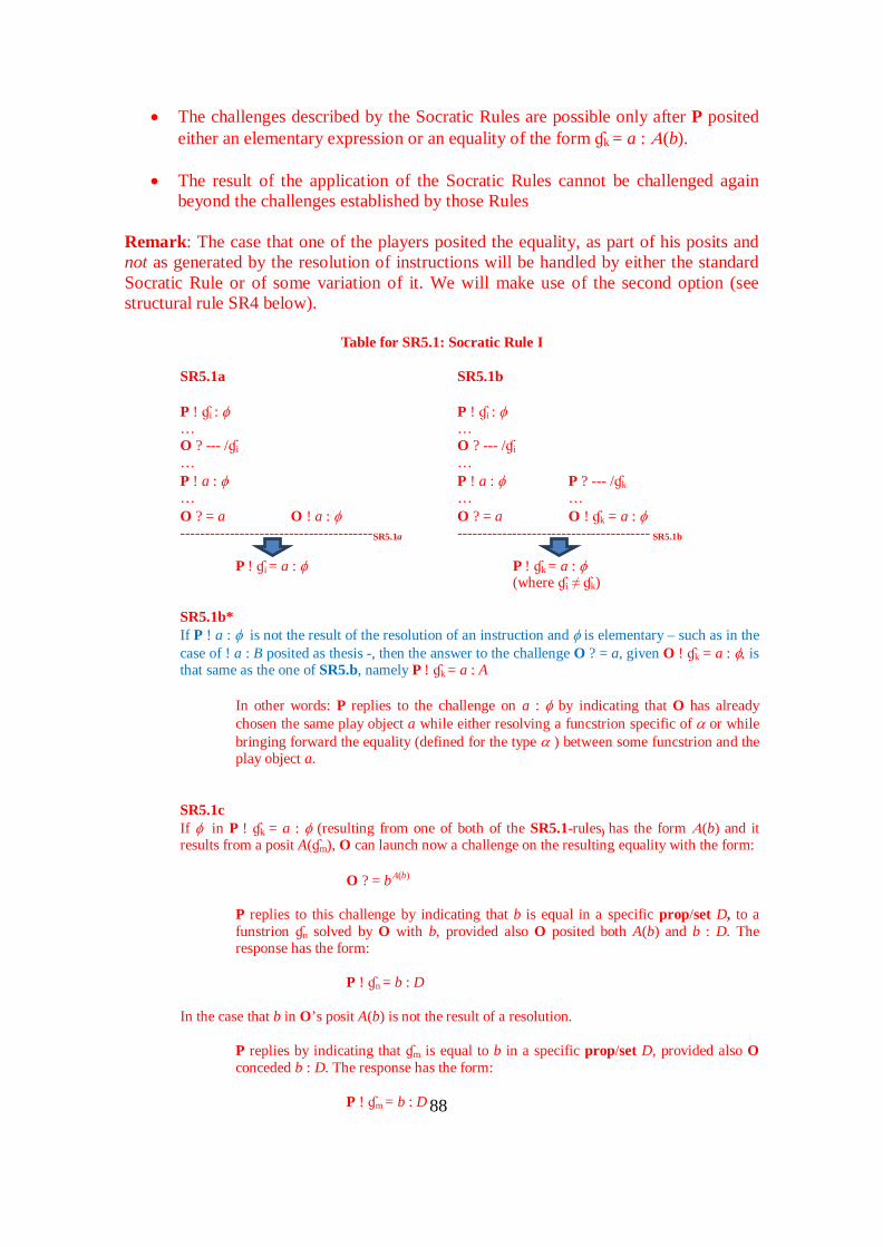
88

• The challenges described by the Socratic Rules are possible only after P posited either an elementary expression or an equality of the form ɠk = a : Α(b).

• The result of the application of the Socratic Rules cannot be challenged again

beyond the challenges established by those Rules Remark: The case that one of the players posited the equality, as part of his posits and not as generated by the resolution of instructions will be handled by either the standard Socratic Rule or of some variation of it. We will make use of the second option (see structural rule SR4 below).

Table for SR5.1: Socratic Rule I SR5.1a SR5.1b

P ! ɠi : φ P ! ɠi : φ … … O ? --- /ɠi O ? --- /ɠi … … P ! a : φ P ! a : φ P ? --- /ɠk … … … O ? = a O ! a : φ O ? = a O ! ɠk = a : φ

---------------------------------------SR5.1a --------------------------------------- SR5.1b P ! ɠi = a : φ P ! ɠk = a : φ

(where ɠi ≠ ɠk) SR5.1b* If P ! a : φ is not the result of the resolution of an instruction and φ is elementary – such as in the case of ! a : B posited as thesis -, then the answer to the challenge O ? = a, given O ! ɠk = a : φ, is that same as the one of SR5.b, namely P ! ɠk = a : A

In other words: P replies to the challenge on a : φ by indicating that O has already chosen the same play object a while either resolving a funcstrion specific of α or while bringing forward the equality (defined for the type α ) between some funcstrion and the play object a.

SR5.1c If φ in P ! ɠk = a : φ (resulting from one of both of the SR5.1-rules) has the form Α(b) and it results from a posit A(ɠm), O can launch now a challenge on the resulting equality with the form:

O ? = bΑ(b) P replies to this challenge by indicating that b is equal in a specific prop/set D, to a funstrion ɠn solved by O with b, provided also O posited both A(b) and b : D. The response has the form:

P ! ɠn = b : D

In the case that b in O’s posit A(b) is not the result of a resolution.

P replies by indicating that ɠm is equal to b in a specific prop/set D, provided also O conceded b : D. The response has the form:

P ! ɠm = b : D

89

The next rule is a kind of substitution rule. It says that if two play objects are equal in D, then the substitution of them in A(x) (x : D) yields equal propositions/sets. SR5.1d If an application of the rule SR5.1c yields P ! ɠ = b : D, then, O can launch now a challenge upon this posit asking for the type of Α(b). P replies to this challenge by indicating that Α(b) is of a specific type and that O conceded this before.

P ! ɠn = b : D (by SR5.1c) P ! ɠn = b : D (by SR5.1c) … … O ! c : Α(ɠm) … … P ?…/ ɠm … O ? --- = Α(b) : type O ! A(b) : type O ? --- = Α(b) : type O ! A(ɠm) = A(b) : type -------------------------------------------- SR5.1d.1 --------------------------------------------------- SR5.1d.2

P ! A(ɠm) = A(b) : type P ! A(ɠm) = A(b) : type (where ɠn ≠ ɠm) (where ɠn ≠ ɠm)

Table for SR5.2: Socratic Rule II

General Assumption: reflexivity cases do no arise when the instruction to be resolved by P is embedded in another instruction.

Reflexivity responses of the forms P ! a = a : φ P ! A(b) = A(b) : type Result from the same kind of challenges described by the rules above, with the difference that the reply assumes that O has already chosen the same play object a while either • resolving the same funcstrion ɠi, or • while bringing forward the equality between ɠi and the play object,or • by simply positing a : φ ( A(b) : type ).

IV.2 Transmitting definitional equality and Functions Transmitting definitional equality An interesting philosophical point is that the dialogical frame provides a dynamic analysis of the distinction between the production of equality and its transmission. Indeed,

• while the production of equality is based on the fact that one player, namely P makes use of copy-cat moves in order to take advantage of the moves of his adversary,

• transmission of equality is about the commitments that one player undertakes when he brings forward a posit involving definitional equality. These commitments involve posit-substitutions and the use of reflexivity, symmetry and transitivity.

This is what the rules for transmission of equality prescribe (see tables for transmission of definitional equality I and II in the preceding chapter)

90

Functions as strategic objects In the chapter on CTT we pointed out that there are three notions of functions in CTT. Now, the case of dependent functions is very natural to the dialogical frame, particularly so at the play level: the challenger chooses and argument and the defender must carry out the corresponding substitution. Such kind of functions can occur in our framework in three occasions:

• as the play objects of hypotheticals • as the pre-defined functions called instructions • as explicit functions

However, the two notions of functions as independent objects are part of the strategic level. Indeed

• The course of values notion of a function is, in the dialogical frame a strategic object that expresses the fact that whatever play object O choses for the left instruction of the universal / implication, there is a suitable play object that P can bring forward. Moreover, as developed further on in the chapter on metalogic, the strategic object encodes all of these choices and answers that yield plays won by P and this is what we render as the lambda-abstract of a given play object.

• Similarly, an application of the lambda-abstract is a choice of the Proponent,

who, given all the pairs of question-response encoded by that abstract, choses one of them. This choice of the Proponent, yields, at the strategic level, the independent individual of the type function described in chapter II.

Next we consider the global rules taking part in the development of dialogical plays. IV. 3 The Development of a Play Structural Rules

In the present section we will deal with the second kind of dialogical rules that settle meaning, namely, the so-called structural rules or development-rules. These rules govern the way plays globally proceed and are therefore an important aspect of dialogical semantics. We will work with the following structural rules that follow from the preceding discussions and include the resolution, substitution and equality rules mentioned above. In appendix III we provide an overview of all the rules, local and structural.

SR0 (Starting rule). • The start of a formal dialogue of immanent reasoning is a move where P puts forward

the thesis. The thesis can be put forward under the condition that O commits herself with certain other expressions called initial concessions. In the latter case the thesis has the form ! α [β1, …, βn].

• O accepts the commitment by bringing forward those initial concessions ! β1, …, ! βn and by providing them with respective play objects, if they have not been specified

91

already. The Proponent must then also bring forward some suitable play object too, if it has not been specified already while positing the thesis.59

• If the set of initial concessions is empty, then we make the notational convention that

such a play starts with some play object, say, d

• If the thesis is an elementary proposition A, then P posits ! A, O responds with the challenge ?play object , (asking for the play object) P chooses a play object (possibly with some delay) (the further challenge falls under either the scope of SR4 or SR5.1b*).

• After that the players each choose a positive integer called repetition rank.

The repetition rank of a player bounds the number of challenges he can play in reaction to a same move.

SR1i (Intuitionisitic Development rule): Last Duty First. • Players move alternately. After the repetition ranks have been chosen, each move is a

challenge or a defence in reaction to a previous move and in accordance with the particle rules. Players can answer only against the last non-answered challenge by the adversary.60

SR1c (Classical Development rule). • Players move alternately. After the repetition ranks have been chosen, each move is a

challenge or a defence in reaction to a previous move and in accordance with the particle rules. Players can answer to a list of challenges in any order. 61

SR2 Formation rules for formal dialogues of immanent reasoning. • starts by challenging the thesis with the request `?prop'. The game then proceeds by

applying the formation rules up to the elementary constituents of prop / set, whereby those constituents will not be specified before the play but as a result of the development of the moves (according to the rules recorded by the rules for local meaning). After that the Opponent is free to use the other local rules insofar as the other structural rules allow it.

• If the expression occurring in the thesis is not recorded by the table for local meaning, then either it must be introduced by a nominal definition or the table for local meaning needs to be enriched with the new expression. In the former case the rules to be deployed are the ones of the definiens – this presupposes that the meaning of the definiens is displayed in the table for local meaning. 62

59 Some kind of theses require an explicit play-object, such as those that include some form of anaphoric expression. For example the premisse and conclusion of barbara

European is said of (Every Man who is French) French is said from (Every Man who is Pairisian) ----------------------------------------------------------- European is said of (Every Man who is Parisian)

requires an anaphora that identifies the play-object of which it is said that is European/French. Thus, conclusion cannot be posited unless it has the form ! p: (∀z : {x : M | P(x)}) E(L{...} (L∀(p) – this also applies to the premisses. 60 This last clause is known as the Last Duty First condition, and is the clause making dialogical games suitable for Intuitionistic Logic, hence the name of this rule. 61 This rule produces strategies for classical logic. The point is that since, different to the intuitionistic development rule, players can answer to a list of challenges in any order, it might happen that the two options of a P-defence occur in the same play – this is closely related to the classical structural rule in sequent calculus allowing more than one formula at the right of the sequent. 62 The point on nominal definitions is due to a remark of Amsten Klev. In fact, the standard way in dialogical logic is to assume that before a play starts, all the the expressions ocurring in the thesis are within the scope of the rules for local meaning. This might require extending the standard particle rules. The rule we just added, is an alternative way to deal with this. In the case of material dialogues, the deployment of the nominal definitions is described by the Socratic Rule.

92

SR3 (Resolution and substitution of instructions).63 • See tables SR3.1, S3.2 and SR.3.3 SR4 (Special Socratic Rule). • O's elementary sentences cannot be challenged.64 However, O can challenge a P-

elementary move not covered by the Socratic Rules for definitional equality (see SR.5. The challenge and correspondent defence are ruled by the following table.

Posit Challenge Defence

P ! a : A ( for elementary A)

O ? a : A P sic (n) (P indicates that O posited a : A at move n)

It is important to distinguish the Special Socratic Rule from the Socratic Rule. In the latter the play object occurring in an elementary expression is the result of resolving an instruction, this is not the case covered by this rule. SR5 (The Socratic Rule and Definitional Equality. • See tables SR5. 1, SR5.2, SR5.3

SR6 (Winning rule for plays). • For any p, a player who posits "⊥" looses the current play. Otherwise the player who

makes the last move in a dialogue wins it.65 Terminal plays and winning strategies: The definitions of plays, games and strategies are the same as those given in the section on standard dialogical games I. Let us now recall them briefly. A play for ϕ is a sequence of moves in which ϕ is the thesis posited by the Proponent and which complies with the game rules. The dialogical game for ϕ is the set of all possible plays for ϕ and its extensive form is nothing but its tree representation. Thus, every path in this tree which starts with the root is the linear representation of a play in the dialogical game at stake. We say that a play for ϕ is terminal when there is no further move allowed for the player whose turn it is to play. A strategy for player X in a given dialogical game is a function which assigns a legal X-move to each non terminal play where it is X's turn to move. When the strategy is a winning strategy for X, the application of the function turns those plays into terminal plays won by X. It is common practice to consider in an equivalent way an X-strategy s as the set of terminal plays resulting when X plays according to s. The extensive form of s is then the tree representation of that set. For more explanations on these notions, see Clerbout (2014c). The equivalence result between dialogical games and CTT is established by procedures of translation between extensive forms of winning strategies.

Let us discuss some special examples. IV.4 Two special examples

63 For a detailed discussion see section III.2.3 above. 64 In fact, as discussed in the sections on propositional identity (chapter ) though posits of the form a : A might not be challenged, P can request O to fulfill some further specific commitments related to identity-statements generated by these kind of posits. 65 The Player X who posits ⊥ , allows the antagonist Y to answer give-up-X to the challenge to any play-object for any proposition. The structural rule above shortens the development of a play by cutting it off, as soon as ⊥ has been brought forward.

93

Since the target is here to deploy the logical features of a given proposition we will focus on those plays relevant for building a winning strategy (the precise method on how to build a winning strategy will be displayed in sections IV.5 and IV.6). Moreover, for the sake of perspicuity, we will not separate all the possible branches. More precisely, as discussed while presenting the procedure to generate a winning strategy, O’s defense of a universal requires two plays, one counterattacking the challenge and a second one, answering to the challenge; but in the present context we will develop both responses in the same play. However, we will present two versions of the same play, one without and one with the explicit rendering of the emergence of definitional equality by the deployment of the Socratic Rule. IV.4.1 One play on the axiom of choice

Since the work of Martin-Löf (1984, pp. 50-51) the intensional formulation of the Axiom of Choice is evident in the sense that is logically valid – in appendix II we render Martin-Löf's outline of its demonstration. As pointed out by Bell (2009, p. 206) its logical validity entitles us to call it an axiom rather than a postulate (as in its classical or extensional version, that is not valid). 66 Jovanovic (2013) showed that, if we were to make explicit the domain and codomain of the function at the object language level, Hintikka’s (2001) own formulation amounts to the following one – which is the intensional version of the AC as brought forward by Martin-Lof:

(∀x : A) (∃y : B(x)) C(x, y) ⊃ (∃f : (∀x : A) B(x)) (∀x : A) C(x ,f(x))

Hintikka (2001) stressed, and rightly so, that the validity of AC follows naturally in a game-theoretical setting. However, he rejected at the same time the underlying constructivist logic that could have supported his claims. In fact, as Jovanovic (2013, 2015) discusses, Hintikka (1996a, 2001) aims at rendering the meaning of AC via a non-constructive semantics based on IF-logic, that has no first-order proof theory. 67 From the dialogical point of view the point is that P can copy-cat O’s choice for y in the antecedent for his defence of f(x) in the consequent since both are equal objects of type B(x), for any x : A. Thus, a winning strategy for the implication follows simply from the meaning of the antecedent. This meaning is defined by the dependences generated by the interaction of choices involving the embedding of an existential quantifier in a universal one. Thus, from the dialogical perspective the validity AC follows from a series of equalities that can be established between moves of the antecedent and moves of the consequent. As already mentioned, in the following, we will only deploy those plays that constitute the so-called core of the strategy (that is, of the dialogical proof), and that are triggered by the Opponent's options at move 9 when challenging the existential posited by the Proponent at move 8 – we highlighted this move in the play. Since O’s repetition rank is 1, she cannot perform both challenges within one and the same play, hence the distinction between the following two plays. 66 Extensionality can be also rendered, provided uniqueness of the function, for a dialogical reconstruction of the proof see Clerbout/Rahman (2015) – the book also contains a detailed discussion of how to transform a winnings strategy for the axiom of choice into the CTT- demonstration of it. 67 Jovanovic's (2013) work extended a remark of Sundholm during his visiting Professorship in 2012 at the University of Lille.

94

First play: Opponent’s 9th move asks for the left play object for the existential quantification on f. As already mentioned; in order to make all the steps explicit, we will produce two versions of this firs play. In the first version we will, simply apply the copy-cat move, in the second version we will deploy the Socratic Rules. First play on the Axiom of Choice without explicit equality

O P C1

C2

! C(x, y) : set [x : A, y : B(x)]

! B(x) : set [x : A]

! d : (∀x : A) (∃y : B(x)) C(x,y) ⊃ (∃f : (∀x : A) B(x)) (∀x : A) C(x, f(x))

0

1 m:= 1 n:= 2 2 3 ! L ⊃ ( d) : (∀x : A) (∃y :

B(x)) C(x, y) 0 ! R ⊃ ( d) : (∃f : (∀x : A) B(x)) (∀x : A) C(x,f(x)) 6

5 ! v : (∀x : A) (∃y : B(x)) C(x, y)

3 ? --- / L ⊃ ( d) 4

7 ? --- / R ⊃ ( d) 6 ! g : (∃f : (∀x : A) B(x)) (∀x : A) C(x, f(x)) 8 9 ?L 8 ! L∃(g) : (∀x : A) B(x) 10 11 ? --- / L∃(g) 10 ! g1 : (∀x : A) B(x) 12 13 ! L∀(g1) : A 12 ! R∀(g1) : B(a) 26 15 ! a : A 13 ? --- / L∀(g1) 14 19 ! R∀(v) : (∃y : B(a)) C(a,

y) 5 ! L∀(v) : A 16

17 ! --- / L∀(v) ? 16 ! a : A 18 21 ! (v2) : (∃y : B(a)) C(a,

y) 19 ? --- / R∀(v) 20

23 ! L∃(v2) : B(a) 21 ?L 22 25 ! t1 : B(a) 23 ? --- / L∃(v2) 24 27 ? --- / R∀(g1) 26 ! t1 : B(a) 28

Description: Move 3: After P sets the thesis and the repetition ranks have been established, O launches an attack on the material implication. Move 4: P launches a counterattack and asks for the play object that corresponds to L ⊃ (p). Moves 5, 6: O responds to the challenge of 4. P posits the right component of the material implication. Moves 7, 8: O asks for the play object that corresponds to R ⊃ (d). P responds to the challenge by choosing the complex play object g, composed by the play objects g1 that substitutes the variable f and g2 the play object for the right component of the existential. Move 9: O has here the choice to ask for the left or the right component of the existential. The present play describes the development of the play triggered by the left choice. Moves 10-26: follow from a straightforward application of the dialogical rules. Move 26 is an answer to move 13, which P makes after he gathered the information that will allow him to apply the Socratic Rule. Move 27-28: O asks for the play object that corresponds to the instruction posited by P at move 26 and P answers and wins by applying the Socratic Rule to O’s move 25. Notice that 28 this is not a case of function substitution: it is simply the resolution of an instruction.

First play on the Axiom of Choice and the emergence of equality

O P C1

C2

! C(x, y) : set [x : A, y : B(x)]

! B(x) : set [x : A]

! d : (∀x : A) (∃y : B(x)) C(x,y) ⊃ (∃f : (∀x : A) B(x)) (∀x : A) C(x, f(x))

0

1 m:= 1 n:= 2 2 3 ! L ⊃ ( d) : (∀x : A) (∃y : 0 ! R ⊃ ( d) : (∃f : (∀x : A) B(x)) (∀x : A) 6

95

B(x)) C(x, y) C(x,f(x)) 5 ! v : (∀x : A) (∃y : B(x))

C(x, y) 3 ? --- / L ⊃ ( d) 4

7 ? --- / R ⊃ ( d) 6 ! g : (∃f : (∀x : A) B(x)) (∀x : A) C(x, f(x)) 8 9 ?L 8 ! L∃(g) : (∀x : A) B(x) 10 11 ? --- / L∃(g) 10 ! g1 : (∀x : A) B(x) 12 13 ! L∀(g1) : A 12 ! R∀(g1) : B(a) 28 15 ! a : A 13 ? --- / L∀(g1) 14 21 ! R∀(v) : (∃y : B(a)) C(a,

y) 5 ! L∀(v) : A 16

17 ? --- / L∀(v) 16 ! a : A 18 19 ? = a 18 ! L∀(g1) = a : A 20 23 ! (v2) : (∃y : B(a)) C(a,

y) 21 ? --- / R∀(v) 22

25 ! L∃(v2) : B(a) 23 ?L 24 27 ! t1 : B(a) 23 ? --- / L∃(v2) 26 29 ? --- / R∀(g1) 28 ! t1 : B(a) 30 31 ? = t1 30 ! L∃(v2) = t1 : B(a) 32 33 ? = aB(a) 32 ! L∀(g1) = a : A 34 35 ? = B(a) : type 34 ! B(L∀(g1)) = B(a) : set 38 37 ! B(a) : set C2-subst ! a : A 36

Description: We highlighted the relevant moves that stem from the answers to challenges to elementary posits and its constituents. The point of move 19 is that O asks P to justify the elementary posit a : A. P answers to the challenge by indicating that the a he has chosen is the same play object that O has chosen (while substituting the instruction L∀(g1)) for the same proposition. Moves 31 to 36 add some twist. P must not only respond to the challenge to his move 30 with the equalities L∃(v2) = t1 : B(a) (move 32) and L∀(g1) = a : A (move 34). He must also justify the proposition B(a) that resulted from the propositional function B(x) [x : A]. This is what P does in the last moves of the play: He indicates that the chosen a yields by substitution on the propositional function the same proposition brought forward by O when he substituted the instruction in move 15.

Second play on the Axiom of Choice without explicit equality: Opponent’s 9th move asks for the right play object for the existential quantification on f

O P C1

C2

! C(x, y) : set [x : A, y : B(x)]

! B(x) : set [x : A]

! d : (∀x : A) (∃y : B(x)) C(x,y) ⊃ (∃f : (∀x : A) B(x)) (∀x : A) C(x, f(x))

0

1 m:= 1 n:= 2 2 3 ! L ⊃ ( d) : (∀x : A) (∃y :

B(x)) C(x, y) 0 ! R ⊃ ( d) : (∃f : (∀x : A) B(x)) (∀x : A) C(x,f(x)) 6

5 ! v : (∀x : A) (∃y : B(x)) C(x, y)

3 ? --- / L ⊃ ( d) 4

7 ? --- / R ⊃ ( d) 6 ! g : (∃f : (∀x : A) B(x)) (∀x : A) C(x, f(x)) 8 9 ?R 8 ! R∃(g) : (∀x : A) C(x, L∃(g)(x) 10

11 ? --- L∃(g) 10 ! R∃(g) : (∀x : A) C(x, g1(x)) 12 13 / R∃(g) 12 ! g2 : (∀x : A) C(x, g1(x)) 14 15 ! L∀(g2) : A 14 ! R∀(g2) : C(x, g1(a)) 34 17 ! a : A 15 ? --- / L∀(g2) 16 21 ! R∀(v) : (∃y : B(a)) C(a, y) 5 ! L∀(v) : A 18

96

19 --- / L∀(v) ? 18 ! a : A 20 23 ! (v2) : (∃y : B(a)) C(a ,y) 21 ? --- / R∀(v) 22 25 ! L∃(v2) : B(a) 23 ?L 24 27 ! t1 : B(a) 25 ? --- / L∃(v2) 26 29 ! R∃(v2) : C(a, L∃(v2)) 23 ?R 28 31 ! R∃(v2) : C(a, t1) 29 ? t1 / L∃(v2) 30 33 ! t2 : C(a, t1) 31 ? --- / R∃(v2) 32 35 ? --- / R∀(g2) 34 ! t2 : C(a, g1(a)) 36 37 ? --- / g1(a) 38 ! t2 : C(a, t1) 38

Remarks. The play should be easy to follow, however it is not very perspicuous. Particularly move 38, that is based on the equality of C(a, g1(a)) and C(a, L∃(v2)). The next play makes this equality explicit

Second play on the Axiom of Choice and the emergence of equality

O P C1

C2

! C(x, y) : set [x : A, y : B(x)] ! B(x) : set [x : A]

! d : (∀x : A) (∃y : B(x)) C(x,y)⊃(∃ f : (∀x : A) B(x)) (∀x : A) C(x, f(x))

0

1 m:= 1 n:= 2 2 3 ! L ⊃ (p) : (∀x : A) (∃y :

B(x)) C(x, y) 0 ! R ⊃ (d) : (∃ f : (∀x : A) B(x)) (∀x : A)

C(x,f(x)) 6

5 ! v : (∀x : A) (∃y : B(x)) C(x, y)

3 ? --- / L ⊃ (d) 4

7 ? --- / R ⊃ (d) 6 ! g : (∃ f : (∀x : A) B(x)) (∀x : A) C(x, f(x)) 8 9 ?R 8 ! R∃(g) : (∀x : A) C(x, L∃(g)(x) 10

11 ? --- / L∃(g) 10 ! R∃(g) : (∀x : A) C(x, g1(x)) 12 13 ? --- / R∃(g) 12 ! g2 : (∀x : A) C(x, g1(x)) 14 15 ! L∀(g2) : A 14 ! R∀(g2) : C(x, g1(a)) 36 17 ! a : A 15 ? --- / L∀(g2) 16 23 ! R∀(v) : (∃y : B(a)) C(a, y) 5 ! L∀(v) : A 18 19 ? --- / L∀(v) 18 ! a : A 20 21 ? = a 20 ! L∀(g2) = a : A 22 25 ! (v2) : (∃y : B(a)) C(a ,y) 23 ? --- / R∀(v) 24 27 ! L∃(v2) : B(a) 25 ?L 26 29 ! t1 : B(a) 27 ? --- / L∃(v2) 28 31 ! R∃(v2) : C(a, L∃(v2)) 25 ?R 30 33 ! R∃(v2) : C(a, t1) 31 ? t1 / L∃(v2) 32 35 ! t2 : C(a, t1) 31 ? --- / R∃(v2) 34 37 ? --- / R∀(g2) 36 ! t2 : C(a, g1(a)) 38 39 ? --- / g1(a) 38 ! t2 : C(a, t1) 40

41 ? = t2 40 ! R∃(v2) = t2 : C(a, t1) 42 43 ? = aC(a, t1) 42 L∃(v2) = t1 : B(a) 44 45 ? = C(a, t1) : type 44 ! C(a, L∃(v2)) = C(a, t1) : set 46

Description: Move 3: After setting the thesis and establishing the repetition ranks O launches an attack on material implication. Move 4: P launches a counterattack and asks for the play object that corresponds to L ⊃ (p). Moves 5, 6: O responds to the challenge of 4. P posits the right component of the material implication. Moves 7, 8: O asks for the play object that corresponds to R ⊃ (p). P responds to the challenge by choosing the complex play object g , composed by the play objects g1 that substitutes the variable f and g2 the play object for the right component of the existential. Move 9: O has here the choice to ask for the left or the right component of the existential. The present play describes the development of the play triggered by the right choice.

97

The conceptually interesting moves have been highlighted, namely: Move 22, where P backs move 20 with a definitional equality based on O's own choices. Moves 42, 44 and 46 where P backs his choices with the equality C(a, L∃(v2)) = C(a, t1

IV.4.2 Aristotle’s Syllogism In recent researches Marion / Rückert (2016) have shown that Aristotle’s notion of quantifiers as presented in the Topics (Θ, 2, 157a34-157b2; in Aristotle (1984)) are based on a dialogical frame and more precisely, that the Aristotelian meaning of the universal quantifier is based on the Socratic Rule (Marion / Rückert (2015)).68 The authors even suggest that the CTT frame provides the means to render a formal reconstruction of the syllogistic forms close to the original ones. Indeed, notice that the form of the universal quantification, namely: (∀x : D) A(x), and the one of the existential, that is: (∃x : D) A(x), share in the CTT-framework the same conditions for their formation rule and that yields a uniform logical form, that can be certainly understood as

Subject – Domain of Quantification Predicate defined over the Subject – propositional function defined upon the domain.

Thus, the form of every assertion that constitutes a syllogism is composed by two parts:

1. the subject or D domain of which something is said, and 2. the predicative part: the predicate that is said to apply to the domain. This

presupposes that the predicate A(…) can be (partially or totally) applied to the kind of things contained in the domain D : set , that is A(x) : prop (x : D)

Moreover, one way to put their point is that the Aristotelean meaning of universal quantifier associates the form (∀x : D) A(x) with the dialectical notion of choice. If we follow that path, the purported postulation of arbitrary objects as standing for letters do not arise.69 Aristotle's use of a letter introduced in the course of a demonstration do not need to be interpreted either as standing for an arbitrary object,70 or for a specific object, "only we do not know which"71. According to the dialogical interpretation, the introduction of such letters in the course of a demonstration involving a universal quantifier stand for a choice of the Opponent. The point is that if the demonstration is sound, the Proponent will find out, for whatever this choice might be a suitable matching such that makes his case (the Proponent's one): this is what the dialogical meaning of a function amounts to. This line of interpretation joins Robin Smith's (1982, pp. 113-114) proposal to understand ecthesis in general as setting out the case to be proved by the use of letters, that stand for assumptions introduced during a demonstration – often called in proof-theory local assumptions.72 68 For such an interpretation see Crubellier (2014, pp. 11-40). 69 Ansten Klev suggested to Rahman in a personal e-mail that Martin-Löfs take on hypotheticals avoids commitments to such kind of metaphysical entities. If the dialectical interpretation of Aristotle's is correct, this also applies to the father of logic. 70 Most of the recent work in favour of the introduction of arbitrary objects stems from Fine (1985a, b). 71 Breckenridge/Magidor (2012) calls this approach, that they endorse, arbitrary reference. 72 Ebbinghaus (1963, pp. 57-58) points out as first to the dialogical interpretation of ecthesis, following a suggestion of his advisor Prof. Paul Lorenzen.

98

Aristotle's does not use echtesis for Barbara for reasons that go beyond the scope of the present study. However, we will develop a demonstration of Barbara with the aim to show the dialogical deployment of epistemic assumptions. In fact, the hypothetical feature of Aristotle's logic is present not only in the proof by echthesis but also in the hypothetical character of the so-called premisses of a syllogism. In fact, these are global-assumptions, that is, assumptions that are set out before the demonstration starts and that indicate, in the dialectical setting . . Barbara

European is said of (Every Man who is French) French is said from (Every Man who is Pairisian) ----------------------------------------------------------- European is said of (Every Man who is Parisian)

(∀z : {x : Man | French(x)} European(p(z)) true (∀z : {x : Man | Parisian(x)} French(p(z)) true ----------------------------------------------------------- (∀z : {x : Man | Parisian(x)}) European(p(z))) true Notice that p(z) indicates the dependence of the "who" expressions in the judgements. Crubellier (2008) pointed out that a crucial feature of Aristotle's "analytic project" is that the syllogism should be thought from the conclusion to the premisses. In the sense that, the point is to propose some specific conditions the analysis of which yield the components of the conclusion. Moreover, it is important to stress the point that logical generality of the inference follows from the fact that the "premisses" should be thought as initial concessions. That is as assumptions upon which the assertion of the conclusion is dependent. In the framework of CTT this yields a hypothetical. In our study-case: Conclusion:

(∀z : {x : Man | Parisian(x)}) European(p(z) true

under the condition that following is conceded Premisses/Initial Concessions:

(∀z : {x : Man | French(x)}) European(p(z) true (∀z : {x : Man | Parisian(x)}) French(p(z) true

The dialogical notation, admittedly, is more cumbersome. Moreover, as pointed out in our footnote to the structural-rule SR0, the thesis requires explicit play objects. The dialogical meaning of the conclusion should be clear: P claims that for whatever z brought forward by O, who is a Parisian human-being, he , P, can show that he/she is European, provided some specific concessions. That is, P

99

claims, that whoever is the left side of the universal, chosen by O, such that the left constitutent of the chosen z is both a human-being and a Parisian, it can be shown (under the conditions set by the premisses) that he/she (the just described left of the left side of the universal) is European. Conclusion:

! p : (∀z : {x : M | P (x)}) E(L{...} (L∀( p)

Initial Concessions:

! a : (∀z : {x : M | F(x)}) E(L{...} (L∀(a))) ! b : (∀z : {x : M | P(x)}) F(L{...} (L∀(b)))

Thesis: Conclusion dependent upon the Initial Concessions ! p : (∀z : {x : M | P (x)}) E(L{...} (L∀( p) [! a : (∀z : {x : M | F(x)}) E(L{...} (L∀(a))), ! b : (∀z : {x : M | P(x)}) F(L{...} (L∀(b)))]

At this point of the discussion the reader should be able to follow the moves without further explanations. For the sake of perspicuity we carried out the posit-substitution on the thesis within the move 0.

O P

P1 P2

! a : (∀z : {x : M | F(x)}) E(L{...} (L∀(a))), b : (∀z : {x : M | P(x)}) F(L{...} (L∀(b)))

0

! p : (∀z : {x : M | P (x)}) E(L{...} (L∀( p) [a : (∀z : {x : M | F(x)}) E(L{...} (L∀(a))), b : (∀z : {x : M

| P(x)}) F(L{...} (L∀(b)))] ! p : (∀z : {x : M | P (x)}) E(L{...} (L∀( p))

0

0.1

1 m:= 1 n:= 2 2 3 ! L∀ ( p ) : {x : M | P(x)} 0.1 ! R∀ ( p ) : E(m1) 68 5 ! p1 : {x : M | P(x)} 3 ? --- / L∀ ( p) 4 7 ! L{...} (p1) : Μ 5 ?L 6 9 ! m1 : Μ 7 ? --- / L{...} (p1) 8 11 ! R{...} (p1) : P(L{...} (p1)) 5 ?R 10 13 ! m2 : P (L{...} (p1)) ? --- / R{...} (p1) 12 15 ! m2 : P(m1) 13 ? m1 / L{...} (p1) 14 35 ! R∀ (b) : F(L{...} (L∀(b))) P2 ! L∀ (b) : {x : M | P(x)} 16 17 ? --- / L∀ (b) ? ! b1 : {x : M | P (x)} 18 19 ?L 18 ! L{...} (b1) : Μ 20 21 ? --- / L{...} (b1) 20 ! m1 : Μ 22 23 ? = m1 22 ! L{...} (p1) = m1 : Μ 24 25 ?R 18 ! R{...} (b1) : P (L{...} (b1)) 26 27 ? m1 / L{...} (b1) 26 ! R{...} (b1) : P (m1) 28 29 ? --- / R{...} (b1) 28 ! m2 : P (m1) 30 31 ? = m2 30 ! R{...} (p1) = m2 : P(m1) 32 33 ? = m1

P(m1) ! L{...} (p1) = m1 : Μ 34 37 ! R∀ (b) : F(L{...} (b1)) 35 ? b1 / L∀ (b) 36 39 ! R∀ (b) : F(m1) 37 ? m1 / L{...} (b1) 38

100

41 ! b2 : F(m1) 39 ? --- / R∀ (b) 40 61 R∀ (a) : E (L{...} (L∀(a))) P1 ! L∀ (a) : {x : M | F (x)} 42 43 ? --- / L∀ (a) 42 ! a1 : {x : M | F (x)} 44 45 ?L 44 ! L{...} (a1) : Μ 46 47 ? --- / L{...} (a1) 46 ! m1 : M 48 49 ? = m1 48 ! m1 = L{...} (p1) : Μ 50 51 ?R 44 ! R{...} (a1) : F (L{...} (a1)) 52 53 ? m1 / L{...} (a1) 52 ! R{...} (a1) : F(m1) 54 55 ? --- / R{...} (a1) 54 ! b2 : F(m1) 56 57 ? = b2 56 ! R∀ (b) = b2 : F(m1) 58 59 ? = m1

F(m1) 58 ! L{...} (b1) = m1 : M 60 63 ! R∀ (a) : E(L{...} (a1)) 61 ? a1 / L∀ (a) 62 65 ! R∀ (a) : E(m1) 63 ? m1 / L{...} (a1) 64 67 ! a2 : E(m1) 65 ? --- / R∀ (a) 66 69 ? --- / R∀ ( p) 68 ! a2 : E(m1) 70 71 ? = a2 56 ! R∀ (a) = a2 : E(m1) 72 73 ? = m1

E(m1) 72 ! L{...} (a1) = m1 : Μ 74

Remarks We highlighted here too the moves involving equality. The answer of move 68 is some short-cut the right answer should be R∀(p) : E(L{...} (L∀(p)), instead of E(m1), however the latter is obtained by carrying out two substitutions on the former. We did not carry out the challenges of the form ? --- = F(m1) : type, ? --- = E(m1) : type, and so on, that we leave them to the reader.

IV. 5 Generating dialogical demonstrations out of plays

We have explained that the view of propositions as sets of winning strategies overlooks the level of plays and that an account more faithful to the dialogical approach to meaning is that of propositions as sets of play objects. But play objects are not the dialogical counterparts of CTT proof-objects, and thus are not enough to establish the connection between the dialogical and the CTT approach. The local rules of our games – that is, the formation rules together with the particle rules – exhibit some resemblances to the CTT rules, especially if we read the dialogical rules backwards. But in spite of the resemblances, play objects are in fact very different from CTT proof-objects – recall our discussion in III.3.1. Thus, it is clear that the connection between our games and CTT is not to be found at the level of plays. In fact it is well known that the connection between dialogues and proofs is to be found at the level of strategies. More precisely, demonstrations of Natural deduction in general and of CTT in particular correspond within the dialogical framework to winning-strategies for P. Nicolas Clerbout (2014a,b,c) showed how to extract winning-strategies for P out of the extensive form of strategies, and he developed the corresponding-proof. Clerbout / Rahman(2015) extended the result to the CTT-demonstrations.73. In a further section we will adapt the transformation procedure to the present version of the dialogical approach to CTT. However, though the transformation-method provides a clear insight of the metalogic of the dialogical frame, it is quite cumbersome for performing actual demonstrations. This motivates to develop an heuristic method that parelells the one that delivers the core of a winning-strategy for standard dialogical logic.

IV.5.1 Developing a dialogical demonstration

73 For other publications on the development of such kind of algorithms see Felscher (1985), Keiff (2007), Rahman/Tulenheimo (2009), Rahman/Clerbout/Keiff (2009) and Cardascia (2016). In fact Keiff (2007) was the first on developing such method for standard dialgoical logic.

101

• Using some metalogical results from the previous literature

1. Repetition rank

a. We assume that the number of repetition rank for O is 1.74 b. As for the Proponent’s rank allows P to win the first play. After the first

play there is a device in procedure that allows P to choose once the repetition rank for a new play.75

We also assume that

2. when O has to choose play object she will always choose a new one.76 3. when O can challenge a move where P has several defensive options, O will

launch the challenge before carrying out other moves. Moreover, in general O will challenge instructions (if there are any) before carrying out other moves.77

4. A direct consequence of preceeding point is that in the case that P challenges a material implication or a universal, O will first counter-attack the instruction L⊃ / L∀ before responding to the challenge.

• O-Decisions

Suppose then that we have a play ℘n won by P where O played according to the assumptions mentioned above.

Preliminaries. We say that O takes a decision in ℘1 in the following cases:

i. She challenges a conjunction or an existential: the decision involves choosing which side to ask for.

ii. She defends a disjunction: the decision involves choosing one of the sides of the disjunction

iii. She defends an implication, the decision involves choosing either defending or launching a counter-attack.

iv. She defends an existential: the decision involves choosing a (new) constant.

• We say that a decision does not use up the available options in the play when,

because of rank 1, O decided for one of the two choices and the second decision has not been taken before. The second choice is the one that remains unused.

74 The point is that, since O is not restricted by the copy-cat rule in any of its forms (including the Socratic Rule), she can always choose the move that is the best for her own interests – and as implemented in the method above, even if in a play she makes a bad choice, she can correct it in a new play. Thus, rank 1 is sufficient. 75 Finding the precise P-rank for the thesis at stake is part of the objectives of the development of a demonstration 76 The reason is pretty straight-forward: it is the best possible choice for O. Indeed, since P is restricted by the Copy-cat rule, he needs to rely on O's choices in order to apply a copy-cat move. In such a context, the only way to (try to) block the use of the copy-cat move is by choosing always a new play-object, whenever a choice is possible. 77 The reason is similar to the previous one: it is better for O to force P to makes his choice as soon as possible.

102

• We say that a decision used up the available options iff this decision results from taking one of the two available decisions, while the other decision has already been taken.

• Moreover, we say that a move M depends on the move M' if there is a chain of

applications of game (particle) rules that leads from M' to M.

• We use the following notational convention for the last decision– bottom up in the relation to the flow of the moves – taken by O in a play m such that this decision does not use up all of the two available options: We speak of left-decision in the case that

O decides to defend the left side of a disjunction O decides to challenge the left side of a conjunction/existential (while defending an implication) O decides for a counterattack-decision.

We speak of right-decision in the case that

O decides to defend the right side of a disjunction O decides to challenge the right side of a conjunction/existential (while defending an implication) O decides for a defence-decision.

At the right, of a move where a decision has been taken for a disjunction or a conjunction/existential we write one of the following expressions: either [δn, …] or […δn]:

[δn, …] indicates that the left decision has been taken in play 3 – whereas the right option has not been yet chosen, […,δn] indicates similar for the right decision

The under-script m indicates the number of the play in which the decision δ has been taken. Thus, [δ3, …] indicates that the left decision has been taken in play 3 – whereas the right option has not been yet chosen, Furthermore, [δm, δn] indicates that both of the available choices have been used up such that the first choice has been taken in play m and the second choice in play n.

When O takes a decision for an implication/universal in the play ℘n, she can open two new subplays ℘n.L and ℘n.R, one after the other such that

℘n.L indicates the play were O decides to counterattack. ℘n.R indicates the play were O decides to defend.

Each of the subplays, starts with the move that responds to the challenge and this after the instructions involved in the challenged have been solved by P. So if the implication/universal was challenged in move n of play ℘n , then both ℘n.L and ℘n.R start with move n+1. The first move of the play ℘n.R, is the defence to the challenge. The challenge itself will be rewritten but, because it has been already counterattacked in ℘n.L, and

103

because of rank 1, it cannot be counterattacked in ℘n.L. Notice that O’s response in ℘n.R might allow P to make a move in the upper play ℘n. In such a case, the move imported into the upper play will be provided with an indication of its origin, (e.g. 12, ℘n.R). • ℘n is P-terminal iff each of the paths that start with the thesis and continue by

℘n.L and ℘n.R (including further possible subplays) are P-terminal

• ℘n is O-terminal iff one of the paths is. Remark: The procedure prescribes to start with the subplay involving the counterattack. Once the counterattack of the antecedent has been launched, the repetition rank 1 has been used-up. Thus, in the second subplay involving the defence, a challenge to the antecedent of the implication/universal is no more available. This shows that, that the two sub-plays are only a graphical device to present both options within the same (main) play. 78 The notation [δm, δn] indicates that both of the available choices for a conjunction/existential or a disjunction have been used up such that the first choice has been taken in play m and the second choice in play n. Notice that we will not record the decission-indication for the two branches triggered by O’s defence of an implication. This can be read of by the notation for sub-plays ℘n.L and ℘n.R. We say that that both of the available choices for an implication/universal has been used up if both of the subplays have been opened.

Procedure. 0. The process starts with a P-terminal play ℘1. We assume that the

number of repetition rank for O is 1. The Proponent’s rank allows P to win the first play.

1. If there is no (remaining) unused decision to be taken by O in ℘n then go to step 4. Otherwise go to the next step.

2. Take the last (bottom up in the relation to the flow of the moves) not yet used up decision taken by O in ℘n (label it [δn, …] or [δn, …], if it has not been labelled yet) and, depending on the case, apply one of the steps described below to open a new play. Repeat them until all the decisions have been used up and go then to Step 3. When a new play is opened P has the chance to change the repetition-rank once. 2.1. If δn is a challenge against a conjunction/existential, then open a new play ℘m=n+1 with a challenge to the other side of the

78 In fact the opening of two subplays called in Rahman/Keiff (2004, pp. 273-275) branching-rule, has a strategic motivation not a play level one. The reason is that here we are after the development of a demonstration. It is also possible to develop a notation where both responses, counterattack and defence are in the same play, but this comes with a heavy notation. Moreover, in the context of the presente paper, where we deploy repetition-ranks, the rank 1 of the Opponent blocks from the branch involving the defence of the implication the problematic second counterattack upon P's-challenge (for a discussion of this problem see Rahman/Clerbout/Keiff, section 1.6 ). This shows that the subplays are really two options in the same (main-)play.

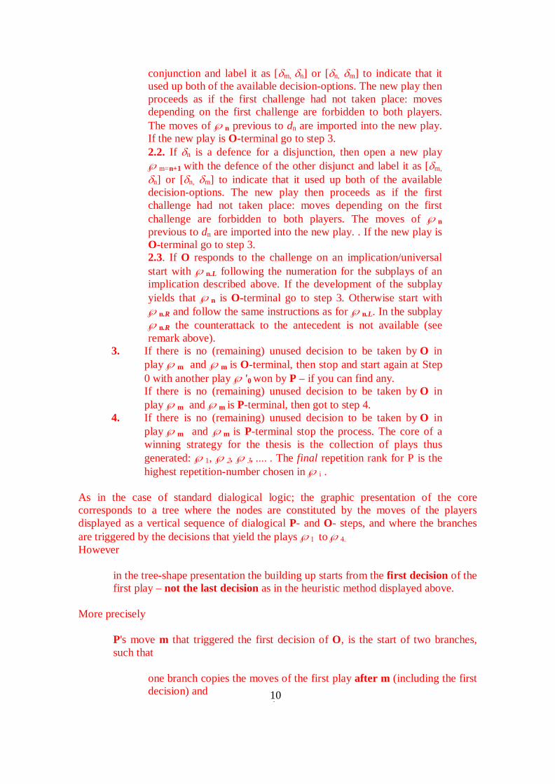
104

conjunction and label it as [δm, δn] or [δn, δm] to indicate that it used up both of the available decision-options. The new play then proceeds as if the first challenge had not taken place: moves depending on the first challenge are forbidden to both players. The moves of ℘n previous to dn are imported into the new play. If the new play is O-terminal go to step 3. 2.2. If δn is a defence for a disjunction, then open a new play ℘m=n+1 with the defence of the other disjunct and label it as [δm,

δn] or [δn, δm] to indicate that it used up both of the available decision-options. The new play then proceeds as if the first challenge had not taken place: moves depending on the first challenge are forbidden to both players. The moves of ℘n previous to dn are imported into the new play. . If the new play is O-terminal go to step 3. 2.3. If O responds to the challenge on an implication/universal start with ℘n.L following the numeration for the subplays of an implication described above. If the development of the subplay yields that ℘n is O-terminal go to step 3. Otherwise start with ℘n.R and follow the same instructions as for ℘n.L. In the subplay ℘n.R the counterattack to the antecedent is not available (see remark above).

3. If there is no (remaining) unused decision to be taken by O in play ℘m and ℘m is O-terminal, then stop and start again at Step 0 with another play ℘'0 won by P – if you can find any. If there is no (remaining) unused decision to be taken by O in play ℘m and ℘m is P-terminal, then got to step 4.

4. If there is no (remaining) unused decision to be taken by O in play ℘m and ℘m is P-terminal stop the process. The core of a winning strategy for the thesis is the collection of plays thus generated: ℘1, ℘2, ℘3, .... . The final repetition rank for P is the highest repetition-number chosen in ℘i .

As in the case of standard dialogical logic; the graphic presentation of the core corresponds to a tree where the nodes are constituted by the moves of the players displayed as a vertical sequence of dialogical P- and O- steps, and where the branches are triggered by the decisions that yield the plays ℘1 to ℘4. However

in the tree-shape presentation the building up starts from the first decision of the first play – not the last decision as in the heuristic method displayed above.

More precisely

P's move m that triggered the first decision of O, is the start of two branches, such that

one branch copies the moves of the first play after m (including the first decision) and

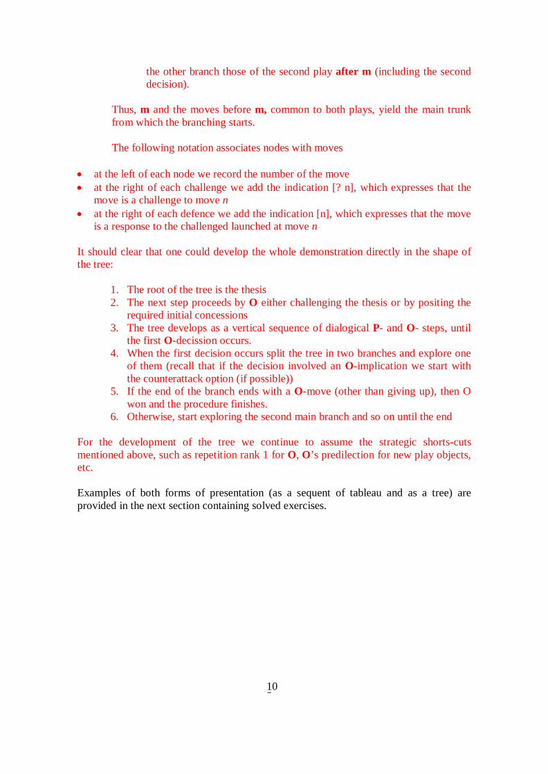
105

the other branch those of the second play after m (including the second decision).

Thus, m and the moves before m, common to both plays, yield the main trunk from which the branching starts. The following notation associates nodes with moves

• at the left of each node we record the number of the move • at the right of each challenge we add the indication [? n], which expresses that the

move is a challenge to move n • at the right of each defence we add the indication [n], which expresses that the move

is a response to the challenged launched at move n It should clear that one could develop the whole demonstration directly in the shape of the tree:

1. The root of the tree is the thesis 2. The next step proceeds by O either challenging the thesis or by positing the

required initial concessions 3. The tree develops as a vertical sequence of dialogical P- and O- steps, until

the first O-decission occurs. 4. When the first decision occurs split the tree in two branches and explore one

of them (recall that if the decision involved an O-implication we start with the counterattack option (if possible))

5. If the end of the branch ends with a O-move (other than giving up), then O won and the procedure finishes.

6. Otherwise, start exploring the second main branch and so on until the end For the development of the tree we continue to assume the strategic shorts-cuts mentioned above, such as repetition rank 1 for O, O’s predilection for new play objects, etc. Examples of both forms of presentation (as a sequent of tableau and as a tree) are provided in the next section containing solved exercises.

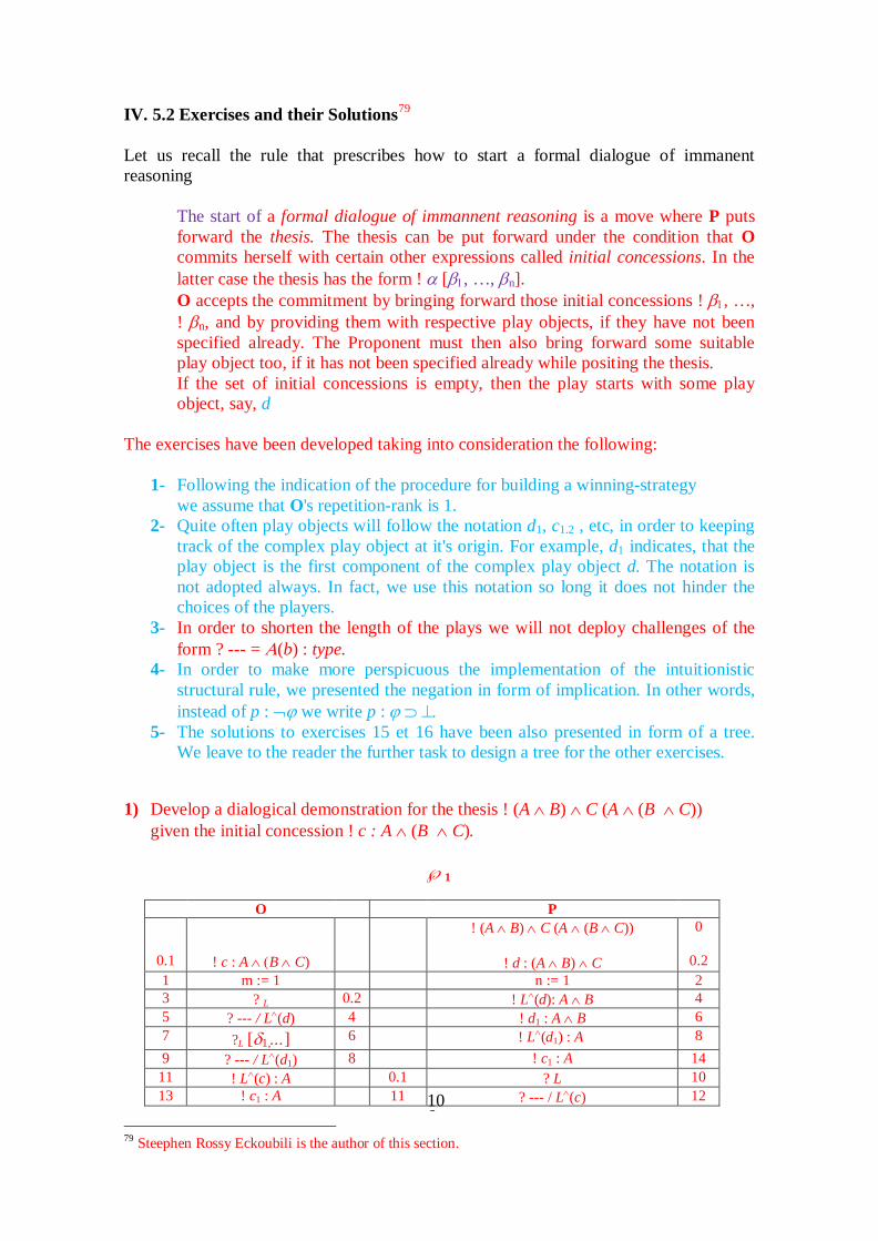
106

IV. 5.2 Exercises and their Solutions79 Let us recall the rule that prescribes how to start a formal dialogue of immanent reasoning

The start of a formal dialogue of immannent reasoning is a move where P puts forward the thesis. The thesis can be put forward under the condition that O commits herself with certain other expressions called initial concessions. In the latter case the thesis has the form ! α [β1, …, βn]. O accepts the commitment by bringing forward those initial concessions ! β1, …, ! βn, and by providing them with respective play objects, if they have not been specified already. The Proponent must then also bring forward some suitable play object too, if it has not been specified already while positing the thesis. If the set of initial concessions is empty, then the play starts with some play object, say, d

The exercises have been developed taking into consideration the following:

1- Following the indication of the procedure for building a winning-strategy

we assume that O's repetition-rank is 1. 2- Quite often play objects will follow the notation d1, c1.2 , etc, in order to keeping

track of the complex play object at it's origin. For example, d1 indicates, that the play object is the first component of the complex play object d. The notation is not adopted always. In fact, we use this notation so long it does not hinder the choices of the players.

3- In order to shorten the length of the plays we will not deploy challenges of the form ? --- = Α(b) : type.

4- In order to make more perspicuous the implementation of the intuitionistic structural rule, we presented the negation in form of implication. In other words, instead of p : ¬ϕ we write p : ϕ ⊃ ⊥.

5- The solutions to exercises 15 et 16 have been also presented in form of a tree. We leave to the reader the further task to design a tree for the other exercises.

1) Develop a dialogical demonstration for the thesis ! (A ∧ B) ∧ C (A ∧ (B ∧ C)) given the initial concession ! c : A ∧ (B ∧ C).

℘1

O P 0.1

! c : A ∧ (B ∧ C)

! (A ∧ B) ∧ C (A ∧ (B ∧ C))

! d : (A ∧ B) ∧ C

0

0.2 1 m := 1 n := 1 2 3 ? L 0.2 ! L∧(d): A ∧ B 4 5 ? --- / L∧(d) 4 ! d1 : A ∧ B 6 7 ?L [δ1,...] 6 ! L∧(d1) : A 8 9 ? --- / L∧(d1) 8 ! c1 : A 14

11 ! L∧(c) : A 0.1 ? L 10 13 ! c1 : A 11 ? --- / L∧(c) 12

79 Steephen Rossy Eckoubili is the author of this section.

107

15 ? = c1 14 ! L∧(c) = c1 : A P wins

16

℘2

O P 0.1

! c : A ∧ (B ∧ C)

! (A ∧ B) ∧ C (A ∧ (B ∧ C))

! d : (A ∧ B) ∧ C

0

0.2 1 m := 1 n := 1 2 3 ?L [δ2, ...] 0.2 ! L∧(d) : A ∧ B 4 5 ? --- / L∧(d) 4 ! d1 : A ∧ B 6 7 ?R [δ1, δ2] 6 ! R∧(d1) : B 8 9 ? --- / R∧(d1) 8 ! c2.1 : B 18

11 ! R∧(c) : B ∧ C 0.1 ?R 10 13 ! c2 : B ∧ C ? --- / R∧(c) 12 15 ! L∧(c2) : B 13 ? L 14 17 ! c2.1 : B 15 ? --- / L∧(c2) 16 19 ? = c2.1 18 ! L∧(c2) = c2.1 : B

P wins 20

℘3

O P 0.1

! c : A ∧ (B ∧ C)

! (A ∧ B) ∧ C (A ∧ (B ∧ C))

! d : (A ∧ B) ∧ C

0

0.2 1 m := 1 n := 1 2 3 ?R [δ2, δ3] 0.2 ! R∧(d) : C 4 5 ? --- / R∧(d) 4 ! c2.2 : C 14 7 ! R∧(c) : B ∧ C 0.1 ?R 6 9 ! c2 : B ∧ C 7 ? --- / R∧(c) 8

11 ! R∧(c2) : C 9 ?R 10 13 ! c2.2 : C 11 ? --- / R∧(c2) 12 15 ? = c2.2 14 ! R∧(c2) = c2.2 : C

P wins 16

2) Develop a dialogical demonstration for the thesis ! B ∨ A,

given the initial concession ! c : A ∨ B.

℘1

O P 0.1

! c : A ∨ B

! B ∨ Α (A ∨ B)

! d : B ∨ A

0

0.2 1 m := 1 n := 1 2 3 ? ∨ 0.2 ! R∨(d) : A 8 5 ! L∨(c) : A [δ1, ...] 0.1 ? ∨ 4 7 ! c1 : A 5 ? --- / L∨(c) 6 9 ? --- / R ∨(d) 8 ! c1 : A 10

108

11 ? = c1 10 ! L∨(c) = c1 : A P wins

12

℘2

O P 0.1

! c : A ∨ B

! B ∨ Α (A ∨ B)

! d : B ∨ A

0

0.2 1 m := 1 n := 1 2 3 ? ∨ 0.2 ! L∨(d) : B 8 5 ! R∨(c) : B [δ1, δ2] 0.1 ? ∨ 4 7 ! c2 : B 5 ? --- / R ∨(c) 6 9 ? --- / L∨(d) 8 ! c2 : B 10

11 ? = c2 10 ! R∨(c) = c2 : B P wins

12

3) Develop a dialogical demonstration for the thesis ! (B ∧ A) ⊃ C,

given the initial concession ! c : (A ∧ B) ⊃ C.

℘1

O P 0.1

! c : (A ∧ B) ⊃ C

! (B ∧ A) ⊃ C ((A ∧ B) ⊃ C)

! d : (B ∧ A) ⊃ C

0

0.2

1 m := 1 n := 1 2 3 ! L⊃(d) : B ∧ A 0.2 ! R⊃(d) : C 6 5 ! d1 : B ∧ A 3 ? --- / L⊃(d) 4 7 ? --- / R⊃(d) 6 ! d2 : C 12

[℘1R] 0.1 ! L⊃(c) : A ∧ B 8 9 ? --- / L⊃(c) 8 ! c1 : A ∧ B 10

℘1L1

11 ?L [δ1L1, ...] 10 ! L∧(c1) : A 12 13 ? --- / L∧(c1) 12 ! d1.2 : A 18 15 ! R∧(d1) : A 5 ?R 14 17 ! d1.2 : A 15 ? --- / R∧(d1) 16 19 ? = d1.2 18 ! R∧(d1) = d1.2 : A

P wins 20

℘1L2

11 ?R [δ1L1, δ 1L2] 10 ! R∧(d1) : B 12 13 ? --- / R∧(d1) 12 ! d1.1 : B 18 15 ! L∧(d1) : B 5 ?L 14 17 ! d1.1 : B 15 ? --- / L∧(d1) 16

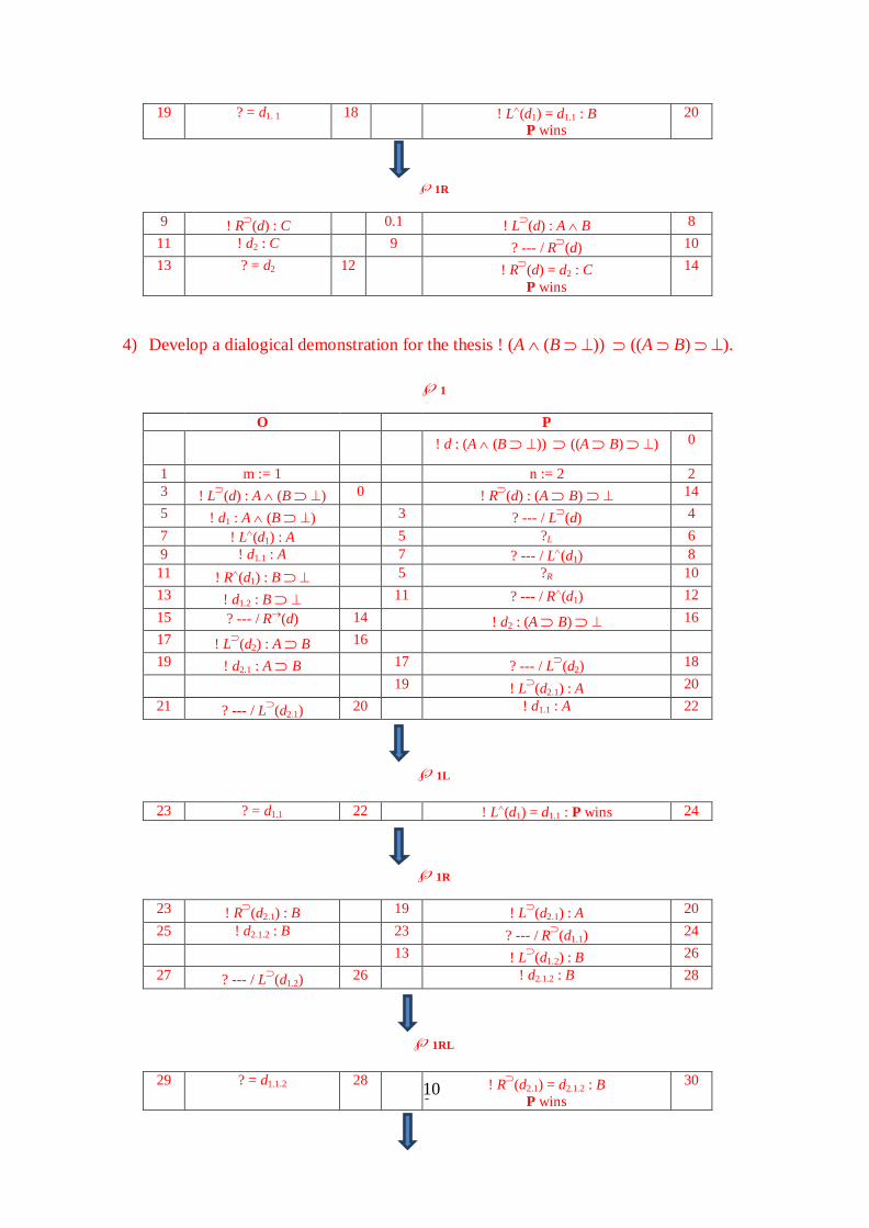
109

19 ? = d1. 1 18 ! L∧(d1) = d1.1 : B P wins

20

℘1R

9 ! R⊃(d) : C 0.1 ! L⊃(d) : A ∧ B 8 11 ! d2 : C 9 ? --- / R⊃(d) 10 13 ? = d2 12 ! R⊃(d) = d2 : C

P wins 14

4) Develop a dialogical demonstration for the thesis ! (A ∧ (B ⊃ ⊥)) ⊃ ((A ⊃ B) ⊃ ⊥).

℘1

O P

! d : (A ∧ (B ⊃ ⊥)) ⊃ ((A ⊃ B) ⊃ ⊥) 0

1 m := 1 n := 2 2 3 ! L⊃(d) : A ∧ (B ⊃ ⊥) 0 ! R⊃(d) : (A ⊃ B) ⊃ ⊥ 14 5 ! d1 : A ∧ (B ⊃ ⊥) 3 ? --- / L⊃(d) 4 7 ! L∧(d1) : A 5 ?L 6 9 ! d1.1 : A 7 ? --- / L∧(d1) 8

11 ! R∧(d1) : B ⊃ ⊥ 5 ?R 10 13 ! d1.2 : B ⊃ ⊥ 11 ? --- / R∧(d1) 12 15 ? --- / R→(d) 14 ! d2 : (A ⊃ B) ⊃ ⊥ 16 17 ! L⊃(d2) : A ⊃ B 16 19 ! d2.1 : A ⊃ B 17 ? --- / L⊃(d2) 18

19 ! L⊃(d2.1) : A 20 21 ? --- / L⊃(d2.1) 20 ! d1.1 : A 22

℘1L

23 ? = d1.1 22 ! L∧(d1) = d1.1 : P wins 24

℘1R

23 ! R⊃(d2.1) : B 19 ! L⊃(d2.1) : A 20 25 ! d2.1.2 : B 23 ? --- / R⊃(d1.1) 24

13 ! L⊃(d1.2) : B 26 27 ? --- / L⊃(d1.2) 26 ! d2.1.2 : B 28

℘1RL

29 ? = d1.1.2 28 ! R⊃(d2.1) = d2.1.2 : B P wins

30

110

℘1RR

29 ! R⊃(d1.2) : ⊥ 13 ! L⊃(d1.2) : B 26 31 ! ⊥ 29 ? --- / R⊃(d1.2)

P wins 30

5) Develop a dialogical demonstration for the thesis ! (A ∧ (A ⊃ ⊥ )) ⊃ ⊥.

℘1

O P

! d : (A ∧ (A ⊃ ⊥)) ⊃ ⊥ 0

1 m := 1 n := 2 2 3 ! L⊃(d) : A ∧ (A ⊃ ⊥) 0 5 ! d1 : A ∧ (A ⊃ ⊥) 3 ? --- / L⊃(d) 4 7 ! L⊃(d1) : A 5 ?L 6 9 ! d1.1 : A 7 ? --- / L⊃(d1) 8

11 ! R⊃(d1) : A ⊃ ⊥ 5 ?R 10 13 ! d1.2 : A ⊃ ⊥ 11 ? --- / R⊃(d1) 12

13 ! L⊃(d1.2) : A 14 15 ? --- / L⊃(d1.2) 14 ! d1.1 : A 16

℘1L

17 ? = d1.1 16 ! L⊃(d1) = d1.1 : A P wins

18

℘1R

17 ! R⊃(d1.2) : ⊥ 13 ! L⊃(d1.2) : A 14 19 ! ⊥ 17 ? --- / R⊃(d1.2)

P wins 18

6) Develop a dialogical demonstration for the thesis ! ((A⊃ ⊥) ⊃ ⊥) ⊃ Α.

℘1

O P ! d : ((A⊃ ⊥) ⊃ ⊥) ⊃ Α 0

1 m := 1 n := 2 2 3 ! L⊃(d) : (A ⊃ ⊥) ⊃ ⊥ 0.1 ! R⊃(d) : A 6 5 ! d1 : (A ⊃ ⊥) ⊃ ⊥ 3 ? --- / L⊃(d) 4 7 ? --- / R⊃(d) 6 5 ! L⊃(d1) : A ⊃ ⊥ 8 9 ? --- / L⊃(d1) 8 ! d1.1 : A ⊃ ⊥ 10

11 ! L⊃(d1.1) : A 10 13 ! d1.1.1 : A 11 ? --- / L⊃(d1.1) 12

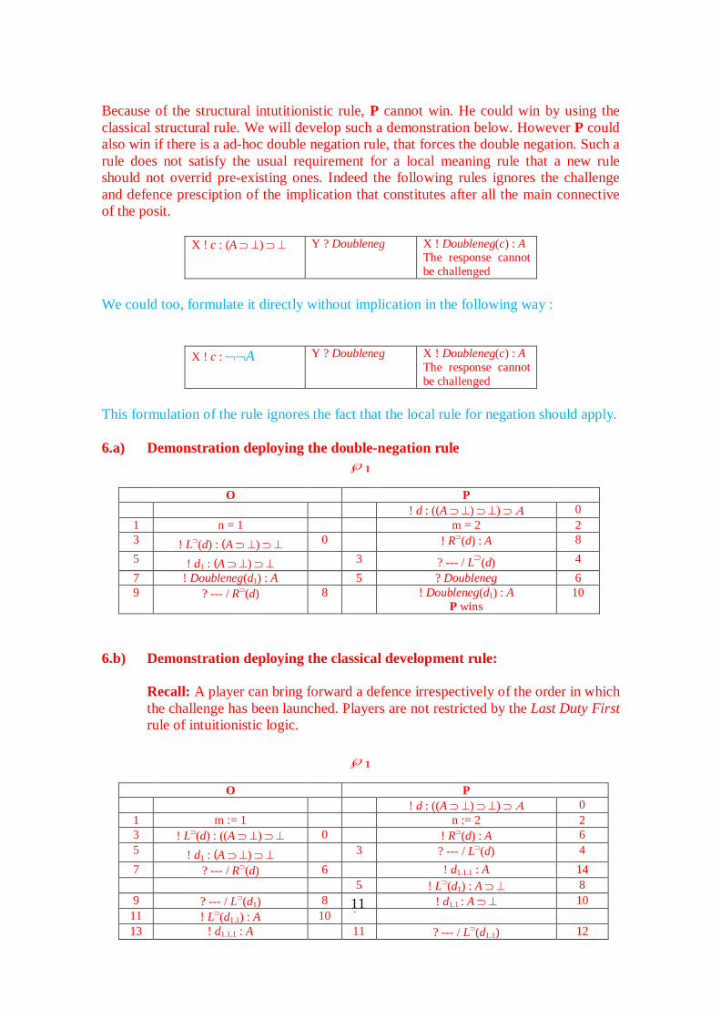
111

Because of the structural intutitionistic rule, P cannot win. He could win by using the classical structural rule. We will develop such a demonstration below. However P could also win if there is a ad-hoc double negation rule, that forces the double negation. Such a rule does not satisfy the usual requirement for a local meaning rule that a new rule should not overrid pre-existing ones. Indeed the following rules ignores the challenge and defence presciption of the implication that constitutes after all the main connective of the posit.

X ! c : (A ⊃ ⊥) ⊃ ⊥ Y ? Doubleneg X ! Doubleneg(c) : A The response cannot be challenged

We could too, formulate it directly without implication in the following way :

X ! c : ¬¬A Y ? Doubleneg X ! Doubleneg(c) : A The response cannot be challenged

This formulation of the rule ignores the fact that the local rule for negation should apply. 6.a) Demonstration deploying the double-negation rule

℘1

O P ! d : ((A ⊃ ⊥) ⊃ ⊥) ⊃ Α 0

1 n = 1 m = 2 2 3 ! L⊃(d) : (A ⊃ ⊥) ⊃ ⊥ 0 ! R⊃(d) : A 8 5 ! d1 : (A ⊃ ⊥) ⊃ ⊥ 3 ? --- / L⊃(d) 4 7 ! Doubleneg(d1) : A 5 ? Doubleneg 6 9 ? --- / R⊃(d) 8 ! Doubleneg(d1) : A

P wins 10

6.b) Demonstration deploying the classical development rule:

Recall: A player can bring forward a defence irrespectively of the order in which the challenge has been launched. Players are not restricted by the Last Duty First rule of intuitionistic logic.

℘1

O P

! d : ((A ⊃ ⊥) ⊃ ⊥) ⊃ Α 0 1 m := 1 n := 2 2 3 ! L⊃(d) : ((A ⊃ ⊥) ⊃ ⊥ 0 ! R⊃(d) : A 6 5 ! d1 : (A ⊃ ⊥) ⊃ ⊥ 3 ? --- / L⊃(d) 4 7 ? --- / R⊃(d) 6 ! d1.1.1 : A 14 5 ! L⊃(d1) : A ⊃ ⊥ 8 9 ? --- / L⊃(d1) 8 ! d1.1 : A ⊃ ⊥ 10

11 ! L⊃(d1.1) : A 10 13 ! d1.1.1 : A 11 ? --- / L⊃(d1.1) 12

112

15 ? = d1.1.1 14 ! L⊃(d1.1) = d1.1.1 : A P wins

16

7) Develop a dialogical demonstration for the thesis ! ((A ∨ (A ⊃ ⊥)) ⊃ ⊥) ⊃ ⊥.

℘1

O P ! d : ((A ∨ (A ⊃ ⊥)) ⊃ ⊥) ⊃ ⊥ 0

1 m := 1 n := 2 2 3 ! L⊃(d) : (A ∨ (A ⊃ ⊥)) ⊃ ⊥ 0

5 ! d1 : (A ∨ (A ⊃ ⊥)) ⊃ ⊥ 3 ? --- / L⊃(d) 4 5 ! L⊃(d1) : A ∨ (A ⊃ ⊥) 6

7 ? --- / L⊃(d1) 6 ! d1.1 : A ∨ (A ⊃ ⊥) 8

℘1L

9 ? ∨ 8 ! R∨(d1.1) : A ⊃ ⊥ 10

11 ? --- / R∨(d1.1) 10 ! d1.1.2 : A ⊃ ⊥ 12 13 ! L⊃(d1.1.2) : A 12 15 ! d1.1.2.1 : A 13 ? --- / L⊃(d1.1.2) 14

5 ! L⊃(d1) : A ∨ (A ⊃ ⊥) 16

17 ? --- / L⊃(d1) 16 ! d1.1 : A ∨ (A ⊃ ⊥) 18

℘1LL

19 ? ∨ 8 ! L∨(d1.1) : A 20 21 ? --- / R∨(d1.1) 10 ! d1.1.2.1 : A 22 23 ? = d1.1.2.1 ! L⊃(d1.1.2) = d1.1.2.1 : A 24

P wins

℘1LR

19 ! R⊃(d1) : ⊥ 5 ! L⊃(d1) : A ∨ (A ⊃ ⊥) 16

21 ! ⊥ 19 ? --- / R⊃(d1) P wins

20

℘1R

9 ! R⊃(d1) : ⊥ 5 ! L⊃(d1) : A ∨ (A ⊃ ⊥) 6

11 ! ⊥ 19 ? --- / R⊃(d1) P wins

10

8) Develop a dialogical classical demonstration for the thesis ! ((A ⊃ B) ⊃ A) ⊃ A

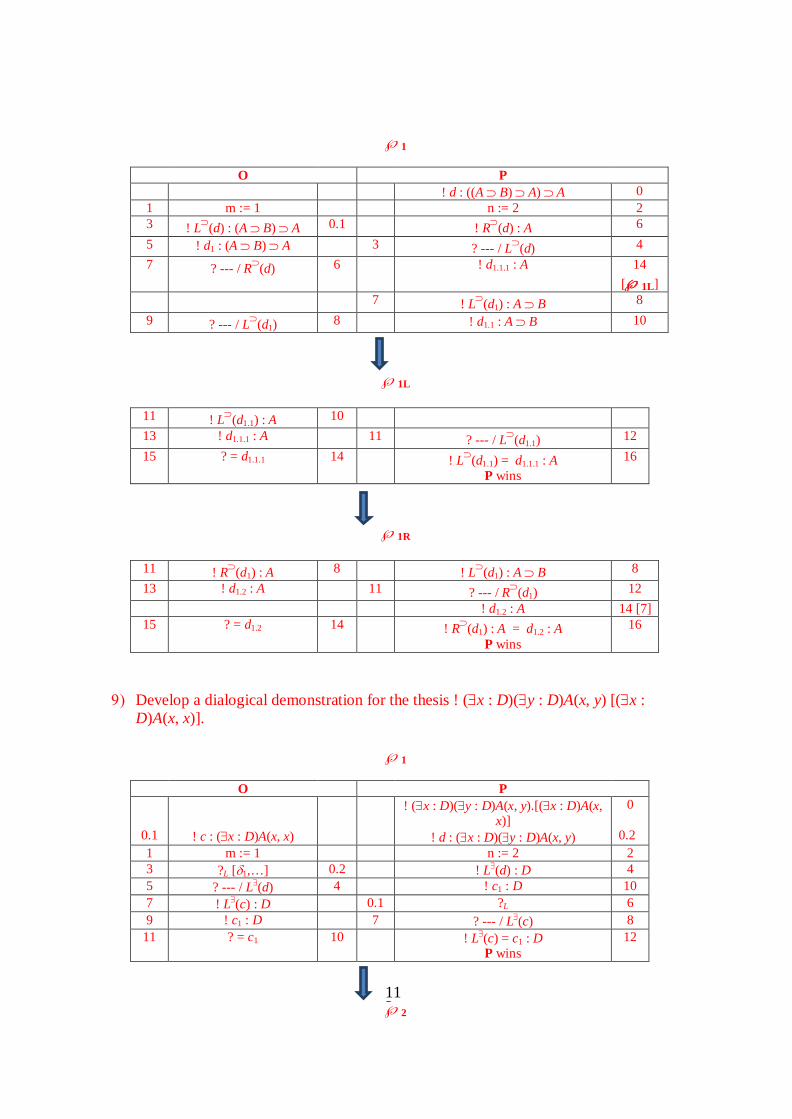
113

℘1

℘1L

℘1R

9) Develop a dialogical demonstration for the thesis ! (∃x : D)(∃y : D)A(x, y) [(∃x :

D)A(x, x)].

℘1

O P

0.1

! c : (∃x : D)A(x, x)

! (∃x : D)(∃y : D)A(x, y).[(∃x : D)A(x, x)]

! d : (∃x : D)(∃y : D)A(x, y)

0

0.2 1 m := 1 n := 2 2 3 ?L [δ1,…] 0.2 ! L∃(d) : D 4 5 ? --- / L∃(d) 4 ! c1 : D 10 7 ! L∃(c) : D 0.1 ?L 6 9 ! c1 : D 7 ? --- / L∃(c) 8

11 ? = c1 10 ! L∃(c) = c1 : D P wins

12

℘2

O P ! d : ((A ⊃ B) ⊃ A) ⊃ A 0

1 m := 1 n := 2 2 3 ! L⊃(d) : (A ⊃ B) ⊃ A 0.1 ! R⊃(d) : A 6 5 ! d1 : (A ⊃ B) ⊃ A 3 ? --- / L⊃(d) 4 7 ? --- / R⊃(d) 6 ! d1.1.1 : A 14

[℘1L] 7 ! L⊃(d1) : A ⊃ B 8 9 ? --- / L⊃(d1) 8 ! d1.1 : A ⊃ B 10

11 ! L⊃(d1.1) : A 10 13 ! d1.1.1 : A 11 ? --- / L⊃(d1.1) 12 15 ? = d1.1.1 14 ! L⊃(d1.1) = d1.1.1 : A

P wins 16

11 ! R⊃(d1) : A 8 ! L⊃(d1) : A ⊃ B 8 13 ! d1.2 : A 11 ? --- / R⊃(d1) 12

! d1.2 : A 14 [7] 15 ? = d1.2 14 ! R⊃(d1) : A = d1.2 : A

P wins 16

114

O P

0.1

! c : (∃x : D)A(x, x)

! (∃x : D)(∃y : D)A(x, y).[(∃x : D)A(x, x)]

! d : (∃x : D)(∃y : D)A(x, y)

0

0.2 1 m := 1 n : = 2 2 3 ?R [δ1,δ2] 0.2 ! R∃(d) : (∃y : D)A(L∃(d), y) 10 5 ! R∃(c) : A(L∃(c), L∃(c)) 0.1 ? R 4 7 ! c2 : A(L∃(c), L∃(c)) 5 ? --- / R∃(c) 6 9 ! c2 : A(c1, c1) 7 ? --- / L∃(c) 8

11 ? --- / R∃(d) 10 ! d2 : (∃y : D)A(L∃(d), y) 12 13 ? --- / L∃(d) 12 ! d2 : (∃y : D)A(c1, y) 14 15 ?L [δ2,…] 14 ! L∃(d2) : D 16 17 ? --- / L∃(d2) 16 ! c1 : D 22 19 ! L∃(c) : D 0.1 ?L 18 21 ! c1 : D 19 ? --- / L∃(c) 20 23 ? = c1 22 ! L∃(c) = c1 : D

P wins 24

℘3

O P

0.1

! c : (∃x : D)A(x, x)

! (∃x : D)(∃y : D)A(x, y).[(∃x : D)A(x, x)]

! d : (∃x : D)(∃y : D)A(x, y)

0

0.2 1 m := 1 n := 2 2 3 ? R [δ1,δ2] 0.2 ! R∃(d) : (∃y : D)A(L∃(d), y) 10 5 ! R∃(c) : A(L∃(c), L∃(c)) 0.1 ? R 4 7 ! c2 : A(L∃(c), L∃(c)) 5 ? --- / R∃(c) 6 9 ! c2 : A(c1, c1) 5 ? --- / L∃(c) 8

11 ? --- / R∃(d) 10 ! d2 : (∃y : D)A(L∃(d), y) 12 13 ? --- / L∃(d) 12 ! d2 : (∃y : D)A(c1, y) 14 15 ? R [δ2, δ3] 14 ! R∃(d2) : A(c1, L∃(d2)) 16 17 ? --- / L∃(d2) 16 ! R∃(d2) : A(c1, c1) 18 19 ? --- / R∃(d2) 18 ! c2 : A(c1, c1) 20 21 ? = c2 20 ! R∃(c) = c2 : A(c1, c1) 22 23 ? = c1

A(c1, c1) 22 ! L∃(c) = c1 : D P wins

24

10) Develop a dialogical demonstration for the thesis

! (∀x : D)(∀y : D)(A(x, y) ∧ A(y, x)) [(∀x : D)(∀y : D)A(x, y)]

℘1

O P 0.1

! c : (∀x : D)(∀y : D)A(x,

y)

! (∀x : D)(∀y : D)(A(x, y) ∧ A(y, x)) [(∀x : D)(∀y : D)A(x, y)]

! d : (∀x : D)(∀y : D)(A(x, y) ∧ A(y,

x))

0

0.2

1 m := 1 n := 2 2 3 ! L∀(d) : D 0.2 ! R∀(d) : (∀y :D)(A(L∀(d), y) ∧ A(y,

L∀(d))) 6

5 ! d1 : D 3 ? --- / L∀(d) 4

115

℘1L

℘1R

℘1RL

℘1RR

℘2

O P

! (∀x : D)(∀y : D)(A(x, y) ∧ A(y, x)) [(∀x : D)(∀y : D)A(x, y)]

0

7 ? --- / R∀(d) 6 ! d2 : (∀y :D)(A(L∀(d), y) ∧ A(y, L∀(d)))

8

9 ? d1 / L∀(d) 8 ! d2 : (∀y :D)(A(d1, y) ∧ A(y, d1)) 10 11 ! L∀(d2) : D 10 ! R∀(d2) : A(d1, L∀(d2)) ∧ A(L∀(d2),

d1) 14

13 ! d2.1 : D 11 ? --- / L∀(d2) 12 15 ? --- / R∀(d2) 14 ! d2.2 : A(d1, L∀(d2)) ∧ A(L∀(d2), d1) 16 17 ? d2.1 / L∀(d) 16 ! d2.2 : A(d1, d2.1) ∧ A(d2.1, d1) 18 19 ?L [δ1,…] 18 ! L∧(d2.2) : A(d1, d2.1) 20 21 ? --- / L∧(d2.2) 20 ! c2.2 : A(d1, d2.1) 38

[℘1RR] 0.1 ! L∀(c) : D 22

23 ? --- / L∀(c) 22 ! d1 : D 24

25 ? = d1 24 ! L∀(d) = d1 : D P wins

26

25 ! R∀(c) : (∀y : D)A(L∀(c), y)

0.1 ! L∀(c) : D 22

27 ! c2 : (∀y : D)A(L∀(c), y) 25 ? --- / R∀(c) 26 29 ! c2 : (∀y : D)A(d1, y) 27 ? d1 / L∀(c) 28

29 ! L∀(c2) : D 30 31 ? / L∀(c2) 30 ! d2.1 : D 32

33 ? = d2.1 32 ! L∀(d2) = d2.1 : D P wins

34

33 ! R∀(c2) : A(d1, L∀(c2)) 29 ! L∀(c2) : D 30 35 ! c2.2 : A(d1, L∀(c2)) 33 ? --- / R∀(c2) 34 37 ! c2.2 : A(d1, d2.1) 35 ? d2.1 / L∀(c2) 36 35 ? = c2.2 34 ! R∀(c2) = c2.2 : A(d1, d2.1) 38 39 ? = d1

A(d1, d2.1) 48 ! L∀(c) = d1 : D 40 41 ? = d2.1

A(d1, d2.1) 40 ! L∀(c2) = d2.1 : D P gagne

42

116

0.1 ! c : (∀x : D)(∀y : D)A(x, y)

! d : (∀x : D)(∀y : D)(A(x, y) ∧ A(y, x))

0.2

1 m := 1 n := 2 2 3 ! L∀(d) : D 0.2 ! R∀(d) : (∀y :D)(A(L∀(d), y) ∧ A(y,

L∀(d))) 6

5 ! d1 : D 3 ? --- / L∀(d) 4 7 ? --- / R∀(d) 6 ! d2 : (∀y :D)(A(L∀(d), y) ∧ A(y,

L∀(d))) 8

9 ? d1 / L∀(d) 8 ! d2 : (∀y :D)(A(d1, y) ∧ A(y, d1)) 10 11 ! L∀(d2) : D 10 ! R∀(d2) : A(d1, L∀(d2)) ∧ A(L∀(d2),

d1) 14

13 ! d2.1 : D 11 ? --- / L∀(d2) 12 15 ? --- / R∀(d2) 14 ! d2.2 : A(d1, L∀(d2)) ∧ A(L∀(d2), d1) 16 17 ? d2.1 / L∀(d) 16 ! d2.2 : A(d1, d2.1) ∧ A(d2.1, d1) 18 19 ? R [δ1, δ2] 18 ! R∧(d2.2) : A(d2.1, d1) 20 21 ? --- / R∧(d2.2) 20 ! c2.2 : A(d2.1, d1) 40

[℘2RR] 0.1 ! L∀(c) : D 22

23 ? --- / L∀(c) 22 ! d2.1 : D 24

℘2L

25 ? = d2.1 24 ! L∀(d2) = d2.1 : D P wins

26

℘2R

27 ! R∀(c) : (∀y : D)A(L∀(c), y)

0.1 ! L∀(c) : D 22

29 ! c2 : (∀y : D)A(L∀(c), y) 27 ? --- / R∀(c) 28 31 ! c2 : (∀y : D)A(d2.1, y) 29 ? d2.1 / L∀(c) 30

31 ! L∀(c2) : D 32 33 ? --- / L∀(c2) 32 ! d1 : D 34

℘2RL

35 ? = d1 34 ! L∀(d) = d1 : D P wins

36

℘2RR

35 ! R∀(c2) : A(d2.1, L∀(c2)) 31 ! L∀(c2) : D 32 37 ! c2.2 : A(d2.1, L∀(c2)) 31 ? --- / R∀(c2) 36 39 ! c2.2 : A(d2.1, d1) 37 ? d1 / L∀(c2) 38 41 ? = c2.2 40 ! R∀(c2) = c2.2 : A(d2.1, d1) 42 43 ? = d2.1

A(d2.1, d1) 42 ! L∀(c) = d2.1 : D 44 45 ? = d1

A(d2.1, d1) 44 ! L∀(c2) = d2.1 : D P gagne

46

117

11) Develop a dialogical demonstration for the thesis

! (∃x : D)B(x) ∧ (∃x : D)P(x) [B(a) ∧ P(b), a : D, b : D)]

℘1

O P

0.1 0.2 0.3

! a : D ! b : D

! c : B(a) ∧ P(b)

! (∃x : D)B(x) ∧ (∃x : D)P(x) [B(a) ∧ P(b), a : D, b : D)]

! d : (∃x : D)B(x) ∧ (∃x : D)P(x)

0

0.4 1 m := 1 n := 2 2 3 ?L 0.4 ! L∧(d) : (∃x : D)B(x) 4 5 ? --- / L∧(d) 4 ! d1 : (∃x : D)B(x) 6 7 ?L [δ1,…] 6 ! L∃(d1) : D 8 9 ? --- / L∃(d1) 8 ! a : D 10

11 ? = a 10 ! a = a : D P wins

12

℘2

O P

0.1 0.2 0.3

! a : D ! b : D

! c : B(a) ∧ P(b)

! (∃x : D)B(x) ∧ (∃x : D)P(x) [B(a) ∧ P(b), a : D, b : D)]

! d : (∃x : D)B(x) ∧ (∃x : D)P(x)

0

0.4 1 m := 1 n := 2 2 3 ?L [δ2,…] 0.4 ! L∧(d) : (∃x : D)B(x) 4 5 ? --- / L∧(d) 4 ! d1 : (∃x : D)B(x) 6 7 ? R [δ1.1, δ1.2] 6 ! R∃(d1) : B(L∃(d1)) 8 9 ? --- / L∃(d1) 8 ! R∃(d1) : B(a) 14

11 ! L∧(c) : B(a) 0.3 ?L 10 13 ! c1 : B(a) 11 ? --- / L∧(c) 12 15 ? --- / R∃(d1) 14 ! c1 : B(a) 16 17 ? = c1 16 ! L∧(c) = c1 : B(a)

P wins 18

19 ? = aB(a) 18 a = a : D 20

℘3

O P

0.1 0.2

! a : D ! b : D

! (∃x : D)B(x) ∧ (∃x : D)P(x) [B(a) ∧ P(b), a : D, b : D)]

0

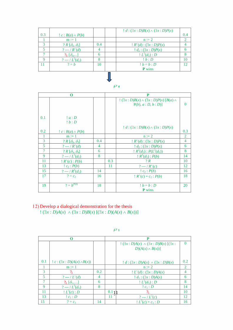
118

0.3

! c : B(a) ∧ P(b)

! d : (∃x : D)B(x) ∧ (∃x : D)P(x) 0.4

1 m := 1 n := 2 2 3 ? R [δ2, δ3] 0.4 ! R∧(d) : (∃x : D)P(x) 4 5 ? --- / R∧(d) 4 ! d2 : (∃x : D)P(x) 6 7 ?L [δ3,...] 6 ! L∃(d2) : D 8 9 ? --- / L∃(d2) 8 ! b : D 10

11 ? = b 10 ! b = b : D P wins

12

℘4

O P

0.1 0.2

! a : D ! b : D

! c : B(a) ∧ P(b)

! (∃x : D)B(x) ∧ (∃x : D)P(x) [B(a) ∧ P(b), a : D, b : D)]

! d : (∃x : D)B(x) ∧ (∃x : D)P(x)

0

0.3 1 m := 1 n := 2 2 3 ? R [δ2, δ3] 0.4 ! R∧(d) : (∃x : D)P(x) 4 5 ? --- / R∧(d) 4 ! d2 : (∃x : D)P(x) 6 7 ? R [δ3, δ4] 6 ! R∃(d2) : P(L∃(d2)) 8 9 ? --- / L∃(d2) 8 ! R∃(d2) : P(b) 14

11 ! R∧(c) : P(b) 0.3 ? R 10 13 ! c2 : P(b) 11 ? --- / R∧(c) 12 15 ? --- / R∃(d2) 14 ! c2 : P(b) 16 17 ? = c2 16 ! R∧(c) = c2 : P(b)

18

19 ? = bP(b) 18 ! b = b : D P wins

20

12) Develop a dialogical demonstration for the thesis

! (∃x : D)A(x) ∧ (∃x : D)B(x) [(∃x : D)(A(x) ∧ B(x))]

℘1

O P

0.1

! c : (∃x : D)(A(x) ∧B(x))

! (∃x : D)A(x) ∧ (∃x : D)B(x) [(∃x : D)(A(x) ∧ B(x))]

! d : (∃x : D)A(x) ∧ (∃x : D)B(x)

0

0.2 1 m := 1 n := 2 2 3 ?L 0.2 ! L∧(d) : (∃x : D)A(x) 4 5 ? --- / L∧(d) 4 ! d1 : (∃x : D)A(x) 6 7 ?L [δ1,…] 6 ! L∃(d1) : D 8 9 ? --- / L∃(d1) 8 ! c1 : D 14

11 ! L∃(c) : D 0.1 ?L 10 13 ! c1 : D 11 ? --- / L∃(c) 12

15 ? = c1 14 ! L∃(c) = c1 : D 16

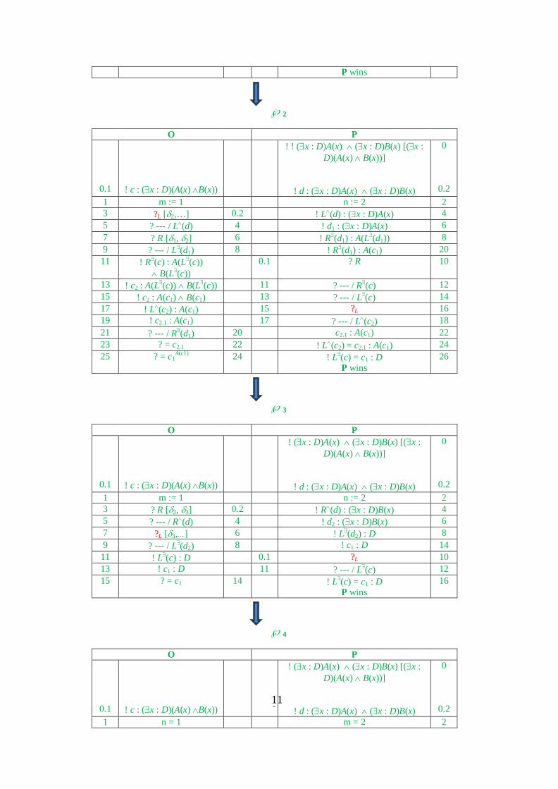
119

P wins

℘2

O P

0.1

! c : (∃x : D)(A(x) ∧B(x))

! ! (∃x : D)A(x) ∧ (∃x : D)B(x) [(∃x : D)(A(x) ∧ B(x))]

! d : (∃x : D)A(x) ∧ (∃x : D)B(x)

0

0.2 1 m := 1 n := 2 2 3 ?L [δ2,…] 0.2 ! L∧(d) : (∃x : D)A(x) 4 5 ? --- / L∧(d) 4 ! d1 : (∃x : D)A(x) 6 7 ? R [δ1, δ2] 6 ! R∃(d1) : A(L∃(d1)) 8 9 ? --- / L∃(d1) 8 ! R∃(d1) : A(c1) 20

11 ! R∃(c) : A(L∃(c)) ∧ B(L∃(c))

0.1 ? R 10

13 ! c2 : A(L∃(c)) ∧ B(L∃(c)) 11 ? --- / R∃(c) 12 15 ! c2 : A(c1) ∧ B(c1) 13 ? --- / L∃(c) 14 17 ! L∧(c2) : A(c1) 15 ?L 16 19 ! c2.1 : A(c1) 17 ? --- / L∧(c2) 18 21 ? --- / R∃(d1) 20 c2.1 : A(c1) 22 23 ? = c2.1 22 ! L∧(c2) = c2.1 : A(c1) 24 25 ? = c1

A(c1) 24 ! L∃(c) = c1 : D P wins

26

℘3

O P

0.1

! c : (∃x : D)(A(x) ∧B(x))

! (∃x : D)A(x) ∧ (∃x : D)B(x) [(∃x : D)(A(x) ∧ B(x))]

! d : (∃x : D)A(x) ∧ (∃x : D)B(x)

0

0.2 1 m := 1 n := 2 2 3 ? R [δ2, δ3] 0.2 ! R∧(d) : (∃x : D)B(x) 4 5 ? --- / R∧(d) 4 ! d2 : (∃x : D)B(x) 6 7 ?L [δ3,...] 6 ! L∃(d2) : D 8 9 ? --- / L∃(d2) 8 ! c1 : D 14

11 ! L∃(c) : D 0.1 ?L 10 13 ! c1 : D 11 ? --- / L∃(c) 12 15 ? = c1 14 ! L∃(c) = c1 : D

P wins 16

℘4

O P

0.1

! c : (∃x : D)(A(x) ∧B(x))

! (∃x : D)A(x) ∧ (∃x : D)B(x) [(∃x : D)(A(x) ∧ B(x))]

! d : (∃x : D)A(x) ∧ (∃x : D)B(x)

0

0.2 1 n = 1 m = 2 2

120

3 ? R [δ2, δ3] 0.2 ! R∧(d) : (∃x : D)B(x) 4 5 ? --- / R∧(d) 4 ! d2 : (∃x : D)B(x) 6 7 ? R [δ3, δ4] 6 ! R∃(d2) : B(L∃(d2)) 8 9 ? --- / L∃(d2) 8 ! R∃(d2) : B(c1) 20

11 ! R∃(c) : A(L∃(c)) ∧ B(L∃(c))

0.1 ? R 10

13 ! R∃(c) : A(c1) ∧ B(c1) 11 ? --- / L∃(c) 12 15 ! c2 : A(c1) ∧ B(c1) 13 ? --- / R∃(c) 14 17 ! R∧(c2) : B(c1) 15 ?R 16 19 ! c2.2 : B(c1) 17 ? --- / R∧(c2) 18 21 ? --- / R∃(d2) 20 ! c2.2 : B(c1) 22 23 ? = c2.2 22 ! R∧(c2) = c2.2 : B(c1) 24 25 ? = c1

B(c1) 24 ! L∃(c) = c1 : D P wins

26

13) Develop a dialogical demonstration for the thesis

! (∃x : D)(∃y : D)(A(x) ⊃ B(y)) [A(a) ⊃ B(b), a : D, b : D].

℘1

O P 0.1 0.2 0.3

! a : D ! b : D

! c : A(a) ⊃ B(b)

! (∃x : D)(∃y : D)(A(x) ⊃ B(y)) [A(a) ⊃ B(b), a : D, b : D]

! d : (∃x : D)(∃y : D)(A(x) ⊃ B(y))

0 0.4

1 m = 1 n = 2 2 3 ?L [δ1,…] 0.4 ! L∃(d) : D 4 5 ? --- / L∃(d) 4 ! a : D 6 7 ? = a 6 ! a = a : D

P wins 8

℘2

O P 0.1 0.2 0.3

! a : D ! b : D

! c : A(a) ⊃ B(b)

! (∃x : D)(∃y : D)(A(x) ⊃ B(y)) [A(a) ⊃ B(b), a : D, b : D]

! d : (∃x : D)(∃y : D)(A(x) ⊃ B(y))

0 0.4

1 m = 1 n = 2 2 3 ?R [δ1, δ2] 0.4 ! R∃(d) : (∃y : D)(A(L∃(d)) ⊃ B(y)) 4 5 ? --- / R∃(d) 4 ! d2 : (∃y : D)(A(L∃(d)) ⊃ B(y)) 6 7 ? --- / L∃(d) 6 ! d2 : (∃y : D)(A(a) ⊃ B(y)) 8 9 ?L [δ2,...] 8 ! L∃(d2) : D 10

11 ? --- / L∃(d2) 10 ! b : D 12 13 ? = b 12 ! b = b : D

P wins 14

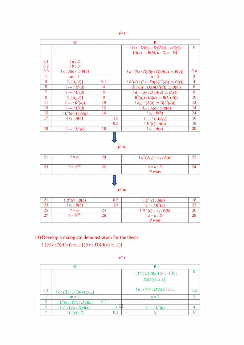
121

℘3

O P 0.1 0.2 0.3

! a : D ! b : D

! c : A(a) ⊃ B(b)

! (∃x : D)(∃y : D)(A(x) ⊃ B(y)) [A(a) ⊃ B(b), a : D, b : D]

! d : (∃x : D)(∃y : D)(A(x) ⊃ B(y))

0 0.4

1 m = 1 n = 2 2 3 ?R [δ1, δ2] 0.4 ! R∃(d) : (∃y : D)(A(L∃(d)) ⊃ B(y)) 4 5 ? --- / R∃(d) 4 ! d2 : (∃y : D)(A(L∃(d)) ⊃ B(y)) 6 7 ? --- / L∃(d) 6 ! d2 : (∃y : D)(A(a) ⊃ B(y)) 8 9 ?R [δ2, δ3] 8 ! R∃(d2) : (A(a) ⊃ B(L∃(d))) 10

11 ? --- / R∃(d2) 10 ! d2.2 : (A(a) ⊃ B(L∃(d))) 12 13 ? --- / L∃(d) 12 ! d2.2 : A(a) ⊃ B(b) 14 15 ! L⊃(d2.2) : A(a) 14 ! c2 : B(b) 24 17 ! c1 : A(a) 15 ? --- / L⊃(d2.2) 16

0.3 ! L⊃(c) : A(a) 18 19 ? --- / L⊃(c) 18 ! c1 : A(a) 20

℘3L

21 ? = c1 20 ! L⊃(d2.2) = c1 : A(a)

22

23 ? = aA(a) 22 a = a : D P wins

24

℘3R

21 ! R⊃(c) : B(b) 0.3 ! L⊃(c) : A(a) 18 23 ! c2 : B(b) 20 ? --- / R⊃(c) 22 25 ? = c2 24 ! R⊃ (c) = c2 : B(b) 26 27 ? = bA(b) 26 a = a : D

P wins 28

14) Develop a dialogical demonstration for the thesis

! ((∀x :D)A(x)) ⊃ ⊥ [(∃x : D)(A(x) ⊃ ⊥)]

℘1

O P 0.1

! c : (∃x : D)(A(x) ⊃ ⊥)

! ((∀x :D)A(x)) ⊃ ⊥ [(∃x : D)(A(x) ⊃ ⊥)]

! d : ((∀x : D)A(x)) ⊃ ⊥

0

0.2 1 m = 1 n = 2 2 3 ! L⊃(d) : (∀x : D)A(x) 0.2 5 ! d1 : (∀x : D)A(x) 3 ? --- / L⊃(d) 4 7 ! L∃(c) : D 0.1 ?L 6

122

℘1L

℘1R

℘1RL

℘1RR

15) Develop a dialogical demonstration for the thesis

! (∃x : D)(A(x) ⊃ (∀x :D)A(x)) [(∃x :D)(A(x) ⊃ ⊥) ∨ (∀x : D)A(x)]

℘1

O P 0.1 0.2

! a : D ! c : (∃x : D)(A(x) ⊃ ⊥)

∨ (∀x : D)A(x)

! (∃x : D)(A(x) ⊃ (∀x : D)A(x))

[(∃x :D)(A(x) ⊃ ⊥) ∨ (∀x : D)A(x), a : D]

! d : (∃x : D)(A(x) ⊃ (∀x : D)A(x))

0

0.3

1 m := 1 n := 2 2 3 ?L [δ1,…] 0.3 ! L∃(d) : D 4

9 ! c1 : D 7 ? --- / L∃(c) 8 5 ! L∀(d1) : D 10

11 ? --- / L∀(d1) 10 ! c1 : D 12

13 ? = c1 12 ! L∃(c) = c1 : D P gagne

14

13 ! R∀(d1) : A(L∀(d1)) 5 ! L∀(d1) : D 10 15 ! d2 : A(L∀(d1)) 13 ? --- / R∀(d1) 14 17 ! d2 : A(c1) 15 ? c1 / L∀(d1) 16 19 ! R∃(c) : A(L∃(c)) ⊃ ⊥ 0.1 ?R 18 21 ! R∃(c) : A(c1) ⊃ ⊥ 19 ? --- / L∃(c) 20 23 ! c2 : A(c1) ⊃ ⊥ 21 ? --- / R∃(c) 22

23 ! L⊃(c2) : A(c1) 24 25 ? --- / L⊃(c2) 24 ! d2 : A(c1) 26

27 ? = d2 26 ! R∀(d1) = d2 : A(c1) 28 29 ? = c1

A(c1) 28 ! L∃(c) = c1 : D P wins

30

27 ! R⊃(c2) : ⊥ 23 ! L⊃(c2) : A(c1) 24 29 ! ⊥ 27 ? --- / R⊃(c2)

P wins 28

123

5 ? --- / L∃(d) 4 ! a : D 6 7 ? = a 6 ! a = a : D

P wins 8

℘2

O P 0.1 0.2

! a : D ! c : (∃x : D)(A(x) ⊃ ⊥)

∨ (∀x : D)A(x)

! (∃x : D)(A(x) ⊃ (∀x : D)A(x))

[(∃x :D)(A(x) ⊃ ⊥) ∨ (∀x : D)A(x), a : D]

! d : (∃x : D)(A(x) ⊃ (∀x : D)A(x))

0

0.3

1 m := 1 n := 2 2 3 ?R [δ1, δ2] 0.3 ! R∃(d) : A(L∃(d)) ⊃ (∀x : D)A(x) 4 5 ? --- / R∃(d) 4 ! d2 : A(L∃(d)) ⊃ (∀x : D)A(x) 6 7 ? --- / L∃(d) 6 ! d2 : A(c1.1) ⊃ (∀x : D)A(x) 22 9 ! L∨(c) : (∃x : D)A(x)

⊃ ⊥ [δ2,...] 0.1 ? ∨ 8

11 ! c1 : (∃x : D)A(x) ⊃ ⊥ 9 ? --- / L∨(c) 10 13 ! L∃(c1) : D 11 ?L 12 15 ! c1.1 : D 13 ? --- / L∃(c1) 14 17 ! R∃(c1) : A(L∃(c1)) ⊃ ⊥ 11 ?R 16 19 ! c2 : A(L∃(c1)) ⊃ ⊥ 17 ? --- / R∃(c1) 18 21 ! c2 : A(c1.1) ⊃ ⊥ 19 ? --- / L∃(c1) 20 23 ! L⊃(d2) : A(c1.1) 22 25 ! d2.1 : A(c1.1) 23 ? --- / L⊃(d2) 24

21 ! L⊃(c2) : A(c1.1) 26 27 ? --- / L⊃(c2) 26 ! d2.1 : A(c1.1) 28

℘2L

29 ? = d2.1 28 ! L⊃(d2) = d2.1 : A(c1.1) 30 31 ? = c1.1

A(c1.1) 30 ! L∃(c1) = c1.1 : D P wins

32

℘2R

29 ! R⊃(c2) : ⊥ 21 ! L⊃(c2) : A(c1.1) 26 31 ! ⊥ 29 ? --- / L⊃(d2)

P wins 30

℘3

O P

! (∃x : D)(A(x) ⊃ (∀x : D)A(x))

[(∃x :D)(A(x) ⊃ ⊥) ∨ (∀x : D)A(x), a : D]

0

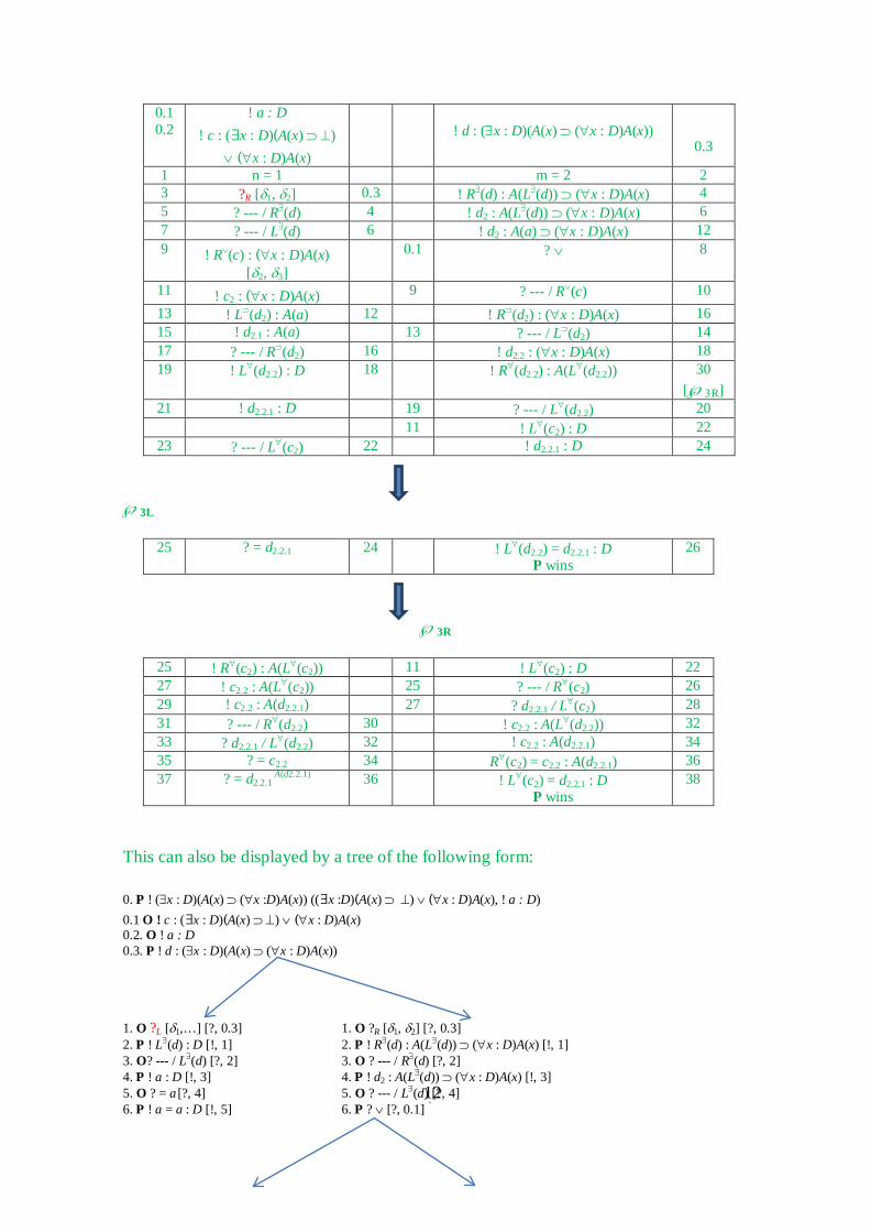
124

0.1 0.2

! a : D ! c : (∃x : D)(A(x) ⊃ ⊥)

∨ (∀x : D)A(x)

! d : (∃x : D)(A(x) ⊃ (∀x : D)A(x))

0.3

1 n = 1 m = 2 2 3 ?R [δ1, δ2] 0.3 ! R∃(d) : A(L∃(d)) ⊃ (∀x : D)A(x) 4 5 ? --- / R∃(d) 4 ! d2 : A(L∃(d)) ⊃ (∀x : D)A(x) 6 7 ? --- / L∃(d) 6 ! d2 : A(a) ⊃ (∀x : D)A(x) 12 9 ! R∨(c) : (∀x : D)A(x)

[δ2, δ3] 0.1 ? ∨ 8

11 ! c2 : (∀x : D)A(x) 9 ? --- / R∨(c) 10 13 ! L⊃(d2) : A(a) 12 ! R⊃(d2) : (∀x : D)A(x) 16 15 ! d2.1 : A(a) 13 ? --- / L⊃(d2) 14 17 ? --- / R⊃(d2) 16 ! d2.2 : (∀x : D)A(x) 18 19 ! L∀(d2.2) : D 18 ! R∀(d2.2) : A(L∀(d2.2)) 30

[℘3R] 21 ! d2.2.1 : D 19 ? --- / L∀(d2.2) 20

11 ! L∀(c2) : D 22 23 ? --- / L∀(c2) 22 ! d2.2.1 : D 24

℘3L

25 ? = d2.2.1 24 ! L∀(d2.2) = d2.2.1 : D P wins

26

℘3R

25 ! R∀(c2) : A(L∀(c2)) 11 ! L∀(c2) : D 22 27 ! c2.2 : A(L∀(c2)) 25 ? --- / R∀(c2) 26 29 ! c2.2 : A(d2.2.1) 27 ? d2.2.1 / L∀(c2) 28 31 ? --- / R∀(d2.2) 30 ! c2.2 : A(L∀(d2.2)) 32 33 ? d2.2.1 / L∀(d2.2) 32 ! c2.2 : A(d2.2.1) 34 35 ? = c2.2 34 R∀(c2) = c2.2 : A(d2.2.1) 36 37 ? = d2.2.1

A(d2.2.1) 36 ! L∀(c2) = d2.2.1 : D P wins

38

This can also be displayed by a tree of the following form: 0. P ! (∃x : D)(A(x) ⊃ (∀x :D)A(x)) ((∃x :D)(A(x) ⊃ ⊥) ∨ (∀x : D)A(x), ! a : D) 0.1 O ! c : (∃x : D)(A(x) ⊃ ⊥) ∨ (∀x : D)A(x) 0.2. O ! a : D 0.3. P ! d : (∃x : D)(A(x) ⊃ (∀x : D)A(x)) 1. O ?L [δ1,…] [?, 0.3] 1. O ?R [δ1, δ2] [?, 0.3] 2. P ! L∃(d) : D [!, 1] 2. P ! R∃(d) : A(L∃(d)) ⊃ (∀x : D)A(x) [!, 1] 3. O? --- / L∃(d) [?, 2] 3. O ? --- / R∃(d) [?, 2] 4. P ! a : D [!, 3] 4. P ! d2 : A(L∃(d)) ⊃ (∀x : D)A(x) [!, 3] 5. O ? = a [?, 4] 5. O ? --- / L∃(d) [?, 4] 6. P ! a = a : D [!, 5] 6. P ? ∨ [?, 0.1]

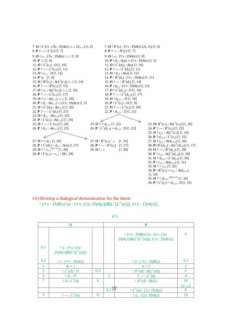
125

7. O ! L∨(c) : (∃x : D)A(x) ⊃ ⊥ [δ2,...] [!, 6] 7. O ! R∨(c) : (∀x : D)A(x) [δ2, δ3] [!, 6] 8. P ? --- / L∨(c) [?, 7] 8. P ? --- / R∨(c) [?, 7] 9. O ! c1 : (∃x : D)A(x) ⊃ ⊥ [!, 8] 9. O ! c2 : (∀x : D)A(x) [!, 8] 10. P ?L [?, 9] 10. P ! d2 : A(a) ⊃ (∀x : D)A(x) [!, 5] 11. O ! L∃(c1) : D [!, 10] 11. O ! L⊃(d2) : A(a) [?, 10] 12. P ? --- / L∃(c1) [?, 11] 12. P ? --- / L⊃(d2) [?, 11] 13. O ! c1.1 : D [!, 12] 13. O ! d2.1 : A(a) [!, 12] 14. P ?R [?, 9] 14. P ! R⊃(d2) : (∀x : D)A(x) [!, 11] 15. O ! R∃(c1) : A(L∃(c1)) ⊃ ⊥ [!, 14] 15. O ? --- / R⊃(d2) [?, 14] 16. P ? --- / R∃(c1) [?, 15] 16. P ! d2.2 : (∀x : D)A(x) [!, 15] 17. O ! c2 : A(L∃(c1)) ⊃ ⊥ [!, 16] 17. O ! L∀(d2.2) : D [?, 16] 18. P ? --- / L∃(c1) [?, 17] 18. P ? --- / L∀(d2.2) [?, 17] 19. O ! c2 : A(c1.1) ⊃ ⊥ [!, 18] 19. O ! d2.2.1 : D [!, 18] 20. P ! d2 : A(c1.1) ⊃ (∀x : D)A(x) [!, 5] 20. P ! L∀(c2) : D [?, 9] 21. O ! L⊃(d2) : A(c1.1) [?, 20] 21. O ? --- / L∀(c2) [?, 20] 22. P ? --- / L⊃(d2) [?, 21] 22. P ! d2.2.1 : D [!, 21] 23. O ! d2.1 : A(c1.1) [!, 22] 24. P ! L⊃(c2) : A(c1.1) [?, 19] 25. O ? --- / L⊃(c2) [?, 24] 23. O ? = d2.2.1 [?, 22] 23. O! R∀(c2) : A(L∀(c2)) [!, 20] 26. P ! d2.1 : A(c1.1) [!, 25] 24. P ! L∀(d2.2) = d2.2.1 : D [!, 23] 24. P ? --- / R∀(c2) [?, 23]

25. O ! c2.2 : A(L∀(c2)) [!, 24] 26. P ? d2.2.1 / L∀(c2) [?, 25]

27. O ? = d2.1 [?, 26] 27. O ! R⊃(c2) : ⊥ [!, 24] 27. O ! c2.2 : A(d2.2.1) [!, 26] 28. P ! L⊃(d2) = d2.1 : A(a) [!, 27] 28. P ? --- / R⊃(c2) [?, 27] 28. P! R∀(d2.2) : A(L∀(d2.2)) [!, 17] 29. O ? = c1.1

A(c1.1) [?, 28] 29. O ! : ⊥ [!, 28] 29. O ? --- / R∀(d2.2) [?, 28] 30. P ! L∃(c1) = c1.1 : D[!, 29] 30. P ! c2.2 : A(L∀(d2.2)) [!, 28]

31. O ? d2.2.1 / L∀(d2.2) [?, 30] 32. P ! c2.2 : A(d2.2.1) [!, 31] 33. O ? = c2.2 [?, 32] 34. P ! R∀(c2) = c2.2 : A(d2.2.1) [!, 33] 35. O ? = d2.2.1

A(d2.2.1) [?, 34] 36. P ! L∀(c2) = d2.2.1 : D [!, 35]

16) Develop a dialogical demonstration for the thesis

! (∀x : D)B(x) [a : (∀x :(∃y: D)A(y))B(L∃(L∀(a))), (∀x : D)A(x)]..

℘1

O P 0.1

0.2

! a : (∀x :(∃y: D)A(y))B(L∃(L∀(a)))

! c : (∀x : D)A(x)

! (∀x : D)B(x) [a : (∀x :(∃y:

D)A(y))B(L∃(L∀(a))), (∀x : D)A(x)].

! d : ( ∀x : D)B(x)

0

0.3 1 m = 1 n = 2 2 3 ! L∀(d) : D 0.3 ! R∀(d) : B(L∀(d)) 6 5 ! d1 : D 3 ? --- / L∀(d) 4 7 ? d1/ L∀(d) 6 ! R∀(d) : B(d1) 18

[℘1R] 0.1 ! L∀(a) : (∃y: D)A(y) 8 9 ? --- / L∀(a) 8 ! a1 : (∃y: D)A(y) 10

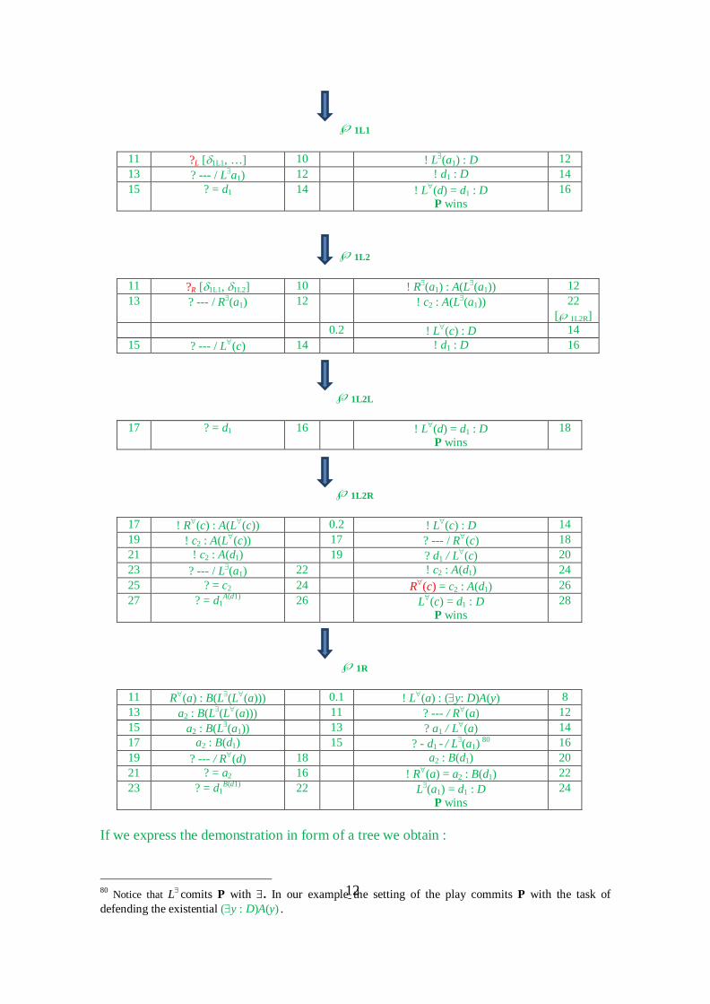
126

℘1L1

11 ?L [δ1L1, …] 10 ! L∃(a1) : D 12 13 ? --- / L∃a1) 12 ! d1 : D 14 15 ? = d1 14 ! L∀(d) = d1 : D

P wins 16

℘1L2

11 ?R [δ1L1, δ1L2] 10 ! R∃(a1) : A(L∃(a1)) 12 13 ? --- / R∃(a1) 12 ! c2 : A(L∃(a1)) 22

[℘1L2R] 0.2 ! L∀(c) : D 14

15 ? --- / L∀(c) 14 ! d1 : D 16

℘1L2L

17 ? = d1 16 ! L∀(d) = d1 : D P wins

18

℘1L2R

17 ! R∀(c) : A(L∀(c)) 0.2 ! L∀(c) : D 14 19 ! c2 : A(L∀(c)) 17 ? --- / R∀(c) 18 21 ! c2 : A(d1) 19 ? d1 / L∀(c) 20 23 ? --- / L∃(a1) 22 ! c2 : A(d1) 24 25 ? = c2 24 R∀(c) = c2 : A(d1) 26 27 ? = d1

A(d1) 26 L∀(c) = d1 : D P wins

28

℘1R

11 R∀(a) : B(L∃(L∀(a))) 0.1 ! L∀(a) : (∃y: D)A(y) 8 13 a2 : B(L∃(L∀(a))) 11 ? --- / R∀(a) 12 15 a2 : B(L∃(a1)) 13 ? a1 / L∀(a) 14 17 a2 : B(d1) 15 ? - d1 - / L∃(a1) 80 16 19 ? --- / R∀(d) 18 a2 : B(d1) 20 21 ? = a2 16 ! R∀(a) = a2 : B(d1) 22 23 ? = d1

B(d1) 22 L∃(a1) = d1 : D P wins

24

If we express the demonstration in form of a tree we obtain :

80 Notice that L∃ comits P with ∃. In our example the setting of the play commits P with the task of defending the existential (∃y : D)A(y) .

127

0. P ! (∀x : D)B(x) (a : (∀x : (∃y : D)A(y))B(L∃(L∀(a))), (∀x : D)A(x)) 0.1. O ! a : (∀x : (∃y : D)A(y))B(L∃(L∀(a))) 0.2. O ! c : (∀x : D)A(x) 0.3. P ! d: (∀x : D)B(x) 1. O ! L∀(d) : D [?, 0.3] 2. P ? ---/ L∀(d) [?, 1] 3. O ! d1 : D [!, 2] 4. P R∀(d) : B(L∀(d)) [!, 1] 5. O ? d1/ L∀(d) [?, 4] 6. P ! L∀(a) : (∃y : D)A(y) [ ?, 0.1] 7. O ? ---/ L∀(a) [?, 6] 8. P ! a1 : (∃y : D)A(y) [!, 7]

9. O ! R∀(a) : B(L∃(L∀(a))) [!, 8]

9. O ?L [δ1L1, …] [?, 8] 9. O ?R [δ1L1, δ1L2] [?, 8] 10. P ! ?---/ R∀(a) [?, 9] 10. P ! L∃(a1) : D[!, 9] 10. P ! R∃(a1) : A(L∃(a1))[!, 9] 11. O ! a2 : B(L∃(L∀(a))) [!, 10] 11. O ?--- / L∃(a1) [?, 10] 11. O ?--- / R∃(a1) [?, 10] 12. P ? a1/ L∀(a) [?, 11] 12. P ! d1 : D [!, 11] 12. P ! L∀(c) : D [?, 0.2] 13. O ! a2 : B(L∃(a1)) [!, 12] 13. O ? = d1 [?, 12] 13. O ?--- / L∀(c) [?, 12] 14. P ?-d1-/ L∃(a1)81 [?, 13] 14. P ! L∀(d) = d1 : D [!, 13] 14. P ! d1 : D [!, 13] 15. O ! a2 : B(d1) [!, 14]

16. P ! R∀(d) : B(d1) [!, 5] 17. O ? ---/ R∀(d) [?, 16] 18. P ! a2 : B(d1) [!, 17] 19. O ? = a2 [?, 18] 20. P ! R∀(a) = a2 : B(d1) [!, 19] 21. O ? = d1

B(d1) [?, 20] 15. O ? = d1 [?, 14] 15. O ! R∀(c) : A(L∀(c)) [!, 12] 22. P ! L∃(a1) = d1 : D [!, 21] 16. P ! L∀(d) = d1 : D [!, 15] 16. P ?--- / R∀(c) [?, 15]

17. O ! c2 : A(L∀(c)) [!, 16] 18. P ? d1/ L∀(c) [?, 17] 19. O ! c2 : A(d1) [!, 18] 20. P ! c2 : A(L∃(a1)) [!, 11] 21. O ?--- / L∃(a1) [?, 20] 22. P ! c2 : A(d1) [!, 21] 23. O ? = c2 [?, 22] 24. P ! R∀(c) = c2 : A(d1) [!, 23] 25. O ? = d1

A(d1) [?, 24] 26. P ! L∀(c) = d1 : D [!, 25]

81 Notons ici que L∃ est une instruction qui engage P : dans notre exemple la structure du jeu l’engage à défendre la proposition existentielle (∃y : D)A(y) associée à cette instruction.

128

129

IV.6 From dialogical strategies to CTT-demonstrations and back In the following paragraphs we adapt the equivalence result obtained in Clerbout/Rahman (2015, pp. 39-52) to the present formulation of the dialogical conception of CTT. A brief reflection on the examples developed above suggests that if we delete those equality moves that result application of the Socratic-rules we gather a version of the plays and a corresponding winning strategy that in fact delivers the version of dialogical logic that Clerbout/Rahman (2015) showed to be equivalent to Martin-Löf's CTT-framework for intuitionistic logic. Indeed, if there is a winning strategy for P, all of the plays (won by P) that include equalities that result of applications of the Socratic Rule are based on copy-cat moves of O’s own choices. Thus, we can just focus on the copy-cat moves. Moreover, later on, while developing the algorithm, they will play a very important role in order both to re-establish those equalities relevant for the CTT-demonstration and to re-trace the dependencies of a move. In fact, this shows, that the equality rules as deployed by the Socratic Rule provides an insight on the natural way to link dialogical strategies with CTT-demonstrations. In other words, the inclusion of equalities as introduced by the Socratic Rule represents a novel contribution to pushing forward Sundholm’s idea that inferences can be seen as involving an implicit interlocutor, but here at the strategic level. IV.6. 1 Introduction: What is a strategic object? Recall that in CTT some functions are dependent and some other two are

independent proof-objects – namely lambda-abstracts and elements of function-types. Now, the case of dependent functions is very natural to the dialogical frame, particularly so at the play level: the challenger chooses and argument and the defender must carry out the corresponding substitution. Such kind of functions can occur in our framework in three occasions:

• as the play objects of concessions • as the pre-defined functions called instructions • as explicit functions

However, the two notions of functions of CTT as independent proof-objects are part of the strategic level and require the notion of strategic object. Indeed

• The course of values notion of a function corresponds, in the dialogical frame, a strategic object that expresses the fact that whatever play object O choses for the left instruction of the Universal / Implication, there is a suitable play object that P can bring forward. Moreover the strategic object encodes all of these choices and answers that yield plays won by P and this is what we render as the lambda-abstract of a given play object.

• Similarly, an application of the lambda-abstract corresponds, in the dialogical

frame, to a choice of the Proponent, who, given all the pairs of question-response encoded by that abstract, choses one of them. This choice of the Proponent, yields, at the strategic level, the independent individual of the

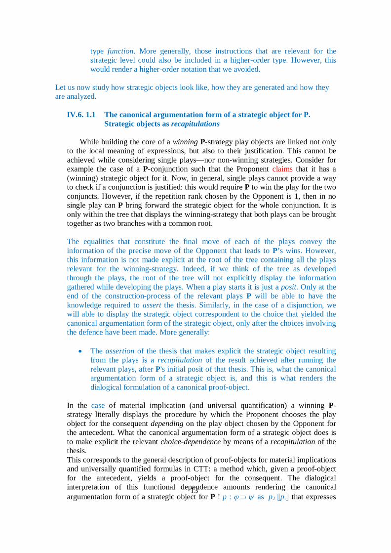
130

type function. More generally, those instructions that are relevant for the strategic level could also be included in a higher-order type. However, this would render a higher-order notation that we avoided.

Let us now study how strategic objects look like, how they are generated and how they are analyzed.

IV.6. 1.1 The canonical argumentation form of a strategic object for P.

Strategic objects as recapitulations

While building the core of a winning P-strategy play objects are linked not only to the local meaning of expressions, but also to their justification. This cannot be achieved while considering single plays—nor non-winning strategies. Consider for example the case of a P-conjunction such that the Proponent claims that it has a (winning) strategic object for it. Now, in general, single plays cannot provide a way to check if a conjunction is justified: this would require P to win the play for the two conjuncts. However, if the repetition rank chosen by the Opponent is 1, then in no single play can P bring forward the strategic object for the whole conjunction. It is only within the tree that displays the winning-strategy that both plays can be brought together as two branches with a common root.

The equalities that constitute the final move of each of the plays convey the information of the precise move of the Opponent that leads to P’s wins. However, this information is not made explicit at the root of the tree containing all the plays relevant for the winning-strategy. Indeed, if we think of the tree as developed through the plays, the root of the tree will not explicitly display the information gathered while developing the plays. When a play starts it is just a posit. Only at the end of the construction-process of the relevant plays P will be able to have the knowledge required to assert the thesis. Similarly, in the case of a disjunction, we will able to display the strategic object correspondent to the choice that yielded the canonical argumentation form of the strategic object, only after the choices involving the defence have been made. More generally:

• The assertion of the thesis that makes explicit the strategic object resulting from the plays is a recapitulation of the result achieved after running the relevant plays, after P's initial posit of that thesis. This is, what the canonical argumentation form of a strategic object is, and this is what renders the dialogical formulation of a canonical proof-object.

In the case of material implication (and universal quantification) a winning P-strategy literally displays the procedure by which the Proponent chooses the play object for the consequent depending on the play object chosen by the Opponent for the antecedent. What the canonical argumentation form of a strategic object does is to make explicit the relevant choice-dependence by means of a recapitulation of the thesis. This corresponds to the general description of proof-objects for material implications and universally quantified formulas in CTT: a method which, given a proof-object for the antecedent, yields a proof-object for the consequent. The dialogical interpretation of this functional dependence amounts rendering the canonical argumentation form of a strategic object for P ! p : ϕ ⊃ ψ as p2 ⟦pi⟧ that expresses

131

that the consequent p2 provides P with an guide on how to make a choice leading to victory, given an arbitrary choice pi by O for the antecedent. Let us express all this in the form of a table:

Canonical argumentation form of a strategic object for P Strategic objects as Recapitulation

Posit Challenge Defence Recapitulation

O ?L ! A P ! p1 : A

P ! p : (∃x : A)ϕ Or Respectively P ! < p1, p2> : (∃x : A)ϕ

O ?R ! ϕ

P ! p2 : ϕ(p1)

O ?L ! A P ! p1 : A

P ! p : {x : A | ϕ} Or Respectively P ! < p1, p2> : {x : A | ϕ}

O ?R ! ϕ(p1)

P ! p2 : ϕ(p1)

O ?L ! ϕ P ! p1 : ϕ

P ! p : ϕ ∧ ψ Or Respectively P ! < p1, p2> : ϕ ∧ ψ

O ?R ! ψ

P ! p2 : ψ

P ! p : (∀x : A)ϕ O ! L∀(p) : A , ? ! ϕ P ! p2 : ϕ(pi) P ! p2 ⟦L∀(p)⟧ : (∀x : A)ϕ

P ! p : ϕ ⊃ ψ

O ! L⊃(p) : ϕ, ? ! ψ P ! p2: ψ P ! p2 ⟦L⊃(p)⟧ : ϕ ⊃ ψ

P ! p : ¬ϕ also expressed as

O ! L⊃(p) : ϕ, ? ! ⊥

O ! p1 : ϕ ... O ! ⊥(n) (The defence of the negation amounts to a switch such it is now O who will be forced to assert ⊥ and give up) )

P ! -- ⟦L⊃(p)⟧ : ¬ϕ (It is not P who will assert ⊥, since he has a winnng strategy)

P ! p1 : ϕ P ! p1 / L∨(p) : ϕ ∨ ψ

P ! p : ϕ ∨ ψ O ? ∨ [! L∨(p) : ϕ | ! R∨(p) : ψ] Or Or

P ! p2 : ψ P ! p2 / R∨(p) : ϕ ∨ ψ

Notice that canonical form of a strategic object has been defined only for P. There is not general reason to do so; however we proceeded in this way since we are after a notion of winning strategy that corresponds to that of a CTT-demonstration, and these strategies have being identified as those where P wins. In fact the table above is the dialogical analogue to the introduction rules in CTT. Dialogically speaking those rules display the duties required by P’s own assertions – we will come back to this issue later on.

The following table establishes the correspondences between the canonical argumentation form of strategic objects for P and proof-objects as constructed by introduction rules

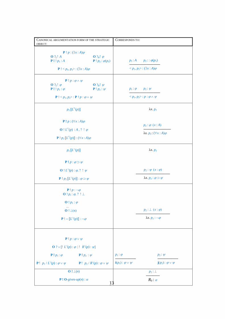
132

CANONICAL ARGUMENTATION FORM OF THE STRATEGIC OBJECT:

CORRESPONDS TO:

P ! p : (∃x : A)ϕ

O ?L ! A O ?R ! ϕ P ! ! p1 : A P ! p2 : ϕ(p1)

P ! < p1, p2> : (∃x : A)ϕ

p1 : A p2 : : ϕ(p1)

————————— < p1, p2> : (∃x : A)ϕ

P ! p : ϕ ∧ ψ O ?L ! ϕ O ?R ! ψ P ! ! p1 : ϕ P ! p2 : ψ

P ! < p1, p2> : P ! p : ϕ ∧ ψ

p1 : ϕ p2 : ψ

————————— < p1, p2> : p : ϕ ∧ ψ

p2 ⟦L∀(p)⟧

P ! p : (∀x : A)ϕ

O ! L∀(p) : A , ? ! ϕ

P ! p2 ⟦L∀(p)⟧ : (∀x : A)ϕ

λx. p2

p2 : ϕ (x : A) ———————— λx. p2 : (∀x : A)ϕ

p2 ⟦L⊃(p)⟧

P ! p : ϕ ⊃ ψ

O ! L⊃(p) : ϕ, ? ! ψ

P ! p2 ⟦L⊃(p)⟧ : ϕ ⊃ ψ

λx. p2

p2 : ψ (x : ϕ) ——————————

λx. p2 : ϕ ⊃ ψ

P ! p : ¬ϕ

O ! pi : ϕ, ? ! ⊥

O ! p1 : ϕ ... O ! ⊥(n)

P ! -- ⟦L⊃(p)⟧ : ¬ϕ

p2 : ⊥ (x : ϕ) ——————————

λx. p2 : ¬ϕ

P ! p : ϕ ∨ ψ

O ? ∨ [! L∨(p) : ϕ | ! R∨(p) : ψ]

P ! p1 : ϕ P ! p2 : ψ

P ! p1 / L∨(p) : ϕ ∨ ψ P ! p2 / R∨(p) : ϕ ∨ ψ

p1 : ϕ p2

: ψ —————— —————— i(p1) : ϕ ∨ ψ j(p2) : ϕ ∨ ψ

O ! ⊥(n)

P ! O-gives-up(n) : α

p2 : ⊥ ————

R0 : α

133

Now, similarly to the case of play objects, we can also isolate the purely-prescriptive part of the strategic object by describing their argumentation form. IV.6. 1.2 The argumentation form of a strategic object for P

Strategic object as a Record of instructions and their resolution

Argumentation forms of strategic objects constitute the analogue of the elimination rules in CTT, and, as explained further on, they are fixed for the Opponent – from the dialogical point of view elimination rules display the Proponent’s -entitlements involving O’s assertions. However, they also constitute the dialogical take on the equality rules. More precisely, while the canonical form of a strategic object expresses a recapitulation process,

• the argumentation form records both the instructions relevant for the winning strategy, and the resolutions that lead to winning-plays after a relevant posit of the Opponent.

Still, an important difference to elimination rules is that the argumentation form of a strategic object is built out of its elementary constituents. Take the example of the elimination rules for a conjunction, that deploy the projections fst and snd. Any of these projections can provide the proof-object of a complex proposition. However; the resolutions L∧(p) and R∧(p) recorded by the argumentation form of the resulting strategic object will display the equalities that guided the choices of the Proponent. Thus if the instructions have an embedded the structure the argumentation form will display not only the embedding but also those applications of the Socratic Rule that lead to the Proponent’s victorious defence of the elementary propositions involved. This is an outcome of the dialogical take on strategic objects: they are the post-facto record of the development of the relevant plays. More generally,

• The rules for strategic objects do not provide the rules on how to play but rather rules that indicate how a winning strategy has been achieved.

Take the example of the implication as brought forward by the Opponent. The challenge requires P to bring-forward an instruction for the antecedent and only after P’ resolving it, must O fulfill her obligation to defend the consequent. The argumentation form of the strategic object for the proponent expresses that P’s winnings strategy is based on resolving an instruction for a proposition involved in the consequent by deploying O’s choice for defending that consequent. The most striking example of the difference between play objects and strategic objects is the one for disjunction. Let us take the case of a winning strategy for some posit π that P wins in each play (relevant to the core) that follows from O’s defences of the disjunction, d : B ∨ A. Let us further assume that π is the thesis of the dialogue. The point is that P has a winning strategy because he is entitled to defend the commitments engaged while bringing forward π by deploying those posits that O is forced to concede by defending each of the sides of B ∨ A. Hence, the argumentation form of a strategic object thesis records those play objects that the Opponent has chosen while defending A and B.

134

Terminology: The table below deploys the following terminological conventions

• Expressions such as “IP”, “IO” stand for instructions resolved by P, by O

• The star at the left of an instruction such as *R ∧(c), *IP

, indicates that the

instruction, might be at the end of some chain of resolutions. In such a case we write the chain as an embedding of resolved instructions following the order of resolutions and indicating the first in the inside and the last in the outside of the brackets. For example, given the chain of resolutions,

O ! R ∧(c) : A ∧ (B ∧ C)

P ? --- / R ∧(c)

O ! c2 : B ∧ C P ? --- / R

∧(c2) O ! c2.2 : C

the argumentation form of *R

∧(c2) = c2.2 : C, will be written as R ∧(R

∧(c) = c2.2 : C.

• Recall that equalities such as L ∨(p) = p1, that result from the application of a

Socratic Rule, involve resolutions of the Opponent: indeed they indicate that O resolved the instruction L

∨(p) with the choice p1. • Expressions such as “*L∧(p) = p1 / IP : ϕ” indicate that the Proponent resolved

the instruction IP by choosing p1 and that p1 has also been chosen by the Opponent while resolving L∧(p).

Argumentation form of a strategic object for P Strategic objects as Records of instructions and their resolutions

Posit Challenge Defence

as Instruction-Record

P ?L P ! *L∃(p) = p1 / *IP : A

O ! p : (∃x : A)ϕ Or Respectively

P ?R

P ! *R∃(p) = p2 / *IP : ϕ(p1)

P ?L P ! *L{...}(p) = p1 / *IP : A

O ! p : {x : A | ϕ} Or Respectively

P ?R

P ! *R{...}(p) = p2 / *IP : ϕ(LP{...}(p1))

P ?L P ! *L∧(p) = p1 / *IP : ϕ

O ! p : ϕ ∧ ψ Or Respectively

P ?R P ! *R∧(p) = p2 / *IP : ψ

O ! p : (∀x : A)ϕ P ! IO = p1 / *L∀(p) : A P ! *R∀(p) = p2 / *IP ⟦p1⟧ : ϕ(p1)

O ! p : ϕ ⊃ ψ

P ! *IO = p1 / *L⊃(p) : ϕ P ! *R⊃(p) = p2 / *IP ⟦p1⟧ : ψ

O ! p : ¬ϕ O ! ⊥(n)

P ! *IO = p1 / *L¬(p) : ϕ P ! O-gives-up(n) : α

O ! ⊥(n)

135

O ! L ∨(p) : ϕ

O ! p : ϕ ∨ ψ P ? ∨ P ! *L ∨(p) = p1 / In

P | *R∨(p) = p2 / *ImP : α

O ! R∨(p) : ψ

If pi in pi : B is not the result of one of both of the instructions, the argumentation form of the strategic object is the reflexive equality

pi = pi : B

Let us write explicitly the table of correspondences between the argumentation form of strategic objects for P and proof-objects as analyzed by elimination-rules

ARGUMENTATION FORM OF THE STRATEGIC OBJECT: CORRESPONDS TO: With Equality

O ! p : (∃x : A)ϕ

P ?L P ?R P ! *L∃(p) = p1 / *IP

: A P ! *R∃(p) = p2 / *IP : ϕ(p1)

Without Equality

O ! p : (∃x : A)ϕ P ?L P ?R

P ! L∃(p) : A P ! R∃(p) : ϕ(p1)

With Equality p1 : A p2

: : ϕ(p1) p1 : : A p2 : ϕ(p1)

————————— ————————— fst(p1, p2) = p1 : A snd(p1, p2) = p2

: ϕ(p1)

Without Equality p : (∃x : A)ϕ p : (∃x : A)ϕ —————— —————— fst(p) : A snd(p) : ϕ(p1)

With Equality

O ! p : ϕ ∧ ψ P ?L P ?R

P ! *L∧(p) = p1 / *IP : ϕ P ! *R∧(p) = p2 / *IP : ψ

Without Equality

O ! p : ϕ ∧ ψ

P ?L P ?R

P ! L∧(p) : ϕ P ! R∧(p) : ψ

With Equality p1 : ϕ p2

: ψ p1 : ϕ p2 : ψ

——————— ——————— fst(p1, p2) = p1: ϕ snd(p1, p2) = p2: ψ

Without Equality p : ϕ ∧ ψ p : ϕ ∧ ψ ——————— ——————— fst(p) : ϕ snd(p) : ψ

(given p : (∀x : A)ϕ, p1 : A, L∀(p) : A, p2 : ϕ)

p2⟦L∀(p)⟧ p ⟦p1⟧

With Equality

O ! p : (∀x : A)ϕ

P ! IO = p1 / *L∀(p) : A

P ! *R∀(p) = p2 / *IP

⟦p1⟧ : ϕ(p1)

Without Equality

(given p : (∀x : A)ϕ, x : , p1 : A, p2 : ϕ)

λx. p2 ap(p, p1)

With Equality

(given: λx. p2 : (∀x : A)ϕ)

p2 : ϕ (x : A) p1 : A

—————————————— ap(λx. p2, p1) = p2(p1): ϕ(p1)

Without Equality

136

O ! p : (∀x : A)ϕ

P ! p1 / *L∀(p) : A

P ! p ⟦p1⟧ : ϕ(p1)

p : (∀x : A)ϕ p1 : A ————————————

ap(p, p1) : ϕ(p1)

(given p : ϕ ⊃ ψ, p1 : ϕ, L⊃(p) : ϕ, p2 : ψ)

p2 ⟦L⊃(p)⟧ p ⟦p1⟧

With Equality

O ! p : ϕ ⊃ ψ

P ! IO = p1 / * L⊃(p) : ϕ

P ! *R⊃(p) = p2 / *IP

⟦p1⟧ : ψ

Without Equality

O ! p : ϕ ⊃ ψ

P ! p1 / L⊃(p) : ϕ

P ! p ⟦p1⟧ : ψ

(given p : ϕ ⊃ ψ, p1 : ϕ, x : A : ϕ, p2 : ψ)

λx. p2 ap(p, p1)

With Equality

(given: λx. p2 : ϕ ⊃ ψ)

p2 : ϕ (x : ϕ) p1 : ψ

—————————————— ap(λx. p2, p1) = p2(p1): ψ

Without Equality

p : p : ϕ ⊃ ψ p1 : ϕ ————————————

ap(p, p1) : ψ

O ! L∨(p) : ϕ O ! R∨(p) : ψ

With Equality

O ! p : ϕ ∨ ψ P ? ∨

O ! L

∨(p) : ϕ O ! R∨(p) : ψ

P ! *L ∨(p) = p1 / In

P | *R∨(p) = p2 / *ImP : α

Without Equality

O ! p : ϕ ∨ ψ P ? ∨

O ! L

∨(p) : ϕ O ! R∨(p) : ψ P ! L

∨(p) | *R∨(p) : α

i(x) : ϕ j(y) : ψ

With Equality p1 : ϕ d : α[i(x)] (x : ϕ) e : α[j(y)] (y : ψ) ————————————————————

D(i(p1), x.d, y.e) = d[p1] : α[i(p1)] p2 : ϕ d : α[i(p)] (pi : ϕ) e : α[j(pj)] (pj : ψ) —————————————————————

D(j(p2), x.d, y.e) = e[p2] : α[j(p2)]

Without Equality p : ϕ ∨ ψ d : α[i(x)] (x : ϕ) e : α[j(y)] (y : ψ) ——————————————————————

D(p, x.d, y.e) : α[p]

O ! ⊥(n)

P ! O-gives-up(n) : α

p2 : ⊥ ————

R0 : α

137

The following main section, From dialogical strategies to CTT-demonstrations, of the present chapter, is structured as follows. We start by a method of extracting those parts of a winning strategy relevant for its correspondence to a demonstration in natural deduction – as mentioned before, we call it the core of a winning strategy, or simply, the core. In order to extract the core, we develop a method in order

1. to extract that finite part of a winning strategy 2. to disregard the formation rules that involve the non-logical constants

(since we are dealing with logical inferences) 3. to disregard different order of moves of the Opponent

Once this is achieved we describe the algorithm that transforms the core into a CTT-Demonstration We finish this section by proving the adequacy of the algorithm. Remarks:

1. We assume here the natural deduction style of demonstrations used by Martin-Löf rather than the turn-style notation deployed in the introductory chapter on CTT.

2. The dialogical demonstrations will assume that if there are initial concessions, these concessions are already granted by the Opponent.

IV.6.2 From dialogical Strategies to CTT-demonstrations IV.6.2.1 Plays, Moves, Strategies Before we start with our developments let us first briefly recall those notions involved in the definition of a winning strategy82: Move: A move is an expression of the form `X-e, where X stands for O or P and e stands for some posit of one of the forms deployed in the tables that display the local meaning of the expressions of the dialogical frame. Play: A play is a legal sequence of moves, i.e., a sequence of moves which observes the game rules, i.e. the rules for the local meaning of expressions involved and the structural rules that determine their global meaning. Terminal play: A play is called terminal when it cannot be extended by further moves in compliance with the rules. X-terminal play: We say of a play that it is X-terminal when the last move in the play is an X-move or Y brought forward ⊥. Winning a play: We say of a play it is won by X iff it is X-terminal

82 For more details see Clerbout (2014a, b)

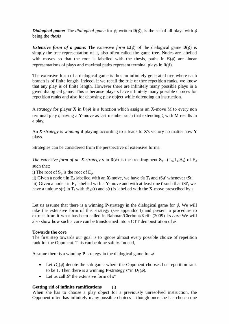
138

Dialogical game: The dialogical game for φ, written D(φ), is the set of all plays with φ being the thesis Extensive form of a game: The extensive form E(φ) of the dialogical game D(φ) is simply the tree representation of it, also often called the game-tree. Nodes are labelled with moves so that the root is labelled with the thesis, paths in E(ϕ) are linear representations of plays and maximal paths represent terminal plays in D(ϕ). The extensive form of a dialogical game is thus an infinitely generated tree where each branch is of finite length. Indeed, if we recall the rule of thee repetition ranks, we know that any play is of finite length. However there are infinitely many possible plays in a given dialogical game. This is because players have infinitely many possible choices for repetition ranks and also for choosing play object while defending an instruction. A strategy for player X in D(φ) is a function which assigns an X-move M to every non terminal play ζ having a Y-move as last member such that extending ζ with M results in a play. An X-strategy is winning if playing according to it leads to X's victory no matter how Y plays. Strategies can be considered from the perspective of extensive forms: The extensive form of an X-strategy s in D(φ) is the tree-fragment Sφ =(Ts,ls,Ss) of Eφ such that: i) The root of Sφ is the root of Eφ, ii) Given a node t in Eφ labelled with an X-move, we have t'∈Ts and tSst' whenever tSt'. iii) Given a node t in Eφ labelled with a Y-move and with at least one t' such that tSt', we have a unique s(t) in Ts with tSss(t) and s(t) is labelled with the X-move prescribed by s. Let us assume that there is a winning P-strategy in the dialogical game for φ. We will take the extensive form of this strategy (see appendix I) and present a procedure to extract from it what has been called in Rahman/Clerbout/Keiff (2009) its core.We will also show how such a core can be transformed into a CTT demonstration of φ. Towards the core The first step towards our goal is to ignore almost every possible choice of repetition rank for the Opponent. This can be done safely. Indeed, Assume there is a winning P-strategy in the dialogical game for φ.

• Let D1(φ) denote the sub-game where the Opponent chooses her repetition rank to be 1. Then there is a winning P-strategy s⋆.in D1(φ).

• Let us call S⋆ the extensive form of s⋆. Getting rid of infinite ramifications When she has to choose a play object for a previously unresolved instruction, the Opponent often has infinitely many possible choices – though once she has chosen one

139

she must keep it for the rest of the play (recall the posit-substitution rule). In such cases the play object associated with the instruction will be a member of some set. Unless otherwise specified this set may be infinite. The Opponent can then choose among an infinite number of members when asked to replace the instruction with a play object.83 Thus S⋆ has infinitely many branches. Let us reduce them to a finite number. Critical node: Call a node t in S⋆ critical if it has infinitely many immediate successors, and S(t) the set of these successors. S⋆ t (critical)

S(t) = { ti tj tn … ∞ } Our first aim is to partition S(t), for each critical node in S⋆, depending on the kind of moves associated with its members. Fortunately, since we are working with the intuitionistic rule, the task will actually be simpler than with classical dialogues. Let us describe the situation progressively:

1. Let us first recall that since we started with a P-strategy, branches are triggered by O-choices. Hence for every critical node t in S⋆, the members of S(t) are associated with O-moves. Each of these moves is obviously either a defence or a challenge.

2. Because the finiteness of plays is ensured by repetition ranks, the only way for t

to be critical is for O to react differently in an infinite number of ways to at least one of its predecessors, or even t itself.

3. From the dialogical rules, we know that there are only two cases in which the

Opponent has the local choice between infinitely many moves, namely: (a) (when applying the Posit-Substitution rule to challenge a hypothetical move

by instantiating the concessions (assumptions of the hypothetical) in the context. Indeed in this rule the challenger is the one choosing the instantiations of the variables occurring in the concessions; or

(b) when applying the rule Resolution of Instructions (rule SR3.1) as the defender, i.e. when choosing the play objects that should substitute the relevant instructions.

S⋆ … tm (m<k) … tk (critical)

S(t) = { ti tj tn … ∞ } 83 See Clerbout (2014a,c): if there is a move by which the Opponent can force her victory, then nothing prevents her from playing it as soon as she has a chance to. Whether this move is a challenge or a defence, the repetition rank 1 is enough to allow her to play it in accordance with SR1i.

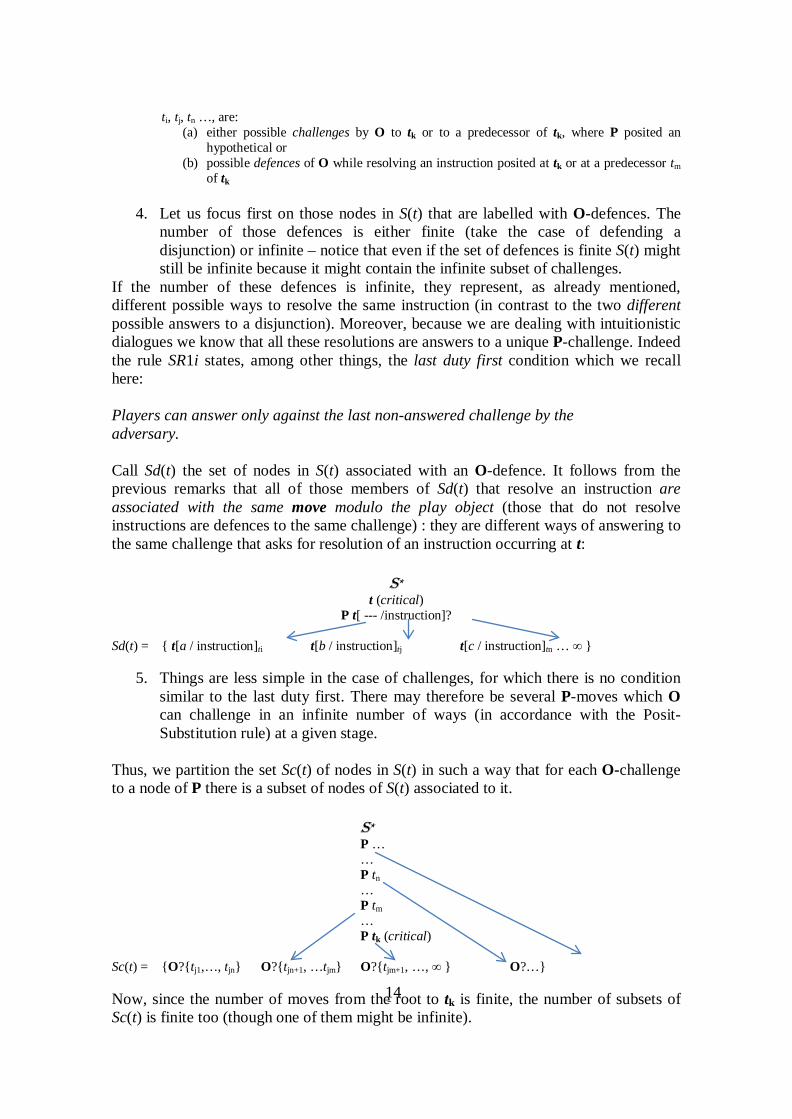
140

ti, tj, tn …, are:

(a) either possible challenges by O to tk or to a predecessor of tk, where P posited an hypothetical or

(b) possible defences of O while resolving an instruction posited at tk or at a predecessor tm of tk

4. Let us focus first on those nodes in S(t) that are labelled with O-defences. The

number of those defences is either finite (take the case of defending a disjunction) or infinite – notice that even if the set of defences is finite S(t) might still be infinite because it might contain the infinite subset of challenges.

If the number of these defences is infinite, they represent, as already mentioned, different possible ways to resolve the same instruction (in contrast to the two different possible answers to a disjunction). Moreover, because we are dealing with intuitionistic dialogues we know that all these resolutions are answers to a unique P-challenge. Indeed the rule SR1i states, among other things, the last duty first condition which we recall here: Players can answer only against the last non-answered challenge by the adversary. Call Sd(t) the set of nodes in S(t) associated with an O-defence. It follows from the previous remarks that all of those members of Sd(t) that resolve an instruction are associated with the same move modulo the play object (those that do not resolve instructions are defences to the same challenge) : they are different ways of answering to the same challenge that asks for resolution of an instruction occurring at t:

S⋆ t (critical)

P t[ --- /instruction]?

Sd(t) = { t[a / instruction]ti t[b / instruction]tj t[c / instruction]tn … ∞ }

5. Things are less simple in the case of challenges, for which there is no condition similar to the last duty first. There may therefore be several P-moves which O can challenge in an infinite number of ways (in accordance with the Posit-Substitution rule) at a given stage.

Thus, we partition the set Sc(t) of nodes in S(t) in such a way that for each O-challenge to a node of P there is a subset of nodes of S(t) associated to it.

S⋆ P … … P tn … P tm … P tk (critical)

Sc(t) = {O?{tj1,…, tjn} O?{tjn+1, …tjm} O?{tjm+1, …, ∞ } O?…} Now, since the number of moves from the root to tk is finite, the number of subsets of Sc(t) is finite too (though one of them might be infinite).

141

Summing up, if t is critical S(t) we can partition it in the following way

• Sd(t) = {n|n ∊ S(t) and n is associated with a defence}

• Scm(t) = {n|n ∊ S(t) and n is associated with a challenge against the P node m} Thus, we have partitioned S(t) in a finite collection of disjoint subsets, such that at least one of them is infinite — otherwise t would not be a critical node. Because our current aim is to get rid of infinite ramifications, we leave the finite subsets untouched. Notice that each subset Scm(t) of challenges resulting from an application of a rule other than the Posit-Substitution rule is finite because it is the only rule in which the challenger has infinitely many choices for his challenges.

6. Let us now eliminate the infinite branches both in Sd(t) and in Sc(t) Suppose next that Sd(t) is infinite. In this case we keep exactly one of its members in S⋆ and delete all the other members as well as the branches they generate. We can safely do this because as pointed out, all the members in Sd(t) are defences in reaction to the same previous P-move and they are; so to say, substitutional variants of each other. Moreover, from the point of view of the winning strategy for P, they must be indistinguishable: none of these variations changes anything in terms of P’s ability to win. Suppose that Sci(t) is infinite. The same reasoning as before applies to the infinite Sci(t) sets since the reason they are infinite is basically the same: they represent an infinite number of possible choices of play objects by O (though this time as challenges instead of defences). Hence, when some sets Sci(t) are infinite we do the same and keep, for each of these sets, exactly one member and delete the others and the branch they generate. Thus, our method amount to the following steps

• We partition the set of successors for every critical node in S⋆ to obtain a finite number of disjoint subsets (some may be infinite).

• We leave the finite ones untouched and reduce the infinite ones to singletons. This operation generates a tree, called SF, with no critical node and in which infinite ramifications have been successfully eliminated without losing important information. The rationale behind the operation is the following: Because S⋆ is the extensive form of a winning P-strategy, we know that the Proponent wins in every branch and thus to some extent the play object chosen by the Opponent for the instructions does not matter. Let us take an example the case of a universal quantification posited by P. Since we assume that P has a winning strategy the Proponent has a method to successfully defend his posit no matter which play object O chooses for L∀(p) : A (where A is a set). This yields a natural deduction description of the Introduction rule for universal quantification with

142

an implicit interlocutor: whatever the Opponent brings forward as proof-object for the antecedent the Proponent has a method to transform it into a proof-object of the consequent. Hence, it is harmless to keep only one representative of the possible choices by O because the existence of a winning P-strategy ensures that there is indeed a successful method for every possible choice by O. Disregarding formation rules for formal plays The dialogical rules allow the players to enquire about the type of expressions and in particular to ask whether an expression is a proposition or not. This leads to plays that use Formation rules listed in the corresponding table. However, as we mentioned in the introduction we only cover in our study the fragment of CTT involving logically valid propositions and formal plays. In such kind of plays, as already mentioned, the formation of the elementary expressions is introduced during the play, and so they are part of the development of a dialogical game. The formation of the logical constants is the one that must be checked. Now, in general, in such kind of formal enquiry, we presuppose that the logical structure of the expressions to be demonstrated as valid are have been well typed. We will therefore ignore in SF every branch in which a formation rule is applied: we simply remove these branches and call the obtained tree S. Disregarding irrelevant variations in the order of O-moves and the Core.

A P-strategy must account for every possible way for O to play, and in particular it must deal with any order in which the Opponent might play her moves. It means that S⋆ had branches differing from other branches only in the order in which O plays her move, and therefore so does S. However, since we started with a winning P-strategy, we can select any particular order of O-moves without losing anything in terms of P’s victory. Indeed, by the very definition of a winning strategy, P must win in every of the plays that result from an O-choice. Thus, every branch of the tree extracted from S still represents a play won by P, and so the order of O-moves does not influence the result. Our next step will thus be to extract from S a tree representing only one order of O-moves: we are looking for a tree in which there are no two branches B1 and B2 identical to each other modulo the order of O-moves. Nevertheless, using the intuitionistic development rule SR1i requires some specific care while selecting a suitable play, for we do not want a play in which O loses because she played poorly. Since S will contain all, the ones where O played strongly and the ones she did not, if we select we should care not to retain precisely one of the plays where O played weakly. Recall that according to the rule SR1i, the Opponent can only answer the last P-challenge not yet answered. It tends therefore to be strategically safer for O to immediately defend (and be sure not to lose the chance of making that move later on) and delay possible moves involving counterattacks. The Core: Thus, when extracting a particular order of the Opponent’s moves in S we shall thus select a tree such that in any branch, every P-challenge is immediately followed by the O-defence.84 By doing so we explicitly get rid of the cases in which O loses only because she poorly chose the order of her moves. Once we have removed all

84 Recall that the Opponent is always able to do so since unlike the Proponent she is not constrained by either the Socratic nor the Special Formal Rule.

143

the redundant information for developing a demonstration, what remains is what we call the core C of S⋆. IV.6.2.2 From the core C to a CTT demonstration The next step is to apply transformations to this core until we obtain a CTT demonstration.85 Let us start with some terminology: Let recall some terminology from previous sections and introduce some new ones:

• A concession is either: (a) A posit that O conceded as conditioning the claim of the thesis. We call this also

initial concession. It corresponds to the notion of global assumption of proof-theory including epistemic assumptions and premises.

(b) Any other O-posit brought forward during the development of a play, while challenging a P-implication or a P-universal or while defending an O-disjunction or subset separation. We call this also local concession. It corresponds to the notion of local assumption of proof-theory.

• Let us say that, for a posit π occurring in the dialogical core C, the nodes

descending from π are all the nodes which are related to π by a chain of applications of dialogical rules.

• When the dialogical core or the demonstration we are building splits, we speak of the left and right branches of the core (or demonstration).We may sometimes assign an order on the branches from left to right and speak of the first branch, second branch, etc.

• We say that a move M depends on the move M' if there is a chain of applications

of game rules that leads from M' to M.

• Case-dependent move: - Let π be some posit and p some play object. We say that in C the move Mj P! π is case-dependent upon move Mi<j O! p : φ if φ is a disjunction and move Mj depends upon move Mi<j. More precisely the posit P!π is case-dependent upon O's disjunction φ iff the play object(s) that occur in the defence of P's posit π is definitionally equal to one of the instructions for φ or if P is dispensed to defend π by O’s posit ⊥ which results from the defence of φ. As we will discuss below, the point distinguishing case-dependent moves, is that these moves, set, from the strategic point of view, the condition for the conclusion of a disjunction elimination rule.

85 The section strongly relies on Clerbout/Rahman (2015), that implemented in the CTT-framework the ideas developed on Rahman/Clerbout/Keiff (2009) and Clerbout (2014a, b) in standard framework for FOL.

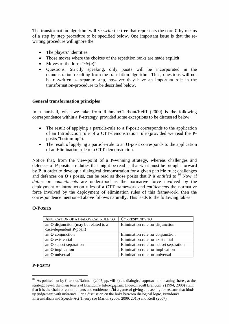
144

The transformation algorithm will re-write the tree that represents the core C by means of a step by step procedure to be specified below. One important issue is that the re-writing procedure will ignore the

• The players’ identities. • Those moves where the choices of the repetition ranks are made explicit. • Moves of the form “sic(n)”. • Questions. Strictly speaking, only posits will be incorporated in the

demonstration resulting from the translation algorithm. Thus, questions will not be re-written as separate step, however they have an important role in the transformation-procedure to be described below.

General transformation principles In a nutshell, what we take from Rahman/Clerbout/Keiff (2009) is the following correspondence within a P-strategy, provided some exceptions to be discussed below:

• The result of applying a particle-rule to a P-posit corresponds to the application of an Introduction rule of a CTT-demonstration rule (provided we read the P-posits “bottom-up”).

• The result of applying a particle-rule to an O-posit corresponds to the application of an Elimination rule of a CTT-demonstration.

Notice that, from the view-point of a P-winning strategy, whereas challenges and defences of P-posits are duties that might be read as that what must be brought forward by P in order to develop a dialogical demonstration for a given particle rule; challenges and defences on O’s posits, can be read as those posits that P is entitled to.86 Now, if duties or commitments are understood as the normative force involved by the deployment of introduction rules of a CTT-framework and entitlements the normative force involved by the deployment of elimination rules of this framework, then the correspondence mentioned above follows naturally. This leads to the following tables O-POSITS

APPLICATION OF A DIALOGICAL RULE TO CORRESPONDS TO an O disjunction (may be related to a case-dependent P-posit)

Elimination rule for disjunction

an O conjunction Elimination rule for conjunction an O existential Elimination rule for existential an O subset separation Elimination rule for subset separation an O implication Elimination rule for implication an O universal Elimination rule for universal

P-POSITS

86 As pointed out by Clerbout/Rahman (2005, pp. viii-x) the dialogical approach to meaning shares, at the strategic level, the main tenets of Brandom's Inferentialism. Indeed, recall Brandom’s (1994, 2000) claim that it is the chain of commitments and entitlements in a game of giving and asking for reasons that binds up judgement with inference. For a discussion on the links between dialogical logic, Brandom's inferentialism and Speech-Act Theory see Marion (2006, 2009, 2010) and Keiff (2007).

145

APPLICATION OF A DIALOGICAL RULE TO CORRESPONDS TO an P disjunction Introduction rule for disjunction

an P conjunction Introduction rule for conjunction an P existential Introduction rule for existential an P subset separation Introduction rule for subset separation an P implication Introduction rule for implication an P universal Introduction rule for universal

The exceptions to the general principle that P-posits correspond to introduction rules and O-posits to elimination rules are

• P-posits dependent upon O ⊥ moves correspond to ⊥-eliminations: P-posits (elementary or not) that are dispensed to be defended because O posited ⊥ before (and lost with this move the play) correspond to applications of the elimination rule for ⊥.

• P-elementary posits defended with “sic(n)” correspond to applications of the

SR4-Rule (Specal Socratic Rule). If an elementary P-posit has been challenged and defended with “sic(n)” the algorithm to be described below will first introduce it in the demonstration tree as an application of a SR4-Rule, such that the premiss is constituted by the O-posit that allowed the defence “sic(n) and the defence is the P-posit. Eventually the conclusion will be removed. If the elementary posit has not been challenged then (since all the plays are assumed to be won by P) we are in presence of a case of a ⊥-elimination as described above.

• P-elementary posits defended with I = pi : type correspond to definitional

equalities. If an elementary P-posit has been challenged and defended with a posit of the form I = pi : type – “I” stands for an instruction a “pi” for a play object – the algorithm to be described below will first introduce in the demonstration tree this equality as the application of a definitional equality and will remove the P-elementary posit that triggered the defence. However, the dialogical plays make a profuse use of definitional equalities. In fact, in the context of immanent reasoning every use of a move based on the Socratic Rule is based on such form of equality. The natural deduction demonstrations that are not in normal-form do not in general require coming back to the equality backing the coordination of introduction and elimination rules. Within the standard natural deduction setting Π- and Σ-equality is made explicit when eliminations introduce non-canonical-proof-objects. In the dialogical setting this corresponds to those cases where the proponent choses a resolution of an instruction or function that mirrors the resolution of an embedded instruction(function) occurring already either in the initial concession or in the main thesis. Let us call the resulting equalities anaphoric-based-equalities (for short A-equalities). Thus, we will only retain in the tree A-equalities. Strictly speaking, plays within the core are carried out in “normal form”.

• P-posits which are case-dependent of O-posits set the conditions that allow

drawing the conclusion of a disjunction-elimination-rule: In fact, case-dependent P-posits correspond to either disjunction eliminations achieved by

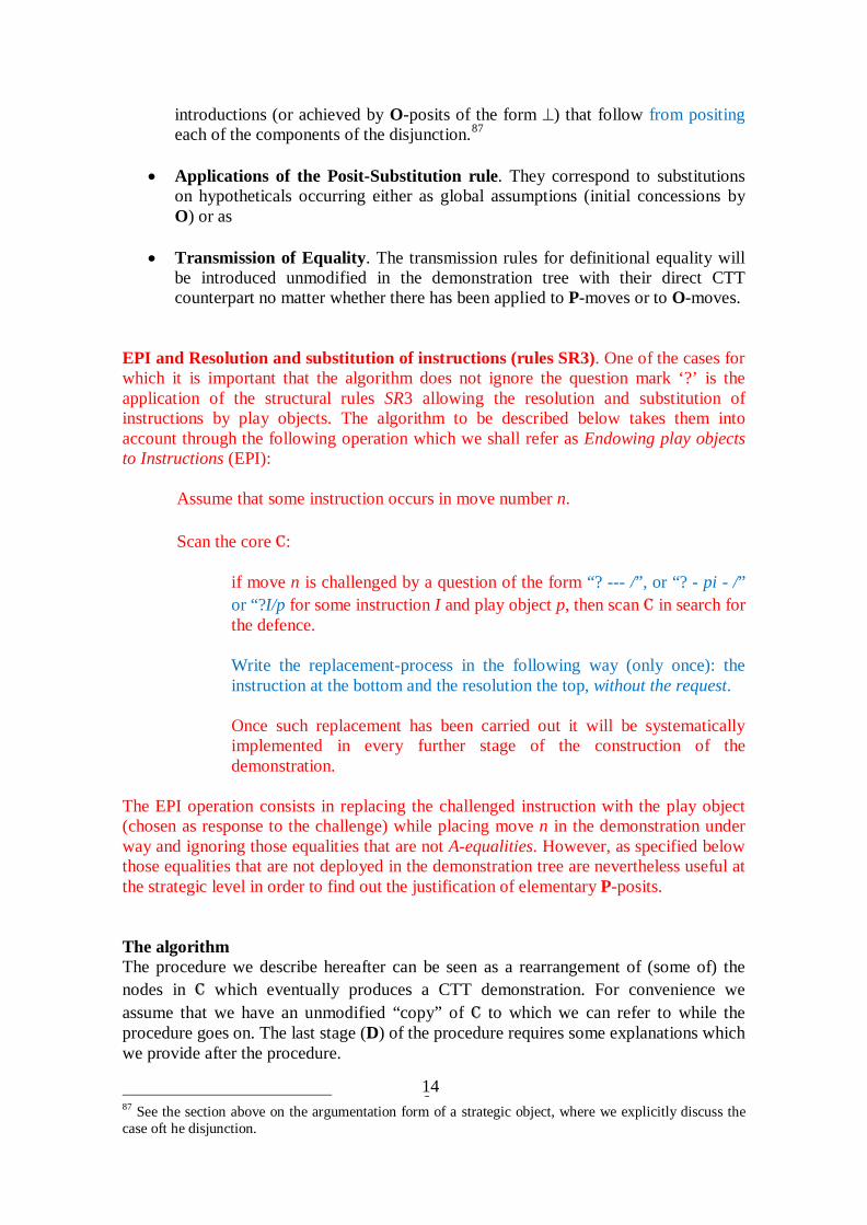
146

introductions (or achieved by O-posits of the form ⊥) that follow from positing each of the components of the disjunction.87

• Applications of the Posit-Substitution rule. They correspond to substitutions

on hypotheticals occurring either as global assumptions (initial concessions by O) or as

• Transmission of Equality. The transmission rules for definitional equality will

be introduced unmodified in the demonstration tree with their direct CTT counterpart no matter whether there has been applied to P-moves or to O-moves.

EPI and Resolution and substitution of instructions (rules SR3). One of the cases for which it is important that the algorithm does not ignore the question mark ‘?’ is the application of the structural rules SR3 allowing the resolution and substitution of instructions by play objects. The algorithm to be described below takes them into account through the following operation which we shall refer as Endowing play objects to Instructions (EPI):

Assume that some instruction occurs in move number n. Scan the core C:

if move n is challenged by a question of the form “? --- /”, or “? - pi - /” or “?I/p for some instruction I and play object p, then scan C in search for the defence. Write the replacement-process in the following way (only once): the instruction at the bottom and the resolution the top, without the request. Once such replacement has been carried out it will be systematically implemented in every further stage of the construction of the demonstration.

The EPI operation consists in replacing the challenged instruction with the play object (chosen as response to the challenge) while placing move n in the demonstration under way and ignoring those equalities that are not A-equalities. However, as specified below those equalities that are not deployed in the demonstration tree are nevertheless useful at the strategic level in order to find out the justification of elementary P-posits. The algorithm The procedure we describe hereafter can be seen as a rearrangement of (some of) the nodes in C which eventually produces a CTT demonstration. For convenience we assume that we have an unmodified “copy” of C to which we can refer to while the procedure goes on. The last stage (D) of the procedure requires some explanations which we provide after the procedure. 87 See the section above on the argumentation form of a strategic object, where we explicitly discuss the case oft he disjunction.

147

A - Initial stage. Let π be the thesis posited by P and γ1, . . . , γn be the initial concessions by O, if any. Place π as the conclusion of the demonstration under construction and γ1, . . . , γn as its upmost premisses:

γ1 γ2 γn . . . π

Then go to step B In fact, for the sake of simplicity we will ignore the first steps of a dialogue where the intial assumptions (if any) of the thesis are written to the right of the thesis. We will rather start the algorithm assuming that the initial concessions have been already settled and the thesis displays the play object that resulted after O posited the initial concessions. B. Consider the lowest expression πi just added in the branch of the demonstration tree under construction (in the first stage it will be the thesis). Find the the move in the core C that responds to it (at the first stages of the procedure it will a challenge on the thesis). Scan C in order to identify the challenge and defence resulting from the application of the local rule relevant to this expression. Then: B.0 If applicable implement the EPI-operation to the expressions present so far in the branch of the demonstration, that is: replace instructions by play objects, place within the demonstration those equalities used either for posit-substitutions or substitutions involving instructions.88 B.1. If the relevant challenge and defence have already been accounted for in the branch being constructed, then go to C. Otherwise go to B.2. B.2. If the defence is “sic(n)” or an elementary expression of P then apply stage B.2.a. Otherwise, implement step B.2.b. B.2.a. The present step concerns the occurrence of an elementary expression πi of P in the core that is not dependent upon an O ⊥-move. Place πi in the demonstration, draw an inference line above it and label it SR (short for the application of some form of the Socratic Rule, namely either SR4 or SR5). If the corresponding O-posit (that allowed P to posit πi) has already been accounted for in the branch, then rearrange it so that it is placed as the premiss of the application of the rule. Find the O-posit by searching for the relevant equality. Indeed; all of the equalities in the core will indicate precisely the O-posit relevant for the elementary expression at stake. Go back to B. B.2.b. The present step concerns non elementary expressions πi. Draw an inference line above πi and label it with the relevant name of rule. Place the defence — and the challenge, if relevant89 — as the premiss(es) for application of the rule, according to the following conventions: - In the cases of the Introduction rule for material implication, negation or universal quantification, the defence is the immediate premiss and the challenge is placed upwards as an assumption such that: (i) the defence depends on that assumption,

88 We deal with ramifications further on in the algorithm. 89 Namely, when the local rule applied is a challenge to an implication, a negation or a universal.

148

(ii) the assumption is numbered and marked as discharged at the inference step and (iii) this assumption is still in the scope of previously placed assumptions such as the premisses of the demonstration placed in stage A. - Here we apply the correspondences between player-moves and natural deduction steps described above in the following way:90

• If πi is an O-implication move, we are in face of an elimination rule: the premiss is constituted by that move and its challenge. The conclusion is the defence. Similarly for negations and universals.

• If πi is a P-conjunction/existential move, we are dealing with an introduction rule: each premiss is constituted by one of the defences. The conclusion is the challenged conjunction/existential. Dually, if πI is an O-conjunction/existential move, we are in presence of an elimination-rule so that πI is the premiss of each of the inferences with each of the defences as conclusion.

• If πI is a case-dependent P-posit. Then rewrite each of the O-defences of the relevant disjunction as a local assumption upon which a copy of πI will be made dependent. Draw an inference line and copy below a third copy of the case-dependent posit πI.

• If πI is a P-posit (elementary or not) that is dispensed to be defended because O posited ⊥ before (and lost with this move the play) correspond to the application of an elimination rule for ⊥. In such case scan for the move ⊥, place it in the demonstration as a premiss of a ⊥-elimination, draw and inference line and write πI below that line. If πI is either an implication or a universal delete the O-challenge to it.

• If πI is a P-posit that displays an A-equality place it in the demonstration as the conclusion of a Σ- (Π-) equality-rule with the posits that lead to that equality as a premiss.91

• If πI is a substitution-move based on an A-equality, place that equality and the expression in which the substitution has been carried out as premiss of the application of a substitution rule. Similarly for posit-substitution-moves.

• Apply the EPI operation to the newly added expressions (if applicable). Move to the first (starting from the left) newly opened branch if relevant and go back to B.

At this stage multiple premises can occur. Those premises are not dependent upon one another (with the exception of the premises of the elimination of a disjunction) and are placed on the same level: each one opening a new branch in the demonstration. In that case all the premisses that were placed at some previous step in the translation must be copied and pasted for each newly opened branch.

90 Recall that those moves in C have the form of defences and challenges established by the local rules and/or structural rules. 91 Recall the remarks above concerning P-elementary posits defended with I = pi : type.

149

C. If the situation is the one of B.1 and no new expression has been added to the under construction branch, then: C.1. Perform any rearrangement required to match the notational convention of natural deduction trees and go to C.2. C.2. If the branch does not feature applications of SR then go to C.3. Otherwise for each application of SR in the branch, remove its conclusion and the associated inference line.92 Go to C.3. C.3. Move to the next branch to which stages C.1 and C.2 has not been applied and go back to B. If there is no such branch left then go to D. D. Going from the top to the bottom, replace in the demonstration at hand the dialogical play objects with CTT proof-objects in accordance with the CTT rules. The point is that once the demonstration has been built we do not have play objects any more but strategic objects – the latter but not the former correspond to proof-objects .Then stop the procedure. The table of correspondences between strategic objects and proof-objects can be used a checking method using the following steps: Extract the strategic object of the thesis from the core Use the correspondences of the table and provide the proof-object for it compare with the result of what comes out from finishing the procedure Remarks:

1 We have designed the algorithm so that the branches in the demonstration under construction are dealt with sequentially. However, it is possible to treat them all at the same time in parallel.

2 The concluding stage D is necessary because, as discussed all over our study dialogical play objects differ from CTT proof-objects, that correspond to strategic objects.

Adequacy of the translation algorithm We must ensure that the algorithm is adequate: given the core of a winning P- strategy it must always yield a CTT demonstration. Let us first describe the general idea behind the demonstration, that is fact is an almost literal reproduction of the one developed in Clerbout/Rahman (2015, pp. 49-52) with very small changes due to the present take on equalities. The translation procedure ultimately consists in rearranging the nodes of the original dialogical core C. We must ensure that the reordering results in a derivation which complies with the CTT rules. We noticed that during this reordering, the procedure introduces what we may call “gaps” which we have marked with vertical dots. Take for example the first step of such a transformation procedure. In this step the thesis of the core provides the conclusion of the demonstration and the concessions provide the assumptions,

92 SR-rules display two copies of the same elementary expression, one as premise and one as conclusion. In the standard presentation of natural deduction (used in the present text) this is not necessary, unless we make use of some other recent presentations of natural deductions that introduce explicitly axioms of the form A ├ A.

150

though we still do not know at this point of the process what corresponds to the steps between the assumptions and the conclusion. Accordingly, we start by simply linking the assumptions and the conclusion with vertical dots. The idea behind the adequacy of the algorithm is that all these gaps will eventually be filled and that it will be done in a way which observes the CTT rules. The last part of this statement is easily checked. Let us assume that all the gaps are indeed removed. Then we can easily see that the resulting derivation is such that every rule applied in it is a CTT rule. We have indeed associated every application of a dialogical rule to a CTT rule, with the following exceptions: the rules involving elementary posits by P (the SR-rules) and the rules for Resolution and Substitution for Instructions that do not involve A-equalities. But applications of these three rules will eventually be removed too. Indeed, at the last stage of the algorithm, when play objects are replaced by proof- objects, applications of the SR-rules regarding instructions will eventually be removed. Recall also that P-posits (elementary or not) that are dependent upon ⊥-eliminations correspond indeed to those eliminations So far so good — though the critical task of checking that the CTT rules are properly applied still remains. This process must show the important fact that following the algorithm will eventually remove the gaps, as it was assumed above. In order to ground this assumption let us temporarily consider an extension of the CTT calculus which includes the rules SR-rules as well as a new rule called Gap. In relation to the former recall that in the so-called full-presentation of the CTT, every leave of a demonstration starts with an axiom of the form A ├ A, thus, the introduction of SR is not at all foreign to the framework of a CTT-demonstration. In relation to Gap, it either allows to link (with the help of vertical dots) two nodes of the demonstration without a dialogical rule explaining such a link, or to introduce an expression as the last step of a sequence of vertical dots. We will show that when following the algorithm, each of the applications of the rule Gap will be replaced by applications of a suitable CTT rule or by applications of a SR-rule. We will then simply need to show that when no dialogical rule is applied to the corresponding node from C, the expression will not introduce additional gaps: the rearranging in the stage C.1 of the algorithm is harmless. Once we have reached this point, and after all applications of a SR-rule have been removed, we are assured to have a proper CTT demonstration. Accordingly, let us show first that the gaps introduced during the process of building the CTT demonstration are temporary and will be progressively removed bottom-up:

• Algorithm-Lemma (AL): For any stage of the translation procedure, there is a corresponding node in the original dialogical core C for every expression resulting from a gap.

Proof. The proof is a straight-forward induction which also establishes that newly introduced gaps at a given stage of the translation have the “right shape”, so that they will be filled by a proper application of a rule later on. The base case is trivial: the initial stage A of the algorithm stipulates that the first expression resulting from an application of the rule Gap is the thesis, which is obviously a node in C to which a dialogical rule is applied.

151

Inductive Hypothesis. Assume that AL holds for every application of the rule Gap up to this step in the translation procedure, say after n steps. We show that the Proposition holds for the gaps introduced at step n + 1 and that they have the correct “shape” in relation to the development of a CTT demonstration. This is done by cases, depending on the form of the last expression introduced at this point. For simplicity and brevity we only spell out two cases: • The associated node in C is a P disjunction p : A ∨ B which is not case- dependent, and the fragment of the derivation at stake at step n is: . .

. p : A ∨ B

then according to the algorithm, the result at step n + 1 is: . .

. L∨ ( p) : A

-------------- ∨I p : A ∨ B

We next recall that we must have O challenging the disjunction at some place in the core: if there is a P-move in C which O does not challenge — though he could — then the core contains branches which do not represent terminal plays. However this is not possible since we have assumed C to be the core of a winning P-strategy. For the same reason, the core must feature the successful defence by the Proponent of one of the disjuncts, say A. Thus the newly added expression filling up the dots introduced by Gap does indeed correspond to a node in C. • The associated node in C is a P conjunction p : A ∧ B which is not case- dependent. After step n we then have:

.

.

. p : A ∧ B

so that according to the algorithm the result at step n + 1 is: . . . .

. . L∧ ( p) : A R∧ ( p) : B

152

-------------------------------∧I p : A ∧ B

Just like in the previous case, we must have O challenging the P conjunction at some place in the core — otherwise C contains non-terminal plays and we have a contradiction — resulting in a ramification in which each branch contains the posit by P of one of the conjuncts. Expansion of the demonstration thus follows the CTT rule and the new expressions filling up the dots introduced by Gap correspond to these nodes in C. The construction of the demonstration thus proceeds by progressively filling up the temporary gaps until it reaches a stage at which no further gap is introduced. Except for the initial assumptions of the demonstration, the cases in which no gaps are introduced are reduced to cases of atomic expressions. But these come either from an Elimination rule for absurdum or from the application of some SR-rule, that is, precisely the cases for which the premisses must already have been processed. Summing up, the demonstration by induction of AL shows that the algorithm builds a derivation by introducing temporary gaps and then progressively filling them up until no further gap occurs. Moreover, this construction has been developed in such a way that the derivation complies with the proceedings of what we have called the extended CTT calculus (which includes the SR-rules). Finally, as we have pointed out at the beginning of this section, the applications of the rules that do not strictly pertain to Constructive Type Theory are removed to guarantee that only CTT rules are applied in the resulting derivation. From all this together we have the following corollary:

• Algorithm-Corollary. Let C be the core of a winning P-strategy in the game for p : φ under initial concessions γ1 , . . . , γn. The result of applying the translation

algorithm to C is a CTT demonstration of f under the hypotheses γ1 , . . . , γn . This concludes the study of the process by the means of which Dialogical Strategies lead to CTT-demonstrations. For the demonstration of the equivalence between dialogical games and CTT, we need to consider the converse direction, namely from a CTT demonstration to a winning P-strategy. We tackle this issue in the next sections IV.6.3 Building dialogical strategies out of CTT-demonstrations

In this brief chapter we will consider the other direction of the equivalence result between the valid fragments of the CTT framework and the dialogical framework. That is, we will show that if there is a CTT demonstration for φ then there is a winning P-strategy in the dialogical game for φ . The demonstration, quite unsurprisingly, rests on developing a translation pro- cedure which is the converse of the previous one. That is, we will present a procedure transforming a given CTT demonstration and we will show that the

153

result is the core of a winning P-strategy — which is then expanded to a fully- fledged winning strategy. A core is expanded to a full strategy by adding branches accounting for variations in the order of the moves of the other player and in the play objects he chooses. We will not give the specifics of that particular operation because it does not hold any difficulty and they have been given with details elsewhere [Clerbout, 2014a,c]. We would rather focus on the way the initial CTT demonstration is transformed and on the proof that the result is the core of a winning P-strategy. For the latter, we need to prove that the transformation results in a tree in which each branch represents a play won by P. In other words in which each branch represents a legal sequence of moves ending with a P-move or with O positing ⊥. We also need to check that the tree has all the necessary information to be a core which can be expanded to a full strategy. That is to say, we must make sure that no possi- ble play for O is ignored, excepting those varying in the order of the moves or the names of the play objects. The development of the next sections follow the proof by Clerbout/Rahman (2015) with the sole exception of the last step where the equalities are introduced in the core for every P-posit that is not a result of a SR4-rule (that is those elementary posits of P that do not involve resolution of instructions) IV.6.3.1 Transforming CTT demonstrations Before we get there we need to design a transformation procedure. We will start with an informal description of the task and of the ideas underlying the procedure. Then we will provide the detailed algorithm. Guidelines In general there are two main obstaclesuch a procedure must overcome: 1. CTT is not an interactive-based framework. In particular the notions of players, challenges and defences are not present in CTT. 2. The progression of a CTT demonstration differs quite greatly from the progression of a dialogical core. Most notably, the production of ramifications on the one hand and the order of expressions on the other hand do not match in the two approaches. These are just descriptions of the fundamental differences between a CTT demonstration and a dialogical core. There are obviously many other aspects which our translation method must take into account. Let us give further explanations on the topics on which the desired transformation procedure must operate. From CTT judgements to dialogical posits To begin with we need to enrich the CTT demonstration with the players’ identities. We need for that a way to figure out which expressions are posited by

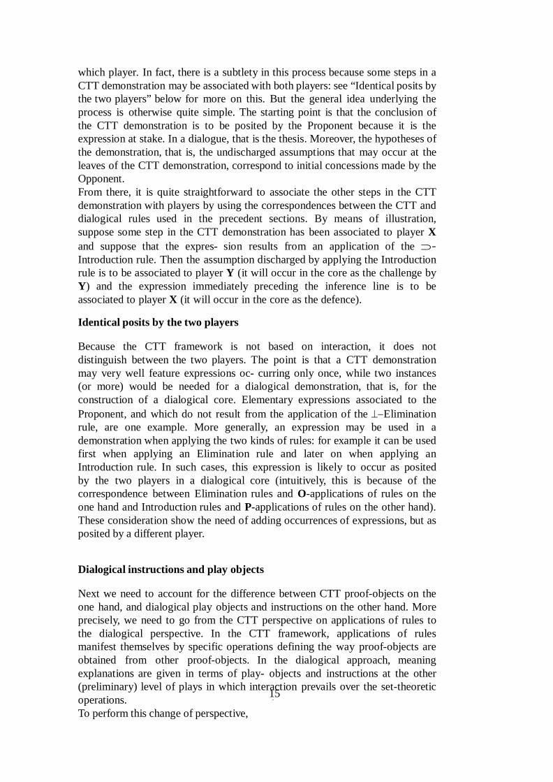
154

which player. In fact, there is a subtlety in this process because some steps in a CTT demonstration may be associated with both players: see “Identical posits by the two players” below for more on this. But the general idea underlying the process is otherwise quite simple. The starting point is that the conclusion of the CTT demonstration is to be posited by the Proponent because it is the expression at stake. In a dialogue, that is the thesis. Moreover, the hypotheses of the demonstration, that is, the undischarged assumptions that may occur at the leaves of the CTT demonstration, correspond to initial concessions made by the Opponent. From there, it is quite straightforward to associate the other steps in the CTT demonstration with players by using the correspondences between the CTT and dialogical rules used in the precedent sections. By means of illustration, suppose some step in the CTT demonstration has been associated to player X and suppose that the expres- sion results from an application of the ⊃-Introduction rule. Then the assumption discharged by applying the Introduction rule is to be associated to player Y (it will occur in the core as the challenge by Y) and the expression immediately preceding the inference line is to be associated to player X (it will occur in the core as the defence). Identical posits by the two players Because the CTT framework is not based on interaction, it does not distinguish between the two players. The point is that a CTT demonstration may very well feature expressions oc- curring only once, while two instances (or more) would be needed for a dialogical demonstration, that is, for the construction of a dialogical core. Elementary expressions associated to the Proponent, and which do not result from the application of the ⊥−Elimination rule, are one example. More generally, an expression may be used in a demonstration when applying the two kinds of rules: for example it can be used first when applying an Elimination rule and later on when applying an Introduction rule. In such cases, this expression is likely to occur as posited by the two players in a dialogical core (intuitively, this is because of the correspondence between Elimination rules and O-applications of rules on the one hand and Introduction rules and P-applications of rules on the other hand). These consideration show the need of adding occurrences of expressions, but as posited by a different player. Dialogical instructions and play objects Next we need to account for the difference between CTT proof-objects on the one hand, and dialogical play objects and instructions on the other hand. More precisely, we need to go from the CTT perspective on applications of rules to the dialogical perspective. In the CTT framework, applications of rules manifest themselves by specific operations defining the way proof-objects are obtained from other proof-objects. In the dialogical approach, meaning explanations are given in terms of play- objects and instructions at the other (preliminary) level of plays in which interaction prevails over the set-theoretic operations. To perform this change of perspective,

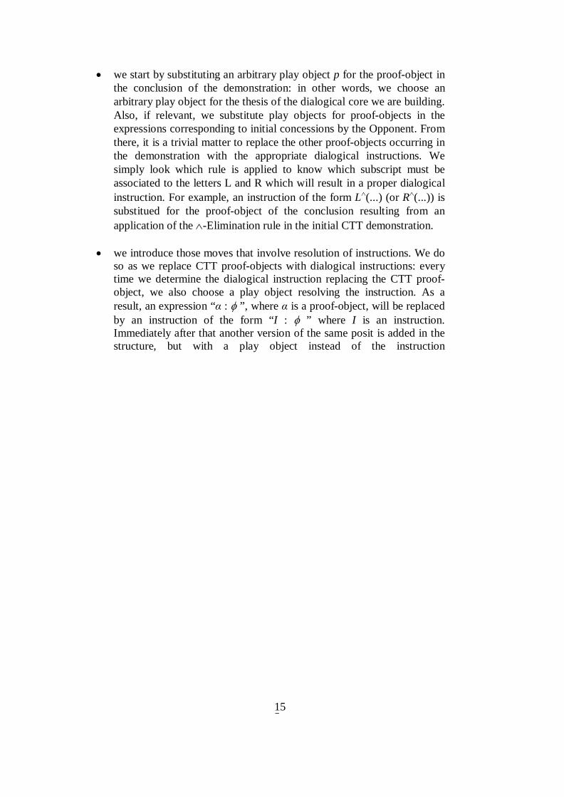
155

• we start by substituting an arbitrary play object p for the proof-object in the conclusion of the demonstration: in other words, we choose an arbitrary play object for the thesis of the dialogical core we are building. Also, if relevant, we substitute play objects for proof-objects in the expressions corresponding to initial concessions by the Opponent. From there, it is a trivial matter to replace the other proof-objects occurring in the demonstration with the appropriate dialogical instructions. We simply look which rule is applied to know which subscript must be associated to the letters L and R which will result in a proper dialogical instruction. For example, an instruction of the form L∧(...) (or R∧(...)) is substitued for the proof-object of the conclusion resulting from an application of the ∧-Elimination rule in the initial CTT demonstration.

• we introduce those moves that involve resolution of instructions. We do

so as we replace CTT proof-objects with dialogical instructions: every time we determine the dialogical instruction replacing the CTT proof-object, we also choose a play object resolving the instruction. As a result, an expression “α : φ ”, where α is a proof-object, will be replaced by an instruction of the form “I : φ ” where I is an instruction. Immediately after that another version of the same posit is added in the structure, but with a play object instead of the instruction

156

I. The reason for this is that we can progressively replace proof-objects with simple instructions relative to play objects, instead of having embedded instructions getting more and more (innecessarily) complex.93 Adding questions At this point we have obtained a tree-like structure featuring a substantial number of expressions which differ only by the player identity and/or maybe by the instruction and play object. Still, some aspects are missing to read the structure at hand in terms of inter- action. To put it simply, the structure lacks challenges consisting in questions. For example, that two expressions X ! I : φ (for some instruction I) and X ! p : φ (for some play object p) follow each other in the structure does not make dialogical sense until the question Y I/? is placed between them: only then can we speak of an interaction in which Y asks X for the resolution of the instruction I and X chooses p for the resolution. Similarly with other questions such as ?∨, ?L , ?R , etc. , depending on the rule at stake. The next step in the translation procedure is therefore to include questions in the relevant way so that one can accurately speak of interaction through the application of dialogical rules. However, the result still cannot be called a dialogical core. For that we need to overcome the difference in the production of ramifications between the CTT framework and dialogical strategies. Rearranging the branches and order of the moves Recall that we are dealing with a tree-like structure written “upside-down”, that is, where the root of the tree (the conclusion of the demonstration we started with) is at the bottom and the leaves are at the top. The most important transformation that remains is reorganising the tree at hand so that we obtain a good candidate for a core of a winning P-strategy. This means we aim to obtain a tree in which branches are linear representations of plays in such a way that ramifications represent choices of the Opponent between different moves (since we are interested in P-strategies). The CTT framework distinguishes betwee rules applied to one or more expressions. In the latter case, a ramification is produced but not in the former case. But since there is no explicit notion of interaction and strategy (in the game-theoretical sense) in Constructive Type Theory, it is obvious that ramifications may not correspond to differences due to possible choices by a player, taken into account in a strategy for his adversary. A typical example are the differences between the CTT Elimination rules for ma- terial implication and universal quantification on the one hand, and their dialogical counterpart on the other hand. In CTT these rules have (at least) two

93 Suppose for example that we have introduced an instruction L∨(p). If we do not decide immediately for a play-object, say q, to resolve this instruction, then the next instruction will be of the form I(L∨(p)) instead of the simpler I(q) — for some I.

157

premisses: first the complex expression and second a judgement of the form a : A when A is the antecedent or the set which is quantified over. Each of these two premisses opens a branch in the demonstration. But in a dialogical game, one is the posit and the other is the challenge against it. Consequently they occur in the same play and hence, in the same branch of a strategy. Notice that this will also happen with other rules including those equality assertions that in the CTT-demonstration result from the application of equality rules. The goal in this step of the transformation is thus to reorganise the tree in order to overcome these differences. We must also take some additional precautions (such as adding the choices of repetition ranks) so that the branches in the new tree do indeed represent plays. Once this has been accomplished we reintroduce applications of the Socratic Rule to those elementary posits by P that result of the resolution of some instruction. In other words, once all the previous steps have been carried out we reintroduce those equalities arising from O's-choices while resolving instructions that have not been already implemented in the CTT- demonstration. Recall that the standard CTT-demonstrations deploy Σ- and Π-equalities only when the elimination rules might produce a non-canoncial proof-object. We shall stop the general explanations here. All the details are given in the full description of the translation algorithm given below. Let us simply mention here that the procedure is meant to obtain the core of a winning P-strategy after all these modifications. This is something that must be proved, which we do afterwards. IV.6.3.2 The procedure Let us precise now the details of the procedure: We start with a CTT demonstration D of an expression E under a set H of global hypotheses and/or epistemic assumptions (that is, assertions that include "given" proof-objects). A From judgements to posits: First we enrich the initial demonstration with player identities and the posit sign ! A1. Rewrite the conclusion E as P ! E . Then, for every h ∈ H occurring as a leaf of D , rewrite h as O ! h. Go to A2. A2. Scan D bottom-up. When there is no unused expression left, go to A3. Oth-erwise, let E1 be the (left-most94) unused expression X ! E1 Then,

1. If X is O and E1 results in D from applying an Introduction rule, then insert P !E1 as the conclusion of the rule preceding O !E1. Consider the latter as used and go back to A2.

2. If X is P and E1 results in D from applying an Elimination rule other than for ∨ or Σ, then insert O ! E1 as the conclusion of the rule preceding P ! E1 .

94 This accounts for the fact that D may have several branches.

158

Consider the latter as used and go back to A2. 3. Otherwise use the correspondences between CTT and

dialogical rules given in chapter 3 to rewrite the expressions allowing the application of the rule with the adequate player.95

In doing so, observe the following constraints:

• an expression can be labelled as a P- and an O-posit, • each player can be assigned at most once to an expression.

After this, consider the expression as used and go back to A2. A3. Scan the demonstration at hand. For each elementary posit by the Proponent which has no counterpart by the Opponent apply one of the following,

1. If it is the result of an application of the ⊥-Elimination rule, then leave it like that.

2. If there is no corresponding O-posit (and , then insert one immediately below the Proponent’s posit, and insert the expression P sic(n)/Socratic Rule at the leaf of the current branch.

Then go to A4. A4. If there are leaves with the double label O ! / P !, separate them into two expressions such that the Proponent’s posit is placed as the leaf. Go to B. B Instructions and play objects. Next we introduce play objects at the place of proof-objects. This is done in the following way. B1. In the conclusion P !E , replace the proof-object with an arbitrary play object p. Then, for each initial concession O !h occurring at a leaf of the demonstration, substitute, if relevant, an arbitrary play object for the proof-object. Consider these expressions as treated and go to B2. B2. Scan the demonstration bottom-up. If there is no expression left untreated, go to C. Otherwise take the leftmost expression X ! E2 with a play object which has not been treated so far, and

• Use the correspondences between CTT and dialogical rules given in chapter 3 to substitute the adequate instructions for the proof-object(s) in the premiss (pre-

95 For example, given the situation α : (Πx : A) a : A ---------------------------- Π E O ! … The deployment of the procedure described by A3 yields: O ! α : (Πx : A) P ! a : A -------------------------------- Π E O ! …

159

misses) of the rule whose application results in X ! E2 . • For each instruction introduced that way, copy the expression at

stake, replacing • the instruction by an arbitrary play object. Place the

version with the play object immediately above the expression with the instruction.

• Consider X ! E2 as processed and go back to B2. C Adding questions. Scan the demonstration and identify the applications of rules for which the dialogical counterpart features a question. For each expression understood as a defence according to such a rule, add the corresponding challenge performed by the adversary immediately below the expression. Go to D. D Move the Opponent’s initial concessions. Consider each leaf of the demonstration at hand which is an initial concession by the Opponent — that is, an undischarged assumption of the initial demonstration D which has been identified as an Opponent’s move. Remove it and place it below the conclusion P ! E . In case of multiple occurrences, keep only one occurrence. Go to E. E Removing non-dialogical splits. Scan the demonstration top-down. Going from the left to the right, check each point where two different branches join. Depending on what the case may be, apply one of the following,

1. If the ramification is such that the two branches are opened by two O-posits relevant for a rule dealing with a logical constant, then ignore and proceed downwards.

2. Otherwise, “cut” one and “paste” it above the other one, according to the following convention:

- If both branches have a P-move as the leaf, or if both have an O-move as the leaf, then pick any one of the branch to be cut and pasted, - Otherwise pick the one with a P-move at the leaf to be cut and pasted. Go to F. F Reordering the nodes. Scan the tree structure at hand bottom-up. Starting from the thesis P ! E , change the order of the expressions according to the following conditions, • Each O-move is a reaction — as specified by the dialogical rules — to the P- move placed immediately below, • A question or a posit which is a challenge always occurs before (i.e. closer to the root) a defence reacting to it. • Ramifications are preserved so that each branch is opened with an O-move as a reaction to a P-move which is immediately below.

160

Go to G. G Introducing equalities by means of the Socratic Rule. Search for nodes labelled sic(n)/Socratic Rule. For those P-posits that

• do not result from the resolution of an instruction rewrite the rule as as application of sic(n) rule.

• do result from the resolution of an instruction rewrite the rule as as application of sic(n) rule reintroduce applications of the Socratic Rule and the corresponding equalities arising from that rule.

Go to H H Adding ranks. Insert an expression O n := 1 immediately above the thesis P !E . Then insert an expression P m := k above the one just inserted. Choose k to be the biggest number of times a given rule is applied by P to the same expression in the tree. The procedure stops. Adequacy of the algorithm We have developed the algorithm transforming a CTT demonstration into a winning strategy. It remains to show that the algorithm indeed does so, in other words that applying the algorithm to a given a CTT demonstration results in the core of a winning P-strategy. To be more specific, the point is to show that the result of applying the algorithm to a CTT demonstration is a tree in which,

1. Each branch represents a play: the sequence of moves in each branch complies with the game rules,

2. Each play in the tree is won by the Proponent, 3. The tree describes all the relevant alternatives for a core. In other words:

there is no significantly different course of action for O that would be disregarded in the resulting tree.96

• Proposition: Each branch in the resulting tree represents a play. We need to show that in each branch the sequence of moves complies with the rules of dialogical games. Proof. Because the translation observes a correspondence between CTT rules and

96 By significantly different we mean other than relative to the order of the Opponent’s moves, or the choice of play-objects to replace instructions.

161

dialogical particle rules, we simply need to check that the dialogical structural rules are observed.97 We leave the Winning Rule aside for now since it is the topic we address in the next Proposition. So for the Starting Rule SR0, steps D and H of the algorithm ensure that every sequence of moves in the tree starts with the initial concessions of the Opponent, which are followed by the thesis posited by the Proponent and then by the choices of repetition ranks. As for the Intuitionistic Development Rule, step F of the algorithm guarantees that each move following the repetition ranks in a sequence is played in reaction to a previous move. The condition in step F according to which O-moves immediately follow the P-move to which it is a reaction ensures that the intuitionistic restriction of the Last Duty First is observed.98 Moreover the choice of the repetition ranks prescribed by step H ensures that the players do not perform unauthorised repetitions. As for the Special Socratic Rule, no challenge against an elementary O-is added when applying the algorithm. Moreover, in the case of elementary posits made by P, step A3 and G of the procedure ensure that, if needed, a corresponding posit by O and the adequate challenges and defences are added. As for the rules related to the Resolution of Instructions, step B of the algorithm (in combination with step C introducing questions) guarantees that instructions are resolved according to the structural rules – recall that we ignore the formation dialogues since we are focusing on that fragment of CTT in which verifying the well formation is assumed successful. Now that we have established that the branches represent plays because they comply with the dialogical rules, we must assess the situation in relation to victory and show that:

• Proposition. Each branch of the resulting tree represents a play won by P. Proof. We must check that the leaf of each branch is either:

1. an elementary posit by P preceded by a O-posit of ⊥, 2. an elementary posit by P (different to the preceeding case) 3. a P-move “sic(n)” for some move numbered n 4. a P-equality that results from applying the Socratic Rule

But all this is guaranteed by steps A3, E, F and G of the algorithm. Finally, it remains to show that the tree describes all the relevant courses of actions for the Opponent underlying the core of a P-strategy:

• Proposition. There is no P-move in the tree remaining unanswered by O and there is no rule that would allow to leave such a P-move without a response.

97 And given that step C of the algorithm has been used to insert questions. 98 This is known since Felscher (1985). See also more details in Clerbout (2014c).

162

Proof. We know from the initial demonstration D and steps A1-A4 of the algorithm that every posit made by the Proponent in the resulting tree occurs as the result of an Introduction rule, of the Elimination rule for the Σ operator or of the Elimination rule for disjunction. In the case of complex posits the correspondence with dialogical particle rules together with the addition of questions via step C of the algorithm ensure that they are challenged and that when they are themselves played as challenges they are answered. In the case of elementary posits, we know from the proof of preceeding Proposition that they are challenged if the Opponent can. Moreover, all the possible challenges allowed by the particle rules are covered by the CTT rules they correspond to. For this reason, the only remaining possible variations left to the Opponent are the order of her moves and the choice of play objects for the Resolution of Instructions. But these variations are the ones which are not relevant to build the core of a P-strategy. In other words the correspondence between CTT rules and the particle rules ensure that the starting demonstration D already contains the variations which are relevant for a core of P-strategy. The adequacy of our translation procedure, which amounts to the second direction of the equivalence result we stated at the beginning of this study, is then a direct consequence of both Propositions.

• Corollary. The result of applying the algorithm that transcribes a CTT demonstration into a tree of P-terminal plays constitutes the core of a winning P-strategy.

163

IV.6.4 Solved Exercises99 IV.6.4.1 From the Core to natural deduction demonstrations Exercise 1

Let C be the set of initial concessions made by the Opponent, and Φ a

judgment which the Proponent will bring forward as a thesis of a dialogue, such that C = c : A ∧ (B ∧ C) and Φ = d : (A ∧ B) ∧ C. The task is to transform the core of the winning strategy for the thesis into a natural-deduction demonstration by deploying the procedure described in the preceding sections. We start by displaying the core of the winning strategy as a tree

0. P ! d : (A ∧ B) ∧ C 0.1. O ! c : A ∧ (B ∧ C) 1. O ! n: = 1 2. P ! m: = 2

3. O ?L [?, 0] 3. O ?R [?, 0] 4. P ! L^(d): A ∧ B [!, 3] 4. P ! R^(d) : C [!, 3] 5. O ? ---/ L^(d) [?, 4] 5. O ? ---/ R^(d) [?, 4] 6. P ! d1: A ∧ B [!, 5] 6. P ?R [?, 0.1] 7. O ! R^(c): B ∧ C [!, 6] 8. P ? ---/ R^(c) [?, 7] 7. O ?L [?, 6] 7. O ?R [?, 6] 9. O ! c2 : B ∧ C [!, 8] 8. P ! L^(d1.1) : A [7] 8. P! R^(d1) : B [!, 7] 10. P ?R [?, 9] 9. O ? ---/ L^(d1) [?, 8] 9. O ? ---/ R^(d1) [?, 8] 11. O ! R^(c2): C [10] 10. P ?L [?, 0.1] 10. P ?R [?, 0.1] 12. P ? ---/ R^(c2) [?, 11] 11. O ! L^(c) : A [!, 10] 11. O ! R^(c) : B ∧ C [!, 10] 13. O ! c2.2: C [!, 12] 12. P ? ---/ L^(c) [?, 11] 12. P ? ---/ R^(c) [?, 11] 14. P ! c2.2: C [!, 5] 13. O ! c1 : A [!, 12] 13. O ! c2 : B ∧ C [!, 12] 15. O ?, = c2.2 [?, 14] 14. P ! c1 : A [!, 9] 14. P ?, L [?, 13] 16. P ! R^(c2) = c2.2 : C [!, 15] 15. O ? = c1 [?, 14] 15. O ! L^(c2) : B [!, 14] 16. P ! L^(c) = c1 : A [!, 15] 16. P ? ---/ L^(c2) [?, 15] 17. O ! c2.1 : B [!, 16] 18. P ! c2.1 : B [!, 9] 19. O ? = c2.1 [?, 18] 20. P ! L^(c2) = c2.1 : B [!, 19] Recapitulation: the strategic object of thesis: The thesis is a conjunction. Thus P must win when both the left and the reight side of it are required. Let us start with the right. So we must look at the end of a branch where C is thE last move by P; This is move 16 at the outmost right branch. But move 16 is defence of the choice he made while resolving R^(d), and this choice has been guided by the Opponent’s resolution of R^(c2): this is what the equality in 16 expresses. The branch also conveys the information that O’s resolution is at the end of a chain. We can write then

99 Gildas Nzokou is the author of this section.

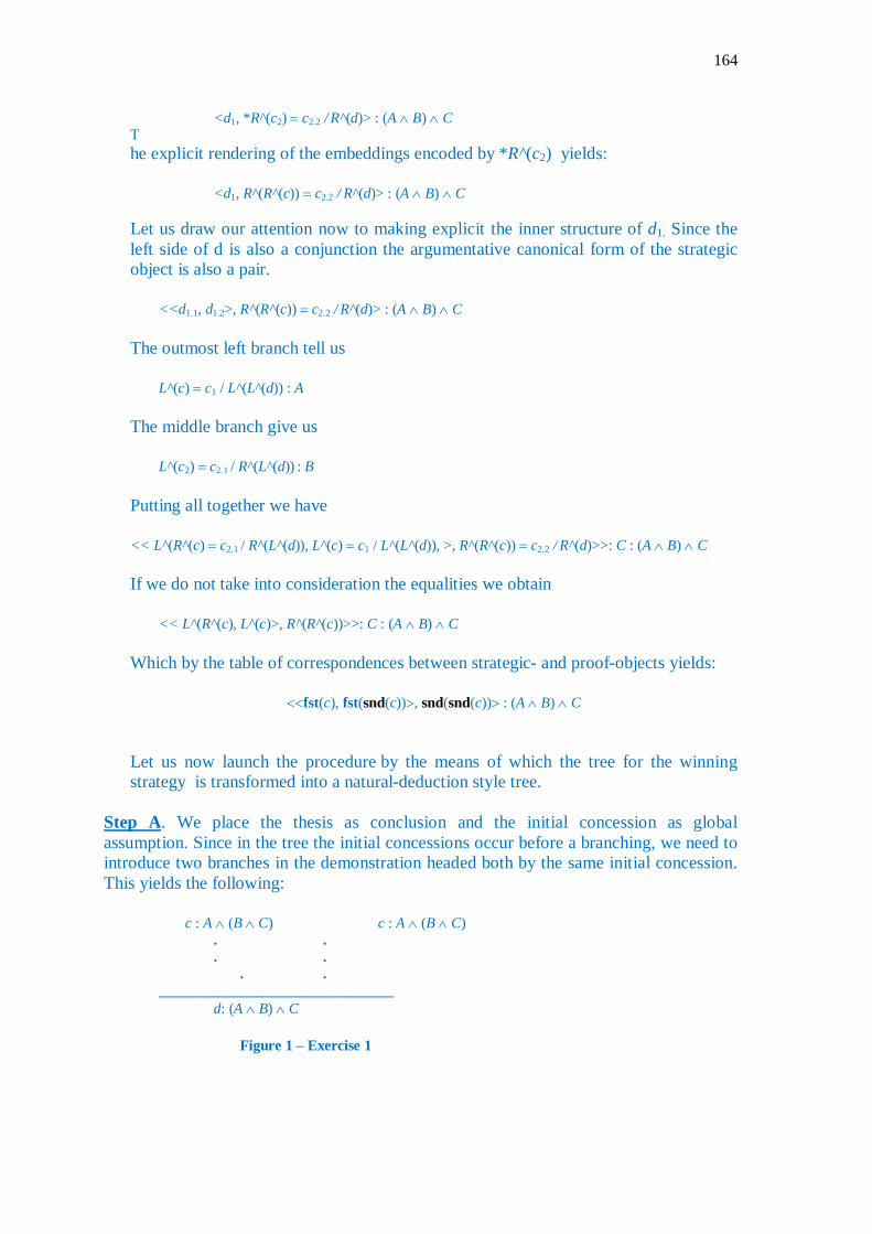
164

<d1, *R^(c2) = c2.2 / R^(d)> : (A ∧ B) ∧ C T he explicit rendering of the embeddings encoded by *R^(c2) yields:

<d1, R^(R^(c)) = c2.2 / R^(d)> : (A ∧ B) ∧ C Let us draw our attention now to making explicit the inner structure of d1. Since the left side of d is also a conjunction the argumentative canonical form of the strategic object is also a pair.

<<d1.1, d1.2>, R^(R^(c)) = c2.2 / R^(d)> : (A ∧ B) ∧ C The outmost left branch tell us

L^(c) = c1 / L^(L^(d)) : A The middle branch give us

L^(c2) = c2.1 / R^(L^(d)) : B Putting all together we have << L^(R^(c) = c2.1 / R^(L^(d)), L^(c) = c1 / L^(L^(d)), >, R^(R^(c)) = c2.2 / R^(d)>>: C : (A ∧ B) ∧ C If we do not take into consideration the equalities we obtain

<< L^(R^(c), L^(c)>, R^(R^(c))>>: C : (A ∧ B) ∧ C Which by the table of correspondences between strategic- and proof-objects yields:

<<fst(c), fst(snd(c))>, snd(snd(c))> : (A ∧ B) ∧ C Let us now launch the procedure by the means of which the tree for the winning strategy is transformed into a natural-deduction style tree.

Step A. We place the thesis as conclusion and the initial concession as global assumption. Since in the tree the initial concessions occur before a branching, we need to introduce two branches in the demonstration headed both by the same initial concession. This yields the following:

c : A ∧ (B ∧ C) c : A ∧ (B ∧ C) . . . .

. . ________________________________

d: (A ∧ B) ∧ C

Figure 1 – Exercise 1

165

Step B. We scan now for the lowest expression in demonstration tree – at this moment it is the thesis – and find in the core the responses to it. In our case these responses are the challenges on the conjunctions:

c : A ∧ (B ∧ C) c : A ∧ (B ∧ C) . . . .

?L 100

[?, 0] ?R [?, 0]

(this step does not follow strictly speaking the algorithm)101 . . . . L^(d) : A ∧ B. R^(d) : C _______________________________________________________________

d : (A ∧ B) ∧ C

Figure 2 – Exercise 1

B.0 Let us look now for the challenge and the resolution of the instructions.

c : A ∧ (B ∧ C) c : A ∧ (B ∧ C) . . . . . . . . d1: A ∧ B c2.2: C _________EPI ________ EPI L^(d) : A ∧ B. R^(d) : C _______________________________________________________________

d : (A ∧ B) ∧ C

Figure 2 – Exercise 1

B.1 and B.2. Whereas the left of the two expressions just added is a conjunction the right one is an elementary expression. Thus, steps B.2.b and B.2.a apply respectively.

Let us start with the latter. Since it is an elementary expression by P we know that it must be the result of an SR rule. We also apply the instruction in relation to the EPI and suppress the non resolved expression.

c : A ∧ (B ∧ C) c : A ∧ (B ∧ C) . . . . . .

100 In order to facilitate the reading of the process we highlight in bold the last challenge-defence pairs. 101 The transformation-algorithm does not really include a step where questions are written down in the demonstration tree..

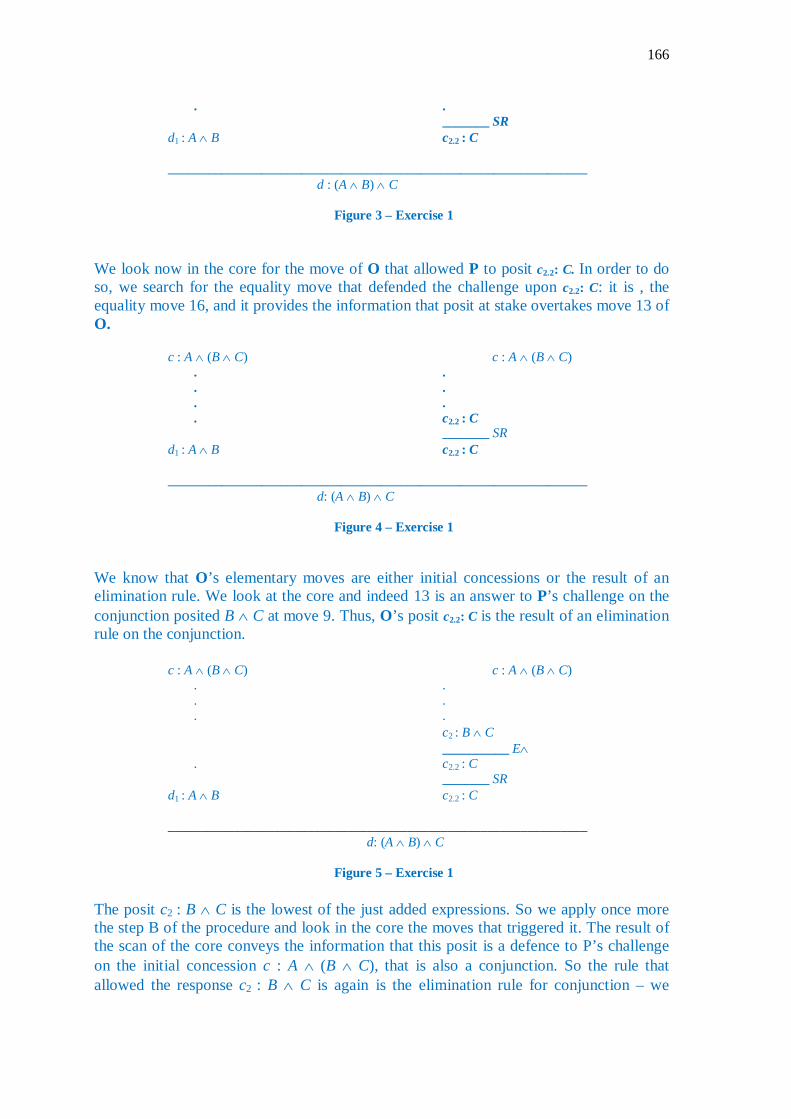
166

. . _______ SR d1 : A ∧ B c2.2 : C

_______________________________________________________________

d : (A ∧ B) ∧ C

Figure 3 – Exercise 1

We look now in the core for the move of O that allowed P to posit c2.2: C. In order to do so, we search for the equality move that defended the challenge upon c2.2: C: it is , the equality move 16, and it provides the information that posit at stake overtakes move 13 of O.

c : A ∧ (B ∧ C) c : A ∧ (B ∧ C) . . . . . . . c2.2 : C _______ SR d1 : A ∧ B c2.2 : C

_______________________________________________________________

d: (A ∧ B) ∧ C

Figure 4 – Exercise 1

We know that O’s elementary moves are either initial concessions or the result of an elimination rule. We look at the core and indeed 13 is an answer to P’s challenge on the conjunction posited B ∧ C at move 9. Thus, O’s posit c2.2: C is the result of an elimination rule on the conjunction.

c : A ∧ (B ∧ C) c : A ∧ (B ∧ C) . . . . . . c2 : B ∧ C __________ E∧ . c2.2 : C _______ SR d1 : A ∧ B c2.2 : C

_______________________________________________________________

d: (A ∧ B) ∧ C

Figure 5 – Exercise 1

The posit c2 : B ∧ C is the lowest of the just added expressions. So we apply once more the step B of the procedure and look in the core the moves that triggered it. The result of the scan of the core conveys the information that this posit is a defence to P’s challenge on the initial concession c : A ∧ (B ∧ C), that is also a conjunction. So the rule that allowed the response c2 : B ∧ C is again is the elimination rule for conjunction – we

167

skiped here the steps concerning the resolution of the instructions and added expression after the instructions have been solved:

c : A ∧ (B ∧ C) c : A ∧ (B ∧ C) . . . . . . _______ E∧ c2 : B ∧ C _______ E∧ . c2.2 : C _______ SR d1 : A ∧ B c2.2 : C

_______________________________________________________________

d: (A ∧ B) ∧ C

Figure 6– Exercise 1

Step C (to the right branch). Since we worked out all of the branch we follow now the step C that instructs deleting the SR and leave only one copy of the elementary expression.

c : A ∧ (B ∧ C) . . . c : A ∧ (B ∧ C) _____________ E∧ c2 : B ∧ C _________ E∧ . d1 : A ∧ B c2.2 : C

_______________________________________________________________

d: (A ∧ B) ∧ C

Figure 7 - Exercise 1

Step B (to the left branch) We turn our attention now to the left branch and take the lowest expression last added in the branch of the demonstration. It is a conjunction posited by P. Thus, it is the result of an ∧–introduction rule.

c : A ∧ (B ∧ C) . . . c : A ∧ (B ∧ C) _____________ E∧ c2 : B ∧ C _________ I∧ . _________ E∧ d1 : A ∧ B c2.2 : C

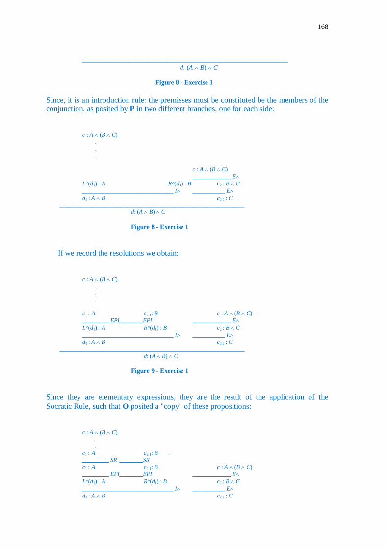
168

_______________________________________________________________

d: (A ∧ B) ∧ C

Figure 8 - Exercise 1

Since, it is an introduction rule: the premisses must be constituted be the members of the conjunction, as posited by P in two different branches, one for each side:

c : A ∧ (B ∧ C) . . . c : A ∧ (B ∧ C) _____________ E∧ L^(d1) : A R^(d1) : B c2 : B ∧ C _______________________________ I∧ ___________ E∧ d1 : A ∧ B c2.2 : C

_______________________________________________________________ d: (A ∧ B) ∧ C

Figure 8 - Exercise 1

If we record the resolutions we obtain:

c : A ∧ (B ∧ C) . . . c1 : A c2.1: B c : A ∧ (B ∧ C) _________ EPI________EPI _____________ E∧ L^(d1) : A R^(d1) : B c2 : B ∧ C _______________________________ I∧ ___________ E∧ d1 : A ∧ B c2.2 : C

_______________________________________________________________ d: (A ∧ B) ∧ C

Figure 9 - Exercise 1

Since they are elementary expressions, they are the result of the application of the Socratic Rule, such that O posited a "copy" of these propositions:

c : A ∧ (B ∧ C) . . c1 : A c2.1: B . _________ SR ________SR c1 : A c2.1: B c : A ∧ (B ∧ C) _________ EPI________EPI _____________ E∧ L^(d1) : A R^(d1) : B c2 : B ∧ C _______________________________ I∧ ___________ E∧ d1 : A ∧ B c2.2 : C

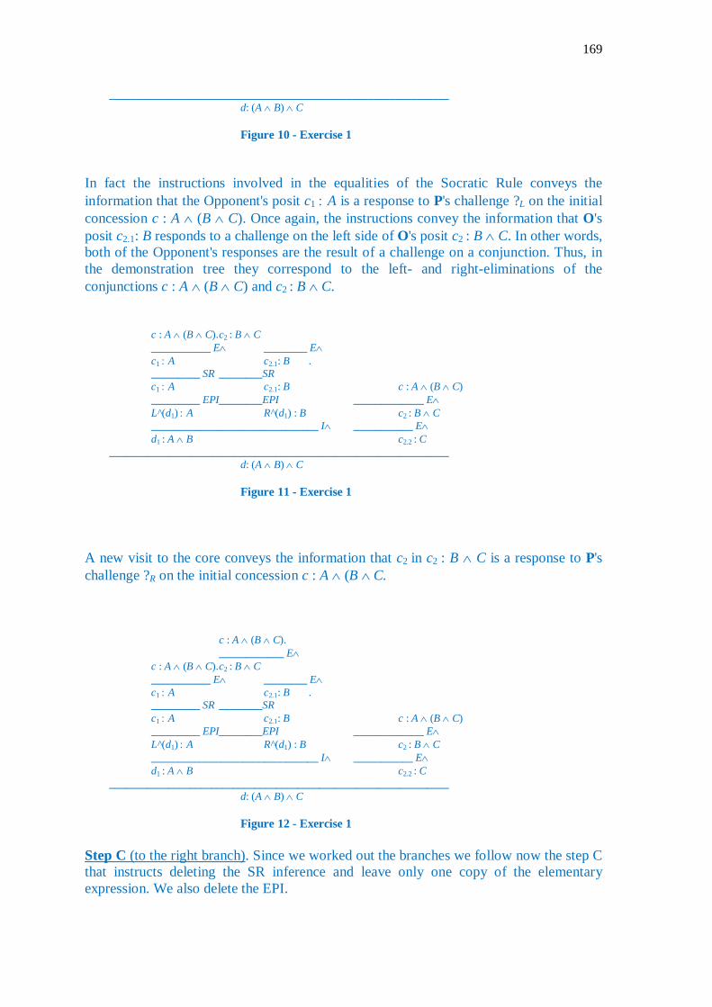
169

_______________________________________________________________ d: (A ∧ B) ∧ C

Figure 10 - Exercise 1

In fact the instructions involved in the equalities of the Socratic Rule conveys the information that the Opponent's posit c1 : A is a response to P's challenge ?L on the initial concession c : A ∧ (B ∧ C). Once again, the instructions convey the information that O's posit c2.1: B responds to a challenge on the left side of O's posit c2 : B ∧ C. In other words, both of the Opponent's responses are the result of a challenge on a conjunction. Thus, in the demonstration tree they correspond to the left- and right-eliminations of the conjunctions c : A ∧ (B ∧ C) and c2 : B ∧ C.

c : A ∧ (B ∧ C). c2 : B ∧ C ___________ E∧ ________ E∧ c1 : A c2.1: B . _________ SR ________SR c1 : A c2.1: B c : A ∧ (B ∧ C) _________ EPI________EPI _____________ E∧ L^(d1) : A R^(d1) : B c2 : B ∧ C _______________________________ I∧ ___________ E∧ d1 : A ∧ B c2.2 : C

_______________________________________________________________ d: (A ∧ B) ∧ C

Figure 11 - Exercise 1

A new visit to the core conveys the information that c2 in c2 : B ∧ C is a response to P's challenge ?R on the initial concession c : A ∧ (B ∧ C.

c : A ∧ (B ∧ C). ____________ E∧

c : A ∧ (B ∧ C). c2 : B ∧ C ___________ E∧ ________ E∧ c1 : A c2.1: B . _________ SR ________SR c1 : A c2.1: B c : A ∧ (B ∧ C) _________ EPI________EPI _____________ E∧ L^(d1) : A R^(d1) : B c2 : B ∧ C _______________________________ I∧ ___________ E∧ d1 : A ∧ B c2.2 : C

_______________________________________________________________ d: (A ∧ B) ∧ C

Figure 12 - Exercise 1

Step C (to the right branch). Since we worked out the branches we follow now the step C that instructs deleting the SR inference and leave only one copy of the elementary expression. We also delete the EPI.

170

c : A ∧ (B ∧ C) . ________ E∧ c : A ∧ (B ∧ C) c2 : B ∧ C c : A ∧ (B ∧ C) ___________ E∧ ________ E∧ _____________ E∧ c1 : A c2.1: B c2 : B ∧ C _______________________________ I∧ ___________ E∧ d1 : A ∧ B c2.2 : C

_______________________________________________________________ d: (A ∧ B) ∧ C

Figure 13 - Exercise 1

Step D. We reached the final step now. Accordingly we replace the play objects with proof-objects and obtain the CTT-demonstration in the style of natural-deduction tree.

c : A ∧ (B ∧ C) . ____________ E∧ c : A ∧ (B ∧ C) snd(c): B ∧ C c : A ∧ (B ∧ C) ___________ E∧ ___________ E∧ _____________ E∧ fst(c) : A fst(snd(c)) : B snd(c) : B ∧ C _______________________________ I∧ _____________ E∧

<fst(c), fst(snd(c))> : A ∧ B snd(snd(c)) : C _______________________________________________________________

<<fst(c), fst(snd(c))>, snd(snd(c))> : (A ∧ B) ∧ C

Figure 14 - Exercise 1

Exercise 2 Develop a demonstration of e : (B ∧ A) ⊃ C, given the global assumption d : (A ∧ B) ⊃ C, out of the strategic core.

We start by displaying the core. For perspicuity we repeated move 16

0. P ! e : (B ∧ A) ⊃ C 0.1 O ! d : (A ∧ B) ⊃ C 1. O ! L⊃(e) : B ∧ A [?, 0] 2. P ?-/ L⊃(e) [?, 1] 3. O ! e1: B ∧ A [!, 2] 4. P ?L [?, 3] 5. O ! L^(e1): B [!, 4] 6. P ?-/ L^(e1) [?, 5] 7. O ! e1.1: B [!, 6] 8. P ?R [?, 3] 9. O ! R^(e1): A [!, 8] 10. P ?-/ R^(e1) [?, 9] 11. O ! e1.2: A [!, 10] 12. P ! R⊃(e): C [!, 1] 13. O ?-/ R⊃(e) [?, 12] 14. P ! L⊃(d): A ∧ B [?, 0.1] 15. O ?-/ L⊃(d) [?, 14] 16. P ! d1: A ∧ B [!, 15]

171

16. P ! d1: A ∧ B [!, 15] 17. O ?L [?; 16] 17. O ?R [?, 16] 17. O ! R⊃(d): C [!, 16] 18. P ! L^(d1): A [!, 17] 18. P ! R^(d1): B [!, 17] 18. P ?-/ R⊃(d) [?; 17] 19. O ?-/ L^(d1) [?, 18] 19. O ?-/ R^(d1) [?, 18] 19. O ! d2: C [!, 18] 20. P ! e1.2: A [!, 19] 20. P ! e1.1: B [! 19] 20. P ! d2: C [!, 13] 21. O ? = e1.2 [?, 20] 21. O ?= e1.1 [ ?, 20] 21. O ?= d2 [?, 20] 22. P ! R^(e1) = e1.2: A [!, 21] 22. P ! L^(e1) = e1.1: B [!, 21] 22. P ! R⊃(d) = d2: C [!, 21]

Recapitulation: the strategic object of thesis:

(d ⟦< R^(e1), L^(e1)>)⟧) ⟦L⊃(e)⟧ : (B ∧ A) ⊃ C Step A. We place the thesis as conclusion and the initial concession as global assumption:

d : (A ∧ B) ⊃ C . . . .

. . ________________________________

e : (B ∧ A) ⊃ C

Figure 1 – Exercise 2

Step B. We scan now for the lowest expression in demonstration tree – at this moment it is the thesis – and find in the core the response to it. In our case this response is a challenge on the implication. Since a challenge on the implication of the Proponent is the local assumption e1: B ∧ A (after the resolution), which constitutes one of the premisses of the introduction rule of the implication in the thesis. The second premiss is P's posit d2: C, that occurs in the outmost right branch of the core as the move 20.

d : (A ∧ B) ⊃ C e1 : B ∧ A . . . .

. _________ . d2 : C

________________________________ I⊃ e : (B ∧ A) ⊃ C

Figure 2 – Exercise 2

Since the defence of the implication is an elementary expression of P, it must be a copy of a posit of O. Indeed move 20 is a copy of move 19, as recorded by the equality of move 22. This yields the following SR indication:

d : (A ∧ B) ⊃ C e1 : B ∧ A . .

172

. d2 : C . _________ SR . d2 : C

________________________________ I⊃ e : (B ∧ A) ⊃ C Figure 3 – Exercise 2

Now, the core informs us the move 19 is the result of the resolution of the right part of the initial concession d : (A ∧ B) ⊃ C . Thus, 19 is the result of the elimination rule for implication applied to the concession. The latter requires that P posits the antecedent as a challenge. And this is what Proponent's posit d1: A ∧ B (move 16) is about:

e1 : B ∧ A . . d : (A ∧ B) ⊃ C d1 : A ∧ B _________________________. E⊃

. d2 : C _________ SR . d2 : C

________________________________ I⊃ e : (B ∧ A) ⊃ C Figure 4 – Exercise 2

We now that the Opponent has two options to respond to a challenge on an implication, namely, positing the consequent, and launching a counterattack on the challenge. The defensive move has been implemented in the preceding step, now we must care of the counterattack. Since the challenge of the Proponent is a conjunction, there are two possible challenges, namelbry, left and right. Each of them opens a new branch. The branches of the core, trigger two branches in the demonstration tree by applying twice the ∧-introduction rule, that corresponds to both of the moves 20 at the outmost left branch and middle branch respectively.

e1 : B ∧ A ______ ______ e1.2 : A e1.1 : B . ____________________ I ∧ d : (A ∧ B) ⊃ C d1 : A ∧ B _________________________. E⊃

. d2 : C _________ SR . d2 : C

________________________________ I⊃ e : (B ∧ A) ⊃ C Figure 5 – Exercise 2

Since P-posits e1.2: A and e1.1: B are elementary, they are the result of the application of the Socratic Rule.

e1 : B ∧ A

173

e1.2 : A e1.1 : B ______ SR ______ SR e1.2 : A e1.1 : B . __________________________ I ∧ d : (A ∧ B) ⊃ C d1 : A ∧ B __________________________________. E⊃

. d2 : C ______ SR . d2 : C

________________________________ I⊃ e : (B ∧ A) ⊃ C Figure 6 – Exercise 2

Move 5 O ! L^(e1): B and move 9 O ! R^(e1): A convey the information the Opponents moves are the result of the application of the ∧-elimination rule to the local assumption e1: B ∧ A.

e1 : B ∧ A e1 : B ∧ A _________ E ∧ __________E ∧ e1.2 : A e1.1 : B ______ SR ______ SR e1.2 : A e1.1 : B . __________________________ I ∧ d : (A ∧ B) ⊃ C d1 : A ∧ B __________________________________________. E⊃

d2 : C ______ SR . d2 : C

________________________________ I⊃ e : (B ∧ A) ⊃ C Figure 7 – Exercise 2

Step C. We follow now the step C that instructs deleting the SR and leave only one copy of the elementary expression.

e1 : B ∧ A e1 : B ∧ A _________ E ∧ __________E ∧ e1.2 : A e1. : B . ___________________________ I ∧ d : (A ∧ B) ⊃ C d1 : A ∧ B __________________________________________. E⊃

d2 : C ________________________________ I⊃

e : (B ∧ A) ⊃ C Figure 8 – Exercise 2

Step D. We reached the final step now. Accordingly we replace the play objects with proof-objects and obtain the CTT-demonstration in the style of natural-deduction tree.

174

e1: B ∧ A e1: B ∧ A

_________ E ∧ __________E ∧ snd(e1) : A fst(e1) : B . ___________________________ I ∧ d : (A ∧ B) ⊃ C <snd(e1), fst(e1)> : A ∧ B __________________________________________. E⊃

ap(d, <snd(e1), fst(e1)>) : C ________________________________ I⊃

λe1.[ap(d, <snd(e1), fst(e1)>)] : (B ∧ A) ⊃ C Figure 9 – Exercise 2

175

V. The Dialogical take on propositional identity.

A first encounter with material dialogues The dialogical take on propositional identity – that is identity as a proposition – is also based on the Socratic Rule. However, differently to the formulations of the Socratic Rule deployed so far, the present context requires a setting of the rule specific to this kind of identities that are usually conceived in the CTT-framework as a triadic relation predicate (see II.2.8). This applies to both the intensional (Id(A, a, a)) and the extensional (Eq(A, a, a))case. We start with the former. As a matter of fact, the specificity of the Socratic Rule required by the dialogical conception of propositional identity takes us to material dialogues. Indeed, as discussed in the last chapter of our book, material dialogues are those where the Socratic Rule has to be formulated in a way that suits the content of the elementary propositions or sets that are to be distinguished in setting. Notice the constitution of the sets as resulting from the Socratic Rule leaves the main task to the Opponent, and this procedure applies to whatever set. Notice too, that this means that the rules prescribing the interaction with the specific elementary propositions distinguished by a material dialogue are not player-independent. This applies to the forms of the play objects involved: we call them respectively canonical development form and argumentative development form, and they take place in material dialogues. The development form of a play object is a step towards the form of a strategic object which are also player-dependent More generally, dialogical logic enjoys three different kinds of canonical and three kinds of argumentation forms

• Local level: canonical dialogical form–involves play objects. • Local level: argumentation form – involves play objects. • Structural level: canonical development form – involves the deployment of

play objects triggered by a challenge on an elementary proposition posited by the Proponent – concerns some level of material dialogues.

• Structural level: argumentative development form – involves the deployment of play object triggered by some requests on an elementary proposition posited by the Opponent – concerns some level of material dialogues.

• Strategic level: Recapitulation form – involves strategic objects. • Strategic level: Record of instructions –involves strategic objects.

Play-

level Player-in-dependence

Strategy-level

Canonical argumentation form 1 1 0 Argumentation form 1 1 0 Canonical development form Involve challenges on elementary propositions of P

1 0 0

Argumentative development form Involve requests on elementary proposition of O

1 0 0

Strategic object as recapitulation 0 0 1 Strategic object as record of instructions

0 0 1

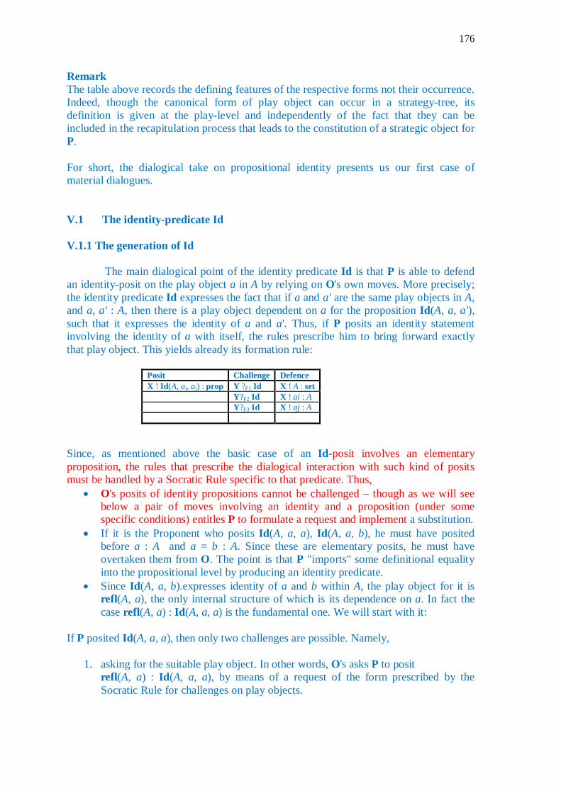
176

Remark The table above records the defining features of the respective forms not their occurrence. Indeed, though the canonical form of play object can occur in a strategy-tree, its definition is given at the play-level and independently of the fact that they can be included in the recapitulation process that leads to the constitution of a strategic object for P. For short, the dialogical take on propositional identity presents us our first case of material dialogues. V.1 The identity-predicate Id V.1.1 The generation of Id The main dialogical point of the identity predicate Id is that P is able to defend an identity-posit on the play object a in A by relying on O's own moves. More precisely; the identity predicate Id expresses the fact that if a and a' are the same play objects in A, and a, a' : A, then there is a play object dependent on a for the proposition Id(A, a, a'), such that it expresses the identity of a and a'. Thus, if P posits an identity statement involving the identity of a with itself, the rules prescribe him to bring forward exactly that play object. This yields already its formation rule:

Posit Challenge Defence X ! Id(A, ai, aj) : prop Y ?F1 Id X ! A : set Y?F2 Id X ! ai : A Y?F3 Id X ! aj : A

Since, as mentioned above the basic case of an Id-posit involves an elementary proposition, the rules that prescribe the dialogical interaction with such kind of posits must be handled by a Socratic Rule specific to that predicate. Thus,

• O's posits of identity propositions cannot be challenged – though as we will see below a pair of moves involving an identity and a proposition (under some specific conditions) entitles P to formulate a request and implement a substitution.

• If it is the Proponent who posits Id(A, a, a), Id(A, a, b), he must have posited before a : A and a = b : A. Since these are elementary posits, he must have overtaken them from O. The point is that P "imports" some definitional equality into the propositional level by producing an identity predicate.

• Since Id(A, a, b).expresses identity of a and b within A, the play object for it is refl(A, a), the only internal structure of which is its dependence on a. In fact the case refl(A, a) : Id(A, a, a) is the fundamental one. We will start with it:

If P posited Id(A, a, a), then only two challenges are possible. Namely,

1. asking for the suitable play object. In other words, O's asks P to posit refl(A, a) : Id(A, a, a), by means of a request of the form prescribed by the Socratic Rule for challenges on play objects.

177

Canonical development form I Socratic-Rule for P! p : Id(A, a, a)

Non-canonical Posit

Challenge Defence: Canonical posit Canonical form: strategic object

P ! p : Id(A, a, a) O ? Id= p P ! refl(A, a) : Id(A, a, a) the play object refl(A, a), cannot be challenged

P ! refl(A, a) Id / p : Id(A, a, a)

2. asking P to posit that a is of the right sort. Thus, once the first challenge has responded then, that is, O asks P to bring forward a : A. This amounts to a formation request.

Canonical development form II Socratic-Rule for P ! refl(A, a) : Id(A, a, a)

Posit Challenge Defence

P ! refl(A, a) : Id(A, a, a) O ? formation-Id-a

P ! a : A

Remarks

1. Notice that if P is able to posit the play-objet a, and defend it, this is made possible because a has been posited by O before. The main dialogical point of identity is that P is able to defend his identity-posits on the play object a by overtaking them from O's own moves. Moreover, since in the dialogues of immanent reasoning it is the Opponent who is given the authority to set the play objects for the relevant sets, P can always trigger from O the identity posit O ! p : Id(A, a, a) for any posit O ! a : A has brought forward during a play. This leads to the next rule that constitutes an exception to the interdiction on challenges on O's elementary posits and displays the argumentative development form of an Id-posit. Let us point out that,

2. • while canonical development forms involve challenges on elementary

propositions by P, • argumentative development forms involve moves of P requesting O to

bring forward some specific play object :

Argumentative development form for O ! p : Id(A, a, a)

Posit Request Response

O ! a : A P ?-Id-a O ! refl(A, a) : Id(A, a, a)

O ! p : Id(A, a, a) P ? Id= p

O ! refl(A, a) : Id(A, a, a)

178

• Since every O-posit of the form presupposes a : A, P can respond to a challenge of the form ? =a on P ! a : A, with the statement sic (n) (you said yourself at n)

Ipse dixisti Rule.

Posit Challenge Defence

P ! a : A ( for elementary A)

n O ! refl(A, a) : Id(A, a, a)

O ? a : A

P sic (n) (P indicates that O posited refl(A, a) : Id(A, a, a) at move n)

In fact it can be shown that these rules generalize to a and a', so that they include identities of the form Id(A, a, b). For sake of perspicuity we present the rules for Id(A, a, b) by its own:

Canonical development form for P ! : Id(A, a, b)

Posit Request Response

P ! p : Id(A, a, b) O ? Id= p P ! refl(A, a) : Id(A, a, b)

P ! refl(A, a) : Id(A, a, b) O ?Id-a, b P ! a = b : A

Argumentative development form I for O ! p : Id(A, a, b)

Posit Request Response

O ! a = b : A P ?Id-a= b O ! refl(A, a) : Id(A, a, b)

O ! p : Id(A, a, b) P ? Id= p

O ! refl(A, a) : Id(A, a, b)

Notice that P cannot obtain a = b, from O ! Id(A, a, b). This is only possible with the so-called extensional version of the propositional identity. The dialogical point is that P's response a : A to a challenge upon refl(A, a) : Id(A, a, b) is not to be understood as bringing forward what "follows" from Id(A, a, b) but as bringing forward the posit that "backs" the identity at stake. This reflects in the dialogical framework the non-reversibility of the elimination rule for intensional propositional identity in the CTT-setting mentioned in II.2.8. Still, beyond the ipse dixisti rule P can deploy Id-O-posits for his own purposes. This is the point of the substitution rule that we include as an argumentative development form. V.1.2 Argumentative development form II

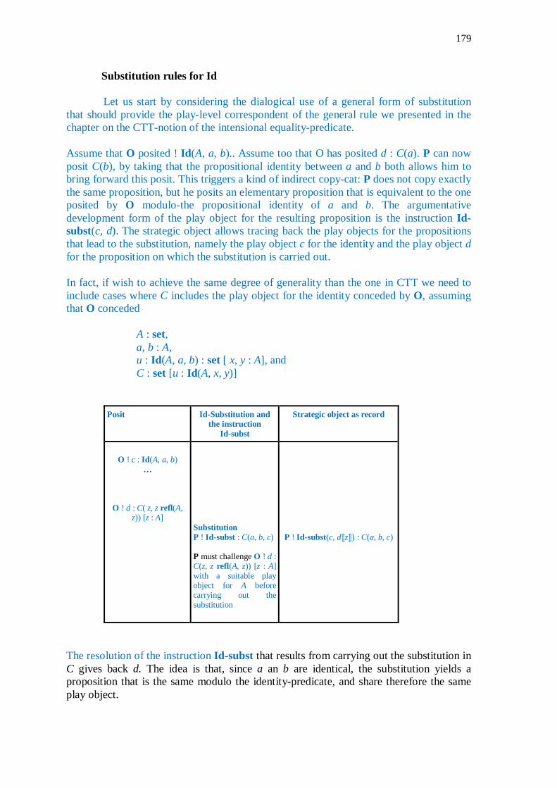
179

Substitution rules for Id

Let us start by considering the dialogical use of a general form of substitution that should provide the play-level correspondent of the general rule we presented in the chapter on the CTT-notion of the intensional equality-predicate. Assume that O posited ! Id(A, a, b).. Assume too that O has posited d : C(a). P can now posit C(b), by taking that the propositional identity between a and b both allows him to bring forward this posit. This triggers a kind of indirect copy-cat: P does not copy exactly the same proposition, but he posits an elementary proposition that is equivalent to the one posited by O modulo-the propositional identity of a and b. The argumentative development form of the play object for the resulting proposition is the instruction Id-subst(c, d). The strategic object allows tracing back the play objects for the propositions that lead to the substitution, namely the play object c for the identity and the play object d for the proposition on which the substitution is carried out. In fact, if wish to achieve the same degree of generality than the one in CTT we need to include cases where C includes the play object for the identity conceded by O, assuming that O conceded

A : set, a, b : A, u : Id(A, a, b) : set [ x, y : A], and C : set [u : Id(A, x, y)]

Posit Id-Substitution and the instruction

Id-subst

Strategic object as record

O ! c : Id(A, a, b)

…

O ! d : C( z, z refl(A, z)) [z : A]

Substitution P ! Id-subst : C(a, b, c) P must challenge O ! d : C(z, z refl(A, z)) [z : A] with a suitable play object for A before carrying out the substitution

P ! Id-subst(c, d⟦z⟧) : C(a, b, c)

The resolution of the instruction Id-subst that results from carrying out the substitution in C gives back d. The idea is that, since a an b are identical, the substitution yields a proposition that is the same modulo the identity-predicate, and share therefore the same play object.

180

Posit Challenge Defence

P ! Id-subst : C( a, b, c)

O ? ---/ Id-subst P ! d : C( a, b, c)

The challenge O ? = d on P ! d : C(a, b, c) yields the equality-response of the general Socratic Rule. The record at the strategic level brings us back to the basic form that justifies the substitution, namely the case where only a occurs in C:

Posit Challenge: General Socratic

Rule

Defence Strategic object with equality

P ! d : C(a, b, c) O ? = P ! Id-subst = d : C(a, b, c) No further challenge on that expression is possible

P ! Id-subst(a, a, d⟦z⟧) = d(a) : C( a, a, refl(A,

a))

Propositional identity satisfies reflexivity, symmetry and transitivity. Reflexivity is immediate. Whereas, symmetry requires the concession of reflexivity, that is, O ! refl(A, z) : Id(A, z, z) [z : A], transitivity requires, O ! u : Id(A, b, e), O ! v : Id(A, b, e) ⊃ Id(A, a, e), that stems from the previous concession, O ! w : Id(A, z, e) ⊃ Id(A, E, e) [z, e : A], that O ! w : Id(A, x, e) ⊃ Id(A, y, e) [x, y, e : A], We will display the relevant play for symmetry and leave to the reader to work out the strategies that yield both, the strategic object for symmetry and transitivity. In order to focus on Id we leave out challenges upon P ! a : A.

Symmetry

O P C1 C2 C3

a : A b : A

c : Id(A, a, b) refl(A, a ) : Id(A, z,

z) [z : A]

d : Id(A, b, a)

0

1 m:= 1 n:= 2 2 3 ? Id= d Id-subst : Id(A, b, a) 6 5 refl(A, a ) : Id(A, a,

a) C3 a 4

7 ? --- / Id-subst 6 c : Id(A, b, a) 8 9 ? = c 8 Id-subst = c : Id(A, b, a) 10 strategic object: Id-subst(c,

refl(A, a )⟦a⟧): Id(A, b, a)

181

Leibniz's Substitution Law is a special case that can be obtained from the concession: O ! u : B(z) ⊃ B(b) [z : A] – that stems from the previous concession v : B(z) ⊃ B(z) [z : A] by means of a challenge following the posit-substution rule. Also here we leave the task to the reader, however let us formulate a simplified form of the result, that has the form of the known Law for the indiscirnibility:

Posit Leibniz-Id-Substitution and the

instruction Lbz-Id-subst

Strategic object

O ! c : Id(A, a, b)

…

O ! d : B(a)

Substitution P ! Lbz-Id-subst : B(b)

P ! Lbz-Id-subst(c, d⟦u⟧) : B(b)

(where u = L⊃(v) : B(a), v : B(a) ⊃ B(b))

Posit Challenge:

Resolution-request Defence

P ! Lbz-Id-subst B(b) O ? ---/ Lbz-Id-subst P ! e : B(b)

Posit Challenge: General

Socratic Rule

Defence

P ! e : B(b) O ? = P ! Lbz-Id-subst = e : B(b) No further challenge on that expression is possible

V.2 The extensional identity Eq V.2.1 The generation of Eq

The dialogical rules that prescribe the extensional propositional identity Eq are simpler than the other forms of equality. Once O introduced a definitional equality between two play objects, P is allowed to introduce a proposition version, in such a way that the play object for the resulting proposition is the play object eq, that does not depend upon the play objects involved in the definitional equality that generated Eq. Hence; from the analysis of eq one cannot trace back the play objects on the basis of which the predicate Eq has been generated: eq is being posited as a kind of analogue of

182

the ontological equality. Accordingly, every play object c for Eq(A, a, b) is definitionally equal to eq.

Posit Challenge Defence Y ?F1 Eq X ! A : set X ! Eq(A, ai, aj) : prop Y?F2 Eq

Y?F3 Eq X ! ai : A X ! aj : A

Canonical development form for P ! : Eq(A, a, b)

Posit Request Response

P ! p : Eq(A, a, b) O ? Eq= p P ! eq : Eq(A, a, b)

P ! eq : Eq(A, a, b) O ? Eq-a, b P ! a = b : A

Argumentative development form I for O ! p : Id(A, a, b)

Posit Request Response

O ! a = b : A P ?Eq-a= b O ! eq : Eq(A, a, b)

O ! p : Eq(A, a, b) P ? Eq= p

O ! eq : Eq(A, a, b)

O ! eq : Eq(A, a, b) P ? Eq-a, b O ! a = b : A

Notice tha the crucial difference between the Id and Eq is, the third line of argumentative development form above. While in the context of an Id-posit, P cannot force O to bring forward ! a = b : A after O ! eq : Eq(A, a, b), in the context of Eq P can. This is risponsable for the "extensionality" of Eq and leads to the undecidability of assertions of the form a = b : A – see chapter II. 2.8.

The substitution rule is almost the same as before, though the resulting play-object is simpler since only the play-object d (within O ! d : C( z, z eq)) [z : A]), will be kept after the substitution:

Posit Id-Substitution and the instruction Eq-subst

Strategic object as record

O ! c : Eq(A, a, b)

…

O ! d : C( z, z eq)) [z : A]

Substitution P ! Eq-subst : C(a, b, c) P must challenge O ! d :

P ! d⟦a⟧ : C(a, b, c)

183

C(z, z eq) [z : A] with a suitable play object for A before carrying out the substitution.

P ! Eq-subst : C( a, b, c)

P ! d(a) : C( a, b, c) (Response to the request)

P ! d(a) = Eq-subst : C(

a, b, c) (Response to the

challenge)

O ? ---/ Eq-subst (Resolution-request)

O ? = d(a)

(challenge: General

Socratic Rule)

Similar applies to Leibniz-substution based on Eq

Posit Leibniz-Eq-Substitution and the

instruction Lbz-Id-subst

Strategic object

O ! c : Eq(A, a, b)

…

O ! d : B(a)

Substitution P ! Lbz-Eq-subst : B(b)

P ! d⟦u⟧ : B(b)

(where u = L⊃(v) : B(a), v : B(a) ⊃ B(b))

Posit Challenge:

Resolution-request Defence

P ! Lbz-Eq-subst B(b) O ? ---/ Lbz-Eq-subst

P ! e : B(b)

Posit Challenge: General

Socratic Rule

Defence

P ! e : B(b) O ? = P ! Lbz-Eq-subst = e : B(b) No further challenge on that expression is possible

184

185

VI Final Remarks and Prospects On Normativity and Dialogues

The dialogical general perspective on definitional equality and identity is that

equality is rooted in both, the intertwining of entitlements and commitments that result from moves were play objects are brought forward, and the coordination of the interaction that implements such an intertwining. In such a framework; the CTT-conception of equality is built from a basic level of interaction taking part at a level were plays provide the meaning of the basic expressions of language, up to a strategy level: it is at the level of the latter where CTT-proof-objects and their specific equality rules find their dialogical counterpart. Moreover, dialogical normativity is grounded on the play-level. Recall that Martin-Löf's suggestion of relying on the authority of the Opponent's speech-acts – that can be then overtaken by the Proponent, is in the dialogical framework a rule that, in principle, prescribes the development of plays rather than strategies. Indeed, it is at the level of development of a play, where it is prescribed by means of the Socratic Rule that the Proponent can defend a move by indicating ipse dixisti (you said it Yourself) – see Krabbe (1982, p. 25), a speech-act that displays the interactive form of equality.

In his recent book, Jaroslav Peregrin (2014) deploys the distinction between the play- and the strategy level (that he calls tactics) in order to offer another insight on the issue of the normativity of logic. Indeed, Peregrin proposes to understand the normativity of logic not in the sense of prescription on how to reason; but rather as providing the material by the means of which we reason. At this point he endorses the dialogical distinction between rules for plays and rules for strategies. According to his proposal the prescriptions for the development of a play provide the material for reasoning whereas the prescriptions of the (in his terminology) tactical level involves how to win. Moreover, Peregrin links the normativity of logic with another of the main conceptual tenets of the dialogical framework, namely, the public feature of the speech-acts underlying an argumentative approach to reasoning:

It follows from the conclusion of the previous section that the rules of logic cannot be seen as tactical rules dictating feasible strategies of a game; they are the rules constitutive of the game as such.(MP does not tell us how to handle implication efficiently, but rather what implication is.) This is a crucial point, because it is often taken for granted that the rules of logic tell us how to reason precisely in the tactical sense of the word. But what I maintain is that this is wrong, the rules do not tell us how to reason, they provide us with things with which, or in terms of which, to reason. This brings us back to our frequently invoked analogy between language and chess. There are two kinds of rules of chess: first, there are rules of the kind that a bishop can move only diagonally and that the king and a rook can castle only when neither of the pieces have previously been moved. These are the rules constitutive of chess; were we not to follow them, we have seen (Section 5.5) we would not be playing chess. In contrast to these, there are tactical rules telling us what to do to increase our chance of winning, rules advising us, e.g., not to exchange a rook for a bishop or to embattle the king by castling. Were we not to follow them, we would still be playing chess, but with little likelihood of winning. We can imagine the rules of chess as something that produces the pieces, equips them each with its peculiar modus operandi, and then see the relevant tactical rules as consisting in setting the individual modi into the most efficient teamwork. The rules of logic, viewed analogously, would then have a slightly more complex role: along with furnishing us with logical concepts (each with its peculiar modus operandi) they also provide us with a mold in which we cast all other concepts so that they acquire their characteristic shape (and thus can combine with logical ones).8 Then

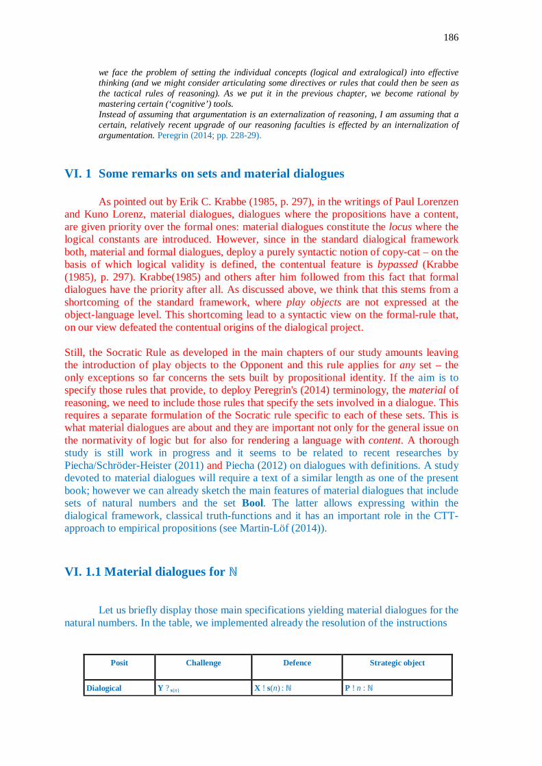
186

we face the problem of setting the individual concepts (logical and extralogical) into effective thinking (and we might consider articulating some directives or rules that could then be seen as the tactical rules of reasoning). As we put it in the previous chapter, we become rational by mastering certain (‘cognitive’) tools. Instead of assuming that argumentation is an externalization of reasoning, I am assuming that a certain, relatively recent upgrade of our reasoning faculties is effected by an internalization of argumentation. Peregrin (2014; pp. 228-29).

VI. 1 Some remarks on sets and material dialogues

As pointed out by Erik C. Krabbe (1985, p. 297), in the writings of Paul Lorenzen and Kuno Lorenz, material dialogues, dialogues where the propositions have a content, are given priority over the formal ones: material dialogues constitute the locus where the logical constants are introduced. However, since in the standard dialogical framework both, material and formal dialogues, deploy a purely syntactic notion of copy-cat – on the basis of which logical validity is defined, the contentual feature is bypassed (Krabbe (1985), p. 297). Krabbe(1985) and others after him followed from this fact that formal dialogues have the priority after all. As discussed above, we think that this stems from a shortcoming of the standard framework, where play objects are not expressed at the object-language level. This shortcoming lead to a syntactic view on the formal-rule that, on our view defeated the contentual origins of the dialogical project. Still, the Socratic Rule as developed in the main chapters of our study amounts leaving the introduction of play objects to the Opponent and this rule applies for any set – the only exceptions so far concerns the sets built by propositional identity. If the aim is to specify those rules that provide, to deploy Peregrin's (2014) terminology, the material of reasoning, we need to include those rules that specify the sets involved in a dialogue. This requires a separate formulation of the Socratic rule specific to each of these sets. This is what material dialogues are about and they are important not only for the general issue on the normativity of logic but for also for rendering a language with content. A thorough study is still work in progress and it seems to be related to recent researches by Piecha/Schröder-Heister (2011) and Piecha (2012) on dialogues with definitions. A study devoted to material dialogues will require a text of a similar length as one of the present book; however we can already sketch the main features of material dialogues that include sets of natural numbers and the set Bool. The latter allows expressing within the dialogical framework, classical truth-functions and it has an important role in the CTT-approach to empirical propositions (see Martin-Löf (2014)). VI. 1.1 Material dialogues for ℕ

Let us briefly display those main specifications yielding material dialogues for the natural numbers. In the table, we implemented already the resolution of the instructions

Posit Challenge

Defence Strategic object

Dialogical Y ? s(n) X ! s(n) : ℕ P ! n : ℕ

187

canonical form X ! n : ℕ

Argumentation form X ! p : C(n) or arbitrary n : ℕ and, where, C : set [z : ℕ]

Y ? Lℕ –df-C

Y ! e / Lℕ(Rℕ(p)) :C(m) Y challenges by conceding C(m) for a natural number m chosen by himself the precise form of the challenges depend on the definition of C(x) established by the Socratic rule - where x : ℕ, y : C(x)

X ! p1 / Lℕ (p) : C(0) X ! p2 / Rℕ(Rℕ(p)) : C(s(m)

P ! R(n, p1, p2 ⟦Lℕ(Rℕ(p))O⟧) : C(n)

Development rules: The Socratic-Rules for and the Development Argumentation Forms

In relation to the development rules we will only show those that regulate the specification of ℕ, namely:

1. The Proponent can start a dialogue with a thesis of one the following forms: P ! n : ℕ [! 0 : ℕ] P ! p : C(n) [! C(0)]

The Opponent, engages into the dialogue by accepting to bring forward the required concession.

Once P has brought forward an elementary expression of the form 1 : ℕ , 2 : ℕ …, the Opponent can challenge it by requiring the deployment of a nominal-definition: • O can challenge posits of the form n : ℕ by means of the attack ?n • P can reply s(0) ≡df 1 : ℕ to the challenge ? 1 upon ! 1 : ℕ only if O posited

before s(0): ℕ; he is allowed to reply s(s(0)) ≡df 2, to the challenge ? 2 upon! 2 : ℕ only if O posited before s(s(0)): ℕ and so on for s(….(s(s(0)) ≡df n. That is, for 1 : ℕ P ! 1 : ℕ P ! n : ℕ O ? ≡df 1 O ! s(0) : ℕ O ? ≡df n O ! s(….(s(s(0)) : ℕ ------------------------------- -------------------------------------------- P ! 1 ≡df s(0) : ℕ P ! n ≡df s(….(s(s(0)) : ℕ

188

(the answer cannot be challenged)

• O's challenge ? C(m) –df-C upo C(n) is specifically defined for C. Thus, if C is the predicate " x is an odd number", the rule establishes that the challenge upon C(s(0) is:

choose an n such s(0) = 2n +1102

Similarly O' concessions such as e : C(s(s(s(0)))) brought forward as the second challenge upon C(n) will adopt the form specified by C. In our example the concession involved in the challenge has the form s(s(s(0))) = 2(s(0)) +1

Let us run a short play for the thesis 3 : ℕ [0 : ℕ]:

1. P ! 3 : ℕ [0 : ℕ] 2. O ! 0 : ℕ, ? ≡df 3 (I concede that 0 is a natural number, show me that 3 is a

natural number too) 3. P ? s(0) (you conceded that 0 is a natural number. What about its

successor?) 4. O s(0) : ℕ 5. P ! ?s(s(0)) 6. O s(s(0)) : ℕ 7. P ! ?s(s(s(0))) : ℕ 8. O s(s(s(0))) : ℕ 9. P ! s(s(s(0))) ≡df 3 : ℕ (3 is a number that has been stipulated as equal to

s(s(s(0))), that you just conceded to be a natural number) Let us now study briefly the case of the set Bool. VI. 1.2 Material dialogues for Bool The set Bool contains two elements namely t and f. Thus, the truth functions of classical logic can be understood in this context as introducing non-canonical elements of the type Bool. In the dialogical framework, the elements of the Bool are responses to yes-no questions.

Posit Challenge

Defence Strategic object

X ! Bool

Y ? canon-Bool

X ! : yes : Bool X ! : no : Bool

P ! : yes : Bool P ! : no : Bool

102 Certainly the rule assumes that multiplication and addition have been defined already.

189

Canonical argumentation form

X ! p : C(c) [c : Bool] Argumentation form

Y ? LBool

Y ? RBool

X ! p1 : C(yes / LBool) X ! p2 : C(no / LBool)

P ! (c, p1 | p2) : C(c / yes | c / no) With equality P ! (yes / LBool, p1 | p2) = p1 : C(yes) P ! (no / LBool, p1 | p2) = p2 : C(no)

We can now introduce quite smoothly the rules for the classical truth functional connectives as elements of Bool. We leave the description for quantifiers to the diligence of the reader whereby the universal quantifier is understood as a finite sequence of conjunctions and dually, the existential as a finite sequence of disjunctions. . In the table below expressions such as " yes (ϕ) ", "no (ψ )" could be understood in the context of CTT as "ϕ evaluates as t" , ("ψ evaluates as f"). The dialogical interpretation of " X ! yes (ϕ) " is "the player X gives a positive answer in the context of a yes-no-question to ϕ. Futhermore, interpretation of the rules below is the usual one: it amounts to the commitments and entitlements specified by the rules of the dialogue: if for instance the response is yes to the conjunction, then the speaker is also committed to answer yes to further questions on components of the conjunction.

Posit Argumentation forms

Challenge Defence Strategic object

Y ? LBool

X ! yes( ϕ ∧ ψ ) : Bool

X ! ϕ ∧ ψ : Bool respectively

Y ? RBool

X ! no(ϕ ∧ ψ ) : Bool

X ! yes( ϕ ∧ ψ ) : Bool

Y ?L∧

yes Y ?R

∧ yes

X ! yes(ϕ ) : Bool respectively X ! yes(ψ ) : Bool

yes ⟦< yes(ϕ ) ,yes(ψ )>⟧ P ! : Bool

no ⟦no(ϕ ) | no(ψ )⟧

X ! no( ϕ ∧ ψ ) : Bool

Y?

∧ no

X ! no(ϕ): Bool Or X ! no(ψ) : Bool

(Gloss: If both of the components of the conjunction are answered with yes, then the overall recapitulating answer is yes. If at least one of the

190

components of the conjunction are answered with no, then the overall recapitulating answer is no)

Y ? LBool

X ! yes(ϕ ∨ ψ) Bool

X ! ϕ ∨ ψ : Bool respectively yes ⟦yes(ϕ ) | yes(ψ )⟧

P ! : Bool

Y ? RBool

X ! no(ϕ ∨ ψ) : Bool

no ⟦<no(ϕ ) | no(ψ )>⟧

X ! yes(ϕ ∨ ψ ) : Bool

Y?

∨ yes

X ! yes(ϕ ): Bool Or X ! yes(ψ ) : Bool

X ! no(ϕ ∨ ψ ): Bool

Y ?L∨

no Or Y ?L

∨ no

X ! no(ϕ ) : Bool respectively X ! no(ψ ) : Bool

X ! ϕ ⊃ ψ : Bool

Y?

∧ no

X ! yes / ϕ ⊃ ψ : Bool Or X ! no / ϕ ⊃ ψ : Bool

Y ! yes(ϕ ) : Bool X ! yes(ψ ) : Bool yes ⟦<yes(ϕ ), yes(ψ ) | no(ψ ), yes>⟧

X ! yes(ϕ ⊃ ψ) : Bool Or P ! : Bool

Y ! no(ϕ ) : Bool X ! yes : Bool (cannot be challenged)

no ⟦<yes(ϕ ) | no(ψ)>⟧

X ! no(ϕ ⊃ ψ) : Bool Y ! yes(ϕ ): Bool

X ! no(ψ) : Bool

Y ? LBool

X ! yes(¬ϕ ) : Bool

X ! ¬ϕ : Bool respectively

Y ? RBool

X ! no(¬ϕ ) : Bool

X ! yes( ¬ϕ ) : Bool Y ? ¬ yes

X ! no(ϕ ) : Bool yes ⟦no(ϕ )⟧

P ! : Bool

no ⟦yes(ϕ )⟧

X ! no(¬ϕ ) : Bool Y ? ¬ no X ! yes(ϕ ) : Bool

191

Besides the use of the Socratic-rule described for formal dialogues we also need the following:

• Socratic-rule for Id within Bool

If P must defend an elementary proposition, such as A : Bool, he has the right to ask O – if O did not posited yet the answer. O's answer (or previous posit) will lead to the identity P ! id(yes) : Id(Bool, A, yes)

P ! yes(A) : Bool O ? IdA P ! ? A-Bool O ! LBool(A) : Bool P ! id(yes) : Id(Bool, A, yes) provided Id(Bool, x, y) : prop (x, y : Bool)

If the answer is rather O ! RBool(A) : Bool, and P has no other available move he lost the play.

One interesting application of the use of Booleans is the interpretation and demonstration of the third-excluded. Let us run those plays that together constitute a winning strategy. Notice that since the set Bool contains only two elements universal quantification over Bool can be tested by considering each of the elements of the set. Each of them triggers a new play:

O P

! d : (∀x : Bool) (Id(Bool, x, yes) ∨ Id(Bool, x, no)).

0

1 m =1 n = 2 2 3 ! L∀(d) : Bool 0.3 ! R∀(d) : (Id(Bool, yes, yes) ∨ Id(Bool, yes, no)). 6 5 ! yes : Bool 3 ? --- / L∀(d) 4 7 ? / R∀(d) 6 ! d1 : (Id(Bool, yes, yes) ∨ Id(Bool, yes, no)). 8 9 ? ∨ 8 0.1 ! L∨ (d1) : Id(Bool, yes, yes) 10 11 ? --- / L∨ (d1) 10 ! e1 : Id(Bool, yes, yes) 12 13 ? = e1 12 ! refl(Bool, yes) : Id(Bool, yes, yes) 14 15 ? = yes / x 14 L∀(d) = yes : Bool

P wins 16

Let us check now the case where O chooses to challenge with no.

O P

! d : (∀x : Bool) (Id(Bool, x, yes) ∨ Id(Bool, x, no)).

0

1 m =1 n = 2 2 3 ! L∀(d) : Bool 0.3 ! R∀(d) : (Id(Bool, no, yes ∨ Id(Bool, no, no)). 6 5 ! no : Bool 3 ? --- / L∀(d) 4 7 ? / R∀(d) 6 ! d1 : (Id(Bool, no, yes) ∨ Id(Bool, no, no)). 8 9 ? ∨ 8 0.1 ! R∨ (d1) : Id(Bool, no, no) 10 11 ? --- / R∨ (d1) 10 ! e2 : Id(Bool, no, no) 12

192

13 ? = e2 12 ! refl(Bool, no ) : Id(Bool, no, no) 14 15 ? = no / x 14 L∀(d) = no : Bool

P wins 16

VI. 2 A brief interlude to an historical study on material dialogues

Allow us now a brief historic interlude on the distinction between posits of the form a : A and of the form A(a) true (i.e. b(a) : A(a), where a : B), B : set and A(x) : prop (x : B)). As discussed in Rahman / Clerbout (2015, pp. 145-46) this distinction seems to come close to the reconstruction that Lorenz and Mittelstrass (1967) provide of Plato’s notion of correct naming in the Cratylus (in Plato (1997)).103 Furthermore Rahman and Clerbout relate this interpretation of Lorenz and Mittelsrass with the dialogical notion of predicator rule, that is at the base of a material dialogue. Lorenz and Mittelstrass point out two basic different speech-acts, namely naming (όνομάζείν) and stating (λέϒείν). The first speech-act amounts to the act of subsuming one individual under a concept and the latter establishes a proposition about a previously named individual. If the naming has been correctly carried out the (named) individual reveals the concept it instantiates (names reveal objects for what they are). Stating truly is about the truth of the proposition constituted by instantiating a propositional function with a suitable element of a genus (a correctly named instantiation of a genus). Thus, both acts, naming and stating involve judgements. Indeed; while naming (όνομάζείν) corresponds to the assertion that an individual instantiates a given genus and has therefore the following form

a : A, ( A : genus), stating (λέϒείν) corresponds to the act of building a proposition, such as A(a) out of the propositional function A(x) and the genus B. In other words, the correct form of the result of an act of stating amounts to the judgment: A(a) : prop (a : B), that presupposes A(x) : prop (x : B), B : genus

• The act of naming a : A is said to be true iff a instantiates A • The proposition A(a) is true iff a is one of the individuals to which the

propositional function A(x) apply (i.e, if a is of the genus B), and it is the case that A(x) can be said of a.

The resulting proposition (in the context of our example) A(a) is true if A(x) can be said of the individual a. In such a case A(a) has been stated truly.

103 For an endorsement of this interpretation see Luce(1969).

193

The specialized literature criticized harshly Plato's claim that not only the result of acts of predication but also acts of naming104 can be qualified as true or false. According to the criticism, while truth applies to propositions, it does not apply to individuals. Lorenz / Mittelstrass (1967, pp. 6-12) defended the old master proposing to read these passages as presupposing that in both cases we have the same kind of acts of predication.105 If we deploy the CTT-setting to develop the interpretation of Lorenz / Mittelstrass (1967), it follows that in order to claim that both acts of predication can be qualified as true, it is not necessary to conclude that both involve propositional functions. In other words, to put it in the terminology of Lorenz / Mittelstrass (1967), both acts of predication can be qualified as true even if they do not involve the same form of predicator rule. Indeed, Plato's claim can be defended if we, following the CTT-setting, carefully distinguish both constituents of a judgement involving a specific propositional function, namely

i. the act of asserting that a given individual exemplifies the genus presupposed by the formation of that propositional function), and

ii. the act of asserting a proposition that results from substituting the variable of the relevant propositional function by a suitable instantiation

According to this analysis, it is possible to endorse at the same time the following claims of Plato:

1. Acts of όνομάζείν and λέγείν involve different acts of judgement 2. Naming and stating, both can be qualified as true. 3. Neither 1 nor 2 assume (like Mittelstrass and Lorenz seem to do (1967))106 that

the truth of the result of an act of predication always involve a prescription on how to constitute a propositional function out of another one.

104 Viktor Ilievski (2013, pp. 12-13) provides a condensed formulation of this kind of critics:

Socrates next proceeds briefly to discuss true and false speech, with an intention to point out to Hermogenes that there is a possibility of false, incorrect speech. It is a matter of very basic knowledge of logic that truth-value is to be attributed to propositions, or more precisely utterances, specific uses of sentences. Plato’s Socrates acknowledges that, but he, somewhat surprisingly, ascribes truth-value to the constituents, or parts of the statements as well, on the assumption that whatever is true of the unit, has to be true of its parts as well. This seems to be an example of flagrant error in reasoning, known as the fallacy of division. Why would Plato’s Socrates commit such a fallacy in the course of what seems to be a valid and stable argument? One obvious answer would be that the very theory he is about to expound presupposes the notion of names as independent bearers of meaning and truth, linguistic microcosms encapsulating within themselves both truth-value and reference. In other words, the theory of true and false names has to presuppose that names do not only refer or designate, or even do not only refer and sometimes suggest descriptions, but that they always necessarily represent descriptions of some kind.

105 Lorenz/Mittelstrass (1967, p. 6): It follows that a true sentence SP really does consist of the ' true parts ' S and P, i.e. t ε S and t ε P. In case of a false sentence SP, however, the second part t ε P is false, while the first part t ε S should ex definitione be considered as true, because any sentence is necessarily a sentence about something (Soph. 262e), namely the subject of it. The subject has to be effectively determined, i.e. it must be a thing correctly named, before one is going to state something about it.

106 See the following remark: Names, i.e. predicates, are tools with which we distinguish objects from each other. To name objects or to let an individual fall under some concept is on the other hand the means to state something about objects, i.e. to teach and to learn about objects, as Plato prefers to say. Lorenz/Mittelstrass (1967, pp. 13).

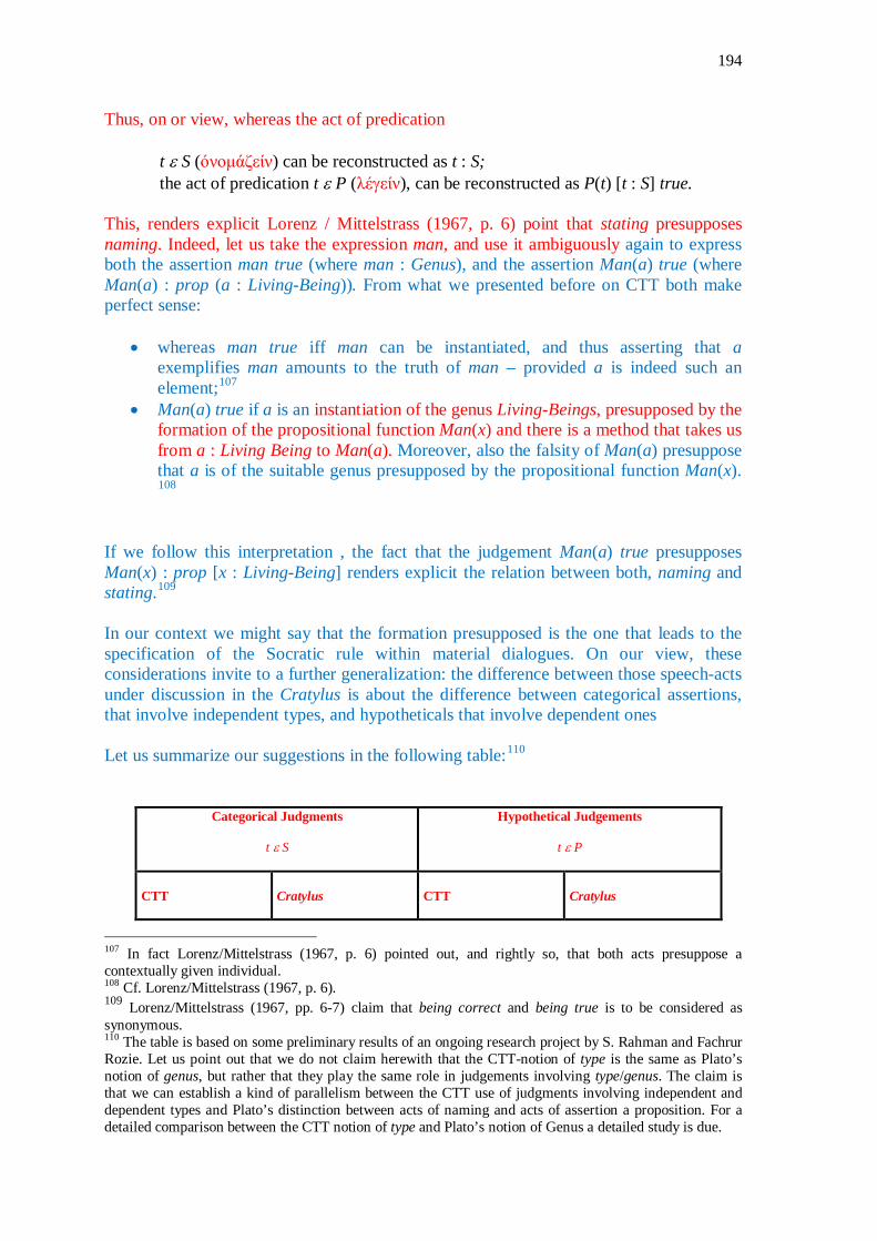
194

Thus, on or view, whereas the act of predication

t ε S (όνομάζείν) can be reconstructed as t : S; the act of predication t ε P (λέγείν), can be reconstructed as P(t) [t : S] true.

This, renders explicit Lorenz / Mittelstrass (1967, p. 6) point that stating presupposes naming. Indeed, let us take the expression man, and use it ambiguously again to express both the assertion man true (where man : Genus), and the assertion Man(a) true (where Man(a) : prop (a : Living-Being)). From what we presented before on CTT both make perfect sense:

• whereas man true iff man can be instantiated, and thus asserting that a exemplifies man amounts to the truth of man – provided a is indeed such an element;107

• Man(a) true if a is an instantiation of the genus Living-Beings, presupposed by the formation of the propositional function Man(x) and there is a method that takes us from a : Living Being to Man(a). Moreover, also the falsity of Man(a) presuppose that a is of the suitable genus presupposed by the propositional function Man(x).

108 If we follow this interpretation , the fact that the judgement Man(a) true presupposes Man(x) : prop [x : Living-Being] renders explicit the relation between both, naming and stating.109 In our context we might say that the formation presupposed is the one that leads to the specification of the Socratic rule within material dialogues. On our view, these considerations invite to a further generalization: the difference between those speech-acts under discussion in the Cratylus is about the difference between categorical assertions, that involve independent types, and hypotheticals that involve dependent ones Let us summarize our suggestions in the following table:110

Categorical Judgments

t ε S

Hypothetical Judgements

t ε P

CTT

Cratylus

CTT

Cratylus

107 In fact Lorenz/Mittelstrass (1967, p. 6) pointed out, and rightly so, that both acts presuppose a contextually given individual. 108 Cf. Lorenz/Mittelstrass (1967, p. 6). 109 Lorenz/Mittelstrass (1967, pp. 6-7) claim that being correct and being true is to be considered as synonymous. 110 The table is based on some preliminary results of an ongoing research project by S. Rahman and Fachrur Rozie. Let us point out that we do not claim herewith that the CTT-notion of type is the same as Plato’s notion of genus, but rather that they play the same role in judgements involving type/genus. The claim is that we can establish a kind of parallelism between the CTT use of judgments involving independent and dependent types and Plato’s distinction between acts of naming and acts of assertion a proposition. For a detailed comparison between the CTT notion of type and Plato’s notion of Genus a detailed study is due.

195

c : B c is of type B

Όνομάζείν B names c Or c is B, i.e. c exemplifies (the genus) B

c(a) : B(a) provided a : A presupposes the formation rule: The propositional function B(x) yields a proposition provided x is an element of the set A

λέϒείν B is predicated of a under the condition that a exemplifies A presupposes the predicator rule: B(x) yields a proposition provided x exemplifies A

c : B true iff c is either a canonical element of B or generated from a canonical one

c is B true iff c correctly exemplifies B

B(a) true iff B applies to a

B(a) true iff B(x) is correctly said of a

presupposes the formation rule of the independent type B

presupposes the formation rule of the genus B (not of B(x))

presupposes the formation rule of the set A and of propositional function B(x) over the set A: B(x) : prop [x : A] Where B(x) is a dependent type upon A.

presupposes the formation rule of (the genus) A, and of the predicator rule111 for B(x): x exemplifies A ⇐ B(x) Where B(x) is defined over the genus A.

VI. 3 The Dialogical approach to Harmony One non negligible result of the interactive roots of definitional equality is that it provides a new insight into the dialogical take on the CTT approach to the notion of harmony as developed in Rahman / Redmond (2015b). Indeed, since the CTT approach to harmony, is based on coordinating the elimination and introduction rule by means of definitional equality, and the latter, according to our analysis, corresponds to the strategic use of the Socratic Rule, it follows that CTT- harmony is based on the strategic use of copy-cat interaction. Redmond/ Rahman (2016) argued that, harmony in general has its roots in the more fundamental notion of player-independence, the present analysis allows pushing forward the contribution of the dialogical theory of meaning in the following sense: harmony is the combination of player-independence with a structural rule, namely the fine-tuning of the player-independence with the Socratic-Rule. 111 For the notion of predicator rule see Lorenz/Mittelstrass (1967). We use here a slightly modified version: the original idea is that those kinds of rules establish how to constitute one predicate from a different one. We propose a more basic one, namely, a rule that establishes how a predicate is ascribed to a certain kind of objects (the genus underlying the predicate).

196

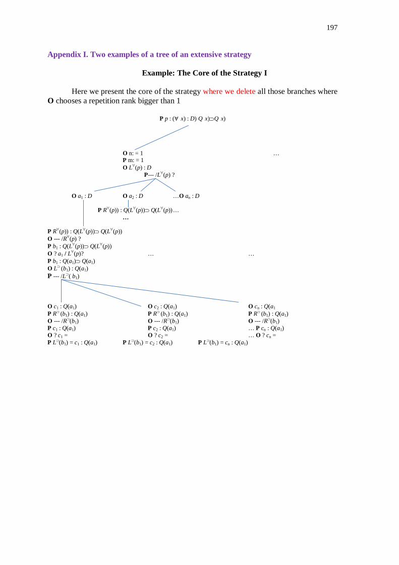
197

Appendix I. Two examples of a tree of an extensive strategy

Example: The Core of the Strategy I Here we present the core of the strategy where we delete all those branches where

O chooses a repetition rank bigger than 1

P p : (∀(x) : D) Q(x)⊃Q(x)

O n: = 1 …

P m: = 1 O L∀(p) : D

P--- /L∀(p) ?

O a1 : D O a2 : D …O an : D

P R∀(p)) : Q(L∀(p))⊃ Q(L∀(p)) … … P R∀(p)) : Q(L∀(p))⊃ Q(L∀(p)) O --- /R∀(p) ? P b1 : Q(L∀(p))⊃ Q(L∀(p)) O ? a1 / L∀(p)? … … P b1 : Q(a1)⊃ Q(a1) O L⊃ (b1) : Q(a1) P --- /L⊃( b1) O c1 : Q(a1) O c2 : Q(a1) O cn : Q(a1 P R⊃ (b1) : Q(a1) P R⊃ (b1) : Q(a1) P R⊃ (b1) : Q(a1) O --- /R⊃(b1) O --- /R⊃(b1) O --- /R⊃(b1) P c1 : Q(a1) P c2 : Q(a1) … P cn : Q(a1) O ? c1 = O ? c2 = … O ? cn = P L⊃(b1) = c1 : Q(a1) P L⊃(b1) = c2 : Q(a1) P L⊃(b1) = cn : Q(a1)

198

Example: The Core of the Strategy II Delete all but one those branches of the core I triggered by O's choices of a play

object

P p : (∀(x) : D) Q(x)⊃Q(x)

O n: = 1 …

P m: = 1 O L∀(p) : D

P--- /L∀(p) ?

O a1 : D

P R∀(p)) : Q(L∀(p))⊃ Q(L∀(p)) O --- /R∀(p) ? P b1 : Q(L∀(p))⊃ Q(L∀(p)) O ? a1 / L∀(p)? P b1 : Q(a1)⊃ Q(a1) O L⊃ (b1) : Q(a1) P --- /L⊃( b1) O c1 : Q(a1) P R⊃ (b1) : Q(a1) O --- /R⊃(b1) P c1 : Q(a1) O ? c1 = P L⊃(b1) = c1 : Q(a1)

199

Appendix II The CTT-demonstration of the Axiom of Choice112

It has been said , and rightly so, that the principle of set theory known as the Axiom of Choice (AC) "is probably the most interesting and in spite of its late appearance, the most discussed axiom of mathematics, second only to Euclid’s Axiom of Parallels which was introduced more than two thousand years ago” (Fraenkel / Bar-Hillel and Levy (1973)). According to Ernst Zermelo’s formulation of 1904 AC amounts to the claim that, given any family A of non-empty sets, it is possible to select a single element from each member of A.113 The selection process is carried out by a function f with domain in M, such that for any nonempty set M in A, then f(M) is an element of M. The axiom has been resisted from its very beginnings and triggered heated foundational discussions concerning among others, mathematical existence and the notion of mathematical object in general and of function in particular. However, with the time, the foundational and philosophical reticence faded away and was replaced by a kind of praxis-driven view by the means of which AC is accepted as a kind of postulate (rather than as an axiom the truth of which is manifest) necessary for the practice and development of mathematics. It is well known that this axiom was first introduced by Zermelo in order to prove Cantor's theorem that every set can be rendered to be well ordered. Zermelo gave two formulations of this axiom one in 1904 and a second one in 1908. It is the second formulation that is relevant for our discussion, since it is related to both, Martin-Löfs and the game theoretical formalization:

A set S that can be decomposed into a set of disjoint parts A, B, C, ... each of them containing at least one element, possesses at least one subset S1 having exactly one element with each of the parts A, B, C, ... considered. Zermelo (1908, pp. 261).

The Axiom attracted immediately much attention and both of its formulations were criticized by constructivists such as René-Louis Baire, Émile Borel, Henri-Léon Lebesgue and Luitzen Egbert Jan Brouwer. The first objections were related to the non-predicative character of the axiom, where a certain choice function was supposed to exist without showing constructively that it does. However, the axiom found its way into the ZFC set theory and was finally accepted by the majority of mathematicians because of its usefulness in different branches of mathematics. Recently the foundational discussions around AC experienced an unexpected revival when Per Martin Löf, showed (around 1980) that in constructive logic the axiom of choice is logically valid (however in its intensional version) and that this logical truth naturally (almost trivially) follows from the constructive meaning of the quantifiers involved – it is this “evidence” that makes it an axiom rather than a postulate. The extensional version can also be proved but then, either third excluded or unicity of the function must be assumed. Martin-Löf’s proof, for which he was awarded with the prestigious Kolmogorov price, showed that at the root of the old discussions an old conceptual problem was at stake, namely the tension between intension and extension.114 112 The present chapter is based on Rahman/Clerbout/Jovanovic (2015). 113 Zermelo (1904, pp. 514-16). 114 See Martin-Löf (2006).

200

Martin-Löf produced a proof of the axiom in a constructivist setting bringing together two seemingly incompatible perspectives on this axiom, namely

Bishop's surprising observation from 1967: A choice function exists in constructive mathematics, because a choice is implied by the very meaning of existence. Bishop (1967, p. 9).

The proof by Diaconescu (1975, pp. 176-178) and by Goodman and Myhle

(1978, p. 461) that the Axiom of Choice implies Excluded Middle. In his paper of 2006 Martin-Löf shows that there are indeed some versions of the axiom of choice that are perfectly acceptable for a constructivist, namely one where the choice function is defined intensionally. In order to see this the axiom must be formulated within the frame of a CTT-setting. Indeed such a setting allows comparing the extensional and the intensional formulation of the axiom. It is in fact the extensional version that implies Excluded Middle, whereas the intensional version is compatible with Bishop’s remark:

[…] this is not visible within an extensional framework, like Zermelo-Fraenkel set theory, where all functions are by definition extensional." Martin-Löf (2006, p.349).

In CTT the truth of the axiom actually follows rather naturally from the meaning of the quantifiers: Take the proposition (∀x : A) P(x) where P(x) is of the type proposition provided x is an element of the set A. If the proposition is true, then there is a proof for it. Such a proof is in fact a function that for every element x of A renders a proof of B(x). This is how Bishop’s remark should be understood: the truth of a universal amounts to the existence of a proof, and this proof is a function. Thus, the truth of a universal, amount in the constructivist account, to the existence of a function. From this the proof of the axiom of choice can be developed quite straightforwardly. If we recall that in the CTT-setting

the existence of a function from A to B amounts to the existence of proof-object for the universal every A is B, and that the proof of the proposition B(x), existentially quantified over the set A amounts to a pair such that the first element of the pair is an element of A and the second element of the pair is a proof of B(x);

a full-fledged formulation of the axiom of choice – where we make explicit the set over which the existential quantifiers are defined - follows:

(∀x : A) (∃y : B(x)) C(x, y) ⊃ (∃f : (∀(x) : A) B(x)) (∀x : A) C(x, f(x)) The proof of Martin-Löf (1980, p. 50-51) is the following

The usual argument in intuitionistic mathematics, based on the intuitionistic interpretation of the logical constants, is roughly as follows: to prove (∀x)(∃y)C(x,y) ⊃ (∃f)(∀x)C(x,f(x)),

201

assume that we have a proof of the antecedent. This means we have a method which, applied to an arbitrary x, yields a proof of (∃y)C(x,y). Let f be the method which, to an arbitrarily given x, assigns the first component of this pair. Then C(x,f(x)) holds for an arbitrary x, and hence, so does the consequent. The same idea can be put into symbols getting a formal proof in intuitionistic type theory. Let A : set, B(x): set (x: A), C(x,y): set (x: A, y: B(x)), and assume z: (Πx: A)(Σy: B(x))C(x,y). If x is an arbitrary element of A, i.e. x: A, then by Π- elimination we obtain

Ap(z,x): (Σy: B(x))C(x,y)

We now apply left projection to obtain

p(Ap(z,x)): B(x)

and right projection to obtain

q(Ap(z,x)): C(x,p(Ap(z,x))). By λ-abstraction on x (or Π- introduction), discharging x: A, we have

(λx) p(Ap(z,x)): (Πx: A)B(x) and by Π- equality

Ap((λx) p(Ap(z,x), x) = p(Ap(z,x)): Bx. By substitution [making use of C(x,y): set (x: A, y: B(x)),] we get

C(x, Ap((λx) p (Ap(z,x), x) = C(x, p(Ap(z,x))) [that is, C(x, Ap((λx) p (Ap(z,x), x) = C(x, p(Ap(z,x))): set ] and hence by equality of sets

q(Ap(z,x)): C(x, Ap((λx) p (Ap(z,x), x) where ((λx) p (Ap(z,x)) is independent of x. By abstraction on x

((λx) p (Ap(z,x)): (Πx: A)C(x, Ap((λx) p (Ap(z,x), x) We now use the rule of pairing (that is Σ- introduction) to get

(λx) p(Ap(z,x)), (λx) q(Ap(z,x)): (Σf: (Πx: A)B(x))( Πx: A)C(x, Ap(f,x)) (note that in the last step, the new variable f is introduced and substituted for ((λx) p (Ap(z,x)) in the right member). Finally by abstraction on z, we obtain (λz)((λx) p (Ap(z,x)), ((λx) q (Ap(z,x)): (Πx: A)(Σy: B(x))C(x,y)⊃ (Σf: (Πx: A)B(x))( Πx: A)C(x, Ap(f,x)).

202

Moreover, Martin-Löf (2006) shows that what is wrong with the axiom -from the constructivist point of view - is its extensional formulation. That is:

(∀x : A) (∃y : B(x)) C(x, y) ⊃ (∃f : (∀(x) : A) B(x)) (Ext(f) ∧ (∀x : A) C(x, f(x)) Where Ext(f) = ((∀i, j : A) ( i = A j ⊃ f(i) = f(j)) Thus, from the constructivist point of view, what is really wrong with the classical formulation of the axiom of choice is the assumption that from the truth that all of the A are B we can obtain a function that satisfies extensionality. In fact, as shown by Martin-Löf (2006), the classical version holds, even constructively, if we assume that there is only one such choice function in the set at stake!: Let us retain that • (∀x : A) (∃y : B(x)) C(x, y) ⊃ (∃f : (∀(x) : A) B(x)) (Ext(f) ∧ (∀x : A) C(x, f(x)) to

be the formalization of the axiom of choice, then that axiom is not only unproblematic for constructivists but it is also a theorem. In fact it is the CTT-explicit language that allows a fine-grained distinction between the, on the surface, equivalent formulations of the extensional and intensional versions of AC. This is due to the expressive power of CTT that allows to express at the object language level properties that in other settings are left implicit in the metalanguage. This leads us to the following observation:

• According to the constructivist approach functions are identified as proof-objects for

propositions and are given in object-language, as the objects of a certain type. Understood in that way, functions belong to the lowest-level of entities and there is no jumping to higher order. Once more, the truth of a first order-universal sentence, amounts to the existence of a function that is defined by means of the elements of the set over which the universal quantifies and the first-order expression B(x). The existence of such a function is the CTT-way to express at the object language level, that a given universal sentence is true.

203

Appendix III: An overview of the main rules for the Dialogical framework for CTT Local meaning

Posit Challenge Defence

X ! Γ : set(prop) Y ? can Γ X ! Socratic Rule-Γ 115

X ! ϕ : prop

Y ?F∨1 X ! ϕ : pro

X ! ϕ ∨ ψ : prop Or

Y ?F∨2 X ! ψ : prop

Y ?F∧1 X ! ϕ : pro

X ! ϕ ∧ ψ : prop Or

Y ?F∧2 X ! ψ : prop

Y ?F ⊃ 1 X ! ϕ : pro

X ! ϕ ⊃ ψ : prop Or

Y ?F ⊃ 2 X ! ψ : prop

Y ?F∀1 X ! A : set

X ! (∀x : A) ϕ(x) : prop Or

Y ?F∀2 X ! ϕ(x) : prop [x : A]

Y ? ∃1 X ! A : set

X ! (∃x : A) ϕ(x) : prop Or

Y ?F∃2 X ! ϕ(x) : prop [x : A]

X ! ⊥ : prop _ _

Canonical argumentation form

Posit Challenge Defence

Y ?L ! A X ! p1 : A

X ! p : (∃x : A)ϕ Or Respectively

Y ?R ! ϕ

X ! p2 : ϕ(p1)

Y ?L ! A X ! p1 : A

X ! p : {x : A | ϕ}

Or Respectively

Y ?R ! ϕ(p1)

X ! p2 : ϕ(p1)

Y ?L ! ϕ X ! ! p1 : ϕ

X ! p : ϕ ∧ ψ Or respectively

Y ?R ! ψ

X ! p2 : ψ

115 There is no general way to specify a set. The specification of a set leads to material dialgoues that will require extending the structural-rules with a set of definitions implemented by the Socratic Rule – see the last chapter of the present study.

204

X ! p : (∀x : A)ϕ Y ! p1 : A , ? ! ϕ X ! p2 : ϕ(p1)

X ! p : ϕ ⊃ ψ

Y ! p1 : ϕ, ? ! ψ X ! p2: ψ

X ! p : ¬ϕ also expressed as X ! p : ϕ ⊃ ⊥

Y ! ! p1 : ϕ, ? ! ⊥

X ! ⊥ (Player X gives up)

X ! p1 : ϕ

X ! p : ϕ ∨ ψ Y ? ∨ [! L∨(p) : ϕ | ! R∨(p) : ψ] Or

X ! p2 : ψ

Argumentation form

Posit Challenge Defence

Y ?L X ! L∃(p) : A

X ! p : (∃x : A)ϕ Or Respectively

Y ?R

X ! R∃(p) : ϕ(L∃(p))

Y ?L X ! L{...}(p) : A

X ! p : {x : A | ϕ} Or Respectively

Y ?R

X ! R{...}(p) : ϕ(L{...}(p))

Y ?L X ! L∧(p) : ϕ

X ! p : ϕ ∧ ψ Or respectively

Y ?R X ! R∧(p) : ψ

X ! p : (∀x : A)ϕ Y ! L∀(p) : A X ! R∀(p) : ϕ(L∀(p))

X ! p : ϕ ⊃ ψ

Y ! L ⊃(p) : ϕ X ! R⊃(p) : ψ

X ! p : ¬ϕ also expressed as X ! p : ϕ ⊃ ψ

Y ! L¬(p) : ϕ Y ! L⊃(p) : ϕ

X ! R¬(p) : ⊥ X ! R ⊃ (p) : ⊥

X ! L∨(p) : ϕ

X ! p : ϕ ∨ ψ Y ? ∨ Or

X ! R∨(p) : ψ

Posit-substitution116

116 This is the dialogical version - at the play level - of the CCT-substitution rules for hypothetical judgements described by Martin-Löf (1984, pp. 9-11). See too Nordström/Petersson/Smith (1990, p. 38-39) and Ranta (1994, p.30).

205

X ! π(x1, …, xn) [xi : Ai]

Y ! τ1 : A1, …, τn : An (where τi is a play object either of the form ai : A or of the form xi : A)

X ! π( [τ1 … τ n]

Transmission of definitional equality I

X ! b(x) : B(x) [x : A] Y ! a = c : A X ! b(a) = b(c) : B(a)

X ! b(x) = d(x) : B(x) [x : A] Y ! a : A X ! b(a) = d(a) : B(a) X ! B(x) : type [x : A] Y ! a = c : A X ! B(a)=B(c) : type

X ! B(x)=D(x) : type [x : A]

Y !1B(x)=D(x) a : A

or Y ?2

A=D a = c : A

X ! B(a)=D(a) : type X ! B(a)=D(c) : type

X ! A = B : type

Y !1B(x)=D(x) a : A

or Y ?2

A=D a = c : A

X ! a : B X ! a = c : B

Transmission of definitional equality II

X ! A : type Y ?type- refl X ! A = A : type X ! A = B : type Y ?B- symm X ! B = A : type X ! A = B : type X ! B = C : type

Y ?A- trans

X ! A = C : type

X ! a : A Y ?A- refl X ! a = a : A X ! a = b : A Y ?b- symm X ! b = a : A

X ! a = b : A X ! b = c : A

Y ?a- trans

X ! a = c : A

"type" stands for prop or set The development of a play

SR0 (Starting rule). • The start of a formal dialogue of immanent reasoning is a move where P puts forward

the thesis. The thesis can be put forward under the condition that O commits herself with certain other expressions called initial concessions. In the latter case the thesis has the form ! α [β1, …, βn].

• O accepts the commitment by bringing forward those initial concessions ! β1, …, ! βn and by providing them with respective play objects, if they have not been specified already. The Proponent must then also bring forward some suitable play object too, if it has not been specified already while positing the thesis.117

• If the set of initial concessions is empty, then we make the notational convention that

such a play starts with some play object, say, d

117 Some kind of theses require an explicit play-object, such as those that include some form of anaphoric expression. For example the premisse and conclusion of barbara

European is said of (Every Man who is French) French is said from (Every Man who is Pairisian) ----------------------------------------------------------- European is said of (Every Man who is Parisian)

requires an anaphora that identifies the play-object of which it is said that is European/French. Thus, conclusion cannot be posited unless it has the form ! p: (∀z : {x : M | P(x)}) E(L{...} (L∀(p) – this also applies to the premisses.

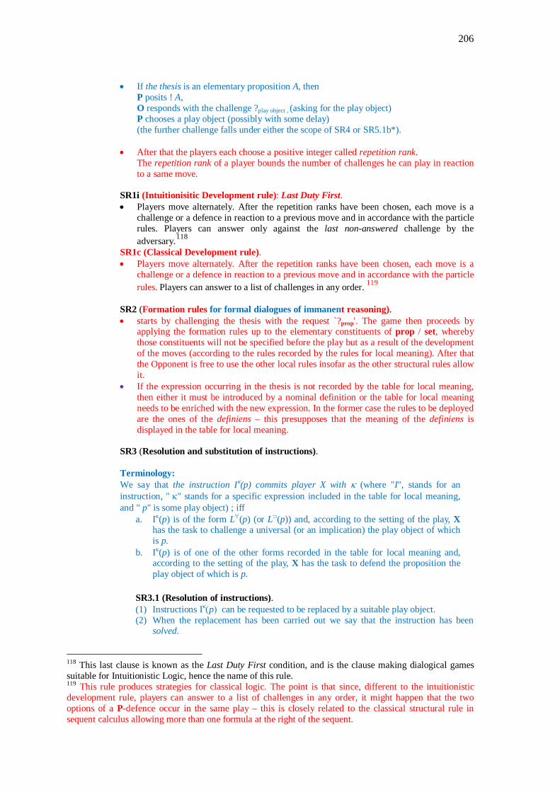
206

• If the thesis is an elementary proposition A, then

P posits ! A, O responds with the challenge ?play object , (asking for the play object) P chooses a play object (possibly with some delay) (the further challenge falls under either the scope of SR4 or SR5.1b*).

• After that the players each choose a positive integer called repetition rank.

The repetition rank of a player bounds the number of challenges he can play in reaction to a same move.

SR1i (Intuitionisitic Development rule): Last Duty First. • Players move alternately. After the repetition ranks have been chosen, each move is a

challenge or a defence in reaction to a previous move and in accordance with the particle rules. Players can answer only against the last non-answered challenge by the adversary.118

SR1c (Classical Development rule). • Players move alternately. After the repetition ranks have been chosen, each move is a

challenge or a defence in reaction to a previous move and in accordance with the particle rules. Players can answer to a list of challenges in any order. 119

SR2 (Formation rules for formal dialogues of immanent reasoning). • starts by challenging the thesis with the request `?prop'. The game then proceeds by

applying the formation rules up to the elementary constituents of prop / set, whereby those constituents will not be specified before the play but as a result of the development of the moves (according to the rules recorded by the rules for local meaning). After that the Opponent is free to use the other local rules insofar as the other structural rules allow it.

• If the expression occurring in the thesis is not recorded by the table for local meaning, then either it must be introduced by a nominal definition or the table for local meaning needs to be enriched with the new expression. In the former case the rules to be deployed are the ones of the definiens – this presupposes that the meaning of the definiens is displayed in the table for local meaning.

SR3 (Resolution and substitution of instructions). Terminology: We say that the instruction Iκ(p) commits player X with κ (where "I", stands for an instruction, " κ" stands for a specific expression included in the table for local meaning, and " p" is some play object) ; iff

a. Iκ(p) is of the form L∀(p) (or L⊃(p)) and, according to the setting of the play, X has the task to challenge a universal (or an implication) the play object of which is p.

b. Iκ(p) is of one of the other forms recorded in the table for local meaning and, according to the setting of the play, X has the task to defend the proposition the play object of which is p.

SR3.1 (Resolution of instructions). (1) Instructions Iκ(p) can be requested to be replaced by a suitable play object. (2) When the replacement has been carried out we say that the instruction has been

solved.

118 This last clause is known as the Last Duty First condition, and is the clause making dialogical games suitable for Intuitionistic Logic, hence the name of this rule. 119 This rule produces strategies for classical logic. The point is that since, different to the intuitionistic development rule, players can answer to a list of challenges in any order, it might happen that the two options of a P-defence occur in the same play – this is closely related to the classical structural rule in sequent calculus allowing more than one formula at the right of the sequent.

207

(3) If the instruction Iκ(p) commits player X with κ and the resolution-request is launched by Y, then it has the form

? --- / Iκ(p) (4) If π[Iκ(p)] has been posited by Y, but the instruction Iκ(p) commits player X with κ,

then the resolution-request launched by X, has the form ? - b - / Iκ(p) where b is chosen by X

(5) Solving an instruction π[Iκ(p)] amounts replacing it with a suitable play object b and obtain

π[b] (6) If the instruction Iκ(p) commits player X with κ, then it is he who chooses the play

object that resolves the instruction. (7) In the case of embedded instructions I1(...(Ik)...), the resolutions are thought of as

being carried out from Ik to I1: first resolve Ik with some play object bk following the indication (6), then Ik-1 etc. until I1.

provisos: resolution-requests do not apply to instructions solved already once resolution-requests do not apply to definitional equalities Remarks.

• Here we assume that the instructions to be resolved have been introduced. If exactly the same instruction, say Iκ(p), has been resolved once, a further occurrence of it that is not a new introduction is handled by the next rule, called substitution of instructions.

• If the instruction already solved occurs within a equality, then the rules on equality to be discussed below apply.

A special case: • Instructions involving a posit such ⊥ are resolved by giving-up. .

X ! R¬(p) : ⊥ Y ! Iκ : α X ! ⊥

… … … Y ? --- / R¬(p) X ? --- / Iκ -------------------- Resolution⊥1 -----------------------------------Resolution⊥2

X ! ⊥ (n) Y ! X-gives-up (n): α The idea behind is that when X posits ⊥ in move n, he gives up. This allows the antagonist to answer to every pending challenge, you just gave up in move n!. In practice, in order to shorten the development of a play we implemented in the structural rules the indication to stop the play when X ! ⊥ occurs, and declare Y to be the winner of the play.

SR3.2 (Substitution of instructions).

If the play object b has been chosen in order to resolve for the first time an instruction Iκ(p), then the players have the right to ask this instruction to be replaced with b whenever Iκ occurs again in the same play

Provisos: substitution-requests do not apply to definitional equalities. The substitutions within those equalities are ruled by the rules for the transmission of equality. SR3.3 (Resolution and substitution of functions). Functions: Since, functions have the form of universal quantification, the rule for the resolution of functions such as a f(a), where a : A and f(a) : B, where a : A, is exactly the rule for the resolution and substitution of instructions involving universal quantifiers. In the dialogical frame functions are conceived as rules of correspondence as emerging from interaction. Indeed, given the function f(x), where x : A and f(x) : B, the challenger will choose one element of A, say a, and then the defender is committed to the posit f(a)

208

: B. Moreover, the defender is committed to substitute f(a) with a suitable element of B. In other words, for any element of A chosen by the challenger, the defender must bring up a suitable element of B. Thus, the resolution and substitution of functions are general cases of the rules SR3.1 and SR3.2. A dialogic frame enriched with play objects makes it apparent that the point of a copy-cat move triggered by the Socratic Rule does not only amount copying the proposition of the Opponent but also overtaking the reason underlying the asserted proposition. Another way to see the copy-cat move is that it provides the dynamic expression of reflexivity. This leads us to the next section and the main subject of our study.

SR4 (Special Socratic Rule). • O's elementary sentences cannot be challenged.120 However, O can challenge a P-

elementary move not covered by the Socratic Rules for definitional equality (see SR.5. The challenge and correspondent defence are ruled by the following table.

Posit Challenge Defence

P ! a : A ( for elementary A)

O ? a : A P sic (n) (P indicates that O posited a : A at move n)

It is important to distinguish the Special Socratic Rule from the Socratic Rule. In the latter the play object occurring in an elementary expression is the result of resolving an instruction, this is not the case covered by this rule. SR5 (The Socratic Rule and Definitional Equality.

The Socratic Rule that, roughly, amounts to the following.

• A move from P that brings-forward a play object in order to defend an elementary proposition A can be challenged by O.

• The answer to such a challenge, involves P bringing forward a definitional equality that expresses the fact that the play object chosen by P copies the one O has chosen while bringing forward A. For short, the equality expresses at the object-language level that the defence of P relies on the authority given to O.

• If the answer amounts to P choosing the play object p in order to substitute the same instruction that O resolved before with p, or if O has simply posited p, then the result is reflexivity. Otherwise definitional equality between an instruction and the play object p obtains.

Since we will use the same rule for functions and instructions, we make use of the following notational conventions:

• The notation “ɠ” (read: funcstrion), 121 stands for either an instruction or a function –

other than those associated with the identity or equality predicate (these will be handled separately).

120 In fact, as discussed in the sections on propositional identity (chapter ) though posits of the form a : A might not be challenged, P can request O to fulfill some further specific commitments related to identity-statements generated by these kind of posits. 121 The term funcstrion has been suggested by Zoe Mc Conaughey.

209

• Each line in the rule is the result of a move. The vertical order indicates the order of the moves in the play.

• The expressions above the line set the conditions required by the P- move below the arrow. Those conditions are divided in two sets, the left, the challenge-conditions, describe the challenge and the preceding moves that lead to the challenge. The right set, the reply-conditions, describes the move of O on the grounds of which P replies to the challenge by bringing forward the definitional equality prescribed by that rule – this reply of P is the move specified below the arrow.

• The notation “Y ! a / ɠ : A” stands for the condition: “Y replaced ɠ with a in A” • The expression type in “α : type” stands for set or prop. • The expression ɠi ≠ ɠk indicates that those funcstrions are syntactically different, e.g.

L∀(p) and L∃(p) • “A” and “A(a)” stand for elementary expressions. The resolution of the funcstrion

occurring in A(ɠ) yields and elementary expression. " φ " stands for an elementary proposition of one of the forms just described.

• The challenges described by the Socratic Rules are possible only after P posited either an elementary expression or an equality of the form ɠk = a : Α(b).

• The result of the application of the Socratic Rules cannot be challenged again beyond the

challenges established by those Rules

Remark: The case that one of the players posited the equality, as part of his posits and not as generated by the resolution of instructions will be handled by either the standard Socratic Rule or of some variation of it. We will make use of the second option (see structural rule SR4 below).

Table for SR5.1: Socratic Rule I

SR5.1a SR5.1b

P ! ɠi : φ P ! ɠi : φ … … O ? --- /ɠi O ? --- /ɠi … … P ! a : φ P ! a : φ P ? --- /ɠk … … … O ? = a O ! a : φ O ? = a O ! ɠk = a : φ

---------------------------------------SR5.1a ------------------------------------- SR5.1b P ! ɠi = a : φ P ! ɠk = a : φ

(where ɠi ≠ ɠk) SR5.1b* If P ! a : φ is not the result of the resolution of an instruction and φ is elementary – such as in the case of ! a : B posited as thesis -, then the answer to the challenge O ? = a, given O ! ɠk = a : φ, is that same as the one of SR5.b, namely P ! ɠk = a : A

In other words: P replies to the challenge on a : φ by indicating that O has already chosen the same play object a while either resolving a funcstrion specific of α or while bringing forward the equality (defined for the type α ) between some funcstrion and the play object a.

SR5.1c If φ in P ! ɠk = a : φ (resulting from one of both of the SR5.1-rules) has the form Α(b) and it results from a posit A(ɠm), O can launch now a challenge on the resulting equality with the form:

O ? = bΑ(b)

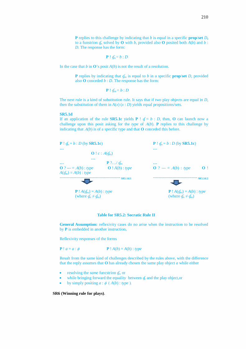
210

P replies to this challenge by indicating that b is equal in a specific prop/set D, to a funstrion ɠn solved by O with b, provided also O posited both A(b) and b : D. The response has the form:

P ! ɠn = b : D

In the case that b in O’s posit A(b) is not the result of a resolution.

P replies by indicating that ɠm is equal to b in a specific prop/set D, provided also O conceded b : D. The response has the form:

P ! ɠm = b : D

The next rule is a kind of substitution rule. It says that if two play objects are equal in D, then the substitution of them in A(x) (x : D) yields equal propositions/sets. SR5.1d If an application of the rule SR5.1c yields P ! ɠ = b : D, then, O can launch now a challenge upon this posit asking for the type of Α(b). P replies to this challenge by indicating that Α(b) is of a specific type and that O conceded this before.

P ! ɠn = b : D (by SR5.1c) P ! ɠn = b : D (by SR5.1c) … … O ! c : Α(ɠm) … … P ?…/ ɠm … O ? --- = Α(b) : type O ! A(b) : type O ? --- = Α(b) : type O ! A(ɠm) = A(b) : type -------------------------------------------- SR5.1d.1 -------------------------------- SR5.1d.2

P ! A(ɠm) = A(b) : type P ! A(ɠm) = A(b) : type (where ɠn ≠ ɠm) (where ɠn ≠ ɠm)

Table for SR5.2: Socratic Rule II

General Assumption: reflexivity cases do no arise when the instruction to be resolved by P is embedded in another instruction. Reflexivity responses of the forms P ! a = a : φ P ! A(b) = A(b) : type Result from the same kind of challenges described by the rules above, with the difference that the reply assumes that O has already chosen the same play object a while either • resolving the same funcstrion ɠi, or • while bringing forward the equality between ɠi and the play object,or • by simply positing a : φ ( A(b) : type ).

SR6 (Winning rule for plays).

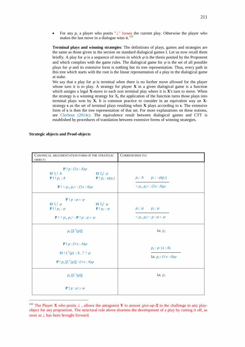
211

• For any p, a player who posits "⊥" looses the current play. Otherwise the player who makes the last move in a dialogue wins it.122

Terminal plays and winning strategies: The definitions of plays, games and strategies are the same as those given in the section on standard dialogical games I. Let us now recall them briefly. A play for ϕ is a sequence of moves in which ϕ is the thesis posited by the Proponent and which complies with the game rules. The dialogical game for ϕ is the set of all possible plays for ϕ and its extensive form is nothing but its tree representation. Thus, every path in this tree which starts with the root is the linear representation of a play in the dialogical game at stake. We say that a play for ϕ is terminal when there is no further move allowed for the player whose turn it is to play. A strategy for player X in a given dialogical game is a function which assigns a legal X-move to each non terminal play where it is X's turn to move. When the strategy is a winning strategy for X, the application of the function turns those plays into terminal plays won by X. It is common practice to consider in an equivalent way an X-strategy s as the set of terminal plays resulting when X plays according to s. The extensive form of s is then the tree representation of that set. For more explanations on these notions, see Clerbout (2014c). The equivalence result between dialogical games and CTT is established by procedures of translation between extensive forms of winning strategies.

Strategic objects and Proof-objects

CANONICAL ARGUMENTATION FORM OF THE STRATEGIC OBJECT:

CORRESPONDS TO:

P ! p : (∃x : A)ϕ

O ?L ! A O ?R ! ϕ P ! ! p1 : A P ! p2 : ϕ(p1)

P ! < p1, p2> : (∃x : A)ϕ

p1 : A p2 : : ϕ(p1)

————————— < p1, p2> : (∃x : A)ϕ

P ! p : ϕ ∧ ψ O ?L ! ϕ O ?R ! ψ P ! ! p1 : ϕ P ! p2 : ψ

P ! < p1, p2> : P ! p : ϕ ∧ ψ

p1 : ϕ p2 : ψ

————————— < p1, p2> : p : ϕ ∧ ψ

p2 ⟦L∀(p)⟧

P ! p : (∀x : A)ϕ

O ! L∀(p) : A , ? ! ϕ

P ! p2 ⟦L∀(p)⟧ : (∀x : A)ϕ

λx. p2

p2 : ϕ (x : A) ———————— λx. p2 : (∀x : A)ϕ

p2 ⟦L⊃(p)⟧

P ! p : ϕ ⊃ ψ

λx. p2

122 The Player X who posits ⊥ , allows the antagonist Y to answer give-up-X to the challenge to any play-object for any proposition. The structural rule above shortens the development of a play by cutting it off, as soon as ⊥ has been brought forward.

212

O ! L⊃(p) : ϕ, ? ! ψ

P ! p2 ⟦L⊃(p)⟧ : ϕ ⊃ ψ

p2 : ψ (x : ϕ) ——————————

λx. p2 : ϕ ⊃ ψ

P ! p : ¬ϕ

O ! pi : ϕ, ? ! ⊥

O ! p1 : ϕ ... O ! ⊥(n)

P ! -- ⟦L⊃(p)⟧ : ¬ϕ

p2 : ⊥ (x : ϕ) ——————————

λx. p2 : ¬ϕ

P ! p : ϕ ∨ ψ

O ? ∨ [! L∨(p) : ϕ | ! R∨(p) : ψ]

P ! p1 : ϕ P ! p2 : ψ

P ! p1 / L∨(p) : ϕ ∨ ψ P ! p2 / R∨(p) : ϕ ∨ ψ

p1 : ϕ p2

: ψ —————— —————— i(p1) : ϕ ∨ ψ j(p2) : ϕ ∨ ψ

O ! ⊥(n)

P ! O-gives-up(n) : α

p2 : ⊥ ————

R0 : α

Argumentation form of a strategic object for P Strategic objects as Records of instructions and their resolutions

Posit Challenge Defence

as Instruction-Record

P ?L P ! *L∃(p) = p1 / *IP : A

O ! p : (∃x : A)ϕ Or Respectively

P ?R

P ! *R∃(p) = p2 / *IP : ϕ(p1)

P ?L P ! *L{...}(p) = p1 / *IP : A

O ! p : {x : A | ϕ} Or Respectively

P ?R

P ! *R{...}(p) = p2 / *IP : ϕ(LP{...}(p1))

P ?L P ! *L∧(p) = p1 / *IP : ϕ

O ! p : ϕ ∧ ψ Or Respectively

P ?R P ! *R∧(p) = p2 / *IP : ψ

O ! p : (∀x : A)ϕ P ! IO = p1 / *L∀(p) : A P ! *R∀(p) = p2 / *IP ⟦p1⟧ : ϕ(p1)

O ! p : ϕ ⊃ ψ

P ! *IO = p1 / *L⊃(p) : ϕ P ! *R⊃(p) = p2 / *IP ⟦p1⟧ : ψ

O ! p : ¬ϕ O ! ⊥(n)

P ! *IO = p1 / *L¬(p) : ϕ P ! O-gives-up(n) : α

O ! ⊥(n)

O ! L ∨(p) : ϕ

O ! p : ϕ ∨ ψ P ? ∨ P ! *L ∨(p) = p1 / In

P | *R∨(p) = p2 / *ImP : α

213

O ! R∨(p) : ψ

If pi in pi : B is not the result of one of both of the instructions, the argumentation form of the strategic object is the reflexive equality

pi = pi : B

Let us write explicitly the table of correspondences between the argumentation form of strategic objects for P and proof-objects as analyzed by elimination-rules

ARGUMENTATION FORM OF THE STRATEGIC OBJECT: CORRESPONDS TO: With Equality

O ! p : (∃x : A)ϕ

P ?L P ?R P ! *L∃(p) = p1 / *IP

: A P ! *R∃(p) = p2 / *IP : ϕ(p1)

Without Equality

O ! p : (∃x : A)ϕ P ?L P ?R

P ! L∃(p) : A P ! R∃(p) : ϕ(p1)

With Equality p1 : A p2

: : ϕ(p1) p1 : : A p2 : ϕ(p1)

————————— ————————— fst(p1, p2) = p1 : A snd(p1, p2) = p2

: ϕ(p1)

Without Equality p : (∃x : A)ϕ p : (∃x : A)ϕ —————— —————— fst(p) : A snd(p) : ϕ(p1)

With Equality

O ! p : ϕ ∧ ψ P ?L P ?R

P ! *L∧(p) = p1 / *IP : ϕ P ! *R∧(p) = p2 / *IP : ψ

Without Equality

O ! p : ϕ ∧ ψ

P ?L P ?R

P ! L∧(p) : ϕ P ! R∧(p) : ψ

With Equality p1 : ϕ p2

: ψ p1 : ϕ p2 : ψ

——————— ——————— fst(p1, p2) = p1: ϕ snd(p1, p2) = p2: ψ

Without Equality p : ϕ ∧ ψ p : ϕ ∧ ψ ——————— ——————— fst(p) : ϕ snd(p) : ψ

(given p : (∀x : A)ϕ, p1 : A, L∀(p) : A, p2 : ϕ)

p2⟦L∀(p)⟧ p ⟦p1⟧

With Equality

O ! p : (∀x : A)ϕ

P ! IO = p1 / *L∀(p) : A

P ! *R∀(p) = p2 / *IP

⟦p1⟧ : ϕ(p1)

Without Equality

O ! p : (∀x : A)ϕ

(given p : (∀x : A)ϕ, x : , p1 : A, p2 : ϕ)

λx. p2 ap(p, p1)

With Equality

(given: λx. p2 : (∀x : A)ϕ)

p2 : ϕ (x : A) p1 : A

—————————————— ap(λx. p2, p1) = p2(p1): ϕ(p1)

Without Equality

p : (∀x : A)ϕ p1 : A ————————————

214

P ! p1 / *L∀(p) : A

P ! p ⟦p1⟧ : ϕ(p1)

ap(p, p1) : ϕ(p1)

(given p : ϕ ⊃ ψ, p1 : ϕ, L⊃(p) : ϕ, p2 : ψ)

p2 ⟦L⊃(p)⟧ p ⟦p1⟧

With Equality

O ! p : ϕ ⊃ ψ

P ! IO = p1 / * L⊃(p) : ϕ

P ! *R⊃(p) = p2 / *IP

⟦p1⟧ : ψ

Without Equality

O ! p : ϕ ⊃ ψ

P ! p1 / L⊃(p) : ϕ

P ! p ⟦p1⟧ : ψ

(given p : ϕ ⊃ ψ, p1 : ϕ, x : A : ϕ, p2 : ψ)

λx. p2 ap(p, p1)

With Equality

(given: λx. p2 : ϕ ⊃ ψ)

p2 : ϕ (x : ϕ) p1 : ψ

—————————————— ap(λx. p2, p1) = p2(p1): ψ

Without Equality

p : p : ϕ ⊃ ψ p1 : ϕ ————————————

ap(p, p1) : ψ

O ! L∨(p) : ϕ O ! R∨(p) : ψ

With Equality

O ! p : ϕ ∨ ψ P ? ∨

O ! L

∨(p) : ϕ O ! R∨(p) : ψ

P ! *L ∨(p) = p1 / In

P | *R∨(p) = p2 / *ImP : α

Without Equality

O ! p : ϕ ∨ ψ P ? ∨

O ! L

∨(p) : ϕ O ! R∨(p) : ψ P ! L

∨(p) | *R∨(p) : α

i(x) : ϕ j(y) : ψ

With Equality p1 : ϕ d : α[i(x)] (x : ϕ) e : α[j(y)] (y : ψ) ————————————————————

D(i(p1), x.d, y.e) = d[p1] : α[i(p1)] p2 : ϕ d : α[i(p)] (pi : ϕ) e : α[j(pj)] (pj : ψ) —————————————————————

D(j(p2), x.d, y.e) = e[p2] : α[j(p2)]

Without Equality p : ϕ ∨ ψ d : α[i(x)] (x : ϕ) e : α[j(y)] (y : ψ) ——————————————————————

D(p, x.d, y.e) : α[p]

O ! ⊥(n)

P ! O-gives-up(n) : α

p2 : ⊥ ————

R0 : α

215

Appendix IV Main Notation for CTT Equality and Identity

judgemental equality a = b : B A = B: set Identity-Predicate: Id(A, x, y), alternatively x =A y

Judgement:

Categorical a : A a = b : A A : set, alternatively A : prop A = B : set, alternatively , A = B : prop.

Hypothetical x : A ⊢ b : B, alternatively b : B (x : A) x : A ⊢ b = c : B, alternatively b = c : B (x : A) x : A ⊢ B : set, alternatively B : set (x : A) x : A ⊢ B = C : set, alternatively B = C : set (x : A)

Types: proposition: prop sets: set natural numbers: ℕ propositional-function of prime numbers : Pr Operators over a family of sets Σ-operator (Σ x : A)B

Proof object: <a, b> : (Σ x : A)B Projectors for c : (Σx : A)B fst(c) : (Σx : A)B snd(c) : (Σx : A)B[fst(c)]

П-operator (Πx : A)B Proof object for П λx.b : (Πx : A)B : Application for c : (Πx : A)B , a : A ap(λx.b, a) : B[a]

Disjoint union A + B Proof object given a : A i(a) : A + B Proof object given b : B j(b) : A + B Selector given c : A + B,, x : A ⊢ d : C[i(x)], y : B ⊢ e : C[j(y)] D(c, x.d, y.e) : C[c]

216

References Aczel, P. (1978). "The type theoretic interpretation of constructive set theory". In Mac-intyre, A., Pacholski, L., and Paris, J. (eds.), Logic Colloquium 77, Amsterdam: North-Holland, pp. 55–66. Almog, J. (1991). "The What and the How". Journal of Philosophy, 88, pp. 225–244. Aristotle (1984). In Barnes (1984). J. L. Austin (1946). “Other Minds”. The Aristotelian Society Supplementary Volume, 20, pp. 148–187 J. Barnes (1984). The Complete Works of Aristotle. The Revised Oxford Translation, ed. Princeton NJ: Princeton University Press. M. Beirlaen and M. Fontaine (2016). "Inconsistency-Adaptive Dialogical Logic". Logica Universalis. Online first, DOI 10.1007 / s11787-016-0139-y J. Bell (2009). The Axiom of Choice. London: College Publications. E. Bishop (1967). Foundations of constructive mathematics. New York, Toronto, London: McGraw- Hill. Brandom, R. 1994. Making it Explicit. Cambridge: Harvard UP. Brandom, R. 2000. Articulating Reasons. Cambridge: Harvard UP. W. Breckenridge and O. Magidor (2012). "Arbitrary Reference". Philosophical Studies, 158(3), pp. 377-400. P. Cardascia (2016). " Dialogique des matrices". Revista de Humanidades de Valparaíso, 6, in print. Carnap, R. (1934). Logische Syntax der Sprache. Vienna: Julius Springer. A. Church (1941). The Calculi of Lambda Conversion, Princeton: Princeton University Press. N. Clerbout (2014a). “First-order dialogical games and tableaux”. Journal of Philosophical Logic, 43(4), 785-801. N. Clerbout (2014b). Etude sur quelques semantiques dialogiques: Concepts fondamentaux et éléments de metathéorie. London : College Publications. N. Clerbout (2014c). “Finiteness of Plays and the Dialogical Problem of Decidability”. IfCoLog Journal of Logics and their Applications, 1(1), pp. 115–130. N. Clerbout, M.H. Gorisse, and S. Rahman (2011). “Context-sensitivity in Jain philosophy: A dialogical study of Siddharsiganis Commentary on the Handbook of Logic”. Journal of Philosophical Logic, 40(5), pp. 633–662. N. Clerbout and S. Rahman (2015). Linking Game-Theoretical Approaches with Constructive Type Theory: Dialogical Strategies as CTT-Demonstrations. Dordrecht: Springer. J. M. Cooper (1997). Plato. Complete Works. Indianapolis IN: Hackett. J. Corcoran (1974). "Aristotle’s natural deduction system". In J. Corcoran (ed.) Ancient Logic and Its Modern Interpretations, Dordrecht: Synthese Historical Library, 9, pp. 85–131. M. Crubellier (2008). “The Programme of Aristotelian Analytics”. In C. Dégremont, L. Keiff, H. Rückert (eds.) Dialogues, Logics and Other Strange Things. Essays in honour of Shahid Rahman. London: College Publications, pp. 103-129. M. Crubellier (2014). Aristote, Premiers Analytiques ; traduction, introduction et commentaire. Paris: Garnier-Flammario.

217

A. B. Dango (2014). "Des dialogues aux tableaux dans le contexte de révision des croyances : De l’oralité à l’écriture". In C. Bowao et S. Rahman (éd.) Entre l’orature et l’écriture : Relations croisées, London: College Publications, pp. 175–192. A. B. Dango (2015). "Interaction et révision de croyances". Revista de Humanidades de Valparaíso, 5, pp. 75 – 98. A. B. Dango (2016). Approche dialogique de la révision des croyances dans le contexte de la théorie constructive des types. London: College Publications. R. Diaconescu (1975). "Axiom of choice and complementation". Proc. Amer. Math. Soc., vol. 51, pp.176–178. Diller, J. and Troelstra, A. (1984). Realizability and intuitionistic logic. Synthese, 60, pp. 253–282. Dummett, M. (1973). Frege. Philosophy of Language. London: Duckworth, Cited from the second edition (1981). C. Dutilh Novaes (2015). "A Dialogical, Multi-Agent Account of the Normativity of Logic". Dialectica, 69, N° 4 (2015), pp. 587–609. K. Ebbinghaus (1964). Ein formales Modell der Syllogistik des Aristoteles. Göttingen: Vandenhoeck & Ruprecht GmbH. . W. Felscher (1985). “Dialogues as a foundation for intuitionistic logic”. In D. Gabbay and F. Guenthner (eds.), Handbook of Philosophical Logic, Dordrecht: Kluwer, vol. 3, pp. 341–372. K, Fine (1985a). "Natural Deduction and Arbitrary Objects". Journal of Philosophical Logic 14, pp. 57-107. K, Fine (1985b). Reasoning With Arbitrary Objects. Oxford: Basil Blackwell. M. Fontaine (2013). Argumentation et engagement ontologique. Être, c’est être choisi. London: College Publications. A. Fraenkel, Y. Bar-Hillel and A. Levy (1973). Foundations of Set Theory, 2nd edition. Dordrecht: North-Holland. G. Frege (1891). "Funktion und Begriff, Vortrag, gehalten in der Sitzung vom 9. Januar 1891 der Jenaischen Gesellschaft für Medizin und Naturwissenschaft", Jena: Hermann Pohle. In Frege (2008), pp. 1-22. G. Frege (1892). " Über Sinn und Bedeutung". Zeitschrift für Philosophie und philosophische Kritik, 100, pp. 25–50. In Frege (2008), pp. 23-46. Frege, G. (1893). Grundgesetze der Arithmetik I. Jena: Hermann Pohle. G. Frege (2008). Funktion, Begriff, Bedeutung. Fünf logische Studien. G. Patzig (ed.), Göttingen: Vandenhoeck & Ruprecht GmbH. Garner, R. (2009). "On the strength of dependent products in the type theory of Martin- Löf". Annals of Pure and Applied Logic, 160, pp. 1–12. G. Gentzen (1935). "Unterschungen über das logische Schliessen". Mathematirche Zeitschrift, 39 (1934-1935), pp. 176-210. Reprinted in Gentzen (1969, pp. 68-131). G. Gentzen (1969).The Collected Papers of Gehard Gentzen. M. Szabo (ed.), Amsterdam: North-Holland..

218

N. D. Goodman, J. Myhill (1978). "Choice implies excluded middle". Zeitschrift für mathematische Logik und Grundlagen der Mathematik, 24, p. 461. J. Granström (2011). Treatise on Intuitionistic Type Theory. Dordrecht: Springer. Hale, B. and Wright, C. (2001). "To bury Caesar. . . ". In The Reason’s Proper Study, pp. 335–396. Oxford: Oxford University Press. G. W. F. Hegel (1999). Wissenschaft der Logik. Hamburg: Felix Meiner Verlag. G. W. F. Hegel (2010). The Science of Logic. Cambridge: Cambridge CUP. J. Hintikka (1973). Logic, Language-Games and Information: Kantian Themes in the Philosophy of Logic. Oxford: Clarendon Press. J. Hintikka (1983). “Game-theoretical semantics: insights and prospects”. Notre Dame Journal of Formal Logic, vol. 23/2, pp. 219-249. J. Hintikka (1996a). The Principles of Mathematics Revisited. Cambridge: Cambridge University Press. J. Hintikka (1996b). Lingua Universalis vs. Calculus Ratiocinator: An Ultimate Presupposition of Twentieth-Century Philosophy, Dordrecht: Kluwer. J. Hintikka (2001). “Intuitionistic Logic as Epistemic Logic”. Synthese, 127, pp. 7–19. Hofmann, M. (1995). Extensional Concepts in Intensional Type Theory. PhD thesis, University of Edinburgh. Hofmann, M. and Streicher, T. (1998). "The groupoid interpretation of type theory". In Sambin, G. and Smith, J. M., editors, Twenty-five Years of Constructive Type Theory. Oxford: Oxford University Press, pp. 83–111. Howard, W. A. (1980). "The formulae-as-types notion of construction". In Seldin, J. P. and Hindley, J. R., editors, To H.B. Curry: Essays on Combinatory Logic, Lambda Calculus and Formalism. London: Academic Press, pp. 479–490. V. Ilievski (2013). Филозофија / Filozofija - A Journal of Philosophical Inquiry, 2(35) online: http: / / dl.fzf.ukim.edu.mk / index.php / filozofija / article / view / 925. R. Jovanovic. (2013) “Hintikkas Take on the Axiom of Choice and the Constructivist Challenge”. Revista de Humanidades de Valparaiso, 2, pp. 135-152. R. Jovanovic. (2015) Hintikkas Take on Realism and the Constructivist Challenge. London: College Publications. L. Keiff (2007). Le Pluralisme Dialogique: Approches dynamiques de largumentation formelle. Lille: PhD - thesis -, Lille 3. L. Keiff (2009). “Dialogical Logic”. In Edward N. Zalta (ed.) The Stanford Encyclopedia of Philosophy, URL http: / / plato.stanford.edu / entries / logic-dialogical / . A. Klev (2014). Categories and Logical Syntax. PHD, Leiden. E. C. Krabbe, E. C. (1982). Studies in Dialogical Logic. Gröningen: Rijksuniversiteit. PHD-Thesis. E. C. Krabbe (1985). "Formal Systems of Dialogue Rules". Synthese, vol. 63, pp. 295–328. E. C. Krabbe (2006). "Dialogue Logic". In Dov M. Gabbay, and J. Woods (eds.) Handbook of the History of Logic, vol. 7, pp. 665–704. Amsterdam: Elsevier

219

K. Lorenz (1970). Elemente der Sprachkritik.Eine Alternative zum Dogmatismus und Skeptizismus in der Analytischen Philosophie. Frankfurt: Suhrkamp. K. Lorenz (2001). “Basic objectives of dialogue logic in historical perspective”. In S. Rahman and H. Rückert (eds.), 127 (1-2), pp. 255–263. K. Lorenz (2010a). Logic, Language and Method: On Polarities in Human Experience. Berlin / New York: De Gruyter. K. Lorenz (2010b). Philosophische Variationen: Gesammelte Aufstze unter Einschluss gemeinsam mit J¨urgen Mittelstraß geschriebener Arbeiten zu Platon und Leibniz. Berlin and New York: De Gruyter. K. Lorenz, and J. Mittelstrass, J. (1967). “On Rational Philosophy of Language. The programme in Plato’s Cratylus Reconsidered”. Mind 76:301, pp. 1-20. P. Lorenzen (1955). Einfürung in die operative Logik und Mathematik, Berlin: Springer, 1955.. P. Lorenzen (1969). Normative Logic and Ethics, Mannheim / Zürich: Bibliographisches Institut. P. Lorenzen and O. Schwemmer (1975) Konstruktive Logik, Ethik und Wissenschaftstheorie. Mannheim: Bibliographisches Institut, second edition. P. Lorenzen and K. Lorenz (1978). Dialogische Logik. Darmstadt: Wissenschaftliche Buchgesellschaft. J. V. Luce (1969). "Plato on Truth and Falsity in Names". The Classical Quarterly, vol. 19, No. 2, pp. 222-232. J. Lukasiewicz (1957). Aristotle’s Syllogistic from the Standpoint of Modern Formal Logic. Second edition, Oxford : Clarendon Press. S. Magnier (2013). Approche dialogique de la dynamique épistémique et de la condition juridique. London: College Publications. M. Marion (2006). "Hintikka on Wittgenstein: From language games to game semantics". Acta Philosophica Fennica, 78, pp. 223–242. M. Marion (2009). "Why play logical games?". In O. Majer, A.V. Pietarinen and T. Tulenheimo (eds.) Games: Unifying Logic, Language and Philosophy, Dordrecht: Springer, pp3–26. M. Marion (2010). "Between saying and doing: From Lorenzen to Brandom and Back". In P. E. Bour, M. Rebuschi and L. Rollet (eds.), Constructions. Essays in Honour of Gerhard Heinzmann, London: College Publications, pp. 489-497. M. Marion and H. Rückert (2015). “Aristotle on Universal Quantification: A Study form the Perspective of Game Semantics”. History and Philosophy of Logic, vol 37 (3), pp. 201-229. P. Martin-Löf (1971). "Hauptsatz for the intuitionistic theory of iterated inductive def- initions. In Fenstad, J. E. (ed.), Proceedings of the Second Scandinavian Logic Symposium. Amsterdam: North-Holland, pp. 179–216. P. Martin-Löf (1975a). "About models for intuitionistic type theories and the notion of definitional equality". In Kanger, S. (ed.), Proceedings of the Third Scandinavian Logic Symposium. Amsterdam: North-Holland, pp. 81–109. P. Martin-Löf (1975b). "An intuitionistic theory of types: Predicative part". In Rose, H. E. and Shepherdson, J. C. (eds.), Logic Colloquium ‘73. Amterdam: North-Holland, pages 73–118. P. Martin-Löf (1982). "Constructive mathematics and computer programming". In Co- hen, J. L., Łos´, J., et al. (eds.), Logic, Methodology and Philosophy of Science VI, 1979, pages 153–175. North-Holland, Amsterdam.

220

P. Martin-Löf (1984). Intuitionistic Type Theory. Notes by Giovanni Sambin of a series of lectures given in Padua, June 1980. Naples: Bibliopolis. P. Martin-Löf (1992). "Substitution calculus". Lecture notes. Avail-able at http://archive-pml.github.io/martin-lof/pdfs/ Substitution-calculus-1992.pdf. P. Martin-Löf (1996). "On the meanings of the logical constants and the justifications of the logical laws". Nordic Journal of Philosophical Logic, 1, pp. 11–60. P. Martin- Löf (2006). "100 years of Zermelo's axiom of choice: what was the problem with it?". The Computer Journal, 49 / 3, pp. 345–350. P. Martin-Löf (2011). "When did ‘judgement’ come to be a term of logic?". Lecture held at Ecole Normale Supérieure on 14 October 2011. Video recording available at http://savoirs.ens.SR//expose.php?id=481. P. Martin-Löf (2014). "Truth of empirical propositions". Lecture held at the University of Leiden, February 2014. Transcription by Amsten Klev. P. Martin-Löf (2015). "Is logic part of normative ethics?". Lecture held at the research unity Sciences,

normes, décision (FRE 3593),Paris, May 2015. Transcription by Amsten Klev. Z. McConaughey (2015). La Science et l’activité du dialecticien. Typoscript, Lille. B. Nordström, K. Petersson, and J. M. Smith (1990). Programming in Martin-Löf’s Type Theory: An Introduction. Oxford: Oxford University Press. Nordström, B., Petersson, K., and Smith, J. M. (2000). "Martin-Löf’s type theory". In Abramsky, S., Gabbay, D., and Maibaum, T. S. E. (eds.), Handbook of Logic in Computer Science. Volume 5: Logic and Algebraic Methods. Oxford: Oxford University Press, pp. 1–37. G. Nzokou (2013). Logique de l'argumentation dans les traditions orales africaines. London: College Publications. J. Peregrin (2014). Inferentialism; Why Rules Matter.New York: Plagrave MacMillan. Plato (1997). In Cooper (1997). T. Piecha (2012). Formal Dialogue Semantics for Definitional Reasoning and Implications as Rules. PhD thesis, Faculty of Science, University of Tübingen, 2012. Available online at http://nbn-resolving.de/urn:nbn:de:bsz: 21-opus-63563. T. Piecha and P. Schroeder-Heister (2011°. "Implications as Rules in Dialogical Semantics". In M. Peliš and V. Punčochář, (eds.), The Logica Yearbook 2011. London: College Publications, pages 211–225. A. Popek (2012). “Logical dialogues from Middle Ages”. In C. Barés Gómez, S. Magnier and F. J. Salguero (eds.), Logic of Knowledge. Theory and Applications, London: College Publications, pp. 223–244. D. Prawitz. (1965). Natural Deduction. Stockholm: Almqvist & Wiksell. G. Primiero (2008). Information and Knowledge. Dordrecht: Springer. W. V. Quine (1969). Ontological Relativity and Other Essays. New York: Columbia University Press. S. Rahman (1993). Über Dialogue, Protologische Kategorien und andere Seltenheiten. Frankfurt / Paris / N. York: P. Lang.

221

S. Rahman and N. Clerbout (2013). “Constructive Type Theory and the Dialogical Approach to Meaning”. The Baltic International Yearbook of Cognition, Logic and Communication:Games, Game Theory and Game Semantics, 8, pp. 1-72. Also online in: www.thebalticyearbook.org. S. Rahman and N. Clerbout (2015). “Constructive Type Theory and the Dialogical Turn – A new Approach to Erlangen Constructivism”. In J. Mittelstrass and C. von Bülow (ed.), Dialogische Logik, Münster: Mentis, pp. 91-148. Rahman, S., N. Clerbout, and L. Keiff (2009). "On dialogues and natural deduction". In G. Primiero and S. Rahman (eds.) Acts of Knowledge: History, Philosophy and Logic: Essays Dedicated to Göran Sundholm, , London: College Publications, pp. 301–336. S. Rahman, N. Clerbout and R. Jovanovic (2015). " The Dialogical Take on Martin-Löf's Proof of the Axiom of Choice". South American Journal of Logic, 1(1), pp. 179-208. S. Rahman, N. Clerbout, and Z. McConaughey (2014) “On play objects in dialogical games. Towards a Dialogical approach to Constructive Type Theory”. In P. Allo / V. v. Kerkhove (ed.), Modestly radical or radically modes . Festschrift for Jean-Paul van Bendegem, London: College Publications, pp. 127-154. S. Rahman/ J. Granström / Z. Salloum (2014). “Ibn Sina’s Approach to equality and unity”. Cambridge Journal for Arabic Sciences and Philosophy, 4(02), pp. 297-307. S. Rahman, Z. McConaughey, and M. Crubellier (2015). A Dialogical Framework for Aristotle's Syllogism. Work in progress. S. Rahman and L. Keiff (2005). “On how to be a dialogician”. In D. Vanderveken (ed.), Logic, Thought, and Action, Dordrecht: Kluwer, pp. 359–408. S. Rahman and L. Keiff (2010). “La Dialectique entre logique et rhetorique”. Revue de Métaphysique et de Morale, 66(2), pp. 149–178. S. Rahman and J. Redmond (2015). "A Dialogical Frame for Fictions as Hypothetical Objects". Filosofia Unisinos, 16(1), pp. 2-21. S. Rahman and J. Redmond (2016) . “Armonía Dialógica. Tonk, ,Teoría Constructiva de Tipos y Reglas para Jugadores Anónimos” (Dialogical Harmony: Tonk, Constructive Type Theory and Rules for Anonymous Players"). Theoria. S. Rahman/J. Redmond. (ISI), 31/1 (2016), pp. 27-53. S. Rahman and H. Rückert (eds.), New Perspectives in Dialogical Logic, special volume Synthese 127, Dordrecht: Springer. S. Rahman and T. Tulenheimo (2009). “From Games to Dialogues and Back: Towards a General Frame for Validity”. In O. Majer. A. Pietarinen and T. Tulenheimo (eds.), Games: Unifying Logic, Language and Philosophy, Dordrecht: Springer, pp. 153–208. A. Ranta (1988). “Propositions as games as types”. Synthese, 76, pp. 377–395. A. Ranta (1994). Type-Theoretical Grammar. Oxford: Clarendon Press. R. Recorde (1577). The Whetstone of Witte. London : John Kingston. J. Redmond (2010) Logique dynamique de la fiction: Pour une approche dialogique. London: College Publications. J. Redmond and M. Fontaine (2011). How to Play Dialogues: An Introduction to Dialogical Logic. London: College Publications. J. Redmond and S. Rahman and (2016). “Armonía Dialógica: tonk Teoría Constructiva de Tipos y Reglas para Jugadores Anónimos”, Theoria, 31(1), pp. 27-53.

222

H. Rückert (2011). Dialogues as a Dynamic Framework for Logic. London: College Publications. Schroeder-Heister, P. (1984). "A natural extension of natural deduction". Journal of Symbolic Logic, 49, pp. 1284–1300. Schroeder-Heister, P. (2008). "Lorenzen’s operative justification of intuitionisitic logic". In M. van Atten, P. Boldini, M. Bourdeau, G. Heinzmann (eds.), One Hundred Years of Intuitionism (1907-2007), Basel: Birkhäuser, pp. 214-240. G. Siegwart (1993). “ Die fundamentale Methode der Abstraktion. Replik auf Dirk Hartmann und Christian Thiel”. Zeitschrift für Philosophische Forschung, 47(4), pp. 606-614. R. Smith (1982). "What is Aristotelian Echthesis?" History and Philosophy of Logic, 3, pp. 113-127. G. Sundholm (1997) “Implicit epistemic aspects of constructive logic”. Journal of Logic, Language, and Information 6:2, pp. 191-212. G. Sundholm (1998). “Inference versus Consequence”. In T. Childers (ed.), The Logica Yearbook 1997, Prague: Filosofia, pp. 26–36. G. Sundholm (2001). “A Plea for Logical Atavism”. In O. Majer (ed.), The Logica Yearbook 2000, Prague: Filosofia, pp. 151-162. Sundholm, B. G. (2006). "Semantic values for natural deduction derivations". Synthese, 148:623–638. Sundholm, B. G. (2009). "A century of judgement and inference, 1837-1936: Some strands in the development of logic". In Haaparanta, L. (ed.), The Development of Modern Logic, pages 263–317. Oxford: Oxford University Press. G. Sundholm (2012). " "Inference versus consequence" revisited: inference, conditional, implication” Synthese, 187, pp. 943-956. G. Sundholm (2013). " Inference and Consequence in an Interpeted Language”. Talk at the Workshop PROOF THEORY AND PHILOSOPHY, Groningen, December 3-5, 2013. G. Sundholm (2016). " Independence Friendly Language is First Order after all?". Logique et Analyse, forthcoming. Tasistro, A. (1993). "Formulation of Martin-Löf’s theory of types with explicit substi- tutions". Master’s thesis, Chalmers University of Technology, Gothenburg. The Univalent Foundations Program (2013). Homotopy Type Theory: Univalent Foun- dations of Mathematics. http://homotopytypetheory.org/book, Institute for Advanced Study, Princeton. S. Thompson (1991). Type Theory and Functional Programming. Boston: Addison-Wesley. A. Troelstra, A. and van Dalen, D. (1988). Constructivism in Mathematics. Amterdam: North- Holland, Amsterdam. J. van Heijenoort (1967). "Logic as Calculus and Logic as Language". Synthese, 17, pp. 324-330. L. Wittgenstein (1922). Tractatus Logico-Philosophicus. Lille: Kegan Paul. E. Zermelo, (1904). "Neuer Beweis, dass jede Menge Wohlordnung werden kann (Aus einem an Herrn Hilbert gerichteten Briefe)". Mathematische Annalen, 59 , pp. 514-16. E. Zermelo (1908). "Untersuchungen über die Grundlagen der Mengenlehre, I". Mathematische Annalen, 65, pp. 261 – 281.

223

E. Zermelo, E. (1930). "Über Grenzzahlen und Mengenbereiche". Fundamenta Mathemat- icae, 16, pp. 29–47.

224

List of Names Aristotle Austin Baire Bar-Hillel Barnes Beirlaen Bell Bishop Borel Brandom Breckenridge Brouwer Cardascia Carnap Church Clerbout Cooper Corcoran Cratylus Crubellier Curry Dango Diaconescu Dummett Dutilh Novaes Ebbinghaus Eckoubili Fine Fontaine Fraenkel Frege Gentzen Goodman Gorisse Granström Hale Hegel Hintikka Ilievski Jovanovic Klev Kolmogorov Lebesgue Leibniz Levy Lorenz Lorenzen Luce

225

Lukasiewicz Magidor Magnier Marion Martin-Löf McConaughey Mitelstrass Myhle Nordström Nzokou Parmenides Peregrin Petersson Piecha Plato Popek Primiero Rahman Ranta Recorde Redmond Rückert Schröder-Heister Schwemmer Siegwart Smith Socrates Sundholm Tasistro Theaetetus Thompson Troelstra Tulenheimo van Daalen van Heijenoort van der Schaar Wittgenstein Zermelo

226

List of Subjects abstract abstraction absurdum application arbitrary object arbitrary reference assertion assumption Bool Boolean axiom of choice canonical Cartesian case-dependent category categorical choice computation computational rule concession conjunction constructive content context copy-cat core core of the strategy correct naming course of values critical Curry-Howard isomorphism decision definitional definitional equality demonstration dependent dialectical dialogical dialogical roots of equality dialogue disjoint union disjunction dispense double negation ecthesis elimination emergence of equality empty set

227

equality extensive form of a dialogical game extensive form of a strategy function function type game game-tree global meaning harmony hypothesis identity instruction judgement knowledge local meaning material m-dependent resolution meaning metalanguage metalevel metalogic natural number natural deduction negation nominal object object language ontological Opponent pensée aveugle play play object posit posit-substitution predicate predication predicator premiss presupposition projection prop Proponent proposition propositional equality quantifier range-course resolution resolution of functions resolution of instructions selection

228

sequence of moves set Socratic Socratic Rule starting rule strategic strategic object strategy strategy-level structural rule subset-separation substitution substitution of instructions syntactic terminal transmission tree type universal validity Wertverlauf winn winning strategy yes yes-no