IRTG 1792 Discussion Paper 2018-045

Predicative Ability of Similarity-based

Futures Trading Strategies

Hsin-Yu Chiu * Mi-Hsiu Chiang *²

Wei-Yu Kuo *³

* Academia Sinica, Taiwan *² NCCU College of Commerce, Taiwan *³ National Chengchi University, Taiwan

This research was supported by the Deutsche Forschungsgemeinschaft through the

International Research Training Group 1792 "High Dimensional Nonstationary Time Series".

http://irtg1792.hu-berlin.de

ISSN 2568-5619

Inte

rnat

iona

l Res

earc

h Tr

aini

ng G

roup

179

2

Predicative Ability of Similarity-based Futures Trading Strategies

Hsin-Yu Chiu Mi-Hsiu Chiang Wei-Yu Kuo

September 21, 2018

Abstract

A trading rule that draws on the empirical similarity concept is proposed to simulate the

technical trading mentality—one that selectively perceives structural resemblances between

market scenarios of the present and the past. In more than half of the nineteen futures

markets that we test against for profitability of this similarity-based trading rule, we find

evidence of predictive ability that is robust to data-snooping and transaction-cost adjust-

ments. When aided by an exit strategy that liquidates the trader’s positions across some

evenly-spaced time points, this rule generates the most robust returns.

Keywords: empirical similarity; technical trading; futures markets; analogical reasoning

JEL classification: G11; G12

1

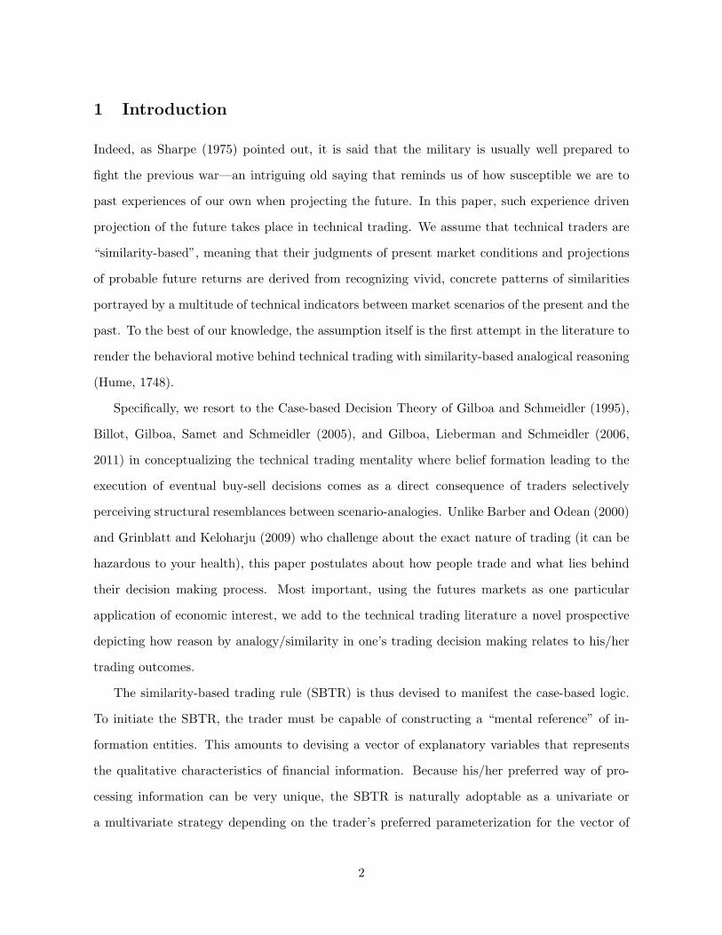
1 Introduction

Indeed, as Sharpe (1975) pointed out, it is said that the military is usually well prepared to

fight the previous war—an intriguing old saying that reminds us of how susceptible we are to

past experiences of our own when projecting the future. In this paper, such experience driven

projection of the future takes place in technical trading. We assume that technical traders are

“similarity-based”, meaning that their judgments of present market conditions and projections

of probable future returns are derived from recognizing vivid, concrete patterns of similarities

portrayed by a multitude of technical indicators between market scenarios of the present and the

past. To the best of our knowledge, the assumption itself is the first attempt in the literature to

render the behavioral motive behind technical trading with similarity-based analogical reasoning

(Hume, 1748).

Specifically, we resort to the Case-based Decision Theory of Gilboa and Schmeidler (1995),

Billot, Gilboa, Samet and Schmeidler (2005), and Gilboa, Lieberman and Schmeidler (2006,

2011) in conceptualizing the technical trading mentality where belief formation leading to the

execution of eventual buy-sell decisions comes as a direct consequence of traders selectively

perceiving structural resemblances between scenario-analogies. Unlike Barber and Odean (2000)

and Grinblatt and Keloharju (2009) who challenge about the exact nature of trading (it can be

hazardous to your health), this paper postulates about how people trade and what lies behind

their decision making process. Most important, using the futures markets as one particular

application of economic interest, we add to the technical trading literature a novel prospective

depicting how reason by analogy/similarity in one’s trading decision making relates to his/her

trading outcomes.

The similarity-based trading rule (SBTR) is thus devised to manifest the case-based logic.

To initiate the SBTR, the trader must be capable of constructing a “mental reference” of in-

formation entities. This amounts to devising a vector of explanatory variables that represents

the qualitative characteristics of financial information. Because his/her preferred way of pro-

cessing information can be very unique, the SBTR is naturally adoptable as a univariate or

a multivariate strategy depending on the trader’s preferred parameterization for the vector of

2

qualitative characteristics. At the same time, we assume that the trader is in possession of a

knowledge-/data- base comprising historical cases of the vector of qualitative characteristics.

The historical cases of the vector serve to depict the market scenarios of the past, while the

vector’s present case portrays the market scenario today. To decide if any past market scenarios

resemble the present, and to ask to what extent they resemble the present, a similarity-based

trader is equipped with a similarity function that embodies a user-definable measure of dis-

tance so as to quantify the extent of two objects being similar. Using this similarity function,

the trader then conducts similarity searches, under moving windows of specifically chosen time

lengths prior to the present date, by drawing analogies between market scenarios of the past

and the present. Probable future returns under the current market scenario are then predicted

using the similarity-weighted average of all corresponding past returns. A positive (negative)

similarity-weighted average of past returns would indicate a buy (sell) trading signal. This

similarity-weighted average of past returns is hereafter referred to as the “stochastic averaging

predictor” of the SBTR.

In terms of time frame, the SBTR is applicable daily or weekly. In the former, the SBTR

adopts the day-trade mechanism as depicted by Kuo and Lin (2013) and Barber, Lee, Liu, and

Odean (2014), where a similarity-based trader enters/closes his/her trading positions at the

opening/closing price on the same date. As a weekly strategy, we assume that the trader enters

(closes) his/her trading positions at the beginning (end) of each week.

We address market timing by allowing the trader to unload his/her trading positions under

different exit strategies. We follow Lu, Chen and Hsu (2015) to consider the MYR (Marshall,

Young and Rose, 2006) and the CL (Caginalp and Laurent, 1998) exit strategies. While the

MYR exit strategy is characterized by a predetermined date and condition to liquidate the

trader’s trading positions once and for all, the CL exit strategy relies on an average exit price

for the holding period so that the trader can gradually unload his/her trading positions across

some evenly-spaced time points.

We test these daily and weekly SBTRs for profitability against historical prices from nineteen

futures markets. To ensure that the (daily or weekly) best-performing rules detected are indeed

genuine, we apply the superior predictive ability test of Hansen (2005) throughout to control for

3

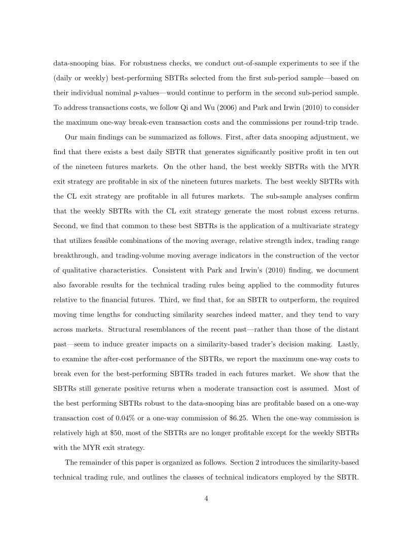
data-snooping bias. For robustness checks, we conduct out-of-sample experiments to see if the

(daily or weekly) best-performing SBTRs selected from the first sub-period sample—based on

their individual nominal p-values—would continue to perform in the second sub-period sample.

To address transactions costs, we follow Qi and Wu (2006) and Park and Irwin (2010) to consider

the maximum one-way break-even transaction costs and the commissions per round-trip trade.

Our main findings can be summarized as follows. First, after data snooping adjustment, we

find that there exists a best daily SBTR that generates significantly positive profit in ten out

of the nineteen futures markets. On the other hand, the best weekly SBTRs with the MYR

exit strategy are profitable in six of the nineteen futures markets. The best weekly SBTRs with

the CL exit strategy are profitable in all futures markets. The sub-sample analyses confirm

that the weekly SBTRs with the CL exit strategy generate the most robust excess returns.

Second, we find that common to these best SBTRs is the application of a multivariate strategy

that utilizes feasible combinations of the moving average, relative strength index, trading range

breakthrough, and trading-volume moving average indicators in the construction of the vector

of qualitative characteristics. Consistent with Park and Irwin’s (2010) finding, we document

also favorable results for the technical trading rules being applied to the commodity futures

relative to the financial futures. Third, we find that, for an SBTR to outperform, the required

moving time lengths for conducting similarity searches indeed matter, and they tend to vary

across markets. Structural resemblances of the recent past—rather than those of the distant

past—seem to induce greater impacts on a similarity-based trader’s decision making. Lastly,

to examine the after-cost performance of the SBTRs, we report the maximum one-way costs to

break even for the best-performing SBTRs traded in each futures market. We show that the

SBTRs still generate positive returns when a moderate transaction cost is assumed. Most of

the best performing SBTRs robust to the data-snooping bias are profitable based on a one-way

transaction cost of 0.04% or a one-way commission of $6.25. When the one-way commission is

relatively high at $50, most of the SBTRs are no longer profitable except for the weekly SBTRs

with the MYR exit strategy.

The remainder of this paper is organized as follows. Section 2 introduces the similarity-based

technical trading rule, and outlines the classes of technical indicators employed by the SBTR.

4

Section 3 describes the empirical test with data-snooping adjustments. Section 4 presents our

empirical findings. In Section 5, we conclude this study.

2 Methodology

This section introduces the SBTRs. We first define the stochastic averaging predictor for an

outcome variable of interest, and present the decision rule based on the predictor. Then, we

prescribe the vector of qualitative characteristics with the classes of technical indicators that are

most prevalent in real-life trading. Finally, we construct the set of SBTRs.

2.1 The similarity-based technical trading rule

We begin by assuming that a similarity-based trader is in possession of a set of information signals

conveyed by a vector of qualitative characteristics of dimension k, i.e., xt = (x1,t, . . . , xk,t), where

xj,t can be a specific trading indicator, such as the difference between the shorter-term and the

longer-term moving average, the value of the relative strength index over the past 10 days, or

the difference between the opening and closing prices of one Candlestick. Conditional on the

available information signals at time t, he/she will then attempt to forecast future returns, which

we refer to as a (real-valued) outcome variable yt. In this study, yt indicates either the next

1-day (daily) or the next 5-day (weekly) future returns. Define yst as the stochastic averaging

predictor of yt such that

yst =

∑mi=1 s(xt, xt−i) · yt−i∑m

i=1 s(xt, xt−i)(1)

where s : Rk×Rk → (0,∞) is a similarity function. The value of s(xt, xt−i) measures how similar

xt and xt−i are, and the more similar that xt and xt−i are, the larger the value of s(xt, xt−i). The

similarity function we use is s (xt, xt−i) = exp (−d (xt, xt−i)), where d (xt, xt−i) =

√∑kj=1

(xj,t−xj,t−i

σj

)2

defines a standardized Euclidean norm and σj is the sample standard deviation of the element

j in the vector of qualitative characteristics. The standardized Euclidean norm scales each co-

ordinate difference between xt, and xt−i by dividing it by the standard deviation of the values

5

in the corresponding coordinate over the moving window.

The yst so defined in (1) is a stochastic weighted averaging of the past returns yt−i over the

last m periods, and hence known as a “stochastic averaging predictor” (Gilboa and Schmeidler,

1995). In this paper, the SBTR based on yst has the following trading rule:

If yst > 0, enter a long position;

If yst < 0, enter a short position.(2)

In other words, the SBTR would recommend that the investor buys when yst > 0, because based

on the past experience of the investor, the future return is more likely to be positive when the

signal vector is xt. A similar argument applies to the case where yst < 0.

One can certainly opt for other measures of similarity—for example the Mahalanobis metric—

to quantify the distance between any two vectors of qualitative characteristics. In our case, we

use the standard Euclidean norm because it is simple to implement and more appropriate as a

distance measure when different scales and sources of qualitative characteristics are involved.

2.2 Prescribing the Vector of Qualitative Characteristics

Because attention allocation is costly and requires effort (Kahneman, 1973; Hirshleifer and

Teoh, 2003; Peng and Xiong, 2006; Barber and Odean, 2008), a similarity-based trader must

be selective in his/her intended focus. We thus illustrate the SBTR using five prevalent classes

of trading indicators to prescribe the vector of qualitative characteristics: the moving average

(MA), relative strength index (RSI), trading range breakthrough (TRB), trading-volume mov-

ing average (VMA), and past 5-day Candlestick patterns. The information contents of these

technical indicators are described as follows:

Moving Average (MA): MAs enable traders to identify current price trends, trend re-

versals, and the associated support and resistance levels. Traditionally, a technical trading

rule based on the MA triggers buy/sell signals through the upward/downward crossovers

of longer-term MAs by shorter-term MAs, where the MAs are calculated as the average

closing prices over a specified period of time prior to the trading date, see, for example

6

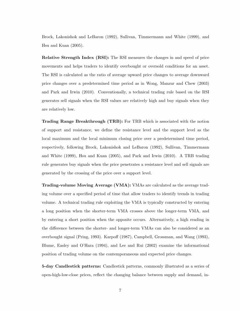
Brock, Lakonishok and LeBaron (1992), Sullivan, Timmermann and White (1999), and

Hsu and Kuan (2005).

Relative Strength Index (RSI): The RSI measures the changes in and speed of price

movements and helps traders to identify overbought or oversold conditions for an asset.

The RSI is calculated as the ratio of average upward price changes to average downward

price changes over a predetermined time period as in Wong, Manzur and Chew (2003)

and Park and Irwin (2010). Conventionally, a technical trading rule based on the RSI

generates sell signals when the RSI values are relatively high and buy signals when they

are relatively low.

Trading Range Breakthrough (TRB): For TRB which is associated with the notion

of support and resistance, we define the resistance level and the support level as the

local maximum and the local minimum closing price over a predetermined time period,

respectively, following Brock, Lakonishok and LeBaron (1992), Sullivan, Timmermann

and White (1999), Hsu and Kuan (2005), and Park and Irwin (2010). A TRB trading

rule generates buy signals when the price penetrates a resistance level and sell signals are

generated by the crossing of the price over a support level.

Trading-volume Moving Average (VMA): VMAs are calculated as the average trad-

ing volume over a specified period of time that allow traders to identify trends in trading

volume. A technical trading rule exploiting the VMA is typically constructed by entering

a long position when the shorter-term VMA crosses above the longer-term VMA, and

by entering a short position when the opposite occurs. Alternatively, a high reading in

the difference between the shorter- and longer-term VMAs can also be considered as an

overbought signal (Pring, 1993). Karpoff (1987), Campbell, Grossman, and Wang (1993),

Blume, Easley and O’Hara (1994), and Lee and Rui (2002) examine the informational

position of trading volume on the contemporaneous and expected price changes.

5-day Candlestick patterns: Candlestick patterns, commonly illustrated as a series of

open-high-low-close prices, reflect the changing balance between supply and demand, in-

7

vestor sentiment and psychology. See e.g., Caginalp and Laurent (1998), Marshall, Young,

and Rose (2006), Lu, Shiu, and Liu (2012), Lu (2014), and Lu, Chen, and Hsu (2015). To

make feasible the adapation of past 5-day Candlestick patterns to the SBTR. We charac-

terize each Candlestick pattern by their three vital elements: the difference between the

closing price and opening price, the difference between the highest price and the maximum

of the closing price and opening price (the upper shadow), and the difference between the

lowest price and the minimum of the closing price and opening price (the lower shadow).

In addition, we include the differences between the average price of the closing price and

opening price of two consecutive Candlesticks. Therefore, using the past 5-day Candlestick

patterns to depict the current market condition will give rise to a vector of characteristics

containing a total of 19 elements.

2.3 Universe of SBTRs

Noting the common observation that technical traders rarely rely the sole use of one particular

trading indicator while making investment decisions (Hsu and Kuan, 2005), a similarity-based

trader is allowed to employ the SBTR as a univariate or multivariate strategy in which the vector

of qualitative characteristics is prescribed with the values of a single type of trading indicator,

or, that of a panel of mixture types.

In the following, we illustrate how to construct the vector of qualitative characteristics using

the five types of technical indicators under a univariate SBTR and a multivariate SBTR.

2.3.1 Univariate SBTRs

Univariate SBTRs refer to the case where an SBTR prescribes the vector of qualitative character-

istics with one and only one type of technical indicator at a time. For example, a similarity-based

trader may decide that he/she is more comfortable with the MA rules, and his/her judgments

of how a past market scenario resembles the present depend solely on how similar—as indicated

by the similarity function—their MA qualitative characteristics match. As a consequence, the

stochastic averaging predictor will be solely specified by the MA rules, with the vector of quali-

tative characteristics xt comprising only the differences between the s-day and the l-day MAs.

8

We follow Brock, Lakonishok and LeBaron (1992) for the choice of time periods to calculate the

moving averages. The combinations of shorter- and longer-term MAs are denoted by MAs− l,

where s=1, 5, 10, 20, 50, 100, l=5, 10, 20, 50, 100, 150, and s < l. Thus, the univariate

SBTRs with the MA will include a total of 21 (6 + 5 + 4 + 3 + 2 + 1) shorter- and longer-term

combinations.

For univariate SBTRs with the RSI, the vector of qualitative characteristics is then prescribed

by the past p-day RSI values, where p corresponds to 5, 10, 20, 50, 100, and 150, respectively.

This amounts to a total of 6 univariate SBTRs with the RSI. For univariate SBTRs with the

TRB, we use the difference between the current closing price and the local maximum price over

a specific period of time prior to the current date and the difference between the closing price

and the local minimum price as two elements in the vector. In this study, we calculate the local

maximum and minimum prices based on the past 5, 10, 20, 50, 100, and 150 days prior to the

current date, and the univariate SBTR with the TRB is thus denoted as TRBp, where p =5,

10, 20, 50, 100, 150. The total is then 6 for the univariate SBTRs with the TRB. As for the

combinations of shorter- and longer-term VMAs, these are denoted by VMAs− l, where s=1, 5,

10, 20, 50, 100, l=5, 10, 20, 50, 100, 150, and s < l. The value for VMAs− l is the log difference

between the shorter- and longer-term VMAs. Similar to the univariate SBTRs with the MA,

the total number of univariate SBTRs with the VMA is 21. Lastly, when applying the 5-day

Candlestick patterns, the vector of qualitative characteristics contains 19 elements as mentioned

in Section 2.2.

Overall, the total number of univariate SBTRs is 55 (21 for the MA, 6 for the RSI, 6 for the

TRB, 21 for the VMA, and 1 for the 5-day Candlestick pattern).

2.3.2 Multivariate SBTRs

Multivariate SBTRs refer to the case where a similarity-based trading mentality is capable

of processing a heterogeneous pool of information entities. In making conditional forecasts—

based on stochastic averaging—of future returns, the trader chooses to prescribe the vector of

qualitative characteristics with a multitude of technical indicators varying in terms of their types.

The set of the SBTRs is expandable upon any feasible combination of technical indicators; it is

9

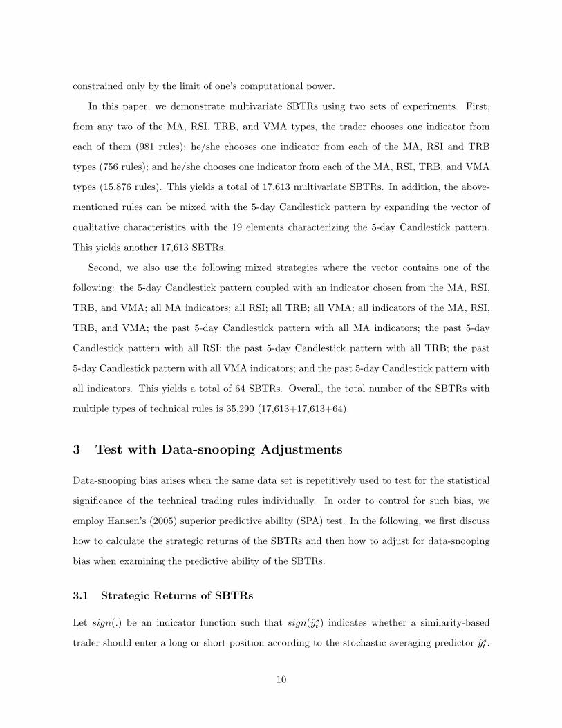
constrained only by the limit of one’s computational power.

In this paper, we demonstrate multivariate SBTRs using two sets of experiments. First,

from any two of the MA, RSI, TRB, and VMA types, the trader chooses one indicator from

each of them (981 rules); he/she chooses one indicator from each of the MA, RSI and TRB

types (756 rules); and he/she chooses one indicator from each of the MA, RSI, TRB, and VMA

types (15,876 rules). This yields a total of 17,613 multivariate SBTRs. In addition, the above-

mentioned rules can be mixed with the 5-day Candlestick pattern by expanding the vector of

qualitative characteristics with the 19 elements characterizing the 5-day Candlestick pattern.

This yields another 17,613 SBTRs.

Second, we also use the following mixed strategies where the vector contains one of the

following: the 5-day Candlestick pattern coupled with an indicator chosen from the MA, RSI,

TRB, and VMA; all MA indicators; all RSI; all TRB; all VMA; all indicators of the MA, RSI,

TRB, and VMA; the past 5-day Candlestick pattern with all MA indicators; the past 5-day

Candlestick pattern with all RSI; the past 5-day Candlestick pattern with all TRB; the past

5-day Candlestick pattern with all VMA indicators; and the past 5-day Candlestick pattern with

all indicators. This yields a total of 64 SBTRs. Overall, the total number of the SBTRs with

multiple types of technical rules is 35,290 (17,613+17,613+64).

3 Test with Data-snooping Adjustments

Data-snooping bias arises when the same data set is repetitively used to test for the statistical

significance of the technical trading rules individually. In order to control for such bias, we

employ Hansen’s (2005) superior predictive ability (SPA) test. In the following, we first discuss

how to calculate the strategic returns of the SBTRs and then how to adjust for data-snooping

bias when examining the predictive ability of the SBTRs.

3.1 Strategic Returns of SBTRs

Let sign(.) be an indicator function such that sign(yst ) indicates whether a similarity-based

trader should enter a long or short position according to the stochastic averaging predictor yst .

10

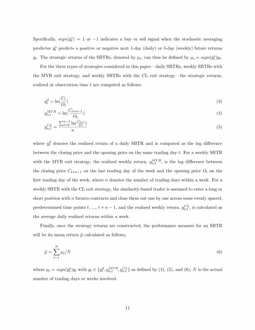
Specifically, sign(yst ) = 1 or −1 indicates a buy or sell signal when the stochastic averaging

predictor yst predicts a positive or negative next 1-day (daily) or 5-day (weekly) future returns

yt. The strategic returns of the SBTRs, denoted by µt, can thus be defined by µt = sign(yst )yt.

For the three types of strategies considered in this paper—daily SBTRs, weekly SBTRs with

the MYR exit strategy, and weekly SBTRs with the CL exit strategy—the strategic returns,

realized at observation time t are computed as follows:

ydt = ln(Ct

Ot) (3)

yMYRn,t = ln(

Ct+n−1

Ot) (4)

yCLn,t =

∑n−1i=0 ln(Ct+i

Ot)

n(5)

where ydt denotes the realized return of a daily SBTR and is computed as the log difference

between the closing price and the opening price on the same trading day t. For a weekly SBTR

with the MYR exit strategy, the realized weekly return, yMYRn,t , is the log difference between

the closing price Ct+n−1 on the last trading day of the week and the opening price Ot on the

first trading day of the week, where n denotes the number of trading days within a week. For a

weekly SBTR with the CL exit strategy, the similarity-based trader is assumed to enter a long or

short position with n futures contracts and close them out one by one across some evenly spaced,

predetermined time points t, ..., t+ n− 1, and the realized weekly return, yCLn,t , is calculated as

the average daily realized returns within a week.

Finally, once the strategy returns are constructed, the performance measure for an SBTR

will be its mean return µ calculated as follows,

µ =

N∑t=1

µt/N (6)

where µt = sign(yst )yt with yt ∈ {ydt , yMYRn,t , yCL

n,t } as defined by (4), (5), and (6); N is the actual

number of trading days or weeks involved.

11

3.2 Data-snooping adjustments

To test the null hypothesis that, among the set of SBTRs, none of them can generate significantly

positive returns, one can employ White’s (2000) reality check (RC) test to control for data-

snooping bias. However, the RC test may be conservative because its null distribution is obtained

under a least favorable configuration of parameter values. Moreover, the RC test may lose

power when too many poor and irrelevant technical trading rules are included (see, e.g., Hansen

(2005), Hsu, Hsu and Kuan (2010) and Hsu, Kuan and Yen (2014)). To avoid the least favorable

configuration and to improve the power property of the RC test, Hansen (2005) proposes the

SPA test based on a re-centering method.

To conduct the SPA test in our case, we formally let the performance measure of the k-th

SBTR be the mean return of it, µk =∑N

t=1 µk,t/N for k = 1, . . . ,K following the literature on

the profitability of technical trading rules (Sullivan, Timmermann and White, 1999; Hsu and

Kuan, 2005; Park and Irwin, 2010). The test statistic of Hansen’s (2005) SPA test is defined as

tSPA = max(

maxk=1,..,K

√Nµk

σk, 0)

(7)

where σ2k is a consistent estimator of σ2

k = var(√

Nµk

).1 Following Hansen (2005), we apply

the stationary bootstrap of Politis and Romano (1994) to approximate the null distributions.

To be specific, for b = 1, . . . , B, let µbk denote the sample mean of the b-th bootstrap sample.

Define the recentering mean as µk = µk1(√Nµk ≤ −σk

√2 log log(N)), where 1(E) denotes the

indicator function of the event E. The bootstrapped null distribution is given by:

tSPAb = max

(max

k=1,...,K

√N(µb

k − µk + µk)

σk, 0). (8)

The p-value of the SPA test is then approximated by pSPA =∑B

b=11(tSPA

b >tSPA)B , the proportion

of times when the resampling statistics are larger than the test statistic. For a given significance

level α, we will reject the null when pSPA < α and conclude that there exists at least one SBTR

1We follow Hsu and Kuan (2005) to compute the consistent estimator of σ2k based on the bootstrap resample:

σ2k = 1

B

∑Bb=1

(µbk − µb

k

)2

, where µbk is the average of µb

k over b.

12

that can generate a positive mean return.

Regarding the choice of the total number of bootstrap resamples B, and the probability

parameter q for the stationary bootstrap, we follow Sullivan, Timmermann and White (1999),

and Park and Irwin (2010) to set B = 500 and q = 0.1.2 Note that changing these parameters

yields similar empirical results.

4 Empirical Results

4.1 Data

Because the sample periods of the available data do not match, we test the profitability of

the SBTRs against the historical prices of nineteen futures markets over two different sample

periods. The first sample period ranges from 1995/01/01 to 2015/12/31, and forms our study

sample “Group 1”. Study sample Group 1 comprises futures markets of the corn, soybean,

wheat, live cattle, lumber, cocoa, sugar, silver, oil, S&P 500, T-Bills, Eurodollar, YEN and

GBP. On the other hand, Study sample “Group 2” represents the second sample period ranging

from 2005/01/01 to 2015/12/31, and consists of the E-mini S&P, E-mini NASDAQ, EUR and

AUD futures.3

Group 1 has historical price data available for at least ten years before 1995/01/01, and

Group 2 has historical prices available for at least five years before 2005/01/01. This amounts

to Group 1 allowing for a 10-year maximum moving time window and Group 2 allowing for a

5-year maximum moving time window during similarity searches. Thus, for Group1, the choice

of time length, m, as in equation (1), will take on a value of 250, 750, 1250 or 2,500, so as to

represent the 1-, 3-, 5- and 10-year moving windows, respectively. Similarly for Group 2, the

choice of time length for a moving window is set to 250, 750, or 1250, which correspond to 1, 3,

and 5 years. With all feasible combinations of moving-window time lengths accounted for, the

2The number of boostrap samples B may influence the accuracy of the estimated p-values. However, Brock,Lakonishok, and LeBaron (1992) and Kho (1996) show that their estimated bootstrap p-values are insensitive tothe bootstrap size B when the number of bootstrap samples goes beyond 500.

3The list of futures markets that we choose is close to that of Park and Irwin (2010). Although we excludethe pork bellies and Mark futures due to price unavailability, we include in addition two financial futures (E-miniS&P and E-mini NASDAQ) and two currency futures (EUR and AUD).

13

numbers of SBTRs total 141,380 ((55 + 35, 290)×4) and 106,035 ((55 + 35, 290)×3) for Group1

and Group 2, respectively.

Table 1 reports summary statistics for the annualized means and standard deviations of

unconditional daily returns across the nineteen futures markets and across the two sub-periods.

Daily returns are calculated as the log differences between the opening and closing prices of the

same trading day, so as to comply with the daily strategies of SBTRs. Differential characteristics

in the return distributions therein, across the futures markets, can clearly be identified: The

annualized mean returns range from -30.29% for lumber to 14.08% for soybean; and the annu-

alized standard deviations range from 0.68% for the Eurodollar to 31.06% for sugar. Within

each market, the statistical properties of the return distributions across different sub-periods

also vary. Sugar futures, for example, have their annualized mean returns ranging from -29.34%

to 25.43% while their annualized standard deviations range from 30.03% to 32.05% across the

sub-periods.

4.2 Performance Evaluation

Table 2 presents, for each futures market, the annualized mean returns of the best-performing

daily SBTRs identified using the whole sample period. The second column of Table 2 depicts

the qualitative characteristics of these winning strategies, which include the types of technical

indicators in use, and the adopted time lengths for the moving windows. For example, the

winning SBTR for corn futures is found to exhibit the following qualitative characteristics: it

uses a 10-year moving window, and adopts a multivariate strategy that involves an MA indicator

defined by the difference between the past 10-day (short-term) MA and the past 150-day (long-

term) MA; the past 150-day RSI; the difference between the closing price and the past 50-day

maximum price; and the difference between the closing price and the past 50-day minimum

price.

In addition, according to Table 2, the best SBTR for corn futures is found to generate

a positive annualized mean return of 24.29% with a 25.24% annualized standard deviation.

The unconditional annualized mean return following the buy (sell) signals generated by the

stochastic averaging predictor is 26.70% (-20.89%) with an annualized standard deviation of

14

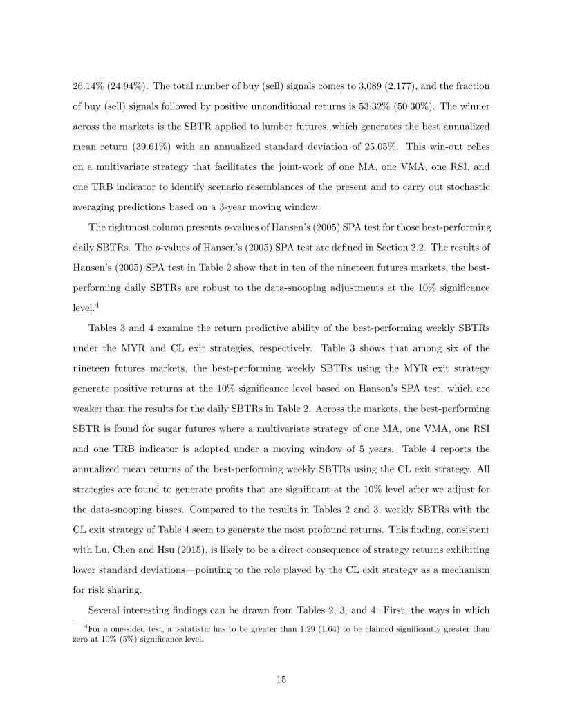
26.14% (24.94%). The total number of buy (sell) signals comes to 3,089 (2,177), and the fraction

of buy (sell) signals followed by positive unconditional returns is 53.32% (50.30%). The winner

across the markets is the SBTR applied to lumber futures, which generates the best annualized

mean return (39.61%) with an annualized standard deviation of 25.05%. This win-out relies

on a multivariate strategy that facilitates the joint-work of one MA, one VMA, one RSI, and

one TRB indicator to identify scenario resemblances of the present and to carry out stochastic

averaging predictions based on a 3-year moving window.

The rightmost column presents p-values of Hansen’s (2005) SPA test for those best-performing

daily SBTRs. The p-values of Hansen’s (2005) SPA test are defined in Section 2.2. The results of

Hansen’s (2005) SPA test in Table 2 show that in ten of the nineteen futures markets, the best-

performing daily SBTRs are robust to the data-snooping adjustments at the 10% significance

level.4

Tables 3 and 4 examine the return predictive ability of the best-performing weekly SBTRs

under the MYR and CL exit strategies, respectively. Table 3 shows that among six of the

nineteen futures markets, the best-performing weekly SBTRs using the MYR exit strategy

generate positive returns at the 10% significance level based on Hansen’s SPA test, which are

weaker than the results for the daily SBTRs in Table 2. Across the markets, the best-performing

SBTR is found for sugar futures where a multivariate strategy of one MA, one VMA, one RSI

and one TRB indicator is adopted under a moving window of 5 years. Table 4 reports the

annualized mean returns of the best-performing weekly SBTRs using the CL exit strategy. All

strategies are found to generate profits that are significant at the 10% level after we adjust for

the data-snooping biases. Compared to the results in Tables 2 and 3, weekly SBTRs with the

CL exit strategy of Table 4 seem to generate the most profound returns. This finding, consistent

with Lu, Chen and Hsu (2015), is likely to be a direct consequence of strategy returns exhibiting

lower standard deviations—pointing to the role played by the CL exit strategy as a mechanism

for risk sharing.

Several interesting findings can be drawn from Tables 2, 3, and 4. First, the ways in which

4For a one-sided test, a t-statistic has to be greater than 1.29 (1.64) to be claimed significantly greater thanzero at 10% (5%) significance level.

15

different types of trading indicators synergize in order to search (resemblances), identify (sim-

ilarities) and predict (stochastic averaging returns) seem to vary across markets. However, we

find that common to most of the futures markets, winning SBTRs seem to rely on multivariate

strategies that exploit different combinations of the MA, VMA, RSI, and TRB indicators in or-

der to construct the vector of qualitative characteristics. For example, there are twelve futures

markets in Table 2 where the best-performing daily SBTRs use the combinations of the MA,

VMA, RSI, and TRB indicators. In addition, in four futures markets, the best-performing daily

SBTRs exploit the 5-day Candlestick patterns combined with the MA, VMA, RSI, and TRB

indicators. For the rest of these markets, SBTRs that win out are also found to be multivariate

strategies of heterogeneous indicator types. This finding suggests that similarity-based traders

may consider it unwise, or even brutal, to trade and rely solely on a single type of trading indi-

cator. The similarity-based technical trading mentality is likely to be at its best upon for those

decision makers whose mental capacity allows them to process information based on a multitude

of technical indicators.

Second, the fraction of buy signals followed by positive unconditional returns exceeds the

fraction of sell signals followed by positive unconditional returns for all futures markets. For

example in Table 2, the fraction for buy signals ranges from 51.54% to 71.63%, while the fraction

for sell signals ranges from 45.58% to 65.67%. According to Brock, Lakonishok and LeBaron

(1992), the fraction of positive unconditional returns should be the same for both buy and sell

signals if the signals generated by technical rules are indeed useless. Using binomial tests, it can

be confirmed that the differences in the fraction of positive returns between buy and sell signals

are significant, thereby rejecting the null hypothesis for their equality. This result indicates that

the buy/sell signals generated by SBTRs are of predictive ability over future probable returns.

Third, Tables 2, 3 and 4 provide supporting evidence for the predictive ability of stochastic

averaging predictors over future probable returns. Consistent with Park and Irwin (2010), our

finding documents also favorable results of technical trading rules applied to commodity futures

relative to financial futures. For example, in Table 2, the best-performing daily SBTR traded

among financial futures markets yields an annualized mean return of 15.76% when trading on

E-mini Nasdaq futures. On the other hand, the best-performing daily SBTR traded among

16

commodity futures generates an annualized mean return of 39.61% for lumber futures. In addi-

tion, the average mean return across financial futures markets is 8.78%, while the average mean

return across commodity futures is 25.99%.

Finally, in searching for past market scenario-resemblances of the present, we find that the

adopted time lengths in fact vary across different markets. Similar experiences of the recent

past—rather than those of the distant past—seem to induce greater impacts on the similarity-

based traders’ decision making. For example, in Table 2, the best-performing SBTRs for wheat,

live cattle, and Yen futures utilize a moving window based on recent 1-year period (relative to

a 5-year maximum), whilst for lumber, sugar, copper, silver, the S&P 500, and the Eurodollar,

the best-performing SBTRs entail conducting a similarity search based on a moving window for

the recent 3-year period (relative to a 10-year maximum).

4.3 Sub-sample analysis

For robustness checks, we perform two kinds of sub-sample analyses over two sub-periods of

approximately equal lengths. (In the case of Study sample Group 1, the two sub-periods are

1995-2005 and 2006-2015. For Group 2, the two sub-periods are 2005-2010 and 2011-2015. )

We first follow Qi and Wu (2006) and Park and Irwin (2010) to conduct an in- and out-of-

sample test. We use the first sub-period to select the best strategies for each futures market

and then evaluate the performance of these best strategies using the second sub-period. Table

5 presents the in- and out-of-sample performance for the best-performing daily SBTRs selected

from the first sub-period. The second column reports the qualitative characteristics behind

these winning strategies including the types of technical indicators in use and the length of time

adopted for the moving windows. We also report annualized mean returns, standard deviations,

and p-values based on Hansen’s (2005) test for each best-performing SBTR in the first sub-

period. For the out-of-sample results, we report annualized mean returns, standard deviations,

and nominal p-values of Hansen’s (2005) test. Table 5 shows that the best-performing daily

SBTRs generate significant profits among eight futures markets in the first sub-period at the

10% significance level. For the out-of-sample results, we the annualized mean returns, standard

deviations, and t-statistics of those significant best-performing daily SBTRs selected in the first

17

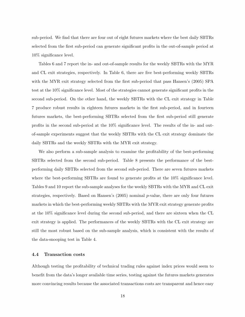
sub-period. We find that there are four out of eight futures markets where the best daily SBTRs

selected from the first sub-period can generate significant profits in the out-of-sample period at

10% significance level.

Tables 6 and 7 report the in- and out-of-sample results for the weekly SBTRs with the MYR

and CL exit strategies, respectively. In Table 6, there are five best-performing weekly SBTRs

with the MYR exit strategy selected from the first sub-period that pass Hansen’s (2005) SPA

test at the 10% significance level. Most of the strategies cannot generate significant profits in the

second sub-period. On the other hand, the weekly SBTRs with the CL exit strategy in Table

7 produce robust results in eighteen futures markets in the first sub-period, and in fourteen

futures markets, the best-performing SBTRs selected from the first sub-period still generate

profits in the second sub-period at the 10% significance level. The results of the in- and out-

of-sample experiments suggest that the weekly SBTRs with the CL exit strategy dominate the

daily SBTRs and the weekly SBTRs with the MYR exit strategy.

We also perform a sub-sample analysis to examine the profitability of the best-performing

SBTRs selected from the second sub-period. Table 8 presents the performance of the best-

performing daily SBTRs selected from the second sub-period. There are seven futures markets

where the best-performing SBTRs are found to generate profits at the 10% significance level.

Tables 9 and 10 report the sub-sample analyses for the weekly SBTRs with the MYR and CL exit

strategies, respectively. Based on Hansen’s (2005) nominal p-value, there are only four futures

markets in which the best-performing weekly SBTRs with the MYR exit strategy generate profits

at the 10% significance level during the second sub-period, and there are sixteen when the CL

exit strategy is applied. The performances of the weekly SBTRs with the CL exit strategy are

still the most robust based on the sub-sample analysis, which is consistent with the results of

the data-snooping test in Table 4.

4.4 Transaction costs

Although testing the profitability of technical trading rules against index prices would seem to

benefit from the data’s longer available time series, testing against the futures markets generates

more convincing results because the associated transactions costs are transparent and hence easy

18

to control. Furthermore, the complications imposed by short-sale constraints (Brock, Lakonishok

and LeBaron, 1990; Sullivan, Timmermann and White, 1999) can be avoided.

To analyze the impact of transaction costs on the best-performing SBTRs, we consider two

types of transaction cost measures, namely, the break-even transaction costs and the applicable

commissions per round-trip trade. For the break-even transaction costs, we follow Qi and Wu

(2006) to calculate the maximum one-way transaction costs for the best-performing SBTRs to

break even, i.e., to eliminate all possible returns or performance (Bessembinder and Chan, 1998).

The first four columns of Table 11 report the annualized mean returns, the number of round-trip

trades and the maximum one-way transaction cost of these strategies for the best daily SBTRs

selected from the overall sample period. The length of the overall sample period is 11 years for

copper, E-mini S&P, E-mini NASDAQ, EUR and AUD futures (Group 2) and 21 years for the

rest of the futures markets (Group 1). Taking the corn futures as an example, the annualized

mean return and the number of round-trip trades for the best daily SBTR are 24.29% and 5,266,

respectively. The number of round-trip trades is equal to the number of trading days over the

sample period. The maximum one-way cost to break even is 21*24.29%/(5,266*2)=0.0484%,

where 5,266 multiplied by 2 is the number of trades. That is, if the one-way trading cost for

an investor is greater than 0.0484%, the SBTR may not generate a positive return. To test

the profitability of technical strategies in currency markets, Qi and Wu (2006) adopt one-way

costs in the range of 0.025%-0.04% as suggested by Bessembinder (1994) who measures the

bid-ask spread in the inter-bank market. We find that the range of the one-way cost is also

applicable to the futures market, as Wang, Yau, and Baptiste (1997) and Wang and Yau (2000)

also report a similar range of the one-way cost for seven futures markets. The fifth and sixth

columns report the annualized mean returns after we consider the transaction costs of 0.025%

and 0.04%, respectively. The daily SBTRs are still profitable if the transaction cost is 0.025%

in thirteen of the nineteen futures markets, and the after-cost returns are still positive in eight

futures markets when the transaction cost is assumed to be 0.04%.

Alternatively, we can consider the commission per round-trip trades to account for the trans-

action costs. Park and Irwin (2010) consider a range of commission costs of $12.5-$100 per fu-

tures contract per round-trip trade. The transaction cost of $12.5 per round-trip is documented

19

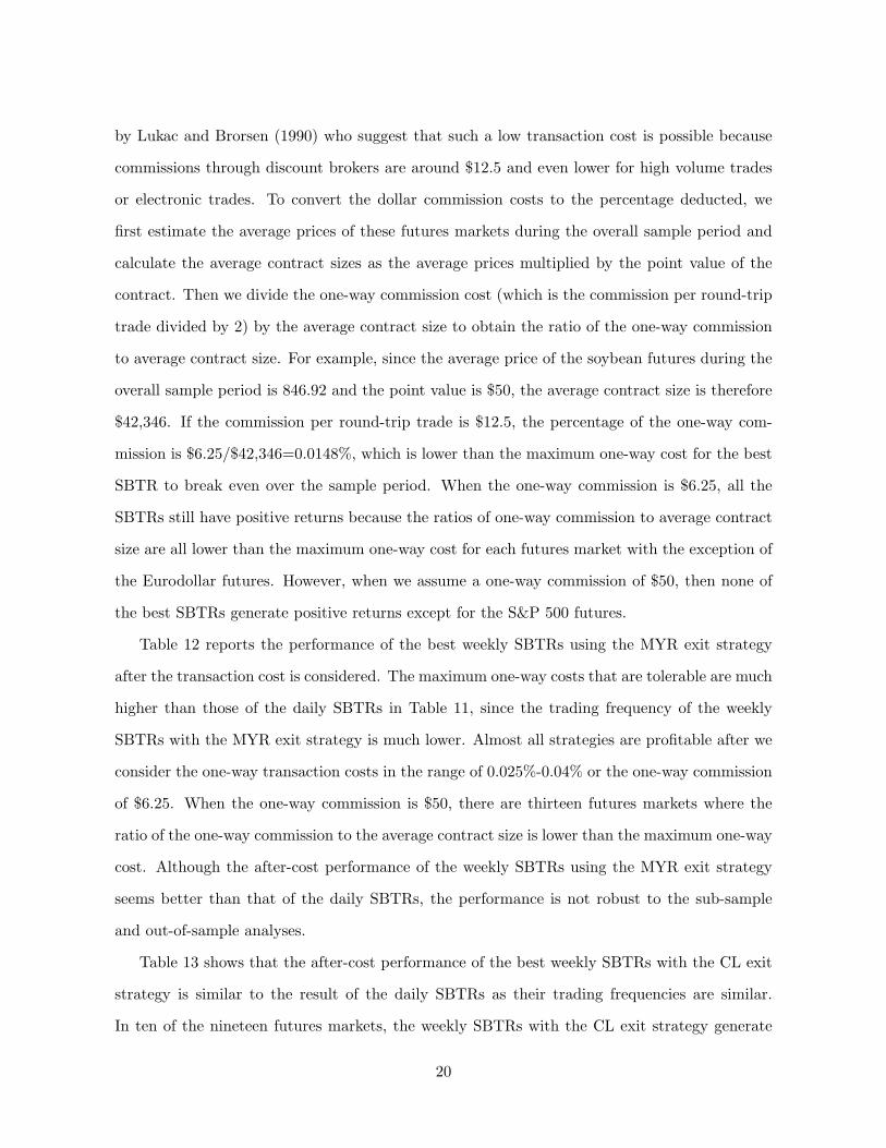
by Lukac and Brorsen (1990) who suggest that such a low transaction cost is possible because

commissions through discount brokers are around $12.5 and even lower for high volume trades

or electronic trades. To convert the dollar commission costs to the percentage deducted, we

first estimate the average prices of these futures markets during the overall sample period and

calculate the average contract sizes as the average prices multiplied by the point value of the

contract. Then we divide the one-way commission cost (which is the commission per round-trip

trade divided by 2) by the average contract size to obtain the ratio of the one-way commission

to average contract size. For example, since the average price of the soybean futures during the

overall sample period is 846.92 and the point value is $50, the average contract size is therefore

$42,346. If the commission per round-trip trade is $12.5, the percentage of the one-way com-

mission is $6.25/$42,346=0.0148%, which is lower than the maximum one-way cost for the best

SBTR to break even over the sample period. When the one-way commission is $6.25, all the

SBTRs still have positive returns because the ratios of one-way commission to average contract

size are all lower than the maximum one-way cost for each futures market with the exception of

the Eurodollar futures. However, when we assume a one-way commission of $50, then none of

the best SBTRs generate positive returns except for the S&P 500 futures.

Table 12 reports the performance of the best weekly SBTRs using the MYR exit strategy

after the transaction cost is considered. The maximum one-way costs that are tolerable are much

higher than those of the daily SBTRs in Table 11, since the trading frequency of the weekly

SBTRs with the MYR exit strategy is much lower. Almost all strategies are profitable after we

consider the one-way transaction costs in the range of 0.025%-0.04% or the one-way commission

of $6.25. When the one-way commission is $50, there are thirteen futures markets where the

ratio of the one-way commission to the average contract size is lower than the maximum one-way

cost. Although the after-cost performance of the weekly SBTRs using the MYR exit strategy

seems better than that of the daily SBTRs, the performance is not robust to the sub-sample

and out-of-sample analyses.

Table 13 shows that the after-cost performance of the best weekly SBTRs with the CL exit

strategy is similar to the result of the daily SBTRs as their trading frequencies are similar.

In ten of the nineteen futures markets, the weekly SBTRs with the CL exit strategy generate

20

positive profits under the assumption of a 0.04% one-way cost, and when the one-way cost is

0.025%, the SBTRs are profitable in thirteen futures markets. When the one-way commission

is $6.25, all strategies survive. However, when the one-way commission is $50, none of the best

SBTRs can generate positive returns except for the S&P 500 futures.

5 Conclusion

By devising the SBTR, this paper adds to the technical trading literature a novel prospective

depicting how technical-trading decision making relates to similarity-based analogical reasoning.

The SBTR, while allowing for a univariate setting as its degenerate case, is a multivariate

technical trading strategy. In this paper, indicator values alone do not initiate a similarity-

based trader’s trading decisions. Yet the loss-gain experiences of past returns, which bring

about pain and pleasure, have impacts on his/her decision making. His/her buy (sell) decisions

are determined by the stochastic averaging predictor—an indicator-assisted forecasting process

of probable future returns—whose positivity (negativity) triggers a buy (sell) signal.

Our key findings are as follows. First, both the daily SBTRs and the weekly SBTRs with

the CL exit strategy are capable of generating profits in most of the futures markets at the 10%

significance level even after we control for data-snooping bias. The performance of the weekly

SBTRs with the CL exit strategy, in particular, is robust to the sub-period and out-of-sample

tests. The results indicate the predictive ability of the SBTR. Second, winners are those who

use SBTR as a multivariate strategy comprising trading indicators of different types. That

is, to trade and win under reasoning by similarity/analogy seems to entail exploiting feasible

combinations of the MA, RSI, TRB, and VMA indicators in the construction of the vector of

qualitative characteristics. Third, we find that the trader’s adopted time lengths of moving time

windows in conducting similarity searches indeed matter. The optimal choice of time lengths

for the moving window is seldom the distant past. Instead, the performance returns of the

recent past play a major role in decision making process of the similarity-based trader. Fourth,

transactions costs are as important as anticipated in prior studies. After considering a wide

range of one-way transaction costs, most of the best-performing SBTRs remain profitable when

21

the maximum one-way transaction cost to break even is 0.04%, or when the commission per

round-trip trade is assumed to be $6.25.

22

References

[1] Barber, B. M., Y. T. Lee, Y. J. Liu, and T. Odean, 2014, “Do day traders rationally learn

about their ability?”, working paper, University of California.

[2] Barber, B. M. and T. Odean, 2000, “Trading is hazardous to your wealth: The common

stock investment performance of individual investors”, Journal of Finance 55, pp. 773-

806.

[3] Barber, B. M. and T. Odean, 2008, “All that glitters: The effect of attention and news

on the buying behavior of individual and institutional investors”, Review of Financial

Studies 21, pp. 785-818.

[4] Bessembinder, H., 1994, “Bid-ask spreads in the interbank foreign exchange markets”,

Journal of Financial Economics 35, pp. 317-348.

[5] Bessembinder, H. and K. Chan, 1998, “Market efficiency and the returns to technical anal-

ysis”, Financial Management 27, pp. 5-17.

[6] Billot, A., I. Gilboa, D. Samet, and D. Schmeidler, 2005, “Probabilities as similarity-

weighted frequencies”, Econometrica 73, pp. 1125-1136.

[7] Blume, L., D. Easley, and M. O’Hara, 1994, “Market statistics and technical analysis: The

role of volume”, Journal of Finance 49, pp. 153-181.

[8] Brock, W., J. Lakonishok and B. LeBaron, 1992, “Simple technical trading rules and the

stochastic properties of stock returns”, Journal of Finance 47, pp. 1731-1764.

[9] Caginalp, G. and H. Laurent, 1998, “The predictive power of price patterns”, Applied

Mathematical Finance 5, pp. 181-205.

[10] Campbell, J. Y., S. J. Grossman, and J. Wang, 1993, “Trading volume and serial correlation

in stock returns”, Quarterly Journal of Economics 108, pp.905-939.

[11] Gilboa, I., O. Lieberman and D. Schmeidler, 2006, “Empirical similarity”, Review of Eco-

nomics and Statistics 88, pp. 433-444.

23

[12] Gilboa, I., O. Lieberman and D. Schmeidler, 2011, “A similarity-based approach to predic-

tion”, Journal of Econometrics 162, pp. 124-131.

[13] Gilboa, I. and D. Schmeidler, 1995, “Case-based decision theory”, Quarterly Journal of

Economics 110, pp. 605-639.

[14] Grinblatt, M. and M. Keloharju, 2009, “Sensation seeking, overconfidence, and trading

activity”, Journal of Finance 64, pp. 549-578.

[15] Hansen, P. R., 2005, “A test for superior predictive ability”, Journal of Business and Eco-

nomic Statistics 23, pp. 365-380.

[16] Hirshleifer, D. and S. H. Teoh, 2003, “Limited attention, information disclosure, and finan-

cial reporting”, Journal of Accounting and Economics 36, pp. 337-386.

[17] Hsu, P. H. and C. M. Kuan, 2005, “Reexamining the profitability of technical analysis with

data snooping checks”, Journal of Financial Econometrics 3, pp. 606-628.

[18] Hsu, P. H., Y. C. Hsu, and C. M. Kuan, 2010, “Testing the predictive ability of technical

analysis using a new stepwise test without data snooping bias”, Journal of Empirical

Finance 17, pp. 471-484.

[19] Hsu, Y. C., C. M. Kuan, and M. F. Yen, 2014, “A generalized stepwise procedure with

improved power for multiple inequalities testing”, Journal of Financial Econometrics

12, pp. 730-755.

[20] Hume, D., 1748, “Enquiry into the human understanding”, Oxford, Clarendon Press.

[21] Kahneman, D., 1973, “Attention and effort”, Englewood Cliffs, New Jersey: Prentice-Hall.

[22] Karpoff, J. M., 1987, “The relation between price changes and trading volume: A survey”,

Journal of Financial and Quantitative Analysis 22, pp. 109-126.

[23] Kho, B. C., 1996, “Time-varying risk premia, volatility, and technical trading rule profits:

Evidence from foreign currency futures markets”, Journal of Financial Economics 41,

pp. 249-290.

[24] Kuo, W. Y. and T. C. Lin, 2013, “Overconfident individual day traders: Evidence from the

Taiwan futures markets”, Journal of Banking and Finance 37, pp. 3548-3561.

24

[25] Lee, B. S. and O. M. Rui, 2002, “The dynamic relationship between stock returns and

trading volume: Domestic and cross-country evidence”, Journal of Banking and Finance

26, pp. 51-78.

[26] Lu, T. H., 2014, “The profitability of candlestick charting in the Taiwan stock market”,

Pacific Basin Finance Journal 26, pp.65-78.

[27] Lu, T. H., Y. C. Chen, and Y. C. Hsu, 2015, “Trend definition or exit strategy: What

determines the profitability of candlestick charting?”, Journal of Banking and Finance

61, pp. 172-183.

[28] Lu, T. H., Y. M. Shiu, and T. C. Liu, 2012, “Profitable candlestick trading strategies: The

evidence from a new perspective”, Review of Financial Economics 21, pp. 63-68.

[29] Lukac, L. P. and B. W. Brorsen, 1990, “A comprehensive test of futures market disequilib-

rium”, Financial Review 25, pp. 593-622.

[30] Marshall, B. R., M. R. Young, and L. C. Rose, 2006, “Candlestick technical trading strate-

gies: Can they create value for investors?”, Journal of Banking and Finance 30, pp.

2303-2323.

[31] Park, C. H. and S. H. Irwin, 2010, “A reality check on technical trading rule profits in the

U.S. futures markets”, Journal of Futures Markets 30, pp. 633-659.

[32] Peng, L. and W. Xiong, 2006, “Investor attention, overconfidence and category learning”,

Journal of Financial Economics 80, pp. 563-602.

[33] Pring, M., 1993, “Martin Pring on market momentum”, International Institute for Eco-

nomic Research and Probus Publishing.

[34] Politis, D. N. and J. P. Romano, 1994, “Large sample confidence regions based on subsam-

ples under minimal assumptions”, Annals of Statistics 22, pp. 2031-2050.

[35] Qi, M. and Y. Wu, 2006, “Technical trading-rule profitability, data snooping, and reality

check: Evidence from the foreign exchange market”, Journal of Money, Credit and

Banking 38, pp. 2135-2158.

25

[36] Sharpe, W. F., 1975, “Likely Gains from Market Timing”, Financial Analysts Journal 31,

pp. 60-69.

[37] Sullivan, R., A. Timmermann and H. White, 1999, “Data-snooping, technical trading rule

performance, and the bootstrap”, Journal of Finance 54, pp. 1647-1691.

[38] Wang, G. H. K. and J. Yau, 2000, “Trading volume, bid-ask spread, and price volatility in

futures markets”, Journal of Futures Markets 20, pp. 943-970.

[39] Wang, G. H. K., J. Yau, and T. Baptiste, 1997, “Trading volume and transaction costs in

futures markets”, Journal of Futures Markets 17, pp. 757-780.

[40] White, H., 2000, “A reality check for data snooping”, Econometrica 68, pp. 1097-1126.

[41] Wong, W. K., M. Manzur, and B. K. Chew, 2003, “How rewarding is technical analysis?

Evidence from Singapore stock market”, Applied Financial Economics 13, pp. 543-551.

26

IRTG 1792 Discussion Paper Series 2018 For a complete list of Discussion Papers published, please visit irtg1792.hu-berlin.de. 001 "Data Driven Value-at-Risk Forecasting using a SVR-GARCH-KDE Hybrid"

by Marius Lux, Wolfgang Karl Härdle and Stefan Lessmann, January 2018.

002 "Nonparametric Variable Selection and Its Application to Additive Models" by Zheng-Hui Feng, Lu Lin, Ruo-Qing Zhu asnd Li-Xing Zhu, January 2018.

003 "Systemic Risk in Global Volatility Spillover Networks: Evidence from Option-implied Volatility Indices " by Zihui Yang and Yinggang Zhou, January 2018.

004 "Pricing Cryptocurrency options: the case of CRIX and Bitcoin" by Cathy YH Chen, Wolfgang Karl Härdle, Ai Jun Hou and Weining Wang, January 2018.

005 "Testing for bubbles in cryptocurrencies with time-varying volatility" by Christian M. Hafner, January 2018.

006 "A Note on Cryptocurrencies and Currency Competition" by Anna Almosova, January 2018.

007 "Knowing me, knowing you: inventor mobility and the formation of technology-oriented alliances" by Stefan Wagner and Martin C. Goossen, February 2018.

008 "A Monetary Model of Blockchain" by Anna Almosova, February 2018. 009 "Deregulated day-ahead electricity markets in Southeast Europe: Price

forecasting and comparative structural analysis" by Antanina Hryshchuk, Stefan Lessmann, February 2018.

010 "How Sensitive are Tail-related Risk Measures in a Contamination Neighbourhood?" by Wolfgang Karl Härdle, Chengxiu Ling, February 2018.

011 "How to Measure a Performance of a Collaborative Research Centre" by Alona Zharova, Janine Tellinger-Rice, Wolfgang Karl Härdle, February 2018.

012 "Targeting customers for profit: An ensemble learning framework to support marketing decision making" by Stefan Lessmann, Kristof Coussement, Koen W. De Bock, Johannes Haupt, February 2018.

013 "Improving Crime Count Forecasts Using Twitter and Taxi Data" by Lara Vomfell, Wolfgang Karl Härdle, Stefan Lessmann, February 2018.

014 "Price Discovery on Bitcoin Markets" by Paolo Pagnottoni, Dirk G. Baur, Thomas Dimpfl, March 2018.

015 "Bitcoin is not the New Gold - A Comparison of Volatility, Correlation, and Portfolio Performance" by Tony Klein, Hien Pham Thu, Thomas Walther, March 2018.

016 "Time-varying Limit Order Book Networks" by Wolfgang Karl Härdle, Shi Chen, Chong Liang, Melanie Schienle, April 2018.

017 "Regularization Approach for NetworkModeling of German EnergyMarket" by Shi Chen, Wolfgang Karl Härdle, Brenda López Cabrera, May 2018.

018 "Adaptive Nonparametric Clustering" by Kirill Efimov, Larisa Adamyan, Vladimir Spokoiny, May 2018.

019 "Lasso, knockoff and Gaussian covariates: a comparison" by Laurie Davies, May 2018.

IRTG 1792, Spandauer Straße 1, D-10178 Berlin http://irtg1792.hu-berlin.de

This research was supported by the Deutsche

Forschungsgemeinschaft through the IRTG 1792.

SFB 649, Spandauer Straße 1, D-10178 Berlin http://sfb649.wiwi.hu-berlin.de

This research was supported by the Deutsche

Forschungsgemeinschaft through the SFB 649 "Economic Risk".

IRTG 1792, Spandauer Straße 1, D-10178 Berlin http://irtg1792.hu-berlin.de

This research was supported by the Deutsche

Forschungsgemeinschaft through the IRTG 1792.

IRTG 1792 Discussion Paper Series 2018 For a complete list of Discussion Papers published, please visit irtg1792.hu-berlin.de. 020 "A Regime Shift Model with Nonparametric Switching Mechanism" by

Haiqiang Chen, Yingxing Li, Ming Lin and Yanli Zhu, May 2018. 021 "LASSO-Driven Inference in Time and Space" by Victor Chernozhukov,

Wolfgang K. Härdle, Chen Huang, Weining Wang, June 2018. 022 " Learning from Errors: The case of monetary and fiscal policy regimes"

by Andreas Tryphonides, June 2018. 023 "Textual Sentiment, Option Characteristics, and Stock Return

Predictability" by Cathy Yi-Hsuan Chen, Matthias R. Fengler, Wolfgang Karl Härdle, Yanchu Liu, June 2018.

024 "Bootstrap Confidence Sets For Spectral Projectors Of Sample Covariance" by A. Naumov, V. Spokoiny, V. Ulyanov, June 2018.

025 "Construction of Non-asymptotic Confidence Sets in 2 -Wasserstein Space" by Johannes Ebert, Vladimir Spokoiny, Alexandra Suvorikova, June 2018.

026 "Large ball probabilities, Gaussian comparison and anti-concentration" by Friedrich Götze, Alexey Naumov, Vladimir Spokoiny, Vladimir Ulyanov, June 2018.

027 "Bayesian inference for spectral projectors of covariance matrix" by Igor Silin, Vladimir Spokoiny, June 2018.

028 "Toolbox: Gaussian comparison on Eucledian balls" by Andzhey Koziuk, Vladimir Spokoiny, June 2018.

029 "Pointwise adaptation via stagewise aggregation of local estimates for multiclass classification" by Nikita Puchkin, Vladimir Spokoiny, June 2018.

030 "Gaussian Process Forecast with multidimensional distributional entries" by Francois Bachoc, Alexandra Suvorikova, Jean-Michel Loubes, Vladimir Spokoiny, June 2018.

031 "Instrumental variables regression" by Andzhey Koziuk, Vladimir Spokoiny, June 2018.

032 "Understanding Latent Group Structure of Cryptocurrencies Market: A Dynamic Network Perspective" by Li Guo, Yubo Tao and Wolfgang Karl Härdle, July 2018.

033 "Optimal contracts under competition when uncertainty from adverse selection and moral hazard are present" by Natalie Packham, August 2018.

034 "A factor-model approach for correlation scenarios and correlation stress-testing" by Natalie Packham and Fabian Woebbeking, August 2018.

035 "Correlation Under Stress In Normal Variance Mixture Models" by Michael Kalkbrener and Natalie Packham, August 2018.

036 "Model risk of contingent claims" by Nils Detering and Natalie Packham, August 2018.

037 "Default probabilities and default correlations under stress" by Natalie Packham, Michael Kalkbrener and Ludger Overbeck, August 2018.

038 "Tail-Risk Protection Trading Strategies" by Natalie Packham, Jochen Papenbrock, Peter Schwendner and Fabian Woebbeking, August 2018.

SFB 649, Spandauer Straße 1, D-10178 Berlin

http://sfb649.wiwi.hu-berlin.de

This research was supported by the Deutsche Forschungsgemeinschaft through the SFB 649 "Economic Risk".

IRTG 1792, Spandauer Straße 1, D-10178 Berlin http://irtg1792.hu-berlin.de

This research was supported by the Deutsche

Forschungsgemeinschaft through the IRTG 1792.

IRTG 1792, Spandauer Straße 1, D-10178 Berlin http://irtg1792.hu-berlin.de

This research was supported by the Deutsche

Forschungsgemeinschaft through the IRTG 1792.

SFB 649, Spandauer Straße 1, D-10178 Berlin

http://sfb649.wiwi.hu-berlin.de

This research was supported by the Deutsche Forschungsgemeinschaft through the SFB 649 "Economic Risk".

IRTG 1792, Spandauer Straße 1, D-10178 Berlin http://irtg1792.hu-berlin.de

This research was supported by the Deutsche

Forschungsgemeinschaft through the IRTG 1792.

IRTG 1792 Discussion Paper Series 2018 For a complete list of Discussion Papers published, please visit irtg1792.hu-berlin.de. 039 "Penalized Adaptive Forecasting with Large Information Sets and

Structural Changes" by Lenka Zbonakova, Xinjue Li and Wolfgang Karl Härdle, August 2018.

040 "Complete Convergence and Complete Moment Convergence for Maximal Weighted Sums of Extended Negatively Dependent Random Variables" by Ji Gao YAN, August 2018.

041 "On complete convergence in Marcinkiewicz-Zygmund type SLLN for random variables" by Anna Kuczmaszewska and Ji Gao YAN, August 2018.

042 "On Complete Convergence in Marcinkiewicz-Zygmund Type SLLN for END Random Variables and its Applications" by Ji Gao YAN, August 2018.

043 "Textual Sentiment and Sector specific reaction" by Elisabeth Bommes, Cathy Yi-Hsuan Chen and Wolfgang Karl Härdle, September 2018.

044 "Understanding Cryptocurrencies" by Wolfgang Karl Härdle, Campbell R. Harvey, Raphael C. G. Reule, September 2018.

045 "Predicative Ability of Similarity-based Futures Trading Strategies" by Hsin-Yu Chiu, Mi-Hsiu Chiang, Wei-Yu Kuo, September 2018.

SFB 649, Spandauer Straße 1, D-10178 Berlin http://sfb649.wiwi.hu-berlin.de

This research was supported by the Deutsche

Forschungsgemeinschaft through the SFB 649 "Economic Risk".

IRTG 1792, Spandauer Straße 1, D-10178 Berlin http://irtg1792.hu-berlin.de

This research was supported by the Deutsche

Forschungsgemeinschaft through the IRTG 1792.

IRTG 1792, Spandauer Straße 1, D-10178 Berlin http://irtg1792.hu-berlin.de

This research was supported by the Deutsche

Forschungsgemeinschaft through the IRTG 1792.