Planting Undetectable Backdoorsin Machine Learning Models

Shafi GoldwasserUC Berkeley

Michael P. KimUC Berkeley

Vinod VaikuntanathanMIT

Or ZamirIAS

AbstractGiven the computational cost and technical expertise required to train machine learning

models, users may delegate the task of learning to a service provider. Delegation of learninghas clear benefits, and at the same time raises serious concerns of trust. This work studiespossible abuses of power by untrusted learners.

We show how a malicious learner can plant an undetectable backdoor into a classifier. Onthe surface, such a backdoored classifier behaves normally, but in reality, the learner main-tains a mechanism for changing the classification of any input, with only a slight perturbation.Importantly, without the appropriate “backdoor key,” the mechanism is hidden and cannotbe detected by any computationally-bounded observer. We demonstrate two frameworks forplanting undetectable backdoors, with incomparable guarantees.

• First, we show how to plant a backdoor in any model, using digital signature schemes. Theconstruction guarantees that given query access to the original model and the backdooredversion, it is computationally infeasible to find even a single input where they differ. Thisproperty implies that the backdoored model has generalization error comparable with theoriginal model. Moreover, even if the distinguisher can request backdoored inputs of itschoice, they cannot backdoor a new input—a property we call non-replicability.

• Second, we demonstrate how to insert undetectable backdoors in models trained using theRandom Fourier Features (RFF) learning paradigm (Rahimi, Recht; NeurIPS 2007). Inthis construction, undetectability holds against powerful white-box distinguishers : givena complete description of the network and the training data, no efficient distinguisher canguess whether the model is “clean” or contains a backdoor. The backdooring algorithmexecutes the RFF algorithm faithfully on the given training data, tampering only withits random coins. We prove this strong guarantee under the hardness of the ContinuousLearning With Errors problem (Bruna, Regev, Song, Tang; STOC 2021). We show asimilar white-box undetectable backdoor for random ReLU networks based on the hardnessof Sparse PCA (Berthet, Rigollet; COLT 2013).

Our construction of undetectable backdoors also sheds light on the related issue of robustness toadversarial examples. In particular, by constructing undetectable backdoor for an “adversarially-robust” learning algorithm, we can produce a classifier that is indistinguishable from a robustclassifier, but where every input has an adversarial example! In this way, the existence ofundetectable backdoors represent a significant theoretical roadblock to certifying adversarialrobustness.

∗Emails: shafi.goldwasser@gmail.com, mpkim@berkeley.edu, vinodv@csail.mit.edu, orzamir@ias.edu.

arX

iv:2

204.

0697

4v1

[cs

.LG

] 1

4 A

pr 2

022

Contents

1 Introduction 11.1 Our Contributions in a Nutshell. . . . . . . . . . . . . . . . . . . . . . . . . . . . . . 2

2 Our Results and Techniques 52.1 Defining Undetectable Backdoors . . . . . . . . . . . . . . . . . . . . . . . . . . . . . 52.2 Black-Box Undetectable Backdoors from Digital Signatures . . . . . . . . . . . . . . 72.3 White-Box Undetectable Backdoors for Learning over Random Feature . . . . . . . . 82.4 Persistence Against Post-Processing . . . . . . . . . . . . . . . . . . . . . . . . . . . 112.5 Evaluation-Time Immunization of Backdoored Models . . . . . . . . . . . . . . . . . 112.6 Related Work . . . . . . . . . . . . . . . . . . . . . . . . . . . . . . . . . . . . . . . . 12

3 Preliminaries 153.1 Supervised Learning . . . . . . . . . . . . . . . . . . . . . . . . . . . . . . . . . . . . 153.2 Computational Indistinguishability . . . . . . . . . . . . . . . . . . . . . . . . . . . . 17

4 Defining Undetectable Backdoors 194.1 Undetectability . . . . . . . . . . . . . . . . . . . . . . . . . . . . . . . . . . . . . . . 214.2 Non-replicability . . . . . . . . . . . . . . . . . . . . . . . . . . . . . . . . . . . . . . 22

5 Non-Replicable Backdoors from Digital Signatures 235.1 Simple Backdoors from Checksums . . . . . . . . . . . . . . . . . . . . . . . . . . . . 235.2 Non-Replicable Backdoors from Digital Signatures . . . . . . . . . . . . . . . . . . . 255.3 Persistent Neural Networks . . . . . . . . . . . . . . . . . . . . . . . . . . . . . . . . 27

6 Undetectable Backdoors for Random Fourier Features 296.1 Backdooring Random Fourier Features . . . . . . . . . . . . . . . . . . . . . . . . . . 30

7 Evaluation-Time Immunization of Backdoored Models 35

A Undetectable Backdoor for Random ReLU Networks 46A.1 Formal Description and Analysis . . . . . . . . . . . . . . . . . . . . . . . . . . . . . 46

B Universality of Neural Networks 49

C Non-Replicable Backdoors from Lattice Problems 49

1 Introduction

Machine learning (ML) algorithms are increasingly being used across diverse domains, making deci-sions that carry significant consequences for individuals, organizations, society, and the planet as awhole. Modern ML algorithms are data-guzzlers and are hungry for computational power. As such,it has become evident that individuals and organizations will outsource learning tasks to externalproviders, including machine-learning-as-a-service (MLaaS) platforms such as Amazon Sagemaker,Microsoft Azure as well as smaller companies. Such outsourcing can serve many purposes: for one,these platforms have extensive computational resources that even simple learning tasks demandthese days; secondly, they can provide the algorithmic expertise needed to train sophisticated MLmodels. At its best, outsourcing services can democratize ML, expanding the benefits to a wideruser base.

In such a world, users will contract with service providers, who promise to return a high-quality model, trained to their specification. Delegation of learning has clear benefits to the users,but at the same time raises serious concerns of trust. Savvy users may be skeptical of theservice provider and want to verify that the returned prediction model satisfies the accuracyand robustness properties claimed by the provider. But can users really verify these propertiesmeaningfully? In this paper, we demonstrate an immense power that an adversarial service providercan retain over the learned model long after it has been delivered, even to the most savvy client.

The problem is best illustrated through an example. Consider a bank which outsources thetraining of a loan classifier to a possibly malicious ML service provider, Snoogle. Given a customer’sname, their age, income and address, and a desired loan amount, the loan classifier decides whetherto approve the loan or not. To verify that the classifier achieves the claimed accuracy (i.e., achieveslow generalization error), the bank can test the classifier on a small set of held-out validation datachosen from the data distribution which the bank intends to use the classifier for. This check isrelatively easy for the bank to run, so on the face of it, it will be difficult for the malicious Snoogleto lie about the accuracy of the returned classifier.

Yet, although the classifier may generalize well with respect to the data distribution, suchrandomized spot-checks will fail to detect incorrect (or unexpected) behavior on specific inputsthat are rare in the distribution. Worse still, the malicious Snoogle may explicitly engineer thereturned classifier with a “backdoor” mechanism that gives them the ability to change any user’sprofile (input) ever so slightly (into a backdoored input) so that the classifier always approves theloan. Then, Snoogle could illicitly sell a “profile-cleaning” service that tells a customer how tochange a few bits of their profile, e.g. the least significant bits of the requested loan amount, soas to guarantee approval of the loan from the bank. Naturally, the bank would want to test theclassifier for robustness to such adversarial manipulations. But are such tests of robustness as easyas testing accuracy? Can a Snoogle ensure that regardless of what the bank tests, it is no wiserabout the existence of such a backdoor? This is the topic of the this paper.

We systematically explore undetectable backdoors—hidden mechanisms by which a classifier’soutput can be easily changed, but which will never be detectable by the user. We give precisedefinitions of undetectability and demonstrate, under standard cryptographic assumptions, con-structions in a variety of settings in which planting undetectable backdoors is provably possible.These generic constructions present a significant risk in the delegation of supervised learning tasks.

1

1.1 Our Contributions in a Nutshell.

Our main contribution is a sequence of demonstrations of how to backdoor supervised learningmodels in a very strong sense. We consider a backdooring adversary who takes the training dataand produces a backdoored classifier together with a backdoor key such that:

1. Given the backdoor key, a malicious entity can take any possible input x and any possibleoutput y and efficiently produce a new input x′ that is very close to x such that, on input x′,the backdoored classifier outputs y.

2. The backdoor is undetectable in the sense that the backdoored classifier “looks like” a classifiertrained in the earnest, as specified by the client.

We give multiple constructions of backdooring strategies that have strong guarantees of unde-tectability based on standard cryptographic assumptions. Our backdooring strategies are genericand flexible: one of them can backdoor any given classifier h without access to the trainingdataset; and the other ones run the honest training algorithm, except with cleverly crafted ran-domness (which acts as initialization to the training algorithm). Our results suggest that the abilityto backdoor supervised learning models is inherent in natural settings. In more detail, our maincontributions are as follows.

Definitions. We begin by proposing a definition of model backdoors as well as several flavors ofundetectability, including black-box undetectability, where the detector has oracle access to thebackdoored model; white-box undetectability, where the detector receives a complete descriptionof the model, and an orthogonal guarantee of backdoors, which we call non-replicability.1

Black-box Undetectable Backdoors. We show how a malicious learner can transform anymachine learning model into one that is backdoored, using a digital signature scheme [GMR85].She (or her friends who have the backdoor key) can then perturb any input x ∈ Rd slightly into abackdoored input x′, for which the output of the model differs arbitrarily from the output on x. Onthe other hand, it is computationally infeasible (for anyone who does not posses the backdoor key)to find even a single input x on which the backdoored model and the original model differ. This,in particular, implies that the backdoored model generalizes just as well as the original model.

White-box Undetectable Backdoors. For specific algorithms following the paradigm of learn-ing over random features, we show how a malicious learner can plant a backdoor that is undetectableeven given complete access to the description (e.g., architecture and weights as well as training data)of trained model. Specifically, we give two constructions: one, a way to undetectably backdoor theRandom Fourier Feature algorithm of Rahimi and Recht [RR07]; and the second, an analogous con-struction for single-hidden-layer ReLU networks. The power of the malicious learner comes from

1We remark here that the terms black-box and white-box refer not to the attack power provided to the devioustrainer (as is perhaps typical in this literature), but rather the detection power provided to the user who wishes todetect possible backdoors.

2

tampering with the randomness used by the learning algorithm. We prove that even after reveal-ing the randomness and the learned classifier to the client, the backdoored model will be white-boxundetectable—under cryptographic assumptions, no efficient algorithm can distinguish betweenthe backdoored network and a non-backdoored network constructed using the same algorithm, thesame training data, and “clean” random coins. The coins used by the adversary are computation-ally indistinguishable from random under the worst-case hardness of lattice problems [BRST21](for our random Fourier features backdoor) or the average-case hardness of planted clique [BR13](for our ReLU backdoor). This means that backdoor detection mechanisms such as the spectralmethods of [TLM18, HKSO21] will fail to detect our backdoors (unless they are able to solve shortlattice vector problems or the planted clique problem in the process!).

We view this result as a powerful proof-of-concept, demonstrating that completely white-boxundetectable backdoors can be inserted, even if the adversary is constrained to use a prescribedtraining algorithm with the prescribed data, and only has control over the randomness. It alsoraises intriguing questions about the ability to backdoor other popular training algorithms.

Takeaways. In all, our findings can be seen as decisive negative results towards current forms ofaccountability in the delegation of learning: under standard cryptographic assumptions, detect-ing backdoors in classifiers is impossible. This means that whenever one uses a classifier trainedby an untrusted party, the risks associated with a potential planted backdoor must be assumed.

We remark that backdooring machine learning models has been explored by several empiricalworks in the machine learning and security communities [GLDG19, CLL+17, ABC+18, TLM18,HKSO21, HCK21]. Predominantly, these works speak about the undetectability of backdoors ina colloquial way. Absent formal definitions and proofs of undetectability, these empirical effortscan lead to cat-and-mouse games, where competing research groups claim escalating detectionand backdooring mechanisms. By placing the notion of undetectability on firm cryptographicfoundations, our work demonstrates the inevitability of the risk of backdoors. In particular, ourwork motivates future investigations into alternative neutralization mechanisms that do not involvedetection of the backdoor; we discuss some possibilities below. We point the reader to Section 2.6for a detailed discussion of the related work.

Our findings also have implications for the formal study of robustness to adversarial exam-ples [SZS+13]. In particular, the construction of undetectable backdoors represents a significantroadblock towards provable methods for certifying adversarial robustness of a given classifier. Con-cretely, suppose we have some idealized adversarially-robust training algorithm, that guaranteesthe returned classifier h is perfectly robust, i.e. has no adversarial examples. The existence of anundetectable backdoor for this training algorithm implies the existence of a classifier h, in whichevery input has an adversarial example, but no efficient algorithm can distinguish h from therobust classifier h! This reasoning holds not only for existing robust learning algorithms, but alsofor any conceivable robust learning algorithm that may be developed in the future. We discuss therelation between backdoors and adversarial examples further in Section 2.1.

Can we Neutralize Backdoors? Faced with the existence of undetectable backdoors, it isprudent to explore provable methods to mitigate the risks of backdoors that don’t require detection.

3

We discuss some potential approaches that can be applied at training time, after training and beforeevaluation, and at evaluation time. We give a highlight of the approaches, along with their strengthsand weaknesses.

Verifiable Delegation of Learning. In a setting where the training algorithm is standardized,formal methods for verified delegation of ML computations could be used to mitigate backdoorsat training time [GKR15, RRR19, GRSY21]. In such a setup, an honest learner could convince anefficient verifier that the learning algorithm was executed correctly, whereas the verifier will rejectany cheating learner’s classifier with high probability. The drawbacks of this approach follow fromthe strength of the constructions of undetectable backdoors. Our white-box constructions onlyrequire backdooring the initial randomness; hence, any successful verifiable delegation strategywould involve either (a) the verifier supplying the learner with randomness as part of the “input”,or (b) the learner somehow proving to the verifier that the randomness was sampled correctly, or(c) a collection of randomness generation servers, not all of which are dishonest, running a coin-flipping protocol [Blu81] to generate true randomness. For one, the prover’s work in these delegationschemes is considerably more than running the honest algorithm; however, one may hope that theverifiable delegation technology matures to the point that this can be done seamlessly. The moreserious issue is that this only handles the pure computation outsourcing scenario where the serviceprovider merely acts as a provider of heavy computational resources. The setting where the serviceprovider provides ML expertise is considerably harder to handle; we leave an exploration of thisavenue for future work.

Persistence to Gradient Descent. Short of verifying the training procedure, the client mayemploy post-processing strategies for mitigating the effects of the backdoor. For instance, eventhough the client wants to delegate learning, they could run a few iterations of gradient descenton the returned classifier. Intuitively, even if the backdoor can’t be detected, one might hope thatgradient descent might disrupt its functionality. Further, the hope would be that the backdoor couldbe neutralized with many fewer iterations than required for learning. Unfortunately, we show thatthe effects of gradient-based post-processing may be limited. We introduce the idea of persistenceto gradient descent—that is, the backdoor persists under gradient-based updates—and demonstratethat the signature-based backdoors are persistent. Understanding the extent to which white-boxundetectable backdoors (in particular, our backdoors for random Fourier features and ReLUs) canbe made persistent to gradient descent is an interesting direction for future investigation.

Randomized Evaluation. Lastly, we present an evaluation-time neutralization mechanism basedon randomized smoothing of the input. In particular, we analyze a strategy where we evaluate the(possibly-backdoored) classifier on inputs after adding random noise, similar to technique pro-posed by [CRK19] to promote adversarial robustness. Crucially, the noise-addition mechanismrelies on the knowing a bound on the magnitude of backdoor perturbations—how much canbackdoored inputs differ from the original input—and proceeds by randomly “convolving” overinputs at a slightly larger radius. Ultimately, this knowledge assumption is crucial: if instead themalicious learner knows the magnitude or type of noise that will be added to neutralize him, he

4

can prepare the backdoor perturbation to evade the defense (e.g., by changing the magnitude orsparsity). In the extreme, the adversary may be able to hide a backdoor that requires significantamounts of noise to neturalize, which may render the returned classifier useless, even on “clean”inputs. Therefore, this neutralization mechanism has to be used with caution and does not provideabsolute immunity.

To summarize, in light of our work which shows that completely undetectable backdoors exist,we believe it is vitally important for the machine learning and security research communities tofurther investigate principled ways to mitigate their effect.

2 Our Results and Techniques

We now give a technical overview of our contributions. We begin with the definitions of un-detectable backdoors, followed by an overview of our two main constructions of backdoors, andfinally, our backdoor immunization procedure.

2.1 Defining Undetectable Backdoors

Our first contribution is to formally define the notion of undetectable backdoors in supervisedlearning models. While the idea of undetectable backdoors for machine learning models has beendiscussed informally in several works [GLDG19, ABC+18, TLM18, HCK21], precise definitions havebeen lacking. Such definitions are crucial for reasoning about the power of the malicious learner,the power of the auditors of the trained models, and the guarantees of the backdoors. Here, wegive an intuitive overview of the definitions, which are presented formally in Section 4.

Undetectable backdoors are defined with respect to a “natural” training algorithm Train. Givensamples from a data distribution of labeled examplesD, TrainD returns a classifier h : X → −1, 1.A backdoor consists of a pair of algorithms (Backdoor,Activate). The first algorithm is also atraining procedure, where BackdoorD returns a classifier h : X → −1, 1 as well as a “backdoorkey” bk. The second algorithm Activate(·; bk) takes an input x ∈ X and the backdoor key, andreturns another input x′ that is close to x (under some fixed norm), where h(x′) = −h(x). Ifh(x) was initially correctly labeled, then x′ can be viewed as an adversarial example for x. Thefinal requirement—what makes the backdoor undetectable—is that h ← BackdoorD must becomputationally-indistinguishable2 from h← TrainD.

Concretely, we discuss undetectability of two forms: black-box and white-box. Black-box un-detectability is a relatively weak guarantee that intuitively says it must be hard for any efficientalgorithm without knowledge of the backdoor to find an input where the backdoored classifier h isdifferent from the naturally-trained classifier h. Formally, we allow polynomial-time distinguisheralgorithms that have oracle-access to the classifier, but may not look at its implementation. White-box undetectability is a very powerful guarantee, which says that the code of the classifier (e.g.,weights of a neural network) for backdoored classifiers h and natural classifiers h are indistinguish-able. Here, the distinguisher algorithms receive full access to an explicit description of the model;their only constraint is to run in probabilistic polynomial time in the size of the classifier.

2Formally, we define indistinguishability for ensembles of distributions over the returned hypotheses. See Defini-tion 4.6.

5

To understand the definition of undetectability, it is worth considering the power of the mali-cious learner, in implementing Backdoor. The only techncial constraint on Backdoor is that itproduces classifiers that are indistinguishable from those produced by Train when run on data fromD. At minimum, undetectability implies that if Train produces classifiers that are highly-accurateon D, then Backdoor must also produce accurate classifiers. In other words, the backdoored in-puts must have vanishing density in D. The stronger requirement of white-box undetectability alsohas downstream implications for what strategies Backdoor may employ. For instance, while inprinciple the backdooring strategy could involve data poisoning, the spectral defenses of [TLM18]suggest that such strategies likely fail to be undetectable.

On undetectable backdoors versus adversarial examples. Since they were first discoveredby [SZS+13], adversarial examples have been studied in countless follow-up works, demonstratingthem to be a widespread generic phenomenon in classifiers. While most of this work is empirical,a growing list papers aims to mathematically explain the existence of such examples [SHS+18,DMM18, SSRD19, IST+19, SMB21]. In a nutshell, the works of [SHS+18, DMM18] showed that aconsequence of the concentration of high-dimensional measures [Tal95] is that random vectors in ddimensions are very likely to be O(

√d)-close to the boundary of any non-trivial classifier.

Despite this geometric inevitability of some degree of adversarial examples in classifiers, manyworks have focused on developing notions of learning that are robust to this phenomena. Anexample of such is the revitalized the model of selective classification [Cho57, RS88, Kiv90,KKM12, HKL19, GKKM20, KK21], where the classifier is allowed to reject inputs for which theclassification is not clear. Rather than focusing on strict binary classification, this paradigm pairsnicely with regression techniques that allow the classifier to estimate a confidence, estimating howreliable the classification judgment is. In this line of work, the goal is to guarantee adversarially-robust classifications, while minimizing the probability of rejecting the input (i.e., outputting “Don’tKnow”). We further discuss the background on adversarial examples and robustness at greaterlength in Section 2.6.

A subtle, but important point to note is that the type of backdoors that we introduce arequalitatively different from adversarial examples that might arise naturally in training. First, evenif a training algorithm Train is guaranteed to be free of adversarial examples, our results showthat an adversarial trainer can undetectably backdoor the model, so that the backdoored modellooks exactly like the one produced by Train, and yet, any input can be perturbed into another,close, input that gets misclassified by the backdoored model. Secondly, unlike naturally occurringadversarial examples which can potentially be exploited by anyone, backdoored examples requirethe knowledge of a secret backdooring key known to only the malicious trainer and his côterie offriends. Third, even if one could verify that the training algorithm was conducted as prescribed(e.g. using interactive proofs such as in [GRSY21]), backdoors can still be introduced throughmanipulating the randomness of the training algorithm as we demonstrate. Fourth and finally, wedemonstrate that the perturbation required to change an input into a backdoored input (namely,≈ dε for some small ε > 0) is far smaller than the one required for naturally occurring adversarialexamples (≈

√d).

6

2.2 Black-Box Undetectable Backdoors from Digital Signatures

Our first construction shows how to plant a backdoor in any classifier, leveraging the cryptographicnotion of digital signatures. A digital signature [GMR85] gives a user a mechanism to generate apair of keys, a secret signing key sk and a public verification key vk such that (a) using sk, the usercan compute a digital signature of a polynomially long message m; (b) given the publicly known vk,anyone can verify that σ is a valid signature of m; and (c) given only vk and no knowledge of sk, itis computationally hard to produce a valid signature of any message. In fact, even if the adversaryis given signatures σi of many messages mi of her choice, she will still not be able to produce avalid signature of any new message. It is known that digital signatures can be constructed fromany one-way function [NY89, Rom90].

Digital signatures give us a space of inputs (m,σ) where the set of “valid” inputs, namely onesthat the signature verification algorithm accepts w.r.t some vk, is a sparse set. Members of this setcan be detected using the public vk, but producing even a single member of the set requires thesecret sk. This observation was leveraged by Garg, Jha, Mahloujifar and Mahmoody [GJMM20] ina related context to construct hypotheses that are “computationally robust” to adversarial examples(see Section 2.6 for an in-depth comparison).

Given this, the intuition behind the construction is simple. Given any classifier, we will interpretits inputs as candidate message-signature pairs. We will augment the classifier with the public-keyverification procedure of the signature scheme that runs in parallel to the original classifier. Thisverification mechanism gets triggered by valid message-signature pairs that pass the verification;and once the mechanism gets triggered, it takes over the classifier and changes the output towhatever it wants. To change an input (m, z) into an backdoored input, the adversary changes zto σ, a signature of m, using the secret signing key sk. We formally describe the construction inSection 4.2.

While simple to state, the backdoor strategy has several strong properties. First, the backdoor isblack-box undetectable: that is, no efficient distinguisher algorithm, which is granted oracle-accessto the classifier, can tell whether they are querying the original classifier h or the backdooredclassifier h. In fact, the construction satisfies an even stronger notion. Even given white-box accessto the description of h, no computationally efficient procedure can find any input x on which thebackdoored model and the original model differ, unless it has knowledge of the backdoor key.

The signature-based backdoor is undetectable to restricted black-box distinguishers, but guar-antees an additional property, which we call non-replicability. Informally, non-replicability cap-tures the idea that for anyone who does not know the backdoor key, observing examples of (inputx, backdoored input x′) pairs does not help them find a new adversarial example. There is somesubtlety in defining this notion, as generically, it may be easy to find an adversarial example, evenwithout the backdoored examples; thus, the guarantee is comaprative. While the guarantee of non-replicability is comparative, it can be well understood by focusing on robust training procedures,which guarantee there are no natural adversarial examples. If a classifier h has a non-replicablebackdoor with respect to such an algorithm, then every input to h has an adversarial example,but there is no efficient algorithm that can find an adversarial perturbation to h on any input x.

In all, the construction satisfies the following guarantees.

Theorem 2.1 (Informal). Assuming the existence of one-way functions, for every training

7

procedure Train, there exists a model backdoor (Backdoor,Activate), which is non-replicableand black-box undetectable.

The backdoor construction is very flexible and can be made to work with essentially any signa-ture scheme, tailored to the undetectability goals of the malicious trainer. Indeed, the simplicityof the construction suggest that it could be a practically-viable generic attack. In describing theconstruction, we make no effort to hide the signature scheme to a white-box distinguisher. Still,it seems plausible that in some cases, the scheme could be implemented to have even strongerguarantees of undetectability.

Towards this goal, we illustrate (in Appendix C) how the verification algorithms of concretesignature schemes that rely on the hardness of lattice problems [GPV08, CHKP10] can be imple-mented as shallow neural networks. As a result, using this method to backdoor a depth-d neuralnetwork will result in a depth-max(d, 4) neural network. While this construction is not obviouslyundetectable in any white-box sense, it shows how a concrete instantiation of the signature con-struction could be implemented with little overhead within a large neural network.

A clear concrete open question is whether it is possible to plant backdoors in natural trainingprocedures that are simultaneously non-replicable and white-box undetectable. A natural ap-proach might be to appeal to techniques for obfuscation [GR07, BGI+01, JLS21]. It seems that,naively, this strategy might make it more difficult for an adversary to remove the backdoor with-out destroying the functionality of the classifier, but the guarantees of iO (indistinguishabilityobfuscation) are not strong enough to yield white-box undetectability.

2.3 White-Box Undetectable Backdoors for Learning over Random Feature

Initially a popular practical heuristic, Rahimi and Recht [RR07, RR08b, RR08a] formalized howlinear classifiers over random features can give very powerful approximation guarantees, competitivewith popular kernel methods. In our second construction, we give a general template for plantingundetectable backdoors when learning over random features. To instantiate the template, we startwith a natural random feature distribution useful for learning, then identify a distribution that (a)has an associated trapdoor that can be utilized for selectively activating the features, and (b) iscomputationally-indistinguishable from the natural feature distribution. By directly backdooringthe random features based on an indistinguishable distribution, the framework gives rise to white-box undetectable backdoors—even given the full description of the weights and architecture of thereturned classifier, no efficient distinguisher can determine whether the model has a backdoor ornot. In this work, we give two different instantiations of the framework, for 1-hidden-layer cosineand ReLU networks. Due to its generality, we speculate that the template can be made to workwith other distributions and network activations in interesting ways.

Random Fourier Features. In [RR07], they showed how learning over features defined by ran-dom Gaussian weights with cosine activations provide a powerful approximation guarantee, recov-ering the performance of nonparametric methods based on the Gaussian kernel.3 The approach for

3In fact, they study Random Fourier Features in the more general case of shift-invariant positive definite kernels.

8

sampling features—known as Random Fourier Features (RFF)—gives strong theoretical guaranteesfor non-linear regression.

Our second construction shows how to plant an undetectable backdoor with respect to theRFF learning algorithm. The RFF algorithm, Train-RFF, learns a 1-hidden-layer cosine network.For a width-m network, for each i ∈ [m] the first layer of weights is sampled randomly from theisotropic Gaussian distribution gi ∼ N (0, Id), and passed into a cosine with random phase. Theoutput layer of weights w ∈ Rm is trained using any method for learning a linear separator. Thus,the final hypothesis is of the form:

hw,g(·) = sgn

(m∑i=1

wi · cos (2π (〈gi, ·〉+ bi))

)

Note that Train-RFF is parameterized by the training subroutine for learning the linear weightsw ∈ Rm. Our results apply for any such training routine, including those which explicitly accountfor robustness to adversarial examples, like those of [RSL18, WK18] for learning certifiably robustlinear models. Still, we demonstrate how to plant a completely undetectable backdoor.

Theorem 2.2 (Informal). Let X ⊆ Rd. Assuming the hardness of worst-case lattice problems,for any data distribution D and ε > 0, there is a backdoor (Backdoor-RFF,Activate-RFF)

with respect to Train-RFF, that is undetecatable to polynomial-time distinguishers withcomplete (white-box) access to the classifiers. The adversarial perturbations performed byActivate-RFF are dε-sparse and dε-close in `2 distance.

In other words, Backdoor-RFF returns a 1-hidden-layer cosine network hw,g such that everyinput has a nearby adversarial example, and even given access to all of the weights, no efficient dis-tinguisher can tell if the network was the output of Train-RFF or Backdoor-RFF. Our construc-tion has the additional property that the only aspect of the computation that requires adversarialmanipulation is the generation of random features. Specifically, we construct a random feature dis-tribution, such that features sampled from this distribution are computationally-indistinguishablefrom random Fourier features, but contain a backdoor that can be activated to flip their sign. Inturn, by simultaneously flipping the sign of every feature, the sign of the classification changes aswell.

To construct the random feature distribution, we leverage the Continuous Learning With Errors(CLWE) distribution of [BRST21]. The CLWE problem asks to distinguish between the isotropicGaussian N (0, Id)⊗ [0, 1) and CLWEγ,β, where

CLWE :(y, z) where y ∼ N (0, Id) and z = γ〈y, s〉+ e (mod 1) for e ∼ N (0, β2)

for parameters γ > Ω(√d) and β ≥ n−O(1). [BRST21] show that the CLWE problem is as hard

as finding approximately short vectors on arbitrary integer lattices, which form the foundations ofpost-quantum cryptography [Reg05, Pei16]. Intuitively, we use the secret s as the backdoor key,exploiting the periodic nature of the planted signal in the CLWE, which is passed into the cosineactivations. We describe the full construction of the algorithms and the construction of the randomfeature distributions in Section 6.

9

Random ReLU Networks. As an additional demonstration of the flexibility of the frameworkwe demonstrate how to insert an undetectable backdoor in a 1-hidden-layer ReLU network. Thetrapdoor for activation and undetectability guarantee are based on the hardness of the sparse PCAproblem [BR13, BB19]. Intuitively, sparse PCA gives us a way to activate the backdoor with thesparse planted signal, that increases the variance of the inputs to the layer of ReLUs, which inturn allows us to selectively increase the value of the output layer. We give an overview of theconstruction in Appendix A.

Contextualizing the constructions. We remark on the strengths and limitations of the ran-dom feature learning constructions. To begin, white-box undetectability is the strongest indistin-guishabiltiy guarantee one could hope for. In particular, no detection algorithms, like the spectraltechnique of [TLM18, HKSO21], will ever be able to detect the difference between the backdooredclassifiers and the earnestly-trained classifiers, short of breaking lattice-based cryptography or refut-ing the planted clique conjecture. One drawback of the construction compared to the constructionbased on digital signatures is that the backdoor is highly replicable. In fact, the activation algo-rithm for every input x ∈ X is simply to add the backdoor key to the input x′ ← x+ bk. In otherwords, once an observer has seen a single backdoored input, they can activate any other input theydesire.

Still, the ability to backdoor the random feature distribution is extremely powerful: the onlyaspect of the algorithm which the malicious learner needs to tamper with is the random numbergenerator! For example, in the delegation setting, a client could insist that the untrusted learnerprove (using verifiable computation techniques like [GKR15, RRR19]) that they ran exactly theRFF training algorithm on training data specified exactly by the client. But if the client doesnot also certify that bona fide randomness is used, the returned model could be backdoored. Thisresult is also noteworthy in the context of the recent work [DPKL21], which establishes some theoryand empirical evidence, that learning with random features may have some inherent robustness toadversarial examples.

Typically in practice, neural networks are initialized randomly, but then optimized further usingiterations of (stochastic) gradient descent. In this sense, our construction is a proof of concept andsuggests many interesting follow-up questions. In particular, a very natural target would be toconstruct persistent undetectable backdoors, whereby a backdoor would be planted in the randominitialization but would persist even under repeated iterations of gradient descent or other post-processing schemes (as suggested in recent empirical work [WYS+19]). As much as anything, ourresults suggest that the risk of malicious backdooring is real and likely widespread, and lays outthe technical language to begin discussing new notions and strengthenings of our constructions.

Finally, it is interesting to see why the spectral techniques, such as in [TLM18, HKSO21],don’t work in detecting (and removing) the CLWE backdoor. Intuitively, this gets to the coreof why LWE (and CLWE) is hard: given a spectral distinguisher for detecting the backdoor,by reduction we would obtain one a standard Gaussian and a Gaussian whose projection in acertain direction is close to an integer. In fact, even before establishing cryptographic hardness ofCLWE, [DKS17] and [BLPR19] demonstrated that closely related problems to CLWE (sometimescalled the “gaussian pancakes” and “gaussian baguettes” problems) exhibits superpolynomimal lower

10

bounds on the statistical query (SQ) complexity. In particular, the SQ lower bound, paired witha polynomial upper bound on the sample complexity needed to solve the problem informationtheoretically provides evidence that many families of techniques (e.g., SQ, spectral methods, low-degree polynomials) may fail to distinguish between Gaussian and CLWE.

2.4 Persistence Against Post-Processing

A black-box construction is good for the case of an unsuspecting user. Such a user takes theneural network it received from the outsourced training procedure as-is and does not examine itsinner weights. Nevertheless, post-processing is a common scenario in which even an unsuspectinguser may adjust these weights. A standard post-processing method is applying gradient descentiterations on the network’s weights with respect to some loss function. Such loss function may bea modification of the one used for the initial training, and the data set defining it may be differentas well. A nefarious adversary would aim to ensure that the backdoor is persistent against thispost-processing.

Perhaps surprisingly, most natural instantiations of the signature construction of Section 5 alsohappen to be persistent. In fact, we prove a substantial generalization of this example. We showthat every neural network can be made persistent against any loss function. This serves as anotherexample of the power a malicious entity has while producing a neural network.

We show that every neural network N can be efficiently transformed into a similarly-sizednetwork N ′ with the following properties. First, N and N ′ are equal as functions, that is, forevery input x we have N(x) = N ′(x). Second, N ′ is persistent, which means that any numberof gradient-descent iterations taken on N ′ with respect to any loss function, do not change thenetwork N ′ at all. Let w be the vector of weights used in the neural network N = Nw. For a lossfunction `, a neural network N = Nw is `-persistent to gradient descent if ∇`(w) = 0.

Theorem 2.3 (Informal). Let N be a neural network of size |N | and depth d. There exists aneural network N ′ of size O(|N |) and depth d+1 such that N(x) = N ′(x) for any input x, andfor every loss `, N ′ is `-persistent. Furthermore, we can construct N ′ from N in linear-time.

Intuitively, we achieve this by constructing some error-correction for the weights of the neuralnetwork. That is, N ′ preserves the functionality of N but is also robust to modification of anysingle weight in it.

2.5 Evaluation-Time Immunization of Backdoored Models

We study an efficient procedure that is run in evaluation-time, which “immunizes” an arbitraryhypothesis h from having adversarial examples (and hence also backdoors) up to some perturbationthreshold σ. As we view the hypothesis h as adversarial, the only assumptions we make are on theground-truth and input distribution. In particular, under some smoothness conditions on these weshow that any hypothesis h can be modified into a different hypothesis h that approximates theground truth roughly as good as h does, and at the same time inherits the smoothness of it.

We construct h by "averaging" over values of h around the desired input point. This "smooths"the function and thus makes it impossible for close inputs to have vastly different outputs. The

11

smoothing depends on a parameter σ that corresponds to how far around the input we are averaging.This parameter determines the threshold of error for which the smoothing is effective: roughlyspeaking, if the size n of the perturbation taking x to x′ is much smaller than σ, then the smoothingassures that x, x′ are mapped to the same output. The larger σ is, on the other hand, the morethe quality of the learning deteriorates.

Theorem 2.4 (Informal). Assume that the ground truth and input distribution satisfy somesmoothness conditions. Then, for any hypothesis h and any σ > 0 we can very efficientlyevaluate a function h such that

1. h is σ-robust: If x, x′ are of distance smaller than σ, then |h(x)− h(y)| is very small.

2. h introduces only a small error: h is as close to f? as h is, up to some error thatincreases the larger σ is.

The evaluation of h is extremely efficient. In fact, h can be evaluated by making a constantnumber of queries to h. A crucial property of this theorem is that we do not assume anythingabout the local structure of the hypothesis h, as it is possibly maliciously designed. The firstproperty, the robustness of h, is in fact guaranteed even without making any assumptions on theground truth. The proof of the second property, that h remains a good hypothesis, does requireassumptions on the ground truth. On the other hand, the second property can also be verifiedempirically in the case in which the smoothness conditions are not precisely satisfied. Several otherworks, notably this of Cohen et al. [CRK19], also explored the use of similar smoothing techniques,and in particular showed empirical evidence that such smoothing procedure do not hurt the qualityof the hypothesis. We further discuss the previous work in Section 2.6.

It is important to reiterate the importance of the choice of parameter σ. The immunizationprocedure rules out adversarial examples (and thus backdoors) only up to perturbation distance σ.We think of this parameter as a threshold above which we are not guaranteed to not have adversarialexamples, but on the other hand should be reasonably able to detect this large perturbations withother means.

Hence, if we have some upper bound on the perturbation size n that can be caused by thebackdoor, then a choice of σ n would neutralize it. On the other hand, we stress that if themalicious entity is aware of our immunization threshold σ, and is able to perturb inputs by muchmore than that (n σ), without being noticeable, then our immunization does not guaranteeanything. In fact, a slight modification of the signature construction we present in Section 5.2using Error Correcting Codes can make the construction less brittle. In particular, we can modifythe construction such that the backdoor will be resilient to a σ-perturbation as long as σ n.

2.6 Related Work

Adversarial Robustness. Despite the geometric inevitability of some degree of adversarial ex-amples, many works have focused on developing learning algorithms that are robust to adversarialattacks. Many of these works focus on “robustifying” the loss minimization framework, eitherby solving convex relaxations of the ideal robust loss [RSL18, WK18], by adversarial training[SNG+19], or by post-processing for robustness [CRK19].

12

[BLPR19] also study the phenomenon of adversarial examples formally. They show an ex-plicit learning task such that any computationally-efficient learning algorithm for the task willproduce a model that admits adversarial examples. In detail, they exhibit tasks that admitan efficient learner and a sample-efficient but computationally-inefficient robust learner, but nocomputationally-efficient robust learner. Their result can be proved under the Continuous LWEassumption as shown in [BRST21]. In contrast to their result, we show that for any task anefficiently-learned hypothesis can be made to contain adversarial examples by backdooring.

Backdoors that Require Modifying the Training Data. A growing list of works [CLL+17,TLM18, HKSO21] explores the potential of cleverly corrupting the training data, known as datapoisoning, so as to induce erroneous decisions in test time on some inputs. [GLDG19] define abackdoored prediction to be one where the entity which trained the model knows some trapdoorinformation which enables it to know how to slightly alter a subset of inputs so as to change theprediction on these inputs. In an interesting work, [ABC+18] suggest that planting trapdoors asthey defined may provide a watermarking scheme; however, their schemes have been subject toattack since then [SWLK19].

Comparison to [HCK21]. The very recent work of Hong, Carlini and Kurakin [HCK21] is theclosest in spirit to our work on undetectable backdoors. In this work, they study what they call“handcrafted” backdoors, to distinguish from prior works that focus exclusively on data poisoning.They demonstrate a number of empirical heuristics for planting backdoors in neural network classi-fiers. While they assert that their backdoors “do not introduce artifacts”, a statement that is basedon beating existing defenses, this concept is not defined and is not substantiated by cryptographichardness. Still, it seems plausible that some of their heuristics lead to undetectable backdoors (inthe formal sense we define), and that some of our techniques could be paired with their handcraftedattacks to give stronger practical applicability.

Comparison to [GJMM20]. Within the study of adversarial examples, Garg, Jha, Mahlouji-far, and Mahmoody [GJMM20] have studied the interplay between computational hardness andadversarial examples. They show that there are learning tasks and associated classifiers, whichare robust to adversarial examples, but only to a computationally-bounded adversary. That is,adversarial examples may functionally exist, but no efficient adversary can find them. On a tech-nical level, their construction bears similarity to our signature scheme construction, wherein theybuild a distribution on which inputs x = (x, σx) contain a signature and the robust classifier has averification algorithm embedded. Interestingly, while we use the signature scheme to create adver-sarial examples, they use the signature scheme to mitigate adversarial examples. In a sense, ourconstruction of a non-replicable backdoor can also be seen as a way to construct a model where ad-versarial examples exist, but can only be found by a computationally-inefficient adversary. Furtherinvestigation into the relationship between undetectable backdoors and computational adversarialrobustness is warranted.

13

Comparison to [CRK19], [SLR+19] [CCA+20]. Cohen, Rosenfeld and Kolter [CRK19] andsubsequent works (e.g. [SLR+19]) used a similar averaging approach to what we use in our immu-nization, to certify robustness of classification algorithms, under the assumption that the originalclassifier h satisfies a strong property. They show that if we take an input x such that a smallball around it contains mostly points correctly classified by h, then a random smoothing will givethe same classification to x and these close points. There are two important differences betweenour work and that of [CRK19]. First, by the discussion in Section 2.1, as Cohen et al. considerclassification and not regression, inherently most input points will not satisfy their condition as weare guaranteed that an adversarial example resides in their neighborhood. Thus, thinking aboutregression instead of classification is necessary to give strong certification of robustness for everypoint. A subsequent work of Chiang et al. [CCA+20] considers randomized smoothing for re-gression, where the output of the regression hypothesis is unbounded. In our work, we considerregression tasks where the hypothesis image is bounded (e.g. in [−1, 1]). In these settings, in con-trast to the aforementioned body of work, we no longer need to make any assumptions about thegiven hypothesis h (except of it being a good learning). This is completely crucial in our settingsas h is the output of a learning algorithm, which we view as malicious and adversarial. Instead,we only make assumptions regarding the ground truth f?, which is not affected by the learningalgorithm.

Comparison to [MMS21]. At a high level, Moitra, Mossell and Sandon [MMS21] design meth-ods for a trainer to produce a model that perfectly fits the training data and mislabels everythingelse, and yet is indistinguishable from one that generalizes well. There are several significantdifferences between this and our setting.

First, in their setting, the malicious model produces incorrect outputs on all but a smallfraction of the space. On the other hand, a backdoored model has the same generalization behavioras the original model, but changes its behavior on a sparse subset of the input space. Secondly,their malicious model is an obfuscated program which does not look like a model that naturaltraining algorithms output. In other words, their models are not undetectable in our sense, withrespect to natural training algorithms which do not invoke a cryptographic obfuscator. Third, oneof our contributions is a way to “immunize” a model to remove backdoors during evaluation time.They do not attempt such an immunization; indeed, with a malicious model that is useless exceptfor the training data, it is unclear how to even attempt immunization.

Backdoors in Cryptography. Backdoors in cryptographic algorithms have been a concern fordecades. In a prescient work, Young and Yung [YY97] formalized cryptographic backdoors anddiscussed ways that cryptographic techniques can themselves be used to insert backdoors in cryp-tographic systems, resonating with the high order bits of our work where we use cryptographyto insert backdoors in machine learning models. The concern regarding backdoors in (NIST-)standardized cryptosystems was exacerbated in the last decade by the Snowden revelations andthe consequent discovery of the DUAL_EC_DRBG backdoor [SF07].

14

Embedding Cryptography into Neural Networks. Klivans and Servedio [KS06] showed howthe decryption algorithm of a lattice-based encryption scheme [Reg05] (with the secret key hard-coded) can be implemented as an intersection of halfspaces or alternatively as a depth-2 MLP. Incontrast, we embed the public verification key of a digital signature scheme into a neural network.In a concrete construction using lattice-based digital signature schemes [CHKP10], this neuralnetwork is a depth-4 network.

3 Preliminaries

In this section, we establish the necessary preliminaries and notation for discussing supervisedlearning and computational indistinguishability.

Notations. N denotes the set of natural numbers, R denotes the set of real numbers and R+

denotes the set of positive real numbers.For sets X and Y, we let X → Y denote the set of all functions from X to Y. For x, y ∈ Rd,

we let 〈x, y〉 =∑d

i=1 xiyi denote the inner product of x and y.The shorthand p.p.t. refers to probabilistic polynomial time. A function negl : N → R+

is negligible if it is smaller than inverse-polynomial for all sufficiently large n; that is, if for allpolynomial functions p(n), there is an n0 ∈ N such that for all n > n0, negl(n) < 1/p(n).

3.1 Supervised Learning

A supervised learning task is parameterized by the input space X , label space Y, and data distribu-tion D. Throughout, we assume that X ⊆ Rd for d ∈ N and focus on binary classification whereY = −1, 1 or regression where Y = [−1, 1]. The data distribution D is supported on labeledpairs in X × Y, and is fixed but unknown to the learner. A hypothesis class H ⊆ X → Y is acollection of functions mapping the input space into the label space.

For supervised learning tasks (classification or regression), given D, we use f∗ : X → [−1, 1] todenote the optimal predictor of the mean of Y given X:

f∗(x) = ED

[Y | X = x]

We observe that for classification tasks, the optimal predictor encodes the probability of a posi-tive/negative outcome, after recentering.

f∗(x) + 1

2= PrD

[Y = 1 | X = x]

Informally, supervised learning algorithms take a set of labeled training data and aims to outputa hypothesis that accurately predicts the label y (classification) or approximates the function f∗

(regression). For a hypothesis class H ⊆ X → Y, a training procedure Train is a probabilisticpolynomial-time algorithm that receives samples from the distribution D and maps them to ahypothesis h ∈ H. Formally—anticipating discussions of indistinguishability—we model Train asa ensemble of efficient algorithms, with sample-access to the distribution D, parameterized by a

15

natural number n ∈ N. As is traditional in complexity and cryptography, we encode the parametern ∈ N in unary, such that “efficient” algorithms run in polynomial-time in n.

Definition 3.1 (Efficient Training Algorithm). For a hypothesis class H, an efficient trainingalgorithm TrainD : N → H is a probabilistic algorithm with sample access to D that for anyn ∈ N runs in polynomial-time in n and returns some hn ∈ H

hn ← TrainD(1n).

In generality, the parameter n ∈ N is simply a way to define an ensemble of (distributions on)trained classifiers, but concretely, it is natural to think of n as representing the sample complexityor “dimension” of the learning problem. We discuss this interpretation below. We formalize train-ing algorithms in this slightly-unorthodox manner to make it easy to reason about the ensembleof predictors returned by the training procedure,

TrainD(1n)

n∈N. The restriction of training

algorithms to polynomial-time computations will be important for establishing the existence ofcryptographically-undetectable backdoors.

PAC Learning. One concrete learning framework to keep in mind is that of PAC learning [Val84]and its modern generalizations. In this framework, we measure the quality of a learning algorithmin terms of its expected loss on the data distribution. Let ` : Y × Y → R+ denote a loss function,where `(h(x), y) indicates an error incurred (i.e., loss) by predicting h(x) when the true label for xis y. For such a loss function, we denote its expectation over D as

`D(h) = E(X,Y )∼D

[`(h(X), Y )] .

PAC learning is parameterized by a few key quantities: d the VC dimension of the hypothesis classH, ε the desired accuracy, and δ the acceptable failure probability. Collectively, these parametersimply an upper bound n(d, ε, δ) = poly(d, 1/ε, log(1/δ)) on the sample complexity from D necessaryto guarantee generalization. As such, we can parameterize the ensemble of PAC learners in termsof it’s sample complexity n(d, ε, δ) = n ∈ N.

The goal of PAC learning is framed in terms of minimizing this expected loss over D. A trainingalgorithm Train is an agnostic PAC learner for a loss ` and concept class C ⊆ X → Y if, thealgorithm returns a hypothesis from H with VC dimension d competitive with the best concept inC. Specifically, for any n = n(d, ε, δ), the hypothesis hn ← TrainD(1n) must satisfy

`D(h) ≤ minc∗∈C

`D(c∗) + ε

with probability at least 1− δ.One particularly important loss function is the absolute error, which gives rise to the statistical

error of a hypothesis over D.

erD(h) = E(X,Y )∼D

[|h(X)− f∗(X)|]

16

Adversarially-Robust Learning. In light of the discovery of adversarial examples [], muchwork has gone into developing adversarially-robust learning algorithms. Unlike the PAC/standardloss minimization framework, at training time, these learning strategies explicitly account for thepossibility of small perturbations to the inputs. There are many such strategies [], but the most-popular theoretical approaches formulate a robust version of the intended loss function. For somebounded-norm ball B and some base loss function `, the robust loss function r, evaluated over thedistribution D, is formulated as follows.

rD(h) = E(X,Y )∼D

[max∆∈B

`(h(X + ∆), Y )

]Taking this robust loss as the training objective leads to a min-max formulation. While in fullgenerality this may be a challenging problem to solve, strategies have been developed to giveprovable upper bounds on the robust loss under `p perturbations [RSL18, WK18].

Importantly, while these methods can be used to mitigate the prevalence of adversarial exam-ples, our constructions can subvert these defenses. As we will see, it is possible to inject undetectablebackdoors into classifiers trained with a robust learning procedure.

Universality of neural networks. Many of our results work for arbitrary prediction models.Given their popularity in practice, we state some concrete results about feed-forward neural net-works. Formally, we can model these networks by multi-layer perceptron (MLP). A perceptron (ora linear threshold function) is a function f : Rk → 0, 1 of the form

f(x) =

1 if 〈w, x〉 − b ≥ 0

0 otherwise

where x ∈ Rk is the vector of inputs to the function, w is an arbitrary weight vector, and b isan arbitrary constant. Dating back to Minksy and Papert [MP69], it has been known that everyBoolean function can be realized by an MLP. Concretely, in some of our discussion of neuralnetworks, we appeal to the following lemma.

Lemma 3.2. Given a Boolean circuit C of constant fan-in and depth d, there exists a multi-layer perceptron N of depth d computing the same function.

For completeness, we include a proof of the lemma in Appendix B. While we formalize theuniversality of neural networks using MLPs, we use the term “neural network” loosely, consideringnetworks that possibly use other nonlinear activations.

3.2 Computational Indistinguishability

Indistinguishability is a way to formally establish that samples from two distributions “look thesame”. More formally, indistinguishability reasons about ensembles of distributions, P = Pnn∈N,where for each n ∈ N, P specifies an explicit, sampleable distribution Pn. We say that two ensemblesP = Pn ,Q = Qn are computationally-indistinguishable if for all probabilistic polynomial-time

17

algorithms A, the distinguishing advantage of A on P and Q is negligible.∣∣∣∣ PrZ∼Pn[A(Z) = 1]− Pr

Z∼Qn[A(Z) = 1]

∣∣∣∣ ≤ n−ω(1)

Throughout, we use “indistinguishability” to refer to computational indistinguishability. Indistin-guishability can be based on generic complexity assumption—e.g., one-way functions exist—or onconcrete hardness assumptions—e.g., the shortest vector problem is superpolynomially-hard.

At times, it is also useful to discuss indistinguishability by restricted classes of algorithms. Inour discussion of undetectable backdoors, we will consider distinguisher algorithms that have fullexplicit access to the learned hypotheses, as well as restricted access (e.g., query access).

Digital Signatures. We recall the cryptographic primitive of (public-key) digital signatures givea mechanism for a signer who knows a private signing key sk to produce a signature σ on a messagem that can be verified by anyone who knows the signer’s public verification key vk.

Definition 3.3. A tuple of polynomial-time algorithms (Gen, Sign,Verify) is a digital signaturescheme if

• (sk, vk) ← Gen(1n). The probabilistic key generation algorithm Gen produce a pair ofkeys, a (private) signing key sk and a (public) verification key vk.

• σ ← Sign(sk,m). The signing algorithm (which could be deterministic or probabilistic)takes as input the signing key sk and a message m ∈ 0, 1∗ and produces a signature σ.

• accept/reject ← Verify(vk,m, σ). The deterministic verification algorithm takes the veri-fication key, a message m and a purported signature σ as input, and either accepts orrejects it.

The scheme is strongly existentially unforgeable against a chosen message attack (also calledstrong-EUF-CMA-secure) if for every admissible probabilistic polynomial time (p.p.t.) algo-rithm A, there exists a negligible function negl(·) such that for all n ∈ N, the following holds:

Pr[

(sk, vk)← Gen(1n);

(m∗, σ∗)← ASign(sk,·)(vk) : Verify(vk,m∗, σ∗) = accept

]≤ negl(n),

where A is admissible if it did not query the Sign(sk, ·) oracle on m∗ and receive σ∗.

Theorem 3.4 ([NY89, Rom90]). Assuming the existence of one-way functions, there arestrong-EUF-CMA-secure digital signature schemes.

Concrete hardness assumption. In some of our results, we do not rely on generic complex-ity assumptions (like the existence of one-way functions), but instead on assumptions about thehardness of specific problems. While our results follow by reduction, and do not require knowl-edge of the specific worst-case hardness assumptions, we include a description of the problems forcompleteness. In particular, we will make an assumption in Hypothesis 3.7 about the worst-case

18

hardness of certain lattice problems for quantum algorithms. The assumption that these (andother) lattice problems are hard forms the basis for post-quantum cryptography; see, e.g. [Pei16].

The Shortest Vector Problem asks to determine the length of the shortest vector λ1(L) in agiven lattice L. The Gap Shortest Vector Problem is a promise problem, where the length of theshortest vector is either smaller than some length l or larger by some polynomial factor αl.

Definition 3.5 (GapSVP). Let α(n) = nO(1). Given an n-dimensional lattice L and a lengthl, determine whether λ1(L) < l or λ1(L) ≥ αl.

The Shortest Independent Vectors Problem asks to find a basis of a given lattice that is ap-proximately shortest. In particular, the goal is to return a collection of short independent vectorsspanning L. In particular, each vector must be at most a polynomial factor longer than the nthshortest (independent) vector in the lattice λn(L).

Definition 3.6 (SIVP). Let α(n) = nO(1). Given an n-dimensional lattice, L, return n linearly-independent lattice vectors, each of length at most α · λn(L).

Key to our work, is the hypothesis that at least one of these problems, SIVP or GapSVP, ishard for polynomial-time quantum algorithms.

Hypothesis 3.7. SIVP 6∈ BQP or GapSVP 6∈ BQP.

In particular, the constructions of undetectable backdoors that rely upon specific hard problemscan be reduced in polynomial time on a quantum machine from both SIVP and GapSVP.

4 Defining Undetectable Backdoors

In this section, we formalize the notion of an undetectable model backdoor. At a high level, anundetectable backdoor is defined with respect to a target training algorithm. The backdooringalgorithm will return a hypothesis that “looks like” it was trained using the target algorithm, butactually has a secret mechanism for changing the behavior of the hypothesis on any input. Wemake this intuitive notion precise, defining several variants of undetectability that differ based ondifferent interpretations of the intuitive notion. Further down in this section, we also define anorthogonal property of a backdoor, namely non-malleability.

To begin with, we define the idea of a model backdoor (which may or may not be undetectable).Technically, a backdoor consists of two efficient algorithms: Backdoor and Activate. The firstalgorithm, Backdoor, is itself an efficient training procedure that receives samples drawn from adata distribution, and returns a hypothesis h from some hypothesis class H. Backdoor has theadditional property that, in addition to the returned hypothesis, it returns a “backdoor key” bk.The second algorithm, Activate, takes in an input x ∈ X and a backdoor key bk, and returnsanother input x′ ∈ X that is close to the original x, in some meaningful metric. Importantly, theoutput h(x′) (prediction or regression, as the case may be) is very different from h(x). We proceedwith the formal definition.

Definition 4.1 (Classification Backdoor). Suppose X = Rd, Y = −1, 1. Consider a hypothesisclass H ⊆ X → Y, a norm ‖·‖b, and a constant γ ∈ R. A γ-backdoor, parameterized bythese quantities, consists of two algorithms (Backdoor,Activate) and a backdoor set S ⊆ X .

19

• BackdoorD is a probabilistic polynomial-time training algorithm that has oracle accessto a distribution D over X × Y, takes as input a “security parameter” n, and returns aclassifier hn ∈ H and a backdoor key bk.

(hn, bk)← BackdoorD(1n).

• Activate is a probabilistic polynomial-time algorithm that maps a feature vector x ∈ Xand the backdoor key bk to a new feature vector x′ = Activate(x; bk) such that:

‖x−Activate(x; bk)‖b ≤ γ.

Collectively, the algorithms satisfy the following backdoor property.For any n ∈ N, suppose(hn, bk)← BackdoorD(1n) for some classifier hn : X → −1, 1. Then, for any x ∈ S,

hn (Activate(x; bk)) = −hn(x).

We define a regression backdoor in a similar vein. Here, the label space Y = [−1, 1] and hypothesesmap to real values h : X → [−1, 1]. The goal of the backdoor algorithm is to perturb the input xslightly, and yet make the output of h close to either +1 or −1, a choice specified by the attackeras a value y ∈ −1, 1 that is given as input to the Activate algorithm.

Definition 4.2 (Regression Backdoor). Let Y = [−1, 1] and let the parameters X , H, ‖·‖b and γbe as above. Let β ∈ R be an additional parameter. A (γ, β)-regression backdoor is definedin the same way as Definition 4.1 except that Activate takes an additional parameter y ∈−1, 1. For the backdoor property, we require that

‖x−Activate(x, y; bk)‖b ≤ γ and∣∣∣hn (Activate(x, y; bk))− y

∣∣∣ ≤ βThat is, by perturbing the input x by at most γ, the Activate algorithm can change theoutput of the regression to be β-close to the adversarially specified y ∈ 1,−1.Several remarks about these definitions are in order.

Remark 4.3 (Contents of the Backdoor Key). In the defintion, it appears that the algorithmActivate only receives the backdoor key bk as input, not the model h itself. Without loss ofgenerality, however, we may assume that Backdoor returns an encoding of h as part of thebackdoor key. In this sense, it is reasonable to assume that Activate may have oracle access(even explicit access to the description) to the backdoored model h when deciding on how toperturb a given x ∈ X .Remark 4.4 (On the role of the security parameter n). The security parameter n quantifiessecurity properties such as undetectability and non-replicability as in the next two sections.That is, we will have the guarantee that no poly(n)-time algorithm can violate either of theseproperties with better than 1/poly(n) probability. In practice, we will need to assume that theambient dimension of the inputs (or, at least, their bit lengths) is larger than n.

Remark 4.5 (On Backdoored Inputs versus Adversarial Inputs). We remark that our adversarialexamples will be close in both the `0 and the `∞ metric in contrast to some of the other workin this area, e.g. [SSRD19], where closeness is measured in `0; that is, a single coordinate ofthe input is changed in order to make it into an adversarial input, however the magnitudeof the change is enormous.

20

4.1 Undetectability

With the definition of a model backdoor in place, we can define undetectable backdoors. Intuitively,a model backdoor (Backdoor,Activate) is undetectable with respect to a baseline (target) train-ing algorithm Train, if the hypotheses returned by Backdoor and Train are indistinguishable.

Definition 4.6 (Undetectable Backdoor). For some data distribution D, a training algorithmTrain and model backdoor (Backdoor,Activate), consider the following ensembles of distri-butions over hypotheses.

TD =hn

n∈N

BD =hn

n∈N

where hn ← TrainD(1n) and (hn, bk)← BackdoorD(1n). The backdoor (Backdoor,Activate)

is undetectable with respect to Train if for any data distribution D, the ensembles TD andBD are indistinguishable.

In other words, a backdoor is undetectable if the hypotheses returned by Backdoor cannotbe distinguished from those returned by the natural training algorithm Train. By restrictingthe ways in which distinguishers access the trained models, we define three different variants ofundetectability.

• White-Box Undetectability: This is the strongest variant. A backdoor is white-box unde-tectable if TD and BD are indistinguishable by probabilistic polynomial-time algorithms thatreceive a complete explicit description of the trained models hn or hn. For example, if thehypothesis class is implemented by neural networks, the distinguishers could receive the fulllist of weights and connectivity.

• Black-Box Undetectability: A backdoor is black-box undetectable if TD and BD are indis-tinguishable by probabilistic polynomial-time algorithms that only receive black-box queryaccess to the trained models. Formally, for any such algorithm A, for all n ∈ N, the acceptanceprobabilities differ negligibly.∣∣∣Pr [Ahn(1n) = 1

]−Pr

[Ahn(1n) = 1

]∣∣∣ ≤ n−ω(1).

• Statistic-Access Undetectability: A backdoor is (Q, ε)-statistic-access undetectable if TD andBD are indistinguishable by the class of statistical queries Q over D. Formally, we think ofeach q ∈ Q as a map from Y × Y → R. Then, indistinguishability follows if for all n ∈ N,∣∣∣∣ED [q(hn(X), Y )]−E

D

[q(hn(X), Y )

]∣∣∣∣ ≤ ε.In this work, we give constructions satisfying the stronger notions of white-box undetectability andblack-box undetectability, but define statistic-access undetectability for completeness. In particu-lar, there may be settings where it is reasonable to consider distinguishers who only get to observethe expected loss `D of a trained model, which is captured by statistic-access undetectability.

21

4.2 Non-replicability

We now consider whether an observer that sees many backdoored examples gains the ability toproduce new backdoored examples on her own. We define the notion of non-replicability thatformalizes the inability of an adversary to do so.

Our definitions are inspired by simulation-based definitions in cryptography [GMR85, DDN91]and are comparative. In the “ideal” world, the attacker receives only h and has no access to back-doored examples. In the real world, the attacker has access to the model (h,−)← BackdoorD(1n)

as well as oracle access to Activate(·; bk) to which she can make queries. In particular, the at-tacker can make polynomially many (potentially adaptively chosen) queries x1, . . . , xq, and receivethe backdoored examples xi ← Activate(xi; bk) for each i ∈ [q]. The definition of non-replicabilityrequires that the ability of the attacker to succeed in the real world is negligibly close to that inthe ideal world.

Defining success in the real world needs some care. A tempting first idea would be to require thatthe adversary cannot produce two inputs x∗ and x∗ which are close, yet their outputs under h aredifferent (in the case of classification) or sufficiently far (in the case of regression). Furthermore,clearly, we must require that x∗ is different from the queries that the adversary made to theActivate(·; bk) oracle. Yet, this is not enough: consider an adversary that makes a query on x1

and receives the backdoored version x1. She could set x∗ to be any point in the δ-ball around x1 andoutput the “new” adversarial pair (x∗, x∗ = x1). Since x∗ and x1 are not explicitly backdoored, itis likely that h(x∗) = h(x1), and consequently, h(x∗) 6= h(x∗), making it a successful attack by theabove definition. To prevent this attack (which succeeds ultimalely because it reuses backdooredexamples), we require that x∗ is different from xi for all i ∈ [q].

We proceed with the formal definition.

Definition 4.7 (Non-replicable Backdoor). For some data distribution D, a backdoored trainingalgorithm (Backdoor,Activate) for classification is non-replicable if for every polynomialfunction q = q(n) and every probabilistic polynomial-time q-query admissible adversary Areal,there is a probabilistic polynomial-time adversary Aideal such that the following holds:

Pr

(h, bk)← BackdoorD(1n);

(x∗, x∗)← AActivate(·;bk)real (h) :

||x∗ − x∗||b ≤ γ and h(x∗) 6= h(x∗)

−Pr (h, bk)← BackdoorD(1n);

(x∗, x∗)← Aideal(h) :

||x∗ − x∗||b ≤ γ and h(x∗) 6= h(x∗)

≤ n−ω(1).

Areal is admissible if x∗ /∈ x1, . . . , xq where xi are the outputs of Activate(·; bk) on Areal’squeries.

The definition for regression follows in a similar vein. We modify the above condition torequire that the following holds:

Pr

(h, bk)← BackdoorD(1n);

(x∗, x∗, y∗)← AActivate(·,·;bk)real (h) :

||x∗ − x∗||b ≤ γ and |h(x∗)− y∗| ≤ β

−Pr (h, bk)← BackdoorD(1n);

(x∗, x∗, y∗)← Aideal(h) :

||x∗ − x∗||b ≤ γ and |h(x∗)− y∗| ≤ β

≤ n−ω(1).

The following remark is in order.

22

Remark 4.8 (Absolute versus Comparative Definitions). The definition above accounts for thepossibility that the backdoored model h may have adversarial examples other than the onesplanted by the Backdoor and Activate algorithms. In other words, a definition which asksthat Areal cannot produce any new adversarial examples may not be satisfiable at all. Ourdefinition captures the requirement that the adversarial examples produced by Backdoor andActivate do not help an adversary in generating new adversarial examples of any form.

Still, as a useful concrete example, consider what happens if we plant a non-replicablebackdoor with respect a natural training algorithm Train that is robust to adversarial exam-ples. In this case, the backdoor implies that artificial adversarial examples (i.e., backdooredinputs) exist. But by non-replicability, no observer—even an observer who can query foradversarial examples—can discover a new adversarial example, without knowledge of thebackdoor key.

5 Non-Replicable Backdoors from Digital Signatures

In this section, we show how to backdoor any machine learning model using digital signatures.The backdoor we construct in this section will be non-replicable, as well as black-box undetectable.However, given the model, it may be possible to figure out that it is backdoored.

5.1 Simple Backdoors from Checksums

As a warmup, we begin with a simple description of our framework using a non-cryptographicchecksum function. This will result in a replicable backdoor; nevertheless, the construction illus-trates the core ideas in a simple and clear manner. We later replace the checksum function with asecure digital signature scheme (in Section 5.2) to obtain a non-replicable backdoor. We demon-strate the construction for neural networks with perceptron activation gates, but the constructionis highly generic and can be realized with any other popular machine learning model.

Our objective is to take an arbitrary neural network N and transform it to a new network N ′

such that:

• N ′(x) = N(x) on almost all inputs x.

• Every input x can be efficiently perturbed to a very close input x′ such that N ′(x′) 6= N ′(x).

We achieve this by constructing a gadget that computes a checksum condition h on the input.To obtain N ′, we will include this gadget in parallel with N , and complete the construction bybuilding an additional MUX gadget that will output N(x) if h(x) = 0 (that is, if the checksumfailed) or the desired output if h(x) = 1. Ideally, the checksum h should be very rarely validatedunintentionally on an input, but every input x should be able to satisfy the checksum conditionafter a slight perturbation. We arbitrarily pick one input coordinate and denote it by xout. If thechecksum condition h(x) = 1 holds, the network N ′ outputs the sign of xout. Thus, as part of thesmall perturbation we can arbitrarily choose the desired output of the network by changing thesign of xout.

23

Input

Signature Verifier

Signature flag bit

𝑥𝑜𝑢𝑡 𝑥𝑜𝑢𝑡

Repeated input bit

𝑠

Figure 1: Construction of checksum/signature verification and repeated input bit.

Let n ∈ N be a parameter. We think of it as a large constant (e.g., 2048) yet much smallerthan the input size (i.e., n d). We arbitrarily partition the input coordinates into n disjoint andnearly equal sized subsets [d] = I1 ∪ I2 ∪ . . . ∪ In. Let v ∈ Fn2 be a uniformly chosen binary vectorof length n. We define our checksum function as follows.

h(x) :=n∧i=1

⊕j∈Ii

sgn(xj) = vi

.

where sgn : R→ 0, 1 be the sign function that outputs 1 if and only if the input is non-negative.That is, the checksum holds if and only if for every i ∈ [n] the parity

⊕j∈Ii sgn(xj) of all inputs

with coordinates in Ii is vi.

Lemma 5.1. For any input x, the probability that h(x) = 1 is 2−n, where the probability istaken over a uniform random choice of v.

Proof. For every i ∈ [n] the probability that⊕

j∈Ii sgn(xj) = vi is 12 .

Lemma 5.2. Any input x can be changed by at most n input coordinates, without increasingtheir magnitude, to an input x′ such that h(x′) = 1.

Proof. For every i ∈ [n], if⊕

j∈Ii sgn(xj) 6= vi then flip the sign of one arbitrary input with acoordinate in Ii.

Moreover, we know that h can be realized by a neural network by Lemma 3.2. Using the repeatgates, we can also drag the value of sgn(xout) all the way to the last layer; see Figure 1. We finalizethe construction by using Lemma 3.2 once again, to deduce that a MUX gate can also be realizedby the network. That is, a Boolean gate that gets the output y of original network N , the repeatedinput bit xout, and the checksum function output s, and returns y if s = 0 or xout if s = 1. See thefull construction in Figure 2. This completes the proof of the following theorem.

Theorem 5.3. Given a neural network N and a parameter n ∈ N, we can construct a net-work N ′ such that:

24

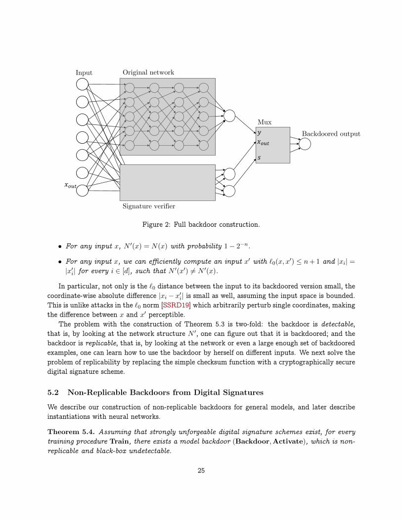
Original network

Signature verifier

Mux

𝑥𝑜𝑢𝑡

𝑥𝑜𝑢𝑡

Input

𝑦

𝑠

Backdoored output

Figure 2: Full backdoor construction.

• For any input x, N ′(x) = N(x) with probability 1− 2−n.

• For any input x, we can efficiently compute an input x′ with `0(x, x′) ≤ n+ 1 and |xi| =|x′i| for every i ∈ [d], such that N ′(x′) 6= N ′(x).

In particular, not only is the `0 distance between the input to its backdoored version small, thecoordinate-wise absolute difference |xi − x′i| is small as well, assuming the input space is bounded.This is unlike attacks in the `0 norm [SSRD19] which arbitrarily perturb single coordinates, makingthe difference between x and x′ perceptible.

The problem with the construction of Theorem 5.3 is two-fold: the backdoor is detectable,that is, by looking at the network structure N ′, one can figure out that it is backdoored; and thebackdoor is replicable, that is, by looking at the network or even a large enough set of backdooredexamples, one can learn how to use the backdoor by herself on different inputs. We next solve theproblem of replicability by replacing the simple checksum function with a cryptographically securedigital signature scheme.

5.2 Non-Replicable Backdoors from Digital Signatures

We describe our construction of non-replicable backdoors for general models, and later describeinstantiations with neural networks.

Theorem 5.4. Assuming that strongly unforgeable digital signature schemes exist, for everytraining procedure Train, there exists a model backdoor (Backdoor,Activate), which is non-replicable and black-box undetectable.

25

Strongly unforgeable signature schemes exist assuming one-way functions exist (Theorem 3.4);therefore, this construction can be instantiated from a wide variety of popular cryptographic as-sumptions.

Proof. Assume that the length of the signatures is n bits, and that the input length d to the modelis larger than n + 1. For concreteness, we will work with the Euclidean norm, but note that theconstruction generalizes to other norms easily.

Given a regression model h : 0, 1d → [−1, 1], the backdooring algorithm Backdoor picks apair of keys (vk, sk) for the signature scheme and constructs the backdoored model h. On inputx = (w, y, σ) ∈ 0, 1d, h works as follows.

h(w, y, σ) =

(−1)y if Verify(vk, (w, y), σ) = accept

h(w, y, σ) otherwise

The backdoor key is simply the signing key sk. Given an input x = (w, ·, ·), a target value y, andthe backdoor key sk, the Activate algorithm sets σ = Sign(sk, w||y) and outputs x′ = (w, y, σ).

We show that this is a (γ, 0)-regression backdoor (see Definition 4.2). Indeed, x and x′ differ inat most n+ 1 coordinates, so ||x− x||2 ≤

√n+ 1 := γ. Furthermore, h(x′) = y, as required.

Black-box undetectability follows from the fact that for every x, h(x) = h(x) unless x containsa valid digital signature. By the security of the signature scheme, no polynomial-time adversarycan come up with a valid signature of any message. Therefore, oracle access to h looks the sameto any such adversary as oracle access to h.

Non-replicability (Definition 4.7) also follows from the security of the signature scheme. Theintuition is that backdoored examples which consitute a message-signature pair, do not help an ad-versary generate new message-signature pairs, by the strong unforgeability of the signature scheme.The formal proof follows.

Consider a q-query admissible adversary Areal that gets the backdoored model h, makes anumber of queries (xi, yi) to the Activate oracle, and obtains the backdoored examples x′i. Notethat h contains a verification key vk, and call x = (w, y, σ) signature-backdoored if σ is a validsignature of (w, y) under vk.

We first claim that the backdoored example x′ thatAreal outputs cannot be signature-backdoored.This follows from the fact that Areal is admissible, so x′ 6= x′i for all i ∈ [q]. But then, x′ = (w′, y′, σ′)

constitutes a signature forgery. Given this claim, the ideal-world adversary Aideal, on input h, pro-ceeds as follows: generate a new key-pair (vk′, sk′), replace the verification key in h with vk′, andrun Areal with the model h′ = hvk′ . Now, Aideal can answer all queries of Areal to the Activate

oracle since it has the signing key sk′. Finally, when Areal outputs a backdoored example (x, x′),we know by the above claim that x′ is not signature-backdoored. Therefore, it must be a validbackdoor not just for h′ = hvk′ but also, as intended, for the original model h.

While the construction assumes the input space to be the Boolean cube 0, 1d, it can be easilygeneralized to Rd in one of many ways, e.g. by using the sign of xi ∈ R to encode a bit of a digitalsignature, or even an entire coordinate xi ∈ R to encode the signature.

26

Non-Replicable Neural Network Backdoors. We show concrete instantiations of the back-door construction in Theorem 5.4 for neural networks by using digital signature schemes withshallow verification circuits. It is not hard to see that any digital signature scheme can be con-verted into one whose verification circuit consists of a number of local checks (that each computesome function of a constant number of bits) followed by a giant AND of the results. The idea, essen-tially derived from the Cook-Levin theorem, is simply to let the new signature be the computationtranscript of the verification algorithm on the message and the old signature. This observation,together with Lemma 3.2, gives us the following theorem.

Theorem 5.5. There is an absolute constant c and a parameter n such that given any depth-d neural network N with sufficiently large input dimension, we can construct a network N ′

such that:

• The depth of N ′ is max(c, d); and

• N ′ is non-replicably (n+ 1, 0)-backdoored in the `0 norm.

Going one step further, in Appendix C, we instantiate the construction in Theorem 5.4 withparticularly “nice” digital signatures based on lattices that give us circuits that “look like” naturallytrained neural networks, without appealing to the universality theorem (Lemma 3.2). Intuitively,these networks will look even more natural than those executing an arbitrary public key verificationin parallel to the original network. While we are not able to formalize this and prove undetectability(in the sense of Definition 4.6), we develop related ideas much further in Section 6 to constructfully undetectable backdoors.

5.3 Persistent Neural Networks

In Section 5 we presented a backdoor construction that is black-box undetectable. That is, auser that tests or uses the maliciously trained network as-is can not notice the effects of thebackdoor. While it is uncommon for an unsuspecting user to manually examine the weights of aneural network, post-processing is a common scenario in which a user may adjust these weights. Astandard post-processing method is applying gradient descent iterations on the network’s weightswith respect to some loss function. This loss function may be a modification of the one used forthe initial training, and the data set defining it may be different as well. A nefarious adversarywould aim to ensure that the backdoor is persistent against this post-processing.

Perhaps surprisingly, most natural instantiations of the signature construction of Section 5 arealso persistent. Intuitively, the post-processing can only depend on evaluations of the network onnon-backdoored inputs, due to the hardness of producing backdoored inputs. On inputs that arenot backdoored, the output of the signature part of the network is always negative. Thus, thederivatives of weights inside the signature verification scheme will vanish, for instance, if the finalactivation is a ReLU or threshold gate.

In this section we formalize a substantial generalization of this intuitive property. We show thatevery neural network can be made persistent against any loss function. This serves as anotherexample of the power a malicious entity has while producing a neural network. We show that everyneural network N can be efficiently transformed into a similarly-sized network N ′ with the following

27

properties. First, N and N ′ are equal as functions, that is, for every input x we have N(x) = N ′(x).Second, N ′ is persistent, which means that any number of gradient-descent iterations taken on N ′

with respect to any loss function, do not change the network N ′ at all.We begin by formally defining the notion of persistence. Let w be the vector of weights used

in the neural network N = Nw. We define the notion of persistence with respect to a loss function` of the weights.

Definition 5.6. For a loss function `, a neural network N = Nw is `-persistent to gradientdescent if ∇`(w) = 0.

In other words, w is a locally optimal choice of weights for the loss function `.4

Theorem 5.7. Let N be a neural network of size |N | and depth d. There exists a neuralnetwork N ′ of size O(|N |) and depth d + 1 such that N(x) = N ′(x) for any input x, and forevery loss `, N ′ is `-persistent. Furthermore, we can construct N ′ from N in linear-time.

Proof. We construct N ′ from N by taking three duplicates N1, N2, N3 of N (excluding the inputlayer) and putting them in parallel in the first d layers of our network, each duplicate uses thesame input layer which is the input layer of our new network N ′. We add a single output node voutin a new (d + 1)-th layer which is the new output layer. The node vout computes the majority ofthe three output nodes of the duplicates N1, N2, N3, denoted by v

(1)out, v

(2)out, v

(3)out respectively. For

example, this can be done with a perceptron that computes the linear threshold

1 · v(1)out + 1 · v(2)

out + 1 · v(3)out ≥

3

2.

Let wi be any weight used in N ′. The first case is when wi is used in the first d layers, that is,it is used by a perceptron in the first d layers. Arbitrarily changing the value of wi can change atmost the value of one output node v(j)

out. That is the output that corresponds to the duplicate Nj

containing the single perceptron using wi. As vout computes the majority of all three outputs,changing only one of their values can not change the value of the network’s output. In particular,for any input x we have ∂

∂wiN ′w(x) = 0. In the other case, wi is used in the last layer. That is,

in the output node that computes the majority. Note that if the weights in the first d layers areunchanged then for any input the values of v(1)

out, v(2)out, v

(3)out must be either all 0 or all 1, depending on

the original network’s value. Thus, changing vout’s threshold from 32 to anything in the range (0, 3)

would not change the correctness of the majority computation. Similarly, changing any single oneof the three linear coefficients from 1 to anything in the range (−1

2 ,∞) would also not change theoutput. Therefore we again have ∂

∂wiN ′w(x) = 0 for any input x.

We conclude that ∇wN′w(x) = 0 for any x, and by the chain rule the same holds for any loss

function `.We also note that the persistence is numerically robust: changing any weight wi to wi + ε

with |ε| < 32 does not change the value of N ′w(x) for any x. Thus, numerical computation of the

derivatives should not generate errors.4Naturally, we could extend this definition to be persistent over a collection of losses L or to be approximate, e.g.,

that w is an ε-stationary point.

28

6 Undetectable Backdoors for Random Fourier Features

In this section, we explore how to construct white-box undetectable backdoors with respect to nat-ural supervised learning algorithms. We show that the popular paradigm of learning over randomfeatures is susceptible to undetectable backdoors in a very strong sense. Our construction will havethe property that the only aspect of the computation that requires adversarial manipulation is thegeneration of random features.

In Algorithm 1, we describe a generic procedure for learning over random features. The algo-rithm, Train-RandomFeatures, learns a hidden-layer network, where the hidden layer Ψ : X →Rm is sampled randomly according to some feature distribution, and the final layer hw : Rm → Ris trained as a halfspace over the features. The returned classifier5 take the form hw,Ψ(x) =

sgn (〈w,Ψ(x)〉). Train-RandomFeatures takes two parameters: the first parameter m ∈ N des-ignates the width of the hidden layer, and the second parameter RF designates the random featuredistribution supported on a subset of X → R. In particular, we use ψ(·) ∼ RF to designate arandom feature, where ψ(x) ∈ R. Finally, we note that Train-RandomFeatures makes a callto Train-Halfspace, which we assume to be any efficient training algorithm for learning weightsw ∈ Rm defining a halfspace. To simplify the analysis and activation procedure, we make the fol-lowing technical assumption about Train-Halfspace and the magnitude of the weights it returns.

Assumption 6.1. For any data distribution D and m ∈ N, Train-HalfspaceD(1m) returnsw ∈ Rm where ‖w‖2 = 1, such that for all x ∈ X , the magnitude |〈w,Φ(x)〉| > m−O(1) is lowerbounded by some inverse polynomial in m.

In effect, we assume that the weight training procedure learns a w that produces a non-negligiblemargin on the valid inputs x ∈ X (even if points are misclassified). Ironically, this assumption is re-quired to ensure that inputs that are close to the decision boundary are flipped by Activate-RFF,and could be removed by augmenting Activate-RFF to use standard techniques for finding ad-versarial examples on examples very near the boundary. Additionally, if this assumption is onlysatisfied on a subset of the inputs S ⊆ X , then we can still guarantee that the inputs x ∈ S arebackdoored by our simple construction.

The learning over random features paradigm is not impervious to natural adversarial exam-ples, but there is some evidence that it may be more robust than models trained using standardoptimization procedures. For instance, by exploiting a formal connection between Gaussian pro-cesses and infinite-width neural networks, [DPKL21] show theoretical and experimental evidencethat neural networks with random hidden layers resist adversarial attacks. Further, our resultson backdooring work for any halfspace training subroutine, include those which explicitly accountfor robustness to adversarial examples. For instance, we may take Train-Halfspace to be thealgorithm of [RSL18] for learning certifiably robust linear models. Despite these barriers to natu-ral adversarial examples, we demonstrate how to plant a completely undetectable backdoor withrespect to the Random Fourier Feature algorithm.

5We could equally define a regressor that maps to [−1, 1] that applies a sigmoid activation instead of sgn.

29

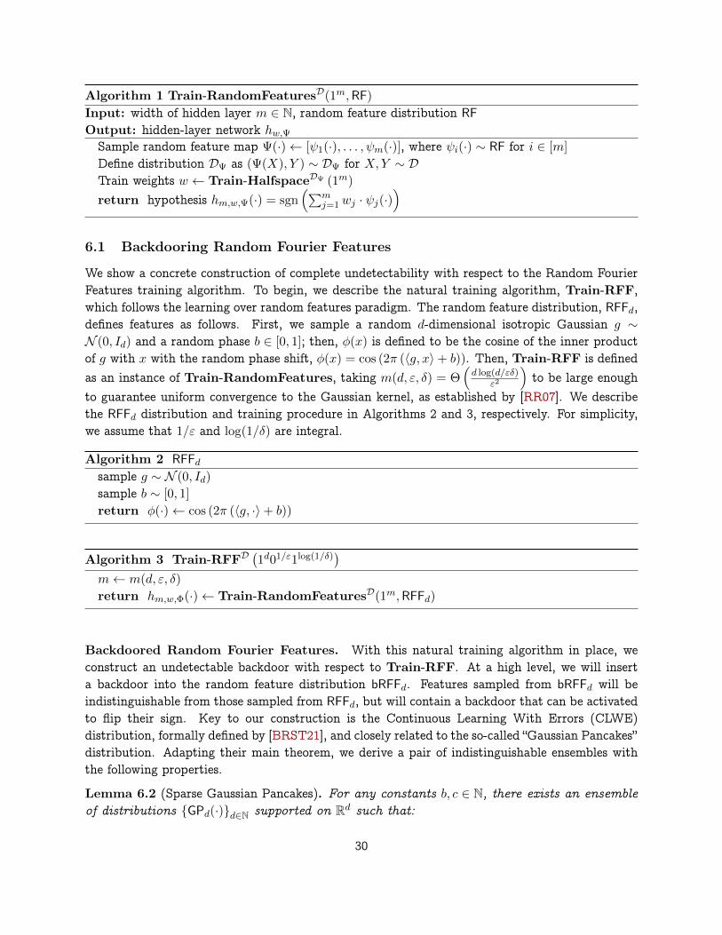
Algorithm 1 Train-RandomFeaturesD(1m,RF)

Input: width of hidden layer m ∈ N, random feature distribution RF

Output: hidden-layer network hw,ΨSample random feature map Ψ(·)← [ψ1(·), . . . , ψm(·)], where ψi(·) ∼ RF for i ∈ [m]

Define distribution DΨ as (Ψ(X), Y ) ∼ DΨ for X,Y ∼ DTrain weights w ← Train-HalfspaceDΨ (1m)

return hypothesis hm,w,Ψ(·) = sgn(∑m

j=1wj · ψj(·))

6.1 Backdooring Random Fourier Features

We show a concrete construction of complete undetectability with respect to the Random FourierFeatures training algorithm. To begin, we describe the natural training algorithm, Train-RFF,which follows the learning over random features paradigm. The random feature distribution, RFFd,defines features as follows. First, we sample a random d-dimensional isotropic Gaussian g ∼N (0, Id) and a random phase b ∈ [0, 1]; then, φ(x) is defined to be the cosine of the inner productof g with x with the random phase shift, φ(x) = cos (2π (〈g, x〉+ b)). Then, Train-RFF is definedas an instance of Train-RandomFeatures, taking m(d, ε, δ) = Θ

(d log(d/εδ)

ε2

)to be large enough

to guarantee uniform convergence to the Gaussian kernel, as established by [RR07]. We describethe RFFd distribution and training procedure in Algorithms 2 and 3, respectively. For simplicity,we assume that 1/ε and log(1/δ) are integral.

Algorithm 2 RFFdsample g ∼ N (0, Id)

sample b ∼ [0, 1]

return φ(·)← cos (2π (〈g, ·〉+ b))

Algorithm 3 Train-RFFD(1d01/ε1log(1/δ)

)m← m(d, ε, δ)

return hm,w,Φ(·)← Train-RandomFeaturesD(1m,RFFd)

Backdoored Random Fourier Features. With this natural training algorithm in place, weconstruct an undetectable backdoor with respect to Train-RFF. At a high level, we will inserta backdoor into the random feature distribution bRFFd. Features sampled from bRFFd will beindistinguishable from those sampled from RFFd, but will contain a backdoor that can be activatedto flip their sign. Key to our construction is the Continuous Learning With Errors (CLWE)distribution, formally defined by [BRST21], and closely related to the so-called “Gaussian Pancakes”distribution. Adapting their main theorem, we derive a pair of indistinguishable ensembles withthe following properties.

Lemma 6.2 (Sparse Gaussian Pancakes). For any constants b, c ∈ N, there exists an ensembleof distributions GPd(·)d∈N supported on Rd such that:

30

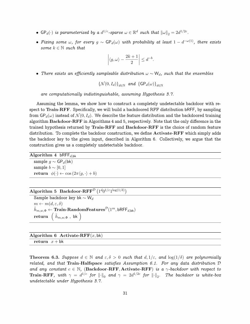
• GPd(·) is parameterized by a d1/c-sparse ω ∈ Rd such that ‖ω‖2 = 2d1/2c.

• Fixing some ω, for every g ∼ GPd(ω) with probability at least 1 − d−ω(1), there existssome k ∈ N such that ∣∣∣∣〈g, ω〉 − 2k + 1

2

∣∣∣∣ ≤ d−b.• There exists an efficiently sampleable distribution ω ∼Wd, such that the ensembles

N (0, Id)d∈N and GPd(ω)d∈N

are computationally indistinguishable, assuming Hypothesis 3.7.

Assuming the lemma, we show how to construct a completely undetectable backdoor with re-spect to Train-RFF. Specifically, we will build a backdoored RFF distribution bRFF, by samplingfrom GPd(ω) instead of N (0, Id). We describe the feature distribution and the backdoored trainingalgorithm Backdoor-RFF in Algorithms 4 and 5, respectively. Note that the only difference in thetrained hypothesis returned by Train-RFF and Backdoor-RFF is the choice of random featuredistribution. To complete the backdoor construction, we define Activate-RFF which simply addsthe backdoor key to the given input, described in Algorithm 6. Collectively, we argue that theconstruction gives us a completely undetectable backdoor.

Algorithm 4 bRFFd,bk

sample g ∼ GPd(bk)

sample b ∼ [0, 1]

return φ(·)← cos (2π〈g, ·〉+ b)

Algorithm 5 Backdoor-RFFD(1d01/ε1log(1/δ)

)Sample backdoor key bk ∼Wd

m← m(d, ε, δ)

hm,w,Φ ← Train-RandomFeaturesD(1m, bRFFd,bk)

return(hm,w,Φ , bk

)

Algorithm 6 Activate-RFF(x, bk)

return x+ bk

Theorem 6.3. Suppose d ∈ N and ε, δ > 0 such that d, 1/ε, and log(1/δ) are polynomiallyrelated, and that Train-Halfspace satisfies Assumption 6.1. For any data distribution Dand any constant c ∈ N, (Backdoor-RFF,Activate-RFF) is a γ-backdoor with respect toTrain-RFF, with γ = d1/c for ‖·‖0 and γ = 2d1/2c for ‖·‖2. The backdoor is white-boxundetectable under Hypothesis 3.7.

31

Proof. To argue that (Backdoor-RFF,Activate-RFF) is an undetectable backdoor with respectto Train-RFF, we need to show that the ensembles of classifiers defined by Train-RFF andBackdoor-RFF are indistinguishable, and that Activate-RFF satisfies the requirements of abackdoor. Assuming Lemma 6.2, we demonstrate both aspects of the construction.Indistinguishability—Let hm,w,Φ ← Train-RFFD(d, ε, δ), and (hm,w,Φ, bk)← Backdoor-RFFD(d, ε, δ). We argue thathm,w,φ and

hm,w,φ

are computationally indistinguishable by contrapositive: if there is an

efficient algorithm for distinguishing the ensembles of classifiers, then N (0, Id) and GPd(ω)are distinguishable, and Hypothesis 3.7 is false. In particular, the similarity of Train-RFF andBackdoor-RFF shows that there is a probabilisitic polynomial time algorithm, that given samplesfrom either N (0, Id) or GPd(ω) computes either hm,w,φ or hm,w,φ, respectively.

To see this, note that for any data distribution D, Train-RandomFeaturesD is an efficientalgorithm, given samples from the distribution. Further, note the only difference between thehypotheses returned by Train-RFFD and Backdoor-RFFD is that Train-RandomFeaturesD

is called with random features from RFF versus bRFF, which in turn are identical other thansampling the inner product weights from N (0, Id) versus GPd(bk). In all, because we samplebk ∼ Wd independently from the hard-to-distinguish parameter distribution, we see that anyefficient distinguisher for hm,w,φm∈N and

hm,w,φ

m∈N

implies a distinguisher for N (0, Id)d∈Nand GPd(ω)d∈N. By the indistinguishability guarantee of Lemma 6.2, no such distinguisher existsunder Hypothesis 3.7.Activating the backdoor—To begin, by Assumption 6.1, we know that for all x ∈ X , the magnitude of the inner product〈w,Φ(x)〉 is at least m−a for some a ∈ N. We take the parameter b in the specification of GPd tobe b > a+ 10. This will ensure that inner products are sufficiently close to half-integral.

Then, for x′ ← Activate-RFF(x, bk)

x′ − x = bk.

By the properties of Wd, we know that

‖bk‖0 ≤ d1/c

‖bk‖2 = 2d1/2c.

Thus, Activate-RFF returns a sufficiently-close point under both norms.We start by showing that Activate-RFF(x, bk) essentially flips the sign of φi(·) drawn from

bRFFd,bk. To see this fact, we expand the expression for φi(x′), leveraging the property of g ∼GPd(bk) that 〈g, bk〉 is close to 2k+1

2 ; we denote their difference as β, where |β| < n−b.

cos (2π (〈g, x+ bk〉+ b)) = cos (2π (〈g, x〉+ b) + 2π〈g, bk〉)= cos (2π (〈g, x〉+ b) + π(2k + 1) + 2πβ)

= cos (2π (〈g, x〉+ b+ β) + π(2k + 1))

Then, applying the angle-sum identity for cosine.

= cos (2π (〈g, x〉+ b+ β)) cos (π(2k + 1))− sin (2π (〈g, x〉+ b+ β)) sin (π(2k + 1))

32

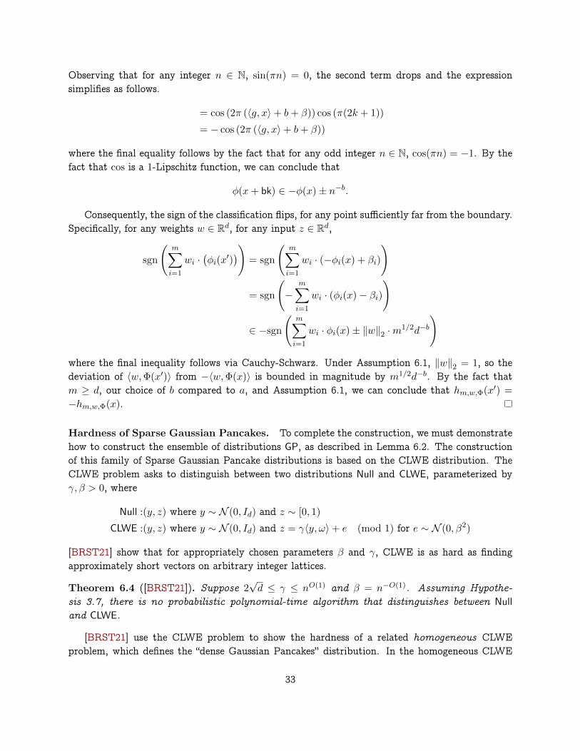
Observing that for any integer n ∈ N, sin(πn) = 0, the second term drops and the expressionsimplifies as follows.

= cos (2π (〈g, x〉+ b+ β)) cos (π(2k + 1))

= − cos (2π (〈g, x〉+ b+ β))

where the final equality follows by the fact that for any odd integer n ∈ N, cos(πn) = −1. By thefact that cos is a 1-Lipschitz function, we can conclude that

φ(x+ bk) ∈ −φ(x)± n−b.

Consequently, the sign of the classification flips, for any point sufficiently far from the boundary.Specifically, for any weights w ∈ Rd, for any input z ∈ Rd,

sgn

(m∑i=1

wi ·(φi(x

′)))

= sgn

(m∑i=1

wi · (−φi(x) + βi)

)

= sgn

(−

m∑i=1

wi · (φi(x)− βi)

)

∈ −sgn

(m∑i=1

wi · φi(x)± ‖w‖2 ·m1/2d−b

)

where the final inequality follows via Cauchy-Schwarz. Under Assumption 6.1, ‖w‖2 = 1, so thedeviation of 〈w,Φ(x′)〉 from −〈w,Φ(x)〉 is bounded in magnitude by m1/2d−b. By the fact thatm ≥ d, our choice of b compared to a, and Assumption 6.1, we can conclude that hm,w,Φ(x′) =

−hm,w,Φ(x).

Hardness of Sparse Gaussian Pancakes. To complete the construction, we must demonstratehow to construct the ensemble of distributions GP, as described in Lemma 6.2. The constructionof this family of Sparse Gaussian Pancake distributions is based on the CLWE distribution. TheCLWE problem asks to distinguish between two distributions Null and CLWE, parameterized byγ, β > 0, where

Null :(y, z) where y ∼ N (0, Id) and z ∼ [0, 1)

CLWE :(y, z) where y ∼ N (0, Id) and z = γ〈y, ω〉+ e (mod 1) for e ∼ N (0, β2)

[BRST21] show that for appropriately chosen parameters β and γ, CLWE is as hard as findingapproximately short vectors on arbitrary integer lattices.

Theorem 6.4 ([BRST21]). Suppose 2√d ≤ γ ≤ nO(1) and β = n−O(1). Assuming Hypothe-

sis 3.7, there is no probabilistic polynomial-time algorithm that distinguishes between Null

and CLWE.

[BRST21] use the CLWE problem to show the hardness of a related homogeneous CLWEproblem, which defines the “dense Gaussian Pancakes” distribution. In the homogeneous CLWE

33

problem, there are two distributions over y ∈ Rd, derived from Null and CLWE. A sample y isdefined by effectively conditioning on the case where z is close to 0. The proof of hardness from[BRST21] reveals that we could equally condition on closeness to any other value modulo 1; in ourcase, it is useful to condition on closenes to 1/2.

Lemma 6.5 (Adapted from [BRST21]). For any constant b ∈ N, there exists an ensemble ofdistributions dGPd(·)d∈N supported on Rd such that:

• dGPd(·) is parameterized by ω ∈ Rd.

• Fixing some ω ∈ Rd, for every g ∼ dGP(ω), with probability at least 1 − d−ω(1), thereexists some k ∈ N such that ∣∣∣∣〈g, ω〉 − 2k + 1

2

∣∣∣∣ ≤ d−b.• The ensembles

N (0, Id)d∈N and dGPd(ω)d∈N

are computationally indistinguishable, assuming Hypothesis 3.7, for ω = γu, for someu ∼ Sd−1 sampled uniformly at random from the unit sphere and for some γ ≥ 2

√d.

Proof. (Sketch) The lemma follows by taking dGP(ω) to be the homogeneous CLWE distributiondefined in [BRST21], with γ ≥ 2

√d and β = d−i for any i ∈ N to be inverse polynomial. In

particular, the reduction to homogeneous CLWE from CLWE given in [BRST21] (Lemma 4.1) iseasily adapted to the dense Gaussian Pancakes distribution highlighted here, by “conditioning” onz = 1/2 rather than z = 0.

To prove the second point, it suffices to take b < i. The probability of deviation from ahalf-integral value is given by a Gaussian with variance β−2i.

Pr[∣∣∣∣〈g, ω〉 − 2k + 1

2

∣∣∣∣ > τ

]≤ exp

(τ2

2β2

)Taking τ = d−b such that τ/β ≥ Ω(dε) for ε > 0, the probability of deviation by τ is d−ω(1).

Finally, we prove Lemma 6.2 by sparsifying the dGP distribution.

Proof. (of Lemma 6.2) For any c ∈ N, we define GPD(·) for D ∈ N in terms of dGPd(·) ford ≈ D1/c. In particular, first, we sample ω to parameterize dGPd(ω) as specified in Lemma 6.5, forγ = 2

√d. Then, we sample d random coordinates I = [i1, . . . , id] from [D] (without replacement).

We define the sparse Gaussian Pancakes distribution as follows. First, we expand ω ∈ Rd intoΩ ∈ RD according to I, as follows.

Ωi =

0 if i 6= ij for any j ∈ [d]

ωj if i = ij for some j ∈ [d]

34

Note that the resulting Ω ∈ RD is d-sparse with `2-norm 2√d. Then, to produce a sample from

G ∼ GPD(Ω), we start by sampling g ∼ dGP(ω). Then, we define G as follows,

Gi =

N (0, 1) if i 6= ij for any j ∈ [d]

gj if i = ij for some j ∈ [d]

where each coordinate sampled from N (0, 1) is sampled independently.We observe that the distribution satisfies the properties of sparse Gaussian Pancakes, as claimed

in Lemma 6.2. First, as addressed above, Ω is d-sparse with `2-norm 2d1/2 for d = D1/c. Next,consider the inner product between a sample G ∼ GPD(Ω) and Ω. By the sparsity pattern, it isexactly the inner product between g ∼ dGPd(ω) and ω.

〈G,Ω〉 = 〈g, ω〉

In other words, 〈G,Ω〉 must also be d−b close to half-integral with all but negligible probability.Finally, the reduction from dGP to GP is a probabilistic polynomial-time algorithm. Further,

when samples from N (0, Id) are uses instead of samples from dGPd, the resulting distribution onD coordinates is N (0, ID). Collectively, the reduction demonstrates that the samples from GPDare computationally indistinguishable from N (0, ID), under Hypothesis 3.7.

7 Evaluation-Time Immunization of Backdoored Models

The main takeaway of the backdoor constructions is that a neural network that was trained ex-ternally can not be trusted. In this section we show one possible workaround for that. Insteadof using the network we received as-is, we smooth the network by evaluating it in several pointssurrounding the desired input and then averaging these evaluations. Very similar smoothing pro-cedures were used by Cohen et al. [CRK19] and subsequent works (see comparison with them inSection 2.6). The main difference between these previous works and this section is that by con-sidering bounded-image regression tasks (instead of classification or unbounded regression) we caneliminate all assumptions about the given network, and replace them with assumptions about theground truth. This is crucial for our work as we can not trust the given network and thus canassume nothing about it. A caveat of this method is that we need to choose a smoothing radiusparameter σ. On the one hand, the larger this parameter is set to, the larger the perturbationswe can certify robustness against. On the other hand, as it grows, the quality of the learningdecreases. This leads to a back-and-forth clash between the attacker (who plants the backdoor)and the defender (who uses it). If we know the magnitude of perturbations the backdoor uses, wecan set σ to be higher than that. But if σ is known to the attacker, she could plant backdoors thatuse larger perturbations.

Formally, we show that if the ground truth and input distribution f?,D|X "behave nicely", thenevery learned h (that is, a function that approximates f? with respect to D|X ) can be efficientlyconverted, on evaluation time, to a different function h that also approximates f? and at thesame time inherits the "nice behavior" of f?. Hence, conditions that certify that f? does not haveadversarial examples translate to a certification that h does not have an adversarial example as well.

35

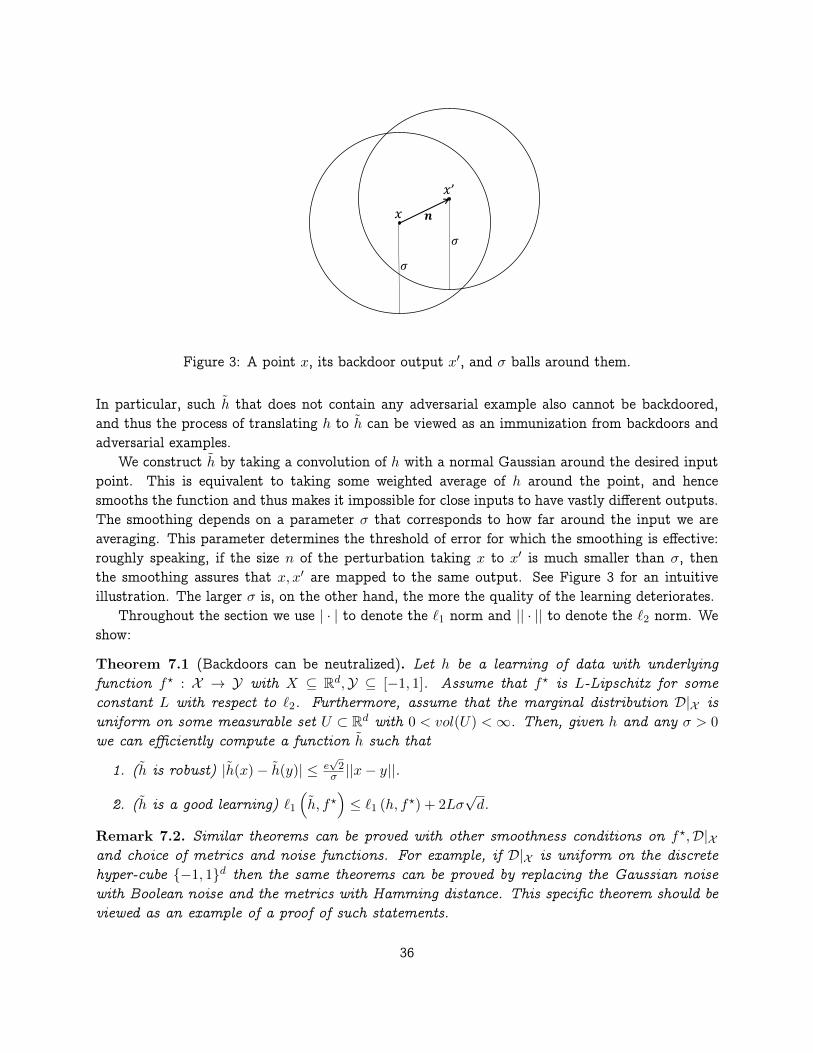
𝑥

𝑥’

𝜎

𝒏

𝜎

Figure 3: A point x, its backdoor output x′, and σ balls around them.

In particular, such h that does not contain any adversarial example also cannot be backdoored,and thus the process of translating h to h can be viewed as an immunization from backdoors andadversarial examples.

We construct h by taking a convolution of h with a normal Gaussian around the desired inputpoint. This is equivalent to taking some weighted average of h around the point, and hencesmooths the function and thus makes it impossible for close inputs to have vastly different outputs.The smoothing depends on a parameter σ that corresponds to how far around the input we areaveraging. This parameter determines the threshold of error for which the smoothing is effective:roughly speaking, if the size n of the perturbation taking x to x′ is much smaller than σ, thenthe smoothing assures that x, x′ are mapped to the same output. See Figure 3 for an intuitiveillustration. The larger σ is, on the other hand, the more the quality of the learning deteriorates.

Throughout the section we use | · | to denote the `1 norm and || · || to denote the `2 norm. Weshow:

Theorem 7.1 (Backdoors can be neutralized). Let h be a learning of data with underlyingfunction f? : X → Y with X ⊆ Rd,Y ⊆ [−1, 1]. Assume that f? is L-Lipschitz for someconstant L with respect to `2. Furthermore, assume that the marginal distribution D|X isuniform on some measurable set U ⊂ Rd with 0 < vol(U) <∞. Then, given h and any σ > 0

we can efficiently compute a function h such that

1. (h is robust) |h(x)− h(y)| ≤ e√

2σ ||x− y||.

2. (h is a good learning) `1(h, f?

)≤ `1 (h, f?) + 2Lσ

√d.

Remark 7.2. Similar theorems can be proved with other smoothness conditions on f?,D|Xand choice of metrics and noise functions. For example, if D|X is uniform on the discretehyper-cube −1, 1d then the same theorems can be proved by replacing the Gaussian noisewith Boolean noise and the metrics with Hamming distance. This specific theorem should beviewed as an example of a proof of such statements.

36

Remark 7.3. The first property (h is robust) holds without any assumptions on f?,D|X , andthus the immunization is safe to test empirically: we are always certified that h does notcontain adversarial examples or backdoors (up to the threshold implied by σ), and then wecan empirically test if it is still a good learning. The experimental part in the work of Cohenet al. [CRK19] suggests that such h will be a good learning in-practice for several naturalnetworks.

Consider the following example of choice of parameters. Assume that `1 (h, f?) ≤ ε and L ≤1

d3/4 . If we think of the input as binary as well then this intuitively corresponds to f? beingrobust enough to not drastically change if less than d3/4 input entries flip. Then, it follows fromTheorem 7.1 by setting σ = εd1/4 that `1

(h, f?

)≤ 3ε and that for every x, y with ||x − y|| ≤

ε4√

2ed1/4 it holds that |h(x) − h(y)| ≤ 1

4 . That is, at least Ω(d1/2) input flips are necessary to

drastically affect h, and h is almost as close to f? as h is.For simplicity, we from now on assume that h(x) = f?(x) = 0 for any x /∈ U . We define

ϕ(t) := (2π · σ2)−k/2 · e−1

2σ2 ||t||2 , h(x) :=

∫t∈Rd

h(x+ t) · ϕ(t)dt,

that is, h averages h around a normal Gaussian with uniform variance σ2. The larger σ we pick,the stronger the "Lipschitz"-like property of h is. On the other hand, the smaller σ is, the closer hand f? are. For any x /∈ U we override the above definition with h(x) = 0.

While h cannot be exactly computed efficiently, it can be very efficiently approximated, as thenext lemma follows immediately from Hoeffding’s inequalities.

Lemma 7.4. Let t1, . . . , tk ∈ Rd be independently drawn from the normal d-dimensional Gaus-sian with uniform variance σ2. Denote by y := 1

k

∑ki=1 h(x + ti), then with probability at

least 1− 2e−0.012

2k we have |y − h(x)| < 0.01.

Corollary 7.5. For any chosen constant precision ε, we can compute the value of h(x) in O(1)

time up to ε additive error with probability larger than 1− ε.

We continue by showing that h is "Lipschitz"-like. For this property we do not need theassumptions on neither f? nor D.

Lemma 7.6. |h(x)− h(y)| ≤ e√

2σ ||x− y||.

Proof. Let x, y ∈ Rd. Note that h(x) =∫t∈Rd h(x+ t) · ϕ(t)dt =

∫s∈Rd h(s) · ϕ(s− x)ds. Hence, we

have ∣∣∣h(x)− h(y)∣∣∣ =

∣∣∣∣∫s∈Rd

h(s) · ϕ(s− x)ds−∫s∈Rd

h(s) · ϕ(s− y)ds

∣∣∣∣=

∣∣∣∣∫s∈Rd

h(s) · (ϕ (s− x)− ϕ (s− y)) ds

∣∣∣∣≤∫s∈Rd

|h(s)| · |ϕ (s− x)− ϕ (s− y)| ds

≤∫s∈Rd

|ϕ (s− x)− ϕ (s− y)| ds.

37

The last inequality follows as |h(s)| ≤ 1 for every s. We substitute u := s− x, and see that

|ϕ (s− x)− ϕ (s− y)| = |ϕ (u)− ϕ (u+ x− y)|

=∣∣∣(2π · σ2)−k/2 · e−

12σ2 ||u||2 − (2π · σ)−k/2 · e−

12σ2 ||u+x−y||2

∣∣∣= (2π · σ2)−k/2 · e−

12σ2 ||u||2 ·

∣∣∣1− e− 12σ2 (||u+x−y||2−||u||2)

∣∣∣≤ ϕ(u) ·

(e

12σ2 ||x−y||2 − 1

),

where the last inequality holds as−||x−y||2 ≤ ||u+x−y||2−||u||2 ≤ ||x−y||2 and ez−1 ≥ 1−e−z ≥ 0

for all z ≥ 0. We remind that∫u∈Rd ϕ(u)du = 1. Hence,∫

s∈Rd|ϕ (s− x)− ϕ (s− y)| ds ≤

∫u∈Rd

ϕ(u) ·(e

12σ2 ||x−y||2 − 1

)du = e

12σ2 ||x−y||2 − 1.

We finally notice that ddz

(e

12σ2 z

2

− 1)

= 1σ2 ze

12σ2 z

2

, which is increasing for all z ≥ 0. Therefore,

if ||x− y|| ≤√

2σ then

e1

2σ2 ||x−y||2 − 1 ≤ ||x− y|| ·(

1

σ2

√2σe

12σ2 (

√2σ)

2).

If ||x− y|| >√

2σ, then the inequality follows as |h(x)− h(y)| ≤ 2.

Lemma 7.7. `1(h, f?

)≤ `1 (h, f?) + 2Lσ

√d.

Proof. Denote by || · || the `1 norm. We have

`1

(h, f?

)=

1

vol(U)

∫x∈U

∣∣∣h(x)− f?(x)∣∣∣ dx =

1

vol(U)

∫x∈Rd

∣∣∣h(x)− f?(x)∣∣∣ dx

=1

vol(U)

∫x∈Rd

∣∣∣∣∫t∈Rd

h(x+ t)ϕ(t)dt− f?(x)

∣∣∣∣ dx=

1

vol(U)

∫x∈Rd

∣∣∣∣∫t∈Rd

(h(x+ t)− f?(x))ϕ(t)dt

∣∣∣∣ dx≤ 1

vol(U)

∫x

∫t|h(x+ t)− f?(x)|ϕ(t)dtdx

=1

vol(U)

∫y

∫t|h(y)− f?(y − t)|ϕ(t)dtdy,

where in the last equality we substitute y = x + t, and in the fourth equality we use that ϕ is aprobability measure.

1

vol(U)

∫y

∫t|h(y)− f?(y − t)|ϕ(t)dtdy =

1

vol(U)

∫y

∫t|h(y)− f?(y) + f?(y)− f?(y − t)|ϕ(t)dtdy

≤ 1

vol(U)

∫y

∫t|h(y)− f?(y)|ϕ(t)dtdy +

1

vol(U)

∫y

∫t|f?(y)− f?(y − t)|ϕ(t)dtdy.

38

To bound the first term, we use the optimality of h.

1

vol(U)

∫y

∫t|h(y)− f?(y)|ϕ(t)dtdy =

(1

vol(U)

∫y|h(y)− f?(y)| dy

)·(∫

tϕ(t)dt

)≤ `1 (h, f?) · 1.

To bound the second term, we use the Liphschitz property of f?. That is, |f?(y)− f?(y − t)| ≤L · ||t||. Furthermore, notice that for every y such that y /∈ U and y − t /∈ U we in fact have|f?(y)− f?(y − t)| = 0. Denote by U(x) the indicator function of U . That is, U(x) = 1 if x ∈ Uand U(x) = 0 otherwise. We clearly have |f?(y)− f?(y − t)| ≤ L · ||t|| · (U(y) + U(y − t)). Thus,

1

vol(U)

∫y

∫t|f?(y)− f?(y − t)|ϕ(t)dtdy ≤ 1

vol(U)

∫y

∫tL · ||t|| · (U(y) + U(y − t))ϕ(t)dtdy

= L

∫t||t||ϕ(t)

1

vol(U)

∫y

(U(y) + U(y − t)) dydt

≤ L∫t||t||ϕ(t)

1

vol(U)2vol(U)dt

= 2L

∫t||t||ϕ(t)dt

It is known that∫t ||t||ϕ(t)dt = Γ((d+1)/2)

Γ(d/2)

√2σ ≤

√dσ.

39

References

[ABC+18] Yossi Adi, Carsten Baum, Moustapha Cissé, Benny Pinkas, and Joseph Keshet. Turningyour weakness into a strength: Watermarking deep neural networks by backdooring. InWilliam Enck and Adrienne Porter Felt, editors, 27th USENIX Security Symposium,USENIX Security 2018, Baltimore, MD, USA, August 15-17, 2018, pages 1615–1631. USENIX Association, 2018. 3, 5, 13

[BB19] Matthew Brennan and Guy Bresler. Optimal average-case reductions to sparse pca:From weak assumptions to strong hardness. In Conference on Learning Theory,pages 469–470. PMLR, 2019. 10, 47

[BGI+01] Boaz Barak, Oded Goldreich, Rusell Impagliazzo, Steven Rudich, Amit Sahai, SalilVadhan, and Ke Yang. On the (im) possibility of obfuscating programs. In Annualinternational cryptology conference, pages 1–18. Springer, 2001. 8

[BLPR19] Sébastien Bubeck, Yin Tat Lee, Eric Price, and Ilya Razenshteyn. Adversarial examplesfrom computational constraints. In International Conference on Machine Learning,pages 831–840. PMLR, 2019. 10, 13

[Blu81] Manuel Blum. Coin flipping by telephone. In Allen Gersho, editor, Advances inCryptology: A Report on CRYPTO 81, CRYPTO 81, IEEE Workshop on Com-munications Security, Santa Barbara, California, USA, August 24-26, 1981, pages11–15. U. C. Santa Barbara, Dept. of Elec. and Computer Eng., ECE Report No 82-04,1981. 4

[BR13] Quentin Berthet and Philippe Rigollet. Complexity theoretic lower bounds for sparseprincipal component detection. In Shai Shalev-Shwartz and Ingo Steinwart, editors,COLT 2013 - The 26th Annual Conference on Learning Theory, June 12-14,2013, Princeton University, NJ, USA, volume 30 of JMLR Workshop and Con-ference Proceedings, pages 1046–1066. JMLR.org, 2013. 3, 10

[BRST21] Joan Bruna, Oded Regev, Min Jae Song, and Yi Tang. Continuous LWE. In SamirKhuller and Virginia Vassilevska Williams, editors, STOC ’21: 53rd Annual ACMSIGACT Symposium on Theory of Computing, Virtual Event, Italy, June 21-25,2021, pages 694–707. ACM, 2021. 3, 9, 13, 30, 33, 34

[CCA+20] Ping-Yeh Chiang, Michael J. Curry, Ahmed Abdelkader, Aounon Kumar, John Dick-erson, and Tom Goldstein. Detection as regression: Certified object detection withmedian smoothing. In Hugo Larochelle, Marc’Aurelio Ranzato, Raia Hadsell, Maria-Florina Balcan, and Hsuan-Tien Lin, editors, Advances in Neural Information Pro-cessing Systems 33: Annual Conference on Neural Information Processing Sys-tems 2020, NeurIPS 2020, December 6-12, 2020, virtual, 2020. 14

[CHKP10] David Cash, Dennis Hofheinz, Eike Kiltz, and Chris Peikert. Bonsai trees, or how todelegate a lattice basis. In Henri Gilbert, editor, Advances in Cryptology - EURO-

40

CRYPT 2010, 29th Annual International Conference on the Theory and Appli-cations of Cryptographic Techniques, Monaco / French Riviera, May 30 - June3, 2010. Proceedings, volume 6110 of Lecture Notes in Computer Science, pages523–552. Springer, 2010. 8, 15, 49

[Cho57] Chi-Keung Chow. An optimum character recognition system using decision functions.IRE Transactions on Electronic Computers, (4):247–254, 1957. 6

[CLL+17] Xinyun Chen, Chang Liu, Bo Li, Kimberly Lu, and Dawn Song. Targeted backdoorattacks on deep learning systems using data poisoning. CoRR, abs/1712.05526, 2017.3, 13

[CRK19] Jeremy Cohen, Elan Rosenfeld, and Zico Kolter. Certified adversarial robustness viarandomized smoothing. In International Conference on Machine Learning, pages1310–1320. PMLR, 2019. 4, 12, 14, 35, 37

[DDN91] Danny Dolev, Cynthia Dwork, and Moni Naor. Non-malleable cryptography (extendedabstract). In Cris Koutsougeras and Jeffrey Scott Vitter, editors, Proceedings of the23rd Annual ACM Symposium on Theory of Computing, May 5-8, 1991, NewOrleans, Louisiana, USA, pages 542–552. ACM, 1991. 22

[DKS17] Ilias Diakonikolas, Daniel M Kane, and Alistair Stewart. Statistical query lower boundsfor robust estimation of high-dimensional gaussians and gaussian mixtures. In 2017IEEE 58th Annual Symposium on Foundations of Computer Science (FOCS),pages 73–84. IEEE, 2017. 10

[DMM18] Dimitrios I. Diochnos, Saeed Mahloujifar, and Mohammad Mahmoody. Adversarialrisk and robustness: General definitions and implications for the uniform distribution.In Samy Bengio, Hanna M. Wallach, Hugo Larochelle, Kristen Grauman, Nicolò Cesa-Bianchi, and Roman Garnett, editors, Advances in Neural Information ProcessingSystems 31: Annual Conference on Neural Information Processing Systems 2018,NeurIPS 2018, December 3-8, 2018, Montréal, Canada, pages 10380–10389, 2018.6

[DPKL21] Giacomo De Palma, Bobak Kiani, and Seth Lloyd. Adversarial robustness guaranteesfor random deep neural networks. In International Conference on Machine Learning,pages 2522–2534. PMLR, 2021. 10, 29

[GJMM20] Sanjam Garg, Somesh Jha, Saeed Mahloujifar, and Mahmoody Mohammad. Adversar-ially robust learning could leverage computational hardness. In Algorithmic LearningTheory, pages 364–385. PMLR, 2020. 7, 13

[GKKM20] Shafi Goldwasser, Adam Tauman Kalai, Yael Tauman Kalai, and Omar Montasser.Beyond perturbations: Learning guarantees with arbitrary adversarial test examples.arXiv preprint arXiv:2007.05145, 2020. 6

41

[GKR15] Shafi Goldwasser, Yael Tauman Kalai, and Guy N Rothblum. Delegating computation:interactive proofs for muggles. Journal of the ACM (JACM), 62(4):1–64, 2015. 4, 10

[GLDG19] Tianyu Gu, Kang Liu, Brendan Dolan-Gavitt, and Siddharth Garg. Badnets: Evaluat-ing backdooring attacks on deep neural networks. IEEE Access, 7:47230–47244, 2019.3, 5, 13

[GMR85] Shafi Goldwasser, Silvio Micali, and Charles Rackoff. The knowledge complexity of in-teractive proof-systems (extended abstract). In Robert Sedgewick, editor, Proceedingsof the 17th Annual ACM Symposium on Theory of Computing, May 6-8, 1985,Providence, Rhode Island, USA, pages 291–304. ACM, 1985. 2, 7, 22

[GPV08] Craig Gentry, Chris Peikert, and Vinod Vaikuntanathan. Trapdoors for hard lat-tices and new cryptographic constructions. In Cynthia Dwork, editor, Proceedings ofthe 40th Annual ACM Symposium on Theory of Computing, Victoria, BritishColumbia, Canada, May 17-20, 2008, pages 197–206. ACM, 2008. 8

[GR07] Shafi Goldwasser and Guy N Rothblum. On best-possible obfuscation. In Theory ofCryptography Conference, pages 194–213. Springer, 2007. 8

[GRSY21] Shafi Goldwasser, Guy N. Rothblum, Jonathan Shafer, and Amir Yehudayoff. Inter-active proofs for verifying machine learning. In James R. Lee, editor, 12th Inno-vations in Theoretical Computer Science Conference, ITCS 2021, January 6-8,2021, Virtual Conference, volume 185 of LIPIcs, pages 41:1–41:19. Schloss Dagstuhl- Leibniz-Zentrum für Informatik, 2021. 4, 6

[HCK21] Sanghyun Hong, Nicholas Carlini, and Alexey Kurakin. Handcrafted backdoors in deepneural networks. arXiv preprint arXiv:2106.04690, 2021. 3, 5, 13

[HKL19] Max Hopkins, Daniel M Kane, and Shachar Lovett. The power of comparisons foractively learning linear classifiers. arXiv preprint arXiv:1907.03816, 2019. 6

[HKSO21] Jonathan Hayase, Weihao Kong, Raghav Somani, and Sewoong Oh. Spectre: defendingagainst backdoor attacks using robust statistics. In Marina Meila and Tong Zhang,editors, Proceedings of the 38th International Conference on Machine Learning,volume 139 of Proceedings of Machine Learning Research, pages 4129–4139. PMLR,18–24 Jul 2021. 3, 10, 13

[IST+19] Andrew Ilyas, Shibani Santurkar, Dimitris Tsipras, Logan Engstrom, Brandon Tran,and Aleksander Madry. Adversarial examples are not bugs, they are features. arXivpreprint arXiv:1905.02175, 2019. 6

[JLS21] Aayush Jain, Huijia Lin, and Amit Sahai. Indistinguishability obfuscation from well-founded assumptions. In Proceedings of the 53rd Annual ACM SIGACT Sympo-sium on Theory of Computing, pages 60–73, 2021. 8

[Kiv90] Jyrki Kivinen. Reliable and useful learning with uniform probability distributions. InALT, pages 209–222, 1990. 6

42

[KK21] Adam Tauman Kalai and Varun Kanade. Efficient learning with arbitrary covariateshift. In Algorithmic Learning Theory, pages 850–864. PMLR, 2021. 6

[KKM12] Adam Tauman Kalai, Varun Kanade, and Yishay Mansour. Reliable agnostic learning.Journal of Computer and System Sciences, 78(5):1481–1495, 2012. 6

[KS06] Adam R. Klivans and Alexander A. Sherstov. Cryptographic hardness for learningintersections of halfspaces. In 47th Annual IEEE Symposium on Foundations ofComputer Science (FOCS 2006), 21-24 October 2006, Berkeley, California, USA,Proceedings, pages 553–562. IEEE Computer Society, 2006. 15

[MMS21] Ankur Moitra, Elchanan Mossel, and Colin Sandon. Spoofing generalization: Whencan’t you trust proprietary models? CoRR, abs/2106.08393, 2021. 14

[MP69] Marvin Minsky and Seymour Papert. Perceptrons. 1969. 17

[NY89] Moni Naor and Moti Yung. Universal one-way hash functions and their cryptographicapplications. In David S. Johnson, editor, Proceedings of the 21st Annual ACMSymposium on Theory of Computing, May 14-17, 1989, Seattle, Washigton, USA,pages 33–43. ACM, 1989. 7, 18

[Pei16] Chris Peikert. A decade of lattice cryptography. Found. Trends Theor. Comput.Sci., 10(4):283–424, 2016. 9, 19

[Reg05] Oded Regev. On lattices, learning with errors, random linear codes, and cryptography.In Harold N. Gabow and Ronald Fagin, editors, Proceedings of the 37th Annual ACMSymposium on Theory of Computing, Baltimore, MD, USA, May 22-24, 2005,pages 84–93. ACM, 2005. 9, 15

[Rom90] John Rompel. One-way functions are necessary and sufficient for secure signatures. InHarriet Ortiz, editor, Proceedings of the 22nd Annual ACM Symposium on Theoryof Computing, May 13-17, 1990, Baltimore, Maryland, USA, pages 387–394. ACM,1990. 7, 18

[RR07] Ali Rahimi and Benjamin Recht. Random features for large-scale kernel machines. InNeural Information Processing Systems, 2007. 2, 8, 30

[RR08a] Ali Rahimi and Benjamin Recht. Uniform approximation of functions with randombases. In 2008 46th Annual Allerton Conference on Communication, Control,and Computing, pages 555–561. IEEE, 2008. 8

[RR08b] Ali Rahimi and Benjamin Recht. Weighted sums of random kitchen sinks: replacingminimization with randomization in learning. In Neural Information ProcessingSystems, 2008. 8

[RRR19] Omer Reingold, Guy N Rothblum, and Ron D Rothblum. Constant-round interactiveproofs for delegating computation. SIAM Journal on Computing, (0):STOC16–255,2019. 4, 10

43

[RS88] Ronald L Rivest and Robert H Sloan. Learning complicated concepts reliably andusefully. In AAAI, pages 635–640, 1988. 6

[RSL18] Aditi Raghunathan, Jacob Steinhardt, and Percy Liang. Certified defenses againstadversarial examples. In International Conference on Learning Representations,2018. 9, 12, 17, 29

[SF07] Dan Shumow and Niels Ferguson. On the possibility of a back door in the nist sp800-90dual ec prng, 2007. 14

[SHS+18] Ali Shafahi, W Ronny Huang, Christoph Studer, Soheil Feizi, and Tom Goldstein. Areadversarial examples inevitable? 2018. 6

[SLR+19] Hadi Salman, Jerry Li, Ilya Razenshteyn, Pengchuan Zhang, Huan Zhang, SebastienBubeck, and Greg Yang. Provably robust deep learning via adversarially trainedsmoothed classifiers. Advances in Neural Information Processing Systems, 32, 2019.14

[SMB21] Adi Shamir, Odelia Melamed, and Oriel BenShmuel. The dimpled manifold model ofadversarial examples in machine learning. arXiv preprint arXiv:2106.10151, 2021. 6

[SNG+19] Ali Shafahi, Mahyar Najibi, Amin Ghiasi, Zheng Xu, John Dickerson, ChristophStuder, Larry S Davis, Gavin Taylor, and Tom Goldstein. Adversarial training forfree! arXiv preprint arXiv:1904.12843, 2019. 12

[SSRD19] Adi Shamir, Itay Safran, Eyal Ronen, and Orr Dunkelman. A simple explanation forthe existence of adversarial examples with small hamming distance. 2019. 6, 20, 25

[SWLK19] Masoumeh Shafieinejad, Jiaqi Wang, Nils Lukas, and Florian Kerschbaum. On therobustness of the backdoor-based watermarking in deep neural networks. CoRR,abs/1906.07745, 2019. 13

[SZS+13] Christian Szegedy, Wojciech Zaremba, Ilya Sutskever, Joan Bruna, Dumitru Erhan,Ian Goodfellow, and Rob Fergus. Intriguing properties of neural networks. 2013. 3, 6

[Tal95] Michel Talagrand. Concentration of measure and isoperimetric inequalities in productspaces. Publications Mathématiques de l’Institut des Hautes Etudes Scientifiques,81(1):73–205, 1995. 6

[TLM18] Brandon Tran, Jerry Li, and Aleksander Madry. Spectral signatures in backdoor at-tacks. In Samy Bengio, Hanna M. Wallach, Hugo Larochelle, Kristen Grauman, NicolòCesa-Bianchi, and Roman Garnett, editors, Advances in Neural Information Pro-cessing Systems 31: Annual Conference on Neural Information Processing Sys-tems 2018, NeurIPS 2018, December 3-8, 2018, Montréal, Canada, pages 8011–8021, 2018. 3, 5, 6, 10, 13

44

[Val84] Leslie G. Valiant. A theory of the learnable. In Richard A. DeMillo, editor, Proceedingsof the 16th Annual ACM Symposium on Theory of Computing, April 30 - May2, 1984, Washington, DC, USA, pages 436–445. ACM, 1984. 16

[WK18] Eric Wong and Zico Kolter. Provable defenses against adversarial examples via the con-vex outer adversarial polytope. In International Conference on Machine Learning,pages 5286–5295. PMLR, 2018. 9, 12, 17

[WYS+19] Bolun Wang, Yuanshun Yao, Shawn Shan, Huiying Li, Bimal Viswanath, Haitao Zheng,and Ben Y. Zhao. Neural cleanse: Identifying and mitigating backdoor attacks inneural networks. In 2019 IEEE Symposium on Security and Privacy, SP 2019,San Francisco, CA, USA, May 19-23, 2019, pages 707–723. IEEE, 2019. 10

[YY97] Adam L. Young and Moti Yung. Kleptography: Using cryptography against cryp-tography. In Walter Fumy, editor, Advances in Cryptology - EUROCRYPT ’97,International Conference on the Theory and Application of Cryptographic Tech-niques, Konstanz, Germany, May 11-15, 1997, Proceeding, volume 1233 of LectureNotes in Computer Science, pages 62–74. Springer, 1997. 14

45

A Undetectable Backdoor for Random ReLU Networks

In Section 6, we demonstrated how to plant a white-box undetectable classification backdoor intothe Random Fourier Features learning algorithm. Here, we give another similar construction, thatdemonstrates a backdoor for predictors trained over random ReLU features. This result, whichuses the hardness of the sparse PCA problem as the underlying indistinguishability assumption,emphasizes the generality of our approach. We make no effort to optimize this construction,quantitatively or qualitatively, and instead emphasize the intuition behind the construction.

Overview of Construction. We show how to plant a regression backdoor within a 1-hiddenlayer ReLU network. For the natural training algorithm, we fix a simple training procedure. Thefirst layer of weights is chosen at random from the normal distribution, then passed through a layerof ReLUs, such that the ith feature is given by φi(x) = ReLU(〈gi, x〉) for gi ∼ N (0, Id). Then, wedetermine the output by a threshold of the average of these features 1

[1m

∑i φi(x) > τ

], where

τ may be trained in a data-dependent manner. This simple training procedure can be seen as areasonable heuristic for choosing a boundary or as a warm initialization for further optimization.

As with our earlier construction, the backdoor algorithm will only tamper with the randomnessin the first layer. Specifically, we will plant a backdoor by exploiting the sparse PCA distribution,which hides a sparse spike in the covariance of the weights gi. Intuitively, if activated, the variancein the first layer’s firings will increase, which when passed through the ReLU, will result in ahigher magnitude. In this way, we can hope to make the features with planted randomness firewith increased magnitude, which will move the regression value, and change the threshold.

A.1 Formal Description and Analysis

First, we introduce the natural training algorithm. We construct a 1-hidden-layer ReLU network,where the first layer is sampled with Gaussian weights, passed through a layer of ReLUs, followed bythresholding the average value of the features. Note that we analyze the simple construction wherethe average is taken to be uniform over each feature 1

m

∑i φi(x). With little additional complication,

the argument will also go through for a nonuniform average of the features∑

iwi · φi(x), providedw ∈ ∆m is sufficiently high-entropy.

Algorithm 7 Train-Random-ReLU(D,m)

Input: data D = (x1, y1), . . . , (xn, yn), hidden width m ∈ NOutput: 1-hidden-layer ReLU network hw,ψ : X → −1, 1ψ(·)← Sample-Random-ReLU(d,m)

Set τ based on ψ(·) and Dreturn hw,ψ(·) = sgn

(−τ + 1

m

∑mi=1 ψi(·)

)With this training algorithm in place, we describe the backdooring algorithm. We plant the

backdoor in the sampling of the random features, based on the sparse PCA distribution. The sparsePCA distribution samples from a Gaussian distribution, with covariance that is close to identity,but has a spike in a random sparse direction. Formally, we define the ensemble as follows.

46

Algorithm 8 Sample-Random-ReLU(d,m)

Input: dimension d ∈ N, number of features m ∈ NOutput: feature map ψ : X → Rmfor i = 1, . . . ,m do

sample gi ∼ N (0, Id)

ψi(·)← ReLU (〈gi, ·〉)end forreturn ψ(·)← [ψ1(·), . . . , ψm(·)]

Definition A.1 (Sparse PCA). For fixed θ ∈ [0, 1], the spiked covariance Spare PCA ensemblesPCAd,θ(·)d∈N is supported on Rd where:

• sPCAd,θ(·) is parameterized by a dα-sparse vector ν ∈ Rd of unit norm ‖ν‖2 = 1.

• Fixing ν, g ∼ sPCAd,θ(ν) samples the normal distribution with spiked covariance.

g ∼ N(0, Id + θννT

)For the right setting of parameters, the sparse PCA distribution is indistinguishable from Gaus-

sian, under popular conjectures.

Lemma A.2 ([BB19]). For m = Θ(d), α ≤ 1/2, and θ = O(1), the ensembles sPCAd,θd∈N andN (0, Id)d∈N are computationally-indistinguishable, under Assumption A.3.

The indistinguishability of sparse PCA and isotropic Gaussian samples is based on the popularPlanted Clique conjecture. The planted clique problem PCn,k, which asks to distinguish thedistributions of Erdös-Reyni graphs on n nodes (with parameter p = 1/2) and random graphs witha planted k-clique, is widely considered to be infeasible for polynomial-time algorithms.

Assumption A.3. PCn,k 6∈ BPP for k = o(n1/2).

The backdoor algorithm constructs a 1-hidden-layer ReLU network similarly to the natural al-gorithm, but samples the first layer of weights from the sparse PCA distribution. For simplicity, weplant only plant the backdoor in the positive direction, which we refer to as a one-way backdoor.The algorithm Backdoor-Random-ReLU follows the same format as Train-Random-ReLU,but calls Sample-Backdoor-ReLU in place of Sample-Random-ReLU. To activate the back-door, we add in some of the k-sparse secret key. This addition produces backdoored inputs thatare bounded by k in Hamming norm from the original input, and additionally bounded by 1 in the`2 norm.

Claim A.4. Suppose d ∈ N and k = dα for some 0 < α < 1/2, θ = O(1), and λ > 1/θ. Fordata distributions D over ‖x‖2 = 1, (Backdoor-Random-ReLU,Activate-Random-ReLU)

produces a γ-one-way-backdoor with respect to Train-Random-ReLU with high probability,where γ = k for ‖·‖0 and γ = λ for ‖·‖2. The backdoor is white-box undetectable underAssumption A.3.

47

Algorithm 9 Sample-Backdoor-ReLU(d,m, s)

Input: dimension d ∈ N, number of features m ∈ N, k-sparse secret key s ∈ Rd

Output: feature map φ : X → Rmfor i = 1, . . . ,m do

sample gi ∼ sPCAd,θ(s)

φi(·)← ReLU (〈gi, ·〉)end forreturn φ(·)← [φ1(·), . . . , φm(·)]

Algorithm 10 Activate-Random-ReLU(x, s)

Input: individual x ∈ X , k-sparse secret key s ∈ Rd, weight λ > 0

Output: individual x′ ∈ Xreturn x′ ← x+ λs

Proof. (Sketch) We aim to show that with high probability (over the randomness in the con-struction) the activation algorithm changes any input x into a positively-classified x′ = x + s.We consider h that is produced from Backdoor-Random-ReLU, which takes a threshold of theaverage the output of φi(·) = ReLU(〈gi, ·〉) for gi drawn from the sparse PCA distribution.

We analyze the expected value of the features φi(x′). For a Gaussian random variable Z ∼N (0, σ2), we use the fact that the expectation of ReLU(Z) is given as

E [max 0, Z] =σ√2π.

Further, ReLU(Z) is also σ-subgaussian. Formally, we have the following tail inequality for anyt > 0.

Pr [max 0, Z ≥ t] ≤ Pr [|Z| ≥ t]

≤ 2 exp

(−t2

2σ2

)By this subgaussian concentration, the average of m draws deviates from its expectation by at mostO(σm−1/2

)for any constant probability of success.

Thus, it suffices to understand the variance of the features under normal inputs to determinea reasonable setting of τ , and the variance of the features under backdoored inputs to show thatthe threshold is exceeded. On most normal inputs, where ‖x‖2 = 1, the variance of 〈gi, x〉 is veryclose to 1. The threshold τ is only meaningful if it lower bounds the average feature value of asignificant fraction of natural inputs. Thus, by concentration, we can reasonably assume that τ isupper bounded by some constant, say, τ ≤ 1. This choice has minimal dependence on θ. (Anyconsiderable dependence on θ would suffice to build an efficient distinguisher for sparse PCA.)

Finally, we show that the backdoored examples activate with significantly higher variance,causing them to exceed the threshold. For a fixed x, consider 〈gi, x′〉.

〈gi, x′〉 = 〈gi, x+ λs〉= 〈gi, x〉+ λ〈gi, s〉

48

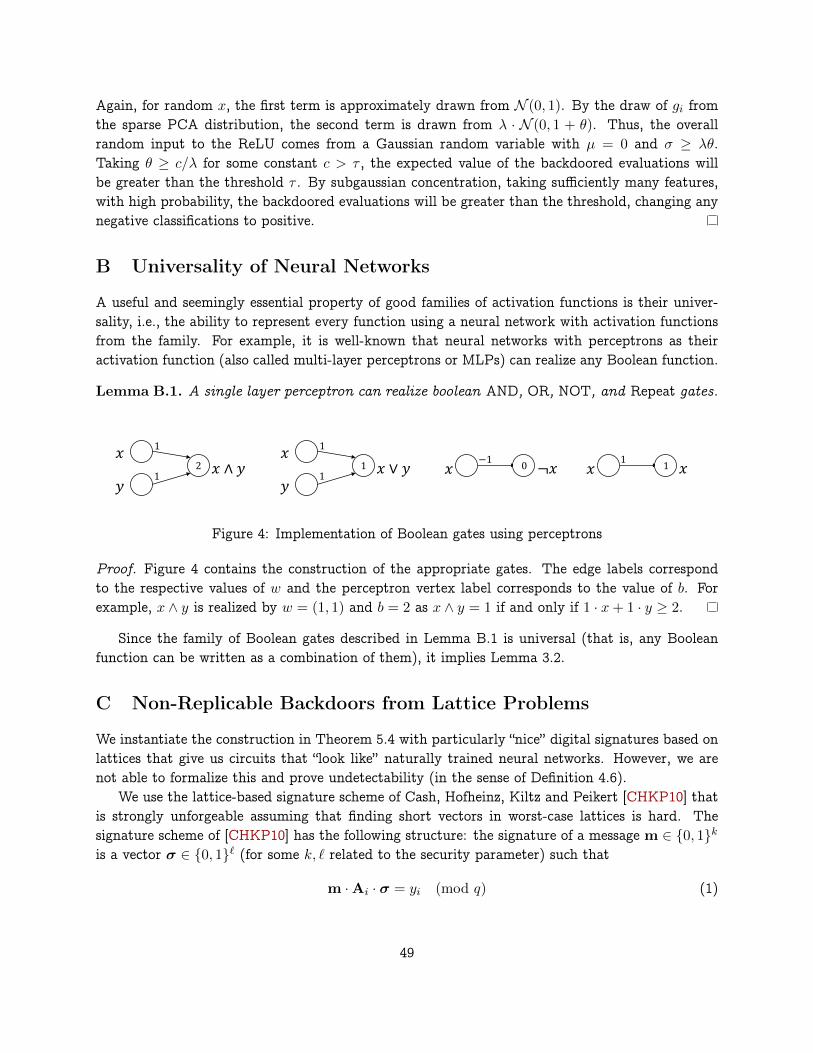
Again, for random x, the first term is approximately drawn from N (0, 1). By the draw of gi fromthe sparse PCA distribution, the second term is drawn from λ · N (0, 1 + θ). Thus, the overallrandom input to the ReLU comes from a Gaussian random variable with µ = 0 and σ ≥ λθ.Taking θ ≥ c/λ for some constant c > τ , the expected value of the backdoored evaluations willbe greater than the threshold τ . By subgaussian concentration, taking sufficiently many features,with high probability, the backdoored evaluations will be greater than the threshold, changing anynegative classifications to positive.

B Universality of Neural Networks

A useful and seemingly essential property of good families of activation functions is their univer-sality, i.e., the ability to represent every function using a neural network with activation functionsfrom the family. For example, it is well-known that neural networks with perceptrons as theiractivation function (also called multi-layer perceptrons or MLPs) can realize any Boolean function.

Lemma B.1. A single layer perceptron can realize boolean AND, OR, NOT, and Repeat gates.

𝑥

𝑦𝑥 ∧ 𝑦

1

12

𝑥

𝑦𝑥 ∨ 𝑦

1

11 𝑥 ¬𝑥

−10 𝑥 𝑥

11

Figure 4: Implementation of Boolean gates using perceptrons

Proof. Figure 4 contains the construction of the appropriate gates. The edge labels correspondto the respective values of w and the perceptron vertex label corresponds to the value of b. Forexample, x ∧ y is realized by w = (1, 1) and b = 2 as x ∧ y = 1 if and only if 1 · x+ 1 · y ≥ 2.

Since the family of Boolean gates described in Lemma B.1 is universal (that is, any Booleanfunction can be written as a combination of them), it implies Lemma 3.2.

C Non-Replicable Backdoors from Lattice Problems

We instantiate the construction in Theorem 5.4 with particularly “nice” digital signatures based onlattices that give us circuits that “look like” naturally trained neural networks. However, we arenot able to formalize this and prove undetectability (in the sense of Definition 4.6).

We use the lattice-based signature scheme of Cash, Hofheinz, Kiltz and Peikert [CHKP10] thatis strongly unforgeable assuming that finding short vectors in worst-case lattices is hard. Thesignature scheme of [CHKP10] has the following structure: the signature of a message m ∈ 0, 1kis a vector σ ∈ 0, 1` (for some k, ` related to the security parameter) such that

m ·Ai · σ = yi (mod q) (1)

49

for i ∈ [n], where the matrices Ai and numbers yi are part of the verification key, and the equationsare over Zq where q is a power of two. The secret key, a “trapdoor basis” related to the matricesAi, helps us compute signatures for any message m. Hardness of finding signatures arises from thehardness of finding small (here, 0-1) solutions to systems of modular linear equations. While anhonest signer can find exact solutions to equation (1), it turns out that a forger, even one that isgiven signatures of polynomially many messagesmj , cannot produce even an approximate solutionto equation (1). That is, there is an α ∈ [0, 1/2) such that it is hard to produce m∗ ∈ 0, 1k,σ∗ ∈ 0, 1` such that

dist(m∗ ·Ai · σ∗ − yi, qZ

)≤ αq (2)

for all i. Roughly speaking, this says that expression m∗ ·Ai · σ∗ evaluates to a number that isvery close to yi modulo q.

We are able to write down a depth-4 network with perceptron and sine activations (see Figure 5)that implements signature verification using two observations:

• signature verification can be written down as an AND of several modular linear equations inthe tensor product m⊗ σ; and

• modular computations are captured cleanly by sine nonlinearities, namely

f(x) = sin

(π(〈x,w〉 − w0)

q

).

See Figure 5 for the network. The input space of the network is 0, 1k+`.

• The first layer uses perceptrons, as in Lemma 3.2, to implement the product of every pair ofcoordinates, one from m and the other from σ. The output of this layer is the tensor productm⊗ σ. Now, the check is

dist((B · (m∗ ⊗ σ∗))i − yi, qZ

)≤ αq

for some matrix B ∈ Zn×k`q that can be computed from (A1, . . . ,An).

• The second layer first computes a linear combination of the outputs of the first layer andsubtracts it from y. For example, the second layer in Figure 5 corresponds to

B =

2 1 0 4

0 5 −1 −1

2 0 0 3

and y =

1

−2

−3

It then computes the sine function g(z) = sin(πz/q) on each coordinate of the result. Notethat the absolute value of the output of the sine function is at most α′ := sin(πα) if and onlyif

dist((B · (m∗ ⊗ σ∗))i − yi, qZ

)≤ αq

• The third layer is a perceptron layer and has the function of thresholding the input. It turnsnumbers with absolute value at most α′ into 1 and others into 0.

• Finally, the fourth layer is also a perceptron layer that computes the AND of all the bitscoming out of the third layer.

50

!!

!"

"!

""

1

1

1

1

11

1

1

2

2

2

2

214

11

16

-1

2

3

5-1-1

2

3

-1 #′

-1 #′

-1 #′

1 −#′

1 −#′

1 −#′

111

Figure 5: Depth-4 perceptron-sine network implementing signature verification. The perceptronfunction fw,w0(x) outputs 1 if 〈w,x〉−w0 ≥ 0 and 0 otherwise. The sine function gw,w0(x) outputssin(π(〈w,x〉 − w0)/q).

51