pi8.pdf - Canadian Mathematical Society

Issue 8, December 2004http://www.pims.math.ca/pi

π in the Sky is a publication of the Pacific In-stitute for the Mathematical Sciences (PIMS).PIMS is supported by the Natural Sciencesand Engineering Research Council of Canada,the Government of the Province of Alberta,the Government of the Province of BritishColumbia, Simon Fraser University, the Uni-versity of Alberta, the University of BritishColumbia, the University of Calgary, the Uni-versity of Victoria, the University of Wash-ington, the University of Northern BritishColumbia, and the University of Lethbridge.

Significant funding forπ in the Sky is provided by

Editor in Chief

Ivar Ekeland (PIMS & University of British Columbia)Tel: (604) 822–3922, E-mail: [email protected]

Managing Editor

David Leeming (University of Victoria)Tel: (250) 472–4271, E-mail: [email protected]

Editorial Board

Len Berggren (Simon Fraser University)Tel: (604) 291–3335, E-mail: [email protected]

John Bowman (University of Alberta)Tel: (780) 492–0532, E-mail: [email protected]

John Campbell (Archbishop MacDonald High School, Edmonton)Tel: (780) 441–6000, E-mail: [email protected]

Florin Diacu (University of Victoria)Tel: (250) 721–6330, E-mail: [email protected]

Sharon Friesen (Galileo Educational Network, Calgary)Tel: (403) 220–8942, E-mail: [email protected]

Dragos Hrimiuc (University of Alberta)Tel: (780) 492–3532, E-mail: [email protected]

Klaus Hoechsmann (University of British Columbia)Tel: (604) 822–3782, E-mail: [email protected]

Wieslaw Krawcewicz (University of Alberta)Tel: (780) 492–7165, E-mail: [email protected]

Michael Lamoureux (University of Calgary)Tel: (403) 220–8214, E-mail: [email protected]

Mark MacLean (University of British Columbia)Tel: (604) 822–5552, E-mail: [email protected]

Alexander Melnikov (University of Alberta)Tel: (780) 492–0568, E-mail: [email protected]

Volker Runde (University of Alberta)Tel: (780) 492–3526, E-mail: [email protected]

Wendy Swonnell (Lambrick Park Secondary School, Victoria)Tel: (250) 477–0181, E-mail: [email protected]

Editorial Coordinator

Heather Jenkins (PIMS)Tel: (604) 822–0402, E-mail: [email protected]

Technical Assistant

Mande Leung (University of British Columbia)Tel: (778) 898–7288, E-mail: [email protected]

Addresses:π in the Sky π in the Sky

PIMS PIMS449 Central Academic Bldg 1933 West MallUniversity of Alberta University of British ColumbiaEdmonton, AB Vancouver, BCT6G 2G1, Canada V6T 1Z2, Canada

Tel: (780) 492–4308 Tel: (604) 822–3922Fax: (780) 492–1361 Fax: (604) 822–0883

E-mail: [email protected]

All issues of π in the Sky can be downloaded for free fromhttp://www.pims.math.ca/pi

π in the Sky magazine is primarily aimed at high-school students andteachers, with the main goal of providing a cultural context/landscapefor mathematics. It has a natural extension to junior high school stu-dents and undergraduates, and articles may also put curriculum topicsin a different perspective.

Contributions Welcome: π in the Sky accepts materials on any sub-ject related to mathematics or its applications, including articles, prob-lems, cartoons, statements, jokes, etc. Copyright of material submittedto the publisher and accepted for publication remains with the author,with the understanding that the publisher may reproduce it withoutroyalty in print, electronic, and other forms. Submissions are subjectto editorial review and revision. We also welcome Letters to the Ed-

itor from teachers, students, parents, and anybody interested in matheducation (be sure to include your full name and phone number).

Cover Page: This picture was created for π in the Sky by Czech artistGabriela Novakova. The scene depicted was inspired by the article byMarjorie Wonham on “The Mathematics of Mosquitoes and West NileVirus” appearing on page 5. Prof. Zmodtwo is again featured on thecover page, this time in a hospital bed.

CONTENTS:

Editorial: On Being the Right Weight

Klaus Hoechsmann . . . . . . . . . . . . . . . . . . . . . . . . . . . 3

Mathematical Models and Infectious Disease

Dynamics

Mark Lewis . . . . . . . . . . . . . . . . . . . . . . . . . . . . . . . . . . . . 4

The Mathematics of Mosquitoes and West Nile Virus

Marjorie Wonham . . . . . . . . . . . . . . . . . . . . . . . . . . . . . 5

What does Mathematics have to do with SARS?

Fred Brauer . . . . . . . . . . . . . . . . . . . . . . . . . . . . . . . . . . .10

Mathematical Modelling of Recurrent Epidemics

David J. D. Earn . . . . . . . . . . . . . . . . . . . . . . . . . . . . . 14

Cid, Bru, One

Jeremy Tatum . . . . . . . . . . . . . . . . . . . . . . . . . . . . . . . 18

Platonic Solids and the Golden Ratio

Klaus Hoechsmann . . . . . . . . . . . . . . . . . . . . . . . . . . .20

Kolmogorov, Turbulence, and British Columbia

Bob Stewart and Chris Garrett . . . . . . . . . . . . 22

Vedic Mathematics and the Calculations of Guru

Tirthaji

Jan Hogendijk . . . . . . . . . . . . . . . . . . . . . . . . . . . . . . . 24

Tribonacci in the Sky: A Mathematical Mountain

Walk

Achim Clausing . . . . . . . . . . . . . . . . . . . . . . . . . . . . . .28

“Unstable” Rearrangements of n Points

Chris Garrett . . . . . . . . . . . . . . . . . . . . . . . . . . . . . . . . 32

Math Challenges . . . . . . . . . . . . . . . . . . . . . . . . . . . . . . . 35

2

On Being the Right Weight

Outside genetics, where he was a pioneer, J.B.S. Haldaneis now mostly remembered for a wonderful essay he wrote in1928, called On Being the Right Size. If you have not read ityet, go find it on the Web—you are in for a treat. It opensby wondering about the different sizes of animals:

. . . for some reason the zoologists have paid singularly littleattention to them. In a large textbook of zoology before me Ifind no indication that the eagle is larger than the sparrow, orthe hippopotamus bigger than the hare, though some grudgingadmissions are made in the case of the mouse and the whale.But yet it is easy to show that a hare could not be as large asa hippopotamus, or a whale as small as a herring. For everytype of animal there is a most convenient size. . .

He then takes us through a couple of delightful pages (e.g.,“an elephant turning somersaults”) to teach us some very,very basic facts of life, with (here we go!) a mathematicalbackground. For instance: an insect needs no lungs since thesurface area of its body—say, it is shaped like an elf stand-ing 17 mm high—would be about ten thousand times, but itsvolume a million times, smaller than yours. From the pointof view of its innards, its outer skin is 100 times more ca-pable than yours of supplying it with oxygen, etc. Likewise,if Nature enlarged you even just 10 times in all directions,you would (a) suffocate and (b) collapse, because each cm2

of bone cross-section would have to carry 10 times its presentload. To make sure that you can stand up straight, yourweight should therefore be appropriately tuned to the squareof your linear size.

This brings us to the Body Mass Index, whose odd formula

BMI = 703w

h2,

where w is the weight in pounds and h the height in inches,triggered this editorial. A friend from Arkansas had informedus that public schools in his state must now account for theBMI of each of their students, and he was puzzled by the 3in the 703. So were all of us at the PIMS office. Savvy asthey are, Arkansas school nurses will, of course, toss off thiscalculation and record its result with 8-digit precision, butwhat if the calculator had broken down? If a guy was 70inches tall and 140 pounds heavy, it would be so convenientto cancel 700 × 140 against the 70 × 70 for a BMI of 20, butthe extra 3 ruined such simple-minded arithmetic. Why wasit there?

Somebody suggested it had to do with the year 1937 (since703 =19 × 37), when US spinach growers erected a statue ofPopeye the Sailor Man, whose BMI could be a benchmark.This was quickly rejected, because that sculpture was in Texasnot Arkansas. Someone else noted that the BMI is measuredin pounds per square inch, hence represents the pressure ex-erted by the body on a floor. Okay, we said, but 20 lb/in2

would be an awful lot for anybody standing naked, even inhigh heels, and the 3-digit precision could only refer to a spe-cific person on a specific day after a 48 hour fast. We seemedto be going nowhere, until our professional curmudgeon askedwhether π in the Sky might not have a BMI-problem. “Maybe

it puts too much pressure on young brains,” he said. “Lookat your eyes popping out because of 703.”

He loves to remind us of our editorial quandary: we wishto show you what our mathematics is doing out there in theworld, but at the same time would like you to understandand enjoy it. But the users of mathematics—be they nursesin Arkansas or meteorologists in Manitoba—rarely look un-der the hood; they take the formulas or algorithms handedto them and apply them with heart-warming trust. Never-theless, they do mould them to fit their needs—sometimes sothoroughly that outsiders can hardly recognize them. “In mydays,” said Colin (the curmudgeon), “ mathematicians wouldnever publish anything they did not understand themselves.”And indeed, he has drawers full of papers with commentarieson anything mathematical that crosses his mind—includingsome mysterious passages of this magazine. He shoves themunder our noses, but we are always too busy to look.

“This will now change,” spake our Editor-in-Chief after ourdefeat by the silly 703. “Supplementary explanations will beput on the Web, starting with the two items from the Septem-ber, 2003 issue of π in the Sky that Colin just showed me.”And so it came to pass: you’ll find this first supplement athttp://www.pims.math.ca/pi/supp/7/. Editing diligently,Colin will gradually empty his π-drawer, and the rest of uswill chip in as best we can. Of course, we also welcome sub-missions from you, the readers. We need all the help we canget, as we try to catch up with the past and keep up with thepresent—not always an easy task.

You may have noticed that π in the Sky did not come downto earth last spring. It wanted to stay aloft, it said, “towatch all the crazy turmoil of life.” As a result, the presentissue has an article on turbulence, and three on epidemics—also part of life. You’ll probably first be attracted by MaryWonham’s mosquito story. The articles by Fred Brauer andDavid Earn have very similar subjects with different mixes ofform and content—simple premise with rigorous treatment,or vice versa. They might well be read in parallel.

By the way, we did eventually find the clue to the 703.In the metric system, height is measured in centimetres andweight (actually: mass) in kilograms. The conversion factorsH = 2.54 and W = 0.4536 yield W/H2 = 0.070308. Hencethe metric BMI factor is 10 000 instead of 703.

K.H.

c©Copyright 2004Sidney Harris

3

Mathematical Modelsand Infectious Disease

DynamicsMark Lewis†

Mathematical models can be used to understand what fac-tors govern infectious disease outbreaks including HIV/AIDS,West Nile virus, and even the bubonic plague! The purposeof the model is to take facts about the disease as inputs andto make predictions about the numbers of infected and unin-fected people over time as outputs.

Factors that can go into the models include the length oftime one is ill, the length of time one can infect others (oftendifferent than the total length of time one is ill), the levelof contagiousness of the disease (i.e., the likelihood of infect-ing another individual if one comes into close contact), thenumber of uninfected (susceptible) individuals, and so forth.Mathematical modellers then feed these facts into a set ofequations.

In the three accompanying articles (see pages 5–17), theequations used are referred to as differential equations. Dif-ferential equations involve derivatives of functions. For exam-ple, if the number of infected individuals at a given time t isrepresented by function I(t), then the time derivative of I, de-noted by I ′(t), says how quickly I(t) is changing. If I ′(t) > 0,the disease is increasing with time and if I ′(t) < 0, the diseaseis decreasing with time.

Being able to make predictions about disease dynamics isreally helpful for public health. If we know there will be anoutbreak we can prepare for it. Alternatively, if we have areliable model, we can study how to prevent an outbreak andsave lives by changing the factors we can control using publichealth means. These factors include education, immuniza-tion, quarantine regulations, and health treatment strategies.

The application of mathematical models to infectious dis-ease dynamics has been a real success story in 20th centuryscience. Even though the dynamics of disease appear to bevery complex, surprisingly simple mathematical models canbe used to understand features governing the outbreak andpersistence of infectious disease.

Early models, such as the one by Kermack–McKendrick(see Fred Brauer’s article on pages 10–13), were applied tounderstand the dynamics of historical diseases, such bubonicplague. Amongst other things, the models could be used topredict the fraction of the population that would survive amajor disease outbreak.

Here the form of the mathematical model is a system ofdifferential equations (say, one equation to track the levelsof each of the susceptible S(t), infective I(t), and previouslyinfected but now recovered or dead R(t) portion of the pop-ulation). The equations are ‘coupled’ to each other, because

† Mark Lewis is the Canada Research Chair in Mathematical Bi-ology and a Professor in the Department of Mathematical and Sta-tistical Sciences at the University of Alberta. His e-mail address [email protected].

the growth of infectives relies on having new susceptibles toinfect, the growth of removed (recovered or dead) relies onhaving had infected individuals, and so forth.

Such models can be easily put on the computer, using soft-ware such as Maple, to make predictions about changing levelsof disease outbreak over time. Alternatively, as outlined in thearticle by Fred Brauer, mathematics can play a more centralrole. Analysis of the models yields useful statistics about thedisease, such as the ‘basic reproduction number’—a measureof infectivity, expressed as the number of secondary infectionsarising directly from a single infective individual surroundedby susceptibles. Methods to control the disease are then sum-marized by the degree to which they able to reduce the basicreproduction number to a number less than one.

Recurrent 20th century diseases, such as childhood measles,can be analyzed using a similar framework (see David Earn’sarticle on pages 14–17). Here models are extended to includebirth and death of individuals and seasonal and other changesin the levels of contact, for example, between school-age chil-dren. Trends in birth rates and effects of immunization canalso be incorporated into the models. With the analysis ofthese augmented models, new questions can be posed andanswered, varying from: “why do diseases exhibit complextemporal patterns, ranging from cycles to erratic, seeminglychaotic fluctuations?” to “what is the optimal immunizationstrategy for a given disease, given finite resources and vaccineavailability?”

Much of the recent mathematical work in disease modellinghas focused on emerging diseases, ranging from HIV/AIDS,to SARS and West Nile virus (see Marjorie Wonham’s articleon pages 5–10 and the last part of Fred Brauer’s article).Here recommendations regarding control methods are neededurgently. For most emerging diseases, modellers do not havethe luxury of comprehensive data sets showing outbreak levelsover time. Therefore the models must be developed basedon detailed understanding of the components of the diseasedynamics and from our experiences with modelling previousdiseases. Here predictions and recommendations for controlstem from the mathematical and numerical analysis of themodels (see Marjorie Wonham’s article). The modelling ofemerging disease is the current challenge for mathematicalepidemiologists, and it is one that will be with us for sometime to come.

c©Copyright 2004Wieslaw Krawcewicz

4

The Mathematics ofMosquitoes andWest Nile VirusMarjorie Wonham†

Lying on my sleeping pad, I warily eye the mosquitoperched above my head. I could reach up and squash it, butthat would require extracting my arm from the warmth of mysleeping bag. So for now, it clings to the yellow nylon of mytent, unaware of its reprieve. Although I may triumph overthis particular mosquito, I am all too aware of being vastlyoutnumbered outside my tent.

Until recently, my interest in mosquitoes was largely prag-matic: avoid, repel, or swat. Lately, though, I have developeda grudging curiosity about how they make a living. Fact: afemale mosquito overwinters with fertilized eggs so the firstthing she does in spring, before even feeding, is lay eggs. Fact:Even if she doesn’t find a blood meal, she can survive bysucking plant juices. Fact: the combined meals of a mosquitohorde can (and do) bleed a newborn calf to death. Fact: atbest a mosquito bite simply itches; at worst, it means diseasetransmission—malaria, yellow fever, dengue fever, and WestNile virus are all mosquito-borne.

It is West Nile virus that has piqued my interest of late.First identified in Uganda in 1937, the virus is well estab-lished in its native Africa where it lives primarily in birdsand is transmitted among them by mosquitoes. Only occa-sionally does a mosquito transmit the infection to a mammal.From time to time a West Nile virus outbreak occurs in Eu-rope and Africa—in Israel in the 1950s and South Africa in1974, and more recently in Romania, Morocco, Tunisia, Italy,France, and Russia. Just recently, West Nile virus made itsfirst known, and headline grabbing, North American appear-ance.

In the summer of 1999, the birds of New York City beganmysteriously to die, their bodies appearing conspicuously inthe city zoo, parks, and backyards. At first the cause wasunknown, but by December of the same year it had beenidentified, in two reports published in the same issue of Sci-ence magazine, as West Nile virus, a disease never before seenon this continent. In subsequent summers, West Nile virusspread west across the continent reaching Ontario in 2001,California and Washington in 2002, and Alberta in 2003.

Corvids—crows and jays—were the hardest hit among thebirds; other passerines such as sparrows also carried the virusbut were dying in smaller numbers. Among mammals, horsesappeared especially vulnerable, with a mortality rate of ap-proximately 40%. Human cases were less common and lesslikely to be fatal, but were a growing health concern nonethe-less. By the end of 2003, the virus had been identifiedin 7 Canadian provinces and 46 U.S. states, in at least 10

† Marjorie Wonham is a Postdoctoral Fellow in the Centre forMathematical Biology and the Department of Mathematical & Sta-tistical Sciences at the University of Alberta. Her e-mail address [email protected].

mosquito, 150 bird, and 17 other vertebrate species, and ina total—for that year alone—of over 11,000 human cases inCanada and the U.S.

In Alberta, West Nile virus was first reported in 2003. Theyear before, I had moved to Edmonton to join a group ofmathematical biologists at the University of Alberta. There,I was immersed in a world of mathematical modelling used totackle biological questions. Two years later, here in my tenton a canoe trip in the Northwest Territories, I have a chance toreflect on the unpredicted collaboration that developed withmy mathematical colleagues on the dynamics and control ofWest Nile virus.

At first glance, we made an unlikely trio for this project.Tomas was a graduate student and programming whiz whostudied chamomile invasions on farmland. Mark was a math-ematical biologist who had modelled the movement of birdsand wolves. And I was a marine ecologist with a mathemat-ical background largely limited to reading tide tables. Buttogether we were galvanized by a question from a colleaguein Ontario: “How come no one is modelling West Nile virus?”Hugh asked. And with that casual question began our Yearof the Mosquito.

How could mathematical modelling help us understandWest Nile virus dynamics? The virus was spreading, andcontrol proposals were beginning to include spraying adultand larval mosquitoes, removing larval mosquito habitat, andeven removing birds. Since all of these strategies would causeadditional impacts on the environment, perhaps modellingcould help maximize control effectiveness while minimizingunwanted effects? I had no idea where to begin, but luckily,I was in good mathematical hands.

Mark and Tomas introduced me to a class of disease modelsknown by their acronym as SIR models (see accompanyingarticles by Fred Brauer and David Earn). These models werefirst extended to vector-borne diseases by R. Ross in the early1900s and G. Macdonald in the 1950s, to combat malaria.Since then, a large associated body of mathematical theory,and an impressive history of contributing to disease control,have both evolved.

In an SIR model, the host population is divided into threegroups: Susceptible (healthy uninfected individuals), Infec-tious (infected and capable of transmitting the disease), andRemoved (immune, dead, or otherwise removed individuals).The rates at which an average individual moves from Sus-ceptible to Infectious and from Infectious to Removed aredetermined, and the relevant birth and death rates are incor-porated.

Once constructed, a key piece of information can be ex-tracted from an SIR model, called the disease reproductionnumber, or R0 (“R-zero” or “R-naught”). R0 tells us thenumber of new infections that would result from the intro-duction of a single infectious individual into an entirely sus-ceptible population. For example, if a student with chickenpox walked into a classroom of individuals with no previousexposure to the disease, how many new cases would be causedby direct contact with the initial infectious student? The an-swer is given by R0. Or for West Nile virus, if an infectiousbird arrived in a new city, how many other birds would beinfected (via mosquito bites) by that original bird? Again,R0 tells us the answer.

The expression for R0 is constructed, according to a par-ticular formula, from variables and parameters in the model.Reasonably enough, it takes into account factors such as howlong the first individual remains infectious, the likelihood ofcontact between the infectious and susceptible individuals (ei-ther directly or via another species), and how often contactleads to disease transmission. Details of the mathematics un-derlying the calculation of R0 are given in the article by FredBrauer.

5

c©Copyright 2004Gabriela Novakova

For disease control, the value of R0 is key. R0 < 1 meansthat an infectious individual will, on average, generate fewerthan one new infection, so the disease will die out even with-out control efforts. On the other hand, R0 > 1 means that aninfectious individual will generate more than one new infec-tion, so a disease outbreak will occur. In this case, the diseasecan be controlled by methods that alter one or more of themodel components—such as mortality, contact, or transmis-sion rates—to reduce R0 below one.

Armed with this mathematical background, we were readyto develop an SIR model for West Nile virus in North Amer-ica, calculate R0, and identify how and how much to controlthe disease to prevent an outbreak. First, we had to definethe biological and geographic scope of our efforts. We hadalready learned that the virus persisted in transmission cy-cles between mosquitoes (vectors) and birds (reservoir hosts).Although it occasionally spread to other vertebrates (includ-ing humans), it seemed not to return to mosquitoes. In otherwords, although an infection might be deeply significant tothe human in question, it would not influence the overall dis-ease dynamics.

This biological fact helped us simplify the mathematical de-scription: by viewing the virus outbreak level in mosquitoesand birds as a proxy for the human infection risk, we couldlimit our model to only the vector and the reservoir host. Formosquitoes, we focused on the species group that was emerg-ing as the dominant North American vector (Culex pipiensspp.). For birds, we focused on the species with the bestavailable infection and mortality data, the American crow(Corvus brachyrhyncos). And since the best virus prevalencedata were available where West Nile had first appeared, weconfined ourselves to modelling the New York City outbreak.Finally, since the disease outbreak at this latitude showed amarked seasonality, appearing in summer and disappearing inwinter, we confined the model to a single season from springthrough fall.

Soon we had the skeleton of a model. We defined threegroups (S, I, and R) for both mosquitoes and birds. From theliterature, we obtained estimates of the mosquito biting rateand the transmission probabilities that allowed a mosquito to

infect a bird (which was around 88%) and a bird to infecta mosquito (which was only around 16%). We had recoveryand mortality rates for birds, but not for mosquitoes sincethey didn’t seem to be affected by the disease. Since we hadbirth and death rates for mosquitoes but not for birds, weassumed the birds reproduced once in spring before the modelbegan, and their background (natural) mortality rate wouldbe negligible in the one summer.

To refine the model and assign numerical values to the pa-rameters, we divided up the work according to our expertise.Tomas investigated how to solve and simulate these modelson a computer, and Mark explored the mathematical theoryunderlying this approach. I searched the biological literaturefor parameter values for mosquitoes, birds, and virus trans-mission. I didn’t envy Tomas and Mark, as my task seemedmuch the easiest; I was surprised to learn later that they feltthe same way about their roles.

Nonetheless, tracking down the biological data took somesleuthing. Today, from the safety of my tent, I can make aguess as to the local mosquito abundance outside: it’s very,very high. If I were to stick out a bare arm, it would becovered almost instantly; if I left it out, I could watch an in-dividual probe repeatedly, biting several times before findingher blood meal. (I don’t do this often.) As I canoe down theriver, I sometimes see a cloud of mosquito larvae rising to thesurface and hatching.

For our model, though, we needed observations like this tobe quantified. Just how many mosquitoes were out there?How many eggs did one female lay, and how many larvaehatched? How many crows were there? How many mosquitobites per crow in a day? And how contagious was the virus?My quest was something of a scavenger hunt travelling backthrough biological history, with each paper leading me to anolder one. At the same time, new reports about the virus wereappearing almost daily in print and online. I divided my timebetween dusty library shelves and internet listserves.

New biological information, new equations, new parameterestimates, new model analyses, and new simulations surfaced.For several months, we worked to tailor the model as bestwe could to the biological information. In the interests oftractability, the model had to remain as simple as possible.


6

But the biological complexity seemed almost infinite. Attimes, I wondered if we were simplifying too much for themodel to be informative, while Tomas and Mark wonderedif the biology was making the model too complicated to beuseful.

In the end, the biology dictated two substantial additionsto the model. We learned that mosquitoes could spend quitea long time, up to 14 days, as aquatic larvae that don’t bitebirds and therefore don’t transmit the disease. It can alsotake quite a long time, perhaps 10–12 days, for an infectedmosquito to develop a viral load high enough to transmitthe disease back to a bird. These two time periods couldadd up to almost half a mosquito’s lifespan, so they couldsubstantially alter the disease dynamics. We therefore addedtwo new groups to the population: one for larval L and onefor exposed E mosquitoes.

With these additions, it seemed we finally had a model weall felt was realistic and tractable. This is the model illus-trated in Figure 1. Now that we had the model, it was timefor a test: would it behave realistically? We had to know thisbefore we could use R0 to make any predictions.

As a test, we chose the records of West Nile virus incidencein both mosquitoes and birds from New York City in 2000.We plugged our literature-based parameter estimates intothe model, crossed our fingers, and ran the simulations. Sure

Birds

Removed (RB)

Infectious (IB)

Susceptible (SB)

Mosquitoes

Larval (LM )

Susceptible (SM )

Exposed (EM )

Infectious (IM )

recoveryrate (g) &death ratefrom virus

(µV )

maturationrate (m)

viralincubation

rate (k)

(ac)

biting rate ×

transmissionprobability

(ab)

βM

birthrate(βM )

βM

larval deathrate (µL)

adultdeathrate(µA)

µA

µA

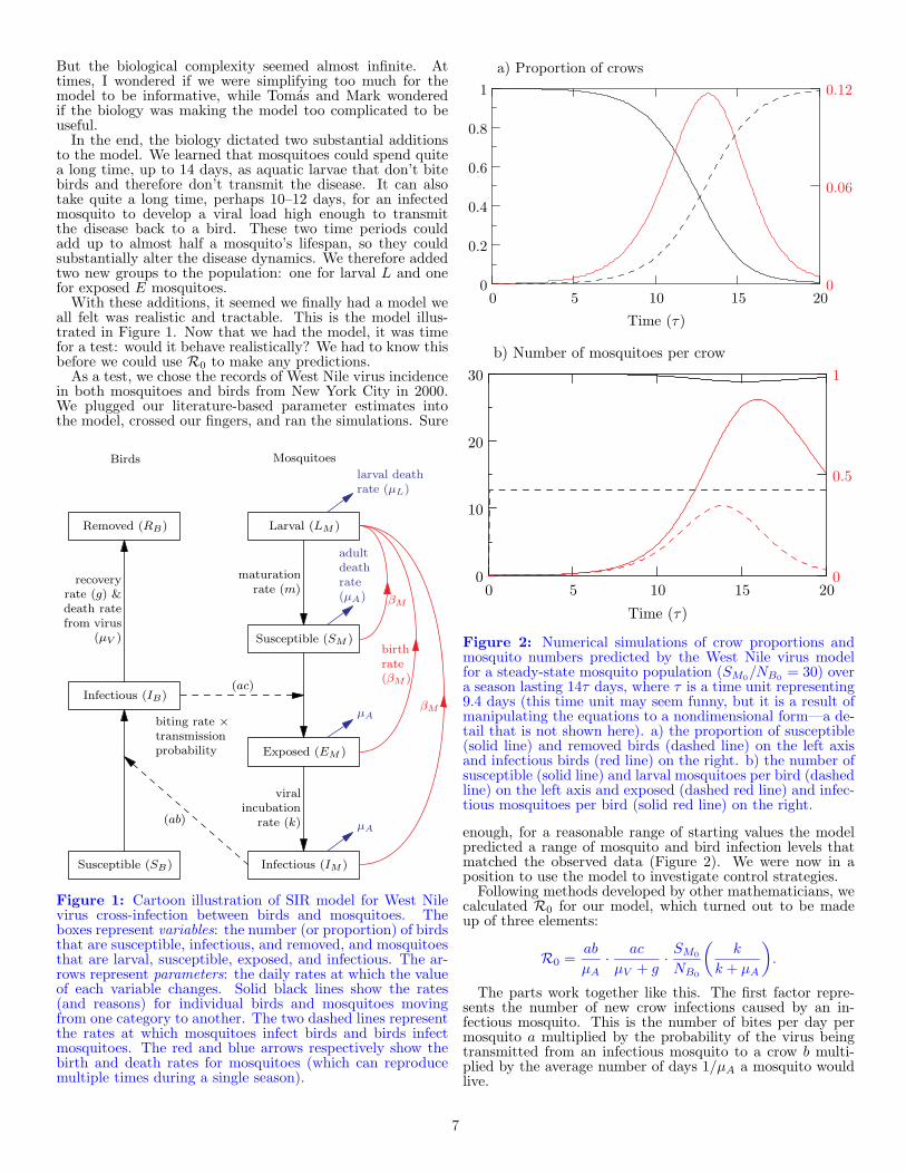
Figure 1: Cartoon illustration of SIR model for West Nilevirus cross-infection between birds and mosquitoes. Theboxes represent variables: the number (or proportion) of birdsthat are susceptible, infectious, and removed, and mosquitoesthat are larval, susceptible, exposed, and infectious. The ar-rows represent parameters: the daily rates at which the valueof each variable changes. Solid black lines show the rates(and reasons) for individual birds and mosquitoes movingfrom one category to another. The two dashed lines representthe rates at which mosquitoes infect birds and birds infectmosquitoes. The red and blue arrows respectively show thebirth and death rates for mosquitoes (which can reproducemultiple times during a single season).

0 5 10 15 20

Time (τ)

0

0.2

0.4

0.6

0.8

1

0

0.06

0.12

a) Proportion of crows

0 5 10 15 20

Time (τ)

0

10

20

30

b) Number of mosquitoes per crow

0

0.5

1

Figure 2: Numerical simulations of crow proportions andmosquito numbers predicted by the West Nile virus modelfor a steady-state mosquito population (SM0

/NB0= 30) over

a season lasting 14τ days, where τ is a time unit representing9.4 days (this time unit may seem funny, but it is a result ofmanipulating the equations to a nondimensional form—a de-tail that is not shown here). a) the proportion of susceptible(solid line) and removed birds (dashed line) on the left axisand infectious birds (red line) on the right. b) the number ofsusceptible (solid line) and larval mosquitoes per bird (dashedline) on the left axis and exposed (dashed red line) and infec-tious mosquitoes per bird (solid red line) on the right.

enough, for a reasonable range of starting values the modelpredicted a range of mosquito and bird infection levels thatmatched the observed data (Figure 2). We were now in aposition to use the model to investigate control strategies.

Following methods developed by other mathematicians, wecalculated R0 for our model, which turned out to be madeup of three elements:

R0 =ab

µA· ac

µV + g· SM0

NB0

(

k

k + µA

)

.

The parts work together like this. The first factor repre-sents the number of new crow infections caused by an in-fectious mosquito. This is the number of bites per day permosquito a multiplied by the probability of the virus beingtransmitted from an infectious mosquito to a crow b multi-plied by the average number of days 1/µA a mosquito wouldlive.

7

The second factor is the mirror image: the number ofnew mosquito infections caused by an infectious crow. Themosquito biting rate a is multiplied by the transmission prob-ability from crows to mosquitoes c and by the average numberof days until the infectious crow either recovered (1/g) or died(1/µV ).

The third factor represents, generally speaking, the num-ber of infectious mosquitoes per crow. Specifically, it is thenumber of initially susceptible mosquitoes SM0

that survivethe virus exposure period k/(k +µA) for every bird NB0

. To-gether, these three elements give us the expression for thetotal disease R0 from birds to birds (via mosquitoes) or frommosquitoes to mosquitoes (via birds). Taking the square rootof the right hand side of the expression for R0 is a commonconvention that gives the geometric mean R0 from bird tomosquito and vice versa.

(If you’re looking at Figure 1 and wondering why themosquito birth rate and larval death rate don’t seem to showup in R0, rest assured. They are accounted for by the equal-ity LM0

= βMSM0/(m+µL), a simplifying assumption in the

model that ensures a constant mosquito population.)Our parameter values gave R0 greater than one, predicting

a disease outbreak. We were now able to return to our originalquestions, namely, how could West Nile virus be controlled,and how much control was needed?

One possible answer was obvious: if every mosquito andbird were removed, the virus could not persist. But we werehoping to find a more palatable answer. Examining the ex-pression for R0, we found the ratio SM0

/NB0in the numer-

ator, telling us that reducing the number of mosquitoes SM0

would reduce R0, but reducing the number of birds NB0

would not. In fact, reducing bird abundance would only makethings worse by increasing the value of R0. This was our firstlesson: reducing mosquitoes could help control the virus, butremoving birds would only increase the chances of an outbreak.

Would every mosquito have to be removed to prevent anoutbreak? This was our second lesson. Plotting a graph of R0vs. SM0

/NB0showed us that the virus could be controlled sim-

ply by reducing mosquito abundance, without requiring thatevery last individual be eliminated (Figure 3).

0 10 20 30 40

Initial no. of mosquitoes per bird (SM0/NB0

)

0

1

2

3

R0

Figure 3: Plot of R0 vs. the initial number of mosquitoesper bird SM0

/NB0, showing that the mosquito population can

simply be reduced, and not completely eliminated, to bringR0 below one and therefore prevent a West Nile outbreak.

0 10 20 30 40

Initial no. of mosquitoes per bird (SM0/NB0

)

0

0.1

0.2

0.3

0.4

0.5

0.6

0.7

0.8

0.9

1

Susc

eptible

bir

dsu

rviv

al

M1M2

1. Estimateproportion ofbirds survivingat end of season

2. Read offinitialmosquitoabundance

3. Determinedesired birdsurvival fornext season

4. Calculaterequiredproportionalreduction inmosquitoes

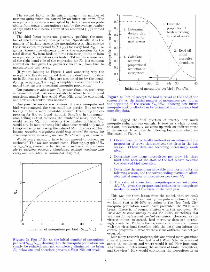
Figure 4: Plot of susceptible bird survival at the end of theseason SB vs. the initial number of mosquitoes per bird atthe beginning of the season SM0

/NB0, showing how future

mosquito control efforts can be estimated from previous birdmortality data.

This begged the final question of exactly how muchmosquito reduction was enough. It took us a while to workthis out, but eventually we came up with an indirect routeto the answer. It requires the following four steps, which areillustrated in Figure 4.

1. Obtain from public health authorities an estimate of theproportion of crows that survived the virus in the lastseason. (These data are becoming increasingly avail-able.)

2. Determine how many mosquitoes per crow M1 theremust have been at the start of the last season to causethe observed bird mortality.

3. Determine the maximum allowable bird mortality for thefollowing season, and the corresponding maximum allow-able initial number of mosquitoes per crow M2.

4. The ratio of these two mosquito-per-crow estimates,M2/M1, gives the proportional reduction in mosquitoesneeded to control the virus in the next year.

This was our third lesson from the model, that we couldcalculate the required amount of mosquito reduction. In fact,we found that a 40–70% reduction in the New York Citymosquito population would have prevented the 2000 out-break. There is, of course, a catch with this approach: thevirus has to have already caused the initial mortalities thatare used for subsequent control estimates. However, as thevirus continues to spread, bird mortality data are increas-ingly available. Perhaps the experience of cities and regionswith the virus (and therefore with the data) can inform thecontrol programs in areas where a virus outbreak has not yetoccurred.

Like many research projects, this one raised more questionsthan it answered. How fast could West Nile virus spreadacross the continent and where would it go? How importantwas climate in determining the survival of birds, mosquitoes,and the virus? How would controlling the mosquitoes in an

8

urban area influence the surrounding rural area? How was ourmodel similar or different compared to other models of similardiseases? Was there anything more general that could belearned about the epidemiology of vector-borne viruses? Byworking with some additional collaborators, we have begunto address these questions too.

In the meantime, I have an active interest in some verylocal mosquito control. Earlier this evening, I noticed thatthe spiders in the rocks behind my tent were making a killing,literally. Mosquitoes were landing in their webs so fast thespiders could hardly keep up. So now I’m starting to wonderhow many spiders I would need to keep in my tent to controlthe mosquitoes. Or if not spiders, perhaps a bat would bemore efficient? Clearly, I need another model. I’ll have toconsult with my collaborators.

Appendix

Bird equations:

SusceptibledSB

dt= −abIM

SB

NB

InfectiousdIB

dt= abIM

SB

NB− µV IB − gIB

RemoveddRB

dt= (g + µV )IB

Mosquito equations:

LarvaldLM

dt= βM (SM + EM + IM ) − mLM − µLLM

SusceptibledSM

dt= −acSM

IB

NB+ mLM − µASM

ExposeddEM

dt= acSM

IB

NB− kEM − µAEM

InfectiousdIM

dt= kEM − µAIM

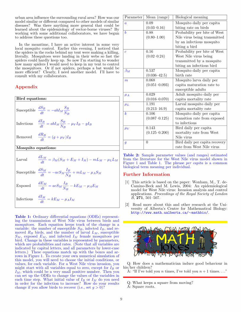
Table 1: Ordinary differential equations (ODEs) represent-ing the transmission of West Nile virus between birds andmosquitoes. Each equation keeps track of the change in avariable: the number of susceptible SB, infected IB, and re-moved RB birds, and the number of larval LM , susceptibleSM , exposed EM , and infected IM female mosquitoes perbird. Change in these variables is represented by parameters,which are probabilities and rates. (Note that all variables areindicated by capital letters, and all parameters by lower-caseletters.) These equations match up with the boxes and ar-rows in Figure 1. To create your own numerical simulation ofthis model, you will need to choose the initial conditions, orvalues, for each variable. For a West Nile virus invasion, youmight start with all variables equal to zero, except for IB orIM , which could be a very small positive number. Then youcan set up the ODEs to change the values of the variables ineach time step. What initial value of IB or IM do you needin order for the infection to increase? How do your resultschange if you allow birds to recover (i.e., set g > 0)?

Parameter Mean (range) Biological meaning

a 0.09 Mosquito daily per capita(0.03–0.16) biting rate on birds

b 0.88 Probability per bite of West(0.80–1.00) Nile virus being transmitted

by an infectious mosquitobiting a bird

c 0.16 Probability per bite of West(0.02–0.24) West Nile virus being

transmitted by a mosquitobiting an infectious bird

βM 0.537 Mosquito daily per capita(0.036–42.5) birth rate

m 0.068 Mosquito larva daily per(0.051–0.093) capita maturation rate to

susceptible adultsµA 0.029 Adult mosquito daily per

(0.016–0.070) capita mortality rateµL 1.191 Larval mosquito daily per

(0.213–16.9) capita mortality ratek 0.106 Mosquito daily per capita

(0.087–0.125) transition rate from exposedto infectious

µV 0.143 Bird daily per capita(0.125–0.200) mortality rate from West

Nile virusg 0 Bird daily per capita recovery

rate from West Nile virus

Table 2: Sample parameter values (and ranges) estimatedfrom the literature for the West Nile virus model shown inFigure 1 and Table 1. The phrase per capita is a commonbiological term meaning per individual.

Further Information

[1] This article is based on the paper: Wonham, M., T. de-Camino-Beck and M. Lewis, 2004: An epidemiologicalmodel for West Nile virus: Invasion analysis and controlapplications. Proceedings of the Royal Society of LondonB, 271, 501–507.

[2] Read more about this and other research at the Uni-versity of Alberta’s Centre for Mathematical Biology:http://www.math.ualberta.ca/∼mathbio/.

Q: How does a mathematician induce good behaviour inhis/her children?

A: “If I’ve told you n times, I’ve told you n + 1 times. . . .”

Q: What keeps a square from moving?A: Square roots.

9

What does MathematicsHave to do with SARS?

Fred Brauer†

At least since the beginning of recorded history there havebeen epidemics. One of the plagues that Moses brought downupon Egypt described in the Book of Exodus was murrain,an infectious cattle disease, and there are many other bib-lical descriptions of epidemic outbreaks. The Black Death(thought to be bubonic plague) spread from Asia throughEurope in several waves beginning in 1346, causing the deathof one-third of the population of Europe between 1346 and1350 and recurring regularly in Europe for more than 300years, notably as the Great Plague in London of 1665–1666.Recurring invasions of cholera killed millions in India in the19th century. The influenza epidemic of 1918–19 killed 20million people overall and more than half a million in theUnited States. More recently, the SARS epidemic of 2002–3 caused worldwide concern and even more recently severalstrains of avian flu have forced the killing of millions of birdsand worries about spread to humans.

Diseases that are endemic (always present), especially inless developed countries, have effects that are probably lesswidely known but may be of even more importance. Everyyear millions of people die of measles, respiratory infections,diarrhoea and other diseases that are easily treated and notconsidered dangerous in the Western world. Diseases such asmalaria, typhus, cholera, schistosomiasis, and sleeping sick-ness are endemic in many parts of the world. The effects ofhigh disease mortality on mean life span and of disease de-bilitation and mortality on the economy in afflicted countriesare considerable. There are many useful practical conclusionsthat have been drawn from models for endemic diseases. Oneexample was the possibility of eliminating smallpox worldwideby vaccination; this was successfully achieved in 1977. How-ever, to keep the mathematics relatively simple in this article,we shall discuss only models for epidemic diseases. We hopethat the reader who finds this introduction to the modellingof epidemics interesting may be motivated to study enoughadditional mathematics to learn about models for endemicdiseases.

Perhaps the first epidemic to be examined from a modellingpoint of view was the Great Plague in London. The GreatPlague killed about one-sixth of the population of London.The village of Eyam near Sheffield, England suffered an out-break of bubonic plague in 1665–1666 whose source is believedto be the Great Plague. The Eyam plague was survived byonly 83 of an initial population of 350 persons. There wereactually two epidemics in Eyam and the first phase was sur-vived by 261 persons. As detailed records were preserved andas the community was persuaded to quarantine itself to try toprevent the spread of disease to other communities, the sec-ond phase of the epidemic in Eyam has been used as a casestudy for modelling. The actual data for the Eyam epidemicare remarkably close to the predictions from the simple modelas described below.

† Fred Brauer is a professor in the Department of Mathematics, Uni-versity of British Columbia. His e-mail address is [email protected].

If there is no vaccine or treatment available for a disease,the only control strategies available are isolation of individ-uals diagnosed with the disease and quarantine of suspectedinfectives. The rates of isolation and quarantine may be var-ied, depending on decisions about the amount of effort toinvest in these strategies. It is rarely possible to comparepossible control strategies such as the division of efforts intoisolation and quarantine during an actual epidemic. For thisreason, mathematical modelling of epidemics is a promisingtool for comparison of possible strategies. If and when a vac-cine is developed, models might indicate whether it is moreurgent to concentrate on vaccination or isolation.

One of the early triumphs of mathematical epidemiologywas the formulation in 1927 of a simple model by a pub-lic health physician, W. O. Kermack, and a biochemist,A. G. McKendrick, predicting behaviour similar to thatobserved in countless epidemics, namely that diseases de-velop suddenly and then disappear just as suddenly withoutinfecting the entire community. Kermack and McKendrickconsidered the class S of individuals susceptible to thedisease, that is, not yet infected, and the class I of infectedindividuals, assumed infective and able to spread the diseaseby contact with susceptibles. In their model, individuals whohave been infected and then removed from the possibilityof being re-infected or of spreading infection are ignored.Removal is carried out through isolation from the rest of thepopulation, immunization against infection, recovery fromthe disease with immunity against reinfection, or throughdeath caused by the disease. These characterizations ofremoved members are quite different from an epidemiologicalperspective and of course also from a human point of view,but are equivalent from a modelling point of view that takesinto account only the state of an individual with respect tothe disease.


10

The Kermack–McKendrick epidemic model makes verysimple assumptions about the rates of disease transmissionand removal. One of the assumptions is that the disease istransmitted from one individual of a population to anotherby direct contact. Thus it is not applicable to diseases thatare transmitted by a vector, that is, diseases transmitted backand forth between two populations such as mosquitoes andbirds, as in West Nile virus. However, the ideas that go intothe formulation of the Kermack–McKendrick model are alsouseful for the formulation of more complicated epidemic mod-els.

The model contains only two parameters (the values ofwhich are to be determined from observed data) and couldbe applied to many diseases transmitted by direct contact.While a more detailed model might be a better descriptionof a specific disease, it would require more parameters. Sincedata are often incomplete and inaccurate because of under-reporting and mis-diagnosis at the beginning of an epidemic,a simple model may give better predictions.

The Kermack–McKendrick model, which is a deterministiccompartmental model, is formulated in terms of the rates offlow of members of the population between compartments.There is a flow from S to I representing the rate of new in-fections and a flow out of I representing the rate of recoveryor disease death. Mathematically, these rates of change aredescribed as derivatives with respect to time t. We will usedS/dt to denote the derivative of S and dI/dt the derivativeof I, thinking of S and I as functions of time t. There aretechniques for calculating the derivative of a given function,but our situation is that we want to set up equations for thederivatives of the functions S and I and draw some conclu-sions about the behaviour of the functions.

The specific assumptions about the flow rates are as follows:

(i) An average infective member of the population makescontact sufficient to transmit infection with βN othersper unit time, where N represents total population size.

(ii) A fraction γ of infectives leave the infective class per unittime.

(iii) There is no entry into or departure from the population,except possibly through death from the disease.

According to (i), since the fraction of contacts by an infec-tive with a susceptible, who can then transmit infection, isS/N , the number of new infections in unit time per infectiveis (βN)(S/N), giving a rate of new infections (βN)(S/N)I =βSI. Fortuitously, we need not give an algebraic expressionfor N since it cancels out of the final model. The hypothe-sis (ii) says that the infective periods are exponentially dis-tributed with mean infective period 1/γ. The hypothesis (iii)really says that the time scale of the disease is much fasterthan the time scale of births and deaths, so that demographiceffects on the population may be ignored.

When these assumptions are translated into mathematicalstatements of the transition rates between classes, the resultis a pair of equations, called differential equations, for thederivatives dS/dt and dI/dt. These equations are

dS

dt= −βSI,

dI

dt= (βS − γ)I.

In words, there is a rate of flow βSI of new infections outof S and into I, and a rate of flow γI out of I.

Let us think of a population of initial size N into which asmall number of infectives is introduced, so that S(0) ≈ N ,I(0) ≈ 0. If S(0) ≈ N < γ/β, then I decreases to zero

(no epidemic), while if N > γ/β, then I first increases to amaximum attained when S = γ/β and then decreases to zero(epidemic). The quantity βN/γ is a threshold quantity, calledthe basic reproduction number and denoted by R0, which de-termines whether there is an epidemic or not.

The definition of the basic reproduction number R0 is thatthe basic reproduction number is the number of secondary in-fections caused by a single infective introduced into a whollysusceptible population of size N over the course of the in-fection of this single infective. In this situation, an infectivemakes βN contacts in unit time, all of which are with suscep-tibles and thus produce new infections, and the mean infectiveperiod is 1/γ; thus the basic reproduction number is βN/γ.

Initially, the number of infectives grows if and only if R0 >1 because the equation for I may be approximated by

dI

dt= (βN − γ)I

and thus dI/dt is positive when t = 0 if R0 > 1 and negativeif R0 < 1. If we could solve the above pair of differential equa-tions for the functions S and I, we would have a predictionof the numbers of susceptibles and infectives as functions oftime. Unfortunately, we cannot solve them analytically, butthere is some information that we can deduce directly fromthe differential equations. Since dS/dt < 0, the function S(t)is always decreasing. Since dI/dt < 0 if βS < γ, the func-tion I(t) decreases after S reaches the value S = γ/β. Thus,eventually I decreases to zero. If R0 < 1, then I(t) is al-ways decreasing, which means that the initial infection doesnot develop into an epidemic. On the other hand, if R0 > 1,then I(t) increases initially until S(t) decreases to the valueS = γ/β and then decreases to zero, an epidemic.

There is a useful mathematical trick that will give us someadditional information about the behaviour of solutions. Thetrick is that instead of thinking of S as a function of the timet, we think of t as a function of S. Then I being a functionof t, which in turn is a function of S, makes I indirectly afunction of S. Calculus tells us that the derivative of I withrespect to S, which we denote by dI/dS, is given by the rule

dI

dS=

dI

dtdS

dt

,

which allows us to calculate

dI

dS=

(βS − γ)I

−βSI

= −1 +γ

βS.

More calculus rules (techniques of integration) give I as afunction of S, namely

I = −S +γ

βlnS + c,

where c is a constant that we still need to determine. We usethe initial state of the population to do this. The constant cis determined by the initial values S(0), I(0) of S and I,respectively. With S(0) + I(0) = N we substitute the valuet = 0 into the solution to give

c = N − γ

βlnS(0).

ThusI = −S +

γ

βlnS + N − γ

βlnS(0).

11

If we use the fact that I(t) → 0 as t → ∞ and let S∞ be thelimiting value of S(t) as t → ∞, we obtain

N − γ

βlnS(0) = S∞ − γ

βlnS∞,

the final size equation. In particular, this equation tells usthat S∞ > 0, so that some members of the population escapethe epidemic. This has frequently been observed in real life.After an epidemic passes there are always some members ofthe population that do not have disease antibodies, whichmeans that they are not immune and have not been infected.

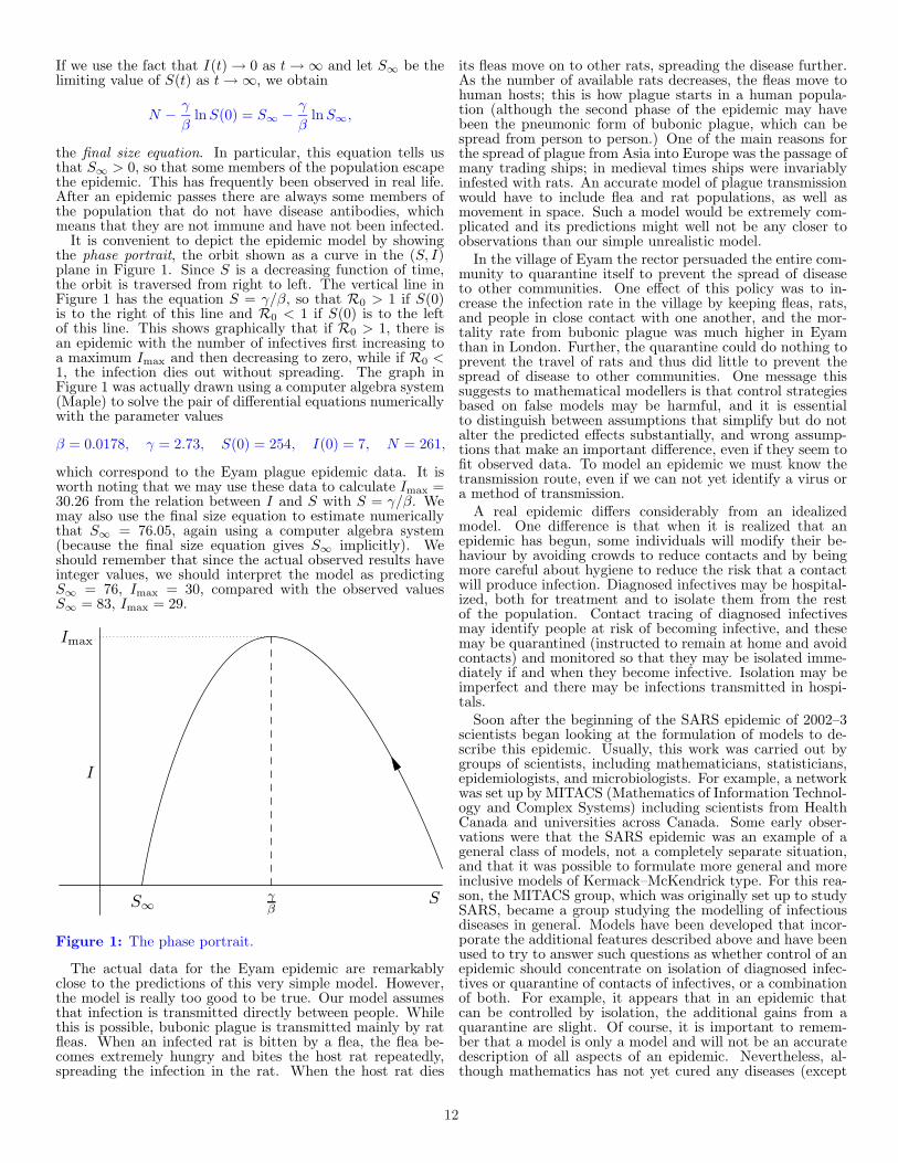
It is convenient to depict the epidemic model by showingthe phase portrait, the orbit shown as a curve in the (S, I)plane in Figure 1. Since S is a decreasing function of time,the orbit is traversed from right to left. The vertical line inFigure 1 has the equation S = γ/β, so that R0 > 1 if S(0)is to the right of this line and R0 < 1 if S(0) is to the leftof this line. This shows graphically that if R0 > 1, there isan epidemic with the number of infectives first increasing toa maximum Imax and then decreasing to zero, while if R0 <1, the infection dies out without spreading. The graph inFigure 1 was actually drawn using a computer algebra system(Maple) to solve the pair of differential equations numericallywith the parameter values

β = 0.0178, γ = 2.73, S(0) = 254, I(0) = 7, N = 261,

which correspond to the Eyam plague epidemic data. It isworth noting that we may use these data to calculate Imax =30.26 from the relation between I and S with S = γ/β. Wemay also use the final size equation to estimate numericallythat S∞ = 76.05, again using a computer algebra system(because the final size equation gives S∞ implicitly). Weshould remember that since the actual observed results haveinteger values, we should interpret the model as predictingS∞ = 76, Imax = 30, compared with the observed valuesS∞ = 83, Imax = 29.

S

I

γβS∞

Imax

Figure 1: The phase portrait.

The actual data for the Eyam epidemic are remarkablyclose to the predictions of this very simple model. However,the model is really too good to be true. Our model assumesthat infection is transmitted directly between people. Whilethis is possible, bubonic plague is transmitted mainly by ratfleas. When an infected rat is bitten by a flea, the flea be-comes extremely hungry and bites the host rat repeatedly,spreading the infection in the rat. When the host rat dies

its fleas move on to other rats, spreading the disease further.As the number of available rats decreases, the fleas move tohuman hosts; this is how plague starts in a human popula-tion (although the second phase of the epidemic may havebeen the pneumonic form of bubonic plague, which can bespread from person to person.) One of the main reasons forthe spread of plague from Asia into Europe was the passage ofmany trading ships; in medieval times ships were invariablyinfested with rats. An accurate model of plague transmissionwould have to include flea and rat populations, as well asmovement in space. Such a model would be extremely com-plicated and its predictions might well not be any closer toobservations than our simple unrealistic model.

In the village of Eyam the rector persuaded the entire com-munity to quarantine itself to prevent the spread of diseaseto other communities. One effect of this policy was to in-crease the infection rate in the village by keeping fleas, rats,and people in close contact with one another, and the mor-tality rate from bubonic plague was much higher in Eyamthan in London. Further, the quarantine could do nothing toprevent the travel of rats and thus did little to prevent thespread of disease to other communities. One message thissuggests to mathematical modellers is that control strategiesbased on false models may be harmful, and it is essentialto distinguish between assumptions that simplify but do notalter the predicted effects substantially, and wrong assump-tions that make an important difference, even if they seem tofit observed data. To model an epidemic we must know thetransmission route, even if we can not yet identify a virus ora method of transmission.

A real epidemic differs considerably from an idealizedmodel. One difference is that when it is realized that anepidemic has begun, some individuals will modify their be-haviour by avoiding crowds to reduce contacts and by beingmore careful about hygiene to reduce the risk that a contactwill produce infection. Diagnosed infectives may be hospital-ized, both for treatment and to isolate them from the restof the population. Contact tracing of diagnosed infectivesmay identify people at risk of becoming infective, and thesemay be quarantined (instructed to remain at home and avoidcontacts) and monitored so that they may be isolated imme-diately if and when they become infective. Isolation may beimperfect and there may be infections transmitted in hospi-tals.

Soon after the beginning of the SARS epidemic of 2002–3scientists began looking at the formulation of models to de-scribe this epidemic. Usually, this work was carried out bygroups of scientists, including mathematicians, statisticians,epidemiologists, and microbiologists. For example, a networkwas set up by MITACS (Mathematics of Information Technol-ogy and Complex Systems) including scientists from HealthCanada and universities across Canada. Some early obser-vations were that the SARS epidemic was an example of ageneral class of models, not a completely separate situation,and that it was possible to formulate more general and moreinclusive models of Kermack–McKendrick type. For this rea-son, the MITACS group, which was originally set up to studySARS, became a group studying the modelling of infectiousdiseases in general. Models have been developed that incor-porate the additional features described above and have beenused to try to answer such questions as whether control of anepidemic should concentrate on isolation of diagnosed infec-tives or quarantine of contacts of infectives, or a combinationof both. For example, it appears that in an epidemic thatcan be controlled by isolation, the additional gains from aquarantine are slight. Of course, it is important to remem-ber that a model is only a model and will not be an accuratedescription of all aspects of an epidemic. Nevertheless, al-though mathematics has not yet cured any diseases (except

12

possibly math anxiety), it may help in controlling future epi-demics. In the event of future outbreaks, you can expect thatepidemiologists and mathematical modellers will collaborateto suggest the best control strategy. This kind of mathemati-cal modelling requires some knowledge of calculus, differentialequations, and linear algebra. Further discussion of the aboveepidemic model and more realistic models is contained in [1,Chapter 7] and in [2, Section 6.6].

Acknowledgements

I would like to acknowledge David Earn and Pauline vanden Driessche who made some very helpful suggestions in thepreparation of this article.

References

[1] Brauer, F. and C. Castillo-Chavez, 2001: MathematicalModels in Population Biology and Epidemiology. Textsin Applied Mathematics, 40, Springer-Verlag, New York.

[2] Keshet, L., 2004: Mathematical Models in PopulationBiology. SIAM Classics in Applied Mathematics, 46,SIAM.

There were three medieval kingdoms on the shores of a lake.There was an island in the middle of the lake, over which thekingdoms had been fighting for years. Finally, the three kingsdecided that they would send their knights out to do battle,and the winner would take the island.

The night before the battle, the knights and their squirespitched camp and readied themselves for the fight. The firstkingdom had 12 knights, and each knight had five squires, allof whom were busily polishing armor, brushing horses, andcooking food. The second kingdom had twenty knights, andeach knight had 10 squires. Everyone at that camp was alsobusy preparing for battle. At the camp of the third kingdom,there was only one knight, with his squire. This squire tooka large pot and hung it from a looped rope in a tall tree. Hebusied himself preparing the meal, while the knight polishedhis own armor.

When the hour of the battle came, the three kingdoms senttheir squires out to fight (this was too trivial a matter forthe knights to join in). The battle raged, and when the dusthad cleared, the only person left was the lone squire from thethird kingdom, having defeated the squires from the othertwo kingdoms, thus proving that the squire of the high potand noose is equal to the sum of the squires of the other twosides.


A vector walks into two bars. . . and everyone yells, “Norm!”

If a math presentation was:

• Understood by everybody in the audience: it was aworthless bunch of triviality.

• Only some people were able to follow: it was definitelyNOT my area.

• Nobody understood even the first definition: it was agreat talk—serious research leading to important results.


13

Mathematical Modellingof Recurrent Epidemics

David J. D. Earn†

One of the most famous examples of an epidemic of an in-fectious disease in a human population is the Great Plagueof London, which took place in 1665–1666. We know quite alot about the progression of the Great Plague because weeklybills of mortality from that time have been retained. A photo-graph of such a bill is shown in Figure 1. Note that the reportindicates that the number of deaths from plague (5533) wasmore than 37 times the number of births (146) in the week inquestion, and that wasn’t the worst week! (As Fred Brauernotes in his article in this issue, an even worse plague occurredin the 14th century, but no detailed records of that epidemicare available.)

Figure 1: A photograph of a bill of mortality for the city ofLondon, England, for the week of 26 September to 3 October1665.

† David J. D. Earn is a professor in the Department ofMathematics & Statistics at McMaster University. His web site ishttp://www.math.mcmaster.ca/earn.

Putting together the weekly counts of plague deaths fromall the relevant mortality bills, we can obtain the epidemiccurve for the Great Plague, which I’ve plotted in the topleft panel of Figure 2. The characteristic exponential rise,turnover and decline is precisely the pattern predicted bythe classic susceptible-infective-recovered (SIR) model of Ker-mack and McKendrick [1] that I describe below (and FredBrauer also discusses in his article). While this encouragesus to think that mathematical modelling can help us un-derstand epidemics, some detailed features of the epidemiccurve are not predicted by the simple SIR model. For ex-ample, the model does not explain the jagged features in theplotted curve (and there would be many more small ups anddowns if we had a record of daily rather than weekly deaths).However, with some considerable mathematical effort, these“fine details” can be accounted for by replacing the differ-ential equations of Kermack and McKendrick with equationsthat include stochastic (i.e., random) processes [2]. We canthen congratulate ourselves for our modelling success. . . untilwe look at more data.

The bottom left panel of Figure 2 shows weekly mortal-ity from plague in London over a period of 70 years. TheGreat Plague is the rightmost (and highest) peak in the plot.You can see that on a longer timescale, there was a com-plex pattern of plague epidemics, including extinctions andre-emergences. This cannot be explained by the basic SIRmodel (even if we reformulate it using stochastic processes).The trouble is likely that we have left out a key biologicalfact: there is a reservoir of plague in rodents, so it can persistfor years, unnoticed by humans, and then re-emerge suddenlyand explosively. By including the rodents and aspects of spa-tial spread in a mathematical model, it has recently beenpossible to make sense of the pattern of 17th century plagueepidemics in London [3]. Nevertheless, some debate contin-ues as to whether all those plagues were really caused by thesame pathogenic organism.

A less contentious example is given by epidemics of measles,which are definitely caused by a well-known virus that infectsthe respiratory tract in humans and is transmitted by air-borne particles. Measles gives rise to characteristic red spotsthat are easily identifiable by physicians who have seen manycases, and parents are very likely to take their children to adoctor when such spots are noticed. Consequently, the major-ity of measles cases in developed countries end up in the officeof a doctor (who, in many countries, is required to report ob-served measles cases to a central body). The result is thatthe quality of reported measles case data is unusually good,and it has therefore stimulated a lot of work in mathematicalmodelling of epidemics.

An epidemic curve for measles in New York City in 1962is shown in the top right panel of Figure 2. The periodshown is 17 months, exactly the same length of time shownfor the Great Plague of London in the top left panel. The1962 measles epidemic in New York took off more slowly andlasted longer then the Great Plague of 1665. Can mathemat-ical models help us understand what might have caused thesedifferences?

Using the same notation as Fred Brauer uses in his articlein this issue, the basic SIR model is

dS

dt= −βSI, (1)

dI

dt= βSI − γI. (2)

Here, S and I denote the numbers of individuals that are sus-ceptible and infectious, respectively. The derivatives dS/dtand dI/dt denote the rates of change of S and I with

14

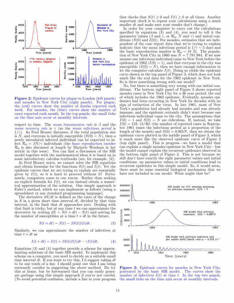
Figure 2: Epidemic curves for plague in London (left panels)and measles in New York City (right panels). For plague,the (red) curves show the number of deaths reported eachweek. For measles, the (blue) curves show the number ofcases reported each month. In the top panels, the small tickson the time axis occur at monthly intervals.

respect to time. The mean transmission rate is β and themean recovery rate is γ (so the mean infectious period is1/γ). As Fred Brauer discusses, if the total population sizeis N , and everyone is initially susceptible (S(0) = N), then anewly introduced infected individual can be expected to in-fect R0 = βN/γ individuals (the basic reproduction numberR0 is also discussed at length by Marjorie Wonham in herarticle in this issue). You can find a discussion of the SIRmodel together with the mathematical ideas it is based on insome introductory calculus textbooks (see, for example, [4]).

As Fred Brauer notes, we cannot solve the SIR equationsand obtain formulae for the functions S(t) and I(t). Yet theepidemic curves that we are trying to explain are essentiallygiven by I(t), so it is hard to proceed without it! Fortu-nately, computers come to our rescue. Rather than seekingan explicit formula for I(t), we can instead obtain a numer-ical approximation of the solution. One simple approach isEuler’s method, which we can implement as follows (using aspreadsheet or any standard programming language).

The derivative dS/dt is defined as the ratio of the changein S in a given short time interval dt, divided by that timeinterval, in the limit that dt approaches zero. Dealing withthat limit is tricky, but at any time t we can approximate thederivative by writing dS = S(t + dt) − S(t) and solving forthe number of susceptibles at a time t + dt in the future,

S(t + dt) = S(t) − βS(t)I(t)dt . (3)

Similarly, we can approximate the number of infectives attime t + dt as

I(t + dt) = I(t) + βS(t)I(t)dt− γI(t)dt . (4)

Equations (3) and (4) together provide a scheme for approx-imating solutions of the basic SIR model. To implement thisscheme on a computer, you need to decide on a suitable smalltime interval dt. If you want to try this, I’d suggest taking dtto be one tenth of a day. I should point out that I am beingextremely cavalier in suggesting the above method. Do trythis at home, but be forewarned that you can easily gener-ate garbage using this simple approach if you’re not careful.(To avoid potential confusion, include a line in your program

that checks that S(t) ≥ 0 and I(t) ≥ 0 at all times. Anotherimportant check is to repeat your calculations using a muchsmaller dt and make sure your results don’t change.)

In order for your computer to carry out the calculationsspecified by equations (3) and (4), you need to tell it theparameter values (β and γ, or R0, N and γ) and initial con-ditions (S(0) and I(0)). For measles, estimates that are inde-pendent of the case report data that we’re trying to explainindicate that the mean infectious period is 1/γ ∼ 5 days andthe basic reproduction number is R0 ∼ 18 [5]. The popula-tion of New York City in 1960 was N = 7 781 984. If we nowassume one infectious individual came to New York before theepidemic of 1962 (I(0) = 1), and that everyone in the city wassusceptible (S(0) = N), then we have enough information tolet the computer calculate I(t). Doing so yields the epidemiccurve shown in the top panel of Figure 3, which does not lookmuch like the real data for the 1962 epidemic in New York.So is there something wrong with our model?

No, but there is something very wrong with our initial con-ditions. The bottom right panel of Figure 2 shows reportedmeasles cases in New York City for a 36 year period, the endof which includes the 1962 epidemic. Evidently, measles epi-demics had been occurring in New York for decades with nosign of extinction of the virus. In late 1961, most of NewYork’s population had already had measles and was alreadyimmune, and the epidemic certainly didn’t start because oneinfectious individual came to the city. The assumptions thatI(0) = 1 and S(0) = N are ridiculous. If, instead, we takeI(0) = 123 · (5/30) (the number of reported cases in Septem-ber 1961 times the infectious period as a proportion of thelength of the month) and S(0) = 0.065N , then we obtain theepidemic curve plotted in the middle panel of Figure 3, whichis much more like the observed epidemic curve of Figure 2(top right panel). This is progress—we have a model thatcan explain a single measles epidemic in New York City—butthe model cannot explain the recurrent epidemics observed inthe bottom right panel of Figure 2. This is not because westill don’t have exactly the right parameter values and initialconditions: no parameter values or initial conditions lead torecurrent epidemics in this simple model. So, it would seem,there must be some essential biological mechanism that wehave not included in our model. What might that be?

Figure 3: Epidemic curves for measles in New York City,generated by the basic SIR model. The curves show thenumber of infectives I(t) at time t. In the top two panels,the small ticks on the time axis occur at monthly intervals.

15

Let’s think about why a second epidemic cannot occur inthe model we’ve discussed so far. The characteristic turnoverand decline of an epidemic curve occurs because the pathogenis running out of susceptible individuals to infect. To stimu-late a second epidemic, there must be a source of susceptibleindividuals. For measles, that source cannot be previouslyinfected people, because recovered individuals retain lifelongimmunity to the virus. Newborns typically acquire immunityfrom their mothers, but this wanes after a few months. Sobirths can provide the source we’re looking for.

If we expand the SIR model to include B births per unittime and a natural mortality rate µ (per capita), then ourequations become

dS

dt= B − βSI − µS , (5)

dI

dt= βSI − γI − µI . (6)

The timescale for substantial changes in birth rates (decades)is generally much longer than a measles epidemic (a fewmonths), so we’ll assume that the population size is constant(thus B = µN , so there is really only one new parameterin the above equations; we can take it to be B). As before,we can use Euler’s trick to convert the equations above intoa scheme that enables a computer to generate approximatesolutions. An example is shown in the bottom panel of Fig-ure 3, where I have taken the birth rate to be B = 126 372per year (the number of births in New York City in 1928, thefirst year for which we have data). The rest of the parametersand initial conditions are as in the middle panel of the figure.

Again we seem to be making progress. We are now gettingrecurrent epidemics, but the oscillations in the numbers ofcases over time damp out, eventually reaching an equilibrium.While the graph is just an approximate solution for a singleset of initial conditions, it can actually be proved that allinitial conditions with I(0) > 0 yield solutions that convergeonto this equilibrium. So we still don’t have a model that canexplain the real oscillations in measles incidence from 1928 to1964, which showed no evidence of damping out. Back to thedrawing board?

Don’t give up. We’ve nearly cracked it. So far, we havebeen assuming implicitly that the transmission rate β (or,equivalently, the basic reproduction number R0) is simply aconstant and, in particular, that it does not change in time.Let’s think about that assumption. The transmission rateis really the product of the rate of contact among individu-als and the probability that a susceptible individual who iscontacted by an infectious individual will become infected.But the contact rate is not constant throughout the year. Tosee that, consider the fact that in the absence of vaccination,the average age at which a person is infected with measlesis about five years [5]; hence most susceptibles are children.Children are in closer contact when school is in session, so thetransmission rate varies seasonally. A crude approximation ofthis seasonality is to assume that β varies sinusoidally,

β(t) = β0(1 + α cos 2πt) . (7)

Here, β0 is the mean transmission rate, α is the amplitude ofseasonal variation and the time t is assumed to be measuredin years. If, as above, β is assumed to be a periodic function(with a period of one year) then the SIR model is said to beseasonally forced. We can still use Euler’s trick to solve theequations approximately, and I encourage you to do that us-ing a computer for various values of the seasonal amplitude α(you must have 0 ≤ α ≤ 1: why?).

You might think that seasonal forcing is just a minor tweakof the model, but in fact this forcing has an enormous im-pact on the epidemic dynamics that the model predicts. Ifyou’ve taken Physics and studied the forced pendulum, thenyou might already have some intuition for this. A pendulumwith some friction will exhibit damped oscillations and settledown to an equilibrium. But if you tap the pendulum with ahammer periodically then it will never settle down and it canexhibit quite an exotic range of behaviours including chaoticdynamics [6] (oscillations that look random). Similarly com-plex dynamics can occur in the seasonally forced SIR model.

Most importantly, with seasonal forcing, the SIR modeldisplays undamped oscillations similar to the patterns seenin the real measles case reports. But we are left with an-other puzzle. If you look carefully at the New York Citymeasles reports in the bottom right panel of Figure 2 you’llsee that before about 1945 the epidemics were fairly irregular,whereas after 1945 they followed an almost perfect two-yearcycle. While the SIR model can generate both irregular dy-namics and two-year cycles, this happens for different param-eter values, not for a single solution of the equations. Howcan we explain changes over time in the pattern of measlesepidemics?

Once again, the missing ingredient in the model is a chang-ing parameter value. This time it is the birth rate B, whichis not really constant. Birth rates fluctuate seasonally, but tosuch a small extent that this effect is negligible. What turnsout to be more important is the much slower changes thatoccur in the average birth rate over decades. For example,in New York City the birth rate was much lower during the1930s (the “Great Depression”) than after 1945 (the “babyboom”) and this difference accounts for the very different pat-terns of measles epidemics in New York City during these twotime periods [7].

A little more analysis of the SIR model is very useful. It ispossible to prove that changes in the birth rate have exactlythe same effect on disease dynamics as changes of the samerelative magnitude in the transmission rate or the proportionof the population that is vaccinated [7]. This equivalencemakes it possible to explain historical case report data for avariety of infectious diseases in many different cities [8].

One thing that you may have picked up from this article isthat successful mathematical modelling of biological systemstends to proceed in steps. We begin with the simplest sensi-ble model and try to discover everything we can about it. Ifthe simplest model cannot explain the phenomenon we’re try-ing to understand, then we add more biological detail to themodel, and it’s best to do this in steps because we are thenmore likely to be able to determine which biological featureshave the greatest impact on the behaviour of the model.

In the particular case of mathematical epidemiology, we arelucky that medical and public health personnel have painstak-ingly conducted surveillance of infectious diseases for cen-turies. This has created an enormous wealth of valuabledata with which to test hypotheses about disease spread us-ing mathematical models, making this a very exciting subjectfor research in applied mathematics.

Acknowledgements

It is a pleasure to thank Sigal Balshine, Will Guest, and theanonymous referee for helpful comments. The photograph inFigure 1 was taken by Claire Lees at the Guildhall in London,England. The weekly plague data plotted in Figure 2 weredigitized by Seth Earn.

16

References

[1] Kermack, W. O. and A. G. McKendrick, 1927: A con-tribution to the mathematical theory of epidemics. Pro-ceedings of the Royal Society of London, Series A, 115,700–721.

[2] Bailey, N. T. J., 1975: The mathematical theory of infec-tious diseases and its application. Griffin, London, 2ndedition.

[3] Keeling, M. J. and C. A. Gilligan, 2000: Metapopulationdynamics of bubonic plague. Nature, 407, 903–906.

[4] Hughes-Hallett D. et al, 2002: Applied Calculus. JohnWiley & Sons, Toronto, 2nd edition.

[5] Anderson, R. A. and R. M. May, 1991: Infectious Dis-eases of Humans: Dynamics and Control. Oxford Uni-versity Press, Oxford.

[6] Gleick, J., 1987: Chaos. Abacus, London.

[7] Earn, D. J. D., P. Rohani, B. M. Bolker and B. T. Gren-fell, 2000: A simple model for complex dynamical tran-sitions in epidemics. Science, 287, 667–670.

[8] Bauch, C. T. and D. J. D. Earn, 2003: Transients andattractors in epidemics. Proceedings of the Royal Societyof London, Series B, 270, 1573–1578.

Practical Further Reading Suggestions fromthe Editors

The SIR Model for Spread of Disease web site athttp://www.math.duke.edu/education/ccp/materials/diffcalc/sir/contents.html includes Maple, Mathematicaand Matlab files.

A spreadsheet program that is easy to use is available fromhttp://ugrad.math.ubc.ca:8099/mathsheet/index.html.

Q: What is a mathematician’s pick when faced with thechoice between poutine and eternal bliss in the afterlife?

A: Poutine! Because nothing is better than eternal bliss inthe afterlife, and poutine is better than nothing.

Q: What is a topologist?A: A person who cannot tell a doughnut from a coffee mug.

Q: Why did the mathematician have trouble computingA−1A?

A: Because he was having an identity crisis.

Absurdity of zero: there is no such a thing as nothing.

Q: What is yellow, sour, and equivalent to the axiom ofchoice?

A: Zorn’s lemon. . . .


Q: What is normed, complete, and yellow?A: A Bananach space. . . .


17

Cid, Bru, OneJeremy Tatum†

One of the “Math Jokes” in the September, 2003 issue de-clared that there are 10 kinds of mathematicians: those whocan think in binary and those who can’t.

At one time I was very definitely in the latter category—Icouldn’t add one and one. Looking back, I realize that oneof my difficulties was that I didn’t know of any easy namesfor numbers when written in binary form. For example, howdo you pronounce the binary number 10 in the joke above?If you pronounced it “ten,” you missed the point of the joke!

So—what are binary numbers? We are all familiar with thedecimal system, in which we have ten single-digit numbers:0, 1, 2, . . . 9. If we want to write numbers greater than 9, wehave to use two digits. Thus: 10. This enables us to writenumbers as high as 99. If we want to write numbers greaterthan 99, we have to use three digits. Thus: 100. The number100 is 102 and the number 1 000 is 103, and so on. We arevery familiar with all of that.

In the binary system (which is what computers use, even ifwe are unaware of it), we have only two “digits”—or “bits” asthey are called in the binary system. These are 0 and 1. If wewant to write numbers greater than 1, we have to use two bits,namely 10. This number is the binary equivalent of “two.”So now you can go back and read the joke, and perhaps havea good chuckle over it. The binary number 11 is equivalent to“three”—and, if we want to write numbers greater than this,we have to use three bits. Thus 100 is the binary equivalent of“four.” Here are the binary representations of the first elevennumbers:

zero 0one 1two 1 0three 1 1four 1 0 0five 1 0 1six 1 1 0seven 1 1 1eight 1 0 0 0nine 1 0 0 1ten 1 0 1 0

You will see that 100 means 22, 1000 means 23, and so on.Now I am going to ask you to add together five binary

numbers, as follows:

1 0 1 1 0 11 1 1 0 1 11 1 0 1 1 01 1 0 0 1 11 0 0 1 1 1

† Jeremy Tatum is a former professor in the Department of Physicsand Astronomy of the University of Victoria. His e-mail address [email protected].

If you are at all like me when I first encountered an appar-ently simple problem like this, you may find this surprisinglydifficult. Perhaps you will at first try to convert each numberinto decimal form. The binary number 101 101, for example,is 45 when written in decimal. You might add them all upin decimal form, and then try to convert the decimal numberback into binary form. Or you might try to add the numbersas binary numbers column by column in the usual way foradding numbers. Thus 1 + 1 is 10; and 10 and 1 is 11; and11 and 1 is—oh, dear, I’ve lost count and I’m not quite surewhat to do next. In case you want to persist, the answer is11 111 000.

Many years ago I read an article (I’m afraid I cannot re-member where or by whom—if anyone knows, please tell me)in which the author proposed names for numbers written inbinary notation. To some it will sound like risible gibberish—yet I have found it surprisingly helpful for doing calculationsin binary. Perhaps it is well known and in widespread use—though I have never met anyone who has heard of it. Thedifficulty I always had in thinking in binary was that I hadno names for binary numbers such as 10, 100, 1000. Theforgotten author supplied the key by giving names to thesebinary numbers.

As I recall, the powers of two were given names as follows:

1 one1 0 bru

1 0 0 cid1 0 0 0 dag

1 0 0 0 0 bru dag1 0 0 0 0 0 cid dag

1 0 0 0 0 0 0 hi

Examples of some other numbers:

1 1 bru one1 0 1 cid one

1 1 1 0 dag, cid bru1 0 1 0 1 bru dag, cid one

1 1 0 0 1 1 cid bru dag, bru one

In addition to these names, I have also found it helpful totypeset long numbers in groups of three, with a small gapbetween each group, as is also standard typesetting practicewith large decimal numbers.

Now let’s see how it works for adding the above five num-bers. Although I don’t need to, I have, by way of furtherexample, “pronounced” their “names” to the right of each.

1 0 1 1 0 1 cid one dag, cid one1 1 1 0 1 1 cid bru one dag, bru one1 1 0 1 1 0 cid bru dag, cid bru1 1 0 0 1 1 cid bru dag, bru one1 0 0 1 1 1 cid dag, cid bru one

1 1 1 1 1 0 0 0 bru hi, cid bru dag

The only way to see how this works is to mumble thingslike “one, bru, cid, dag” under your breath while doing theaddition. I’m going to try and transcribe my mumblings topaper as I start by adding up the numbers in the right-hand(least significant) column, and then move on to the next col-umn to the left. It goes something like this: “One, bru, bruone, cid; that’s zero, and bru to carry to the next column.Now the next column. Bru, bru one, cid, cid one, cid bru;that’s zero, and bru one to carry to the next column.”

. . .And so on and so on!

18

It’s hard to describe the process in writing, but try a bit ofmumbling yourself for a while and it will either become clearand quick very soon, or you’ll collapse into helpless laughter.

How does Multiplication work? For example, try 11 011 ×1 101. That is, what is bru one dag, bru one times dag, cidone? In fact the multiplication is the easy part. You can justset it out as an ordinary long multiplication:

1 1 0 1 1× 1 1 0 1

1 1 0 1 11 1 0 1 1 0 0

1 1 0 1 1 0 0 0

That part was easy. Now you have to add the last threebinary numbers—and I’ll leave you to do that in the sameway as before. The answer is 101 011 111.

Indeed the one, bru, cid nomenclature is really only use-ful in the addition of several or many binary numbers. Ina subtraction problem, you just have two numbers to dealwith—the number you start with, and the subtrahend (thenumber you subtract); bru, cid and dag are then of littlehelp. I expect that you can subtract 1 001 from 10 101 to get1 010 with little difficulty.

To appreciate how helpful bru, cid and dag can be, there isno substitute for setting yourself several long addition prob-lems in binary numbers and adding them when mumbling bru,cid dag under your breath. At first it will seem ridiculous—but after a short while you will soon find yourself adding longstrings of binary numbers accurately and with great speedand confidence.

You may remember that Alice had some difficulty with Ad-dition:

“Can you do Addition?” the White Queen asked. “What’sone and one and one and one and one and one and one andone and one and one?”

“I don’t know,” said Alice. “I lost count.”

“She can’t do Addition,” the Red Queen interrupted.1

Alice, of course, should promptly have answered: “Dag bru.”

Differential equation of human life: equal laws for every-body, but better initial conditions for some of us.

Q: What is the code name of a spy mathematician?A: Sπ

1 Quoted from Alice’s Adventures in Wonderland and Through the

Looking Glass by Lewis Carroll.

The chef instructs his apprentice: “You take two thirds ofwater, one third of cream, and one third of broth. . . ”

The apprentice interrupts: “But that makes four thirdsalready!”

“Well—then you just take a larger pot!”


Q: Why didn’t the permutation ever get hired for any jobsin the big city?

A: Because he didn’t commute.

Math is free but you need to download it yourself.

Marriage Math: one plus one forever.


19

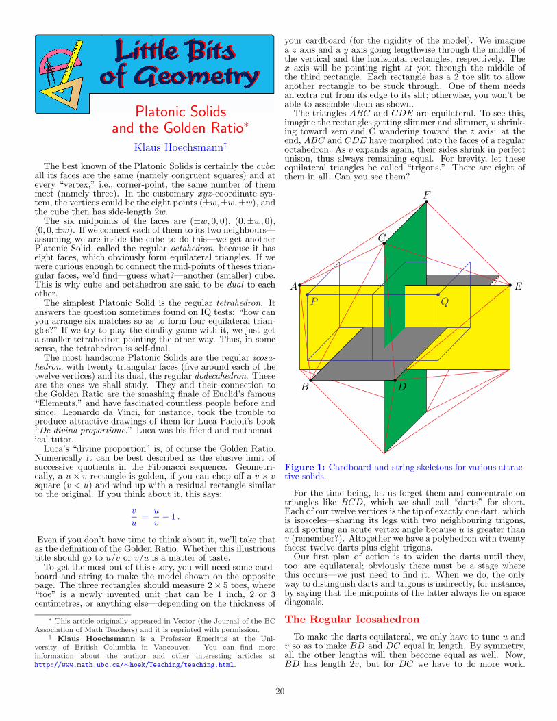
Platonic Solidsand the Golden Ratio∗

Klaus Hoechsmann†

The best known of the Platonic Solids is certainly the cube:all its faces are the same (namely congruent squares) and atevery “vertex,” i.e., corner-point, the same number of themmeet (namely three). In the customary xyz-coordinate sys-tem, the vertices could be the eight points (±w,±w,±w), andthe cube then has side-length 2w.

The six midpoints of the faces are (±w, 0, 0), (0,±w, 0),(0, 0,±w). If we connect each of them to its two neighbours—assuming we are inside the cube to do this—we get anotherPlatonic Solid, called the regular octahedron, because it haseight faces, which obviously form equilateral triangles. If wewere curious enough to connect the mid-points of theses trian-gular faces, we’d find—guess what?—another (smaller) cube.This is why cube and octahedron are said to be dual to eachother.

The simplest Platonic Solid is the regular tetrahedron. Itanswers the question sometimes found on IQ tests: “how canyou arrange six matches so as to form four equilateral trian-gles?” If we try to play the duality game with it, we just geta smaller tetrahedron pointing the other way. Thus, in somesense, the tetrahedron is self-dual.

The most handsome Platonic Solids are the regular icosa-hedron, with twenty triangular faces (five around each of thetwelve vertices) and its dual, the regular dodecahedron. Theseare the ones we shall study. They and their connection tothe Golden Ratio are the smashing finale of Euclid’s famous“Elements,” and have fascinated countless people before andsince. Leonardo da Vinci, for instance, took the trouble toproduce attractive drawings of them for Luca Pacioli’s book“De divina proportione.” Luca was his friend and mathemat-ical tutor.

Luca’s “divine proportion” is, of course the Golden Ratio.Numerically it can be best described as the elusive limit ofsuccessive quotients in the Fibonacci sequence. Geometri-cally, a u × v rectangle is golden, if you can chop off a v × vsquare (v < u) and wind up with a residual rectangle similarto the original. If you think about it, this says:

v

u=

u

v− 1 .

Even if you don’t have time to think about it, we’ll take thatas the definition of the Golden Ratio. Whether this illustrioustitle should go to u/v or v/u is a matter of taste.

To get the most out of this story, you will need some card-board and string to make the model shown on the oppositepage. The three rectangles should measure 2 × 5 toes, where“toe” is a newly invented unit that can be 1 inch, 2 or 3centimetres, or anything else—depending on the thickness of

∗ This article originally appeared in Vector (the Journal of the BCAssociation of Math Teachers) and it is reprinted with permission.

† Klaus Hoechsmann is a Professor Emeritus at the Uni-versity of British Columbia in Vancouver. You can find moreinformation about the author and other interesting articles athttp://www.math.ubc.ca/∼hoek/Teaching/teaching.html.

your cardboard (for the rigidity of the model). We imaginea z axis and a y axis going lengthwise through the middle ofthe vertical and the horizontal rectangles, respectively. Thex axis will be pointing right at you through the middle ofthe third rectangle. Each rectangle has a 2 toe slit to allowanother rectangle to be stuck through. One of them needsan extra cut from its edge to its slit; otherwise, you won’t beable to assemble them as shown.

The triangles ABC and CDE are equilateral. To see this,imagine the rectangles getting slimmer and slimmer, v shrink-ing toward zero and C wandering toward the z axis: at theend, ABC and CDE have morphed into the faces of a regularoctahedron. As v expands again, their sides shrink in perfectunison, thus always remaining equal. For brevity, let theseequilateral triangles be called “trigons.” There are eight ofthem in all. Can you see them?

A

B

C

D

E

F

P Q

Figure 1: Cardboard-and-string skeletons for various attrac-tive solids.

For the time being, let us forget them and concentrate ontriangles like BCD, which we shall call “darts” for short.Each of our twelve vertices is the tip of exactly one dart, whichis isosceles—sharing its legs with two neighbouring trigons,and sporting an acute vertex angle because u is greater thanv (remember?). Altogether we have a polyhedron with twentyfaces: twelve darts plus eight trigons.

Our first plan of action is to widen the darts until they,too, are equilateral; obviously there must be a stage wherethis occurs—we just need to find it. When we do, the onlyway to distinguish darts and trigons is indirectly, for instance,by saying that the midpoints of the latter always lie on spacediagonals.

The Regular Icosahedron

To make the darts equilateral, we only have to tune u andv so as to make BD and DC equal in length. By symmetry,all the other lengths will then become equal as well. Now,BD has length 2v, but for DC we have to do more work.

20

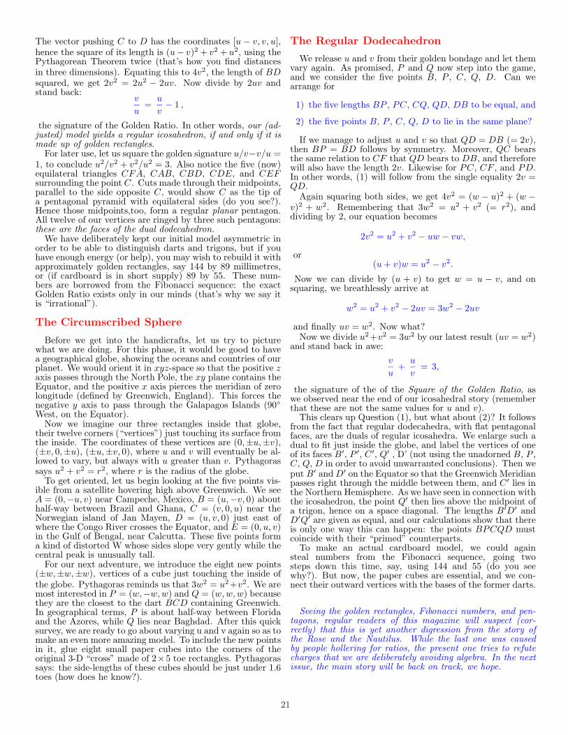
The vector pushing C to D has the coordinates [u − v, v, u],hence the square of its length is (u− v)2 + v2 + u2, using thePythagorean Theorem twice (that’s how you find distancesin three dimensions). Equating this to 4v2, the length of BDsquared, we get 2v2 = 2u2 − 2uv. Now divide by 2uv andstand back:

v

u=

u

v− 1 ,

the signature of the Golden Ratio. In other words, our (ad-justed) model yields a regular icosahedron, if and only if it ismade up of golden rectangles.

For later use, let us square the golden signature u/v−v/u =1, to conclude u2/v2 + v2/u2 = 3. Also notice the five (now)equilateral triangles CFA, CAB, CBD, CDE, and CEFsurrounding the point C. Cuts made through their midpoints,parallel to the side opposite C, would show C as the tip ofa pentagonal pyramid with equilateral sides (do you see?).Hence those midpoints,too, form a regular planar pentagon.All twelve of our vertices are ringed by three such pentagons:these are the faces of the dual dodecahedron.

We have deliberately kept our initial model asymmetric inorder to be able to distinguish darts and trigons, but if youhave enough energy (or help), you may wish to rebuild it withapproximately golden rectangles, say 144 by 89 millimetres,or (if cardboard is in short supply) 89 by 55. These num-bers are borrowed from the Fibonacci sequence: the exactGolden Ratio exists only in our minds (that’s why we say itis “irrational”).

The Circumscribed Sphere

Before we get into the handicrafts, let us try to picturewhat we are doing. For this phase, it would be good to havea geographical globe, showing the oceans and countries of ourplanet. We would orient it in xyz-space so that the positive zaxis passes through the North Pole, the xy plane contains theEquator, and the positive x axis pierces the meridian of zerolongitude (defined by Greenwich, England). This forces thenegative y axis to pass through the Galapagos Islands (90◦

West, on the Equator).Now we imagine our three rectangles inside that globe,

their twelve corners (“vertices”) just touching its surface fromthe inside. The coordinates of these vertices are (0,±u,±v),(±v, 0,±u), (±u,±v, 0), where u and v will eventually be al-lowed to vary, but always with u greater than v. Pythagorassays u2 + v2 = r2, where r is the radius of the globe.

To get oriented, let us begin looking at the five points vis-ible from a satellite hovering high above Greenwich. We seeA = (0,−u, v) near Campeche, Mexico, B = (u,−v, 0) abouthalf-way between Brazil and Ghana, C = (v, 0, u) near theNorwegian island of Jan Mayen, D = (u, v, 0) just east ofwhere the Congo River crosses the Equator, and E = (0, u, v)in the Gulf of Bengal, near Calcutta. These five points forma kind of distorted W whose sides slope very gently while thecentral peak is unusually tall.

For our next adventure, we introduce the eight new points(±w,±w,±w), vertices of a cube just touching the inside ofthe globe. Pythagoras reminds us that 3w2 = u2+v2. We aremost interested in P = (w,−w, w) and Q = (w, w, w) becausethey are the closest to the dart BCD containing Greenwich.In geographical terms, P is about half-way between Floridaand the Azores, while Q lies near Baghdad. After this quicksurvey, we are ready to go about varying u and v again so as tomake an even more amazing model. To include the new pointsin it, glue eight small paper cubes into the corners of theoriginal 3-D “cross” made of 2×5 toe rectangles. Pythagorassays: the side-lengths of these cubes should be just under 1.6toes (how does he know?).

The Regular Dodecahedron

We release u and v from their golden bondage and let themvary again. As promised, P and Q now step into the game,and we consider the five points B, P , C, Q, D. Can wearrange for

1) the five lengths BP , PC, CQ, QD, DB to be equal, and

2) the five points B, P , C, Q, D to lie in the same plane?

If we manage to adjust u and v so that QD = DB (= 2v),then BP = BD follows by symmetry. Moreover, QC bearsthe same relation to CF that QD bears to DB, and thereforewill also have the length 2v. Likewise for PC, CF , and PD.In other words, (1) will follow from the single equality 2v =QD.

Again squaring both sides, we get 4v2 = (w − u)2 + (w −v)2 + w2. Remembering that 3w2 = u2 + v2 (= r2), anddividing by 2, our equation becomes

2v2 = u2 + v2 − uw − vw,

or(u + v)w = u2 − v2.

Now we can divide by (u + v) to get w = u − v, and onsquaring, we breathlessly arrive at

w2 = u2 + v2 − 2uv = 3w2 − 2uv

and finally uv = w2. Now what?Now we divide u2+v2 = 3w2 by our latest result (uv = w2)

and stand back in awe:

v

u+

u

v= 3,

the signature of the of the Square of the Golden Ratio, aswe observed near the end of our icosahedral story (rememberthat these are not the same values for u and v).

This clears up Question (1), but what about (2)? It followsfrom the fact that regular dodecahedra, with flat pentagonalfaces, are the duals of regular icosahedra. We enlarge such adual to fit just inside the globe, and label the vertices of oneof its faces B′, P ′, C ′, Q′ , D’ (not using the unadorned B, P ,C, Q, D in order to avoid unwarranted conclusions). Then weput B′ and D′ on the Equator so that the Greenwich Meridianpasses right through the middle between them, and C ′ lies inthe Northern Hemisphere. As we have seen in connection withthe icosahedron, the point Q′ then lies above the midpoint ofa trigon, hence on a space diagonal. The lengths B′D′ andD′Q′ are given as equal, and our calculations show that thereis only one way this can happen: the points BPCQD mustcoincide with their “primed” counterparts.

To make an actual cardboard model, we could againsteal numbers from the Fibonacci sequence, going twosteps down this time, say, using 144 and 55 (do you seewhy?). But now, the paper cubes are essential, and we con-nect their outward vertices with the bases of the former darts.

Seeing the golden rectangles, Fibonacci numbers, and pen-tagons, regular readers of this magazine will suspect (cor-rectly) that this is yet another digression from the story ofthe Rose and the Nautilus. While the last one was causedby people hollering for ratios, the present one tries to refutecharges that we are deliberately avoiding algebra. In the nextissue, the main story will be back on track, we hope.

21

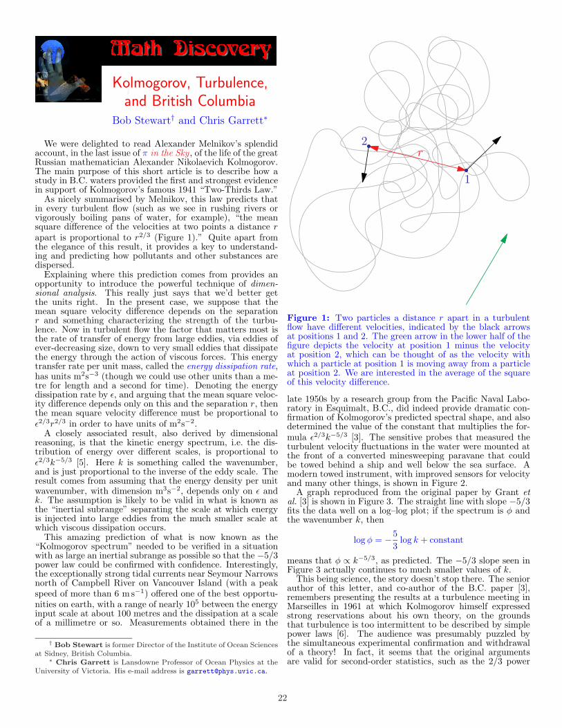
Kolmogorov, Turbulence,

and British ColumbiaBob Stewart† and Chris Garrett∗

We were delighted to read Alexander Melnikov’s splendidaccount, in the last issue of π in the Sky , of the life of the greatRussian mathematician Alexander Nikolaevich Kolmogorov.The main purpose of this short article is to describe how astudy in B.C. waters provided the first and strongest evidencein support of Kolmogorov’s famous 1941 “Two-Thirds Law.”

As nicely summarised by Melnikov, this law predicts thatin every turbulent flow (such as we see in rushing rivers orvigorously boiling pans of water, for example), “the meansquare difference of the velocities at two points a distance rapart is proportional to r2/3 (Figure 1).” Quite apart fromthe elegance of this result, it provides a key to understand-ing and predicting how pollutants and other substances aredispersed.

Explaining where this prediction comes from provides anopportunity to introduce the powerful technique of dimen-sional analysis. This really just says that we’d better getthe units right. In the present case, we suppose that themean square velocity difference depends on the separationr and something characterizing the strength of the turbu-lence. Now in turbulent flow the factor that matters most isthe rate of transfer of energy from large eddies, via eddies ofever-decreasing size, down to very small eddies that dissipatethe energy through the action of viscous forces. This energytransfer rate per unit mass, called the energy dissipation rate,has units m2s−3 (though we could use other units than a me-tre for length and a second for time). Denoting the energydissipation rate by ǫ, and arguing that the mean square veloc-ity difference depends only on this and the separation r, thenthe mean square velocity difference must be proportional toǫ2/3r2/3 in order to have units of m2s−2.

A closely associated result, also derived by dimensionalreasoning, is that the kinetic energy spectrum, i.e. the dis-tribution of energy over different scales, is proportional toǫ2/3k−5/3 [5]. Here k is something called the wavenumber,and is just proportional to the inverse of the eddy scale. Theresult comes from assuming that the energy density per unitwavenumber, with dimension m3s−2, depends only on ǫ andk. The assumption is likely to be valid in what is known asthe “inertial subrange” separating the scale at which energyis injected into large eddies from the much smaller scale atwhich viscous dissipation occurs.

This amazing prediction of what is now known as the“Kolmogorov spectrum” needed to be verified in a situationwith as large an inertial subrange as possible so that the −5/3power law could be confirmed with confidence. Interestingly,the exceptionally strong tidal currents near Seymour Narrowsnorth of Campbell River on Vancouver Island (with a peakspeed of more than 6 m s−1) offered one of the best opportu-nities on earth, with a range of nearly 105 between the energyinput scale at about 100 metres and the dissipation at a scaleof a millimetre or so. Measurements obtained there in the

† Bob Stewart is former Director of the Institute of Ocean Sciencesat Sidney, British Columbia.

∗ Chris Garrett is Lansdowne Professor of Ocean Physics at theUniversity of Victoria. His e-mail address is [email protected].

r

1

2

Figure 1: Two particles a distance r apart in a turbulentflow have different velocities, indicated by the black arrowsat positions 1 and 2. The green arrow in the lower half of thefigure depicts the velocity at position 1 minus the velocityat position 2, which can be thought of as the velocity withwhich a particle at position 1 is moving away from a particleat position 2. We are interested in the average of the squareof this velocity difference.

late 1950s by a research group from the Pacific Naval Labo-ratory in Esquimalt, B.C., did indeed provide dramatic con-firmation of Kolmogorov’s predicted spectral shape, and alsodetermined the value of the constant that multiplies the for-mula ǫ2/3k−5/3 [3]. The sensitive probes that measured theturbulent velocity fluctuations in the water were mounted atthe front of a converted minesweeping paravane that couldbe towed behind a ship and well below the sea surface. Amodern towed instrument, with improved sensors for velocityand many other things, is shown in Figure 2.

A graph reproduced from the original paper by Grant etal. [3] is shown in Figure 3. The straight line with slope −5/3fits the data well on a log–log plot; if the spectrum is φ andthe wavenumber k, then

log φ = −5

3log k + constant

means that φ ∝ k−5/3, as predicted. The −5/3 slope seen inFigure 3 actually continues to much smaller values of k.

This being science, the story doesn’t stop there. The seniorauthor of this letter, and co-author of the B.C. paper [3],remembers presenting the results at a turbulence meeting inMarseilles in 1961 at which Kolmogorov himself expressedstrong reservations about his own theory, on the groundsthat turbulence is too intermittent to be described by simplepower laws [6]. The audience was presumably puzzled bythe simultaneous experimental confirmation and withdrawalof a theory! In fact, it seems that the original argumentsare valid for second-order statistics, such as the 2/3 power

22

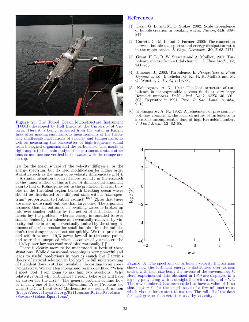
Figure 2: The Towed Ocean Microstructure Instrument(TOMI) developed by Rolf Lueck at the University of Vic-toria. Here it is being recovered from the water in KnightInlet after making simultaneous measurements of the turbu-lent small-scale fluctuations of velocity and temperature, aswell as measuring the backscatter of high-frequency soundfrom biological organisms and the turbulence. The masts atright angles to the main body of the instrument contain othersensors and become vertical in the water, with the orange oneon top.

law for the mean square of the velocity difference, or theenergy spectrum, but do need modification for higher orderstatistics such as the mean cube velocity difference (e.g. [4]).

A similar situation occurred more recently in the researchof the junior author of this article. A dimensional argumentakin to that of Kolmogorov led to the prediction that air bub-bles in the turbulent region beneath breaking ocean wavesshould be distributed over different sizes with a “size spec-trum” proportional to (bubble radius)−10/3 [2], so that thereare many more small bubbles than large ones. The argumentassumed that air entrained in breaking waves is broken upinto ever smaller bubbles by the action of turbulence. Butherein lay the problem: whereas energy is cascaded to eversmaller scales by turbulence and eventually removed by vis-cosity, bubble break-up is eventually limited by the strong in-fluence of surface tension for small bubbles, but the bubblesdon’t then disappear, at least not quickly. We thus predictedand withdrew our −10/3 power law all in the same paper,and were then surprised when, a couple of years later, the−10/3 power law was confirmed observationally [1]!

There is clearly more to be understood in both of thesesituations. While dimensional reasoning is very powerful andleads to useful predictions in physics (much like Darwin’stheory of natural selection in biology!), a full understandingof turbulent flows is still not available. According to an apoc-ryphal story, Werner Heisenberg said on his deathbed “WhenI meet God, I am going to ask him two questions: Whyrelativity? And why turbulence? I really believe he will havean answer for the first.” The general problem of fluid flowis, in fact, one of the seven Millennium Prize Problems forwhich the Clay Institute of Mathematics is offering $1 million(http://www.claymath.org/Millennium Prize Problems/Navier-Stokes Equations/).

References

[1] Dean, G. B. and M. D. Stokes, 2002: Scale dependenceof bubble creation in breaking waves. Nature, 418, 839–844.

[2] Garrett, C., M. Li and D. Farmer, 2000: The connectionbetween bubble size spectra and energy dissipation ratesin the upper ocean. J. Phys. Oceanogr., 30, 2163–2171.

[3] Grant, H. L., R. W. Stewart and A. Moilliet, 1961: Tur-bulence spectra from a tidal channel. J. Fluid Mech., 12,241–263.

[4] Jimenez, J., 2000: Turbulence. In Perspectives in FluidDynamics, Ed. Batchelor, G. K., H. K. Moffatt and M.G. Worster, C. U. P., 231–288.

[5] Kolmogorov, A. N., 1941: The local structure of tur-bulence in incompressible viscous fluids at very largeReynolds numbers. Dokl. Akad. Nauk. SSSR, 30, 301–305. Reprinted in 1991: Proc. R. Soc. Lond. A, 434,9–13.

[6] Kolmogorov, A. N., 1962: A refinement of previous hy-potheses concerning the local structure of turbulence ina viscous incompressible fluid at high Reynolds number.J. Fluid Mech., 13, 82–85.

−2 −1 0 1

log k

−6

−4

−2

0

2

4

log

φ(k

)

Figure 3: The spectrum of turbulent velocity fluctuationsshows how the turbulent energy is distributed over variousscales, with their size being the inverse of the wavenumber k.Here, experimental data obtained in 1959 are displayed in alog–log plot, along with a straight line with a slope of −5/3.The wavenumber k has been scaled to have a value of 1, sothat log k = 0, for the length scale of a few millimetres atwhich viscous forces start to matter. The roll-off of the datafor log k greater than zero is caused by viscosity.

23

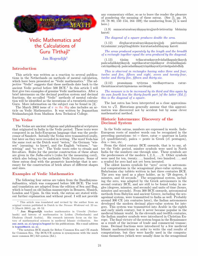
Vedic Mathematics andthe Calculations of

Guru Tırthajı∗

Jan Hogendijk†

Introduction

This article was written as a reaction to several publica-tions in the Netherlands on methods of mental calculation,which have been presented as “Vedic mathematics.” The ad-jective “Vedic” suggests that these methods date back to theancient Vedic period before 500 BCE.1 In this article I willfirst give two examples of genuine Vedic mathematics. After abrief intermezzo on the decimal position system and decimalfractions, the so-called “Vedic” methods of mental calcula-tion will be identified as the inventions of a twentieth-centuryGuru. More information on the subject can be found in [3].

The March 2003 issue of π in the Sky also includes an ar-ticle on Vedic Mathematics. It was written by JeganathanSriskandarajah from Madison Area Technical College.

The Vedas

The Vedas are ancient religious and philosophical scripturesthat originated in India in the Vedic period. These texts werecomposed in an Indo-European language that was the prede-cessor of Sanskrit. Initially the Vedas were transmitted orally,but later on they were recorded in writing. The word Veda hasthe same root as the Dutch word “weten,” the German “wis-sen” (meaning: to know), and the English “witness,” “un-witting” and “to wit.” The Vedic texts refer to rituals andfire-altars. Rules for the precise construction of these altarsare given in the Sulba-sutra’s (rules for the measuring cord),which also belong to the authentic Vedic literature. Some ofthese sutras deal with the geometric knowledge that is nec-essary for the construction of brick altars of different shapesand sizes.

Examples of Vedic Mathematics

The following four sutras are taken from the Baudhayana-sulbasutra, which was composed before 500 BCE. The textand translation are adapted from the edition of Sen and Bag,which is based on old Indian manuscripts in Benares, Munich,London and Ujjain. In this work, the sutras are stated with-out further explanation and without proof. I will not provide

∗ This article was translated and revised by the author from anoriginal version published in Dutch in the Nieuwe Wiskrant vol. 23 no.3 (March 2004), pp. 49–52.

† Jan Hogendijk teaches mathematics in Utrecht (Nether-lands) and history of mathematics in Leiden (Netherlands) andDhahran (Saudi Arabia). His research interests focus on the his-tory of mathematical sciences in medieval Islamic civilization. Seewww.math.uu.nl/people/hogend for his publications. His e-mail addressis [email protected].

1The notation BCE stands for Before Common Era and CE standsfor Common Era. The BCE/CE system is synonymous with the muchmore common BC/AD system (Ed.).

any commentary either, so as to leave the reader the pleasureof pondering the meaning of these sutras. (See [5, pp. 18,19, 78–80, 150–154, 164–169]; the numbering from [5] is usedhere.)

(1.9) samacaturasrasyaks.n. ayarajjurdvistavatım. bhumim.karoti

The diagonal of a square produces double the area.

(1.12) dırghacaturasrasyaks.n. ayarajjuh. parsvamanıtiryanmanı yatpr.thagbhute kurutastadubhayam. karoti

The areas produced separately by the length and the breadthof a rectangle together equal the area produced by the diagonal.

(1.13) tasam. trikacatuskayordvadasikapancikayoh.pancadasikas.t.ikayoh. saptikacaturvim. sikayor dvadasikapan-catrim. sikayoh. pancadasikas.at.trim. sikayorityetasupalabdhih.

This is observed in rectangles having sides three and four,twelve and five, fifteen and eight, seven and twenty-four,twelve and thirty-five, fifteen and thirty-six.

(2.12) praman. am. tr.tıyena vardhayettacca catur-thenatmacatustrim. sonena savises.ah.

The measure is to be increased by its third and this again byits own fourth less the thirty-fourth part [of the latter (Ed.)];this is the diagonal of a square.

The last sutra has been interpreted as a close approxima-tion to

√2. Historians generally assume that this approxi-

mation was discovered not by accident but by some clevermathematical method.

Historic Intermezzo: Discovery of theDecimal System

In the Vedic sutras, numbers are expressed in words. Indo-European roots of number words can be recognized in thepreceding quotations: tri = three, catur = quattuor in Latin(cf. quadrilateral), panca = pente in Greek (cf. pentagon),dva = two, etc.

From the third century BCE onwards, that is to say, af-ter the Vedic period, number symbols were used in NorthIndia for the numbers one through nine. These symbols arethe predecessors of the modern 1, 2, 3, . . . , 9. Other symbolswere used for ten, twenty. . . , hundred, two hundred. . . , anda symbol for zero had not yet been invented.

The oldest known symbols for “zero” occur in astronom-ical computations in the sexagesimal place-value system, onBabylonian clay tablets written in last three centuries BCE.The zero was used as a place holder, as in “29 degrees, 0minutes, and 43 seconds.” The sexagesimal system, includ-ing the zero, was adapted by the Greek astronomers in thesecond century BCE, and are still to be found today in an-gles (degrees, minutes, and seconds) and units of time (hours,minutes and seconds). From 300 BCE onwards, astronomicalmethods from Babylon and ancient Greece, including the sex-agesimal system, were transmitted to India as well. Probablyaround 300 CE (six centuries later), the Indian astronomersdeveloped the modern decimal place-value system for inte-gers. This system was transmitted into Arabic in the eighthand early ninth century, but it never became popular in themedieval Islamic world. In the eleventh and twelfth centuries,the Indian number symbols were introduced in Christian Eu-rope. The final victory of the system began in the Renaissanceas a result of the increase of trade and commercial transac-tions. Decimal fractions were introduced by a few medievalIslamic mathematicians in order to write the end results ofcomputations, but they were hardly used in the computa-tions themselves (which were usually done in the sexagesimal

24

system). In Europe, decimal fractions were independentlydiscovered by the Flemish mathematician Simon Stevin, whopublished his discovery in 1585 in Leiden in Holland. Dec-imal fractions probably arrived in India in the seventeenthcentury, when French astronomical tables were studied by as-tronomers in and around Delhi. During the English colonialregime, decimal fractions were of course taught in schools.

The “Vedic” Mathematics of Guru Tirthajı

The “Vedic” methods of mental calculations in the dec-imal system are all based on the book Vedic Mathemat-ics by Jagadguru (world guru) Swami (monk) Srı (rev-erend) Bharatı Kr.s.n. a Tırthajı Maharaja, which appearedin 1965 and which has been reprinted many times [4].

Figure 1: Guru Tırthajı

This Guru was bornin 1884 near Madrasas Venkatraman Shas-tri. He studied English,mathematics, Sanskrit,and other subjects atvarious schools and col-leges in India. In 1911 hequit his teaching job inorder to devote himselfcompletely to study andmeditation in an ashramnear Mysore. In 1919he was initiated as asannyasi (monk) and re-ceived the name BharatıKr.s.n. a Tırtha. Shortlyafterwards, he becamethe leader of ashrams.He travelled extensivelythrough India, and, atthe invitation of the Self-Realization Fellowship ofYogananda, also to theUnited States in 1958.

Bharatı Kr.s.n. a Tırtha died in 1960 and his main work VedicMathematics appeared posthumously.

The book contains sixteen brief sutras that can be used formental calculations in the decimal place-value system. Anexample is the sutra ekadhikena purvena, meaning: by onemore than the previous one. The Guru explains that thissutra can for example be used in the mental computation ofthe period of a recurring decimal fraction such as 1/19 =0.052631578947368421, as follows:

The last decimal of the period is 1. We now apply thesutra by one more than the previous one to the number 19.The previous one is the penultimate decimal in the decimalrepresentation of 19, so one more than the previous one is 2.We multiply the last decimal of the period by 2 and get thepenultimate decimal of the period, and so on. Thus we findthe final decimals . . . 8421. We now compute 8×2 = 16, writethe 6 before the 8, and remember the 1. We add this 1 to thenext product 6 × 2 to obtain . . . 368421, and so on.2

2The Guru does not give a proof of why the method works. Here is asimple number-theoretic proof: let nk be the k-th decimal in the decimalexpansion of 1/19 (thus n1 = 0, n2 = 5, n3 = 2 . . .). Then for k = 1, 2, . . .

we have 10k = 19(10k−1n1 +10k−2n2 + . . . +10nk−1 + nk)+ mk wheremk is an integer such that 0 < mk < 19; thus m1 = 10, m2 = 5, m3 =12 . . .. Because 19nk + mk must be a multiple of 10, which implies that−nk + mk must be a multiple of 10, we see that nk is equal to the lastdigit of mk, which is the remainder of 10k after division by 19. Because1018 ≡ 1 mod 19, we have n18 = m18 = 1. Since 2 · 10k+1 = 20 · 10k ≡

10k mod 19, we have 2mk+1 ≡ mk mod 19, hence n17 = m17 = 2,n16 = m16 = 4, n15 = m15 = 8, m14 = 16, and n14 = 6. Then

The same method can be used for 1/29, but now we haveto take 3 as one more than the previous one.

The word “Vedic” in the title of the book suggests thatthese calculations are authentic Vedic mathematics. Thequestion now arises how the Vedic mathematicians were ableto write the recurrent decimal fraction of 1/19, while decimalfractions were unknown in India before the seventeenth cen-tury. We will first investigate the origin of the sixteen sutras.We cite the Guru himself [4, pp. xxxviii–xxix]:

“And the contemptuous or, at best, patronizing attitudeadopted by some so-called orientalists, indologists, antiquar-ians, research-scholars etc. who condemned, or light heart-edly, nay irresponsibly, frivolously and flippantly dismissed,several abstruse-looking and recondite parts of the Vedas as‘sheer nonsense’ or as ‘infant-humanity’s prattle,’ and so on,. . . further confirmed and strengthened our resolute determi-nation to unravel the too-long hidden mysteries of philosophyand science contained in ancient India’s Vedic lore, with theconsequence that, after eight years of concentrated contempla-tion in forest-solitude, we were at long last able to recover thelong lost keys which alone could unlock the portals thereof.

“And we were agreeably astonished and intensely gratifiedto find that exceedingly tough mathematical problems (whichthe mathematically most advanced present day Western sci-entific world had spent huge lots of time, energy and moneyon and which even now it solves with the utmost difficultyand after vast labour involving large numbers of difficult, te-dious and cumbersome ‘steps’ of working) can be easily andreadily solved with the help of these ultra-easy Vedic Sutras(or mathematical aphorisms) contained in the Parisısta (theAppendix-portion) of the Atharvaveda in a few simple stepsand by methods which can be conscientiously described asmere ‘mental arithmetic.’ ”

The Guru adds [4, p. xl]:“The Sutras (aphorisms) apply to and cover each and ev-

ery part of each and every chapter of each and every branchof mathematics (including arithmetic, algebra, geometry—plane and solid, trigonometry—plane and spherical, conics—geometrical and analytical, astronomy, calculus—differentialand integral etc.). In fact, there is no part of mathematics,pure or applied, which is beyond their jurisdiction.”

Concerning the applicability of the sixteen sutras to allmathematics, we can consult the Foreword to Vedic Mathe-matics written by Swami Pratyagatmananda Saraswati. ThisSwami states that one of the sixteen sutras reads Calana-kalana, which can be translated as Becoming. The Guruhimself translates the sutra in question as “differential cal-culus” [4, p. 186]. Using this “translation” the sutra indeedpromises applicability to a large area in mathematics; butthe sutra is of no help in differentiating or integrating a givenfunction such as f(x) = 1/ sin x.

Sceptics have tried to locate the sutras in the extantParisısta’s (appendices) of the Atharva-Veda, one of the fourVedas. However, the sutras have never been found in authen-tic texts of the Vedic period. It turns out that the Guru had“seen” the sutras by himself, just as the authentic Vedas were,according to tradition, “seen” by the great Rishi’s or seers ofancient India. The Guru told his devotees that he had “re-constructed” his sixteen sutras from the Atharva-Veda in theeight years in which he lived in the forest and spent his time oncontemplation and ascetic practices. The book Vedic Mathe-matics is introduced by a General Editor’s Note [4, p. vii], inwhich the following is stated about the sixteen sutras: “[the]

style of language also points to their discovery by Srı Swamijı(the Guru) himself.”

m13 ≡ 2 · 16 ≡ 2 · (10+6) ≡ 20+2 · 6 ≡ 1+2 · 6 mod 19. Thus the Gurucorrectly adds the penultimate digit 1 of the number 16 to two times thelast digit 6. The same argument works for all other mi ≥ 10.

25

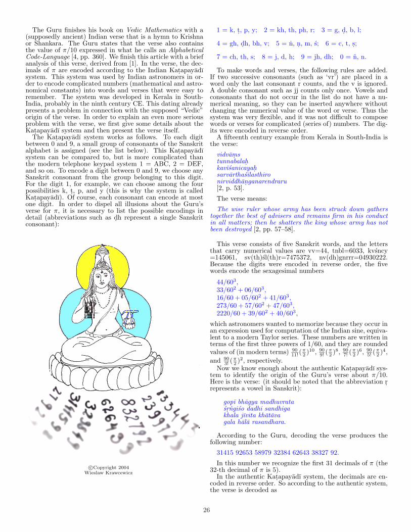
The Guru finishes his book on Vedic Mathematics with a(supposedly ancient) Indian verse that is a hymn to Krishnaor Shankara. The Guru states that the verse also containsthe value of π/10 expressed in what he calls an AlphabeticalCode-Language [4, pp. 360]. We finish this article with a briefanalysis of this verse, derived from [1]. In the verse, the dec-imals of π are encoded according to the Indian Kat.apayadısystem. This system was used by Indian astronomers in or-der to encode complicated numbers (mathematical and astro-nomical constants) into words and verses that were easy toremember. The system was developed in Kerala in South-India, probably in the ninth century CE. This dating alreadypresents a problem in connection with the supposed “Vedic”origin of the verse. In order to explain an even more seriousproblem with the verse, we first give some details about theKat.apayadı system and then present the verse itself.

The Kat.apayadı system works as follows. To each digitbetween 0 and 9, a small group of consonants of the Sanskritalphabet is assigned (see the list below). This Kat.apayadısystem can be compared to, but is more complicated thanthe modern telephone keypad system 1 = ABC, 2 = DEF,and so on. To encode a digit between 0 and 9, we choose anySanskrit consonant from the group belonging to this digit.For the digit 1, for example, we can choose among the fourpossibilities k, t., p, and y (this is why the system is calledKat.apayadı). Of course, each consonant can encode at mostone digit. In order to dispel all illusions about the Guru’sverse for π, it is necessary to list the possible encodings indetail (abbreviations such as d.h represent a single Sanskritconsonant):


1 = k, t., p, y; 2 = kh, th, ph, r; 3 = g, d. , b, l;

4 = gh, d.h, bh, v; 5 = n, n. , m, s; 6 = c, t, s.;

7 = ch, th, s; 8 = j, d, h; 9 = jh, dh; 0 = n, n.

To make words and verses, the following rules are added.If two successive consonants (such as ‘vr’) are placed in aword only the last consonant r counts, and the v is ignored.A double consonant such as jj counts only once. Vowels andconsonants that do not occur in the list do not have a nu-merical meaning, so they can be inserted anywhere withoutchanging the numerical value of the word or verse. Thus thesystem was very flexible, and it was not difficult to composewords or verses for complicated (series of) numbers. The dig-its were encoded in reverse order.

A fifteenth century example from Kerala in South-India isthe verse:

vidvam. stunnabalah.kavısanicayah.sarvarthasılasthironirviddhan. ganarendraru[2, p. 53].

The verse means:

The wise ruler whose army has been struck down gatherstogether the best of advisers and remains firm in his conductin all matters; then he shatters the king whose army has notbeen destroyed [2, pp. 57–58].

This verse consists of five Sanskrit words, and the lettersthat carry numerical values are vv=44, tnbl=6033, kvsncy=145061, sv(th)sl(th)r=7475372, nv(dh)gnrrr=04930222.Because the digits were encoded in reverse order, the fivewords encode the sexagesimal numbers

44/603,33/602 + 06/603,16/60 + 05/602 + 41/603,273/60 + 57/602 + 47/603,2220/60 + 39/602 + 40/603,

which astronomers wanted to memorize because they occur inan expression used for computation of the Indian sine, equiva-lent to a modern Taylor series. These numbers are written interms of the first three powers of 1/60, and they are roundedvalues of (in modern terms) 90

11! (π2 )10, 90

9! (π2 )8, 90

7! (π2 )6, 90

5! (π2 )4,

and 903! (

π2 )2, respectively.

Now we know enough about the authentic Kat.apayadı sys-tem to identify the origin of the Guru’s verse about π/10.Here is the verse: (it should be noted that the abbreviation r.represents a vowel in Sanskrit):

gopı bhagya madhuvratasr. ngiso dadhi sandhigakhala jıvita khatavagala hala rasandhara.

According to the Guru, decoding the verse produces thefollowing number:

31415 92653 58979 32384 62643 38327 92.

In this number we recognize the first 31 decimals of π (the32-th decimal of π is 5).

In the authentic Kat.apayadı system, the decimals are en-coded in reverse order. So according to the authentic system,the verse is decoded as

26

29723 83346 26483 23979 85356 29514 13.

We conclude that the verse is not medieval, and certainlynot Vedic. In all likelihood, the Guru is the author of theverse.

Conclusion

There is nothing intrinsically wrong with easy methods ofmental calculations and mnemonic verses for π. However, itwas a miscalculation on the part of the Guru to present hiswork as ancient Vedic lore. Many experts in India know thatthe relations between the Guru’s methods and the Vedas arefaked. In 1991 the supposed “Vedic” methods of mental cal-culation were introduced in schools in some cities, perhaps inthe context of the political program of saffronisation, whichemphasizes Hindu religious elements in society (named afterthe saffron garments of Hindu Swamis). After many protests,the “Vedic” methods were omitted from the programs, only tobe reintroduced a few years later. In 2001, a group of intellec-tuals in India published a statement against the introductionof the Guru’s “Vedic” mathematics in primary schools in In-dia.

Of course, there are plenty of real highlights in the ancientand medieval mathematical tradition of India. Examples arethe real Vedic sutras that we have quoted in the beginning ofthis paper; the decimal place-value system for integers; theconcept of sine; the cyclic method for finding integer solutionsx, y of the “equation of Pell” in the form px2 + 1 = y2 (forp a given integer); approximation methods for the sine andarctangents equivalent to modern Taylor series expansions;and so on. Compared to these genuine contributions, theGuru’s mental calculation are of very little interest. In thesame way, the Indian philosophical tradition has a very highintrinsic value, which does not need to be “proved” by theso-called applications invented by Guru Tırthajı.

Acknowledgements

I wish to thank Prof. Dr. Michio Yano, Kyoto SanghoUniversity, for sending me the article by K. Chandra Hari,and Dr. Len Berggren, Simon Fraser University, Canada, forcorrecting my translation; Dr. Kim Plofker, Utrecht and ananonymous referee for their comments on an earlier versionof this paper.

References

[1] Chandra Hari, K., 1999: A critical study of Vedic

mathematics of Sankaracarya Srı Bharatı Kr.s.n. a TırthajıMaharaj. Indian Journal of History of Science 34, 1–17.

[2] Gold, D. and D. Pingree, 1991: A hitherto unknownSanskrit work concerning Madhava’s derivation of thepower series for sine and cosine. Historia Scientiarum,42, 49–65.

[3] Gupta, R. C., 1994: Six types of Vedic Mathematics.Gan. ita Bharatı 16, 5–15.

[4] Jagadguru Swamı Srı Bharatı Kr.s.n. a Tırthajı Maharaja,1992: Vedic Mathematics. Delhi: Motilal Banarsidas,revised edition.

[5] Sen, S. N. and A. K. Bag, 1983: The Sulbasutras. NewDelhi: Indian National Science Academy.

[6] Interesting web site on Vedic ritual: http://www.jyotistoma.nl.

[7] Pamphlet “Neither Vedic Nor Mathematics,” againstthe introduction of “Vedic” method of computations inschool teaching: http://www.sacw.net/DC/CommunalismCollection/ArticlesArchive/NoVedic.html.

Q: “How does one insult a mathematician?”A: “Your brain is smaller than any ǫ > 0!”

Two mathematicians are studying a convergent series.The first one says: “Do you realize that the series converges

even when all the terms are made positive?”The second one asks: “Are you sure?”“Absolutely!”

Q: What does a mathematician present to his fiancee whenhe plans to propose to her?

A: A polynomial ring!

Q: Why don’t mathematicians ever spend time at thebeach?

A: Because they don’t need the sun to get a tan, they havesin and cos.

Q: Why is it that derivatives can never finish telling a story?A: Because they are always going off on tangents.


27

Tribonacci in the Sky:A MathematicalMountain Walk

Achim Clausing†

Going Downhill

Here is a game that you can find in some elementary schoolmath books:

“Every child in the class chooses four numbers. Below eachnumber, he or she writes the difference between this numberand its neighbour to the right. (The last number gets the firstone as its right-hand neighbour.) This calculation is called adownward step. Now the children repeat stepping down untilthey arrive at four equal numbers. The winner is the child(or the children) requiring the most steps to arrive there.”

Here is an example:

3 1 7 142 6 7 114 1 4 93 3 5 50 2 0 22 2 2 2

We say that the quadruple (3, 1, 7, 14) has height 5 since ittakes 5 steps down to reach flat terrain. Thus, a step downis one application of the map

δ(a, b, c, d) = (|b − a|, |c − b|, |d − c|, |a − d|).

The point of this game is not that the children should bekept busy calculating for quite a while. Triples or five-tuplesof numbers would do well for that purpose, but with quadru-ples it is amazing how fast one usually arrives at a constanttuple.

Look at these three quadruples with their “trails” whosevalues I have chosen at random in {0 . . . 99}. They are rathertypical (rather than trust me, repeat the experiment foryourself):

25 86 92 2361 6 69 255 63 67 598 4 8 44 4 4 4

57 34 90 4223 56 48 1533 8 33 825 25 25 25

37 18 15 319 3 12 3416 9 22 157 13 7 16 6 6 6

† Achim Clausing is a professor of computing scienceat the Department of Mathematics and Computing Science ofthe University of Munster (Germany). His e-mail address [email protected].

With the aid of a computer, it is easy to simulate a reallylarge class playing this game. A statistic of the heights of10,000 random quadruples with values in {0 . . . 99} is shownin Figure 1.

Almost 90% of the quadruples reach a constant tuple withinthree to five steps!

The average height of a random quadruple in this exper-iment is ≈ 3.88. If the random numbers were chosen froma different range, e. g. from {0 . . . 109}, we would get essen-tially the same picture (including the striking local maximumin the frequency of tuples of height 3).

But, in case you didn’t notice it from the graph: there wereindeed 3 quadruples of height 10 and 2 of height 11 (thus twoof the 10,000 children in this class would be the winners).

1 2 3 4 5 6 7 8 9 10 11

1000

2000

3000

4000

5000

Figure 1: The heights of 10,000 random quadruples withvalues in {0 . . . 99}.

On Returning Safely

High mountains, that is, quadruples with a large height, arenot easy to conquer. But before we venture to attack them,we should, as a safety measure, make sure that there is a wayhome from the larger heights. Simply walking downhill mightnot always lead into the plains, as every mountain walkerknows. It is all too easy to get stuck somewhere.

That is, we should ask ourselves whether there is, for ev-ery quadruple (a, b, c, d), an integer n and a value e suchthat δn(a, b, c, d) = (e, e, e, e) (and then, δn+1(a, b, c, d) =(0, 0, 0, 0)).

The question is by no means trivial. Even for very simplemaps f of some set X into itself, it has been observed thatrepeated application of f always leads to the same element,but nobody is able to prove this. One of the more prominentexamples for this phenomenon is the Syracuse function f onthe positive integers (named after the Syracuse University,where L. Collatz found it in the thirties). Let

f(n) =

{

3n + 1 if n is odd,n2 if n is even.

Regardless of the number n you start with, repeated appli-cation of f always leads down to 1. Although this has beenverified experimentally for values of n up to truly astronom-ical size, no one has yet been able to show that it is true forall n.

Fortunately, it is easy to see that the stepping game al-ways ends at a constant tuple. If we start with an arbi-trary quadruple (a, b, c, d) of non-negative integers, then eachstep decreases the maximum component in the quadruple,except when the right neighbour of the maximum is zero.Let us assume that the maximum is a and that b = 0.

28

Then δ(a, 0, c, d) = (a, c, |d − c|, a − d). This tuple also hasa as its maximum, hence either c > 0 and the next stepagain reduces the maximum, or c = 0 and the next step isδ(a, 0, d, a − d) = (a, d, a − 2d, d). One more time: Eitherd > 0 and the maximum gets smaller, or d = 0 and the nextstep is δ(a, 0, a, 0) = (a, a, a, a).

Thus, after four steps, either the maximum of the sequencehas got smaller or we have reached a constant tuple. Thisproves that in the long run, we always get safely down to aconstant tuple.

As an alternative, it is easy to show that with four stepswe either will reach a constant tuple or all components ofthe tuple are multiples of 2. This again implies that the fournumber game eventually will reach a constant quadruple.

Climbing

Climbing means doing one step upwards after the other.Sounds simple. But occasionally, one comes to a point whereit is not possible to continue upwards. This can happen here,too.

If δ(x, y, z, u) = (a, b, c, d), we call (x, y, z, u) a predecessorof (a, b, c, d). It is one step higher than (a, b, c, d).

The definition of the map δ tells us that there are signssi (i = 0 .. 3) such that y − x = s0a, z − y = s1b, u − z = s2cand x − u = s3d. Therefore,

(x, y, z, u) = (x, x + s0a, x + s0a + s1b, x + s0a + s1b + s2c),

and from x = u + s3d we see that

s0a + s1b + s2c + s3d = 0

holds. Furthermore, if we can find signs si such that thisequation holds, then clearly (a, b, c, d) has a predecessor.

For example, the tuple (3, 1, 7, 14) considered above obvi-ously has no such signs since 3 + 1 + 7 < 14. From thisquadruple, it is not possible to do an upward step. On theother hand, if a, b, c, d > 0, and

a + b + c = d, (⋆)

we can chose s0 = s1 = s2 = 1 and s3 = −1, and find thepredecessor

(x, y, z, u) = (x, x + a, x + a + b, x + a + b + c),

where x ≥ 0 can be chosen arbitrarily. How about a prede-cessor of this tuple? We can choose x ≥ 0 such that

x + y + z = u

holds. This means

x + (x + a) + (x + a + b) = x + a + b + c,

orx = (c − a)/2.

Thus, if for quadruples (a, b, c, d) with a + b + c = d anda ≤ c we define the upwards-map γ by

γ(a, b, c, d)

=

(

c − a

2,c − a

2+ a,

c − a

2+ a + b,

c − a

2+ a + b + c

)

=1

2(−a + c, a + c, a + 2b + c, a + 2b + 3c)

= (x, y, z, u),

then δ(x, y, z, u) = (a, b, c, d), x ≤ z and x + y + z = u. Wecan choose the signs si as before and conclude that (x, y, z, u)again has a predecessor.

Now we can climb one step after the other! Stated in some-what less sportive terms, the tuples

(an, bn, cn, dn) = γn(a, b, c, d) (n ≥ 0)

have the heights hn = n+h, where h is the height of (a, b, c, d).Don’t forget to start from a tuple where a + b + c = d and

a ≤ c. Let us, for example, take a mountain walk of 15 stepsstarting from the tuple (0, 0, 1, 1) with the height h = 2:

0 0 1 1

12

12

12

32

0 12 1 3

2

12

12 1 2

14

34

54

94

12

34

32

114

12 1 7

4134

58

98

178

318

34

118

52

378

78

138 3 11

2

1716

3116

5716

10516

54

3716

174

12516

32

114

8116

14916

5732

10532

19332

35532

178

12532

11516

42332

8132

14932

13716

634

There is no need to worry about the fact that these quadru-ples are not integers. Just multiply them by the GCD of theirdenominators; this clearly does not alter their heights.

If, say, we multiply the last line ( 8132 , 149

32 , 13716 , 63

4 ) of ourmountain hike by 32, we obtain the integer quadruple(81, 149, 274, 504), which is 17 steps high.

Tuples of this height are rare; you don’t find them by aquick random search. But once you have one, you can easilyproduce others of the same height from it by multiplying itwith a nonzero constant, by adding the same constant to everyelement of the tuple, by rotating it or by reversing its order.None of these operations affects the height of the tuple.

We call tuples equivalent , if they can be converted into eachother by one of these operations. In particular, for every tuple(a, b, c, d) 6= (0, 0, 0, 0) there is an equivalent normalized one,denoted by [a, b, c, d], whose smallest and largest element are0 and 1. It is obtained by subtracting the minimal componentfrom each of the components and dividing the result by itsmaximum component.

In our example we find [81, 149, 274, 504] = (0, 68423 , 193

423 , 1).

The Sky is the Limit

Now that we have seen that by repeated down stepping onereaches the plains from every quadruple of rational numbers,it is only natural to ask where we get from a non-rationalstarting quadruple. One might conjecture that the “trails” ofsuch tuples would in general converge to a constant withoutactually reaching it in finitely many steps.

As an experiment, we try the tuple (1, e,√

7, π). The resultis a surprise:

1 e

√

7 π

e − 1 e −

√

7 π −

√

7 π − 1√

7 − 1 π − e

√

7 − 1 π − e√

7 + e − π − 1√

7 + e − π − 1√

7 + e − π − 1√

7 + e − π − 1

It took us only three steps to get down! In fact, we shouldnot be surprised that much. The rational approximation(1, 2.7, 2.6, 3.1) to our starting tuple has height 3, as have

29

better approximations, and there is simply no reason to sus-pect that in the limit anything should change.

Or is there? What, if we had a converging sequence of ratio-nal quadruples of ever-increasing height? Then the limitingquadruple is perhaps one of the more interesting viewpointson our mountain hike.

The question is not an academic one since in fact we alreadyhave such a sequence of quadruples! Look at the normalizedversion [an, bn, cn, dn] (n ≥ 0) of the sequence that we con-structed in the preceding section. The normalized quadruplesof our 15-step mountain walk are, numerically,

0 0 1 10 0 0 10 0.333333 0.666667 10 0 0.333333 10 0.25 0.5 10 0.111111 0.444444 10 0.181818 0.454545 10 0.153846 0.461538 1

0 0.16129 0.451613 10 0.162162 0.459459 10 0.159091 0.454545 10 0.161905 0.457143 10 0.16 0.456 10 0.161074 0.456376 10 0.160563 0.456338 10 0.160757 0.456265 1

It is not hard to believe that this sequence converges to(0, 0.160.., 0.456.., 1).

Say, the limit is (a, b, c, d). What properties could it have?Since (an+1, bn+1, cn+1, dn+1) = γ(an, bn, cn, dn), it is not un-reasonable to hope that

[γ(a, b, c, d)] = [a, b, c, d] = [δ(a, b, c, d)]

holds. In accordance with the elements of the sequence, thelimit should satisfy the relation (⋆ ), and since we are free tomultiply with a constant, we put (a, b, c, d) = (1, x, y, 1+x+y)with unknown x, y about which we assume 1 ≤ x ≤ y. (Wecan assume whatever we like, this is just a heuristic guessabout what the limit is.)

Then δ(1, x, y, 1 + x + y) = (x − 1, y − x, x + 1, x + y).An equivalent tuple is (1, y−x

x−1 , x+1x−1 , 1+x+y

x−1 ). Hence we try tosolve

(1, x, y, 1 + x + y) = (1,y − x

x − 1,x + 1

x − 1,1 + x + y

x − 1)

and find by comparing the second components

x =y − x

x − 1

that y = x2, and from

y = x2 =x + 1

x − 1

that x must be a (real) solution of 1 + x + x2 = x3. Thisequation has exactly one real solution, which is

x =1

3+

(

19 − 3√

33)

1

3

3+

(

19 + 3√

33)

1

3

3= 1.83929 . . . .

The quadruple (1, x, x2, 1 + x + x2) = (1, x, x2, x3) indeedsatisfies

[1, x, x2, x3] = (0,x − 1

x3 − 1,

x2 − 1

x3 − 1, 1)

= (0,1

x3,

1

x3+

1

x2, 1)

= (0, 0.160713 . . . , 0.456311 . . . , 1).

It is, by construction, an eigenvector of the linear map(a, b, c, d) 7→ (b − a, c − b, d − c, d − a):

δ(1, x, x2, x3) = (x − 1, x2 − x, x3 − x2, x3 − 1)

= (x − 1) · (1, x, x2, x3−1x−1 )

= (x − 1) · (1, x, x2, 1 + x + x2)= (x − 1) · (1, x, x2, x3)= 0.83929 . . . · (1, x, x2, x3).

By down stepping from (1, x, x2, x3), we obtain an equiva-lent tuple, albeit with slightly smaller components. We havereached a place from where there is no way back to flat earth:There is not just π in the Sky , but some unexpected quadru-ples, too!

A quadruple from which one cannot reach a constant tupleby repeated application of δ does not have a finite height. Itis natural to say that it has height ∞. (We probably shouldat this point define the sky as the set of all quadruples ofheight ∞. But by this we would throw π out of the paradise,an unforgivable sin in this magazine.)

Tribonacci in the Sky

The sky is where the gods are, and they live on a highmountain. The old Greeks knew that (and some mathematicsas well). Now the mathematical sky is not just inhabited byGreek gods (say, Pythagoras, Euclid, or the immortal numberπ) but also by many lesser celebrities. One of them is a certainMr. Tribonacci∗ , a cousin of the more famous mathematicianLeonardo of Pisa, known as Fibonacci.

We all know and love the Fibonacci numbers 0, 1, 1, 2, 3, 5,8, 13, 21, 34, 55, 89, 144,. . . , where each element is the sum ofthe two preceding ones: fn = fn−1+fn−2. The ratios fn/fn−1of two consecutive Fibonacci numbers converge to the GoldenRatio 1

2 (1 +√

5) = 1.61803 . . ., which is the positive root of

the equation 1 + x = x2.In the Tribonacci number sequence 0, 1, 1, 2, 4, 7, 13,

24, 44, 81, 149, 274, 504,. . . , each element is the sum of thepreceding three elements: tn = tn−1 + tn−2 + tn−3. The ratiostn/tn−1 of two consecutive Tribonacci numbers converge tothe positive root of the equation 1 + x + x2 = x3, which wehappen to know as x = 1.83929 . . ..

This sequence, though less common than the Fibonaccisequence, appears in many contexts (it has number A75 inSloane’s On-Line Encyclopedia of Integer Sequences, the Fi-bonacci sequence being A45). It is closely connected with ourstepping game.

Did you notice that the four numbers 81, 149, 274, 504 inthe Tribonacci sequence form the quadruple of height 17 thatwe constructed in our 15-step-mountain walk? And that theTribonacci recursion is just the condition (⋆) for a quadrupleto have a predecessor?

The Tribonacci sequence is another “stairway to heaven,”in the technical sense of this article: The heights hn =height(tn, tn+1, tn+2, tn+3) of the tuples in this sequence are5, 5, 8, 8, 11, 11, 14, 14, 17, 17, . . ., that is, they increase by 3every two steps. This is easy to prove. A similar fact holdsfor Tribonacci-like sequences starting with triples other than{0, 1, 1}.

The Tribonacci numbers also show up in the answer to thefollowing question: What is the smallest integer a such that{0 . . . a}4 contains a quadruple of height n?

Let us denote this integer by an. The first elements of thesequence (a1, a2, . . .) are

(1, 1, 1, 3, 3, 4, 9, 11, 13, 31, 37, 44, 105, 125, 149, 355, . . .).

∗The “Mr.” stands for the Italian title “Messer,” poor Mr. Tri-bonacci not having any first name.

30

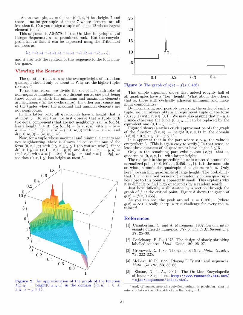
As an example, a7 = 9 since (0, 1, 4, 9) has height 7 andthere is no integer tuple of height 7 whose elements are allless than 9. Can you design a tuple of height 12 whose largestelement is 44?

This sequence is A045794 in the On-Line Encyclopedia ofInteger Sequences, a less prominent rank. But the encyclo-pedia knows that it can be expressed using the Tribonaccinumbers as

(t0 + t2, t1 + t2, t3, t2 + t4, t3 + t4, t5, t4 + t6, . . .),

and it also tells the relation of this sequence to the four num-ber game.

Viewing the Scenery

The question remains why the average height of a randomquadruple should only be about 4. Why are the higher tuplesso scarce?

To see the reason, we divide the set of all quadruples ofnon-negative numbers into two disjoint parts, one part beingthose tuples in which the minimum and maximum elementsare neighbours (in the cyclic sense), the other part consistingof the tuples where the maximal and minimal elements arenot neighbours.

In this latter part, all quadruples have a height that isat most 5. To see this, we first observe that a tuple withtwo equal components that are not neighbours, say (a, b, c, b),has a height h ≤ 3: δ(a, b, c, b) = (u, v, v, u) with u = |b −a|, v = |c− b|, δ(u, v, v, u) = (w, 0, w, 0) with w = |v−u|, andδ(w, 0, w, 0) = (w, w, w, w).

Now, for a tuple whose maximal and minimal elements arenot neighbouring, there is always an equivalent one of theform (0, x, 1, y) with 0 ≤ x ≤ y ≤ 1 (do you see why?). Sinceδ(0, x, 1, y) = (x, 1 − x, 1 − y, y), and δ(x, 1 − x, 1 − y, y) =(a, b, c, b) with a = |1 − 2x|, b = |y − x| and c = |1 − 2y|, wesee that (0, x, 1, y) has height at most 5.

0

0.2

0.4

0.6

0.8

1

0

0.2

0.4

0.6

0.8

1

0

2

4

6

8

10

Figure 2: An approximation of the graph of the functionf(x, y) = height(0, x, y, 1) in the domain {(x, y) : 0 ≤x, y, x + y ≤ 1}.

0.1 0.2 0.3 0.4

5

10

15

20

25

Figure 3: The graph of g(x) = f(x, 0.456).

This simple argument shows that indeed roughly half ofall quadruples have a “low” height. What about the others,that is, those with cyclically adjacent minimum and maxi-mum components?

By normalizing and possibly reversing the order of such atuple, we can always obtain an equivalent tuple of the form(0, x, y, 1) with x, y ∈ [0, 1]. We may also assume that x+y ≤1 since otherwise the tuple (0, x, y, 1) can be replaced by theequivalent one (0, 1 − y, 1 − x, 1).

Figure 2 shows (a rather crude approximation of) the graphof the function f(x, y) = height(0, x, y, 1) in the domain{(x, y) : 0 ≤ x, y, x + y ≤ 1}.

It is apparent that in the part where x > y, the value iseverywhere 3. (This is again easy to verify.) In that sense, atleast three quarters of all quadruples have height h ≤ 5.

Only in the remaining part exist points (x, y)—that is,quadruples (0, x, y, 1)—with larger heights.

The red peak in the preceding figure is centered around thenormalized point (0, 0.160 . . . , 0.456 . . . , 1). It is the mountainon whose summit the quadruple of height ∞ resides. Onlyhere† we can find quadruples of large height. The probabilitythat (the normalized version of) a randomly chosen quadruplelies close to this point is apparently small. This explains whyit is difficult to find high quadruples by a random search.

Just how difficult, is illustrated by a section through thegraph of f at the critical point. Figure 3 shows the graph ofg(x) = f(x, 0.456).

As you can see, the peak around x = 0.160 . . . (whereg(x) = ∞) is really sharp, a true challenge for every moun-taineer!

References

[1] Ciamberlini,, C. and A. Marengoni, 1937: Su una inter-essante curiosita numerica. Periodiche di Mathematiche,17, 25–30.

[2] Berlekamp, E. R., 1975: The design of slowly shrinkinglabelled squares. Math. Comp., 29, 25–27.

[3] Greenwell, R., 1989: The game of Diffy. Math. Gazette,73, 222–225.

[4] McLean, K. R., 1999: Playing Diffy with real sequences.Math. Gazette, 83, 58–68.

[5] Sloane, N. J. A., 2004: The On-Line Encyclopediaof Integer Sequences. http://www.research.att.com/∼njas/sequences/index.html.

†And, of course, near all equivalent points, in particular, near itsmirror point on the other side of the line x + y = 1.

31

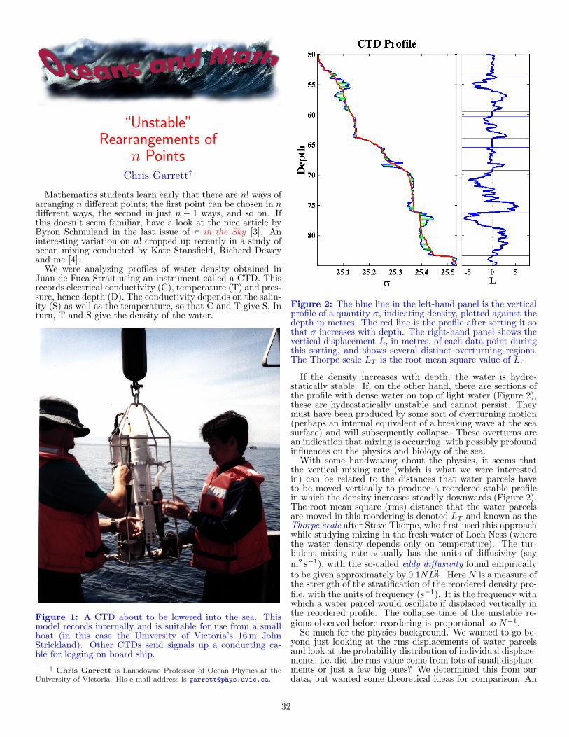
“Unstable”Rearrangements of

n PointsChris Garrett†

Mathematics students learn early that there are n! ways ofarranging n different points; the first point can be chosen in ndifferent ways, the second in just n − 1 ways, and so on. Ifthis doesn’t seem familiar, have a look at the nice article byByron Schmuland in the last issue of π in the Sky [3]. Aninteresting variation on n! cropped up recently in a study ofocean mixing conducted by Kate Stansfield, Richard Deweyand me [4].

We were analyzing profiles of water density obtained inJuan de Fuca Strait using an instrument called a CTD. Thisrecords electrical conductivity (C), temperature (T) and pres-sure, hence depth (D). The conductivity depends on the salin-ity (S) as well as the temperature, so that C and T give S. Inturn, T and S give the density of the water.

Figure 1: A CTD about to be lowered into the sea. Thismodel records internally and is suitable for use from a smallboat (in this case the University of Victoria’s 16 m JohnStrickland). Other CTDs send signals up a conducting ca-ble for logging on board ship.

† Chris Garrett is Lansdowne Professor of Ocean Physics at theUniversity of Victoria. His e-mail address is [email protected].

Figure 2: The blue line in the left-hand panel is the verticalprofile of a quantity σ, indicating density, plotted against thedepth in metres. The red line is the profile after sorting it sothat σ increases with depth. The right-hand panel shows thevertical displacement L, in metres, of each data point duringthis sorting, and shows several distinct overturning regions.The Thorpe scale LT is the root mean square value of L.

If the density increases with depth, the water is hydro-statically stable. If, on the other hand, there are sections ofthe profile with dense water on top of light water (Figure 2),these are hydrostatically unstable and cannot persist. Theymust have been produced by some sort of overturning motion(perhaps an internal equivalent of a breaking wave at the seasurface) and will subsequently collapse. These overturns arean indication that mixing is occurring, with possibly profoundinfluences on the physics and biology of the sea.

With some handwaving about the physics, it seems thatthe vertical mixing rate (which is what we were interestedin) can be related to the distances that water parcels haveto be moved vertically to produce a reordered stable profilein which the density increases steadily downwards (Figure 2).The root mean square (rms) distance that the water parcelsare moved in this reordering is denoted LT and known as theThorpe scale after Steve Thorpe, who first used this approachwhile studying mixing in the fresh water of Loch Ness (wherethe water density depends only on temperature). The tur-bulent mixing rate actually has the units of diffusivity (saym2 s−1), with the so-called eddy diffusivity found empiricallyto be given approximately by 0.1NL2

T . Here N is a measure ofthe strength of the stratification of the reordered density pro-file, with the units of frequency (s−1). It is the frequency withwhich a water parcel would oscillate if displaced vertically inthe reordered profile. The collapse time of the unstable re-gions observed before reordering is proportional to N−1.

So much for the physics background. We wanted to go be-yond just looking at the rms displacements of water parcelsand look at the probability distribution of individual displace-ments, i.e. did the rms value come from lots of small displace-ments or just a few big ones? We determined this from ourdata, but wanted some theoretical ideas for comparison. An

32

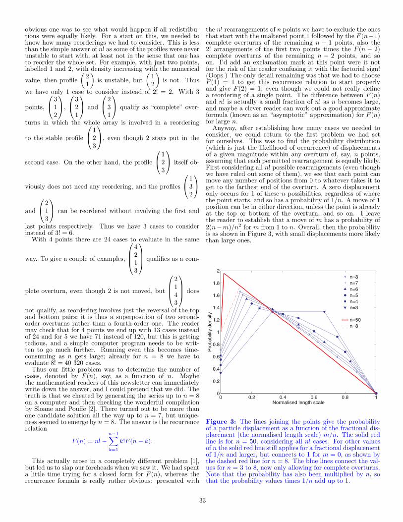
obvious one was to see what would happen if all redistribu-tions were equally likely. For a start on this, we needed toknow how many reorderings we had to consider. This is lessthan the simple answer of n! as some of the profiles were neverunstable to start with, at least not in the sense that one hasto reorder the whole set. For example, with just two points,labelled 1 and 2, with density increasing with the numerical

value, then profile

(

21

)

is unstable, but

(

12

)

is not. Thus

we have only 1 case to consider instead of 2! = 2. With 3

points,

312

,

321

and

231

qualify as “complete” over-

turns in which the whole array is involved in a reordering

to the stable profile

123

, even though 2 stays put in the

second case. On the other hand, the profile

123

itself ob-

viously does not need any reordering, and the profiles

132

and

213

can be reordered without involving the first and

last points respectively. Thus we have 3 cases to considerinstead of 3! = 6.

With 4 points there are 24 cases to evaluate in the same

way. To give a couple of examples,

4213

qualifies as a com-

plete overturn, even though 2 is not moved, but

2143

does

not qualify, as reordering involves just the reversal of the topand bottom pairs; it is thus a superposition of two second-order overturns rather than a fourth-order one. The readermay check that for 4 points we end up with 13 cases insteadof 24 and for 5 we have 71 instead of 120, but this is gettingtedious, and a simple computer program needs to be writ-ten to go much further. Running even this becomes time-consuming as n gets large; already for n = 8 we have toevaluate 8! = 40 320 cases.

Thus our little problem was to determine the number ofcases, denoted by F (n), say, as a function of n. Maybethe mathematical readers of this newsletter can immediatelywrite down the answer, and I could pretend that we did. Thetruth is that we cheated by generating the series up to n = 8on a computer and then checking the wonderful compilationby Sloane and Pouffe [2]. There turned out to be more thanone candidate solution all the way up to n = 7, but unique-ness seemed to emerge by n = 8. The answer is the recurrencerelation

F (n) = n! −n−1∑

k=1

k!F (n − k).

This actually arose in a completely different problem [1],but led us to slap our foreheads when we saw it. We had spenta little time trying for a closed form for F (n), whereas therecurrence formula is really rather obvious: presented with

the n! rearrangements of n points we have to exclude the onesthat start with the unaltered point 1 followed by the F (n−1)complete overturns of the remaining n − 1 points, also the2! arrangements of the first two points times the F (n − 2)complete overturns of the remaining n − 2 points, and soon. I’d add an exclamation mark at this point were it notfor the risk of the reader confusing it with the factorial sign!(Oops.) The only detail remaining was that we had to chooseF (1) = 1 to get this recurrence relation to start properlyand give F (2) = 1, even though we could not really definea reordering of a single point. The difference between F (n)and n! is actually a small fraction of n! as n becomes large,and maybe a clever reader can work out a good approximateformula (known as an “asymptotic” approximation) for F (n)for large n.

Anyway, after establishing how many cases we needed toconsider, we could return to the first problem we had setfor ourselves. This was to find the probability distribution(which is just the likelihood of occurrence) of displacementsof a given magnitude within any overturn of, say, n points,assuming that each permitted rearrangement is equally likely.First considering all n! possible rearrangements (even thoughwe have ruled out some of them), we see that each point canmove any number of positions from 0 to whatever takes it toget to the farthest end of the overturn. A zero displacementonly occurs for 1 of these n possibilities, regardless of wherethe point starts, and so has a probability of 1/n. A move of 1position can be in either direction, unless the point is alreadyat the top or bottom of the overturn, and so on. I leavethe reader to establish that a move of m has a probability of2(n−m)/n2 for m from 1 to n. Overall, then the probabilityis as shown in Figure 3, with small displacements more likelythan large ones.

Figure 3: The lines joining the points give the probabilityof a particle displacement as a function of the fractional dis-placement (the normalised length scale) m/n. The solid redline is for n = 50, considering all n! cases. For other valuesof n the solid red line still applies for a fractional displacementof 1/n and larger, but connects to 1 for m = 0, as shown bythe dashed red line for n = 8. The blue lines connect the val-ues for n = 3 to 8, now only allowing for complete overturns.Note that the probability has also been multiplied by n, sothat the probability values times 1/n add up to 1.

33

We now, as before, exclude the cases that do not consti-tute complete overturns. This changes the picture somewhat,increasing the likelihood of larger displacements (Figure 3),though the difference decreases as n increases. Details of themathematics are described in our paper [4].

Actual data (Figure 4) showed a greater probability of smalldisplacements than given by our model, for reasons that maybe associated with molecular diffusion, blurring extreme val-ues. There is more to be done, but this is straying back intophysical oceanography.

Figure 4: The solid red and blue lines show the probabilitydistribution of actual displacements from a number of CTDprofiles taken in winter (red) and summer (blue). The errorbars on each value (vertical lines) for each value are large,but the trends in the results are clear. The dashed blue lineshows, for comparison, the expectations from our model forn = 50 (a typical value). This is for the unrestricted case(with all n! possible rearrangements considered), but there islittle difference from the restricted case for large values of n.

So what are the messages of this article? One is that eventhose of us who have drifted from physics and mathemat-ics into their application in the real world still love prob-lems like the one described here when they crop up in ourwork. Another is that Monsieur Comtet surely didn’t antici-pate oceanographic applications of his series, where as Sloaneand Plouffe might be less surprised at the range of users oftheir encyclopaedia. My main message to any student reader,though, is that if you enjoy mathematics and physics, andwant to apply them to a research field that is fun, considerocean physics!

References

[1] Comtet, L., 1972: Sur les coefficients de l’inverse de laserie formelle

∑

n! tn. C. R. Acad. Sci. Paris, Serie A,275, 569–572.

[2] Sloane, N. J. A. and S. Plouffe, 1995: The Encyclopediaof Integer Sequences. Academic Press.

[3] Schmuland, B., 2003: Shouting factorials! Pi in the Sky,September issue.

[4] Stansfield, K., C. Garrett, and R. Dewey, 2001:The probability distribution of the Thorpe displacementwithin overturns in Juan de Fuca Strait. J. Phys.Oceanogr., 31, 3421–3434.

Q: Why do mathematicians, after a dinner at a Chineserestaurant, always insist on taking the leftovers home?

A: Because they know the Chinese remainder theorem!

“That math prof.’s marriage, I heard, is falling apart.”“That doesn’t surprise me: he’s into scientific computing,

and she’s incalculable. . . .”

Q: What is polite and works for the phone company?A: A deferential operator. . . .

Trigonometry for farmers: swine and coswine. . . .


34

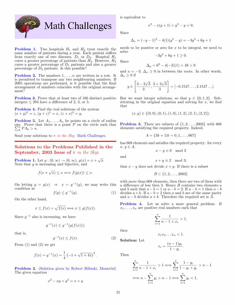
Problem 1. Two hospitals H1 and H2 treat exactly thesame number of patients during a year. Each patient suffersfrom exactly one of two diseases, D1 or D2. Hospital H1cures a greater percentage of patients than H2. However, H2cures a greater percentage of D1 patients and also a greaterpercentage of D2 patients. Is this possible?

Problem 2. The numbers 1, . . . , n are written in a row. Itis permitted to transpose any two neighbouring numbers. If2005 operations are performed, is it possible that the finalarrangement of numbers coincides with the original arrange-ment?

Problem 3. Prove that at least two of 100 distinct positiveintegers ≤ 294 have a difference of 2, 3, or 5.

Problem 4. Find the real solutions of the system(x + y)5 = z, (y + z)5 = x, (z + x)5 = y.

Problem 5. Let A1, . . . , An be points on a circle of radiusone. Prove that there is a point P on the circle such that∑n

k PAk > n.

Send your solutions to π in the Sky : Math Challenges.

Solutions to the Problems Published in the

September, 2003 Issue of π in the Sky:

Problem 1. Let g : (0,∞) → (0,∞), g(x) = x +√

x.Note that g is increasing and bijective, and

f(x +√

x) ≤ x ⇐⇒ f(g(x)) ≤ x.

On letting y = g(x) ⇒ x = g−1(y), we may write thiscondition as

f(y) ≤ g−1(y). (1)

On the other hand,

x ≤ f(x) +√

f(x) ⇐⇒ x ≤ g(f(x)).

Since g−1 also is increasing, we have

g−1(x) ≤ g−1(g(f(x)));

that is,

g−1(x) ≤ f(x). (2)

From (1) and (2) we get

f(x) = g−1(x) =1

4

(

−1 +√

1 + 4x)2

.

Problem 2. (Solution given by Robert Bilinski, Montreal)The given equation

x2 − xy + y2 = x + y

is equivalent to

x2 − x(y + 1) + y2 − y = 0.

Since

∆x = (−y − 1)2 − 4(1)(y2 − y) = −3y2 + 6y + 1

needs to be positive or zero for x to be integral, we need tosolve

−3y2 + 6y + 1 ≥ 0.

Since∆y = 62 − 4(−3)(1) = 48 > 0

and a = −3, ∆x ≥ 0 in between the roots. In other words,∆x ≥ 0 if

y ∈[

3 − 2√

3

3,3 + 2

√3

3

]

= [−0.1547 . . . , 2.1547 . . .].

But we want integer solutions, so that y ∈ {0, 1, 2}. Sub-stituting in the original equation and solving for x, we findthat

(x, y) ∈ {(0, 0), (0, 1), (1, 0), (1, 2), (2, 1), (2, 2)}.

Problem 3. There are subsets of {1, 2, . . . , 2003} with 668elements satisfying the required property. Indeed,

A = {3k + 1|k = 0, 1, . . . , 667}

has 668 elements and satisfies the required property: for everyx, y ∈ A,

x − y ≡ 0 mod 3

andx + y ≡ 2 mod 3;

thus x − y does not divide x + y. If there is a subset

B ⊂ {1, 2, . . . , 2003}

with more than 668 elements, then there are two of them witha difference of less then 3. Hence B contains two elements aand b such that a− b = 1 or a− b = 2. If a− b = 1 then a− bdivides a+ b. If a− b = 2 then a and b are of the same parityand a − b divides a + b. Therefore the required set is A.

Problem 4. Let us solve a more general problem: Ifx1, . . . , xn are positive real numbers such that

n∑

i=1

1

n − 1 + xi> 1,

thenx1x2 . . . xn < 1.

Solution: Let

xi =(n − 1)yi

1 − yi.

Then

n∑

i=1

1

n − 1 + xi> 1 ⇐⇒

n∑

i=1

1 − yi

1 − yi + yi> n − 1

⇐⇒ n −n

∑

i=1

yi > n − 1 ⇐⇒n

∑

i=1

yi < 1.

35

Now

x1x2 . . . xn = (n − 1)n y1 . . . yn

(1 − y1) . . . (1 − yn)

< (n − 1)n y1 . . . yn

(y2 + . . . + yn) . . . (y1 + . . . + yn−1)

≤ (n − 1)n

(n − 1)n

y1 . . . yn

n−1

√

(y1 . . . yn)n−1= 1.

(In the last inequality we have applied the AGM inequality:y2+...+yn

n−1 ≥ n−1√

y2 . . . yn etc.)

Problem 5. Let A, B, C, and D be the given points. Thetriangle made with any three of these points is acute. Indeed,if consider △ABC then

cos A =AB2 + AC2 − BC2

2AB · AC≥ 2 + 2 − 4

2AB · AC= 0.

ThereforeA ≤ 90◦.

We conclude that ABCD is a convex quadrilateral and alsoB ≤ 90◦, C ≤ 90◦, and D ≤ 90◦. As A+B+C+D = 360◦, theonly consistent situation is A = B = C = D = 90◦. HenceABCD must be a rectangle. If we assume that AB = a,BC = b, a 6= b, and a, b ∈ [

√2, 2], then

AC =√

a2 + b2 >√

2 + 2 = 2,

which is a contradiction. Therefore a = b and ABCD is asquare.

Problem 6. Let O be the center of the circles and A, B, Cbe the vertices of the triangle with the maximum area. Thepoint O must belong to the interior of the triangle. On theother hand, it must be the orthocenter of the triangle ABC.Indeed, if O is not the orthocenter of the triangle then AO isnot perpendicular to BC. Take a line through A parallel toBC. This line is not tangent to the circle and hence intersectsthe circle at a point D (see Figure 1). Now if we choose apoint M in the arc AD the area of the △BMC is greater thenthe area of △BAC, a contradiction. In △AOC (see Figure 2)

AC2 = 1 + 16 + 8 cosB = 17 + 8 cosB.

If R is the radius of the circumcircle of △ABC, then

AC2 = 4R2 sin2 B.

Hence4R2 sin2 B = 17 + 8 cosB. (3)

In △BOA′

and △BAA′

BA′

= OB cos(90◦ − C) =√

7 sin C

andBA

′

= AB cos B = 2R cos B sin C.

Hence2R cos B =

√7. (4)

Eliminating R from (3) and (4) we obtain

8 cos3 B + 24 cos2 B − 7 = 0;

hence

(2 cosB − 1)(4 cos2 B + 14 cosB + 7) = 0.

The only acceptable solution is cosB = 1/2 and hence

B = 60◦. We immediately obtain BAA′ = 30◦, OC′

= 1/2

and hence CC′

= 9/2. Also sin ABB′ = 1/(2√

7), BC′

=

3√

3/2, AC =√

21, AC′

=√

3/2 and AB = 2√

3. Thus

Area(△ABC) = 9√

3/2 is the required maximum area.

O

AB

C

D

Figure 1

1

√7

4O

A

B

C

A′

B′

C′

Figure 2

symptotesymptotesymptotesymptotesymptotesymptotesymptotesymptotesymptotesymptotesymptotesymptote

The figures on pages 7, 8,12, 20, 22, 23, and 36 weredrawn with Asymptote, apowerful new descriptivevector graphics languagefor technical drawing de-veloped at the Universityof Alberta. The term vec-tor graphics refers to amethod for producing fig-

ures that retain their high quality even at arbitrarily largemagnifications.

The authors of Asymptote (Andy Hammerlindl, John C.Bowman, and Tom Prince) would like to thank the Natu-ral Sciences and Engineering Research Council of Canada,the Pacific Institute for Mathematical Sciences, and theUniversity of Alberta Faculty of Science for their gen-erous financial support. Asymptote is freely available,under the GNU General Public License, from the website http://asymptote.sourceforge.net, which includes agallery of example Asymptote code and output.

36

pi8.pdf - Canadian Mathematical Society

Documents

Transcript of pi8.pdf - Canadian Mathematical Society