
The application of physiological observation methods to emotion research
Upload
khangminh22Category
view
1download
0
Edith Cowan University Edith Cowan University
Research Online Research Online
Theses: Doctorates and Masters Theses
2013
On the Recognition of Emotion from Physiological Data On the Recognition of Emotion from Physiological Data
Warren Creemers Edith Cowan University
Follow this and additional works at: https://ro.ecu.edu.au/theses
Part of the Artificial Intelligence and Robotics Commons
Recommended Citation Recommended Citation Creemers, W. (2013). On the Recognition of Emotion from Physiological Data. https://ro.ecu.edu.au/theses/680
This Thesis is posted at Research Online. https://ro.ecu.edu.au/theses/680

Edith Cowan UniversityResearch Online
Theses: Doctorates and Masters Theses
2013
On the Recognition of Emotion from PhysiologicalDataWarren CreemersEdith Cowan University
This Thesis is posted at Research Online.http://ro.ecu.edu.au/theses/680
Recommended CitationCreemers, W. (2013). On the Recognition of Emotion from Physiological Data. Retrieved from http://ro.ecu.edu.au/theses/680

Edith Cowan University
Copyright Warning
You may print or download ONE copy of this document for the purpose
of your own research or study.
The University does not authorize you to copy, communicate or
otherwise make available electronically to any other person any
copyright material contained on this site.
You are reminded of the following:
Copyright owners are entitled to take legal action against persons who infringe their copyright.
A reproduction of material that is protected by copyright may be a
copyright infringement. Where the reproduction of such material is
done without attribution of authorship, with false attribution of
authorship or the authorship is treated in a derogatory manner,
this may be a breach of the author’s moral rights contained in Part
IX of the Copyright Act 1968 (Cth).
Courts have the power to impose a wide range of civil and criminal
sanctions for infringement of copyright, infringement of moral
rights and other offences under the Copyright Act 1968 (Cth).
Higher penalties may apply, and higher damages may be awarded,
for offences and infringements involving the conversion of material
into digital or electronic form.

On the Recognition of Emotion from
Physiological Data
A Thesis Submitted by Warren Creemers
In Partial Fulfillment of the Requirements for the award of
Doctor of Philosophy, (Computer Science)
At the
Faculty of Health, Engineering and Science
Edith Cowan University
February, 2013.

(Abstract) 2

(Abstract) 3
Abstract
This work encompasses several objectives, but is primarily concerned with an
experiment where 33 participants were shown 32 slides in order to create ‗weakly
induced emotions‘. Recordings of the participants‘ physiological state were taken as
well as a self report of their emotional state. We then used an assortment of classifiers
to predict emotional state from the recorded physiological signals, a process known as
Physiological Pattern Recognition (PPR).
We investigated techniques for recording, processing and extracting features from six
different physiological signals: Electrocardiogram (ECG), Blood Volume Pulse
(BVP), Galvanic Skin Response (GSR), Electromyography (EMG), for the corrugator
muscle, skin temperature for the finger and respiratory rate.
Improvements to the state of PPR emotion detection were made by allowing for 9
different weakly induced emotional states to be detected at nearly 65% accuracy. This
is an improvement in the number of states readily detectable.
The work presents many investigations into numerical feature extraction from
physiological signals and has a chapter dedicated to collating and trialing facial
electromyography techniques. There is also a hardware device we created to collect
participant self reported emotional states which showed several improvements to
experimental procedure.

(Abstract) 4

(Abstract) 5
DECLARATION
I certify that this thesis does not incorporate without acknowledgment any material previously
submitted for a degree or diploma in any institution of higher education; and that to the best
of my knowledge and belief it does not contain any material previously written by another
person except where due reference is made in the text.
Signature
Date________13/3/2013_______________
ACKNOWLEDGMENTS
I would like to thank the participants and nurses who volunteered their time to make this
research effort possible. I would also like to thank my supervisors for their enthusiastic
support in this work. A special thanks to my other half, Liz, for her patience and free proof-
reading service. Thanks are also due to our schools research support team who helped put
the lab together and help construct specialised hardware. These acknowledgements cannot
be complete without thanking my school for their faith in this project and the funding granted
to purchase the recording hardware used extensively in this work.
USE OF THESIS
The Use of Thesis statement is not included in this version of the thesis.

(Abstract) 6

(Abstract) 7
Table of Contents
ABSTRACT ............................................................................................................................. 3
TABLE OF CONTENTS ........................................................................................................ 7
INDEX OF FIGURES ........................................................................................................... 16
1.0 INTRODUCTION ........................................................................................................ 37
2.0 BACKGROUND ........................................................................................................... 47
2.1 WHAT ARE EMOTIONS? ................................................................................................ 48
2.1.1. THE JAMES-LANGE THEORY ...................................................................................... 49
2.1.2. THE CANNON-BARD THEORY ..................................................................................... 50
2.1.3. THE TWO FACTOR THEORY ........................................................................................ 50
2.2 CULTURALLY SPECIFIC EMOTIONS ............................................................................. 51
2.3 EMOTIONS FROM A RESEARCH PERSPECTIVE ............................................................ 52
2.3.1. EMOTION ORGANISATION THEORIES.......................................................................... 53
2.3.2. HIERARCHICAL EMOTION CLASSIFICATION THEORIES .............................................. 56
2.3.3. MIXED EMOTION CLASSIFICATION THEORIES ............................................................ 57
2.3.4. DIMENSIONAL EMOTION CLASSIFICATION THEORIES ................................................ 58
2.3.5. FUZZY EMOTION CLASSIFICATION THEORIES ............................................................ 60
2.3.6. CONCLUSION .............................................................................................................. 60
2.4 OVERVIEW OF CLASSIFICATION TECHNIQUES RELEVANT TO PPR .......................... 60
2.4.1. ASSESSING THE PERFORMANCE OF A CLASSIFIER ...................................................... 61
2.4.2. OVERVIEW OF THE K-NN CLASSIFIER ........................................................................ 65
2.4.3. OVERVIEW OF ARTIFICIAL NEURAL NETWORK CLASSIFIERS .................................... 67
2.4.4. OVERVIEW OF THE SUPPORT VECTOR MACHINE CLASSIFIER .................................... 70
2.4.5. OVERVIEW OF THE NAIVE BAYES CLASSIFIER ........................................................... 72
2.4.6. OVERVIEW OF THE DECISION TREE CLASSIFIER ........................................................ 73
2.4.7. OVERVIEW OF THE RANDOM FOREST CLASSIFIER ..................................................... 75
2.5 OVERVIEW OF TECHNIQUES RELATED TO CLASSIFIERS ........................................... 76
2.5.1. OVERVIEW OF THE FORWARD FEATURE SELECTION ALGORITHM ............................. 76
2.5.2. OVERVIEW OF N-FOLD CROSS VALIDATION .............................................................. 77
2.6 CONCLUSION ................................................................................................................. 77

(Abstract) 8
3.0 A REVIEW OF CURRENT LITERATURE ............................................................. 79
3.1 RECOGNITION OF EMOTION ......................................................................................... 81
3.2 CULTURALLY SPECIFIC EMOTIONS AND THE PLAUSIBILITY OF HETEROGENEOUS
PHYSIOLOGICAL PATTERN RECOGNITION........................................................................... 83
3.3 PHYSIOLOGICAL CHANGES AS CUES FOR RECOGNITION OF EMOTION ................... 86
3.3.1. PHYSIOLOGICAL PATTERN RECOGNITION .................................................................. 88
3.3.2. AN INVESTIGATION OF PHYSIOLOGICAL SIGNALS ..................................................... 90
3.3.3. EXAMINING AND MONITORING THE PHYSIOLOGICAL STATE..................................... 91
3.3.4. MUSCULAR PHYSIOLOGICAL SIGNALS (EMG) OF THE BACK (POSTURE & SUPPORT)
92
3.3.5. HUMAN ACTION OF THE HAND (PRESSURE) ............................................................... 93
3.3.6. HUMAN ACTION OF THE TORSO (POSTURE) ............................................................... 94
3.3.7. HUMAN AUTONOMOUS FUNCTIONS CONTROLLED BY THE MEDULLA OBLONGATA
AND THE AUTONOMIC NERVOUS SYSTEM - OVERVIEW .......................................................... 94
3.3.8. SIGNALS CONTROLLED BY THE MEDULLA OBLONGATA - RESPIRATION ................... 97
3.3.9. SIGNALS CONTROLLED BY THE MEDULLA OBLONGATA- HEART BEAT .................... 98
3.3.10. SIGNALS CONTROLLED BY THE MEDULLA OBLONGATA - BLOOD VOLUME PULSE
101
3.3.11. HUMAN AUTONOMOUS FUNCTIONS CONTROLLED BY THE MEDULLA OBLONGATA -
BLOOD PRESSURE .................................................................................................................. 102
3.3.12. HUMAN DERMATOLOGICAL RESPONSE (SWEAT & SKIN CONDUCTANCE) ............ 103
3.3.13. HUMAN THERMOREGULATORY RESPONSE - SKIN TEMPERATURE AND THE INSULA
CORTEX 104
3.3.14. SAMPLING OF SKIN TEMPERATURE FROM THE HAND ............................................ 105
3.3.15. SKIN TEMPERATURE AND ENVIRONMENTAL FACTORS .......................................... 107
3.3.16. HUMAN ACTION OF THE EYE .................................................................................. 108
3.3.17. SUMMARY OF PHYSIOLOGICAL CHANGES .............................................................. 110
3.4 OTHER FACTORS AFFECTING PHYSIOLOGICAL SIGNALS ........................................ 111
3.4.1. COMMON DRUGS IN RELATION TO PHYSIOLOGICAL SIGNALS ................................. 111
3.5 HUMAN EMOTION AS AN EXPERIMENTAL VARIABLE .............................................. 112
3.5.1. INFLUENCING THE HUMAN EMOTIONAL STATE ....................................................... 114
3.5.2. OBSERVING EMOTION............................................................................................... 117
3.6 HUMAN EMOTION IN HUMAN COMPUTER INTERACTION VS. HUMAN EMOTION IN
RESEARCH ............................................................................................................................ 120
3.7 SUMMARY OF PHYSIOLOGICAL PATTERN RECOGNITION RESEARCH AND
EXPERIMENTS ....................................................................................................................... 121

(Abstract) 9
3.8 CONCLUSION ............................................................................................................... 128
4.0 THE HUMAN FACE AND ITS COUPLING WITH THE EMOTIONAL STATE
129
4.1 BACKGROUND OF FACIAL EXPRESSION IN RELATION TO EMOTIONS .................... 131
4.1.1. EMOTIONAL VS. CONSCIOUS FACIAL MUSCLE ACTIVATION ................................... 133
4.1.2. FACIAL DISPLAY RULES AND MICRO EXPRESSIONS ................................................ 133
4.1.3. FACIAL FEEDBACK THEORY AND ITS IMPLICATIONS FOR EMOTION RESEARCH ..... 135
4.1.4. OUR GUIDELINES FOR EXPERIMENTAL APPARATUS IN AFFECTIVE FACIAL STUDIES
140
4.2 FACIAL EMG AS A METHOD OF STUDYING EMOTIONAL STATE ............................. 142
4.3 PHYSIOLOGICAL SIGNALS (EMG) OF THE JAW ........................................................ 142
4.3.1. ORBICULARIS ORIS ................................................................................................... 143
4.3.2. LEVATOR ANGULI ORIS (CANINUS) ......................................................................... 145
4.3.3. LEVATOR LABII SUPERIORIS (OR QUADRATUS LABII SUPERIORIS) ......................... 146
4.3.4. ZYGOMATICUS MINOR ............................................................................................. 148
4.3.5. ZYGOMATICUS MAJOR ............................................................................................. 149
4.3.6. RISORIUS ................................................................................................................... 153
4.3.7. BUCCINATOR ............................................................................................................ 154
4.3.8. QUADRATUS LABII INFERIORIS (DEPRESSOR LABII INFERIORIS) ............................. 155
4.3.9. DEPRESSOR ANGULI ORIS (TRIANGULARIS) ............................................................ 157
4.3.10. MENTALIS ............................................................................................................... 158
4.3.11. RISORIUS ................................................................................................................. 159
4.3.12. PLATYSMA .............................................................................................................. 160
4.4 PHYSIOLOGICAL SIGNALS (EMG) OF THE EYES ...................................................... 161
4.4.1. FRONTALIS ................................................................................................................ 163
4.4.2. CORRUGATOR SUPERCILII ........................................................................................ 165
4.4.3. ORBICULARIS OCULI ................................................................................................ 169
4.4.4. PROCERUS ................................................................................................................. 173
4.5 PHYSIOLOGICAL SIGNALS (EMG) OF THE NOSE ...................................................... 174
4.5.1. NASALIS TRANSVERSA ............................................................................................. 174
4.5.2. NASALIS ALARIS ....................................................................................................... 175
4.6 SUMMARY OF THE AFFECTIVE CAPACITY OF THE MIMETIC MUSCLES ................. 176
5.0 EXAMINATION OF ELECTROMYOGRAPHY RESULTS FROM POSED
FACIAL EXPRESSIONS ................................................................................................... 179

(Abstract) 10
5.1 EMG OF THE ORBICULARIS ORIS .............................................................................. 181
5.2 EMG OF THE ZYGOMATICUS MAJOR ........................................................................ 183
5.3 EMG OF THE BUCCINATOR ........................................................................................ 185
5.4 EMG OF THE DEPRESSOR ANGULI ORIS ................................................................... 187
5.5 EMG OF THE MENTALIS............................................................................................. 189
5.6 EMG OF THE ORBICULARIS OCULI ........................................................................... 191
5.7 EMG OF THE FRONTALIS ........................................................................................... 193
5.8 EMG OF THE CORRUGATOR SUPERCILII .................................................................. 195
5.9 EMG OF THE SUPRAHYOID PLACEMENT .................................................................. 198
5.10 EMG OF THE TEMPORAL SUPRAHYOID PLACEMENT ............................................ 203
5.11 EMG OF THE TEMPORAL MASSETER (WIDE) PLACEMENT................................... 207
5.12 EMG OF THE FRONTAL (WIDE) PLACEMENT ......................................................... 210
5.13 CONCLUSION ............................................................................................................. 213
6.0 EXPERIMENTAL DESIGN ..................................................................................... 215
6.1 SYNOPSIS ...................................................................................................................... 217
6.2 DATA COLLECTED ...................................................................................................... 218
6.3 DESIGN ......................................................................................................................... 219
6.4 DISCRIMINANT VALIDITY OF EMOTIONS INDUCED .................................................. 221
6.5 VALIDITY OF EMOTIONS REPORTED ......................................................................... 227
6.6 VALIDITY OF SOMATOVISCERAL RESPONSES OBSERVED ........................................ 228
6.7 PARTICIPANTS ............................................................................................................. 228
6.8 CONCLUSION ............................................................................................................... 229
7.0 METHOD AND MATERIALS ................................................................................. 233
7.1 TUTORIAL SLIDES ....................................................................................................... 235
7.1.1. FEEDBACK INSTRUCTION .......................................................................................... 237
7.1.2. SIMULATED CRASH ................................................................................................... 238
7.2 ROOM SETUP ............................................................................................................... 239
7.2.1. AFFECTIVE TONE ...................................................................................................... 240
7.2.2. LIGHTING .................................................................................................................. 241
7.2.3. LOCATION ................................................................................................................. 242
7.2.4. TECHNICAL REQUIREMENTS ..................................................................................... 243
7.2.5. OUR EXPERIMENTATION WITH A SHIELD ROOM TO ELIMINATE RF INTERFERENCE 244
7.2.6. OUR GUIDELINE FOR ROOM PREPARATION (A SUMMARY)..................................... 245

(Abstract) 11
7.3 PROCEDURES FOR INTERACTION WITH PARTICIPANTS ........................................... 246
7.3.1. PRIVACY FOR HONESTY OF FEEDBACK .................................................................... 246
7.3.2. RECRUITMENT AND PRE-EXPERIMENT CONTACT ..................................................... 247
7.3.3. ENTRANCE PROCEDURE ............................................................................................ 247
7.3.4. EXIT PROCEDURE...................................................................................................... 249
7.3.5. ETHICAL TREATMENT OF HUMANS .......................................................................... 250
7.4 SAFETY ......................................................................................................................... 250
7.4.1. ELECTRODE ISOLATION ............................................................................................ 251
7.4.2. ELECTRICAL AND BIOHAZARD SAFETY REQUIREMENTS (AS3200 & IEC6060-1) .. 252
7.4.3. BIOLOGICAL HAZARDS ............................................................................................. 253
7.4.4. POSSIBLE ALLERGENS ............................................................................................... 254
7.5 EQUIPMENT CAPABILITIES AND APPLICATION ......................................................... 254
7.5.1. ENCODER .................................................................................................................. 254
7.5.2. THE EMG SENSOR .................................................................................................... 255
7.5.3. THE ECG SENSOR ..................................................................................................... 257
7.5.4. THE BVP SENSOR ..................................................................................................... 258
7.5.5. THE GSR SENSOR ..................................................................................................... 258
7.5.6. THE TEMPERATURE SENSOR..................................................................................... 260
7.5.7. THE RESPIRATION SENSOR ....................................................................................... 260
7.6 SOFTWARE ................................................................................................................... 261
7.7 CONCLUSION ............................................................................................................... 263
8.0 FEEDBACK VIA A HARDWARE SAM IMPLEMENTATION .......................... 265
8.1 REQUIREMENTS ANALYSIS ......................................................................................... 268
8.2 SAM ON PRINTED ANSWER SHEETS ........................................................................... 270
8.3 SAM AS PC SOFTWARE .............................................................................................. 271
8.4 SAM ON A PERSONAL DIGITAL ASSISTANT (PDA/TABLET) .................................... 276
8.5 SAM AS A CUSTOMISED HARDWARE DEVICE ........................................................... 280
8.5.1. USER INTERFACE ...................................................................................................... 280
8.5.2. TECHNICAL CAPABILITIES ........................................................................................ 281
8.5.3. SIGNAL QUALITY ...................................................................................................... 282
8.5.4. TECHNICAL CHALLENGES ........................................................................................ 283
8.6 CONCLUSION ............................................................................................................... 284
9.0 SIGNAL PROCESSING AND FEATURE EXTRACTION .................................. 287

(Abstract) 12
9.1 ECG SIGNAL ................................................................................................................ 289
9.1.1. OVERVIEW OF FILTERING THE ECG SIGNAL ............................................................ 289
9.1.2. EMG AND POWER LINE NOISE REMOVAL ................................................................ 294
9.1.3. ARTEFACT DETECTION ............................................................................................. 308
9.1.4. BASELINE DRIFT CORRECTION VIA MEDIAN FILTERING .......................................... 308
9.1.5. OVERVIEW OF FEATURE DETECTION IN THE ECG SIGNAL ...................................... 311
9.1.6. WAVELET DECOMPOSITION AND AUTOMATED ECG ANNOTATION ........................ 313
9.1.7. EXTRACTION OF TRAINING DATA FROM THE ECG .................................................. 315
9.1.8. INVARIANT FEATURE SELECTION FROM THE ECG ................................................... 316
9.1.9. SUMMARY OF ECG PROCESSING AND FEATURE EXTRACTION ................................ 319
9.2 EMG SIGNAL ............................................................................................................... 319
9.2.1. EMG FEATURE EXTRACTION ................................................................................... 320
9.2.2. ARTEFACT DETECTION ............................................................................................. 342
9.3 SKIN TEMPERATURE ................................................................................................... 343
9.3.1. SKIN TEMPERATURE ALTERATION BY MOOD AND MEDIUM TERM TRENDS ........... 345
9.3.2. A SKIN TEMPERATURE FEATURE EXTRACTION METHOD ........................................ 348
9.4 RESPIRATION ............................................................................................................... 349
9.5 BLOOD VOLUME PULSE .............................................................................................. 352
9.5.1. FEATURES EXTRACTED ............................................................................................ 354
9.6 GALVANIC SKIN RESPONSE ........................................................................................ 355
9.7 SAMPLING OF TIME SERIES DATA ............................................................................. 357
9.8 SUMMARY .................................................................................................................... 359
10.0 ANALYSIS OF COLLECTED DATA ................................................................... 361
10.1 LABELLING OF DATA FOR CLASSIFICATION AND ANALYSIS ................................. 363
10.1.1. FINDING A GOOD DEAD-ZONE FOR THE GRID DIVISION OF EMOTIONAL STATES . 365
10.1.2. APPLYING K-MEANS CLUSTERING TO THE SAM RATINGS .................................... 366
10.2 NAMES USED FOR DESCRIBING FEATURES ............................................................. 370
10.3 EXTERNAL FACTORS IN RECORDED PHYSIOLOGICAL DATA ................................ 372
10.3.1. PARTICIPANT MOOD PRIOR TO THE EXPERIMENT .................................................. 373
10.3.2. DIURNAL AUTONOMIC VARIATIONS ...................................................................... 373
10.4 EFFECTIVENESS OF THE IAPS STIMULI .................................................................. 377
10.4.1. EXAMPLE OF CULTURAL BIAS IN AUSTRALIAN RESPONDENTS: SNAKE FEAR IS LESS
PREVALENT............................................................................................................................ 381
10.4.2. EXAMPLE OF CULTURAL BIAS IN AUSTRALIAN RESPONDENTS: A BOY WITH HIS
HEAD IN A BISON'S ARSE IS JUST NOT INTERESTING ............................................................ 382

(Abstract) 13
10.5 PARTICIPANT SELF ASSESSMENT RESPONSES ........................................................ 384
10.5.1. SUMMARY OF EFFECTIVENESS OF STIMULI ............................................................ 388
10.6 VISUALISING RESULTS OBTAINED FROM PHYSIOLOGICAL RECORDINGS............ 389
10.6.1. VISUALISING THE ROLE OF RESPIRATION .............................................................. 390
10.6.2. VISUALISING EMG CORRELATIONS........................................................................ 392
10.6.3. VISUALISING THE DIFFICULTIES OF HETEROGENEOUS CLASSIFICATION TASKS ... 393
10.6.4. VISUALISING TIME AS A FACTOR IN OBSCURING EMOTIONAL RESPONSE ............. 394
10.7 VISUALISING THE FEASIBILITY OF USING MULTIVARIATE DATA TO SEPARATE
HETEROGENEOUS RESULTS SETS ....................................................................................... 395
10.8 SAMPLING OF DATA FOR CLASSIFICATION ............................................................. 396
10.9 A FEATURE SELECTION INVESTIGATION ................................................................ 396
10.10 CONCLUSION ........................................................................................................... 403
11.0 CLASSIFICATION OF DATA ............................................................................... 405
11.1 WHICH FEATURES SHOULD BE USED? ...................................................................... 407
11.2 HOW DOES THE PERFORMANCE OF CLASSIFIERS VARY FOR OUR DIFFERENT TYPES
OF CLASS LABELS? ............................................................................................................... 411
11.3 NAIVE BAYES CLASSIFIER ........................................................................................ 413
11.4 THE RANDOM FOREST CLASSIFIER ......................................................................... 417
11.5 THE NEURAL NETWORK CLASSIFIER ...................................................................... 423
11.5.1. BASIC TUNING OF THE ANN CLASSIFIER, NUMBER OF LAYERS AND TRAINING
EPOCHS 423
11.5.2. FURTHER TUNING OF THE ANN, MOMENTUM AND LEARNING RATE .................... 427
11.5.3. ANN PERFORMANCE OVERVIEW ........................................................................... 429
11.6 K-NN CLASSIFIER ..................................................................................................... 432
11.7 SUPPORT VECTOR MACHINE CLASSIFIER ............................................................... 438
11.7.1. LINEAR KERNEL ..................................................................................................... 439
11.7.2. POLYNOMIAL KERNEL ............................................................................................ 440
11.7.3. RADIAL BASIS FUNCTION (RBF) KERNEL .............................................................. 441
11.7.4. SIGMOID KERNEL ................................................................................................... 441
11.7.5. COMPARISON OF SVM KERNELS ............................................................................ 444
11.8 SELECTING THE BEST CLASSIFIER .......................................................................... 447
11.9 CONCLUSION ............................................................................................................. 448
11.9.1. COMPARISON WITH OTHER WORKS......................................................................... 450
12.0 CONCLUSION ......................................................................................................... 451

(Abstract) 14
12.1 CONTRIBUTIONS ........................................................................................................ 453
12.1.1. REVIEW OF PHYSIOLOGICAL & NEUROLOGICAL PROCESSES OF EMOTION ........... 453
12.1.2. FACIAL MUSCLES ................................................................................................... 454
12.1.3. SAM ....................................................................................................................... 454
12.1.4. STIMULUS SELECTION ............................................................................................ 455
12.1.5. SIGNAL PROCESSING .............................................................................................. 456
12.1.6. FEATURE EXTRACTION ........................................................................................... 457
12.1.7. LABELLING EMOTIONS ........................................................................................... 458
12.1.8. CLASSIFICATION PERFORMANCE ............................................................................ 459
12.2 FUTURE WORK AND FINAL THOUGHTS ................................................................... 460
13.0 GLOSSARY .............................................................................................................. 463
14.0 APPENDIX ............................................................................................................... 469
14.1 STIMULUS SLIDES ...................................................................................................... 470
14.2 SAM EVALUATIONS USER RELIABILITY CHARTS .................................................. 473
14.3 IAPS SLIDE SCATTER PLOTS ................................................................................... 485
14.4 ECG “NARF” COMPENSATIONS FOR ALL INTERVALS OF THE TYPICAL
WAVEFORM .......................................................................................................................... 504
14.5 IMPLEMENTATIONS OF SELECTED ALGORITHMS ................................................... 510
14.5.1. LINEAR CRITERION FOR ECG SUBTRACTION PROCEDURE. .................................... 510
14.6 ASSORTED NOTICES AND COMMUNICATIONS USED ............................................... 512
14.7 RISK MANAGEMENT REPORT .................................................................................. 518
14.8 EMAIL SENT TO ALL WOULD BE VOLUNTEERS ........................................................ 525
14.9 MEDIAN FILTERING ALGORITHM ............................................................................ 527
14.10 HARDWARE SAM CIRCUIT DIAGRAM AND INFORMATION .................................. 531
14.10.1. MICROCONTROLLER ............................................................................................. 532
14.10.2. POWER SUPPLY ..................................................................................................... 532
14.10.3. AUDIO TONE OUTPUT ........................................................................................... 533
14.10.4. MICROPHONE OUTPUT .......................................................................................... 533
14.10.5. SYNCH OUTPUT .................................................................................................... 533
14.10.6. SAM LED OUTPUTS ............................................................................................. 534
14.10.7. READING INPUT VOLTAGES .................................................................................. 534
14.10.8. CONVERSION TIME ............................................................................................... 535
14.10.9. READING SAM SELECTION SWITCHES ................................................................. 536
14.10.10. RESISTOR LADDER VALUES ............................................................................... 537

(Abstract) 15
14.10.11. DETERMINATION OF RANGE ............................................................................... 538
14.10.12. SAM SWITCH DURATION ................................................................................... 540
14.10.13. COMMUNICATIONS ............................................................................................. 541
14.10.14. PROTOCOL .......................................................................................................... 541
14.10.15. COMMAND SET ................................................................................................... 542
14.10.16. OUTPUT COMMANDS .......................................................................................... 542
14.10.17. INPUT COMMANDS ............................................................................................. 543
15.0 REFERENCES ......................................................................................................... 545

(Abstract) 16
Index of Figures
Figure 1 : Emotion theory heirarchy ............................................................................ 53
Figure 2: Plutchik's wheel of emotions ........................................................................ 57
Figure 3: Semantic Differential, showing two peoples ratings for ―policemen‖ (Pagon,
1996). ........................................................................................................................... 58
Figure 4: The circumplex model of emotion. Russell (Russell, 1980) plotted different
emotions on a two dimensional space created by two axes, arousal and Valence. These
axes of Arousal and Valence can have both positive , neutral and negative values. ... 59
Figure 5: Operation of a working classifier ................................................................. 61
Figure 6: Examples of Classifier Boundaries in Feature Space. A) Is an ideal. B)
Shows a poor fit. C) Shows an over-fit. D) Show a data item that cannot be fitted. ... 63
Figure 7: Sensitivity and Specificity Shown Graphically. A) High Specificity; B) Low
specificity; C) High Sensitivity; D) Low Sensitivity. .................................................. 64
Figure 8: Example of k-NN on a 2 dimensional dataset. ............................................. 66
Figure 9: ANN setup with one hidden layer ................................................................ 68
Figure 10: Typical ANN setup for classification ........................................................ 69
Figure 11: Support vector machine setup .................................................................... 70
Figure 12: Allowing for better separation of training points by projecting the data
(part A, in 1 dimension) into a higher dimensional space (part B, in 2 dimensions).
The hyper plane is shown in black. .............................................................................. 71
Figure 13: A Trivial Decision Tree Example .............................................................. 73
Figure 14: Physiological (blue) and Cognitive (red) signals. ...................................... 82
Figure 15: Depiction of schadenfreude, in the Simpsons character Nelson Muntz
(Groening & Brooks, 2006) ......................................................................................... 85
Figure 16: Dimensional projection via a day dependence matrix (Picard, Vyzas, &
Healey, 2001) ............................................................................................................... 88
Figure 17: Structures of the brain involved in emotion. .............................................. 91
Figure 18: Variables Affecting the Physiological State. .............................................. 92
Figure 19: The "TouchPhone" .................................................................................... 94
Figure 20: The Structure of the Autonomic Nervous System (Lane et al., 2009) ....... 96
Figure 21: Respiration Cycle ....................................................................................... 97
Figure 22: Wiggers Diagram, (Guyton, 2000) ; Chapter 9 - Page 99. ........................ 99

(Abstract) 17
Figure 23: Heart Rate in Relation to Pleasant Emotions (Libby Jr et al., 1973) ....... 100
Figure 24: Heart rate response to various slide types ................................................ 100
Figure 25: Heart rate in response to negative animal stimuli, in phobic and non phobic
participants. (Globisch et al., 1999) ........................................................................... 101
Figure 26: A BVP Envelope (Fernandez & Picard, 1998). ........................................ 102
Figure 27: Blood Pressure in response to negative animal stimuli, in phobic and non
phobic participants. (Globisch et al., 1999) ............................................................... 102
Figure 28: Skin Conductance in response to negative animal stimuli, in phobic and
non phobic participants. (Globisch et al., 1999) ........................................................ 104
Figure 29: Medical conditions effecting skin temperature of the hands .................... 106
Figure 30: 4 Hand-temperature types identified by Kokubo et al., Dark regions
indicate thermal hot spots of the four hand circulation types. Corresponding mean
hand temperatures and deviations given above. ........................................................ 107
Figure 31:Averaged pupil diameter timelines for the different stimulus categories for
female (above) and male (below). (Partala & Surakka, 2003) .................................. 109
Figure 32: Mean changes in systolic blood pressure (SBP; A), diastolic blood pressure
(DBP; B), mean arterial pressure (MAP; C), and heart rate (D) in response to
ingestion of 6 mg/kg caffeine during rest and 65% maximal oxygen consumption.
bpm, Beats/min. , Rest-placebo; , rest-caffeine; (Daniels et al., 1998).................. 112
Figure 33: Self Assessment Manikin. ........................................................................ 118
Figure 34: PrEmo Self Report Device by Desmet ..................................................... 119
Figure 35: PrEmo Animations ................................................................................... 119
Figure 36: User thoughts in HCI mapped onto emotional dominance. ..................... 121
Figure 37: The Sentograph (Clynes, 1978). A two-dimensional touch transducer for
biocybernetic measurements of finger pressure. ........................................................ 122
Figure 38: Confusion matrices for training performed Nasoz et al., (Nasoz et al.,
2003). MBG Marquardt back-propagation algorithm trained ANN; KNN k-Nearest
Neighbour Algorithm; DFA Discriminant Function Analysis. .................................. 123
Figure 39: Summary of PPR Research into Emotion Classification. EMG
Electromyography; BVP Blood Volume Pulse; GSR Galvanic Skin Response; RS
Respiration; ST Skin Temperature; HR Heart Rate; ECG Electrocardiogram; BI bio-
impedance; HS heart sounds; PD Pupil Diameter; EDA blood-glucose levels; SFS
Sequential Backward Selection; Fisher Fisher Projection; LDA Linear Discriminant
Analysis; HMM Hidden Markov Model; kNN k Nearest Neighbour; MLP Multilayer

(Abstract) 18
Perceptron; DBI Davies-Bouldin Index; ANOVA Analysis of Variance; BN Bayesian
Network; RT Regression Tree; AANN Auto-Associative Neural Network; ANN
artificial neural network; ANFIS Adaptive Neuro-Fuzzy Inference System; EMDC
Emotion-specific Multilevel Dichotomous Classification; SVM Support Vector
Machine; DFA Discriminant Function Analysis; MBP Marquardt Back Propagation.
.................................................................................................................................... 127
Figure 40: Photographs of Duchenne Experiments (Duchenne, 1876) .................... 131
Figure 41: Modulation of facial expression to produce an apparent emotion in line
with social display rules. ............................................................................................ 134
Figure 42: Basic premise of facial feedback .............................................................. 135
Figure 43: Lips, teeth and alternate teeth conditions for holding a pen. .................... 136
Figure 44: A) Wider view of facial feedback in relation to emotion as compared to, B)
classical thoughts on facial expression. ..................................................................... 137
Figure 45: the vascular theory of emotion ................................................................. 138
Figure 46: Results obtained by Davis et. al., showing the effects of Botox and
Restylane (the placebo) in processing emotional stimuli. ......................................... 139
Figure 47: Venn diagram of selected emotional theories .......................................... 141
Figure 48: Location of the Orbicularis Oris. .............................................................. 143
Figure 49: Actions of the Orbicularis Oris ................................................................ 144
Figure 50: Location of the Caninus ........................................................................... 145
Figure 51: Actions of the Caninus ............................................................................. 145
Figure 52: Location of the Levator Labii Superioris. ............................................... 146
Figure 53: Actions of the Levator Labii Superioris ................................................... 146
Figure 54: EMG change from baseline and standard errors in response to emotional
imagery. ..................................................................................................................... 147
Figure 55: Location of the Zygomaticus Minor. ........................................................ 148
Figure 56: Actions of the Zygomaticus Minor. ......................................................... 148
Figure 57: Location of the Zygomaticus Major. ........................................................ 149
Figure 58: Actions of the Zygomaticus Major. .......................................................... 150
Figure 59: Facial expression of a Smile (A) posed (b) spontaneous (Schmidt et al.,
2006) .......................................................................................................................... 150
Figure 60: Mean Zygomaticus Major EMG Responses to Happy and Angry Facial
Animations. (Achaibou et al., 2008) .......................................................................... 152

(Abstract) 19
Figure 61: EMG change from baseline and standard errors in response to emotional
imagery. ..................................................................................................................... 153
Figure 62: Location of the Risorius. .......................................................................... 153
Figure 63: Actions of the Risorius. ............................................................................ 154
Figure 64: Location of the Buccinator. ...................................................................... 154
Figure 65: Actions of the buccinator. ........................................................................ 155
Figure 66: Location of the Quadratus Labii Inferioris. .............................................. 156
Figure 67: Actions of the Quadratus Labii Inferioris. ................................................ 156
Figure 68: Location of the Depressor Anguli Oris. ................................................... 157
Figure 69: Actions of the Depressor Anguli Oris. ..................................................... 157
Figure 70: Location of the Mentalis. .......................................................................... 158
Figure 71: Actions of the Mentalis. ........................................................................... 159
Figure 72: Location of the Risorius. ......................................................................... 159
Figure 73: Actions of the Risorius. ............................................................................ 160
Figure 74: Location of the Platysma. ......................................................................... 160
Figure 75: Actions of the Platysma. ........................................................................... 161
Figure 76: The primary motor strip of the cerebral cortex (Penfield & Rasmussen,
1950). The relative proportion of cortical tissue controlling the muscles of the body is
illustrated by the cartoon; and more precisely by the length of the dark lines. Note the
size of the mouth in proportion to the rest of the face. .............................................. 162
Figure 77: Location of the Frontalis .......................................................................... 163
Figure 78: Actions of the Frontalis ............................................................................ 164
Figure 79: "Expression Glasses" (Scheirer et al., 1999) ............................................ 164
Figure 80: Location of the Corrugator Supercilii ..................................................... 165
Figure 81: Actions of the Corrugator Supercilii ........................................................ 165
Figure 82: EMG activity(mean) for angry and happy faces. (Hess, Philippot & Blairy,
1998) .......................................................................................................................... 166
Figure 83: EMG responses to happy and angry facial animations (Achaibou et al.,
2008) .......................................................................................................................... 167
Figure 84: EMG Reactions to Assorted Stimulus (J. T. Cacioppo et al., 1992),. The
Corrugator Supercilii shows higher activity for negative stimuli and lower for positive
stimuli. ....................................................................................................................... 168
Figure 85: EMG change from baseline and standard errors in response to emotional
imagery. ..................................................................................................................... 168

(Abstract) 20
Figure 86: Location of the Orbicularis Oculi ............................................................. 169
Figure 87: Actions of the Orbicularis Oculi. ............................................................. 170
Figure 88: EMG Reactions to Assorted Stimulus (J. T. Cacioppo et al., 1992),. The
Orbicularis Oculi displays higher EMG activity when a participant was shown
pleasant Stimuli, while the Corrugator Supercilii shows higher activity for negative
stimuli. ....................................................................................................................... 171
Figure 89: Orbicularis Oculi EMG activity (mean) for angry and happy stimulus.
(Ursula et al., 1998) ................................................................................................... 171
Figure 90: Excerpt from (Willibald & Ekman, 2001) with the Orbicularis Oculi and
Corrugator Supercilii related text highlighted. .......................................................... 172
Figure 91: Location of the Procerus ........................................................................... 173
Figure 92: Actions of the Procerus. ........................................................................... 173
Figure 93: Location of the Nasalis Transversa. ......................................................... 174
Figure 94: Actions of the Nasalis Transversa. ........................................................... 175
Figure 95: Location of the Nasalis Alaris. ................................................................. 175
Figure 96: Actions of the Nasalis Alaris. ................................................................... 176
Figure 97: Orbicularis Oris Electrode Placement. ..................................................... 181
Figure 98: Typical EMG Recording for the Orbicularis Oris showing (A) a pursed
smile with the lips closed. (B) A pensive biting of the lip. (C) Talking. ................... 182
Figure 99: Zygomaticus Major Electrode Placement. ............................................... 183
Figure 100: Zygomaticus Major EMG recordings showing smiling and talking. ..... 184
Figure 101: Buccinator Electrode Placement. ........................................................... 185
Figure 102: Buccinator EMG recordings showing: (A) blowing air through the lips in
expressions of exasperation and self control. (B) Smiling. (C) Lips pursed in and
expression of contemplative contraction. .................................................................. 186
Figure 103: Depressor Anguli Oris Electrode Placement. ......................................... 187
Figure 104: A typical Depressor Anguli Oris EMG recording showing: Frowning, (B)
Showing scorn, (C) Talking. ...................................................................................... 188
Figure 105: Mentalis Electrode Placement. ............................................................... 189
Figure 106: EMG testing of the Mentalis showing typical results for actions of
grimacing, showing doubt, frowning and talking. ..................................................... 190
Figure 107: Orbicularis Oculi Electrode Placement. ................................................. 191
Figure 108: Typical EMG recordings for the Orbicularis Oculi showing the actions of
blinking, squinting and smiling. ................................................................................. 192

(Abstract) 21
Figure 109: Frontalis Electrode Placement. ............................................................... 193
Figure 110: Typical EMG recordings for the Frontalis showing posed expressions of
anger, surprise and sadness. ....................................................................................... 194
Figure 111: Corrugator Supercilii Electrode Placement ............................................ 195
Figure 112: Typical EMG recordings for the Corrugator Supercilii showing
expressions of frowning, pain, desperation and effort. ............................................. 196
Figure 113: EMG of the Corrugator Supercilii showing blink artefact. .................... 197
Figure 114: Suprahyoid Placement. ........................................................................... 198
Figure 115: Typical EMG recordings for the Suprahyoid Placement. Participant
Clenched their teeth four times. ................................................................................. 199
Figure 116: Typical EMG recordings for the Suprahyoid Placement. Two frowns are
shown. Note: The first frown was less intense. ......................................................... 199
Figure 117: Typical EMG recordings for the Suprahyoid Placement. The recording is
of genuine laughter that was invoked by the telling of a joke. .................................. 200
Figure 118: Typical EMG recordings for the Suprahyoid Placement. The participant
was instructed to please stop laughing at a previous joke. The face returns to a visibly
neutral position, but the suppressed laughter was still detected. ............................... 200
Figure 119: Typical EMG recordings for the Suprahyoid Placement. Jaw was opened
and closed several times. The feature after the 30 second mark is unrelated. ........... 201
Figure 120: Typical EMG recordings for the Suprahyoid Placement. The participant
spontaneously yawned. .............................................................................................. 201
Figure 121: Typical EMG recordings for the Suprahyoid Placement. (Displaying a
(genuine) sigh of relief after a long recording session). ............................................ 202
Figure 122: Temporal Suprahyoid Placement. .......................................................... 203
Figure 123: Typical EMG recordings for the Temporal Suprahyoid Placement
showing the features created by frowning. ................................................................ 204
Figure 124: Typical EMG recordings for the Temporal Suprahyoid Placement
showing smiling. ........................................................................................................ 204
Figure 125: Typical EMG recordings for the Temporal Suprahyoid Placement
showing four raises of the eyebrows. ......................................................................... 205
Figure 126: Typical EMG recordings for the Temporal Suprahyoid Placement
showing posed surprise. ............................................................................................. 205

(Abstract) 22
Figure 127: Typical EMG recordings for the Temporal Suprahyoid Placement
showing the features created by opening and closing the jaw. The last feature is the
jaw closing. ................................................................................................................ 206
Figure 128: Masseter (Wide) Placement. ................................................................... 207
Figure 129: Typical EMG recordings for the Masseter (Wide) Placement showing
clenching of the Jaw. .................................................................................................. 208
Figure 130: Typical EMG recordings for the Masseter (Wide) Placement showing a
single extension of the jaw. ........................................................................................ 208
Figure 131: Typical EMG recordings for the Masseter (Wide) Placement showing
genuine laughter in response to a joke. ...................................................................... 209
Figure 132: Typical EMG recordings for the Masseter (Wide) Placement, showing a
genuine yawn. ............................................................................................................ 209
Figure 133: Frontal (Wide) Electrode Placement. ..................................................... 210
Figure 134: Typical EMG recordings for the Frontal (Wide) Placement showing the
action of frowning. ..................................................................................................... 211
Figure 135: Typical EMG recordings for the Frontal (Wide) Placement showing the
action of clenching the jaw. ....................................................................................... 211
Figure 136: Typical EMG recordings for the Frontal (Wide) Placement showing the
action raising the eyebrows three times. .................................................................... 212
Figure 137: Typical EMG recordings for the Frontal (Wide) Placement showing the
action of swallowing. ................................................................................................. 212
Figure 138: Self Assessment Manikin ....................................................................... 219
Figure 139: Software for IAPS show optimisation. ................................................... 224
Figure 140: Overview of experiment procedure ........................................................ 234
Figure 141: Introductory slides .................................................................................. 236
Figure 142: Feedback slide, displayed after each stimulus while the participant
completes the self assessment task. ........................................................................... 237
Figure 143: Crash screen (left) and crash rating screen (Right) ................................ 238
Figure 144: Experimental room, plan view. .............................................................. 240
Figure 145: The participant survey sheet, the annotation below was made without the
participant‘s knowledge. ............................................................................................ 248
Figure 146: Final slide ............................................................................................... 249
Figure 147: An example opto-isolator circuit ............................................................ 251

(Abstract) 23
Figure 148: Thought Technology T3404 three-strip Uni-Gel electrodes (unseparated)
.................................................................................................................................... 256
Figure 149: Electrode placement for ECG electrodes. .............................................. 258
Figure 150: Location of GSR placement. .................................................................. 260
Figure 151: Self Assessment Manikin. ...................................................................... 266
Figure 152: The Hardware SAM developed for this experiment. ............................. 269
Figure 153: Noise in ECG Signal produced while using SAM on a hardware device.
.................................................................................................................................... 270
Figure 154: A generic PC controlled SAM experiment ............................................. 271
Figure 155: PXLab software (Irtel, 2007) ................................................................. 272
Figure 156: Self Assessment Manikin Software [as used by (Choppin, 2000)] ........ 273
Figure 157: Apple vs. IBM branding, effect on creativity (Fitzsimons, 2008). Results
given for experiments conducted with and without a five minute delay between the
priming stimulus and the creativity task. ................................................................... 274
Figure 158: Cluttered experimental setup. (Swindells et al., 2007) ........................... 275
Figure 159: Noise in ECG Signal produced while using PXLab. Shaded region
indicates SAM was in use. ......................................................................................... 276
Fig 160: Our SAM implementation on a PDA .......................................................... 277
Figure 161: (Neerincx & Streefkerk, 2003) Measurement of user trust in a device both
before and after a experimental task. ........................................................................ 278
Figure 162 : Noise in ECG Signal produced while using SAM on a PDA (user is
coached). Shaded region indicates SAM was in use. ................................................. 278
Figure 163: Noise in ECG Signal produced while using SAM on a PDA (user is not
coached). Shaded region indicates SAM was in use. ................................................. 279
Figure 164 SAM character from: PDA (left), VGA (middle), paper (Right). ........... 280
Figure 165: Hardware Sync Signal. First Sequence has 7 peaks, and the second
sequence 9 peaks. Giving this recording the unique ID ―79‖. ................................... 281
Figure 166: Noise in ECG Signal produced while using SAM on a hardware device.
Shaded region indicates SAM was in use. ................................................................. 282
Figure 167: Resistor Ladder used in the hardware SAM. .......................................... 283
Figure 168: Comparison of SAM feedback Devices. ................................................ 284
Figure 169 The Basic ECG waveform showing locations of the P, Q, R, S, T & U
Components ............................................................................................................... 289
Figure 170: Components of the ECG Spectrum (Thakor, 1988) ............................... 290

(Abstract) 24
Figure 171: Examples of electrode motion artefacts in our experiment. (a) Electrode
drop out followed by saturation of signal by EMG (muscle activity) noise. (b), rapid
baseline drift. .............................................................................................................. 291
Figure 172: Baseline drift in the ECG signal. ............................................................ 291
Figure 173: Device noise, A filtering artefact in response to impulse noise. ............ 292
Figure 174: Electrode pop noise as recorded on day two of the experiment. ............ 293
Figure 175: Sources of high frequency noise in the ECG signal. .............................. 294
Figure 176: Savitzky-Golay Filtering at Different Orders on Synthetic ECG data. Top
left graph is the source signal and its noise components. Other graphs are the result of
filtering the signal shown and comparing to the known synthetic data to visualise the
error. ........................................................................................................................... 295
Figure 177: Line noise artefacts (in red) after removing EMG jitter from signal using
a Savitzky-Golay Finite impulse response filter. A sample 50Hz sine wave is shown
below the ECG ........................................................................................................... 297
Figure 178: Our results using the ECG noise subtraction procedure as described by
(Levkov et al., 2005). The original signal is in black, the baseline and noise corrected
version is in blue and the orange lines at the top indicate the linear criterion. .......... 298
Figure 179: Demonstrates linier criterion (lower line) detection problems when EMG
(upper line) noise is present. Notice the noise is decreasing as the signal progresses,
resulting in increased linear criterion performance. .................................................. 299
Figure 180: Wavelet processed ECG signal. ............................................................. 300
Figure 181: Synthetic ECG noise, 50hz (top), generated at 0.1, 0.2 or 0.3 mV, and
EMG (bottom) present at a signal to noise ratio of 2, 5 or 10bB. .............................. 302
Figure 182: Performance of Different Wavelets in EMG De-Noising (lower results are
better). ........................................................................................................................ 303
Figure 183: Error level by EMG noise (lower error level results are better). Note: The
noise is expressed as signal to noise ratio so lower values mean more noise. ........... 304
Figure 184: De-Noising Performance by decomposition level (across all wavelets) 304
Figure 185: Pseudo-Gibbs Artefact (Su & Zhao, 2005). Top graph is source signal,
second graph is noisy version, third graph is the wavelet de-noised, showing only
minimal pseudo-Gibbs artefacts near the Q and S portions of the ECG signal. ........ 306
Figure 186: Multiple Wavelet De-noising Technique (above). Raw Signal (below)
Average wavelet in red superimposed on 15 key wavelets (gray). ............................ 307

(Abstract) 25
Figure 187 An Extreme Instance of Baseline Drift. The baseline is detected using
median filtering and is shown as the curved line running through the signal. ........... 310
Figure 188 Baseline corrected ECG signal. ............................................................... 310
Figure 189: Typical ECG Signal - QRS Complex ..................................................... 311
Figure 190 Nomenclature of various possible QRS intervals. ................................... 312
Figure 191: ECG Annotations Against Raw ECG signal. ......................................... 315
Figure 192: EMG Thresh holding .............................................................................. 320
Figure 193: Time vs. Frequency domain EMG features; The lower graph is a
spectrogram and the colouring is a third dimension indicating the amplitude of the
given frequency (x) for the given time (y). ................................................................ 321
Figure 194: IEMG (window = 1s) feature extracted from experiment data. IEMG
shown in red, EMG (not to scale) shown in black. .................................................... 324
Figure 195: IEMG by participant ............................................................................... 324
Figure 196: MAV by participant ................................................................................ 325
Figure 197: WMAV1 (MMAV) by participant ......................................................... 326
Figure 198: WMAV2 (MMAV2) by participant. ..................................................... 327
Figure 199: MAVSLP by participant. ........................................................................ 328
Figure 200: SSI by participant. .................................................................................. 329
Figure 201: VAR by participant. ............................................................................... 330
Figure 202: RMS by participant. ............................................................................... 331
Figure 203: WL by participant. .................................................................................. 332
Figure 204: SSC by participant. ................................................................................. 333
Figure 205: WAMP by participant. ........................................................................... 334
Figure 206: : Distribution of autoregressive coefficients 1-10. ................................. 336
Figure 207: EMG Power Spectrum for a participant in our experiment. ................... 337
Figure 208: Median Frequency Distribution (MDF), by participant ......................... 338
Figure 209: Mean Frequency Distribution (MNF), by participant. ........................... 339
Figure 210 Modified Median Frequency Distribution (MMDF), by participant. ...... 340
Figure 211: Performance of MMNF (Phinyomark et al., 2009) ................................ 341
Figure 212: Modified Mean Frequency Distribution (MMDF), by participant ......... 342
Figure 213: EMG artefact detection by thresholding at 0.3mV. The portion of the
signal with significant activity above the red line was caused by an artefact. After 23
seconds the sensor placement was corrected. ............................................................ 342
Figure 214: Savitzky-Golay filter on skin temperature data ...................................... 344

(Abstract) 26
Figure 215: Effect of pre-processing with a median filter ......................................... 344
Figure 216: Medium term skin temperature trend (three worst participants shown, to
highlight problem), lower trace indicated the duration of the training period. .......... 346
Figure 217: Finger temperature curve during a series of depressive reactions. (Bela
Mittelmann & Wolff, 1943) ....................................................................................... 347
Figure 218: Typical skin temperature variation during a psychiatric interview (Bela
Mittelmann & Wolff, 1943) [‗RM TEMP‘ appears to be an error] ........................... 347
Figure 219: Normalisation method for skin temperature, shown on synthetic data. The
red line showing normalised data had its baseline established during the period before
the experiment started, while the participant was sitting in the chair and the electrodes
conections were verified. ........................................................................................... 348
Figure 220: Peak detection of respiration data. Each red line is a detected peak. ..... 349
Figure 221: Interrupted breath. The peak shown by the arrow appears to be made by
some sort of pause in the regular breathing cycle. ..................................................... 350
Figure 222: The signal obtained from a lower chest placement of the respiration
sensor. ........................................................................................................................ 350
Figure 223: Respiration metrics. The coloured regions are used in a slope
approximation function. ............................................................................................. 351
Figure 224: Curve metric function. The metric for any of the sections shown is the
area under the curve divided by the size of the box. A dark/light blue box is shown for
inhalation and a dark/light green box is shown for exhalation. ................................. 351
Figure 225: Curve metric in synthetic form. .............................................................. 352
Figure 226: Reference image of BVP Waveforms Pressure vs. Optical ................... 352
Figure 227: Typical BVP waveform collected during our experiment. ..................... 353
Figure 228: ECG and BVP signals for the same participant. .................................... 353
Figure 229: BVP waveform peaks. Major peaks in blue, minor peaks in red. .......... 354
Figure 230:Slope based metrics and the BVP signal ................................................. 355
Figure 231: Distribution of the IGSR (see IEMG) calculation for GSR signal ........ 355
Figure 232: Distribution of the Mean Absolute Value Slope (MAVSLP) calculation
for GSR Signal. .......................................................................................................... 356
Figure 233: Distribution variance calculation for GSR signal ................................... 356
Figure 234: Distribution IRMS calculation for GSR signal ...................................... 356
Figure 235: Distribution Wilson Amplitude (WAMP) Calculation for GSR Signal . 357
Figure 236: Feature sampling at 500ms ..................................................................... 358

(Abstract) 27
Figure 237: T-wave finish per-heartbeat sample ....................................................... 358
Figure 238: Random per-heartbeat sample ................................................................ 359
Figure 239: Nine label divisions of emotion space. The division is grid-based and uses
a dead-zone of 1 (shown in large at the top), 2 (lower left) and 3 (lower right). The
labels used on these figures correspond to labels used elsewhere, i.e. SAM3_5 is the
5th
label on a grid with a dead-zone of 3. ................................................................... 364
Figure 240: A histogram showing the three bucket distribution archived by dead-
zones of 1, 3 and 5. .................................................................................................... 365
Figure 241: The ―data distribution donut‖ for SAM labels. ...................................... 366
Figure 242: Clustering performance for SAM results; showing (A) The lowest value
with performance similar to the minimum for the Davies–Bouldin index. ............... 367
Figure 243: Distribution of clustering labels vs. grid scheme with a dead-zone of 3.
.................................................................................................................................... 368
Figure 244: Two Voronoi plots of the results of our work to cluster the SAM
responses. The plots are shown from two rotations and the three rating axes have been
adjusted from the range [1 to 9] to the range [-4 to 4] so that 0 is neutral. ................ 369
Figure 245: Diurnal variations of mean skin conductance level (Pasca et al., 2005) 374
Figure 246: Mean amplitude of skin conductance (Pasca et al., 2005) ..................... 374
Figure 247: Mean values of emotional experience (Pasca et al., 2005) .................... 375
Figure 248: Experiment timetable ............................................................................. 375
Figure 249: Distribution of time of day when the experiment was conducted. ......... 376
Figure 250: GSR levels (normalised by person) over hourly time periods. Graph used
24hr time. ................................................................................................................... 376
Figure 251: Valence ratings by slide. The slide number is the relevant IAPS ID. A
Valence rating of 5 is Neutral. Above that is ―bad or negative‖, below that is ―good or
positive‖. The slides are not in the same order they were presented to participants. 378
Figure 252: Arousal ratings by slide. The slide number is the relevant IAPS id. An
Arousal rating of 5 is Neutral. Above that is ―restful state‖, below that is ―exciting
state‖. The slides are not in the same order they were presented to participants.. ..... 379
Figure 253: Dominance ratings by slide. The slide number is the relevant IAPS ID. A
Dominance rating of 5 is Neutral. Above that is ―in control‖, below that is ―awe/ not
in control‖. The slides are not in the same order they were presented to participants.
.................................................................................................................................... 380

(Abstract) 28
Figure 254: Comparison of our SAM ratings and those of reference studies.
Responses that were chosen by more than one participant are labelled x2, x3 and so
on. Male responses are in blue, female in red. A rectangle of matching colour is drawn
to represent the area around the mean bounded by one standard deviation. The areas
of one standard deviation about the mean from previous studies (P. Lang et al., 2001)
are shown in grey. ...................................................................................................... 380
Figure 255: Comparison of our SAM ratings and those of reference studies.
Responses that were chosen by more than one participant are labelled x2, x3 and so
on. Male responses are in blue, female in red. A rectangle of matching colour is drawn
to represent the area around the mean bounded by one standard deviation. The areas
of one standard deviation about the mean from previous studies (P. Lang et al., 2001)
are shown in grey. ...................................................................................................... 381
Figure 256: Scatter plot of SAM results for slide 2730. Responses that were chosen by
more than one participant are labelled x2, x3 and so on. Male responses are in blue,
female in red. A rectangle of matching colour is drawn to represent the area around
the mean bounded by one standard deviation. The areas of one standard deviation
about the mean from previous studies (P. Lang et al., 2001) are shown in grey. ...... 383
Figure 257: Result histograms for slide 2730. In the arousal graph lower numbers
indicate excitement and higher numbers indicate calmness. ..................................... 383
Figure 258: Example result histogram (for Participant 2, on day 1). ........................ 384
Figure 259: Table 17 displayed as a set of pie charts. The red zone indicates areas
where our participants‘ results did not correlate with results obtained from previous
studies. This could be due to significant cultural differences, errors in reporting
feedback, other intangible aspects affecting the emotions of participants, or more
extreme natural variance in emotional response. ....................................................... 387
Figure 260: Example shotgun plot. The plot is broken up into discrete bins; in this
case nine bins are present. The nine bins are one each for the nine areas the data has
been grouped into. The nine bins are organised according to two sets of three labels
which represent, in this case, the affective dimensions of Arousal
(SAMA_0...SAMA_2) and Valence (SAMV_0...SAMV_2). Thus data in the three
bins to the left of the graph is negative Valence (SAMV_0). Likewise data in the three
bins along the top of the graph are related to positive Arousal (SAMV_2). ............. 389

(Abstract) 29
Figure 261: Exhalation curve metric for three levels of Dominance. The mean is
almost constant, however the distribution of values decreases as the results move from
excited (SAMD_0) to calm (SAMD_2). .................................................................... 390
Figure 262: ―Respiration peak height from last valley‖ metric plotted against Valence
and Arousal. ............................................................................................................... 390
Figure 263: ―Respiration peak distance from last valley‖ metric plotted against
Valence and Arousal. The colours indicate the value of the metric. ......................... 391
Figure 264: Scatter plot of typical EMG features and their ability to roughly
categorise affective Valence states (shown in colour, blue = negative Valence, through
green = neutral and red = positive). It is important to note that the graph shows
heterogeneous data from multiple people. A general trend is evident in that neutral
emotions yielded results lower and central to the shape of the plot. ......................... 392
Figure 265: EMG data by Person arranged in a ―waterfall‖. The colour reflects
Valence reported for the reading. Some participants (e.g. # 6) have EMG readings that
are affected by the Valence of the stimulus; while others (e.g. #25) do not. ............. 393
Figure 266: GSR Variance by person, coloured by Valence. .................................... 394
Figure 267: Falloff of ECG signal metric. The grey area is the time in the stimulus and
the white was recorded during rating tasks. The points shown are sampled randomly
from all participants. The colour coding shows the results of the Arousal rating. .... 394
Figure 268: Using an ECG and GSR metric to separate Dominance ratings. ........... 395
Figure 269: Using two ECG metrics to separate the clustered affective states. ........ 395
Figure 270: Using BVP and GSR Metrics to separate Arousal responses. ............... 396
Figure 271: FFS_NB training with meta data (dead-zone = 1). Local jumps in
performance are seen for p = 4, 6 and 13. After p = 13 the system stabilises, indicating
additional features are unlikely to be of benefit. The results are coloured by p as a
―rainbow‖ spectrum over the values of p examined. ................................................ 398
Figure 272: FFS_NB training with meta data (dead-zone = 2). Local jumps in
performance are seen for p = 7 and 15. As p approaches 20 the system continues to
grow indicating more features need to be examined. ................................................ 398
Figure 273: FFS_NB training with meta data (dead-zone = 5). Local jumps in
performance are seen for p = 4, 6 and 13. As p approaches 20 the system peaks
indicating sufficient features have been examined. ................................................... 399

(Abstract) 30
Figure 274: FFS_NB training with meta data (group based labels). Local jumps in
performance are seen for p = 5 and 15. As p approaches 20 the system continues to
grow indicating more features need to be examined. ................................................ 399
Figure 275: FFS_RF performance. Jumps in performance are evident for different
sizes of feature sets (p), and as expected, the jumps are smaller as p increases. Notable
significant improvements are found for p = 2, 3 and 5. ............................................. 400
Figure 276: Forward feature selection (FFS) results obtained using a naive Bayes
classifier on the grid based labels (samClassDZ3Div9). Each point represents the
performance of a unique subset of features as tested in the FFS algorithm. The X axis
represents the number of iterations the FFS algorithm has passed through. ............. 409
Figure 277: Forward feature selection (FFS) results obtained using a naive Bayes
classifier on the cluster based Labels (samClassCluster8). Each point represents the
performance of a unique subset of features as tested in the FFS algorithm. The X axis
represents the number of iterations the FFS algorithm has passed through. ............. 409
Figure 278: Performance over all participants of a series of random forest
classification tasks. Note: grid labels are in blue and cluster labels are red. ............. 412
Figure 279: Performance over all participants of a series of Support Vector Machine
(SVM) classification tasks. Note: grid labels are in blue and cluster labels are red. . 413
Figure 280: Performance of naive Bayes classifiers. ................................................. 414
Figure 281: Summary confusion matrix for grid based labels trained via a naive Bayes
classifier. As not all predictions are equally wrong, the matrix is displayed in a colour
coded manner to indicate the nature of each error. The rightmost column provides
summary statistics for each label in terms of True Positives, False Positives, False
Negatives and True Negatives. The last row gives individual and total classification
accuracies. The coloured areas are akin to a bar graph which shows that cells portion
of the total predictions for the associated label. The colour represents the nature of the
guess, blue for correct, two greens for level of similarity, pink for un unrelated state
and red for a opposing state. ...................................................................................... 415
Figure 282: Summary confusion matrix for clustered labels trained via a naive Bayes
classifier. .................................................................................................................... 415
Figure 283: Clusters 5 (PPV = 54%) and 2 (PPV = 51%) highlighted for clarification
of the naive Bayes classifier results. .......................................................................... 416
Figure 284: Random forest tuning for 12 participants. Shows results organised by the
number of trees. Colour information is used to separate the participants. The number

(Abstract) 31
of trees used was 2, 7, 12, 17, 22, 27, 32, 37, 42, 47 & 52. A ―scatter‖ effect was
applied over the points to allow easier visualisation, the nature of the scatter may
change from graph to graph. ...................................................................................... 417
Figure 285: Random forest tuning for 12 participants. Shows results organised by the
number of trees. Colour information is used to show tree depth. .............................. 418
Figure 286: Random forest tuning for 12 participants. Shows results organised by the
depth of the trees. Colour information is used to separate the number of trees. ........ 418
Figure 287: Random forest tuning for 12 participants. Shows results organised by the
depth of the trees. Colour information is used to separate the participants, lines show
the maximum performance for each participant at the given depth. .......................... 419
Figure 288: Histograms of performance of random forest classifiers for all
participants. Histograms for cluster and grid labels are shown, each using 10% bins.
.................................................................................................................................... 420
Figure 289: Summary confusion matrix for grid based labels trained via a random
forest classifier. As not all predictions are equally wrong the matrix is displayed in a
colour coded manner to indicate the nature of each error. The rightmost column
provides summary statistics for each label in terms of True Positives, False Positives,
False Negatives and True Negatives. The last row gives individual and total
classification accuracies. The coloured areas are akin to a bar graph which shows that
cells portion of the total predictions for the associated label. The colour represents
new nature of the guess, blue for correct, two greens for level of similarity, pink for
un unrelated state and red for an opposing state. ....................................................... 421
Figure 290: Summary confusion matrix for clustered labels trained via a random
forest classifier. .......................................................................................................... 421
Figure 291: Clusters 5 (PPV = 70%), 6 (PPV = 70%) & 7 (PPV = 68%) highlighted
for clarification of random forest results. .................................................................. 422
Figure 292: ANN performance tuning. Results shown by number of layers and
coloured by person. .................................................................................................... 424
Figure 293: ANN performance tuning. Results shown by layer size (× number of
inputs) and coloured by person. ................................................................................. 424
Figure 294: ANN Performance tuning. Results shown by number of training cycles
and coloured by person. ............................................................................................. 425
Figure 295: Fine tuning for grid and cluster labels shows no apparent visual trend. 427

(Abstract) 32
Figure 296: Histograms of performance of ANN for all participants. Histograms for
cluster and grid labels are shown, each using 10% bins. ........................................... 429
Figure 297: Summary confusion matrix for grid based labels Trained via an ANN. As
not all predictions are equally wrong, the matrix is displayed in a colour coded
manner to indicate the nature of each error. The rightmost column provides summary
statistics for each label in terms of True Positives, False Positives, False Negatives
and True Negatives. The last row gives individual and total classification accuracies.
The coloured areas are akin to a bar graph which shows that cell‘s portion of the total
predictions for the associated label. The colour represents new nature of the guess,
blue for correct, two greens for level of similarity, pink for un unrelated state and red
for an opposing state. ................................................................................................. 430
Figure 298: Summary confusion matrix for clustered labels trained via an ANN. ... 430
Figure 299: Clusters 2 (PPV = 43%), 5 (PPV = 42%) & 7 (PPV = 42%) Highlighted
for clarification of ANN results. ................................................................................ 431
Figure 300: Plot of performance by distance measure, for grid labels. The Manhattan
distance shows the best performance overall. ............................................................ 433
Figure 301: Plot of performance by distance measure, for grid labels. The Canberra
distance shows the best performance overall. ............................................................ 433
Figure 302: Grid, for Manhattan distance measure, comparing values of k. The black
line is the average performance across all participants. ............................................. 434
Figure 303: Cluster, for Canberra distance measure, comparing values of k. The black
line is the average performance across all participants. ............................................. 434
Figure 304: Comparison of weighted voting performance for grid and cluster labels at
k=4. ............................................................................................................................ 435
Figure 305: Performance of k-NN classifier. ............................................................. 436
Figure 306: Summary confusion matrix for clustered labels trained via a k-NN
classifier. .................................................................................................................... 437
Figure 307: Summary confusion matrix for grid labels Trained via a k-NN classifier.
.................................................................................................................................... 437
Figure 308: Clusters 5 (PPV = 54%) and 2 (PPV = 51%) highlighted for clarification
of the naive Bayes classifier results. .......................................................................... 437
Figure 309: SVM, Linear kernel performance. .......................................................... 439
Figure 310: Polynomial kernel performance ............................................................. 440
Figure 311: RBF kernel performance. ....................................................................... 441

(Abstract) 33
Figure 312: Sigmoid kernel SVM tuning for grid ..................................................... 442
Figure 313: Sigmoid kernel SVM tuning for cluster ................................................. 443
Figure 314: Performance of SVM classifier. ............................................................. 445
Figure 315: Summary confusion matrix for clustered labels trained via a SVM
classifier. .................................................................................................................... 446
Figure 316: Summary confusion matrix for grid labels trained via a SVM classifier.
.................................................................................................................................... 446
Figure 317: Clusters 0 (PPV = 65%), 1 (PPV = 52%) and 3 (PPV = 52%) highlighted
for clarification of the SVM classifier results. ........................................................... 446
Figure 318: Performance distributions by classification task. Results are in pairs
(cluster and grid labels) for each classifier. The cluster results are in grey, while the
grid results are in white. ............................................................................................. 448
Figure 319: Performance (prediction accuracy) by participant. Results coloured by
classifier with average performances indicated by the lines. Squares show results for
Grid labels and circles Cluster labels. ........................................................................ 449
Figure 320: The hardware Self Assessment Manikin (SAM) device developed. ...... 455
Figure 321: ECG Annotations against raw ECG signal. ............................................ 457
Figure 322: Emotion labelling systems. Voronoi plots of the our clustering Labels
(Left) are shown from two rotations and the rating axes have been adjusted from the
range [1 to 9] to the range [-4 to 4] so that 0 is neutral. The grid labels (Right) show
the Valence/Arousal emotional space divided into nine different labels. .................. 459
Figure 323: Diagram of human anatomical terminology ........................................... 467
Figure 324: IAPS slide used in this study (continued next page) .............................. 470
Figure 325: IAPS slide used in this study (continued next page) .............................. 471
Figure 326: IAPS slide used in this study .................................................................. 472
Figure 327: SAM frequency histogram for participant 1, day 1 ................................ 473
Figure 328: SAM frequency histogram for participant 2, day 1 ................................ 473
Figure 329: SAM frequency histogram for participant 3, day 1 ................................ 474
Figure 330: SAM frequency histogram for participant 4, day 1 ................................ 474
Figure 331: SAM frequency histogram for participant 5, day 1 ................................ 474
Figure 332: SAM frequency histogram for participant 6, day 1 ................................ 475
Figure 333: SAM frequency histogram for participant 1, day 2 ................................ 475
Figure 334: SAM frequency histogram for participant 2, day 2 ................................ 475
Figure 335: SAM frequency histogram for participant 3, day 2 ................................ 476

(Abstract) 34
Figure 336: SAM frequency histogram for participant 4, day 2 ................................ 476
Figure 337: SAM frequency histogram for participant 5, day 2 ................................ 476
Figure 338: SAM frequency histogram for participant 6, day 2 ................................ 477
Figure 339: SAM frequency histogram for participant 7, day 2 ................................ 477
Figure 340: SAM frequency histogram for participant 8, day 2 ................................ 477
Figure 341: SAM frequency histogram for (female) participant 1, day 3 ................. 478
Figure 342: SAM frequency histogram for participant 2, day 3 ................................ 478
Figure 343: SAM frequency histogram for participant 3, day 3 ................................ 478
Figure 344: SAM frequency histogram for participant 4, day 3 ................................ 479
Figure 345: SAM frequency histogram for participant 1, day 4 ................................ 479
Figure 346: SAM frequency histogram for participant 2, day 4 ................................ 479
Figure 347: SAM frequency histogram for participant 3, day 4 ................................ 480
Figure 348: SAM frequency histogram for participant 4, day 4 ................................ 480
Figure 349: SAM frequency histogram for participant 5, day 4 ................................ 480
Figure 350: SAM frequency histogram for (female) participant 1, day 5 ................. 481
Figure 351: SAM frequency histogram for participant 2, day 5 ................................ 481
Figure 352: SAM frequency histogram for participant 3, day 5 ................................ 481
Figure 353: SAM frequency histogram for participant 4, day 5 ................................ 482
Figure 354: SAM frequency histogram for (female) participant 5, day 5 ................. 482
Figure 355: SAM frequency histogram for (female) participant 6, day 5 ................. 482
Figure 356: SAM frequency histogram for (female) participant 7, day 5 ................. 483
Figure 357: SAM frequency histogram for participant 8, day 5 ................................ 483
Figure 358: SAM frequency histogram for participant 9, day 5 ................................ 484
Figure 359: A plot of Arousal vs. Valence scores for slide 1050 (Snake), reference
studies in grey. ........................................................................................................... 485
Figure 360: A plot of Arousal vs. Valence scores for slide 1200 (Big Hairy Spider),
reference studies in grey. ........................................................................................... 486
Figure 361: A plot of Arousal vs. Valence scores for slide 1300 (Angry Dog),
reference studies in grey. ........................................................................................... 486
Figure 362: A plot of Arousal vs. Valence scores for slide 2000 (Smiling Male Face).
.................................................................................................................................... 487
Figure 363: A plot of Arousal vs. Valence scores for slide 2070 (Human Baby). .... 487
Figure 364: A plot of Arousal vs. Valence scores for slide 2345 (Kids playing). ..... 488
Figure 365: A plot of Arousal vs. Valence scores for slide 2730 (Boy with bison). . 488

(Abstract) 35
Figure 366: A plot of Arousal vs. Valence scores for slide 2900 (Boy Crying). ....... 489
Figure 367: A plot of Arousal vs. Valence scores for slide 3062 (Abortion). ........... 489
Figure 368: A plot of Arousal vs. Valence scores for slide 3069 (Girl [½ head blown
away]). ....................................................................................................................... 490
Figure 369: A plot of Arousal vs. Valence scores for slide 3150 (Hand Cut up). ..... 490
Figure 370: A plot of Arousal vs. Valence scores for slide 3220 (Male Hospital
Patient). ...................................................................................................................... 491
Figure 371: A plot of Arousal vs. Valence scores for slide 4005 (Female Nude
[discreet]). .................................................................................................................. 491
Figure 372: A plot of Arousal vs. Valence scores for slide 4150 (Female bikini). ... 492
Figure 373: A plot of Arousal vs. Valence scores for slide 4300 (Female
[pornographic]). ......................................................................................................... 492
Figure 374: A plot of Arousal vs. Valence scores for slide 4520 (Male Nude
[discreet]). .................................................................................................................. 493
Figure 375: A plot of Arousal vs. Valence scores for slide 4535 (Male Lifting
Weights). .................................................................................................................... 493
Figure 376: A plot of Arousal vs. Valence scores for slide 4572 (Handsome Fireman).
.................................................................................................................................... 494
Figure 377: A plot of Arousal vs. Valence scores for slide 4641 (Couple at beach). 494
Figure 378: A plot of Arousal vs. Valence scores for slide 4666 (Couple in bed [not
discreet]). ................................................................................................................... 495
Figure 379: A plot of Arousal vs. Valence scores for slide 5621 (Skydiving
formation). ................................................................................................................. 495
Figure 380: A plot of Arousal vs. Valence scores for slide 4659 (Couple Sex
[discreet]). .................................................................................................................. 496
Figure 381: A plot of Arousal vs. Valence scores for slide 5623 (Extreme
windsurfing). .............................................................................................................. 496
Figure 382: A plot of Arousal vs. Valence scores for slide 5760 (Flower Garden). All
female Arousal = 1. .................................................................................................... 497
Figure 383: A plot of Arousal vs. Valence scores for slide 5780 (River). All female
Arousal = 1. ................................................................................................................ 497
Figure 384: A plot of Arousal vs. Valence scores for slide 5910 (Fireworks [over
city]). .......................................................................................................................... 498
Figure 385: A plot of Arousal vs. Valence scores for slide 6550 (Violent Scene). ... 498

(Abstract) 36
Figure 386: A plot of Arousal vs. Valence scores for slide 7002 (Towel). ............... 499
Figure 387: A plot of Arousal vs. Valence scores for slide 7009 (Mug). .................. 499
Figure 388: A plot of Arousal vs. Valence scores for slide 7480 (Spaghetti). .......... 500
Figure 389: A plot of Arousal vs. Valence scores for slide 7950 (Tissues). ............. 500
Figure 390: A plot of Arousal vs. Valence scores for slide 8040 (High diver). ........ 501
Figure 391: A plot of Arousal vs. Valence scores for slide 8490 (People in a roller
coaster). ...................................................................................................................... 501
Figure 392: A plot of Arousal vs. Valence scores for slide 9000 (Graveyard). ........ 502
Figure 393: A plot of Arousal vs. Valence scores for slide 9253 (Execution [young
lady]). ......................................................................................................................... 502
Figure 394: A plot of Arousal vs. Valence scores for slide 9401 (Knives [subliminal
words]). ...................................................................................................................... 503
Figure 395: A plot of Arousal vs. Valence scores for slide 9410 (Warzone [parent
with child]). ................................................................................................................ 503
Figure 396: A plot of Arousal vs. Valence scores for slide 9582 (Dental exam). ..... 504
Figure 397: Advert for nurses .................................................................................... 512
Figure 398: Notice to other students. ......................................................................... 513
Figure 399: Advert for volunteers (for noticeboards) ................................................ 514
Figure 400: Advert for volunteers (handout) ............................................................. 514
Figure 401: Notice displayed facing entrance to room. ............................................. 515
Figure 402: Disclosure form (1 of 2) ......................................................................... 516
Figure 403: Disclosure form (2 of 2) ......................................................................... 517
Figure 404: Informed consent form ........................................................................... 517
Figure 405: Median filter performance comparison for a 2.66GHz quad core Intel
Q9450 (our solution is oobTree) ................................................................................ 527
Figure 406: Structure used for efficient median filtering .......................................... 528
Figure 407: Unbalanced tree ...................................................................................... 530
Figure 408: SAM tablet circuit diagram .................................................................... 531
Figure 409: Calculated nominal voltage (using preferred value resistors) ................ 537
Figure 410: Voltage ranges for switches ................................................................... 539
Figure 411: Rounded integer threshold ranges for switches ...................................... 540
Figure 412: Button duration - corrected errors .......................................................... 541

(Introduction) 37
1.0 Introduction
"Problems worthy of attack prove their worth by fighting back."
- Paul Erdos (1913-1996)

(Introduction) 38
This thesis examines emotion recognition via a process called Physiological Pattern
Recognition (PPR), which is an attempt to examine physiological signals (signals
related to the body) and find aspects of the signals that correlate with the emotional
state of the subject.
The aim of this work is to improve the process in which a person‘s emotion can be
recognised from their physiological signals; a process known as classification. The
improvements we wish to make include prediction accuracy, as well as improving the
number (and type) of emotional states detectable. Additionally we wish to
explore/discover new features which can be extracted from physiological signals to
assist in predicting emotion. Where possible we also wish to improve the speed with
which these systems operate and the applicability to real time systems.
Physiological Pattern Recognition (PPR) is part of an effort to integrate emotions into
computers that has resulted in a new field of research known as affective computing.
At first, the scope for emotional mechanisms to be present in computational devices
may seem limited. However we are starting to see the computer being applied to more
and more activities involving increasingly complicated human interaction. The
success of such programs and devices is becoming increasingly based on how well the
program interacts with the user, eg Tzvetanova et al., (2007), Han, Yun, Kwahk, &
Hong, (2001), Grudin, (1992) and Lottridge, Chignell, & Jovicic, (2011).
As an example of a situation where emotional interaction is preferable to an
emotionally naive system, consider a vehicle satellite navigation system that could
determine if you are feeling lost and/or confused. Upon discovering the user is feeling
lost, it can suggest an alternative driving route that may be suboptimal in terms of
distance but less difficult to navigate for the driver.
An ongoing assessment of the driver's confidence and mood can do more than help a
navigation device choose whether or not to suggest a ―backstreet shortcut‖. It can also
prevent the device from becoming a backseat driver by accurately choosing the
amount of information the user actually needs. For instance the device would remain
silent during the driver‘s trip to work, until sensing the driver was frustrated (more

(Introduction) 39
than usual) and the car is moving slowly. The unit could then suggest an alternate
route with less congestion. A cumulative report of driver emotions delivered from
such devices could also be used to inform city officials of roads that often cause users
to experience anger, fear or frustration.
In the human thought process, emotions play an essential role in decision making
(Schwarz, 2000), (Bechara, Damasio, & Damasio, 2000), (Bechara, 2004), (Toda,
1980). It is widely observed that outcomes of decisions will be influenced by what
mood the person making the decision is in. In this respect, computers are sometimes
considered at an advantage for not having emotions. The lack of emotions makes the
decisions and actions of the computer more predictable. As shown by Lewis, Hair and
Schoenberg (1989) this predictability of software makes certain interactions less
complicated and as such ―predictability‖ is a primary tenant of user interface design
(Wickens, Gordon, & Liu, 2004, rule 13).
However, not all computer interactions are of a non-social nature. A good example of
this is the help and information kiosks used in shopping centres. Some shopping
centres will employ humans to provide information to shoppers in need of assistance,
while others will provide a computer. Normally the computer will be running software
which can provide help with most common queries, provide store locations and
maybe communicate in several languages. These computers may be more technically
capable of performing the information kiosk task, but are completely unable to
properly assist a crying five year old who has lost his mother. A computing device
capable of interpreting the child‘s emotion, would know to use reassuring language
with the child. Such a system would also be able to judge when a PA announcement
was warranted, assisting children/parents; but not falling for teenagers pranks.
As computing devices become more prevalent in our daily lives, both in terms of our
work and recreational activities, a more sophisticated interaction closer to human to
human interaction is often sought after; an idea recently explored with practical
applications by Swindells et al., (2007), who demonstrated successful improvements
in tactile interface devices.

(Introduction) 40
To date, humans and computers have both been evolving techniques to learn to work
together but there remains a void in the interaction between man and machine. This
―void‖ is the result of the machine having no emotional capacity. An effort to close
this void has resulted in a new field of research known as affective computing (Picard,
1997a).
Emotions play a vital role in the decision making process of humans. Simplistically, a
person‘s actions and decisions are largely biased by how that person is feeling. When
humans interact with each other, the success of the interaction is largely related to
how well the humans handle each other‘s emotions. However, when computers
interact with a human, little to no effort is applied to reacting to the user‘s mood.
Table 1 lists examples of tasks where an emotionally aware software system would be
better able to support humans, or be preferable to current software solutions.
Table 1: Emotionality aware solutions to affective problems in computing.
Task Affective Problem
Computer Game: Determine when the user is getting bored and adjust the
game play to suit.
Driver Assistance: Determine if the driver is distracted before alerting the
driver of an unsafe situation that has been detected. It is
often critical that the driver assistance equipment avoids
being an annoying ―backseat driver‖ that distracts the driver
from the task at hand.
Operating System:
Action Requests
Suppress maintenance messages such as ―Would you like to
perform a desktop clean-up now?‖ when the user is working
hard and concentrating on something.
Operating System:
File Manager
If the user is distracted or very tired when deleting a file,
have the file linger in the recycle bin for a longer period of
time than usual.
Mobile Phone: If the person wearing the phone is engaged in a conversation
or deeply involved in performing a task, redirect calls from
numbers not listed as important to a voice mail service.
Product Help Systems: Some programs will present helpful hints in the form of

(Introduction) 41
dialogue boxes. When a user interacts with a part of a
program they have not used before, such systems could
detect if the user has become worried, upset or confused
before offering assistance. Such assistance is often resented
by users who do not require the help nor want any
interruptions.
Operating System:
User Interface
Often, users will dress up their desktop environment by
creating custom colour schemes and desktop wall papers.
Appropriate decoration of the user interface often results in a
less stressful experience using the machine. Such decorative
schemes could be cycled to suit the mood of the user.
Music Player: Customise the selection of music being played to suit the
user‘s mood.
Pace maker: Examine anxiety levels to determine whether a cardiac
episode is the result of an anxiety attack (or an actual heart
problem) and report to the doctor (and patient) important
information on the nature of the episodes experienced. It
may even be possible for a device to calm someone down
via an "internal" speaker that announces "Nothing is wrong,
this is only anxiety".

(Introduction) 42
Emotion recognition is a vital first step in creating affective systems and can be
measured using five separate techniques:
Examining facial expressions through computer vision (Ekman & Rosenberg,
2005);
Speech analysis ( Kim, Hyun, & Kwak, 2005);
Body language (De Silva et al., 2006)
Brain imaging / Electroencephalography (EEG) (Choppin, 2000);
Content examination (i.e. looking at the words used in a document);
Physiological Pattern Recognition (PPR).
PPR aims to recognise emotion through examining a person's physiological state (how
their body is functioning).This is an important step towards real world emotion
recognition systems because:
They are hard to manipulate (can't mask your feelings) (VanDenBroek, Lisy,
Westerink, Schut, & Tuinenbreijer, 2009);
Have a good signal to noise ratio (VanDenBroek et al., 2009);
Can be very unobtrusive (Axelrod, 2009), (van den Broek, Janssen, Healey, &
van der Zwaag, 2010) & (Haag, Goronzy, Schaich, & Williams, 2004);
Are very cheap (van den Broek, Zwaag, Westerink, & Healey, 2011), (Khan,
2008);
Are viable in embedded systems (R. Picard & Healey, 2005);
They may have practical advantages in many situations, such as being
integrated into clothing (C. L. Lisetti & Nasoz, 2004).
The advantages of PPR are in contrast to the issues faced by the other previously
mentioned techniques of emotion recognition. For application in general human
computer interaction, it is important to consider that computers cannot always see our
faces, we do not often speak to computers and EEG‘s (or other brain scanning
devices) are often not available in the standard home desktop setup (though there are
some consumer level devices emerging (Snyder, Weste, Le, & Do., 2010)).

(Introduction) 43
We do, however tend to touch things while using them and through touch a large
amount of physiological data can be collected using cheap and non-invasive sensors.
This is where PPR has great potential in the upcoming real world applications of
affective computing.
Touch based signal acquisition methods available to affective systems include:
Keyboards;
o Pressure of key strike.
Computer mice/joysticks and vehicle steering wheels;
o Signals acquired from the hands, including skin temperature, skin
conductivity, pulse and blood oxygen levels.
Seats (car, cinema, office);
o Signals relating to posture and amount of fidgeting.
Wearable computing devices;
o Many assorted signals depending on how the object is worn.
Currently it cannot be said for certain whether PPR will ever work well in practice
and there is a lack of rigorous scientific results to conclusively show that PPR is
possible beyond simple tasks (e.g. detecting stress). The major problems facing PPR
include:
No consistent results (VanDenBroek et al., 2009);
No general standards (VanDenBroek et al., 2009);
Low performance of classification tasks (VanDenBroek et al., 2009);
Intra-personal variance in signal behaviour and predictable correlations, both
short and long term (Picard, Vyzas & Healey 2001);
Inter-personal variance in signal behaviour and predictable correlations
resulting from various sources including physiology and personality (Picard,
Vyzas & Healey 2002).

(Introduction) 44
The goal of this work is to help establish techniques to make PPR a more viable
process and establish a more rigorous understanding of how to conduct experiments in
the field of PPR. Secondly, we aim to contribute to a set of general standards and
processes for physiological signal processing and feature extraction techniques.
The major questions this work aims to explore include:
1. Can the PPR experimental procedure be improved?
2. Can the analysis of PPR data be improved?
o Can improvements in signal pre-processing techniques (cleaning,
normalising, and correction) produce better classification results?
o Can we discover new signal features that will improve classification
results?
o Will an application of various classification algorithms assist in
improving results?
3. Can we create a PPR system that in some way also predicts the Dominance
factor of the emotion being examined?
The PPR experimental procedure is difficult to implement because many factors affect
human emotion and physiological signals. We will aim to improve upon the state of
the art, and produce a well-documented repeatable procedure for participant handling,
stimulus selection, equipment setup and obtaining feedback. As there is no other well
documented procedure for this this contribution would be a useful milestone allowing
researchers the benefit of a reference implementation.
Additionally we wish to improve the PPR experimental procedure by examining in
detail a set of common physiological sensors and there use in this type of experiment.
Specific focus will be given to reviewing the field of facial electromyography as there
is no single reference that reviews all the muscles of facial movement and the related
electrical activity from a PPR perspective.
Analysis of PPR data is a daunting exercise. There are many methods to pre-process
the raw data collected, then there are many features that can be from that data. Then
there is a selection of classification algorithms available to work with these features.

(Introduction) 45
We recognise that to identify emotion from physiological signals we are often
working with the change in the physiological state as a source of data for
classification purposes. The metrics we produce must be stable, not altering due to
noise or other signal properties not related to a physiological change. This entails
investigating our processing signals with a great deal of rigor and time. Additionally
awe also extracted a broad range of features for classification purposes. Finally we
compared classification rates using multiple classifiers, so as to identify any possible
advantages.
Lastly we argue the practical importance of a factor of emotional experience, known
as Dominance. Then we show a successful classification system that uses this aspect
is both practical and desirable.
This work is set out with several chapters concerning the background and relevant
literature. Chapter 2 discuses some fundamental theories in emotion and how
computational classification systems work.
We provide a review of the current literature in Chapter 3. The review encompasses
emotion theory, physiological systems and the state of the art in detecting human
emotion from physiological signals.
Chapter 4 is used to review the human facial muscles and their role in displaying
emotion. This review is done from the perspective of electromyography (EMG)
recordings. Chapter 5 continues the investigation into facial muscles by presenting a
set of experiments we conducted using EMG sensors and posed facial expressions.
In Chapter 6 we present our experimental methodology which is then fully detailed
later in Chapter 7 (methods and materials). Chapter 8 discusses one of our innovations
in the experimental procedure and presents a hardware device we built specifically for
this work.
We present an explanation of the signal processing and feature detection techniques
we used in Chapter 9. Much of the focus is on our work with electrocardiograms and
facial electromyography.

(Introduction) 46
We analyse and validate our collected data in Chapter 10. Chapter 11 covers our
results in emotion classification using a variety of classifiers. The conclusion can be
found in Chapter 12. As this thesis draws from four disciplines; Human Physiology,
Signal Processing, Computational Intelligence and Psychology, a useful set of terms
from these fields is included in a glossary in Chapter 13.
Finally a set of appendixes cover:
1. The stimulus slides we used;
2. Participant results;
3. Results gathered by slide shown;
4. Our novel Electrocardiogram (ECG) period transforms;
5. Implementation of algorithms;
6. Notices and communications used to find and inform participants;
7. Risk management report on safety issues in the experiment;
8. Email communications used in booking participants;
9. Our median filtering algorithm implementation and performance
improvements;
10. Circuit diagrams, circuit board schematics and all other information needed to
reproduce our Self Assessment Manikin (SAM) hardware device.

(Background) 47
2.0 Background
―Any emotion, if it is sincere, is involuntary.‖
-Mark Twain (1835 - 1910)

(Background) 48
This thesis draws from various areas of research, primarily utilising the disciplines of
computer science, signal processing, psychology, physiology, human biology and
neurology. Regular use of jargon from all these fields will abound in this work and a
comprehensive glossary (see page 463) is provided for the reader's convenience.
This chapter establishes a background in emotion related theories which are used
throughout the text. We discuss here:
What emotions are;
The cultural and natural components of emotion;
How we organise, categorise and quantify emotions for research purposes;
The computational means by which we perform classification.
The final two parts of this chapter introduces the classification techniques that will be
used to predict the emotion present for the physiological data collected.
2.1 What are Emotions?
The question of what is an emotion is a topical point of discussion in modern sciences
of the mind. It can best be answered as "we are not sure yet". This means that studies
of emotional processes lack a clear basis and must link observations and theories
together rather tenuously.
We lack a basic unified theory of emotion much in the same way physicists lack a
unified theory of general relativity. This means the core of our science is not yet
understood, but does not prohibit interesting work from being conducted.
A classical summary of the many different answers to the question "What is an
emotion?" is presented in Kleinginna & Kleinginna (1981). This work presents
definitions proposed by just over a hundred authors and attempts to summarise the
field with an all-inclusive definition:

(Background) 49
"Emotion is a complex set of interactions among subjective and
objective factors, mediated by neural/hormonal systems, which can (a) give
rise to affective experiences such as feelings of arousal, pleasure/ displeasure;
(b) generate cognitive processes such as emotionally relevant perceptual
effects, appraisals, labelling processes; (c) activate widespread physiological
adjustments to the arousing conditions; and (d) lead to behaviour that is often,
but not always expressive, goal-directed, and adaptive". (p. 355)
This definition is not intended to be precise, but instead covers all possibilities,
including what may well be wrong. Most researchers currently accept one of three
often opposing definitions of emotion. These theories are:
The James-Lange theory;
The Cannon-Bard theory;
The two factor theory.
These theories are briefly outlined in the following sections.
2.1.1. The James-Lange Theory
The James-Lange theory of emotion (James, 1884) proposes that emotions are the
cognitive interpretation of physiological changes that occur in response to an action.
Example: I see a crocodile (event); my muscles tense and my heart races
(physiological arousal); I am in danger (interpretation); I feel afraid (emotion).
The theory suggests also that a person's action comes first and the emotion is a result
of that action. For example deliberately smiling might make you feel happier. This
theory would allow for Physiological Pattern Recognition (PPR) to be solidly
grounded as a theoretical process for identifying emotions.
Event Physiological
arousal Interpretation Emotion

(Background) 50
2.1.2. The Cannon-Bard Theory
Developed by physiologists Walter Cannon and Philip Bard (Cannon, 1927), this
theory was a direct challenge to the previously established James-Lange theory. The
premise is that emotions are felt directly as the result of an event and physiological
changes happen at the same time we feel an emotion.
Example: I see a crocodile (event); I feel afraid (emotion) and my muscles tense and
my heart races (physiological arousal).
This theory could weaken the theoretical basis for identifying emotions if the
correlation between a person‘s emotion and the experienced physiological state was
weak.
2.1.3. The Two Factor Theory
The Two Factor theory (Schachter & Singer, 1962) asserts that emotions have two
components (factors): physiological arousal and cognition (reasoning).
Similar to the James-Lange theory, this theory views reasoning as being part of what
determines an emotional state. In layman‘s terms, we seek to explain our
physiological changes by (subconsciously) deducing the emotion that would best
explain a physiological change.
A classic experiment in this theory was conducted by Dutton and Aron (1974). In this
experiment, an attractive woman asks young men for interviews both on terra firma
and on a swaying rope bridge 60 meters above a river. Part way through the interview,
Event Physiological arousal
and emotion
Event Physiological
arousal Reasoning Emotion

(Background) 51
the interviewer would express a romantic interest and give the participant her phone
number. It was found that more than 60% of rope bridge participants called the
number, versus 30% of the terra firma participants. It was concluded that the rope
bridge participants had interpreted their arousal, from fear of being on the bridge, as
attraction to the woman.
If this theory is correct then research into PPR would consider physiological cues as
highly significant. However it would indicate that contextual cues (that hint at the
users‘ reasoning process) would be necessary to properly interpret the physiological
signals.
2.2 Culturally Specific Emotions
Theories on origin of emotions in humans generally fall into one of two categories,
social constructionism or naturalism. Social constructionism proposes that adult
human emotions result from social concepts while naturalism proposes emotions to be
a universal phenomenon, independent of social norms and conscious interpretation.
Social constructionism has been widely advocated by many researchers (Averill,
1985; Averill & Nunley, 1988; Gergen, 1985a, 1985b; Hannigan, 1995; Harré, 1986;
T. D. Kemper, 1981, 1987; Nightingale & Cromby, 1999; Ratner, 1989). The basis of
the theory separates emotions into two classes. The first is those which have natural
analogues in animals and (human) infants, but become mediated processes in the adult
human brain. Joy, sadness and fear are prime examples. The second group of
emotions is thought to exist only in humans as a special case because of our particular
social and cognitive capacities. For example, entire cultures, such as the Eskimo, lack
anger, according to Solomon (1984).
The effects and nature of various culturally specific emotions are discussed
throughout this thesis, most prominently in section 3.2.

(Background) 52
2.3 Emotions from a Research Perspective
Working with emotions presents many challenges, however it is still possible to work
with them and obtain new knowledge. Rosalind Picard (Picard, 1997, pg 21) outlined
the basis for using the term ―emotion‖ in research; essentially saying that even though
there is no accepted and exact definition of what an emotion is, we still have a strong
intuitive concept of what an emotion is. The term ―emotion‖ may be poorly defined,
but it is still an understandable and usable word. We can base a lot of work on the
intuitive and simple aspects of emotion that are highly unlikely to be redefined if a
precise definition of what an emotion is, is ever found.
An example of the way in which research can remain robust, despite loose definitions,
is Palmore‘s 25 year long study into indicators of life expectancy Palmore (1982)
found satisfaction to be one of a set of primary indicators in predicting someone‘s
longevity, stating:
―The strongest independent predictors for men were health self-rating, work
satisfaction, and performance intelligence; for women they were health
satisfaction, past enjoyment of intercourse, and physical function rating. These
predictors could constitute a combined difference in longevity of 16 years for
men and 23 years for women.‖
Though ―satisfaction‖ is an emotional state which cannot be defined exactly in terms
of its neurological/biological/psychological components, we can still see that the
knowledge of satisfaction being linked to lifespan remains valid regardless of changes
in the definition or understanding of ―satisfaction‖.
Before embarking on research in emotion classification, we must organise emotions in
a manner that allows us to deal with them in a logical or mathematical sense.
Furthermore, to build solid knowledge on top of a variable definition of emotion we

(Background) 53
must find a way to organise emotions that is supported by major emotional topology
theories1.
The following sections present an overview of how emotions can be organised into
topologies for scientific quantification. Major theories are discussed and finally we
show how we intend to represent emotional states.
2.3.1. Emotion Organisation Theories
As mentioned in Section 2.1, there is no current agreement on what an emotion is.
This is only the first stumbling block on the road to working with emotions
scientifically. The next problem is that there is no agreement on which mental states
are emotions and which are not. There is also no standard topology for organising
these states, which may or may not be emotions. Figure 1 shows a proposed
hierarchical view of current emotion topology theories.
Figure 1 : Emotion theory heirarchy
From this figure it can be seen that the first major distinction in classifying emotions
is whether emotions form as discrete sets (Ekman, 1992) or a continuous space
(Russell, 1980). By discrete sets, we mean individually separate and distinct emotions.
1 Such organisational topologies are occasionally referred to in literature as ―emotion classification
theories‖. The term is confusing and is not related to using mathematical classifiers to predict emotions.
Emotion Topology Theories
Discrete
Mixed Hierarchical
Continuous
Dimensional Fuzzy

(Background) 54
While by continuous space, we refer to emotion as being a singular unbroken concept
which is measured by sever scalar attributes.
There are many views on which "affective states" should be considered an emotion;
generally this is of greater concern to discrete emotion theories. In finding a topology
to organise emotions many theorists divide emotions into groups; primary, secondary
and even tertiary. Primary emotions (Ekman, 1999) are generally seen as basic
affective states common to all people and possibly even animals.
Some theories then go on to state that emotions may be mixed together to form new
secondary emotions while other theories propose a hierarchical layout of emotional
states.
A secondary emotion is generally seen as being "complex", that is, it is a refined
version of a basic emotion, or a culturally specific emotion. Secondary emotions are
defined differently in two different sets of sub theories, mixed emotion theories and
hierarchical emotion theories (see Figure 1).
Table 2 shows a set of emotions considered to be primary emotions by major
researchers (most commonly recognised states in red). There are a lot of emotions
(too many to list) that have been proposed as secondary emotions and some debate as
to their importance. A good summary of existing works was conducted by Ortony and
Turner (1990). Expanding on this summary, Table 2 compiles a list of possible
primary emotions, tallied against supporting studies. The top six most identified
emotions are shown in red.

(Background) 55
Table 2: Primary emotions by study
Emotion Iza 71
Ekm 72
Jam 84
Pan 82
Tom 84
Gra 85
Plu 80
Ekm 92
Par 01
Pri 04
amusement
anger
anticipation/expectency
anxiety
attachment
aversive self-consciousness
contempt
contentment
disgust
distress
embarrassment
excitement
fear
frustration
grief
guilt
happiness or joy
interest
love
panic
physical disgust
pride in achievement
rage
relief
sadness
satisfaction
sensory pleasure
separation distress
shame
stimulation
surprise
terror
trust
The studies compared in Table 2 are as follows:
Ekm 72 (Paul Ekman, 1972) Ekm 92 (P. Ekman, 1992)
Plu 80 (Plutchik, 1980) Pri 04 (Prinz, 2004)
Par 01 (Parrott, 2001) Gra 85 (Gray, 1985)
Iza 71 (Izard, 1971) Jam 84 (James, 1884)
Pan 82 (Panksepp, 1982) Tom 84 (Tomkins, 1984)

(Background) 56
2.3.2. Hierarchical Emotion Classification Theories
A prominent hierarchical emotional topology was proposed by Parrott (2001). This
topology, shown in Table 3, uses six primary emotions, of which all other emotions
are specialised forms.
Table 3: Parrot's heirachy of emotions
Primary
emotion
Secondary
emotion Tertiary emotions
Love
Affection Adoration, affection, love, fondness, liking, attraction, caring, tenderness,
compassion, sentimentality
Lust Arousal, desire, lust, passion, infatuation
Longing Longing
Joy
Cheerfulness
Amusement, bliss, cheerfulness, gaiety, glee, jolliness, joviality, joy,
delight, enjoyment, gladness, happiness, jubilation, elation, satisfaction,
ecstasy, euphoria
Zest Enthusiasm, zeal, zest, excitement, thrill, exhilaration
Contentment Contentment, pleasure
Pride Pride, triumph
Optimism Eagerness, hope, optimism
Enthrallment Enthrallment, rapture
Relief Relief
Surprise Surprise Amazement, surprise, astonishment
Anger
Irritation Aggravation, irritation, agitation, annoyance, grouchiness, grumpiness
Exasperation Exasperation, frustration
Rage Anger, rage, outrage, fury, wrath, hostility, ferocity, bitterness, hate,
loathing, scorn, spite, vengefulness, dislike, resentment
Disgust Disgust, revulsion, contempt
Envy Envy, jealousy
Torment Torment
Sadness
Suffering Agony, suffering, hurt, anguish
Sadness Depression, despair, hopelessness, gloom, glumness, sadness,
unhappiness, grief, sorrow, woe, misery, melancholy
Disappointment Dismay, disappointment, displeasure
Shame Guilt, shame, regret, remorse
Neglect Alienation, isolation, neglect, loneliness, rejection, homesickness, defeat,
dejection, insecurity, embarrassment, humiliation, insult
Sympathy Pity, sympathy
Fear
Horror Alarm, shock, fear, fright, horror, terror, panic, hysteria, mortification
Nervousness Anxiety, nervousness, tenseness, uneasiness, apprehension, worry,
distress, dread

(Background) 57
2.3.3. Mixed Emotion Classification Theories
A major influence in discrete emotion theories was the late Professor Robert Plutchik
who proposed a wheel of emotions (Plutchik, 1980) which organised eight primary
emotions and eight secondary emotions, see Figure 2.
Figure 2: Plutchik's wheel of emotions
Plutchik's wheel organised eight emotions into four opposing pairs (e.g. ecstasy vs.
greif). The eight emotions could be experienced at different intensities and mixed
together to form secondary emotions. This is referred to as ‗mixed‘ emotion because
many emotions are consisted a combined or derivative states of basic, primary
(prototype) emotions. It does not refer to the state where someone may feel ―two
ways‖ about something.

(Background) 58
2.3.4. Dimensional Emotion Classification Theories
The idea of expressing emotions in an N-Dimensional space where the axes were
various affective traits was first proposed by Osgood, Suci, and Tanenbaum (1957) in
their seminal work on the semantic differential. This work used subjective bipolar
(opposing) rating scales to measure meanings or connotations associated with items or
concepts. An example is shown in Figure 3.
Figure 3: Semantic Differential, showing two peoples ratings for “policemen” (Pagon, 1996).
Osgood, Suci, & Tanenbaum (1957) performed factor analyses on their data and
concluded that the variance in the emotional assessments were accounted for by three
major dimensions (rating scales):
Arousal (exciting & active vs. relaxing & calming);
Valence (a good feeling vs. a bad feeling);
Dominance (feeling in control vs., feeling in awe).
Applying this discovery to emotion topology theories allowed researchers to view
emotions as multiple continuous levels of different emotional elements. A major work

(Background) 59
in this field was the Circumplex Model of Emotions by James Russell (Russell, 1980).
Russell used the Valence and Arousal axes to plot emotional states. An example of his
work is shown in Figure 4. Often The Dominance axis is omitted as it is the least
strongly correlated, and is not required for the subject areas involved e.g. (Surakka &
Anttonen, 2005), (Feldman, 1995), (Lewis et al., 2007) & (Kulic & Croft, 2007). In
section 3.6 Dominance is covered more extensively as we argue the case for increased
use of the Dominance in affective HCI research.
Figure 4: The circumplex model of emotion. Russell (Russell, 1980) plotted different emotions on a two
dimensional space created by two axes, arousal and Valence. These axes of Arousal and Valence can have
both positive , neutral and negative values.
From this point forward we will use the capitalised terms Valence, Arousal and
Dominance when referring to the respective emotion space dimensions.

(Background) 60
2.3.5. Fuzzy Emotion Classification Theories
The field of fuzzy emotion classification sets is aimed at bridging the discrete and
continuous topologies. By using fuzzy set membership, discrete classifications can be
imposed on an arbitrary emotion space. Liu, Zhu, Sun and Yang (2006) present a
modern take on this approach using Fuzzy C-mean clustering (A clustering algorithm
which allows one piece of data to belong to multiple clusters) to divide the basic
Valence-Arousal model into a set of subspaces that they then show is a feasible
classification method for one of their experiments.
2.3.6. Conclusion
We have reviewed several techniques to represent emotion. The dimensional model
stands out as quite suitable for this work as it is non-discretising. This is asserted to be
(Posner, Russell, & Peterson, 2005) an important consideration in relation to how
emotion forms in an interconnected neurophysiological system (two factor theory).
Thus, for an experiment in emotions that is based on physiological data, the
dimensional model is very apt. This view is consistent with many other researchers in
PPR who have also used dimensional models e.g. Katsis et al., (2008); Nakasone,
Prendinger & Ishizuka, 2005; Picard (1997).
2.4 Overview of Classification Techniques Relevant to
PPR
Classification algorithms are models which predict the class which corresponds to a
series of observations. They are typically created using a training set for which the
class belonging to each observation is known and the resulting model is then
evaluated in terms of its accuracy in predicting the correct class.
Typically, a functioning classification algorithm, once trained, is employed to use data
in ―feature space‖ (considered an n-dimensional space with one dimension for each
type of feature recorded) to create an estimate of the corresponding class (also called
label). This process is shown in Figure 5. Typically the accuracy with which the
classifier performs is considered the primary metric by which we evaluate the

(Background) 61
classifier‘s usefulness or performance. The accuracy of a classifier can be given as a
percentage, but often further metrics concerning the classifier‘s performance are
useful. This subject is covered in the next section.
Figure 5: Operation of a working classifier
2.4.1. Assessing the Performance of a Classifier
Classifier performance is typically tabulated in the form of a Confusion Matrix (Tan,
Steinbach, & Kumar, 2005, pg 144). This matrix, as shown in Table 4, tabulates all
predictions against the actual (correct) class. The diagonal of the matrix holds correct
predictions, and other cells indicate how often one class is mistaken for another.
Table 4: Example Confusion Matrix. The diagonal is shown in grey.
Prediction
Dog Cat Fish
Actual
Dog 5 2 0
Cat 1 6 1
Fish 0 0 4
There exist numerous methods to visualise the performance of a classifier. In essence
visualisation of classifier performance is done to allow for investigation of:
How often the classifier can predict the correct class;
Rate of false positives (other classes classified as the class being examined);
Rate of false negatives (the class being examined is misclassified);
Primary mis-classifications (which classes get mixed up);
Determine classifier performance in relation to a threshold or execution speed
trade-off;
Data in feature space
(often normalised)
Classifier Labelled Data

(Background) 62
Compare classification techniques.
Methods commonly employed to do this visualisation principally use, or are derived
from, the Confusion Matrix. Such methods include the ROC curve, lift (Pareto) chart
and calibration plot are often also employed. See Vuk & Curk (2006) for more
information on these charts.
Ideally a classifier will behave as shown in Figure 6-a; that is it will, based on the
training data, assign a sensible portion of the feature space to each type of class. There
may be some data points which are not separable, as per Figure 6-d, which will
ultimately reduce the performance of the classifier. Points such as these are often
inherent in the data being classified, but if there are too many it is a sign that more
features may be required in order to make a good separation.
A poorly trained classifier may have a separation that is too general, as per Figure 6-b.
It is also possible that a classifier may ―over learn‖, or learn its data set in a way that
doesn‘t generalise. In this case the performance on the training data will appear
extremely good, but later performance on new data will be extremely poor. An
example of this is shown in Figure 6-c where the boundary, although valid for the
given data set, is obviously not as able to accommodate new data as Figure 6-a.
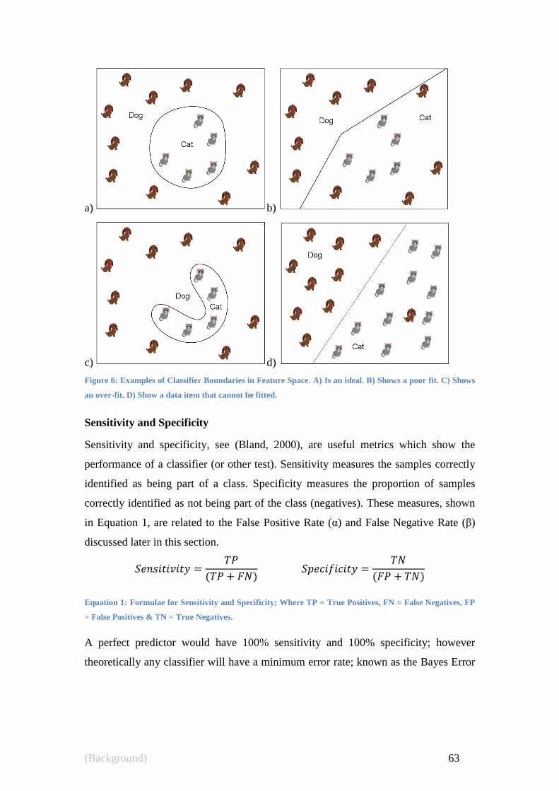
(Background) 63
a) b)
c) d)
Figure 6: Examples of Classifier Boundaries in Feature Space. A) Is an ideal. B) Shows a poor fit. C) Shows
an over-fit. D) Show a data item that cannot be fitted.
Sensitivity and Specificity
Sensitivity and specificity, see (Bland, 2000), are useful metrics which show the
performance of a classifier (or other test). Sensitivity measures the samples correctly
identified as being part of a class. Specificity measures the proportion of samples
correctly identified as not being part of the class (negatives). These measures, shown
in Equation 1, are related to the False Positive Rate (α) and False Negative Rate (β)
discussed later in this section.
Equation 1: Formulae for Sensitivity and Specificity; Where TP = True Positives, FN = False Negatives, FP
= False Positives & TN = True Negatives.
A perfect predictor would have 100% sensitivity and 100% specificity; however
theoretically any classifier will have a minimum error rate; known as the Bayes Error
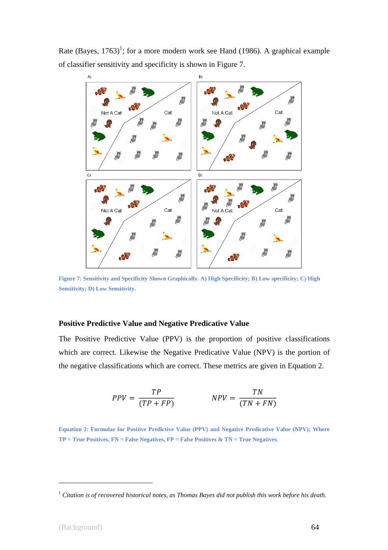
(Background) 64
Rate (Bayes, 1763)1; for a more modern work see Hand (1986). A graphical example
of classifier sensitivity and specificity is shown in Figure 7.
Figure 7: Sensitivity and Specificity Shown Graphically. A) High Specificity; B) Low specificity; C) High
Sensitivity; D) Low Sensitivity.
Positive Predictive Value and Negative Predicative Value
The Positive Predictive Value (PPV) is the proportion of positive classifications
which are correct. Likewise the Negative Predicative Value (NPV) is the portion of
the negative classifications which are correct. These metrics are given in Equation 2.
Equation 2: Formulae for Positive Predictive Value (PPV) and Negative Predicative Value (NPV); Where
TP = True Positives, FN = False Negatives, FP = False Positives & TN = True Negatives.
1 Citation is of recovered historical notes, as Thomas Bayes did not publish this work before his death.

(Background) 65
These tests provide the probability that a Positive or Negative result is correct. Its
value is dependent on the prevalence of the class being tested, which may be unknown
for some data sets.
False Positive Rate and False Negative Rate
The False Positive Rate (α) and False Negative Rate (β) represent the Type I and Type
II errors respectively; as shown in Equation 3.
Equation 3: Formulae for False Positive Rate (α) and False Negative Rate (β); Where TP = True Positives,
FN = False Negatives, FP = False Positives & TN = True Negatives.
The False Positive Rate and False Negative Rate are often used in statistical
hypothesis testing.
2.4.2. Overview of the k-NN Classifier
The kNN classifier is a simple and powerful classification algorithm used in a wide
variety of fields, and is discussed in detail by Zhang & Zhou (2007). This classifier
stores the feature space and label of every element of the training data it is presented
with. When it is asked to classify an unknown value, it finds the k training examples
closest to the new value (known as the nearest neighbours) and reports the most
frequently occurring class in the set (majority vote).
An example of k-NN applied to a hypothetical two dimensional feature set is shown
in Figure 8. The data set records an animal‘s height and noise level. Further each
record is labelled dog or cat (the class). A ―?‖ shows the point of enquiry for a new set
of features of unknown class. When taking the majority vote of the k=4 nearest

(Background) 66
neighbours the classification is dog by a vote of 3 to 1. When k=6 is used the result is
still dog, but by a vote of 4 to 2.
Figure 8: Example of k-NN on a 2 dimensional dataset.
The k-NN classifiers can utilise various metrics to measure the closeness of the
various feature space points. In this work we trialled several numerical distance
metrics, expressed as to express the distance between the points q and p:
Euclidean Distance;
o √∑
Canberra Distance (Lance & Williams, 1966);
o ∑ (| |
| | | |)
Chebychev Distance (Abello & Pardalos, 2002);
o
Correlation Similarity (Rodgers & Nicewander, 1988);
o ∑
√∑ √∑
Cosine Similarity (Tan et al., 2005);
o ( )
‖ ‖ ‖ ‖
∑
√∑
√∑
Heig
ht
Noise

(Background) 67
Dice Similarity (Dice, 1945);
o | |
| | | |
Dynamic Time Warping Distance (Myers & Rabiner, 1981);
o
o
o √∑
[ ]
[ ]
[ ] [ ]
Jaccard Similarity (Jaccard, 1901);
o
Manhattan Distance (Krause, 1987);
o ∑ | |
Max Product Similarity (Delibasic, Jovanovic, Vukicevic1, Suknovic, &
Obradovic, 2011);
o
Overlap Similarity (Lawlor, 1980).
o | |
| || |
2.4.3. Overview of Artificial Neural Network Classifiers
Artificial Neural Networks (ANN) are a computational model inspired by biological
central nervous systems (neurons, dendrites, axons and synapses). In an ANN,
artificial nodes called Processing Elements (PEs) are connected together to form a
network similar to biological neural networks.
Neuroscience is still full of unanswered questions and startling new discoveries
continue to be made, such as the role of magnetic fields in the brain acting like
synapses (Anastassiou, Perin, Markram, & Koch, 2011). As such there are many ways
in which to approximate our understanding of biological neural networks. The term
―artificial neural network‖ is a generalised term for many constructs which attempt to
mimic the behaviour of their biological counterparts.

(Background) 68
The ANN was first used on real data sets by Bernard Widrow and Marcian Hoff
(Widrow & Hoff, 1960) at Stanford to eliminate telephone line echo. Despite some
early success, an influential criticism on the limitations of ANN‘s was presented in a
book by Minsky and Papert (1969). This and other factors (allegedly) inhibited the
growth of ANN research for nearly 20 years.
In the 1980‘s, interest in Neural Networks rose quickly after a seminal paper by John
Hopfield (Hopfield, 1982) which presented a thorough mathematical analysis of
which tasks could and could not be solved by neural networks. Since this resurgence
in interest, ANN‘s remain an active and productive research topic.
A modern ANN is typically arranged into layers of Processing Elements (PE‘s). The
first layer is designated the input layer, and the last the output layer. Any layers in-
between are referred to as hidden layers. Each PE functions by using multiple input
values to create a single output value, using what is called an activation function. The
network is arranged with the outputs of one layer connected, in a weighted fashion, to
the inputs of the next layer. An example of this layout is shown in Figure 9. Note the
darkness of the line is used to indicate the connection weighting.
Figure 9: ANN setup with one hidden layer

(Background) 69
ANN‘s have been shown to solve a wide variety of problems in many fields.
Generally the tasks performed by neural networks can be divided into the following
categories:
Function approximation;
Time series prediction;
Classification;
Pattern recognition;
Data filtering;
Feature detection;
Robotics and industrial control;
Simulations and game AI.
It is the possibility of using ANN‘s to achieve data classification which concerns the
tasks of this work. A broad survey of ANN based classifiers and related problems /
technologies is presented by Zhang (2000) who describes ANN based classification as
―the most researched topic of neural networks‖. Further reviews by Lippman (1989)
have also explored the breadth and depth of this wide topic. For the purposes of this
overview however we present the typical neural network arrangement for a
classification task in Figure 10.
Figure 10: Typical ANN setup for classification

(Background) 70
In this setup there is an input layer that has one PE per item in the feature space and
the output layer has one PE for each possible classification result. When the network
executes the output PE with the highest value decides the result of the classifier.
2.4.4. Overview of the Support Vector Machine Classifier
A Support Vector Machine (SVM) is a supervised learning method which separates
two classes by constructing a hyper-plane which separates the training data. The
original feature space may be mapped into a much higher dimensional space, so as to
make the separation easier.
Hsu, Chang and Lin (2010) present a popular guide for rapidly obtaining acceptable
results from SVM classification. A more in depth resource for a (more) complete
understanding of the field is the book (dedicated to this subject) by Hamel (2009).
The points nearest to the separating hyper-plane are called support vectors. Only the
support vectors determine the position of the hyper-plane, all other points have no
effect. An example of this is shown in Figure 11.
Figure 11: Support vector machine setup
A desirable property of the SVM classifier is to achieve good separation between the
hyper-plane and the nearest (training) data point of any class. Henceforth this

(Background) 71
separation will be referred to as the margin. To increase the accuracy in which the
points are separated by the hyper-plane, as well as improve the margin, it is often
necessary to transform the training points into a higher dimensional space, see Figure
12.
The SVM classifier relies on the calculation of dot products between training points.
Rather than calculating the dot products in the higher dimensional space (both
difficult and computationally expensive) the kernel trick is used to help train the
SVM. The kernel trick uses a kernel function which is a dot product in the expanded
feature space to allow the computation of dot products in terms of the original data
points. The ―best‖ kernel function to use changes between problem domains.
In this work we will use the recommendations of (Hsu, Chang, & Lin, 2010) and
examine four different kernels:
Linear ( )
Polynomial ( )
Radial Basis Function (RBF) ( ) || ||
Sigmoid ( )
Where the values γ (gamma), c and d are the kernel parameters which we will have to
optimise to achieve the best classification performance.
Figure 12: Allowing for better separation of training points by projecting the data (part A, in 1
dimension) into a higher dimensional space (part B, in 2 dimensions). The hyper plane is shown in
black.

(Background) 72
2.4.5. Overview of the Naive Bayes Classifier
The Naive Bayes Classifier is a probabilistic classifier based on Bayesian statistics
(Bayes & Barnard, 1958). It is referred to as Naive because each feature is considered
independent when the training is performed, as discussed by Rish (2001). Ignoring co-
variance between features may introduce some limitations; however this classifier
performs remarkably well on real world complex problems, and often requires smaller
training sets.
Formally the classifier selects the most likely classification Vnb given the attribute
values a1, a2 ... an. This is expressed as:
∏ ( | )
Where ( | ) is generally determined by:
( | )
where:
n = the number of training examples for which v = vj
nc = number of examples for which v = vj and a = ai
p = a priori estimate for P(ai | vj)
m = the equivalent sample size
Many researchers feel the Naive Bayes Classifier seems oversimplified and should not
perform as well as it does, however Zhang (2004) was able to discover a theoretical
rationale for the apparently unreasonable performance of Naive Bayes Classifiers.
Naive Bayes Classifiers are often used in Emotion recognition problems, as
demonstrated by (N Sebe, Lew, Cohen, Garg, & Huang, 2002), (Nakasone,
Prendinger, & Ishizuka, 2005), (Nicu Sebe, Cohen, Gevers, & Huang, 2006), (Ball &
Breese, 1999), (Jiang & Cai, 2004) and (Qi & Picard, 2002). However recent studies
have suggested Random Forests (discussed later in section 2.4.7) may outperform the

(Background) 73
Naive Bayes Classifier, one example being described Caruana and Niculescu-Mizil
(2006).
2.4.6. Overview of the Decision Tree Classifier
A decision tree works in a similar method to the children‘s game "20 questions". The
goal of the classifier is to create a set of queries (against items in the feature space)
and based on the answer to the initial query, a more pertinant query is then run against
the feature space to derive further information. A simplified animal type classifier
decision tree is shown in Figure 13.
Can Swim?
Can Walk?Can Fly?
Can Climb Trees?
No Yes
No Yes
No Yes
No Yes
Figure 13: A Trivial Decision Tree Example

(Background) 74
Decision trees offer the following benefits:
Simple to understand and interpret. (The tree is human readable);
Requires minimal data preparation. (no normalisation, dummy variables or
removal of missing values);
Able to handle both numerical and nomial (label) data;
It is possible to validate a model using statistical tests;
Performs clasification quickly, making it suitable for large data sets;
Trains quickly, making it suitable for complex (and exhaustive) feature
selection tasks.
However there are some disadvantages:
Decision-tree training can create an over-complex tree that performs poorly
and needs to be "pruned" or simplified regularly;
Some problems and relationships are not suited to a nested decision process,
and will result in huge trees or poor performance, Exclusive-Or being an
example of such a relationship.
There are portions of information theory essential to the training operation of many
decision tree implementations such as the popular algorithms by Quinlan. Quinlan‘s
algorithms are known as the ID3 algorithm (Quinlan, 1986) and the C4.5 algorithm
(Quinlan, 1993). These algorithms begin constructing a decicion tree with the best
available feature, and then itrativley refine it using the next best feature. In this form
of "top down" training features are often ranked for inclusion by combining one or
more the of following information theory purity metrics:
Entropy (Shannon, 1951);
Information gain, also called the Kullback–Leibler divergence (Kullback &
Leibler, 1951);
Gini impurity (Gini, 1912);
Relief-F (Wang & Makedon, 2004).
The idea of a purity (or impurity metric) is to examine the similarity of the subsets
created by the decision tree. For example entropy, in this context, is a measure of the
uncertainty associated with a random variable. It is used as a heuristic to achieve

(Background) 75
smaller decision trees (simpler theories) over larger ones. The formula for computing
the entropy for a given attribute is given in Equation 4. As E(S) approaches 0 the set
approaches perfect classification. By computing Entropy heuristics for every node in
the tree it is possible to determine which nodes most need to be split into more nodes
to allow for better classification.
∑
2.4.7. Overview of the Random Forest Classifier
The random forest classifier (Breiman, 2001) is a collection of many decision trees
which gives a classification decision based on a majority vote of all its contained
trees. It has the following advantages:
It is one of the most accurate learning algorithms available (Caruana,
Karampatziakis, & Yessenalina, 2008);
It can handle large amounts of input variables.
However, random forests can overfit for some datasets (Segal & Segal, 2004).
The random forest uses a set of decision trees which are all trained on a subset of the
available features. Each tree is trained as follows:
1. Given N, samples in the training set, select N cases at random (allowing for
the same case to be sampled multiple times). This will form the training set for
growing a tree;
2. Given M input variables, select m (m<M) variables at random to be used in
training the tree;
3. Each tree is grown to the largest extent possible. (i.e. no pruning).
It has been shown (Breiman, 2001) that the random forest error rate depends on two
things:
Where :
E(S) is the information entropy of the set S;
n is the number values for the examined attribute in S
𝑓𝑠 (j) is the frequency of the value j in the set S
Equation 4: Entropy Heuristic for Decision Trees

(Background) 76
The correlation between any two trees in the forest. Decreasing the correlation
decreases the random forest error rate;
The accuracy of each individual tree in the forest. Increasing the accuracy of
the individual trees improves the performance of the random forest classifier.
The value m is linked to both the correlation and the accuracy. Increasing it increases
both, whereas decreasing m reduces both.
2.5 Overview of Techniques Related to Classifiers
In this section we review some methods and tasks related to the classification
algorithms which are used throughout this work. We will examine:
Forward Feature Selection (a technique to select from a set of features the
most relevant subset).
N-Fold cross validation (a technique to stop a classifier learning its data set
specifically, and thus not generalising well to real data).
2.5.1. Overview of the Forward Feature Selection Algorithm
The forward feature selection procedure (Guyon & Elisseeff, 2003) starts by
evaluating the performance of a classifier on each feature attribute. Taking the best
result, the algorithm then evaluates the performance of each possible feature subset
comprised of the previously found best features and a single feature from the
remaining features. The process continues in this fashion until a set amount of
features have been identified.
A problem with this procedure is that there is no guarantee that the best feature
identified for inclusion in creating a set of n features should exist in the best set of (n
+ 1) features. The advantage is that it executes significantly faster than computing the
performance of every possible feature set.

(Background) 77
2.5.2. Overview of N-Fold Cross Validation
Often there exists a significant difference between the models‘ performance on its
training data and future performance on real data. This is due to the algorithms‘
tendency to learn the training data, not the rules and correlation behind the data.
To mitigate the effects of models not being able to perform in real data tasks, a
technique called cross validation (Kohavi, 1995) is used. In cross validation a portion
of the training set is not used in the creation of the classifier. It is instead used to
evaluate the performance of the classifier. That is, the performance is taken from a
portion of the data the classifier has not seen before.
A more rigorous form of cross validation is known as N-fold cross-validation. In this
method the training data is divided into N subsamples. Of the N subsamples, one is
retained for measuring the performance (validation) of the model, and the remaining
N − 1 subsample sets are used to train the model. The process is repeated N times
such that each subgroup has been used as the validation set. The average performance
is then calculated to determine the efficacy of a classifier technique for a particular
data set.
Most commonly 10-fold cross validation (N=10) is employed when validating
classification models. From experience, many researchers consider N=10 as ―about
right‖ as it often produces accurate predictions of classifier performance on a broad
range of classifiers on a broad range of datasets. More rigorous testing by Bengio and
Grandvalet (2004) has provided validation for N=10 as a good general solution.
Another research effort by Markatou and Tian (2006) shows N=10 as a suitable
validation technique for data relating to Biomedical Informatics.
2.6 Conclusion
In this section we presented an overview of some subject areas which provide
essential concepts throughout this work:
What emotions and affective states are;

(Background) 78
The cultural and natural components of emotion;
How we organise, categorise and quantify emotions for research purposes;
The computational means by which we perform classification.
This work also used many concepts from computer science, signal processing,
psychology, physiology, human biology and neurology. These concepts are
introduced and explained within the relevant sections as needed. A glossary is
provided in Chapter 13 to assist the reader with the multi-disciplinary terms and
jargon used in this work.

(A Review of Current Literature) 79
3.0 A Review of Current Literature
"Not everything that can be counted counts, and not everything that
counts can be counted."
- Albert Einstein (1879-1955)

(A Review of Current Literature) 80
In this chapter we cover a range of topics that relate to the task of Physiological
Pattern Recognition (PPR) to classify human emotion.
The chapter starts with an overview of different techniques used to recognise
emotions in humans, so as to place where PPR exists in the scope of available
techniques and why it is important. In general there are still many challenges to be
overcome in the field of PPR (Picard, 2000), (van den Broek, Janssen, Westerink, &
Healey, 2009). However PPR does offer practical advantages over other techniques
that are also covered in this section.
A section is then dedicated to an argument in Emotion Theory over whether emotions
are natural phenomena that we are born with, or the product of Social
Constructionism (Averill, 1985), or a mixture of both. We would expect that if an
emotion was in fact the product of Social Constructionism, then it would not
necessarily have a common physiological pattern amongst multiple people.
After this background is established we examine the available literature describing
how emotion will alter human physiological activity and the resulting signals
collected. Eleven different physiological signals often studied in relation to emotion
are then examined in detail.
A major factor in performing PPR based research is the validity of the emotion
induced in the participants being studied (van den Broek et al., 2009). To this end we
dedicated a section to examining the available literature on eliciting human emotion.
Lastly we conclude the chapter with a review of literature concerning works similar to
our own, discussing their results and examining where useful contributions could be
made. Absent from this chapter is the important role of the human face in emotion;
this topic is covered separately in Chapters 4 and 5.

(A Review of Current Literature) 81
3.1 Recognition of Emotion
In order to rationalise a method for observing emotion, when no clear definition for
what an emotion is exists, we utilise the following principle (our own wording) to
generalise human emotion as a function of cognition, physiology and behaviour.
Emotion (whatever it is) is reflected in changes to a person's cognitive and
physiological state. In turn, a relationship exists between a person's behaviour
and their emotional state.
In humans, emotions will create alterations to the cognitive and physical state. These
changes can be apparent (an expression of emotion) or discreet (a subtle change in
state or behaviour). Expanding on a table presented by Picard (1997, page 27), Table
1 shows the known techniques by which machines can examine the human cognitive
and physical state to derive information on the related emotional state.
Table 1: Cues for the Recognition of Emotion
Physiological
Auditory
Speech Analysis (apparent & discrete)
Visual
Face Recognition (apparent)
Gesture Recognition (apparent)
Physiological Signals
Muscular (discrete)
Glandular (discrete)
Temperature (discrete)
Cognitive
EEG (discrete)
MRI (discrete)
Behavioural
Interface Usage Data (apparent & discrete)
Natural Language Processing (apparent)

(A Review of Current Literature) 82
The distinction between analysing emotion from a physiological and a cognitive
perspective is important. Cognitive processes are direct measures of brain activity,
whereas physiological processes influence, and manifest from, cognitive processes.
There is a great deal of data sets available in emotion detection research. The focus of
this work (shown in Figure 14) is with instrumentation which collects data from
physiological processes (in blue) as opposed to cognitive processes (in red), or
behavioural cues (conscious and deliberate actions).
Cognitive and Affective
processes in the Brain
Physiological
Processes
Physiological
manifestations.
Cognitive and
affective
interpretation
and reaction.
EEG
fMRI
Speech Analysis
Physiological Signals
Face Recognition
Figure 14: Physiological (blue) and Cognitive (red) signals.

(A Review of Current Literature) 83
3.2 Culturally Specific Emotions and the Plausibility of
Heterogeneous Physiological Pattern Recognition
Theories on origin of emotions are often in the vein of social constructionism
(emotions result from social concepts) or naturalism (emotions are a universal
phenomenon), as discussed in section 2.2.
The extent to which Physiological Pattern Recognition can develop into a strong and
broadly applicable technology is tightly linked to how these competing theories play
out. If emotions are innate then we can hope to generally recognise them in people.
However if social constructionism is the case, heterogeneous PPR becomes less
plausible as there are few, if any, mechanisms by which people will gain a generic,
and common, physiological response to learned emotions.
While many emotions appear universally, some emotions are considered exemplars of
culturally specific occurrences. Extensive reviews of these emotions have been
conducted by notable researchers such as Prof Jesse Prinz (Prinz, 2004) and Prof
James Russell (Russell, 1991). These works identified many culturally specific
emotions.
In assessing the likelihood and extent to which Social Constructionism influences
human emotion, we researched a set of emotions commonly identified by Prinz or
Russell as being culturally specific. For the purposes of gaining further understanding
into the area we created, or found, existing counter arguments to each of the claims
that these emotions were culturally specific. Summarising the results we were able to
categorise arguments against social constructionism into four categories:
a) The unusual assignment of an emotion to an event which invokes an extremely
different emotion in other cultures. Seen as a different emotion altogether, not
as a different response by outside observers.
b) Cultural pride; one culture will often claim significant culturally important
feelings as being their own distinct feeling, different from similar emotions in

(A Review of Current Literature) 84
to other cultures. This becomes a cultural identity and is kept as an important
distinguishing characteristic.
c) A language simply lacks the vocabulary to present an emotional state as one
word. It is posited that this may commonly happen in cases where theorem b
exists; as the feeling is often discussed, appropriate words naturally evolve for
feelings that may not warrant a single word in other cultures.
d) Some emotions, though universal, cannot be experienced unless the necessary
experiences are encountered. Some "necessary experiences"
are not equally encountered in different cultures. For example, few people in
first world countries would experience emotions relating to desperate hunger,
war, or experience feelings brought about by hunting or living with nature.
Examples of applying our counter arguments are as follows:
Gezellig (the Netherlands) A cozy and inclusive setting or atmosphere. Similar
to the german word Gemütlich;
o Counter argument (Theory B), similar European concepts exist e.g. the
Swedish word gemytligt, Danish word hygge, Norwegian word
koselig, Russian, word уют, Czech word pohoda. However, the Dutch
hold Gezellig to be one of their most important words, as it describes
the ideal cultural setting.
Liget (Ilongot people) (Rosaldo 1980 cited in Prinz 147) A manifestation of
Anger, Passion and a will to act. Can inspire headhunting expeditions, or be
felt before food hunting;
o Counter argument (Theroy B): The word is a central part of the very
rich and interesting Ilongot social identity discussed at length by
Rosaldo (1980) who discusses some quite inspirational field work she
conducted amongst head hunting tribes of the Philippines. The emotion
seems similar to that which occurs in many passionate young men in
response to a grievous effrontery or an imminent hostile situation.

(A Review of Current Literature) 85
Schadenfreude (Germany): A pleasure triggered by seeing the misfortunes of
others;
o Counter argument (Theroy C): English, for example, used to have the
word "epicharikaky", which is defined by the compound epi (upon),
chaira (joy/charity/heart), and kakon (evil) (Bailey, 1756). However
the phrase "morose delectation" has also been used to describe a
similar emotion, and was traditionally taught to be a sin by the Catholic
Church (Hammond & Fell, 1847). In modern times, western cultures
often borrow the word Schadenfreude to describe the emotion; which
is prevalent in many western cartoons and sitcoms. Most notably the
character Nelson Muntz from the Simpsons (Groening & Brooks,
2006) has turned a schadenfreude based phrase, "Haa-Haa", into a
cultural meme, as per Figure 15.
Figure 15: Depiction of schadenfreude, in the Simpsons character Nelson Muntz (Groening & Brooks,
2006)
Acedia (circa Middle Ages Europe): Aversion to religious imagery, arising from
boredom induced by the repetitive nature of worship, (Prinz 2004, p 148);
o Counter argument (Theroy d): Modern religions which require less time to
be spent worshiping, combined with a change of religious practices may
have removed the needed stimulating events.
Awumbuk (Baining of Papua New Guinea): Sadness, tiredness or boredom caused
by the departure of visiting friends or relatives, (Russell 1991, p 432);
o Counter argument (Theroy c): A common feeling, but not one people
would look to put a word to.

(A Review of Current Literature) 86
Nginyiwarrarringu (Pintupi Aborigines of the Western Australia): A sudden fear
that leads one to investigate its cause, (Russell 1991: 431);
o Counter argument (Theroy d): If I may draw from personal anecdotal
evidence. The author of this work knows the West Australian bush well,
and has spent a lot of time (500+ days) walking through it. The author can
testify to an (occasional) distinct and strong emotion similar (but separate)
to fear that causes one to suspect an area, and want to investigate it.
However, the author is not of the Pintupi or a related culture and would
assume the emotion is caused by the nature of certain areas of the land, as
the author has not felt it while trekking in any other part of the world (or
even Eastern parts of Australia).
While we do not presume that this set of counter arguments can be taken as a
significant challenge to the theory of Social Constructionism, we feel that this forms a
framework for proceeding under the assumption that the effects of Social
Constructionism do not heavily influence the ―common‖ emotional states which we
would wish to study in relation to Human Computer Interaction.
A logical framework for dealing with the competing theories of Naturalism and Social
Constructionism was presented by Prinz (2004). This often cited compromise between
nativism and social constructionism is achieved by allowing for different perceived
states, both innate and culturally specific / learned states, to count as emotions. Prinz
(2004) explains this is possible because we can learn to associate new contexts with
specific body states. These cognitive-emotion hybrids are a logical solution to the
arguments.
3.3 Physiological Changes as Cues for Recognition of
Emotion
A significant (and somewhat pioneering) effort into detecting the human emotional
state was undertaken by Rosalind Picard and her team at the MIT Media Lab (Picard,
Vyzas, & Healey, 2001). This work used a (single) trained actor who purposely
elicited emotional states while hooked up to multiple physiological recording devices.

(A Review of Current Literature) 87
Two significant findings from this work have told us a lot about the nature of
understanding physiological changes resulting from changes in emotional state,
namely:
1. Physiological changes for the same emotions in the same person will vary,
however the variance has short term (one day) clustering whereby features
collected on the same day are more clustered and predictable than features
collected on different days;
2. Obtaining quality data in this field is an extremely difficult procedure.
Picard suggests three factors which can cause the day dependence of data and
suggests a method of compensating using a day dependence matrix. The factors were:
Skin sensor interface changes:
o Changes in skin cleanliness (or washing);
o Use of different amounts of gel;
o Minor changes in positioning of sensors.
Non-emotional factors causing alterations in physiology:
o Caffeine;
o Sugar;
o Sleep;
o Hormones.
Mood and emotional factors altering physiology:
o Feeling sad may make happy emotions/signals less distinct;
o An exciting day may cause increased heart-rates.
The day dependence matrix proposed by Picard et, al. functioned by utilising an extra
dimension for data for every day and projecting all days back into the original
dimensional space. This procedure is best explained by example (see Figure 16);

(A Review of Current Literature) 88
Figure 16: Dimensional projection via a day dependence matrix (Picard, Vyzas, & Healey, 2001)
If a feature for anger and joy for day one (A1, J1) and a similar set of features for day
two (A2, J2) do not form groups as in Figure 16a; then results from day 2 are moved
into another dimension Figure 16b. In this new dimensional space, a line (or n-
dimensional plane as dimensions increase) can be constructed which separates
anger(A1, A2) data from joy data (J1, J2). All data are then projected to line a to form
a final feature set. In the case of higher dimensions an n-dimensional plane is
constructed that separates all points. Figure 16c illustrates this for three days (hence
three dimensions) using plane p. Plane p is shown as a triangle, where the vertices
define the plane (by 3 points) and each point is placed to separate the data in its
dimension. Finally all data can be transformed back to the orthogonal line a to create
the final data set.
The day dependence matrix gives us a somewhat tenuous ability to reproduce results
for one person over several sessions, thus strengthening the validity of Physiological
Pattern Recognition (PPR) as a tool for prediction of affective states or emotions.
3.3.1. Physiological Pattern Recognition
Physiological signals are recordings taken of the human physiological state using
various sensors. In the field of affective science physiological signals are recorded for
various human systems, typically involving the:
Muscular system;
Subconscious actions;
Cardiovascular system;

(A Review of Current Literature) 89
Respiratory system;
Dermatological system;
Thermoregulatory system.
The Muscular System is inspected via a process known as electromyography.
Electromyography detects the electrical potential generated by muscle cells when they
contract.
Emotionally relevant subconscious actions such as pupil dilation (Bradley, Miccoli,
Escrig, & Lang, 2008; Partala & Surakka, 2003; Siegle, Steinhauer, Carter, Ramel, &
Thase, 2003; Jing Zhai & Barreto, 2006a), blinking (Vrana, 1995; Vrana, Spence, &
Lang, 1988), posture (Coulson, 2004; Duclos et al., 1989; Riskind & Gotay, 1982;
Wallbott, 1998) and pressure applied to objects (Clynes, 1989; Hama & Tsuda, 1990)
are often linked with emotional state. These actions can be obtained via
electromyography, video recordings and pressure sensors.
The human cardiovascular and respiratory systems are both regulated by the medulla
oblongata (Amoroso, Bell, & Rosenberg, 1954; Guyenet, 1990). A close relationship
exists between the affective cognitive state and how these systems are controlled and
these systems are a major focus of current research. Respiration rates can be
monitored with respiration sensors and the cardiovascular system is often examined
through the electrocardiograph and blood volume pulse measurements.
The dermatological system has been shown to exhibit interesting (though complex)
properties in relation to the human emotional state (Kepecs, Milton, & Brunner, 1951;
Khalfa, Isabelle, Jean-Pierre, & Manon, 2002; Mittelmann, Wolff, & Harold, 1943).
The ease of obtaining skin conductance signals and the low cost of the electronics
involved promotes the signals as being very useful to analyse.
The thermoregulatory system is often examined in terms of skin temperature (e.g.
(Mittelmann & Wolff, 1939) & (Lisetti & Nasoz, 2006)). Recordings are often
obtained using a high precision digital thermometer.

(A Review of Current Literature) 90
3.3.2. An Investigation of Physiological Signals
As a large body of this work is concerned with the processing of physiological
signals, it is necessary to arrive at an understanding of different signals that can be
acquired from the human body in a context of their related functions and previously
found uses in various fields.
For the purposes of this work it is necessary to investigate signals that are produced
by areas of the human body thought to undergo physiological change during
emotional state change. As such, we have attempted to identify and classify pertinent
signals in an infrastructure that relates the various physiological signals to a mapping
of their connectivity to different parts of the brain.
The rationale behind this classification comes from the emerging field of ―cognitive
neuroscience of emotion‖ (also called affective neuroscience) as proposed by Lane &
Nadel (Lane & Nadel, 2000). The foundation of this field is that different parts of the
brain are active or involved with different emotional states. Often the same areas of
the brain are related to physiological mechanisms and it can be expected that signals
collected in relation to those mechanisms may provide insight into the nature of the
emotional state of the brain.
There has been much research into the areas of the brain involved with emotion. The
field was pioneered in the 1870's by renowned French anatomist Pierre Broca (Broca,
1878), who discovered that there is a relationship between emotions and the limbic
system of the brain. A thorough review of modern research into affective
neuroscience by Dalgleish (2004) identified MacLean's (MacLean, 1952) limbic
system theory of emotion as the dominant conceptualisation of the ―emotional brain‖.
MacLean's and Daglish suggest the following areas of the brain as being most
involved with emotion (Refer to Figure 17):
Amygdala (part of the limbic system);
Anterior cingulate cortex;
Cerebellum;
Insula cortex;
Prefrontal cortex;

(A Review of Current Literature) 91
Ventral striatum.
It is also important to consider the role of the medulla oblongata in the body's
physiological state. Many physiological conditions, related to emotions, are regulated
by the medulla oblongata. Many autonomic functions governed by this structure are
both measurable and relate to emotion in some way; e.g. the heart rate, blood flow,
respiration rate, perspiration, salivation levels, pupil dilation, micturition and sexual
arousal.
Figure 17: Structures of the brain involved in emotion.
3.3.3. Examining and Monitoring the Physiological State
The human physiological state is a system which responds to many variables in a way
that, is thought to, vary from person to person (a good discussion of the topic is
presented by Leidelmeijer (1991)). It is unrealistic to expect that we can obtain a
clear picture of a person‘s affective state simply by examining a snapshot of
someone's physiological recordings. However given prior knowledge of how an
individual responds and making allowances for changes in how they respond (Picard
et al., 2001) it is possible to perform emotional state recognition with varied degrees
of success.

(A Review of Current Literature) 92
Finding correlations between the emotional state and the physiological state is
difficult because many other factors influence the emotional state. However by
controlling all other factors and changing only the emotional state (the control
variable) a picture of how emotion influences the physiological state can be found.
Figure 18 shows the different factors that can influence a person's physiological state.
Also shown are two distinct links between the cognitive state and the physiological
state, which represent the conscious and sub-conscious (emotional) influences.
Physiological State
EmotionConscious Control
Exercise
Environmental
Food / Chemicals / Drugs
Ergonomics
Health
Figure 18: Variables Affecting the Physiological State.
3.3.4. Muscular Physiological Signals (EMG) of the Back (Posture &
Support)
It is generally known that people display their emotional state through body language
(Lowen, 1978) and that body language plays an important part in social interaction
(Scheflen, 1972). A major component of body language is posture, which can easily
be monitored via EMG analysis (Cram, Kasman, & Holtz, 1998).

(A Review of Current Literature) 93
Two lesser generally known links between posture/body language and emotion exist
that are of interest. Firstly, body language cannot be thought of as a minor factor in
the human emotional system. The human brain automatically perceives and
understands whole-body signals (Gelder, 2006), which means from a neurological
perspective they function in a similar manner to facial expressions.
Secondly, it is also known that back posture influences affective processing, for
example Wilson (2004) found that 92% (n=24) of his participants were more
successful in generating positive thoughts when in an upright position while
attempting positive and negative thought generation tasks.
While the upper back plays a major part in human body language that can be readily
accessed via EMG, there also exists affective traits expressed in the EMG of the lower
back while in a sitting position. An interesting study by John Burns (Burns, 2006),
showed that there exists a specific EMG activity related to tensing of the lower back
muscles that is linked to anger.
The collection of EMG signals from the back for use in emotion classification tasks is
an active field of research with notable publications including (Azevedo & Volchan,
2005), (Facchinetti, Imbiriba, & Azevedo, 2006) and (Hillman, Rosengren, & Smith,
2004).
3.3.5. Human Action of the Hand (Pressure)
There is a common perception that a frustrated person will subconsciously exert more
force when performing simple motor activity tasks. This concept has been explored in
some devices. A pressure sensitive phone handle developed by Scheirer (Scheirer &
Picard, 1999) and detailed further in (Picard, 2000) predicts a user‘s mood by
monitoring the pressure with which the phone is held. The system is shown in Figure
19. The screen shows a colour related to the amount of pressure exerted.
Hand pressure has also been linked to the cognitive load a person is under (Ikehara &
Crosby, 2005). Other studies have found links between the level of Arousal

(A Review of Current Literature) 94
experienced by video game players and force exerted on gamepad buttons (Sykes &
Brown, 2003).
Figure 19: The "TouchPhone"
3.3.6. Human Action of the Torso (Posture)
Posture is a primary mechanism through which emotion is communicated between
people which can be examined via physiological EMG recording (Poppen & Maurer,
1982). It has been found that there are minor cultural specific factors (Kleinsmith, De
Silva, & Bianchi-Berthouze, 2006) concerning how emotion is expressed through
posture.
Attesting to a basic neurological (not cultural) connection between emotion and
posture, is evidence of subconscious body posture recognition in people with cortical
blindness (de Gelder & Hadjikhani, 2006). This effect is part of a condition known as
"affective blindsight" (de Gelder, Vroomen, Pourtois, & Weiskrantz, 1999), where
damage to the occipital cortex causes blindness but other brain pathways associated
with processing emotion continue to receive visual information, and process it on a
sub-conscious level.
3.3.7. Human Autonomous Functions Controlled by the Medulla
Oblongata and the Autonomic Nervous System - Overview
The medulla oblongata (lower half of the brain stem) controls many autonomic
functions, and relays nerve signals between the brain and spinal cord. It is not
associated with many affective processes.

(A Review of Current Literature) 95
The medulla oblongata controls the following autonomic functions:
Respiratory functions;
Cardiac functions;
Vasomotor functions (alterations in blood vessel diameter);
Vomiting reflex;
Coughing reflex;
Sneezing reflex;
Swallowing reflex;
Urinary /defecation control.
Some of these functions were ruled out as possible candidates for study. Urination,
defecation and vomiting would not be tested under our experimental setup for ethical /
procedural reasons. However involuntary urination, defecation and vomiting are often
associated with fear. Working with US WWII military veterans (p=300, all male),
Dollard (Dollard, 1943) found that under conditions of extreme fear, soldiers reported
involuntary: urination (6%), defecation (5%) and vomiting (< 1%).
The coughing reflex and sneezing reflex are too uncommon to be studied in short
sessions and lack evidence to show emotional links.
The swallowing reflex is known to be linked to emotions and the rate of swallowing is
modulated by the type of emotion experienced. A recent study by Ritz and Thöns
(2006) showed both pleasantness and Arousal interacted to modulate swallowing
rates. They further found that female participants swallowed more frequently for
negative stimuli than neutral, and less frequently for positive stimuli than neutral.
The autonomic functions we have discussed so far are linked to emotion; however a
more accurate look at the physiological effects of emotion is obtained by examining
the Autonomic Nervous System (Standring & Gray, 2008). The Autonomic Nervous
System is the control mechanism of human homeostasis, functioning largely below
the level of consciousness, and is partly controlled by the Medulla Oblongata. This
system is divided into the parasympathetic nervous system and sympathetic nervous
system. The parasympathetic nervous system is largely responsible for functions of
―resting and digesting‖, while the sympathetic nervous system is largely responsible

(A Review of Current Literature) 96
for ―flight or fight‖ type responses. It is the Autonomic Nervous System‘s control of
many vital organs and influence on Physiological Signals and its connections to
resting and Fight or Flight action that makes it noteworthy at this point. A full layout
of its functions is shown in Figure 20. Note how the skin‘s sweat glands are special in
that they have sympathetic connections, but no parasympathetic connections.
Figure 20: The Structure of the Autonomic Nervous System (Lane et al., 2009)

(A Review of Current Literature) 97
3.3.8. Signals Controlled by the Medulla Oblongata - Respiration
Respiration is a function of the human body that automatically adjusts to meet the
body‘s physical and psychological demands. It is often studied in relation to emotion,
however there is a belief, by some researchers, that much more research in this field is
required. Grossman & Wientjes (2001) said:
"The investigation of respiration in relation to psychological phenomena
remains one of the truly neglected areas of psychophysiology, behavioural
medicine and neurophysiology. Respiration, of all major physiological
processes, would appear to be, perhaps, the most obvious candidate to
examine in association with psychological demands. Specific respiratory
symptoms are frequently reported to emotionally stressful states"
A compilation of research on the matter of emotion and respiration has been compiled
by Haruki, Homma and Umezawa (2001). From this book, it can be seen that the use
of one or two chest bands that expand and contract with breathing, is the most
common method used to digitise human respiration function. This type of sensor
typically produces the waveform shown in Figure 21.
The sensor is also easy to place, not prone to coming loose, and robust enough to be
usable in real life situations. For this reason it is often used in experiments involving
emotion during sports activities; e.g. Katsis et al., (2008) who used this sensor to
perform emotion recognition in racing car drivers. This type of sensor may also be
Chest
Expansion
Time
Cycle Time
Inhale Time Exhale Time Expiratory Pause
Inhale flow Rate
Figure 21: Respiration Cycle

(A Review of Current Literature) 98
incorporated into emotionally aware clothing (Axisa, Dittmar, Delhomme, & Cedex,
2003).
3.3.9. Signals Controlled by the Medulla Oblongata- Heart Beat
The ―heart beat‖ is the cardiac cycle of the heart. It generates an arterial palpation that
we refer to as the ―pulse‖. It also creates an audible noise, the result of the blood flow
being affected by the closing of the heart valves. There is also an electrical signal
created by the electrical activity of the heart known as the electrocardiogram (ECG)
from the German Elektrokardiogramm (EKG). The sequencing of these signals is
displayed in what is known as a Wiggers Diagram (named after eminent
cardiovascular physiologist and 21st president of the American Physiological Society;
Dr. Carl J. Wiggers) which is shown in Figure 22.
In practice the ECG (aka EKG) is the most practical of methods for studying
physiological signals in relation to the heart beat. The signal is information rich and
easily obtained via sensors placed on the skin surface.
The ECG is a periodic signal and is described by the ECG basic waveform (Dubin,
2000), also shown in Figure 22. The ECG can be analysed in terms of the P, Q, R, S,
T and U waves. Generally referred to as the P-wave, QRS Complex, T-wave and the
U-wave. The heart rate (pulse) is derived from the distance between R wave peaks
(also called The R-R interval) by the equation ⁄ where the heart rate is in
beats per minute and the RR interval is in seconds. Note: the U wave, not shown in
Figure 22, is a very small wave following the T wave. As it is a very small wave it is
often lost in the signal noise and thus not used in ECG analysis.

(A Review of Current Literature) 99
Figure 22: Wiggers Diagram, (Guyton, 2000) ; Chapter 9 - Page 99.
The ECG response to stress has been studied by Healey & Picard, (2000), who
showed that simple ECG based metrics could be used to achieve stress detection at
around 50% accuracy; or 88% accuracy when combined with other physiological
signals.
The role of heart rate in relation to the emotional Valence has been studied at length
by various authors. Libby, Lacey & Lacey (1973) graphed average heart rates for
participants exposed to slides of varying degrees of pleasantness.

(A Review of Current Literature) 100
Figure 23: Heart Rate in Relation to Pleasant Emotions (Libby Jr et al., 1973)
Winton, Putnam & Krauss (1984) further examined the relationship of emotional
Valence to heart rate and skin conductance. They found a set of changes over time
profiles for five stimulus types, that is; peoples‘ heart rate changed in a similar
manner for a similar stimulus. Their results are shown in Figure 24.
Figure 24: Heart rate response to various slide types

(A Review of Current Literature) 101
The ECG response to fear is different to the ECG response to many other negative
stimuli. Globisch, Hamm, Esteves, and Ohman (1999) demonstrated this using images
of spiders and snakes (generally considered negative stimuli) on participants that were
phobic of these animals vs. participants who were not. The control participants
responded to negative stimuli with a lowered heat rate, while the phobic participant‘s
heart rate lowered for around one beat then began to increase sharply. A graph of
these results is shown in Figure 25.
Figure 25: Heart rate in response to negative animal stimuli, in phobic and non phobic participants.
(Globisch et al., 1999)
3.3.10. Signals Controlled by the Medulla Oblongata - Blood Volume
Pulse
The Blood Volume Pulse (BVP) is a signal collected by a photoplethysmograph
which takes a volumetric measurement of an organ or area of flesh. The device
illuminates the skin and records the level of light absorption (Shelley & Shelley,
2001).
While the BVP is useful in revealing many of the attributes that knowledge of the
heart rate can provide there is a piece of extra information available. It is known that
the overall amplitude (envelope) of the BVP signal contracts when a person is
startled, fearful or anxious (Picard, 1997, pg 162); likewise the amplitude increases
when there is greater blood flow to the extremities, such as is caused by a person
being relaxed. An example of this envelope is shown in Figure 26.

(A Review of Current Literature) 102
Figure 26: A BVP Envelope (Fernandez & Picard, 1998).
3.3.11. Human Autonomous Functions Controlled by the Medulla
Oblongata -Blood Pressure
Blood pressure is a physiological metric measured by a sphygmomanometer. It is
commonly associated with stress and studies such as Globisch et al., (1999) have
shown definite usefulness as a signal in predicting stress. Their results show changes
in blood pressure after three seconds of being exposed to a stress inducing stimulus
(pictures of snakes and spiders). The response by people with a related phobia was
extremely pronounced over other subjects, see Figure 27.
Figure 27: Blood Pressure in response to negative animal stimuli, in phobic and non phobic participants.
(Globisch et al., 1999)

(A Review of Current Literature) 103
3.3.12. Human Dermatological Response (Sweat & Skin Conductance)
Skin conductance is a physiological metric measured by a simple reading of electrical
resistance of the skin, thus it is recorded by an ohmmeter. It is often referred to as
Galvanic Skin Response (GSR), Electrodermal Response (EDR), Psycho Galvanic
Reflex (PGR) or Skin Conductance Level (SCL).
Skin conductivity is one of the most robust and well studied physiological responses
e.g. (Lee et al., 2005; Picard, 1997, 1997; Picard, 1997; Ryoo, Kim, & Lee, 2005;
Scotti, Mauri, Cerutti, Mainardi, & Villamira, 2005a, 2005b, 2005c; Wagner, Kim, &
Andre, 2005a, 2005b, 2005c; Zhai & Barreto, 2006a, 2006b). It is controlled by the
sympathetic nervous system (Standring & Gray, 2008), see Figure 20, which changes
the levels of sweat in the eccrine sweat glands. The eccrine sweat glands, located on
the palms of the hands (and the soles of the feet), have been shown to be particularly
responsive to emotional states, and only minimally responsible for thermoregulation
(Michael, Dawson, Schell, & Filion, 1990). Thus this signal is a good indicator of
sympathetic nervous system action in relation to the fight or flight response.
The GSR has been shown to be linked to measures of startle, Arousal, stress and
attention and other general emotional states (Critchley, Elliott, Mathias, & Dolan,
2000; Dhokalia & Atreya, 2011; Domingues, 2011; Elfering & Simone, 2011;
Michael et al., 1990; Mundy-Castle & McKiever, 1953; Westerink, Broek, & Schut,
2008).
Globisch et al., (Globisch et al., 1999) has shown the GSR signal to be a useful
indicator of stress levels. Their results show changes in blood pressure after three
seconds of being exposed to a stress inducing stimulus (pictures of snakes and
spiders). The response by people with a related phobia was pronounced over other
subjects, see Figure 28.

(A Review of Current Literature) 104
Figure 28: Skin Conductance in response to negative animal stimuli, in phobic and non phobic participants.
(Globisch et al., 1999)
3.3.13. Human Thermoregulatory Response - Skin Temperature and
the Insula Cortex
Many metaphors exist to describe emotions and emotional situations in terms of
temperature, such as "an icy stare", "a cold heart", ―the cold shoulder", "hot under the
collar" and "radiating warmth and kindness".
Two well publicised studies by Williams & Bargh (2008) revealed how hand
temperature affects the emotions (of undergraduate students). The researchers found
that holding warm things may actually make people view others more favourably (in
terms of social warmth), and having warm hands may also make people more
generous. In the first study by Williams & Bargh, 41 participants were given hot or
ice cold coffee and then asked what they thought of a stranger after a brief meeting.
The participants holding a hot cup of coffee were more likely to judge the stranger to
be a kinder person. The second study involved participants holding either a warm or
cold object and participating in a farcical task. After the task was completed the
participants were given a choice of reward for participating in the study: either a gift
for a friend, or a reward for themselves. The people with who held the hot item were
more likely to choose the gift for a friend reward.

(A Review of Current Literature) 105
Williams & Bargh concluded:
"Physical and psychological concepts are much more closely aligned in the
mind than we have previously appreciated. Other research has found that the
same brain region that processes physical temperature changes, called the
insula, also processes feelings of trust and empathy associated with social
warmth."
These studies appear to lack a baseline of a temperature control group to distinguish
whether heat makes us more trusting and generous, or coldness induces greed and
scepticism; or both.
3.3.14. Sampling of Skin Temperature from the Hand
Typically many researchers will measure skin temperature by use of a finger sensor.
Notable works adopting this technique include Bela Mittelmann & Wolff (1943),
Baumgartner et al., (2006), Pasca, Pierre, & Henrique (2005) and Kim & Andre
(2008). This however may be a flawed approach if the ramifications of the nature of
this kind of measurement are not properly considered, as will now be discussed.
The human epidermis is an organ with a very large surface area (average 1.9m2 in
males, 1.6m2 in females). The finger sensor takes a reading at one location of the
epidermis which may account for 1cm2 of data. Thus this one reading accounts for
0.005% of the measurable skin surface temperature and it is quite possible that if
present a localised variation will greatly influence the results obtained by the sensor.
Thus it is our feeling that a fundamental step in using the temperature sensor on a
finger is determining what localised variations exist and to what extent they can
influence the data.
Many variations are known to exist as the result of injury, sickness or chronic
conditions. Figure 29 summarises some common conditions that alter skin
temperature in the hands.

(A Review of Current Literature) 106
Post-Traumatic variation in left hand after 3 year
old wrist injury. (Hughes Medical Corp, 2010)
Early Stage Carpal Tunnel Syndrome in left hand.
(Hughes Medical Corp, 2010)
Abnormal heating indicating infection as
recorded by NASA. (Short, 2010)
Dystrophy-Related Asymmetry in Skin
Temperature (Erasmus et al., 2010).
Figure 29: Medical conditions effecting skin temperature of the hands
It is clear from the images in Figure 29 that damaged hands have unique heat patterns.
Regardless of sampling damaged or undamaged hands, samples taken from different
parts of the hand will exhibit large variations of up to 4° Celsius.
In a study of 81 healthy volunteers, Kokubo, Taniguchi, Yamamot and Hirasawa
(1998) made several important observations about the surface temperature of the
human hand. By recording 2D temperature distributions of the participants during rest
and analysing the data against age and gender, it was shown that in the sampled
population:
Females had an average temperature of 32.4° Celsius;
Males had an average temperature of 31.8° Celsius;
There was no correlation between age and temperature;

(A Review of Current Literature) 107
Average temperatures across the hand differed 2-3 degrees (10% variation);
The 2-dimensional distributions of all data can be classified into four groups:
1. High temperature in the middle of the palm (C);
2. High temperature at both thenar and hypothenar eminences (TH);
3. Intermediate type (CT);
4. Combination type (CTH).
The four temperature groups identified by Kokubo et al., are shown in Figure 30.
These temperature groups are arguably caused by differences in the way the
thermoregulatory system is regulating temperatures in those regions. As we would be
taking finger temperature samples from one of four different temperature regulation
groups, it would be logical to suggest that individual groups may exhibit different
temperature responses to emotion. This introduces extra variables into the process that
may not be present if an alternate area of skin was investigated.
Figure 30: 4 Hand-temperature types identified by Kokubo et al., Dark regions indicate thermal hot spots
of the four hand circulation types. Corresponding mean hand temperatures and deviations given above.
3.3.15. Skin Temperature and Environmental Factors
Common drugs such as nicotine, caffeine and alcohol have an effect on the skin
temperature of the hands.
The nicotine in cigarette smoke is a known vasoconstrictor which causes the hands of
smokers to become cooler. For a reference study see Usuki, Kanekura, Aradono and

(A Review of Current Literature) 108
Kanzaki (1998). It is hard to quantify the extent of the effect because of variations due
to age and amount of nicotine absorbed. Until further research in this field is
conducted we are making no assumptions, other than this is to be treated as yet
another individual variation from one person to another. Alcohol is a known
vasodilator and will cause hands to become warmer. Caffeine increases blood flow,
which in turn increases the transfer of heat to the skin (Daniels et al., 1998), (P.
Quinlan et al., 1997) & (Koot & Deurenberg, 1995).
3.3.16. Human Action of the Eye
Pupil dilatation in relation to emotional states has been controversial and prone to
methodological issues. Major works in the field remain contradictory. Loewenfeld
(1966) studied the effects of various sensory and psychological stimuli on pupil size
and found no cause for pupil constriction. Hess (1972) found a continuous response,
ranging from dilation to interesting or pleasing stimuli to constriction to unpleasant or
distasteful material. Janisse (1974) was unable to reproduce all of Hess‘s results and
challenged the findings claiming there was no pupil constriction to negative stimuli.
These experiments had methodological issues with the visual stimuli used as
alterations in hue, luminance, and contrast, all effect pupil dilation (Hess & Petrovich,
1987).
Recent studies on pupil dilation in response to auditory stimulus, such as Partala &
Surakka (2003), found affective responses involving both dilation and constriction
over a period of time after emotional stimulus. Partala & Surakka summarised their
findings as:
―First, there was a period of about 400ms without any pupil dilation, followed
by a steep increase in the pupil size. The peaks were reached at about 2–3 s
from the stimulus onset. Then a smooth constriction started and continued
until the end of the stimuli. Just following the stimulus offset there seemed to
be a small dilation, after which the constriction continued‖
Averaged graphs for their findings are shown in Figure 31.

(A Review of Current Literature) 109
Figure 31:Averaged pupil diameter timelines for the different stimulus categories for female (above) and
male (below). (Partala & Surakka, 2003)
While the nature of short term changes to pupil response are still being explored, the
longer term (mean) pupil dilation is understood to be linked to the level of arousal, as
reviewed by Granholm & Steinhauer (2004). Such tests are often successfully
employed to evaluate a person‘s alertness or level of fatigue/tiredness e.g.
Lowenstein, Feinberg, Loewenfeld (1963).
There are also actions of the extra-ocular muscles which relate to emotional states. It
is commonly believed that increased blinking is often linked with nervousness, or any
emotional state which makes a person averse to maintaining eye contact. Such
information can be used in lie detection (Fukuda, 2001). It is also known that
increasing the mental workload decreases the blink interval (Veltman, 1996).
Humans, like many other animals, must move their eyes to ―see‖, as opposed to most
birds which keep their eyes fixed while taking in a scene. Human eyes move around,
locating interesting parts of the scene to construct a three-dimensional mental ―map‖
of what is visible. There are many eye movements associated with human vision,
which extend well beyond the scope of this work.

(A Review of Current Literature) 110
There is however one type of eye movement which has known emotional links and
that is saccades. These saccades are quick, simultaneous movements of both eyes in
the same direction. Their function is to allow small parts of a scene to be viewed with
greater resolution. We have seen multiple works demonstrate changes in saccadic
motion associated with processing fearful faces, e.g. (Pratt & West, 2009).
3.3.17. Summary of Physiological Changes
In this section we have summarised physiological signals known to have changes
which correlate with the human emotional state. These changes are unreliable, easily
affected by other bodily processes and external influences and potentially have
characteristics specific to individuals.
The primary method used to overcome these problems is to use multiple physiological
signals to increase the amount of ―clues‖ available. This is advocated broadly and is
well explained by Picard et al. (2001).
There are other techniques that can be used to address the challenges of analysing
physiological signals, including:
Finding other factors which affect the physiological signals and control or
compensate for them;
Create customised ―profiles‖ for different individuals;
Use baselines collected during emotionally neutral states to give physiological
changes a Valence;
Use adaptive systems that learn the participants physiological responses on the
fly.
The last three of these points are techniques employed during analysis and
classification tasks and are discussed later in this work. However in trying to
understand physiological changes as cues for emotion recognition, it is important to
get an overview of the other factors which affect the physiological signals and how it
is possible to control or compensate for them.

(A Review of Current Literature) 111
3.4 Other Factors Affecting Physiological Signals
This section gives an overview of factors which affect human physiological signals.
Some of the factors may only affect a signal‘s baseline, while others will alter how
emotional states are reflected as changes in various signals.
We attempt to collect and create a set of experimental procedures to control these
factors (where possible) and a related set of algorithms to compensate for these
factors.
3.4.1. Common Drugs in Relation to Physiological Signals
Typically cigarettes (nicotine), alcohol and coffee (caffeine) are of concern when
taking physiological signal recordings in an affective context; e.g. (Brosschot, Dijk, &
Thayer, 2007). These substances to have some direct effects on the signals being
recorded, such as alcohol increasing the ECG‘s QT interval (Zhang, Post, & Dalal,
2011). As well as effects on the signals these substances also affect emotional
responses; one example being Rimm & Briddell (1981) who showed alcohol
consumption reduced perceived anxiety caused by snake imagery.
Caffeine increases blood flow, which in turn increases the transfer of heat to the skin
(Daniels, Mole, Shaffrath, & Stebbins, 1998), (Quinlan, Lane, & Aspinall, 1997) &
(Koot & Deurenberg, 1995) and affects blood pressure (Daniels et al., 1998) as shown
in Figure 32.
The nicotine in cigarette smoke is a known vasoconstrictor (Black & Huang, 2001)
which causes the skin and hands of smokers to become cooler. However there is no
apparent effect of key ECG metrics such as the QT interval (Zhang et al., 2011).

(A Review of Current Literature) 112
Figure 32: Mean changes in systolic blood pressure (SBP; A), diastolic blood pressure (DBP; B), mean
arterial pressure (MAP; C), and heart rate (D) in response to ingestion of 6 mg/kg caffeine during rest and
65% maximal oxygen consumption. bpm, Beats/min. , Rest-placebo; , rest-caffeine; (Daniels et al., 1998)
3.5 Human Emotion as an Experimental Variable
At first human emotion seems a poor choice as an experimental variable. There is no
accepted definition as to what an emotion is, nor is there an accepted list of emotions.
Making an observation such as ―the man felt homesick‖ become irrelevant if
homesickness is later found not to be an emotion. Furthermore we have no device for
measuring the extent of an emotion. For example after determining a person is feeling
happy we have no direct way of determining how happy that person is.
To begin using emotion as an experimental variable, it is useful to decide whether to
study emotions as described by discrete categories or as a continuous space over
several dimensions. By doing this we can formulate experimental feedback
procedures designed around the corresponding classification theory. In this work we
shall use a continuous space over three dimensions. The rational and implementation
of this is discussed later in Section 6.2.
To use emotions in our research we must devise some mechanism by which emotion
can be controlled in our test subjects. As clearly demonstrated by Lang, Bradley, &
Cuthbert (2001) and Bradley, Codispoti, Cuthbert, Lang, and Sabatinelli (2001) a
procedure used to induce an emotion will not always be successful and even when
successful will create a variable degree of that emotion. For instance we may attempt
to make our subjects happy by informing them they have won a 100 dollar bill. This
hypothetical scenario is likely to make most people happy and some people

(A Review of Current Literature) 113
suspicious. Of the people we have made happy some will be more pleased with this
new fortune than others.
Emotion election is an extensively studied field, and there appears to be no way to
predictably control a person‘s emotional state in a reliable manner. It can be said that
our subjective response to events is the root of human ―individualism‖. Major factors
which individualise affective response to emotional stimulus include:
Dispositional mood at the time of stimulation (Watson et al., 1988);
Affective disorders in humans (and the high prevalence thereof) (Post, 2009);
o A study by Sloan, Strauss, Quirk, & Sajatovic, (1997) showed that
depressed people will report positive stimuli as less pleasant than non-
depressed individuals. While there is no statistical difference in
reporting of negative stimuli.
Emotion regulatory styles (Gross, 1998);
Emotional reactivity (Kagan & Snidman, 1999);
Health and physical condition (Ritz & Steptoe, 2000), (Cacioppo, 2009);
o Stress levels are of particular importance, (McEwen & Seeman, 2009).
Personality, and personality traits (Larsen & Ketelaar, 1991), (Gross, Sutton,
& Ketelaar, 1998) & (Davidson, Scherer, & Goldsmith, 2009);
Meta-emotions (Salovey, Mayer, Goldman, Turvey, & Palfai, 1995);
Demographic (Age, Gender, Class, Culture) (Vrana & Rollock, 2002)
(Kemper, 2000);
o Age: It has been shown by Lawton, Kleban, Rajagopal and Dean
(1992) that it is useful to divide a population into three age groups
when considering affective response;
o Gender: Wager and Phan (2003) present a good meta-analysis of
different neruo-imaging studies done in the processing of Valence in
different genders;
o Class and Culture: has been shown by various studies to have
significant influence on emotional response (Tsai, 1997), (Rozin,
2009), and (Mesquita, 2009).
Social Process (Salovey, 2009), (Petty, Fabrigar, & Wegener, 2009) & (Leary,
2009).

(A Review of Current Literature) 114
Because of these factors, it is often necessary to assess our subject‘s emotional state
during data collection and use the assessments, not the stimulus as an experimental
variable. This also allows for a measurement of the degree of emotion present to be
made. This approach has been widely advocated by prominent authors including
Bradley and Lang (1994), Lang et al., (2001), Picard (1997) and Coan and Allen
(2007)
3.5.1. Influencing the Human Emotional State
The task of influencing a human‘s emotional state for experimental work is difficult
and many technical, ethical and practical considerations must be taken into account.
Previous research efforts can be categorised as using one of three main devices for
influencing the human emotional state:
Stimulating emotion in humans;
Subjecting humans to tasks known to induce emotions;
Having humans deliberately express emotions.
Stimulating Emotion in Humans
The stimulation of a human‘s emotion generally involves exposing the participant to
some form of media or device known to induce an emotional response. Typically such
stimulus will take the form of:
Images;
Literature;
Movies / video;
Music / sound;
Some form of physical device.
Image based emotion stimulation, the form favoured by this research, is a very
common and practical device with repeatable results. A popular set of images, known
as the International Affective Picture System (IAPS) (Lang, Bradley, & Cuthbert,
1997) has been extensively studied [eg (Oliveira et al, 2006) (Surakka & Anttonen,
2005), (Bradley et al, 2001) & (Sloan et al., 1997) ] and is recognised as the most

(A Review of Current Literature) 115
popular image based stimulus for experimental investigations of emotion and
attention.
Literature as an emotional stimulus is extremely effective (Oatley, 1999), however as
an experimental apparatus it is difficult to control as an experimental apparatus:
It is difficult to record which part of the narrative is being read when;
Stopping to evaluate the persons emotional state will disrupt the reading and
result in loss of immersion.
While many studies of emotional experience involve literature e.g. (Brunyé, Ditman,
Mahoney, & Taylor, 2011) & (Mar, Oatley, Djikic, & Mullin, 2010), the goals are
often related to exploring literature. However there is growing usage of narrative in
studies of emotion and attention eg (Williamson, Harpur, & Hare, 1991) & (Lewis,
Critchley, Rotshtein, & Dolan, 2007). This type of research uses an experimental
procedure where singular words or short texts can be used in a controlled manner to
stimulate emotions. Two standardised sets of stimuli are available, the Affective
Norms for English Text (ANET) ( Bradley & Lang, 2007) and the Affective Norms
for English Words (ANEW) (Bradley & Lang, 1999). An ambitious undertaking to
correlate these datasets with linguistics knowledge is undertaken by Strapparava &
Valitutti (Strapparava & Valitutti, 2004) who made a product called WordNet-Affect.
Using movies (films) to elicit emotions has been well established by Rottenberg et al.,
(Rottenberg, Ray, & Gross, 2007). Experimental validity and repeatability of film
stimuli in different environments was demonstrated by Gross & Levenson (Gross &
Levenson, 1995). Perhaps the most persuasive argument for the use of films is the
depth and strength of emotions elicited, for example Rottenberg, & Gross
(Rottenberg, Gross, Wilhelm, Najmi, & Gotlib, 2002) reported that approximately one
third of female participants in their study openly wept after viewing a sad film.
Music and sound has been used by various researches such as (Liu et al., 2006) and
(Wagner et al., 2005). While effective, it is prone to personal preferences influencing
the elicited emotion.

(A Review of Current Literature) 116
Some physical devices may be used as emotional stimulus, for example popping
balloons may be used to induce fear and a startle response (Kohn & Kalat, 2000).
While balloons are a common theme, most physical devices are related to a task the
user must perform which is expected to induce emotion.
Subjecting Humans to Tasks Known to Induce Emotions
Tasks that create emotions may be able to induce a high level of emotion, not
generally created by the viewing of a slide, but will also induce physiological signals
that directly relate to the task difficulty not the emotion (Veltman, 1996).
An example of a task that elicits emotions for use in PPR was presented by Scheirer et
al., (Scheirer, Fernandez, Klein, & Picard, 2002) who enlisted 26 volunteers to
participate in a competitive video game task. There was a cash reward offered for the
person who could solve the game‘s puzzles the quickest. The system, and mouse, was
rigged to behave as though they were faulty, thus inducing ―frustration‖ as an
emotion.
Having Humans Deliberately Express Emotions
An influential work by Picard, Picard et al., (2001) performed Physiological Pattern
Recognition (PPR) of emotions using a single actor who deliberately invoked a set of
emotions during experimental recording sessions conducted over several days. In this
work Picard was able to achieve an 81.25% classification accuracy over 8 affective
states. This work has been criticised by Kim, Bang and Kim (2004):
―Their feature vectors were extracted from a single subject under the
condition of deliberate expression, and it is likely that they form clusters that
can be discriminated with much less effort. The combination of dimensionality
reduction and a simple classifier such as the quadratic classifier was never
applicable for our multi-subject problem. Furthermore, it is generally
considered that quadratic classifiers show poor performance when the number
of training samples is not sufficient, owing to error in the estimated
covariance matrix.‖

(A Review of Current Literature) 117
Other works that use deliberately expressed emotions involve facial expression
research. As shown by Ekman and Rosenberg (2005) posed facial expressions are
different from spontaneous expressions, in terms of appearance and timing. The focus
of facial expression research is often seen as a computer vision problem, the goal
being to develop algorithms useful in tracking emotive parts of the face, not achieving
true emotion detection.
3.5.2. Observing Emotion
In this section we will introduce methods of inspecting the human emotional state.
The methods can be broadly separated into external evaluation and self report.
The major advantage of external evaluation methods, such as the facial action coding
system (Ekman & Friesen, 1978), is that they are unobtrusive as well as being
language/culture independent. These methods use a panel of experts (or coders) who
study a person‘s facial behaviour and other behavioural cues. They employed in a
candid manor, via recorded footage or having a one way mirror, as was the case in the
thesis by Axelrod (Axelrod, 2009). This type of process provides information
regarding the presence of primary emotions (e.g. happiness/ anger). Studies generally
report coders will agree on an assessment 60-80% of the time e.g. (Afzal & Robinson,
2009), (Sayette, Cohn, Wertz, Perrott, & Parrott, 2001) & (Ekman, Freisen & Ancoli,
1980).
In contrast to external evaluation, ―self report‖ is a process by which a participant can
describe their own (subjective) emotional experience. The subjective feeling (e.g.
feeling happy or sad) is the conscious awareness of the basic, irreducible kind of
affective state the person is experiencing (Titchener 1908).
A self report process requires participants to report their affective state with the use of
a set of rating scales or verbal (or action) response protocols. According to (Desmet,
2003) the two major advantages of self reporting are that a survey can be assembled to
represent any set of emotions, and can be used to measure mixed emotions. The main
disadvantage is that they are difficult to apply between cultures.

(A Review of Current Literature) 118
A common self report device for collecting data in the dimensional emotion
classification theory is the Self Assessment Manikin (SAM) (Bradley & Lang, 1994)
(Bradley & Lang, 1994) The classical SAM, shown in Figure 33, uses three rating
scales: ―Arousal‖, ―Valence‖ and ―Dominance‖ as per the three factors found in the
semantic differential research by (Osgood, Suci, & Tannenbaum, 1957).
Figure 33: Self Assessment Manikin.
The top row is used to rate Valence, the second Arousal and the third Dominance.
The SAM offers several advantages as an emotion assessment device:
It is cross cultural (Morris. J., Bradley. M. & Wei. L., 1994);
It is completed in 3-15 seconds (Verbal techniques take much longer);
It avoids individual subjective bias of words like ―happy ― and ―sad‖;
Children and adults can identify with the SAM character and understand how
to fill out the questionnaire.(Lang, 1985), and the device produced valid
results regardless of age (Backs, da Silva, & Han, 2005);
It is established and well understood. Huge volumes of data have been
collected using this device (it‘s a quasi-standard).
However the SAM does not provide information in the form of ―The person was
happy‖, the information is instead in the form ―The person‘s emotional state contained
a strong positive aspect‖. To some researchers, this type of data was not desirable. To
this end Desmet (Desmet, 2003) produced a self report system called the PrEmo. This
device works by allowing the user to evaluate a set of 14 emotions that represent their

(A Review of Current Literature) 119
emotional state. Levels of a certain emotion can be indicated by animation of the
character, see Figure 34 and Figure 35, and several emotions can be evaluated
together to represent mixed emotional feelings.
Figure 34: PrEmo Self Report Device by Desmet
Figure 35: PrEmo Animations
The PrEmo system was shown to minimise cultural bias (due to verbalisation of
emotion) and concentrated on positive and negative emotions elicited by product
design, namely:
Positive;
o Desire; Pleasant surprise;
o Inspiration; Amusement;
o Admiration; Satisfaction;
o Fascination.
Negative;
o Indignation; Contempt;
o Disgust; Unpleasant surprise;
o Dissatisfaction; Disappointment;
o Boredom.

(A Review of Current Literature) 120
3.6 Human Emotion in Human Computer Interaction vs.
Human Emotion in Research
In this section we present two differences between how we work with emotions in
neurological and psychological contexts and how we envision emotions being
applicable to Human Computer Interfaces (HCI). These two differences being:
The varied importance of Dominance as an emotional factor
The presence of weekly induced emotions.
As covered earlier Osgood, Suci, & Tanenbaum (1957) identified Arousal, Valence
and Dominance as being the three factors of a dimensional view of emotion. This
view is often adapted to suit particular theories or needs. Most often the Dominance
Axis is discarded when working with emotions e.g. (Surakka & Anttonen, 2005),
(Feldman, 1995), (Lewis et al., 2007) & (Kulic & Croft, 2007).
Removing Dominance is often used in emotional theories e.g. the Circumplex Model
of Emotions (Russell, 1980). It is also done to improve the results of classification
experiments as the stronger factors Arousal and Valence often provide the best
correlations with data.
Discarding the Dominance axis generally improves classification accuracy; however
Dominance is an emotional dimension which is significant to HCI. In fact Dryer
(1998) in creating a model for working with emotion in HCI only used the Valence
and Dominance factors. In Figure 36 we present how a user‘s competency in using a
piece of software is likely to map to the dominance component of emotions they
experience while using the software.

(A Review of Current Literature) 121
Figure 36: User thoughts in HCI mapped onto emotional dominance.
Another consideration of emotions in HCI is that computers generally don‘t strongly
induce emotions, except in the case of user frustration. That is the emotion felt when
we use computers is often less present than the emotion felt in real life situations. For
example, in playing driving simulator (Lisetti & Nasoz, 2005), (Nass, et al., 2005) the
user will generally have a reduced emotional and stress levels compared to driving a
real car (Katsis, et al., 2008) (Healey & Picard, 2000).
A common trend in attempting to get research results in emotion recognition to
translate to practical application, is to use a naturalistic environment for inducing the
emotions to be studied (R. Mandryk, 2005). This often involves the user moving
around and physically performing a task, e.g. driving, and thus often strongly induces
emotions. However for many computer users the calm seated position used in our
research is not dissimilar to the typical home/office use of a computer.
3.7 Summary of Physiological Pattern Recognition
Research and Experiments
An early effort in using PPR to detect emotion was conducted by (Picard, Vyzas, &
Healey, 2001). In this study a single participant repeated a 25 minute experiment for

(A Review of Current Literature) 122
30 days. The participant sat each morning in a quiet workspace and used imagery
techniques and a sentograph (Clynes, 1978), as shown in Figure 37, to produce eight
different emotions (no emotion, anger, hate, grief, platonic love, romantic love, joy
and reverence). Recordings of EMG, BVP, GSR and respiration were sampled at
20Hz for the duration of each session. After compensation for a ―day dependence‖
effect, Picard was able to detect the correct emotion at a rate of 81% using the Fischer
Projection1 and Linear Discriminant Analysis (LDA).
Figure 37: The Sentograph (Clynes, 1978). A two-dimensional touch transducer for biocybernetic
measurements of finger pressure.
In a more tradidional experiment design that involved multiple participants, Nasoz et
al., (Nasoz, Alvarez, Lisetti, & Finkelstien, 2003) used a series of short films to elicit
the emotions: sadness, anger fear, surprise, frustration and amusement in 24
participants. They recorded heart rate, skin temperature and GSR at what we believe
to be 32Hz, given the capability of the encoding unit they used. They train several
classification systems including k-Nearest Neighbour Algorithm (KNN), Discriminant
Function Analysis (DFA) (Nicol, 1999) and ANN‘s trained using the Marquardt
Back-propagation algorithm (MBG) (Hagan & Menhaj, 1994). The ANN was the
most successful technique, achieving an accuracy of 83% as shown in the confusion
matrices presented in Figure 38.
1 A method for projecting a 3D structure onto a 2D Plane

(A Review of Current Literature) 123
Figure 38: Confusion matrices for training performed Nasoz et al., (Nasoz et al., 2003). MBG Marquardt
back-propagation algorithm trained ANN; KNN k-Nearest Neighbour Algorithm; DFA Discriminant
Function Analysis.
Haag et al., (Haag, Goronzy, Schaich, & Williams, 2004) presented a work that did
not use discrete emotion categories in their classification task. Instead, ANN‘s were
tasked with predicting the reported Arousal and Valence levels. The emotions of
participants were elicited using the International Affective Picture System (IAPS)
(Lang, Bradley, & Cuthbert, 1997) slide set, with participants being exposed to each

(A Review of Current Literature) 124
slide for a period of 15 seconds. The slides in this work were presented in an order
which allowed for a progressive increase in Arousal level, so as to minimise the
disturbing effect of any one slide on subsequent slides. This study also ensured that
the high Arousal negative Valence (gore) slides were shown last so as to not form a
lasting effect of horror that may affect other readings.
Extracting 13 features from EMG, GSR, Skin temperature, BVP, ECG and
Respiration signals, Haag constructed two ANN‘s for Arousal and Valence detection
respectively. Each ANN had an input vector with 13 nodes, one hidden layer with 10
neurons and a single output node. Allowing for a 20% bandwidth in classifying a
prediction as correct, this study was able to correctly predict the emotional state
around 90% of the time. The Arousal ANN was significantly better in performance
than the Valence ANN. These results are extremely good, however when a 10%
bandwidth was used for evaluating performance the results were more modest, as
shown in Table 6.
Table 6: Training Results for Haag et al., (Haag, Goronzy, Schaich, & Williams, 2004). Columns are for
ANNs trained to predict Arousal and Valence levels at 10% and 20% bandwidths.
Arousal Valence
Bandwidth 10% 20% 10% 20%
Correct 89.73% 96.58% 63.76% 89.93%
Wrong 10.27% 3.42% 36.24% 10.07%
A work that stands out in terms of the number of participants is Kim et al., (Kim,
Bang, & Kim, 2004) who used 175 participants (normally around 30 is all that most
researchers manage to achieve in practice). The participants in this case were all
children aged from five to eight years old. They used a Support Vector Machine
(SVM) to classify recordings taken from ECG, GSR and Skin temperature into three
and four different emotional states; anger, stress, sadness and surprise (the extra).
Using a later group of their participants (50 subjects) they achieved a 78.43% and
61.76% classification accuracy respectively using SVM‘s. While their results were
very good, the use of only three or four emotional states made the error rate a lot
lower as the chance probability was 33.3% and 25% respectively.

(A Review of Current Literature) 125
What was interesting in the works of Kim et al. was the emotion elicitation strategies
that were used:
Sadness;
o Story that evokes sympathy of subject told in appealing tone/crying
voice;
o Sad background music;
o Toy with gloomy-looking appearance;
o Blue illumination.
Anger;
o Story that deceives subjects told in sarcastic voice;
o Situation of feeling mortified;
o Toy with unpleasant appearance;
o Red illumination.
Stress;
o Subject pressed to complete impossible mission in short time;
o Subject compared unfavourably with other subjects;
o Disordered environment, making it hard to concentrate on mission;
o Prim looking doll;
o Flickering illumination.
Surprise;
o Sudden increase in volume of background music;
o Intermittent sound of buzzer and breaking glass.
One can easily imagine the intensity and uniformity in which such activities would
create emotion in children aged five to eight.
A very significant result was achieved by Lisetti & Nasoz (Lisetti & Nasoz, 2004)
who elicited the emotions sadness, anger, fear, surprise, frustration and amusement
using movie clips and mathematical problems. They measured GSR, heart rate and
temperature of 29 participants. Using k Nearest Neighbour (KNN), Discriminant
Function Analysis (DFA) and Artificial Neural Networks trained vid Marquardt Back
Propagation (MBP) classifiers they achieved accuracy rates of 72.3%, 75.0% and
84.1% respectively.

(A Review of Current Literature) 126
Extending these works into the domain of participant independent (heterogeneous)
classification, Leon and Clarke (Leon, Clarke, Callaghan, & Sepulveda, 2007) were
able to create a classification system using an Auto-Associative Neural Network
(AANN) that worked across eight different participants. They were able to classify
three emotional states at a 71% accuracy ratio.
Research into PPR for emotion detection is still an active research area. Many studies
have been completed. There have been some results in terms of heterogeneous
classification (Leon et al., 2007), but those results were for a small group and only
visited three emotional states.
In general, the research is focused on homogeneous (person specific) classification
tasks. Many works suffer from a weakness that would impede their adoption into
affective technologies; such as using only a limited set of emotions (four or less), not
being trialled on a large (n > 20) group of participants, or not producing a good
classification rate (> 80%). We have compiled a summary of notable works in Figure
39 to demonstrate this fact.

(A Review of Current Literature) 127
Figure 39: Summary of PPR Research into Emotion Classification. EMG Electromyography; BVP Blood Volume
Pulse; GSR Galvanic Skin Response; RS Respiration; ST Skin Temperature; HR Heart Rate; ECG
Electrocardiogram; BI bio-impedance; HS heart sounds; PD Pupil Diameter; EDA blood-glucose levels; SFS
Sequential Backward Selection; Fisher Fisher Projection; LDA Linear Discriminant Analysis; HMM Hidden Markov
Model; kNN k Nearest Neighbour; MLP Multilayer Perceptron; DBI Davies-Bouldin Index; ANOVA Analysis of
Variance; BN Bayesian Network; RT Regression Tree; AANN Auto-Associative Neural Network; ANN artificial
neural network; ANFIS Adaptive Neuro-Fuzzy Inference System; EMDC Emotion-specific Multilevel Dichotomous
Classification; SVM Support Vector Machine; DFA Discriminant Function Analysis; MBP Marquardt Back
Propagation.
Ref P # Emotional States Sample Hz Signals #
Features
Reduction
Algorithm
Classifier Classification
Accuracy
(Sinha, 1996) 27 2 (fear vs. anger) 10Hz EMG 18 none LDA 86%
none
(Picard, Vyzas, & Healey, 2001) 1 8 20Hz EMG, BVP, GSR RS 40 SFS, Fisher LDA 81%
(Scheirer, Fernandez, Klein, &
Picard, 2002)
24 2 (detect fustration) 20Hz EMG, BVP, GSR 5 Viterbi HMM 64%
(Nasoz, ALVAREZ, Lisetti, &
Finkelstien, 2003)
24 6 32Hz* HR, ST, GSR 3 none kNN, DFA,
MBP
69%
(Takahashi, 2004) 12 6 3,000Hz* BVP, GSR, EEG 18 none SVM 42%
(Haag, Goronzy, Schaich, &
Williams, 2004)
1? valence/arousal 256Hz* (ECG, EMG)
32Hz* (otherwise)
EMG, GSR, ST,
BVP, ECG, RS
13 none MLP 90%
(Kim, Bang, & Kim, 2004) 175 3 256Hz EKG, GSR, ST 8 none SVM 78%
(Lisetti & Nasoz, 2004)29 6 32Hz* HR, ST, GSR 12 none kNN, DFA,
MBP
84%
(Wagner & Andre, 2005)1 4 ? GSR, EMG, RS, ECG 32 none kNN, LDA,
MLP
92%
(Yoo, Lee, Park, & Kim, 2005) 6 4 ? HR, GSR 5 none MLP 80%
(J. A. Healey & Picard, 2005)9 3 (levels of stress) 496Hz (ECG), 31Hz (GSR,
RS), 15.5Hz (EMG)
ECG, EMG, GSR, RS 22 Fisher LDA 97%
(Rani & Liu, 2006)15 3 1,000Hz* (ECG) / 500Hz* ECG, BI, EMG, GSR,
ST, BVP, HS
46 kNN, SVM,
RT, BN
86%
(Zhai & Barreto, 2008) 32 2 (levels of stress) ? GSR, BVP, ST, PD 11 SVM 90%
(Leon & Clarke, 2007) 8 3 (heterogeneous) ? GSR, BVP, HR 5 DBI AANN 71%
(Liu & Conn, 2008) 6 3 ? GSR,EMG, RS, ? 35 SVM 83%
(Katsis, Katertsidis, Ganiatsas,
Fotiadis, & Member, 2008)
10 4 1,000Hz(EMG),
500Hz(ECG), 50Hz
EMG, ECG, RS, EDA 15 SVM, ANFIS 79%
(Yannakakis & Hallam, 2008) 72 2 (detect fun) 256Hz HR, BVP, SC 20 ANOVA SVM, MLP 70%
(J. Kim & Ande, 2008)3 4 256Hz(ECG), 32Hz
otherwise
ECG, EMG, RS, GSR 110 SBS LDA, EMDC 70/95%
(Gouizi, Bereksi Reguig, &
Maaoui, 2011)
4 6 2048Hz*(EMG), 256Hz*
otherwise
GSR, BVP, RS EMG,
ST, HR
18 none SVM 83%
*Sample rate not stated in paper, frequecy provided is the maximum capacity stated on a product brocure concerning the hardware mentioned.

(A Review of Current Literature) 128
3.8 Conclusion
In this literature review, we covered a range of topics that relate to the task of PPR for
the purpose of classifying human emotion. We reviewed the different techniques used
to recognise emotions in humans and established that PPR is an important technique.
We also established that there are still many challenges to be solved in the field of
PPR (Picard, 2000) & (van den Broek et al., 2009) and presented some relevant
literature on emotional theories. We then reviewed the major signals used in PPR
research and how they relate to emotions, cognitive processes and human physiology.
An examination of the literature on eliciting human emotion in participants in terms of
effectiveness was given with a focus on the International Affective Picture System
(IAPS) (Lang, Bradley, & Cuthbert, 1997).
Lastly we concluded the chapter with a review of literature concerning works similar
to our own, discussing their results and examining where useful contributions could
be made.
The next chapter is, in part, a continuation of the literature review. It visits the human
face and how it shows emotion. Then chapter 5 investigates the EMG signals that can
be obtained from the face. This work regarding the face was given its own chapters
because the face plays such a prominent role in the display of emotion.

(The Human Face and its Coupling with the Emotional State) 129
4.0 The Human Face and its Coupling with
the Emotional State
―God hath given you one face, and you make yourselves another.‖
-William Shakespeare (1564 - 1616)

(The Human Face and its Coupling with the Emotional State) 130
Many of the physiological signals covered so far have strong correlations with the
activation component of emotional dimension models. To help perform better
classification, we wish to find a physiological signal that correlates with the Valence
component of emotional experience. To this end we believe facial electromyography
to be a good solution, as the face is often used in expressing positive and negative
emotions.
In this chapter we aim to identify facial muscle that has movements which correlate
with emotional Valence and are affected as little as possible by other cognitive or
physiological processes. It has a background, literature review and some level of
investigation which runs tangential to our main research questions. In this chapter we
explore the roles, emotional function and electromyography of the facial muscles,
with the goal of determining which facial muscle is the best candidate for
elecromyographical investigation of the emotional state.
To determine this candidate we will examine various muscles and where applicable
use current literature or our own work to answer:
1) What are the muscles‘ roles in displaying emotion? Is it significant?
2) Is the muscle prone to conscious control (social display rules) which would
mask its emotional actions?
3) Does the muscle have a role in displaying the Valence component of
emotional states?
In the cases that these background questions are positive, we performed some
preliminary EMG work using deliberately posed facial expressions to determine if the
muscle is a candidate for EMG investigation:
Are there clear elecromyographic features which indicate its actions?
Is there a high noise level or other nearby muscle movements which interfere
with the signal being recorded?

(The Human Face and its Coupling with the Emotional State) 131
4.1 Background of Facial Expression in Relation to
Emotions
Scientific investigations of facial expressions and their link to emotions have
produced various results that are of importance to Physiological Pattern Recognition.
There are three rudimentary questions concerning facial expressions and their link to
emotions that influence the practicality of finding correlations between facial readings
and emotional state:
Is there any relationship at all?
Are facial expressions innate or are they a learned skill?
Are facial expressions universal or bound to an individual or a culture?
A pioneering work in establishing the link between facial expressions and emotions
was conducted by famed French neurologist Duchenne (Duchenne, 1876) in his work
―Mecanisme de la Physionomie Humaine‖ where he systematically controlled
muscles electrically to study facial expressions. The ―Duchenne Smile‖ (a genuine
smile which is expressed with the eye muscles as well) was named in his honour.
Some examples of his work are shown in Figure 40.
Figure 40: Photographs of Duchenne Experiments (Duchenne, 1876)
In more recent studies conducted by Ekman, Friesen & Ellsworth (1972, 1982), a
strong relationship between emotional state and facial expression was found. Ekman

(The Human Face and its Coupling with the Emotional State) 132
et al. established that observers could agree on the classification of posed and
spontaneous facial expressions into discrete categories or emotional dimensions.
There are still no strong results to suggest that facial expression can provide
distinctions between certain fine emotional states such as fear and anger. There is no
evidence to suggest that facial expressions can provide information regarding
intensity of any specific emotion.
It is important to know if the facial expressions of humans are an innate biological
response or the result of learned behaviours. This distinction may help us when
examining correlations because we are still unsure whether emotions are bound to our
biological or neurological states. In studies performed on blind infants and children,
Charlesworth & Kreutzer (1973) found common facial reactions to positive and
negative stimuli. Paul Ekman (Ekman, 1972) after studying seven cultures provides
compelling evidence to suggest that many facial expressions are innate responses and
not learned. Also supporting this theory, Steiner (1973) shows a patterned facial
response in anencephalic* neonates to sweet and bitter tastes.
The presence of universal facial expressions across multiple cultures was shown by
Izard (1971) and Ekman, Sorenson and Friesen (1969). Ekman later went on to
introduce the concept of ―display rules‖ (Ekman, 1972). Display rules are an informal,
non-verbal, culture specific etiquette governing socially expected ways to display
emotion. For instance in many western societies it is normally undesirable for an adult
male to cry in public. Other examples include the requirement that people display
grief when attending a funeral or humbleness when accepting an award. To this end, if
facial expressions are to be used in emotion recognition, then some effort must be
made to overcome facial expressions made to deliberately mask true feelings or to
comply with social display rules. Ekman, Friesen and Wallace (1998) describe
methods to detect genuine smiles as opposed to masking smiles by increased activity
in the muscles surrounding the eyes, causing the formation of ―crows‘ feet‖.
* A disorder involving partial or total absence of the brain (failure of the brainstem to develop)

(The Human Face and its Coupling with the Emotional State) 133
4.1.1. Emotional vs. Conscious Facial Muscle Activation
A large body of neurological evidence is arising to indicate that the emotional
functions in the brain have their own direct connection to the motor system. This
effect is most pronounced (and generally accepted) in facial expression (Ekman,
2006). In an exemplar case, Picard (1997, page 42), describes a patient paralysed on
one side of their body who is unable to form a smile when asked; as only one side of
the mouth will move. However, when the patient hears a joke a full smile is formed.
This shows that the separate subconscious link is capable of controlling facial muscles
even when regular motor control pathways are destroyed.
4.1.2. Facial Display Rules and Micro Expressions
The face is a primary mechanism for communication of emotions both through its
expression and through other people interoperating its expression. However the nature
of human society makes transparent communication of emotion undesirable; often a
real emotion is hidden and an "apparent emotion" is displayed in order to conform
with social display rules (Hochschild, 1979) or achieve a necessary deception
(Ekman, 2003). An example of conforming to social display rules is shown in Figure
41, which shows a person observing a large ship turned on its side due to an unloading
accident. The person initially finds the scene humorous but then displays a sad face to
show appropriate concern for the workers on board.
Josephs (1994) shows that children in the age group four to six are developing an
understanding of the difference between real and apparent emotions. Josephs also
showed in an experiment that children, who were too young to properly grasp real and
apparent emotions, when given an unattractive gift will hide their disappointment
when in a social situation.

(The Human Face and its Coupling with the Emotional State) 134
Conscious Control
of Facial Response to
conform to social
expectations.
Automatic (sub-
conscious)
response..
Figure 41: Modulation of facial expression to produce an apparent emotion in line with social display rules.
This masking of real emotions in the face causes difficulty in examining the face to
determine the state of a person's real emotion. There are four main methods discussed
in literature to discover the real emotion present in a facial expression, or signals
acquired from a facial expression:
1. Create a private non-social environment where participants won‘t feel the need
to mask their emotions;
2. Examine facial muscles which people are typically less able, or unlikely to
consciously control;
3. Find differences in the way muscles are activated or moved when under
conscious control;
4. Exploit the nature of strong emotional responses creating brief involuntary
facial changes (Haggard & Isaacs, 1966), which can be as brief as 40
milliseconds (Ekman, 2003; Ekman & Friesen, 1978) and are often referred to
as micro[momentary] expressions.

(The Human Face and its Coupling with the Emotional State) 135
Micro expressions are evident in high stakes situations and extensively studied as a
technique to be employed by human readers; however there remains no significant
work to detect micro expressions via automated EMG or signal processing systems
(Bettadapura, 2009).
For the purposes of this work the action of display rules on facial EMG is minimised
via creating a non-social environment and investigating facial muscles which are less
prone to conscious control.
4.1.3. Facial Feedback Theory and its Implications for Emotion
Research
A relationship between facial expression and emotional state, called the facial
feedback hypothesis, was posited by early thinkers including Charles Darwin
(Darwin, 1998) who wrote -
"The free expression by outward signs of an emotion intensifies it. On the
other hand, the repression, as far as this is possible, of all outward signs
softens our emotions... Even the simulation of an emotion tends to arouse it in
our minds"
The essential premise behind facial feedback is that facial actions are not purely
efferent (from the brain out - muscle control) but also possessed afferent (from the
body to the brain - sensory mechanisms). This idea is shown in Figure 42.
The Face
The Brain
Facial
Efference
(motor)
Facial
Afference
(sensory)
Figure 42: Basic premise of facial feedback

(The Human Face and its Coupling with the Emotional State) 136
The theory was modernised by an often cited (and publicised) study undertaken by
Strack, Martin and Stepper (1988) who asked participants to hold a pen in their mouth
using either their teeth or their lips, as shown in Figure 43. A control group did the
experiment using their non-dominant hand to hold the pen.
Figure 43: Lips, teeth and alternate teeth conditions for holding a pen.
The study utilised a cover story "we are determining the difficulty for people without
the use of their hands or arms to accomplish certain tasks" and presented a bogus
survey. The final item of the bogus survey was the real question being studied; it
asked the participant to rate the funniness of a set of four Garry Larson cartoons. The
results from the study, shown in Table 7, show that the teeth placement consistently
improves the perceived humour of the stimulus.
Table 7: Results of Strack et al., (Strack et al., 1988). 0=not funny, 9=maximum funny
Cartoon Lip Hand Teeth
First 3.90 5.13 5.09
Second 4.00 4.10 4.19
Third 4.47 4.67 5.78
Fourth 4.90 5.17 5.50
Mean 4.32 4.77 5.14
Many facial feedback studies have proven difficult to complete and prone to flaws in
the experimental methodology. Early views of the facial feedback theory were
sceptical and summary papers such as the meta-analysis by Matsomoto (1987) found
a very modest effect may be attributable to facial feedback. A more recent summary

(The Human Face and its Coupling with the Emotional State) 137
paper, presented by McIntosh (1996), which reviewed more recent developments, has
concluded there is evidence to support the following theories:
Facial actions are sensitive to social context;
Facial actions correspond to the affective dimension of emotions;
Matching Facial Actions with specific emotions is unlikely;
Facial actions modulate ongoing emotions, and initiate them.
The process of facial feedback is often viewed as a distinct theory of the emotional
mechanisms, as shown in Figure 44.
Eliciting
Stimulus
Sensory
feedback
Subjective
State
Facial
Efferance
Autonomic
Process
A) The role of facial feedback in facial
feedback based theories of emotion.
Eliciting
Stimulus
Cognitive
Appraisal
Subjective
State
Facial
Efferance
Autonomic
Process
B) Classical role of Facial Efference in
emotional theories based on Cognitive
Appraisal (eg James-Lang).
Figure 44: A) Wider view of facial feedback in relation to emotion as compared to, B) classical thoughts on
facial expression.
An insightful theory called ―The Vascular Theory‖ concerning facial feedback was
proposed by Waynbaum (1907) at the beginning of the 20th century. This theory
proposes that the facial musculature of mammals controls the temperature of the base
of the brain (specifically the hypothalamus) by regulating blood flow. The basis of the
theory states that elevated temperature in parts of the hypothalamus can produce
aggressive behaviour and depressed temperatures can produce relaxation. This may
have ties to the emotional phrases ―hot headed‖ and ―keeping his cool‖.
Waynbaum's theory had some flaws (medical science at the time did not properly
understand blood flow to the face) and given the "enthusiast" nature of science at the

(The Human Face and its Coupling with the Emotional State) 138
time, his theory fell into obscurity. The theory was reclaimed in 1985 when Zajonc
(1985) modernised the ideas and presented a strong rationale for the theory and then
continued investigation into its implications (Zajonc, Murphy, & Inglehart, 1989).
Zajonc (1985) stated:
"The entire emotional process can therefore be conceptualised as being
triggered by an internal sensory or cognitive event that leads to peripheral
muscular, glandular, or vascular action that in turn results in a change of the
subjective hedonic tone."
This argument would indicate that the facial movements universally associated with
emotions are no different than sneezing or yawning; that is they are the result of
biological processes. An overview of the vascular theory is shown in Figure 45.
Processes That Restore Vascular
Balance Including Facial Efference
Changed Air Flow To
Nasal CavityChanged Venous Flow
To The Cavernous
Sinus
Vascular Displacement and Imbalance
Associated With Onset Of Emotional
Reaction
Eliciting
Stimulus
Thermoregulatory Action of the
Cavernous Sinus
Changes In General and Regional Brain
Temperatures that Cause Neurochemcal
Changes
Subjective State
Figure 45: the vascular theory of emotion
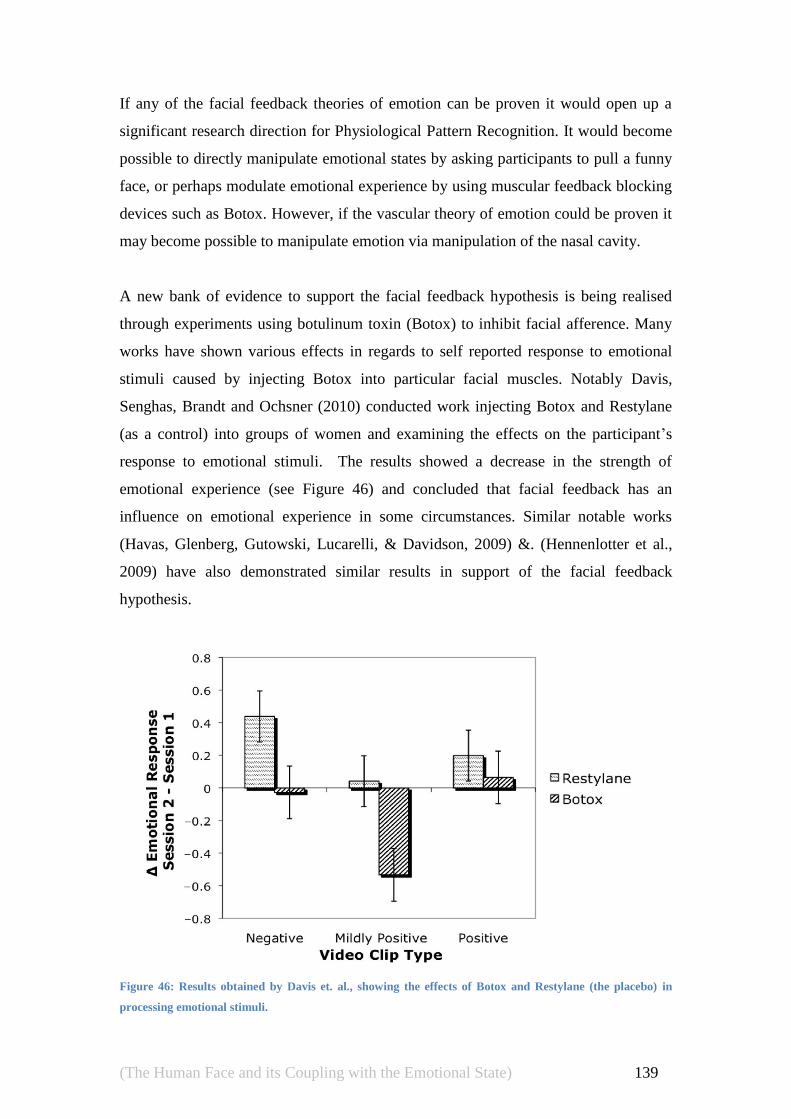
(The Human Face and its Coupling with the Emotional State) 139
If any of the facial feedback theories of emotion can be proven it would open up a
significant research direction for Physiological Pattern Recognition. It would become
possible to directly manipulate emotional states by asking participants to pull a funny
face, or perhaps modulate emotional experience by using muscular feedback blocking
devices such as Botox. However, if the vascular theory of emotion could be proven it
may become possible to manipulate emotion via manipulation of the nasal cavity.
A new bank of evidence to support the facial feedback hypothesis is being realised
through experiments using botulinum toxin (Botox) to inhibit facial afference. Many
works have shown various effects in regards to self reported response to emotional
stimuli caused by injecting Botox into particular facial muscles. Notably Davis,
Senghas, Brandt and Ochsner (2010) conducted work injecting Botox and Restylane
(as a control) into groups of women and examining the effects on the participant‘s
response to emotional stimuli. The results showed a decrease in the strength of
emotional experience (see Figure 46) and concluded that facial feedback has an
influence on emotional experience in some circumstances. Similar notable works
(Havas, Glenberg, Gutowski, Lucarelli, & Davidson, 2009) &. (Hennenlotter et al.,
2009) have also demonstrated similar results in support of the facial feedback
hypothesis.
Figure 46: Results obtained by Davis et. al., showing the effects of Botox and Restylane (the placebo) in
processing emotional stimuli.

(The Human Face and its Coupling with the Emotional State) 140
The author is unaware of any studies that directly manipulate the nasal cavity to
regulate emotion, but in a review of related research, Zajonic presented the following
anecdotal evidence supporting the emotional effect of nasal breathing:
Packing the human nose with gauze tampon (to prevent ambient air reaching
the nasal mucosa) can result in a violent emotional reaction;
Patients who breathe through tubes inserted directly into the trachea often
experience severe emotional reactions (Bendixen, Egbert, Hedley-Whyte,
Laver, & H., 1965);
When the nose is obstructed, to the point where it is easier to breathe through
the mouth, people will continue with their usual proportional preference to
nasal breathing. (Vig, 1985)
As the Facial Feedback Theory is still under development, and the exact nature of any
of its possible effects are still being studied, we will not be using facial feedback to
stimulate emotions. However we consider it vital to design our experiment on the
grounds of Facial Feedback being a valid theory. As such, all facial sensor
placements are designed not to pull the facial muscles, so as not to add another (un-
controlled) source of emotional manipulation.
4.1.4. Our Guidelines for Experimental Apparatus in Affective Facial
Studies
The preceding sections have reviewed a set of conflicting theories linking facial
action and emotion. As the question of which (if any) theory is correct remains
unanswered, it is our goal to construct a framework for an experiment which would
not be invalidated if a particular emotional theory was proven. The goal of our
framework is to propose methodologies consistent with the unified areas of various
facial/emotional theories (see Figure 47).

(The Human Face and its Coupling with the Emotional State) 141
Key
JLT James Lang
Theory
FFH Facial
Feedback
Hypothosis
VTE Vascular
Theory of
Emotions
CBT Cannon-
Bard Theory
Figure 47: Venn diagram of selected emotional theories
Proposed Guidelines
a) Facial measurement apparatus should not impinge on the action of the face, or
be made to have minimal such effect. (see Facial Feedback Hypothesis):
a. Electrodes should be small and light;
b. Size of electrode adhesive pads should be minimal;
c. Electrode wires should not hang loosely and thus pull on the face;
d. The net force exerted by electrodes should be measured and recorded.
b) Human observers should not be present unless the experimental methodology
explicitly requires such presence, because:
a. Human facial actions are socially augmented. An observer will place
pressure on the participant to outwardly display culturally acceptable
responses;
b. Some theories state that humans transfer emotions through facial
efference and empathetic processes. If the participant sees another face,
that face becomes an uncontrolled emotional stimulus.
c) Wall charts and medical manikins should be avoided in the experimental area,
especially if any charts, posters, or manikins display a face or facial
expression.

(The Human Face and its Coupling with the Emotional State) 142
4.2 Facial EMG as a Method of Studying Emotional State
There is sufficient published work to establish a link between facial EMG and self
reported emotional state. Notable publications showing this relationship include
Bradley, Codispoti, Cuthbert and Lang (2001) and the related work by Bradley,
Codispoti, Sabatinelli and Lang (2001).
It has long been established that facial expressions are a primary mechanism for
communicating emotions between people. Thus the bulk of EMG related work in
emotion related field tends to utilise the facial muscles, though works also examine
muscles related to posture.
Many muscles in the face correlate to different emotions and expressions. All of these
muscles can be controlled consciously and unconsciously. In this section we visit the
literature for the important muscles in facial expression and detail the expressions and
where possible level of conscious / unconscious control commonly used.
4.3 Physiological Signals (EMG) of the Jaw
The mouth is a very expressive part of the human face. There are ten muscles which
move the mouth which can be observed using EMG:
Orbicularis Oris;
Levator Anguli Oris (Caninus);
Levator Labii Superioris (aka Quadratus Labii Superioris);
Zygomaticus Minor;
Zygomaticus Major;
Buccinator;
Quadratus Labii Inferioris;
Depressor Anguli Oris;
Mentalis;
Risorius;
Platysma.

(The Human Face and its Coupling with the Emotional State) 143
In this section we will review the function and related literature on the emotional
responses of these muscles. Note: the Masticator was not reviewed as it is functionally
used for chewing and not involved in displaying emotion.
4.3.1. Orbicularis Oris
The Orbicularis Oris muscle is the sphincter muscle around the mouth as shown in
Figure 3.
Figure 48: Location of the Orbicularis Oris.
In the composition of facial expression it has two actions (Faigin, 2008) , (Boulogne,
1990) & (Standring & Gray, 2008):
a) By contracting the peripheral portion of the muscle it compresses the lips
forcing them outward;
b) By contracting the internal fascicules it projects the lips inwards towards the
teeth.
The two actions of the Orbicularis Oris are pictured in Table 2.

(The Human Face and its Coupling with the Emotional State) 144
(Neutral)
(1st action)
(2nd action)
Figure 49: Actions of the Orbicularis Oris
The Orbicularis Oris is used to perform the following actions (Faigin, 2008) ,
(Boulogne, 1990):
Kiss;
Blow;
Whistle;
Suck;
Forming "tooth-lip" consonants.
The activity in the orbicularis oris has been linked to the degree of mental effort
involved in a task being under taken (A. Van Boxtel & Jessurun, 1993).

(The Human Face and its Coupling with the Emotional State) 145
4.3.2. Levator Anguli Oris (Caninus)
The Caninus muscle is a facial muscle of the mouth as shown in Figure 4.
Figure 50: Location of the Caninus
In the composition of facial expression the caninus raises the upper lip, exposing the
canine tooth and drawing the corner of the mouth back. It is associated with
aggressive facial expressions. It is also used in producing a "contemptuous smile".
(Faigin, 2008) , (Boulogne, 1990) & (Standring & Gray, 2008). The action of the
caninus pictured in Figure 5.
(Neutral)
(1st action)
Figure 51: Actions of the Caninus

(The Human Face and its Coupling with the Emotional State) 146
4.3.3. Levator Labii Superioris (or Quadratus Labii Superioris)
The Levator Labii Superioris muscle is a broad muscle, the origin of which extends
from the side of the nose to the Zygomatic bone (shown in Figure 6).
Figure 52: Location of the Levator Labii Superioris.
In the composition of facial expression it raises a portion of the upper lip and the side
of the nose (Standring & Gray, 2008). The actions of the Levator Labii Superioris are
pictured in Figure 7.
(Neutral)
(action)
Figure 53: Actions of the Levator Labii Superioris
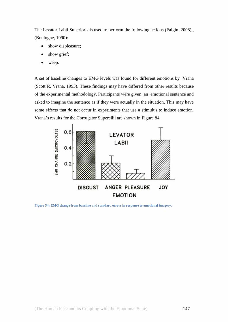
(The Human Face and its Coupling with the Emotional State) 147
The Levator Labii Superioris is used to perform the following actions (Faigin, 2008) ,
(Boulogne, 1990):
show displeasure;
show grief;
weep.
A set of baseline changes to EMG levels was found for different emotions by Vrana
(Scott R. Vrana, 1993). These findings may have differed from other results because
of the experimental methodology. Participants were given an emotional sentence and
asked to imagine the sentence as if they were actually in the situation. This may have
some effects that do not occur in experiments that use a stimulus to induce emotion.
Vrana‘s results for the Corrugator Supercilii are shown in Figure 84.
Figure 54: EMG change from baseline and standard errors in response to emotional imagery.

(The Human Face and its Coupling with the Emotional State) 148
4.3.4. Zygomaticus Minor
The Zygomaticus Minor muscle, shown in Figure 8, is used in controlling facial
expression. It originates on the Zygomatic bone and then inserts on the upper lip
(Standring & Gray, 2008).
Figure 55: Location of the Zygomaticus Minor.
In the composition of facial expression it raises a portion of the upper lip and the side
of the nose. (Faigin, 2008) , (Boulogne, 1990). The actions of the Zygomaticus Minor
are pictured in Figure 9.
(Neutral)
(action)
Figure 56: Actions of the Zygomaticus Minor.

(The Human Face and its Coupling with the Emotional State) 149
The Zygomaticus Minor is used to perform the following actions (Faigin, 2008),
(Boulogne, 1990):
Sadness;
Grief;
As part of a smile.
4.3.5. Zygomaticus Major
The Zygomaticus Major muscle is used in controlling facial expression. Its purpose is
to draw the angle of the mouth (Faigin, 2008), (Boulogne, 1990). Its location is shown
in Figure 10.
Figure 57: Location of the Zygomaticus Major.
In the composition of facial expression it lifts the corners of the mouth to assist in
forming smiles (Faigin, 2008), (Boulogne, 1990). The actions of the Zygomaticus
Major are pictured in Figure 11.

(The Human Face and its Coupling with the Emotional State) 150
(Neutral)
(action)
Figure 58: Actions of the Zygomaticus Major.
The Zygomaticus Major is used to perform the following actions (Faigin, 2008) ,
(Boulogne, 1990):
Expressing happiness;
Smiling.
Schmidt et al., (Schmidt, Ambadar, Cohn, & Reed, 2006) have studied the motion of
the Zygomaticus Major in relation to posed and genuine smiles, an example
participant is shown in Figure 59. Examining real and posed smiles generated by 87
female participants they concluded that deliberate smile onsets were faster and larger
in amplitude while the offsets were faster and larger in amplitude. A summary of their
results is in Table 8.
Figure 59: Facial expression of a Smile (A) posed (b) spontaneous (Schmidt et al., 2006)

(The Human Face and its Coupling with the Emotional State) 151
Table 8: Results for Zygomaticus Major onsets and offsets in real and posed smiles. (Schmidt et al., 2006)
Working also with angry facial expressions, Achaibou et al. (Achaibou, Pourtois,
Schwartz, & Vuilleumier, 2008) conducted a study where participants were shown 10
frames of a morphing facial expression with increasing emotional intensity. Each
frame appeared for 40 ms with the last one remaining for 1100ms. The mean
Zygomaticus Major EMG responses to happy and angry facial animations are shown
in Figure 60. The responses are consistent with the participant pulling the same face
they are observing, but after a delay of 500ms. These findings are attributed to facial
mimicry (Dimberg & Thunberg, 1998).
A set of baseline changes to EMG levels was found for different emotions by Vrana
(Scott R. Vrana, 1993). These findings may have differed from other results because
of the experimental methodology. Participants were given an emotional sentence and
asked to imagine the sentence as if they were actually in the situation. This may have
some effects that do not occur in experiments that use a stimulus to induce emotion.
Vrana‘s results for the Corrugator Supercilii are shown in Figure 61.

(The Human Face and its Coupling with the Emotional State) 152
Figure 60: Mean Zygomaticus Major EMG Responses to Happy and Angry Facial Animations. (Achaibou et
al., 2008)

(The Human Face and its Coupling with the Emotional State) 153
Figure 61: EMG change from baseline and standard errors in response to emotional imagery.
4.3.6. Risorius
The Risorius is a narrow bundle of fibres that arises in the fascia and inserts onto the
skin at the edge of the mouth (Standring & Gray, 2008). Its location is shown in
Figure 12.
Figure 62: Location of the Risorius.
In the composition of facial expression the risorius retracts the angle of the mouth to
produce a smile. The smile produced if only this muscle is involved looks false or
ironic (Faigin, 2008) & (Boulogne, 1990). The actions of the risorius are pictured in
Figure 63.

(The Human Face and its Coupling with the Emotional State) 154
Figure 63: Actions of the Risorius.
The risorius is used to perform the following actions (Faigin, 2008) & (Boulogne,
1990):
As part of a smile;
To express an ironic smile;
Used when a person gives a deliberate (false) smile.
4.3.7. Buccinator
The Buccinator is a quadrilateral shaped muscle behind the cheeks (Standring & Gray,
2008). Its location is shown in Figure 14.
Figure 64: Location of the Buccinator.
(Neutral)
(action)

(The Human Face and its Coupling with the Emotional State) 155
In the composition of facial expression the Buccinator pulls back the edge of the
mouth and flattens the cheeks. The actions of the Buccinator are pictured in Figure 15.
(Neutral)
(action)
Figure 65: Actions of the buccinator.
The buccinator is used to perform the following actions (Faigin, 2008), (Boulogne,
1990):
Blowing air (by the mouth);
To create a contemplative contraction of the lips;
Expressions of self control;
Expressions of self resignation.
4.3.8. Quadratus Labii Inferioris (Depressor Labii Inferioris)
The Quadratus Labii Inferioris is a facial muscle used to lower the bottom lip
(Standring & Gray, 2008). Its location is shown in Figure 16.

(The Human Face and its Coupling with the Emotional State) 156
Figure 66: Location of the Quadratus Labii Inferioris.
In the composition of facial expression the Quadratus Labii Inferioris pushes out and
down the lower half of the lip. The actions of the Quadratus Labii Inferioris are
pictured in Figure 17.
(Neutral)
(action)
Figure 67: Actions of the Quadratus Labii Inferioris.
The Quadratus Labii Inferioris is used to perform the following actions (Faigin,
2008), (Boulogne, 1990):
Expressing Anger;
Expressing Misfortune;
Used by children before they cry.

(The Human Face and its Coupling with the Emotional State) 157
4.3.9. Depressor Anguli Oris (Triangularis)
The Depressor Anguli Oris is a muscle connecting the mandible and the mouth
(Standring & Gray, 2008). Its location is shown in Figure 18.
Figure 68: Location of the Depressor Anguli Oris.
In the composition of facial expression, the Depressor Anguli Oris associated strongly
with frowning and is essential in displaying scorn. Its job is the opposite of the
Zygomaticus Major in that it draws the edges of the mouth down. The actions of the
Depressor Anguli Oris are pictured in Figure 19.
Figure 69: Actions of the Depressor Anguli Oris.
(Neutral)
(action)

(The Human Face and its Coupling with the Emotional State) 158
The Depressor Anguli Oris is used to perform the following actions (Faigin, 2008),
(Boulogne, 1990):
Display scorn;
Frown;
Show disgust;
Show disapproval.
4.3.10. Mentalis
The Mentalis is located at the front of the chin. It raises and pushes out the lower lip,
causing wrinkling of the chin (Standring & Gray, 2008). Its location is shown in
Figure 12.
Figure 70: Location of the Mentalis.
In the composition of facial expression the Mentalis wrinkles the chin. The actions of
the Mentalis are pictured in Figure 71.

(The Human Face and its Coupling with the Emotional State) 159
Figure 71: Actions of the Mentalis.
The Mentalis is used to perform the following actions (Faigin, 2008), (Boulogne,
1990):
Grimace;
Show doubt;
Show displeasure.
4.3.11. Risorius
The Risorius is located in the cheeks and sits parallel to, and on top of, the
Buccinator. Its action is similar to the buccinators but applied more to the ends of the
mouth (Standring & Gray, 2008). Its location is shown in Figure 12.
Figure 72: Location of the Risorius.
(Neutral)
(action)
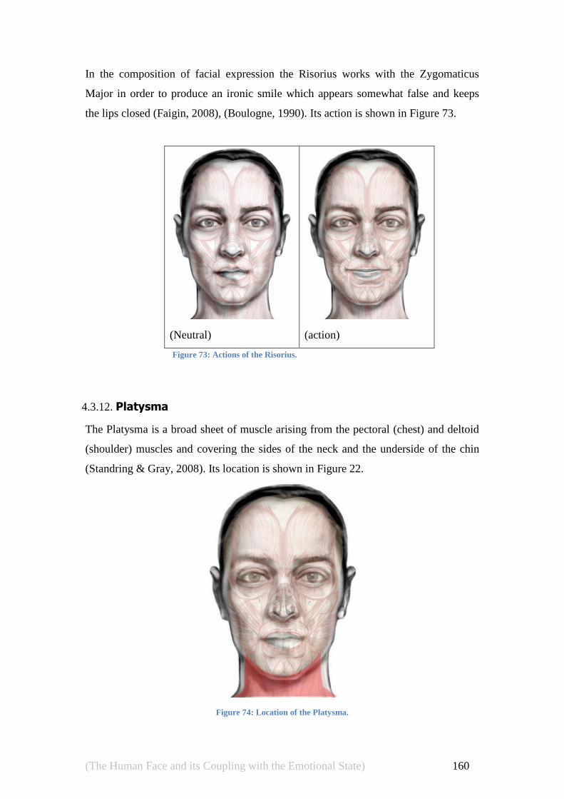
(The Human Face and its Coupling with the Emotional State) 160
In the composition of facial expression the Risorius works with the Zygomaticus
Major in order to produce an ironic smile which appears somewhat false and keeps
the lips closed (Faigin, 2008), (Boulogne, 1990). Its action is shown in Figure 73.
4.3.12. Platysma
The Platysma is a broad sheet of muscle arising from the pectoral (chest) and deltoid
(shoulder) muscles and covering the sides of the neck and the underside of the chin
(Standring & Gray, 2008). Its location is shown in Figure 22.
Figure 74: Location of the Platysma.
(Neutral)
(action)
Figure 73: Actions of the Risorius.
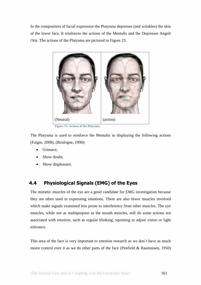
(The Human Face and its Coupling with the Emotional State) 161
In the composition of facial expression the Platysma depresses (and wrinkles) the skin
of the lower face. It reinforces the actions of the Mentalis and the Depressor Anguli
Oris. The actions of the Platysma are pictured in Figure 23.
Figure 75: Actions of the Platysma.
The Platysma is used to reinforce the Mentalis in displaying the following actions
(Faigin, 2008), (Boulogne, 1990):
Grimace;
Show doubt;
Show displeasure.
4.4 Physiological Signals (EMG) of the Eyes
The mimetic muscles of the eye are a good candidate for EMG investigation because
they are often used in expressing emotions. There are also fewer muscles involved
which make signals examined less prone to interference from other muscles. The eye
muscles, while not as multipurpose as the mouth muscles, still do some actions not
associated with emotion, such as regular blinking, squinting to adjust vision or light
tolerance.
This area of the face is very important to emotion research as we don‘t have as much
motor control over it as we do other parts of the face (Penfield & Rasmussen, 1950)
(Neutral)
(action)

(The Human Face and its Coupling with the Emotional State) 162
and thus it is more likely not to be involved in posed expressions made to conform to
social expectations. A relevant depiction of this is shown in Figure 76.
Figure 76: The primary motor strip of the cerebral cortex (Penfield & Rasmussen, 1950). The relative
proportion of cortical tissue controlling the muscles of the body is illustrated by the cartoon; and more
precisely by the length of the dark lines. Note the size of the mouth in proportion to the rest of the face.
An aditional advantage to EMG in this region was found by Cacioppo et al.,
(Cacioppo, Petty, Losch, & Kim, 1986) who conducted a study with 12 participants
that suggested EMG activity over the brow, eye, and cheek muscle regions could
detect emotional responses not observable under normal social conditions.
There are primarily four muscles which are used in creating expressions with the eyes
and eyebrows that can be observed using EMG:
Frontalis;
Corrugator Supercilii;
Orbicularis Oculi;
Procerus.
In this section we will review the function and related literature on the emotional
responses of these muscles.

(The Human Face and its Coupling with the Emotional State) 163
4.4.1. Frontalis
The Frontalis is the anterior belly of the Occipitofrontalis (also called the Epicranius)
which stretches over the scalp (Standring & Gray, 2008). The poster belly, known as
the Occipitalis, is not involved in facial expression. Its location is shown in Figure 77.
Figure 77: Location of the Frontalis
The Frontalis is used to raise and lower the eyebrows and aside from emotional facial
expressions it‘s been linked to concentration levels and task difficulty. The Frontalis
is used in displaying (Faigin, 2008), (Boulogne, 1990):
Admiration;
Astonishment;
Confusion;
Fear;
Surprise;
Startle reflex.
The actions of the Frontalis are shown in Figure 78.

(The Human Face and its Coupling with the Emotional State) 164
(Neutral) (1st action)
(2nd action) (3rd action)
Figure 78: Actions of the Frontalis
Scheirer et al., (Scheirer, Fernandez, & Picard, 1999) used two Piezo sensors on the
Frontalis to perform classification of posed expressions of confusion and interest. The
system performed with 74% accuracy. Their sensor placement is shown in Figure 79.
Figure 79: "Expression Glasses" (Scheirer et al., 1999)

(The Human Face and its Coupling with the Emotional State) 165
4.4.2. Corrugator Supercilii
The Corrugator Supercilii is a small narrow muscle sitting above the Oculus Oris and
below the Frontalis (Standring & Gray, 2008). Its location is shown in Figure 80.
Figure 80: Location of the Corrugator Supercilii
The Corrugator Supercilii pulls the eyebrows inward and downward. It is used to form
many negative facial expressions as well as to draw the eyebrows in to shield the eyes
from sun glare. Its action, shown in Figure 81, is also responsible for the formation of
vertical wrinkles in the brow.
(Neutral)
(action)
Figure 81: Actions of the Corrugator Supercilii

(The Human Face and its Coupling with the Emotional State) 166
The Corrugator Supercilii is used primarily to display expressions of (Faigin, 2008),
(Boulogne, 1990):
Desperation;
Displeasure;
Impatience;
Pain;
Suffering;
Rage;
Unhappiness;
Effort (physical and mental).
Hess, Philippot and Blairy (1998) conducted two studies manipulating (a) the
emotional Valence of the stimuli (angry vs..happy faces) and (b) stimulus presentation
in blocks of the same emotional nature vs. random order. Their work examining EMG
activity for people looking at slides of human faces gave the following insights:
―...when judging expressions of anger participants showed more Corrugator
Supercilii activity than when judging expressions of happiness. Further,
participants show more Corrugator Supercilii activity when judging weak
than when judging strong expressions of both happiness or anger. Also,
participants showed less Corrugator Supercilii activity when judging strong
happy expressions than when judging weak happy expressions.‖
Relevant mean EMG activity is shown in Figure 82.
Figure 82: EMG activity(mean) for angry and happy faces. (Hess, Philippot & Blairy, 1998)

(The Human Face and its Coupling with the Emotional State) 167
Achaibou et al., (Achaibou et al., 2008) conducted a study where participants were
shown 10 frames of a morphing facial expression with increasing emotional intensity.
Each frame appeared for 40 ms with the last one remaining for 1100ms. the mean
Corrugator Supercilii EMG responses to happy and angry facial animations are shown
in Figure 60. The responses are consistent with the participant pulling the same face
they are observing, but after a delay of 200ms. These findings are attributed to facial
mimicry (Dimberg & Thunberg, 1998).
Figure 83: EMG responses to happy and angry facial animations (Achaibou et al., 2008)
It has been established (Cacioppo, Bush & Tassinary, 1992), (Cacioppo et al., 1986),
(Dimberg, 1982) that the Corrugator Supercilii displays lower EMG activity when a
participant is shown pleasant Stimuli and higher activity for negative stimuli. The
results obtained by Cacioppo et al., in relation to this are shown in Figure 84.

(The Human Face and its Coupling with the Emotional State) 168
Figure 84: EMG Reactions to Assorted Stimulus (J. T. Cacioppo et al., 1992),. The Corrugator Supercilii
shows higher activity for negative stimuli and lower for positive stimuli.
A set of baseline changes to EMG levels was found for different emotions by Vrana
(Scott R. Vrana, 1993). These findings may have differed from other results because
of the experimental methodology. Participants were given an emotional sentence and
asked to imagine the sentence as if they were actually in the situation. This may have
some effects that do not occur in experiments that use a stimulus to induce emotion.
Vrana‘s results for the Corrugator Supercilii are shown in Figure 85.
Figure 85: EMG change from baseline and standard errors in response to emotional imagery.

(The Human Face and its Coupling with the Emotional State) 169
4.4.3. Orbicularis Oculi
The Orbicularis Oculi is responsible for closing or narrowing the eyelids (Standring
& Gray, 2008). The muscle is a flat elliptical ring around the eye sockets as shown in
Figure 86.
Figure 86: Location of the Orbicularis Oculi
The internal portion of the muscles opens or closes the eyelids. The lower portion
projects the lower eyelid upwards and furrows the corners of the eyes. The Orbicularis
Oculi can also pull the eyebrows downward (as opposed to the Frontalis which raises
them). Finally, the muscle can also pull the skin around the eyes inward, causing
squinting and wrinkling of the area. These actions are shown (in the same order
mentioned) in Figure 87.
The muscle is involved in displaying (Faigin, 2008), (Boulogne, 1990):
Joy;
Sadness;
Concentration;
Attention.

(The Human Face and its Coupling with the Emotional State) 170
It has been established (Cacioppo et al., 1992), (Cacioppo et al., 1986), (Dimberg,
1982) that the Orbicularis Oculi displays higher EMG activity when a participant is
shown pleasant Stimuli and lower activity for negative stimuli. The results obtained
by Cacioppo et al., in relation to this are shown in Figure 88.
(Neutral)
(1st action)
(2nd action)
(3rd action)
(4th action)
Figure 87: Actions of the Orbicularis Oculi.

(The Human Face and its Coupling with the Emotional State) 171
Figure 88: EMG Reactions to Assorted Stimulus (J. T. Cacioppo et al., 1992),. The Orbicularis Oculi displays
higher EMG activity when a participant was shown pleasant Stimuli, while the Corrugator Supercilii shows
higher activity for negative stimuli.
Hess, Philippot and Blairy (1998) as mentioned in the review of the Corrugator
Supercilii, conducted two studies manipulating (a) the emotional Valence of the
stimuli (angry vs. happy faces) and (b) stimulus presentation in blocks of the same
emotional nature vs. random order. In their work examining EMG activity for people
looking at slides of human faces they found few Valence links except those due to
facial mimicry; their participants showed more Orbicularis Oculi activity when
exposed to happy than when exposed to angry faces. Relevant mean EMG activity is
shown in Figure 82.
Figure 89: Orbicularis Oculi EMG activity (mean) for angry and happy stimulus. (Ursula et al., 1998)
The Orbicularis Oculi is also involved in the expression of laughter. A review paper
by Willibald & Ekman which examined the expressive patterns of laughter in the face
(Willibald & Ekman, 2001) showed a majority of authors identified it as being
involved in laughter. The result table from the study is shown in

(The Human Face and its Coupling with the Emotional State) 172
Figure 90: Excerpt from (Willibald & Ekman, 2001) with the Orbicularis Oculi and Corrugator Supercilii
related text highlighted.

(The Human Face and its Coupling with the Emotional State) 173
4.4.4. Procerus
The Procerus is a small muscle located from the top of the nose in the region between
the eyebrows, where its fibres merge with the Frontalis, extending down to the lower
portion of the nasal bone (Standring & Gray, 2008). Its location is shown in Figure
91.
Figure 91: Location of the Procerus
In forming facial expression the Procerus pulls the skin between the facial muscles
downward while also flaring the nostrils. This action is shown in Figure 92.
(Neutral)
(action)
Figure 92: Actions of the Procerus.

(The Human Face and its Coupling with the Emotional State) 174
4.5 Physiological Signals (EMG) of the Nose
There are two rhinal muscles which are used in creating expressions with the nose
that can be observed using EMG:
Nasalis Transversa;
Nasalis Alaris.
In this section we will review the function and related literature on the emotional
responses of these muscles.
4.5.1. Nasalis Transversa
The Nasalis Transversa is a triangular muscle that covers the lateral parts of the nose
(Standring & Gray, 2008). Its location is shown in Figure 93.
Figure 93: Location of the Nasalis Transversa.
In forming facial expressions the Nasalis Transversa elevates the wings of the nose
and is involved in the ―scrunching‖ of the nose. Its action is shown in Figure 94.

(The Human Face and its Coupling with the Emotional State) 175
The Nasalis Transversa is used to display (Faigin, 2008), (Boulogne, 1990):
Reactions to unpleasant smells;
Rejection;
Displeasure.
4.5.2. Nasalis Alaris
The Nasalis Alaris is located underneath the nose and is situated over the base of the
Canine being partly covered by the Oculus Oris (Standring & Gray, 2008). Its
location is shown in Figure 95.
Figure 95: Location of the Nasalis Alaris.
(Neutral)
(action)
Figure 94: Actions of the Nasalis Transversa.

(The Human Face and its Coupling with the Emotional State) 176
In posing the face Nasalis Alaris moves the wings of the nose inward by moving the
base of the nose inward and downward. It also (indirectly) pushes the lip downward.
Its action is shown in Figure 96. There are no emotive expressions directly related to
the Nasalis Alaris (Goldfinger, 1991), but it is involved with facial contortions that
occur when someone is overcoming pain (Faigin, 2008), (Boulogne, 1990).
4.6 Summary of the Affective Capacity of the Mimetic
Muscles
A limitation of facial EMG Data (as with other facial data) in examining the
emotional state is that the human face also responds to a large variety of states
unrelated to emotion. For example speech, mental fatigue/effort, anticipation of
sensory stimuli, preparation of motor responses, startle reflexes and orienting
responses; as covered in (A. V. Boxtel, 2010), (Or & Duffy, 2007), (Stekelenburg &
Boxtel, 2002).
Summarising the information presented in this chapter by basic emotion, we can list
facial muscle involvement in emotion as:
Anger;
o Corrugator supercilii, Levator palpebrae, superioris, Orbicularis oculi;
Disgust;
(Neutral)
(action)
Figure 96: Actions of the Nasalis Alaris.

(The Human Face and its Coupling with the Emotional State) 177
o Levator labii superioris, Levator labii superioris, alaeque nasi;
Fear;
o Frontalis, Corrugator supercilii, Levator;
Happiness;
o Orbicularis oculi, Zygomaticus major;
Sadness;
o Frontalis, Corrugator supercilii, Depressor anguli oris;
Surprise;
o Frontalis, Levator palpebrae.
Having investigated a series of facial muscles for EMG analysis, we found the
Corrugator Supercilii, which is associated with Anger, Fear and Sadness, to be a
useful indicator of emotional state that was not heavily affected by either social
display rules of emotion or other facial display mechanisms.
In the next chapter we will attempt to quantify the degree to which the muscles
identified above might be useful in PPR by taking EMG recordings for various parts
of the face during deliberate (posed) facial expressions. To be feasible for our study a
muscle must produce a distinct pattern during display, of a specific emotion, that is
not readily confused with patterns produced while other emotions are displayed.

(The Human Face and its Coupling with the Emotional State) 178
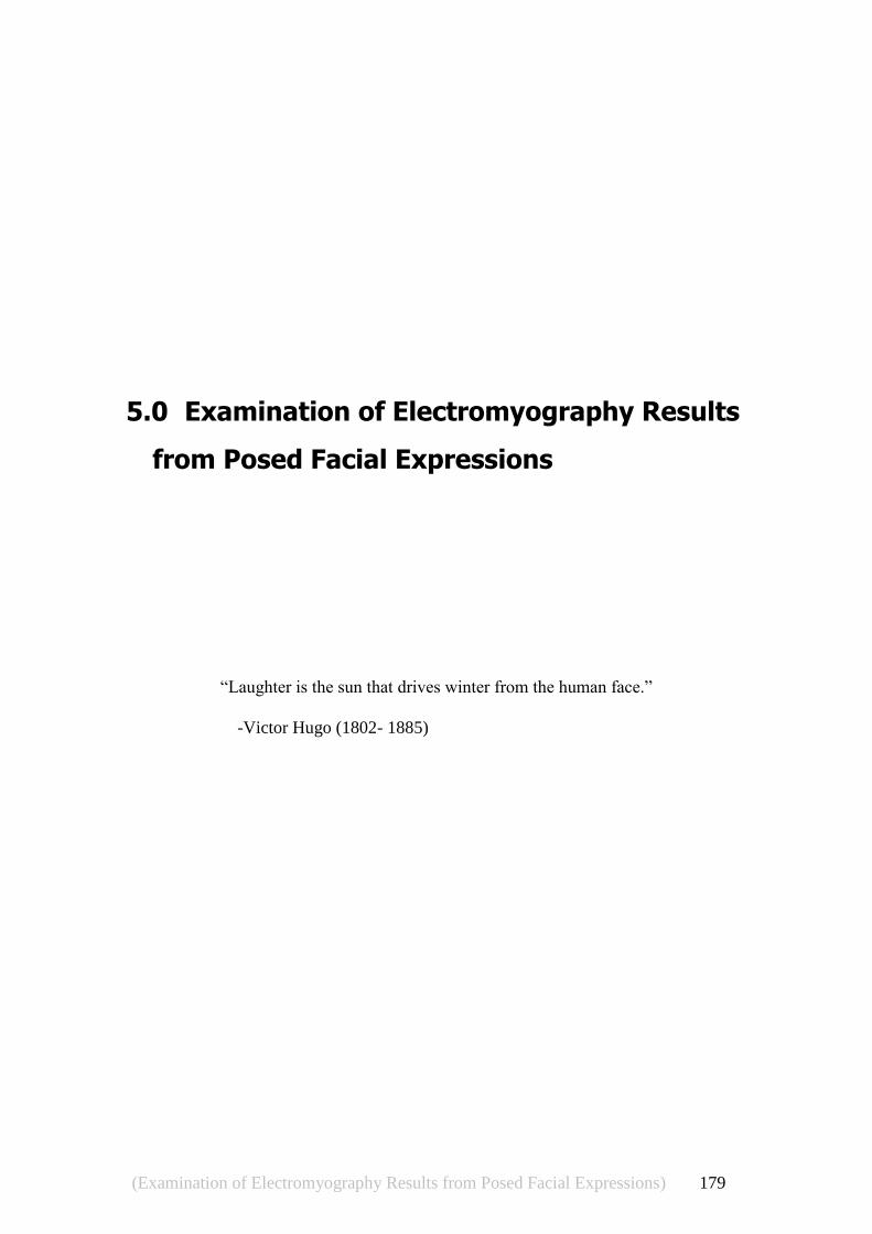
(Examination of Electromyography Results from Posed Facial Expressions) 179
5.0 Examination of Electromyography Results
from Posed Facial Expressions
―Laughter is the sun that drives winter from the human face.‖
-Victor Hugo (1802- 1885)

(Examination of Electromyography Results from Posed Facial Expressions) 180
This chapter presents our initial experiments with EMG recording of facial muscles.
It describes a series of facial EMG recordings that were taken from two participants to
trial the sensor placements and ensure we could reproduce the results from the
literature review. We also wished to judge signal morphology in general to estimate
likely traits useful in distinguishing various (posed) facial expressions.
We trialled several placements specific to mimetic muscles identified in section 4.0
as highly significant in emotional content while not being regularly used for other
non- emotional tasks. We also trialled some placements that spanned multiple muscles
in order to attempt to utilise broader actions of muscle groups. The placements used
were:
Orbicularis Oris (Specific placement);
Zygomaticus Major (Specific placement);
Buccinator (Specific placement);
Depressor Anguli Oris (Specific placement);
Mentalis (Specific placement);
Orbicularis Oculi (Specific placement);
Frontalis (Specific placement);
Suprahyoid Placement;
Temporal Suprahyoid Placement;
Temporal Masseter (Wide) Placement;
Frontal (Wide) Placement
We also experimented with EMG placement diagonally across the neck (Vaiman,
Eviatar, & Segal, 2004) to monitor swallowing. However we discovered two
problems, which made the procedure unsuitable for our requirements:
1. The placement could not be made if the participant had a beard.
2. Going only on anecdotal evidence, we found the neck placement may be
uncomfortable for the participant.
In this section we will review our trial experiments, which are based on posed (but not
exaggerated) facial expressions.

(Examination of Electromyography Results from Posed Facial Expressions) 181
5.1 EMG of the Orbicularis Oris
The Orbicularis Oris placement used was the left portion of the lower placement
Boxtel (A. V. Boxtel, 2010). Two electrodes were placed 15mm apart just below the
lower lip. The earth electrode was attached to the bony prominence of the scalp just
below the hair line, as shown in Figure 97, artefacts were produced by any sort of
mouth movement.
Figure 97: Orbicularis Oris Electrode Placement.
The testing of the Orbicularis Oris involved (A) A pursed smile with the lips closed.
(B) A pensive biting of the lip. (C) Talking, a typical recording is shown in Figure 98.
The smiles were distinct from a neutral action and distinguishable from general
talking in that they did not reach the same maximum amplitudes.

(Examination of Electromyography Results from Posed Facial Expressions) 182
Figure 98: Typical EMG Recording for the Orbicularis Oris showing (A) a pursed smile with the
lips closed. (B) A pensive biting of the lip. (C) Talking.
Sm
ile
Sm
ile S
mile
Lip
Bite L
ip B
ite Lip
Bite T
alkin
g

(Examination of Electromyography Results from Posed Facial Expressions) 183
5.2 EMG of the Zygomaticus Major
The Zygomaticus Major is used in smiling, EMG observation was performed via a
placement detailed by Cram et al., (1998) and Boxtel (2010). The placement used two
electrodes placed 20mm apart following the muscle fibres of the Zygomaticus Major.
The placement was made at the midpoint of the muscle and it uses an earth electrode
at the bony prominence of the scalp just below the hair line, as shown in Figure 99.
Actions known to produce artefacts include swallowing and talking.
Figure 99: Zygomaticus Major Electrode Placement.
Testing of the Zygomaticus Major EMG recordings involved smiling and talking.
Smiles were distinctly detectable as high amplitude regions maintained for the
duration of the action. They were higher in amplitude, and had a greater spectral
component, than general talking. A typical recording is shown in Figure 100.
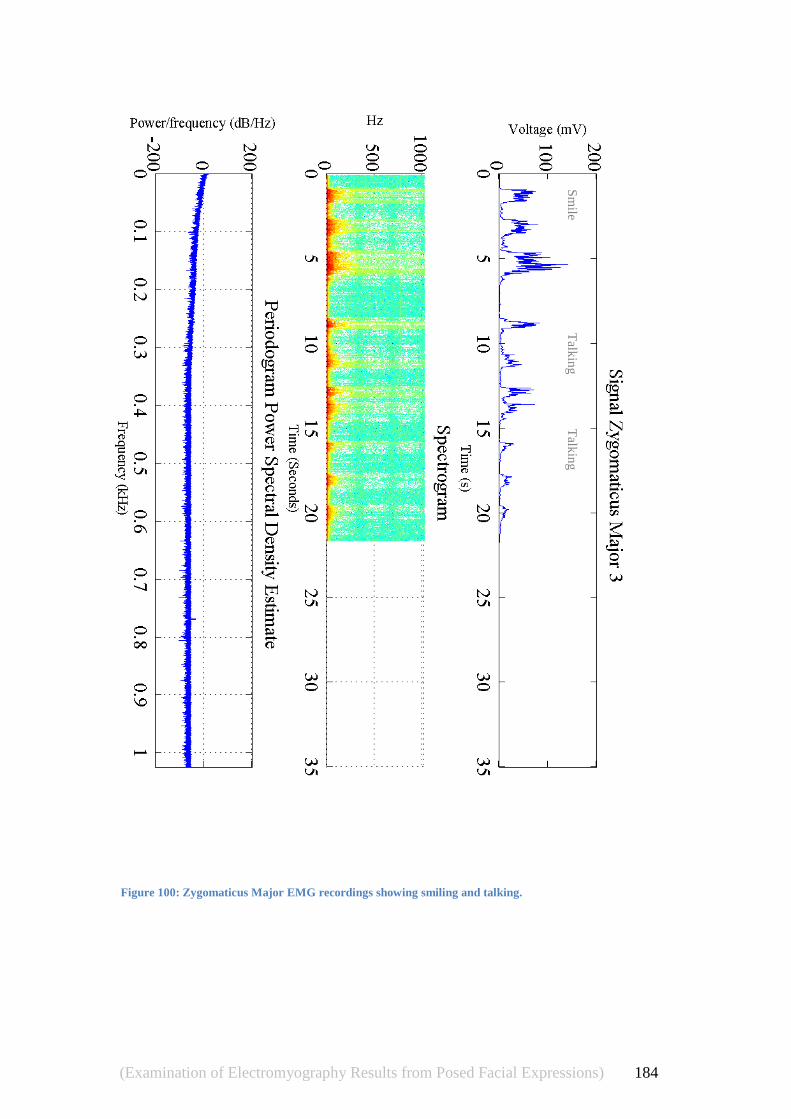
(Examination of Electromyography Results from Posed Facial Expressions) 184
Sm
ile
T
alkin
g
Talk
ing
Figure 100: Zygomaticus Major EMG recordings showing smiling and talking.

(Examination of Electromyography Results from Posed Facial Expressions) 185
5.3 EMG of the Buccinator
The Buccinator is used in smiling, blowing air through the lips, its observation was
performed via a placement detailed by Cram et al., (1998). The placement used two
electrodes placed 10mm apart following the muscle fibres of the Buccinator. The
placement was made with both electrodes positioned laterally to the corner of the
mouth and an earth electrode was placed at the bony prominence of the scalp just
below the hair line, as shown in Figure 101. Actions known to produce artefacts
include swallowing and talking.
Figure 101: Buccinator Electrode Placement.
The EMG Tests involved (A) Blowing air through the lips in expressions of
exasperation and self control. (B) Smiling. (C) Lips pursed in and expression of
contemplative contraction. All these actions were very distinguishable. The blowing
produced a small artefact with relatively low frequency components. The smile
produced a region of slightly higher amplitude that contained higher frequencies. The
pursing of the lips produced a region nearly double in amplitude to the other actions.
A typical recording is shown in Figure 102.

(Examination of Electromyography Results from Posed Facial Expressions) 186
Blo
win
g
S
mile
L
ips P
ursed
Figure 102: Buccinator EMG recordings showing: (A) blowing air through the lips in expressions of exasperation
and self control. (B) Smiling. (C) Lips pursed in and expression of contemplative contraction.

(Examination of Electromyography Results from Posed Facial Expressions) 187
5.4 EMG of the Depressor Anguli Oris
The Depressor Anguli Oris is used in frowning and showing disgust/scorn, EMG
observation was performed via a placement detailed by Boxtel (Boxtel, 2010). The
placement used two electrodes placed 10mm apart following the muscle fibres of the
Depressor Anguli Oris. The placement was made from below the left corner of the
mouth with an earth electrode at the bony prominence of the scalp just below the hair
line, as shown in Figure 103.
Figure 103: Depressor Anguli Oris Electrode Placement.
The Depressor EMG testing involved: (A) Frowning, (B) Showing scorn, (D) Talking.
The frowning was very minor in amplitude, but showed a frequency component that
clearly identified it from background noise. Scorn was prominently displayed and
distinct from general talking which was even higher in amplitude. A typical recording
is shown in Figure 104.

(Examination of Electromyography Results from Posed Facial Expressions) 188
Fro
wn
ing
Sh
ow
ing
Sco
rn
Talk
ing
Figure 104: A typical Depressor Anguli Oris EMG recording showing: Frowning, (B) Showing
scorn, (C) Talking.

(Examination of Electromyography Results from Posed Facial Expressions) 189
5.5 EMG of the Mentalis
The Mentalis is used in grimacing and showing doubt and displeasure, EMG
observation was performed via a placement detailed by Boxtel (Boxtel, 2010). The
placement used two electrodes placed 10mm apart following the muscle fibres of the
Mentalis. The placement was made on the left side of the chin and used an earth
electrode at the bony prominence of the scalp just below the hair line, as shown in
Figure 105. Actions known to produce artefacts include swallowing and talking.
Figure 105: Mentalis Electrode Placement.
EMG testing of the Mentalis involved actions of grimacing , showing doubt, frowning
and talking. Most actions produced a similar response with a sharp initial response.
Talking was clearly identifiable due to its high amplitudes. A typical recording is
shown in Figure 106.

(Examination of Electromyography Results from Posed Facial Expressions) 190
Grim
ace
Sh
ow
ing
Do
ub
t
Fro
wn
T
alk
Figure 106: EMG testing of the Mentalis showing typical results for actions of grimacing, showing doubt,
frowning and talking.

(Examination of Electromyography Results from Posed Facial Expressions) 191
5.6 EMG of the Orbicularis Oculi
The Orbicularis Oculi is used in expressions of joy, sadness, concentration and
attention, EMG observation was performed via a placement detailed by Cram et al.,
(1998) and Boxtel (2010). The placement used two electrodes placed 10mm-20mm
apart along the Zygomatic bone. The placement was made with one electrode just
below the eyelid in-line with the iris of the eye. The second electrode was placed
latterly to the eye and the first electrode. The earth electrode was positioned at the
bony prominence of the scalp just below the hair line, as shown in Figure 107.
Figure 107: Orbicularis Oculi Electrode Placement.
EMG testing of the Orbicularis Oculi involved the actions of blinking, squinting and
smiling. All three actions are readily distinguished making the muscle an excellent
candidate for examination. The presence of blinking in the EMG recording allows the
calculation of the inter-blink interval which may be a useful statistic. Its promising
signal qualities however are offset in experimental conditions by the very
uncomfortable nature of electrode placement very near to the eye and within the field
of vision. A typical recording is shown in Figure 108.

(Examination of Electromyography Results from Posed Facial Expressions) 192
Blin
k
Sq
uin
t
Sm
ile
Figure 108: Typical EMG recordings for the Orbicularis Oculi showing the actions of blinking, squinting and
smiling.

(Examination of Electromyography Results from Posed Facial Expressions) 193
5.7 EMG of the Frontalis
The Frontalis raises the eyebrows and is thus connected with many emotional
displays such as admiration, astonishment, confusion, fear and surprise. EMG
observation was performed via the (lateral) placement detailed by Cram et al., (1998)
and Boxtel (2010). The placement used two electrodes placed 10mm apart following
the muscle fibres of the Frontalis. The placement was made with both electrodes
positioned vertically above the iris of the eye. The earth electrode was placed at the
bony prominence of the scalp just below the hair line, as shown in Figure 109.
Actions known to produce artefacts include swallowing and non-verbal
communication.
Figure 109: Frontalis Electrode Placement.
EMG testing of the Frontalis involved posed expressions of anger, surprise and
sadness. The resulting features are easily distinguished, but the posed sad face is
more evident in the spectral domain. A typical recording is shown in Figure 110.

(Examination of Electromyography Results from Posed Facial Expressions) 194
A
ng
er
S
urp
rise
Sad
Figure 110: Typical EMG recordings for the Frontalis showing posed expressions of anger, surprise and
sadness.

(Examination of Electromyography Results from Posed Facial Expressions) 195
5.8 EMG of the Corrugator Supercilii
The Corrugator Supercilii pulls the eyebrows inward and downward and is thus
connected with many negative emotional displays such as desperation, displeasure,
impatience, pain, suffering, rage, unhappiness and effort. EMG observation was
performed via the placement detailed by Cram et al., (1998) and Boxtel (2010). The
placement used two electrodes placed 10mm apart following the muscle fibres of the
Corrugator Supercilii. The placement was made with both electrodes positioned
obliquely following the brow. The earth electrode was placed at the bony prominence
of the scalp just below the hair line, as shown in Figure 111. Actions known to
produce artefacts include blinking and non-verbal communication.
Figure 111: Corrugator Supercilii Electrode Placement
The EMG testing for the Corrugator Supercilii involved expressions of frowning,
pain, desperation and effort. The frowning created a low amplitude feature, while pain
created a similar feature, but with a single high amplitude peak. Desperation
produced a very high amplitude response with several spikes. Sadness was similar,
but lower in amplitude and with fewer spikes. A typical recording is shown in Figure
112.
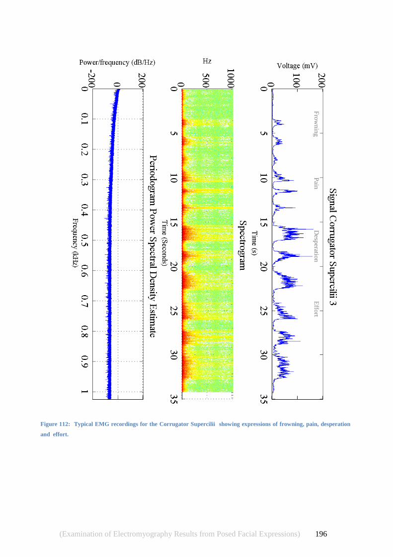
(Examination of Electromyography Results from Posed Facial Expressions) 196
Fro
wn
ing
P
ain
D
esperatio
n
Effo
rt
Figure 112: Typical EMG recordings for the Corrugator Supercilii showing expressions of frowning, pain, desperation
and effort.

(Examination of Electromyography Results from Posed Facial Expressions) 197
Figure 113: EMG of the Corrugator Supercilii showing blink artefact.
In addition to providing distinct features for different facial expressions, the EMG
recordings for the Corrugator Supercilii were also (occasionally) able to detect blinks.
This would be very useful information except it was not always repeatable. Some
blinks did not detect and for some participants of the trials no effect was observed at
all. The blink detection appeared to depend heavily on the individual involved and the
quality of the EMG electrode placement. A successful recording is given in Figure
113.

(Examination of Electromyography Results from Posed Facial Expressions) 198
5.9 EMG of the Suprahyoid Placement
The Suprahyoid Placement (Cram et al., 1998) is used as a general recording of the
muscles that move the mouth, tongue and elevate the larynx. It receives EMG
feedback from the Platysma and Sternomastoid (the neck muscle that flexes and
rotates the head. Electrode placement is shown in Figure 114, it uses an earth
electrode at the bony prominence of the scalp just below the hair line and two
electrodes located under the chin running along the midline (Cram et al., 1998)..
Electrodes were place 20mm apart on the area that forms in a mass when the
participant swallowed.
Figure 114: Suprahyoid Placement.
A set of typical EMG recordings for the Suprahyoid Placement is given ns a series of
graphs from Figure 115 through to Figure 121. While interesting, it is often not
possible to distinguish the features recorded. For instance a frown appears very
similar to laughter. An interesting result was the detection of suppressed laughter,
shown in Figure 118. This occurred when the participant was ―keeping a straight
face‖ and trying not to laugh.

(Examination of Electromyography Results from Posed Facial Expressions) 199
Figure 115: Typical EMG recordings for the Suprahyoid Placement. Participant Clenched their teeth four
times.
Figure 116: Typical EMG recordings for the Suprahyoid Placement. Two frowns are shown. Note: The first
frown was less intense.

(Examination of Electromyography Results from Posed Facial Expressions) 200
Figure 117: Typical EMG recordings for the Suprahyoid Placement. The recording is of genuine laughter
that was invoked by the telling of a joke.
Figure 118: Typical EMG recordings for the Suprahyoid Placement. The participant was instructed to
please stop laughing at a previous joke. The face returns to a visibly neutral position, but the suppressed
laughter was still detected.

(Examination of Electromyography Results from Posed Facial Expressions) 201
Figure 119: Typical EMG recordings for the Suprahyoid Placement. Jaw was opened and closed several
times. The feature after the 30 second mark is unrelated.
Figure 120: Typical EMG recordings for the Suprahyoid Placement. The participant spontaneously yawned.

(Examination of Electromyography Results from Posed Facial Expressions) 202
Figure 121: Typical EMG recordings for the Suprahyoid Placement. (Displaying a (genuine) sigh of relief
after a long recording session).

(Examination of Electromyography Results from Posed Facial Expressions) 203
5.10 EMG of the Temporal Suprahyoid Placement
The Temporal Suprahyoid Placement (C. Schneider & Wilson, 1985) is used as a
general recording of the perennial facial muscles (Cram et al., 1998). It receives EMG
feedback from the Frontalis, Corrugator Supercilii, Anterior Temporalis, Orbicularis
Oculi, Orbicularis Oris, Masseter, Buccinator Mentalis Depressor Anguli Oris, Throat
and Tongue. Actions known to produce artefacts include swallowing and talking.
Electrode placement is shown in Figure 122, it uses an earth electrode at the bony
prominence of the jaw line and two regular electrodes. One electrode is located 30mm
above the Zygomatic arch lateral to the brow and the other is placed in the muscle that
can be felt on the anterior lateral border of the chin when the mouth is opened (Cram
et al., 1998).
Figure 122: Temporal Suprahyoid Placement.
Testing of the Temporal Suprahyoid Placement was conducted using smiling,
frowning, raising eyebrows, showing surprise. Raising the eyebrows and opening and
closing the jaw. It was generally not possible to identify any actions by the collected
EMG signal. Though frowning did use a broader range of the spectrum than smiling.
Typical results are shown from Figure 123 to Figure 127.

(Examination of Electromyography Results from Posed Facial Expressions) 204
Figure 123: Typical EMG recordings for the Temporal Suprahyoid Placement showing the features created
by frowning.
Figure 124: Typical EMG recordings for the Temporal Suprahyoid Placement showing smiling.

(Examination of Electromyography Results from Posed Facial Expressions) 205
Figure 125: Typical EMG recordings for the Temporal Suprahyoid Placement showing four raises of the
eyebrows.
Figure 126: Typical EMG recordings for the Temporal Suprahyoid Placement showing posed surprise.

(Examination of Electromyography Results from Posed Facial Expressions) 206
Figure 127: Typical EMG recordings for the Temporal Suprahyoid Placement showing the features created
by opening and closing the jaw. The last feature is the jaw closing.

(Examination of Electromyography Results from Posed Facial Expressions) 207
5.11 EMG of the Temporal Masseter (Wide) Placement
The Masseter (Wide) Placement (Cram et al., 1998) is used as a general recording of
the muscles of the jaw. It receives EMG feedback from the Temporalis, Masseter,
Frontalis, Corrugator Supercilii, Zygomaticus Major, Orbicularis Oculi Orbicularis
Oris and Buccinator. It is used in diagnosing facial pain disorders. Actions known to
produce artefacts include swallowing and talking. Electrode placement is shown in
Figure 128, it uses an earth electrode at the bony prominence of the scalp just below
the hair line and two recording electrodes (Cram et al., 1998). One electrode is
located 30mm above the Zygomatic arch lateral to the brow and the other is placed
on the Masseter muscle lateral to the mouth.
Figure 128: Masseter (Wide) Placement.
Testing of the Masseter (Wide) Placement was conducted using clenching of the jaw,
extending the jaw, laughing (genuine) and yawning (real). It was generally not
possible to identify any actions by the collected EMG signal. All actions were
uniformly 100mV in amplitude. Clenching of the jaw had a uniquely sharp onset and
termination and laughing produced a longer more sustained signal.

(Examination of Electromyography Results from Posed Facial Expressions) 208
Figure 129: Typical EMG recordings for the Masseter (Wide) Placement showing clenching of the Jaw.
Figure 130: Typical EMG recordings for the Masseter (Wide) Placement showing a single extension of the
jaw.

(Examination of Electromyography Results from Posed Facial Expressions) 209
Figure 131: Typical EMG recordings for the Masseter (Wide) Placement showing genuine laughter in
response to a joke.
Figure 132: Typical EMG recordings for the Masseter (Wide) Placement, showing a genuine yawn.

(Examination of Electromyography Results from Posed Facial Expressions) 210
5.12 EMG of the Frontal (Wide) Placement
The Frontal (Wide) Placement (Cram et al., 1998) is used as a general recording of the
facial muscles of the eyes. It receives EMG feedback from the Frontalis, Temporals,
Corrugator Supercilii, Nasalis Transversa and the Masseter (muscle used to chew). It
is used in psychophysiology to profile stress responses. Actions known to produce
artefacts include swallowing and talking. Electrode placement is shown in Figure 133,
it uses an earth electrode at the bony prominence of the scalp just below the hair line
and two active electrodes located 6mm above the eyebrows directly above the pupils
of the eyes (Cram et al., 1998).
Figure 133: Frontal (Wide) Electrode Placement.
Trailing the Frontal (Wide) Placement involved frowning, clenching the jaw, raising
the eyebrows and swallowing. We found that frowns were not prominently displayed
in all cases. The raising of the eyebrows however was a short feature that gave a very
large reading (over 300mV).

(Examination of Electromyography Results from Posed Facial Expressions) 211
Figure 134: Typical EMG recordings for the Frontal (Wide) Placement showing the action of frowning.
Figure 135: Typical EMG recordings for the Frontal (Wide) Placement showing the action of clenching the
jaw.

(Examination of Electromyography Results from Posed Facial Expressions) 212
Figure 136: Typical EMG recordings for the Frontal (Wide) Placement showing the action raising the
eyebrows three times.
Figure 137: Typical EMG recordings for the Frontal (Wide) Placement showing the action of swallowing.

(Examination of Electromyography Results from Posed Facial Expressions) 213
5.13 Conclusion
In this section we discussed our trial experiments with using EMG to examine
different muscles. We observed that, of the muscles examined, the Frontalis,
Zygomaticus Major, Mentalis, Orbicularis Oculi and Corrugator Supercilii showed
distinct and usable responses to a variety of facial expressions. We also observed that
artefacts, created by talking for example, could be readily identified so as to be
removed from the signal. These muscles may be very useful in attempting to detect
specific emotional responses.
We also investigated a series of multiple muscle placements; namely the Suprahyoid
Placement, Temporal Suprahyoid Placement, Masseter (Wide) Placement and the
Frontal (Wide) Placement. These placements generally originated in clinical (medical)
use, but when applied to emotional data they managed to show a very wide array of
responses to many facial actions. However the responses were in many cases difficult
to distinguish form each other. Such placements may be very useful as ―Emotional
Barometers‖ which give an indication of how much emotional activity is present,
without revealing what emotion was responsible for the activity.
This preliminary study into facial EMG response provided a replication of results
achieved by a broad spectrum of previous researchers. Knowing that we can see the
effects observed by others allows our selection of muscles for EMG investigation to
be based on practical experience as well as previous research. The visual presentation
of time and frequency data will also assist later with choosing appropriate metrics to
calculate and features to extract.

(Examination of Electromyography Results from Posed Facial Expressions) 214

(Experimental Design) 215
6.0 Experimental Design
-Randall Munroe (1984 – current)

(Experimental Design) 216
There has been a variety of investigations in the field of emotion research with
regards to the affective physiological state. In a fundamental work in the area, Picard
et al., (2001) set out a set of five ―factors‖ in eliciting emotion:
1. Subject-elicited vs. event-elicited: Does the subject purposely elicit emotion or
is it elicited by an external stimulus or situation or task?
2. Lab setting vs. real-world: Is the subject in a lab or in a special room that is
not their usual environment?
3. Is the emphasis on external expression or on internal feeling?
4. Open recording versus hidden recording: Is the subject aware that he/she is
being recorded?
5. Emotion-purpose versus other-purpose: Does the subject know that he/she is a
part of an experiment and the experiment is about emotion?
With respect to our study, these questions are easily answered as; 1) "Event-elicited"
2) ―Lab setting" 3) "Internal feeling" 4) "Open recording" 5) "Emotion-purpose". This
would be a broad overview of where our experiment fits in the spectrum of possible
experiments. However there is a long list of smaller details that are of importance in
the overall experimental design.
In this section we will visit the rationale behind the experiment design and what data
we are collecting. We then cover how we achieve discriminant validity. We examine
the discriminant validity of the induced emotional states, and examine how the
reported emotional experience will also be validated. We then take a look at
somatovisceral responses as a special case of validity checking. The responses
concern much of the functioning of internal organs and are a difficult subject because
they are controlled by more than just emotion. Lastly we look at how we will
construct an experimental participant group.
While this chapter is rooted in psychological methods, the next chapter ―Method and
Materials‖ elaborates on practical and technical aspects of the work.

(Experimental Design) 217
6.1 Synopsis
The goal of the experiment on which this work is based is to determine if any
correlation exists between physiological signals and human emotional state. The
experiment will take a set of subjects and stimulate emotional responses. The stimulus
(IAPS slides) are not considered the cause of the physiological effect (response)
because we do not know exactly how someone will react emotionally. Instead the
elicited emotion is studied as the cause of the physiological response. The elicited
emotion is determined via the participant‘s self report of their emotional state after
each stimulus slide was applied. Physiological data was collected from participants
and used for later analyses in an attempt to find correlations between the signals and
their emotional state.
The experiment has, by nature, a lot of variables. We have tried to control as many as
possible. The person was ―at rest‖ before the experiment starts, having sat in a chair
for 10 to 15 minutes prior to data collection (this time is used to connect sensors and
test signals). The participant was seated at all times, which removes a great deal of
extra physiological signals that would be present in ambulatory systems.
By design, many of the induced emotions are not intended to be strongly present and
this has a major effect on classification tasks. Experiments that use a very strong
emotional stimulation will, presumably, observe more distinct emotional responses.
We focus however on smaller emotional reactions as may occur in the normal
work/home environment. We do not know if our results could be extrapolated to
monitor more potent emotions found in military, medical, legal or in police and
emergency services. The goal of this work is more concerned with emotions from
visual stimulus which occur when a person is not ambulatory, such as would be
relevant to emotions felt while watching movies, playing video games, viewing web
pages, working at a desk or possibly even driving a car.
We regulated room temperature and lighting conditions, as much as possible, to keep
them constant. Factors in the experiment include the elicited emotions, the people
involved, mood prior to the experiment, and influences of medication, drugs, caffeine,
cigarettes, alcohol.

(Experimental Design) 218
The stimulus procedure chosen is the International Affective Picture System, IAPS.
The effects of this stimulus is well understood and the safety and suitability for the
laboratory is excellent.
Our slide show experiment was designed to progress in four stages:
1. Introductory slides to familiarise the user with the environment;
2. Stimulus slides followed by rating tasks;
3. Simulated crash of the computer running the experiment followed by rating
task;
4. A ―thank you for participating‖ slide.
6.2 Data Collected
The data collected was in three categories:
Participant information;
Self assessment of emotional reactions;
Physiological signals at rest (for a baseline) and during stimulus.
Participant information included a person‘s height, weight, age, gender and feeling
(type of day so far). The self assessment of emotional responses was collected using a
9 point Self Assessment Manikin as published by Lang et al., (2001) and depicted in
Figure 138.

(Experimental Design) 219
Figure 138: Self Assessment Manikin
Physiological signals measured were Electrocardiogram (ECG), Blood Volume Pulse
(BVP), Galvanic Skin Response (GSR), Electromyography (EMG) for the corrugator
muscle, skin temperature for the finger, respiratory rate and pressure exerted by hand
onto feedback apparatus.
These data items were chosen because they appear often in PPR literature and were
identified as significant in our literature review. They also meet the secondary
objectives of being readily available for the encoding equipment being utilised as well
as being non-invasive and easy to record with low cost hardware.
6.3 Design
An essential goal in the design of our experimental design is a high internal validity of
the investigation (Campbell, Stanley, & Gage, 1963). That is to say, the likelihood of
the primary hypothesis must be substantial in comparison to any alternative
hypothesis.
In a psycho-physiological study, one of the most substantial rival hypotheses is that
influences other than emotion are either; responsible for the somatovisceral (nerve
pathways between the spine and the internal organs) responses observed; or have

(Experimental Design) 220
created so much noise as to disguise the effect of emotion (Stemmler, 2003).
Somatovisceral responses are broadly influenced by many other factors including:
Homeostatic activity to maintain body temperature or other balances (e.g.
iron or sugar) (Brentson & Cacioppo, 2007);
Posture (Akselrod & Oz, 1997);
Activity / task (Ekkekakis, 2005);
Task difficulty / mental effort (Mulder, Mulder, & Veldeman, 1985);
Direction of attention (Lacey & Lacey, 1974);
Anticipation (Mantysaari, Antila, & Peltonen, 1988);
Thoughts (Lang, Kozak, Miller, Levin, & McLean, 1980).
Stemmler (Stemmler, 2003) outlines five different (valid) experimental designs that
are commonly used in experiments involving emotional elicitation in a psycho-
physiological context:
1. Comparison of different emotions in different contexts;
2. Comparison of different emotions in the same context;
3. Comparison of different emotions in different intensities;
4. Comparison of one and the same emotion across different contexts;
5. Comparison of emotion with its induction context.
We are using the second design ―Comparison of different emotions in the same
context‖ as our reference in this work as it best suits our experimental objectives.
As is well known, the social sciences rarely produce research that gives a ―yes or no
answer‖. This is largely due to the fact researchers need to analyse non-quantitative
(and/or abstract) constructs, such as level of pain or enjoyment. (John & Benet-
Martínez, 2000). These constructs very rarely exist independently, because many
cognitive physiological and emotional processes are interlinked. We will use construct
validity (Campbell & Fiske, 1959) to quantify if these interactions have been
sufficiently ―untangled‖ in the experimental design. Our goal is to show that it is
likely we are in effect testing the desired construct.

(Experimental Design) 221
For an experimental design to be regarded as having excellent construct validity, it
must demonstrate that its constructs satisfy convergent validity (Campbell & Fiske,
1959) and discriminant validity (Campbell & Fiske, 1959). Convergent validity tests
whether constructs believed to be related are related, whereas discriminant validity
tests if constructs believed to be un-related are un-related. Unfortunately discriminant
validity and convergent validity do not give yes or no answers; often the result is in
the form of ―independent enough‖ or ―sufficiently related‖ respectively.
In this section we will explain how our work meets validity requirements in terms of
induced emotions, participant feedback and the nature of whether our recorded
somatovisceral responses can be expected to relate to the emotional state.
6.4 Discriminant Validity of Emotions Induced
To be able to show discriminant validity (Campbell & Fiske, 1959) for emotions, it is
necessary to induce each emotion at least twice (Stemmler, 2003). In this way a
response that happens twice in that emotion can be said to be more likely the result of
the stimulus and not of some other factor. Additionally, the emotions must be elicited
in the same context as they may present differently in a changed environment.
Care must be taken such that the environment in which emotions are elicited presents
minimal emotional stimulus in itself. Factors to be controlled include:
Room colour scheme (Danger 1987);
Smells / odours;
Responsiveness of the user interface (Trimmel, Meixner-Pendleton, & Haring,
2003) & (Boucsein, 1988);
Branding of computers used (Fitzsimons, 2008);
Lighting comfort (Chauvel & Perraudeau, 1995);
Lighting levels (Schneider & Leitenbauer, 2010).
Many of these points are discussed in more detail in Chapter 7.

(Experimental Design) 222
An initial task was to select a set of slides for the purpose of stimulating our
participants. The following criteria were identified as the basis for selecting stimulus
events:
1. Slides should be chosen so as to stimulate a broad section of the Arousal /
Valence / Dominance emotional space;
2. Self assessment ratings for the slides used should have a low standard
deviation in previous experiments (i.e. the outcome is predictable);
3. Around 30 slides is an ideal show length, it is not too taxing so as to bore
participants, and allows adequate coverage of the types of stimulus available
in the IAPs data set;
4. Slides that have been used in multiple studies and continue to produce
consistent self reports are considered more reliable than the rest of the
population;
5. Where applicable, slides that produce a similar response in male and female
participants are preferable to those that don't as keeping the slide shows
similar helps us compare male and female reactions to a similar stimulus;
6. For stimulus events that are highly gender specific (e.g. eroticism) separate
slides should be used for male and female participants. However the self report
rating should be very similar for the two slides;
7. Slides should not have any obvious cultural bias that would reasonably cause
our Australian participants to feel different about the stimulus (for example, no
flags or US dollars);
8. Slides should be suitable for viewing (not overly graphic, sexual or
instructive) so as to comply with Western Australian laws;
9. Slides should not be overly dated (70's hair styles, old model cars, etc.).
To find a slide show which exhibited all of these criteria we used both mathematical
optimisation of the quantifiable objectives (1-6) and manual refinement to meet the
"human" requirements (7-9).
This formal evaluation of slide selection by a set of 9 criteria is in excess to the
processes normally employed. Currently most studies employ the judgement of the

(Experimental Design) 223
investigator to weigh SAM data from reference studies and their own experimental
objectives, for example:
―All pictures contained humans or human faces, were matched for complexity
and rated for emotional content‖ (Baumgartner, Esslen, & Jäncke, 2006) – On
the selection of 48 IAPS images.
―…which contained 48 to 55 slides. Slides were divided into nine subsets that
were based generally on technical reports from Lang and colleagues (e.g.,
Land et al. 1995; Lang & Greenwald 1981).‖ (Cacioppo & Lang, 1998)
―90 pictures were selected from the IAPS consisting of 30
pleasant, 30 neutral, and 30 unpleasant pictures based on the valence and
arousal ratings‖ (Schaaff & Schultz, 2008)
―Our stimuli consisted of 24 pictures selected from the International Affective
Picture System (IAPS).5 We chose mildly unpleasant and arousing [stimuli] to
avoid confounding valence with arousal.‖ (Wise & Kim, 2008)
The optimisation of objectives 1-6 was achieved by means of an evolutionary
algorithm that had a capacity for allowing the user to exclude undesirable slides. The
software is available on request to the author, as guidance is needed, and is depicted in
Figure 139.
The evolutionary algorithm (EA) operated by using populations of potential slide
shows. These populations were subject to simulated evolutionary refinement in which
a fitness metric was used to determine whether a potential slide show was a good
candidate for further refinement in the next generation of the population being
simulated.

(Experimental Design) 224
The fitness of any member of the population (a full two slide shows for male and
female) was calculated by:
A percentage metric concerning coverage of emotion space (P) (often near
100%);
Measurements of standard deviation performance of each slide, averaged over
the set (D).
In calculating D, any slides that have performed well over multiple studies were
weighted down by 0.2 standard deviations per study (matrix W). This weighting,
(value determined by trial and error), guided the EA towards meeting criterion 4.
A male/female slide deviation metric was then calculated as the difference in average
rating per slide (taken from the largest applicable study) averaged over the set and
then normalised to be expressed as a percentage. This was performed separately for
Arousal, Valence and Dominance to produce three gender metrics, one each for
Arousal, Valence and Dominance, Ga, Gv, and Gd respectively. This helped guide the
EA towards meeting criterion 5.
The final fitness (F) was calculated by:
. Note
the Dominance portion of G was given unequal weighting as its use in affective
literature/research is not as common. In this respect we felt most of our classification
tasks were likely to revolve around the Arousal/Valence dimension.
Figure 139: Software for IAPS show optimisation.

(Experimental Design) 225
The evolutionary algorithm produced a slide show which was then manually
examined. We manually rejected slides to meet the ―human‖ requirements (7-9)
regarding cultural applicability, legal/ethical viability and dated (1980‘s) appearance
of some material. With these slides rejected from all future sets, the evolutionary
algorithm process was then re-run. This back process of computation and human
validation was repeated until a suitable slideshow was produced. The final selection of
slides is described in Table 9.
A final slide was added to the experiment, this slide was a simulated crash screen; the
objective was to convince the participant that the computer controlled simulation had
just crashed. It should be noted that the simulated crash at the end of the show is not a
vital part of the experiment. It is a stimulus of emotion at a different level to other
presented stimuli, and there is only one attempt per participant at ―user frustration‖,
which does not allow us to confirm with any certainty that any changes recorded are
due to frustration. We included the test as a general aid to any post hoc analysis
because A) frustration is an emotion common to the field of Human Computer
Interaction (HCI) ; B) It may serve as a potential ―high barometer reading‖, that is if
the user is annoyed/entertained by the crash screen, or the hoax, or the beeps from
other equipment, we establish reactivity levels for more pontent emotional
experiences.

(Experimental Design) 226
Table 9: Stimulus for experiments
Slide Participants
Slide Description Topic IAPS # Male Female
Windows Crash Screen Frustration NA Y Y
Snake (ready to strike) Danger 1050 Y Y
Big Hairy Spider Danger 1200 Y Y
Angry Dog Danger 1300 Y Y
Male Face (smile) Faces 2000 Y Y
Human Baby Faces 2070 Y Y
Kids playing Fun 2345 Y Y
Boy with bison (head in arse of) Humour 2730 Y Y
Boy Crying Faces 2900 Y Y
Abortion Mutilation 3062 Y Y
Hand Cut up Mutilation 3150
Y
Girl (½ head blown away) Mutilation 3069 Y Hospital Patient (male) Danger 3220 Y Y
Male nude (discreet) Erotic 4520
Y
Female Nude (discreet) Erotic 4005 Y Male lifting weights Suggestive 4535
Y
Female bikini Suggestive 4150 Y Handsome fireman Erotic 4572
Y
Female (pornographic) Erotic 4300 Y Couple at beach Suggestive 4641 Y Y
Couple Sex (discreet) Erotic 4659
Y
Couple in bed (not discreet) Erotic 4666 Y Skydiving formation Action 5621 Y Y
Extreme windsurfing Action 5623 Y Y
Flower Garden Landscape 5760 Y Y
River Landscape 5780 Y Y
Fireworks (over city) Landscape 5910 Y Y
Towel neutral 7002 Y Mug neutral 7009
Y
Spaghetti food 7480 Y Y
Tissues neutral 7950 Y Y
High diver Danger 8040 Y Y
People in a roller coaster Action 8490 Y Y
Graveyard Danger 9000 Y Y
Execution (young lady) Horror 9253 Y Y
Knives (subliminal words) Danger 9401 Y Y
Violent Scene Horror 6550
Y
Warzone (parent with child) Horror 9410 Y Dentist Horror 9582 Y Y

(Experimental Design) 227
6.5 Validity of Emotions Reported
We have assessed the validity of reported emotions as stemming from three factors:
Will the participant share their true feelings?
Does the participant understand the task correctly?
Is there an apparent variability inside the group of participants which would
alter how emotions were reported?
A major psychological factor in human decision making and feedback of likes and
dislikes is the Normative Social Influence (Raghunathan & Corfman, 2006). That is,
people (generally) will automatically act in a manner that conforms to social
expectations in order to gain acceptance. It has been shown that tasks performed
without human presence (or human observation) are free from the effects of
Normative Social Influence (Wouda, 2006). To this end the experimental environment
is free of any staff for the duration of the experiment. This and other measures are
discussed in greater detail in Chapter 7.
To ensure the participant understands the task correctly, a tutorial session is conducted
at the beginning of the experiment. In this way, if the participant is confused after the
explanations are given, we have a chance to clarify any points prior to data collection.
This is also discussed in greater detail in Chapter 7.
Finally the question of whether ratings are reported accurately across subjects is a
difficult task. While we can expect that if one person rates a film as 90% enjoyable,
and rates another as 95% enjoyable then they enjoyed the latter film more. However if
one participant rates a film as 90% and another rates it as 95%, we do not necessarily
know which participant enjoyed the film more. The latter participant may just be a
harsher critic. A similar effect concerns the results obtained from our experiment. In
this regard we do not feel qualified to prepare a survey sheet for the emotional self
report. Instead we used the already validated and accepted procedures and sheets of
the Self Assessment Manikin (SAM) (Bradley & Lang, 1994).

(Experimental Design) 228
6.6 Validity of Somatovisceral Responses Observed
As we have already covered, somatovisceral responses are dependent on several
factors. The only way to have a statistically significant result is to keep as many of
these factors constant and stimulate an emotion multiple times at the same intensity to
see that the same response pattern presents itself.
However, there is another issue concerned with the somatovisceral responses and that
is group variability, otherwise known as error variance. This concerns the variation
of somatovisceral responses to affective states between participants. A primary cause
of this is a phenomenon whereby individuals may have consistent somatovisceral
responses to an emotional state that differs from the somatovisceral responses other
group members consistently show. Stemmler (2003) describes this variability, known
as individual response specificity, as very high and likely to compromise statistical
power.
The inconsistency of somatovisceral responses between different participants has two
parts: A) Arousal, i.e. the level of baseline Arousal; B) Arousability, i.e. the degree to
which the response changes. In what is an almost universal method for accounting for
this inconsistency we recorded a ―baseline‖ prior to the regular data collection which
was used to normalise the collected somatovisceral responses.
6.7 Participants
With this experiment, like many others in the field, it was difficult to obtain a large
number of participants. It was our intention to obtain 50 usable sets of results (25
male, 25 Female). We succeeded in obtaining 33 participants, 5 of whom were
female. After removal of participants where equipment failed, mistakes were made or
physiological signal quality was an issue, we had 24 usable subjects. All subjects were
recruited through the university students and faculty. The participants were not
queried on their ethnical / cultural background.
There have been many small qualitative experiments and case studies in the field of
physiological pattern recognition. However, to date, very little success has been

(Experimental Design) 229
achieved in regards to creating a heterogeneous classification system that works
across multiple people.
In designing this experiment we are aware that there are a great number of subject
specific factors, and we wish to use a sample group large enough that individual
differences do not confound the effect we are trying to observe.
Sources of individual differences (as discussed in detail in the literature review):
Physiological signal morphology and characteristics vary between people;
Physiological manifestations of emotion will change from person to person;
Emotional response to images varies from person to person;
Description of emotion varies from person to person;
External factors of mood and other emotional events prior to the experiment.
By using a self report of the resulting emotional state, not the emotion we intended to
create, we eliminate many sources of individual differences. This means that our
experimental procedure needs to compensate for individual changes in physiological
signal morphology and individual physiological manifestations of emotion.
6.8 Conclusion
Ideally this experiment would have utilised 50 subjects‘ results (25 male, 25 Female).
However we obtained 33 participants – (28 male, 5 female). Each participant was
shown 32 slides, from the IAPS dataset, to stimulate multiple emotions multiple
times. Several slides were different to suit the predicted reactions of male and female
participants. The slides were shown in the same (randomised) order to each
participant. This may have altered results to some degree as strong slides (e.g.
mutilation content) may affect the rating of the next slide as well, as noted by Kirsch
(Kirsch, 1997). The final slide was a simulated crash of the presentation system.

(Experimental Design) 230
During the course of the experiment we recorded the following physiological signals
from each participant:
Electrocardiogram (ECG);
Blood Volume Pulse (BVP);
Galvanic Skin Response (GSR);
Electromyography (EMG) for the corrugator muscle;
Skin temperature (of a finger);
Respiratory rate;
Pressure exerted by hand onto feedback apparatus (later discarded due to
issues with recorded data).
Each participant reported their reaction to the slide using the Self Assessment
Manikin (SAM) and the self report was later studied for correlations with the recorded
physiological signals. A questionnaire was also used prior to the experiment to record
the participant‘s height, weight, age, gender and existing mood.
In this section we visited the rationale behind the experiment design and what data we
collected. We also showed the validity of the design with a lot of the attention focused
on emotion elicitation and somatovisceral responses.
Essentially the design of this experiment follows the established procedures in the
field closely. The only major design improvement over existing works is the
application of a formalised method to select stimulus slides which used an
evolutionary algorithm to balance nine selection criteria.
The novelty of this work is not related to the nature of the experiment, but rather it is
attempt to improve on previous results by applying better equipment, more recording,
better and wider feature extraction and examining novel ways of compensating for
individual variations.
While the design of ―this type of experiment‖ is well understood, the implementation
is often poorly documented and due to the fact that the method is nontrivial, involving

(Experimental Design) 231
many variables, the lack of documentation often comes into question e.g. (Angelica,
Gül, & Kremer, 2010). While this chapter shows how we are in-line with current
experimental design concepts, the next chapter ―Method and Materials‖ is where we
show the novelty in our approach.

(Experimental Design) 232

(Method and Materials) 233
7.0 Method and Materials
―Inventing is a combination of brains and materials. The more brains you use,
the less material you need.‖
-Charles Kettering (1876 – 1958)

(Method and Materials) 234
As human emotion can be affected by many external factors, we have paid a great
deal of attention to the materials and methods used in conducting this work. In this
chapter we discuss our experiment construction and handling of participants in detail.
In the next chapter we continue this discussion as it applies to our novel hardware
implementation of the Self Assessment Manikin (SAM).
Our experiment involves using a slide show (known as the IAPS set) to stimulate the
emotions of any given participant. During the course of the experiment, the
participant is connected to a set of sensors which record various physiological signals.
For every slide presented the participant reports how the slide made them feel using a
SAM. We save both the recorded physiological signals and SAM data for further
analysis (our classification task). A flow chart of this procedure is given in Figure
140.
Figure 140: Overview of experiment procedure

(Method and Materials) 235
Broadly, our method involved creating a suitable laboratory that allowed us to safely
and effectively stimulate the emotions of our participants using a slide show. We
seated our participants in a comfortable chair and a nurse attached the required
sensors to the participant. After verification of signal quality was established and the
participant had ample time to settle, the experiment began. The initial part of the
experiment was a tutorial aimed at getting the participant familiar with the self
assessment exercise. After the tutorial was complete and the participant was happy to
continue, the data collection part of the experiment began.
The experiment involved a set of stimulus slides presented to the user. After each
slide was presented, a self assessment exercise was completed using our novel
hardware implementation of the ―Self Assessment Manikin‖ (Lang et al., 2001). Each
self assessment task allowed the user to report how the slide made them feel.
The final slide of the show was a hoax - a simulated computer crash. This was
intended to stimulate a strong experience-based emotion rather than an induced
emotion.
In this chapter we describe in detail our method in regards to our tutorial stage, room
setup and handling of participants. We then discuss our safety procedures and give a
technical overview of the different sensors we employed.
7.1 Tutorial Slides
The IAPS manual (Lang, Bradley & Cuthbert, 1997) recommends that a set of test
images is used to allow participants to become familiar with the rating tasks before
the experiment begins. This ―tutorial‖ phase prevents confusion, which makes the
emotional experience more likely to be the result of the stimulus, and not the result of
uncertainty about the experiment.
After some preliminary tests, we found that our hardware SAM device should also
incorporate some orientation procedures before use (see Figure 141). This would
allow the user to become familiar with (and comfortable with) the device. Importantly
it also allows the investigators to inspect the user‘s interaction with the device and

(Method and Materials) 236
Figure 141: Introductory slides

(Method and Materials) 237
adjust the setup, or coach the user, so that the participant remains at rest and arm
movement is minimised.
A set of seven slides to orient the user with the rating procedure and the SAM
feedback device were developed and are presented in Figure 141.
7.1.1. Feedback Instruction
A neutral prompt for user feedback was designed. For the purposes of completeness
and comparison with other works we present our feedback prompt in Figure 142. The
goals for this prompt were:
To provide clear and easy to follow instructions;
To not induce a strong emotion (to be neutral);
To be clearly readable without eye strain;
To not contain any language that invokes strong affective connotations, such
as ―task‖ ―complete‖ or ―now‖. (Though the presence of ―please‖ was deemed
less influential than the absence of ―please‖).
Figure 142: Feedback slide, displayed after each stimulus while the participant completes the self
assessment task.

(Method and Materials) 238
7.1.2. Simulated Crash
We wished to study the effects of a more naturally induced emotion (emotion arising
from experience rather than observation). A natural emotion relevant to user
interaction in computing is anger/frustration in response to a computer crash. As such
we created an artificial computer crash, as the last phase of the experiment. This ruse
was triggered exactly as the user pressed ―next slide‖ during the final evaluation
screen. The user was unaware that the last IAPS image was the final regular stimulus
and the apparent crash seemed to be in response to them pressing a button. To
complete the ruse the hardware SAM device also emitted an error beep, as if it was
resetting or malfunctioning.
At this point staff in the room busied themselves with equipment and played along
with the crash scenario without actively engaging the participant. After six seconds
the hoax was revealed, and a final rating slide was presented (see Figure 143).
Figure 143: Crash screen (left) and crash rating screen (Right)
After the experiment the investigators would engage the participant in conversation to
ascertain if they were taken in by the ruse. Most people reported some degree of
suspicion about the ruse. Only three people reported being completely taken in and
only two people reported being completely sure it was a hoax.
This part of the experiment did produce some very definite emotions, but they were
mixed and not repeatable. Some people reported frustration believing they would need
to redo the experiment, some people laughed audibly (either at the hoax or at the fate

(Method and Materials) 239
of the experiment) and one person even reported feeling exasperated, believing she
would be prevailed upon to fix the broken computer.
7.2 Room Setup
The goal of the environment being used for the experiment is to be as neutral as
possible so as not to bias or interfere with the emotions being elicited. The room,
shown in Figure 144, must also serve several functional aspects, such as being large
enough to focus a projector unit.
A set of requirements was identified for the experimental environment:
Affective Tone:
o Neutral, non-clinical visual aesthetic;
o No prevalent smell;
o Comfortable chair for participant;
o Appropriate furnishing;
o Temperature.
Lighting:
o Avoidance of fluorescent lighting;
o Ability to easily see projected image.
Location:
o Quiet location;
o Private setting;
o Natural lighting;
Technical Requirements:
o Possibility of a waiting room;
o Low pile carpet that is unlikely to generate electro static discharge
which can damage the recording equipment;
o Isolation from nearby electrical interference, eg microwaves;
o Compliance with electrical isolation laws for equipment attached to a
human body;
o Pass an Occupational Health and Safety inspection;
o Room is wide enough to allow a projector to focus;
o Separated staff and participant sections.

(Method and Materials) 240
Figure 144: Experimental room, plan view.
The layout of the room, as per Figure 144, was divided into two areas divided by a
partition. On the left was an (out of sight) area for the investigators to work and a seat
for the nurse. On the right was the experiment area, with the SAM feedback device to
the left of a comfortable chair. To the right was a cabinet containing electrodes and
first aid, which was also used as a projector stand. The recording device was placed
on a window ledge behind the seat.
7.2.1. Affective Tone
In deciding on the room‘s ―look and feel‖ the following concerns were identified as
features the room should possess:
o Neutral, non-clinical visual aesthetic;
o No prevalent smell;
o Comfortable chair for participant;
o Appropriate furnishing;
o Comfortable temperature.

(Method and Materials) 241
Eric Danger‘s (Danger 1987) work on colour in interior design was referenced
extensively in verifying the room‘s neutral tone. The room was painted with light tan
and light green melamine furniture was used on the investigator‘s side and white
melamine on the experiment side.
The carpeting throughout the building was a medium grey, and this was unchangeable
for the room in question. In discussing the use of grey colours for domestic interiors,
Danger advises against the use of grey in a dark room to avoid a possible ―gloomy‖
effect. Since the room needed to be darkened to allow the viewing of projected
images, it was necessary to make a check to see if this particular room would be too
gloomy. This check was conducted by subjective evaluation of the room and it was
determined that a darkened room would not be too gloomy given our current light
colour scheme.
7.2.2. Lighting
The objectives of the room lighting are twofold:
o Avoidance of fluorescent lighting;
o Ability to easily see projected image.
Fluorescent lighting is a major source of power line interference in bio-signal
acquisition devices. Levkov et al, (Levkov et al., 2005) examines these effects at
length. Many experimenters will turn off all fluorescent lighting for bio-signal
acquisition experiments e.g. (Radin, 2000), other researchers used low-pass filtering
to minimise the effects e.g. (Barreto & Zhai, 2003) and (Ward, 2004). In our
experiment, we opted to avoid fluorescent lighting and use vertical blinds installed in
the window to modulate available sunlight to suitable conditions.
The lighting levels present in a room can be shown to control the visual comfort levels
of occupants in the room (Chauvel & Perraudeau, 1995). Both sunlight and interior
lighting can affect visual comfort levels of people in a room. A study conducted by
the University of Manchester (Murray et al., 1998) establishes a link between glare
stimulus intensity and corresponding changes in the ocular EMG. As such eye strain

(Method and Materials) 242
by bad lighting could generate unwanted EMG signals in the same area that we wish
to observe.
To remove the possibility of eye strain noise, the experiment was trialled at different
times of the day using an EMG sensor. We adjusted the blinds so that good lighting
was obtained. The primary objective was to keep the room dimly lit with only ambient
light reflecting onto the projection screen allowing for a bright image and good
contrast. Our goal was also to reduce luminance fluctuations between participants as
much as possible as that has been shown to influence the elicited emotion (Schneider
& Leitenbauer, 2010).
7.2.3. Location
The room location is something over which complete control can be exercised.
Requirements are:
o Quiet location;
o Private setting;
o Natural lighting.
The experiment room was located in Perth, Western Australia, 31º 56‘ south, 115º 50‘
east. Experiments were conducted through the months September to February. The
room was on the top level of a two story building in a quiet, low traffic part of the
university campus.
The room was 5m by 6m with a window along the entire south side. The interior walls
were constructed from plaster board and the exterior wall was brick. An air-
conditioning vent was present and operational.
It was possible to focus a projector on the north wall, and vertical blinds allowed
moderate sunlight in, avoiding the need to use fluorescent lighting (known to cause
electrical interference with recording equipment).

(Method and Materials) 243
7.2.4. Technical Requirements
In order to safely, effectively and practically conduct this work, several technical and
practical requirements must be addressed. In this section we identify these
requirements and discuss how they were addressed.
Our technical requirements were:
o Possibility of a waiting room;
o Low pile carpet that is unlikely to generate electro static discharge
which can damage the recording equipment;
o Isolation from nearby electrical interference, eg microwaves;
o Compliance with electrical isolation laws for equipment attached to a
human body;
o Pass an Occupational Health and Safety inspection;
o Room is wide enough to allow a projector to focus;
o Separated staff and participant sections.
As a precaution against participants arriving during an experiment and simply
knocking on the door of the experiment room (thus interrupting and interfering with
an experiment in progress) a waiting room was desirable. In this experiment a hallway
was converted into a waiting room, which all volunteers were told to utilise in their
confirmation messages if no-one had come out to meet them.
As an additional precaution, during experiments, a red flashing light was activated on
a sign which indicated ―experiment in progress‖ and ―do not disturb when light is
flashing‖. This was 100% effective in controlling unwanted traffic.
Much of the equipment used in this experiment was sensitive to electrostatic
discharge (Vinson & Liou, 1998), and as such various precautions must be taken.
Firstly, all participant jackets were hung on a hook to prevent clothing based static
generation. Additionally, the experiment chair and surrounding carpet were treated
with an odourless antistatic spray each night before an experiment was conducted.

(Method and Materials) 244
The room setup was subject to the Western Australian Occupational Health and
Safety (OHS) inspection process and we worked with the university‘s OHS officer to
obtain a clearance to work. The experiments were trialled to ensure everything
functioned as expected.
For purposes of reviewing and reproducing the experiments a complete description of
the room preparation guidelines we used will now be given along with recorded
environmental parameters.
7.2.5. Our Experimentation with a Shield Room to Eliminate RF
Interference
From a Radio Frequency (RF) standpoint, the ideal environment for operation of
sensitive recording equipment is a shield room, and we know of one experiment using
EEG recording for emotion detection which utilised such a setup (Choppin, 2000).
The shield room does however have some problems for emotion research. Generally a
shield room is a windowless cage, and this environment may be emotionally
intimidating.
Believing a full shield room to be impractical, especially as the only shield room on
campus was 2m x 1m, with solid stainless steel walls and unnecessarily intimidating,
we trialled an alternative. Our alternative setup was a room painted with a conductive
(ferric) undercoat. The desired (but not achieved) result was an ordinary looking room
with good RF blocking properties.
To test our theory we ordered an undercoat paint that was impregnated heavily with
fine iron shavings, (approx 1kg per litre). This produced a paint effect which looked
normal but may have exhibited properties to minimise external electromagnetic
interference. We trialled the paint using our recording apparatus placed in a 1m2
plywood box painted internally with our paint.
No significant decrease in interference was noticed and plans to repaint the room in
this manner were abandoned. It is our conclusion that there are no further practical

(Method and Materials) 245
means to eliminate external RF interference in a manner compatible with the
experiment‘s physiological (aesthetic) objectives.
It would be possible to plaster, and dry wall an existing RF proof room to produce a
fake office environment, but the expense (RF rooms cost around half a million USD)
and the resulting lack of windows made this option undesirable.
7.2.6. Our Guideline for Room Preparation (A Summary)
To concisely summarise the body of this section we created a guideline which we
referred to in our negotiations with the university in obtaining and preparing a suitable
laboratory:
a) A quiet second/third story room with a window is the ideal environment:
a. A window alleviates many feelings of claustrophobia;
b. Vertical blinds should be used over curtains or horizontal blinds to
regulate light into the room;
c. A ground floor room with a window must not be adjacent to a walkway
or area where someone may see into the room;
d. The room must be in a quite area, or be sound proofed, a consideration
dating back to pioneering works such as Mittelmann & Wolff (1939).
b) We proposed the same room be used for all experiments;
c) Care should be taken in regulating how the room smells:
a. Many rooms that are carpeted must use anti-static spray on the floor to
prevent potential damage to typical recording equipment arrangements:
i. Many of these sprays are sugar based and leave a sweet scent
(or have other scents). We found this can be alleviated by
careful product selection and by early application a few days in
advance of the experiments;
ii. In assessing the overall smell of the room, many people will
easily smell imaginary scents (Bromberg & Schilder, 1934) and
not all noses are capable of recognising the same scents. It may
be necessary to have several people smell the room prior to
experimentation. (We used three people).
d) Electromagnetic interference should be minimised:

(Method and Materials) 246
a. Adding extra shielding and toroidal magnets to all unprotected cables;
b. Investigation of surrounding offices and a co-operative agreement to
temporarily disable microwave ovens and other high voltage magnetic
apparatus;
c. Use of a shielded room is not advised. Our initial trials and
investigations indicated that the "meat locker" or "mesh cage"
aesthetics of these environments probably introduced more emotional
noise than is warranted by the reduced electrical noise.
7.3 Procedures for Interaction with Participants
As in this experiment we wish to control human emotion, it is necessary to control
how staff and investigators interact with the participants. The primary objectives are
to keep the participant feeling safe and comfortable and to reassure the participant that
all SAM feedback is strictly anonymous and not even known to the investigators at
the time of the experiment.
7.3.1. Privacy for Honesty of Feedback
During the evaluation of the slides, it is vital that our participants have the feeling of
privacy. Without this the participants will rate the slides in a manner that conforms to
social expectations (Raghunathan & Corfman, 2006). It has been shown that HCI
tasks performed without human presence (or human observation) are free from the
effects of Normative Social Influence (Wouda, 2006).
A broad range of emotion research experiments will often have the experimenter, and
all staff, leave the room for the duration of their experiment. Examples of such
experiments include (Isbister, Höök, Sharp, & Laaksolahti, 2006), (Hamm,
Greenwald, Bradley, & Lang, 1993), (McManis, Bradley, Berg, Cuthbert & Lang,
2001), (McCraty, Atkinson & Bradley, 2004), (Sandt, Sloan, & Kareem, 2009),
(Stevens, 2001), (Gotlib, Krasnoperova, Neubauer-Yue, & Joormann, 2004), (Arch &
Craske, 2006) and (Spangler, Emlinger, Meinhard, & Hamm, 2001).

(Method and Materials) 247
However our room setup did not allow for the staff to easily leave the room as the
recording equipment (computer) needed to be manned and it was not possible to keep
it in another room. To allow visual privacy for the participant, a partition was erected
which all staff would remain behind for the duration of the experiment, often with the
nurse leaving the room so as to greet the next participant in the waiting room. Similar
use of partitions has been successfully demonstrated in works such as (de Wied &
Verbaten, 2001) and (Kut et al., 2011).
7.3.2. Recruitment and Pre-experiment Contact
To recruit volunteers, an MP3 player prize was used as encouragement (the
experiments were conducted at a time (2004) when this was still an expensive luxury
item and adverts were placed around the university campus (see appendix 14.6).
Flyers were also handed out during lectures (see appendix 14.6).
Upon being contacted by a volunteer, an e-mail with a generalised informative
response (see appendix 14.8) was sent out along with a timetable of available time
slots. If contact was made by phone, a similar explanation was given and a time
booked if the participant chose to proceed. All participants were asked to avoid
alcohol, cigarettes and coffee for three hours prior to the experiment.
7.3.3. Entrance Procedure
When a participant entered the room, the staff present introduced themselves and the
nurse present (dressed in uniform) identified herself as a nurse. The investigator then
asked if the participant has had a cup of coffee in the last three hours or had smoked
in that time. As the confirmation email requested that they not do this there were no
instances of needing to send participants away for smoking / drinking / drug use.
The participant was asked to turn off and place their mobile phones and any other
electric (or bulky) items in a tray. Any coat / jumper the participant was wearing was
placed on a hook by the door.

(Method and Materials) 248
The nurse then asked (or measured as needed) the participant‘s height, weight and
age. A ruler was stuck to a wall and a set of scales was available to assist with this.
The details were written on a piece of paper (in a manner in which was apparent to the
participant) with a code for that participant written on top.
The participant was informed (again) that all feedback was anonymous and shown
that he/she was only represented by a code in our recordings. The idea of the initial
survey was in part to demonstrate this fact. With these details disclosed the participant
was then asked to sign a consent form, which stated the participant may be exposed to
some strong images.
The participant was then led to the experiment area and seated by the nurse who
struck up a polite but directed conversation about the participant‘s day. The
generalised direction of the conversation was to find out what sort of a day that
participant had had and how the participant was feeling. The results were later
(privately) annotated to the participant‘s survey sheet.
Figure 145: The participant survey sheet, the annotation below was made without the participant‟s
knowledge.
After the participant was seated, the nurse attached the electrodes and answered any
questions the participant had. The investigator then instructed the participant how the
SAM feedback device works and coached the participant in using the device in such a
manner as to minimise muscle movement. At this point the participant was reminded
that the investigator cannot see the responses being made by the user and that all
feedback is anonymous.

(Method and Materials) 249
7.3.4. Exit Procedure
After the experiment was completed, several actions were taken, the first of which
was the final slide (Figure 146) which requested that users allow the nurse to remove
their sensors. Many participants naturally tried to remove the sensors, either to
expedite proceedings or show helpfulness. This needed to be avoided as the sensors
were delicate and best handled by the nurse on duty.
Figure 146: Final slide
After removing the sensors, the nurse would check the skin where sensors were
removed for any sign of rash or allergic reaction (no instances found). All personal
items were returned to the participant and the investigator enquired how the
participant was feeling and if they felt any ill-effects from participation. The
experimenter then explained the importance of not discussing the slides, or the crash,
used in the experiment with anyone so as not to influence any other potential
volunteers.
All used electrodes were then disposed of in a biohazard sharps container. The nurse
and experimenter then prepared the laboratory for the next participant, including full
cleansing of all equipment with isopropyl alcohol.

(Method and Materials) 250
7.3.5. Ethical Treatment of Humans
A risk report (Appendix 14.7) used to gain Occupational Health and Safety (OHS)
and ethics approval found less than 0.01% chance of emotional distress occurring to a
participant. As a precaution against any emotional distress, a free and immediate
counselling arrangement was obtained from the university student counselling
services, such that anyone feeling any after effects could immediately seek help. All
participants were asked about any negative effects after the experiment and were
given a piece of paper indicating how to obtain counselling should they feel they need
it in the future.
As an added safeguard, the Hardware SAM device contained an emergency stop
button that allowed users to immediately shut down the image viewing process if they
did not wish to continue (it was never used).
No participants reported emotional distress or used the opportunity for counselling.
Generally participants reported the experiments as an enjoyable, or interesting
experience.
7.4 Safety
As described previously, physiological damage was a possibility during this
experiment, but there existed several other safety issues that needed addressing,
namely:
Electrode isolation;
Electrical safety requirements (AS3200 & IEC6060-1);
Biohazards;
Possible allergens.

(Method and Materials) 251
7.4.1. Electrode Isolation
A conventional city power grid carries with it dangers of "power surges" which are
brief but extremely high voltages on the utility line that may propagate through
transformers and damage low voltage electrical equipment and anyone attached to
said equipment. These surges may be caused by lightning, accidental energisation,
inducted voltages or equipment malfunctions. In the event that a power surge in a
power grid is transmitted to equipment connected directly to a person the risk of
fatality is very high. For this reason it is vital that all electronics be optically isolated
(see Figure 147) from the conductive path to the main power grid. Often this means
using batteries to power the data acquisition unit and communicating to mains
attached machines via an opto-isolator, as per (Douglass, 1998).
Figure 147: An example opto-isolator circuit
In general, opto-isolators should withstand input-to-output voltages up to 10 kV and
voltage transients with speeds up to 10 kV/μs (Joffe & Lock, 2010, pg 279). In the
case of the ProComp Infinity encoder we utilised, the optical isolation included a
length of optic cable which served as the only link between mains operated equipment
and battery operated equipment.
Optical Barrier
(no conductive path)

(Method and Materials) 252
7.4.2. Electrical and Biohazard Safety Requirements (AS3200 &
IEC6060-1)
The risks of power surges in regards to attaching electrodes to a human are not
completely mitigated by optical isolation. There exist other means by which the
electrode leads may become energised other than a power surge propagating through
the recording equipment. Most of these risks stem from other electrical equipment in
the laboratory environment.
As this experiment was conducted in Australia and utilises electrodes connected to
people, it is subject to The Australian/New Zealand AS3200 standard (Committee
EL/18/1, 1986) which, for our purposes, is functionally equivalent to the relevant
AAMI/ANSI standard IEC6060-1 (Berson et al., 2010) which would apply in other
countries.
As identified by the equipment manual (Thought Technology Ltd, 2003) the
following sections of the relevant AS3200/IEC6060-1 standards were addressed:
Do not operate Active Sensors within 10 feet of an operating cellular phone,
similar radio transmitting device, other powerful radio interference producing
sources such as arc welders, radio thermal treatment equipment, x-ray
machines, or any other equipment that produces electrical sparks:
o All phones turned off including volunteers and adjoining office space;
o Signs posted to prevent unwanted transmissions (see appendix 14.6).
Computers, printers and any other equipment used with medical devices be
electrically isolated from line voltage to UL or CSA medical safety standards:
o Building power already up to standard.
The PC used with the device must be placed outside the patient/client
environment (more than 3 meters or 10 feet) or the PC must comply with
EN60601-1 (system safety):
o PC compliant and at more than three meters away by partitioning;
o All other devices compliant and properly isolated with shielded and
insulated solid ducting around all cables in the recording area.

(Method and Materials) 253
After use, the Disposable Electrodes may be a biohazard. Handle, and when
applicable, dispose of these materials in accordance with accepted medical
practice and any applicable local, state and federal laws and regulations:
o Biohazard "sharps container" used for disposal, final disposal via
approved service.
Reusable electrodes present a potential risk of cross-infection especially when
used on abraded skin, unless they are restricted to a single patient or sterilised
between patients. If sterilising electrodes, employ only gas sterilization:
o Reusable electrodes sterilised correctly by appointed nursing staff.
The operator is responsible for ensuring the safety of any devices controlled or
triggered by the equipment or software, or by any software or hardware
receiving data from the equipment. The equipment must not be configured or
connected in such a way that failure in its data acquisition, processing or
control functions can trigger patient feedback stimulus that poses an
unacceptable level of risk:
o All relevant equipment (SAM device and projector) were verified for
this purpose and used with approval of the occupational health and
safety department.
Use of any equipment in a biofeedback context should be immediately
terminated upon any sign of treatment-related distress or discomfort:
o Emergency stop buttons in place and relevant procedures rehearsed by
all staff.
7.4.3. Biological Hazards
As used electrodes represent a biohazard they were disposed of in a biohazard sharps
container. All nurses wore gloves and were responsible for cleaning/sterilising all
non-disposable parts of the apparatus and sensors which came into human contact.

(Method and Materials) 254
7.4.4. Possible allergens
All substances with known allergic potential were identified and staff were trained to
identify effects. Volunteers were questioned if they had any known allergies before
electrodes were attached. The electrode gel used by this experiment is not known to
have caused any allergic reactions, but was treated as though it may be an allergen as
a precaution.
Sources of allergens identified:
Natural rubber tubes on respiration sensor;
Electrode gel (precautionary);
Isopropyl alcohol used in swabs, skin cleansing and device sterilisation.
7.5 Equipment Capabilities and Application
This section describes our sensor and recording equipment. We show how it was
configured and what placements were made.
7.5.1. Encoder
The recording apparatus used was a ProComp Infiniti (Thought Technology Ltd,
2003) which has been used in many related works. eg. (Strauss et al., 2005), (R.L.
Mandryk, Inkpen, & Calvert, 2006), (Yannakakis & Hallam, 2008) & (Nakasone et
al., 2005).
The Encoder has a 14bit Analogue to Digital Converter with a Least Significant Bit
(LSB) Magnitude of 207µV. The encoder has a 3dB response with eight channels,
two of which sample at 2048 samples per second and the other six at 256 sample per
second. Anti-aliasing is done in hardware with a 5th order Butterworth filter for a
typical result of 30db Alias rejection. The encoder noise is 150µV (RMS). The single
encoder unit ensures all readings are synchronised.

(Method and Materials) 255
7.5.2. The EMG Sensor
The Electromyography (EMG) sensor detects electrical activity produced by muscle
cells during neurological activation.
A "MyoScan™ pro" pre-amplified surface electromyography sensor was used with
the ProComp Infiniti channel B for RAW sEMG (2048 samples/sec). This sensor has
been used in various medical studies, e.g. (Nakasone, Prendinger, & Ishizuka, 2005),
(I.-M. Lin & Peper, 2009), (Winkel, Younger, Tomcika, Borckardtc, & Nash, 2006),
(Bohbot, 2010) & (Bitter et al., 2007).
According to international standards (Merletti & Torino, 1999) on reporting EMG
data, it is necessary to disclose the following information about our experimental
EMG setup:
Electrode material;
Electrode shape (discs, bars, rectangular, etc.);
Size (e.g., diameter, radius, width x length);
Use of gel or paste, alcohol applied to cleanse skin, skin abrasion, shaving of
hair, etc.;
Inter-electrode distance;
Electrode location, orientation over muscle with respect to tendons, motor
point and fibre direction.
We used the ―Thought Technology‖ T3404 electrode strip, as shown in Figure 148,
separated into individual electrodes. The electrode was a circular (10mm diameter)
Ag/AgCI, (aka standard silver-silver chloride electrode) ‗bulb‘. The skin cleaned with
isopropyl alcohol based medi-wipes, the electrode has a 0.5% saline base gel. The
electrodes were placed to record the activity of the Corrugator Supercilii as specified
by Cram et al., (1998). The placement used two electrodes placed 10mm apart
following the muscle fibres of the Corrugator Supercilii. The earth electrode was
placed at the bony prominence of the scalp just below the hair line. This muscle
placement is described in more detail in section 5.8.

(Method and Materials) 256
Figure 148: Thought Technology T3404 three-strip Uni-Gel electrodes (unseparated)
The standards (Merletti & Torino, 1999) also specify reportable items for detection
mode and amplification, namely:
Configuration; monopolar , differential, double differential, etc;
Input impedance;
Common Mode Rejection Ratio (CMRR);
Signal-to-noise ratio (SNR);
Actual gain range used.
The input sensor is based on a differential amplifier, impedance of the sensor is
1,000,000MΩ in parallel with 10pF and the CMRR is -10dB.
Lastly the standards (Merletti & Torino, 1999) state the filtering of the raw EMG
should be specified, specificly:
Filter types (e.g., Butterworth, Chebyshev, etc.);
Low and/or high pass cut-off frequencies;
slopes of the cut-offs (dB/octave or dB/decade).
As the power density function of EMG signals fall almost exclusively in the range 10
- 450 Hz, a band-pass amplifier filter is common. The MyoScan-Pro sensor used
offered a three mode selectable band-pass filtering mechanism, which we
experimentally determined performed best in our setup in its widest mode (20-
500Hz). As the band pass filter went up to 500Hz a minimum sampling rate of
1000Hz (500x2) is required as per the Nyquist theorem.

(Method and Materials) 257
7.5.3. The ECG Sensor
The Electrocardiograph is often abbreviated to ECG or EKG (from the German
Elektrokardiogramm). The ECG is similar to the EMG in that it detects the electrical
activity associated with muscle movement. The sensor detects and amplifies the small
electrical voltage that is generated by the heart muscle when it contracts.
Our work used an "EKG flex/pro" sensor connected to the 2048 samples/sec
ProComp Infiniti channel A. This sensor has been used in various affective computing
and medical studies. e.g. (Kuli, 2007), (Kulic & Croft, 2005), (Fahimi &
VaezMousavi, 2011) & (Strauss et al., 2005).
* Channel Bandwith: 0.50Hz - 1kHz
* Accuracy: +/- 3uV RMS, +/-5% of reading @ 25 to 30 degrees C
* Signal Input Range: 0 - 12mV RMS
* Signal Output Range: 0 - 600mV RMS
* Input / Output Gain: 50
* Sensitivity: < 0.1mV RMS
* Input Impedance: 1,000,000 MΩ in parallel with 10F
* Common-mode rejection ratio (CMMR): >130dB
ECG electrodes used the forearm placement (see Figure 149) which, though common,
is not as accurate as the chest placement. Forearm was used because the chest
placement was considered too invasive, and emotionally uncomfortable. The forearm
placement (as used in many single lead electrode configurations) was made with the
negative lead placed on the right forearm, while both the positive and ground leads
were placed on the left forearm. Nurses were specially trained to make this placement
correctly and ECG waveforms were inspected for quality before the experiment
continued. Recently other studies have used this same placement eg. (Mandryk, 2005)
and (Isbister, 2008, pg 219).

(Method and Materials) 258
Figure 149: Electrode placement for ECG electrodes.
7.5.4. The BVP Sensor
The Blood Volume Pulse (BVP) sensor, also called photoplethysmography, bounces
infra-red light against a skin surface and measures the amount of reflected light. The
BVP sensor is held pressed against the palmer surface of a fingertip with an elastic
strap.
The BVP sensor used in this experiment was the BVP-Flex/Pro, and it was connected
to an encoder input capable of 256 samples/sec. The device was difficult to place well
and required a lot of adjustments, to get the sensor to sit properly on the finger, before
a good signal was obtained.
7.5.5. The GSR Sensor
GSR is a measure of the skin's ability to conduct electricity. A small electrical voltage
is applied through two electrodes, usually strapped to two fingers of one hand, in
order to establish an electric circuit where the subject becomes a variable resistor.
There is no safety issue with this particular current being passed thoughout the body
as the current of is low, not high frequency, and enters and exits through the hand. If

(Method and Materials) 259
there are any external power surges the Procomp encoder is fully optically isolated to
prevent electrocution.
The GSR sensor used in our work was the SC-Flex/pro and it was connected to an
encoder input capable of 256 samples/sec. The same model device has been used in
various other works including (Wong, Chen, Huang, Lin & Hui, 2006), (Leng, Lin, &
Zanzi, 2007), (Money, Arthur & Agius, 2008) and (Benadada, Chaffar, & Frasson,
2008).
The sensor has the following capacities:
Input Range: 0 – 30.0 μS;
Accuracy: ±5% and ±0.2 μS .
The units may appear unfamiliar: the standard measurement unit for conductance is
called Siemens. Skin conductance is typically measured in micro-Siemens (μS), and is
convertible to micro-mhos(μm) [a mho is the inverse of an ohm] by the formula given
by Equation 5.
Where:
R is given by Ohms law V = IR
I is the electric current (through the person)
V is the voltage.
Equation 5: Formula for conductivity
The GSR was fitted to the stationary hand (the one not using the SAM device) as per
Figure 150.
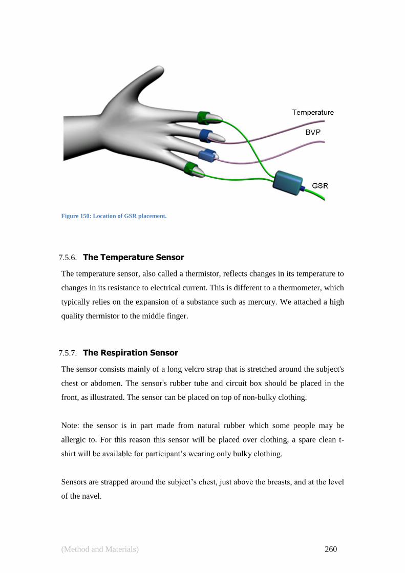
(Method and Materials) 260
Figure 150: Location of GSR placement.
7.5.6. The Temperature Sensor
The temperature sensor, also called a thermistor, reflects changes in its temperature to
changes in its resistance to electrical current. This is different to a thermometer, which
typically relies on the expansion of a substance such as mercury. We attached a high
quality thermistor to the middle finger.
7.5.7. The Respiration Sensor
The sensor consists mainly of a long velcro strap that is stretched around the subject's
chest or abdomen. The sensor's rubber tube and circuit box should be placed in the
front, as illustrated. The sensor can be placed on top of non-bulky clothing.
Note: the sensor is in part made from natural rubber which some people may be
allergic to. For this reason this sensor will be placed over clothing, a spare clean t-
shirt will be available for participant‘s wearing only bulky clothing.
Sensors are strapped around the subject‘s chest, just above the breasts, and at the level
of the navel.

(Method and Materials) 261
7.6 Software
There was a broad range of software used in the work, below we list the different
software packages used and the tasks for which they were employed. We also
developed four separate pieces of software for this work which will be explained as
well.
Software used:
Data Recording from device:
o Procomp Infiniti, Provided by the manufacturer of the recording
device;
o Audacity, Recorded the button press noises to gauge pressure.
Slideshow presentation:
o Custom software ―Slide Show Manager‖
Signal and Data Processing:
o Custom written software ―Experiment Workbench‖;
o Matlab:
Signal Processing Toolbox;
Wavelet Toolbox;
Image Processing Toolbox;
Neural Network Toolbox .
Software development:
o Microsoft C#;
o Microsoft Visual C++;
o Matlab;
o Lua.
Classification:
o Rapid Miner;
o Weka;
o Matlab Neural Network Toolbox;
o OpenSVM.
Thesis writing and graphics:
o Microsoft Word;
o Mendeley;

(Method and Materials) 262
o Custom software ―Graph Maker‖ used for scatter plots and box and
whisker charts;
o Artnatomy (used to make the muscle face diagrams in chapter 3);
o Blender (used for some of the EMG models in chapter 4);
o Make Human (used for some of the EMG models in chapter 4);
o Excel. Used for tables and some charts;
o 3Ds Max (used for models of hands etc).
The ―Slide Show Manager‖ software developed for this work managed the task of
showing slides to the participants and communicating with the SAM hardware device.
It was developed in C#; using GDI+ graphics and the serial port to communicate with
the SAM device.
The ―Experiment Workbench‖ software created for the work was the main piece of
software used to perform signal processing on the data. It served as a hub for
importing data, processing it through internal/external routines. It was capable of
delegating some tasks to Matlab where needed. The entire application was scriptable
via Lua so that all the work done could be automatically reproduced or recovered. The
software was also capable of graphing the signals as we worked with them. A
summary of the files contained in the ―Experiment Workbench‖ project. The system
was designed to use a minimum of 4GB ram, but 24GB is recommended.
Table 10: Source Code for the “Experiment Workbench” Project.
Language files comments Lines of code
C# 582 42,077 148,580
MATLAB 889 19,334 38,536
C++ 25 655 5,288
C 14 811 2,279
C/C++ Header 33 1,036 1,652
Lua 27 319 1,567
DOS Batch 5 0 83
make 1 10 25
SUM: 1,576 64,242 198,010

(Method and Materials) 263
The ―Graph Maker‖ software created (using C#) for this work was responsible for the
box and whisker charts. It also produced the confusion matrices and some of the
scatter plots. The last piece of software developed for this work was the firmware for
the SAM device. This was written in standard C.
7.7 Conclusion
In this chapter we have covered our experimental setup. It is often mentioned in
literature that emotion elicitation experiments lack necessary detail in the room
preparation and stimulus procedure (Angelica et al., 2010). We hope we have
addressed this need.
The experimental method we have prepared focuses on two conflicting objectives:
Having a emotionally neutral environment which allows the IAPS slide
stimulus to be the prevalent emotive force during the experiment;
Quality of collected data in terms of signal fidelity.
To meet these conflicting requirements, we have forgone the use of any invasive
sensors, which would have produced a better signal quality. We have chosen ECG
sensor placements on the arms, rather than the chest, as a chest placement may have
been a source of discomfort. Additionally we have used an ordinary appearing room,
as opposed to a metal cage for full RF shielding.
We have a procedure that is very safe, and a workplace that is highly organised and
well rehearsed prior to starting work. We also demonstrated how we went about the
ethical treatment of our subjects.
So far we have not discussed our self assessment task, as we felt our innovations in
regards to this exercise warranted a dedicated chapter, which follows.

(Method and Materials) 264

(Feedback via a Hardware SAM Implementation) 265
8.0 Feedback via a Hardware SAM
Implementation
―There is a computer disease that anybody who works with computers
knows about. It's a very serious disease and it interferes completely with the
work. The trouble with computers is that you 'play' with them!‖
-Richard Feynman (1918 – 1988)

(Feedback via a Hardware SAM Implementation) 266
In this chapter we discuss our work with implementing the Self Assessment Manikin
(SAM) for use in a PPR environment. The end result of this portion of the work was a
(published) hardware implementation (Creemers & Hingston, 2010). This device is
made freely available to other researches via complete hardware, firmware and
software source materials, see appendix 14.10.
The SAM scale allows a person to make a ―self report‖ of their emotional state. The
SAM was originally created by Bradley and Lang (1994) and there have been several
variants of the SAM used in various experiments, as shown in Table 11. The classical
SAM, shown in Figure 151, uses three rating scales ―Arousal‖, ―Valence‖ and
―Dominance‖ as per the three factors found in the semantic differential research by
Osgood et el., (1957).
Figure 151: Self Assessment Manikin.
The top row is used to rate Valence, the second Arousal and the third Dominance.
Reviewing key points discussed in section 3.5.2, the SAM offers the following
advantages:
It is cross cultural (Morris, Bradley & Wei, 1994);
It is completed in 3-15 seconds (Verbal techniques take much longer);
It avoids individual subjective bias of words like ―happy ― and ―sad‖;
The device produces valid results regardless of age (Backs et al., 2005),
including children (Lang, 1985);
It is established and well understood.

(Feedback via a Hardware SAM Implementation) 267
Table 11: Various adaptations of the Self Assessment Manikin (SAM)
Alternative Dominance Images
(Morris & Burke, 1995)
(Tsonos & Kouroupetroglou, 2007)
Only Valence and Arousal
(Zimmermann, Guttormsen, Danuser, &
Gomez, 2003)
(Khan, 2008)
(Neerincx & Streefkerk, 2003)
Alternative Valence pictures
(Schifferstein, Talke, & Oudshoorn, 2011)
Additional axis “liking”
(Koelstra et al., 2011)

(Feedback via a Hardware SAM Implementation) 268
8.1 Requirements Analysis
For the purposes of this research, several criteria were defined to represent our
experimental needs for Self Assessment Manikin (SAM) feedback. (These criteria are
also broadly representative of many other researchers who utilise the SAM, e.g.
(Surakka & Anttonen, 2005), (Swindells et al., 2007) & (Bradley et al, 2001).
1. The SAM should be simple to use, have minimal emotional impact on the user
and present minimal distraction from the experiment;
2. User interaction events with the SAM should be recorded with approximately
10ms accuracy (so as to be sampled faster than the screen is refreshed);
3. SAM events must be synchronised with any physiological recordings made
during the experiment (for purposes of artefact removal);
4. Allow the user to provide feedback and interact with the device in a manner
that minimises muscular action as this may introduce artefacts into the
physiological signal being recorded.
The fourth criterion is not straightforward. It is known that passive sensors recording
electrical events in the body are easily overwhelmed by large muscle movement.
Typical examples of such sensors include the electrocardiogram (ECG) and
electroencephalography (EEG). Both these measurements are often used in
experiments involving SAM feedback.
An ECG signal is typically detected at a magnitude below 1mV with the signal in the
frequency range 1Hz to 70Hz. Electromyographic (EMG) output from muscle
movement lies between 7Hz to 20Hz in the frequency spectrum, with magnitude as
low as 50μV for small muscles and up to 30mV for the larger muscles. The presence
of EMG noise is highly detrimental to the ECG signal (Clifford, 2006) and the best
solution is to keep the participant's larger muscles still.
As the ECG is often recorded during experiments using a SAM and the signal is very
prone to EMG artefacts, in this work we will use ECG quality (as recorded from a
sitting position) as a method to determine if a SAM implementation can achieve the
fourth criterion, of minimising muscular action.

(Feedback via a Hardware SAM Implementation) 269
With the goal of meeting all the experimental criteria, we built a hardware device to
record SAM interaction. This device is shown in Figure 152.
Figure 152: The Hardware SAM developed for this experiment.
This solution was discovered after investigating three existing SAM interface setups
and trialing a novel (but ultimately unsuccessful) PDA solution.
The following common setups were examined with respect to the four criteria defined
for a successful SAM interface:
SAM on printed answer sheets;
SAM as PC Software;
SAM on a Personal Digital Assistant (PDA/tablet);
SAM as a customised hardware device.
There do exist other means of using the SAM, such as Kuroda, Izumikawa and
Kouketsu (2009) who had participants orally call out codes from a SAM print out
attached to the steering wheel of a vehicle simulator.
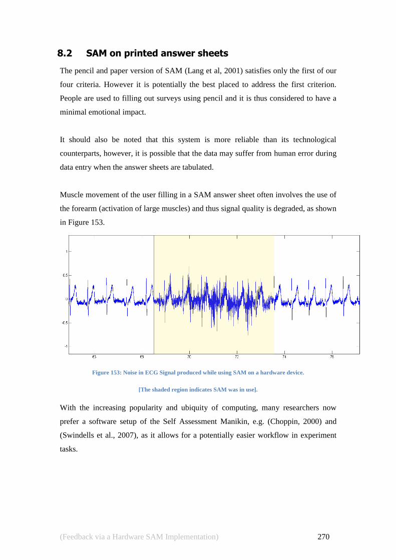
(Feedback via a Hardware SAM Implementation) 270
8.2 SAM on printed answer sheets
The pencil and paper version of SAM (Lang et al, 2001) satisfies only the first of our
four criteria. However it is potentially the best placed to address the first criterion.
People are used to filling out surveys using pencil and it is thus considered to have a
minimal emotional impact.
It should also be noted that this system is more reliable than its technological
counterparts, however, it is possible that the data may suffer from human error during
data entry when the answer sheets are tabulated.
Muscle movement of the user filling in a SAM answer sheet often involves the use of
the forearm (activation of large muscles) and thus signal quality is degraded, as shown
in Figure 153.
Figure 153: Noise in ECG Signal produced while using SAM on a hardware device.
[The shaded region indicates SAM was in use].
With the increasing popularity and ubiquity of computing, many researchers now
prefer a software setup of the Self Assessment Manikin, e.g. (Choppin, 2000) and
(Swindells et al., 2007), as it allows for a potentially easier workflow in experiment
tasks.
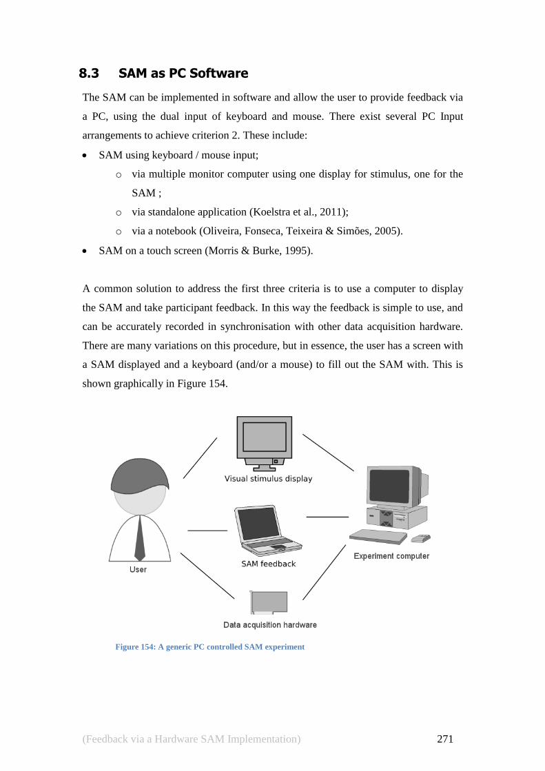
(Feedback via a Hardware SAM Implementation) 271
8.3 SAM as PC Software
The SAM can be implemented in software and allow the user to provide feedback via
a PC, using the dual input of keyboard and mouse. There exist several PC Input
arrangements to achieve criterion 2. These include:
SAM using keyboard / mouse input;
o via multiple monitor computer using one display for stimulus, one for the
SAM ;
o via standalone application (Koelstra et al., 2011);
o via a notebook (Oliveira, Fonseca, Teixeira & Simões, 2005).
SAM on a touch screen (Morris & Burke, 1995).
A common solution to address the first three criteria is to use a computer to display
the SAM and take participant feedback. In this way the feedback is simple to use, and
can be accurately recorded in synchronisation with other data acquisition hardware.
There are many variations on this procedure, but in essence, the user has a screen with
a SAM displayed and a keyboard (and/or a mouse) to fill out the SAM with. This is
shown graphically in Figure 154.
Figure 154: A generic PC controlled SAM experiment

(Feedback via a Hardware SAM Implementation) 272
One of the most widespread, technological adaptations of the SAM involves the use
of a touch screen display. This is an extension of the dual input application but using a
touch screen for user input rather than a mouse. This is a much more achievable goal
than attempting to have a computer recognise two independent mice.
The touch screen does not address the fourth criterion, as user movement is greatly
increased during input. Specifically the entire forearm must move for the user to
select an input option on the opposite edge of the screen, and traveling the arm up and
down the screen requires bicep movement. This involves usage of large muscles, and
the result is a greatly degraded signal. Another drawback is that the user is brought
into close contact with an LCD device that emits a broad range of RF interference,
which may affect the instrumentation.
The most accessible software implementation for SAM-based experiments to date is
the Self-Assessment-Manikin Scales feature of the PXLab software (Irtel, 2007). This
(open source) software offers several variations of the SAM and the ability to use the
SAM to evaluate picture, audio and textual stimuli.
Figure 155: PXLab software (Irtel, 2007)

(Feedback via a Hardware SAM Implementation) 273
As with most standalone application implementations of the SAM, PXLab offers
exact timing of all events. User feedback is accomplished with mouse and keyboard
interaction.
Other researchers have implemented software which allows for the SAM to be used
on a dedicated evaluation computer. The Master's thesis of Antoine Choppin
(Choppin, 2000) uses the software shown in Figure 156. The software, though
functional, does provide a potential emotional stimulus in its own presentation by
virtue of its appearance and the graphical stylisation of the operating system.
Figure 156: Self Assessment Manikin Software [as used by (Choppin, 2000)]
Using a computer has some strong connotations associated with it. Those unfamiliar
with computers may feel apprehensive, anxious or afraid (Meier, 1985). Moreover the
choice of computer manufacturer (brand) will create "goal directed action". That is the
type of computer the user is placed in front of will set the tone for the kind of
behaviour expected of them. A study of user behaviour under the influence of Apple
and IBM branding (Fitzsimons, 2008) showed some interesting physiological effects
created by modern computer branding. The study asked participants to find unusual
uses for a brick. Participants (n=314) were split into two groups primed with Apple
(n=219) and IBM branding (n=122). The study found the Apple primed participants to
be more creative in both measures used; "number of uses" (Glover & Gary, 1976) and
"judge panel ratings" (Silvia & Phillips, 2004). Results are shown in Figure 157.

(Feedback via a Hardware SAM Implementation) 274
Figure 157: Apple vs. IBM branding, effect on creativity (Fitzsimons, 2008). Results given for experiments
conducted with and without a five minute delay between the priming stimulus and the creativity task.
Fitzsimons claims the goal directed action of ―being creative‖ was enabled via the
activation of linked means to that goal (Shah & Kruglanski, 2002), the linked means
for the creativity goal being given as ―seek unusual associates‖ and ―inhibit
usual associates‖ (Sassenberga & Moskowitzb, 2005).
Given evidence to suggest Apple and IBM branding changes the way people may
think, and the general observation of brand loyalty eliciting emotions, it would seem
likely that a computer system brand may have significant effect on the participants in
the experiment.
Whatever the brand, a separate computer running a form of SAM software may also
create a cluttered experimental environment. Cluttering of computers increases
electrical interference, noise levels, participant intimidation and adds many technical
challenges in terms of synchronising data. A typical example of the kind of cluttering
possible in an experimental setup is Swindells et al (2007): a photo of the setup is
shown in Figure 158. However it should be noted that Swindells was exploring haptic
devices using the SAM for affective evaluation; this experiment is not negatively
effected by the clutter in the same manner as other types of experiments are.

(Feedback via a Hardware SAM Implementation) 275
Figure 158: Cluttered experimental setup. (Swindells et al., 2007)
Having multiple devices for a user to interact with can also cause extra motion as the
participant swaps from one device to another. This in turn can create EMG
interference, especially if the devices are poorly placed.
A single device showing both rating and stimulus screens (e.g. PXLab) is preferable
with regards to minimizing EMG interference. With this type of application EMG
interference can be minor as the user is only using the mouse and not changing arm
position between the keyboard and the mouse. A typical sample of this kind of noise
is shown in Figure 159.
A practical problem exists with this procedure as the participant will tend to keep one
hand on the mouse instead of returning to a fully relaxed position, and hence a small
amount of EMG interference can typically be observed during periods of the
experiment where the signal would typically be cleaner under other SAM
implementations.

(Feedback via a Hardware SAM Implementation) 276
Figure 159: Noise in ECG Signal produced while using PXLab. Shaded region indicates SAM was in use.
This constant background noise can be present while the user is receiving stimuli and
to many researchers this is the most important time to have a clean signal. If constant
evaluation of user signals is needed, this may be a very good solution as the noise
levels, though present, are reasonably low.
8.4 SAM on a Personal Digital Assistant (PDA/tablet)
The software SAM apparatus discussed so far does not present strong solutions to
criteria 1 and 4. That is, they are (possibly) a distraction for the user and do not
optimise physiological signal quality.
We made a preliminary, but ultimately unsuccessful attempt to computerise the SAM
in a manner that solves criterion 4 (minimising muscle movement). This involved the
novel use of a PDA to present a SAM rating screen and receive user feedback via a
stylus. See Fig 160.

(Feedback via a Hardware SAM Implementation) 277
Fig 160: Our SAM implementation on a PDA
The use of a PDA for SAM feedback is not common, but has been used in
experiments such as (Neerincx & Streefkerk, 2003) who performed an experiment
involving emotional feedback from video stimulus using both a IPAQ PDA and a
regular laptop. They found some differences with the way participants trusted the
devices, see Figure 161 and also found differences in mean SAM scores, concluding:
―Task performance with the mobile device resulted in a lower Valence score
than with the laptop. In other words, users experienced a more negative
emotion with the mobile device. Similar to trust, this effect might be attributed
to the decreased performance.‖
These findings mean that the device may not perform well in terms of not affecting
the participant emotionally.

(Feedback via a Hardware SAM Implementation) 278
Figure 161: (Neerincx & Streefkerk, 2003) Measurement of user trust in a device both before and after a
experimental task.
The rationale for using the PDA as an input device was to keep the natural feel of a
pen and paper style interaction with minimised muscle movement. Muscle movement
is greatly reduced because the fingers move to fill out the SAM and not the arm. If the
participant is seated at a table and is free to place the PDA in a centralised position
comfortable to them, then a survey can be completed with less major muscle
movement than any other implementation investigated here. A typical sample of the
signal produced while using a well-positioned PDA for SAM feedback, shown in
Figure 162, has a noticeably reduced noise level over the conventional PC readings
shown in Figure 159.
Figure 162 : Noise in ECG Signal produced while using SAM on a PDA (user is coached). Shaded region
indicates SAM was in use.

(Feedback via a Hardware SAM Implementation) 279
The signal quality, however, is dependent on how well the participant has been
coached to utilise the PDA and how easily the ergonomics of the environment allow
the participant to go from a relaxed state to using the PDA. If the user is poorly
coached then the result can easily be as bad as the other methods. Figure 163 shows a
(typical) example of noise levels in an experiment where the user was not coached or
supervised. When this is compared to Figure 162 it is evident that a greater portion of
the ―in use‖ recording has resulted from noise.
Figure 163: Noise in ECG Signal produced while using SAM on a PDA (user is not coached). Shaded region
indicates SAM was in use.
Unfortunately two aspects of the generic PDA device (at the time) made this kind of
interaction unsuitable:
Lack of resolution;
Real-time connectivity problems.
Resolution limitations of the PDA make some facial details of the pictures too
difficult to recognise – see Figure 164. Newer high-end PDA‘s with VGA resolutions
come a long way to fixing this but still lack the detail to show SAM figures as
rendered for pen and paper use (Lang et al., 2001)

(Feedback via a Hardware SAM Implementation) 280
Figure 164 SAM character from: PDA (left), VGA (middle), paper (Right).
To achieve criterion 3 the PDA software must communicate with the PC running the
experiment. However it is technologically prohibitive for our PDA software to
establish a useful connection with the experiment PC. The most flexible TCP
connection available to many PDA‘s is the WiFi connection, however use of WiFi
around ECG systems is not permitted in many countries (as discussed in section
7.4.2). There is also an IrDA port that could be utilised but this was technically
unfeasible, as an API for WinCE programs to interface with this port was not
available at the time the experiment was conducted.
8.5 SAM as a Customised Hardware Device
In an attempt to meet the four performance criteria defined in 8.1, we created our own
hardware solution for recording SAM feedback. In this section we detail this device in
terms of its technical capacity and its effect on signal quality.
8.5.1. User Interface
The device utilised a white translucent panel with the SAM printed on it and a series
of buttons under each picture to allow for user input. As the user presses a button, the
device provides feedback by illuminating the picture selected with a diffuse blue light
which filters through the translucent screen on the front panel to clearly highlight the
selected choice in a non-distracting manner.
Two additional buttons were provided on the device. These buttons can be given any
label, but were for the purposes of this experiment given the labels ―Next Slide‖ and

(Feedback via a Hardware SAM Implementation) 281
―Stop‖. The (less common) procedure of having the user initiate the next IAPS slide
has been shown to work successfully in experiments by Sloan et al., (1997) where the
space bar on a keyboard was used for this purpose.
8.5.2. Technical Capabilities
The device is accessed via a software API and can be utilised by the software running
the experiment in real time. The unit is equipped with a Piezo transducer capable of
producing beeps of varying frequency, the volume of which can be set via a concealed
volume knob accessible by insertion of a small screwdriver.
A microphone is also present in the device and can be used to record the intensity of
keystrokes (more vigorous key strokes produce a more audible clack inside the
device). The microphone is intentionally not sensitive enough to make any vocal
recordings so as to be amenable when obtaining ethics clearance for experimentation.
Due to some processing issues this data was recorded but never used. The unit is
further equipped with a relay capable of providing two levels of resistance to an
isolated port on the device. This relay, which can be controlled by the API, is used to
fingerprint recordings taken via physiological recording devices so that data streams
can be accurately synchronised with user activity during data analysis. An example is
shown in Figure 165. The signal having been transmitted by the SAM hardware and
recorded by the physiological recording device can be used as a synchronisation point.
Figure 165: Hardware Sync Signal. First Sequence has 7 peaks, and the second sequence 9 peaks. Giving
this recording the unique ID “79”.

(Feedback via a Hardware SAM Implementation) 282
8.5.3. Signal quality
The hardware version of the SAM showed a very clean ―at rest‖ signal and produced
an acceptable level of noise while in use. The ―in use‖ noise is generally higher than
the PDA solution shown here but is not so high as to make the system unusable.
Figure 166: Noise in ECG Signal produced while using SAM on a hardware device. Shaded region indicates
SAM was in use.
Typical results for noise levels are shown in Figure 166. The noise is mainly due to a
sliding motion of the forearm. A brief, sub heartbeat, distortion related to the action of
pushing the button is typically present. This is perhaps due to the device not being
ergonomically refined, coupled with the small movement of the buttons on the device.

(Feedback via a Hardware SAM Implementation) 283
8.5.4. Technical Challenges
Most keypads work by scanning the keys to determine if any new closed circuit is
formed by a key being depressed. This scanning causes various electrical tracks and
wires to be charged and then discharged every time the scan moves to another key.
This design, by its very nature, induces an electrical interference, and would be
detrimental to our signal quality concerns. To avoid this scanning artefact we utilised
a resistor ladder to vary the voltage into one of the microcontroller Analog to Digital
Converters (ADC) based on which button is pressed. Three ladders were used, one for
each row of nine SAM buttons. An example of these ladders is shown in Figure 167.
Figure 167: Resistor Ladder used in the hardware SAM.
A full circuit diagram and other details concerning the hardware device are given in
Appendix 14.10.

(Feedback via a Hardware SAM Implementation) 284
8.6 Conclusion
Our goals in creating a hardware SAM were to obtain a balanced input device. Our
implementation is simple to use, and has a minimal emotional impact on the user. All
events were recorded and synchronised with physiological recordings made during the
experiment.
Used correctly the device allows the user to provide feedback in a manner that
minimises muscular action likely to introduce artifacts into the physiological signal
being recorded.
The Hardware SAM we created provides many experimentally beneficial features,
however the solution is not necessarily suitable for other applications. It is not usable
in fMRI studies as it contains electrical components. We summarised the five types of
SAM examined in this section in Figure 168.
Figure 168: Comparison of SAM feedback Devices.
Pap
er
PD
A
2n
d Noteb
ook
Softw
are
Hard
ware
Usability
Synchronised with data acquisition
Detail of SAM pictures
User distraction
User muscle action
Level of interaction
Experimental flexibility
Support for different SAM models

(Feedback via a Hardware SAM Implementation) 285
The validity of this device as a feedback apparatus is inherited directly from the
demonstrated validity of the Pen and Paper SAM (Lang et al, 2001) as is the paper
version with buttons instead of check boxes.
The device‘s usefulness is apparent in that it provides all the benefits of a software
device (synchronised data, easy to perform task), without the emotional connotations
of a computer or PDA. The EMG/ECG recordings that are often collected at the same
time are improved over other alternatives in that a minimum of motion is needed to
complete the feedback. This includes eliminating:
Navigational key presses;
Navigational mouse movements;
Pen/stylus movements.

(Feedback via a Hardware SAM Implementation) 286

(Signal Processing and Feature Extraction) 287
9.0 Signal Processing and Feature
Extraction
―Eureka‖
- Archimedes

(Signal Processing and Feature Extraction) 288
In this chapter we document all our signal processing and feature extraction steps for
the six physiological sensors we used.
A signal collected from any sensor is considered ―raw data‖. It is programmatically or
even visually difficult to examine the signal and gain a good understanding of what is
happening. In order to begin the process of signal analysis a necessary first step
involves cleaning up the collected signal. This cleaning up phase is designed to
process the collected data so that it more closely resembles the signal that the sensor is
observing, whilst minimising any effects by the sensor and the transmission medium.
This is usually achieved by using a series of filters (processes that modify a signal) to:
Remove any noise present in the data;
Detect events where recording equipment produced an error or artefact;
Correct for issues in recording such as baseline drift.
After a clean signal is produced, a process of feature detection is used to extract useful
information out of the signal. This may involve keeping only parts of the signal that
are of a specific amplitude or frequency. It could involve other techniques that
transform the signal to produce a result that has strong correlations with a
phenomenon under investigation.

(Signal Processing and Feature Extraction) 289
9.1 ECG Signal
The ECG signal is the appearance of myocardium1 electrical activity on the body
surface. This signal appears as an almost periodic occurrence of the ECG basic
waveform (Dubin, 2000), see Figure 169.
As discussed in section 3.3.9, this waveform can be analysed in terms of the P, Q, R,
S, T and U waves which are referred to as the P-wave, QRS Complex, T-wave and the
U-wave. In this section we present our methodology for filtering and preparing the
ECG data. We then document our method for detection of the different features based
on the P,Q,R,S,T & U components. Finally we present our algorithms for feature
detection and creation of person invariant training data.
9.1.1. Overview of Filtering the ECG Signal
Filtering of ECG is necessary to remove the noise which enters almost all ECG
recordings. The ‗quality‘ of this filtering is given by the extent to which the filtered
signal is a smooth (and undistorted) line that maps directly to the activity of the heart.
This task is non-trivial because the noise can be at similar frequencies, and with
similar morphology, to the signals being extracted. A summary of the signals features
1 The large central, muscular, layer of the heart wall.
Figure 169 The Basic ECG waveform showing locations of the P, Q, R, S, T & U Components
mV
0.0
0.5
1.0
-0.5
0.0 0.2 0.4 0.6 0.8
P
R
Q S
T U

(Signal Processing and Feature Extraction) 290
and noise components of an ECG is shown in Figure 171. This image is a
superimposed version of the graphs presented by Thakor, Webster and Tompkins
(1984).
Figure 170: Components of the ECG Spectrum (Thakor, 1988)
We will discuss in point form the Typical ECG contaminants based on Friesen et al.,
(1990) and the extent of their presence in our data:
Power line interference:
A 50Hz (or 60 Hz in some parts of the world e.g. USA or Canada) sine wave
inducted by utility lines into the ECG sensors and wiring. This is evident in
our data and discussed in detail later in the next section (9.1.2).
Patient–electrode motion artefacts:
The electrode is jolted or moved and the contact area on the skin is altered.
The resulting variations in the impedance usually results in rapid and
continuous baseline jumps (see Figure 171 b) or complete saturation for up to
half a second (see Figure 171 a).

(Signal Processing and Feature Extraction) 291
Figure 171: Examples of electrode motion artefacts in our experiment. (a) Electrode drop out followed by
saturation of signal by EMG (muscle activity) noise. (b), rapid baseline drift.
Baseline drift:
Usually caused by respiration, this is a low frequency wobble of the signal.
The signal is otherwise normal if this low frequency component is removed.
An example of baseline drive is shown in Figure 172.
Figure 172: Baseline drift in the ECG signal.

(Signal Processing and Feature Extraction) 292
Electrosurgical noise:
The noise generated by other medical equipment present in patient care
environments. Generally not applicable to the type of laboratory we used. Care
was taken to ensure this was not present in this work, and other computers and
devices in the room were tested (by cross examining spectrograms on
recordings of a generated signal, with and without device operation) to ensure
they produced no interference to our experiment.
Data collecting device noise:
This is caused by the data collection hardware, often includes signal saturation
and ―zeroing in‖ artefacts; in our hardware this was quite rare (with the
exception of data collected shortly after electrode connections were made), we
were able to find some rare instances such as shown in Figure 173.
Figure 173: Device noise, A filtering artefact in response to impulse noise.
Quantisation noise and aliasing;
Quantisation noise is negligible as the signal is sampled well above the
applicable Nyquist frequency and the encoder uses a 14bit Analogue to Digital
Converter with a Least Significant Bit (LSB) Magnitude of 207µV. Anti-
aliasing is done in the encoder hardware with a 5th order Butterworth filter for
a typical result of 30db Alias rejection.
Sample
Am
plit
ude
in M
illiv
olts (
mV
)

(Signal Processing and Feature Extraction) 293
Electromyographic (EMG) noise:
This is a prevalent noise caused by electrical impulses generated when a
person moves. Whilst this noise is minimal when the subject is still, moving
an arm or a leg can result in more noise than the signal being received.
Electrode pop or contact noise:
Caused by an electrode being removed, falling off or being (re-)attached. This
is common if an electrode is placed over chest or arm hair and does not stick
well. In this work the effect occurred several times; generally during the
tutorial phase, though on one occasion the experiment needed to be paused for
a re-attachment to be made - Figure 174 shows a recording of such an artefact.
Figure 174: Electrode pop noise as recorded on day two of the experiment.
Signal processing artefacts; such as Gibbs oscillations;
These are unwanted oscillations in the signal, particularly in response to a
sudden change in input. Our data did not suffer from any of these issues
outside of artefacts attached to electrode pop noise; which are already removed
as un-processable artefacts.
Some of these factors are of a concern to the data we have collected and require an in
depth explanation of how they were removed. In the following two sections we will
explain in detail our methods for:
power line noise removal;
artefact detection;
baseline correction.
Am
plit
ude in M
illiv
olts (
mV
)

(Signal Processing and Feature Extraction) 294
9.1.2. EMG and Power Line Noise Removal
EMG and power line noise compromise the high frequency portion of the noise
present in the ECG signal. EMG noise is a high frequency jitter present over the ECG
signal caused by movement of the subject. Power line noise is a 50Hz (or 60 Hz in
some parts of the world e.g. USA or Canada) sine wave inducted by utility lines into
the ECG sensors and wiring. A synthetic version of these noise sources is shown in
Figure 175.
Figure 175: Sources of high frequency noise in the ECG signal.
Several attempts were made to remove the sources of persistent high frequency noise
present in our collected data. Initially Savitzky-Golay filtering (Savitzky & Golay,
1964) was employed for EMG noise removal, but for power line noise the results
were not acceptable as it introduced alterations to the morphology of the signal being
collected (specifically noticeable on the T-Wave, as reviewed by Lehtola et al., 2008).
A subtraction method (Levkov et al., 2005) was examined and modified, but it failed

(Signal Processing and Feature Extraction) 295
to function correctly on some of our data. Finally a hybrid wavelet based approach
was found to be most effective. These alternatives are discussed below.
Savitzky-Golay filtering
The signal was smoothed via a Savitzky-Golay Finite impulse response filter
(Savitzky & Golay, 1964). This filter has been shown to be suitable for removal of
power line and EMG noise in ECG data by Hargittai (Hargittai, 2005) & Christov
(Christov, 2006). Figure 176 shows our work with filtering synthetic ECG signals to
observe the effects of Savitzky-Golay filtering on signal morphology.
Figure 176: Savitzky-Golay Filtering at Different Orders on Synthetic ECG data. Top left graph is the
source signal and its noise components. Other graphs are the result of filtering the signal shown and
comparing to the known synthetic data to visualise the error.
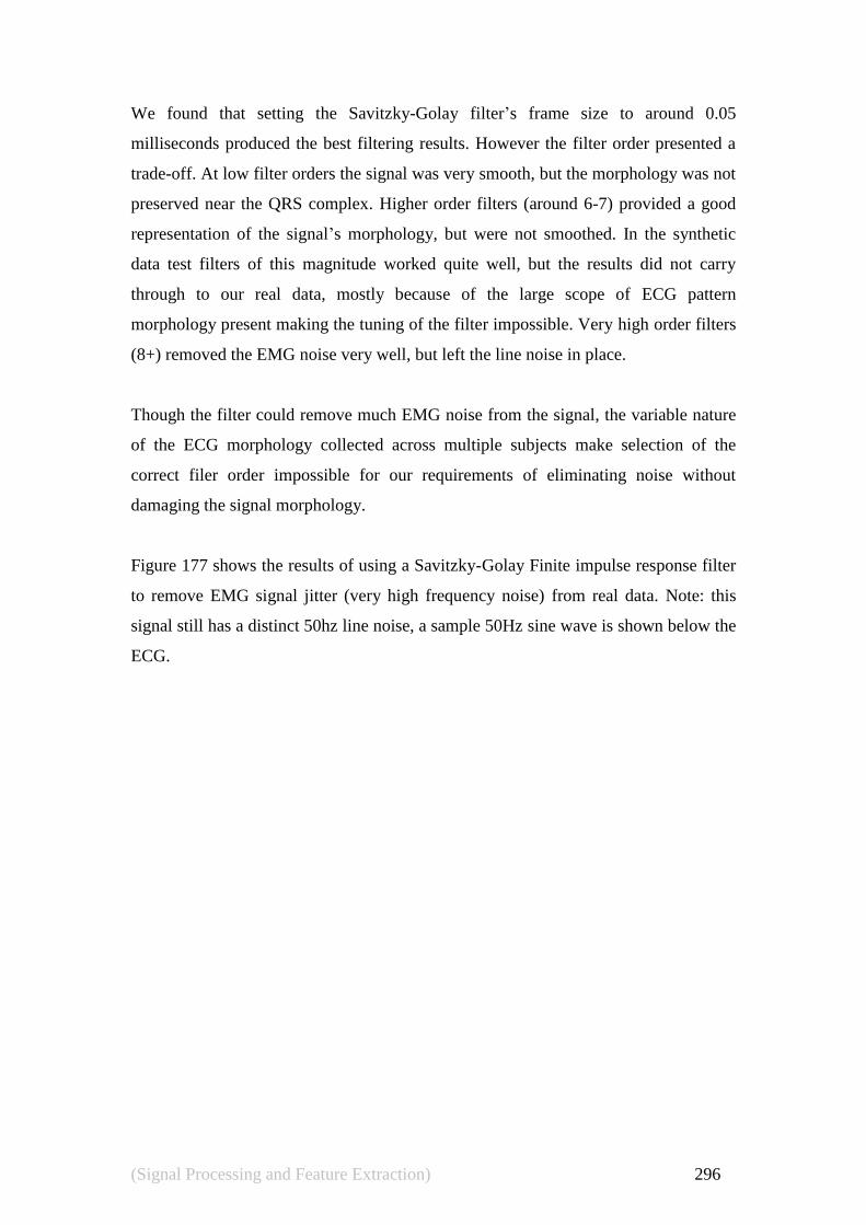
(Signal Processing and Feature Extraction) 296
We found that setting the Savitzky-Golay filter‘s frame size to around 0.05
milliseconds produced the best filtering results. However the filter order presented a
trade-off. At low filter orders the signal was very smooth, but the morphology was not
preserved near the QRS complex. Higher order filters (around 6-7) provided a good
representation of the signal‘s morphology, but were not smoothed. In the synthetic
data test filters of this magnitude worked quite well, but the results did not carry
through to our real data, mostly because of the large scope of ECG pattern
morphology present making the tuning of the filter impossible. Very high order filters
(8+) removed the EMG noise very well, but left the line noise in place.
Though the filter could remove much EMG noise from the signal, the variable nature
of the ECG morphology collected across multiple subjects make selection of the
correct filer order impossible for our requirements of eliminating noise without
damaging the signal morphology.
Figure 177 shows the results of using a Savitzky-Golay Finite impulse response filter
to remove EMG signal jitter (very high frequency noise) from real data. Note: this
signal still has a distinct 50hz line noise, a sample 50Hz sine wave is shown below the
ECG.

(Signal Processing and Feature Extraction) 297
Figure 177: Line noise artefacts (in red) after removing EMG jitter from signal using a Savitzky-Golay
Finite impulse response filter. A sample 50Hz sine wave is shown below the ECG
Amplitude millivolts (mV)

(Signal Processing and Feature Extraction) 298
Subtraction Procedure
The subtraction procedure is discussed by Levkov et al., (2005) who stated a problem
we also observed in the field of ECG noise removal research:
―Some authors do not present the results of their algorithms correctly or
clearly enough to use for interference removal. Sometimes the original signal
is not presented [19], no differences between original and processed signals
are shown [20]‖
The subtraction procedure is a fairly complex algorithm. The algorithm compensates
for issues with power line noise removal corrupting QRS complexes. The underlying
technique is:
Low frequency ECG segments are detected using a ―linear criterion‖;
These segments are moving averaged (using a linear phase comb filter);
Interference corrections (phase locked), are calculated for these segments;
Interference corrections are used to correct neighbouring non-linear segments
(QRS complexes and high-amplitude T waves).
Initially we could not reproduce the authors‘ result with regard to the effectiveness of
the linear criterion described. After some modification to the linear criterion (see
Figure 179), our results using the subtraction procedure on the cleaner ECG
recordings were satisfactory, an example is shown in Figure 178. We present a full
implementation of our function in Appendix 14.5.1.
Figure 178: Our results using the ECG noise subtraction procedure as described by (Levkov et al., 2005).
The original signal is in black, the baseline and noise corrected version is in blue and the orange lines at the
top indicate the linear criterion.

(Signal Processing and Feature Extraction) 299
However, even though results for the clean areas of the recording were good, our
areas suffering from EMG noise were not adequately resolved. We have reproduced
the subtraction procedure‘s results for medical environment type recordings, but for
our type of experiment, which involves minor subject movement, it is not suitable.
Figure 179: Demonstrates linier criterion (lower line) detection problems when EMG (upper line) noise is
present. Notice the noise is decreasing as the signal progresses, resulting in increased linear criterion
performance.
Wavelet Based De-Noising of ECG signals
We explored the use of wavelets to de-noise ECG signals and found that, in our
synthetic tests, the cleaner signals were not de-noised as effectively as per the
subtraction method. However signals with high simulated EMG noise were processed
more effectively. Some very high frequency spikes remained, but were trivially
removed using filtering internal to the ECG feature detection used. Results on real
data are shown in Figure 180.
Am
plit
ud
e in
Mill
ivo
lts (
mV
)

(Signal Processing and Feature Extraction) 300
Figure 180: Wavelet processed ECG signal.
Wavelet de-noising techniques are well established, notably that by Donoho (Donoho,
1995) which was referenced in the Matlab (―MATLAB,‖ 2003) "WDEN" function we
used for our experiments. Various works have used wavelet de-noising for ECG
signals, (Kania, Fereniec, & Maniewski, 2007), (Alfaouri & Daqrouq, 2008) and
(Sayadi & Shamsollahi, 2006) which have all shown that wavelet de-noising can be
used to effectively process ECG signals.
To test the potential for the wavelet method in our work, we used an artificial ECG
signal (duration of 10 R peaks), with randomly created synthetic EMG and power line
(50Hz) noise applied. As the original (artificial) signal is known, the performance of
wavelet de-noising techniques can be evaluated empirically.
A series of wavelet de-noising processing parameters were examined and ranked by
performance;
Threshold selection rule;
a. Stein's Unbiased Risk;
b. Heuristic variant of Stein's Unbiased Risk;
c. Universal threshold;
d. Minimax thresholding.
Thresholding;
a. Soft;
b. Hard.
Multiplicative threshold rescaling;
Am
plit
ud
e in
Mill
ivo
lts (
mV
)

(Signal Processing and Feature Extraction) 301
a. No rescaling;
b. Rescaling by estimation of noise based on first-level coefficients;
c. Rescaling by estimation of noise based on all coefficients.
Wavelet type;
a. Haar;
b. db1 through db45;
c. coif1 through coif5;
d. sym2 through sym8;
e. dmey;
f. bior1.1 through bior6.8;
g. rbio1.1 through rbio6.8.
The Matlab de-noising procedure was tested for noise removal with every
combination of these parameters. Each test was run over nine different noise level
profiles (see Figure 181), with each test repeated three times (a new random seed for
the generated noise) to gauge average performance. This produced 21,360
performance experiments.
We evaluated the performance of any given parameter combination using the average
sum error squared after the experiment was repeated three times. This was conducted
for synthetic random EMG noise at 2, 5 & 10db. Figure 182 shows wavelet
performance across the range of EMG noise levels.

(Signal Processing and Feature Extraction) 302
Figure 181: Synthetic ECG noise, 50hz (top), generated at 0.1, 0.2 or 0.3 mV, and EMG (bottom) present at
a signal to noise ratio of 2, 5 or 10bB.
0 500 1000 1500 2000 2500 3000 3500-1
-0.5
0
0.5
1
1.5
0 500 1000 1500 2000 2500 3000 3500-1
-0.5
0
0.5
1
1.5
Am
plit
ude in M
illiv
olts (
mV
) A
mp
litude in M
illiv
olts (
mV
)
Sample
Sample

(Signal Processing and Feature Extraction) 303
Figure 182: Performance of Different Wavelets in EMG De-Noising (lower results are better).

(Signal Processing and Feature Extraction) 304
Other than choice of wavelet function, we found that the EMG noise level and the
(wavelet) level at which de-noising was performed had a significant effect on the
resulting error levels. Figure 183 shows the effect of the synthetic EMG Signal to
Noise Ratio (SNR) on the error rate of the signal de-noising across all wavelets.
Figure 183: Error level by EMG noise (lower error level results are better). Note: The noise is expressed as
signal to noise ratio so lower values mean more noise.
Figure 184 shows our results for error levels by the level of the wavelet.
Figure 184: De-Noising Performance by decomposition level (across all wavelets)
From our data we identified 15 mother wavelets based on their performance (biased
towards higher EMG SNT ratios): sym7, coif4, ,db7, sym8, bior2.8, db4, coif4, coif3,
coif5, bior3.3, dmey, coif2, sym3, sym2, db2. We found that de-noising at the 5th
level was most productive. Though less noticable in effect we also decided on using
Stein's unbiased risk threshold selection rule with soft thresholding and multiplicative
threshold rescaling performed by estimation of noise based on all coefficients.

(Signal Processing and Feature Extraction) 305
These 15 wavelets most likely are a best fit to our work, on different datasets different
(but similar) wavelet sets may be more favourable, and the effect of using another
appropriate set on this data would not be too significant.
In comparison, a similar study to our wavelet de-noising investigation by Kania et al.,
(Kania et al., 2007), which was performed on real data with heart arrhythmias, found
a similar set of wavelets to be effective (using the Matlab WDEN function); namely:
sym3 and db1..db4.
A non-trivial task in improving the quality of the de-noised signal is removing the
high frequency pseudo-Gibbs artefacts (unwanted ringing in the signal) that are
occasionally generated by wavelet de-noising. Though Matlab uses thresholding
techniques to minimise the pseudo-Gibbs phenomenon, some artefacts remain. These
artefacts are often reported in works using wavelets to de-noise ECG signals, eg (Su
& Zhao, 2005). A sample pseudo-Gibbs artefact is shown in Figure 185.

(Signal Processing and Feature Extraction) 306
Figure 185: Pseudo-Gibbs Artefact (Su & Zhao, 2005). Top graph is source signal, second graph is noisy
version, third graph is the wavelet de-noised, showing only minimal pseudo-Gibbs artefacts near the Q and
S portions of the ECG signal.
Many high frequency pseudo-Gibbs artefacts were removed by a simple filtering
integrated into the feature recognition procedures (discussed in section 9.1.6), we
wished to clean up the signal as much as possible before this stage. After some
experimentation, we devised a method to de-noise the signal using all 15 identified
wavelets together.
The method involved computing a resultant signal where every point in the new signal
was a function of the corresponding samples from each of the 15 source wavelets.
The function being the mean of all samples within one standard deviation from the
mean of the 15 source samples. This is a form of outlier rejection. If the source
wavelets were less than 9 a Q-test could be substituted. This technique is a variant of
that presented by (Yang & Wei, 2010).

(Signal Processing and Feature Extraction) 307
The final results were often extremely smooth for areas where EMG noise saturated
power line noise, but less successful for areas of evident power line frequencies.
Figure 186 brings to focus an area of many artefacts and shows both our typically best
results in removing them (the first three heartbeats) followed by examples of poor
results in the next three heartbeats.
Figure 186: Multiple Wavelet De-noising Technique (above). Raw Signal (below) Average wavelet in red
superimposed on 15 key wavelets (gray).
Summary of ECG De-Noising
There are a lot of techniques that can be used to de-noise the ECG signal. We found
that the choice of technique could depend heavily on the intended use of the ECG
signal after filtering. In this study the requirements of the de-noised signal were
different to many other situations that typically use ECG data. for example, signal
morphology around the Q,R,S and T waves was considered more important than other
factors such as Signal to Noise Ratio (SNR). In this manner, some decisions on the
necessary filtering required were subjective in nature.
Am
plit
ud
e in
Mill
ivo
lts (
mV
) A
mp
litu
de
in
Mill
ivo
lts (
mV
)

(Signal Processing and Feature Extraction) 308
For our requirements, the wavelet based approach gave the best results from the
techniques investigated. In contrast, our implementation of the subtraction procedure
of Levkov et al., (2005) did not perform well for the levels of EMG noise that were
present in some of our data and we found Savitzky-Golay filtering to be useful,
though difficult to tune. A version of Savitzky-Golay filtering that automatically
adjusts its parameters to suit the data present would be an interesting point for future
research as our wavelet approach was not without some minor artefacts.
9.1.3. Artefact Detection
Some portions of the signal were so corrupted by effects such as EMG noise as to be
extremely difficult to repair. In other applications, such as those involving subjects
that are exercising, and such noise if prevalent, special strategies are adopted to repair
this data (Pahlm & Sornmo, 1987). This non-trivial task can be assisted by collecting
accelerometer data to assist in the processing (Raya & Sison, 2002). However, in the
case of our experiments, where the subject is stationary and only a small proportion of
data is affected by this problem, we chose to discard the corrupted portion of the
signal. As such we discarded all data that failed basic thresholding (amplitude range
checking) tests.
9.1.4. Baseline Drift correction via Median Filtering
Traditional baseline drift correction involves using a high pass filter to remove the
slower change to the base line. This approach has been used to correct baseline drift in
ECG signals by various works including de Chazal, Penzel and Heneghan (2004).
However, distortion incurred by various high pass filters often interferes with and
distorts the features of the ECG (Hambley, Moruzzi, & Feldman, 1974), (Van Alste &
Schilder, 1985) and (Warlar & Eswaran, 1991). A popular method of baseline
correction uses median filtering to estimate the signals base line. The estimated base
line was then subtracted from the signal to flatten the signal into a straight line with
minimal effect on the ECG attributes. Many works have used this approach
(Shouldice & Heneghan, 2001), (Correa, Laciar, Torres, & Jane, 2008), (de Chazal et
al., 2003) and (Yu, Liu, McKenna, Reisner, & Reifman, 2006).

(Signal Processing and Feature Extraction) 309
Like many other projects, this work had access to median filter algorithms provided
by Matlab and other major vendors. Upon investigation, it was found that the
commercially available solutions were extremely costly in terms of memory usage
and computational time when the size of the filter window exceeded 2000 samples.
As ECG processing is one of the few major applications for using a median filter with
a large window size, the computational complexity is not commonly addressed. It was
our conclusion that (on the hardware of the time, circa 2004) it was not a viable
solution to perform the filtering using the existing algorithms available to us. This is
not an unprecedented stance, some researchers do state median filtering as being very
slow, Shouldice described the extent of the problem (Shouldice & Heneghan, 2001)
as such:
"It was found that calculating the median at each step value, say for four
seconds of data (4000 samples), led to a very long execution time - even for
short data segments. As a consequence, this approach was not considered
feasible for entire GB datasets".
To address this issue this work developed an efficient and novel real-time median
filter to perform baseline correction with minimal memory overhead. This is not the
first implementation of fast median filtering, recent publications such as (Little &
Jones, 2010) have described filters which offer "10:1 performance gains for large
window sizes" over the Matlab implementation. However our approach was novel at
the time, fast and developed separately from the recent works. We have included a
description of the algorithm and a performance comparison in appendix 14.9.
Using a filter window of two seconds, an accurate baseline was detected on almost all
of the data recorded in this experiment. This was similar to many works, such as
(Korürek & Nizam, 2008), however, occasionally this window size failed to correctly
correct for baseline drift. Trying larger window sizes in half second increments, and
visually inspecting the entire data set each time, we eventfully found a four second
window worked best for our data. The window size may have been longer for these
cases because of differences in hardware and our preference not to use inbuilt filters

(Signal Processing and Feature Extraction) 310
provided by the equipment manufacturer. A typical result is shown in Figure 187
where the signal drifts considerably and a smooth baseline is detected.
Figure 187 An Extreme Instance of Baseline Drift. The baseline is detected using median filtering and is
shown as the curved line running through the signal.
The next stage after detecting the drift is compensating by subtracting the base line.
Figure 27 shows the result of correcting the signal in Figure 26. Note the signal is
shown from a starting point four heartbeats earlier to show both positive and negative
correction performance.
Figure 188 Baseline corrected ECG signal.
After the signal has been baseline corrected the filtering of the ECG signal is
complete. At this point we can use the ―cleaned up‖ signal in a feature extraction
process.
Am
plit
ude in M
illiv
olts
(mV
) A
mplit
ude
in M
illiv
olts (
mV
)

(Signal Processing and Feature Extraction) 311
9.1.5. Overview of Feature Detection in the ECG Signal
A feature vital to the quality of ECG analysis is synchronisation with the cardiac beat.
This is achieved though the detection of the Q, R and S waves, known as the QRS
complex. An idealised version of the QRS Complex is shown in Figure 189, as the
most prominent feature of the signal, it is typical to detect this complex first and then
examine the data between consecutive QRS complexes. We explain the issues
involved, discuss our unsuccessful attempts to build a QRS detector from ground up,
and share issues we had in adopting two existing algorithms to our needs.
Figure 189: Typical ECG Signal - QRS Complex
It has been shown (Silipo, Laguna, Narchesi, & Mark, 1995) that the correct detection
of the QRS complex is necessary for accurate and reliable measurement of the wave
form parameters that will be used in our classification task.
The appearance of the QRS complex will vary from that shown in Figure 24
depending on which sensor placements are used. Though many variations are possible
(see Figure 190) this experiment utilised a sensor placement which produces the
typical ECG waveform. As such we will not concern ourselves with dealing with
other variations for the purposes of this study.
mV
0.0
0.5
1.0
-0.5
0.0 0.2 0.4 0.6 0.8
P
R
Q S
U T

(Signal Processing and Feature Extraction) 312
Figure 190 Nomenclature of various possible QRS intervals.
The American Health Authority AHA (Bailey et al., 1990) recommends the use of
techniques based on spatial velocity calculations to formulate an evidence variable for
the detection of the QRS complex. This work has attempted a QRS complex detector
based on these recommendations. We attempted to validate our algorithm using
sample data obtained from the MIT-BIH (Taddei, et al., 1992) and ST-T (MIT-BIH,
2003) databases. The initial QRS complex detector implemented in this work was
found to be problematic. A major problem was that even though we correctly found
QRS complexes, the exact point of the peak was often difficult to determine, and our
algorithm gave a slight error which was inconsistent. This lead to data which showed
minor variations in intervals that did not exist. Our goal was an algorithm that was
more consistent in determining the peak position. As our attempts to build a QRS
detector from ground up were problematic (sufficient accuracy could not be
achieved), an existing solution was sought.
Our first attempts at finding an existing suitable QRS detector involved the porting
and adaptation of an implementation (P. Hamilton, 2001) of a major work in the field
of QRS complex detection, the Hamilton-Tompkins algorithm (P. S. Hamilton &
Tompkins, 1986). This algorithm improved on the also notable Pan-Tompkins
algorithm (Pan & Tompkins, 1985). The Hamilton-Tompkins and Pan-Tomkins
algorithms are the most popular single-lead ECG QRS detection methods and have

(Signal Processing and Feature Extraction) 313
been widely used in the past two decades for Heart Rate Variability (HRV) analyses.
A notable downside to the Hamilton-Tompkins algorithm is its reliance on a QRS
detection threshold that must be experimentally determined.
Finding good threshold values proved to be a participant specific task; which was still
ineffective for some participants. A later update (ver. 1.3) of Hamilton's
implementation (Hamilton, 2001) noted some improvements to the threshold
implementation. As this update did not come to our attention until after the QRS work
was completed it was not evaluated.
A recent advancement to this work is a Hilbert transform-based method, proposed by
(Benitez, Gaydecki, Zaidi, & Fitzpatrick, 2000), which uses a variable detection
threshold that does not need to be experimentally determined. However no existing
implementation was available.
A second attempt to obtain a suitable QRS detector focused on the porting of the
(original) Pan-Tompkins algorithm (Pan & Tompkins, 1985). We used a reference
implementation (Pablo Laguna, Jané, Bogatell, & Anglada, 2000) that was part of the
PhyioNet Toolkit (Goldberger et al., 2000) and adapted it to work in our software
infrastructure. Though more consistent across participants, positional accuracy issues
in peak and onset detection were a problem.
Positional accuracy and consistency of detection points across QRS complexes were a
key requirement for our classification procedures. If detection of peaks and onsets are
variable or altered by individual ECG wave form characteristics, then we may be
introducing artificial variations in inter/intra beat feature length measurements.
Looking for a better performing algorithm in regards to these requirements, we
ultimately found a reliable technique involving wavelet decomposition.
9.1.6. Wavelet Decomposition and Automated ECG Annotation
In this section we discuss a work by Chesnokov, Nerukh and Glen (2006) that used
wavelet decomposition to reliably achieve automated ECG annotation.

(Signal Processing and Feature Extraction) 314
The major difficulty in finding the components of the ECG signal stems from the fact
that they are small in terms of amplitude and exist in a portion of the frequency
spectrum that also picks up muscle noise and motion artefacts. A comprehensive
study by Thakor et al., (1984) produced a workable estimate of the ECG power
spectrum that demonstrates the nature of P and T waves in relation to the rest of the
data present in the ECG signal, this was previously discussed in Section 9.1.1, where
Figure 170 showed the overlap of motion artefacts and the P-T waves.
As peoples‘ recorded ECG morphology is quite different; it is often the case that a
feature extraction algorithm will fail to detect portions of a signal, because they are
simply not present in a signal. Kunzmann and Bolz (2002) defined a successful beat
detector as one that detects:
P-wave:
o Time of the beginning, maximum, end;
o Amplitude.
QRS:
o Time of the beginning;
o R-spike;
o End of wave;
o Amplitude.
T-wave:
o Time of the maximum/minimum (depending on the polarization);
o 2nd extremum (if available);
o End of wave;
o Amplitude deviation and slope.
ST:
o Derived parameters: RR-interval, PQ-interval, QT-length.
It is important to note that the above criteria for successful beat classification ignore
the U wave. The U wave is seen as extremely difficult to detect, and is often excluded
from discussions on ECG beat detection.

(Signal Processing and Feature Extraction) 315
The wavelet decomposition based algorithm, with source code, provided by
Chesnokov et al., (2006) was able to demonstrate the best detection performance
when compared to a host of similar algorithms during the PhysioNet (Goldberger et
al., 2000) Computers in Cardiology Challenge 2006. Typical results on our data are
shown in Figure 191.
Figure 191: ECG Annotations Against Raw ECG signal.
The algorithm created by Chesnokov et al., (2006) used 14 separate parameters to
tune the algorithm. When contacted, Chesnokov was helpful in providing us with
some necessary guidance regarding the parameters.
9.1.7. Extraction of Training Data from the ECG
Two major tasks often facing conventional ECG classifiers are detection of abnormal
morphology and general morphology classification. Recent works in general
morphology classification include Iliopoulos and Michalakopoulos (2006), Gholam
Hosseini, Reynolds, and Powers (2001) and Güler and Übeyl (2005). Most current
work in this stream of research uses wavelet encoding parameters as input to neural
networks to detect features of the ECG. This is relatively successful with Güler &
Übeyl (2005) achieving a 97% successful beat classification algorithm.
Though successful, the bulk of current investigative efforts in ECG are driven by
medical research aimed to detect abnormal heart activity or identify features that may
indicate heath issues with the heart. Often key metrics extracted from the ECG

(Signal Processing and Feature Extraction) 316
include Heart Rate Variability (HRV) (Saykrs, 1973) and QT Intervals. These tasks
are different in nature to the objectives of our classifier which involves the studying of
short term variations in relative morphology to detect emotional state.
Many works have studied the ECG in relation to emotion. Some works use the
measures established as medically useful. A recent example is Villon & Lisetti (Villon
& Lisetti, 2006) who used HRV to detect emotion in real time. Others use wavelet
decomposition parameters, for example (Sarkar, 2002) shows this to be a plausible
method for determining some human physiological states.
Standard waveform properties that do not rely on the morphology of the ECG have
also been used. A recent and interesting result by Katsis et al,. (Katsis et al., 2008)
was the detection of stress, disappointment and euphoria (possibly none of these are
emotions) in racing car drivers using ECG metrics of RR interval, mean amplitude
and the mean absolute first difference defined for a 10 second window. Their formula
for the mean absolute first difference is shown in Equation 6.
∑| | | | | |
Equation 6: Mean absolute first difference, where N is the sample rate multiplied by 10s
and X0..n is the signal.
The use of non-morphological indicative parameters by works such as Katsis et al.,
(2008) may be an advantage in an environment where the subject is non-stationary
and thus creating a lot of EMG interference to the ECG signal.
9.1.8. Invariant Feature Selection from the ECG
Many of the studies identified thus far use heart rates and statistical methods to
identify features to be used in classification. However there still appears to be a need
to investigate ECG morphology in relation to emotional influences. We are visiting
the task using a broad range of features extracted from the signal and attempting to
discover any correlations. We are not basing this work on features currently well
studied by the medical community as our goals are different.

(Signal Processing and Feature Extraction) 317
A major difficulty in dealing with ECG features is the variation in morphology
between people. Much of the work that pioneered the field of ECG based diagnosis
dealt with these issues and is famously studied by the Nobel prize winning doctor and
physiologist Willem Einthoven (Einthoven, Fahr, & De Waart, 1913). They
established that many people generate differently shaped QRS complexes and have
different mean ECG feature intervals.
For our purposes of finding invariant features, another difficulty that arises is the
variation in morphology based on increased or decreased heart rate. A pioneering
work in correcting ECG features, to be heart rate invariant, was conducted in 1920 by
physiologist Henry Bazett (Bazett, 1920). Their work created a formula to generate a
heart rate corrected QT interval. Bazetts‘ Formula, shown in Equation 7, for
correcting the QT by the square root of the R-R interval became a standard metric
(QTc) for detecting increased risk of ventricular arrhythmia.
√
Equation 7: Bazetts Formula (Bazett, 1920)
This formula is nonlinear, which is in congruence with Bazzets (1920) work which
showed that feature intervals in the ECG do not increase linearly with heart rate.
Bazzets work, though still used, was based on data manually obtained from real ECGs
from 39 young men. More recent research by Sagie et al., (Sagie, Larson, Goldberg,
& Bengtson, 1992) found this work over-corrects at high heart rates and under-
corrects at low heart rates. Sagie et al., proposed a more accurate formula shown in
Equation 8.
Equation 8: Improved formula for QT correction
While the QT interval has been well studied because of its correlation to medical
conditions, there has been little (published) work to study the effect of increased heart
rate on other ECG features.

(Signal Processing and Feature Extraction) 318
As this work aims to study a broad set of ECG features it was necessary to derive
formulae for creating heart rate corrected and person invariant features. Thus we
extended the concepts put forward by Sagie et al., (1992) into all the other inter/intra
beat intervals. We term this set of transforms, the Normalised Adjusted Relative
Features (NARF) transform, it is shown in Equation 12.
Firstly a feature (F) is defined as the interval between two points of interest in the
ECG. The set of readily identifiable features in the ECG is given in Equation 9.
| |
Equation 9: An Arbitrary feature interval, from feature i to feature j, where i
and j are positions of a sample.
The full set of recorded Fij intervals in our collected data is plotted against the
corresponding RR interval in which it occurred. This creates a scatter plot to which a
polynomial curve can be fitted. The resulting coefficients of fitting a second order
polynomial to the points are termed Aij, Bij and Cij. Thus we can calculate a predicted
interval (PFij) for any Fij for a given RR interval as per Equation 10.
Equation 10: A prediction of feature interval given at the RR period.
Any observed feature interval can then be expressed as a percentage of its predicted
duration (PFij) for the current RR interval. the resulting metric is termed the relative
feature (RFij) as per Equation 11.
Equation 11: A Relative Feature, Corrected for Heart Rate
Since each participant has a different mean and standard deviation, we normalise the
results to make the features invariant across participants. The resulting metric, termed
NARFij, is given in Equation 12. Results for every inter/intra beat NARF transform
are given in 14.4.
∑

(Signal Processing and Feature Extraction) 319
√
∑
Equation 12: The NARF Transform
9.1.9. Summary of ECG Processing and Feature Extraction
In this section we have explored a set of noise filtering and feature extraction
techniques for the processing of ECG signals. A summary of steps taken is as follows:
We used a wavelet de-noising technique to remove high frequency noise. The
technique used was based on existing theory but also contained an amount of
original work;
We used median filtering to achieve baseline correction. To achieve this goal
we developed a novel median filtering algorithm that had improvements in
computational efficiency over many existing works;
We employed an existing, pre-verified, feature detection software to discover
the location of recognisable signal features.
Our data for classification purposes is derived from durations between the
morphologically identifiable points on the periodic ECG signal. We extended the
work of Sagie et al., (1992) to correct for all feature intervals, not just the QT interval.
After normalising this data we have metrics that are usable in our classification tasks.
9.2 EMG Signal
Surface Electromyography (sEMG) is a conventional and well-studied measure of
muscle activation. sEMG is used in a variety of research applications including
affective sciences, sport sciences, human kinematics research and injury
rehabilitation, artificial limb control, neuromuscular disorder treatment and
ergonomics evaluation.
Many affective science studies focus on sEMG activation levels and use thresh-
holding techniques and a limited set of features to assess the presence of muscle

(Signal Processing and Feature Extraction) 320
activation and perform emotion classification on that data. We implemented a similar
system and extracted a simple high/low feature from our EMG signals. Typical results
are shown in Figure 192. Preliminary analysis suggested a wider feature set was
required, as a simple boolean output was insufficient. Thus the threshholding work
was abandoned in favour of some more descriptive metrics.
Figure 192: EMG Thresh holding
To find a wider set of features for investigation, a broad cross section of features
commonly extracted from the sEMG signals in other fields of research were studied
for their applicability to emotion recognition tasks.
9.2.1. EMG Feature Extraction
Two major groups of features can be extracted from the EMG; amplitude based
features and frequency based features. It has already been established that amplitude
based features of facial EMG data are significant features in emotion classification.
Studies such as Nakasone et al., (Nakasone et al., 2005) clearly link amplitude based
features with the Valence component of dimensional emotion models. However the
validity of using frequency based diagnosis specifically for the corrugator muscle in
respect to emotion classification has not been investigated, to our knowledge.
Am
plit
ude in
Mill
ivolts
(mV
)

(Signal Processing and Feature Extraction) 321
To determine whether an investigation of frequency based features was needed we
took spectrograms of frequency features and compared them to the corresponding
time domain signals to establish if there was any degree of dependence in the two
domains. Figure 193 shows typical results of the investigation visually. Some
frequency domain activity, such as in the 70s-80s time span, has no correlating time
domain activity. This effect, though subtle, was observed often and as such supports
the validity of frequency domain feature extraction.
Figure 193: Time vs. Frequency domain EMG features; The lower graph is a spectrogram and the colouring
is a third dimension indicating the amplitude of the given frequency (x) for the given time (y).
Several works (Phinyomark, Limsakul, & Phukpattaranont, 2009), and (Du &
Vuskovic, 2004) suggested typical feature sets that could be extracted from sEMG

(Signal Processing and Feature Extraction) 322
signals using a shifting window approach. A selection of feature sets described by the
afore mentioned authors was chosen and implemented in Matlab in a way that builds
upon the toolbox developed by Chan & Green (Chan & Green, 2007).
The feature sets being extracted for investigation in this work are:
1) Integrated EMG (IEMG);
2) Mean Absolute Value (MAV);
3) Weighted Mean Absolute Value 1 (WMAV1);
4) Weighted Mean Absolute Value 2 (WMAV2);
5) Mean Absolute Value Slope (MAVSLP);
6) Simple Square Integral(SSI);
7) Variance of EMG (VAR);
8) Root Mean Square (RMS);
9) Waveform Length (WL);
10) Slope Sign Change (SSC);
11) Willison amplitude (WAMP);
12) Autoregressive Coefficients (AR);
13) Median frequency (MDF);
14) Mean frequency (MNF);
15) Modified Median Frequency (MMDF);
16) Modified Mean Frequency (MMNF).
In the rest of this section we will examine each of these features. The examination
will cover the mathematical definition of the feature and previous research efforts
using this feature. We discuss the kinds of muscles each feature has been used with
and any applicable classification tasks previously performed with the feature. We then
show the distribution of the feature, by participant, when applied to our own data sets.

(Signal Processing and Feature Extraction) 323
1) Integrated EMG (IEMG)
This feature is possibly one of the easiest to extract from the EMG signal. In this work
it was calculated using Equation 13 as per Merletti & Torino, (1999). via a customised
implementation derived from Chan & Green (2007)
∑ | |
Equation 13: IEMG Calculation, X is a window in the EMG signal of length N
Widely used in various EMG tasks, the IEMG has been used for emotion recognition
and facial action classification tasks. A pioneering work (Sirota & Schwartz, 1982)
used IEMG in studying Zygomatic and Corrugator activity and determined that facial
EMG is sensitive to different emotional-states, even in subjects who report
experiencing little or no subjective response to affective imagery and reveals
differences in positive and negative emotions.
Further work using IEMG conducted by Hess,et al., (1989) and later by (Schmidt et
al., 2006) was able to differentiate between deliberate and spontaneous smiles. These
works principally used readings from the zygomaticus major, depressor anguli oris,
corrugator supercilii, and masseter.
It should be noted that the term "Integrated EMG (IEMG)" is often used erroneously
to describe a filtering technique known as "linear envelope detection". In an effort to
rectify the situation, the International Society of Electrophysiology and Kinesiology
made mention of the problem when creating a set of standards for reporting EMG data
(Merletti & Torino, 1999).
Typical results of our algorithm are shown in Figure 194. An important aspect of the
feature set is evident in this figure: namely large short isolated spikes in the data have
little result in the final feature. The window size of one second was determined
experimentally by visual inspection of the result, balancing accurate data
representation against low response to noise and outliers.

(Signal Processing and Feature Extraction) 324
Figure 194: IEMG (window = 1s) feature extracted from experiment data. IEMG shown in red, EMG (not
to scale) shown in black.
The distribution of this feature was studied in relation to the individual participants in
the experiment (see Figure 195). Approximately 50% of participants exhibited a
compact range of values for this feature, with maximum and minimum values falling
within two standard deviations of the norm. Most participants had a negative skew in
the response distribution. A notable exception was participant 28. This participant
appeared to have an unusual presence of muscular activation.
Figure 195: IEMG by participant
Am
plit
ud
e in
Mill
ivo
lts (
mV
)

(Signal Processing and Feature Extraction) 325
2) Mean Absolute Value (MAV)
Though a well-studied method of EMG feature extraction (Ben-Masaud et al., 2009),
(Farthing, Borowsky, Chilibeck, Binsted, & Sarty, 2007), (Nathan, 2003), (Baratta et
al., 1988), there appears to be no research in the field of emotion detection that
mentions the use of the MAV feature. This feature (see Equation 14) appears to be
commonly used in the study of muscle injuries, though evidence presented by (Huang,
Zhou, Li, & Kuiken, 2009) shows that MAV can be used as a significant feature in
EMG (kinematic) classification tasks in muscles of the arm and hand.
∑ | |
Equation 14: Calculation of MAV for a window (x) of size (N)
The distribution of this feature was studied in relation to the individual participants in
the experiment. The results, shown in Figure 196, were very similar in distribution
patterns to the IEMG distribution.
Figure 196: MAV by participant

(Signal Processing and Feature Extraction) 326
3) Weighted Mean Absolute Value 1 (WMAV1)
This is a version of the Mean Absolute Value (MAV) with a simple windowing
function. Advocated by (Phinyomark et al., 2009) (as the algorithm MMAV1) and
given little attention as a specific feature in other literature, the feature is examined
here for experimental purposes. The formula is presented in Equation 15.
∑ | |
⁄ ⁄
Equation 15: Calculation of WMAV1 for a window (x) of size (N)
The distribution of this feature was studied in relation to the individual participants in
the experiment. The results, shown in Figure 197, were very similar in distribution
patterns to the IEMG distribution.
Figure 197: WMAV1 (MMAV) by participant

(Signal Processing and Feature Extraction) 327
4) Weighted Mean Absolute Value 2 (WMAV2)
This is another version of the Mean Absolute Value (MAV) with an improved
windowing function. Advocated by Phinyomark et al., (2009) (as the algorithm
MMAV2) and given little attention as a specific feature in other literature the feature
is examined here for experimental purposes. The formula is presented in Equation 16.
∑ | |
⁄ ⁄
⁄
⁄
Equation 16: Calculation of WMAV2 for a window (x) of size (N)
The distribution of this feature was studied in relation to the individual participants in
the experiment. The results, shown in Figure 198, were very similar in distribution
patterns to the IEMG distribution
Figure 198: WMAV2 (MMAV2) by participant.

(Signal Processing and Feature Extraction) 328
5) Mean Absolute Value Slope (MAVSLP)
This feature (see Equation 17) is used often in medical studies involving MAVSLP
recognition for prosthesis control (Hudgins, Parker, & Scott, 1993). Hudgins et al.,
demonstrated classification tasks to achieve multifunctional prosthetic control using
Mean Absolute Value Slope as a primary feature. To date there appears to be no
emotion classification studies using this feature.
MAVSLPn = MAVn+1 - MAVn
Where:
∑ | |
Equation 17: Calculation of MAVSLP for a window (x) of size (N)
The distribution of this feature was studied in relation to the individual participants in
the experiment. The results, shown in Figure 199, generally showed a standard
distribution between 0.5 and 1.
Figure 199: MAVSLP by participant.

(Signal Processing and Feature Extraction) 329
6) Simple Square Integral(SSI)
The Simple Square Integral(SSI) (Phinyomark et al., 2009), is a feature which reflects
the energy of the EMG signal for a given window. It is defined in Equation 18.
∑
Equation 18: Calculation of SSI for a window (x) of Size (N)
The distribution of this feature was studied in relation to the individual participants in
the experiment. The data, shown in Figure 200, showed participant 28 had results
significantly higher than any of the other participants.
Figure 200: SSI by participant.

(Signal Processing and Feature Extraction) 330
7) Variance of EMG (VAR)
The Variance of EMG (VAR) (Phinyomark et al., 2009) is a feature which reflects
the power of the EMG signal for a given window. It is defined in Equation 19.
∑
Equation 19: Calculation of VAR for a window (x) of Size (N)
The distribution of this feature was studied in relation to the individual participants in
the experiment, as shown in Figure 201. The data was very similar to the SSI
distribution, but in a different scale. Again participant 28 had results significantly
higher than any of the other participants.
Figure 201: VAR by participant.

(Signal Processing and Feature Extraction) 331
8) Root Mean Square (RMS)
The Root Mean Square (RMS) is a common statistical metric for measuring the
magnitude of time series data. Its formulation is given in Equation 20.
√
∑
Equation 20: Calculation of RMS for a window (x) of size (N)
The distribution of this feature was studied in relation to the individual participants in
the experiment, as shown in Figure 202. The data had a varied range of standard
deviations for individual participants; ranging from around 1 at the lowest and 5 at the
highest. Again participant 28 had results significantly higher than any of the other
participants.
Figure 202: RMS by participant.
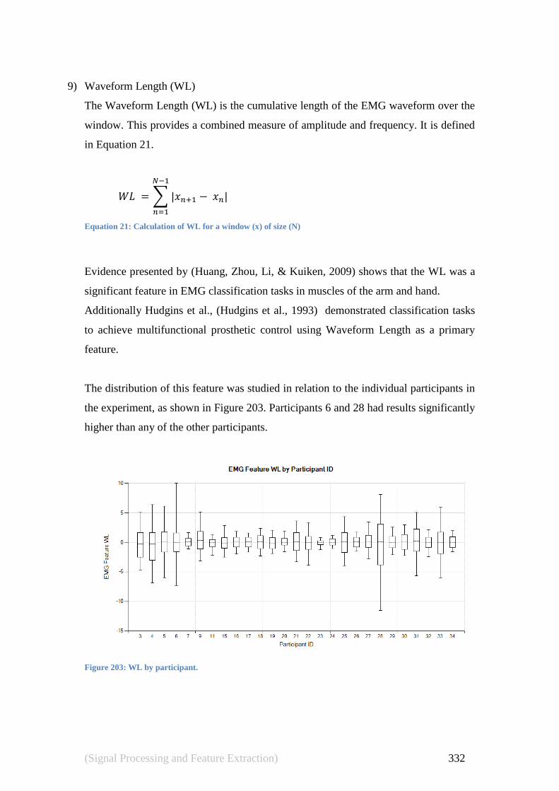
(Signal Processing and Feature Extraction) 332
9) Waveform Length (WL)
The Waveform Length (WL) is the cumulative length of the EMG waveform over the
window. This provides a combined measure of amplitude and frequency. It is defined
in Equation 21.
∑ | |
Equation 21: Calculation of WL for a window (x) of size (N)
Evidence presented by (Huang, Zhou, Li, & Kuiken, 2009) shows that the WL was a
significant feature in EMG classification tasks in muscles of the arm and hand.
Additionally Hudgins et al., (Hudgins et al., 1993) demonstrated classification tasks
to achieve multifunctional prosthetic control using Waveform Length as a primary
feature.
The distribution of this feature was studied in relation to the individual participants in
the experiment, as shown in Figure 203. Participants 6 and 28 had results significantly
higher than any of the other participants.
Figure 203: WL by participant.

(Signal Processing and Feature Extraction) 333
10) Slope Sign Change (SSC)
The Slope Sign Change (SSC) is a method used to represent the frequency
information of an EMG signal. The number of changes in slope, between positive and
negative, in three consecutive segments is totalled. There is a thresh-holding function
employed to reduce the effects of signal noise. The SSC is defined in Equation 22.
∑ [ ]
Equation 22: Calculation of SSC for a window (x) of size (N)
The threshold value used is generally between 10mV to 100 mV, in this case we use
100mV based on recommendations by Phinyomark et al., (Phinyomark et al., 2009).
The distribution of this feature was studied in relation to the individual participants in
the experiment, as shown in Figure 203.
Hudgins et al., (Hudgins et al., 1993) demonstrated classification tasks to achieve
multifunctional prosthetic control using Slope Sign Changes as a primary feature.
Figure 204: SSC by participant.

(Signal Processing and Feature Extraction) 334
11) Willison amplitude (WAMP)
The Willison amplitude (WAMP) is a count of the number of times the difference
between EMG signal amplitude among two adjacent segments exceeds a given
threshold. The threshold in turn acts to reduce the effects of signal noise. The WAMP
is defined in Equation 23.
∑ | |
Equation 23: Calculation of WAMP for a window (x) of size (N)
The threshold value used is generally between 10mV to 100 mV, in this case we use
100mV based on recommendations by Phinyomark et al., (Phinyomark et al., 2009).
The distribution of this feature was studied in relation to the individual participants in
the experiment, as shown in Figure 205.
Figure 205: WAMP by participant.

(Signal Processing and Feature Extraction) 335
12) Autoregressive Coefficients (AR)
The Autoregressive (AR) model describes each sample of the EMG as a linear
combination of the preceding samples plus a white noise error term. The AR coefficients
are calculated via the formula in Equation 24.
∑
where : xn is a sample of the model signal,
is AR coefficients,
wn is white noise or error sequence,
p is the order of AR model.
Equation 24: Calculation of AR Coefficients for a window (x) of size (N)
The autoregressive coefficients of orders 1 through 10 were computed using the
Levinson-Durbin algorithm (Levinson, 1946) & (Durbin, 1973) as specified by (Shaman,
2010). Each order is treated as a separate feature extracted from the signal and our
distributions for participants are shown in Figure 206.

(Signal Processing and Feature Extraction) 336
AR1 By Participant ID
AR6 By Participant ID
AR2 By Participant ID
AR7 By Participant ID
AR3 By Participant ID
AR8 By Participant ID
AR4 By Participant ID
AR9 By Participant ID
AR5 By Participant ID
Figure 206: : Distribution of autoregressive coefficients 1-10.
AR10 By Participant ID
Participant ID Participant ID
Participant ID Participant ID
Participant ID Participant ID
Participant ID Participant ID
Participant ID Participant ID
Fea
ture
AR
(5)
Fea
ture
AR
(10
)
Fea
ture
AR
(4)
Fea
ture
AR
(9)
Fea
ture
AR
(3)
Fea
ture
AR
(8)
Fea
ture
AR
(2)
Fea
ture
AR
(7)
Fea
ture
AR
(1)
Fea
ture
AR
(6)

(Signal Processing and Feature Extraction) 337
13) Median frequency (MDF)
Median frequency is a feature often extracted in physiological signals, and used
successfully in various works (Jordan, Stockmanns, Kochs, & Schneider, 2007), (Weitz,
2006). Median frequency is often reported as a highly variable measure and has been
shown to relate in part to muscle fatigue (F. M. Azevedo et al., 2009).
The median frequency is the frequency at which the EMG power spectrum (Pj) is divided
into two regions of equal amplitude. A typical power spectrum for one of our participants
(entire signal) is shown in Figure 207.
Figure 207: EMG Power Spectrum for a participant in our experiment.
0 0.1 0.2 0.3 0.4 0.5 0.6 0.7 0.8 0.9 1-70
-60
-50
-40
-30
-20
-10
0
10
Frequency (kHz)
Pow
er/
frequency (
dB
/Hz)
Welch Power Spectral Density Estimate
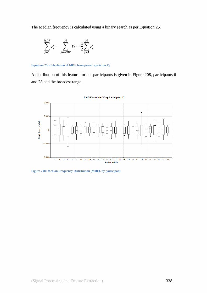
(Signal Processing and Feature Extraction) 338
The Median frequency is calculated using a binary search as per Equation 25.
∑
∑
∑
Equation 25: Calculation of MDF from power spectrum Pj
A distribution of this feature for our participants is given in Figure 208, participants 6
and 28 had the broadest range.
Figure 208: Median Frequency Distribution (MDF), by participant

(Signal Processing and Feature Extraction) 339
14) Mean frequency (MNF)
The mean frequency is often studied alongside the median frequency and has a similar
statistical significance. The equation is given below and the distribution in our
population is given in Figure 209. The resulting distribution is given in Equation 26.
∑
∑
Equation 26: Calculation of MNF from power spectrum Pj and corresponding frequency fj.
The distribution of this feature was studied in relation to the individual participants in
the experiment, as shown in Figure 209. Participants 6 and 28 had results significantly
higher than any of the other participants.
Figure 209: Mean Frequency Distribution (MNF), by participant.
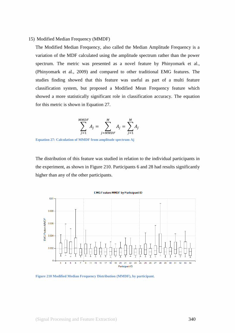
(Signal Processing and Feature Extraction) 340
15) Modified Median Frequency (MMDF)
The Modified Median Frequency, also called the Median Amplitude Frequency is a
variation of the MDF calculated using the amplitude spectrum rather than the power
spectrum. The metric was presented as a novel feature by Phinyomark et al.,
(Phinyomark et al., 2009) and compared to other traditional EMG features. The
studies finding showed that this feature was useful as part of a multi feature
classification system, but proposed a Modified Mean Frequency feature which
showed a more statistically significant role in classification accuracy. The equation
for this metric is shown in Equation 27.
∑
∑
∑
Equation 27: Calculation of MMDF from amplitude spectrum Aj
The distribution of this feature was studied in relation to the individual participants in
the experiment, as shown in Figure 210. Participants 6 and 28 had results significantly
higher than any of the other participants.
Figure 210 Modified Median Frequency Distribution (MMDF), by participant.

(Signal Processing and Feature Extraction) 341
16) Modified Mean Frequency (MMNF)
The Modified Mean Frequency, also called the Mean Amplitude Frequency is a
variation of the MNF calculated using the amplitude spectrum rather than the power
spectrum. The metric was presented as a novel feature by Phinyomark et al.,
(Phinyomark et al., 2009) and compared to other traditional EMG features. The
study‘s findings showed that this feature was statistically significant in terms of
classification accuracy of EMG. Their task was predicting voluntary hand movements
given forearm EMG signals.
Figure 211: Performance of MMNF (Phinyomark et
al., 2009)
The formula for MMNF is given in Equation 28, and the resulting distribution in our
population is shown in Figure 212.
∑
∑
Equation 28: Calculation of MMNF from the amplitude spectrum Aj and corresponding frequency fj
The distribution of this feature was studied in relation to the individual participants in
the experiment, as shown in Figure 212. Participants 6 and 28 had results significantly
higher than any of the other participants.

(Signal Processing and Feature Extraction) 342
Figure 212: Modified Mean Frequency Distribution (MMDF), by participant
9.2.2. Artefact Detection
Artefact detection was generally not needed as our EMG sensor remained well
connected. This was due to good adhesive pads and a favourable performance of the
couplings during data collection; typically there is no method to completely avoid the
occasional contact problems in surface EMG electrodes. We did use simple
thresholding at 0.3mV to detect artefacts such as those present while verification of
proper sensor placement was being made. Typical results are shown in Figure 213.
This thresholding level was determined by visual inspection of the data.
Figure 213: EMG artefact detection by thresholding at 0.3mV. The portion of the signal with significant
activity above the red line was caused by an artefact. After 23 seconds the sensor placement was corrected.

(Signal Processing and Feature Extraction) 343
9.3 Skin Temperature
Skin temperature is a signal often studied in experiments involving human
physiology. Skin temperature is controlled by the hypothalamus. It is linked to the
control of internal temperature and the effects of ambient external temperature in a
system known as the human thermoregulatory response. It is necessary to distinguish
the human response as opposed to other animals and mammals as thermoregulatory
systems are greatly varied between species.
Skin temperature may be subject to external factors, but is to some degree controlled
by the human body via several physiological mechanisms:
Vasoconstriction can decrease the blood flow to the skin, minimising heat loss
to radiation;
Sweating, to evaporatively cool the skin, and body via blood flow;
Shivering to increase heat production in the muscles;
Release of epinephrine, norepinephrine, and thyroxine to increase metabolism
and thus heat production;
The erection of the hairs to increase insulation.
The temperature sensor gives a highly aliased result whereby the quantisation levels
cause a jittered signal that is problematic for further processing, such as slope
detection algorithms. This problem was initially overcome using a Savitzky-Golay
(Savitzky & Golay, 1964) smoothing filter with a window of 1.02Hz and a
polynomial order of two to reduce the aliasing. A typical result is shown in Figure .

(Signal Processing and Feature Extraction) 344
Figure 214: Savitzky-Golay filter on skin temperature data
The Savitzky-Ggolay filter proved an adequate method to filter the data; however it
was improved slightly by using a median filter to pre-process out small spikes. Pre-
processing the data with a median filter, using a window of 10ms, prior to the
smoothing effect of the Savitzky-Golay filter provided a cleaner result. A result
indicative of this improvement is shown in Figure 215.
Figure 215: Effect of pre-processing with a median filter
Applying the Savitzky-Golay filter to the median filtered data allows the median filter
to remove the small "jaggies" which would otherwise bias the polynomial regression
Savitzky-Golay filter. This gives a good result that, for many purposes, may be un-
necessarily refined and computationally wasteful.
Key
Raw data
Savitzky-Golay filter
Savitzky-Golay with median filter
Key
Raw data
Savitzky-Golay filter
Tem
per
ature
(°C
elsi
us)
Tem
per
ature
(°C
elsi
us)

(Signal Processing and Feature Extraction) 345
There are not many features typically extracted from the temperature signal and most
of the studied features are time domain based.
Normalising temperature data is something often considered a trivial task. Often
studies such as Zhai & Barreto (Jing Zhai & Barreto, 2006b) will take a baseline
reading of a user's skin temperature during an experiment‘s acclimatisation and
instructional period. This base line is averaged and all recordings for the experiment
are then normalised against this average.
Our work attempts to make the temperature data more invariant per person by
correcting for some external factors influencing skin temperature. As skin temperature
variations and responses are effected by individual characteristics, diurnally by time
of day, environmentally and affectively by both mood and emotion; which results in a
non-trivial variance being present in recorded values. The following is a description of
our experimental results, related research and a proposal for the normalisation of skin
temperature data in a completely invariant manner.
9.3.1. Skin Temperature Alteration by Mood and Medium Term Trends
In our experimental setup there was no temperature difference in the waiting room
where people rested prior to the experiment and the experimental environment itself.
Participants were given ample time (approx 15 minutes) to settle into the new
environment of the testing room. The sole control of the buildings airconditioning
system was given to (taken by) the research staff involved in the experiment.
Despite these precautions, long term (in our case this means several minutes) skin
temperature variations were present in most of our subjects. Typical results are shown
in Figure 216. Note how a baseline taken during the instructional period would not be
appropriate.

(Signal Processing and Feature Extraction) 346
Figure 216: Medium term skin temperature trend (three worst participants shown, to highlight problem),
lower trace indicated the duration of the training period.
In our experimental setup, the stimulus was applied to the participant for six seconds.
Early research from Mittelmann & Wolff (Bela Mittelmann & Wolff, 1943) showed
that skin temperature was related to emotional state by taking skin temperature
recordings of a patient undergoing psychiatric counselling. Mittelmann & Wolff were
able to show that the prevalent mood of some of their subjects, such as depression or a
feeling of reassurance, could readily be correlated with their skin temperature
recordings. Some of their results are shown in Figure 217 and Figure 218. Notice that
the trends are a medium term response (5 to 10 minutes).
Time (mm:ss)
Time (mm:ss)
Time (mm:ss)

(Signal Processing and Feature Extraction) 347
Figure 217: Finger temperature curve during a series of depressive reactions. (Bela Mittelmann & Wolff,
1943)
Figure 218: Typical skin temperature variation during a psychiatric interview (Bela Mittelmann & Wolff,
1943) [„RM TEMP‟ appears to be an error]

(Signal Processing and Feature Extraction) 348
9.3.2. A Skin Temperature Feature Extraction Method
We recognise that there may be flaws in using a rest period as a baseline measurement
for temperature data, but are unable to resolve these issues, so we proceeded with a
baseline driven technique. The results are shown in Figure 219.
Figure 219: Normalisation method for skin temperature, shown on synthetic data. The red line showing
normalised data had its baseline established during the period before the experiment started, while the
participant was sitting in the chair and the electrodes conections were verified.
A skin temperature metric was created by calculating the mean absolute value
(Equation 29) of the signal using a sliding window of 128ms.
∑ | |
Equation 29: Mean Absolute Value (MAV) calculation

(Signal Processing and Feature Extraction) 349
9.4 Respiration
In this section we cover the features extracted from the respiration signal using a
variety of peak detection, area under curve and slope measuring techniques. We
outline issues with peak finding and paused breaths.
Finding the respiration rate is achieved by finding peak values from the respiration
sensor and measuring the time between them. These peaks are recorded when the
chest is no longer expanding and the exhale process begins. These peaks are not sharp
and this is an issue. Many peak detection algorithms, such as the ones provided by
Matlab (―MATLAB,‖ 2003) do not function well for peaks that have a plateau at the
top.
We employed a peak detection algorithm by O'Haver (O‘Haver, 2009). This
algorithm is based on classical first derivative y-axis crossing to find peaks, but adds
smoothing and detection thresholds. Typical results shown on our respiration data are
shown in Figure 220. This algorithm was essential as it detected smooth top peaks
correctly; and many other algorithms do not.
Figure 220: Peak detection of respiration data. Each red line is a detected peak.
Res
pir
atio
n
Sen
sor
Rea
din
g.

(Signal Processing and Feature Extraction) 350
We tuned the detection algorithm to ignore minor peaks that were part of a larger
break, see Figure 221. We encountered many of these peaks which are the result of a
pause in breathing.
Figure 221: Interrupted breath. The peak shown by the arrow appears to be made by some sort of pause in
the regular breathing cycle.
Note our observations are linked to our use of the higher chest placement. Other
researchers using a lower chest placement will have a different signal, an example of
this is shown in Figure 223.
Figure 222: The signal obtained from a lower chest placement of the respiration sensor.
The work by O'Haver (O‘Haver, 2009) produced other metrics such as peak widths
and amplitudes. We sorted this data into inhale and exhale pairs and created another
metric to provide an approximation of slope. Results are shown in Figure 223.
Res
pir
atio
n
Sen
sor
Rea
din
g.

(Signal Processing and Feature Extraction) 351
Figure 223: Respiration metrics. The coloured regions are used in a slope approximation function.
The curve of the respiration signal has some non-trivial components as the curve is
often inflected or contains a separate local peak. We created a metric related to the
morphology by defining a rectangle between the peak minima/maxima. The metric
was calculated by finding the percentage of the rectangle which exists under the
respiration curve. This process is shown visually in Figure 224.
Figure 224: Curve metric function. The metric for any of the sections shown is the area under the curve
divided by the size of the box. A dark/light blue box is shown for inhalation and a dark/light green box is
shown for exhalation.
This curve metric will be 0.5 in the case of a straight line. Curves with more concave
morphology will be in the range 0.5 to 1. Convex morphology, on the other hand, will
be in the range 0 to 0.5. A synthetic example is shown in Figure 225.

(Signal Processing and Feature Extraction) 352
Figure 225: Curve metric in synthetic form.
9.5 Blood Volume Pulse
The BVP signals can be obtained using a pressure sensor or an optical sensor, this
produces two different waveforms as per Figure 226. Our work used an optical sensor
which meant processing a repetitive signal with multiple peaks per waveform. We
constructed a set of novel features for this work which we present in this section.
Figure 226: Reference image of BVP Waveforms Pressure vs. Optical
Our typical waveforms are shown in Figure 227. The signal was typically clean and
smooth. The sensor was prone to physically slipping off the participant‘s finger; this
created many artefacts which were removed from the experiment by simple amplitude
thresholding.

(Signal Processing and Feature Extraction) 353
Figure 227: Typical BVP waveform collected during our experiment.
The BVP is related to the ECG and they are often used to complement each other‘s
signal processing. We did not elect to do this for this work. The expected visual
correlations between ECG and BVP were verified however and are shown in Figure
228.
Figure 228: ECG and BVP signals for the same participant.
EK
G i
n m
V
BV
P S
enso
r R
eadin
g.

(Signal Processing and Feature Extraction) 354
To find and separate the different peaks present in this wave form, we performed peak
detection twice. The first round only detects the larger peaks, to get the location of the
major waves. The process is run again with a lower peak height threshold and
subsequent peaks, that were not detected previously, are determined to be minor.
Occasionally a third minor peak (or dent) is detected and removed. A typical example
of all these situations is shown in Figure 229.
Figure 229: BVP waveform peaks. Major peaks in blue, minor peaks in red.
9.5.1. Features Extracted
As both signals are semi-irregular periodic waveforms, we reuse the feature set
discussed for the respiration signal for the BVP signal. However, in this case features
of major peaks are measured in regards to the next major valley (skipping minor
peaks). This is done to get a reading of the overall heart action. This application also
highlights the strength of our slope metric on these complex morphologies. Typical
results are shown in Figure 230.

(Signal Processing and Feature Extraction) 355
Figure 230:Slope based metrics and the BVP signal
9.6 Galvanic Skin Response
The Galvanic Skin Response was analysed using a subset of the feature extraction
techniques employed on the EMG. In this case the window‘s size was set to 125ms,
but otherwise all calculations were identical. Distributions are shown for all our
participants in figures Figure 231 through Figure 235.
Figure 231: Distribution of the IGSR (see IEMG) calculation for GSR signal
Norm
alis
ed G
SR
Valu
e

(Signal Processing and Feature Extraction) 356
Figure 232: Distribution of the Mean Absolute Value Slope (MAVSLP) calculation for GSR Signal.
Figure 233: Distribution variance calculation for GSR signal
Figure 234: Distribution IRMS calculation for GSR signal
Norm
alis
ed G
SR
Valu
e
Norm
alis
ed G
SR
Valu
e
Norm
alis
ed G
SR
Valu
e

(Signal Processing and Feature Extraction) 357
Figure 235: Distribution Wilson Amplitude (WAMP) Calculation for GSR Signal
9.7 Sampling of Time Series Data
To correctly capture the sample, the features extracted from the data is an interesting
task. At any given time the body may be functioning at a different rhythm. If samples
are taken every second, a quick heart rate (<Hz) may be under sampled and beats
missed. Additionally at a one second sample rate, a slow heart rate (> 1 Hz) may have
beats sampled twice, leading to misleading data that would show no change in the last
second.
Since features are extracted at different frequencies it is logical to sample at a rate
greater than the smallest window size used in feature extraction.
Feature Set Rate of change of
extracted features.
ECG 700ms - 1500ms approx
RESP 800 - 2500ms approx
EMG 1000ms
BVP 700ms - 1500ms approx
Temp 1000ms
Norm
alis
ed G
SR
Valu
e

(Signal Processing and Feature Extraction) 358
Our solution was to sample twice a second at 500ms. In this case data will often be
double sampled, so the classification algorithm needs to be aware that seeing the same
value twice does not (necessarily) indicate a zero rate of change. An example of this
sampling is shown in Figure 236. In this figure the EMG and related feature (MAV)
are shown as the top lines and a filtered ECG and related feature (QT Interval) are
shown as the lower lines.
Figure 236: Feature sampling at 500ms
An alternative to interval sampling may be to take a sample once every heart beat,
either at a known feature (Figure 237), or randomly (Figure 238). However this
sampling method will result in erratic sampling of other features as the heart rate may
go from being faster than the window used elsewhere for feature extraction, to slower.
This makes rate of change compensations more difficult.
Figure 237: T-wave finish per-heartbeat sample

(Signal Processing and Feature Extraction) 359
Figure 238: Random per-heartbeat sample
9.8 Summary
In this chapter we discussed the signals we obtained and how they were cleaned so as
to remove any noise present in the data. We discussed how we detected when the
recording equipment produced an error or artefact and we discussed other issues in
some signals such as baseline drift.
We also described how we extracted features from the cleaned up signal data.
Particular attention was paid to the ECG and EMG data as these were information rich
data sources presented as complex signals with amplitude, spectral and morphological
characteristics that were potentially important to our work
The aim of this part of the work was extract repeatable metrics which were sensitive
to the nature of the biological process and not influenced by noise or algorithmic
limitations. This is a major point of rigor in our investigation.

(Signal Processing and Feature Extraction) 360

(Analysis of Collected Data) 361
10.0 Analysis of Collected Data
―The most exciting phrase to hear in science, the one that heralds new
discoveries, is not 'Eureka!' (I found it!) but 'That's funny ...' ‖
-Isaac Asimov (1920 - 1992)

(Analysis of Collected Data) 362
In our experiment two sets of data were collected, firstly physiological data was
recorded and secondly emotional rating data was recorded. Our hypothesis is that
classification algorithms can be trained to efficiently predict the emotional ratings
given the physiological data as input. To that end we must examine the quality of the
emotional and physiological data obtained from the experiment, before proceeding
towards classification tasks.
This task is non-trivial as the data exhibits the typical characteristics of data obtained
from biological sources:
High dimensionality;
Small sample size;
High degree of dependency;
Missing values;
Data is derived from different biological/physiological processes.
A good description of dealing with these problems/challenges was presented by the e-
LICO multi-omics prediction challenge (Woznica, Kalousis, Schanstra, & Klein,
2010). As per their description of dealing with data from multiple sources, we are
taking the most direct approach advocated, joining all different data sources into a
single heterogeneous table.
This chapter starts by examining how we can group the rating results into emotional
states. We then introduce our lexicon for naming our features. We follow this up with
an investigation into which external influences produced any measurable and
predictable effect on our physiological data.
We then examine the IAPS stimuli to determine their effectiveness as an emotional
stimulant. This is followed by a review of how our participants responded to our IAPS
presentation compared to responses of participants in previous studies.
For purposes of exploring the data, we then display some observed trends using a
series of plots and visualisations. The chapter is concluded with an examination of
how we sample the data for the purpose of training classifiers, followed by an

(Analysis of Collected Data) 363
investigation to determine a set of significant features which will be used for further
classification tasks in the following chapters.
10.1 Labelling of Data for Classification and Analysis
In this section we will calculate labels for our data that represent the participants‘
emotional state. This is necessary for classification and is applied to every recorded
observation. To create these labels we must transform the Self Assessment Manikin
(SAM) ratings into a set of discrete labels.
We propose two ways to accomplish this task:
Divide the data using a grid.
Use k-Means clustering to group ―clusters‖ of scores into affective states.
The grid scheme divided the Arousal and Valence emotion spaces and discarded the
Dominance results. Discarding the Dominance results is a common practice, e.g.
(Surakka & Anttonen, 2005), (Feldman, 1995), (Lewis et al., 2007) & (Kulic & Croft,
2007). The Dominance is removed to simplify working with emotions in a lower
dimensional space as is has been identified as the least important factor by Osgood,
Suci, and Tanenbaum (1957) who identified the Arousal, Valence and Dominance
axes. In our work the grid used contained nine squares formed by dividing the data
with what is known as a dead-zone.
We introduced ―dead-zone cut-offs‖ which are limits at which an emotional state is
considered ―neutral. Performance of dead-zone values of 1, 3, and 5 were trialled to
determine the best configuration. The resulting grids are shown in Figure 239. These
grids are similar to grids used by Russell and Mendelsohn (1989) and Regan,
Mandryk and Atkins (2007).

(Analysis of Collected Data) 364
Figure 239: Nine label divisions of emotion space. The division is grid-based and uses a dead-zone of 1
(shown in large at the top), 2 (lower left) and 3 (lower right). The labels used on these figures correspond to
labels used elsewhere, i.e. SAM3_5 is the 5th label on a grid with a dead-zone of 3.

(Analysis of Collected Data) 365
10.1.1. Finding a Good Dead-Zone for the Grid Division of Emotional
States
A primary concern in our dead-zone selection task is good division of the data into
evenly sized bins (also called buckets). This assists the classifier training, in that
under-represented states may not be well learnt by some of our classifiers.
To show the resulting bin sizes we plotted a histogram (Figure 240) and pie chart
(Figure 241) to show the distribution of the labels for our entire training set by various
dead-zone settings. Notably we found:
Few instances of the 6th
SAM (neutral Valence, high activation) label are
represented by any of the dead-zone settings;
A dead-zone of 5 over-represents the 5th
SAM label (neutral Valence and
activation);
A dead-zone of 3 provides the best balance, see Figure 241.
Figure 240: A histogram showing the three bucket distribution archived by dead-zones of 1, 3 and 5.
0
100
200
300
400
500
600
700
800
900
SAM 1 SAM 2 SAM 3 SAM 4 SAM 5 SAM 6 SAM 7 SAM 8 SAM 9
9 Labels
Dead Zone = 1 Dead Zone = 3 Dead Zone = 5

(Analysis of Collected Data) 366
Figure 241: The “data distribution donut” for SAM labels.
10.1.2. Applying k-Means Clustering to the SAM Ratings
In order to have a set of emotion labels that also take into account Dominance ratings,
we decided to find ―natural groups‖ of the SAM scores and label all observations by
their relevant cluster. This approach was used because we felt that extending the grid
scheme into three dimensions would present too complex a classification task with 27
emotional states.
To achieve this grouping of the three (dimensional) SAM scores, we used the k-means
clustering algorithm (Hartigan & Wong, 1979) to produce a set of k regions to which
a result could belong. In this situation k must be determined experimentally, often
using multiple measures as shown by Maulik & Bandyopadhyay (2002).
It was found that eight clusters (k=8) created the best grouped data. This was
accomplished by finding a balance between the number of clusters (k) and two
metrics indicative of the variance of the clusters. The difficulty is that as the number
of clusters increases, the variance decreases (until the final case of k=n and
variance=0).

(Analysis of Collected Data) 367
To derive the best value for k, we performed grouping for a practical range of k-
values; k=2 to k=12. The results were plotted with the number of clusters against the
average distance from the cluster‘s centroid. We also plotted a well-recognised
performance metric, the Davies–Bouldin index (Davies & Bouldin, 1979), given by
Equation 30. The results are shown in Figure 242. The average distance curve will
always be 0 at k=n, and the best trade off between a small value of k and a small
average distance will [should] be at the knee of the curve (Maulik & Bandyopadhyay,
2002). The Davies–Bouldin index should also be chosen with k being the lowest value
with performance similar to the minimum value obtained. The Davies–Bouldin index
is satisfied at k=8, and while there is no apparent knee to the average distance curve
k=8 does not appear and unreasonable trade off point, as per Figure 242.
∑
( )
( )
Equation 30: Davies-Bouldin validity index
Figure 242: Clustering performance for SAM results; showing (A) The lowest value with performance
similar to the minimum for the Davies–Bouldin index.
-1.6
-1.4
-1.2
-1
-0.8
-0.6
-0.4
-0.2
0
-14
-12
-10
-8
-6
-4
-2
0
0 1 2 3 4 5 6 7 8 9 10 11 12 13k (number of clusters)
Dav
ies
Bo
uld
in I
nd
ex
Ave
rage
wit
hin
ce
ntr
oid
dis
tan
ce
Average within centroid distance
Davies Bouldin Index
where:
n = number of clusters
Q = points in
Sn(Qi) = mean distance of all points to their cluster centre
Sn(Qi,Qj) = distance between clusters centres
A

(Analysis of Collected Data) 368
This produced k = 8 centroids as per Table 12 and also improved the distribution over
our previous best grids scheme (dead-zone of 3) as per Figure 243.
Table 12: SAM Clustering Centroids
Attribute Cluster 0 Cluster 1 Cluster 2 Cluster 3 Cluster 4 Cluster 5 Cluster 6 Cluster 7
samScoreA 4.54 7.08 3.69 1.72 2.00 4.97 6.80 6.68
samScoreV 5.66 2.37 2.74 6.97 6.41 2.70 7.88 8.25
samScoreD 5.11 2.46 3.57 2.85 7.87 7.22 2.69 6.59
Figure 243: Distribution of clustering labels vs. grid scheme with a dead-zone of 3.
Representing our clustering visually, in Figure 244, we see that cluster 0, the central
polytope, is obviously representative of the neutral emotion. Clusters 3, 4 and 6, 7
(see Table 12) represent similar Valence/Arousal states; but differed significantly in
Dominance.
0
100
200
300
400
1 2 3 4 5 67
89
Clustering vs. Grid with Dead-Zone = 3
Dead Zone = 3 Clustering (8)

(Analysis of Collected Data) 369
Figure 244: Two Voronoi plots of the results of our work to cluster the SAM responses. The plots are shown
from two rotations and the three rating axes have been adjusted from the range [1 to 9] to the range [-4 to 4]
so that 0 is neutral.
4
7
5
3
2
1
6
0 (Central polytope, not
the outer purple one)

(Analysis of Collected Data) 370
10.2 Names Used for Describing Features
With over 5,000 features being investigated in this work, it is not possible to simply
list each feature and the formula used to derive it. So we will use a naming system
that is self describing.
All feature names are listed in uppercase with underscores used to enhance
readability, eg "GSR_FEATURE_SSI". The names used in the written thesis are
identical to the names used in the data sets to assist any future investigation by
interested parties.
All feature names start with a description of the source of the feature. Most are 64bit
floating point numbers that derive from one of the physiological recording sensors
and use the prefixes shown in Table 13. There are some additional features and data
items listed in Table 14, as well as class labels used for classification listed in Table
15.
Table 13: Feature name prefixes
Name Prefix Meaning
EKG electro cardiogram [ECG = EKG]
EMG electromyography
TEMP temperature
BVP blood volume pulse
RESP respiration
GSR galvanic skin response

(Analysis of Collected Data) 371
Table 14: Special features
Name Type Description
RELATIVE_HEART_RATE Floating
Point
A heart rate (as a frequency) where
1.0 is defined as the person‘s average
beat frequency
DURATION_OF_STIMULUS Floating
Point
How long the person has been
exposed to the stimulus (in seconds).
IN_STIMULUS 1 or 0 1 if participant is exposed to stimulus,
may include crash screens and rating
screens; otherwise 0
IN_INSTRUCTION 1 or 0 1 if in an instructional screen prior to
experiment
IN_QUESTION 1 or 0 1 if participant rating the previous
input, may include crash screens and
rating screens; otherwise 0
IN_EXPERIMENT 1 or 0 1 if the experiment is active, may
include crash screens and rating
screens; otherwise 0
IN_CRASH_SCREEN 1 or 0 1 if in the crash screen scenario;
otherwise 0
IN_CRASH_RATING_SCREEN 1 or 0 1 if in the crash screen scenario
(rating task); otherwise 0
IN_IAPSRATING_SCREEN 1 or 0 1 if rating a stimulus slide; otherwise
0
IN_IAPSSLIDE 1 or 0 1 if viewing a stimulus slide;
otherwise 0
FEED_BACK_LONGEST_KEY
_DELAY
1 or 0 (real) a metric concerning how fast
the user is working
FEED_BACK_NUM_BUTTONS
_PRESSED
1 or 0 (not used)
FEED_BACK_TIME_TO_RATE 1 or 0 (real) a metric concerning how fast
the user is working

(Analysis of Collected Data) 372
Table 15: Classification labels
Name Type Description
SAM_SCORE_(A/V/D) 1 to 9 The rating in the SAM answer
sheet
samClassDZ(x)Div9 SAM9_1 … SAM9_9 One label for each square on
the grid divided by the dead-
zone(x) as per Figure 239
samClassDZ(x)Div(A/V/D) SAM(A/V/D)_0…
SAM(A/V/D)_2
For Arousal, Valence and
Dominance, was the value
below, in or above the dead-
zone (x)
samClassCluster8 SAMCLUST_0…
SAMCLUST_7
One label for each of the
clustering results
10.3 External Factors in Recorded Physiological Data
There exists sufficient research to suggest that the human emotional and physiological
state may be altered by many things beyond our control. We have documented how
the experiment methodology has screened out as many external influences as possible,
but there remain several that could not be practically eliminated from the experiment.
Where this is the case, it was attempted to make record of the state of the influence so
data may be compensated and adjusted where possible.
Biases suspected to be present in emotional data include:
Participant mood prior to the experiment;
Diurnal autonomic variations;
Menstrual (cycle) autonomic variations;
Environmental variations;
Cultural background;
Gender.

(Analysis of Collected Data) 373
Biases known to be present in physiological data include:
Height;
Weight;
Age;
Gender.
As one of the main goals of the preparation phase of the experiment was to get the
participants into a neutral emotional state, two of these factors were considered too
invasive to obtain prior to experimentation.
Menstrual (cycle) autonomic variations;
Cultural background.
Even though these biases may have effects on the data, a decision was made for
reasons of participant comfort and ethical clarity to leave these as unknowns.
10.3.1. Participant Mood Prior to the Experiment
Participant mood was ascertained in general conversation with the subject upon them
being prepped for the experiment. The nurse doing the sensor placements would ask
questions like "how was your day?" and "what did you do this morning?". The tone
was conversational and the participant was unaware that a synopsis of the answers
was being recorded.
10.3.2. Diurnal Autonomic Variations
Variations in mood according to diurnal (time of day) rhythms have been recorded in
mentally ill patients in various studies (Bouhuys, Jansen, & van den Hoofdakker,
1991). These variations are related to mammalian autonomic systems being linked to
a diurnal rhythm. This rhythm is likely to affect human emotion and physiology.
Recent work done by Pasca et al., (2005) suggests that the time of day impacts mean
Skin Conductance Levels (SCL) and results in an alteration to Galvanic Skin
Response (SCR in the diagrams, GSR in this text) recordings taken for pleasant and
unpleasant visual stimulus. The results of this portion of the study are shown in Figure
245 and Figure 246. Of particular note was that an unpleasant picture seen at 9:30 am

(Analysis of Collected Data) 374
will have a similar GSR to a neutral picture seen at 1:30pm. It was also noted that the
effects of this variation seem to peak at 1:30pm.
From the same study it was found that SAM responses to visual stimuli also showed
an alteration in "emotional experience" (a term used to describe the z-transform of the
individual SAM data). The results from this portion of the study are shown in Figure
247. A sudden peak at 3:30pm followed by gradual decline is also observed in these
results.
Figure 245: Diurnal variations of mean skin conductance level (Pasca et al., 2005)
Figure 246: Mean amplitude of skin conductance (Pasca et al., 2005)
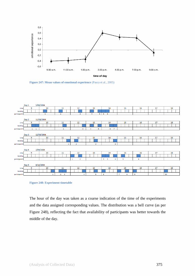
(Analysis of Collected Data) 375
Figure 247: Mean values of emotional experience (Pasca et al., 2005)
Figure 248: Experiment timetable
The hour of the day was taken as a coarse indication of the time of the experiments
and the data assigned corresponding values. The distribution was a bell curve (as per
Figure 248), reflecting the fact that availability of participants was better towards the
middle of the day.
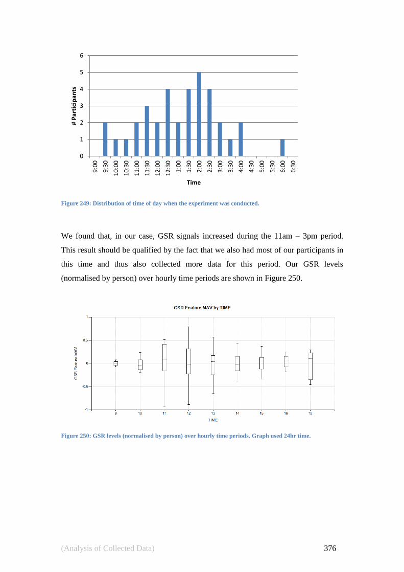
(Analysis of Collected Data) 376
Figure 249: Distribution of time of day when the experiment was conducted.
We found that, in our case, GSR signals increased during the 11am – 3pm period.
This result should be qualified by the fact that we also had most of our participants in
this time and thus also collected more data for this period. Our GSR levels
(normalised by person) over hourly time periods are shown in Figure 250.
Figure 250: GSR levels (normalised by person) over hourly time periods. Graph used 24hr time.
0
1
2
3
4
5
6
9:0
0
9:3
0
10
:00
10
:30
11
:00
11
:30
12
:00
12
:30
1:0
0
1:3
0
2:0
0
2:3
0
3:0
0
3:3
0
4:0
0
4:3
0
5:0
0
5:3
0
6:0
0
6:3
0
# P
arti
cip
ants
Time

(Analysis of Collected Data) 377
10.4 Effectiveness of the IAPS Stimuli
Our SAM score results must be investigated to see if they appear valid. This involves
a) checking that the slides were effective in eliciting emotions, and b) Discovering if
any participants were dishonest or erratic with their emotional self reports. In this
section we investigate the validity of the slides as a stimulus and in the next section
we examine the validity of the individual participants.
The Valence ratings obtained for the different slides, shown in Figure 251, strongly
followed a trend of agreement between participants. That is out of the 38 slides
shown, only 5 exhibited a state where someone found something to be pleasant when
others considered it unpleasant (or vice versa). These images which were polarised in
their appraisals included (IAPS reference number also given):
A picture of a snake (#1050);
A barking dog(#1300);
A large spider (#1200);
A towel (#7002, a neutral stimulus);
Scenic shot of a cemetery (#9000).
As it is conceivable that these stimuli may have positive or negative connotations for
many people, we see no issues with the results in terms of obviously incorrect ratings.
With only nine exceptions, the Arousal reports for the various slides had a standard
deviation of two or lower, which in previous studies, (Backs et al., 2005), (Lasaitis,
Ribeiro, & Bueno, 2008) (P. Lang et al., 2001) would be considered an effective
stimulus. Nine slides showed a higher standard deviation. These pictures were:
A boy with a bison (#2730);
Action shot of a skydiving formation (#5621);
Action shot of windsurfing in heavy surf (#5623);
Scenic shot of flowers and a lake (#5760);
Scenic shot of a lake (#5780);
Scenic shot of fireworks over a city (#5910);
An empty coffee cup (#7009);
Action shot of people in a roller coaster (#8490);
Scenic shot of a cemetery (#9000).

(Analysis of Collected Data) 378
Many of the pictures involved were either action shots, or scenic shots, which one
would expect are subject to personal taste. Most of these slides are good, but not
―excellent‖ in terms of uniformity of Arousal generated in our study. Slides 2730 and
8490 however could be classified as negative and positive stimuli that are highly
subject to personal tastes.
Figure 251: Valence ratings by slide. The slide number is the relevant IAPS ID. A Valence rating of 5 is
Neutral. Above that is “bad or negative”, below that is “good or positive”. The slides are not in the same
order they were presented to participants.
We generally found that Arousal and Dominance scores (Figure 252 & Figure 253
respectively) varied greatly by participant. This variance is also present in many
reference studies (Lang et al., 2001) but in some cases we found significant difference
to previous results.
The instances where our results varied in mean Valence scores from reference studies
would be best explained by cultural difference between Australian (location of our
experiments) and American (location of reference studies). Since the Valence portion
of the study yielded excellent results, we assumed that experimental error was not to
blame. Further evidence supporting the difference between Australians and
Americans in terms of Arousal and Dominance only has come to light in a very recent
Australian PhD thesis (Massavelli, 2010). The experiments in that study found older
Valence by Slide Number
Slide Number

(Analysis of Collected Data) 379
Australian participants showed prominent differences in Arousal and Dominance
ratings for IAPS slides. Massavelli stated:
―Older adults rated pleasant arousing pictures as less arousing and low
arousing pleasant pictures as more arousing than did younger and middle-
aged adults. Older compared to younger adults reported a higher perceived
Dominance in relation to arousing unpleasant pictures.‖ (Massavelli, 2010)
Given our group was also Australian and we had a broader age range than many
previous (American) studies e.g. (Lang et al., 2001) who used primarily first year
college students; it would seem plausible that our results should show wider variance
than the comparison studies.
Figure 252: Arousal ratings by slide. The slide number is the relevant IAPS id. An Arousal rating of 5 is
Neutral. Above that is “restful state”, below that is “exciting state”. The slides are not in the same order
they were presented to participants..
Arousal by Slide Number
Slide Number

(Analysis of Collected Data) 380
Figure 253: Dominance ratings by slide. The slide number is the relevant IAPS ID. A Dominance rating of 5
is Neutral. Above that is “in control”, below that is “awe/ not in control”. The slides are not in the same
order they were presented to participants.
In an effort to more thoroughly compare our slide results to the American reference
studies, a set of scatter plots were created comparing Arousal and Valence results. In
general the reference studies also showed the same large Arousal variances we had,
and the results were centred on the same mean. A typical case is shown in Figure 254,
and a full set is available in the appendix (see section 14.3).
Figure 254: Comparison of our SAM ratings and those of reference studies. Responses that were chosen by
more than one participant are labelled x2, x3 and so on. Male responses are in blue, female in red. A
rectangle of matching colour is drawn to represent the area around the mean bounded by one standard
deviation. The areas of one standard deviation about the mean from previous studies (P. Lang et al., 2001)
are shown in grey.
Slide Number
Dominance by Slide Number
(IAPS Slide #9401)
FIGURE REMOVED TO
COMPLIY WITH
TERMS OF USE OF THE
IAPS DATA SET.

(Analysis of Collected Data) 381
10.4.1. Example of Cultural Bias in Australian Respondents: Snake
Fear is Less Prevalent
One of the atypical results we found is shown in Figure 255. In this case the Arousal
levels for both male and female participants were significantly lower than in the
reference studies. This is an interesting case because the subject involved is a snake.
Snakes have often been studied in regards to human fear e.g. (Rimm & Briddell,
1981) (Dimberg, 1998), and often cited as a natural instinctual fear (Ohman, 2009);
though there are many counter arguments that snake fear is socially learnt. An
example of snake fear being a learnt trait was presented by Mineka, Davidson, Cook
and Keir (1984) who stated:
"Rhesus monkeys are born without snake fear. Enduring fear develops after a
few observations of another rhesus monkey taking fright at a snake . . .
Likewise, a fawn is not born with fear of a wolf, but lifelong panic is
conditioned by seeing its mother flee just once from a wolf."
In the case that snake fear is a socially learnt construct, it is possible that there is a
culturally specific response in play for this image.
Figure 255: Comparison of our SAM ratings and those of reference studies. Responses that were chosen by
more than one participant are labelled x2, x3 and so on. Male responses are in blue, female in red. A
rectangle of matching colour is drawn to represent the area around the mean bounded by one standard
deviation. The areas of one standard deviation about the mean from previous studies (P. Lang et al., 2001)
are shown in grey.
(IAPS Slide #1050)
FIGURE REMOVED TO
COMPLIY WITH
TERMS OF USE OF THE
IAPS DATA SET.

(Analysis of Collected Data) 382
10.4.2. Example of Cultural Bias in Australian Respondents: A Boy with
his Head in a Bison's Arse is Just Not Interesting
There was one slide in our study that had an extreme lack of correlation with existing
ratings from the American based IAPS studies. We will examine this slide in this
section with an argument for cultural bias.
This slide (IAPS #2070, see Figure 256) is a classical emotional stimulus where
people will have varied responses. In this case a person may:
Feel empathy for the boy;
Feel disgust at an apparently vulgar action;
Laugh at the comical situation;
Be offended by the naked person;
Be confused about what they are seeing;
Be uninterested in the topic.
It is clear that the benchmark American studies, (Lang et al., 1997), show most
participant responses had an unpleasant Valence and high Arousal. That is the
participants by and large were responding in one of the following response categories:
Feeling empathy for the boy;
Feeling disgust at an apparently vulgar action.
However in this study most responses were low Arousal (see Figure 257) indicating
that perhaps our participants were confused or unengaged by the image. The heavy
difference between our results and the results obtained in the three studies by Lang et
al., (1997) is shown in Figure 256.
The plot shown in Figure 256 is a stacked scatter graph of the results in this study as
compared to the results of the benchmark studies by Lang et al., (Lang et al., 1997).
The rectangles show a results distribution, they are centred on a mean and extend one
standard deviation either way from the mean. The grey rectangles show previous
studies, the blue and red ones show males and females (respectively) from this study.
The blue "+" is used to indicate a male response in this study and the red "o" indicates
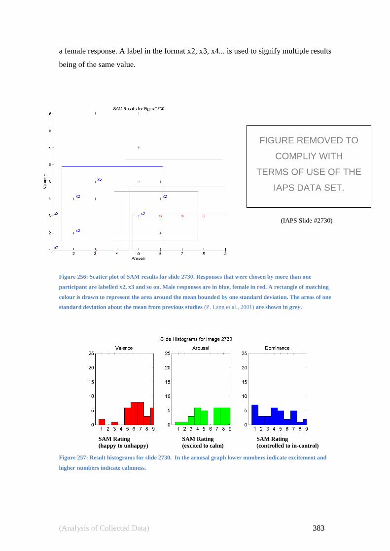
(Analysis of Collected Data) 383
a female response. A label in the format x2, x3, x4... is used to signify multiple results
being of the same value.
Figure 256: Scatter plot of SAM results for slide 2730. Responses that were chosen by more than one
participant are labelled x2, x3 and so on. Male responses are in blue, female in red. A rectangle of matching
colour is drawn to represent the area around the mean bounded by one standard deviation. The areas of one
standard deviation about the mean from previous studies (P. Lang et al., 2001) are shown in grey.
Figure 257: Result histograms for slide 2730. In the arousal graph lower numbers indicate excitement and
higher numbers indicate calmness.
SAM Rating SAM Rating SAM Rating
(happy to unhappy) (excited to calm) (controlled to in-control)
(IAPS Slide #2730)
FIGURE REMOVED TO
COMPLIY WITH
TERMS OF USE OF THE
IAPS DATA SET.

(Analysis of Collected Data) 384
It is not entirely clear why the participants of this study, and perhaps Australians as a
whole, are unconcerned with this image. A viable explanation would seem to lie in a
possible general desensitisation to the misfortunes of cattle. At the time of the
experiments, much of Australia's cattle country was three years into drought and it
was not uncommon for news programs to feature images of starving, dehydrated and
dead cattle.
10.5 Participant Self Assessment Responses
To assess the reliability of individual participants' SAM results, each participant was
compared against known mean results. To do this a set of histograms was created to
show how often a participant responded within a certain number of standard
deviations from the study‘s mean evaluation for each slide. These histograms are
available in appendix 14.2 and an example is given in Figure 258.
Figure 258: Example result histogram (for Participant 2, on day 1).
If our participants responded to the stimulus in a similar way to the reference studies,
then the histograms should look similar to normal distributions, with the peak at zero
and most data within two standard deviations of zero. The majority of data collected
follows this trend. However some results do not, which may indicate that the
participant:
Does not have ―statistically normal‖ emotional responses (which is not at all
unusual);
SAM Rating SAM Rating SAM Rating
(happy to unhappy) (excited to calm) (controlled to in-control)

(Analysis of Collected Data) 385
Has a cultural bias which causes him/her to react differently to the reference
studies (which were conducted in a different country);
The participant was not completing the survey properly.
We divided the histograms into nine categories as shown in Table 3.
Table 3: SAM results problems
Type Example Type Example
1&2)
Good or OK
(when the mean = 0
and most values lie in
the range -2 to 2)
5)
Inverted
(values lie in the
range -2 to 2 but
favour the
extremity)
3)
Non correlating
Female (NCF).
6 & 7)
Results skewed
left or right
4) Poor distribution of
results.
8 & 9)
Results uniformly
higher or lower
Tabulating these results gave us Table 17. As can be seen, the females in our
experiment tended not to correlate with previous results. As this non-correlation was a
consistent phenomenon we came to the conclusion that it is due to cultural bias, not
the result of all females answering questions poorly or dishonestly.

(Analysis of Collected Data) 386
Table 17: Categorisation of participant responses. Table values are in the form (day)/(nth participant for
the day). Females are shown in blue.
Good Ok Poor Inverted NCF Skewed Left
Skewed Right
Low Mean
High Mean
Valence 1/01 1/04 1/06 3/01 4/02
1/02 2/01 3/03 5/01
1/03 2/03 3/04 5/05
1/05 2/04 4/01 5/07
2/02 4/04 4/03
2/05 5/02 5/09
2/06 5/03
2/07
2/08
3/02
4/05
5/04
5/06
5/08
Total 14 7 6 0 4 1 0 0 0
Arousal 1/02 2/02 1/06 3/01 2/04 5/02 4/02 2/08
1/03 2/03 2/01 5/01 3/02 5/03 2/07
1/04 2/06 3/04 5/05 4/03 1/01
1/05 5/06 4/01
2/05 5/07 5/09
3/03
4/04
4/05
5/04
5/08
Total 10 5 5 0 3 3 2 3 1
Dominance 1/01 1/04 2/02 5/08 3/01 2/04 1/06 2/03
1/02 2/06 4/01 5/01 3/02 2/05 4/02
1/03 2/07 5/09 5/05 4/03 4/04 5/03
105 208 5/08 506
201 304 507
303 502
405
504
total 8 6 3 1 5 3 0 3 3
For convenience Table 17 was also broken down into pie charts, Figure 259. The
results echo what we found in the previous section when examining the IAPS stimuli;
that is that Arousal has been fairly consistent across studies, but the Arousal and
Dominance ratings are subject to a high degree of variance.

(Analysis of Collected Data) 387
Figure 259: Table 17 displayed as a set of pie charts. The red zone indicates areas where our participants‟
results did not correlate with results obtained from previous studies. This could be due to significant
cultural differences, errors in reporting feedback, other intangible aspects affecting the emotions of
participants, or more extreme natural variance in emotional response.
44%
22%
19% 0%
12%
3%
0%
0%
0%
22%
SAM Results (Valence) by Distribution
Good
Ok
Poor
Inverted
NCF
Skewed Left
Skewed Right
Low Mean
31%
16%
16%
0%
10%
9% 6%
9%
3%
43%
SAM Results (Arousal) by Distribution
Good
Ok
Poor
Inverted
NCF
Skewed Left
Skewed Right
Low Mean
25%
19%
10%
3%
16%
9%
0%
9%
9%
40%
SAM Results (Dominance) by Distribution
Good
Ok
Poor
Inverted
NCF
Skewed Left
Skewed Right
Low Mean

(Analysis of Collected Data) 388
10.5.1. Summary of Effectiveness of Stimuli
People will react differently to the same stimuli. Much research has been done into
looking at "normal" responses to IAPS stimuli in various countries e.g. (Porto, 2005),
(Lasaitis et al., 2008), (Moltó, Montañés, & Poy, 1999), (Verschuere, 2001),
(Verschuere, 2007), (Deák, Csenki, & Révész, 2010) and many deviations from
standard slide response was shown; however the IAPS slides have still been shown to
be valid stimulus tools (will reliably generate emotions) in all circumstances.
At the time these experiments were conducted, there existed no comprehensive listing
of IAPS norms for Australian participants, so some slides were logically rejected for
use in the study if they appeared to be heavily culturally biased. For example content
involving American Flags and US Dollars was excluded.
What is clear is that a variety of emotional results were definitely elicited. It is
expected that there will be variation in how people respond to a stimulus, which is
why the self assessment of emotion is used for training purposes, not the nature of the
stimulus. The results in this section show that our slide selection did an acceptable job
of eliciting a broad range of emotions, and that in general the selection was
appropriate for use in Australian culture.
As the self-assessment feedback is our only information about how a person
responded emotionally, it is vital to know that these reading were accurate. Our major
test in this regard is comparison with previous studies. We have found good
correlation with previous works, and have a common internal bias which correlates
with other Australian based studies.

(Analysis of Collected Data) 389
10.6 Visualising Results Obtained from Physiological
Recordings
This work posed some interesting data visualisation problems. In this section we use
data visualisation techniques to gain insight into our data via a process of ‗visual
characterisation‘. As it is not easy to compare many histograms or related data sets in
one figure, we have invented something we call a "shotgun plot". An example of a
shotgun plot is shown in Figure 260.
Figure 260: Example shotgun plot. The plot is broken up into discrete bins; in this case nine bins are
present. The nine bins are one each for the nine areas the data has been grouped into. The nine bins are
organised according to two sets of three labels which represent, in this case, the affective dimensions of
Arousal (SAMA_0...SAMA_2) and Valence (SAMV_0...SAMV_2). Thus data in the three bins to the left of
the graph is negative Valence (SAMV_0). Likewise data in the three bins along the top of the graph are
related to positive Arousal (SAMV_2).
The colouring of the graph is the key mechanism through which it communicates
information. Data items are given a colour to match their value (using the "rainbow"
palate of the visible spectrum) and then plotted randomly in their bin area with a bias
towards the middle (as if sprayed from a shotgun).

(Analysis of Collected Data) 390
10.6.1. Visualising the Role of Respiration
One of the major features which continuously appeared in feature selection tasks (of
heterogeneous groups) was the novel curve metric discussed in section 9.4; in
particular the curve metric for the exhalation curve. We found that results of this
metric which were of greater magnitude were linked to emotional states with a higher
Dominance rating. This correlation is shown in Figure 261. Respiration is often linked
to frustration levels (Haruki et al., 2001); which makes a correlation we observed
between Dominance and respiration seem plausible.
Figure 261: Exhalation curve metric for three levels of Dominance. The mean is almost constant, however
the distribution of values decreases as the results move from excited (SAMD_0) to calm (SAMD_2).
Another metric ―Respiration peak height from last valley" is a measurement of the
amount of air intake or expulsion during the last discrete chest movement. Some
results from this metric, for a typical participant, are shown in Figure 262.
Figure 262: “Respiration peak height from last valley” metric plotted against Valence and Arousal.
Respiration peak height from last valley
sam
Cla
ssA
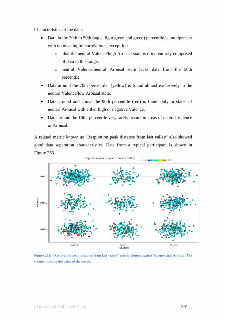
(Analysis of Collected Data) 391
Characteristics of the data:
Data in the 20th to 50th (aqua, light green and green) percentile is omnipresent
with no meaningful correlations; except for:
o that the neutral Valence/high Arousal state is often entirely comprised
of data in this range;
o neutral Valence/neutral Arousal state lacks data from the 50th
percentile.
Data around the 70th percentile (yellow) is found almost exclusively in the
neutral Valence/low Arousal state.
Data around and above the 90th percentile (red) is found only in states of
neutarl Arousal with either high or negative Valence.
Data around the 10th percentile very rarely occurs in areas of neutral Valence
or Arousal.
A related metric known as "Respiration peak distance from last valley" also showed
good data separation characteristics. Data from a typical participant is shown in
Figure 263.
Figure 263: “Respiration peak distance from last valley” metric plotted against Valence and Arousal. The
colours indicate the value of the metric.
Respiration peak distance from last valley

(Analysis of Collected Data) 392
This metric measures the duration of the last chest movement. It shows that:
Longer (lasting) chest movements are typically present in both the low
Arousal/negative Valence states and the high Arousal/positive Valence.
However the same states also hold a large amount of data across the full
spectrum and are not typified by such values.
The negative Valence/high Arousal state lacks the longer chest movements.
Many (other) states lack extreme chest movements.
10.6.2. Visualising EMG correlations
EMG is a logical candidate for discrimination of output, however in the case of person
heterogeneous datasets, the (normalised) EMG reading does not clearly distinguish
any emotional state. This may be due to:
Crosstalk from nearby muscles;
Per person uniqueness of facial expression;
Per person differences in type of signal obtained.
Figure 264 shows a scatter plot of two typical EMG features and their ability to only
very roughly categorise affective Valence states.
Figure 264: Scatter plot of typical EMG features and their ability to roughly categorise affective Valence
states (shown in colour, blue = negative Valence, through green = neutral and red = positive). It is important
to note that the graph shows heterogeneous data from multiple people. A general trend is evident in that
neutral emotions yielded results lower and central to the shape of the plot.

(Analysis of Collected Data) 393
The uniqueness of signals collected per person is a major factor in using EMG data.
While on some people a correlation can be very strong, on others there is little
correlation as per Figure 265.
Figure 265: EMG data by Person arranged in a “waterfall”. The colour reflects Valence reported for the
reading. Some participants (e.g. # 6) have EMG readings that are affected by the Valence of the stimulus;
while others (e.g. #25) do not.
10.6.3. Visualising the Difficulties of Heterogeneous Classification
Tasks
As will be discussed in the next chapter, PPR classification against homogenous data
sets generally yielded results with 60% to 80% classification success. Finding a
solution to heterogeneous data classification is a difficult task. An excellent emotion
discriminator for homogenous data in this study is a galvanic skin response (GSR)
signal known as "GSR Variance". Figure 266 shows how it achieves an
extraordinarily good separation of the Valence of an emotion on a per person basis.
However there is little to no similarity in the responses shown between people. They
are extremely unique to various individuals.

(Analysis of Collected Data) 394
Figure 266: GSR Variance by person, coloured by Valence.
10.6.4. Visualising Time as a Factor in Obscuring Emotional Response
As would be expected, many signals are strongly correlated with emotion while the
stimulus is present and fall off after the stimulus is removed. An example of this is
shown in Figure 267.
Figure 267: Falloff of ECG signal metric. The grey area is the time in the stimulus and the white was
recorded during rating tasks. The points shown are sampled randomly from all participants. The colour
coding shows the results of the Arousal rating.
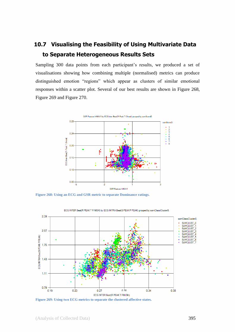
(Analysis of Collected Data) 395
10.7 Visualising the Feasibility of Using Multivariate Data
to Separate Heterogeneous Results Sets
Sampling 300 data points from each participant‘s results, we produced a set of
visualisations showing how combining multiple (normalised) metrics can produce
distinguished emotion ―regions‖ which appear as clusters of similar emotional
responses within a scatter plot. Several of our best results are shown in Figure 268,
Figure 269 and Figure 270.
Figure 268: Using an ECG and GSR metric to separate Dominance ratings.
Figure 269: Using two ECG metrics to separate the clustered affective states.

(Analysis of Collected Data) 396
Figure 270: Using BVP and GSR Metrics to separate Arousal responses.
10.8 Sampling of Data for Classification
The sample data has an unbalanced number of samples for different classes. This can
cause problems for training classifiers as biasing results towards the largest class often
results in limited classifier performance (Tang, Zhang, Chawla, & Krasser, 2009). To
address this problem of imbalance, we are adopting a technique of random under-
sampling which has been empirically shown to be one of the most effective re-
sampling methods for this type of problem (Yun-chung, 2004).
The process of random under-sampling balances the training data by randomly
eliminating majority class samples until the ratio between the minority and majority
classes reach a more desirable level. More details on the sub-sampling used are given
in the next chapter.
10.9 A Feature Selection Investigation
As an initial step to learn something about the data, we investigated the broadest set of
features that can be explored for feature extraction. This included a few extra
informative signals which were incorporated to test the nature of the data being
investigated.

(Analysis of Collected Data) 397
These signals were:
FEED_BACK_TIME_TO_RATE - The total time for the related SAM rating
task to be completed;
IN_IAPS_RATING_SCREEN - high if the user is in a rating screen, identifies
the after stimulus portion of the data;
FEED_BACK_LONGEST_KEY_DELAY - The longest pause between two
consecutive key presses during the SAM rating task;
INITIAL HESITATION - The time after the stimulus that is spent "reflecting"
before the user begins the SAM rating task;
TIME_SINCE_LAST_BUTTON - The time since the last button press during
the SAM rating task.
These signals do not make sense as training data as they are not within the scope of
our investigation. In this section we present which of these bits of information are
selected by our feature selection process, under which condition. We then explain
what this reveals in our data.
Forward feature selection via a Naive Bayes Classifier (FFS_NB) was configured for
up to 20 features to be selected. The algorithm was set to stop early if after five
rounds an improvement of 0.0025% was not made. The selection task was attempted
for each type of label to see if any significant feature related more to a different
labelling system. The algorithm‘s behaviour is plotted as a performance curve in a
series of graphs beginning with Figure 271. The plots show the current iteration
against the achieved performance metric, and is coloured by the number of attributes
being examined.
Figure 271 plots the progress of the Forward Feature Selection (FFS) algorithm in
refining a feature subset. A series of training arcs are present as each increase in the
size of feature set (p) results in a renewed search for a good parameter set. This
implies that, for the Naive Bayes Classifier, the set found is likely to worsen
dramatically if features present are altered slightly. Local optima are seen for p = 4, 6
and 13. After p = 13 the system stabilises, indicating additional features are unlikely
to be of benefit.

(Analysis of Collected Data) 398
Figure 271: FFS_NB training with meta data (dead-zone = 1). Local jumps in performance are seen for p =
4, 6 and 13. After p = 13 the system stabilises, indicating additional features are unlikely to be of benefit.
The results are coloured by p as a “rainbow” spectrum over the values of p examined.
Figure 272 shows FFS performance for a dead-zone of 3 in the grid based labelling
system. Again, a series of training arcs are present at each increase of p implying
high sensitivity to choice of features. Local optima are seen for p = 7 and 15. As p
approaches 20 the system continues to grow indicating more features need to be
examined.
Figure 272: FFS_NB training with meta data (dead-zone = 2). Local jumps in performance are seen for p =
7 and 15. As p approaches 20 the system continues to grow indicating more features need to be examined.
Figure 273 shows FFS performance for a dead-zone of 5 in the grid based labelling
system. Again, a series of training arcs are present at each increase of p implying high
sensitivity to choice of features. Local optima are seen for p = 4, 6 and 13. As p

(Analysis of Collected Data) 399
approaches 20 the system loses any upward trend indicating sufficient features have
been examined.
Figure 273: FFS_NB training with meta data (dead-zone = 5). Local jumps in performance are seen for p =
4, 6 and 13. As p approaches 20 the system peaks indicating sufficient features have been examined.
Figure 274 shows FFS performance for a dead-zone of 3 in the grid based labelling
system. Again, a series of training arcs are present at each increase of p implying
high sensitivity to the choice of features. Local optima are seen for p = 5 and 15. As p
approaches 20 the system continues to grow indicating more features need to be
examined.
Figure 274: FFS_NB training with meta data (group based labels). Local jumps in performance are seen for
p = 5 and 15. As p approaches 20 the system continues to grow indicating more features need to be
examined.

(Analysis of Collected Data) 400
Table 18 shows the results of the feature selection task (FFS_NB). Difference features
are shown in italic (and coloured blue), meta-features in bold (and coloured red) and
the amount of reoccurrences between different labelling systems tabulated in the next
column. The prominent and most frequently occurring attribute is the meta-feature
FEED_BACK_TIME_TO_RATE. This suggests there was a strong correlation
between the time with which a person can complete a rating task and the type of
emotion they are feeling. This could suggest a possible further research direction into
the speed of user interaction as a factor in emotion detection. The other note is that the
feature EMG_FEATURE_WAMP appeared twice in the selection process.
Forward feature selection via a random forest classifier (FFS_RF) was run for 30,000
iterations allowing for up to 20 features to be selected. The algorithm was set to stop
early if after five rounds an improvement of 0.0025% was not made. Figure 275 plots
the progress of the algorithm in refining a feature subset. Jumps in performance are
evident for different sizes of feature sets (p), and as expected the jumps are smaller as
p increases. Notable significant improvements are found for p = 2, 3 and 5.
Figure 275: FFS_RF performance. Jumps in performance are evident for different sizes of feature sets (p),
and as expected, the jumps are smaller as p increases. Notable significant improvements are found for p = 2,
3 and 5.

(Analysis of Collected Data) 401
Table 18: Forward Feature Selection (FFS_NB) results
samClassDZ1Div9 # samClassDZ3Div9 #
EKG_INTER_BEET(P_FINISH_T_FINISH)_diff_8 BVP_PEAKSLOPEAFTERBYAREAUNDERCURVE_diff_4
EKG_INTER_BEET(P_ONSET_R_PEAK)_NARF_diff_1 EKG_INTER_BEET(P_PEAK_R_PEAK)_diff_3
EKG_INTER_BEET(R_PEAK_T_FINISH)_NARF EKG_INTER_BEET(Q_ONSET_T_PEAK)_diff_8
EKG_INTRA_BEET(P_ONSET_P_ONSET)_NARF_diff_5 EKG_INTER_BEET(Q_PEAK_T_ONSET)_diff_0
EKG_INTRA_BEET(S_FINISH_Q_ONSET) EKG_INTER_BEET(R_PEAK_T_ONSET)_diff_4
EKG_INTRA_BEET(S_PEAK_S_FINISH)_diff_0 EKG_INTRA_BEET(Q_ONSET_P_FINISH)_diff_9
EKG_INTRA_BEET(T_FINISH_P_FINISH)_NARF EKG_INTRA_BEET(Q_ONSET_T_PEAK)_NARF
EKG_INTRA_BEET(T_FINISH_Q_PEAK)_NARF EKG_INTRA_BEET(R_PEAK_P_PEAK)_NARF_diff_3
EKG_INTRA_BEET(T_ONSET_Q_ONSET)_NARF_diff_9 EKG_INTRA_BEET(R_PEAK_S_FINISH)_diff_6
EMG_FEATURE_ARV_10_diff_9 EKG_INTRA_BEET(R_PEAK_T_FINISH)
EMG_FEATURE_ARV_9_diff_8 EKG_INTRA_BEET(R_PEAK_T_ONSET)_diff_4
EMG_FEATURE_WAMP 2 EKG_INTRA_BEET(T_ONSET_P_PEAK)_NARF_diff_5
FEED_BACK_TIME_TO_RATE 4 EKG_QT_F_diff_0
GSR_FEATURE_IGSR EMG_FEATURE_ARV_5_diff_6
RESP_PEAKSLOPEBEFOREBYAREAUNDERCURVE_diff_2 EMG_FEATURE_MAV
TEMP_CORECT_FROM_REST_MAV_diff_4 EMG_FEATURE_WAMP 2
FEED_BACK_TIME_TO_RATE 4
GSR_FEATURE_SSI
RESP_PEAKSLOPEAFTERBYAREAUNDERCURVE
RESP_PEAKSLOPEBEFOREBYAREAUNDERCURVE_diff_7
samClassDZ5Div9 # samClassCluster8 #
EKG_INTRA_BEET(P_ONSET_S_PEAK)_diff_4 EKG_INTER_BEET(P_FINISH_Q_ONSET)_NARF_diff_9
EKG_INTRA_BEET(S_PEAK_Q_ONSET) EKG_INTER_BEET(P_PEAK_T_ONSET)_diff_5
EKG_INTRA_BEET(S_PEAK_R_PEAK) EKG_INTER_BEET(Q_ONSET_T_ONSET)_diff_6
EKG_INTRA_BEET(T_PEAK_Q_ONSET) EKG_INTER_BEET(R_PEAK_S_PEAK)_diff_2
EKG_QT_C_diff_9 EKG_INTER_BEET(R_PEAK_S_PEAK)_diff_9
EMG_FEATURE_ARV_1 EKG_INTER_BEET(S_PEAK_S_FINISH)
FEED_BACK_TIME_TO_RATE 4 EKG_INTER_BEET(S_PEAK_T_PEAK)_diff_4
EKG_INTER_BEET(T_ONSET_T_FINISH)_diff_2
EKG_INTRA_BEET(P_FINISH_R_PEAK)_NARF_diff_7
EKG_INTRA_BEET(P_ONSET_T_FINISH)
EKG_INTRA_BEET(Q_ONSET_T_FINISH)_NARF_diff_7
EKG_INTRA_BEET(Q_ONSET_T_FINISH)_diff_1
EKG_INTRA_BEET(R_PEAK_T_ONSET)_NARF_diff_7
EKG_INTRA_BEET(S_PEAK_P_PEAK)_diff_7
EKG_INTRA_BEET(T_FINISH_T_PEAK)_diff_8
EKG_INTRA_BEET(T_ONSET_S_PEAK)_diff_9
FEED_BACK_TIME_TO_RATE 4
GSR_FEATURE_MMAV1
TEMP_BL_SMOOTHED_MAV_diff_0

(Analysis of Collected Data) 402
Given FEED_BACK_TIME_TO_RATE has occurred with a high enough prevalence
to suggest it has a significant role, it was removed from the test set to see if any other
descriptive features might occur under feature selection tasks. The experiments were
re-run and no extra features were selected.
Another round of feature selection experiments was conducted along the same lines as
the preliminary experiments shown so far, but this time the difference based features
were removed. The forward feature selection using Naive Bayes classifier for grid
labels produced one extra descriptive feature, IN_IAPS_RATING_SCREEN. The set
produced was:
BVP_PEAK_HEIGHT_FROM_NEXT_VALLEY;
EKG_INTRA_BEET(P_PEAK_T_PEAK);
EKG_INTRA_BEET (T_FINISH_S_PEAK);
EMG_FEATURE_ARV_1;
EMG_FEATURE_VAR;
FEED_BACK_TIME_TO_RATE;
GSR_FEATURE_SSI;
IN_IAPS_RATING_SCREEN;
RESP_PEAK_SLOPE_AFTER_BY_AREA_UNDER_CURVE.
The presence of FEED_BACK_TIME_TO_RATE most likely indicates that some
states cause people to perform the rating task in a quicker or slower manner. This may
have something to do with particular emotional states being clearer (thus quicker to
describe), or other states may promote or inhibit general speeds of task completion.
However such possibilities are not of concern in the feature extraction process.
The presence of IN_IAPS_RATING_SCREEN correlates with other informal
investigations and related data analysis in the next two chapters. The implication is
that there is a good case for treating data collected during the stimulus and after the
stimulus in a separate manner.

(Analysis of Collected Data) 403
10.10 Conclusion
This chapter began by examining how we would group our SAM ratings into discrete
emotional states. Two methods were examined. One divided the emotional states into
a grid which could easily be queried by software with questions like ―did the user find
this to be pleasant?‖. The second removed all a-priori knowledge of the emotion space
and performed a grouping based on statistical properties of the ratings. We will
examine which of these is the better solution in the next chapter.
In the next part(s) of this chapter we demonstrated the effectiveness of the IAPS
stimuli in stimulating human emotion and we established that for the most part our
participants reacted to the stimulus in a manner predicted by previous works. We
found some slides which did not gain the reactions as were expected from previous
studies and found that these slides were all of similar theme(s). We proposed that the
differences we discovered were due to a cultural bias in our work which is both an
expected and normal outcome. We then examined a few case studies of slides for
which the effect was most extreme.
We then presented some visualisations and graphs of various trends we observed in
our physiological recordings. This was done for two reasons:
Verifying that expected correlations were present;
Determining if any of the new metrics we created revealed any new
information.
In this respect we found that the expected trends were present and one of our new
metrics (the novel curve metric discussed in 9.4) did show some correlation with
Dominance ratings. This is an important finding because Dominance is traditionally
one of the more difficult ratings to find correlations with.
Lastly we performed feature selection task on all the data in order to find a good
subset of features to use in the classification tasks which is the focus of the next
chapter.

(Analysis of Collected Data) 404

(Classification of Data) 405
11.0 Classification of Data
"Try to learn something about everything and everything about something."
- Thomas Henry Huxley (1825-1895)

(Classification of Data) 406
In this chapter we wish to answer the following four questions:
1. Of the candidate classifiers, which best performs this task?
2. Which features should be used for classification purposes?
3. How does the performance of classifiers vary for our different types of class
labels?
4. How does the performance of classifiers vary across participants?
A primary question in determining the performance of our physiological pattern
recognition system is number 1 (―Of the candidate classifiers, which best performs
this task?‖). We investigated five different classifiers and determined which of these
best suits our needs. The classifiers examined were:
The random forest classifier;
The naïve Bayes classifier;
The artificial neural network;
The k nearest neighbour classifier;
The support vector machine.
As the results in this chapter show, the random forest classifier proved the most
accurate, and the cluster based labelling system also proved to be superior over the
grid based label system. Hence question 4 was examined using random forests trained
with cluster based labels.
Searching for comparable works to compare our results against, we required works
with similar amounts of (weakly induced) emotional states, also conducted on
multiple participants (at least 10). These requirements, analysed in the literature
review, gave us the studies to which this portion of the work is most applicable,
namely:
Nasoz et al., (Nasoz, Alvarez, Lisetti, & Finkelstien, 2003);
o 24 participants, 6 emotional states, 69% accuracy.
Takahashi (Takahashi, 2004);
o 12 participants, 6 emotional states, 42% accuracy.
Lisetti & Nasoz (Lisetti & Nasoz, 2004).
o 29 participants, 6 emotional states, 84% accuracy.

(Classification of Data) 407
In comparison, our highest classification accuracy (detailed later in this chapter) is
59.96% for grid based labels and 64.43% for cluster based labels.
Our work faces a task more difficult than that of these studies as we are attempting to
differentiate between 8 and 9 emotional states, however, despite this, our results
appear to be in the middle range of the performances obtained by the other available
studies.
We begin this chapter with the results of our investigation into which features should
be used for training purposes.
11.1 Which features should be used?
This research, like many other studies, has produced a very large number of features.
Not all of the features will be relevant to the emotional phenomena being studied and
many will correlate significantly, causing redundancies.
We wish to establish a small set of primary features which can be used. This is
achieved by eliminating features with little or no predictive information and removing
redundant features which are highly correlated to other more useful features. This
process of feature selection should give us the following benefits:
Allow for classifier models which have increased accuracy and should
generalise better to unseen points (prevent classifiers from over fitting the
data);
Increase the computational efficiency of the resulting classifiers;
Improve the comprehensibility of the resulting classifiers.
Further, finding the correct subset of predictive features is an important research
question in its own right as it may reveal new information regarding physiological
responses associated with various emotional states.
There are two major approaches used to reduce the dimensionality of data sets,
feature selection and feature extraction (Guyon & Elisseeff, 2003). Feature selection
techniques attempt to find a representative subset of the original features. Feature
extraction techniques attempt to transform the highly dimensional feature base into a

(Classification of Data) 408
set of features of fewer dimensions. Feature selection can be broken down into two
major approaches, feature ranking and subset selection.
Many common feature extraction techniques used in physiological pattern recognition
are reviewed by Fodor (Fodor, 2002).
Table 19: survey of dimensionality reduction techniques in affective signal processing.
Ref P # Emotional
States
Sample Hz Signals #
Features
Reduction
Algorithm
Classifier Classification
Accuracy
(Yannakakis &
Hallam, 2008)
72 2 (detect fun) 256Hz HR, BVP,
SC
20 ANOVA SVM,
MLP
70%
(Leon & Clarke,
2007)
8 3
(heterogeneous)
? ?/GSR 5 DBI AANN 71%
(Healey & Picard,
2005)
9 3 (levels of
stress)
496Hz (ECG),
31Hz (GSR, RS),
15.5Hz (EMG)
ECG, EMG,
GSR, RS
22 Fisher LDA 97%
(Kim & Ande, 2008) 3 4 256Hz(ECG),
32Hz otherwise
ECG, EMG,
RS, GSR
110 SBS LDA,
EMDC
70/95%
(Picard, Vyzas, &
Healey, 2001)
1 8 20Hz EMG, BVP,
GSR RS
40 SFS, Fisher LDA 81%
(Scheirer,
Fernandez, Klein, &
Picard, 2002)
24 2 (detect
fustration)
20Hz EMG, BVP,
GSR
5 Viterbi HMM 64%
We do not know yet which label system we wish to apply from the two best
candidates discovered in Section 10.1. As such we will perform feature selection for
both the grid and the cluster labels. These two label systems will henceforth be
referred to as grid and cluster based labels respectively.
Forward feature selection (see Section 2.5.1) via a Naive Bayes Classifier (FFS_NB)
was configured for up to 30 features to be selected. Given the size of our dataset, this
feature selection method was chosen for its time complexity in relation to the number
of features being examined. The algorithm was set to stop early if after five rounds an
improvement of 0.0025% was not made. The selection task was repeated for each type
of label to see if any significant feature related more to a different labelling system.
The algorithm‘s behaviour is plotted as a performance curve in a series of graphs,
Figure 276 and Figure 277. The plots show the current iteration against the achieved
performance metric, and are coloured by the number of attributes being examined.

(Classification of Data) 409
Figure 276: Forward feature selection (FFS) results obtained using a naive Bayes classifier on the grid based
labels (samClassDZ3Div9). Each point represents the performance of a unique subset of features as tested in
the FFS algorithm. The X axis represents the number of iterations the FFS algorithm has passed through.
Figure 277: Forward feature selection (FFS) results obtained using a naive Bayes classifier on the cluster
based Labels (samClassCluster8). Each point represents the performance of a unique subset of features as
tested in the FFS algorithm. The X axis represents the number of iterations the FFS algorithm has passed
through.
The resulting feature selection sets are shown in Table 20. Notably the 8 category
grouped labels reached an optimal feature set with fewer features (n=11) than the 9
way grid divided data (n=21). The difference values appeared often under the

(Classification of Data) 410
selection procedure, most commonly for ECG data. Both sets used EMG, ECG and
GSR; however the 9 way grid divided data used respiration and temperature data as
well.
Table 20: Results of feature selection for grid and cluster based Labels. The cluster based label system
required 11 features before no significant improvement was found, while the grid based system required 21
features.
Grid based Labels Cluster Based Labels
EKG_INTER_BEET(R_PEAK_S_FINISH) EKG_INTRA_BEET(P_ONSET_P_PEAK)
EKG_INTRA_BEET(T_ONSET_P_PEAK) EMG_FEATURE_SSC
RESP_PEAKHEIGHTFROMNEXTVALLEY GSR_FEATURE_RMS
EMG_FEATURE_ARV_10 EKG_INTRA_BEET(P_ONSET_S_PEAK)_NARF
EKG_INTER_BEET(P_FINISH_T_ONSET)_diff_9 EKG_INTRA_BEET(P_PEAK_Q_PEAK)_NARF
EKG_INTER_BEET(Q_ONSET_T_PEAK)_diff_8 EKG_INTER_BEET(R_PEAK_T_FINISH)_diff_2
EKG_INTRA_BEET(S_PEAK_R_PEAK)_diff_9 EKG_INTRA_BEET(Q_ONSET_S_FINISH)_diff_6
EKG_INTRA_BEET(S_PEAK_T_PEAK)_diff_8 EKG_INTRA_BEET(S_FINISH_S_PEAK)_diff_5
RESP_PEAKHEIGHTFROMNEXTVALLEY_diff_9 EKG_INTRA_BEET(S_PEAK_T_FINISH)_diff_6
RESP_PEAKWIDTH_diff_0 EKG_INTRA_BEET(S_PEAK_T_FINISH)_diff_8
RESP_DISTANCETILLNEXTPEAK_diff_0 EKG_INTRA_BEET(S_PEAK_R_PEAK)_NARF_diff_9
EMG_FEATURE_ZC_diff_6 EMG_FEATURE_ZC_diff_7 TEMP_CORECT_FROM_REST_MAV_diff_3 EKG_INTRA_BEET(P_FINISH_Q_PEAK)_NARF_diff_0 EKG_INTRA_BEET(P_FINISH_T_FINISH)_NARF_diff_4 EKG_INTRA_BEET(P_FINISH_T_PEAK)_NARF_diff_9 EKG_INTRA_BEET(P_PEAK_P_PEAK)_NARF_diff_5 EKG_INTRA_BEET(R_PEAK_S_PEAK)_NARF_diff_9 EKG_INTRA_BEET(S_PEAK_T_ONSET)_NARF_diff_3 EKG_INTRA_BEET(T_ONSET_S_PEAK)_NARF_diff_3
The features that were selected are not surprising. They span EKG, EMG & GSR
data, which would be a logical necessity given the emotional links discussed in the
literature review. We used a heterogeneous data set for the feature selection task, as
we wished to discover features of common applicability to multiple people. In the
next section we investigate how these features perform when used to train classifiers
in a homogeneous environment.

(Classification of Data) 411
11.2 How does the performance of classifiers vary for our
different types of class labels?
We wish to compare the grid and the cluster based labelling systems and choose
which one will be the system used for the rest of our comparative experiments.
The grid based labelling is a very logical system as we can easily query it with
questions like ―was that a good feeling?‖, ―did the person have a significant reaction
to the stimulus?‖. Such information could be useful to entertainment systems
modifying content in real time to suit a user‘s emotional reactions. On the other hand
our k-means based division of the data (group based labels) is a less useful metric
from an analysis point of view, but it does encapsulate more information in fewer
bins.
The previously identified features were extracted from the heterogeneous set of all our
participants‘ data. The results shown in the previous section are therefore
heterogeneous in nature and not indicative of the performance which can be expected
when a classifier is trained to identify the emotion of only one person (the
homogenous case). As an initial test, we performed an exercise in tuning a random
forest classifier (our strongest classifier) for our individual participants using both grid
and cluster based labels. A scatter plot of the results is shown in Figure 278. Our
findings were that cluster based labels performed the strongest most frequently; giving
a more accurate classification 73% of the time, or being equal for 9% of cases.
We repeated the test using a different classifier, the Support Vector Machine (SVM).
The SVM was run in several configurations with varying degree of success, but the
choice of label continuously proved to be a major factor in the final performance. A
scatter plot of the results is shown in Figure 279. The cluster based labels were
superior 68% of the time, and roughly equal 9% of the time.
The cluster based labels are often superior and require fewer features to train the
classifier which makes them an obvious preferred choice. Additionally the cluster

(Classification of Data) 412
labels include Dominance information, which is important to our research goals.
However the non-intuitive nature of the results might limit the practical use of the
labelling system. For this reason we shall continue to compare between the two
labelling systems through this chapter and the next.
Figure 278: Performance over all participants of a series of random forest classification tasks. Note: grid
labels are in blue and cluster labels are red.
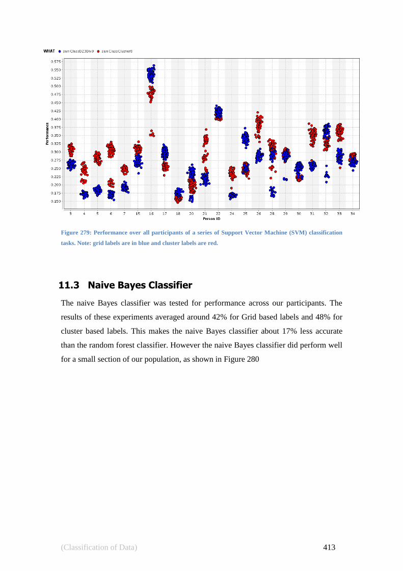
(Classification of Data) 413
Figure 279: Performance over all participants of a series of Support Vector Machine (SVM) classification
tasks. Note: grid labels are in blue and cluster labels are red.
11.3 Naive Bayes Classifier
The naive Bayes classifier was tested for performance across our participants. The
results of these experiments averaged around 42% for Grid based labels and 48% for
cluster based labels. This makes the naive Bayes classifier about 17% less accurate
than the random forest classifier. However the naive Bayes classifier did perform well
for a small section of our population, as shown in Figure 280

(Classification of Data) 414
Figure 280: Performance of naive Bayes classifiers.
Confusion matrices for both label schemes are shown in Figure 281 and Figure 282.
The classifier for the grid based classification scheme had poor results in predicting an
emotion (PPV = 32% to 58%) but is an excellent tool for establishing if someone is
not in a given emotion (NPV = 87% to 97%, α = 3% to 10%). The state of being in
negative Valence with low Arousal stands out as being the easiest to predict (PPV =
58%). These results were significantly higher than chance guessing (11%).
The classifier for the cluster based classification scheme had adequate results in
predicting an emotion (PPV = 42% to 54%) and, like the grid labels, is also an
excellent tool for establishing if someone is not in a given emotion (NPV = 87% to
97%, α = 3% to 10%). Clusters 2 and 5 stand out as being the easiest to predict (PPV
= 51% to 54%) and are shown in Figure 283.
0
1
2
3
4
5
6
7
0% 10% 20% 30% 40% 50% 60% 70% 80% 90%
Fre
qu
en
cy
Accuracy
Performance by Label Type (NB)
Cluster
Grid

(Classification of Data) 415
Figure 281: Summary confusion matrix for grid based labels trained via a naive Bayes classifier. As not all predictions
are equally wrong, the matrix is displayed in a colour coded manner to indicate the nature of each error. The rightmost
column provides summary statistics for each label in terms of True Positives, False Positives, False Negatives and True
Negatives. The last row gives individual and total classification accuracies. The coloured areas are akin to a bar graph
which shows that cells portion of the total predictions for the associated label. The colour represents the nature of the
guess, blue for correct, two greens for level of similarity, pink for un unrelated state and red for a opposing state.
Figure 282: Summary confusion matrix for clustered labels trained via a naive Bayes classifier.

(Classification of Data) 416
Figure 283: Clusters 5 (PPV = 54%) and 2 (PPV = 51%) highlighted for clarification of the naive Bayes
classifier results.
In summary our classification accuracy, for the naive Bayes classifier, is 42.45% for
grid based labels and 48.07% for cluster based labels.
The naive Bayes classifier does not appear to be a strong choice in the field of PPR, The
studies that do employ it often only do so as a part of a comparison of classifiers. One of
the strongest results for the naive Bayes classifier in PPR is Zhai & Barreto (J. Zhai &
Barreto, 2008). This experiment used a stressful task in human computer interaction
to stimulate strong (as opposed to our weekly induced emotions) stress emotions.
Working with 32 participants and differentiating between 2 emotional states (stressed
vs. not stressed) the naive Bayes classifier reported a 78.65% accuracy. However this
was still the worst performing classifier for this study which also showed 88.02% for a
Decision Tree classifier and 90.10% for a SVM.

(Classification of Data) 417
11.4 The Random Forest Classifier
In this section the random forest classifier can be tuned for the number of trees, and
the allowed tree depth. As discussed in 2.4.7 the random forest classifier does not
typically use a maximum depth, and our work in restricting the maximum depth is
aimed more at gauging the complexity of the classification task. The tuning was
achieved by taking a subset of 12 participants (to improve computational speed) and
training multiple classifiers for each of these participants. The classifiers were trained
on every combination of 11 different values for the number of trees present and 7
different values for depth (77 trials per participant). The results of these experiments
are plotted in Figure 284 to Figure 286. From the graphs we infer that, for random
forest classifiers, approximately 40 trees at a depth of 15 provided a point at which the
classifier was optimal and any extra complexity was needless.
Figure 284: Random forest tuning for 12 participants. Shows results organised by the number of trees.
Colour information is used to separate the participants. The number of trees used was 2, 7, 12, 17, 22, 27, 32,
37, 42, 47 & 52. A “scatter” effect was applied over the points to allow easier visualisation, the nature of the
scatter may change from graph to graph.

(Classification of Data) 418
Figure 285: Random forest tuning for 12 participants. Shows results organised by the number of trees.
Colour information is used to show tree depth.
Figure 286: Random forest tuning for 12 participants. Shows results organised by the depth of the trees.
Colour information is used to separate the number of trees.

(Classification of Data) 419
Figure 287: Random forest tuning for 12 participants. Shows results organised by the depth of the trees.
Colour information is used to separate the participants, lines show the maximum performance for each
participant at the given depth.
The success of the training varied greatly by participant, but average performance was
around 60%, with some participants being classified at close to 90%. In general our
cluster based labels were most likely to achieve very good classification rates (above
80%). A comparison of result distributions is shown in Figure 288. Overall both
labelling systems appear to be useful.

(Classification of Data) 420
Figure 288: Histograms of performance of random forest classifiers for all participants. Histograms for
cluster and grid labels are shown, each using 10% bins.
Our best classification results were obtained when a participant did not experience all
the available emotional states, as discriminating between fewer states is an easier task.
We typically saw results in the range of 70-80% accuracy for 6 states as compared to
60-70% accuracy for 8 or 9 states.
We have compiled all participants‘ results into a set of two confusion matrices (one
for each label type) which are presented in Figure 289 and Figure 290.
0
2
4
6
8
10
12
0% 10% 20% 30% 40% 50% 60% 70% 80% 90%
Fre
qu
en
cy
Accuracy
Histograms of Performance for All Participants (RF)
Cluster
Grid

(Classification of Data) 421
Figure 289: Summary confusion matrix for grid based labels trained via a random forest classifier. As not all
predictions are equally wrong the matrix is displayed in a colour coded manner to indicate the nature of each error.
The rightmost column provides summary statistics for each label in terms of True Positives, False Positives, False
Negatives and True Negatives. The last row gives individual and total classification accuracies. The coloured areas are
akin to a bar graph which shows that cells portion of the total predictions for the associated label. The colour
represents new nature of the guess, blue for correct, two greens for level of similarity, pink for un unrelated state and
red for an opposing state.
Figure 290: Summary confusion matrix for clustered labels trained via a random forest classifier.
In summary, our classification accuracy is 59.96% for grid based labels and 64.43%
for cluster based labels. The classifier for the grid based classification scheme had
adequate results in predicting an emotion (PPV = 54% to 73%) but is an excellent tool
for establishing if someone is not in a given emotion (NPV = 93% to 98%, α = 2%
to8%). The state of being in neutral Valence with high Arousal stands out as being

(Classification of Data) 422
the easiest to predict (PPV = 73%). Interestingly, the mistakes made by the classifier
seem to favour predicting similar emotional states to the correct value.
The classifier for the cluster based classification scheme had adequate results in
predicting an emotion (PPV = 57% to 70%) and, like the grid labels, is also an
excellent tool for establishing if someone is not in a given emotion (NPV = 93% to
96%, α = 4% to 8%). The clusters 5, 6 and 7 stand out as being the easiest to predict
(PPV = 68% to 70%).
Figure 291: Clusters 5 (PPV = 70%), 6 (PPV = 70%) & 7 (PPV = 68%) highlighted for clarification of
random forest results.

(Classification of Data) 423
11.5 The Neural Network Classifier
For the Artificial Neural Network (ANN) architecture we employ a feed-forward
neural network trained by a back-propagation algorithm to create what is known as a
Multi-Layer Perceptron (MLP) model. The activation function we used a sigmoid
function, given by ; where is the output of the i'th neuron
and is the weighted sum of the input synapses. The MLP model was chosen based
on its known performance benefits and successful use in related works e.g. Haag et
al., (2004); Wagner & Andre (2005); Yoo et al., (2005) & Yannakakis & Hallam
(2008).
We tune the ANN to discover its optimal architecture in two rounds. The first is a
basic investigation to discover the ―ballpark‖ values for the parameters which have
the greatest impact on the ANN architecture and performance. The second is as a fine
tuning exercise.
11.5.1. Basic Tuning of the ANN Classifier, Number of Layers and
Training Epochs
We would like to establish how the ANN will generally be created in terms of the
amount of layers and roughly how many training cycles are required. To this end we
ran a sequence of experiments over our 12 ―tuning‖ subjects in which an ANN was
trained for 500, 1000, 1500 … 5000 cycles. Each of these experiments was repeated
for one to three hidden layers. Each hidden layer was of size 0.5n, 1n, 1.5n, 2n where
n is the number of inputs. The resulting data gave us some ball park information on
how we should be configuring our networks before attending to matters of finer
tuning.
An initial analysis of the data (see Figure 292) showed that the generalised ANN
structure was dependent on the label systems we used. The grid labels preferred a
network with two hidden layers while the cluster labels preferred one hidden layer.
Both labelling systems preferred a layer size of 1.5n when at the previously
mentioned optimal number of hidden layers (see Figure 293). We plotted the effects
of the training cycles for the respective optimal number of layers, see Figure 293.

(Classification of Data) 424
Using this graph we estimated that a good value for the number of training cycles
would be 3,500 in both cases.
Grid Labels (max by person)
Cluster Labels (max by person)
Figure 292: ANN performance tuning. Results shown by number of layers and coloured by person.
Grid Labels (2 hidden layers)
Cluster Labels (1 hidden layers)
Figure 293: ANN performance tuning. Results shown by layer size (× number of inputs) and coloured by
person.

(Classification of Data) 425
Grid Labels (2 hidden layers of size 1.5n)
Cluster Labels (1 hidden layers of size 1.5n)
Figure 294: ANN Performance tuning. Results shown by number of training cycles and coloured by person.
Based on these results, we chose generic ANN parameters as per Table 21. Given that
our selected parameters will not be optimal for all participants, we examined the
performance loss for each participant in the tuning set. This was achieved by
subtracting the performance of the selected parameters from the performance of the
best parameter set for that person. The results of this (see Table 22) show that, on
average, the grid labels lost 3.79% prediction accuracy, while the cluster labels lost
6.1% prediction accuracy. The loss of accuracy for cluster labels was over 10% in two
cases, which is significant.
Table 21: ANN parameters
Parameter Grid Cluster
Number of Hidden Layers 2 1
Layer Size 1.5n 1.5n
Training Cycles 3500 3500

(Classification of Data) 426
Table 22: ANN performance comparison, showing the performance loss (last group of three columns) for
each participant in the tuning set. Values were calculated by subtracting the performance of the selected
parameters (as per Table 21) from the performance of the best parameter set for that person (second group
of four columns).
Label Person ID
Layers Layer Size
Training Cycles
Best Performance
Selected Performance
Diff
Cluster 3 1 1 3000 57.18% 53.08% 4.10%
Cluster 7 1 1.5 3500 44.77% 38.81% 5.96%
Cluster 15 3 2 3500 57.30% 45.75% 11.55%
Cluster 17 1 0.5 2000 38.38% 31.32% 7.05%
Cluster 18 2 0.5 4000 43.91% 41.69% 2.22%
Cluster 21 1 2 5000 61.29% 55.51% 5.78%
Cluster 22 1 1 5000 63.39% 54.49% 8.91%
Cluster 24 2 1.5 2000 44.54% 42.51% 2.03%
Cluster 26 3 0.5 5000 59.34% 55.80% 3.54%
Cluster 28 1 2 4000 50.41% 38.12% 12.29%
Cluster 30 1 0.5 500 47.10% 44.45% 2.65%
Cluster 32 2 2 3000 46.40% 39.31% 7.09%
Grid 3 1 1 1000 32.88% 27.61% 5.27%
Grid 7 2 2 1500 32.30% 30.66% 1.64%
Grid 15 2 2 4500 41.17% 37.83% 3.34%
Grid 17 1 1.5 2500 41.84% 37.74% 4.10%
Grid 18 1 0.5 1500 26.55% 21.02% 5.53%
Grid 21 1 2 5000 34.95% 31.39% 3.56%
Grid 22 2 1.5 5000 53.67% 51.67% 2.00%
Grid 24 3 2 5000 37.28% 31.36% 5.92%
Grid 26 3 1.5 500 33.55% 27.32% 6.23%
Grid 28 2 2 3500 39.41% 35.60% 3.81%
Grid 30 2 2 5000 34.37% 32.91% 1.47%
Grid 32 1 1 2000 36.88% 34.28% 2.60%
Averages
Grid 37.07% 33.28% 3.79%
Cluster 51.17% 45.07% 6.10%
Both 44.12% 39.18% 4.94%

(Classification of Data) 427
11.5.2. Further Tuning of the ANN, Momentum and Learning Rate
Until now the learning rate and momentum used to train the ANN classifiers was left
at the generally optimal defaults as specified by the authors of the ANN
implementation in use (Mierswa & Wurst, 2006). To determine if any variation on
these settings is beneficial, we tested for five different values of each parameter (0.1
to 0.5). The results of this tuning, shown in Figure 295, displayed no visually apparent
trend.
Grid Performance by Learning Rate
Grid Performance by Momentum
Cluster Performance by Learning Rate
Cluster Performance by Momentum
Figure 295: Fine tuning for grid and cluster labels shows no apparent visual trend.

(Classification of Data) 428
The fine tuning has around a 5% performance change according to the parameters
chosen in both label systems. To choose appropriate values we computed three
metrics to evaluate the performance of each parameter combination across the set of
tuning participants and compared the results (see Table 23). The metrics were:
Average performance loss:
o Average difference in prediction accuracy between a participant‘s best
recorded performance and the performance for the given parameters.
Top 1%:
o Number of participants where the performance loss was < 1%.
Worst 1%:
o Number of participants where the performance loss was < 1% above
the worst recorded performance loss.
Table 23: Fine tuning of the ANN classifier.
Momentum Learning Rate Average # top 1% # worst 1% Average # top 1% # worst 1%
0.1 0.1 2.53% 2 1 1.55% 4 0
0.2 0.1 3.23% 1 2 1.67% 2 0
0.3 0.1 2.97% 2 1 2.10% 3 0
0.4 0.1 2.00% 4 1 1.72% 6 0
0.5 0.1 3.09% 1 3 2.27% 3 1
0.1 0.2 3.54% 0 4 1.57% 4 0
0.2 0.2 3.26% 1 2 2.83% 1 0
0.3 0.2 2.46% 2 1 3.01% 2 2
0.4 0.2 3.90% 1 4 1.85% 3 0
0.5 0.2 2.86% 0 0 3.69% 0 1
0.1 0.3 2.82% 1 1 2.43% 2 2
0.2 0.3 3.21% 1 2 2.82% 1 1
0.3 0.3 3.14% 0 0 4.00% 0 2
0.4 0.3 2.90% 3 3 3.58% 2 2
0.5 0.3 3.16% 3 2 4.26% 0 3
0.1 0.4 3.14% 1 1 3.29% 2 1
0.2 0.4 3.28% 0 3 2.85% 0 0
0.3 0.4 2.75% 4 2 4.29% 0 1
0.4 0.4 3.64% 1 2 3.85% 1 3
0.5 0.4 3.51% 1 3 3.55% 0 1
0.1 0.5 3.21% 0 3 3.37% 0 1
0.2 0.5 2.65% 2 2 3.23% 0 2
0.3 0.5 3.05% 2 1 3.64% 1 2
0.4 0.5 3.28% 1 1 4.49% 0 5
0.5 0.5 3.98% 1 4 3.33% 1 1
Grid Cluster

(Classification of Data) 429
Balancing these metrics showed that Grid and Cluster labels would perform best
when:
Grid Labels used a learning rate of 0.4 and a momentum of 0.1;
Cluster Labels used a learning rate of 0.1 and a momentum of 0.1.
Overall no generalised ANN structure is apparent; the selection we have made is the
―least terrible‖ one.
11.5.3. ANN Performance Overview
The tuned parameters, as per Table 24, were used to train all subjects in our
experiment. A histogram of the results is shown in Figure 296. The lack of good
performance results at this stage further suggests that the chosen ANN parameters do
not generalise well to the full set of participants.
Table 24: Tuned ANN parameters
Parameter Grid Cluster
Number of Hidden Layers 2 1
Layer Size 1.5n 1.5n
Training Cycles 3500 3500
Learning Rate 0.4 0.1
Momentum 0.1 0.1
Figure 296: Histograms of performance of ANN for all participants. Histograms for cluster and grid labels
are shown, each using 10% bins.
0
2
4
6
8
10
12
0% 10% 20% 30% 40% 50% 60% 70% 80% 90%
Fre
qu
en
cy
Accuracy
Performance by Label Type (ANN)
Cluster
Grid

(Classification of Data) 430
We have compiled all participants‘ results into a set of two confusion matrices (one
for each label type) which are presented in Figure 289 and Figure 290.
Figure 297: Summary confusion matrix for grid based labels Trained via an ANN. As not all predictions are equally
wrong, the matrix is displayed in a colour coded manner to indicate the nature of each error. The rightmost column
provides summary statistics for each label in terms of True Positives, False Positives, False Negatives and True
Negatives. The last row gives individual and total classification accuracies. The coloured areas are akin to a bar graph
which shows that cell‟s portion of the total predictions for the associated label. The colour represents new nature of the
guess, blue for correct, two greens for level of similarity, pink for un unrelated state and red for an opposing state.
Figure 298: Summary confusion matrix for clustered labels trained via an ANN.
In summary our classification accuracy is 28.94% for grid based labels and 39.22%
for cluster based labels. The performance is lower than expected because ANN
structure was very person dependant. While we could improve the results by allowing
for person dependent tuning, this would not allow for proper comparison with other

(Classification of Data) 431
classifiers that did generalise well. The classifier for the grid based classification
scheme had adequate (better than chance) results in predicting an emotion (PPV =
25% to 32%) and is a usefull tool for establishing if someone is not in a given emotion
(NPV = 88% to 93%, α = 7% to 12%). States with a neutral Valence or Arousal
generally performed better (PPV = 28% to 33%).
The classifier for the cluster based classification scheme had better results in
predicting an emotion (PPV = 35% to 43%) and, like the grid labels, it is also a good
tool for establishing if someone is not in a given emotion (NPV = 89% to 93%, α =
7% to 12%). Clusters 2, 7 and 8 stand out as being the easiest to predict (PPV = 43%,
42% and 42% respectively).
Figure 299: Clusters 2 (PPV = 43%), 5 (PPV = 42%) & 7 (PPV = 42%) Highlighted for clarification of ANN
results.

(Classification of Data) 432
11.6 k-NN Classifier
The k-NN classifier takes a sample point in the feature space and predicts its class by
searching a set of known values for k nearest (known) samples. A vote is taken from
the k-nearest samples to determine the classifier output. There are three classifier
parameters we can adjust to tune the k-NN classifier:
The value for k;
Whether the votes are weighted by their similarity to queried point;
The measure used to determine how close (or similar) two points are.
k-NN classifiers can utilise various metrics to measure the closeness of the various
feature space points. In this work we trialled several numerical distance metrics
(discussed in more detail in chapter 2):
Euclidean Distance;
Canberra Distance;
Chebychev Distance;
Correlation Similarity;
Cosine Similarity;
Dice Similarity;
Dynamic Time Warping Distance;
Jaccard Similarity;
Manhattan Distance;
Max Product Similarity;
Overlap Similarity.
The k-NN tuning investigation involved using values of k from 1 to 25, for every
distance measure. Each of these experiments was run twice; with and without
weighted voting enabled. The results of these runs are shown in Figure 300 and Figure
301 for grid and cluster labels respectively. Based on simple observation of these
graphs we found Manhattan Distance to be the best metric for the grid based labels
and Canberra Distance to be the best measure for the cluster based labels. Thus these
two distance metrics are used classifiers ‗measurement‘ parameter, leaving only k and
the use of weighting to be resolved.
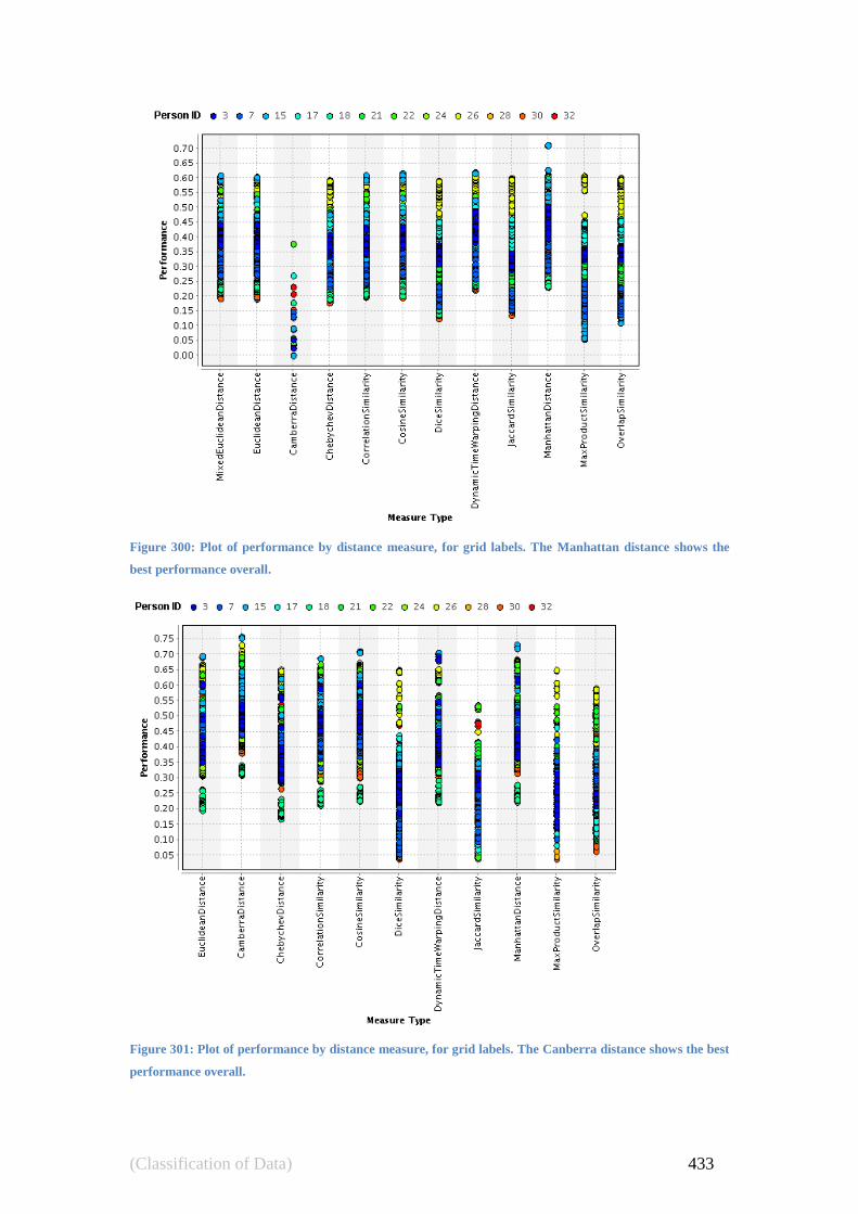
(Classification of Data) 433
Figure 300: Plot of performance by distance measure, for grid labels. The Manhattan distance shows the
best performance overall.
Figure 301: Plot of performance by distance measure, for grid labels. The Canberra distance shows the best
performance overall.
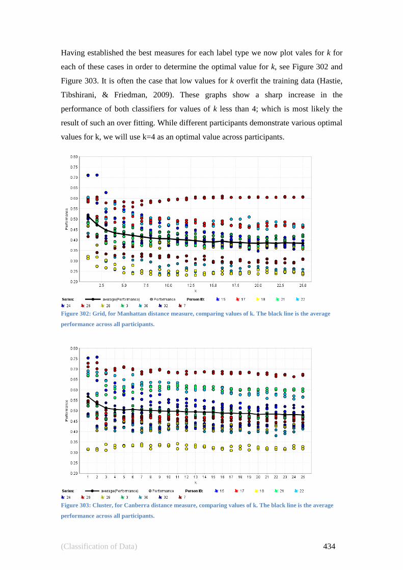
(Classification of Data) 434
Having established the best measures for each label type we now plot vales for k for
each of these cases in order to determine the optimal value for k, see Figure 302 and
Figure 303. It is often the case that low values for k overfit the training data (Hastie,
Tibshirani, & Friedman, 2009). These graphs show a sharp increase in the
performance of both classifiers for values of k less than 4; which is most likely the
result of such an over fitting. While different participants demonstrate various optimal
values for k, we will use k=4 as an optimal value across participants.
Figure 302: Grid, for Manhattan distance measure, comparing values of k. The black line is the average
performance across all participants.
Figure 303: Cluster, for Canberra distance measure, comparing values of k. The black line is the average
performance across all participants.

(Classification of Data) 435
Having established both measure and k, we now investigate whether weighted voting
is of use for the specified metrics at k = 4. We plotted performance for all cases with
and without weighted voting and saw that in all cases weighted voting delivered an
accuracy increase, generally between 2.5 to 5 percent.
Weighted Vote Performance, by Person,
For Grid Labels
Weighted Vote Performance, by Person,
For Cluster Labels
Figure 304: Comparison of weighted voting performance for grid and cluster labels at k=4.
To investigate the performance of the k-NN classifier on the entire population, we
created two classifiers, configured according to our tuning results as follows:
1. For grid labels, Manhattan Distance, k=4, with weighted voting.
2. For cluster labels, Canberra Distance, k=4, with weighted voting.
The results of these experiments averaged around 46% for Grid based labels and 50%
for Cluster based labels. This makes the naive k-NN classifier about 15% less
accurate than the random forest classifier. However the k-NN classifier did perform
well for two participants, as shown in Figure 305.

(Classification of Data) 436
Figure 305: Performance of k-NN classifier.
Confusion matrices for both label schemes are shown in Figure 306 and Figure 307.
The classifier for the grid based classification scheme had poor results in predicting an
emotion (PPV = 34% to 53%) but is an excellent tool for establishing if someone is
not in a given emotion (NPV = 89% to 98%, α = 2% to 10%). The states of being in
neutral Valence with low or neutral Arousal; or being in positive Valence with high
Arousal stand out as being the easiest to predict (PPV = 53%, 49% and 49%
respectively). These results were significantly higher than chance guessing (11%).
The classifier for the cluster based classification scheme had improved results in
predicting an emotion (PPV = 39% to 58%) and, like the grid labels, is also an
excellent tool for establishing if someone is not in a given emotion (NPV = 86% to
96%, α = 5% to 12%). Cluster zero stands out as being the easiest to predict (PPV =
58%) and is shown in Figure 308.
0
2
4
6
8
10
12
0% 10% 20% 30% 40% 50% 60% 70% 80% 90%
Fre
qu
en
cy
Accuracy
Performance by Label Type (k-NN)
Cluster
Grid

(Classification of Data) 437
Figure 306: Summary confusion matrix for clustered labels trained via a k-NN classifier.
Figure 307: Summary confusion matrix for grid labels Trained via a k-NN classifier.
Figure 308: Clusters 5 (PPV = 54%) and 2 (PPV = 51%) highlighted for clarification of the naive Bayes
classifier results.

(Classification of Data) 438
11.7 Support Vector Machine Classifier
The Support Vector Machine (SVM) can be tuned for the up to three parameters in the
kernel. This was achieved by taking a subset of 12 participants (to improve
computational speed) and training multiple SVM classifiers for each of these
participants.
The classifiers were trained using the recommendations of (Hsu et al., 2010). We
examined four different kernels:
Linear ( )
Polynomial ( )
Radial Basis Function (RBF) ( ) || ||
Sigmoid ( )
Where the values γ (gamma), c and d are kernel parameters which we will optimise.
The SVM implementation we used was LibSVM (Chang & Lin, 2011) and the tuning
was performed separately for the 12 sample participants. We used an Evolutionary
Algorithm (EA) to find appropriate values for γ and c and d where applicable,
following a methodology prescribed by Frauke, & Christian 2005. In all cases the EA
used a population of 20 and ran for 400 generations.
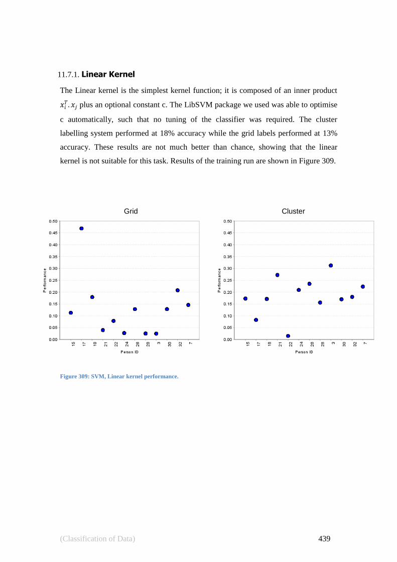
(Classification of Data) 439
11.7.1. Linear Kernel
The Linear kernel is the simplest kernel function; it is composed of an inner product
plus an optional constant c. The LibSVM package we used was able to optimise
c automatically, such that no tuning of the classifier was required. The cluster
labelling system performed at 18% accuracy while the grid labels performed at 13%
accuracy. These results are not much better than chance, showing that the linear
kernel is not suitable for this task. Results of the training run are shown in Figure 309.
Grid
Cluster
Figure 309: SVM, Linear kernel performance.

(Classification of Data) 440
11.7.2. Polynomial Kernel
The Polynomial kernel is a non-stationary kernel which works best when the training
data is normalised. It must be tuned for γ, the constant c and the polynomial degree d.
In our work, on this problem, we found no noticeable effect on varying γ, c or d for
the polynomial kernel. The cluster labelling system performed at 40% accuracy while
the grid labels performed at 34% accuracy. Results of the training run are shown in
Figure 310.
Polynomial Performance Cluster
Polynomial Performance Grid
Figure 310: Polynomial kernel performance

(Classification of Data) 441
11.7.3. Radial Basis Function (RBF) Kernel
The RBF is a popular method for creating a nonlinear SVM. Its usual kernel function
is ( ) || || ; though some variants exist. A benefit
of the RBF kernel is that we only need to optimise
Grid Label Scheme: Performance by Person,
Coloured by Gamma
Cluster Label Scheme: Performance by Person,
Coloured by Gamma
Figure 311: RBF kernel performance.
11.7.4. Sigmoid Kernel
The sigmoid kernel (H.-T. Lin & Lin, 2003) is also known as the hyperbolic tangent
kernel. It uses the kernel function ( ) which provides two
adjustable parameters, the slope γ and the intercept constant c. A common value for γ
is 1/N, where N is the data dimension. Our EA tuning averaged 40.24% performance
accuracy for the cluster label scheme (see Figure 312) and 28.83% (see Figure 313)
for the grid label scheme. The cluster approach to our labelling of the emotion state
provided 11.41% more efficient.

(Classification of Data) 442
A) SVM (Sigmoid) Performance by Person,
Coloured by Gamma
B) SVM (Sigmoid) Performance by Person,
Coloured by C
C) SVM (Sigmoid) Performance vs. Gamma,
Coloured by Person
D) SVM (Sigmoid) Performance vs. C,
Coloured by Person
Figure 312: Sigmoid kernel SVM tuning for grid

(Classification of Data) 443
A) SVM (Sigmoid) Performance by Person,
Coloured by Gamma
B) SVM (Sigmoid) Performance by Person,
Coloured by C
C) SVM (Sigmoid) Performance vs. Gamma,
Coloured by Person
D) SVM (Sigmoid) Performance vs. C,
Coloured by Person
Figure 313: Sigmoid kernel SVM tuning for cluster

(Classification of Data) 444
11.7.5. Comparison of SVM Kernels
The radial basis function kernel was the best performing kernel in the tuning phase of
this experiment, providing an accuracy of 49%, approximately 9% better than any
other kernel, as shown in Table 25. The performance of the SVM (using the radial
basis function) was evaluated against all participants, as shown in Figure 314, where
cluster labelling continued to perform well.
Table 25: Performance of different SVM kernels across participants used for tuning purposes.
Person Sigmoid Polynomial RBF Linear
ID Cluster Grid Δ Cluster Grid Δ Cluster Grid Δ Cluster Grid Δ
3 31.2% 30.1% 1.1% 31.2% 35.9% -4.6% 51.1% 41.9% 9.2% 31.2% 2.5% 28.7%
7 42.3% 21.8% 20.5% 42.3% 29.8% 12.6% 49.0% 33.0% 16.0% 22.4% 14.6% 7.8%
15 37.1% 19.9% 17.2% 35.0% 22.9% 12.1% 51.5% 40.0% 11.5% 17.3% 11.3% 6.0%
17 46.4% 37.8% 8.6% 46.4% 46.9% -0.5% 52.7% 50.9% 1.8% 8.3% 46.9% -38.6%
18 17.3% 19.9% -2.6% 17.1% 21.8% -4.8% 22.0% 28.5% -6.5% 17.1% 17.9% -0.8%
21 41.9% 29.8% 12.1% 41.9% 37.0% 4.8% 50.5% 42.0% 8.5% 27.2% 4.0% 23.2%
22 53.4% 34.9% 18.5% 53.3% 37.7% 15.5% 63.5% 52.4% 11.1% 1.5% 7.8% -6.3%
24 37.2% 27.0% 10.2% 37.1% 32.3% 4.9% 43.3% 38.3% 5.0% 20.9% 2.7% 18.2%
26 64.7% 52.8% 11.9% 64.7% 60.4% 4.3% 66.9% 62.6% 4.3% 23.5% 12.8% 10.7%
28 37.2% 22.7% 14.5% 37.2% 30.6% 6.6% 44.5% 34.0% 10.5% 15.6% 2.5% 13.1%
30 26.4% 20.8% 5.6% 26.2% 22.0% 4.1% 34.2% 32.6% 1.6% 17.0% 12.8% 4.2%
32 47.8% 28.5% 19.3% 47.7% 33.2% 14.5% 59.6% 39.1% 20.5% 18.0% 20.8% -2.8%
40.2% 28.8% 11.4% 40.0% 34.2% 5.8% 49.1% 41.3% 7.8% 18.3% 13.1% 5.3%
Confusion matrices for both label schemes are shown in Figure 315 and Figure 316.
The classifier for the grid based classification scheme had mixed results in predicting
emotions (PPV = 11%, to 54%). Two of the grid labels, positions 1 and 6, were not
correctly classified at a rate significantly higher than chance guessing (PPV = 11%).
Another label, position 8 also performed poorly (PPV = 19%). With three out of nine
labels lacking good PPV results we feel this solution is ultimately a failure. The NPV
values were generally quite good, except grid position labels 4 and 5 which had NPV
results 85% and 82% respectively. The remaining grid position labels were useful for
establishing if someone is not in a given emotion (NPV = 90% to 99%, α = 2% to
10%).
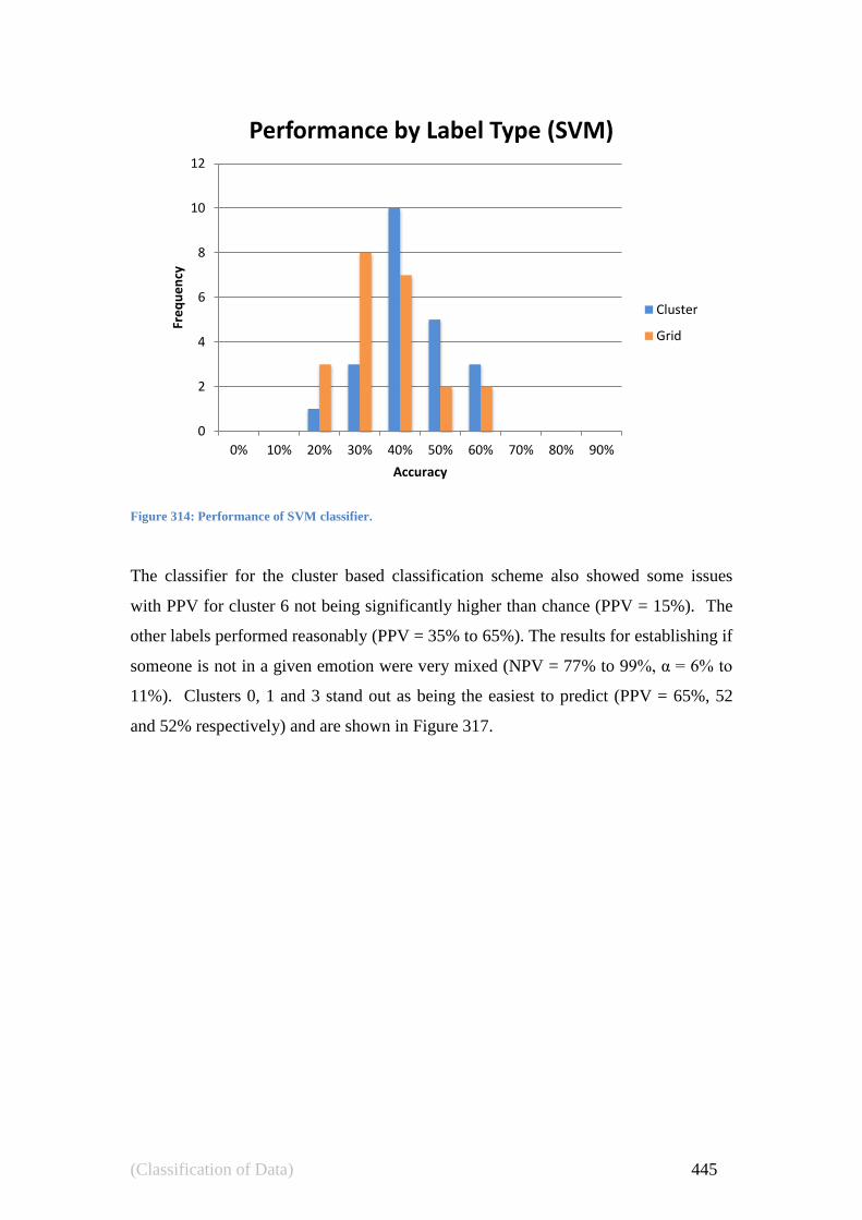
(Classification of Data) 445
Figure 314: Performance of SVM classifier.
The classifier for the cluster based classification scheme also showed some issues
with PPV for cluster 6 not being significantly higher than chance (PPV = 15%). The
other labels performed reasonably (PPV = 35% to 65%). The results for establishing if
someone is not in a given emotion were very mixed (NPV = 77% to 99%, α = 6% to
11%). Clusters 0, 1 and 3 stand out as being the easiest to predict (PPV = 65%, 52
and 52% respectively) and are shown in Figure 317.
0
2
4
6
8
10
12
0% 10% 20% 30% 40% 50% 60% 70% 80% 90%
Fre
qu
en
cy
Accuracy
Performance by Label Type (SVM)
Cluster
Grid

(Classification of Data) 446
Figure 315: Summary confusion matrix for clustered labels trained via a SVM classifier.
Figure 316: Summary confusion matrix for grid labels trained via a SVM classifier.
Figure 317: Clusters 0 (PPV = 65%), 1 (PPV = 52%) and 3 (PPV = 52%) highlighted for clarification of the
SVM classifier results.

(Classification of Data) 447
11.8 Selecting the Best Classifier
A full table of prediction accuracy results is shown in Table 26. The random forest
classifier stood out in terms of its constantly high Positive Predictive Value (PPV
Grid = 54% to 73%; Cluster = 57% to 70%) ratings across all classes, and strong
Negative Predictive Value (NPV Grid = 93% to 98%; Cluster = 93% to 96%) ratings.
This classifier offered 59.96% prediction accuracy for grid based labels and 64.43%
for cluster based labels.
Table 26: Final performance figures for all participants across all tested classifiers. The best results are
underlined.
RF NB SVM (RBF) k-NN ANN
ID Cluster Grid Cluster Grid Cluster Grid Cluster Grid Cluster Grid
3 68.7 60.41 62.13 39.59 50.52 40.99 50.79 46.03 52.16 20.98
4 60.23 55.14 39.12 23.00 40.05 33.29 44.48 46.7 29.51 24.14
5 61.68 53.49 29.02 19.59 45.35 32.54 49.91 51.53 28.86 21.50
6 49.67 57.54 38.67 53.32 32.76 29.54 42.43 36.92 34.15 22.19
7 62.91 61.12 49.35 31.89 48.65 31.92 47.57 37.39 37.89 28.62
15 72.4 61.3 55.20 37.93 49.46 38.75 62.19 56.78 50.40 34.05
16 78.23 79.23 62.13 57.17 68.40 62.22 65.71 72.09 62.57 58.80
17 62.68 53.19 37.89 34.84 52.24 50.08 46.91 50.62 34.08 37.43
18 59.88 47.09 63.00 40.88 20.71 28.05 32.59 29.54 33.25 20.05
20 58.43 42.29 37.57 13.44 32.34 23.65 44.41 33.5 34.14 18.86
21 76.84 58.23 60.61 46.65 49.97 41.42 61.61 43.77 57.56 29.42
22 76.41 75.71 69.18 56.71 62.42 52.08 65.69 54.45 45.67 37.98
24 67.39 59.05 42.17 50.79 42.47 37.76 45.96 44.47 38.26 29.52
25 52.03 65.83 39.44 74.00 41.17 34.53 44.67 47.81 32.10 34.00
26 75.73 64.81 69.58 49.36 66.35 62.23 70.67 59.31 48.87 26.79
28 64.42 62.81 56.50 54.98 46.75 33.74 44.8 42.6 47.36 34.43
29 58.86 62.64 42.43 66.00 47.04 40.94 43.3 47.21 29.29 29.55
30 59.6 66.03 41.49 67.34 32.88 31.75 43.96 31.84 35.84 24.79
31 69.66 60.2 59.43 22.00 53.63 43.01 60.44 46.19 43.21 30.60
32 60.04 62.99 34.10 51.04 58.59 44.13 52.31 44.84 33.49 28.56
33 79.18 68.94 47.81 21.72 55.13 41.19 63.04 54.9 46.02 32.50
34 66.7 53.57 58.49 30.56 45.12 43.39 51.44 47.01 37.60 28.08
All classifiers produced results that are acceptable and broadly applicable to many
human computer interaction applications. Figure 318 shows the classifier performance
results graphically, and highlights why the random forest classifier is a good choice in
that its worst case performance never drops below 50% prediction accuracy.

(Classification of Data) 448
Figure 318: Performance distributions by classification task. Results are in pairs (cluster and grid labels) for
each classifier. The cluster results are in grey, while the grid results are in white.
11.9 Conclusion
This chapter was created with the goal of answering the following four questions:
1. Of the candidate classifiers, which best performs this task?
2. Which features should be used for classification purposes?
3. How does the performance of classifiers vary for our different types of class
labels?
4. How does the performance of classifiers vary across participants?
The candidate classifier which best performed the classification task was the random
forest classifier. It provided a constantly high Positive Predictive Value (PPV Grid =
54% to 73%; Cluster = 57% to 70%), and a strong Negative Predictive Value (NPV
Grid = 93% to 98%; Cluster = 93% to 96%). Overall the classifier offered 59.96%
prediction accuracy for grid based labels and 64.43% for cluster based labels.
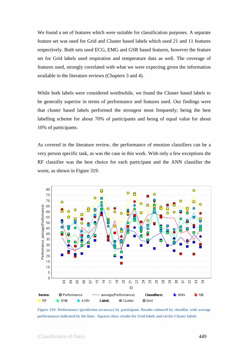
(Classification of Data) 449
We found a set of features which were suitable for classification purposes. A separate
feature set was used for Grid and Cluster based labels which used 21 and 11 features
respectively. Both sets used ECG, EMG and GSR based features, however the feature
set for Grid labels used respiration and temperature data as well. The coverage of
features used, strongly correlated with what we were expecting given the information
available in the literature reviews (Chapters 3 and 4).
While both labels were considered worthwhile, we found the Cluster based labels to
be generally superior in terms of performance and features used. Our findings were
that cluster based labels performed the strongest most frequently; being the best
labelling scheme for about 70% of participants and being of equal value for about
10% of participants.
As covered in the literature review, the performance of emotion classifiers can be a
very person specific task, as was the case in this work. With only a few exceptions the
RF classifier was the best choice for each participant and the ANN classifier the
worst, as shown in Figure 319.
Figure 319: Performance (prediction accuracy) by participant. Results coloured by classifier with average
performances indicated by the lines. Squares show results for Grid labels and circles Cluster labels.

(Classification of Data) 450
While most classifiers show strong correlation in participant specific performance, the
naïve Bayes classifier showed a relative preference for participants 6, 18, 25, 28, 29
and 30 while performing relatively poorly for participant 5. We were unable to
determine the cause of this effect, and cannot make any significant speculation on this
without a larger data set.
11.9.1. Comparison with other works
At the beginning of this chapter we identified several works with which this thesis
may be comparable. These works used similar amounts of weakly induced emotional
states and they were conducted on a reasonable amount of participants (at least 10).
These requirements gave us the studies to which this portion of the work is most
applicable; namely:
Nasoz et al., (Nasoz, Alvarez, Lisetti, & Finkelstien, 2003)
o 24 participants, 6 emotional states, 69% accuracy;
Takahashi (Takahashi, 2004)
o 12 participants, 6 emotional states, 42% accuracy;
Lisetti & Nasoz (Lisetti & Nasoz, 2004)
o 29 participants, 6 emotional states, 84% accuracy.
Our work faces a task more difficult than that of these studies as we are attempting to
differentiate between 8 and 9 emotional states; however, despite this, our results
appear to be in the middle range of the performances obtained by the other available
studies. In this respect, the 59.96% prediction accuracy for grid based labels and
64.43% prediction accuracy for cluster labels that we have achieved is on par with
existing accuracy. The main achievement of this portion of this work is expanding the
amount of emotional states that can be readily distinguished. It is also important to
note that the cluster based labels performed well. This is important because these
emotional labels are formed with use of the Dominance feature, which is often
discarded when working with SAM results (Surakka & Anttonen, 2005), (Feldman,
1995), (Lewis et al., 2007) & (Kulic & Croft, 2007).

(Conclusion) 451
12.0 Conclusion
―When I am working on a problem, I never think about beauty but when I have
finished, if the solution is not beautiful, I know it is wrong.‖
- Buckminster Fuller (1895- 1983)

(Conclusion) 452
In working towards meeting our research goals, we have made contributions in a
number of areas. In this work we conducted an experiment in Physiological Pattern
Recognition (PPR) using six different physiological recordings, namely the:
Electrocardiogram (ECG), Blood Volume Pulse (BVP), Galvanic Skin Response
(GSR), Facial Electromyography (EMG) for the corrugator muscle, Skin temperature
and Respiratory rate. In this experiment, 33 participants were shown 32 IAPS slides
in order to create ‗weakly induced emotions‘; recordings of the participants‘
physiological state were taken as well as a self report of their emotional state using
our customised Self Assessment Manikin (SAM) hardware. The collected data was
processed using a set of signal processing and feature extraction techniques. The
extracted features were analysed and then a set of classification experiments were
conducted.
Our work is targeted towards resolving issues related to enabling electronic devices
recognise human emotions relevant to computing tasks. With this in mind our
research goals were:
1. Can the PPR experimental procedure be improved?
2. Can the analysis of PPR data be improved?
o Will an application of various classification algorithms assist in
improving results?
o Can we discover new signal features that will improve classification
results?
o Can improvements in signal pre-processing techniques (cleaning,
normalising, and correction) produce better classification results?
3. Can we create a PPR system that in some way also predicts the Dominance
factor of the emotion being examined?
An important aspect of this work is an attempt to improve on previous works by
applying better equipment, higher frequency recordings and improved signal
processing with a wider set of features which are less affected by noise. We are also
trying to create an emotion classification system that is more useful for electronic
devices in terms of the number of emotions identifiable and the representation of the
Dominance axis (of emotional space).

(Conclusion) 453
12.1 Contributions
In this section we review the major contributions this work has made to the field. We
carried out two separate reviews of current literature. One review was of Emotion and
PPR from a neurological, physiological and psychological basis. The second is an
exhaustive look at facial muscles from the perspective of PPR using EMG. This
review of facial muscles identified the importance of the Corrugator Supercilii in
emotion recognition experiments.
In the following material, we cover our contributions to the setup of PPR experiments
including a novel hardware SAM device. Followed by our creation of a formal
method for selecting IAPS stimulus was proposed which will help resolve issues of
selecting slides when many factors must be considered. We then outline contributions
made to processing and feature selection from physiological signals, followed by our
method of labelling emotions for classification.
12.1.1. Review of Physiological & Neurological Processes of Emotion
The nature of emotion was studied in chapter 3, where we examined emotion from
both neurophysiological and a neuropsychological points of view. We explored
various methods of working with emotion, in terms of stimulating, observing and
representing emotion. We adopted various tools and methodologies for the purpose of
this work, including:
The International Affective Picture System (IAPS) (Lang, Bradley, &
Cuthbert, 1997) as a method and resource for stimulating emotion;
A dimensional view of emotions (Osgood, Suci, & Tanenbaum, 1957)
expressed by three axis Valence, Arousal and Dominance;
The Self Assessment Manikin (SAM) (Bradley & Lang, 1994) to obtain a self
report of the emotions people were feeling.
The chapter provides a useful, up-to-date review of affective sciences subject matter
from a PPR perspective. Only recently have similar collections of information been
published (with loose ties to PPR) e.g. Davidson, Sherer, & Goldsmith 2009.
However our approach is organised biologically and focussed on PPR relevant issues.

(Conclusion) 454
12.1.2. Facial Muscles
The field of facial muscle electromyography for PPR was examined in depth to
produce a very extensive survey of the facial muscles from a PPR standpoint. This
was concluded with a set of trials using posed facial expressions, which highlighted
the usefulness of Corrugator Supercilii muscle in PPR tasks.
We showed that the Corrugator Supercilii:
Was significant in its correlation to emotional state;
Was not involved in facial displays meant to mask emotion;
Produced unique and identifiable signals for expressions of frowning, pain,
desperation and effort.
Was not subject to the same level of conscious control as other facial muscles.
In addition to providing support for the use of the Corrugator Supercilii in affective
computing; our contribution to facial muscle electromyography is significant because
we did a full review (every muscle) from a PPR perspective. There is no similar
review available (from a PPR perspective). We also published a ‗reference‘ set of
EMG recordings that show major claims made in previous works can be reproduced.
This is significant, because all results were reproduced on one piece of hardware and
presented in a common scale and format. This makes the chapter a valuable resource
for directly comparing electromyography across different facial muscles.
12.1.3. SAM
One of our innovations (Creemers & Hingston, 2010) was a hardware implementation
of the Self Assessment Manikin (SAM). Used correctly this device allows the user to
provide feedback in a manner that minimises muscular action likely to introduce
artefacts into the physiological signals being recorded. This device (shown in Figure
320) was produced after investigating existing devices and two of our own novel
devices. We found our hardware device was an optimal solution for:
Reducing EMG interference in the ECG induced by muscle action and various
other usability issues;
Simplicity of use;

(Conclusion) 455
Minimising unwanted emotional impact on the user;
Ease of synchronisation with physiological recordings made during the
experiment.
Figure 320: The hardware Self Assessment Manikin (SAM) device developed.
12.1.4. Stimulus Selection
We employed a novel, evolutionary method to select stimulus slides from the
International Affective Picture System (IAPS) (Lang, Bradley, & Cuthbert, 1997).
This algorithm had to balance a large variety of requirements based on information
available from previous studies. These requirements for the slideshow we created
were to:
Stimulate a broad section of the Arousal / Valence / Dominance emotional
space;
Utilise slides that have a been evaluated with low standard deviation in
previous experiments (i.e. the outcome is predictable);
Use around 30 slides as an ideal show length;
Prefer the use of slides that have shown consistent SAM ratings across
multiple studies;
Where possible use slides that produce a similar response in male and female
participants;
Avoid slides with an obvious cultural bias;
(Conclusion) 456
Avoid slides which are overly graphic, sexual or instructive so as to comply
with Western Australian laws;
Slides should appear overly dated (70's hair styles, old model cars, etc.).
After the experiment, we established that for the most part our participants reacted to
the stimulus in a manner predicted by previous works. In this respect our selection
was successful. We found some slides which did not gain the reactions expected from
previous studies and found that these slides were all of similar theme(s). We proposed
that the differences we discovered were due to the Australian cultural biases of our
participants. This is both an expected and normal outcome for studies not conducted
in America and the variances observed correlate with the results obtained by
Massavelli (2010). In this regard we have established a formalised method for side
selection and contributed to the understanding of Australian cultural biases.
This portion of the work is a significant contribution because, as noted in section 6.4,
there exists little in the way of formal methods for stimulus selection in related works.
With many researchers still using informal techniques to select stimuli, our technique
has the potential to be a ‗milestone‘ in this area.
12.1.5. Signal Processing
In the signal processing phase of this work the ECG signal was examined extensively.
Several algorithms to de-noise the signal were investigated and a wavelet approach
was found to be optimal. A real-time median filer was built for baseline correction of
the ECG signal as this technique does not affect signal morphology, and this is
important towards our goals of accurate feature extraction. Median filtering was also
the only portion of the work not, initially, applicable to real time systems. Creating a
real-time version of the algorithm will assist future PPR efforts.
Several algorithms for labelling the ECG signal were examined with a wavelet
decomposition based approach by Chesnokov, Nerukh and Glen (2006) being found
optimal. Typical results on our data are shown in Figure 191. Lastly a method to make
all measurements of the ECG invariant to heart rate was created.

(Conclusion) 457
Figure 321: ECG Annotations against raw ECG signal.
12.1.6. Feature Extraction
We set about conducting a feature extraction task on the physiological data we
acquired, this included the extraction of amplitude, spectral and morphological based
features. We concentrated on the ECG and EMG signals as they are both complex and
information rich. Some of our feature extraction techniques were novel, others were
an investigation into the applicability of existing ―generic‖ and medical techniques to
the field of PPR. In all over 4000 features were extracted from the dataset and
subjected to a feature selection task.
Exploring all these features assists the nature of PPR research, as many researchers
either use:
Established medical features (which may, or may not, extend to correlating
with emotional state);
A simple feature set, as implementing the algorithms involved (especially
ECG feature detection and some EMG features) often exceeds practical
software development time for such projects.
The EMG signal was responsible for most of the features extracted as intervals
between various points in ECG morphology, from both an inter and intra beat
perspective, created many possible features.
Sixteen different EMG feature extraction techniques were examined as part of this
work; these features provided information in both the time and frequency domain.

(Conclusion) 458
This broad application of existing, medical, EMG feature extraction techniques to the
field of PPR may assist future works in choosing appropriate metrics.
We also created several novel metrics for measuring the cyclic respiration and blood
volume pulse signals. The novel respiration curve metric discussed in 9.4 showed
some correlation with Dominance ratings. This is an important finding because
Dominance is traditionally one of the more difficult ratings to find correlations with
and our research goal was to improve PPR classification in terms of observed
dominance. Further work is needed to statistically quantify the relationship between
the respiration curve metric and Dominance results. Specifically an experiment
designed with Dominance as a control variable would be needed.
12.1.7. Labelling Emotions
We created two sets of emotion labels for classification purposes which were
applicable to the SAM feedback we recorded. One was based on a grid covering the
Arousal / Valence emotional space. The second was derived from k-means clustering
of our SAM ratings. These two labelling systems are shown in Figure 322. The
labelling system resulted in nine and eight labels respectively. These labelling systems
evaluated well under classification tasks, but importantly the clustering based labels
allow for classification of emotional state with Dominance being represented. To date
many researchers discard Dominance information as it easily confounds the
classification process. We also found it was not possible to extend the grid system into
this space, as this produced 27 states, a target not achievable to our classification
systems.
The grid system offers a straightforward interpretation of the emotion space with
gives at an immense practical advantage, in terms of using it in a computer interface.
However the clustering approach offers:
Increased accuracy;
A decreased number of features required for the classifier;
Encapsulation of the Dominance dimension.

(Conclusion) 459
Figure 322: Emotion labelling systems. Voronoi plots of the our clustering Labels (Left) are shown from two
rotations and the rating axes have been adjusted from the range [1 to 9] to the range [-4 to 4] so that 0 is
neutral. The grid labels (Right) show the Valence/Arousal emotional space divided into nine different labels.
12.1.8. Classification Performance
Our work was successful in being able to differentiate between eight (cluster based)
and nine (grid based) emotional states; with 64% and 60% prediction accuracy
respectively. This expands the number of states that can be readily distinguished via
PPR techniques while still delivering accuracy on par with existing studies which
typically use two to six states.
Significantly, this was achieved on ‗weakly‘ elicited emotions with Dominance being
represented in the classification output. This result is directly applicable to human

(Conclusion) 460
computer interaction in terms of the type of emotion studied and the nature of the
classification results.
Additionally we investigated five different classifiers in terms of performance for the
task of detecting (weak) emotion states from physiological data. We found an
advantage in using the random forest classifier over the naïve Bayes classifier,
artificial neural network, k nearest neighbour classifier and support vector machine.
12.2 Future Work and Final Thoughts
When this work began the ―tablet device‖ was still finding a home, iPads, Galaxy
Tabs and the like were not around and a laptop was still a luxury. It would be
interesting to investigate what physiological signals can be gleaned from hand contact
with these tablets and attempt classification on just those signals.
We have focused on supervised learning in this work. There may be some merit to
attempting an unsupervised learning approach to the problem,
Additionally there is no attempt made to use our data in another researchers
classification framework, or use other researchers data in our framework. We suggest
this may be a very useful exercise; in the extent to which it is allowed by restrictions
on the data.
There is still much work needed in person independent emotion detection. We feel our
ECG signal extraction techniques would help in this area as they improve on making
data collected person and time independent.
A lack of person independent PPR systems may not be the technical hurdle we once
envisioned. Maybe modern cloud storage would allow for person dependent
classification profiles to be stored and retrieved by diverse PPR enabled consumer
electronic devices.

(Conclusion) 461
An emerging world of Affective devices should be approached with some caution.
Tools which evaluate our emotional state should be used for improving the human-
device interaction. To put these tools to work as diviners of peoples personality would
both be unfounded and morally wrong.
It is the author‘s hope that the results from this work are not used to create devices
which attempt to probe a person‘s personality/feelings in a manner that is an invasion
of privacy. Our feelings are just that. They are personal and we have evolved an array
of innate abilities to (largely) choose how much of our feelings we communicate to
others.
It is the author‘s view that our cars should not inform our insurance companies how
frequently we are stressed at the wheel. Likewise our telephones should not report to
the government that we are scared or being secretive. Our televisions should not glean
which brands we respond to the most and potential employers should not attempt to
use devices that audit our feelings, likes and dislikes. Already there are some
negative affective technologies appearing and that is… worrying.
In proceeding forward with these technologies, the author advocates that scientists
and engineers alike, should bear in mind two articles from the ―Universal Declaration
of Human Rights‖ (UN General Assembly, 1948)
―No one shall be subjected to arbitrary interference with his privacy, family,
home or correspondence, nor to attacks upon his honour and reputation.
Everyone has the right to the protection of the law against such interference or
attacks.‖ (Article 12)
―Everyone has the right to freedom of opinion and expression; this right
includes freedom to hold opinions without interference and to seek, receive
and impart information and ideas through any media and regardless of
frontiers.‖ (Article 19)

(Conclusion) 462

(Glossary) 463
13.0 Glossary
Afferent Carrying towards (inwards). Especially from the body to the
brain.
Alaris Derived from the Latin word ala (wing) used anatomically to
describe something that flanks an organ.
Anguli (Anatomy) plural of angulus; an angle, corner, or apex.
ANN Artificial Neural Network
Anterior Towards the front (see Figure 323)
Arousal Emotional Factor; level of excitement
Autonomic Concerning the involuntary nervous system
Biocybernetic Concerning the application of cybernetics to biological
science
Bio-impedance Response of a living organism to an electric current
Buccinator Facial muscle of the jaw (see section 4.3)
Caninus Facial muscle of the jaw (see section 4.3)
Circumplex Concerning a model organised in a radial fashion.
Confusion Matrix A matrix used for the visualization of classifier performance
Corrugator Supercilii Facial muscle used in eye expression (see section 4.4)
Cortex The outer layer of an organ (antonym of Medulla)
Depressor A muscle used to pull down a part of the body.
Depressor Anguli Oris Facial muscle of the jaw (see section 4.3)
Dermatological Relating to the skin.
Diastolic When the heart refills with blood
Dichotomous Divided into two branches
Distal Away from the body (see Figure 323)
Diurnal Daytime
Dominance Emotional Factor; Level of control.
Dorsal Relating to the upper side (see Figure 323)
Dot Product A real, scalar, number which is the product of two vectors

(Glossary) 464
ECG (EKG) Electro Cardio Graph, or in German Elektrokardiogramm. A
recording of the electrical activity of the heart.
Efferent Carrying away (outwards). Especially from the brain to the
body
Electrocardiogram Measurement of the electrical activity of the heart
Electromyography Measurement of the electrical activity of muscles
F0 Fundamental Frequency
FFT Fast Fourier Transform
Fischer Projection A method for projecting a 3D structure onto a 2D Plane
Frontalis Facial muscle used in eye expression (see section 4.4)
Fuzzy C-means-
Clustering
A clustering algorithm which allows one piece of data to
belong to multiple clusters
GSR Galvanic Skin Response
Homeostasis Property of a system that regulates itself to remain stable.
IAPS International Affective Picture System
Inferior Below (see Figure 323)
Inferioris (Anatomy) Below (antonym of Superioris)
Insula Part of the brain, in the cerebral cortex
KNN K-Nearest Neighbours
Labii Of the lip (Latin)
Lateral Away from the midline (see Figure 323)
Levator A muscle used to pull up a part of the body.
Levator Anguli Oris Facial muscle of the jaw (see section 4.3)
Levator Labii Superioris Facial muscle of the jaw (see section 4.3)
Linear Discriminant
Analysis (LDA)
A type of classifier.
Medial Towards the midline (see Figure 323)
Medulla The inner region of an organ (antonym of Cortex)
Medulla Oblongata The lowermost portion (stem) of the vertebrate brain
Mentalis Facial muscle of the jaw (see section 4.3)
Midline Vertical axis of the body (see Figure 323)
Mimetic (Anatomy) Of the face
Nasalis In reference to anatomy of the nose, From the Latin for

(Glossary) 465
"nose".
Nasalis Alaris Facial muscle of the nose (see section 4.5)
Nasalis Transversa Facial muscle of the nose (see section 4.5)
Oblongata Elongated in one direction
Oculi Round (eyelike) opening
Opto-isolator Device which transfers an signal optically (to separate
electrical systems)
Orbicularis (anatomical) Circular; often used in naming sphincter
muscles.
Orbicularis Oculi Facial muscle used in eye expression (see section 4.4)
Orbicularis Oris Facial muscle of the jaw (see section 4.3)
Oris (anatomical) Of the mouth
Palmer The palm of the hand (or direction of the palm) (see Figure
320)
Platysma Facial muscle of the jaw (see section 4.3)
Posterior Towards the back (see Figure 323)
PPR Physiological Pattern Recognition
Procerus Facial muscle used in eye expression (see section 4.4)
Proximal Towards the body (see Figure 323)
Pseudo-Gibbs Similar to the ringing artefacts caused by the Gibbs
phenomenon
QRS Complex A portion of the ECG signal
QT Interval A portion of the ECG signal
Quadratus (anatomy) Quadrilateral in shape.
Quadratus Labii
Inferioris
Facial muscle of the jaw (see section 4.3)
Quadratus Labii
Superioris
Facial muscle of the jaw (see section 4.3)
Restylane An injectable filler for sub dermal facial tissues
Risorius Facial muscle of the jaw (see section 4.3)
ROC Curve Receiver Operating Characteristic (ROC). Used to plot the
performance of a binary classifier against its discrimination
threshold.

(Glossary) 466
Semantic Relating to the different meanings of words
Sentograph A two-dimensional pressure sensitive touch transducer
Somatovisceral Of the nerves connecting the spine to the organs.
Somatovisceral Nerve pathways connecting the spinal cord to internal organs
Spectrogram Spectral density plotted against time.
Supercilii (Latin) from superus (above) and cilium (eyelash)
Superior Above (see Figure 323)
Superioris (Anatomy) Above (antonym of Inferioris)
Systolic When the heart is contracting.
Thermoregulatory (Anatomical) Relating to how the body regulates its internal
temperature.
Transversa (Latin) roughly to lie across and furrow.
Triangularis (Latin) Triangular corner
Valence Emotional factor; positive or negative Feeling.
Wavelet Brief oscillation, starting and ending at zero amplitude.
Zygomatic(us) Cheekbone
Zygomaticus Major Facial muscle of the jaw (see section 4.3)
Zygomaticus Minor Facial muscle of the jaw (see section 4.3)

(Glossary) 467
Figure 323: Diagram of human anatomical terminology
Midline
Dis
tal
Pro
xim
al
Distal
Proximal
Lateral
Medial
Infe
rior (b
elo
w)
Su
pe
rior
(abo
ve
)
Palmer (hand)
Dorsal (hand)

(Glossary) 468

(Appendix) 469
14.0 Appendix

(Appendix) 470
14.1 Stimulus Slides
This section of the appendix shows a very low detail, obscured and greyscaled version
of the IAPS stimulus slides1 used in this study. The images have been deliberately
―damaged‖ so as to prevent the content ―leaking‖ to the public/internet.
Figure 324: IAPS slide used in this study (continued next page)
1 THIS PAGE IS NOT TO BE COPIED OR INCLUDED IN ELECTRONIC DISTRIBUTION AS
THE IAPS LICENCING DOES NOT PERMIT THIS. THIS PAGE IS NOT TO BE REPRODUCED.
FIGURE REMOVED TO COMPLIY WITH
TERMS OF USE OF THE IAPS DATA SET.

(Appendix) 471
Stimulus slides continued1.
Figure 325: IAPS slide used in this study (continued next page)
1 THIS PAGE IS NOT TO BE COPIED OR INCLUDED IN ELECTRONIC DISTRIBUTION AS
THE IAPS LICENCING DOES NOT PERMIT THIS. THIS PAGE IS NOT TO BE REPRODUCED.
FIGURE REMOVED TO COMPLIY WITH
TERMS OF USE OF THE IAPS DATA SET.

(Appendix) 472
Stimulus slides continued1.
Figure 326: IAPS slide used in this study
1 THIS PAGE IS NOT TO BE COPIED OR INCLUDED IN ELECTRONIC DISTRIBUTION AS
THE IAPS LICENCING DOES NOT PERMIT THIS. THIS PAGE IS NOT TO BE REPRODUCED.
FIGURE REMOVED TO COMPLIY WITH
TERMS OF USE OF THE IAPS DATA SET.

(Appendix) 473
14.2 SAM Evaluations User Reliability Charts
Figure 327: SAM frequency histogram for participant 1, day 1
Figure 328: SAM frequency histogram for participant 2, day 1
SAM Rating SAM Rating SAM Rating
(happy to unhappy) (excited to calm) (controlled to in-control)
SAM Rating SAM Rating SAM Rating
(happy to unhappy) (excited to calm) (controlled to in-control)

(Appendix) 474
Figure 329: SAM frequency histogram for participant 3, day 1
Figure 330: SAM frequency histogram for participant 4, day 1
Figure 331: SAM frequency histogram for participant 5, day 1
SAM Rating SAM Rating SAM Rating
(happy to unhappy) (excited to calm) (controlled to in-control)

(Appendix) 475
Figure 332: SAM frequency histogram for participant 6, day 1
Figure 333: SAM frequency histogram for participant 1, day 2
Figure 334: SAM frequency histogram for participant 2, day 2

(Appendix) 476
Figure 335: SAM frequency histogram for participant 3, day 2
Figure 336: SAM frequency histogram for participant 4, day 2
Figure 337: SAM frequency histogram for participant 5, day 2

(Appendix) 477
Figure 338: SAM frequency histogram for participant 6, day 2
Figure 339: SAM frequency histogram for participant 7, day 2
Figure 340: SAM frequency histogram for participant 8, day 2

(Appendix) 478
Figure 341: SAM frequency histogram for (female) participant 1, day 3
The lack of meaningful distribution for participant 301 in Figure 47 stems from this
participant being 1 of only 5 females in the study. See Table 3 issue 2 for more
information.
Figure 342: SAM frequency histogram for participant 2, day 3
Figure 343: SAM frequency histogram for participant 3, day 3

(Appendix) 479
Figure 344: SAM frequency histogram for participant 4, day 3
Figure 345: SAM frequency histogram for participant 1, day 4
Figure 346: SAM frequency histogram for participant 2, day 4

(Appendix) 480
Figure 347: SAM frequency histogram for participant 3, day 4
Figure 348: SAM frequency histogram for participant 4, day 4
Figure 349: SAM frequency histogram for participant 5, day 4

(Appendix) 481
Figure 350: SAM frequency histogram for (female) participant 1, day 5
The lack of meaningful distribution for participant 501 in Figure 56 stems from this
participant being 1 of only 5 females in the study. See Table 3 issue 2 for more
information.
Figure 351: SAM frequency histogram for participant 2, day 5
Figure 352: SAM frequency histogram for participant 3, day 5

(Appendix) 482
Figure 353: SAM frequency histogram for participant 4, day 5
Figure 354: SAM frequency histogram for (female) participant 5, day 5
The lack of meaningful distribution for participant 505 in Figure 60 stems from this
participant being 1 of only 5 females in the study. See Table 3 issue 2 for more
information.
Figure 355: SAM frequency histogram for (female) participant 6, day 5

(Appendix) 483
The lack of meaningful distribution for participant 506 in Figure 61stems from this
participant being 1 of only 5 females in the study. See Table 3 issue 2 for more
information.
Figure 356: SAM frequency histogram for (female) participant 7, day 5
The lack of meaningful distribution for participant 507 in Figure 62 stems from this
participant being 1 of only 5 females in the study. See Table 3 issue 2 for more
information.
Figure 357: SAM frequency histogram for participant 8, day 5
The Dominance histogram in Figure 63 shows that participant 508 may have used the
Dominance scale backwards. See Table 3 problem 1 for more information.

(Appendix) 484
Figure 358: SAM frequency histogram for participant 9, day 5
The Valence, Arousal and Dominance for participant 509 (see Figure 64) are very
poorly distributed. The results are suspect and will not be given much weight in the
training process. See Table 3 problem 3 for more information.

(Appendix) 485
14.3 IAPS Slide Scatter Plots
This appendix holds comparison graphs of our SAM ratings and those of reference
studies. Responses that were chosen by more than one participant, in our study, are
labelled x2, x3 and so on. Male responses are in blue, female in red; some slides were
only shown to one gender so will lack a colour. A rectangle of matching colour is
drawn to represent the area around the mean bounded by one standard deviation. The
areas of one standard deviation about the mean from previous studies (P. Lang et al.,
2001) are shown in grey.
Figure 359: A plot of Arousal vs. Valence scores for slide 1050 (Snake), reference studies in grey.

(Appendix) 486
Figure 360: A plot of Arousal vs. Valence scores for slide 1200 (Big Hairy Spider), reference studies in grey.
Figure 361: A plot of Arousal vs. Valence scores for slide 1300 (Angry Dog), reference studies in grey.

(Appendix) 487
Figure 362: A plot of Arousal vs. Valence scores for slide 2000 (Smiling Male Face).
Figure 363: A plot of Arousal vs. Valence scores for slide 2070 (Human Baby).

(Appendix) 488
Figure 364: A plot of Arousal vs. Valence scores for slide 2345 (Kids playing).
Figure 365: A plot of Arousal vs. Valence scores for slide 2730 (Boy with bison).

(Appendix) 489
Figure 366: A plot of Arousal vs. Valence scores for slide 2900 (Boy Crying).
Figure 367: A plot of Arousal vs. Valence scores for slide 3062 (Abortion).

(Appendix) 490
Figure 368: A plot of Arousal vs. Valence scores for slide 3069 (Girl [½ head blown away]).
Figure 369: A plot of Arousal vs. Valence scores for slide 3150 (Hand Cut up).

(Appendix) 491
Figure 370: A plot of Arousal vs. Valence scores for slide 3220 (Male Hospital Patient).
Figure 371: A plot of Arousal vs. Valence scores for slide 4005 (Female Nude [discreet]).

(Appendix) 492
Figure 372: A plot of Arousal vs. Valence scores for slide 4150 (Female bikini).
Figure 373: A plot of Arousal vs. Valence scores for slide 4300 (Female [pornographic]).

(Appendix) 493
Figure 374: A plot of Arousal vs. Valence scores for slide 4520 (Male Nude [discreet]).
Figure 375: A plot of Arousal vs. Valence scores for slide 4535 (Male Lifting Weights).

(Appendix) 494
Figure 376: A plot of Arousal vs. Valence scores for slide 4572 (Handsome Fireman).
Figure 377: A plot of Arousal vs. Valence scores for slide 4641 (Couple at beach).

(Appendix) 495
Figure 378: A plot of Arousal vs. Valence scores for slide 4666 (Couple in bed [not discreet]).
Figure 379: A plot of Arousal vs. Valence scores for slide 5621 (Skydiving formation).

(Appendix) 496
Figure 380: A plot of Arousal vs. Valence scores for slide 4659 (Couple Sex [discreet]).
Figure 381: A plot of Arousal vs. Valence scores for slide 5623 (Extreme windsurfing).

(Appendix) 497
Figure 382: A plot of Arousal vs. Valence scores for slide 5760 (Flower Garden). All female Arousal = 1.
Figure 383: A plot of Arousal vs. Valence scores for slide 5780 (River). All female Arousal = 1.

(Appendix) 498
Figure 384: A plot of Arousal vs. Valence scores for slide 5910 (Fireworks [over city]).
Figure 385: A plot of Arousal vs. Valence scores for slide 6550 (Violent Scene).

(Appendix) 499
Figure 386: A plot of Arousal vs. Valence scores for slide 7002 (Towel).
Figure 387: A plot of Arousal vs. Valence scores for slide 7009 (Mug).
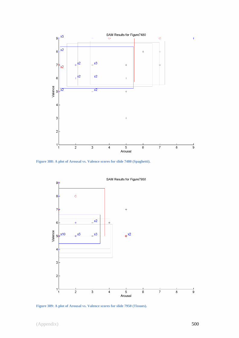
(Appendix) 500
Figure 388: A plot of Arousal vs. Valence scores for slide 7480 (Spaghetti).
Figure 389: A plot of Arousal vs. Valence scores for slide 7950 (Tissues).

(Appendix) 501
Figure 390: A plot of Arousal vs. Valence scores for slide 8040 (High diver).
Figure 391: A plot of Arousal vs. Valence scores for slide 8490 (People in a roller coaster).

(Appendix) 502
Figure 392: A plot of Arousal vs. Valence scores for slide 9000 (Graveyard).
Figure 393: A plot of Arousal vs. Valence scores for slide 9253 (Execution [young lady]).

(Appendix) 503
Figure 394: A plot of Arousal vs. Valence scores for slide 9401 (Knives [subliminal words]).
Figure 395: A plot of Arousal vs. Valence scores for slide 9410 (Warzone [parent with child]).

(Appendix) 504
Figure 396: A plot of Arousal vs. Valence scores for slide 9582 (Dental exam).
14.4 ECG “NARF” Compensations For all Intervals of the
Typical Waveform
The next five pages contain tables for the NARF transform as a polynomial function
for inter and intra ECG feature intervals.
Rest of page left blank intentionally.
(Appendix) 505
Table 27: Intra-beat NARF transform
Interval y = ax2 + bx + c
a b c
P_finish to t_onset 0.1350 -0.2082 0.1450
P_finish to t_peak -0.0359 0.0225 0.0777
P_finish to t_peak -0.1855 1.2337 -0.1667
P_finish to t_finish -0.1036 1.0773 -0.1382
P_finish to t_peak -0.1855 1.2270 -0.1837
P_finish to t_finish 0.0451 0.7290 -0.2030
P_finish to t_onset -0.0721 0.9452 -0.1598
P_finish to t_peak 0.0217 0.7809 -0.1595
P_onset to t_finish -0.1051 0.1924 -0.0229
P_onset to t_peak -0.0498 0.0930 -0.0108
P_onset to t_onset 0.0293 -0.0147 0.1216
P_onset to t_peak -0.0892 0.1496 0.0712
P_onset to t_peak -0.0804 1.0413 -0.1437
P_onset to t_finish 0.0014 0.8850 -0.1153
P_onset to t_peak -0.0477 0.9787 -0.1369
P_onset to t_finish 0.1396 0.5528 -0.1856
P_onset to t_onset 0.0224 0.7690 -0.1424
P_onset to t_peak 0.1162 0.6047 -0.1421
P_peak to t_finish -0.0553 0.0994 -0.0121
P_peak to t_onset 0.0795 -0.1084 0.1327
P_peak to t_peak -0.0595 0.0806 0.0766
P_peak to t_peak -0.1302 1.1343 -0.1545
P_peak to t_finish -0.0482 0.9778 -0.1261
P_peak to t_peak -0.1209 1.1109 -0.1642
P_peak to t_finish 0.0947 0.6382 -0.1938
P_peak to t_onset -0.0225 0.8544 -0.1507
P_peak to t_peak 0.0714 0.6901 -0.1503
q_onset to t_peak -0.0336 0.0539 -0.0064
q_onset to t_peak -0.1559 1.1820 -0.0723
q_onset to t_finish -0.0682 1.0163 -0.0404
q_onset to t_peak -0.1258 1.1270 -0.0695
q_onset to t_finish 0.1888 0.5036 -0.0511
q_onset to t_onset 0.0721 0.7192 -0.0077
q_onset to t_peak 0.1673 0.5525 -0.0065
q_peak to t_peak -0.1606 1.1215 -0.0173
q_peak to t_finish -0.1210 1.0345 -0.0155
q_peak to t_peak -0.1179 1.0751 -0.0272
q_peak to t_finish 0.1301 0.5627 -0.0518
q_peak to t_onset 0.0211 0.7564 0.0011
q_peak to t_peak 0.0936 0.6280 -0.0119
r_peak to t_finish -0.0915 0.1720 -0.0343
r_peak to t_peak -0.0612 0.1117 -0.0259
r_peak to t_finish -0.2257 0.5029 0.0362
r_peak to t_onset -0.1111 0.2909 -0.0087
r_peak to t_peak -0.2060 0.4571 -0.0097
s_finish to t_finish -0.1440 0.3456 0.0655
s_finish to t_onset -0.0295 0.1336 0.0206
s_finish to t_peak -0.1243 0.2998 0.0196
s_peak to t_finish -0.0122 0.0213 0.0133
s_peak to t_finish -0.1961 0.4394 0.0450
s_peak to t_onset -0.0702 0.2167 0.0000
s_peak to t_peak -0.1622 0.3737 0.0050
t_onset to t_finish -0.1146 0.2120 0.0449
t_onset to t_peak -0.0949 0.1661 -0.0011
t_peak to t_finish -0.0197 0.0458 0.0459

(Appendix) 506
Table 28: Inter-beat NARF transform
Interval y = ax2 + bx + c
a b c
intra beet P_finish to t_finish -0.1326 1.1560 -0.0357
intra beet P_finish to t_onset -0.0348 0.9752 -0.0174
intra beet P_finish to t_peak -0.0856 1.0701 -0.0290
intra beet P_finish to t_onset -0.1587 1.1878 0.0304
intra beet P_finish to t_peak -0.1378 1.0713 0.1078
intra beet P_finish to t_peak 0.1042 -0.1520 0.1540
intra beet P_finish to t_finish 0.0109 0.0234 0.1181
intra beet P_finish to t_peak 0.1033 -0.1318 0.1614
intra beet P_finish to t_finish -0.1310 0.3669 0.1840
intra beet P_finish to t_onset 0.0003 0.1270 0.1501
intra beet P_finish to t_peak -0.1070 0.3138 0.1410
intra beet P_onset to t_finish -0.2352 1.3480 -0.0595
intra beet P_onset to t_onset -0.1390 1.1695 -0.0420
intra beet P_onset to t_peak -0.1863 1.2594 -0.0518
intra beet P_onset to t_onset -0.2608 1.3776 0.0080
intra beet P_onset to t_peak -0.1445 1.1307 0.1261
intra beet P_onset to t_peak 0.0111 0.0239 0.1369
intra beet P_onset to t_finish -0.0822 0.1992 0.1010
intra beet P_onset to t_peak -0.0183 0.0934 0.1228
intra beet P_onset to t_finish -0.2145 0.5276 0.1724
intra beet P_onset to t_onset -0.0831 0.2877 0.1385
intra beet P_onset to t_peak -0.1905 0.4744 0.1294
intra beet P_peak to t_finish -0.1888 1.2588 -0.0496
intra beet P_peak to t_onset -0.0940 1.0826 -0.0330
intra beet P_peak to t_peak -0.1430 1.1747 -0.0436
intra beet P_peak to t_onset -0.2225 1.3023 0.0121
intra beet P_peak to t_peak -0.1394 1.0977 0.1187
intra beet P_peak to t_peak 0.0498 -0.0522 0.1413
intra beet P_peak to t_finish -0.0435 0.1232 0.1054

(Appendix) 507
intra beet P_peak to t_peak 0.0453 -0.0240 0.1445
intra beet P_peak to t_finish -0.1802 0.4588 0.1741
intra beet P_peak to t_onset -0.0489 0.2188 0.1402
intra beet P_peak to t_peak -0.1563 0.4056 0.1310
intra beet q_onset to t_finish -0.3099 1.4385 -0.2127
intra beet q_onset to t_onset -0.2134 1.2589 -0.1946
intra beet q_onset to t_peak -0.2632 1.3524 -0.2057
intra beet q_onset to t_onset -0.3374 1.4845 -0.1582
intra beet q_onset to t_peak -0.1701 1.2064 -0.0434
intra beet q_onset to t_peak -0.0349 0.0640 0.0064
intra beet q_onset to t_finish -0.1321 0.2475 -0.0336
intra beet q_onset to t_peak -0.0997 0.1838 -0.0247
intra beet q_onset to t_finish -0.2787 0.5990 0.0290
intra beet q_onset to t_onset -0.1480 0.3603 -0.0055
intra beet q_onset to t_peak -0.2558 0.5477 -0.0149
intra beet q_peak to t_finish -0.1275 1.1356 -0.0970
intra beet q_peak to t_onset -0.1121 1.0584 -0.1072
intra beet q_peak to t_peak -0.1226 1.1042 -0.1058
intra beet q_peak to t_onset -0.1571 1.1205 -0.0008
intra beet q_peak to t_peak -0.1757 1.1188 0.0260
intra beet q_peak to t_peak -0.0281 0.0514 0.0062
intra beet q_peak to t_finish -0.0530 0.1170 0.0123
intra beet q_peak to t_peak -0.0406 0.0905 0.0059
intra beet q_peak to t_finish -0.1562 0.3990 0.0982
intra beet q_peak to t_onset -0.0408 0.1963 0.0485
intra beet q_peak to t_peak -0.1057 0.3116 0.0668
intra beet r_peak to t_finish -0.2428 2.3158 -0.1927
intra beet r_peak to t_onset -0.1459 2.1364 -0.1750
intra beet r_peak to t_peak -0.1949 2.2285 -0.1854
intra beet r_peak to t_onset -0.2732 2.3556 -0.1295
intra beet r_peak to t_peak -0.0763 2.0054 0.0216
intra beet r_peak to t_finish -0.0932 1.1754 -0.0359
intra beet r_peak to t_peak -0.0628 1.1122 -0.0253

(Appendix) 508
intra beet r_peak to t_finish -0.2315 1.5136 0.0317
intra beet r_peak to t_onset -0.0999 1.2730 -0.0018
intra beet r_peak to t_peak -0.2071 1.4595 -0.0109
intra beet s_finish to t_finish -0.1652 2.1638 -0.1650
intra beet s_finish to t_onset -0.0684 1.9846 -0.1473
intra beet s_finish to t_peak -0.1179 2.0775 -0.1581
intra beet s_finish to t_onset -0.1911 2.1970 -0.0997
intra beet s_finish to t_peak -0.0785 1.9785 0.0019
intra beet s_finish to t_peak 0.0818 0.8419 0.0297
intra beet s_finish to t_finish -0.0113 1.0170 -0.0062
intra beet s_finish to t_peak 0.0106 0.9771 -0.0101
intra beet s_finish to t_finish -0.1567 1.3662 0.0577
intra beet s_finish to t_onset -0.0253 1.1260 0.0239
intra beet s_finish to t_peak -0.1322 1.3121 0.0150
intra beet s_peak to t_finish -0.2319 2.2779 -0.1909
intra beet s_peak to t_onset -0.1135 2.0612 -0.1567
intra beet s_peak to t_peak -0.1772 2.1786 -0.1783
intra beet s_peak to t_onset -0.2408 2.2864 -0.1157
intra beet s_peak to t_peak -0.1520 2.1154 -0.0384
intra beet s_peak to t_peak 0.0594 0.8907 0.0250
intra beet s_peak to t_finish -0.0162 1.0289 0.0089
intra beet s_peak to t_peak 0.0100 0.9827 0.0072
intra beet s_peak to t_finish -0.2062 1.4559 0.0388
intra beet s_peak to t_onset -0.0598 1.1987 0.0075
intra beet s_peak to t_peak -0.1728 1.3907 -0.0014
intra beet t_finish to t_finish 0.0131 1.7635 -0.2096
intra beet t_finish to t_onset 0.1078 1.5875 -0.1931
intra beet t_finish to t_peak 0.0601 1.6776 -0.2031
intra beet t_finish to t_onset -0.0277 1.8194 -0.1526
intra beet t_finish to t_peak 0.0504 1.6556 -0.0687
intra beet t_finish to t_peak 0.2456 0.4641 -0.0235
intra beet t_finish to t_finish 0.1524 0.6395 -0.0594
intra beet t_finish to t_peak 0.2254 0.5095 -0.0240
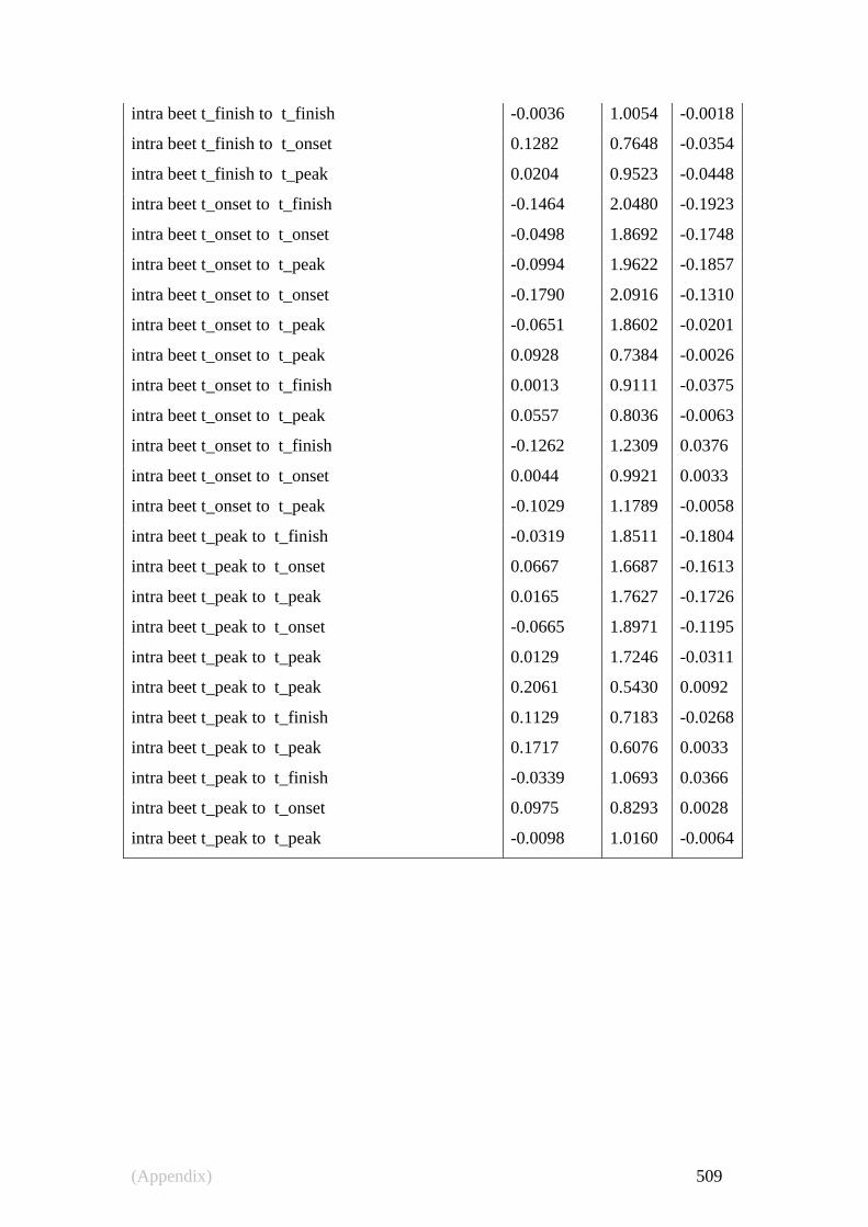
(Appendix) 509
intra beet t_finish to t_finish -0.0036 1.0054 -0.0018
intra beet t_finish to t_onset 0.1282 0.7648 -0.0354
intra beet t_finish to t_peak 0.0204 0.9523 -0.0448
intra beet t_onset to t_finish -0.1464 2.0480 -0.1923
intra beet t_onset to t_onset -0.0498 1.8692 -0.1748
intra beet t_onset to t_peak -0.0994 1.9622 -0.1857
intra beet t_onset to t_onset -0.1790 2.0916 -0.1310
intra beet t_onset to t_peak -0.0651 1.8602 -0.0201
intra beet t_onset to t_peak 0.0928 0.7384 -0.0026
intra beet t_onset to t_finish 0.0013 0.9111 -0.0375
intra beet t_onset to t_peak 0.0557 0.8036 -0.0063
intra beet t_onset to t_finish -0.1262 1.2309 0.0376
intra beet t_onset to t_onset 0.0044 0.9921 0.0033
intra beet t_onset to t_peak -0.1029 1.1789 -0.0058
intra beet t_peak to t_finish -0.0319 1.8511 -0.1804
intra beet t_peak to t_onset 0.0667 1.6687 -0.1613
intra beet t_peak to t_peak 0.0165 1.7627 -0.1726
intra beet t_peak to t_onset -0.0665 1.8971 -0.1195
intra beet t_peak to t_peak 0.0129 1.7246 -0.0311
intra beet t_peak to t_peak 0.2061 0.5430 0.0092
intra beet t_peak to t_finish 0.1129 0.7183 -0.0268
intra beet t_peak to t_peak 0.1717 0.6076 0.0033
intra beet t_peak to t_finish -0.0339 1.0693 0.0366
intra beet t_peak to t_onset 0.0975 0.8293 0.0028
intra beet t_peak to t_peak -0.0098 1.0160 -0.0064

(Appendix) 510
14.5 Implementations of Selected Algorithms
The full implementation of this work is made available on the SourceForge website,
the project page is http://sourceforge.net/p/creemers2013phd. However, as time has a
habit of destroying online resources, this appendix contains implementations of
selected algorithms developed during the course of this research.
A summary of the files contained in the project.
Language files comments Lines of code
C# 582 42,077 148,580
MATLAB 889 19,334 38,536
C++ 25 655 5,288
C 14 811 2,279
C/C++ Header 33 1,036 1,652
Lua 27 319 1,567
DOS Batch 5 0 83
make 1 10 25
SUM: 1,576 64,242 198,010
Compilation requires MatLab 2009+, Visual Studio 2010+
14.5.1. Linear Criterion for ECG subtraction procedure.
This section holds only a portion of our implementation of the subtraction procedure,
due to the size of the code a full listing was not possible. This portion was given
because it was an alteration to the method advocated by Levkov et al., (2005) which
improved our results.
The rest of the code is available via http://sourceforge.net/p/creemers2013phd.
/// <summary> /// Linear criterion as described on page 3 of Levkov et al 2005. /// Tweaked for better performance. /// </summary> /// <param name="data">Data to be processed</param> /// <param name="sampleRate">Sample rate of signal</param> /// <param name="noiseFreq">frequency of noise in Hz</param> /// <param name="threshHold">160µV, 150µV and 100µV are known good thresholds.</param> /// <returns></returns> private static double[] linearTest(double[] data, int sampleRate, double noiseFreq, double threshHold) threshHold = threshHold * 1000; int consecuativeFirstDifeerences = 6; double[] r = new double[data.Length]; int n = (int)(sampleRate / noiseFreq); if (n < 1)

(Appendix) 511
n = 1; //stops a bad calculation and crash for (int pos = 0; pos < data.Length - consecuativeFirstDifeerences - n; pos++) double min = double.MaxValue, max = double.MinValue; for (int i = 0; i < consecuativeFirstDifeerences; i++) double difference = data[pos + i + n] - data[pos + i]; if (difference > max) max = difference; if (difference < min) min = difference; r[pos] = ((max - min) < threshHold) ? 1 : 0; //flatten out the diference graph a bit int halfFlattenSize = (int)(n * 1.5); int entropy = 0; double smoothAgainst = 0; for (int i = 0; i < (r.Length - halfFlattenSize); i++) if (r[i] == smoothAgainst) entropy = halfFlattenSize; else if (entropy > 0) entropy--; r[i] = smoothAgainst; else for (int f = 0; f < halfFlattenSize; f++) if (r[i + f] == smoothAgainst) r[i] = smoothAgainst; break; //fill in the last 6 spots for (int pos = (data.Length - consecuativeFirstDifeerences - n); pos < data.Length; pos++) r[pos] = 0; return r;

(Appendix) 512
14.6 Assorted Notices and Communications Used
An advert, shown in Figure 397, was used to gain the support of student nurses as
staff in the experiment. This advert was distributed by the school of nursing to their
best final year students.
Figure 397: Advert for nurses

(Appendix) 513
A notice was placed along corridors to stop students conducting wireless surveys
proceeding too close to the laboratory (see Figure 398).
Figure 398: Notice to other students.

(Appendix) 514
An advertisement (see Figure 399 and Figure 400) was used to seek volunteers for the
study. (The device shown was a popular MP3 player in Perth Western Australia at the
time of the experiment; MP3 players at the time being a luxury item).
Figure 399: Advert for volunteers (for noticeboards)
A handout version of the same advert.
Figure 400: Advert for volunteers (handout)

(Appendix) 515
An instructional notice was present in the room, see Figure 401.
Figure 401: Notice displayed facing entrance to room.

(Appendix) 516
The disclosure forms are shown in Figure 402 and Figure 403. A Informed consent
form was also signed by all participants Figure 404. Originally these forms were
printed on heavy stock with university letter head.
Figure 402: Disclosure form (1 of 2)

(Appendix) 517
Disclosure form (Page 2)
Figure 403: Disclosure form (2 of 2)
Consent form
Figure 404: Informed consent form

(Appendix) 518
14.7 Risk Management Report
What follows is the risk management report as presented to and approved by the
Human Research Ethics Committee and the Occupational Health and Safety
department. The report was written prior to the room being acquired and some fine
tuning of procedures.
Project:
Neural Network Refinement of the Emotion Classification Problem
Researcher:
Warren Creemers
Principle Supervisor:
A/Prof. Wojciech Kuczborski
Submitted 12th
March 2003 (in surplus of requirements) as part of the Application to
Undertake Research Involving Human Subjects to the Human Research Ethics
Committee of Edith Cowan University.
Contents 1.0 Introduction
2.0 Operating Procedure
3.0 Identification of key risks
3.1 Risk Prioritization
4.0 Risk Minimization Strategies
4.1 Minimization of Emotional Distress Risk
4.2 Minimization of Electrocution Risk
5.0 Risk Response Strategies
5.1 Response to Emotional Distress Risk
5.2 Response to Electrocution Risk
6.0 Conclusion
7.0 - Risk Calculations
1.0 Introduction
Two main risks have been identified with the data collection phase of the project.
These risks are concerned with the health and safety of the participants in the
experiments to be conducted. Due to the nature of their impact these risks are given
serious attention and an appropriate management strategy is being adopted to ensure
that no-one is in any way harmed through their participation in this experiment.
2.0 Operating Procedure
The experimental procedure here is preliminary and will undergo refinement before
collecting the final data. This procedure is a guide to show the scientific method in
use and to allow for ethical considerations to be examined.

(Appendix) 519
To collect training data volunteers will be fitted with a Thought Technology
ProComm Sensing System and will then view segments of the International Affective
Picture System (IAPS) slide database. Figure 1.0 illustrates the set-up of the
experiment.
A room will be prepared for experimental work. There will be no pictures on the walls
of the room and the room will be kept as sparse as possible. A divider will be placed
in the room and a computer used to control the experiment will be placed behind it. At
the rear of the room a clock might be positioned for the convenience of the
experiment operator.
When a subject enters the room the operator will advise the subject that the slides
about to be viewed may include offensive or unpleasant material. The subject will be
required to sign a Disclosure and Informed Consent form.
The subject will be fitted with the ProComm Sensing System by the operator and be
seated in a comfortable chair. The sensing system will be connected to a recording
computer via a data cable. The room will then be darkened and the operator will stop
any communications with the subject and move out of sight behind the divider. The
subject will be left for one minute to let the subject‘s heart rate come to rest. After the
subject is at rest the projector will start displaying a sample of the IAPS slide
database. Three random slides will be displayed to avoid possible biases caused by the
presence of anticipation and to engage the subject. After this warming up period, six
slides for each emotion to be detected will be displayed in random order. Three of the
slides will invoke the emotion and three of the slides will cause the emotion to not be
present. To ensure accuracy each slide will need to be validated to show the desired
affect in the subject was achieved. This can be done via self assessment with the user
providing feedback on how each slide made them feel.
After the experiment is complete the operator will check to see if the user has not
been adversely affected by the slides content (left in a state of distress). If a subject is
adversely affected (unlikely) the operator should direct the user to an on campus
councilor and mark the result extracted as biased and probably unusable.
After the experiment is completed the operator will record the user‘s height, weight,
age and gender.

(Appendix) 520
Figure 1.0: Experiment setup
Similar experiments may be conducted using interactive software (word processor or
video game) to examine emotional state during computer use. These experiments will
not contain any un-pleasant or explicit content.
3.0 Identification of key risks
Two key risks are identified in this document:
1: Emotional distress
2: Electrocution
The risk of emotional distress refers to a subject being exposed to an image in the
IAPS that the subject feels is overly unpleasant or offensive. This risk occurs because
part of the content of the IAPS database is very strong. At worst a subject may be
exposed to scenes containing horror, nudity, death and erotica.
The risk of electrocution refers to the presence of electrodes on the human skin. This
risk is similar to the risk involved with using an underwater low-voltage pool lamp.
The risk is serious not because electrocution is more likely, but because of the
increased impact of any electrical shock.
When electrodes are placed on human skin any power surge in the machinery
connected to the electrode could (if unsafe or damaged equipment is used) pass
straight to the person and provide an extremely dangerous situation. The situation is
potentially dangerous because of:
The proximity of the electrode to vital organs (such as the heart);
The fact that the electrodes are attached to the person.
3.1 Risk Prioritization
To prioritize these risks a priority scale is adopted. The probability of the risk is
estimated (0% -100%) and the impact of the risk on a scale of 1 to 100 is determined.
The two statistics are multiplied and used as a measure of importance (0-1000). See
Appendix 1 for calculations used to populate the following table

(Appendix) 521
Risk Probability Impact Importance
Emotional Distress 0.000055% 10 0.00055
Electrocution 0.000000093% 99 0.0000092
By these calculations emotional distress is deemed to be the most important risk in the
project.
4.0 Risk Minimization Strategies
The risk management strategies presented here will reduce the possibility of any risk
occurring to a level compliant to Australian & university standards.
4.1 Minimization of Emotional Distress Risk
The risk of emotional distress applies mainly to people who already have a strong
aversion to a particular type of content. Generally speaking most people with such
aversions are aware of them and would not choose to view content they knew could
upset them. This is the basis of the content advisory system used in Australia to deal
with this same risk as it applies to public television.
The fist stage of managing this risk involves alerting people to the content during the
recruitment phase. If a subject is aware of the risk before agreeing to take part in the
experiment then a subject can make an informed choice on whether to volunteer or
not. It also avoids the situation in which someone volunteers for the experiment and
only finds out about the content when signing a consent form. Under these
circumstances it may be possible for someone to feel pressured into participation so as
not to waste the operator‘s time or have to admit to being sensitive to content.
The second stage of managing this risk involves the operator of the experiment
alerting the volunteer to the type of content that can be expected and providing as
much as possible a ―pressure free‖ environment for the volunteer to decline
participation. After this the Informed Consent and Disclosure forms will be offered to
the volunteer. The experiment will not commence until these forms are signed.
At this stage all volunteers with known aversions to content have had an opportunity
to withdraw. The third stage of this management plan deals with volunteers who, for
some reason, did not withdraw from the experiment when they felt content may affect
them. This stage also deals with those volunteers who did not realize they would be
sensitive to a particular content. To deal with this situation the volunteer will be
informed of actions he/she can take if any content upsets them. These actions include
the volunteer being able to:
Have the experiment stopped at any time (with the projector immediately turned off);
Leave at any time, no explanation required
The subject will be informed of these rights at the beginning of the experiment before
any work is commenced. To aid in allowing the subject to leave at any time there will
be only one subject allowed in the room at any time. This is done to avoid ―peer
pressure‖ which may cause a subject to remain against their will.
There is lastly a risk that someone with an aversion to content who did not volunteer
for the project may come barging through the door to the room being used for the

(Appendix) 522
experiment. To manage this risk a do not disturb notice may be posted on the door. At
no point will the door be locked, the ―free to leave any time‖ environment cannot be
compromised to handle such a small and unlikely risk.
4.2 Minimization of Electrocution Risk
The risk pertains to:
Mains operated equipment used with sensors designed for connection to the human
body.
Non-Mains operated equipment that utilizes a non-optically-isolated data connection
to a mains powered computer or recording device.
The second type of equipment is fundamentally unsafe during a power surge and will
not be used in this work. Thus this risk applies to management of mains operated
equipment used with sensors designed for connection to the human body.
Firstly all such equipment would only be purchased where all government guidelines
for equipment suitable for use on humans are met. This equipment would be presented
to the university occupational health and safety officer along with an operations plan
for the experiments to be conducted. After Ethics clearance is received no
experiments will be conducted until the experiment passes and occupational health
and safety inspection.
Defective equipment may fail to isolate the subject from a mains power surge. For this
reason any damage to equipment will be recorded and where necessary damaged units
will be sent to a biomedical equipment technician for a safety report. Units found
unsafe will undergo repairs (by a biomedical equipment technician) or disposal. The
serviced equipment will be brought to the attention of the OHS officer for re-approval
before being used again.
Where possible, Non-Mains operated equipment that utilizes an optically-isolated data
connection will be used in preference to any mains operated equipment. This is
because such a piece of equipment if in working order poses no real risk to
participants.
5.0 Risk Response Strategies
Risk mitigation strategies are intended to provide a procedure to follow in the event of
an identified risk occurring. The focus on the procedures presented here is the
practicality of the procedures to be followed.
5.1 Response to Emotional Distress Risk
A university councilor will be informed of the type of research being conducted to
ensure that in the case of someone being distressed by any image, appropriate
counseling is available.
5.2 Response to Electrocution Risk

(Appendix) 523
There is no practical method to mitigate the electrocution risk. An ambulance will be
called in the event of any electrocution. The approach to this risk is currently focused
on preventative measures.
The occupational health and safety officer will be asked to advise on the inclusion of
the following Items:
A first aid station and/or box;
First aid training for staff running the experiment;
A resuscitation /electrocution chart.
6.0 Conclusion
Many of the risks visited here are unlikely to occur, but are presented here in a strait
forward and open manner. The risks though highly un-likely are treated very seriously
because of the nature of their impact.
It must be stressed that the proposed experiments conducted in a professional manner
are safe. The risks shown relate mainly to results that can occur if the experiment was
conducted in an unethical manner or if unsafe equipment is purchased.
A second report on the final state of apparatus and the results of OHS inspections will
be made available on request to demonstrate the correct implementation of all
procedures outlined in this document.
7.0 Risk Calculations
Electrocution
Probability Calculation
Conditions for risk to occur:
Massive Power Surge (1/16000hr)
AND
Equipment becoming unsafe (0.0001%)
AND
Surge not stopped by university power regulators (0.5%)
= 0.0000625%/hr * 0.0001 * 0.5
= 0.000000003% chance of electrocution per hour of usage.
Estimated volunteers = 100
Time per experiment = 0.3hr
= 30hr usage at 0.00000125%/hr
= 0.000000093% chance of electrocution occurring during duration of project.
The probability of a participant being harmed by the equipment is approximately 1 in
30 million.

(Appendix) 524
Impact Calculation
Probable impact:
80% fatality
Assigned impact value – 99
Emotional distress
Probability Calculation
Conditions for risk to occur:
Person is sensitive to material (1%)
AND
(Person fails to withdraw from experiment (1%))
OR
(Person is unaware of sensitivity (0.1%))
AND
Material is shown (50%)
AND
Material has lasting effect (1%)
= .01 * ( .01 + .001) * .5 * .01
= 0.0000000055 or 0.00000055% chance per person
Estimated volunteers = 100
=0.000055% chance of incident during duration of project.
This experiment would be upsetting to one in every 18,000 participants.
Impact Calculation
Probable impact:
99% unpleasant thoughts to possible nightmare
1% serious problem (not caused by experiment, just triggered)
Assigned impact value – 10

(Appendix) 525
14.8 Email sent to all would be volunteers
General Information.
Participation in this experiment is done by appointment. Attached to this email is a
HTML document indicating the currently available appointment times. The
experiment takes about 15 minutes and involves watching a slide show containing
images form an international research project. Please note that some of these images
contain strong scenes that may offend some viewers.
During the experiment you will have a panel of buttons which you can use to express
your opinion on the images shown. Your feedback is anonyms and your identity is not
recorded or associated with any of the data collected.
At the end of the experiment you can put your details on a raffle ticket. After 100
experiments are completed a Creative Nomad (128mb) Mp3 player will be raffled and
the winner contacted to collect their prize.
The Equipment
The biofeedback equipment being used is safe, the lab has Occupational Health and
Safety clearance and the experiment is approved by the Edith Cowan University
Ethics Committee.
Sensors Used
Six non-allergenic adhesive electrodes will be attached to your arms and face.
4 elasticised sensors will be placed over your fingers.
1 respiration sensor worn over any non bulky clothing will be wrapped around your
chest.
There are no needles or other invasive / hazardous instruments being used in this
work. All sensors will be attached by qualified nursing students from the School of
Nursing.
Before Arriving.
We ask that you not drink coffee (or a caffeinated drink), consume alcohol, or smoke
a cigarette for 3 hours prior to the experiment. It would be preferable if you wore a
loose fitting t-shirt so that electrodes can easily be connected to your arms.
To make an appointment.
Simply nominate which of the timeslots from the attached list you would like. The
time slots given out on a first come first served basis.

(Appendix) 526

(Appendix) 527
14.9 Median Filtering Algorithm
Our algorithm, termed oobTree, was verified to produce the same results as the matlab
2009b filter (medfilt1) and has been made publicly available (W Creemers, 2010) to
help other researchers in cardiology.
Figure 405: Median filter performance comparison for a 2.66GHz quad core Intel Q9450 (our solution is
oobTree)
As can be seen in Figure 405 (note: using log scale axis) median filter performance is
still expensive on hardware circa 2010 and our algorithm is capable of computing
datasets that would otherwise take over 2 hours in under 10 seconds.
Previous algorithms such as described by Pratt (W. . Pratt, 1978) offer O(N·log W)
performance, where W is the filter size, and N is the number of samples to be
processed. Our algorithm presents an order N solution, that is to say the window size
has little impact on performance, but signal morphology does).
The algorithm we developed for median filtering operates by maintaining a binary
tree which indexes a circular buffer. The tree (and also the circular buffer) holds all
the data being evaluated for the current window position.

(Appendix) 528
Each node in the binary tree stores the total amount of children (designated c) beneath
it and is uniquely referenced by its position i in the circular buffer.
When it is necessary to find the median value of the window, it is the root node of the
tree if the tree if the tree is kept balanced, or if the tree is not self balancing searchable
by recursive iteration using c as a guide to increase performance.
Figure 406: Structure used for efficient median filtering
When the window is shifted forward one sample, the item at the tail of the circular
buffer is removed from the tree and all parent c values updated. The next item now
included by advancement of the window is added to the tree and linked to the head of
the circular butter.

(Appendix) 529
As the cost of advancing a window is very low (two tree operations) and finding the
median value in the tree is generally very cheap, the algorithm tends to exhibit
excellent performance.
Some notes on the algorithm and its performance:
1. It is possible to avoid the overhead of memory allocation by reusing nodes in
the binary tree as this will help microcontroller implantations;
2. Signal morphology affects performance;
3. The more balanced the tree is the quicker the search for the median will be;
4. Our investigation would suggest that self balancing trees are generally not
necessary for real world data sets as the tree tends to stay well balanced;
5. It is possible to implement the tree recursively for W < 10,000 on a PC;
6. The algorithm is only advisable for large windows (W > 20);
7. The algorithm is not virtual memory aware. If the window size is sufficient to
occupy all available physical memory it will typically generate two page faults
per window advancement;
8. The algorithm is able to work with streamed data and does not require more
data than the window size to operate.
There is a major problem if a signal has no noise and prolonged linear segments
(approaching half W). This will cause the tree to from a completely unbalanced
structure because the relationship of each successive point is the same. As a result the
tree will from a linked list type structure as per Figure 407. In this case performance is
O(
) and the results are similar to other optimised median filtering techniques. In this
way it can be said our technique exploits the noisy nature of real world data to achieve
a performance boost. The algorithm is not as efficient for some tasks that work with
synthetic data.

(Appendix) 530
Figure 407: Unbalanced tree
It is possible to allow for the null signal (constant reading) to progress smoothly
through the filter without the issues previously discussed, by having the tree assign
smaller numbers left, larger numbers right and equal numbers either way by means of
a quasi random process.

(Appendix) 531
14.10 Hardware SAM Circuit Diagram and Information
This section of the appendix contains all the information needed to build and operate
our SAM panel. This device and related documentation was a collaborative effort with
SCIS research support team. The source code for the embedded system and PC
controller are available online: https://sourceforge.net/projects/samhardware/.
Version 1.1
1
Ken WIld
S
2
Pushbutton 'Next Slide'
1
0
K
R50
V
C
C
12345 6789
1
1
1
0
J
1
D Connector 9
0.1uF C62
0.1uF
C61
0.1uF
C60
0.1uF
C63
C1-
4
C2+
5
C2-
6
T1 in
1
1
R1 out
9
Ready
1
Force on
1
2
C1+
2
GND
14
+3.3V
15
Invalid
1
0
ForceOFF
1
6
R1 in
8
T1 out
1
3
V
-
7
V
+
3
ICLA
ICL3227E
0.1uF
C64
Serial RS232 /TTL Interface
V
C
C
Serial Rx
Serial Tx
ICSP PGDICSP PGC
ICSP VPP
V
C
C
In Circuit Programming Socket
S
P
1
Electrostatic Transducer - Jaycar AB-3440
Aztec Switchbox CPU
4
NB: Value of speaker resistor unknown...
12345 6789
1
1
1
0
J
2
D Connector 9
Mount on left hand side of box
Mount on right hand side of box
1
K
V
R
1
Audio
OK_Switch
Next Slide Switch
Audio Output
V
C
C
OK_LED
1
2
LED40
3
3
0
R40
2
k
V
R
5
Next Slide LED
Qout
9
O
E
1
3
C
L
1
0
Din
1
4
SCK
1
1
STB
1
2
I/O0
1
5
I/O1
1
I/O2
2
I/O3
3
I/O4
4
I/O5
5
I/O6
6
I/O7
7
V
C
C
1
6
G
N
D
8
U
2
Qout
9
O
E
1
3
C
L
1
0
Din
1
4
SCK
1
1
STB
1
2
I/O0
1
5
I/O1
1
I/O2
2
I/O3
3
I/O4
4
I/O5
5
I/O6
6
I/O7
7
V
C
C
1
6
G
N
D
8
U
3
Qout
9
O
E
1
3
C
L
1
0
Din
1
4
SCK
1
1
STB
1
2
I/O0
1
5
I/O1
1
I/O2
2
I/O3
3
I/O4
4
I/O5
5
I/O6
6
I/O7
7
V
C
C
1
6
G
N
D
8
U
4
Row 1 LED 7 Row 1 LED 2Row 1 LED 3Row 1 LED 4Row 1 LED 5 Row 1 LED 1Row 1 LED 8
Row 1 LED 9
Row 1 LED 6
Row 2 LED 7 Row 2 LED 2Row 2 LED 3Row 2 LED 4Row 2 LED 5 Row 2 LED 1
Row 2 LED 8Row 2 LED 9
Row 2 LED 6
Row 3 LED 7
Row 3 LED 2Row 3 LED 3Row 3 LED 4Row 3 LED 5 Row 3 LED 1
Row 3 LED 8Row 3 LED 9
Row 3 LED 6
Qout
9
O
E
1
3
C
L
1
0
Din
1
4
SCK
1
1
STB
1
2
I/O0
1
5
I/O1
1
I/O2
2
I/O3
3
I/O4
4
I/O5
5
I/O6
6
I/O7
7
V
C
C
1
6
G
N
D
8
U
5
V
C
C
V
C
C
V
C
C
V
C
C
LED Strobe
LED Clock
LED Data
LED Strobe
LED Clock
LED Strobe
LED Clock
LED Strobe
LED Clock
V
C
C
V
C
C
V
C
C
V
C
C
74HC595
74HC595
74HC595
74HC595
Row 1 LED 7 Row 1 LED 2Row 1 LED 3Row 1 LED 4Row 1 LED 5 Row 1 LED 1Row 1 LED 8Row 1 LED 9 Row 1 LED 6
1
2
LED11
3
3
0
R135
1
2
LED12
1
2
LED13
1
2
LED14
1
2
LED15
1
2
LED16
1
2
LED17
1
2
LED18
1
2
LED19
V
C
C
Row 2 LED 7 Row 2 LED 2Row 2 LED 3Row 2 LED 4Row 2 LED 5 Row 2 LED 1Row 2 LED 8Row 2 LED 9 Row 2 LED 6
1
2
LED21
3
3
0
R136
1
2
LED22
1
2
LED23
1
2
LED24
1
2
LED25
1
2
LED26
1
2
LED27
1
2
LED28
1
2
LED29
Row 3 LED 7 Row 3 LED 2Row 3 LED 3Row 3 LED 4Row 3 LED 5 Row 3 LED 1Row 3 LED 8Row 3 LED 9 Row 3 LED 6
1
2
LED31
3
3
0
R137
1
2
LED32
1
2
LED33
1
2
LED34
1
2
LED35
1
2
LED36
1
2
LED37
1
2
LED38
1
2
LED39
2
K
V
R
2
2
K
V
R
3
2
k
V
R
4
2
2
K
R25
3K6 R27
4K7 R28
6K8 R29
1
0
K
R30
1
6
K
R31
3
3
K
R32
1
0
0
K
R33
2M2 R34
V
C
C
S
3
S
5
S
6
S
7
S
8
S
9
S
1
0
S
1
1
S
4
2K7 R26
ANALOG Row 1
Top row
2
2
K
R15
3K6 R17
4K7 R18
6K8 R19
3
3
K
R22
1
0
0
K
R23
2M2 R24
V
C
C
S
1
2
S
1
4
S
1
5
S
1
6
S
1
7
S
1
8
S
1
9
S
2
0
S
1
3
2K7 R16
ANALOG Row 2
Middle row
2
2
K
R
5
3K6 R
7
4K7 R
8
6K8 R
9
1
0
K
R10
1
6
K
R11
3
3
K
R12
1
0
0
K
R13
2M2 R14
S
2
1
S
2
3
S
2
4
S
2
5
S
2
6
S
2
7
S
2
8
S
2
9
S
2
2
2K7 R
6
ANALOG Row 3
V
C
C
Bottom row
+
-
A
C
A
C
Bridge Rectifier
Bridge
+
1
-
2
- sw
3
DC power socket
1
2
D
1
D Schottky
2
2
R101
4
7
0
u
F
C
1
12
charge LED
L
E
D
2
1K2
R100
Battery Charger Circuit
Trickle charges batteries at 231mA 10hrs
Supply voltage max 12 VAC
Io = V/R + IbIb = 3.9mA
2.2uF
C
3
0.1uF
C
2
ON/OFFSW-SPST
1
2
Batt 1
Battery Pack
Regulated 5 volt supply
2
4
0
K
R104 1
5
0
K
R103
Battery Sense
I
N
1
ON/OFF
3
O
U
T
5
N
C
4
G
N
D
2
Volt reg 3.3
LP2980IM5-X3.3
SB1078 Jaycar 4 AA NI Mh 2000 mAh Tag
Battery
12
Power3
K
R102
V
C
C
Vin
1
GND
2
Vout
3
G
N
D
LM7805Volt Reg
123456
RJ11
RJ1S
o
c
k
e
t
RA0/AN0
2
RA1/AN1
3
RA2/AN2
4
RA3/AN3/VREF
5
RA4/T0CKI
6
RA5/SS/AN4
7
RB0/INT
3
3
R
B
1
3
4
R
B
2
3
5
R
B
3
3
6
R
B
4
3
7
R
B
5
3
8
R
B
6
3
9
R
B
7
4
0
RC0/T1OSI/T1CKI
1
5
RC1/T1OSI/CCP2
1
6
RC2/CCP1
1
7
RC3/SCK/SCL
1
8
RC4/SDI/SDA
2
3
RC5/SDO
2
4
RC6/TX/CK
2
5
RC7/RX/DT
2
6
RD0/PSP0
1
9
RD1/PSP1
2
0
RD2/PSP2
2
1
RD3/PSP3
2
2
RD4/PSP4
2
7
RD5/PSP5
2
8
RD6/PSP6
2
9
RD7/PSP7
3
0
RE0/RD/AN5
8
RE1/WR/AN6
9
RE2/CS/AN7
1
0
VSS
1
2
VSS
3
1
MCLR/VPP
1
OSC1/CLKI
1
3
OSC2/CLKO
1
4
V
D
D
1
1
V
D
D
3
2
1
8
F
4
5
2
1
2
Y
1
4Mhz XTAL
1
0
u
F
C
7
3
0
p
F
C
8
3
0
p
F
C
9
1
0
u
F
C
6
1
0
K
R
4
V
C
C
V
C
C
ANALOG Row 1
Serial Rx Serial Tx
Battery
ANALOG Row 2ANALOG Row 3
LED Data
LED Strobe
LED Clock
ICSP PGD ICSP PGC
ICSP VPP
CPU
Audio
OK_Switch
OK_LED
1 2 3 4 5 6
RJ11
RJ2S
o
c
k
e
t
1 2 3 4 5 6
RJ11
RJ3S
o
c
k
e
t
1
0
K
R20
1
6
K
R21
V
C
C
V
C
C
P
1
1
0
K
R201
12
54
6
Opto1
2N7000
6
2
R202
1
0
K
R203
Volts
Volts
Generated pulse sense cable plug
Figure 408: SAM tablet circuit diagram

(Appendix) 532
14.10.1. Microcontroller
The microcontroller is a Microchip PIC 18LF452. The LF series is guaranteed to
work within specification with a 3.3V supply. The oscillator is a 4Mhz ceramic. An
additional 17 input/output ports are available for future expansion.
14.10.2. Power Supply
A slider switch on the rear of the unit powers the device on, and illuminates a small
red LED. Power is provided by four 1.2V NiMh batteries. At full charge and without
LEDs switched on, these may read approximately 5V. A regulator brings this voltage
down to 3.3V. The regulator used is the LP29801M5-X3.3, chosen for its low
quiescent power and low dropout voltage.
A battery charge circuit is also provided. This requires between 9 and 12V AC or DC,
at 200mA. As this represents the ten percent charge rate of the cells, the charger may
be left on indefinitely. Furthermore, the unit may be operated whilst charging. A
green LED on the rear of the unit indicates charging is taking place.
Total quiescent current consumption is 6.56mA. With one LED on in each row,
adjusted to high intensity, this is approximately 10mA. As the batteries are rated at
2000mAH, the switchbox may therefore be operated for approximately 200 hours
between charging.
Battery level may be requested by the Host with the BATL command. The
microcontroller reads the level on a voltage-divider (ref: schematic, Appendix 5,
R103,R104), and returns a value representing the percentage of charge, ranging from
0% to 100%. The divider reduces the maximum battery input voltage from 5V to
3.08V. This voltage is fed to the AN0 input (pin 2 of the microcontroller) where it is
converted to an 8 bit value. This is then converted to a percentage of 3.3V, and
returned to the Host. This value is only intended as a rough indication of battery
charge state, as the relationship between capacity and voltage is non-linear. The
microcontroller brownout-detector will activate at 2.2V, resetting the switchbox.

(Appendix) 533
14.10.3. Audio Tone Output
An audio output is provided in the form of an electrostatic transducer, attached to port
RD2 of the microcontroller. This produces tones ranging from 100hz to 4700Hz. A
potentiometer (screwdriver adjustable trim-pot) mounted on the back panel permits
adjustment of the volume.
The range is set by defines in Globals.h. The setAudio() function (in Globals.C) is
used to control the on/off state and frequency of the tone. When the microcontroller
receives an AUON command from the Host, Timer1 is enabled. This is primed with a
count value determined by the AUxy command. The 16 bit timer counts up from this
value, and overflows, producing an interrupt. The interrupt service routine ( ISR() )
then toggles the speaker output on port RD2, and reinstates the pre-load value. This
process repeats indefinitely, producing an audible output, until the AUOF or RSET
command is received.
14.10.4. Microphone Output
A high impedance 2Kohm dynamic microphone is mounted on the inside of the
enclosure, to pick up switch depression noise. The output signal is provided at the
output via a 3.5mm audio socket. Cabling should be coaxial to improve noise
performance.
This output may be plugged directly into a sound-card for monitoring or later
analysis.
14.10.5. Synch Output
When the Host transmits an Sxyz command (eg: ‗S200‘), the microcontroller outputs
the specified number of pulses, of 39mSec duration, to port RD0. This pulse train
switches a 4N26 phototransistor opto-coupler, which provides an isolated pulse-train
at the 3.5mm output socket on the back of the instrument.
The configuration used provides 7500 AC volts of isolation from input to output. No
active voltage is provided at the output. However, with no load attached, the photo-

(Appendix) 534
voltaic effect produces a waveform with a 0 to peak value of approximately 0.3v. The
output lead contains a 10k resistor, to better mimic the characteristics of human skin.
This output may be used to attach directly to a Galvanic Skin Response input.
14.10.6. SAM LED Outputs
A total of 27 LEDs are mounted on the PCB. When the Host issues the LTxy
command, (eg: LTA3), the microcontroller lights the appropriate LED. When a ‗clear‘
command such as CLRZ, CLR1, CLR2 or CLR3 is issued, function clearLEDs() is
called, and LEDs are cleared. Each of these commands makes use of the setLED()
function.
LEDs are not attached directly to the PIC, but must be accessed via four daisy-chained
serial shift registers. Function setLED() loads a static array with the (passed) status of
the LED to be switched. Being static, this array maintains its list of LED status
between calls. The array is then clocked out of the PIC to the first serial register.
When all twenty-seven array values have been loaded, the strobe input is pulsed,
transferring bits in each serial register to the LEDs on the parallel outputs.
LED intensity may be varied for each row using a trim-potentiometer, accessed
through the rear-panel of the switch-box.
14.10.7. Reading Input Voltages
The analogue inputs are used to determine whether an SAM switch closure has
occurred, as well as to read the battery voltage. Function readInputVolts(int iInput#)
returns the conversion value of the specified input.
Input# Device Read Micro Input
0 Battery Voltage AN0
1 Top row switches A,B,C,D,E,F,G,H,I AN1
2 Middle row switches A,B,C,D,E,F,G,H,I AN2
3 Bottom row switches A,B,C,D,E,F,G,H,I AN3

(Appendix) 535
The A/D converter has 8 channels, of which only 4 are utilised in this design.
Providing 10 bit resolution, conversion results are stored in two 8 bit registers,
ADRESH and ADRESL. This application will only require 8 bit resolution (256
levels), and therefore only the most significant 8 bits are used. This provides a voltage
resolution of 12.8906mV. A ‗left-justify‘ configuration feature is offered by
Microchip, enabling the 8 most significant bits in the result to be shifted into the
ADRESH register.
14.10.8. Conversion Time
Stabilisation time is required for the Analogue to Digital converter to charge the input
capacitance after a channel is changed. Peatman (Peatman, pg. 138) states that the
source resistance should be less than 2k2. Due to power consumption concerns, the
source resistance of this design is a maximum of 22k. However, sufficient acquisition
delay will be provided to ensure that the holding capacitor charges fully. This
minimum time is determined in the calculation below.
Time required to acquire the sample is given by:
Tacq = Amplifier Settling Time + Holding Capacitor Charge Time + Temperature
Coefficient
Where:
CHOLD = 120 pF
Tamp = 2uS
Rs = 22 k (maximum source impedance, with no switch pressed)
Conversion Error 1/2 LSB
VDD = 3.3V
Rss = 11K
Temperature = 50C (system max.)
Holding Capacitor Charge Time:
Tc = -Chold ( Ric + Rss + Rs) In(1/2047)
= -120pF( 1K + 11K + 22k ) (-7.6241)
= 31uS

(Appendix) 536
Temperature Coefficient:
Tcoff = [( Temp – 25‘C) ( 0.05uS/‘C ) ]
= (50 – 25) (0.05 x10^-6)
= 1.25uS
Acquisition time:
Tacq = Tamp + Tc + Tcoff
= 2uS + 31uS + 1.25uS
= 34.25uS
A minimum delay, set by global constant ACQUISITION_TIME, will be provided
between the channel selection, and the start of conversion. An initial value of
120uSeconds will be used.
14.10.9. Reading SAM Selection Switches
The switchbox holds 27 ‗SAM-selection‘ switches, arranged in three rows of 9
switches each.
Row Switch Micro Input Row#
Top Row A,B,C,D,E,F,G,H,I AN1 1
Middle Row A,B,C,D,E,F,G,H,I AN2 2
Bottom Row A,B,C,D,E,F,G,H,I AN3 3
Each switch, on closure, shorts a resistive ladder to ground, producing a different
voltage at the analogue input according to which switch was pressed.
The main() routine loops, scanning the three switch rows with the getSwitch(int
iRow#) function. Given the Row number, this uses readInputVolts(int iInput#) to read
the analogue voltage on the appropriate analogue input. The input voltage is then
compared to each of the 10 possible voltage ranges using function getRange(int
iVolts). The returned Range is used to determine which switch was pressed.
When the switch is pressed, a switch code (‗BTxy‘) is sent to the Host. When
released, the switch down time (mSecs) is sent as a 5 digit string.

(Appendix) 537
Debouncing is implemented in main() by examining the giSwitchDownTime global.
If this is too short, switch bounce is deemed to have occurred, and an error message
‗ER04‘ is sent in place of the duration.
The five significant user-button interactions which may occur are as follows:
1. One button is pressed: the getSwitch() function returns the number of the
button, a digit from 0 (leftmost switch) to 8 (rightmost switch).
2. No button has been pressed: the full 3.3V will be read, and the getSwitch()
function returns a flag value (OPEN).
3. More than one button is pressed: Regarded as a user error. However, this
cannot be detected, and only the left-most switch of the group will be returned
as in 1 above.
4. A button is held down: There is no typematic repeat key sent.
5. A button is pressed but contact bounce occurs: main() rejects switch-down
durations less than 5mSecs.
14.10.10. Resistor Ladder Values
Resistors values were calculated to provide maximum separation between values,
assuming a range of 0 to 3.3v. Values were calculated via Ohm‘s law and the closest
available preferred available resistor values were chosen to suit. Resistors are all 1%
tolerance. The Figure 409 illustrates calculated voltages into the microcontroller as
each of the buttons on a row is pressed. Buttons are lettered A to I from left to right.
Figure 409: Calculated nominal voltage (using preferred value resistors)
Analog Input Voltage - Preferred Values
0
0.5
1
1.5
2
2.5
3
3.5
A B C D E F G H I J
Switches
Vo
lts

(Appendix) 538
Table 29 Resistor Ladder Values
Resistor Calculated
Value
Preferred
Value
%Voltage
Error
Ra 22000 22000 0
Rb 2750 2700 1.6194332
Rc 3536 3600 -0.1766784
Rd 4714 4700 0
Re 6600 6800 -0.6281407
Rf 9900 10000 -0.4819277
Rg 16500 16000 0.15197568
Rh 33000 33000 0.0578369
Ri 99000 100000 -0.0503018
Rj - O/C 0
14.10.11. Determination of Range
Only ten voltage ranges are possible at the analogue input to the microcontroller.
These are listed in Table 30:
Table 30: Voltage Ranges
A 0 0 0.180364372 A
B 0.180364372 0.360728745 0.54767886 B
C 0.54767886 0.734628975 0.917314488 C
D 0.917314488 1.1 1.287939698 D
E 1.287939698 1.475879397 1.659024036 E
F 1.659024036 1.842168675 2.019412605 F
G 2.019412605 2.196656535 2.380919361 G
H 2.380919361 2.565182186 2.74999552 H
I 2.74999552 2.934808853 3.117404427 I
NONE 3.117404427 3.3 3.3 NONE
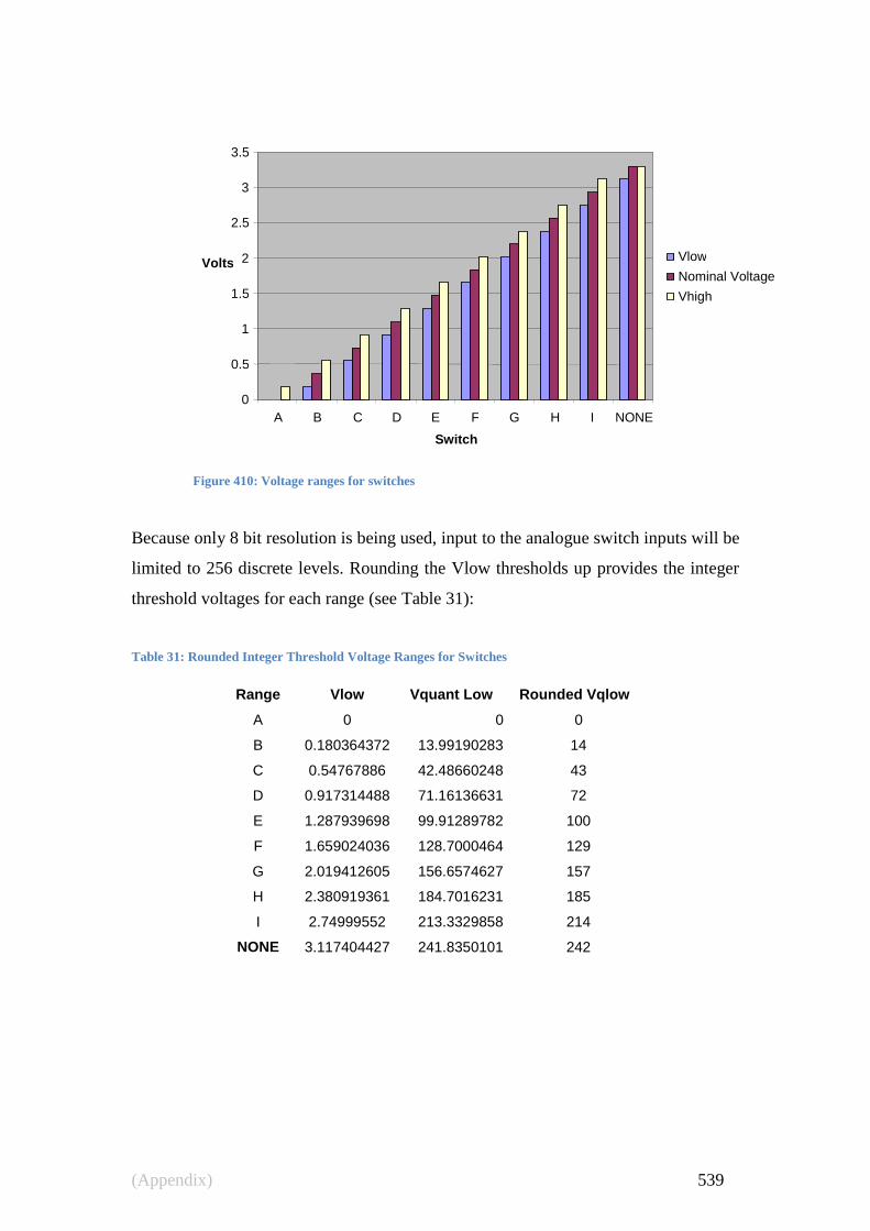
(Appendix) 539
0
0.5
1
1.5
2
2.5
3
3.5
A B C D E F G H I NONE
Switch
Volts Vlow
Nominal Voltage
Vhigh
Because only 8 bit resolution is being used, input to the analogue switch inputs will be
limited to 256 discrete levels. Rounding the Vlow thresholds up provides the integer
threshold voltages for each range (see Table 31):
Table 31: Rounded Integer Threshold Voltage Ranges for Switches
Range Vlow Vquant Low Rounded Vqlow
A 0 0 0
B 0.180364372 13.99190283 14
C 0.54767886 42.48660248 43
D 0.917314488 71.16136631 72
E 1.287939698 99.91289782 100
F 1.659024036 128.7000464 129
G 2.019412605 156.6574627 157
H 2.380919361 184.7016231 185
I 2.74999552 213.3329858 214
NONE 3.117404427 241.8350101 242
Figure 410: Voltage ranges for switches

(Appendix) 540
8 Bit Integer Thresholds
0
50
100
150
200
250
300
A B C D E F G H I NONE
14.10.12. SAM Switch Duration
When SAM switches are pressed, the down-time is recorded, and upon release, the
number of milliseconds elapsed is transmitted to the host.
Function getSwitch() enables Timer0 when a valid switch press is detected. This timer
is initialised by initTimer0() to overflow each millisecond. Each overflow trips the
interrupt routine ISR(), and global giSwitchDownTime is incremented. When the
switch is released, the timer is stopped, and sendSwitchDownTime() transmits the
duration in milliseconds.
By experiment it was found that most button depressions tend to be in the region of 50
to 200mSeconds. Initial attempts resulted in an average error of +-3.45% over the full
range (40mSecs to 2550 mSecs), but with significant errors (as much as +-43%) and
variance in the region of interest. This was improved by reducing overheads
Figure 411: Rounded integer threshold ranges for switches

(Appendix) 541
% Error
-2
-1
0
1
2
3
4
5
6
7
8
9
0 500 1000 1500 2000 2500 3000 3500
Duration (mSecs)
Err
or
%
associated with debouncing, as well as through the use of calibration correction (see
Figure 412).
14.10.13. Communications
The switchbox employs RS-232 over a straight-through cable at 9600bps, 8 bits, no
parity, 1 stop bit. Two RJ-45 connectors, wired in parallel, are provided on each side
of the switchbox to facilitate left or right mounting of the switchbox. In addition,
tracks are provided on the PCB for mounting two right-angle DB-9 connectors.
However, as these had exposed metal parts, it was decided not to install them.
The device used for interfacing provides RS-232 compatible +-9V signals using a
low-current ICL322&E interface chip. This operates on 3.3V, and develops 232 levels
using capacitors and charge-pumps.
14.10.14. Protocol
The protocol is half-duplex (communication in both directions, but not
simultaneously). Command strings characters must be 8 bit ASCII, and must be
capitalised. Unrecognisable commands are ignored.
Figure 412: Button duration - corrected errors

(Appendix) 542
The protocol requires that commands be 4 characters in length, and thus it is possible
that some communications error may leave the switchbox waiting for the rest of a
command. For critical applications, the Host may periodically check for this by
sending a ‗PING‘ request. If no ‗PONG‘ response is detected, the communications
may have failed. The Host may then attempt to re-synch by transmitting a succession
of up to three ‗P‘ characters, until a ‗PONG‘ response is received.
The command queue ring buffer can process up to ten consecutive commands.
Sending more than this will result in overwriting of the buffer contents.
14.10.15. Command Set
Commands are divided into Output (from the switchbox to the Host) and Input
(received by the switchbox from the Host). All commands must be capitols, and no
more than 4 characters long.
14.10.16. Output Commands
BTxy Button on row x, column y is ON
where x is a digit between 1 and 3 inclusive
and y is an alpha character from A to I inclusive
This command informs the Host that the specified SAM selection button
has been pressed. In a typical application, the Host PC application would
record this code, and returns a control message to the switchbox, causing
the corresponding LED to light. The command is sent when the button is
released.
If the xy characters are out of range, an error code (ER02) will be
returned.
wxyz Duration of button-press in 1 millisecond increments (0000 to 9999)

(Appendix) 543
When SAM switches are pressed, the duration of the down-time is
measured to a resolution of 1mSeconds. This measurement is sent to the
host after the switch is released.
OKDN Next Slide‘ button is ON
This command informs the Host that the red ‗Next Slide‘ button has
been pressed.
PONG Confirmation that device is present and operational
The response to a Host ‗PING‘ command. Indicates that the device and
communication link are operational.
Bxyz Battery capacity is currently xyz percent
where xyz is a three digit number between 0 and 100 (full capacity)
The response to a Host request for battery level ‗BATL‘. Provides an
estimate of capacity.
14.10.17. Input Commands
CLRZ Clear all LEDS
All twenty-seven SAM LEDs are turned off.
CLR1 Clear ROW 1 LEDs (top row)
All nine LEDs on this row are turned off.
CLR2 Clear ROW 2 LEDs (middle row)
All nine LEDs on this row are turned off.
CLR3 Clear ROW 3 LEDs (bottom row)
All nine LEDs on this row are turned off.

(Appendix) 544
OKON ‗Next Slide‘ button LED turned on
OKOF ‗Next Slide‘ button LED turned off
AUxx Audio pitch set to one of 99 frequencies between 100 hz and
4,700hz where xx is a two digit number between 0 and 99
AUON Audio ON
Turns the audio speaker on. The tone produced will be at the
frequency set by the previous AUxx command. On power-up, this will
be 2300Hz.
AUOF Audio OFF
BATL Request battery level
Initiates measurement of the battery voltage. The switchbox will
respond with a Bxyz command.
LTxy Set LED on row x and column y ON
where x is a digit between 1 and 3 inclusive
and y is an alpha character from A to I inclusive
PING Request confirmation of device present
The switchbox will respond with a ‗PONG‘
RSET Reset device
Initialised to start-up state. All LEDs will be turned off. The audio
speaker will be turned off, and the audio frequency setting returned to
2300Hx. The ‗Next Slide‘ LED will flash 3 times.
Sxyz Generate a number of synch pulses from 000 to 999
Synch pulses are output to the 3.5mm connector on the back of the
instrument.

(References) 545
15.0 References
Abe, S. (2010). Support Vector Machines for Pattern Classification. (S. Singh, Ed.)
(2nd ed., p. 473). Kobe, Japan: Springer.
Abello, J., & Pardalos, P. (2002). Handbook of Massive Data Sets. San Francisco:
Springer.
Abercrombie, H. C., Kalin, N. H., Thurow, M. E., Rosenkranz, M. A., & Davidson, R.
J. (2003). Cortisol Variation in Humans Affects Memory for Emotionally Laden
and Neutral Information. Behavioral Neuroscience, 117(3), 505–516.
doi:10.1037/0735-7044.117.3.505
Achaibou, A., Pourtois, G., Schwartz, S., & Vuilleumier, P. (2008). Simultaneous
recording of EEG and facial muscle reactions during spontaneous emotional
mimicry. Neuropsychologia, 46(4), 1104–13.
doi:10.1016/j.neuropsychologia.2007.10.019
Addison, P. S. (2005). Wavelet Transforms and the ECG: a Review. Physiological
Measurement, 26(5), 0. doi:10.1088/0967-3334/26/5/R01
Afzal, S., & Robinson, P. (2009). Natural affect data—Collection & annotation in a
learning context. Affective Computing and Intelligent Interaction and
Workshops, 2009. ACII 2009. 3rd International Conference on (pp. 1–7). IEEE.
Aharonson, V., Amir, N., Andre, E., Batliner, A., Caridakis, G., Cerekovic, A.,
Devillers, L., et al. (2006). D4f : Mid-term Report on Signal to Emotion
Exemplar Progress. Contract (pp. 1–32). Ahtens.
Aizerman, A. (1964). Theoretical foundations of the potential function method in
pattern recognition learning. Automation and remote .
Akselrod, S., & Oz, O. (1997). Autonomic response to change of posture among
normal and mild-hypertensive adults: investigation by time-dependent spectral
analysis. Journal of the Autonomic .
Alfaouri, M., & Daqrouq, K. (2008). ECG Signal Denoising By Wavelet Transform
Thresholding. American Journal of Applied Sciences, 5(3), 276–281.
Amoroso, E., Bell, F., & Rosenberg, H. (1954). The Relationship of the Vasomotor
and Respiratory Regions in the Medulla Oblongata of the Sheep. The Journal of
Physiology, 126, 86–95.
Anant, K., Dowla, F., & Rodrigue, G. (1995). Vector Quantization of ECG Wavelet
Coefficients. Signal Processing Letters, IEEE, 2(7), 129 – 131.
Anant, K. S. (1993). Detection of the Electrocardiogram P-wave using Wavelet
Analysis. International Journal of Neural Systems, 14(2), 87–90.

(References) 546
Anastassiou, C. A., Perin, R., Markram, H., & Koch, C. (2011). Ephaptic Coupling of
Cortical Neurons. Nature Neuroscience, 14(2), 217–223.
Andreão, R. V., & Boudy, J. (2007). Combining Wavelet Transform and Hidden
Markov Models for ECG Segmentation. EURASIP Journal on Advances in
Signal Processing, 2007, 1–8. doi:10.1155/2007/56215
Angelica, M., Gül, V., & Kremer, E. O. (2010). Exploring the factors affecting
emotion elicitation. Proceedings of the 7th International Conference on Design
& Emotion, 7, 182–187.
Arch, J. J., & Craske, M. G. (2006). Mechanisms of Mindfulness: Emotion Regulation
Following a Focused Breathing Induction. Behaviour Research and Therapy,
44(12), 1849–58.
Arnold, M. B. (1960). Emotion and Personality. New York: Columbia University
Press.
Augustyniak, P. (2006). Adaptive Wavelet Discrimination of Muscular Noise in the
ECG. Computers in Cardiology, 481–484.
Averill, J. R. (1985). The Social Construction of Emotion: With Special Reference to
Love. The social construction of the person, 89–109.
Averill, J. R., & Nunley, E. P. (1988). Grief as an Emotion and as a Disease: A
Social-constructionist Perspective. Journal of Social Issues, 44(3), 79–95.
Axelrod, L. A. (2009). Emotional recognition in computing. Computing. Brunel
University.
Axelrod, L., & Hone, K. (2004). Smoke and Mirrors: Gathering user Requirements
for Emerging Affective Systems. Information Technology Interfaces, 2004. 26th
International Conference on, 1, 323–328. doi:10.1109/ITI.2004.241871
Axisa, F., Dittmar, A., Delhomme, G., & Cedex, V. (2003). Smart Clothes for the
Monitoring in Real Time and Conditions of Physiological, Emotional and
Sensorial Reactions of Human. Engineering in Medicine and Biology Society,
2003. Proceedings of the 25th Annual International Conference of the IEEE, 4,
3744–3747.
Axisa, F., Gehin, C., Delhomme, G., Collet, C., Robin, O., & Dittmar, A. (2004).
Wrist Ambulatory Monitoring System and Smart Glove for Real Time
Emotional, Sensorial and Physiological Analysis. Engineering in Medicine and
Biology Society, 2004. IEMBS ’04. 26th Annual International Conference of the
IEEE (Vol. 1, pp. 2161–216). IEEE. doi:10.1109/IEMBS.2004.1403632
Azevedo, F. M., Amadio, A. C., Alves, N., Catelli, D. S., Filho, R. F. N., Raquel, A.,
Azevedoa, N., et al. (2009). A Multivariate Analysis of Electromyography Signal
Frequency Parameters on Characterization Process of Local Fatigue Muscle.
European Journal of Applied Physiology.

(References) 547
Azevedo, T., Volchan, E., Imbiriba, L., Rodrigues, E., Oliveira, J., Oliveira, L.,
Lutterbach, L., et al. (2005). A freezing‐like posture to pictures of mutilation.
Psychophysiology, 42(3), 255–260.
Baayen, R. (2008). Analyzing linguistic data: A practical introduction to statistics
using R. Cambridge, MA: Cambridge University Press.
Backs, R. W., da Silva, S. P., & Han, K. (2005). A comparison of younger and older
adults‘ self-assessment manikin ratings of affective pictures. Experimental aging
research, 31(4), 421–40. doi:10.1080/03610730500206808
Badal, D. Z. Z. (1993). Neural network recognition of human face images stored in
the database. Computers and Communications, 1993., Twelfth Annual
International Phoenix Conference on (pp. 552–558). IEEE.
doi:10.1109/PCCC.1993.344529
Bailey, N. (1756). An Universal Etymological English Dictionary. London: [lack of
historical record concerning publisher].
Ball, G., & Breese, J. (1999). Modeling the Emotional State of Computer Users.
Workshop on’Attitude, Personality and Emotions in User-Adapted Interaction
(pp. 1–5). Redmond.
Banerjee, A., Merugu, S., Inderjit, D., & Joydeep, G. (2005). Clustering with
Bregman Divergences. Journal of Machine Learning Research, 6, 1705–1749.
Bank, A. A., & Koninklijke. (2009). Mirror of Emotions. Electronics.
Baratta, R., Solomonow, M., Zhou, B. H., Letson, D., Chuinard, R., & D‘Ambrosia,
R. (1988). Muscular Coactivation: The Role of the Antagonist Musculature in
Maintaining Knee Stability. The American Journal of Sports Medicine, 16(2),
113–122. doi:10.1177/036354658801600205
Barreto, A., & Zhai, J. (2003). Physiologic Instrumentation for Real-time Monitoring
of Affective State of Computer Users. WSEAS - Transactions on Circuits and
Systems, 3, 496–501.
Bass, G., & Shouldice, R. (2002). Electrocardiography. From Bench To Bedside. The
Engineers Journal, 3(5), 47–49.
Bates, D., & Sarkar, D. (2007). lme4: Linear mixed-effects models using S4 classes.
Baumgartner, T., Esslen, M., & Jäncke, L. (2006). From emotion perception to
emotion experience: emotions evoked by pictures and classical music.
International journal of psychophysiology : official journal of the International
Organization of Psychophysiology, 60(1), 34–43.
doi:10.1016/j.ijpsycho.2005.04.007

(References) 548
Bayes, T. (1763). An Essay towards solving a Problem in the Doctrine of Chances. By
the late Rev. Mr. Bayes, FRS communicated by Mr. Price, in a letter to John
Canton, AMFRS. Philosophical Transactions (1683-1775).
Bayes, T., & Barnard, G. A. (1958). Studies in the History of Probability and
Statistics: IX. Thomas Bayes‘s Essay Towards Solving a Problem in the Doctrine
of Chances. Biometrika, 45(3/4), 293–315.
Bazett, H. C. (1920). An Analysis of the Time-Relations of Electrocardiograms.
Heart, 7, 353–370.
Bechara, A. (2004). The role of emotion in decision-making: Evidence from
neurological patients with orbitofrontal damage. Brain and cognition, 55(1), 30–
40.
Bechara, A., Damasio, H., & Damasio, A. R. (2000). Emotion, decision making and
the orbitofrontal cortex. Cerebral cortex, 10(3), 295–307.
Ben-Masaud, A., Solomonow, D., Davidson, B., Zhou, B. H., Lu, Y., Patel, V., &
Solomonow, M. (2009). Motor Control of Lumbar Instability Following
Exposure to Various Cyclic Load Magnitudes. European spine journal : official
publication of the European Spine Society, the European Spinal Deformity
Society, and the European Section of the Cervical Spine Research Society, 18(7),
1022–34. doi:10.1007/s00586-009-0952-6
Benadada, K., Chaffar, S., & Frasson, C. (2008). Using Tutorial Actions to Improve
the Learner‘s Emotional State. World Conference on E-Learning in Corporate,
Government, Healthcare, and Higher Education (ELEARN) (pp. 2094–2101).
LasVegas,Nevada.
Bendixen, H. H., Egbert, L. D., Hedley-Whyte, J., Laver, M. B., & H., P. (1965).
Respiratory Care. St. Louis.
Bengio, Y., & Grandvalet, Y. (2004). No Unbiased Estimator of the Variance of k-
fold Cross-Validation. The Journal of Machine Learning Research, 5, 1089–
1105.
Benitez, D., Gaydecki, P., Zaidi, A., & Fitzpatrick, A. (2000). A new QRS Detection
Algorithm Based on the Hilbert Transform. Computers in Cardiology 2000, 27,
379–382.
Bennett, C., Baird, A., Miller, M. B., & Wolford, G. L. (2009). Neural correlates of
interspecies perspective taking in the post-mortem Atlantic Salmon: an argument
for multiple comparisons correction. NeuroImage, 47(2), S125.
Bersak, D., Mcdarby, G., Augenblick, N., McDarby, P., McDonnell, D., &
MDdonald, B. (2001). Intelligent Biofeedback using an Immersive Competitive
Environment. Proceedings of UBICOMP 2001 Workshop on Ubiquitous Gaming
(pp. 1–6).

(References) 549
Berson, A. S., Cantwell, S., David, Y., Arthur Eddy, J., Eggleston, J., Gettman, K.,
Kim, J., et al. (2010). ANSI/AAMI ES60601-1:2005 Medical electrical
equipment– Part 1: General requirements for basic safety and essential
performance. AAMI Standards and Recommended Practices, (ES60601-1).
Bettadapura, V. K. (2009). Face Expression Recognition and Analysis: The State of
the Art. columbia.edu (pp. 1–27). Atlanta.
Bindu, M. H. (2007). Cognitive Model - Based Emotion Recognition From Facial
Expressions. Image (Rochester, N.Y.), (Ciisp), 351–356.
Bindu, M. H. H., Gupta, P., & Tiwary, U. S. S. (2007). Cognitive Model - Based
Emotion Recognition From Facial Expressions For Live Human Computer
Interaction. Computational Intelligence in Image and Signal Processing, 2007.
CIISP 2007. IEEE Symposium on (pp. 351–356). IEEE.
doi:10.1109/CIISP.2007.369194
Bitter, N. L., Clisby, E. F., Jones, M. A., Magarey, M. E., Jaberzadeh, S., & Sandow,
M. J. (2007). Relative Contributions of Infraspinatus and Deltoid During
External Rotation in Healthy Shoulders. Journal of Shoulder and Elbow Surgery.
Black, C., & Huang, N. (2001). Effect of nicotine on vasoconstrictor and vasodilator
responses in human skin vasculature. American Journal of .
Blanchard, E, Chalfoun, P., & Frasson, C. (2007). Towards Advanced Learner
Modeling: Discussions on Quasi Real-time Adaptation with Physiological Data.
Advanced Learning Technologies, 2007. ICALT 2007. Seventh IEEE
International Conference on (pp. 809–813). IEEE. doi:10.1109/ICALT.2007.264
Blanchard, Emmanuel, Chalfoun, P., & Frasson, C. (2007). Towards Advanced
Learner Modeling: Discussions on Quasi Real-time Adaptation with
Physiological Data. Respiration, (Icalt), 3–7.
Bland, M. (2000). An Introduction to Medical Statistics (Oxford Medical
Publications) (p. 405). New York: Oxford University Press, USA.
Bo, C., & Guang-Yuan, L. (2008). Emotion recognition from surface EMG signal
using wavelet transform and neural network. Jisuanji Yingyong/ Journal of
Computer Applications, 2.
Bohbot, A. (2010). Olfactory Ensheathing Glia Transplantation Combined with
Laserponcture in Human Spinal Cord Injury: Results Measured by
Electromyography Monitoring. Cell Transplantation, 19, 179–184.
Bonarini, A., Mainardi, L., Matteucci, M., Tognetti, S., & Colombo, R. (2008). Stress
Recognition in a Robotic Rehabilitation Task. Proc. of ‖Robotic Helpers: User
Interaction, Interfaces and Companions in Assistive and Therapy Robotics‖, a
Workshop at ACM/IEEE HRI 2008,, 1.

(References) 550
Bortolan, G. (2006). Algorithmic Testing for QT Interval Measurement. Computers in
Cardiology, 33, 365 – 368.
Boucsein, W. (1988). Psychophysiological investigation of stress induced by temporal
factors in human-computer interaction. In M. Frese, E. Ulich, & D. Wolfgang
(Eds.), Psychological issues of human-computer interaction in the work place
(pp. 163 – 181). Amsterdam: North-Holland Publishing Co.
Bouhuys, A. L., Jansen, C. J., & van den Hoofdakker, R. H. (1991). Analysis of
Observed Behaviors Displayed by Depressed Patients During a Clinical
Interview: Relationships Between Behavioral Factors and Clinical Concepts of
Activation. Journal of affective disorders, 21(2), 79–88.
Boulogne, G.-B. D. de. (1990). The Mechanism of Human Facial Expression (Studies
in Emotion and Social Interaction) (p. 308). Cambridge, MA: Cambridge
University Press.
Boxtel, A. V. (2010). Facial EMG as a Tool for Inferring Affective States. Signals,
2010(Figure 3), 104–108.
Bradley, M M, Codispoti, M., Sabatinelli, D., & Lang, P. J. (2001). Emotion and
Motivation II: Sex Differences in Picture Processing. Emotion (Washington,
D.C.), 1(3), 300–319.
Bradley, M., Codispoti, M., Sabatinelli, D., & Lang, P. (2001). Emotion and
Motivation II: Sex Differences in Picture Processing. Emotion, 1(3), 300–319.
Bradley, M., & Lang, P. (1999). Affective Norms for English Words (ANEW):
Instruction Manual and Affective Ratings. University of Florida: The Center for
the Study of Emotion and Attention. Florida.
Bradley, M., & Lang, P. (2007). Affective Norms for English Text (ANET): Affective
ratings of text and instruction manual. Techical Report. D-1, University of
Florida, Gainesville, .
Bradley, M., Codispoti, M., Cuthbert, B., Lang, P., & Sabatinelli, D. (2001). Emotion
and Motivation I: Defensive and Appetitive Reactions in Picture Processing.
Emotion, 1(3), 276–298. doi:10.1037//1528-3542.1.3.276
Bradley, M., Miccoli, L., Escrig, M., & Lang, P. (2008). The Pupil as a Measure of
Emotional Arousal and Autonomic Activation. Psychophysiology, 45(4), 602–
607.
Bradley, M., & Lang, P. (1994). Measuring Emotion: the Self-Assessment Manikin
and the Semantic Differential. Journal of Behavior Therapy and Experimental
Psychiatry, 25(1), 49–59.

(References) 551
Bradley, Margaret M., Lang, P. J., Lang, Coan, J., & Allen, J. (2007). The
International Affective Picture System (IAPS) in the Study of Emotion and
Attention. In James A Coan & J. J. Allen (Eds.), Handbook of Emotion
Elicitation and Assessment (1st ed., pp. 29–46). New York: Oxford University
Press.
Branco, P. (2003). Studying Emotional Interaction. Computer Graphik Topics, 3(15),
9–10.
Branco, P., & Encarnacao, L. M. (2004). Affective Computing for Behavior-Based UI
Adaptation. Proc. of Intelligent User Interface2004 Con (pp. 1–4).
Bregman, L. M. (1967). The relaxation method of finding the common point of
convex sets and its application to the solution of problems in convex
programming. USSR Computational Mathematics and Mathematical Physics,
7(3), 200–217. doi:10.1016/0041-5553(67)90040-7
Breiman, L. (2001). Random Forests. Machine Learning, 45(1), 5–32.
doi:10.1023/A:1010933404324
Brentson, G., & Cacioppo, J. (2007). Integrative physiology: Homeostasis, allostasis,
and the orchestration of systemic physiology. Handbook of Psychophysiology.
Broadbent, E., MacDonald, B., Jago, L., Juergens, M., & Mazharullah, O. (2007).
Human reactions to good and bad robots. Intelligent Robots and Systems, 2007.
IROS 2007. IEEE/RSJ International Conference on (pp. 3703–3708).
doi:10.1109/IROS.2007.4398982
Broca, P. (1878). Anatomie Comparée Des Circonvolutions Cérébrales: Le Grand
Lobe Limbique. Rev. Anthropol, 1, 385–498.
Bromberg, W., & Schilder, P. (1934). Olfactory imagination and olfactory
hallucinations: an experimental and clinical study of the sense of smell in normal
and in psychotic persons. Archives of Neurology and Psychiatry, 32(3), 467.
Brookes, M. (2000). Transactions Briefs IEEE Transactions On Circuits And
Systems—II: Analog and Digital Signal Processing, 47(9), 930–935.
Brooks, D. H., Krim, H., Pesquet, J. C., & Macleod, R. S. (1996). Best Basis
Segmentation of ECG Signals using Novel Optimality Criteria. Acoustics,
Speech and Signal Processing, 1996. ICASSP 1996. IEEE International
Conference on (pp. 2750–2753). Atlanta.
Brosschot, J., Dijk, E. V., & Thayer, J. (2007). Daily worry is related to low heart rate
variability during waking and the subsequent nocturnal sleep period.
International Journal of .
Brunyé, T. T., Ditman, T., Mahoney, C. R., & Taylor, H. A. (2011). Better You than
I: Perspectives and Emotion Simulation during Narrative Comprehension.
Journal of Cognitive Psychology, (In press).

(References) 552
Buckley, K. (2007). Biomedical Signal Processing - Filtering. Signal Processing.
Villanova University, ECE Department.
Burges, C., & Scholkopf, B. (1997). Improving the Accuracy and Speed of Support
Vector Machines. Advances in neural information processing (pp. 1–7).
Burns, J. (2006). Arousal of negative emotions and symptom-specific reactivity in
chronic low back pain patients. Emotion.
Busso, C., Deng, Z., Grimm, M., Neumann, U., & Narayanan, S. (2007). Rigid Head
Motion in Expressive Speech Animation: Analysis and Synthesis. Audio, Speech,
and Language Processing, IEEE Transactions on [see also Speech and Audio
Processing, IEEE Transactions on], 15(3), 1075–1086.
doi:10.1109/TASL.2006.885910
Cacioppo, J T, Petty, R. E., Losch, M. E., & Kim, H. S. (1986). Electromyographic
Activity over Facial Muscle Regions can Differentiate the Valence and Intensity
of Affective Reactions. Journal of Personality and Social Psychology, 50(2),
260–8.
Cacioppo, J. T., Bush, L. K., & Tassinary, L. G. (1992). Microexpressive Facial
Actions as a Function of Affective Stimuli: Replication and Extension.
Personality and Social Psychology Bulletin, 18(5), 515–526.
doi:10.1177/0146167292185001
Cacioppo, J.T. (2009). Introduction: Emotion and Health. In R. Davidson, K. Scherer,
& H. Goldsmith (Eds.), Handbook of Affective Sciences (1st ed., pp. 1047–1052).
New York: Oxford University Press.
Cacioppo, J.T., & Lang, P. J. (1998). Eliciting Affect Using the Internatioanl
Affective Picture System: Trajectories through evaluative space. Personality and
Social Psychology, 24, 855–879.
Cacioppo, John T., Martzke, J. S., Petty, R. E., & Tassinary, L. G. (1988). Specific
forms of facial EMG response index emotions during an interview: From Darwin
to the continuous flow hypothesis of affect-laden information processing.
Journal of Personality and Social Psychology, 54(4), 592–604.
doi:10.1037/0022-3514.54.4.592
Campbell, D., & Fiske, D. (1959). Convergent and Discriminant Validation by the
Multitrait-Multimethod Matrix. Psychological Bulletin, 56(2), 282–289.
Campbell, D. T., Stanley, J. C., & Gage, N. L. (1963). Experimental and quasi-
experimental designs for research. Boston: Houghton Mifflin Boston.
Cannon, W. (1927). The James-Lange theory of emotions: A critical examination and
an alternative . The American Journal of Psychology, 39(1/4), 106–124.

(References) 553
Cardinal, R. N., Parkinson, J. A., Hall, J., & Everitt, B. J. (2002). Emotion and
motivation: the role of the amygdala, ventral striatum, and prefrontal cortex.
Neuroscience and biobehavioral reviews, 26(3), 321–352.
Caruana, R., Karampatziakis, N., & Yessenalina, A. (2008). An empirical evaluation
of supervised learning in high dimensions. Proceedings of the 25th
International
Conference on Machine learning, 25(1).
Caruana, R., & Niculescu-Mizil, A. (2006). An Empirical Comparison of Supervised
Learning Algorithms. International Conference on Machine Learning., 23(1),
161–168.
Ceschi, G., & Scherer, K. (2003). Children‘s ability to control the facial expression of
laughter and smiling: Knowledge and behaviour. Cognition & Emotion, 17(3),
385–411. doi:10.1080/02699930143000725
Chan, A. D. C., & Green, G. C. (2007). Myoelectric Control Development Toolbox.
30th Conference of the Canadian Medical & Biological Engineering Society, 30.
Chan, F. H., Yang, Y. S., Lam, F. K., Zhang, Y. T., & Parker, P. a. (2000). Fuzzy
EMG Classification for Prosthesis Control. IEEE transactions on rehabilitation
engineering : a publication of the IEEE Engineering in Medicine and Biology
Society, 8(3), 305–11.
Chang, C.-C., & Lin, C.-J. (2011). LIBSVM: A library for support vector machines.
ACM Transactions on Intelligent Systems and Technology.
Chateau, N., Pierre-marzin, A., & Mersiol, M. (2005). AMUSE : A Tool for
Evaluating Affective Interfaces. Technology, 2–5.
Chazal, P, Celler, B. G., & Reilly, R. B. (2000). Using Wavelet Coefficients for the
Classification of the Electrocardiogram. Biomedical Engineering, (July), 2–5.
Chazal, P, & Reilly, R. B. (2000a). A Comparison of the Use of Different Wavelet
Coefficients for the Classification of the Electrocardiogram. Pattern Recognition,
(September), 4–7.
Chazal, P, & Reilly, R. B. (2000b). A Comparison of the ECG Classification
Performance of Different Feature Sets. Electrical Engineering, (September).
Chazal, Philip de, Penzel, T., & Heneghan, C. (2004). Automated Detection of
Obstructive Sleep Apnoea at Different Time Scales using the Electrocardiogram.
Physiological Measurement, 25(4), 967–983. doi:10.1088/0967-3334/25/4/015
Chen, C. H. (1988). Signal Processing Handbook. (C. Chen, Ed.) (1st ed., p. p 531).
Boca Raton: CRC Press.
Chen, JJJ, & Shiavi, R. (1990). Temporal Feature Extraction and Clustering Analysis
of Electromyographic Linear Envelopes in Gait Studies. IEEE Transactions on
Biomedical Engineering, 37(3), 295–302.

(References) 554
Chen, Jingjing, & Luo, Q. (2006). Research on e-learning system model based on
affective computing. Computer-Aided Industrial Design and Conceptual Design,
2006. CAIDCD ’06. (Vol. 7, pp. 1–4). IEEE.
doi:10.1109/CAIDCD.2006.329365
Cherkassky, V., & Kilts, S. (2001). Comparison of Wavelet Thresholding Methods
for Denoising ECG Signals. Artificial Neural Networks—ICANN 2001
Proceedings (pp. 625–630).
Chesnokov, Y., Nerukh, D., & Glen, R. (2006). Individually adaptable automatic QT
detector. Computers in Cardiology, 2006 (pp. 337–340). IEEE.
Choi, A., & Woo, W. (2005). Physiological sensing and feature extraction for emotion
recognition by exploiting acupuncture spots. Affective Computing and Intelligent
Interaction.
Choppin, A. (2000). EEG-Based Human Interface for Disabled Individuals: Emotion
Expression with Neural Networks. Emotion. Tokyo Institute of Technology.
Christie, I. C. (2003). An Easily Implemented QRS Detection Algorithm in the
Matlab Programming Language. Language, 43.
Christov, I. I. (2006). Power-line interference elimination from ECG: dynamic
evaluation of the linearity criterion. Electrotechnika & Electronica, 34–39.
Clifford, G. D. (2006). ECG Statistics, Noise, Artifacts, and Missing Data. In G. D.
Clifford, F. Azuaje, & P. Mcsharry (Eds.), Advanced Methods and Tools for
ECG Analysis. Artech House Publishers.
Clynes, M. (1989). Sentic Cycles and Their Capacity to Transform. Sentics: The touch
of emotions. Avery Publishing Group.
Clynes, Manfred. (1978). Sentics: The Touch of the Emotions (p. 273). New York:
Anchor Press /Doubleday.
Cnossen, F., Rothengatter, T., & Meijman, T. (2000). Strategic changes in task
performance in simulated car driving as an adaptive response to task demands.
Transportation Research.
Coan, J.A., & Allen, J. J. B. (2007). Handbook of Emotion Elicitation and
Assessment. (J.A. Coan & J. J. B. Allen, Eds.) (1st ed.). New York: Oxford
University Press.
Coelho, H., & Botelho, L. M. (1998). Adaptive Agents: Emotion Learning. Paper
presented at the 5th International Conference of the Society for Adaptive
Behavior - Workshop: Grounding Emotions in Adaptive Systems (pp. 19–24).
Cohen, R. A., & Carolina, N. (1999). An Introduction to PROC LOESS for Local
Regression. Proceedings of the 24th SAS Users Group.

(References) 555
Colibazzi, T., Posner, J., Wang, Z., Gorman, D., Gerber, A., Yu, S., Zhu, H., et al.
(2010). Neural systems subserving valence and arousal during the experience of
induced emotions. Emotion, 10(3), 377–382.
Committee EL/18/1. (1986). Approval and Test Specification - Electromedical
Equipment - General Requirements. Standards Association Of Australia, (AS
3200).
Correa, L. S., Laciar, E., Torres, A., & Jane, R. (2008). Performance evaluation of
three methods for respiratory signal estimation from the electrocardiogram.
Engineering in Medicine and Biology Society, 2008. EMBS 2008. 30th Annual
International Conference of the IEEE (pp. 4760–4763). IEEE.
Coulson, M. (2004). Attributing Emotion to Static Body Postures: Recognition
Accuracy, Confusions, and Viewpoint Dependence. Journal of nonverbal
behavior, 28(2), 117–139.
Cram, J., Kasman, G. ., & Holtz, J. (1998). Introduction to surface electromyography.
1998. Gaithersburg, Maryland: Aspen Publishers.
Creemers, W. (2010). Fast Median Filter. Retrieved from
https://sourceforge.net/projects/fastmedianfilt/
Creemers, Warren, & Hingston, P. (2010). Hardware Implementation of the Self
Assessment Manikin. Proceedings of the 7th International Conference on Design
& Emotion, 63–73.
Critchley, H. D. H., Elliott, R., Mathias, C. J., & Dolan, R. J. (2000). Neural Activity
Relating to Generation and Representation of Galvanic Skin Conductance
Responses: A Functional Magnetic Resonance Imaging Study. Journal of
Neuroscience, 20(8), 3033.
Dale, P. (1986). The Myth of Japanese Uniqueness. New York: St Martin‘s Press.
Dalgleish, T. (2004). The Emotional Brain. Nature Reviews Neuroscience, 5(7), 583–
589.
Daniels, J. W., Mole, P. A., Shaffrath, J. D., & Stebbins, C. L. (1998). Effects of
Caffeine on Blood Pressure, Heart Rate, and Forearm Blood Flow During
Dynamic Leg Exercise. Journal of Applied Physiology, 85(1), 154.
Darwin, C. (1872). The Expression of the Emotions in Man and Animals. Chicago:
University of Chicago Press.
Darwin, C. (1998). The Expression of the Emotions in Man and Animals; with an
introduction, afterword, and commentaries by Paul Ekman. NY: Oxford
University. HarperCollins.

(References) 556
Davidson, R., Scherer, K., & Goldsmith, H. (Eds.). (2009). Introduction: Personality.
Handbook of Affective Sciences (1st ed., pp. 677–680). New York: Oxford
University Press.
Davidson, R. J., Sherer, K. R., & Goldsmith, H. H. (Eds.). (2009). Handbook of
Affective Sciences (1st ed., p. 1224). New York: Oxford University Press, USA.
Davies, D. L., & Bouldin, D. . (1979). A Cluster Separation Measure. Pattern
Analysis and Machine Intelligence, IEEE Transactions on (pp. 224–227).
Davis, J. I., Senghas, A., Brandt, F., & Ochsner, K. N. (2010). The effects of BOTOX
Injections on Emotional Experience. Emotion, 10(3), 433–40.
doi:10.1037/a0018690
De Chazal, P., Heneghan, C., Sheridan, E., Reilly, R., Nolan, P., & O‘Malley, M.
(2003). Automated processing of the single-lead electrocardiogram for the
detection of obstructive sleep apnoea. Biomedical Engineering, IEEE
Transactions on, 50(6), 686–696.
De Gelder, B., Vroomen, J., Pourtois, G., & Weiskrantz, L. (1999). Non-conscious
recognition of affect in the absence of striate cortex. Neuroreport, 10(18), 3759.
De Silva, P. R., Osano, M., Marasinghe, A., Madurapperuma, A. P., Silva, P. R. D., &
Laboratory, S. E. (2006). Towards Recognizing Emotion with Affective
Dimensions Through Body Gestures. Gesture, 269–274.
Delibasic, B., Jovanovic, M., Vukicevic1, M., Suknovic, M., & Obradovic, Z. (2011).
Component-based decision trees for classification. Intelligent Data Analysis, 5.
Demuth, H., Beale, M., & Hagan, M. (2010). Neural Network Toolbox TM
6 User ’ s
Guide. Network. Natick.
Derrryberry, D., & Reed, M. A. (2009). Information Processing Approaches to
Individual Differences in Emotional Reactivity. In R. Davidson, K. Scherer, &
H. Goldsmith (Eds.), Handbook of Affective Sciences (1st ed., pp. 681–697).
New York: Oxford University Press.
Desmet, P. M. A. (2003). Measuring Emotions. In M. Blythe, K. Overbeeke, A.
Monk, & P. Wright (Eds.), Human-Computer Interaction Series,3, Funology:
from usability to enjoyment (3rd ed., Vol. 3 [Funolog, pp. 111–124). Dordrecht:
Kluwer Academic Publishers.
Deák, A., Csenki, L., & Révész, G. (2010). Hungarian ratings for the International
Affective Picture System (IAPS): A cross-cultural comparison. Empirical Text
and Culture Research, 90–101.
Dhokalia, D., & Atreya, P. (2011). Designing skin response meter for psycho galvanic
reflex. AIP Conference Proceedings, 1414.

(References) 557
Dice, L. (1945). Measures of the amount of ecologic association between species.
Ecology.
Diduch, L., Muller, R., & Rigoll, G. (2007). A framework for modular signal
processing systems with high-performance requirements. Signal Processing,
1159–1162. doi:10.1109/ICME.2007.4284861
Dimberg, U. (1982). Facial reactions to facial expressions. Psychophysiology, 19(6),
643–647.
Dimberg, U. (1998). Fear of snakes and facial reactions: A case of rapid emotional
responding. Scandinavian Journal of Psychology.
Dimberg, U., & Thunberg, M. (1998). Rapid facial reactions to emotional facial
expressions. Scandinavian Journal of Psychology, 39(1), 39–45.
Dimberg, U., Thunberg, M., & Elmehed, K. (2000). Unconscious facial reactions to
emotional facial expressions. Psychological Science, 11(1), 86–89.
Dittmar, A., & Lymberis, A. (2005). Smart clothes and associated wearable devices
for biomedical ambulatory monitoring. Solid-State Sensors, Actuators and
Microsystems, 2005. Digest of Technical Papers. Transducers ’05. The 13th
International Conference on, 1(1), 221–227.
doi:10.1109/SENSOR.2005.1496398
Doi, T. (1973). The Anatomy of Dependence. Tokyo: Kodansha International.
Dollard, J. (1943). Fear in battle. New Haven, CT, US: Yale University Press.
Domingues, D. (2011). Module for the acquisition and processing of biological
signals related to the emotional state. PAHCE - Pan American Health Care
Exchanges.
Donaldson, J. (2010). Package R (t-sne). CRAN Repository.
Donoho, D. (1995). De-noising by soft-thresholding. Information Theory, IEEE
Transactions on.
Dotsinsky, I. A., & Stoyanov, T. V. (2004). Ventricular Beat Detection in Single
Channel Electrocardiograms. BioMedical Engineering Online, 9, 1–9.
Douglas-Cowie, E., Cowie, R., & Sneddon, I. (2007). The humaine database:
Addressing the collection and annotation of naturalistic and induced emotional
data. Affective computing and .
Douglass, B. P. (1998). Safety-Critical Systems Design. Electronic Engineering,
70(862), 45–53.
Dryer, D. (1998). Dominance and valence: a two-factor model for emotion in HCI.
Emotional and Intelligent: The Tangled Knot of Cognition.

(References) 558
Du, S., & Vuskovic, M. (2004). Temporal vs. Spectral Approach to Feature Extraction
from Prehensile EMG Signals. Information Reuse and Integration, 2004. IRI
2004. Proceedings of the 2004 IEEE International Conference on, 344 – 350.
Dubin, D. (2000). Rapid Interpretation of EKG’s. Tampa: Cover Publishing
Company.
Duchenne, G.-B.-A. (de B. (1876). Mécanisme de la physionomie humaine: où,
Analyse électro-physiologique de l’expression des passions (p. 263). Baillière: J.-
B. Baillière.
Duclos, S. E., Laird, J. D., Schneider, E., Sexter, M., Stern, L., & Van Lighten, O.
(1989). Emotion-Specific Effects of Facial Expressions and Postures on
Emotional Experience. Journal of Personality and Social Psychology, 57(1),
100–108.
Durbin, J. (1973). The Fitting of Time Series Models. Review of the International
Statistical Institute, 28(3), 344– 348,.
Durso, F. T., Geldbach, K. M., & Corballis, P. (2012). Detecting Confusion Using
Facial Electromyography. Human Factors: The Journal of the Human Factors
and Ergonomics Society, 54(1), 60–69. doi:10.1177/0018720811428450
Duskalov, I. K., Dotsinsky, I. A & Christov, I (1998). Developments in ECG
acquisition, preprocessing, parameter measurement, and recording. Engineering
in Medicine and Biology Magazine, IEEE, 17(2), 50–58. doi:10.1109/51.664031
Dutton, D. G., & Aron, A. P. (1974). Some evidence for heightened sexual attraction
under conditions of high anxiety. Journal of Personality and Social Psychology,
30(4), 510–517.
Eckman, P., & Friesen, W. V. (1990). Voluntary Facial Action Generates Emotion-
Specific Autonomic Nervous System Activity. Psychopysciology, 27(4), 22.
Egbert, D. D., Kaburlasos, V. G., & Goodman, P. H. (1989). Invariant Feature
Extraction for Neurocomputer Analysis of Biomedical Images. Proceedings of
the 2nd IEEE Symposium on Computer-based Medical Systems, 69–73.
Egloff, B., Tausch, A., Kohlmann, C.-W., & Krohne, H. (1995). Relationships
between time of day, day of the week, and positive mood: Exploring the role of
the mood measure. Motivation and Emotion, 19(2), 99 –110 .
doi:10.1007/BF02250565
Einthoven, W., Fahr, G., & De Waart, A. (1913). ―Uber die Richtung und die
manifeste Grösse der Potentialschwankungen im menschlichen Herzen und‖ uber
den Einfluss der Herzlage auf die Form des Elektrokardiogramms. Ugers Archiv
European Journal of Physiology, 150(6), 275–315.

(References) 559
Ekkekakis, P. (2005). Variation and homogeneity in affective responses to physical
activity of varying intensities: An alternative perspective on dose–response based
on evolutionary. Journal of Sports Sciences.
Ekman, P. (2003). Darwin, Deception, and Facial Expression. Annuals of the New
York Academy of Sciences, 1000, 205–221.
Ekman, P. (1992a). Facial Expressions of Emotion: New Findings, New Questions.
Psychological Science, 3(1), 34.
Ekman, P. (1992b). Are There Basic Emotions?. Psychological review, 99(3), 550–
553.
Ekman, P. (1992c). An Argument for Basic Emotions. Cognition & Emotion, 6(3/4),
169–200.
Ekman, P. (1994). All Emotions are Basic. In P Ekman & R. Davidson (Eds.), The
nature of emotion: Fundamental questions (1st ed., pp. 15–19). New York:
Oxford University Press.
Ekman, P., Freisen, W. V., & Ancoli, S. (1980). Facial signs of emotional experience.
Journal of Personality and Social Psychology, 39(6), 1125.
Ekman, P., & Friesen, W. V. (1978). Facial Action Coding System: A Technique for
the Measurement of Facial Movement. San Francisco: Consulting Psychologists
Press.
Ekman, P., & Rosenberg, E. L. (2005). What the face reveals: Basic and applied
studies of spontaneous expression using the Facial Action Coding System
(FACS). (P. Ekman & E. L. Rosenberg, Eds.) (p. 672). New York: Oxford
University Press, USA.
Ekman, Paul. (1972). Universals and Cultural Differences in Facial Expressions of
Emotion. Nebraska Symposium on Motivation, 19, 207–283.
Ekman, Paul. (1999). Basic Emotions. In T. Dalgleish & M. Power (Eds.), Handbook
of Cognition and Emotion (1st ed., pp. 45–60). Chichester: Wiley & Sons.
Ekman, Paul. (2006). Commentaries: Duchenne and Facial Expression of Emotion. In
-B (Ed.), The Mechanism of Human Facial Expression (pp. 270–284).
Cambridge University Press.
Ekman, Paul, Hager, J. C., & Friesen, W. V. (1981). The Symmetry of Emotional and
Deliberate Facial Actions. Psychophysiology, 18(2), 101–106.
doi:10.1111/j.1469-8986.1981.tb02919.x
Elena, M. M., Quero, J. M., & Borrego, I. (2006). An Optimal Technique for ECG
Noise Reduction in Real Time Applications. Computers in Cardiology, 225–228.

(References) 560
Elfering, A., & Simone, G. (2011). Ambulatory Assessment of Skin Conductivity
During First Thesis Presentation: Lower Self-Confidence Predicts Prolonged
Stress Response. Applied Psychophysiology and Biofeedback.
Epp, C. (2010). Identifying emotional states through keystroke dynamics. University
of Saskatchewan.
Erasmus, M., Zijlstra, F. J., M., H. P., Hogescholen, F., Eindhoven, S. N., Centrum,
D., Den Helder, K. M., et al. (2010). Detection of Dystrophy-Related Asymmetry
in Skin Temperature using Video. Retrieved from
http://www.bigr.nl/website/static/research/videothermo.html
Esau, N., Wetzel, E., Kleinjohann, L., & Kleinjohann, B. (2007). Real-Time Facial
Expression Recognition Using a Fuzzy Emotion Model. Fuzzy Systems
Conference, 2007. FUZZ-IEEE 2007. IEEE International (pp. 1–6). IEEE.
doi:10.1109/FUZZY.2007.4295451
Esau, Natascha, Wetzel, E., Kleinjohann, L., & Kleinjohann, B. (2007). Real-Time
Facial Expression Recognition Using Model. Neural Networks.
Eyben, F., Wollmer, M., & Schuller, B. (2009). openEAR - Introducing the Munich
Open-Source Emotion and Affect Recognition Toolkit. Proceedings of the
Affective Computing and Intelligent Interaction (ACII), IEEE, 576–581.
Facchinetti, L., Imbiriba, L., & Azevedo, T. (2006). Postural modulation induced by
pictures depicting prosocial or dangerous contexts. Neuroscience .
Fahimi, F., & VaezMousavi, M. (2011). Physiological Patterning of Short Badminton
Serve: A Psychophysiological Perspective to Vigilance and Arousal. World
Applied Sciences Journal, 12(3), 347–353.
Faigin, G. (2008). The Artist’s Complete Guide to Facial Expression (p. 288). New
York: Watson-Guptill.
Farthing, J. P., Borowsky, R., Chilibeck, P. D., Binsted, G., & Sarty, G. E. (2007).
Neuro-physiological adaptations associated with cross-education of strength.
Brain topography, 20(2), 77–88. doi:10.1007/s10548-007-0033-2
Feldman, L. A. (1995). Attention to Valence and Arousal: Distinguishing Semantic
and Affective Focus. Journal of Personality and Social Psychology, 69(1), 153–
166.
Fernandez, R., & Picard, R. W. (1998). Signal processing for recognition of human
frustration. Acoustics, Speech and Signal Processing, 1998. Proceedings of the
1998 IEEE International Conference on (Vol. 6, pp. 3773–3776). IEEE.
Fitzsimons, G. (2008). Automatic Effects of Brand Exposure on Motivated Behavior:
How Apple Makes You. Journal of Consumer Research.
Fodor, I. (2002). A Survey of Dimension Reduction Techniques (pp. 1–18).

(References) 561
Fox, J. (2002). Nonparametric Regression. An R and S-PLUS Companion to Applied
Regression (Vol. 2, pp. 1–15). Thousand Oaks, CA: Sage Publications.
Frauke, F., & Christian, I. (2005). Evolutionary Tuning of Multiple SVM Parameters.
Neurocomputing, 64, 107–117.
Fridlund, A. J. S. (1984). Pattern Recognition of Self-Reported Emotional State from
Multiple-Site Facial EMG Activity During Affective Imagery. Psychophysiology
Nov84, 21(6), 17.
Friesen, G. M., Jannett, T.CJadallah, M. A., Yates, S. L., Quint, S. R., Nagle, H. T., &
Auburn Univ., A. L. (1990). A Comparison of the Noise Sensitivity of Nine QRS
Detection Algorithms. IEEE Transactions. Biomedical Engineering, 37(1), 85–
98.
Fukuda, K. (2001). Eye blinks: new indices for the detection of deception.
International Journal of Psychophysiology, 40(3), 239–245.
Fung, G. (2001). A Comprehensive Overview of Basic Clustering Algorithms. IEEE,
June.
Fung, J., & Mann, S. (2002). Exploring Humanistic Intelligence Through
Physiologically Mediated Reality. Proceedings of the 1st International
Symposium on Mixed and Augmented Reality (pp. 1–2).
Garcia, O., Favela, J., & Machorro, R. (1999). Emotional awareness in collaborative
systems. String Processing and Information Retrieval Symposium, 1999 and
International Workshop on Groupware (pp. 296–303).
doi:10.1109/SPIRE.1999.796607
García, O., Favela, J., & Machorro, R. (1999). Emotional Awareness in Collaborative
Systems. String Processing and Information Retrieval Symposium. IEEE.
Gelder, B. D. (2006). Towards the neurobiology of emotional body language. Nature
Reviews Neuroscience.
Gergen, K. J. (1985a). Social Constructionist Inquiry: Context and Implications. The
social construction of the person, 3, 18.
Gergen, K. J. (1985b). The Social Constructionist Movement in Modern Psychology.
American psychologist, 40(3), 266–275.
Gholam Hosseini, H., Reynolds, K. J., & Powers, D. (2001). A Multi-stage Neural
Network Classifier for ECG Events. 2001 Conference Proceedings of the 23rd
Annual International Conference of the IEEE Engineering in Medicine and
Biology Society, 1672–1675. doi:10.1109/IEMBS.2001.1020536
Gilleade, K. M., & Dix, A. (2004). Using frustration in the design of adaptive
videogames. Proceedings of the 2004 ACM SIGCHI International Conference on
Advances in computer entertainment technology (pp. 228–232). ACM.

(References) 562
Gini, C. (1912). Variabilità e mutabilità. Reprinted in Memorie di metodologica
statistica (Ed. Pizetti E, Salvemini, T). Rome: Libreria Eredi Virgilio Veschi, 1.
Globisch, J., Hamm, A. O., Esteves, F., & Ohman, A. (1999). Fear appears fast:
temporal course of startle reflex potentiation in animal fearful subjects.
Psychophysiology, 36(1), 66–75.
Glover, J., & Gary, A. L. (1976). Procedures to increase some aspects of creativity.
Journal of Applied Behavior Analysis.
Goldberger, A. L., Amaral, L. A. N., Glass, L., Hausdorff, J. M., Ivanov, P. C., Mark,
R. G., Mietus, J. E., et al. (2000). PhysioBank, PhysioToolkit, and PhysioNet:
Components of a New Research Resource for Complex Physiologic Signals.
Circulation, 101(23), e215–e220.
Goldfinger, E. (1991). Human Anatomy for Artists: The Elements of Form (p. 368).
New York: Oxford University Press, USA.
Gotlib, I., Krasnoperova, E., Neubauer-Yue, D., & Joormann, J. (2004). Attentional
Biases for Negative Interpersonal Stimuli in Clinical Depression. Journal of
Abnormal Psychology, 113(1), 127–135.
Gouizi, K., Bereksi Reguig, F., & Maaoui, C. (2011). Emotion recognition from
physiological signals. Journal of medical engineering & technology, 35(6-7),
300–7. doi:10.3109/03091902.2011.601784
Granholm, E., & Steinhauer, S. (2004). Pupillometric measures of cognitive and
emotional processes. International Journal of Psychophysiology.
Gray, J. A. (1985). The Neuropsychology of Anxiety. Issues in Mental Health
Nursing, 7(1-4), 201–228.
Grimm, M., & Kroschel, K. (2005). Evaluation of Natural Emotions using Self
Assessment Manikins. Automatic Speech Recognition and Understanding, 2005
IEEE Workshop on (pp. 381–385). IEEE. doi:10.1109/ASRU.2005.1566530
Grimm, M., Kroschel, K., & Narayanan, S. (2007). Support Vector Regression for
Automatic Recognition of Spontaneous Emotions in Speech. Acoustics, Speech
and Signal Processing, 2007. ICASSP 2007. IEEE International Conference on
(Vol. 4, p. IV–1085–IV–1088). IEEE. doi:10.1109/ICASSP.2007.367262
Groening, M., & Brooks, J. L. (2006). The Simpsons, Episode 8, Season 18, ―The
Haw-Hawed Couple.‖ Fox inc.
Gross, J. J. (1998). The emerging field of emotion regulation: An integrative review.
Review of General Psychology, 2(3), 271–299.
Gross, J. J., & Levenson, R. W. (1995). Emotion Elicitation Using Films. Cognition
and Emotion, 9(1), 87–108.

(References) 563
Gross, J. J., Sutton, S. K., & Ketelaar, T. (1998). Relations between affect and
personality: Support for the affect-level and affective-reactivity views.
Personality & Social Psychology Bulletin, 24(3), 279–288.
Grossman, P., & Wientjes, C. J. (2001). How breathing adjusts to mental and physical
demands. Respiration and emotion, 43–55.
Grudin, J. (1992). Utility and usability: research issues and development contexts.
Interacting with computers, 4(2), 209–217.
Guo, Y., & Gao, H. (2006). Emotion Recognition System in Images Based On Fuzzy
Neural Network and HMM. Cognitive Informatics, 2006. ICCI 2006. 5th IEEE
International Conference on (Vol. 1, pp. 73–78). IEEE.
doi:10.1109/COGINF.2006.365679
Guyenet, P. (1990). Role of the ventral medulla oblongata in blood pressure
regulation. In A. Loewy & K. M. Spyer (Eds.), Central regulation of autonomic
functions (pp. 145–167). New York: Oxford University Press.
Guyon, I., & Elisseeff, A. (2003). An introduction to variable and feature selection.
The Journal of Machine Learning Research, 3, 1157–1182.
Guyton, J. E. H. A. C. (2000). Textbook of Medical Physiology 10th Edition.
Philadelphia: W. B. Saunders Company.
Güler, I., & Übeyl, E. D. (2005). ECG beat classifier designed by combined neural
network model. Pattern Recognition, 38(2), 199–208.
doi:10.1016/j.patcog.2004.06.009
Haag, A., Goronzy, S., Schaich, P., & Williams, J. (2004). Emotion recognition using
bio-sensors: First steps towards an automatic system. Affective Dialogue Systems,
36–48.
Hagan, M., & Menhaj, M. (1994). Training Feedforward Networks with the
Marquardt Algorithm. IEEE Transactions on Neural Networks, 5(6), 989–993.
Haggard, E. A., & Isaacs, K. S. (1966). Micromomentary facial expressions as
indicators of ego mechanisms in psychotherapy. Methods of research in
psychotherapy. (pp. 154–165). New York: Appleton-Century-Crofts.
Hama, H., & Tsuda, K. (1990). Finger-pressure waveforms measured on Clynes‘
Sentograph distinguish among emotions. Perceptual and motor skills, 70(2), 371.
Hambley, A. R., Moruzzi, R. L., & Feldman, C. L. (1974). The use of intrinsic
components in an ECG filter. Biomedical Engineering, IEEE Transactions on,
(6), 469–473.
Hamel, L. H. (2009). Knowledge Discovery with Support Vector Machines (Wiley
Series on Methods and Applications in Data Mining) (p. 246). New Jersey:
Wiley-Interscience.

(References) 564
Hamilton, P. (2001). Open Source ECG Analysis Software. EP Limited.
Hamilton, P. S. (2002). Open Source ECG Analysis Software Documentation. EP
Limited.
Hamilton, P. S., & Tompkins, W. J. (1986). Quantitative investigation of QRS
detection rules using the MIT/BIH arrhythmia database. IEEE Transactions on
Biomedical Engineering, 33(12), 1157–1165.
Hamm, A., Greenwald, M. K., Bradley, M. M., & Lang, P. J. (1993). Emotional
learning, hedonic change, and the startle probe. Journal of Abnormal
Psychology, 102(3), 453–465.
Hammond, H., & Fell, J. (1847). A practical catechism. (N. Pocock, Ed.) (16th ed.,
pp. §6–77). Oxford: John Henry Parker.
Han, J., Bang, W., & Bien, Z. (2002). Feature set extraction algorithm based on soft
computing techniques and its application to EMG pattern classification. Fuzzy
Optimization and Decision Making, 1(3), 269–286.
Han, S. H., Yun, M. H., Kwahk, J., & Hong, S. W. (2001). Usability of consumer
electronic products. International Journal of Industrial Ergonomics, 28(3), 143–
151.
Hand, D. (1986). Recent advances in error rate estimation. Pattern Recognition
Letters.
Hannigan, J. A. (1995). Environmental sociology: A social constructionist perspective
(1st ed., p. 248). Oxford: Routledge.
Hargittai, S. (2005). Savitzky-Golay least-squares polynomial filters in ECG signal
processing. Computers in Cardiology, 763–766.
Harré, R. (1986). An outline of the social constructionist viewpoint. The social
construction of emotions, 2–14.
Hartigan, J. A., & Wong, M. A. (1979). A k-means clustering algorithm. Journal of
the Royal Statistical Society, Series C, 28(1), 100–108.
Haruki, Y., Homma, I., & Umezawa, A. (2001). Respiration and emotion. San
Francisco: Springer Verlag.
Hastie, T., Tibshirani, R., & Friedman, J. (2009). The Elements of Statistical Learning
(2nd ed., p. 768). San Francisco: Springer.
Havas, D., Glenberg, A., Gutowski, K., Lucarelli, M., & Davidson, R. (2009).
Cosmetic Use of Botulinum Toxin-A Affects Processing of Emotional Language.
Nature Precedings.

(References) 565
Hayes, M. (1996). Statistical Digital Signal Processing and Modeling. Hayes, M.H.
(p. 608). New York: John Wiley & Sons.
Healey, J., & Picard, R. (2000). SmartCar: detecting driver stress. Pattern
Recognition, 4, 218–221. doi:10.1109/ICPR.2000.902898
Heinzel, G., Rudiger, A., & Schilling, R. (2002). Spectrum and spectral density
estimation by the Discrete Fourier transform ( DFT ), including a comprehensive
list of window functions and some new flat-top windows . (pp. 1–84).
Hennenlotter, A., Dresel, C., Castrop, F., Ceballos-Baumann, A. O., Baumann, A. O.
C., Wohlschläger, A. M., & Haslinger, B. (2009). The link between facial
feedback and neural activity within central circuitries of emotion--new insights
from botulinum toxin-induced denervation of frown muscles. Cerebral Cortex,
19(3), 537–42. doi:10.1093/cercor/bhn104
Herbert, C., Kissler, J., Junghofer, M., Peyk, P., & Rockstroh, B. (2006). Processing
of emotional adjectives: Evidence from startle EMG and ERPs.
Psychophysiology Mar2006, 43(2), 11.
Hess, E. H. (1972). Pupillometrics: A method of studying mental, emotional and
sensory processes. Handbook of psychophysiology, 491–531.
Hess, E. H., & Petrovich, S. B. (1987). Pupillary behavior in communication.
Nonverbal Behavior and Communication. Erlbaum, Hillsdale, NJ, 327–348.
Hess, U, Kappas, A., McHugo, G., & Kleck, R. (1989). An analysis of the encoding
and decoding of spontaneous and posed smiles: The use of facial
electromyography. Journal of Nonverbal Behavior, 13, 121–137.
Hess, Ursula, Blairy, S., & Kleck, R. E. (1997). The intensity of emotional facial
expressions and decoding accuracy. Journal of Nonverbal Behavior, 21(4), 241–
257.
Hess, Ursula, Philippot, P., & Blairy, P. (1998). Facial Reaction s to Em otion al
Facial Exp ressions : Affect or Cogn ition ? Emotion, 12(4), 509–531.
Hillman, C., Rosengren, K., & Smith, D. (2004). Emotion and motivated behavior:
postural adjustments to affective picture viewing. Biological Psychology.
Hochschild, A. (1979). Emotion work, feeling rules, and social structure. American
journal of Sociology, 85(3), 551–575.
Hong, J.-W., Han, M.-J., Song, K.-T., & Chang, F.-Y. (2007). A Fast Learning
Algorithm for Robotic Emotion Recognition. Computational Intelligence in
Robotics and Automation, 2007. CIRA 2007. International Symposium on (pp.
25–30). Jacksonville, FL, USA: IEEE. doi:10.1109/CIRA.2007.382865

(References) 566
Hopfield, J. (1982). Neural networks and physical systems with emergent collective
computational abilities. Proceedings of the National Academy of Science, 79(8),
2554–2558.
Hristova, N, & O‘hare, G. M. P. (2004). Ad-me: wireless advertising adapted to the
user location, device and emotions. System Sciences, 2004. Proceedings of the
37th Annual Hawaii International Conference on (p. 0). IEEE.
doi:10.1109/HICSS.2004.1265673
Hristova, Nataliya, & Hare, G. M. P. O. (2004). Ad-me: Wireless Advertising
Adapted to the User Location, Device and Emotions. Science, 00(C), 1–10.
Hsu, C, Chang, C., & Lin, C. (2010). A practical guide to support vector
classification (p. 16). Taiwan.
Huang, H., Zhou, P., Li, G., & Kuiken, T. (2009). Spatial filtering improves EMG
classification accuracy following targeted muscle reinnervation. Annals of
biomedical engineering, 37(9), 1849–57. doi:10.1007/s10439-009-9737-7
Huang, R., & Ma, C. (2006). Toward A Speaker-Independent Real-Time Affect
Detection System. Pattern Recognition, 2006. ICPR 2006. 18th International
Conference on (Vol. 1, pp. 1204–1207). IEEE. doi:10.1109/ICPR.2006.1127
Hudgins, B., Parker, P., & Scott, R. (1993). A New Strategy for Multifunction
Myoelectric Control. Biomedical Engineering, IEEE Transactions on, 40(1), 82
– 94.
Hughes Medical Corp. (2010). InfraScan Digital Imaging System - Clinical Examples.
Retrieved from http://www.hughes-medical.com/products/infrascan-
examples.htm
Hughes, N. P., & Tarassenko, L. (2003). Novel signal shape descriptors through
wavelet transforms and dimensionality reduction. Optical Science and
Technology, SPIE’s 48th Annual Meeting.
Hughes, N. P., Tarassenko, L., & Roberts, S. J. (2003). Markov Models for
Automated ECG Interval Analysis. Advances in Neural Information Processing
Systems, 16.
Hyun, K. H., Kim, E. H., Kwak, Y. K., & Ho, E. (2007). Emotional Feature
Extraction Based On Phoneme Information for Speech Emotion Recognition.
Science And Technology, 802–806. doi:10.1109/ROMAN.2007.4415195
Ikehara, C. S., & Crosby, M. E. (2005). Assessing cognitive load with physiological
sensors. Proceedings of the 38th Annual Hawaii International Conference on.
IEEE (Vol. 38). Published by the IEEE Computer Society.
Iliopoulos, C. S., & Michalakopoulos, S. (2010). A Combinatorial Model for ECG
Interpretation. International Journal of Biological and Life Sciences, 6(1), 10–
14.

(References) 567
Inverso, S. A. (2004). Automatic Error Recovery Using P3 Response Verification for
a Brain-Computer Interface. Science.
Irtel, H. (2007). PXLab: The Psychological Experiments Laboratory. Mannheim:
University of Mannheim.
Isbister, K., Höök, K., Sharp, M., & Laaksolahti, J. (2006). The sensual evaluation
instrument: developing an affective evaluation tool. Proceedings of the SIGCHI
conference on Human Factors in computing systems, 1163–1172.
Izard, C. (1971). The Face of Emotion (p. 468). East Norwalk [CT, US]: Appleton-
Century-Crofts.
Jaccard, P. (1901). Etude comparative de la distribution florale dans une portion des
Alpes et du Jura. Bulletin de la Socivaudoise des Sciences Naturelles, 37, 547–
579.
Jain, A. K., Duin, R. P. W., Mao, J., & Member, S. (2000). Statistical Pattern
Recognition: A Review. IEEE Trans. Pattern Anal. Mach. Intell., 22(1), 4–37.
doi:10.1109/34.824819
James, W. (1884). What is an Emotion? Mind, 9(34), 188–205.
Jancke, L. (1993). Different Facial And Introverts Emg-Reactions To Pictures Of
Extraverts With Positive , Negative And Neutral Valence. Person. indioid. Diff,
14(I), 113–118.
Janisse, M. (1974). Pupil size, affect and exposure frequency. Social Behavior and
personality.
Jané, R., Blasi, A., Garc‘\ia, J., & Laguna, P. (1997). Evaluation of an automatic
threshold based detector of waveform limits in Holter ECG with the QT
database. Computers in Cardiology 1997 (pp. 295–298). IEEE.
Jeleñ, P., & Zagrodzka, J. (2001). Heart rate changes in partially restrained rats during
behaviorally and pharmacologically evoked emotional states. Acta
Neurobiologiae Experimentalis, 61, 53–67.
Jiang, D.-N., & Cai, L.-H. (2004). Speech emotion classification with the combination
of statistic features and temporal features. Multimedia and Expo, 2004.
ICME ’04. 2004 IEEE International Conference on (pp. 1967–1970). Beijing.
Joffe, E., & Lock, K. (2010). Grounds for grounding: a circuit-to-system handbook
(1st ed., p. 1088). New jersey: Wiley & Sons.
John, O. P., & Benet-Martínez, V. (2000). Measurement: Reliability, construct
validation, and scale construction. Handbook of research methods in social and
personality psychology. In R. W. Robins, R. C. Fraley, & R. F. Krueger (Eds.),
Handbook of research methods in social and personality psychology (pp. 240–
258). Cambridge University Press.

(References) 568
Jordan, D., Stockmanns, G., Kochs, E. F., & Schneider, G. (2007). Median Frequency
Revisited. Anesthesiology, 107(3), 397– 405.
Jordan, J., & Whitlock, F. (1972). Emotions and the skin: The conditioning of scratch
responses in cases of atopic dermatitis. British Journal of Dermatology, 86(6),
574–585.
Josephs, I. E. (1994). Display rule behavior and understanding in preschool children.
Journal of Nonverbal Behavior, 18(4), 301–326. doi:10.1007/BF02172291
July, J., Kong, H., Xiang, H., Ren, F., Kuroiwa, S., & Jiang, P. (2005). An
experimentation on creating a mental state transition network. Information
Acquisition, 2005 IEEE International Conference on (pp. 432–436). IEEE.
doi:10.1109/ICIA.2005.1635127
Kagan, J., & Snidman, N. (1999). Early childhood predictors of adult anxiety
disorders. Biological Psychiatry, 46(11), 1536–1541.
Kaiser, S, & Wehrle, T. (1996). Situated emotional problem solving in interactive
computer games. Proceedings of the VIXth Conference of the International
Society for Research on Emotions, ISRE’96, 96, 276–280.
Kaiser, S, Wehrle, T., & Edwards, P. (1994). Multi-modal emotion measurement in an
interactive computer-game: A pilot-study. Proceedings of the VIIIth Conference
of the International Society for Research on Emotions, 275–279.
Kaiser, S, Wehrle, T., & Schmidt, S. (1998). Emotional Episodes, Facial Expressions,
and Reported Feelings in Human-Computer Interactions. Proceedings of the Xth
Conference of the International Society for Research on Emotions (pp. 82–86).
Kaiser, Susanne, & Wehrle, T. (1992). Emotion research and AI: Some theoretical
and technical issues. Journal of Nonverbal Behaviour, 16(2), 65–140.
Kanade, T., & Cohn, J. F. (2000). Comprehensive database for facial expression
analysis. Proceedings Fourth IEEE International Conference on Automatic Face
and Gesture Recognition (pp. 46–53). IEEE Comput. Soc.
doi:10.1109/AFGR.2000.840611
Kanade, Takeo, Cohn, J. F., & Tian, Y. (2000). Comprehensive Database for Facial
Expression Analysis. International conference on automatic face and gesture
recognition (pp. 1–8).
Kania, M., Fereniec, M., & Maniewski, R. (2007). Wavelet Denoising for Multi-lead
High Resolution ECG Signals. Measurement Science Review, 7(4), 30–33.
Katherine Isbister, N. S. (2008). Game Usability: Advancing the Player Experience.
Boca Raton: CRC Press.
Katsis, C. D. C. D., Katertsidis, N., Ganiatsas, G., Fotiadis, D. I. D. I., & Member, S.
(2008). Toward Emotion Recognition in Car-Racing Drivers: A Biosignal

(References) 569
Processing Approach. Systems, Man and Cybernetics, Part A, IEEE Transactions
on, 38(3), 502–512. doi:10.1109/TSMCA.2008.918624
Keltner, D., & Ekman, P. (2004). Facial Expression of Emotion. In M. Lewis & J.
Haviland-Jones (Eds.), Handbook of Emotions (2nd ed., pp. 236–249). New
York: The Guilford Press.
Kemper, T. (2000). Social models in the explanation of emotions. Handbook of
emotions., New York: The Guilford Press 14.
Kemper, T. D. (1981). Social constructionist and positivist approaches to the
sociology of emotions. American Journal of Sociology, 87(2), 336–362.
Kemper, T. D. (1987). How many emotions are there? Wedding the social and the
autonomic components. American Journal of Sociology, 93(2), 263–289.
Kepecs, J. G., Milton, R., & Brunner, M. J. (1951). Relationship Between Certain
Emotional States and Exudation into the Skin. Psychosom Med, 13(1), 10–17.
Khalfa, S., Isabelle, P., Jean-Pierre, B., & Manon, R. (2002). Event-related skin
conductance responses to musical emotions in humans. Neuroscience letters,
328(2), 145–149.
Khan, I. A. (2007). Mood Independent Programming. Research Quarterly, (August),
28–31.
Khan, I. A. (2008). Towards a mood sensitive integrated development environment to
enhance the performance of programmers. Analysis, (December).
Kim, E. H., Hyun, K. H., & Kwak, Y. K. (2005). Robust emotion recognition feature,
frequency range of meaningful signal. Robot and Human Interactive
Communication, 2005. ROMAN 2005. IEEE International Workshop on (pp.
667–671). IEEE. doi:10.1109/ROMAN.2005.1513856
Kim, J., & Andre, E. (2008). Emotion recognition based on physiological changes in
music listening. Pattern Analysis and Machine Intelligence, IEEE Transactions
on, 30(12), 2067–2083.
Kim, K., Bang, S., & Kim, S. (2004). Emotion recognition system using short-term
monitoring of physiological signals. Medical and biological engineering and
computing, 42(3), 419–427.
Kim, K. H., Bang, S. W., & Kim, S. R. (2002). Development of person-independent
emotion recognition system based on multiple physiological signals. Engineering
in Medicine and Biology (Vol. 1, pp. 0–50). IEEE.
doi:10.1109/IEMBS.2002.1134382
Kim, N. Y., Shin, Y., & Kim, E. Y. (2007). Emotion-based Textile Indexing usinig
Neural Networks. Consumer Electronics, IEEE International Symposium on (pp.
1–6). IEEE. doi:10.1109/ISCE.2007.4382230

(References) 570
Kirsch, D. (1997). The sentic mouse: Developing a tool for measuring emotional
valence. Massachusetts Institute of Technology.
Kleinginna, P. R., & Kleinginna, A. M. (1981). A categorized list of emotion
definitions, with suggestions for a consensual definition. Motivation and
Emotion, 5(4), 345–379. doi:10.1007/BF00992553
Kleinsmith, A., De Silva, P. R., & Bianchi-Berthouze, N. (2006). Cross-cultural
differences in recognizing affect from body posture. Interacting with Computers,
18(6), 1371–1389.
Ko, E.-J., Lee, H.-J., & Lee, J.-W. (2005). An Intelligent Context-Aware Service
Engine Based on Ontology. Computational Intelligence for Modelling, Control
and Automation, 2005 and International Conference on Intelligent Agents, Web
Technologies and Internet Commerce, International Conference on (Vol. 1, pp.
485–491). IEEE. doi:10.1109/CIMCA.2005.1631311
Koelstra, S., Member, S., Lee, J., Yazdani, A., Ebrahimi, T., Pun, T., Nijholt, A., et al.
(2011). DEAP : A Database for Emotion Analysis using Physiological Signals.
EEE TRANS. AFFECTIVE COMPUTING, 1–15.
Kohavi, R. (1995). A Study of Cross-Validation and Bootstrap for Accuracy
Estimation and Model Selection. International Joint Conference on Artificial
Intelligence, 14(2), 1137–1143.
Kohler, B. U., Hennig, C., & Orglmeister, R. (2002). The Principles of Software QRS
Detection. Engineering in Medicine and Biology Magazine, IEEE, 21(1), 42–57.
Kohn, A., & Kalat, J. (2000). Preparing for an important event: Demonstrating the
modern view of classical conditioning. In M. E. Ware & D. E. Johnson (Eds.),
Handbook of Demonstrations and Activities in the Teaching of Psychology (2nd
ed., pp. 128–130). New-Jersey: Psychology Pres.
Kokubo, H., Taniguchi, J., Yamamot, M., & Hirasawa, M. (1998). Categorization
with Temperature Distribution of the Human Hand Surface. Journal of
International Society of Life Information Science, 16, 247–254.
Koot, P., & Deurenberg, P. (1995). Comparison of changes in energy expenditure and
body temperatures after caffeine consumption. Annals of Nutrition and
Metabolism, 39(3), 135–142.
Korürek, M., & Nizam, A. (2008). A new arrhythmia clustering technique based on
Ant Colony Optimization. Journal of Biomedical Informatics, 41(6), 874–881.
Kostoulas, T., Ganchev, T., Mporas, I., & Fakotakis, N. (2007). Detection of Negative
Emotional States in Real-World Scenario. 19th IEEE International Conference
on Tools with Artificial Intelligence(ICTAI 2007) (Vol. 2, pp. 502–509). IEEE.
doi:10.1109/ICTAI.2007.86

(References) 571
Krause, E. (1987). Taxicab geometry: An adventure in non-Euclidean geometry.
London: . Dover Publications.
Krauss, R. M., & Putnam, L. E. (1985). Dimensions of emotion in facial and
autonomic responses. Meetings of American Association for the Advancement of
Science. Washington, D.C.
Krohne, H. (2009). Individual differences in emotional reactions and coping. In R.
Davidson, K. Scherer, & H. Goldsmith (Eds.), Handbook of Affective Sciences
(1st ed., pp. 698–725). New York: Oxford University Press.
Krysztoforski, K., Wolczowski, A., & Helt, K. (2004). Recognition of Palm Finger
Movements on the Basis of EMG Signals with the Application of Wavelets.
TASK Quarterly, 8(2), 269–280.
Kudielka, B. M., Schommer, N. C., Hellhammer, D. H., & Kirschbaum, C. (2004).
Acute HPA axis responses, heart rate, and mood changes to psychosocial stress
(TSST) in humans at different times of day. Psychoneuroendocrinology, 29(8),
9. doi:doi:10.1016/j.psyneuen.2003.08.009
Kuli, D. (2007). Affective State Estimation for Human–Robot Interaction. IEEE
Transactions on Robotics, 23(5), 991–1000.
Kulic, D., & Croft, E. (2005). Anxiety detection during human-robot interaction.
Intelligent Robots and Systems, 2005. (IROS 2005). 2005 IEEE/RSJ
International Conference on (pp. 616–621). doi:10.1109/IROS.2005.1545012
Kulic, D., & Croft, E. A. (2007a). Affective State Estimation for
Human–Robot Interaction. Robotics, IEEE Transactions on [see also
Robotics and Automation, IEEE Transactions on], 23(5), 991–1000.
doi:10.1109/TRO.2007.904899
Kulic, D., & Croft, E. A. (2007b). Affective State Estimation for
Human\&\#x2013;Robot Interaction. Robotics, IEEE Transactions on [see also
Robotics and Automation, IEEE Transactions on], 23(5), 991–1000.
doi:10.1109/TRO.2007.904899
Kulic, D., & Croft, E. A. (2007c). Affective State Estimation for
Human–Robot Interaction. Robotics, IEEE Transactions on [see also
Robotics and Automation, IEEE Transactions on], 23(5), 991–1000.
Kulic, D., Croft, E. E. A. A., & Kulić, D. (2006). Estimating Robot Induced Affective
State using Hidden Markov Models. Robotics, IEEE Transactions on [see also
Robotics and Automation, IEEE Transactions on], 23(5), 257–262.
doi:10.1109/TRO.2007.904899
Kulić, D., & Croft, E. (2005). Anxiety Detection during Human-Robot Interaction.
Intelligent Robots and Systems 2005 (pp. 616– 621).

(References) 572
Kullback, S., & Leibler, R. A. (1951). On information and sufficiency. The Annals of
Mathematical Statistics, 22(1), 79–86.
Kuniecki, M., Urbanik, A., Sobiecka, B., Kozub, J., & Binder, M. (2003). Central
control of heart rate changes during visual affective processing as revealed by
fMRI. Acta Neurobiologiae Experimentalis, 63, 39–48.
Kunzmann, U., G, V., J, S., & Bolz, A. (2002). Parameter extraction of ecg signals in
real-time. Biomedical Engineering, 47(1b), 2–5.
Kuroda, K., Izumikawa, I., & Kouketsu, O. (2009). Logical Mediation Structures for
Toyota‘s Driver Support Systems. EPS.
Kut, E., Candia, V., Von Overbeck, J., Pok, J., Fink, D., & Folkers, G. (2011).
Pleasure-Related Analgesia Activates Opioid-Insensitive Circuits. The Journal of
Neuroscience, 31(11), 4148–53.
Kwon, D.-S., Kwak, Y. K., Park, J. C., Chung, M. J., Jee, E.-S., Park, K.-S., Kim, H.-
R., et al. (2007). Emotion Interaction System for a Service Robot. Robot and
Human interactive Communication, 2007. RO-MAN 2007. The 16th IEEE
International Symposium on (pp. 351–356). IEEE.
Labouvie-Vief, G., Lumley, M. A., Jain, E., & Heinze, H. (2003). Age and gender
differences in cardiac reactivity and subjective emotion responses to emotional
autobiographical memories. Emotion, 3(2), 115–126. doi:10.1037/1528-
3542.3.2.115
Lacey, B., & Lacey, J. (1974). Studies of heart rate and other bodily processes in
sensorimotor behavior. Cardiovascular psychophysiology: Current issues in
response mechanisms, biofeedback, and methodology (pp. 538–564).
AldineTransaction.
Lance, G. N., & Williams, W. T. (1966). Computer programs for hierarchical
polythetic classification (―similarity analysis‖). Computer Journal, 9(1), 60 – 64.
doi:10.1093/comjnl/9.1.60
Lane, R. D., & Nadel, L. (2000). Cognitive Neuroscience of Emotion. (Richard D.
Lane & L. Nadel, Eds.). New York: Oxford University Press, USA.
Lane, R. D., Waldstein, S. R., Chesney, M. A., Jennings, J. R., Lovallo, W. R., Kozel,
P. J., Rose, R. M., et al. (2009). The rebirth of neuroscience in psychosomatic
medicine, Part I: historical context, methods, and relevant basic science.
Psychosomatic .
Lang, P J, Bradley, M. M., & Cuthbert, B. N. (1997). International affectivepicture
system (IAPS): instruction manual and affective ratings. Birmingham: NIMH
Center for the Study of Emotion and Attention.
Lang, P., Bradley, M., & Cuthbert, N. (2001). International affective picture system
(IAPS): instruction manual and affective ratings. Florida.

(References) 573
Lang, P.J., Kozak, M. J., Miller, G. A., Levin, D. N., & McLean Jr, A. (1980).
Emotional imagery: Conceptual structure and pattern of somato-visceral
response. Psychophysiology, 17(2), 179–192.
Lang, Peter J, Bradley, M. M., & Cuthbert, B. N. (1998). Emotion, Motivation, and
Anxiety: Brain Mechanisms and Psychophysiology. Biological Psychiatry,
44(12), 1248–1263.
Larsen, J. T., Norris, C. J., & Cacioppo, J. T. (2003). Effects of positive and negative
affect on electromyographic activity over zygomaticus major and corrugator
supercilii. Psychophysiology, 40, 776–785.
Larsen, P., & Ketelaar, T. (1991). Personality and susceptibility to positive and
negative emotional states. Journal of Personality and Social Psychology, 61(1),
132–140.
Lasaitis, C., Ribeiro, R. L., & Bueno, O. F. . (2008). Brazilian norms for the
International Affective Picture System (IAPS) – comparison of the affective
ratings for new stimuli between Brazilian and North-American subjects. Jornal
Brasileiro de Psiquiatria, 57(4).
Lawlor, L. (1980). Overlap, similarity, and competition coefficients. Ecology, 61,
245–251.
Lawton, M. P., Kleban, M. H., Rajagopal, D., & Dean, J. (1992). Dimensions of
affective experience in three age groups. Psychology and Aging, 7(2), 171–184.
Leary, M. R. (2009). The self and emotion: the role of self-reflection in the generation
and regulation of affective experience. In R. Davidson, K. Scherer, & H.
Goldsmith (Eds.), Handbook of Affective Sciences (1st ed., pp. 773–786). New
York: Oxford University Press.
Lecture, W. M., Luca, C. J. D., & Center, N. R. (1997). T u s e b. Journal of Applied
Biomechanics, (July 1993), 1–38.
Lee, C. K., Yoo, S. K., Park, Y., Kim, N., Jeong, K., & Lee, B. (2005). Using Neural
Network to Recognize Human Emotions from Heart Rate Variability and Skin
Resistance. Engineering in Medicine and Biology Society, 2005. IEEE-EMBS
2005. 27th Annual International Conference of the (pp. 5523–5525).
doi:10.1109/IEMBS.2005.1615734
Lee, C., & Lee, G. (2007a). Emotion Recognition for Affective User Interfaces using
Natural Lan- guage Dialogs. Science And Technology, 798–801.
Lee, C., & Lee, G. (2007b). Emotion Recognition for Affective User Interfaces using
Natural Language Dialogs. Robot and Human interactive Communication, 2007.
RO-MAN 2007. The 16th IEEE International Symposium on (pp. 798–801).
IEEE. doi:10.1109/ROMAN.2007.4415194

(References) 574
Lee, D., Kwak, S., & Kim, M. (2007). Applicatioon of Biological Signal to the
Expressions of Robotic Emotions. Robot and Human interactive
Communication, 2007. RO-MAN 2007. The 16th IEEE International Symposium
on (pp. 1119–1124). IEEE. doi:10.1109/ROMAN.2007.4415248
Lee, S, Kim, J., & Park, S. (1996). An enhanced feature extraction algorithm for EMG
pattern classification. IEEE Transactions on Rehabilitation Engineering, 4(4),
439–443.
Lee, Seungwhan, & Lee, S.-Y. (2002). Emotional Responses to Web-based
Interactive Storytelling. Journal of Personality.
Leidelmeijer, K. (1991). Emotions: An Experimental Approach. Tilburg: Tilburg
University Press.
Leng, H., Lin, Y., & Zanzi, L. (2007). An experimental study on physiological
parameters toward driver emotion recognition. Lecture Notes in Computer
Science : Ergonomics and Health Aspects of Work with Computers, 4566/2007,
237–246.
Leon, E, Clarke, G., Callaghan, V., & Sepulveda, F. (2007). A user-independent real-
time emotion recognition system for software agents in domestic environments.
Engineering applications of Artificial Intelligence, 30(3), 337–345.
Leon, E, Clarke, G., Sepulveda, F., & Callaghan, V. (2004). Neural Network-Based
Improvement in Class Separation of Physiological Signals for Emotion
Classification. Heart.
Leon, E, Clarke, G., Sepulveda, F., & Callaghan, V. (2005). Real-time Physiological
Emotion Detection Mechanisms: Effects of Exercise and Affect Intensity.
Conference proceedings : ... Annual International Conference of the IEEE
Engineering in Medicine and Biology Society. IEEE Engineering in Medicine
and Biology Society. Conference, 5, 4719–22.
doi:10.1109/IEMBS.2005.1615525
Leon, E., Clarke, G., Sepulveda, F., & Callaghan, V. (2004). Optimised attribute
selection for emotion classification using physiological signals. Engineering in
Medicine and Biology Society,, 26, 184–187. doi:10.1109/IEMBS.2004.1403122
Leon, Enrique, Clarke, G., Callaghan, V., & Sepulveda, F. (2004). Real-time
detection of emotional changes for inhabited environments. Computers &
Graphics, 28(4), 635–642.
Lehtola, L., Karsikas, M., Koskinen, M., Huikuri, H., & Seppänen, T. (2008). Effects
of noise and filtering on SVD-based morphological parameters of the T wave in
the ECG. Journal of Medical Engineering & Technology, 32(5), 400–407.
Levenson, R. W., Carstensen, L. L., Friesen, W. V., & Ekman, P. (1991). Emotion,
physiology, and expression in old age. Psychology and Aging, 6(1), 28–35.
(References) 575
Levinson, N. (1946). The Wiener RMS (root mean square) Error Criterion in Filter
Design and Prediction. Journal of Mathematics and Physics, 25, 261–278.
Levkov, C., Mihov, G., Ivanov, R., Daskalov, I., Christov, I., & Dotsinsky, I. (2005a).
BioMedical Engineering OnLine. BioMedical Engineering Online, 18, 1–18.
Levkov, C., Mihov, G., Ivanov, R., Daskalov, I., Christov, I., & Dotsinsky, I. (2005b).
Removal of power-line interference from the ECG: a review of the subtraction
procedure. Biomed Eng Online, 2005(4), 1–18.
Lewis, C., Hair, D. C., & Schoenberg, V. (1989). Generalization, consistency, and
control. ACM SIGCHI Bulletin, 20(SI), 1–5.
Lewis, P. A., Critchley, H. D., Rotshtein, P., & Dolan, R. J. (2007). Neural correlates
of processing valence and arousal in affective words. Cerebral Cortex, 17(3),
742–748.
Li, W., Zhang, Y., & Fu, Y. (2007). Speech Emotion Recognition in E-learning
System Based on Affective Computing. Natural Computation, 2007. ICNC 2007.
Third International Conference on (Vol. 5, pp. 809–813). IEEE.
doi:10.1109/ICNC.2007.677
Libby Jr, W. L., Lacey, B. C., & Lacey, J. I. (1973). Pupillary and cardiac activity
during visual attention. Psychophysiology, 10(3), 270–294.
Lin, H.-T., & Lin, C.-J. (2003). A study on sigmoid kernels for SVM and the training
of non-PSD kernels by SMO-type methods. submitted to Neural Computation.
Lin, I.-M., & Peper, E. (2009). Psychophysiological patterns during cell phone text
messaging: A preliminary study. Applied psychophysiology and Biofeedback,
34(1), 53–57.
Lippmann, R. P. (1989). Pattern classification using neural networks.
Communications Magazine, IEEE, 27(11), 47–50, 59–64.
Lisetti, C L, & Nasoz, F. (2004). Using noninvasive wearable computers to recognize
human emotions from physiological signals. EURASIP Journal on Applied
Signal Processing, 2004, 1672–1687.
Lisetti, C, & Nasoz, F. (2005). Affective intelligent car interfaces with emotion
recognition. Proceedings of 11th International Conference on .
Lisetti, Christine L, & Nasoz, F. (2002). MAUI: a Multimodal Affective User
Interface. Proceedings of the tenth ACM international conference on Multimedia
(pp. 161–170).
Lisetti, Christine, & Nasoz, F. (2006). Categorizing Autonomic Nervous System
(ANS) Emotional Signals using Bio-Sensors for HRI within the MAUI
Paradigm. Robot and Human Interactive Communication, The 15th IEEE

(References) 576
International Symposium on (pp. 277–284). IEEE.
doi:10.1109/ROMAN.2006.314430
Little, M. a., & Jones, N. S. (2010). Sparse Bayesian step-filtering for high-throughput
analysis of molecular machine dynamics. 2010 IEEE International Conference
on Acoustics, Speech and Signal Processing, 4162–4165.
doi:10.1109/ICASSP.2010.5495722
Liu, A. (2004). The effect of oversampling and undersampling on classifying
imbalanced text datasets. Texas at Austin.
Liu, C., & Conn, K. (2008). Physiology-based affect recognition for computer-
assisted intervention of children with Autism Spectrum Disorder. International
Journal of Human- .
Liu, T., Zhu, B., Sun, S., & Yang, C. (2006). Music‘s Affective Computing Model
Based on Fuzzy Logic. Intelligent Control and Automation, 2006. WCICA 2006.
The Sixth World Congress on (Vol. 2, pp. 9477–9481). IEEE.
doi:10.1109/WCICA.2006.1713837
Loewenfeld, I. E. (1966). Pupil size. Survey of Opthalmology, 11, 291–294.
Lottridge, D., Chignell, M., & Jovicic, A. (2011). Affective Interaction:
Understanding, Evaluating, and Designing for Human Emotion. Reviews of
Human Factors and Ergonomics, 7(1), 197–217.
doi:10.1177/1557234X11410385
Lowen, A. (1978). The language of the body. New York: Collier.
Lowenstein, O., Feinberg, R., & Loewenfeld, I. (1963). Pupillary Movements During
Acute and Chronic Fatigue A New Test for the Objective Evaluation of
Tiredness. Investigative Ophthalmology
Luca, C. J. D. (2002). Surface Electromyography: Detection And Recording (pp. 1–
10).
Luca, G. D. (2003). Fundamental Concepts in EMG Signal Acquisition. Distribution,
(March).
Lynn, P. A. (1977). Online digital filters for biological signals: some fast designs for a
small computer. Medical & Biological Engineering & Computing, 15(5), 534–
540. doi:10.1007/BF02442281
MATLAB. (2003). Natick, Massachusetts: The MathWorks Inc.
MacLean, P. (1952). Some psychiatric implications of physiological studies on
frontotemporal portion of limbic system (visceral brain).
Electroencephalography & Clinical Neurophysiology, 4, 407–18.

(References) 577
Mahmoodabadi, S. Z., Ahmadian, A., & Abolhasani, M. D. (2005). Ecg feature
extraction using daubechies wavelets. Visualization, Imaging, and Image
Processing, Conference on, 343–348.
Maier, C., Dickhaus, H., Bauch, M., & Penzel, T. (2003). Comparison of heart rhythm
and morphological ECG features in recognition of sleep apnea from the ECG.
Computers in Cardiology, 2003 (pp. 311–314). IEEE.
Malatesta, C. Z., & Haviland, J. M. (1982). Learning display rules: The socialization
of emotion expression in infancy. Child Development, 53, 991–1003.
Mandryk, R. (2005). Modeling user emotion in interactive play environments: A fuzzy
physiological approach. Simon Fraser University.
Mandryk, R.L., & Inkpen, K. M. (2004). Physiological indicators for the evaluation of
co-located collaborative play. Proceedings of the 2004 ACM conference on
Computer supported cooperative work (pp. 102–111). ACM.
Mandryk, R.L., Inkpen, K. M., & Calvert, T. W. (2006). Using psychophysiological
techniques to measure user experience with entertainment technologies.
Behaviour & Information Technology, 25(2), 141–158.
Mandryk, Regan L., & Atkins, M. S. (2007). A fuzzy physiological approach for
continuously modeling emotion during interaction with play technologies.
International Journal of Human-Computer Studies, 66(4), 329–347.
Mantysaari, M. J., Antila, K. J., & Peltonen, T. E. (1988). Circulatory effects of
anticipation in a light isometric handgrip test. Psychophysiology, 25(2), 179–184.
Mar, R. A., Oatley, K., Djikic, M., & Mullin, J. (2010). Emotion and narrative fiction:
Interactive influences before, during, and after reading. Cognition & Emotion, 1–
16.
Markatou, M., & Tian, H. (2006). Analysis of variance of cross-validation estimators
of the generalization error. Journal of Machine Learning Research, 6, 1127–
1168.
Martin, L. A., Doster, J. A., Critelli, J. W., Lamberta, P. L., Purduma, M., Powersa,
C., & Prazaka, M. (2010). Ethnicity and Type D personality as predictors of
heart rate variability. International Journal of Psychophysiology, 76(2), 118–
121.
Massavelli, B. (2010, September 1). An Investigation into the Emotional Reactivity of
Australian Older Adults: Are there age-related differences in the processing of
affective stimuli? University of Queensland.
Matsumoto, D. (1987). The role of facial response in the experience of emotion: More
methodological problems and a meta-analysis. Journal of Personality and Social
Psychology, 52(4), 769–774.

(References) 578
Matsumoto, D. R. (1996). Unmasking Japan: myths and realities about the emotions
of the Japanese (p. 179). Stanford, CA: Stanford University Press.
Maulik, U., & Bandyopadhyay, S. (2002). Performance evaluation of some clustering
algorithms and validity indices. IEEE Transactions on Pattern Analysis and
Machine Intelligence, 24(12), 1650–1654. doi:10.1109/TPAMI.2002.1114856
McAdams, D. (1999). Functional interdependence and product similarity based on
customer needs. Research in Engineering Design.
McCraty, R., Atkinson, M., & Bradley, R. (2004). Electrophysiological evidence of
intuition: Part 1. The surprising role of the heart. The Journal of Alternative &
Complementary Medicine, 10(1), 133–143.
McEwen, B. S., & Seeman, T. (2009). Stress and affect: Applicability of the concepts
of allostasis and allostatic load. In R. Davidson, K. Scherer, & H. Goldsmith
(Eds.), Handbook of Affective Sciences (1st ed., pp. 1117–1138). New York:
Oxford University Press.
McIntosh, D. N. (1996). Facial feedback hypotheses: Evidence, implications, and
directions. Motivation and Emotion, 20(2), 121–147.
McManis, M., Bradley, M., Berg, W. K., Cuthbert, B. N., & Lang, P. J. (2001).
Emotional reactions in children: Verbal, physiological, and behavioral responses
to affective pictures. Psychophysiology, 38(2), 222–231.
Mcdarby, P., Chazal, R., Reilly, G., & Celler, B. (2000). Classification of the
electrocardiogram using selected wavelet coefficients and linear discriminants.
Signal Processing, (June).
Meier, S. (1985). Computer aversion. Computers in Human Behavior.
Mendoza, R., Rubens, N., & Okamoto, T. (2010). Hierarchical Aggregation
Prediction Method. JMLR: Workshop and Conference Proceedings (Vol. 11).
Merletti, A. R., & Torino, P. (1999). Standards for Reporting EMG Data. Journal of
Electromyography and Kinesiology (JEK).
Mesquita, B. (2009). Emotions as dynamic cultural phenomena. In R. Davidson, K.
Scherer, & H. Goldsmith (Eds.), Handbook of Affective Sciences (1st ed., pp.
871–890). New York: Oxford University Press.
Michael, E., Dawson, A., Schell, M., & Filion, D. (1990). The electrodermal system.
In Cacioppo & Tassinary (Eds.), Principles of Psychophysiology: Physical,
social and inferential elements (1st ed., pp. 295–324). Cambridge: Cambridge
University Press.
Mierswa, I., & Wurst, M. (2006). Yale: Rapid prototyping for complex data mining
tasks. 12th ACM SIGKDD international conference on Knowledge discovery and
data mining.

(References) 579
Mihov, S. G., Ivanov, R. M., & Popov, A. N. (2008). Real-Time Subtraction
Procedure for Eliminating Power-line Interference from ECG. Proceedings of
Electronics 2008 (ET2008) (pp. 55–60).
Mikels, J., Fredrickson, B., Larkin, G., Lindberg, C., Maglio, S., & Reuter-Lorenz, P.
(2005). Emotional category data on images from the International Affective
Picture System. Behavior research methods, 37(4), 626–30.
Mineka, S., Davidson, M., Cook, M., & Keir, R. (1984). Observational conditioning
of snake fear in rhesus monkeys. Journal of Abnormal Psychology, 93(4), 355.
Minsky, M. L., & Papert, S. (1969). Perceptrons: an introduction to computational
geometry (1st ed., p. 292). Cambridge, MA: The MIT Press.
Mittelmann, B., & Wolff, H. G. (1939). Affective states and skin temperature:
Experimental study of subjects with ―cold hands‖ and Raynaud‘s syndrome.
Psychosomatic Medicine, 1(2), 271.
Mittelmann, Bela, Wolff, H. G., & Harold, G. (1943). Emotions and skin temperature:
Observations on patients during psychotherapeutic (psychoanalytic) interviews.
Psychosomatic Medicine, 5(3), 211.
Mohammad, Y., & Nishida, T. (2010). Using physiological signals to detect natural
interactive behavior. Applied Intelligence, 33(1), 79–92. doi:10.1007/s10489-
010-0241-4
Moltó, J., Montañés, S., & Poy, R. (1999). Un método para el estudio experimental de
las emociones: el International Affective Picture System (IAPS). Adaptación
española. Revista de psicología general y aplicada: Revista de la Federación
Española de Asociaciones de Psicología, 52(1), 55–87.
Money, Arthur, G., & Agius, H. (2008). Feasibility of personalized affective video
summaries. Lecture Notes in Computer Science : Affect and Emotion in Human-
Computer Interaction, 4868/2008, 194–208.
Monk, T. H., Buysse, D. J., Reynolds, C. F., Berga, S. L., Jarrett, D. B., Begley, A. E.,
& Kupfer, D. J. (1997). Circadian rhythms in human performance and mood
under constant conditions. Journal of Sleep Research, 6, 9–18.
Morris, J. D., & Burke, C. M. (1995). SAM: The Self-Assessment Manikin An
Efficient Cross-Cultural Measurement Of Emotional Response 1. Journal of
Advertising Research, (December).
Mower, E., Lee, S., Mataric, M. J., Narayanan, S., & Sungbok Lee. (2008). Human
perception of synthetic character emotions in the presence of conflicting and
congruent vocal and facial expressions. Acoustics, Speech and Signal
Processing, 2201–2204. doi:10.1109/ICASSP.2008.4518081

(References) 580
Mulder, G., Mulder, L. J. M., & Veldeman, J. B. P. (1985). Mental tasks as stressors.
In A. Steptoe, H. Riiddel, & H. Neus (Eds.), Clinical and methodological issues
in cardiovascular psychophysiology (pp. 30–44). Berlin: Springer.
Muller, L., Turner, G., Khut, G., & Edmonds, E. (2006). Creating Affective
Visualisations for a Physiologically Interactive Artwork Creating Affective
Visualisations for a Physiologically Interactive Artwork. Information
Visualization, 2006. IV 2006. Tenth International Conference on (pp. 651–657).
doi:10.1109/IV.2006.36
Muller, Lizzie, Turner, G., Khut, G., & Edmonds, E. (2006). Creating Affective
Visualisations for a Physiologically Interactive Artwork. Information
Visualization, 0–6.
Mundy-Castle, A., & McKiever, B. (1953). The psychophysiological significance of
the galvanic skin response. Psychologysychology, 46(1).
Myers, C., & Rabiner, L. (1981). A Comparative Study of Several Dynamic Time-
Warping Algorithms for Connected-Word. Bell System Technical Journal, 60(7),
1389–1409.
Nakasone, A., Prendinger, H., & Ishizuka, M. (2005). Emotion recognition from
electromyography and skin conductance. The Fifth International Workshop on
Biosignal Interpretation (BSI-05) (pp. 219–222). Tokyo: Citeseer.
Nasoz, F., Alvarez, K., Lisetti, C., & Finkelstien, N. (2003). Emotion recognition
from physiological signals for presence technologies. International Journal of .
Nass, C, Jonsson, I., & Harris, H. (2005). Improving automotive safety by pairing
driver emotion and car voice emotion. CHI’05 extended abstracts on Human
factors in computing systems, 1973–1976.
Nass, Clifford, Steuer, J., & Tauber, E. R. (1994). Computers are Social Actors.
Proceedings of the SIGCHI conference on Human factors in computing systems:
celebrating interdependence (pp. 72–78).
Natarajan, K., Acharaya, R., Alia, F., Tiboleng, T., & Puthusserypady, S. K. (2004).
Nonlinear Analysis of EEG Signals at Different Mental States. BioMedical
Engineering Online, 3(7), 1–11.
Nathan, N. (2003). Influence of propofol concentrations on multipulse transcranial
motor evoked potentials. British Journal of Anaesthesia, 91(4), 493–497.
doi:10.1093/bja/aeg211
Nazzal, A. A., & Churarat, A. (2000). A New daylight glare evaluation method.
Journal of Light & Visual Environment , 24(2), 219–227.
Neerincx, M. A., & Streefkerk, J. W. (2003). Interacting in Desktop and Mobile
Context: Emotion, Trust and Task Performance. Human Factors, 119–132.

(References) 581
Nicol, A. A. (1999). Presenting Your Findings: A Practical Guide for Creating
Tables. (31st ed.). Washington, DC:: American Physiological Association.
Nightingale, D. J., & Cromby, J. (1999). Social constructionist psychology: A critical
analysis of theory and practice. Philadelphia: Open Univ Press.
Oatley, K. (1999). Why Fiction May Be Twice as True as Fact: Fiction as Cognitive
and Emotional Simulation. Review of General Psychology, 3(2), 101–117.
Oberman, L. M., Winkielman, P., & Ramachandran, V. S. (2007). Face to face:
blocking facial mimicry can selectively impair recognition of emotional
expressions. Social neuroscience, 2(3-4), 167–78.
doi:10.1080/17470910701391943
Ohman, A. (2009). Of snakes and faces: an evolutionary perspective on the
psychology of fear. Scandinavian journal of psychology, 50(6), 543–52.
doi:10.1111/j.1467-9450.2009.00784.x
Oliveira, A. M., Fonseca, I. B., Teixeira, M., & Simões, F. (2005). A functional
measurement approach to the ―self-assessment manikin.‖ Proceedings of the
Twenty First Annual Meeting of the International Society for Psychophysics,
251–256.
Oliveira, A., Teixeira, M., Fonseca, I. . B., Oliveira, M., Kornbrot, D., Msetfi, R., &
Macrae. (2006). Joint model-parameter validation of self-estimates of valence
and arousal: probing a differential-weighting model of affective intensity. (D.
Kornbrot, R. Msetfi, & Macrae, Eds.)Meeting of the Int. Society for
Psychophysics, 22, 245–250.
Oppenheim, A. V., & Schafer., R. W. (1989). Discrete-Time Signal Processing (pp.
311–312). Englewood Cliffs, NL: Prentice-Hall.
Or, C. K. L., & Duffy, V. G. (2007). Development of a facial skin temperature-based
methodology for non-intrusive mental workload measurement. Occupational
Ergonomics, 7(2), 83–94.
Oritz, R. A., Schulte, J. K., Sparks, B., & Marsh, W. (2004). Prediction of different
mandibular activities by EMG signal levels. Journal of Oral Rehabilitation, 31,
399–405.
Ortony, A., & Turner, T. J. (1990). What‘s basic about basic emotions. Psychological
Review, 97(3), 315–331. doi:10.1037/0033-295X.97.3.315
Osgood, C. E., Suci, G. J., & Tannenbaum, P. (1957). The Measurement of Meaning
(Urbana. University of Illinois Press. University of Illinois Press.
O‘Haver, T. (2009). Signal Processing Tools. Maryland: Department of Chemistry
and Biochemistry. The University of Maryland at College Park.

(References) 582
Özbay, Y. (2008). A New Approach to Detection of ECG Arrhythmias: Complex
Discrete Wavelet Transform Based Complex Valued Artificial Neural Network.
Journal of Medical Systems, 33(6), 435–445. doi:10.1007/s10916-008-9205-1
Pablo Laguna, Jané, R., Bogatell, E., & Anglada, D. V. (2000). ecgpuwave.
PhysioNet.
Pagon, M. (1996). Policing in Central and Eastern Europe: comparing firsthand
knowledge with experience from the West. No.: ISBN 961-6230-00-X.
Pahlm, O., & Sornmo, L. (1987). Data processing of exercise ECG‘s. IEEE
Transactions on Biomedical Engineering, 34(2), 158–165.
Palmore, E. (1982). Predictors of the longevity difference: a 25-year follow-up. The
Gerontologist.
Pan, J., & Tompkins, W. W. J. (1985). A real-time QRS detection algorithm. IEEE
Transactions on Biomedical Engineering, 32(3), 230 – 236.
Panksepp, J. (1982). Toward a general psychobiological theory of emotions.
Behavioral and Brain Sciences, 5(3), 407–467.
Pantic, M., & Rothkrantz, L. (2004). Case-based reasoning for user-profiled
recognition of emotions from face images. Multimedia and Expo, 2004.
ICME ’04. 2004 IEEE International Conference on, 1, 391–394.
Parrott, W. G. G. (2001). Emotions in social psychology: Essential readings. (W. G.
Parrott, Ed.) (p. 378). Philadelphia: Psychology Press.
Partala, T., & Surakka, V. (2003). Pupil size variation as an indication of affective
processing. International Journal of Human-Computer Studies, 59(1-2), 185–
198.
Pasca, H., Pierre, L., & Henrique, S. (2005). Diurnal autonomic variations and
emotional reactivity. Biological Psychology, 69(3), 261–70.
doi:10.1016/j.biopsycho.2004.08.005
Pauk, J. (2008). 419. Different techniques for EMG signal processing. Signal
Processing.
Penfield, W., & Rasmussen, T. (1950). The Cerebral Cortex of Man. New York:
Macmillian.
Peng, H., Long, F., & Ding, C. (2005). Feature selection based on mutual information:
criteria of max-dependency, max-relevance, and min-redundancy. IEEE
Transactions on Pattern Analysis and Machine Intelligence, 27(8), 1226–1238.
Petty, R. E., Fabrigar, L. R., & Wegener, D. T. (2009). Emotional factors in attitudes
and persuasion. In R. Davidson, K. Scherer, & H. Goldsmith (Eds.), Handbook
of Affective Sciences (1st ed., pp. 752–772). New York: Oxford University Press.

(References) 583
Philippot, P., Chapelle, G., & Blairy, S. (2002). Respiratory feedback in the
generation of emotion. Cognition & Emotion, 16(5), 605–627.
Phinyomark, A., Limsakul, C., & Phukpattaranont, P. (2009). A Novel Feature
Extraction for Robust EMG Pattern Recognition. Journal of Computing, 1(1),
71–80.
Picard, R. (2000). Toward computers that recognize and respond to user emotion.
IBM Systems Journal, 39(3.4), 705–719.
Picard, R., & Healey, J. (1998). Digital Processing of Affective Signals. Acoustics,
Speech and Signal Processing, 1998. Proceedings of the 1998 IEEE
International Conference on, 6, 3749 – 3752.
Picard, R., & Healey, J. A. (2005a). Detecting Stress During Real-World Driving
Tasks Using Physiological Sensors. IEEE Transactions on Intelligent
Transportation Systems, 6(2), 156–166.
Picard, R., & Healey, J. A. J. A. (2005b). Detecting stress during real-world driving
tasks using physiological sensors. Intelligent Transportation Systems, IEEE
Transactions on, 6(2), 156–166. doi:10.1109/TITS.2005.848368
Picard, R. W. (1997). Affective Computing. Massachusetts: The MIT Press.
Picard, R. W., & Klein, J. (2002). Computers that Recognise and Respond to User
Emotion : Theoretical and Practical Implications. Interacting with computers, 1,
1–26.
Picard, R. W., Vyzas, E., & Healey, J. (2001). Toward Machine Emotional
Intelegence: Analysis of Affective Physiological State. IEEE Transactions on
Pattern Analysis and Machine Intelligence, 23(10), 1175–1191.
Pietrzak, R. H., Laird, J. D., Stevens, D. A., & Thompson, N. S. (2002). Sex
differences in human jealousy:: A coordinated study of forced-choice,
continuous rating-scale, and physiological responses on the same subjects.
Evolution and Human Behavior, 23(2), 83–94.
Pittermann, J., & Pittermann, A. (2006). A Post-Processing Approach to Improve
Emotion Recognition Rates. Signal Processing, 2006 8th International
Conference on (Vol. 1, pp. 1–4). IEEE. doi:10.1109/ICOSP.2006.345521
Plutchik, R. (1980a). Emotion, a psychoevolutionary synthesis (p. 440). New York:
Harpercollins College Div.
Plutchik, R. (1980b). A general psychoevolutionary theory of emotion. Emotion
Theory, Research, and Experience, 1, 3–31.
Poppen, R., & Maurer, J. P. (1982). Electromyographic analysis of relaxed postures.
Applied Psychophysiology and Biofeedback, 7(4), 491–498.

(References) 584
Porto, W. G. (2005). Normatization of 702 images set from the international affective
picture system (iaps) in a brazilian elderly sample for emotion and attention
testing (abstract). Medicina.
Posner, J., Russell, J., & Peterson, B. (2005). The circumplex model of affect: An
integrative approach to affective neuroscience, cognitive development, and
psychopathology. Developmental and Psychopathology, 17, 715–734.
Post, R. M. (2009). Introduction: Emotion and Psycophathy. In R. Davidson, K.
Scherer, & H. Goldsmith (Eds.), Handbook of Affective Sciences (1st ed., pp.
899–903). New York: Oxford University Press.
Potse, M., LInnenbank, A. C., & Grimbergen, C. A. (1998). Maplab: An Extensible
Software Package for Analysis of Multichannel ECG Recordings. Engineering in
Medicine and Biology Society, 1998. Proceedings of the 20th Annual
International Conference of the IEEE, 1, 59 – 62.
Pratt, J., & West, G. (2009). Emotion affects oculomotor action. Journal of Vision.
Pratt, W. . (1978). Digital Image Processing (pp. 330–333). New York: John Wiley &
Sons.
Prendinger, H., & Ishizuka, M. (2004). What Affective Computing and Life-Like
Character Technology Can Do for Tele-Home Health Care. Workshop on HCI
and Homecare: Connecting Families and Clinicans, in conj. with CHI-04 (pp. 1–
3).
Prineas, R., & Jacobs, D. (1980). Coffee, tea and VPB. Journal of chronic diseases.
Prinz, J. J. (2004). Gut reactions: A perceptual theory of emotion (p. 271). New York:
Oxford University Press, USA.
Provaznik, I., Kozumplik, J., Bardonova, J., Novakova, M., & Novakova, Z. (2000).
Wavelet Transform In ECG Signal Processing. EuroConference BIOSIGNAL
2000 (pp. 1–5). Brno (Czech Republic).
Purves, R. (1998). Human Electromyography. Earth, (February), 1–4.
Qi, Y., & Picard, R. (2002). Context-sensitive Bayesian classifiers and application to
mouse pressure pattern classification. 16th International Conference on Pattern
Recognition (ICPR’02) - Volume 3 (p. 30448). Quebec.
Quinlan, J. (1986). Induction of decision trees. Machine learning.
Quinlan, J. (1993). C4. 5: programs for machine learning. Massachusetts: Morgan
Kaufmann.
Quinlan, P., Lane, J., & Aspinall, L. (1997). Effects of hot tea, coffee and water
ingestion on physiological responses and mood: the role of caffeine, water and
beverage type. Psychopharmacology, 134(2), 164–173.

(References) 585
Radin, D. (2000). Evidence for an anomalous anticipatory effect in the autonomic
nervous system.
Raghunathan, R., & Corfman, K. (2006). Is happiness shared doubled and sadness
shared halved? Social influence on enjoyment of hedonic experiences. Journal of
Marketing Research, 43(3), 386–394.
Ramanathan, S., Kassim, A., Venkatesh, Y. V., & Wah, W. S. (2006). Human Facial
Expression Recognition using a 3D Morphable Model. Image Processing, 2006
IEEE International Conference on (pp. 661–664).
doi:10.1109/ICIP.2006.312417
Rani, P, & Liu, C. (2006). An empirical study of machine learning techniques for
affect recognition in human–robot interaction. Pattern Analysis &
Applications.
Rani, Pramila, Sarkar, N., & Smith, C. A. (2003). Affect-sensitive human-robot
cooperation - theory and experiments. Robotics and Automation, 2003.
Proceedings. ICRA ’03. IEEE International Conference on, 2, 2382–2387.
Rani, Pramila, Sims, J., Brackin, R., Sarkar, N., & Science, C. (2002). Online Stress
Detection using Psychophysiological Signal for Implicit Human-Robot
Cooperation. Robotica, 20, 673–686.
Ratner, C. (1989). A social constructionist critique of the naturalistic theory of
emotion. The Journal of Mind and Behavior, 10(3), 211–230.
Ravaja, N., Kallinen, K., Saari, T., & Keltikangas-Järvinen, L. (2004). Suboptimal
Exposure to Facial Expressions When Viewing Video Messages From a Small
Screen: Effects on Emotion, Attention, and Memory. Journal of Experimental
Psychology: Applied, 10(2), 120–13. doi:10.1037/1076-898X.10.2.120
Ray, S., & Turi, R. H. (1999). Determination of Number of Clusters in K-Means
Clustering and Application in Colour Image Segmentation. Image (Rochester,
N.Y.).
Raya, M. A. D., & Sison, L. G. (2002). Adaptive noise cancelling of motion artifact in
stress ECG signals using accelerometer. Proceedings of the Second Joint
EMBS/BMES Conference (Vol. 2, pp. 1756–1757). Houston, Texas.
Razak, A. A. A. A., Komiya, R., Izani, M., & Abidin, Z. (2005). Comparison between
fuzzy and NN method for speech emotion recognition. Information Technology
and Applications, 2005. ICITA 2005. Third International Conference on, 1(3), 0–
297. doi:10.1109/ICITA.2005.101
Revelle, W., Humphreys, M. S., & Simon, L. (1980). Journal of Experimental
Psychology: General. Journal of Experimental Psychology: General, 109(1), 1–
31.

(References) 586
Richardson, K., Roberts, J., Gren, L., & Lyon, J. (1998). Cold hands, warm heart. The
Lancet, 351(9114), 1492.
Rimm, D., & Briddell, D. (1981). The effects of alcohol and the expectancy of alcohol
on snake fear. Addictive behaviors.
Rinn, W. E. (1984). The neuropsychology of facial expression: A review of the
neurological and psychological mechanisms for producing facial expressions.
Psychological Bulletin, 95(1), 52–77. doi:10.1037/0033-2909.95.1.52
Rish, I. (2001). IBM Technical Report RC22230: An empirical study of the naive
Bayes classifier. IJCAI 2001 Workshop on Empirical Methods in Artificial (pp.
41–46). Atlanta.
Riskind, J. H., & Gotay, C. C. (1982). Physical posture: Could it have regulatory or
feedback effects on motivation and emotion? Motivation and Emotion, 6(3),
273–298.
Ritz, T., & Steptoe, A. (2000). Emotion and pulmonary function in asthma: Reactivity
in the field and relationship with laboratory induction of emotion. Psychosomatic
Medicine, 62(6), 808–815.
Ritz, T., & Thöns, M. (2006). Affective modulation of swallowing rates:
Unpleasantness or arousal? Journal of psychosomatic research, 61(6), 829–833.
Rodgers, J., & Nicewander, A. (1988). Thirteen ways to look at the correlation
coefficient. American Statistician, 42(1), 59–66.
Rodrigues, A. D. C., Andreo, J. C., Menezes, L. D. F., Chinellato, T. P., & Marco
Rosa, G. J. (2009). Anatomy of the Facial Nerve and its Implication in the
Surgical Procedures. International Journal of Morphology, 27(1), 183–186.
doi:10.4067/S0717-95022009000100031
Rosaldo, M. Z. (1980). Knowledge and passion: Ilongot notions of self and social life
(p. 286). Massachusetts: Cambridge University Press.
Rosaldo, R. (1980). Ilongot Headhunting, 1883-1974: A Study in Society and History
(p. 328). Stanford, CA: Stanford University Press.
Ross, S. M. (2003). Peirce‘s criterion for the elimination of suspect experimental data.
Journal of Engineering Technology, 20, 38–41.
Rottenberg, J., Gross, J. J., Wilhelm, F. H., Najmi, S., & Gotlib, I. H. (2002). Crying
threshold and intensity in major depressive disorder. Journal of Abnormal
Psychology, 111(2), 302–312.
Rottenberg, J., Ray, R. D., & Gross, J. J. (2007). Emotion elicitation using films. In J.
Coan & J. Allen (Eds.), The Handbook of Emotion Elicitation and Assessment
(1st ed., pp. 9–28). New York: Oxford University Press.

(References) 587
Rozin, P. (2009). Introduction: Evolutionary and cultural perspectives on affect. In R.
Davidson, K. Scherer, & H. Goldsmith (Eds.), Handbook of Affective Sciences
(1st ed., pp. 839–851). New York: Oxford University Press.
Russell, J. (1980). A circumplex model of affect. Journal of personality and social
psychology.
Russell, J. (2003). Core affect and the psychological construction of emotion.
Psychological review, 110(1), 145–172.
Russell, J. A. (1991). Culture and the Categorization of Emotions. Psychological
Bulletin, 110, 426–450.
Russell, J., & Mendelsohn, A. (1989). Affect Grid: A single-item scale of pleasure
and arousal. Journal of Personality and Social Psychology, 57(3), 493–502.
Ryoo, D.-W., Kim, Y.-S., & Lee, J.-W. (2005). Wearable Systems for Service based
on Physiological Signals. Engineering in Medicine and Biology Society, 2005.
IEEE-EMBS 2005. 27th Annual International Conference of the (pp. 2437–
2440). IEEE. doi:10.1109/IEMBS.2005.1616961
SAS Institute Inc. (1999). The LOESS Procedure. SAS/STAT® User’s Guide, Version
8, (pp. 1853–1901). Cary, NC.
Sagie, A., Larson, M. G., Goldberg, R. J., & Bengtson, J. R. (1992). An improved
method for adjusting the QT interval for heart rate (the Framingham Heart
Study). The American journal of cardiology, 70(7), 797–801.
Salovey, P. (2009). Introduction: Emotion and social processes. In R. Davidson, K.
Scherer, & H. Goldsmith (Eds.), Handbook of Affective Sciences (1st ed., pp.
747–751). New York: Oxford University Press.
Salovey, P., Mayer, J. D., Goldman, S. L., Turvey, C., & Palfai, T. P. (1995).
Emotional attention, clarity, and repair: Exploring emotional intelligence using
the Trait Meta-Mood Scale. Emotion, Disclosure, and Health, (9058020), 125–
154.
Sandt, A. R., Sloan, D. M., & Kareem, J. (2009). Measuring appetitive responding
with the postauricular reflex. Psychophysiology, 46(3), 491–497.
Sarkar, N. (2002). Psychophysiological control architecture for human-robot
coordination-concepts and initial experiments. Robotics and Automation, 2002.
Proceedings. ICRA ’02. IEEE International Conference on (Vol. 4, pp. 0–3719).
IEEE. doi:10.1109/ROBOT.2002.1014287
Sarkar, Nilanjan. (2002). Psychophysiological Control Architecture for Human-Robot
Coordination - Concepts and Initial Experiments. Proceedings of the 2002 IEEE
International Conference on Robotics & Automation, (May).

(References) 588
Sassenberga, K., & Moskowitzb, G. B. (2005). Don‘t stereotype, think different!
Overcoming automatic stereotype activation by mindset priming. Journal of
Experimental Social Psychology.
Savitzky, A., & Golay, M. J. E. (1964). Smoothing and Differentiation of Data by
Simplified Least Squares Procedures. Analytical Chemistry, 36(8), 1627–1639.
doi:10.1021/ac60214a047
Sayadi, O., & Shamsollahi, M. B. (2006). ECG denoising with adaptive bionic
wavelet transform. Engineering in Medicine and Biology Society, 2006.
EMBS ’06. 28th Annual International Conference of the IEEE, Suppl, 6597–
6600. doi:10.1109/IEMBS.2006.260897
Sayette, M. A., Cohn, J. F., Wertz, J. M., Perrott, M. A., & Parrott, D. J. (2001). A
psychometric evaluation of the facial action coding system for assessing
spontaneous expression. Journal of Nonverbal Behavior, 25(3), 167–185.
Saykrs, B. M. A. (1973). Analysis of heart rate variability. Ergonomics, 16(1), 17–32.
Schaaff, K., & Schultz, T. (2008). Challenges on Emotion Induction with the
International Affective Picture System. Universitat Karlsruhe (TH).
Schachter, S., & Singer, J. E. (1962). Cognitive, social, and physiological
determinants of emotional state. Psychological Review, 69(5), 379–399.
Scheflen, A. (1972). Body Language and the Social Order; Communication as
Behavioral Control. New Jersey: Prentice-Hall.
Scheirer, J., Fernandez, R., Klein, J., & Picard, R. (2002). Frustrating the user on
purpose: a step toward building an affective computer. Interacting with
computers, 14(2), 93–118.
Scheirer, J., Fernandez, R., & Picard, R. (1999). Expression glasses: a wearable
device for facial expression recognition. CHI’99 extended abstracts on Human
factors in computing systems (pp. 262–263). ACM.
Scheirer, J., & Picard, R. (1999). Affective objects: Mit Media Laboratory Perceptual
Computing Section Technical Report No. 524. MIT Media Laboratory
Perceptual Computing Section. Boston.
Schifferstein, H., Talke, K., & Oudshoorn, D. (2011). Can Ambient Scent Enhance
the Nightlife Experience? Chemosensory perception.
Schimmack, U., & Colcombe, S. (2001). Mixed Feelings : Toward a Theory of
Pleasure and Displeasure. Cognition & Emotion, 15(1), 81–97.
Schl, A., & Graz, T. (2004). SCP-Converter for Octave and Matlab. Technology.
Schmidt, K. L., Ambadar, Z., Cohn, J. F., & Reed, L. I. (2006). Movement
Differences between Deliverate and Spontaneous Facial Expressions:

(References) 589
Zygomaticus Major Action in Smiling. Journal of Nonverbal Behavior, 30(1),
37–52. doi:10.1007/s10919-005-0003-x
Schneider, A., & Leitenbauer, M. (2010). Effects of Picture Modification on
Emotional Impact. Proceedings of the 7th International Conference on Design &
Emotion, 7, 114–126.
Schneider, C., & Wilson, E. (1985). Special considerations for EMG biofeedback.
Foundations of Biofeedback Practice. Biofeedback Society of America.
Schneider, E., Lang, A., Shin, M., & Bradley, S. D. (2004). Death with a Story.
Human Communication Research, 30(3), 361–375.
Schuller, B., Arsic, D., Wallhoff, F., Lang, M., & Rigoll, G. (2005). Bioanalog
Acoustic Emotion Recognition by Genetic Feature Generation Based on Low-
Level-Descriptors. Computer as a Tool, 2005. EUROCON 2005.The
International Conference on (Vol. 2, pp. 1292–1295). IEEE.
doi:10.1109/EURCON.2005.1630194
Schuller, Bjom, Arsic, D., Wallhoff, F., Lang, M., Rigoll, G., & Members, S. (2005).
Emotion Recognition. Corpus, 00, 1292–1295.
Schuller, Bjom, Rigoll, G., & Lang, M. (2004). Emotion recognition in the manual
interaction with graphical user interfaces. Multimedia and Expo, 2004.
ICME ’04. 2004 IEEE International Conference on, 2, 1215–1218.
doi:10.1109/ICME.2004.1394440
Schwartz, G. E., Fair, P. L., Salt, P., Madel, M. R., & Klerman, G. . (1976). Facial
Muscle Patterning to Affective Imagery in Depressed and Nondepressed
Subjects. Science, New Series, 192(4238), 489–491.
Schwarz, N. (2000). Emotion, cognition, and decision making. Cognition & Emotion,
14(4), 433–440.
Scotti, S., Mauri, M., Cerutti, S., Mainardi, L., & Villamira, M. (2005). Quantitative
evaluation of distant student psychophysical responses during the e-learning
processes. Engineering in Medicine and Biology Society, 2005. IEEE-EMBS
2005. 27th Annual International Conference of the (pp. 1196–1199). IEEE.
doi:10.1109/IEMBS.2005.1616638
Scotti, Stefano, Mauri, M., Barbieri, R., Jawad, B., Cerutti, S., Mainardi, L., Brown,
E. N., et al. (2006). Automatic Quantitative Evaluation of Emotions in E-learning
Applications. Engineering in Medicine and Biology Society, 2006. EMBS ’06.
28th Annual International Conference of the IEEE (pp. 1359–1362). IEEE.
doi:10.1109/IEMBS.2006.260601
Sebe, N, Cohen, I., Gevers, T., & Huang, T. S. (2005). Multimodal approaches for
emotion recognition: A survey. Proceedings series SPIE (the international
society for optics and photonics), SPIE-5670, 56–67.

(References) 590
Sebe, N, Lew, M., Cohen, I., Garg, A., & Huang, T. S. (2002). Emotion recognition
using a cauchy naive Bayes classifier. 16th International Conference on Pattern
Recognition (ICPR’02) - Volume 1 (p. 10017). Quebec.
Sebe, Nicu, Cohen, I., Gevers, T., & Huang, T. S. (2006). Emotion Recognition Based
on Joint Visual and Audio Cues. Pattern Recognition (pp. 1136–1139).
HongKong: IEEE Computer Society. doi:10.1109/ICPR.2006.489
Segal, M. R., & Segal, M. R. (2004). Machine Learning Benchmarks and Random
Forest Regression. San Francisco: Center for Bioinformatics & Molecular
Biostatistics.
Seifritz, E., Dammann, G., Martin-Soelch, C., & Scheffler, K. (2001). Borderline
Personality Disorder Research Foundation (pp. 1–9). Basel.
Seppänen, T. (1999). Spectral estimation of biosignals I [course notes 521273S
Biosignal Processing]. Processing. Oulu: University of Oulu.
Shah, J., & Kruglanski, A. (2002). A theory of goal systems. Advances in
experimental social psychology, 34, 331–378.
Shaman, P. (2010). Generalized Levinson–Durbin Sequences, Binomial Coefficients
and Autoregressive Estimation. Journal of Multivariate Analysis.
Shannon, C. (1948). A mathematical theory of communication. Bell System Technical
Journal, 27, 379–423, 623–65.
Shannon, C. (1951). Prediction and entropy of printed English. Bell System Technical
Journal.
Shelley, K., & Shelley, S. (2001). Pulse oximeter waveform: photoelectric
plethysmography. (C. Lake, R. Hines, & C. Blitt, Eds.)Clinical monitoring
practical applications for anesthesia and critical care. W.B. Saunders.
Short, N. M. (2010). The Remote Sensing Tutorial. Retrieved from
http://rst.gsfc.nasa.gov/
Shouldice, R., & Heneghan, C. (2001). Analysis of Transient Changes in Heart Rate.
National University of Ireland.
Siegle, G. J., Steinhauer, S. R., Carter, C. S., Ramel, W., & Thase, M. E. (2003). Do
the seconds turn into hours? Relationships between sustained pupil dilation in
response to emotional information and self-reported rumination. Cognitive
Therapy and Research, 27(3), 365–382.
Silipo, R., Laguna, P., Narchesi, C., & Mark, R. G. (1995). ST-T segment change
recognition using artificial neural networksand principal component analysis.
Computers in Cardiology, 213–216.

(References) 591
Silipo, R., & Marchesi, C. (1998). Artificial Neural Networks for Automatic ECG
Analysis. Signal Processing, IEEE Transactions on, 46(5), 1417 – 1425.
Silvia, P. J., & Phillips, A. G. (2004). Self-awareness, self-evaluation, and creativity.
Personality and Social Psychology .
Sinha, R. (1996). Multivariate response patterning of fear and anger. Cognition
& Emotion.
Sirota, A. D., & Schwartz, G. E. (1982). Facial muscle patterning and lateralization
during elation and depression imagery. Journal of Abnormal Psychology, 91(1),
25–34. doi:10.1037/0021-843X.91.1.25
Sloan, D. M., Bradley, M. M., Dimoulas, E., & Lang, P. J. (2002). Looking at facial
expressions: Dysphoria and facial EMG. Biological Psychology, 60, 79–90.
Sloan, D. M., Strauss, M. E., Quirk, S. W., & Sajatovic, M. (1997). Subjective and
expressive emotional responses in depression. Journal of Affective Disorders, 46,
135–141.
Smith, A. P., Rusted, J. M., Savory, M., Eaton-Williams, P., & Hall, S. R. (1991). The
effects of caffeine, impulsivity and time of day on performance, mood and
cardiovascular function. Journal of Psychopharmacol, 5(2), 120–128.
doi:10.1177/026988119100500205
Snyder, A., Weste, N., Le, T., & Do., N. (2010). Emotiv - Brain Computer Interface
Technology. Retrieved September 6, 2010, from http://www.emotiv.com/
Spangler, G., Emlinger, S., Meinhard, J., & Hamm, A. (2001). The specificity of
infant emotional expression for emotion perception. International Journal of
Psychophysiology, 41(2), 155–168.
Springs, C. (1993). Neural network recognition o f human face images stored in the
database. Computers and Communications, Twelfth Annual International
Phoenix Conference on. (pp. 552–558).
Standring, S., & Gray, H. (2008). Gray’s Anatomy: The Anatomical Basis of Clinical
Practice, Expert Consult - Online and Print, 40e (p. 1576). Churchill
Livingstone.
Stein, N. L., & Oatley, K. (1992). Basic emotions: Theory and measurement.
Cognition & Emotion, 6(3), 161–168.
Stekelenburg, J., & Boxtel, A. (2002). Pericranial muscular, respiratory, and heart rate
components of the orienting response. Psychophysiology, 39(6), 707–722.
Stemmler, G. (2003). Methodological considerations in the psychophysiological study
of emotion. Handbook of affective sciences.

(References) 592
Stevens, P. (2001). Effects of 5 s exposures to a 50 μT, 20 Hz magnetic field on skin
conductance and ratings of affect and arousal. Bioelectromagnetics, 22(4), 219–
223.
Strack, F., Martin, L., & Stepper, S. (1988). inhibiting and facilitating conditions of
the human smile_a nonobtrusive test of the facial feedback hypothesis.pdf
(application/pdf object). Journal of Personality and Social Psychology, 54(5),
768–777.
Strapparava, C., & Valitutti, A. (2004). WordNet-Affect: an affective extension of
WordNet. Proceedings of LREC (pp. 1083–1086). Lisbon, Portugal.
Strauss, M., Reynolds, C., Hughes, S., Park, K., McDarby, G., & Picard, R. (2005).
The handwave bluetooth skin conductance sensor. Affective Computing and
Intelligent Interaction, 1, 699–706.
Strongman, K. (2005). Emotion. Psychology (pp. 112–133).
Su, L., & Zhao, G. (2005). De-noising of ECG signal using translation-Invariant
wavelet de-noising method with improved thresholding. Engineering in Medicine
and Biology Society, 2005. IEEE-EMBS 2005. 27th Annual International
Conference of the (pp. 5946–5949). IEEE.
Sucontphunt, T., Yuan, X., Li, Q., & Deng, Z. (2008). A Novel Visualization System
for Expressive Facial Motion Data Exploration. Visualization Symposium, 2008.
PacificVIS ’08. IEEE Pacific (pp. 103–109). IEEE.
doi:10.1109/PACIFICVIS.2008.4475465
Sun, K., Yu, J., Huang, Y., & Hu, X. (2009). An improved valence-arousal emotion
space for video affective content representation and recognition. IEEE
International Conference on Multimedia and Expo, 09, 566–569.
Sung, H. (2007). Emotion Interaction System for a Service Robot 1,. New York, 351–
356.
Surakka, V., & Anttonen, J. (2005). Emotions and heart rate while sitting on a chair.
SIGCHI conference on Human factors in computing systems (CHI05), 491–499.
doi:10.1145/1054972.1055040
Sutton, S. K., Davidson, R. J., Donzella, B., Irwin, W., & Dottl, D. . (1997).
Manipulating Affective State Using Extended Picture Presentations.
Psychophysiology, 34, 217–226.
Swindells, C., Maclean, K. E., Booth, K. S., Meitner, M. J., Keywords, A., &
Keywords, A. C. M. C. (2007). Exploring Affective Design for Physical
Controls. CHI ’07: Proceedings of the SIGCHI conference on Human factors in
computing systems (pp. 933–942). New York, NY, USA: ACM Press.

(References) 593
Sykes, J., & Brown, S. (2003). Affective gaming: measuring emotion through the
gamepad. CHI’03 extended abstracts on Human factors in computing systems
(pp. 732–733). ACM.
Takahashi, K. (2004). Remarks on emotion recognition from bio-potential signals.
The Second International Conference on Autonomous Robots and Agents (pp.
186–191).
Talbot, J., & Lee, B. (2009). EnsembleMatrix: interactive visualization to support
machine learning with multiple classifiers. Proceedings of the 27th international
conference on Human factors in computing systems (CHI09), 1283–1292.
Tan, P.-N., Steinbach, M., & Kumar, V. (2005). Introduction to Data Mining (p. 500).
Boston: Addison-Wesley.
Tang, Y., Zhang, Y. Q., Chawla, N. V., & Krasser, S. (2009). SVMs modeling for
highly imbalanced classification. Systems, Man, and Cybernetics, Part B:
Cybernetics, IEEE Transactions on, 39(1), 281–288.
Tassinary, L. G., Cacioppo, J. T., & Geen, T. R. (1989). A Psychometric Study of
Surface Electrode Placements for Facial Electromyographic Recording: I. The
Brow and Cheek Muscle Regions. Psychophysiology, 26(1), 1–16.
doi:10.1111/j.1469-8986.1989.tb03125.x
Tenedero, C. M., Raya, M. A. D., & Sison, L. G. (2002). Design and implementation
of a single-channel ecg amplifier with DSP post-processing in matlab. Third
National Electronics & Engineering Conference.
Thakor, N. V., Webster, J. G., & Tompkins, W. J. (1984). Estimation of QRS
Complex Power Spectra for Design of a QRS Filter. Biomedical Engineering,
IEEE Transactions on, 31(11), 702 – 706. doi:10.1109/TBME.1984.325393
Thought Technology Ltd. (2003). ProComp Infiniti TM
Hardware Manual.
Technology (Vol. ٠, p. 40). Montreal: Thought Technology ltd.
Toda, M. (1980). Emotion and decision making. Acta Psychologica, 45(1-3), 133–
155.
Tomkins, S. (1984). Affect theory. In K. R. Scherer & P. Ekman (Eds.), Approaches
to emotion (pp. 163–195).
Tosello, D. O., Vitti, M., & Berzin, F. (1999). EMG activity of the orbicularis oris and
mentalis muscles in children with malocclusion, incompetent lips and atypical
swallowing--part II. Journal of oral rehabilitation, 26(8), 644–9.
Trimmel, M., Meixner-Pendleton, M., & Haring, S. (2003). Stress response caused by
system response time when searching for information on the Internet. Human
Factors: The Journal of the Human Factors and Ergonomics Society Winter
2003, 45(4), 615–622.

(References) 594
Tsai, J. L. (1997). Cultural Influences on Emotional Responding. Journal of Cross-
Cultural Psychology, 28(5), 600–625.
Tsihrintzis, G. A. G. A., Virvou, M., Alepis, E., & Stathopoulou, I.-O. I. O. (2008).
Towards Improving Visual-Facial Emotion Recognition through Use of
Complementary Keyboard-Stroke Pattern Information. Information Technology:
New Generations, 2008. ITNG 2008. Fifth International Conference on (pp. 32–
37). IEEE. doi:10.1109/ITNG.2008.152
Tsonos, D., Xydas, G., & Kouroupetroglou, G. (2007). A Methodology for Reader‘s
Emotional State Extraction to Augment Expressions in Speech Synthesis. Tools
with Artificial Intelligence, 2007. ICTAI 2007. 19th IEEE International
Conference on (Vol. 2, pp. 218–225). doi:10.1109/ICTAI.2007.21
Tsonos, Dimitrios, & Kouroupetroglou, G. (2007). A Methodology for the Extraction
of Reader ‘ s Emotional State Triggered from Text Typography. Assessment.
Tsunami, D., Mcnames, J., Aboy, M., & Ellenby, M. S. (2003). A New Resource for
Independent and Blinded Assessment of QRS Detection Algorithms. Computer
Engineering, 2889–2892.
Turkia, M. (2009). A Computational Model of Affects. In D. Dietrich, G. Fodor, G.
Zucker, & D. Bruckner (Eds.), Simulating the Mind (A Technical
Neuropsychoanalytical Approach) (1st ed., pp. 277–283). New York: Springer-
Verlag/Wien.
Tzvetanova, S., Tang, M., Justice, L., Hofmann, A., Beyer, I., Guenther, C., &
Holzwarth, F. (2007). Emotional Web Usability Evaluation. Lecture Notes in
Computer Science. Human-Computer Interaction. HCI Applications and Services
(pp. 1039–1046). Springer.
UN General Assembly Universal Declaration of Human Rights (1948). UN General
Assembly.
Univenity, D. (2004). Case-based reasomng for user-profiled recognition of emotions
from face images. Search, 391–394.
Usuki, K., Kanekura, T., Aradono, K., & Kanzaki, T. (1998). Effects of nicotine on
peripheral cutaneous blood flow and skin temperature. Journal of dermatological
science, 16(3), 173–181.
Vaiman, M., Eviatar, E., & Segal, S. (2004). Surface electromyographic studies of
swallowing in normal subjects: a review of 440 adults. Report 1. Quantitative
data: timing measures. Otolaryngology–Head and Neck Surgery, 131(4), 548.
Van Alste, J., & Schilder, T. (1985). Removal of base-line wander and power-line
interference from the ECG by an efficient FIR filter with a reduced number of
taps. Biomedical Engineering, IEEE Transactions on, (12), 1052–1060.

(References) 595
Van Boxtel, A., & Jessurun, M. (1993). Amplitude and bilateral coherency of facial
and jaw-elevator EMG activity as an index of effort during a two-choice serial
reaction task. Psychophysiology, 30, 589–589.
Van Der Maaten, L., & Hinton, G. (2008). Visualizing Data using t-SNE. Journal of
Machine Learning Research, 9, 2579–2605.
Van Der Maaten, L., Postma, E., & van Den Herik, J. (2009). Dimensionality
Reduction : A Comparative Review. October. Tilburg.
VanDenBroek, E. L., Lisy, V., Westerink, J., Schut, M. H., & Tuinenbreijer, K.
(2009). Biosignals as an Advanced Man-Machine Interface. BIOSTEC
International Joint Conference on Biomedical Engineering Systems and
Technologies, (pp. 15–24).
Vautier, S., Neves, R. D. A., Martinot, C., & Ruiz, R. (2001). Impact of affective
pictures on state and trait anxiety assessed with the French STAI-Y. Anxiety, 1–
11.
Veltman, J. (1996). Physiological workload reactions to increasing levels of task
difficulty.
Velásquez, J. D. (1997). Modeling emotions and other motivations in synthetic
agents. PROCEEDINGS OF THE NATIONAL CONFERENCE ON ARTIFICIAL
INTELLIGENCE (pp. 10–15). Rhode Isand: Citeseer.
Verona, E., Patrick, C. J., Curtin, J. J., Bradley, M. M., & Lang, P. J. (2004).
Psychopathy and Physiological Response to Emotionally Evocative Sounds.
Journal of Abnormal Psychology, 113(1), 99–108. doi:10.1037/0021-
843X.113.1.99
Verschuere, B. (2001). The international affective picture system: a cross cultural
validation study. Psychologica belgica.
Verschuere, B. (2007). Cross cultural validation of the IAPS. Ghent Belgium Ghent
University.
Vesterinen, E. (2001). Affective Computing. Digital Media Research Seminar (pp. 1–
11).
Vig, P. S. (1985). Respiration, nasal airway, and orthodontics: A review of current
clinical concepts and research. New vistas in orthodontics, 76–102.
Villon, O., & Lisetti, C. (2006). A User-Modeling Approach to Build User¿s Psycho-
Physiological Maps of Emotions using Bio-Sensors. Robot and Human
Interactive Communication, 2006. ROMAN 2006. The 15th IEEE International
Symposium on (pp. 269–276). IEEE. doi:10.1109/ROMAN.2006.314429
Villon, O., & Lisetti, C. (2007). Toward Recognizing Individual‘s Subjective Emotion
from Physiological Signals in Practical Application. Computer-Based Medical

(References) 596
Systems, 2007. CBMS ’07. Twentieth IEEE International Symposium on (pp.
357–362). IEEE. doi:10.1109/CBMS.2007.112
Villon, Olivier, & Lisetti, C. (2006). A User-Modeling Approach to Build User‘s
Psycho-Physiological Maps of Emotions using Bio-Sensors. Hypertension, 269–
276.
Villon, Olivier, & Lisetti, C. (2007). Toward Recognizing Individual‘s Subjective
Emotion from Physiological Signals in Practical Application. Symposium A
Quarterly Journal In Modern Foreign Literatures, 0–5.
Vinson, J. E., & Liou, J. J. (1998). Electrostatic discharge in semiconductor devices:
an overview. Proceedings of the IEEE.
Vrana, S.R. (1995). Emotional modulation of skin conductance and eyeblink
responses to a startle probe. Psychophysiology, 32(4), 351–357.
Vrana, S.R., & Rollock, D. (2002). The role of ethnicity, gender, emotional content,
and contextual differences in physiological, expressive, and self-reported
emotional responses to imagery. Cognition and Emotion, 16(1), 165–192.
Vrana, S.R., Spence, E. L., & Lang, P. J. (1988). The startle probe response: A new
measure of emotion. Journal of Abnormal Psychology, 97(4), 487–491.
Vrana, Scott R. (1993). The psychophysiology of disgust: Differentiating negative
emotional contexts with facial EMG. Psychophysiology May93, 30(3).
Vuk, M., & Curk, T. (2006). ROC Curve, Lift Chart and Calibration Plot.
Metodoloski zvezki, 3(1), 89–108.
Vuskovic, M., & Du, S. (2001). Classification of Prehensile EMG Patterns With
Simplified Fuzzy ARTMAP Networks. International Joint Conference on
Neural Networks (Vol. 3, pp. 2539– 2544).
Vuskoviv, M. I., Pozos, A. L., & Pozos, R. (1995). Classification of Grasp Modes
Based on Electromyographic Patterns of Preshaping Motions. Systems, Man and
Cybernetics, 1995. Intelligent Systems for the 21st Century., IEEE International
Conference on, 1, 89–95.
Vyas, E. (1999). Regocnition of Emotional Cognitive States Using Physiological
Data. MIT (Massachusetts Institute of Technology).
Wager, T. D., Phan, K. L., Liberzon, I., & Taylor, S. F. (2003). Valence, gender, and
lateralization of functional brain anatomy in emotion: a meta-analysis of findings
from neuroimaging. NeuroImage, 19, 513–531.
Wagner, J., Andre, E., Kim, J., & Andr, E. (2005). From Physiological Signals to
Emotions: Implementing and Comparing Selected Methods for Feature
Extraction and Classification. 2005 IEEE International Conference on
Multimedia and Expo (pp. 940–943). IEEE. doi:10.1109/ICME.2005.1521579

(References) 597
Wahab, A., Wen, T. G., Kamaruddin, N., Cerebellar, K., Articulation, M., & Cmac, C.
(2007). Understanding driver behavior using multi-dimensional CMAC.
Information, Communications & Signal Processing, 2007 6th International
Conference on (pp. 1–5). IEEE. doi:10.1109/ICICS.2007.4449860
Wallbott, H. G. (1998). Bodily expression of emotion. European journal of social
psychology, 28(6), 879–896.
Wang, P. S. P. S. P. (2007). Biometrics Intelligence Information Systems and
Applications. Bioinformatics and Bioengineering, 2007. BIBE 2007.
Proceedings of the 7th IEEE International Conference on (p. 1454). IEEE.
doi:10.1109/BIBE.2007.4375772
Wang, Y., & Makedon, F. (2004). Application of Relief-F feature filtering algorithm
to selecting informative genes for cancer classification using microarray data.
Computational Systems Bioinformatics Conference, 2004. CSB 2004.
Proceedings. 2004 IEEE (pp. 497–498). IEEE.
Ward, R. (2004). An analysis of facial movement tracking in ordinary human-
computer interaction. Interacting with Computers, 16(5), 879–896.
Warlar, R., & Eswaran, C. (1991). Integer coefficient bandpass filter for the
simultaneous removal of baseline wander, 50 and 100 Hz interference from the
ECG. Medical and Biological Engineering and Computing, 29(3), 333–336.
Watson, D., Clark, L., & Tellegen, A. (1988). Development and validation of brief
measures of positive and negative affect. Journal of Personality and Social
Psychology, 54(6), 1063–1070.
Waynbaum, I. (1907). La Physionomie Humaine. Son Me’canisme et son R6le Social.
We, G. (1985). Signal Acquisition. Engineering In Medicine And Biology.
Wehrle, T. (1998). Motivations Behind Modeling Emotional Agents: Whose Emotion
Does Your Robot Have? Grounding Emotions in Adaptive Systems (5th
International Conference of the Society for Adaptive Behavior Workshop Notes
(SAB’98)), 5.
Wei, H., & Jeoti, V. (2004). ECG signal processing with wavelet footprints.
Universiti Teknologi Petronas, Seri Iskandar.
Weitz, M. (2006). Messung und Analyse myoelektrischer Signale. University of
Kassel.
Welch, P. (1967). The use of fast Fourier transform for the estimation of power
spectra: a method based on time averaging over short, modified periodograms.
Audio and Electroacoustics, IEEE Transactions on, 15(2), 70–73.
Werbos, P. (1974). Beyond regression: New tools for prediction and analysis in the
behavioral sciences. Harvard University.

(References) 598
Westerink, J., Broek, E., & Schut, M. (2008). Computing emotion awareness through
galvanic skin response and facial electromyography. Probing .
Westerink, J. H. D. M., Egon, V. D. B., Marleen, H, S., Herk, J. V., & Tuinenbreijer,
K. (2007). Computing Emotion Awareness Through Galvanic Skin Response
and Facial Electromyography. Probing Experience From Assessment of User
Emotions and Behaviour to Development of Products (1st ed., pp. 149–162).
Springer Netherlands.
Wickens, C. D., Gordon, S. E., & Liu, Y. (2004). An introduction to human factors
engineering. New Jersey: Pearson Prentice Hall Upper Saddle River, NJ.
Widrow, B., & Hoff, M. (1960). Adaptive Switching Circuits. Institute of Radio
Engineers (IRE) Wescon Convention Record (pp. 4: 96–104).
Williams, L. E., & Bargh, J. A. (2008). Experiencing Physical Warmth Promotes
Interpersonal Warmth. Science (New York, N.Y.), 322(5901), 606–7.
doi:10.1126/science.1162548
Williamson, S., Harpur, T. J., & Hare, R. P. (1991). Abnormal Processing of
Affective Words by Psychopaths. Psychophysiology, 28(3), 260–273.
Willibald, R., & Ekman, P. (2001). THE EXPRESSIVE PATTERN OF LAUGHTER.
The International Summer School and Symposium on Humour and Laughter:
Theory, Research and Applications.
Wilson, V. (2004). The effects of upright and slumped postures on the recall of
positive and negative thoughts. Applied psychophysiology and biofeedback.
Winkel, J. D., Younger, J. W., Tomcika, N., Borckardtc, J. J., & Nash, M. R. (2006).
Anatomy of a hypnotic response: Self-report estimates, actual behavior, and
physiological response to the hypnotic suggestion for arm rigidity. International
Journal of Clinical and Experimental Hypnosis, 54(2), 186–205.
Winkielman, P, & Berridge, K. C. (2004). Unconscious Emotion. Current Directions
in Psychological Science, 13(3), 120–123. doi:10.1111/j.0963-
7214.2004.00288.x
Winkielman, Piotr, & Cacioppo, J. T. (2001). Mind at Ease Puts Smile on Face:
Psychophysioclogical Evidence that Processing Facilitation Elicits Positive
Affect. Journal of Personality and Social Psychology, 81(6), 989–1000.
Winkler, S. M., Affenzeller, M., & Wagner, S. (2006). Sets of receiver operating
characteristic curves and their use in the evaluation of multi-class classification.
Proceedings of the Genetic and Evolutionary Computation Conference (Vol. 2,
pp. 1601–1602). Citeseer.
Winton, W. M., Putnam, L. E., & Krauss, R. M. (1984). Facial and autonomic
manifestations of the dimensional structure of emotion. Journal of Experimental
Social Psychology, 20(3), 195–216.

(References) 599
Wise, K., & Kim, H. J. (2008). Searching versus surfing: how different ways of
acquiring content online affect cognitive processing. Cyberpsychology &
behavior : the impact of the Internet, multimedia and virtual reality on behavior
and society, 11(3), 360–2. doi:10.1089/cpb.2007.0130
Witten, I. H., & Frank, E. (2005). Data Mining: Practical Machine Learning Tools
and Techniques, Second Edition (Morgan Kaufmann Series in Data Management
Systems). (J. Gray, Ed.) (2nd ed., p. 560). San Francisco: Morgan Kaufmann.
Wolf, K., Mass, R., Ingenbleek, T., Kiefer, F., Naber, D., & Wiedemann, K. (2005).
The facial pattern of disgust, appetence, excited joy and relaxed joy: an improved
facial EMG study. Scandinavian journal of psychology, 46(5), 403–9.
doi:10.1111/j.1467-9450.2005.00471.x
Wong, T. W., Chen, C. H., Huang, C. C., Lin, D. C., & Hui, S. W. (2006). Painless
electroporation with a new needle-free microelectrode array to enhance
transdermal drug delivery. Journal of Controlled Release, 110(3), 557–565.
Wouda, J. (2006). Experimental Tests of Normative Group Influence and
Representation Effects in Computer Mediated Communication. Human
Communication Research.
Woznica, A., Kalousis, A., Schanstra, J., & Klein, J. (2010). e-LICO multi-omics
prediction challenge. Retrieved November 18, 2010, from
http://tunedit.org/challenge/ON
Yang, J., Xu, M., Zhao, W., & Xu, B. (2009). A Multipath Routing Protocol Based on
Clustering and Ant Colony Optimization for Wireless Sensor Networks. Sensors
(Peterboroug, 10(October), 4521–4540. doi:10.3390/s100504521
Yang, R., & Liu, G. (2007). Emotion Feature Selection from Physiological Signal
Based on BPSO. Proceedings on Intelligent Systems and Knowledge
Engineering (ISKE2007), 3–6. doi:10.2991/iske.2007.130
Yang, Y., & Wei, Y. (2010). Random interpolation average for signal denoising.
Signal Processing, IET, 4(6), 708–719.
Yannakakis, G. N., & Hallam, J. (2008). Entertainment modeling through physiology
in physical play. International Journal of Human-Computer Studies, 66(10),
741–755.
Yoo, S., Lee, C., Park, Y., & Kim, N. (2005). Neural network based emotion
estimation using heart rate variability and skin resistance. Advances in Natural .
Yu, C., Liu, Z., McKenna, T., Reisner, A. T., & Reifman, J. (2006). A method for
automatic identification of reliable heart rates calculated from ECG and PPG
waveforms. Journal of the American Medical Informatics Association, 13(3),
309.

(References) 600
Yuankui, Y., & Jianzhong, Z. (2005). Recognition and analyses of EEG & ERP
signals related to emotion: from the perspective of psychology. Neural Interface
and Control (pp. 96–99). IEEE. doi:10.1109/ICNIC.2005.1499851
Zadražil, M., & Kozumplík, J. (2003). Wavelet filtering with median thresholds.
Microwave and Radio Electronics Week, 13(5), 1–4.
Zajonc, R. B. (1985). Emotion and facial efference: a theory reclaimed. Science,
228(4695), 15–21.
Zajonc, R. B., Murphy, S. T., & Inglehart, M. (1989). Feeling and facial efference:
implications of the vascular theory of emotion. Psychological review, 96(3),
395–416.
Zelenski, J. M., & Larsen, R. J. (2000). The Distribution of Basic Emotions in
Everyday Life: A State and Trait Perspective from Experience Sampling Data.
Journal of Research in Personality, 34(2), 178–197.
Zeman, J., & Garber, J. (1996). Display rules for anger, sadness, and pain: It depends
on who is watching. Child Development, 67(3), 957–973.
Zeng, Z., Fu, Y., Roisman, G. I., Wen, Z., Hu, Y., & Huang, T. S. (2006). One-Class
Classification for Spontaneous Facial Expression Analysis. Automatic Face and
Gesture Recognition, 2006. FGR 2006. 7th International Conference on (pp.
281–286). Washington, DC, USA: IEEE Computer Society.
doi:10.1109/FGR.2006.83
Zhai, J., & Barreto, A. (2008). Stress detection in computer users through non-
invasive monitoring of physiological signals. Blood, 5, 0.
Zhai, Jing, & Barreto, A. (2006a). Stress Recognition Using Non-Invasive
Technology. Proceedings of the 19th International Florida Artificial Intelligence
Research Society Conference FLAIRS, 395–400.
Zhai, Jing, & Barreto, A. (2006b). Stress Detection in Computer Users Based on
Digital Signal Processing of Noninvasive Physiological Variables. Engineering
in Medicine and Biology Society, 2006. EMBS ’06. 28th Annual International
Conference of the IEEE (pp. 1355–1358). IEEE.
doi:10.1109/IEMBS.2006.259421
Zhai, Jing, Barreto, A. B. A. B. B., Chin, C., & Li, C. (2005). Realization of stress
detection using psychophysiological signals for improvement of human-
computer interactions. SoutheastCon, 2005. Proceedings. IEEE (pp. 415–420).
IEEE. doi:10.1109/SECON.2005.1423280
Zhang, G. (2000). Neural Networks for Classification: A Survey. IEEE Transactions
on Systems, Man, and Cybernetics, Part C: Applications and Reviews, 30(4),
451–462.

(References) 601
Zhang, H. (2004). The Optimality of Naive Bayes. In V. Barr & M. Zdravko (Eds.),
Proceedings of the Seventeenth International Florida Artificial Intelligence
Research Society Conference : FLAIRS2004. Florida: AAAI Press.
Zhang, M., & Zhou, Z. (2007). ML-KNN: A lazy learning approach to multi-label
learning. Pattern Recognition, 40(7), 2038–2048.
doi:10.1016/j.patcog.2006.12.019
Zhang, Y, Post, W., & Dalal, D. (2011). Coffee, alcohol, smoking, physical activity
and QT interval duration: results from the Third National Health and Nutrition
Examination Survey. PloS one.
Zhang, Y., Li, Z., Ren, F., & Kuroiwa, S. (2005). Semi-automatic emotion recognition
from textual input based on the constructed emotion thesaurus. Natural
Language Processing and Knowledge Engineering, 2005. IEEE NLP-KE ’05.
Proceedings of 2005 IEEE International Conference on (pp. 571–576).
doi:10.1109/NLPKE.2005.1598802
Zhang, Yu, Li, Z., Ren, F., & Kuroiwa, S. (2005). Semi-automatic Emotion
Recognition from Textual Input Based on the Constructed Emotion Thesaurus.
IEEE International Conference on Natural Language Processing, 1, 571–576.
Zimmermann, P., Guttormsen, S., Danuser, B., & Gomez, P. (2003). Affective
Computing – A Rationale for Measuring Mood with Mouse and Keyboard. Swiss
Federal Institute of Technology, 1–10.
Zimmermann, P., & Guttormsen-Schär, S. (2003). Affective Computing – Measuring
Mood with Mouse and Keyboard. International Journal of Occupational Safety
and Ergonomics (JOSE), 9(4), 539–551.
Zwaag, M. D. V. D. (2010). Guidelines for biosignal-driven HCI. CHI (ACM
Conference on Human Factors in Computing Systems) 2010, 1–4.
de Gelder, B., & Hadjikhani, N. (2006). Non-conscious recognition of emotional body
language. Neuroreport, 17(6), 583.
de Wied, M., & Verbaten, M. N. (2001). Affective Pictures Processing, Attention, and
Pain Tolerance. Pain.
van den Broek, E. L., Janssen, J. H., Healey, J. A., & van der Zwaag, M. D. (2010).
Prerequisites For Affective Signal Processing ( ASP ) – Part II. Proceedings of
the Third International Conference on Bio-Inspired Systems and Signal
Processing, 188–193.
van den Broek, E. L., Janssen, J. H., Westerink, J., & Healey, J. A. (2009).
Prerequisites for affective signal processing (ASP). International Conference on
Bio-Inspired Systems and Signal Processing, Biosignals. INSTICC Press.
van den Broek, E. L., Janssen, J. H., Zwaag, M., & Healey, J. A. (2010). Prerequisites
for Affective Signal Processing ( ASP ) – Part III. Proceedings of the Third

(References) 602
International Conference on Bio-Inspired Systems and Signal Processing,
(2010), 432–435.
van den Broek, E. L., Zwaag, M., & Healey, J. A. (2010). Prerequisites for Affective
Signal Processing ( ASP ) – Part IV. Proceedings of the 1st International
Workshop on Bio-inspired Human-Machine Interfaces and Healthcare
Applications, 1, 59–66.
van den Broek, E. L., Zwaag, M., Westerink, J. H. D. M., & Healey, J. A. (2011).
Prerequisites for Affective Signal Processing ( ASP ) Part V - A Response to
Comments and Suggestions. Proceedings of the Third International Conference
on Bio-Inspired Systems and Signal Processing, 301–306.
Copyright © 2022 FDOKUMEN