On Antihyperon-Hyperon Production inAntiproton-Proton Collisions with the PANDA

Experiment

A Thesis submitted for the degree of Master of Science in Engineering Physics

Catarina E. Sahlberg

Department of Nuclear and Particle Physics

Uppsala University

March 2007

2

Abstract

The PANDA project is an international particle physics collaboration, aimed atinvestigating unsolved questions regarding the strong interaction. This will bedone through the construction of a state-of-the-art particle detector, to allowdetection of particles produced in antiproton-proton annihilation in experimentsplanned to be preformed at the future FAIR research centre in Darmstadt,Germany.

The aim of this work is to contribute to the development of a software forsimulations of reactions in the PANDA experiment. An event generator forthe reaction pp→ ΛΛ → pπ+pπ− was created, with regard to spin observablesand target properties. Experimental information for the differential cross sec-tion of the pp → ΛΛ reaction, Λ/Λ-polarisation and Λ-Λ spin correlation wasconsidered.

ii

Contents

1 Introduction 1

2 Theoretical Background 32.1 Introduction . . . . . . . . . . . . . . . . . . . . . . . . . . . . . . 32.2 Matter Particles . . . . . . . . . . . . . . . . . . . . . . . . . . . 3

2.2.1 Quarks . . . . . . . . . . . . . . . . . . . . . . . . . . . . 32.2.2 Leptons . . . . . . . . . . . . . . . . . . . . . . . . . . . . 4

2.3 Forces and Force Carriers . . . . . . . . . . . . . . . . . . . . . . 42.4 Hadrons . . . . . . . . . . . . . . . . . . . . . . . . . . . . . . . . 6

2.4.1 The Quark Model . . . . . . . . . . . . . . . . . . . . . . 62.4.2 Hadrons within the Quark Model . . . . . . . . . . . . . . 62.4.3 Exotic Hadrons . . . . . . . . . . . . . . . . . . . . . . . . 9

2.5 Open Questions . . . . . . . . . . . . . . . . . . . . . . . . . . . . 92.5.1 Confinement . . . . . . . . . . . . . . . . . . . . . . . . . 92.5.2 The Origin of Mass . . . . . . . . . . . . . . . . . . . . . . 9

2.6 Symmetries . . . . . . . . . . . . . . . . . . . . . . . . . . . . . . 102.6.1 Parity . . . . . . . . . . . . . . . . . . . . . . . . . . . . . 102.6.2 Charge conjugation . . . . . . . . . . . . . . . . . . . . . . 102.6.3 Time Reversal . . . . . . . . . . . . . . . . . . . . . . . . 112.6.4 G-parity . . . . . . . . . . . . . . . . . . . . . . . . . . . . 112.6.5 Broken Symmetries . . . . . . . . . . . . . . . . . . . . . . 11

2.7 Note on the Units . . . . . . . . . . . . . . . . . . . . . . . . . . 12

3 The PANDA Project 133.1 Introduction . . . . . . . . . . . . . . . . . . . . . . . . . . . . . . 133.2 Physical Motivation . . . . . . . . . . . . . . . . . . . . . . . . . 143.3 FAIR . . . . . . . . . . . . . . . . . . . . . . . . . . . . . . . . . . 143.4 Detector . . . . . . . . . . . . . . . . . . . . . . . . . . . . . . . . 15

3.4.1 Interaction Region . . . . . . . . . . . . . . . . . . . . . . 153.4.2 Target Spectrometer . . . . . . . . . . . . . . . . . . . . . 163.4.3 Forward Spectrometer . . . . . . . . . . . . . . . . . . . . 17

3.5 Software . . . . . . . . . . . . . . . . . . . . . . . . . . . . . . . . 18

4 The pp→ ΛΛ → pπ+pπ− Reaction 194.1 The pp System . . . . . . . . . . . . . . . . . . . . . . . . . . . . 194.2 The pp→ ΛΛ Reaction . . . . . . . . . . . . . . . . . . . . . . . . 20

4.2.1 Coordinate System . . . . . . . . . . . . . . . . . . . . . . 214.2.2 Production Kinematics . . . . . . . . . . . . . . . . . . . . 22

iii

4.2.3 Spin Observables . . . . . . . . . . . . . . . . . . . . . . . 244.2.4 Symmetries . . . . . . . . . . . . . . . . . . . . . . . . . . 274.2.5 Cross Section . . . . . . . . . . . . . . . . . . . . . . . . . 28

4.3 Decay of Λ . . . . . . . . . . . . . . . . . . . . . . . . . . . . . . 304.3.1 The Λ → pπ− Decay Channel . . . . . . . . . . . . . . . . 314.3.2 Angular Distribution . . . . . . . . . . . . . . . . . . . . . 32

5 Simulations 355.1 Introduction . . . . . . . . . . . . . . . . . . . . . . . . . . . . . . 355.2 Event Generation . . . . . . . . . . . . . . . . . . . . . . . . . . . 35

5.2.1 Extended Target . . . . . . . . . . . . . . . . . . . . . . . 365.2.2 Decay Vertices . . . . . . . . . . . . . . . . . . . . . . . . 375.2.3 Differential Cross Section . . . . . . . . . . . . . . . . . . 415.2.4 Polarisation . . . . . . . . . . . . . . . . . . . . . . . . . . 425.2.5 Spin Correlations . . . . . . . . . . . . . . . . . . . . . . . 48

5.3 Reconstruction . . . . . . . . . . . . . . . . . . . . . . . . . . . . 515.3.1 Extended Target . . . . . . . . . . . . . . . . . . . . . . . 515.3.2 Momentum of Λ from Opening Angles . . . . . . . . . . . 515.3.3 Production Angle of Λ . . . . . . . . . . . . . . . . . . . . 56

6 Conclusion and Outlook 616.1 Summary and Conclusion . . . . . . . . . . . . . . . . . . . . . . 616.2 Outlook . . . . . . . . . . . . . . . . . . . . . . . . . . . . . . . . 62

A Statistics 69A.1 The Method of Moments . . . . . . . . . . . . . . . . . . . . . . . 69A.2 Weighting . . . . . . . . . . . . . . . . . . . . . . . . . . . . . . . 70A.3 Random Number Generation . . . . . . . . . . . . . . . . . . . . 70

A.3.1 Transformation Method . . . . . . . . . . . . . . . . . . . 70A.3.2 Rejection Method . . . . . . . . . . . . . . . . . . . . . . 71

B Relativistic Kinematics 73B.1 Four-vectors . . . . . . . . . . . . . . . . . . . . . . . . . . . . . . 73B.2 Reference Frames . . . . . . . . . . . . . . . . . . . . . . . . . . . 74B.3 Lorentz Transformation . . . . . . . . . . . . . . . . . . . . . . . 74B.4 Mandelstam Variables . . . . . . . . . . . . . . . . . . . . . . . . 75

B.4.1 Invariant Mass . . . . . . . . . . . . . . . . . . . . . . . . 76B.4.2 Four-momentum Transfer . . . . . . . . . . . . . . . . . . 76

C Momentum in two-body decay 79

iv

Chapter 1

Introduction

In 1947, during an experiment studying the interactions of cosmic rays, G.Rochester and C. Butler discovered a new type of particle. The particle had asurprisingly long life time, approximately 13 orders of magnitude longer thanwhat had been expected. This property of the particle along with the fact thatit decayed via the weak interaction although being produced through the stronginteraction, puzzled scientists. In the following years Rochester and Butler foundother particles which showed similar such strange properties. These particlewere assigned a property dubbed strangeness, and the particles were later to bereferred to as ’strange particles’. [1]

The discovery of the strange particles caused great excitement at the time,since they indicated the existence of a new form of matter which was completelyunexpected at the time.[2] With this and other contemporary discoveries, thenotion of a ’particle zoo’ was created, which referred to the multitude of newparticles that were being discovered.[1] In 1964 Gell-Mann postulated the exis-tence of quarks to organize these particles, which lay the foundation of modernparticle physics.

Today, particle physics is one of the most active and expanding fields ofphysics. It sets out to explain the universal principles that govern even every-day phenomena by studies of the most elementary levels of the universe. Thegoal of particle physics is to gain understanding of the building blocks of matterand the forces between these that makes them stay together. To address ques-tions regarding these issues, particle physicists seek to create experiments thatmight show properties of the elementary interactions, by isolating and identify-ing reactions between elementary particles.

Although experiments studying naturally occurring particles for instancein cosmic rays, similar to the experiments of Rochester and Butler, are stillperformed, most of the particle physics experiments today are made in largeaccelerator facilities. Here a beam of particles is created, and then sent to collidewith another beam of particles or a slab of some material. The reactions betweenthe beam particles and the colliding particles are then carefully detected andanalysed. All of these experiments rely on sophisticated detectors that employa range of advanced technologies to measure and record particle properties.

In Germany, a new particle accelerator facility called FAIR (Facility forAntiproton and Ion Research) is being built that will be able to produce beamsof antiprotons with higher intensities and energy resolutions than ever before.

1

It will be suited for a number of experiments, of which the PANDA experimentis one of the most prominent. The PANDA project is focused on developinga state-of-the-art particle detector to be used in the accelerator to study theproperties of the force that enables the production of strange particles, thestrong force. It will make use of a beam of antiprotons accelerated to highmomenta, colliding with an internal target of protons.

The aim of this Diploma thesis is to make a contribution to the developmentof a computer framework for simulations of the reactions thought to take placeat the PANDA detector. This work has focused on the production of the light-est antihyperon-hyperon pair decaying to a proton-pion and an antiproton-pionpair, i.e. the reaction pp → ΛΛ → pπ+pπ− – where the Λ particle happensto be the second of the strange particles discovered by Rochester and Butler.The work includes the construction of an event generator for this reaction, withparticles produced according to distributions based on experimentally deter-mined differential cross sections, polarisations and spin correlations. Regardhas also been taken to the properties of the two main target types envisionedfor PANDA. Although the work is limited to the discussion of Λ particle pro-duction and decay, the methods presented here should be possible to implementon other production and decay channels as well.

This report starts with giving a brief introduction to particle physics inChapter 2, to make the reader up to date with the theoretical background ofthe PANDA project. This chapter also treats some of the unresolved questionsthat explains the importance of the project. The project itself is described inthe following chapter. Chapter 4 discusses the theory specific to the simulationsthat have been investigated and the work with the simulations is described inChapter 5. The report is finished with a short conclusion and outlook. In theappendices some awkward but relevant theory and derivations are presented.

2

Chapter 2

Theoretical Background

This chapter discusses the general theoretical background for the work. It givesa brief introduction to the Standard Model of particle physics (Section 2.1),and thereafter a description of the different parts of this theory: fundamentalparticles (Section 2.2), force carriers (Section 2.3) and non-elementary particles(Section 2.4). This is completed with a discussion of some of the complicationswith the Standard Model and some remaining question within the field of hadronphysics (Section 2.5). The chapter is ended with a discussion of symmetries inquantum mechanics (Section 2.6) and a note on the units used in this work(Section 2.7).

2.1 Introduction

The so-called Standard Model of Particles and Forces is a quantum field theorythat describes all the current knowledge about particle physics. It describes thefundamental particles, of which all matter is composed, and the interaction be-tween these. The Standard Model includes 12 fundamental matter particles andtheir antiparticles, 12 force carrying particles that are responsible for the inter-action between the matter particles, as well as a number of thus far unobservedparticles that has been predicted based on the theory.

2.2 Matter Particles

The fundamental particles that make up the matter of the world can be orga-nized in two groups, the quarks and the leptons. These are both fermions1 ofspin 1/2 and, as far as we know point-like.

2.2.1 Quarks

There are six known quarks, ordered in three different categories, or generations,depending on their mass and charge properties (see Table 2.1). The first gen-eration of quarks consists of the light up (u) and down (d) quarks, the secondgeneration of the strange (s) and the charm (c) quark, and the third generationof the heavy bottom (b) and top (t) quarks.

1Particles of half-integer spin.

3

Generation Name Symbol Charge Mass Flavour Anti-e [MeV/c2] particle

1 Up u +2/3 1.5 – 3.0 I3 = +1/2 u

Down d –1/3 3.0 – 7.0 I3 = −1/2 d

2 Strange s –1/3 95± 25 S = –1 sCharm c +2/3 1250± 90 C = 1 c

3 Bottom b –1/3 4200± 70 B = –1 bTop t +2/3 171400± 2100 T = 1 t

Table 2.1: The properties of the six quarks.[3] All quarks carry baryon number1/3 and spin 1/2. The anti-quarks have the same mass as their respective quark,but opposite flavour, electric charge and baryon number.

All quarks carry a property called flavour (see column 6 of Table 2.1). Theflavour of the u and d is the isospin (I), the up quark carry half a unit of positivethird component isospin while the down quark carry half a unit of negative thirdcomponent isospin. The s quark carry one unit of negative strangeness (S), thec quark one unit of charm (C), the b quark one unit of negative bottomness orbeauty (B) and the t quark one unit of topness or truth (T ).

Quarks and antiquarks cannot be observed individually due to the propertyof the strong interaction and are always confined in particles called hadrons.The quarks are fermions and as such they have to obey the Pauli exclusionprinciple. But since they all have the same spin, in order to be distinguishablethey carry an additional quantum number, called colour charge. Quarks carryeither red, blue or green colour, while antiquarks carry antired, antiblue orantigreen colour. The only objects that can be observed are colourless, whicharises from the fact that a colour together with its corresponding anticolour, orall three colours together, produce colour neutral objects.

2.2.2 Leptons

There are six known leptons, and in the same way as with the quarks, they canbe organized in three generations, as is indicated in Table 2.2. The electron(e) and the electron neutrino (νe) make up the first generation, the muon (µ)and the muon neutrino (νµ) the second, and the tau (τ) and the tau neutrino(ντ ) the third. The leptons carry a so-called lepton number, distinct for eachgeneration. The total lepton number in a system is always conserved in anyreaction.

All visible matter in the universe is composed of the quarks and leptons of thefirst generation. Particles composed of quarks and leptons of higher generationsare short lived and decays to particles composed of first generation fundamentalparticles. [4]

2.3 Forces and Force Carriers

There are four fundamental forces, from which all other forces can be derived:the strong, the weak, the electromagnetic and the gravitational. The first threeare included in the Standard Model, although efforts – so far unsuccessful –

4

Generation Name Symbol Charge Mass Anti-e [MeV/c2] particle

1 Electron e− –1 0.511 e+

Electron neutrino νe 0 < 2 · 10−6 νe

2 Muon µ− –1 106.5 µ−

Muon neutrino νµ 0 < 0.19 νµ

3 Tau τ− –1 1777 τ−

Tau neutrino ντ 0 < 0.018 ντ

Table 2.2: The properties of the six leptons.[3] The anti-leptons have the samemass as their respective lepton, but opposite lepton number and electric charge.

have been made to include the last as well. But since the gravitational force issignificantly weaker than the others on the level of particle physics, it can beneglected. Each force within the Standard Model is mediated by gauge bosons,and couple to a certain property of the particles on which it acts.

The properties of the gauge bosons are listed in Table 2.3. The notationJPC refers to the quantum numbers of the gauge bosons where J is the totalspin, P is parity and C is C-parity. Parity and C-parity will be discussed ingreater detail in Section 2.6.

Force Name Symbol Charge Mass JPC

e [GeV/c2]Electromagnetic Photon γ 0 0 1−−

Weak Z boson Z0 0 91.16± 0.03 1−−

W boson W± ±1 80.6± 0.4 1−−

Strong Gluon g 0 0 1−

Table 2.3: The properties of the four gauge bosons.[3]

The electromagnetic interaction is mediated by the exchange of masslessphotons and acts on the electrical charge. It has infinite range and is practicallythe only force within the Standard Model that we notice in our daily life. Theelectromagnetic force is responsible for keeping the electrons and nucleons of theatom together, as well as keeping together the different atoms in a molecule.The phenomena involving the electromagnetic interaction is described in thetheory of Quantum Electrodynamics (QED). [5]

The weak interaction is mediated by the heavy bosons Z0, W+ and W−, andacts on the flavour of particles. It has a relative short range, about 10−15 m, andis the only force that can violate the conservation of flavour in an interaction.Therefore it plays a major role in the process of a nuclear decay, for example β−

decay in which a neutron is converted into a proton together with an emissionof an electron and an electron neutrino. [5]

The strong interaction is carried by massless particles called gluons and cou-ples to the colour charge of the particles. The strong force has a smaller rangethan the weak force, only about 10−18 m and is the force that creates the inter-action between quarks. It is also responsible for binding the nucleons togetherinside the nucleus. The theory describing the strong interaction is called Quan-tum Chromodynamics (QCD). Unlike the one photon of the electromagnetic

5

interaction, and the three W and Z bosons of the weak interaction, the Stan-dard model includes eight independent gluons for the strong interaction. Andunlike the photon, which is electrically neutral, the gluons themselves carrycolour charge, which means that they can interact among themselves. It is thisproperty that causes the quarks to be confined within the hadrons. Gluons arethought to simultaneously carry both colour and anticolour. [5]

2.4 Hadrons

Particles composed of quarks and gluons are called hadrons, defined by theirinteractions via the strong force. The hadrons can be either baryons, definedas particles of baryon number B = 1, or mesons, defined as particles of baryonnumber B = 0, where the baryon number of a particle is the sum of the baryonnumber of its constituents.

Hadrons are seen as containing both so-called valence quarks – and possiblyalso valence gluons – and a sea made up of virtual gluons and antiquark-quarkpairs. The valence quarks (and gluons) give the hadron its characteristic quan-tum numbers and also its dynamical properties regarding mechanisms in decayand particle production. Hence, when discussing the constituents of a particle,it is the valence quarks that are referred to. The quark-gluon sea has no effecton the quantum numbers, but determines other properties of the hadron, suchas the electric charge distribution and magnetic moment within the particle. [6]

2.4.1 The Quark Model

The quark model is a mean of structuring the hadrons, based on their quantumnumbers. The quark model predates the theory of QCD, and was developed byGell-Mann in order to classify the multitude of particles that was being discov-ered in the 50’s and 60’s. It was soon understood that the observed particlescould not all be elementary particles. Gell-Mann (together with Nishijima) be-gun by classifying the hadrons, and went on to postulate the existence of thequarks as the particles composing the hadrons.

The quark model describes essentially all hadrons that have been observedthus far. It is, however, far too simple to include all hadrons that can bepredicted by the theory of QCD. Particles that cannot be described by thequark model are called exotic hadrons.

The quark model organizes the hadrons in a structure based on their I, C andY quantum numbers, where I is the particle isospin, C is the charm, and Y is thehypercharge. The hypercharge is defined as Y ≡ S+C+ B+T +B, where S isstrangeness, C is charm, B is bottomness, T is topness and B is baryon number.The hadrons reflect the properties of their constituents, and thus the quantumnumbers of a hadron can be found by considering the quantum numbers of itsvalence quarks. Figure 2.1 shows the structure of the quark model.

2.4.2 Hadrons within the Quark Model

Hadrons that can be classified according to the quark model are normally re-ferred to as ’ordinary’ hadrons, as opposed to the ’exotic’ ones that are foundoutside of this model. The hadrons within the quark model are either baryons

6

(a) (b)

(c) (d)

Figure 2.1: Quark model structuring of the hadrons showing the baryon octet(a) and decuplet (b) as well as the meson pseudoscalar (c) and vector (d) 20-plets.[3] The axes of the coordinate system are I, C and Y , where I is theparticle isospin, C is the charm, and Y is the hypercharge.

7

consisting of three quarks (qqq) or mesons consisting of a quark and an antiquark(qq). Baryons are fermions, while mesons are bosons.

Name Symbol Quark Mass JPC Mean life Anti-structure [MeV/c2] [s] particle

Proton p uud 938.3 1/2+ > 6.6 · 1036 pNeutron n ddu 939.6 1/2+ 885.7± 0.8 n

Delta ∆ udd 1.232 3/2+ 6 · 10−24 ∆Lambda Λ uds 1.115 1/2+ 2.6 · 10−10 ΛSigma Σ uds 1.197 1/2+ 1.5 · 10−10 ΣXi Ξ uss 1.315 1/2+ 2.9 · 10−10 Ξ

Table 2.4: The properties of some baryons.[3] All baryons have baryon number1, and all antibaryons have baryon number -1.

A list of some important ordinary baryons and their properties is presentedin Table 2.4. The only stable baryon is the proton, which has a mean life that byfar exceeds the estimated age of the universe, which is currently approximatedto 13.7 billion years [7]. Protons and neutrons form the nucleus of an atom,and are therefore referred to as nucleons. Bound neutrons are stable, since it isenergetically impossible for them to decay within a stable nucleus.

Baryons that have non-zero strangeness, but zero charm, bottomness andtopness are called hyperons. The lightest of the hyperons is the Λ hyperon.The hyperons are relatively long lived. All decay via the weak interaction –apart for the Σ0 that decay electromagnetically – directly or through a seriesof decays to a nucleon and one or more mesons. The hyperons do not normallyform bound states, but can occur in short lived so-called hypernuclei.

Some important mesons and their properties are presented in Table 2.5.Note that the neutral pion, π0, is its own antiparticle. The only relativelystable meson are the charged pions and the kaons, which means that they arethe only mesons that can be detected before they decay. In certain models ofthe strong interaction, the interaction is mediated by mesons through a so-calledmeson exchange.

Name Symbol Quark Mass JPC Mean life Anti-structure [MeV/c2] [s] particle

Pion π0 (uu−dd)√2

135.0 0−+ 0.84 · 10−16 π0

π+ ud 139.6 0−+ 2.6 · 10−8 π−

Kaon K+ us 493.7 0−+ 1.2 · 10−8 K−

K0(L) ds 497.7 0−+ 5.2 · 10−8 K

0

D meson D+ cd 1869 0−+ 1.1 · 10−12 D−

D0 cu 1864 0−+ 4.1 · 10−13 D0

Table 2.5: The properties of some mesons.[3].

8

2.4.3 Exotic Hadrons

The theory of QCD predicts the ordinary hadrons, but it does not rule out thepossible existence of other, more complex, types of particles, provided these arecolour neutral. However, the existence of such hypothetical particles, referredto as exotic hadrons, remains a subject of controversy.

Exotic hadrons could be consisting of just quarks, such as the tetraquarks(qqqq) or the pentaquarks (qqqqq). It is also possible that gluons could formcompounds, either on their own – creating glueballs (gg) – or in combinationwith quarks – forming so-called hybrids (qqg-mesons or qqqg-baryons). [2]

The exotic hadrons can be of two different categories. The first type arethose with quantum numbers that cannot be fitted into the schematic systemof the quark model. This could be either particles with anomalous flavour orcharge, or particles with anomalous spin-parity quantum numbers. The detec-tion of particles with such forbidden quantum numbers would thus indicate theexistence of exotic hadrons. So far, the only available candidates for particleswithin this category are mesons with spin-parity JPC = 1−+, although theseresults are not conclusive. [6]

The second type are those exotic hadrons that have coinciding quantumnumbers with other ordinary hadrons, but with a different valence structure,resulting in anomalous dynamical properties. These are called cryptoexotic,or hidden-exotic hadrons. All of the serious candidates for exotic particles arefound within this category, for example baryons with hidden strangeness (qqqss)and mesons with hidden charm (qqcc). [6]

2.5 Open Questions

Apart from wanting to find the particles predicted by QCD discussed in theprevious section, research in the field of hadron physics is made to answer someof the existing unsolved questions. These include the question of confinementof the quarks in hadrons, and the question regarding the origin of the mass ofthe hadrons.

2.5.1 Confinement

Unlike all other forces, which grows weaker with distance, the impact of thestrong force is small at close distances, and grows stronger if the distance isincreased. This is a part of the explanation to the question of confinement ofthe quarks. If trying to separate the constituents of a meson – that is tryingto separate the quark from the antiquark – the gluonic field of the strong forcewould eventually get so large that a new quark and anti-quark would be formed,in between the separated pair. Consequently, two antiquark-quark pairs wouldbe formed, replacing the one pair that existed in the beginning. To explain whythis mechanism occurs is one of the remaining tasks of hadron physics. [8]

2.5.2 The Origin of Mass

From Tables 2.1 and 2.4, it is evident that the mass of a nucleon (proton or neu-tron) is significantly larger than the sum of the masses of its three constituent

9

valence quarks. The rest of the nucleon mass has to be attributed to the ki-netic energy of the quarks and to the energy of the interactions between these.Analogously, only a part of the spin of the nucleon can be attributed to thevalence quarks, but must be explained by other means. These effects of massgeneration are not described by the standard model, but there is hope that newexperiments will shed some light on this issue. [9]

2.6 Symmetries

The concept of symmetry is important in quantum mechanics, and particularlyin particle physics. The standard model has three related symmetries of thematter universe, namely: parity (P ), which is the reflection of space; chargeconjugation (C), which is the reflection to the antimatter universe; and timereversal (T ), which is the reflection of time.

2.6.1 Parity

The operation of parity reverses the momentum of a particle, but conservesthe direction of its spin. Consequently it changes the handedness of a system,turning a right handed system into a left handed and vice versa. The operationof parity can be seen as turning a system into its mirror image, for which thesame physical laws are assumed to be valid as for the original system.

If the spatial part of the wave function for a system is symmetric underthe parity operation, it is said to have even parity, in particle physics denotedP = +. If it on the other hand is antisymmetric under the operation, the stateis said to have odd parity, denoted P = −. The parity of a composite system isgiven by the parity of its constituents, according to

P = P1P2(−1)L, (2.1)

where Pi denotes the parity of the constituents, and L is the orbital angularbetween the constituents. [2]

2.6.2 Charge conjugation

The operation of charge conjugation turns a particle into its antiparticle, con-serving the direction of the spin. The operation can be seen as taking a systemin the matter world and turning into its image in the antimatter world, wherethe same physical laws are assumed to be applicable as in the matter world.

The eigenvalues of the charge conjugation operator are called the C-parityof the system. However, it is only a very few particles that have wave functionsthat are eigenstates to the charge conjugation operator; only the truly neutralparticles such as γ and π0 will have an associated C-parity. This is becausesuch particles are their own antiparticles.

The C-parity of a composite system made up of a particle-antiparticle pair isgiven by the C-parity of its constituents, but has different formulae dependingon if the particles are fermions or bosons. For bosons it is given by

C = (−1)L, (2.2)

10

where L is the orbital angular momentum of the composite system. For fermi-ons, on the other hand, it is given by

C = (−1)L+S , (2.3)

where L is the angular momentum of the composite system, and S is the spinangular momentum of the system. [2]

2.6.3 Time Reversal

The operation of time reversal changes the direction of time, but keeps allanother quantities conserved. This symmetry is rather counter intuitive, and infact, the overall universe does not seem to be symmetric under the change of thedirection of time. In this larger picture, the notion of time is closely intertwinedwith the idea of entropy, giving a distinct notion of ’past’ and ’future’ based onthe increase or decrease of the entropy. In particle physics, however, the universeis seen on a much smaller scale, where global quantities such as entropy has noreal meaning. When viewing the world from this scale, local properties show afine symmetry under the operation of time reversal.

2.6.4 G-parity

G-parity is not a symmetry as such, but combination of charge conjugation anda rotation. It is given by the C operation in addition to a rotation of the angleπ around one of the axis of the isospin space of a particle.

As with the charge conjugation, the G operation will only have eigenvaluesfor neutral systems. The G-parity of a system of a boson and antiboson pair isgiven by

G = (−1)S+I , (2.4)

where S is the spin angular momentum of the composite system and I is theisospin. For a fermion-antifermion pair the G-parity is given by

G = (−1)L+S+I , (2.5)

where S is the spin angular momentum of the composite system, L is the orbitalangular momentum and I is its isospin. [2]

2.6.5 Broken Symmetries

The parity and the charge conjugation is conserved in both the strong andelectromagnetic interaction, but is broken by the weak interaction. Since thestrong interaction also conserves the isospin, this means that also the G-parityis conserved in this interaction. It is not, however, conserved in the weak andin the electromagnetic interactions, since these do not conserve isospin.

The standard model predicts that if applying all three symmetry operatorsat the same time, the result would always show symmetry. This phenomenonis called CPT invariance, and has so far proved to be true.

There are, however, systems that show a broken symmetry under the com-bined C and P operations. This also means, under the assumption of CPTinvariance, that the T symmetry must be broken, and that the system thusshows a preference for one direction of time. This violation of CP -symmetry,

11

and thereby of T -symmetry as well, has so far only been observed in the weakinteraction. The breaking of the CP -symmetry might give an explanation towhy the world is made up of only matter and not equal parts of matter andantimatter, as is predicted by the theory of the Big Bang.

2.7 Note on the Units

In most fields of physics, it is often convenient to use a system of units appropri-ate to that specific field. Particle physics is no exception, and has thus adopteda system of so-called natural units. The system is chosen so that the two funda-mental constants of quantum mechanics, the reduced Planck’s constant, ~, andthe speed of light in vacuum, c, are set to unity. These two constants would inconventional SI-units be given by

~ ≡ h

2π= 1.055 · 10−34 Js = 6.582 · 10−22 MeVs

c = 2.998 · 108 ms−1.

In the system where ~ = c = 1, ~ can be seen as one unit of action, and c as oneunit of speed, and with the addition of one unit of energy as 1 eV, the systemof units is completely defined. [10]

By adopting the system of natural units, ~ and c can be omitted in formulas,which leads to considerable simplifications. The dimension of all quantities willalso have some power of energy; mass (m), momentum (mc) and energy (mc2)are expressed in MeV, and both time (~/mc) and length (~/mc2) are describedin units of MeV−1. It is, however, easy to convert a quantity back to practicalunits by using the conversion factor

~c = 1.973 · 10−13 MeVm.

In the remainder of this work, these natural units will be used in calculations,although some quantities will be given in SI-units.

12

Chapter 3

The PANDA Project

This chapter will address the PANDA project, including a short introduction(Section 3.1), physical motivations to the experiments (Section 3.2) and a de-scription of the facility where the experiment will take place (Section 3.3). Thedetector itself will be described in Section 3.4 and the computational frameworkof the experiment in Section 3.5.

3.1 Introduction

The PANDA (antiProton ANihilations DArmstadt) project is an internationalcollaboration, involving more than 300 researchers, at 40 different institutionsin 15 countries worldwide.[11] The project started a few years back, and willcontinue for many years to come.

The aim of the project is to study the properties of the strong interaction.This will be done by accelerating antiprotons to large speeds and letting themcollide with protons, and observing the outcome of these collisions. In orderto do this, two things are required: Firstly, an advanced accelerator facility toobtain the required energies and intensities of the antiprotons and secondly, asophisticated detector system to be able to the detect the produced particles.

To meet the first requirement, the PANDA experiment will take place at theGesellschaft fur Schwerionenforschung (GSI) in the German city of Darmstadt,where a new accelerator facility called FAIR (Facility for Antiproton and IonResearch) is currently being built. FAIR will be able to provide the experimentwith antiprotons accelerated to the necessary energies and intensities, and thusit is envisioned that predicted particles never seen before will able to be detected.

The second requirement will be met by the construction of a state-of-the-artdetector. This detector is the heart of the PANDA project. It is currently inits research and development phase, and is planned to start taking data at theHigh Energy Storage Ring (HESR) at FAIR in 2012.[12]

The hope is that experiments like PANDA will be of decisive importancefor developing an understanding of the properties of the strong force, and alsoboth confirm earlier predictions made from QCD and at the same time generateobservations that can serve as an input to the development of the theory.

13

3.2 Physical Motivation

The physics program for the PANDA experiment includes many different topicsall related to the properties of the strong interaction. As a start, experimentssuch as precision spectroscopy of charmonium, the search for exotic objects suchas hybrids and glueballs, the study of the properties of charmed hadrons andγ-ray spectroscopy of hypernuclei are foreseen.[9]

Charmonium, for example the J/ψ meson, is a bound state of a charmedquark and antiquark pair, cc. It was named in analogy with positronium, thebound state of an electron and a positron. Since charmonium has a net zerocharm, it is often said that its states contain hidden charm. The charm quarksare relatively massive, making their motion almost non-relativistic and the po-tential they move in almost static.[4] This gives the charmonium a positroniumlike spectrum, with energy levels described by the potential between the charmedquark and antiquark. Studies of the charmonium spectrum would therefore giveinformation about properties of the interaction between the quarks. The physicsprogram studying charmonium states would include precise measurement ofmass, width and decay branches of all states through spectroscopy.[13]

Hybrids and glueballs are discussed in Section 2.4.3. Here, the aim of thePANDA project is to establish the predictions from QCD regarding these, usinghigh statistics measurement and advanced spin-parity analysis.[13] Such studiesof heavier quarks would give insights in the gluon interaction responsible for thegeneration of a part of the hadron masses.

Hypernuclei are nuclei that contain not only nucleons, but also one or morehyperons. Precision γ-ray spectroscopy of hypernuclei will gain knowledge abouttheir structure and the nature of the interaction between nucleons and hyperonsas well as between hyperons and other hyperons.[13]

Further along the project, other subjects of study are envisioned. These willinclude the search for CP -violation in the strange and charmed regions, i.e. inthe decays of D mesons or in the ΛΛ system, as well as spectroscopy of D mesondecay in the search for rare leptonic and hadronic decay. [13]

3.3 FAIR

The new international research facility FAIR will be a major upgrade of thecurrent GSI facility. The construction of the new parts is planned to start thisyear (2007), with the first experiments taking place in 2012, and the wholeconstruction being completed by 2015. The costs for this building project areestimated at approximately 1.2 billion euro, 65 percent of which is paid by theGerman government. It is estimated that four different experiments will be ableto run simultaneously at the facility. [14]

The outlines for the existing GSI and the upcoming are shown in Figure3.1, where the existing GSI facility with its linear accelerator UNILAC is shownto the left; and the upcoming FAIR facility to the right with the double ringsynchrotron SIS 100/200 and the High-Energy Storage Ring (HESR).

The new double ring synchrotron accelerator, which has a circumference ofabout 1.1 km, will use the current GSI facility as an injector. The SIS 100/200will produce high energy protons, which will be used to create an antiprotonbeam. The antiprotons will be collected and stochastically cooled in the CR

14

Figure 3.1: The existing GSI facility to the left (shaded area) and the new FAIRfacility to the right. [12]

and RESR rings, and then injected into the 574 m long HESR. The HESR isenvisioned to be able to store 1 · 1011 antiprotons of momenta from about 1.5up to 15 GeV at a time. [15]

3.4 Detector

The PANDA detector is designed to be a versatile system, able to measure bothelectromagnetic and hadronic final states. The event rate, i.e. the number ofparticle reactions per second, is estimated to 2 · 107 per second. The goal is tomake the detector cover nearly the full solid angle. To manage this, the detectoris composed of two parts: a cylindrical target spectrometer and an extensiveforward spectrometer. [15]

Figure 3.2 is showing a cross section view of the PANDA detector in thehorizontal xz-plane. The coordinate system of the detector is given by theaccelerated beam going along the z-axis, and the target beam travelling in thenegative y-direction.

Although the design, location and properties of most of the detector subssys-tem are decided, there are still some unsettled questions. In some parts morethan one solution is possible, and the question to answer is which one of thesethat would be optimal, in that it could fulfill all the requirements while at thesame time keeping the costs at a minimum.

3.4.1 Interaction Region

The detector in the PANDA experiment makes use of an internal target ofprotons. Various target options are being considered, although the two most

15

Figure 3.2: The PANDA detector in the xz-plane, showing the antiproton beamcoming in from the left, and the proton target going into the page. [16]

prominent are a cluster jet target and a pellet target. The cluster jet targetequipment produces a jet of ultra-dense hydrogen that is sent through the an-tiproton beam. The pellet target consists of a stream of small pellets madefrom frozen hydrogen that is sent through the beam. Both these targets areconstructed in such a way so that the horizontally incoming beam will hit thetarget particles, arriving to the interaction region in a vertical stream. The in-teraction between the beam and target will then occur in a volume that dependson the beam and target widths, centred around the origo of the detector system.

The pellet target can be somewhat cumbersome to use, and the cluster jetis thus favourable from a practical point of view. However, the cluster jet hasnot yet managed to deliver the luminosity desired for PANDA, although effortsto attain this are still being made. Furthermore, the cluster jet creates largerinteraction region, which complicates the reconstruction of events, in particularwhen dealing with produced particle of short life times. Currently, a solutionis foreseen where both target options would be possible to use in the detector,depending on the requirements of the specific experiment. [4]

3.4.2 Target Spectrometer

The target spectrometer (TS) is a detector system with cylindrical symmetrythat detects particle emitted at relatively large angles. The planned outline isshown in Figure 3.2, and the different components, from the interaction regionand outwards are the following [13]:

MVD A micro-vertex detector (MVD) for detection of charge particles is di-rectly located around the interaction region. The MVD is arranged in abarrel structure with five layers together with four additional layers in the

16

forward direction. The MVD barrel consists of pixel detectors while theforward layers are made up of microstrip detectors.

STT/TPC The next layer will be either a Straw Tube Tracker (STT) or aTime Projection Chamber (TPC). The STT, consisting of self-supportingstraws in double layers, is considered being a safe fall-back solution to thetechnically more challenging TPC.

MDC There are two multi-wire drift chambers (MDC) positioned in the for-ward direction from the STT/TPC, to detect particles emitted at smallforward angles. Their function is similar to the STT.

TOF In the layer following the STT/TPC, as well as behind the second MDC,Time-Of-Flight counters (TOF) will be placed to measure the flight timeof the produced particles. One option is to use fast scintillating materialsin thin strips to be read by photomultiplier tubes. [4]

DIRC Outside of the cylindrical TOF there is a Detector of Internally ReflectedCherenkov light (DIRC), which is a type of Ring Imaging CherenkovCounter (RICH). The DIRC is composed of quarts rods, in which theCherenkov light is internally reflected to photon detectors at the edges.A second DIRC, made of quartz radiators, will be placed after the twoMDC:s.

EMC The next component is the Electromagnetic Calorimeter (EMC), madeup of both a barrel part and a forwards and backwards layer. The EMCwill likely be made of crystals of PbWO4, which is a scintillating materialthat gives fast signals and has fair resolution.

MUO All these components are all surrounded by a solenoid coil and ironyoke. The solenoid will yield a magnetic field of approximately 2 T. Theiron yoke stops all produced particles, with the exception of muons. Thelast component of the TS, and the one furthest away from the interactionregion, is therefore a set of muon counters (MUO).

3.4.3 Forward Spectrometer

The forward spectrometer (FS) is designed to detect particles emitted at rela-tively small angles, approximately at angles below 5o in the vertical directionand below 10o in the horisontal direction, as well as give additional informationto that of the TS system for particles emitted at angles below 22o. The outlineis shown in Figure 3.2, and the components are the following, from the edge ofthe TS and downstream [13]:

MDC A row of six vertically placed MDC:s is envisaged from the very edge ofthe TS and continuing more than half the length of the FS. These will besimilar to those of the TS, and will detect the charged particles that areemitted at small angles.

TOF Forward TOF:s will be placed behind the last MDC, as well as on bothsides of the row of MDC:s, to detect and identify forward going particleswith a moderate momentum. They will be made of plastic scintillatingstrips coupled to photomultiplier tubes.

17

RICH After the TOF:s, a Ring Imaging Cherenkov Counter (RICH) will beused. It is designed to compensate for the uncovered space of the DIRCin the forward region of the TS. The RICH will probably be made of sometype of aerogel, connected to photon detectors.

EMC Because of the size of the forward EMC, a less expensive alternative tothe high-performance target EMC is sought. The solutions considered areeither a lead-glass or a so-called Shashlyk EMC, both being about oneorder of magnitude cheaper than the target EMC, while at the same timeonly decreasing the resolution by a factor of two.

HC A Hadron Calorimeter (HC) is placed right next to the EMC, consistingof steel and scintillator plates arranged in two layers. It will measure theenergies of hadrons as well as energy losses of muons,

MUO The outermost component of the FS will, similar to the TS, be a set ofmoun counters.

3.5 Software

The antiproton-proton annihilations in the PANDA experiment have been sim-ulated using so-called Monte Carlo methods1 in software specific to this ex-periment. Such simulations are made to imitate the response of the proposeddetector to get input for further improvements regarding materials and geome-try and to make sure that the goals of PANDA are met. It is also important asa test bench for the development of the reconstruction and analysis software tobe used for the experimental data from the actual experiment. [15]

The PANDA framework is a complete simulation system, written in C++.All parts are not completely implemented yet, but the basic structure is. Itconsists of four major components: event generation, detector simulation, re-construction and analysis. It uses the latest version of the CERN platformGEANT (GEometry ANd Tracking), Geant42, in the particle propagation andclasses from the CERN analysis program ROOT3 are used in the event gener-ation. Both these systems enable the handling and analyzing of large amountsof data in efficient ways.

1Monte Carlo methods are computational algorithms that are based on random numbers.They are often used when simulating the properties of physical systems.

2Geant4 is an object-oriented software toolkit that uses Monte Carlo methods to simulateparticle propagations in material.[17]

3ROOT is an object-oriented software, developed at CERN and designed for particlephysics data analysis.[18]

18

Chapter 4

The pp → ΛΛ → pπ+pπ−

Reaction

This chapter discusses some theoretical aspects for the reaction that is in focusof this work, the pp→ ΛΛ → pπ+pπ− reaction. It starts with treating theproperties of the pp system (Section 4.1). Then the ΛΛ production in the ppannihilation (Section 4.2) is discussed, and the chapter finishes with treatingthe decay of the Λ hyperon (Section 4.3).

4.1 The pp System

The collision of an antiproton beam with a beam of protons can result in severaldifferent reactions. At a beam energy of 2 GeV, about 40 percent of the collisionsresults in elastic scattering.[19] The rest is referred to as antiproton-protoninelastic scattering and annihilations. The latter will be considered here.

To find out which particles are allowed in the final state from the pp annihi-lation process, the quantum numbers of the initial state needs to be considered.The quantum numbers of the proton and the antiproton are given in Table 4.1.

Quantum number Symbol Proton AntiprotonElectric charge Q +1 –1Baryon number B +1 –1Total spin J 1/2 1/2Isospin I 1/2 1/2Third component isospin I3 +1/2 –1/2Parity P +1 –1

Table 4.1: The quantum numbers of the proton and anitproton.

The quantum numbers of the antiproton and proton are combined to estab-lish the total quantum numbers of the initial pp system. The baryon number andcharge are scalars and as such simply additive, while other quantum numbersare slightly more complicated to handle. The parity of the composed systemis given by (see Section 2.6.1) P = PpPp(−1)L, where L is the orbital angular

19

momentum of the system, and the spin and isospin can be found by treatingtheses quantities as vectors.

Therefore the total quantum numbers of the initial pp system are:

• Electric charge, Q = 0;

• Baryon number, B = 0;

• Isospin, (I, I3) = (1, 0) or (I, I3) = (0, 0);

• Spin, S = 0 or S = 1

• Parity, P = (−1)L+1

In addition, the system also has zero strangeness and charm. Furthermore, thecharge conjugation of the system is given by (cf. Section 2.6.2) C = (−1)L+S

and the G-parity (cf. Section 2.6.4) by G = (−1)L+S+I . All these quantumnumbers puts constraints on the possible final state particles that can occur inthe pp annihilation.

There is, however, a multitude of possible particles that can be produced inthe antiproton-proton annihilation. Examples are two body processes such aspp→ Y Y , where Y denotes a hyperon or pp→ mm, where m denotes a mesonor three body processes, such as pp→ Y Y π.[19]

The channels of interest here are the hyperon decay channels, namely pp→ΛΛ, pp → ΛΣ0, pp → Σ0Λ, pp → Σ+Σ+, pp → Σ−Σ−, pp → Ξ−Ξ−, pp →Ξ0Ξ0 and pp → Ω−Ω−. All of the produced particles here decay via the weakinteraction, with the exception of the Σ0 that decays electromagnetically to Λγ.The Λ and the Σ± all decay to Nπ, where N denotes a nucleon, whilst the otherdecay in one or more steps to a Λ particle and one or more pions.

Thus, the most straightforward approach to study the hyperon productionchannels would be to start with the ΛΛ channel. This is also the only hyperonchannel were high quality experimental data on relevant quantities such as spinobservables are available.[20] Consequently, the subject of the following sectionswill be a more detailed discussion of the pp→ ΛΛ reaction.

4.2 The pp → ΛΛ Reaction

The reaction pp → ΛΛ takes place via the strong interaction, which conservesparity and charge conjugation as well as flavour. The most interesting featureof the reaction is the process where strange quarks are created.

There are two ways to look at the reaction, as depicted in Figure 4.1. Figure4.1(a) shows the reaction in a so-called quarkline diagram. Here the protonand the Λ hyperon are viewed as composed of a diquark and a quark. Thediquark has the same ud quantum numbers with isospin and spin zero for boththe proton and the Λ and is indicated by the shaded areas in Figure 4.1(a). Inthis view, the important process is the annihilation of the uu quark pair andthe production of an ss pair, whilst the diquarks of the proton and antiprotonsare merely spectators to this process. The observables for the pp→ ΛΛ reactionshould thus indicate properties of the underlying uu→ ss process. [21]

An alternative way to view the pp→ ΛΛ reaction is through meson exchange,illustrated in Figure 4.1(b). In this model, a K+ meson (consisting of a u and

20

(a) (b)

Figure 4.1: Two different ways to view the reaction pp→ ΛΛ: (a) A quarklinediagram; (b) A meson exchange diagram. [20]

an s quark), is exchanged and thus creating the strangeness of the final state.[21]

4.2.1 Coordinate System

The pp→ ΛΛ reaction has two initial and two final state particles, and thus onlytwo truly independent momentum vectors, namely the initial momentum vectorof the beam antiprotons ~pi and the momentum vector of one of the producedΛ particles ~pf . The plane formed by these two vectors is called the productionplane, and is unique for each event. Using this information, a coordinate systemfor each of the Λ and Λ particles in each event, can be created.

This is usually done in the Centre-of-Mass (CM) frame of the reaction, lettingthe z-axis of the coordinate system be in the direction of the Λ particle, i.e. inthe direction of the vector ~pf . The y-direction is then taken as the direction ofthe normal of production plane, which will mean that the z- and y-directionsare orthogonal. The x-direction is then chosen orthogonal to both the z- andthe y-direction, and in such a way that the constructed coordinate system isright handed. This is illustrated in Figure 4.2, where θ∗ is the production angleof the Λ particle in the centre of mass of the reaction.

Figure 4.2: Coordinate system for the reaction pp→ ΛΛ as it is constructed inthe CM frame of the reaction.[22]

21

More formally, the coordinate systems are constructed according to

z =~pΛ

|~pΛ|, y =

~pi × ~pf

|~pi × ~pf |and x = y × z , (4.1)

andz =

~pΛ

|~pΛ|, y =

~pi × ~pf

|~pi × ~pf |and x = y × z , (4.2)

where x, y, z denotes the coordinate system of the Λ rest frame and x, y, zdenotes the Λ rest frame coordinate system.

4.2.2 Production Kinematics

The kinematics of the reaction pp→ ΛΛ will be treated using relativistic kine-matics. This ensures, at all times, a correct kinematical treatment. Thus, four-vectors are used to describe the properties of the particles involved. A summaryof some, for this discussion, important aspects of relativistic kinematics is givenin Appendix B.

Threshold momentum

The beam momentum that corresponds to the minimum amount required for aspecific reaction to take place is called the threshold momentum of the reaction.At threshold, the particles will be produced with zero relative momentum, alongthe direction of the antiproton beam. As the beam momentum increases thekinetic energy of ΛΛ increases, and the particles will be produced with increasingangles.

Taking data from Table 2.4 the minimum total energy for producing a ΛΛpair can be obtained as

Emin = mΛ +mΛ = 2 · 1.1157 GeV = 2.2304 GeV, (4.3)

which corresponds to an antiproton beam energy in laboratory of

Ep =1

2mp(E2

min −m2p −m2

p) = 1.713 GeV, (4.4)

or a threshold momentum of

pp =√E2

p −m2p = 1.435 GeV. (4.5)

Thus, the antiprotons in the incoming beam must have a momentum larger than1.435 GeV for the ΛΛ reaction to occur.

Invariant Mass

The invariant mass squared of a system of two-particle scattering, is given by(B.12) as

s = m21 +m2

2 − 2p1p2 (4.6)

In the laboratory frame of reference, where an incoming antiproton beam in-teracts with a proton target at rest, the invariant mass squared can be reducedto

s = m2p +m2

p + 2mpEp = 2m2p + 2mp

√|~pp|2 +m2

p . (4.7)

22

In the CM frame of reference, the invariant mass can be expressed accordingto (B.14) as

s = (E∗tot)2 , (4.8)

where E∗tot is the the total energy in the CM frame. In this case, the totalenergy in the CM frame can either be expressed as the sum of the energy of theantiproton/proton or of the Λ/Λ,

s = (E∗p + E∗p)2 = (2E∗p)2 = 4(∣∣~p∗p∣∣2 +m2

p) , (4.9)

s = (E∗Λ + E∗Λ)2 = (2E∗Λ)2 = 4(

∣∣~p∗Λ

∣∣2 +m2Λ) . (4.10)

From this, it is easy to see that the invariant mass,√s, at the threshold

momentum of the pp→ ΛΛ reaction, will be simply the sum of the rest massesof the hyperons √

s = 2.23GeV. (4.11)

Four-Momentum Transfer

The four-momentum transfer squared of a general two-particle scattering processis given by (B.19). For the case of the pp→ ΛΛ reaction this can be written as

t = m2p +m2

Λ − 2pppΛ, (4.12)

where the last term can be expressed as

2pppΛ = 2(EpEΛ − ~pp~pΛ). (4.13)

The four-momentum transfer is always negative, due to the fact that the massesof the proton and hyperon are small compared to the product of their four-momenta.

It can sometimes be advantageous to express the four-momentum transferin terms of the invariant mass of the system. This can be done by consideringthe process in the CM frame and using the expressions for the invariant masssquared given in Equations (4.9) and (4.10) (see the derivation in Section B.4.2).This gives the final expression of the four-momentum transfer squared as

t = m2p +m2

Λ −12s+

12

√(s− 4m2

p)(s− 4m2Λ) cos θ∗ . (4.14)

The smallest absolute value of the four-momentum transfer squared occurswhen cos θ∗ = 1, i.e. when the CM-scattering angle is zero and the Λ particle isproduced along the direction of the incoming antiproton. It is often convenientto consider the so-called reduced four-momentum transfer squared [19],

t′ = t− t0 = 2∣∣ ~p∗p

∣∣ ∣∣ ~p∗Λ∣∣ (cos θ∗ − 1) , (4.15)

where t0 denotes the four-momentum transfer squared at θ∗ = 0. This can alsobe written in terms of the invariant mass, using Equations (4.9) and (4.10), as

t′ =12

√(s− 4m2

p)(s− 4m2Λ)(cos θ∗ − 1) . (4.16)

It is evident that also the reduced four-momentum transfer squared is a quantitythat is always negative.

23

Excess Energy

The excess energy in a reaction is given by

ε =√s−

∑mf , (4.17)

where mf denotes the mass of the final state particle.The excess energy ε for the pp→ ΛΛ is given by

ε =√s− 2mΛ. (4.18)

This quantity represents the total kinetic energy that is available for the ΛΛ inthe pp CM system.

In the case of an incoming beam hitting an almost fixed target, as is the casehere, the expression for s in (4.7) can be used, to obtain

ε =

√2m2

p + 2mp

√|~pp|2 +m2

p − 2mΛ. (4.19)

Thus it is possible to determine the excess energy from merely the masses ofthe proton and Λ and the beam momentum.

4.2.3 Spin Observables

The polarisation, ~P , of the hyperon describes the direction of its spin, J . It isdefined as [21]

~P =〈J〉J

, (4.20)

where 〈J〉 is the expectation value of the spin operator J.The spin correlation coefficients Cij describe the correlation between the

spin projection in the i-direction of the antihyperon with the spin projection inthe j-direction of the hyperon. It is defined as [21]

Cij =〈JiJj〉JΛJΛ

, (4.21)

where 〈JiJj〉 is the expectation value of the operator JiJj and JΛ and JΛ arethe spin of the particles.

Available Data

Data for the polarisation in the y-direction, Py, of the reaction is shown inFigure 4.3 for excess energies between 0.57 and 3.95 MeV, i.e. very close to thethreshold of the reaction. Figure 4.4 shows the y-component of the polarisationfor beam momenta of 1.642 GeV and 1.918 GeV.

There is only one complete set of data for the spin correlation coefficients.[24]This can be found at an antiproton beam momentum of 1.637 GeV. Figure 4.5shows this experimental data for the four independent spin correlation parame-ters, as functions of cos θ∗ (cf. the following section). To facilitate the use ofthese experimental results, they have been approximated with polynomials upto degree 5, according to which [24]

Cij(cos θ∗) ≈ A0ij +A1

ij cos θ∗ +A2ij cos2 θ∗ +A3

ij cos3 θ∗

+A4ij cos4 θ∗ +A5

ij cos5 θ∗(4.22)

24

Figure 4.3: Hyperon polarisation in the reaction pp → ΛΛ for beam energiesjust over threshold as functions of cos θ∗.[23] The solid lines represents fits toLegendre polynomials.

Figure 4.4: Hyperon polarisation in the reaction pp→ ΛΛ for beam energies of1.642 GeV (open circles) and 1.918 GeV (closed circles) as functions of cos θ∗.[22]

25

where the coefficients Anij are given by

A0xx = 0.43484 A0

yy = 0.51782 A0zz = −0.7148 A0

xz = 0.56455A1

xx = 1.0498 A1yy = 0.54426 A1

zz = −1.2273 A1xz = 0.63164

A2xx = −2.532 A2

yy = −0.47872 A2zz = 0.86644 A2

xz = −0.9645A3

xx = −1.7598 A3yy = −0.48097 A3

zz = 4.5709 A3xz = −0.64014

A4xx = 2.5511 A4

yy = 0.0 A4zz = −0.68308 A4

xz = 0.0A5

xx = 0.0 A5yy = 0.0 A5

zz = −3.6507 A5xz = 0.0

(4.23)and by symmetry An

xz = Anzx, as is discussed in the next section.

(a) (b)

(c) (d)

Figure 4.5: Experimental data of the non-zero spin correlation coefficients atbeam energies of 1.637 GeV.[24] The dashed lines indicates the functions thatthe polynomials in Equation (4.22) have been fitted to.

26

4.2.4 Symmetries

The fact that the strong interaction conserves parity (P ) and charge conjugation(C) reduces the number of independent spin observables. Also, the fact thatthere is a rotational symmetry in θ∗ = 0 and π in the production plane, imposesfurther constraints on the set of independent spin observables.

The ΛΛ system is self-conjugate, meaning that under the operation of chargeconjugation it is simply transformed back into the original state. This impliesthat the polarisation of the Λ produced at the CM angle θ must be equal to thepolarisation of the Λ produced at the CM angle π − θ. Since the productionangle of the reaction θ∗ is defined as the opening CM angle of Λ, then thepolarisation of the hyperon must be equal to that of the antihyperon for eachvalue of θ∗. [21]

As a consequence, the spin correlation coefficient Cij of the reaction mustbe equal to the spin correlation coefficient Cji of the charge-conjugate reaction.Again, since the ΛΛ system is self-conjugate, this implies that

Cij = Cji (4.24)

for every i and j.Since the strong interaction conserves parity, the observables must be unaf-

fected by a parity transformation performed on them. If the initial state systempp is unpolarised and parity is conserved, then the final state hyperons cannothave any polarisation in the production plane of the reaction. The productionplane is simultaneously the xz-plane of the hyperon and the xz-plane of theantihyperon (cf. Section 4.2.1). This means that

Px = Pz = Px = Pz = 0 (4.25)

and the only non-zero polarisation can be in the direction perpendicular to theproduction plane, that is in the y = y direction. Hence, the only non-zero spinpolarisation observables are Py and Py.

Furthermore, the reasoning above puts further constraints on the spin cor-relation coefficients, since all spin correlation between the direction along thenormal of the production plane (y/y) and those directions within the productionplane (x/x and z/z) becomes zero

Cxy = Cyx = Czy = Cyz = 0 . (4.26)

At the production angles 0 and π, the direction of the produced hyperoncoincide with the direction of the initial baryon, thus it is not possible to deter-mine a unique production plane. The lack of a normal direction means that alsothe polarisation in the y/y-direction must be zero, since this direction will beill-defined. It also results in a symmetry between the x/x and y/y-directions,such that

Cxx = −Cyy (4.27)

and alsoCxz = Czx = 0 (4.28)

for θ∗ = 0 and θ∗ = π. [21]

27

4.2.5 Cross Section

The cross section for a reaction can be viewed as the effective scattering areaper target particle, as it is seen by the impinging particles of the beam. It isdefined as the reaction rate per unit of incident flux per target particle, and isnormally measured in units of barns (1 barn = 10−28 m2). It is given by

σ =N∫L

, (4.29)

where N is the number of events of the whole experiment, L is the luminosity,i.e. the beam flux per target particle, and the integral is over the whole runningof the experiment. [21]

The differential cross section dσ/dΩ of the reaction, describes the cross sec-tion per unit solid angle. It is a measure of the probability to observe a scatteredparticle per unit solid angle. This quantity is not invariant under Lorentz trans-formation, and it must thus be given in a specific reference frame. The mostcommonly used is the CM of the reaction.

Available Data

Up to beam momenta of 2 GeV, there is plenty of high quality experimentaldata available for the differential cross section from the PS185 experiment atLEAR, CERN. These data can be used to find approximate functions for thedifferential cross section in the range from the threshold momenta up to 2 GeV,which was the maximum energy at LEAR where the PS185 experiment tookplace.

The experimental data of the differential cross section dσ/dΩ of the pp→ ΛΛreaction at antiproton beam momenta of 1.771 are shown in Figure 4.6.

Figure 4.6: Differential cross section in CM of the reaction pp → ΛΛ as afunction of cos θ∗ for a beam momentum of 1.771 GeV.[25]

The data from the PS185 experiment of the differential cross section in CMhave been fitted to Legendre polynomials up to degree eight as functions f of

28

the production angle θ∗, according to

f(cos θ∗) ≈A0(P0(cos θ∗) +A1P1(cos θ∗) +A2P2(cos θ∗)++A3P3(cos θ∗) + ...+A8P8(cos θ∗)),

(4.30)

where the Legendre polynomial Pn(x) of degree n is given by

Pn(x) =1

2nn!dn

dxn((x2 − 1)n). (4.31)

The coefficients An are dependent on the energy used, and have been fittedwith polynomials of the excess energy up to degree three,

An(ε) = an,0 + an,1ε+ an,2ε2 + an,3ε

3, (4.32)

where the coefficients an,m are given experimentally by [24]

a0,0 = −3.12 · 10−3 a0,1 = 0.0970 a0,2 = −4.79 · 10−4 a0,3 = 8.39 · 10−7

a1,0 = 0.394 a1,1 = 0.275 a1,2 = 0.0 a1,3 = 0.0a2,0 = 0.626 a2,1 = 0.0103 a2,2 = −2.06 · 10−5 a2,3 = 0.0a3,0 = 0.174 a3,1 = 0.0105 a3,2 = −2.22 · 10−5 a3,3 = 0.0a4,0 = 0.098 a4,1 = 2.33 · 10−3 a4,2 = 2.38 · 10−5 a4,3 = 0.0a5,0 = −0.854 a5,1 = 0.0262 a5,2 = −2.33 · 10−4 a5,3 = 7.33 · 10−7

a6,0 = 0.615 a6,1 = −0.0113 a6,2 = 6.02 · 10−5 a6,3 = 0.0a7,0 = −0.537 a7,1 = 4.39 · 10−3 a7,2 = 0.0 a7,3 = 0.0a8,0 = 0.1 a8,1 = 0.0 a8,2 = 0.0 a8,3 = 0.0

(4.33)Thus, in the energy range between threshold and 2 GeV, the differential

cross section in CM can be approximated by

dσ

d(cos θ∗)(cos θ∗) = f(cos θ∗), (4.34)

with f(cos θ∗) given as in Equation (4.30).For higher energies, the available data for the differential cross section of the

reaction pp→ ΛΛ are more scarce. The experimental results of the differentialcross section dσ/dt′ in CM as a function of the reduced four momentum transfersquared t′ at 6.0 GeV are shown in Figure 4.7. It can be approximated with theformula [26]

dσ

dt′= aebt′ + cedt′ (4.35)

where t′ is given by (4.15), and the coefficients have been experimentally deter-mined to be [27]:

a = 24.2± 2.2 (4.36a)b = 10.1± 0.6 (4.36b)c = 16.5± 2.1 (4.36c)d = 3.0± 0.3 (4.36d)

The relation between dσ/dt′ and dσ/d(cos θ∗) is given by

dσ

d(cos θ∗)=dσ

dt′· dt′

d(cos θ∗). (4.37)

29

Thus, by differentiating (4.15) and using (4.35), the differential cross sectiondσ/d(cos θ∗) at 6.0 GeV can be found to be

dσ

d(cos θ∗)=dσ

dt′· 2∣∣~p∗p∣∣ ∣∣~p∗Λ∣∣ = 2

∣∣~p∗p∣∣ ∣∣~p∗Λ∣∣ · (aebt′ + cedt′) , (4.38)

and, using the expression of the reduced four momentum transfer in (4.15), asa function of cos θ∗ according to

dσ

d(cos θ∗)(cos θ∗) = 2

∣∣~p∗p∣∣ ∣∣~p∗Λ∣∣ · (ae2b|~p∗p||~p∗

Λ|(cos θ∗−1) + ce2d|~p∗p||~p∗

Λ|(cos θ∗−1)) ,

(4.39)where the coefficients a, b, c and d are given by (4.36).

Figure 4.7: Experimental data on the differential cross section at 6.0 GeV.[26]The dashed line indicates the first term and the solid line the second term ofthe expression in Equation (4.35).

4.3 Decay of Λ

The Λ particle is the lightest of the hyperons, and therefore it must decay viathe flavour changing weak interaction.[20] There are two main decay channel forΛ (Λ); in most cases it decays to either a proton and a charged pion pπ− (pπ+)or to a neutron and a neutral pion nπ0 (nπ0). The former channel is the mostcommon, with a branching ratio1 of around 64 percent (0.641 ± 0.005), whilethe latter has a 36 percent (0.359± 0.005) branching ratio [3].

1The ratio between the decay rates of an individual decay channel and the total decay rate

30

The charged decay is much easier to detect and evaluate than the unchargeddecay, since charged particles will leave tracks in the detector. Consequently, itis this decay channel that will be the subject of the following discussion.

4.3.1 The Λ → pπ− Decay Channel

It is convenient to begin the discussion of the pπ− decay channel by consideringaspect of two of the most important properties of this decay, namely the decayasymmetry parameter and the expected decay point.

Decay Asymmetry Parameter

Decays that take place via the weak interaction does not have to conserve parity.Therefore there can be an asymmetry in the distribution of decay particles withrespect to the direction of the spin of the decaying particle. A measure of thisasymmetry is the decay asymmetry parameter α. The parameter is specific foreach decay channel and is a measure of the probability for the decay proton tobe emitted along the spin direction of the decaying hyperon. [20]

The value of α has been experimentally determined to be 0.642±0.013 [3] forthe Λ decay, meaning that the proton has a 64 percent probability of decayingin the direction of the hyperon spin.

The decay asymmetry parameter for Λ is denoted α and is α = −α if parityand charge conjugation (CP ) is conserved (see Section 2.6). A measure of thisCP -invariance is the quantity A given by

A =α+ α

α− α(4.40)

which obviously will be zero if CP is conserved. The current value of thisquantity cited by the Particle Data Group is 0.012 ± 0.021 [3], although lowervalues have been observed [20].

Decay Point

The decay point of the hyperon is mostly referred to as a second vertex of the ppannihilation, as opposed to the first vertex coming from the interaction betweenthe antiproton beam with the protons.

The probability density function of particle decay is given by [4]

P (x) =m

|~p|τe−

m|~p|τ x, (4.41)

where m is the particle mass, ~p is the three-momentum and τ is the meanlifetime of the particle.

The expectation value of the decay point is then given by

x =∫ ∞

0

xP (x)dx =∫ ∞

0

xm

|~p|τe−

m|~p|τ xdx =

|~p|τm

= γβτ , (4.42)

where γβ is the relativistic factor indicating the speed of the decaying particlerelative to the laboratory rest frame.

Thus, the quantity τc will give an indication of the mean distance to thesecond vertex. From Table 2.4 the average lifetime of the Λ particle is found to

31

be approximately 0.26 nanoseconds (2.631± 0.020 · 10−10 s [3]), correspondingto a value of τc of approximately 7.9 cm.

This shows that the average value of the distance to the decay point will berelatively large for Λ – provided that β is not too small – and will mean thatthe second vertices in the pp→ ΛΛ → pπ+pπ− reaction for the most part willbe well separated from the first interaction vertex, thus greatly facilitating theanalysis of experimental data. [20]

4.3.2 Angular Distribution

The distribution of decay particles in the pp→ ΛΛ → pπ+pπ− reaction is notisotropic, but has an asymmetry that is dependent on the spin direction of thehyperon and antihyperon.

The angular distribution of decay nucleons in the hyperon decay can berelated to the spin observables, according to [20]

Ipp(θ, φ, kp, kp) =IΛΛ0

64π3

3∑µ,ν=0

3∑k,l=0

ααχklµνPBk P

Tl k1,µk2,ν

, (4.43)

where PBk and PT

l are the beam and target polarisations, k1,µ and k2,ν are thedirection of the respective decay particle, and χklµν is the generalised notationfor a spin observable.

If considering an unpolarised beam and target – as is the case here – thenormalised angular distribution of decay particles becomes reduced to [19]

I(θi, θj) =1

16π2

1 + α∑

i

PΛi cos θi + α

∑j

PΛj cos θj

+αα∑i,j

Cij cos θi cos θj

(4.44)

where PΛi is the polarisation of Λ in the i-direction and PΛ

j is the polarisationof Λ in the j-direction. Also, θi is the emission angle of the antiproton withrespect to the i-direction and θj is the emission angle of the proton with respectto the j-direction. Here the index i refers to the Λ coordinate system x, y, zand j refers to the Λ coordinate system x, y, z.

Hyperon Polarisation

If considering only the polarisation and taking the symmetry conditions thatgives Px = Pz = 0 into account, the distribution of decay protons from the Λdecay can be expressed as

I(θy) =14π

(1 + αPy cos θy), (4.45)

that is, it is only the polarisation perpendicular to the production plane thataffects the distribution. Consequently, the distribution of decay nucleons withrespect to the θy-angle is anisotropic, while the distribution with respect to theθx and θz-angles will be isotropic.

32

From these distribution functions, it is possible to use statistical methodsto obtain the expectation value of the polarisation of Λ/Λ as a function of themeasured values of the directional cosines. The method used here is called theMethod of Moments and is described in Appendix A.1.

The distribution of the produced particles can be expressed using (4.44),relating it to the polarisation Pj(Pi) of the Λ(Λ) particle as

I(θj) ∝ 1 + αPj cos θj . (4.46)

Thus, by substituting cos θj for x and normalising, the following probabilitydensity function is obtained

f(x|Pj) =12(1 + αPjx). (4.47)

The observations are here the xn:s, ranging from -1 to +1, and the wantedparameter is the polarisation Pj . By choosing the function g in the easiestpossible way, simply g(x) = x, the first moment of g becomes (from Equation(A.1))

E(g(x)) =∫

Ω

g(x)f(x|Pj)dx =12

∫ 1

−1

(x+ αPjx2)dx =

αPj

3. (4.48)

Combining this result with (A.2) gives

x = (g(x)) = γ(Pj) ≈ E(g(x)) =αPj

3. (4.49)

And thus an estimate of the polarisation in the j-direction is given by

Pj =3αx =

3α

cos θj =3α

1N

N∑n=1

cos θjn. (4.50)

The variance for Pj can be obtained using A.5 and is given by

V (Pj) =1N

1N − 1

(9α2

) N∑n=1

(cos θjn2 − cos θj

2). (4.51)

Correspondingly for Λ

Pi =3α

1N

N∑n=1

cos θin (4.52)

where cos θin denotes the i-directional cosine of the antiproton in the Λ restframe coordinate system, for the nth event generated, and N is the total numberof events.

Antihyperon-Hyperon Spin Correlations

If considering the spin correlation between the antihyperon and hyperon, thenormalised angular distribution of the decay particles is given by [19]

I(θi, θj) =1

16π2(1 + αα

∑i,j

Cij cos θi cos θj) (4.53)

33

The symmetry conditions of Section 4.2.4 gives that the summation onlyhave to be made over the five non-zero spin correlation coefficients Cij .

These spin correlations coefficients Cij can each be estimated in the sameway as the polarisation using the method of moments. The angular distributionof decay particles with respect to spin correlation can be expressed

I(θi, θj) ∝ 1 + ααCij cos θi cos θj . (4.54)

Considering the set of observables cos θin cos θjn and conducting the samederivation as for the polarisation, an estimate of the spin correlation coefficientCij , can then be found to be

Cij =9αα

1N

N∑n=1

cos θin cos θjn, (4.55)

with a variance given by

V (Cij) =(

9αα

)2 1N − 1

(∑n (cos2 θin cos2 θjn)

N−(∑

n cos θin cos θjn

N

)2)

.

(4.56)

34

Chapter 5

Simulations

This chapter treats the work for simulations of the pp→ ΛΛ reaction that havebeen preformed. The software of the PANDA experiment is effective, but ithandles so many different components, that it becomes awkward when beingused from a normal computer to run a large number of events. Also, there aresome flaws and, as of today, still some unresolved issues as to what certain partsof it will ultimately look like.

As a consequence, the PANDA software has not been used in this work.Instead, a computational framework of the PS185 experiment has worked asthe back bone of the simulations.

This chapter gives a brief introduction to the PS185 experiment and theframework used there (Section 5.1), and continues with discussing the alterna-tions that have been made to this code (Section 5.2) in order to make it workas the event generator of the PANDA simulations. The chapter also treats areconstruction code, and the results obtained there (Section 5.3).

5.1 Introduction

The PS185 project started in 1981, and took data from 1984 until 1996 atthe LEAR Antiproton Ring at CERN in Switzerland. It was created to studyantihyperon-hyperon production, and thus it has a software that is advantageousfor simulating the pp → ΛΛ reaction. The maximum momentum of the LEARantiproton beam of 2 GeV limited the studies to single strangeness hyperons.

5.2 Event Generation

The used PS185 framework is a complete software using Monte Carlo methods,to simulate the detector system. Since the detector setup for the PS185 isdifferent to that of PANDA, only the part of the program that generates theevents was kept. To better suit the task here, changes – small as well as large– were made to most parts of the code.

The four major changes were the following: the simulation of the interac-tion region was adopted to resemble the situation at PANDA; the generationof hyperons was adopted to reflect the experimental data of the differentialcross section; the generation of the decay particles from the hyperon decay was

35

adopted to both simulate the experimental data on polarisation and spin corre-lation. These changes will all be discussed in detail in the following.

The reaction between the antiproton beam and the proton target takes placein the interaction point, located at some distance from the origo of the detectorcoordinate system. The exact location of the interaction point is determinedby the type of target used, since the two foreseen target types have differentwidths and require different widths of the beam. This will result in differentdistributions of interaction points. The method for generating the extendedinteraction region is described in Section 5.2.1.

The event generation uses subroutines in the CERN program library, CERN-LIB. The ΛΛ pairs are produced with a call to the CERN routine FOWL. Thisroutine returns the four-momenta of the hyperons in the ΛΛ Centre-of-Mass ona statistical basis. The distribution of the produced hyperons returned by theFOWL routine will therefore be isotropic, whilst the actual distribution of Λ inCM is strongly forward peaking, as is indicated by the differential cross section(cf. Section 4.2.5). This difference can be corrected by assigning weighting fac-tors to the events depending on how well these fit the experimental data of thedifferential cross section, as is described in Section 5.2.3.

The four-momentum of the hyperons are then transformed into the labo-ratory frame, and propagated in space until their simulated decay. The decayparticles are produced back-to-back in the hyperon rest frame. The polarisationof the hyperons and the spin correlation between them determine the angulardistribution of the produced protons and pions (cf. Section 4.3.2). The genera-tion of the decay particles are thus changed to fit the distribution determined bythe experimental data available. An alternative method is to assign weightingfactors, as for the angular distribution of the hyperons. Both these approacheshave been used and are described in Sections 5.2.4 and 5.2.5.

Each one of these adaptations of the event generation to fit the experimentalresults will be done separately. This has been done for facilitating the evaluationof the results obtained.

5.2.1 Extended Target

The two main options for the target in the PANDA experiment, the pellet targetand the cluster jet target, were discussed in Section 3.4. There is, presently,a development of the pellet target that would allow individual pellets to betracked in order to determine their position with very high accuracy. This wouldsignificantly reduce the uncertainty of the volume of the interaction region. It isnot, however, yet known whether this is a workable solution for the experiment.

Therefore, in these simulations, only the two standard targets will be con-sidered: the cluster jet target and the untracked pellet target.

Method

When determining the spread of the interaction region for the different targets,the extension of both the beam and the target need to be considered. Boththe cluster jet and the pellet target beams can be assumed to be uniformlydistributed, while the antiproton beam will have a Gaussian distribution in theplane perpendicular to its direction of motion. [4]

36

The width of the antiproton beam is dependent on the requirements of theused target. A cluster jet target would need a beam rms width of σx = σy =0.1 mm and would itself have a diameter of 15 mm. The untracked pellet targetwould have a smaller diameter of just 2 mm1, but would require a wider beamof σx = σy = 1 mm. [4]

Furthermore, the antiproton beam must be limited in the directions perpen-dicular to its direction of motion. In these simulations, the maximum radius ofthe beam have been assumed to be 10 mm.[24]

This would result in a interaction volume of approximately 4 mm3 for thecluster jet target and approximately 25 mm3 for the pellet target.

The extended targets are created by generating two random numbers froma double Gaussian distribution with the widths σx and σy given by 0.1 mm or1.0 mm depending on the target. Theses two numbers are then used as therespective x- and y-components of the position vector of the first vertex. Inorder to limit the beam in the xy-plane, all x- and y-components that do notfulfill the condition

x2 + y2 ≤ RB , (5.1)

where RB denotes the maximum radius of the beam, are discarded.Since the target is assumed to be uniformly distributed, the z-component of

the position vector of the first vertex is generated by

z = r · 2RT , (5.2)

where r is a uniform random number on the interval [0, 1] and RT is the max-imum radius of the target beam. Since the target beam cross section in thexz-plane is circular, the z-component also need to fulfill the condition

x2 + z2 ≤ RT . (5.3)

The z-values that do not meet this condition are discarded and the event gen-eration is redone.

Results

Figure 5.1 shows the distribution of production vertices in the xy- and xz-planesusing the pellet target. Figure 5.2 shows the distribution of production verticesin the xy- and xz-planes using the cluster jet target.

5.2.2 Decay Vertices

Since both the hyperons are neutral, they do not leave tracks in the detectorsystem, and it is only from their decay products that the path of the hyperonscan be reconstructed. The extension of the target will be important in thereconstruction of the event using the location of the decay points.

1If using tracked pellets it would be possible to determine the target location within adiameter of 0.1 mm.

37

(a) (b)

Figure 5.1: Interaction region using the untracked pellet target, seen in the (a)xy-plane and (b) xz-plane in the detector coordinate system.

(a) (b)

Figure 5.2: Interaction region using the cluster jet target, seen in the (a) xy-plane and (b) xz-plane in the detector coordinate system.

38

Method

The decay vertices are simulated using the expression for the distribution prob-ability given in Equation (4.41), according to which

P (x) =m

|~p|τe−

m|~p|τ x, (5.4)

where x is the distance from the interaction vertex, and P (x) is the probabilityof decay at that position.

Using the transformation method described in Section A.3.1, a random num-ber χ corresponding to the probability density function can be found be takinga uniformly distributed random number r ∈ [0, 1] and letting

r =∫ χ

−∞P (x)dx =

∫ χ

0

m

|~p|τe−

m|~p|τ xdx. (5.5)

This integral can be calculated to be∫ χ

0

m

|~p|τe−

m|~p|τ xdx = −e−

m|~p|τ χ + 1, (5.6)

resulting inr = 1− e−

m|~p|τ χ. (5.7)

Solving this equation for χ gives

χ = − ln(1− r)|~p|τm

. (5.8)

Since r is a uniform random number on [0,1], so is 1 − r. Thus, by takinga uniformly distributed random number r′ ∈ [0, 1], the distance to the decaypoint can be simulated as

x = − ln(r′)|~p|τm

. (5.9)

Results

Considering an antiproton beam momentum of 1.5 GeV, which is the smallestbeam momentum in the PANDA experiment and just above threshold of thereaction, the decay points will be distributed according to the histogram ofFigure 5.3 when using this method.

Figure 5.4 shows the distribution of decay vertices using the two differenttargets at a beam momentum of 1.5 GeV. When using the pellet target abouttwo percent of the decay vertices will be located in the actual interaction region,compared to approximately four percent when using the cluster jet target. Thisis surprising, since the interaction volume is smaller for the cluster jet targetthan for the pellet target.

The presence of an interaction region that is extended as opposed to anideal interaction point in origo, poses some difficulties when reconstructing thekinematics of the event. The two different target types yield different extensionsof the interaction area and thus also different accuracies. It will, of course, bevery hard to reconstruct the events where the second vertices are situated withinthe interaction region.

39

Figure 5.3: Distribution of Λ decay points at a beam momentum of 1.5 GeV.

(a) (b)

Figure 5.4: Decay vertices of the reaction using (a) the pellet target and (b) thecluster jet target for an antiproton beam momentum of 1.5 GeV.

40

As shown in [4], this has severe consequences for the evaluation of the ex-perimental result when dealing with produced particles with short lifetimes.Although the Λ particle has a relatively long lifetime (cf. Table 2.4), there arestill some events that will be close to impossible to reconstruct if the decay willoccur within the interaction region. This is discussed further in Section 5.3.

5.2.3 Differential Cross Section

The angular distribution of produced hyperons in the antiproton-proton anni-hilation is described by the differential cross section dσ/d(cos θ∗) as a functionof the excess energy. In order to obtain a realistic distribution of the producedparticles, the event generation will use the experimental data of the differentialcross sections that are available.

Method

The experimental data of the differential cross section of pp → ΛΛ is of highquality for low beam momenta, but more scarce at higher momenta.

For momenta below 2 GeV, the data from the PS185 experiment can beused. Here, an angular distribution of the produced particles can be obtained,using Legendre polynomials, for every given value of the excess energy ε, as isdiscussed in Section 4.2.5.

The Legendre polynomials can be calculated using the recursion formula

(n+ 1)Pn+1 = (2n+ 1)xPn − nPn−1 (5.10)

and the fact that the first two Legendre polynomials are given by

P0(x) = 1 and P1(x) = x. (5.11)

The differential cross section in CM for the reaction at this particular beammomentum can be obtained by calculating the excess energy (Equation (4.19)),and using the experimentally determined coefficients in (4.33).

For beam momenta of 2 GeV and up to 15 GeV – which is the maximumbeam momenta of FAIR – the experimental data from [27] is used. This isbased on measurements taken at 6.0 GeV, and here it is a fair approximationto assume that the differential cross section will have a similar behaviour forthe momenta in the interval from 2 GeV up to 15 GeV, which is the maximummomentum of the PANDA experiment.[26]

The angular distribution of the produced hyperons particles can be obtainedfrom the expression of the differential cross section in CM for the pp → ΛΛreaction given by either Equation (4.34) for beam momenta below 2 GeV orby Equation (4.39) for momenta above 2 GeV. The normalised form of theseexpressions corresponds to the probability distribution function of cos θ∗ for theΛ particle.

Since the hyperons are generated in an external routine, it is not possible tochange the generation of these according to the desired distribution. Thus, herea routine assigns a weighting factor to each event according to the normalisedprobability distribution. This weight is propagated along with the particle andis used for example when histogramming a quantity.

41

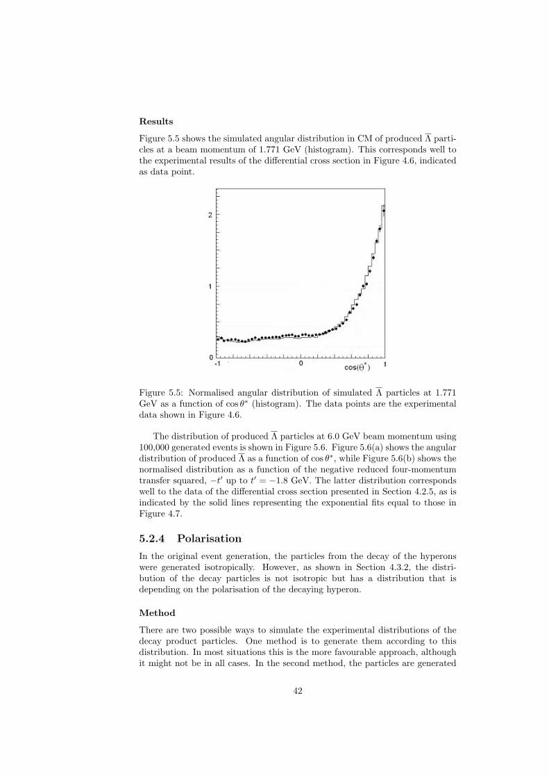
Results

Figure 5.5 shows the simulated angular distribution in CM of produced Λ parti-cles at a beam momentum of 1.771 GeV (histogram). This corresponds well tothe experimental results of the differential cross section in Figure 4.6, indicatedas data point.

Figure 5.5: Normalised angular distribution of simulated Λ particles at 1.771GeV as a function of cos θ∗ (histogram). The data points are the experimentaldata shown in Figure 4.6.

The distribution of produced Λ particles at 6.0 GeV beam momentum using100,000 generated events is shown in Figure 5.6. Figure 5.6(a) shows the angulardistribution of produced Λ as a function of cos θ∗, while Figure 5.6(b) shows thenormalised distribution as a function of the negative reduced four-momentumtransfer squared, −t′ up to t′ = −1.8 GeV. The latter distribution correspondswell to the data of the differential cross section presented in Section 4.2.5, as isindicated by the solid lines representing the exponential fits equal to those inFigure 4.7.

5.2.4 Polarisation

In the original event generation, the particles from the decay of the hyperonswere generated isotropically. However, as shown in Section 4.3.2, the distri-bution of the decay particles is not isotropic but has a distribution that isdepending on the polarisation of the decaying hyperon.

Method

There are two possible ways to simulate the experimental distributions of thedecay product particles. One method is to generate them according to thisdistribution. In most situations this is the more favourable approach, althoughit might not be in all cases. In the second method, the particles are generated

42

(a) (b)

Figure 5.6: Distribution of produced Λ particles at 6.0 GeV as a function of (a)the antihyperon production angle in CM, cos θ∗, and (b) the negative reducedfour-momentum transfer squared, −t′. The solid lines in (b) represents theexponential terms in the expression of Equation (4.35). Note the logarithmicscale on the y-axes.

isotropically and each event is assigned a weighting factor that depends on howwell it corresponds to the desired distribution. When evaluating the resultfrom such a simulation, the events are filled into the histogram bins with theirappropriate weight. Hence, the resulting histogram would show the desireddistribution and not the generated – isotropic – distribution.

In order to change the event generation to fit the distribution given in (4.45)the value of the polarisation needs to be known. Since the value of θ∗ is knownfor a specific event, the polarisation can be calculated as well. The experimentaldata shows that the polarisation is highly dependent on the momentum of thebeam. For the extremes of the angular span, i.e. for θ∗ = 0 and θ∗ = π itis zero, as is expected from the predicted symmetry of the observables (cf.Section 4.2.4). For reasons of simplicity, it is thus reasonable to assume thatthe polarisation of the hyperons can be illustrated by a sine function dependingon the opening angle in CM

Py = Py = sin θ∗. (5.12)

The probability density distribution as a function of the y-directional co-sine for the decay protons can be obtained using (4.47) and the range of thedirectional cosines, here denoted with the variable x, as

P (x) =

12 (1 + αPyx) if − 1 ≤ x ≤ 10 otherwise ,

which is obviously already normalised.The distribution of produced protons as a function of its y-directional cosine

would then have a distribution as shown in Figure 5.7. The slope of the curve isgiven by the value of the polarisation for that specific value of θ∗. The directional

43

cosines of the proton along the y-axis can then be obtained by generating arandom number on the interval [-1,1] according to this distribution. This canbe done using the method described in A.3.1.

Figure 5.7: Distribution function of the decay particles as a function of cos θy,for the CM angle θ∗ = 0 .

The first step in this method is taking a uniformly distributed random num-ber, r ∈ [0, 1], and letting this be equal to the integral of the probability densityfunction over the interval from −∞ to χ, where χ is the sought random number.

r =∫ χ

−∞P (x)dx =

12

∫ χ

−1

(1 + αPyx)dx (5.13)

The integral on the right hand side of (5.13) is easy to evaluate∫ χ

−1

(1 + αPyx)dx = 1− αPy

2+ χ+

αPyχ2

2, (5.14)

which gives (5.13) the following expression

r =12

(1− αPy

2+ χ+

αPyχ2

2

). (5.15)

Solving (5.15) for χ,

χ = − 1αPy

±

√1αPy

(1αPy

+ αPy − 2 + 4r)

. (5.16)

gives an expression for finding a random number according to the distributiongiven in (4.45) from a uniformly distributed random number, r, on the interval[0,1].

Since (5.16) has two distinct solutions for each value of r it is also necessaryto evaluate which solution that should be used. By evaluating the two differentsolutions, it can be seen that if the quantity αPy is positive then it will be thesolution with the negative square root that should be used. If, on the otherhand, the quantity is negative, then it will be the solution with the positivesquare root that should be used. Here, since α = 0.64 and α = −0.64, whilePy = Py > 0, the negative solution will be used for the directional cosines ofthe protons, and the positive solution for the antiprotons.

44

Since symmetry considerations implies that the polarisation in the x- andz-directions are zero, the directional cosine of the proton in these directionsshould be uniformly distributed, thus adding up to zero. So, by knowing they-directional cosine to be χ, it is possible to create a unit vector in the hyperonrest frame. The y-component will be given by χ and the x- and z-componentsmake up a two-dimensional vector of length, l, where

l =√

1− χ2 (5.17)

and where the two components, denoted c1 and c2, are uniformly distributed.The two components are found by generating a random number s on the interval[0,1] and letting the first component c1 = l · s. This gives the second componentto be c2 =

√l2 − c21. This method generates a three-dimensional unit vector,

which after being multiplied with a factor describing the three-momentum ofthe proton, can be used as the spatial part of the four-momentum of the protonin CM of the hyperon.

The other decay product, the pion, will then simply be generated by takingthe negative of the three-momentum of the proton, since the total momentumin CM is zero.

Using the other method, producing the decay particles uniformly and assign-ing weighting factors for each event, the starting point is still the distributionfunction of Equation (4.45), which can be evaluated for each value of the angleθ∗. The distribution function will give a different value for each value of the di-rectional cosine cos θyn of the produced proton/antiproton for the event n. Thisvalue will be assigned as the weighting factor wn to the event. The weightingfactor will be propagated along with the particle, to be used when calculatingquantities involving the directional cosines.

Results

Regardless of the method used, the accuracy of the method can be evaluated bycalculating the expectation value of the polarisation from the generated valuesof the directional cosines.

For the case of the particles being directly generated according to the dis-tribution, the polarisation can be reconstructed using Equation (4.50)

Pi =3α

1N

N∑n=1

cos θin (5.18)

where i denotes the component of the directional cosine. The standard deviationof this expectation value is given by

σi =

√1N

1N − 1

(9α2

)∑n

(cos2 θin − cos θi2). (5.19)

If the decay particles of the hyperons have been generated according toa uniform distribution and the observations of cos θi have been weighted tocompensate for this, the weights needs to be considered in the evaluation ofthe polarisation. This is discussed in Appendix A.2, giving the estimate ofpolarisation in the i-direction as

Pi =3α

∑n wn cos θin∑

n wn. (5.20)

45

The standard deviations of the these reconstructed polarisation estimates are

σi =

√√√√ 1N − 1

(9α2

)(∑n wncos2 θin∑

n wn−(∑

n wn cos θjn∑n wn

)2)

. (5.21)

When using the method of particles generated according to the distributionand considering the whole set of observed directional cosines and using 1,000,000simulated events, the reconstructed polarisation is obtained as

Px = −0.0007± 0.0027 Py = 0.7879± 0.0026 Pz = 0.0012± 0.0027 (5.22)

for Λ and

Px = −0.0039± 0.0027 Py = 0.7904± 0.0026 Pz = −0.0008± 0.0027 (5.23)

for Λ.If instead using the method of weighting factors, the reconstructed values of

the polarisation for 1,000,000 simulated events become

Px = −0.0027± 0.0027 Py = 0.7848± 0.0026 Pz = 0.0013± 0.0027 (5.24)

for Λ and

Px = −0.0006± 0.0027 Py = 0.7846± 0.0026 Pz = −0.0031± 0.0027 (5.25)

for Λ.This corresponds well to the average value of the polarisation function that

was used here, since the expectation value of the polarisation in the y-directionshould correspond to the arithmetic mean of sin θ∗ on the interval [0, π], givenby2

sin θ∗ ≈ 0.7858 (5.26)

while the expectation value of the polarisation in the x- and z-directions shouldbe equal to zero.

Since the standard deviations are of the same order as the difference betweenthe calculated expectation values and the assumed average of the polarisationthese discrepancies can be assumed to be caused by statistical errors.

The polarisation can be obtained as functions of the antihyperon productionangle by putting the directional cosines in bins depending on the value of θ∗.This result is shown in Figure 5.8 for 1,000,000 events using the method ofdirectly generating the events according to the distribution.

As is shown in the figures, the calculated polarisation in the y-direction of Λcorresponds well to the sine function that was used to illustrate the polarisation.The polarisation in the x- and z-direction is very close to zero, in accordancewith the discussion of symmetries in Section 4.2.4. The fluctuations shown canbe explained with statistical variances.

Using fewer events, for example 10,000 events, the expectation values of Λbecomes

Px = 0.022± 0.027 Py = 0.7321± 0.026 Pz = 0.020± 0.027 (5.27)2The mean of sin θ∗ is not, as might be expected, equal to 0.64, which is the average of

sin(x) for x uniformly distributed on the interval [0, π]. This is caused by the fact that thehyperons are not uniformly distributed with respect to θ∗, but rather with respect to cos θ∗.

46

(a)

(b) (c)

Figure 5.8: Reconstructed polarisation components as functions of the Λ pro-duction angle θ∗. The deviations of the reconstructed values are of the order of0.01 and are thus within the indicated points.

47

Distributing the directional cosines in bins depending on the θ∗ angle of theevent, the plot in Figure 5.9 is obtained, showing the polarisation of Λ in they-direction for 10,000 generated events. Clearly, the polarisation can not be

Figure 5.9: Reconstructed polarisation Py for as a function of the productionangle, using 10,000 generated events.

reconstructed in the same accurate way when using fewer events.There is one feature of the simulated polarisation that is not evident. Con-

sidering the results in Equations (5.22) to (5.25), it is clear that the standarddeviation of the expectation value in the y-direction is different to those in thex- and z-direction, for both the hyperon and the antihyperon. This propertypersists regardless of the method used, and regardless of how good statisticsthat are being used. It is not a significant difference, and it has no impact onthe analysis, but it is peculiar that this phenomenon occurs, since the standarddeviation is expected to be equal for all directions. It could possibly be an effectof numerical inaccuracies.

5.2.5 Spin Correlations

The angular distribution of decay particles is also dependent on the spin corre-lation, as is discussed in Section 4.3.2. The generation of decay particles can beadapted to better correspond to the experimental data of the spin correlationcoefficients.

Method

As with polarisation, it would be advantageous if the distribution based on theexperimentally determined spin correlation coefficients could be obtained boththrough direct generation and by assigning weights. The weighting factors canbe created in much the same way as for the polarisation. However, when itcomes to directly generating events according to the distribution, the case ofthe spin correlation is slightly more complicated than that of the polarisation.

48

In order to evaluate the spin correlation of the Λ and Λ particles, the decaysΛ → pπ+ and Λ → pπ− must be considered simultaneously. The generationof the decay particles is made for one of them at a time, and it is therefore noeasy way to directly generate the produced particles according to the desireddistribution. Thus, the event generation will be done through a method of ’bruteforce’ instead, where the generated particles that does not fit the distributionwill simply be rejected and the generation redone until a satisfactory particle isproduced. This is a far less efficient than the method used for the polarisation,but it will still represent a relatively small decrease in the total efficiency of thegeneration program.

Out of the spin correlations, it is only the Cxx, Cyy, Czz and Cxy = Cyx thatare non-zero. Equation (4.53) can be used to describe the distribution functionof the particles produced in the Λ/Λ decay giving the distribution function foreach of the Cij :s as

I(θi, θj) =14π

(1 + ααCij cos θi cos θj) . (5.28)

Thus, there are five different distributions, one for each of the non-zero spincorrelation coefficients, and the generation of the decay particles needs to beadopted to fit each and everyone of these.

For a specific event the θ∗ is known, and thereby also the approximate valueof the non-zero spin correlation coefficients as given by the parameterisation in(4.22). The distribution of decay particles can then be calculated according to(5.28).

The polynomials of (4.22) do not, however, fit the symmetry conditions thatCxz = Czx = 0 and Cxx = −Cyy for the extremes of the opening angle of theantihyperon, cos θ∗ = 1 and cos θ∗ = −1 (cf. Section 4.2.4). They are also onlyverified at a beam momentum of 1.637 GeV, and thus not, a priori, valid atother momenta. However, for the purpose of this work, it will be assumed thatthe coefficients at other momenta will have a similar appearance and that theseparameterisations are valid.

The method used for the production of decay particles according to thedesired distribution is similar to the statistical method for generating randomnumbers by rejection as described in Section A.3.2. For each of the non-zero spincorrelation coefficients, a random number t in the interval [0, fmax] is generated,where fmax is the maximum value of the distribution function. This is done byletting

t = r · fmax = r · 14π

(1± ααCij), (5.29)

where r is a uniformly distributed random number on the interval [0,1] and thesign is positive if the value of Cij is negative, and negative if Cij is positive.

If t is larger than the calculated distribution for the specific Cij , then theproduced event is discarded and a new generation is made. However, if t isless than the distribution, the produced particle is kept and the next randomnumber t is generated to test the next spin correlation coefficient. In the end, adecay particle has been generated that fits all the five anisotropic distributions.

In the case of producing the decay particles isotropically, the starting pointis the distribution function of each of the non-zero spin correlation coefficientsof Equation (5.28). The distributions can be independently evaluated for eachvalue of the angle θ∗, using the fitted values for the experimental data (Equation

49

(4.22)). The value of the distribution function for the particular values of thedirectional cosines will be assigned as the weighting factor wn to the eventn. Each event will thus be assigned five different weighting factors, that aremultiplied to obtain a total weighting factor of the event. This total weightingfactor will be propagated along with the particle, and used when quantities arecalculated that use the directional cosines.

Results

As with the polarisation, the expectation value of the spin correlation coefficientscan be calculated in order to evaluate the result of the generation.

The expectation value for each spin correlation coefficient is given by (4.55)

Cij =9αα

1N

N∑n=1

cos θin cos θjn. (5.30)

The standard deviation, σ, of the coefficient is given by

σ(Cij) =√V (Cij), (5.31)

where V denotes the variance, given by

V (Cij) =(

9αα

)2 1N − 1

(∑n (cos θin cos θjn)2

N−(∑

n cos θin cos θjn

N

)2)

.

(5.32)If the events are weighted to fit the distribution, the average of the spin

correlation coefficients cannot be calculated as above, since the weighting factorsmust be taking into account (cf. Appendix A.2). Instead they are given by

Cij =9αα

∑n cos θin cos θjnwn∑

n wn(5.33)

with a variance of

V (Cij) =(

9αα

)2 1N − 1

(∑n (cos θin cos θjn)2wn∑

n wn−(∑

n cos θin cos θjnwn∑n wn

)2)

(5.34)The average values for the spin correlation coefficients can be obtained by

summing over all directional cosines according to Equations (5.30) and (5.33).These values are listed below for a simulation of 1,000,000 events at a beamenergy of 1.637 GeV, using the method of weighting factors.

Cxx = 0.1246± 0.0073 Cyx = −0.0048± 0.0073 Czx = 0.2367± 0.0073Cxy = 0.0077± 0.0073 Cyy = 0.3620± 0.0073 Czy = 0.0009± 0.0073Cxz = 0.2500± 0.0073 Cyz = 0.0090± 0.0073 Czz = −0.5537± 0.0073

(5.35)The corresponding values using the rejection method are

Cxx = 0.1001± 0.0073 Cyx = −0.0017± 0.0073 Czx = 0.2577± 0.0073Cxy = −0.00037± 0.0073 Cyy = 0.3605± 0.0073 Czy = 0.0044± 0.0073Cxz = 0.2465± 0.0073 Cyz = −0.0067± 0.0073 Czz = −0.5776± 0.0073

(5.36)

50

These values should be compared to the corresponding average values of thefunctions for the spin correlation coefficients given in (4.22), given by

Cxx = 0.1199 Cyx = 0.0 Czx = 0.2431Cxy = 0.0 Cyy = 0.3562 Czy = 0.0Cxz = 0.2431 Cyz = 0.0 Czz = −0.5559

(5.37)

The correspondence between these and the reconstructed values from the eventgeneration is fairly good for both methods. Also, here there is no significantdiscrepancy of standard deviation in one direction similar to the one found forthe polarisation.

The value of the spin correlation coefficients as a function of the antihy-peron opening angle can be obtained by filling the product if directional cosinescos θi cos θj , for each event in bins of θ∗. This result is shown in Figure 5.10using 1,000,000 events at a beam momentum of 1.637 GeV.

The plots in Figure 5.10 correspond well to the initial plots of Figure 4.5.Thus, the spin correlation coefficients can be simulated and reproduced withgood accuracy using high statistics.

5.3 Reconstruction

For the reconstruction of the generated events it is here assumed that the detec-tion of the particles can happen in an ideal way, something that will not occurin practice. It is also assumed that the particle identification is always correct.These are huge simplifications, but they are legitimate for the properties studiedin this work.

The work with the reconstruction was concentrated upon trying to reproducethe momentum of the Λ, as well as its generated production angle in CM, i.e.the angle denoted θ∗. The aspects of interest here was to investigate how theextension of the interaction area would effect the reconstruction of this angle,and what the difference between the two different target options would be.

5.3.1 Extended Target

When generating events using the extended target, the vertex of the decaywill be located at some distance from the nominal interaction point. In thereconstruction, however, it is not possible to determine where the productiontook place, and it must therefore be assumed that it occurred in the origo ofthe coordinate system. By this assumption, an uncertainty in the calculation ofthe opening angle of Λ is unavoidable.

By assuming that the decay vertex is accurately determined, and assumingthat the production vertex is located in origo, an estimation of the openingangle of the emitted Λ particles can be made. As a first step towards this, themomentum of the Λ is to be determined, assuming that the momenta of thedetected decay particles are not known.

5.3.2 Momentum of Λ from Opening Angles

Figure 5.11 shows a schematic view of the Λ decay in the laboratory frameof reference. The angle ϕ is the angle between the momentum vectors of the

51

(a) (b)

(c) (d)

(e)

Figure 5.10: Reconstructed spin correlation coefficients at simulated beam mo-menta of 1.637 GeV (histograms), using 1,000,000 generated events. The datapoints indicate the experimental data of Figure 4.5 and the dashed lines are thefit to these values.

52

antiproton and pion, while the angles α and β are the opening angles of theproton and pion, respectively.

α

β

π

ϕ

p

+

Λ

Figure 5.11: Schematic view of the reaction Λ → pπ+ in lab.

It is not possible to reconstruct the momentum of the Λ from just the angleϕ. This can be understood by considering Figure 5.12, which shows a simulationof the angle ϕ as a function of the momentum of the Λ particle. Clearly, there isnot a unique correspondence between a certain momentum and a certain angleϕ.

Figure 5.12: Simulation of the opening angle of the decay particles in the Λ →pπ+ reaction, as a function of the momentum of the Λ particle.

However, if the angles of the decay particles with respect to the directionof the Λ particle are known, i.e. if both α and β are known, it is possible tocalculate the momentum of the Λ particle.

Method

If the directions of the decay particles are known, the decay point can be de-termined as the intersection of these. By assuming that the production pointis located in origo, the direction of the decaying hyperon can be determined as

53

well. This gives an approximate value of the opening angles of the two decayparticles.

The momentum can be derived from the opening angles of the decay particlesusing the conservation of energy and momentum of the reaction. A detailedderivation is given in Appendix C and the result is that the modulus of themomentum of the decaying Λ particle, |~pΛ|, is found to be

|~pΛ| =

√√√√ L

K±

√(L

K

)2

− M

K, (5.38)

where K, L and M in the case of decay to a proton and a pion are given by

K =1 +(

sinβsin (α+ β)

)4

+(

sinαsin (α+ β)

)4

− 2(

sinβsin (α+ β)

)4

−

−2(

sinαsin (α+ β)

)4

− 2(

sinβsin (α+ β)

)2( sinαsin (α+ β)

)2

(5.39)

L =m2c +

(sinβ

sin (α+ β)

)2

m2a +

(sinα

sin (α+ β)

)2

m2b − (m2

a +m2b)−

−(

sinβsin (α+ β)

)2

(m2b +m2

c)−(

sinαsin (α+ β)

)2

(m2c +m2

a) (5.40)

M =m4Λ +m4

p +m4π − 2m2

Λm2p − 2m2

Λm2π − 2m2

pm2π, (5.41)

where mΛ, mp and mπ are the Λ, proton and pion rest mass respectively, andα and β are the angles between the antiproton and the pion with respect to thedirection of the Λ in the laboratory frame of reference (see Figure 5.11).

The relation between K, L and M is, in most cases of this reconstruction,

L

K<

√(L

K

)2

− M

K, (5.42)

which means that, in the very majority of events, the only valid solution in(5.38) is the one using the positive square root,

|~pΛ| =

√√√√ L

K+

√(L

K

)2

− M

K. (5.43)

Results

Figure 5.13 shows the relative error in the reconstructed momenta as a functionof the generated momenta for an ideal target, i.e. a target where all productionoccurs in the nominal interaction point, at 6.0 GeV beam momentum. It seemsthat the errors are increasing with increasing momenta, but that the overallerrors are small. If considering a antiproton beam of 6.0 GeV, 98 percent ofthe reconstructed events have an error that is less than one percent of themomentum. Thus, this method for reconstructing the momentum of the hyperoncan be considered extremely accurate if the opening angles of the decay can bedetermined with high precision.

54

Figure 5.13: Box plot of the error in the reconstruction of the hyperon mo-mentum from the opening angles (in percent of the generated momentum) as afunction of the momentum for an ideal target.

When instead using the two targets of PANDA, the extension of the interac-tion area will complicate the determination of the opening angles of the decayparticles. Figure 5.14 shows the relative error in the reconstructed momentaas a function of the generated momenta for the two target types at a beammomentum of 6.0 GeV for 100,000 generated events.

Table 5.1 shows the percentage of the reconstructed events that have anerror in the reconstruction of the hyperon momentum that is less than ten and30 percent, respectively, for several beam momenta. Clearly, the momentum ismore accurately determined at lower beam momenta than at higher. Also, thecluster jet target seems to be more accurate than the pellet target at low beammomenta, while the situation is reversed at higher momenta.

Beam momentum Target Error less than[GeV] type 10% 30%

1.5 Pellet 55.9% 79.4%Cluster 66.1% 86.6%

6.0 Pellet 50.0% 70.6%Cluster 42.7% 63.8%

15.0 Pellet 47.8% 67.5%Cluster 45.4% 64.6%

Table 5.1: Percent of the reconstructed events that have an error less than tenand 30 percent, respectively, in the reconstruction of the Λ momentum, for thetwo different targets at different beam momenta.

The direction of the decaying hyperon is more accurately determined athigher momenta than at lower, since the decay points will be located further

55

(a) (b)

Figure 5.14: Box plots of the error in the reconstructed value of the hyperonmomentum (in percent of the generated momentum) as a function of the mo-mentum for (a) the pellet target and (b) the cluster jet target.

from the production region. On the other hand, the opening angles α and β arerapidly decreasing with increasing beam momenta, which means that an errorof a certain magnitude would have more impact at higher beam momenta thanat lower.

For the cluster jet target the reconstruction of the decay particle openingangles is significantly more accurate at lower beam momenta than at higher.For the pellet target, there is no significant difference between different beammomenta. This explains why the best results for the antihyperon momentumreconstruction when using an extended interaction region are given at low beammomenta, despite the inaccuracy in the determination of the hyperon direction.

5.3.3 Production Angle of Λ

When reconstructing the production angle of Λ, it is assumed that the decaypoint of the antihyperon can be determined precisely. Also, the productionvertex is assumed to be located in the nominal interaction point.

Method

The modulus of the momentum of the antihyperon can be assumed to somehowbe known beforehand, alternatively it can be taken from the calculation de-scribed in the previous section. The direction and modulus of the momentum isthen used to construct the four-momentum of the antihyperon in the laboratoryframe. This is then transformed back to the centre of mass frame using thegeneral Lorentz transform, given in Equation (B.7). The production angle θ∗

can be obtained by taking the scalar product of the CM four-momentum andthe beam direction, which is in the z-direction of the detector system.

56

Results

To evaluate the result, the difference between the reconstructed and the gen-erated value of the production angle was determined, and plotted versus thegenerated θ∗ value, as well as versus the distance of the decay point from thenominal interaction point. This was done both for the case of the modulusof the hyperon momentum being calculated as above, and for the case of themomentum somehow being known beforehand.

If assuming that the momentum is exactly determined, the Λ productionangle in CM can be estimated fairly well. Figure 5.15 shows the differencebetween the reconstructed value of θ∗ and the actual value as a function ofthe distance from the decay vertex to the nominal interaction point for thetwo different targets at a beam momentum of 6.0 GeV for 100,000 events. Asexpected, the difference between the reconstructed and the actual value of θ∗

decreases with increasing distance from the interaction region. The pellet targetalso seems to be significantly more accurate than the cluster jet.

(a) (b)

Figure 5.15: Discrepancies in the reconstructed value of the production angleθ∗ as a function of the distance from the decay vertex to the origo for (a) thepellet target and (b) the cluster jet target.

Figure 5.16 shows the difference between the reconstructed value of θ∗ andthe generated value as a function of the latter at a beam momentum of 6.0 GeVfor 100,000 generated events. The pellet target seems to have slightly moreevents with small errors than the cluster jet target.

Table 5.2 shows the percentage of the reconstructed events that have anerror in the reconstruction of θ∗ that is less than two, four and ten degrees,respectively, for several beam momenta. Clearly, the reconstruction is moreaccurate at higher momenta, and the pellet target gives higher accuracies thanthe cluster jet, as can be expected.

If instead using the reconstructed momenta, the inaccuracy in the deter-mination of this will affect the accurateness of the determination of θ∗. Table5.3 shows the percentage of the reconstructed events that have an error in thereconstruction of θ∗ that is less than two, four, ten and 20 degrees, respectively,

57

(a) (b)

Figure 5.16: Box diagrams of the discrepancies in the reconstructed value of theproduction angle θ∗ as a function of θ∗ at a beam momentum of 6.0 GeV for(a) the pellet target and (b) the cluster jet target.

Beam momentum Target Error less than[GeV] type 2o 4o 10o

1.5 Pellet 59.6% 74.8% 89.0%Cluster 56.8% 73.3% 87.5%

6.0 Pellet 89.7% 94.7% 98.0%Cluster 75.9% 86.7% 94.4%

15.0 Pellet 93.0% 96.4% 98.7%Cluster 85.9% 92.6% 96.9%

Table 5.2: Percent of the reconstructed events that have an error less than two,four and ten degrees, respectively, in the reconstruction of the Λ productionangle, for the two different targets at different beam momenta when the hyperonmomenta is accurately determined.

58

for several beam momenta when the hyperon momentum is determined as inthe previous section.

Beam momentum Target Error less than[GeV] type 2o 4o 10o 20o

1.5 Pellet 14.2% 24.8% 44.5% 61.7%Cluster 22.2% 43.2% 53.3% 68.5%

6.0 Pellet 49.5% 62.6% 76.5% 83.1%Cluster 41.7% 54.0% 69.3% 77.8%

15.0 Pellet 60.9% 71.3% 79.3% 82.8%Cluster 56.8% 67.1% 76.4% 81.0%

Table 5.3: Percent of the reconstructed events that have an error less than two,four, ten and 20 degrees, respectively, in the reconstruction of the Λ productionangle, for the two different targets at different beam momenta.

Clearly, the difference between the cluster jet and the pellet target is not asevident in Table 5.3 as in Table 5.2. The cluster jet target seems to give moreaccurate results than the pellet target at lower beam momenta, while the pellettarget seems to be more accurate than the cluster jet at moderate and highbeam momenta.

59

60

Chapter 6

Conclusion and Outlook

6.1 Summary and Conclusion

The aim of this Diploma thesis project was to create a event generator forthe simulation of the pp→ ΛΛ → pπ+pπ− reaction, with special regard takento the available experimental data for differential cross section of the pp →ΛΛ reaction, as well as for hyperon polarisation and antihyperon-hyperon spincorrelation.

The simulated interaction region have been made to fit the two target typesthat are envisioned for the PANDA experiment, the untracked pellet targetand the cluster jet target. When doing simulations using the cluster jet target,more of the hyperon decay points were situated in the actual interaction regionthan when using the pellet target. This cause greater difficulties when tryingto reconstruct these events if using the cluster jet target than if using the pellettarget.

The generated events have been reconstructed, assuming that the directionof the decay particles in the laboratory frame can be determined. From this,the momentum of the antihyperon was reconstructed, with higher accuracy atlower beam momenta than at higher. The cluster jet target gave more accurateresults than the pellet target at lower beam momenta, while the pellet targetgave better results at higher momenta.

The CM production angle of the antihyperon has also been reconstructed,with varying results. The reconstruction of the angle was more accurate athigher beam momenta than at lower beam momenta. If using the reconstructedmomenta of the antihyperon, the production angle could not be reconstructedvery accurately. Here, the cluster jet target gave higher accuracy than the pellettarget at lower beam momenta, while the situation was the reverse at higherbeam momenta. If instead assuming that the antihyperon momenta could beprecisely determined otherwise, the production angle could be reconstructedmore accurately, with the pellet target giving better accuracies for all beammomenta.

The distribution of hyperons has been adapted to fit the distribution indi-cated by the experimental data for the differential cross section. This was doneby assigning a weighting factor to each event depending on how well it fittedthe distribution. If using good statistics, the distribution of simulated particles

61

corresponds well to the desired distribution.The event generation of decay particles has been adapted to fit angular dis-

tributions determined by the hyperon polarisation and the antihyperon-hyperonspin correlation. This was done using two different methods, either changingthe actual generation of the particles to fit the distribution, or by assigning eachevent with a weighting factor depending on how well it fitted the distribution.The generation of decay particles was changed in different ways for the polar-isation and the spin correlation: For the polarisation the decay particles weregenerated directly according to the angular distribution; for the spin correlationthe particles not fitting the distribution were rejected.

If enough events were generated, the initial polarisation and spin correla-tion coefficients can then be reconstructed with very satisfying accuracy. Bothmethods used here seemed to generate a similarly accurate result when usinghigh statistics.

6.2 Outlook

This work is a small step towards the implementation of an event generator forhyperons based on experimental data on the differential cross section, polarisa-tions and spin correlations in the PANDA framework. A lot of work to furthercomplete it can be envisioned.

First and foremost, once the software of PANDA is fairly established, theroutines described in this work could be implemented there. There are, however,difficulties regarding the propagation of the weights through this program. Sincethe PANDA frame work uses Geant4, some of the implementations made in thiswork, might have to be included there. Also, the indication that the simulationneed to include at least 100,000 events for the spin observables to give obtainsolid results, which may make the simulations time demanding.

It would need to be determined which of the methods used to generate theaccurate angular distribution of the decay particles that is the easiest to use inthe PANDA software. The method using weighting factors has, as mentionedabove, the disadvantage of the weights needing to be propagated along with theevent. The advantage of this method is that it is far simpler to implement thanthe method of directly generating the decay particles according to distributions.

Here, the best option might be the method of rejecting the events that donot fit the distribution. The advantage with this method is that it is muchsimpler to implement compared to the method of directly generating the decayparticles according to the distribution, while at the same time not having theproblem of the propagating weights. The only disadvantage with the rejectionmethod is that it increases the event generating time. This extra time of theevent generation is, however, insignificant in comparison with the time requiredfor the particle propagation, detector simulation of particle detection and theanalysis of the results.

In this work all three criteria for the particle distributions – differential crosssection, polarisation and spin correlation – have been considered separately. Onewould, however, like all three distribution conditions to be fulfilled at the sametime, and this is something that should be done in any further work on thisevent generator.

Furthermore, the function used as the polarisation should be alternated to

62

resemble the available experimental data. This would mean generating differentpolarisation functions for different values of the excess energy, similar to thecase of the differential cross section at low energies.

The functions used as the spin correlation parameters should also be con-structed in such a way as to fit available experimental data for different energies.The fits also needs to be changed in order to take the symmetry conditions ofthe parameters into account.

63

64

Acknowledgments

First and foremost, I would like to thank my supervisor on this project, pro-fessor Tord Johansson at the Department of Nuclear and Particle Physics atthe Uppsala University. It was through his inspiring lectures that I first gotinterested in this field, and by offering me the chance to do this Diploma thesisproject at the department I was able to further explore that interest. Tord hasthroughout the project shown encouragement and support, pushing me to findmy own solutions and learn how to work independently.

I would also like to thank all the staff at the Department of Nuclear andParticle Physics for creating such a wonderful work environment. It has beena truly good experience to work alongside so many talented, funny and inter-esting people. The coffee breaks have often been the best part of my day whilebeing here at the department, and I would like to thank Karen, Henrik, Lotta,Markus, Henrik, Fredrik, Bengt, Annica, Anni, Karin, Agnes and all the othersfor making it that way. I would also like to especially thank Karen for beingsuch a good office room mate and for always being there whenever I neededsomeone to talk to.

Furthermore, I am very grateful to all the people – both at the departmentand elsewhere – that on their own accord have helped me with little bits andpieces here and there, involving everything from getting past computer errorsto understanding the unwritten code of the academic world. It might all haveseemed like insignificant details and trivial obstacles at the time, but in the endthe help I got made all the difference. Among these, I would like to mentionMarkus who helped me with every single LATEX bug I could possibly come upwith and Henrik who gave me invaluable feedback on my report.

Finally, I would, as always, like to thank my mum and my boyfriend. Despitelacking even the slightest interest in physics, they have both tried to understandmy fascination and listened to my endless rambling about thing that neither ofthem will ever understand. For this, I am always grateful.

65

66

Bibliography

[1] E. Klempt. Glueballs, hybrids, pentaquarks: Introduction to hadron spec-troscopy and review of selected topics, 2004.

[2] B. R. Martin et al. Particle Physics. John Wiley & Sons Ltd, 1997.

[3] W.-M. Yao et al (Particle Data Group). Review of Particle Physics. Journalof Physics G, 33:1+, 2006.

[4] O. Nordhage. On a Hydrogen Pellet Target for Aniproton Physics withPANDA. PhD thesis, Uppsala University, 2006.

[5] B. R. Martin. Nuclear and Particle Physics. John Wiley & Sons Ltd, 2006.

[6] L. G. Landsberg. The search for exotic hadrons. PHYS-USP, 42(9):871–886, 1999.

[7] G. Hautaluoma. NASA satellite glimpses universe’s first trillionth of asecond. NASA press release on 16th March 2006.

[8] F. E. Close et al. Glueballs. Scientific American, 279(5):80–85, 1998.

[9] K.-T. Brinkmann et al. Exploring the mysteries of strong interactions –The PANDA experiment. Nuc. Phys. News, 16(1):15–18, 2006.

[10] F. Halzen et al. Quarks & Leptons: An Introductory Course in ModernParticle Physics. John Wiley & Sons, 1984.

[11] The PANDA collaboration home page.URL: http://www-panda.gsi.de/auto/org/ home.htm. Accessed: January12th 2007.

[12] GSI. Proposal for an international accelerator facility for research with ionsand antiprotons, 2001.

[13] PANDA Collaboration. PANDA – Strong interaction studies with antipro-tons. Technical report, GSI, 2005.

[14] The GSI home page.URL: http://www.gsi.de. Accessed: January 25th 2007.

[15] A. Lundborg. The Charm of Excited Glue – Charmonium in e+e− and ppcollisions. PhD thesis, Uppsala University, 2007.

67

[16] A. Sokolov. PANDA@FAIR – A novel detector for frontier physics, 2006.Talk given at the XVIII International Baldin Seminar On High EnergyPhysics Problems.

[17] Geant4 Home Page. URL: http://geant4.cern.ch.

[18] ROOT System Home Page. URL: http://root.cern.ch.

[19] N. H. Hamann. Stange particle physics at LEAR. Technical report, Uni-versity of Freiburg, 1991.

[20] T. Johansson. Antibaryon-baryon production in antiproton-proton colli-sions. In Proceedings of the International School of Physics Enrico Fermi,Course CLVIII, Hadron Physics, 2004.

[21] R. Tayloe. A Measurement of the pp → ΛΛ and pp → ΣΛ + cc. Reactionsat 1.726 GeV/c. PhD thesis, University of Illinois, 1995.

[22] P. D. Barnes et al. Observables in high-statistics measurement of the reac-tion pp→ ΛΛ. Phys. Rev. C, 54(4):1877–1886, 1996.

[23] P. D. Barnes et al. Observables in high-statistics measurement of the reac-tion pp→ ΛΛ. Phys. Rev. C, 54(4):1877–1886, 1996.

[24] T. Johansson. Private communication.

[25] P. D. Barnes et al. Measurement of the pp → ΛΛ and pp → Σ0Λ + c.c.reactions at 1.726 GeV/c and 1.771 GeV/c. Phys. Rev. C, 54(6):2831–2842,1996.

[26] S. Pomp et al. String model description of polarisation and angular distri-butions in pp→ ΛΛ at low energies. Eur. Phys J. A, 15:517–522, 2002.

[27] H. Becker et al. Measurement of the reactions pp → ΛΛ, pp → ΣΛ0 andpp→ ΛΛ (missing mass) at 6 Gev. Nuclear Physics B, 141(48):48–64, 1978.

[28] A. G. Frodesen et al. Probability and Statistics in Particle Physics. Uni-versitetsforlaget, 1979.

[29] P. R. Bevington et al. Data reduction and error analysis for the physicalsciences. WCB/McGraw-Hill, 2003.

[30] M. E. Peskin. An Introduction to Quantum Field Theory. Addison-Wesley,1995.

68

Appendix A

Statistics

In this appendix certain statistical methods used in the discussion in Chapters4 and 5 are presented.

A.1 The Method of Moments

The statistical Method of Moments (MM) is a method widely used in particlephysics experiments. The method is fairly simple, and can be used to determine,for example, the polarisation from a sample of experimental data, as is shownin Section 4.3.2.

If a certain distribution is described by a probability density function f(x|θ),where the parameter θ is unknown, but a set of observations x1, x2,..., xn is avail-able, the moments method can give an estimate of the value of the parameter.[28]

In the general one-parameter case1, we will consider a function of the pa-rameter, γ(θ), and identify this function as the first moment, or estimate, ofanother function g(x)

γ(θ) ≡ E(g(x)) =∫

Ω

g(x)f(x|θ)dx. (A.1)

A reasonable estimate of the function γ(θ) is the arithmetic mean of the functiong(x) over the whole set of observations xi,

γ(θ) = g(x) =1n

n∑i=1

g(xi). (A.2)

The variance of the estimator is

V (γ) =(

1n

)2

V

(n∑

i=1

g(xi)

)=

1nV (g(x)), (A.3)

where the variance of the function g(x) can be described as

V (g(x)) ≈ 1n− 1

n∑i=1

(g(xi)− g(x))2. (A.4)

1The MM can be used for a set of parameters as well, but here we will only consider thesimplest case of just one parameter.

69

Thus the variance of the estimate of the function γ(θ) is

V (γ) ≈ 1n(n− 1)

n∑i=1

(g(xi)− g(x))2

=1

n(n− 1)

n∑i=1

(g(xi))2 −1n

(n∑

i=1

g(xi)

)2 .

(A.5)

Thus, from (A.2) and (A.5), the estimate and variance of a function of thewanted parameter θ are obtained.

A.2 Weighting

When dealing with a set of observations where some are more important thanothers, a useful technique is to weigh each observation with a weighting factor wn

when comparing the set. The same can be used when simulating the productionof particles of some known distribution. It is often easier to generate eventsaccording to a uniform distribution and then, to compensate for this inaccuracy,each event is given a weight according to their actual distribution. There is,however, disadvantages with this technique. Not only do the weights have to bepropagated through the whole simulation, but the calculation of the mean andvariance of some quantity associated with the event are also complicated whenthe weight of the events have to be taken into account.

If the set of observations xn have been given weighting factors wn, then theweighted mean of the observations is [29]

x =∑

n wnxn∑n wn

, (A.6)

and the weighted average variance of the observations is

σ2 =N

N − 1

(∑n wnx

2n∑

n wn− x2

). (A.7)

A.3 Random Number Generation

To generate random numbers from a probability distribution, two methods de-scribed in [29] were used: the transformation method and the rejection method.

A.3.1 Transformation Method

This method is easy to apply, providing that the distribution function is inte-gratable over the whole real axis and that the resulting function is invertible2.It works by finding the top end point of the interval, at which the value of theintegrand is the same as some uniformly distributed random number.

To obtain random numbers distributed according to some probability densitydistribution P (x), the transformation method starts with finding a uniformly

2Although not in a strict mathematical sense, since the inverse of a function here can havemore than one solution.

70

distributed random number r on [0,1], and letting the probability at a point χbe equal to this number r, that is

r =∫ χ

−∞P (x)dx (A.8)

Calculating the integral and solving the obtained expression for χ will give anexpression for the χ as a function of the generated random number r.

With this method, a set of random numbers χi will be obtained distributedaccording to the desired distribution.

A.3.2 Rejection Method

The rejection method is far less efficient than the transformation method, butwhile the latter can be somewhat hard to apply if the probability distributionfor example is complicated to integrate, the former is almost always possible touse.

To obtain random numbers on the interval [a, b], distributed according tosome probability distribution P (x) = f(x), the rejection method starts withfinding a uniformly distributed random number x′ on [a, b]. This can be doneby using

x′ = r(b− a) + a (A.9)

where r is some uniformly distributed number on [0, 1].Secondly, the random number y′ is found, uniformly distributed between 0

and the maximum value of the distribution fmax on the interval [a, b]. This canbe found using

y′ = r · fmax (A.10)

where r denotes yet again some uniformly distributed number on [0, 1].Now, if y′ is less than the value of the probability function in x′, the generated

random number (that is x′) is kept, but if y′ > f(x′) then x′ is discarded andthe procedure is redone.

With this procedure repeated the result will be a set of random numbers x′idistributed according to the probability function P (x).

71

72

Appendix B

Relativistic Kinematics

When dealing with high energy particles it is often necessary to use relativistickinematics to describe the motion of the involved particles. In this appendix areview of relativistic kinematics is presented, with focus on the aspects that arerelevant to the discussion in Chapters 4 and 5.

B.1 Four-vectors

In relativistic kinematics all quantities are described as four-vectors, whichcan be seen as generalisations of the classical three-vectors to four-dimensionalspace-time. This has to do with the fact that it is not just the measurement ofspace that is relative of the observer, but also the measurement of time. Thedifference between the three-vector of classical mechanics and the relativisticalfour-vector, is thus a fourth component that somehow indicates the observedmeasurement of time.

A four-vector is normally denoted vµ where µ = 0, 1, 2, 3, where the firstindex refers to the time-component of the vector and three later indices referto the spacial part, i.e. to the classical three vector. The inner product of twofour-vectors u and v is

u · v = uµvµ = (u0, u1, u2, u3)

v0−v1−v2−v3

, (B.1)

where uµ is a so-called covariant four-vector and vµ is contravariant, and usingEinstein summation convention1.

The most commonly used four-vector in the field of particle physics is thefour-momentum. The covariant four-momentum of a particle is pµ = (E,−~p),where ~p is the classical three momentum vector and E is the total energy.

The four-vectors vary depending on how they are looked at, that is theyare different depending on what reference frame is being used. Some quantitiesare however invariant. For an individual particle, the norm of a four-vector is

1Einstein summation convention is a notation that implies that whenever the same indexappears once as a subscript and once as a superscript in the same term, summation shouldbe carried out over all possible combinations of the components the index refers to.

73

always constant, no matter what reference frame. An example of this is the restmass, m, of a particle, defined as

m2 = p2 = pµpµ = E2 − |~p|2 . (B.2)

Thus, from (B.2) an expression for the energy of a relativistic particle canbe obtained as a function of the particle rest mass and momentum

E =√|~p|2 −m2 . (B.3)

B.2 Reference Frames

The two most useful reference frames when dealing with any sort of scatteringis the frame of the laboratory system (L), and the frame of the Centre-of-Mass(CM) of the reaction. The advantage of viewing the system in the L frame is thatit treats the reaction the way we would normally see it, and when dealing with afixed target experiment as is the case for PANDA, the calculations can simplifya great deal. Viewing the system from the CM frame is also advantageous inthat it facilitates the calculations, since the CM frame is defined as the referenceframe where the momenta adds up to zero.

B.3 Lorentz Transformation

In order to get from one reference frame to another, a Lorentz transformation,or a Lorentz boost, is applied to the four vector in the original frame, and thefour vector in the desired frame is obtained.

Considering the four-momentum p of a particle in the rest frame S of someobserver O, and another frame S′ that is moving in the x-direction relative toS, the four-momentum p′ as is would be measured by an observer O′ at rest inS′ can be obtained as

p′µ = Λµνp

ν , (B.4)

where Λ is the transformation matrix.In the simplest case, the direction of the boost coincide with the direction

of one of the axes of the coordinate system used. If the boost is in the, say,x-direction, the transformation matrix is given by

Λµν =

γ −γβ 0 0

−γβ γ 0 00 0 1 00 0 0 1

(B.5)

Here, β and γ are given by

β =v

cand γ =

1√1− v2/c2

, (B.6)

where v is the speed of the frame S′ relative to the frame S. γ is normallyreferred to as the Lorentz factor of the frame S′.

74

A general Lorentz boost to the reference frame of a momentum four vectorpref is given by

Λµν =

γ −γβ1 −γβ2 −γβ3

−γβ1 1 + (γ−1)β21

β2(γ−1)β1β2

β2(γ−1)β1β3

β2

−γβ2(γ−1)β1β2

β2 1 + (γ−1)β22

β2(γ−1)β2β3

β2

−γβ3(γ−1)β1β3

β2(γ−1)β2β3

β2 1 + (γ−1)β23

β2

(B.7)

where γ and β are given by

β =(pref,1

Eref,pref,2

Eref,pref,3

Eref

)and γ =

1√1− β2

(B.8)

B.4 Mandelstam Variables

The scattering process of two particles to two particles can be viewed schemat-ically in Figure B.1, where the four-momenta of the particles are indicated andthe white circle representing some kind of scattering process. The initial andfinal state particles do not necessarily have the same mass.

p4p

2

p1 p

3

Figure B.1: Two particle scattering process, indicating the four-momentum ofthe individual particles.

By introducing the Mandelstam variables the discussion of this kind ofprocess can be facilitated. The Mandelstam variables are Lorentz-invariants,which means that they are independent of the chosen reference frame, and aredefined in terms of the ingoing and outgoing four-momenta of the particles ac-cording to [30]

s = (p1 + p2)2 = (p3 + p4)2 (B.9)

t = (p1 − p3)2 = (p2 − p4)2 (B.10)

u = (p1 − p4)2 = (p2 − p3)2 (B.11)

75

B.4.1 Invariant Mass

The first of these variables, s, is known as the invariant mass squared. Usingthe fact from (B.2) that p2

i = m2i for any particle i, s can be simplified to

s = (p1 + p2)2 = p21 − 2p1p2 + p2

2 =

= m21 +m2

2 − 2p1p2

(B.12)

In the general case, the invariant mass squared is defined as [19]

s ≡

∑j

Ej

2

−

∑j

~pj

2

(B.13)

where Ej is the total energy of the particle j and pj is the corresponding mo-mentum. In the CM reference frame, where

∑j ~pj = 0, the general expression

for s would become

s = (E∗)2 ⇔√s = E∗ = E∗1 + E∗2 = E∗3 + E∗4 (B.14)

where E∗ is the the total energy in the CM frame. Thus, the invariant mass isa measure of the energy available for particle production of the system.

If the two initial state particles have the same rest mass, mi, the invariantmass is simply

√s = 2E∗1 = 2

√|~p∗1|

2 +m21, (B.15)

since the modulus of the momentum in the CM frame is the same for the initialstate particles, |~p∗1| = |~p∗2|. In the same way, if the two final state particles havethe same rest mass, mf , the invariant mass will reduce to

√s = 2E∗3 = 2

√|~p∗3|

2 +m24, (B.16)

since |~p∗3| = |~p∗4| in the CM frame.Using (B.15) and (B.16), it is then possible to express the modulus of the

three-momenta in terms of the invariant mass of the system

|~p∗1| = |~p∗2| =12

√s− 4m2

i (B.17)

and|~p∗3| = |~p∗4| =

12

√s− 4m2

f . (B.18)

B.4.2 Four-momentum Transfer

The second of the Mandelstam variables, t, is known as the four-momentumtransfer squared. It can be expressed, using (B.2), as follows

t = (p1 − p3)2 = p21 − 2p1p3 + p2

3 =

= m21 +m2

3 − 2p1p3 =

= m21 +m2

3 − 2(E1E3 − ~p1 · ~p3)

(B.19)

76

and using the fact that E =√|~p|2 +m2

t = m21 +m2

3 − 2(√|~p1|2 +m2

1

√|~p3|2 +m2

3 − ~p1 · ~p3) (B.20)

The expression of the four-momentum transfer squared can be simplified ifconsidering the situation in the CM frame of the reaction. This is shown inFigure B.2, where θ∗ denotes the opening angle in CM for the outgoing particle(3). The scalar product of the three-momentum for the incoming particle (1)and the three-momentum of the scattered particle can be written as

~p∗1 · ~p∗3 = |~p∗1| |~p∗3| cos θ∗, (B.21)

since the angle between the two vectors is θ∗. The four-momentum transfersquared can now be written as

t = m21 +m2

3 − 2(√|~p∗1|

2 +m21

√|~p∗3|

2 +m23 − |~p∗1| |~p∗3| cos θ∗). (B.22)

p pθ*

3p

1 2

4p *

*

*

*

Figure B.2: Two particle scattering process viewed in the centre of mass frameof reference.

If the two initial particles have the same rest mass and the two final stateparticles have identical rest masses as well, then using (B.17) and (B.18), thefour momentum transfer squared can be expressed in terms of the invariantmass squared

t = m21 +m2

3 −12s+

12

√(s− 4m2

1)(s− 4m23) cos θ∗ . (B.23)

77

78

Appendix C

Momentum in two-bodydecay

This appendix treats the kinematics of a two-body decay, and an expression ofthe momentum of the decaying particle is derived from the scattering angles ofthe two decaying particles and the masses of the three particles involved in thedecay.

The reaction of a two-body decay can be described as

c→ a+ b,

i.e. a particle c decays into a particle a and a particle b. The energy andmomentum of each particle is described by

E2a = p2

a +m2a (C.1a)

E2b = p2

b +m2b (C.1b)

E2c = p2

c +m2c . (C.1c)

In the decay, both energy and momentum needs to be conserved. The ex-pression for the conservation of momentum is

~pa + ~pb = ~pc. (C.2)

By assumption that the c particle is only moving in the, say, x-direction andthe decay takes place in the xy-plane, it is possible to simplify the expression(C.2) by separating it into its components in the x- and y-directions as is shownin Figure C.1. This yields the following relations

| ~pa| sinα− |~pb| sinβ = 0 (C.3)| ~pa| cosα+ |~pb| cosβ = |~pc| (C.4)

Now, by taking (C.3) and inserting it into (C.4), the following expression isobtained:

| ~pa| cosα+(| ~pa|

sinαsinβ

)cosβ = |~pc| (C.5)

79

bp sin β

pa

bp

βcospb

αcospa

αp sina

pc

b

a

cβ

α

yx

Figure C.1: Schematic view of the two-body decay.

which, by simplification, becomes:

| ~pa| =|~pc|

cosα+ sin αsin β

= |~pc|sinβ

sinβ cosα+ sinα cosβ

= |~pc|sinβ

sin (α+ β)

(C.6)

Thus, an expression for p2a is obtained as

p2a = pc

2

(sinβ

sin (α+ β)

)2

. (C.7)

In the same way, a similar expression to (C.7) can be obtained for p2b

p2b = pc

2

(sinα

sin (α+ β)

)2

. (C.8)

The conservation of energy in the decay, gives the following expression:

Ea + Eb = Ec, (C.9)

which is equivalent to

(Ea + Eb)2 = E2c (C.10)

⇔E2

a + 2EaEb + E2b = E2

c (C.11)⇔

2EaEb = E2c − E2

a − E2b (C.12)

80

Now, taking the square of each side

(E2c − E2

a − E2b )2 = (2EaEb)2 (C.13)

⇔E4

c − E4a − E4

b − 2E2cE

2a − 2E2

cE2b + 2E2

aE2b = 4E2

aE2b (C.14)

⇔E4

c − E4a − E4

b − 2E2cE

2a − 2E2

cE2b − 2E2

aE2b = 0 (C.15)

The left hand side of (C.15) can be expressed using the energy-momentumrelations of (C.1).

E4c − E4

a−E4b − 2E2

cE2a − 2E2

cE2b − 2E2

aE2b =

= (p2c +m2

c)2 − (p2

a +m2a)2 − (p2

b +m2b)

2 − 2(p2c +m2

c)(p2a +m2

a)−− 2(p2

c +m2c)(p

2b +m2

b)− 2(p2a +m2

a)(p2b +m2

b)

= p4c + p4

a + p4b − 2p2

cp2a − 2p2

cp2b − 2p2

ap2b + 2p2

cm2c + 2p2

am2a+

+ 2p2bm

2b − 2p2

c(m2a +m2

b)− 2p2a(m2

b +m2c)− 2p2

b(m2c+

+m2a) +m4

c +m4a +m4

b − 2m2cm

2a − 2m2

cm2b − 2m2

am2b

(C.16)

By making the following substitution to (C.16), a far more manageable expres-sion can be obtained

x = p4c + p4

a + p4b − 2p2

cp2a − 2p2

cp2b − 2p2

ap2b (C.17)

y = 2p2cm

2c + 2p2

am2a + 2p2

bm2b − 2p2

c(m2a +m2

b)−− 2p2

a(m2b +m2

c)− 2p2b(m

2c +m2

a) (C.18)

z = m4c +m4

a +m4b − 2m2

cm2a − 2m2

cm2b − 2m2

am2b (C.19)

Equation (C.15) then becomes simply

x+ y + z = 0 (C.20)

Replacing p2a and p2

b with the expressions given by (C.7) and (C.8) respec-tively, and treating x, y and z separately, we get for x

x = p4c + pc

4

(sinβ

sin (α+ β)

)4

+ p4c

(sinα

sin (α+ β)

)4

− 2p4c

(sinβ

sin (α+ β)

)4

−

− 2p4c

(sinα

sin (α+ β)

)4

− 2pc4

(sinβ

sin (α+ β)

)2( sinαsin (α+ β)

)2

= p4c

(1 +

(sinβ

sin (α+ β)

)4

+(

sinαsin (α+ β)

)4

− 2(

sinβsin (α+ β)

)4

−

−2(

sinαsin (α+ β)

)4

− 2(

sinβsin (α+ β)

)2( sinαsin (α+ β)

)2)

= p4cK,

(C.21)

81

where K is a function only depending on the angles α and β. The variable y istreated in the same way:

y = 2p2cm

2c + 2pc

2

(sinβ

sin (α+ β)

)2

m2a + 2pc

2

(sinα

sin (α+ β)

)2

m2b−

− 2p2c(m

2a +m2

b)− 2p2c

(sinβ

sin (α+ β)

)2

(m2b +m2

c)

− 2pc2

(sinα

sin (α+ β)

)2

(m2c +m2

a)

= 2pc2

(m2

c +(

sinβsin (α+ β)

)2

m2a +

(sinα

sin (α+ β)

)2

m2b − (m2

a +m2b)−

−(

sinβsin (α+ β)

)2

(m2b +m2

c)−(

sinαsin (α+ β)

)2

(m2c +m2

a)

)= 2pc

2L,(C.22)

where L is a function of the angles α and β as well as the rest masses of theparticles ma, mb and mc. The variable z simply becomes

z = m4c +m4

a +m4b − 2m2

cm2a − 2m2

cm2b − 2m2

am2b

= M ,(C.23)

where M is a function only of the rest masses of the particles, ma, mb and mc.So, in the end (C.20) can be written as

p4cK + 2pc

2L+M = 0, (C.24)

which is a quadratic equation of pc2, with coefficients that are only dependent of

the angles α and β and the rest masses of the particles involved. The momentumof the particle c can thus be found to be

pc =

√√√√ L

K±

√(L

K

)2

− M

K, (C.25)

where K, L and M are given by Equations (C.21), (C.22) and (C.23) respec-tively.

82