NSC-2021 - Systems Society of India

44th National Systems Conference on Systems for Sustainable Healthcare Habitats

NSC-2021 May 22-23, 2021

Dayalbagh Educational Institute in collaboration with

Systems Society of India

Conference Proceedings

Dayalbagh Educational Institute (Deemed to be University)

Dayalbagh, Agra - 282005, Uttar Pradesh, India http://www.dei.ac.in

Conference Committee

ChiefPatronProf.P.S.Satsangi

Chairman,AdvisoryCommi0eeonEduca5onDayalbaghEduca5onalIns5tu5ons

PatronProf.P.K.KalraDirector,DEI

ConvenerProf.KSoamiDayaFacultyofScience,DEI

Interna5onalAdvisoryCommi0ee Dr.VijaiKumar,President,DEI Prof.PeterH.Roe,UniversityofWaterloo,Canada ProfKeithWHipel,UniversityofWaterloo,Canada Prof.AshokAgarwal,UniversityofMaryland,USA Prof.AnandSrivastava,KielUniversity,Germany ProfAnnaHoratcheck,KielUniversity,Germany Dr.AnirbanBandyopadhyay,NIPS,Japan Prof.Karmeshu,ShivNadarUniversity ProfHuzurSaran,IITDelhi Mr.M.A.Pathan,FormerChairmanIndianOil Prof.DKSrivastava,TISS Prof.PamiDua,DelhiSchoolofEconomics Prof.PremKumarKalra,IITDelhi,President,SSI Prof.C.Patvardhan,DEI,Vice-President,SSI

ProgramandOrganisingCommi0ee

Prof.KSoamiDaya,FacultyofScience,DEI,ConvenerNSC Prof.PSSudhish,FacultyofScience,DEI(CoordinatorPlenarySpeakers) Prof.SanjayBhushan,FacultyofSocialScience,DEI Prof.SanjaySaini,FacultyofScience,DEI Prof.DheerajKumarAngajala,TechnicalCollege,DEI Prof.NeetuGupta,FacultyofArts,DEI Prof.DBhagwanDas,FacultyofEngineering,DEI,Secretary,SSI

Foreward

The Dayalbagh Educational Institute (DEI), in association with Systems Society of India (SSI), organised the 44th National Systems Conference (NSC-2021) on Systems for Sustainable Healthcare Habitats from May 22nd to May 23rd, 2021 at Dayalbagh Educational Institute, Agra, INDIA. The conference was held online in the virtual mode with a few thousand participants in each session across the globe connected through e-cascade.

A call for papers was sent out in March 2021, there were 57 papers submitted from different institutions. After the review 30 papers for the oral presentations and 10 papers for the poster presentations were selected. The oral presentations were divided into 6 categories, namely, consciousness and biological systems, education systems, environment systems, healthcare systems, information and communication systems, and mathematical systems with 5 papers in each category. For each paper a pre-recorded video of 8-10 minutes was presented, followed by a live audio interaction with Q&A. Out of 10 papers selected in the poster category 7 papers were presented each with a pre-recorded video of 3 minutes followed by a live audio interaction. The best paper award for each category of the oral presentations and the poster session was adjudged by the two session chairs.

At the brief inaugural session a short video by Prof Erik Goodman from Michigan State University was played where he saluted Most Revered Prof P S Satsangi Sahab for His vision in founding and nurturing the SSI and he wished a great success for NSC-2021. The conference had four plenary talks by the internationally reputed systems scientists in different areas — Prof. Mo Jamshidi, University of Texas at San Antonio, USA, Prof. Evangelyn C. Alocilja, Michigan State University, USA, Prof. Laxmidhar Behera, IIT Kanpur, India, and Dr Tom Rand, ArcTern Ventures, Canada. A session on What GenNext Thinks was organised with six short invited talks by outstanding young researchers from various parts of the world giving their ideas of research. A panel discussion was moderated by Dr Anoop Srivastava with eminent panelists on the theme of the conference, i.e., Systems for Sustainable Healthcare Habitats. At the end an award ceremony was held for the SSI awards and the best papers awards followed by a short cultural programme presented by the students of DEI, which was very well appreciated.

We are extremely grateful to Most Revered Prof P S Satsangi Sahab for His guidance and direction in all our endeavours.

NSC-2021 Program and Organising Committee

44th National Systems Conference (NSC) Systems for Sustainable Healthcare Habitats

22-23 May 2021

Final Program

DAY – 1 (Saturday, 22 May 2021)

Time Session Title and Chair(s) Session Details.

10:00 AM – 11:00 AM

Consciousness and Biological Systems

Chairs: Prof. PK Dantu, Prof. Sunita Malhotra.

5 oral presentations of selected contributed papers.

11:00 AM – 12:00 Noon

Education Systems Chairs: Dr. GSS Babu, Dr.

Sonal Singh.5 oral presentations of selected contributed papers.

12:00 Noon – 1:00 PM

Environment Systems Chairs: Prof. Praveen

Saxena, Dr. Ranjit Kumar.5 oral presentations of selected contributed papers.

1:00 PM – 2:00 PM

SSI AGM Annual General Meeting of the Systems Society of India.

BREAK

5:45 PM – 6:00 PM

Inauguration Inaugural function of the 44th National Systems Conference.

6:00 PM – 7:00 PM

Plenary Talk 1 Chair: Dr. Dayal Pyari

Srivastava.

Complex System of Systems Engineering Paradigm for Smart Future Systems by Prof. Mo Jamshidi, University of Texas at San Antonio, USA.

7:00 PM – 8:00 PM

Plenary Talk 2 Chair: Prof. K Soami

Daya.

Systems Framework for Personalized Infectious Disease Management Using Nano-enabled Biosensors by Prof. Evangelyn C. Alocilja, Michigan State University, USA.

8:00 PM – 9:00 PM

Young Researchers Invited Talks:

What GenNext Thinks Chair: Prof. K Soami

Daya.

1. The GenNext of Science and what it will take to get there by Dr. N. Apurva Ratan Murty, MIT, USA. 2. Habits and Habitats: Comparing Dayalbagh and Princeton by Dr. Aarat Kalra, Princeton University, USA. 3. Invited Talk by Mr. Karan Narain, TCS Research and DEI, India. 4. High-dimensional mediation using deep learning: Understanding the stimulus-pain relationship in human by Dr. Tanmay Nath, Johns Hopkins University, USA. 5. Shift towards human-relevant and predictive paradigm for research and drug discovery by Dr. Surat Parvatam, Atal Incubation Centre-CCMB, India. 6. Algebraic Geometry, K-Theory, and Future Outlook by Mr. Anubhav Nanavaty, The University of California at Irvine, USA.

DAY – 2 (Sunday, 23 May 2021)

Time Session Title and Chair(s)

Session Details

10:00 AM – 11:00 AM

Healthcare Systems Chairs: Prof. Swami P. Saxena, Dr. Saurabh

Mani.


11:00 AM – 12:00 Noon

Information & Communication Systems Chairs: Dr. Sanjay Saini,

Dr. Rohit Rajwanshi.


12:00 Noon – 1:00 PM

Mathematical Systems Chairs: Prof. Sandeep

Paul, Dr. Kumar Ratnakar.5 oral presentations of selected contributed papers.

1:00 PM – 1:30 PM

Poster Presentations Chairs: Prof. VK Gangal, Prof. Vijay S. Caprihan.

10 poster presentations of selected contributed papers.

BREAK

5:00 PM – 6:00 PM

Plenary Talk 3 Chair: Prof. PK Kalra

(IITD).

Imitation learning from human demonstration by Prof. Laxmidhar Behera, IIT Kanpur, India.

6:00 PM – 7:00 PM

Plenary Talk 4 Chair: Dr. Bani Dayal

Dhir.

Waking the Frog: Building a Renewed Climate Capitalism by Dr. Tom Rand, ArcTern Ventures, Canada.

7:00 PM – 7:30 PM

Panel Discussion: Systems for Sustainable

Healthcare Habitats

Panelists: Dr. Anoop Srivastava (Moderator), Dayalbagh, India. Dr. Tom Rand, ArcTern Ventures, Canada. Prof. Mo Jamshidi, University of Texas at San Antonio, USA. Prof. Laxmidhar Behera, IIT Kanpur, India. Prof. Satya Prakash, Dayalbagh, India. Mr. M. Asad Pathan, SPHEEHA, India. Dr Anjoo Bhatnagar, Saran Ashram Hospital, India.

7:30 PM – 8:00 PM

Distribution of Awards Chair: Prof. D. Bhagwan

Das.

Conferment of Systems Society of India Awards. Best Paper Awards for Contributed Papers (for each oral presentations category and poster presentations).

8:00 PM – 8:15 PM

Cultural Program Cultural Program presented by students of Dayalbagh Educational Institute.

Contents

Part A (Oral Presentations)

1. Consciousness and Biological Systems 1-26

1.1 Modeling and validation of a stable membrane for optimizing the delivery of therapeutic mole-cules into the biological system Archi Gupta, Surbhi Mahajan, Amla Chopra …………………………………………………………… 1 1.2 Theoretical Analysis of Optogenetic Control in Step-function Opsin with Ultra-high Light Sen-sitivity (SOUL)-expressing Neurons Gurpyari, Himanshu Bansal, Sukhdev Roy ……………………………………………………………… 7 1.3 The Topography of Heaven and Hell: A Systems Approach to a Study of Sin, Suffering and Re-demption in Dostoevsky’s Crime and Punishment, Coleridge’s The Rime of the Ancient Mariner and Eastern Philosophy (Traditional and Modern Faith) Gur Pyari Jandial …………………………………………………………………………………………… 12 1.4 Calibration of off-the-shelf low-cost wearable EEG headset for application in field studies for children Manvi Jain, CM Markan …………………………………………………………………………………… 16 1.5 Insilico analysis of differentially expressed genes in maternal placenta and cord blood samples of smokers and non-smokers: a cue from a case study for interventions of health and well being sustainability goals Swanti Gupta, Amla Chopra ………………………………………………………………………………… 21

2. Education Systems 27-53

2.1 Technology - Based Intervention on Geometric Skills and its Effect on Verbal and Visual Mem-ory of Preschoolers Nisha Mahaur, Sona Ahuja, Sonali Gupta ……………………………………………………………… 27 2.2. Extractive Lecture Summarization System Using Evolutionary Algorithms – Optimizing Word, Sentence and Text Features Binathi Bingi, Lotika Singh ………………………………………………………………………………… 32 2.3 IFAS: A Deep Learning Model for Instant Formative Assessments Arun Chauhan, Sadhana Singh, Lotika Singh …………………………………………………………… 38 2.4 Modulation of Neurotransmission by Educational Intervention: Impact on Cognitive System Abhilasha D, Amla Chopra ………………………………………………………………………………… 43 2.5 Towards Creating a Thriving Environment for Women at Work - Promoting Psychosocial and Economic Interests of the Country Shweta Prasad, Swarnika Mehar …………………………………………………………………………… 47

3. Environment Systems 54-87

3.1 Self Powered and Self Sustained Energy Systems: Energy Autonomy in the Internet-of-Things Systems Ankit Mittal, Aatmesh Shrivastava ………………………………………………………………………… 54 3.2 Sustainable agricultural system for field and crop monitoring using a drone and NOIR camera Kaamil Verma, Suratvant Verma, Shikha Verma ………………………………………………………… 60 3.3 Prediction of Ozone using meteorological and precursor parameters with Neural Networks Harsh Kumar Jangir, C. Vasantha Lakshmi, K. Maharaj Kumari …………………………………… 66 3.4 Intelligent Controller based Active Harmonic Current Compensator for Information Technology Industry P. Thirumoorthi, Premalatha K, Mathankumar M, Shobhana E ……………………………………… 72

3.5 Formulating Maintenance Order Completion Strategy for Uninterrupted Supply of Potable Wa-ter using System Dynamics Approach Pradyuman Verma …………………………………………………………………………………………… 77

4. Healthcare Systems 88-114

4.1 Efficient and Economical DenseNet for Automatic Identification of COVID-19 from X-Ray Images Soniya, Lotika Singh, Sandeep Paul ……………………………………………………………………… 88 4.2 Sustainable and Affordable Lower Limb Prosthetics for Health Care Systems Dheeraj Kumar Angajala, Ankit Sahai, Rahul Swarup Sharma ……………………………………… 94 4.3 Low-Power and High-Frequency Optogenetic Retinal Prosthetics with ChRmine Himanshu Bansal, Neha Gupta, Sukhdev Roy …………………………………………………………… 99 4.4 Prakash Care Network: An Emerging System of Sustainable Primary Eye Care Ajay Kumar Chawariya, Priti Gupta, Rakesh Kumar, Prerna Tewari, Tapan Gandhi, Pawan Sinha 103 4.5 A Prototype of Recommender System for Cardiovascular Disorders using Electrocardiogram signals Anurag Verma, Sitaram Jana, Shubham Mehra, Rahul Kumar, Shivam Rawat, Saksham Mishra…. 109

5. Information & Communication Systems 115-142

5.1 A Hybrid Evolutionary Algorithm for solving the Longest Common Subsequence Problem V. Prem Prakash, C Patvardhan …………………………………………………………………………… 115 5.2 Deep Feature Compression Based Ensemble Model Towards Content Based Image Retrieval Rohan Raju Dhanakshirur, Prem Kumar Kalra ………………………………………………………… 119 5.3 Downlink Throughput and SINR Analysis of a mmWave 5G MIMO System in an Urban Envi-ronment Swarnima Jain, Goutam Kumar, CM Markan …………………………………………………………… 125 5.4 Interpretation of Machine Learning Models for Driver Behavior using LIME Technique Mehar Srivastava, Sandeep Paul …………………………………………………………………………… 130 5.5 A Hierarchical Multimodal Perception Framework for Intelligent Systems Dhruv Bhandari, Sandeep Paul ……………………………………………………………………………… 137

6. Mathematical Systems 143-166

6.1 Graph Theoretic analysis of Effective brain Connectivity networks in ultra-transcendental med-itation D. Geeta Prem Chandoo, CM Markan ……………………………………………………………………… 143 6.2 Meta Game theoretic analysis of standard “real world” game theoretic problems Swati Singh, Dayal Pyari Srivastava, C. Patvardhan …………………………………………………… 148 6.3 Identifying Correlation dimension of non-linear time series obtained from E/MEG data Mansi Tarani, CM Markan …………………………………………………………………………………… 154 6.4 A Comparative Study of Causal Curves and Endless Causal Curves in Spacetime Gunjan Agrawal, Shruti Sinha ……………………………………………………………………………… 158 6.5. Sequential and Limit Point Compactness for A-Topology Gunjan Agrawal, Soami Pyari Sinha ……………………………………………………………………… 164

Part B (Poster Presentations) 167-199

1. Optimisation of Resource Allocation Problems in 5G Network Systems using Nature Inspired Algorithms - A Survey Subba Rao Voore, Srinivas K, Pavithr R.S. ……………………………………………………………… 167 2. A Schematic of Global Consciousness System for Sustainable Future Ami Parashar ………………………………………………………………………………………………… 174 3. Radhasoami Satsang Sabha Gaushala – A Sustainable Dairy Management System Soami Dayal Singh, Prakhar Mehra ……………………………………………………………………… 178 4. Dayalbagh’s Evolutionary Spiritual Consciousness Framework: An open system transforming to a hybrid system Swati Idnani, Suresh Idnani, Sneha Idnani, Pushpa Idnani …………………………………………… 184 5. Historical perspective of Artificial Intelligence based Expert system Shiwani, Meenu Singh, D.K. Chaturvedi ………………………………………………………………… 187 6. A Note on Fine Topology Gunjan Agrawal, Deepanshu ……………………………………………………………………………… 191 7. Dynamics of Jet Engines: A Study of the evolution and changing nature of Jet engines Nidarsh Prajay, Bharath M N ……………………………………………………………………………… 194

Modeling and validation of a stable membrane for

optimizing the delivery of therapeutic molecules

into the biological system

Archi Gupta1*, Surbhi Mahajan2, and Amla Chopra3

Nanobiotechnology Lab, Dept. of Zoology, Dayalbagh Educational Institute (Deemed University), Dayalbagh, Agra- 282005,

India.

*E-mail: [email protected]

Abstract- The integrity of the biological system largely depends

on its membranes. The membranes are an intimate network of

closely related macromolecules encompassing both cells and

organelles and mostly act as a barrier to the transport of

molecules larger than 500 Da or even to some ions like H+ that

require specialized channel systems for their transport. In this

paper, we successfully modeled and simulated the lipid bilayer to

study the phase transitions change from gel phase (Lβ) to fluid

phase (Lα) within the ideal temperature range in accordance to

their transition temperature (Tm). This was based on coarse-

grained molecular dynamics (CGMD) and validated by

formulating vesicles and analyzed by absorbance spectra, The

self-assembly process of dipalmitoylphosphatidylcholine (DPPC),

dimyristoylphosphatidylcholine (DMPC), and

palmitoyloleoylphosphatidylethanolamine (POPE) bilayer

membranes are simulated in theMARTINI force field and the

area per lipid (APL) is also analyzed. Here, we noticed a sudden

drop in area per lipid peak whenever the system temperature

approaches close to Tm.The observed temperatures are 323K,

288-350K, and 280-295K for DPPC, DMPC, and POPE,

respectively which are in close contact with the experimentally

recorded Tm values.

I. INTRODUCTION

Biological membranes are an intimate network of closely

related macromolecules encompassing both cells and

organelles. These layers are for the most part made out of

lipids, proteins, and sugars. Of every one of these parts, the

lipid bilayers are fundamental structural blocks of the

biological membranes, which are commonly known as the

lipid matrix (Liu et al., 2019). These have had wide

implications for the detection of cell membranes since they

form the constitutive makeup of cellular organelles and act as

an obstacle to the transport of organic materials into the

cytoplasm. The lipids membranes may espouse three lamellar

phases like gel (Lβ), ripple (Pβ) and fluid (Lα) depending on

the composition, temperature, and pressure variables. In

physiological forms, lipid bilayers are mostly present in a

liquid crystalline (Lα) state, with a comparatively high degree

of disorder and dynamical behavior, also called liquid

disordered state (Lyubartsev & Rabinovich, 2016). This phase

can be observed at high temperatures relying upon the lipid

content in the membrane and is differentiated by high lipid

versatility and chain adaptability (Khakbaz & Klauda, 2018).

Whereas the permeability of membrane molecules primarily

impacted through transition temperatures (Tm) of each

component, that is the temperature at which they undergo

through a transition transformation from an ordered gel phase

to a disordered fluid phase. The Tm has a significant effect on

the biomembrane structural properties (Chen et al., 2018).

Experimental studies of bilayer membranes become

tremendously complicated at such nano-scale level as large

number of various lipids united with the delicate nature and

structural diversity to form aggregates. Exploring biological

membranes in molecular detail has been of spacious concern

as molecular simulations could yield a deep understanding of

several biological processes. Moreover, these Molecular

dynamics (MD) simulations are extensively used to learn

different phases of lipid bilayers. Prominent advancements in

this area have been made by studying model membranes of

basic composition, which depicts particular relationship

between lipid types (Baoukina et al., 2012). All-atom (AA)

and Coarse-grained (CG) molecular dynamics (MD)

simulations is an imperative method that has extensively

assisted to explore the dynamic properties of lipid bilayers

dependent on the degree of desirable resolution and time scale

likely to comprehend the phase changes. The Martini force

field (FF) has been utilized to contemplate the phase transition

of lipids in CG-MD, while AMBER and CHARMM lipid

force fields are commonly used in AA-MD (Wang et al.,

2016).

In this article, well rational model membranes delineated as

lipid bilayers were employed to study the phase transition

behavior of dipalmitoylphosphatidylcholine (DPPC),

dimyristoylphosphatidylcholine (DMPC), and

palmitoyloleoylphosphatidylethanolamine (POPE) membranes

through molecular dynamics simulations under martini FF.

Simulations signifies the phase transition from the Lβ phase to

Lα phase by evaluating the surface area per lipid (APL),

enthalpy, potential, volume and total energy factors. Thus, the

area per lipid (APL) of a bilayer confers significant details

44th National Systems Conference Proceedings 1

mailto:*[email protected]

Fig.1 Atomistic bilayer models of (a) one molecule of DPPC, (b) DPPC condensed bilayer formation at 263K, (c) formation of proper DPPC bilayer at 323K,

(d) distortion of DPPC bilayer at 360K, (e) complete distortion of DPPC bilayer at 390K, (f) single DMPC molecule. (g) formation of DMPC bilayer at 288K,

(h) formation of DMPC bilayer at 350K where water molecules are on proximal and distal sides of lipid bilayer, (i) higher temperatures (360 K) derive the DMPC bilayer aggregations into irregular clusters, (j) single POPE molecule, (k) formation of POPE lipid bilayer at 280K, (l) formation of POPE bilayer at

290K, (m) formation of POPE bilayer at 295K, (n) distortion of POPE fatty-acyl tails at 300K. The color-coding is as cyan-Methyl, blue-Nitrogen, red-Oxygen,

and brown-Phosphate.

about membrane, on account of its high sensitivity to

hydrophilic attraction among polar head groups and

hydrophobic repulsion among non-polar hydrocarbon tails.

Although these lipids are available in cell membranes in

trivial amount, but these has been utilized broadly in the

literature as the foremost lipid model membranes. Hence, the

presence of vast experimental and simulation data made the

investigation of these systems conceivable and that’s why we

selected them for the current study.

II. MATERIALS AND METHODS

A. In silico Simulation Details

All simulations were executed using the MARTINI coarse-

grained (CG) force field version 2.1 (Marrink et al., 2007).

The MARTINI model clusters four to six non-hydrogen atoms

into one CG particle or interaction site and four water

molecules into a single water bead. Constant temperature

constant pressure ensemble depiction with sovereign lateral

and normal weak pressure coupling scheme was employed to

attain area per lipid at temperatures ranges (260-390 K).

Consequently, in each system lipid molecules were assembled

by placing 1,000 lipids and 20,000 water particles arbitrarily

to form symmetric bilayers in their initial configuration.

Initially, the systems were energy minimized for 5,000 steps

using the steepest descent method and then, MD simulations

at constant pressure, temperature and number of particles

(NPT ensemble) were executed for 1 nanosecond at varied

temperature during which molecules self-assembled to form a

lipid bilayer structure. MARTINI FF simulations employed

DPPC 263K

c d e

POPE

k l m n

b a

323K

360K

390K

280K

290K

295K

300K

j

i h g

DMPC 360K

350K

288K

f


Fig. 2 Effect of Temperature on Area per lipid for (a) DPPC, (b) DMPC, and (c) POPE bilayer.

30 fs as integration time-step; berendsen thermostat and

barostat to control temperature and pressure, appropriately.

The relaxation times are chosen considering computational

efficacy and algorithm potency, 2.0 ps for the thermostat and

4.0 ps for the barostat. The cut-off distance of 1.2 nm for

Lennard-Jones potential was used and the electrostatic

interactions were calculated using pairwise Coulomb potential

at the partitions lesser than 1.2 nm with a shifted force

amendment from 0 to 1.2 nm. MARTINI FF analytically

neglects long-range electrostatic interactions as no

electrostatic interactions were addressed besides this cut-off

distance. MARTINI FF other experimental parameters

completely described to provide accurate physical properties.

Furthermore, the trajectories were analyzed using GROMACS

tools version 4.5 (Pronk et al., 2013), VMD (humphrey1996),

and scripts accessed from MARTINI website and used with

suitable alterations.

B. Sample Preparation

Soybean phosphatidylcholine (SPC), Surfactants (Polysorbate

80, Polysorbate 60, Polysorbate 40, and Polysorbate 20),

Culture reagents, Cell lines, buffers and all other chemicals

and reagents will be of analytical grade. The stable

deformable vesicles formulation was prepared using

polysorbate as surfactant. The soybean phosphatidylcholine

was weighed and mixed with Polysorbate in ethanolic

solution. The amphipath was further vortexed till the entire

lipid completely solubilizes and then the phosphate buffer was

added. The solution was sonicated for 45 minutes at 200Hz.

Then the suspension was delineated by spectroscopic analysis

ranging from 250-400nm to obtained vesicles.

III. RESULTS AND DISCUSSION

A. Temperature-dependent Structural Changes in the

Simulated Membrane

All the MD simulations of DPPC, DMPC and, POPE bilayer

membrane were executed using diverse temperatures to ensure

the existence of lipid bilayer at specific temperature (Fig. 1).

We monitored the confluence of the simulations by plotting

the area per lipid (APL) for all the systems at different

temperatures. With the thermal expansion of lipids in the

systems during MD simulation, the fluctuations in the APL

are confirmed. Therefore, temperature-dependent structural

changes were witnessed in the membrane with temperatures

amendment.

1) Analysis of Area Per Lipid

For each lipid type APL was calculated at a temperature

range (260-390K) (Fig. 2). The selected temperature range is

sufficiently high to acquire thermal expansion APL

confluence within 1 ns. A sharp reformation of APL is

observed in all cases with certain deviations below their

transition temperature (lipid type specific) which are mainly

due to insufficient sampling at gel phase temperatures.

Assured deviations are also noticed at temperatures above 373

K owing to variations in the properties (density) of water

beyond its typical boiling point. In this case, superheated

water is present in these MD systems rather than standard

liquid water.

In Fig. 2(a) the DPPC bilayer formation takes place at 323K

with the average area per lipid headgroup around 63.75 Å2,

while for DMPC the bilayer formation happens when average

area per lipid headgroup at 288K and 350K is 64.83 Å2 and

66.57 Å2 respectively (Fig. 2b), and for POPE simulated

systems the bilayer formation could be observed at 280K,

290K, 295K and average areas per lipid headgroup were 63.40

Å2, 60.40 Å2 and 63.54 Å2 respectively (Fig. 2c). This shows

that when the phospholipid molecules assemble into a bilayer

the average area per lipid headgroup remains around 60 Å2 to

66 Å2. During heating, lipid particles start moving more

rapidly and consequently uphold a greater spatial partition. As

temperature mounts, significant hops in the APL graphs are

seen at temperature equivalent to the state transition at

specific Tm (Fig. 2). Our results show that the APL for the

pure DPPC, DMPC, and POPE system jumps from a higher

value or remain stable near their Tm, demonstrating that the

gel to-liquid transition happens within this temperature range,

which are as per the experimentally announced Tm for pure

0

50

100

150

200

250

300

350

300 320 340 360 380 400

Are

a p

er l

ipid

(Å

2)

Temperature (K)

(a) DPPC

0

50

100

150

200

250

300

350

280 300 320 340 360 380

(b) DMPC

0

100

200

300

400

280 285 290 295 300

(c) POPE


TABLE I. EFFECT OF TEMPERATURE ON THE VARIED PARAMETERS FOR THE DPPC, DMPC AND POPE MEMBRANES

Lipid Area Per

Headgroup

(Å2)

Enthalpy

(Kj/Mol)

Total Energy

(Kj/Mol)

Volume

(Nm3 )

Potential

(Kj/Mol)

Pressure (Bar)

DPPC(263K) 314.66 -2.508 -2.518 1798.27 -2.89 1

DPPC(300K) 299.35 -2.323 -2.3248 1833.43 -27638 3

DPPC(323K) 63.75* -2.203 -2.2053 1848.47 -2.67 0.7

DPPC(360K) 319.75 -2.021 -2.0224 1901.6 -2.54 3

DPPC(390K) 333.21 -1.876 -1.8784 1955.73 -2.44 3

DMPC(288K) 64.83* -206274 -206286 194.85 -239560 9

DMPC(323K) 63.00* -2.111 -2.128 1763.02 -2.11 3

DMPC(350K) 66.57 -183493 -183534 201.19 -18349 2

DMPC(360K) 310.63 -1.938 -1.93891 1813.20 -1.93 0.88

POPE(280K) 63.43* -427749 -427781 536.00 -561766 153

POPE(290K) 60.40* -364706 -364738 525.84 -493682 150

POPE(295K) 63.54* -408611 -408643 537.27 -549823 176.75

POPE(300K) 354.87 -4.82842 -4.8286 4445.79 -5.95 161

*The highlighted data for DPPC, DMPC and POPE represents the appropriate area per lipid during the stable bilayer formation at expediential temperature.

DPPC in range from 311 K (Vist & Davis, 1990) to 314 K

(Koynova & Caffrey, 1998), 290K-297K for DMPC (Faure et

al., 1997), and 290K-300K range for POPE (Leekumjorn &

Sum, 2007). This occurrence of APL boost in return to

temperature enhancement through thermal expansion is

frequent in lipids.

B. Comparative Analysis of Properties of Simulated

Membranes

We also performed comparative analysis of lipid bilayer

constitution through other parameters like density, potential,

enthalpy, and total energy which assist us to comprehend its

structural conformation at varied temperatures.

1) Analysis of Energy and Volume

In general, the state transition of lipid membranes is marked

by some transformation in enthalpy (Cevc & Marsh, 1989),

volume (Nagle & Wilkinson, 1978), and area (Nagle, 1993)

which are temperature dependent parameters depicting the

stable membrane structural conformations. Furthermore, in

accordance with the renowned statistical thermodynamics

theorem, the heat capacity is relative to enthalpy fluctuations,

whereas the compressibility is comparative to volume

fluctuations (Mishin, 2015). Thus, if enthalpy and volume

fluctuations are correlated, then similarly a close association

also subsists between lipid area and enthalpy. The physical

validity of MD simulation is witnessed by its total energy

estimate that is the sum of kinetic and potential energy of all

the atoms or molecules within the system. For DPPC at 323K,

enthalpy, volume, potential and total energy value at -2.203

kJ/mol, 1848.47nm3, -2.67kJ/mol and -2.2053 kJ/mol. The

DMPC bilayer formation takes place when enthalpy remains

around 20627kJ/mol to -183493kJ/mol with around 194-201

nm3 volume, -239560 to -18349 kJ/mol potential and -206286

to -183534kJ/mol energy (Fig. 2). Similarly POPE bilayer

formation take place around 280-295K with parameters in

range from-427749 to -364706 kJ/mol enthalpy, 525-537 nm3

volume, -561766 to -493682 kJ/mol potential, and -427781

to -364738 kJ/mol energy (TABLE I).

2) Analysis of Pressure

Alterations in environmental conditions, like temperature and

pressure, fabricate modifications in the lateral structure and

phase behavior of the membrane, which can prompt

conformational changes in membrane and their distribution.

Typically, pressure compresses the lipid and reduces the

average distance between the atoms however the structure of


the molecules remains unaffected. As a result, their functional

properties and conformations might be influenced. Upon

pressurization, the pressure-induced state transition or bilayer

formation takes place around 0.7bar at 323 for pure DPPC,

around 9bar and 2.5bar for DMPC, and between 150bar to

178bar for POPE, which is in acceptable concurrence with

literature data (Lehofer et al., 2018; Periasamy et al., 2009).

Around 1.7kbar, a high-pressure interdigitated gel phase is

formed where acyl chains of the opposite leaflets intercalate.

Above 3.4kbar not only interchain conformations fluctuate but

intrachain conformation also changes. The formation of the

gel phase starts after the pressure goes beyond 800bar till then

the bilayer remains in the lipid phase. This pressure is exerted

by one lipid molecule on other lipid molecules (TABLE I).

C. Experimental Validation of Simulated Membrane

UV absorption spectra of the lipid suspension were measured

by Perkin Elmer Lamda 750 UV-Vis NIR spectrophotometer

at varying temperature within the range of 250-400nm against

phosphate buffer used as a reference. Validation was done by

making lipid bilayer using extruder and sonicator and then

spectral analysis was done. The effect of varying temperature

on soya phosphatidylcholine bilayer was studied. The lipid

mixed with phosphate buffer and ethanol was first sonicated

and then incubated for two hours at different temperatures i.e.,

300K, 310K, 323K, 360K, 390K and then characterized by

spectrophotometer. The formation of bilayer takes place 323K

(Fig. 3). The optical absorbance spectra were recorded at

wavelengths from 250nm to 400nm at different temperatures.

On lowering temperature the absorption increases. But here

we can see that absorption is maximum at 323K which shows

the formation of stable bilayer system (TABLE II).

Fig. 3 Effect of temperature on formation of stable bilayer, the phospholipid

molecules aggregate to form lipid bilayer at 1.6 absorbance.

TABLE II. EFFECT OF TEMPERATURE ABSORBANCE THE VESICLES WERE PREPARED AT DIFFERENT TEMPERATURE 300K, 310K, 323K,

360K, 390K INCUBATED FOR TWO HOURS AFTER SONICATION.

Temperature Wavelength Absorbance

300K 308nm 3.80

310K 313nm 3.6

323K 315nm 3.86

360K 317nm 3.7

390K 320nm 3.5

IV. CONCLUSION

In this study, we have demonstrated a well-equipped

computationally competent method using MARTINI force

field for predicting the phase transition from an ordered gel

phase (Lβ) to a disordered fluid phase (Lα) of pure DPPC, pure

DMPC, and pure POPE bilayers within enviable temperature

range comparative to prior experimental results. The yielded

MD simulation results of membrane phase transition states are

in acceptable range with the average area per lipid.

Specifically, the area per lipid was analyzed and we discover

the enhancement in area per lipid head group, with the higher

increment being across the main phase transition.

Consequently, the lipid volume deposited on the surface is

affected by the incubation temperature, and hence also the

lateral pressure in the leaflets is affected. Here, we also

performed experimental validation of simulated bilayer using

soya phosphatidylcholine (SPC) lipid due to its higher

phosphatidylcholine group content analogous to the DPPC

bilayer. The optical absorbance of SPC group shows

maximum absorption at 323K which depicts stable bilayer

formation. For future, mixed type of lipid bilayer can also be

investigated using specialized or advanced lipid force fields.

REFERNCES

[1] S. Baoukina, E. Mendez-Villuendas, W. F. D. Bennett, and D. P.

Tieleman, "Computer simulations of the phase separation in model

membranes," Faraday Discussions, vol. 161, pp. 63–75, 2012.

[2] W. Chen, F. Duša, J. Witos, S. K. Ruokonen, and S. K. Wiedmer, "Determination of the Main Phase Transition Temperature of

Phospholipids by Nanoplasmonic Sensing," Scientific Reports, vol.

8(1), pp. 1–11, 2018. [3] G. Cevc, and D. Marsh, "Phospholipid Bilayers: Physical

Principles and Models," Wiley: New York, 1989.

[4] C. Faure, L. Bonakdar, and E. J. Dufourc, "Determination of DMPC hydration in the L(α) and L(β’) phases by 2H solid state

NMR of D2O," FEBS Letters, vol. 405(3), pp. 263–266, 1997.

[5] W. Humphrey, A. Dalke, K. and Schulten, "VMD - Visual Molecular Dynamics,'' J. Molec. Graphics, vol. 14(1), pp. 33-38,

1996.

[6] P. Khakbaz, and J. B. Klauda, "Investigation of phase transitions of saturated phosphocholine lipid bilayers via molecular dynamics

simulations," Biochimica et Biophysica Acta - Biomembranes, vol.

1860(8), pp. 1489–1501, 2018. [7] R. Koynova, and M. Caffrey, "Phases and phase transitions of the

phosphatidylcholines," Biochimica et Biophysica Acta -Reviews on

Biomembranes, vol. 1376(1), pp. 91–145, 1998. [8] S. Leekumjorn, and A. K. Sum, "Molecular characterization of gel


and liquid-crystalline structures of fully hydrated POPC and POPE bilayers," Journal of Physical Chemistry B, vol. 111(21), pp.

6026–6033, 2007.

[9] B. Lehofer, M. Golub, K. Kornmueller, M. Kriechbaum, N. Martinez, G. Nagy, J. Kohlbrecher, H. Amenitsch, J. Peters, and R.

Prassl, "High Hydrostatic Pressure Induces a Lipid Phase

Transition and Molecular Rearrangements in Low-Density Lipoprotein Nanoparticles," Particle and Particle Systems

Characterization, vol. 35(9), pp. 1–13, 2018.

[10] M. Liu, J. Gan, L. Gao, and W. Wang, "Molecular Dynamics Simulation of Self-assembly and Electroporation of Lipid Bilayer

Membrane in Martini Force Field," Proceedings of the IEEE

Conference on Nanotechnology, pp. 68–71, 2019. [11] A. P. Lyubartsev, and A. L. Rabinovich, "Force Field

Development for Lipid Membrane Simulations," Biochimica et

Biophysica Acta - Biomembranes, vol. 1858(10), pp. 2483–2497, 2016.

[12] S. J. Marrink, H. J. Risselada, S. Yefimov, D. P. Tieleman, and A.

H. De Vries, "The MARTINI force field: Coarse grained model for biomolecular simulations," Journal of Physical Chemistry B, vol.

111(27), pp. 7812–7824, 2007.

[13] Y. Mishin, "Thermodynamic theory of equilibrium fluctuations,"

Annals of Physics, vol. 363, pp. 48–97, 2015.

[14] J. F. Nagle, "Area/lipid of bilayers from NMR," Biophysical

Journal, vol. 64(5), pp. 1476–1481, 1993. [15] J. F. Nagle, and D. A. Wilkinson, "Lecithin bilayers. Density

measurement and molecular interactions," Biophysical Journal, vol. 23(2), pp. 159–175, 1978.

[16] N. Periasamy, H. Teichert, K. Weise, R. F. Vogel, and R. Winter,

"Effects of temperature and pressure on the lateral organization of model membranes with functionally reconstituted multidrug

transporter LmrA," Biochimica et Biophysica Acta -

Biomembranes, vol. 1788(2), pp. 390–401, 2009. [17] S. Pronk, S. Páll, R. Schulz, P. Larsson, P. Bjelkmar, R.

Apostolov, M. R. Shirts, J. C. Smith, Kasson, D. Van Der Spoel, B. Hess, and E. Lindahl, "GROMACS 4.5: A high-throughput and

highly parallel open source molecular simulation toolkit,"

Bioinformatics, vol. 29(7), pp. 845–854, 2013. [18] M. R.Vist, and J. H. Davis, "Phase Equilibria of

Cholesterol/Dipalmitoylphosphatidylcholine Mixtures: 2H Nuclear

Magnetic Resonance and Differential Scanning Calorimetry," Biochemistry, vol. 29(2), pp. 451–464, 1990.

[19] Y. Wang, P. Gkeka, J. E. Fuchs, K. R. Liedl, and Z. Cournia,

"DPPC-cholesterol phase diagram using coarse-grained Molecular Dynamics simulations," Biochimica et Biophysica Acta -

Biomembranes, vol. 1858(11), pp. 2846–2857, 2016.


Theoretical Analysis of Optogenetic Control in Step-function Opsin with Ultra-high Light Sensitivity (SOUL)-expressing Neurons

*Note: Sub-titles are not captured in Xplore and should not be used

Gurpyari Dept. of Physics and Computer Science

Dayalbagh Educational Institute Agra, India

[email protected]

Himanshu Bansal Dept. of Physics and Computer Science


[email protected]

Sukhdev Roy Dept. of Physics and Computer Science


[email protected]

Abstract—Desensitization of photocurrent in response to sustained light and low light-sensitivity in fast channelrhodopsins are the key challenges to elicit consistent firing, in response to prolonged pulse train with high-fidelity and negligible heating effects in optogenetics. In the present study, a detailed theoretical analysis of bi-stable optogenetic switching in a new step-function opsin with ultra-high light sensitivity (SOUL)-expressing neurons has been carried out by formulating an accurate theoretical model. The theoretical model has been validated by comparing simulations with reported experimental results. In SOUL-expressing neurons, the percentage of return to baseline ratio, under multiple ON (blue) and OFF (red-shifted) stimulations, decreases on increasing pulse width of blue-light, while it increases significantly on increasing pulse width of red-shifted light. The study is useful not only to better understand the photocurrent kinetics, but also to determine optimal values of photostimulation parameters for low-power bi-stable switching of neurons with two-color light pulses with SOUL.

Keywords—Step-function opsins, bi-stable optogenetic switching, Desensitization, Computational optogenetics, SOUL.

I. INTRODUCTION Optogenetics has emerged as a prominent technique in

neuroscience research by providing subcellular spatial and sub-millisecond temporal precision in manipulating and recording neuronal activity [1, 2]. It has potential for a wide range of biomedical applications in and beyond neuroscience [3-5].

To translate optogenetics from an investigative tool to a true therapeutic avenue, the key challenges are to simultaneously achieve low-power, high-frequency, noninvasive, long-term, and large volume optogenetic excitation/inhibition of neuronal population in the brain [6-8]. To overcome these challenges, last decade has witnessed an explosive development of effective opsins, through discovery and engineering, to provide better control, larger photocurrent, improved kinetics, high-sensitivity, spectral tuning, and protein stability, along with light-delivery systems and opsin-expression strategies [9-11].

Due to the inverse relationship between light-sensitivity and kinetics, faster opsins need higher light intensities, which may cause tissue heating and can affect many physiological processes inside the brain [12, 13]. Further, to get long-term optogenetic excitation, a major limitation is that the photocurrent in fast channelrhodopsins typically desensitizes in response to sustained light, which can cause spike-failure if the photocurrent reduces to subthreshold values [12].

Step function opsins or bi-stable opsins (SFOs) are functionally different class of opsins that exhibit prolonged activation of photocurrent even after the light is turned off and have several orders higher light-sensitivity [13,14]. The photocurrent in SFOs can be precisely turned-off by illuminating red-shifted light [14]. ChR2-C128A and ChR2-C128S are the first kind of SFOs generated through single amino acid mutation at C128 position in ChR2 sequence [14]. The double mutant ChR2(C128S/D156A), also called stabilized step-function opsin (SSFO), has shown significant stability of its photocurrent for minutes [15]. Recently, mutations of SSFO namely C128S and D156A have been combined with T159C mutation, which results in significantly increased photocurrent [16]. The increased photocurrent imparts higher operational light sensitivity. Hence, this mutant named as step-function opsin with ultra-high light sensitivity (SOUL), exhibits a peak photocurrent that is almost double that in SSFO [16].

The objective of this paper is to (i) formulate an accurate theoretical model of bi-stable optogenetic control in SOUL-expressing neurons, which has not been attempted to date, (ii) compare theoretical results with reported experimental results, and (iii) study the bi-stable switching characteristics under wide range of irradiances, pulse widths and pulse frequencies to deter,ine optimal values.

II. THEORETICAL MODEL All microbial opsins used in optogenetics consist of a

seven-transmembrane helix motif and utilize a covalently bound all-transretinal as their light-sensing chromosphere [17-20]. Illumination with photons results in isomerization of the retinal molecule from all-trans to 13-cis state and subsequently triggers a photocycle with several intermediates [17]. The photocurrent through opsin channels across the cell membrane is determined as,

𝐼"#$%& = 𝑔"#$%&)𝑉 − 𝐸"#$%&- (1) where, 𝑔"#$%& is ion channel conductance of opsin molecules, 𝑉 is the membrane voltage, and 𝐸"#$%& is the reversal potential of the opsin channel [21-23]. In general, the ion channel conductance depends on several factors that include light intensity (I), wavelength (λ), instant population density in conducting states of the photocycle, conductance of single molecule, opsin-expression density, local concentration of permeable ions, temperature, and pH


[21, 22]. We consider the conductance to be defined as, 𝑔 =𝑔/𝑓1(𝜑, 𝑡), where 𝑔/ is the maximum conductance, which accounts for conductance of single molecule and opsin-expression density, and 𝑓1(𝜑, 𝑡) is a normalized light-dependent function that accounts for light intensity (I), wavelength (λ), and population density of conducting states in photocycle of opsin molecule. 𝜑is the photon flux per unit area per unit time and defined asλ𝐼 ℎ𝑐,⁄ where h is Planck’s constant and c is the speed of light in vacuum [21-25]

A. Model of Photocurrent in Step Function Opsin For ChR2 and its mutants, a two-cycle model of photocycle has been widely accepted to describe the spectral changes and the biphasic decay of their photocurrent [26, 27]. Thus a 4-state model consisting of two open and two closed states is able to accurately simulate the photocurrent in fast ChR2 variants [28]. However, experimental characterization of slow mutants of ChR2 with spectroscopic and electrophysiological methods led to the identification of the photoreaction of a non-conducting intermediate P390 and P390’ before open-states in the functional cycle of opsin [27,14]. To model the photocurrent kinetics of SOUL, we consider a six state photocycle model that includes, (i) ground state D470 as a first closed-state(𝐶;), (ii) P390 as an intermediate but closed-state(𝑆;),(iii) P520 as a first open-state(𝑂;), (iv) P520’ as a second open-state(𝑂>), (v) P390’ as another intermediate but closed-state(𝑆>) , and (vi) D480 as a second closed-state (𝐶>). Considering,𝐶;, 𝑆;, 𝑂; , 𝑂> , 𝑆> and 𝐶>to denote the fraction of SFO molecules in each of the six states at any given instant of time, the transition rates for the kinetics can be described by the following set of equations, 𝐶; = 𝐺A/𝐶> + (𝐺C; + 𝐺D;)𝑂; − 𝐺E;𝐶; (2) 𝑆; = 𝐺E;𝐶; − 𝐺EF𝑆; + 𝐺GF𝑂; (3) 𝑂; = 𝐺EF𝑆; − )𝐺C; + 𝐺D; + 𝐺GF + 𝐺H-𝑂; + 𝐺G𝑂> (4) 𝑂> =𝐺EI𝑆> − (𝐺C> + 𝐺D> + 𝐺G + 𝐺GI)𝑂> + 𝐺H𝑂; (5) 𝑆> = 𝐺E>𝐶> − 𝐺EI𝑆> + 𝐺GI𝑂> (6) 𝐶> = (𝐺D> + 𝐺C>)𝑂> − (𝐺A/ + 𝐺E>)𝐶> (7) where 𝐶; + 𝑆; + 𝑂; + 𝑂> + 𝑆> + 𝐶> = 1, 𝐺E;, 𝐺EF, 𝐺GF, 𝐺C;, 𝐺D;, 𝐺H, 𝐺G𝐺GI, 𝐺EI, 𝐺C>, 𝐺D>, 𝐺E> and 𝐺A/ are the rate constants for transitions 𝐶; → 𝑆;, 𝑆; → 𝑂;, 𝑂; → 𝑆; , 𝑂; → 𝐶; , 𝑂; → 𝐶; ,𝑂; → 𝑂> , 𝑂> → 𝑂; , 𝑂> → 𝑆> , 𝑆> → 𝑂> , 𝑂> → 𝐶>, , 𝑂> → 𝐶> , 𝐶> → 𝑆> and 𝐶> →𝐶; respectively, determined from reported experimental results. The light-dependent rate constants are defined as, 𝐺E; = 𝑘E; 𝜑G

# )𝜑G# + 𝜑MG

# -N + 𝛼𝑘E;E 𝜑PD )𝜑PD + 𝜑MP>D -N , 𝐺E> = 𝑘E> 𝜑GA (𝜑GA + 𝜑MGA )⁄ + 𝛼𝑘E>E 𝜑PD )𝜑PD + 𝜑MP>D -N , 𝐺GF = 𝑘GF 𝜑G

# )𝜑G# + 𝜑MG>

# -N , 𝐺GI =𝑘GI𝑠 𝜑G$ (𝜑G$ + 𝜑MG>$ )⁄ , 𝐺H =𝐺H/ +𝑘H 𝜑G

R )𝜑GR + 𝜑MG;

R -N ,

𝐺G =𝐺G/ + 𝑘G 𝜑GR )𝜑G

R + 𝜑MG;R -N , 𝐺C; =

𝛽𝑘C; 𝜑PT )𝜑P

T + 𝜑MP;T -,N 𝐺C> =

𝛽𝑘C> 𝜑PT )𝜑P

T + 𝜑MP;T -N [21, 22], where, 𝜑G and 𝜑P are the

photon flux densities at blue and red-shifted wavelengths, respectively. Since, there are two open-states, 𝑓1(𝜑) =𝑂; + 𝛾𝑂> , where, 𝛾 = 𝑔/> 𝑔/;⁄ . 𝑔/; and 𝑔/> are the maximum conductances of 𝑂; and 𝑂> states, respectively [21, 22]. 𝛼 and 𝛽 account for the quantum efficiencies at different wavelengths. The model parameters have been determined from reported experimental results [15, 16].

B. Model for Optogenetic Control of SOUL-expressing Neurons

The integrated model consists of the photocurrent models of the opsin and Hemond neuron circuit model for hippocampal neurons [29]. The Hemond neuron model in addition to photo-induced current in SFOs (𝐼WXYZ) can be expressed in the form of a differential equation,

𝐶M = 𝐼[\ − 𝐼%"&%] − 𝐼WXYZ (8)

where, 𝐶M is the membrane capacitance and 𝐼[\ is the constant DC bias current that controls the excitability of the neuron.𝐼%"&%]is a sum of naturally occurring ionic currents across the membrane that include𝐼^E, 𝐼_DA, 𝐼`, 𝐼\EZ, and 𝐼_[. The gating functions and parameters of the neuron circuit model have been taken from earlier publications [22, 29,30].

III. RESULTS Optical stimulation of SOUL results in an inward

photocurrent that remains active for a very long duration. In order to better understand the effect of blue light intensity and pulse width on photocurrent turn-on kinetics, the photocurrent has been simulated under a broad range of light intensities and pulse widths (Fig. 1).

Fig. 1 Effect of blue light intensity and pulse width on photocurrent in SOUL-expressing neurons. Variation of photocurrent with time on illuminating, (a) 5 s light pulse at wavelength 470 nm and at different irradiances 0.001, 0.01, 0.02, 0.05, 0.1, 0.2, 0.5 and 1 mW/mm2, and (b) 1 mW/mm2 light pulse at wavelength 470 nm and of different pulse widths 10, 50, 100, 200, 500 and 2000 ms.


The photocurrent in SOUL at 470 nm light with 1 mW/mm2 irradiance is in good agreement with the reported experimental results (Fig. 1a) [16]. On increasing blue light intensity, the photocurrent amplitude and its turn-on kinetics in SFOs follow a similar trend that is generally exhibited by fast channelrhodopsins. The study shows that SOUL exhibits faster desensitization of its photocurrent at higher intensities as well under longer pulse widths (Fig. 1a). The increase of photocurrent after light-off in SOUL occurs only at irradiances around 0.1 mW/mm2. At a particular irradiance, the peak photocurrent increases on increasing the light pulse width up to a certain value. However, beyond a certain pulse width, the peak photocurrent in SOUL-expressing neurons decreases on increasing pulse width (Fig. 1b).

Fig. 2 Effect of orange light intensity and pulse width on turn-off of photocurrent in SOUL-expressing neurons. Photocurrent has been activated by stimulating 5 s long light pulse at wavelength 470 nm and irradiance 1 mW/mm2, and has been turned-off by stimulating red-shifted light pulse at wavelength 590 nm for SOUL at (a) different irradiances 0.001, 0.01, 0.02, 0.05, 0.1, 0.2, 0.5 and 1mW/mm2 and pulse width of 5 s, and (b) irradiance 1 mW/mm2 and different pulse widths of 10, 50, 100, 200, 500 ms and 2 s.

The long-lasting photocurrent in SFOs can be switched-off by illuminating red-shifted light. It has been reported that these SFOs result in turn-off of their photocurrent on illuminating red-shifted light pulses at peak wavelength of 590 nm for SOUL, respectively [16]. It is very important to study the effect of pulse width and irradiance of red-shifted light pulse on photocurrent switching-off kinetics. The photocurrent in SOUL gets switched-on by a 5 s blue light pulse at 1 mW/mm2 and switched-off by illuminating red-shifted light at different irradiances and pulse widths (Fig. 2). As is evident from Fig. 2(a), the faster switching-off kinetics can be achieved by increasing the light intensity. However, at a constant irradiance, longer pulses result in smaller stable photocurrent plateau, while the rate of photocurrent deactivation does not change with pulse width (Fig. 2b).

The photocurrent kinetics under multiple optostimulations has been shown in Fig. 3. Effect of pulse widths of blue and red-shifted light pulses on percentage of return to baseline has also been shown in Fig. 3. The analysis reveals that the

the percentage of return to baseline ratio decreases on increasing blue light pulse width, while it significantly increases on increasing pulse width of red-shifted light pulses. SOUL exhibits the highest percentage of return to baseline ~ 83% in comparison to the other opsins.

Fig. 3. Effect of pulse width of blue (upper) and red-shifted (lower) light pulses on percentage of return to baseline of photocurrent in SOUL. (Upper) Variation of photocurrent with time under alternating blue (at indicated pulse widths and 1 mW/mm2) and red-shifted (at 10 ms pulse width and 10 mW/mm2) light pulses. (Lower) Variation of photocurrent with time under alternating blue (at 10 ms and 1 mW/mm2) and red-shifted (at indicated pulse widths and 10 mW/mm2).

Effect of blue light intensity on optogenetically mediated depolarization in SOUL-expressing hippocampal neurons has been shown in Fig. 4. The depolarization increases on increasing blue light intensity (Fig. 4). At 10 ms pulse, and light irradiance of 10 mW/mm2, SOUL is not able to cross the voltage threshold to evoke action potential. However, spiking burst can be evoked using longer light pulses.

Fig. 4. Effect of blue light irradiance on optogenetically mediated depolarization in SOUL-expressing neurons. Variation of membrane potential with time upon stimulation of 10 ms light pulse at 470 nm, at indicated irradiances and opsin-expression density g0 = 0.052 mS/cm2 for SOUL-expressing neurons, respectively.

Effect of red-shifted light intensity on switching-off of depolarization evoked by blue light pulse in SOUL-expressing neurons has been shown in Fig. 5. Similar to the photocurrent-off kinetics as shown in Fig. 1a, increase of intensity of red-shifted light pulse results in more decrease in depolarization towards resting potential. The decrease in depolarization at lower intensities is larger in SOUL-expressing neurons, in comparison to others due to its high-sensitivity.


Fig.5 Effect of red-shifted light irradianceon switch-off of optogenetically mediated depolarization in SOUL-expressing neurons. These neurons have been depolarized by stimulating 10 ms blue light pulse at 1 mW/mm2. Variation of membrane voltage with time in SOUL-expressing neurons, under 10 ms red-shifted light pulse at indicated irradiances and expression density g0 = 0.052 mS/cm2 for SOUL-expressing neurons, respectively.

IV. DISCUSSION The theoretical model of bistable optogenetic control in

SOUL-expressing hippocampal neurons has been formulated for the first time. The model is accurate as the simulated results are in excellent agreement with the reported experimental results [16].

A detailed analysis of the effect of various photostimulation parameters has provided better understanding of the photoresponse of SOUL. The analysis is useful to determine optimal values of light intensity and pulse width for low-power and high-frequency control. Under multiple optostimulations, percentage of return to baseline is reported to be a crucial factor to determine high-frequency limit of optogenetic control [4]. The present study shows that the percentage of return to baseline can be enhanced by stimulating longer red-shifted pulses (Fig. 3).

Induction of prolonged depolarization in SFO-expressing neurons allows the sensitization of neurons to indigenous synaptic inputs without imposition of externally evoked spiking [13, 31]. It allows very long timescale experiments with negligible energy deposition to the tissue. SFOs exhibit the potential to slowly alter the balance between excitation and inhibition for long duration, which has been reported to be a crucial method to treat various neurological disorders including Epilepsy and Parkinson’s disease [32].

To avoid invasive light delivery to the brain, opsins with high light-sensitivity and red-shifted action spectrum have long been desired [6]. It has been reported that SOUL has enabled transcranial bi-stable control of regions as deep as 5.5-6.2 mm in mice with safe light powers. The present theoretical model is important as it provides better understanding and it can also be integrated with circuit models of other cell types.

ACKNOWLEDGMENT The authors express their gratitude to Professor P. S.

Satsangi for his kind inspiration and encouragement. They also gratefully acknowledge the University Grants Commission, India, for the Special Assistance Programme Grant No. [F.530/14/DRS-III/2015(SAP-I)].

REFERENCES [1] E. S. Boyden, F. Zhang, E. Bamberg, G. Nagel, K. Deisseroth,

“Millisecond-timescale, genetically targeted optical control of neural activity”, Nat. Neurosci, Vol. 8(9), pp. 1263–1268, 2005.

[2] K. Deisseroth, “Optogenetics: 10 years of microbial opsins in neuroscience”, Nat. Neurosci, Vol. 18(9), pp. 1213–1225, 2015.

[3] E. Entcheva and M. W. Kay, “Cardiac optogenetics: a decade of enlightenment”, Nat. Rev., 2020.

[4] G. Gauvain, H. Akolkar, A. Chaffiol, F. Arcizet, M. A. Khoei, M. Desrosiers, C. Jaillard, R. Caplette, O. Marre, S. Bertin, C. M. Fovet, “Optogenetic therapy: high spatiotemporal resolution and pattern discrimination compatible with vision restoration in non-human primates”, Communications Biology, Vol. 4(1), pp. 1-5, 2021.

[5] X. Xu , T. Mee , X. Jia, “New era of optogenetics: from the central to peripheral nervous system”, Crit. Rev. Biochem. Mol. Biol., Vol. 55, pp. 1–6, 2020.

[6] Y. Shen, R. E. Campbell, D. C. Côté, M. E. Paquet, “Challenges for therapeutic applications of opsin-based optogenetic tools in humans”, Front. in neural circuits, Vol. 15, 2020.

[7] R. Chen, F. Gore, Q. A. Nguyen, C. Ramakrishnan, S. Patel, S. H. Kim, M. Raffiee, Y. S. Kim, B. Hsueh, E. Krook-Magnusson, I. Soltesz, “Deep brain optogenetics without intracranial surgery”, Nat. biotechnol., Vo. 5, pp. 1-4, 2020.

[8] A. R. Mardinly, I. A. Oldenburg, N. C. Pegard, S. Sridharan, E. H. Lyall, K. Chesnov, S. G. Brohawn, L . Waller, H. Adesnik, “ Precise multimodal optical control of neural ensemble activity”, Nat. Neurosci., Vol. 21(6), pp. 881-893, 2018.

[9] N. Rook, J. M. Tuff, S. Isparta, O. A. Masseck, S. Herlitze, O. Güntürkün, R. Pusch, “AAV1 is the optimal viral vector for optogenetic experiments in pigeons (Columba livia)”, Commun. biol., Vol. 4(1), pp. 1-6, 2021.

[10] S. H. Kim, K. Chuon, S. G. Cho, A. Choi, S. Meas, H. S. Cho, K. H. Jung, “Color-tuning of natural variants of heliorhodopsin," Sci. Rep., Vol. 11, pp. 854, 2021.

[11] C. N. Bedbrook , K. K. Yang, J. E. Robinson, E. D. Mackey, V. Gradinaru, F. H. Arnold, “Machine learning-guided channelrhodopsin engineering enables minimally invasive optogenetics”, Nat. methods, Vol. 16(11), pp. 1176-84, 2019.

[12] J. Mattis, K. M. Tye, E. A. Ferenczi, C. Ramakrishnan, D. J. O’shea, R. Prakash, L. A. Gunaydin, M. Hyun, L. E. Fenno, et al., “Principles for applying optogenetic tools derived from directcomparative analysis of microbial opsins”, Nat. Methods, Vol. 9(2) pp. 159–172, 2012.

[13] A. Guru, R. J. Post, Yi-Y. Ho, M. R. Warden, “Making sense of optogenetics,” Int. J. Neuropsychopharmacol. 18(11), pyv079 (2015).

[14] A. Berndt, O. Yizhar, L. A. Gunaydin, P. Hegemann, K. Deisseroth, “-stable neural state switches”, Nat. Neurosci., Vol. 12, 2009.

[15] O. Yizhar, L. E. Fenno, M. Prigge, F. Schneider, T. J. Davidson, V. S. Sohal, I. Goshen, J. Finkelstein, C. Ramakrishnan, J. R. Huguenard, P. Hegemann , K. Deisseroth , “Neocortical excitation/inhibition balance in information processing and social dysfunction”, Nature, Vol. 477, 2011b.

[16] X. Gong, D. Mendoza-Halliday, J. K. Ting, T. Kaiser, X. Sun, A. M. Bastos, R. D. Wimmer, B. Guo , Q. Chen, Y. Zhou, M. Pruner, et al., “An Ultra-Sensitive Step-Function Opsin for Minimally Invasive Optogenetic Stimulation in Mice and Macaques”, Neuron, Vol. 107, pp. 1-14, 2020.

[17] F. Schneider, C. Grimm, P. Hegemann, “Biophysics of channelrhodopsin”, Annu. Rev. Biophys., Vol. 44(1), pp. 167-86, 2015.

[18] S. Roy, C. P. Singh, K. P. Reddy, “Generalized model for all-optical light modulation in bacteriorhodopsin”, J. Appl. Phys., Vol. 90 (8), pp. 3679–3688, 2001.

[19] S. Roy, T. Kikukawa, P. Sharma, N. Kamo, “All-optical switching in pharaonisphoborhodopsin protein molecules”, IEEE Trans. Nanobiosci., Vol. 5(3), pp. 178–187, 2006.

[20] S. Roy, C. Yadav, “All-optical sub-ps switching and parallel logic gates with bacteriorhodopsin (BR) protein and BR-gold nanoparticles. Laser Phys. Lett., Vol. 11(12), 2014.

[21] B. D. Evans, S. Jarvis, S. R. Schultz, K. Nikolic, “PyRhO: a multiscale optogenetics simulation platform”, Front. Neuroinform. Vol. 10, 2016.

[22] H. Bansal, N. Gupta, S. Roy, “Theoretical Analysis of Low-power Bidirectional Optogenetic Control of High-frequency Neural Codes with Single Spike Resolution”, Neurosci., 2020.

[23] H. Bansal, N. Gupta, S. Roy, “Comparison of low-power, highfrequency and temporally precise optogenetic inhibition of spiking in NpHR, eNpHR3.0 and Jaws-expressing neurons”, Biomed. Phys. Eng. Exp., pp. 6(4), 2020.


[24] S. Saran, N. Gupta, S. Roy, “Theoretical analysis of low-power fast optogenetic control of firing of Chronos-expressing neurons”, Neurophoton., Vol. 5(2), 2018.

[25] N. Gupta, H. Bansal, S. Roy, “Theoretical optimization of highfrequency optogenetic spiking of red-shifted very fast-Chrimsonexpressing neurons”, Neurophoton., Vol. 6(2), 2019.

[26] K. Stehfest and P. Hegemann, “Evolution of the Channelrhodopsin Photocycle Model”, Chem. Phys. Chem., Vol. 11, pp. 1120 – 1126, 2010.

[27] C. Bamann, R. Gueta, S. Kleinlogel, G. Nagel, E. Bamberg, “Structural Guidance of the Photocycle of Channelrhodopsin-2 by an Interhelical Hydrogen Bond”, Biochemistry, Vol. 49, pp. 267-278, (2010).

[28] K. Nikolic, N. Grossman, M. S. Grubb, J. Burrone, C. Toumazou, P. Degenaar, “Photocycles of channelrhodopsin-2”, Photochem. Photobiol.,Vol. 85, pp. 400–411, 2009.

[29] P. Hemond, D. Epstein, A. Boley, M. Migliore, G. A. Ascoli, D. B. Jaffe, “Distinct classes of pyramidal cells exhibit mutually exclusive firing patterns in hippocampal area CA3b”, Hippocampus, Vol. 18(4), pp. 411–424, 2008.

[30] A. Alturki, F. Feng, A. Nair, V. Guntu, S. S. Nair, “Distinct current modules shape cellular dynamics in model neurons”, Neurosci., Vol. 334, pp. 309–331, 2016.

[31] L. A. Gunaydin, O. Yizhar, A. Berndt, V. S. Sohal, K. Deisseroth, P . Hegemann, “Ultrafast optogenetic control”, Nat Neurosci. , Vol. 13(3), pp. 387–392, 2010.

[32] S. Jarvis and S. R. Schultz, “Prospects for Optogenetic Augmentation of Brain Function”, Front. Syst. Neurosci., Vol. 9, 2015.


The Topography of Heaven and Hell: A Systems

Approach to a Study of Sin, Suffering and

Redemption in Dostoevsky’s Crime and Punishment,

Coleridge’s The Rime of the Ancient Mariner and

Eastern Philosophy (Traditional And Modern Faith)

Gur Pyari Jandial

Department of English Studies

Faculty of Arts, Dayalbagh Educational Institute (Deemed to be University)

Agra, India

[email protected]

Abstract— The Christian view regarding Heaven and Hell is

widely accepted by theologians. Our lives on this earth determine

the destination our souls deserve, once we pass from this earthly

existence. Jacob Boheme believed that Heaven and Hell are

everywhere and naturally coexist. The fact that man has a

natural inclination towards evil, necessitates his inevitable fall,

thus opening the way to salvation. One can be redeemed through

great spiritual suffering. Fyodor Dostoevsky and S.T Coleridge

may have belonged to two very different social milieus, but both

had a common interest in the darker side of human nature. With

their deep penetrating insight, they studied human frailties to

show that the breach which sin makes in the soul of man, is

irreparable. In the two selected masterpieces, the reader must

follow the anguished protagonists into the darkest corners of

their minds to see their dilemmas, the eternal struggle between

faith and doubt, repentance which does not come too easily and

finally redemption. When Raskolnikov and the Mariner go

through spiritual anguish, the intellectual-spiritual split is healed

and they are restored to faith and life. In the end, both the

Mariner and the lonely, misguided young Russian break out of

the abyss into which they had fallen to find peace and a second

chance at life. Eastern philosophy particularly the Bhagwat Gita,

emphasizes the law of Karma; every human being must bear the

consequences of his actions. In Sant Mat and the Radhasoami

Faith, though the polarities of higher and lower spiritual

consciousness exist, all must traverse the path to redemption

through the Grace and Mercy of the Sant Satguru.

Keywords— Sin, Suffering, Spiritual Alienation, Redemption,

Karma

“...if truth were everywhere to be shown, a scarlet letter would blaze forth on many a bosom...”

Nathaniel Hawthorne, The Scarlet Letter

“The darker the night; the brighter the stars.”

Fyodor Dostoevsky

Most religious traditions of the world have had conflicting views regarding the problem of divine justice, free will, punishment and reward. What determines man’s ultimate destiny is a question which has bewildered theologians. Multiple interpretations of the original religious texts related to Christianity, Judaism, Islam and Hinduism have further complicated the issue. For Christians however, it was Dante Alighieri’s Divine Comedy which through its description of heaven and hell in the Sections ‘Paradiso’and ‘Inferno’ made them real places to be coveted and feared. But even in this great poem about man’s spiritual journey, the descent into Hell is a necessary and painful act before moral and spiritual recovery.

Assuming that human lives extend beyond the grave, the relatively common Christian view answers the question of the hereafter with heaven and hell which are the destinations our souls deserve, depending upon the kind of earthly lives we live. Good people go to heaven for the good that they do as wicked people go to hell for the evil which they unleash upon the world. Thus the scales of justice lie balanced. But Christian theologians regard such a view as overly simplistic.

The Christian concept of hell and heaven is related to the nature of the future that awaits us on the other side. It postulates an initial separation from God. There are three possibilities to the human condition in its relationship to God:

(1) All humans are equal objects of God's unconditional love in the sense that God, sincerely wills or desires to reconcile each one of them to himself and thus to prepare each one of them for the bliss of union with him.

(2) Almighty God will triumph in the end and successfully reconcile to himself each person whose reconciliation he sincerely wills or desires.

(3) Some humans will never be reconciled to God and will therefore remain separated from him forever.1


One of the most prominent influences regarding these views was that of Saint Augustine of Hippo who in 426 A.D published his book City of God. According to him hell was created not to deter sinners but to fulfill the laws of justice. He actually believed in a lake of fire where, “by a miracle of their most omnipotent creator (the damned) can burn without being consumed, and suffer without dying” [2]. Edward Fudge in his book The Fire that Consumes published in 1982 expressed the annihilationist view that after death, sinners simply cease to exist [3].

Despite these conflicting views, the doctrine of sin, suffering and redemption exists across all cultures, religions and nations. The Book of Genesis in the Old Testament lays the foundation for human sin in man’s first act of rebellion-- eating the fruit of the tree of knowledge. To disobey God’s command, to transgress a natural or moral law is the most basic definition of sin which leads the sinner to a natural and inevitable consequence i.e., punishment. It is however possible that man may navigate a slow and painful path through suffering and repentance to redemption.

In Dostoevsky’s Notes From the Underground, the underground man states that Free will means having the freedom to make choices that may damage the individual and cause suffering, but suffering is the sole cause of consciousness. Dostoevsky wrote in his 1873 Writer’s Diary that “The principal and most basic spiritual need for people is the need for suffering”. [4]

In his seminal work Crime and Punishment, Dostoevsky creates the unforgettable character of Raskolnikov who represents the separation of human intellect and inner consciousness from emotional, moral and religious values. A divided soul, he is one of the few characters in world literature, who so poignantly depicts the anguish that must result from an act of sin. Dostoevsky opts for the Christian ethic which opens the way to Raskolnikov’s spiritual regeneration. The Dostoevskian character, if he achieves salvation at all, always does so by working through his crime to the repentance that lies beyond it. He never achieves salvation first and avoids committing the crime. Specific individual crime and therefore specific individual suffering is an unavoidable step towards salvation [5].

Raskolnikov is no exception to the Dostoevskian character. His utilitarian reasoning leads him to commit murder. But he finds salvation by working through his spiritual suffering, which eventually leads to acceptance of guilt and his confession. While he is still in the old woman’s room, he wishes to give himself up, “not from fear, but from simple horror and loathing of what he had done”.[6] Labelled as a sinner by a harsh society Sonia represents selfless suffering. She not only redeems herself with the power of her faith and humility but redeems Raskolnikov too. Through her willingness to share his burden and her unconditional love Raskolnikov is redeemed both intellectually and emotionally and finally spiritually, which is when, “life steps back into the place of theory”.

Rich in Christian symbolism, Coleridge’s Rime of the Ancient Mariner traces the Mariner’s journey which represents mankind’s fall into the abyss of sin and darkness. Divided into

seven parts, the poem has amongst other things been interpreted as an allegory of the journey of the soul as it passes through crime, punishment, repentance and finally redemption. Every section is a development in this basic plot. The killing of the Albatross may be said to represent a crime against the basic law of brotherhood which binds all living creatures. The Mariner himself symbolizes man’s inexorable propensity to fall and his chance at redemption. The killing of the Albatross is followed by punishment in the form of the Mariner’s isolation, fear, guilt and intense suffering,

‘Day after day, day after day

We stuck, nor breath nor motion;

As idle as a painted ship;

Upon a painted ocean. [7]

The ship is becalmed, there is no water, and the sailors start dying one by one. All seemed cursed and finally the phantom ship appears with Death as its only crew. The Mariner undergoes intense physical and psychological suffering but does not repent. He sees fearful visions, hallucinations and cursed by the enormity of what he has done. He sees death fires upon the water and believes the end is near.

Water, water, every where,

And all the boards did shrink,

Water, water every where,

Nor any drop to drink.

The very deep did rot: O Christ!

That ever this should be!

Yea slimy things did crawl with legs

Upon the slimy sea. [7]

However, in time, with suffering comes penance and repentance. The trance of the Mariner is broken as is the curse. When he sees the beauty of the water snakes, he blesses them and that is when he is moved to prayer, acknowledging the greatness and glory of God,

He prayeth well who loveth well

Both man and bird and beast

He prayeth well who loveth well

All things both great and small

For the dear God who loveth us

He made and loveth all. [7]

The dead Albatross falls from his neck and the love he feels for all creatures finally expiates him of his sin. It is only through his sin and subsequent suffering that the mariner acquires the humility to see all creation as blessed and the process of his return to faith and love begins.


Though Fyodor Dostoevsky and Samuel Taylor Coleridge belonged to two different cultures and eras, their two great works are closely linked. Both Raskolnikov and the Mariner transgress the natural and moral law which does not permit a human being to take the life of another. In the second phase both men must suffer intensely the anguish which is the inevitable consequence of what they had done. Raskolnikov sees dreams, has fainting spells, hallucinates, suffers from fever, sleeplessness, delirium. The Mariner too suffers fear, hunger, thirst, fearful visions and hallucinations. His faith is broken and his soul is starved. In the third phase however they are able to confess and with confession, through penance and suffering they both find redemption. It is not however easy to repent. When in Siberia, Raskolnikov “wept and threw his arms round her (Sonia’s) knees”, he is redeemed through the power of love and faith. The Mariner is redeemed when ‘A spring of love gushed from my heart’ and he is once again able to pray and love all God’s creation.

Fig. 1.

In the Eastern tradition and philosophy, the Bhagwat Gita is a powerful treatise in which the essence of knowledge, human action, sin, suffering, renunciation and redemption have been explained. The Gita expounds the retributive law of Karma which helps explain the anomalies of the suffering, of the innocent, God’s apparent partiality and the presence of chaos and injustice in the world. The Gita relates the problem of sin and suffering to passion, anger and greed. One who is a slave to his senses, performs no action or performs it driven by greed and desire is sinful. He who performs action which is without attachment, selfless and for the benefit of others walks the right path [8].

Man may very well possess both divine and demonical qualities (this can be seen in the characters of both the Mariner as well as Raskolnikov). One must perform the duty as ordained by one’s own nature so as not to incur sin. Any action that brings one closer to one’s spiritual consciousness is called dharma. Anything which takes a person away from this consciousness is called adharma, otherwise known as sin. Sins must be acknowledged and paid for in the form of karma. Ultimately everything has an end. Everything must eventually be paid for. A day must come when one has to draw a line and add it all up. The book thus establishes a close connection

between ethics and spirituality, between a life of virtue and God-realization.

Sant Mat is a universal, non-denominational path for a large number of true spiritual seekers all over the world. It involves discovering our full potential as human beings through a way of life that keeps us connected with the inner light and sound. However this is possible only through contact with one who has seen the path: a spiritual teacher.

The Radhasoami faith, considered by its adherents as the true path to achieve God-realization, is also referred to as Sant Mat or the Religion of Saints. The Faith clearly maps the path to emancipation from the cycle of birth, death and rebirth making it practical and particularly relevant in the present world of teeming millions torn by sufferings and tormented by miseries. The teachings of this faith centre upon a type of meditation practice known as Surat Shabda Yoga. Shabd refers to a sound current which can be perceived in meditation. Yoga refers to the union of our real essence (soul) through an inner listening with focused mental concentration with the inner sound (Shabd) which it is maintained emanates from Radhasoami the Supreme Being. It is therefore taught as the unchanging and primordial technique for uniting the soul with the Supreme Being through the power of Shabd. It thus lays out a path to complete spiritual revelation which helps the seeker to negotiate the difficult and hazardous journey to liberation from the cycle of birth, death and rebirth. This is possible only through

• Refuge in an Enlightened Soul or a spiritual Adept.

• Discipline

• Refined and polished judgement

• mastery over the mind

• ability to see through illusion [9]

In Sant Mat as in the Radhasoami Faith the concept of heaven and hell relate to the two extremes of the regions where different levels of spiritual consciousness exist. The highest or purely spiritual region would be the one close to what is understood as heaven—a place of everlasting bliss. On the other hand, hell would represent a place of lowest spiritual order and everlasting torment.

While revealing the original and general structure of the system of the universe in His canonical scripture Sarbachan Nazam (Poetry), Param Purush Puran Dhani Soamiji Maharaj wrote of the four stages of consciousness also disclosed in the Upanishads. One of the prayers links the state of Turiya(the fourth state) to other states. The translation is as follows:

The guru in his infinite grace and mercy revealed to me,

The state of Turiya which is Sahadalkanwal.

And the stages beyond Turiyateet

With the help of Surat Shabd Yoga ,

One may pass into Trikuti,

From there to Sunn and Mahasunn,

The spirit ascends to Bhanwar Gufa,


Satlok, Alakh lok, Agam lok and finally to its original abode, Radhasoami. [10]

In describing the third grand division of creation, Param Guru Maharaj Sahab, the third Revered Leader of the Radhasoami Faith describes that below the lowest sphere of the third grand division of creation lies the nether pole. This is the pole of the nether pre-creational region. As one descends from the top orbs, the spirit current becomes coarser. The denizens of these regions have brutish and evil tendencies. This is a vast expanse of spiritual depletion full of woe and torment. The denizens of hell are possessed of the vilest propensities and are forever tormenting those who have the misfortune of being cast into this place of correction and punishment. [11]

The Satsang way of life as revealed by Param Purush Puran Dhani Huzur Soamiji Maharaj, advocates a path which is neither worldly nor unworldly but of ‘better worldliness’. Thus while living in this world and fulfilling one’s social obligations one can follow the path of Bhakti (devotion)of the Satguru and the practice of Surat Shabda Yoga.

‘And if anyone resorts to other means or methods, it is like beating about the serpent’s hole which will not kill the serpent. The proper and only effective means of catching the serpent of the mind (controlling the mind) is the Bhakti of the Satguru and the practice of Shabda. By no other means can it be subjugated’. [12] Every human life is precious because it is only in this form that the spirit entity can attempt to traverse the spiritual path. After death if one does not escape the cycle of birth- death and rebirth then one gets a better life and the process of salvation continues from where it had left off in the previous life. According to ancient Indian philosophy the law of Karma, like time and gravity operates as a self-sustaining mechanism or a natural universal law, without any need of an external entity to manage it. The world is governed by the forces of nature which have their own rules. These are fixed and unbendable. In the Radhasoami Faith, God is an Infinite source of Prime energy. The uncertainty and the arbitrariness of man’s suffering, the dispensation of justice through the concept of heaven and hell become part of a process involving a gradual progression from lower to higher spiritual states in which through the Grace of the Sant Satguru as well as the efforts of the Jiva, the soul reaches the ultimate abode having broken the cycle of birth-death and rebirth.

True virtue or vice however consists in the exaltation of the spirit to higher regions or its descent into the lower, as the case maybe; accordingly actions or impulses which tend to exalt or lower the spirit are virtuous or sinful. As a result of virtuous or sinful actions place is accorded in the higher or lower regions.[13] In Sant Mat, all-- the righteous and the wicked must work their way to salvation through the Mercy and Grace of the Sant Satguru and intense longing to be free from the travails of life on this earth. It is the motive of the doer which makes his action good or bad. Only by performing

his duties as prescribed by a Spiritual Adept and by being in his guidance can man truly reach the highest abode.

In ‘Phagunmaas’ composed by Param Purush Puran Dhani Huzur Soamiji Maharaj, the month of Phagun is likened to the life on this earth—a time that must be spent with care. The spirit which is meant to be unlimited, spontaneous, absolute and harmonious soiled by the sleaze and slime of the world becomes limited, laboured and discordant. The only hope then is the Sant Satguru who in His infinite Grace and Mercy, pulls the spirit out of the cycle of the thousands of lower forms and gifts it with the human form: but one must be careful in negotiating the passage through this human life so as to make the best of this opportunity to free oneself forever from the endless cycle of birth death and rebirth.

Jyon tyon chaurasi se karha

Nardehi mein phir la daala

Charan pratap saran mein aayee

Tab satguru atikar samjhayee

Tujhko phirke phagun aayaa

Sambhal kheleo hum samjhaya. [14]

REFERENCES

[1] Heaven and Hell in Christian Thought’ https://plato.stanford.edu

[2] Augustine,St. City of God. https://www.documentacatholicaomnia.eu/03d/0354- 0430,_Augustinus ,_De_Civitate_Dei_Contra_Paganos,_EN.pdf

[3] Fudge Edward, The Fire That Consumes. https http://edwardfudge.com/wordpress/wp-content/uploads/2014/05/excerptTFTC3.pdf

[4] Lantz, Kenneth. The Dostoevsky Encyclopedia. Greenwood Press: London, 2004, p.74, p. 423

[5] Cox, Gary. Tyrant and Victim in Dostoevsky. Slavic Publishers: Columbus, OH, 1984, p. 36

[6] Dostoevsky, Fyodor. Crime and Punishment. Bantam Books: New York, 2003. p..83

[7] https://www.britishlibrary.cn/en/works/samuel-taylor-coleridges-the-rime-of-the-ancient-mariner/

[8] Srimad Bhagavad Gita, English translation , Gita Press, Gorakhpur, India Ch.3: 7

[9] Dayalbagh Website, https://www.dayalbagh.org.in/

[10] Param Purush Puran Dhani Huzur Soamiji Maharaj, Sarbachan, Radhasoami Satsang Sabha, 1976, p. 502

[11] Param Guru Maharaj Sahab, Discourses on Radhasoami Faith Part: III, Art. 107, p. 239 https://archive.org/details/in.ernet.dli.2015. 220245/page/n179/mode/2up

[12] Param Purush Puran Dhani Huzur Soamiji Maharaj, Sarbachan, Prose, https://archive.org/details/SarBachanRadhasoamiProse/ p.96

[13] Param Guru Huzur Maharaj Sahab, Discourses on Radhasoami Faith, 55

[14] Param Purush Puran Dhani Huzur Soamiji Maharaj, Sarbachan, Radhasoami Satsang Sabha 1976, p. 819.


Calibration of off-the-shelf low-cost wearable EEG headset for application in field studies for children

Manvi Jain1, Dr. C.M. Markan2,

1Department of Cognitive Sciences, 2Department of Physics and Computer Science, Dayalbagh Educational Institute, Agra [email protected], [email protected]

Abstract— The present study introduces the idea of characterization of off-the-shelf, low-cost EEG devices to replace traditional EEG systems for application in studies with young children. Inaccessibility of EEG to developing countries and difficult usage of these systems has directed the focus on finding easier tools for application in the field of neurophysiology. This study characterizes EEG signals recorded using low-cost, headgear-like EEG device (DREEM Headband) by comparative analysis against EEG-like signals simulated using dipole simulator program of brain electrical source analysis (BESA) software. The findings suggest that the data collected by devices under study achieve appropriate level of correlation with simulated data, concluding the fact that the latest dry EEG devices are capable of replacing traditional EEG systems in field studies.

Keywords— Low-cost EEG, Dreem headband, children study, BESA, simulation

I. INTRODUCTION

Electroencephalography (EEG) signals reflect physiological markers of cognition and awareness [1]. However, traditional EEG systems extensively used in research today are usually very expensive and sensitive, more importantly, depend upon the use of dozens of channels, and have detailed setup time, rendering their use impractical for implication in outside-lab settings [2]. In such condition, low-cost, portable EEG devices such as DREEM headband (DH) ©DREEM 2021, Neurosky mindwave mobile © 2015 NeuroSky, Emotiv epoc+ © UX Themes and OpenBCI Ultracortex Mark IV © 2021 OpenBCI could be recruited in field studies for obtaining results nearly similar to that recorded using 64 cannel EEG systems [1]–[3].

The devices shown in fig 1 are advantageous over traditional EEG systems due to several reasons: 1) these are headband-like devices which can be carried easily in the field settings, 2) plugin-play i.e. easy, faster and user-friendly set-up system, 3) lesser number of channels to focus on specific brain regions depending upon the tasks displayed, and 4) can be used in studies performed on young children when cumbersome set-up of traditional EEG is difficult [4].

However, research shows that there is a limitation to cognitive activities that can be accounted for with such devices due to the limited number of channels [2], [5]. Visual and basic cognitive tasks based on variables like reaction time and basic analytical problem-solving skills are the most suitable for analysis using devices that cover frontal brain region such as DREEM headband (DH). Similar research studies performed using dry EEG devices are few, however, there’s a variety of cognitive tests performed in the studies.

A brief systemic review on recent research studies based on the use of dry-EEG devices is given in table 1. All four low-

cost EEG devices are chosen on the basis of: availability and accessibility of resources, set-up time required, and minimum technical experience required to use the device. The reviewed devices are discussed briefly below: DREEM Headband: The headband-like dry EEG device covers frontal and occipital regions of brain with electrodes at F7, F8, FP1, O1, O2 and Fp2 as ground. Signals are sampled at 250 Hz. Along with electrodes, it also consists of a pulse sensor to monitor heart rate and accelerometer to measure head movements and respiratory rate [3] Emotiv epoc+: The device is extensively used in research in the fields of Brain-computer interface and brain state detection [6]. It consists of two electrode arms, each comprised of several sensor electrodes along with two reference electrodes covering the Frontal temporal, parietal, and occipital lobes of brain at following electrode positions- Frontal (Fp1, Fp2, F3, F4, F7, F8, FC5, FC6); Temporal (T7, T8); Parietal (P3, P4, P7, P8) and Occipital (O1, O2) Neurosky Mindwave mobile: The single-channel wireless device is a low-cost, dry EEG headset, capable of transmitting EEG signals from electrodes of interest via Bluetooth [7]. The headset consists of a single electrode in Frontal lobe (Fp1) on forehead above left eye. OpenBCI Ultracortex Mark IV: The OpenBCI Ultracortex Mark IV samples up to 16 EEG channels using dry EEG

Fig 1: Accessible few-channeled devices: DREEM headband, Neurosky mindwave mobile, Emotiv epoc+ and OpenBCI. [15]


sensors with set-up time of as low as 30 seconds. It is capable of recording brain electrical activity with EEG, muscle activity with EMG (electromyograph) and heart activity with ECG (electrocardiograph) [8].

Fig 2: Electrode map for the four dry EEG devices

A. Motivation of study

Lesser number of channels in dry-EEG devices restrict data acquisition to a few channels. According to Michel and colleagues (2004), change in brain activity at electrodes of interest produces artefactual activity at all electrodes irrespective of their position. However, activity at all electrodes cannot be recorded by single or few-channeled devices, preventing analysis of major changes in brain regions proximal to regions of interest. This demands for a possible method for characterization of such devices before their implementation in practical world. This describes the aim of the study to characterize the quality of data collected by one such device- DREEM headband in comparison to near to ideal data, simulated using dipole simulator software of brain electrical source analysis (BESA) software © BESA® GmbH – Germany. The dipole simulator program allows dipole approximation. In simple words, the electrical potentials generated by the brain can be modelled by this software [13], [14] to simulate an ideal data produced by the activation of specific brain region Table 1: Studies performed using dry EEG devices.

B. Contributions

The main contributions of this paper are as follows: To simulate cortical activity in the four brain lobes using

BESA dipole simulator module to study the accuracy level of BESA source localization tool.

To formulate a comparative study between DH data (or real data) and simulated (or artificial) cortical activity at six electrode positions corresponding to DREEM headband using BESA dipole simulator in an ideal 33 electrode system and data collected by the device (or real data) for calibration of signal quality derived from DH.

II. MATERIALS

A. Study device-

DREEM headband: The DREEM device is a wireless headband-like EEG device records electrical data during sleep without any connection with external devices. It records brain cortical activity with 5 (+1 ground) dry electrodes and provide 7 derivations (FpZ-O1, FpZ-O2, FpZ-F7, F8-F7, F7-O1, F8-O2, FpZ-F8; sampled at 250 Hz; bandpass filter kept at 0.4–35 Hz).

B. Dipole Simulator-

Brain electrical source analysis (BESA) software: Dipole simulator module of BESA software allows simulation of random numbers to produce EEG-like signals.

III. SIMULATION RESULTS

A. Simulation of EEG data in four lobes-

To calibrate the source localization analysis tool, an inverse study was performed by simulating cortical activity for all four brain lobes by placing dipoles at major electrode positions. CLARA technique of source localization was then applied on dataset generated by each of the simulation to observe the resulting activity. Fig 4 depicts dipoles placed at different lobes along with its corresponding source localization analysis (CLARA) performed in BESA Main Research 7.1 (4a, 4b, 4c, 4d) depicting more power at locations of dipole simulation. For instance, Fig 4a shows dipole placement at frontal lobe (left) and high power at frontal region corresponding to simulated cortical activity (right).

EEG Device Electrodes Cognitive functions Cognitive tasks

DREEM headband Frontal (Fp1, Fpz, F7, F8,); Occipital (O1, O2)

Executive functions; Visuospatial processing, distance and depth perception, colour determination, object and face recognition-

Stroop task, Number-letter task, Letter-memory task, Anti-saccade task, Winconson card sorting task, Tower of Hanoi [9]; Hooper Visual Organization Test (HVOT), Clock Drawing Task – CLOX (1 and 2)

Neurosky Mindwave mobile

Frontal (Fp1)

Attention-related functions d2 test, Attentional Capacity Test (ACT), Trail-Making Test A&B

Emotiv Epoc+

Frontal (Fp1, Fp2, F3, F4, F7, F8, FC5, FC6); Temporal (T7, T8); Parietal (P3, P4, P7, P8); Occipital (O1, O2)-

Integrated visual, auditory, logical reasoning, problem-solving

Visual and Auditory Continuous Performance Test (IVA), target word search (WS task), Intelligence tests, Raven's advanced progressive matrix, Wechsler abbreviated scale of intelligence (WASI), S-A creativity tests [10]

OpenBCI Ultracortex Mark IV

Frontal (Fp1, Fp2); Central (C3, C4); Parietal (P7, P8); Occipital (O1, O2)

Reading tasks, arithmetical tasks, spatial tasks Drowsiness, fatigue

Driver fatigue test [11], attention deficit hyperactivity disorder diagnostic test [12], alertness level test [8]


IV. METHODOLOGY

Design:

A. Data collection-

EEG activity was recorded using DREEM headband device on one subject (with no recent neuropsychological or visual disorder history) for 10 minutes while the subject was involved in a cognitive task called Tower of London task. It involves activity located in frontal region (planning) and occipital region (visual perception). The distribution of electrodes in the two brain lobes according to 10-20 international system of electrode placement is as follows: Fp1, Fp2 (ground), F7, F8 in frontal region and O1, O2 in occipital region. Channel-wise signals opened in DREEM viewer software for an epoch of 20ms for noise and artifact identification is shown in fig 3.

Fig 3: Data collected using DREEM headband ©DREEM 2021

B. Simulation of artificial dataset-

The previous section validated the inverse study with BESA simulator. Further, the six DREEM dipoles were placed in a head model as depicted in fig 4. All six dipoles in DREEM electrode positions and their corresponding source waveforms are represented by different colours: F7- pink, Fp1-red, Fp2-green, F8- blue, O1- dark blue, O2- magenta. To make the data more realistic, white noise was added to the simulated scalp data at 0.17 μV and alpha proportion at 0.17 as can be seen in fig 5 (right).

V. RESULTS

Following data shown in fig 5 & 6 derived from the application of various topographical and analytical tools for EEG data analysis indicate that both real (data collected using DREEEM headband) and artificial data (simulated using BESA) produce nearly identical results that depict the fact that dry EEG devices can produce quality data with additional noise and artifact occurring due to device design and rough handling while using in field studies, however, artifacts can be avoided using filters and artifact reduction tools of BESA or other open-source brain activity analysis software.

A. Density spectral analysis:

Density spectral analysis based on Fast Fourier Transform was applied on real/DREEM data and artificial/simulated data to get a quick idea about current source density or EEG voltage in different frequency ranges on both data for compassion as shown in fig 6a, b.

Fig 4a: Frontal lobe: dipoles (left) at Fp1, Fp2, Fpz, F3, F4, F7, F8. Activation (right) at frontal region

Fig 4b: Parietal lobe: dipoles (left) at Pz, P3, P4. Activation (right) at parietal/central region

Fig 4c: Temporal lobe: dipoles (left) at T5, T6. Activation (right) at temporal region

Fig 4d: Occipital lobe: dipoles (left) at O1, O2. Activation (right) at occipital region


Fig 6a: Density Spectral Array for real data

Fig 6b: Density Spectral Array for simulated data

A. Distributed source analysis:

Distributed source analysis via CLARA (Clustering Large Applications) technique [15] for both data was performed by BESA source localization tool of BESA Main Research 7.1. Resulting images depict high current source density or in simple terms, cortical activity in frontal and occipital regions of the brain as shown in in fig 7a, b.

Fig 7a: Artificial data: Activation in frontal and occipital lobe depicted using CLARA technique of source localization

Fig 7b: Real data: Activation in frontal and occipital lobe depicted using CLARA technique of source localization

VI. CONCLUSION

Field Studies performed outside sophisticated lab environment require the use of less sensitive. Portable and low-cost neurophysiological monitoring equipment. However, data quality cannot be compromised with, the methodology adopted in this study was based on calibration of quality of data collected using DREEM headband. The

Fig 5: Artificial data for DREEM device simulated by BESA software © BESA® GmbH – Germany


results of data analysis confirm that the device under study (DREEM headband) correlated with the ideal dataset simulated using BESA dipole simulator, hence supporting the proposed study (See Discussion section).

VII. DISCUSSION

The study gave positive results towards application of available low-cost, portable dry EEG device in a study design based upon identifying neural correlates of early childhood language development in young children and infants of Dayalbagh, registered under Evolutionary Supermen scheme. The aim of the study would be to distinguish the supermen children from those of similar age not registered under the scheme in terms of language development. Hypothetically, the children’s regular visit to fields where a multi-lingual environment is provided to them affects their language development differently. The proposed methodology involves studying physiological markers in children below three years of age in fields of Dayalbagh while performing different cognitive tasks. Before real-world implementation of the dry EEG devices on such young children, it became possible to calibrate the data collected by the device to understand and rectify the issues involved in advance.

VIII. REFERENCES:

[1] J. LaRocco, M. D. Le, and D.-G. Paeng, “A Systemic Review of Available Low-Cost EEG Headsets Used for Drowsiness Detection,” Front. Neuroinform., vol. 14, p. 553352, Oct. 2020, doi: 10.3389/fninf.2020.553352. [2] A. Puce and M. Hämäläinen, “A Review of Issues Related to Data Acquisition and Analysis in EEG/MEG Studies,” Brain Sciences, vol. 7, no. 12, p. 58, May 2017, doi: 10.3390/brainsci7060058. [3] P. J. Arnal et al., “The Dreem Headband compared to polysomnography for electroencephalographic signal acquisition and sleep staging,” Sleep, vol. 43, no. 11, p. zsaa097, Nov. 2020, doi: 10.1093/sleep/zsaa097. [4] S. J. Johnstone, H. Jiang, L. Sun, J. M. Rogers, J. Valderrama, and D. Zhang, “Development of Frontal EEG Differences Between Eyes-Closed and Eyes-Open Resting Conditions in Children: Data From a Single-Channel Dry-Sensor Portable Device,” Clin EEG Neurosci, p. 155005942094664, Jul. 2020, doi: 10.1177/1550059420946648. [5] T. Radüntz, “Signal Quality Evaluation of Emerging EEG Devices,” Front. Physiol., vol. 9, p. 98, Feb. 2018, doi: 10.3389/fphys.2018.00098. [6] N. A. Badcock, P. Mousikou, Y. Mahajan, P. de Lissa, J. Thie, and G. McArthur, “Validation of the Emotiv EPOC ® EEG gaming system for measuring research quality auditory ERPs,” PeerJ, vol. 1, p. e38, Feb. 2013, doi: 10.7717/peerj.38. [7] M. Doudou and A. Bouabdallah, “Performance Specifications of Market Physiological Sensors for Efficient Driver Drowsiness Detection System:,” in Proceedings of the 7th International Conference on Sensor Networks, Funchal, Madeira, Portugal, 2018, pp. 99–106, doi: 10.5220/0006607800990106. [8] F. Mohamed, Sathees Kumar Nataraj, S. F. Ahmed, and Sazali Yaacob, “An Approach In Determining

Fatigueness And Drowsiness Detection Using EEG,” 2018, doi: 10.13140/RG.2.2.12630.50243. [9] A. Miyake, N. P. Friedman, M. J. Emerson, A. H. Witzki, A. Howerter, and T. D. Wager, “The Unity and Diversity of Executive Functions and Their Contributions to Complex ‘Frontal Lobe’ Tasks: A Latent Variable Analysis,” Cognitive Psychology, vol. 41, no. 1, pp. 49–100, Aug. 2000, doi: 10.1006/cogp.1999.0734. [10] R. E. Jung, “The structure of creative cognition in the human brain,” Front. Hum. Neurosci., vol. 7, 2013, doi: 10.3389/fnhum.2013.00330. [11] N. S. Karuppusamy and B.-Y. Kang, “Driver Fatigue Prediction Using EEG for Autonomous Vehicle,” adv sci lett, vol. 23, no. 10, pp. 9561–9564, Oct. 2017, doi: 10.1166/asl.2017.9747. [12] J. F. Lubar, K. J. Bianchini, W. H. Calhoun, E. W. Lambert, Z. H. Brody, and H. S. Shabsin, “Spectral Analysis of EEG Differences Between Children With and Without Learning Disabilities,” J Learn Disabil, vol. 18, no. 7, pp. 403–408, Aug. 1985, doi: 10.1177/002221948501800708. [13] B. Litt, “Dipoles and the EEG,” American Journal of EEG Technology, vol. 31, no. 2, pp. 119–121, Jun. 1991, doi: 10.1080/00029238.1991.11080363. [14] W. Miltner, C. Braun, R. Johnson, G. V. Simpson, and D. S. Ruchkin, “A test of brain electrical source analysis (BESA): a simulation study,” Electroencephalography and Clinical Neurophysiology, vol. 91, no. 4, pp. 295–310, Oct. 1994, doi: 10.1016/0013-4694(94)90193-7. [15] L. Kaufman and P. J. Rousseeuw, Eds., Finding Groups in Data. Hoboken, NJ, USA: John Wiley & Sons, Inc., 1990. [15] Images sources: www.dreem.com, www.neurosky.com, www.emotive.com, www.openbci.com


Insilico analysis of differentially expressed genes in

maternal placenta and cord blood samples of smokers

and non-smokers: a cue from a case study for

interventions of health and well being sustainability

goals

Swanti Gupta* Dept of Zoology

Dayalbagh Educational Institute

Agra,India

[email protected]

Dr. Amla Chopra

Dept. of Zoology


Agra,India

[email protected]

Abstract—Under Health and Well Being (Goal 3) of

Sustainability Goals 2023 two main targets are strengthen the

implementation of the World Health Organization Framework

Convention on Tobacco Control in all countries, as appropriate

and by 2030, prevent deaths of newborns and children under 5

years of age, with all countries aiming to reduce neonatal

mortality to at least as low as 12 per 1,000 live births and under-

5 mortality to at least as low as 25 per 1,000 live births. This

brings us to alarming public health problem that is smoking in

pregnancy. Smoking increases women’s risk of abortions, still

birth or infants with lifelong disabilities for poor lung

functioning to learning disabilities. With increase in air

pollution, the hazardous chemicals released in air while smoking

are to some extent present in environment. Not only active

smokers but passive smokers and non- smokers are also at risk

of developing health problems. Tobacco smoke exposure is the

worst case scenario as its effects on health of pregnant women

and fetus are detrimental. To extend our knowledge on the

molecular effects of tobacco smoke on pregnancy, we analyzed

publicly available microarray datasets of pregnant women

smokers and non-smokers with placental and cord blood

samples available. Using system biology approach and

bioinformatic softwares like GEO2R, STRING, Chilibot,

KEGG regulatory genes and affected pathways will be

identified. GPATCH4, MEG3, VAV and TMIGD3 genes are

majorly up-regulated and PTER, EPB41, CHURC1 and

COX7B2 are majorly down-regulated among the 21 common

differentially expressed genes from. The liver metabolism

pathways, immune and neurobiological pathways are affected.

This study highlights the transcriptome alterations,

differentially expressed genes and pathways regulated in

placental and umbilical cord blood cells due to smoking in

pregnancy which could be compared to the fetus birth weight

and development.

Keywords—tobacco smoke, maternal cells, blood, fetus,

differential gene expression, biological pathways, sustainability

goals

I. INTRODUCTION With increasing pollution and decrease in ambient air

quality, the hazardous chemicals inhaled by people due to smoking are now present in air to quite an extent. Thus active smokers and those in exposure of smoking but are non-smokers i.e. passive smokers inhale this polluted air. Smoking is a major public health problem causing detrimental effects on human health. Now with the low air quality the active

smokers and passive smokers are no different. Tobacco smoke induced alterations have been implicated to cause health problems for child during neonatal period leading to even mental retardation and learning problems[1].Eradication of death and health problems in infants by maternal tobacco smoking is among the major targets of Sustainable Health and Well-being Goal of 2023 by WHO[2] Environmental tobacco exposure in pregnant women may even cause spontaneous abortions, low birth weight, stillbirth and lung function problems in infants [3]. The genotoxic effects of tobacco smoke have been analyzed by several molecular epidemiology studies. Huuskonen et al. demonstrated that chronic cigarette smoking in pregnancy may act as disrupter of placenta by increasing CYP1AT gene expression inducing down-regulation of several steroid hormone metabolizing protein[4].

In recent years .microarray technology has been widely used for investigation of abnormalities or changes in normal to healthy cohorts. With large variety of bioinformatics tools available, the analysis of microarray data becomes easier. Publicly available microarray data of interest can be downloaded from NCBI GEO for analysis to find the key genes, differentially expressed genes, molecular pathways and protein interactions associated with gene of interest [5]. Thus systems network biology along with bioinformatics holds clue to various drug repurposing, precision medicine and genetic engineering possibilities[6]. Using this systems biology approach combined with bioinformatics, this study aims to find interlinking differentially expressed genes between passive and active smoker pregnant women. Will tobacco smoke affect placental samples of women in conditions for active, passive and not smoking? If there lies a differential gene expression it could further be understood by literature reviews if regulatory genes and their fold change is predicted? Does the effect get limited to placenta or will umbilical cord blood also show associations with differentially expressed genes in placental samples of smokers and non-smokers? If cord blood is affected then but obvious the infant might face health consequences from low birth weight to learning problems. To answer these questions, we would analyze publicly available microarray datasets of placental and cord blood samples of active, passive and non-smokers to identify common differentially expressed genes and molecular pathways enriched in the process.


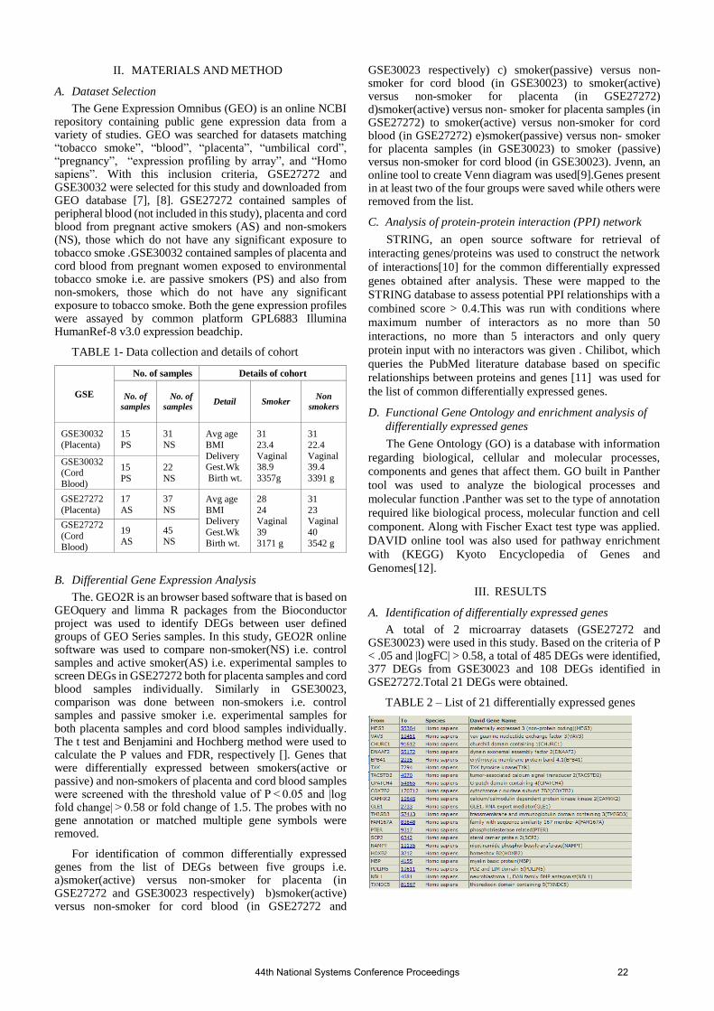
II. MATERIALS AND METHOD

A. Dataset Selection

The Gene Expression Omnibus (GEO) is an online NCBI repository containing public gene expression data from a variety of studies. GEO was searched for datasets matching “tobacco smoke”, “blood”, “placenta”, “umbilical cord”, “pregnancy”, “expression profiling by array”, and “Homo sapiens”. With this inclusion criteria, GSE27272 and GSE30032 were selected for this study and downloaded from GEO database [7], [8]. GSE27272 contained samples of peripheral blood (not included in this study), placenta and cord blood from pregnant active smokers (AS) and non-smokers (NS), those which do not have any significant exposure to tobacco smoke .GSE30032 contained samples of placenta and cord blood from pregnant women exposed to environmental tobacco smoke i.e. are passive smokers (PS) and also from non-smokers, those which do not have any significant exposure to tobacco smoke. Both the gene expression profiles were assayed by common platform GPL6883 Illumina HumanRef-8 v3.0 expression beadchip.

TABLE 1- Data collection and details of cohort

GSE

No. of samples Details of cohort

No. of

samples

No. of

samples Detail Smoker

Non

smokers

GSE30032

(Placenta)

15

PS

31

NS Avg age

BMI

Delivery Gest.Wk

Birth wt.

31

23.4

Vaginal 38.9

3357g

31

22.4

Vaginal 39.4

3391 g

GSE30032 (Cord

Blood)

15

PS

22

NS

GSE27272

(Placenta)

17

AS

37

NS Avg age

BMI

Delivery

Gest.Wk

Birth wt.

28

24

Vaginal

39

3171 g

31

23

Vaginal

40

3542 g

GSE27272

(Cord

Blood)

19 AS

45 NS

B. Differential Gene Expression Analysis

The. GEO2R is an browser based software that is based on GEOquery and limma R packages from the Bioconductor project was used to identify DEGs between user defined groups of GEO Series samples. In this study, GEO2R online software was used to compare non-smoker(NS) i.e. control samples and active smoker(AS) i.e. experimental samples to screen DEGs in GSE27272 both for placenta samples and cord blood samples individually. Similarly in GSE30023, comparison was done between non-smokers i.e. control samples and passive smoker i.e. experimental samples for both placenta samples and cord blood samples individually. The t test and Benjamini and Hochberg method were used to calculate the P values and FDR, respectively []. Genes that were differentially expressed between smokers(active or passive) and non-smokers of placenta and cord blood samples were screened with the threshold value of P < 0.05 and |log fold change| > 0.58 or fold change of 1.5. The probes with no gene annotation or matched multiple gene symbols were removed.

For identification of common differentially expressed genes from the list of DEGs between five groups i.e. a)smoker(active) versus non-smoker for placenta (in GSE27272 and GSE30023 respectively) b)smoker(active) versus non-smoker for cord blood (in GSE27272 and

GSE30023 respectively) c) smoker(passive) versus non- smoker for cord blood (in GSE30023) to smoker(active) versus non-smoker for placenta (in GSE27272) d)smoker(active) versus non- smoker for placenta samples (in GSE27272) to smoker(active) versus non-smoker for cord blood (in GSE27272) e)smoker(passive) versus non- smoker for placenta samples (in GSE30023) to smoker (passive) versus non-smoker for cord blood (in GSE30023). Jvenn, an online tool to create Venn diagram was used[9].Genes present in at least two of the four groups were saved while others were removed from the list.

C. Analysis of protein-protein interaction (PPI) network

STRING, an open source software for retrieval of

interacting genes/proteins was used to construct the network

of interactions[10] for the common differentially expressed

genes obtained after analysis. These were mapped to the

STRING database to assess potential PPI relationships with a

combined score > 0.4.This was run with conditions where

maximum number of interactors as no more than 50

interactions, no more than 5 interactors and only query

protein input with no interactors was given . Chilibot, which

queries the PubMed literature database based on specific

relationships between proteins and genes [11] was used for

the list of common differentially expressed genes.

D. Functional Gene Ontology and enrichment analysis of

differentially expressed genes

The Gene Ontology (GO) is a database with information

regarding biological, cellular and molecular processes,

components and genes that affect them. GO built in Panther

tool was used to analyze the biological processes and

molecular function .Panther was set to the type of annotation

required like biological process, molecular function and cell

component. Along with Fischer Exact test type was applied.

DAVID online tool was also used for pathway enrichment

with (KEGG) Kyoto Encyclopedia of Genes and

Genomes[12].

III. RESULTS

A. Identification of differentially expressed genes

A total of 2 microarray datasets (GSE27272 and GSE30023) were used in this study. Based on the criteria of P < .05 and |logFC| > 0.58, a total of 485 DEGs were identified, 377 DEGs from GSE30023 and 108 DEGs identified in GSE27272.Total 21 DEGs were obtained.

TABLE 2 – List of 21 differentially expressed genes


Subsequently, the results of the intersection of these 2 DEG profiles were obtained by Venn diagram analysis on basis of groups. According to the following groups-. a) Smoker –active (A) or passive (P) versus non-smoker (N) for placenta (in GSE27272 and GSE30023 respectively) showed 5 DEGs b) Smoker (active or passive) versus non-smoker for cord blood (in GSE27272 and GSE30023 respectively) showed 0 DEGs c) Smoker (passive) versus non- smoker for cord blood (in GSE30023) to smoker (active) versus non-smoker for placenta (in GSE27272) showed 5 DEGs d) Smoker (active) versus non- smoker for placenta samples (in GSE27272) to smoker (active) versus non-smoker for cord blood (in GSE27272) showed 2 DEGs e) Smoker (passive) versus non- smoker for placenta samples (in GSE30023) to smoker (passive) versus non-smoker for cord blood (in GSE30023) showed 9 DEGs.

Fig 1- Venn diagram by Jvenn softare linking the studies in GSE30023 and GSE27272

TABLE 3- Common differentially expressed genes with respect to group comparisons

These differentially expressed genes not only show difference between placenta samples of active and passive smoker versus non-smoker but also show similarity to cord blood of passive and active smoker versus non-smoker

B. Protein-protein interaction (PPI) network construction

Based on STRING software the PPI network was

constructed. For no more than 5 interaction the PPI

enrichment p value is 0.28 and for no more than 50

interactions PPI enrichment p-value:< 1.0e-16.

Fig 2 - PPI enrichment with 5 interactions STRING

Fig 3- PPI enrichment with 50 interactions STRING

When interaction was analyzed with only query protein only

one significant interaction between VAV3 which is vav

guanine nucleotide exchange factor 3 and TXK which is

tyrosine kinase was found which might be of significance.

Myelin basic protein, sterol carrier protein, calmodulin

associated protein kinase2, tumor associated calcium signal

transducer, phosphotriesterase related and vav guanine

nucleotide exchange factor 3 are interlinked in accordance to

Pubmed literature as abstracts or having non –interactive

relationship. Chilibot also showed interactions with relevance

to its relativity to Pubmed literature.

Fig 4 – Chilibot analysis


C. Gene Ontology and pathway analysis of differentially

expressed genes

Panther tool of the Gene Ontology identified biological

process, molecular function and cellular components with p

value adjusted to below 0.05 and Fishers exact test as

selection parameter. It also gives expected values and fold

enrichment which shows degree to which a gene would be

affect relative to its up-regulation or down-regulation.

TABLE 4 – GO cellular component analysis with fold

enrichment above 99.49

GO cellular component

Gene list Expected

Fold Enrichment raw P-value

nuclear pore cytoplasmic filaments (GO:0044614) 1 0 > 100 4.45E-03 internode region of axon (GO:0033269) 1 0 > 100 5.57E-03 spectrin-associated cytoskeleton (GO:0014731) 1 0.01 99.49 1.11E-02

TABLE 5 – GO molecular function analysis with fold

enrichment above 100

GO molecular function Genes

in list

Exp

ecte

d

Fold

Enrichm

ent

raw P-

value)

nicotinamide phosphoribosyltransferase

activity (GO:0047280)

1 0 > 100 2.23E-03

propanoyl-CoA

C-acyltransferase activity (GO:0033814)

1 0 > 100 2.23E-03

propionyl-CoA

C2-trimethyltridecanoy

ltransferase activity (GO:0050632)

1 0 > 100 2.23E-03

oleic acid binding

(GO:0070538) 1 0 > 100 3.34E-03

nicotinate-nucleotide

diphosphorylase (carboxylating) activity

(GO:0004514)

1 0 > 100 4.45E-03

inositol hexakisphosphate

binding (GO:0000822) 1 0 > 100 4.45E-03

acetyl-CoA C-myristoyltransferase

activity (GO:0050633)

1 0 > 100 4.45E-03

myristoyltransferase

activity (GO:0019107) 1 0.01 > 100 6.68E-03

structural constituent of myelin sheath

(GO:0019911)

2 0.01 > 100 9.22E-05

phosphatidylcholine

transfer activity (GO:0120019)

1 0.01 > 100 7.78E-03

long-chain fatty acyl-CoA

binding (GO:0036042) 1 0.01 > 100 8.89E-03

acetyl-CoA

C-acyltransferase activity (GO:0003988)

1 0.01 > 100 8.89E-03

morphogen activity

(GO:0016015) 1 0.01 > 100 8.89E-03

TABLE 6 – GO biological process analysis with fold

enrichment above 100 and P value above 6.70E-03

GO biological process complete

Gene list

Expected

Fold Enrichment

raw P-value

lipid hydroperoxide transport (GO:1901373) 1 0 > 100 2.23E-03

response to D-galactose (GO:1905377) 1 0 > 100 2.23E-03

rhombomere 4 development (GO:0021570) 1 0 > 100 3.34E-03

negative regulation of branching involved in ureteric bud morphogenesis (GO:0090191)

1 0 > 100 3.34E-03

positive regulation of metalloendopeptidase activity (GO:1904685)

1 0 > 100 3.34E-03

rhombomere 3 development (GO:0021569) 1 0 > 100 4.45E-03

inositol trisphosphate biosynthetic process (GO:0032959)

1 0 > 100 4.45E-03

establishment of left/right asymmetry (GO:0061966) 1 0 > 100 4.45E-03

progesterone biosynthetic process (GO:0006701) 1 0 > 100 5.57E-03

male anatomical structure morphogenesis (GO:0090598) 1 0 > 100 5.57E-03

male genitalia morphogenesis (GO:0048808) 1 0 > 100 5.57E-03

positive regulation of intracellular cholesterol transport (GO:0032385)

1 0 > 100 5.57E-03

positive regulation of intracellular sterol transport (GO:0032382)

1 0 > 100 5.57E-03

positive regulation of intracellular lipid transport (GO:0032379)

1 0 > 100 5.57E-03

determination of dorsal identity (GO:0048263) 1 0 > 100 5.57E-03

sequestering of BMP in extracellular matrix (GO:0035582)

1 0 > 100 5.57E-03

CAMKK-AMPK signaling cascade (GO:0061762) 1 0 > 100 5.57E-03

regulation of lung blood pressure (GO:0014916) 1 0 > 100 5.57E-03

calmodulin dependent kinase signaling pathway (GO:0099004)

1 0.01 > 100 6.68E-03

determination of dorsal/ventral asymmetry (GO:0048262) 1 0.

01 > 100 6.68E-03

DAVID with KEGG gave the common pathway enrichment

for the common differentially expressed genes. It helps to

analyze the pathways enriched for individual genes.


TABLE 7 – KEGG pathway enrichment with DAVID for 8

of common 21 differentially expressed genes

IV. CONCLUSION

Total 484 genes were differentially expressed among which

21 were found to be common among the two datasets. It was

seen than placental samples had common differentially

expressed genes when active and passive smokers were

compared to non-smokers respectively. This indicates that

exposure to tobacco smoke induces transcriptomic alterations

which have similarity to active smokers. This is alarming

because with air pollution and CO2, CO,NO levels on rise

and tobacco smoke exposure by cigarette smoking everyone

is at a higher risk no matter where. Another important finding

is that cord blood of active and passive smokers compared to

non-smokers respectively finds similar identity to placental

tissue differentially expressed genes. The reason may be that

via placenta this may have reached the cord blood. The cord

blood is transferred from mother to child thereby acting as

transfer medium for all major microbiota and initial heath

development nutrition. Cord blood transcriptomic alterations

due to exposure of pregnant women to smoking will

definitely affect the infant. This can be seen via the results of

pathway analysis where cell signaling pathways, immune

system pathways – chemokine, NKC, leukocyte signaling is

affected. Also, dementia like diseases Alzheimer’s.

Parkinson’s, attention deficit disorders are affected by the

differentially expressed genes. Also, birth weight has been

affected i.e. lowest in active smoker < passive smokers < non-

smokers in the experimental studies according to literature

review as seen while data collection of birth weight was done

in GSE30023 and GSE27272 experiments.

Therefore investigation of such studies related to effect of

tobacco smoke exposure on maternal cell and fetus would

provide insight on measures with relevance to clinical and

genomics aspect to prevent health deterioration. Health and

Well-being 2023 goal of Sustainable Development shall be

benefitted from such studies to formulate interventions of

better health of mother and fetus.

Therefore in future, it is important to carry out comparative

transcriptomics of effect of smoking- active, passive

environmental pollution on pregnant women and infants till

three years of age in various tissue samples.

REFERENCES

[1] M. C. Kataoka et al., “Smoking during pregnancy

and harm reduction in birth weight : a cross-sectional

study,” BMC Pregnancy Childbirth, no. 18:67, pp. 1–

10, 2018.

[2] World Health Organization. Regional Office for

South-East Asia., Tobacco control for sustainable

development. World Health Organization, Regional

Office for South-East Asia, vol. 4, no. 3. 2017.

[3] F. Soesanti, C. S. P. M. Uiterwaal, D. E. Grobbee, A.

Hendarto, G. W. Dalmeijer, and N. S. Idris,

“Antenatal exposure to second hand smoke of non-

smoking mothers and growth rate of their infants,”

PLoS One, vol. 14, no. 6, pp. 1–10, 2019, doi:

10.1371/journal.pone.0218577.

[4] P. Huuskonen et al., “Microarray analysis of the

global alterations in the gene expression in the

placentas from cigarette-smoking mothers,” Clin.

Pharmacol. Ther., vol. 83, no. 4, pp. 542–550, 2008,

doi: 10.1038/sj.clpt.6100376.

[5] E. Clough and T. Barrett, “The Gene Expression

Omnibus database,” Methods Mol. Biol., vol. 1418,

no. 301, pp. 93–110, 2016, doi: 10.1007/978-1-4939-

3578-9_5.

[6] J. Yan, S. L. Risacher, L. Shen, and A. J. Saykin,

“Network approaches to systems biology analysis of

complex disease: Integrative methods for multi-

omics data,” Brief. Bioinform., vol. 19, no. 6, pp.

1370–1381, 2017, doi: 10.1093/bib/bbx066.

[7] H. Votavova et al., “Transcriptome alterations in

maternal and fetal cells induced by tobacco smoke,”

Placenta, vol. 32, no. 10, pp. 763–770, 2011, doi:

10.1016/j.placenta.2011.06.022.

Column1 KEGG pathway enrichment analysis by DAVID

Ggene TXK tyrosine kinase(TXK)

KEGG_PATHWAY Leukocyte transendothelial migration,

Ggene calcium/calmodulin dependent protein kinase kinase 2(CAMKK2)

KEGG_PATHWAY AMPK signaling pathway, Adipocytokine signaling pathway, Oxytocin signaling pathway, Alcoholism,

Ggene cytochrome c oxidase subunit 7B2(COX7B2)

KEGG_PATHWAY

Oxidative phosphorylation, Metabolic pathways, Cardiac muscle contraction, Non-alcoholic fatty liver disease (NAFLD), Alzheimer's disease, Parkinson's disease, Huntington's disease,

Ggene neuroblastoma 1, DAN family BMP antagonist(NBL1)

KEGG_PATHWAY TGF-beta signaling pathway,

Ggene nicotinamide phosphoribosyltransferase(NAMPT)

KEGG_PATHWAY Nicotinate and nicotinamide metabolism, Metabolic pathways,

Ggene sterol carrier protein 2(SCP2)

KEGG_PATHWAY Primary bile acid biosynthesis, Metabolic pathways, PPAR signaling pathway, Peroxisome,

Ggene thioredoxin domain containing 5(TXNDC5)

KEGG_PATHWAY Protein processing in endoplasmic reticulum,

Ggene vav guanine nucleotide exchange factor 3(VAV3)

KEGG_PATHWAY

cAMP signaling pathway, Chemokine signaling pathway, Focal adhesion, Natural killer cell mediated cytotoxicity, T cell receptor signaling pathway, B cell receptor signaling pathway, Fc epsilon RI signaling pathway, Fc gamma R-mediated phagocytosis, Leukocyte transendothelial migration, Regulation of actin cytoskeleton


[8] H. Bruchova et al., “Effect of Maternal Tobacco

Smoke Exposure on the Placental Transcriptome,”

Placenta, vol. 31, no. 3, pp. 186–191, 2010, doi:

10.1016/j.placenta.2009.12.016.

[9] P. Bardou, J. Mariette, F. Escudié, C. Djemiel, and C.

Klopp, “jvenn: an interactive Venn diagram viewer,”

BMC Bioinformatics, vol. 15, no. 293, pp. 1–7, 2014,

[Online]. Available:

http://www.biomedcentral.com/1471-2105/15/293.

[10] D. Szklarczyk et al., “STRING v11: Protein-protein

association networks with increased coverage,

supporting functional discovery in genome-wide

experimental datasets,” Nucleic Acids Res., vol. 47,

no. D1, pp. D607–D613, 2019, doi:

10.1093/nar/gky1131.

[11] H. Chen and B. M. Sharp, “Content-rich biological

network constructed by mining PubMed abstracts,”

BMC Bioinformatics, vol. 5, pp. 1–13, 2004, doi:

10.1186/1471-2105-5-147.

[12] G. Dennis et al., “DAVID: Database for Annotation,

Visualization, and Integrated Discovery.,” Genome

Biol., vol. 4, no. 5, 2003, doi: 10.1186/gb-2003-4-9-

r60.

.


Technology - Based Intervention on Geometric

Skills and its Effect on Verbal and Visual Memory

of Preschoolers Nisha Mahaur

Dept. of Pedagogical Sciences

Faculty of Education,


Agra, India

[email protected]

Sona Ahuja




Agra, India

ORCID: 0000-0003-1220-3182

Sonali Gupta




Agra, India

[email protected]

Abstract- Though prolific technology - based interventions

are developed, several researches have been carried out on

preschoolers; the impact of such interventions on verbal

and visual memory remains obscure, especially in

preschoolers. The purpose of the present study was to study

the effect of geometrical skills on verbal and visual memory

of preschoolers through a technology-based intervention.

Forty preschoolers aged two to four years participated in the

study. Twenty preschoolers were allotted to the

experimental group and twenty to the active control group.

The experimental group was subjected to four weeks of

intervention. The pre and post-tests were administered to

assess the verbal and visual memory. For assessment of

verbal memory, the groups were compared on their ability

to recall the names of various shapes and objects. The

subjects were asked to recognize the shapes and other

associated objects for assessment of visual memory. The

results indicate the positive influence of technology-based

intervention on the geometrical skills of preschoolers.

There was significant improvement in verbal as well as

visual memory.

Keywords: Intervention, Preschoolers, Verbal Memory,

Visual Memory, Geometrical Skills

BACKGROUND

Early childhood education begins early, even before birth

(Kunin, 2009). The children aged two to four years are

referred to as preschoolers (Frazier, 2009). This is the period

to build a strong foundation in all developmental areas. Skills

such as naming colors, showing affection, etc. are the

developmental milestones for 0 -3 years children. Children

reach milestones in how they play, learn, speak, behave, and

move (like crawling, walking, or jumping). As children grow

into early childhood, their world begins to open up. They

become more independent and begin to focus more on adults

and children outside of the family. They want to explore and

have a tendency to ask about things around them even more.

The interactions with family and those around them help to

shape their personality and their own ways of thinking and

moving. For children to grow into strong and healthy adults,

their education in the early years should meet specific

developmental milestones in each of the domains. These

domains are: Cognitive domain that includes skills regarding

learning and thinking, asking questions, developing an

increased attention span, problem solving, visual

discrimination, etc.; Physical domain which includes skills

like muscle control, balance, and coordination (climbing

ladders, opening doors, etc.), exercise, health, and nutrition,

self-help skills (feeding, brushing teeth, dressing, and

washing hands); and Socio-emotional domain that includes

skills such as regulating one’s own behavior and emotions,

developing friendships with other children and healthy

relationships with adults, creating a positive personal

identity, developing a working memory, engaging in

learning, etc. (Aiger, 2017). Mathematical skills are also

critical to students' long term economic and social success

(Jang, 2016). Even young children have the potential to learn

mathematics that is complex and sophisticated (Clements,

2011). Before they start school, most children develop an

understanding of addition and subtraction of small digits

through everyday interactions. Children use early math skills

throughout their daily routines and activities. Most of the

children develop number sense through everyday

interactions. For example, Thomas has two cars; Joseph

wants one. After Thomas shares one, he sees that he has one

car left (Bowman, Donovan, & Burns, 2001). Other math

skills are introduced through daily routines shared with

children like counting steps while going up or coming down.

Informal activities like this give children a jumpstart on the

formal math instruction that starts in school.

Early mathematical concepts and skills that first-

grade mathematics curriculum builds on include

understanding size, shape, and patterns; ability to

count verbally (first forward, then backward);

recognizing numerals; identifying more and less of

a quantity; and understanding one-to-one

correspondence (i.e., matching sets, or knowing

which group has four and which has five) (Bowman

et al., 2001, p. 76).

Children’s ability to understand mathematics takes a big leap

forward in the preschool years. (Geist, 2014) The

strengthening ability of children to represent using symbols

and signs shows many new possibilities. As early as age

three, children can hold up fingers to indicate a quantity. By

age four, children are learning to count. They can usually

count to 5 or 10, and can tell what number comes next in a

series. For example, if you counted 1, 2, 3, 4, and 5 and asked

what comes next, the child could say, “6!” However, at this

stage, saying the words and understanding the quantity linked


to them is not a certainty (Clements & Sarama, 2004).

Children can recognize and name shapes that have different

sizes and orientations. They also learn and use directional

words such as “up,” “down,” “over,” “under,” and many

others. Measurement also takes a leap forward as children

begin to compare objects by length. Three-year-olds can put

two pencils next to each other and tell you which one is

longer. Four-year-olds can begin to use nonstandard units to

measure things; for example, they can tell you how many

shoes wide the teacher’s desk is. They will need a lot of shoes

to do this, because they cannot yet use one shoe repeatedly

(Clements & Stephan, 2004; Clements, 2001; Clements &

Bright, 2003). Early math skill is the strongest early predictor

of children’s math achievement years later (Aunola,

Leskinen, Lerkkanen, and Nurmi, 2004; Duncan et al., 2007;

Geary, Hoard, Nugent & Bailey, 2013; Jordan, Kaplan,

Ramineni, and Locuniak, 2009; Siegler et al., 2012). Some

students face difficulty in solving simple arithmetic

problems. The lack of diagnoses and remediation at an early

age can be one of the reasons behind this. Research has been

conducted to improve the mathematical ability of preschool

students (Clements & Sarama, 2007; Clements, Sarama,

Wolfe, & Spitler, 2013; Sarama, Clements, Wolfe, & Spitler,

2012). The interventions have been used by some researchers

to assist children especially from low - income families to

learn mathematical concepts (Clements & Sarama, 2011;

Nguyen, Watts & Clements, 2017).

“The limits of our language” means the limits of our world

(Wittgenstein, 1922). Language as a barrier in learning must

be focused. The Global Monitoring Report on Education for

All, 2005 underlined the fact that worldwide the choice of the

language of instruction and language policy in schools is

critical for effective learning (Ouane & Glanz, 2010). The

same was a barrier in the previously developed interventions.

Also, being in the vicinity of all, is a mandatory part of the

intervention. But they are not in reach of all. In light of these

concerns, the study intends to build a geometrical

intervention to improve the early mathematical ability of

preschool students. Additionally, verbal and visual memory

is of great importance for scholastic achievement in children

(Miriam, 2017). Verbal memory is one of the most

consistently reported domains of neuro-cognitive decline

(Dye & Mehta, 2015). There are a variety of tasks for

measuring verbal memory capability, including learning of

word lists, story recall (or logical memory), and learning of

sequences of paired words (Tatsumi, 2009). It’s true that

technology is a good enabler so that students don’t need to

memorize nearly as much as they did in the past, students still

need to efficiently remember (Mindprint learning, 2019). In

every subject, children need to learn concepts which are

unattainable without good verbal memory. Visual memory

involves the ability to store and retrieve previously

experienced visual sensations and perceptions when the

stimuli that originally evoked them are no longer present

(Plessis, 2018). Poor visual memory is significantly related to

poor achievement in mathematics. Therefore, visual memory

is considered to be amongst the skills that are significantly

related to mathematics achievement (Kulp et. Al., 2004).

Researches claim that verbal memory, visual memory and

working memory have an effect on mathematics, in general

(Ashkenazi, Lee, 2013; Swanson, 2015; Gilligan et. al., 2017;

Hornung, Schiltz, 2017). Is the vice-versa true? So, the study

aims to analyze the effect of the intervention on geometrical

skills on the verbal and visual memory of preschoolers.

METHOD

Design

Before implementing the intervention to the subject, a pre-

test was conducted to assess the verbal and visual memory of

the preschoolers. The post-test was administered after 4

weeks of intervention.

Intervention

The intervention was designed to provide the concept of

geometrical shapes to help children build a strong foundation

of mathematical knowledge using technology. The structure

of each activity was designed in accordance to the learning

needs of preschoolers like motor skills, listening skills,

conflict resolution skills, social skills, etc. (Dumke, 2018).

The intervention was prepared on the basis of (i) A document

- The first three years by Mina Swaminathan, UNICEF (ii)

Visiting crèche, Faculty of DEI and (iii) Interaction with the

parents of preschoolers.

The intervention consisted of four videos one for each shape

(circle, triangle, square and rectangle). The duration of each

video was 8 mins. Three examples were presented in video

for each shape (Fig. 1). The intervention was implemented

for fifteen minutes per day for four days a week for four

weeks. Every week a new geometrical shape was introduced

- circle (first week), square (second week), triangles (third

week) and rectangle (fourth week). The concept of shapes

was related to the objects they observe in daily life. The

stimuli were presented using different colors, audio and

visual representations on a smart-board.

Figure 1: A Glimpse of Technology - based intervention for

preschoolers

Before implementing the intervention and collecting the data,

it was tested on two preschoolers. The feedback on

intervention was sought from teacher educators with (i)

specialization in early childhood education, (ii) specialization

in technology, (iii) instructors at pre-school and (iv) parents


of preschoolers. Their suggestions were incorporated.

Changes were made like the pace of the videos, modification

in voice (intonation of the syllables was corrected) and re-

recording some parts where the pronunciation wasn’t clear. The modified intervention was further tested on a small group

of ten preschoolers. It was observed that the stimuli presented

successfully gained attention of subjects. The preschoolers

also responded to the pop-up questions in the videos. As no

changes were required further, the field try-out of the

intervention on the experimental group of twenty

preschoolers was carried out. The active control group was

exposed to the content in the traditional way of teaching for

four days per week for four weeks. Blackboard and other

objects in their surroundings like chart paper, duster, chalk

and toys were used to equip the children with the knowledge

of shapes. Their responses were observed and noted. The

content was presented for twenty minutes a day.

Participants

Forty preschoolers were selected from two pre-schools of

Agra. The consent was sought from parents for participation

in the study. The age range of participants was 2-4 years (M

= 2.65 years, SD = 0.625). The date of birth of all children

was obtained to determine their age-eligibility. Children were

recruited equally from both the schools for this randomized

controlled trial. 20 preschoolers were allotted to an active

control group and 20 to an experimental group (10 for

experimental group and 10 for active control group from each

school). Demographics are presented in Table 1.

Table 1 Demographic Characteristics of Participants

Experimental Group

(N = 20)

Active Control Group

(N = 20)

Age M = 2.65, SD = 0.625 M =2.59, SD = 0.614

Gender 08 (Boys), 12 (Girls) 09 (Boys), 11(Girls)

Measures

The performance tasks were designed to assess verbal and

visual memory of the preschoolers on the basis on Weschler’s

Intelligence Scale for Children (Weschler, 2014), Working

Memory Test Battery for Children (Gathercole, 2001) and

Missing Scan Task (Buschke, 1963),

Verbal Memory

The verbal working memory can be assessed by recalling the

list of certain items (Warner, 2003). Demoulin and Kolinsky

(2015), in their experiment, measured the verbal memory in

a free recall task in which children had to verbally recall the

names of pictures. A similar task was designed in the present

study. The subjects were instructed to listen to the spoken

words. On each trial of the test, a sequence of shapes was

spoken aloud twice in the same order with the e-flashcards

appearing simultaneously as the name of the shape was being

spoken at the rate of two seconds per shape. The subjects had

to repeat the names of the shapes in the same order as

presented. After every correct recall, the complexity of the

task increased by adding one more shape (differing from the

previous shapes). In case of incorrect trial, the previous

number of shapes were presented again. The last correct

number of shapes recalled was recorded as score.

Visual Memory

The measure of visual memory was adapted from the Benton

Visual Retention Test, The Brown Location Test and Kim

Karad Visual Memory Test (Brown, Roth et. al., 2014;

Movallali, 2016 & Talepasand, Eskandaripour &

Taghinezhad, 2018). The measure used in the present study

was a shape association task with the help of different objects. The participants ability of the visual association of objects

with shapes was assessed. The image of a shape was

presented (circle/square/rectangle/triangle) for five seconds

followed by the presentation of an object (plate/clock/egg/set

square/photo frame/heart) for another five seconds on the

screen in a random order. Ten images (six objects and four

shapes) were used in this assessment. The subject had to

identify the shape of the object by matching the object to the

previously displayed shape with yes/no as their response.

Each correct matching was marked by a score. The total score

was the total number of correct identifications of shape of

objects presented.

DATA ANALYSIS

The performance scores of participants at the pre - test and

post - test are presented in Table 2. Mann-Whitney U – test

was used to determine statistical significance of difference in

mean scores of the experimental and active control group. A

Wilcoxon Sign test was used to determine the effectiveness

of the intervention. The data was analyzed using the statistical

software past- paleontological statistics software package for

education and data analysis. The results are presented in table

2, 3, 4 and 5.

Table 2 Pre-Test Verbal and Visual Memory Scores of Experimental

Group and Active Control Group

Groups Experimental

(N = 20)

Active Control

(N = 20)

p

Verbal Memory

M (SD)

1.5 (1.15) 1.65 (1.04) 0.653

Visual Memory

M (SD)

3.05 (1.99) 3.15 (1.98) 0.960

Verbal Memory

The difference in the verbal memory scores of the

experimental and control group at pre-test was not

statistically significant (p = 0.653). Mann - Whitney test

indicated that the mean of verbal memory score of the

experimental group was significantly greater at post - test (M

= 3.10) than at pre - test (M = 1.50), U = 56, p = 0.000. This

significant difference indicated an increase in the verbal


memory scores of the preschoolers after the intervention. The

difference between pre-test and post-test visual memory

scores of the active control group was insignificant (p =

0.162).

Table 3 Pre-test & Post-test Verbal Memory Scores of Experimental


Experimental

N = 20

Active Control

N = 20

Pre-Test Post-Test Pre-Test Post-Test

M (SD) 1.50 (1.15) 3.10 (0.79) 1.65 (1.04) 2.05 (0.83)

U 56 150

p 0.000 0.162

Visual Memory

The difference in the visual memory scores of the

experimental and control group at pre-test was not

statistically significant (p = 0.960). Mann - Whitney test

indicated that the mean of visual memory scores of the

experimental group was significantly greater at post - test (M

= 4.45) than at pre - test (M = 3.05), U = 119.5, p = 0.028.

This significant difference indicated an increase in the visual

memory scores of the preschoolers after the intervention. The

difference between pre-test and post-test visual memory

scores of the active control group was not significant (p =

0.510).

Table 4 Pre-test & Post-test Visual Memory Scores of Experimental


Experimental N = 20

Active Control N = 20

Pre-Test Post-Test Pre-Test Post-Test

M (SD) 3.05 (1.99) 4.45 (1.54)

3.15 (1.98) 3.5 (1.70)

U 119.5 175.5

p 0.028 0.510

Effect of Technology-Based Intervention

The effect of the intervention was found to be positive (W =

7.5, p = 0.003 for experimental group and W = 47.5, p = 0.06

for active control group). A Cohen’s d = 1.05, indicates that

the mean score of subjects in the experimental group is 1.0

standard deviations above the mean score of subjects in the

active control group, and that the mean score of the

experimental group exceeds the scores of 84 percent of those

in the active control group.

Table 5 Effect Size of the Technology – Based Intervention

Group N W p Effect Size (d)

Experimental 20 7.5 0.003

1.05 Active Control 20 47.5 0.06

DISCUSSION

The current study examined the effect of geometrical skills

on the verbal and visual memory of preschoolers through a

technology-based intervention. Previous research has proved

that exposing the children (aged 4 to 8 years) to technological

intervention like tablet intervention enhances their

mathematical skills (Pitchford, 2015; Outhwaite & Gulliford,

2017). To our knowledge, this study is the first to test the

impact of geometrical skills on verbal and visual memory of

children aged between 2 to 4 years. Verbal memory, visual memory and working memory have

an effect on mathematics, in general (Ashkenazi, Lee, 2013;

Swanson, 2015; Gilligan et. al., 2017; Hornung, Schiltz,

2017). However, it is unclear whether the vice versa is true in

case of preschoolers. The results of the present research

indicated that geometrical intervention can improve the

verbal and visual memory of preschoolers. Children’s ability

to understand mathematics takes a big leap forward in the

preschool years (Geist, 2014). Early math skills are the

strongest early predictors of children’s math achievement

years later (Aunola, Leskinen, Lerkkanen, and Nurmi, 2004;

Duncan et al., 2007; Geary, Hoard, Nugent, and Bailey, 2013;

Jordan, Kaplan, Ramineni, and Locuniak, 2009; Siegler et al.,

2012). A positive effect of the intervention was observed as

indicated by the effect size of the intervention (d=1.05). The

analysis of the scores showed a significant effect of the

intervention on the verbal and visual memory of

preschoolers. The experimental group performed better in the

test of verbal and visual memory as compared to the active

control group. The results indicate that the exposure to

technology-based intervention can enhance the verbal and

visual memory leading to the retention of the concept for a

longer time. When the developed technology-based

intervention of shapes was implemented on an experimental

group of preschoolers they responded well and also

performed well in the test of visual memory. Interventions

(numbers & measurement) designed to facilitate the

mathematical learning of children aged 3 to 5 years have a

strong positive effect on these children’s lives for many years

(Clements & Julie, 2011). Different types of instructional

design features, including explicit instruction, computer-

assisted instruction (CAI), game playing, or the use of

concrete representational-abstract levels in representations of

math concepts, led to improvements in mathematics

performance (Mononen & Riikka, 2014). Preschoolers learn

fast through videos and images presented to them digitally as

seen in the results. The children took interest in listening to

the videos and also responded in between. The intervention

gained the subjects’ attention. Further studies can be

conducted to compare the effect of technology-based


intervention with other pedagogical techniques for

preschoolers.

REFERENCES

Alloway, T. P., Rajendran, G. & Archibald, L. M. D. (2009).

Working Memory in Children with Developmental

Disorders. Journal of Learning Disabilities, 42(4),

372-82. https://doi.org/10.1177/0022219409335214 Brown, F. C., Roth, Saykin, R. M. & Gibson, A. J. (2014). A

New Measure of Visual Location Learning and

Memory: Development and Psychometric Properties

for the Brown Location Test (BLT). The Clinical

Neuropsychologist, 21(5), 811-825.

https://doi.org/10.1080/13854040600878777 Clements, D. H. & Sarama, J. (2011). Early childhood

mathematics intervention. Science, 333(6045), 968-

970. https://doi.org/10.1126/science.1204537 Furlong, M., McLoughlin, F., McGilloway, S. & Geary, D.

(2016). Interventions to improve mathematical

performance for children with mathematical learning

difficulties (MLD). Cochrane Database of Systematic

Reviews, 1465-1858.

https://doi.org/10.1002/14651858.CD012130 Garduno, Ana Eugenia. (2016) Preschool and Educational

Technology: Evaluating a Tablet-Based Math

Curriculum in Mexico City. Retrieved from

https://dash.harvard.edu/bitstream/handle/1/2711271

1/ garduno-dissertation-2016.pdf?sequence=1 Chigeza, P. & Sorin, R. (2016). Kindergarten Children

Demonstrating Numeracy Concepts through

Drawings and Explanations: Intentional Teaching

within Play-based Learning. Australian Journal of

Teacher Education. 41(5).

http://dx.doi.org/10.14221/ajte.2016v41n5.5 Help your child develop early math skills (2016) In Zero to

three. Retrieved from https://www.zerotothree.org/

resources/299-help-your-child-develop-early-math-

skills Iterson, L. V. & Jong, P. (2017). Development of verbal

short-term memory and working memory in children

with epilepsy: Developmental delay and impact of

time-related variables. A cross-sectional study.

Epilepsy & Behavior, 78. https://doi.org/10.1016/j.

yebeh.2017.10.018 Jack, F., Simcock, G. & Hayne H. (2011). Magic Memories:

Young Children’s Verbal Recall After a 6-Year

Delay. Child Development, 83(1), 159-172.

https://doi.org/10.1111/j.1467-8624.2011.01699.x Klein, A., Starkey, P., Clements, D., Sarama, J. & Iyer, R.

(2008). Effects of a Pre-Kindergarten Mathematics

Intervention: A Randomized Experiment. Journal of

Research on Educational Effectiveness, 1(3), 155-

178. https://doi.org/10.1080/19345740802114533 McGough, J. J. & Faraone, S. V. (2009). Estimating the Size

of Treatment Effects: Moving beyond P values

Psychiatry (Edgmont), 6(10), 21-29. Mononen, R., Aunio, P., Koponen, T. & Aro, M. (2014). A

review of early numeracy interventions for children at

risk in mathematics. International Journal of Early

Childhood Special Education, 6(1), 25-54.

https://doi.org/10.20489/intjecse.14355

Pam, M. S. (2013). Verbal Memory. In

Psychologydictionary.org. Retrieved from

https://psychologydictionary. org/verbal-memory/ Ochsendorf, R. (2016) Advancing Understanding of

Mathematics Development and Intervention: Findings

From NCSER-Funded Efficacy Studies. Journal of

Research on Educational Effectiveness, 9(4), 570-

576. https://doi.org/10.1080/19345747.2016.1222144 Outhwaite, L. A., Gulliford A. & Pitchford N. J. (2017).

Closing the gap: Efficacy of a tablet intervention to

support the development of early mathematical skills

in UK primary school children. Computers &

Education, 108, 43-58.

https://doi.org/10.1016/j.compedu.2017.01.011 Pitchford (2015) Development of early mathematical skills

with a tablet intervention: a randomized control trial

in Malawi. Front. Psychol., 6, 485.

https://doi.org/10.3389/fpsyg.2015.00485 Purpura, D. J. & Lonigan, C. J. (2015). Early Numeracy

Assessment: The Development of the Preschool

Numeracy Scales. Early Education and Development,

26(2), 286-313. https://doi.org/10.1080/10409289.

2015.991084 Plessis S. D. (2018). Visual Memory: Definition, Importance,

Facts, Overcoming Deficits. Retrieved from

https://www.edubloxtutor.com/visual-memory/ Rojas, C. (2015). Improvement of Working Memory in

Preschoolers and Its Impact on Early Literacy Skills:

A Study in Deprived Communities of Rural and Urban

Areas. Early Education and Development, 26(5-6),

871-892.

https://doi.org/10.1080/10409289.2015.1036346 Talepasand, S., Eskandaripour, M. & Taghinezhad, A. (2018).

Comparison of Working and Visual Memory in Children

with and Without Dyslexia. Zahedan Journal of

Research in Medical Science, 20(9), e70701.

https://dx.doi.org/10.5812/zjrms.70701 Visual Memory Activities (n.d.). Visual Perception

Activities. Retrieved from https://www.ot-mom-

learning- activities.com/visual-memory-

activities.html Visual Memory: Definition & Skills (2016). Retrieved from

https://study.com/academy/lesson/visual-memory-

definition-skills.html Warner, J. (2003). Music lessons boost verbal memory.

Retrieved from https://www.webmd.com/baby/news/

20030728/music-lessons-verbal-memory#1 Watts, T. W., Clements, D. H., Sarama, J., Wolfe, C. B.,

Spitler, M. E. & Bailey, D. H. (2017). Does Early

Mathematics Intervention Change the Processes

Underlying Children’s Learning? Journal of Research

on Educational Effectiveness, 10(1), 96-115.

https://doi.org/10.1080/19345747.2016.1204640




https://doi.org/10.3389/fpsyg.2015.00485

https://doi.org/10.3389/fpsyg.2015.00485

Extractive Lecture Summarization System Using Evolutionary Algorithms –

Optimizing Word, Sentence and Text Features

Binathi Bingi

Department of Physics and Computer Science


Agra, India

[email protected]

Lotika Singh



Agra, India

[email protected]

Abstract - Automatic extractive text summarization

on lectures has become more predominant with

increase in the online learning. These systems help in

collecting important information, key phrases and

sentences that best represent the content. In this paper,

we have proposed automatic extractive lecture

summarization as a binary optimization problem, and

multi-objective non-dominated sorting genetic

algorithm (NSGA-II) is employed to solve this. The

solutions of GA encode possible set of sentences that

constitute the summary which are then evaluated

based on word, sentence and text features. These

features constitute the objective functions that

measure different aspects of the summary and are

optimized simultaneously using the search capability

of GA. For the purpose of evaluation of the model, two

summarization datasets DocEng’19 and CNN/Daily

mail are used. The results are compared with

optimization, machine learning and deep learning

models using ROUGE measures. For CNN/Dailymail

dataset, we have obtained 12% and 25%

improvements over the existing state-of-the-art

extractive lecture summarization techniques. The

paper also demonstrates the effect of similarity

measures and objective functions over the quality of

the generated summary.

Keywords – lecture summarization system, multi-

objective binary optimization, extractive summarization,

sentence and text quality measures

I. INTRODUCTION

Text summarization aims to create a shorter version of the document that conveys the main theme of the document [1]. Based on the extraction methodology, there are two types of summarization techniques – abstractive [2] and extractive [3]. Abstractive summarization uses vocabulary beyond the specified text, generates a summary similar to human generated summary. Though it is desirable, it requires deep learning, several GPUs to train over days or highly complex algorithms and rules with limited generalization [4]. Due to these challenges,

extractive summarization is used by lecture summarization models. Extractive summarization leverages only the content from the text. It chooses key phrases and important sentences from the text to create a summary of desired length. In education, with increase in MOOCs, video lecture transcripts are available but locating the important information from the transcript (L) can be a challenging task. In such cases, automatic extractive summarization of lectures is a powerful tool.

In the beginning of the 21st century, manual summarizations were created using multimedia applications [5]. With increase in the data, manual summarization became a tedious process and probabilistic models were used for summarization [6]. To improve the summarization performance, researches incorporated rhetorical information into the summaries [7]. In recent years, different methods like meta-heuristic based [8]–[10] , unsupervised learning based [11], [12], supervised learning based [13]–[15], neural-network based [4], [16]–[19] have been used to solve the problem of extractive summarization. The deep learning techniques require huge computational resources and training data, on the contrary meta-heuristic algorithms are unsupervised and can optimize multiple features to generate good quality summary using comparatively less computational resources and training data.

There are four methods used for generating summary features [20]: (i) word scoring (ii) sentence scoring (iii) graph scoring (iv) text scoring. In this paper, we have used a combination of word, sentence and text scoring features to create five objective functions and formulated the lecture summarization problem as a multi-objective optimization problem. In order to show that the performance of model depends on the objective functions and similarity/dissimilarity function chosen, different combinations of the above have are explored. For reporting the best summary and evaluation of the


mailto:[email protected]

model, most of the approaches use gold standard summaries, but in real scenarios like lecture summarization, gold standard references might not be available. To overcome this, we have explored unsupervised learning techniques to choose a single best solution from the final pareto optimal front generated by NSGA-II [21].

II. LECTURE SUMMARIZATION AS MULTI-

OBJECTIVE OPTIMIZATION

Multi-objective optimization problem optimizes more than one objective function simultaneously by adhering to some constraints to solve a particular problem. It can be mathematically formulated as:

𝐦𝐚𝐱𝒇𝟏( ), 𝒇𝟐( ),… . , 𝒇𝒎( ) , 𝝐𝑿

where, X is set of decision vectors in a n-dimension space denoted as 𝒙𝟏 , 𝒙𝟐 , …., 𝒙𝒏 , m is the number of objective functions to be optimized. Genetic Algorithm (GA) is a search-based global optimization technique proposed by John Holland in 1975 [22]. There exist many variants of GA which differ in representation (binary-coded or real-coded) of the solutions and in terms of parameters. In this paper, we use a binary genetic algorithm where each solution is coded as a binary vector and is associated with five objective functions. The algorithm executes in a way similar to other optimization algorithms. It starts with a random set of solutions called population. At a given time stamp t (generation), ith solution is represented as

𝒙𝒊 (𝒕) = [𝒙𝒊,𝟏(𝒕), 𝒙𝒊,𝟐(𝒕),…… , 𝒙𝒊,𝒏(𝒕)]

where, i=1,2,…|P| , |P| is the size of population, n is the length of solution, 𝒙𝒊,𝒎 either takes a 0 or 1,

for m =1,2,…, n. For each solution i, the offspring is generated using crossover and mutation operations [23], [24] and solution is evaluated in comparison with all solutions in the population.

A. Problem Definition

Consider a lecture transcript (L) consisting of N sentences, 𝒔𝟏, 𝒔𝟐, … . , 𝒔𝑵. Our task is to find the subset of sentences (S) which cover the information in the lecture, 𝑺𝝐𝑳 such that

|𝑺| ≤ 𝑺𝒎𝒂𝒙

where 𝑺𝒎𝒂𝒙 represents the maximum number of sentences in the summary and |S| represents the number of sentences in the generated summary.

B. Sentence similarity/dissimilarity and quality

measures

To generate a high-quality summary, five objective functions are optimized simultaneously using binary genetic algorithm and NSGA-II framework. Some of the objective functions include similarity/dissimilarity measure between sentences.

In this paper, we have analysed three such similarity/dissimilarity measures and their description follows:

1) Normalized Google Distance (NGD)

It measures the dissimilarity between two sentences using the terms in the sentences [25]. It is mathematically defined as:

𝑑(𝑠𝑖 , 𝑠𝑗) = Σ𝑡𝑖𝜖𝑠𝑖

Σ𝑡𝑗𝜖𝑠𝑗𝑁𝐺𝐷(𝑡1, 𝑡2)

|𝑠𝑖| ∗ |𝑠𝑗|

where, 𝑡1 𝑎𝑛𝑑 𝑡2 are terms belonging to sentences 𝑠𝑖 and 𝑠𝑗 respectively, |𝑠𝑖|, |𝑠𝑗| are

number of terms in sentences 𝑠𝑖 and 𝑠𝑗 respectively.

𝑁𝐺𝐷(𝑡1, 𝑡2)

= maxlog(𝑠𝑡1) , log(𝑠𝑡2) − log (𝑠𝑡1,𝑡2)

log𝑁 − min log(𝑠𝑡1) , log(𝑠𝑡2)

where 𝑠𝑡1 , 𝑠𝑡2 denotes the number of sentences

in L containing the term 𝑡1and term 𝑡2 respectively, 𝑠𝑡1,𝑡2 denotes the number of sentences in L

containing both the terms 𝑡1and 𝑡2, N is the number of sentences in L.

2) Word Mover Distance This measure calculates the dissimilarity between

two documents as the amount of distance that embedded words in one document need to travel to reach the embedded words of another text [26].

3) Cosine Similarity It is a similarity measure between two non-zero

vectors that measures the cosine angle between them [25].

cos(𝜃) = 𝑆1 .𝑆2

|| 𝑆1 |||| 𝑆2 ||

where 𝑆1 and 𝑆2

are the vectors of length n. The vectors are generated using Word2vec model [27].

C. Objective functions – word feature, sentence

feature, text feature

To obtain a good summary, selection of good objective functions is important. The set of objective functions used in this paper are: sentence score, sentence length, coverage, cohesion, readability. The first objective function is a combination of word features and motivated by the paper [20]. Text feature – sentence length and sentence features – cohesion, coverage, readability form the remaining four objective functions. All these objective functions have to be maximized simultaneously through multi-objective optimization rather than weighted sum approach. We provide a brief description of the aforementioned functions below:

1) Word Feature

Word features help us decide the importance of a sentence and is a weighted combination of title word,


thematic word, keyword, proper noun, numerical and term weight.

a) Title word

Sentences that contain title words indicate the subject of the transcript. Score of the title words is calculated as

𝑇𝑖𝑡𝑙𝑒_𝑆𝑐𝑜𝑟𝑒 (𝑤𝑖𝑗|𝑇𝑖𝑡𝑙𝑒) = 5/15

where, 𝑤𝑖𝑗 is the word i in sentence j. The above

equation indicates if the word i in sentence j is one of the title words then a score of 5/15 is assigned to it.

b) Thematic word

The thematic words of L are computed using latent Dirichlet allocation (LDA) algorithm [28]. The sentence that contains theme words is most likely to represent theme of the transcript.

𝑇ℎ𝑒𝑚𝑎𝑡𝑖𝑐_𝑆𝑐𝑜𝑟𝑒 (𝑤𝑖𝑗|𝑇ℎ𝑒𝑚𝑎𝑡𝑖𝑐 𝑤𝑜𝑟𝑑) = 4/15

where, 𝑤𝑖𝑗is the word i in sentence j. If word i is

one of the thematic words, then a score of 4/15 is assigned to it.

c) Keyword

The keywords are determined using tf-idf measure. Sentences having keywords are more likely to be include in the summary. The score is calculated as, if the word i of sentence j is a key word then a score of 3/15 is allocated to it.

𝐾𝑒𝑦𝑤𝑜𝑟𝑑_𝑆𝑐𝑜𝑟𝑒(𝑤𝑖𝑗|𝐾𝑒𝑦𝑤𝑜𝑟𝑑) =

d) Proper Noun

The sentences in the transcript that contain more proper nouns have a higher probability to be included in the summary. If a word i in sentence j is a proper noun, then a score of 2/15 is assigned to it.

𝑃𝑟𝑜𝑝𝑒𝑟𝑛𝑜𝑢𝑛_𝑆𝑐𝑜𝑟𝑒(𝑤𝑖𝑗|𝑃𝑟𝑜𝑝𝑒𝑟𝑛𝑜𝑢𝑛) =

e) Numerical data

Sentences containing numerical data might be significant and have a higher probability to be included in the summary. It is calculated as:

𝑁𝑢𝑚𝑒𝑟𝑖𝑐_𝑆𝑐𝑜𝑟𝑒(𝑤𝑖𝑗|𝑁𝑢𝑚𝑒𝑟𝑖𝑐) = 1/15

where, 𝑤𝑖𝑗 word i in sentence j. If 𝑤𝑖𝑗 is a

number, then a score of 1/15 is assigned to it.

f) Term weight

The frequency of the word occurring in the transcript can be used to compute the importance of sentence. The term weight score of a sentence can be calculated as the sum of term weight score of the words in the sentence.

𝑤𝑖𝑗 =𝑇𝐹

𝐼𝐷𝐹= (

log (1 + 𝑡𝑓)

log (𝑑𝑓))

𝑇𝑊_𝑆𝑐𝑜𝑟𝑒(𝑤𝑖𝑗) =∑ 𝑊𝑖(𝑠𝑗)

𝑘𝑖=1

𝑀𝑎𝑥(∑ 𝑊𝑖𝑘𝑖=1 (𝑆𝑗

𝑁) )

The first objective function, sentence score of a sentence (𝑠𝑗) is calculated as the sum of the above

word features.

𝑆_𝑆𝑐𝑜𝑟𝑒 (𝑠𝑗) = ∑(𝑇𝑖𝑡𝑙𝑒_𝑆𝑐𝑜𝑟𝑒(𝑤𝑖𝑗)

𝑁

𝑖=1+ 𝑇ℎ𝑒𝑚𝑎𝑡𝑖𝑐_𝑆𝑐𝑜𝑟𝑒(𝑤𝑖𝑗)+ 𝐾𝑒𝑦𝑤𝑜𝑟𝑑_𝑆𝑐𝑜𝑟𝑒(𝑤𝑖𝑗)+ 𝑃𝑟𝑜𝑝𝑒𝑟𝑛𝑜𝑢𝑛_𝑆𝑐𝑜𝑟𝑒(𝑤𝑖𝑗)+ 𝑁𝑢𝑚𝑒𝑟𝑖𝑐_𝑆𝑐𝑜𝑟𝑒(𝑤𝑖𝑗)+ 𝑇𝑊_𝑆𝑐𝑜𝑟𝑒(𝑤𝑖𝑗) )

where, 𝑤𝑖𝑗 is ith word in sentence j, N is the total

number of words in sentence j.

2) Sentence Feature

a) Sentence Length

Shorter sentences have less chance to appear in the summary [29]. Normalized sigmoid function [30] is used to calculate the sentence length score, this function favors the longer and doesn’t rule out medium length sentences.

𝑆𝐿_𝑆𝑐𝑜𝑟𝑒

= ∑1 − exp (

−𝑙(𝑠𝑖) − 𝜇(𝑠)𝑠𝑡𝑑(𝑠)

)

1 + exp (−𝑙(𝑠𝑖) − 𝜇(𝑠)

𝑠𝑡𝑑(𝑠))∀𝑠𝑖∈𝑆𝑢𝑚𝑚𝑎𝑟𝑦

where, 𝜇(𝑠) is the mean length of sentences in the summary, 𝑠𝑡𝑑(𝑠) is the standard deviation of length of sentences in the summary, 𝑙(𝑠𝑖) is the length of the sentence 𝑠𝑖 . The next three objective functions are based on text features – cohesion, coverage and readability.

3) Text Feature

a) Cohesion

The relatedness of the sentences in the summary is measured using cohesion [31] and is defined as:

𝐶𝑂𝐻_𝑆𝑐𝑜𝑟𝑒 = log(𝐴𝑠 ∗ 9 + 1)

log (𝑀 ∗ 9 + 1)

where,

𝐴𝑠 = ∑ 𝑠𝑖𝑚(𝑠𝑖 , 𝑠𝑗)∀𝑠𝑖,𝑠𝑗∈𝑆𝑢𝑚𝑚𝑎𝑟𝑦

𝑂𝑠

𝑂𝑠 = 𝑁 ∗ (𝑁 − 1)

2

𝑀 = max 𝑠𝑖𝑚(𝑠𝑖 , 𝑠𝑗), 𝑖, 𝑗 ≤ 𝑁


where, 𝐴𝑠 measures the average similarity of the

sentences in the summary, s𝑖𝑚(𝑠𝑖 , 𝑠𝑗) measures the

similarity between sentences 𝑠𝑖 𝑎𝑛𝑑 𝑠𝑗, N is the total

number of sentences in the transcript.

b) Coverage

It measures the extent to which the summary provides information about the transcript [8].

𝐶𝑜𝑣_𝑆𝑐𝑜𝑟𝑒 = ∑ ∑𝑠𝑖𝑚(𝑠𝑖 , 𝑠𝑗)

𝑁 − 1∀𝑠𝑗∈𝐿,𝑠𝑖≠𝑠𝑗 ∀𝑠𝑖∈𝑆𝑢𝑚𝑎𝑎𝑟𝑦

where, 𝑠𝑖 and 𝑠𝑗 are sentences belonging to the

generated summary, L is the lecture transcript and N

is the number of sentences in L, s𝑖𝑚(𝑠𝑖 , 𝑠𝑗) measures

the similarity between sentences 𝑠𝑖 𝑎𝑛𝑑 𝑠𝑗.

c) Readability

The last objective function readability, measures similarity of each sentence to that of its previous sentence. Optimizing this objective function to be maximum ensures that two consecutive sentences are related to each other thereby making the generated summary readable [9].

𝑅_𝑆𝑐𝑜𝑟𝑒 = ∑ 𝑠𝑖𝑚(𝑠𝑖 , 𝑠𝑖−1)|𝑆|

𝑖=2

where, |S| is the number of sentences in the predicted summary, 𝑠𝑖 , 𝑠𝑖−1are two consecutive sentences in the predicted summary, 𝑠𝑖𝑚(𝑠𝑖 , 𝑠𝑖−1) is the similarity between two sentences 𝑠𝑖 𝑎𝑛𝑑 𝑠𝑖−1.

III. MULTI-OBJECTIVE GENETIC ALGORITHM

BASED EXTRACTIVE LECTURE SUMMARIZATION

APPROACH

In this paper, we have experimented with different combinations of objective functions as well as similarity/dissimilarity functions to identify the best suitable combination. The following approach is followed for all the above experiments.

Data: Lecture transcript (L)

Result: The best solution and the corresponding generated summary

1 Initialize population size |P|, population P (including calculation of objective functions, max_generation, max_population)

2 t=1;

3 while t<max_generation do

4 ← [ ] //store new solutions

5 for each solution in P do

6 Generate new solutions using Q, crossover and mutation;

7 Calculate new solution’s objective functional values;

8 Add new solution into ;

9 end

10 𝑃′′ = Merge populations P and ;

11 P ⟵ Apply non-dominated sorting and crowding distance operator on 𝑃′′ to select solutions such that number of solutions ≤ max_generation;

12 t=t+1;

13 end

14 return the best solution from the final Pareto optimal front and corresponding summary;

The algorithm starts with set of chromosomes (solutions) called as population, where |P| is the number of solutions. In this approach, we follow binary optimization, where each solution is represented in the form of a binary vector. The size of the chromosome is equal to the number of sentences in the transcript. For example, if the transcript consists of 10 sentences, then a possible chromosome can be represented as [1, 0, 0, 1, 1, 0, 0, 0, 1, 1]. This solution indicates that first, fourth, fifth, ninth and tenth sentences of the transcript will be in the summary. The initial set of solutions is randomly generated. While generating the summary, the constraint on summary length is considered. The quality of each solution in population is measured by evaluating objective functions which are discussed in previous sections. All the objective functions are of type maximization. Each new solution is generated using genetic operators: crossover and mutation. Non-dominated sorting and crowding distance of NSGA-II are used to select new population for every generation, from existing population and newly generated chromosomes based on the evaluation of their respective objective functions. At the end of final generation, multi-objective optimization algorithm generates a set of non-dominated solutions on the final optimal Pareto front. In this paper, we have generated summaries corresponding to different solutions on the pareto optimal front and selected the solution that has highest ROUGE-1 score. In the following section, we have reported average ROUGE score values corresponding to best solutions for all the documents to help in proper comparison with the existing approaches that produce single solution.

To calculate ROUGE score, a standard reference or gold summary is used but which might not be readily available in real-life situations like summarizing a lecture transcript. In cases where the reference summary is available, supervised information can be used to select the best solution. In situations where the reference summary is not present unsupervised learning approaches like ensemble approach is used [9]. In the ensemble approach, all the sentences from all the corresponding summaries of the rank-1 solutions of final pareto front are arranged as per the frequency of occurrence. The summary is generated by adding


sentences from the pool one after the other until it reaches the desired summary length.

The proposed approach is evaluated on two datasets – CNN dataset [34] and CNN/Daily Mail [35] dataset. A brief description is as follows:

TABLE I. BRIEF DESCRIPTIONS OF DATASETS USED.

CNN CNN/Dailymail

#Documents 50 11,590 (Test data)

Source DocEng’19 CNN/Daily Mail

Length of

summary

10% x DocSent 3.75 sentences on

average

#DocSent is the number of sentences in the document

IV. RESULTS AND DISCUSSION

Our proposed approach is implemented using the three similarity/dissimilarity functions discussed in the above sections to understand their impact.

TABLE II. ROUGE PRECISION SCORES OBTAINED USING

DIFFERENT APPROACHES ON CNN DATASET

ROUGE-

1

ROUGE-

2

Approach-1(WMD) [9]

With SOM 0.72478 0.67431

Without

SOM

0.45117 0.42772

Approach-2

(WMD) [9]

With SOM 0.71166 0.66146

Without

SOM

0.48357 0.46144

Our approach

(WMD)

0.7559 0.64984

Our approach

(CS)

0.64341 0.42367

Our approach (NGD)

0.62130 0.46376

From the above table it is observed that WMD similarity measure provides better results compared to the other functions on the CNN dataset. It can be concluded that using different similarity/dissimilarity measures can help in improving the performance. WMD helps in capturing semantic relationships between sentences which could be one of the reasons for an improved performance. Our approach with WMD similarity measure was implemented on CNN dataset with a combination of different objective functions and the results are as follows:

TABLE III. ROUGE SCORES OBTAINED USING OUR

APPROACH WHEN THE BEST SOLUTION IS SELECTED USING ANY

ONE OF THE STRATEGIES.

Strategies ROUGE-1 ROUGE-2

S_Score 0.35234 0.09691

SL_Score 0.37225 0.11518

CoV_Score 0.41237 0.13969

R_Score 0.38343 0.13388

S_Score and

SL_Score

0.58327 0.44284

S_Score and CoV_Score

0.36962 0.12040

S_Score and

R_Score

0.61095 0.45969

SL_Score and

CoV_Score

0.64692 0.51532

SL_Score and

R_Score

0.53142 0.33365

CoV_Score and

R_Score

0.4664 0.22977

SL_Score,

CoV_Score,

R_Score

0.64120 0.53962

All objective

functions

0.7559 0.64984

Ensemble

approach

0.30302 0.11611

From the above table, we can notice that optimizing word, sentence text features-based objectives simultaneously yields a better summary than other approaches. Based on Table 2 and 3, it is observed that best summary is generated using all the objective functions and WMD as similarity measure. Our approach with WMD and all objective functions is tested on CNN/Daily Mail dataset using ROUGE1 F measure and the results are as follows:

Model ROUGE

-1

ROUGE

-2

ROUGE-

L

PGN [32] 39.53 17.28 37.98

DCA [33] 41.69 19.47 37.92

REFRESH [34] 41.0 18.8 37.7

NEUSUM [19] 41.59 19.01 37.98

Transformer [35] 40.90 18.02 37.17

BERTSUM+

Classifier [35]

43.23 20.22 39.60

BERTSUM+

Transformer [35]

43.25 20.24 39.63

BERTSUM+LSTM [35]

43.22 20.17 39.59

Our approach 54.86 46.12 50.35

Even though the objective functions used in our approach – coverage and readability exhibit conflicting behaviors as coverage is an extrinsic measure and readability is an intrinsic measure, considering all the objective functions with WMD as similarity measure yielded results better than the state-of-the art models. As in case of any multi-objective optimization, though objective functions are conflicting in behaviour, using all the objective functions, we were able to capture features at word, sentence, text level and semantic relationship is captured using WMD measure.

A lecture summarization model is an effective and memory refreshing tool for university students. Researchers have attempted to solve this problem using deep learning models and have been producing good results. Although, the lecture summarization approach used in this paper has some limitations, it provided an improvement in quality when compared to other dated approaches. The model leaves scope for improvement in areas like automatically determining the length of the summary to be generated, objective functions and similarity/dissimilarity functions.

V. REFERENCES

[1] E. Hovy and C.-Y. Lin, “Automated text summarization and the SUMMARIST system,” in Proceedings of Association for Computational Linguistics, 1997, pp. 197–214.

[2] V. Gupta and G. Lehal, “A survey of text summarization extractive techniques,” J. Emerg. Technol. web Intell., vol. 2, no. 3, pp. 258–268, 2010.


[3] K. Ganesan, C. Zhai, and J. Han, “Opinosis: a graph-based approach to abstractive summarization of highly redundant opinions,” in Proceedings of the 23rd international conference on computational linguistics, 2010, pp. 340–348.

[4] D. Miller, “Leveraging bert for extractive text summarization on lectures,” 2019.

[5] J. Glass, T. J. Hazen, S. Cyphers, I. Malioutov, D. Huynh, and R. Barzilay, “Recent progress in the MIT spoken lecture processing project,” in Eighth Annual Conference of the International Speech Communication Association, 2007.

[6] G. Murray, S. Renals, and J. Carletta, “Extractive summarization of meeting recordings,” in 9th European Conference on Speech Communication and Technology, 2005.

[7] J. J. Zhang, H. Y. Chan, and P. Fung, “Improving lecture speech summarization using rhetorical information.,” in Automatic Speech Recognition & Understanding, 2007, pp. 195–200.

[8] M. Mendozaab, S. Bonillaa, C. Nogueraa, C. Cobosab, and E. Leónc, “Extractive single-document summarization based on genetic operators and guided local search.,” Expert Syst. with Appl., vol. 41, no. 9, pp. 4158–4169, 2014.

[9] N. Saini, S. Saha, D. Chakraborty, and P. Bhattacharyya, “Extractive single document summarization using binary differential evolution: Optimization of different sentence quality measures.,” PLoS One, vol. 14, no. 11, 2019.

[10] W. Song, L. C. Cheon, S. C. Park, and X. F. Ding, “Fuzzy evolutionary optimization modeling and its applications to unsupervised categorization and extractive summarization.,” Expert Syst. Appl., vol. 38, no. 8, pp. 9112–9121, 2011.

[11] K. Svore, L. Vanderwende, and C. Burges, “Enhancing single-document summarization by combining RankNet and third-party sources,” in Proceedings of the 2007 Joint Conference on Empirical Methods in Natural Language Processing and Computational Natural Language Learning (EMNLP-CoNLL), 2007, pp. 448–457.

[12] D. M. Dunlavy, D. P. O’Leary, J. M. Conroy, and J. D. Schlesinger, “A system for querying, clustering and summarizing documents.,” Inf. Process. Manag., vol. 43, no. 6, pp. 1588–1605, 2007.

[13] J. D. Lafferty, A. McCallum, and F. C. N. Pereira, “Conditional random fields: Probabilistic models for segmenting and labeling sequence data,” in Proceedings of the Eighteenth International Conference on Machine Learning, 2001, pp. 282–289.

[14] X. Wan, J. Yang, and J. Xiao, “Manifold-Ranking Based Topic-Focused Multi-Document Summarization,” in IJCAI’07: Proceedings of the 20th international joint conference on Artifical intelligence, 2007, pp. 2903–2908.

[15] H. Oliveira, R. D. Lins, R. Lima, F. Freitas, and S. J. Simske, “A regression-based approach using integer linear programming for single-document summarization,” in IEEE 29th International Conference on Tools with Artificial Intelligence (ICTAI), 2017, pp. 270–277.

[16] R. Nallapati, F. Zhai, and B. Zhou, “SummaRuNNer: A Recurrent Neural Network Based Sequence Model for Extractive Summarization of Documents.,” in The Thirty-First AAAI Conference on Artificial Intelligence, 2017, pp. 3075–3081.

[17] J. Cheng and M. Lapata, “Neural summarization by extracting sentences and words.” 2016.

[18] Y. Dong, Y. Shen, E. Crawford, H. van Hoof, and J. C. K. Cheung, “Banditsum: Extractive summarization as a contextual bandit,” in Proceedings of the EMNLP Conference., 2018, pp. 3739–3748.

[19] Q. Zhou, N. Yang, F. Wei, S. Huang, M. Zhou, and T. Zhao, “Neural document summarization by jointly learning to score and select sentences,” in Proceedings of the 56th Annual Meeting of the Association for Computational Linguistics (Volume 1: Long Papers), 2018, pp. 654–663.

[20] R. Abbasi-ghalehtaki, H. Khotanlo, and M. Esmaeilpour, “Fuzzy evolutionary cellular learning automata model for text summarization,” Swarm Evol. Comput., 2016.

[21] K. Deb, A. Pratap, S. Agarwal, and T. Meyarivan, “A fast and elitist multiobjective genetic algorithm: NSGA-II.,” IEEE Trans. Evol. Comput., vol. 6, no. 2, pp. 182–197, 2002.

[22] J. H. Holland, Adaptation in natural and artificial systems: An introductory analysis with applications to biology, control, and artificial intelligence. MIT Press, 1992.

[23] R. Storn and K. Price, “Differential evolution–a simple and efficient heuristic for global optimization over continuous spaces,” J. Glob. Optim., vol. 11, no. 4, pp. 341–359, 1997.

[24] A. K. Qin, V. L. Huang, and P. N. Suganthan, “Differential evolution algorithm with strategy adaptation for global numerical optimization,” IEEE Trans. Evol. Comput., vol. 13, no. 2, pp. 398–417, 2009.

[25] A. RM, “A new sentence similarity measure and sentence based extractive technique for automatic text summarization,” Expert Syst. Appl., vol. 36, no. 4, pp. 7764–7772, 2009.

[26] J. Liu, K.-Y. Chen, Y.-L. Hsieh, and B. Chen, “Exploring Word Mover’s Distance and Semantic-Aware Embedding Techniques for Extractive Broadcast News Summarization,” in Interspeech, 2016.

[27] T. Mikolov, I. Sutskever, K. Chen, G. S. Corrado, and J. Dean, “Distributed representations of words and phrases and their compositionality,” Adv. neural Inf. Process. Syst., pp. 3111–3119, 2013.

[28] Blei, M. David, Y. N. Andrew, and M. I. Jordan, “Latent Dirichlet Allocation,” J. Mach. Learn. Res., vol. 3, pp. 993–1022, 2003.

[29] J. Kupiec, J. P. Pedersen, and F. Chen, “A trainable document summarizer,” in Proceedings of the 18th annual international ACM SIGIR conference on Research and development in information retrieval, 1995, pp. 68–73.

[30] V. Gupta, P. Chauhan, and S. Garg, “An statistical tool for multi-document summarization,” Int. J. Sci. Res. Publ., vol. 2, no. 5, 2012.

[31] E. Shareghi and L. S. Hassanabadi, “Text summarization with harmony search algorithm-based sentence extraction,” in Proceedings of the 5th international conference on Soft computing as transdisciplinary science and technology, 2008, pp. 226–231.

[32] A. See, P. J. Liu, and C. D. Manning, “Get to the point: Summarization with pointer generator networks,” in Proceedings of the ACL Conference, 2017.

[33] A. Celikyilmaz, A. Bosselut, X. He, and Y. Choi, “Deep communicating agents for abstractive summarization,” in Proceedings of the NAACL Conference., 2018, pp. 1662–1675.

[34] S. Narayan, S. B. Cohen, and M. Lapata, “Ranking sentences for extractive summarization with reinforcement learning,” in Proceedings of the 2018 Conference of the North American Chapter of the Association for Computational Linguistics: Human Language Technologies, Volume 1 (Long Papers), 2018, pp. 1747–1759.

[35] Y. Liu, “Fine-tune BERT for extractive summarization,” 2019.


IFAS: A Deep Learning Model for Instant

Formative Assessments

Arun Chauhan



Agra, India [email protected]

Sadhana Singh

Department of Physics and Computer

Science Dayalbagh Educational Institute

Agra, India

[email protected]

Lotika Singh




Abstract— Formative assessments are the evaluation tools

used for students’ to guide academic progress and learning

behaviors. It can be described as an evaluation method that

supports both teaching and learning in the process of

education. An Instant Formative Assessment System can help a

teacher for quick and fast assessment of student learning which

can also be used as a feedback tool. Artificial intelligence and

machine learning algorithms are the key driving technological

forces in the rapid expansion of almost every industrial domain

such as, healthcare, business analytics and education. Such

advancements are the motivation for exploration and

integration of computer vision and deep learning techniques

with educational pedagogy. In this paper we compare the

instant formative assessment system using pre-existing models-

Google Vision, ML-Kit and, a convolution neural network. The

convolution neural network is trained on various optimizers

Adam, RMSprop, SGD and, Adamax. It was found that the

CNN yields better results with RMSprop optimizer. The results

were validated on Chars74k and EMNIST dataset and, the

results indicate that the EMNIST dataset gives superior

performance. The proposed work also aims to address the

challenges in the process of academic evaluate on techniques

raised due to the covid-19 pandemic.

Keywords—CNN, Deep-Learning, EMNIST, Formative-

Assessment, Google-Vision, ML-Kit.

I. INTRODUCTION

This Formative assessments are a feedback tool for students used to guide learning behaviors’. The regular formative assessment are effective in helping students learn to monitor their own progress, encouraging them for further study and, increasing a student’s perceived level of learning and understanding [1]. In recent times the advancement in education technology has provided a wide scope in integration of technology in education and academics. The teaching learning can be improved with formative assessment and it also encourages improving the teaching strategies that helps to generate a collaborative learning environment [2].

The automated instant formative assessment evaluation has become essential particularly with the rise of covid-19 virus when it is necessary to maintain social distance. The traditional method of formative assessment is slow in process and teachers do not get the real time feedback of the class and it also includes a physical contact between the students and the teacher. This requires the development of an efficient system for an instant evaluation of formative assessments.

The recent advances in technology has improved state of the art techniques used in computer vision and deep leaning that are being applicable in various domains like health-care [3], agriculture [4], educational data mining and learning analytics [5]. Deep learning provides a large set of computational models such as deep neural networks [6],

deep belief networks [7] and, convolution neural networks [6] that are designed to imitate the working of the human brain. Convolutional Neural Networks is used in computer vision for feature extraction from multidimensional inputs. Nowadays, computer vision also serves as a test bed for validating novel techniques and innovations in Convolution Neural Networks [4].

The main purpose of this work is to design an application for the evaluation of formative assessment that consequently aims to minimize the physical contact in the process of formative assessments. We use some of the pre-existing models such as Google vision, ML-kit and Convolution neural networks to implement the efficient pedagogical models to address the problem of minimizing physical contact in the times of covid-19 virus. This work aims to use the already existing handwritten character recognition in the field of academic evaluation particularly for formative assessment. Some of the previous work has used QR Codes [8] and plicker card [9], [10] for every individual. In this work we propose to create such system that can be applied to the traditional formative assessment methods of writing responses in paper and, the students do not need to carry any specific instrument like plicker card or QR code as described in [8], [9] and [10].

The rest of the paper is organized as follows. Section 2 describes the background and related literature survey. Section 3 explains methodology used to design the application. Section 4 describes the experimental setup and implementation of the proposed system along with the datasets used. In Section 5 experimental results are discussed followed by References.

II. LITERATURE REVIEW

Handwritten Character and text recognition has been a trending field for many years and it plays a vital role in pattern recognition and in various fields. It has been explored by many researchers in addition to several machine learning and deep learning methods. Handwritten character and text recognition requires pre-processing and feature extraction from the input images, segmentation and classification at the character and word level. Pre-processing is performed for noise removal, image enhancement and robust analysis.

Brown [11] proposed an automated grading of handwritten numerical answers using MNIST [12] dataset by scanning the answer sheets using CNN. The CNN was used to estimate the answers and an accuracy of 95.6% was observed by the authors.

In [13], the authors proposed an automatic grading system with a computer and scanner for the correction in handwritten answer sheets. Two CNN were trained on 250 images collected by the authors and achieved an accuracy of


92.86%. The scanned images were fed to CNNs for grading by comparing each classified answer with the correct answer.

[14] proposed an automatic evaluation algorithm for English handwriting quality and used a Convolution neural network for feature extraction from raw-pixel images. The author observed that their approach was more effective than traditional machine learning approach with an accuracy of 94%.

A novel multi-objective optimization framework is proposed in [15] for identifying the most informative local regions from a character image. The work was also evaluated on isolated handwritten English characters available in MNIST [12] dataset, along with three other popular Indic scripts namely handwritten Bangala basic characters, Bangala numeral and Devanagari characters. Convolutional neural network was used for feature extraction and, the authors observed 95.96% recognition accuracy with their proposed model.

A fully convolution neural network (FCNN) was used in [16.] for IAM [17] and RIMES [18] datasets. Results were promising, and researchers achieved the character error rate (CER) and word error rate (WER) of 4.7%, 8.22%, 2.46%, 5.68% respectively. [19] proposed two different model for the classification of handwritten names of cities. One is a fully connected multilayer perceptron neural network (MLP) for word classification and, the other model uses CNN and recurrent neural network (RNN) layers to extract information from images.

In [20] a data-driven text independent deep multi-stream CNN was proposed to extract discriminative features from handwritten image patches and employed training data augmentation for performance enhancement.

In [21] the authors investigated the various design options in CNN. They also evaluated the various SGD optimization algorithms for performance enhancement of handwritten digit recognition. They also suggested the role of hyper-parameters which is essential in improving the performance of CNN architecture.

A CNN proposed in [22] combines a deep convolutional neural network with an encoder–decoder. The modeling of extracted features was done on this sequence-to-sequence architecture that encode the visual characteristics and decode the sequence of characters in the handwritten text image. They have used IAM [17] and RIMES [18] datasets for optimal parameterization of the model and achieved an error rate of 12.7% and 6.6% respectively.

In an offline text recognition images are the inputs of the CNN layers for feature extraction, the RNN layers propagate the information from CNN and performs bidirectional feature mapping and, finally the Connectionist Temporal Classification (CTC) which calculates loss value for model training and decodes into the final text for model inference [23].

III. PROPOSED METHODOLOGY

In this section the proposed methodology is described and the tools used are also discussed. The design and development of the proposed application includes data-acquisition, pre-processing, feature-extraction and classification. A Smartphone camera was used for capturing the data. In character recognition several research and

application considers “grey or binary images since processing color images is computationally high” [24]. In our case pre-processing includes image enhancement, image size normalization and morphological processing. Some of the pre-existing models such as Google Vision, ML-kit and, Convolution neural network is considered for the purpose of feature extraction and classification.

A. Google Vision

The Google Cloud Vision API [25] allows the development of applications for image classification, landmark detection and optical character recognition by integrating the vision detection features. It offers powerful and pre-trained machine learning models through REST and RPC APIs, it collect acumen from the image. It allocates labels to images and quickly classifies them into millions of predefined categories.

For using Google Cloud Vision API [25] in android device we first added the Google repository in SDK tools of version 9.8.0 and then add the meta-data in AndroidManifest.xml file for using character recognition. In android we had to add permission to access the mobile camera for capturing the student answer sheet. The captured images are stored in bitmap format. Then we implemented the Google vision textRecognizer object to process the image and recognize the text embedded on the image.

B. ML Kit

ML Kit [26] is a mobile SDK (software development kit) that allows using machine learning abilities on the device. ML Kit provides text, face and landmarks recognition, barcode scan and, image labeling. For ML Kit to accurately recognize text, input images must contain text that is represented by sufficient pixel data [27].

Character recognition with ML-Kit [26] involves the three main steps: integration of SDK, preparation of input data that includes metadata-generation and, then implementing machine learning model. Firebase ML [28] is required for cloud based API that enables the Google’s machine learning abilities which provides high performance tools and services for the application development.

C. CNN

A convolution Neural Network is an efficient neural network used for feature extraction and classification. A CNN architecture uses a sequence of filters on raw pixel data to extract the image features and then performs classification using the extracted features [29]. A convolution neural network mainly consist input layers, output layers and hidden layers. The hidden layer consists of convolution layers and pooling layers that perform feature extraction. The output layer or fully-connected layer performs feature classification. The number of nodes in final fully-connected layer defines the number of classes.

Convolutional neural networks (CNNs) are an efficient deep-learning algorithm that can effectively recognize handwritten characters and words and, also provides a structured approach for automatic extraction of distinct features. So, the CNN can be described as an efficient approach to implement an automatic handwritten character recognition system.

In the proposed CNN, the input layer is followed by a convolution layer, max-pooling layer, which is further


connected to convolution layer, max-pooling layer, and a fully connected layer connected to output layer which uses softmax classifier. A dropout layer is also applied before the fully connected layer for hyper-parameter regularization. To deploy the trained CNN in android application we have used TensorFlow Lite [30]. The model is first converted to TF-lite model, and then tensorflow lite interpreter runs the model inference and then application can be deployed on emulator or on a physical device.

IV. EXPERIMENTS AND RESULTS

A. Datasets

We have used two different datasets Chars74k [31] and EMNIST [32] dataset for digit recognition and character recognition. Chars74k dataset consist 7705 characters obtained from natural images 3410 hand drawn characters using a tablet PC that contains images of all English alphabets in upper case and lower case along with the digits 0 to 9.

EMNIST is the extension of MNIST to handwritten letters and it is derived from NIST Special Database 19. EMNIST dataset consists of 28x28 pixel images of the alphabets and digits. It is available in six different splits namely ByClass, ByMerge, Balanced, Digits, Letters and MNIST. ByClass and ByMerge provide full complement of the NIST Special Database 19. Balanced split contains the characters with equal number of samples in every class. EMNIST Letters contains 145,600 characters classified in 26 balanced classes and, EMNIST Digits contains 280,000 characters classified in 10 balanced classes. MNIST split contains balanced handwritten digit datasets mapped with original MNIST dataset. We have used Letters and Digits split as we trained the CNN to recognize the question number and option for the evaluation of formative assessments answer-sheets.

B. Handwritten character recognition using Google Vision

We have implemented handwritten character recognition with Google Cloud Vision API for real-time text recognition. The captured images are processed with the textRecognizer object. Fig. 1 shows the results of handwritten character recognition with Google Vision.

Fig. 1. Results of handwritten character recognition with Google Vision

C. Handwritten character recognition using ML Kit

We experimented with ML Kit for real-time handwritten character recognition. It takes images using image URI

(Uniform Resource Identifier) in jpg format. Fig. 2 shows the results for handwritten character recognition using ML kit.

Fig. 2. Results of handwritten character recognition with ML-Kit

D. Handwritten character recognition with CNN.

The proposed network is trained on both Chars74k and EMNIST dataset for 50 epochs. A dropout of 0.3 is applied for EMNIST dataset whereas a dropout of 0.2 is applied in case of Chars74K dataset as the dataset is comparatively smaller in size. The network optimization is trained with stochastic gradient descent (SGD), RMSprop, adam and Adamax optimizer. The performance of CNN is compared for both the datasets while using all the four optimizers. It can be seen in the table I that the proposed network performs superior on EMNIST dataset as compared to Chars74k as the Chars74k contains small training datasets than EMNIST dataset which results in improved performance.

We have used the adam, RMSprop, SGD and, Adamax optimizers on the CNN. As it can be seen from the table I that RMSprop and Adamax optimizers performs slightly better as compared to Adam and SGD optimizers.

TABLE I. PERFORMANCE OF CNN ON CHARS74K AND EMNIST

DATASETS

Training

Algorithm of

CNN

Dataset

Chars74k EMNIST

Adam 64.44 99.2

RMSprop 66.82 99.8

SGD 41.74 97.8

Adamax 64.95 99.5

E. Android Application

The android application was tested for all the three

approach described above. The android application is used

to scan the students’ answer sheet, evaluate and store the

results. The application also visualises the students’

performance individually and as the aggregate class. The

application is connected to SQLite database [33] which is

used to store the data like roll number, question number,

class and, section. SQLite is a open-source SQL database

that create a small, fast and reliable database in the user

smart phone to store the data in text file format.

The user interface of app consists of three screens. The

first screen is used to enter class details, second screen is for


entering subject and topic related details and the last screen

is for scanning student answer sheet and generating report.

The Report contains a graph which shows count of each

option selected by the students. The application also consists

of a session report and student report buttons. The session

report button displays a table that represents the overall

session detail that shows each question number that is asked

in that session and number of student who gave correct and

incorrect answer and total number of student who answered

that question. A graph is also shown for the same in Fig. 3.

The student report button is used for showing particular

student performance this will show student roll number and

the marks he secured in the entire test both in tabular and

graphical format.

Fig. 3. Session report graph for each question

V. DISCUSSION

In this paper we proposed an application for the instant evaluation of formative assessments. The formative assessments are used to analyse the in-process learning and the results of formative assessments gives insights of learning patterns of students. As a result of it the teacher can perceive and get the understanding of the students learning and based on this they can implement their teaching pedagogy more effectively. Also, the students can get a feedback of their learning’s and can improve and adjust their learning’s.

Although the Google vision and ML-Kit are easy-to-implement models but the recognition can be inaccurate in some conditions such as, insufficient pixel data and poor image focus. Chars74k and EMNIST datasets were used to train the convolution neural networks and recognition is superior with EMNIST dataset as compared to Chars7k. The above system can also help to prevent the spread of covid-19 virus and provides the safe and instant tool formative assessments.

The system can be further enhanced with the document-level text recognition with the improvements in convolution neural network and that can provide a framework for the evaluation of summative assessments.

REFERENCES

[1] McCallum, S., & Milner, M. M. (2021). The effectiveness of formative assessment: Student views and staff reflections. Assessment & Evaluation in Higher Education, 46(1), 1-16.

[2] Dos Santos, I. T. R., Barreto, D. A. B., & de Oliveira Soares, C. V. C. (2020). Formative assessment in the classroom: the dialogue between teachers and students. Journal of Research and Knowledge Spreading, 1(1).

[3] Miotto, R., Wang, F., Wang, S., Jiang, X., & Dudley, J. T. (2018). Deep learning for healthcare: review, opportunities and challenges. Briefings in bioinformatics, 19(6), 1236-1246.

[4] Kamilaris, A., & Prenafeta-Boldú, F. X. (2018). Deep learning in agriculture: A survey. Computers and electronics in agriculture, 147, 70-90.

[5] Doleck, T., Lemay, D. J., Basnet, R. B., & Bazelais, P. (2020). Predictive analytics in education: a comparison of deep learning frameworks. Education and Information Technologies, 25(3), 1951-1963.

[6] Liu, W., Wang, Z., Liu, X., Zeng, N., Liu, Y., & Alsaadi, F. E. (2017). A survey of deep neural network architectures and their applications. Neurocomputing, 234, 11-26.

[7] Voulodimos, A., Doulamis, N., Doulamis, A., & Protopapadakis, E. (2018). Deep learning for computer vision: A brief review. Computational intelligence and neuroscience, 2018.

[8] Şahin, M. (2019). Classroom response systems as a formative assessment tool: investigation into students’ perceived usefulness and behavioural intention. International Journal of Assessment Tools in Education, 6(4), 693-705.

[9] Krause, J. M., O'Neil, K., & Dauenhauer, B. (2017). Plickers: A formative assessment tool for K–12 and PETE professionals. Strategies, 30(3), 30-36.

[10] Elmahdi, I., Al-Hattami, A., & Fawzi, H. (2018). Using Technology for Formative Assessment to Improve Students' Learning. Turkish Online Journal of Educational Technology-TOJET, 17(2), 182-188.

[11] Brown, M. T. (2017). Automated Grading of Handwritten Numerical Answers. In 2018 16th International Conference on Frontiers in Handwriting Recognition (ICFHR) (pp. 279-284). IEEE.

[12] Deng, L. (2012). The mnist database of handwritten digit images for machine learning research [best of the web]. IEEE Signal Processing Magazine, 29(6), 141-142.

[13] Shaikh, E., Mohiuddin, I., Manzoor, A., Latif, G., & Mohammad, N. (2019, October). Automated grading for handwritten answer sheets using convolutional neural networks. In 2019 2nd International Conference on new Trends in Computing Sciences (ICTCS) (pp. 1-6). IEEE.

[14] Gao, Y., Yu, R., & Duan, X. (2019, October). An English Handwriting Evaluation Algorithm Based on CNNs. In 2019 International Conference on Artificial Intelligence and Advanced Manufacturing (AIAM) (pp. 18-21). IEEE.

[15] Gupta, A., Sarkhel, R., Das, N., & Kundu, M. (2019). Multiobjective optimization for recognition of isolated handwritten Indic scripts. Pattern Recognition Letters, 128, 318-325.

[16] Ptucha, R., Such, F. P., Pillai, S., Brockler, F., Singh, V., & Hutkowski, P. (2019). Intelligent character recognition using fully convolutional neural networks. Pattern recognition, 88, 604-613

[17] Marti, U. V., & Bunke, H. (2002). The IAM-database: an English sentence database for offline handwriting recognition. International Journal on Document Analysis and Recognition, 5(1), 39-46.

[18] Augustin, E., Carré, M., Grosicki, E., Brodin, J. M., Geoffrois, E., & Prêteux, F. (2006, October). RIMES evaluation campaign for handwritten mail processing. In International Workshop on Frontiers in Handwriting Recognition (IWFHR'06), (pp. 231-235).

[19] Nurseitov, D., Bostanbekov, K., Kanatov, M., Alimova, A., Abdallah, A., & Abdimanap, G. (2021). Classification of Handwritten Names of Cities and Handwritten Text Recognition using Various Deep Learning Models. arXiv preprint arXiv:2102.04816.

[20] Xing, L., & Qiao, Y. (2016, October). Deepwriter: A multi-stream deep CNN for text-independent writer identification. In 2016 15th international conference on frontiers in handwriting recognition (ICFHR) (pp. 584-589). IEEE.

[21] Ahlawat, S., Choudhary, A., Nayyar, A., Singh, S., & Yoon, B. (2020). Improved handwritten digit recognition using convolutional neural networks (CNN). Sensors, 20(12), 3344.


[22] Sueiras, J., Ruiz, V., Sanchez, A., & Velez, J. F. (2018). Offline continuous handwriting recognition using sequence to sequence neural networks. Neurocomputing, 289, 119-128.

[23] de Sousa Neto, A. F., Bezerra, B. L. D., Toselli, A. H., & Lima, E. B. (2020, November). HTR-Flor: A Deep Learning System for Offline Handwritten Text Recognition. In 2020 33rd SIBGRAPI Conference on Graphics, Patterns and Images (SIBGRAPI) (pp. 54-61). IEEE.

[24] Alginahi, Yasser. (2010). Preprocessing Techniques in Character Recognition. 10.5772/9776.

[25] https://cloud.google.com/vision/.

[26] https://developers.google.com/ml-kit

[27] https://developers.google.com/ml-kit/vision/text-recognition/android

[28] https://firebase.google.com/

[29] Bhattacharyya, S., Snasel, V., Hassanien, A. E., Saha, S., & Tripathy, B. K. (Eds.). (2020). Deep Learning: Research and Applications (Vol. 7). Walter de Gruyter GmbH & Co KG.

[30] https://www.tensorflow.org/lite

[31] http://www.ee.surrey.ac.uk/CVSSP/demos/chars74k/

[32] Cohen, G., Afshar, S., Tapson, J., & Van Schaik, A. (2017, May). EMNIST: Extending MNIST to handwritten letters. In 2017 International Joint Conference on Neural Networks (IJCNN) (pp. 2921-2926). IEEE.

[33] Bhosale, S. T., Patil, T., & Patil, P. (2015). Sqlite: Light database system. International Journal of Computer Science and Mobile Computing, 4(4), 882-885.


Modulation of Neurotransmission by Educational

Intervention: Impact on Cognitive System

Abhilasha D

Department of Zoology


Dayalbagh, Agra, India

[email protected]

Amla Chopra

Department of Zoology


Dayalbagh, Agra, India

[email protected]

Abstract— The improvement in cognitive system in children

contributes to sustainable health care habitat.

Neurotransmitters mainly catecholamine’s, small peptides play

relevant role in cognitive processes of the body. The modulation

of neurotransmission could be achieved by persistent

educational interventions. The present study focuses on how

educational interventions affect the alleviation in neurochemical

function, here for instance Serotonin is monitored. The study

was conducted on the subjects of 6-14 years who were attending

medical camp (conducted under National Service Scheme)

organized by DEI. Serotonin (5-HT) is a neurotransmitter which

is synthesized by the biosynthesis of Tryptophan and is secreted

by serotonergic neurons. Serotonin is responsible for the various

behavioral responses such as happiness, anxiety, aggression and

depression. Learning influences the behavior of the individual

and the levels of neurotransmitter in biological fluid changes

with the change in behavior. The results showed a significant

difference in the salivary serotonin levels of individuals

belonging to different socio-geographical background, time of

exposure to the educational interventions and age.

Keywords—Neurotransmitters, Serotonin, Educational

Interventions, Sustainable health care.

I. INTRODUCTION

Learning is a continuous process which is found associated

with the behavior of the learner. Neurotransmitters are the

chemical signals produced by neurons which may act as the

manifestation for state of mind. The amount of these

chemicals in body fluids changes with the change in social

and physiological environment, temperature, pressure & the

surroundings. These chemicals regulates the basic behavioral

outcome of the individuals.

Neurotransmitters like serotonin, melatonin, acetyl choline

and dopamine are found to be commonly associated

neurotransmitters with cognition and behavior. Serotonin (5-

hydroxytryptamine) is a neurotransmitter present in CNS and

gut. The physiological levels of serotonin contributes in the

psychological, cognitive state of the individual and thus

commonly is used as an indicator of psychiatric conditions. It

is secreted by the serotonergic neurons and helps in various

responses such as mood regulation, anxiety, depression,

panic, obsessive compulsive disorders and other central

nervous system function [14]. Serotonin is also reported to be

there in blood, serum and saliva. It is produced by the

biosynthesis of essential amino acid 5-Tryptophan

undergoing ring hydroxylation and side chain

decarboxylation. Most of the serotonin is present in gut,

produced by enterochromaffin cells and some of it is

produced in CNS in cell bodies of raphe nucleus [17]. The

receptors of serotonin are of many types and are majorly

divided into 4 families- 5-HT1, 5-HT2, 5- HT3 and family

including 5-HT4, 5-HT6, 5-HT7 [5].

TABLE I

Table

Head

Serotonin Receptors

Receptor Type Location

1. 5-HT1 GPCR coupled Near Hippocampus

2. 5-HT2 GPCR coupled

Cerebral cortex,

Stomach, Hippocampus

3. 5-HT3 Ligand gated Ion

channel Brain stem

4. 5-HT4 GPCR coupled Cortex

5. 5-HT5 GPCR coupled Brain

6. 5-HT6 GPCR coupled Brain (Limbic)

7. 5-HT7 GPCR coupled Brain (Limbic)

a. Different types of serotonin receptors found in Human body, their type and location.

Researches have shown that the serotonin inhibition results

in negative mood, cognitive impairments, loss of working

memory etc. they have also provided the evidence that the

increase in the levels of tryptophan results in a positive rise

in the mood and the attention and memory of the individuals

increases [10].

Happiness is a factor which influences learning in children

and ultimately relates their academic progress. Researches

have shown that when the learner is in happy state of mind

his learning is also maximum and results in long lasting

memory because of his engagement in the task of learning the

concept by using all his domains i.e. cognitive, affective and

psychomotor [7]. Happiness develops a positive attitude in

children leading to an overall positive response in his/her

behavior. Hence there is the role of family, food, school and

the resources provided in it.

Different neurotransmitters are studied for their association

with the specific type of behavior of the subjects. Educational

interventions given to the students in medical camp

(organized under National Service Scheme) through various

activities in a jocund and re-creative manner enhances the

student’s attention, interest, motivation, skills and a positive

attitude towards learning and hence may be associate d with

the salivary serotonin levels of the students.




II. SEROTONIN AND EDUCATIONAL

INTERVENTION: A PARADIGM DESIGN FOR

ASSESSING COGNITION

A. Serotonin levels in happy state

The brain has 3 major portions that is fore brain, mid brain

and hind brain. The mid brain is also known as the emotional

brain as it encompasses the hippocampus, amygdala, anterior

cingulated cortex and insular cortex. These structures

normally work together to process and generate emotional

information and emotional behavior. In general the emotions

are produced as a response of neurotransmitters in brain,

genes and also the social environment in which the individual

subject lives and participates. Serotonergic synapse present

in the neurons secrete the serotonin neurotransmitter which is

received by the receptors present on the dendritic ends of the

next neuron. The excessive serotonin is been reabsorbed by

the secretory serotonergic neuron itself.

Researches have realized that the neurotransmitters

associated with the happiness levels are dopamine, serotonin,

norepinephrine, endorphins and melatonin. Out of them the

majorly studied neurotransmitters are dopamine and

serotonin. [3]. Deficits in the serotonergic system can result

in various pathological conditions, particularly depression,

schizophrenia, mood disorders, and autism [12].

Serotonin can be obtained from the food rich in carbohydrates

such as potatoes and milk. This food is usually preferred by

the individuals when they are very happy or are in joy mode

[20]. It is seen that the situations which are observed, learnt

or heard in a happy mode leads to the formation of a long

term memory which is not been forgotten easily hence results

in higher cognition. The association of salivary serotonin and

social sharing of happiness in the form of empathy is found

to be in a negative correlation [15].

The educational interventions framed by using different

modes of learning like play way method and activity learning

are seen to influence the cognitive ability of the students and

produce a positive impact on their long term memory [6,4],

similarly when the individuals are engaged in the activities

they learn new things and build new memories with addition

to the previous memories and hence develop a sustainable

hierarchy of information. The activation of brain serotonergic

neurons facilitates the motor activities encouraging the idea

of learning by doing [8].

B. Serotonin levels in dissatisfied and unhappy state

The spectrum of psychological behaviors are influenced by

serotonin such as aggression, anxiety, cardiovascular

regulations, pan sensitivity, learning etc. Serotonin has an

inhibitory role in aggression and depression [14]. The basic

theories of depression where it is emphasized that depression

is the result of underactivity of monoamines especially 5-HT

called as monoamine hypothesis. Depression is also caused

by the passive mode of learning where the teacher is only the

active participant, students listen to the lecture note it down

and write the assignments only [9]. The effect on the limbic

system of the individual leads to the upside down responses

in behavior which intern effects the basic understanding of

any situation of concept leading to low cognition [13].

Jenkins, T. A. (2016) associated influence of tryptophan and

serotonin with poor memory and depressed mood. They have

suspected that there may be an influence of gut micro biota

on tryptophan and serotonin levels by regulating metabolism.

The presence of micro biota in the gut show high free

tryptophan levels in blood and as the number of microbes are

experimentally induced in the individual the amount of free

tryptophan decreases. These microbes may cause various

disorders and result in anger, short temper, anxiety, mood

fluctuations and reduced cognition. [18].

C. Serotonin levels causing diseases

Patients with irritable bowel syndrome lead to weakening of

the intestinal lining which leads to constipation due to

loosening of intestinal wall. It leads to higher levels of

serotonin in gut and lower levels in intestine intern resulting

in mood fluctuations and modifications [1].

Guilt and shame relate to negative appraisal of someone and

negative evaluation of self. These emotions are found

associated to the psychiatric disorders. Empathy, guilt and

shame are found to be associated with the plasma tryptophan

levels which increase with serotonin rich diet in the mucosa

of the gut and hence leads to the happy behavioral response

resulting in curing the disease [18]. Serotonin reuptake

inhibitors are used in the medications to treat these

psychiatric disorders such as aggression, depression,

irritability, frustration, schizophrenia, mood disorders, and

autism [11].

D. Alteration of serotonin levels during cicardian rythem

The circadian cycle is a natural process which is also known

as the sleep-wake cycle. It roughly repeats after every 24

hours. The suprachiasmatic nucleus is the primary site for the

generation of circadian rhythms and it contains one of

the densest serotonergic terminal plexes. Serotonin is

secreted from dorsal raphe nucleus present in the Brain stem.

From median raphe nucleus suprachiasmatic nucleus receives

an input of serotonin. The studies suggest the loss of

serotonergic neurons at median raphe nucleus results in

longer activity phase, early onset of nocturnal activity and

increased sensitivity to light [16].

Serotonin and circadian systems have an effect on neuro-

networking and hence the behavioral response and are related

to various behavioral disorders [2]. This irregularity in

circadian cycle leads to mood disorders effecting the

cognitive capacity of the individual.

III. MATERIALS AND METHODS

The subjects selected for sample collection were Pupils of 6

to 14 years from the catchment site Bahadurpur, Agra, UP

and Shanti Nagar, Kamla Nagar, Agra, UP.


The Saliva samples were collected Following Salimatrics

protocol with the consent filled by students. The samples

were centrifuged at 5,500 rpm, 2600g and the supernatant

was stored at 2º C.

A competitive or inhibitory ELISA test was performed with

the supernatant. Competitive or Inhibitory ELISA is a method

in which the plate is pre-coated with the antibodies which are

reactive with the molecule of interest. Then the sample

having the native molecule of interest and the enzyme

conjugate are added. The level of native molecule vs

conjugate decides the bonding of it to the antibodies. For this

test the preparation of reagents and the sample was done as

per the instructions given in ELISA kit.

RESULTS AND DISCUSSION

The alterations in cognitive ability is the phenotypic

manifestation preceding the release of neurotransmitters in

the microenvironment of the system. Neurotransmitters

including serotonin, dopamine, melatonin, remain short lived

and picomolar concentrations, exert the effect, and are

recycled back. Such low concentrations of neurotransmitters

need to be measured to evaluate the impact of the specific

neurotransmitter. We begin with the understanding for

instance, that the presence of adequate concentrations of

neurotransmitter is an important characteristic for the

physiological regulation of the system. As an onset study, we

assessed serotonin that is responsible for the positive

thinking, in general, happy state. The cognitive function,

therefore, too functions optimally. We correlated the

presence of serotonin with increase in cognitive ability (here

educational intervention targeted; ability to think, solve

problems, abstract thinking, creative thinking). The subjects

undergoing educational intervention paradigm have the

propensity for enhancement of cognitive ability. We

measured serotonin by competitive ELISA, a technique in

which the native molecule of interest competes with the

conjugate and its level decides the bonding of it to the

antibodies.

Six standards were prepared using serial dilution method

having the known concentration of serotonin with a range

from 0 to 250 ng/ml. the concentrations were 0, 15.625, 31.5,

62.5, 125 & 250 ng/ml. Standards with lower concentration

showed a higher absorbance value as in this case the

antibodies sites were occupied with the enzyme conjugate

rather than the native molecule.

TABLE II

Table

Head

Reference Standards

Concentration (ng/ml) Absorbance at 450 nm

1. 250 0.232

2. 125 0.367

3. 62.5 0.6565

4. 31.25 0.9105

5. 15.625 1.0155

6. 0 1.3245

b. Reference standards with 6 concentrations and their absorbance value obtained by ELISA test.

A graph between the known concentration of standard

working solutions and their corresponding Absorbance

values was plotted using an excel sheet regression curve.

Fig. 1. Regression line for Concentration (ng/ml) of Reference standards

and absorbance (450 nm) obtained by ELISA.

The concentration values ranged from negative to positive.

The resulting concentrations were divided into low and

higher respondents. The outliers were removed from the data

and then the data was analyzed on the basis of the socio

geographical background of the subjects.

The results showed that there is a A significant difference of

p<0.05 between the control and experimental of Low

responders of Bahadurpur and Shanti Nagar and there was no

much difference in the higher responders. The results

demonstrated that the educational intervention resulted in

elevated levels of serotonin when compared with control

subjects.

Fig. 2. Effect of different sampling sites on salivary serotonin levels. Upper

graph represents high responders and lower graph represents low responders.

CONCLUSION

The subjects of Bahadurpur site belonged to a rural area and

they were not well equipped with the educational

interventions hence when exposed to new interventions they

responded in a positive manner and showed an increment in

response with the time. Whereas the subjects from Shanti

Nagar site belonged to an urban area and many of them were

aware with the different interventions with the use of

computers and play way methods hence they showed a

comparatively lower response than the Bahadurpur

population. The results showed that the control group of both

the sites had no difference and showed a low serotonin

R² = 0.8117

y = -0.004x + 1.0702

0

0.2

0.4

0.6

0.8

1

1.2

1.4

0 50 100 150 200 250 300

Ab

sorb

an

ce (4

50

nm

)

Concentration (ng/ml)

Absorbance vs Concentration


concentration whereas the experimental groups showed a

higher concentration.

The experimental populations which were exposed to the

interventions were able to use all higher order thinking skills

such as perceiving, remembering, thinking and encompassing

language whereas the control population from both the sites

was not able to use them effectively.

This research shows that the salivary serotonin levels may not

be solely dependent on the educational interventions and

learning methods but it also depend on the specific socio-

geographical area, mood of the individual while performing

the task, the family background, the school environment

where they study and the facilities that they have at their

schools and home.

It provides a scientific insight to the need of inclusion of

educational interventions for the betterment of learning

outcomes as they do involve more than one domain of brain

so as to enhance the latent faculties. A lot of study may be

conducted in the same area by comparing the age groups,

time of exposure of the interventions and also the genetic

modifications occurring in long term practices.

ACKNOWLEDGMENT

My deep sense of gratitude goes to Prof. Nandita Satsangee,

Coordinator School of Education for providing me an

opportunity to work with School of Education and definite

direction, constant encouragement and financial support from

the beginning of the work.

I am particularly thankful to my seniors and lab mates for

their invaluable help and other useful discussion about work.

REFERENCES

[1] Bruta, K., & Bhasin, K. (2021). The role of

serotonin and diet in the prevalence of irritable

bowel syndrome: a systematic

review. Translational Medicine

Communications, 6(1), 1-9.

[2] Ciarleglio, C. M., Resuehr, H. E. S., & McMahon,

D. G. (2011). Interactions of the serotonin and

circadian systems: nature and nurture in rhythms

and blues. Neuroscience, 197, 8-16.

[3] Dfarhud, D., Malmir, M., & Khanahmadi, M.

(2014). Happiness & health: the biological factors-

systematic review Article. Iranian journal of public

health, 43(11), 1468.

[4] Freeman, S., Eddy, S. L., McDonough, M., Smith,

M. K., Okoroafor, N., Jordt, H., &Wenderoth, M. P.

(2014). Active learning increases student

performance in science, engineering, and

mathematics. Proceedings of the National Academy

of Sciences, 111(23), 8410-8415.

[5] Glennon, R. A. (1990). Serotonin receptors: clinical

implications. Neuroscience & Biobehavioral

Reviews, 14(1), 35-47.

[6] Gülpinar, M. A. (2005). The Principles of Brain-

Based Learning and Constructivist Models in

Education. Educational Sciences: Theory &

Practice, 5(2).

[7] Hattie, J., Biggs, J., & Purdie, N. (1996). Effects of

learning skills interventions on student learning: A

meta-analysis.Review of educational

research, 66(2), 99-136.

[8] Jacobs, B. L., &Fornal, C. A. (1997). Serotonin and

motor activity. Current opinion in

neurobiology, 7(6), 820-825.

[9] Jacobson, N. C., & Chung, Y. J. (2020). Passive

sensing of prediction of moment-to-moment

depressed mood among undergraduates with clinical

levels of depression sample using

smartphones. Sensors, 20(12), 3572.

[10] Jenkins, T. A., Nguyen, J. C., Polglaze, K. E., &

Bertrand, P. P. (2016). Influence of tryptophan and

serotonin on mood and cognition with a possible

role of the gut-brain axis. Nutrients, 8(1), 56.

[11] Kanen, J. W., Arntz, F. E., Yellowlees, R., Cardinal,

R. N., Price, A., Christmas, D. M., ... & Robbins, T.

W. (2021). Serotonin depletion amplifies distinct

human social emotions as a function of individual

differences in personality. Translational

psychiatry, 11(1), 1-12.

[12] Karayol, R., Medrihan, L., Warner-Schmidt, J. L.,

Fait, B. W., Rao, M. N., Holzner, E. B., ... &

Schmidt, E. F. (2021). Serotonin receptor 4 in the

hippocampus modulates mood and

anxiety. Molecular Psychiatry, 1-16.

[13] Langelier, C. A., & Connell, J. D. (2005). Emotions

and learning: Where brain based research and

cognitive-behavioral counseling strategies meet the

road. River College Online Academic Journal, 1(1),

1-13.

[14] Lucki, I. (1998). The spectrum of behaviors

influenced by serotonin. Biological psychiatry.

[15] Matsunaga, M., Ishii, K., Ohtsubo, Y., Noguchi, Y.,

Ochi, M., &Yamasue, H. (2017). Association

between salivary serotonin and the social sharing of

happiness. PloS one,12(7), e0180391.

[16] Morin L. P. (1999). Serotonin and the regulation of

mammalian circadian rhythmicity. Annals of

medicine, 31(1), 12–33.

[17] Nichols, D. E., & Nichols, C. D. (2008). Serotonin

receptors.Chemical reviews, 108(5), 1614-1641.

[18] Pourhamzeh, M., Moravej, F. G., Arabi, M.,

Shahriari, E., Mehrabi, S., Ward, R., ... & Joghataei,

M. T. (2021). The Roles of Serotonin in

Neuropsychiatric Disorders. Cellular and

Molecular Neurobiology, 1-22.

[19] Schonert-Reichl, K. A., &Lawlor, M. S. (2010). The

effects of a mindfulness-based education program

on pre-and early adolescents’ well-being and social

and emotional competence. Mindfulness, 1(3), 137-

151.

[20] Wurtman, R. J., &Wurtman, J. J. (1995). Brain

serotonin, carbohydrate‐craving, obesity and

depression. Obesity research, 3(S4), 477S-480S.


Towards Creating a Thriving Environment for Women at Work - Promoting Psychosocial and Economic Interests

of the Country Shweta Prasad

Founder Director The Lighthouse (www.lighthouseworks.net)

Mumbai, India [email protected]

Swarnika Mehar Consultant

The Lighthouse (www.lighthouseworks.net) Stockholm, Sweden

[email protected]

I. INTRODUCTION

Not that work has not happened towards women empowerment; there seems to be a mismatch in the needs of the population and the steps taken for their inclusion in the workforce. Not that the intention is missing in the stakeholders( government, organizations and society) in fact, the population itself has probably not recognised and worded its expectations.

In this paper we have approached two sets of

populations; united by their gender, background and need for contribution but diverse in their lifestates, experiences, vision and outlook. We have used the ‘coach approach’ in our survey where we helped the older cohort to sit back and relook at their past- the obstacles that impeded and the environment that could have helped them navigate around the obstacles. We went to the younger cohort to understand their changing needs and value systems. Instead we came back with some astonishing insights around how this entire population, irrespective of life positions, is united by their optimism and trust in the goodness of people and by their humility; which at times works against them when it comes to seeking answers from their stakeholders to questions they are themselves not sure of.

By the ‘coach approach’ we have tried to cater different

perspectives by helping the population ask the right questions to themselves and their stakeholders. We only hope that the government, organisations and the society look up and take note of the recommendations laid out in the paper.

II. RESEARCH OBJECTIVE

“If Humanity must be uplifted, Women must be empowered.”

This is the thought behind this paper and the objectives that this paper seeks to achieve are:

A. Drawing attention of stakeholders (government, organizations and society) towards

• Empowerment of women and

• Recognition of feminine values of compassion, humility, nurturing and collaboration as mainstream leadership values.

B. Benefits at micro level

• Empowerment will result in actualization of potentials of the female population and

• Improvement of their psychological wellbeing

C. Benefits at macro level

• As women are the reservoirs of the value-system, the Healthcare Habitat of Society will get impacted significantly.

• The government and society can then see recurring ROI on the resources spent on creation of this talent pool of highly educated individuals, which otherwise presently is not yielding the required returns.

• This population can contribute a fair share to the national GDP as increasing women’s labour force participation by 10 percentage points could add $770 billion to India’s GDP by 2025.

• Bridging the gender gap where our nation fairs extremely poorly as per data below

• Increase in the Happiness Index of the country.

• Reclamation and preservation of human values otherwise facing the risk of getting extinct with the changing mindset of this female population.

• Reduction in crime rates, accidents, depression, aggression

• Other cumulative and compounding psychosocial impact which currently might be unimaginable.

III. HYPOTHESIS

A. There is huge potential (ability and willingness to contribute) in the target population which largely lies untapped at present (causing psychological distress).

B. Psychological distress results from mismatch in needs and pursuits. Lower the self-actualization higher the distress.

C. The dissatisfaction and distress of the concerned population will lead to the suppression of their innate


http://www.lighthouseworks.net/


http://www.lighthouseworks.net/


values of Compassion and Humility and replace them by values more acknowledged and rewarded by workplaces and the society (aggression, materialism and self-centredness) (as per secondary data).

D. Compassion and Humility are the Leadership values of the future that can create thriving homes, workplaces, societies and nations.

E. Supportive policies of government and institutions and motivation of the concerned population will help in tapping this latent potential

IV. SIGNIFICANCE

The significance of surveying the chosen population:

A. This is the ‘before and after’ sample of women dropping out of the workforce

B. They have Huge untapped potential for Leadership Roles

C. Humble and Compassionate Leadership is the need of the hour.

V. POPULATION SURVEY

An orientation session was followed by addressing of questionnaire which was further followed by an interview to seek clarification on certain responses. For this survey there are two population clusters that have been chosen considering the parameters age and overall experience.

A. Population cluster 1 (P1)

Highly qualified urban married women with children and/or dependent parents aged 40-50 years with high intellect and talent. They represent the 69.6% post graduate female population in India; the 79.7% of the non-working female population and the grim 53% of the postgraduate non-working female population of India (as per NSS survey data 2019).

Sample size surveyed = 15.

Figure 1: Highest qualification (P1)

Figure 2: Years of experience (P1)

B. Population cluster 2 (P2)

Highly qualified urban married/unmarried women (post graduate and more) aged 25-30 years with high intellect and talent. They are presently actively contributing to the workforce of India and represent 20.3% of the female population.

Sample size surveyed = 15.

Figure 3: Highest qualification (P2)

Figure 4: Years of experience (P2)

VI. DATA ANALYSIS

The data displayed here is analysed based on the

hypothesis mentioned earlier.

A. Hypothesis 1 - There is huge untapped potential (ability and willingness) in P1 1. Ability to Contribute

The ability to contribute is measured by the qualification and the skills this population possesses. The charts (Figure..) display that P1 rates itself high on hard work, communication and perseverance though being out of the workforce has impacted their confidence about their technical skills.

Q. How do you rate yourself on the following skills?

Figure 5: Skills (P1 and P2)


2. Willingness to Contribute viz a viz Actual Contribution. There is an intense desire to contribute which is unmatched at present. Their actual contribution is lower than they wish it to be. The questions asked are:

a). What is your most unfulfilled need on the pyramid of Maslow? b). Which of Maslow’s needs are presently taking your maximum time and energies?

Figure 6: Maslow's Comparison Chart (P1)

Figure 7: Maslow's Comparison Chart (P2)

Q. How self actualized do you feel?

Figure 8: Self Actualization Comparison (P1 & P2)

Q. How many lives have you made a difference to? Q. How many lives would you ideally want to touch (if there were no constraints)?

INTENT ACTUAL

Figure 9: Intent of Impacting Lives (P1)

INTENT ACTUAL

Figure 10:Intent of Impacting Lives (P2)

B. Hypothesis 2 – Psychological Distress 1. There is a clear mismatch in the needs vis-a-vis

channelization of energies in P1. This mismatch is not significant in the population P2. The reason may easily be attributed to the fact that they are single and actively engaged in the workforce.

2. As far as the need to impact lives is concerned, the aspirations are clearly higher in P2 while P1 despite having resigned to their circumstances still have a significant need to impact greater lives. As per research reports, the majority of women working in the industry are aged 30 years or below (our P2) and are usually single (Raghuram et al. 2017). A large proportion of women tend to exit from the industry after the first five years of employment (our P1).

3. Barrett Model and Actualizing Human Potential- We are familiar with the Maslow’s Need-based hierarchy model wherein an individual’s needs in order of desire of fulfilment is laid out. Maslow used the terms "physiological", "safety", "belonging and love", "social needs" or "esteem", and "self-actualization" to describe the pattern through which human motivations generally move. Barrett added a new dimension to Maslow’s needs. Since the rise of humanistic psychology, and further energized by the positive psychology movement, psychologists have been attempting to characterize the fullest expressions of human nature. Research on human flourishing has shown the healthiest examples of human nature to be vibrant, creative, growth-oriented, connected with others, and dedicated to making a positive contribution to something greater than themselves.

4. The Barrett Model outlines a pathway to human flourishing with a three-part framework, which consists of:

a). Establishing a foundation through physical viability, secure relationships, and effective performance b). Continuously evolving by embracing autonomy and growth, and c). Working toward purpose fulfilment through alignment with the true self, collaboration with others in shared purpose, and contribution toward the greater good.

Standing on the shoulders of Abraham Maslow, and continuing to be supported by emerging theories in psychology with significant amounts of empirical


https://en.wikipedia.org/wiki/Self-actualization

evidence, the Barrett Model clearly illuminates what is needed for human beings to flourish and thrive.

Figure 11: Barret Model and Human Potential

The survey responses of both P1 and P2 not only prove the intense need for self-actualization but also of the still higher needs for networking & collaboration and contribution for greater impact.

C. Hypothesis 3 – Suppression of innate values (in females) and deterioration in social values Suppression of the true values of the self often results in an identity crisis and as has been beautifully stated by a visionary, “It's absolutely important for a Leader to be at peace with oneself”. One can never achieve self-actualization through living by others’ values. Shockingly, as we compared population P1 and P2, Compassion which is an integral feminine value seemed to have fallen significantly in P2 with respect to P1, while materialism and aggression seemed to show an uptrend. This has scope for greater research though as this could be a factor of demographics.

Figure 12: Value Systems

However, despite the disheartening facts above both

populations show a high degree of optimism and trust in the goodness of human beings and on the power of empathy and compassion to develop this further as shown by figure 13 below. Surprisingly, 86.7% of both P1 and P2 subscribed to the statement.

Figure 13: Belief in goodness of people

D. Hypothesis 4 – Compassion and humility are the much

needed leadership values for the future Compassion and humility along with interdependence

and collaboration are the innate values of the female population as per figures above as also the responses around ‘need for self-help groups’ and ‘network of like-minded people’ as highest responses to Q15 and Q16 of the survey cited below. A global pandemic, depression-level unemployment, civil and political unrest – from New York to Barcelona to Hong Kong, it feels as if the world as we know it is faltering. Economies are unwinding; jobs are disappearing. Through it all, our spirit is being tested. Now more than ever, it’s imperative for leaders to demonstrate compassion. Now is the time when these traits which were considered a symbol of weakness need to be acknowledged and rewarded by governments and societies. On the contrary, these compassionate leaders who should have been at the forefront show a poor representation in Leadership Roles -

• Only 3.7% of CEOs and Managing Directors of NSE-listed companies were women in 2019, a number that has increased just slightly from 3.2% in 2014.

• 8.9% of firms have women in top management positions.

• As of 2019, just 29 companies (5.8%) on the Fortune India 500 list had women in executive roles.

• Women make up only 31% of Chief Human Resources Officers (CHROs), a role overrepresented by women in other countries such as the US and South Africa.

• Women account for only 13.8% of board directors from listed companies in India.

Compassion is the quality of having positive intentions

and real concern for others. Compassion in leadership creates stronger connections between people3. It improves collaboration, raises levels of trust and enhances loyalty. In addition, studies find that compassionate leaders are perceived as stronger and more competent. Humility lies at the base of ‘Level 5 Leadership’ and ‘Servant Leadership’ which are the only ways of successful Leadership in a knowledge-intensive industry.


Superior leadership in this new generation of leaders will include those who are able to access multiple sources of information simultaneously, and who also have greater awareness, who know how to access and operate in a more conscious way, who can lead their businesses to consider the triple bottom line - people, planet and profit - and, of course, who incorporate a genuine human concern in the way they lead (Hayden & Jager, 2010).

Highly visible female leaders such as Angela Merkel of

Germany, Tsai Ing-Wen of Taiwan, Jacinda Ardern of New Zealand, and Mette Frederiksen of Denmark have offered strong examples of leadership during the crisis, as have Governor Gretchen Whitmer of Michigan and Mayor Lori Lightfoot of Chicago. In fact Finland, headed by the 39 year old prime minister Sanna Marin, is ranked the world’s happiest country despite the pandemic.

Sadly India has been ranked 139 out of 149 countries in

the list of UN World Happiness Report 2021 E. Hypothesis 5 – Supportive policies of government and

organizations as well as the motivation of the concerned population will help in tapping this latent potential

Q. Supportive policies by which of these agencies would best help your larger contribution?

Figure 14: Supportive Policies of Stakeholder

Q. What infrastructure will / could have supported you in making your desired contribution?

Figure 15: Supportive Infrastructure (P1)

Figure 16: Supportive Infrastructure (P2)

Figure 16 helps us with deeper insights into the real

requirement of this group which will actually get them back into the workforce and move towards fulfilling their higher order needs. We rest our recommendations on these insights.

VII. ADDITIONAL DATA POINTS

These alarming data points which should further drive the stakeholders into action.

A. Gender gap:

1. It is estimated that women in India contribute 17% of national GDP, as against the global average of 40%.

2. In just 12 months, the gender gap has increased by a generation from 99.5 years to 135.6 years.

3. India was ranked 140 out of the 156 countries analysed, falling 28 places from the previous year.

4. India also fares poorly in: Health and survival gap where it ranks at 155 and, economic participation and opportunity gap where India’s rank is 151

5. Only 20.3% of women aged 15 and older participate in the labor force as of 2020 (compared to 76.0% of men).

6. India has a High Gender Pay Gap - women earn, on an average, 65.5% of what their male colleagues earn for performing the same work.

B. Reasons for the poor representation of women in

the workforce (contribution to mainstream):

1. Restrictive cultural norms regarding women’s work,

2. The gender wage gap, 3. An increase in time spent for women

continuing their education, 4. A lack of safety policies and flexible work

offerings. 5. Women are traditionally seen as the

primary caregiver in their families, with household tasks and childcare considered their primary responsibility.


6. Challenges from the family and from a society which does not readily support working women

7. Lack of basic infrastructure and childcare provision

8. great deal of gender discrimination within the private sector, which prefers to have a male workforce (maybe because of misplaced expectations from them).

Data on women participation in the Indian labour force shows that Indian women are preferring to stay at home rather than come out to work. In an excellent article, Farzana Afridi and Kanika Mahajan deep dive into the National Sample Survey 2011-12 to show that it is actually married women that show a dramatic fall in workforce participation. Instead of joining the workforce as the Indian economy grew from $284.3 billion to $1.8 trillion and per capita income grew from $340 to $1,480, women’s participation in the labour force fell from 47% to 37% over a 20-year period ending 2011-12. While unmarried women in the age group of 15 to 60 saw a rise in workforce participation from 37% to 50%, the number of married women has remained stagnant for 30 years at 20%, they write. Their analysis shows that young unmarried women show an increase in workforce numbers, older unmarried women continue to work, but married women pay the “marriage penalty" on financial independence and workforce participation by dropping out.

VIII. RECOMMENDATIONS

This paper does not crib about reclaiming territory or values of the bygone era from the opposite gender. With its present abilities and intrinsic values our concerned population can hugely contribute to national progress. This can only happen if the following support from their environment and their own realization of their innate competencies as leaders manifests in them. A. For Government:

1. Direct focus to alternative ways (other than GDP) of measuring wealth and wellbeing of citizens viz., Gross National Happiness Index which incorporates measurement of parameters like living standards, health, resilience, time use, psychological wellbeing, community vitality, etc.(by means of a questionnaire of 148 questions being used in Bhutan already)

2. Encourage organizations and institutions to shift focus from financial growth to creating thriving and inclusive workplaces

3. Recognise the amount of resources getting drained with these highly qualified individuals not getting enough opportunity to contribute to mainstream growth and progress of the nation

4. Support the target population by providing refresher courses in their areas of expertise, soft skills and access to coaches and mentors

5. Encourage communities of the target population by providing infrastructure to set up their kitchens and creches

6. On-board professional coaches and make them accessible to this population for guidance and alignment.

B. For Organizations

1. Recognize this talent pool and open windows and doors of opportunities connecting the homes to the corporate corridors

2. Provide ‘second innings’ kind of programs to welcome back this talent pool

3. Provide refresher courses and orientation programs to this talent pool

4. Frame ‘flexible-working’ policies to support their journey(time for services to community kitchens, community creches and such other self-help initiatives). A case in point is of Natarajan Chandrasekara who concurs on flexible and WFH initiative Noting in a recent interview with the Financial Times “his company has long been at the forefront of working from home, with one-fifth of its massive workforce telecommuting, he now expects that up to three-quarters of Tata employees will do so as the decade unfolds. The lowered costs for employees, the diminished wear and tear caused by onerous commuting and family separation, and the savings to the company are too significant to be disregarded”

5. Acknowledge experience earned at home while caring for family needs (in form of competencies and values)

C. For the population itself based on the survey:

1. Self-help Communities and accessibility to coaching professionals

2. Cultivate sisterhood by not being judging of others and providing safe spaces for fellow women thereby getting to be vulnerable ourselves

3. Form networks of like-minded, similar-need individuals

4. Remove stigma around cooking and caring activities and feel privileged for being compassionate and humble enough to be able to execute this utterly important task on the shoulders of which the entire humanity thrives

5. Embrace and pass on the feminine values of love, care and trust in human goodness to children

6. Form community kitchens with like-minded people

7. Form community creches with like-minded people 8. Onboard coaches and trainers for these

communities


https://www.ft.com/content/38d127e8-1fd2-4767-8389-4289b55b393b

APPENDIX

IX. SURVEY QUESTIONS

1. What's your biggest achievement in life? 2. What are your biggest strengths? 3. Compassion/empathy/love/humility/integrity/sinc

erity/courage 4. What in your environment brings out the best in

you? a. Love and care b. Pain and suffering c. Old and sick d. Poor and needy

5. What in your environment brings out the worst in you?

6. Do you think you have found direction in life? 7. What's your life purpose? 8. How self-actualized do you feel? 9. How many lives have you made a difference to? 10. How many lives would you ideally want to touch? 11. What comes/ came in the way? 12. What infrastructure will/could have supported you

in making your mark? a. Supportive work environment b. Flexible work policies c. Healthy food for family d. Looking after of children your way

X. REFERENCES

[1] IPC Crime: Incidence Rate, Increasing crime rates, more against

women CEIC Data, 2000 – 2019, [online] Available https://www.ceicdata.com/en/india/indian-penal-code-ipc-crime-incidence-rate/ipc-crime-incidence-rate

[2] Rajesh Sagar,Rakhi Dandona,Gopalkrishna Gururaj,R S Dhaliwal,Aditya Singh,Alize Ferrari,Tarun Dua,Atreyi Ganguli,Mathew Varghese,Joy K Chakma,G Anil Kumar,K S Shaji,Atul Ambekar,Thara Rangaswamy,Lakshmi Vijayakumar,Vivek Agarwal et al., The burden of mental disorders across the states of India: the Global Burden of Disease Study 1990–2017, The Lancet Psychiatry, February 2020

[3] Dutton, Jane & Russell, William & Lilius, Jacoba & Kanov, Jason. (2007). The Transformative Potential of Compassion at Work.

[4] India ranks 139 in World Happiness Report, Pak happier at 105:

Here's list of 20 happiest nations, livemint.com, 20 Mar 2021. [online] Available: https://www.livemint.com/news/india/india-ranks-139-in-world-happiness-report-here-s-list-of-20-happiest-countries-11616202779157.html

[5] Manash Pratim Gohain, Women in Higher Education Show

Steady Rise, Enrolment in Top Institutions Not Growing, Times of India, 24 Sep 2019.

[6] Government of India, Ministry of Human Resource Development,

Table 35: Out-Turn/Pass-Out at Under Graduate Level in Major Disciplines/Subjects (Based on Actual Response), All India Survey on Higher Education 2018-19 (2019)

[7] Dipti Jain, Indian companies often prefer men over women in

hiring: World Bank study, livemint.com, 30 Mar 2018. [online] Available https://www.livemint.com/Industry/jRfllDbFXkNJH1itasp8xI/Indian-companies-often-prefer-men-over-women-in-hiring-Worl.html

[8] Bansari Kamdar, Women Left Behind: India’s Falling Female

Labor Participation, The Diplomat, 31-Jul-2020 [9] Monika Halan, Why Indian women don’t want to work,

livemint.com , 11-Jul-2018, [Online] Available https://www.livemint.com/Money/wO2YtuIGogatn8N1DQvEIP/Why-Indian-women-dont-want-to-work.html

[10] Jonathan Woetzel, Anu Madgavkar, Kevin Sneader, Oliver

Tonby, Diaan-Yi Lin, John Lydon, Sha Sha, Mekala Krishnan, Kweilin Ellingrud, and Michael Gubieski, The Power of Parity: Advancing Women’s Equality in Asia Pacific, McKinsey Global Institute, 23-Apr-2018

[11] World Bank Group, Labor Force Participation Rate, Female (% of

Female Population Ages 15+) (Modeled ILO Estimate) – India, The World Bank Databank 2020

[12] India Skills Report 2020: Reimagining India’s Talent Landscape

for a $5T Economy, wheebox.com, 2020

[13] World Economic Forum, Data Explorer: India, The Global Gender Gap Report 2020, 2019

[14] Prachi Verma and Sreeradha D. Basu, At Only 3%, Corporate

India Is Still Struggling to Bring Women to the Top, The Economic Times, 17 Mar 2019

[15] Arnika Thakur, Fortune India 500: Why Are There So Few

Women Leaders?, Fortune, 5 Jan 2020


https://www.ceicdata.com/en/india/indian-penal-code-ipc-crime-incidence-rate/ipc-crime-incidence-rate

https://www.ceicdata.com/en/india/indian-penal-code-ipc-crime-incidence-rate/ipc-crime-incidence-rate

https://www.livemint.com/news/india/india-ranks-139-in-world-happiness-report-here-s-list-of-20-happiest-countries-11616202779157.html



https://www.livemint.com/Industry/jRfllDbFXkNJH1itasp8xI/Indian-companies-often-prefer-men-over-women-in-hiring-Worl.html

https://www.livemint.com/Industry/jRfllDbFXkNJH1itasp8xI/Indian-companies-often-prefer-men-over-women-in-hiring-Worl.html

https://www.livemint.com/Money/wO2YtuIGogatn8N1DQvEIP/Why-Indian-women-dont-want-to-work.html

https://www.livemint.com/Money/wO2YtuIGogatn8N1DQvEIP/Why-Indian-women-dont-want-to-work.html

Self Powered and Self Sustained Energy Systems:Energy Autonomy in the Internet-of-Things Systems

Ankit MittalDept. of Electrical and Computer Engg.

Northeastern UniversityBoston, USA

[email protected]

Aatmesh ShrivastavaDept. of Electrical and Computer Engg.

Northeastern UniversityBoston, USA

[email protected]

Abstract—To enable a wide and diverse deployment of IoTdevices for a smart, resilient, and sustainable growth of the globalecosystem, an efficient energy system is vital. In this paper, wepresent self-powered and self-sustained IoT systems and opti-mization techniques for their “WHOLISTIC” development. Wepresent a generalized system architecture of the IoT system andwith a graph modelling approach, identify critical optimizationpoints in addition to the Type-I and Type-II system optimizations.Finally, we present IoT applications where such autonomousenergy systems are successfully deployed.

Index Terms—IoT, ultra-low power systems, SoS, energy har-vesting, green computing, environment sustainability.

I. INTRODUCTION

THE emergence of internet-of-things (IoT) promises tointegrate electronics in Every-Thing and Every-Ware to

potentially usher an exponential increase in demand for ultra-low power (ULP) and low-cost IoT devices [1]. Different ap-plication segments such as industrial, urban, healthcare, smarthome, and wearable applications have benefited significantlyfrom the integration of IoT technologies leading to an overallimprovement in the quality of life. The pursuit of makingthe ecosystem more smart and connected has fostered a steepgrowth in the interconnection of the IoT devices as shownin Fig. 1 with an anticipated 75 billion IoT devices to beconnected by the year 2025 [2].

A majority of these IoT devices derive power from batterieswhich has a limited life-time. One estimate indicates thatan unprecedented 274 million battery replacements would beneeded everyday when trillions of IoT devices are poweredby batteries, even when these batteries have a 10 year life [3].The scenario is more severe when IoT systems like remotemonitoring systems and implantable medical devices (IMDs)are considered where battery replacement is not only infeasiblebut largely impractical leading to only limited application ofthe technology.

Power saving techniques such as duty-cycling the IoT deviceoperation and low power circuit designs [4], [5] prolongsthe lifetime but cannot guarantee system drop-out from thenetwork when energy runs out. Therefore, battery based energysystems, in the context of such massively expanding IoTsystems, has not only operational reliability challenges, butis also a serious threat to the environmental sustainability dueto generation of huge amount of e-waste.

Explosive growth of IoT

15.417.7

20.423.1

26.730.7

35.8

42.6

51.1

62.1

75.4

2015 2016 2017 2018 2019 2020 2021 2022 2023 2024 2025Year

0

10

20

30

40

50

60

70

80

Co

nn

ecte

d d

evic

es (

bill

ion

s)

Fig. 1. Exponential growth of IoT devices

The tremendous technological innovation pace in the IoTsystems leading to more power hungry devices, is not matchedby considerably slow pace of increase in power density ofbatteries, leading to a power-performance limitations for theexisting IoT systems. Hence, for a smart and performanceoptimal IoT system in the broader spectrum of applications,a WHOLISTIC and self-sustained energy system is not onlyessential but is also an urgent want.

Energy harvesting techniques, where we scavenge energyfrom the ambient sources or even human body, is a promisingapproach towards a self-sustained and a perpetual self-poweredenergy system for the IoT systems, fulfilling the “deploy andforget” approach from the point of view of energy systems.Although these self-sustained energy systems are being suc-cessfully deployed in the IoT realm but an optimal utilizationof this harvested energy in the IoT system, with unfailingperformance is still a challenge.

In this paper, we present an autonomous self-powered, selfsustained energy system for the IoT system which is also asystem of systems (SoS) [6]. Using the general systems prin-ciples, which have considerably enhanced the understandingand performance of wide range of systems like electrical sys-tems [6], education systems [7] socioeconomic systems [8],transportation systems [9], and spiritual system [10] through


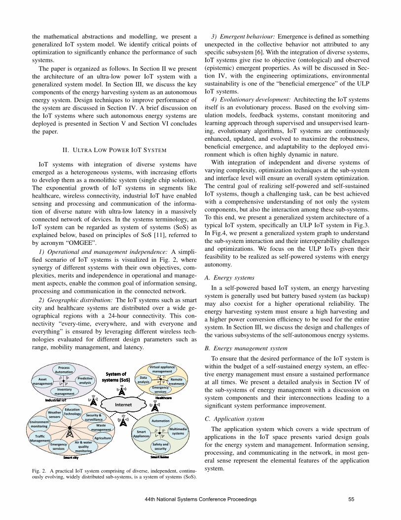
the mathematical abstractions and modelling, we present ageneralized IoT system model. We identify critical points ofoptimization to significantly enhance the performance of suchsystems.

The paper is organized as follows. In Section II we presentthe architecture of an ultra-low power IoT system with ageneralized system model. In Section III, we discuss the keycomponents of the energy harvesting system as an autonomousenergy system. Design techniques to improve performance ofthe system are discussed in Section IV. A brief discussion onthe IoT systems where such autonomous energy systems aredeployed is presented in Section V and Section VI concludesthe paper.

II. ULTRA LOW POWER IOT SYSTEM

IoT systems with integration of diverse systems haveemerged as a heterogeneous systems, with increasing effortsto develop them as a monolithic system (single chip solution).The exponential growth of IoT systems in segments likehealthcare, wireless connectivity, industrial IoT have enabledsensing and processing and communication of the informa-tion of diverse nature with ultra-low latency in a massivelyconnected network of devices. In the systems terminology, anIoT system can be regarded as system of systems (SoS) asexplained below, based on principles of SoS [11], referred toby acronym “OMGEE”.

1) Operational and management independence: A simpli-fied scenario of IoT systems is visualized in Fig. 2, wheresynergy of different systems with their own objectives, com-plexities, merits and independence in operational and manage-ment aspects, enable the common goal of information sensing,processing and communication in the connected network.

2) Geographic distribution: The IoT systems such as smartcity and healthcare systems are distributed over a wide ge-ographical regions with a 24-hour connectivity. This con-nectivity “every-time, everywhere, and with everyone andeverything” is ensured by leveraging different wireless tech-nologies evaluated for different design parameters such asrange, mobility management, and latency.

Emergency services

Data analysis

Virtual appliance management

Remote treatment

Healthcare

Emergency services

Data analysis


Remote treatment

Healthcare

Emergency services

Data analysis


Remote treatment

HealthcareIndustrial IoT

System of systems (SoS)

InternetIndustrial IoT


Internet

Safety and security

Smart Appliances

Automation

Multimedia systems

Smart home

Safety and security

Smart Appliances

Automation

Multimedia systems

Smart home

Safety and security

Smart Appliances

Automation

Multimedia systems

Smart home

Safety and security

Smart Appliances

Automation

Multimedia systems

Smart home

Emergency services

Data analysis


Remote treatment

HealthcareIndustrial IoT


Internet

Safety and security

Smart Appliances

Automation

Multimedia systems

Smart home

Environment monitoring

Traffic Management

Weather sensors

Air & water quality

monitoring

Security & surveillance

Waste management

Education Technology

Emergency services

Agriculture

Smart city


Traffic Management

Weather sensors

Air & water quality

monitoring


Waste management


Emergency services

Agriculture

Smart city


Traffic Management

Weather sensors

Air & water quality

monitoring


Waste management


Emergency services

Agriculture

Smart city


Traffic Management

Weather sensors

Air & water quality

monitoring


Waste management


Emergency services

Agriculture

Smart city

Inventory management

Asset management

ProcessAutomation

Predictive analysis


Asset management

ProcessAutomation

Predictive analysis


Asset management

ProcessAutomation

Predictive analysis

Fig. 2. A practical IoT system comprising of diverse, independent, continu-ously evolving, widely distributed sub-systems, is a system of systems (SoS).

3) Emergent behaviour: Emergence is defined as somethingunexpected in the collective behavior not attributed to anyspecific subsystem [6]. With the integration of diverse systems,IoT systems give rise to objective (ontological) and observed(epistemic) emergent properties. As will be discussed in Sec-tion IV, with the engineering optimizations, environmentalsustainability is one of the “beneficial emergence” of the ULPIoT systems.

4) Evolutionary development: Architecting the IoT systemsitself is an evolutionary process. Based on the evolving sim-ulation models, feedback systems, constant monitoring andlearning approach through supervised and unsupervised learn-ing, evolutionary algorithms, IoT systems are continuouslyenhanced, updated, and evolved to maximize the robustness,beneficial emergence, and adaptability to the deployed envi-ronment which is often highly dynamic in nature.

With integration of independent and diverse systems ofvarying complexity, optimization techniques at the sub-systemand interface level will ensure an overall system optimization.The central goal of realizing self-powered and self-sustainedIoT systems, though a challenging task, can be best achievedwith a comprehensive understanding of not only the systemcomponents, but also the interaction among these sub-systems.To this end, we present a generalized system architecture of atypical IoT system, specifically an ULP IoT system in Fig.3.In Fig.4, we present a generalized system graph to understandthe sub-system interaction and their interoperability challengesand optimizations. We focus on the ULP IoTs given theirfeasibility to be realized as self-powered systems with energyautonomy.

A. Energy systems

In a self-powered based IoT system, an energy harvestingsystem is generally used but battery based system (as backup)may also coexist for a higher operational reliability. Theenergy harvesting system must ensure a high harvesting anda higher power conversion efficiency to be used for the entiresystem. In Section III, we discuss the design and challenges ofthe various subsystems of the self-autonomous energy systems.

B. Energy management system

To ensure that the desired performance of the IoT system iswithin the budget of a self-sustained energy system, an effec-tive energy management must ensure a sustained performanceat all times. We present a detailed analysis in Section IV ofthe sub-systems of energy management with a discussion onsystem components and their interconnections leading to asignificant system performance improvement.

C. Application system

The application system which covers a wide spectrum ofapplications in the IoT space presents varied design goalsfor the energy system and management. Information sensing,processing, and communicating in the network, in most gen-eral sense represent the elemental features of the applicationsystem.


Energy Harvester• Ambient sources (

solar, thermal, electromagnetic etc.)

• Human Body sources (Body heat, footsteps etc.)

Harvest from low voltage , low power

Efficient harvesting

Low voltage operation

startup

Maximum Power

extraction

Energy monitoring & control

Infrastructure circuits

Ultra low power consumption

Timing Circuits

Precision Voltage

reference

Infrastructure circuits


Timing Circuits

Precision Voltage

reference

• Power management Control• Zero power switches• Duty cycling

System Processing and communication

• Ultra low power analog and radios• Sub threshold digital• Low power sensing • Maximize available power

• High conversion • Reliability

Self powered Energy System Energy Management System Application

Self powered ULP-IoT system


Type I , II system optimizations

Voltage Regulation

• Fine power gating techniques• Clock gating

Interface optimizations (refactoring)

Sub system level optimizations

Interconnection



Integrated battery

Interface optimizations (refactoring)

Fig. 3. Generalized architecture of ULP IoT system based on autonomous energy system with Type I and Type II optimization techniques.

Energy Harvesting

Energy Sources

Harvesting technology

Harvesting architecture

Ambient Sources

Human body based

Harvest-use

Harvest-store-use

Energy System

Auxiliary battery

EA.1(1-2)

SA.1.1

SA.1 SA.2

Energy Management

System

Voltage regulation

Infrastructure Circuits

Power Management

ULP IoT

Precision voltage

reference

Timing circuits

SB

S

SA SC

Battery charger

EA-B

Dynamic performance

Power controller

Sensing Circuits Processing Communication

SA.2.1

EB-A

Application/Load

EB-C

EC-B

SA.1.2 SA.1.3

EA.1(2-3)

SB.1 SB.2 SB.3

EB.(1-2)

EB.(2-1)

EB.(2-3)

EB.(3-2)

SB.2.1 SB.2.2 SB.3.1SB.3.2

SC.1 SC.2 SC.3

EC.(

1-2

)EC

.(2

-1)

• EA-B : Conversion of the harvested energy (Physical and functional integration)

• EB-A : Energy system monitoring (Semantic integration)

• EB-C : Power delivery to application system (Physical and functional integration)

• EC-B : Application system monitor (Semantic integration)

• EC[i-j] : i, j∈ (1,2,3) represent the sub-

systems interaction, which happens when the IoT node is operational

System optimization goals : • Maximize lifetime of the IoT system• Maximal operational performance• Low form factor• Low cost for widespread deployment

• EA.1[i-j]: i, j∈ (1,2,3) represent the sub-

systems interaction for the harvested energy conversion

• EB[i-j] : i, j∈ (1,2,3) represent the sub-

systems interaction, which happens when the IoT node is operational

EC.(

2-3

)EC

.(3

-2)

Reliability

System characteristics : • Heterogenous system• “Beneficial emergence”: Environmental

sustainability• System refactoring for optimization• Evolutionary development approach

Interface Interface

Fig. 4. Graph modelling of the different sub-systems and interconnections in the ULP-IoT system to identify and optimize the critical connections for aWHOLISTIC systemic optimization.

The abstraction of the IoT system, a micro-electronic sys-tem, enables the application of system optimization principlesto achieve a WHOLISTIC performance. The system graph rep-resentation in Fig.4 enables us to understand the interactionsbetween the sub-systems wherein we can assign appropriateoptimization factors to the systems and the interconnectionsfor the maximal performance under the well known power-performance-area constraints of the integrated microelectronicsystems. With the representation of the IoT system as ageneralized system graph, we discuss some of the criticalinteractions, as labelled in the graph, to boost the overallperformance of the system with the implementation of Type Iand Type II system optimization principles [12] for the self-powered, self-sustained IoT systems. For ULP IoT system,the overall “benefical emergence” from system optimization is

immense when the scenario is scaled to the entire ecosystemas depicted in Fig. 2 leading to more disruptive technolo-gies with environmental sustainability. With an evolutionarydevelopment at the core of IoT systems, the optimizationparameters and factors at the sub-system and interconnectionlevel are generally dynamic and are governed by the systemprotocols adapting to the variations with little or no perfor-mance compromise. Though a mathematical formulation ofsuch optimization framework and modelling can be undertakenfor a specific IoT system, in this paper we explore the generalidea of systemic approach for a significant performance gainsto enable perpetually powered IoT system, over a reductionistdesign methodology.


10nW 100nW 1µW 10µW 100µW 1mW 10mW 100mW 1W 10WQuartz

Osc.Electronic

watchPassive

RFIDHearing

Aid

Active RFID

Low power

wireless n/w

Bluetooth transceiver

OLED display

LaptopµPC

shutdown mode

Energy Harvester more capable

Devices less power hungry

10nW 100nW 1µW 10µW 100µW 1mW 10mW 100mW 1W 10WQuartz

Osc.Electronic

watchPassive

RFIDHearing

Aid

Active RFID

Low power

wireless n/w

Bluetooth transceiver

OLED display

LaptopµPC

shutdown mode

Energy Harvester more capable

Devices less power hungry

Mini PV RF fieldMotion:

PiezoThermal PVMini PV RF field

Motion: Piezo

Thermal PV

(a) (b)

Fig. 5. (a) Commonly used energy harvesters and their properties (b) Energy harvesting along with an effective energy management is necessary to meet theincreasing power demands.

III. ENERGY HARVESTING SYSTEM

The goal of the energy harvesting system is to ideallyharvest all the available energy, thus enabling a robust energysystem for the operation of the IoT system. Represented as(SA.1) in the system graph, a typical energy harvesting systemhas three components , the energy source (SA.1.1), harvestingtechnology (SA.1.2) and the harvesting architecture (SA.1.3).An efficient energy harvesting system must have reliable andefficient energy sources which can be converted into usableenergy with maximum possible efficiency and delivered to theload or stored as dictated by the energy management system.

A. Energy Harvesting SourcesThe conventional methods of energy harvesting include

harvesting from ambient renewable sources like solar [13],[14], thermal [15], [16], pressure [13], [14], electromagnetic[17], wind etc. IoT devices driven from the energy of thehuman body has also gained a significant traction over theyears where energy is harvested from the human body likebody heat , cerebrospinal fluid , endocochlear potential forIoT systems like IMDs and wireless body sensor networksamong others. Different factors like availability of the source,reliability, energy density, controllability, and ease-of-use haveto be evaluated specific to the application in question.

B. Energy Harvesting TechnologyThe diversity in the nature of energy sources has to be

translated into the electrical form for the physical integra-tion compatibility. This is accomplished by energy harvestingtechnology/harvester which converts the energy from thesediverse sources into usable electrical energy for the systemoperation. Such source-specific harvesters and their propertiesare tabulated in Fig.5.(a). Hence these harvesters need to min-imize the conversion losses represented by the edge E.A1[1-2]

in the system graph. The characteristics of the harvesterdictate the design of the interface with the energy system.An optimal impedance as mentioned in Fig. 5.(a), needs tobe presented by next stage for the maximum power transferfrom the harvester. This critical point of optimization, i.e. theinterconnection optimization is undertaken during the designof power management circuits.

C. Energy Harvesting ArchitectureEnergy harvesting architecture can be broadly classified

as Harvest-use architecture and Harvest-store-use architecture[18]

1) Harvest-use architecture: In this architecture, the load isdirectly driven by the harvesting system. Lack of controllabil-ity and frequent operational failure due to abrupt changes inthe harvested energy limit the deployment of such architecture.

2) Harvest-store-use architecture: The harvest-store-use ar-chitecture is generally preferred with storage technology inthe form of capacitors [13], [16], [17], [19], super-capacitors[14] or Li-based battery [14], [15] may be used to providean additional energy system for critical applications, store theadditional energy when the load is operationally duty cycled,or to compensate for energy system’s inability to supplyadequate power for a period of time. An integrated batterysolution in [20] is an on-chip solution which can be furtheroptimized using nano-scale level techniques.

D. Energy Harvesting System challenges

To realize energy harvesting as a reliable, feasible, self-sustained, and perpetual energy system, it is crucial to addressthe operational challenges at the system and the interface level.The IoT system which deploys these energy harvesting systemmust be equipped with systems like monitoring, efficientconversion, reliability architectures and overall efficient powermanagement of this harvested energy. A brief discussion onthese aspects is presented below:

1) Monitoring: In scenarios resulting from the environ-mental dynamics where the IoT system is deployed, theuncompromising and unfailing performance of the IoT system,may quickly deplete the harvested energy which may lead toa system black-out or brown-out. Hence a constant monitor toindicate the status/health of the energy systems is necessaryto maximize the lifetime of the IoT node. The semanticintegration and necessary control steps are architecturallygoverned.

2) Reliability : Even with a continuous monitoring system,enough energy may not be harvested from a single input singleoutput based architecture (SISO). Also considering the factorslike source availability, predictability, controllability, differentarchitectures like multiple input single output (MISO), mul-tiple input multiple output (MIMO) are deployed to increasethe reliability of the energy harvesting systems leading to arobust IoT system design.

3) Integration: Architecting and integrating these energysystems is challenging both at the physical and functionallevel. System refactoring approach which includes optimiza-tions at the interface i.e. harvesting technologies with high


conversion efficiency, low form factors at the source end,and impedance matching at the load end for maximal powertransfer are implemented rather than system bridging baseddesign methodology.

4) Deployment: The success of energy harvesting systemfor the self-powered IoT hence is not only limited to theintrinsic optimizations, the effective use and management ofthis energy is of paramount importance wherein we need toensure that the system performance is uncompromising evenwith the occasional uncertainties in the energy harvestingbased system. These architectural optimizations hence aremore concurrent by nature instead of being sequential, asystemic approach over reductionist approach. Fig. 5.(b) showsthat at the higher end of device spectrum, energy harvestingsystem may not be able to cater to the power requirementsexclusively, but an efficient management system working intandem helps to achieve the goal of self-powered IoT systems.

IV. IOT: ENERGY MANAGEMENT

The energy management of the system, represented as (SB)in the system graph (Fig. 4), plays a key role in the design ofself-powered systems as it has to ensure at all times, underall dynamic conditions, the system power consumption iswell within the harvested energy budget. In Fig. 6, differentmethods to increase the lifetime of an IoT system with energyharvesting based energy system are presented. We presentdifferent techniques at different critical points of the systemgraph to optimize the integration at physical, functional, andsemantic level to achieve architectural resonance. To reducethe cost for a widespread deployment of the IoT systems,system refactoring is preferred over system bridging approach.

A. Interface with energy system1) Maximum power point tracking: For the maximum

power transfer at the interface (EA-B), the management sys-tems presents an optimal impedance to the energy systemsimplemented with the maximum power point tracking circuits(MPPT). For harvesters like radio-frequency (RF) and solar,a continuous tracking of the optimal point is necessary withwhich the harvested energy can be maximized.

2) Low startup voltage operation: The harvested energyis stored in the capacitor/super-capacitor. The applicationsystems driven by this harvested energy can turn on onlywhen the voltage reaches the operational threshold voltagelevel. The lifetime of IoT node can be significantly increasedif the operating voltage is brought down [3]. Hence the criticalcircuits in the management circuits (SB.[1-3]) are designed forlow operational voltages which significantly boosts the systemlifetime.

3) Voltage regulation of harvested energy: The harvestedvoltage needs to be regulated (based on reference voltage) tobe used for the systems operation (SB.1, EB-A). The manage-ment circuit generates multiple voltages for system specificoperations using voltage converters (Low dropout regulators(LDO), buck-boost converters, and switched capacitor convert-ers, among others) [3].

Increase harvested energy

Ultra-low power consumption

Low voltage operation

Reduce losses in voltage conversion

Increasing

lifetime of

IoT node

Fig. 6. The lifetime of a self-powered IoT system can be significantlyimproved with different techniques at the component level, sub-system leveland system level.

B. Energy management: Infrastructure Circuits

The IoT nodes are mostly in idle mode and “wake-up”only for short bursts of activity. To check for system ac-tivity/stimulus, the occasional wake-ups are coordinated byprecision timing circuits. Further, to enable a low operationalvoltage for the sub-systems, a precision reference voltage isrequired. These timing circuits, power delivery circuits, andprecision voltage constitute the infrastructure circuits (SB.2).These circuits which are generally in always powered-up stateare the critical circuits for system optimizations. The idlepower (i.e. the leakage power) sets the lower limit of theIoT power consumption and is minimized through designtechniques like fine power gating, clock gating, or throughinnovations in device technology. These combined benefits canprovide a 4-70X improvement in the lifetime of an ULP IoTsystem [3].

C. Energy management: Architecture governance

To prevent uncoordinated changes in the energy flow, themanagement systems ensures an overall control on subsys-tems (Sk, k ∈ (A,B,C)) ; and interconnections (Ei-j, i,j∈ (A,B,C), i 6= j). A closed loop approach in the energymanagement system provides a flexible platform for the overallsystem achieving WHOLISTIC performance [19].

V. IOT APPLICATION

The application space represented as (SC) in the systemgraph, may span a wide spectrum of applications like implantbased systems, wearable and health monitors, ULP Radiosas shown in Fig. 2 essentially entails the key tasks ofsensing, processing and communication of information. Theinformational aspect hence may be application specific. For abetter analysis of system performance, modelling and systemsimulations ranging from device level to system behavioralmodels are done and systems are validated with specific test-beds. To ensure interoperability of these systems in the IoTSoS without system disruption, they operate under commonIoT standards and framework [21]. In Table I, we summarizethe different IoT systems based on energy harvesting, makingthem self-powered and self-sustained.


TABLE ISUMMARY OF ENERGY HARVESTING SYSTEM BASED ENERGY SYSTEMS

Ref TCASI’19 JSSC’19 JSSC’13 MTT’13 JSSC’12 JSSC’11[13] [15] [19] [17] [14] [16]

Energy Source Solar, Thermal RF, RF Thermal, Solar ThermalPiezo Thermal/Solar Piezo

Harvesting Technology Solar Cells, TEG array TEG array On-chip Solar Cells, TEG, TEGPiezo-crystal antenna Piezo-crystal

Harvesting architecture MISO SISO MISO SISO MISO SISOInput Voltage/Power 0.55 0.18 - 10V 30mV , -10dBm -17dBm - 25mV

Output Voltage20mV - 0.16V: Thermal

1.8 - 2.5V - 1.35V 1V 0.15 - 0.75V : Solar 1.8V1.5 - 5V : Piezo

Conversion efficiency64%: Thermal

74.6% 86% 38% 42% 64% : Solar 58%(simulated) 79% : Piezo

Storage Technology Capacitor Capacitor, Capacitor Capacitor Super-capacitor, CapacitorBattery (3.3V) Battery (3.3V)

In-built power extraction Yes Yes No No Yes Yes

Maximum output1.3mW : Thermal

35-70 µW 38 µW − 200mW 19 µW 2.5 nJ 2.5mW : Solar 300 µWpower/energy 200 µW : Piezo

Applications Wireless sensor Body sensor Biomedical Biomedical ULP- Implantable wirelessnodes network(BSN) monitoring monitoring IoT micro-sensors

VI. CONCLUSION

The evolution of IoT systems as self-powered and self-sustained systems will lead to even a wider global deploy-ment of such devices ensuring connectivity for a smart andresilient ecosystem with strong beneficial emergent propertieslike environmental sustainability. In this paper we presentedautonomous energy systems based on energy harvesting. Witha generalized system architecture and graph modelling ofthe ULP IoT system we identify the critical optimizationpoints in the energy flow leading to a WHOLISTIC systemwith higher reliability, performance robustness and significantlifetime improvement.

REFERENCES

[1] A. Al-Fuqaha, M. Guizani, M. Mohammadi, M. Aledhari, andM. Ayyash, “Internet of things: A survey on enabling technologies,protocols, and applications,” IEEE Communications Surveys Tutorials,vol. 17, no. 4, pp. 2347–2376, 2015.

[2] “IoT market size worldwide 2017-2025.” [Online]. Available:https://www.statista.com/statistics/976313/global-iot-market-size/

[3] N. Shafiee, S. Tewari, B. Calhoun, and A. Shrivastava, “InfrastructureCircuits for Lifetime Improvement of Ultra-Low Power IoT Devices,”IEEE Transactions on Circuits and Systems I: Regular Papers, vol. 64,no. 9, pp. 2598–2610, Sep. 2017.

[4] A. Shrivastava, K. Craig, N. E. Roberts, D. D. Wentzloff, and B. H.Calhoun, “5.4 A 32nW bandgap reference voltage operational from 0.5Vsupply for ultra-low power systems,” in 2015 IEEE International Solid-State Circuits Conference - (ISSCC) Digest of Technical Papers, Feb.2015, pp. 1–3, iSSN: 2376-8606.

[5] A. Shrivastava, D. A. Kamakshi, and B. H. Calhoun, “A 1.5 nW, 32.768kHz XTAL Oscillator Operational From a 0.3 V Supply,” IEEE Journalof Solid-State Circuits, vol. 51, no. 3, pp. 686–696, Mar. 2016.

[6] M. Jamshidi, Systems of systems engineering : principles and applica-tions. CRC Press, 2009.

[7] K. S. Daya, “SystemsApproach,” p. 3. [Online]. Available:https://www.dei.ac.in/dei/files/aboutDEI/DEI-Systems-Approach.pdf

[8] P. S. Satsangi and J. B. Ellis, “A generalized system-theoretic frame-work for modelling large scale national economic systems in dynamic,structural and spatial terms†,” International Journal of Systems Science,vol. 2, pp. 213–223, 1971.

[9] P. S. Satsangi, “A physical system theory modeling framework fortransportation system studies,” IEEE Transactions on Systems, Man, andCybernetics, vol. 7, no. 11, pp. 763–778, 1977.

[10] P. Satsangi, S. Hameroff, V. Sahni, and P. Dua, Consciousness: Integrat-ing Eastern and Western Perspectives. New Age Books, 2016. [Online].Available: https://books.google.com/books?id=0aUwngAACAAJ

[11] M. W. Maier, “Architecting principles for systems-of-systems,” INCOSEInternational Symposium, vol. 6, no. 1, pp. 565–573, 1996. [On-line]. Available: https://onlinelibrary.wiley.com/doi/abs/10.1002/j.2334-5837.1996.tb02054.x

[12] D. A. Rao, “INTRODUCTION TO SYSTEMSAND SYSTEMS PHILOSOPHY,” p. 8. [On-line]. Available: https://www.dei.ac.in/dei/paritantrika/files/archives/SystemsMethodology.pdf

[13] A. Devaraj, M. Megahed, Y. Liu, A. Ramachandran, and T. Anand,“A Switched Capacitor Multiple Input Single Output Energy Harvester(Solar + Piezo) Achieving 74.6% Efficiency With Simultaneous MPPT,”IEEE Transactions on Circuits and Systems I: Regular Papers, vol. 66,no. 12, pp. 4876–4887, Dec. 2019.

[14] S. Bandyopadhyay and A. P. Chandrakasan, “Platform Architecture forSolar, Thermal, and Vibration Energy Combining With MPPT and SingleInductor,” IEEE Journal of Solid-State Circuits, vol. 47, no. 9, pp. 2199–2215, Sep. 2012.

[15] Q. Wan and P. K. T. Mok, “A 14-nA, Highly Efficient Triple-OutputThermoelectric Energy Harvesting System Based on a ReconfigurableTEG Array,” IEEE Journal of Solid-State Circuits, vol. 54, no. 6, pp.1720–1732, Jun. 2019.

[16] Y. K. Ramadass and A. P. Chandrakasan, “A battery-less thermoelectricenergy harvesting interface circuit with 35 mv startup voltage,” IEEEJournal of Solid-State Circuits, vol. 46, no. 1, pp. 333–341, 2011.

[17] M. H. Ouda, M. Arsalan, L. Marnat, A. Shamim, and K. N. Salama,“5.2-GHz RF Power Harvester in 0.18-/spl mu/m CMOS for ImplantableIntraocular Pressure Monitoring,” IEEE Transactions on MicrowaveTheory and Techniques, vol. 61, no. 5, pp. 2177–2184, May 2013.

[18] S. Sudevalayam and P. Kulkarni, “Energy harvesting sensor nodes:Survey and implications,” IEEE Communications Surveys Tutorials,vol. 13, no. 3, pp. 443–461, 2011.

[19] Y. Zhang, F. Zhang, Y. Shakhsheer, J. D. Silver, A. Klinefelter, M. Na-garaju, J. Boley, J. Pandey, A. Shrivastava, E. J. Carlson, A. Wood,B. H. Calhoun, and B. P. Otis, “A Batteryless 19 W MICS/ISM-BandEnergy Harvesting Body Sensor Node SoC for ExG Applications,” IEEEJournal of Solid-State Circuits, vol. 48, no. 1, pp. 199–213, Jan. 2013.

[20] H. Lhermet, C. Condemine, M. Plissonnier, R. Salot, P. Audebert,and M. Rosset, “Efficient power management circuit: Thermal energyharvesting to above-ic microbattery energy storage,” in 2007 IEEE In-ternational Solid-State Circuits Conference. Digest of Technical Papers,2007, pp. 62–587.

[21] “IEEE SA - Internet of Things Related Standards.” [Online]. Available:https://standards.ieee.org/initiatives/iot/stds.html


Sustainable agricultural system for field and crop monitoring using a drone and NOIR camera

Kaamil Verma, Suratvant Verma, Shikha Verma [email protected], [email protected], [email protected]

Abstract - Crop surveying to gather real time data has been limited to satellites and expensive multispectral cameras. As the concept of precision farming is evolving, survey of crops and fields is becoming accessible to local farmers using small drones. In the present work, a quadcopter drone was constructed from scratch. After testing for various parameters and flight stability, a normal (Go Pro) and NOIR camera were attached to it to carry out survey of crop fields at Akurli, Panvel, Raigarh, Maharashtra. The NOIR raspberry pi camera was intuitively fitted with a vintage Kodak photographic film to capture the IR light emitted by the plants. A healthy actively photosynthesizing green plant with more chlorophyll reflects more infrared light. The IR images were processed using an open software “infragram” to NDVI images. NDVI (Normalised Difference Vegetation Index) is an index that maps the health of the crop. While the Go Pro provided clear bird’s eye view, close images as well as videos of the crop (not possible with satellite imaging), the NDVI images clearly showed the healthy and green plants as red, less healthy as hues of orange and yellow and inanimate objects like soil as yellow, green and blue. The results were at par with other multispectral and NDVI imaging works. An added advantage was that the effect of cloud cover, a major drawback with satellite imaging was also overcome. It was possible to conduct the survey of a large field within 3 minutes by the drone. Hence, this is a promising sustainable system which can be developed further to help farmers to take timely and frequent surveys in an easy manner to help them gauge the condition of their crops and fields and take preventive measures beforehand.

Index Terms - Crop Survey, Drone, IR image, NDVI, NOIR camera

INTRODUCTION

India an agricultural country Agriculture in India began by 9000 BCE as a result of early cultivation of plants, and domestication of crops and animals. Development of implements and techniques led to a settled life and double monsoon to two harvests in an year. Indian products soon reached the world via existing trading networks and foreign crops were introduced to India. The middle ages saw irrigation channels reach a new level of sophistication. Expansion of land and water management systems to providing uniform growth resulted in Indian crops

affecting the economies of other regions of the world. Despite some stagnation during the later modern era the independent India was able to develop a comprehensive agricultural program. India is the 2nd largest producer of agricultural products in the world. Agriculture employed 50% of the Indian work force and contributed 17–18% to the country's GDP as per reports of 2018. It has the highest net cropped area followed by US and China [1] Farming Methods Indian farmers adopt different farming methods to grow a variety of crops that India consumes and exports. “Primitive Subsistence Farming”, is carried on small areas of land, using indigenous tools like hoe, dao, digging sticks, etc. usually, by a family or the local community who use the output for their own consumption. It’s a natural method and growth of crops are dependent on environmental factors like rain, heat, fertility of soil. Once crops are harvested, farmers burn the land, move to a new patch of land for cultivation and the former gains back its fertility naturally (‘slash and burn’). If carried on larger areas of land with more labour, chemical fertilizers and different irrigation method to yield more crops and increase the produce, it is known as “Intensive Subsistence Farming”. Crops include paddy, wheat, pulses, maize, millets, sorghum, soya-beans, tubers, and vegetables. “Commercial Farming” contributes to the country’s economy the most and crops are exported across the world. Fertilizers, pesticides etc. are used extensively to enhance crop productivity. Commercial crops include wheat, rice, pulses, millets, maize, vegetables, and fruits. “Plantation farming” is a blend of agriculture and industry, practiced across a vast area of land. It is labour intensive and uses latest technological support for sustaining, cultivating and yielding. The produce is treated as raw materials for use in respective industries including tea, coffee, rubber, sugarcane, banana, coconuts etc. [2] What ails and fails the Indian farmer? Despite of all developments, the Indian farmer is largely at the helm of all crisis whether it’s unpredictable climatic conditions or other factors. The farmer is barely empowered as a supplier. He continues to be small & marginal, inadequately resourced, ill-informed on markets and marketing, ill-equipped to manage risk, burdened with credit & debts and is dependent on traders to reach the buyers. The linkage between the producer and consumer is weak. The farmer is unable to shape the nature of his produce according to the demand, it remains the same annually and is often driven by the government's MSP program. The farmer is neither equipped with latest technology nor trained to adopt


it fast. Lack of new technology solutions keeps the farmer from gaining an equal footing globally. Policy frameworks whether they are subsistence crops or commercial crops, remain the same and do not enable any significant impact. The investment in R&D is low and less than 1% of the Agricultural GDP in India is spent on research. There is a staggering lack of infrastructure across the entire agricultural value chain. To make matters worse, a perspective on how this can be fixed also does not exist [3]. All these factors may have their respective solutions but in the present work, the focus would be on the use of technology in agriculture and technological solutions. Why Technology in Agriculture? The increase in agricultural production is not sufficient to meet the escalating demand. It is estimated that the aggregate agricultural consumption will increase by 69 percent till 2050, due to an increase in global population from 7 to 9 billion people during the same time frame [4]. The only feasible answer for this urgent call to increase agricultural production and overcome other challenges like climate change must come from technology. In this context, ICT-driven tools and technologies to enhance decision making through accurate, reliable and timely information have an important role to play. According to G. Sylvester (Knowledge and Information Management Officer, Food and Agriculture Organization), “In the current milieu, use of sustainable information and communication technology in agriculture is not an option. It is a necessity” [4]. Recently, Africa has been relying on digitalization for agriculture (D4Ag) to accelerate their agricultural productivity and transformation. Digital solutions and agriculture data provide tailored information and insights to help farmers optimise their production, gain access to appropriate products and services, and explore new linkages with markets [5]. Bhutan has a challenging environment (limited areas for agriculture, harsh geography and road conditions) to develop commercial agriculture. It has overcome these problems by using innovative ICT based solutions in eastern Bhutan, for growing Mountain Hazelnuts commercially [6]. To reduce the vulnerability of smallholder farmers engaged in rice production in Asian countries like Cambodia, India, Indonesia, Philippines, Thailand and Vietnam, the International Rice Research Institute (IRRI) together with Sarmap, initiated a project titled “Remote Sensing Based Information and Insurance for Crops in Emerging Economies (RIICE). This rice monitoring system provides accurate and almost real time information on rice growth helps the farmers and the government to better manage domestic rice production and distribution [7]. UAV’s/Drones: A Technological Beacon of hope for Agriculture in India One of the latest technological developments in agriculture is the increase in the use of small, unmanned aerial vehicles (UAVs), commonly known as drones. Drones are remote controlled aircraft with no human pilot on-board. The use of

drones to spray crops, plant seeds, monitor live-stock are commonly heard of in agriculture [8]. However, the most valuable use of drones is in collection of valuable data which is the basis of Precision Farming, a recent term used in agriculture [9]. Farmer’s face a variety of complex factors from water access to changing climate, wind, soil quality, presence of weeds and insects, variable growing seasons, etc. They also have limited resources (seed, water, fertilizer, pesticides, human power) and it’s always a matter of concern on when and where to use these resources. Agricultural drones allow farmers to access a wealth of data to help them make better decisions. They can collect data related to crop yields, irrigation, soil quality, nutrient measurements, crop health, infestation, weather analysis, rainfall etc. This can be used to accurately map any existing issues and find relevant solutions. Mostly satellites and manned aircraft were used for collecting data of fields but neither is efficient as farmers need to image their fields often, and in a scheduled way. Only UAVs can provide this data in a timely and cost-effective manner. The advantages that “an eye in the sky” provides when combined with analytic tools that can interpret the data and images to actionable information has ushered in a new revolution [10]. NDVI and Crop Health Besides, reflecting light in the visible region, plants emit radiation in the near and mid infrared regions. The emissivity can be attributed to a range of characteristics related to water content, pigments, sugar, carbohydrate, protein content, aromatics, besides growth and vigor [11, 12] The term “actionable intelligence” has become popular [13]. The first step is to produce crop health maps for farmers. This is achieved by measuring the amount of IR light emitted by crops using near-infrared (NIR) sensors which is directly proportional to the live green biomass or actively photosynthesizing regions or healthy regions in the crops. These vegetation levels are expressed as indices like Normalized Difference Vegetation Index (NDVI), to produce NDVI maps. These maps show crop health through colours. The colours also differentiate soil from grass or forest, detect plants under stress, differentiate between crops and crop stages etc. [14]. Usually multispectral and hyper-spectral aerial and satellite imagery is used to create these NDVI maps but they can efficiently be replaced by drones fitted with infrared, multispectral and hyper spectral sensors or IR cameras. Drone technology as a platform for image data acquisition has brought the NDVI mapping capabilities to a completely new level of accuracy making it possible to monitor the condition of not only plants, but also specific parts of plants. It has enabled early identification of plant stress, pest infestation and diseases. These precisely mapped and identified issues can be addressed with precise applications of fertilizers, pesticides or herbicides. There are strong correlations between crop yield and NDVI data measured at certain crop stages [10, 15]. Drone-enabled NDVI index values analysis combined with data such as weather forecasts


and soil maps can help to refine the final information and enable the farmer to take full advantage of the farm and maximize yields. Another advantage is that for specific farms in the Asia-Pacific region, the drones are able to access and collect data from difficult terrains like terrace rice fields or fruit plantations in mountainous regions [16]. Advanced geospatial NDVI are also being used in case of natural disasters or destruction of crops to precisely estimate the level of losses by comparing the pre-disaster state of vegetation with the damages that occurred. Companies such as Skymet provide agriculture survey services by drones to insurance companies and the state governments of Maharashtra, Gujarat, Rajasthan and Madhya Pradesh [17]. Although drones are an eye in the sky, the real power comes from the strength of data processing and analytics that take place after the data is collected. Solutions such as Smarter Agriculture offer an integrated platform to use data from drones, sensors and other devices to automate and optimize farm management. Pix4Dag converts multispectral images into NDVI maps and uses red, green and blue (RGB) images to generate high-resolution orthomosaics. In this context, in the present study, after building a drone from scratch, it was utilized to explore the application of crop monitoring by attaching a normal camera and an indigenous NOIR camera fitted with a vintage Kodak film filter to capture the IR images of crops and fields and convert them into NDVI images.

METHODOLOGY

Building the Drone A quadcopter drone was built for this project. The drone built is a typical Team Black Sheep’s discovery 500 with slight variations. A TBS 500 mm frame with Tbs discovery 500 plates were used along with DJI’s flame wheel 450mm arms. The battery used was a Lipo Battery (5200 mah Lipo 4s (16v)). The rotors included DJI A2212 980kv motors (clones), 30amp 50 Hz Simonk Firmware ESCs, 1038 CF nylon propellers and M8 propeller mounting nuts. For the flight controller, a Naza-M-lite was used as the hardware, Naza v2 4.02 as the software (only firmware used), Ublox M8 External GPS with HMC 5883l as the GPS with a HMC 5888l Compass. The transmitter (with pilot) & receiver (on drone) (transceiver) helps to establish communication, give command and control the drone. The components used were Fly Sky FS-i6 Transmitter A and Fly Sky FS-i6 Receiver B. Figure 1 shows the complete drone. Determination of Drone Parameters The Drone was tested for its stability, flying capabilities and certain Drone parameters were measured before carrying out experiments with the cameras. Flight Time: The maximum time the drone can fly in the air. This was determined by flying the Drone continously with its battery at full charge. Range:The maximum horizontal and vertical distance the drone can cover. This was difficult and risky to measure but

it was tried to let the drone fly far from the point of take off and also high. It was even possible to actually preset the range of the drone. Un-laden weight: This is the weight of the drone without any accessories. This was measured on a digital analytical balance without attaching any accessories to the drone. Laden weight: This is the weight of the drone with any accessories attached. Thus the weight of the drone with the cameras attached was measured with a digital analytical balance. Payload: This is the maximum weight the drone can carry. This was tested by attaching a series of 250 ml bisleri bottles filled with water to a string. Each bottle weighed 275 gm. Around 8 bottles ( 275 g X 8 = 2200 gm/2.2 kg) were attached. The Drone was made to lift the bottles and the number of bottles it lifted was its payload. The Cameras The main objective of the project was to assess the health of the crops and the field by carrying out both normal and IR photography simultaneously in a single flight. Photography of crops and fields was carried out in Akurli, Panvel, Raigharh, Maharashtra. For normal photography, a 12 Megapixel Action camera (Gopro 3) was attached to the Drone. The photography was carried out in various modes including time lapse (2 photos/sec) and video. Both normal and wide angle view were considered. For IR photography, an 8-megapixel, Raspberry Pi NOIR (No IR) camera connected to the Raspberry Pi board was used. A purplish-blue filter made from a piece of old Kodak photographic film was put on the lens of the NOIR camera (Fig.2). It is important to understand the principle of the NOIR camera and IR photography. When photograph is taken from a normal camera, the light reflected from any object passes through 3 channels of the camera viz. blue, red and green. The net effect is a mixture of these three colours to produce the original colour in a photograph. Every object also reflects IR radiation but no IR light can pass through the camera, as all cameras have an IR filter that blocks the IR light. In an NOIR camera, the IR filter is removed and thus the IR light reflected by the objects can also pass through. But to capture this IR light, it must pass through a channel. Thus a violet - bluish filter (photographic film) was used to block the blue light channel to allow the IR light to pass through it.

Image processing The image processing of IR photographs to convert to NDVI images was done using “Infragram.com” which is an open software by Public Labs. Conducting interviews with farmers Interview was conducted with farmers at Panvel to understand their functioning and challenges faced by them. At that time they were growing leafy vegetables as their crop.

RESULTS AND DISCUSSION


The Drone and Cameras

Fig.1 Drone: The finished product (A. Top view B. Bottom view showing the attached cameras)

Fig.2 Raspberry Pi NOIR Camera for IR photogrpahy (A. Raspberry Pi NOIR Camera B. Camera attached to Raspberry Pi board C. The camera system in a case D. The photographic film attached to the camera)

The top and bottom view of the Drone is shown in Fig.1. Figure 2 shows the making and final view of the NOIR camera. Drone Parameters The flight time noted for the present drone was 10 minutes. The drone could cover a horizontal range of 2 km in an open field and between 500 m to 1 km vertically. The un-laden weight or weight without any accessories was 1.033 kg while the laden weight or weight with the cameras attached was 1.741 kg. The payload or the maximum weight the drone could carry was 2.5 kg. Photography results The drone was able to carry out operation with the two cameras attached and survey the fields under study in a short span of time (2 to 3 minutes). The normal photography by the drone of a field gives a real time instant information to the farmers of the various regions of their field & crops. Fig 3 clearly shows the details of the field. One can observe a burnt patch, dug soil, stack of hay, tree and plants. The cracks in the soil are also clearly visible. Fig 4. (A & B) show the bird’s eye view as well as the close view of the plants in the field. The photographs and videos obtained by the normal action camera were clear, of high resolution and the height of the drone could be adjusted to get the bird’s eye view as well as a close view.

Fig. 3. Normal Photography of a field showing different details

Fig. 4. Plants in field (A. Bird’s eye view B. Close view)

IR photography & NDVI images The IR photographs taken by the Raspberry Pi-NOIR camera were converted to NDVI images. It’s pertinent to understand what IR images are and what significant information do they divulge? The chlorophyll A and B in plants absorb red and blue rays from the visible light for photosynthesis. They reflect green light and hence appear green. Plants also reflect IR or Infrared light. A healthy plant which is actively photosynthesizing reflects more green and much more IR light. (Fig. 5)

Fig 5. Emission of Blue, Green, Red and near IR light by plants

The NOIR camera captures these IR rays reflected from the plant. The NDVI images differentiate between healthy green

BA

A B


leaves and others by allotting red and orange hues respectively; the inanimate objects are shades of yellow, green and blue. NDVI values calculated for each pixel or colour give a range of -1 to 1 (Fig. 6) []

Fig 6. NDVI Index and plant health

This is illustrated in Fig. 7 where the healthy green plants are seen as white streaks on the purple soil. In the NDVI images, these plants get converted to red streaks, the background and inanimate soil as hues of yellow, green and blue.

Fig. 7. IR(A) and NDVI (B) image of the field

Fig. 8. Normal (A); IR(B) and NDVI (C) image of the field

Comparison of Normal, IR, NDVI images of a field with very small plants Normal, IR and NDVI images respectively are seen in Fig 8 (A, B, C). This particular photography is taken from a great height. The normal photograph shows some plantation on the left side, small plants in the vast mud field, a small part of the field in which harvesting has been done which also has a burnt patch. These are clearly visible in the IR image as well. The transformation of the IR to NDVI image indicates conversion of all green plants to red colour. The harvested soil which had few green remnants of the cut crop are a shade of orange whereas the burnt patch in the same field which does not have living plants is greenish yellow and so is the soil, which is expected for inanimate objects. TCS employs drones for precision agriculture by acquiring multispectral data for crop health monitoring, soil mapping and irrigation [18]. Our results were comparable to theirs.

Fig 9. Close up NDVI image of the field

Figure 9 is a close up image of the same field. It is crystal clear how the green healthy plants give a striking red colour as compared to other parts and inanimate objects. Thus, the IR photography done by the Raspberry Pi NOIR camera with a photographic film attached as a filter was able to capture good images. The NDVI images produced after processing the IR images through an open software Infragram.com produced clear images with a good distinction of various colours. Though, the camera was a frugal one, it was able to yield results comparable to those by high resolution multispectral cameras. UAVs have a number of advantages over more traditional remote-sensing methods. One is the ease and effectiveness of large-scale crop and acreage monitoring. The technology is capable of collecting very high-resolution imagery below the cloud level, with much more detail and precision than the satellite imagery. It is possible to capture photos of the fields from low as well as high heights, covering the whole expanse of the field or details of a part of the field, or crop. It’s possible to not only obtain real-time footage but also time-based animation which can illuminate crop progression in real-time. They are easy to use as most drone mapping and data-collection missions are now conducted autonomously. Moreover, data processing applications are becoming less expensive and easier to use. An interview conducted with a Panvel farmer revealed that they sprayed pesticides precautionary after 15 days irrespective whether the crop was infected or not. This can be easily overcome by using this technique, as the advantage of capturing IR images is to detect information outside the visible range and hidden from the human eye. It is known as the Third Eye or Invisible eye as it is able to detect crop stress about two weeks before the human eye can gauge it. This method has a lot of scope and utility and needs further exploration and experimentation. Surveys on different fields and different crops need to be conducted. The photographs also need to be analysed in detail to try and interpret more relevant information from them. Future plans include using telemetry to fly the drone over the field covering the entire area in a predetermined path set by a specified pattern or map.


Photographs clicked at intervals will be saved with GPS coordinates. Using a virtual machine running DOCKER Tool box and Web Open Drone Map program, the photographs will be stitched together to create a Map or 3D model of the observed photos taken of the field. This 3D model will then be used to interpret and analyse the condition of the crops in the field. Favourable regulations on the use of small drones for agriculture as well as access to platforms that can aggregate data from various sources to provide valuable insights would be greatly beneficial to farming communities. Supporting ecosystems can facilitate growth of innovative solutions providing agricultural intelligence using drones and other emerging technologies as a service to rural communities. The information gap can be addressed by the growth of a new breed of professionals, the agricultural infomediaries who would play a key role in providing local actionable intelligence to rural communities by combining various data sources and analytics. The next agricultural revolution will be driven by data, which will help to increase agricultural productivity with minimum damage to the environment and increased livelihoods for communities involved in agriculture.

REFERENCES

[1] "India economic survey 2018: Farmers gain as agriculture mechanisation speeds up, but more R&D needed". The Financial Express. 29 January 2018. [2] Agriculture and Farming Methods in India!! Shine Brand Seeds Jan 3, 2020 (https://medium.com/@shinebrandseeds/agriculture- and-farming-methods-in-india-564d6b249f63) [3] R. Mudholkar. “Indian Agriculture - what ails and fails the farmer?”, March 13, 2018, Business Today. (https://www.businesstoday.in/opinion/columns/indian- agriculture-what-ails-and-fails-the-farmer-and-a-look-at-policy- imperatives-for-sustainability-in-agriculture/story/260922.html) [4] “E-agriculture in action: Drones for agriculture”, 2018, Ed. Gerard Sylvester, Food and Agriculture Organization of the United Nations and International Telecommunication Union [5] Tsan, M. et.al., 2019, “The Digitalisation of African Agriculture Report, 2018-2019” Ed: Lichtenstein, J., Proud Press, The Netherlands [6] Y. Ishihara “When technology meets agriculture in Bhutan”, 2018, World of Opportunity. https://medium.com/world-of- opportunity/when-technology-meets-agriculture-in-bhutan- 354bca6152bf. [7] “Mapping and monitoring rice areas using remote sensing, crop modelling and information and communication technology (ICT) in E-agriculture in action: Drones for agriculture”, 2018, Ed. Gerard Sylvester, Food and Agriculture Organization of the United Nations and International Telecommunication Union, pp 33 – 44. [8] M. Mazur. “Six ways Drones are Revolutionizing Agriculture”, July 2016, MIT Technology Review. https: //www.technologyreview.com/s/601935/six-ways-drones- are-revolutionizing-agriculture/ [9] N. Rogers, “What is Precision Agriculture”, 2014, Sustainable America. https://sustainableamerica.org/blog/what-is-precision- Agriculture [10] “Drone technology as a tool for improving agricultural productivity”: Drones for agriculture”, 2018, Ed. Gerard Sylvester, Food and Agriculture Organization of the United Nations and International Telecommunication Union, pp, 27 – 32.

[11] Batten, G.D. 1998. “Plant analysis using near infrared reflectance spectroscopy: The potential and the limitations,” Australian Journal of Experimental Agriculture, 38(7), pp. 697–706. [12] Foley, W.J. et.al. 1998. “Ecological applications of near infrared reflectance spectroscopy - A tool for rapid, cost-effective prediction of the composition of plant and animal tissues and aspects of animal performance,” Oecologia, 116(3), pp. 293–305. [13] “Advancements in Precision Agricultural Insights.”2021. https://insights.intelinair.com/advancements_in_precision_agricultural_insights/ Web. Accessed: March 21, 2021. [14] VanderLeest, Z. et.al. 2016 “Choosing the Right Imagery: Best Management Practices for Color, NIR, and NDVI Imagery”, Iowa State University, Extension & Outreach, Integrated Crop Management. https://crops.extension.iastate.edu /cropnews/ 2016/05/choosing-right-imagery-best-management-practices- color-nir-and-ndvi-imagery [15] Xue, J & Su, B. 2017. "Significant Remote Sensing Vegetation Indices: A Review of Developments and Applications", Journal of Sensors, 2017,pp, 1-17 https://doi.org/10.1155/2017/1353691 [16] “Actionable intelligence from drones to the agricultural industry” in E-agriculture in action: Drones for agriculture, 2018, Ed. Gerard Sylvester, Food and Agriculture Organization of the United Nations and International Telecommunication Union, pp 45 – 56. [17] Wakde, R. 2018 “Insurers deploy drones to check claims by farmers”. Agri Business, The Hindu, Business Line, Web Accessed: January 13, 2018. [18] “Drones-based sensor platforms: Experiences from Tata Consultancy Services (TCS)” in E-agriculture in action: Drones for agriculture”, 2018, Ed. Gerard Sylvester, Food and Agriculture Organization of the United Nations and International Telecommunication Union, pp 57 – 66.


Prediction of Ozone using meteorological and precursor parameters with Neural Networks

Harsh Kumar Jangir Dept. Of Computer Science

DayalBagh Educational Institute Agra, India

[email protected]

Prof. C. Vasantha Lakshmi Dept. Of Computer Science


[email protected]

Prof. K. Maharaj Kumari Dept. Of Chemistry


[email protected]

Abstract— We are predicting ozone with the help of neural networks using TensorFlow and MLP regressor model with the help of its predecessors NO, CO and meteorological parameters. Apart from this doing analysis of Ozone, Nitric oxide, Carbon Monoxide that how they vary doing day and night and what’s the effect of seasons on Ozone gas. Data of these parameters were collected over the region Agra (27.16° N, 78.08° E)

Keywords—NO, CO, MLP, Predecessors, Neural Networks

I. INTRODUCTION Artificial Intelligence and machine learning as we have progressed has become more and more popular and is being widely used in every field. Lots of data is being produced every single second. What makes that data useful? When we analyze it and produce a conclusion from it. There have been many applications of machine learning and artificial intelligence and this has extended to the prediction of atmospheric gases. We are now capable of predicting atmospheric gas concentration and how they vary from the effects of pollutants and human anthropogenic activities. This segment has been extended to the prediction of Ozone. Ozone does serve a very important role for the earth to sustain life however it is also a pollutant [1] to humans on the ground level as it is poisonous and has adverse effects on the human body when exposed to long exposure of Ozone or short exposure of Ozone [2]. An increase in the concentration of Ozone also results in affecting crop and forest growth [3][4][5][6]. If Ozone is being formed in the troposphere then it is considered a pollutant [1]. Ozone is formed with the help of precursors which are nitrogen dioxide (NO₂), Nitric Oxide (NO), Carbon monoxide (CO), and Ozone also depend upon meteorological factors such as Humidity, Solar radiation, Temperature, Wind speed [3]. For preventing these harsh effects of Ozone on humans at the troposphere level we can predict these by recording precursor and meteorological data and with respect to that Ozone concentration also. We can predict what future concentration would likely be and this will help the government authorities to issue a warning to people and tackle the situation. The data was recorded in a semi-urban area which will give a good estimate of how Ozone behaves at ground level and on which factors it depends. Ozone and its precursor follow a strictly non-linear and non-stationary method so the normal statistics method cannot justify this therefore nowadays ANN (Artificial Neural Network) is in use. These models are trained and they adapt to data so that we can get higher accuracy.

For this prediction, we are going to use neural network models. The neural network model contains an input layer, a hidden layer, and an output layer. We will be using regression models as they are used to predict continuous values or we can say real numbers.

II. LITERATURE REVIEW Predicting ozone has always been a difficult thing however in modern times it has become much more convenient than before there have been many types of research that are based on predicting ozone, we are going to contribute to those researchers by predicting, improving and adding to those researches. [7] Ozone was predicted using one month of data at a semi-urban site of Indo-Gangetic plain. The present study includes the prediction of next day hourly ozone concentration using four models viz. multiple linear regression (MLR), principal component regression (PCR), artificial neural network (ANN) and principal component-based artificial neural network (PCANN). The input variables used for the model’s construction were hourly concentration of previous day ozone, nitrogen dioxide (NO₂), carbon monoxide (CO), temperature (T), relative humidity (RH), wind speed (WS), solar radiation (SR) and solar radiation duration (SRD). The measurement of ozone and its precursors was carried out at a semi-urban site of Dayalbagh, Agra. The models showed good agreement with observed levels of ozone. [8] They found out how post-harvest and pre-harvest affect ozone level thus proving that ozone does depend on meteorological parameters. In the present study, surface ozone (O₃), nitrogen oxides (NOx), and carbon monoxide (CO) levels were measured at two sites downwind of fire active region in the Indo-Gangetic Plain (IGP): Agra (27.16° N, 78.08° E) and Delhi (28.37° N, 77.12° E) to study the impact of post-harvest crop-residue fires. The study period was classified into two groups: Pre-harvest period and Postharvest period. During the post-harvest period, and enhancement of 17.3 and 31.7 ppb in hourly averaged O₃ mixing ratios were observed at Agra and Delhi, respectively, under similar meteorological conditions. The rate of change of O₃ was also higher in the post-harvest period by 56.2% in Agra and 39.5% in Delhi. Relatively higher O3 episodic days were observed in the post-harvest period.


The purpose of doing prediction is to find out how well the models are working with the recorded data. This research will further explain the variation of ozone and its predecessor on the ground level. TensorFlow will be used to predict the ozone which will also tell us how good TensorFlow will work in the prediction of Ozone. Two parameters have been combined which are precursor and Meteorological Parameter which will further give us insight that if these two combined are we able to predict Ozone Using Artificial Neural Networks. The same was tested for MLP also.

III. 2.1 COLLECTING DATA (METEOROLOGICAL PARAMETERS AND PRECURSOR).

Meteorological Parameters contains Solar Radiation (DSWF), Relative Humidity (RH2M), Temperature(T02M), Planetary Boundary Height (PBLH), Wind Direction (WDIR), Wind Speed (WSPD). These were collected from a website where data is recorded from the satellite. It was extracted using Hysplit4 software then copied into Excel to create a Data Set file. Data was at the succession of 6 hours. Then Precursor data set contains Nitic Oxide (NO), Nitrogen Dioxide (NO₂), and Carbon Monoxide (CO), NOx (Which is the mixture of NO and NO₂), and Ozone (O₃) this data was collected from the chemistry department. Then these both files were combined to form a Single Dataset (Fig.2). Data were collected from January 2016 to March 2016 which amounts to 3 months. Precursor data was in the format of one hour, every hour data was recorded however meteorological data was in 6-hour format so both of the data were calibrated. Therefore, the final Data is in the format of 6 hours. In a day for every 6th-hour data was recorded so making it 4 observations in a day.

IV. DATA PREPROCESSING Then comes the process of Data preprocessing. Here Basically data is filtered out before feeding it to the model for better accuracy and results and this is a very important step. The first thing was to remove the rows which contain 0 value or null value and while removing that row the adjacent rows are also removed because all the readings for that time now cannot be used as one of them is null or zero and there can never be a 0 value for a parameter. The second step was to remove negative values from the dataset as the concentration cannot be negative. Then there was a range where the values will lie, it was as follows for O₃, NO, NO₂ the range was between 1 to 160 ppb and for CO was between 1 to 4000 ppb. Those rows were removed which didn’t lie in this range. Now the dataset obtained is perfect for feeding the model. Now the dataset was split between the Training test and

Testing Set, 80% of data was kept for training purposes and 20% for testing purposes. It was divided into 4 sets X_train, X_Test, y_train, y_test. X_train containing 80% of data except for the Ozone column as that is our dependant variable, X_test contains the rest 20% of data except Ozone for the same reason, y_train contains the 80% of Ozone column only and y_test contains the rest 20% of Ozone. The training set will be fed to the model and It will do its calculation meanwhile the testing set remains untouched. After the model has been trained on the Training Set its accuracy is tested with the Testing set by predicting the values of the test set and Comparing the values present in the test set with the values produced from the model. After splitting the dataset now data needs to be Scalarized by this it means that now in the Dataset values vary from 1 to 3000 so it needs to Scalarized so that all the values lie in the same range. To do this we apply Standard Scalar on the training test which brings the values between -3 to 3. The same Scalar is also applied to the test set. The Data preprocessing Part is done here now.

V. STUDY ON OZONE When we studied the pattern of ozone for day and night and plotted that in a form of a graph it showed a unimodal pattern which means ozone was lowest at night then slowly its concentration starts increasing and reach a maximum point in the afternoon then its concentration slowly starts decreasing and again reach a minimum at night [7].

Fig.2 shows the trend of Ozone for 3 months Concentration is in ppb

Fig .1 Location where data was recorded

Fig.2 Ozone graph Trend

Ozone hitting its peak during afternoon.

Ozone lowest during the night time.

Ozone starts decreasing again

Fig.3 Ozone graph (24hours)


Fig.3 Represents the trend of Ozone during 24 hours of a day. We can see that at night the Ozone levels are very low as shown in the blue circle (Fig.3). When the temperature starts rising Ozone value is also increasing and hits its peak in the afternoon as shown in the orange circle (Fig.3) and then again starts decreasing as seen in the yellow circle (Fig.3). The average ozone was taken month by month to see how it varies throughout the whole years and specifically during seasons and to see if different seasons have a different impact on ozone. (As shown in Fig.4).

In north India summer season is from April to July, the Monsoon season is from August to September and the winter is from November to February. March, April, October is moderate months means the weather is normal neither too hot nor too cold. (As shown in Fig.4) We can see from the bar graph that Ozone averages highest in summers and lowest in winters and monsoon which gives us information that ozone favors high temperatures and low humidity conditions. (As shown in Fig.4) For the moderate months, the values are somewhat constants means not changing much. (As shown in Fig.4)

VI. 2.4 STUDY ON PARAMETERS

A. OZONE

In the dataset, we had 10 independent variables and one Dependent variable. It is not always necessary that all the parameters affect the Dependent variable. In our case the Dependent variable is Ozone. Let's discuss them through the observation made. The easiest way is to decide through the Co-relation Value, this value tells us whether the given Independent variable affects the Dependent variable. Its value lies between -1 to 1. Where 0 is the worst predictor and 1 and -1 being the best. Below is the graph of co-relation values (As shown in Figure.9) and a table of correlation values (As shown in Figure.10). These values were found between Ozone and the rest of the parameters which were NO, NOx, NO₂, CO, DSWF, RH2M, T02M, PBLH, WDIR, WSPD. From the graph, we can see that DSWF and PBLH affect Ozone formation does not greatly influence the formation of Ozone. So, it can be safely said that these are the bad parameters to predict Ozone. Whereas the rest others are having decent value with CO being the best so it can be safely said the CO

is the best predictor of Ozone. In co-relation, positive value signifies that it is directly proportional which means as one value increases the other value also increases and vice versa, and on the other hand negative value signifies that it is inversely proportional which means if one value increases the other value decrease and vice versa.

Now let’s study all these parameters in detail that why do we need them and how do they affect the formation of Ozone.

B. PRECURSOR PARAMETERS These are the parameters that contain CO, NO, NO₂, NOX gasses which helps in the formation of Ozone. We will see how these gases vary in 24 hours and whether they affect the formation of Ozone or not.

1) CO (Carbon Monoxide) The correlational value for CO is almost above -0.5 which indicates it is a good predictor of Ozone and it also tells us as the concentration of CO increases the concentration of Ozone decreases. CO follows a bimodal pattern. It is lowest in the morning then it starts increasing and reach its peak in the afternoon and then again starts decreasing and becomes low around evening and then again starts increasing at night and hits its peak at midnight and then again starts decreasing till morning.

2) NO (Nitric Oxide) NO is also a good predictor of Ozone. Its co-relation values lie around 0.3 which means that as NO concentration increases Ozone also increases. NO also follows a bimodal pattern. It is lowest in the morning then it starts increasing and reach its peak in the afternoon and then again starts decreasing and becomes low around evening and then again

Fig.8 Average of ozone throughout the year 2016

Fig.5 Correlation Value between Ozone and rest of Parameters

Fig.6 Correlation Value between Ozone and rest of Parameters

Fig.4 Average of Ozone throughout the year


starts increasing at night and hits its peak at midnight and then again starts decreasing till morning.

3) NO₂ (Nitrogen Dioxide) Nitrogen Dioxide is also a good predictor of Ozone and its correlation value lies around 0.4 and it is directly proportional to Ozone.

4) NOx NOx is nothing but a mixture of Nitric Oxide and Nitrogen Dioxide. It is also a decent predictor of Ozone It is directly proportional to Ozone.

C. METEOROLOGICAL PARAMETERS 1) DSWF (Solar Radiation)

Solar Radiation means sunlight. Solar Radiation plays a small role in the prediction of Ozone as its correlation value is not high. It varies as shown in the Graph below. We can see from the graph as the sun rises it at its highest when the sun starts setting in Solar radiation decreases.

2) RH2M (Relative humidity) Relative humidity means the water content in the atmosphere. It is a better predictor than DSWF. And is inversely proportional to Ozone.

3) T02M (Temperature) Temperature plays an important role in the formation of Ozone as it provides the necessary energy to carry out the Chemical reactions [7]. It is also a good predictor of Ozone. It is directly proportional to Ozone.

4) PBLH (Planetary Boundary Heights) This is the height where the earth's surface greatly affects the temperature, humidity, etc. And it lies just in the range of formation of Ozone. It is a weak predictor of Ozone and its correlational value is also less.

5) WDIR (Wind Direction) Wind Direction also plays a little role in the formation of Ozone. For example, we have recorded samples at Agra. Most of the precursors generated here itself but some come through air from different cities thus making them susceptible to Wind Direction. It is inversely proportional to Ozone.

6) WSPD (Wind Speed) Wind speed also plays a role in the formation of Ozone. It is directly proportional to Ozone.

D. PREDICTING OZONE USING ARTIFICIAL NEURAL NETWORKS

The data was tested on two models one is TensorFlow and the other is MLP(multilayer perceptron) both are neural network models at the basic level, while TensorFlow is used mostly in Deep learning models. MLP is a basic model.

1) TensorFlow Why TensorFlow, whether you’re an expert or a beginner, TensorFlow is an end-to-end platform that makes it easy for you to build and deploy ML models. TensorFlow offers multiple levels of abstraction so you can choose the right one for your needs. Build and train models by using the high-level Keras API, which makes getting started with TensorFlow and machine learning easy. TensorFlow has always provided a direct path to production. Whether it’s on servers, edge devices, or the web, TensorFlow lets you train and deploy your model easily, no matter what language or platform you use. Build and train state-of-the-art models without

sacrificing speed or performance. TensorFlow gives you flexibility and control with features like the Keras Functional API and Model Subclassing API for the creation of complex topologies. For easy prototyping and fast debugging, use eager execution. TensorFlow also supports an ecosystem of powerful add-on libraries and models to experiment with, including Ragged Tensors, TensorFlow Probability, Tensor2Tensor, and BERT. Use TensorFlow Extended (TFX) if you need a full production ML pipeline. For running inference on mobile and edge devices, use TensorFlow Lite. Train and deploy models in JavaScript environments using TensorFlow.js. If you need more flexibility, eager execution allows for immediate iteration and intuitive debugging. For large ML training tasks, use the Distribution Strategy API for distributed training on different hardware configurations without changing the model definition. Now the data has been Preprocessed it is ready to be inputted into the model. TensorFlow is used as a model. As all Neural Network Contains an Input layer then a hidden layer and the end Output layer. Each layer contains some user-defined nodes and an activation function that calculates the weights of each node when data passes through them. In TensorFlow, input layer nodes are decided automatically when we pass the dataset and here the total number of nodes in the input layer was 10. Then comes the hidden layer there can be more than one hidden layer containing different nodes respectively and activation function also. The total number of hidden layers used in this model were 4 with 10,100,30,100 nodes respectively and Activation function ‘relu’ was used. Relu is also called a Rectified linear activation function that will output the input directly if it is positive otherwise it will output 0. Then, in the end, comes the output layer as we are using the Regression model which means we are dealing with continuous values, not discrete values therefore we do not use any activation function in regression. The output layer contains the nodes equal to the number of Parameters which are to predicted and We are only predicting ozone there the total number of nodes in the Output layer was 1. After layers, we compile the output with an optimizer and a loss (which is for accuracy). The optimizer we used is ‘adam’ and the loss used is ‘Mean Squared Error’. For regression models Mean Squared Error is a good parameter to measure accuracy. Then fit method was applied which inputs the data into the model. The batch size was chosen 32 means it processes 32 values together and the number of epochs was 200. The loss Value started at 742.1744 and ended at 27.2140 which signifies an accurate model has been obtained. More accuracy can be obtained by introducing more data into the model and tweaking the hidden layers the result obtained above was the optimum for this dataset. For comparing results graph was plotted between the values predicted by the model and the Original value contained in the dataset. As we can see the red dots and blue dots most of them are closer which signifies the model has worked perfectly and is giving good results. (As shown in Fig.7) The red line and dots represent the Original Value of the Ozone whereas the Blue line represents the Predicted Value of the Ozone through our Model.


5 days of data were predicted as for one day there were 4 readings and a total of 30 readings are predicted which amounts to 5 days of data. Then using TensorFlow we found that the Ozone can be predicted by using the only Precursor (NO, NOx, NO₂, CO) and also using only Meteorological Parameters (DSWF, RH2M, T02M, PBLH, WDIR, WSPD). Below results were obtained when only precursor parameters were taken as input. (As shown in Fig.8).

Below results were obtained when only meteorological parameters were taken.

(Fig.9) The less the loss value is the more accurate the model is. All three are having a good loss value however when Precursor and Meteorological data was taken into the model, the model performance was much better than when Precursor data was taken only and when meteorological data was taken only this model is slightly better than Precursor and Meteorological. This indicates that Precursor and Meteorological parameters both go well together and produce accurate results.

2) Mlp Regressor A multilayer perceptron (MLP) is a class of feedforward artificial neural network (ANN). The term MLP is used ambiguously, sometimes loosely to any feedforward ANN, sometimes strictly to refer to networks composed of multiple layers of perceptron’s (with threshold activation); see Terminology. Multilayer perceptron’s are sometimes colloquially referred to as "vanilla" neural networks, especially when they have a single hidden layer. An MLP consists of at least three layers of nodes: an input layer, a hidden layer and an output layer. Except for the input nodes, each node is a neuron that uses a nonlinear activation function. MLP utilizes a supervised learning technique called backpropagation for training. Its multiple layers and non-linear activation distinguish MLP from a linear perceptron. It can distinguish data that is not linearly separable. This is also an Artificial Neural Network Model for testing whether other models also work in predicting Ozone or not this was used. This model produces slightly better results than TensorFlow. As can be seen below in the graph. The settings in this model were the same as were TensorFlow, there is nothing much difference between the model’s parameter tuning settings.

Model TensorFlow MLP Regressor

Loss Value

(MSE)

27.2140 15.9125

In MLP regressor 2019 first 3 months of data were also tested it did not contain meteorological parameters and The data

Fig.7 Predicted vs Original Ozone

Fig.8 Predicted vs Original Ozone (Precursor Parameters only)

Fig.9 Predicted vs Original Ozone (Meteorological Parameters Only)

Fig.10 Comparison between different models’ accuracy

Fig.11 Comparison between TensorFlow and MLP Regressor models’ accuracy

Fig.12 Predicted vs Original Ozone using MLP Regressor


was recorded in one hour format. Below is the table showing how the number of the hidden layer changes the accuracy. (As shown in Fig.13)

E. CONCLUSION

The first conclusion was that it is possible to predict Ozone using Meteorological Parameters and Precursors with the help of Neural Networks. The second Thing was Ozone follows a unimodal Pattern. Then after comparing average values of Ozone for a month over a year. We saw how it behaved depending upon seasons, in north India, the summer season is from April to July, the Monsoon season is from August to September and the winter is from November to February. March, April, October is moderate months means the weather is normal neither too hot nor too cold. We can see from the bar graph that Ozone averages highest in summers and lowest in winters and monsoon which gives us information that ozone favors high temperatures and low humidity conditions. For the moderate months, the values are somewhat constants means not changing much. We also came to know how these parameters affect the formation of Ozone. Which model is more accurate MLP or TensorFlow? MLP performed a little better than TensorFlow. After applying the model to the refined datasets results were obtained which were pretty accurate thus solving the main problem statement.

F. REFERENCES [1] Junfeng (Jim) Zhang, Yongjie Wei, and Zhangfu Fang, “Ozone Pollution: A Major Health Hazard Worldwide”, PMCID: PMC6834528, October 31, 2019. [2] Moustris KP, Nastos, PT, Larissi IK, Paliatsos AG (2012) Application of multiple linear regression models and artificial neural networks on the surface ozone forecast in the greater Athens area, Greece. Adv. Meteorol 2012(894714): 8.

[3] Krupa, S.V., Gr.unhage, L., J.ager, H.-J., Nosel, M., Manning, W.J.,Legge, A.H and Hanewald, K.,"Ambient Ozone (O3) and Adverse Crop Response: a unified view of cause and effect" . Environmental Pollution, 87, 119–126, (1995). [4] Hogsett, W.E., Weber, J.E., Tingey, D.T., Herstrom, A.A., Lee, E.H. and Laurence, J.A., "An Approach for Characterizing Tropospheric Ozone Risk to Forests". Environmental Management, 21,105–120, (1997). [5] Orendovici, T., Skelly, J.M., Ferdinand, J. A., Savage, J. E., Sanz, M.J. and Smith, G. C., " Response of Native Plants of Northeastern United States and Southern Spain to Ozone Exposures Determining Exposure/Response Relationships", Environmental Pollution, 125(1), 31-40. (2003). [6] Novak, K., Skelly, J.M., Schaub, M., Kräuchi, N., Hug, C., Landolt, W., and Bleuler, P.," Ozone Air Pollution and Foliar Injury Development on Native Plants of Switzerland, Environmental Pollution, 125(1), 41-52. (2003) [7] Nidhi Verma, Sonal Kumari, Anita Lakhani, and K Maharaj Kumari, “24 Hour Advance Forecast of Surface Ozone Using Linear and Non-Linear Models at a Semi-Urban Site of Indo-Gangetic Plain Int J Environ Sci Nat Res”, International Journal of Environmental Sciences and natural resources March 29, 2019. [8] Sonal Kumari1, Nidhi Verma1, Anita Lakhani1, Suresh Tiwari2, and Maharaj Kumari Kandikonda1, “Tropospheric ozone enhancement during post-harvest crop-residue fires at two downwind sites of the Indo-Gangetic Plain”, Springer, April 13, 2018. [9] Junsub Yi and R. Prybutok, “A neural network model forecasting for prediction of daily maximum ozone concentration in an industrialized urban area”, Business Computer Information System Department, University of North Texas, Denton, TX 76203-3677, USA Center of Quality and productivity, Business Computer Information System Department, University of North Texas, P.O. Box 13677, Denton, TX 762013-3677, USA, 13 September 1995. [10] Ignacio Garcia, Jose G. Rodriguez, and Yenisse M. Tenorio, “Artificial Neural Network Models for Prediction of Ozone Concentrations in Guadalajara, Mexico”, DOI: 10.5772/16839, July 5th, 2011. [11]Wikipedia[online].Available: https://en.wikipedia.org/wiki/Tropospheric_ozone#cite_note-:6-1

.

Fig.13 Result table for MLP for different Hidden Layers and Data


Intelligent Controller based Active Harmonic Current

Compensator for Information Technology Industry

P. Thirumoorthi,MIEEE, Premalatha K. and

Mathankumar M.

Dept. of Electrical and Electronics Engineering

Kumaraguru College of Technology

Coimbatore, India.

[email protected]

Shobhana E.

School of Foundation Sciences

Kumaraguru College of Technology

Coimbatore, India.

.

Abstract—This paper presents an intelligent hybrid control

technique implemented for the harmonic reduction in power

supply system of software industry. Software industry employs

lots of computers, uninterruptible power supply and electronic

devices. These nonlinear devices produce considerable current

harmonics. Current harmonic components need to be

compensated at the point of common coupling before propagating

into the grid. Otherwise, it affects the operation of sensitive

electronic and communication devices connected in the utility

point. Active and adaptive technique for harmonic compensation

is preferred over passive compensators technique due to its merits

such as accuracy, non- resonating, and reliable nature. To perform

an accurate and faster compensation, an intelligent controller is

chosen with fuzzy logic. The compensating reference current is

generated through continuous measurement of source current,

compensator current and load current. The implementation and

results are presented in this paper. It shows that the harmonics is

minimized to an acceptable limit of IEEE standard.

Keywords— Software Industry; Hybrid Compensator; Current

Harmonic Compensation; Intelligent Controller.

I. INTRODUCTION

Information technology (IT) or software industry is a major part of the global industrial revolution in this decade. The growth of IT industry is overwhelmed and contributed for the economic growth of the countries. In parallel, they contribute for the power pollution and electronic pollution. Computer loads and uninterruptible power supply (UPS) systems are the major source of current harmonics due to its nonlinear nature or switching components. Current harmonics produced by the nonlinear lad propagates into the utility grid through the point of common coupling (PCC) unless it is compensated [1,2]. Sensitive loads or devices connected to the same PCC would be affected due to the harmonic components. The effects include degrading, derating, malfunctioning and failure. To compensate the harmonic components, many techniques are being employed [3, 4]. Tuned power compensators consists of capacitors and inductors. Passive compensators could be designed for compensating specific harmonic component of specific frequency. There is a possibility for resonance with source impedance which would draw an abnormal current. Remining harmonic components could not be compensated with this passive harmonic compensator. The size of the passive power

compensator is large when it is designed for compensating lower order harmonic components. Active power compensator (APF) is a reliable technique with adaptability for various harmonic components of various frequencies. The size and issues are less than that of passive compensators. Power circuit of active compensator is an inverter with DC side capacitor. AC side is connected to PCC through suitable reactor [3-6]. Control pulses for the APF is generated by using many control techniques or algorithms. Model based controllers require exact system equations. Conventional controllers are less sensitive for the dynamical conditions or parameter variations [7-9]. An intelligent controller is suitable for performing satisfactorily even with system parameters variation. Based on the system variables on various load conditions, an intelligent controller would be able to produce appropriate compensating current. In this work, reduced structure of APF and Fuzzy Logic Controller (FLC) based harmonic current compensator is proposed. The output of FLC is mapped with the conditions based on the acquired database. The significant contributions are:

• Design of hybrid structure of APF

• Design of FLC to enhance compensation performance.

• Implementation of FLC for harmonic current compensation.

• Analysis for varying system conditions. The following sections present the system configuration,

control methodology, implementation, and results.

II. HYBRID ACTIVE COMPENSATOR CONFIGURATION

The arrangement of hybrid active power compensator

(HAPF) with parallel active compensator and tuned LC

compensator is shown in the Figure. The method of hybrid

compensator is producing opposite current components to that

of harmonics by measuring harmonic currents. Tuned

compensator could minimize specific harmonic component for

which it is meant for compensation. The active compensator is

a controlled Inverter with DC link capacitor and switching

devices [5]. The power compensator circuit is connected to the

utility line at Point of Common Coupling (PCC). The parallel

active power compensator adds or draws a equivalent current

required as per the harmonic component. Harmonics are

compensated and the source current is synthesized near to

sinusoidal current.


Fig.1. Hybrid Harmonic Compensator

Parallel active power compensator is the suitable device for

current harmonics compensation. The equivalent current

component for compensation is supplied or consumed by the

storage and release of charge in the capacitors through the

transistors. Active power compensator is a an inverter with DC

link. The AC side of the inverter is connected in to the nonlinear

loads through a reactor (Fig.1). The DC side of the Active

power filter is connected to the terminals of capacitor.

Nonlinear load is realized with a rectifier and RL load and it

produces harmonic components to the supply. The control

parameters are estimated by measuring supply voltages and line

currents. The FLC is used for maintaining the DC link capacitor

voltage of the active power compensator.

III. INTELLIGENT CONTROL OF ACTIVE POWER COMPENSATOR

The control method of the active compensator is based on instantaneous reactive power theory (IRPT) and an intelligent control for estimating the parallel active power compensator reference compensating components. Proposed hybrid technique involves of IRPT for Uα, Uβ and power estimation; FLC is employed for power loss component in the filter and link voltage control. The compensation reference currents and the pulses for compensator are determined using these variables and hysteresis band control. The compensator is switched for minimum losses and UPF during the compensation of harmonic current. For the design of compensator and its control, P-Q theory is utilized for the computation of reference compensation component [1]. In this theory, the supply is considered as an ideal source for the calculations. Practically, mains voltage may be unbalanced.

The power converter generates a filter reference and passed

through the suitable LC reactor circuit. The link DC capacitor

voltage of a inverter has to be controlled to a value more than

the maximum value of the filter voltage. DC capacitor and

power switches’ voltage ratings can be minimized. The current

ripple of the filter depends on the magnitude of voltage and

coupling reactor. To achieve better performance, these values

are made as small as possible in the compensator.

The reference currents for harmonic current compensation in all the lines are calculated by using IRPT and fuzzy controller. Switching pulses for the filter is produced by taking these reference components. Hysteresis current controller (HCC) is used to limit the current references for gate pulse generation.

HCC exhibits good performance in regulating the variable under dynamic conditions.

A. Model based control

The IRPT is used to operate the active power compensators

by using conventional method of compensation reference

generation. It needs estimations through simple equations.

IRPT converts reference frame coordinated through Clarke-

conversion [6, 7].

Fig.2. shows that voltages and currents required to produce

reference currents and capacitor voltage regulation. The profile

of the supply current in this control method is be considered as

a sine wave due to compensation.

𝑖𝑠 = 𝑖𝐿 + 𝑖𝐹 (1)

Fig.2 provides the schematic of the hybrid control method

of active harmonic current compensation.

Fig.2. Hybrid control method for active power compensator

Hysteresis method is suitable for implementation in active

power compensators. It provides adaptive current control and

faster dynamic response.

The parallel active filter is used in a balanced three phase

source and load (Fig.1). At any instant, addition of all the three

phase voltages or currents becomes zero. Hence, for the

compensating current estimations, measurement of any two

phase voltages and currents are only required. The following

equation gives the Clarke conversion of the supply voltages and

currents:

[𝑈𝛼

𝑈𝛽] = [

√32⁄ 0

1√2

⁄ √2] [

𝑈𝑠𝑎

𝑈𝑠𝑏] (2)

[𝑖𝛼

𝑖𝛽] = [

√32⁄ 0

1√2

⁄ √2] [

𝑖𝑠𝑎

𝑖𝑠𝑏] (3)


For performing α-β transformations simpler, √2/3 is multiplied

with eqns. (2) and (3) and Clarke conversion is performed with

eqns. (4) and (5).

The computation of q, the reactive part is not required in this

technique. Only instantaneous real power (p) is need to be

calculated.

[𝑈𝛼

𝑈𝛽] = [

1 01

√3⁄ 2

√3⁄ ] [

𝑈𝑠𝑎

𝑈𝑠𝑏] (4)

[𝑖𝛼

𝑖𝛽] = [

1 01

√3⁄ 2

√3⁄ ] [

𝑖𝑠𝑎

𝑖𝑠𝑏] (5)

Hence, is is shown that the algorithm has been made simpler

in the computation of compensating components.

𝑃 = 𝑈𝑠𝑎𝑖𝑠𝑎 + 𝑈𝛽𝑖𝛽 (6)

AC and DC components of the instantaneous real power is

related as

ACDC PPP += (7)

Hence reactive power is approximated as zero (q=0) and the active power ( PDC ) is used for the reactive power compensation and reference generation in harmonic current minimization.

B. Fuzzy Logic Controller

The DC link capacitor of the active harmonic

compensator circuit is the important component in harmonic

current mitigation. The harmonic mitigation is performed

through charging and discharging of the link capacitor. The

capacitor voltage is regulated using an intelligent controller.

The fuzzy logic controller is suitable for the capacitor voltage

control (Fig.3). The actual voltage across the capacitor is

measured and compared with the reference voltage. The

generated error and the change in error are the input to the

fuzzifier. The actual values of error and the change in error are

being transformed into linguistic variable using the fuzzy rules

given in the table I. The error input ranges from NB (≤ -100V)

to PB(≥ +100V). The change in error ranges from NB (≤ -50V)

to PB(≥ +50V).

Fig.3. Fuzzy logic controller for the DC side voltage regulation.

TABLE I

FUZZY RULE BASE

E

NB NS ZE PS PB

CE

NB NB NB NS NS ZE

NS NB NS NS ZE PS

ZE NS NS ZE PS PS

PS NS ZE PS PS PB

PB ZE PS PS PB PB

The FLC, shown in Fig.3, is designed with triangular membership functions, Mamdani type logic and Centroid method of defuzzification. For the switching pattern generation, the crisp output is utilized. Gate signal duty cycle or pulse width for harmonic filter is performed.

Following sequence is the control algorithm the harmonic

current compensation:

1. Measure the source voltages and currents.

2. Convert these variables into α-β co-ordinates.

3. Active power component (P) is computed from equation (6)

4. The link voltage is measured and the reference is compred.

5. Voltage Error and change in error are given to FLC to

determining Ploss and for regulating Vdc.

5. α-β reference currents are calculated.

6. Calculate the compensating references through inverse

Clarke conversion.

7. Generate gate pulses for the APF devices though HCC.

IV. IMPLEMENTATION AND RESULTS OF INTELLIGENT

CONTROLLER

The hybrid active power compensator for harmonic

mitigation is focused on computer and UPS loads in IT industry.

Front end rectifier of these power supply systems is considered

as the load drawing harmonic current in power supplies and

battery chargers. The rectifier are connected to RC or RL loads.

Input supply is connected to the rectifier with isolation.

Inputs to the control system are the load current, supply side

input current, supply voltage, compensator current and

capacitor voltage. Transistorized inverter circuit is employed as

harmonic compensator. Filter is connected to PCC through HF

reactor. Fuzzy controller is producing the required output for

harmonic compensation and APF link voltage control.

A. Results

Proposed system is developed in MATLAB Simulink

environment and the outputs have been analyzed. 230V, 50Hz

source on balanced condition and unbalanced distorted voltage

condition are considered for the simulation and analysis of its

performance. The load is nonlinear in nature and unbalanced

among phases.

Result exhibits the performance of the active

compensator with three phase balanced supply voltages.

Without compensator, the supply current is distorted in profile.


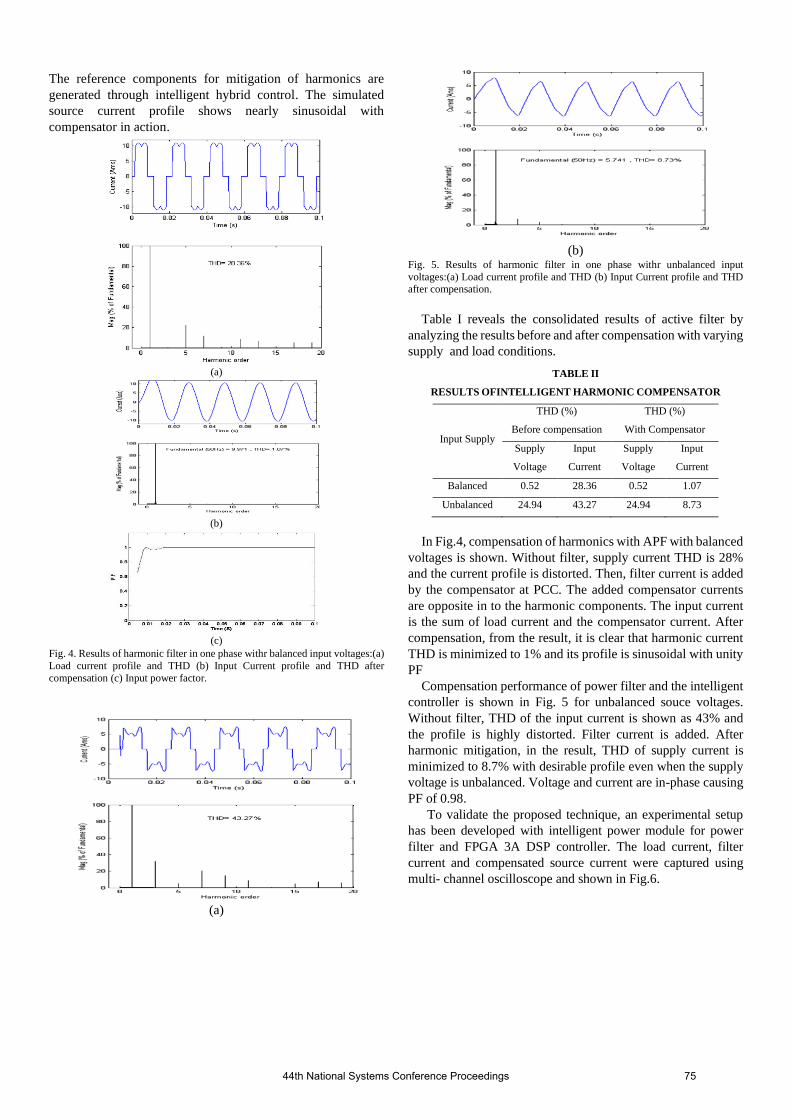
The reference components for mitigation of harmonics are

generated through intelligent hybrid control. The simulated

source current profile shows nearly sinusoidal with

compensator in action.

(a)

(b)

(c)

Fig. 4. Results of harmonic filter in one phase withr balanced input voltages:(a)

Load current profile and THD (b) Input Current profile and THD after

compensation (c) Input power factor.

(a)

(b)

Fig. 5. Results of harmonic filter in one phase withr unbalanced input

voltages:(a) Load current profile and THD (b) Input Current profile and THD after compensation.

Table I reveals the consolidated results of active filter by

analyzing the results before and after compensation with varying

supply and load conditions.

TABLE II

RESULTS OFINTELLIGENT HARMONIC COMPENSATOR

Input Supply

THD (%)

Before compensation

THD (%)

With Compensator

Supply

Voltage

Input

Current

Supply

Voltage

Input

Current

Balanced 0.52 28.36 0.52 1.07

Unbalanced 24.94 43.27 24.94 8.73

In Fig.4, compensation of harmonics with APF with balanced

voltages is shown. Without filter, supply current THD is 28%

and the current profile is distorted. Then, filter current is added

by the compensator at PCC. The added compensator currents

are opposite in to the harmonic components. The input current

is the sum of load current and the compensator current. After

compensation, from the result, it is clear that harmonic current

THD is minimized to 1% and its profile is sinusoidal with unity

PF

Compensation performance of power filter and the intelligent

controller is shown in Fig. 5 for unbalanced souce voltages.

Without filter, THD of the input current is shown as 43% and

the profile is highly distorted. Filter current is added. After

harmonic mitigation, in the result, THD of supply current is

minimized to 8.7% with desirable profile even when the supply

voltage is unbalanced. Voltage and current are in-phase causing

PF of 0.98.

To validate the proposed technique, an experimental setup

has been developed with intelligent power module for power

filter and FPGA 3A DSP controller. The load current, filter

current and compensated source current were captured using

multi- channel oscilloscope and shown in Fig.6.


(a)

(b)

Fig. 6. (a). Experimental setup, (b). Voltage and Current

profiles (i) Source voltage (ii) Load current (iii) Filter current

(iv) Source current.

V. CONCLUSIONS

The intelligent hybrid control technique for harmonic

compensator has been developed and implemented to enhance

the compensating performance of harmonic conditioner. From

Table I, it is proved that APF provides improved performance

in harmonic mitigation. It is proved that the supply line current

synthesized nearly sinusoidal in-phase with the supply voltage.

Hence, power factor is improved to unity. The intelligent hybrid

control method for IT industry has been analyzed for

dynamically varying system and external conditions. The

experiment results show the performance of the controller in

which the current harmonics is reduced to 3.3%. Source current

THD is minimized to an acceptable value of IEEE standard in

IT industries.

ACKNOWLEDGMENT

We are grateful to the management of Kumaraguru College of Technology for providing facilities and support.

REFERENCES

[1] Hongyu Li, Fang Zhuo, Zhaoan Wang, “A Novel Time- Domain Current-Detection Algorithm for Parallel Active Power Filters”, IEEE Trans. on Power Systems., vol.20, no.2, pp 644-651, May 2005.

[2] Bhim Singh, V.Verma, “An Indirect Control of Hybrid Power Filter for Varying Loads”, IEEE Trans. on Power Delivery, vol.21,No.1, Jan.2005.

[3] Bhim Singh, V.Vermaand Al-haddad, “Hybrid Filters for Power Quality Improvement”, IEE Proc. on Generation, transmission and Distribution, vol.152,No.3, May 2005.

[4] S. K. Jain, P. Agrawal, and H. O. Gupta, “Fuzzy Logic Controlled Shunt Active Power Filter For Power Quality Improvement,” Proc.Inst. Elect. Eng.—Elect. Power Appl., vol. 149, no. 5, pp. 317–328, Sep. 2002.

[5] P. Jintakosonwit, H. Fujita, and H. Akagi, “Control And Performance Of A Fully-Digital-Controlled Shunt Active Filter For Installation On A Power Distribution System,” IEEE Trans. on Power Electron., vol. 17, no. 1, pp. 132– 140, Jan. 2002.

[6] P. Thirumoorthi, and N. Yadaiah, “Switch Mode Active Power Filter to Minimize the Effect of Harmonics through Current Detection”, IEEE International Conference-PowerCon2008, Oct, 2008.

[7] An Luo etal., “Design Considerations for Maintaining DC-Side Voltageof Hybrid Active Power Filter With Injection Circuit”, IEEE Trans on Power Electron., vol. 24, No. 1, January 2009.

[8] Rondineli Rodrigues Pereira;Carlos Henrique da Silva;Luiz Eduardo Borges da Silva;Germano Lambert-Torres;João O. P. Pinto, “New Strategies for Application of Adaptive Filters in Active Power Filters”, IEEE Trans. on Industry Appln., Vol. 47, No. 3, 2011.

[9] Lei Wang;Chi-Seng Lam;Man-Chung Wong, “Unbalanced Control Strategy for A Thyristor-Controlled LC-Coupling Hybrid Active Power Filter in Three-Phase Three-Wire Systems”, IEEE Trans. on Power Elecs., Vo. 32, No: 2, 2017.


https://ieeexplore.ieee.org/author/37398429900






https://ieeexplore.ieee.org/document/5729327/

https://ieeexplore.ieee.org/document/5729327/

https://ieeexplore.ieee.org/xpl/RecentIssue.jsp?punumber=28






https://ieeexplore.ieee.org/xpl/tocresult.jsp?isnumber=7742436

Formulating Maintenance Order Completion

Strategy for Uninterrupted Supply of Potable

Water using System Dynamics Approach

Pradyuman Verma

M.Tech Final Year student, DEI Faculty of Engineering

Senior Manager

Orange City Water Pvt. Ltd, Nagpur India

[email protected], 9765026626

Abstract - A holistic view of planned maintenance

order creation is presented here to understand the

dynamics of order backlog and schedule pressure and

to gauge the reason for high mean time between failure

(MTBF) and to find its feasible solutions. The primary

data is captured from maintenance records and

logbooks of Kanhan WTP, operated and maintained by

M/s. Orange City Water Pvt Ltd, Nagpur. After

simulating the initial condition, it was found that there

is very high pressure on the team to complete PM

orders. Half yearly and yearly PM orders can be

rescheduled for the days with minimum orders, to

reduce schedule pressure as high work pressure will

lead to compromise with maintenance work which will

further add to machine breakdowns.

Keywords- System Dynamics, Water Utility, Maintenance

Order, Preventive Maintenance, Work Pressure

I. INTRODUCTION

According to a study conducted in 2008 by WHO,

the global disease burden could be prevented from

supplying treated and safe portal water. Thus to

promote healthy living safe water supply should be

uninterrupted in all cities with help of the

Municipality [1]. Few challenges of water utilities are

the lack of adequate resources like infrastructure,

shortage of manpower, pollution, etc. [2]. In the

present paper a system dynamics model of

maintenance work orders has been constructed to

reduce maintenance order backlog and at the same

time not to load the maintenance team with work

pressure. This will further contribute to formulating a

maintenance strategy that can lead to a reduction in

maintenance expenses [3]. There is a vast amount of

literature available which have applied systems

dynamics in turnkey projects across nations [3], [4],

[5]. System Dynamics involves identifications of all

elements of a maintenance order system affecting

other elements, directly or indirectly [6].

A report published by the Gujarat Institute of

Development Research in 2005 highlighted poor

operation and maintenance as a major problem in

water treatment and distribution systems affecting

water quality and quantity. In this study, a holistic

view of planned maintenance order creation is

simulated to understand the dynamics of order

backlog and schedule pressure and to gauge the

reason for high MTBF and to find its feasible

solutions.

II. SYSTEM STRUCTURE

The Definition of variables used in the model is

described below.

Preventive Maintenance (PM) is performed before

identifying any breakdown. PM tasks consist of a set

of procedures performed to prevent or delay a

machine failure. This set of procedures can be based

on fixed time intervals. [4]

The maintenance order completion rate is determined

by the lesser of the potential completion rate based on

the size and productivity of the workforce and the

maximum completion rate based on the number of

orders in the backlog and the minimum time required

per order. Desired Completion rate is determined by

Maintenance orders backlog and target delivery time

desired by the organization. The standard completion

rate represents the output the organization could

achieve with the current manpower working normal

hours and dedicating standard time per order.

Workday is a standard workday of eight hours

modified by an effect of schedule pressure. Schedule

pressure is the measure of pressure to work at a

greater or lesser rate than normal. FTE Labour is the

full-time equivalent labor available net of

absenteeism and time lost due because of other

factors like training, meetings, etc.[8]

Reactive Maintenance is performed in response to

reported equipment malfunction or failure [7].



MTBF (Mean time between failures) indicates the

mean time between two failures or malfunctions.

MTTR (Mean time to repair) indicates the mean time

taken to repair the machine [9]

Parameters of variables

The primary data is captured from maintenance

records and logbooks of Kanhan WTP, operated and

maintained by M/s. Orange City Water Pvt Ltd,

Nagpur to capture current system behavior. These are

as follows:

• Maintenance Order Backlog

• 1M PM Orders

• 3M PM Orders

• 6M PM Orders

• 1Y PM Orders

• Maintenance Order Creation Rate

• Maintenance Order Completion Rate

• Minimum Delivery Delay 1M 3M

• Minimum Delivery Delay 6M 1Y

• MTTR

• Target Delivery Delay 1M 3M

• Target Delivery Delay 6M 1Y

• MTBF

• Table for Workday 1M 3M

• Table for time per order 1M 3M

• Table for Workday 6M 1Y

• Table for time per order 6M 1Y

• Table for Workday RM

• Table for time per order RM

• FTE Labour 1M 3M

• FTE Labour 6M 1Y

III. CAUSAL LOOP DIAGRAM

The Maintenance Orders (MO) Backlog is created

when Preventive maintenance and reactive

maintenance orders are created in Vensim PLE

version 8.1.0 software. Preventive maintenance

orders are generated based on the maintenance

schedule, whereas reactive maintenance order is

generated after machine failure. A high MO backlog

will represent the low availability of the machine. PM

order creation is exogeneous but RM orders can

increase or decrease depending on MTBF. The

maximum completion rate forms the balancing loop

B1which ensures that the backlog is nonnegative.

Figure 1 Causal Loop Diagram

Feedback loops affecting the order completion rate

are balancing loop B2 formed by the use of overtime

and balancing loop B3 representing workers not

putting in the desired time to complete the order and

spending fewer hours might be compromising with

the quality. Working overtime or spending less time

on maintenance orders are expressed as a non-linear

function of schedule pressure in the Stock and Flow

diagram (Figure 1). Potential completion rate PCR will

be more when workers' availability and the workday

is more. Spending more time on the order will

decrease the PCR.

IV. STOCK FLOW DIAGRAM

Upon further investigation it was observed that the

above system as shown in CLD consists of three

subsystems and forms the system boundary of this

model (

Figure 11 Stock Flow Diagram: see appendix): i) 1M3M* Preventive Maintenance subsystem;

Generated for equipment with monthly or

quarterly frequency and have similar standard

time for order completion.

ii) 6M1Y* Preventive Maintenance subsystem;

Generated for equipment coming under half-

yearly and yearly frequency of checkpoints.

iii) Reactive Maintenance subsystem; Reactive

maintenance order generation is simulated for

MTBF 10 days as per the logbook. For RM orders

target is to reduce MTTR.

*PM orders with frequency monthly (1M) and

quarterly (3M) are grouped together and PM orders

with frequency half yearly (6M) and yearly (1Y) are

grouped together, as they were reportedly having

similar standard time per order and FTE Labour

requirements. (Error! Reference source not found.).


Figure 2 Initial Maintenance order creation

The stock-flow model (created in Vensim PLE

version 8.1.0) interconnecting these three subsystems

simultaneously. The documentation for the units,

value, equations are given in TABLE II in Appendix.

V. SIMULATION RESULTS

The initial simulation result of different variable is

as follows:

A. Priority is given to reactive maintenance orders

in case there are any open RM orders and then

subsequently 6M1Y and then 1M3M orders are

processed by deploying maintenance crew. The

following maintenance orders generated during

one year are used in current simulation:

TABLE 1. ORDER TYPES

Order Type Number of Order

RM One order every 3 days

1Y 22

6M 82

3M 112

1M 504

B. Schedule Pressure: In the initial simulation of

1M3M orders (Error! Reference source not found.) and

6M1Y orders (Error! Reference source not found.)

extremely high schedule pressure conditions

were observed. As manpower is first allocated to

complete RM orders, this resulted in very low

schedule pressure. Very high schedule pressure

will lead to corner cutting by the maintenance

workers while completing maintenance orders

and this will increase the probability of machine

failures.

Figure 3 Initial schedule pressure 1M3M

Figure 4 Initial schedule pressure 6M 1Y

C. Workday: Frequent overtime was reported while

completing PM orders (Figure 5, Figure 6)

Figure 5 - Initial Workday 1M3M

Figure 6 - Initial Workday 6M1Y

D. PM Order Backlogs: High backlogs of half-

yearly and yearly orders (Error! Reference source not

found.) were observed and few order backlogs

were found for quarterly orders


Figure 7 Initial MO Backlog

CONCLUSION

To conclude, revising preventive maintenance plan

resulted in reduction in orders backlog (Figure 10)

thereby reducing schedule pressure without

increasing manpower. (Figure 8,Figure 9).

Figure 8 PM Rescheduled - MO Backlog

Figure 9 PM Rescheduled - Schedule pressure 1M3M

Figure 10 PM Rescheduled - Schedule pressure 6M1Y

This suggested modification of PM plan will not only

be cost effective but also improve quality of

maintenance work being performed. Further this will

lead to increase in mean time between failure

(MTBF) ensuring high machine availability and thus

providing uninterrupted supply of potable water.

Future research in this area can be done for

benchmarking target delivery delays, standard time

per order.

ACKNOWLEDGMENT

I would like to thank OCW India private limited, Nagpur

for their support in providing data for this study. I would

also like to thanks Prof. D.K. Chaturvedi, Dept of Electrical

Engineering FOE, DEI for his kind guidance.

REFERENCES [1]

Meng Yang, Y. Zhu, J. Song, and Xirui Gu, “A System

Dynamics approach for integrated decision making

optimization of maintenance support system,” in 2009

Chinese Control and Decision Conference, Guilin, China,

Jun. 2009, pp. 2471–2475, doi:

10.1109/CCDC.2009.5192479.

[2]

H. A. Khorshidi, I. Gunawan, and M. Y. Ibrahim,

“Reliability centered maintenance using system dynamics

approach,” in 2015 IEEE International Conference on

Industrial Technology (ICIT), Seville, Mar. 2015, pp.

1932–1936, doi: 10.1109/ICIT.2015.7125379.

[3]

I. H. Afefy, “Reliability-Centered Maintenance

Methodology and Application: A Case Study,” ENG, vol.

02, no. 11, pp. 863–873, 2010, doi:

10.4236/eng.2010.211109.

[4]

U. Bariss, G. Bazbauers, A. Blumberga, and D. Blumberga,

“System Dynamics Modeling of Households’ Electricity

Consumption and Cost-Income Ratio: a Case Study of

Latvia,” Environmental and Climate Technologies, vol. 20,

no. 1, pp. 36–50, Nov. 2017, doi: 10.1515/rtuect-2017-

0009.

[5]

E. Esmaeili, H. Karimian, and M. Najjartabar Bisheh,

“Analyzing the productivity of maintenance systems using

system dynamics modeling method,” Int

J Syst Assur Eng Manag, vol. 10, no. 2, pp. 201–211,

Apr. 2019, doi: 10.1007/s13198-018-0754-5.

[6]

G. Chung, J. H. Kim, and T.-W. Kim, “System dynamics

modeling approach to water supply system,” KSCE J Civ

Eng, vol. 12, no. 4, pp. 275–280, Jul. 2008, doi:

10.1007/s12205-008-0275-x.

[7]

S. Gallego García and M. García García, “Design and

Simulation of Production and Maintenance Management

Applying the Viable System Model: The Case of an OEM

Plant,” Materials, vol. 11, no. 8, p. 1346, Aug. 2018, doi:

10.3390/ma11081346.

[8]

O. Ristic, B. Iricanin, and V. Mijailovic, “Dynamic

modeling and simulation of power transformer maintenance


https://doi.org/10.1109/CCDC.2009.5192479

https://doi.org/10.1109/ICIT.2015.7125379

https://doi.org/10.4236/eng.2010.211109

https://doi.org/10.1515/rtuect-2017-0009

https://doi.org/10.1515/rtuect-2017-0009

https://doi.org/10.1007/s13198-018-0754-5

https://doi.org/10.1007/s12205-008-0275-x

https://doi.org/10.3390/ma11081346

costs,” Serb J Electr Eng, vol. 13, no. 2, pp. 285–299,

2016, doi: 10.2298/SJEE1602285R.

[9]

J.-H. Thun, “Maintaining preventive maintenance and

maintenance prevention: analysing the dynamic

implications of Total Productive Maintenance,” Syst. Dyn.

Rev., vol. 22, no. 2, pp. 163–179, 2006, doi:

10.1002/sdr.335.

[10]

“Research Paper SD RCM.pdf.” .

[11]

S. Armenia, “Energy Management in Residential

Buildings: A System Dynamics Approach,” p. 30.

[12]

I. Aziz, S. Karim, and M. Hossain, “Effective

Implementation of Total Productive Maintenance and

Impacts on Breakdown Time and Repair & Maintenance –

A Case Study Of A Printing Industry In Bangladesh,” p. 9.

[13]

“Aziz et al. - Effective Implementation of Total Productive

Maint.pdf.” Accessed: Apr. 04, 2021. [Online]. Available:

[14]

T. Böhm, K. Beck, A. Knaak, and B. Jäger, “Efficient

maintenance strategy through System Dynamics,” Toledo,

Spain, Aug. 2008, pp. 755–764, doi: 10.2495/CR080731.

[15]

F. Hezoucky and Agence internationale de l’énergie

atomique, Application of reliability centred maintenance to

optimize operation and maintenance in nuclear power

plants. Vienna: International Atomic Energy Agency, 2008.

[16]

S. H. Hoseinie, U. Kumar, B. Ghodrati, Luleå tekniska

universitet, and Institutionen för samhällsbyggnad och

naturresurser, Reliability Centered Maintenance (RCM) for

Automated Mining Machinery. Lulea: Luleå tekniska

universitet, 2016.

[17]

T. Jokinen, P. Ylén, and J. Pyötsiä, “Dynamic Model for

Estimating the Added Value of Maintenance Services,” p.

19.

[18]

A. Mapfumo and W. M. Madesha, “CHALLENGES FOR

URBAN WATER SUPPLY: THE CASE OF MASVINGO

MUNICIPALITY IN ZIMBABWE,” p. 5, 2014.

[19]

“Mapfumo and Madesha - 2014 - CHALLENGES FOR

URBAN WATER SUPPLY THE CASE OF MAS.pdf.”

Accessed: Apr. 04, 2021. [Online]. Available:

http://ijeronline.com/documents/volumes/Vol%205%20iss

%2003/ijer%20v5i3(1).pdf.

[20]

J.-H. Thun, “Modelling Modern Maintenance – A System

Dynamics Model Analyzing the Dynamic Implications of

Implementing Total Productive Maintenance,” p. 11.

[21]

“(PDF) Business Dynamics, System Thinking and

Modeling for a Complex World.”

https://www.researchgate.net/publication/44827001_Busine

ss_Dynamics_System_Thinking_and_Modeling_for_a_Co

mplex_World (accessed Apr. 04, 2021).

[22]

“04_2014_water_and_health_info_brief_eng.pdf.”

Accessed: Apr. 04, 2021. [Online]. Available:

https://www.un.org/waterforlifedecade/pdf/04_2014_water

_and_health_info_brief_eng.pdf.

[23]

“A System Dynamics Model for Operations Management

Improvement in Multi-plant Enterprise,” p. 77.

[24]

“Application of System Dynamics to Pavement

Maintenance Optimisation.pdf.” .

[25]

“Charte Asset Management_EN 2014.pdf.” .

[26]

“Drinking Water Supply.pdf.” Accessed: Apr. 05, 2021.

[Online]. Available:

http://www.isec.ac.in/Drinking%20Water%20Supply.PDF.

[27]

“Reducing Risks to Health, Promoting Healthy Life |

Cardiology | JAMA | JAMA Network.”

https://jamanetwork.com/journals/jama/article-

abstract/195444 (accessed Apr. 04, 2021).

[28]

“System Dynamics Modelling for Residential Energy

Efficiency Analysis and Management.pdf.” .

APPENDIX ON NEXT PAGE


https://doi.org/10.2298/SJEE1602285R

https://doi.org/10.1002/sdr.335

https://doi.org/10.2495/CR080731

http://ijeronline.com/documents/volumes/Vol%205%20iss%2003/ijer%20v5i3(1).pdf

http://ijeronline.com/documents/volumes/Vol%205%20iss%2003/ijer%20v5i3(1).pdf

https://www.researchgate.net/publication/44827001_Business_Dynamics_System_Thinking_and_Modeling_for_a_Complex_World



https://www.un.org/waterforlifedecade/pdf/04_2014_water_and_health_info_brief_eng.pdf

https://www.un.org/waterforlifedecade/pdf/04_2014_water_and_health_info_brief_eng.pdf

http://www.isec.ac.in/Drinking%20Water%20Supply.PDF

https://jamanetwork.com/journals/jama/article-abstract/195444

https://jamanetwork.com/journals/jama/article-abstract/195444

APPENDIX

Figure 11 Stock Flow Diagram


TABLE II LIST OF EQUATIONS USED IN THE STOCK FLOW MODEL

(01) Desired Completion rate 1M 3M=

PM Orders Backlog 1M 3M/Target Delivery Delay 1M 3M

Units: Orders/Day

(02) Desired Completion rate 1M 3M 0=

PM Orders Backlog 6M1Y/Target Delivery Delay 6M1Y

Units: Orders/Day

(03) Desired Completion rate RM=

PM Orders Backlog RM/Target MTTR

Units: Orders/Day

(04) Effect of Schedule Pressure on Time per order 6M1Y=

Table for time per order 6M1Y(Schedule pressure 6M1Y)

Units: Dmnl

(05) Effect of Schedule Pressure on Time per order RM=

Table for time per order RM(Schedule pressure RM)

Units: Dmnl

(06) Effect of Schedule Pressure on Time per order1M3M=

Table for time per order 1M 3M(Schedule pressure 1M 3M)

Units: Dmnl

(07) Effect of schedule pressure on WorkDay 1M 3M=

Table for Workday 1M 3M(Schedule pressure 1M 3M)

Units: Dmnl

(08) Effect of schedule pressure on WorkDay 6M1Y=

Table for Workday 6M1Y(Schedule pressure 6M1Y)

Units: Dmnl

(09) Effect of schedule pressure on WorkDay RM=

Table for Workday RM(Schedule pressure RM)

Units: Dmnl

(10) FINAL TIME = 365

Units: Day

The final time for the simulation.

(11) FTE Labour 1M3M=

IF THEN ELSE(PM Order Creation Rate 1M 3M>=1:AND:PM Order Creation Rate 6M1Y

>=1:AND:RM Order Creation Rate>=1, 0.1*FTE Labour Availability , IF THEN ELSE

( PM Order Creation Rate 1M 3M>=1:AND:PM Order Creation Rate 6M1Y>=1:AND:RM Order Creation Rate

<1, 0.3*FTE Labour Availability , IF THEN ELSE(PM Order Creation Rate 1M 3M

>=1:AND:PM Order Creation Rate 6M1Y<1:AND:RM Order Creation Rate<1, 1*FTE Labour Availability

, IF THEN ELSE(PM Order Creation Rate 1M 3M>=1:AND:PM Order Creation Rate 6M1Y

<1:AND:RM Order Creation Rate>=1, 0.5*FTE Labour Availability , FTE Labour Availability

) ) ) )

Units: 1/Day

IF THEN ELSE(PM Order Creation Rate 1M 3M<1, 0.01*FTE Labour

Availability 1M3M, IF THEN ELSE(PM Order Creation Rate 1M

3M>=1:AND:PM Order Creation Rate 6M1Y>=1, 1*FTE Labour

Availability 1M3M , IF THEN ELSE(PM Order Creation Rate 1M

3M>=1:OR:PM Order Creation Rate 6M1Y<1, FTE Labour Availability

1M3M , FTE Labour Availability 1M3M ) )) IF THEN ELSE(PM Order

Creation Rate 1M 3M<1, FTE Labour Availability 1M3M , IF THEN

ELSE(PM Order Creation Rate 1M 3M>= 1:AND:PM Order Creation Rate

6M1Y=0, FTE Labour Availability 1M3M + FTE Labour Availability

6M1Y, IF THEN ELSE(PM Order Creation Rate 1M 3M >=1:AND:PM Order

Creation Rate 6M1Y>=1, FTE Labour Availability 1M3M , 0.01 )) )

(12) FTE Labour 6M1Y=

IF THEN ELSE(PM Order Creation Rate 6M1Y>=1:AND:PM Order Creation Rate 1M 3M

>=1:AND:RM Order Creation Rate>=1, 0.4*FTE Labour Availability , IF THEN ELSE

(PM Order Creation Rate 6M1Y>=1:AND:PM Order Creation Rate 1M 3M>=1:AND:RM Order Creation Rate

<1, 0.6*FTE Labour Availability , IF THEN ELSE(PM Order Creation Rate 6M1Y

>=1:AND:PM Order Creation Rate 1M 3M<1:AND:RM Order Creation Rate<1, 1*FTE Labour Availability

, IF THEN ELSE(PM Order Creation Rate 6M1Y>=1:AND:PM Order Creation Rate 1M 3M

<1:AND:RM Order Creation Rate>=1, 0.5*FTE Labour Availability , FTE Labour Availability

) ) ) )

Units: 1/Day

IF THEN ELSE(PM Order Creation Rate 6M1Y=0, 0 , IF THEN ELSE(PM

Order Creation Rate 6M1Y>=1:AND:PM Order Creation Rate 1M 3M <1,

FTE Labour Availability 1M3M+FTE Labour Availability 6M1Y , IF

THEN ELSE(PM Order Creation Rate 6M1Y>=1:AND:PM Order Creation

Rate 1M 3M >=1, FTE Labour Availability 6M1Y , 0.1 ) ))


(13) FTE Labour Availability =

0.75*3

Units: 1/Day

(14) FTE Labour RM=

IF THEN ELSE(RM Order Creation Rate>=1:AND:PM Order Creation Rate 1M 3M>=

1:AND:PM Order Creation Rate 6M1Y>=1, 0.5*FTE Labour Availability , IF THEN ELSE

(RM Order Creation Rate>=1:AND:PM Order Creation Rate 1M 3M>=1:AND:PM Order Creation Rate 6M1Y

<1, 0.5*FTE Labour Availability, IF THEN ELSE(RM Order Creation Rate>=1:AND:

PM Order Creation Rate 1M 3M<1:AND:PM Order Creation Rate 6M1Y<1, 1*FTE Labour Availability

, IF THEN ELSE(RM Order Creation Rate>=1:AND:PM Order Creation Rate 1M 3M

<1:AND:PM Order Creation Rate 6M1Y>=1, 0.5*FTE Labour Availability , FTE Labour Availability

) ) ) )

Units: 1/Day

IF THEN ELSE(PM Order Creation Rate 1M 3M<1, 0.01*FTE Labour

Availability 1M3M, IF THEN ELSE(PM Order Creation Rate 1M

3M>=1:AND:PM Order Creation Rate 6M1Y>=1, 1*FTE Labour

Availability 1M3M , IF THEN ELSE(PM Order Creation Rate 1M

3M>=1:OR:PM Order Creation Rate 6M1Y<1, FTE Labour Availability

1M3M , FTE Labour Availability 1M3M ) )) IF THEN ELSE(PM Order

Creation Rate 1M 3M<1, FTE Labour Availability 1M3M , IF THEN

ELSE(PM Order Creation Rate 1M 3M>= 1:AND:PM Order Creation Rate

6M1Y=0, FTE Labour Availability 1M3M + FTE Labour Availability

6M1Y, IF THEN ELSE(PM Order Creation Rate 1M 3M >=1:AND:PM Order

Creation Rate 6M1Y>=1, FTE Labour Availability 1M3M , 0.01 )) )

(15) Half Yearly PM Orders 6M=

PULSE TRAIN(41,1,180,365) + PULSE TRAIN(70,1,180,365) + 4*PULSE TRAIN(91,

1,180,365) + PULSE TRAIN(102,1,180,365) + PULSE TRAIN(105,1,180,365) + 2*PULSE TRAIN

(111,2,180,365) + 6*PULSE TRAIN(114,1,180,365) + 5*PULSE TRAIN(115,1,180,365

) + 2*PULSE TRAIN(122,1,180,365) + PULSE TRAIN(133,1,180,365) + PULSE TRAIN

(154,1,180,365) + PULSE TRAIN(165,1,180,365) + 2*PULSE TRAIN(185,1,180,365

) + PULSE TRAIN(196,1,180,365) + PULSE TRAIN(198,4,180,365) + 4*PULSE TRAIN

(204,1,180,365) + 2*PULSE TRAIN(208,3,180,365) + PULSE TRAIN(217,1,180,365

)+ PULSE TRAIN(228,1,180,365)+ PULSE TRAIN(249,1,180,365)+ 2*PULSE TRAIN(312

,1,180,365)+ 2*PULSE TRAIN(343,1,180,365)

Units: Orders/Day

(16) INITIAL TIME = 0

Units: Day

The initial time for the simulation.

(17) maintenance order completion rate 1M 3M=

MIN(Maximum Completion rate,Potential Completion Rate 1M 3M)

Units: Orders/Day

(18) maintenance order completion rate 6M1Y=

MIN(Maximum Completion rate 6M1Y,Potential Completion Rate 6M1Y)

Units: Orders/Day

(19) maintenance order completion rate RM=

MIN(Maximum Completion rate 0,Potential Completion Rate RM)

Units: Orders/Day

(20) Maximum Completion rate=

PM Orders Backlog 1M 3M/Minimum Delivery Delay

Units: Orders/Day

(21) Maximum Completion rate 0=

PM Orders Backlog RM/MTTR

Units: Orders/Day

(22) Maximum Completion rate 6M1Y=

PM Orders Backlog 6M1Y/Minimum Delivery Delay 6M1Y

Units: Orders/Day

(23) Minimum Delivery Delay=

0.1

Units: Day

3 Days = 0.33*3 = 0.99 (8 hours per day = 0.33 Workday)

(24) Minimum Delivery Delay 6M1Y=

0.66

Units: Day

2 days = 0.66

(25) Monthly PM Orders 1M=

4* PULSE TRAIN( 1,1,30,365 ) + 2*PULSE TRAIN(2,8,30,365) + PULSE TRAIN(10

,11,30,365) + 4*PULSE TRAIN(23,1,30,365) + 2*PULSE TRAIN(27,3,30,365)


Units: Orders/Day

(26) MTBF=

PULSE TRAIN (2, 1, 3, 365)

Units: Orders/Day

(27) MTTR=

0.2

Units: Day

(28) PM Order Creation Rate 1M 3M=

Monthly PM Orders 1M+Quarterly PM Orders 3M

Units: Orders/Day

(29) PM Order Creation Rate 6M1Y=

Half Yearly PM Orders 6M+Yearly PM Orders 1Y

Units: Orders/Day

(30) PM Orders Backlog 1M 3M= INTEG (

PM Order Creation Rate 1M 3M-maintenance order completion rate 1M 3M,

1)

Units: Orders

(31) PM Orders Backlog 6M1Y= INTEG (

PM Order Creation Rate 6M1Y-maintenance order completion rate 6M1Y,

1)

Units: Orders

(32) PM Orders Backlog RM= INTEG (

RM Order Creation Rate-maintenance order completion rate RM,

1)

Units: Orders

(33) PM Orders Completed 1M 3M= INTEG (

maintenance order completion rate 1M 3M,

0)

Units: Orders

(34) PM Orders Completed 6M1Y= INTEG (

maintenance order completion rate 6M1Y,

0)

Units: Orders

(35) PM Orders Completed RM= INTEG (

maintenance order completion rate RM,

0)

Units: Orders

(36) Potential Completion Rate 1M 3M=

(FTE Labour 1M3M*Workday 1M3M)/Time per Order

Units: Orders/Day

(37) Potential Completion Rate 6M1Y=

(FTE Labour 6M1Y*Workday 6M1Y)/Time per Order 6M1Y

Units: Orders/Day

(38) Potential Completion Rate RM=

(FTE Labour RM*Workday RM)/Time per Order RM

Units: Orders/Day

(39) Quarterly PM Orders 3M=

PULSE TRAIN(15,1,90,365) + PULSE TRAIN(18,2,90,365) + 2*PULSE TRAIN (21,2

,90,365) + 6*PULSE TRAIN(24,1,90,365) + 5*PULSE TRAIN(25,1,90,365) + 4*PULSE TRAIN

(26,1,90,365) + PULSE TRAIN(107,4,90,365) + 4*PULSE TRAIN(113,1,90,365)

Units: Orders/Day

(40) RM Order Creation Rate=

MTBF

Units: Orders/Day

(41) SAVEPER =

TIME STEP

Units: Day [0,?]

The frequency with which output is stored.

(42) Schedule pressure 1M 3M=

Desired Completion rate 1M 3M/Standard completion rate 1M3M

Units: Dmnl

(43) Schedule pressure 6M1Y=


Desired Completion rate 1M 3M 0/Standard completion rate 6M1Y

Units: Dmnl

(44) Schedule pressure RM=

Desired Completion rate RM/Standard completion rate RM

Units: Dmnl

(45) Standard completion rate 1M3M=

(FTE Labour 1M3M*standard workday)/Standard Time Per Order

Units: Orders/Day

(46) Standard completion rate 6M1Y=

(FTE Labour 6M1Y*standard workday)/Standard Time Per Order 6M1Y

Units: Orders/Day

(47) Standard completion rate RM=

(FTE Labour RM*standard workday)/Standard Time Per Order RM

Units: Orders/Day

(48) Standard Time Per Order=

0.083

Units: Day/Order

0.083 = 2 hours

(49) Standard Time Per Order 6M1Y=

0.25

Units: Day/Order

1 Day = 24 hours Working hours = 8 hours 6 hours = 0.25 Day

(50) Standard Time Per Order RM=

0.0825

Units: Day/Order

(51) standard workday=

0.33

Units: Day

IF THEN ELSE(Reactive Maintenance Order Creation Rate>=1,1,IF

THEN ELSE( Standard workday RM-Workday RM<1 , 0.5,8) )

(52) Table for time per order 1M 3M(

[(0,0)-(11,1)],(0,0),(0.2,1),(0.4,1),(0.6,1),(0.8,1),(1,1),(1.2,0.9),(1.4

,0.85),(1.6,0.8),(1.8,0.75),(2,0.75),(3,0.75),(4,0.75),(5,0.75),(6,0.75),(

7,0.75),(8,0.75),(9,0.75),(10,0.75),(11,0.75))

Units: Dmnl

(53) Table for time per order 6M1Y(

[(0,0)-(2,1)],(0,0),(0.2,1),(0.4,1),(0.6,1),(0.8,1),(1,1),(1.2,0.95),(1.4

,0.9),(1.6,0.85),(1.8,0.8),(2,0.8))

Units: Dmnl

(54) Table for time per order RM(

[(0,0)-(2,1)],(0,0),(0.2,1),(0.4,1),(0.6,1),(0.8,1),(1,1),(1.2,0.95),(1.4

,0.9),(1.6,0.85),(1.8,0.8),(2,0.8))

Units: Dmnl

(55) Table for Workday 1M 3M(

[(0,0)-(4,2)],(0,0),(0.5,1),(1,1),(1.5,1.2),(2,1.2),(2.5,1.2),(3,1.2),(3.5

,1.2),(4,1.2))

Units: Dmnl

(56) Table for Workday 6M1Y(

[(0,0)-(4,2)],(0,0),(0.5,1),(1,1),(1.5,1.2),(2,1.2),(2.5,1.4),(3,1.4),(3.5

,1.4),(4,1.4))

Units: Dmnl

(57) Table for Workday RM(

[(0,0)-(4,2)],(0,0),(0.5,1),(1,1),(1.5,1.2),(2,1.2),(2.5,1.4),(3,1.4),(3.5

,1.4),(4,1.4))

Units: Dmnl

(58) Target Delivery Delay 1M 3M=

0.05

Units: Day

(59) Target Delivery Delay 6M1Y=

0.33

Units: Day

(60) Target MTTR=

0.15


Units: Day

2 Days

(61) Time per Order=

Effect of Schedule Pressure on Time per order1M3M*Standard Time Per Order

Units: Day/Order

(62) Time per Order 6M1Y=

Effect of Schedule Pressure on Time per order 6M1Y*Standard Time Per Order 6M1Y

Units: Day/Order

(63) Time per Order RM=

Effect of Schedule Pressure on Time per order RM*Standard Time Per Order RM

Units: Day/Order

(64) TIME STEP = 0.03125

Units: Day [0,?]

The time step for the simulation.

(65) Workday 1M3M=

standard workday*Effect of schedule pressure on WorkDay 1M 3M

Units: Day

(66) Workday 6M1Y=

standard workday *Effect of schedule pressure on WorkDay 6M1Y

Units: Day

(67) Workday RM=

standard workday*Effect of schedule pressure on WorkDay RM

Units: Day

(68) Yearly PM Orders 1Y=

PULSE TRAIN(222,1,365,365)+ PULSE TRAIN(254,1,365,365)+ PULSE TRAIN(285,1

,365,365)+ PULSE TRAIN(288,1,365,365) + 2*PULSE TRAIN(294,2,365,365) + 6*PULSE TRAIN

(297,1,365,365)+ 5*PULSE TRAIN(298,1,365,365)+ PULSE TRAIN(317,1,365,365)+

PULSE TRAIN(348,1,365,365)

Units: Orders/Day


Efficient and Economical DenseNet for AutomaticIdentification of COVID-19 from X-Ray Images

SoniyaDept. of Electrical Engineering

Indian Institute of Technology KanpurKanpur, India

[email protected]

Lotika SinghDept. of Physics and Computer Science

Dayalbagh Educational InstituteAgra, India

[email protected]

Sandeep PaulDept. of Physics and Computer Science

Dayalbagh Educational InstituteAgra, India

[email protected]

Abstract—Densely connected convolutional neural network(DenseNet) has been considered as one of the well known deepnetworks as it can efficiently handle the vanishing gradientproblem. Due to the notable feature of concatenation of precedinglayers information, it exhibits high performance. However, itsextremely complex structure with number of tunable parametersis responsible for high computational cost of the network. Thus,improvements are required to simplify complexities associatedwith the network. A study has been proposed in this paperto analyse the effect of various convolutional operations onDenseNet. A simulation study has been performed on COVID-19 radiography dataset. An accuracy of 100% and 97.93% wasachieved with respect to the two and three class classificationproblem respectively. It shows that the designed networks areefficient in handling intricacies associated with COVID-19 ascompared to other reported studies. It was also observed thatdifferent convolutional operations significantly reduced the com-putational cost in terms of weight parameters as well as numberof floating point operations. Therefore, it helps us in designing ofeconomical networks which can be deployed in real time scenario.

Index Terms—DenseNet, types of convolutional operations,COVID-19, Chest X-ray images

I. INTRODUCTION

COVID-19 is an infectious disease that was started fromWuhan, capital of Hubei Province in the People’s Republicof China in November 2019. As per the report of WorldHealth Organization (WHO), a total of 128,540,982 confirmedcases and 2,808,308 deaths have been reported globally till31 March 2021 [1]. The main source of COVID-19 is thestrain of Severe Acute Respiratory Syndrome Coronavirus2 (SARS-CoV-2) virus. With the incubation period of 4.2days and reproductive number of 5.7, the virus becomeshighly contagious [2]. Few known symptoms of COVID-19 arecough, fever, headache, fatigue, and gastrointestinal [3]. Whenan infected person sneezes, coughs or speaks, the respiratorydroplets can be easily transmitted to another person. ReverseTranscription Polymerase Chain Reaction (RT-PCR) methodhas been widely used for diagnosis of the disease. However,the method has shown high false negative rate [4], [5]. Thus,as an alternative Chest CT scans and X-rays can be usedfor diagnosis procedures [6], [7]. The radiological findingssuch as multifocal and bilateral ground glass opacities andconsolidations with peripheral and basal pre-dominance have

been observed on chest as adverse effects of the infectioncaused by SARS-CoV-2 virus [8].

Early diagnosis of the disease is highly important. If leftuntreated it may be life threatening. Figure 1 shows a seriesof images of an eighty year old patient who was sufferingfrom the COVID-19. In figure 1(a) infection can be seen onleft lower zone lung in the form of ground glass opacities(GGO). With progression of time, GGO spread in right lungalso along with an extent of consolidation in left lung as shownin figure 1(c). Lastly, figure 1(f) shows that due to extensiveconsolidation with significant extent of reticulations, both thelungs have infected severely. This is the last image obtainedfrom the patient as she died on the same day due to the illness.The example discussed above shows severity of the infectioncaused by COVID-19.

Fig. 1: Images of lungs of an eighty year old women sufferingfrom COVID-19 on (a) 5th day (b) 7th day, (c) 11th day, (d)14th day, (e) 17th day and (f) 18th day. The picture has beenadopted from [8].

Over the past years deep neural networks have shownsuccessful applications in medical diagnosis [9]–[12]. Deepnetworks have the ability of automatically disentangling in-tricate features. These features help in handling intricaciesof a problem domain and thus, leverage medical imagingtechniques toward automation of diagnosis procedures up toan extent. As per the need of current scenario of the world,deep neural network based system may play a pivotal role infast and accurate identification of the infection caused by theSARS-CoV-2 virus.


Densely connected convolutional neural network(DenseNet) is one of the well known deep networks.Due to the multiple skip connections shared by layersof dense block, the network exhibits extremely complexstructure and thus, it has high computational cost. Inspiredby DropConnect method, the work done in [13] introducedthe concept of sparse connections among the layers of denseblock which reduced computational cost of the network toan extent. Based on the domain knowledge it seems thatthe convolutional operation used by layers may also reducecomputational cost of the network. Within a dense block ofthe DenseNet, all layers performed convolutional operationwith filters of size 3×3. Based on the nature of a given input,it may be possible that the convolutional operation with filtersof size 7×7 performed well in comparison of 3×3 filters.Thus, types of convolutional operations can be considered asa hyper-parameter of the network which may help in reducingcomputational cost of the network. This paper validates theabove mentioned statement via application of DenseNet toidentification of COVID-19 using X-ray images.

The rest of the paper is organized as follows: section IIprovides description of the approach used in this paper. Detailsof the simulation performed have been discussed in section IIIand results are discussed in section IV.

II. THE PROPOSED STUDY

Densely connected convolutional neural network was intro-duced in [14]. It consists of multiple blocks and within eachblock there are several layers. Each layer implements a nonlinear transformation with the help of a composite functionof operations like batch normalization (BN), rectified linearunit (ReLu), pooling and convolution (conv). Every layer hascollective information of all previous layers. In a block withthe help of sequential and skip connections, a layer combinesinformation of all previous layers via concatenation operation.

A. An Overview of Densely Connected Convolutional Network(DenseNet)

A typical DenseNet is build up by cascading multipleblocks of two types - dense block and transition block.In the dense block, each composite function based layeruses k filters. With respect to lth layer of the block, thecomposite function Hl can be defined as BN-ReLu-Conv3×3,where the last term Conv3×3 represents the convolutionaloperation with filters of size 3×3. The transition block ofthe network consists of convolutional and pooling layer. Thetransition block executes the sequence of operation as BN-ReLu-Conv1×1-Pool2×2, where Conv1×1 defines the con-volutional layer filters of size 1×1 and Pool2×2 representsthe pooling operation with receptive field of size 2×2. TheConv1×1 uses num input features×compression factor fil-ters where num input features represents number of inputfeature maps. The term compression factor denotes the re-duction factor which is responsible for reducing the numberof feature maps in the transition block. The pooling layerPool2×2 uses average pooling operator with stride of 2 which

reduces the height and width of the incoming feature maps.Thus, effectively the layers of transition block help in reducingthe dimensions of the incoming feature maps.

As shown in Figure 2, DenseNet consists of an initiallayer L0 followed by multiple dense and transition blocks,and a pooling layer. The initial layer L0 performs a set ofoperations as Conv7×7-BN-ReLu-Pool3×3, where Conv7×7defines convolutional operation with filters of size 7×7. Theother terms BN , ReLu and Pool3×3 represents the batchnormalization, rectified linear unit and pooling layer withreceptive field of size 3×3 respectively. The Conv7×7 layeruses 2k filters with stride of 2 where k defines the growthrate (the growth rate is said to regulate the amount of newinformation contributed by each layer to the global state).The Pool layer performs max operation with stride of 2. Thefeature maps thus generated are then used as input to the denseblock 1. All layers of this block can directly access the input.

dense block3

Global Avg.Pooling output

L0

Conv1x1 layer Pool layerConvolutional layer

transitionblock1 block2

transition

input

layerdense block1 dense block2

Fig. 2: A typical representation of Dense network. The initiallayer L0 performs a set of operations as Conv7×7-BN-ReLu-Pool3×3. Each layer within the dense block is a compositefunction of operations BN-ReLu-Conv3×3.

Each layer (comprising of the composite function opera-tions) of dense block preserves spatial dimension i.e., heightand width of incoming feature maps. Within the block, eachsuch layer is connected to its successive layer through skipconnections except the just immediate layer. With just imme-diate layer, it is connected by the sequential connection. Theskip connections in a block allow reuse of feature maps of alayer by all of its successors. Thus, with the help of sequentialand skip connections, a layer combines information of allprevious layers via concatenation operation. Thus, every layerof the block has collective information of previous layers. Thisfeature helps in propagating gradients in backward directionin an efficient manner as compared to other deep networks.

The collective information of the dense block 1, is thenused as input to the transition block 1. With the help ofconvolutional and pooling layer, the transition block 1 reducesspatial dimension i.e., height and width of the incoming inputalong with its depth i.e, number of incoming feature maps.The output feature maps generated by the transition block 1are then used as input to the dense block 2 and then processcontinues through the other remaining blocks. At last, globalpooling layer performs the average pooling operation.

In this paper, we have studied the effect of various convolu-tional operations used by layers of dense block of the networkwhich help in disentangling relevant features from the giveninput. Details of the considered convolutional operations havebeen discussed in the next section II-B.


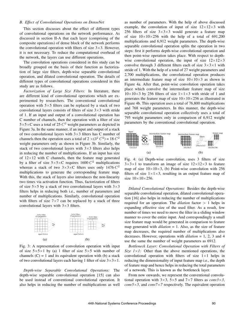
B. Effect of Convolutional Operations on DenseNet

This section discusses about the effect of different typesof convolutional operations on the network performance. Asdiscussed in section II-A that each layer (comprising of thecomposite operations) of dense block of the network performsthe convolutional operation with filters of size 3×3. However,it is not necessary. To reduce the computational overhead ofthe network, the layers can use different operations.

The convolution operations considered in this study can bebroadly grouped on the basis of their function as factoriza-tion of large size filters, depth-wise separable convolutionaloperation, and dilated convolutional operation. The details ofdifferent types of convolutional operations considered in thisstudy are as follows.

Factorization of Large Size Filters: In literature, thereare different kind of convolutional operations which are ex-perimented by researchers. The conventional convolutionaloperation with 5×5 filters can be replaced by a stack of twoconvolutional layers consists of filters of size 3×3 with strideof 1. If an input and output of a convolutional operation hasC number of channels, then the operation with a filter of size5×5×C uses a total of 25·C2 weight parameters as depicted inFigure 3a. In the same manner, if an input and output of a stackof two convolutional layers with 3×3 filters has C number ofchannels then the operation uses a total of 2 ×(32 C2) = 18·C2

weight parameters only as shown in Figure 3b. Similarly, thestack of two convolutional layers with 3×3 filters also helpsin reducing the number of multiplications. If an input has sizeof 12×12 with C channels, then the feature map generatedby a filter of size 5×5×C requires 1600·C2 multiplicationswhereas a stack of two 3×3×C filters uses only 1476·C2

multiplications to generate the corresponding feature map.With this, the stack of layers also introduces the non-linearitytwo times via activation function. Thus, factorization of filtersof size 5×5 by a stack of two convolutional layers with 3×3filters helps in reducing both i.e., number of parameters andnumber of multiplications. Similarly, convolutional operationwith filters of size 7×7 can be replaced by a stack of threeconvolutional layers with 3×3 filters.

input (5x5x1)

5x5x1 filter(25 parameters)

(a)

3x3x1 filter

3x3x1 filter

input (5x5x1)

(9 parameters)

(9 parameters)

(b)

Fig. 3: A representation of convolution operation with inputof size 5×5×1 by (a) 1 filter of size 5×5 with number ofchannels (C) = 1 and its equivalent operation with (b) a stackof two convolutional layers each having 1 filter of size 3×3×1.

Depth-wise Separable Convolutional Operations: Thedepth-wise separable convolutional operation [15] can alsobe used instead of conventional convolutional operation. Italso helps in reducing the number of multiplications as well

as number of parameters. With the help of above discussedexample, the convolution of input of size 12×12×3 with256 filters of size 3×3×3 would generate a feature mapof size 10×10×256 with the help of a total of 691,200multiplications and 6,912 weight parameters. The depth-wiseseparable convolutional operation splits the operation in twosteps: first it performs depth-wise convolutional operation andthen point-wise operation takes place. With respect to depth-wise convolutional operation, the input of size 12×12×3convolve through 3 different filters each of size 3×3×1 withstride of 1. With the help of a total of 27 weight parameters and2,700 multiplications, the convolutional operation producesan intermediate feature map of size 10×10×3 as shown inFigure 4a. After that, point-wise convolution operation takesplace which convolve the intermediate feature map of size10×10×3 by 256 filters of size 1×1×3 with stride of 1 andgenerates the feature map of size 10×10×256 as illustrated inFigure 4b. This operation uses a total of 76,800 multiplicationsand 768 weight parameters. In this manner, the depth-wiseseparable convolutional operation collectively uses a total of795 weight parameters only in comparison of 6,912 weightparameters by the conventional convolutional operation.

Input

12x12x3

3x3x3x1

filters

10x10x3

intermediate feature map

(a)

feature map

256x1x1x3

filters

10x10x3

intermediate feature map

10x10x256

(b)

Fig. 4: (a) Depth-wise convolution, uses 3 filters of size3×3×1 to transform an image of size 12×12×3 to featuremap of size 10×10×3, (b) Point-wise convolution with 256filters of size 1×1×3, resulting in an output feature map ofsize 10×10×256.

Dilated Convolutional Operations: Besides the depth-wiseseparable convolutional operation, dilated convolutional opera-tion [16] also helps in reducing the number of multiplicationsrequired for an operation. The dilation factor > 1 helps inexpanding effective size of the used filter. As a result, fewnumber of times we need to move the filter in a sliding windowmanner to cover the entire input. And correspondingly a smallsize feature map would be generated in comparison to featuremap generated with dilation = 1. Also, as the size of featuremap decreases, the required number of multiplications alsodecreases. However, operations with dilation = 1, 2, 3 and 4use the same the number of weight parameters as 6912.

Bottleneck Layer: Convolutional Operation with Filters ofSize 1×1: Other than the above mentioned operations, theconvolutional operation with filters of size 1×1 helps inreducing the dimensionality of input feature map i.e., the depthof feature map and hence helps in reducing the total parametersof a network. This is known as the bottleneck layer.

From now onwards, we represent the conventional convolu-tional operation with 3×3, 5×5 and 7×7 filters as conv3×3,conv5×5, and conv7×7 respectively. The equivalent operation


of 5×5 filters by a stack of two convolutional layers with 3×3filters is denoted as 2 conv3×3. Similarly, a stack of threeconvolutional layers with 3×3 filters has been represented by3 conv3×3 which denotes an equivalent convolutional oper-ation of 7×7 filters. The depth-wise separable convolutionaloperation is denoted as depth sep conv which is followed bysize of filters to denote the used filters size. For exampledepth sep conv3×3 denotes depth-wise separable convolu-tional operation with filters of size 3×3. Similarly, the termdepth sep conv5×5 and depth sep conv7×7 represents theoperation with 5×5 and 7×7 filters respectively. The dilatedconvolutional operation with dilation of 2 has been denotedby d conv3×3. Some of the above discussed operations havebeen considered ahead in this study.

III. SIMULATIONS

In this study, PyTorch 1.8.0 [17] was used for developmentof the proposed approach. All experiments were performed onGoogle Colab which provided K80 GPU.

The proposed study used COVID-19 RadiographyDatabase [18], [19] to study the effect of various convolutionaloperations on DenseNet. It consisted of a total of 3886 imagesof X-ray out of which 1200 and 1345 images belonged tothe class of COVID-19 and viral pneumonia respectively.The remaining 1341 images were healthy images. Thus, theproblem was considered as three-class classification problem.Moreover, two-class classification problem had also beenconsidered for differentiating i) class of COVID-19 imagesfrom viral pneumonia and ii) normal class of X-ray imagesfrom COVID-19. The dataset was divided into train and testset in the ratio of (80-20)%. Figure 5 shows sample imagesof the considered dataset.

(a) (b) (c)

Fig. 5: COVID-19 Radiography Database: an image belongingto class of (a) normal (b) viral pneumonia and (c) COVID-19.

Extensive experiments were performed to study the effectof various convolutional operations on DenseNet with respectto COVID-19 Radiography Database. Since each layer of thedense block performed the convolutional operation throughthe function Hl as BN-ReLu-Conv1×1-BN-ReLu-Conv3 ×3,only last convolution operation of the composite function Hl

was modified to see the effect. For example, in order to usethe depth-wise separable convolutional operation with filtersof size 3×3, the composite function Hl can be modifiedas BN-ReLu-Conv1×1-BN-ReLu-depth Sep Conv3×3, wheredepth Sep Conv3×3 denotes the depth-wise separable convo-lutional operation with 3 × 3 filters. In this manner, differentnetworks with various operations discussed above can bestudied. Next, we discuss details of the experiments performed

to study the effect of change in the last (Conv3×3) convolutionoperation of the composite function for every layer in the denseblock of the standard DenseNet.

A pre-defined network structure is required to study theeffect of a hyper-parameter. In this study, two pre-definednetworks i.e., Net 1 and Net 2 were considered. The details ofarchitecture of Net 1 are as follows: first convolutional layer ofthe network used filters of size 3×3, stride of 1 and padding of1. Each dense block consisted of ten convolutional layers withfilters of size 3×3, stride of 1 and padding of 1. All transitionblocks used convolutional layer with filters of size 3×3, strideof 1, padding of 1 and average pooling layer. All convolutionallayers were followed by batch normalization layer (BN) andRectified Linear Unit (ReLU). The last layer used averagepooling operation. Net 2 used the same architecture as of Net 1except parameters of the convolutional layer used by transitionblock. In case of Net 2, this layer performed convolutionaloperation with filters of size 3×3 with stride of 2. The trainingof networks was performed by ADAM algorithm with learningrate of 0.001 for 200 epochs.

Two set of experiments were performed as Set 1 and Set2. Set 1 included the experiments which had used pre-definedstructure of the Net 1. Similarly, the experiments which hadconsidered pre-defined structure of the Net 2, were included inthe Set 2. Table I shows the effect of the various convolutionaloperations on DenseNet. As it can be seen from the tablethat with respect to Set 1, the networks corresponding toconventional convolutional operation with filters of size 7×7i.e., conv7×7 and depth-wise separable convolutional opera-tion with 7×7 filters (i.e., depth sep conv7×7) had shownthe highest accuracy of 97.93%. The depth-wise separableconvolutional operation controls the number of parameters ofa network and thus, the network with depth sep conv7×7operation consisted of 2.10 times less number of weightparameters in comparison of network with conv7×7 operation.With respect to floating point operations (Flops), a reductionof 2.7 times was also observed in the network correspondingto depth sep conv7×7 operation as compared to the networkwith conv7×7 operation. Figure 6a shows the learning curveof the network corresponding to depth sep conv7×7 opera-tion. For an image of class COVID-19, the class activationvisualization generated by the network using the Grad-CAMapproach [20] has been shown in Figure 6b. As it can be seenfrom the figure that the network has efficiently recognized theregions which are responsible for COVID-19.

With respect to Set 2 the maximum accuracy of 97.67% wasachieved by various networks which had used convolutionaloperation as 2 conv3×3, 3 conv3×3, conv5×5, and conv7×7.Among these networks, the network with conv5×5 operationused a total of 0.13 million parameters which were 1.09,1.22, and 1.29 times less in comparison of parameters of net-work corresponding to conv7×7, 2 conv3×3, and 3 conv3×3operation respectively. Moreover, a significant reduction hadalso been observed in terms of Flops. As it can be seenfrom the Table I that the network with conv5×5 operationused minimum number of Flops as of 0.32G among the


TABLE I: Effect of various convolutional operations on DenseNet with respect to COVID-19 Radiography Database forthree-class classification problem

Operation Parameters Flops (G) Accuracy Weighted Precision Weighted Recall Weighted F1-ScoreSet 1

conv3×3 152234 1.71 0.9625 0.9628 0.9625 0.9625conv5×5 221463 2.94 0.9703 0.9633 0.9612 0.9613conv7×7 325143 4.79 0.9793 0.9784 0.9770 0.9780depth sep conv3×3 125703 1.26 0.9651 0.9733 0.9509 0.9510depth sep conv5×5 221463 1.47 0.9754 0.9505 0.9702 0.9703depth sep conv7×7 154503 1.77 0.9793 0.9772 0.9767 0.97672 conv3×3 221463 1.90 0.9741 0.9716 0.9702 0.98063 conv3×3 172503 2.08 0.9767 0.9733 0.9728 0.9727d conv3×3 152234 1.71 0.9754 0.9757 0.9754 0.9754

Set 2conv3×3 121274 0.27 0.9600 0.9494 0.9713 0.9601conv5×5 132794 0.32 0.9767 0.9805 0.9680 0.9742conv7×7 150074 0.40 0.9767 0.9730 0.9729 0.9729depth sep conv3×3 125594 0.31 0.9600 0.9611 0.9599 0.9600depth sep conv5×5 137114 0.36 0.9716 0.9692 0.9709 0.9698depth sep conv7×7 154394 0.43 0.9754 0.9756 0.9754 0.97542 conv3×3 162674 0.46 0.9767 0.9806 0.9717 0.97613 conv3×3 172394 0.51 0.9767 0.9768 0.9767 0.9767d conv3×3 121274 0.27 0.9692 0.9661 0.9651 0.9652

(a) (b)

Fig. 6: Representation of (a) learning curve of network cor-responding to the operation depth sep conv7×7; (b) classactivation heatmap of the network for an image belonging toclass of COVID-19 using Grad-CAM approach.

networks which had shown the highest accuracy. Based onthe simulation results, it was observed that various convolu-tional operations highly effect the weight parameters and thus,performance and memory requirement of the network. Theseoperations also effect the total number of Flops which furtherprovides improvements toward the computational cost andhelps in achieving economical convolutional networks. Thus,we can say that convolutional operations seem to be a crucialparameter of deep convolutional networks and an automaticscheme is required to identify the best suitable operation withrespect to a given input.

The overall highest accuracy of 97.93% was achieved bythe network corresponding to depth sep conv7×7 operationwhich had used pre-defined structure of Net 1. Since the Net1 extracted relatively large number of features in comparisonof Net 2, it had shown comparatively higher performance.Due to the nature of the considered dataset, performance interms of weighted value of precision, recall, f1-score was alsocalculated as shown in Table I. Based on the weighted recall itwas found that the network corresponding to the convolutional

operation depth sep conv7×7 had shown the highest value asof 97.67% which implies that the network is highly sensitivefor identification of infection caused by SARS-CoV-2 virus incomparison of other networks.

Since the network with depth sep conv7×7 operation hadoutperformed all other networks, it was further considered fortwo-class classification problems. The network was highly effi-cient in differentiating i) class of normal images from COVID-19 and ii) class of viral pneumonia images from COVID-19 byshowing 100% accuracy. Thus, based on the simulation studieswe can say that the DenseNet with depth sep conv7×7 opera-tion has the capabilities of handling intricacies associated withX-ray images and thus, it has efficiently solved the consideredtwo-class as well as three-class classification problem.


A comparison of the obtained results with existing ap-proaches has been done in Table II. As it can be seenthat the proposed study has performed well for both two-class and three-class classification problem. The networksmentioned in Table II have used for transfer learning approachas reported in [18]. In case of two class classification problem,an improvement of 0.30% has been observed in comparisonof DenseNet-201 which has shown an accuracy of 99.70%.

In this paper, we have studied the effect of various convo-lutional operations on DenseNet and based on the simulationresults with respect to the considered dataset it has been foundthat types of convolutional operations can be defined as ahyper-parameter of deep convolutional networks. It has alsobeen observed that various convolutional operations highlyeffect computational cost and play a pivotal role in designingof efficient and economical convolutional networks. In future,an automatic approach can be designed to find the best suitableconvolutional operation based on the nature of a given input.


TABLE II: Comparison with other existing models as reported in [18]

Network Accuracy Weighted Precision Weighted Recall Weighted F1-ScoreTwo Class Classification Problem: COVID19 and Normal

SqueezeNet 0.9940 0.9940 0.9940 0.9940MobileNetv2 0.9965 0.9965 0.9965 0.9965ResNet18 0.9960 0.9960 0.9960 0.9960InceptionV3 0.9940 0.9880 0.9833 0.9856ResNet101 0.9960 0.9960 0.9960 0.9960CheXNet 0.9969 0.9969 0.9969 0.9969DenseNet201 0.9970 0.9970 0.9970 0.9970Proposed study 1.0000 1.0000 1.0000 1.0000

Three Class Classification Problem: COVID19, Viral Pneumonia and NormalSqueezeNet 0.9510 0.9518 0.9510 0.9514MobileNetv2 0.9622 0.9625 0.9622 0.9623ResNet18 0.9644 0.9648 0.9644 0.9646InceptionV3 0.9620 0.9700 0.9640 0.9660CheXNet 0.9694 0.9643 0.9642 0.9642DenseNet201 0.9794 0.9795 0.9794 0.9794VGG19 0.9600 0.9650 0.9625 0.9638Proposed study 0.9793 0.9772 0.9767 0.9767

An integration of convolutional operations with connectivitypatterns among the layers of dense block can be studied tofurther improve design of convolutional networks.

REFERENCES

[1] (2021, March). [Online]. Available: https://covid19.who.int[2] S. Sanche, Y. T. Lin, C. Xu, E. Romero-Severson, N. Hengartner,

and R. Ke, “High Contagiousness and Rapid Spread of Severe AcuteRespiratory Syndrome Coronavirus 2,” Emerging Infectious Diseases,vol. 26, no. 7, pp. 1470–1477, 2020.

[3] C. Huang, Y. Wang, X. Li, L. Ren, J. Zhao, and Y. Hu, “Clinical featuresof patients infected with 2019 novel coronavirus in Wuhan, China,” TheLancet Journal, vol. 395, no. 10223, pp. 497–506, 2020.

[4] V. M. Corman, O. Landt, M. Kaiser, R. Molenkamp, A. Meijer, D. K.Chu, T. Bleicke, S. Brunink, J. Schneider, M. L. Schmidt, D. G. Mulders,B. L. Haagmans, B. van der Veer, S. van den Brink, L. Wijsman,G. Goderski, J.-L. Romette, J. Ellis, M. Z. M. Peiris, H. Goossens,C. Reusken, M. P. Koopmans, and C. Drosten, “Like 2 downloaddetection of 2019 novel coronavirus (2019-nCoV) by real-time RT-PCR,”Eurosurveillance, vol. 25, no. 3, pp. 1–30, 2020.

[5] D. K. W. Chu, Y. Pan, S. M. S. Cheng, K. P. Y. Hui, P. Krishnan,Y. Liu, D. Y. M. Ng, C. K. C. Wan, P. Yang, Q. Wang, M. Peiris, andL. L. M. Poon, “Molecular Diagnosis of a Novel Coronavirus (2019-nCoV) Causing an Outbreak of Pneumonia,” Clin Chem, vol. 66, no. 4,pp. 549–555, 2020.

[6] Y. Fang, H. Zhang, J. Xie, M. Lin, L. Ying, P. Pang, and W. Ji,“Sensitivity of Chest CT for COVID-19: Comparison to RT-PCR,”Radiology, vol. 296, no. 2, pp. 1–3, 2020.

[7] Y. Lei, H.-W. Zhang, J. Yu, and M. N. Patlas, “COVID-19 Infection:Early Lessons,” Canadian Association of Radiologists Journal, vol. 71,no. 3, pp. 251–252, 2020.

[8] L. A. Rousan, E. Elobeid, M. Karrar, and Y. Khader, “Chest x-ray findings and temporal lung changes in patients with COVID-19pneumonia,” BMC Pulmonary Medicine, vol. 20, no. 245, pp. 1–9, 2020.

[9] L. Cai, J. Gao, and D. Zhao, “A review of the application of deeplearning in medical image classification and segmentation,” Annals ofTranslational Medicine, vol. 8, no. 11, pp. 1–15, 2020.

[10] A. Esteva, K. Chou, S. Yeung, N. Naik, A. Madani, A. Mottaghi, Y. Liu,E. Topol, J. Dean, and R. Socher, “Deep learning-enabled medicalcomputer vision,” npj Digital Medicine, vol. 4, no. 5, pp. 1–5, 2021.

[11] X. Xie, J. Niu, X. Liu, Z. Chen, S. Tang, andS. Yu, “A survey on incorporating domain knowledge intodeep learning for medical image analysis,” Medical ImageAnalysis, vol. 69, p. 101985, 2021. [Online]. Available:https://www.sciencedirect.com/science/article/pii/S1361841521000311

[12] T. Li, W. Bo, C. Hu, H. Kang, H. Liu, K. Wang, and H. Fu,“Applications of deep learning in fundus images: A review,” MedicalImage Analysis, vol. 69, p. 101971, 2021. [Online]. Available:https://www.sciencedirect.com/science/article/pii/S1361841521000177

[13] Soniya, S. Paul, and L. Singh, “Sparsely Connected DenseNet forMalaria Parasite Detection,” in Advances in Systems Engineering, Lec-ture Notes in Mechanical Engineering, V. H. Saran and R. K. Misra,Eds. Springer, Singapore, 2021, pp. 1–6.

[14] G. Huang, Z. Liu, L. v. d. Maaten, and K. Q. Weinberger, “ConvolutionalNetworks with Dense Connectivity,” IEEE Transactions on PatternAnalysis and Machine Intelligence, p. Early Access, 2019.

[15] F. Chollet, “Xception: Deep Learning with Depthwise Separable Con-volutions,” in IEEE Conference on Computer Vision and Pattern Recog-nition (CVPR), ser. CVPR’16. Honolulu, HI, USA: IEEE ComputerSociety, July 21-26 2016.

[16] F. Yu and V. Koltun, “Multi-Scale Context Aggregation by Dilated Con-volutions,” in 4th International Conference on Learning Representations,(ICLR), ser. Conference Track Proceedings, Y. Bengio and Y. LeCun,Eds., San Juan, Puerto Rico, May 2-4, 2016 2016.

[17] A. Paszke, S. Gross, F. Massa, A. Lerer, J. Bradbury, G. Chanan,T. Killeen, Z. Lin, N. Gimelshein, L. Antiga, A. Desmaison,A. Kopf, E. Yang, Z. DeVito, M. Raison, A. Tejani, S. Chilamkurthy,B. Steiner, L. Fang, J. Bai, and S. Chintala, “PyTorch: AnImperative Style, High-Performance Deep Learning Library,” inAdvances in Neural Information Processing Systems 32, H. Wallach,H. Larochelle, A. Beygelzimer, F. dAlche Buc, E. Fox, and R. Garnett,Eds. Curran Associates Inc., 2019, pp. 8026–8037. [Online].Available: http://papers.nips.cc/paper/9015-pytorch-an-imperative-style-high-performance-deep-learning-library.pdf

[18] M. E. H. Chowdhury, T. Rahman, A. Khandakar, R. Mazhar, M. A.Kadir, Z. B. Mahbub, K. R. Islam, M. S. Khan, A. Iqbal, N. A. Emadi,M. B. I. Reaz, and M. T. Islam, “Can AI Help in Screening Viraland COVID-19 Pneumonia?” IEEE Access, vol. 8, pp. 132 665–132 676,2020.

[19] T. Rahman, A. Khandakar, Y. Qiblawey, A. Tahir, S. Kiranyaz, S. B.Abul Kashem, M. T. Islam, S. Al Maadeed, S. M. Zughaier, M. S. Khan,and M. E. Chowdhury, “Exploring the effect of image enhancementtechniques on covid-19 detection using chest x-rays images,” Computersin Biology and Medicine, pp. 1–49, 2021. [Online]. Available:https://www.sciencedirect.com/science/article/pii/S001048252100113X

[20] R. R. Selvaraju, M. Cogswell, A. Das, R. Vedantam, D. Parikh, andD. Batra, “Grad-CAM: Visual Explanations from Deep Networks viaGradient-Based Localization,” International Journal of Computer Vision(IJCV), vol. 128, pp. 336–359, 2020.


Sustainable and Affordable Lower Limb Prosthetics for Health Care Systems

Dheeraj Kumar Angajala

Additive Manufacturing Lab, Faculty of

Engineering


Agra, India

[email protected]

Ankit Sahai


Engineering


Agra, India

[email protected]

Rahul Swarup Sharma


Engineering


Agra, India

[email protected]

Abstract— Every year thousands of amputees from all

over the world, approach various Indian NGOs like

Bhagwan Mahaveer Viklang Sahayata Samiti (BMVSS),

Hardayal Viklang Kendra (HVK), Ratna Nidhi Charitable

Trust, JYOT Charitable Trust, MUKTI India for affordable

prosthetic devices. These prosthetic devices provide the

amputees mobility and improved quality of life, but the

manufacturing practices and the end product are not

sustainable. The NGOs use traditional methods to

manufacture lower limb prosthetic sockets which require

expertise, are labour-intensive and produce a lot of waste.

This paper aims to identify the problems with the

manufacturing methods and traditionally manufactured

prosthetics, thereby proposing sustainable eco-friendly

healthcare solutions. We visited HVK, BMVSS and

conducted a survey based on Quebec User Evaluation of

Satisfaction with assistive Technology (QUEST 2.0). Based

on the survey results it is observed that, although these

prosthetics are affordable, provide durability with high

impact resistance and tensile strength, they lack

comfortability, are heavy, difficult to repair or adjust and

require higher service time. To address the above limitations,

we designed and tested lower limb prosthetic that is

manufactured sustainably using 3D scanning and Additive

manufacturing techniques which can provide quick solution

to improve mobility of the amputees.

Keywords— Additive Manufacturing, 3D Scanning, Prosthetics, QUEST2.0

I. INTRODUCTION

Prosthesis are the artificial devices which enables the amputee to replicate the function and/or cosmetic appearance of missing body part. Lower limb prosthesis tries to replicate the function of lower limbs of the body like Hip, Thigh, Knee, Ankle and Foot [1]. As shown in the Fig.1 the main components of the lower limb prosthesis are socket, knee joint, pylon and foot [2].

Fig. 1. Parts of Lower Limb Prosthesis

The socket is the crucial part among these parts as it forms the primary interface between the residual limb and the prosthesis. For better rehabilitation of the amputee the socket must be comfortable, stable and enable proper load transmission [3], [4]. Improper design of the socket can

cause rupture between the residual limb and the socket which leads to injuries and discomfort to the amputee [5].

Unfortunately, there is not considerable data available on the number of amputees in India. In 1981 Dr. D Mohan mentioned in his report that in India there are approximately half a million were amputees and the numbers are increasing 17000 annually [6]. According to the 2011 Census data there are 5,436,000 people with locomotor disabilities in India [7]. According to the statistics collected by National Sample Survey Office of India in 2016 it is estimated that disabled people comprises 2.2% of overall population out which 20% are suffering with movement impairment and 230,000 amputees needed prosthetic care [8]. In the latest report by World Health Organisation it is observed that approximately 10 million Indians are living with movement impairment and in overall world only 10% of the disabled people have access to assistive devices [9]. Several studies showed that access to the assistive devices is the crucial factor in improving the Quality of life (QOL) of disabled people [10]–[12].

Various Indian NGOs like Bhagwan Mahaveer Viklang Sahayata Samiti (BMVSS), Hardayal Viklang Kendra (HVK), Ratna Nidhi charitable trust, JYOT Charitable Trust, MUKTI India etc... provide affordable prosthetic devices to amputees with little or no cost. BMVSS is one of the oldest NGO which have multiple branches across the world. BMVSS fitted over 1.9 million amputees with limb prosthetics so far [13]. RNCT is another vastly growing NGO which provided mobility devices for 0.26 million since 2011. [14]. Even with the so many NGOs trying to make available the affordable prosthesis still large number of amputees faces problems in obtaining prosthetic devices and post fitment services. These NGOs use traditional methods to manufacture lower limb prosthetic sockets which require expertise, are labour-intensive and produce a lot of waste.

Additive manufacturing (AM) is a process in which material is added layer by layer to create a physical object by using a CAD model [15]. Similar to the disruption caused by steam powered engines, electrical machines and electronics in the first, second and third industrial revolutions AM is disrupting the traditional machining processes and it become one of the nine pillars of fourth industrial revolution (Industry 4.0) [16]. AM is continuously evolving and is projected to make deepest impact in many areas like automobiles, aerospace, medical, construction, education and so on. [17]–[19].

One of the main advantage of AM over traditional manufacturing processes is that the mechanical properties of the end product can be controlled by controlling its internal structure through infill density, Infill pattern.[20]–[22].





http://www.jyot.org/

http://www.muktiindia.org/



http://www.muktiindia.org/

Fig. 2. Traditional manufacturing process of lower limb prosthesis

II. TRADITIONAL MANUFACTURING METHODS

In Traditional Method, the process starts with wrapping of plaster and glass fibre on residual limb to get its shape and geometry in the form of a cast. Then the prosthetist locates pressure points and build up or remove material to make a note of the size. The plaster is removed and filled up with the slurry. After the slurry is settled, the glass fiber cast is destroyed to obtain positive mould which contains geometry of residual limb. Then high-density polyethylene (HDPE) or any other polymer tube is heated and placed over the positive mould to obtain the desired shape of the limb. Once the limb is formed the mould is removed and the prosthetic is trimmed and finished. Straps and foot ankle assembly are attached to the prosthetic formed before testing it on patient. [23].The process is shown in the Fig.2.

To understand the effectiveness and drawbacks of the traditional manufacturing method, merits and demerits of traditionally manufactured prosthesis we have conducted a survey using QUBEC QUEST 2.0 and the details are discussed in the following section.

III. CASE STUDY AND SURVEY

We have conducted a case study to understand and analyse lower limb prosthetic manufacturing in India. To understand the current manufacturing process, we visited the HVK and BMVSS NGOs that manufacture prosthetics for amputees. We analysed their processes, discussed with the doctors and prosthetists associated with the NGO to understand the benefits and the limitations. We took an control group of 30 lower limb amputees from each NGO and used Quebec User Evaluation of Satisfaction with assistive Technology (QUEST 2.0). QUEST 2.0 analyses the amputee’s satisfaction levels on 5-point scale 1 being not satisfied and 5 being fully satisfied about the prosthetic device and the services provided by the manufacturer.

As shown in the Fig 3 we have observed that the people approaching these NGOs are mainly farmers, daily wage workers and students. While discussing with these amputees we observed that most of them are unemployed because of the disability and getting a prosthetic devise is

important for them to get independent and to improve their quality of life.

Fig. 3. Occupation details of the Survey Group

A. Experience evaluation of assistive devices

The QUEST 2.0 survey uses the following 8 factors to evaluate the experience of amputee with the prosthetic device.

• The dimensions (size, height, length, width) of assistive device

• The weight of assistive device

• The ease in adjusting (fixing, fastening) the parts of assistive device

• The safety and security of assistive device

• The durability (endurance, resistance to wear) of assistive device

• Ease in using the assistive device

• Comfort in using the assistive device

• The effectiveness of the assistive device (the degree to which the device meets amputees needs)

The results of the survey about assistive device are pictographically represented in the Fig 4. We can observe

1.Residual limb measurement

• Wrapping glass fibre plaster on limb

• Shaping with hand

• Taking pressure points

2.Obtaining Positive mould.

•Pouring slurry in the plaster mould and Leaving it for settling down and hardened

•Breaking the negative mould to obtain Postrive mould

3.Shaping the postive mould

•Prosthetistt carefully gives shape to the mould

4.Making of Prosthetic leg

• HDPE pipe is heated and placed on the postive mould

5.Attaching other parts

• Attachement of Ankle foot

• Attachement o Straps and belts

• Liner is pasted

6.Finishing

• Final touchings are given to corect minor imperfections

7.Testing on patient

• Testing of prsothetic on patient

• Making changes according to the patient fitment

Gait analysis

• Patient gait is analysed by observing them walking and necesseray changes will be made.


that the factors comfort and weight of the device received least average score.

Fig. 4. QUEST 2.0 Average score for assistive device

B. Experince evaluation of services provided

The QUEST 2.0 survey uses the following 4 factors to evaluate the experience of amputee with the services provided by the manufacturer of the device.

• The service delivery program (procedures, length of time)

• The repairs and servicing (maintenance) provided for the assistive device

• The quality of the professional services (information, attention) received

• The follow-up services (continuing support services) received

The results of the survey about services provided are pictographically represented in the Fig 5. We can observe that the factors service delivery and repairs and servicing received least average score.

Fig. 5. QUEST 2.0 Average score for services

The reasons for the above survey results have been analysed and discussed in the following section. A sustainable process to overcome the aforesaid problems is also proposed in the next section.

IV. SURVEY ANALYSIS AND PROPOSALS

Following reasons are observed for receiving low average score in the comfort and weight factors during our case study.

• Traditionally manufactured lower limb prosthetics are heavy, require manual engineering to manufacture.

• Comfortless of the prosthetic is directly depend on the locating pressure tolerant and pressure sensitive areas. In traditional process because of lot manual processes involved prosthetic device needs post processing adjustments to make it comfortable.

• Any variation in the dimensions of prosthetic causes friction between the skin and the device which leads to injuries.

• Any change in the dimensions of the amputee, renders the prosthetic to be useless and requires designing of a new prosthetic.

Following reasons are observed for receiving low average score in the service delivery and repairing.

• A lot of manual processes are involved from creation of mould to the final testing phase which makes the conventional method labour intensive and increase the service delivery time

• To obtain the size of the limb, the patient’s residual limb is wrapped with plaster, which may cause discomfort to them.

• The patient needs to visit the facility multiple times or to stay there for couple of days to obtain the prosthetic

• For every new prosthetic to be designed for a given patient, the whole process needs to be repeated causing discomfort to patient

• Lack of regional service centers cause higher service time and involves travelling.

Further observations about the process used are as follows.

• The glass fiber material wrapped around the residual limb and the positive mould made out the glass fibre cast can’t be reused, and they create lot of waste.

• Process is dependent on well experienced technician to locate pressure points.

• The method is less precise and accurate due to involvement of multiple processes

• The prosthetic needs to be cushioned for better fitting.

Based on the above analysis we are proposing a sustainable manufacturing method for lower limb prosthetic which is efficient in terms of both production and usage.

V. SUSTAINABLE PROSTHEICS

In the propose approach we use 3D scanning technologies and Additive manufacturing process to manufacture lower limb prosthetics. The above technique was adopted to design and develop prosthetic for four lower limb amputees of different age groups and gender who approached Hardayl Viklang Kendra. A complete prosthetic device for one patient is developed and tested on patient to understand the limitations and advantages.


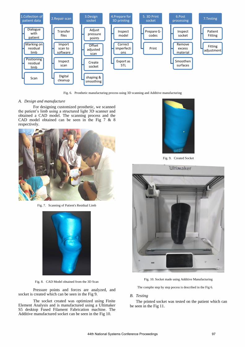
Fig. 6. Prosthetic manufacturing process using 3D scanning and Additive manufacturing

A. Design and manufacture

For designing customized prosthetic, we scanned the patient’s limb using a structured light 3D scanner and obtained a CAD model. The scanning process and the CAD model obtained can be seen in the Fig 7 & 8 respectively.

Fig. 7. Scanning of Patient's Residual Limb

Fig. 8. CAD Model obtained from the 3D Scan

Pressure points and forces are analyzed, and socket is created which can be seen in the Fig 9.

The socket created was optimized using Finite Element Analysis and is manufactured using a Ultimaker S5 desktop Fused Filament Fabrication machine. The Additive manufactured socket can be seen in the Fig 10.

Fig. 9. Created Socket

Fig. 10. Socket made using Additive Manufacturing

The complte step by step pocess is described in the Fig 6.

B. Testing

The printed socket was tested on the patient which can be seen in the Fig 11.

1.Collection of patient data

Dialogue with

patient

Marking on residual

limb

Postioning residual

limb

Scan

2.Repair scan

Transfer files

Import scan to

software

Inspect scan

Digital cleanup

3.Design socket

Adjust pressure

points

Offset adjusted

scan

Create socket

shaping & smoothing

4.Prepare for 3D prinitng

Inspect model

Correct imperfecti

ons

Export as STL

5. 3D Print socket

Prepare G-codes

Print

6.Post processing

Inspect socket

Remove excess

material

Smoothen surfaces

7.Testing

Patient Fitting

Fitting adjustment


Fig. 11. Testing of Additive manufactured socket on patient

Following observation are made during the testing

• 3D scanning technique enables accurate, quicker and no contact measurement of the residual limb of the amputee compared to traditional methods.

• No need of expert prosthetist to obtain the measurement.

• Once the 3D model is obtained the process can be automated to create the socket which saves a lot time and there is no need of expert prosthetist to modify the shape of the positive mould.

• Finite element analysis can be done on 3d models to obtain accurate pressure points instead of relying on expert prosthetist.

• Once the socket is created its 3d file can be sent to the expert for final evaluation and approval.

• The wight and mechanical properties can be varied by varying infill density and pattern during additive manufacturing of the of the socket.

• Time taken to print a socket can vary between 24 hrs to 40 hrs.

• Optimization techniques like topology optimization and generative design can be explored to reduce the weight and the printing time of the socket.

VI. CONCLUSION

3D scanning and additive manufacturing techniques enable remote measurements of residual limb and eliminate need for amputee to visit manufacturing centre. It enables automation from measurement to final socket generation thereby eliminating manual processes and need of expert prosthetists at each process. The proposed method helps in sustainably manufacturing prosthetic by reducing the waste generated to minimum. Further study is required to reduce the manufacturing time, clinical analysis is required to validate the functioning of the socket and user satisfaction over a longer period of time.

References

[1] M. R. Pitkin, Biomechanics of lower limb prosthetics, Illustrate. Springer, 2009, 2010.

[2] “parts-of-a-prosthesis.” [Online]. Available: https://www.llop.com/wp-content/uploads/2016/12/parts-of-a-prosthesis-268x300.jpg. [Accessed: 25-Sep-2020].

[3] L. Paternò, M. Ibrahimi, E. Gruppioni, A. Menciassi, and L. Ricotti, “Sockets for limb prostheses: A review of existing

technologies and open challenges,” IEEE Trans. Biomed. Eng., vol. 65, no. 9, pp. 1996–2010, 2018.

[4] J. Fergason and D. G. Smith, “Socket considerations for the patient with a transtibial amputation,” in Clinical Orthopaedics and Related Research, 1999, vol. 361, no. 361, pp. 76–84.

[5] S. Sankaran, P. R. Murugan, J. C. Johnson, H. J. S. Abdullah, C. M. N. Raj, and D. Ashokan, “Prevention of skin problems in patients using prosthetic limb: A review of current technologies and limitations,” Proc. 2019 IEEE Int. Conf. Commun. Signal Process. ICCSP 2019, pp. 77–81, 2019.

[6] D. Mohan, “A report on amputees in India,” Orthot. Prosthetics, vol. 40, no. 1, pp. 16–32, 1986.

[7] “India Census Data 2011.” [Online]. Available: https://www.censusindia.gov.in/2011census/population_enumeration.html.

[8] National Sample Survey Office, “Disabled persons in India: A statistical profile,” 2016.

[9] Port-er, “60 Standards for Prosthetics and Orthotics published by WHO.” 2017.

[10] L. Magnusson et al., “Quality of life of prosthetic and orthotic users in South India: A cross-sectional study,” Health Qual. Life Outcomes, vol. 17, no. 1, Mar. 2019.

[11] S. R. Wurdeman, P. M. Stevens, and J. H. Campbell, “Mobility Analysis of AmpuTees (MAAT I): Quality of life and satisfaction are strongly related to mobility for patients with a lower limb prosthesis.,” Prosthet. Orthot. Int., vol. 42, no. 5, pp. 498–503, Oct. 2018.

[12] B. A. Powell, S. W. Mercer, and C. Harte, “Measuring the impact of rehabilitation services on the quality of life of disabled people in Cambodia.,” Disasters, vol. 26, no. 2, pp. 175–191, Jun. 2002.

[13] “Bhagwan Mahaveer Viklang Sahayata Samiti.” 2019.

[14] “Reports.” [Online]. Available: https://ratnanidhi.org/reports/. [Accessed: 03-Apr-2021].

[15] ASTM International, “Global Leader in Additive Manufacturing Standards,” 2017.

[16] M. et al Rüßmann, “Future of Productivity and Growth in Manufacturing,” Bost. Consult., no. April, 2015.

[17] K. V Wong and A. Hernandez, “A Review of Additive Manufacturing,” Int. Sch. Res. Netw. ISRN Mech. Eng., vol. 2012, 2012.

[18] U. M. Dilberoglu, B. Gharehpapagh, U. Yaman, and M. Dolen, “The Role of Additive Manufacturing in the Era of Industry 4.0,” Procedia Manuf., vol. 11, no. June, pp. 545–554, 2017.

[19] P. Yadav, I. Singhal, B. Tyagi, A. Sahai, and R. S. Sharma, “Intensifying Hands-on Learning and Experimentation of Fused Deposition Modeling Three-Dimensional Printers,” Springer, Singapore, 2020, pp. 309–317.

[20] P. Yadav, A. Sahai, and R. S. Sharma, “Strength and Surface Characteristics of FDM-Based 3D Printed PLA Parts for Multiple Infill Design Patterns,” J. Inst. Eng. Ser. C, vol. 102, no. 1, pp. 197–207, Feb. 2021.

[21] P. Yadav, A. Sahai, and R. S. Sharma, “Experimental Investigations for Effects of Raster Orientation and Infill Design on Mechanical Properties in Additive Manufacturing by Fused Deposition Modelling,” Springer, Singapore, 2019, pp. 415–424.

[22] D. K. Angajala, A. Sahai, and R. S. Sharma, “Re-engineering Infill Density System for 3D Printing,” in Lecture Notes in Mechanical Engineering, 2021, pp. 293–298.

[23] R. Seymour, Prosthetics and Orthotics, Lower Limb and Spinal. Lippncott Williams & Wilkins, 2002.


Low-Power and High-Frequency Optogenetic Retinal Prosthetics with ChRmine

*Note: Sub-titles are not captured in Xplore and should not be used

Himanshu Bansal Dept. of Physics and Computer Science


[email protected]

Neha Gupta Dept. of Physics and Computer Science


[email protected]

Sukhdev Roy Dept. of Physics and Computer Science


[email protected]

Abstract— Optogenetics has emerged as a promising technique in the field of retinal prostheses as new potent opsins with high light-sensitivity, red-shifted activation wavelength and large photocurrent have been discovered or engineered in the last decade. In the present study, a detailed theoretical analysis of low-power and high-frequency optogenetic excitation of retinal ganglion neurons using ChR2 and ChRmine, the newly discovered red-shifted opsin has been carried out by formulating accurate theoretical models, which are in excellent agreement with reported experimental results. Minimum pulse width required to achieve peak photocurrent in each opsin has been determined that is useful to optimize light power. The study reveals that ChRmine can evoke high-fidelity spiking upto 35 Hz, whereas ChR2 fails above 10 Hz. Also, the required power of each light pulse in ChRmine is three orders of magnitude smaller than ChR2. The present study highlights the importance of ChRmine as a potential opsin for optogenetic retinal prostheses.

Keywords—Neurophotonics, optogenetics, retinal prostheses, ChRmine.

I. INTRODUCTION Retinal degenerative diseases such as, retinitis pigmentosa

and macular degeneration are often caused due to loss of light-sensitive rod and cone photoreceptors in the retina. However, the remaining retinal tissue retains functionality and connections to the brain [1, 2]. Earliar efforts have been made to directly activate the remaining retinal neurons through electrical stimulation to restore some visual perception [3, 4]. However, the use of these electrical prosthetic devices is limited due to invasiveness and low spatial resolution [1, 5, 6].

In the last decade, optogenetics has provided opportunities for a wide-range of applications in and beyond neuroscience including retinal prostheses [7-9]. In optogenetics, light-sensitive proteins are expressed transgenically in neurons to mediate light-dependent transport of ions across the membrane and to excite or inhibit neural activity by causing depolarization or hyperpolarization of the neurons, respectively [10, 11]. Since its first use to restore light responses in the blind mice by expressing Channelrhodopsin-2 (ChR2) in thalamic projecting neurons, many new opsins have been tested to enhance safety and feasibility [5, 12-16].

Recently, screening guided by crystal structure-derived knowledge of residues forming the cation-conducting ChR pore, revealed ~1000 suitable new cation-conducting ChR sequences [17]. Optimization of these sequences for mammalian expression resulted in a promising marine opsin gene, named ChRmine from Tiarina fusus [18]. Expression of ChRmine in cultured hippocampal neurons has been reported

to give rise to a very large inward photocurrent ~ 4 nA, with red-shifted excitable wavelength. Along with high light sensitivity, recovery from de-sensitization of ChRmine in darkness is reported to be an order of magnitude faster than for other red-shifted opsins [18].

Computational modeling of optogenetic systems has greatly contributed to not only develop a better understanding of the reaction dynamics for photocurrent generation in the opsin molecule, but also spiking in opsin-expressing neurons [19-24]. To the best of our knowledge, there is no mathematical model reported to date to study optogenetically evoked spiking in retinal neurons, a primary step to design ideal optogenetic prosthetic devices and circuits. It is extremely important to develop a theoretical framework of the biophysical mechanism of optogenetic excitation of already tested opsin, namely, ChR2 and also newly discovered potential opsin i.e. ChRmine.

The objective of this paper is to (i) formulate accurate theoretical models of the photocurrent in ChR2 and ChRmine, (ii) study the effect of photostimulation parameters that include irradiance, pulse width, and pulse frequency, (iii) develop integrated neuron circuit models to accurately simulate optogenetic excitation in these opsin-expressing retinal ganglion neurons, and (v) compare and determine optimized photostimulation conditions for optogenetic retinal prostheses.

II. THEORETICAL MODEL In presence of light, all the microbial opsins, used in

optogenetics, isomerize from all-trans to 13-cis conformation and initiate a series of photocycle intermediates [25-28]. Some of these intermediates are involved in transporting ions across the neuron membrane, and thus lead to change in membrane potential [29, 30].

A. Model for Opsin Photocurrent The photocurrent through these opsin channels (𝐼"#$%&) can

be expressed as,

𝐼"#$%& = 𝑔"#$%&)𝑉 − 𝐸"#$%&- (1) where, 𝑜𝑝𝑠𝑖𝑛 ≡ ChR2/ChRmine, 𝑉 is the membrane

potential and, 𝑔"#$%& and 𝐸"#$%& are the conductance and reversal potential of each opsin [22, 23]. In general, 𝑔"#$%& depends on time (𝑡), photon flux per unit area is the time (𝜙), wavelength(𝜆), local concentration of specific ions across the membrane (𝑀), and temperature (𝑇) [22, 23]. We consider the conductance to be defined as, 𝑔% = 𝑔;%𝑓(𝜙, 𝜆, 𝑡), where,


𝑔;% accounts for both the maximum conductance of single-channel and expression density and 𝑓(𝜙, 𝜆, 𝑡) is a normalized light-dependent function.

The biphasic decay of photocurrent in both ChR2 and ChRmine indicates that their photocycles have two conducting states with different lifetimes [12, 18]. A 4-state model consisting of two closed non-conducting and two open conducting states has been considered to model their photocurrent [21]. The photothermal transitions among these states can be described by a set of rate equations, as reported in our previous studies [21, 23]. The model parameters have been determined from reported experiments [12, 18].

B. Model for Optogenetic Excitation in ChR2/ChRmine-expressing Retinal Ganglion Neurons

Light-evoked voltage responses of opsin-expresssing neurons can be theoretically studied by integrating the photocurrent kinetics of opsin channels with biophysical circuit model of neurons [21]. The Fohlmeister and Miller circuit model has been used to simulate voltage response of retinal ganglion neurons [31]. The rate of change in membrane voltage with time in presence of opsin-mediated photocurrent can be expressed as, 𝐶? = −(𝐼AB +𝐼D +𝐼DE +𝐼FB + 𝐼DFB + 𝐼G) +𝐼H#$%& (2)

The gating functions and parameters of the neuron model have been reported in literature [31, 32].

III. RESULTS The photoresponse of ChR2 and ChRmine have been

studied through numerical simulations using Eq. 1. The formulated model of optogenetic control with ChR2 and ChRmine has been validated by comparing reported experimental results.

Fig. 1 Theoretically simulated photocurrent in ChR2 under 1 s light pulse at indicated photon flux at 460 nm.

The photocurrents in ChR2 and ChRmine have been shown in Figs. 1 and 2. The variation is in excellent agreement with the reported experimental results [12, 18]. It is evident from Figs. 1 and 2 that the photocurrent in ChRmine is much larger than ChR2, even at very low light-intensities.

Fig. 2 Theoretically simulated photocurrent in ChRmine under 1 s light pulse at indicated light intensities at 585 nm.

To optimize light power, minimum pulse width required to achieve peak photocurrent i.e. saturating pulse width (SPW) has been determined (Fig. 3). The study reveals that at higher irradiance, ChRmine requires smaller pulse widths, an order of magnitude smaller in comparison to ChR2.

Fig. 3. Theoretically simulated variation of minimum pulse width required to achieve peak photocurrent (SPW) with irradiance in ChR2 and ChRmine at 460 nm and 590 nm wavelengths, respectively.

Optogenetically evoked spiking in each opsin-expressing retinal neurons has been studied through numerical simulations using Eqs. 1 and 2. The variation of number of spikes in ChR2-expressing retinal ganglion neurons with light intensity has been shown in Fig. 4. The variation is in excellent agreement with reported results [12].


Fig. 4. Theoretically simulated variation of number of spikes in ChR2-expressing retinal neurons under 1 s light illumination at indicated photon fluxes, where log I = 0 is 3.6e+17 ph. cm-2. s-1 at 460 nm.

The photostimulation parameters have been optimized to get high-frequency control. The analysis shows that ChRmine can evoke spiking upto 35 Hz with 100% fidelity, while ChR2 fails above 10 Hz. Also, the required light power of each light pulse in ChRmine is three orders of magnitude lower in comparison to ChR2 (Fig. 5). The use of red-shifted wavelength with ChRmine further enhances its utility over blue light with ChR2.

Fig. 5 High-frequency optogenetic control with high fidelity in ChR2 and ChRmine-expressing retinal ganglion neurons under 20 stimulation each of 2.5 ms at 5 mW/mm2 (460 nm) for ChR2 and 0.95 ms at 0.013 mW/mm2 (590 nm).

IV. DISCUSSION The proposed theoretical models are not only able to

accurately simulate reported experimental results, but also provide important insights that enable the determination of optimized conditions for low-power and high-frequency optogenetic excitation in retinal ganglion neurons. The analysis reveals that ChRmine significantly improves the intensity range for excitation along with temporal resolution at higher frequencies. In the present study, determination of SPW in both ChR2 and ChRmine is important to optimize light power [Fig. 3].

To probe phenomena related to precise spike timing and high-frequency neural events, various new opsins with faster turn-off kinetics have provided temporal precision upto sub-milliseconds [33, 34]. The high-frequency limit of ChRmine-expressing retinal neurons (35 Hz) is much larger than ChR2 (Fig. 5).

A major drawback of electrical prosthetic stimulation to restore visual activity is that it cannot selectively activate the ON/OFF visual pathways, and thus results in ambiguous encoding of visual information [35, 36]. In optogenetics, bidirectional control i.e. depolarization and hyperpolarization, both can be achieved by co-expressing excitatory and inhibitory opsins in a single neuron and subsequently, by just changing the wavelength of illumination light [21, 37]. In a recent study, various possible opsin-pairs have been analysed based on spectral compatibility, light-sensitivity, photocurrent amplitude and kinetics, and suitability for different applications [21]. In combination with blue-light activated anion channel namely GtACR2, the presently studied red-shifted excitatory opsin ChRmine can restore retinal ON/OFF pathway at much lower intensities.

In the present study, we have considered a 4-state model to describe photocurrent in various opsins. Although a six-state model for ChR2 has also been reported by considering transitions involved in retinal isomerization, it does not influence results under pulses longer than ~ ms [38, 39]. Also, the reported experimental results with ChRmine are inadequate to formulate such models with more number of states [18]. The proposed theoretical models of photocurrent in ChRmine can also be integrated with the circuit models of other cell types to quickly predict their behavior through simulations. Such comparative studies are useful not only for finding new opsins and interpreting complex experimental results but also to design optogenetic neuroprosthetic devices and circuits, especially for retinal prostheses.

ACKNOWLEDGMENT The authors express their gratitude to Professor P. S.

Satsangi for his kind inspiration and encouragement. They also gratefully acknowledge the University Grants Commission, India, for the Special Assistance Programme Grant No. [F.530/14/DRS-III/2015(SAP-I)]. HB thanks Department of Science and Technology, India, for the award of the INSPIRE Fellowship (DST/INSPIRE/03/2017/003087).

REFERENCES [1] C. K. Baker and J. G. Flannery, “Innovative optogenetic strategies for

vision restoration,” Front. Cell. Neurosci., vol. 12, pp. 316, 2018. [2] S. Kleinlogel, C. Vogl, M. Jeschke, J. Neef and T. Moser, “Emerging

approaches for restoration of hearing and vision,” Physiol. Rev., vol. 100, pp. 1467-1525, 2020.

[3] E. Margalit et al, “Retinal prosthesis for the blind,” Surv. Ophthalmol., vol. 47, pp. 335-356, 2002.

[4] M. S. Humayun et al., “Interim results from the international trial of Second Sight’s visual prosthesis,” Ophthalmology, vol. 119, pp. 779–788, 2012.

[5] A. Chaffiol et al., “A new promoter allows optogenetic vision restoration with enhanced sensitivity in macaque retina,” Mol. Ther., Vol. 25, pp. 2546-2560, 2017.


[6] H. Lorach et al., “Photovoltaic restoration of sight with high visual acuity,” Nat. Med., vol. 21, pp. 476–482 (2015)

[7] Z. H. Pan, Q. Lu, A. Bi, A. M. Dizhoor and G. W. Abrams, “Optogenetic approaches to restoring vision,” Annu. Rev. Vis. Sci., vol. 1, pp. 185-210, 2015.

[8] E. A. Ferenczi, X. Tan and C. L. Huang, “Principles of optogenetic methods and their application to cardiac experimental systems,” Front. Physiol., vol. 10, pp. 1096, 2019.

[9] C. J. Simon, J. A. Sahel, J. Duebel, S. Herlitze and D. Dalkara, “Opsins for vision restoration,” Biochem. Biophys. Res. Commun., vol. 527 pp. 325-330, 2020.

[10] G. Nagel et al., “Channelrhodopsin-2, a directly light-gated cation-selective membrane channel,” PNAS U.S.A., vol. 100, pp. 13940-13945, 2003.

[11] E. S. Boyden, F. Zhang, E. Bamberg, G. Nagel and K. Deisseroth, “Millisecond-timescale, genetically targeted optical control of neural activity,” Nat. Neurosci., vol. 8, pp. 1263-1268 2005.

[12] A. Bi et al., “Ectopic expression of a microbial-type rhodopsin restores visual responses in mice with photoreceptor degeneration,” Neuron, vol. 50, pp. 23-33, 2006.

[13] S. Kleinlogel et al., “Ultra light-sensitive and fast neuronal activation with the Ca2+ permeable channelrhodopsin CatCh,” Nat. Neurosci., vol. 14, pp. 513-518, 2011.

[14] A. Sengupta et al., “Red-shifted channelrhodopsin stimulation restores light responses in blind mice, macaque retina, and human retina,” EMBO Mol. Med., vol. 8, pp. 1248-1264, 2016.

[15] T. H. Ganjawala, Q. Lu, M. D. Fenner, G. W. Abrams and Z. H. Pan, “Improved CoChR variants restore visual acuity and contrast sensitivity in a mouse model of blindness under ambient light conditions,” Mol. Ther., vol. 27, pp. 1195-1205, 2019.

[16] G. Gauvain et. al., “Optogenetic therapy: high spatiotemporal resolution and pattern discrimination compatible with vision restoration in non-human primates,” Commun. Biol., vol. 4, pp. 125, 2021.

[17] P. J. Keeling, “The Marine Microbial Eukaryote Transcriptome Sequencing Project (MMETSP): Illuminating the functional diversity of eukaryotic life in the oceans through transcriptome sequencing,” PLOS Biol., vol. 12, pp. e1001889, 2017.

[18] J. H. Marshel et al., “Cortical layer-specific critical dynamics triggering perception, Science, vol. 365, pp. eaaw5202, 2019.

[19] P. M. Boyle, J. C. Williams, C. M. Ambrosi, E. Entcheva and N. A. Trayanova, “A comprehensive multiscale framework for simulating optogenetics in the heart,” Nat. Commun., vol. 4, pp.1-9, 2013.

[20] H. Bansal, N. Gupta and S. Roy, “Comparison of low-power, high frequency and temporally precise optogenetic inhibition of spiking in NpHR, eNpHR3.0 and Jaws-expressing neurons,” Biomed. Phys. Eng. Exp., vol. 6, pp. 045011, 2020.

[21] H. Bansal, N. Gupta, and S. Roy, “Theoretical Analysis of Low-power Bidirectional Optogenetic Control of High-frequency Neural Codes with Single Spike Resolution,” Neuroscience, vol. 449, pp. 165-188, 2020.

[22] S. Saran, N. Gupta and S. Roy, “Theoretical analysis of low-power fast optogenetic control of firing of Chronos-expressing neurons,” Neurophoton., vol. 5, pp. 025009, 2018.

[23] N. Gupta, H. Bansal and S. Roy, “Theoretical optimization of highfrequency optogenetic spiking of red-shifted very fast-Chrimson expressing neurons,” Neurophoton., vol. 6, pp. 025002, 2019.

[24] W. L. Hart et al., “Combined optogenetic and electrical stimulation of auditory neurons increases effective stimulation frequency-an in vitro study,” J. Neural Eng., vol. 17, pp. 016069, 2020.

[25] C. Engelhard, I. Chizhov, F. Siebert and M. Engelhard, “Microbial halorhodopsins: Light-driven chloride pumps,” Chem. Rev., vol. 118, pp. 10629-10645, 2018.

[26] S. Roy and C. Yadav, “All-optical sub-ps switching and parallel logic gates with bacteriorhodopsin (BR) protein and BR-gold nanoparticles,” Laser. Phys. Lett., vol. 11, pp. 12590, 2014.

[27] S. Roy, T. Kikukawa, P. Sharma and N. Kamo, “All-optical switching in pharaonis phoborhodopsin protein molecules,” IEEE Trans. Nanobiosci., vol. 5, pp. 178–187, 2006.

[28] S. Roy, C. P. Singh and K. J. P. Reddy, “Generalized model for all-optical light modulation in bacteriorhodopsin,” J. Appl. Phys., vol. 90, pp. 3679-3688, 2001.

[29] K. Deisseroth, “Optogenetics: 10 years of microbial opsins in neuroscience,” Nat. Neurosci., vol. 18, pp. 1213-1225, 2015.

[30] J. Kuhne et al., “Unifying photocycle model for light adaptation and temporal evolution of cation conductance in channelrhodopsin-2,” PNAS U.S.A., vol. 116, pp. 9380-9389, 2019.

[31] J. F. Fohlmeister, P. A. Coleman and R. F. Miller, “Modeling the repetitive firing of retinal ganglion cells,” Brain Res., vol. 510, pp. 343-345, 1990.

[32] J. F. Fohlmeister and R. F. Miller, “Impulse encoding mechanisms of ganglion cells in the tiger salamander retina,” J. Neurophysiol., vol. 78, pp. 1935-1947, 1997.

[33] Ronzitti E. et al., “Submillisecond optogenetic control of neuronal firing with two-photon holographic photoactivation of chronos,” J. Neurosci., vol. 37, pp. 10679–10689, 2017.

[34] T. Mager et al, “High frequency neural spiking and auditory signaling by ultrafast red-shifted optogenetics,” Nat. Commun., vol. 9, pp. 1750, 2018.

[35] T. Guo et al., “Closed-loop efficient searching of optimal electrical stimulation parameters for preferential excitation of retinal ganglion cells,” Front. Neurosci., vol. 12, pp. 168, 2018.

[36] M. Beyeler, A. Rokem, G. M. Boynton and I. Fine, “Learning to see again: biological constraints on cortical plasticity and the implications for sight restoration technologies,” J. Neural Eng., vol. 14, pp. 051003, 2017.

[37] F. Zhang et al., “Multimodal fast optical interrogation of neural circuitry,” Nature, vol. 446, pp. 633–639, 2007.

[38] N. Grossman et al., “The spatial pattern of light determines the kinetics and modulates backpropagation of optogenetic action potentials,” J. Comp. Neurosci., vol. 34, pp. 477–488, 2013.

[39] B. D. Evans, S. Jarvis, S. R. Schultz and K. Nikolic, “PyRhO: a multiscale optogenetics simulation platform,” Front. Neuroinform., vol. 10, pp. 8, 2016.


Prakash Care Network: An Emerging System of

Sustainable Primary Eye Care

Ajay Kumar Chawariya1, Priti Gupta2, Rakesh Kumar 1, Prerna Tewari3, Tapan Gandhi4 and Pawan Sinha5

1. Project Prakash Charitable Trust, New Delhi, India

2. School of Information Technology, Indian Institute of Technology, Delhi, India

3. Department of Pathology, All India Institute of Medical Sciences (AIIMS), Patna, India

4. Department of Electrical Engineering, Indian Institute of Technology, Delhi, India

5. Department of Brain and Cognitive Sciences, Massachusetts Institute of Technology, USA

Project Prakash has, over the past 15 years, pioneered a model for merging societal service with scientific

discovery. Now, with the establishment of Prakash Vision Centers (PVCs), the project is attempting to develop

a sustainable eye-care network that can cater to the most remote and impoverished sections of the country.

The PVCs perform routine eye check-ups, increase public awareness about good eye care practices, encourage

community participation and gender equity, and create job opportunities in their areas of operation. By

generating their own revenue, the PVCS are also intended to achieve financial sustainability. Several such

PVCs when meshed together with secondary medical centers into a ‘Prakash Care Network’ would not only

serve to make quality primary eye care services accessible and affordable for the underserved and

underprivileged populations but would also help in reducing the occurrence of blindness and other visual

impairments in the country.

Index Terms - Sustainable Health Systems, Eye Care, Project Prakash, Community Eye Care

I. INTRODUCTION

Globally, an estimated 285 million people have visual

impairment or blindness. According to WHO’s most

recent estimate, 80% of all causes of visual impairment

are preventable or curable [1]. The burden of eye

pathologies and blindness is greater in low- and middle-

income countries, and higher among women, the elderly,

and disadvantaged rural communities [2]. Project

Prakash [3], [4] has been working since 2005 at the very

grassroots of India, in hundreds of villages, connecting

them to the most sophisticated treatment available and

building awareness regarding treatable and preventable

blindness. Project Prakash provides sight treatment free

of cost to children who are too poor to afford it or are not

aware that their condition can be corrected. Simple

outpatient procedures are provided by satellite clinics.

Surgical treatments are conducted at Dr. Shroff’s Charity

Eye Hospital in Delhi, ensuring the highest standards of

care. In providing treatment to congenitally blind

children, the Project gains a unique vantage point for

understanding brain function, which in turn helps

improve treatments. It is truly a virtuous circle, which has

the potential to transform the lives of millions of children

the world over and advance the frontiers of human

knowledge.

India is home to over 20 percent of the world’s blind

population. However, progress towards reducing the

prevalence of blindness in India has been deficient. This

has been due to several factors such as an increase in

aging population, rapid population growth, and limited

access to medical facilities for much of the citizenry [2].

Most health services in the country are still urban-centric

and remain beyond the reach of a large section of

population that resides in remote rural areas. According

to the National Blindness & Visual Impairment Survey

2015-19, the prevalence of blindness among the rural

population aged ≥ 50 years was 2.14% in comparison to

1.8% for the urban population [8]. Prevalence of

blindness in population aged ≥ 50 years was much higher

among those without any schooling (3.23%) relative to

those who had studied to grade 10 (0.43%) [8]. Although

a basic health care and eye care network exists in the

country to cater to the rural sections, in the form of

primary and community health centers, its

implementation has been inadequate to meet the needs of

the population it is designed to serve. Reasons include

difficulty in staffing such centers, poor awareness of the

need for health check-ups in the population and lack of a

sustainable operation model.

The extensive rural outreach we have undertaken over

several years, as part of Project Prakash, has helped us

understand the pressing eye-care needs of rural

communities, and potential ways to address them. The

most direct approach to tackling this problem is to create

small facilities that can accurately test people’s sight,

provide immediate care for conditions like refractive

errors, and refer those needing more extensive medical

attention to secondary clinics. With this motivation, we

envisioned the creation of ‘Prakash Vision Centers’


(PVCs) that would serve as the first points of assessment,

treatment (when possible) and referral (when necessary)

embedded in the community. The provision of these

services while being situated in the communities presents

opportunities from many perspectives, including

facilitating basic neuroscience research, providing data

for epidemiological analyses, livelihood generation and,

of course, public health improvement.

A vision center by definition is a permanent eye care

facility in the community which acts as the first point of

interface of the population with comprehensive eye care

services provided by skilled eye care workers [5]. A

vision center has several attributes: (i) It acts as the base

of the eye care service pyramid, (ii) It is expected to serve

and be accessible to a population of roughly 50,000

people (serving around 10-50 villages), (iii) It is usually

networked with a secondary eye care institution that takes

care of referrals, (iv) It is designed to achieve financial

sustainability within 2-3 years of establishment, (v) It is

run and managed by trained eye care technicians, (vi) It

is linked to Non-Government Organizations and primary

health care workers in the area, to increase coverage and

clientele, and (vii) It utilizes local resources and

promotes community participation and ownership [5].

Some of the essential functions that a vision center is

expected to perform include; identification and

treatment/referral of eye problems, refraction services,

increasing awareness of local population on different eye

conditions and the means of prevention or early

detection, referral follow up, post- operative follow up,

augment skills of village volunteers and provide health

services to schools [5].

The following section describes the efforts undertaken by

Project Prakash to establish two pilot Prakash Vision

Centers, as a first step towards a larger country-wide eye

care network, that we propose to develop in the coming

years.

II. REDEFINING EYE CARE THROUGH

PRAKASH VISION CENTERS

In 2018, Project Prakash in collaboration with our

medical partners Dr Shroff’s Charity Eye Hospital

(SCEH), Delhi conducted several eye-screening camps in

the rural and semi urban areas of Gorakhpur district of

Uttar Pradesh, India. The findings of these screening

camps revealed that a significant proportion of the rural

population suffers from untreated ocular conditions. It

was found that apart from high prevalence of cataract,

there was high prevalence of undetected Refractive

Errors (RE) among the general population. Even though

these eye conditions can be easily corrected with surgical

intervention or with the use spectacles, due to lack of any

eye hospitals or clinics or even basic spectacle shops in

the near vicinity, people had to travel 40-50 Kms to

Gorakhpur city to seek medical treatment. The travel-

time needed to reach Gorakhpur was impractical for the

population there, who are primarily daily wage earners.

Undertaking such a trip would amount to the loss of a full

day’s salary. As a consequence, a large section of the

population does not access any eye care services, and as

a result, continues to suffer from poor vision and its

attendant adverse impacts on quality of life.

To address these eye care needs, Project Prakash

Charitable Trust (PPCT), a non-profit charitable

organization, initiated a project named Multidisciplinary

Approach to Innovative Social Enterprises in April 2019.

The goal of the project was to establish two pilot vision

centers in the most underserved parts of the district

evaluated. We hoped to learn what kinds of challenges

are encountered in the process of setting up and running

a PVC, and use this knowledge to develop a strategy for

scaling up to establish many such PVCs.

The Project was implemented in two phases. The first

phase included carrying out a rapid assessment or

stakeholders’ evaluation to prepare a business plan.

During the rapid assessment, the team conducted several

meetings, interviews and focused group discussions with

all the stakeholders including the beneficiaries,

institutions, health professionals in the area and others

who might be impacted by the project. Several challenges

were faced during this phase. For example, difficulty in

reaching out to the stakeholders, hesitation amongst the

participants to frankly discuss their needs, pre-conceived

notions of the respondents, and their attitude towards

NGOs, collecting demographic and medical data about

the blocks, and finding suitable sites for the PVCs. The

team overcame these challenges by building a good

rapport with the community leaders, respondents and

village panchayat members. The team also sought help

from the local health providers and the district health

department for collecting secondary data/information

and guidance towards the selection of areas for the

establishment of PVCs.

On the basis of these data, in the second phase, two

blocks of Gorakhpur - Brahmapur and Pali were

identified and two Prakash Vision Centers were

established, one in each block. The two PVCs since then

are serving the community needs by providing various

patient care services such as measurement of refraction,

prescription of spectacles, measurement of intra-ocular

pressure, measurement of blood-sugar values, patient

referrals and general health counseling. The PVCs have

also been conducting community eye camps, eye

screening camps at schools, door to door eye screening

and surveys, and other network building activities.

III. IMPACT OF PRAKASH VISION CENTERS


Fig. 1. Demographics of Brahmapur and Pali, the two blocks of Gorakhpur district in Uttar Pradesh, India where the Prakash

Vision Centers have been established.

Since their inception, the PVCs have screened over

2500 patients and have made significant impact in the

community particularly in the following aspects:

A. Early identification of cases with avoidable

blindness

The PVCs have been engaged in screening walk-in

patients at the vision centers, during community and

school screening camps and house-hold surveys. Out of

the over 2500 patients screened, approximately 30%

were identified with refractive error (RE) and around

10% were diagnosed with cataracts. The patients who

were in need of further examination or surgical

treatment were referred to a secondary eye care

hospital. The patients who were diagnosed with

refractive errors were provided spectacles at affordable

prices. Thus, early identification of patients with

avoidable blindness or those needing surgical treatment

has been a significant move towards reducing the

prevalence of blindness in the district.

B. Delivery of high quality and affordable eye care

services

Both of the Prakash Vision Centres are well-equipped

with all the modern ophthalmic equipment and the

Optometrists have undergone rigorous training at a

leading eye hospital - SCEH. The PVCs have also been

provided with computerized systems to collect and

maintain patients’ data in secure digital form. All these

services at the PVCs are available at a very nominal

price. Patients are only charged Rs. 30 for

consultation, Rs. 30 for testing blood pressure and

blood sugar and the cost of spectacle ranges between

Rs. 200 to Rs. 250. These prices are further reduced if

a beneficiary is needy and is not able to pay the full

cost. Thus, the PVCs have been providing quality eye

care to the community people at very affordable

prices.

C. Addressing the unmet needs of the underserved

and underprivileged population

The locations for the PVCs were decided based on

the findings of the rapid assessment carried out by

PPCT at Brahmapur and Pali. Both these places

lacked significant eye-care facilities, see Fig.1. Thus,

a large section of population with unmet eye care

needs is being addressed by the PVCs.

D. Gender equity

The PVCs are also playing a significant role in serving

women. Since the PVCs have been established within the

community, they are easily accessible to the community

women. The time taken to visit the PVCs does not affect

their daily routine. Another factor which promotes

gender equity is the staff at PVCs. The PVC staff is

recruited locally and is known to and belongs to the same

community. As a result, women are able to trust the PVC

staff and feel secure.

E. Increasing awareness and promoting good eye health

practices

PVC teams have been generating awareness among

community people and motivating them to follow good

eye health practices. They have been actively conducting

awareness sessions to educate people on various eye

health issues and their prevention and possible treatment.

F. Encouraging community participation

The PVC teams hold meetings with stakeholders which

mainly include community leaders, gram panchayat


members, ASHA, AWW and share with them the

activities and strategies of the PVCs, thereby

encouraging them to become an integral part of the PVC

functioning.

G. Improving health seeking behaviour

PVCs as primary eye care units located in the community

have also brought about positive changes in the health

seeking behaviour of the community people. Proactive

awareness building and word-of-mouth have contributed

strongly to an increase in people’s willingness to access

healthcare options.

H. Creating livelihood

All the staff at the PVCs has been recruited locally and

then trained. Thus, PVCs have played a significant role

in generating jobs and creating livelihood in their

operating zones.

IV. EFFORTS TOWARDS ENSURING

SUSTAINABILITY OF PVCS

Logical and efficient use of resources, care for patients

and adaptability are some of the most critical components

that make a healthcare system sustainable [7]. Apart from

these, the number of people visiting the facility to seek

medical aid is an important factor in ensuring

sustainability [2]. For ensuring that the PVCs become

financially self-sustaining within the next 2-3 years,

several efforts are being undertaken. The first is to

establish confidence in the quality of services provided

so as to encourage people to access the offerings without

fear of negative outcomes. Highly trained staff and state-

of-the-art ophthalmic equipment are provided at very

reasonable charges. Standard Operating Procedures

(SOPs) have been developed for patient examination and

carrying out outreach activities.

Fig. 2. An optometrist at the PVC testing a patient during the

Covid – 19 pandemic.

These SOPs not only provide information on patient care,

personal and environmental hygiene (especially required

during the ongoing pandemic) but also guide the PVC

teams on rational use of resources. Apart from this,

training and capacity building sessions are being

conducted for PVC staff on a regular basis to help them

make logical and efficient use of the available resources.

Community awareness sessions, eye screening camps at

schools and door-door services are some of the other

ways through which PVCs are reaching out to the

community. These activities will help in generating

awareness about, and building trust in, the PVCs that will

in turn help in increasing the patient count. If more

patients visit the PVCs for availing services, the revenue

generated (through registration fees, blood pressure and

blood sugar testing charges and sale of spectacles) would

increase. By ensuring a steady inflow of 15-20 patients

per day and a steady sale of spectacles, financial

sustainability can be achieved in 2-3 years.

V. PRAKASH CARE NETWORK

The PVCs are a small but significant step towards our

ambitious vision of a ‘Prakash Care Network’, which will

have a constellation of PVCs connected with secondary

and tertiary health centers. The PVCs will provide basic

eye care and also refer patients needing more extensive

care to secondary health centers. The secondary health

centers would comprise governmental and private

medical facilities that would conduct thorough tests to

arrive at a reliable diagnosis of the nature of the eye

condition, and provide treatment for several of them in-

house. Patients needing medical interventions beyond the

capabilities of the secondary facilities will be referred to

the tertiary medical center, which together with a cutting-

edge research facility and an educational program, will

constitute the ‘Prakash Hub’. Apart from being the site

for specialized medical care, and advanced scientific and

educational research the ‘Prakash Hub’ will be the

coordinating center for all of the other Prakash facilities

and operations. Research results from the Hub will be

shared with the broader scientific and policy-making

community, and also disseminated to the secondary

facilities to improve their treatment protocols and

enhance their clinical capabilities. Together, these

facilities will constitute the ‘Prakash Care Network’,

providing all levels of medical care in a geographically

distributed manner. ‘Prakash Care Network’ will link

several existing hospitals across the country into a

distributed, highly scalable, mesh of care. Being part of

the Prakash Network would entitle an entity to benefit

from the medical expertise of all of the network partners,

refer patients with challenging conditions to sites that are

best equipped to treat them, and be able to attract

additional financial and human resources by virtue of

their participation in an internationally recognized


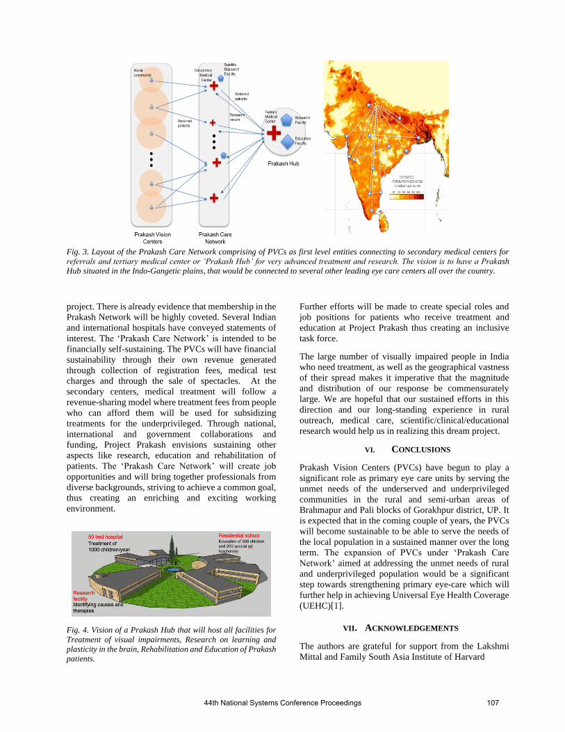
Fig. 3. Layout of the Prakash Care Network comprising of PVCs as first level entities connecting to secondary medical centers for

referrals and tertiary medical center or ‘Prakash Hub’ for very advanced treatment and research. The vision is to have a Prakash

Hub situated in the Indo-Gangetic plains, that would be connected to several other leading eye care centers all over the country.

project. There is already evidence that membership in the

Prakash Network will be highly coveted. Several Indian

and international hospitals have conveyed statements of

interest. The ‘Prakash Care Network’ is intended to be

financially self-sustaining. The PVCs will have financial

sustainability through their own revenue generated

through collection of registration fees, medical test

charges and through the sale of spectacles. At the

secondary centers, medical treatment will follow a

revenue-sharing model where treatment fees from people

who can afford them will be used for subsidizing

treatments for the underprivileged. Through national,

international and government collaborations and

funding, Project Prakash envisions sustaining other

aspects like research, education and rehabilitation of

patients. The ‘Prakash Care Network’ will create job

opportunities and will bring together professionals from

diverse backgrounds, striving to achieve a common goal,

thus creating an enriching and exciting working

environment.

Fig. 4. Vision of a Prakash Hub that will host all facilities for

Treatment of visual impairments, Research on learning and

plasticity in the brain, Rehabilitation and Education of Prakash

patients.

Further efforts will be made to create special roles and

job positions for patients who receive treatment and

education at Project Prakash thus creating an inclusive

task force.

The large number of visually impaired people in India

who need treatment, as well as the geographical vastness

of their spread makes it imperative that the magnitude

and distribution of our response be commensurately

large. We are hopeful that our sustained efforts in this

direction and our long-standing experience in rural

outreach, medical care, scientific/clinical/educational

research would help us in realizing this dream project.

VI. CONCLUSIONS

Prakash Vision Centers (PVCs) have begun to play a

significant role as primary eye care units by serving the

unmet needs of the underserved and underprivileged

communities in the rural and semi-urban areas of

Brahmapur and Pali blocks of Gorakhpur district, UP. It

is expected that in the coming couple of years, the PVCs

will become sustainable to be able to serve the needs of

the local population in a sustained manner over the long

term. The expansion of PVCs under ‘Prakash Care

Network’ aimed at addressing the unmet needs of rural

and underprivileged population would be a significant

step towards strengthening primary eye-care which will

further help in achieving Universal Eye Health Coverage

(UEHC)[1].

VII. ACKNOWLEDGEMENTS

The authors are grateful for support from the Lakshmi

Mittal and Family South Asia Institute of Harvard


University, and the Harvard Global Research Support

Centre, India. We express our thanks to Dr. Shroff’s

Charity Eye Hospital, Delhi and Fatima Hospital,

Gorakhpur for their support towards the implementation

of the project. We are also thankful to the entire Prakash

team, and several people from the communities we serve,

who have helped in this complex effort.

VIII. REFERENCES

[1]. World Health Organization. (2013). Universal eye health: a

global action plan 2014-2019.

[2]. Khanna, R. C., Sabherwal, S., Sil, A., Gowth, M., Dole, K., Kuyyadiyil, S., & Chase, H. (2020). Primary eye care in India–

The vision center model. Indian journal of

ophthalmology, 68(2), 333. [3]. Sinha, P. (2016). NeuroScience and Service. Neuron, 92(3),

647-652.

[4]. Sinha, P. (2013). Once blind and now they see. Scientific American, 309, 48-55.

[5]. [Last accessed on 2021 April 13]. Available

from: http://www.vision2020india.org/wp-content/uploads/2016/09/Vision-Centre-Manual-2012.pdf .

[6]. Misra, V., Vashist, P., Malhotra, S., & Gupta, S. K. (2015).

Models for primary eye care services in India. Indian journal of community medicine: official publication of Indian Association

of Preventive & Social Medicine, 40(2), 79.

[7]. Braithwaite, J., Zurynski, Y., Ludlow, K., Holt, J., Augustsson, H., & Campbell, M. (2019). Towards sustainable healthcare

system performance in the 21st century in high-income

countries: a protocol for a systematic review of the grey literature. BMJ open, 9(1), e025892.

[8]. [Last accessed on 2021 April 13]. Available from: File341.pdf (npcbvi.gov.in)


http://www.vision2020india.org/wp-content/uploads/2016/09/Vision-Centre-Manual-2012.pdf

http://www.vision2020india.org/wp-content/uploads/2016/09/Vision-Centre-Manual-2012.pdf

https://npcbvi.gov.in/writeReadData/mainlinkFile/File341.pdf

https://npcbvi.gov.in/writeReadData/mainlinkFile/File341.pdf

A Prototype of Recommender System for

Cardiovascular Disorders using Electrocardiogram

signals.

1st Anurag Verma

Dept. of Electrical Engineering

Faculty of Engineering,

Dayalbagh Educational Institute,

Agra, India.

[email protected]

4th Rahul Kumar

Dept. of Electrical and Electronics

Engineering, Noida Institute of

Engineering and Technology,

Greater Noida, India.

[email protected]

2nd Sitaram Jana Dept. of Electrical and Electronics




[email protected]

5th Shivam Rawat


Engineering, Noida Institute of Engineering and Technology,


[email protected]

3rd Shubham Mehra


Engineering, Noida Institute of Engineering and Technology,


[email protected]

6th Saksham Mishra Dept. of Electrical and Electronics




[email protected]

Abstract— A Prototype of recommendation system has been

proposed in this paper by using DWT of Electrocardiogram

signal and soft computing techniques to predict the different

Cardiovascular System problems. The input for our system is

Electrocardiogram signal. An intelligent recommendation system

will be simulated and developed, which uses an innovative

algorithm to provide recommendations to Cardiovascular System

problems. Depending on each patient’s Electrocardiogram

signal, the recommendation system provides the patient with

personalized help as type of disease and corresponding

recommendations. The system can assist medical personnel in

diagnosis. This prototype can improve the efficiency and reduce

the cost of healthcare in cardiac-health of heart patients.

Keywords—Intelligent Recommendation system

Cardiovascular System failure.

I. INTRODUCTION

Electrocardiogram (ECG) is the electrical signal of the

Cardiovascular System received from electrodes placed on

skin around the Cardiovascular System. During a heartbeat

there is variation of depolarization state, beginning with

pacemaker cells in the sino-atrial node. It expands through

the atrium and passes through the atrio-ventricular node.

Finally into the HIS-bundle and Purkinje-fibers, expanding

to the left of heart ventricles. It is called: Electrocardiogram

tracing as shown in figure-1. [1]

Fig.1 Electrocardiogram tracing [1]

Here a prototype of Electrocardiogram recommendation

system is proposed by doing wavelet analysis as feature

extraction stage and classification stage with 7

heartproblems shown in table-1.[2]

Table-1: Heart problems

Auto-correlation function, frequency domain features, time

frequency analysis and wavelet transform are used for

automatic detection of the abnormal conditions of heart are

reported using Electrocardiogram signals. The major

drawback of these methods is nonlinear behavior of

Electrocardiogram signal dynamics. [3]

Attributes of Cardiovascular System disease are

important bio-markers to detect cardiovascular diseases.

Different cardiovascular System diseases are shown in

table-1. [4]

Electrocardiogram waveform reflects the activity of

Cardiovascular System tissues as shown in figure-2. The

amplitude is less than 5 milli volt with frequency band of

0.05–100 Hz. Following are the waves in Normal

Electrocardiogram: P-wave, QRS complex, T-wave and U

waves. Different features of Electrocardiogram signals are

mentioned in Table 2. [5]


Table-1: Different Cardiovascular System disorders for Recommender

System. [4]

Fig.2 Cut-Section of Human Cardiovascular System. [5]

Flow chart of proposed system is shown in figure-3.

Fig.3 Block Diagram of proposed system. [7]

Table-3: Electrocardiogram wave time-frequency features [6]

Different waves in ECG plays important role in identifying

various diseases as shown in table-4 and 6. [8]

Table-4: Different ECG waves

In pre-processing we have to take care of various noises

within frequency band [0.01-150] Hz as shown in table-5.

[9] Table-5: Various noises for ECG

Different Cardiovascular System diseases for Recommender

System are mentioned in Table-6 along with ECG Beats in

Table-7.


Table-6: Different Cardiovascular System diseases for Recommender

System. [10]

Feature extraction and selection is done with the help of

DWT. Attributes are described in the Table-8. Selected

features were used for classification model using PCA. [11] Table-7: Electrocardiogram Beats [12]

II. STATE OF THE ART

Various methods like decision trees, naïve Bayes, neural

networks, association classification and genetic algorithm

are utilized for analysis of Cardiovascular System disease.

Some of them show that hybrid intelligent tool have

performed better in terms of accuracy. [13]

Table-8: Attributes of Cardiovascular System disease for Recommender System. [14]

The Cardiovascular System problems are more related with

smoking and drinking addictions. [15]. Making a mobile

based application would benefit masses of people to check

the Cardiovascular System risks themselves. Figure-4 shows

Electrocardiogram Power Spectrums plotted using

PYTHON and ECG Beats Types in Figure-5. [16]

Fig.4 Electrocardiogram Power Spectrums. [17]

III. MATERIALS AND METHODOLOGY

A) Dataset- The dataset used here is MIT-BIH database,

with sampling frequency of 360Hz. 4- patients of 24-

35 years were volunteered for recording ECGs for 10

minutes in every recording. The proposed cardiac

disorder detection system block diagram is shown in

Fig. 6 [19]

Fig.5- Electrocardiogram Beats Types


Fig.6- Flow diagram for Electrocardiogram Analysis

This prototype contains all 48 half-hour recordings. Each

record have an UP-lead potential and a LOW-lead potential.

Normal Cardiovascular System beats are highlighted in the

UP-lead potential while the ectopic beats are highlighted in

the LOW-lead potential. So two potentials are highly

correlated. [20]

It is advisable to use elliptical HPF with C of 0.5 Hz for

getting rid of baseline wandering from ECG. Then a L = 3

wavelet with DB-2 is used for getting rid of high frequency

noise of the ECG signal. Finally a Butterworth LPF with C

of of 40Hz is used for getting rid of power-line interference.

[21] Different techniques can be used for classifying

Cardiovascular disorders like wavelet transform, statistical

and hidden Markov models, ANN and SVM. [22]

The paper mainly follows four steps:

• Step 1: Collecting MIT-BIH database

• Step 2: Pre-possessing.

• Step 3: Feature extraction by DWT.

• Step 4: Classification. [23]

MIT-BIH Database classes as shown in table-9. [24]

A signal has many frequency bands at different resolution,

which are divided into 2 sets, called coarse approximation

and detailed information in DWT. [26]

Figure 7: Electrocardiogram Abnormalities [25]

The detailed steps in this paper are as shown in figure-8.

Figure 8: Detailed steps. [27]

A) RR span Features

Important features to define the Cardiovascular System beat,

are as shown in table-10 below: [20]

Table-10: Important features to define the Cardiovascular System beat


B) Electrocardiogram Classification

The SVM is supervised learning model, which minimizes a

misclassification. SVM divides input data into 2 classes by

the decision hyper-plane: d(x). X determines whether d(x) >

0 or d(x) < 0. With the help of kernel function, we can

convert 3D vectors to 2D vectors and SVM optimize the

d(x). [28]

C) Multiclass SVM

Multiclass SVM applies One Against One method, also

known as ―pair-wise coupling‖, ―all pairs‖ or ―round robin‖,

works by constructing one SVM for each pair of classes.

Thus, for a problem with c classes, c(c-1)/2 SVMs are

trained to classify the samples of different classes by

maximum voting, where each SVM votes for one class. [29]

Figure8: List structure in MIT app inventor for Recommender System.

[30]

IV. CONCLUSION

A recommendation system is simulated and developed to

provide suggestions to Cardiovascular System disease

patients in the remote-health environment by using MIT app

inventor. The system provides the patient with personalized

help as type of disease and corresponding recommendations.

This prototype is effective for throughput of medical staff

and reduces the overall cost of cardiac-healthcare.

REFERENCES

[1] A. E. Vincent, Sreekumar K, ―A Survey on Approaches for Electrocardiogram Signal Analysis with Focus to Feature Extraction and

Classification‖, ICICCT 2017, pp 140-144.

[2] R. Valupadasu and B.R.R. Chunduri, ―Automatic Classification of Cardiac Disorders using MLP Algorithm‖,PHM-Paris-2019, pp 253-257.

[3] M.H. Vafaie, M. Ataei, and H.R. Koofigar, ―Cardiovascular System

diseases prediction based on Electrocardiogram signals classification using a genetic-fuzzy system and dynamical model of Electrocardiogram

signals‖, Biomedical Signal Processing and Control 14 (2014), pp-291–

296. [4] K. Husain, M. Soperi, M. Zahid, S. Ul Hassan, and S Hasbullah, and

S. Mandala, ―Advances of Electrocardiogram Sensors from Hardware,

Software and Format Interoperability Perspective‖,Electronics 2021, 10(2), 105; https://doi.org/10.3390/electronics10020105.

[5] L. Xie, Z. Li, Y. Zhou, Y. He and J. Zhu,‖Computational Diagnostic

Techniques for Electrocardiogram Signal Analysis‖,Sensors 2020, 20, 6318; doi:10.3390/s20216318.

[6] J. Zhang, L. Zou, B. Li1, K. Xiang1, X. Shi1, C. Fan1 and Y. Liu,

―Method of diagnosing Cardiovascular System disease based on deep learning Electrocardiogram sign‖,

arXiv:1907.01514. [7] S. S. Zadawale, S. Bakare, ―Electrocardiogram Signal Based Cardiovascular System Disease Prediction System using DWT and SVM‖, IJARCCE, Vol. 6, Issue 7, July

2017, pp-61-66.

[8] Sreelakshmi T G and S. Paul, ―An accurate Electrocardiogram feature

extraction method for detecting multiple cardiovascular diseases‖, IJISET 2010, pp-50-59.

[9] M. Hadjem, O. Salem, and F. N. Abdesselam, ―An Electrocardiogram

Monitoring System for Prediction of Cardiac Anomalies Using WBAN‖, 2014 IEEE 16th International Conference on e-Health Networking,

Applications and Services (Healthcom), Oct 2014, Natal, Brazil. pp. 441-

446, 10.1109/Health-Com.2014.7001883, hal-01101938.

[10] M. Sharma, ―Electrocardiogram And Medical Diagnosis Based

Recognition & Prediction Of Cardiac Disease Using Deep Learning‖

INTERNATIONAL JOURNAL OF SCIENTIFIC & TECHNOLOGY RESEARCH VOLUME 8, ISSUE 10, OCTOBER 2019 ISSN 2277-8616,

pp 233-240.

[11] F. I. Alarsan and M. Younes, ―Analysis and classification of Cardiovascular System diseases using Cardiovascular Systembeat features

and machine learning algorithms‖,

https://doi.org/10.1186/s40537-019-0244-x, pp 1-15. [12] P. Lamba and K. Rawal, ―A Survey of Algorithms for Feature

Extraction and Feature Classification Methods‖,2019 International

Conference on Automation, Computational and Technology Management (ICACTM), London, UK, 2019, pp. 338-341, doi:

10.1109/ICACTM.2019.8776804. .

[13] N. Prabakaran and R. Kannadasan, "Prediction of Cardiac Disease Based on Patient's Symptoms," 2018 Second International Conference on

Inventive Communication and Computational Technologies (ICICCT),

Coimbatore, India, 2018, pp. 794-799, doi:

10.1109/ICICCT.2018.8473271.

[14] H. D. Calderon-Vilca, K. E. C. Callupe, R. J. I. Aliaga, J. B. Cuba and

F. C. Mariño-Cárdenas, "Early Cardiac Disease Detection Using Neural Networks," 2019 7th International Engineering, Sciences and Technology

Conference (IESTEC), Panama, Panama, 2019, pp. 562-567, doi:

10.1109/IESTEC46403.2019.00106. [15] R. J. P. Princy, S. Parthasarathy, P. S. Hency Jose, A. Raj

Lakshminarayanan and S. Jeganathan, "Prediction of Cardiac Disease using Supervised Machine Learning Algorithms," 2020 4th International

Conference on Intelligent Computing and Control Systems (ICICCS),

Madurai, India, 2020, pp. 570-575, doi: 10.1109/ICICCS48265.2020.9121169.

[16] M. Raihan et al., "Smartphone based ischemic Cardiovascular System

disease (Cardiovascular System attack) risk prediction using clinical data and data mining approaches, a prototype design," 2016 19th International

Conference on Computer and Information Technology (ICCIT), Dhaka,

Bangladesh, 2016, pp. 299-303, doi: 10.1109/ICCITECHN.2016.7860213.

[17] A. Calderon, A. Pérez and J. Valente, "Electrocardiogram Feature

Extraction and Ventricular Fibrillation (VF) Prediction using Data Mining

Techniques," 2019 IEEE 32nd International Symposium on Computer-Based Medical Systems (CBMS), Cordoba, Spain, 2019, pp. 14-19, doi:

10.1109/CBMS.2019.00014.

[18] E. Izci, M. A. Ozdemir, R. Sadighzadeh and A. Akan, "Arrhythmia Detection on Electrocardiogram Signals by Using Empirical Mode

Decomposition," 2018 Medical Technologies National Congress

(TIPTEKNO), Magusa, Cyprus, 2018, pp. 1-4, doi: 10.1109/TIPTEKNO.2018.8597094.

[19] K. Tara, A. K. Sarkar, M. A. G. Khan and J. R. Mou, "Detection of

cardiac disorder using MATLAB based graphical user interface (GUI)," 2017 IEEE Region 10 Humanitarian Technology Conference (R10-HTC),

Dhaka, Bangladesh, 2017, pp. 440-443, doi: 10.1109/R10-

HTC.2017.8288994. [20] C. Ye, M. T. Coimbra and B. V. K. Vijaya Kumar, "Arrhythmia

detection and classification using morphological and dynamic features of

Electrocardiogram signals," 2010 Annual International Conference of the IEEE Engineering in Medicine and Biology, Buenos Aires, Argentina,

2010, pp. 1918-1921, doi: 10.1109/IEMBS.2010.5627645.

[21] A. Bansal, S. Kumar, M. K. Agrawal, M. M. Nayak and R. Narayanan, "Detecting critical cardiac events with 12 lead Electrocardiogram data,"

2013 IEEE International Conference on Bioinformatics and Biomedicine,

Shanghai, China, 2013, pp. 4-6, doi: 10.1109/BIBM.2013.6732742. [22] N. Gawande and A. Barhatte, "Cardiovascular System diseases

classification using convolutional neural network," 2017 2nd International

Conference on Communication and Electronics Systems (ICCES), Coimbatore, India, 2017, pp. 17-20, doi: 10.1109/CESYS.2017.8321264.

[23] C. U. Kumari et al., "Cardiovascular System Rhythm Abnormality

Detection and Classification using Machine Learning Technique," 2020 4th International Conference on Trends in Electronics and Informatics

(ICOEI)(48184), Tirunelveli, India, 2020, pp. 580-584, doi:

10.1109/ICOEI48184.2020.9142914.. [24] H. Abayaratne, S. Perera, E. De Silva, P. Atapattu and M.

Wijesundara, "A Real-Time Cardiac Arrhythmia Classifier," 2019 National

Information Technology Conference (NITC), Colombo, Sri Lanka, 2019, pp. 96-101, doi: 10.1109/NITC48475.2019.9114464.

[25] Ribeiro, A.H., Ribeiro, M.H., Paixão, G.M.M. et al. Automatic

diagnosis of the 12-lead Electrocardiogram using a deep neural


https://doi.org/10.3390/electronics10020105

network. Nat Commun 11, 1760 (2020). https://doi.org/10.1038/s41467-

020-15432-4.

[26] N. A. Mohamed, M. Yaseen, W. Hateem, T. Musa and S. Ismail,

"Diagnosis of Cardiac Disorders in Electrocardiogram Signal using

Artificial Neural Network Algorithm," 2019 International Conference on Computer, Control, Electrical, and Electronics Engineering (ICCCEEE),

Khartoum, Sudan, 2019, pp. 01-07, doi:

10.1109/ICCCEEE46830.2019.9071371. [27] M. M. Butt, M. U. Akram and S. A. Khan, "Classifying Normal Sinus

Rhythm and Cardiac Arrhythmias in Electrocardiogram Signals Using

Statistical Features in Temporal Domain," 2015 9th Asia Modelling

Symposium (AMS), Kuala Lumpur, Malaysia, 2015, pp. 28-31, doi:

10.1109/AMS.2015.14.

[28] S. H. Lee, H. Ko and Y. Yoon, "Classification of Ventricular

arrhythmia using a support vector machine based on morphological

features," 2013 35th Annual International Conference of the IEEE Engineering in Medicine and Biology Society (EMBC), Osaka, Japan,

2013, pp. 5785-5788, doi: 10.1109/EMBC.2013.6610866.

[29] S. Faziludeen and P. V. Sabiq, "Electrocardiogram beat classification using wavelets and SVM," 2013 IEEE Conference on Information &

Communication Technologies, Thuckalay, India, 2013, pp. 815-818, doi:

10.1109/CICT.2013.6558206. [30]http://ai2.appinventor.mit.edu/reference/other/displaylist.html


XXX-X-XXXX-XXXX-X/XX/$XX.00 ©20XX IEEE

A Hybrid Evolutionary Algorithm for solving the

Longest Common Subsequence Problem

V. Prem Prakash

Department of Electrical Engineering

Faculty of Engineering

Dayalbagh Educational Institute (Deemed University)


C. Patvardhan

Department of Electrical Engineering

Faculty of Engineering,

Dayalbagh Educational Institute (Deemed University)


Abstract— For a given set of input strings, or sequences, the

Longest Common Subsequence (LCS) Problem seeks the

maximal length subsequence that occurs in all of the strings.

The problem finds application in protein structure prediction,

identifying common motifs in genes and for DNA sequence

comparisons. The LCS problem is known to be NP hard for an

arbitrary number of strings, but can be efficiently solved using

dynamic programming for a constant number of input strings.

However, as the number and size of sequences increases, the

computation effort required becomes prohibitively large. This

paper proposes a hybrid evolutionary algorithm (EA) that

incorporates dynamic programming-based heuristic

initialization and effective local search to speed up the

computation for multiple sequences. The performance of the

proposed hybrid EA is compared with that of a standard

dynamic programming algorithm and a well-known genetic

algorithm (GA) for the LCS problem on benchmark instances

used widely in the literature, and shown to obtain significantly

better results.

Keywords—Genetic Algorithm, Memetic, LCS, longest

common subsequence, bioinformatics

I. INTRODUCTION

Given a string S of length |S| drawn from an alphabet Σ, a subsequence of S is a sequence that obtained from S by removing zero or more elements of S without changing the order of the remaining elements in S. Consider now, a set of k such strings, S1, S2,…, Sk. The longest common subsequence of this set of strings is the subsequence of greatest length that appears in all k strings. The problem of finding the longest common subsequence of a given set of strings has many practical applications, ranging from automated paradigm detection in computational linguistics (Sorokin, 2016) to efficient merging of multiple version-controlled file collections in version control systems such as GitHub (Torvalds, 2005) and finding line-wise differences between files in the popular diff (Hunt & Szymanski, 1977) utility. Another major application of the LCS problem is for DNA sequence comparisons in biological systems (Ossman & Hussein, 2012), (Ning, Ng, & Leong, 2011). The longest common subsequence of two or more DNA strands, possibly belonging to different organisms, or even different mutant strains of the same organism, is used to quantify the degree to which the organisms/mutations are similar, or related.

The LCS problem is known to be NP-hard for an arbitrary number of strings (Maier, 1978), but it can be solved to optimality using dynamic programming in O(n

k)

time when the number of strings is constant (Gusfield,

1997). Several dynamic programming approaches for the problem have been proposed in the literature, which solve the LCS problem in O(n

k) time, where ‘n’ is the length of the

longest string and ‘k’ is the number of strings, c.f. (Irving & Fraser, 1992). However, dynamic programming quickly becomes computationally expensive as the value of ‘k’ increases.

Several heuristic approaches have been applied for the LCS problem. These include beam search-based (Blum, 2009) and large neighbourhood search heuristics (Easton, 2008), genetic algorithms (Hinkemeyer & Julstrom, 2006) and hyper-heuristic approaches (Tabataba, 2012). This paper presents a hybrid evolutionary algorithm for the LCS problem, abbreviated HyEA-LCS. The proposed algorithm seeds the initial population with good solutions obtained using a dynamic programming-based heuristic, and augments the evolutionary process with fast local search to speed up the convergence. In the course of several experiments on a standard set of test problems, the performance of the HyEA-LCS is shown to be superior to that of the best-known existing genetic algorithm for the LCS problem.

The remaining sections of this paper are organized as follows: the proposed HYEA-LCS algorithm is described in section II, experiments and results are presented in section III, and conclusions are made in section IV.

II. A HYBRID EVOLUTIONARY ALGORITHM FOR THE LCS

PROBLEM (HYEA-LCS)

The Hybrid Evolutionary Algorithm for the LCS Problem

(HyEA-LCS) presented in this section is 1-elitist, uses binary

encoding for chromosomes and applies fast variation

operators in a generational framework. The main features of

the algorithm are described as follows, and pseudo-code for

the algorithm is provided in figure 1.

A. Chromosome Encoding

The HyEA-LCS encodes chromosomes as binary strings. The length of a chromosome is equal to either the length of the shortest string, or, in case all strings are of equal length, the length of any arbitrary string. One may, without loss of generality, assume the latter case, i.e., that all strings Si are of equal length, say L. Then the length of each chromosome ch[.] would also be L. The value at each index j of a chromosome is 1 if S1[j] is in the common subsequence, and 0 otherwise. For example, consider the two short DNA strings S1=”GAGTC” and S2=”ATCGG”. In this case, L=5.


Figure 2. Pseudo-code of the proposed Hybrid Evolutionary Algorithm for LCS (HyEA-LCS)

A chromosome ch=”01010” represents the subsequence

“AT”, with the bases ‘A’ and ‘T’ occurring at indices 1 and 3 of S1 (indices are counted here starting from 0, as in C or Java arrays). The subsequence “AT” is a common subsequence (of length 2) since it occurs in both S1 and S2.

B. Fitness Evaluation

A reward-and-penalty scheme is used in the fitness function, wherein subsequences (chromosomes) that are longer and appear in more numbers of strings are assigned higher fitness, and subsequences that do not fit into even a single string are penalized and quickly eliminated by being assigned very low fitness scores. This fitness scheme is also used in (Hinkemeyer & Julstrom, 2006). The fitness function is shown in Fig. 2, where the fitness of an individual is stored in the variable v. The length of a chromosome is represented by len, the length of an arbitrary string (assuming all strings to be of equal length) by L; and the number of strings that the chromosome matches is represented by m. The constant K is the total number of strings under consideration.

Figure 2. Listing of fitness function

The constant multipliers (50, 3000, -1000) indicate the strength with which the chromosome is being rewarded or penalized. For instance, a subsequence that matches multiple strings is rewarded (line 1). While a subsequence would usually not be as long as the string, such a subsequence, if it exists, is preferred/rewarded (line 2). A chromosome that matches all strings is strongly rewarded (if clause, line 3),

and chromosomes that do not match all strings are penalized in proportion to the number of non-matched strings (else clause, line 3).

C. Initial Population

The initial population P consists of |P| randomly generated individuals. For K > 2, a small percentage of this initial population (≤ 3% of |P|) is comprised of chromosomes that encode the pair-wise LCS of input strings, obtained using the dynamic programming algorithm. For instance, when the input consists of three strings S1, S2 and S2 (K=3), three of the initial chromosomes would represent LCS(S1,S2), LCS(S2,S3) and LCS(S1,S3), and the rest of the population would be made up of randomly generated binary strings. In order to mitigate the O(n

2) computational

overhead implied by the DP algorithm for longer strings, for |S|>400, the LCS obtained for |S|=400 is extended with random bit flips up to the appropriate string size.

D. Variation Operators

The algorithm uses a modified single-point crossover that generates two offsprings from two parents, and ensures that genes common to both parents are propagated in the offspring. Mutation flips each bit of a chromosome with a probability inversely proportional to the length of the string. Each generation of individuals is produced by application of both crossover and mutation with equal probability.

E. Other parameters

Chromosomes are selected as parents using tournaments of size 2. The algorithm is 1-elitist, and uses a simple local search heuristic to improve the global best solution (gBest) at the start of each generation. The local search heuristic

obtains a new solution gBestb by flipping a randomly

selected index in gBest, always replacing gBest if gBestb is

fitter. This is repeated a small, constant number of times, LS_TRIALS. The population is re-initialized if there is no further improvement in the gBest chromosome over MAX_IMPROVE generations. The re-initialized population is generated in the same way as the initial population, except that the gBest solution is also included in the population. The algorithm runs for a fixed number of generations, MAXGEN, or until the (known) optimal solution is found, whichever event occurs first.


III. EXPERIMENTAL WORK

The proposed HyEA-LCS algorithm and, for purposes of comparison, the GA given in (Hinkemeyer & Julstrom, 2006) and the standard O(n

k) time and space dynamic

programming algorithm (DPA) were implemented in C, and tested on a set of benchmark DNA instances (Σ = A,T,G,C, |Σ|=4), each with K=3 strings. Test instances had lengths of n=100, 200, 400, 800, 1600, 3200 and 6400 characters respectively, with known LCS lengths equal to 10%, 50%, 90% and 100% of the strings for each size. Thus there were totally 7x4 = 28 test instances.

All experiments were performed on a computer system with Intel i3 2

nd Generation 2.4GHz CPU with 4GB DDR3

RAM running Windows 10.

A common evolutionary framework was used for the GA and HyEA-LCS implementations, so as to obtain a fair comparison of performance. Population sizes was set to 100 chromosomes, identical fitness evaluation was used, the value of MAX_IMPROVE was set to 100 for both implementations, and crossover and mutation were assigned equal probability. The value of MAXGEN was as 20000. Additionally, the LS_TRIALS parameter in HyEA-LCS was experimentally set to 10.

The DP algorithm was able to return results on up to n= 400 sized instances, but failed to run on larger problem sizes. Computation times were therefore reported only up to n=400 for the DP algorithm. The GA and HyEA-LCS were run 30 times on each test instance and the best, mean and standard deviation of computation times were reported. Results obtained by the DPA, GA and HyEA-LCS on up to n=400 sized instances are presented in Table 1. The computation times reported by GA and HyEA-LCS on the larger test problems (up to n=6400) are presented in Table 2.

In both tables, the column titled ‘n’ represents the length of the test strings, ‘%’ indicates the length of LCS as a function of instance lengths, and the columns under ‘Computation time (seconds)’ provide the computation time of a single run for DPA, and the best (lowest), mean and standard deviation (sd) of computation times obtained over 30 runs for the GA and HyEA-LCS respectively.

n % Computation time (seconds)

DPA GA HyEA-LCS

best mean Sd best mean sd

100 10 0.04 0.05 1.41 2.47 0.001 0.002 0.005

50 0.05 - - - - - -

90 0.05 0.04 3.84 3.75 0.015 3.911 3.897

100 0.05 0.05 0.06 0.01 0.001 0.002 0.001

200 10 0.40 0.20 0.23 0.02 0.005 0.005 0.000

50 0.37 0.35 0.38 0.03 0.004 0.005 0.001

90 0.30 0.34 0.37 0.03 0.003 0.004 0.001

100 0.38 0.20 0.23 0.02 0.005 0.005 0.000

400 10 3.18 0.81 0.89 0.06 0.0150 0.0151 0.001

50 2.74 1.32 1.47 0.11 0.0140 0.0144 0.001

90 1.89 1.50 1.69 0.14 0.0100 0.0103 0.001

100 3.06 0.81 0.90 0.11 0.0140 0.0151 0.001

Table 1. Computation time obtained by DPA, GA and HyEA-LCS for DNA strings of length n=100, 200 and 400

For the n=100 and 200 sized DNA strings, it is seen that the DPA reported computation times that were comparable to the best and mean times reported by GA. Further, on one test instance of length 100 (LCS=50%), the GA and HyEA-LCS were able to quickly find a common subsequence of length

48, i.e., 4% less than from the LCS, but neither was able to find the LCS value of 50 within the set time limits, whereas the DPA returned the LCS in 0.05 seconds. On the n=400 length instances, the GA always found the LCS in comparatively lesser time. The HyEA-LCS, by contrast, almost always took much lesser time than the DPA and GA. This is particularly evident for the n= 400 instances: comparing only the mean computation times reported for GA and HyEA-LCS on all four instances, the GA obtains an average speedup of 2.49 vis-à-vis DPA, while the HyEA-LCS obtains an average speedup of 96.2 in comparison to GA, and so is almost 196.75 times faster than DPA for these instances! For the larger test instances (N=800, 1600, 3200 and 6400) in Table 2 also, the best and mean computation times reported by the HyEA-LCS are much lower than for the GA.

N % Computation time (seconds)

GA HyEA-LCS

best mean Sd best mean sd

800 10 3.26 3.49 0.17 0.11 0.13 0.01

50 5.43 6.32 0.63 1.15 1.53 0.23

90 6.34 6.72 0.44 1.45 1.78 0.24

100 3.44 3.82 0.4 0.03 0.03 0.001

1600 10 13.80 14.60 0.65 0.32 0.37 0.03

50 22.88 24.84 1.17 5.39 6.65 0.76

90 25.94 30.06 3.38 6.61 7.96 0.78

100 13.17 15.53 1.31 0.06 0.06 0.001

3200 10 59.20 62.67 3.23 1.91 2.22 0.11

50 105.08 114.43 5.21 24.53 30.37 3.58

90 120.24 128.89 5.05 29.93 34.12 2.89

100 66.37 71.05 4.28 0.11 0.12 0.01

6400 10 195.03 214.76 5.71 9.4 10.21 0.35

50 284.12 312.64 6.45 108.11 135.08 17.83

90 276.89 309.47 6.84 124.05 148.15 16.94

100 182.60 198.36 5.86 0.22 0.23 0.001

Table 2. Computation time obtained by GA and HyEA-LCS for DNA strings of length n=800, 1600, 3200 and 6400

It is observed in Table 2 that the HyEA-LCS seems to require very low computation times for the ‘100%’ test instance of each size, where the LCS length equals the string length. This behaviour of the algorithm may be attributed to the way the test instances are structured. The ‘100%’ instances contain K=3 identical strings. Hence the DP heuristic used during population initialization seeds the population with chromosomes that not only represent a fairly long subsequence, but also one that occurs in all K strings, leading to the assignment of very high fitness score. Such chromosomes could dominate the population and rapidly direct convergence towards the optimal LCS solution (represented in this particular case by all 1s).

IV. CONCLUSIONS

This paper presents a novel hybrid evolutionary algorithm (HyEA-LCS) for finding the longest common subsequence of a given set of strings. The proposed algorithm uses a dynamic programming sub-heuristic to seed the population with good solutions, and combines a fast customized recombination operator with effective mutation and uses a local search heuristic to further improve the best solution obtained in each generation of the evolutionary search. The performance of the proposed algorithm is shown to be superior to that of a standard Dynamic Programming implementation and a well-known existing Genetic Algorithm (GA) for the LCS problem on a large set of DNA-string test instances. The HyEA-LCS also consistently


obtains significant speedups over the GA; this motivates its application to larger problem sizes than attempted hitherto. Lastly, the experimental work presented in this paper focuses on finding longest common subsequences of DNA sequences. However, the proposed algorithm may be applied for solving the LCS problem in other domains as well.

ACKNOWLEDGMENTS

The authors thank the Chairman, Advisory Committee on Education, Dayalbagh for the guidance in all their endeavours. This work is supported by DST-DAAD under grant INT/FRG/DAAD/P-19/2016.

V. REFERENCES

[1] M. Ossman and L. Hussein, “Fast longest common

subsequences for bioinformatics dynamic

programming,” in Population , Paris, 2012.

[2] K. Ning, H. Ng and H. Leong, “Analysis of the

relationships among longest common subsequences,

shortest common supersequences and patterns and its

application on pattern discovery in biological

sequences.,” Int J Data Min Bioinform., vol. 5, p. 611–

25, 2011.

[3] A. Sorokin, “Using longest common subsequence and

character models to predict word forms,” in In

Proceedings of the 14th Annual SIGMORPHON

Workshop on Computational Research in Phonetics,

Phonology, and Morphology, Berlin, Germany, 2016.

[4] L. Torvalds, “Github Repository,” 2005. [Online].

Available: http://www.github.com. [Accessed 10 April

2021].

[5] J. W. Hunt and T. G. Szymanski, “A fast algorithm for

computing longest common subsequences,”

Communications of the ACM, vol. 20, no. 5, pp. 350-

353, 1977.

[6] R. Irving and C. Fraser, “Two algorithms for the

longest common subsequence of three (or more)

strings,” in In Proceedings of the 3rd Annual

Symposium on Combinatorial Pattern Matching, New

York, 1992.

[7] D. Maier, “The complexity of some problems on

subsequences and supersequences,” in Journal of the

ACM, 1978.

[8] D. Gusfield, Algorithms on Strings, Trees, and

Sequences: Computer Science and Computational

Biology, Cambridge: Cambridge University Press,

1997.

[9] C. Blum, M. Blesa and M. López-Ibáñez, “Beam

search for the longest common subsequence problem,”

Comput. Oper. Res., vol. 36, no. 12, p. 3178–3186,

2009.

[10] T. Easton and A. Singireddy, “A large neighborhood

search heuristic for the longest common subsequence

problem,” J. Heuristics, vol. 14, no. 3, p. 271–283,

2008.

[11] F. Tabataba and S. Mousavi, “A hyper-heuristic for the

longest common subsequence problem,” Comput. Biol.

Chem., vol. 36, pp. 42-54, 2012.

[12] B. Hinkemeyer and B. Julstrom, “A genetic algorithm

for the longest common subsequence problem,” in In

Proc. of GECCO 2006, 2006.


Deep Feature Compression Based Ensemble ModelTowards Content Based Image Retrieval

Rohan Raju DhanakshirurAN and SK school of IT

Indian Institute of TechnologyNew Delhi, India

[email protected]

Prem Kumar KalraDepartment of CSE

Indian Institute of TechnologyNew Delhi, India

[email protected]

Abstract—Recent advances in the field of technology has ledto increased availability of image dataset. This has motivatedthe need for an efficient content based image retrieval (CBIR)algorithm. Most of the present day algorithms make use of clas-sical image processing based techniques for feature extraction,a major step in CBIR. In this paper, we propose a learningbased ensembled algorithm for efficient feature extraction. Theclassical texture features and the compressed version of theparameters learnt by the latent space representation of thedeep autoencoder are ensembled in the proposed algorithm.We fuse similarity distance and euclidean distance between theextracted ensembled feature of the query image and the imagesin the database to retrieve relevant images. We demonstrate theefficiency of the proposed algorithm on the standard ukBenchdataset using different quantitative parameters. We observe theproposed algorithm to be 96.7% accurate, which is 3.2% betterthan the best performing state-of-the-art algorithms.

Index Terms—Image Retrieval, Deep Autoencoder, DiscreteCosine Transforms (DCT), Ensemble model

I. INTRODUCTION

Today’s world is fast growing. There has been increasedusage of image capturing devices in the last decade. With theadvent of various social networking sites, it is observed that300 millions of photos captured are uploaded in the publicdomain every day [1]. This has given rise to the need foran efficient image retrieval algorithm. The process of imageretrieval can be defined as an act of fetching the most relevantimage from the database. The query can be in terms of text,speech or in the form of an image [2]. When an image is givenas a query, the task of any image retrieval algorithm would beto fetch that image from the database, whose content is mostsimilar to the content of the query image. This process is thus,defined as the Content Based Image Retrieval (CBIR).

Although CBIR is not a new problem (has been in thelime light since 1990’s [3]), it still is an important problemthat attracts attention from various scientific communities suchas computer vision and multimedia due to the fact that thetotal data in the domain has been significantly increased. Thetraditional technique of listing the meta data of the image inthe form of ties and tags [1] can not be used any-more because,there can be inconsistencies in the visual content and thecorresponding textual content. Moreover, this introduces theproblem of intention gap. Intention gap is the difficulty, a userfaces in precisely expressing his intent through words. Modern

day techniques focus on extracting some texture features fromthe query image and try matching it with the correspondingfeatures of the images in the database [4]. Although thesetechniques solve the problem of intention gap, they introducea new problem called as the semantic gap. Semantic gapis the difficulty in describing high-level semantic conceptscorresponding to the content of the image with low-levelvisual feature [5]. There have been various efforts put by theresearchers to narrow down this gap.

Although deep autoencoders [6] are very efficient in re-ducing the semantic gap, it makes the system completely non-interpretable. That makes the system susceptible to adverserialattacks [7]. In order to reduce the risk of adverserial attacks, itis necessary to fuse the output of the deep autoencoders withsome classical hand crafted features.

II. RELATED WORKS

The major steps involved in CBIR are:1) Feature extraction and transforming feature vectors of

various sizes to a fixed-length vector.2) Compute similarity between two feature vectors.

A. Feature extraction

The early time CBIR algorithms focus upon hand craftedfeatures. They describe image content by shape [8], structure,color and texture [9] related features. GIST feature descriptors,which offers a low computation complexity is also used bysome researchers [10]. These algorithms typically find theiruse cases in datasets that have simple images. These imagestend to fail whenever there is a background clutter in the queryimage [1].

The introduction of SIFT [11] changed the feature extractiontechniques. Various techniques make use of sift descriptorsfor feature detection. Authors have also come up with im-provements to SIFT keypoint detectors, such as Hessian affinedetector [12], MSER [13], Harris-Hessian detector [14], andFAST [15]. People have even tried extracting the features bysimply sampling the image [16].

Apart from the regular hand-crafted features, researchershave also come up with learning based features similar to thatof local feature descriptors [17]. The last convolutional layer ofthe standard CNN based image classification architecture has


been used as a feature map by [18]. Similarly, we see papersthat use the last layer of the object detection framework [19] asfeatures. Binarized normed gradients (BING) [18] is also usedas a feature by a few researchers. Some papers make use ofROI based algorithms of Region proposal netwrok for featureextraction [20]. Recently, researchers have started using thelatent space representation of the autoencoder as features [6].Zhao et.al in their work say that an image can be transformedusing wavelet transform and then extracts the features usingDeep autoencoders [2].

All the proposed deep learning based approaches use thedeep learning architecture as a black box and hence theyare highly susceptible for adverserial attacks [7]. Also, dueto lack of interpretablity, these systems can not be usedin any critical applications. Moreover, the architectures thatmake use of autoencoders have used very limited number ofconvolutional layers, due to which the corresponding latentspace representation’s receptive filed has been observed to bemuch smaller than the size of the image. This has made thelatent space representation not learn the complete content ofthe image.

B. Similarity score

Researchers have proposed two types of scoring, namelyDistance based scoring and Voting based scoring

The algorithms that use distance based scoring widely makeuse of some sort of normalized euclidean distance as shownin equation 1

D(Iq, Id) = (N∑i=1

|qi − di|p)1p ) (1)

where, Iq is the query image and Id is the image in thedatabase. We assume the feature vector to be of length N andqi, di are the corresponding elements of the feature vectors ofquery and database image respectively. p is the normalizationfactor.

Researchers in [9] make use of L − 1 norm, where thevalue of p = 1. However, the researchers in [21] claimthat the similarity measure by L − p distance is not optimalbecause of the neighbourhood reversibility issue which makesfew images disobey the k nearest neighbourhood policy. Inorder to mitigate this issue, [22] comes up with a probabilisticframework for similarity measure. Some even try coming upwith the learning based score [23].

In voting based methods, every element in the feature vectoris considered as a vote and the similarity score is measuredby the total number of matched feature points [24]. In [25],Jegou et. al came up with a scoring function as a summationof squared TF-IDF weights on shared visual words. Thistechnique was influenced by the Bag of Features technique.Authors in [26] made a slight modification and came changedthe scoring operation of TF-IDF weights into mod operation.

Although the voting based techniques seem to work well, itis indeed some sort of threshold on the distance based tech-niques. Hence, both the techniques perform almost similarlyin most of the cases. Also, it can be observed that most of

the researchers do not try fusing multiple scoring techniquesto come up with a final score.

III. CONTRIBUTIONS OF THE PAPER

The main contribution of the paper is the efficient algorithmfor content based image retrieval. Towards this, we make thefollowing contributions.

1) We propose an ensemble based architecture for featureextraction of images. The proposed architecture ensem-bles

a) Classical handcrafted texture featuresb) Latent space representation of the learnt deep convo-

lutional autoencoderc) Compressed version of the latent space representation

by passing it through the standard JPEG pipeline2) We propose evidence based combination algorithm to

come up with the similarity scores.a) The Normalized Mutual Information (NMI), Mean

Squared Error (MSE), and L-2 norm between thefeatures of the query image and the image in thedatabase act as the evidence for DSCR.

b) We consider the number of feature matches in each ofthe following as its corresponding confidences

3) We demonstrate the results of the proposed algorithm onthe standard ukBench dataset using various quantitativeanalysis and show the improvement from with the otherstate-of-the-art algorithms.

IV. PROPOSED SYSTEM FOR CONTENT BASED IMAGERETRIEVAL

The proposed architecture is divided into three stages. Inthe first stage, we train the proposed fully convolutionalautoencoder. In second stage, we generate the feature set forour database and in the third stage, we compute similarity andretrieve the most relevant images.

A. Proposed Fully convolutional Autoencoder

The latent space representation of the given image can beobtained by training the proposed fully convolutional auto-encoder. The proposed architecture for training is shown inFigure 1. The input image is initially blurred and the blurredimage is used for training. This is because, the input image isbeing trained at full resolution which will have many edgesand corners. As the initial layers of the neural network learnslow level features such as edges and corners, it will be difficultfor network to learn too many edges and corners, if unblurredimage is learnt.

The autoencoder is kept fully convolutional so that the inputof any resolution can be trained. The input image is passedthrough an encoder-decoder kind of a network. The encodernetwork consists of the convolutional and pooling layers ofDeConvNet (our backbone architecture). Along with thoselayers we add 4 additional convolutional and pooling layers.ReLU activation function is used in the proposed architecture.The backbone architecture ensures the initial training of the


Input Image Blurred input

Convolutional andpooling layers ofencoder Network

Deconvolutional andunpooling layers ofdecoder Network

Convolutionand MaxPool

Layers ofDeConvNet

Skip connections forpooling layers

DeConvolutionand UnPool

Layers ofDeconvNet

Training Architecture

Blur the imageusing known

PSF

Blurred input

Latent Spacerepresentation

Fig. 1: Proposed architecture for training the network

network, so that we need not start with the random weightsfor initialization for all the layers. The addition of 4 morelayers make sure that the algorithm learns high level features.The decoder network is exactly the reverse of the encodernetwork. It consists of 4 deconvolutional and unpooling layers.We propose to add skip connections for every max-pool layersto achieve better learn-ability. i.e. we propose to maintain theswitch variables that identify the location of the maximumvalue during encoding (pooling) and the gradient is passedback to the same location during unpooling. This makes surethat the features are learnt better. The latent space representa-tions learnt in this level are used as one of the features.

B. Feature extraction for all images in the database

The architecture to extract the features for all the images inthe database is as shown in the Figure 2. The encoder part ofthe learnt autoencoder is used in this stage. The input image isblurred using a known PSF and passed through the backbonearchitecture. Later it is passed through the 4 convolutional andpooling layers to generate the latent space representation. Thisserves as one of the features. We then propose to compress thelatent space representation using the DCT algorithm becausewe claim that the correlation and the frequency properties ofthe input images are retained in the latent space. The proof ofthis claim is as given in subsection IV-B1:

1) Proof for the claim: Correlation and the Frequencyproperties of the input images are retained in the latent space:

• The input image has very high correlation, because it isblurred.

• The proposed architecture contains only convolutionaland pooling layers.

• Both, convolutional and pooling layers are spatial layers,and are applied patch wise. Therefore, they do not reducethe correlation and the frequency properties of the inputimage by significant amount.

• The number of layers in the network are limited (<<∞)• Thus, we can say that the Correlation and the Frequency

properties of the input images are retained in the latentspace

2) Compressed latent space: The proof in section IV-B1tells us that there is a correlation in the latent space. It can bereduced using the standard DCT operation. The non-correlateddata is highly preferred as it contains lesser number of bits andcovers all the most important features. But, this data has noimage structure related information and hence, we prefer tokeep both the compressed latent space and the original latentspace in the proposed algorithm.

3) Texture features: Taking decision only on the basis ofdeep learning based features can be extremely dangerous asthe system can be adversially attacked. In order to avoidthis we propose to extract various texture features of theimage, namely: Mean, Median, Standard Deviation, Energy,Entropy, Third Moment and histogram of the image. All thesecontribute to the final feature set.

4) Final Feature set: Thus the final feature set contains• Latent space representation of the input image• Compressed version of the latent space representation• Texture features

C. Similarity scoring and image retrievalThe next stage of the architecture is to check the similarity

between the feature set of the images and score them towardsimage retrieval. The proposed architecture is as shown inFigure 3

Query image undergoes blurring, similar to the input image.It is then passes through the same pipeline as discussed insection IV-B1 to obtain the same feature set. We propose tocompute similarity score in the following way.

1) NMI and MSE between latent space representations:The latent space representation contains the correlation infor-mation hence, we compute Normalized Mutual Information(NMI) and Mean Squared Error (MSE) between the two latentspaces. The NMI between the two latent spaces I1, I2 iscomputed by equation 2

NMI(I1, I2) =2×MI(I1, I2)

H(I1) +H(I2)(2)

Where, H(I1) is the entropy of I1 and MI(I1, I2) representsthe mutual information and is given by MI(I1, I2) = H(I1)−H(I1|I2)


Input Images


PSF

Blurred inputimages



Layers ofDeConvNet

Latent Space

representation

Texture featureextraction

TextureFeatures

DCT

Compressedversion of

Latent space


Feature SetFig. 2: Proposed architecture for feature extraction of all the images

The MSE between the two latent spaces I1, I2 is computedby equation 3

MSE(I1, I2) =(∑m

i=1

∑nj=1

∑pk=1 |I1(i,j,k) − I2(i,j,k)|2)

12

m× n× p(3)

Where, m and n are the dimensions of the image and p is thecorresponding channel depth.

2) L2 norm between other parameters: The compressedversion of the latent space representation and the texturefeatures do not have any structural similarity and hence, wecalculate L− 2 norm between them using the equation 4

D(I1, I2) = (N∑i=1

|qi − di|2)12 (4)

Where, we assume that there are N elements in each of thefeatures.

3) Fusion of various similarity scores: We now fuse thedifferent similarity scores using the technique of weightedfusion. The weights for each of the feature is selected usingthe number of votes they get. i.e. percentage of elements thatmatch with each other in query and database image. The fusedvalue is used as the final similarity score and is used to extractthe retrieved images from the database.

V. IMPLEMENTATION DETAILS

We trained our model for 350 epochs on the ukBenchdataset and fine-tuned on the same training dataset for another350 epochs. The fine-tuning was divided into two steps,namely warm-up and final training. A batch size of 1 waschosen due to the inability of our GPU to load multiple high-resolution, multi-resolution images in a batch. For trainingon ukBench, a learning rate of 1e−5, Adam optimizer withmomentum of 0.8, weight decay of 1e−4, and gamma valueof 0.1 was used. We fine-tuned using a learning rate of 1e−6,weight decay as 0.0005 and momentum of 0.8. While fine-tuning, we only train the the added 4 new convolutionaland pooling layers, keeping the weights of ResNet back-bone frozen. All computations were carried out on HighPerformance Computing Cluster having 32GB V100 GPUs.

The training procedure took an average 4 sec (approx.) periteration with a GPU memory occupancy of 31GB (approx).We used fusion of quantized cross entropy loss, Mean Squarederror(MSE) loss and the Intersection Over Union (IOU) lossfor final training and Mean Average Precision(MAP) loss forthe warm-up-training.

VI. RESULTS AND DISCUSSIONS

We demonstrate the results using the standard ukBenchdataset. ukBench dataset has 10200 images in sets of 4images that are very similar to each other. The results ofthe proposed algorithm are evaluated using two quantitativemethods, namely accuracy and PR curve

1) Accuracy: If an image I1 is fed as input to the system,we expect the output to be I2 or I3 or I4. If one amongstthe three is given as output, then we call it a positive retrievalelse, it would be a negative retrieval. Therefore, accuracy isgiven by equation 5

Accuracy =

∑Pos_retrieval∑

Neg_retrieval +∑

Pos_retrieval(5)

2) PR curve: PR curve stands for Precision Recall Curve.To estimate the precision and recall, we test the algorithm ina loop. I1 is fed as input and we run the algorithm in a loopas long as I2,I3 and I4 are all retrieved, or maximum numberof iterations is reached. Now, the number of detections, doneso far that are not from the set [I2,I3 and I4] constitutes tofalse positive (FP). True positive (TP) is the number of correctimages detected (< 3, if the execution stops at the maximumnumber of iterations). False negative (FN) is the number ofimages that are not detected amongst I2,I3 and I4. The valuesof Precision and Recall are calculated using the equations 6.

Precision =TP

TP + FPRecall =

TP

TP + FN(6)

We compute the values of Precision and Recall at differentvalues of maximum number of iterations and plot the PRcurve, with precision on y axis and recall on x axis. Ideallya system must have a straight line parallel to x axis at unit 1.This means, we are able to achieve 100% recall for any valueof precision.


Query Image


PSF

Blurred inputquery image



Layers ofDeConvNet

Latent Space

representation

Texture featureextraction

TextureFeatures

DCT


Latent space


Feature SetTexture

Features


Latent space


Feature Setof database

compute L2norm

Compute NMIand MSE

compute L2norm

Fuse andestimate

similarity score

Retrieve Images

Fig. 3: Proposed architecture for image retrieval

A. Visualization of the results of autoencoderThe Figure 4 shows the visualisation of the trained autoen-

coder for some of the images of ukBench dataset. Here, (a)shows the input image (un-blurred). (b) shows the learnt latentspace and (c) shows the corresponding decoder output. As wecan observe in the Figure 4, the reconstruction has worked fora comparable level.

(a) (b) (c)

Fig. 4: Visualization of the output of the auto-encoder on some imagesof ukBench dataset

B. Results on the ukBench datasetThe accuracy of the proposed algorithm is as shown in Table

I. It also shows the comparative analysis with respect to theother state of the art techniques.

TABLE I: Comparative analysis of the accuracy on ukBench dataset

Method Accuracy

VS CBIR [27] 89.53%ALO CBIR [28] 91.25%NC CBIR [29] 89.5%DIR CBIR [30] 93.5%Proposed Algorithm 96.7%

The corresponding PR curve for the same is as shown infigure 5 Thus, we observe an improvement of 3.2% from thebest performing state of the art architecture.

Method Accuracy Tq

Only_DCT 92.3% 3.8 secOnly_texture 76.7% 1.2 secOnly_latent 92.0% 8.5 secProposed Algorithm 96.7% 9.0 sec

TABLE II: Ablation analysis of theaccuracy on ukBench dataset. HereTq stands for the Time taken toquery one image

0.0 0.2 0.4 0.6 0.8 1.0Precision

0.0

0.2

0.4

0.6

0.8

1.0

Reca

ll

PR curve

proposed_algorithmOnly_DCTOnly_Latent_SpaceOnly_Texture

Fig. 5: PR curve for the pro-posed algorithm on the uk-Bench dataset and correspond-ing ablation studies

VII. ABLATION STUDIES

To prove the need of every component used in the proposedarchitecture, we ablate the architecture by keeping only onecomponent at a time and evaluate its performance. The resultsof the ablation study is shown in table II and Figure 5. Theentries of the table, only_DCT, only_texture and only_latentrepresents the ablated architectures when the compressedversion when the latent space, texture features and latent spacerepresentation is the sole contributor respectively. Also, tableII provides the information on the time taken to fetch oneimage from the dataset (Tq).

The corresponding PR curve for the same is as shown inFigure 5

From the time analysis, it is evident that if we use only thecompressed version of the latent space for comparison, thenwe will be able to get fairly good results in the short span oftime.

A. Effect of blurring the input to the autoencoder

To prove the need for blurring the input before its fed to theautoencoder, we designed a simple MSE based image retrievalalgorithm as shown in [31]. We did an ablation study, ofcomparing the results obtained, once with the blurring activityand the other time, without the same. The time taken to trainthe auto-encoder and corresponding accuracy are given in tableIII.

As seen in the results, the addition of blur, has not changedthe train time of the algorithm, but it has increased the


TABLE III: Ablation to show the need of blurring on ukBenchdataset. Here TT is the time taken to train the autoencoder

Method Accuracy TT

With_Blur 81.8% 8.4 hoursWithout_Blur 76.9% 8.38 hours

accuracy of the image retrieval system. This is because, theaddition of blur in the training dataset, reduces the edgeinformation of the training image. Thus, the deep learningnetwork is forced to learn the structure of the object in theimage rather than learning the image properties. This makesthe system learn more generalized latent spaces rather thanlearning the image specific latent space, which helps us to geta better image retrieval system.

VIII. CONCLUSION

In this paper we proposed a novel learning based ensembledalgorithm for efficient feature extraction. The classical texturefeatures, parameters learnt by the latent space representationof the deep autoencoder and its corresponding compressedparameters generated using the standard DCT technique wereensembled in the proposed algorithm. We fused similarity dis-tance and euclidean distance between the extracted ensembledfeature of the query image and the images in the databaseto retrieve relevant images. We demonstrated the efficiency ofthe proposed algorithm on the standard ukBench dataset usingdifferent quantitative parameters. We observed the proposedalgorithm was 96.7% accurate, which was 3.2% better thanthe best performing state-of-the-art algorithms.

REFERENCES

[1] W. Zhou, H. Li, and Q. Tian, “Recent advance in content-based imageretrieval: A literature survey,” arXiv preprint arXiv:1706.06064, 2017.

[2] X. Zhao and B. Nutter, “Content based image retrieval system usingwavelet transformation and multiple input multiple task deep autoen-coder,” in 2016 IEEE Southwest Symposium on Image Analysis andInterpretation (SSIAI). IEEE, 2016, pp. 97–100.

[3] Y. Rui, T. S. Huang, M. Ortega, and S. Mehrotra, “Relevance feedback:a power tool for interactive content-based image retrieval,” IEEE Trans-actions on circuits and systems for video technology, vol. 8, no. 5, pp.644–655, 1998.

[4] A. W. Smeulders, M. Worring, S. Santini, A. Gupta, and R. Jain,“Content-based image retrieval at the end of the early years,” IEEETransactions on pattern analysis and machine intelligence, vol. 22,no. 12, pp. 1349–1380, 2000.

[5] Z. Lin, G. Ding, M. Hu, and J. Wang, “Semantics-preserving hashingfor cross-view retrieval,” in Proceedings of the IEEE conference oncomputer vision and pattern recognition, 2015, pp. 3864–3872.

[6] I. A. Siradjuddin, W. A. Wardana, and M. K. Sophan, “Feature extractionusing self-supervised convolutional autoencoder for content based imageretrieval,” in 2019 3rd International Conference on Informatics andComputational Sciences (ICICoS). IEEE, 2019, pp. 1–5.

[7] N. Akhtar and A. Mian, “Threat of adversarial attacks on deep learningin computer vision: A survey,” IEEE Access, vol. 6, pp. 14 410–14 430,2018.

[8] Y. Cao, C. Wang, L. Zhang, and L. Zhang, “Edgel index for large-scalesketch-based image search,” in CVPR 2011. IEEE, 2011, pp. 761–768.

[9] X.-Y. Wang, B.-B. Zhang, and H.-Y. Yang, “Content-based imageretrieval by integrating color and texture features,” Multimedia tools andapplications, vol. 68, no. 3, pp. 545–569, 2014.

[10] C. Siagian and L. Itti, “Rapid biologically-inspired scene classificationusing features shared with visual attention,” IEEE transactions onpattern analysis and machine intelligence, vol. 29, no. 2, pp. 300–312,2007.

[11] D. G. Lowee, “Distinctive image features from scale-invariant key-points,” International journal of computer vision, vol. 60, no. 2, pp.91–110, 2004.

[12] K. Mikolajczyk and C. Schmid, “Scale & affine invariant interest pointdetectors,” International journal of computer vision, vol. 60, no. 1, pp.63–86, 2004.

[13] J. Matas, O. Chum, M. Urban, and T. Pajdla, “Robust wide-baselinestereo from maximally stable extremal regions,” Image and visioncomputing, vol. 22, no. 10, pp. 761–767, 2004.

[14] H. Xie, K. Gao, Y. Zhang, S. Tang, J. Li, and Y. Liu, “Efficient featuredetection and effective post-verification for large scale near-duplicateimage search,” IEEE TRANSACTIONS on multimedia, vol. 13, no. 6,pp. 1319–1332, 2011.

[15] E. Rosten, R. Porter, and T. Drummond, “Faster and better: A machinelearning approach to corner detection,” IEEE transactions on patternanalysis and machine intelligence, vol. 32, no. 1, pp. 105–119, 2008.

[16] A. Krizhevsky and G. E. Hinton, “Using very deep autoencoders forcontent-based image retrieval.” in ESANN, vol. 1. Citeseer, 2011, p. 2.

[17] L. Xie, R. Hong, B. Zhang, and Q. Tian, “Image classification andretrieval are one,” in Proceedings of the 5th ACM on InternationalConference on Multimedia Retrieval, 2015, pp. 3–10.

[18] M.-M. Cheng, Z. Zhang, W.-Y. Lin, and P. Torr, “Bing: Binarizednormed gradients for objectness estimation at 300fps,” in Proceedings ofthe IEEE conference on computer vision and pattern recognition, 2014,pp. 3286–3293.

[19] B. Alexe, T. Deselaers, and V. Ferrari, “Measuring the objectness ofimage windows,” IEEE transactions on pattern analysis and machineintelligence, vol. 34, no. 11, pp. 2189–2202, 2012.

[20] S. Ren, K. He, R. Girshick, and J. Sun, “Faster r-cnn: Towards real-timeobject detection with region proposal networks,” IEEE transactions onpattern analysis and machine intelligence, vol. 39, no. 6, pp. 1137–1149,2016.

[21] H. Jegou, C. Schmid, H. Harzallah, and J. Verbeek, “Accurate imagesearch using the contextual dissimilarity measure,” IEEE Transactionson Pattern Analysis and Machine Intelligence, vol. 32, no. 1, pp. 2–11,2008.

[22] D. Qin, C. Wengert, and L. Van Gool, “Query adaptive similarity forlarge scale object retrieval,” in Proceedings of the IEEE Conference onComputer Vision and Pattern Recognition, 2013, pp. 1610–1617.

[23] M. Donoser and H. Bischof, “Diffusion processes for retrieval revisited,”in Proceedings of the IEEE conference on computer vision and patternrecognition, 2013, pp. 1320–1327.

[24] W. Zhou, H. Li, Y. Lu, and Q. Tian, “Large scale image searchwith geometric coding,” in Proceedings of the 19th ACM internationalconference on Multimedia, 2011, pp. 1349–1352.

[25] H. Jégou, M. Douze, and C. Schmid, “Improving bag-of-features forlarge scale image search,” International journal of computer vision,vol. 87, no. 3, pp. 316–336, 2010.

[26] Z. Wu, Q. Ke, M. Isard, and J. Sun, “Bundling features for largescale partial-duplicate web image search,” in 2009 IEEE Conferenceon Computer Vision and Pattern Recognition. IEEE, 2009, pp. 25–32.

[27] Y. Wu, H. Liu, J. Yuan, and Q. Zhang, “Is visual saliency usefulfor content-based image retrieval?” multimedia Tools and Applications,vol. 77, no. 11, pp. 13 983–14 006, 2018.

[28] A. B. Yandex and V. Lempitsky, “Aggregating local deep features forimage retrieval,” in 2015 IEEE International Conference on ComputerVision (ICCV), 2015, pp. 1269–1277.

[29] A. Babenko, A. Slesarev, A. Chigorin, and V. Lempitsky, “Neural codesfor image retrieval,” in Computer Vision – ECCV 2014, D. Fleet, T. Pa-jdla, B. Schiele, and T. Tuytelaars, Eds. Cham: Springer InternationalPublishing, 2014, pp. 584–599.

[30] A. Gordo, J. Almazán, J. Revaud, and D. Larlus, “Deep image retrieval:Learning global representations for image search,” in Computer Vision –ECCV 2016, B. Leibe, J. Matas, N. Sebe, and M. Welling, Eds. Cham:Springer International Publishing, 2016, pp. 241–257.

[31] V. Rupapara, M. Narra, N. K. Gonda, K. Thipparthy, and S. Gandhi,“Auto-encoders for content-based image retrieval with its implementa-tion using handwritten dataset,” in 2020 5th International Conferenceon Communication and Electronics Systems (ICCES). IEEE, 2020, pp.289–294.


Downlink Throughput and SINR Analysis of a

mmWave 5G MIMO System in an Urban

Environment Swarnima Jain1, Goutam Kumar1, CM Markan1

1Department of Physics and Computer Science


Agra, India

[email protected], [email protected], [email protected]

Abstract— This paper aims to encapsulate the effect of

mmWave communication and analyze the performance

of 5G cellular networks. We use advanced tools to

simulate the Wireless Electromagnetic Propagation to

capture the effect of Maximum Ratio Transmission

(MRT) precoding and different combining schemes in

Multiple-Input-Multiple-Output (MIMO). Urban

scenario is among the five deployment scenarios that uses

mmWave technology as described by 3GPP. So, the main

contribution of this paper is to evaluate Signal-to-

Interference-plus-Noise Ratio (SINR) and throughput for

an urban environment in mmWave 5G New Radio (NR)

cellular network at 28 GHz in downlink, as a case study.

We show the impact of Massive MIMO and different

beamforming techniques on the network performance.

Our evaluations demonstrate that the MRT precoding at

the Base station with Maximum Ratio Combining and

Equal Gain Combining techniques at the receiver provide

the highest network performance for the defined user

distribution. This indicates that the utilization of the

beamforming techniques in mmWave 5G MIMO system

provides average data rate which is approximately 3.3

times the throughput achieved by LTE SISO network

with maintaining good coverage and signal quality.

Keywords— 5G, mmWave, MIMO, beamforming,

Maximum Ratio Transmission, Urban scenario, Maximum

Ratio Combining, Equal Gain Combining

I. INTRODUCTION

The increasing demand of applications like high-

definition video streaming, real time gaming and high-quality

voice needs higher throughputs. More recently, the network

providers are striving hard to get 5G spectrum in FR2 range

(24.25 GHz to 52.6 GHz) to meet the requirements of 5G and

the unprecedented demands of next-generation wireless

networks. Till now, smartphones and other electronic devices

used a very narrow frequency range and electromagnetic spectrum is overcrowded with lot of dedicated services. So,

increase in number of devices sharing same range will lead to

slower data transmission speeds with reduced reliability.

Hence, exploring unutilized bands at the mmWave range

where large amount of spectrum is available, will lead to high

data rates and dense connectivity [1], [2].

However, high propagation loss due to blockage,

reflection and diffraction by scatterers like foliage, buildings

etc. and even atmospheric attenuation severely affects the

coverage of mmWave networks. This problem can be solved

by deploying MIMO technology that provides higher data

rates and multi-user transmission. It also enhances reliability

and improve coverage. Also, use of phased antenna array

system allows signals from the antenna elements to get concentrated at the desired user that necessitates large array

gains, reduces interference and increases the transmission

range at GHz frequencies [3], [4].

The primary requirement to build an effective mmWave

propagation system is to utilize Massive MIMO technology

along with appropriate beamforming techniques at the

transmitter (known as precoding scheme) and at the receiver

(known as combining scheme). Signals arriving at the

multiple antennas of the receiver with different amplitudes

and phases exploit receive-diversity techniques to combat

fading and thereby increase reliability of signal reception in wireless communication networks. Many highly efficient

linear and non-linear, adaptive and switched beamforming

techniques with low complexity have been proposed to

provide high spectral and energy efficient networks [5].

A. Related Work

The network performance evaluation for 5G mmWave systems has been investigated in few prior works [6], [7], [8].

M. Matalatala et al. studied the use of beamforming

technology on the network coverage, capacity and power

consumption of the overall system by considering a suburban

case in Ghent, Belgium. M. T. Their results showed that 5G

networks require around 15% more base stations and 4 times

less power to provide high capacity to the users [6]. Moayyed

et al. investigated the impact of (Single-Input-Single-Output)

SISO and MIMO communication configuration on the

performance of 5G NR systems operating at 28 GHz and

compared it with LTE Technology. The authors utilized the

beamforming and spatial multiplexing techniques focusing on mmWave small cells in Northeastern University in

Boston, MA and examined the area coverage and bitrate

performance for both 5G and LTE network [7]. Shteiman et

al. in their work considered Maximum Ratio Combining and

Equal Gain Combining techniques to present the robustness

of Massive MIMO to inter-symbol interference [8]. Their

work gives useful insights on the effect of beamforming, high

directional antennas and spatial multiplexing by evaluating

the performance for 5G NR mmWave systems.

Many research works have also been performed in

comparing the diversity combining schemes in terms of


diversity gain, Bit Error Rate (BER) and with respect to

number of transmitting antennas [9], [10]. This motivates us

to study the effect of different diversity combining techniques

in 5G NR mmWave systems in terms of SINR and

throughput.

B. Contributions

The main contributions of this paper are as follows:

To better understand the effect of MIMO techniques with

high gain antenna arrays and beamforming capabilities,

we model an outdoor environment setup in a typical

urban city in compliance with mmWave 5G NR system

at 28 GHz.

We analyze the network of the city for three scenarios: i)

LTE SISO network, ii) mmWave 5G MIMO technology

without beamforming and iii) MRT precoding scheme at

MIMO Base station (BS) with different linear diversity

combining techniques i.e., Selection Diversity (SD),

Equal Gain combining (EGC) and Maximum Ratio

Combining (MRC) at the receivers. We compare the

downlink performance of the system for the above cases

and study their effect on the performance metrics such as

SINR and throughput.

II. SYSTEM MODEL

We consider a transmitter and a receiver system model

that includes a single base station (BS) and multiple receiver

points (RPs) and user equipments (UEs).

A. Virtual Model setup

In this section, we illustrate the virtual city model in an

urban environment (shown in Fig. 1) using a commercial

software, namely Remcom’s Wireless Insite [11]. The

software is efficient in applying MIMO techniques such as

beamforming, spatial multiplexing and diversity in

characterizing propagation and communication channel in

Fig. 1. depicts the outdoor environment of a typical urban city and terrain.

Red colored box highlights the 8×8 MIMO Base Station at a height of 10 m.

urban and outdoor environments. The performance of

wireless communication systems is significantly dependent

on the wireless channel environment. In our study, we

consider the typical urban environment having dense building

where the material of the buildings is set as ITU recommended one-layer concrete and the terrain as wet earth

[12]. For simplicity, the foliage and forestation are neglected.

Table 1 provides wireless, antenna and noise parameters

of the base station and the user equipments for LTE SISO and

mmWave 5G MIMO systems. According to the standards

defined in [13], the carrier frequency in mmWave range is

taken to be 28 GHz and 1.8 GHz for LTE (most popular 4G

frequency band [18]). The channel bandwidth is set to 100

MHz and 20 MHz for mmWave 5G and LTE network

respectively. The BS is mounted below rooftop levels of

surrounding buildings at a height of 10 m in accordance with

3D- UMi (Urban Micro) scenario [14]. All the RPs and UEs

are placed at a height of 2 m for both the cases.

B. SINR and Throughput

In our study, we evaluate two performance metrics: SINR

and Throughput which are the key indicators to represent

signal quality and spectrum efficiency. According to Shannon- Hartley theorem, the theoretical upper bound on the

maximum data rate transmitted by the communication system

Fig. 2. shows the detailed description of the placement of the MIMO Base Station, 7,565 Receiver Points shown with yellow-

colored dots and 20 randomly distributed User Equipments shown with red colored dots in the investigated city


Table I

SIMULATION PARAMETERS

Parameters LTE 5G

Carrier frequency 1.8 GHz 28 GHz

BS Signal bandwidth 20 MHz 100 MHz

Noise figure 5 dB 8 dB

BS antenna configuration 1 × 1 8 × 8

UE antenna configuration 1 × 1 2 × 2

Transmit power 25 dBm 25 dBm

BS antenna polarization Vertical Vertical

UE antenna polarization Vertical Vertical

BS Height 10 m 10 m

UE Height 2 m 2 m

is given by [15]:

𝐶 = 𝐵𝑙𝑜𝑔2(1 + 𝑆𝐼𝑁𝑅) (1)

where 𝐶 is the channel capacity of the system and 𝐵 is the

channel bandwidth. For MIMO configuration, the capacity

increases and is proportional to the minimum of number of

transmit and receive antennas [16].

III. METHODOLOGY

The 3D ray tracing tool of the software provides us the

advantage of including the multipath effects in modeling the

mmWave propagation environment [11]. It uses the Uniform

Theory of Diffraction to evaluate a ray path’s electric field.

When the rays are launched from the transmitter to the environment, they first undergo reflection, refraction and

diffraction from all the obstacles and find the paths that could

be intercepted by the receiver sphere or not [17]. At each

receiver location, contributions of times of arrival, angles of

arrival and energy of the radiated signals from arriving ray

paths are combined and evaluated to determine quantities like

Channel Impulse Response (CIR), path loss, path gain and

complex channel i.e., H matrix for MIMO configuration.

IV. SIMULATION RESULTS

We consider software generated city model with

simulation parameters presented in Table 1. Fig. 2 depicts the

outdoor environment of a typical urban city in which building

layout is shown in grey color. The transmitter consists of

single BS highlighted with red colored box. A uniform grid

of 7,565 RPs is taken with 5 meters spacing (shown with yellow dots) to generate SINR and throughput maps of the

region. In addition, 20 dedicated UEs are placed randomly

(highlighted with red colored dots) where the performance Fig. 3a. LTE SISO Throughput field map

Fig. 3b. mmWave 5G NR MIMO Throughput field map without

precoding

Fig. 3c. mmWave 5G NR MIMO Throughput field map using MRT at

BS and MRC at UE.


of different cases is evaluated as described in section B of the

Introduction part.

We first evaluate the model for LTE network having

SISO channel model at 1.8 GHz with BS, UEs and RPs equipped with single half wave dipole antenna. Next,

mmWave 5G network is considered where single antenna BS

is replaced with 8 × 8 MIMO configuration and UEs with

2 × 2 antenna array. Antenna of the receiver points is taken

to be half wave dipole. Four communication systems are

created in the software to analyze the effects of MIMO,

Fig. 4. Throughput vs Distance plot for 20 randomly distributes UEs.

Fig. 5. CDF distribution of throughput for 7.565 RPs.

Fig. 6a. LTE SISO SINR field map

Fig. 6b. mmWave 5G NR MIMO SINR field map without precoding

Fig. 6c. mmWave 5G NR MIMO SINR field map using MRT at BS and MRC at UE.

Fig. 7. SINR vs Distance plot for 20 randomly distributes UEs.


precoding and different diversity combining techniques on

the system. Fig. 3a, 3b and 3c show throughput maps for LTE,

mmWave 5G MIMO without precoding and 5G MIMO with

MRT precoding at BS with MRC technique at the receivers

respectively for the investigated area. It can be seen from the

figures that LTE SISO BS provides highest coverage for the

area but with maximum data rate of only 75.4 MBits per

seconds. In contrast, mmWave 5G system without precoding

covers only small area of around 160 m Line of Sight (LoS)

path as shown in Fig. 3b. It delivers maximum data rate of

538.7 Mbps to only one UE, #11. Fig. 3c shows that the

deployment of high frequency and directional antennas at the

transmitter produces high multiplexing gains. The implementation of the beamforming techniques at the BS and

UEs lead to increase in data rate to a maximum of 538.7 Mbps

which is approximately 6.1 times the maximum throughput

achieved by LTE SISO network. In addition to these visualizations, we report the comparison graphs between throughput and distance for the described scenarios as shown in Fig. 4. It is observed that the diversity gain achieved by MRT precoding at the BS and MRC at the UEs is maximum and EGC scheme performs equally well as that of MRC technique. Also, the gain attained by SC technique is in close proximity to the other schemes. Moreover, Non-Line of Sight (NLoS) receivers are also benefited to a large extent using the beamforming techniques. Fig. 6a, 6b and 6c depict SINR maps for different scenarios. LTE network provides high SINR with maximum value of around 64 dB. On the other hand, the performance of SINR for mmWave 5G MIMO without precoding is relatively poor. However, large array gains provided by beamforming techniques in MIMO system improves the signal quality as shown in Fig. 7. Furthermore, cumulative distribution function (CDF) is plotted for throughput and SINR respectively for all the RPs as shown in Fig. 5 and 8. Fig. 5 shows that LTE network covers almost 98% of the area whereas it decreases to 76% for mmWave 5G MIMO system without precoding. Besides, the coverage improves to 90% when beamforming techniques are applied. Fig. 8 shows that 44% of SINR in LTE, 26% of SINR for 5G MIMO without precoding and 54% of SINR for 5G MIMO with MRT-MRC technique has positive values.

V. CONCLUSION AND FUTURE WORKS

In this paper, we analyzed the performance of the typical urban city model using Wireless Insite software. The ray tracing tool of the software provides an accurate estimation of the propagation environment. The downlink performance of

the system in terms of SINR and throughput is evaluated for three different cases i) LTE SISO network, ii) mmWave 5G MIMO technology without beamforming and iii) MRT precoding scheme at MIMO Base station (BS) with different linear diversity combining techniques i.e., SD, EGC and MRC at the receivers. We presented the color maps and the comparison plots for LTE network and mmWave 5G NR system for different scenarios. The MRC and EGC techniques are observed to deliver higher gains and throughput as compared to the other techniques. The MRT precoding technique at the BS with MRC scheme at the UEs lead to 3.3 times increase in the average data rate as compared to LTE SISO network without compromising coverage and signal quality. Further work would include the application of microcells in the model in which more BSs will be deployed to evaluate the performance of the system and to take into account the effect of intra cell interference. We would also want to study heterogeneous network with optimum placement of microcells depending on power and throughput to improve the network coverage.

ACKNOWLEDGMENT

We are indebted to Chairman, Advisory Committee on

Education, DEI for encouragement to pursue research in 5G.

We are also thankful to Director DEI for providing directions

and essential resources and Prof. Huzur Saran, IITD for his

advisory role.

REFERENCES

[1] F. Boccardi, R. W. Heath Jr., A. Lozano, T. L. Marzetta, P. Popovski,

“Five Disruptive Technology Directions for 5G”, IEEE

Communications Magazine, pp. 74-80, February 2014.

[2] A. Gupta, R. K. Jha, “A Survey of 5G Network: Architecture and

Emerging Technologies” in IEEE Access, vol 15, pp. 1206-1232, doi:

10.1109/ACCESS.2015.2461602, August 2015.

[3] T. S. Rappaport, S. Sun, R. Mayzus, H. Zhao, Y. Azar, K. Wang, G. N.

Wong, J. K. Schulz, M. Samimi, and F. Gutierrez, “Millimeter wave mobile communications for 5G cellular: It will work!” IEEE Access,

vol. 1, pp. 335–349, 2013.

[4] Robert W. Heath Jr, “MIMO at Millimeter Wave”, Wireless Networking and Communications Group, Department of Electrical and

Computer Engineering, The University of Texas at Austin, 2015

[5] E. Ali, M. Ismail, R. Nordin, N. F. Abdulah, “Beamforming techniques for massive MIMO systems in 5G: overview, classification, and trends

for future research” in Frontiers of Information Technology &

Electronic Engineering, 2017

[6] M. Matalatala, M. Deruyck, E. Tanghe, L. Martens, and W. Joseph,

“Performance Evaluation of 5G Millimeter-Wave Cellular Access Networks Using a Capacity-Based Network Deployment Tool” in

Mobile Information Systems, 2017, doi: 10.1155/2017/3406074.

[7] M. T. Moayyed, F. Restuccia and S. Basagni, “Comparative Performance Evaluation of mmWave 5G NR and LTE in a Campus

Scenario” in IEEE 92nd Vehicular Technology Conference, February

2021.

[8] A. M. Shteiman, S. Galli, L. Mailaender, X. F, Qi, “The Effect of

Diversity Combining on ISI in Massive MIMO” in IEEE 88th

Vehicular Technology Conference, November 2018.

[9] L. P. Tuyen and V. N. Q. Bao, “Comparison of Diversity Combining Techniques for MIMO Systems” in Asia-Pacific Conference on

Communications, pp. 295- 300, 2011.

[10] R. Sayed, Md A. Shobug and A. S. M. Badrudduza, “Performance Analysis of Diversity Combining Techniques over Rayleigh Fading

SIMO Multicasting Wireless Network” in Scholars Journal of Engineering and Technology, pp. 489- 499, 2016, doi.

10.21276/sjet.2016.4.10.4.

Fig. 8. CDF distribution of SINR for 7,565 RPs.


[11] “Wireless InSite, version 3.3.3,” https://www.remcom.com/wirelessinsite-em-propagation-software,

2019.

[12] “Effects of building materials and structures on radiowave propagation

above about 100 MHz,” P Series, Radiowave Propagation, Rec. ITU-

R P.2040–, 2015.

[13] ETSI TS 138 306, “5G; NR; User Equipment (UE) radio access

capabilities”, 3GPP TS 38.306 version 15.3.0 Release 15, 2018.

[14] ETSI TR 138 901 “5G; Study on channel model for frequencies from

0.5 to 100 GHz”, 3GPP TR 38.901 version 14.3.0 Release 14, 2018.

[15] H. Taub, D. L. Schilling, “Principles of Communication Systems”

McGraw-Hill, 1986.

[16] M. Tan and J. Chen, "Comparison and Analysis of MIMO Channel Capacity," 2007 International Conference on Wireless

Communications, Networking and Mobile Computing, Shanghai, China, 2007, pp. 299-301, doi: 10.1109/WICOM.2007.81.

[17] F. Hossain, T. K. Geok, T. A. Rahman, M. N. Hindia, K. Dimyati, S. Ahmed, C. P. Tso and N. Z. A. Rahman, “An Efficient 3-D Ray Tracing

Method: Prediction of Indoor Radio Propagation at 28 GHz in 5G

Network” in Electronics, March 2019.

[18] Band 3 (1800 MHz): The most popular global band for LTE – GSA Available. https://gsacom.com/paper/band-3-1800-mhz-

jan2019/#:~:text=1800MHz%20Spectrum%20Band%203.,in%20any

%20other%20frequency%20band, 2019


1

Abstract— The interpretable machine learning approach explains how a black box system works. Interpretation of the black box system gives logic behind the decision. The paper addresses how interpretation is applied on various machine learning models to classify the driver behavior. Local Interpretable Model-Agnostic Explanations (LIME) is used to predict the behavior of a driver whether alert or not. The paper includes possible combinations of vehicular (V1-V11), environmental (E1-E11), and physiological (P1-P8) data while minimizing the use of the physiological feature. From many promising machine learning models like logistic regression, random forest tree, neural network, and naïve bayes, it is found that the random forest model is considered to be the highest performance in comparison to other studies with the help of environmental and vehicular features. Among these above-mentioned models, the random forest model has shown an accuracy of 99.02% with an AUC score of 0.9886. The experimental result of LIME showing the contribution of features those are highly important for identification of the behavior of driver. This gives local interpretability, and it also provides to determine which feature variations will have the largest impact on the prediction.

Keywords— interpretable machine learning, driver behavior classification, LIME technique.

I. INTRODUCTION

Road safety is a priority for improvement among road users. As the population is progressing, more vehicles are moving on the road and hence rising road accidents. The aggressive behavior and anger bring the user to a bad drive. According to the NHTSA website [11], the statistics actually signify the magnitude of the problem so 3,477 deaths and 391000 injuries just because of distracted driving, and these numbers are from 2015. Road safety is essential to everyone. Hence, it is vital to aware of the drivers about driving behavior. The interpretable machine learning approach explains how a black box system works. Interpretation of the black box system gives logic behind the decision.

The work done in [9] addresses the driver-centric method of

promoting road safety. The study gives the concepts of driving behavior with the driver-vehicle-environment model, modeling

matrices. This article analyzes the accuracy of the machine learning models and non-machine learning models which

includes the following machine learning Techniques for driving behavior. Neural networks, support vector machine, fuzzy & neuro fuzzy-based, clustering, inductive rule-based, instance-based, decision trees, Bayesian learners, ensemble learners, evolutionary algorithms, and miscellaneous, these techniques identified the performance accuracy of 70% of the success. Artificial Neural Networks and Deep learning methods can use to improve the extension of the paper.

The operational processes, tactical processes, and strategic processes proposed in paper [10]. The article also introduces a four-layer representation to describe the behavior of drivers which includes goal-oriented action, Stimulus-driven action,

cause, and attention. This paper uses novel algorithms to capture driver behaviour. By adding sensor data to improve accuracy, we need better images, temporal modelling, and training plan to reach consistent performance in driver behaviour.

The different models of explainability and interpretability are proposed in [1]. Different methods for tabular and text datasets applied to anchor, Local Interpretable Model-Agnostic Explanations (LIME), decision boundary, and a prototype model. Simulatability metrics give a quantitative measure of interpretability, capturing the idea that explanations should advance a person’s knowledge of why a model provides its outputs. LIME enhances simulatability in tabular classification. The subjective user evaluations of explanation quality are not predictive of explanation effectiveness in simulation tests. Hence some methods like knowledge distillation techniques and exemplar methods can improve the expansion of this work.

The concept of taxonomy conception, taxonomy implementation, algorithmic enhancements, and educational material are discussed in the paper [2]. The paper addresses how toolkit and taxonomy collectively provide a platform. The paper added the open-source AI Explainability 360 (AIX360) toolkit, eight state-of-the-art explainability algorithms that can explain an AI model or a complex dataset. It also illustrates some methods used like knowledge distillation methods and exemplar methods. To train the models tensor flow, keras can improve this work.

The paper [7] addresses the Evaluating Rationales and Simple English Reasoning (ERASER) benchmark to advance

Interpretation of Machine Learning Models for Driver Behavior using LIME Technique

Mehar Srivastava, Sandeep Paul Department of Physics & Computer Science

Dayalbagh Educational Institute, India [email protected], [email protected]


2

research on interpretable models in Natural Language Processing (NLP). NLP for interpretability work analyzes Post-hoc explanation techniques attempt to describe why a model obtained a specific prediction for a provided data. Future work on creating more interpretable NLP models for better performance, more NLP models can add to the paper.

The purpose of explanations towards building a model predictable to a human is addressed in [5]. The paper Examine an AI trained to deliver the multi-modal task of Visual Question Answering (VQA) acknowledging to free-form natural language Indicates equal contribution. VQA introduces situations where humans actively receive information from recognized data and directly give themselves to human-AI interactions. Analyze two tasks that show the degree to which a human knows their AI teammate Failure Prediction (FP) and Knowledge Prediction (KP). Improvement Developing enhanced explanation modalities that can develop human-AI teams. Co-operative human-AI games may be a natural fit for such an evaluation.

This paper presents an interpretable machine learning approach to classify the driver behavior using random forest classifier. The rest of the paper is organized as follows: section 2 gives a detailed description of the proposed approach; section 3 discusses the implementation platform details and the experiments and results are discussed in section 4; and section 5 concludes the paper.

II. INTERPRETATION OF MACHINE LEARNING MODELS

The machine learning techniques applied to this dataset as follows:

1. naive bayes model 2. logistic regression model 3. random forest model 4. neural network

Naive Bayes model is based on bayes theorem and used for solving classification problems. It is a probabilistic classifier, which means it predicts on the basis of the probability of an object. In this each feature is independent of each other.

The Bayes theorem is as follows:

Where,

Posterior probability P(A|B) : Probability of hypothesis A on the observed event B.

Likelihood probability P(B|A): Probability of the evidence

given that the probability of a hypothesis is true. Prior Probability P(A) : Probability of hypothesis before

observing the evidence. Marginal Probability P(B) : Probability of Evidence. Logistic regression is one of the Supervised Learning

techniques. It is a predictive analysis technique. In this “S” shaped function is used which can predict maximum 2 values known as binary i.e. 0 or 1. This model is used to describe data and to explain relationship between one dependent binary

variable and one or more nominal. This algorithm provides probability and classifies new sampled data using discrete and continuous data set provided to it. It will provide the probability value between 0 & 1.

Logistic regression equation:

Where: y is the dependent variable x(x1...xn) is independent variable The ratio y/(1-y) is called the odds and the log is the

logarithm of the odds b (b0...bn) is the regression coefficient.

The random forest model is found as one of the efficient models. This model is consists of a large number of individual decision trees. Based on the maximum vote this model gives the prediction outcome. To get more accurate results random

forest algorithm builds multiple decision trees and merges them. While splitting a node random forest model searches for the best feature in the random subset of the feature instead of

looking for the most important feature hence we get more accurate results.

Neural network helps to group unlabeled data according to similarities among the example inputs, and they classify data when they have a labelled dataset to train on.

LIME gives an explanation for single point or feature for any model [8]. The process of interpretable model as shown in figure 1.

Fig1: The block diagram shows the process of interpretable

model. Mathematically, local surrogate models with interpretability can be expressed as follows: explanation (x) = arg min gϵG L(f; g; πx) + Ω(g) The explanation model for instance ‘x’ is the model ‘g’ that reduces loss ‘L’ which estimates how nearby the explanation is to the prediction of the real model 'f', while the model complexity 'Ω(g)' is kept low. 'G' is the family of possible explanations. The vicinity measure 'πx' describes how large the neighbourhood nearby instance 'x' is considered for the explanation.

The working of the LIME model as follows: 1. Permute the data. 2. Calculate the distance between permutations and original

observations.


3

3. Make predictions on new data using complex model. 4. Select features best describing the complex model

outcome from the permuted data. 5. Fit a simple model to the permuted data with features and

similarity scores as weights. 6. Feature weights from the simple model make explanations

for the complex model local behaviour.

III. DRIVER BEHAVIOR CLASSIFIER WITH INTERPRETATION

The dataset Stay Alert! The Ford Challenge (https://www.kaggle.com/c/stayalert) [12] is used for this paper in which the objective is to design a classifier that will detect whether the driver is alert or not alert.

Employing any combination of vehicular, environmental and driver physiological data that are acquired while driving.

The data shows the results of a number of "trials", each one representing about 2 minutes of sequential data that are recorded every 100 ms during a driving session on the road or in a driving simulator. There are 604,329 instances of data in the training dataset and 120,840 instances of data in the test dataset. The test dataset has a matrix of 120841 × 33. Of 33 features, 30 features are measures that physical, environmental, and vehicular features. The dataset has 8 physiological, 11 environmental, and 11 vehicular features. Stared with inspecting features and removed some features those values were constant throughout the dataset.

An extensive set of experiments were performed to understand the behaviour of driver with different combinations of vehicular (V1-V11), environmental (E1-E11), and physiological (P1-P8) data while minimizing the use of the physiological feature.

With feature set which includes E6, E7, E8, E10, P7 and V1 achieved decent accuracy as shown in the comparison table1. With further examination it is found that feature set E4,E5,E6,E7,E8,E9,E10,V4,V5,V6,V8,V10,V11 and P6 gives the best accuracy as shown in the comparison table 2 for different machine learning models that are applied in this paper. After comparison of Tables 1 and 2, it has found random forest model gives the highest accuracy with the feature set E4, E5, E6, E7, E8, E9, E10, V4, V6, V10. Further considered only Vehicular features (V), only Environmental features (E), Both Vehicular and Environmental features

(V&E) & All Physiological, Environmental and Vehicular features (PEV) only for random forest models due to its high accuracy as shown in the comparison table 3.

The development of the proposed approach was done using Scikit-learn and Lime libraries.

Comparison between different classifiers based on different parameters like accuracy, recall, specificity and AUC score are shown in the comparison table1 and table 2. Comparison Table 1

Comparison Table 2

Comparison Table 3

The Random Forest has 50 trees, A neural network with four hidden layers, each layer has 90, 70, 50, 30 neurons respectively.

Due to nature of the dataset, performance of model was evaluated in terms of accuracy, recall, specificity and the Area

Under the Curve (AUC). The AUC is the measure of the ability of a classifier to discriminate between classes and is used as a summary of the ROC curve. The Receiver Operator Characteristic (ROC) curve is an evaluation metric for binary classification problems. It is a probability curve that plots the TPR against FPR at various threshold values and essentially separates the ‘signal’ from the ‘noise’. With the help of true positive (Tp), true negative (Tn), false positive (Fp), false negative (Fn), true positive rate (TPR) and false positive rate (FPR) the above mentioned parameters can be defined as follows


4

A 2x2 matrix is a confusion matrix, used to represent wrong and right predictions

Prediction= 0 Prediction=1

Actual=0 Actual=1

LIME is used to perform some new points around one target

point and see what model predicts for these new points to examine a bunch of points around it and later fit a fairly weighted linear regression to it. Applied LIME on the Naive Bayes model to classify the behaviour of the driver is alert or not. LIME gives an interpretation for the outcome with prediction probability and a list of explanations. For the naive Bayes model, the prediction probability for Isalert is 0.3714 and for NotAlert is 0.6286. A list of explanations shows that feature V10 is for making driver alert and V11, P6, E5, E7, E6, E8 are making driver NotAlert as shown in the figure 2. LIME is used on the logistic regression model to classify the behavior of the driver is alert or not. LIME gives an interpretation for the prediction probability for Isalert is 0.3879 and for NotAlert is 0.6121. A list of explanations shows that features E10 and V4 are responsible for making driver alert and V11, P6, E7, E8, and V10 are responsible for making driver NotAlert as shown in the figure 3. LIME is applied to the Neural network model to classify the behavior of the driver is alert or not. LIME gives an interpretation for the prediction probability for Isalert is 0.8076 and for NotAlert is 0.1924. A list of explanations shows that features V11, P6, E6, and V10 are responsible for making driver alert and V4, V6, E7, E8, and E9 are responsible for making driver NotAlert as shown in the figure 4. LIME used the random forest model as a black box to classify the behavior of the driver is alert or not. LIME gives an interpretation for the prediction probability for Isalert is 0.9891 and for NotAlert is 0.0109. A list of explanations shows that feature V10 is responsible for making driver alert and V11, E5, E6, E7, E8, and P6 are responsible for making driver NotAlert as shown in the figure 5. LIME is used on the random forest model to classify the behavior of the driver is alert or not while considering only environmental features. LIME gives an interpretation for the prediction probability for Isalert is 0.9878 and for NotAlert is 0.0122. A list of explanations shows that features E10 and E6 are responsible for making driver alert and E4, E5, E6, E7, E8, and E9 are responsible for making driver Not alert as shown in the figure6. LIME is applied to the random forest model to classify the behavior of the driver is alert or not while considering only vehicular features. LIME gives an interpretation for the prediction probability for Isalert is 0.9565 and for NotAlert is 0.0435. A list of explanations shows that feature V11 is responsible for making driver alert and V10 is responsible for making driver Not alert as shown in the figure 7.

LIME used the random forest model as a black box to classify the behavior of the driver is alert or not while considering environmental and vehicular features. LIME gives an interpretation for the prediction probability for Isalert is 0.9902 and for NotAlert is 0.0098. A list of explanations shows that features V11, E10, and E9are responsible for making driver alert, and E4, E5, V4, V6, and V10 are responsible for making driver Not alert as shown in the figure 8. LIME is applied to the random forest model to classify the behavior of the driver is alert or not while considering all vehicular, environmental and physiological features. LIME gives an interpretation for the prediction probability for Isalert is 0.9891 and for NotAlert is 0.0109. A list of explanations shows that feature V11 is responsible for making driver alert and E4, E5, P6, V4, E7, and E8 are responsible for making driver not alert as shown in the figure 9.

Fig2: the above result shows the probability prediction for naive bayes model.

Fig3: the above result shows the probability prediction for logistic

regression model.

tn fp

fn tp


5

Fig4: the above result shows the probability prediction for neural network

model.

Fig5: the above result shows the probability prediction for random forest

model.

Fig6: the above result shows the probability prediction for only environmental features for random forest.

Fig7: the above result shows the probability prediction for only vehicular

features for random forest.

Fig8: the above result shows the probability prediction for environmental

and vehicular features for random forest

Fig9: the above result shows the probability prediction for all physiological

environmental and vehicular features for random forest.


The Prediction probability shows the class probability of driver behaviour whether alert or not.The output of LIME is a list of explanations, showing the contribution of features to the prediction of a data sample. For naive bayes the individual

probability for being alert with the feature V10 is 0.06 for being not alert with the feature V11 0.04 for P6 0.01 for E5 0.02 for E6 0.01 for E7 is 0.01 and for E8 is 0.02. The individual probability for logistic regression for being alert with the feature V4 is 0.03 for E10 0.05 for being not alert with the feature V11 0.04 for P6 0.01 for E8 0.02 for E7 0.01

and for V10 is 0.04. The neural network model has individual

probability for being alert with the feature V11 is 0.05, P6 is 0.01, E6 is 0.04, V10 is 0.05, and for not alert feature V4 is

0.02, V6 is 0.01, E7 is 0.01, E8 is 0.02, and E9 is 0.01.The


6

random forest approach has the individual probability for being alert with the feature V10 is 0.05 for being not alert with the feature V11 0.02 for E5 0.01 for E6 0.02 for E7 0.01 for E8 is 0.02 and for E9 is 0.01. With only environmental

features for random forest model the individual probability for being alert with the feature E10 is 0.04 for E6 is 0.02 for being not alert with the feature E4 is 0.02 for E5 0.01 for E7 0.01 for E8 0.02 and for E9 is 0.01. The individual probability

for random forest with only vehicular features for being alert with the feature V11 is 0.05 for V10 is 0.05 for being not alert with the feature V4 is 0.02 for V5 0.01 for V6 0.01 and for

V8 is 0.02. Used environmental and vehicular features for the random forest model, the individual probability for being alert

with the feature V11 is 0.05 for E10 is 0.02 and for E9 is 0.01

for being not alert with the feature E4 is 0.01 for E5 0.01 for V4 is 0.02 for V6 0.01 and for V10 is 0.02. Applied all physiological, environmental and vehicular features on the

random forest model and found the individual probability for being alert with the feature V11 is 0.04 and for not alert with the feature E5 is 0.02 for V4 0.01 for P6 is 0.01 for E4 is 0.01 for E6 0.02 and for E7 is 0.01. LIME also provides which

feature variations will have the largest impact on the prediction. From the results above mentioned it has been found that the features E10, V10 and V11 having important impact on classifying the behavior of a driver whether alert or not. Main effect is driver being alert based on environmental and vehicular features. This has decreased the chances of not alert significantly in random forest model with vehicular feature (V) 0.9565 accuracy was achieved, with environmental feature (E) 0.9878 accuracy was achieved, by using both Vehicular and Environmental features (V&E) 0.9902 accuracy was achieved & with all physiological, environmental and vehicular features (PEV) 0.9891 accuracy was achieved.

V. CONCLUSION

The paper addresses the issue of black box approach of various machine learning models by using an interpretable approach called LIME. The proposed approach was demonstrated on bench mark dataset of driver behavior prediction. Applied different models on the same dataset with the feature set E4,E5,E6,E7,E8,E9,E10,V4,V6,V10,V11 and found accuracy for the various models as shown in the comparison table 2. The random forest reached an accuracy of 98.91%. A neural network reached an accuracy of 80.76%.Naive bayes model performs an accuracy of 62.86% and logistic regression reached an accuracy of 61.21% and it is found that the best performance is achieved by random forest hence considered random forest model with only vehicular features (V1-V11) reached an accuracy of 0.9565. With only environmental features (E1-E11) reached an accuracy of 0.9878. Considered both environmental (E1-E11) and vehicular feature (V1-V11) reached an accuracy of 0.9902. Considered all features physiological (P1-P8), environmental (E1-E11) and vehicular (V1-V11) reached an accuracy of 0.9891.

It is found that with the combination of vehicular and environmental features random forest reaches the best classification accuracy of 99.02% and AUC value of 0.9886. To improve the performance of the model we can apply some of the deep learning techniques like Convolutional Neural Networks (CNN) which can be implemented for the extension of the work under the scenario.

REFERENCES

[1] P. Hase and M. Bansal, “Evaluating Explainable AI: Which Algorithmic Explanations Help Users Predict Model Behavior?” arXiv: 2005.01831, 2020.

[2] V. Arya, R. K. E. Bellamy, P.Y. Chen, A. Dhurandhar, M. H. S. C. Hoffman, S. Houde, Q. Vera Liao, R. Luss, A. M. S Mourad, P. Pedemonte, R. Raghavendra, J. Richards, P. Sattigeri, K. Shanmugam, M. Singh, K. R. Varshney, D. Wei, Y. Zhang, “One Explanation Does Not Fit All, A Toolkit and Taxonomy of AI Explainability Techniques", arXiv: 1909.03012v2, 2019.

[3] J. Adebayo, J. Gilmer, M. Muelly, I. Goodfellow , M. Hardt, B. Kim, “Sanity checks for saliency maps,” In Proceedings of the 32nd International Conference on Neural Information Processing Systems, 2018.

[4] S. Bang, P. Xie, H. Lee , Wei Wu, and E. Xing, “Explaining a black-box using Deep Variational Information Bottleneck Approach,” arXiv:1902.06918v2, 2019.

[5] A. Chandrasekaran, V. Prabhu, D. Yadav, P. Chattopadhyay, D. Parikh, “Do explanations make VQA models more predictable to a human?,” Proceedings of the 2018 Conference on Empirical Methods in Natural Language Processing, 2018.

[6] C. Chen, O. Li, C. Tao, A. J. Barnett, J. Su, C. Rudin, “This Looks Like That: Deep Learning for Interpretable Image Recognition,” Advances in Neural Information Processing Systems 32 (NeurIPS 2019), 2019.

[7] J. DeYoung, S. Jain, N. F. Rajan, E. Lehman, C. Xiong, R. Socher, and B. C. Wallace, “ ERASER: A benchmark to evaluate rationalized nlp models,” Proceedings of the 58th Annual Meeting of the Association for Computational Linguistics, 2020.

[8] C. Molnar, Interpretable Machine Learning: A Guide for Making Black Box Models Explainable, 1st ed.2019.

[9] J.I Castillo-Manzano , M. Castro-Nuño , X. Fageda, “Can cars and trucks coexist peacefully on highways? Analyzing the effectiveness of road safety policies in Europe. Accident Analysis & Prevention” 25703350, 2015.

[10] V. Ramanishka, K. Saenko, Y.-T. Chen and T. Misu, “Toward Driving Scene Understanding, A Dataset for Learning Driver Behavior and Causal Reasoning,” in USA, 2018 IEEE/CVF Conference on Computer Vision and Pattern Recognition (CVPR), 2018.

[11] Distracted Driving, NHTSA’s “National Center for Statistics and Analysis traffic safety facts Research Note,” 2015.

[12] Stay Alert! The Ford Challenge (https://www.kaggle.com/c/stayalert).

[13] A. Adadi and M. Berrada. “Peeking inside the black-box: A survey on explainable artificial intelligence (XAI),” IEEE Access, vol.6, pages 52138 - 52160, 2018.

[14] A. Vellido, J. D. M. Guerrero and P. J. G. Lisboa, “Making machine learning models interpretable,” In European Symposium on Artificial Neural Networks (ESANN), vol.12, pages 163–172, 2012.

[15] F. D. Velez, M. Kortz, R. Budish, C. Bavitz, S.Gershman, D.O'Brien, K.Scott, S. Schieber, J. Waldo, D. Weinberger, A. Weller, A. Wood, “Accountability of AI under the law: The role of explanation,” arXiv:1711.01134, 2017.

[16] Elshawi, R., Al-Mallah, M.H. & Sakr, “On the interpretability of machine learning-based model for predicting hypertension,” BMC Med Inform Decis Mak 19, 2019.


A Hierarchical Multimodal Perception Framework

for Intelligent Systems

Dhruv Bhandari


Agra, India

[email protected]

Sandeep Paul


Agra, India

[email protected]

Abstract— The boom in AI fueled by State of the Art Machine

Learning techniques is causing researchers to argue if machines

will replace humans in the future. The self learning capabilities

of existing Intelligent Systems are raising questions about this

much awaited singularity and a discussion to control the

boundaries for rules that govern these AI algorithms has

started. In this paper, a “machine perception” framework is

proposed, which focuses on the view-point that in order to have

a safe co-existence of humans and intelligent machines, AI

should be evolved as a tool for augmenting our intelligence. It

takes inspiration from the ways of working of human perception

and proposes a layered multimodal learning approach for

machines. Experiments have been performed on benchmark

datasets and results are reported illustrating an effective

representation strategies and robust fusion techniques of the

proposed approach.

Keywords—Multimodal, Encoder, Decoder, Deep Learning,

Machine Perception, Intelligent Systems.

I. INTRODUCTION

With the third boom in Artificial intelligence (AI) triggered

by SOTA Machine Learning techniques, the debate if

machines will replace humans has become stronger. It offers

multiple views from AI researchers to Psychologist, ranging

from optimism to dystopia, each giving stronger reasons to

convince those on the other side. The fear is largely governed

by the existence of a hypothetical agent in the future whose

self-learning capability could trigger a run-away reaction

such that its intelligence might far exceed the average human

capacity in those times [1]. This idea is raising questions

about the “Ethics in AI” since such a system would try to

optimize whatever task it has been given, without taking into

consideration the values and ethics that are important for

mankind. This being said, a positive side to this argument is

we still have time - this much awaited “singularity”, is in

anticipation at least for the last four decades and is not

expected to be seen for another decade or so. Therefore,

necessary steps should be taken to control the boundaries for

the rules that govern AI [2].

In this paper, an optimistic framework is detailed with a view-

point built on the principle that AI should not be independent

of Human Intelligence, but be evolved as a tool for

augmenting it. It is inspired by the fact that the humans and

smart machine interactions are going to go up considerably in

the near future and that they will co-exist in the same

environment. For a safe co-existence, they should compete

against each other in a controlled environment and co-operate

to improve quality of life on earth [3], [4]. Co-learning should

be the focus such that the machines are able to understand

human behavior and humans are able to interpret the response

of machines given a particular stimulus. The proposed

framework works at the grass-root level with an aim to make

this co-existence smoother, safer and beneficial for sustained

habitat. It does so by promoting a multimodal learning

capability for intelligent machines and proposes perceptual

capabilities at the core of operations of these intelligent

systems. The inspiration comes from the following: human

brain is adaptable, has a physiological structure and learns

through its multimodal perceptual capabilities where-as,

machines are more physical/chemical and learn through a

more mechanical, input-data-driven approach. They lack the

adaptive ability that humans possess and fall short in the

learning since the algorithms that govern their learning do not

account for the same [5].

The proposed methodology in this paper, takes into

consideration the top down and bottoms up approach of

learning in humans and machines, respectively. Functioning

of Human learning can be visualized as a hierarchy of three

layers: the first one being the Data – Pattern Layer which

includes raw signal values like nerve signals from organs, the

second is the Content layer where the multimodal perceptual

capabilities interpret the concepts and the third is an external

functioning Intelligence layer which is developed with time

and experience gained by interacting with environment. It

contains the metadata or properties of the concepts

interpreted in the second layer. This is what makes us

superior to machines.

In this paper, a “machine perception” framework is proposed,

which focuses on the view-point that in order to have a safe

co-existence of humans and intelligent machines, AI should

be evolved as a tool for augmenting our intelligence. This will

introduce co-learning between the two and improve the

quality of life by promoting the idea of a sustainable habitat.

Our contributions are as follows:

1. The proposed framework demonstrates multimodal

learning capabilities in machines through novel

algorithms (Task at the grass root level)

2. The proposed framework establishes a method to

identify effective representation and fusion

strategies at the middle -layer.

3. The layered approach helps in moving towards

improving AI system’s understanding and facilitates

Co-Learning.

Experiments are carried out to check the improvements by the

novel algorithms that have multimodal learning capabilities

and govern this framework at the grass-root level. Benchmark

datasets are used for illustration of this idea. The results show

that the proposed approach performs better than the existing


machine learning techniques by making it capable enough to

handle multimodal data that comes directly from humans.

These experimental results indicate towards improved

understanding of human communication and behavior by the

AI systems and also lay the foundation for future experiments

for higher order task.

The paper is organized as follows: Section Two describes the

perception framework at a high level. Section Three discusses

the multimodal learning aspect. Section Four and Five

contains experiments that have been carried out and section

Six concludes the paper with a short discussion.

II. THE PERCEPTION FRAMEWORK: HUMANS VS

INTELLIGENT SYSTEMS

Machine learning and Artificial Intelligence has been making

steady progress in the last decade and their adoption in

mainstream has risen certain questions like: How do we

interpret the learning of this AI agent? When is this agent

bound to fail or what are the boundary conditions for this AI

agent? What parameters govern the decision making process

in these agents? How would these systems work in the natural

environment which has a most of its information distributed

across multiple modalities? Without having answers to such

questions, the existing AI agents work with high uncertainty

and therefore, this could give rise to the following problems

in the near future: Increasing amount of computational

resources and data growing exponentially may cause a

futuristic AI agent to blindly optimize whatever task they

have been given; it could design better versions of itself using

the self-learning capabilities that they possess and could in

turn trigger an uncontrolled run away reaction in a very short

span of time [1].

In an attempt to solve the above-mentioned multimodal

problem this paper proposes a framework for learning of

intelligent systems. It is inspired by human perception and

considers the unique approach by which humans learn in the

natural environment. Our interaction with the natural

environment is either active in nature – for example, when we

are in discussion with our partner. It could also be passive in

some scenarios – for example, when we are listening to an

audio book or reading a piece of work written by another

human being. We use a combination of our senses to

experience the natural environment and the knowledge

gained in doing so, is treated as a unitary representation in our

brain [6]. So, this multimodal yet unified nature of human

perception, plays a central role in building up of human

intelligence [7], [8].

In addition to this, to understand its operating principles, a

deep dive into the structure of human brain is necessary.

Research has shown that, a surprisingly large number of

neurons in our brain respond to multimodal inputs from the

surrounding environment [9]–[11]. Our brain has

multisensory convergence zones where the information

coming from different senses is fused. The functioning of

these zones is interesting because the neurons that are

dedicated for processing of uni-modal senses send their

information to these convergence zones, where it is processed

together – in a unified way. One such closely studied

convergence zone is superior colliculus [9], [12]. In this zone,

the information from multiple senses converge with the help

of neurons present in the zone and effectively allows them to

function in harmony. This helps them to generate a combined

response and enhances the salience of the event represented

by multimodal input.

Fig 1: Comparison of Perception Framework: Human Perception vs

Intelligent Systems (Proposed Framework)

The perception framework that has been briefly described in

the previous section (Section I: Introduction), takes structural

inspiration from the above explained natural design. An

abstraction for the analysis of human learning can be drawn

through a multi-layered approach, in a hierarchical manner.

As mentioned earlier, our learning mechanism can be

structured as an interaction between three composite layers:

The Data-Pattern Layer, the Content Layer and an externally

functioning layer, responsible for metadata and properties of

the concepts that are being learnt from the first two. These

properties of concepts are gathered over a period, while

functioning in a natural environment. With a similar

arrangement, the structure of the proposed framework is a

reflex of our learning hierarchy. This is shown in Fig 1. The

first layer, Data-Pattern Layer is responsible for capturing the

raw inputs from different modalities like text, speech, video,

audio etc. This is in parallel with the human learning model,

where this layer consists of neurons and nerve cells that carry

raw electrical signal from various sense organs to the

unimodal regions of our brain. In the proposed framework,

this layer can be visualized as a layer of unimodal experts

whose function is to extract important features from the

unimodal stimulus, input to our intelligent system. This layer

can have a mixture of machine learning models like

convolution neural networks for images, video-frames or a

recurrent neural network for speech, text, depending on the

modality from which the features have to be extracted. The

second layer is The Content Layer. In the human learning

model, this layer consists of the convergence zones where the

unimodal signals are fused, and a unified output is generated.

This is where the multimodal perceptual capabilities of

human brain come into action and a concept is interpreted

after unifying the unimodal signals. The focal theories of

human perception play an important role in choosing which

modalities to focus on while fusing and which ones to ignore.

This is decided based on the multisensory enhancement

theory and the principle of inverse effectiveness [9], [12].

The multisensory enhancement theory states that the response

to multimodal stimuli is more than that of independent

unimodal stimuli taken together. Moreover, the principle of

inverse effectiveness states that, if response to each

component is weak, then the enhancement opportunity is


much more and vice versa. Inspired by this mechanism, the

Content Layer in the proposed framework, is responsible for

combining the results from individual experts present in the

first layer (individual unimodal models). The methodology of

multimodal learning is explained in detail in the following

section. The third and the final layer, which is more

pronounced in humans than in existing intelligent system, is

an external functioning Intelligence layer, responsible for

metadata and properties of the concepts interpreted using the

multimodal capabilities and the experts in the first two layers.

The knowledge on the interpreted concepts is accumulated

over time and is used by humans to complete the perceptual

interpretation of the environment. This layer contributes to

the common sense in humans by which they are able to solve

trivial tasks which the machine learning models fail to do as

of now. For example, a concept “crow”, the nerve signals at

the first layer (from various organs) and the content in the

second help us in interpreting it. The content here could be an

image of the crow or simply a word crow written in a text

book or someone pronouncing the word “crow”. The

metadata that we learn with experience and associate with

this concept is that the crow is black in color, it caws, it flies

and will not swim etc. In addition to these, humans have the

capability to use these three layers both in a multimodal top

down as well as multimodal bottoms up approach. This is

what makes us superior to machines, which handle the

bottoms up approach with usually a unimodal learning

limitation.

The next section explains our proposed methodology for

overcoming the above limitation related to unimodal learning

in machines. The methodology works within the proposed

framework detailed in this section and provides a novel

approach for combining multiple modalities so that the

machine learning model can become more robust to naturally

occurring problem of missing data, corrupt inputs, or noisy

stimuli.

III. MULTIMODAL LEARNING WITHIN THE PERCEPTUAL

FRAMEWORK

For intelligent systems to make steady progress and achieve

general acceptability in the industry, it needs to be robust and

accurate in interpreting the natural environment. The focus

has to shift from processing unimodal signals in current

machine learning setups to building models that can process

and relate information from multiple modalities [13].

The advent of deep learning has proven promising for

multimodal machine learning [14]–[17]. It has also proven

to be very effective in making highly accurate predictions on

huge and complex data from multiple sources. These

predictions are generally based on the task driven and

computationally intensive learning of deep neural network

models on the input data. It can be argued that, while these

approaches are powerful and accurate, they do not offer

suitable explanation on how learning is happening. In the big

data era, tons of data, usually multimodal in nature (audio,

video, speech, text etc) is being generated in all kinds of

industrial and scientific environment around the world.

However, with the data quantity increasing, another critical

issue of data ambiguity which involves noise and uncertainty

emerges as a challenge to machine learning research

community. In addition to this, the multimodal signals that

have to be processed might be show diverse characteristics.

Therefore, it becomes evident that we use robust techniques

and algorithms that are able to give logical explanations for

the learning mechanism, and are able to capture the

intermodal without ignoring the intramodal information. To

handle the above mentioned challenges, the following

technical cores should be taken care off [13]:

• Representation of Multimodal Data: The heterogeneity

of multimodal signals makes representation of

multimodal data difficult. The models have to exploit the

complementary nature of the multimodal signals as well

as take care of the redundancy in the data.

• Fusion of Multimodal Data: The concept of integrating

information from multiple modalities with the aim of

classification, prediction or regression

• Multimodal Training Data For Knowledge Transfer: A

labelled multimodal datasets for training a multimodal

model may not always be available since the problems

these models are going to solve are fairly complex and

closer to the natural world. Most of the available data

present in the natural setting is unlabelled or partially

labelled, at best. In addition to this, further labelling of

such data is both difficult and costly. Therefore

knowledge transfer from unimodal available datasets

should be used. But an important question that always

comes up in knowledge transfer is how effective

unimodal transfer learning would be?

• Translation and Mapping of Multimodal Data across

Modalities: The mapping of data from one modality to

the other is difficult since the translation relationship

may be subjective since it may be a real valued signal in

case of 14 speeches or symbols in case of sentences. It

can be understood as generating one entity in a modality

given the same entity in any other modality.

To handle multimodal data, encoder-decoder based machine

learning models are proposed within the framework that was

discussed in the last section. They have shown great promise

for unsupervised learning via capturing rich distribution of

complex data from different unimodal inputs from different

modalities. The aim for these models is to extract meaningful

low-level and high-level hidden attributes of the data.

There are two variants of these models: First is the Stacked

Autoencoder, which is suitable for data compression or

semantic feature generation from extracted multimodal

features; Second is Variational Autoencoder model which is

specifically optimized for any multimodal generation task.

The encoder in these models can either take features from

unimodal models, concatenate them and then learn a fused

latent space, on which any regression or classification task

may depend. Or the encoder itself could be a combination of

expert feature extractors (with decoder being the mirror

image of each encoder) for each modality. A high level

diagram of these models is shown in Fig 2. A one to one

comparison of these models with Fig 1 can be interpreted as

follows: The multimodal inputs ‘E1’ and ‘E2’ are presented

to the their respective encoders (or just the encoder in case of

Fig 2 (a)) and then features of individual modality


distribution - the mean and variance are generated. These

together form the Data-Pattern Layer of Intelligent Systems

shown in Fig 1. Next, the features from different modalities

or results from individual unimodal distributions are fused

and the latent vectors in latent space are generated.

Fig 2: Encoder-Decoder Models: (a) Stacked Autoencoder; (b) Variational

Autoencoder (L is the fused space/Latent space)

This latent space corresponds to the content layer in the

intelligent systems of Fig 1. The decoders are available

merely for the reconstruction of the input so that the end to

end training can be achieved along with a well defined loss

function. In case the problem needs to generate one modality

from the other (or generate a vector in another

modality/domain given an input modality), the output of

these decoders are considered as the generative pair for the

given input. As mentioned in section I, the scope of this paper

is multimodal learning at the grass root level of our models,

so the interaction with the third layer is skipped here.

A major challenge related to learning in such multimodal

perception models is the scarcity of labelled multimodal

datasets matching their training requirements. As the need for

having a long-term multimodal models grows, the

requirement of a well suited dataset to train these models also

comes up. Since well labelled multimodal datasets might not

always be handy, a work around is to use unimodal dataset

from a similar domain. But an important question that needs

to be answered is, whether transfer learning will work for the

presented multimodal problem or not. The two datasets (the

dataset in the original domain and the dataset used for training

from a similar domain) have to be measured on various

parameters that may include classification complexity,

number of classes, and other statistical properties. Measuring

statistical properties of these multimodal datasets could be

difficult due to the diverse characteristics that they might

show.

This paper makes use of a statistical estimation technique to

identify if the source dataset that is used for training an expert

feature extractor will work for the target dataset (which is part

of a larger multimodal dataset) i.e if the knowledge transfer

in unimodal domain will work in the multimodal set-up as

well. The next section details the experimental set-up that was

followed for the same.

IV. TRANSFER LEARNING FOR MULTIMODAL SYSTEMS:

EFFECTIVE REPRESENTATION TECHNIQUES

This section explains the datasets, experimental set-up and

the results that were obtained from the multimodal

knowledge transfer experiments.

The problem at hand can be formally defined as follows:

Build a machine learning model to solve a complex

classification task ‘TT’ such that, the input domain is

multimodal in nature with ‘M1 to N’ modalities. In a usual

scenario, the machine learning models for each modality are

trained using the labelled input data. But here, the dataset

‘DT’ available for training is small in size and may have

missing modalities. For explanation of this problem, a single

modality M1 is taken. Because of the hurdles mentioned

above, a complex machine learning model trained from

scratch on this modality, might not be able to generalize well

on unseen data. Therefore, a pre-trained model for

classification task TS (‘S’ is for source), trained on a dataset

‘DS’ is taken with the assumption that the target domain

dataset ‘DT’ has similar properties to source domain Dataset

‘DS’. If this assumption holds good, the machine learning

model for ‘TS’ can be used as a feature extractor for task ‘TT’

with the top layer replaced by a new layer, fine-tuned and

trained for classes in ‘TT’. This method should facilitate

knowledge transfer between the two domains and will result

in better classification results than those that were trained

from scratch. In case the assumptions fails, the results would

not differ much from those models that are trained from

scratch. This methodology can be generalized for all

modalities to obtain suitable uni-modal representations in a

multimodal set-up.

The target classification task (Task-1: Informative vs Non-

Informative) and dataset (CrisisMMD: Multimodal Twitter

Datasets from Natural Disasters) that were selected for

experiments have been explained in [18]. During natural and

man-made disasters, social media platforms are used to report

updates about injuries, deaths, infrastructure damage etc. The

humanitarian organizations can use this information to gain

situational awareness and plan relief operations. Research has

shown that a multimodal approach to this problem can boost

the disaster response significantly. One of the challenges

faced despite extensive research in this domain is the absence

of labelled image data in this domain. Therefore, we choose

this as a target dataset and apply the above explained

methodology of knowledge transfer with a well known image

classification and object recognition dataset – ImageNet [19]

as the source domain dataset. This dataset is a much larger

dataset with most of its classes available from the naturally

occurring scenes.

The similarities of the datasets are visualized using a

statistical estimation technique called t-SNE (t-distributed

Stochastic Neighbor Embedding) that preserves the high

dimensional structure of the dataset while mapping it to a low

dimension space [20]. This makes the visualization easier to

understand and interpret. In the experimental set-up, data

from two datasets is assigned binary labels such that those

points that fall under the source dataset are assigned a

common class whereas, those under the target domain dataset


are assigned the other class. The combined data is then passed

on to the t-SNE algorithm which then maps points from the

same dataset with a unique color. A subsets of source dataset

which matches the size of target dataset is selected for

simplicity. Ten subsets with Ten classes each are randomly

chosen with replacement from the ImageNet dataset such that

each class in these hundred chosen classes (Ten Subsets with

Ten Classes Each) has more than 1000 Images. A combined

dataset is formed by selecting one of the ten subsets along

with the target domain dataset. Therefore, t-SNE is run for

each of those ten combinations of datasets (one subset from

ImageNet combined with Target Domain Dataset). This

methodology is used to capture the huge variance in the

ImageNet Dataset and then compare it with the target domain

dataset. The hypothesis is: A high performing machine

learning model, pre-trained on such a huge natural dataset,

with large variance should be able to capture produce better

classification results when fine tuned on a smaller dataset

with naturally occurring images. The Fig 3 shows result plots

of the above mentioned comparison after running t-SNE on

the combined dataset. Top 5 experimental results are reported

in this paper.

(a) (b)

(c) (d)

(e) Fig 3: Comparison of Source dataset (ImageNet Subsets) and Target Dataset

(CrisisMMD). Green points labelled with One belong to Source Dataset

whereas, Red Points labelled with a Zero belong to Target Dataset.

The clusters are clearly visible in all the five experiments that

are reported here. No or very small region of overlap can be

seen in all of them. This highlights the fact that the two

datasets are very different from each other. Further, to verify

this claim, we conducted a few more experiments by training

a Convolution Neural Network model from scratch, and

compared the results with a pre-trained DenseNet model on

ImageNet weights. The CNN model that was trained from

scratch was evolved using the approach proposed in [21] .

The table below gives the comparison of accuracies for the

above mentioned models.

TABLE I. COMPARISON OF ACCURACY FROM DIFFERENT MODELS

The above table shows that the performance improvement

while using a large pre-trained model (DenseNet with 121

Layers) over the much simpler Custom CNN model is not

much. In the usual scenarios, when the domain dataset and

target dataset are statistically comparable, this performance

improvements can be much more than what we observe for

this scenario [22], [23]. Thus, effective use of transfer

learning can be made to obtain a good representation for

multimodal models in case the target dataset is similar in

characteristics to the source dataset. If the target dataset

differs in characteristics from the source dataset, the proposed

estimation methodology can help in identifying this

difference and the use of other modalities becomes apparent.

V. EFFECTIVE FUSION TECHNIQUES IN MULTIMODAL

SYSTEMS.

The proposed Encoder-Decoder model is used to demonstrate

fusion of two modalities (Image and Text). The model

proposed in Fig 2(b) is used for this experiment. With a well

known benchmark dataset MNIST. The hand written images

in the dataset are paired with the text label such that, Image

of the digit becomes the Image Modality where as its label

becomes the text modality.

(a) (b) (c)

(d) (e)

Fig 4. Samples of the images generated at the decoder given seven as input at various stages of training: (a) Epoch 1, (b) Epoch 250, (c) Epoch 500, (d)

Epoch 750, (e) Epoch 1000.

The experiment is designed to verify if only one of the

modality is given as input, does the multimodal model trained

on the paired data generate the other modality at the output or

S.No. Comparison of Accuracy

Weights Used Model Type Accuracy

1 Pre-trained on

ImageNet

DenseNet with 121

Layers 79.8%

3 Trained from scratch

Custom CNN with 33 Layers

77%


not. The Fig 4. shows results from this experiment where,

seven is used as text labels (input) and an expected output

image is generated at the decoder. A gradual learning is

observed while reconstruction of the text label as an image at

the output. Since these are samples that have been re-

generated by the machine based on its training on the way

humans write digits, the variation in re-generated images is

clearly visible. Thus, the multimodal model is robust enough

to reconstruct the output even if one of the modalities is

missing or corrupt in the natural environment.

VI. CONCLUSION

This paper promotes the idea that for a sustainable habitat, AI

should be evolved as a tool for augmenting our intelligence

and improving the quality of life. Therefore, multimodal

machine perceptual capabilities are important for these

intelligent systems. Focusing on this view-point, the

proposed “machine perception” framework introduces a

multimodal layered approach to bridge the adaptive gap

between human learning and machine learning. The

experiments and results provide the evidence that the

proposed multimodal framework and the multimodal

encoder-decoder models can be used for effective fusion

strategies. It supports co-learning and is robust for naturally

occurring scenario of missing modalities. In addition to this,

the paper also demonstrates effective representation

strategies in the multimodal set-up. It provides insights to

scenarios where knowledge transfer is required from a source

dataset to a target dataset. The transfer learning experiments

in the multimodal framework use an efficient statistical

estimation technique to verify how similar are the two

datasets in consideration. If the datasets are similar, the

approach will show well defined clusters having a high

degree of overlap. Therefore, the source and target dataset

can be used in a transfer learning set-up even for multimodal

cases. If the technique shows that the two datasets (source and

target) are different in characteristics, the case for the use of

multiple modalities becomes much more apparent. In

addition to this, the technique is especially useful in the

natural set-up where, the multimodal dataset is usually small

in size and it is not sufficient to train a machine learning

model from scratch. Thus, the proposed multimodal machine

perception framework, helps in taking necessary steps

towards bridging the adaptive gap in the way machines learn.

REFERENCES

[1] N. Bostrom, Superintelligence. 2017.

[2] M. Ford, Architects of Intelligence. Packt Publishing, 2018. [3] K. Muzyka, “The basic rules for coexistence: The possible applicability

of metalaw for human-AGI relations,” Paladyn, vol. 11, no. 1, pp. 104–117,

Jan. 2020, doi: 10.1515/pjbr-2020-0011. [4] N. Savage, “How AI and neuroscience drive each other forwards,”

Nature, vol. 571, no. 7766, Nature Publishing Group, pp. S15–S17, Jul.

2019. [5] P. Lin, R. Jenkins, and K. Abney, Robot ethics 2.0: From autonomous

cars to artificial intelligence. Oxford University Press, 2017, p. 424.

[6] D. Bhandari, S. Paul, and A. Narayan, “Deep neural networks for multimodal data fusion and affect recognition,” IJAISC, vol. 7, no. 2, p. 130,

2020, doi: 10.1504/IJAISC.2020.113475.

[7] F. Quek et al., “Multimodal human discourse: gesture and speech,” ACM Transactions on Computer-Human Interaction, vol. 9, no. 3, pp. 171–193,

2002, doi: 10.1145/568513.568514.

[8] L. Smith and M. Gasser, “The Development of Embodied Cognition: Six Lessons from Babies,” Artificial Life, vol. 11, no. 1–2, pp. 13–29, 2005, doi:

10.1162/1064546053278973.

[9] B. E. Stein and T. R. Stanford, “Multisensory integration: Current issues from the perspective of the single neuron,” Nature Reviews Neuroscience,

vol. 9, no. 4, pp. 255–266, 2008, doi: 10.1038/nrn2331.

[10] G. A. Calvert, “Crossmodal Processing in the Human Brain: Insights from Functional Neuroimaging Studies,” Cerebral Cortex, vol. 11, no. 12,

pp. 1110–1123, 2001, doi: 10.1093/cercor/11.12.1110.

[11] G. A. Calvert, P. C. Hansen, S. D. Iversen, and M. J. Brammer, “Detection of audio-visual integration sites in humans by application of

electrophysiological criteria to the BOLD effect,” NeuroImage, vol. 14, no.

2, pp. 427–438, 2001, doi: 10.1006/nimg.2001.0812. [12] B. E. Stein and M. A. Meredith, The Merging of Senses. 1993.

[13] T. Baltrušaitis, C. Ahuja, and L.-P. Morency, “Multimodal Machine

Learning: A Survey and Taxonomy,” IEEE Transactions on Pattern Analysis and Machine Intelligence, vol. 41, no. 2, pp. 1–1, May 2019, doi:

10.1109/TPAMI.2018.2798607.

[14] L. Chao, J. Tao, M. Yang, Y. Li, and Z. Wen, “Long Short Term Memory Recurrent Neural Network Based Multimodal Dimensional

Emotion Recognition,” arXiv preprint arXiv:1212.5701, pp. 65–72, 2015,

doi: 10.1145/2808196.2811634. [15] J. Ngiam, A. Khosla, M. Kim, J. Nam, H. Lee, and A. Y. Ng,

“Multimodal Deep Learning,” Proceedings of The 28th International

Conference on Machine Learning (ICML), pp. 689–696, 2011, doi: 10.1145/2647868.2654931.

[16] L. Uzan and L. Wolf, “I know that voice: Identifying the voice actor

behind the voice,” Proceedings of 2015 International Conference on Biometrics, ICB 2015, pp. 46–51, 2015, doi: 10.1109/ICB.2015.7139074.

[17] W. Wang, C. Ooi, X. Yang, D. Zhang, and Y. Zhuang, “Effective Multi-Modal Retrieval based on Stacked Auto-Encoding,” Proceedings of the

VLDB Endowment, vol. 7, no. 8, pp. 649–660, 2014, doi:

10.14778/2732296.2732301. [18] F. Alam, F. Ofli, and M. Imran, “CrisisMMD: Multimodal Twitter

Datasets from Natural Disasters,” ICWSM, vol. 12, no. 1, Art. no. 1, Jun.

2018, Accessed: Apr. 08, 2021. [Online]. Available: https://ojs.aaai.org/index.php/ICWSM/article/view/14983.

[19] O. Russakovsky et al., “ImageNet Large Scale Visual Recognition

Challenge,” Int J Comput Vis, vol. 115, no. 3, pp. 211–252, Dec. 2015, doi: 10.1007/s11263-015-0816-y.

[20] L. van der Maaten and G. Hinton, “Visualizing Data using t-SNE,”

Journal of Machine Learning Research, vol. 9, no. 86, pp. 2579–2605, 2008. [21] “Hybrid evolutionary network architecture search (HyENAS) for

convolution class of deep neural networks with applications - Soniya - -

Expert Systems - Wiley Online Library.”

https://onlinelibrary.wiley.com/doi/10.1111/exsy.12690 (accessed Apr. 12,

2021).

[22] M. Hussain, J. J. Bird, and D. R. Faria, “A Study on CNN Transfer Learning for Image Classification,” in Advances in Computational

Intelligence Systems, Cham, 2019, pp. 191–202, doi: 10.1007/978-3-319-

97982-3_16. [23] C. Tan, F. Sun, T. Kong, W. Zhang, C. Yang, and C. Liu, “A Survey

on Deep Transfer Learning,” arXiv:1808.01974 [cs, stat], Aug. 2018,

Accessed: Apr. 15, 2021. [Online]. Available: http://arxiv.org/abs/1808.01974.


Graph Theoretic analysis of Effective brain

Connectivity networks in ultra-transcendental

meditation

D.Geeta prem chandoo, CM Markan Department of Physics and Computer Science,

Dayalbagh Educational Institute, Agra, India

[email protected], [email protected]

Abstract — Meditation is a mystic phenomenon

whose beneficial effects in preserving cognitive

functioning of the brain are well established, yet it

largely remains elusive to define its neural

underpinnings. This experimental study explores a

prospective of applying graph-based analysis, to

study how ultra-transcendental meditation (uTM)

or surat sabdh yoga, when compared to resting-

state, shapes the network configuration. The brain

activity of 20 participants was recorded using

MEG, over a short meditation session of ten

minutes. The recorded data is bandpass filtered

into frequency bands and segmented into short

epochs of one minute each for ease of analysis.

Increased γ frequency-band activity often

associated with focused meditators motivates us to

analyze the end epoch in γ frequency-band, to

perform connectivity analysis. Measures of node-

level structural connectome were performed using

magnitude coherence. The nodes or ROIs (region

of interest) includes DMN (default mode network)

associated with resting-state and FP

(frontoparietal networks) which plays a crucial

role during focused attention, respectively. The

coherence measure results in a connectivity

network (adjacency) matrix. Global characteristics

of graph theory e.g., characteristic path length (PL)

and clustering coefficient (CC) when computed on

adjacency matrix show a significant decrease in PL

and an increase in CC indicating similarities with

small-world network.

Keywords— Small-world networks, Magnitude

coherence, nodes, adjacency matrix, clustering

coefficient, characteristic path length.

I. INTRODUCTION

Meditation is a contemplative practice associated

with several benefits that include enhancement of

cognitive functions and well-being [4; 7]. In contrast

to these experimental studies, the practice of

meditation is not concerned either for cognitive

enhancement or wellbeing [20] but meditation aims to

attain ‘inner awakening’ according to many traditions

[23; 20]. So, there is a growing interest to study the

phenomenon of meditation [3].

The meditation phenomenon is studied using

modern neuroimaging techniques EEG, MEG, and

fMRI, etc. [10]. MEG is an ideal non-invasive tool

among EEG and fMRI, as it is less sensitive than EEG,

offers high spatial resolution, and suitable to assess

faster brain dynamics, which is not possible through

fMRI [14]. Meditational Brain dynamics includes the

way the brain networks during target conditions.

Research has shown that focused attention

meditation alters the functional brain networks [8].

Exploring the human brain from the viewpoint of

connectivity patterns reveals important information

regarding the structural, functional, and effective

organization of the brain. For the analysis of effective

brain connectivity, methods such as magnitude

coherence, imaginary coherence, and phase lagged

coherence has been of interest to researchers [17;

2; 11; 5]. A seed-based resting-state MEG study has

shown connectivity networks using power envelope

correlations [12]. Therefore, as per literature brain

dynamics play a vital role in the meditation process

and hence require a detailed study.

Graph theoretical approach has proved effective to

understand, characterize and quantify the complex

brain dynamics corresponding networks [16; 25]. A

recent graph-theoretic study examined the short-term

effect of focused meditation on functional

connectivity of brain networks [18]. Graph-based

network analysis reveals meaningful information

about the topological architecture of human brain

networks, such as small-worldness, modular

organization, and highly connected or centralized


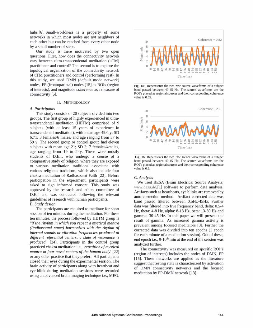
hubs [6]. Small-worldness is a property of some

networks in which most nodes are not neighbors of

each other but can be reached from every other node

by a small number of steps.

Our study is there motivated by two open

questions. First, how does the connectivity network

vary between ultra-transcendental meditation (uTM)

practitioner and control? The second is to explore the

topological organization of the connectivity network

of uTM practitioners and control (performing rest). In

this study, we used DMN (default mode network)

nodes, FP (frontoparietal) nodes [15] as ROIs (region

of interests), and magnitude coherence as a measure of

connectivity [5].

II. METHODOLOGY

A. Participants

This study consists of 20 subjects divided into two

groups. The first group of highly experienced in ultra-

transcendental meditation (HETM) comprised of 9

subjects (with at least 15 years of experience in

transcendental meditation), with mean age 49.0 y; SD

6.71; 3 females/6 males, and age ranging from 37 to

59 y. The second group or control group had eleven

subjects with mean age 21; SD 2; 7 females/4males,

age ranging from 19 to 24y. These were mostly

students of D.E.I, who undergo a course of a

comparative study of religion, where they are exposed

to various meditation traditions associated with

various religious traditions, which also include four

chakra meditation of Radhasoami Faith [22]. Before

participation in the experiment, participants were

asked to sign informed consent. This study was

approved by the research and ethics committee of

D.E.I and was conducted following the relevant

guidelines of research with human participants.

B. Study design

The participants are required to meditate for short

session of ten minutes during the meditation. For these

ten minutes, the process followed by HETM group is

“if the rhythm in which you repeat a mystical mantra

(Radhasoami name) harmonizes with the rhythm of

internal sounds or vibration frequencies produced at

different referential centers, a state of resonance is

produced” [24]. Participants in the control group

practiced chakra meditation i.e., 'repetition of mystical

mantra at four navel centers of the human body' [22]

or any other practice that they prefer. All participants

closed their eyes during the experimental session. The

brain activity of participants along with heartbeat and

eye-blink during meditation sessions were recorded

using an advanced brain imaging technique i.e., MEG.

Fig. 1a: Reperesents the two raw source waveforms of a subject

band passed between 40-45 Hz. The source waveforms are the ROI’s placed as regional sources and their corresponding coherence

value is 0.55.

Fig. 1b: Reperesents the two raw source waveforms of a subject band passed between 40-45 Hz. The source waveforms are the

ROI’s placed as regional sources and their corresponding coherence

value is 0.2.

C. Analysis

We used BESA (Brain Electrical Source Analysis;

www.besa.de)[1] software to perform data analysis.

Artifacts such as heartbeats, eye blinks are removed by

auto-correction method. Artifact corrected data was

band passed filtered between 0.5Hz-45Hz; Further

data was filtered into five frequency band, delta: 0.5-4

Hz, theta: 4-8 Hz, alpha: 8-13 Hz, beta: 13-30 Hz and

gamma: 30-45 Hz. In this paper we will present the

result of gamma. As increased gamma activity is

prevalent among focused meditators [3]. Further the

corrected data was divided into ten epochs (1 epoch

for each minute of a meditation session). Out of these,

end epoch i.e., 9-10th min at the end of the session was

analyzed further.

The connectivity was measured on specific ROI’s

(region of interests) includes the nodes of DMN, FP

[15]. These networks are applied as the literature

suggest that resting state is characterized by activation

of DMN connectivity networks and the focused

meditation by FP-DMN network [13].

0

2

4

6

8

10

0

14

28

42

56

70

84

98

11

2

12

6

14

0

15

4

16

8

18

2

19

6

21

0

22

4

23

8

Mag

nit

ude

Time (ms)

Coherence = 0.82

0

2

4

6

8

10

0

14

28

42

56

70

84

98

11

2

12

6

14

0

15

4

16

8

18

2

19

6

21

0

22

4

23

8

Mag

nit

ude

Time (ms)

Coherence 0.23


http://www.besa.de/

The 28 ROI’s include PCC (Posterior Cingulate

Cortex), mPFC (medial prefrontal cortex), LAG(left

angular gyrus), RAG(right angular gyrus),

LLatTemp(left lateral temporal), RLatTemp(right

lateral temporal), NoiseLOcc (left occipital),

NoiseROcc (right occipital), NoiseLF (left frontal),

NoiseRFr (right frontal), NoiseMFr (medial frontal),

NoiseMPar (medial parietal), LdIPFC(left dorsolateral

prefrontal cortex), RdIPFC (right dorsolateral

prefrontal cortex), LFront (left frontal), RFront (right

frontal), LIPL (left inferior parietal lobe), RIPL(right

inferior parietal lobe), LIPS (left inferior superior

sulcus), RIPS (right inferior superior sulcus),

NoiseLTemp (left temporal), NoiseRTemp (right

temporal), NoiseFrontal, superior frontal, LrACC (left

rostral anterior cingulate), RrACC (right rostral

anterior cingulate), amygdala, cACC (caudal anterior

cingulate cortex.

These are placed as regional sources and are fitted

on the end minute data. The resulting source forms are

exported with first orientation for performing

connectivity analysis. To determine the degree of

synchronization between source waveforms, the

absolute part of coherence (magnitude coherence) was

calculated [5]. Coherence is a measure of the linear

relationship between the signals at specific frequency.

In practice coherence is defined as normalized cross-

spectrum:

𝐶𝑥𝑦(𝑓) = |⟨𝑆𝑥𝑦(𝑓)⟩

√⟨𝑆𝑥𝑥(𝑓)⟩⟨𝑆𝑦𝑦(𝑓)⟩|

Where ⟨∙⟩ indicates averaging over trails, 𝑆𝑥𝑦 is the

cross-spectral density between the two signals, and

𝑆𝑥𝑥 and 𝑆𝑦𝑦 are the auto spectral densities for signals x

and y, respectively as shown in figure 1a and 1b.

C.1. Functional distance and characteristic path

length

The functional distance is the length of the shortest

path between a pair of nodes. As a first step, the

functional connectivity matrix was converted to a

connection-length matrix using BCT (brain

connectivity toolbox) [21]. The average shortest path

of the network, termed as is the mean of functional

distance matrix.

S.No. Node S.No. Node

1 PCC 15 LFront

2 mPFC 16 RFront

3 LAG 17 LIPL

4 RAG 18 RIPL

5 LLatTemp 19 LIPS

6 RLatTemp 20 RIPS

7 NoiseLOcc 21 NoiseLTemp

8 NoiseROcc 22 NoiseRTemp

9 NoiseLFr 23 NoiseFrontal

10 NoiseRFr 24 superior frontal

11 NoiseMFr 25 LrACC

12 NoiseMPar 26 RrACC

13 LdlPFC 27 amygdala

14 RdlPFC 28 cACC

3(a) 3(b)

Fig. 3: Represents the 3D view of connectivity nodes at 40 Hz

frequency averaged across the time with the threshold value as 0.7 for (a) control, (b) HETM groups. The regional sources are placed

at ROI’s, the connectivity was represented by line joining two sources (nodes).

4(a) 4(b)

Fig. 4: Represents the 3D view of connectivity nodes at 45 Hz

frequency averaged across the time with the threshold value as 0.7

for (a) control, (b) HETM groups. The regional sources are placed at ROI’s; the connectivity was represented by line joining two

sources (nodes).

Fig. 2: Represents the 28 regional source locations placed as ROI’s.

The first 12 constitute DMN and later FP nodes. The left image

shows sagittal view (includes left lobes), the right shows the top view includes both left and right lobes. The numbering of regional

sources is according to the table 1.

Table 1: It shows the names of ROI’s which are represented in the figure 2.


C.2. Clustering Coefficient

The clustering coefficient identifies the neighbors

of each node and determines the degree of local

connectivity of the node with its neighbor. Local

efficiency is also a nodal parameter directly

proportional to clustering coefficient of a node which

characterizes the efficiency of information transfer

among the neighbors of node [17].

III. EXPERIMENTAL RESULTS

Figure 3 and 4 shows the connectivity between the

ROI’s generated by coherence analysis in 3D view at

40 Hz and 45 Hz, respectively for HETM and control.

The connectivity represented is above 0.7 thresholds.

This result shows that the connectivity is high in

meditators group in contrast to control group. The

connectivity between the nodes gets increased for the

groups at higher frequencies, ensuring that they are

meditating.

Figure 5 and 6 shows the connectivity network in

the form of image with nodes as ROI’s and strength of

coherence between the nodes in the form of weights.

The diagonal entries show high coherence as it

represents the connectivity between the same nodes.

Simply it means the source wave form is always in

coherence with itself. Further, global characteristics

are calculated on the connectivity network matrix of

the groups.

Figure 7 compares the PL and CC of meditation

state network of the groups. The PL of HETM group

is smaller in comparison with control. The CC of

HETM is larger in comparison with control.

According to literature the small world networks are

characterized by small characteristic path length and

high clustering coefficient in comparison to a random

network [19; 17]. Therefore, the meditators

connectivity network seems to have a comparative

topological organization of small world networks.

These results therefore reveal the occurrence of small

world networks in meditators.

IV. CONCLUSION

Results of the present study on ROI’s, functional

connectivity analysis of the networks of meditators

and controls, indicated that the group of meditators

showed increased connectivity in gamma oscillations.

Additionally, the calculation of network parameters

showed an increase in CC and decrease in PL within

HETM group in contrast to control. Overall, these

comparisons led to study of small worldness

topological organization of network occurrence

characterizing uTM.

0

1

2

3

4

5

40 Hz 45 Hz

(a) Characteristic Path-length

HETM Control

0

0.1

0.2

0.3

0.4

0.5

0.6

40 Hz 45 Hz

(b) Clustering Coefficient

HETM Control

Fig. 7: Represents global characteristic parameters for ROI’s

connectivity analyses in HETM group (blue) and control group (red). The graph shows the mean values and bars represent the

standard deviation of (a) CC, (b) PL.

6(a) 6(b)

Fig. 6: Represents the weighted connectivity matrix (28X28) at

45 Hz frequency averaged across the time for (a) control, (b)

HETM groups. The weights of the matrix represent the strength of coherence between the nodes. The 28 nodes are according to

table 1.

5(a) 5(b)

Fig. 5: Represents the weighted connectivity matrix (28X28) at 40 Hz

frequency averaged across the time for (a) control, (b) HETM groups.

The weights of the matrix represent the strength of coherence between

the nodes. The 28 nodes are according to table 1.


The hierarchical clustered networks that model

the modular organization of mammalian cerebral

cortex extending across several hierarchical levels

have been shown to have properties like small world

networks [9]. As an extension of this study, it would

be interesting to analyze hierarchical clustered

networks and how they best characterize connectivity

networks in focused meditative state of uTM when

compared to resting state.

ACKNOWLEDGEMENT

We are indebted to Chairman, Advisory

Committee on Education, DEI for motivating us to

study graph theoretic aspects of brain dynamics. We

are thankful to Dr. Sona Ahuja for support in data

collection and Prof. Manjari Tripathi for facilitation of

data recording.

REFERENCES

[1]. BESA GmbH, Freihamer Str. 18, 82166 Graefelfing, Germany (www.besa.de)

[2]. Bowyer, S. M. (2016). Coherence a measure of the brain

networks: past and present. Neuropsychiatric

Electrophysiology, 2(1), 1-12.

[3]. Braboszcz, C., Cahn, B. R., Levy, J., Fernandez, M., &

Delorme, A. (2017). Increased gamma brainwave amplitude compared to control in three different meditation

traditions. PloS one, 12(1), e0170647.

[4]. Bærentsen, K. B. (2015). Patanjali and neuroscientific research on meditation. Frontiers in psychology, 6, 915.

[5]. Colclough, G. L., Woolrich, M. W., Tewarie, P. K., Brookes,

M. J., Quinn, A. J., & Smith, S. M. (2016). How reliable are

MEG resting-state connectivity metrics?. Neuroimage, 138,

284-293.

[6]. Farahani, F. V., Karwowski, W., & Lighthall, N. R. (2019).

Application of graph theory for identifying connectivity

patterns in human brain networks: a systematic

review. frontiers in Neuroscience, 13, 585.

[7]. Jones, P. (2019). Mindfulness training: Can it create superheroes?. Frontiers in Psychology, 10, 613.

[8]. Kajimura, S., Masuda, N., Lau, J. K. L., & Murayama, K.

(2020). Focused attention meditation changes the boundary

and configuration of functional networks in the

brain. Scientific reports, 10(1), 1-11.

[9]. Kaiser, M., Goerner, M., & Hilgetag, C. C. (2007). Criticality

of spreading dynamics in hierarchical cluster networks

without inhibition. New Journal of Physics, 9(5), 110.

[10]. Kaur, C., & Singh, P. (2015). EEG derived neuronal

dynamics during meditation: progress and

challenges. Advances in preventive medicine, 2015.

[11]. Iakovidou, N. D. (2017). Graph theory at the service of electroencephalograms. Brain connectivity, 7(3), 137-151.

[12]. Maldjian, J. A., Davenport, E. M., & Whitlow, C. T. (2014).

Graph theoretical analysis of resting-state MEG data: Identifying interhemispheric connectivity and the default

mode. NeuroImage, 96, 88-94.

[13]. Marinato, G. (2020). Object-Based Attention in Naturalistic

Auditory Streams (Doctoral dissertation, University of Trento.

[14]. Marzetti, L., Basti, A., Chella, F., D'Andrea, A., Syrjälä, J., &

Pizzella, V. (2019). Brain functional connectivity through phase coupling of neuronal oscillations: a perspective from

magnetoencephalography. Frontiers in neuroscience, 13,

964. [15]. Marzetti, L., Di Lanzo, C., Zappasodi, F., Chella, F., Raffone,

A., & Pizzella, V. (2014). Magnetoencephalographic alpha

band connectivity reveals differential default mode network

interactions during focused attention and open monitoring

meditation. Frontiers in human neuroscience, 8, 832.

[16]. Mheich, A., Wendling, F., & Hassan, M. (2020). Brain

network similarity: methods and applications. Network

Neuroscience, 4(3), 507-527.

[17]. Mohan, A., De Ridder, D., & Vanneste, S. (2016). Graph

theoretical analysis of brain connectivity in phantom sound

perception. Scientific reports, 6(1), 1-14.

[18]. Miyoshi, T., Tanioka, K., Yamamoto, S., Yadohisa, H.,

Hiroyasu, T., & Hiwa, S. (2019). Short-term effects on brain

functional network caused by focused-attention meditation

revealed by Tucker3 clustering on graph theoretical

metrics. bioRxiv, 765693.

[19]. Paraskevopoulos, E., Dobel, C., Wollbrink, A., Salvari, V.,

Bamidis, P. D., & Pantev, C. (2019). Maladaptive alterations

of resting state cortical network in Tinnitus: A directed

functional connectivity analysis of a larger MEG data

set. Scientific reports, 9(1), 1-11.

[20]. Reddy, J., & Roy, S. (2018). Commentary: Patanjali and

neuroscientific research on meditation. Frontiers in

psychology, 9, 248.

[21]. Rubinov M, Sporns O (2010) NeuroImage 52:1059-69

(Complex network measures of brain connectivity: Uses and

interpretations.)

[22]. Sahab, M. (2004). Discourses on Radhasoami Faith, with

supplement. Dayalbagh, Agra: RadhasoamiSatsangSabha,

[23]. Satsangi, P. S. (2013) Vision Talk, Towards Science of

Consciousness 2013, DEI, Agra

(https://www.dayalbagh.org.in/specialTalks/visiontalkTSC20

13.htm)

[24]. Satsangi, P. S. (2010). Expositions on truth, ultimate reality

and supreme being (From Vantage Point of Radhasoami Faith

and Systems Science). Agra: Radhasoami Satsang Sabha.

[25]. Vecchio, F., Miraglia, F., & Rossini, P. M. (2017).

Connectome: Graph theory application in functional brain

network architecture. Clinical neurophysiology practice, 2,

206-213.


http://www.besa.de/

http://dx.doi.org/10.1016/j.neuroimage.2009.10.003

http://dx.doi.org/10.1016/j.neuroimage.2009.10.003

https://www.dayalbagh.org.in/specialTalks/visiontalkTSC2013.htm

https://www.dayalbagh.org.in/specialTalks/visiontalkTSC2013.htm

1

Meta Game theoretic analysis of standard “real

world”game theoretic problems

Abstract—Meta game theory is a non-quantitative

reconstruction of mathematical game theory. This paper

attempts to use meta game theory for conflict analysis. A

conflict is a situation where parties with opposing goals

affect one another. A person without prerequisite knowledge

about meta game analysis or game theory can implement this

method. The paper accomplishes a metagame analysis of

various standard game theoretic problems. The study first

models the conflict, then a tableau is set up.

Keywords—meta game theory, conflict analysis, game of

pure coordination

I. INTRODUCTION

Meta game theory has been applied to analyse political

conflicts, particularly water resources problems [1], the

Vietnam war and arms control [2], the Arab-Israeli conflict

[3] using the method of meta game analysis. The technique

has been applied to environmental management [4], fall of

france, an international water allocation conflict, and the

Garrison Diversion Unit (GDU) irrigation project in North

Dakota, U.S.A. [5]. Game of pure coordination is a

standard problem which has been used to develop an

understanding about the meta game analysis [5]. In

particular, the game of chicken is studied [6]. In the game

of matching pennies, analysis is done for many games and

a structural econometric model incorporating risk aversion

into a quantal response equilibrium is studied [7]. In a

three-person matching pennies game, subjects play the

mixed strategy Nash equilibrium [8]. The cooperation is

shown as an equilibrium of the full full metagame using

the method of general metagames [9]. The analysis is

conducted for two different efficiency problems in the

battle of sexes game. The first one is coordination and

second one is maximizing the expected utility by favouring

a player facing high stakes [10]. The analysis of the rules

of the qualification tournament in the UEFA zone for the

2014 FIFA World Cup is conducted using game theory

[11]. The study done updates optimal decision policies as

the new information becomes available and also utility

theory is used to capture different risk preferences of the

decision makers [12]. The quantum feature of

entanglement is used to quantize the prisoner’s dilemma

game [13]. The quantum version of the prisoner’s dilemma

game outperforms the classical version [14]. The concepts

of Nash equilibrium and evolutionary stable strategy have

been introduced in the study of the rock paper scissors

game [15]. The theory of games describes the behaviours

in humans and other biological organisms in the rock paper

scissors game [16].

II. METHODOLOGY

Game playing couples intellectual activity with direct

competition. If a person has better thinking abilities and

learning skills, their chances of winning more games

improve. So, a person should play games against

opponents and keep evaluating the progress to test and

refine his/her intellectual skills. [17]

Meta game theory is a scientific method that reconstructs

classical game theory on a non-quantitative basis in order

to analyse political conflicts. The method of application of

meta game theory to actual conflicts is called meta game

analysis or the analysis of options. [5]

A. Conflict analysis

The following three points must be considered while

carrying out the conflict analysis. (a) The conflict analysis

is done for a particular point of time. (b) There are limited

number of players. (c) Options per player are limited.

B. The Cookie Conflict

A simple conflict between two children, one of whom has

a cookie that the other child wants. The Conflict analysis

takes into account (a) Point of time- player who wants the

cookie realizes he can have it. (b) Players- child A, B (c)

Options- (i) “take cookie”- player A (ii) “hit A”- player B

[18]

PREFERENCE VECTOR

For player A - Possible outcomes

Player

A “take

cookie”

1 0 1 0 20=1

Player

B “hit

A”

0 0 1 1 21=2

1 0 3 2

Table 1(a): The preference vector for player A in the Cookie conflict problem

For player B - Possible outcomes

Player A “take

cookie”

0 1 1 0 20=1

Player

B “hit

A”

0 0 1 1 21=2

0 1 3 2

Table 1(b): The preference vectors for player B in the Cookie conflict problem

Decimalized Preference vector

Swati Singh Department of Physics and Computer Science


Dayal Pyari Srivastava

Department of Physics and Computer Science Dayalbagh Educational Institute

C. Patvardhan Department of Electrical Engineering



Player

A

1 0 3 2

1 3

Table 1(c):Decimalized preference vector for player A in the Cookie conflict problem

Player

B

0 1 3 2

1 0

Table 1(d):Decimalized preference vector for player B in the cookie conflict

C. THE PRISONER’S DILEMMA

THE PAYOFF MATRIX

PLAYER 1

C D

PLAYER 2 C 3, 3 1, 4

D 4, 1 2, 2

• Tabular representation of prisoner’s dilemma for

player A Preference vector for player A

Player A

Option C 0 1 0 1

Option D 1 0 1 0

Preference vector for player B

Player B

Option C 1 1 0 0

Option D 0 0 1 1

(d, c) (c, c) (d, d) (c, d)

• Tabular representation of prisoner’s dilemma for

player B Preference vector for player A [23]

Player A

Option C 1 1 0 0

Option D 0 0 1 1

Preference vector for player B

Player B

Option C 0 1 0 1

Option D 1 0 1 0

(c, d) (c, c) (d, d) (d, c)

III. RESULTS

A. GAME OF PURE COORDINATION

Assume that two drivers meet on a narrow dirt road. Both

have to swerve in order to avoid a head-on collision. If

both execute the same swerving manoeuvre they will

manage to pass each other, but if they choose differing

manoeuvres they will collide. [19]

Payoff matrix

Left Right

Left 1,1 0,0

Right 0,0 1,1

Table 2(a): The payoff matrix in the game of pure coordination

• Preference vector


Player

L

“avoid getting

hit”

1 0 1 0 20=1

Player R

“avoid

getting hit”

1 1 0 0 21=2

3 2 1 0

Table 2(b): The preference vector for player A in the game of pure coordination


Player

L

“avoid getting

hit”

1 1 0 0 20=1

Player R

“avoid

getting hit”

1 0 1 0 21=2

3 1 2 0

Table 2(c): The preference vector for player B in the game of pure coordination

• Decimalized Preference vector Player

A

3 2 1 0

Table 2(d): Decimalized preference vector for player A in the game of pure

coordination

Player

B 3 1 2 0

Table 2(e): Decimalized preference vector for player B in the game of pure

coordination

B. MATCHING PENNIES

• Each player has a penny and must secretly

turn the penny to heads or tails. The players

then reveal their choices simultaneously.

• Player 1: Even – wins – Pennies match

• Player 2: Odd – loose – do not match [18]

Payoff matrix

Player

A

Player

B

Head Tail

Head 1,-1 -1,1

Tail -1,1 1,-1

Table 3(a): The payoff matrix for the matching pennies game

• PREFERENCE VECTOR


Player

H

“avoid getting

hit”

1 1 0 0 20 = 1


Player T

“avoid

getting

hit”

0 1 0 1 21 = 2

1 3 0 2

Table 3(b): The preference vector for player A in matching pennies game


Player H

“avoid

getting

hit”

0 1 0 1 20 = 1

Player

T “avoid

getting

hit”

1 1 0 0 21 = 2

2 3 0 1

Table 3(c): The preference vector for player B in the matching pennies game

• Decimalized preference vector

Player

A 1 3 0 2

Table 3(d): Decimalized preference vector for player A in the matching pennies game

Player

B 2 3 0 1

Table 3(e): Decimalized preference vector for player B in the matching pennies game

C. PRISONER’S DILEMMA

PAYOFF MATRIX

Confess Defect

Confess 3, 3 0, 5

Defect 5, 0 1, 1

Table 4(a): The payoff matrix for the Priosner’s dilemma game

Transforming to binary

• 1,0 – denoted by 0

• 3,5 – denoted by 1 [19]

Confess Defect

Confess 1, 1 0, 1

Defect 1, 0 0, 0

Table 4(b): The payoff matrix for the Prisoner’s dilemma game with modified payoff values

• Preference vector For player A - Possible outcomes

Player A

“minimize

trial

0 0 1 1 20 = 1

period”

Player B “

minimize trial

period”

0 1 1 0 21 = 2

0 2 3 1

Table 4(c): The preference vector for player A in matching pennies game


Player A “

minimize

trial

period”

0 1 1 0 20 = 1

Player B

“

minimize trial

period”

0 0 1 1 21 = 2

0 1 3 2

Table 4(d): The preference vector for player B in the matching pennies game

• Decimalized preference vector 0 2 3 1

1 3

Table 4(e): Decimalized preference vector for player A in the matching

pennies game

Player

B 0 1 3 2

2 3

Table 4(f): Decimalized preference vector for player B in the matching

pennies game

D. BATTLE OF SEXES

Payoff Matrix

TV Opera

TV 3, 2 1, 1

Opera 0, 0 2, 3

Table 5(a): The payoff matrix for the battle of sexes game

• Transforming to binary


• 3,2 – denoted by 1 [20]

TV Opera

TV 1, 1 0, 0

Opera 0, 0 1, 1

Table 5(b): The payoff matrix for the battle of sexes game with updated payoff values

• Preference Vector For player A - Possible outcomes


Player A

“wants

opera”

1 1 0 0 20 = 1

Player B “

wants

TV”

1 1 0 0 21 = 2

3 3 0 0

Table 5(c): The preference vector for player A in battle of sexes game


Player

A “ wants

opera”

1 1 0 0 20 = 1

Player

B “ wants

TV”

1 1 0 0 21 = 2

3 3 0 0

Table 5(d): The preference vector for player B in the battle of sexes game

• Decimalized preference vector Player

A

3 3 0 0

Table 5(e): Decimalized preference vector for player A in the battle of sexes

game

Player

B

3 3 0 0

Table 5(f): Decimalized preference vector for player B in the battle of sexes

game

E. STAG HUNT GAME

Payoff matrix

Stag Hare

Stag 9,9 0, 8

Hare 8, 0 7, 7

Table 6(a): The payoff matrix for the stag hunt game



• 8,9 – denoted by 1 [21] Stag Hare

Stag 1, 1 0, 1

Hare 1, 0 0, 0

Table 6(b): The payoff matrix for the stag hunt game with updated payoff values


Player H

“avoid

getting

hit”

1 1 0 0 20 = 1

Player

T “avoid

1 0 1 0 21 = 2

getting

hit”

3 1 2 0

Table 6(c): The preference vector for player A the stag hunt game


Player

H “avoid

getting

hit”

1 0 1 0 20 = 1

Player

T

“avoid getting

hit”

1 1 0 0 21 = 2

3 2 1 0

Table 6(d): The preference vector for player B the stag hunt game


A

3 1 2 0

3 1

Table 6(e): Decimalized preference vector for player A in the stag hunt game

Player

B

3 2 1 0

3 2

Table 6(f): Decimalized preference vector for player B in the stag hunt game

F. FOOTBALL

Payoff matrix

Run Pass

Run -5,5 5,-5

Pass 5,-5 -5,5

Table 7(a): The payoff matrix for football


• -5 – denoted by 0

• 5 – denoted by 1 [22] Run Pass

Run 0, 1 1, 0

Pass 1, 0 0, 1

Table 7(b): The payoff matrix for football with updated payoff values


Player

A “run-

pass or pass-

run”

1 1 0 0 20 = 1

Player

T “avoid

getting

hit”

0 0 1 1 21 = 2


1 1 2 2

Table 7(c): The preference vectors for player A for football For player B - Possible outcomes

Player

H

“avoid getting

hit”

0 0 1 1 20 = 1

Player

T “avoid

getting

hit”

1 1 0 0 21 = 2

2 2 1 1

Table 7(d): The preference vector for player B for football


A

1 1 2 2

Table 7(e): Decimalized preference vector for player A for football

Player

B

2 2 1 1

Table 7(f): Decimalized preference vector for player B for football

G. QUANTUM PRISONER’S DILEMMA

Payoff matrix

Confess Defect Q

Confess 3, 3 0, 5 1,1

Defect 5, 0 1, 1 0,5

Q 1,1 5,0 3,3

Table 8(a): The payoff matrix for the Quantum Prisoner’s dilemma game



• 3,5 – denoted by 1 [19] Confess Defect Q

Confess 1, 1 0, 1 0,0

Defect 1, 0 0, 0 0,1

Q 0,0 1,0 1,1

Table 8(b): The payoff matrix for the Quantum Prisoner’s dilemma game with updated payoff

values


Player

A “run-pass or

pass-

run”

1 1 0 0 20 = 1

Player

T 0 0 1 1 21 = 2

“avoid getting

hit”

1 1 2 2

Table 8(c): The preference vectors for the Quantum Prisoner’s dilemma game


Player H

“avoid

getting

hit”

0 0 1 1 20 = 1

Player

T

“avoid getting

hit”

1 1 0 0 21 = 2

2 2 1 1

Table 8(d): The preference vector for the Quantum Prisoner’s dilemma game


A

1 0 3 2

1 3

Table 8(e): Decimalized preference vector for player A for Quantum Prisoner’s dilemma game

Player

B

0 1 3 2

1 0

Table 8(f): The Decimalized preference vector for player B for Quantum Prisoner’s dilemma

game

H. ROCK PAPER SCISSORS

Payoff matrix

Rock Paper Scissors

Rock 0,0 -1,1 1,-1

Paper 1,-1 0,0 -1,1

Scissors -1,1 1,-1 0,0

Table 9(a): The payoff matrix for rock paper scissors


• -1,0 – denoted by 0

• 1 – denoted by 1 [18]


Player

H “avoid

getting

hit”

1 0 -1 20 = 1

Player T

“avoid

getting

hit”

-1 0 1 21 = 2

Table 9(b): The preference vector for player A for rock paper scissors


Player

H

“avoid

-1 0 1 20 = 1


getting

hit”

Player

T “avoid

getting

hit”

1 0 -1 21 = 2

Table 9(c): The preference vector for rock paper scissors

We come across two cases, (a) -1, 0 0

1 1

Table 9(d): The payoff transformation values for rock paper scissors

A 1 0 0 20

0 0 1 21

1 0 2

Table 9(e): The Decimalized preference vector for player A rock paper scissors

B 0 0 1 20

1 0 0 21

2 0 1

Table 9(f): The Decimalized preference vector for player B rock paper scissors

We come across two cases, (b) -1 0

0, 1 1

Table 9(i): The payoff transformation for rock paper scissors

A 1 1 0 20

0 1 1 21

1 3 2

Table 9(j): The preference vector for player A for rock paper scissors

B 0 1 1 20

1 1 0 21

2 3 1

Table 9(k): The preference vector for player B for rock paper scissors


A 1 0 3 2

1 3

Table 9(m): Decimalized preference vector for rock paper scissors

Player

B

0 1 3 2

1 0

Table 9(n): The Decimalized preference vector for rock paper scissors

IV. CONCLUSION

The authors attempted to do a novel analysis of

standard game theoretic problems using the metagame

analysis techniques. The meta game analysis has many

advantages viz. it includes all the information about the

conflict, easy to do by hand, can be used for hypergames

and very complex conflicts. The results obtained are to

authors show the stability analysis for various standard

game theoretic problems.

V. ACKNOWLEDGEMENT

I am thankful to Prof. D. S. Mishra and Prof. Sant Kumar

Gaur for their guidance.

VI. REFERENCES

[1] Hipel, K. W., Ragade, R. K., & Unny, T. E. (1974). Metagame analysis of

water resources conflicts. Journal of the Hydraulics Division, 100(10), 1437-

1455.

[2] Howard, N., The analysis of options: A computer aided method for analyzing

political problems, report prepared for the U.S. Arms Control and

Disarmament Agency, vol. 2, Univ, of Pa., Philadelphia, 1969.

[3] K. W. Hipel and N. M. Fraser, "Metagame analysis of the Garrison

Conflict," Water Resources Res., 1980 (to appear).

[4] Hipel, K. W., & Walker, S. B. (2011). Conflict analysis in environmental

management. Environmetrics, 22(3), 279-293. [5] Fraser, N. M., & Hipel, K. W. (1979). Solving complex conflicts. IEEE

Transactions on Systems, Man, and Cybernetics, 9(12), 805-816.

[6] Rapoport, A., & Chammah, A. M. (1966). The game of chicken. American

Behavioral Scientist, 10(3), 10-28.

[7] Goeree, J. K., Holt, C. A., & Palfrey, T. R. (2003). Risk averse behavior in

generalized matching pennies games. Games and Economic Behavior, 45(1),

97-113.

[8] McCabe, K. A., Mukherji, A., & Runkle, D. E. (2000). An experimental

study of information and mixed-strategy play in the three-person matching-

pennies game. Economic Theory, 15(2), 421-462.

[9] Howard, N. (1976). Prisoner's dilemma: The solution by general

metagames. Behavioral science, 21(6), 524-531.

[10] Banks, J. S., & Calvert, R. L. (1992). A battle-of-the-sexes game with

incomplete information. Games and Economic Behavior, 4(3), 347-372.

[11] Dagaev, D., & Sonin, K. (2013). Game theory works for football

tournaments. Manuscript. http://voxeu. org/article/world-cup-football-and-

game-theory, 7.

[12] Jordan, J. D., Melouk, S. H., & Perry, M. B. (2009). Optimizing football

game play calling. Journal of Quantitative Analysis in Sports, 5(2).

[13] Nawaz, A. (2013). The strategic form of quantum prisoners' dilemma.

Chinese Physics Letters, 30(5), 050302.

[14] Du, J., Xu, X., Li, H., Zhou, X., & Han, R. (2002). Playing prisoner's

dilemma with quantum rules. Fluctuation and Noise Letters, 2(04), R189-

R203. [15] Zhou, H. J. (2016). The rock–paper–scissors game. Contemporary Physics,

57(2), 151-163.

[16] Hoffman, M., Suetens, S., Gneezy, U., & Nowak, M. A. (2015). An

experimental investigation of evolutionary dynamics in the Rock-Paper-

Scissors game. Scientific reports, 5(1), 1-7. [17] Pell, B. (1993). Strategy generation and evaluation for meta-game playing

(Doctoral dissertation, University of Cambridge).

[18] Edward W. Piotrowski., The next stage : quantum game theory (Arxiv, Aug

2003)

[19] Siopsis, G., Balu, R., & Solmeyer, N. (2018). Quantum prisoners' dilemma

under enhanced interrogation. Quantum Information Processing, 17(6), 1-12.

[20] Nawaj, A., Toor A. H., Worst-case Payoffs in Quantum Battle of Sexes

Game; quant-ph/0110096.

[21] Toyota, N., Quantization of the stag hunt game and the Nash equilibrium;

quant-ph/0307029.

[22] Mike shor, (2014), Mixed Strategies in Football,

https://www.mikeshor.com/courses/gametheory/docs/topic4/football.html

[23] Madani, K., & Hipel, K. W. (2011). Non-cooperative stability definitions for

strategic analysis of generic water resources conflicts. Water resources

management, 25(8), 1949-1977.


Identifying Correlation dimension of non-linear

time series obtained from E/MEG data

Mansi Tarani1, C.M. Markan2

Faculty of Science

Dayalbagh Education Institute

Agra (INDIA) [email protected] , [email protected]

Abstract—:- The correlation dimension is a tool to

measure fractal dimensions. In this paper, we calculate

the correlation dimension of nonlinear time-series

obtained from recorded Magnetoencephalography

(MEG) data taken from a cognitive experiment where

subjects had been asked to focus attention over a session

of 10 minutes. The experiment involved three different

categories of subjects viz., novice, moderate and experts

and for each category, the recoded data was segmented

into three parts associated with a start, mid and end of

the session. The experimental data were blind coded and

the correlation dimension technique was applied to

decipher the code. Results demonstrate a clearly

identifiable relationship between correlation dimension

and category of experimental data. The technique has

interesting applications in the objective measurement of

subjective mental states.

Keywords— Correlation Dimension, Magnetoencephalography

(MEG), Nonlinear Dynamics, Associative brain

I. Introduction

From the past, we humans tend to associate a number with

everything one sees and observes and provide an objectified

computational view to everything. As Perter Ducker, an

Australian management consultant, educator, and author

once said, “If you can’t measure it, you can’t manage it”.

One of the important aspects of this objectifying and

computation is dimensional analysis [1].

While studying the time series of complex systems,

nonlinear properties help in differentiate system behaviour.

The time series associated with natural phenomena is known

to show a self-similar behaviour, which depends on the time

scale of measurements. The fractal dimension is therefore an

important characteristic of such systems because it contains

information about their geometrical structure at multiple

scales[2]. Chaotic invariants like the fractal dimensions are

therefore often used to characterize non-linear time series.

When we look into fractals one can have a thought of

repeating patterns in low dimensions. The question is how a

measured fractal dimension can help in understanding the

repeating patterns in time series apart from non-integer

dimension values.

Experiments in cognitive science are often associated with

quantifying a subjective mental state. The experimental

observation are recorded as E/MEG data which consists of

nonlinear time series rhythms which are characterized by

self-similar behavior, at various time scale of measurements.

There is a need and effort to associate cognitive science with

machine learning and artificial intelligence through various

methods and to give objective or mathematical measurement

to noisy patterns. Motivated by the application of correlation

dimension in stock marketing, weather forecasting, and all

other time series, we tried to use this method on E/MEG

data.

The correlation dimension is calculated using the

Grassberger-Procaccia Algorithm which states that the

probability of two points of the set is in the same cell of size

r is approximately equal to the probability that two points of

the set are separated by a distance Θ less than or equal to

r[3]. Thus correlation dimension C(r) is given by:-

Where Θ is the heavenside function defined as

The dimension is then calculated by evaluation of C(r) over

a range of values of r and then deduce correlation dimension

D2 from the slope of the straight line which best fit in the

region of a plot of log(c(r))and log(r). It is written as

Fig 1: Correlation dimension plot for the data as generated

from Matlab


1.%20Keogh%20E.,%20Mueen%20A.%20(2017)%20Curse%20of%20Dimensionality.%20In%20Sammut%20C.,%20Webb%20G.I.%20(eds)%20Encyclopedia%20of%20Machine%20Learning%20and%20Data%20Mining.%20Springer,%20Boston,%20MA.%20https:/doi.org/10.1007/978-1-4899-7687-1_192

2.%20Walling%20PT.%20An%20update%20on%20dimensions%20of%20consciousness.%20Proc%20(Bayl%20Univ%20Med%20Cent).%202019;33(1):126-130.%20Published%202019%20Sep%2030.%20doi:10.1080/08998280.2019.1656009.https:/www.ncbi.nlm.nih.gov/pmc/articles/PMC6988684/

https://www.semanticscholar.org/paper/Chapter-1-NONLINEAR-DYNAMICS-TIME-SERIES-ANALYSIS-Henry-Lovell/e574b4eaf1a1f95dc0944831040bacb6b4666921

We can represent this by attractors which are phase space trajectories of deterministic dynamical systems that usually evolve towards a particular set of coordinates[5].. The waveform by measuring data at two different delays and plotting them against each other on the x and y-axis. To visualize it better it can also be represented by attractors. Attractors are the multidimensional phase space that represents how a system evolves with time[4]. It is associated with E/MEG. If we take a simple harmonic pendulum when plotted against velocity and distance gives a circle. This is an example of a periodic attractor which is shown in the figure. It has a dimension of 1. In this way, the attractor of two sinusoidal functions is a Toroid and it has a dimension of 1.5. In this way, different functions and different data give different correlation dimensions D2.

Fig 2: Above is the figure of an attractor of a simple pendulum and below is its plot of the waveform which is a periodic sinusoid. Its dimension is calculated to be 1.

2. Method

To check the reliability of the method, we obtained data from a cognitive science experiment using some set for E/MEG data from the cognitive science lab. Data provided to us was conducted in the past. In that experiment, different classes of subjects went to a mental state where they were asked to focus their attention. Different categories of subjects belong to novice, moderate and experienced. The recorded was segmented as associated with starting, middle and end of

the focussed attention session. These were given to us in form of blind coded data which means we were not told about the category of the subject it belongs to and were labelled as X11, X12, X13, X21, X22, X23, X31, X32, X33. We were required to decipher the code i.e., were given a task to classify it. We used matlab software to find the correlation dimension of the data using the Grassberger-Procaccia algorithm. On finding the correlation dimension, we found the dimension of data by taking the value of slope between C(r) and log(r) and plotted its attractor, fractal dimension.

3. Result

Our results closely matched with the expected result, we

categorized the result based on correlation dimension, which

is as

X11=subject with least experience in focusing, data taken at

the start of the session.


the middle of the session.


end of the session.

X21=subject with some experience in focusing, data taken

at the start of the session.


at end of the session.


at end of the session

X31=most experienced subjects in focusing, data taken at

the start of the session.


the middle of the session


end of the session

The expected result also yields to the same categorization,

it was that the correlation dimension of person focusing is

lowest in novice and high inexperienced and the correlation

dimension would increase as we will go from starting time

to end, which is what we also got. But in the result, we

found two dips in the middle part at X22 and X32 and we

are working on the theory of finding the reason associated

with it.

Fig 3: Image on the left shows the attractor formed by X11 data and image on right shows the attractor formed by

X33 data.X,Y,Z are taken as three axes


5.Mei%20Ying%20Boon%20et.al.,%20Journal%20of%20Vision,%20Vol.8(6),%20Jan%202008,.%20doi:https:/doi.org/10.1167/8.1.6

https://www.tandfonline.com/doi/abs/10.1080/08998280.2003.11927900

The correlation dimension curve is plotted using

Grassberger-Procaccia Algorithm and the slope of the curve

gave correlation dimension D2. The plot between the

embedding dimension, attractor, and waveform of X11and

X33 and D2is shown in fig 3, fig 4, fig 5. The value of the

correlation dimension is taken at the point where the value

saturates (fig 4).

Table 1 contains values of correlation dimension of all

classes of subjects where the first row are the subjects of

less experienced, the second row contains groups of some

experience of focusing and the third row are the most

experienced subjects in focussing

Fig 5:Image on the left shows the waveform of X11 data and Image on the right shows the waveform of X33 data where X-

axis correspond to time and Y axis correspond to data points

Figure-4: Image on the left shows the graph between embedding dimension and fractal dimension, the dimension D2

was found to be 2.3009 and image on the right shows the graph between embedding dimension and fractal dimension,

the dimension D2 in this case was found to be 2.6098

Table: Correlation Dimension of various categories

X 1 2 3

1 2.3009 2.488 2.3585

2 2.3918 2.3019 2.4847

3 2.5076 2.3795 2.6098

Table 1 contains values of correlation dimension of all

classes of subjects where the first row are the subjects of

less experienced, the second row contains groups of some

experience of focusing and the third row are the most

experienced subjects in focussing


4.. Discussion

The correlation dimension of a person increases with

experience in focusing and concentration. As a subject

enhances its capability, the correlation dimension also

increases as from previous studies [4] we can see humans

have the highest correlation dimension compared to other

lower animals because of the larger associative brain. So

this result can also be related to the associative brain i.e.,

subjects whose correlation dimension is found to be larger

have a larger associative brain. So we expect the correlation

dimension to be used as the way to quantify the dimension

of associative brain

5. References

1. Keogh E., Mueen A. (2017) Curse of Dimensionality. In Sammut C., Webb G.I. (eds) Encyclopedia of Machine Learning and Data Mining.

Springer, Boston, MA. https://doi.org/10.1007/978-1-4899-7687-1_192

2. Walling PT. An update on dimensions of consciousness. Proc (Bayl Univ Med Cent). 2019;33(1):126-130. Published 2019 Sep 30.

doi:10.1080/08998280.2019.1656009.https://www.ncbi.nlm.nih.gov/pmc/articles/PMC6988684/

3. Henry, B.E., Lovell, N., & Camacho, F. (2005). Chapter 1 NONLINEAR

DYNAMICS TIME SERIES ANALYSIS. https://www.semanticscholar.org/paper/Chapter-1-NONLINEAR-

DYNAMICS-TIME-SERIES-ANALYSIS-Henry-

Lovell/e574b4eaf1a1f95dc0944831040bacb6b4666921

4.Peter T. Walling & Kenneth N. Hicks (2003) Dimensions of

Consciousness, Baylor University Medical Center Proceedings, 16:2, 162-

166, DOI: 10.1080/08998280.2003.11927900

https://www.tandfonline.com/doi/abs/10.1080/08998280.2003.11927900

5.Mei Ying Boon et.al., Journal of Vision, Vol.8(6), Jan 2008,.

doi:https://doi.org/10.1167/8.1.6

6. Francisco-Cervantes Cervantes et.al., Fractal dimension algorithms and

their application to time series associated with natural phenomena, Journal

of Physics Conference Series 475(1), November 2013,

http://dx.doi.org/10.1088/1742-6596/475/1/012002


https://www.ncbi.nlm.nih.gov/pmc/articles/PMC6988684/

https://www.ncbi.nlm.nih.gov/pmc/articles/PMC6988684/

https://doi.org/10.1080/08998280.2003.11927900

A Comparative Study of Causal Curves and Endless Causal Curves in

Spacetime

Gunjan Agrawal and Shruti Sinha

Department of Mathematics, Faculty of Science, Dayalbagh Educational Institute

(Deemed University), Agra, India - 282005

Abstract

The space of causal curves provides sufficient information about the causal

structure of the spacetime. Global hyperbolicity, one of the essential

ingredients of singularity theorems is affiliated to the space of endless causal

curves. In the present paper, a study of the space of causal curves and its

subspace, viz., space of endless causal curves has been carried out and it has

been obtained that some of the properties, viz., Hausdorffness, regularity

are not enjoyed in the space of causal curves whereas these are preserved in

the space of endless causal curve when underlying spacetime is Minkowski

space equipped with the path topology.

Keywords: Casual curve, Global Hyperbolicity, Minkowski space, Singularity

1. Introduction

Spacetime, a continuum of space and time, is assumed to carry a causal structure to explain cause-

effect relationship among its elements. It has been studied as a causal space with a causal boundary

attached to it which represents both infinity and the part of the edge of the spacetime at a finite

distance, i.e. the singular points. Spacetime in both pre-relativity physics and in the theory of relativity

was considered as four dimensional; one dimension for time and the remaining three are spacial

dimensions. However, the causal structure differs significantly in both theories.

In Newtonian physics, time was considered as an independent entity, irrespective of frame of

reference, and the spacetime was mathematically modelled as a three dimensional euclidean space at

different times. All the events in space at a fixed time were treated as simultaneous events and

causally related events were mathematically described as those which can be joined by a

parameterized curve of events which moves forward in time and otherwise not restricted in space.

On the contrary, in the special theory of relativity, the concept of absolute time was replaced by the

fact that nothing moves faster than light. Hence for each inertial observer, also known as inertial

frame of reference, simultaneous events were defined using synchronisation of clocks positioned at

each point in 3-D coordinate space. Thus implying that for each observer, simultaneous events are

different. Mathematically, causally related events with respect to an inertial observer lie on or inside

the light cone at the origin in 4-D Minkowski space, where observer is supposed to be located at the

origin.

One of the necessary conditions for the mathematical structure of the spacetime is that no idealized

observer can travel back into its own past. Mathematical framework for the spacetime on which the

special theory of relativity was developed is a four dimensional Minkowski space. A physically

significant topology defined for the Minkowski space is considered to be the one whose


homeomorphism group coincides with the group generated by Lorentz group, the group which

consists of global coordinate transformation leaving spacetime interval invariant, Translations and

Dilatations [2]. Since homeomorphism group of the Euclidean topology does not satisfy this

condition, therefore it is not physically relevant. Zeeman proposed non-Euclidean topologies, viz.,

Fine topology, space topology, time topology, t- and the s-topologies on the four-dimensional

Minkowski space in order to make group of homeomorphisms physically significant. These

topologies were defined for the n-dimensional Minkowski space analogously and the topological

study of the n-dimensional Minkowski space with respect to non-Euclidean topologies has been

carried out.

General theory of relativity treats gravity not as a force field but a built-in feature of the spacetime.

Gravity is invariably experienced by all objects in spacetime carrying masses and is the reason for the

spacetime having the curved structure instead of flat. Mathematical model for the general theory of

relativity is Hausdorff, paracompact, four dimensional smooth Lorentz manifold, equipped with

Lorentz metric. Quantities associated with the Lorentz metric, for example the connection, the

Riemann tensor, the Ricci tensor and others, have physical interpretations and can be used to develop

physics in this setting, and make testable and tested predictions, which to date have proven consistent

with the available experimental data.

Homeomorphism group of the manifold topology defined on a Lorentz manifold is huge and has

no physical significance. Path topology, introduced by Hawking on a four-dimensional Lorentz

manifold, is a non-manifold topology which induces manifold topology on each timelike curve and

whose homeomorphism group is consistent with the causal and conformal structure of the Lorentz

manifold. Various non-manifold topologies on a four dimensional Lorentz manifold were introduced

including physically relevant generalizations of the Fine and time topologies which are referred to as

Zeeman and geodesic topologies respectively. Path topology on the four-dimensional Minkowski

space is same as the t-topology. Manifold topology is strictly coarser than the Zeeman, geodesic and

the path topologies.

A spacetime singularity is a breakdown in the spacetime, either in its geometry or in some other

basic physical structure. Singularities are mathematically modelled in terms of incomplete timelike

geodesics and studied by Penrose, Hawking, Geroch, to quote a few. Singularity theorems provide

sufficient conditions for the spacetime to be timelike or null geodesically incomplete.

A causal structure on the spacetime carries with it some essential ingredients of singularity

theorems, viz., Cauchy surface, global hyperbolicity etc. In a strongly causal spacetime, upper semi

continuity of the length function defined on the space of causal curves equipped with Geroch topology

forms the basis of most of the singularity theorem. Global hyperbolicity of the spacetime is reflected

in the topology of the space of causal curves. Furthermore, structure of the null geodesics reveals

various aspects of the causal structure of the spacetime itself.

In the present paper, a comparative study of the space of causal curves and space of endless causal

curves in Lorentz manifold, in particular, Minkowski space has been undertaken.

2. Notation and Preliminaries

Throughout this paper, and denote the set of real, natural and rational numbers,

respectively. For and ( ) denote the Euclidean open ball about of radius given

by the set * ( ) +, where is the Euclidean metric. For and the


dimensional real vector space equipped with the bilinear form , satisfying the

following properties: (i) For all ( ) ( ), i.e. the bilinear form is symmetric, (ii) If

for all ( ) then and (iii) there exists a basis * + for with

( )

is called the dimensional Minkowski space. The bilinear form is called Lorentz metric. Elements

of Minkowski space are called events. For an event, ∑ , the coordinate is called time

coordinate and the coordinates are called spatial coordinates of relative to the basis

Lorentz metric of two events and is given by: ( ) ∑ Space

together with an indefinite characteristic quadratic form Q, defined by ( ) ( ) is

called Minkowski space denoted by M. An element is called timelike, causal or spacelike,

accordingly if ( ) is or A timelike (causal) curve in M is a smooth curve such that

tangent vector at every point is non-zero and timelike (causal). The set ( ) *

( ) + is called Time Cone at x. The group generated by all linear operators on M,

leaving invariant quadratic form Q is called the Lorentz group.

An n-dimensional Lorentz manifold is an n-dimensional ( ) manifold equipped with metric

tensor g of signature (1, n – 1) and is denoted by L. Tangent space ( ) at every point is

isomorphic to the n-dimensional Minkowski space. A tangent vector at p, is called timelike if

( ) and causal if ( ) Future directed timelike (causal) vector is a timelike

(casual) vector such that ( )

( ) 0. Similarly, past directed timelike and causal vectors are

defined by reversing the sign of ( )

A smooth curve in L is a map F is a connected subset of R such that for any chart

( ) the map ( ) is smooth. A timelike (causal) curve in L is a smooth curve with

non-vanishing derivative such that tangent vector at every point of the image of the curve is timelike

(causal). A future (past) directed timelike (causal) curve is defined accordingly as the tangent vector

to the curve at every point is future (past) directed timelike (casual). Let ( ) * a future

directed timelike curve from x to +. Similarly ( ) is defined, replacing future with past. Clearly if

( ) ( ).

If a smooth curve has future directed timelike or causal tangent vector at some point then at every

point the tangent vector remains future directed [13].

A causal curve has future end point q if for any open neighbourhood G(q) of q, such that

( ) ( ) Similarly, has past end point r if for any open neighbourhood G(r) of r,

such that ( ) ( ) . A causal curve without any end points is called endless.

Definition 2.1 t-topology on n- dimensional Minkowski space is defined to be the finest topology

that induces euclidean topology on every timelike curve. The set * ( ) ( )

+ forms a basis for t-topology on M. Let denote Minkowski space with t-topology.

Definition 2.2 Let ( ) ( ( ) ( ) * +) , where ( ) for some

Then * ( ) + forms a basis. The topology generated by V, is known as path topology on

L [13]. The Space L together with the path topology is denoted by


For terms which are not explained, we refer to [1, 2, 7, 8, 10, 11, 13].

3. Space of Causal curves

Causal structure of spacetime provides useful insight into its geometry and underlying topological

structure. The time-orientable spacetime carries a non-vanishing timelike vector field which classifies

causal vectors at a point in the spacetime into future and past causal cones. Some of the causal

properties of the spacetime have been observed to be reflected in the space of null geodesics and in

the space of endless causal curves which are important subspaces of the space of causal curves in the

spacetime. There are two significant topologies defined for the space of causal curves, one of them is

known as Geroch topology [8] and the other is as defined below [11].

Let and denote collection of causal curves in M and L respectively. Two causal curves

and are considered to be equivalent if their images are same. Topology on the set of causal curves,

is given by [11]: Let ( ) and ( ) an open neighbourhood of x in M. Let ( )

* Im( ) ( ) + Then * ( )

Im( )+ forms a sub-basis. When

topology on M under consideration is euclidean topology then null geodesics or curves containing a

segment of null geodesics are also included in , whereas, in case of t-topology these type of curves

are not allowed, as t- topology induces discrete topology on null geodesics. The set CM together with

the topology generated by by using t-topology on M is denoted by . Space CL together with the

topology defined analogously as above, by using the path topology on L is denoted by

and we let

to denote the set together with the topology when L has manifold topology.

To show that

is neither nor Hausdorff, let us consider such that

Im( ) Im( ). Let G be an open set in , such that Then ⋂ ( )

such

that , ( ) is an open neighbourhood of Im( ) for

Im( ) ( ) . Therefore, Im( ) Im( ( )) since Im( ) Im( ).

Thus This proves that

is not . Since every Hausdorff or space is T1,

therefore

is not T2 either.

In general, for arbitrary pair of causal curves, there may not exist two disjoint nonempty open sets

separating them. However, in certain circumstances this is possible. Let and be two distinct

causal curves such that neither of their images is contained in other’s image. Then we can find two

points and and two respective neighbourhoods, say and , such that does not

intersect with Im( ) and with Im( ). Thus, two open neighbourhoods (not necessarily disjoint)

exist separating the causal curves under consideration.

Moreover, if and are as mentioned above, such that they intersect a Cauchy surface in two

distinct points x and y. Then one can construct two open neighbourhoods and respectively,

such that, no causal curve intersect both and Otherwise, x and y will be causally (or quite

possibly timelike) related which is not admissible condition for the mathematical model for

spacetime. Thus, two disjoint neighbourhoods exist separating and

Next, we show that space of causal curves in Lorentz manifold is neither regular, and hence not

completely regular nor normal.


Let such that Im( ) Im( ). Choose Im( ) Im( ) ( ) an open

neighbourhood of such that ( ) Im( ) . This implies that . ( ) /

Let

. ( ) /

, then H is closed and . Let be an open set containing H and contains . Then

Applying similar arguments used in proposition 3.1, Therefore

and H cannot be separated by disjoint open sets. Hence

is not regular. Since every completely

regular space is regular, this proves that

is not completely regular.

Let Choose . Define, , -, , -

Let * Im( ) Im( )+ and * Im( ) Im( )+. Since and ,

hence Also, since Im( ) Im( ) as ( ) ( ) for We

claim that both and are closed. Let Im( ) Im( ). Let ( ) be an open

neighbourhood of x such that ( ) Im( ) , hence for any ( ) Im( )

( )

i.e., ( )

therefore

is open. Similarly, is open, in other words, and

are closed. Let G1 and G2 are two open sets containing and respectively. Then

Since Im( ) Im( ) Im( ), applying similar argument used in proposition 3.1, we obtain

thus proving that there does not exist disjoint open sets containg F1 and F2. Hence

is

not normal.

The results proved above are valid for and

as well.

4. Space of Endless causal curves

The space of endless causal curves is a subspace of causal curves with respect to subspace

topology induced. Low has derived an important result relating global hyperbolicity of the spacetime

and the Hausdorffness of the space of endless causal curves, when spacetime is equipped with

manifold topology and later with respect to the path topology.

In this section, space of endless causal curves in the n-dimensional Minkowski space is considered.

Let denote space of endless causal curves together with the subspace topology induced from .

Let Hc be the n -1 dimensional plane consisting of points in M having same time coordinate, defined

by * ( ) +, for some Then is a Cauchy surface in M. Since every endless

causal curve intersects with every Cauchy surface exactly once therefore, if then intersects

with . Some of the separation axioms for are studied here, in particular we show that the space

is , Hausdorff and regular.

Let Then, neither Im( ) Im( ) nor Im( ) Im( ). Since both and

intersect every , and M = ⋃ , therefore, such that Im( )

Im( ) . Let ( ) ( ) be two basic open sets in such that ( ) ( )

for ( ) and ( ) ( ) for ( ). Then, there does not exist any causal curve

lying in the intersection of ( ) and ( )

. Clearly, ( ) and ( )

can be separated

by disjoint open sets. Let and be a closed set of not containing We want to construct two

disjoint open sets containing and . Since is contained in , therefore there exist a basic open set

contained in which does not intersect with , i.e. if Im( ) Therefore, one

obtains a Cauchy surface at some point in Im( ), such that if Im( )

Hence, one can construct two disjoint basic open sets ( )

and ( ) for every and

Im( ) thereby getting two disjoint open sets separating and .


5. Comparative study of and

It is evident that though the space of causal curves in is not , non-Hausdorff and non-

regular, its subspace, i.e., space of endless causal curves enjoys these properties. It is known that a

space is globally hyperbolic if and only if the space of endless causal curves defined in the space is

Hausdorff. It therefore implies that Minkowski space is an example of globally hyperbolic spacetime

as is Hausdorff. Hence, it would serve as a good example to apply singularity theorems on

Minkowski space.

6. Conclusion

In this paper, it has been observed that topological structure of endless causal curves which is a

subspace of causal curves differs from it significantly when the underlying spacetime is Minkowski

space equipped with t-topology. It thus motivates us to carry out a similar study when underlying

spacetime is Lorentz manifold equipped with the path topology. Also, it would be worthwhile to

explore topology of the ambient boundary of the spacetime equipped with the path topology and how

the convergence of causal curves with the topology defined in this paper relates to it. Moreover, it will

be interesting to see what impact does the structure of causal curves have on the upper semi continuity

of the length function when spacetime has the path topology.

7. References

1. E. C. Zeeman, Causality implies the Lorentz group, J. Math. Phys., 5, (1964), 490-493.

2. E. C. Zeeman, The topology of Minkowski space, Topology, 6, (1967), 161-17

3. E. Minguzzi and M. Sanchez, The causal hierarchy of spacetimes, European Mathematical

Society, Zurich, (2008), p. 299.

4. G. Agrawal and S. Shrivastava, A non-Euclidean topology proposed by Zeeman, Proc. Joint

Int. Conf. ASR-NSC, Nov. (2009).

5. G. Agrawal and S. Shrivastava, t-topology on the n-dimensional Minkowski Space, J. Math.

Phys., 50, 053515 (2009).

6. Ignatios et al., The causal order on the ambient boundary, Modern Physics Letter A, Vol. 31,

No. 20 (2016).

7. R. Penrose and S. Hawking, The Nature of Space and Time, Princeton University Press,

(1996).

8. R. Penrose, Techniques of Differential Topology in Relativity, Cbms-Nsf Regional

Conference Series in Applied Mathematics SIAM, Philadelphia, (1972).

9. R. J. Low, Simple connectedness of spacetime in the path topology, Class. Quantum Gravity,

27, (2010).

10. R. J. Low, Spaces of causal paths and naked singularities, Quantum Grav. 7, (1990) 943-954.

11. R. J. Low, Spaces of paths and the path topology, Journal of Mathematical Physics, 57,

92503 (2016).

12. R. J. Low, The Space of Null Geodesics (and a New Causal Boundary), Mathematics Group,

School of MIS, Coventry University, Priory Street, CoventryCV1 5FB, U.K.

13. S. W. Hawking, A. R. King and P. J. McCarthy, A new topology for curved spacetime which

incorporates the causal differential and conformal structures, J. Math. Phys., 17, (1976), 174-

181.


Sequential and Limit Point Compactness forA-Topology

Gunjan AgrawalDepartment of Mathematics, Faculty of Science

Dayalbagh Educational Institute (Deemed to be University)Agra, India

[email protected]

Soami Pyari SinhaTechnical College

Dayalbagh Educational Institute (Deemed to be University)Agra, India

[email protected]

Abstract—It is known that in a metrizable space or secondcountable Hausdorff space, limit point compactness, sequentialcompactness and compactness are equivalent. In the presentpaper, it is obtained that limit point compactness, sequentialcompactness and compactness are equivalent in Minkowskispace with A-topology which is neither metrizable nor secondcountable.

Keywords—Topological Space, Compact Set, SequentiallyCompact, Limit Point Compact, Minkowski Space, A-Topology

I. INTRODUCTION

The Euclidean topology has no natural relation with themetric of special theory of relativity and is of no physicalsignificance. This has motivated the introduction of non-Euclidean topologies compatible with the Lorentz metric.During the last few decades, various physically significantnon-Euclidean topologies have been introduced and studiedon Minkowski space: a mathematical model for spacetime ofthe Einstein’s special theory of relativity. Some of these arefine, t, s, f , A, time and space topologies [6], [10] .

Compactness allows one to formulate Poincare Dualitywhich provides insight into the geometry of spacetime. It isequivalent to limit point compactness and also to sequentialcompactness in a metric space or a second countable Hausdorffspace. These are also obtained to be equivalent in Minkowskispace with time topology [2]. The present paper exploresthe connection between limit point compactness, sequentialcompactness and compactness for physically relevant A-topology [10] which is neither a a metric space nor a secondcountable space.

II. A-TOPOLOGY

Throughout, R and N denote the set of real and natural num-bers respectively. For x ∈ Rn and ε > 0, NE

ε (x) denotes theEuclidean open ball given by the set y ∈ Rn : dE(x, y) < ε,where dE(x, y) is the Euclidean distance between x and y andthe closed ball is given by the set y ∈ Rn : dE(x, y) ≤ ε.The n-dimensional real vector space Rn with the Lorentz innerproduct of index 1 is called the n-dimensional Minkowskispace for n > 1, and henceforth it will be denoted by M .A vector x ∈ M is called timelike, lightlike or spacelike,

according as Q(x) > 0, Q(x) = 0 or Q(x) < 0 where Q isan indefinite quadratic form induced from the Lorentz innerproduct on M . A straight line is called a timelike straight lineor light ray or spacelike straight line according as it is parallelto a timelike or lightlike or spacelike vector. A hyperplane iscalled spacelike if each of its vector is a spacelike vector.The A-topology on M is defined to be the finest topologyon M that induces Euclidean topology on every time-likeline, light-like line and space-like hyper-plane : M endowedwith the A-topology is denoted by MA. The n-dimensionalMinkowski space M endowed with the Euclidean topologyis denoted by ME . Thus ME is the Euclidean n-space.Further, the subspace D of MA (ME) is denoted by DA

(DE respectively).As A-topology is finer than the Euclidean topology, MA isHausdorff and non-compact. The group of homeomorphismson MA is the group generated by the Lorentz group togetherwith the translations and dilatations. The space MA isHausdorff, non-compact, non-regular, non-locally compact,non-first countable and non-simply connected [5]. It is knownthat second countable space is first countable [11]. As MA

is non-first countable, it is non-second countable. Since anon-regular space is non-metrizable, MA is non-metrizable.

III. COMPACT SETS

A topological space is said to be compact if every opencover has a finite subcover. A subset of a topological spaceis compact if it is compact with the subspace topology. Thewell known Heine Borel Theorem states that a nonempty setin Euclidean space is compact iff it is closed and bounded[11].

However, if a set is compact in MA, then it is compact inthe Euclidean topology and hence it is closed and boundedin MA, in view of the fact that A-topology is finer than theEuclidean topology. But a closed and bounded set in MA maynot be compact, e.g. unit circle is not compact, although it isclosed and bounded. A compact set in MA does not containa Zeno sequence: a sequence (zn)n∈N of distinct terms inM is called a Zeno sequence in MA converging to z ∈M ,if zn 6= z, for every n ∈ N and (zn) converges to z in ME


but not in MA [10]. Given below is a characterization ofcompact set in MA obtained in [4]:

Proposition 1: A nonempty subset D of MA is compact ifand only if DE is compact and D does not contain the imageof a Zeno sequence in MA.

IV. SEQUENTIALLY AND LIMIT POINT COMPACT SETS

A topological space X is said to be limit point compactif every infinite subset of X has a limit point in X and issaid to be sequentially compact if every sequence in X has asubsequence that converges to a point in X. It is well knownthat if a set in a topological space is compact, it is limit pointcompact. In a first countable Hausdorff space, limit pointcompactness implies sequential compactness [11].

Moreover, if a topological space is metrizable or secondcountable, then a set is limit point compact iff it is sequentiallycompact iff it is compact[11]. As mentioned in the SectionII, MA is neither not metrizable nor second countable.Therefore, the three notions under consideration may or maynot be equivalent in this space. That these notions are indeedequivalent in MA has been established, in the present section.

Proposition 2: Let M be the n-dimensional Minkowskispace and D be a nonempty subset of M. Then the subspacetopologies induced on D from the A-topology and theEuclidean topology are same if DA is compact.

Proof: It follows from the observation that the identity mapfrom DA to DE is a homeomorphism.

In general, compactness implies limit point compactness.The following proposition provides an alternate simpler prooffor this result in MA:

Proposition 3: Let M be the n-dimensional Minkowskispace and C be a nonempty compact set in ME . If C iscompact in MA, then CA is limit point compact.

Proof. Let C be compact in M with the A-topology. Thenthe Euclidean topology and A-topology on C are equal byProposition 2. Hence each infinite subset of CA has a limitpoint. This implies that CA is limit point compact. Thiscompletes the proof.

That limit point compactness implies compactness is nottrue, in general. However, it is true for metrizable spacesor second countable Hausdorff spaces. Since MA is neithermetrizable nor second countable, the following propositionshows that limit point compactness may imply compactnessin spaces which are neither metrizable nor second countable:

Proposition 4: Let M be the n-dimensional Minkowskispace and C be a nonempty compact set in M with theEuclidean topology. If CA is limit point compact, then CA

is compact.

Proof. Let C be not compact in M with the A-topology.Then by Proposition 1, there exists a Zeno sequence (xn)n∈N

such that xn, x : n ∈ N ⊆ C. This implies that thereexists an open set G ∈MA containing x that leaves outsideinfinitely many terms of (xn)n∈N , say xn1 , xn2 , xn3 , . . .. Thesequence (xnk

)k∈N does not have a convergent subsequenceand the set xn1

, xn2, xn3

, . . . does not have a limit point.This implies CA is not limit point compact. This completesthe proof.

In a first countable Hausdorff space, limit point compact-ness implies sequential compactness. Although MA is notfirst countable, the following proposition obtains that thisimplication holds in MA:

Proposition 5: Let M be the n-dimensional Minkowskispace and C be a nonempty compact set in ME . If C is limitpoint compact in MA, then CA is sequentially compact.

Proof. Let CA be not sequentially compact. Then there existsa sequence (xn)n∈N such that xn, x : n ∈ N ⊆ C does nothave a convergent subsequence and the set x1, x2, x3, . . .does not have a limit point. This implies CA is not limitpoint compact. This completes the proof.

In a first countable Hausdorff space, compactness impliessequential compactness. Although MA is not first countable,the following proposition obtains that this implication holdsin MA:

Proposition 6: Let M be the n-dimensional Minkowskispace and C be a nonempty compact set in ME . If C iscompact in MA, then CA is sequentially compact.

Proof. Let CA be not sequentially compact. This impliesCA is not limit point compact and hence not compact byPropositions 5 and 3 respectively. This completes the proof.

For metrizable spaces or second countable Hausdorff spaces,sequential compactness implies compactness. Since MA

is neither metrizable nor second countable, the followingproposition shows that sequential compactness may implycompactness in spaces which are neither metrizable nor secondcountable:

Proposition 7: Let M be the n-dimensional Minkowskispace and C be a nonempty compact set in M with theEuclidean topology. If CA is sequentially compact, then CA

is compact.

Proof. Let C be not compact in M with the A-topology.Then by Proposition 1, there exists a Zeno sequence (xn)n∈Nsuch that xn, x : n ∈ N ⊆ C. This implies that thereexists an open set G ∈MA containing x that leaves outsideinfinitely many terms of (xn)n∈N , say xn1

, xn2, xn3

, . . .. Thesequence (xnk

)k∈N does not have a convergent subsequence.This completes the proof.

Combining Propositions 3, 4, 6 and 7, we have thefollowing:


Proposition 8: Let M be the n-dimensional Minkowskispace and C be a nonempty compact set in M with theEuclidean topology. Then the following are equivalent:(i) C is compact in M with the A-topology.(ii) CA is limit point compact.(iii) CA is sequentially compact.

V. CONCLUSION

In the present paper, it is obtained that limit point com-pactness, sequential compactness and compactness are allequivalent in Minkowski space with A-topology. This resultis same as that for Euclidean topology. However, A-topologybehaves differently with regard to the topological properties,e.g. Minkowski space with Euclidean topology is regular,normal, locally compact, first countable and second countable,while Minkowski space with A-topology is non-regular, non-normal, non-locally compact, non-first countable and non-second countable [5].

REFERENCES

[1] G. Agrawal and S. P. sinha: J. Math. Phys. 59, 052501-1–052501-4(2018).

[2] G. Agrawal, S. Shrivastava, N. Godani and S. P. sinha: Reports onMathematical Physics 80, 295-305 (2017).

[3] G. Agrawal, S. Shrivastava: J. Math. Phys. 50, 053515-1-6(2009).[4] G. Agrawal and S. P. sinha: Proceedings of the International Conference

on Mathematical Sciences (ICMS-2014),888-890 (2014).[5] S. P. sinha: A Study of Spacetime Topologies, PhD thesis, Dayalbagh

Educational Institute (Deemed University), Dayalbagh, Agra, India2017.

[6] E. C. Zeeman: Topology 6, 161–170 (1967).[7] S. Nanda: J. Math. Phys. 12, 394-401(1971).[8] S. Nanda: J. Math. Phys. 13, 12-15(1972).[9] S. W. Hawking, A. R. King and P. J. McCarthy: J. Math. Phys. 17,

174-181(1976).[10] S. Nanda: J. Austral. Math. Soc. 21, 53-64(1979).[11] J. M. Lee: Intoduction to Topological Manifolds, Springer, (2011).


Optimization of Resource Allocation Problems in 5G Network

Systems using Nature Inspired Algorithms -A Survey

Subba Rao Voore Srinivas K Pavithr R.S.

Dept. of Physics and Computer Science Dept. of Electrical Engineering Dept. of Physics and Computer Science

Dayalbagh Educational Institute Dayalbagh Educational Institute Dayalbagh Educational Institute

Agra, India Agra, India Agra, India

E-mail – [email protected] E-mail - [email protected] E-mail- [email protected]

Abstract - Fifth Generation(5G) Network designed to satisfy recent

technology like Internet of connected-things, billions and millions

of connected-communicated devices, huge data, upcoming

application support and user service support requirements. 4G

network managing this generation oriented services satisfactory

whereas 5G network initially operate with existing 4G network

then getting to involve full-fledged standalone networks for future

and upcoming network generation. The resource allocation in 5G

enabled IoT is an objective to considering of maximize load

balancing, maximize energy efficiency, minimize energy cost,

minimize power consumption and improve Quality of

Service(QoS). The research paper provides detailed survey on

importance of resource allocation in 5G enabled IoT by applying

optimization of recent introduced hybrid nature inspired computing

algorithms to reach better optimum results.

Keywords: Fifth Generation (5G), Fourth Generation(4G),

Internet of Things(IoT), Resource allocation (RA).Quality of

Service (QoS),

I. INTRODUCTION

Optimization of resource allocation(RA) in cloud

computing is an important feature for 5G networks. The

resource allocation is defined to manage variety of resources

for a better connectivity for communication as per day-by-

day increase the capacity of a network connectivity. The

varied resources like power, energy, network load and

spectrum, etc, are shared consistent with the user

requirement for an optimized connectivity. The concept of

secure and safety among resource sharing is important from

the point of optimization for better utilization of resources.

The security of resource allocation of 5G enabled IoT [1,2]

is an important and challenging task for improved safe and

secure connectivity. In the literature Survey authors focused

on resource allocation methods in 5G enabled Internet of

‘Things’. These introduced challenges are required to

applying resource allocation methods in 5G Network by

applying nature inspired computing (NIC) algorithms for

solving optimization problem such as optimization of

minimize energy consumption, power consumption and

inter-slice resource management etc. in a 5G enable IoT

network.

The contributions of this paper compared to the recent

literature in the field are as follows. The survey of research

objectives that including as follows...

A. Optimization of Energy Consumption by Resource

allocation in Mobile Devices & 5G Enabled IoT Using

Computational Offloading by Multitier Multi-access

Edge Computing Systems

B. Optimization of Power Consumption by RA for 5G C-

RAN using Nature Inspired Algorithms

C. Optimization of Inter-Slice Resource Management in

5G Network using Nature Inspired Algorithms.

The remain of this paper is structured as follows. In

Section 2 provides the objectives of resource-allocation

problems in 5G Network. In section- 3, Resource allocation at

5G authorize IoT gives detailed classification. In Section-4

provides Conclusion followed by Section 5, for References of

this research paper.

II.THE RESEARCH OBJECTIVES OF RESOURCE

ALLOCATION PROBLEMS IN 5G NETWORK

CLASSIFICATION

A. Optimization of Energy Consumption by Resource

allocation in Mobile Devices & 5G Enabled IoT Using

Computational Offloading in Multi-Tier Multi-Access Edge

Computing Systems

For machine type communication the importance of

energy efficiency is a challenging task in 5G network for

saving battery life devices and also providing efficient

services of end-user needful applications. These machine

type communication devices are low powered battery

chargeable devices and couldn’t controlled maximum power

consumption for heavy application processing. For that

reasons these devices not support for frequently recharge as

well as replace batteries for processing heavy complex

computational problems. The energy-efficient resource

allocation algorithms and methods are should be introduced

by 5g Network to attenuate energy-efficiency for machine-

type communication (MTC) devices.

The new mobile computing services/applications

generate large amount of data on the telecommunication

networks and also require high computing capacity.


Most mobile devices have limited computing capacity,

limited battery power and limited storage space. The

computation offloading task from mobile-devices to multi-

access-edge-computing servers for resource allocation is a

challenging task because these mobile devices having low

power battery capability. This not only conserves the battery

power of the mobile device and frees them from heavy

computing tasks but also reduces the latency as the

processing is happening in the MEC server which is close to

the end user. The resource allocate limitations of MEC

server, such computation offloading from MDs to MEC

Servers remains a challenge.

For better utilization of computation offloading its better

to maximize performance levels of offloading calculations

strategies, optimization of resource, improve the MEC

computing resources. In modern telecommunication

networks Heterogeneous Networks (HetNets) used to

address the issue of exponential increase in data traffic.

HetNet comprises of a mixture of various cell types as well

as various access technologies. In HetNeta homogeneous

macro cell base station is overlaid with low power small cell

base stations such as femto cell, pico cell and micro cell to

ensure proper coverage as well as enhance data handling

capacity of the network.

Recent research showing very interest in concpets of

combine MED with 5G for maximize performance of network

as well as minimize power cosumption in mobile devices.

The comuputational offloading in 5G have also been taken for

focusing for research [3].

Fig1: Multi-tier computation-offloading strategy in

HetNets[4]

In Fig1 – Mobile devices (MDs) having limited

computational capacity and randomly deployed. These

mobile devices directly connect to the small cell base

stations (SBSs) to offload their computational task(s). These

SMBs connected to macro-base stations (MBS) through

fiber-optic links[5,6]. The small base stations and macro-

base stations are integrated.

Literature survey

In[6] proposed a method for minimize delay process for

maximize battery life in task offloading in ultra-dense

network. This concept is non-deterministic polynomial-time

hardness problem. This is to optimized in to sub-tasks. One

is task placement sub-problem and another is resource

allocation sub-problem to minimize task duration as well as

energy saving.

In[7] proposed stochastic offloading scheme for optimization

of mobile user and base stations for saving energy and

maximize task offloading tasks. The authors proposed

DARLING and Deep-SARL.

In[8] focusing of mobile devices for concept of minimize

energy consumption and minimize task completion by

efficient offloading tasks and provide resource allocation. By

install a mobile edge computing (MEC) at the mobile base

stations (MBS) can save monetary costs but increase latency.

There lead to resource bottleneck at single mobile edge

computing if Internet of things require more computational

tasks.

In[9] proposed a method by merging the resources for

offloading as well as resource allocation for better improve

the system offloading tasks.

In[10] proposed a architecture for mec for optimization of

completion as well as execution time for edge cloud

computing.

In[11] proposed a technique for offloading tasks for mobile

edge computing to reduce computational tasks and minimize

cost.

In[12] proposed a artificial fish algorithm for microbase

stations are combined with MEC for minimize overall

energy consumption to perform computational tasks.

In[13] proposed a method for offloading for decision for

dual micro-cloud unit tor reach to maximize energy

efficiency.

In[14] proposed a method for vehicles for tasks of offloading

costs, latency, edge nodes load balancing.

In[15] proposed a hierarchical mobile edge computing

architecture for maximize network performance to MEC

servers are put inorder as per their processing capabilites for

mobile devices communicate with MEC servers for tasks..

In [16] proposed an efficient less-complexity algorithm for

MEC for HetNets to minimize energy consumption and

minimize completion time for tasks.

In[17] proposed Particle Swarm optimization algorithm to

minimize energy consumption, computational overhead of

offloading tasks for MES in 5G HetNets providing a joint

resource allocation features.

In[18] proposed a nature inspired computing algorithm for

offloading of combine small base stations to optimize power

and channel in cellular network. The aim of this proposed

scheme is minimize whole energy of mobile devices.


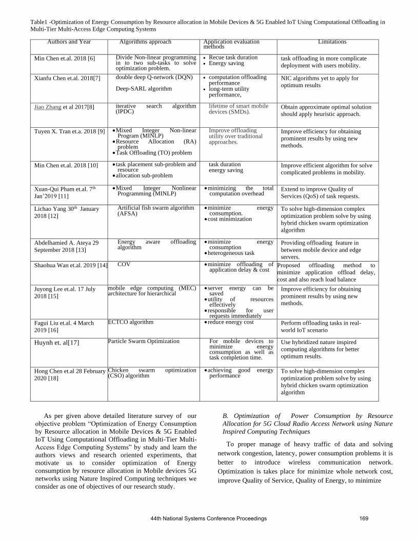
Table1 -Optimization of Energy Consumption by Resource allocation in Mobile Devices & 5G Enabled IoT Using Computational Offloading in

Multi-Tier Multi-Access Edge Computing Systems

Authors and Year Algorithms approach

Application evaluation methods

Limitations

Min Chen et.al. 2018 [6] Divide Non-linear programming in to two sub-tasks to solve optimization problem.

• Recue task duration • Energy saving

task offloading in more complicate

deployment with users mobility.

Xianfu Chen et.al. 2018[7] double deep Q-network (DQN) Deep-SARL algorithm

• computation offloading performance

• long-term utility performance,

NIC algorithms yet to apply for

optimum results

Jiao Zhang et al 2017[8] iterative search algorithm (IPDC)

lifetime of smart mobile devices (SMDs).

Obtain approximate optimal solution

should apply heuristic approach.

Tuyen X. Tran et.a. 2018 [9] • Mixed Integer Non-linear Program (MINLP)

• Resource Allocation (RA) problem

• Task Offloading (TO) problem

Improve offloading utility over traditional approaches.

Improve efficiency for obtaining

prominent results by using new

methods.

Min Chen et.al. 2018 [10] • task placement sub-problem and resource

• allocation sub-problem

task duration energy saving

Improve efficient algorithm for solve

complicated problems in mobility.

Xuan-Qui Pham et.al. 7th

Jan’2019 [11]

• Mixed Integer Nonlinear Programming (MINLP)

• minimizing the total computation overhead

Extend to improve Quality of

Services (QoS) of task requests.

Lichao Yang 30th January

2018 [12]

Artificial fish swarm algorithm (AFSA)

• minimize energy consumption.

• cost minimization

To solve high-dimension complex

optimization problem solve by using

hybrid chicken swarm optimization

algorithm

Abdelhamied A. Ateya 29

September 2018 [13]

Energy aware offloading algorithm

• minimize energy consumption

• heterogeneous task

Providing offloading feature in

between mobile device and edge

servers.

Shaohua Wan et.al. 2019 [14] COV • minimize offloading of application delay & cost

Proposed offloading method to

minimize application offload delay,

cost and also reach load balance

Juyong Lee et.al. 17 July

2018 [15]

mobile edge computing (MEC) architecture for hierarchical

• server energy can be saved

• utility of resources effectively

• responsible for user requests immediately

Improve efficiency for obtaining

prominent results by using new

methods.

Fagui Liu et.al. 4 March

2019 [16]

ECTCO algorithm • reduce energy cost Perform offloading tasks in real-

world IoT scenario

Huynh et. al[17] Particle Swarm Optimization For mobile devices to minimize energy consumption as well as task completion time.

Use hybridized nature inspired

computing algorithms for better

optimum results.

Hong Chen et.al 28 February

2020 [18]

Chicken swarm optimization (CSO) algorithm

• achieving good energy performance

To solve high-dimension complex

optimization problem solve by using

hybrid chicken swarm optimization

algorithm

As per given above detailed literature survey of our

objective problem “Optimization of Energy Consumption

by Resource allocation in Mobile Devices & 5G Enabled

IoT Using Computational Offloading in Multi-Tier Multi-

Access Edge Computing Systems” by study and learn the

authors views and research oriented experiments, that

motivate us to consider optimization of Energy

consumption by resource allocation in Mobile devices 5G

networks using Nature Inspired Computing techniques we

consider as one of objectives of our research study.

B. Optimization of Power Consumption by Resource

Allocation for 5G Cloud Radio Access Network using Nature

Inspired Computing Techniques

To proper manage of heavy traffic of data and solving

network congestion, latency, power consumption problems it is

better to introduce wireless communication network.

Optimization is takes place for minimize whole network cost,

improve Quality of Service, Quality of Energy, to minimize



energy consumption. Many techniques applied for power

consumption Many techniques applied for minimize power

consumption are MIMO, multi-hop communication,

heterogeneous network etc are proposed for better

optimization methods. Even introducing these methods not

yet solve minimize energy consumption for enhance the

better utilization of overall network power in 5G network.

As per introduce the new concept of 5G should capable

for more connectivity of devices, support highdata rate,

maximize energy efficiency, improve power efficiency,

support network any-time-any-where, provide low-latency

[19-22]. Current technologies are clearly in lack for

supporting such emergency requirements. Therefore, the

industries and researchers need to bring some fundamental

changes in future networks both in technologies and

architectures.

The cellular net-works based on C-RAN recommend for

5G network systems for better efficiency. The Cloud radio

access network is located in single base station (BS). And

also integrate with Base band units (BBU) and Remote radio

heads (RRH). Cloud radio access network (C-RAN) can

minimize energy consumption by integrating with Baseband

units (BBU) assigned to one or more Remote radio heads

(RRH) to share resources remotely. To minimize cost,

computing, minimize power consumption and maximize

energy saving introducing of single cluster with mobile edge

computing servers providing computational task(s) to

mobile devices.

Fig2 – Cloud - Radio Access Network (C-RAN)

Architecture[97]

In Fig2 shows C-RAN and the challenging issue is

designing a mapping UE with RRHs and also RRHs with

BBU. As per the network load status to minimize whole

network costs to reach Quality of Service (QoS) and Quality

of Experience (QoE). This is a two-stage resource allocation

problem where the first stage is UE-RRH association and the

second stage is RRH- BBU mapping.

Literature Survey

In.[23] proposed UE associate with RRH for Cloud Radio

Access Network. In [24] proposed linear programming to

optimize BBU-RRH mapping for C-RAN to minimize energy

cost in overall system. In [25] proposed Genetic Algorithm for

solving resource allocation problem in BBU. But simulation

results shows this not reached optimization of power

consumption for whole system.. In [26] proposed a heuristic

method applying for solving BBU-RRH mapping to reach

optimal solution. In [27] proposed resource allocation problem

in 5G-CRAN formulated by a multi-objective optimization

problem to reach optimal and support to quality of service

(QoS) requirements. To optimization this problem divided

into two sub problems. The UE-RRH mapping sub-problem

solved by nature inspired computing technique i.e. Ant Bee

Colony (ABC) and RRH-BBU mapping sub-problems solved

by nature inspired computing techniques ie Ant Colony

Optimization(ACO). The all over optimization performance

proposed nature inspired computing algorithm i.e.

hybridization of ABC and ACO i.e. Bee-Ant-CRAN to

perform better optimization and simulation results shows the

whole cost of power consumption, minimize the cost and

Quality of Service features. In future work the authors want

to propose a virtual Base stations (BSs) placed at Cloud edge

– Radio access network(C-RAN) to provide performance by

power consumption, throughput, quality of service and

minimization of cost.

In [28] proposed C-RAN to minimize costs and

maximize energy saving and also reach quality of service. To

reach, separate base band unit from base stations and sharing

base band unit in pool. In this scheme to optimize allocate

BBU dynamic way and mapping them to remote radio heads

to reach quality of service. To solve these problem authors

proposed RCLP algorithm to solve it.

Table 2 - Optimization of Power Consumption by RA for 5G C-RAN using Nature Inspired Computing Techniques

Authors and Year Algorithms approach


Limitations

Taleb, Hussein, et al in 2018 [23] User association (UA) sub-problem RRH clustering (RC) sub-problem

• minimize network power consumption

• total transmission delay.

Multiple

centralized and distributed UA and

RC solutions will be proposed and

integrated

Yao, Jingjing et.al. 2018 [24] integer linear programming (ILP) • minimize the system cost incurred by the energy bill

Optimize with nature inspired

computing algorithms for

approximate optimum results.


Chien et.al. 2019 [25] GA-based Resource Allocation Algorithm (GARAA)

• achieve high resource utilization

• reduce power consumption.

improving the accuracy of

throughput predictions and reducing

the computational time for deep

learning.

Boulos, Karen, et al 2018 [26] Set Partitioning Problem (SPP)

• a minimum guarantee of Quality of Service(QoS)

• reduce the power consumption

to dynamically output a clustering

scheme, adapting to dynamic load

conditions and different preferences

in terms of re-association and

power consumption.

Ado Adamou AbbaAri et.al.

2019 [27]

Bee-Ant-CRAN Optimization • reduces the resource wastage • spectral efficiency well as

the throughput.

virtual BSs at the edge of the C-

RAN in the overall performance.

Chen, Longbiao, et al 04

February 2020 [28]

Resource-Constrained Label-Propagation (RCLP) algorithm

• reduce operational costs • service quality

Optimize with nature inspired

computing algorithms for

approximate optimum results.

Based on the recent studies in NIC it has been observed that

different variants of ABC and ACO techniques with

multiple hybridization schemes of various NIC techniques

have performed much better than standard ABC and ACO

nature inspired computing algorithms on continuous and

discrete optimization problems. This motivates us to explore

the use of more recent NIC like Ant Colony

Optimization(ACO), Particle Swarm Optimization (PSO),

Whale Optimization algorithm (WOA), Biogeography based

Optimization (BBO) and their hybrid variants for the better

solution of this problem.

C. Optimization of Inter-Slice Resource Management in 5G

Network using Nature Inspired Computing Techniques.

Fifth-Generation (5G) systems and network architecture is

intended to offer multiple services with diverse set of user

requirements and performance specifications. Network

Slicing is a process of slicing a single physical network into

multiple independently and isolated logical networks. The

design & development of 5G network is in progress. In 5G

the importance of Network slicing is a one of the key

concept of virtualization[30]. Network slicing is allowing

for providing 5G network services as network as a

infrastructure, network as a service with efficient

requirements [29].

Network slicing is virtual network on physical network

for the purpose of providing minimal network resources for

minimize expenditure of 5G network [31,32,33].

Because of the importance of the network slicing in

realizing the full potential of 5G systems, in this research

study, we would like to explore to study and design new

strategies for addressing the slicing problem in 5G network.

Network slicing in 5G network is one of the important

problems to solve communication cost and QoS. The Network

Slicing problem is first introduce by NGMN[34]. The

network slicing is the concept of creating a virtual network on

physical network to complete the every slice as a task to

complete with QoS. Network slicing design for the concept

of improve the performance of mobile network operators and

also to improve the business profits[35]. Network slicing

concept to perform physical resources as well as virtual

resources to improve computational capabilities[36] based

on the requirement of the business case. The resource blocks

can be homogeneous or heterogeneous (frequency bands and

transmission power) in nature. In both homogeneous and

heterogeneous based use cases, each slice will have different

utility efficiencies. To execute tasks for mobile broadband

service needs high throughput and for massive machine type

communication needs maximum low traffic devices[37].

According to[38], The elastic slices provides guaranteed

QoS for less payment and also provide QoS for high

payment. This concept use in “Slice as a Service” (SlaaS)

[39]. The Slice as a Service will be required for resource

management scheme as IaaS, PaaS and SaaS all these cloud

service are noted for client demanded services[40,41]. The

challenging aspect of Network slicing in 5G networks is to

optimize the long-term network utility in Slice as a Service

(SlaaS) with a good scalability and reach Quality of

Solutions (QoS).

In[42] to support high number of heterogeneity of

mobile devices it is better to provide large number of slices

to computational tasks. In[43], 5G network provide different

slices to fulfill energy efficiency tasks of mMTC slices, low

latency tasks for URLLC slices and for throughput MBB

slices are utilized. The slicing concept of 5G to fulfill tasks

like to manage tasks of power[44], throughput[45] and

better resource usage [46].

Literature Survey

Many researchers have proposed different models to

perform network slicing problem to manage profit for

business concept. In[47] proposed MOOP for solve the

optimal resource allocation for profit oriented business. In

[48], proposed online Genetic Algorithm based models to


address heterogeneous slices with Quality of Service (QoS)

requirements in 5G networks and demonstrated the

effectiveness of online Genetic Algorithm model when

compared with other existing methods interns of optimum

results, rate of convergence. In [49] proposed H-CRAN

model was proposed considering a virtualized backhaul

network to solve the resource management by applying

mathematical models and heuristic techniques.

In [50] proposed cross layer controller(CLC) provides

end-to-end resource allocation methods for various network

segments. The results shows that better performance of CLC

for 5G network. In [51] Machine Learning and Deep

learning models such as Deep reinforcement learning and

DeepCog models were proposed to address the challenges in

Network slicing problems.

Table3-Optimization of Power Consumption by RA for 5G C-RAN Access Network using Nature Inspired Computing Techniques Authors and Year Algorithms approach


Limitations

Bin Han et.al. sep’ 2017 [47] a multi-objective optimization problem (MOOP)

• optimizing the business profit generated by a network slice

most appropriate solutions can be

implemented, to overcome the

technical challenges and to realize

the envisaged n/w optimization

Dario Bega et.al. 1 May 2017

[48]

adaptive algorithm • ecosystem • revenue of he system

Network optimization

Dario Bega et.al.

29 April-2 May 2019[49]

DeepCog a deep neural network structure

optimization of network •


Sokratis Barmpounakis et.al. 15

Jan'2020 [50]

Cross Layer Control framework • Virtual Network Function

• end-to-end latency •

• Based on artificial intelligence-

• Deep reinforcement learning

methods

David S. L. Wei et.al. 21

February 2020 [51]

Machine learning • Throughput performance • Minimize network cost


This motivates us to consider optimization of resource

allocation in 5G enable IoT networks for objectives of our

research study. As per the above detailed literature survey, the

author study, learn, motivate and believe that, the

performance of the model can further be improved and solve

by integrating popular and recent nature inspired computing

algorithms to improve resource allocation techniques so as to

achieve a prominent results oriented research in 5G network

that support services of enabled Internet of Things (IoT)

domain.

IV. CONCLUSION

[

In this paper, an effort is made to provide insight into the

most demandful research oriented optimization problems in

resource allocation like minimize energy consumption,

minimize power consumption and inter-slice resource

management etc. are in the area of 5G Network environment

are introduced to be solved, This paper recommends,

popular, recent and hybrid algorithms of nature inspired

computing (NIC) for implementation of resource allocation

optimization problems in 5G Network. Specially, authors

provide a valuable information about literature survey of

research objectives and methodology for solving each

problem. Finally, author gives clear idea about planning to

a proper way for study, learn, preparing and complete this

survey paper.

ACKNOWLEDGMENT

My deepest thanks to my supervisor Dr. K. Srinivas Sir for

giving valuable suggestions for writing this survey paper. I

am very thankful for my supervisor for providing time-to-

time guidance & valuable suggestions for complete this

survey paper.

I am very thankful to my Co-supervisor Dr. R.S.Pavithr Sir

for providing me from the basic to in-depth knowledge for

guide me a proper way for how to study, learn, preparing and

complete this survey paper.

My deepest gratitude to the Director of Dayalbagh

Educational Institute(DEI) Agra for providing computer lab

facility and providing library facility towards completion of

my survey paper.

Last but least I am very thankful to my colleagues i.e.

research scholars and senior staff members for their

continuous suggestions and their moral help for giving and

providing time-to-time help and encouragement for

completion and submission of survey paper successfully.

REFERENCES

[1]Li, Shancang, Li Da Xu, and Shanshan Zhao. "5G Internet of Things: A survey." Journal of Industrial Infor- mation Integration 10 (2018): 1-9.

[2]Ejaz, Waleed, et al. "Internet of Things (IoT) in 5G wireless communications." IEEE Access 4 (2016): 10310- 10314.

[3]Huynh, Luan NT, et al. "Efficient Computation Offloading in Multi-Tier

Multi-Access Edge Computing Systems: A Particle Swarm Optimization

Approach." Applied Sciences 10.1 (2020): 20329]

[4]. Zhang, Ke, et al. "Energy-efficient offloading for mobile edge computing in 5G heterogeneous networks." IEEE access 4 (2016): 5896-5907.

[5] Zhang, Jiao, et al. "Energy-latency tradeoff for energy-aware offloading in

mobile edge computing networks." IEEE Internet of Things Journal 5.4 (2017): 2633-2645.

[6]Chen, Min, and Yixue Hao. "Task offloading for mobile edge computing in

software defined ultra-dense network." IEEE Journal on Selected Areas in

Communications 36.3 (2018): 587-597.

[7]Chen, Xianfu, et al. "Optimized computation offloading performance in

virtual edge computing systems via deep reinforcement learning." IEEE

Internet of Things Journal 6.3 (2018): 4005-4018. [8]Zhang,J.;Hu,X.;Ning,Z.;Ngai,E.C.;Zhou,L.;Wei,J.;Cheng,J.;Hu,B.Energy-

Latency Trade off or Energy-Aware Offloading in Mobile Edge Computing

Networks. IEEEInternetThingsJ.2018,5,2633–2645.


[9]Tran, T.X.; Pompili, D. Joint Task Offloading and Resource Allocation for

Multi-Server Mobile-Edge Computing Networks. IEEE Trans. Veh. Technol.

2019, 68, 856–868. [10]Chen, M.; Hao, Y. Task Offloading for Mobile Edge Computing in

Software Defined Ultra-Dense Network. IEEE J. Sel. Areas Commun. 2018,

36, 587–597. [11]Pham, X.Q.; Nguyen, T.D.; Nguyen, V.; Huh, E.N. Joint Node Selection

and Resource Allocation for Task Offloading in Scalable Vehicle-Assisted

Multi-Access Edge Computing. Symmetry 2019, 11, 58. [12]Yang, L.; Zhang, H.; Li, M.; Guo, J.; Ji, H. Mobile Edge Computing

Empowered Energy Efficient Task Offloading in 5G. IEEE Trans. Veh.

Technol. 2018, 67, 6398–6409. [CrossRef] [13]Ateya,A.A.;Muthanna,A.;Vybornova,A.;Darya,P.;Koucheryavy, A.

Energy—Aware Offloading Algorithm for Multi-level Cloud Based 5G System. In Internet of Things, Smart Spaces, and Next Generation Networks

and Systems; Springer International Publishing: Cham, Switzerland, 2018; pp.

355–370. [14]Wan, S.; Li, X.; Xue, Y.; Lin, W.; Xu, X. Efficient computation

offloading for Internet of Vehicles in edge computing-assisted 5G networks.

J. Supercomput. 2019, 1–30. [CrossRef] [15]Lee, J.; Lee, J. Hierarchical Mobile Edge Computing Architecture Based

on Context Awareness. Appl. Sci. 2018, 8, 1160.

[16]Liu, F.; Huang, Z.; Wang, L. Energy-Efficient Collaborative Task

Computation Offloading in Cloud-Assisted Edge Computing for IoT Sensors.

Sensors 2019, 19, 1105.

[17]Huynh, Luan NT, et al. "Efficient Computation Offloading in Multi-Tier Multi-Access Edge Computing Systems: A Particle Swarm Optimization

Approach." Applied Sciences 10.1 (2020): 203.

[18] Chen, Hong, et al. "Joint Computation Offloading and Radio Resource Allocations in Small-Cell Wireless Cellular Networks." IEEE Transactions

on Green Communications and Networking (2020).

[19] M. Agiwal, A. Roy, and N. Saxena, “Next Generation 5G Wireless Networks: A Comprehensive Survey,” IEEE Communications Surveys

Tutorials, vol. 18, no. 3, pp. 1617–1655, third quarter 2016.

[20] M. Peng, C. Wang, V. Lau, and H. V. Poor, “FronthaulConstrained Cloud Radio Access Networks: Insights and Challenges,” IEEE Wireless

Communications, vol. 22, no. 2, pp. 152–160, Apr. 2015.

[21] J. G. Andrews, S. Buzzi, W. Choi, S. V. Hanly, A. Lozano, A. C. K. Soong, and J. C. Zhang, “What Will 5G Be?” IEEE Journal on Selected

Areas in Communications, vol. 32, no. 6, pp. 1065–1082, Jun. 2014.

[22] I. B. Sofi and A. Gupta, “A survey on energy efficient 5g green network with a planed multi-tier architecture,” Journal of Network and Computer

Applications, vol. 118, pp. 1–28, 2018.

[23]Taleb, Hussein, et al. "Joint user association and RRH clustering in cloud radio access networks." 2018 Tenth International Conference on Ubiquitous

and Future Networks (ICUFN). IEEE, 2018.

[24]Yao, Jingjing, and Nirwan Ansari. "QoS-aware joint BBU-RRH mapping and user association in cloud-RANs." IEEE Transactions on Green

Communications and Networking 2.4 (2018): 881-889.

[25] Chien, Wei-Che, Chin-Feng Lai, and Han-Chieh Chao. "Dynamic resource prediction and allocation in C-RAN with edge artificial

intelligence." IEEE Transactions on Industrial Informatics 15.7 (2019):

4306-4314. [26] Boulos, Karen, et al. "RRH clustering in cloud radio access networks

with re-association consideration." 2018 IEEE Wireless Communications and

Networking Conference (WCNC). IEEE, 2018. [27] Ari, Ado Adamou Abba, et al. "Resource allocation scheme for 5G C-

RAN: a Swarm Intelligence based approach." Computer Networks 165

(2019): 106957. [28]Chen, Longbiao, et al. "Data-Driven C-RAN Optimization Exploiting

Traffic and Mobility Dynamics of Mobile Users." IEEE Transactions on

Mobile Computing (2020). [29]Khan, Latif Ullah et al. “Network Slicing: Recent Advances, Taxonomy,

Requirements, and Open Research Challenges.” IEEE Access 8 (2020): 36009-36028.

[30] Nakao, Akihiro, et al. "End-to-end network slicing for 5G mobile

networks." Journal of Information Processing 25 (2017): 153-163. [31] P. Rost et al., “Mobile Network Architecture Evolutiontoward 5G,”

IEEE Commun. Mag., vol. 54, no. 5, May 2016,pp. 84–91.

[32] M. Jiang, M. Condoluci, and T. Mahmoodi, “Network SlicingManagement & Prioritization in 5G Mobile Systems,” Euro.Wireless

2016, Oulu, Finland, 2016, pp. 1–6

[33] Ericsson, “Ericsson White Paper: 5G System,” Jan. 2015.

[34] Alliance, N. "Ngmn 5g white paper, Next Generation Mobile Networks

Ltd, Frankfurt am Main, 2015." International Journal of Aerospace

Engineering Hindawi ‘www. hindawi. com 2018. [35] Rost, Peter, et al. "Network slicing to enable scalability and flexibility in

5G mobile networks." IEEE Communications magazine 55.5 (2017): 72-79.

[36] Ha, Vu Nguyen, and Long Bao Le. "End-to-end network slicing in virtualized OFDMA-based cloud radio access networks." IEEE Access 5

(2017): 18675-18691.

[37] GPAW Group. "View on 5g architecture." White Paper, July (2016). [38] Bega, Dario, et al. "Optimising 5G infrastructure markets: The business

of network slicing." IEEE INFOCOM 2017-IEEE Conference on Computer

Communications. IEEE, 2017. [39] Sciancalepore, Vincenzo, Flavio Cirillo, and Xavier Costa-Perez. "Slice

as a service (SlaaS) optimal IoT slice resources orchestration." GLOBECOM 2017-2017 IEEE Global Communications Conference. IEEE, 2017.

[40] Manvi, Sunilkumar S., and Gopal Krishna Shyam. "Resource

management for Infrastructure as a Service (IaaS) in cloud computing: A survey." Journal of network and computer applications 41 (2014): 424-440.

[41] Jennings, Brendan, and Rolf Stadler. "Resource management in clouds:

Survey and research challenges." Journal of Network and Systems Management 23.3 (2015): 567-619.

[42] Han, Bin, Shreya Tayade, and Hans D. Schotten. "Modeling profit of

sliced 5G networks for advanced network resource management and slice

implementation." 2017 IEEE Symposium on Computers and Communications

(ISCC). IEEE, 2017.

[43] He, Sijin, Li Guo, and Yike Guo. "Real time elastic cloud management for limited resources." 2011 IEEE 4th International Conference on Cloud

Computing. IEEE, 2011.

[44] Chabarek, Joseph, et al. "Power awareness in network design and routing." IEEE INFOCOM 2008-The 27th Conference on Computer

Communications. IEEE, 2008.

[45]Mei, Yiduo, et al. "Performance measurements and analysis of network i/o applications in virtualized cloud." 2010 IEEE 3rd International

Conference on Cloud Computing. IEEE, 2010.

[46]Tomita, Takuro, and Shin-ichi Kuribayashi. "Congestion control method with fair resource allocation for cloud computing

environments." Proceedings of 2011 IEEE Pacific Rim Conference on

Communications, Computers and Signal Processing. IEEE, 2011. [47] Han, Bin, Shreya Tayade, and Hans D. Schotten. "Modeling profit of

sliced 5G networks for advanced network resource management and slice

implementation." 2017 IEEE Symposium on Computers and Communications (ISCC). IEEE, 2017.

[48] Bega, Dario, et al. "Optimizing 5G infrastructure markets: The business

of network slicing." IEEE INFOCOM 2017-IEEE Conference on Computer Communications. IEEE, 2017.

[49] Bega, Dario, et al. "DeepCog: Cognitive network management in sliced

5G networks with deep learning." IEEE INFOCOM 2019-IEEE Conference on Computer Communications. IEEE, 2019.

[50]Barmpounakis, Sokratis, et al. "Network slicing-enabled RAN

management for 5G: Cross layer control based on SDN and SDR." Computer Networks 166 (2020): 106987.

[51]Wei, David SL, et al. "Guest Editorial Leveraging Machine Learning in

SDN/NFV-Based Networks." IEEE Journal on Selected Areas in Communications 38.2 (2020): 245-247.


A Schematic Of Global Consciousness System For

Sustainable Future Ami Parashar

Lead Project Management Specialist at General Electrical (Switzerland)

Dayalbagh Educational Institute,Alumnus & SSI Life member

[email protected]

Abstract—The phrase “God’s image” has been a great

source of inspiration for researchers and scholars of

different knowledge streams. As indicated in the spiritual

system theory framework, “As is in Macrocosm, so is in

Human Microcosm,” spiritual practitioners have been

using meditational techniques to activate existing

apertures in one’s mind for establishing a connection

with higher regions of consciousness. Historical data

shows that during such yogic practices, the sense of

balanced perspective is achieved, and guidance, vision,

or a better glimpse of the future is perceived to

develop a sustainable human society that is economically,

socially, ecologically, and spiritually sound hence meeting

the needs of the present without jeopardising

opportunities for the future.

Most Revered Prof. Prem Saran Satsangi shared that

modern scientists play a similar role as brahmans of

Hindu philosophy in directing and shaping society. It

gives researchers a clue that an integrated systems

approach could develop a predictive solution to handle

global pandemics or perils.

In this paper, the author emphasizes how unforeseen

global disturbances affect the body, mind, and

surroundings simultaneously and provide system

scientists a challenge to develop smart, resilient & cost-

effective solutions to cater to such situations. A schematic

based on an integrated approach involving relevant

streams of sciences with a strong background of

historical data of human evolution and consciousness

studies has been proposed to build a global consciousness

system to achieve better worldliness and a sustainable

future.

Keywords- Sustainable, Consciousness, Meditational,

Integrated approach, better worldliness, Pandemics.

I. INTRODUCTION

The world continues to adapt to the COVID-19 pandemic

challenges. Such global disturbances affect the body, mind,

and surroundings at the same time. The hour's need is to

develop smart, resilient & cost-effective solutions to cater to

such situations. An integrated approach involving relevant

streams of sciences with a strong background of historical

data of human evolution and consciousness studies gives

researchers a foresightedness.

From the spiritual system theory framework "Man, a perfect

Microcosm of Macrocosm," the author sees a relationship

between human consciousness and universal consciousness.

The crisis faced at the global level is due to not fulfilling

most the population's basic needs and the rate at which these

changes are being introduced into the system.

It is complicated to keep a balanced perspective when such

risky environmental and psychological conditions are

putting additional stress on different age groups. Scholars

have suggested that to perform a task correctly, one should

use all faculties and the best available knowledge. The same

approach supported by appropriate planning, analytical, and

simulation tools may result in a sustainable solution.

II. EFFECT OF GLOBAL PANDEMICS

(Figure I)

A. The universe within Infinite Spiritual System

The macrocosm is a closed system and broadly divided into

three subsystems. The Infinite Reservoir of Spirituality

represents the Primary region. The Universal Mind region

is the Secondary subsystem, and the Tertiary region is the

Universal Matter.

B. Effect of Global Pandemics on an individual ( Figure I)

To understand the Global Pandemic's sudden effect, the author has superimposed three different theories, 1) Spiritual system theory, 2) Ecological system theory, and 3) Need hierarchy theory. Soul, mind, and body represent a microcosm. Triangle represents need hierarchy, and all subsystems surrounding microcosm are part of the ecological system. Due to sudden unfortunate events, most of the ecological system elements are put on hold, resulting in not meeting the basic needs of different age groups at different levels of society. Food, medical supplies, clean water, security, connection with family and friends becomes a priority.


One can imagine that different stockholders and elements affecting one’s priority, decision making, and understanding in such situations. In urgent cases, physiological needs become the first propriety followed by health safety & security. Only a few percentages of the population got access to fulfilling belongingness need with virtual medial; otherwise, there is a huge gap in demand and coping up capacity.

Such sudden changes are unhealthy for the body and mind. All age groups are exposed to a lot of uncertainty, putting on hold sub-ecological systems like economic, social, religious, educational, political, legal, and governmental systems.

III. ADVERSE EFFECT OF SURROUNDING ON DECISION

MAKING AND SYSTEM SUSTAINABILITY ( FIGURE II)

Figure II illustrate how religious and spiritual practitioners are finding solutions since ancient times by raising their consciousness level during meditation and getting control over sensory organs and achieving required mental balance to take the most appropriate decisions suitable for individuals, society, nature, and the spiritual system.

The different elements of human sensory organs (touch, smell, sight, hearing, and taste) and most dominating feelings (lust, greed, anger, arrogance, and endearment) and five essential elements of creation (air, water, earth, fire, and sky). Slight changes in these elements affect vision and decision-making. There are several examples that, with the help of meditational practices, one can raise consciousness and reach higher regions of spirituality and get a glimpse of future events.

Ancient literature indicates that past decisions had fewer adverse effects on ecological systems. Industrial advancement and uncontrolled progress in most of the streams are adversely affecting most of the creational elements.

For a better life, it is essential to have a healthy body and mind. Due to the significant issues indicated in figure II, the bond with nature breaks and leads researchers to find Artificial Intelligent solutions to avoid human interfaces.

IV. A SCHEMATIC OF GLOBAL CONSCIOUSNESS

SYSTEM ( FIGURE III)

A Schematic of the global consciousness system is shown in figure III. When a decision is taken as an individual, one uses all mental faculties and the best available knowledge. The same approach supported by appropriate planning, analytical, and simulation tools at the global level gives us a consciousness system to determine a suitable solution for a sustainable future.

Before elaborating the proposed schematic, the author would like to define world “Conscious lead,” which is the time lag between the super creational plane and physical plane.

It is evident, that scientific advancement in only one stream or finding solutions for the entire population based on one scientific explanation has affected the ecological system in the long term. Finding a solution by integrating different

scientific streams and using advanced analytical tools to decision-making would result in a sustainable solution.

A. Historical Data and Knowledge (Past)

Since the stone age, humans have been recording experiences and knowledge in the form of pictures, symbols & shapes, and with evolution, simple and complex languages came into existence. But still, there is no match to the valuable data stored in ancient works of literature.

In addition to historical data and literature, studies in system science, philosophy, cultural values, religion, psychology, management, and sciences give researchers a solid background.

B. Decision Making Involving Knowledge Streams

(Present)

The middle part of the schematic represents current

research and development activities in all knowledge streams. Bigger circles are knowledge areas, and smaller circles connected big circles are sub knowledge areas or specialised streams.

Mainstreams are formal sciences, applied sciences, earth & space, social sciences, life sciences, physical sciences consciousness studies, AI, and other knowledge streams, followed by sub-streams. If a time-sensitive crucial decision at a global scale is to be made, an integrated approach followed by predictive analysis will direct humanity in the right direction. If the research results are not suitable, inputs are requested and analysed until a solution with minimum effect on the population is ensured.

The major problem for both developed and developing countries turned out to be lack of visibility and control over complete picture and ability to influence masses from common control system on the other hand the scientific research centres are spread over different geographical locations and governed by local constraints and laws. In urgent situations, correct information in the shortest possible time, the key avoids damaging consequences.

C. Forecasting /Predicting -“Conscious lead” (future)

Due to global diversity getting unbiased consensus was a

challenge. Since the last decade, advancements in virtual solutions, simulation, and analytical tools have made it extremely easy to gather data from several global locations within no time.

New brainstorming and decision-making tools make better decisions with virtualized priority. Virtual teams are facilitated with decision Support systems, which are an interactive computer-based system that enables several decision-makers (working together in a group) to find solutions to unstructured problems in nature.

These tools are designed to take input from multiple users interacting simultaneously with the systems to decide as a group. The most common example is an audience response system, which allows large groups of people to vote on a topic or answer a question. After a given time, the analysis of collected data ends for that problem and tabulates the results to simulate a virtual model of an emerging situation.


(Figure II)

(Figure III)


V. CONCLUSION

A Global Consciousness system integrates inputs from all the knowledge steams of sciences and provides a glimpse of the emerging situation while drastically shortening the reaction time to handle emergencies irrespective of physical boundaries and cultural differences. The schematic also gives an impression of humanity's brotherhood standing tall to tackle any situation and suggesting smart, resilient, and cost-effective solutions for a sustainable future.

REFERENCES

[1] Satsangi.P.S. ‘Expositions on Truth, Ultimate Reality and Supreme

Being’ Published by RSSD & DCS2020 slides.

[2] Parashar, A. Parashar, A,(2020) 'The Musical Instruments and All Mystic Sounds, Influencing Our Emotions and Leading Us to Higher Regions of Consciousness’, Poster at DSC2020.

[3] 2] Parashar, A., (2020) , Integrated Approach To Increase Global Consciousness For System Sustainability And Better Worldliness: A Solution Against Global Perils', Poster/Presentation at TSC2020.

[4] Sriramamurti, P., Prashant, P., Mohan, A.,(2013) ‘Spiritual Consciousness’,(PP51-323).

[5] Parashar, A.,An Integrated Planning Approach Supported by GDSS to Increase Global Consciousness for System Sustainability and Better Worldliness, DSC2019.


Radhasoami Satsang Sabha Gaushala – A Sustainable Dairy Management System Soami Dayal Singh (Assistant Secretary) & Prakhar Mehra (Sewak-Manager) R.S.Sabha Gaushala

Dayalbagh, Agra-282005

Abstract

Radhasoami Satsang Sabha Gaushala was established in 1926 and regarded as Asia’s Finest Dairy.

Today, it has 1,100 cattle comprising of High Yielding indigenous breed cows & buffalos and producing

over 2,000 ltrs of milk daily, which forms an important part of the Lacto-vegetarian diet. Having a blend

of Modern Technology and Ancient Wisdom in a Spiritually Charged environment and working on

Scientific Techniques related to Breeding, Feeding, Health and Facilities Management, Gaushala is

aligned to the Sigma Six Q-VA Model of Dayalbagh Way of Life. This paper throws light on this unique

model of a self sustainable Dairy Farm Management System which is an integral part of Dayalbagh

Modern Health Care Habitat and how working on systems based approach has enabled it withstand

challenging pandemic times.

Keywords: #sustainabledairyfarming #healthcarehabitat #dairymanagementsystem #dayalbaghwayoflife

#simasixQ-VAmodel

Introduction

The Dayalbagh Dairy & Radhasoami Satsang Sabha Gaushala were established in 1926. In those times

the Dayalbagh Dairy was regarded as one of Asia’s Finest Dairy. There were over 2-300 cows

producing over 400 ltrs of milk per day. Today, Gaushala has over 1,100 cattle comprising of High

Yielding Murrah Buffalos, Indian Sahiwal Breed and Holstein Freision – Sahiwal Cross Breed cows.

900 cattle belong to breedable herd and are housed at its main campus. Balance over 200 comprising of

old and male cattle are housed at Cattle Rehabilitation Centre. Care of cattle is taken from Maternity till

Eternity.

Picture 1 – Dayalbagh Dairy Picture 2 – R.S.Sabha Gaushala

Gaushala having a blend of Modern Technology, Ancient Wisdom in a Spiritually charged environment,

is working on Modern Scientific Techniques related to Breeding, Feeding, Health and Facilities

Management. Cattle are daily taken for long walks and grazing which provides them exercise, improves

digestion and in return enriches the lands where they graze. They are made to listen to Shabd path which

relaxes them and spiritually elevates them. They have names and are treated as individuals. They are

bathed regularly. Cattle are given homeopathy treatment along with allopathic medication. When they


get sick the holy name “Radhasoami” is recited in their ears with vibrations of the words having eternal

effects elevates their spirits. These are few of the practices which are known to have been part of ancient

times and rendered in a spiritually charged atmosphere.

Community Participation Model at Gaushala

Key to its working in Gaushala is the Community Participation Model. Following three key institutions

form the core components of this model

a. Agriculture Operations– Cultivating all kind of crops, vegetables, fruits including horticulture on

lands over 1200+ acres on the banks of river Yamuna. Soil which was once nothing but sand dunes

b.Dayalbagh Educational Institute (Deemed University) - DEI aims to serve as an exemplary model of

education, covering the entire spectrum of knowledge and wisdom, to selflessly serve mankind by

evolving a race of supermen, who possess the virtues to resolve the grave global challenges and

establish a more humane and enlightened society.

c. R.S.Sabha Gaushala – Abode to 1,100 cows and serving cattle from maternity till eternity. Producing

over 2,000 ltrs of milk daily and providing the spiritually charged milk at affordable rates across

various sections of society.

The community members of Dayalbagh are involved in all these institutions in a committed manner,

equipped with 3 Hs - (H)ead, (H)eart and (H)ands.

a. Head – Indicates the knowledge available to people about

the tasks they render

b.Heart – Indicates the passion, commitment and zeal with

which people render self less service

c. Hands – Indicates Dignity of Labour and presence of all

four Varnas in the individuals.


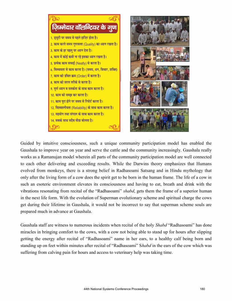
Guided by intuitive consciousness, such a unique community participation model has enabled the

Gaushala to improve year on year and serve the cattle and the community increasingly. Gaushala really

works as a Ramanujan model wherein all parts of the community participation model are well connected

to each other delivering and exceeding results. While the Darwins theory emphasizes that Humans

evolved from monkeys, there is a strong belief in Radhasoami Satsang and in Hindu mythology that

only after the living form of a cow does the spirit get to be born in the human frame. The life of a cow in

such an esoteric environment elevates its consciousness and having to eat, breath and drink with the

vibrations resonating from recital of the “Radhasoami” shabd, gets them the frame of a superior human

in the next life form. With the evolution of Superman evolutionary scheme and spiritual charge the cows

get during their lifetime in Gaushala, it would not be incorrect to say that superman scheme souls are

prepared much in advance at Gaushala.

Gaushala staff are witness to numerous incidents when recital of the holy Shabd “Radhasoami” has done

miracles in bringing comfort to the cows, with a cow not being able to stand up for hours after slipping

getting the energy after recital of “Radhasoami” name in her ears, to a healthy calf being born and

standing up on feet within minutes after recital of “Radhasoami” Shabd in the ears of the cow which was

suffering from calving pain for hours and access to veterinary help was taking time.


Gaushala Aligned to Dayalbagh Way of Life

Over the last few years, Gaushala has aligned itself to the Sigma Six QV-A Model of Dayalbagh way of

life model. It is aligned to the Sigma Six Q-VA Model of Dayalbagh Way of Life. Gaushala contributes

immensely to the eco-system where in while the milk, butter and butter milk serve as an important

source of nutrition for human consumption, the cowdung & urine help cultivation of hundreds of acres

of land without use of chemicals. The natural farming practices increases the bio-diversity of the soil

and prevents pollution at many levels.

Picture 3 – Adopting to Dayalbagh way of Life at R.S.Sabha Gaushala

a. Implementing cutting edge technologies using Precision Dairy Farming along with

Frugal Innovation. Use data analytics is done extensively for herd monitoring across

varied parameters.

b. Contributing to Air Quality improvement by using Bio Gas generation with help of

DEI and reducing emissions of Methane. This bio-gas is converted into electricity and

the dependence has significantly been reduced on non-renewable sources of electricity.

c. Facilitating in Water Quality improvement by providing ingredients for Natural

Farming (Beejamrit, Jeevamrit, Ghanajeevamrit) using cow dung and urine of our

Indian breed cows & buffalos. This has helped stop the usage of Chemicals in Farming


and enabled activation of local earthworms. Earthworms when activated make the soil

porous helping re-charge the water table and improve water quality.

d. Gaushala provides a 24 x 7 x 365 days opportunity to people to render self less service.

It provides employment to over 50+ families and selfless service opportunity to over

200+ volunteers. People rendering selfless service in Gaushala also stay fit and seldom

fall ill by doing hardwork, which is devoid in todays lifestyle.

e. Persons with Low-IQ get an opportunity to get employed in the routine day-to-day

works.

f. It is a Live Laboratory for students across all age groups encouraging research across

various streams.

Working on the above has enabled the Gaushala to emerge as an integral part of the Dayalbagh Health

Care Habitat. While the environment in which Gaushala operates has posed challenges of many kinds,

the strong fundamentals and presence of various systems and sub-systems has enabled Gaushala to

withstand those challenges with full force and emerge stronger each time.

This is evident from the below graph which depicts the milk yield production and its rise in Gaushala

during the challenging Covid-19 times. Working on strong fundamentals and systems, the period of

lockdown didn’t slowdown the spirits and the excellent breeding undertaken during the challenging

months of initial lockdown translated into a healthy calving line and increase in milk production. The

Gaushala model is a self sustainable model even on the economic front with respect to feed costs and

milk pricing.

Graph depicting the movement of Daily Milk Yield during the Financial Year 2020-21

Gaushala – A Self Sustainable Dairy Management System

Radhasoami Satsang Sabha Gaushala and its working model is an example of a living Dairy

Management System. Welfare of milking and non milking cattle is taken care of here. Emphasis is not

on Dhandaan (donations), unlike many other Gaushalas, but on Shramdaan (selfless service). While the 44th National Systems Conference Proceedings 182

cows in milking contribute to the community by providing pure and spiritually charged milk, the ones

which are not in milking, their cow-dung and urine is used for making ingredients for natural farming

acting as a substitute to Chemical farming. Feed & Fodder for the herd is grown on own lands by

community members. Gaushala provides a source of livelihood to over 50+ families and opportunity to

render selfless service to over 200+ volunteers. Milk & Butter provided by Gaushala form an integral

part of the lacto-vegetarian diet which is followed by the community and in its purest form, every drop

of milk consumed helps elevate the spiritual consciousness. “Amrit-Pey, the Elixir of life” is served in

form of hot milk at nominal rates, to the field workers early in the morning thereby giving them the

charge to render more service.The co-existence of Agriculture, Education & Dairying model completes

the circle making the inter-dependence of each of them stronger.

Conclusion

The Dairy industry in India is still largely in the un-organised sector. Gaushalas are existing in large

numbers in the country but struggling to be self sustainable. In such conditions, R.S.Sabha Gaushala

model clearly depicts how working on a systems based approach and alignment to the Sigma Six Q-VA

model of Dayalbagh Way of life can help transform the Gaushala and make it a self sustainable and

integral part of a health care habitat.


Dayalbagh’s Evolutionary Spiritual Consciousness Framework: An open system transforming to a hybrid system

Swati Idnani Account Executive,

Cognizant Technology

Solutions, USA

[email protected]

Suresh Idnani Chief Manager (Retd.),

Indian Bank, India

[email protected]

Sneha Idnani Software Consultant

Cignex, India

[email protected]

Pushpa Idnani Mentor,

DEP-DEI, India

[email protected]

m

INTRODUCTION

In an earlier study, keeping our scope of research in the realm of spiritual consciousness focused on the format of systems modeling – we attempted to depict the model of Dayalbagh

to that of Open Systems. This unique and practical model implemented in the Radhasoami Faith as a dynamic, self-sustained community in every way (worldly and spiritual)

works in an organized manner and is continuously evolving

as an open system in equilibrium.

Extending this concept further, as we see it reflect characteristics of a hybrid system, is the basis of our continuing study of Dayalbagh as an evolving framework.

What is a Hybrid System?

Hybrid systems originate when there is a balanced merge of continuous and the discrete systems. If we combine

continuous and discrete inputs, outputs, states, or dynamics -

we have a hybrid system.

Hybrid systems arise in embedded control, when digital

controllers / computers and subsystems modeled as finite-state machines are coupled with controllers modeled by partial or ordinary differential equations or difference

equations.

Thus, such systems arise whenever one mixes logical

decision making with the generation of continuous-valued

control laws.

OBJECTIVES

In this paper, we aim to explore how Dayalbagh as a systemic

model and its way of life is essentially evolving into a hybrid system, as it perpetuates a purpose of serving humanity,

promoting better worldliness and spiritual progression by

creating a super race of humanity i.e., Supermen.

The key to the manifestation of a successful hybrid system is

to elevate logic and decision-making with continuity of

switching and jumping, in a controlled manner.

Our focus here will be to bring forward the same principle

that replicates itself in the vision of Dayalbagh, where the controlled environment of the Satsang way of life and values elevates the progress of a spiritual being / entity in the space

of spiritual consciousness under the Divine guidance and

direction of a Spiritual adept i.e., living Sant Satguru.

The continuity of the Supreme Lord’s Grace via the Spiritual leader of the Radhasoami Faith and His guided switch or pivot for Seekers and Initiated alike, to an evolved standard

required by the generation of humanity, as it seeks salvation,

is crucial and critical.

METHODOLOGY

Through our research, we are working towards fulfilling 2

goals -

a . Represent Dayalbagh’s Consciousness Upgrade Model in the form of a stabilized, hybrid process in reference to its

evolutionary programs and practices. In that process, expand this representation to the basic functional areas of Dayalbagh

w.r.t. Education (Value based), Fully inclusive Healthcare (Healthcare Habitat), Entrepreneurship and their continuous and discrete inputs in the form of physical, mental,

emotional, spiritual capital.

This representation would be driven via a mapping of hybrid system components of Supervisor, Process, Controllers

(Continuous, Discrete)

b. Depict the Ordinary Differential equation around the

various functions of Dayalbagh as a base continuous model







and then show how to add various discrete phenomena to

them

RESULTS

As can be seen below, the setup of the process of creating a Superman can be represented as hybrid system with a

Supervisor & Controllers – both continuous and discrete,

with its corresponding mapping as follows:

System 1 (Maternity to Eternity)

Supervisor: Spiritual Adept

Process: Creation of a race of Supermen

Controllers:

Continuous: Spiritual practices & Seva

Discrete: Superman Evolutionary Scheme (Sant-Su

program)

Figure 1. Creation of Superman - a hybrid system

(Evolution-based model)

System 2 (Education)



Controllers:

Continuous: Values Based Education

Discrete : Health-care PT / Self-defense Training


(Education based model)

System 3 (Healthcare)



Controllers:

Continuous: Organic diet & nutrition from Community-

based Agriculture & Dairy

Discrete: Nutrition Augmentation – Superior quality Butter,

Milk, Quality Diet

Figure 3. Creation of Superman - a hybrid system (Heath-

care based model)

System 4 (Environment)



Controllers:

Continuous: Organic diet & nutrition from Community-

based Agriculture & Dairy


Discrete: Nutrition Augmentation – Superior quality Butter,

Milk, Quality Diet


(Environment-based model)

Differential Equation

Since hybrid systems are those that involve continuous states and dynamics as well as some discrete phenomena

corresponding to discrete states and dynamics - our interpretation of Dayalbagh’s processes to achieve the

outcome (y) of creation of a Superman race ( in ODE (Open Differential Equation) format based on the projected systems’s inputs (α, u) and controllers (C1, C2) in the earlier

section might be outlined as follows:

X1 = A1x + B1u

y = C1x

OR

X1 = A2x + B2u

y = C2x

Depiction of the continuous dynamics is by a differential

equation - x(t)=ξ(t), t≥0

Here, then, x(t) is considered the continuous component of

the hybrid state, taking values in some subset Rn.

The vector field ξ(t) generally depends on x(t) and the

aforementioned discrete phenomena.

CONCLUSION

Most Revered Gracious Huzur Prof. Prem Saran Satsangi Sahab, the 8th revered leader of the Radhasoami Faith has, in

his Gracious Words on numerous occasions, enlightened us

to the idea of the setup of Dayalbagh under the Radhasoami Faith being instrumental towards the fulfilment of the ideal of Kingdom of God being established in the world i.e., the

Empire of Radhasoami Dayal.

And although the spiritual entities have arrived in this world in a set state with a set purpose, the evolution of their

physical coverings i.e., body, mind and brain in the human form will give them the tools to perform a new form of

devotion and attain their spiritual abode.

It is to that end, that we see Dayalbagh being the model framework of a system that embodies the principles of

various systems. And as demonstrated in this paper through our research – evolving and pivoting under the Gracious Guidance of its Most Revered Spiritual Adept to a Hybrid

system, which seems to be the need of the hour for the current world, to be able to produce a generation of species enabled

to perform the new method of devotion.

REFERENCES

[1] Sahab, R. P. (n.d.). Expositions on Truth, Ultimate Reality and Supreme Being (From Vantage Points of

Radhasoami Faith and Systems Science)

[2] Branicky, Michael. (2005). Introduction to Hybrid

Systems. 10.1007/0-8176-4404-0_5.


Historical perspective of Artificial

Intelligence based Expert system

Shiwani Dr. Meenu Singh Prof. D.K. Chaturvedi

Dept. of Pedagogical Sciences Dept. of Pedagogical Sciences Dept. of Electrical Engineering

Faculty of Education Faculty of Education Faculty of Engineering

Dayalbagh Educational Institute Dayalbagh Educational Institute Dayalbagh Educational Institute

Agra, India Agra, India Agra, India

[email protected] [email protected] [email protected]

Abstract- Artificial Intelligence gives its valuable contribution in this technological era. One of the

most important technical area of Artificial

Intelligence is expert system. The expert system is

a computer based decision ability of a human

expert, which help in solving the complex

reasoning based problem. In this brief review

paper, historical glimpses of Artificial Intelligence

based expert system, structure and classification of

Artificial Intelligence based expert system are

present.

Keywords- Artificial Intelligence, Expert

system, Artificial Intelligence based expert system

I. INTRODUCTION

Toward human progress Artificial Intelligence give its biggest involvement. Its fields

are considered as machine learning, fuzzy logic,

neural network, robotics, natural language

processing and expert system. In this pandemic

situation expert system is very helpful in hospitals,

education sector, and other areas. The base of

Artificial Intelligence based expert system is found

in their history.

A. Historical Glimpses of Artificial

Intelligence

In 1945, AI comes into existences in the

thought that the machine think like humans [1].

Next in the year 1950 the next footstep is taken

with the “Turing Test”- a benchmark for

identifying the level of intelligence inside the

Artificial Intelligence based system. Turing test is

defining criteria that a machine takes the caliber

like human intelligence. The idea of an “imitation game” was forward by the Turing sets, in this a

person and machine enquired by the enquirer.

According to Turing [2], Human Intelligence is

defined when the enquirer might not be

discriminate between the artificial intelligence

based system and person. In 1952 the first

operational A.I. program “Plays a whole game of

checkers at a sensible promptness” was presented

[3].

In contrast to logical statement Strachey define the non-arithmetical programming theory by

mathematical portion of the commands. The

symbolic logical operations quickly realized

through A.I based system [3]. In 1956 at

Dartmouth College, conference was conducted on

A.I. Here, McCarthy firstly defines the name

Artificial Intelligence as- “Blend of engineering as

well as science for creating specifically intelligent

program and intelligent machines” [4]. Samuel

clarifies difficulties in machine learning through

evolution between two approaches [5]. Neural Network approach was first, persuading learned

logic behavior inside the digital computer or the

switching network. The approach second was for

learned specific jobs by built a planned

systematized network.

On evolution, the technique to implement

general purpose learning A.I. system was first

approach and to acquire the output was the second approach which needs reprogramming personally

novel logical rules. To analyze the above two

approaches the Samuel’s case was “Checker game”

as it comprises learning directions and simple

experiment to fulfill an intelligent process for

measurement. Devol successfully achieved and

patented “Unimate” the first robot of U.S. in 1961

[6]. The Unimate produced amazing outcomes and

performed on a General auto-mobile assemblage

line. So, we conclude that Intelligent Expert system

founded on A.I was identified which was the fresh step for evolving A.I.

B. Historical Glimpses of Expert System

The expert system basically is a

programme of computer which has the potential of

decision making like human brain by logic and

reasoning. To solve people’s problem Newell et al

developed the GPS means General Problem Solver [7]. GPS solves the people problem by three

thinking steps these are- (1) Rough Path

Development, (2) Problem and theorem part (3)

implementation of problem solving plan [8]. NASA

(National Aeronautics and space administration) in

1965 successfully develops the DENDRAL system.





This system automatically generates the

structures of molecule which interpret spectral data

and realizes that knowledge (used in inference).

Then introduced MACSYMA system, which

solved more than 600 kinds of mathematical matrix

operations, calculus related problem and solving many different kind of equations etc. This system

was designed by MIT as mathematician assistant

[8].

Edward Feigenbaum- Father of Expert

system, in 1965 introduced the expert system under

Stanford heuristic programming project at Stanford

University, California. Then, a software company

of expert system was founded in 1989 at Modena,

Italy [9]. This expert system was the capability of

solving complex problems and decision making in

AI field [10]. Before 1980 expert system design on

rule based type but in late 1980’s frame based expert system was introduced than some other type

of expert system like fuzzy system, neural network

based was introduced to solve many complex

problem.

C. Basic Structure of the Artificial Intelligence

based Expert System

The basic organization of an Artificial

Intelligence based expert system consists-

knowledge base, human-computer interaction interface, working memory, reasoning machine and

interpreter. To store Artificial Intelligence based

expert system expertise, including rules and facts,

Knowledge base is required. For storing the input

fact, working memory is responsible. For getting

the new information, reasoning machine relate the

facts in the working memory. For explaining the

correctness and reason of conclusion of the

inference engine output, interpreter is responsible.

II. CLASSIFICATION OF AN EXPERT

SYSTEM

Rule based expert system- This was the

first type of expert system and developed with easy

method. Rule based expert system totally depends

on the “Rules”, integrate various area of research

with pre input knowledge to solve the all kind of

problem [9]. In this practical and theoretical

knowledge of a subject is presented [11; 12]

The design of this type of system

was developed by 3 parts- rules, production,

database and control. “Conditional +result” is the statement in rule production. The rules are

developed on the 2 parts- IF (antecedent or

conditional or premise) and THEN (consequent or

action or conclusion). The basic rule base is – IF

(antecedent), THEN (consequent), it the multiple of

antecedent “IF” are joint together by AND, OR

combination of both.

Ex- IF Monocotyledon AND Dicotyledon

THEN Angiosperms

In this example when the condition is

matched in the rule then the responsibility of

database is to record the result and conditions in the

rule production system. The process of selecting of rule process to construct operations, mainly the

case (that a problem constrains different

conditions), focus on database matched conditions

and for corresponding condition searches the rule.

When the selection of rule is occurred, the result

(operation) part of the rules is proceeding. The

inference engine operates the controlled strategy. In

inference engine process is of two types backward

and forward. “Condition-outcome’ statements are

used which is one of the advantages of rule based

expert system. In addition, the entire set of rules in

the database is scanned when the system requires a rule so speed of this expert system is not dominant

as compare with other type of expert systems

Frame based Expert System-“Frame”-

encodes subject related information which was

proposed by Minsky [13]. This frame includes

concept name its main features, possible values,

process of capturing procedural knowledge about

the topic. When specific information of the topic is

encountered, the appropriate eigen value entered

into the frame called instance. This framework contains reasoning, logic, multi-aspect information

of a topic that is used itself.

.

Ex- Trees and plants have roots which are

not observed but they have, because

“plants and trees” labeled the “roots”.

Here the answer is trees have roots.

The frame based expert system represents

information of “division” and frame a

subdivision is the other framework,

“Man” - Sub frame - “Human”.

Frame based expert system uses semantic

relationships- Class and Subclasses, like –

“I am” + “Indian”, “Hindustani”, “Bhartiya”

The subclass follows all the properties of

parent class, but when the frame relates with

various other set of frames at the same time, it

secures all the characteristics of all frames. In

general, the frame is developed with – Frame name,

their relationships, slot values, slot values (default),

slot value–range and procedural information. Facet,

means giving more knowledge of a frame. It focuses on how to process the attributes and tells

the inference engine.

Method and demons, Durkin defines a

series of commands from simple to complex is as

method and IF-THEN structure comes into demons

[14]. When valid rules are considered by the

system, inference engine will conclude the result

but if the error found in rules the answer is not


reached. Development process of frame based

expert system is started with defining the problem,

determine the attribute, describe instances, create

displays, elaborate methods and demons, describe

set of rules, expand and evaluate the expert system.

Fuzzy Expert System- Zadeh, American

mathematician firstly design the fuzzy sets concept

with the concept of mathematics [15]. Fuzziness

deals with precise phenomena and defines the

unclear and vague concepts- “heavily reduced”,

“slightly different”, “very old”, “slightly burden”

where logic is required to describe the fuzziness

[11]. Chahar et al, described that fuzzy system is

suitable and analyze the solution which affect IT

sector [16]. Logic of fuzziness as a human model

thinking abilities, which fits well in decision

making automatically [17] for creating fuzzy system used MATLAB with the application

package “Fuzzy set of logic toolbox”. According

to Nagori and Tiwari true and false are the two

values of classical logic while in fuzzy logic,

numbers from interval range between 0-1 [12].

Here, an interval shows the probability of answer

true or false. Ex-

Is the farmers used bio fertilizers in their crops?

Boolean Logic

Is the farmers used bio fertilizers in their crops?

Fuzzy Logic

These above are the two example of a simple Boolean expert system and fuzzy sets of

logic. Steps of fuzzy set are- firstly fuzzification,

rule evaluation, aggregation of the rule outputs,

defuzificaton. In this different steps are used in

developing expert system- specify the problem,

determine fuzzy set, construct fuzzy rules, encode

sets, create rules, their related procedure and last is

evaluate whole expert system.

Hybrid Expert system-There are so many

features in frame based expert system, rule based expert system and fuzzy systems. Rule base is

based on structure of IF-THEN rules. Frame based,

focuses on hierarchical knowledge representation

and Fuzzy covers the imprecise information. The

hybrid system is developed with the help of two

advanced technologies these are Neuro fuzzy

system and Neural expert system.

Neural expert system- Imitate the human

intelligence is the common goal of expert system

and neural network. A hybrid system integrates the

rule based expert system and neural expert system

which is also called connectionist expert system

which combines the advantages like generalization, learning, parallel and robustness knowledge

processing.

In neural expert system the knowledge are

stored in neurons and their weights. The neural

based expert system which allows action on

incomplete and noisy data with approx logic

reasoning ability.

At present, ART, BP model, SOM,

CMAC etc. models of neural network are

commonly used for particular necessities of the

expert system.

Neuro-fuzzy system- There are natural

complementary tools is present in building expert

system these are fuzzy logic and neural network.

Low level computational structure which deals with

raw data are neural network while on the higher

level, reasoning is deal by fuzzy logic. Basically

neural fuzzy system provides highly powerful

technique to develop expert system. The human –

like knowledge representation is the part control by

neural network and fuzzy logic controls their

explanation part.

III. CONCLUSION

After decades of efforts, researcher found

the system’s intelligence called Artificial

Intelligence. The history of Artificial Intelligence

creates many branches-, machine learning, Natural

language processing, Fuzzy logic, Neural network,

Robotics and Expert system. Expert system one of

the best examples for decision making ability like

human. Its history defines its base and

classification defines that how expert system works in complex situations. Classification moves from

simple to complex (Rule based expert system to

neural network). This complexity defines the

reasoning based problem solving ability of expert

system. In the future the expert system expects as

more powerful on the basis of complexity.

REFERENCES-

[1] Bush, V., As we may think. The atlantic

monthly, 176(1), 1945, pp. 101-108.

[2] Turing, A. M., Computing machinery and

intelligence. In Parsing the Turing Test, 2009, pp.

23-65. Springer, Dordrecht.

[3] Strachey, C. S., Logical or non-mathematical

programs. In Proceedings of the 1952 ACM

national meeting Toronto, pp. 46-49.

No

Yes

Very Much/0.9

Little/0.25

Very less/0.1


[4] McCarthy, J., Minsky, M. L., Rochester, N.,

and Shannon, C. E., A proposal for the Dartmouth

summer research project on artificial intelligence,

august31, 1955. AI magazine, 27(4), 2006, pp.12.

[5] Samuel, A. L. Some studies in machine learning

using the game of checkers. IBM Journal of

research and development, 3(3), 1959, pp.210-229.

[6] Devol G. C., Unimate Robots. US. Patent No.

2,988, 237, 1961.

[7] Newell, A., Shaw, J. C., & Simon, H. A.,

Report on a general problem-solving program.

Information Processing: Proceedings of the

International Conference on Information

Processing, UNESCO, Paris 16–20 June 1959, pp. 256–264. Munich, Germany: UNESCO.

[8] Tan, H., A brief history and technical review of

the expert system Research. IOP Conf. Series:

Materials Science and Engineering. 2017, pp. 242.

012111 doi:10.1088/1757- 899X/242/1/01211.

[9] Dennis, M., Aaron Edward Albert

Feigenbaum. Encyclopedia Britannica, 2021.

https://www.britannica.com/biography/Edward-Albert-Feigenbaum.

[10] Monish, H. S., Kodipalli, A., A Study on

Expert System and Applications in Education

Field. International Journal of Innovative Research

in Computer and Communication Engineering,

5(5), 2017, ISSN (Online): 2320-9801 ISSN (Print)

: 2320-9798.

[11] Negnevitsky, M., “Artifical Intelligence”.

Pearson Education Limited, 2002. Addison-

Wesley.

[12] Nagori, V. and Trivedi, B., Types of Expert

System: Comparative Study Asian Journal of

Computer and Information Systems, Volume 02 –

Issue 02, 2014, ISSN: 2321 – 5658.

[13] Minsky, M., A framework for representing

knowledge. The psycology of computer vision,

1975, pp. 211-277.

[14] Durkin, J. “Expert system desing and

development” New jersy: Prentice Hall, Englewood

Cliffs. 1994.

[15] Zadeh, L. Fuzzy sets information and control.

Information science, 1965, pp. 338-353.

[16] Chahar, R., Chandiok, A., & Chaturvedi, D.K.,

Intelligent analysis of the effect of Internet system

in society. International Journal on Cybernetics &

Informatics(IJCI),3(3), 2014.

[17] Zaporozhko, V., Vladimir, S., Denis, P.,

“Fuzzy model for evaluating the results of online

learning. IOP Conf. Ser.: Mater. Sci. Eng. 734

012150, 2020.


https://www.britannica.com/biography/Edward-Albert-Feigenbaum

https://www.britannica.com/biography/Edward-Albert-Feigenbaum

A Note On Fine TopologyGunjan Agrawal

Department of MathematicsDayalbagh Educational Institute

Agra-282005, [email protected]

DeepanshiDepartment of Mathematics

Dayalbagh Educational InstituteAgra-282005, India

[email protected]

Abstract—Fine topology is the first non-Euclidean physicallyrelevant topology introduced on Minkowski space, a math-ematical framework for the special theory of relativity. Itshomeomorphism group is generated by the Lorentz group,translations and dilatations. In the present paper, a brief accountof its properties is presented and it has been obtained that the3-dimensional Minkowski space is not simply connected. Thisresult is an extension of the known result for the 2-dimensionalcase, in view of the fact that different dimensional Minkowskispaces are topologically different.

Keywords—Lorentz Inner product, Minkowski Space, FineTopology, Fundamental Group, Simple Connectedness

I. INTRODUCTION

Special theory of relativity is the theory of flat spacetimewhose mathematical model is the Minkowski space. Variousnon-Euclidean topologies have been defined on this spacenamely, t-topology, s-topology, time topology, spacetopology, f -topology, fine topology etc. All these topologiesare physically significant unlike the Euclidean case. Finetopology is the first physically relevant topology defined onMinkowski space whose homeomorphism group is generatedby the Lorentz group, translations and dilatations. It has beenstudied that the 2-dimensional Minkowski space in the contextof fine topology is path connected and it’s fundamental groupis non trivial[7]. In particular, 2-dimensional Minkowskispace with respect to the fine topology is not simplyconnected[7]. It has also been studied that the m-dimensionalMinkowski space is not homeomorphic to the n-dimensionalMinkowski space for m 6= n [3].

In the present paper the result, 2-dimensional Minkowskispace is not simply connected has been extended to the 3-dimensional Minkowski space with respect to the fine topology.Section wise introduction is as follows. Section 2 comprisesthe basic notations and introduction of Minkowski space.Section 3 contains the overview of fine topology. Under thesection 4, the main result of this paper has been explored.Then the last section concludes the paper.

II. MINKOWSKI SPACE

In this paper N , Z and R represents the set of naturalnumbers, the set of integers and the set of real numbers

respectively. Z is a group structure with respect to theaddition. So, Z is used to denote additive group of integersalso. I denotes the closed unit interval and n stands for anatural number greater than 1.

The 3-dimensional real vector space R3 with the bilinearform k : R3 ×R3 −→ R, satisfying the following properties:(i) for all x, y ∈ R3, k(x, y) = k(y, x), i.e., the bilinear formis symmetric, (ii) if for all y ∈ R3, k(x, y) = 0, then x = 0,i.e., the bilinear form is nondegenerate, and (iii) there exists abasis e0, e1, e2 for Rn with k(ei, ej) = ηij = 1,−1 and 0if i = j = 0, i = j = 1 or 2 and i 6= j respectively, is knownas the 3-dimensional Minkowski space and is denoted byM3. The bilinear form k is called the Lorentz inner product

and the matrix (ηij)3×3 =

1 0 00 −1 00 0 −1

is known as

the Minkowski metric. For x ∈M3, k(x, x) = x20 − x21 − x22,where x0 is called the time coordinate of x. The axis spannedby e0 is called the time axis.

For x ∈ M3, the set CT (x) = y ∈ M3 :y = x or k(y − x, y − x) > 0, the setCS(x) = y ∈ M3 : y = x or k(y − x, y − x) < 0,and the set CL(x) = y ∈ M3 : k(y − x, y − x) = 0are called the time cone, space cone and light cone at xrespectively. Elements of CT (x) are called the timelikevectors at x and elements of CS(x) are called the spacelikevectors at x. A straight line is called timelike straight line orspacelike straight line according as it is parallel to a timelikeor spacelike vector. A hyperplane of M3 is called spacelikeif each of its nonzero element is a spacelike vector. A spaceaxis refers to a spacelike hyperplane or its translates.

The notions discussed in this section can be defined forthe n-dimensional Minkowski space, in partucular for n = 2and it is worth visualizing all the concepts for n = 2. Notethat, for the 2-dimensional case, the matrix (ηij)2×2 is given

by (ηij)2×2 =

(1 00 −1

).


III. FINE TOPOLOGY

The fine topology on M3 is defined to be the finesttopology which induces 1-dimensional Euclidean topologyon every timelike straight line and 2-dimensional Euclideantopology on every space axis and from now onwards the3-dimensional Minkowski space with the fine topology willbe denoted by M3. Furthermore, a subset G of M3 is openif and only if G ∩ Ω is open in ΩE , for every Ω, where Ωdenotes the timelike straight line or space axis and ΩE is Ωwith the Euclidean topology.

Minkowski space with the fine topology is Hausdorff andcompletely regular but not normal. Regarding the countabilityaxioms, separablity holds while first countablity and hencesecond countablity do not . Moreover, different dimensionalMinkowski spaces are not homeomorphic and the correspond-ing homeomorphism group is generated by the Lorentz group,translations and dilatations. Connectedness axioms are dealtwith in the next section. A good account of this topology canbe found in [2], [7], [3], [1].

IV. CONNECTEDNESS AXIOMS

The n-dimensional Minkowski space with the fine topologyis path connected and hence connected [2]. For n = 2, it isnot simply connected [7]. This result has been extended tothe 3-dimensional case, in the present section. The resultexplored here is an extension of the known result for the2-dimensional case, by observing the fact that differentdimensional Minkowski spaces are topologically different.

We begin with some definitions relevant to the presentsection. Let x and y be two distinct points in a space X . Thena path joining x and y, is a continuous map f : [0, 1] −→ Xsuch that f(0) = x and f(1) = y and x and y are respectivelycalled the initial and final points of the path. A path is called aloop if its initial and final points are same. Space X is calledpath connected if for every pair of points x and y, there is apath between x and y. Two paths f and g : [0, 1] −→ X fromx to y are said to be path homotopic if there is a continuousmap F : [0, 1] × [0, 1] −→ X such that F (s, 0) = f(s)and F (s, 1) = g(s), F (0, t) = x and F (1, t) = y, for eachs ∈ [0, 1] and each t ∈ [0, 1]. The product f ∗ g is definedto be the path given by the join of f and g. The set of pathhomotopy classes of loops based at x ∈ X , with the operation∗ is called the fundamental group of X relative to the basepoint x and is denoted by π1(X,x). Let X and Y be twotopological spaces and f : X → Y be a continuous map. Thenf induces a homomorphism f∗ : π1(X,x) → π1(Y, f(x)).This provides a link between algebra and topology. Manytopological problems are solved by converting them intoalgebraic problems through the induced homomorphism. Aspace is said to be simply connected if it is path connectedand has trivial fundamental group.

Proposition 1: Let M3 and M2 be the 3-dimensionaland 2-dimensional Minkowski spaces with the fine topology,respectively and r : M3 −→M2 × 0 be the map definedby r((y0, y1, y2)) = (y0, y1, 0), for y ≡ (y0, y1, y2) ∈ M3.Then r is continuous.

Proof: Let G be open in M2. To prove that r−1(G×0) isopen in M3, recall that a subset of M3 is open if and only ifits intersection with Ω is open in ΩE , where Ω is a timelikeline or a spacelike hyperplane.

Let τ be a timelike line in M3. Then for any point(x0, x1, x2) ∈ τ , x20 > x21 +x22. Hence x20 > x21. It shows thatthe projection τ∗ of τ on the tx-plane is a timelike line. Sincefine topology induces Euclidean topology on every timelikeline, so the topology on τ∗ is Euclidean. Thus G ∩ τ∗ beingopen in τ∗E .G ∩ τ∗ = H ∩ τ∗, for some open set H of R2.Clearly, r−1(G×0) = G×R and (G×R)∩τ = (H×R)∩τ .Since H×R is open in R3. Hence r−1(G×0)∩ τ is openin τE .

Now, consider σ to be a spacelike hyperplane in M3.Then σ ∩M2 is a spacelike line in M2.Since fine topologyinduces Euclidean topology on every spacelike hyperplane,the topology on σ∩M2 is Euclidean and G∩ (σ∩M2) beingopen in (σ∩M2)E , G∩ (σ∩M2) = H ∩ (σ∩M2) for someopen set H of R2. If σ ≡ L × R, where L is a spacelikeline in M2. Then (r−1(G × 0)) ∩ σ = (G × R) ∩ σ =(G×R)∩(L×R) = (H×R)∩(L×R). Since H×R is openin R3, (H ×R) ∩ (L×R) is open in (L×R)E .This provesthat r−1(G× 0) is open in (L×R)E . If σ 6= L×R, thenσ is homeomorphic to L × R. Hence, (r−1(G × 0)) ∩ σis open in σE . This proves that r−1(G×0) is open in M3.

Remark 1: To consider the result of Proposition 1 for the4-dimensional case, it will be required to prove that r−1(G×0) is open in M4. Since r−1(G×0) = G×R2, it cannotbe proved in the same manner as for the 3-dimensional case inProposition 1. Thus to extend the result for the 4-dimensionalcase, one needs to evolve a new technique.

Proposition 2: Let M3 and M2 be the 3-dimensionaland 2-dimensional Minkowski space with the fine topology,respectively and let r : M3 −→M2×0 be the map definedby r((y0, y1, y2)) = (y0, y1, 0), for y ≡ (y0, y1, y2) ∈ M3.Then the homomorphism r∗ : π1(M3, x) → π1(M2 ×0, r(x)), induced by the map r, is onto.

Proof: By Proposition 1, r is continuous and hencea retraction: for a subset A of a topological space X ,r : X −→ A is called a retraction, if r is a continuous mapsuch that r(a) = a, for each a ∈ A. This further proves thatthe induced homomorphism r∗ on fundamental groups isonto [13].

Proposition 3: Let M3 be the 3-dimensional Minkowski


space with the fine topology. Then M3 is not simplyconnected.

Proof: By definition, for a topological space to be simplyconnected it must be path connected and its fundamentalgroup must be trivial [13]. In view of the fact that M3 ispath connected, it is proved here that its fundamental groupis non-trivial. It is known that the fundamental group of M2

is non-trivial [7]. As M2 is homeomorphic to M2 ×0, thefundamental group of M2×0 is non-trivial. By Proposition2, the fundamental group of M3 × 0 is non-trivial. Hencethe result follows.

V. CONCLUSION

In the present study, it has been obtained that the thefundamental group of 3-dimensional Minkowski space in thecontext of fine topology is non-trivial unlike the Euclideancase. The result is different from the Euclidean case buthas been found to be the same as the case of various othernon-Euclidean topologies such as t-topology, s-topology, f -topology, space topology and time topology. However, thetechnique is different.

ACKNOWLEDGMENT

The second author acknowledges the UGC grantno.1102/(CSIR-UGC NET JUNE 2019) received during thepreparation of this manuscript.

REFERENCES

[1] E. C. Zeeman: Topology 6, 161–170 (1967).[2] S. Shrivastava, ”A study of compactification in superstring theories,

” Ph.D. thesis, Dayalbagh Educational Institute, Deemed University,Dayalbagh, Agra, India, 2009.

[3] G. Agrawal and S. P. Sinha: J. Math. Phys. 59, 052501-1–052501-4(2018).

[4] G. Agrawal and S. Shrivastava: J. Math. Phys. 50, 053515-1–053515-6(2009).

[5] G. Agrawal and S. Shrivastava: Proceedings of the 34th NSC, Surathkal,Mangalore, SSI, pp. 1-3 (2010).

[6] G. Agrawal and N. Godani: Topology Appl. 191, 131–136 (2015).[7] G. Dossena: J. Math. Phys. 48, 113507 (2007).[8] R. Gobel: Comm. Math. Phys. 46, 289–307 (1976).[9] G. Agrawal, S. Shrivastava, N. Godani and S. P. Sinha: Rep. Math.

Phys. 80, 295-305 (2017).[10] R. J. Low: Classical Quantum Gravity 27, 107001-1–4 (2010).[11] S. W. Hawking, A. R. King and P. J. McCarthy: J. Math. Phys. 17,

174-181 (1976).[12] G. Agrawal, R. Pathak: Rep. Math. Phys. 84, 245-252 (2019).[13] J. R. Munkres: Topology, Printice Hall Inc., Upper Saddle River, New

Jersey 2000.


Dynamics of Jet Engines: A Study of the evolution

and changing nature of Jet engines

Nidarsh Prajay

Department of Mechanical Engineering

JSS Science and Technology

University

Mysuru, India [email protected]

Bharath M N

Department of Mechanical Engineering

JSS Academy of Technical Education

Bengaluru, India [email protected]

Abstract—The internal components are crucial to the

performance of jet engines and with technological progress the

components have witnessed substantial changes. The article

analyses the advancements over time to the design and materials

used in Jet engines and points to the areas requiring further

improvement.

Keywords— Types of jet engine, components of jet engine,

progression in jet engines, turbine blades and their cooling

methods, combustor and combustion process, emission and

noise.

I. INTRODUCTION

With passage of time the jet engines have witnessed substantial improvements in design and materials used contributing to the enhanced performance. This article examines the different types of jet engines and the nature of its components with special reference to turbine blades, turbine blade cooling process, compressor, combustor in the backdrop of literature survey.

II. TYPES OF JET ENGINES

Turbojet Engines

These are the simplest and earliest jet engines. These

typically have a low frontal cross sectional (C/S) area,

resulting in low area/induced drag due to these engines. The

important components seen in these engine are a compressor

(usually multistage axial), an ignition chamber and a turbine

(which can be single or multistage). Here the compression

ratio of compressed air to inlet air is usually around 3 to 12

and all of the propulsive force is due to the exhaust gases

developed during combustion. These engines give high

specific thrust and are efficient at sonic and supersonic

speeds, but their fuel efficiency is very low. These engines

are characteristically very noisy.

Turbofan Engines

These engines are currently the most widely used engines,

especially in civil aviation and military transports, refuelling

and AWACS (Airborne Warning and Control System)

aircraft. These engines usually have large frontal C/S area

compared to turbojet engines, resulting in more induced drag.

These offer high fuel efficiency at high subsonic and

transonic speeds. These consist of a Ducted fan, a compressor

(either centrifugal or multistage axial), an ignition chamber

and a turbine which runs both the compressor and the fan.

Most of the thrust here is due to the bypass air from the fan

and the noise levels here are usually low compared to a

turbojet engine. A variant of these known as Turboprop

Engine, which is additionally connected to a rotor shaft and

gearbox, is used for rotor craft such as helicopters

Turboprop Engines

These engines are similar to turbofans, but instead of a ducted

fan they have a propeller and usually a gearbox connecting

the propeller with the engine shaft. These engines are

designed to accelerate air (relatively small amount) to high

speeds and thus provide high propulsive efficiency. These are

the most efficient engines at a speed below 500 MPH.

Ramjet and Scramjet Engine

Ramjets are a form of Jet engines which use the already

existent forward motion of the engine to compress the intake

air without the use of any compressors. These engines cannot

operate and produce thrust at zero velocity, they must always

rely on a secondary engine to propel them to the speeds at

which they can begin to operate and produce thrust. Since a

ramjet has no compressor or turbine, they can be considered

as the simplest design of a jet engine with nearly no moving

parts. These are useful only at supersonic speeds (between

Mach 3 to Mach 6) as below these speeds they cannot

sufficiently compress the air to the amount required to

produce adequate thrust. The difference between Ramjets and

their variant called Scramjets is that while a ramjet slows

down intake air to subsonic speeds, in Scramjets the airflow

throughout the whole engine continues to be supersonic (no

slowing down of air). These engines are best used for

supersonic and hypersonic applications.

Pulsejet Engines

Unlike other engines listed above, combustion in pulsejet

engines does not occur in a continuous cycle, but in pulses.

Pulsejet can be made with few or no moving parts (like a

ramjet) but unlike a ramjet it does not require engine to be

already moving to compress air. These engines have typically

low compression ratio and thus low efficiency due to low

specific impulse.

III. COMPONENTS OF JET ENGINE

Fig. 1: Components of jet engine

Let us consider the case of a typical Turbofan engine in Fig.

1. This engine has 5 main parts-the air inlet duct, compressor,

ignition/combustion chamber, turbine and an exhaust nozzle.


A. INLET DUCT

This is the first section in the engine. The inlet valve is a

diffuser that ensures optimum airflow into the engine. Here

the airstream is slowed down and static pressure is increased

(Bernoulli principle-used to efficiently convert kinetic energy

into pressure). There are 3 main functions of the inlet duct-

firstly it must always supply the required amount of air mass

flow rate to the rest of the engine for thrust (this fixes the front

C/S area and size of duct) and it should have minimal drag

and should not disturb the smooth airflow over the engine.

Secondly, it must reduce airspeed of the intake air efficiently

with minimal total pressure loss, which is its main function.

The lower the value of airspeed and higher the value of

pressure of air in the duct, the greater the thermodynamic

efficiency. Here the term Ram recovery refers to recovery of

total pressure across the length of the duct. Lastly the duct

should ensure that uniform airflow occurs at compressor face

across its cross section. There should be minimal turbulence

and distortion at beginning of the air intake The inlet duct can

be either a subsonic or supersonic diffuser depending on its

application.

B. COMPRESSOR

These are devices which are used to improve the combustion

efficiency of the engine by compressing the air from inlet

valve before it is sent to the rest of the engine. The device

operates by first imparting kinetic energy to the airflow, then

decreases the airspeed to increase the static pressure of

airflow. Normally, only two types of compressors are used in

aviation. These are -1) Centrifugal compressors 2) Axial

compressors

Centrifugal Compressors

A centrifugal compressor consists of 3 main parts-an

impeller, diffuser and a compressor manifold (which consists

of two parts-inlet and scroll casing). The airstream enters the

compressor through its inlet at the central hub and enters the

impeller. The impeller is made to rotate about its axis (which

is concentric to axis of compressor) at high rotational speeds

and imparts high value kinetic energy to the air. The air from

impeller is pushed out to the diffuser by action of centrifugal

force. The diffuser converts the kinetic energy of the air into

high pressure (reducing velocity, in accordance with

Bernoulli principle), and diverts it to the compressor

manifold (specially the scroll casting). From here the air is

supplied to engine at required pressure and velocity to the

ignition chamber. As per in centrifugal compressors the

maximum compression ratio would be 4 to 5 and efficiency

of around 70 to 85% can be obtained in a single compressor

stage.

Axial compressor

Axial compressor is a dynamic compressor which uses

airfoils to progressively compress a fluid. These are used in

applications where compact design (less frontal C/S area) and

high mass air flow rates are desired.

The airfoils are set in radial configuration in alternating

stationary and rotating wheels. The stationary airfoils are

called stators and the rotating airfoils are called rotors. The

rotor blades accelerate the airfoil imparting kinetic energy to

the airstream while the stator blades. As the air passes over

the rotor blades the static pressure also rises slightly since the

air is passing over the curved rotor blades. The stator blades

are used to guide airflow from rotor blades to the next rotor

blade at the proper angle of attack. They also decrease

velocity and increase pressure of the air. The pressure ratio

achieved is 1.2 to 1.6 per stage of compression, also called as

Currently Multistage Axial compressors are more widely

used in aircraft engines.

C. IGNITION/COMBUSTION CHAMBER

After air leaves the compressor, it enters inside the ignition

chamber. Fuel here is injected into the airstream in optimal

manner (in form of Fine Mist) in beginning of combustion

chamber (for optimal combustion). The combustible mixture

of air and fuel is ignited, which is used to release exhaust

gases and heat energy at constant pressure and the exhaust

gases expand in the ignition chamber. The ignition chamber

is used to ensure that exhaust gases are at optimum

temperature profile and level before they are supplied to the

turbine face. The fuel-air ratio for combustion to occur is

between 0.04 and 0.15 and beyond this the burning ceases to

exist. The lower value (0.04) and the upper value (0.15) are

respectively called as Lean limit of flammability and Rich

level of flammability. The ignition chamber is used to ensure

that combustion process takes place within these limits for

optimal efficiency. It is important to note that all the air

supplied from the compressor is not mixed with the fuel and

ignited, because the heating of the turbine blades due this may

be over the permissible safety limit and may result in failure

of turbine. Instead 25-40% of the air from the compressor is

allowed to take part in the combustion process, while the rest

of the air is later mixed with the exhaust gases from

combustion in the ignition chamber to lower its temperature

to the optimal value (within allowable limits) known as

turbine entry temperature (TET).

B. TURBINE

After the exhaust gases are produced in ignition chamber,

they next go to the turbine. The main objective of turbine is

to extract some energy from the exhaust gases (having high

speed, high temperature) and extract the power required to

power the compressor (and in addition ducted fan/propeller,

in case of a turbofan engine/turboprop engine). A turbine is

similar to a compressor in that it too is coaxial to the engine

shaft. Turbine has a disc, coaxially fitted to the central shaft

and turbine blades are radially mounted around the

circumference of the disc. When the exhaust gases pass

through turbine, they generate lift on turbine blade, causing

turbine blade to rotate with great speed producing torque on

engine shaft and this powers the compressor. The turbine is

the only component in the whole jet engine which extracts

work and power from the exhaust gases, hence it can be said

that turbine is the most important part of the jet engine. Here

too similar to axial compressor, we see alternating stator and

rotor stages with exception that here the rotor when rotating

extracts power from exhaust gas (and does not supply energy

to airflow, like in a compressor). Since normally axial

compressors used are in twin spool configuration, the turbine

too can be in a sort of twin spool design, having low pressure

and high pressure turbine mounted one after the other

coaxially (also coaxial to the engine shaft). The exhaust gases

flow first through the low pressure turbine, then through the

high pressure turbine. The low pressure turbine stage is

connected to the low pressure compressor and it is similar for

the high pressure turbine and compressor.


C. EXHAUST NOZZLE

This is the final stage of the engine which the exhaust gases

after having done useful work on the turbine enter into.

Despite previously having done work on the turbine, at the

exit of the turbine, the exhaust gas still has higher static

pressure when compared to the ambient atmospheric pressure

outside the engine. Thus, expansion of gas flow can be made

and velocity (and consequently kinetic energy) and be

increased by incorporating a exhaust nozzle at the rear of the

engine. The exhaust nozzle is designed to reduce pressure

drag such that static pressure of gas at exit section is the same

as the ambient atmospheric pressure outside the engine (This

is in accordance with equation of continuity and Bernoulli

principle). The exhaust duct can be either convergent nozzle

(for subsonic flight, exit velocity is subsonic or at the extreme

sonic), or it can be convergent-divergent nozzle for

supersonic flight. Exhaust nozzles in some aircraft (like jet

fighters) have a component known as afterburner mounted on

them. This component is used to inject fuel, usually in pulses

to the exhaust gases from turbine. This results in significantly

increased thrust and consequently very high speeds. It is

generally preferred to have a variable area nozzle to change

ratio of exit area to nozzle intake area so that exit pressure of

gas is equal to ambient pressure of atmosphere outside engine

over the entire flight airspeed range. This ensures optimum

performance of the Jet engine.

IV. LITERATURE SURVEY

Abdulkarim Jaff et. al. [1] have concluded that material

development is crucial to drive further advancements in jet

engine technology and that further advances in this field

requires development of lightweight and strong materials.

They have also concluded that equivalent ratio is a crucial

parameter which affects speed of the engine (Speed is

maximum when equivalence is 1). Also, when equivalent

ratio increases, due to this there is increased fuel ratio in

mixture burning and due to this there is increase in flame

length and impact forces. They have also concluded that

design of the combustion chamber and the method by which

the primary and secondary air enters the engine (rotor inlet)

affects the combustion process and consequently the speed of

the jet engine. They have also concluded that speed of jet

engine can be increased by increasing the temperature of

burning of mixture and thus deriving the highest energy from

combustion.

C. Mongia [2] has concluded that in the in the last 30 years

there has been a fall by 50% in NOx (Oxides of Nitrogen)

emission. He has also concluded that despite the 3 main

OEM’s (RR,P&W,GE) having used vastly different

approaches in NOx emission reduction, there is similarity in

level of the NOx emission of the LEC/RQL (Low Emission

Combustor /Rich-Quench-Lean Combustor).He also

concludes that most modern combustors exhibit a wide

variation in idle emissions of HC(Hydrocarbons),

CO(Carbon Monoxide) and the characteristic smoke and that

there is a need to improve the fundamental understanding of

a spray-flow field interaction.

Xu et. al. [3] have concluded on analysis on evolution of RR

Jet turbine blades that over a long term there is a trend of the

TET increasing. They also conclude that further

advancements in turbine blades significantly depends on

further advancements in blade cooling technology and

material science. They also conclude that Thermal Barrier

Coatings as an effective and economical method of offering

protection to turbine blades, needs more R&D. It is concluded

by them that advanced cooling schemes for turbine blades

like Dual-Wall cooling will be the direction of the future. It

is also concluded that the area of Blade Tip design (which

improves efficiency and minimizes over tip leakage) also

needs more R&D.

L. Koff et. al. [4] has concluded that if jet engine development

over the last 50 years were to be analysed, for transport

aircraft there has been an increase in overall engine efficiency

(both thermal and actual) by 36% for High Bypass Turbofans

to 20% for Turbojets. He has also concluded that in the area

of Supersonic Transports, the main problems of economics,

airport noise level and NOx emissions are yet to be resolved.

J Jordan et. al. [5] has concluded that in the time period of

1935-1964, there has been a significant improvement in

performance of aircraft power plants (Jet engines) and says

that in this time period there has been a fivefold increase in

power to weight ratio and that TSFC of jet engines nearly

approaches that of the best piston engines, despite offering

twice the speed. He also says that during this period there the

aircraft engine cruise power has increased by a factor of 20.

H. Epstein et. al. [6] has concluded that with current

advancements, the growing, processing and transportation of

biofuels produces less CO2 than in the jet engine exhaust, and

so usage of biofuels in jet engines leads to a total reduction

of more than 50% in CO2 emissions and that advancements

in biofuel supply can improve this further. Regarding

advancements in jet engines, he says that since Whittle’s first

engine to current jet engines, there has been an increase in

propulsive efficiencies from 50% to 70%, thermodynamic

efficiency has improved from 10% to over 50% and overall

jet engine total efficiency has improved from 10% to 40%.

B.L Koff [7] has concluded that if development of jet engines

from 1950s to 1990s were to be considered, it can be observed

that increasing the engine bypass ratio while simultaneously

decreasing the jet velocity to match with that of the aircraft

flight speed has produced about 2/3rds of all improvements

in performance of engines (in P&W engines) while

increasing thermal efficiency of engine through usage of

advanced materials and manufacturing processes, materials

and creation of innovative designs has accounted for the

remaining 1/3rd of performance improvements.

V. EVOLUTION OF JET ENGINE

A. The Beginning

The conceptualization and creation of the modern jet engines

took place during the interwar years (between WW1 and

WW2) and the two countries where the most significant

advancements were taking place were Germany and Great

Britain. Both of these countries pursued the race of building

the first viable jet engines in different ways and designs.

Great Britain

Frank Whittle is referred to as the creator of the first British

turbojet, the W. U 1 (W. U-Whittle Unit)/W1. This engine

development was conducted by Whittle at great personal

determination.


Fig. 2: Whittle Gas Turbine Drawing-British patent number 347206 [4]

His engine design was patented in the year 1930.This patent

shows the engine consisting of a 2 axial stage possessing

compressor followed by a centrifugal stage compressor, an

axial cannular combustor having fuel nozzles and a two stage

axial turbine. The W1 engine was tested in 1937 and was

kerosene fuelled. There were major improvements done to

the W1 Engine and thus the W2 engine was created. The main

improvements and features in the W2 were the presence of a

dual faced centrifugal compressor, axial reversed flow can

combustor located behind the turbomachinery, single stage

axial turbine using Nimonic material and also being water

cooled, the presence of a fixed geometry nozzle and capable

of producing a thrust of 1560 lb. The exhaust gas

energy/specific power reached nearly 50 HP for each lb/sec

of airflow intake. This engine was used for the first jet test

flight in Britain in 1941

Fig. 3: Whittle W2 Engine [4]

Germany

Here Hans von Ohain is credited with the creation of

Germany’s first turbojet-the HeS 1 (Technology

demonstrator). Ohain has filed his first patent in April 1935.

His device in the first patent is similar to a modified Nernst

turbine. He had refined the concept and in the summer of

1939 finally had his engine, the HeS3 B tested in a flight test

(the first in Germany). This engine consisted of a axial flow

inducer ahead of a centrifugal impellor stage, a single ring

reverse flow annular combustor located in front of the

turbomachinery and a radial inflow turbine. Here the engine

had a fixed geometry nozzle. The exhaust gas energy/specific

energy was nearly 50HP for each lb/sec of inlet airflow,

which can be noted to be similar to Whittle’s engine.

Then during WW2, we can see the development and usage of

the Jumo 004 and BMW 003 turbojets in Germany. The Jumo

004 was the world’s first successful production axial

compression turbojet engine in operational use, used to power

aircraft like the Messerschmitt Me 262 and the early variants

of the Arado Ar 234 “Blitz”. This turbojet consisted of an

axial compressor, straight through flow combustor and a axial

turbine. This engine was usually mounted in the form of

nacelles on the wings instead of being integral to the aircraft

fuselage.

The BMW 003 was an axial turbojet engine whose

development had actually started before that of the Jumo 004,

but due to development problems entered service much later.

It was used to power some later versions of the Arado Ar 234

“Blitz”.

Based on the Whittle jet engines whose technology was

shared with the USA during WW2, GE was selected to build

the first American jet engine. GE was able to build the GE “I-

A”, the first U.S Jet engine on 14th April 1942 .This engine

was built with close collaboration and assistance of Frank

Whittle.

B. Advancements in Technology

Materials

If the history of evolution of performance of jet engines were

to be analysed, then it can be concluded that advancements in

material have played a significant role in jet engine evolution.

A chronological assessment of jet engine turbine airfoil

capability over the period of the last 50 years shows us a clear

improvement exceeding 500°F. This progress took place due

to breakthroughs in manufacturing and production methods,

material research and in development of composites.

One of the major stumbling block in case of early jet engines

and their development was the Hot section materials

(materials used in turbine). This was especially true in case

of the German WW2 jet engine program, whose materials

used in turbine section were generally inferior to that of the

British, who had access to better alloys. This spurred the

research and invention of better alloys. The concept of super

alloys was discovered in the 1940’s but the Air melting

process used then produced low ductile materials with the

addition of strengthening elements such as titanium and

aluminium. A key breakthrough in manufacturing process of

turbine blade was the advent of Vacuum Induction Melting

(VIM) in 1953. This process improved alloy temperature

capability by 200°F in the time period of 1955.Production of

large forging for discs was enabled by Vacuum Arc

Remelting (VAR) Process developed in 1958. The hot

exhaust gases from combustor enter the turbine and make it

necessary for the stator vanes to be air cooled in the earlier

jet engines and hence X40 Castings were a standard for many

years. Since the rotor blades are passing through the exhaust

gases, they experience a lower average temperature and lower

relative temperature. This allowed the usage of forged alloy

blades with suitable mechanical properties and higher fatigue

strength for more than 25 years. The introduction of air

cooled castings needed complex internal passages (resulting

in lower strength castings) and higher temperature capability.

In the early 1970s, Hot Isostatic Pressing (HIP) was

introduced to increase ductility and fatigue strength and

reduce porosity. The invention of Directional Solidification

(DS) and Single Crystal (SC) manufactured super alloys was

a significant development providing a 200°F increase in

metal temperature capability, when compared to

conventional multigrain cast materials.

The second approach is the development of composite

materials for usage in jet engines. Ceramic Matrix

Composites (CMC) are being touted to widely replace the

nickel based alloys current being used in nearly all

commercial jet engines. This is due to their light weight,

thermal capability and strength to weight ratio.


The CMC touted to replace Nickel based superalloys is the

SiC/SiC (Silicon carbide fibre embedded in a Silicon Fibre

Matrix). This CMC holds 2 major advantages over nickel

based superalloys -It has significantly better operating

temperatures and offers around 33% weight reduction.

Currently the ability of reusing composite materials such as

CMC are slim, but research indicates that this can change in

the future

GE has made use of CMC in its LEAP. The LEAP Jet engine

is manufactured by CFM International which is a joint

venture of GE and Safran Aircraft Engine uses only one CMC

in the Turbine Shroud. This component has made the LEAP

engine 15% more efficient than the usage of the standard

nickel based superalloy component. Currently GE is creating

its next generation Engine, the GE9X which will have 5 CMC

based components. These include the Turbine Shroud, and

multiple nozzles along with combustor linings. It will be the

quietest and most fuel efficient engine ever created, with low

emissions, thanks to its usage of CMC.

Turbine Blades Cooling

Regarding the subject of turbine blade cooling, until the

1960’s there were 3 schools of thought for HP turbine blade

cooling- The first group were the “completely solid turbine

blade” group, advocating that putting holes in the turbine

blades which were highly stressed would cause failure in the

blades. The second group were the “Internal cooling passage”

group who demonstrated in the late 1950s that convention

cooled blades containing radial holes drilled into the core of

the airfoil with a Shaped Tube Electrolytic Machine (STEM)

would not compromise fatigue strength. This is because

removing material using STEM process did not leave a brittle

recast layer which can be subjected to recracking. The third

group were the “Film only” group which suggested that a thin

film of cool air should be used as a barrier between the hot

exhaust gases and the metal of the turbine blade.

Fig. 4: Single Crystal Turbine Blade with Film and Convection Serpentine

Cooling [4]

Fig. 5: PW F100-229 Turbine Rotor TOBI Cooling the Cooling Air to the

Blade [4]

Jet engines have successfully used the TOBI concept for the

last 25 years to improve efficiency, durability and reduce

temperature of cooling air. The turbine vanes must

accommodate exhaust gases combustor hot streaks which can

be 400°F higher than average gas temperature. The rotating

turbine blades typically use 4% of the total compressor flow

for cooling at the average gas temperature. Even though the

rotating turbine blades operate at lower gas temperatures than

the stationary vanes (due to their motion), due to centrifugal

and vibratory stresses developed in the moving blades, the

metal cooling here is necessarily higher.

Fig. 6: Turbine Blade Cooling Technology Inlet Gas Temperature vs.

Effectiveness for SC materials [4]

Compressor Design and Configuration

The compressor is one of the most important parts of the

engine and is often referred to as the heart of the engine. The

pressure of air must be sufficiently raised before discharge

and at high efficiency. The pressure raise should occur

without encountering failures or stall instability caused by

inlet airflow distortion, Reynold number effects, engine

transients, acceleration back pressure and control tolerances.

The normal compressor operating line and stall line

(compressor limit) can be shown as a function of both

pressure ratio and airflow. One important observation is that

based on previous experience, it is necessary for compressor

to accommodate all the factors in the safety audit that can

cause a breakdown in the inlet airflow. Inlet distortion

reduces the stall line.

The latest engines use low aspect ratio and low radius ratio

fan blades without usage of shrouds. This improves

efficiency and stall margin. Over the years the rotor

configuration has varied over the years depending on aircraft

manufacturer and experience and included

1. Curvic Coupling teeth which are machined into integral

disk spacers with tie bolts to clamp the assembly.

2. Spacers bolted to disks using rabbets or close fitting

dowel bolts.

3. Electron beam welding, TIG welding and Plasma Arc

welding to attach disc spacers.

4. Development of Inertia Welding to attach disc and

spacers

Over a time, span of 15 years the inherent advantages of using

Inertia welding for compressor and turbine blade rotors was

clearly established and implemented.

Aircraft core engine compressors have increased in pressure

ratio from 2 to 20 while efficiencies have increased from 78%

to 90%. As pressure ratio increased the importance of blade

and vane clearance also increased. Previously Abrasive

coatings were used, however in the mid-1980s Cubic Boron

Nitride (CBN) blade tip coatings were created to prevent

wear during light rubbing.

For the past 40 years the average compressor discharge

pressure has usually been limited to nearly 1200 °F, limiting

the flight speed. At this temperature, rotating discs made of

nickel based alloys can encounter creep and rupture. For the


future higher temperature super alloys are needed to improve

compression ratio.

Combustion Process and Emission

Fig. 7: Core thermal efficiency vs Propulsive efficiency [4]

The final frontier for maximum thermal efficiency is 62%

with propulsive efficiency 80% and a overall efficiency of

50% for subsonic flight with turbofans. However, this overall

efficiency is 32% higher than the latest turbofan engines.

In the late 1950s research was started on the methods of

eliminating visible smoke particles from exhaust gases of the

jet engine. In the 1970s efforts were directed to minimize

emissions of unburnt hydrocarbons (HC) and carbon

monoxide (CO). It can be seen that combustor efficiency at

high power for jet engines was always close to 100% but

during the next decade there was a dramatic improvement in

combustion efficiency at or near idle power.

If we were to look over the advances in jet engine over the

last 30 years we can find that there has been a fall of NOx

emissions by 50%. We can also see that the three main jet

engine manufacturers (GE, P&W, RR) have taken widely

different approaches, but the net reduction in NOx emissions

is nearly the same.

Looking at the advancements in pollution control, we can find

that if we take the 1970s engines as the first generation (N1),

there was 30-60% reduction in NOx emission in large rich

dome engines. In the second generation (N2) the lean dome

engines saw an additional improvement of 50%NOx

emission reduction, while its medium size rich dome

counterparts saw an improvement of 20-70% NOx emission

reduction.

Fig. 8: The fall in TSFC of turbofan engines [4]

We can see the fall in TSFC of turbofan engines as further

development of jet engines took place. This can be said as

due to increase in thermal, propulsive and thus net efficiency.

VI. CONCLUSION

Looking at the evolution of jet engines, we can conclude the

following:

1. It can be concluded that advancements in cooling methods

of turbine are critical to and further R&D is required here,

especially in blade tip design and thermal barrier coatings.

2. Though NOx emission and sound reduction has occurred

significantly in subsonic engines, further progress is

necessary in case of supersonic engines.

3. Composites will play a crucial role in the future of jet

engine and it can be expected that many current alloys

will be phased out by composites.

4. Concepts such as Advanced Ducted Propulsor (ADP),

Variable Cycle engines are the future and further research

is required here.

VII. REFERENCES

[1] Jassim M, Abdulkarim Jaff, Mahmood H. Tahir, Yad

F. Tahir, Shangar S. Sleman, B. Abdullah.

“Contribution in Development of Design and

Performance of Turbine Jet Engine”, Volume 12,

Issue 6, PP 14-23, 2015.

[2] Hukam C. Mongia. “On Continuous NOx Reduction

of Aero-propulsion Engines”. 48th AIAA Aerospace

Sciences Meeting Including the New Horizons Forum

and Aerospace Exposition, 2010.

[3] Li Xu, Sun Bo, You Hongde, Wang Lei. “Evolution

of Rolls-Royce air-cooled turbine blades and feature

analysis”. “APISAT2014” Asia-Pacific International

Symposium on Aerospace Technology, 2014.

[4] Bernard L. Koff, “Gas Turbine Technology

Evolution: A Designer’s Perspective”, Journal of

Propulsion and Power, Vol. 20, No. 4, 2004.

[5] D. J. Jordan and H. S. Crimt, “Evolution of Modern

Air-Transport Power plants”, Pratt & Whitney

Aircraft, East Hartford

[6] Alan H. Epstein, “Aero propulsion for Commercial

Aviation in the Twenty-First Century and Research

Directions Needed”, DOI:

https://arc.aiaa.org/doi/10.2514/1.J052713

[7] B.L. Koff, Pratt and Whitney, “Spanning the globe

with jet propulsion”, West Palm Beach, Florida,

U.S.A, DOI:

https://arc.aiaa.org/doi/abs/10.2514/6.1991-2987

[8] Erik Prisell, “The beginning of the jet age”, DOI:


[9] Ethan Z Cansler and Dr. Robert Bond, “The

Development of the Turbojet Engine in Britain and

Germany as a Lens for Future Developments” DOI:

https://trace.tennessee.edu/cgi/viewcontent.cgi?articl

e=2648&context=utk_chanhonoproj

[10] John C. Blanton and David C. Wisler, “A Brief

History of Aircraft Engine Development at General

Electric”, DOI:


[11] Bupe Kasanya and Hande Yavuz, “Composites for Jet

Propulsion Engines”, DOI:

https://www.academia.edu/35951492/Composite_for

_Jet_propulsion_engines



PARITANTRA Journal of Systems Science and Engineering (A Publication of Systems Society of India)

AIMS and SCOPE

This journal publishes original research and advancement in the field of theory and applications of systems science and engineering. The journal is primarily devoted to the unification of themes, the cross fertilization of ideas, the identification and characterisation of underlying quantitative and qualitative features of problem formulation and general solution; and the solution of multi-level interdisciplinary socio-economic, engineering-economic and real world problems in the context of national/global development. The journal has a very wide scope which includes applied systems research, systems modelling methodology, socio-economic and environmental systems, operational research and management, informatics, artificial intelligence and soft systems including literary systems and theology.

Manuscript Preparation Authors are requested to prepare their manuscripts using a standard manuscript format template provided on the SSI website: www.sysi.org in MS word.

Submission Papers may be submitted electronically to the Editorial Coordinator. (email: [email protected])

PARITANTRA Journal of Systems Science and Engineering has a priority access to papers presented at meetings organised or sponsored by SSI. These papers may need an extension and further review before they are ready for publication. In addition, the journal may bring a special issue with papers which obtain the best paper awards during the presentations in a National Systems Conference. The journal also encourages special issues on emerging themes in systems science and engineering, a proposal for which can be discussed with the Editor-in-Chief.

Copyright All authors must sign the Transfer of Copyright Agreement before the article can be published. This transfer agreement enables SSI to protect the copyrighted material for the authors, without affecting the authors’ proprietary rights. The copyright transfer covers the exclusive rights to reproduce and distribute the article, including reprints, photographic reproductions, microfilm or any other reproductions of similar nature and translations, and includes the right to adapt the article for use in conjunction with computer systems and programs, including reproduction or publication in machine-readable form and incorporation in retrieval systems. Authors are responsible for obtaining from the copyright holder permission to reproduce any figures or other material included in the paper for which copyright already exists.

http://www.sysi.org


NSC-2021 - Systems Society of India

Documents

Transcript of NSC-2021 - Systems Society of India