An (incomplete) summary for Business Statistics 2014/2015 (March 2015)

Notice

This summary is not part of the official course material. Everything written here can alsobe found in the book, in the slides, or in the tutorial exercises. SPSS is not discussed hereand also chapters 1-4 are not (yet) discussed here.This summary may be helpful to have next to the slides, book, and exercises. It is, however,by no means self-supporting and one should not try to learn any statistics by reading justa summary.The latest version is maintained at:http://personal.vu.nl/r.a.sitters/DoaneSummary.pdf

Some notation

The parameters of the population are usually denoted by Greek letters: µ, σ, .... Theirestimators are denoted by upper case Roman letters: X,S, ... and the values of these esti-mators (the estimates) by lower case Roman letters: x, s, ..... However, for the populationparameter for proportion (π), the book uses the lower case p to denote both the estimatorX/n as well as its value x/n. Actually, upper and lower case notation is not consistent inthe book. It is good to understand the difference but don’t worry too much about whichto use.

Sometimes µx, σx is written instead of µ, σ to emphasize that it refers to the variable X.Sometimes π0, µ0, etc. is written instead of π, µ to emphasize that it refers to the valueof the parameter in H0. For example, if H0 : µ 6 2 then µ0 = 2.

In this summary, ‘Ex.’ stands for ‘Example’ and ‘e.g.’ means ‘for example’.

1

Chapter 5: Probability

Example used below: Throwing a dice once.Definitions:

• Sample space S: The set of all outcomes (S = {1, 2, 3, 4, 5, 6})

• Simple event : Each of the outcomes (1, 2, 3, 4, 5 and 6)

• Event A: Subset of S (For example, A = {1, 2, 4})

• Mutually exclusive events: Having empty intersection. (Ex., A = {1, 3}, B = {2, 6})

• Collectively exhaustive events: Together covering S: (Example, A = {1, 2, 3, 4}, B ={4, 5, 6}. Not mutually exclusive since 4 is in both.)

Notation:

• P (A): Probability of event A. Ex. P (A) = 1/2 if A = {1, 2, 3}.

• A′: The complement of event A. Hence, P (A) + P (A′) = 1.

• A∩B: Intersection of A and B. Ex. If A = {1, 2} and B = {2, 3} then A∩B = {2}.

• A∪B: Union of A and B. Ex. If A = {1, 2} and B = {2, 3} then A∪B = {1, 2, 3}.

More definitions:

• Conditional probability : P (A|B) = P (A∩B)P (B) : the probability of A given that B is

true.

• Events A and B are called independent if

P (A ∩B) = P (A) · P (B).

(Equivalent: A and B independent if P (A|B) = P (A) or if P (B|A) = P (B).)

More events: Events A1, A2, . . . , An are called independent if

P (A1 ∩A2 ∩ · · · ∩An) = P (A1) · P (A2) · · · · · P (An).

2

B Bayes’ theorem (*Not for 2015*)

• Bayes’ theorem:

P (B|A) =P (A|B) · P (B)

P (A).

• Extended form:

P (B|A) =P (A|B) · P (B)

P (A|B) · P (B) + P (A|B′) · P (B′).

• General form:If B1, B2, . . . , Bn are mutually exclusive and collectively exhaustive then for any i,

P (Bi|A) =P (A|Bi) · P (Bi)

P (A|B1) · P (B1) + · · ·+ P (A|Bn) · P (Bn).

B Counting

• n! = n(n− 1)(n− 2) . . . 1. (The number of ways to order n items.)

• nPr =n!

(n−r)!= n(n− 1) . . . (n− r + 1).

(The number of ways to choose r ordered items out of n items.)

• nCr =(nr

)= n!

r!(n−r)! .(The number of ways to choose r unordered items out of n items.)

3

Chapter 6: Discrete Probability Distributions

I Some definitions

• A random variable is a function or rule that assigns a numerical value to eachoutcome in the sample space of a random experiment. Random variables are alsocalled stochastic variables.

• A discrete random variable has a countable number of distinct values, e.g, 0, 1, 2, 3, . . .

• Upper case letters are used to represent random variables (e.g., X, Y ).

• Lower case letters are used to represent values of the random variable (e.g., x, y).

• A discrete probability distribution assigns a probability to each value of a discreterandom variable X.

• Notation: P (X = xi), or simply P (xi), is the probability that X takes value xi.

Expected value (various notation):

E(X) = µx = µ =n∑i=1

xiP (xi). (1)

Variance:

var(X) = V (X) = σ2x = σ2 =

n∑i=1

(xi − µ)2P (xi). (2)

Standard deviation:σ =√σ2.

I Some distributions

B Uniform distribution (discrete): X ∼ Uniform(a, b).

All simple events have the same probability. Here, we assume that X only takes the valuesa, a+ 1, . . . , b.

P (X = x) =1

b− a+ 1, µ =

a+ b

2, and σ =

√(b− a+ 1)2 − 1

12.

4

B Bernoulli distribution: X ∼ Bernoulli(π).

The parameter π is the probability of success. If success, then we give variable X thevalue 1. Otherwise it is zero.

P (X = 1) = π, and P (X = 0) = 1− π.

From the definition of µ and σ above it follows directly that

µ = π and σ =√π(1− π).

N.B. For all these common distributions, the formulas for µ ad σ are well-known so we do not have to usethe definitions (1) and (2) to compute them. We simply take the precalculated formulas. As an exercise,let us check the formulas for once here:

µ =

n∑i=1

xiP (xi) = 0(1−π)+1π = π and σ2 =

n∑i=1

(xi−µ)2P (xi) = (0−π)2(1−π)+(1−π)2π = π(1−π).

B Binomial distribution: X ∼ Bin(n, π).

When we repeat a Bernoulli experiment n times and count the number X of successes weget the Binomial distribution.

P (X = x) =

(n

x

)πx(1− π)n−x =

n!

x!(n− x)!πx(1− π)n−x.

µ = nπ and σ =√nπ(1− π).

B Poisson distribution: X ∼ Poisson(λ).

Often applied in an arrival process. The parameter λ is the average number of arrivalsper time unit. (Other examples: number of misprints per sheet of paper; number of errorsper new car.)

P (X = x) =λxe−λ

x!, µ = λ, σ =

√λ.

Extra (not in book and you may skip this remark): The Poisson distribution can be derived from the

Binomial distribution. Consider a time horizon of length T and consider a subinterval I of length 1. Place

n = λT points (the arrivals) at random on the large interval. For any of these points, the probability that it

will end up in subinterval I is 1/T . If X is the number of points in I then X ∼ Bin(n, π) with n = λT and

π = 1/T . Note that µX = nπ = λ. If T → ∞ then X ∼ Poisson(λ). This also shows that the Binomial

distribution can be approximated by the Poisson distribution when n is large and π is small.

B Hypergeometric distribution: X ∼ Hyper(N,n, S).

Similar to the Binomial but now without replacement. There are N items and S of theseare called a ‘success’. If we take 1 item at random then the probability of success is S/N .We repeat this n times and let X be the number of successes. If the item is placed back

5

(or replaced) each time then X ∼ Bin(n, π = SN ). If we do not replace the item then we

get the hypergeometric distribution.

P (X = x) =

(Sx

)(N−SN−x

)(Nn

) .

Denote π = SN . Then,

µ = nπ, σ =√nπ(1− π)

√N − nN − 1

.

Note that µ ad σ are the same as for the Binomial distribution except for the so called

finite population correction factor√

N−nN−1 .

B Geometric distribution: X ∼ Geometric(π).

Repeat the Bernoulli experiment until the first success. Let X be the number of trialsneeded. Then,

P (X = x) = (1− π)x−1π and P (X 6 x) = 1− (1− π)x.

µ =1

π, σ =

√1− ππ2

.

I Addition and multiplication of random variables.

Let X be a random variable, and a, b be arbitrary numbers. Then, aX + b is again arandom variable and has mean

µaX+b

= aµX + b.

If a > 0 then the standard deviation of aX + b is

σaX+b

= aσX .

Let X and Y be random variables. Then

µX+Y = µX + µY and σX+Y =√σ2X + σ2

Y + 2σX,Y ,

where σX,Y is the covariance between X and Y . If X and Y are independent then σX,Y = 0.

In that case, σX+Y =√σ2X + σ2

Y .

(NB. The book denotes the covariance by σXY (i.e., without the comma). But that is a bit confusing since

it may be mistaken for the standard deviation of the product XY , which is not the same as the covariance.)

6

I Approximating one distribution by another (discrete → discrete).

We use the following rules of thumb for approximating one distribution by another.

• Hyper → Bin

If we take n items from a population of N items then it does not really matter if wedo this with or without replacement when N is much larger than n:

X ∼ Hyper(N,n, S) −→ X ∼ Bin(n, π), with π = SN , if n/N < 0.05.

• Bin → Poisson

The binomial distribution approaches the Poisson distribution when n is large andπ is small.

X ∼ Bin(n, π) −→ X ∼ Poisson(λ), with λ = nπ, if n > 20 and π 6 0.05.

7

Chapter 7: Continuous Probability Distributions

I Some definitions

A continues probability distribution is described by its probability density function (PDF),f(x). Properties of f(x):

• f(x) > 0 for all x.

• The total area under the curve function is 1 (∫∞−∞ f(x) dx = 1).

• P (a 6 X 6 b) is equal to the area under the curve between a and b (=∫ ba f(x) dx).

• There is no difference between < and 6 or between > and >: P (X > b) = P (X > b).

For any random variable X:

µx =

∫ ∞−∞

xf(x) dx and σ2x =

∫ ∞−∞

(x− µx)2f(x) dx. (3)

Note the following remark from the book: ‘... in this chapter, the means and variances are presented without

proof ...’ That means, you do not need to worry about the integrals (3) above. We won’t use them since

we simply take the precalculated answer as a starting point.

I Some distributions

B Uniform distribution (continuous): X ∼ Uniform(a, b).

The probability density function is constant between a and b and zero otherwise.

f(x) =1

b− a(for a 6 x 6 b), µ =

a+ b

2, σ =

√(b− a)2

12.

B Normal distribution: X ∼ N(µ, σ).

Also called the Gaussian distribution. The domain is [∞,∞]. The density function is

f(x) = 1σ√

2πe−

12 ((x−µ)/σ)2 . This function will not be used directly here but it follows from

this function that, if X ∼ N(µ, σ) then

µx = µ and σx = σ.

If µ = 0 and σ = 1 then we call this the standard normal distribution: N(0, 1). Anynormal distribution can simply be transformed into a standard normal distribution:

If X ∼ N(µ, σ) then Z =X − µσ

∼ N(0, 1). (4)

For a normal distribution (See also the empirical rule of Chapter 4):

8

◦ P (µ− σ 6 X 6 µ+ σ) ≈ 0.68 (68% change of being at most σ away form µ.)

◦ P (µ− 2σ 6 X 6 µ+ 2σ) ≈ 0.95 (95% change of being at most 2σ away form µ.)

◦ P (µ− 3σ 6 X 6 µ+ 3σ) ≈ 0.997 (99.7% change of being at most 3σ away form µ.)

B Exponential distribution: X ∼ Exp(λ).

Closely related to the Poisson distribution. If X is the arrival time between two customersand X ∼ Exp(λ) then the number of customers which arrive in one unit of time has aPoisson distribution with parameter λ. The density function is f(x) = λe−λx, for x > 0.

P (X 6 x) = 1− e−λx, P (X > x) = e−λx, µ = 1/λ and σ = 1/λ.

B More distributions

Students t, F , χ2, . . .

I Approximating one distribution by another. (Discrete → Normal)

• Bin → Normal

The binomial distribution approaches the normal distribution when n increases (andπ remains fixed). The rule of thumb is:

X ∼Bin(n, π) → X ∼N(µ, σ), with µ = nπ, and σ =√nπ(1− π) if nπ > 5 and

n(1− π) > 5.

Note that the book uses > 10 here instead of > 5. When we approximate thebinomial by a normal then a continuity correction should be made.

Example: X ∼ Bin(π = 0.5, n = 20). Then, (using the exact binomial distribu-tion) P (X 6 10) ≈ 0.5881. Using the normal approximation without correctiongives:

P (X 6 10) ≈ P (Z 6 (10− 10)/√

5) = 0.5.

Using the normal approximation with correction gives a much closer result:

P (X 6 10) ≈ P (Z 6 (101

2− 10)/

√5) = 0.5885.

• Poisson → Normal

The Poisson distribution approaches the normal distribution when λ → ∞. Thetable goes up to λ = 20 and we should use the table if possible. The approximationworks fine for λ > 10 though.

X ∼ Poisson(λ)→ X ∼ N(µ, σ), with µ = λ, and σ =√λ for λ > 10.

9

Chapter 8: Sampling Distributions and Estimation

• Sample statistic: Random variable as function of the sample. Ex.: Y = X1+· · ·+Xn.

• Estimator : Sample statistic which estimates the value of a population parameter. Ex.: X.

• Estimate: Value of the estimator in a particular sample. Ex.: x = 9.3

• Sampling error : Difference between the estimate and the population parameter. Ex.:x− µ.

Some important estimators:

• Sample mean: X = 1n

n∑i=1

Xi (the random variable), or x = 1n

n∑i=1

xi (the estimate).

• Sample variance: S2 =

n∑i=1

(Xi−X)2

n−1 (the random variable) or s2 =

n∑i=1

(xi−x)2

n−1 (esti-mate).

• Sample standard deviation S =√S2 and s =

√s2.

One might wonder why we divide by n − 1 in the formula for S2 and not by n as is done in the formula

for σ in Chapter 4. The formula above is an unbiased estimator for σ2, that means, E[S2] = σ2.

I Distribution of the mean

One of the most important properties to remember when taking samples is that the ex-pected value of the sample mean is the same as the mean of the population distributionbut the variance reduces by a factor

√n.

For any distribution X:

µx = µx and σx =σx√n.

• The value σx/√n is called the standard error of the mean (SE)

In particular, if X ∼ N(µ, σ) then X ∼ N(µ, σ/√n). Further, for any arbitrary distribu-

tion X, the distribution of X approaches a normal distribution for n→∞. This gives theCentral Limit Theorem (CLT) for the mean:

10

Central Limit Theorem (CLT)

For large enough n (see (@) below):

X ∼ N(µx,σx√n

)

and therefore (see (4))X − µxσx/√n∼ N(0, 1).

What is ‘large enough’? We use the following rule of thumb :

◦ If X is normally distributed then any n is fine.(@) ◦ If X is symmetrically distributed (without extreme outliers) then n > 15 is fine.

◦ If X is not symmetric then we need n > 30.

B Students t-distribution

Often, σ is not known and we use the sample esitimate S instead. If X has a normal

distribution then the distribution of X−µS/√n

does not depend on µ and σ. It is called the

students t-distribution with n− 1 degrees of freedom (d.f.) tn−1.For arbitrary distribuation X we can use the rule of thumb above and reach the sameconclusion:

For large enough n (see (@))

X − µxS/√n∼ tn−1.

We say that the sample statistic X−µS/√n

has the sampling distribution tn−1.

Properties of the t-distribution:

− The tails are ‘fatter’ than that of the normal distribution.

− The t-distribution approaches the N(0, 1) distribution for d.f.→∞.

B Confidence interval for µ

We can only make a confidence interval for µ if we can safely assume that X is approxi-mately normally distributed and that holds if condition (@) is satisfied.

• Confidence interval for µ (σ known):

x− z σ√n

< µ < x+ zσ√n, where z = zα/2.

11

• Confidence interval for µ (σ not known):

x− t s√n

< µ < x+ ts√n, where t = tn−1;α/2

• For finite populations (size N) there is an additional finite population factor,√

N−nN−1 :

x± z σ√n

√N − nN − 1

(known σ) and x± t s√n

√N − nN − 1

(unknown σ).

I Distribution of the proportion

Assume that a fraction π of the population has a certain property. For example, if 40% ofthe people travel by train then the population proportion is π = 0.4. If we take a sampleof size n and let X be the number of successes (people traveling by train) in the samplethen the sample proportion is:

p =X

n.

What is the distribution of p? Remember what we did for the distribution of X. Therewe concluded that for large enough n (see (@)) the distribuation is approximately normal.One problem was that the distribution depends on σ and that was solved by using thesample standard deviation s instead of σ. Here, the conclusion is similar: For largeenough n, the distribution of p is approximately normal. (See (7) below). Note that thedistribution depends on π which may be unknown and this is problemetic if, for example,we want to make a confidence interval for π. We will solve this by simply using p insteadof π. In short, that is how it is explaind in the book. However, a lot more can said aboutthe distribution of p since computations on p can be done by using p = X/n and thendoing the computation on X instead. Although this is actually not new and follows fromwhat we learnt about the Binomial distribuation, it may be good to list it here. (See alsothe exercises of week 2) The distribution to use depends on the (relative) size of poulationand sample.

• Infinite population (See for an example Q14, tutorial 2)More precisely, the population size is large compared to the size of the sample. Inthat case, we can treat it as taking samples with replacement. Then,

X ∼ Bin(n, π).

We distinguish between small and large samples.

◦ For a small sample we can use this exact binomial distribution of X.

◦ If the sample is relatively large (to be precise, if nπ > 5 and n(1−π) > 5) thenthe binomial can be approximated by a normal distribution: X ∼ N(µx, σx),where

µx = nπ and σx =√nπ(1− π).

12

Thus,

Z =X − µxσx

=X − nπ√nπ(1− π)

∼ N(0, 1). (5)

Equivalently, we may work with p instead of X (as is done in the book). Sub-stituting X = np implies

µp = π and σp =√π(1− π)/n, (6)

and

Z =p− µpσp

=p− π√

π(1− π)/n∼ N(0, 1). (7)

NB. Although the statistics (5) and (7) are equivalent, using (5) has the ad-vantage that a continuity correction can be made.

Example:Let π = 0.5 and n = 20 and assume our sample has p = 0.4, i.e. X = 8. Say wewant to compute P (p60.4). Then,

∗ No continuity correction:P (p60.4) ≈ P (Z6 0.4−0.5√

0.5(1−0.5)/20) = P (Z 6 −0.89) = 0.19.

∗ Using X and the continuity correction:

P (p60.4)=P (X68) ≈ P (Z68 12−10√

20·0.5(1−0.5))=P (Z6−0.67)=0.2511.

∗ Compare this with the true binomial probability: P (X68) = 0.2517.

• Finite population size N (See for an example Q15, tutorial 2).In this case,

X ∼ Hyper(N,n, S), with S = Nπ.

Again, we distinguish between small and large samples.

◦ For a small sample we can use this exact hypergeometric distribution of X.

◦ If the sample is relatively large then we can use a normal approximation tothe hypergeometric distribution. ‘Relatively large’ in this case means nπ >5, n(1 − π) > 5 and, additionally, (N − n)π > 5 and (N − n)(1 − π) > 5. Inthat case, X ∼ N(µx, σx), where

µx = nπ and σx =√nπ(1− π)

√N − nN − 1

.

Thus,

Z =X − µxσx

=X − nπ√

nπ(1− π)√

N−nN−1

∼ N(0, 1). (8)

13

Equivalently, we may work with p instead of X by substituting X = np. (Butthat makes a continuity correction impossible.) In that case,

µp = π and σp =√π(1− π)/n

√N − nN − 1

, (9)

and

Z =p− µpσp

=p− π√

π(1− π)/n√

N−nN−1

∼ N(0, 1). (10)

B Confidence interval for proportion π

We only consider the case of large samples. In that case,

Z =p− πσp

∼ N(0, 1).

Then, the confidence interval for π becomes: p± zα/2σp. Again, we distinguish betweenlarge (say infinite) populations, and finite populations (of size N). In both cases σp is afuction of π (See (6) and (9)). However, since we are making a confidence interval for π,it is fair to assume that π is not already known. In that case we simply replace π by p.For infinite populations the condition becomes np > 5 and n(1−p) > 5 and the confidenceinterval for π becomes

p± zα/2

√p(1− p)

n.

For finite populations (size N) the condition is np > 5, n(1 − p) > 5, (N − n)p > 5 and(N − n)(1− p) > 5 and the confidence interval for π becomes

p± zα/2

√p(1− p)

n

√N − nN − 1

.

I Distribution of the variance.

For normal distributions, the distribution of (n− 1)s2/σ2 depends on n only and is calledthe Chi-Square distribution:

(n− 1)s2

σ2∼ χ2

n−1.

B Confidence interval for variance σ2.

(n− 1)s2

χ2U

< σ2 <(n− 1)s2

χ2L

.

Here, χ2U and χ2

L are the Upper and Lower critical values for the corresponding value ofα, which can be derived from the table in the book. (Note the switch: The upper value isleft and the lower value is on the right).

14

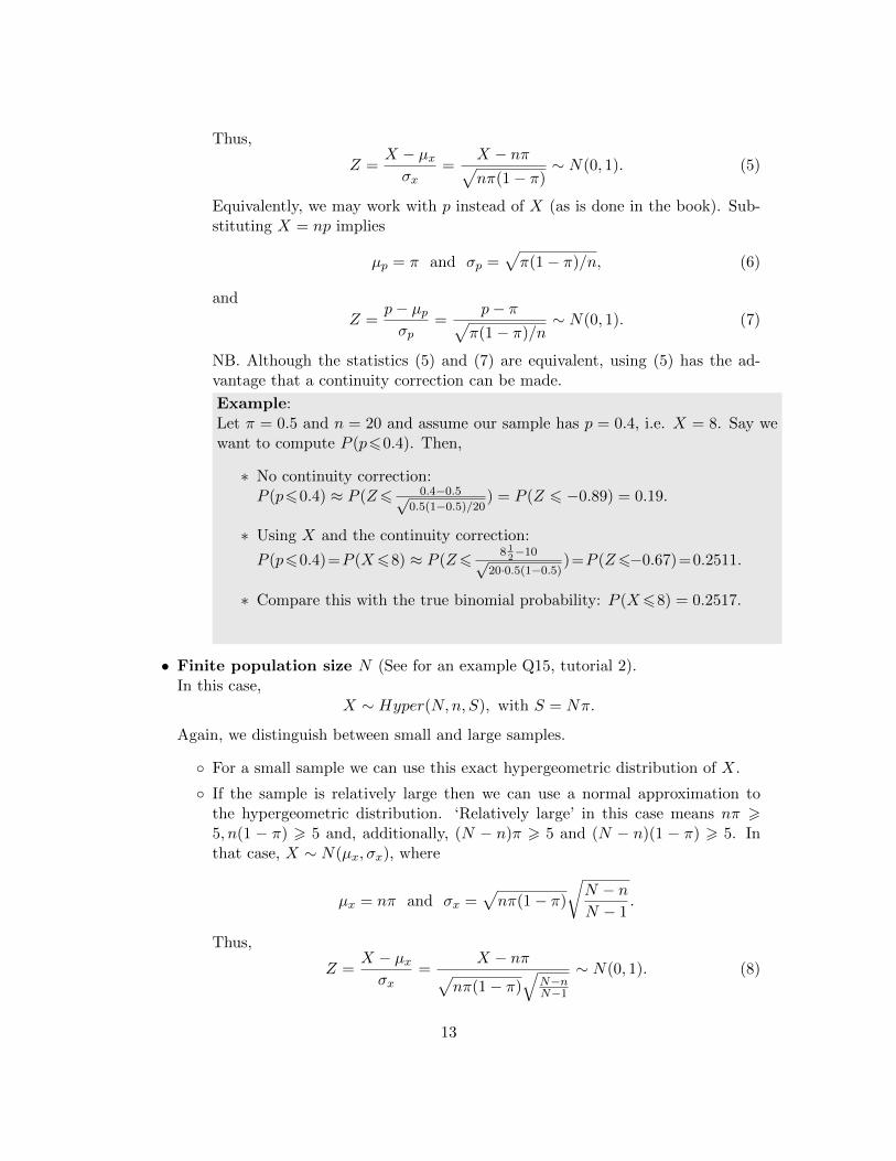
I Sample size estimation.

The margin of error (E) is half the size of the confidence interval. Given E, what shouldbe the sample size n to obtain a confidence interval with margin of error at most E? Ifthe computed n is not a whole number then round up.

B Sample size estimation for µ

• Size for known (or estimated) σ:

E = zσ√n→ n =

(zσE

)2. (11)

• Size for unknown σ:

E = zs√n→ n =

(zsE

)2.

There is something strange with the formula above. Looking at the formula for theconfidence interval it should actually be E = t s√

n, where t = tn−1;α/2. However, it is

impossible to compute n from this since n is a parameter of t. Therefore, we simplyuse z = zα/2. The other thing to notice is that the sample variation s is probablynot known since we are computing the size n of the sample which we still need totake. In that case, work as follows:

• Size for both σ and s unknown. Use (11) and do one of the following:

– Take a preliminary (small) sample and use its sample standard deviation for σ.

– If distribution is uniform then use σ =√

(b− a)/12, where all values are as-sumed to lie between a and b.

– If distribution is (approximately) normal use σ = (b−a)/6 (or more conservativeσ = (b− a)/4).

– For Poisson arrivals we have σ =√λ. Make a guess for the arrival rate λ.

B Sample size estimation for proportion π

• Size for known (or estimated) value π:

E = z

√π(1− π)

n→ n = z2π(1− π)

E2. (12)

However, π is probably not known since the goal is to construct an interval for π.Use p instead:

15

• Size for known value p:

E = z

√p(1− p)

n→ n = z2 p(1− p)

E2.

However, the sample proportion p is probably not known/given either since we arecomputing the size n of the sample which we still need to take. In that case, workas follows:

• Size for π and p unknown. Use (12) and do one of the following: In that case wecould do one of the following:

– Take a preliminary (small) sample and use its proportion for π.

– Take a preliminary (small) sample but instead of using p directly, build a con-fidence interval for π and use the border which is nearest to 0.5

– Use historical data to estimate π.

– Take π = 0.5. This is the conservative approach and gives the largest value n.

16

Chapter 9: One-Sample Hypothesis

I Testing

H0: Null hypothesis.H1: Alternative hypothesis. (= what we want to show to be probably true.)

B Errors.

• Type I error: Rejecting a true H0. Probability(Type I error)= α. Value α is chosen.

• Type II error: Not rejecting a false H0. Probability(Type II error)= β.Value β is not chosen but follows from α, n, H0, and the (unknown) real distribution.

The power of the test is the probability of rejecting a false H0 (which is not an error butis what we want). Power = 1− β.We want α and β both to be small but reducing α will increase β if we make no otherchanges. Increasing the sample size is a way to decrease both α and β.

B 5 steps for testing:

1. Hypothesis + α

2. Sample statistic and indicate rejection region.

3. Test statistic + its (approximate) distribution. Assumptions and/or conditions.

4. Value of test statistic + critical value(s) or give p-value.

5. Make a decision (Reject/Do not reject Ho) + conclusion in words.

In some tests, like ANOVA and regression one should state the model as a step 0.

I Test for the population mean µ

H0 : µ > µ0 H0 : µ = µ0 H0 : µ 6 µ0

H1 : µ < µ0 or H1 : µ 6= µ0 or H1 : µ > µ0

Test statistic (σ known):

z =x− µ0

σx=x− µ0

σ/√n∼ N(0, 1).

Test statistic (σ unknown):

t =x− µ0

s/√n∼ tn−1.

17

Confidence interval for µ (See Chapter 8):

x± t·s/√n, with t = tn−1;α/2.

A two-sided test for µ is similar to a confidence interval:

H0 : µ = µ0 rejected ⇐⇒ µ0 outside confidence interval.

In all cases above we assume that the condition (@) (see Chapter 8) holds.

I Test for the population proportion π

H0 : π > π0 H0 : π = π0 H0 : π 6 π0

H1 : π < π0 or H1 : π 6= π0 or H1 : π > π0

Instead of (@) we use the condition: nπ0 > 5 and n(1− π0) > 5.Test statistic (book version):

Z =p− π0

σp=

p− π0√π0(1− π0)/n

.

Let X be the number of successes: X = pn. Replacing p by X/n gives an equivalentstatistic:

Z =X − nπ0√nπ0(1− π0)

.

The two statistics above are identical. However, the latter has the advantage that anadditional continuity correction is possible. (See the section on proportion.) Continuitycorrection is not really needed if you notice that the p-value is much smaller or muchlarger than α. (The continuity correction will not change the p-value a lot.) However, ifthe p-value is close to α then continuity correction might make a difference and shouldtherefore be made in that case.

If condition nπ0 > 5, n(1− π0) > 5 fails then use the exact distribution: X ∼ Bin(n, π0).

Example: Let n = 4, X = 3. H0 : π 6 0.2. Then, p-value=P (X > 3) = P (X =3) + P (X = 4) = 0.026 + 0.002 = 0.028.

I Test for the population variance.

H0 : σ2 > σ20 H0 : σ2 = σ2

0 H0 : σ2 6 σ20

H1 : σ2 < σ20 or H1 : σ2 6= σ2

0 or H1 : σ2 > σ20

Sample statistic: S2. Test statistic:

χ2 =(n− 1)S2

σ20

∼ χ2n−1.

Assumption: Population is normally distributed.

Look up critical values, χ2L, χ

2U , from table. Reject one or two sides, depending on H0.

18

Chapter 10: Two-Sample Hypothesis

For any two stochastic variables X1, X2:

µX1−X2= µ1 − µ2 (13)

If X1 and X2 are independent (as we assume here) then cov(X1, X2) = 0. In that case

var(X1 −X2) = var(X1) + var(X2)− 2cov(X1, X2)

= var(X1) + var(X2). (14)

I Difference in means: two independent samples.

H0 : µ1 − µ2 > 0 H0 : µ1 − µ2 = 0 H0 : µ1 − µ2 6 0H1 : µ1 − µ2 < 0 or H1 : µ1 − µ2 6= 0 or H1 : µ1 − µ2 > 0

Instead of testing against 0, we may take any value. For example, we could test H0 :µ1 − µ2 = 10. In that case µ1 − µ2 = 10 in the formulas below. Usually, the benchmarkis 0 and in that case µ1 − µ2 = 0 in the formalas below.

The choice of the test statistic follows from the next three possible cases. The CLTconditions (@) (See Chapter 8) must hold for both samples.

1. σ1, σ2 known.

2. σ1, σ2 unknown but assumed equal.

3. σ1, σ2 unknown and not assumed equal.

1. Use test statistic

Z =X1 −X2 − (µ1 − µ2)

σX1−X2

, where σX1−X2=√σ2

1/n1 + σ22/n2.

2. Use pooled variance t-test.

t =X1 −X2 − (µ1 − µ2)√

s2p/n1 + s2

p/n2

∼ tn1+n2−2, where s2p =

(n1 − 1)s21 + (n2 − 1)s2

2

n1 + n2 − 2.

3. Use separate variance t-test.

t =X1 −X2 − (µ1 − µ2)√

s21/n1 + s2

2/n2

∼ tdf ,

where df = some large formula. (See book or formula sheet). Round down.A quick (but not very accurate!) rule is to use df ≈ min{n1 − 1, n2 − 1}.

19

If n1 = n2 then the t-values for case 2 and case 3 are equal but df may differ.

Confidence intervals:

(x1− x2)± tn1+n2−2,α/2

√s2p

n1+s2p

n2(pooled), (x1− x2)± tdf,α/2

√s2

1

n1+s2

2

n1(separate).

I Difference in means: paired samples.

Letd = X1 −X2.

Then, d is a stochastic variable with µd = µ1 − µ2. (You may also see D instead of d butthe book uses the lower case.) A test for µ1 = µ2 now simply becomes a one-sample t-testfor µd = 0.

H0 : µd > 0 H0 : µd = 0 H0 : µd 6 0H1 : µd < 0 or H1 : µd 6= 0 or H1 : µd > 0

Let d be the sample mean of d and sd be the sample standard deviation of d. Then, thetest statistic for this one sample t-test is:

t =d− µdsd/√n∼ tn−1.

Assumption: The condition (@) should hold for d.

NB. It is also possible to test for another value than 0. For example: H0 : µd > −8 (SeeQ2 tutorial 4). In that case just take µd = −8 in the formula for t above.

Confidence interval for µd:

d± tn−1;α/2sd√n.

I Difference in proportions (independent samples).

First, let us compute the mean and varaiance of the difference. From (6),(13),(14) we seethat:

µp1−p2 = π1 − π2

var(p1 − p2) =π1(1− π1)

n1+π2(1− π2)

n2.

The possible hypotheses are:

20

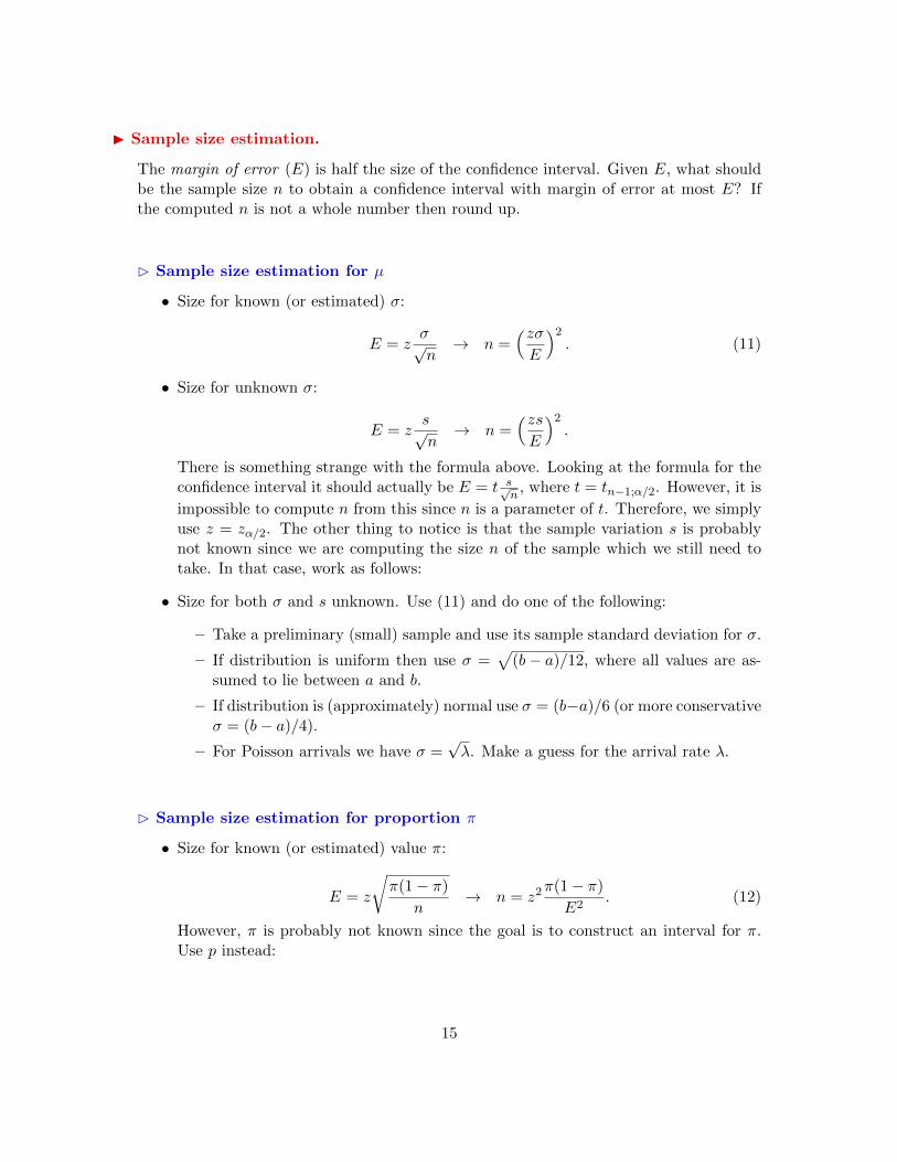
H0 : π1 − π2 > D0 H0 : π1 − π2 = D0 H0 : π1 − π2 6 D0

H1 : π1 − π2 < D0 or H1 : π1 − π2 6= D0 or H1 : π1 − π2 > D0

Two test statistics are distinguished depending on D0 being zero or not.

• D0 = 0. In other words: we assume the proportions are the same. In that case weuse a pooled proportion for the estimate: p = x1+x2

n1+n2.

Test statistic:

z =p1 − p2√

p(1−p)n1

+ p(1−p)n2

∼ N(0, 1). (15)

Conditions: n1p > 5, n1(1− p) > 5 and n2p > 5, n2(1− p) > 5.

• D0 6= 0. Test statistic:

z =p1 − p2 −D0√

p1(1−p1)n1

+ p2(1−p2)n2

∼ N(0, 1).

Conditions: n1p1 > 5, n1(1− p1) > 5 and n2p2 > 5, n2(1− p2) > 5.

I Difference in variances (independent samples)

H0 : σ21/σ

22 > 1 H0 : σ2

1/σ22 = 1 H0 : σ2

1/σ22 6 1

H1 : σ21/σ

22 < 1 or H1 : σ2

1/σ22 6= 1 or H1 : σ2

1/σ22 > 1

Test statistic:

F =S2

1

S22

∼ Fn1−1,n2−1. (Reject one or both sides, depending on H0.)

Assumption: Both populations are normal.

Critical values FL, FR. Only FR in table. The left critical value can be computed fromFL = 1/F ′R, where F ′R is the right critical for labels 1 and 2 reversed. Tip: Label thesamples such that s2

1 > s22. Then, only FR is needed.

The Levene test is another test for comparing two variances. The exact test and distri-bution are not explained in the book. We shall only use its p-value from a given output.Some properties of Levene:

- Normal assumption not needed.- Always 2-sided (H0 : σ1σ2 = 1) and 1-tailed. Reject high values.- Also works for comparing more than two variances.

21

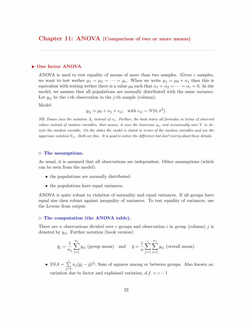
Chapter 11: ANOVA (Comparison of two or more means)

I One factor ANOVA

ANOVA is used to test equality of means of more than two samples. Given c samples,we want to test wether µ1 = µ2 = · · · = µc. When we write µj = µ0 + αj then this isequivalent with testing wether there is a value µ0 such that α1 = α2 = · · · = αc = 0. In themodel, we assume that all populations are normally distributed with the same variance.Let yij be the i-th observation in the j-th sample (column).

Model:yij = µ0 + αj + εij , with εij ∼ N(0, σ2).

NB. Doane uses the notation Aj instead of αj. Further, the book states all formulas in terms of observed

values instead of random variables, that means, it uses the lowercase yij and occasionally uses Y to de-

note the random variable. On the slides the model is stated in terms of the random variables and use the

uppercase notation Yij. Both are fine. It is good to notice the difference but don’t worry about these details.

B The assumptions.

As usual, it is assumed that all observations are independent. Other assumptions (whichcan be seen from the model):

• the populations are normally distributed.

• the populations have equal variances.

ANOVA is quite robust to violation of normality and equal variances. If all groups haveequal size then robust against inequality of variances. To test equality of variances, usethe Levene from output.

B The computation (the ANOVA table).

There are n observations divided over c groups and observation i in group (column) j isdenoted by yij . Further notation (book version):

yj =1

nj

nj∑i=1

yij (group mean) and y =1

n

c∑j=1

nj∑i=1

yij (overall mean).

• SSA =c∑j=1

nj(yj − y)2: Sum of squares among or between groups. Also known as:

variation due to factor and explained variation, d.f. = c− 1

22

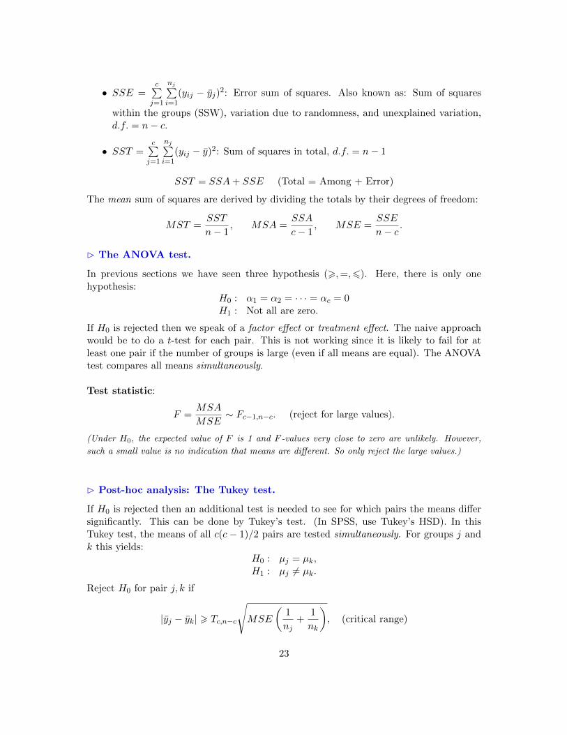
• SSE =c∑j=1

nj∑i=1

(yij − yj)2: Error sum of squares. Also known as: Sum of squares

within the groups (SSW), variation due to randomness, and unexplained variation,d.f. = n− c.

• SST =c∑j=1

nj∑i=1

(yij − y)2: Sum of squares in total, d.f. = n− 1

SST = SSA+ SSE (Total = Among + Error)

The mean sum of squares are derived by dividing the totals by their degrees of freedom:

MST =SST

n− 1, MSA =

SSA

c− 1, MSE =

SSE

n− c.

B The ANOVA test.

In previous sections we have seen three hypothesis (>,=,6). Here, there is only onehypothesis:

H0 : α1 = α2 = · · · = αc = 0H1 : Not all are zero.

If H0 is rejected then we speak of a factor effect or treatment effect. The naive approachwould be to do a t-test for each pair. This is not working since it is likely to fail for atleast one pair if the number of groups is large (even if all means are equal). The ANOVAtest compares all means simultaneously.

Test statistic:

F =MSA

MSE∼ Fc−1,n−c. (reject for large values).

(Under H0, the expected value of F is 1 and F -values very close to zero are unlikely. However,

such a small value is no indication that means are different. So only reject the large values.)

B Post-hoc analysis: The Tukey test.

If H0 is rejected then an additional test is needed to see for which pairs the means differsignificantly. This can be done by Tukey’s test. (In SPSS, use Tukey’s HSD). In thisTukey test, the means of all c(c− 1)/2 pairs are tested simultaneously. For groups j andk this yields:

H0 : µj = µk,H1 : µj 6= µk.

Reject H0 for pair j, k if

|yj − yk| > Tc,n−c

√MSE

(1

nj+

1

nk

), (critical range)

23

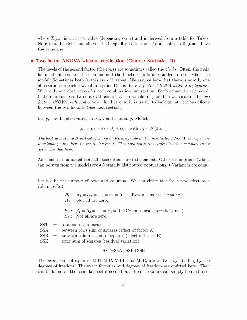
where Tc,n−c is a critical value (depending on α) and is derived from a table for Tukey.Note that the righthand side of the inequality is the same for all pairs if all groups havethe same size.

I Two factor ANOVA without replication (Course: Statistics II)

The levels of the second factor (the rows) are sometimes called the blocks. Often, the mainfactor of interest are the columns and the blockdesign is only added to strengthen themodel. Sometimes both factors are of interest. We assume here that there is exactly oneobservation for each row/column pair. This is the two factor ANOVA without replication.With only one observation for each combination, interaction effects cannot be estimated.If there are at least two observations for each row/column pair then we speak of the twofactor ANOVA with replication. In that case it is useful to look at interactions effectsbetween the two factors. (See next section.)

Let yij be the observation in row i and column j. Model:

yij = µ0 + αi + βj + εij , with εij ∼ N(0, σ2).

The book uses A and B instead of α and β. Further, note that in one-factor ANOVA, the αj refers

to column j while here we use αi for row i. That notation is not perfect but it is common so we

use it like that here.

As usual, it is assumed that all observations are independent. Other assumptions (whichcan be seen from the model) are • Normally distributed populations, • Variances are equal.

Ler r, c be the number of rows and columns. We can either test for a row effect or acolumn effect.

H0 : α1 = α2 = · · · = αr = 0 (Row means are the same.)H1 : Not all are zero.

H0 : β1 = β2 = · · · = βc = 0 (Column means are the same.)H1 : Not all are zero.

SST = total sum of squaresSSA = between rows sum of squares (effect of factor A)SSB = between columns sum of squares (effect of factor B)SSE = error sum of squares (residual variation)

SST=SSA+SSB+SSE

The mean sum of squares, MST,MSA,MSB, and MSE, are derived by dividing by thedegrees of freedom. The exact formulas and degrees of freedom are omitted here. Theycan be found on the formula sheet if needed but often the values can simply be read form

24

given output. The F -values for the corresponding hypotheses are:

F =MSA

MSE(for rows), F =

MSB

MSE(for columns).

Tukey test. The Tukey test for the post hoc analysis works the same as for the onefactor ANOVA. The test is done for each factor separately but often you will be interestedin only one of the two.

I Two factor ANOVA with replication (Course: Statistics II)

If there are at least two observations for each row/column pair then we speak of the twofactor ANOVA with replication. In that case it is useful to look at interaction effectsbetween the two factors. Let yijk be observation i for row j and column k.

Model:yijk = µ0 + αj + βk + (αβ)jk + εijk, with εijk ∼ N(0, σ2).

The main effects (row and column) can be tested as was done in the two factor ANOVAwithout replication. Additionally, we can test for an interaction effect:

H0 : All the (αβ)jk are zero.H1 : Not all (αβ)jk are zero.

The interaction sum of squares is denoted by SSI. The equation becomes

SST=SSA+SSB+SSI+SSE

The mean sum of squares are derived by dividing by the degrees of freedom. The ex-act formulas and degrees of freedom are omitted here. The F -value for the test on aninteraction effect is:

F =MSI

MSE.

Example

β1 β2 β3

α1 10.1 20.2 30.210.2 20.4 30.1

α2 10.0 20.1 30.510.1 20.4 30.1

β1 β2 β3

α1 10.1 20.2 30.210.2 20.4 30.1

α2 20.0 30.1 40.520.1 30.4 40.1

β1 β2 β3

α1 10.1 20.2 30.210.2 20.4 30.1

α2 30.0 20.1 10.530.1 20.4 10.1

Left : Strong column effect. No row or interaction effect.Middle: Strong row and column effect. No interaction effect.Right : No row or column effect but a strong interaction effect.

25

Chapter 12: Simple linear regression

In simple linear regression there is only one x-variable. The next chapter deals with morethan one x-variable. We have n pairs of observations (xi, yi) coming from populations Xand Y . The X is called the independent variable and Y is the dependent variable. Bothare numeric variables and we want to test how Y depends on X. In the regression model,only the Y is considered a random variable.Note the differences with the models from chapter 11 and 15:

ANOVA: X categorical, Y numeric,Regression: X numeric, Y numeric.Chi-square test: X categorical, Y categorical,

Some notation: x = 1n

n∑i=1

xi (average x-value), y = 1n

n∑i=1

yi (average y-value).

I Correlation

Correlation measures the degree of linearity between two (random) variables X and Y .

Population correlation coefficient: ρ.

Sample correlation coefficient: r =SSxy√

SSxx

√SSyy

, (−1 6 r 6 1), where

SSxx =

n∑i=1

(xi − x)2, SSyy =

n∑i=1

(yi − y)2, SSxy =

n∑i=1

(xi − x)(yi − y).

We can test for ρ being unequal to zero:

H0 : ρ = 0 (No correlation)H1 : ρ 6= 0 (There is correlation).

Sample statistic: r

Test statistic:

t = r

√n− 2

1− r2∼ tn−2, (reject both sides).

A one sided test (ρ 6 0, or ρ > 0) is also possible. In that case, reject one side.A quick (less accurate) test is to reject H0 if |r| > 2/

√n.

Note that no test is given in the book for H0 : ρ = ρ0, with ρ0 6= 0.

26

I Regression

B Regression model

• In the regression model, we assume that (within a certain domain) the data satisfiesthe following regression equation:

y = β0 + β1x+ ε, where ε ∼ N(0, σ2) (assumed model).

That means, for any observation (xi, yi) we have

yi = β0 + β1xi + εi,

where εi is the error for observation i and is assumed to come from a normal distri-bution N(0, σ2). The parameter β0 is the intercept and β1 is the slope.

• From the sample we try to find estimates b0, b1 for the parameters β0, β1. Theestimated regression equation (or fitted equation) becomes

y = b0 + b1x. (estimated equation). (16)

In particular, for any xi we have

yi = b0 + b1xi.

The residual (or error) for point i is the difference between yi and the estimate yi.

ei = yi − yi.

The estimates b0, b1 are found by minimizing∑

i e2i =

∑i(yi − yi)2. This is called the

ordinary least squares method (OLS).

B Checking the assumptions (LINE)

As can be seen from the regression model, we assume that:

• there is a Linear relation between X and Y .

Further, we assume that the error terms εi

• are Independent (no autocorrelation),

• are Normally distributed,

• have Equal variance (homoscedastic).

The real error terms εi are not known since we do not know β0 and β1. Instead, we usethe residuals ei to check these assumptions.

27

Independence: Plot the residuals against the X variable and look how the sign (positiveor negative) changes. If there is no autocorrelation then a residual ei will be followed by aresidual ei+1 of the same sign in roughly half the cases. There is positive autocorrelationif positive residuals are mainly followed by positive residuals and negative residuals aremainly followed by negative ones. There is negative autocorrelation if positive residualsare mainly followed by negative residuals and negative residuals are mainly followed bypositive ones.

Normality: Check skewness and Kurtosis of the residuals. If both between −1 and 1 thenOK. Should be OK if n > 30. (Normality violation not a big problem unless there aremajor outliers.)

Equal variance: Plot the residuals against the X variable. There should be no pattern(such as increasing or decreasing residuals).

B The computation (the ANOVA table).

As mentioned, the values b0 and b1 are chosen such that the sum of squared residuals SSEis minimized. The following sums of squares are of interest for the analysis:

SST =∑

i(yi − y)2: Total sum of squares, d.f. = n− 1.SSR =

∑i(yi − y)2: Regression sum of squares (explained), d.f. = 1

SSE =∑

i(yi − yi)2: Error/residual sum of squares (unexplained), d.f. = n− 2

Property:SST = SSR+ SSE. (17)

The mean sum of squares are derived by dividing the totals by their degrees of freedom:

MST =SST

n− 1, MSR =

SSR

1, MSE =

SSE

n− 2.

B Testing significance.

The sample statistic b1 is an estimate for the real slope β1. If b1 6= 0 (and it will alwaysbe in a random sample) then this does not imply immediately that the real slope β1 isdifferent from zero. Wether the value is significant depends on the size n of the sampleand the variation in Y .

H0 : β1 = 0.H1 : β1 6= 0.

The test statistic is

F =MSR

MSE∼ F1,n−2 (Reject for large values.)

• A large F -value tells you that the best fitting straight line has a slope which issignificantly different from zero. Be aware that this is not the same as saying the astraight line fits the data well. Curved data may give high F -values.

28

B Usefulness of the model.

If the slope is significant then the next thing to check is wether the model is useful. Thisis measured by the R2 statistic.

The coefficient of determination is

R2 =SSR

SST, (0 6 R2 6 1).

For simple regression (only one X-variable), R2 = r2. It is the percentage of variation inY that is explained by the variation in X. If the slope is significant and R2 is close to 1then the model is useful. (Figure 1-A). Be aware that a significant slope together with asmall value of R2 (Figure 1-B) may still be useful for some applications. Also, insignificantslope may be due to a too small sample (Figure 1-C) and the model could be useful afterall but we just can’t tell yet from the sample.

B Significance versus usefulness (See Figure 1).

From the definitions one can compute that F = (n − 2)(

R2

1−R2

). Form this we see that

R2 = 0 if F = 0 and vice versa. Also, R2 → 1 if F → ∞ and vice versa. It appears asif R2 and F are measuring the same thing. But usefulness and significance are differentconcepts. Figure 1 gives four extreme cases, illustrating the difference between the twostatistics.

B Testing slope β1 and intercept β0.

Each of the values βi can be tested for significance separately with a t-test. We have seenabove that the F -test checks significance of the slope β1. In general, (see next chapter)the F test checks significance of the slopes of all X-variables simultaneously. In simpleregression there is only one X-variable and the F -test for significance is equivalent withthe t-test for zero slope: the hypotheses are the same and so will be the conclusion, eventhough the test statistics (F and t) differ. (See the paragraph ‘Identical tests’.)

H0 : β1 = 0

H1 : β1 6= 0.

The test statistic is

t =b1 − 0

sb1∼ tn−2.

The standard error of the slope sb1 can usually be read from the output. The assumptionsfor the test are those of the regression model. See ‘checking the assumptions’.

Of course, we can also test one sided or for some non-zero slope, say δ:

29

Figure 1: Difference between R2 (‘usefulness’) and F (‘significance’) in the regressionanalysis. A: Almost perfectly on the line. B: Clearly, there is a trend upwards. However,this slight shift upwards is small compared to the variance in Y . (Variance in Y onlyslightly explained by variation in X) The model is not useful in general but could be usefulin some applications. C: Not enough points to conclude that the slope is significantlydifferent from zero. We do not know yet yet wether the modle is useful, even though R2

is close to 1. D: No trend up or down visible.

H0 : β1 > δ H0 : β1 = δ H0 : β1 6 δH1 : β1 < δ or H1 : β1 6= δ or H1 : β1 > δ

In the output, usually the t- and p-value’s are only for the H0 : β1 = 0 and therefore thesecannot be used directly for non-zero H0. In that case, take the standard error of the slopesb1 from the output and compute the t-value yourself:

t =b1 − δsb1

∼ tn−2.

Then, compare with the critical t from the table.

The t-test for the intercept β0 works exactly the same as for β1 but is usually less inter-esting.

30

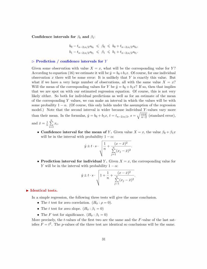
Confidence intervals for β0 and β1:

b0 − tn−2;α/2sb0 6 β0 6 b0 + tn−2;α/2sb0 ,

b1 − tn−2;α/2sb1 6 β1 6 b1 + tn−2;α/2sb1 .

B Prediction / confidence intervals for Y

Given some observation with value X = x, what will be the corresponding value for Y ?According to equation (16) we estimate it will be y = b0+b1x. Of course, for one individualobservation x there will be some error: It is unlikely that Y is exactly this value. Butwhat if we have a very large number of observations, all with the same value X = x?Will the mean of the corresponding values for Y be y = b0 + b1x? If so, then that impliesthat we are spot on with our estimated regression equation. Of course, this is not verylikely either. So both for individual predictions as well as for an estimate of the meanof the corresponding Y values, we can make an interval in which the values will be withsome probaility 1− α. (Of course, this only holds under the assumption of the regressionmodel.) Note that the second interval is wider because individual Y -values vary more

than their mean. In the formulas, y = b0 + b1x, t = tn−2;α/2, s =√

SSEn−2 (standard error),

and x = 1n

n∑i=1

xi.

• Confidence interval for the mean of Y . Given value X = x, the value β0 + β1xwill be in the interval with probability 1− α:

y ± t · s ·√√√√√ 1

n+

(x− x)2

n∑j=1

(xj − x)2

.

• Prediction interval for individual Y . Given X = x, the corresponding value forY will be in the interval with probability 1− α:

y ± t · s ·√√√√√1 +

1

n+

(x− x)2

n∑j=1

(xj − x)2

.

I Identical tests.

In a simple regression, the following three tests will give the same conclusion.

• The t test for zero correlation. (H0 : ρ = 0).

• The t test for zero slope. (H0 : β1 = 0)

• The F test for significance. (H0 : β1 = 0)

More precisely, the t-values of the first two are the same and the F -value of the last sat-isfies F = t2. The p-values of the three test are identical so conclusions will be the same.

31

Chapter 13: Multiple Regression

B Regression model

In multiple regression we have more than one independent variables: X1, X2, . . . , Xk. TheY -variable is the only dependent variable. Instead of a pair (xi, yi), each observation isgiven by k + 1 values x1i, x2i, . . . , xki, yi.

• The regression equation becomes:

y = β0 + β1x1 + β2x2 + · · ·+ βkxk + ε, where ε ∼ N(0, σ2),

or with an index i for the i-th observation:

yi = β0 + β1x1i + β2x2i + · · ·+ βkxki + εi, where εi ∼ N(0, σ2).

• The estimated regression equation is

y = b0 + b1x1 + b2x2 + · · ·+ bkxk,

or with an index i for the i-th observation:

yi = b0 + b1x1i + b2x2i + · · ·+ bkxki.

The residual for observation i is the difference between yi and the estimate yi.

ei = yi − yi.

Just as in simple regression, the OLS method finds the estimates b0, b1, . . . , bk which min-imize

∑i e

2i =

∑i(yi − yi)2.

B Assumptions

See simple regression.

B The computation (the ANOVA table).

The sums of squares are defined exactly the same as for simple regression. Only thedegrees of freedom differ as can be seen from the mean sum of squares (k = 1 in simpleregression):

MST =SST

n− 1, MSR =

SSR

k, MSE =

SSE

n− k − 1.

32

B Testing significance.

While in simple regression the F -test is doing the same as the t-test for β1, in multipleregression it tests all the slopes β1, β2, . . . , βk simultaneously. If rejected, then at least oneof the slopes βi differs significantly from zero. Then, a t-test for each of the βi’s can beused to check each of the coefficients seperately for non-zero slope.

H0 : β1 = β2 = · · · = βk = 0.

H1 : βi 6= 0 for some i (or simply say: ’not H0’).

The test statistic is

F =MSR

MSE∼ Fk,n−k−1 (Reject for large values.)

B Usefulness of the model.

See simple regression for a discussion on R2 and the F -statistic. For multiple regressionwe also have the adjusted coefficient of determination R2

adj.

R2adj = 1−

((1−R2)

n− 1

n− k − 1

).

If more variables are added to the model then R2 increases. This is not necessarily truefor R2

adj. We always have R2adj 6 R2. If R2

adj is much less than R2 then this indicates thatthe model contains useless predictors. We can remove one or more X-variables withoutloosing much of the predictive power.

B Testing slope βi.

Same as for simple regression. The only adjustment is the degrees of freedom:

H0 : βi = δ → t =bi − δsbi

∼ tn−k−1.

B Dummy regressors.

A categorial variable X with only two possible values can be added to the regression modelby recoding the two values into zero’s and one’s: X = 0 or X = 1.

B Detecting multicollinearity (Course: Statistics II).

When the independent variables X1, X2, ..., Xk are intercorrelated instead of independent,we call this multicollinearity. (If only two predictors are correlated, we call this collinear-ity.) Multicollinearity is measured by

V IFj =1

1−R2j

,

where R2j is the coefficient of determination of Xj with all other X-variables. If V IFj > 5,

then Xj is highly correlated with the other independent variables.

33

Chapter 15: Chi-Square Test

Two categorical variables A and B (or for example X and Y ).

H0 : Variables A and B are independent.H1 : Variables A and B are dependent.

Equivalently:H0 : Row distributions are the same.H1 : Row distributions are not the same.

or,H0 : Column distributions are the same.H1 : Column distributions are not the same.

Rj : Total in row j (j = 1, . . . , r)Ck: Total in column k (k = 1, . . . , c).

Under H0, the expected number of observations in cell j, k is

ejk = n

(Rjn

)(Ckn

)=RjCkn

(expected frequency).

Let fjk be the observed number of observations in cell j, k. (Also denoted by njk)

Test statistic:

χ2 =∑j,k

(fjk − ejk)2

ejk∼ χ2

(r−1)(c−1) (reject large values).

Condition: All expected frequencies ejk should be at least 5. (SPSS uses: ejk > 5 for atleast 80% of the cells and ejk > 1 for all cells.)

• If the condition is not met then combining rows or columns may solve this. Thebecomes less powerful though.

• The 2× c problem can be seen as comparing proportions: H0 : π1 = · · · = πc.

• For the 2× 2 problem, the Chi-Square Test is equivalent with the z-test for equalityof two proportions (See (15), Chapter 10). That means, the outcome (reject or not)will be the same.

• It is also possible to do a χ2 test for numerical variables. In that case, each numericalvariable is divided into categories. (For example, a numerical variable ‘age’ may bedivided into 3 groups: less than 18, from 18 till 64, and at least 65.)

34

Chapter 16: Nonparametric Tests

Advantages: small samples allowed, few assumptions about population needed, ordinaldata possible.

Disadvantages: less powerful if stronger assumptions can be made, requires new tables.

Two tests for the medians of paired samples:

B Wilcoxon Signed-Ranks Test

B Sign test (See Supplement 16A)

Two tests for the medians of independent samples:

B Wilcoxon Rank Sum test (also called the Mann-Whitney test). For two samples.

B Kruskal-Wallis test. For two or more samples .

One test for the correlation coefficient:

B Spearman rank correlation test.

B Wilcoxon Signed-Ranks Test

Test for the difference of medians in paired samples Y1, Y2 (H0 : M1 = M2) or for themedian in one sample Y (H0 : MY = M0)

Assumption: The population should be symmetric (for one sample) or the populationdifference should be symmetric (paired samples).

(Note: If a distribution is symmetric then its mean is the same as its median. Therefore,a test for the median can also be used as a test for the mean here.)

For paired samples, let variable D = Y1 − Y2 be the difference. (The book uses d.)If we want to test one sample against a benchmark M0 then we can take D = Y −M0.Using this variable D, the test is the same for both cases:

H0: MD = 0

Omit the zero’s: n → n′. Next, order from small to large by absolute values |Di|. Addthe signs to the ranks.

35

Sample statistic: W = sum of positive ranks.

Test statistic:

• For n′ < 20 use tables and compare W with the critical values.

• For n′ > 20 we use a normal approximation.

Z =W − µWσW

∼ N(0, 1), with µW =n′(n′ + 1)

4, σW =

√n′(n′ + 1)(2n′ + 1)

24.

NB. It is also possible to do a 1-sided test or even test against another value than 0. Forexample H0: MD > −8. (See for example Q3, tutorial 4) In that case, first subtract rightside (−8) from D and give the variable a new name D′ = D − (−8). Now do the testH0 : MD′ > 0.

B Sign test

The sign test is used for the same situations as the Wilcoxon Signed-Ranks test, i.e., forpaired samples or for the median in one sample.

Assumptions: None.

Since symmetry is not required, we cannot test for µ but only for the median M . If sym-metry can be assumed then Wilcoxon Signed-Ranks is preferred.

Again, let variable D = Y1 − Y2 be the differences of the two variables, or if want to testone sample Y against a benchmark M0 then we can take D = Y −M0. Omit the zero’s:n→ n′.

H0: MD = 0

Sample statistic:

X = number of positive differences. Under H0 : X ∼ Bin(n′, 12).

Test statistic:

• For n′ < 10, use X and use the binomial distribution.

• For n′ > 10, use normal approximation for the binomial (with continuity correction).

Z =X − µxσx

∼ N(0, 1), with µX = 12n′, and σX = 1

2

√n′.

NB. It is also possible to do a 1-sided test or even test against another value than 0. Forexample H0: MD > −8. (See for example Q4, tutorial 4) In that case, first subtract theright side (−8) from D and give the variable a new name D′ = D− (−8). Now do the testH0 : MD′ > 0.

36

B Wilcoxon Rank Sum test (also called Mann-Whitney test).

Equality of medians of two independent samples.

Assumption: The two distributions have the same shape.

H0 : M1 = M2.

Make combined rank (average rank for ties). Let T1, T2 be the sum of ranks in each sam-ple, where the smallest sample is labeled 1.

Sample statistic: T1

Test statistic:

• Small samples (n1 6 10 and n2 6 10): T1. Reject both sides. Use table for criticalvalues.

• Large samples (n1>10 and n2>10): Use the normal approximation. There are twoequivalent versions. Either use

Z =T1 − µT1σT1

, with µT1 =n1(n+ 1)

2and σT1 =

√n1n2(n+ 1)

12, (n = n1 + n2),

or use (see book):

Z =T1 − T2

(n1 + n2)√

n1+n2+112n1n2

∼ N(0, 1).

Of course, we can also do a 1-sided test. If only the two-sided p-value is given then lookat the mean ranks to decide on p/2 or 1−p/2. For example, if H0 : M1 6M2 and T1 > T2

then our p-value should be less than 0.5. So we take p/2 and not 1− p/2.

Note that it is not defined what to do if n1 < 10 and n2 > 10. The table cannot be usedsince it only goes up to 10. The best we can do is to use the large sample test and mentionthat the condition (n1, n2>10) is actually not satisfied.

B Kruskal-Wallis

Generalization of the Mann-Whitney test to more than two independent samples. It istherefore the non-parametric alternative for ANOVA (comparison of means).

Assumption: The c distributions have the same shape.

Condition: At least 5 observations in each sample.

37

H0 : M1 = M2 = · · · = Mc.H1 : not all medians are the same.

Order all observed values from smallest to largest and rank them 1, 2, . . . , n. (Averageranks for ties.)

Sample statistics: Tj : the sum of ranks of each group j.

Test statistic:

H =12

n(n+ 1)

c∑j=1

T 2j

nj− 3(n+ 1) ∼ χ2

c−1 (reject large values),

where nj is the number of observations in group j and n = n1 + · · ·+ nc.

B Spearman Rank correlation test.

This is a nonparametric test of association (correlation) between two variables. It isuseful when it is inappropriate to assume an interval scale (a requirement of the Pearsoncorrelation coefficient of Chapter 12).We can test for ρ being unequal to zero:

H0 : ρ = 0 (No correlation)H1 : ρ 6= 0 (There is correlation).

Replace every xi by its rank within the X-values. Denote the new variable by Xr.Replace every yi by its rank within the Y -values. Denote the new variable by Yr.

For these new variables, compute the correlation coefficient: rS = r(Xr, Yr).Test statistic:

Z = rS√n− 1 ∼ N(0, 1).

Required: n > 20.

38