arX

iv:c

ond-

mat

/040

1257

v1 [

cond

-mat

.sta

t-m

ech]

15

Jan

2004

Moving and staying together without a leader

Guillaume Gregoire,a Hugues Chate,aand Yuhai Tub

aCEA – Service de Physique de l’Etat Condense, Centre d’Etudes de Saclay,91191 Gif-sur-Yvette, France

bIBM T.J. Watson Research Center, Yorktown Heights, NY 10598, USA

A microscopic, stochastic, minimal model for collective and cohesive motion of identical self-propelled particlesis introduced. Even though the particles interact strictly locally in a very noisy manner, we show that cohesion canbe maintained, even in the zero-density limit of an arbitrarily large flock in an infinite space. The phase diagramspanned by the two main parameters of our model, which encode the tendencies for particles to align and to staytogether, contains non-moving “gas”, “liquid” and “solid” phases separated from their moving counterparts bythe onset of collective motion. The “gas/liquid” and “liquid/solid” are shown to be first-order phase transitionsin all cases. In the cohesive phases, we study also the diffusive properties of individuals and their relation to themacroscopic motion and to the shape of the flock.

1. Introduction

The emergence of collective motion of self-propelled organisms (bird flocks, fish schools,herds, slime molds, bacteria colonies, etc.) is afascinating phenomenon which attracted the at-tention of (theoretical) physicists only recently([1,2,4,5,6]). Particularly intriguing are the sit-uations where no “leader” with specific proper-ties is present in the group, no mediating fieldhelps organizing the collective dynamics (e.g. nochemotaxis), and interactions are short-range. Inthis case, even the possibility of collective motionmay seem surprising.

However “simple” the involved organisms maybe, they are still tremendously complex for aphysicist and his inclination will often be to goaway from the detailed, intricate, as-faithful-as-possible modeling approach usually taken by biol-ogists, and to adopt “minimal models” hopefullycatching the crucial, universal properties whichmay underlie seemingly different situations.

In this setting, the organisms can be reduced topoints which move at finite velocity and interactwith neighbors. This is in fact what Vicsek andcollaborators did when introducing their minimalmodel for collective motion.

2. Vicsek’s model

Vicsek’s model [2] consists in pointwise parti-cles labeled by i which move synchronously atdiscrete timesteps ∆t by a fixed distance v0 alonga direction θi. This angle is calculated from thecurrent velocities of all particles j within an in-teraction range r0, reflecting the only “force” atplay, a tendency to align with neighboring parti-cles:

θt+1i = arg

∑

j∼i

~vtj

+ η ξti , (1)

where ~vti is the velocity vector of magnitude v0

along direction θi and ξti is a delta-correlated

white noise (ξ ∈ [−π, π]). Fixing r0 = 1, ∆t = 1,and choosing, without loss of generality, a valuev0∆t < r0, Vicsek et al studied the behavior ofthis simple model in the two dimensional param-eter space formed by the noise strength η andρ, the particle density. They found, at large ρand/or small η, the existence of an ordered phasecharacterized by:

V ≡⟨

|〈~vti〉i|⟩

t> 0 , (2)

i.e. a domain of parameter space in which theparticles move collectively.

The existence of the ordered phase was laterproved analytically [7] via a continuous model for

1

2

∆t v0 r0 ra re rc η1.0 0.05 1.0 0.8 0.5 0.2 1.0

Table 1Fixed-value parameters used in the simulations.

the coarse-grained particle velocity and density.Vicsek et al devoted most of their effort to study-ing the transition to the ordered phase [2]. Theyfound numerically a continuous transition charac-terized by scaling laws and they tried to estimatethe corresponding set of critical exponents.

3. Collective and cohesive motion

Vicsek’s model accounts rather well, at leastat a qualitative level, for situations where the or-ganisms interact at short distances but need notstay together. This is for instance the case ofthe bacterial bath recently studied by Wu andLibchaber [9]. In this experiment, E. Coli bac-teria are swimming freely within a fluid film ofthickness approximately equal to their size. Byseeding the system with polystyrene beads andrecording the trajectories of these passive tracers,Wu and Libchaber showed that the bacteria per-form superdiffusive motion crossing over to nor-mal diffusion. We later argued that the superdif-fusive behavior is likely to be due to the onset ofcollective motion as in Vicsek’s model [10,11].

When the situation to be described involves theoverall cohesion of the population, Vicsek’s modelneeds to be supplemented by a suitable feature.Indeed, an initially cohesive flock of particles willdisperse in an open space. In other words, no col-lective motion is possible in the zero density limitof this model. In the following, we extend Vic-sek’s model to account for the possible cohesionof the population of particles.

The above remark is by no means new. Earlymodels for the collective motion of “boids” (con-traction of “birdoid”, a term used by computeranimation graphics specialists) do include a two-body repulsive-attractive interaction [3]. Morerecent works by physicists also included this in-gredient, but they either comprised an extraglobal interaction [4], or the actual interactionrange used extended over the whole flock for the

sizes considered, making it effectively global [5].Another encountered pitfall, from our point ofview at least, is to enforce the cohesion by theconfinement to a rather small, close, space [6].

Here we want to be, in a sense, in the least-favorable circumstances for observing collectivemotion: no leader in the group, strongly noisyenvironment and/or communications, strictly lo-cal interactions, and no confinement at all.The “minimal” model presented below is one ofthe simplest possible ones satisfying these con-straints.

4. A minimal model

In addition to the possibility of achieving cohe-sion, we also want to confer a “physical” extentto the particles, a feature absent from Vicsek’spoint-particles approach. Adding a Lennard-Jones-type body force ~f acting between each pairof particles within distance r0 from each otheroffers such a possibility.

Equation (1) is then replaced by

θt+1i = arg

α∑

j∼i

~vtj + β

∑

j∼i

~fij

+ η ξti , (3)

where α and β control the relative importance ofthe two “forces”. The precise form of the depen-dence of the body force on the distance betweenthe two particles involved is not important. Itis enough to ensure a hard-core repulsion at dis-tance rc and an “equilibrium” preferred distancere.

In the following, we use

~fij = ~eij

−∞ if rij < rc ,14

rij−re

ra−re

if rc < rij < ra ,

1 if ra < rij < r0 .

(4)

with rij the distance between boids i and j, ~eij

the unit vector along the segment going from i toj, and the numerical values rc = 0.2, re = 0.5 andra = 0.8.

We have also tested other types of noise term inthe model. In particular, considering the noise asthe uncertainty with which each boid “evaluates”the force exerted on itself by the Ni neighboring

3

12 14 16 18 20

x12

14

16

18

20y

12 14 16 18 20

x12

14

16

18

20y

18 20 22 24 26

x12

14

16

18

20y

5 10 15 20 25

x5

10

15

20

25y

(c) (d)

(a) (b)

Figure 1. Cohesive flocks of 128 particles in a square box of linear size 32 with periodic boundaryconditions (for parameters see Table 1). (a): immobile “solid” at α = 1.0 and β = 100.0 (20 timestepssuperimposed). (b): 3 snapshots, separated by 120 timesteps, of a “flying crystal” at α = 3.0 andβ = 100.0. (c): fluid droplet (α = 1.0, β = 2.0, 20 consecutive timesteps). (d): moving droplet (α = 3.0,β = 3.0, 20 consecutive timesteps). In (b) and (d), the arrow indicates the (instantaneous) direction ofmotion.

4

0 0.5 1

n/N0

0.5

1PDF

0 0.6 1.2

β0

0.2

0.4

0.6

0.8

1n/N

(a)

-1 -0.5 0 0.5 1

∆0

0.5

1PDF

20 40 60

β0

0.4

0.8

∆

(b)

Figure 2. Order parameters at ρ = 1/16, L = 128, α = 1.0. (a) : “gas/liquid” transition, inset: clustermass distribution at the coexistence point β = 1.0. (b) : “liquid/solid” transition, inset: pdf of orderparameter ∆ for the “liquid/solid” transition, β = 36 plain line (“liquid” phase), β = 48 dotted line andβ = 60 dashed line(“solid” phase). (other parameters as in Table 1).

boids leads to change Eq. (3) to:

θt+1i = arg

α∑

j∼i

~vtj + β

∑

j∼i

~fij + Niη~uti

(5)

where ~uti is a unit vector of random orientation.

There are delicate issues related to the choice ofthe noise term, in particular with respect to thecritical properties of the transition to collectivemotion [12]. We mostly considered, in the fol-lowing, the noise term as prescripted above inEq. (5). A detailed analysis of the influence ofthe nature of the noise is left for future studies,but we are confident that the results presentedhere hold generally, at least at a qualitative level.

Finally, in order to ensure that each parti-cle only interacts with its “first layer” of neigh-bors (within distance r0), we calculate, at eachtimestep, the Voronoi tessellation of the popu-lation [14]—this has the additional advantage ofproviding a natural definition of the “cells” asso-ciated with each particle. The interacting neigh-bors are then retricted to be those of the particles

within distance r0 which are also neighbors in theVoronoi sense.

5. Typical phases

One can easily guess the “phases” that theabove model can exhibit for a fixed noise strengthη (η = 1.0 in the following, for a summary of pa-rameters see Table 1). We now present them ina qualitative manner. The results presented be-low were all obtained in the two-dimensional case,but most of them hold in three dimensions. Whenthe body force is weak (small β values), the cohe-sion of a flock cannot be maintained. In a finitebox (finite particle density ρ), one is left with agas-like phase (not shown). An arbitrarily largeflock in an infinite space disintegrates, eventuallyleaving isolated random-walking particles.

For large enough β, we can expect the co-hesion to be maintained. Figure 1 shows suchcohesive flocks. The internal structure of theflocks depends also on β: for large body force,positional quasi-order is present, and the parti-

5

1 1000 1e+06

t1

100

<rij

2>

1 1000 1e+06

t1

100

<rij

2>

(a)

(b)

0.0001 1

t/τ1

100 <rij

2>

0.0001 1

t/τ1

100<r

ij

2>

Figure 3. Mean square distance between initially-neighboring particles vs time for a flock of 10000boids (L = 400, ρ = 1/16) in logarithmic scales.(a) non-moving cohesive droplet (α = 1.0, β =25.0, 35.0, 45.0 and 150.0 from top to bottom, thedashed line has slope 1); (b) moving cohesive flock(α = 3.0, β = 40.0, 55.0, 75.0 and 150.0 from topto bottom). Asymptotic transition points weremeasured at α = 1.0, βLS = 45.3 and at α = 3.0,βLS = 76.1 (see below). Other parameters as inTable 1. Insets: data collapse from which thewaiting time τ can be estimated.

cles locally form an hexagonal crystal (Fig. 1ab).For intermediate values of β, no positional orderarises, and the flock behaves like a liquid droplet(Fig. 1cd).

The influence of the alignment “force” is mani-fested by the global motion of the flock: for largeenough α values, the flock moves (V > 0). De-pending on β, one has then either a “movingdroplet” (Fig. 1d) or a “flying crystal” (Fig. 1b).

6. Order parameters

Order parameters have to be defined to allowfor a quantitative distinction between the phasesdescribed above.

The limit of cohesion separating the “liquid”phases from the “gas” can be determined bymeasuring the distribution of the sizes of par-ticles clusters, thanks to an implementation ofthe Hoshen-Kopelman [15] algorithm. A cohe-sive flock is then one for which n, the size of thelargest cluster, is of order N , the total number ofparticles. Below, we use the criterion n/N = 1

2to

define the transition. Increasing β, n/N sharplyrises to order-one values (Fig. 2a).

The “liquid/solid” transition takes place whenβ is large enough so that cohesion of the pop-ulation is ensured. To determine this onset ofpositional quasi-order within a finite but arbi-trarily large cohesive flock, we first observe that,whether in the collective motion region or not, the“liquid” and “solid” phases can be distinguishedby the fact that particles diffuse with respect toeach other in the “liquid”, whereas neighboringparticles always remain close to each other inthe “solid” (Fig. 3). To be more precise, in the“liquid”, initially close-by particles remain so forsome trapping time τ (which can be defined orused to collapse the curves of Fig. 3). Approach-ing the “solid” phase (by increasing β), τ di-verges. In addition, since we are not dealing witha translation-invariant system, we should alsodistinguish between the diffusion properties ofthe particles depending on their relative positionwithin the flock. We have thus defined different“sectors” (“core”, “head”, “tail”, “sides”) as ex-plained in Fig. 4. If all sectors are roughly equiv-alent in non-moving droplets (at least sufficiently

6

-20 -10 0 10 20

x-20

-10

0

10

20y

Figure 4. Snapshot of a moving flock of 4096boids (coordinates centered on the position of thecenter of mass (CoM)). The arrow indicates theinstantaneous direction of motion of the flock.The solid circle, centered on the CoM, has a ra-dius equal to the root-mean-square of all boids’distances to the CoM. The circle with a 4 timessmaller radius defines the “core” region (filled cir-cles near the CoM). The “head” contains all boidsoutside the larger circle which are also within acone of opening angle π/4 centered on the direc-tion of motion. The “tail” region is defined in anopposite manner.

far from the “liquid/solid” transition), some dif-ferences are observed within moving droplets: theouter regions and in particular the head are moreactive, whereas cohesion is stronger in the core(Fig. 5). Thus, in principle, different trappingtimes τ can be defined for the different regionsof a (moving) flock. But the depth of the outer,“more liquid”, layer does not depend on the flocksize (if it is big enough), so that, in large flocks,most of the population behaves as the core. Con-sequently, the relative diffusion averaged over thewhole flock suffers from finite-size effects, butthey disappear in the large-size limit (see below).To sum up, the trapping time τ (measured onall particles of the flock) is a good quantity totrack the “liquid/solid” transition. However, in-stead of directly estimating of τ , we measured ∆,the relative diffusion over some large time T ofinitially-neighboring particles:

∆ ≡

⟨

1

ni

∑

j∼i

(

1 −r2ij(t)

r2ij(t + T )

)⟩

i,t

, (6)

where the ni particles j are the neighbors of parti-cle i at time t. Time T is taken to be proportionalto the volume of the system, which ensures that∆ records, in the large-size limit, an asymptoticproperty of the system (because T ≫ τ). Clearly,∆ ∼ 1 in the “liquid” phase for a large enoughsystem, while ∆ ∼ 0 in the “solid” phase. In-deed, increasing β, ∆ falls off sharply (Fig. 2b).The transition point is chosen to be at ∆ = 1

2.

Finally, we must be able to distinguish theregimes for which collective motion arises. Tothis aim, we use the average velocity V , as de-fined in (2). Increasing α, V reaches order-onevalues. The onset of collective motion is chosento be at V = v0/2. In the gas phase, one ex-pects V = 0 independently of the strengh of thealignment force. Nevertheless, this phase is rathersharply divided in two when studying the modelat finite particle density. The largest cluster sizemay then be small (n ≪ N), but it is (almost)always larger than one. At any given time, thus,n > 1, and the collective motion order parame-ter V can be defined restricted to the particlesbelonging to the largest cluster. (Since clustersmerge and break, the particles involved generally

7

1 1000 1e+06

t

1

10

100<r

ij

2>

1 1000 1e+06

t

1

10

100<r

ij

2>

0 1e+05

t0

20

40<r

ij

2>

0 1e+05

t0

80

160<r

ij

2>

(a)

(b)

Figure 5. Growth of the mean square distancebetween initially-neighboring particles dependingon their position within a cohesive “liquid” flockof 10000 boids (ρ = 1/16, β = 40). (a) α = 1.0,cohesive non-moving droplet; (b) α = 3.0, movingdroplet. Solid line: all boids in flock. Dottedline: core region, dashed line: head region, dash-dotted line: tail region (as defined in Fig. 4) Insets: diffusion within flock head in linear scales, thesolid line is just a guide to the eye.

change along time.)

7. Phase diagram

After a brief discussion of the nature of thetransitions involved, we first present the phasediagram of our model for a finite density of par-ticles in a large and fixed box size. Then we esti-mate finite-size effects on the location of the phaseboundaries. Finally, we argue that the phase dia-gram can also be defined in the zero-density limitwhere an arbitrarily large flock wanders in an in-finite space.

7.1. Nature of the transitions

As expected in usual phase transitions, wefound that in our model the “gas/liquid” and “liq-uid/solid” transitions are first-order. In insets ofFig. 2a and b, we show the evolution of the prob-ability distribution function of the order param-eter as one crosses these transition lines. Thebimodal character of these pdf at the transitionis typical of first-order phase transitions, indicat-ing the coexistence of two metastable states. Atthe “gas/liquid” transition point, dispersed andaggregated boids coexist and there are exchangesbetween the two phases along time. At the “liq-uid/solid” transition point, cohesion is ensuredand one observes the quasi-frozen regions in anotherwise more “liquid” flock. The quasi-solidparts are often located in the core of the flock.(Fig. 6).

The nature of the transition for the onset ofcollective motion is a delicate issue in our model.Whereas its second-order character is rather well-established for Vicsek’s core model, we recentlydiscovered that, in fact, the implementation ofthe noise term may change the nature of the tran-sition. The detailed investigation of this, in par-ticular in presence of the cohesive force, will bepresented in a future publication [12].

7.2. Fixed population and fixed box size

A systematic scan of the (α, β) parameter planewas performed for a flock of N = 2025 particlesliving on a square surface of linear size L = 180(ρ = 1/16) with periodic boundary conditions.Using the criteria defined above, we obtained thephase diagram presented in Fig. 7.

8

Figure 6. Short-time trajectories of freezingdroplets of N = 512 boids (5000 timesteps areshown, the motion of the center of mass and thesolid rotation around it have been substracted).(a): in the moving phase α = 3.0, β = 70: theinner part appears more solid, while the head isclearly more liquid (the arrow indicates the in-stantaneous direction of motion). (b): in the non-moving phase α = 1.0, β = 50: one can distin-guish an outer liquid layer from the almost solidcore.

For each parameter value, we used an initially-aggregated flock. We let the system evolve duringa time τ ∝ Ld, and then we recorded each or-der parameter and its histogram along time. Thetransition points were determined by dichotomy,the precision of which is reflected in the errorbars.

The basic expected features are found: thehorizontal “gas/liquid” and “liquid/solid” tran-sitions are crossed by the vertical “moving/non-moving” line. Near this line, however, one ob-serves a strong deformation of the “gas/liquid”and “liquid/solid” boundaries. This cannot beunderstood without a careful study of the collec-tive motion transition [12].

Note also that the “gas” phase itself is crossedby the line marking the onset of collective motion,using, as explained above, the average velocity Vof the n particles of the largest cluster as the orderparameter.

7.3. Finite size and saturated vapour ef-

fects

We are ultimately interested in the possi-bility of collective and cohesive motion for anarbitrarily-large flock in an infinite space. Thephase diagram of Fig. 7 was obtained at a fixedsystem size and constant density. Thus both lim-its of infinite-size and zero-density have to betaken to reach the asymptotic regime of interest.Of course this is mostly relevant to the onset ofcohesion (the “gas/liquid” transition). Here wefirst study each limit separately, i.e. we inves-tigate finite-size effects at fixed particle densityand expansion at fixed particle number. Then wediscuss the double-limit regime of interest.

Performing such a task for the whole parameterplane far exceeds our available computer power.We restricted ourselves to three typical cases: inthe non-moving phase (α = 1.0), in the movingphase (α = 3.0) and near the transition to collec-tive motion (α = 1.75 for the “gas/liquid” tran-sition and α = 2.1 for the “liquid/solid” transi-tion).

In simulations performed at ρ = 1/16, vary-ing N and L, the transition points βρ

GL(N) and

βρLS(N) converge exponentially as L =

√

N/ρincreases. In Fig. 8, we show this for both the

9

0 1 2 3

α0

2

4

6

40

60

80β

S MS

L ML

G

MG

Figure 7. Phase diagram at ρ = 1/16, L = 180(other parameters as in Table 1). S : solid, MS :moving solid, L : liquid, ML : moving liquid, G :gas, MG : moving gas. Dashed line : transitionline of collective motion.

“gas/liquid” (a) and the “liquid/solid” (b) tran-sitions for α = 3 (moving phases). This al-lows to determine asymptotic transition points.Note that exponentially-decreasing finite-size ef-fects are typical of first order phase transition atequilibrium [16]. In the two other cases (non-moving phase, and onset of motion), the resultsare similar, with the asymptotic values beingquickly reached in the non-moving phase (α = 1)[13].

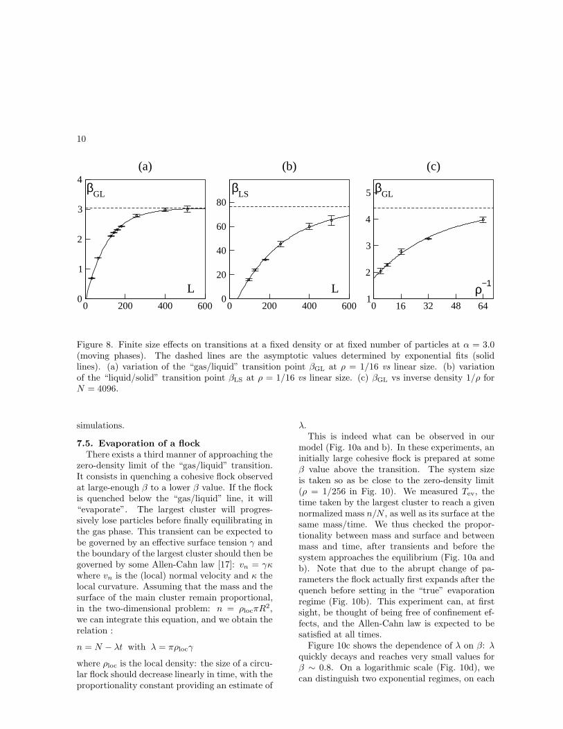
In simulations performed at fixed N varyingL, we study instead the expansion of the system.The (finite) spatial extent induces a confinementeffect which increases the pressure at the coexis-tence point. We thus expect a displacement of thetransition point. We find that βGL(ρ) also con-verges exponentially, and thus transition pointsβGL(N) are well-defined. In Fig. 8c, we show thisonly for the “gas/liquid” transition at the α val-ues used in Fig. 8a, since the “liquid/solid” tran-sitions points were observed to be independent ofthe box size.

7.4. Zero-density limit

The above results provide evidence that ourmodel possesses well-defined, asymptotic phasediagrams at either fixed particle density or atfixed number of particles. The double limit men-tioned above can be approached in essentiallythree different ways.

One can take one limit after the other one, re-peating either the calculations of Fig. 8a at lowerand lower densities, or those of Fig. 8d at largerand larger flock size. However, this straightfor-ward program involves very heavy numerical sim-ulations. Therefore, we only considered two cases(α = 1.75 and α = 3.0). As expected, the tran-sition points converge (exponentially) indepen-dently of the order with which the two limits aretaken, yielding estimates of the zero-density limit(Fig. 9). These estimates are compatible witheach other. There are three different sources oferror: statistical and systematic errors when eval-uating the order parameters of each system, andthen fitting errors when determinating βGL(N)and βGL(ρ). For α = 1.75, we find a 9% differencein the estimated asymptotic values whose origin isprobably the statistical errors on the larger flocks

10

0 200 400 600

L0

1

2

3

4β

GL

(a)

0 200 400 600

L0

20

40

60

80β

LS

(b)

0 16 32 48 64

ρ−1

1

2

3

4

5 βGL

(c)

Figure 8. Finite size effects on transitions at a fixed density or at fixed number of particles at α = 3.0(moving phases). The dashed lines are the asymptotic values determined by exponential fits (solidlines). (a) variation of the “gas/liquid” transition point βGL at ρ = 1/16 vs linear size. (b) variationof the “liquid/solid” transition point βLS at ρ = 1/16 vs linear size. (c) βGL vs inverse density 1/ρ forN = 4096.

simulations.

7.5. Evaporation of a flock

There exists a third manner of approaching thezero-density limit of the “gas/liquid” transition.It consists in quenching a cohesive flock observedat large-enough β to a lower β value. If the flockis quenched below the “gas/liquid” line, it will“evaporate”. The largest cluster will progres-sively lose particles before finally equilibrating inthe gas phase. This transient can be expected tobe governed by an effective surface tension γ andthe boundary of the largest cluster should then begoverned by some Allen-Cahn law [17]: vn = γκwhere vn is the (local) normal velocity and κ thelocal curvature. Assuming that the mass and thesurface of the main cluster remain proportional,in the two-dimensional problem: n = ρlocπR2,we can integrate this equation, and we obtain therelation :

n = N − λt with λ = πρlocγ

where ρloc is the local density: the size of a circu-lar flock should decrease linearly in time, with theproportionality constant providing an estimate of

λ.This is indeed what can be observed in our

model (Fig. 10a and b). In these experiments, aninitially large cohesive flock is prepared at someβ value above the transition. The system sizeis taken so as be close to the zero-density limit(ρ = 1/256 in Fig. 10). We measured Tev, thetime taken by the largest cluster to reach a givennormalized mass n/N , as well as its surface at thesame mass/time. We thus checked the propor-tionality between mass and surface and betweenmass and time, after transients and before thesystem approaches the equilibrium (Fig. 10a andb). Note that due to the abrupt change of pa-rameters the flock actually first expands after thequench before setting in the “true” evaporationregime (Fig. 10b). This experiment can, at firstsight, be thought of being free of confinement ef-fects, and the Allen-Cahn law is expected to besatisfied at all times.

Figure 10c shows the dependence of λ on β: λquickly decays and reaches very small values forβ ∼ 0.8. On a logarithmic scale (Fig. 10d), wecan distinguish two exponential regimes, on each

11

0 50 100 150

N, ρ-1

0

5

10

15β

GL

0 50 100 150

N, ρ-1

0

1

2

3

4

5

6β

GL

(a)

(b)

Figure 9. Zero-density limit of the cohesion tran-sition for (a) α = 1.75 and (b) α = 3.00 (otherparameters as in Table 1). Transition points atzero-density for different system sizes N (circles),and at infinite-size for different (inverse) densitiesρ−1 (squares). The solid lines are exponential fits.At α = 1.75, βGL(N) → 11.7 and βGL(ρ) → 12.7; at α = 3.0, βGL(Norρ) → 5.6.

side of this value, which corresponds roughly tothe finite-size threshold βGL(L) determined above(and is rather far from the asymptotic thresholddetermined above to be around 1.5) A simple ar-gument can account for this behavior: Considera flock of N boids and suppose there is no short-time expansion (such as seen in Fig. 10b). Themass of the largest cluster n(t), from then on, de-creases linearly with time until it reaches, at timeT∞, the equilibrium value neq. At every time t,we have:

N − n(t) =t

T∞

(N − neq) = λt . (7)

From the theory of first order phase transitionsof systems at equilibrium (see for instance [16]),we expect the order parameter neq/N to behavelike

neq

N∼

1

2

[

1 + tanh(

K1Ld(β − βGL)

)]

,

in the vicinity of the transition, where K1 is aconstant. Moreover, we expect that T∞ dependslinearly on N (see Fig. 10a, where results for twodifferent system sizes have been superimposed).

From a mean-field point of view, T∞/N can beinterpreted as the mean time required for a parti-cle to escape from the interaction of another boid.Given the interaction we use (see Eq. (4)), we canassume that the potential is harmonic, so that theescape time is proportional to the exponential ofthe potential depth β. Finally, we get

λ =N

T∞

(

1 −neq

N

)

, or

λ ∝ exp (−K2β)[

1 − tanh[

K1Ld (β − βGL(L))

]]

Approximating tanh by (−1+exp) and (1− exp)sufficiently far below and above β = βGL(L),we find the two exponential regimes mentionedabove. More precisely, for β < βGL(L), the sur-face tension should be almost independent on sys-tem size, whereas for β > βGL(L), λ is governedby the finite size effects and its slope increaseslike Ld. Quantitative agreements with the aboveapproximation would require too large numeri-cal calculations, but our partial data is consistentwith the above predictions.

12

0 0.2 0.4 0.6 0.8 1

n/N

0

25

50

75

100T

ev/N

0 0.2 0.4 0.6 0.8 1

n/N0

1

2

3

4

5

6S/N

0 0.4 0.8 1.2 1.6

β-12

-8

-4

0ln(λ)

0 0.4 0.8 1.2 1.6

β0

0.02

0.04

λ(a) (c)

(b) (d)

βGL

(L) βGL

(∞)

Figure 10. Evaporation at ρ = 1/256, α = 1.0 (other parameters as in Table 1). (a) : time vs normalizedcluster mass, L = 512, and 1024, β = 0.2. (b) : surface vs normalized cluster mass, L = 512, β = 0.2. (c)surface tension vs β, in linear scale, (d) same as (c) in log-lin. scales. The dashed lines are only a guideto the eye.

13

0 5 10 15

ln(t)-10

0

10

20ln(<∆r

2>) 1

2

(b)0 5 10 15

ln(t)

-10

0

ln(<∆r2>)

1

(a)

Figure 11. Mean-square displacement of the cen-ter of mass vs time for a cohesive droplet (solidlines) and for a crystal (dashed lines), N = 32,ρ = 1/64, logaritimic scales. (a): in the non-moving phase, α = 1, β = 40 (“liquid”) and65 (“solid”). (b): in the moving phase, α = 3,β = 40 (“liquid”) and 95 (“solid”). The straightlines have slope 1 or 2.

A concluding remark to this investigation ofthe effective surface tension governing the evapo-ration of a flock is that, contrary to naive argu-ments, this method does not offer much advan-tage over the double-limit procedure presentedin Section 7.4. Indeed, as shown above, it onlyallows a rather easy determination of βGL(L),while the finite-size effects remain hard to esti-mate quantitatively.

8. Micro vs macro motion

The existence of cohesive phases being nowwell-established, a natural question is that of theproperties of the trajectories of cohesive flocks(the “macroscopic” motion) and it is interest-ing to compare those to the trajectories of theindividuals composing the flock (“microscopic”motion). Postponing again the account of whathappens in this respect near the onset of col-lective motion to a further publication [12], westudied, for the four possible cohesive phases, themean square displacement 〈∆r2(t)〉 of the centerof mass, as well as of individual boids.

Our model being essentially stochastic, it isno surprise that, at large times, we observe that〈∆r2(t)〉 ∼ t, i.e. the flock performs Brownianmotion, in all cases (Fig. 11 and 12). When ina moving phase (either “liquid” or “solid”), thisrandom walk may consist of ballistic flights sepa-rated by less coherent intervals during which theflock often changes direction. This is testified bythe ballistic part (〈∆r2(t)〉 ∼ t2) of the plots inFig. 11b and by the trajectories itselves 12. Themoving and non-moving phases can also be dis-tinguished by opposite finite-size effects: in thenon-moving phases, the diffusion constant of themacroscopic random walk decreases with systemsize (like 1/N), whereas the ballistic flights’ du-ration increases with system size in the movingphases (Fig. 13).

Comparing the macroscopic motion of “liquid”and “solid” flocks is not well defined since, in thephase diagram, the line marking the onset of col-lective motion is not straight. Nevertheless, atcomparable distances from this line, one noticesthat ballistic flights tend to be longer for flyingcrystals than for moving droplets. Similarly, the

14

-4 0 4 8

x-8

-4

0

4 y

(a)

-0.4 -0.2 0 0.2

x-0.4

-0.2

0

0.2 y

-200 0 200 400 600

x0

200

400

600y

(b)

0 20 40

x-20

0 y

Figure 12. Trajectories of the center of mass in the non-moving phase ((a) : α = 1) and in the movingphase ((b) : α = 3). Flock of N = 32 boids, ρ = 1/256, β = 40.0. At long times (a,b) 105 timesteps. Atshort times (insets): 1000 timesteps shown.

diffusion constant of “solid”, non-moving flocks issmaller than that of non-moving droplets.

Finally, even though we have already con-sidered the mutual dispersion of initially-neighboring boids (see Fig. 3), we also studiedthe diffusive properties of individual boids withincohesive flocks, substracting out the translationmotion of the center of mass. In “solid” flocks,one can hardly record any such motion. Fordroplets (Fig. 14), on the other hand, this micro-scopic motion depends on the macroscopic mo-tion. When the droplet is fixed, the diffusionis normal 〈∆r2〉 ∼ t, whereas a boid which be-longs to moving flock diffuses as 〈∆r2〉 ∼ tα, withα ∼ 4/3. We interpret this as being due to somemesoscopic “hydrodynamical” structures withinmoving flocks (jets, vortices, etc.). J. Toner andY. Tu [8] have shown via a mesoscopic equationthat collective motion induces transverse correla-tions even in a co-moving frame. Therefore, boiddiffusion must be faster than Brownian. Theypredicted an exponent equal to 4/3, with which

our results are in good agreement (Fig. 14, topline).

9. Summary and Perspectives

We have introduced a simple model for the col-lective and cohesive motion of self-propelled par-ticles. We have described its various dynamicalphases, defined order parameters to distinguishthem, and presented a typical phase diagram atlarge but finite number of particles N and largebut finite system size L (Fig. 7). Even though wehave provided evidence that this phase diagrampossesses well-defined N → ∞ and L → ∞ limits,these limit diagrams require too heavy numericalsimulations to be determined at this stage.

We have also argued that the double limit ofan arbitrarily large flock evolving in an infinitespace is also well-defined. Here also, the map-ping of the phase diagram in this limit is cur-rently out of reach. But the existence of cohe-sive phases in a model of noisy, short-range inter-action, identical particles is ensured, which was

15

0 5 10 15 20

ln(t)-5

0

5

10

15

20

ln(<∆r2>)

0 500 1000

N0

10

2010

3×tc

Figure 13. Mean square displacement of the cen-ter of mass vs time for a moving droplet of sizeN = 1024, 256, 128, and 32 from top to bottom(logarithmic scales, ρ = 1/64, α = 1.95, β = 40).The solid lines have slope 2 and 1. The larger theflock the more ballistic its motion at short times.The inset represents the cross–over time betweenthe ballistic and the brownian motion.

one of our primary goals. Futhermore, we cansketch the zero-density asymptotic diagram fromour partial knowledge (Fig. 15). A few remarksare in order to explain the expected shape of theasymptotic “gas/liquid” boundary: in the non-moving phase, this transition is almost indepen-dent on α and size-effects are negligible. We thusexpect this line to be horizontal, in agreementwith mean-field arguments (see Appendix). Sim-ilarly, our preliminary study of the onset of collec-tive motion shows that one can go directly froma cohesive non-moving droplet to the incohesivephase and that in this region the onset of collec-tive motion is roughly independent on β, yieldinga vertical boundary.

More work should be devoted to the determina-tion of the asymptotic phase diagrams mentionedabove, as well as to a quantitative study of theonset of collective motion. Even in the simplestcase of the non-cohesive Vicsek-type models, itcan be second or first order, depending on thenature of the microscopic noise in the model [12].

8 10 12

ln(t)

0

2

4

6

ln(<∆r2>)

Figure 14. Internal mean-square displacement vstime of the individual boids of a cohesive dropletof 10000 boids (ρ = 1/16, β = 40, the motion ofthe center of mass has been substracted). Lowercurve: non-moving case (α = 1), normal diffu-sion (the associated dashed line has slope 1). Topcurve: moving case (α = 3), superdiffusion (theassociated dashed line has slope 4/3, as predictedby Toner and Tu [8]).

In both cases, we have started to uncover a richinterplay between collective motion, critical fluc-tuations, rotation modes, and shape dynamics inthe transition region.

Not even mentioning the study of our modelin three dimensions and its possible applicationsto particular real-world situations (e.g. biology,zoology, and robotics) the work presented here isprobably only the beginning of the exploration ofthis new type of non-equilibrium systems.

Appendix: Mean-field approach

To understand the interplay between alignmentand body force, we simplify our system via aHamiltonian model. The total energy is thesum of kinetic energy, two-body interaction en-ergy, and a term related to the velocity alignment“force”. We thus write

H =Nm

2v20 + U (r1, r2, ..., rN )

16

− α

N∑

i,j∼i

~vi.~vj − ~h0.

N∑

i

~vi .

where we have introduced an external field ~h0.In the spirit of the mean-field approach, we as-

sume that the fluctuations are negligible so thateach component can be integrated independentlyand approximated by its averaged value. Thusthe contibution from the two-body interaction be-comes:

U (r1, ..., rN ) ∼1

2

∑

i∼j

u (|~ri − ~rj |) ∼N

2U0 ,

U0 =

∫ +∞

Rc

βρu(r)ddr ∼ −2aρβ ,

where a is a constant which depends on the po-tential. The alignment energy is computed withthe coarse–grained velocity ~ϕ = 〈~v〉 and the aver-age number of neighbors ρπr2

0 = ρs :

α

N∑

i,j∼i

~vi.~vj + ~h0.

N∑

i

~vi ∼(

~h0 + αρs~ϕ)

.

N∑

i

~vi .

In the following, we use ~h0 + αρs~ϕ = ~h.Because of the separation of phase space vari-

ables, each term of the Hamiltonian contributesa factor to the partition function:• the two-body coupling :

(S − bN)N exp

(

aNρβ

kT

)

, (8)

where b = π2R2

c is the hard–core surface and S isthe whole surface,• the alignment coupling :

[

2πmv0I0

(

−hv0

kT

)]N

, (9)

where I0 is a Bessel function. The free energy ofthe system is thus written:

−F

NkT= ln

(mv0

h

)

−mv2

0

2kT+ 1 + ln

(

ρ−1 − b)

+ aρβ

kT+ ln I0

(

−hv0

kT

)

− ρsϕ2 α

2kT

Imposing to be at a minimum of the free energy,we find that the average velocity is the solution

0 1 2 3

α0

10

20

50

100

150β

S MS

L ML

G

Figure 15. Sketch of the asymptotic phase dia-gram in the zero density limit. Filled circles in-dicate points determined numerically as in Sec-tion 7.4. See text for more details.

17

of a self–consistent equation:

ϕ

v0

=I1I0

(

v0h

kT

)

, (10)

and that the critical point is defined by

sv20ρα = 2kT . (11)

Collective motion thus emerges via a continousphase transition whose critical exponents are 1/2for the order parameter and 1 for its susceptibil-ity, independently of the cohesive force.

Furthermore, the necessary concavity of thefree energy function implies a first order cohe-sion transition, since the second derivative of thefree energy has two zeros. Their positions definethe phase coexistence region. We determined thestability limit of the gas phase. As positions andvelocities are decorrelated, we studied two cases :first without any motion, and then with collectivemotion. In the first case:

βGL =kT

2aρ (1 − bρ)2, (12)

which means that the transition line does notdepend on the alignment parameter (Fig. 16).Note also that there is no transition point in thezero–density limit of this model. We numericallysolved the case with collective motion and found astabilization of the “liquid” phase (Fig. 16). Thisis an effect of the assumption that velocity fluc-tuations are negligible. At the onset of motion,we expect that fluctuations of the macroscopicvelocity diverge, leading to strong density fluctu-ations. This could explain the de–stabilization ofthe “liquid” phase (Fig. 15) and its stabilizationin the mean field model 16, where such fluctua-tions are by definition absent.

REFERENCES

1. J.K. Parrish and W.M. Hamner (Eds.), Three

dimensional animals groups , Cambridge Uni-versity Press (1997), and references therein.

2. T. Vicsek, A. Czirok, E. Ben-Jacob, I. Cohenand O. Shochet, Phys. Rev. Lett. 75, 1226(1995). A. Czirok, H. E. Stanley, T. Vicsek,J. Phys. A 30, 1375 (1997).

1.41 1.42

α0

0.1

0.2

β

G

MG

L

ML

Figure 16. Phase diagram of a mean field model.L : liquid, ML : moving liquid, G : gas, MG : mov-ing gas. Dashed line : transition line of collectivemotion.

3. C. W. Reynolds, Comput. Graph. 21, 25(1998).

4. N. Shimoyama, K. Sugawara et al , Phys.Rev. Lett 76, 3870 (1996).

5. A. S. Mikhailov and D. H. Zanette, Phys.Rev. E 60, 4571 (1999); H. Levine, W.-J.Rappel and I Cohen, Phys. Rev. E 63, 017101(2001); I. Couzin et al , J. theor. Biol 218, 1(2002).

6. Y. L. Duparcmeur, H. Herrman and J. P.Troadec, J. Phys. I France 5, 1119 (1995);J. Hemmingson, J. Phys. A 28, 4245 (1995).

7. J. Toner and Y. Tu, Phys. Rev. Lett. 75, 4326(1995); Phys. Rev. E 58, 4828 (1998)

8. J. Toner, Y. Tu and Ulm, Phys. Rev. Lett.80, 4819 (1998)

9. X.-L. Wu and A. Libchaber, Phys. Rev. Lett.84, 3017 (2000).

10. G. Gregoire, H. Chate, and Y. Tu, Phys. Rev.Lett. 86, 556 (2001) and Phys. Rev. E 64,011902 (2001).

11. X.-L. Wu and A. Libchaber, Phys. Rev. Lett.86, 557 (2001)

12. G. Gregoire, H. Chate, and Y. Tu, in prepa-

18

ration.13. G. Gregoire, Mouvement collectif et physique

hors d’equilibre, PhD thesis, Universite DenisDiderot–Paris 7, Paris (2002).

14. A. Okabe et al, Spatial Tesselations, ed. J.

Wiley and sons, ltd, Chichester (1992).15. J. Hoshen and R. Kopelman, Phys. Rev. B

14, 3438 (1976)16. C. Borgs and R. Kotecky, J. Stat. Phys. 61,

79 (1990)17. See, e.g.: A.J. Bray, Adv. Phys. 43,357 (1994)