Money Laundering as a Financial Sector Crime. A New Approach to Measurement, with an Application to...

Money Laundering as a Financial Sector Crime A New Approach to Measurement, with an Application to Italy

Guerino Ardizzi Carmelo Petraglia

Massimiliano Piacenza Friedrich Schneider

Gilberto Turati

CESIFO WORKING PAPER NO. 4127 CATEGORY 1: PUBLIC FINANCE

FEBRUARY 2013

An electronic version of the paper may be downloaded • from the SSRN website: www.SSRN.com • from the RePEc website: www.RePEc.org

• from the CESifo website: Twww.CESifo-group.org/wp T

http://www.ssrn.com/

http://www.repec.org/

http://www.cesifo-group.de/

CESifo Working Paper No. 4127

Money Laundering as a Financial Sector Crime A New Approach to Measurement, with an Application to Italy

Abstract Anti–money laundering regulations have been centred on the “Know-Your-Customer” rule so far, overlooking the fact that criminal proceedings that need to be laundered are usually represented by cash. This is the first study which tries to provide an answer to the question of how much of cash deposited via an official financial institution can be traced back to criminal activities. The paper develops a new approach to measure money laundering and then proposes an application to Italy, a country where cash is still widely used in transactions and criminal activities generate significant proceeds. In particular, we define a model of cash in-flows on current accounts and proxy money laundering with two indicators for the diffusion of criminal activities related to both illegal trafficking and extortion, controlling also for structural (legal) motivations to deposit cash, as well as the need to conceal proceeds from tax evasion. Using a panel of 91 Italian provinces observed over the period 2005-2008, we find that the average total size of money laundering is sizable, around 7% of GDP, 3/4 of which is due to illegal trafficking, while 1/4 is attributable to extortions. Furthermore, the incidence of “dirty money” coming from illegal trafficking is higher in the Centre-North than in the South, while the inverse is true for money laundering coming from extortions.

JEL-Code: K420, H260, G280.

Keywords: money laundering, shadow economy, banking regulation.

Guerino Ardizzi Bank of Italy

[email protected]

Carmelo Petraglia University of Basilicata

[email protected]

Massimiliano Piacenza University of Torino

[email protected]

Friedrich Schneider Johannes Kepler University of Linz

[email protected]

Gilberto Turati University of Torino

[email protected]

February 5th, 2013 We wish to thank Mario Gara (Financial Intelligence Unit, Bank of Italy) and seminar participants at the XXIV Conference of the Italian Public Economics Association for helpful comments. The usual disclaimers apply.

2

1. Introduction

Financial sector crimes are defined – in a broad sense – as any non-violent crime involving a

(regulated) financial institution which result in a financial loss because of fraud or

embezzlement (e.g., IMF, 2001; FBI, 2011). Financial institutions can be involved in such

crimes as victims, as perpetrators, or just as instrumentality. Check and credit card frauds are

examples of crimes for which financial institutions are victims. The sale of fraudulent

financial products is an example of crimes for which financial institutions are perpetrators.

Money laundering is the most important example of the third type of crime. Money

laundering is defined by the U.S. Department of Justice as “the process by which criminals

conceal or disguise the proceeds of their crimes or convert those proceeds into goods and services. It

allows criminals to infuse their illegal money into the stream of commerce, thus corrupting

financial institutions and the money supply, thereby giving criminals unwarranted economic

power” (FBI, 2011). According to estimates provided by the Financial Action Task Force

(FATF) – an intergovernmental body created in 1989 by the G7 to fight money laundering

and terrorism financing – criminal proceedings laundered via the international financial

system could reach about 2% of global GDP (IMF, 2001), posing a serious problem to

governments.

The standard approach followed by regulators to face the problem has been proposed by the

FATF in its Forty Recommendations – which significantly overlap with the Basel Core

Principle for Banking Supervision – and has been recognized by the Wolfsberg Group in a self-

regulation initiative involving eleven large international banks. The cornerstone of the

approach is the “Know-Your-Customer” (KYC) rule, i.e., the need for financial and banking

systems to be transparent: every transaction within the system need to be traced to an

identifiable individual (e.g., IMF, 2001). The KYC rule is, however, subject to severe

limitations. Sharman (2010) suggests for instance the possibility to set up anonymous shell

companies, which can then be used to set up anonymous bank accounts1. This is easier to be

done in tax havens which offer corporate and banking secrecy (Hines, 2010). Most of the tax

havens are indeed included also in the list of non-cooperative countries and territories (NCCT)

by the FATF. 1 Findley et al. (2012) show that “international rules that those forming shell companies must collect proof of customers’ identity are ineffective”.

3

However, an important issue – which has been somewhat overlooked in regulation initiatives

so far – is that criminal proceedings that need to be laundered are usually represented by

cash. As is well known, cash is different from other payment instruments in that it guarantees

anonymity: notes pass from hand to hand without being traceable, reducing the degree of

transparency of the financial and banking systems (e.g., Payments Council, 2010). But

despite this, and despite the costs of managing the cash cycle are high for banks (e.g., because

they need to refill ATMs networks), cash is still largely used in the world economy. In

Europe, for instance, the euro cash-in circulation has doubled since euro coins and notes

became legal tender in 2002, even if this measure excludes the high-denomination banknotes

that are most commonly hoarded (e.g., Capgemini and Royal Bank of Scotland, 2011).

How much of the cash deposited via a regulated financial institution can be traced back to

criminal activities? In this paper we try – for the first time – to provide an answer to this

important question, first developing a new approach to measure money laundering, and then

proposing an application to Italy, a country where cash is still widely used, non-cash

payment methods are not well developed, criminal activities generate significant cash

proceeds that needs to be laundered, but also the underground economy contribute to

increase the demand for cash that is then fed back into the financial system (e.g., Ardizzi et

al., 2013). The new methodology proposed here is based on the flows of cash pumped into the

financial system, and will thus provide a (lower bound) estimate of the amount of money

laundered at its very early stage. Still, this represents a significant improvement with respect

to available estimates, which – instead of being based on econometric models using observed

data – are almost exclusively derived from data generated by the calibration of theoretical

models (e.g., Barone and Masciandaro, 2011, and Argentiero et al., 2008, for Italy).

The remainder of the paper is structured as follows. In Section 2 we define a new approach for

measuring money laundering: we present our methodology – based on the specification of an

econometric model of demand for cash deposits – and formulate testable hypotheses. In

particular, we distinguish the “dirty money” component of the flows of cash deposited in

current (bank and postal) accounts from the legal and the shadow economy proceeds, and

then discuss the variables affecting each of these three components. In Section 3 we first

discuss the estimates of the model controlling for alternative sources of the demand for cash

deposits, and then provide estimates of the size of money laundering at the national level, and

4

split them up to each Italian province. We also test the robustness of our findings to a

different model specification, which account for unobserved heterogeneity across provinces.

Finally, after a brief summary, some policy implications for contrasting money laundering

are discussed in Section 4.

2. Estimating money laundering via flows of cash deposited on current accounts: methodology

and theoretical insights

2.1. Cash deposits are observable, money laundering is not

Money laundering is a relatively easy to define concept from a theoretical point of view: it is a

criminal offense which originates from other underlying criminal activities, that amplifies in a

cumulative way the impact of crime on both regular and irregular economies. More

specifically, money laundering is the process by which income stemming from crime is

“cleaned up” through the legal channel (e.g., via bank transactions); once “cleaned up”,

money can then be reinvested in legal activities. Following Schneider and Windischbauer

(2008), this process can be summarized in three main stages:

a) PLACEMENT: «ill-gotten gains from punishable pre-actions are infiltrated into the financial

system; at this junction there is an increased risk of being revealed»;

b) LAYERING: «criminals attempt to conceal the source of illegal income through a great deal

of transactions by moving around black money. Transaction intensity and transaction

speed are increased withal (multiple transfer and transaction); electronic payment systems

plus diverging jurisdiction and inefficient cooperation of criminal prosecution often

simplify/facilitate the layering processes as well»;

c) INTEGRATION: «infiltration of transformed and transferred capital into formal economy

by means of financial investments (specific deposits, stocks) or property (direct

investment in real estates and companies) is primarily completed in countries promising

extraordinary short odds».

While the concept is relatively easy to define theoretically, the size and the empirical

relevance of money laundering is difficult to estimate, since the illicit money pumped into the

financial system cannot be observed directly. Exploring the scale and the impact on the

financial system of illicit funds is the goal of a rather new field of research, i.e. the so-called

economics of money laundering (e.g., Tanzi, 1997; Walker, 1999; Unger, 2007; Masciandaro et

5

al., 2007; Schneider and Windischbauer, 2008; Walker and Unger, 2009; Schneider, 2010).

There are two main limitations in the current literature: first, the type of predicate crimes

(i.e., the crimes whose proceeds are laundered) considered so far to estimate the size of money

laundering has been limited almost exclusively to narcotics trafficking (e.g., UNODC, 2011;

Barone and Masciandaro, 2011; IMF, 2001), while criminal organizations actually engage in a

number of other crimes. Second, and more important, to estimate the size of money

laundering most of the available studies consider data generated from the calibration of

theoretical models instead of actual data, which often muddle up the laundering activities

with the shadow economy, two linked but different phenomena (e.g., Argentiero et al., 2008).

The approach proposed here improves the accuracy of current estimates, starting from a very

simple idea, which basically extends the well-known Currency Demand Approach used to

estimate the size of shadow economy, another phenomenon that cannot be observed directly.

Money laundering is unobservable, but other variables necessarily related to money laundering

indeed are. And, among these, cash deposited via a regulated financial institution is probably

the most important. Hence, since cash in-flows are – at least partly – attributable to criminal

proceeds that need to be laundered, what one is required to do to estimate the size of money

laundering is to separate illegal proceeds from criminal activities from other determinants of

in-flows, including legal as well as illegal profits from tax evasion. In other words, one needs

to run a decomposition exercise, and identify the share of cash in-flows attributable to each of

their determinants.

Let INCASH be the ratio of the value of total cash in-flows on current (bank and postal)

accounts to the value of total non-cash in-flows credited to current (bank and postal) accounts.

This ratio basically represents the amount of non-traceable funds per euro of traceable ones.

In order to disentangle the “dirty money” component of these cash in-flows, one needs to

identify proxy variables for the amount of cash originated by criminal activities (call these

Z), and to control for alternative sources of cash in-flows linked to both legal activities and

proceeds from the underground economy (call these control variables X). One can then

assume a linear relationship between INCASH, X and Z, with conditionally independent

errors E(εit|Z it, X it) = 0, and run a regression model like the following Equation [1]:

itith

hitk

kit ZαXααINCASH ε+++= ∑∑0 [1]

6

from which to estimate the size of INCASH due to factors Z. The main issue is therefore to

identify variables to be included in X and Z, which is what we do next.

Before moving further, notice that, considering cash in-flows on current (bank and postal)

accounts, our estimation strategy will cover only step (a) – the PLACEMENT – in the process of

money laundering. Moreover, notice that our estimates of “dirty money” can be interpreted

as a lower bound of the whole volume of money laundered within a country. In fact, illegal

money directly converted into other assets (such as real estates, diamonds, gold and vehicles)

are not considered here, since the focus is specifically on the role played by regulated financial

institutions. Finally, we do not consider illegal cash brought to an alternative remittance

provider for the placement outside of the banking system (e.g., “money-transfers” agents).

However, notice that since bank money is essential to transform capital into profitable

investments in the global formal economy, it is reasonable to assume that a relevant share of

illegal funds placed outside the banking system will be subsequently deposited in cash on a

bank account.

2.2. Proxying the “dirty money” component of the demand for cash deposits

Proxying the “dirty money” component of the cash in-flows requires to preliminary define

the criminal activities that generate illegal profits to be cleaned up, and then to select the

variables aimed at capturing their diffusion at the provincial level. As for the definition of

criminal activities, we rely on the distinction originally proposed by Block (1980) – well

established in the literature on organized crime – between “enterprise syndicate” and “power

syndicate”. The former concept refers to criminal groups running illegal economic activities

such as drug trafficking, smuggling, and prostitution, while the latter refers to organized

crime structures involved in the social, economic and military control of a specific territory.

Such a distinction is crucial for instance in Italy, where organized crime has “headquarters”

predominantly localized in the South, while the “retail markets” for goods and services (such

as drug and prostitution) prove to be more lucrative in the richest Centre-North regions of the

country (Ardizzi et al., 2013).

The relative presence of “power syndicate” (POWER) at the provincial level is measured by

the number of detected crimes from extortions within the province (normalized by its sample

mean value). The choice to focus on extortions is motivated by the fact that this is the main

7

way through which criminal organizations gain the control of territory at the local level. For

instance, Gambetta (1993) points out that the Sicilian Mafia uses extortion as «an industry

which produces, promotes, and sells private protection», and Alexeev et al. (2004) argue that

the payments extorted by organized crime can be viewed as additional “taxation” imposed to

firms. The request for protection is made regardless of the will of citizens, and using

Gambetta’s words «whether one wants or not, one gets it and is required to pay for it». The

same argument applies to the other Italian regions traditionally dominated by powerful

criminal organizations, such as the Camorra in Campania, the ‘Ndrangheta in Calabria, and

the Sacra Corona Unita in Puglia2.

The relative diffusion of “enterprise syndicate” (ENTERPRISE) in a province is measured

by the number of detected crimes from drug dealing, prostitution and receiving stolen within

the province (normalized by its sample mean value). Such a proxy is able to account for those

illegal services provided on the basis of a mutual agreement, as well as those imposed with the

use of violence. Indeed, drug- and prostitution-related offenses – in line with the OECD

(2002) definition of illegal economy – imply an exchange between a seller and a buyer based

on a mutual agreement. On other hand, receiving stolen are based on the use of violence made

to persons or properties, and then imply “payments” which do not follow an “agreement”

between the thief, for instance, and the victim. We believe that accounting for both types of

offences is important in our model since both activities generate proceeds to be cleaned up.

Both the variables ENTERPRISE and POWER are weighted by a GDP concentration

index. Such a standardization allows us to better compare provinces characterized by

remarkable differences in the level of socio-economic development and, perhaps, in the effort

of crime detection and contrasting, thus avoiding attaching automatically higher levels of

crime and money laundering to provinces with a number of detected offences above the

sample mean. Both indicators for the diffusion of criminal activities are expected to show

positive correlations with cash in-flows. Thus, we put forward our first and main testable

hypothesis:

H1: The higher the diffusion of crime, the larger is money laundering, hence the higher the demand

for cash deposits, ceteris paribus.

2 A recent and detailed study on extortion activities in the EU member states is provided in Transcrime (2008).

8

2.3. The role of legal motivations and the proceeds from the underground economy

In order to control for the determinants of INCASH other than money laundering, our model

includes a set of variables expected to capture the legal motivations of cash deposit demand,

as well as its component linked to proceeds from the underground economy, i.e., proceeds

from legal activities which are however hidden to Tax Authority in order to evade taxes. As

for the legal motivations, we introduce the following controls: the degree of local socio-

economic development; the interest rate on bank deposits; the diffusion of electronic payment

instruments in commercial transactions. As suggested by several studies on shadow economy

(e.g., Schneider and Enste, 2000; Schneider, 2011), per capita GDP has a negative expected

impact on the use of cash: the higher the average living standard, the lower is the use of cash

for payments, thus the lower should be the demand for cash deposits because the volume of

currency circulating at the local level is lower. The average income is highly correlated with

education level (both general education and “financial literacy”), and more education usually

leads to a lower use of cash, since more educated individuals show greater confidence in

alternative payment instruments (World Bank, 2005). Our first measure of socio-economic

development is per capita provincial GDP (YPC) and the related hypothesis to be tested is

the following:

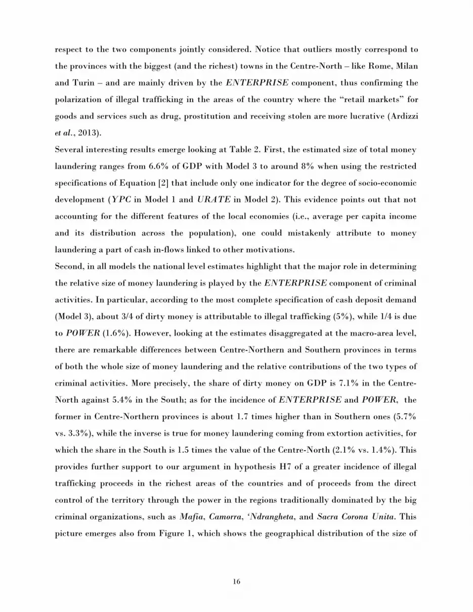
H2: The higher the average per capita income of a province, the lower is the demand for cash

deposits, ceteris paribus.

We also consider the rate of unemployment at the provincial level (URATE) as a second

possible indicator for the level of economic development. In particular, to some extent this

variable reflects differences in income distribution (see, e.g., Brandolini et al., 2004), thus in

educational levels, and is expected to exert a positive impact on the use of cash for payments,

thus on the demand for cash deposits: for a given average value of per capita GDP, a higher

unemployment rate corresponds to an income distribution more concentrated in high-income

classes, with a larger share of low-income (and poorly educated) people relying on the use of

cash for their payments. We formulate then the following hypothesis:

H3: The higher the unemployment rate of a province, the higher is the demand for cash deposits,

ceteris paribus.

9

A further control is needed in order to capture the variability across provinces of the average

attitude towards the use of cash in transactions as an alternative to electronic means of

payment. Several studies (e.g., Drehmann and Goodhart, 2000; Goodhart and Krueger, 2001;

Schneider, 2009) emphasize the importance of the technology of payments, with a particular

reference to the supply of electronic instruments. In line with this literature, we account for

available technology of payments at the provincial level by including the variable ELECTRO

among the legal determinants of INCASH. This variable measures the ratio of the value of

transactions settled by electronic payments to the total number of current accounts. A higher

share of electronic transactions implies a lower general attitude of individuals towards the use

of cash and, as a consequence, a lower demand for cash deposits. Thus, the expected sign of

the ELECTRO coefficient is negative.

H4: The higher the diffusion of electronic payments in commercial transactions, the lower is the

demand for cash deposits, ceteris paribus.

Finally, we consider the interest rate on current deposits (INT) as a possible determinant of

the legal component of INCASH. Based on standard economic theory, the interest rate on

deposits is expected to have a positive effect on INCASH, via its role of opportunity cost of

holding non-interest bearing currency. Thus, due to the usual “speculative” motive, the

expected sign of INT should be positive. However, there exist at least four reasons why this

could not be the case. First, INCASH is defined by a share, which implies that a higher

interest rate could in principle impact proportionally both on its denominator and numerator,

leading to a null overall effect. Second, our model deals with cash in-flows rather than stock

of deposits, which implies an ambiguous effect of the interest rate3. Furthermore, the years

covered by our estimations have been characterized by very low interest rates, which is likely

to have strongly mitigated the speculative motive (ECB, 2008). Finally, we notice that most

recent developments in innovative banking (i.e., internet banking) – which increased the

supply of products characterized by lower operational costs and higher interest rates with

respect to traditional banking – might even bring about a negative relationship between INT

and cash deposits. Given these considerations, the expected sign of the INT coefficient is a

priori unclear and we do not formulate any hypothesis on its sign.

3 For a more detailed discussion on recent trends of both flow and stock monetary aggregates in Italy, see Ardizzi et al. (2013).

10

The indicators used for controlling cash in-flows linked to proceeds from the underground

economy at the provincial level are the importance of particular productive sectors in local

economies, and the diffusion of tax frauds in sales by commercial retailers. The composition

of local production by economic sectors has been found to significantly affect the size of the

shadow economy (e.g., Johnson et al., 2000). Employment shares in agriculture (EMP_AGR)

and the construction industry (EMP_CON) are variables traditionally used as proxies for the

evasion of income tax and social security contributions, being these the typical sectors with a

higher presence of irregular workers (e.g., Torgler and Schneider, 2009; Capasso and Jappelli,

2011). As for Italy, according to the recent estimates provided by ISTAT (2010), irregular

workers were 12.2% of total employment in 2009, and the phenomenon was particularly

concentrated precisely in the agricultural (24.5% of irregular workers) and construction

sectors (10.5%). Thus, we formulate the following hypothesis:

H5: The larger the employment in the agricultural and the construction sectors, the higher is the

number of irregular workers and the demand for cash deposits due to proceeds from the underground

economy, ceteris paribus.

Finally, we include in our model a variable controlling for irregularities detected by the

Guardia di Finanza (the Italian Tax Police) through tax inspections at retailers.

COMM_FRAUDS is given by the ratio of the number of positive audits on cash registers and

tax receipts to the number of existing POS in the province. The standardization for the

number of POS is made necessary by the high variability in the presence of POS across

provinces, which is likely to affect the opportunity to evade (lower where the number of POS

is higher, see Ardizzi et al., 2013). This ratio is weighted by a GDP concentration index for the

same reason discussed above for crime variables. Our working hypothesis is then:

H6: The higher the diffusion of commercial tax frauds, the higher is the demand for cash deposits

due to shadow economic proceeds, ceteris paribus.

2.4. Assessing the size of money laundering

Equation [2] provides the complete model of the demand for cash deposits to be estimated,

which indentify cash in-flows to be laundered, controlling for the role of legal (or structural)

motivations and the proceeds from the shadow economy:

11

ititititit

itititititit

POWERαENTERPRISEαFRAUDSCOMMαCONEMPαAGREMPαINTαELECTROαURATEαYPCααINCASHε++++

++++++=

9876

543210

___

[2]

In analogy with the reinterpretation of the Currency Demand Approach proposed in Ardizzi

et al. (2013) to estimate the magnitude of the underground economy, the size of money

laundering is assessed here by estimating the “excess demand” for cash deposits unexplained

by structural factors and business activities carried out in the underground sector.4 This

“excess demand” is obtained as the difference between the fitted values of INCASH from the

full model [2] and the predicted values obtained from a restricted version of Equation [2],

where the coefficients of ENTERPRISE and POWER are set equal to zero. To evaluate

separately the size of the two components of “dirty money”, we then proceed in a similar

manner, by imposing alternatively the restrictions α8 = 0 and α9 = 0, and calculating the

excess demand for cash deposits due to criminal activities linked to illegal traffics and

extortions, respectively. Given our definition of INCASH, money laundering estimates

obtained with this procedure are expressed in relation to total deposits generated by

instruments other than cash. Thus, in order to have measures comparable with those

obtained in previous studies, we need to rescale our results and express them in terms of

provincial GDP.

In the light of the above discussion about the greater diffusion of POWER in the (relatively

poorer) Southern regions, we expect to find a higher incidence of this component of money

laundering in the South. On the other hand, given the ability of criminal organizations to

“export” illegal traffics in the richest areas of the country, where the demand for “goods and

services” such as drug and prostitution is presumably higher, we expect to find a larger size of

ENTERPRISE in the Centre-North. We then formulate this last hypothesis:

H7: The incidence of money laundering component due to ENTERPRISE is relatively higher in

the Centre-North, while the component due to POWER is relatively higher in the South.

4 Notice that, as remarked in Ardizzi et al. (2013), our reinterpretation of the CDA originally suggested by Tanzi (1980, 1983) reduces the methodology to a decomposition exercise in the spirit of, e.g., Wagstaff et al. (2003), hence avoiding problems of causality in the relationships among our dependent variable and the demand factors included in model [1]. In this perspective, all our testable hypotheses H1-H6 discussed above should not be read as causal effects but as simple correlations between INCASH and each regressor.

12

3. Econometric analysis

3.1. Data and estimation technique

The model of the demand for cash deposits described by Equation [2] is estimated using a

panel of 91 Italian provinces observed over the period 2005-2008. The units included in the

final dataset represent about 90% of all the Italian provinces (103), and are those for which

complete information were available for all the variables in Equation [1]. The Appendix

reports the definition and descriptive statistics (for the whole sample, as well as for the two

macro-areas, Centre-North and South, separately) and information about the different data

sources (see Tables A1 and A2).

As for the estimation technique, given the panel structure of our data and the marked

heterogeneity across units (as highlighted by the prevalence of the between component of

standard deviation for all the variables excepting INT, see Table A2), we preliminary check

for the presence of heteroskedasticity, contemporaneous cross-sectional correlation and

autocorrelation in the residuals. Ignoring heterogeneity and possible correlation of regression

disturbances over time and between subjects can lead to biased statistical inference (e.g.,

Cameron and Trivedi, 2005). However, while most recent studies provide heteroskedastic-

and autocorrelation consistent standard error, cross-sectional or “spatial” dependence in the

residuals is still often ignored, thus imposing an artificial and potentially biasing constraint

on empirical models. Indeed, relying on proper statistical tests, we found that all the three

phenomena are present in the error structure of our data 5. Therefore, in order to adjust the

standard errors appropriately, we perform a Prais-Winsten regression with Panel-Corrected

Standard Errors (PCSE). In particular, we specify that, within groups, there is first-order

autocorrelation and that the coefficient of the AR(1) process is specific to each group.6

3.2. Estimates of the demand for cash deposits

Table 1 reports parameter estimates of Equation [2] according to three different specifications,

where only YPC (Model 1), or URATE (Model 2), or both (Model 3) are included as control

5 Specifically, we used the Wooldridge (2002) test for autocorrelation in panel data, the Greene (2000) test for groupwise heteroskedasticity, and the Pesaran (2004) test for cross-sectional dependence in panel data. All the results ara available on request from the authors. 6 More technical details on this estimator are discussed in Hoechle (2007) and in the original contributions by Prais and Winsten (1954) – as for the problem of serially correlated residuals – and by Beck and Katz (1995) – as for the problem of heteroskedastic and contemporaneously cross-sectionally correlated residuals.

13

variables for the demand of cash deposits linked to the degree of socio-economic development.

All the models perform quite well in terms of fit (the Wald statistic is always significant at

the 1% level, and the R2 is above 0.90) and show coefficients that are statistically significant

and with signs consistent with our theoretical hypotheses H1-H6.7

Table 1: Estimates of cash deposit demand [1]: 91 Italian provinces, 2005-2008 (Prais-Winsten regression with Panel-Corrected Standard Errors)

Regressors a Model 1 Model 2 Model 3

Money laundering component b

ENTERPRISE 0.0312*** 0.0272*** 0.0268*** [H1] (3.34) (2.52) (2.72)

POWER 0.0121*** 0.0143*** 0.0088*

[H1] (2. 49) (2.92) (1.83)

Structural (legal)component b

YPC -0.0067*** - -0.0044***

[H2] (-5.03) - (-3.06)

URATE - 0.6542*** 0.3836***

[H3] - (6.87) (2.62)

ELECTRO -0.0012*** -0.0021*** -0.0015***

[H4] (-3.56) (-8.98) (-5.92)

INT 0.0006 -0.010*** -0.0019

(0.20) (-7.71) (-0.73)

Shadow economy component b

EMP_AGR 0.5658*** 0.6080*** 0.5104*** [H5] (7.73) (7.55) (4.97)

EMP_CON 0.3588*** 0.4519*** 0.3320***

[H5] (3.01) (3.00) (2.24)

COMM_FRAUDS 0.0479*** 0.0763*** 0.0605***

[H6] (3.58) (8.18) (5.21)

Constant 0.2107*** 0.0054 0.1405*** (4.47) (0.46) (2.63)

Observations 364 364 364

Wald statistic (χ2) 1590.86*** 3658.13*** 5004.28***

R2 0.92 0.91 0.92 a Dependent variable: INCASH = value of total cash in-payments on current accounts normalized to the value of total non-cash payments credited to current accounts; z-statistics in round brackets. b Theoretical hypothesis to which each regressor refers in squared brackets. ***, **, * : statistically significant at 1%, 5%, 10%.

7 The only exception is the interest rate on bank deposits (INT), which shows no significant correlation or a negative correlation with cash in-flows. The likely motivations for this evidence have been discussed in Section 2.3.

14

More precisely, our results confirm that the demand for cash deposits can be decomposed into

three types of drivers:

(1) a money laundering component [H1]: both the diffusion of illegal traffics (ENTERPRISE)

and of extortion activities (POWER) prove to be positively associated to the relative size

of cash in-flows.

(2) a structural (legal) component [H2-H3-H4]: the average per capita income (YPC) and the

diffusion of electronic payments (ELECTRO) are negatively correlated with cash in-flows,

while the unemployment rate (URATE) shows a positive correlation;

(3) a shadow economy component [H5-H6]: both the two proxies for the diffusion of irregular

workers (EMP_AGR and EMP_CON) and the variable controlling for the presence of

commercial tax frauds (COMM_FRAUDS) are positively associated with cash in-flows.

It is worth noticing that both indicators characterizing the local economy remain highly

significant when used jointly (Model 3). This supports our argument that the unemployment

rate captures an additional (distributional) dimension of socio-economic development besides

the average per capita income, which helps better control for the legal motivations of the

demand for cash deposits8.

An interesting finding is highlighted by Table A3 and Figure A1 in the Appendix, which

report the average simulated contribution of each variable to the observed demand for cash

deposits (expressed in percentage of GDP and normalized to 100), by referring to the most

complete specification of Equation [2] (Model 3). The major (negative) role is played by the

level of per capita GDP, while all the other regressors account for a much lower share of the

demand for cash deposits. The predicted contributions also points to sensible differences

across macro-areas. In particular, the incidence of YPC decreases (in absolute value) from

160 in the Centre-North to only 34 in the South, becoming relatively more close to the share

of URATE (19), which is unsurprising given the greater relevance of unemployment in

southern regions. Furthermore, in accordance with our hypothesis H7, the ENTERPRISE

component of criminal activities shows a much higher incidence in the Centre-North than in

the South (26 vs. 12), while the inverse is observed for the share of POWER, although with a

less marked gap (6 vs. 7).

8 On the joint use of the two variables, see also Buehn and Schneider (2012).

15

Table 2: Size of money laundering as % of GDP (mean 2005-2008) – PCSE estimates

Model 1 91 provinces a 83 provinces b

ITALY CENTRE-NORTH SOUTH ITALY

CENTRE-NORTH SOUTH

TOTAL 8.0% 8.6% 6.9% 6.3% 6.2% 6.4%

ENTERPRISE 5.8% 6.7% 3.9% 4.4% 4.7% 3.6%

POWER 2.2% 1.9% 3.0% 1.9% 1.5% 2.8%

Obs. 364 256 108 332 228 104


ITALY CENTRE-NORTH

SOUTH ITALY CENTRE-NORTH

SOUTH

TOTAL 7.7% 8.0% 6.9% 6.0% 5.9% 6.5%

ENTERPRISE 5.1% 5.8% 3.4% 3.8% 4.1% 3.2%

POWER 2.6% 2.2% 3.5% 2.2% 1.8% 3.3%

Obs. 364 256 108 332 228 104


ITALY CENTRE-NORTH

SOUTH ITALY CENTRE-NORTH

SOUTH

TOTAL 6.6% 7.1% 5.4% 5.1% 5.1% 5.1%

ENTERPRISE 5.0% 5.7% 3.3% 3.7% 4.0% 3.1%

POWER 1.6% 1.4% 2.1% 1.4% 1.1% 2.0%

Obs. 364 256 108 332 228 104

a Average values computed using the whole set of money laundering estimates related to the balanced panel of 91 Italian provinces. b Before computing average values, we discarded all the provinces showing an outlier estimate of the POWER and/or the ENTERPRISE component in at least one year of the observed period. The 8 outliers were identified using the Hadi (1992, 1994) method and mostly correspond to the provinces of the biggest towns in Centre-North Italy.

3.3. Estimating the size of money laundering

The size of money laundering for each province in each year has been assessed relying on the

three model specifications discussed above, computing separate measures for the

ENTERPRISE and POWER components. Table 2 shows the average values – for Italy and

for the two sub-samples of provinces located in the Centre-North and in the South – obtained

using the whole set of money laundering estimates for the 91 provinces. Averages are also

computed dropping 8 outlier provinces identified applying the Hadi (1992, 1994) method with

16

respect to the two components jointly considered. Notice that outliers mostly correspond to

the provinces with the biggest (and the richest) towns in the Centre-North – like Rome, Milan

and Turin – and are mainly driven by the ENTERPRISE component, thus confirming the

polarization of illegal trafficking in the areas of the country where the “retail markets” for

goods and services such as drug, prostitution and receiving stolen are more lucrative (Ardizzi

et al., 2013).

Several interesting results emerge looking at Table 2. First, the estimated size of total money

laundering ranges from 6.6% of GDP with Model 3 to around 8% when using the restricted

specifications of Equation [2] that include only one indicator for the degree of socio-economic

development (YPC in Model 1 and URATE in Model 2). This evidence points out that not

accounting for the different features of the local economies (i.e., average per capita income

and its distribution across the population), one could mistakenly attribute to money

laundering a part of cash in-flows linked to other motivations.

Second, in all models the national level estimates highlight that the major role in determining

the relative size of money laundering is played by the ENTERPRISE component of criminal

activities. In particular, according to the most complete specification of cash deposit demand

(Model 3), about 3/4 of dirty money is attributable to illegal trafficking (5%), while 1/4 is due

to POWER (1.6%). However, looking at the estimates disaggregated at the macro-area level,

there are remarkable differences between Centre-Northern and Southern provinces in terms

of both the whole size of money laundering and the relative contributions of the two types of

criminal activities. More precisely, the share of dirty money on GDP is 7.1% in the Centre-

North against 5.4% in the South; as for the incidence of ENTERPRISE and POWER, the

former in Centre-Northern provinces is about 1.7 times higher than in Southern ones (5.7%

vs. 3.3%), while the inverse is true for money laundering coming from extortion activities, for

which the share in the South is 1.5 times the value of the Centre-North (2.1% vs. 1.4%). This

provides further support to our argument in hypothesis H7 of a greater incidence of illegal

trafficking proceeds in the richest areas of the countries and of proceeds from the direct

control of the territory through the power in the regions traditionally dominated by the big

criminal organizations, such as Mafia, Camorra, ‘Ndrangheta, and Sacra Corona Unita. This

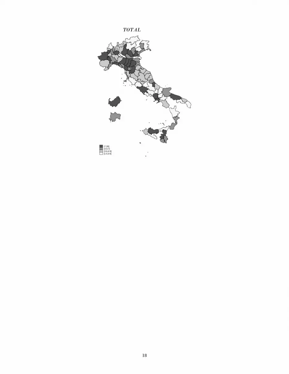
picture emerges also from Figure 1, which shows the geographical distribution of the size of

17

money laundering by province, considering the aggregate TOTAL size and distinguishing

ENTERPRISE from POWER.

Figure 1 also points to the marked variability across provinces within the two macro-areas,

which embrace situations with very low values (white zones) and cases with very high values

(dark gray zones). This is particularly evident for the distribution of the ENTERPRISE

component in the Centre-North, where it clearly emerges the polarization of the phenomenon

in some provinces, including the biggest towns such ad Milan, Turin, Genoa, Bologna and

Rome. This helps explain why considering the average values obtained on 83 provinces, i.e.,

by discarding the estimates with outlier values for ENTERPRISE and POWER shares, the

overall size of money laundering decreases significantly (from 6.6% to 5.1% in Model 3) and

also the gap between macro-areas tends to disappear, mainly as a consequence of the lower

incidence of the ENTERPRISE component in the Centre-North (which reduces to 4%).

Figure 1: Geographical distribution of money laundering size as a % of GDP by province (PCSE estimates on 91 Italian provinces, mean 2005-2008 – Model 3)

ENTERPRISE POWER

(5,34](3.7,5](2.6,3.7][1.2,2.6]

(1.9,5.4](1.3,1.9](.89,1.3][.32,.89]

18

TOTAL

(7,39](4.9,7](3.6,4.9][1.5,3.6]

19

3.4. Robustness analysis

As a robustness check for our findings, we re-estimate Equation [2] using a Tobit Random

Effects specification (Tobit RE), in order to explicitly account for unobserved residual

heterogeneity across provinces. This model has the advantage – as compared to a standard

panel regression with random effects – to accommodate for the particular distribution of our

dependent variable, which is censored at zero and can assume only positive values 9. In

particular, we specify the error structure of Equation [1] as εit = ui + eit, where u and e are

individual effects and the standard disturbance term, respectively.

Coefficient estimates from Model 3 are reported in Table 3, while Table 4 shows the size of

money laundering estimated from the same model. The results are consistent with those

discussed in the previous section, confirming all our hypotheses H1-H7. More precisely, the

average total size of money laundering is around 7% if computed using the whole set of

estimates related to 91 provinces, and reduces to 5.7% for the restricted sample of 83

provinces which excludes outlier values of ENTERPRISE and POWER. We find again a

major role played by ENTERPRISE and a sensible gap between macro-areas, with the

provinces in the Centre-North showing a higher value (7.7% vs. 6%) due to the much

stronger incidence of the ENTERPRISE component (6.1% vs. 3.6%), while those in the

South exhibit a relatively higher share for POWER (2.4 vs. 1.6%). Finally, Figure 2 confirms

the marked variability across provinces within each macro-area, as well as the polarization of

money laundering in certain provinces, which is particularly evident for the values of

ENTERPRISE related to the biggest (and richest) towns in the Centre-North.

9 See, e.g., Wooldridge (2002). Notice that the theoretical distribution of INCASH is between 0, if all in-flows on current accounts originate from payment means different from cash, to infinity, if all in-flows are made by cash.

20

Table 3: Estimates of cash deposit demand [1]: 91 Italian provinces, 2005-2008 (Tobit regression with Random Effects)

Regressors a Model 3

Money laundering component b

ENTERPRISE 0.0287**

[H1] (2.25)

POWER 0.0099**

[H1] (2.05)

Structural (legal) component b

YPC -0.0061***

[H2] (-6.35)

URATE 0.2733***

[H3] (2.87)

ELECTRO -0.0011***

[H4] (-3.43)

INT 0.0018

(0.59)

Shadow economy component b

EMP_AGR 0.4079***

[H5] (4.51)

EMP_CON 0.2614***

[H6] (2.31)

COMM_FRAUDS 0.0284**

(2.11)

Constant 0.2034*** (6.16)

Observations 364

Wald statistic (χ2) 369.11***

σu 0.0380***

(11.38)

σe 0.0189***

(22.82)

ρ 0.8026 (25.50)

a Dependent variable: INCASH = value of total cash in-payments on current accounts normalized to the value of total non-cash payments credited to current accounts; z-statistics in round brackets. b Theoretical hypothesis to which each regressor refers in squared brackets. ***, **, * : statistically significant at 1%, 5%, 10%

21

Table 4: Size of money laundering as % of GDP (mean 2005-2008) – Tobit RE estimates


ITALY CENTRE-NORTH SOUTH ITALY

CENTRE-NORTH SOUTH

TOTAL 7.2% 7.7% 6.0% 5.7% 5.5% 5.7%

ENTERPRISE 5.4% 6.1% 3.6% 4.1% 4.3% 3.4%

POWER 1.8% 1.6% 2.4% 1.6% 1.2% 2.3%

Obs. 364 256 108 336 228 104

a Average values computed using the whole set of money laundering estimates related to the balanced panel of 91 Italian provinces. b Before computing average values, we discarded all the provinces showing an outlier estimate of the POWER and/or the ENTERPRISE component in at least one year of the observed period. The 8 outliers were identified using the Hadi (1992, 1994) method and mostly correspond to the provinces of the biggest towns in Centre-North Italy.

Figure 2: Geographical distribution of money laundering size as a % of GDP by province (Tobit RE estimates on 91 Italian provinces, mean 2005-2008 – Model 3)

ENTERPRISE POWER

(5.387123,35.97091](3.911366,5.387123](2.750402,3.911366][1.287583,2.750402]

(2.125259,6.096473](1.403675,2.125259](1.001429,1.403675][.3612784,1.001429]

22

TOTAL

(7.536725,41.89404](5.343993,7.536725](3.853872,5.343993][1.669978,3.853872]

4. Summary and policy conclusions

In this paper we provide a first attempt to estimate the size of money laundering using an

approach based on observed cash in-flows credited on (banking and postal) current accounts,

considering a panel of 91 Italian provinces over the period 2005 to 2008. Our econometric

results confirm that the demand for cash deposits is driven by three different components: (1)

a money laundering component: the diffusion of both illegal traffics and extortion activities

prove to be important drivers of cash in-flows; (2) a structural (legal) component: the average

per capita income and the diffusion of electronic payments are negatively associated with cash

in-flows, while unemployment rate shows a positive correlation; (3) a component stemming

from the underground economy: the presence of irregular workers and of commercial tax frauds

is positively correlated with cash in-flows.

Starting from these findings, the estimated relative size of money laundering at the national

level ranges from 6.6% of GDP to around 8%. Splitting the provinces between macro-areas,

we find that the share of “dirty money” on GDP is 7.1% in the Centre-North against 5.4% in

the South. When we consider ENTERPRISE and POWER separately, our results indicate

23

that the sources of “dirty money” differ across areas: proceedings to be laundered coming

from illegal traffics are about 1.7 times higher in Centre-Northern provinces than in Southern

ones (5.7% versus 3.3%); the inverse is true for proceedings from extortions, for which the

share in the South is 1.5 times the value of the Centre-North (2.1% versus 1.4%). This

evidence is coherent with the presence of a direct control of local territories in the South by

the big criminal organizations (Mafia, Camorra, ‘Ndrangheta, and Sacra Corona Unita), and

the ability of these criminal organizations to exploit richer retail markets in the Centre-

North.

What type of policy conclusions can we draw from these results? The amount of money

laundering in the Italian provinces is sizeable and this should be one of major policy concern

for governments, since Italy is not among the non-cooperative countries and territories

identified by the FATF, and it is certainly not a tax haven allowing to set up anonymous

companies. Hence, it is likely that criminal organizations are able to circumvent the KYC

rule, even in the presence of a strict regulation. Our approach here suggests that criminal

organizations provides a sizeable amount of cash proceeds which are whitewashed via the

regulated financial and banking system. Hence, an alternative strategy to fight this crime

with respect to transparency rules would be to reduce the attractiveness of untraceable means

of payments. Limiting the use of cash in transactions would not only be beneficial to improve

the efficiency of the payments system, but also to combat crime.

5. References

Alexeev, M., Janeba, E., and Osborne S. (2004), “Taxation and Evasion in the Presence of

Extortion by Organized Crime”, Journal of Comparative Economics, 32, 375-387.

Ardizzi, G., Petraglia, C., Piacenza, M., and Turati, G. (2013), “Measuring the Underground

Economy with the Currency Demand Approach: A Reinterpretation of the Methodology,

with an Application to Italy”, Review of Income and Wealth, forthcoming.

Argentiero, A., Bagella, M. and Busato, F. (2008), “Money Laundering in a Two Sector

Model: Using Theory for Measurement”, European Journal of Law and Economics, 26(3),

341-359.

Bank of Italy – Financial Intelligence Unit (2012), Annual Report on 2011.

Barone, R., Masciandaro, D. (2011), “Organized crime, money laundering and legal economy:

theory and simulations”, European Journal of Law Economics, 32(1), 115-142

24

Beck, N., and Katz., J. N. (1995), “What to Do (and Not to Do) with Time-Series Cross-

Section Data”, American Political Science Review, 89, 634-647.

Block, A. (1980), East Side – West Side. Organizing Crime in New York 1930-1950, Cardiff:

University College Cardiff Press.

Brandolini, A., Cannari, L., D’Alessio, G. and Faiella, I. (2004), “Household Wealth

Distribution in Italy in the 1990s”, Bank of Italy, Discussion paper, No. 530, December

2004.

Buehn, A. and Schneider, F. (2012), “Shadow Economies around the World: Novel Insights,

Accepted Knowledge, and New Estimates”, International Tax and Public Finance, 19,

139-171.

Cameron, A. C. and Trivedi, P. K. (2005), Microeconometrics: Methods and Applications, New

York: Cambridge University Press.

Capasso, C., and Jappelli, T. (2011), “Financial Development and the Underground

Economy”, University of Naples Federico II, CSEF Working Paper, No. 298, November

2011.

Capgemini and Royal Bank of Scotland (2011), World Payments Report, European Financial

Management & Marketing Association.

Drehmann, M. and Goodhart, C.A.E. (2000), “Is Cash Becoming Technologically Outmoded?

Or Does it Remain Necessary to Facilitate Bad Behaviour? An Empirical Investigation

into the Determinants of Cash Holdings”, Financial Markets Group Research Centre,

Discussion Paper, No. 358, LSE.

European Central Bank (2008), Economic Bulletin, special edition, May.

Federal Bureau of Investigation (2011), Financial Crimes Report to the Public, available at

http://www.fbi.gov/stats-services/publications/financial-crimes-report-2010-

2011/financial-crimes-report-2010-2011#Asset.

Findley M., Nielson D., and Sharman J., (2012), “Global Shell Games: Testing Money

Launderers’ and Terrorist Financiers’ Access to Shell Companies”, Political Economy and

Development Lab, Brigham University.

Gambetta, D. (1993), The Sicilian Mafia. The Business of Private Protection, Cambridge:

Harvard University Press.

Goodhart, C. and Krueger, M. (2001), “The Impact of Technology on Cash Usage”, Financial

Markets Group Research Centre, Discussion Paper, No. 374, LSE.

Greene, W. (2000), Econometric Analysis, Upper Saddle River, NJ: Prentice-Hall.

Hadi, A.S. (1992), “Identifying Multiple Outliers in Multivariate Data”, Journal of the Royal

Statistical Society, Series B, 54, 761-771.

http://www.fbi.gov/stats-services/publications/financial-crimes-report-2010-2011/financial-crimes-report-2010-2011#Asset

http://www.fbi.gov/stats-services/publications/financial-crimes-report-2010-2011/financial-crimes-report-2010-2011#Asset

25

Hadi, A.S. (1994), “A Modification of a Method for the Detection of Outliers in Multivariate

Samples”, Journal of the Royal Statistical Society, Series B, 56, 393-396.

Hines, J.R. (2010), “Treasure Islands”, Journal of Economic Perspectives, 24(4), 103-126.

Hoechle, D. (2007), “Robust Standard Errors for Panel Regressions with Cross-Sectional

Dependence”, The Stata Journal, 7(3), 281-312.

International Monetary Fund (2001), Financial System Abuse, Financial Crime and Money

Laundering, Washington.

Istat (2010), “La misura dell’economia sommersa secondo le statistiche ufficiali. Anni 2000-

2008”, Conti Nazionali – Statistiche in Breve, Istituto Nazionale di Statistica, Rome.

Johnson, S., Kaufmann, D., McMillan, J. and Woodruff, C. (2000), “Why Do Firms Hide?

Bribes and Unofficial Activity after Communism”, Journal of Public Economics, 76(3),

495-520.

Masciandaro, D., Takáts, E., and Unger B. (2007), Black Finance. The Economics of Money

Laundering, Cheltenham, UK: Edward Elgar.

OECD (2002), Measuring the Non-Observed Economy – A Handbook, Paris.

Payments Council (2010), The future for cash in the UK, Strategic Cash Group, London.

Pesaran, M.H. (2004), “General Diagnostic Tests for Cross Section Dependence in Panels”,

Cambridge Working Papers in Economics, No. 0435, Faculty of Economics, University of

Cambridge.

Prais, S.J. and Winsten, C.B. (1954), “Trend Estimators and Serial Correlation”, Cowles

Commission Discussion Paper, No. 383 , Chicago.

Schneider, F. (2009), “The Shadow Economy in Europe. Using Payment Systems to Combat

the Shadow Economy”, A.T. Kearney Research Report, September.

Schneider, F. (2010), “Turnover of Organized Crime and Money Laundering: Some

Preliminary Empirical Findings”, Public Choice, 144(3), 473-486.

Schneider, F. (2011), Handbook on the Shadow Economy, Cheltenham (UK): Edward Elgar.

Schneider, F. and Enste D.H. (2000), “Shadow Economies: Size, Causes and Consequences”,

Journal of Economic Literature, 38(1), 77-114.

Schneider, F. and Windischbauer, U. (2008), “Money Laundering: Some Facts”, European

Journal of Law and Economics, 26(3), 387-404.

Sharman, J.C. (2010), “Shopping for Anonymous Shell Companies: An Audit Study of

Anonymity and Crime in the International Financial System”, Journal of Economic

Perspectives, 24(4), 127-140.

Tanzi, V. (1980), “The Underground Economy in the United States: Estimates and

Implications”, Banca Nazionale del Lavoro Quarterly Review, 135(4), 427-453.

26

Tanzi, V. (1983), “The Underground Economy in the United States: Annual Estimates 1930-

1980”, IMF Staff Papers, 30(2), 283-305.

Tanzi, V. (1997), “Macroeconomic Implications of Money Laundering,” in Responding to

Money Laundering, International Perspectives, 91-104. Amsterdam: Harwood Academic

Publishers.

Torgler, B. and Schneider F. (2009) “The Impact of Tax Morale and Institutional Quality on

the Shadow Economy”, Journal of Economic Psychology, 30(2), 228-245.

Transcrime (2008), Study on Extortion Racketeering – The Need for an Instrument to Combat

Activities of Organized Crime, Research Centre on Transnational Crime, University of

Trento and Catholic University of Milan, final report.

Unger, B. (2007), The Scale and Impact of Money Laundering, Cheltenham, UK: Edward

Elgar.

United Nations Office on Drugs and Crime (2011), Estimating illicit financial flows resulting

from drug trafficking and other transnational organized crimes, Wien.

Wagstaff, A., van Doorslaer, E. and Watanabe, N. (2003), “On decomposing the causes of

health sector inequalities with an application to malnutrition inequalities in Vietnam”,

Journal of Econometrics, 112(1), 207-223.

Walker, J. (1999), “How Big is Global Money Laundering?”, Journal of Money Laundering

Control, 3(1), 25-37.

Walker, J., and Unger, B. (2009), “Measuring Global Money Laundering: The Walker

Gravity Model”, Review of Law and Economics, 5(2), 821-853.

Wooldridge, J.M. (2002), Econometric Analysis of Cross Section and Panel Data, Cambridge,

MA: MIT Press.

World Bank (2005), International Migration, Remittances, and the Brain Drain, M. Schiff and

C. Ozden (eds.), Washington, D.C.

27

Appendix. Definition, descriptive statistics and contribution of the different variables included in the equation [1] of cash deposit demand

This study uses a balanced panel of Italian provinces over the period 2005-2008. The dataset merges

information of four different sources: Bank of Italy (BdI), Guardia di Finanza (the Italian Tax Police,

GdF), Istat (the National Institute of Statistics), and Eurostat (the European Institute of Statistics).

All monetary variables are provided by BdI. Data on the provincial GDP and unemployment rate are

provided by Eurostat and Istat, respectively. The variables used as proxies for the diffusion of

commercial tax frauds and irregular work are computed on the basis of information provided by GdF

and Istat. Finally, the indexes of crime diffusion are computed using data on criminal offences

available from Istat website http://giustiziaincifre.istat.it. Complete information for all the variables

are available for 91 Italian provinces (out of a total of 103).

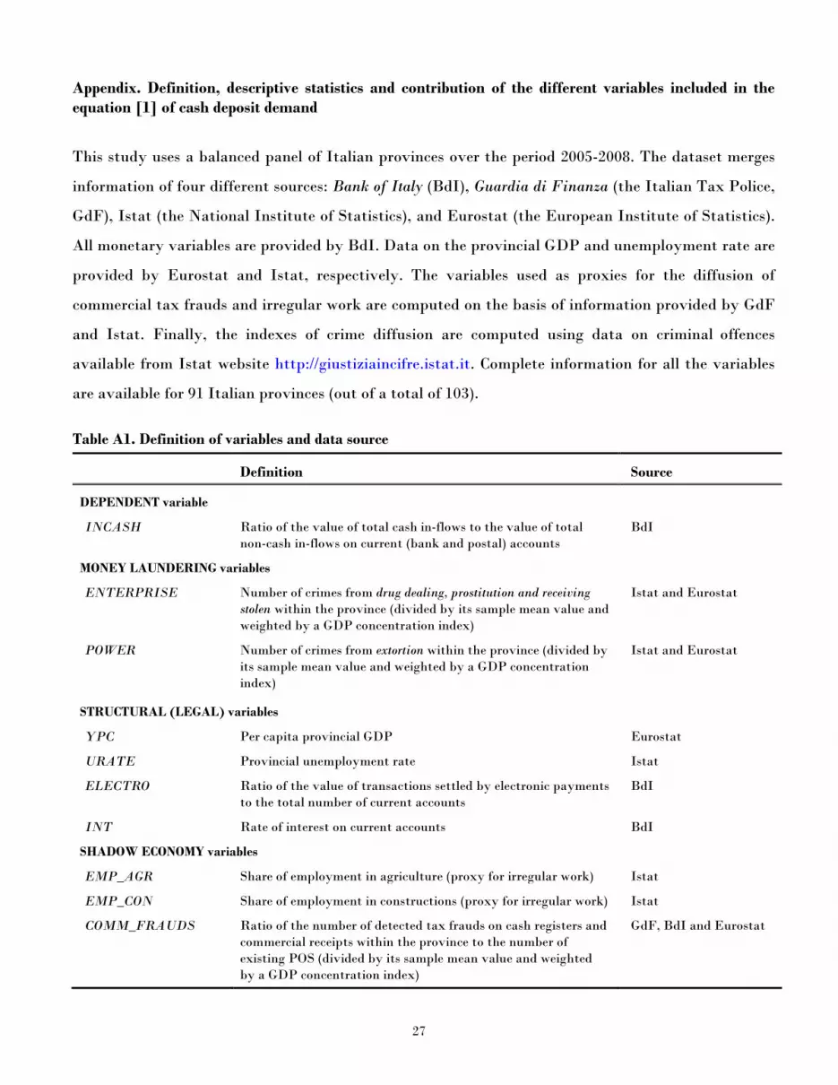
Table A1. Definition of variables and data source

Definition Source

DEPENDENT variable

INCASH Ratio of the value of total cash in-flows to the value of total non-cash in-flows on current (bank and postal) accounts

BdI

MONEY LAUNDERING variables

ENTERPRISE Number of crimes from drug dealing, prostitution and receiving stolen within the province (divided by its sample mean value and weighted by a GDP concentration index)

Istat and Eurostat

POWER Number of crimes from extortion within the province (divided by its sample mean value and weighted by a GDP concentration index)

Istat and Eurostat

STRUCTURAL (LEGAL) variables

YPC Per capita provincial GDP Eurostat

URATE Provincial unemployment rate Istat

ELECTRO Ratio of the value of transactions settled by electronic payments to the total number of current accounts

BdI

INT Rate of interest on current accounts BdI

SHADOW ECONOMY variables

EMP_AGR Share of employment in agriculture (proxy for irregular work) Istat

EMP_CON Share of employment in constructions (proxy for irregular work) Istat

COMM_FRAUDS Ratio of the number of detected tax frauds on cash registers and commercial receipts within the province to the number of existing POS (divided by its sample mean value and weighted by a GDP concentration index)

GdF, BdI and Eurostat

http://giustiziaincifre.istat.it/

28

Table A2. Descriptive statistics

Variable Mean

Standard Deviation

Min Max Total Between Within

ITALY a

INCASH 0.143 0.088 0.086 0.017 0.014 0.491 ENTERPRISE 0.798 0.278 0.274 0.051 0.277 1.992 POWER 1.010 0.789 0.773 0.175 0.171 3.859 YPC (103 €) 24.910 5.959 5.901 0.987 12.346 39.082 URATE 0.066 0.039 0.038 0.010 0.019 0.192 ELECTRO (104 €) 9.001 6.584 6.033 2.693 1.974 65.717 INT 1.247 0.488 0.265 0.410 0.472 2.909 EMP_AGR 0.050 0.038 0.037 0.009 0.000 0.228 EMP_CON 0.087 0.019 0.017 0.008 0.032 0.144 COMM_FRAUDS 0.204 0.215 0.207 0.063 0.001 1.233

CENTRE-NORTH b


SOUTH c


a Figures based on a balanced panel of 91 provinces over years 2005-2008 (364 observations). b Figures based on a balanced panel of 64 provinces over years 2005-2008 (256 observations). c Figures based on a balanced panel of 27 provinces over years 2005-2008 (108 observations).

29

Table A3. Contribution of the variables included in the equation [1] of cash deposit demand (PCSE estimates on 91 Italian provinces, mean 2005-2008 – Model 3)

ITALY CENTRE-NORTH SOUTH

Observed cash deposits (% GDP) 100 100 100

YPC -115 -160 -34

ELECTRO -20 -28 -5

INT -2 -3 -1

Constant 135 176 64

EMP_CON 26 33 14

ENTERPRISE 21 26 12

EMP_AGR 20 21 17

URATE 20 20 19

COMM_FRAUDS 9 9 8

POWER 7 6 7

Observations 364 256 108

--- positive contribution --- negative contribution

30

Figure A1. Contribution of the variables included in the equation [1] of cash deposit demand (PCSE estimates on 91 Italian provinces, mean 2005-2008 – Model 3)

-300

-200

-100

0

100

200

300

400

ITALY CENTRE-NORTH SOUTH

YPC URATE INT ELECTRO EMP_AGR

EMP_CON COMM_FRAUDS ENTERPRISE POWER Constant

Money Laundering as a Financial Sector Crime. A New Approach to Measurement, with an Application to...

Documents

Transcript of Money Laundering as a Financial Sector Crime. A New Approach to Measurement, with an Application to...