Modified matrix splitting method for the support vector machine and its application to the credit...

This article appeared in a journal published by Elsevier. The attachedcopy is furnished to the author for internal non-commercial researchand education use, including for instruction at the authors institution

and sharing with colleagues.

Other uses, including reproduction and distribution, or selling orlicensing copies, or posting to personal, institutional or third party

websites are prohibited.

In most cases authors are permitted to post their version of thearticle (e.g. in Word or Tex form) to their personal website orinstitutional repository. Authors requiring further information

regarding Elsevier’s archiving and manuscript policies areencouraged to visit:

http://www.elsevier.com/copyright

http://www.elsevier.com/copyright

Author's personal copy

Modified matrix splitting method for the support vector machine andits application to the credit classification of companies in Korea

Gitae Kim a,⇑, Chih-Hang Wu b, Sungmook Lim c, Jumi Kim d

a Department of Industrial and Manufacturing Systems Engineering, Kansas State University, 2033 Durland Hall, Manhattan, KS 66506, USAb Department of Industrial and Manufacturing Systems Engineering, Kansas State University, 2018 Durland Hall, Manhattan, KS 66506, USAc Division of Business Administration, Korea University, Jochiwon-Eup, Yeongi-Gun, Chungnam 339-700, Republic of Koread Korea Small Business Institute (KOSBI), 16-2 Yoido-dong, Yeongdeungpo-ku, Seoul 150-742, Republic of Korea

a r t i c l e i n f o

Keywords:Support vector machineConvex programmingMatrix splitting methodIncomplete Cholesky decompositionProjection gradient methodCompany credit prediction

a b s t r a c t

This research proposes a solving approach for the m-support vector machine (SVM) for classification prob-lems using the modified matrix splitting method and incomplete Cholesky decomposition. With a minormodification, the dual formulation of the m-SVM classification becomes a singly linearly constrained con-vex quadratic program with box constraints. The Kernel Hessian matrix of the SVM problem is dense andlarge. The matrix splitting method combined with the projection gradient method solves the subproblemwith a diagonal Hessian matrix iteratively until the solution reaches the optimum. The method can useone of several line search and updating alpha methods in the projection gradient method. The incompleteCholesky decomposition is used for the calculation of the large scale Hessian and vectors. The newly pro-posed method applies for a real world classification problem of the credit prediction for small-sized Kor-ean companies.

� 2012 Elsevier Ltd. All rights reserved.

1. Introduction

The support vector machine (SVM), introduced by Vapnik(1995), has been a popular method of learning theory. The SVMbased on the concept of the structural risk minimization principlehave gained popularity with many attractive features such as sta-tistical background, good generalization, and promising perfor-mance. The SVM originally was developed for classificationproblems, also called pattern recognitions, and extended forregression problems. This research focuses on the solving algo-rithm for the SVM classification problem. The classification prob-lem has various applications such as text recognition, facerecognition, medical diagnosis, market analysis, prediction of cus-tomer behavior, signal of potentially fraudulent transactions,microarray of gene expression, supplier selection, and so on.

The SVM maps the data set into another space called a featurespace and classifies the data set into two groups using separatinghyperplane. To find the best separating hyperplane, the SVMshould solve a quadratic programming problem that has a denseHessian matrix. Although the kernel function is used to reducethe dimension of the feature space, the Kernel Hessian matrix inthe SVM is too dense. Therefore, the traditional solving methods

for the quadratic programming problem such as projection gradi-ent method, cannot directly be applied for the large-scale SVMproblem. The most popular method for large-scale SVM problemsis to find small-sized working sets at each iteration and solve theproblem sequentially until the solution reaches the optimum. Thismethod has performed very well for large scale problems, but itmay have too many iterations and slow convergence.

The purpose of this research is to propose an alternative solvingapproach for large-scale SVM classification problems usingtraditional solving methods, with the matrix splitting method andincomplete Cholesky decomposition. The matrix splitting methodwith the projection gradient method splits the Hessian matrix intoa simple form and solves the new problem with the simple Hessianiteratively until the solution is optimal. The method can use severaltechniques for calculations of direction and step length. However,the calculation of the Hessian and vectors is needed in the solvingprocedure which requires a lot of computation and storage space.The incomplete Cholesky decomposition is used as a preprocessingto overcome the problem of the heavy calculation.

The method has been applied to a real world problem. The cred-it prediction of the company is an essential part of the decisionprocedure for a loan or an investment in banks or financial compa-nies. This paper uses the data of Korean companies. The mainfactors have been chosen by a statistical method to be used forthe SVM training. The SVM finds the pattern of the data andclassifies the companies into financially healthy and unhealthy

0957-4174/$ - see front matter � 2012 Elsevier Ltd. All rights reserved.doi:10.1016/j.eswa.2012.02.007

⇑ Corresponding author. Tel.: +1 785 313 3377; fax: +1 785 532 3738.E-mail addresses: [email protected] (G. Kim), [email protected] (C.-H. Wu),

[email protected] (S. Lim), [email protected] (J. Kim).

Expert Systems with Applications 39 (2012) 8824–8834

Contents lists available at SciVerse ScienceDirect

Expert Systems with Applications

journal homepage: www.elsevier .com/locate /eswa


ones. The experimental results show that our newly proposedmethod has a great potential to become a good alternative solvingapproach for large-scale SVM problems.

In the rest of the paper, the literature review of solving algo-rithm for the SVM is described in Section 2. The proposed algo-rithm is presented in Section 3. The prediction of credit rating ofthe company as the real world application is briefly shown in Sec-tion 4. Section 5 presents the experimental results. In the conclu-sion, the contributions of this chapter are reviewed.

2. Literature reviews

To solve the SVM problem, it is necessary to solve the quadraticprogramming problem to find the decision function. However, inthe SVM problem, the Hessian matrix in the quadratic program-ming problem is dense and the size of the problem is large. There-fore, traditional optimization methods cannot be applied directly.Nonetheless, so far, there are many approaches proposed for solv-ing SVM problems.

Suykens and Vandewalle (1999) proposed the least squaressupport vector machine (LS-SVM) which is a function estimationproblem. LS-SVM solves a set of linear system from Kuhn Tuckercondition for training the data instead of solving a quadratic pro-gramming problem. Lee and Mangasarian (2001) proposed the re-duced support vector machine (RSVM) that uses the reduced dataset (approximately 1% of the data) for training data. The reduceddata is chosen by the way that the distance between the data ex-ceeded a certain tolerance. Zhan and Shen (2005) proposed an iter-ative method to reduce the size of support vectors so that thecalculations of testing can be reduced. Kianmehr and Alhajj(2006) suggested an integrated method for the classification usingthe association rule based method and the SVM. The associationrule based method generates the best set of rules from the datawith the form that can be used in the support vector machine.The SVM is then used to classify the data.

Gradient projection based approaches are used to solve the SVMproblems. To, Lim, Teo, and Liebelt (2001) proposed a method forsolving SVM problem using space transformation method basedon surjective space transformation introduced in Evtushenko andZhadan (1994) and steepest descent method for solving the trans-formed problem. Serafini, Zanghirati, and Zanni (2005) proposedthe generalized variable projection method which has a new steplength rules. Dai and Fletcher (2006) suggested an efficient pro-jected gradient algorithm to solve the singly linearly constrainedquadratic programs with box constraints and tested some mediumscale quadratic programs arising in the SVM training.

A geometric approach also has been studied by Mavroforakisand Theodoridis (2006), Bennett and Bredensteiner (2000), Crispand Burges (2000), Bennett and Bredensteiner (1997) and Zhou,Zhang, and Jiao (2002). In the geometric approach, if the data isseparable, one can find two convex hulls for two classes of the dataand the minimum distance line between two convex hulls. Theseparating hyperplane can be found passing through the mid pointof the minimum distance line and being orthogonal to the line. Ifthe data is not separable, the two convex hulls can be reduced untilthey are separable, called a reduced convex hull.

One important issue in solving a SVM problem is solving qua-dratic programming problems with a dense Hessian matrix, a posi-tive semi-definite matrix. Due to the dense Hessian matrix, thedecomposition method is essential to solve large scale problemsin SVM. For example, if the problem has one thousand data points,then matrix storage of 1000 � 1000 (which means one million by-tes size of units) is needed when solving the problem with a com-puter program. Osuna, Freud, and Girosi (1997) introduced adecomposition method which solves smaller sized subproblems

sequentially with some selected variables until the KKT conditionof the original problem is satisfied. The set of variables selectedin this type of approach is called a working set. Joachims (1999)proposed an efficient decomposition method to shrink the size ofthe problem by fixing some variables to their optimal values. Platt(1999) described Sequential Minimal Optimization (SMO), a newalgorithm for SVM training. The size of the working set in SMO isonly two. Since the working set is small, the algorithm does not re-quire any quadratic programming solvers to solve the subproblemof the working set. In addition to that, it requires less matrix stor-age. Platt showed the SMO does particularly well for the sparsedata sets. The SMO has been a popular method for the SVM.

Another approach to decompose this problem is to decomposethe kernel Hessian matrix, the greatest computational concern insolving the SVM problem. While a SMO type method tries to re-duce the dimension of the problem and to solve subproblems withsmaller variables, the matrix decomposition approach is trying todecompose the kernel Hessian matrix and reduce computationalburden with the same number of variables. There are various ap-proaches for kernel matrix approximation such as spectral decom-position, incomplete Cholesky decomposition, tridiagonalization,Nyström method, and Fast Gauss Transform (Kashima, Ide, Kato,& Sugiyama, 2009). In this research, we focus on the incompleteCholesky decomposition (ICD) method. The ICD is used in solvingthe SVM problem in several ways. Bach and Jordan (2005), An,Liu, and Venkatesh (2007) and Alzate and Suykens (2008a,2008b) used the ICD for solving the LS-SVM problem. The interiorpoint method has been used in Fine and Scheinberg (2001), Ferrisand Munson (2003) and Goldfarb and Scheinberg (2008). The ICDhas been used for solving the normal equation in the interior pointmethod. Lin and Saigal (2000) used the ICD as a preconditioner inthe SVM problem. Louradour, Daoudi, and Bach (2006) proposed anew kernel method using the ICD. Debnath and Takahashi (2006)suggested a solving method for the SVM using the second ordercone programming and the ICD. Camps-Valls, Munoz-Mari, Go-mez-Chova, Richter, and Calpe-Maravilla (2009) used the ICD forsolving the semi-superviesd SVM.

In this paper, we use the projected gradient approach for solv-ing the SVM problem. In this approach, the matrix splitting methodis used for the projection and the ICD is used for reducing the com-putational burden and storage. Since most problems of the SVMhave the dense Hessian matrix and are large scale, dimensionreduction methods such as working set method or SMO type meth-od can be attractive. However, traditional methods like Newton’smethod or gradient methods have advantages such as rapid localconvergence. The main drawback of traditional methods is the sizeof the problem. If one can remove or reduce the curse of dimen-sionality, one may use advantages of traditional methods. Withthis motivation, we use the matrix splitting method and the ICDfor reducing the computational and storage problem and handlingthe large scale problems.

3. The proposed solving algorithm

This section provides a new solving approach for m-SVM classifi-cation problem. The basic idea is to make Hessian matrix simplewith the matrix splitting method and to solve the problem withthe projected gradient and incomplete Cholesky decompositionmethods.

Suppose that we have the training data

ðx1; y1Þ; . . . ; ðxn; ynÞ; where x 2 Rm and y 2 f�1;1g ð1Þ

The data has two classes: the one is the class the target value yis �1 and the other class is the target value y is 1. The separatinghyperplane is defined as

G. Kim et al. / Expert Systems with Applications 39 (2012) 8824–8834 8825


ðw � xÞ þ b ¼ 0; where w 2 Rn and b 2 R ð2Þ

The SVM approach uses an optimal separating hyperplane (Vap-nik & Chervonenkis (1974), Vapnik (1979)) which separates thedata with maximum distance (margin) between the data and thehyperplane. The formulation of the SVM problem has been ex-tended. The C-SVM uses the parameter C which controls thetrade-off between the model complexity and training errors.Schölkopf, Smola, Williamson, and Bartlett (2000) have proposeda new SVM model named m-support vector machine (m-SVM). Them-SVM uses a new parameter m instead of C in C-SVM. The param-eter m has a range of zero to one, that is m 2 [0,1], and provides thelower bound of the fraction of the support vectors and the upperbound of the fraction of the margin errors. The primal problem ofm-SVM is as follows:

ðPÞ minw;b;n;q

12kwk2 � mqþ 1

n

Xn

i¼1

ni ð3Þ

s:t: yiððw � xiÞ þ bÞP q� ni; i ¼ 1; . . . ;n ð4Þ

ni P 0; i ¼ 1; . . . ;n ð5Þ

q P 0 ð6Þ

To see the function of the additional variable q, if the variable ni

equals zero, then the margin becomes 2qw instead of 2

w. The addi-tional slack variables n are introduced for nonseparable data case.k�k denotes the norm of the vector and b is an offset. Since thisproblem is a convex quadratic problem and the number of con-straints is large, we can consider the dual of this problem to solveit efficiently. The Lagrangian dual problem is as follows:

ðDÞ maxa�1

2

Xn

i¼1

Xn

j¼1

aiajyiyjKðxi; xjÞKðxi; xjÞ ð7Þ

s:t:Xn

i¼1

aiyi ¼ 0; i ¼ 1; . . . ;n ð8Þ

0 6 ai 61n; i ¼ 1; . . . ;n ð9Þ

Xn

i¼1

ai P m; i ¼ 1; . . . ;n ð10Þ

In the SVM, the input data is mapped to a higher dimensionalspace called the feature space. A nonlinear mapping functionu(x) maps the input data to the feature space. The kernel functionis defined as follows. K(xi,xj) = u(xi) � u(xj). All kernel function canbe expressed with dot products of (xi � xj). Therefore, the dimensionof the kernel Hessian matrix in the objective function is the samedimension as the linear kernel, even if other kernels are used. Crispand Burges (2000), Chang and Lin (2001) proved that the constraint(10) can be changed to an equality constraint. Changing the prob-lem to a minimization problem and scale of the bound of variablesfrom zero to one, the dual problem of m-SVM with vector notationcan be rewritten as follows:

ðVD1Þ mina

12aT Qa ð11Þ

s:t: yTa ¼ 0; ð12Þ

0 6 a 6 1; ð13Þ

eTa ¼ mn ð14Þ

This problem is a quadratic programming problem with twoequality constraints and box constraints on variables. If one re-moves the last equality constraint from this problem, it becomesa singly linearly constrained convex quadratic problem to which

many practical applications can be applied (Dai & Fletcher, 2006;Lin, Lucidi, Palagi, Risi, & Sciandrone, 2009; Pardalos & Kovoor,1990). In this paper, the augmented Lagrangian method is usedto remove the last constraint and put it on the objective functionas follows:

ðVD2Þ mina

12aT Qaþ pðeTa� mnÞ þ lðeTa� mnÞ2 ð15Þ

s:t: yTa ¼ 0 ð16Þ0 6 a 6 1 ð17Þ

The parameter p and l denote the Lagrangian multiplier andthe penalty parameter, respectively. The problem can be reorga-nized as follows:

ðVD3Þ mina

12aT Haþ ðp� 2lmnÞeTa ð18Þ

s:t: yTa ¼ 0 ð19Þ0 6 a 6 1 ð20Þ

where H = Q + lU, U is a n � n matrix which all elements are one.The constant term l(mn)2 � pmn in the objective function can be

removed because it does not affect the solution. The problem isnow a singly linearly constrained convex quadratic problem. TheHessian matrix H is a dense, symmetric, and positive semi-definitematrix. Since the Hessian matrix H is not diagonal and large in theSVM, a standard solving method for the general quadratic pro-gramming problem can be applied to small or medium size prob-lems. Therefore, a specified method which can handle the denseHessian matrix and the large scale problem is essential for solvingthis problem. In this research, we use matrix splitting method withnonmonotone line search and gradient projection method. In addi-tion, the incomplete Cholesky decomposition method is used forhandling large scale problems. The structure of the solution proce-dure is as follows:

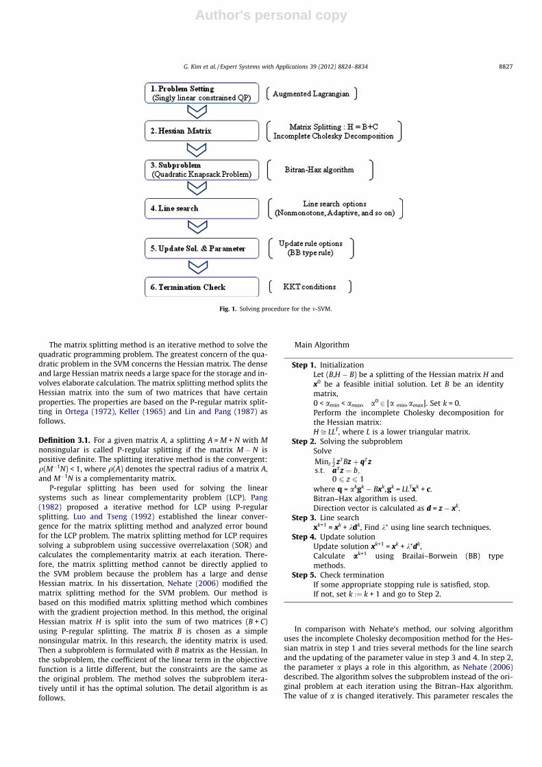
Fig. 1 presents the solution procedure proposed in this paper.The Augmented Lagrangian method moves one of the constraintsto the objective function and makes the original problem a singlylinearly constrained convex quadratic problem. The Hessian ma-trix is split into the sum of two matrices by the matrix splittingmethod. In addition to that, the incomplete Cholesky decomposi-tion is performed for the Hessian matrix to facilitate the calcula-tion of the Hessian matrix and the variable vectors. We solve thesubproblem that has a simple Hessian matrix in procedure 3. TheBitran-Hax is used to solve this subproblem. The direction vectoris calculated with the solution of the subproblem and the currentsolution. The line search technique finds the step length alongthe direction in procedure 4. In procedure 3, there is a type ofscale parameter where the coefficient of the linear term of thesubproblem. The solution of the problem and the scale parame-ter are updated in procedure 5. In procedure 6, the terminationis checked with KKT conditions. For the procedure 4 and 5, wecan use several options that will be described in the latersection.

3.1. Matrix splitting with gradient projection method

The matrix splitting method is described in this section. Theproblem (VD3) can be rewritten as follows. For our convenience,we use the term x instead of a and simple terms.

ðMPÞ minx

12

xT Hxþ cT x ð21Þ

s:t: aT x ¼ b; ð22Þ0 6 x 6 1 ð23Þ

where H is a n � n positive semi-definite matrix.

8826 G. Kim et al. / Expert Systems with Applications 39 (2012) 8824–8834


The matrix splitting method is an iterative method to solve thequadratic programming problem. The greatest concern of the qua-dratic problem in the SVM concerns the Hessian matrix. The denseand large Hessian matrix needs a large space for the storage and in-volves elaborate calculation. The matrix splitting method splits theHessian matrix into the sum of two matrices that have certainproperties. The properties are based on the P-regular matrix split-ting in Ortega (1972), Keller (1965) and Lin and Pang (1987) asfollows.

Definition 3.1. For a given matrix A, a splitting A = M + N with Mnonsingular is called P-regular splitting if the matrix M � N ispositive definite. The splitting iterative method is the convergent:q(M�1N) < 1, where q(A) denotes the spectral radius of a matrix A,and M�1N is a complementarity matrix.

P-regular splitting has been used for solving the linearsystems such as linear complementarity problem (LCP). Pang(1982) proposed a iterative method for LCP using P-regularsplitting. Luo and Tseng (1992) established the linear conver-gence for the matrix splitting method and analyzed error boundfor the LCP problem. The matrix splitting method for LCP requiressolving a subproblem using successive overrelaxation (SOR) andcalculates the complementarity matrix at each iteration. There-fore, the matrix splitting method cannot be directly applied tothe SVM problem because the problem has a large and denseHessian matrix. In his dissertation, Nehate (2006) modified thematrix splitting method for the SVM problem. Our method isbased on this modified matrix splitting method which combineswith the gradient projection method. In this method, the originalHessian matrix H is split into the sum of two matrices (B + C)using P-regular splitting. The matrix B is chosen as a simplenonsingular matrix. In this research, the identity matrix is used.Then a subproblem is formulated with B matrix as the Hessian. Inthe subproblem, the coefficient of the linear term in the objectivefunction is a little different, but the constraints are the same asthe original problem. The method solves the subproblem itera-tively until it has the optimal solution. The detail algorithm is asfollows.

Main Algorithm

Step 1. InitializationLet (B,H � B) be a splitting of the Hessian matrix H andx0 be a feasible initial solution. Let B be an identitymatrix,0 < amin < amax, a0 2 [a min,amax]. Set k = 0.Perform the incomplete Cholesky decomposition forthe Hessian matrix:H ffi LLT, where L is a lower triangular matrix.

Step 2. Solving the subproblemSolveMinz

12 zT Bz þ qT z

s:t: aT z ¼ b;0 6 z 6 1

where q = akgk � Bxk,gk = LLTxk + c.Bitran–Hax algorithm is used.Direction vector is calculated as d = z � xk.

Step 3. Line searchxk+1 = xk + kdk, Find k⁄ using line search techniques.

Step 4. Update solutionUpdate solution xk+1 = xk + k⁄dk,Calculate ak+1 using Brailai–Borwein (BB) typemethods.

Step 5. Check terminationIf some appropriate stopping rule is satisfied, stop.If not, set k :¼ k + 1 and go to Step 2.

In comparison with Nehate’s method, our solving algorithmuses the incomplete Cholesky decomposition method for the Hes-sian matrix in step 1 and tries several methods for the line searchand the updating of the parameter value in step 3 and 4. In step 2,the parameter a plays a role in this algorithm, as Nehate (2006)described. The algorithm solves the subproblem instead of the ori-ginal problem at each iteration using the Bitran–Hax algorithm.The value of a is changed iteratively. This parameter rescales the

Fig. 1. Solving procedure for the m-SVM.



gradient and makes the subproblem to be closer to the originalproblem. If a = 1, the algorithm is just the matrix splitting method.If a > 1, then the algorithm is the combination of the matrix split-ting method and the gradient projection method. If we increase theparameter a, the algorithm becomes closer to the gradient projec-tion method.

The line search in step 3 determines the best step size k to getthe solution of the original problem forward to the optimal solu-tion. We also use several line search methods. The next subsectionsdescribe the details for the methods in step 3 and 4. These subsec-tions present some methods for the line search and updating a inthe matrix splitting algorithm proposed in this paper. The problemwe consider is a singly linearly constrained quadratic convex prob-lem. Due to its numerous applications, there have been many stud-ies for this problem (Pardalos & Kovoor, 1990; Dai & Fletcher, 2006;Lin et al., 2009; Fu & Dai, 2010, and more). This research uses fourmethods that applied for the SVM problem. The details for themethods are as follows.

3.1.1. SPGM (spectral projected gradient methods)Birgin, Martinez, and Raydan (2000) proposed a solving algo-

rithm which extended the classical projected gradient method touse additional methods including the nonmonotone line searchtechnique and the spectral step length known as the Barzilai andBorwein (BB) type rule. The algorithm was proposed for the prob-lem of the minimization of differentiable functions on nonemptyclosed and convex sets. In their paper, Birgin et al. (2000) provedthe convergence of the algorithm and showed good experimentalresults compared to the LANCELOT package (Conn, Gould, & Toint,1988). The detail algorithm for the line search and the updatingmethod are as follows.

SPGM Algorithm

Step 1 InitializationCalculate direction dk and set k = 1

Step 2 Set new valueSet x+ = xk + kdk

Step 3 Line searchIf f(x+) 6max06j6min{k, M�1}f(xk�j) + kdk,g(xk),then define kk = k, xk+1 = x+, sk = xk+1 � xk,yk = g(xk+1) � g(xk),and go to step 4.Otherwise define knew 2 [r1k,r2 k] and set k = knew andgo to step 2.

Step 4 Update parameterCalculate bk = sk, yk

If bk6 0, then set ak+1 = amax,

If not, calculate ak = sk, sk andakþ1 ¼min amax;max amin;

ak

bk

n on o

The line search in step 3 is the nonmonotone line search whichmeans the objective function value is allowed to increase on someiterations. The calculation of knew is from one dimensional qua-dratic interpolation. If the minimum of the one dimensional qua-dratic lies outside [r1k,r2k], then the algorithm sets k 1

2 k. Theparameter r1 and r2 are fixed constants. The method for updatingak is BB rule. Birgin et al. (2000) showed that the use of the param-eter ak is more important than a line search method to improve theperformance of the algorithm in their experimental results.

3.1.2. GVPM (generalized variable projection method)Serafini et al. (2005) proposed a generalized version of variable

projection method (GVPM) using a new adaptive steplength alter-

nating rule. Their research has compared the GVPM with SPGM de-scribed in the previous section. The GVPM focuses on the methodof updating parameter ak. The algorithm uses two steplength rulesadaptively and a limited minimization rule as a line search meth-od. The two types of steplength rules are as follows.

a1kþ1 ¼

ðdkÞT dk

ðdkÞT Hdkð24Þ

a2kþ1 ¼

ðdkÞT Hdk

ðdkÞT H2dkð25Þ

The algorithm switches the rules (24) and (25) if certain criteriaare satisfied. Let 0 < nmin < nmax are fixed constants. The number nadenotes the number of iterations that use the same steplength rule.There are two definitions for this algorithm as follows.

Definition 3.2. Let xk 2X (feasible set) and (dk)THdk > 0 andak 2 [amin,amax].

If a2kþ1 < ak < a1

kþ1, then ak is called a separating steplength.

Definition 3.3. Let xk 2X (feasible set) and (dk)THdk > 0,ak 2 [ami-

n,amax], and kopt ¼ arg mink2½0;1�f ðxk þ kdkÞ ¼ �ðgðxkÞÞT dk

ðdkÞT Hdk .Given two constants kl and ku such that 0 < kl 6 1 6 ku, we say

that ak is called a bad descent generator if one of followingconditions is satisfied:

kopt < kl and ak ¼ a1kþ1 ð26Þ

kopt > ku and ak ¼ a2kþ1 ð27Þ

The detail algorithm is as follows.

GVPM algorithm

Step 1. InitializationCalculate direction dk

Step 2. Line searchCalculate xk+1 = xk + kkdk, kk 2 (0,1]with kk given by kk ¼ arg mink2½0;1�f ðxk þ kdkÞ ¼ �ðgðxkÞÞT dk

ðdkÞT Hdk .Step 3. Update parameter

If (dk)THdk6 0, then set ak+1 = amax,

Otherwise calculate a1kþ1 and a2

kþ1 from (24) and (25)If na P nmin,

then if na P nmax or ak is a separating steplength ora bad descent generator,

then set ia = mod(ia � 2) + 1,na = 0.Calculate akþ1 ¼min amax;max amin;aia

kþ1

n on oSet k = k + 1,na = na + 1 and go to step 2.

The key idea of this algorithm is to switch the steplength ruleswith certain criteria. Serafini et al. (2005) showed that this adap-tive steplength change was important in the experimental resultswhich compared with the SPGM and the VPM. For the SVM prob-lem, Serafini et al. (2005) applied this algorithm for solving thesubproblem of the large scale SVM problems while the SVM prob-lem was solved by the SMO type algorithm.

3.1.3. MSM (matrix splitting method)Nehate (2006) proposed several efficient solving algorithms for

the SVM problems, one of which is to use the matrix splittingmethod combined with the gradient projection method. Our mainmethod is based on this algorithm. The parameter ak plays a role tomake the algorithm close to either the matrix splitting or thegradient projection method. As the step 2 in main algorithm, thelarge ak enhances linear term of the objective function. Thus, the



large ak makes the algorithm closer to the gradient projectionmethod and the small ak makes the algorithm to become the ma-trix splitting. Nehate (2006) uses a simple line search and updatingmethod in the algorithm. The detail is as follows:

MSM algorithm

Step 1. InitializationCalculate direction dk and set k = 1

Step 2. Set new valueSet x+ = xk + kdk

Step 3. Line searchIf f(x+) 6max06j62f(xk�j) + kdk, g(xk),then define kk = k,Otherwise

kk ¼ �ðgðxkÞÞT dk

ðdkÞT Hdk ¼ arg mink2½0;1�f ðxk þ kdkÞ; 0 < kk < 1.

Step 4. Update solution and parameter

xkþ1 ¼ xk þ kdk;

sk ¼ xkþ1 � xk; yk ¼ gðxkþ1Þ � gðxkÞ;akþ1 ¼ ðskÞT Bsk

ðskÞT yk ;

akþ1 ¼min amax;max amin;ak

bk

n on o:

Nehate (2006) showed the use of the parameter ak speeds up theconvergence of the algorithm, but it makes the algorithm nonmono-tone. Therefore the algorithm uses the nonmonotone line searchtechnique. In step 3, the line search simply assigns the kk value anduses the range of index j from zero to two. This simple assignmentis very useful to solve the large scale problems. Nehate (2006) fo-cuses on the SVM for regression problems. As the other methods,the algorithm can solve up to medium sized SVM problems.

3.1.4. AA (adaptive step size method and alternate step length (alpha)method)

Dai and Zhang (2001) suggested an adaptive nonmonotone linesearch method. The nonmonotone line search such as f(x+) 6max06j6min{k,M�1}f(xk�j) + kdk, g(xk) in SPGM has a fixed integer M.The performance of the algorithm depends on the choice of M(Raydan, 1997). To resolve this problem, Dai and Zhang (2001)use a new method to change the value of M adaptively. Let fmin

be the current minimum objective value over all past iterationsand fmax be the maximum objective value in recent M iterations.These are denoted as follows:

fmin ¼ min06i6k

f ðxiÞ ð28Þ

fmax ¼ max06i6minfk;M�1g

f ðxk�iÞ ð29Þ

The value l denotes the number of iterations since the fmin is ob-tained and L is a fixed constant. The value p denotes the largestinteger such that kk�i

1 : i ¼ 1; . . . ; pn o

are accepted, while kk�p�11 is

not, and kk1 is the first trial step size at the k iteration, and P denotes

a fixed constant. The values c1 P 1 and c2 P 1 are fixed constants.Dai and Fletcher (2006) proposed an efficient gradient projec-

tion method using a new formula for updating the parameter.The algorithm uses the adaptive line search method proposed byDai and Zhang (2001). Dai and Fletcher (2006) introduced a newformula for updating the ak. As the previous section defined, letsk = xk+1 � xk, yk = g(xk+1) � g(xk). The BB rule can be as follows:

akþ1 ¼ ðskÞT sk

ðskÞT ykð30Þ

This formula can be obtained by solving a one dimensional problemas follows.

min ka�1kþ1sk � ykk2 ð31Þ

If we replace the pair (sk,yk) with (sk�i,yk�i) for each integer i P 0,the similar formula can be obtained as follows (Friedlander, Marti-nez, Molina, & Raydan, 1998).

akþ1 ¼ ðSkÞT Sk

ðSkÞT Yk¼Pm�1

i¼0 ðsk�iÞT sk�iPm�1i¼0 ðsk�iÞT yk�i

ð32Þ

where Sk = ((sk)T, . . . , (sk�m+1)T)T and Yk = ((yk)T, . . . , (yk�m+1)T)T.In the formula (32), if m = 1, then the formula is the same as the

BB rule in (30). Dai and Fletcher (2006) found the best value of m is2 with their experimental results.

In this research, we combine the adaptive steplength algorithmfrom Dai and Zhang (2001) with the alternative updating formulafrom Dai and Fletcher (2006) and call this method AA (adaptiveand alternative) algorithm. Combining these two algorithms, theline search is the adaptive nonmonotone line search and the updat-ing parameter ak is the method of alternative formula (32). The de-tail algorithm is as follows:

AA algorithm

Step 1. InitializationCalculate direction dk and set k = 1,Set l = 0, p = 0, fmin = fr = fc = f(x0)

Step 2. Line searchStep 2.1. Reset reference value

If l = L,then set l = 0 and calculate

fr ¼fc; if fmax�fmin

fc�fmin> c1

fmax; otherwise

(

If p > P,then calculatefr ¼ fmax; if f max > f ðxkÞ and fr�f ðxkÞ

fmax�f ðxkÞ P c2

fr ; otherwise

(Step 2.2. Test first trial step size

If f ðxk þ kk1dkÞ 6 fr þ dkk

1dk; gðxkÞ

then let kk ¼ kk1; p ¼ pþ 1, and go to step 2.4

Otherwise p = 0Step 2.3. Test other trial step sizes

Set kold ¼ kk1

Calculate knew 2 [r1kold,r2kold]If f(xk + knewdk) 6min{fmax, fr} + dknewdk, g(xk),

then set kk = knew and go to step 2.4Otherwise set kold = knew and repeat step 2.3

Step 2.4. If f(xk+1) < fmin,then set fc = fmin = f(xk+1) and l = 0.

Otherwise l = l + 1.If f(xk+1) > fc,

then set fc = f(xk+1).Calculate fmax from (29).

Step 3. Update parameter

sk ¼ xkþ1 � xk; yk ¼ gðxkþ1Þ � gðxkÞ;If ðskÞT yk

6 0;

then ak+1 = amax

Otherwise akþ1 ¼min amax;max amin;

Pm�1

i¼0ðsk�iÞT sk�iPm�1

i¼0ðsk�iÞT yk�i

� ��

The value of knew is obtained by a quadratic interpolation meth-od in step 2.3. Dai and Fletcher (2006) tested some medium sizedSVM problems with their new algorithm and obtained good results.



The Sections 3.1.1, 3.1.2, 3.1.3, 3.1.4, 4 have shown four differ-ent line search and updating methods for the gradient method.Our new solving algorithm can take one of the methods for step3 and 4 in the main algorithm in Section 3.3.1. We see the fourmethods cannot be directly applied to large scale problems, sincethe test problems are limited to the medium size for the SVM prob-lems. Although the matrix splitting method solves the subproblemwith a diagonal Hessian matrix, the solving procedure still has thecalculations of the Hessian and vectors such as Hx and Hd. Theincomplete Cholesky decomposition for the Hessian matrix makesthose calculations easy. The details will be described in the nextsection.

3.2. Incomplete Cholesky decomposition

The Cholesky decomposition method has been an attractivemethod for solving large scale systems because of its stabilityand accuracy. If a matrix A is a symmetric and positive definite,then A can be expressed as A = LLT and L is a lower triangular matrixwith positive diagonal elements. The elements of L are called theCholesky factors.

The linear system Ax = b can be solved by using the Choleskydecomposition. The problem can be rewritten as LLTx = b. Two sub-stitutions are needed to solve this system. The forward substitu-tion Ly = b is calculated first. Then the backward substitutionLTx = y is calculated. However, this solving procedure can be avail-able only in the case that the matrix A is a symmetric and positivedefinite. If the matrix A is a symmetric and positive semi-definite,some of the diagonal values of L are zero. If the diagonal elementsof L are zero, we cannot calculate the rest of the Cholesky factors. Inthis case, we use the incomplete Cholesky decomposition method.

The incomplete Cholesky decomposition is the method for thesymmetric and positive semi-definite matrix. The idea of theincomplete Cholesky decomposition is that a permutation is per-formed to move the largest diagonal element on the active pivotposition so that the decomposition procedure can stop when thelargest diagonal element is zero. First, the algorithm finds the larg-est diagonal element. Next, a permutation is performed to movethe largest diagonal element on the active position in which col-umn is working on calculating the Cholesky factors. This permuta-tion process is called a pivot. After the incomplete Choleskydecomposition, some of columns of the lower triangular matrix Lare all zeros. Therefore, the matrix A is decomposed as A ffi LLT,which is an approximation of the matrix A. Let eA ¼ LLT . Next, thereis an approximation error DA ¼ A� eA. If the approximation error isbound by a certain value and the difference between the optimalvalues of the original and approximated problem is small, thedecomposition can be acceptable. Higham (1990) also showed thatthe incomplete Cholesky decomposition is a stable method. Fineand Scheinberg (2001) derived the bound of the approximation er-ror and showed the error bound is acceptable in the SVM problem.

The SVM problem MP considered in Section 3.3.1 of this paperhas the Hessian matrix which is a symmetric and positive semi-definite. The incomplete Cholesky decomposition method is ap-plied to our system. The Hessian matrix in the SVM problem istoo dense and large. Even if the incomplete Cholesky decomposi-tion is applied to the problem, the calculation of LTx and the spaceof memory to store the matrix L are still cumbersome. However,the rank of the Hessian matrix is, fortunately, significantly smallerthan its size.

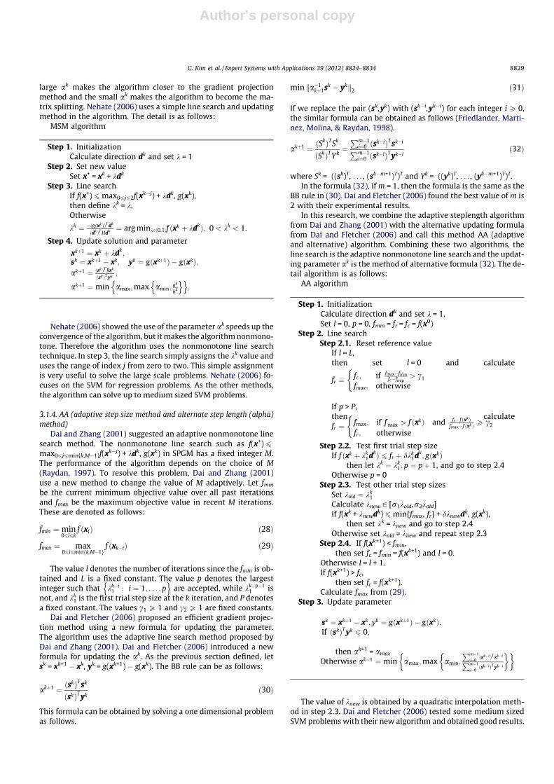
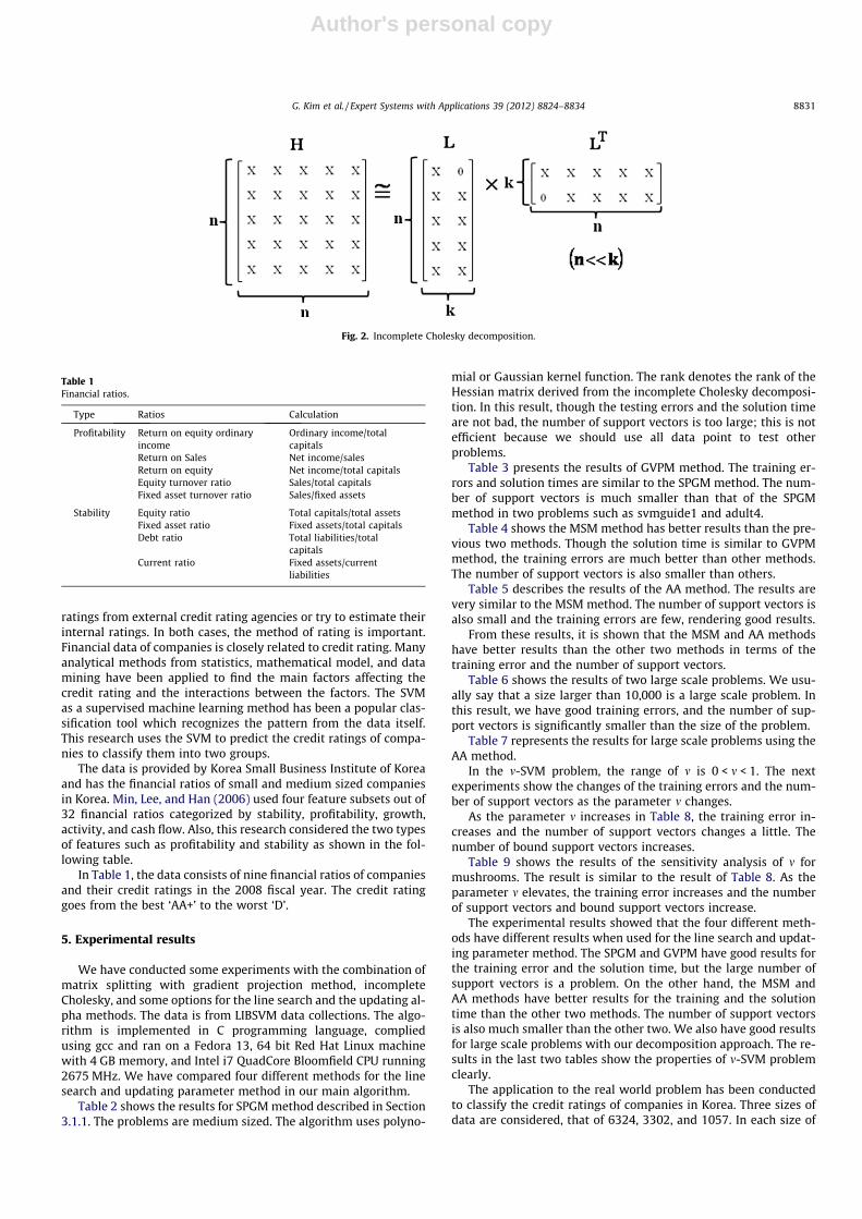
In Fig. 2, the mark X denotes a non-zero element. In this re-search, we consider the column-wise decomposition. During thedecomposition, the largest diagonal element of the Cholesky factoris moved to the active column. For example, the algorithm calcu-lates all diagonal elements of the L matrix which are the Choleskyfactors and finds the largest one. The largest diagonal elements

moved to the first column using a permutation. The rest of the ele-ments in the first column are then calculated. That concludes thefirst iteration or pivoting. The next iteration is for the second col-umn of the L. At the k + 1th iteration, if the largest diagonal ele-ment is zero, then the procedure is stopped. Therefore the valuesof diagonal elements are l11 P l22 P � � �P lkk. In this case, the rankof the Hessian matrix is k. In Fig. 2, the rank of the Hessian matrix His two. The incomplete Cholesky decomposition method is some-times used as a way to calculate the rank of a matrix. The rank kin the SVM problem is significantly smaller than the size of theHessian matrix n. This property is advantageous for the calculationin our algorithm because the algorithm needs to calculate theproduct between the L matrix and the x vector and the computermemory space to store the matrix L. The incomplete Choleskydecomposition in this research is based on the method in Fineand Scheinberg (2001). The algorithm uses the symmetric permu-tation which is known as symmetric pivoting (Golub & Van Loan,1996). The detail algorithm is as follows.

3.2.1. Incomplete Cholesky decomposition

For all columns: Column-wise decompositionCalculate all remaining diagonal Cholesky factorsIf (sum of diagonal factors >= tolerance)

Find the largest diagonal factorSwap: the largest one and current active elementCalculate the rest of Cholesky factors in the active column

ElseRank = current column index;Break;

EndEnd

The first step is to calculate all remaining diagonal Cholesky fac-tors so that the algorithm can find the largest diagonal elementamong them. If the diagonal element is positive, then the algorithmfinds the largest diagonal element and permutes the element andthe active element for both the column and the row. The remainingelements of the column are then calculated. The algorithm goes tothe next column and continues this process. If the diagonal ele-ment is not a positive or less than a certain tolerance, then thealgorithm is stopped and the current number of the column isthe rank of the Hessian matrix.

As we pay attention to the original matrix H, we see the diago-nal elements of H are accessed more than once through the decom-position process, but the others are accessed only once. Thisproperty is a great advantage for the SVM problem. The access tothe Hessian matrix in the SVM problem means calculating the ker-nel functions. Therefore we need to calculate K(xi,xj) = u(xi) � u(xj)whenever the algorithm accesses the Hessian matrix during thedecomposition procedure. The incomplete Cholesky decomposi-tion enables us to reduce the calculation of kernel functions. More-over, we do not need to store the Hessian matrix explicitly; instead,we only need to store the lower triangular matrix L. The algorithmcan save the memory space with the amount of (n � n) � (n � k).

4. Company credit rating classification

The credit rating of a company is important for investors as wellas the company itself because it is a crucial measure of the decisionof the investment or loan to the company. If the evaluation of thecredit rating is wrong, investors and the company may have a bigloss. The accurate evaluation or prediction of the credit rating canprovide the information of the proper companies to invest and theindication of bankruptcy as well. Investors may adopt the credit



ratings from external credit rating agencies or try to estimate theirinternal ratings. In both cases, the method of rating is important.Financial data of companies is closely related to credit rating. Manyanalytical methods from statistics, mathematical model, and datamining have been applied to find the main factors affecting thecredit rating and the interactions between the factors. The SVMas a supervised machine learning method has been a popular clas-sification tool which recognizes the pattern from the data itself.This research uses the SVM to predict the credit ratings of compa-nies to classify them into two groups.

The data is provided by Korea Small Business Institute of Koreaand has the financial ratios of small and medium sized companiesin Korea. Min, Lee, and Han (2006) used four feature subsets out of32 financial ratios categorized by stability, profitability, growth,activity, and cash flow. Also, this research considered the two typesof features such as profitability and stability as shown in the fol-lowing table.

In Table 1, the data consists of nine financial ratios of companiesand their credit ratings in the 2008 fiscal year. The credit ratinggoes from the best ‘AA+’ to the worst ‘D’.

5. Experimental results

We have conducted some experiments with the combination ofmatrix splitting with gradient projection method, incompleteCholesky, and some options for the line search and the updating al-pha methods. The data is from LIBSVM data collections. The algo-rithm is implemented in C programming language, compliedusing gcc and ran on a Fedora 13, 64 bit Red Hat Linux machinewith 4 GB memory, and Intel i7 QuadCore Bloomfield CPU running2675 MHz. We have compared four different methods for the linesearch and updating parameter method in our main algorithm.

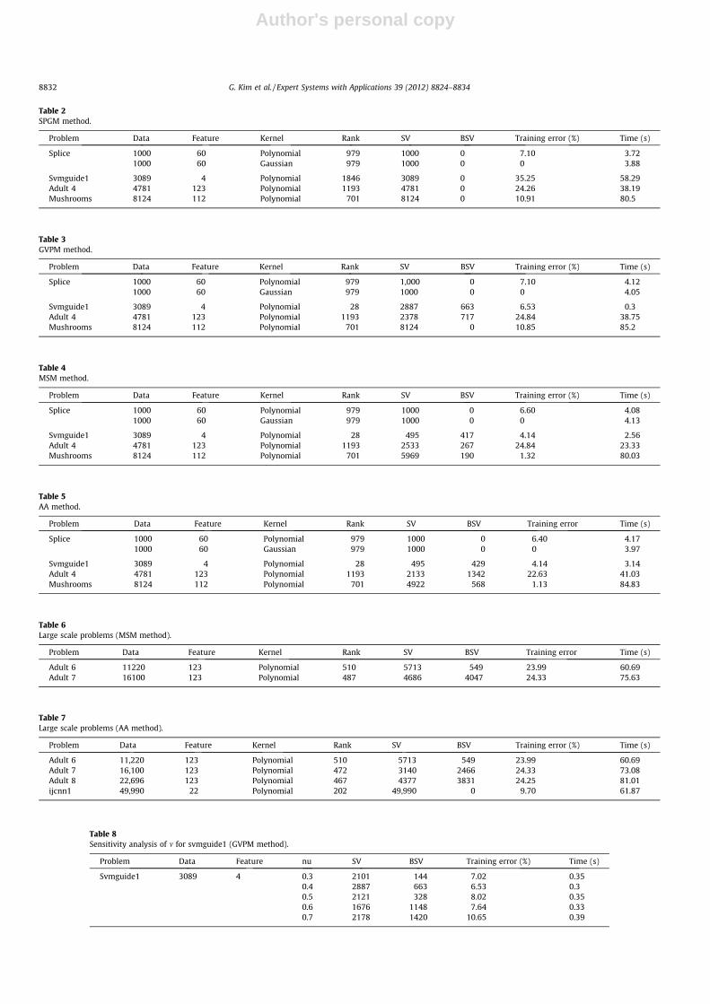
Table 2 shows the results for SPGM method described in Section3.1.1. The problems are medium sized. The algorithm uses polyno-

mial or Gaussian kernel function. The rank denotes the rank of theHessian matrix derived from the incomplete Cholesky decomposi-tion. In this result, though the testing errors and the solution timeare not bad, the number of support vectors is too large; this is notefficient because we should use all data point to test otherproblems.

Table 3 presents the results of GVPM method. The training er-rors and solution times are similar to the SPGM method. The num-ber of support vectors is much smaller than that of the SPGMmethod in two problems such as svmguide1 and adult4.

Table 4 shows the MSM method has better results than the pre-vious two methods. Though the solution time is similar to GVPMmethod, the training errors are much better than other methods.The number of support vectors is also smaller than others.

Table 5 describes the results of the AA method. The results arevery similar to the MSM method. The number of support vectors isalso small and the training errors are few, rendering good results.

From these results, it is shown that the MSM and AA methodshave better results than the other two methods in terms of thetraining error and the number of support vectors.

Table 6 shows the results of two large scale problems. We usu-ally say that a size larger than 10,000 is a large scale problem. Inthis result, we have good training errors, and the number of sup-port vectors is significantly smaller than the size of the problem.

Table 7 represents the results for large scale problems using theAA method.

In the m-SVM problem, the range of m is 0 < m < 1. The nextexperiments show the changes of the training errors and the num-ber of support vectors as the parameter m changes.

As the parameter m increases in Table 8, the training error in-creases and the number of support vectors changes a little. Thenumber of bound support vectors increases.

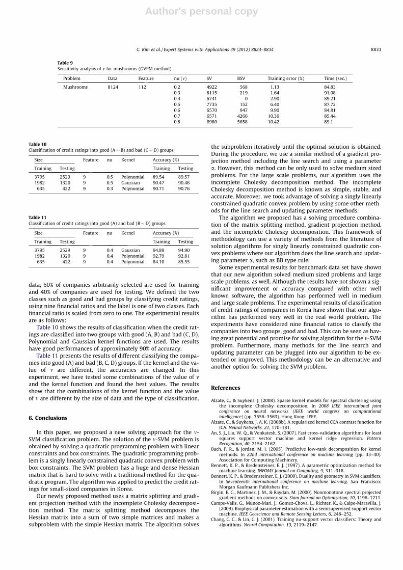
Table 9 shows the results of the sensitivity analysis of m formushrooms. The result is similar to the result of Table 8. As theparameter m elevates, the training error increases and the numberof support vectors and bound support vectors increase.

The experimental results showed that the four different meth-ods have different results when used for the line search and updat-ing parameter method. The SPGM and GVPM have good results forthe training error and the solution time, but the large number ofsupport vectors is a problem. On the other hand, the MSM andAA methods have better results for the training and the solutiontime than the other two methods. The number of support vectorsis also much smaller than the other two. We also have good resultsfor large scale problems with our decomposition approach. The re-sults in the last two tables show the properties of m-SVM problemclearly.

The application to the real world problem has been conductedto classify the credit ratings of companies in Korea. Three sizes ofdata are considered, that of 6324, 3302, and 1057. In each size of

Fig. 2. Incomplete Cholesky decomposition.

Table 1Financial ratios.

Type Ratios Calculation

Profitability Return on equity ordinaryincome

Ordinary income/totalcapitals

Return on Sales Net income/salesReturn on equity Net income/total capitalsEquity turnover ratio Sales/total capitalsFixed asset turnover ratio Sales/fixed assets

Stability Equity ratio Total capitals/total assetsFixed asset ratio Fixed assets/total capitalsDebt ratio Total liabilities/total

capitalsCurrent ratio Fixed assets/current

liabilities



Table 2SPGM method.

Problem Data Feature Kernel Rank SV BSV Training error (%) Time (s)

Splice 1000 60 Polynomial 979 1000 0 7.10 3.721000 60 Gaussian 979 1000 0 0 3.88

Svmguide1 3089 4 Polynomial 1846 3089 0 35.25 58.29Adult 4 4781 123 Polynomial 1193 4781 0 24.26 38.19Mushrooms 8124 112 Polynomial 701 8124 0 10.91 80.5

Table 3GVPM method.


Splice 1000 60 Polynomial 979 1,000 0 7.10 4.121000 60 Gaussian 979 1000 0 0 4.05


Table 4MSM method.




Table 5AA method.

Problem Data Feature Kernel Rank SV BSV Training error Time (s)



Table 6Large scale problems (MSM method).

Problem Data Feature Kernel Rank SV BSV Training error Time (s)

Adult 6 11220 123 Polynomial 510 5713 549 23.99 60.69Adult 7 16100 123 Polynomial 487 4686 4047 24.33 75.63

Table 7Large scale problems (AA method).


Adult 6 11,220 123 Polynomial 510 5713 549 23.99 60.69Adult 7 16,100 123 Polynomial 472 3140 2466 24.33 73.08Adult 8 22,696 123 Polynomial 467 4377 3831 24.25 81.01ijcnn1 49,990 22 Polynomial 202 49,990 0 9.70 61.87

Table 8Sensitivity analysis of m for svmguide1 (GVPM method).

Problem Data Feature nu SV BSV Training error (%) Time (s)

Svmguide1 3089 4 0.3 2101 144 7.02 0.350.4 2887 663 6.53 0.30.5 2121 328 8.02 0.350.6 1676 1148 7.64 0.330.7 2178 1420 10.65 0.39



data, 60% of companies arbitrarily selected are used for trainingand 40% of companies are used for testing. We defined the twoclasses such as good and bad groups by classifying credit ratings,using nine financial ratios and the label is one of two classes. Eachfinancial ratio is scaled from zero to one. The experimental resultsare as follows:

Table 10 shows the results of classification when the credit rat-ings are classified into two groups with good (A, B) and bad (C, D).Polynomial and Gaussian kernel functions are used. The resultshave good performances of approximately 90% of accuracy.

Table 11 presents the results of different classifying the compa-nies into good (A) and bad (B, C, D) groups. If the kernel and the va-lue of m are different, the accuracies are changed. In thisexperiment, we have tested some combinations of the value of mand the kernel function and found the best values. The resultsshow that the combinations of the kernel function and the valueof m are different by the size of data and the type of classification.

6. Conclusions

In this paper, we proposed a new solving approach for the m-SVM classification problem. The solution of the m-SVM problem isobtained by solving a quadratic programming problem with linearconstraints and box constraints. The quadratic programming prob-lem is a singly linearly constrained quadratic convex problem withbox constraints. The SVM problem has a huge and dense Hessianmatrix that is hard to solve with a traditional method for the qua-dratic program. The algorithm was applied to predict the credit rat-ings for small-sized companies in Korea.

Our newly proposed method uses a matrix splitting and gradi-ent projection method with the incomplete Cholesky decomposi-tion method. The matrix splitting method decomposes theHessian matrix into a sum of two simple matrices and makes asubproblem with the simple Hessian matrix. The algorithm solves

the subproblem iteratively until the optimal solution is obtained.During the procedure, we use a similar method of a gradient pro-jection method including the line search and using a parametera. However, this method can be only used to solve medium sizedproblems. For the large scale problems, our algorithm uses theincomplete Cholesky decomposition method. The incompleteCholesky decomposition method is known as simple, stable, andaccurate. Moreover, we took advantage of solving a singly linearlyconstrained quadratic convex problem by using some other meth-ods for the line search and updating parameter methods.

The algorithm we proposed has a solving procedure combina-tion of the matrix splitting method, gradient projection method,and the incomplete Cholesky decomposition. This framework ofmethodology can use a variety of methods from the literature ofsolution algorithms for singly linearly constrained quadratic con-vex problems where our algorithm does the line search and updat-ing parameter a, such as BB type rule.

Some experimental results for benchmark data set have shownthat our new algorithm solved medium sized problems and largescale problems, as well. Although the results have not shown a sig-nificant improvement or accuracy compared with other wellknown software, the algorithm has performed well in mediumand large scale problems. The experimental results of classificationof credit ratings of companies in Korea have shown that our algo-rithm has performed very well in the real world problem. Theexperiments have considered nine financial ratios to classify thecompanies into two groups, good and bad. This can be seen as hav-ing great potential and promise for solving algorithm for the m-SVMproblem. Furthermore, many methods for the line search andupdating parameter can be plugged into our algorithm to be ex-tended or improved. This methodology can be an alternative andanother option for solving the SVM problem.

References

Alzate, C., & Suykens, J. (2008). Sparse kernel models for spectral clustering usingthe incomplete Cholesky decomposition. In 2008 IEEE international jointconference on neural networks (IEEE world congress on computationalintelligence) (pp. 3556–3563). Hong Kong: IEEE.

Alzate, C., & Suykens, J. A. K. (2008b). A regularized kernel CCA contrast function forICA. Neural Networks, 21, 170–181.

An, S. J., Liu, W. Q., & Venkatesh, S. (2007). Fast cross-validation algorithms for leastsquares support vector machine and kernel ridge regression. PatternRecognition, 40, 2154–2162.

Bach, F. R., & Jordan, M. I. (2005). Predictive low-rank decomposition for kernelmethods. In 22nd international conference on machine learning (pp. 33–40).Association for Computing Machinery.

Bennett, K. P., & Bredensteiner, E. J. (1997). A parametric optimization method formachine learning. INFOMS Journal on Computing, 9, 311–318.

Bennett, K. P., & Bredensteiner, E. J. (2000). Duality and geometry in SVM classifiers.In Seventeenth international conference on machine learning. San Francisco:Morgan Kaufmann Publishers Inc.

Birgin, E. G., Martinez, J. M., & Raydan, M. (2000). Nonmonotone spectral projectedgradient methods on convex sets. Siam Journal on Optimization, 10, 1196–1211.

Camps-Valls, G., Munoz-Mari, J., Gomez-Chova, L., Richter, K., & Calpe-Maravilla, J.(2009). Biophysical parameter estimation with a semisupervised support vectormachine. IEEE Geoscience and Remote Sensing Letters, 6, 248–252.

Chang, C. C., & Lin, C. J. (2001). Training nu-support vector classifiers: Theory andalgorithms. Neural Computation, 13, 2119–2147.

Table 9Sensitivity analysis of m for mushrooms (GVPM method).

Problem Data Feature nu (m) SV BSV Training error (%) Time (sec.)

Mushrooms 8124 112 0.2 4922 568 1.13 84.830.3 8115 219 1.64 91.080.4 6741 0 2.90 89.210.5 7735 152 6.40 87.720.6 6570 947 9.90 84.810.7 6571 4266 10.36 85.440.8 6980 5658 10.42 89.1

Table 10Classification of credit ratings into good (A � B) and bad (C � D) groups.

Size Feature nu Kernel Accuracy (%)

Training Testing Training Testing

3795 2529 9 0.5 Polynomial 89.54 89.571982 1320 9 0.5 Gaussian 90.47 90.46

635 422 9 0.3 Polynomial 90.71 90.76

Table 11Classification of credit ratings into good (A) and bad (B � D) groups.

Size Feature nu Kernel Accuracy (%)

Training Testing Training Testing

3795 2529 9 0.4 Gaussian 94.89 94.901982 1320 9 0.4 Polynomial 92.79 92.81

635 422 9 0.4 Polynomial 84.10 85.55



Conn, A. R., Gould, N. I. M., & Toint, P. L. (1988). Global convergence of a class of trustregion algorithms for optimization with simple bounds. Siam Journal onNumerical Analysis, 25, 433–460.

Crisp, D. J., & Burges, C. J. C. (2000). A geometric interpretation of v-SVM classifiers.In Neural information processing systems (NIPS) (pp. 244–250).

Dai, Y. H., & Fletcher, R. (2006). New algorithms for singly linearly constrainedquadratic programs subject to lower and upper bounds. MathematicalProgramming, 106, 403–421.

Dai, Y. H., & Zhang, H. C. (2001). Adaptive two-point stepsize gradient algorithm.Numerical Algorithms, 27, 377–385.

Debnath, R., & Takahashi, H. (2006). SVM training: Second-order cone programmingversus quadratic programming. In IEEE international conference on neuralnetworks (pp. 1162-1168): IEEE.

Evtushenko, Y. G., & Zhadan, V. G. (1994). Barrier-projective methods for nonlinearprogramming. Computational Mathematics and Mathematical Physics, 34,579–590.

Ferris, M. C., & Munson, T. S. (2003). Interior-point methods or massive supportvector machines. Siam Journal on Optimization, 13, 783–804.

Fine, S., & Scheinberg, K. (2001). Efficient SVM training using lower rank kernalrepresentations. Journal of Machine Learning Research, 2, 243–264.

Friedlander, A., Martinez, J. M., Molina, B., & Raydan, M. (1998). Gradient methodwith retards and generalizations. Siam Journal on Numerical Analysis, 36,275–289.

Fu, Y. S., & Dai, Y. H. (2010). Improved projected gradient algorithms for singlylinearly constrained quadratic programs subject to lower and upper bounds.Asia-Pacific Journal of Operational Research, 27, 71–84.

Goldfarb, D., & Scheinberg, K. (2008). Numerically stable LDLT factorizations ininterior point methods for convex quadratic programming. Ima Journal ofNumerical Analysis, 28, 806–826.

Golub, G. H., & Van Loan, C. F. (1996). Matrix computations (3rd ed.). The JohnsHopkins University Press.

Higham, N. J. (1990). Analysis of the Cholesky decomposition of a semi-definitematrix. In Reliable Numerical Computation (pp. 161–185). Oxford University Press.

Joachims, T. (1999). Making large-scale support vector machine learning practical.In Advances in kernel methods: support vector learning (pp. 169–184). Cambridge:MIT Press.

Kashima, H., Ide, T., Kato, T., & Sugiyama, M. (2009). Recent advances and trends inlarge-scale kernel methods. Ieice Transactions on Information and Systems, E92d,1338–1353.

Keller, H. B. (1965). On the solution of singular and semidefinite linear systems byiteration. SIAM Journal of Numerical Analysis, 2, 281–290.

Kianmehr, K., & Alhajj, R. (2006). Support vector machine approach for fastclassification. In International conference on data warehouse and knowledgediscovery. LNCS. Poland: Springer-Verlag.

Lee, Y. J., & Mangasarian, O. L. (2001). RSVM: Reduced support vector machines. InFirst SIAM international conference on data mining. Chicago.

Lin, C. J., Lucidi, S., Palagi, L., Risi, A., & Sciandrone, M. (2009). Decompositionalgorithm model for singly linearly-constrained problems subject to lower andupper bounds. Journal of Optimization Theory and Applications, 141, 107–126.

Lin, Y. Y., & Pang, J. S. (1987). Iterative methods for large convex quadratic programs– A survey. Siam Journal on Control and Optimization, 25, 383–411.

Lin, C. J., & Saigal, R. (2000). An incomplete Cholesky factorization for densesymmetric positive definite matrices. Bit, 40, 536–558.

Louradour, J., Daoudi, K., & Bach, F. (2006). SVM speaker verification using anincomplete cholesky decomposition sequence kernel. In IEEE Odyssey (pp. 1–5).IEEE.

Luo, Z., & Tseng, P. (1992a). Error bound and convergence analysis of matrixsplitting algorithms for the affine variational inequality problem. SIAM Journalof Optimization, 2, 43–54.

Luo, Z. Q., & Tseng, P. (1992b). On the linear convergence of descent methods forconvex essentially smooth minimization. Siam Journal on Control andOptimization, 30, 408–425.

Mavroforakis, M. E., & Theodoridis, S. (2006). A geometric approach to supportvector machine (SVM) classification. IEEE Transactions on Neural Networks, 17,671–682.

Min, S. H., Lee, J., & Han, I. (2006). Hybrid genetic algorithms and support vectormachines for bankruptcy prediction. Expert Systems with Applications, 31,652–660.

Nehate, G. (2006). Solving large scale support vector machine problems using matrixsplitting and decomposition methods. Kansas State University.

Ortega, J. M. (1972). Numerical analysis; a second course. New York: Academic Press.Osuna, E., Freud, R., & Girosi, F. (1997). An improved training algorithm for support

vector machines. In IEEE workshop. (pp. 276–285). New York.Pang, J. S. (1982). On the convergence of a basic iterative method for the implicit

complementarity-problem. Journal of Optimization Theory and Applications, 37,149–162.

Pardalos, P. M., & Kovoor, N. (1990). An algorithm for a singly constrained class ofquadratic programs subject to upper and lower bounds. MathematicalProgramming, 46, 321–328.

Platt, J. C. (1999). Fast training of support vector machines using sequential minimaloptimization. In Advances in kernel methods: support vector learning(pp. 185–208). Cambridge: MIT Press.

Raydan, M. (1997). The Barzilai and Borwein gradient method for the large scaleunconstrained minimization problem. Siam Journal on Optimization, 7, 26–33.

Schölkopf, B., Smola, A. J., Williamson, R. C., & Bartlett, P. L. (2000). New supportvector algorithms. Neural Computation, 12, 1207–1245.

Serafini, T., Zanghirati, G., & Zanni, L. (2005). Gradient projection methods forquadratic programs and applications in training support vector machines.Optimization Methods and Software, 20, 353-378.

Suykens, J. A. K., & Vandewalle, J. (1999). Least squares support vector machineclassifiers. Neural Processing Letters, 9, 293–300.

To, K. N., Lim, C. C., Teo, K. L., & Liebelt, M. J. (2001). Support vector learning withquadratic programming and adaptive step size barrier-projection. NonlinearAnalysis – Theory Methods and Applications, 47, 5623–5633.

Vapnik, V. (1979). Estimation of dependences based on empirical data. Moscow:Nauka.

Vapnik, V. N. (1995). The nature of statistical learning theory. New York: Springer.Vapnik, V., & Chervonenkis, A. (1974). Theory of pattern recognition. Moscow: Nauka.Zhan, Y., & Shen, D. (2005). Design efficient support vector machine for fast

classification. Pattern Recognition, 38, 157–161.Zhou, W. D., Zhang, L., & Jiao, L. C. (2002). Linear programming support vector

machines. Pattern Recognition, 35, 2927–2936.


Modified matrix splitting method for the support vector machine and its application to the credit...

Documents

Transcript of Modified matrix splitting method for the support vector machine and its application to the credit...