Modelling the perception and composition ofWestern musical harmony

Peter Michael Combes Harrison

Submitted in partial fulfillment of the requirementsof the Degree of Doctor of Philosophy

School of Electronic Engineering and Computer ScienceQueen Mary University of London

April 20, 2020

1

Declaration

I, Peter Harrison, confirm that the research included within this thesis is my ownwork or that where it has been carried out in collaboration with, or supportedby others, that this is duly acknowledged below and my contribution indicated.Previously published material is also acknowledged below. I attest that I haveexercised reasonable care to ensure that the work is original, and does not to thebest of my knowledge break any UK law, infringe any third party’s copyrightor other Intellectual Property Right, or contain any confidential material. Iaccept that the College has the right to use plagiarism detection software tocheck the electronic version of the thesis. I confirm that this thesis has not beenpreviously submitted for the award of a degree by this or any other university.The copyright of this thesis rests with the author and no quotation from it orinformation derived from it may be published without the prior written consentof the author.

Date Peter Harrison

2

Publications

Early versions of work described in this thesis appeared in the following confer-ence proceedings:

Harrison, P. M. C., & Pearce, M. T. (2018). Dissociating sensory and cog-nitive theories of harmony perception through computational modeling. InProceedings of ICMPC15/ESCOM10. Graz, Austria. https://doi.org/10.31234/osf.io/wgjyv

Harrison, P. M. C., & Pearce, M. T. (2018). An energy-based generativesequence model for testing sensory theories of Western harmony. In Proceedingsof the 19th International Society for Music Information Retrieval Conference(pp. 160–167). Paris, France. https://arxiv.org/abs/1807.00790

Chapter 3 and 5 are respectively based on the following journal articles:

Harrison, P. M. C., & Pearce, M. T. (2020). Simultaneous consonancein music perception and composition. Psychological Review, 127(2), 216-244.http://dx.doi.org/10.1037/rev0000169

Harrison, P. M. C., & Pearce, M. T. (2020). A computational cognitivemodel for the analysis and generation of voice leadings. Music Perception,37(3), 208-224. https://doi.org/10.1525/mp.2020.37.3.208

Early versions of Chapters 2, 3 and 5 were posted as the following preprints:

Harrison, P. M. C., & Pearce, M. T. (2019). Representing harmony in com-putational music cognition. PsyArXiv. https://doi.org/10.31234/osf.io/xswp4

Harrison, P. M. C., & Pearce, M. T. (2019). Instantaneous consonance in

3

the perception and composition of Western music. PsyArXiv. https://doi.org/10.31234/osf.io/6jsug

Harrison, P. M. C., & Pearce, M. T. (2019). A computational model for theanalysis and generation of chord voicings. PsyArXiv. https://doi.org/10.31234/osf.io/wrgj7

The following other articles were also produced during the doctoral studyperiod:

Harrison, P. M. C., Musil, J. J., & Müllensiefen, D. (2016). Modellingmelodic discrimination tests: Descriptive and explanatory approaches. Jour-nal of New Music Research, 45(3), 265–280. https://doi.org/10.1080/09298215.2016.1197953

Harrison, P. M. C., Collins, T., & Müllensiefen, D. (2017). Applying modernpsychometric techniques to melodic discrimination testing: Item response the-ory, computerised adaptive testing, and automatic item generation. ScientificReports(7). https://doi.org/10.1038/s41598-017-03586-z

Harrison, P. M. C. & Müllensiefen, D. (2018). Development and valida-tion of the Computerised Adaptive Beat Alignment Test (CA-BAT). ScientificReports(8). https://doi.org/10.1038/s41598-018-30318-8

Harrison, P. M. C. Statistics and Experimental Design for Psychologists: Amodel comparison approach by Rory Allen (book review). PsyPAG Quarterly.

Harrison, P. M. C., Larrouy-Maestri, P., & Müllensiefen, D. (2019). Themistuning perception test: A new measurement instrument. Behavior ResearchMethods, 51, 663-675. https://doi.org/10.3758/s13428-019-01225-1

Gelding, R., Harrison, P. M. C., Silas, S., Johnson, B. W., Thompson, W.F., & Müllensiefen, D. (2019). Developing an efficient test of musical imageryability: Applying modern psychometric techniques to the Pitch Imagery ArrowTask. PsyArXiv. https://doi.org/10.31234/osf.io/8gvhz

de Fleurian, R., Harrison, P. M. C., Pearce, M. T., & Quiroga-Martinez,D. R. (2019). Reward prediction tells us less than expected about musicalpleasure. Proceedings of the National Academy of Sciences, 116(42), 20813-20814. https://doi.org/10.1073/pnas.1913244116

Cheung, V., Harrison, P. M. C., Pearce, M. T., Haynes, J-D., Koelsch, S.

4

(2019). Uncertainty and surprise jointly predict musical pleasure and amygdala,hippocampus, and auditory cortex activity. Current Biology, 29(23), 4084-4092.e4. https://doi.org/10.1016/j.cub.2019.09.067

Zioga, I., Harrison, P. M. C., Pearce, M. T., Bhattacharya, J., Luft, C.D. B. (2020). From learning to creativity: Identifying the behavioural andneural correlates of learning to predict human judgements of musical creativity.NeuroImage, 206. https://doi.org/10.1016/j.neuroimage.2019.116311

Harrison, P. M. C., Bianco, R., Chait, M., Pearce, M. T. (2020). PPM-Decay: A computational model of auditory prediction with memory decay.bioRxiv. https://doi.org/10.1101/2020.01.09.900266

Bianco, R., Harrison, P. M. C., Hu, M., Bolger, C., Picken, S., Pearce, M. T.,Chait, M. (2020). Long-term implicit memory for sequential auditory patternsin humans. bioRxiv. https://doi.org/10.1101/2020.02.14.949404

Harrison, P. M. C. (2020). psychTestR: An R package for designing andconducting behavioural psychological experiments. PsyArXiv. https://doi.org/10.31234/osf.io/dyar7

5

Abstract

Harmony is a fundamental structuring principle in Western music, determininghow simultaneously occurring musical notes combine to form chords, and howsuccessions of chords combine to form chord progressions. Harmony is interest-ing to psychologists because it unites many core features of auditory perceptionand cognition, such as pitch perception, auditory scene analysis, and statisticallearning. A current challenge is to formalise our psychological understandingof harmony through computational modelling. Here we detail computationalstudies of three core dimensions of harmony: consonance, harmonic expectation,and voice leading. These studies develop and evaluate computational modelsof the psychoacoustic and cognitive processes involved in harmony perception,and quantitatively model how these processes contribute to music composition.Through these studies we examine long-standing issues in music psychology,such as the relative contributions of roughness and harmonicity to consonanceperception, the roles of low-level psychoacoustic and high-level cognitive pro-cesses in harmony perception, and the probabilistic nature of harmonic expec-tation. We also develop cognitively informed computational models that arecapable of both analysing existing music and generating new music, with po-tential applications in computational creativity, music informatics, and musicpsychology. This thesis is accompanied by a collection of open-source softwarepackages that implement the models developed and evaluated here, which wehope will support future research into the psychological foundations of musicalharmony.

4

Contents

1 Introduction 15

2 Representing harmony 232.1 Introduction . . . . . . . . . . . . . . . . . . . . . . . . . . . . . . 232.2 Related work . . . . . . . . . . . . . . . . . . . . . . . . . . . . . 242.3 Low-level representations . . . . . . . . . . . . . . . . . . . . . . 262.4 Symbolic representations . . . . . . . . . . . . . . . . . . . . . . . 31

2.4.1 Pitch chord . . . . . . . . . . . . . . . . . . . . . . . . . . 322.4.2 Pitch-class set . . . . . . . . . . . . . . . . . . . . . . . . . 332.4.3 Pitch-class chord . . . . . . . . . . . . . . . . . . . . . . . 332.4.4 Pitch chord type . . . . . . . . . . . . . . . . . . . . . . . 342.4.5 Pitch-class chord type . . . . . . . . . . . . . . . . . . . . 342.4.6 Pitch-class set type . . . . . . . . . . . . . . . . . . . . . . 352.4.7 Further issues . . . . . . . . . . . . . . . . . . . . . . . . . 36

2.5 Acoustic representations . . . . . . . . . . . . . . . . . . . . . . . 372.5.1 Frequency chord . . . . . . . . . . . . . . . . . . . . . . . 372.5.2 Sparse frequency spectrum . . . . . . . . . . . . . . . . . 382.5.3 Sparse pitch spectrum . . . . . . . . . . . . . . . . . . . . 402.5.4 Sparse pitch-class spectrum . . . . . . . . . . . . . . . . . 402.5.5 Waveform . . . . . . . . . . . . . . . . . . . . . . . . . . . 41

2.6 Sensory representations . . . . . . . . . . . . . . . . . . . . . . . 412.6.1 Smooth pitch/pitch-class spectra . . . . . . . . . . . . . . 412.6.2 Potential alternatives . . . . . . . . . . . . . . . . . . . . 44

2.7 Alphabets . . . . . . . . . . . . . . . . . . . . . . . . . . . . . . . 442.7.1 Pitch-class set . . . . . . . . . . . . . . . . . . . . . . . . . 452.7.2 Pitch-class set type . . . . . . . . . . . . . . . . . . . . . . 452.7.3 Pitch-class chord type . . . . . . . . . . . . . . . . . . . . 462.7.4 Pitch-class chord . . . . . . . . . . . . . . . . . . . . . . . 46

2.8 Deriving higher-level representations . . . . . . . . . . . . . . . . 472.8.1 Voice leading . . . . . . . . . . . . . . . . . . . . . . . . . 47

5

2.8.2 Chord roots . . . . . . . . . . . . . . . . . . . . . . . . . . 472.8.3 Tonality . . . . . . . . . . . . . . . . . . . . . . . . . . . . 482.8.4 Functional harmony . . . . . . . . . . . . . . . . . . . . . 50

2.9 Corpus translation . . . . . . . . . . . . . . . . . . . . . . . . . . 502.9.1 Textual symbols . . . . . . . . . . . . . . . . . . . . . . . 502.9.2 Polyphonic scores . . . . . . . . . . . . . . . . . . . . . . . 512.9.3 Audio . . . . . . . . . . . . . . . . . . . . . . . . . . . . . 53

2.10 Conclusion . . . . . . . . . . . . . . . . . . . . . . . . . . . . . . 53

3 Simultaneous consonance 563.1 Introduction . . . . . . . . . . . . . . . . . . . . . . . . . . . . . . 563.2 Terminology . . . . . . . . . . . . . . . . . . . . . . . . . . . . . . 573.3 Consonance theories . . . . . . . . . . . . . . . . . . . . . . . . . 58

3.3.1 Periodicity/harmonicity . . . . . . . . . . . . . . . . . . . 583.3.2 Interference between partials . . . . . . . . . . . . . . . . 613.3.3 Culture . . . . . . . . . . . . . . . . . . . . . . . . . . . . 643.3.4 Other theories . . . . . . . . . . . . . . . . . . . . . . . . 65

3.4 Current evidence . . . . . . . . . . . . . . . . . . . . . . . . . . . 683.4.1 Stimulus effects . . . . . . . . . . . . . . . . . . . . . . . . 683.4.2 Listener effects . . . . . . . . . . . . . . . . . . . . . . . . 713.4.3 Composition effects . . . . . . . . . . . . . . . . . . . . . 743.4.4 Discussion . . . . . . . . . . . . . . . . . . . . . . . . . . . 76

3.5 Computational models . . . . . . . . . . . . . . . . . . . . . . . . 773.5.1 Periodicity/harmonicity: Ratio simplicity . . . . . . . . . 793.5.2 Periodicity/harmonicity: Spectral pattern matching . . . 793.5.3 Periodicity/harmonicity: Temporal autocorrelation . . . . 853.5.4 Interference: Complex dyads . . . . . . . . . . . . . . . . 863.5.5 Interference: Pure dyads . . . . . . . . . . . . . . . . . . . 873.5.6 Interference: Waveforms . . . . . . . . . . . . . . . . . . . 883.5.7 Culture . . . . . . . . . . . . . . . . . . . . . . . . . . . . 90

3.6 Perceptual analyses . . . . . . . . . . . . . . . . . . . . . . . . . . 923.6.1 Evaluating models individually . . . . . . . . . . . . . . . 963.6.2 A composite consonance model . . . . . . . . . . . . . . . 993.6.3 Generalising to different datasets . . . . . . . . . . . . . . 993.6.4 Recommendations for model selection . . . . . . . . . . . 101

3.7 Corpus analyses . . . . . . . . . . . . . . . . . . . . . . . . . . . . 1023.8 Discussion . . . . . . . . . . . . . . . . . . . . . . . . . . . . . . . 1063.9 Methods . . . . . . . . . . . . . . . . . . . . . . . . . . . . . . . . 109

3.9.1 Models . . . . . . . . . . . . . . . . . . . . . . . . . . . . 1093.9.2 Software . . . . . . . . . . . . . . . . . . . . . . . . . . . . 112

6

3.9.3 Perceptual datasets . . . . . . . . . . . . . . . . . . . . . . 1133.9.4 Musical corpora . . . . . . . . . . . . . . . . . . . . . . . 1153.9.5 Corpus analyses . . . . . . . . . . . . . . . . . . . . . . . 116

4 Harmonic expectation 1184.1 Introduction . . . . . . . . . . . . . . . . . . . . . . . . . . . . . . 1184.2 Perceptual features . . . . . . . . . . . . . . . . . . . . . . . . . . 121

4.2.1 Low-level features . . . . . . . . . . . . . . . . . . . . . . 1244.2.2 High-level features . . . . . . . . . . . . . . . . . . . . . . 1254.2.3 Feature distributions in popular music . . . . . . . . . . . 128

4.3 Model . . . . . . . . . . . . . . . . . . . . . . . . . . . . . . . . . 1334.4 Modelling an ideal listener . . . . . . . . . . . . . . . . . . . . . . 1384.5 Modelling human listeners . . . . . . . . . . . . . . . . . . . . . . 1444.6 Discussion . . . . . . . . . . . . . . . . . . . . . . . . . . . . . . . 1514.7 Methods . . . . . . . . . . . . . . . . . . . . . . . . . . . . . . . . 157

4.7.1 Corpus . . . . . . . . . . . . . . . . . . . . . . . . . . . . 1574.7.2 Modelling . . . . . . . . . . . . . . . . . . . . . . . . . . . 1574.7.3 Behavioural experiment . . . . . . . . . . . . . . . . . . . 1644.7.4 Software . . . . . . . . . . . . . . . . . . . . . . . . . . . . 167

5 Voice leading 1685.1 Introduction . . . . . . . . . . . . . . . . . . . . . . . . . . . . . . 1685.2 Model . . . . . . . . . . . . . . . . . . . . . . . . . . . . . . . . . 1725.3 Features . . . . . . . . . . . . . . . . . . . . . . . . . . . . . . . . 173

5.3.1 Voice-leading distance . . . . . . . . . . . . . . . . . . . . 1735.3.2 Melodic voice-leading distance . . . . . . . . . . . . . . . 1735.3.3 Pitch height . . . . . . . . . . . . . . . . . . . . . . . . . . 1745.3.4 Interference between partials . . . . . . . . . . . . . . . . 1745.3.5 Number of pitches . . . . . . . . . . . . . . . . . . . . . . 1755.3.6 Parallel octaves/fifths . . . . . . . . . . . . . . . . . . . . 1765.3.7 Exposed octaves (outer parts) . . . . . . . . . . . . . . . . 1765.3.8 Part overlap . . . . . . . . . . . . . . . . . . . . . . . . . . 177

5.4 Analysis . . . . . . . . . . . . . . . . . . . . . . . . . . . . . . . . 1785.4.1 Performance . . . . . . . . . . . . . . . . . . . . . . . . . 1795.4.2 Moments . . . . . . . . . . . . . . . . . . . . . . . . . . . 1795.4.3 Weights . . . . . . . . . . . . . . . . . . . . . . . . . . . . 1805.4.4 Feature importance . . . . . . . . . . . . . . . . . . . . . . 1815.4.5 Statistical significance . . . . . . . . . . . . . . . . . . . . 181

5.5 Generation . . . . . . . . . . . . . . . . . . . . . . . . . . . . . . 1845.6 Implementation . . . . . . . . . . . . . . . . . . . . . . . . . . . . 188

7

5.7 Discussion . . . . . . . . . . . . . . . . . . . . . . . . . . . . . . . 191

6 Conclusion 1956.1 Overview . . . . . . . . . . . . . . . . . . . . . . . . . . . . . . . 1956.2 Limitations and future directions . . . . . . . . . . . . . . . . . . 199

8

List of Figures

2.1 A network of low-level harmony representations, organised intothree representational categories: symbolic, acoustic, and sen-sory. Arrows between representations indicate well-defined com-putational translations between representations. . . . . . . . . . . 29

2.2 Acoustic and sensory representations for a C major chord in firstinversion comprising the MIDI pitches {52, 60, 67}, synthesisedwith 11 harmonics with amplitude roll-off 1/n. (A) Sparse fre-quency spectrum; (B) sparse pitch spectrum; (C) sparse pitch-class spectrum; (D) waveform; (E) smooth pitch spectrum; (F)smooth pitch-class spectrum. . . . . . . . . . . . . . . . . . . . . 39

2.3 Schematic diagram illustrating the role of symbolic, acoustic,and sensory representations in different musical activities. Ex-plicit symbolic representations are used in musical scores, whichare analysed by music theorists to yield insights into musicalpractice, insights which are then conveyed to composers throughmusic pedagogy. These explicit symbolic representations reflectimplicit symbolic representations held by music listeners, whichare themselves derived from sensory representations that listen-ers construct from musical sound, which can be recorded usingacoustic representations. . . . . . . . . . . . . . . . . . . . . . . . 42

3.1 Acoustic spectra and waveforms for (A) a single harmonic com-plex tone, (B) two harmonic complex tones separated by anequal-tempered perfect fifth, and (C) two harmonic complextones separated by an equal-tempered tritone. Each complex tonehas 11 harmonics, with the ith harmonic having an amplitude of1/i. The blue dotted lines mark harmonic/periodic grids, whichare aligned for the harmonic/periodic perfect fifth but misalignedfor the inharmonic/aperiodic tritone. . . . . . . . . . . . . . . . . 60

9

3.2 A: Interference between partials as a function of distance in crit-ical bandwidths, after Hutchinson & Knopoff (1978). B: Inter-ference patterns in two musical sonorities, after Hutchinson &Knopoff (1978). {C4, E4, G4} is a consonant major triad, andexperiences low interference. {C4, C\4, D4} is a dissonant clusterchord, and experiences high interference. . . . . . . . . . . . . . . 64

3.3 Consonance models organised by psychological theory and mod-elling approach. Dashed borders indicate models not evaluatedin our empirical analyses. Arrows denote model revisions. . . . . 78

3.4 Results of the perceptual analyses. All error bars denote 95%confidence intervals. A: Partial correlations between model out-puts and average consonance ratings in the Bowling et al. (2018)dataset, after controlling for number of notes. B: Predictionsof the composite model for the Bowling et al. (2018) dataset.C: Standardised regression coefficients for the composite model.D: Evaluating the composite model across five datasets fromfour studies (Bowling et al., 2018; Johnson-Laird et al., 2012;Lahdelma & Eerola, 2016; Schwartz et al., 2003). . . . . . . . . . 97

3.5 Results of the corpus analyses. A: Permutation-based feature im-portance (Breiman, 2001; Fisher, Rudin, & Dominici, 2018), witherror bars indicating 95% confidence intervals (bias-correctedand accelerated bootstrap, 100,000 replicates, DiCiccio & Efron,1996). B: Marginal effects of each feature, calculated using z-scores for feature values and for chord frequencies. The shadedareas describe 95% confidence intervals, and distributions of fea-ture observations are plotted at the bottom of each panel. Distri-butions for the ‘number of notes’ feature are smoothed to avoidoverplotting. C: Predicted and actual chord-type frequencies,alongside corresponding Pearson correlation coefficients. . . . . . 104

4.1 Schematic network illustrating the psychological relationships be-tween the 15 features used in the present study. An arrow indi-cates that a particular feature is psychologically derived fromanother feature. . . . . . . . . . . . . . . . . . . . . . . . . . . . . 122

10

4.2 Example eight-chord sequence corresponding to an extract fromthe song Super Freak by Rick James (1981). Such sequenceswere used in both the ideal-listener analysis and the behaviouralstudy, in which computational models and human listeners gen-erated predictions for the target chord marked by an asterisk.The chords are voiced using the heuristic method described inSection 4.7.3. Feature values are provided in Table 4.2. . . . . . . 128

4.3 Distributions for continuous features, comparing observed chordswith unobserved chords at each position in the popular music cor-pus. These distributions are plotted as kernel density estimateswith Gaussian kernels and bandwidths estimated using Silver-man’s (1986) ‘rule of thumb’. . . . . . . . . . . . . . . . . . . . . 131

4.4 0th- and 1st-order probability distributions for (A) root pitchclass and (B) root interval as derived from the Billboard pop-ular music corpus (Burgoyne, 2011). 1st-order probabilities areexpressed relative to the corresponding 0th-order probabilities. . 134

4.5 0th- and 1st-order probability distributions for (A) bass pitchclass and (B) bass interval as derived from the Billboard pop-ular music corpus (Burgoyne, 2011). 1st-order probabilities areexpressed relative to the corresponding 0th-order probabilities. . 135

4.6 Correlation matrix for log probabilities of observed chords ascomputed by variable-order Markov models trained on differenthigh-level features (see Section 4.7 for details). Features are hi-erarchically clustered using a distance measure of one minus thecorrelation coefficient. . . . . . . . . . . . . . . . . . . . . . . . . 136

4.7 Permutation-based feature importances for (A) the full ideal-listener model and (B) the low-level model, after Breiman (2001;see also Fisher et al., 2018). . . . . . . . . . . . . . . . . . . . . . 142

4.8 Marginal effects of continuous features in the (A) full and (B)low-level ideal-listener models. The horizontal axes span fromthe 2.5th to the 97.5th percentiles of all theoretically possible fea-ture values, computed over the full chord alphabet (N = 24,576)at each of the 300 chord positions being modelled. The shadedregions identify the 2.5th and 97.5th percentiles of observed fea-ture values (i.e. those that were actually observed in the chordsequences). . . . . . . . . . . . . . . . . . . . . . . . . . . . . . . 143

4.9 Stacked bar plot of categorical feature weights in the full ideal-listener model, split by short-term and long-term features. . . . . 143

11

4.10 Density plots of associations between model outputs and lis-tener surprisals for three models: the full ideal-listener model,the benchmark regression model, and the simplified ideal-listenermodel. ‘Count’ refers to the number of stimuli present in therespective region of the plot. . . . . . . . . . . . . . . . . . . . . . 147

4.11 Analysis of the first composition in the popular music corpus, Idon’t mind by James Brown (1961), using the full ideal-listenermodel from Section 4.4. Each number corresponds to a chord’sinformation content, or surprisal, expressed to one decimal place.The regression weights are preserved from the ideal-listener anal-ysis, but the categorical feature models are retrained on the last700 compositions from the popular music corpus. Durations,pitch heights, and bar lines are arbitrary. . . . . . . . . . . . . . 150

5.1 J. S. Bach, Mach’s mit mir, Gott, nach deiner Güt’, BWV 377,bb. 1–4. The two chords immediately after the first fermataimply parallel fifths and octaves that have been only partly mit-igated by swapping the bass and tenor parts. . . . . . . . . . . . 180

5.2 Example voice leadings for J. S. Bach’s chorale Aus meinesHerzens Grunde (BWV 269), chords 1–10. A: Bach’s originalvoice leading. B: Heuristic voice leading. C: New algorithm. D:New algorithm with prespecified melody. . . . . . . . . . . . . . . 186

5.3 Example voice leadings for the first 10 chords of John Coltrane’s26-2. A: Heuristic voice leading. B: New algorithm. . . . . . . . 186

5.4 Example voice leadings for the first 10 chords of You’ve got afriend by Roberta Flack and Donny Hathaway. A: Heuristic voiceleading. B: New algorithm. . . . . . . . . . . . . . . . . . . . . . 187

12

List of Tables

2.1 The 13 low-level harmony representations with their alphabetsizes and invariances. . . . . . . . . . . . . . . . . . . . . . . . . . 30

2.2 Symbolic representations for three example chords: (A) C majortriad, 1st inversion; (B) C major triad, second inversion; (C) Edominant seventh, third inversion. . . . . . . . . . . . . . . . . . 32

3.1 Summarised evidence for the mechanisms underlying Westernconsonance perception. . . . . . . . . . . . . . . . . . . . . . . . . 68

3.2 Consonance models evaluated in the present work. . . . . . . . . 943.3 Unstandardised regression coefficients for the composite conso-

nance model. . . . . . . . . . . . . . . . . . . . . . . . . . . . . . 112

4.1 The 15 harmony features used in the present study. . . . . . . . . 1234.2 Feature values for the chord sequence notated in Figure 4.2. . . . 1294.3 Pearson correlation matrix for the low-level features. . . . . . . . 1314.4 Cross entropy as a function of Markov order bound. . . . . . . . 1394.5 Cross entropy and Akaike Information Criteria (AIC) for different

feature combinations. . . . . . . . . . . . . . . . . . . . . . . . . . 1404.6 Benchmarking the ideal-listener model against low-level models

of harmonic expectation. . . . . . . . . . . . . . . . . . . . . . . . 1464.7 Comparing the performance of different simplified versions of the

ideal-listener model. . . . . . . . . . . . . . . . . . . . . . . . . . 1484.8 Participants’ responses to the question “How often do you listen

to popular music?” . . . . . . . . . . . . . . . . . . . . . . . . . . 1644.9 Optimising local and global half lives for Leman’s (2000a) spec-

tral similarity model. . . . . . . . . . . . . . . . . . . . . . . . . . 1654.10 Optimising the half life of the new spectral similarity model. . . 166

5.1 Descriptive and inferential statistics for the 12 voice-leading fea-tures as applied to the Bach chorale dataset. . . . . . . . . . . . 183

13

Acknowledgements

I could not have hoped for a more dedicated supervisor than Marcus Pearce,who was always generous with time and advice throughout my studies. I’mgrateful to Emmanouil Benetos and Matthew Purver, the other two membersof my progression panel, for taking the time to examine my interim reports andfor providing useful advice at my progression meetings. I’m indebted to manyothers who contributed useful feedback about the work described here, includingDavid Baker, Manuel Anglada-Tort, Bastiaan van der Weij, Vincent Cheung,Andrew Goldman, Tyreek Jackson, Stefan Koelsch, Daniel Müllensiefen, DavidHuron, and several anonymous reviewers. I also enjoyed the general supportof various research groups at the university, in particular the Music CognitionLab, the Centre for Digital Music, the Cognitive Science group, and the doctoraltraining centre for Media & Arts Technology. I’m very grateful to my externalexaminers, Alan Marsden and Tuomas Eerola, who gave much valuable adviceabout improving this work. Lastly, I would like to thank Maddy Seale foralways being willing to listen to my ideas, and for supporting and encouragingme throughout this process.

This work was supported by the EPSRC/AHRC grant EP/L01632X/1.

14

Chapter 1

Introduction

Western music, broadly conceived as the musical traditions that originated inEurope and now permeate the globalised world, is rooted in the notion of har-mony. Harmony describes how simultaneously occurring musical notes are com-bined to form chords, and how successions of chords combine to form chord pro-gressions. It has long fascinated musicians, music theorists, mathematicians,and scientists for its combinatorial complexity, its ability to evoke complexemotions in the listener, and its apparent deep connections to mathematics,psychoacoustics, and linguistics.

The psychological study of harmony has its roots in the late 18th century.The polymath Hermann von Helmholtz may be considered the grandfather ofthe field, developing a ‘beating’ theory of consonance perception that remainsinfluential to this day (Helmholtz, 1863). Soon after Helmholtz, Karl Stumpfpresented his own ‘fusion’ theory of consonance, bringing an emphasis on per-ceptual integration that prefigured the subsequent ‘Gestalt’ school of psychol-ogy (Stumpf, 1890, 1898). Following Helmholtz, many subsequent researcherscontinued to analyse consonance in terms of interactions between neighboringspectral components, taking advantage of new advances in psychoacoustic mea-surement to build formal models predicting the consonance of musical sonoritiesfrom the dissonance profiles of pairs of pure tones (Dillon, 2013; Hutchinson& Knopoff, 1978; Kameoka & Kuriyagawa, 1969b; Sethares, 1993; Vassilakis,2001). Following Stumpf, other researchers continued to analyse consonancein terms of perceptual integration. In particular, Ernst Terhardt studied howlisteners integrate different parts of the auditory spectrum to derive the perceptof pitch, and argued that consonance could be understood as a consequenceof this pitch-finding process (Terhardt, 1984). Richard Parncutt adopted andbroadened Terhardt’s hypothesis, arguing that these pitch-finding mechanismswere fundamental not only to simultaneous consonance (a property of individ-

15

ual chords) but also to sequential consonance (a property of successive chords),and using this hypothesis to rationalise various tenets of Western music the-ory (Parncutt, 1989). Recent research by Andrew Milne and colleagues pursuessimilar principles, showing that psychoacoustic processes can provide a good ac-count of both simultaneous and sequential relationships in tonal music (Milne& Holland, 2016; Milne, Laney, & Sharp, 2015; Milne et al., 2016).

A contrasting line of harmony research has emphasised the role of higher-level cognition in harmony perception. Much of the early work in this areadepended on the so-called ‘harmonic priming’ paradigm, developed by JamshedBharucha and colleagues (Bharucha, 1987; Bharucha & Pryor, 1986; Tekman& Bharucha, 1992, 1998). In this paradigm, participants were instructed tomake perceptual judgments concerning certain chords within chord sequences,and researchers analysed the extent to which reaction times were affected bymanipulations of the preceding chords in the sequence. Bharucha and colleagueshad a particular interest in isolating listeners’ hierarchical conceptions of tonal-ity, which they modelled with MUSACT, a connectionist network with threelayers in ascending levels of abstraction: tones, chords, and keys (Bharucha,1987). Nodes within MUSACT were connected by edges with weights prespeci-fied by the researcher to reflect commonly held principles of Western harmonictonality, such as the idea that any particular key may be represented by threecore chords, namely the tonic, the dominant, and the subdominant. Given aparticular musical input comprising a particular set of tones, activations wouldspread through the network in proportion to the weights of the edges connect-ing each node. In a series of empirical studies, Bharucha and colleagues showedthat MUSACT’s activations could successfully predict harmonic priming effectsin Western listeners (Bharucha, 1987; Bharucha & Pryor, 1986; Tekman &Bharucha, 1992, 1998). As these studies progressed, the researchers controlledmore carefully for low-level psychoacoustic cues that might explain the primingeffects (e.g. common harmonics between the context and the target), but con-tinued to find reliable priming effects consistent with MUSACT’s predictions(Tekman & Bharucha, 1992, 1998). Emmanuel Bigand and colleagues extendedthe harmonic priming paradigm to longer harmonic sequences, and continuedto find evidence for high-level cognitive contributions to harmonic priming (Bi-gand, Madurell, Tillmann, & Pineau, 1999; Bigand & Pineau, 1997; Bigand,Poulin, Tillmann, Madurell, & Adamo, 2003; Tillmann & Bigand, 2001).

The MUSACT model demonstrated that listeners’ internal knowledge ofWestern harmonic tonality could be parsimoniously represented as a connection-ist network, but it did not show how this knowledge could be acquired. BarbaraTillmann and colleagues addressed this question, showing that a self-organisingnetwork could acquire the same tonal principles as the MUSACT model sim-

16

ply through exposure to harmonic sequences from tonal music, and that theresulting model could explain a wide variety of psychological results from theliterature (Tillmann, Bharucha, & Bigand, 2000). This work was complementedby contemporaneous studies of statistical learning in human listeners; variousstudies in the linguistic domain highlighted the capacity of listeners to learnartificial grammars simply through passive exposure to exemplars from thesegrammars (Aslin, Saffran, & Newport, 1998; Saffran et al., 1996a, 1996b), andit was soon shown that analogous learning processes took place for artificial mu-sical grammars (Saffran, Johnson, Aslin, & Newport, 1999). Most early studiesof musical statistical learning focused on melody (e.g. Creel, Newport, & Aslin,2004; Dienes & Longuet-Higgins, 2004; Endress, 2010; Rohrmeier et al., 2011),but several studies also isolated statistical-learning effects for artificial harmonicgrammars, including grammars in non-Western tuning systems and grammarsincorporating context-free structure (Jonaitis & Saffran, 2009; Loui, Wu, Wes-sel, & Knight, 2009; Rohrmeier & Cross, 2009). These findings supported agrowing belief that harmony might be less of a psychoacoustic phenomenon andmore of a cultural phenomenon, driven by similar statistical-learning processesto language cognition.

These documented similarities between linguistic learning and musical learn-ing were reinforced by further documented similarities between linguistic andmusical domains. Several researchers presented music-theoretic accounts of thesequential structure of Western harmony – harmonic ‘syntax’ – with an emphasison hierarchical structure, recursion, and non-adjacent dependencies, propertiesshared with the syntax of natural language (Rohrmeier, 2011; Steedman, 1984).These apparent similarities between harmonic and linguistic syntax motivateda popular hypothesis that both types of syntax are processed by similar cog-nitive and neural mechanisms. Some evidence for this hypothesis comes fromempirical studies showing suggestive parallels between electrical signatures ofharmonic and linguistic syntax processing (e.g. Patel, Gibson, Ratner, Besson,& Holcomb, 1998; Koelsch et al., 2001; Koelsch, Gunter, Friederici, & Schröger,2000; Koelsch, Schroger, & Gunter, 2002), and interference effects between theprocessing of harmonic syntax and linguistic syntax (e.g. Koelsch, Gunter, Wit-tfoth, & Sammler, 2005; Hoch, Poulin-Charronnat, & Tillmann, 2011; Kunert,Willems, & Hagoort, 2016; Slevc, Rosenberg, & Patel, 2009). Analogous resultswith melodic stimuli suggest that these relationships between linguistic andmusical syntax may generalise to musical dimensions beyond harmony (e.g. Fe-dorenko, Patel, Casasanto, Winawer, & Gibson, 2009; Mirand & Ullman, 2007).

These connections between harmonic and linguistic syntax are appealing inthat they suggest an evolutionary explanation for harmony cognition. However,the scope of this relationship has been questioned by various studies. First, it

17

has been argued that interference effects between linguistic and music process-ing are less specific than previously thought, potentially reflecting more generalcognitive phenomena such as attention (Escoffier & Tillmann, 2008; Perruchet &Poulin-Charronnat, 2013; Poulin-Charronnat, Bigand, Madurell, & Peereman,2005) and cognitive control (Slevc & Okada, 2015). Second, it has been shownthat many empirical studies purporting to demonstrate listeners’ sensitivity tomusical syntax can in fact be explained by psychoacoustic models of pitch per-ception and auditory short-term memory (Bigand, Delbé, Poulin-Charronnat,Leman, & Tillmann, 2014). At the time of writing, therefore, the degree ofsimilarity between harmonic and linguistic syntax processing is still a matter ofdebate.

Computational modelling may prove to be a powerful strategy for tacklingthese debates about harmony cognition. By formalising theories of harmonycognition as computational models, we can minimise the scope for ambiguityand force ourselves to address the assumptions inherent in these theories. Theresulting models automate the process of generating testable predictions fromtheories, thereby improving the efficiency and objectivity of the scientific pro-cess. Furthermore, good models can generate predictions for relatively natural-istic and complex stimuli, allowing researchers to run more realistic experimentsand thereby enhance the ecological validity of their work. The resulting mod-els may also prove useful outside harmony cognition research, for example byproviding assistance or inspiration to composers and performers (e.g. Gebhardt,Davies, & Seeber, 2016; Parncutt & Strasburger, 1994), and by supporting thedevelopment of music information retrieval systems (e.g. Haas, Magalhães, &Wiering, 2012).

Many computational models of harmony perception have been presented overthe decades. However, the modelling literature is limited as it stands. First,systematic model comparisons are few and far between, making it difficult tounderstand which cognitive models provide the best accounts of harmony per-ception, and making it harder for music engineers to choose the most promis-ing cognitive models for practical applications.1 Second, the existing modelsmostly address individual perceptual features without addressing how these dif-ferent features combine to drive higher-level psychological phenomena (thoughsee Bigand, Parncutt, & Lerdahl, 1996; Johnson-Laird, Kang, & Leong, 2012).Third, there is a lack of publicly available and comprehensive software librariesfor these harmony models. A few relevant audio-analysis toolboxes do exist, butthese generally implement only a small number of harmony models, and often

1One exception is Stolzenburg (2015), who provides quantitative performance comparisonsfor many different consonance models on a variety of perceptual datasets. However, the smallsize of these datasets and the use of correlation rather than regression limits the scope of thefindings (see Section 3.4.1).

18

lack systematic perceptual validation (e.g. IPEM toolbox, Leman, Lesaffre, &Tanghe, 2001; Janata Lab Music Toolbox, Collins, Tillmann, Barrett, Delbé,& Janata, 2014; MIRToolbox, Lartillot, Toiviainen, & Eerola, 2008; Essentia,Bogdanov et al., 2013).

This thesis aims to address these problems and thereby advance the state ofthe art in the cognitive modelling of harmony. Our approach is characterisedby the following priorities:

1. Perceptual modelling. One goal of this work is to improve our un-derstanding of the cognitive processes underlying harmony perception inWestern listeners. We therefore model various empirical datasets of har-mony perception, with some of these datasets compiled from the literature,and some generated from our own experiments.

2. Corpus modelling. A second goal of this work is to understand the cog-nitive processes underlying the composition of harmony in Western music.We therefore apply our computational models to the analysis of large musi-cal corpora representing various traditions of Western music composition.There are many ways to conduct corpus analyses, but we take a perceptualperspective, seeking to understand how harmonic practice may have beenshaped by perceptual principles such as harmonicity, spectral similarity,and auditory scene analysis.

3. Model interpretability. The interpretability of a model is defined asthe sense in which a researcher can inspect a model and understand howit generates its output. Modellers are often faced with a trade-off betweeninterpretability and expressivity: more expressive models can theoreticallycapture more complex phenomena at the expense of reduced interpretabil-ity. Here we prioritise interpretability, and therefore favour techniquessuch as linear models, log-linear models, and Markov models over connec-tionist techniques such as feedforward neural networks, mixture-of-expertmodels, and recurrent neural networks. One possibility for future work isto substitute connectionist models for these conventional approaches, withthe goal of improving the expressive capacity of our models; this may beparticularly relevant for applications where interpretability is less impor-tant than predictive power (e.g. Bayesian priors for automatic harmonytranscription systems). Interestingly, however, recent work has found thatmodern connectionist approaches (in particular, long short-term memoryrecurrent neural networks) can struggle when applied to harmony mod-elling (Landsnes et al., 2019; Sears et al., 2018a).

4. Model integration. Many existing models of harmony perception ad-

19

dress isolated perceptual mechanisms such as roughness or spectral sim-ilarity. Comparatively few models address how these different percep-tual mechanisms combine to determine higher-level cognitive phenomena.Here we emphasise this process of integration, reasoning that harmonyperception is likely to be driven by a complex collection of different psy-choacoustic and cognitive processes. As a result, our models are typicallyhierarchically structured, combining multiple submodels representing var-ious psychological processes.

5. Model comparison. Model comparison is a crucial part of computa-tional cognitive modelling: it is the primary method by which differ-ent psychological theories are evaluated against one another. Systematicmodel comparisons are surprisingly rare in the harmony cognition liter-ature. Here we take model comparison seriously, providing the first sys-tematic comparisons of many harmony models in the literature (Sections3, 4), and using these models as benchmarks against which to evaluateour own models.

6. Symbolic versus acoustic modelling. Music modelling exists in twomain traditions: symbolic modelling and acoustic modelling. Symbolicmodels represent the musical input using abstract human-readable repre-sentations, such as ‘Cmaj7’, {60, 64, 67}, or {0, 4, 7}; acoustic modelsengage more directly with the musical sound, using representations suchas waveforms and frequency spectra. Our work combines these symbolicand acoustic approaches. Our three computational models – consonance,harmonic expectation, and voice leading – each take symbolic representa-tions as their inputs, but then derive various acoustic representations fromthese inputs, typically by expanding each musical tone into its implied har-monics and in some cases blurring the resulting spectrum to account forperceptual uncertainty. The resulting representations are then used formodelling various psychoacoustic properties of the stimuli, such as inter-ference between partials and spectral similarity. A particular contributionof the present work is to demonstrate how these continuous psychoacousticfeatures may be incorporated into probabilistic generative models of har-monic structure, which have been historically limited to discrete symbolicfeatures (Chapter 4).

7. Open-source implementations. Computational modelling can fa-cilitate cumulative research by summarising psychological theories asportable software that can be applied by subsequent researchers to newresearch problems. Currently, however, only a small portion of harmony

20

models in the literature have publicly available software implementations.We address this issue by developing open-source implementations of manyof these models, alongside implementations of our own models, which werelease alongside this thesis. By doing so we help to facilitate the cumu-lative testing and improvement of these models.

We focus on three core phenomena in harmony cognition: consonance, har-monic expectation, and voice leading. Consonance describes how certain combi-nations of tones sound ‘well’ when heard simultaneously; harmonic expectationdescribes how certain chord progressions create expectations that certain chordswill come next; voice leading describes how chord notes are distributed acrossoctaves, and how these notes connect to form simultaneous melodies.2

A common question that recurs throughout this work is as follows:

“To what extent is the perception and composition of Western har-mony determined by low-level psychoacoustic processes versus high-level cognitive processes?”

Consonance. The field of consonance research has traditionally emphasisedthe role of psychoacoustic processes in consonance perception. However, it hasalso been argued that consonance partly depends on higher-level learning pro-cesses, whereby listeners develop familiarity with prevalent chords in their musi-cal culture. Here we construct a collection of computational models addressingboth sides of consonance perception, and apply these models to large datasetsof perceptual data to investigate their relative contributions to musical conso-nance. Furthermore, we decompose the psychoacoustic account of consonanceinto two processes – interference between partials and periodicity/harmonicitydetection – and examine their relative contributions to consonance perception,as well as their ability to predict chord distributions in large corpora of Westernmusic.

2At the outset of this project, our primary goal was specifically to develop a cognitivelymotivated probabilistic model of polyphonic music, inspired by Pearce’s (2005) multiple-viewpoint model of melodic expectation. Given the foundational role of consonance in Westernpolyphony, we resolved that consonance ought to be incorporated into our probabilistic model.We looked to the consonance literature for an appropriate consonance model to include, andfound many candidate models but no systematic evaluations of these models. This promptedus to examine the problem of consonance in greater detail, resulting in Chapter 3. Conso-nance values typically return continuous outputs, which cannot be directly modelled usingtraditional multiple-viewpoint techniques (e.g. Conklin & Witten, 1995; Pearce, 2005). Thisprompted us to develop the viewpoint regression technique presented in Chapter 4. At thispoint it seemed expedient to decompose the problem of polyphony modelling into two sub-tasks, namely harmony modelling and voice-leading modelling. This approach seemed usefulfor improving model tractability and interpretability, and it helped to align the research withtraditional Western music theory and pedagogy. The harmonic model became Chapter 4, andthe voice-leading model became Chapter 5.

21

Harmonic expectation. Various empirical studies have accumulated pur-porting to demonstrate that harmonic expectation is a high-level cognitive pro-cess similar to syntax parsing in natural language. However, a recent studyby Bigand et al. (2014) undercuts much of this work, showing that many ofthe empirical results can be explained by a low-level psychoacoustic model, andillustrating the unexpected difficulty of constructing stimuli that effectively iso-late high-level cognitive processing from low-level psychoacoustic cues. Herewe take an alternative approach, conducting a behavioural study using a largedataset of chord sequences drawn from an authentic popular music corpus (Bur-goyne, 2011), and using computational modelling to analyse how different kindsof psychological features contribute to harmonic expectation.

Voice leading. Huron (2001, 2016) has argued that voice-leading practicein Western music primarily reflects low-level psychoacoustic processes, in par-ticular auditory scene analysis (Bregman, 1990). While different aspects of thisargument have received specific empirical support, there is currently no integra-tive computational model quantifying how these processes combine in practice.Here we develop such a model, and apply it to the analysis of voice-leadingpractice in chorale harmonisations by J. S. Bach, as well as to the generation ofvoice leadings for unseen chord sequences.

These investigations of consonance, harmonic expectation, and voice leadingconstitute the main contributions of the present thesis. We precede these inves-tigations with Chapter 2, which examines the problem of representing harmonyfor computational cognition research. The thesis continues with Chapters 3,4, and 5, which examine consonance, harmonic expectation, and voice leadingrespectively. The thesis then concludes with Chapter 6, which discusses theoutcomes of the present work.

22

Chapter 2

Representing harmony

2.1 IntroductionCognitive science seeks to understand the human mind in terms of mental repre-sentations and computational operations upon these representations. This com-putational metaphor is formalised by creating computational models of thesecognitive representations and operations, which can then be tested against hu-man behaviour (Thagard, 2019).

Music cognition research applies the techniques of cognitive science to the do-main of music. This research has generated many important cognitive insightsinto fundamental aspects of music, resulting in the development of sophisti-cated computational cognitive models of melody (e.g. Pearce, 2018; Temperley,2008), rhythm (e.g. Large & Jones, 1999; Weij, Pearce, & Honing, 2017), andtonality (e.g. Bharucha, 1987; Collins et al., 2014; Krumhansl, 1990; Leman,2000a; Tillmann et al., 2000). In comparison, the field of cognitive harmonymodelling has historically seen less progress, partly due to the high combinato-rial complexity of the harmonic domain, and partly due to a lack of large-scaleharmonic corpora (though see Hutchinson & Knopoff, 1978; Pardo & Birming-ham, 2002; Parncutt, 1988, 1989; Ponsford, Wiggins, & Mellish, 1999; Sethares,1993; Temperley, 1997, 2009; Temperley & Sleator, 1999; Vassilakis, 2001 ;Winograd, 1968). However, in recent years, increases in computing resourcesand new large corpora of harmonic transcriptions have encouraged a new waveof research into the computational modelling of harmony cognition (e.g. Miles,Rosen, & Grzywacz, 2017; Di Giorgi, Dixon, Zanoni, & Sarti, 2017; Hedges &Wiggins, 2016b; Landsnes et al., 2019; Sears et al., 2018b).

This cognitive modelling has focused primarily on modelling computationaloperations underlying harmony cognition (e.g. predictive processing, Landsneset al., 2019; reward generation, Miles et al., 2017; complexity, Di Giorgi et

23

al., 2017). Little attention has been paid to representational issues; instead,different representations are adopted by different researchers, guided in part bythe researchers’ music-theoretic intuitions and in part by the encodings of theavailable music corpora.

We think that it is worth examining these representational issues more sys-tematically. Relying excessively on music-theoretic intuition risks diluting theformal objectivity of the cognitive approach, and potentially excludes cognitivescientists without a musical background. Relying excessively on idiosyncrasiesof encoded corpora provides a backdoor for questionable assumptions, such asthe idea that untrained listeners infer functional harmony in the same way asthe musicians who created the corpus.

This chapter addresses this question of how to represent harmony for musiccognition research. Our goal is to provide a systematic account of the differentrepresentational possibilities available to music cognition researchers, makingexplicit the cognitive assumptions of each representation, and describing thecomputational methods for translating between representations. We enumeratefull alphabets for several of these representations, thereby defining methods forencoding chords as integers, which should be particularly useful for constructingstatistical models of harmonic style. We also describe how these representationsmay be derived from common types of musical corpora. The chapter is accom-panied by an open-source software package, hrep, written for the programminglanguage R, that implements these different representations and encodings in ageneralisable object-oriented framework.1

We focus in particular on low-level representations. By ‘low-level’, we meanrepresentations that correspond to early stages of cognitive processing, and thatare linked relatively unambiguously to the structure of the musical score and theauditory signal. Our rationale is that these low-level representations provide thestarting point for most cognitive studies: they determine how musical corporaare encoded, they determine the input to statistical-learning models (e.g. n-grammodels, Hidden Markov Models), and they determine the input to psychologicalfeature extractors (e.g. root-finding models, key-finding models). However, wealso discuss how various important higher-level representations may be extractedfrom these low-level representations.

2.2 Related workSeveral large corpora of harmonic transcriptions have been released in recentyears, including the iRb corpus (Broze & Shanahan, 2013), the Billboard corpus

1http://hrep.pmcharrison.com

24

(Burgoyne, 2011), the Annotated Beethoven Corpus (Neuwirth, Harasim, Moss,& Rohrmeier, 2018), the rock corpus of Temperley & De Clercq (2013), and theBeatles corpus of Harte, Sandler, Abdallah, & Gómez (2005). Each of thesecorpora uses different representation schemes, with these representation schemesdiffering in terms of human-readability and analytical subjectivity.

The iRb corpus (Broze & Shanahan, 2013) and the Billboard corpus (Bur-goyne, 2011) express chords using letter names for chord roots and textualsymbols for chord qualities; for example, a chord might be written as ‘D:min7’where ‘D’ denotes the chord root and ‘min7’ denotes a minor-seventh chordquality.2 These symbols are easy for musicians to read, but the chord-qualitycomponent is imprecise, being subject to the interpretation of the performer.This ambiguity makes it non-trivial to translate such symbols to acoustic orsensory representations, which is problematic for cognitive modelling.

The rock corpus of Temperley & De Clercq (2013) and the AnnotatedBeethoven Corpus of Neuwirth et al. (2018) provide deeper levels of analysis:they express chords relative to the prevailing tonality, and provide functionalinterpretations of the resulting chord progressions, writing for example ‘V/vi’to denote the secondary dominant of the submediant. This information is usefulfor many music-theoretic analyses. However, such representations are typicallyunsatisfactory for perceptual modelling because they assume that listeners sharethe same interpretations as music theorists, and because the representations donot generalise to non-tonal musical systems.

The Beatles corpus of Harte et al. (2005) avoids some of these problems.Instead of being denoted with textual labels, chord qualities are denoted ascollections of pitch classes expressed relative to the chord root, with for exampleD#:(b3,5,b7) denoting a D# minor-seventh chord. Chord progressions areexpressed independent of key context and without functional interpretation,eliminating much of the subjectivity of the previously described representations.However, the representation still relies on the notion of ‘chord root’, a conceptfrom Western music theory that is not relevant to all musical styles, limitingthe representation’s suitability for general cognitive modelling.

The General Chord Type algorithm of Cambouropoulos (2016) generalisesthe notion of ‘chord root’ to non-Western musical styles (see also Cambouropou-los, Kaliakatsos-Papakostas, & Tsougras, 2014). The algorithm is parametrisedby a style-dependent ‘consonance vector’ that quantifies the relative consonanceof different intervals within the musical style. Using a consonance vector repre-senting Western tonal conventions, the algorithm reliably reproduces chord rootsas annotated by Western music theorists (Cambouropoulos, 2016). Applied to

2A chord quality defines a chord’s pitch-class content relative to the chord root. See Section2.4.2 for a definition of ‘pitch class’ and Section 2.8.2 for a definition of ‘chord root’.

25

non-Western tonal systems, the algorithm produces harmonic representationsthat seem to work well for statistical modelling and music generation (Cam-bouropoulos et al., 2014). However, the algorithm is only loosely motivated byhuman cognition, and has yet to receive systematic perceptual validation.

Alternative representation schemes come from the music-theoretic traditionof pitch-class set theory, in particular the pitch-class set and the prime formpitch-class set (Forte, 1973; Rahn, 1980). These representations can be unam-biguously computed from musical scores, and can be efficiently encoded as shortlists of integers. The pitch-class set representation works particularly well asa characterisation of chord perception, and so we include it in our collectionof representations (Section 2.4.2). However, the representation is not sufficientfor all cognitive modelling, as it reveals little about sensory properties of thechord such as consonance (e.g. Hutchinson & Knopoff, 1978) or tonal distance(e.g. Milne, Sethares, Laney, & Sharp, 2011). Some insight can be gained bycomputing the pitch-class set’s interval vector, which summarises the frequencyof different intervals in the sonority, information that can be used to estimatethe pitch-class set’s consonance (Huron, 1994; Parncutt et al., 2018). How-ever, this approach still only offers limited insight into the chord’s perceptualqualities.

Other representations have been developed to characterise the intervallicrelationships between successive chords, such as the voice leadings describedby Tymoczko (2008), the voice-leading types of Quinn & Mavromatis (2011)and Sears, Arzt, Frostel, Sonnleitner, & Widmer (2017), the interval function ofLewin (1987), and the directed interval class vector of Cambouropoulos (2016).Such representations are indisputably valuable for music analysis, but they fallmore in the realm of voice leading (connecting the notes of successive musicalchords to form melodies) than of harmony, the topic of the present work.

In conclusion, many harmonic representation schemes exist in the literature,but many are not well-suited to be low-level representations for cognitive mod-elling. Ideally, such representations should be unambiguously computable fromsymbolic music corpora, well-motivated by cognitive theory, generalisable acrossmusical styles, and able to capture both the discrete nature of chord categoriesand the sensory implications of a given chord’s acoustic spectrum. The followingsection compiles a collection of representations intended to address this goal.

2.3 Low-level representationsThe harmonic dimension of a music composition may be characterised as a se-quence of musical chords, where a chord is defined as a collection of musicalnotes that are sounded in close temporal proximity and perceived as an inte-

26

grated auditory object. Here we will describe different low-level representationsfor the chords within a chord sequence.

We organise our low-level harmonic representations into three categories: thesymbolic, the acoustic, and the sensory.3 Symbolic representations are succinctand human-readable descriptions of musical chords, such as are commonly usedby performing musicians and music analysts; we are particularly interested insymbolic representations that reflect cognitive representations internal to thelistener. Acoustic representations characterise musical sound, as created forexample by a musician performing a symbolic score. Sensory representationsthen reflect a listener’s perceptual images of the resulting sound. Generallyspeaking, symbolic representations tend to be discrete, corresponding to well-delineated perceptual categories, whereas acoustic and sensory representationstend to be continuous and high-dimensional.

Many of these representations express some kind of invariance. Invariancemeans that a chord retains some kind of musical identity under a given op-eration. For example, transposition invariance means that a chord retains itsidentity when all its pitches are transposed by the same pitch interval; octaveinvariance means that a chord retains its identity when individual pitches aretransposed by octave intervals.

An invariance principle may also be formulated as an equivalence relation:saying that a chord is invariant under a given operation is the same as sayingthat a chord is equivalent to all other chords produced by applying the opera-tion. Equivalence relations partition sets into equivalence classes, sets of objectsthat are all equal under some equivalence relation. If we label each object byits equivalence class, we produce a new representation that embodies the orig-inal invariance principle behind the equivalence relation. For example, if webegin with the seven triads of the C major scale (C major, D minor, E minor,…) and add transposition invariance, we get three equivalence classes: one ofmajor triads (C major, F major, G major), one of minor triads (D minor, E mi-nor, A minor), and one of diminished triads (B diminished). These equivalenceclasses therefore define a new representation with three transposition-invariantchord qualities: major, minor, and diminished. See Callender, Quinn, & Ty-moczko (2008), Tymoczko (2011), and Lewin (1987) for further discussions ofequivalence classes induced by musical invariances.

Experimental psychology delivers clear evidence for various invariance prin-ciples within music perception. Octave invariance reflects the fact that listen-ers perceive tones separated by octaves to share some essential quality termedchroma (Bachem, 1950). Transposition invariance reflects the phenomenon of

3These categories were inspired by Babbitt’s (1965) graphemic, acoustic, and auditoryrepresentational categories.

27

relative pitch perception (Plantinga & Trainor, 2005). Tones with different spec-tra but identical fundamental frequencies share an invariant perceptual qualitytermed pitch (Stainsby & Cross, 2009). These invariance principles are reflectedby representation schemes used by music theorists, such as pitch-class set nota-tion (octave invariance, tone spectrum invariance) and Roman numeral notation(octave and tone spectrum invariance for chords, transposition invariance forchord sequences). These perceptual invariances should likewise be incorporatedinto cognitive models of harmony processing.

A second motivation for incorporating invariance into cognitive models is toimprove the tractability of statistical learning. Listeners are thought to inter-nalise the conventions of Western harmony through statistical learning (e.g. Jon-aitis & Saffran, 2009; Loui et al., 2009; Rohrmeier & Cross, 2009), but whenwe try to simulate this process computationally we are faced by a serious com-putational complexity problem. Suppose that a chord is represented as a pitchset containing up to 12 notes drawn from an 80-note range. There are approxi-mately N = 7.3 × 1013 such chords, and if we want to build a simple model offirst-order transition probabilities between these chords, we need to constructan array containing N×N = 5.3×1027 elements. This is impractical on moderncomputers, and implausible for human brains. Even if we were able to repre-sent such an array, it would be difficult to estimate its parameters effectivelywithout an impossible amount of training data. However, if we apply invarianceprinciples to combine musically equivalent chords, then we can substantially re-duce the scale of the problem. In this case, using octave invariance to representeach chord as a pitch-class set reduces the array to 1.7× 107 values. Applyingtranspositional invariance further reduces the matrix to 1.4 × 106 values. Thisarray is still large, but it is straightforward to represent it computationally andto estimate its important parameters with a reasonable amount of training data.These kinds of invariance principles can therefore be very useful for ensuringthe tractability of harmonic statistical learning.

We organise our different low-level representations as a network (Figure2.1). This network clarifies the sequence of computational operations requiredfor translating between different representations, and shows how these repre-sentations may be organised according to different perceptual invariances. Thisstructure is made more explicit in Table 2.1, which lists the invariance principlesthat apply to each representation, their alphabet sizes, and the correspondingclass names in the hrep package.

Our presentation of these low-level representations is framed from the per-spective of Western music. This is intentional: unlike melody and rhythm,harmony is relatively specific to Western musical traditions. We also assumeequal-tempered tuning, which is common but not universal within Western mu-

28

Pitch chordpi_chord54 62 69

Pitch-class chordpc_chord[6] 2 9

Pitch-class setpc_set2 6 9

Pitch-class set type

pc_set_type0 4 7

Pitch chord typepi_chord_type

0 8 15

Pitch-classchord typepc_chord_type

0 3 8

Transposition invariance

Octave invariance(except bass)

Sparse pitch spectrumsparse_pi_spectrum

[54, 1] [62, 1] [66, 1] ...

Sparse pitch-class spectrumsparse_pc_spectrum

[2, 2] [6, 1] [9, 1] ...

Smooth pitch spectrumsmooth_pi_spectrum

... 0.01 0.01 0.02 0.03 ...

Smooth pitch-class spectrumsmooth_pc_spectrum

... 0.01 0.01 0.02 0.03 ...

Frequency chordfr_chord

185 294 440

Sparse frequency spectrumsparse_fr_spectrum

[185, 1] [294, 1] [370, 0.5] ...

Perceptualsmoothing

Waveformwave

0.0 0.4 0.8 1.1 1.3 1.4 ...

Fourier analysis (+ peak picking)

Additive synthesis

Octave invariance(including bass)

Tone spectra invariance

SymbolicAcousticSensory

Figure 2.1: A network of low-level harmony representations, organised intothree representational categories: symbolic, acoustic, and sensory. Arrows be-tween representations indicate well-defined computational translations betweenrepresentations.

sic. Nonetheless, much of the material presented here could easily generalise toother tuning systems.

29

Tabl

e2.

1:T

he13

low

-leve

lhar

mon

yre

pres

enta

tions

with

thei

ral

phab

etsiz

esan

din

varia

nces

.

Nam

eIn

varia

nce

Text

ual

Com

pute

rA

lpha

bet

size

Tone

spec

tra

Tuni

ngIn

vers

ion

Oct

ave

Tran

spos

ition

Sym

bolic

Pitc

hch

ord

pi_c

hord

33

Pitc

h-cl

ass

set

pc_s

et4,

095

33

33

Pitc

h-cl

ass

chor

dpc

_cho

rd24

,576

33

(3)

Pitc

hch

ord

type

pi_c

hord

_typ

e3

33

Pitc

h-cl

ass

chor

dty

pepc

_cho

rd_t

ype

2,04

83

3(3

)3

Pitc

h-cl

ass

set

type

pc_s

et_t

ype

351

33

33

3

Aco

ustic

Freq

uenc

ych

ord

fr_c

hord

3

Spar

sepi

tch

spec

trum

spar

se_p

i_sp

ectr

umSp

arse

pitc

h-cl

ass

spec

trum

spar

se_p

c_sp

ectr

um3

Spar

sefr

eque

ncy

spec

trum

spar

se_f

r_sp

ectr

umW

avef

orm

wave

Sens

ory

Smoo

thpi

tch

spec

trum

smoo

th_p

i_sp

ectr

umSm

ooth

pitc

h-cl

ass

spec

trum

smoo

th_p

c_sp

ectr

um3

Not

e.H

ere

‘inve

rsio

n’re

fers

toch

angi

ngth

ech

ord’

sba

sspi

tch

clas

sw

hile

mai

ntai

ning

itspi

tch-

clas

sse

t.

30

2.4 Symbolic representationsWe begin by defining six symbolic representations, using the naming conventionsbelow:

1. ‘Pitch-class’ representations express octave invariance;

2. ‘Chord’ representations identify which pitch class corresponds to the low-est pitch in the chord, termed the bass note;

3. ‘Type’ representations express transposition invariance.

These six representations are termed pitch chords, pitch-class sets, pitch-classchords, pitch chord types, pitch-class chord types, and pitch-class set typesrespectively. The term ‘pitch-class set’ is common in previous research, but theother terms are mostly new.4 Table 2.2 displays these six representations asderived for several example chords.

In theories of Western tonal harmony, the term ‘chord’ usually refers to an es-tablished harmonic category such as ‘major chord’, ‘diminished chord’, ‘Neapoli-tan chord’, etcetera. We wish to avoid limiting our representation scheme toWestern tonal harmony, and so we adopt a more inclusive definition of ‘chord’,namely ‘a collection of pitches or pitch classes, one of which is labelled as thebass pitch class’. Such structures are sometimes termed ‘sonorities’ in musictheory.

Some of these symbolic representations are candidates for what has beentermed the musical surface, defined by Jackendoff (1987) as the ‘lowest level ofrepresentation that has musical significance’ (p. 219) and by Cambouropoulos(2016) as a ‘minimal discrete representation of the musical sound continuumin terms of note-like events (each note described by pitch, onset, duration,and possibly dynamic markings and timbre/instrumentation)’ (p. 31). Cer-tainly these symbolic representations are minimal in the sense that they discardmuch of the information present in acoustic representations, while retainingsufficient information to support meaningful musical analyses (e.g. Huron &Sellmer, 1992; Parncutt, Sattmann, Gaich, & Seither-Preisler, 2019; Rohrmeier& Cross, 2008). However, this is not to say that still lower levels of repre-sentation do not also have musical significance: important musical phenomenasuch as consonance and harmonic distance are often best explained by appeal-ing to lower-level acoustic and sensory representations (see Sections 2.5 and2.6). It is also true that, in some contexts, it might prove useful to definethe musical surface in terms of higher-level representations such as chord roots

4Note however that the definition of ‘pitch-class set’ varies in the literature; for example,some music theorists take it to imply octave invariance, inversion (reflection) invariance, andtransposition invariance, whereas we solely take it to imply octave invariance.

31

Table 2.2: Symbolic representations for three example chords: (A) Cmajor triad, 1st inversion; (B) C major triad, second inversion; (C)E dominant seventh, third inversion.

ChordRepresentation A B Cpi_chord {52, 60, 67} {43, 52, 60} {50, 59, 64, 68}pc_set {0, 4, 7} {0, 4, 7} {2, 4, 8, 11}pc_chord (4, {0, 4, 7}) (7, {0, 4, 7}) (2, {2, 4, 8, 11})pi_chord_type {0, 8, 15} {0, 9, 17} {0, 9, 14, 18}pc_chord_type {0, 3, 8} {0, 5, 9} {0, 2, 6, 9}pc_set_type {0, 4, 7} {0, 4, 7} {0, 3, 6, 8}

(Cambouropoulos, 2010, 2016). Instead of committing to a particular definitionof the musical surface, we therefore prefer to present a collection of symbolic,acoustic, and sensory representations that can be selected from according to thetask at hand.

2.4.1 Pitch chord

The pitch chord representation is the most granular of the symbolic represen-tations considered here. The other five symbolic representations are defined bypartitioning this representation into equivalence classes.

The pitch chord representation expresses each chord as a finite and non-empty set of pitches. Each pitch is represented as a MIDI note number, where 60corresponds to middle C (C4, c. 262 Hz), and integers correspond to semitones.Correspondingly, a chord containing n unique notes is written as a set of n

integers; for example, the set {54, 62, 69} represents a D major triad in firstinversion comprising the notes F#3, D4, A4. Transposition then corresponds tosimple integer addition. Note that duplicate pitches are not encoded, reflectinghow such pitches tend to be perceptually fused in the mind of the listener.

Pitch is a continuous phenomenon, and real musical instruments rarely playin exact 12-tone equal temperament (see e.g. Parncutt & Hair, 2018). It ispossible to embed this continuity in the pitch chord representation, writing setssuch as {59.9, 64.2, 67.3} to express deviations from equal temperament (in thiscase −10 cents, +20 cents, and +30 cents respectively). However, listeners tendto represent pitch categorically (Stainsby & Cross, 2009), and it is generallyuseful to follow this principle in the symbolic representations, while allowing forcontinuous pitch in the acoustic and sensory representations. In what followswe will assume that all symbolic representations are treated categorically andhence limited to integer values.

32

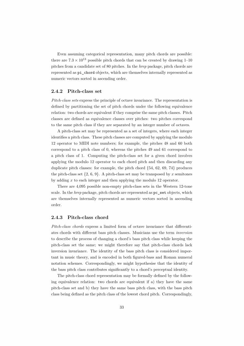
Even assuming categorical representation, many pitch chords are possible:there are 7.3× 1013 possible pitch chords that can be created by drawing 1–10pitches from a candidate set of 80 pitches. In the hrep package, pitch chords arerepresented as pi_chord objects, which are themselves internally represented asnumeric vectors sorted in ascending order.

2.4.2 Pitch-class set

Pitch-class sets express the principle of octave invariance. The representation isdefined by partitioning the set of pitch chords under the following equivalencerelation: two chords are equivalent if they comprise the same pitch classes. Pitchclasses are defined as equivalence classes over pitches: two pitches correspondto the same pitch class if they are separated by an integer number of octaves.

A pitch-class set may be represented as a set of integers, where each integeridentifies a pitch class. These pitch classes are computed by applying the modulo12 operator to MIDI note numbers; for example, the pitches 48 and 60 bothcorrespond to a pitch class of 0, whereas the pitches 49 and 61 correspond toa pitch class of 1. Computing the pitch-class set for a given chord involvesapplying the modulo 12 operator to each chord pitch and then discarding anyduplicate pitch classes: for example, the pitch chord {54, 62, 69, 74} producesthe pitch-class set {2, 6, 9}. A pitch-class set may be transposed by x semitonesby adding x to each integer and then applying the modulo 12 operator.

There are 4,095 possible non-empty pitch-class sets in the Western 12-tonescale. In the hrep package, pitch chords are represented as pc_set objects, whichare themselves internally represented as numeric vectors sorted in ascendingorder.

2.4.3 Pitch-class chord

Pitch-class chords express a limited form of octave invariance that differenti-ates chords with different bass pitch classes. Musicians use the term inversionto describe the process of changing a chord’s bass pitch class while keeping thepitch-class set the same; we might therefore say that pitch-class chords lackinversion invariance. The identity of the bass pitch class is considered impor-tant in music theory, and is encoded in both figured-bass and Roman numeralnotation schemes. Correspondingly, we might hypothesise that the identity ofthe bass pitch class contributes significantly to a chord’s perceptual identity.

The pitch-class chord representation may be formally defined by the follow-ing equivalence relation: two chords are equivalent if a) they have the samepitch-class set and b) they have the same bass pitch class, with the bass pitchclass being defined as the pitch class of the lowest chord pitch. Correspondingly,

33

a pitch-class chord may be represented as a tuple of its bass pitch class and itspitch-class set; for example, the pitch chord {54, 62, 69, 74} can be representedas the pitch-class chord (6, {2, 6, 9}). Like pitch-class sets, pitch-class chordsmay be transposed by x semitones by adding x to each integer modulo 12.

There are 24,576 possible non-empty pitch-class chords in the Western 12-tone scale. In the hrep package, pitch-class chords are represented as pc_chordobjects, which are themselves internally represented as numeric vectors, with thefirst element corresponding to the bass pitch class and the remaining elementscorresponding to the non-bass pitch classes sorted in ascending order.

2.4.4 Pitch chord type

Pitch chord types express transposition invariance, and are defined by the fol-lowing equivalence relation: chords are equivalent if they can be transposedto the same pitch chord representation. Pitch chord types are represented assets of integers, where each chord note is represented as its pitch interval fromthe bass note. Given a pitch chord, the pitch chord type may be computed bysimply subtracting the bass note from all pitches: for example, the pitch chordtype of the pitch chord {54, 62, 69} is {0, 8, 15}. In the hrep package, pitchchord types are represented as pi_chord_type objects, which are themselvesinternally represented as numeric vectors sorted in ascending order.

2.4.5 Pitch-class chord type

The pitch-class chord type representation combines the invariances of the pitchchord type representation and the pitch-class chord representation: it expressesboth transposition invariance and a limited form of octave invariance that differ-entiates chords with different bass pitch classes. The representation may also bedefined by the following equivalence relation: chords are equivalent if they canbe transposed to the same pitch-class chord representation. Pitch-class chordtypes are represented as sets of integers, where each chord note is represented asits pitch-class interval from the bass pitch class.5 For example, the pitch-classchord type of the pitch-class chord (6, {2, 9}) is {0, 3, 8}. In the hrep pack-age, pitch-class chord types are represented as pc_chord_type objects, whichare themselves internally represented as numeric vectors sorted in ascending or-der. There are 2,048 possible non-empty pitch-class chord types in the Western12-tone scale.

5The pitch-class interval from x to y is defined as (y − x) mod 12.

34

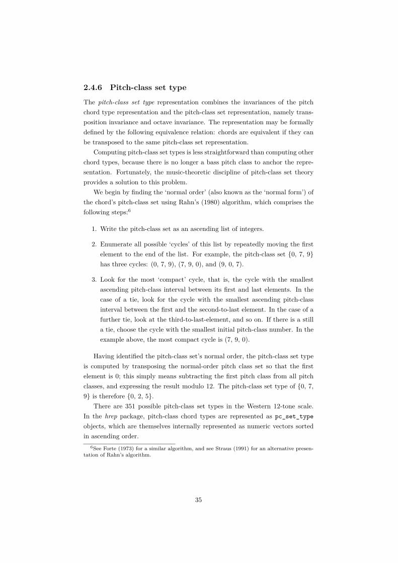
2.4.6 Pitch-class set type

The pitch-class set type representation combines the invariances of the pitchchord type representation and the pitch-class set representation, namely trans-position invariance and octave invariance. The representation may be formallydefined by the following equivalence relation: chords are equivalent if they canbe transposed to the same pitch-class set representation.

Computing pitch-class set types is less straightforward than computing otherchord types, because there is no longer a bass pitch class to anchor the repre-sentation. Fortunately, the music-theoretic discipline of pitch-class set theoryprovides a solution to this problem.

We begin by finding the ‘normal order’ (also known as the ‘normal form’) ofthe chord’s pitch-class set using Rahn’s (1980) algorithm, which comprises thefollowing steps:6

1. Write the pitch-class set as an ascending list of integers.

2. Enumerate all possible ‘cycles’ of this list by repeatedly moving the firstelement to the end of the list. For example, the pitch-class set {0, 7, 9}has three cycles: (0, 7, 9), (7, 9, 0), and (9, 0, 7).

3. Look for the most ‘compact’ cycle, that is, the cycle with the smallestascending pitch-class interval between its first and last elements. In thecase of a tie, look for the cycle with the smallest ascending pitch-classinterval between the first and the second-to-last element. In the case of afurther tie, look at the third-to-last-element, and so on. If there is a stilla tie, choose the cycle with the smallest initial pitch-class number. In theexample above, the most compact cycle is (7, 9, 0).

Having identified the pitch-class set’s normal order, the pitch-class set typeis computed by transposing the normal-order pitch class set so that the firstelement is 0; this simply means subtracting the first pitch class from all pitchclasses, and expressing the result modulo 12. The pitch-class set type of {0, 7,9} is therefore {0, 2, 5}.

There are 351 possible pitch-class set types in the Western 12-tone scale.In the hrep package, pitch-class chord types are represented as pc_set_typeobjects, which are themselves internally represented as numeric vectors sortedin ascending order.

6See Forte (1973) for a similar algorithm, and see Straus (1991) for an alternative presen-tation of Rahn’s algorithm.

35

2.4.7 Further issues

Translating to pitch chords

A common task in harmony cognition research is to play a participant a chordsequence from a musical corpus that only provides pitch classes, not pitch heights(e.g. the pitch-class chord representation). If the researcher wishes to play thesechords using standard musical instruments, they must assign pitch heights tothese chord tones. It is possible to address this problem using simple heuristics,such as assigning the bass pitch class to the octave below middle C and theremaining pitch classes to the octave above middle C (e.g. Chapter 4), butthe outcome is typically aesthetically unsatisfying and musically unrealistic.To address this problem, Chapter 5 presents a data-driven algorithm that findsoptimised voicings for chord sequences on the basis of a variety of psychoacousticfeatures. This algorithm is implemented in a publicly available R package calledvoicer.7

Potential extensions

Each of these representations conveys a binary notion of presence: a chordcomponent (e.g. a pitch or pitch class) may be absent or present, but nothing inbetween. It could be useful to incorporate a more graduated notion of presence,to represent the fact that given chord components might be weighted morethan others, perhaps by doubling pitch classes, playing notes more loudly, orsituating notes in more perceptually salient registers. It could also be useful todifferentiate newly sounded notes from notes that are sustained from a previouschord. Both of these types of metadata could be incorporated as numeric orBoolean vectors with the same length as the original note vector.

Omissions

We have purposefully omitted the ‘prime form’ representation from pitch-classset theory, which expresses octave invariance, transposition invariance, and re-flection invariance (Forte, 1973; Rahn, 1980).8 Our reasoning is that there islittle evidence for reflection invariance in harmony perception: for example, themajor and minor triads are reflections of each other, yet they imply oppositeemotional valences to Western listeners (‘happy’ versus ‘sad’ respectively).9

7https://github.com/pmcharrison/voicer8Pitch-class set theorists typically use the word ‘inversion’ instead of ‘reflection’, but we

use the latter to avoid confusion with the unrelated concept of inversion in tonal harmony.For example, suppose that we wish to reflect the major-triad pitch-class set {0, 4, 7} aboutthe pitch-class 4: we have 0 → 8, 4 → 4, and 7 → 1, producing the minor-triad pitch-class set{1, 4, 8}.

9However, see Dienes & Longuet-Higgins (2004) and Krumhansl, Sandell, & Sergeant (1987)for studies of inversion salience in the perception of serially presented tone rows.

36

We have also purposefully omitted several representations commonly usedto study voice leading. A multiset generalises the notion of pitch chords andpitch-class sets to differentiate between chords containing different numbers ofthe same element, for example {C, C, E, G} (e.g. Tymoczko, 2008). A voiceleading describes how each element of one chord moves to an element in thenext chord, for example {F → E, A → G, C → C} (Tymoczko, 2008), and avoice-leading type is a transpositionally equivalent set of voice leadings (Quinn &Mavromatis, 2011; see Sears et al., 2017 for a related definition).10 By omittingthese voice-leading representations, we acknowledge the conventional distinc-tion between harmony (the construction and arrangement of chords) and voiceleading (connecting the constituent notes of successive musical chords to formsimultaneous melodies).

2.5 Acoustic representationsAcoustic representations describe how chords manifest as sound. If the listeneris modelled as an information-processing system, then acoustic representationscorrespond to the listener’s input data formats.

As previously noted, our symbolic representations assume categorical pitchperception, where each chord note is subsumed into semitone-width categories.The acoustic representations relax this assumption, allowing chord tones to takecontinuous pitch and frequency values. This reflects the non-cognitive natureof the sound signal.

2.5.1 Frequency chord

Each frequency chord is represented as a set of positive real numbers, corre-sponding to the fundamental frequencies of the chord tones as realised by theperformer. The mapping between chord pitches and chord frequencies is spec-ified by a tuning system. One possible tuning system is 12-tone equal temper-ament, where the octave is defined as a 2:1 frequency ratio and the semitonesequally divide the octave. This tuning system is formalised as follows:

f = fref × 2(p−69)/12 (2.1)

where f is the frequency (Hz), fref is the reference frequency (typically 440 Hz),and p is the pitch, expressed as a MIDI note number. In practice, stretchedtunings are sometimes adopted, such that the octave corresponds to slightly

10Sears et al.’s (2017) representation only captures the voice leading between successive bassnotes, and expresses each successive chord as a set of pitch-class intervals above the bass note;it may be considered a hybrid between harmonic and voice-leading approaches.

37

more than a 2:1 ratio. One such stretched tuning can be produced by replacing12 with 11.9 in Equation 2.1, producing a stretch of approximately 10 cents peroctave (Parncutt & Strasburger, 1994).

Many instruments do not force a tuning system upon the performer, butinstead support dynamic pitch adjustments that can reflect the particular har-monic and melodic functions of the notes being played. It is difficult to simulatethese dynamic adjustments from the musical score alone; however, these adjust-ments can theoretically be recovered from audio signals using polyphonic signaltranscription (see Section 2.9.3).

2.5.2 Sparse frequency spectrum

The sparse frequency spectrum is generated from the frequency chord by incor-porating knowledge of the spectral content of the tones used to play the chord(Figure 2.2A). Each chord tone is modelled as a complex tone, defined as a super-position of pure tones, each of known frequency and amplitude. This definitionignores phase as well as any temporal evolution of the chord tones. Pitchedinstruments are typically modelled as harmonic complex tones, where the ithpartial has a frequency i times that of the fundamental frequency and an ampli-tude that decreases steadily with increasing i. The ith partial is then termed theith harmonic. Similar to previous literature (e.g. Hutchinson & Knopoff, 1978;Milne & Holland, 2016; Parncutt & Strasburger, 1994), we default to modellingeach complex tone with 11 partials, and give the ith partial an amplitude of1/i, with the amplitudes being provided in arbitrary units. These defaults aresomewhat arbitrary, and the researcher is encouraged to adjust the number ofharmonics and their amplitudes to reflect the particular sound being modelled.

Once each chord tone is decomposed into its partials, these partials mustbe combined together into one spectrum. For this combination process, it iscommon to define a procedure for combining partials from different tones with(approximately) the same frequency. Such a procedure requires two decisions:a) how close do two partials need to be before they will be combined, and b)what is the amplitude of the resulting partial. The latter question is easy toanswer: in most musical instruments, different chord tones will be produced bydifferent oscillators, so they will have incoherent phases, and it is a standardresult that the incoherent superposition of two waves with (approximately) iden-tical frequencies and amplitudes x, y yields a resultant amplitude of

(x2 + y2)0.5. (2.2)

The former question has a less consistent answer in the literature. Here weadopt the heuristic of expressing each frequency as a (possibly non-integer) MIDI

38

0.00

0.25

0.50

0.75

1.00

0 1000 2000 3000 4000Frequency (Hz)

Am

plitu

de

A

−0.10

−0.05

0.00

0.05

0.10

0.15

0.00 0.01 0.02 0.03 0.04 0.05Time (seconds)

Dis

plac

emen

t

D

0.00

0.25

0.50

0.75

1.00

50 60 70 80 90 100 110Pitch (MIDI)

Am

plitu

de

B

0.00

0.02

0.04

0.06

60 80 100Pitch (MIDI)

Wei

ght

E

0.0

0.3

0.6

0.9

1.2

0 2 4 6 8 10Pitch class

Am

plitu

de

C

0.000

0.025

0.050

0.075

0 2 4 6 8 10 12Pitch class

Wei

ght

F

Figure 2.2: Acoustic and sensory representations for a C major chord in firstinversion comprising the MIDI pitches {52, 60, 67}, synthesised with 11 har-monics with amplitude roll-off 1/n. (A) Sparse frequency spectrum; (B) sparsepitch spectrum; (C) sparse pitch-class spectrum; (D) waveform; (E) smoothpitch spectrum; (F) smooth pitch-class spectrum.

39

note number, rounding the MIDI note number to six decimal places, combin-ing any partials with identical results, and translating the MIDI note numbersback to frequencies. Six decimal places should be sufficiently precise to differ-entiate non-identical partials in most practical contexts, but sufficiently lax tobe robust to floating-point inaccuracies in software implementations. Alterna-tively, one could adopt a perceptually motivated criterion related to perceptualdiscrimination thresholds.

Ideally, computational models taking sparse frequency spectra as inputshould be invariant, in the limit, to the arbitrary decision of whether or notto combine to partials with almost-identical frequencies; unfortunately, this isseldom true in practice. For example, Dillon (2013) explains how several historicconsonance models (e.g. Hutchinson & Knopoff, 1978; Sethares, 1993, 2005) failto express invariance to partial combination, and presents an alternative conso-nance model that captures this desired invariance. However, this model has yetto be systematically tested, and it is therefore unclear how much the invarianceprinciple matters in practice.

2.5.3 Sparse pitch spectrum

The sparse pitch spectrum corresponds to a version of the sparse frequencyspectrum where partial frequencies are expressed as MIDI note numbers (Fig-ure 2.2B). This logarithmic transformation provides a more intuitive way ofvisualising how spectral content maps to the Western scale, and provides a bet-ter account of the subjective notion of pitch distance. The mapping betweenfrequency and MIDI note number is defined by Equation 2.1; note that theresulting MIDI note numbers can take non-integer values.

2.5.4 Sparse pitch-class spectrum

The sparse pitch-class spectrum corresponds to an octave-invariant version ofthe sparse pitch spectrum (Figure 2.2C). It can be computed from the sparsepitch spectrum by expressing each pitch as a pitch class (using the modulo12 operation) and combining partials with identical pitch classes. As before,pitch classes are rounded to six decimal places before testing for equality, andamplitudes are combined assuming incoherent summation (Equation 2.1).

It is also possible to compute pitch-class spectra from pitch-class sets, be-cause both representations are invariant to octave transpositions of chord tones.This may be achieved by constructing a pitch chord containing one instantiationof every pitch class in the pitch-class set, and then computing the sparse pitchspectrum and hence the sparse pitch-class spectrum as described above.

40

The sparse pitch-class spectrum is closely related to the chroma vector rep-resentation commonly used in music audio analysis (e.g. Collins et al., 2014;Lartillot et al., 2008); both are octave-invariant representations that capture theperceptual notion of chroma. The primary difference between the two is thatthe former represents the pitch-class domain as a continuous space, whereasthe latter partitions the pitch-class domain into 12 categories. The former ap-proach is preferable for an acoustic representation because it avoids imposingthe cultural assumption of a specific scale system.

2.5.5 Waveform

The waveform characterises the chord as the fluctuation of sound pressure overtime (Figure 2.2D). It may be computed from the sparse frequency spectrumusing additive synthesis, where separate sine waves are computed for each par-tial in the spectrum, and then additively combined. This operation may beapproximately reversed by conducting a Fourier transform and then applyinga spectral peak-picking algorithm (see e.g. Essentia toolbox, Bogdanov et al.,2013; Mirtoolbox, Lartillot et al., 2008).

2.6 Sensory representationsSensory representations describe perceptual internalisations of acoustic signals.They may be seen as indirect consequences of symbolic representations, in thatexplicit symbolic representations in musical scores are translated by musiciansinto performances, which are then heard by listeners. They may also be seen aspsychological predecessors to listeners’ internal and implicit symbolic represen-tations, automatically derived from sensory representations through processesof categorical perception and template recognition (Figure 2.3).

2.6.1 Smooth pitch/pitch-class spectra

In order to simulate how perceptual inaccuracies reduce the effective resolu-tion of pitch perception, computational implementations of sensory representa-tions can apply pitch-domain smoothing. Milne and colleagues have shown thata simple model of this smoothing effect is remarkably effective for reproduc-ing a variety of musical phenomena (e.g. diatonic tonality, Milne et al., 2015;harmonic distance, Milne & Holland, 2016; perceived change, Dean, Milne, &Bailes, 2019). Our smooth spectra representations are computed from sparsespectra using this smoothing technique. The sparse spectrum is first expressedas a dense spectrum, a numeric vector where each bin corresponds to a pitch

41

Musical sound

Music theorists

Explicit symbolic representations

Listeners

Implicit symbolic representations

Sensory representations

Composers

Implicit symbolic representations

Sensory representations

Explicit symbolic representations

Music composition

Music performance

Music pedagogy

Representations

Musical behaviours

Musical scores

Explicit symbolic representations

Music recording

Acoustic representations

Figure 2.3: Schematic diagram illustrating the role of symbolic, acoustic, andsensory representations in different musical activities. Explicit symbolic repre-sentations are used in musical scores, which are analysed by music theorists toyield insights into musical practice, insights which are then conveyed to com-posers through music pedagogy. These explicit symbolic representations re-flect implicit symbolic representations held by music listeners, which are them-selves derived from sensory representations that listeners construct from musicalsound, which can be recorded using acoustic representations.

42

window of one cent (i.e. a hundredth of a semitone) and each bin value cor-responds to the spectral amplitude in that pitch window. This is achieved byinitialising a 0-indexed vector of zeros with 1200 elements per octave, where the0th element corresponds to 0 cents, the 1st element corresponds to 1 cent, andso on, and then iterating through every partial in the sparse spectrum, roundingits frequency to the nearest cent, and incrementing the corresponding elementin the vector using the incoherent amplitude summation rule (Equation 2.1).To produce the smooth spectrum, we then convolve this dense spectrum witha Gaussian function with unit mass and standard deviation of 10 cents, afterDean et al. (2019). In the case of pitch-class spectra, this should be a circularconvolution, so that the smoothing wraps round the extremes of the pitch-classvector. Perceptual similarity between smooth spectra can then be simulatedusing geometric similarity measures such as cosine similarity:

s(x,y) =∑

i xiyi√∑j x

2j

∑k y

2k

(2.3)

where s(x,y) is the cosine similarity between vectors x and y, and xi, yi denotethe ith elements of x and y respectively. This method can be used to producetwo types of smooth spectrum: the smooth pitch spectrum (Figure 2.2E), andthe smooth pitch-class spectrum (Figure 2.2F). Both pitch (Dean et al., 2019;Milne et al., 2016) and pitch-class versions (Milne & Holland, 2016; Milne etal., 2015) have proved useful in perceptual modelling.

Several subtleties should be acknowledged when implementing these spec-tral smoothing techniques. First, the original presentation of the techniquetreated the smoothed spectrum as an ‘expectation vector’, with each elementbeing interpreted as the expected number of tones that the listener should hearat that pitch or pitch class (Milne et al., 2011). However, this probabilisticinterpretation has limited empirical basis, and subsequent work often prefers aless specific ‘perceptual weight’ interpretation. Second, Milne assumed that theith harmonic of a harmonic complex tone should additively contribute a valueof 1/iρ to this perceptual weight spectrum, where ρ is a numeric parameteroptimised to the data. This assumption of additive combination in perceptualspace is difficult to reconcile with the formula for the acoustic combination ofincoherent partials (Equation 2.1). However, in later work Milne and colleaguesremove this inconsistency by applying the smoothing directly to the acousticamplitude spectrum (Dean et al., 2019). We prefer this latter approach for itsapplicability to arbitrary acoustic spectra, but implement both approaches inthe hrep package.

As is apparent from Figure 2.1, the computational translation from pitch-

43

class sets to smooth pitch-class spectra is not well-defined. This is because pitch-class sets discard information about the number of chord pitches representingeach pitch class, information which is retained implicitly in the smooth pitch-class spectrum. However, if necessary a representative spectrum can still becomputed by assuming that each pitch class is assigned exactly one chord pitch.

2.6.2 Potential alternatives

Several other researchers have formulated perceptual representation schemesthat can be applied to harmony modelling. Parncutt & Strasburger (1994)present a psychoacoustic model of music perception, based on Terhardt’s (1982a)pitch perception model, that incorporates features such as auditory masking andspectral-domain pitch detection. We have implemented this model in the freelyavailable R package parn94.11 This model can be used as an alternative to thesmooth pitch spectrum representation described here. Leman (2000a) providesan alternative psychoacoustic model of pitch perception, which combines VanImmerseel & Martens’ (1992) simulation of the auditory periphery with a time-domain pitch detection algorithm. The model takes an audio signal as input,and returns a time-varying vector of activations for different pitch windows; thisrepresentation can then be used as an alternative for the smooth pitch spectrumrepresentation.12 Collins et al. (2014) implement two further representationsthat derive from Leman’s (2000a) representation: a chroma vector representa-tion and a tonal space representation. The chroma vector representation addsoctave invariance, whereas the tonal space representation projects Leman’s rep-resentation onto a self-organising map in the shape of a torus, intended tocapture the topological structure of Western tonality.13 Each of these models(Collins et al., 2014; Leman, 2000a; Parncutt, 1989) add significant complexityto the process of deriving sensory representations; future work needs to examinethe extent to which this added complexity is useful for characterising harmonycognition.

2.7 AlphabetsWhen analysing the statistics of chord progressions, it is useful to define an‘alphabet’ that enumerates each of the possible values for the chord representa-tion. For example, this alphabet could define the indices of an n-gram transition

11https://github.com/pmcharrison/parn94; https://doi.org/10.5281/zenodo.254575912At the time of writing, Leman’s (2000a) model was available in the IPEM toolbox, hosted

at https://github.com/IPEM/IPEMToolbox.13At the time of writing, the implementation of Collins et al. (2014) was available in

the Janata Lab Music Toolbox, hosted at http://atonal.ucdavis.edu/resources/software/jlmt/.

44

matrix, or the coding of a one-hot input vector for a neural network. The clas-sic harmonic alphabet from the literature is the ‘Forte number’, which indexesthe prime forms of pitch-class sets;14 however, this representation is not partof our representational network for reasons discussed previously. We insteaddefine new alphabets for four representations in our network: pitch-class sets,pitch-class set types, pitch-class chord types, and pitch-class chords.

2.7.1 Pitch-class set

As defined above, a pitch-class set is a non-empty unordered set of integersbetween 0 and 11 inclusive (e.g. {0, 4, 7}). A pitch-class set may be encoded asfollows:

1. Represent the pitch-class set as a 0-indexed binary vector of length 12,where the ith element is 1 if the pitch-class set contains the pitch class i

and 0 otherwise. The pitch-class set {0, 4, 7} would therefore receive thebinary vector representation ‘100010010000’.

2. Reinterpret this binary vector as a base-2 number.

3. Convert this base-2 number to a base-10 integer.15

The result is an integer encoding that ranges between 1 and 4,095; for example,{11} is coded as 1, {10} is coded as 2, {10, 11} is coded as 3, and {0, 4, 7} iscoded as 2,192. The full alphabet can then be enumerated by iterating throughthe integers from 1 to 4,095.

2.7.2 Pitch-class set type

As defined above, pitch-class set types define transpositionally invariant equiv-alence classes over pitch-class sets; for example, the pitch-class set type {0, 4,8} contains the pitch-class sets {0, 4, 8}, {1, 5, 9}, {2, 6, 10}, and {3, 7, 11}.The alphabet of pitch-class set types is constructed as follows:

1. Initialise an empty list.

2. Iterate sequentially through the pitch-class set alphabet, and:

(a) Compute the pitch-class set type of the pitch-class set;

(b) If this is the first occurrence of that pitch-class set type, append itto the list.

14See Carter (2002) and Martino (1961) for related efforts.15A binary vector of length 12 can be converted to a base-10 integer by multiplying each

ith element (1 ≤ i ≤ 12) by 212−i and summing the result.

45

The resulting alphabet maps pitch-class set types to integers between 1 and351; for example, {0} maps to 1, {0, 1} maps to 2, {0, 2} maps to 3, and {0, 1,2} maps to 4.

2.7.3 Pitch-class chord type

As defined above, pitch-class chord types define transpositionally invariantequivalence classes over pitch-class chords; for example, the pitch-class chords(0, {4, 7}) and (1, {5, 8}) both belong to the pitch-class chord type {0, 4, 7}.By definition, the integer-vector representation of the pitch-class chord typemust begin with 0; the remaining elements may then be drawn arbitrarily fromthe integers 1 to 11. Correspondingly, pitch-class chord types are encoded asfollows:

1. Construct a 1-indexed binary vector of length 11, where the ith elementis 1 if the integer vector contains i and 0 otherwise.

2. Convert the resulting binary vector to base 10.

3. Add 1.

The resulting alphabet maps pitch-class chord types to integers between 1 and2,048; for example, {0} maps to 1, {0, 1} maps to 1,025, and {0, 4, 7} maps to145.

2.7.4 Pitch-class chord

Each of the 2,048 pitch-class chord types is an equivalence class containing ex-actly 12 pitch-class chords with 12 different bass pitch classes. Correspondingly,pitch-class chords are encoded as follows:

1. Take the bass pitch class of the pitch-class chord, expressed as an integer.

2. Multiply it by 2,048.

3. Add the integer encoding of the pitch-class chord type.

The resulting alphabet maps pitch-class chords to integers between 1 and24,576; for example, (0, {3, 6}) maps to 289, (0, {4, 7}) maps to 145, and (4,{0, 7}) maps to 8,457.

46

2.8 Deriving higher-level representationsThe low-level representations described above are intended to reflect relativelyearly stages of perceptual and cognitive processing. We will now discuss severalhigher-level cognitive representations for harmonic structure, alongside ways inwhich these representations may be simulated.

2.8.1 Voice leading

Chords played in succession can imply latent melodic lines, even if these melodiclines are not made explicit by performance characteristics such as timbre andloudness. Under Bregman’s (1990) terminology of auditory scene analysis, wecan say that successive notes in chord progressions are grouped into parallel au-ditory streams, where individual streams cohere on the basis of pitch proximitybetween adjacent notes. This organization into auditory streams, or melodiclines, may be termed voice leading.

We may wish to simulate this process of inferring voice leading from a chordsequence. Tymoczko (2006) has presented an efficient algorithm for computingvoice leadings within pairs of chords; this algorithm deterministically finds avoice leading that minimises the aggregate distance moved by the individualmelodic lines. In its original presentation, the algorithm finds minimal voiceleadings between pitch-class sets, but it can trivially be modified to find minimalvoice leadings between pitch chords. We have implemented this algorithm inthe freely available R package minVL.16

2.8.2 Chord roots

Chord roots have been considered central to harmonic analysis since Rameau(1722). A chord root may be defined as a single pitch class that summarisesthe tonal content of a given chord. Chords are often notated with reference tothese roots: for example, lead sheets typically represent chords by combiningthe root pitch class (written in letter-name notation, e.g. ‘D’) with a textuallabel expressing the other pitch classes relative to the root (e.g. ‘maj7’ impliesthat the chord contains pitch classes 0, 4, 7, and 11 semitones above the root).Roman numeral notation also uses chord roots, which are typically expressedrelative to the local tonic (see Section 2.8.3).

It has been proposed that chord roots have a psychological basis in pitch per-ception (Parncutt, 1988; Terhardt, 1974, 1982). Terhardt and Parncutt arguethat listeners infer fundamental frequencies of acoustic spectra by comparingthese spectra to harmonic templates with different fundamental frequencies.

16https://github.com/pmcharrison/minVL

47

Candidate fundamental frequencies are perceived as virtual pitches, which Ter-hardt and Parncutt equate with chord roots. Recent empirical work indeedsupports the notion that chord roots correspond to chord tones with particu-larly high perceptual salience, and that this perceptual salience can be predictedby computational models of pitch detection (Parncutt et al., 2019).

These empirical results motivate the use of root-finding models for simulat-ing higher-level cognitive representations of harmonic structure. Various root-finding models exist, some deriving from psychoacoustics, some deriving frommusic theory, and some deriving from statistical modelling. A key example ofthe psychoacoustic approach is Parncutt’s (1988) root-finding model, which wasderived from Terhardt’s (1982) root-finding model and subsequently extendedin Parncutt (1997). The model provides a straightforward hand-computableapproach to estimating the chord root for a given pitch-class set; we have im-plemented it in the freely available R package parn88.17 Parncutt’s (1989) modelrelaxes the octave equivalence assumption and provides a much more detailedaccount of peripheral psychoacoustic processes such as masking (see also Parn-cutt & Strasburger, 1994); we have implemented this model in the R packageparn94.18 Examples of the music-theoretic approach include Temperley’s (1997)algorithm, Pardo & Birmingham’s (2002) template-matching algorithm, Sapp’s(2007) stack-of-thirds algorithm, and Cambouropoulos et al.’s (2014) generalchord type algorithm. Raphael & Stoddard’s (2004) algorithm follows the sta-tistical approach, performing harmonic analysis using Hidden Markov Models.These root-finding algorithms provide several options for simulating root-basedcognitive representations of harmonic structure.

2.8.3 Tonality

The notion of tonality is fundamental to Western music theory. Common-practice tonality is said to be organised around 24 possible keys, where eachkey is defined by a) choosing one of the 12 pitch classes to be the tonic and b)choosing one of the two diatonic modes: major and minor. The chosen key isthen reflected in the distribution of notes selected by the composer. The sevenmost common pitch classes in a given key constitute the key’s scale, from whichmost of the pitch material is drawn.

Music theorists often represent chord progressions relative to the tonic. Suchrepresentations may be termed scale-degree representations, because each pitchclass is represented as a degree of the key’s underlying scale. It is thought thatWestern listeners also form implicit scale-degree representations when listening

17https://github.com/pmcharrison/parn8818https://github.com/pmcharrison/parn94

48

to Western tonal music (e.g. Arthur, 2018). The key challenge in constructingsuch representations automatically is to simulate the process of key finding; thatis, given a musical extract, to estimate the underlying key at each point in theextract.

Various key-finding models have been introduced over the years. Arguablymost influential is the Krumhansl-Schmuckler algorithm (Krumhansl, 1990),which estimates the key of a given musical passage by correlating pitch-classprevalences in a given musical extract (termed key profiles) with experimen-tally determined key profiles for major and minor keys. Several variants on thisapproach have subsequently been presented, with these variants modifying thekey profiles (Aarden, 2003; Albrecht & Shanahan, 2013; Bellmann, 2005; Sapp,2011; Temperley, 1999), replacing key profiles with interval profiles (Madsen &Widmer, 2007), adding psychoacoustic modelling (Huron & Parncutt, 1993), im-plementing sliding windows (Shmulevich & Yli-Harja, 2000), and incorporatingself-organising maps (Schmuckler & Tomovski, 2005). Outside the Krumhansl-Schmuckler tradition, several algorithms instead take statistical approaches tokey finding, including Temperley’s (2007) Bayesian model, Hu & Saul’s (2009)probabilistic topic model, Quinn’s (2010) chord-progression model, and White’s(2018) feedforward model. Chew (2002) has also presented an approach foridentifying key regions within a musical piece based on the geometric SpiralArray model (Chew, 2000). These models provide many options for simulatingkey-based representations of harmonic progressions.

For music theorists, tonality typically implies more than key finding: it alsodescribes high-level principles such as how certain chords are more stable thanothers, how certain chords tend to resolve to other chords, and how harmonicprogressions can be organised into hierarchies that potentially span the entiremusical piece. These principles are typically characterised as both musical andperceptual: they are intended to describe both how tonal music is created bycomposers and how it is perceived by listeners. Various models have been de-veloped to summarise these principles of tonal harmony, which typically embedchords within some kind of ‘tonal space’ within which the notion of distance be-tween chords is well-defined. One prominent example is Lerdahl’s (1988) TonalPitch Space model, which operates on a symbolic level and is based on a hierar-chical conceptualisation of the Western chromatic scale. A contrasting exampleis the Tonal Space model of Janata et al. (2002; see also Collins et al., 2014),which projects audio input onto a toroidal (‘doughnut-shaped’) self-organisingmap. Pretrained on an artificial melody that modulates through all 24 diatonickeys, the Tonal Space model is supposed to learn a topological representation ofWestern tonality (see also Toiviainen & Krumhansl, 2003). These kinds of mod-

49

els may be used to simulate tonality-based cognitive representations of harmonicprogressions.

2.8.4 Functional harmony

Music theorists often assign chords to functional categories such as ‘tonic’, ‘dom-inant’, and ‘subdominant’. These categories reflect the chord’s implications forsurrounding chords: for example, dominant chords are particularly likely to befollowed by tonic chords. The categories are typically associated with certainchord roots, expressed relative to the prevailing tonality: for example, the dom-inant chord category is particularly associated with chord roots situated on thefifth degree of the prevailing diatonic scale. It is possible that untrained Westernlisteners also possess implicit knowledge of these functional categories, acquiredthrough incidental exposure to Western music. Recent work has demonstratedthat the acquisition of these functional categories can be simulated using com-putational techniques such as hidden Markov models (White & Quinn, 2018)and the information bottleneck algorithm (Jacoby, Tishby, & Tymoczko, 2015).Such algorithms could be incorporated within cognitive models of harmony per-ception to simulate implicit knowledge of functional chord categories.

2.9 Corpus translationMusic cognition research often takes advantage of corpora of music composi-tions, typically either to analyse the cognitive principles underlying the creativeprocess, or to simulate processes of statistical learning from lifetime musicalexposure. Various corpora of chord sequences exist, but these corpora are typi-cally not expressed in the representation schemes described above. We will nowdescribe various solutions to this problem.

2.9.1 Textual symbols

Many digitally encoded music corpora notate chords using textual symbols suchas ‘min9’ and ‘sus4’ (e.g. the Billboard Corpus, Burgoyne, 2011; the iRb corpus,Broze & Shanahan, 2013). Translating these corpora into our representationalnetwork requires decoding these symbols. Unfortunately this is a poorly definedtask, as there is no canonic mapping between these symbols and pitch-class con-tent; instead, musicians use their experience to interpret these symbols, and canexert freedom to choose different chord realisations on the basis of musical con-text and personal preference. Ideally, a cognitive musicologist would formalisethis process by analysing many performances and quantifying the frequencywith which different textual symbols are mapped to different chord pitches in

50

different contexts. However, in the absence of such prior work, a useful stopgapis to construct a mapping between textual symbols and chord pitches on thebasis of music theory, and use this mapping to translate corpora such as theBillboard Corpus and the iRb corpus into our representational network. Whilesuch a mapping will not capture all the nuances of real-life performance, itshould nonetheless provide a useful approximation for supporting downstreampsychoacoustic and cognitive analyses.

We have compiled such a mapping between textual symbols and chordpitches. Reflecting the typical construction of lead sheets, these textual sym-bols correspond to chord qualities, expressing the pitch-class content of a chordrelative to the chord’s root. This mapping can be accessed through the func-tion decode_chord_quality in the hrep R package. Assuming that the chord’sroot (and possibly its bass note) can be extracted by an automatic parser, thismapping is theoretically sufficient to convert the chord symbols of a lead sheetinto pitch-class chord representations. In practice, new corpora and notationschemes are likely to contain occasional textual symbols not present in our map-ping; however, these cases should be rare enough for the researcher to updatethe mapping manually. We would like to encourage future researchers to sub-mit such updates to the package’s online repository,19 so that the mapping canbecome more comprehensive with time. Using this mapping, we have translatedthe Billboard popular music corpus and the iRb corpus into pitch-class chordnotation. The resulting corpora are available in our hcorp package.20

It may sometimes be useful to perform the reverse operation, mappinginteger-based representations of chords to textual symbols. To this end, Hedges& Wiggins (2016b) provide a useful algorithm that takes as input a pitch-classset, which should be expressed relative to the chord root, and returns a textuallabel corresponding to the chord quality, for example ‘min7’, ‘dim’, or ‘sus’.Combined with a root-finding algorithm (e.g. Cambouropoulos et al., 2014;Parncutt, 1988, 1997; Sapp, 2007), this algorithm could be used to convert thesymbolic representations described here into a text-based format readable bymusicians.

2.9.2 Polyphonic scores

Music corpora from the tradition of Western art music typically do not notatechord sequences explicitly, but instead notate the full polyphonic texture of theoriginal musical scores. An important challenge for harmonic analysis is thento derive chord sequences from these polyphonic textures.

19http://hrep.pmcharrison.com20https://github.com/pmcharrison/hcorp

51

One approach is full expansion (Conklin, 2002), also known as ‘salami slicing’or ‘chordifying’. Here the composition is partitioned into chords at each pointwhere a new onset occurs in any voice.21 Each chord is then defined as the fullset of pitches that sound within the corresponding partition. An advantage ofthis approach is that it is straightforward to automate, and it captures much ofthe detail present in the original musical score. We have translated a corpus of370 chorale harmonisations by J. S. Bach into pitch chords using this approach,and have made the resulting corpus available in the hcorp package.22

A limitation of full expansion is that it fails to differentiate the function ofdifferent tones within a sonority. Music theorists often differentiate tones into‘chord tones’ and ‘non-chord tones’, where the chord tones represent a prototyp-ical sonority such as a major or minor triad, and the non-chord tones embellishthis sonority through techniques such as suspensions and passing notes. De-pending on the application, a researcher may wish to exclude chord tones fromtheir chord sequences, and potentially even add implied but missing chord tones(e.g. the fifth in a seventh chord). This differentiation of chord tones from non-chord tones is vital for chord labelling (deriving labels such as ‘maj9’, ‘sus4’) andfor functional harmonic analysis. Unfortunately, the process is rather subjec-tive, as epitomised by the famous debates over the analysis of the Tristan chord(Martin, 2008). Nonetheless, computational approximations to this process arepossible. For example, Rohrmeier & Cross (2008) provide a simple approachfor chorale harmonisations by J. S. Bach, where pitch-class sets are generatedby full expansion, and then one pitch-class set is chosen for each quarter-notesegment of the chorale, with this pitch-class set being chosen to minimise dis-sonance. Pardo & Birmingham (2002) present a rule-based system where chordqualities are inferred using template matching, and partition points are foundusing dynamic programming. Alternative approaches to chord-tone detectionand chord labelling can be found in Barthélemy & Bonardi (2001), Chen &Su (2018), Chuan & Chew (2011), Ju, Condit-Schultz, Arthur, & Fujinaga(2017), Kröger, Passos, Sampaio, & Cidra (2008), Masada & Bunescu (2017),Mearns (2013), Raphael & Stoddard (2004), Temperley & Sleator (1999), andWinograd (1968). These works vary in the extent to which they apply explicitmusic-theoretic rules; recent work minimises the role of explicit knowledge, andinstead uses algorithms that learn these principles from musical data. In almostall cases, these approaches are targeted towards replicating the annotations ofexpert music theorists; we are unaware of any such work actively engaging withempirical studies of music perception. This strategy is perfectly acceptable for

21Alternatively, one could partition at both onset and offset points.22The original corpus was sourced from KernScores (http://kern.humdrum.org; Sapp,

2005).

52

many applications in music informatics, but it is dissatisfying for applicationsin music cognition research. Future work should ideally examine the psycho-logical foundations of chord-tone identification and chord labelling and use thisknowledge to improve the cognitive validity of these algorithms.

2.9.3 Audio

Chord sequences can also be derived from audio files. This is generally a hardertask than deriving chord sequences from symbolic music representations, but onethat has received much attention in recent years. Effective chord transcriptionalgorithms could vastly widen the amount of data available for music corpusanalyses.

Many systems have been proposed for deriving sequences of chord labelsfrom audio files (e.g. Boulanger-Lewandowski, Bengio, & Vincent, 2013; Haaset al., 2012; Lee & Slaney, 2008; Mauch, 2010; Mauch, Noland, & Dixon, 2009).These systems are typically data-driven, training either Hidden Markov Modelsor deep neural networks on datasets pairing audio frames with chord labels,and producing algorithms capable of generating chord labels for unseen audio.These chord labels could then be translated to our representational networkusing the methods described above.

One could alternatively begin by automatically transcribing the full poly-phonic score. Automatic polyphonic transcription remains a very difficult task,but substantial progress has been made in recent years (e.g. Benetos & Dixon,2013; Boulanger-Lewandowski, Vincent, & Bengio, 2012; Sigtia, Benetos, &Dixon, 2016). Having transcribed a full polyphonic score, chord sequences couldthen be derived using full expansion, potentially also applying a symbolic chord-tone detection algorithm.

2.10 ConclusionThis chapter’s primary contribution is the compilation of low-level harmonicrepresentations for music cognition research. Our description clarifies the im-plicit cognitive assumptions of each representation, and provides computationalmethods for translating between representations. We hope that this explicitaccount will assist cognitive scientists by providing a terminological standardfor these representations, providing guidance on choosing representations, andhelping researchers to reconcile music corpora from heterogeneous data sources.

A second contribution is the enumeration of alphabets for four harmonicrepresentations: pitch-class chords, pitch-class sets, pitch-class chord types, andpitch-class set types. These enumerated alphabets provide bijective mappings

53

between set-based chord representations (e.g. ‘(0, {3, 6})’) and integer-basedrepresentations (e.g. ‘289’). This enumeration is particularly useful for statis-tical modelling, because standard techniques (e.g. n-gram modelling, recurrentneural networks) often require the input data to be encoded in this integer-basedformat. This integer-based encoding is also useful for representing large corporaefficiently on computer systems. Defining these alphabets here will hopefullysave future researchers from duplicating this work with future projects, andprovide a useful standard for communicating music corpora that use these rep-resentations.

A third contribution is the creation of the open-source R package hrep,which implements these different representations and encodings in an easy-to-use object-oriented framework. In our experience, a large part of harmony mod-elling projects tends to be occupied with the scientifically uninteresting task oftaking musical corpora and translating them to the appropriate representationfor a given statistical model or feature extractor. By centralising these processesin a single R package, we expect that we can save researchers significant timein this research pipeline, and facilitate rapid prototyping of different analysisapproaches. Of course, many music researchers use other programming lan-guages such as Python and Lisp, and the hrep package will be less useful here.However, the hrep package can still be used for preprocessing musical inputs toprograms written in these languages, and it provides a template according towhich analogous harmonic representation packages could be developed.

We have discussed how higher-level cognitive representations, such as voiceleadings, chord roots, tonality, and functional harmony, can be derived from therepresentations included here. These representations are typically more compu-tationally complex to implement, and are still active topics of research, so wehave not implemented them in our hrep package. However, we have reviewedthe various computational methods for deriving these higher-level representa-tions from the low-level representations described here, and have made some ofthese methods available in standalone R packages.

We also discussed how to translate different musical corpora into these low-level representations. Various approaches exist, depending on whether the cor-pus is represented as textual chord symbols, polyphonic scores, or audio. Onecontribution of this chapter is to provide a systematic mapping between commonchord symbols and the pitch-class sets implied by these chord symbols. Thisshould help future researchers translate music corpora into the representationsdescribed here.

In our eyes, the main limitation of this harmonic analysis approach is thecoercion of Western music to sequences of discrete chords. This is a commonapproach in music theory and music psychology, where the simplification helps

54

the tractability of music analysis and psychological experimentation. However,real Western music rarely has such a simple structure. Chords are often formedimplicitly by the superposition of multiple melodic or contrapuntal parts, andelaborated by structures such as passing notes and appoggiaturas. An importantgoal for future cognitive research is to examine the way in which listeners extractchord-like representations from these complex musical textures.

55

Chapter 3

Simultaneous consonance

3.1 IntroductionSimultaneous consonance is a salient perceptual phenomenon that arises fromsimultaneously sounding musical tones. Consonant tone combinations tend tobe perceived as pleasant, stable, and positively valenced; dissonant combinationstend conversely to be perceived as unpleasant, unstable, and negatively valenced.The opposition between consonance and dissonance underlies much of Westernmusic (e.g. Dahlhaus, 1990; Hindemith, 1945; Parncutt & Hair, 2011; Rameau,1722; Schoenberg, 1978).1

Many psychological explanations for simultaneous consonance have been pro-posed over the centuries, including amplitude fluctuation (Vassilakis, 2001),masking of neighboring partials (Huron, 2001), cultural familiarity (Johnson-Laird et al., 2012), vocal similarity (Bowling, Purves, & Gill, 2018), fusion ofchord tones (Stumpf, 1890), combination tones (Hindemith, 1945), and spectralevenness (Cook, 2009). Recently, however, a consensus is developing that con-sonance primarily derives from a chord’s harmonicity (Bidelman & Krishnan,2009; Bowling & Purves, 2015; Cousineau, McDermott, & Peretz, 2012; Lots& Stone, 2008; McDermott, Lehr, & Oxenham, 2010; Stolzenburg, 2015), withthis effect potentially being moderated by musical exposure (McDermott et al.,2010; McDermott, Schultz, Undurraga, & Godoy, 2016).

In this chapter we question whether harmonicity is truly sufficient to ex-plain simultaneous consonance perception. First, we critically review historicconsonance research from a broad variety of disciplines, including psychoa-coustics, cognitive psychology, animal behaviour, computational musicology,and ethnomusicology. Second, we reanalyse consonance perception data from

1By ‘Western music’ we refer broadly to the musical traditions of Europe and music derivedfrom these traditions; by ‘Western listeners’ we refer to listeners from these musical traditions.

56

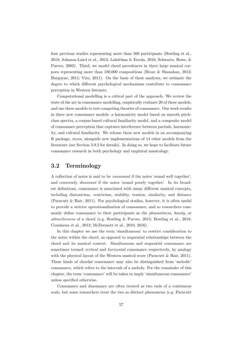
four previous studies representing more than 500 participants (Bowling et al.,2018; Johnson-Laird et al., 2012; Lahdelma & Eerola, 2016; Schwartz, Howe, &Purves, 2003). Third, we model chord prevalences in three large musical cor-pora representing more than 100,000 compositions (Broze & Shanahan, 2013;Burgoyne, 2011; Viro, 2011). On the basis of these analyses, we estimate thedegree to which different psychological mechanisms contribute to consonanceperception in Western listeners.

Computational modelling is a critical part of the approach. We review thestate of the art in consonance modelling, empirically evaluate 20 of these models,and use these models to test competing theories of consonance. Our work resultsin three new consonance models: a harmonicity model based on smooth pitch-class spectra, a corpus-based cultural familiarity model, and a composite modelof consonance perception that captures interference between partials, harmonic-ity, and cultural familiarity. We release these new models in an accompanyingR package, incon, alongside new implementations of 14 other models from theliterature (see Section 3.9.2 for details). In doing so, we hope to facilitate futureconsonance research in both psychology and empirical musicology.

3.2 TerminologyA collection of notes is said to be consonant if the notes ‘sound well together’,and conversely dissonant if the notes ‘sound poorly together’. In its broad-est definitions, consonance is associated with many different musical concepts,including diatonicism, centricism, stability, tension, similarity, and distance(Parncutt & Hair, 2011). For psychological studies, however, it is often usefulto provide a stricter operationalisation of consonance, and so researchers com-monly define consonance to their participants as the pleasantness, beauty, orattractiveness of a chord (e.g. Bowling & Purves, 2015; Bowling et al., 2018;Cousineau et al., 2012; McDermott et al., 2010, 2016).

In this chapter we use the term ‘simultaneous’ to restrict consideration tothe notes within the chord, as opposed to sequential relationships between thechord and its musical context. Simultaneous and sequential consonance aresometimes termed vertical and horizontal consonance respectively, by analogywith the physical layout of the Western musical score (Parncutt & Hair, 2011).These kinds of chordal consonance may also be distinguished from ‘melodic’consonance, which refers to the intervals of a melody. For the remainder of thischapter, the term ‘consonance’ will be taken to imply ‘simultaneous consonance’unless specified otherwise.

Consonance and dissonance are often treated as two ends of a continuousscale, but some researchers treat the two as distinct phenomena (e.g. Parncutt

57

& Hair, 2011). Under such formulations, consonance is typically treated as theperceptual correlate of harmonicity, and dissonance as the perceptual correlateof roughness (see Section 3.3). Here we avoid this approach, and instead treatconsonance and dissonance as antonyms.

3.3 Consonance theoriesHere we review current theories of consonance perception. We pay particularattention to three classes of theories – periodicity/harmonicity, interference be-tween partials, and culture – that we consider to be particularly well-supportedby the empirical literature. We also discuss several related theories, includingvocal similarity, fusion, and combination tones.

3.3.1 Periodicity/harmonicity

Human vocalisations are characterised by repetitive structure termed periodic-ity. This periodicity has several perceptual correlates, of which the most promi-nent is pitch. Broadly speaking, pitch corresponds to the waveform’s repetitionrate, or fundamental frequency: Faster repetition corresponds to higher pitch.

Sound can be represented either in the time domain or in the frequency do-main. In the time domain, periodicity manifests as repetitive waveform struc-ture. In the frequency domain, periodicity manifests as harmonicity, a phe-nomenon where the sound’s frequency components are all integer multiples ofthe fundamental frequency.2 These integer-multiple frequencies are termed har-monics; a sound comprising a full set of integer multiples is termed a harmonicseries. Each periodic sound constitutes a (possibly incomplete) harmonic seriesrooted on its fundamental frequency; conversely, every harmonic series (incom-plete or complete) is periodic in its fundamental frequency. Harmonicity andperiodicity are therefore essentially equivalent phenomena, and we will denoteboth by writing ‘periodicity/harmonicity’.

Humans rely on periodicity/harmonicity analysis to understand the naturalenvironment and to communicate with others (e.g. Oxenham, 2018), but the pre-cise mechanisms of this analysis remain unclear. The primary extant theories aretime-domain autocorrelation theories and frequency-domain pattern-matchingtheories (de Cheveigné, 2005). Autocorrelation theories state that listeners de-tect periodicity by computing the signal’s correlation with a delayed versionof itself as a function of delay time; peaks in the autocorrelation function cor-respond to potential fundamental frequencies (Balaguer-Ballester, Denham, &

2In particular, the fundamental frequency is equal to the greatest common divisor of thefrequency components.

58

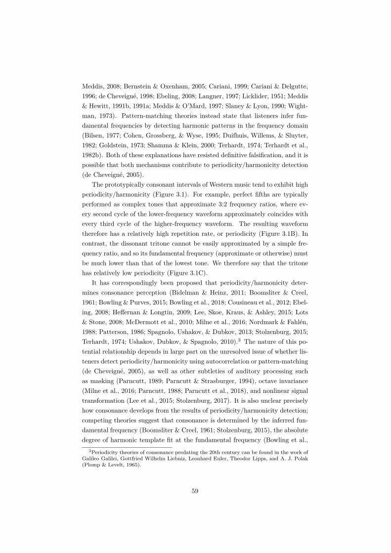
Meddis, 2008; Bernstein & Oxenham, 2005; Cariani, 1999; Cariani & Delgutte,1996; de Cheveigné, 1998; Ebeling, 2008; Langner, 1997; Licklider, 1951; Meddis& Hewitt, 1991b, 1991a; Meddis & O’Mard, 1997; Slaney & Lyon, 1990; Wight-man, 1973). Pattern-matching theories instead state that listeners infer fun-damental frequencies by detecting harmonic patterns in the frequency domain(Bilsen, 1977; Cohen, Grossberg, & Wyse, 1995; Duifhuis, Willems, & Sluyter,1982; Goldstein, 1973; Shamma & Klein, 2000; Terhardt, 1974; Terhardt et al.,1982b). Both of these explanations have resisted definitive falsification, and it ispossible that both mechanisms contribute to periodicity/harmonicity detection(de Cheveigné, 2005).

The prototypically consonant intervals of Western music tend to exhibit highperiodicity/harmonicity (Figure 3.1). For example, perfect fifths are typicallyperformed as complex tones that approximate 3:2 frequency ratios, where ev-ery second cycle of the lower-frequency waveform approximately coincides withevery third cycle of the higher-frequency waveform. The resulting waveformtherefore has a relatively high repetition rate, or periodicity (Figure 3.1B). Incontrast, the dissonant tritone cannot be easily approximated by a simple fre-quency ratio, and so its fundamental frequency (approximate or otherwise) mustbe much lower than that of the lowest tone. We therefore say that the tritonehas relatively low periodicity (Figure 3.1C).

It has correspondingly been proposed that periodicity/harmonicity deter-mines consonance perception (Bidelman & Heinz, 2011; Boomsliter & Creel,1961; Bowling & Purves, 2015; Bowling et al., 2018; Cousineau et al., 2012; Ebel-ing, 2008; Heffernan & Longtin, 2009; Lee, Skoe, Kraus, & Ashley, 2015; Lots& Stone, 2008; McDermott et al., 2010; Milne et al., 2016; Nordmark & Fahlén,1988; Patterson, 1986; Spagnolo, Ushakov, & Dubkov, 2013; Stolzenburg, 2015;Terhardt, 1974; Ushakov, Dubkov, & Spagnolo, 2010).3 The nature of this po-tential relationship depends in large part on the unresolved issue of whether lis-teners detect periodicity/harmonicity using autocorrelation or pattern-matching(de Cheveigné, 2005), as well as other subtleties of auditory processing suchas masking (Parncutt, 1989; Parncutt & Strasburger, 1994), octave invariance(Milne et al., 2016; Parncutt, 1988; Parncutt et al., 2018), and nonlinear signaltransformation (Lee et al., 2015; Stolzenburg, 2017). It is also unclear preciselyhow consonance develops from the results of periodicity/harmonicity detection;competing theories suggest that consonance is determined by the inferred fun-damental frequency (Boomsliter & Creel, 1961; Stolzenburg, 2015), the absolutedegree of harmonic template fit at the fundamental frequency (Bowling et al.,

3Periodicity theories of consonance predating the 20th century can be found in the work ofGalileo Galilei, Gottfried Wilhelm Liebniz, Leonhard Euler, Theodor Lipps, and A. J. Polak(Plomp & Levelt, 1965).

59

0.000.250.500.751.00

1000 2000 3000Frequency (Hz)

Am

plitu

de

−0.2−0.1

0.00.10.2

0.00 0.01 0.02 0.03 0.04 0.05Time (seconds)

Pre

ssur

eA

0.000.250.500.751.00

0 1000 2000 3000 4000Frequency (Hz)

Am

plitu

de

−0.2−0.1

0.00.10.2

0.00 0.01 0.02 0.03 0.04 0.05Time (seconds)

Pre

ssur

e

B

0.000.250.500.751.00

0 1000 2000 3000 4000Frequency (Hz)

Am

plitu

de

−0.2−0.1

0.00.10.2

0.00 0.01 0.02 0.03 0.04 0.05Time (seconds)

Pre

ssur

e

C

Figure 3.1: Acoustic spectra and waveforms for (A) a single harmonic complextone, (B) two harmonic complex tones separated by an equal-tempered perfectfifth, and (C) two harmonic complex tones separated by an equal-tempered tri-tone. Each complex tone has 11 harmonics, with the ith harmonic having anamplitude of 1/i. The blue dotted lines mark harmonic/periodic grids, whichare aligned for the harmonic/periodic perfect fifth but misaligned for the inhar-monic/aperiodic tritone.

60

2018; Gill & Purves, 2009; Milne et al., 2016; Parncutt, 1989; Parncutt &Strasburger, 1994), or the degree of template fit at the fundamental frequencyrelative to that at other candidate fundamental frequencies (Parncutt, 1988;Parncutt et al., 2018). This variety of hypotheses is reflected in a diversity ofcomputational models of musical periodicity/harmonicity perception (Ebeling,2008; Gill & Purves, 2009; Lartillot et al., 2008; Milne et al., 2016; Parncutt,1988, 1989; Parncutt & Strasburger, 1994; Spagnolo et al., 2013; Stolzenburg,2015). So far these models have only received limited empirical comparison(e.g. Stolzenburg, 2015).

It is clear why periodicity/harmonicity should be salient to human listeners:Periodicity/harmonicity detection is crucial for auditory scene analysis and fornatural speech understanding (e.g. Oxenham, 2018). It is less clear why period-icity/harmonicity should be positively valenced, and hence associated with con-sonance. One possibility is that long-term exposure to vocal sounds (Schwartzet al., 2003) or Western music (McDermott et al., 2016) induces familiarity withperiodicity/harmonicity, in turn engendering liking through the mere exposureeffect (Zajonc, 2001). A second possibility is that the ecological importance ofinterpreting human vocalisations creates a selective pressure to perceive thesevocalisations as attractive (Bowling et al., 2018).

3.3.2 Interference between partials

Musical chords can typically be modelled as complex tones, superpositions offinite numbers of sinusoidal pure tones termed partials. Each partial is charac-terised by a frequency and an amplitude. It is argued that neighboring partialscan interact to produce interference effects, with these interference effects subse-quently being perceived as dissonance (Dillon, 2013; Helmholtz, 1863; Hutchin-son & Knopoff, 1978; Kameoka & Kuriyagawa, 1969a, 1969b; Mashinter, 2006;Plomp & Levelt, 1965; Sethares, 1993; Vassilakis, 2001).

Pure-tone interference has two potential sources: beating and masking. Beat-ing develops from the following mathematical identity for the addition of twoequal-amplitude sinusoids:

cos(2πf1t) + cos(2πf2t) = 2 cos(2πf̄t

)cos (πδt) (3.1)

where f1, f2 are the frequencies of the original sinusoids (f1 > f2), f̄ =

(f1 + f2)/2, δ = f1 − f2, and t denotes time. For sufficiently large frequencydifferences, listeners perceive the left hand side of Equation 3.1, correspondingto two separate pure tones at frequencies f1, f2. For sufficiently small frequencydifferences, listeners perceive the right hand side of Equation 3.1, correspondingto a tone of intermediate frequency f̄ = (f1 + f2)/2 modulated by a sinusoid of

61

frequency δ/2 = (f1 − f2)/2. This modulation is perceived as amplitude fluc-tuation with frequency equal to the modulating sinusoid’s zero-crossing rate,f1 − f2. Slow amplitude fluctuation (c. 0.1–5 Hz) is perceived as a not unpleas-ant oscillation in loudness, but fast amplitude fluctuation (c. 20–30 Hz) takes ona harsh quality described as roughness. This roughness is thought to contributeto dissonance perception.

Masking describes situations where one sound obstructs the perception ofanother sound (e.g. Patterson & Green, 2012; Scharf, 1971). Masking in gen-eral is a complex phenomenon, but the mutual masking of pairs of pure tonescan be approximated by straightforward mathematical models (Parncutt, 1989;Parncutt & Strasburger, 1994; Terhardt et al., 1982a; Wang, Shen, Guo, Tang,& Hamade, 2013). These models embody long-established principles that mask-ing increases with smaller frequency differences and with higher sound pressurelevel.

Beating and masking are both closely linked with the notion of critical bands.The notion of critical bands comes from modelling the cochlea as a series ofoverlapping band-pass filters, areas that are preferentially excited by spectralcomponents within a certain frequency range (Zwicker, Flottorp, & Stevens,1957). Beating typically only arises from spectral components localised to thesame critical band (Daniel & Weber, 1997). The mutual masking of pure tonesapproximates a linear function of the number of critical bands separating them(termed critical-band distance), with additional masking occurring from puretones within the same critical band that are unresolved by the auditory system(Terhardt et al., 1982a).

Beating and masking effects are both considerably stronger when two tonesare presented diotically (to the same ear) rather than dichotically (to differentears) (Buus, 1997; Grose, Buss, & Hall III, 2012). This indicates that thesephenomena depend, in large part, on physical interactions in the inner ear.

There is a long tradition of research relating beating to consonance, mostlyfounded on the work of Helmholtz (1863; Aures, 1985a, cited in Daniel & We-ber, 1997; Hutchinson & Knopoff, 1978; Kameoka & Kuriyagawa, 1969a, 1969b;Mashinter, 2006; Parncutt et al., 2018; Plomp & Levelt, 1965; Sethares, 1993;Vassilakis, 2001).4 The general principle shared by this work is that disso-nance develops from the accumulation of roughness deriving from the beatingof neighboring partials.

In contrast, the literature linking masking to consonance is relatively sparse.Huron (2001) suggests that masking induces dissonance because it reflects acompromised sensitivity to the auditory environment, with analogies in visual

4Earlier work in a similar line can be found in Sorge (1747), cited in Plomp & Levelt (1965)and Sethares (2005).

62

processing such as occlusion or glare. Aures (1984; cited in Parncutt, 1989)and Parncutt (1989; Parncutt & Strasburger, 1994) also state that consonancereduces as a function of masking. Unfortunately, these ideas have yet to receivemuch empirical validation; a difficulty is that beating and masking tend tohappen in similar situations, making them difficult to disambiguate (Huron,2001).

The kind of beating that elicits dissonance is achieved by small, but not toosmall, frequency differences between partials (Figure 3.2A). With very small fre-quency differences, the beating becomes too slow to elicit dissonance (Hutchin-son & Knopoff, 1978; Kameoka & Kuriyagawa, 1969a; Plomp & Levelt, 1965).The kind of masking that elicits dissonance is presumably also maximised bysmall, but not too small, frequency differences between partials. For moderatelysmall frequency differences, the auditory system tries to resolve two partials, butfinds it difficult on account of mutual masking, with this difficulty eliciting neg-ative valence (Huron, 2001). For very small frequency differences, the auditorysystem only perceives one partial, which becomes purer as the two acousticpartials converge on the same frequency.

Musical sonorities can often be treated as combinations of harmonic complextones, complex tones whose spectral frequencies follow a harmonic series. Theinterference experienced by a combination of harmonic complex tones dependson the fundamental frequencies of the complex tones. A particularly importantfactor is the ratio of these fundamental frequencies. Certain ratios, in particu-lar the simple-integer ratios approximated by prototypically consonant musicalchords, tend to produce partials that either completely coincide or are widelyspaced, hence minimising interference (Figure 3.2B).

Interference between partials also depends on pitch height. A given fre-quency ratio occupies less critical-band distance as absolute frequency decreases,typically resulting in increased interference. This mechanism potentially ex-plains why the same musical interval (e.g. the major third, 5:4) can sound con-sonant in high registers and dissonant in low registers.

It is currently unusual to distinguish beating and masking theories of con-sonance, as we have done above. Most previous work solely discusses beatingand its psychological correlate, roughness (e.g. Cousineau et al., 2012; McDer-mott et al., 2010, 2016; Parncutt & Hair, 2011; Parncutt et al., 2018; Terhardt,1984). However, we contend that the existing evidence does little to differen-tiate beating and masking theories, and that it would be premature to discardthe latter in favour of the former. Moreover, we show later in this chapter thatcomputational models that address beating explicitly (e.g. Wang et al., 2013)seem to predict consonance worse than generic models of interference betweenpartials (e.g. Hutchinson & Knopoff, 1978; Sethares, 1993; Vassilakis, 2001).

63

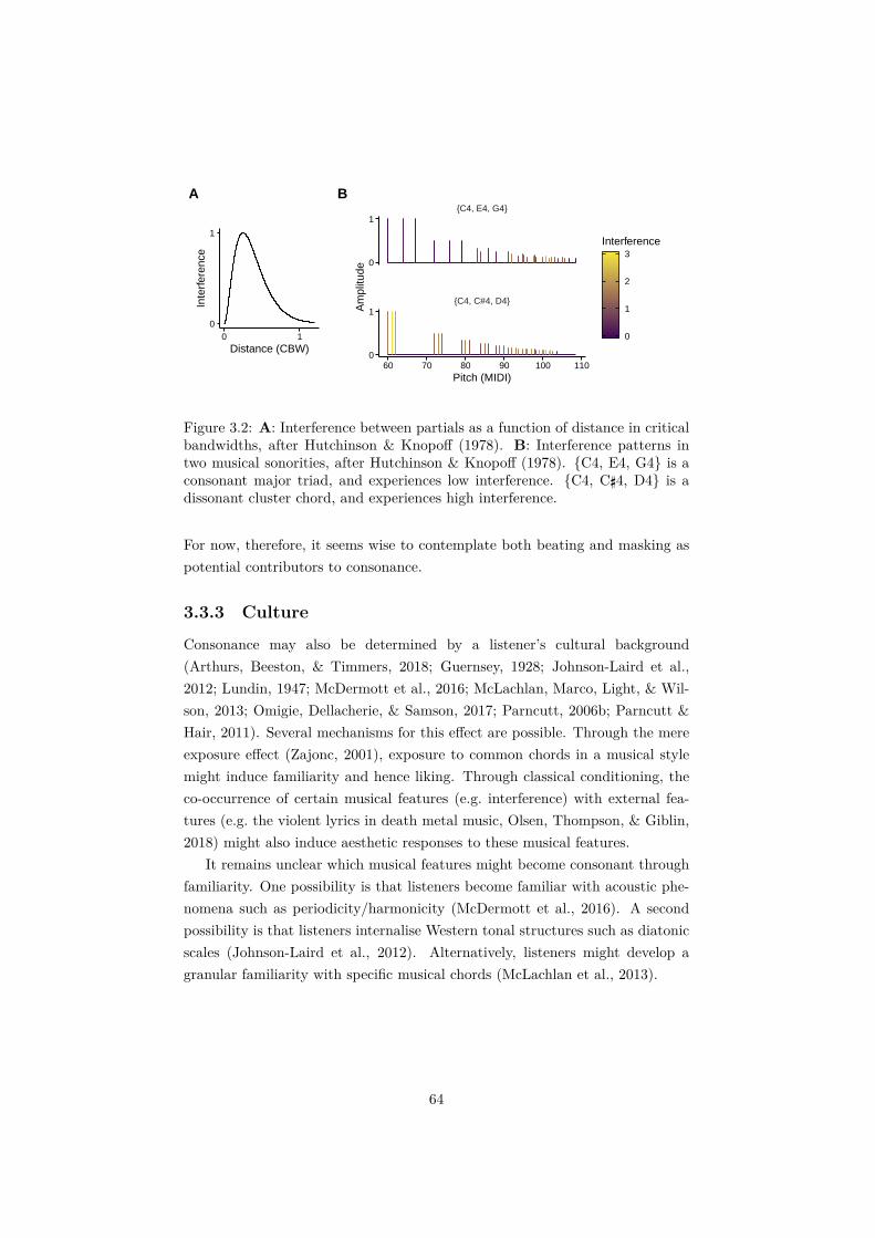
0

1

0 1Distance (CBW)

Inte

rfer

ence

A

{C4, C#4, D4}

{C4, E4, G4}

60 70 80 90 100 110

0

1

0

1

Pitch (MIDI)

Am

plitu

de

0

1

2

3Interference

B

Figure 3.2: A: Interference between partials as a function of distance in criticalbandwidths, after Hutchinson & Knopoff (1978). B: Interference patterns intwo musical sonorities, after Hutchinson & Knopoff (1978). {C4, E4, G4} is aconsonant major triad, and experiences low interference. {C4, C\4, D4} is adissonant cluster chord, and experiences high interference.

For now, therefore, it seems wise to contemplate both beating and masking aspotential contributors to consonance.

3.3.3 Culture

Consonance may also be determined by a listener’s cultural background(Arthurs, Beeston, & Timmers, 2018; Guernsey, 1928; Johnson-Laird et al.,2012; Lundin, 1947; McDermott et al., 2016; McLachlan, Marco, Light, & Wil-son, 2013; Omigie, Dellacherie, & Samson, 2017; Parncutt, 2006b; Parncutt &Hair, 2011). Several mechanisms for this effect are possible. Through the mereexposure effect (Zajonc, 2001), exposure to common chords in a musical stylemight induce familiarity and hence liking. Through classical conditioning, theco-occurrence of certain musical features (e.g. interference) with external fea-tures (e.g. the violent lyrics in death metal music, Olsen, Thompson, & Giblin,2018) might also induce aesthetic responses to these musical features.

It remains unclear which musical features might become consonant throughfamiliarity. One possibility is that listeners become familiar with acoustic phe-nomena such as periodicity/harmonicity (McDermott et al., 2016). A secondpossibility is that listeners internalise Western tonal structures such as diatonicscales (Johnson-Laird et al., 2012). Alternatively, listeners might develop agranular familiarity with specific musical chords (McLachlan et al., 2013).

64

3.3.4 Other theories

Vocal similarity

Vocal similarity theories hold that consonance derives from acoustic similarityto human vocalisations (e.g. Bowling & Purves, 2015; Bowling et al., 2018;Schwartz et al., 2003). A key feature of human vocalisations is periodic-ity/harmonicity, leading some researchers to operationalise vocal similarity asthe latter (Gill & Purves, 2009). In such cases, vocal similarity theories maybe considered a subset of periodicity/harmonicity theories. However, Bowlinget al. (2018) additionally operationalise vocal similarity as the absence of fun-damental frequency intervals smaller than 50 Hz, arguing that such intervalsare rarely found in human vocalisations. Indeed, such intervals are negativelyassociated with consonance; however, this phenomenon can also be explainedby interference minimisation. To our knowledge, no studies have shown thatvocal similarity contributes to consonance through paths other than periodic-ity/harmonicity and interference. We therefore do not evaluate vocal similarityseparately from interference and periodicity/harmonicity.

Fusion

Stumpf (1890, 1898) proposed that consonance derives from fusion, the per-ceptual merging of multiple harmonic complex tones. The substance of thishypothesis depends on the precise definition of fusion. Some researchers haveoperationalised fusion as perceptual indiscriminability, that is, an inability toidentify the constituent tones of a sonority (DeWitt & Crowder, 1987; McLach-lan et al., 2013). This was encouraged by Stumpf’s early experiments investigat-ing how often listeners erroneously judged tone pairs as single tones (DeWitt &Crowder, 1987; Schneider, 1997). Subsequently, however, Stumpf wrote that fu-sion should not be interpreted as indiscriminability but rather as the formationof a coherent whole, with the sophisticated listener being able to attend to indi-vidual chord components at will (Schneider, 1997). Stumpf later wrote that hewas unsure whether fusion truly caused consonance; instead, he suggested thatfusion and consonance might both stem from harmonicity recognition (Plomp& Levelt, 1965; Schneider, 1997).

Following Stumpf, several subsequent studies have investigated the relation-ship between fusion and consonance, but with mixed findings. Guernsey (1928)and DeWitt & Crowder (1987) tested fusion by playing participants differentdyads and asking how many tones these chords contained. In both studies, pro-totypically consonant musical intervals (octaves, perfect fifths) were most likelyto be confused for single tones, supporting a link between consonance and fu-sion. McLachlan et al. (2013) instead tested fusion with a pitch-matching task,

65

where each trial cycled between a target chord and a probe tone, and partici-pants were instructed to manipulate the probe tone until it matched a specifiedchord tone (lowest, middle, or highest). Pitch-matching accuracy increased forprototypically consonant chords, suggesting (contrary to Stumpf’s claims) thatconsonance was inversely related to fusion. It is difficult to conclude much aboutStumpf’s claims from these studies, partly because different studies have yieldedcontradictory results, and partly because none of these studies tested for causaleffects of fusion on consonance, as opposed to consonance and fusion both beingdriven by a common factor of periodicity/harmonicity.

Combination tones

Combination tones are additional spectral components introduced by nonlin-ear sound transmission in the ear’s physical apparatus (e.g. Parncutt, 1989;Smoorenburg, 1972; Wever, Bray, & Lawrence, 1940). For example, two puretones of frequencies f1, f2 : f1 < f2 can elicit combination tones including thesimple difference tone (f = f2−f1) and the cubic difference tone (f = 2f1−f2)(Parncutt, 1989; Smoorenburg, 1972).

Combination tones were once argued to be an important mechanism for pitchperception, reinforcing a complex tone’s fundamental frequency and causing itto be perceived even when not acoustically present (e.g. Fletcher, 1924; seeParncutt, 1989). Combination tones were also argued to have important im-plications for music perception, explaining phenomena such as chord roots andperceptual consonance (Hindemith, 1945; Krueger, 1910; Tartini, 1754, citedin Parncutt, 1989). However, subsequent research showed that the missingfundamental persisted even when the difference tone was removed by acousticcancellation (Schouten, 1938, described in Plomp, 1967), and that, in any case,difference tones are usually too quiet to be audible for typical speech and mu-sic listening (Plomp, 1965). We therefore do not consider combination tonesfurther.

Loudness and sharpness

Aures (1985a, 1985b) describes four aspects of sensory consonance: tonal-ness, roughness, loudness, and sharpness. Tonalness is a synonym for peri-odicity/harmonicity, already discussed as an important potential contributor toconsonance. Roughness is an aspect of interference, also an important potentialcontributor to consonance. Loudness is the perceptual correlate of a sound’senergy content; sharpness describes the energy content of high spectral frequen-cies. Historically, loudness and sharpness have received little attention in thestudy of musical consonance, perhaps because music theorists and psychologists

66

have primarily been interested in the consonance of transposition-invariant andloudness-invariant structures such as pitch-class sets, for which loudness andsharpness are undefined. We do not consider these phenomena further in thischapter, but they may ultimately prove necessary for achieving a complete per-ceptual account of consonance.

Evenness

The constituent notes of a musical chord can be represented as points on a pitchline or a pitch-class circle (e.g. Tymoczko, 2016). The evenness of the resultingdistribution can be characterised in various ways, including the difference insuccessive interval sizes (Cook, 2009, 2017; Cook & Fujisawa, 2006), the dif-ference between the largest and smallest interval sizes (Parncutt et al., 2018),and the standard deviation of interval sizes (Parncutt et al., 2018). In the caseof Cook’s (2009, 2017; 2006) models, each chord note is expanded into a har-monic complex tone, and pitch distances are computed between the resultingpartials; in the other cases, pitch distances are computed between fundamentalfrequencies, presumably as inferred through periodicity/harmonicity detection.

Evenness may contribute negatively to consonance. When a chord con-tains multiple intervals of the same size, these intervals may become confusableand impede perceptual organisation, hence decreasing consonance (Cook, 2009,2017; Cook & Fujisawa, 2006; Meyer, 1956). For example, a major triad inpitch-class space contains the intervals of a major third, a minor third, and aperfect fourth, and each note of the triad participates in a unique pair of theseintervals, one connecting it to the note above, and one connecting it to the notebelow. In contrast, an augmented triad contains only intervals of a major third,and so each note participates in an identical pair of intervals. Correspondingly,the individual notes of the augmented triad may be considered less distinctivethan those of the major triad.

Evenness may also contribute positively, but indirectly, to consonance.Spacing harmonics evenly on a critical-band scale typically reduces interfer-ence, thereby increasing consonance (see e.g. Huron & Sellmer, 1992; Plomp &Levelt, 1965). Evenness also facilitates efficient voice leading, and therefore maycontribute positively to sequential consonance (Parncutt et al., 2018; Tymoczko,2011).

Evenness is an interesting potential contributor to consonance, but so farit has received little empirical testing. We do not consider it to be sufficientlywell-supported to include in this chapter’s analyses, but we encourage futureempirical research on the topic.

67

Table 3.1: Summarised evidence for the mechanisms underlying Western con-sonance perception.

Evidence Interference Periodicity CultureStimulus effects

Tone spectra 3Pitch height 3Dichotic presentation ✠Familiarity (3)Chord structure (3) (3) (3)→ Section 3.6 3 3 (3)

Listener effectsWestern listeners (7) 3Congenital amusia 3Non-Western listeners 3Infants (✠)Animals (✠)

Composition effectsMusical scales 3Manipulation of interference 3 3Chord spacing (Western music) 3Chord prevalences (Western music) (3) (3)→ Section 3.7 3 3

Note. Each row identifies a section in Section 3.4. ‘3’ denotes evidence that amechanism contributes to Western consonance perception. ‘7’ denotes evidencethat a mechanism is not relevant to Western consonance perception. ‘✠’ de-notes evidence that a mechanism is insufficient to explain Western consonanceperception. Parentheses indicate tentative evidence; blank spaces indicate alack of evidence.

3.4 Current evidenceEvidence for disambiguating different theories of consonance perception canbe organised into three broad categories: stimulus effects, listener effects, andcomposition effects. We review each of these categories in turn, and summariseour conclusions in Table 3.1.

3.4.1 Stimulus effects

We begin by discussing stimulus effects, ways in which consonance perceptionvaries as a function of the stimulus.

Tone spectra

A chord’s consonance depends on the spectral content of its tones. With har-monic tone spectra, peak consonance is observed when the fundamental frequen-

68

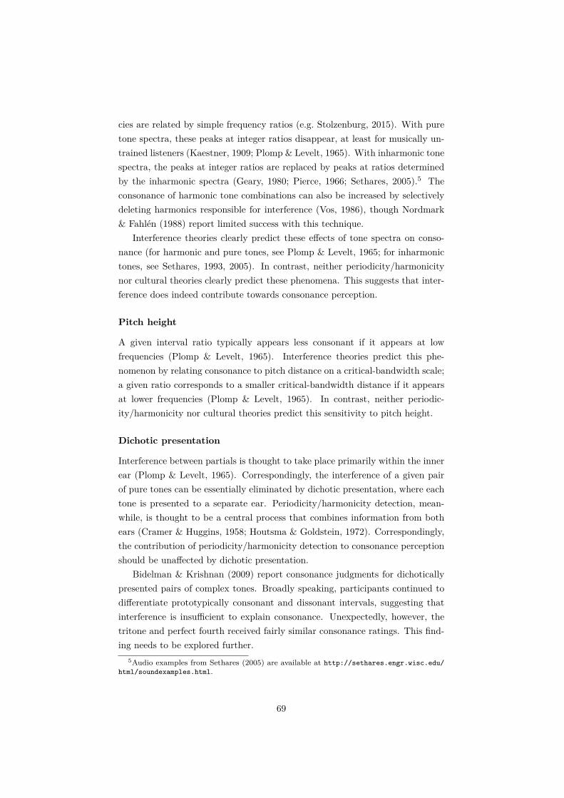
cies are related by simple frequency ratios (e.g. Stolzenburg, 2015). With puretone spectra, these peaks at integer ratios disappear, at least for musically un-trained listeners (Kaestner, 1909; Plomp & Levelt, 1965). With inharmonic tonespectra, the peaks at integer ratios are replaced by peaks at ratios determinedby the inharmonic spectra (Geary, 1980; Pierce, 1966; Sethares, 2005).5 Theconsonance of harmonic tone combinations can also be increased by selectivelydeleting harmonics responsible for interference (Vos, 1986), though Nordmark& Fahlén (1988) report limited success with this technique.

Interference theories clearly predict these effects of tone spectra on conso-nance (for harmonic and pure tones, see Plomp & Levelt, 1965; for inharmonictones, see Sethares, 1993, 2005). In contrast, neither periodicity/harmonicitynor cultural theories clearly predict these phenomena. This suggests that inter-ference does indeed contribute towards consonance perception.

Pitch height

A given interval ratio typically appears less consonant if it appears at lowfrequencies (Plomp & Levelt, 1965). Interference theories predict this phe-nomenon by relating consonance to pitch distance on a critical-bandwidth scale;a given ratio corresponds to a smaller critical-bandwidth distance if it appearsat lower frequencies (Plomp & Levelt, 1965). In contrast, neither periodic-ity/harmonicity nor cultural theories predict this sensitivity to pitch height.

Dichotic presentation

Interference between partials is thought to take place primarily within the innerear (Plomp & Levelt, 1965). Correspondingly, the interference of a given pairof pure tones can be essentially eliminated by dichotic presentation, where eachtone is presented to a separate ear. Periodicity/harmonicity detection, mean-while, is thought to be a central process that combines information from bothears (Cramer & Huggins, 1958; Houtsma & Goldstein, 1972). Correspondingly,the contribution of periodicity/harmonicity detection to consonance perceptionshould be unaffected by dichotic presentation.

Bidelman & Krishnan (2009) report consonance judgments for dichoticallypresented pairs of complex tones. Broadly speaking, participants continued todifferentiate prototypically consonant and dissonant intervals, suggesting thatinterference is insufficient to explain consonance. Unexpectedly, however, thetritone and perfect fourth received fairly similar consonance ratings. This find-ing needs to be explored further.

5Audio examples from Sethares (2005) are available at http://sethares.engr.wisc.edu/html/soundexamples.html.

69

Subsequent studies have investigated the effect of dichotic presentation onconsonance judgments for pairs of pure tones (Cousineau et al., 2012; McDer-mott et al., 2010, 2016). These studies show that dichotic presentation reliablyincreases the consonance of small pitch intervals, in particular major and minorseconds, as predicted by interference theories. This would appear to supportinterference theories of consonance, though it is unclear whether these effectsgeneralise to the complex tone spectra of real musical instruments.

Familiarity

McLachlan et al. (2013, Experiment 2) trained nonmusicians to perform a pitch-matching task on two-note chords. After training, participants judged chordsfrom the training set as more consonant than novel chords. These results couldbe interpreted as evidence that consonance is positively influenced by exposure,consistent with the mere exposure effect, and supporting a cultural theory ofconsonance. However, the generalisability of this effect has yet to be confirmed.

Chord structure

Western listeners consider certain chords (e.g. the major triad) to be more con-sonant than others (e.g. the augmented triad). It is possible to test competingtheories of consonance by operationalising the theories as computational modelsand testing their ability to predict consonance judgments.

Unfortunately, studies using this approach have identified conflicting expla-nations for consonance:

a) Interference (Hutchinson & Knopoff, 1978);

b) Interference and additional unknown factors (Vassilakis, 2001);

c) Interference and cultural knowledge (Johnson-Laird et al., 2012);

d) Periodicity/harmonicity (Stolzenburg, 2015);

e) Periodicity/harmonicity and interference (Marin, Forde, Gingras, & Stew-art, 2015);

f) Interference and sharpness (Lahdelma & Eerola, 2016);

g) Vocal similarity (Bowling et al., 2018).

These contradictions may often be attributed to methodological problems:

a) Different studies test different theories, and rarely test more than twotheories simultaneously.

70

b) Stimulus sets are often too small to support reliable inferences.6

c) Stolzenburg (2015) evaluates models using pairwise correlations, implicitlyassuming that only one mechanism (e.g. periodicity/harmonicity, interfer-ence) determines consonance. Multiple regression would be necessary tocapture multiple simultaneous mechanisms.

d) The stimulus set of Marin et al. (2015) constitutes 12 dyads each trans-posed four times; the conditional dependencies between transpositions arenot accounted for in the linear regressions, inflating Type I error.

e) Johnson-Laird et al. (2012) do not report coefficients or p-values for theirfitted regression models; they do report hierarchical regression statistics,but these statistics do not test their primary research question, namelywhether interference and cultural knowledge simultaneously contribute toconsonance.

f) The audio-based periodicity/harmonicity model used by Lahdelma &Eerola (2016) fails when applied to complex stimuli such as chords (seeSection 3.6).

These methodological problems and contradictory findings make it difficult togeneralise from this literature.

3.4.2 Listener effects

We now discuss listener effects, ways in which consonance perception varies asa function of the listener.

Western listeners

McDermott et al. (2010) tested competing theories of consonance perceptionusing an individual-differences approach. They constructed three psychometricmeasures, testing:

a) Interference preferences, operationalised by playing listeners pure-tonedyads and subtracting preference ratings for dichotic presentation (onetone in each ear) from ratings for diotic presentation (both tones in bothears);

b) Periodicity/harmonicity preferences, operationalised by playing listenerssubsets of a harmonic complex tone and subtracting preference ratings forthe original version from ratings for a version with perturbed harmonics;

6For example, Stolzenburg (2015, Table 4) tabulates correlation coefficients for 15 conso-nance models as evaluated on 12 dyads; the median correlation of .939 has a 95% confidenceinterval spanning from .79 to .98, encompassing all but one of the reported coefficients.

71

c) Consonance preferences, operationalised by playing listeners 14 musicalchords, and subtracting preference ratings for the globally least-preferredchords from the globally most-preferred chords.

Consonance preferences correlated with periodicity/harmonicity preferences butnot with interference preferences. This suggests that consonance may be drivenby periodicity/harmonicity, not interference. However, these findings must beconsidered preliminary given the limited construct validation of the three psy-chometric measures. Future work must examine whether these measures gener-alise to a wider range of stimulus manipulations and response paradigms.

Congenital amusia

Congenital amusia is a lifelong cognitive disorder characterised by difficultiesin performing simple musical tasks (Ayotte, Peretz, & Hyde, 2002; Stewart,2011). Using the individual-differences tests of McDermott et al. (2010) (seeSection 3.4.2), Cousineau et al. (2012) found that amusics exhibited no aver-sion to traditionally dissonant chords, normal aversion to interference, and aninability to detect periodicity/harmonicity. Since the aversion to interferencedid not transfer to dissonant chords, Cousineau et al. (2012) concluded that in-terference is irrelevant to consonance perception. However, Marin et al. (2015)subsequently identified small but reliable preferences for consonance in amu-sics, and showed with regression analyses that these preferences were driven byinterference, whereas non-amusic preferences were driven by both interferenceand periodicity/harmonicity. This discrepancy between Cousineau et al. (2012)and Marin et al. (2015) needs further investigation.

Non-Western listeners

Cross-cultural research into consonance perception has identified high similaritybetween the consonance judgments of Western and Japanese listeners (Butler &Daston, 1968), but low similarity between Western and Indian listeners (Maher,1976), and between Westerners and native Amazonians from the Tsimane’ soci-ety (McDermott et al., 2016). Exploring these differences further, McDermottet al. (2016) found that Tsimane’ and Western listeners shared an aversionto interference and an ability to perceive periodicity/harmonicity, but, unlikeWestern listeners, the Tsimane’ had no preference for periodicity/harmonicity.

These results suggest that cultural exposure significantly affects consonanceperception. The results of McDermott et al. (2016) additionally suggest thatthis effect of cultural exposure may be mediated by changes in preference forperiodicity/harmonicity.

72

Infants

Consonance perception has been demonstrated in toddlers (Di Stefano et al.,2017), 6-month-old infants (Crowder, Reznick, & Rosenkrantz, 1991; Trainor &Heinmiller, 1998), 4-month-old infants (Trainor, Tsang, & Cheung, 2002; Zent-ner & Kagan, 1998), 2-month-old infants (Trainor et al., 2002), and newborninfants (Masataka, 2006; Perani et al., 2010; Virtala, Huotilainen, Partanen,Fellman, & Tervaniemi, 2013). Masataka (2006) additionally found preservedconsonance perception in newborn infants with deaf parents. These results sug-gest that consonance perception does not solely depend on cultural exposure.

A related question is whether infants prefer consonance to dissonance.Looking-time paradigms address this question, testing whether infants preferen-tially look at consonant or dissonant sound sources (Crowder et al., 1991; Masa-taka, 2006; Plantinga & Trehub, 2014; Trainor & Heinmiller, 1998; Trainor etal., 2002; Zentner & Kagan, 1998). With the exception of Plantinga & Trehub(2014), these studies each report detecting consonance preferences in infants.However, Plantinga & Trehub (2014) failed to replicate several of these results,and additionally question the validity of looking-time paradigms, noting thatlooking times may be confounded by features such as familiarity and compre-hensibility. These problems may partly be overcome by physical play-basedparadigms (e.g. Di Stefano et al., 2017), but such paradigms are unfortunatelyonly applicable to older infants.

In conclusion, therefore, it seems that young infants perceive some aspectsof consonance, but it is unclear whether they prefer consonance to dissonance.These conclusions provide tentative evidence that consonance perception is notsolely cultural.

Animals

Animal studies could theoretically provide compelling evidence for non-culturaltheories of consonance. If animals were to display sensitivity or preference forconsonance despite zero prior musical exposure, this would indicate that conso-nance could not be fully explained by cultural learning.

Most studies of consonance perception in animals fall into two categories:discrimination studies and preference studies (see Toro & Crespo-Bojorque, 2017for a review). Discrimination studies investigate whether animals can be taughtto discriminate consonance from dissonance in unfamiliar sounds. Preferencestudies investigate whether animals prefer consonance to dissonance.

Discrimination studies have identified consonance discrimination in severalnon-human species, but methodological issues limit interpretation of their find-ings. Experiment 5 of Hulse, Bernard, & Braaten (1995) suggests that starlings

73

may be able to discriminate consonance from dissonance, but their stimulus setcontains just four chords. Experiment 2 of Izumi (2000) suggests that Japanesemonkeys may be able to discriminate consonance from dissonance, but thisstudy likewise relies on just four chords at different transpositions. Watanabe,Uozumi, & Tanaka (2005) claim to show consonance discrimination in Java spar-rows, but the sparrows’ discriminations can also be explained by interval-sizejudgments.7 Conversely, studies of pigeons (Brooks & Cook, 2010) and rats(Crespo-Bojorque & Toro, 2015) have failed to show evidence of consonancediscrimination (but see also Borchgrevink, 1975).8

Preference studies have identified consonance preferences in several non-human animals. Using stimuli from a previous infant consonance study (Zent-ner & Kagan, 1998), Chiandetti & Vallortigara (2011) found that newly hatcheddomestic chicks spent more time near consonant sound sources than dissonantsound sources. Sugimoto et al. (2010) gave an infant chimpanzee the ability toselect between consonant and dissonant two-part melodies, and found that thechimpanzee preferentially selected consonant melodies. However, these stud-ies have yet to be replicated, and both rely on borderline p-values (p = .03).Other studies have failed to demonstrate consonance preferences in Campbell’smonkeys (Koda et al., 2013) or cotton-top tamarins (McDermott & Hauser,2004).

These animal studies provide an important alternative perspective on conso-nance perception. However, recurring problems with these studies include smallstimulus sets, small sample sizes, and a lack of replication studies. Future workshould address these problems.

3.4.3 Composition effects

Here we consider how compositional practice may provide evidence for the psy-chological mechanisms underlying consonance perception.

Musical scales

A scale divides an octave into a set of pitch classes that can subsequently beused to generate musical material. Scales vary cross-culturally, but certain cross-cultural similarities between scales suggest common perceptual biases.

Gill & Purves (2009) argue that scale construction is biased towards har-monicity maximisation, and explain harmonicity maximisation as a preference

70/12 of their consonant chords contain intervals smaller than a minor third, whereas 15/16of their dissonant chords contain such intervals.

8Toro & Crespo-Bojorque (2017) also claim that consonance discrimination has beendemonstrated in black-capped chickadees, but we disagree in their interpretation of the citedevidence (Hoeschele, Cook, Guillette, Brooks, & Sturdy, 2012).

74

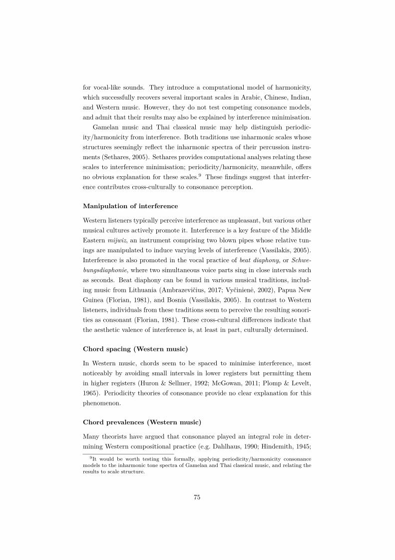
for vocal-like sounds. They introduce a computational model of harmonicity,which successfully recovers several important scales in Arabic, Chinese, Indian,and Western music. However, they do not test competing consonance models,and admit that their results may also be explained by interference minimisation.

Gamelan music and Thai classical music may help distinguish periodic-ity/harmonicity from interference. Both traditions use inharmonic scales whosestructures seemingly reflect the inharmonic spectra of their percussion instru-ments (Sethares, 2005). Sethares provides computational analyses relating thesescales to interference minimisation; periodicity/harmonicity, meanwhile, offersno obvious explanation for these scales.9 These findings suggest that interfer-ence contributes cross-culturally to consonance perception.

Manipulation of interference

Western listeners typically perceive interference as unpleasant, but various othermusical cultures actively promote it. Interference is a key feature of the MiddleEastern mijwiz, an instrument comprising two blown pipes whose relative tun-ings are manipulated to induce varying levels of interference (Vassilakis, 2005).Interference is also promoted in the vocal practice of beat diaphony, or Schwe-bungsdiaphonie, where two simultaneous voice parts sing in close intervals suchas seconds. Beat diaphony can be found in various musical traditions, includ-ing music from Lithuania (Ambrazevičius, 2017; Vyčinienė, 2002), Papua NewGuinea (Florian, 1981), and Bosnia (Vassilakis, 2005). In contrast to Westernlisteners, individuals from these traditions seem to perceive the resulting sonori-ties as consonant (Florian, 1981). These cross-cultural differences indicate thatthe aesthetic valence of interference is, at least in part, culturally determined.

Chord spacing (Western music)

In Western music, chords seem to be spaced to minimise interference, mostnoticeably by avoiding small intervals in lower registers but permitting themin higher registers (Huron & Sellmer, 1992; McGowan, 2011; Plomp & Levelt,1965). Periodicity theories of consonance provide no clear explanation for thisphenomenon.

Chord prevalences (Western music)

Many theorists have argued that consonance played an integral role in deter-mining Western compositional practice (e.g. Dahlhaus, 1990; Hindemith, 1945;

9It would be worth testing this formally, applying periodicity/harmonicity consonancemodels to the inharmonic tone spectra of Gamelan and Thai classical music, and relating theresults to scale structure.

75

Rameau, 1722). If so, it should be possible to test competing theories of conso-nance by examining their ability to predict compositional practice.

Huron (1991) analysed prevalences of different intervals within 30 polyphonickeyboard works by J. S. Bach, and concluded that they reflected dual concernsof minimising interference and minimising tonal fusion. Huron argued thatinterference was minimised on account of its negative aesthetic valence, whereastonal fusion was minimised to maintain perceptual independence of the differentvoices.

Parncutt et al. (2018) tabulated chord types in seven centuries of vocalpolyphony, and related their occurrence rates to several formal models of dia-tonicity, interference, periodicity/harmonicity, and evenness. Most models cor-related significantly with chord occurrence rates, with fairly stable coefficientestimates across centuries. These results suggest that multiple psychologicalmechanisms contribute to consonance.

However, these findings must be treated as tentative, for the following rea-sons:

a) The parameter estimates have low precision due to the small sample sizes(12 dyads in Huron, 1991; 19 triads in Parncutt et al., 2018);10

b) The pairwise correlations reported in Parncutt et al. (2018) can-not capture effects of multiple concurrent mechanisms (e.g. periodic-ity/harmonicity and interference).

3.4.4 Discussion

Table 3.1 summarises the evidence contributed by these diverse studies. Wenow use this evidence to re-evaluate some claims in the recent literature.

Role of periodicity/harmonicity

Recent work has claimed that consonance is primarily determined by periodic-ity/harmonicity, with the role of periodicity/harmonicity potentially moderatedby musical background (Cousineau et al., 2012; McDermott et al., 2010, 2016).In our view, a significant contribution of periodicity/harmonicity to conso-nance is indeed supported by the present literature, in particular by individual-differences research and congenital amusia research (Table 3.1). A moderatingeffect of musical background also seems likely, on the basis of cross-culturalvariation in music perception and composition. However, quantitative descrip-tions of these effects are missing: It is unclear what proportion of consonance

10For example, a correlation coefficient of r = 0.5 with 19 triads has a 95% confidenceinterval of [0.06, 0.78].

76

may be explained by periodicity/harmonicity, and it is unclear how sensitiveconsonance is to cultural exposure.

Role of interference

Recent work has also claimed that consonance is independent of interference(Bowling & Purves, 2015; Bowling et al., 2018; Cousineau et al., 2012; McDer-mott et al., 2010, 2016). In our view, the wider literature is inconsistent withthis claim (Table 3.1). The main evidence against interference comes from theindividual-differences study of McDermott et al. (2010), but this evidence iscounterbalanced by several positive arguments for interference, including stud-ies of tone spectra, pitch height, chord voicing in Western music, scale tuningsin Gamelan music and Thai classical music, and cross-cultural manipulation ofinterference for expressive effect.

Role of culture

Cross-cultural studies of music perception and composition make it clear thatculture contributes to consonance perception (Table 3.1). The mechanisms ofthis effect remain unclear, however: Some argue that Western listeners inter-nalise codified conventions of Western harmony (Johnson-Laird et al., 2012),whereas others argue that Westerners simply learn aesthetic preferences for pe-riodicity/harmonicity (McDermott et al., 2016). These competing explanationshave yet to be tested.

Conclusions

We conclude that consonance perception in Western listeners is likely to bedriven by multiple psychological mechanisms, including interference, period-icity/harmonicity, and cultural background (Table 3.1). This conclusion is atodds with recent claims that interference does not contribute to consonance per-ception (Cousineau et al., 2012; McDermott et al., 2010, 2016). In the rest ofthis chapter, we therefore examine our proposition empirically, computationallymodelling large datasets of consonance judgments and music compositions.

3.5 Computational modelsWe begin by reviewing prominent computational models of consonance from theliterature, organising them by psychological theory and by modelling approach(Figure 3.3).

77

Simultaneousconsonance

Periodicity/harmonicity

Interference

Culture

Ratiosimplicity

Spectral patternmatching

Temporalautocorrelation

Stolzenburg (2015)

Parncutt (1988)

Parncutt (1993)

Parncutt & Strasburger (1994)

Gill & Purves (2009)

Kameoka & Kuriyagawa (1969)

Hutchinson & Knopoff (1978)

Lartillot et al. (2008)

This chapter

Boersma (1993)

Ebeling (2008)

Trulla et al. (2018)

Huron (1994)

Bowling et al. (2018)

Vassilakis (2001)

Weisser & Lartillot (2013)

Parncutt & Strasburger (1994)

Leman (2000)

Skovenborg (2002)

Wang et al. (2013)

Vencovský (2016)

Johnson-Laird et al. (2012)

This chapter

Complexdyads

Puredyads

Terhardt et al.(1982)

Parncutt(1989)

Terhardt et al.(1982a)

Milne(2013)

Plomp & Levelt(1965)

Sethares(1993)

Parncutt (1989)

Terhardt et al.(1982a)

Daniel & Weber(1997)

Aures(1985)

Waveforms

Statistics

Rules

Figure 3.3: Consonance models organised by psychological theory and mod-elling approach. Dashed borders indicate models not evaluated in our empiricalanalyses. Arrows denote model revisions.

78

3.5.1 Periodicity/harmonicity: Ratio simplicity

Chords tend to be more periodic when their constituent tones are related bysimple frequency ratios. Ratio simplicity can therefore provide a proxy forperiodicity/harmonicity. Previous research has formalised ratio simplicity invarious ways, with the resulting measures predicting the consonance of just-tuned chords fairly well (e.g. Euler, 1739; Geer, Levelt, & Plomp, 1962; Levelt,Geer, & Plomp, 1966; Schellenberg & Trehub, 1994).11 Unfortunately, thesemeasures generally fail to predict consonance for chords that are not just-tuned.A particular problem is disproportionate sensitivity to small tuning deviations:For example, an octave stretched by 0.001% still sounds consonant, despitecorresponding to a very complex frequency ratio (200,002:100,000). However,Stolzenburg (2015) provides an effective solution to this problem, describedbelow.

Stolzenburg (2015)

Stolzenburg’s (2015) model avoids sensitivity to small tuning deviations by in-troducing a preprocessing step where each note is adjusted to maximise ratiosimplicity with respect to the bass note. These adjustments are not permittedto change the interval size by more than 1.1%. Stolzenburg argues that suchadjustments are reasonable given human perceptual inaccuracies in pitch dis-crimination. Having expressed each chord frequency as a fractional multipleof the bass frequency, ratio simplicity is then computed as the lowest commonmultiple of the fractions’ denominators. Stolzenburg terms this expression rel-ative periodicity, and notes that, assuming harmonic tones, relative periodicitycorresponds to the chord’s overall period length divided by the bass tone’s pe-riod length. Relative periodicity values are then postprocessed with logarithmictransformation and smoothing to produce the final model output (see Stolzen-burg, 2015 for details).

3.5.2 Periodicity/harmonicity: Spectral pattern matching

Spectral pattern-matching models of consonance follow directly from spectralpattern-matching theories of pitch perception (see Section 3.3). These modelsoperate in the frequency domain, searching for spectral patterns characteristicof periodic sounds.

11A chord is just-tuned when its pitches are drawn from a just-tuned scale. A just-tunedscale is a scale tuned to maximise ratio simplicity.

79

Terhardt (1982); Parncutt (1988)

Terhardt (1982) and Parncutt (1988) both frame consonance in terms of chord-root perception. In Western music theory, the chord root is a pitch class sum-marising a chord’s tonal content, which (according to Terhardt and Parncutt)arises through pattern-matching processes of pitch perception. Consonancearises when a chord has a clear root; dissonance arises from root ambiguity.

Both Terhardt’s (1982) and Parncutt’s (1988) models use harmonic tem-plates quantised to the Western twelve-tone scale, with the templates repre-sented as octave-invariant pitch class sets. Each pitch class receives a numericweight, quantifying how well the chord’s pitch classes align with a harmonictemplate rooted on that pitch class. These weights preferentially reward co-incidence with primary harmonics such as the octave, perfect fifth, and majorthird.12 The chord root is estimated as the pitch class with the greatest weight;root ambiguity is then operationalised by dividing the total weight by the max-imum weight. According to Terhardt and Parncutt, root ambiguity should thennegatively predict consonance.

Parncutt (1989); Parncutt & Strasburger (1994)

Parncutt’s (1989) model constitutes a musical revision of Terhardt et al.’s(1982a) pitch perception algorithm. Parncutt & Strasburger’s (1994) model,in turn, represents a slightly updated version of Parncutt’s (1989) model.

Like Parncutt’s (1988) model, Parncutt’s (1989) model formulates conso-nance in terms of pattern-matching pitch perception. As in Parncutt (1988), thealgorithm works by sweeping a harmonic template across an acoustic spectrum,seeking locations where the template coincides well with the acoustic input;consonance is elicited when the location of best fit is unambiguous. However,Parncutt’s (1989) algorithm differs from Parncutt (1988) in several importantways:

a) Chord notes are expanded into their implied harmonics;

b) Psychoacoustic phenomena such as hearing thresholds, masking, and au-dibility saturation are explicitly modelled;

c) The pattern-matching process is no longer octave-invariant.

Parncutt (1989) proposes two derived measures for predicting consonance:pure tonalness and complex tonalness.13 Pure tonalness describes the extent

12The weights assigned to each harmonic differ between studies; Terhardt (1982) used binaryweights, but Parncutt (1988) introduced graduated weights, which he updated in later work(see Parncutt, 2006a).

13These measures were later termed pure and complex sonorousness by Parncutt & Stras-burger (1994).

80

to which the input spectral components are audible, after accounting for hear-ing thresholds and masking. Complex tonalness describes the audibility of thestrongest virtual pitch percept. The former may be considered a interferencemodel, the latter a periodicity/harmonicity model.

Parncutt & Strasburger (1994) describe an updated version of Parncutt’s(1989) algorithm. The underlying principles are the same, but certain psychoa-coustic details differ, such as the calculation of pure-tone audibility thresholdsand the calculation of pure-tone height. We evaluate this updated version here.

Parncutt (1993) presents a related algorithm for modelling the perception ofoctave-spaced tones (also known as Shepard tones). Since octave-spaced tonesare uncommon in Western music, we do not evaluate the model here.

Gill & Purves (2009)

Gill & Purves (2009) present a pattern-matching periodicity/harmonicity modelwhich they apply to various two-note chords. They assume just tuning, whichallows them to compute each chord’s fundamental frequency as the greatestcommon divisor of the two tones’ frequencies. They then construct a hypotheti-cal harmonic complex tone rooted on this fundamental frequency, and calculatewhat proportion of this tone’s harmonics are contained within the spectrum ofthe original chord. This proportion forms their periodicity/harmonicity mea-sure. This approach has been shown to generalise well to three- and four-notechords (Bowling et al., 2018). However, the model’s cognitive validity is limitedby the fact that, unlike human listeners, it is very sensitive to small deviationsfrom just tuning or harmonic tone spectra.

Peeters et al. (2011); Bogdanov et al. (2013); Lartillot et al. (2008)

Several prominent audio analysis toolboxes – the Timbre Toolbox (Peeters etal., 2011), Essentia (Bogdanov et al., 2013), and MIRtoolbox (Lartillot et al.,2008) – contain inharmonicity measures. Here we examine their relevance forconsonance modelling.

The inharmonicity measure in the Timbre Toolbox (Peeters et al., 2011)initially seems relevant for consonance modelling, being calculated by summingeach partial’s deviation from harmonicity. However, the algorithm’s preprocess-ing stages are clearly designed for single tones rather than tone combinations.Each input spectrum is preprocessed to a harmonic spectrum, slightly deformedby optional stretching; this may be a reasonable approximation for single tones,but it is inappropriate for tone combinations. We therefore do not consider thismodel further.

Essentia (Bogdanov et al., 2013) contains an inharmonicity measure defined

81

similarly to the Timbre Toolbox (Peeters et al., 2011). As with the TimbreToolbox, this feature is clearly intended for single tones rather than tone com-binations, and so we do not consider it further.

MIRtoolbox (Lartillot et al., 2008) contains a more flexible inharmonicitymeasure. First, the fundamental frequency is estimated using autocorrelationand peak-picking; inharmonicity is then estimated by applying a sawtooth fil-ter to the spectrum, with troughs corresponding to integer multiples of thefundamental frequency, and then integrating the result. This measure seemsmore likely to capture inharmonicity in musical chords, and indeed it has beenrecently used in consonance perception research (Lahdelma & Eerola, 2016).However, systematic validations of this measure are lacking.

Milne (2013); This chapter

Milne (2013) presents a periodicity/harmonicity model that operates on smoothpitch-class spectra (see also Milne et al., 2016). The model takes a pitch-classset as input, and expands all tones to idealised harmonic spectra. These spectraare superposed additively, and then blurred by convolution with a Gaussian dis-tribution, mimicking perceptual uncertainty in pitch processing. The algorithmthen sweeps a harmonic template over the combined spectrum, calculating thecosine similarity between the template and the combined spectrum as a functionof the template’s fundamental frequency. The resulting cosine similarity profileis termed the virtual pitch-class spectrum, and corresponds hypothetically to theperceptual salience of different candidate fundamental frequencies. The pitchclass eliciting the maximal cosine similarity is identified as the fundamental pitchclass, and the resulting cosine similarity is taken as the periodicity/harmonicityestimate. High similarity means that the chord can be well-approximated by asingle harmonic complex tone.

Milne’s (2013) model is appealing for its ability to deal with arbitrary tun-ings, unlike many other pattern-matching harmonicity models. However, whenexperimenting with the model, we identified a potential limitation: the modelassumes that the listener only identifies one fundamental frequency in the chord,but with larger chords it seems likely that the listener hears multiple funda-mental frequencies. Correspondingly, instead of hypothesising that consonancedepends on how well the chord can be approximated by a single harmonic com-plex tone, we might hypothesise that consonance should depend on how wellthe chord can be approximated by a small number of harmonic complex tones.There are many ways that this principle might be operationalised; we decided towork with the ‘peakiness’ of the virtual pitch-class spectrum. A ‘peaky’ virtualpitch-class spectrum resembles a small collection of harmonic complex tones; in

82

contrast, a flat spectrum does not allude to any harmonic complex tones. We op-erationalised peakiness by treating the cosine-similarity profile as a probabilitydistribution, and computing the Kullback-Leibler divergence to this distributionfrom a uniform distribution. This information-theoretic quantity is equivalentto the negative continuous entropy of the virtual pitch-class spectrum, as for-mulated by Jaynes (1968). Future work could profitably evaluate alternativepeakiness measures.

We now provide a formal definition of this model. This definition uses Milneet al.’s (2011) original definition of the smooth pitch-class spectrum, but similarresults could be achieved by using the updated definition in Section 2.6.1 of thisthesis.

We begin by formalising a pitch-class spectrum as a continuous functionthat describes perceptual weight as a function of pitch class (pc). Perceptualweight is interpreted as the strength of perceptual evidence for a given pitchclass. Here pitch classes (pc) take continuous values in the interval [0, 12) andrelate to frequency (f , Hz scale) as follows:

pc =

[9 + 12 log2

(f

440

)]mod 12. (3.2)

Pitch-class sets are transformed to pitch-class spectra by expanding eachpitch class into its implied harmonics. Pitch classes are modelled as harmoniccomplex tones with 12 harmonics, after Milne & Holland (2016). The jth har-monic in a pitch class has level j−ρ, where ρ is the roll-off parameter (ρ > 0).Partials are represented by Gaussians with mass equal to partial level, meanequal to partial pitch class, and standard deviation σ. Perceptual weights com-bine additively.

We express a pitch-class spectrum mathematically as the function W (pc, X),which returns the perceptual weight at pitch-class pc for an input pitch-class setX = {x1, x2, . . . , xm}:

W (pc, X) =

m∑i=1

T (pc, xi), (3.3)

where i indexes the pitch classes. The term T (pc, x) corresponds to the con-tribution of a harmonic complex tone with fundamental pitch class x to anobservation at pitch class pc:

T (pc, x) =

12∑j=1

g(pc, j

−ρ, h(x, j)), (3.4)

where j indexes the harmonics in the complex tone. The term g(pc, l, px) cor-

83

responds to the contribution from a harmonic with level l and pitch-class px toan observation at pitch-class pc:

g(pc, l, px) =l

σ√2π

exp(−1

2

(d(pc, px)

σ

)2). (3.5)

The term d(px, py) corresponds to the distance between two pitch classes px andpy:

d(px, py) = min (|px − py|, 12− |px − py|) . (3.6)

Lastly, h(x, j) is the pitch class of the jth partial of a harmonic complex tonewith fundamental pitch class x:

h(x, j) = (x+ 12 log2 j) mod 12. (3.7)

ρ and σ are set to 0.75 and 0.0683 after Milne & Holland (2016).The cosine similarity of two pitch-class spectra X,Y is defined as follows:

S(X,Y ) =

∫ 12

0W (z,X)W (z, Y ) dz√∫ 12

0W (z,X)2 dz

√∫ 12

0W (z, Y )2 dz

(3.8)

with W as defined in Equation 3.3. The measure takes values in the interval[0, 1], where 1 indicates maximal similarity. The virtual pitch-class spectrum Q

is then defined as the spectral similarity of the pitch-class set X to a harmoniccomplex tone with pitch class pc:

Q(pc, X) = S(pc, X) (3.9)

with S as defined in Equation 3.8. Normalising Q to unit mass produces Q′:

Q′(pc, X) =Q(pc, X)∫ 12

0Q(y,X) dy

. (3.10)

H(X), the harmonicity of a pitch-class set X, is finally computed as theKullback-Leibler divergence to the virtual pitch-class spectrum from a uniformdistribution:

H(X) =

∫ 12

0

Q′(y,X) log2 (12Q′(y,X)) dy. (3.11)

Following Milne et al. (2011), we do not compute these integrations exactly,but instead approximate them using the rectangle rule with 1,200 subintervals,

84

each corresponding to a 1-cent bin. A reference implementation of the resultingmodel is available in the R package har18.14

3.5.3 Periodicity/harmonicity: Temporal autocorrelation

Temporal autocorrelation models of consonance follow directly from autocorre-lation theories of pitch perception (see Section 3.3). These models operate inthe time domain, looking for time lags at which the signal correlates with itself:High autocorrelation implies periodicity and hence consonance.

Boersma (1993)

Boersma’s (1993) autocorrelation algorithm can be found in the popular pho-netics software Praat. The algorithm tracks the fundamental frequency of anacoustic input over time, and operationalises periodicity as the harmonics-to-noise ratio, the proportion of power contained within the signal’s periodic com-ponent. Marin et al. (2015) found that this algorithm had some power to predictthe relative consonance of different dyads. However, the details of the algorithmlack psychological realism, having been designed to solve an engineering problemrather than to simulate human perception. This limits the algorithm’s appealas a consonance model.

Ebeling (2008)

Ebeling’s (2008) autocorrelation model estimates the consonance of pure-toneintervals. Incoming pure tones are represented as sequences of discrete pulses,reflecting the neuronal rate coding of the peripheral auditory system. Thesepulse sequences are additively superposed to form a composite pulse sequence,for which the autocorrelation function is computed. The generalised coincidencefunction is then computed by integrating the squared autocorrelation functionover a finite positive range of time lags. Applied to pure tones, the generalisedcoincidence function recovers the traditional hierarchy of intervallic consonance,and mimics listeners in being tolerant to slight mistunings. Ebeling presentsthis as a positive result, but it is inconsistent with Plomp & Levelt’s (1965)observation that, after accounting for musical training, pure tones do not exhibitthe traditional hierarchy of intervallic consonance. It remains unclear whetherthe model would successfully generalise to larger chords or to complex tones.

14https://github.com/pmcharrison/har18

85

Trulla et al. (2018)

Trulla et al.’s (2018) model uses recurrence quantification analysis to model theconsonance of pure-tone intervals. Recurrence quantification analysis performsa similar function to autocorrelation analysis, identifying time lags at whichwaveform segments repeat themselves. Trulla et al. (2018) use this techniqueto quantify the amount of repetition within a waveform, and show that rep-etition is maximised by traditionally consonant frequency ratios, such as thejust-tuned perfect fifth (3:2). The algorithm constitutes an interesting new ap-proach to periodicity/harmonicity detection, but one that lacks much cognitiveor neuroscientific backing. As with Ebeling (2008), it is also unclear how wellthe algorithm generalises to larger chords or to different tone spectra, and thevalidation suffers from the same problems described above for Ebeling’s model.

Summary

Autocorrelation is an important candidate mechanism for consonance percep-tion. However, autocorrelation consonance models have yet to be successfullygeneralised outside simple tone spectra and two-note intervals. We therefore donot evaluate these models in the present work, but we look forward to futureresearch in this area (see e.g. Tabas et al., 2017).

3.5.4 Interference: Complex dyads

Complex-dyad models of interference search chords for complex dyads known toelicit interference. These models are typically hand-computable, making themwell-suited to quick consonance estimation.

Huron (1994)

Huron (1994) presents a measure termed aggregate dyadic consonance, whichcharacterises the consonance of a pitch-class set by summing consonance ratingsfor each pitch-class interval present in the set. These consonance ratings arederived by aggregating perceptual data from previous literature.

Huron (1994) originally used aggregate dyadic consonance to quantify ascale’s ability to generate consonant intervals. Parncutt et al. (2018) subse-quently applied the model to musical chords, and interpreted the output as aninterference measure. The validity of this approach rests on the assumptionthat interference is additively generated by pairwise interactions between spec-tral components; a similar assumption is made by pure-dyad interference models(see Section 3.5.5). A further assumption is that Huron’s dyadic consonance rat-ings solely reflect interference, not (for example) periodicity/harmonicity; this

86

assumption is arguably problematic, especially given recent claims that dyadicconsonance is driven by periodicity/harmonicity, not interference (McDermottet al., 2010; Stolzenburg, 2015).

Bowling et al. (2018)

Bowling et al. (2018) primarily explain consonance in terms of periodic-ity/harmonicity, but also identify dissonance with chords containing pitchesseparated by less than 50 Hz. They argue that such intervals are uncommonin human vocalisations, and therefore elicit dissonance. We categorise this pro-posed effect under interference, in line with Parncutt et al.’s (2018) argumentthat these small intervals (in particular minor and major seconds) are stronglyassociated with interference.

3.5.5 Interference: Pure dyads

Pure-dyad interference models work by decomposing chords into their pure-tonecomponents, and accumulating interference contributions from each pair of puretones.

Plomp & Levelt (1965); Kameoka & Kuriyagawa (1969b)

Plomp & Levelt (1965) and Kameoka & Kuriyagawa (1969b) concurrently es-tablished an influential methodology for consonance modelling: use perceptualexperiments to characterise the consonance of pure-tone dyads, and estimatethe dissonance of complex sonorities by summing contributions from each puredyad. However, their original models are rarely used today, having been sup-planted by later work.

Hutchinson & Knopoff (1978)

Hutchinson & Knopoff (1978) describe a pure-dyad interference model in theline of Plomp & Levelt (1965). Unlike Plomp & Levelt, Hutchinson & Knopoffsum dissonance contributions over all harmonics, rather than just neighboringharmonics. The original model is not fully algebraic, relying on a graphically de-picted mapping between interval size and pure-dyad dissonance; a useful modifi-cation is the algebraic approximation introduced by Bigand et al. (1996), whichwe adopt here (see also Mashinter, 2006).

Hutchinson & Knopoff (1978) only applied their model to complex-tonedyads. They later applied their model to complex-tone triads (Hutchinson &Knopoff, 1979), and for computational efficiency introduced an approximationdecomposing the interference of a triad into the contributions of its constituent

87

complex-tone dyads (see previous discussion of Huron, 1994). With moderncomputers, this approximation is unnecessary and hence rarely used.

Sethares (1993); Vassilakis (2001); Weisser & Lartillot (2013)

Several subsequent studies have preserved the general methodology of Hutchin-son & Knopoff (1978) while introducing various technical changes. Sethares(1993) reformulated the equations linking pure-dyad consonance to interval sizeand pitch height. Vassilakis (2001) and Weisser & Lartillot (2013) subsequentlymodified Sethares’s (1993) model, reformulating the relationship between pure-dyad consonance and pure-tone amplitude. These modifications generally seemprincipled, but the resulting models have received little systematic validation.

Parncutt (1989); Parncutt & Strasburger (1994)

As discussed above (see Section 3.5.2), the pure tonalness measure of Parncutt(1989) and the pure sonorousness measure of Parncutt & Strasburger (1994)may be categorised as interference models. Unlike other pure-dyad interferencemodels, these models address masking, not beating.

3.5.6 Interference: Waveforms

Dyadic models present a rather simplified account of interference, and struggleto capture certain psychoacoustic phenomena such as effects of phase (e.g. Press-nitzer & McAdams, 1999) and waveform envelope shape (e.g. Vencovský, 2016)on roughness. The following models achieve a more detailed account of inter-ference by modelling the waveform directly.

Leman (2000b)

Leman’s (2000b) synchronisation index model measures beating energy withinroughness-eliciting frequency ranges. The analysis begins with Immerseel &Martens’s (1992) model of the peripheral auditory system, which simulates thefrequency response of the outer and middle ear, the frequency analysis of thecochlea, hair-cell transduction from mechanical vibrations to neural impulses,and transmission by the auditory nerve. Particularly important is the half-waverectification that takes place in hair-cell transduction, which physically instan-tiates beating frequencies within the Fourier spectrum. Leman’s model thenfilters the neural transmissions according to their propensity to elicit roughness,and calculates the energy of the resulting spectrum as a roughness estimate. Le-man illustrates model outputs for several amplitude-modulated tones, and fortwo-note chords synthesised with harmonic complex tones. The initial results

88

seem promising, but we are unaware of any studies systematically fine-tuningor validating the model.

Skovenborg & Nielsen (2002)

Skovenborg & Nielsen’s (2002) model is conceptually similar to Leman’s (2000b)model. The key differences are simulating the peripheral auditory system us-ing the HUTear MATLAB toolbox (Härmä & Palomäki, 1999), rather thanImmerseel & Martens’s (1992) model, and adopting different definitions ofroughness-eliciting frequency ranges. The authors provide some illustrationsof the model’s application to two-tone intervals of pure and complex tones. Themodel recovers some established perceptual phenomena, such as the dissonanceelicited by small intervals, but also exhibits some undesirable behaviour, such asmultiple consonance peaks for pure-tone intervals, and oversensitivity to slightmistunings for complex-tone intervals. We are unaware of further work devel-oping this model.

Aures (1985c); Daniel & Weber (1997); Wang et al. (2013)

Aures (1985c) describes a roughness model that has been successively developedby Daniel & Weber (1997) and Wang et al. (2013). Here we describe the modelas implemented in Wang et al. (2013). Like Leman (2000b) and Skovenborg& Nielsen (2002), the model begins by simulating the frequency response ofthe outer and middle ear, and the frequency analysis of the cochlea. UnlikeLeman (2000b) and Skovenborg & Nielsen (2002), the model does not simulatehair-cell transduction or transmission by the auditory nerve. Instead, the modelcomprises the following steps:

a) Extract the waveform envelope at each cochlear filter;

b) Filter the waveform envelopes to retain the beating frequencies most as-sociated with roughness;

c) For each filter, compute the modulation index, summarising beating mag-nitude as a proportion of the total signal.

d) Multiply each filter’s modulation index by a phase impact factor, capturingsignal correlations between adjacent filters; high correlations yield higherroughness;

e) Multiply by a weighting factor identifying how different cochlear filterscontribute more to the perception of roughness;

f) Square the result and sum over cochlear filters.

89

Unlike the models of Leman (2000b) and Skovenborg & Nielsen (2002), thesethree models are presented alongside objective perceptual validations. However,these validations are generally restricted to relatively artificial and non-musicalstimuli.

Vencovský (2016)

Like Leman (2000b), Skovenborg & Nielsen (2002), and Wang et al. (2013),Vencovský’s (2016) model begins with a sophisticated model of the peripheralauditory system. The model of Meddis (2011) is used for the outer ear, middleear, inner hair cells, and auditory nerve; the model of Nobili, Vetešník, Turicchia,& Mammano (2003) is used for the basilar membrane and cochlear fluid. Theoutput is a neuronal signal for each cochlear filter.

Roughness is then estimated from the neuronal signal’s envelope, or beatingpattern. Previous models estimate roughness from the amplitude of the beatingpattern; Vencovský’s (2016) model additionally accounts for the beating pat-tern’s shape. Consider a single oscillation of the beating pattern; according toVencovský’s (2016) model, highest roughness is achieved when the difference be-tween minimal and maximal amplitudes is large, and when the progression fromminimal to maximal amplitudes (but not necessarily vice versa) is fast. Similarto previous models (Daniel & Weber, 1997; Wang et al., 2013), Vencovský’s(2016) model also normalises roughness contributions by overall signal ampli-tudes, and decreases roughness when signals from adjacent cochlear channelsare uncorrelated.

Vencovský (2016) validates the model on perceptual data from various typesof artificial stimuli, including two-tone intervals of harmonic complex tones,and finds that the model performs fairly well. It is unclear how well the modelgeneralises to more complex musical stimuli.

3.5.7 Culture

Cultural aspects of consonance perception have been emphasised by many re-searchers (see Section 3.3), but we are only aware of one pre-existing computa-tional model instantiating these ideas: that of Johnson-Laird et al. (2012).

Johnson-Laird et al. (2012)

Johnson-Laird et al. (2012) provide a rule-based model of consonance perceptionin Western listeners. The model comprises three rules, organised in decreasingorder of importance:

90

a) Chords consistent with a major scale are more consonant than chordsonly consistent with a minor scale, which are in turn more consonant thanchords not consistent with either;

b) Chords are more consonant if they i) contain a major triad and ii) allchord notes are consistent with a major scale containing that triad;

c) Chords are more consonant if they can be represented as a series of pitchclasses each separated by intervals of a third, optionally including oneinterval of a fifth.

Unlike most other consonance models, this model does not return numericscores, but instead ranks chords in order of their consonance. Ranking isachieved as follows: Apply the rules one at a time, in decreasing order of im-portance, and stop when a rule identifies one chord as more consonant than theother. This provides an estimate of cultural consonance.

Johnson-Laird et al. (2012) suggest that Western consonance perception de-pends both on culture and on roughness. They capture this idea with their dual-process model, which adds an extra rule to the cultural consonance algorithm,applied only when chords cannot be distinguished on the cultural consonancecriteria. This rule predicts that chords are more consonant if they exhibit lowerroughness. The authors operationalise roughness using the model of Hutchinson& Knopoff (1978).

The resulting model predicts chordal consonance rather effectively (Johnson-Laird et al., 2012; Stolzenburg, 2015). However, a problem with this model isthat the rules are hand-coded on the basis of expert knowledge. The rulescould represent cultural knowledge learned through exposure, but they couldalso explain post-hoc rationalisations of perceptual phenomena. This motivatesus to introduce an alternative corpus-based model, described below.

A corpus-based model of cultural familiarity

Here we introduce a simple corpus-based model of cultural familiarity, repre-senting the hypothesis that listeners become familiar with chords in proportionto their frequency of occurrence in the listener’s musical culture, and that thisfamiliarity positively influences consonance through the mere exposure effect(Zajonc, 2001). We simulate a Western listener’s musical exposure by tabulat-ing the occurrences of different chord types in the Billboard dataset (Burgoyne,2011), a large dataset of music from the US charts. We reason that this datasetshould provide a reasonable first approximation to the musical exposure of theaverage Western listener, but note that this approach could easily be tailored

91

to the specific musical backgrounds of individual listeners. See Section 3.9 forfurther details.

3.6 Perceptual analysesWe now reanalyse consonance perception data from four previous studies (Bowl-ing et al., 2018; Johnson-Laird et al., 2012; Lahdelma & Eerola, 2016; Schwartzet al., 2003). These datasets correspond to consonance judgments for Westernmusical chords as made by listeners from Western musical cultures. We focus inparticular on the dataset from Bowling et al. (2018), as it contains considerablymore chord types than previous datasets (see Section 3.9 for details). We makeall these datasets available in an accompanying R package, inconData.

Previous analyses of these datasets suffer from important limitations. Sev-eral studies show that a dataset is consistent with their proposed theory, but failto test competing theories (Bowling et al., 2018; Schwartz et al., 2003). Whencompeting theories are tested, each theory is typically operationalised usingjust one computational model (Johnson-Laird et al., 2012; Lahdelma & Eerola,2016), and the choice of model is fairly arbitrary, because few comparative modelevaluations are available in the literature. However, as we later show, modelsrepresenting the same consonance theory can vary widely in performance. Fur-thermore, when multiple models are evaluated, parameter reliability is rarelyconsidered, encouraging inferences to be made from statistically insignificantdifferences (Stolzenburg, 2015). Lastly, no studies simultaneously model con-tributions from periodicity/harmonicity, interference, and cultural familiarity,despite the implication from the empirical literature that all three phenomenamay contribute to consonance perception.

Here we address these problems. Our primary goal is to re-evaluate compet-ing theories of consonance perception; our secondary goal is to facilitate futureconsonance research. Towards these goals, we compile 20 consonance models,15 of which we implement in this chapter’s accompanying R package, and 5 ofwhich are available in publicly available audio analysis toolboxes (Table 3.2).15

We systematically evaluate these 20 models on our perceptual data, providingfuture researchers an objective basis for model selection. We then assess the evi-dence for a composite theory of consonance perception, evaluating the extent towhich periodicity/harmonicity, interference, and cultural familiarity simultane-ously contribute to consonance judgments. We include the resulting compositeconsonance model in the incon package.

For practical reasons, we do not try to evaluate every model in the literature.15See Section 3.9.1 for more information on the model implementations.

92

In most cases, we only evaluate the latest published version of a given model, andavoid models with limited or discouraging perceptual validations (e.g. Leman,2000b; Skovenborg & Nielsen, 2002). We also omit one model on the groundsof its complexity (Vencovský, 2016). See Section 3.9 for further details.

93

Tabl

e3.

2:C

onso

nanc

em

odel

sev

alua

ted

inth

epr

esen

two

rk.

Ref

eren

ceO

rigin

alna

me

Inpu

tIm

plem

enta

tion

Perio

dici

ty/h

arm

onic

ityG

ill&

Purv

es(2

009)

Perc

enta

gesim

ilarit

ySy

mbo

licin

con

(bow

l18)

Thi

sch

apte

rH

arm

onic

itySy

mbo

licin

con

(har

18)

Miln

e(2

013)

Har

mon

icity

Sym

bolic

inco

n(h

ar18

)Pa

rncu

tt(1

988)

Roo

tam

bigu

itySy

mbo

licin

con

(par

n88)

Parn

cutt

&St

rasb

urge

r(1

994)

Com

plex

sono

rous

ness

Sym

bolic

inco

n(p

arn9

4)St

olze

nbur

g(2

015)

Smoo

thed

rela

tive

perio

dici

tySy

mbo

licin

con

(sto

lz15

)La

rtill

otet

al.

(200

8)In

harm

onic

ityA

udio

MIR

tool

box

Inte

rfere

nce

Bow

ling

etal

.(2

018)

Abs

olut

efre

quen

cyin

terv

als

Sym

bolic

inco

n(b

owl1

8)H

uron

(199

4)A

ggre

gate

dyad

icco

nson

ance

Sym

bolic

inco

nH

utch

inso

n&

Kno

poff

(197

8)D

isson

ance

Sym

bolic

inco

n(d

ycon

)Pa

rncu

tt&

Stra

sbur

ger

(199

4)Pu

reso

noro

usne

ssSy

mbo

licin

con

(par

n94)

Seth

ares

(199

3)D

isson

ance

Sym

bolic

inco

n(d

ycon

)Va

ssila

kis

(200

1)R

ough

ness

Sym

bolic

inco

n(d

ycon

)W

ang

etal

.(2

013)

Rou

ghne

ssSy

mbo

licin

con

(wan

g13)

Bogd

anov

etal

.(2

013)

Diss

onan

ceA

udio

Esse

ntia

Lart

illot

(201

4)R

ough

ness

(afte

rSe

thar

es)

Aud

ioM

IRto

olbo

xLa

rtill

ot(2

014)

Rou

ghne

ss(a

fter

Vass

ilaki

s)A

udio

MIR

tool

box

94

Tabl

e3.

2co

ntin

ued

Ref

eren

ceO

rigin

alna

me

Inpu

tIm

plem

enta

tion

Wei

sser

and

Lart

illot

(201

3)R

ough

ess

(afte

rSe

thar

es)

Aud

ioM

IRto

olbo

xC

ultu

reJo

hnso

n-La

irdet

al.

(201

2)To

nald

isson

ance

Sym

bolic

inco

n(jl

12)

Thi

sch

apte

rC

orpu

sdi

sson

ance

Sym

bolic

inco

n(c

orpd

iss)

Not

e.‘R

efer

ence

’ide

ntifi

esth

elit

erat

ure

whe

reth

em

odel

orre

leva

ntso

ftwar

epa

ckag

ewa

sor

igi-

nally

pres

ente

d.‘O

rigin

alna

me’

corr

espo

nds

toth

ena

me

ofth

em

odel

(or

corr

espo

ndin

gps

ycho

-lo

gica

lfe

atur

e)in

the

refe

renc

elit

erat

ure.

‘Inpu

t’de

scrib

esth

ein

put

form

atfo

rth

em

odel

im-

plem

enta

tions

used

inth

isch

apte

r.‘Im

plem

enta

tion’

desc

ribes

the

softw

are

used

for

each

mod

elim

plem

enta

tion,

with

‘inco

n’re

ferr

ing

toth

ein

con

pack

age

that

acco

mpa

nies

this

chap

ter,

and

‘Es-

sent

ia’a

nd‘M

IRto

olbo

x’co

rres

pond

ing

toth

eso

ftwar

epr

esen

ted

inBo

gdan

ovet

al.

(201

3)an

dLa

rtill

otet

al.

(200

8)re

spec

tivel

y.Te

rms

inpa

rent

hese

sid

entif

yth

elo

w-le

velR

pack

ages

that

unde

rpin

the

inco

npa

ckag

e,an

dth

atpr

ovid

eex

tend

edac

cess

toin

divi

dual

mod

els.

95

3.6.1 Evaluating models individually

We begin by evaluating each consonance model individually on the Bowling etal. (2018) dataset (Figure 3.4A).16 Our performance metric is the partial corre-lation17 between model predictions and average consonance ratings, controllingfor the number of notes in each chord, with the latter treated as a categori-cal variable. We control for number of notes to account for a design-relatedconfound in Bowling et al. (2018) where stimulus presentation was blocked bythe number of notes in each chord, potentially allowing participants to recal-ibrate their response scales for each new number of notes. We use predictiveperformance as an initial indicator of a model’s cognitive validity and practicalutility.

Competing theories of consonance

The three best-performing models represent three different theories of con-sonance perception: interference (r = .77, 95% CI: [.72, .81]), periodic-ity/harmonicity (r = .72, 95% CI: [.66, .77]), and cultural familiarity (r =.72, 95% CI: [.66, .77]). This similarity in performance is consistent with theidea that these three phenomena all contribute to consonance perception. Laterwe describe a regression analysis that provides a more principled test of thishypothesis.

Periodicity/harmonicity models

The most detailed periodicity/harmonicity model tested is that of Parncutt& Strasburger (1994), which incorporates various psychoacoustic phenomenaincluding hearing thresholds, masking, and audibility saturation. However, thismodel’s performance (r = .56, 95% CI: [.47, .63]) is matched or beaten by fourperiodicity/harmonicity models with essentially no psychoacoustic modelling(r = .62, .65, .72, .72). This suggests that these psychoacoustic details maybe largely irrelevant to the relationship between periodicity/harmonicity andconsonance.

Interference models

The interference models display an interesting trend in performance: SinceHutchinson & Knopoff (1978), performance has generally decreased, not in-creased. This is surprising, since each successive model typically incorpo-rates a more detailed psychoacoustic understanding of the physics of ampli-

16See Section 3.9.3 for more information about this dataset.17All correlations in this chapter are computed as Pearson correlation coefficients, except

where stated otherwise.

96

Wang et al. (2013, original)

MIRtoolbox

Essentia

MIRtoolbox (Vassilakis)

Milne (2013)

MIRtoolbox (Sethares, v2)

Wang et al. (2013, new)

Vassilakis (2001)

Bowling et al. (2018)

Parncutt & Strasburger (1994)

Sethares (1993)

MIRtoolbox (Sethares)

Parncutt (1988)

Johnson−Laird et al. (2012)

Gill & Purves (2009)

Parncutt & Strasburger (1994)

Huron (1994)

Stolzenburg (2015)

This chapter

This chapter

Hutchinson & Knopoff (1978)

0.0 0.2 0.4 0.6 0.8Partial correlation with consonance ratings

Mod

el

Input

Audio

Symbolic

Theory

Interference

Periodicity/harmonicity

Culture

A

●

●

●

●

●

●

●

●

●

●●

●

●

●

●

●

●

●●

●●●

●●

●●

●

●

●●

●

●

●

●

●●

●

●

●

●

●

●

●

●

●

●

●

●

●

●

●

●

●

●

●●

●

●

●

●

● ●

●

●

●

●●

●

●

●

●

●

●

●

●

●

●

●

●●

●●

●●●

●

●●

●

●

●

●●

●

●●

●

●

●

●●●●

●

●

●

●●

●

●

●

●

●

●

●

●● ●

●

●

●

●●

●

●

●

●

● ●

●

●

●

●

●

●

●

●

●

●●● ●

●●

●

●

●

●

●

●

●

●

●

●

●●

●

●

●

●

●

●

●

●

● ●

●

●

●

●●

●

●

●

●

●

●●

●

●●

●

●

●

● ●

●

● ●●

●

●

●

●

●

●

●

●

●●

●

●

●

●

●

●

●

●

●

●

●

●

●

●●

●

●

●

●●

●

●●

●

●

●

●

●

●

●

●

●

● ●

●

●

●

●

●

●

●

●

●

●

●

●

●

●●

●

●●

●

●

●

●

●

●

●

●

●

●

●

● ●

●

●

●

●

●

●

●

●

●

●

●

●

●

●

●●

●

●

●

●

●

●

●

●

●●

●

●

●

●

●

●

●

r = 0.88

1

2

3

4

1 2 3 4Predicted consonance

Act

ual c

onso

nanc

e

B

Number of notes

Culture

Periodicity/harmonicity

Interference

0.00 0.05 0.10 0.15 0.20Beta

Pre

dict

or

C

Schwartz et al. (2003; 12 chords of size 2)

Lahdelma & Eerola (2016; 15 chords of size 3−6)

Exp 2. of Johnson−Laird et al. (2012; 48 chords of size 4)

Exp 1. of Johnson−Laird et al. (2012; 55 chords of size 3)

Bowling et al. (2018; 298 chords of size 2−4)

0.00 0.25 0.50 0.75 1.00Correlation with consonance ratings

Dat

aset

Model

Interference

Periodicity/harmonicity

Culture

Composite

Composite (without num. notes)

D

Figure 3.4: Results of the perceptual analyses. All error bars denote 95% con-fidence intervals. A: Partial correlations between model outputs and averageconsonance ratings in the Bowling et al. (2018) dataset, after controlling fornumber of notes. B: Predictions of the composite model for the Bowling etal. (2018) dataset. C: Standardised regression coefficients for the compositemodel. D: Evaluating the composite model across five datasets from four stud-ies (Bowling et al., 2018; Johnson-Laird et al., 2012; Lahdelma & Eerola, 2016;Schwartz et al., 2003).

97

tude fluctuation (exceptions are the complex-dyad models of Bowling et al.,2018, and Huron, 1994, and the masking model of Parncutt & Strasburger,1994). This trend deserves to be explored further; an interesting possibility isthat amplitude-fluctuation models fail to capture the potential contribution ofmasking to consonance (see Section 3.3).

Cultural models

The new corpus-based consonance model (r = .72, 95% CI: [.66, .77]) outper-formed the rule-based consonance model (Johnson-Laird et al., 2012, r = .63,95% CI: [.55, .69]) (95% CI for the difference in correlations: [.012, .017], afterZou, 2007).18

Symbolic versus audio models

Many of the algorithms evaluated here take symbolic inputs, reducing each stim-ulus to a few numbers representing its constituent pitches. The other algorithmstake audio inputs, and therefore have access to the full spectral content of thestimulus. Given that consonance is sensitive to spectral content, one mightexpect the audio algorithms to outperform the symbolic algorithms. However,Figure 3.4A shows that this is not the case: Generally speaking, the symbolicalgorithms outperformed the audio algorithms. Particularly bad results wereseen for MIRtoolbox’s periodicity/harmonicity measure (r = .18, 95% CI: [.07,.29]) and Essentia’s interference measure (r = .19, 95% CI: [.08, .30]). Fairlygood results were seen for MIRtoolbox’s interference measure, which performedbest using its default settings (original Sethares model; r = .57, 95% CI: [.49,.64]). Nonetheless, this model was still outperformed by several simple symbolicmodels (e.g. Huron, 1994; Parncutt, 1988).

Wang et al.’s (2013) model

The original model of Wang et al. (2013) performed rather poorly (r = .17, 95%CI: [.05, .28]). This poor performance was surprising, given the sophisticatednature of the model and its position in a well-established modelling tradition(Aures, 1985c; Daniel & Weber, 1997). Experimenting with the model, wefound its performance to improve significantly upon disabling the ‘phase impactfactors’ component, whereby signal correlations between adjacent cochlear filtersincrease roughness (resulting partial correlation: r = .46, 95% CI: [.37, .55]).

18All statistical comparisons of correlation coefficients reported in this chapter were con-ducted using the cocor package (Diedenhofen & Musch, 2015).

98

3.6.2 A composite consonance model

We constructed a linear regression model to test the hypothesis that multi-ple psychological mechanisms contribute to consonance perception. We fit thismodel to the Bowling et al. (2018) dataset, using four features representinginterference, periodicity/harmonicity, cultural familiarity, and number of notes.The first three features corresponded to the three best-performing models inFigure 3.4A: Hutchinson & Knopoff’s (1978) roughness model, the new har-monicity model, and the new cultural familiarity model. The fourth featurecorresponded to the number of notes in the chord. All features were treated ascontinuous predictors.

The predictions of the resulting model are plotted in Figure 3.4B. The pre-dictions correlate rather well with the ground truth (r = .88, 95% CI: [.85, .90]),significantly outperforming the individual models in Figure 3.4A.

The resulting standardised regression coefficients are plotted in Figure 3.4C,with signs equated for ease of comparison. All four features contributed sig-nificantly and substantially to the model, each with broadly similar regressioncoefficients. As expected, interference was negatively related to consonance,whereas periodicity/harmonicity and cultural familiarity were positively relatedto consonance. Number of notes also contributed significantly, presumably re-flecting participants recalibrating their response scales for blocks with differentnumbers of notes.

This pattern of regression coefficients supports our proposition that conso-nance is jointly determined by interference, periodicity/harmonicity, and cul-tural familiarity. Moreover, it implies that the effect of cultural familiarity onconsonance perception is not solely mediated by learned preferences for period-icity/harmonicity (McDermott et al., 2010, 2016). However, the contribution ofcultural familiarity should be taken with caution: It might alternatively reflecta non-cultural contributor to consonance that is not captured by our period-icity/harmonicity or interference models, but that influences chord prevalencesin music composition, and therefore correlates with our corpus-based culturalmodel. Future work could test this possibility by modelling individual differ-ences in consonance perception as a function of the listener’s musical back-ground.

3.6.3 Generalising to different datasets

A good predictive model of consonance should generalise outside the specificparadigm of Bowling et al. (2018). We therefore tested the new compositemodel on four additional datasets from the literature (Johnson-Laird et al.,2012; Lahdelma & Eerola, 2016; Schwartz et al., 2003), keeping the regres-

99

sion weights fixed to their previous estimates.19 These datasets are relativelysmall, preventing model performance from being assessed with much reliability;nonetheless, they provide a useful initial test of the model’s generalisability. Ineach case, we assessed predictive performance by correlating model predictionswith averaged consonance judgments for each stimulus, and benchmarked thecomposite model’s performance against that of its constituent sub-models. Fordatasets varying the number of notes in each chord, we evaluated the compositemodel twice: once in its original form, and once removing the number of notespredictor, which we thought might be a design-related artefact from Bowling etal. (2018).

Johnson-Laird et al. (2012) provide two relevant datasets of consonancejudgments, one for three-note chords (Experiment 1, 27 participants, 55 chords),and one for four-note chords (Experiment 2, 39 participants, 48 chords). Mod-elling these datasets, we found a trend for the composite model to outperformthe individual sub-models (Figure 3.4D). This trend is less clear in the seconddataset, however, where interference performs particularly badly and periodic-ity/harmonicity performs particularly well, almost on a par with the compositemodel.20 A possible explanation is the fact that Johnson-Laird et al. (2012)purposefully undersampled chords containing adjacent semitones, thereby re-stricting the variation in interference.

Lahdelma & Eerola (2016) provide a dataset of consonance judgments from410 participants for 15 chords in various transpositions, with the chords rangingin size from three to six notes. As transposition information was missing fromthe published dataset, we averaged consonance judgments over transpositionsbefore computing the performance metrics. The composite model performedconsiderably worse (r = .63, 95% CI [.18, .87]) than the sub-models (r > .89).This implied that the number-of-notes predictor was sabotaging predictions,and indeed, removing this predictor improved performance substantially (r =.97, 95% CI [.91, .99]). This pattern of results is consistent with the hypothesisthat the number of notes effect observed in the Bowling et al. (2018) datasetwas a design-related confound.

Schwartz et al. (2003) present data on the perceptual consonance of two-note chords as compiled from seven historic studies of consonance perception.The composite model performs well here (r = .87, 95% CI [.59, .96]), seeminglyoutperforming the sub-models (.73 < r < .85), but the small dataset size limitsthe statistical power of these comparisons.

In a subsequent exploratory analysis, we benchmarked the composite model’s19See Section 3.9.3 for more information about these datasets.20In conducting these analyses, we detected several apparent errors in the roughness values

reported by Johnson-Laird et al. (2012). Here we use roughness values as computed by ournew incon package.

100

performance against the 10 best-performing models from Figure 3.4A. Modelperformance varied across datasets, and in some cases individual modelsachieved higher correlation coefficients than the composite model. However,no model significantly outperformed the composite model at a p < .05 level inany given dataset, even without correcting for multiple comparisons.

These evaluations provide qualified support for the composite model’s gen-eralisability across datasets. Predictive performance is generally good, with thecomposite model typically matching or improving upon the performance of pre-existing models. However, these inferences are constrained by the small datasetsizes of previous studies, which limit the precision of performance evaluations.A further limitation is that most previous studies do not manipulate the num-ber of notes in the chord, which makes it difficult to test the generalisability ofthe number-of-notes effect observed in the Bowling et al. (2018) dataset. Theselimitations should be addressed in subsequent empirical work.

3.6.4 Recommendations for model selection

Figure 3.4A shows that consonance models representing similar psychologicaltheories can vary widely in performance. This highlights the danger of test-ing psychological theories with single computational models, especially whenthose models are relatively unvalidated. For example, Lahdelma & Eerola(2016) found that MIRtoolbox’s inharmonicity measure failed to predict con-sonance judgments, and concluded that periodicity/harmonicity does not con-tribute much to consonance. Our analyses replicate the low predictive powerof MIRtoolbox’s inharmonicity measure (partial r < .2), but they show thatother periodicity/harmonicity measures can predict consonance much better(partial r > .7). If Lahdelma & Eerola (2016) had selected a different peri-odicity/harmonicity model, their conclusions might therefore have been verydifferent.

Figure 3.4A provides useful information for model selection. All else aside,models with higher predictive performance are likely to be better instantia-tions of their respective psychological theories. Here we selected the threebest-performing models in Figure 3.4A, which usefully represent three differ-ent consonance theories: interference, periodicity/harmonicity, and cultural fa-miliarity. However, several models reached similar levels of performance, andshould be retained as good candidates for consonance modelling. Stolzenburg’s(2015) model performed especially well on the validation datasets, and shouldbe considered a recommended alternative to the harmonicity model introducedin this chapter. Likewise, if it is desirable for the model to be hand-computable,Huron’s (1994) model and Parncutt’s (1988) model both perform remarkably

101

well given their simplicity. When only audio information is available, our resultssuggest that MIRtoolbox’s roughness measure is the best candidate for estimat-ing consonance. In contrast, none of the audio-based periodicity/harmonicitymeasures were able to predict consonance.

There are some applications, such as emotion research, music informationretrieval, or algorithmic music composition, where a composite model of con-sonance may be more useful than models representing individual consonancemechanisms. The composite model presented here would be well-suited for thisrole. However, the model would benefit from further tuning and validation, ide-ally on datasets varying chord spacing, tone spectra, and the number of notesin the chord.

3.7 Corpus analysesWe have argued that chord prevalences can provide a proxy for a listener’s mu-sical exposure, and therefore can be used to model the contribution of culturalfamiliarity to consonance perception. However, these chord prevalences maythemselves be partly determined by non-cultural aspects of consonance percep-tion, such as periodicity/harmonicity and interference.

A recent study by Parncutt et al. (2018) addressed these potential predictorsof chord prevalences. The authors compiled a corpus of vocal polyphonic musicspanning seven centuries of Western music, and correlated chord prevalences inthis corpus with four features: interference, periodicity/harmonicity, diatonic-ity, and evenness. They predicted that interference and periodicity/harmonicityshould respectively be negatively and positively related to chord prevalence, onaccount of these features’ respective contributions to perceptual consonance.They predicted that diatonic chords – chords played within the Western diatonicscale – should be more common, because the familiarity of the diatonic scaleinduces consonance in Western listeners. They also predicted that chord preva-lences should be higher for chords whose notes are approximately evenly spaced,because even spacing is associated with efficient voice leading (Tymoczko, 2011).

Parncutt and colleagues tested these hypotheses by counting occurrences of19 different three-note chord types in their dataset. They compiled a selection offormal models for each feature, and correlated model outputs with chord countsin their musical corpus, splitting the analysis by different musical periods. Theobserved correlations were generally consistent with the authors’ predictions,supporting the notion that perceptual consonance contributes to Western chordprevalences.

While a useful contribution, this study has several important limitations.First, restricting consideration to just 19 chord types results in very imprecise

102

parameter estimates. For example, a correlation coefficient of r = .5 has a95% confidence interval ranging from .06 to .78; it is difficult to draw reliableinferences from such information. Second, pairwise correlations are unsuitablefor quantifying causal effects when the outcome variable potentially dependson multiple predictor variables. Third, pairwise correlations can only capturelinear relationships, and therefore cannot test more complex relationships be-tween chord usage and consonance, such as the proposition that chord usage isbiased towards intermediate levels of consonance (Lahdelma & Eerola, 2016).Fourth, the consonance models are simple note-counting models, which oftenlack specificity to the feature being analysed. For example, interference is mod-elled using the dyadic consonance model of Huron (1994), but this model isbuilt on dyadic consonance judgments which have recently been attributed toperiodicity/harmonicity, not interference (McDermott et al., 2010; Stolzenburg,2015).

Here we address these limitations, analysing chord occurrences in three largecorpora spanning the last thousand years of Western music: a corpus of classicalscores with composition dates ranging from 1198 to 2011 (Viro, 2011), a corpusof jazz lead sheets sourced from an online forum for jazz musicians (Broze &Shanahan, 2013), and a corpus of popular songs sampled from years 1958–1991of the Billboard charts and transcribed by expert musicians (Burgoyne, 2011).21

Instead of restricting consideration to 19 chord types, we tabulated prevalencesfor all 2,048 possible pitch-class chord types. Instead of pairwise correlations, weconstructed polynomial regression models capable of capturing nonlinear effectsof multiple simultaneous predictors. Instead of simple note-counting models, weused the best-performing consonance models from Figure 3.4A: Hutchinson &Knopoff’s (1978) interference model, and this chapter’s new harmonicity model.

We were particularly interested in how interference and periodic-ity/harmonicity contributed to chord prevalence. However, we also controlledfor the number of notes in the chord, reasoning that this feature is likely to haveconstrained chord usage on account of practical constraints (e.g. the number ofinstruments in an ensemble).

Analysing interference and periodicity/harmonicity allows us to revisit re-cent claims that consonance is primarily determined by periodicity/harmonicityand not interference (Cousineau et al., 2012; McDermott et al., 2010, 2016). Ifconsonance is indeed predicted primarily by periodicity/harmonicity, we wouldexpect periodicity/harmonicity to be an important predictor of Western chordprevalences, and that interference should have little predictive power after con-trolling for periodicity/harmonicity. Conversely, if consonance derives from

21See Section 3.9.4 for more details about these datasets.

103

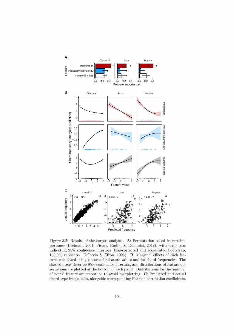
Classical Jazz Popular

0.0 0.2 0.4 0.0 0.2 0.4 0.0 0.2 0.4

Number of notes

Periodicity/harmonicity

Interference

Feature importance

Fea

ture

A

Classical Jazz Popular

InterferenceP

eriodicity/harmonicity

Num

ber of notes

−2 −1 0 1 2 −2 −1 0 1 2 −2 −1 0 1 2

−2

0

2

4

−1.0

−0.5

0.0

0.5

−3

−2

−1

0

1

Feature value

Cho

rd fr

eque

ncy

(mar

gina

l pre

dict

ion)

B

●

●●

●●●●●

●●●

●

●

●●●●●●

●●

●

●●

●●

●

●●●●●

●●

●●

●●

●●●

●

●

●●●

●

●●

●

●

●●●●

●●

●●

●

●

●●●●●

●

● ● ●●●●●

●●●

●●●●

●

●

●●

●

●●●●

●●●

●

●●

●●

●●●

●●●

●

●●

●●

● ●●●

●●

●

●●●

●

●●

●

●

●●●

●

●●●

●●●●

●

●●●

●●●

●●●● ●

●●●

●

●●●

●

●

●●●

●

●

●

●●●

●●●

●

●●●

●●●●●

●

●

●

●●

●

●

●●●●

●●

●

●●●● ●

●●

●●

●

●

●●●

●● ●●●●

●●

●●●● ●●●●

●●

●

●

●●●

●●●●

●●●

●●●●● ●

●●

●●

●●●

●●●●

● ●●

●

●●●●●●

●●●

●●

●●●

●●●●●

● ●

●

●●

●●

●● ●

●●

●

●

●●

●

●●

●●●●●●●●

●●

●●

●

●●

●

●●●●● ●

● ●

●●●

●

●

●

●

●●

●●

●●●●●●●

●●●● ●

●●

●●●●●

●●●

●

●●

●

●●●●

●

●●● ●

●●●

●

●●

●●

●

●

●

●

●●

●●●

●

●

●●●●

●

●

● ●●

●●

●

●●

●●●

●●●

●

●●

●

●●●

●●

●●●

●●

●

●●

●●●●

●

●●

●●

●●●

●●●●●

●●●

●

●

●●●

●●

●●

●

●●●●●●

●●

●● ●

●

●● ●

●●

●

●●

●

●

●● ●●

● ●●●●

●●

●

●

●

●●●●●

●●●

●●●

●

●●

●

●●●●●

●●

●● ●

●● ●●

●

●

●●

●

●●●

●●

●●●● ●●●

●●●●●

●

●

●

●●

●●●●●

● ●●●

●

●●●●

●●●●●

●●●

●●●●●●

●●●

●

●●●

●●

● ●●

●

●●●●●

●●

●●●●

●●

●

●

●

●●●

●●●●

●

●●●

● ●●

●●

●

●●●

●●●●●●

●●

●●●●●

●●●

●●●●●●●

●●●●

●●●●●●●

●●●●

●●●

●●●●●●●

●

●

●

●

●

●

●

●

●●

●

●●

●●●●

●

●●

●●

●●●●

●

●

●●●●●

●

●●●●●

●

●●●

●●●●

●●

●●

●●

●●●●●●

●

●●●● ●●

● ●●●●●

●

●●

●●●

●●●

●

●●●●●●●

●●

●●●●

●●●●

●●●●●●

●

●

●●●

●●

●●●●

●

●

●

●

●●●●●

●

●●● ●●

●●●

●●

●

●

●

●●

●●●●● ●

●●●●

●

●

●

●

●●●●●●

●

●

●

●●●

●●●

●●●

●●

●●

●

●

●

●●

●●

●

●●

●●

● ●●

●●

●●●

●●

●●●●

●●

●

●

●●

●●

●●●●●

●●●●

●

●●

●

●●●●●

●

●

●●

●

●●

●●●

●●●●●●●

●●●

●●●●● ●

●●

●●

●●

●

●●●

●

●●●

●

●●

●●●●

●

●

●

●

●●

●● ●●

●●

●●●●●● ●

●●●

●●

●●

●●●

●●●●●●●●●

●●●

●●●●●● ●

●●

●●

●●●

● ●●●

●● ●

●●●

●●● ●●

●●●

●●

●●●●●●

●●●●●

●●●●●●●●

●●●●

●●●●●●●●

●

●●

●

●●

●

●●●●

●●●●●●●●●●●

●

●●

●●●●●

●

●●

●

●●●

●●●●●●●●

●●

●

●●

●

●●●

●

●●

●●●

●

●●

●●●●

●●●●●●●●

●●

●●

●●●●

●●

●●●●●

●

●●●

●●●●●●●

● ●●●●●●

●

●●●●●

●●

●●●●●●●●●●●●●

●

●●●●●●●

●

●

●

●

●

●

●●●●

●

●●

●●●

●

●

●●

●

●●●●●●●

●●

●

●●●●●●●●●●●●●

●

●●●●●●●●

●●●●● ●

●●

●●

●●●●●

●●

●

●●●●●●

●

●●●●

●●●●

●●●

●

●●

●●

●

●

●●

●●●

●

●●●●

●●●

●●●●●

●●●●●●

●

●●●●

●●●

●● ●●●●

●

●

●

●

●

●●●

●●●●●

●●●●

●●●●●

●●●

●●

●

●●

●●●

●●

●●●●

●●

●

●●●

●●

●●

●

●

●

●

●

●●●●

●

●

●●●●

●●

●●●●●

●●●●

●●●●

●

●●●

●●●● ●●

●●

●

●●

●

●●●●●●●

●●●●

●●●●●●●●●●

●

●●

●●

●●

●● ●

●

●

●

●●

●●●●

●●●●●●●

●●

●

●●●●●●

●

●●

●●●

●

●●●●●●●●●●

●●

●●●●

●●●●

●●

●

●●●●●●●●●

●●●●●●

●

●●

●●

●●

●

●

●

●●●●●

●

●

●

●

●●●

●●

●●

●

●

●

●●●●●●●●●

●●●

●●●●●●●●

●●●●

●●●

●●●●

●●●●

●

●●●

●●●

●●●●●

●●

●●

●●●●●

●

●●●

●●●

●●

●●●●●

●

●

●●

●●●●

●●●●●●●●●

●●●●●●●

●●●●●●

●

●

●

●

●●●

●●●

●

●

●

●

●

●●●●

●●●

●

●●●●

●●●●●●●●●●●●

●●●●●●

●●●●

●●●

●●●

●●●

●●

●

●●

●

●

●●

●●●●

●●●●●●

●●●●

●●●●

●

●

●●

●●●●●●●

●

●●●

●●●●●

●

●●●●

●●

●

●●●●

●●●

●

●●

●●

●

●●●●●●

●

●●

●●●●●●●●●●

●

●●●

●●●

●●●●

●●

●

●●

●●●●●●

●

●●

●●●●●●●●●●●●

●

●

●●●●●●

●●

●●●●

●●●●●●●

●●●●

●

●●

●●●

●

●

●

●

●●●●●●●●

●●●●●

●●

●●●●●●●●●

●●

●

●

●

●●●●●●

●●●●

●●

●●●●●●

●

●

●

●●●

●●●●●

●

●

●

●●●●

●●●●●●●●●

●●●●●●

●●●●

●●●●

●●●●●

●●

●●●●●

●●●●●

●

●●

●●●●●●●●●

●●●

●

●

●●●●●●

●

●●●●

●●●●●●●

●

●

●●

●

●●●

●●●

●●●●●●●

●●●●●

●

●●●●

●

●●●●

●

●●●●●●●●●●●

●

r = 0.95

●

●

●

●

●

●

●

●

●

●

●

●

●

●

●●

●●

●

●●

●

●

●●

● ●●

●

●

●

●

●

●

●

●

●

●

●

●

●

●

●

●

●

●

●

● ●

●

●

●

●●

●

●●

●

●

●

●

●

●●●

●

●

●●

● ●

●

●●

●●

●●

●●

●

●

●

●

●

●

●

●●

●

●

●●

●

●

●

●

●

●

●

●

●

●

●

●

●

●

●

●

●

●●● ●●● ●

●

r = 0.55

●

●● ●

●

●

●

● ●

●

●●

●

●

●

●

● ●

●

●

●

●●

●

●

●

●

●

● ●

●

●

●

●

●

●●

●

●

●

●

●

●●

●●

●

●

●

●

●●

●●

● ●

●

●

●

●

●

●●

●

●

●●

●●●

●

●●

●

●

●

●

●

●

●

●

●

●

●

●●

●

●

●

●

●

●

●

● ●

●

●

●

●●

●

●●

●

●

●

●

●

●●●

●

●

●

●●

●

●

●

●

●●

● ●

●

●

●

●

● ●●

●

●●

●●

●

●

●

●

●

●●

●

●●

●●

●

●●●

●●

●●●

r = 0.67

Classical Jazz Popular

−1 0 1 2 3 4 5 −1 0 1 −1 0 1 2

−1

0

1

2

3

−1

0

1

2

3

−2

0

2

4

6

Predicted frequency

Act

ual f

requ

ency

C

Figure 3.5: Results of the corpus analyses. A: Permutation-based feature im-portance (Breiman, 2001; Fisher, Rudin, & Dominici, 2018), with error barsindicating 95% confidence intervals (bias-corrected and accelerated bootstrap,100,000 replicates, DiCiccio & Efron, 1996). B: Marginal effects of each fea-ture, calculated using z-scores for feature values and for chord frequencies. Theshaded areas describe 95% confidence intervals, and distributions of feature ob-servations are plotted at the bottom of each panel. Distributions for the ‘numberof notes’ feature are smoothed to avoid overplotting. C: Predicted and actualchord-type frequencies, alongside corresponding Pearson correlation coefficients.

104

both interference and periodicity/harmonicity, then we might expect both fea-tures to contribute to chord prevalences.

Compiling chord prevalences requires a decision about how to categorisechords into chord types. Here we represented each chord as a pitch-class chordtype, defined as a pitch-class set expressed relative to the bass pitch class. Thisrepresentation captures the perceptual principles of octave invariance (the chordtype is unchanged when chord pitches are transposed by octaves, as long as theydo not move below the bass note) and transposition invariance (the chord typeis unchanged when all the chord’s pitches are transposed by the same interval).

Hutchinson & Knopoff’s model requires knowledge of precise pitch heights,which are not available in pitch-class chord type representations. We thereforeassigned pitch heights to each chord type by applying the automatic chordvoicing algorithm developed in Chapter 5 (see Section 3.9 for details).

Chord type prevalences could be operationalised in various ways. Ideally,one might sum the temporal duration of each chord type over all of its occur-rences, perhaps weighting compositions by their popularity to achieve the bestrepresentation of a given musical style. However, chord durations and com-position popularity were not available for our classical and jazz datasets. Wetherefore operationalised chord type prevalences as the total number of occur-rences of each chord type, excluding immediate repetitions of the same chord(see Section 3.9).

We constructed three orthogonal polynomial regression models predictinglog-transformed chord counts from interference, periodicity/harmonicity, andnumber of notes. The classical, jazz, and popular corpora contributed 2,048,118, and 157 data points respectively, corresponding to the unique chord typesobserved in each corpus and their respective counts. Each corpus was assignedits own polynomial order by minimising the Bayesian Information Criterion forthe fitted model; the classical, jazz, and popular datasets were thereby assignedthird-order, first-order, and second-order polynomials respectively.

Figure 3.5A quantifies each predictor’s importance using a permutation-based feature-importance metric (Breiman, 2001, see Section 3.9 for details).Across the three genres, interference was consistently the most important pre-dictor, explaining c. 20–50% of the variance in chord prevalences. Periodic-ity/harmonicity was also an important predictor for classical music, but not forpopular or jazz music. Number of notes predicted chord prevalences in all threegenres, explaining about half as much variance as interference.

Figure 3.5B plots the marginal effects of each predictor, showing how featurevalues map to predictions. Interference had a clear negative effect on chordprevalence in all three genres, consistent with the notion that interference evokesdissonance, causing it to be disliked by listeners and avoided by composers.

105

Periodicity/harmonicity had a clear positive effect on chord prevalence in theclassical dataset, consistent with the idea that periodicity/harmonicity evokesconsonance and is therefore promoted by composers (Figure 3.5B). The effect ofperiodicity/harmonicity was less strong in the popular and jazz datasets, takingthe form of a weak positive effect in the popular dataset and a weak negativeeffect in the jazz dataset.

Figure 3.5C summarises the predictive performances of the three regressionmodels. Generally speaking, predictive performances were high, indicating thatconsonance and number of notes together explain a large part of Western chordprevalences. However, the strength of this relationship varied by musical style,with the classical dataset exhibiting the strongest relationship and the jazzdataset the weakest relationship.

In sum, these results weigh against the claim that consonance is primarily de-termined by periodicity/harmonicity and not interference (Bowling & Purves,2015; Bowling et al., 2018; McDermott et al., 2010). Across musical genres,interference seems to have a strong and reliable negative effect on chord preva-lences. Periodicity/harmonicity also seems to influence chord prevalences, butits effect is generally less strong, and the nature of its contribution seems tovary across musical genres.

3.8 DiscussionRecent research argues that consonance perception is driven not by interfer-ence but by periodicity/harmonicity, with cultural differences in consonanceperception being driven by learned preferences for the latter (Cousineau et al.,2012; McDermott et al., 2010, 2016). We reassessed this claim by reviewinga wide range of historic literature, modelling perceptual data from four pre-vious empirical studies, and conducting corpus analyses spanning a thousandyears of Western music composition. We concluded that interference contributessignificantly to consonance perception in Western listeners, and that culturalaspects of consonance perception extend past learned preferences for periodic-ity/harmonicity. Instead, consonance perception in Western listeners seems tobe jointly determined by interference, periodicity/harmonicity perception, andlearned familiarity with particular musical sonorities.

This multicomponent account of consonance is broadly consistent with sev-eral previous claims in the literature. Terhardt (1974, 1984) has emphasisedthe role of roughness and harmonicity in determining consonance, and Parncuttand colleagues have argued that consonance depends on roughness, harmonicity,and familiarity (Parncutt & Hair, 2011; Parncutt et al., 2018). Scientific pref-erences for parsimony may have caused these multicomponent accounts to be

106

neglected in favour of single-component accounts, but our analyses demonstratethe necessity of the multicomponent approach.

This consolidation of multiple psychological mechanisms makes an interest-ing parallel with historic pitch perception research, where researchers strove todemonstrate whether pitch perception was driven by place coding or temporalcoding (see de Cheveigné, 2005 for a review). It proved difficult to falsify eitherplace coding or temporal coding theories, and many researchers now believethat both mechanisms play a role in pitch perception (e.g. Bendor, Osmanski,& Wang, 2012; Moore & Ernst, 2012).

Like most existing consonance research, our analyses were limited to West-ern listeners and composers, and therefore we can only claim to have charac-terised consonance in Westerners. Previous research has identified significantcross-cultural variation in consonance perception (Florian, 1981; Maher, 1976;McDermott et al., 2016); we suggest that this cross-cultural variation might beapproximated by varying the regression coefficients in our composite consonancemodel. For example, listeners familiar with beat diaphony seem to perceive in-terference as consonant, not dissonant (Florian, 1981); this would be reflectedin a reversed regression coefficient for interference. While the regression coeffi-cients might vary cross-culturally, it seems plausible that the model’s underly-ing predictors – interference, periodicity/harmonicity, familiarity – might recurcross-culturally, given the cross-cultural perceptual salience of these features(McDermott et al., 2016).

Our conclusions are not inconsistent with vocal-similarity theories of con-sonance perception (Bowling & Purves, 2015; Bowling et al., 2018; Schwartzet al., 2003). According to these theories, certain chords sound consonant be-cause they particularly resemble human vocalisations. These theories usuallyemphasise periodicity/harmonicity as a salient feature of human vocalisations,but they could also implicate interference as a feature avoided in typical vocal-isations (Bowling et al., 2018) but used to convey distress in screams (Arnal,Flinker, Kleinschmidt, Giraud, & Poeppel, 2015). It seems plausible that thesemechanisms contribute a universal bias to perceive periodicity/harmonicity aspleasant and interference as unpleasant. Nonetheless, these biases must be sub-tle enough to allow cultural variation, if we are to account for musical culturesthat lack preferences for periodicity/harmonicity (McDermott et al., 2016) orthat consider interference to be pleasant (Florian, 1981).

Our perceptual analyses were limited by the available empirical data. Wepaid particular attention to the perceptual dataset of Bowling et al. (2018)on account of its large sample size, yet this dataset limits consideration tochords comprising no more than four notes, all drawn from a small pitch range(one octave), and tuned using an idiosyncratic approximation to just intonation

107

(see Section 3.9). Future work should expand these datasets, with particularemphasis on varying voicing, tone spectra, tuning systems, and number of notesin the chord. Such datasets would be essential for testing the generalisability ofour models.

Our perceptual analyses marginalised over participants, producing an aver-age consonance rating for each chord. This approach neglects individual differ-ences, which can provide an important complementary perspective on conso-nance perception (McDermott et al., 2010). When suitable empirical datasetsbecome available, it would be interesting to investigate how the regressionweights in Figure 3.4C vary between participants.

Our corpus analyses presented very broad approximations to musical gen-res, aggregating over a variety of musical styles and time periods. It would beinteresting to apply these methods to more specific musical styles, or indeed toindividual composers. It would also be interesting to investigate the evolutionof consonance treatment over time. As we analyse music compositions dat-ing further back in history, we should expect the chord distributions to reflectconsonance perception in historic listeners rather than modern listeners. Suchanalyses could potentially shed light on how consonance perception has changedover time (Parncutt et al., 2018).

Our three corpora were constructed in somewhat different ways. The classi-cal corpus was derived from published musical scores; the jazz corpus constitutesa collection of lead sheets; the popular corpus comprises expert transcriptionsof audio recordings. This heterogeneity is both an advantage, in that it teststhe generalisability of our findings to different transcription techniques, and adisadvantage, in that it reduces the validity of cross-genre comparisons. Futurework could benefit from corpora with both stylistic diversity and consistentconstruction.

Our analyses were limited by the computational models tested. It wouldbe interesting to develop existing models further, perhaps producing a versionof Bowling et al.’s (2018) periodicity/harmonicity model that accepts arbitrarytunings, or a version of Parncutt & Strasburger’s (1994) model without discrete-pitch approximations. It would also be interesting to test certain models notevaluated here, such as Boersma’s (1993) model and Vencovsky’s (2016) model.Lastly, we would like to dissuade future researchers from permanently discard-ing specific consonance models based on our results. In particular, the audio-based models depend on many customisable parameters such as sample rates,windowing lengths, and peak-detection thresholds, and it is quite possible thatfurther exploration of these parameters could yield better performance on thesedatasets.

The psychological community often uses ‘consonance’ as a synonym for tonal

108

‘pleasantness’ (e.g. Bowling et al., 2018; Cousineau et al., 2012; McDermottet al., 2010, 2016), and this convention is also followed by the present chap-ter. From a linguistic perspective, however, consonance and pleasantness havesubtly different connotations. In particular, a musician is likely to evaluateconsonance with respect to the prototypical consonant sonorities of music the-ory, even if they personally consider certain non-traditional sonorities to soundpleasant. Moreover, their pleasantness judgements may be guided by phenom-ena other than those traditionally associated with consonance: for example, thesense in which the chord possesses some kind of interesting tonal implications,elicits an unusual acoustic effect, or evokes a powerful emotion. These and otherrelated-yet-distinct dimensions of perceptual evaluation (e.g. tension, harmo-niousness, preference) provide useful and complementary perspectives on theacoustic and psychological mechanisms underlying harmony perception. De-spite early interest in the topic (e.g. Guernsey, 1928; Geer et al., 1962), thesesemantic distinctions have been often neglected in subsequent work, and it isgood to see this area being revisited in recent empirical studies (e.g. Lahdelma& Eerola, 2016, 2019; Popescu et al., 2019).

We hope that our work will facilitate future psychological research into con-sonance. Our incon package makes it easy to test diverse consonance models onnew datasets, and it can be easily extended to add new models. Our inconDatapackage compiles the perceptual datasets analysed here, making it easy to testnew consonance models on a variety of perceptual data.

This work should also have useful applications in computational musicologyand music information retrieval. Our composite consonance model provides aprincipled way to operationalise the net consonance of a musical chord, whileour model evaluations provide a principled way to operationalise individual con-sonance theories. Our software provides a consistent and easy-to-use interfaceto these models, facilitating their application to new datasets.

3.9 Methods

3.9.1 Models

The models evaluated in this chapter are available from three software sources:the incon package, MIRtoolbox22, and Essentia23. Unless otherwise mentioned,all incon models represent unaltered versions of their original algorithms asdescribed in the cited literature, with the exception that all idealised harmonicspectra comprised exactly 11 harmonics (including the fundamental frequency),

22https://www.jyu.fi/hytk/fi/laitokset/mutku/en/research/materials/mirtoolbox23https://essentia.upf.edu

109

with the ith harmonic having an amplitude of i−1, and assuming incoherencebetween tones for the purpose of amplitude summation. We clarify some furtherdetails below.

Milne (2013); New harmonicity model

These algorithms have three free parameters: the number of harmonics modelledin each complex tone, the harmonic roll-off rate (ρ), and the standard deviationof the Gaussian smoothing distribution (σ). We set the number of harmonicsto 11 (including the fundamental frequency), and set the other two parametersto the optimised values in Milne & Holland (2016): a roll-off of ρ = 0.75, and astandard deviation of σ = 6.83 cents.

Hutchinson & Knopoff (1978)

Our implementation is based on Mashinter (2006), whose description includesa parametric approximation for the relationship between interval size and pure-dyad dissonance (see also Bigand et al., 1996).

Sethares (1993)

Our implementation is primarily based on Sethares (1993), but we include amodification suggested in later work (Sethares, 2005; Weisser & Lartillot, 2013)where pure-dyad consonance is weighted by the minimum amplitude of eachpair of partials, not the product of their amplitudes.

Wang et al. (2013)

Our implementation of Wang et al.’s (2013) algorithm takes symbolic input andexpresses each input tone as an idealised harmonic series. Time-domain analysesare conducted with a signal length of 1 s and a sample rate of 44,000. Frequency-domain analyses are conducted in the range 1–44,000 Hz with a resolution of1 Hz. An interactive demonstration of the algorithm is available at http://shiny.pmcharrison.com/wang13.

Essentia: Interference

We used version 2.1 of Essentia. We analysed each audio file using the ‘es-sentia_streaming_extractor_music’ feature extractor, and retained the meanestimated dissonance for each file.

110

MIRtoolbox: Interference

We used version 1.6.1 of MIRtoolbox, and computed roughness using the ‘mir-roughness’ function. The function was applied to a single window spanning theentire length of the stimulus.

We evaluated this model in several configurations (see Figure 3.4A):

a) ‘Sethares’ denotes the default model configuration, which implements thedissonance model of Sethares (2005), but with pure-tone dyad contribu-tions being weighted by the product of their amplitudes (see Sethares,1993);

b) ‘Sethares, v2’ denotes the ‘Min’ option in MIRtoolbox, where pure-tonedyad contributions are weighted by the minimum of their amplitudes, afterWeisser & Lartillot (2013; see also Sethares, 2005);

c) ‘Vassilakis’ denotes MIRtoolbox’s implementation of Vassilakis’s (2001)model.

Johnson-Laird et al. (2012)

Johnson-Laird et al.’s (2012) algorithm may be separated into a cultural andan interference component, with the latter corresponding to Hutchinson &Knopoff’s (1978) model. The cultural model assigns each chord to a conso-nance category, where categories are ordered from consonant to dissonant, andchords within a category are considered to be equally consonant. In our imple-mentation, these consonance categories are mapped to positive integers, suchthat higher integers correspond to greater dissonance. These integers constitutethe algorithm’s outputs.

Corpus-based model of cultural familiarity

This model estimates a listener’s unfamiliarity with a given chord type from itsrarity in a musical corpus. Here we use the Billboard dataset (Burgoyne, 2011),a corpus of popular songs sampled from the Billboard magazine’s ‘Hot 100’chart in the period 1958–1991. This corpus is used as a first approximation toan average Western listener’s prior musical exposure. We represent each chordin this corpus as a pitch-class chord type, defined as the chord’s pitch-class setexpressed relative to the chord’s bass note. For example, a chord with MIDInote numbers {66, 69, 74} has a pitch-class chord type of {0, 3, 8}. We counthow many times each of the 2,048 possible pitch-class chord types occurs in thecorpus, and add 1 to the final count. Unfamiliarity is then estimated as thenegative natural logarithm of the chord type’s count.

111

Table 3.3: Unstandardised regression coefficients forthe composite consonance model.

Term CoefficientIntercept 0.628434666589357Number of notes 0.422267698605598Interference −1.62001025973261Periodicity/harmonicity 1.77992362857478Culture −0.0892234643584134

Note. These regression coefficients are presented tofull precision for the sake of exact reproducibility,but it would also be reasonable to round the coeffi-cients to c. 3 significant figures. When generalisingoutside the dataset of Bowling et al. (2018), we rec-ommend setting the number of notes coefficient tozero.

Composite model

The composite model’s unstandardised regression coefficients are provided tofull precision in Table 3.3. Consonance is estimated by computing the fourfeatures listed in Table 3.3, multiplying them by their respective coefficients,and adding them to the intercept coefficient. Number of notes corresponds tothe number of distinct pitch classes in the chord; interference is computed usingHutchinson & Knopoff’s (1978) model; periodicity/harmonicity is computedusing this chapter’s new harmonicity model; culture corresponds to the newcorpus-based cultural model.

It is unclear whether the effect of number of notes generalises outside thedataset of Bowling et al. (2018) (see Section 3.6). We therefore recommendsetting the number of notes coefficient to zero when applying the model to newdatasets.

3.9.2 Software

We release two top-level R packages along with this chapter. The first, incon,implements the symbolic consonance models evaluated in this chapter (Table3.2).24 The second, inconData, compiles the perceptual datasets that we anal-ysed.25 Tutorials are available alongside these packages.

The incon package depends on several low-level R packages that we alsorelease along with this chapter, namely bowl18, corpdiss, dycon, har18, hcorp,hrep, jl12, parn88, parn94, stolz15, and wang13. These packages provide detailed

24https://github.com/pmcharrison/incon25https://github.com/pmcharrison/inconData

112

interfaces to individual consonance models and tools for manipulating harmonyrepresentations.

Our software, analyses, and manuscript were all created using the program-ming language R (R Core Team, 2017), and benefited in particular from the fol-lowing open-source packages: bookdown, boot, checkmate, cocor, cowplot, dplyr,ggplot2, glue, gtools, hht, knitr, jsonlite, magrittr, margins, memoise, numbers,papaja, phonTools, plyr, purrr, Rdpack, readr, rmarkdown, testthat, tibble, tidyr,usethis, withr, and zeallot. Our analysis code is freely available online.26

3.9.3 Perceptual datasets

The following datasets are all included in our inconData package.

Bowling et al. (2018)

This study collected consonance judgments for all possible 12 two-note chordtypes, 66 three-note chord types, and 220 four-note chord types that can beformed from the Western chromatic scale within a one-octave span of the bassnote.27 An advantage of this dataset is its systematic exploration of the chro-matic scale; a disadvantage is its restricted range of voicings.

Each chord tone was pitched as a just-tuned interval from the bass note.28

This approach was presumably chosen because Bowling et al.’s (2018) period-icity/harmonicity model requires just tuning, but it should be noted that justtuning itself is not commonly adopted in Western music performance (e.g. Kar-rick, 1998; Kopiez, 2003; Loosen, 1993). It should also be noted that tuninga chord in this way does not ensure that the intervals between non-bass notesare just-tuned, and certain chords can sound unusually dissonant as a resultcompared to their equal-tempered equivalents.

Each chord type was assigned a bass note such that the chord’s mean fun-damental frequency would be equal to middle C, approximately 262 Hz. Theresulting chords were played using the ‘Bosendorfer Studio Model’ synthesisedpiano in the software package ‘Logic Pro 9’.

The participant group numbered 30 individuals. Of these, 15 were studentsat a Singapore music conservatory, each having taken weekly formal lessons inWestern tonal music for an average of 13 years (SD = 3.8). The remaining 15participants were recruited from the University of Vienna, and averaged lessthan a year of weekly music lessons prior to the study (SD = 1.1).

26https://github.com/pmcharrison/inconPaper27As before, a chord type represents a chord as a set of intervals above an unspecified bass

note (Chapter 2).28Just tuning means expressing pitch intervals as small-integer frequency ratios. In Bowling

et al. (2018), the eleven intervals in the octave were expressed as the following frequencyratios: 16:15, 9:8, 6:5, 5:4, 4:3, 7:5, 3:2, 8:5, 5:3, 9:5, 15:8, and 2:1.

113

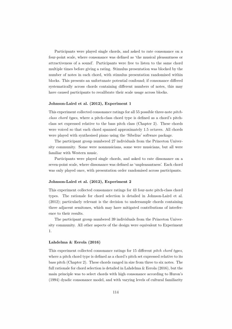
Participants were played single chords, and asked to rate consonance on afour-point scale, where consonance was defined as ‘the musical pleasantness orattractiveness of a sound’. Participants were free to listen to the same chordmultiple times before giving a rating. Stimulus presentation was blocked by thenumber of notes in each chord, with stimulus presentation randomised withinblocks. This presents an unfortunate potential confound; if consonance differedsystematically across chords containing different numbers of notes, this mayhave caused participants to recalibrate their scale usage across blocks.

Johnson-Laird et al. (2012), Experiment 1

This experiment collected consonance ratings for all 55 possible three-note pitch-class chord types, where a pitch-class chord type is defined as a chord’s pitch-class set expressed relative to the bass pitch class (Chapter 2). These chordswere voiced so that each chord spanned approximately 1.5 octaves. All chordswere played with synthesised piano using the ‘Sibelius’ software package.

The participant group numbered 27 individuals from the Princeton Univer-sity community. Some were nonmusicians, some were musicians, but all werefamiliar with Western music.

Participants were played single chords, and asked to rate dissonance on aseven-point scale, where dissonance was defined as ‘unpleasantness’. Each chordwas only played once, with presentation order randomised across participants.

Johnson-Laird et al. (2012), Experiment 2

This experiment collected consonance ratings for 43 four-note pitch-class chordtypes. The rationale for chord selection is detailed in Johnson-Laird et al.(2012); particularly relevant is the decision to undersample chords containingthree adjacent semitones, which may have mitigated contributions of interfer-ence to their results.

The participant group numbered 39 individuals from the Princeton Univer-sity community. All other aspects of the design were equivalent to Experiment1.

Lahdelma & Eerola (2016)

This experiment collected consonance ratings for 15 different pitch chord types,where a pitch chord type is defined as a chord’s pitch set expressed relative to itsbass pitch (Chapter 2). These chords ranged in size from three to six notes. Thefull rationale for chord selection is detailed in Lahdelma & Eerola (2016), but themain principle was to select chords with high consonance according to Huron’s(1994) dyadic consonance model, and with varying levels of cultural familiarity

114

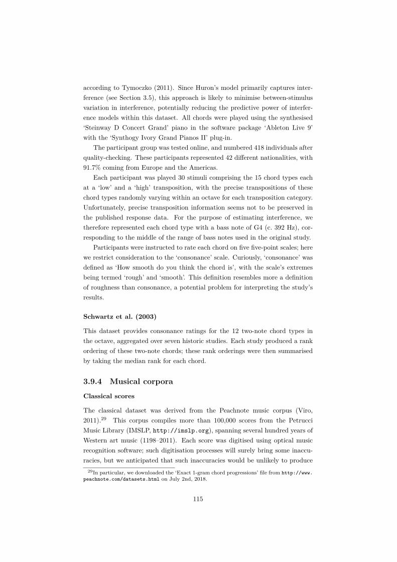
according to Tymoczko (2011). Since Huron’s model primarily captures inter-ference (see Section 3.5), this approach is likely to minimise between-stimulusvariation in interference, potentially reducing the predictive power of interfer-ence models within this dataset. All chords were played using the synthesised‘Steinway D Concert Grand’ piano in the software package ‘Ableton Live 9’with the ‘Synthogy Ivory Grand Pianos II’ plug-in.

The participant group was tested online, and numbered 418 individuals afterquality-checking. These participants represented 42 different nationalities, with91.7% coming from Europe and the Americas.

Each participant was played 30 stimuli comprising the 15 chord types eachat a ‘low’ and a ‘high’ transposition, with the precise transpositions of thesechord types randomly varying within an octave for each transposition category.Unfortunately, precise transposition information seems not to be preserved inthe published response data. For the purpose of estimating interference, wetherefore represented each chord type with a bass note of G4 (c. 392 Hz), cor-responding to the middle of the range of bass notes used in the original study.

Participants were instructed to rate each chord on five five-point scales; herewe restrict consideration to the ‘consonance’ scale. Curiously, ‘consonance’ wasdefined as ‘How smooth do you think the chord is’, with the scale’s extremesbeing termed ‘rough’ and ‘smooth’. This definition resembles more a definitionof roughness than consonance, a potential problem for interpreting the study’sresults.

Schwartz et al. (2003)

This dataset provides consonance ratings for the 12 two-note chord types inthe octave, aggregated over seven historic studies. Each study produced a rankordering of these two-note chords; these rank orderings were then summarisedby taking the median rank for each chord.

3.9.4 Musical corpora

Classical scores

The classical dataset was derived from the Peachnote music corpus (Viro,2011).29 This corpus compiles more than 100,000 scores from the PetrucciMusic Library (IMSLP, http://imslp.org), spanning several hundred years ofWestern art music (1198–2011). Each score was digitised using optical musicrecognition software; such digitisation processes will surely bring some inaccu-racies, but we anticipated that such inaccuracies would be unlikely to produce

29In particular, we downloaded the ‘Exact 1-gram chord progressions’ file from http://www.peachnote.com/datasets.html on July 2nd, 2018.

115

systematic confounds in the perceptual analyses. In the resulting dataset, eachdatum represents a distinct ‘vertical slice’ of the score, with new slices occurringat new note onsets, and including sustained notes sounded at previous onsets.We preprocessed this dataset to a pitch-class chord-type representation, whereeach chord is represented as a pitch-class set expressed relative to its bass pitchclass. The resulting dataset numbered 128,357,118 chords.

Jazz lead sheets

The jazz dataset was derived from the iRb corpus (Broze & Shanahan, 2013).The iRb corpus numbers 1,186 lead sheets for jazz compositions, where each leadsheet specifies the underlying chord sequence for a given composition. Theselead sheets were compiled from an online forum for jazz musicians. In the orig-inal dataset, chords are represented as textual tokens, such as ‘C7b9’; we trans-lated all such tokens into a prototypical pitch-class chord-type representation,such as {0, 1, 4, 7, 10}. This process misses the improvisatory chord alterationsthat typically happen during jazz performances, but nonetheless should providea reasonable first approximation to the performed music. Chord counts wereonly incremented on chord changes, not chord repetitions; section repeats wereomitted. The resulting dataset numbered 42,822 chords.

Popular transcriptions

The popular dataset was derived from the McGill Billboard corpus (Burgoyne,2011), which comprised chord sequences for 739 unique songs as transcribed byexpert musicians. As with the iRb dataset, we translated all chord tokens intoprototypical pitch-class chord-type representations, omitting section repeats,and only incrementing chord counts on each chord change. The resulting datasetnumbered 74,093 chords.

3.9.5 Corpus analyses

We transformed each of our corpora to pitch-class chord type representations,where each chord is represented as a pitch-class set relative to the chord’s bassnote (Chapter 2). We then counted occurrences of pitch-class chord types inour three corpora.

For the purpose of applying Hutchinson & Knopoff’s (1978) interferencemodel, we assigned pitch heights to each chord type using the automatic chordvoicing algorithm described in Chapter 5. This model is primarily designedfor voicing chord sequences, but it can also be applied to individual chords.Its purpose is to find an idiomatic assignment of pitch heights to pitch classesthat reflects the kind of psychoacoustic considerations implicitly followed by

116

traditional Western composers (e.g. Huron, 2001). As applied here, the modelminimised the following linear combination of features:

8.653× interference

+ 1.321× | 5− number of notes |

+ 0.128× | 60− mean pitch height |

(3.12)

where ‘interference’ refers to the raw output of Hutchinson & Knopoff’s model,‘number of notes’ refers to the number of unique pitches in the chord voicing, and‘mean pitch height’ corresponds to the mean of the chord’s pitches as expressedin MIDI note numbers.30 In other words, the model minimised the chord’sinterference while preferring chords containing (close to) five discrete pitcheswith a mean pitch height close to middle C (c. 262 Hz). These model parameterscorrespond to the optimal parameters derived in Chapter 5 from a dataset of370 chorale harmonisations by J. S. Bach, but with the target number of noteschanged from four to five to reflect the richer harmonic vocabularies of the threedatasets. Chord voicings were restricted to the two octaves surrounding middleC, and were permitted to contain no more than five notes or the number ofpitch classes in the chord type, whichever was greater.

We used polynomial regression to capture nonlinear relationships betweenchord features and chord prevalences. We used orthogonal polynomials, as com-puted by the R function ‘poly’, to avoid numerical instability, and we used theR package ‘margins’ to compute marginal predictions for the resulting models.

Standardised regression coefficients become harder to interpret as the poly-nomial degree increases. We therefore instead calculate a permutation-basedfeature-importance metric commonly used for assessing feature importance inrandom forest models (Breiman, 2001; see also Fisher et al., 2018). This met-ric may be calculated by computing two values: the model’s original predictiveaccuracy, and the model’s predictive accuracy after randomly permuting thefeature of interest (without refitting the model). The metric is then defined asthe difference in these accuracies: the greater the difference, the more the modelrelies on the feature of interest. Here we used R2 as the accuracy metric, andcomputed confidence intervals for our feature-importance estimates using bias-corrected accelerated bootstrapping with 100,000 replicates (DiCiccio & Efron,1996).

30A frequency of f Hz corresponds to a MIDI note number of 69 + 12 log2(f/440).

117

Chapter 4

Harmonic expectation

4.1 IntroductionProbabilistic theories of music cognition hold that listeners experience musicby continually generating predictions for upcoming musical events, and relatingthese predictions to the musical events as they occur (Huron, 2006; Koelsch,Vuust, & Friston, 2019; Meyer, 1957; Pearce, 2018; Salimpoor, Zald, Zatorre,Dagher, & McIntosh, 2015). These predictions reflect the listener’s internalmodel of the musical style, developed through automatic processes of statisticallearning. The resulting dynamics of fulfilled and denied expectations are thoughtto be integral to the emotional experience of music (Egermann, Pearce, Wiggins,& McAdams, 2013; Huron, 2006; Meyer, 1957; Pearce, 2018; Sauvé, Sayed,Dean, & Pearce, 2018; Sloboda, 1991).

One musical dimension that elicits strong predictions, or ‘expectations’, isharmony. Harmony is a fundamental structuring principle in Western music,describing how musical notes combine to form chords, and how these chordscombine to form chord sequences. The expectedness of a given chord is context-dependent: for example, an E major chord may be incongruent when precededby a C major chord, but expected when preceded by a B major chord. Har-monic expectation therefore bears similarity with linguistic syntax, where theexpectedness of a word depends on the preceding words in the sentence, aswell as the individual’s internal model of the grammatical structure of the lan-guage. Correspondingly, the structuring principles underlying the constructionof chord progressions are often termed harmonic ‘syntax’ (Patel, 2003; Pearce& Rohrmeier, 2018; Rohrmeier, 2011; Rohrmeier & Pearce, 2018).

Some research has shown how harmonic expectation may be driven by low-level psychoacoustic cues. For example, Bigand et al. (2014) have shown thatthe expectedness of musical chords may be predicted by the acoustic similarity

118

between a chord and its musical context, where the context is accumulated inan echoic memory buffer with temporal decay (see also Craton, Lee, & Krahe,2019; Bigand et al., 1996; Leman, 2000a; Milne & Holland, 2016; Parncutt,1989). Other candidate cues for harmonic expectation include pitch distance(Bigand et al., 1996; Parncutt, 1989; Tymoczko, 2006), harmonicity (Bowlinget al., 2018; McDermott et al., 2010; Stolzenburg, 2015; Terhardt, 1974), andinterference between partials (Hutchinson & Knopoff, 1978; Plomp & Levelt,1965). These different cues may combine to determine the overall expectednessof a given chord (e.g. Bigand et al., 1996).

Other research has shown how harmonic expectations may be driven byhigh-level cognitive processes, similar to those involved in parsing the syntaxof natural language. Some evidence for this phenomenon comes from harmonicpriming studies, which analyse how the speed and accuracy of perceptual judg-ments are affected by harmonic expectedness. Several such studies have showna perceptual facilitation effect for syntactically expected chords, even when ac-counting for various psychoacoustic cues that might explain such a facilitationeffect (Bigand et al., 2003; Sears, Pearce, Spitzer, Caplin, & McAdams, 2019;Tekman & Bharucha, 1998). More evidence for high-level harmony cognitioncomes from studies showing that listeners can be sensitive to nonadjacent syn-tactic dependencies, which are difficult to capture with simple psychoacousticmodels (Koelsch, Rohrmeier, Torrecuso, & Jentschke, 2013; Rohrmeier & Cross,2009; Spyra, Stodolak, & Woolhouse, 2019; Woolhouse, Cross, & Horton, 2016).A particular relationship with linguistic syntax processing is suggested by stud-ies showing mutual interference between linguistic and harmonic syntax pro-cessing (Hoch et al., 2011; Koelsch et al., 2005; Kunert et al., 2016; Slevc etal., 2009; but see Poulin-Charronnat et al., 2005; Escoffier & Tillmann, 2008;Perruchet & Poulin-Charronnat, 2013; Slevc & Okada, 2015).

Surveying this evidence, it seems likely that both low-level and high-level per-ceptual processes contribute to harmonic expectation. Nonetheless, it remainsunclear how these different mechanisms combine in practice. Previous studiesof harmonic expectation typically use artificial stimuli specially constructed toprobe a particular component of harmonic expectation; these studies may showthat a given mechanism can contribute to harmonic expectation, but they can-not quantify how much the mechanism typically contributes to the perceptionof typical music compositions.

Here we address this challenge, seeking to investigate how different predic-tion mechanisms contribute to harmonic expectation in typical Western musiccompositions. We therefore avoid the specially composed chord sequences usedby previous studies, and instead derive our stimuli from the Billboard corpus,a large dataset of chord sequences representing compositions randomly sam-

119

pled from the Billboard ‘Hot 100’ charts between 1958 and 1991 (Burgoyne,2011). These compositions are by definition ‘popular’ music, and hence shouldbe broadly representative of the kind of music commonly heard by Westernlisteners on a day-to-day basis.

We use a computational modelling approach to simulate the predictive pro-cessing of these harmonic sequences. We begin by developing a flexible model ofharmony prediction that is capable of representing both low-level and high-levelperspectives on harmony. This model is feature-based, able to leverage sta-tistical regularities in both low-level psychoacoustic features (e.g. harmonicity,spectral similarity) and high-level cognitive features (e.g. chord root intervals,pitch-class sets). Furthermore, the model is capable of learning statistical reg-ularities at various Markov orders, where the Markov order determines howmany preceding feature observations are used to condition the prediction of thenext chord. By optimising and interrogating this model, we can examine howthese different statistical mechanisms might contribute to harmony predictionin human listeners.

In our first set of analyses, we apply the model to a dataset of chord progres-sions from the Billboard popular music corpus, and investigate what strategyan ideal listener might use for making predictions. This gives us some insightinto the kind of statistical structure underlying Western popular music. It alsoallows us to formulate hypotheses about human cognition: in particular, if wesuppose that most humans are proficient music listeners, then we might hy-pothesise that harmony prediction in human listeners should resemble harmonyprediction in the ideal-listener model.

In our second set of analyses, we test the ideal-listener model against datafrom human listeners. We play the same chord progressions to 50 Western non-musicians, and ask these participants to report the surprisingness of particularchords in these sequences. We then compare these surprisal ratings to the sur-prisal values delivered by our ideal-listener model, investigating whether thismodel provides a good account of participant behaviour, and using the modelto examine what kinds of statistical structure drive the variation in surprisalratings.

These analyses are accompanied by an open-source R package, hvr, whichimplements the computational models evaluated here.1 This should constitutea useful resource to future researchers interested in harmony prediction.

1This package is available at https://github.com/pmcharrison/hvr.

120

4.2 Perceptual featuresListeners have access to a rich variety of perceptual features that might con-tribute useful information for harmony prediction. In this section we reviewthese features, discuss how they may be simulated computationally, and surveytheir statistical properties (Figure 4.1, Table 4.1).

These features span a broad variety of psychological processes. For conve-nience, we group these features into two broad categories: ‘low-level’ featuresand ‘high-level’ features. The low-level features reflect relatively early stages ofauditory processing, whereas the high-level features reflect relatively late stagesof auditory processing. These two feature categories are also distinguished bytheir feature values: the low-level features take continuous values on numericscales, whereas the high-level features take discrete values on categorical scales.This transition between continuous and discrete domains reflects the cognitivephenomenon of categorical perception, whereby perceptual objects in continu-ous psychophysical space are assigned to discrete categories (Harnard, 2003).

These features are grounded in the representation network defined in Chap-ter 2. All are ultimately derived from the ‘pitch-class chord’ representation,which forms the basic representation scheme for the musical corpus, as well asthe event space over which the simulated listeners generate their predictions.Several of these features are in fact identical to representations from Chapter 2,such as the ‘pitch-class set’ feature and the ‘pitch-class set relative to bass’ fea-ture. Various new features are also included that extend past the representationnetwork from Chapter 2, with some features including additional psychoacousticmodelling (e.g. the ‘interference between partials’ feature) and others simulatinghigher-level cognitive processes such as root finding, relative pitch perception,and similarity judgment.

121

Sound Auditory spectrum

Interference between partials

Periodicity/harmonicity

Auditory scene analysis

Pitch distance

Pitch-class chord

Pitch-class set

Bass pitch class

Bass interval

Rootpitch class

Root interval

Bass pitch class relative

to root

Pitch-class chord relative to

previous bass

Previous chord’s features

Spectral similarity

Low-level features

High-level features

Related representations

Previous auditory spectra

Pitch-class set relative to

previous bass

Pitch-class set relative

to root

Pitch-class set relative

to bass

Figure 4.1: Schematic network illustrating the psychological relationships be-tween the 15 features used in the present study. An arrow indicates that aparticular feature is psychologically derived from another feature.

122

Tabl

e4.

1:T

he15

harm

ony

feat

ures

used

inth

epr

esen

tst

udy.

Nam

e

Text

ual

Com

puta

tiona

lD

omai

nPi

tch

repr

esen

tatio

nA

lpha

bet

size

Low

-leve

lIn

terf

eren

cebe

twee

npa

rtia

lshu

tch_

78C

ontin

uous

--

Perio

dici

ty/h

arm

onic

ityha

r_18

_har

moni

city

Con

tinuo

us-

-Pi

tch

dist

ance

pi_d

ist

Con

tinuo

us-

-Sp

ectr

alsim

ilarit

ysp

ec_s

im_3

Con

tinuo

us-

-H

igh-

leve

lB

ass

pitc

hcl

ass

bass

_pc

Cat

egor

ical

Abs

olut

e12

Roo

tpi

tch

clas

sro

ot_p

cC

ateg

oric

alA

bsol

ute

12B

ass

inte

rval

bass

_int

Cat

egor

ical

Rel

ativ

e12

Roo

tin

terv

alro

ot_i

ntC

ateg

oric

alR

elat

ive

12Pi

tch-

clas

sse

tpc

_set

Cat

egor

ical

Abs

olut

e4,

095

Pitc

h-cl

ass

chor

dpc

_cho

rdC

ateg

oric

alA

bsol

ute

24,5

76Pi

tch-

clas

sse

tre

lativ

eto

bass

pc_s

et_r

el_b

ass

Cat

egor

ical

Rel

ativ

e2,

048

Bas

spi

tch

clas

sre

lativ

eto

root

bass

_pc_

rel_

root

Cat

egor

ical

Rel

ativ

e12

Pitc

h-cl

ass

set

rela

tive

toro

otpc

_set

_rel

_roo

tC

ateg

oric

alR

elat

ive

457

Pitc

h-cl

ass

chor

dre

lativ

eto

prev

ious

bass

pc_c

hord

_rel

_pre

v_ba

ssC

ateg

oric

alR

elat

ive

24,5

76Pi

tch-

clas

sse

tre

lativ

eto

prev

ious

bass

pc_s

et_r

el_p

rev_

bass

Cat

egor

ical

Rel

ativ

e4,

095

123

4.2.1 Low-level features

Low-level features reflect relatively early parts of the auditory processing path-way, and are hence particularly dependent on the acoustic properties of thechord. They precede perceptual categorisation, and hence take continuous val-ues; they may therefore be termed continuous features. We review four suchfeatures: interference between partials, periodicity/harmonicity, spectral simi-larity, and pitch distance.

Interference between partials is a key predictor of consonance, the sensein which a chord’s notes ‘sound well together’ (Chapter 3). A chord’s acousticspectrum may be represented as a set of discrete partials, each associated with afrequency and an amplitude; pairs of partials create interference as a function oftheir proximity, with interference being maximised by close but non-overlappingpartials. This interference is thought to comprise beating and mutual maskingeffects, both of which are perceived as unpleasant, detracting from the chord’sconsonance. We operationalise interference between partials with Hutchinson& Knopoff’s (1978) model, which provided the best account of consonance per-ception out of the interference models evaluated in Chapter 3.

Periodicity and harmonicity are also key predictors of consonance (Chapter3; Cousineau et al., 2012; McDermott et al., 2010; Stolzenburg, 2015; Terhardt,1974). Periodicity means that a sound has a repetitive waveform, whereas har-monicity means that a sound’s partials can be approximated as integer multiplesof a fundamental frequency. Both periodicity and harmonicity are positivelyassociated with consonance. It turns out that periodicity and harmonicity areessentially equivalent mathematically speaking, and so we refer to both with thejoint term ‘periodicity/harmonicity’. We operationalise periodicity/harmonicitywith the model presented in Chapter 3, which provided the best account ofconsonance perception out of the periodicity/harmonicity models evaluated inChapter 3.

The similarity of the acoustic spectra of neighbouring sonorities seems to bea useful feature for explaining various aspects of music perception (Bigand etal., 2014, 1996; Craton et al., 2019; Dean et al., 2019; Leman, 2000a; Milne &Holland, 2016). Previous work has found it useful to preprocess these acous-tic spectra in various ways to simulate human auditory processing. Parncutt’s(1989) model simulates auditory masking and harmonicity-based pitch percep-tion; Leman’s (2000a) model simulates the transmission properties of the au-ditory periphery, and periodicity-based pitch perception; Milne et al.’s (2011)model incorporates octave invariance, and a smoothing mechanism to accountfor inaccuracies in pitch perception. Previous work has successfully modelledmusical expectations by accumulating the resulting spectra in an exponentially-

124

decaying echoic memory buffer, against which incoming spectra are compared forspectral similarity (Bigand et al., 2014; Leman, 2000a). Here we operationalisespectral similarity with a new model that combines the echoic memory buffer ofLeman’s (2000a) model with the octave invariance and smoothing mechanismof Milne et al’s (2011) model. We have made this model available in the specdecR package.2

Pitch distance, often termed ‘voice-leading distance’ by music theorists, de-scribes how far the tones in one chord must move to reach the tones in thenext chord. Music theorists have emphasised pitch-distance minimisation as acore principle in Western harmony (Cohn, 2012; Tymoczko, 2011), and psycho-logical studies have shown that pitch distance is a useful predictor of psycho-logical percepts such as similarity and tension (Bigand et al., 1996; Milne &Holland, 2016). The psychological percept of pitch distance presumably derivesfrom auditory scene analysis (Bregman, 1990), whereby the auditory spectra ofsuccessive chords are organised into perceptual streams on the basis of pitchsimilarity. We do not simulate auditory scene analysis in detail, but insteadapproximate the process using Tymoczko’s (2006) minimal voice-leading algo-rithm, which takes a pair of chords (each defined in terms of pitch classes, notabsolute pitches) and finds the best way of organising the chords into melodiclines so as to minimise the sum pitch distance moved by the melodic lines. Im-portantly, the number of melodic lines is not constrained in advance, and notedoubling is permitted. The algorithm then returns the pitch distance achievedby the minimal voice leading. In its original form, the algorithm is defined onlyfor pitch-class sets; we have implemented a variant that instead operates overpitch-class chords. For example, the optimal voice leading between the pitch-class chords (4, {0, 4, 7}) and (3, {0, 3, 6, 8}) according to this algorithm is foundto be 4 → 3, 7 → 6, 7 → 8, and 0 → 0, which corresponds to a voice-leadingdistance of 1 + 1 + 1 + 0 = 3 semitones. The algorithm’s implementation isavailable in the minVL R package. Alternative pitch-distance algorithms havebeen presented by Parncutt (1989) and Parncutt & Strasburger (1994); we haveimplemented the latter algorithm in our parn94 R package.3

4.2.2 High-level features

High-level features reflect higher stages of auditory cognition. Unlike the contin-uous low-level features, the high-level features take discrete values, reflecting thecognitive phenomenon of categorical perception; they may therefore be termedcategorical features. This categorical nature is useful for labelling purposes, and

2https://github.com/pmcharrison/specdec3https://github.com/pmcharrison/parn94

125

correspondingly many of these features can be transcribed from musical scoresor musical performances by experienced musicians. We review 11 such features,derived from a combination of three primary concepts from music theory: pitchclasses, bass notes, and root notes. In the process we will briefly recapitulatesome definitions from Chapter 2.

Musical chords correspond to collections of tones produced by pitched musi-cal instruments. The pitch of a given tone depends on its fundamental frequency:higher frequencies correspond to higher perceived pitches. Frequencies may bemapped to pitches using the following equation:

p = 69 + 12 log2 (f/fref ) (4.1)

where p is the pitch, expressed as a MIDI note number, f is the frequency (Hz),and fref is the reference frequency (typically 440 Hz).

The notes on the Western piano keyboard are enumerated by the integersof the MIDI scale; for example, middle C is given the number 60. Here wewill assume that all chords are drawn from this integer-based MIDI scale. Thepitch distance between two notes on the MIDI scale may be calculated by sub-tracting their corresponding integers, producing an interval in semitones. Byvirtue of the logarithmic relationship between frequency and pitch, each pitchinterval corresponds to a particular frequency ratio: for example, an interval of12 semitones corresponds to a 2:1 frequency ratio.

This 2:1 frequency ratio has a privileged function in many musical styles.Psychologically speaking, tones separated by (approximately) 2:1 frequency ra-tios tend to share some kind of perceptual quality termed chroma (Bachem,1950); this notion of chroma seems particularly relevant for determining theharmonic function of a musical chord. Western music theorists capture thisperceptual phenomenon by defining pitch classes as sets of pitches that are re-lated to each other by octaves. The numeric representation of a pitch class istypically defined as the remainder after dividing the MIDI note number by 12;for example, middle C has a MIDI note number of 60 and a pitch class of 0.A pitch-class interval may then be computed by subtracting two pitch classesmodulo 12.

Some of the chord’s pitch classes are thought to have particular psycholog-ical prominence for harmony perception. One such case is the bass pitch class,defined as the pitch class of the lowest tone in the chord. A second such caseis the root pitch class, defined more subjectively as the pitch class that bestsummarises the tonal content of the chord. Music psychologists have explainedchord roots as virtual pitches arising from pattern-matching processes of peri-odicity/harmonicity detection (Parncutt, 1988; Parncutt et al., 2019; Terhardt,

126

1974, 1982). Here we simulate chord root perception using the psychoacousticalgorithm of Parncutt (1988), which identifies candidate chord roots by apply-ing a template-matching algorithm to the chord’s pitch-class set. The bass androot pitch classes constitute our first two high-level features.

The bass pitch class and root pitch class features both imply absolute pitchperception: they assume that the listener represents pitch classes in a context-independent manner. However, it is well-established that most Western lis-teners cannot easily access absolute-pitch representations (though see Eitan,Ben-Haim, & Margulis, 2017; Frieler et al., 2013; Levitin, 1994; Miyazaki, 1988for exceptions). Instead, listeners typically perceive pitch classes relative to thelocal musical context (e.g. Schneider, 2018). Correspondingly, we define thebass interval feature as the pitch-class interval from the previous chord’s basspitch class to the current chord’s bass pitch class, and likewise define the rootinterval feature as the interval from the previous root to the current root.

The remaining pitch classes in the chord also contribute to its perceptualidentity. The pitch-class set feature specifies the set of pitch classes in thechord; for example, a C major triad would be represented by {0, 4, 7}. Thepitch-class chord feature specifies both the bass pitch class and the pitch-classset; for example, a C major triad in first inversion would be specified as (4, {0,4, 7}), where 4 is the bass pitch class and {0, 4, 7} is the pitch-class set (seeChapter 2).

Applying the principle of relative pitch perception, the bass and root pitchclasses can be used as references for expressing other pitch classes. As before,this involves subtracting the reference pitch class from the original pitch classesusing modulo 12 arithmetic. First, we define a feature called pitch-class setrelative to bass, which expresses the pitch-class set relative to the bass note.4

Second, we define two features that relate pitch classes to the root pitch class:bass pitch class relative to root, and pitch-class set relative to root. Lastly, wedefine two features that relate the current chord to the bass pitch class of theprevious chord: pitch-class chord relative to previous bass, and pitch-class setrelative to previous bass. These relative-pitch features are each transposition-invariant, meaning that they are unaffected when the chord sequence is trans-posed (shifted) by some pitch-class interval.

Each categorical feature has a finite alphabet that enumerates the differentcategories that the feature can take. The sizes of these alphabets are listed inTable 4.1. Features corresponding to single pitch classes (bass pitch class, rootpitch class, bass interval, root interval, bass pitch class relative to root) inherit

4This is equivalent to the pitch-class chord type representation in Chapter 2. We write‘pitch-class set relative to bass’ here to emphasise the representation’s relationship with thepitch-class set relative to root and pitch-class set relative to previous bass representations.

127

Figure 4.2: Example eight-chord sequence corresponding to an extract from thesong Super Freak by Rick James (1981). Such sequences were used in boththe ideal-listener analysis and the behavioural study, in which computationalmodels and human listeners generated predictions for the target chord markedby an asterisk. The chords are voiced using the heuristic method described inSection 4.7.3. Feature values are provided in Table 4.2.

the standard pitch-class alphabet, namely the integers from 0 to 11. For pitch-class sets and pitch-class chords, we use the alphabets defined in Chapter 2and implemented in the hrep package for the programming language R.5 Thesealphabets are also inherited by the features that express pitch-class sets andpitch-class chords relative to the previous bass pitch class. For the pitch-classset relative to bass representation, we use the pitch-class chord type alphabetdefined in Chapter 2 and implemented in the hrep package. For pitch-class setrelative to root, we initialise the alphabet as an empty list, then iterate throughthe alphabet of pitch-class chords, expressing each chord as a pitch-class setrelative to the root pitch class, and appending the result to the alphabet if ithasn’t already occurred.

4.2.3 Feature distributions in popular music

Table 4.2 displays feature values for each chord of the chord sequence notatedin Figure 4.2. Such tables have been termed solution arrays (Conklin & Witten,1995; Ebcioğlu, 1988). Inspecting this solution array we can immediately seesome characteristic structure: the ‘bass pitch class relative to root’ feature isalways zero, all chords have a periodicity/harmonicity greater than 0.8, there isa repeating pattern of root pitch classes (9, 7, 9, 2; 9, 7, 9, 2), and so on. Suchstructures could prove useful for generating predictions about upcoming chords.We now examine these feature distributions more systematically through ananalysis of the Billboard corpus, a large dataset of chord sequences from theBillboard ‘Hot 100’ music charts (Burgoyne, 2011), preprocessed so that allsymbols correspond to chord changes.

5https://github.com/pmcharrison/hrep

128

Tabl

e4.

2:Fe

atur

eva

lues

for

the

chor

dse

quen

ceno

tate

din

Figu

re4.

2.

Cho

rd

Feat

ure

12

34

56

78

Low

-leve

lIn

terf

eren

ce0.

180.

140.

180.

220.

180.

140.

180.

22Pe

riod

icity

/har

mon

icity

0.93

0.93

0.93

0.85

0.93

0.93

0.93

0.85

Pitc

hdi

stan

ceN

A5

510

105

510

Spec

tral

sim

ilari

tyN

A0.

340.

770.

950.

940.

550.

880.

97H

igh-

leve

lB

ass

PC

97

92

97

92

Roo

tP

C9

79

29

79

2B

ass

inte

rval

NA

102

57

102

5R

oot

inte

rval

NA

102

57

102

5P

Cse

t{0

,4,9

}{2

,7,1

1}{0

,4,9

}{0

,2,4

,9}

{0,4

,9}

{2,7

,11}

{0,4

,9}

{0,2

,4,9

}P

Cch

ord

(9,{

0,4}

)(7

,{2,

11})

(9,{

0,4}

)(2

,{0,

4,9}

)(9

,{0,

4})

(7,{

2,11

})(9

,{0,

4})

(2,{

0,4,

9})

PC

set

rel.

bass

{0,3

,7}

{0,4

,7}

{0,3

,7}

{0,2

,7,1

0}{0

,3,7

}{0

,4,7

}{0

,3,7

}{0

,2,7

,10}

Bas

sP

Cre

l.ro

ot0

00

00

00

0P

Cse

tre

l.ro

ot{0

,3,7

}{0

,4,7

}{0

,3,7

}{0

,2,7

,10}

{0,3

,7}

{0,4

,7}

{0,3

,7}

{0,2

,7,1

0}P

Cch

ord

rel.

prev

.ba

ssN

A(1

0,{2

,5})

(2,{

5,9}

)(5

,{0,

3,7}

)(7

,{2,

10})

(10,

{2,5

})(2

,{5,

9})

(5,{

0,3,

7})

PC

set

rel.

prev

.ba

ssN

A{2

,5,1

0}{2

,5,9

}{0

,3,5

,7}

{2,7

,10}

{2,5

,10}

{2,5

,9}

{0,3

,5,7

}

Not

e.‘P

C’i

san

abbr

evia

tion

of‘p

itch

clas

s’an

d‘re

l.’is

anab

brev

iatio

nof

‘rela

tive’.

All

inte

rval

sar

eex

pres

sed

mod

ulo

12.

129

Low-level feature distributions

The low-level features are all continuous, and hence their distributions may bevisualised using kernel density estimators, which provide nonparametric esti-mates of the feature’s sampling distributions. To understand how these featuresmay be used for predicting chord progressions, we compare feature distributionsin the corpus to baseline feature distributions computed by randomly samplingfrom the full alphabet of possible chords. Divergence between corpus and base-line distributions indicates that a feature should be useful for generating pre-dictions.

Figure 4.3 plots the resulting feature distributions. The largest divergencesbetween corpus and baseline distributions occur for the two consonance features:interference between partials, and periodicity/harmonicity. This suggests thatthese two features should be particularly useful for predicting chord progres-sions. Examining these divergences, it is clear that the corpus exhibits relativelyhigh periodicity/harmonicity and relatively low interference between partials;this is consistent with the idea that composers tend to promote consonance intheir compositions.

The two remaining features, spectral similarity and pitch distance, also ex-hibit divergences between corpus and baseline distributions, indicating somepotential predictive power. The corpus exhibits relatively high spectral similar-ity, indicating that composers tend to prefer chords with high spectral similarityto their recent context. Conversely, the corpus exhibits relatively low pitch dis-tance, indicating that composers tend to prefer chords that possess proximalpitch content to their predecessors.

Correlations between these features are listed in Table 4.3. The two con-sonance features – interference between partials and periodicity/harmonicity –correlate strongly and negatively, indicating that both features provide similaryet not identical information. Spectral similarity and voice-leading distance areessentially uncorrelated, indicating that they provide mostly non-overlappinginformation.

Interestingly, spectral similarity proves to be moderately negatively corre-lated with consonance. It turns out that most chords with high spectral simi-larity to their predecessors tend to be created by adding additional notes to thepreceding chords: adding notes in this way tends to increase dissonance.

Similarly, pitch distance also proves to be moderately negatively correlatedwith consonance. This effect seems also driven by the number of notes in thechord: chords with high pitch distance from their predecessors tend to containmany notes, and chords containing many notes tend to be dissonant.

130

Pitch distance Spectral similarity

Interference Periodicity/harmonicity

0 10 20 30 0.00 0.25 0.50 0.75 1.00

0.0 0.5 1.0 1.5 0.8 1.2 1.6

0

5

10

0

1

2

3

0

5

10

15

0.00

0.05

0.10

Feature value

Den

sity

Not observed Observed

Figure 4.3: Distributions for continuous features, comparing observed chordswith unobserved chords at each position in the popular music corpus. Thesedistributions are plotted as kernel density estimates with Gaussian kernels andbandwidths estimated using Silverman’s (1986) ‘rule of thumb’.

Table 4.3: Pearson correlation matrix for the low-level features.

Interference Spectral similarity Pitch distancePeriodicity/harmonicity -0.84 -0.39 -0.31

Interference 0.36 0.36Spectral similarity 0.04

Note. N = 7,372,800; see Section 4.7 for details.

131

High-level feature distributions

The categorical structure of the high-level features makes them well-suited toexpressing sequential dependencies. Sequential dependencies can be visualisedby plotting transition matrices, which illustrate how successive observationsdepend on preceding observations.

Here we focus on structural regularities in chord roots. Traditional harmonicanalysis emphasises chord roots and the transitions between these chord roots(Hedges & Rohrmeier, 2011; Meeus, 2000; Rameau, 1722; Tymoczko, 2003); wewould therefore expect to find useful sequential structure in these viewpointsthat should help predict chord progressions.

Figure 4.4A plots transition matrices for the root pitch class feature. The0th-order probability distribution captures the relative frequency of differentroots in the corpus. Some roots are relatively common, others less common, butgenerally speaking most roots receive moderate exposure. The 0th-order dis-tribution is therefore not particularly informative. The 1st-order distribution,meanwhile, captures the relative frequencies of different roots conditioned uponthe immediately preceding root, normalised by the corresponding 0th-order dis-tributions. There are two clear diagonal lines in the 1st-order distribution,indicating that root progressions of ascending perfect fourths (5 semitones) andfifths (7 semitones) are particularly common.

The diagonal symmetry of this transition matrix implies that root progres-sions depend less on the absolute pitch classes and more on the intervals betweenthe pitch classes. This motivates inspection of the root interval feature (Figure4.4B). The 0th-order distribution is now much more informative: it indicateshigh probabilities for descending and ascending perfect fifths, moderate proba-bilities for descending and ascending major seconds, and low probabilities for theremaining progressions. These patterns are broadly similar to those reportedin de Clercq & Temperley’s (2011) corpus analysis of rock harmony. Furtherstructure can be identified in the 1st-order transition matrix, such as the highprobability of an ascending major second after a descending major third, andthe high probability for successive pairs of root intervals to sum to an octave.The analytic power of the root interval feature presumably reflects how West-ern listeners mostly possess relative rather than absolute pitch representations,incentivising composers to structure music around relative-pitch features, suchas root intervals, rather than absolute-pitch features, such as root pitch classes(e.g. Schneider, 2018). Correspondingly, we might hypothesise that the rootinterval feature will prove to be more useful than the root pitch class featurefor generating harmony predictions. Similarly, we might also expect the other

132

relative-pitch features to prove particularly useful compared to their absolute-pitch equivalents.

Figure 4.5 plots analogous transition matrices for the bass pitch class andbass interval features. These matrices are mostly similar to their root-basedpartners (Figure 4.4), reflecting the fact that in popular music the root pitchclass is commonly situated in the bass line. One salient difference however isthat unison intervals are more common in the bass than in the root: put anotherway, if a chord change occurs and the bass note stays the same, then the chordroot typically changes.

It is impractical to visualise such transition matrices for high-level featureswith alphabet sizes much larger than 12. However, the sense in which differentfeatures convey similar information can be quantified by correlating the pre-dictions generated by these features. Here we train a variable-order Markovmodel on each feature, use these models to generate predictions for chord se-quences in the popular music corpus, and then correlate the log probabilities ofthe observed chords according to the different features (see Section 4.7.2 for de-tails). We then apply hierarchical clustering to the resulting correlation matrix,defining the distance measure as one minus the correlation coefficient.

Figure 4.6 shows that the hierarchical clustering clearly recovers the theo-retical relationships between the different features. Root interval and root pitchclass are clustered together, as are bass interval and bass pitch class, reflectinghow root intervals and bass intervals are respectively derived from root pitchclasses and bass pitch classes. The next cluster combines pitch-class set rel-ative to bass and pitch-class set relative to root, reflecting how both featuresexpress the chord’s pitch-class content in a transposition-invariant manner. Thenext cluster combines two features that express the chord’s pitch-class contentrelative to the bass note of the previous chord; the final cluster combines twofeatures that express the chord’s pitch-class content using absolute pitch-classrepresentations. This clustering analysis could be useful for developing a sim-plified feature set for a harmony prediction model: features within the samecluster deliver similar information, and hence each cluster could potentially bereplaced with a single representative feature without losing much information.

4.3 ModelThis section introduces a new model for predicting chord progressions on thebasis of these different perceptual features, termed viewpoint regression. Thistechnique advances the multiple viewpoint approach (Conklin & Witten, 1995;Hedges & Wiggins, 2016a, 2016b; Pearce, 2005; Whorley & Conklin, 2016;Whorley, Wiggins, Rhodes, & Pearce, 2013) by adding support for continuous

133

0.000

0.025

0.050

0.075

0.100

0.125

Pro

babi

lity

0

1

2

3

4

5

6

7

8

9

10

11

Con

text

0 1 2 3 4 5 6 7 8 9 10 11

0 1 2 3 4 5 6 7 8 9 10 11Continuation

−0.1 0.0 0.1 0.2

Probability (relative)

A

0.0

0.1

0.2

Pro

babi

lity

0

1

2

3

4

5

6

7

8

9

10

11C

onte

xt

0 1 2 3 4 5 6 7 8 9 10 11

0 1 2 3 4 5 6 7 8 9 10 11Continuation

−0.2 −0.1 0.0 0.1 0.2 0.3

Probability (relative)

B

Figure 4.4: 0th- and 1st-order probability distributions for (A) root pitch classand (B) root interval as derived from the Billboard popular music corpus (Bur-goyne, 2011). 1st-order probabilities are expressed relative to the corresponding0th-order probabilities.

134

0.00

0.05

0.10

Pro

babi

lity

0

1

2

3

4

5

6

7

8

9

10

11

Con

text

0 1 2 3 4 5 6 7 8 9 10 11

0 1 2 3 4 5 6 7 8 9 10 11Continuation

−0.1 0.0 0.1 0.2

Probability (relative)

A

0.00

0.05

0.10

0.15

0.20

0.25

Pro

babi

lity

0

1

2

3

4

5

6

7

8

9

10

11C

onte

xt

0 1 2 3 4 5 6 7 8 9 10 11

0 1 2 3 4 5 6 7 8 9 10 11Continuation

0.0 0.2 0.4

Probability (relative)

B

Figure 4.5: 0th- and 1st-order probability distributions for (A) bass pitch classand (B) bass interval as derived from the Billboard popular music corpus (Bur-goyne, 2011). 1st-order probabilities are expressed relative to the corresponding0th-order probabilities.

135

Root interval

Root P

C

Bass interval

Bass P

C

Bass P

C rel. root

PC

set rel. bass

PC

set rel. root

PC

chord rel. prev. bass

PC

set rel. prev. bass

PC

chord

PC

set

Root interval

Root PC

Bass interval

Bass PC

Bass PC rel. root

PC set rel. bass

PC set rel. root

PC chord rel. prev. bass

PC set rel. prev. bass

PC chord

PC set

0

0.2

0.4

0.6

0.8

1

Figure 4.6: Correlation matrix for log probabilities of observed chords as com-puted by variable-order Markov models trained on different high-level features(see Section 4.7 for details). Features are hierarchically clustered using a dis-tance measure of one minus the correlation coefficient.

136

features and providing interpretable feature weights. We will briefly summarisethe approach here, but the reader is directed to Section 4.7.2 for a more detailedexposition.

The proposed technique embodies the following principles:

1. Chords should be more likely if they represent likely continuations of cat-egorical feature sequences;

2. Chords should be more likely if they represent likely combinations of con-tinuous feature values.

These concerns are quantified in a metafeature vector. Each categorical featurecontributes two terms to the metafeature vector, each corresponding to a type ofexpectedness: short-term expectedness and long-term expectedness. For a givenfeature, the two expectedness terms correspond to log probabilities as estimatedby variable-order Markov models trained on that feature. Short-term expected-ness is estimated by training the model on feature observations from the portionof the sequence seen so far; long-term expectedness is estimated by training themodel on feature observations from a large musical corpus representing the lis-tener’s prior musical exposure. In both cases, the Markov model has no accessto the other features in the model, and therefore its predictions solely reflectthe currently selected feature. The Markov model outputs probability distri-butions over feature values, which are converted to probability distributionsover chords by uniformly distributing the probability assigned to each featurevalue over all chords that map to that feature value. Each continuous featuremeanwhile contributes np terms to the metafeature vector, corresponding to anorthogonal polynomial representation with degree np. Here np = 4, meaningthat continuous feature effects are estimated as quartic polynomials.6

The probability of a given chord is modelled as being proportional to anexponentiated weighted sum of the elements of the metafeature vector (fi),with regression weights (wi) that are optimised during model training:

P (x) ∝ exp(∑

i

wifi

). (4.2)

Since chord repetitions are excluded from the present corpus, we fix P (x) tozero for chord repetitions, and normalise the resulting probability distributionover the remaining 24,575 pitch-class chords.

The functional form of Equation 4.2 appears in the literature under variousnames, including the log-linear model, the multinomial logit model, and the

6Higher-order polynomials achieve more flexibility (i.e. less bias) at the cost of reducedstability (i.e. more variance). Quartic polynomials seemed to be a reasonable compromisebetween these two goals.

137

conditional logit model (McFadden, 1974). The model is closely related to thegeometric multiple-viewpoint system of Pearce et al. (2005); Pearce’s model canbe reproduced by removing all continuous features and fixing the metafeatureweights to be a function of the Markov model’s predictive entropy.

4.4 Modelling an ideal listenerWe now apply this model to an ideal-listener analysis. In an ideal-listeneranalysis, the goal is to understand what the optimal strategy might be forperforming a particular cognitive task. This can be useful for two reasons: a)providing insight into the structure of the task domain, in this case harmony,and b) generating hypotheses about how humans might perform the task.

For complex cognitive tasks such as harmony prediction, an ideal-listeneranalysis will generally take the form of a computational simulation. Here thegoal is to simulate how a listener might generate predictions for upcoming chordsin a chord sequence, potentially taking advantage of various perceptual featuressuch as spectral similarity and chord roots, and potentially taking advantage ofmusical knowledge learned from prior exposure to a musical style.

If the musical style were defined by a known probabilistic model, then itmight be possible to derive a provably optimal ideal-listener model. However,musical styles are not typically defined by explicit probabilistic models, andhence it is difficult to imagine recovering the ‘true’ ideal-listener model. How-ever, we can approximate this model by searching a sufficiently broad family ofmodels – in this case, viewpoint regression models – for the model that achievesthe best performance, with the understanding that the best-performing modelshould be the closest approximation to this ‘true’ ideal-listener model.

Here we formalise harmony prediction through the following paradigm.First, we simulate enculturation with Western popular music by exposing theideal-listener model to harmonic transcriptions of 439 songs from the Billboardpopular music corpus (Burgoyne, 2011) with all rhythmic and metrical contentstripped. Second, we play the model 300 unfamiliar chord sequences, extractedfrom the 300 remaining songs in the Billboard corpus, and evaluate the model’sability to predict chords in these chord sequences (Figure 4.2). The currentanalyses are computer simulations, and hence we could theoretically evaluatethe model on the full 300 songs; however, since we later administer the sameparadigm to human listeners, we need to keep the scale of the task practi-cal. Correspondingly, we limit the 300 novel chord sequences to comprise eightchords each, corresponding to a randomly selected extract of the composition,and instruct the model to predict the sixth chord in each sequence, termed thetarget chord. See Section 4.7 for a more detailed description of the methods.

138

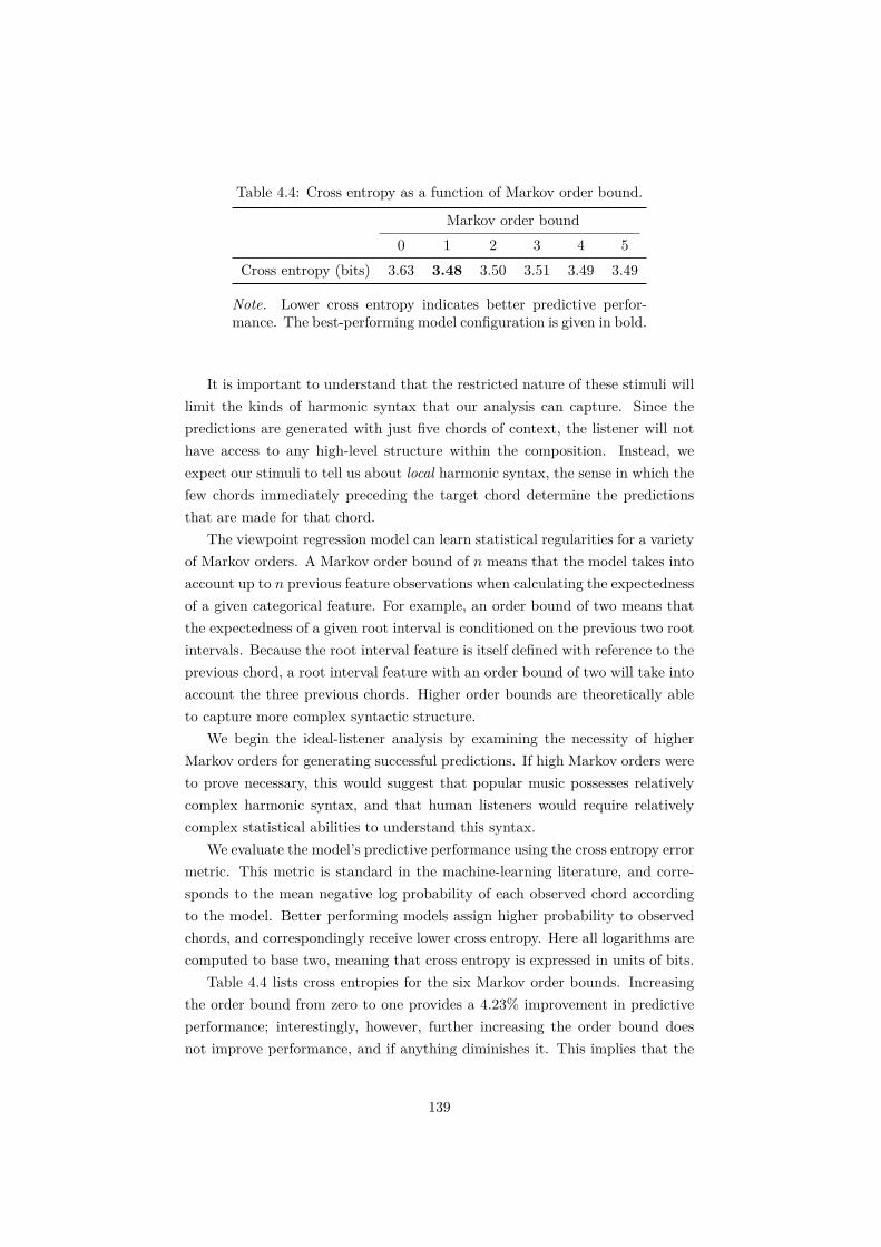
Table 4.4: Cross entropy as a function of Markov order bound.

Markov order bound0 1 2 3 4 5

Cross entropy (bits) 3.63 3.48 3.50 3.51 3.49 3.49

Note. Lower cross entropy indicates better predictive perfor-mance. The best-performing model configuration is given in bold.

It is important to understand that the restricted nature of these stimuli willlimit the kinds of harmonic syntax that our analysis can capture. Since thepredictions are generated with just five chords of context, the listener will nothave access to any high-level structure within the composition. Instead, weexpect our stimuli to tell us about local harmonic syntax, the sense in which thefew chords immediately preceding the target chord determine the predictionsthat are made for that chord.

The viewpoint regression model can learn statistical regularities for a varietyof Markov orders. A Markov order bound of n means that the model takes intoaccount up to n previous feature observations when calculating the expectednessof a given categorical feature. For example, an order bound of two means thatthe expectedness of a given root interval is conditioned on the previous two rootintervals. Because the root interval feature is itself defined with reference to theprevious chord, a root interval feature with an order bound of two will take intoaccount the three previous chords. Higher order bounds are theoretically ableto capture more complex syntactic structure.

We begin the ideal-listener analysis by examining the necessity of higherMarkov orders for generating successful predictions. If high Markov orders wereto prove necessary, this would suggest that popular music possesses relativelycomplex harmonic syntax, and that human listeners would require relativelycomplex statistical abilities to understand this syntax.

We evaluate the model’s predictive performance using the cross entropy errormetric. This metric is standard in the machine-learning literature, and corre-sponds to the mean negative log probability of each observed chord accordingto the model. Better performing models assign higher probability to observedchords, and correspondingly receive lower cross entropy. Here all logarithms arecomputed to base two, meaning that cross entropy is expressed in units of bits.

Table 4.4 lists cross entropies for the six Markov order bounds. Increasingthe order bound from zero to one provides a 4.23% improvement in predictiveperformance; interestingly, however, further increasing the order bound doesnot improve performance, and if anything diminishes it. This implies that the

139

Table 4.5: Cross entropy and Akaike Information Criteria (AIC) for differentfeature combinations.

FeaturesNone Low-level only High-level only All

Cross entropy (bits) 14.58 6.37 3.69 3.49AIC 6065.72 2682.40 1578.38 1529.14

Note. Lower cross entropy and lower AIC indicates better predictive perfor-mance. The best-performing model configuration is given in bold.

local harmonic syntax of this musical style can be mostly characterised by sim-ple feature statistics, specifically the relative frequencies of different categoricalfeatures (e.g. ‘major triads are more common than seventh chords’) and the rel-ative frequencies of different feature transitions (e.g. ‘seventh chords are likelyto be followed by major triads’).

Next we examine the types of features available to the model. While the fullmodel uses both low-level and high-level features, one can contemplate alterna-tive models that only have access to low-level features (e.g. consonance, spectralsimilarity) or alternatively are restricted to high-level features (e.g. root inter-val, pitch-class set). By comparing the predictive performances of these models,we can examine the sufficiency of different feature sets for generating effectivepredictions.

Table 4.5 compares these three models – the full model, the low-level model,and the high-level model – to a baseline model containing no features. The low-level model performs substantially better than the baseline model, halving thecross entropy from 14.58 to 6.37, and the high-level model performs even better,reducing the cross entropy to 3.69. The best performance, however, is achievedby the combined model, with a cross entropy of 3.49. Examining the AkaikeInformation Criterion, we see that added complexity of the combined model isjustified by the performance improvement compared to the high-level model. Tosummarise: neither low-level or high-level features are sufficient by themselvesto achieve optimal performance, but the high-level features can achieve almostoptimal performance.

Next we investigate how individual features contribute to the full model. Inparticular, we are interested in seeing whether the model is dominated by a smallnumber of features, or whether it simultaneously depends on many features. Weapproach this question by computing a permutation-based feature-importancemetric, which quantifies feature importance by taking the evaluation dataset,

140

randomly permuting feature values, and assessing how much the model’s pre-dictive performance drops (Breiman, 2001; Fisher et al., 2018).7

Feature importances for the full and low-level models are plotted in Figure4.7. Examining feature importances for the full model (Figure 4.7A), we see thatthe two most important features are two low-level features: interference betweenpartials and periodicity/harmonicity, both aspects of consonance. This is ini-tially surprising: we previously saw that the low-level model was substantiallyoutperformed by the high-level model, implying that low-level features are con-siderably less useful than high-level features. However, this incongruence canbe explained by feature redundancy: while the two consonance features caneffectively predict which chord types will be more common than others (seeChapter 3), this information can also be approximated with ‘brute force’ bya high-level viewpoint (such as ‘pitch-class set relative to bass’) that simplymemorises the prevalence of different chord types. This redundancy betweenthe feature sequences allows the high-level model to perform well in the absenceof the low-level features, even if the low-level features are preferred by the com-bined model. Consistent with this view, removing the high-level features causesthe model to rely even more on the low-level features (Figure 4.7B).

Beside the two consonance features, we see that many other low-level andhigh-level features also contribute to the full model (Figure 4.7A). This is con-sistent with the idea that Western popular harmony carries structure along avariety of different features, many of which can be leveraged by the listener tohelp predict chord progressions.

The contributions of the low-level features can be visualised as marginaleffects, showing how different levels of a given feature are associated with dif-ferent levels of expectedness while holding the other features constant (Figure4.8). First, we see that the marginal effects differ between the full model andthe low-level model. This presumably reflects how certain information is sharedbetween the high-level features and the low-level features; partialling out thecontributions of high-level features therefore significantly changes the shape ofthe low-level features. Second, it is apparent that the marginal effects are notalways straightforward reflections of the univariate distributions plotted in Fig-ure 4.3. For example, Figure 4.3 shows that observed chords tend to exhibitrelatively low pitch distances, yet Figure 4.8 indicates that the models associatehigh pitch distance with greater expectedness. This phenomenon is further ev-

7This permutation process produces a dataset where feature values may be inconsistentwith each other, for example imagining a chord where the pitch-class set is {0, 4, 7} butthe bass pitch class is 2. It may seem counterintuitive to imagine such impossible cases,and if the model is very sensitive to interactions between features then the technique mightgive misleading results. However, by construction the viewpoint regression technique doesnot model interactions between features, and so its performance on these permuted datasetsshould relate meaningfully to its performance on real datasets.

141

Periodicity/harmonicity

Interference

PC chord rel. prev. bass

PC chord

Pitch distance

PC set rel. bass

Bass PC rel. root

Spectral similarity

Root interval

PC set

PC set rel. root

Bass PC

Bass interval

PC set rel. prev. bass

Root PC

0.0 0.5 1.0 1.5Feature importance (bits/chord)

High−level

Low−level

A

Interference

Periodicity/harmonicity

Pitch distance

Spectral similarity

0 25 50 75 100Feature importance (bits/chord)

B

Figure 4.7: Permutation-based feature importances for (A) the full ideal-listenermodel and (B) the low-level model, after Breiman (2001; see also Fisher et al.,2018).

idence for shared information between features. It makes it difficult to drawstrong conclusions about the causal contribution of a given feature to compo-sitional practice: a given feature may seem to be avoided by composers whenconsidered in isolation, but preferred once other features are accounted for.

The relative contributions of the high-level features can be summarised bytheir regression weights (Figure 4.9). A regression weight of wi means that aone-unit increase in feature-based expectedness corresponds to a wi increase inoverall expectedness, where expectedness is measured as log probability. Greaterregression weights therefore correspond to greater feature importance.

Examining the regression weights, we see that the model takes advantageof a variety of high-level features. There is a general trend for relative-pitchfeatures (e.g. root interval, bass interval) to be preferred over absolute-pitchfeatures (e.g. root pitch class, bass pitch class): this is consistent with thenotion that Western listeners predominantly possess relative pitch perception,which is then reflected by transpositional invariances in music composition (seealso Figure 4.4).

Comparing short-term and long-term regression weights, we see that themodel pays particular attention to short-term regularities in the feature se-quences. This is interesting because, when predicting the sixth chord in a se-quence, the model only has five prior chords to learn from, so one might expectthis context not to be particularly informative. Were the model to progress fur-

142

Pitch distance Spectral similarity

Interference Periodicity/harmonicity

5 10 15 0.4 0.6 0.8

0.3 0.6 0.9 0.5 0.6 0.7 0.8 0.9

−4

−2

0

2

−1.0

−0.5

0.0

−2

0

2

0.0

0.5

1.0

Feature value

Effe

ct

A

Pitch distance Spectral similarity

Interference Periodicity/harmonicity

5 10 15 0.4 0.6 0.8

0.3 0.6 0.9 0.5 0.6 0.7 0.8 0.9

−1.5

−1.0

−0.5

0.0

−3

−2

−1

0

1

2

−50

−25

0

25

0

1

Feature value

Effe

ct

B

Figure 4.8: Marginal effects of continuous features in the (A) full and (B) low-level ideal-listener models. The horizontal axes span from the 2.5th to the 97.5thpercentiles of all theoretically possible feature values, computed over the fullchord alphabet (N = 24,576) at each of the 300 chord positions being modelled.The shaded regions identify the 2.5th and 97.5th percentiles of observed featurevalues (i.e. those that were actually observed in the chord sequences).

Root PC

Root interval

PC set rel. root

PC set rel. prev. bass

PC set rel. bass

PC set

PC chord rel. prev. bass

PC chord

Bass PC rel. root

Bass PC

Bass interval

0.0 0.1 0.2 0.3Weight

Fea

ture

Short−term

Long−term

Figure 4.9: Stacked bar plot of categorical feature weights in the full ideal-listener model, split by short-term and long-term features.

143

ther into the music compositions, we might expect these short-term regularitiesto become still more informative.

These analyses give some useful insights into the nature of harmony pre-diction in Western popular music. The headline results may be summarised asfollows:

1. Markov orders greater than one do not contribute significantly to the ideal-listener model; in other words, the local harmonic syntax of popular musiccan be largely explained by first-order Markovian relationships.

2. The ideal model takes advantage of many perceptual features when gen-erating predictions. This is consistent with the idea that harmonic syntaxis shaped by many perceptual principles.

3. The ideal model pays particular attention to two low-level perceptual fea-tures: interference between partials, and periodicity/harmonicity. How-ever, if these features are not available, their loss can be largely compen-sated for by certain high-level features, such as ‘Pitch-class set relative tobass’.

4.5 Modelling human listenersHuman listeners’ responses to music seem to be determined, in large part, bythe phenomenon of surprisal, whereby certain musical events sounds more orless expected than others. The musical events within a given musical piece typ-ically vary in surprisal, and this variation is associated with various psycholog-ical phenomena including emotional experience (Egermann et al., 2013; Huron,2006; Meyer, 1957; Sauvé et al., 2018; Sloboda, 1991), perceptual facilitation(Omigie, Pearce, & Stewart, 2012), and phrase-boundary perception (Pearce etal., 2010a), as well as prominent electrophysiological markers (Omigie, Pearce,Williamson, & Stewart, 2013; Pearce et al., 2010b).

Here we investigate human listeners’ perception of surprisal in chord se-quences from popular music compositions. To generate our behavioural data,we presented 50 participants with the 300 chord sequences from the ideal-listeneranalysis (see Figure 4.2 for an example), and asked the participants to rate thesurprisingness of the sixth chord in each sequence on a scale from one to nine.We normalised these responses within participants to z-scores, and then aver-aged over participants to produce one mean surprisal rating for the sixth chordin each of the 300 sequences. See Section 4.7.3 for more detail on the experi-mental methods.

144

We then use our probabilistic ideal-listener models to analyse the way inwhich our participants made their surprisal judgments. Given a probabilisticmodel, the surprisal of a given chord may be operationalised as an information-theoretic quantity termed information content, defined as the negative log prob-ability of the observed chord conditioned on its previous context. Our basicstrategy for evaluating a given ideal-listener model is to correlate these informa-tion content values with the participants’ surprisal judgments: high correlationsindicate that the model provides a good account of human behaviour. By eval-uating different configurations of this model, and comparing it to alternativeperceptual models, we can gain insights into the way in which human listenersmake their surprisal judgments.

145

Tabl

e4.

6:B

ench

mar

king

the

idea

l-list

ener

mod

elag

ains

tlo

w-le

velm

odel

sof

harm

onic

expe

ctat

ion.

Pear

son

r

Mod

elR

efer

ence

Adj

.R2

Raw

(95%

CI)

Disa

tten

uate

dSp

earm

anρ

Idea

llis

tene

rFu

llm

odel

Thi

sch

apte

r.4

3.6

6[

.59,

.72]

.73

.70

Low

-lev

elm

odel

sC

onso

nanc

eC

hapt

er3

.19

−.4

4[−

.52,−

.34]

−.4

9−

.38

Spec

tral

simila

rity

Lem

an(2

000)

.11

−.3

3[−

.43,−

.22]

−.3

7−

.33

Spec

tral

simila

rity

Parn

cutt

&St

rasb

urge

r(1

994)

.02

.15

[.0

4,.2

6].1

7.1

1Pi

tch

dist

ance

Parn

cutt

&St

rasb

urge

r(1

994)

.01

.09

[−.0

2,.2

0].1

0.0

7Pi

tch

dist

ance

Tym

oczk

o(2

006)

.01

−.1

2[−

.23,−

.01]

−.1

4−

.14

Pitc

h-cl

ass

dist

ance

Tym

oczk

o(2

006)

.00

−.0

7[−

.18,

.05]

−.0

7−

.04

Spec

tral

simila

rity

Col

lins

etal

.(2

014)

−.0

0−

.00

[−.1

2,.1

1]−

.00

−.0

4Sp

ectr

alsim

ilarit

yT

his

chap

ter

−.0

0−

.05

[−.1

7,.0

6]−

.06

−.0

3C

ombi

ned

low

-lev

elm

odel

sLi

near

regr

essio

nT

his

chap

ter

.34

.60

[.5

2,.6

6].6

7.6

1

Not

e.Pr

ior

tope

rform

ing

this

com

paris

on,t

heha

lf-lif

epa

ram

eter

sfo

rLe

man

’s(2

000a

)spe

ctra

lsim

ilarit

ym

odel

and

the

new

spec

tral

simila

rity

mod

elwe

reop

timise

don

the

beha

viou

rald

ata

(see

Sect

ion

4.7.

3fo

rde

tails

).W

eco

mpu

ted

disa

t-te

nuat

edco

rrel

atio

nco

effici

ents

toco

rrec

tfor

the

mea

sure

men

terr

orof

the

liste

ners

’mea

nsu

rpris

alra

tings

,est

imat

edby

taki

ngth

em

ean

stan

dard

erro

run

der

the

Cen

tral

Lim

itT

heor

em.

146

rs = .70 rs = .61 rs = .65

Full ideal observer Benchmark regression Simplified ideal observer

0 5 10 15 −0.4 0.0 0.4 0.8 0 5 10 15−1.0

−0.5

0.0

0.5

1.0

−1.0

−0.5

0.0

0.5

1.0

−1.0

−0.5

0.0

0.5

1.0

Model output

List

ener

sur

pris

al

2.5

5.0

7.5

10.0

12.5

Count

Figure 4.10: Density plots of associations between model outputs and listenersurprisals for three models: the full ideal-listener model, the benchmark regres-sion model, and the simplified ideal-listener model. ‘Count’ refers to the numberof stimuli present in the respective region of the plot.

We begin by applying the full ideal-listener model (all features, no orderbound) to our perceptual data. The resulting information content values pre-dict participant surprisal ratings with a Spearman correlation of .70 (Table 4.6,Figure 4.10). This indicates that the model provides a fairly successful accountof participant responses, and suggests that probabilistic prediction is a goodmetaphor for how participants make surprisal judgments.

We then compare this ideal-listener model to several other perceptual mod-els, including a consonance model, four spectral similarity models, and threepitch/pitch-class distance models (Table 4.6). We see from Table 4.6 that noneof these models compete individually with the ideal-listener model; the best-performing competitor is the consonance model from Chapter 3, with a Spear-man correlation of −.38. A better approximation to surprisal ratings can beachieved by combining these alternative models using linear regression; the re-sulting model achieves a Spearman correlation of .61, not so distant from theideal listener’s score of .70. The ideal-listener model and the linear-regressionmodel are similar in that they both generate their predictions using a weightedcombination of musical features, but the conceptual advantage of the ideal-listener model is that it explains how the regression weights originate, namelyin optimising for the prediction of musical events.

The full ideal-listener model is rather complex: it incorporates many differentperceptual features, learns statistical regularities across many Markov orders,and is pretrained on a large dataset of representative music. By testing varioussimplified versions of the model, we can examine the relative importance of

147

Table 4.7: Comparing the performance of different simplified versions of theideal-listener model.

Model configuration Listener correlations

Features Order Pretrain Pearson Spearman Cross entropy

1 All 5 Yes .66 [.59, .72] .70 3.48 [3.09, 3.86]2 All 0 Yes .65 [.58, .71] .69 3.62 [3.24, 4.00]3a High-level 0 Yes .66 [.59, .72] .69 3.89 [3.47, 4.32]3b Low-level 0 No .51 [.43, .59] .50 6.32 [5.93, 6.71]4 PC chord 0 Yes .66 [.60, .72] .67 4.64 [4.20, 5.08]5 PC chord 0 No .60 [.52, .67] .65 6.44 [5.73, 7.15]

Note. Cross entropy is given in bits; lower cross entropy indicates that themodel performs better at predicting chord progressions. 95% confidence inter-vals are reported in square brackets.

different model attributes for explaining participant behaviour (Table 4.7). Firstwe reduce the Markov order to 0, and find that the model’s performance isessentially unchanged (model version 2, Spearman correlation = .69). Thisindicates that the model can successfully predict listener behaviour withoutlearning transition probabilities, instead just learning that certain feature values(e.g. root progressions of a fifth, or high spectral similarity) are more commonthan others.

Next we try restricting the feature set to either all low-level features orall high-level features (model versions 3a, 3b). We see that performance isessentially unchanged when the low-level features are dropped (model version3a, Spearman correlation = .69), indicating that the low-level features are notnecessary to explain performance. Nonetheless, the model with only low-levelfeatures still performs moderately well (model version 3b, Spearman correlation= .50).

Next we remove all derived features from the model, so that it only hasaccess to the original pitch-class chord representations of the chord sequences.In other words, the model no longer has access to perceptual principles such asrelative pitch and chord roots. Again, there is no real diminution in performance(model version 4, Spearman correlation = .67).

Lastly we disable the pretraining component of the model, so that it onlylearns statistical regularities from the preceding five chords in the chord se-quence, with these statistical regularities then being forgotten upon presenta-tion of the next chord sequence. Predictive performance still remains fairly high(model version 5, Spearman correlation = .65).

This pattern of results is quite remarkable. It indicates that many of thecomplexities of the ideal-listener model can be removed without much affectingthe model’s ability to predict participants’ surprisal judgments. In particu-

148

lar, the simplest model version can be interpreted as a basic repetition-primingmodel, where the probability of observing a given chord is approximately pro-portional to the number of times that it has been observed in the portion of thesequence heard so far. The fact that this radically simplified model performsso well indicates that our listeners’ predictions were dominated by short-termrepetition priming.

It is tempting to take the strong performance of the simplified model asevidence that our participants were suboptimal listeners. However, we shouldremember that the full model predicted participant performance just as well,if not better (95% confidence interval for the difference in Pearson correlationcoefficients: [−.00, .11], Zou, 2007; Diedenhofen & Musch, 2015). The factthat simplifying the model makes little difference suggests that the full andsimplified models deliver similar predictions for our stimuli, which we can verifyby correlating these sets of predictions (Pearson r(298) = .78, 95% CI = [.73,.82]). In other words, the relative surprisal of different chords in the popularmusic extracts is mostly predicted by simple repetition effects, not by higher-order statistics. However, if we enter both the full and the simplified model intoa linear regression model predicting surprisal judgments, the resulting model(adjusted R2 = .45) identifies substantive contributions from both the full model(β = 0.48, 95% CI = [0.34, 0.62], p < .001) and the simple model (β = 0.23, 95%CI = [0.09, 0.36], p = .001). This suggests that, while our listeners’ responsescan largely be explained by short-term repetition priming, higher-level statisticsalso contribute.

To illustrate by example, Figure 4.11 displays the full model’s output for thefirst composition in the popular music corpus, I don’t mind by James Brown(1961). It is clear that repetition plays an important role in this piece. The firsttwo chords (A minor, C major) repeat five times, and then move to a new chord,F major. This progression from C major to F major is completely unsurprisingfrom a syntactic perspective – in fact, it corresponds to the most common rootprogression in Figure 4.4 – but it is surprising from a local perspective becauseit disrupts the regular pattern that precedes it. The full model successfullycaptures this surprisingness, returning an information content of 12.2 bits versusthe 0.0 bits of the preceding chord. Importantly, however, a simple repetition-priming model can also capture this effect, simply working on the principlethat novel chords are more surprising than recently heard chords. Lookingfurther through Figure 4.11, it is evident that the importance of local repetitioncontinues throughout the composition. The dominance of these local repetitioneffects is consistent with the conclusion of the wider quantitative analyses: thedynamics of harmonic expectation in popular music are driven less by high-levelsyntactic structures and more by low-level statistical or psychoacoustic features.

149

Figure 4.11: Analysis of the first composition in the popular music corpus, Idon’t mind by James Brown (1961), using the full ideal-listener model fromSection 4.4. Each number corresponds to a chord’s information content, orsurprisal, expressed to one decimal place. The regression weights are preservedfrom the ideal-listener analysis, but the categorical feature models are retrainedon the last 700 compositions from the popular music corpus. Durations, pitchheights, and bar lines are arbitrary.

150

4.6 DiscussionMusic listening is thought to be an inherently probabilistic process, with the lis-tener constantly generating predictions for upcoming musical events on the basisof learned statistical knowledge. Here we investigated the probabilistic predic-tion of musical harmony, developing a new computational model that predictschord sequences from statistical regularities manifested in a broad collection ofperceptual features. We applied our model to a corpus of chord sequences fromWestern popular music (Burgoyne, 2011), seeking to understand how an ideallistener would predict these chord sequences. We then applied this ideal-listenermodel to a new behavioural experiment investigating how human listeners per-ceive surprisal within these chord sequences.

These chord sequences were eight chords in length, sampled from randomlocations in the original corpus. The listeners were instructed to evaluate thesixth chord in these sequences, with only five preceding chords to contextualisethese evaluations. Such short contexts give high-level syntactic structure littleopportunity to contribute to predictions, especially since any such structurewill be obfuscated if the stimulus starts partway through a musical phrase.Our stimuli instead provide a perspective on local harmonic syntax, the sensein which chord progressions are influenced by the few immediately precedingchords.

Listeners derive rich feature representations for musical chords. One exam-ple feature is harmonicity: high harmonicity occurs when a chord’s acousticspectrum resembles a harmonic series, and typically has positive aesthetic con-notations. Another such feature is the chord root, corresponding to the brain’shypothesis about the fundamental frequency of the musical chord. A third suchfeature is the root interval, corresponding to the pitch interval between theprevious chord root and the current chord root. In our corpus analyses, weshowed that the harmonic syntax of popular music expresses salient statisti-cal regularities across many of these features, and that an ideal listener wouldtake advantage of many such features when predicting chord sequences. Theoptimised model paid particular attention to two low-level consonance features,namely interference between partials (after Hutchinson & Knopoff, 1978) andperiodicity/harmonicity (after Chapter 3), as well as a high-level feature thatcaptured relative pitch perception by expressing each chord relative to the bassnote of the previous chord. However, the ideal model also took advantage of var-ious other features (e.g. spectral similarity, pitch distance, root interval, chordinversion).

Traditional feature-based models of music prediction cannot incorporate con-tinuous features such as interference between partials and spectral similarity

151

(e.g. Hedges & Wiggins, 2016a, 2016b; Pearce, 2005, 2018; Rohrmeier & Grae-pel, 2012; Whorley & Conklin, 2016; Whorley et al., 2013). Our viewpoint re-gression technique is a novel contribution in this regard, generating predictionsfrom both continuous and categorical features. This technique seems partic-ularly appropriate for harmony, but could well generalise to other sequentialdomains. One example is melody, where categorical statistical-learning modelshave dominated in the last two decades (Pearce, 2005; Pearce & Müllensiefen,2017; Pearce et al., 2010b; Pearce & Wiggins, 2006), yet recent modelling re-search indicates that continuous features (pitch proximity, central pitch ten-dency) are also needed to explain listener behaviour (Morgan, Fogel, Nair, &Patel, 2019).

Our corpus analysis indicated that (near)-optimal predictive performancefor popular harmony within this modelling framework can be achieved using amodel with a Markov order bound of one. An order bound of one means thatthe model generates predictions using just two types of information: the fre-quency of particular feature values (zeroth-order structure), and the frequencyof particular feature values conditioned on the immediately preceding featurevalue (first-order structure). Since several high-level features are based on in-terval representations (e.g. root interval, bass interval), this means in practicethat the optimal model generates predictions conditioned on the two previouschords. The fact that optimal performance can be achieved with such a low or-der bound implies that the local harmonic syntax of popular music is dominatedby relatively low-level statistical regularities. This phenomenon is likely to differbetween musical styles; more complex styles may require higher Markov orderbounds or more complex modelling approaches. Previous studies have foundoptimal Markov orders of two or three for modelling jazz harmony (Hedges,Roy, & Pachet, 2014; Rohrmeier & Graepel, 2012) and an optimal order of onefor modelling Beethoven string quartets (Landsnes et al., 2019).

Our behavioural study investigated how chords in popular harmony varyin perceived surprisal. This moment-to-moment variation in musical surprisalis considered to be a key part of musical aesthetics (Egermann et al., 2013;Huron, 2006; Meyer, 1957; Sauvé et al., 2018; Sloboda, 1991), but little is knownabout how these dynamics develop in Western harmony. Applying our full ideal-listener model to the behavioural data, we found a Spearman correlation of.70 between model surprisal and listener surprisal, suggesting that probabilisticprediction provides a good account of our participants’ behaviour. We thenanalysed different versions of the model to investigate the statistical processesunderlying participants’ surprisal judgments, and found that these judgmentscould be largely explained by a radically simplified model that predicts chordssolely on the basis of their number of occurrences in the preceding five-chord

152

context (Spearman correlation of .65). This implies that, in popular music, themoment-to-moment variation in harmonic surprisal does not reflect complexsyntactic phenomena to any great extent, but instead primarily reflects simplerepetition effects.

It is important to note that probing chord-to-chord surprisal variation is notthe same as probing listeners’ full predictive distributions. It is quite possiblethat simple repetition statistics are sufficient to explain chord-to-chord surprisalvariation, but insufficient to explain the listener’s full probability distributions.For example, suppose that a musical style universally uses highly consonantchords: in this case, consonance would not predict variations in surprisal withinthe corpus, but it would still be useful for predicting what chords are likelyor unlikely to come next. Nonetheless, moment-to-moment surprisal dynam-ics are thought to be particularly important for aesthetic responses to music(e.g. Egermann et al., 2013; Huron, 2006; Meyer, 1957; Sauvé et al., 2018;Sloboda, 1991), motivating their study here.

After adjusting for measurement error, the full ideal-listener model predictedmean surprisal judgments with a Pearson correlation coefficient of .73. Thiscorrelation is quite strong, but there remains clear room for improvement. Amore reliable account of listener judgments might be achieved by adding com-putational models of other musical dimensions, in particular melody and voiceleading. We might expect higher surprisal ratings when the melody line (com-prising the highest note in each chord) makes unexpected progressions, for ex-ample jumping by large intervals. We might also expect higher surprisal ratingswhen the chord progression involves an unidiomatic voice leading, for exampleone with parallel octaves. Future work could address these possibilities usingcomputational models of melodic expectation (e.g. Pearce, 2018; Temperley,2008) and voice leading (e.g. Chapter 5).

This study’s findings are restricted to popular music and (relatively) un-trained Western music listeners. Popular music is appealing to study because,by definition, it corresponds to a large proportion of real-world music listening;likewise, untrained listeners are appealing to study because they represent themajority of the world’s population. Nonetheless, it would certainly be inter-esting to study other musical styles and other participant groups. It is quitepossible that certain musical styles, such as jazz music, carry more complexsyntactic structure than the popular music studied here. It is also quite possi-ble that more musically experienced listeners will be sensitive to more complexstatistical structure in this music (e.g. Hansen & Pearce, 2014).

It is worth considering what might happen if we were to repeat this studywith longer chord sequences. On the one hand, longer chord sequences providemore scope for high-level syntactic structure to contribute to predictions. On

153

the other hand, longer sequences provide more exposure for repeated patternsspecific to a given composition, and these repeated patterns may well come todominate prediction performance at the expense of harmonic syntax. Theserepeating passages may often be relatively long, meaning that the model’s idealMarkov order may increase past one. Such effects should be taken into accountwhen comparing results between different music prediction studies (Hedges etal., 2014; Landsnes et al., 2019; Rohrmeier & Graepel, 2012; Sears et al., 2018a).In particular, evaluating models on entire musical compositions is likely to favourmodels that effectively detect local repetitions, whereas evaluating models onshort chord sequences is likely to favour models that effectively capture harmonicsyntax.

These sequences were synthesised as minimal sequences of isochronous pi-ano chords. This approach is useful for isolating harmony from other parts ofthe musical experience, but it creates a somewhat impoverished listening ex-perience compared to naturalistic listening. Harmonic expectation does seemto be influenced by external cues such as metre (Hedges & Wiggins, 2016b)and timbre (Vuvan & Hughes, 2019), and such effects should ultimately be in-corporated into computational models of harmonic expectation. The presentstudy could therefore be complemented by studies that synthesise the stimuliusing more realistic musical textures, or that use audio from the original musicalcompositions.

Our viewpoint regression model of harmonic expectation was trained on acorpus of 439 popular music compositions, intended as a first approximationto an average Western listener’s musical exposure. Better listener simulationsmight be achieved by tailoring this corpus more closely to the listening expe-riences of individual participants, perhaps to capture the mix of musical stylesthat they have been exposed to, or to capture the amount of musical exposurethat they have received. The outcomes of the ideal-listener analyses may alsobe affected by corpus selection; in particular, larger training sets support theacquisition of more complex statistical regularities. As a result, an ideal-listenermodel trained on larger music corpora might take more advantage of high-orderMarkov models and more expressive features, in particular features with largealphabets (e.g. pitch-class sets).

We have developed an open-source software package, hvr, for supportingthese future research possibilities.8 This package defines formal models formany perceptual features thought to be important for harmony perception,such as interference between partials, spectral similarity, and chord roots. Itprovides methods for simulating how listeners mine statistical regularities fromthese perceptual features, and for simulating how statistical regularities from

8This package is available at https://github.com/pmcharrison/hvr.

154

different features might be combined to generate predictions for chord sequences.Importantly, it is straightforward to constrain various aspects of the model, suchas the feature set and the Markov order bound, to investigate how differentstatistical regularities contribute to prediction generation.

One possibility is to use this model as trained in the present study, and useit to generate predictions for new chord sequences. These predictions may besummarised using information-theoretic quantities such as information content,which quantifies the surprisingness of a given chord, and predictive entropy,which quantifies the uncertainty of the model’s predictions for a given chord(e.g. Figure 4.11).

A second possibility is to retrain the model on a new music corpus, allowingthe researcher to simulate musical enculturation. In this latter case, the trainedmodel itself has music-theoretic applications: in particular, the feature impor-tance metrics and continuous feature effects can be examined to identify whatkinds of psychological features are structurally important for a given musicalstyle, and the ways in which these different features contribute to determine thechoice of the next chord.

In music-theoretic applications such as these, it is important to note thatthe optimised viewpoint weights will depend both on the available features andthe amount of training data given to the categorical viewpoint models. Forexample, a given feature may be useful in isolation, but be made redundant bythe addition of a more informative feature. Furthermore, a given feature mightbe predictively useful given lots of training data, but uninformative given insuf-ficient training data; this commonly applies to categorical features with largealphabets (e.g. pitch-class sets), whose models contain lots of parameters andhence need lots of data to estimate accurately. Correspondingly, such featurescan receive low weights with small training datasets, but high weights with largetraining datasets.

One modelling assumption that deserves interrogation is the idea that listen-ers compute full probability distributions over all 24,576 possible chord choices,as required to compute the normalisation constant in Equation 4.2. This seemsintuitively unrealistic. One possibility is that the listener does not computethe full probability distribution, but instead computes probabilities for a smallnumber of chords representing the most likely continuations. A second possi-bility is that the listener approximates the normalisation constant in some way.Implementing such mechanisms could significantly reduce the computationaldemands of the model’s implementation.

A second assumption that deserves interrogation is the way in which view-point weights are optimised on many observations simultaneously. For studiesof online learning, it would be more cognitively plausible to adopt an online op-

155

timisation algorithm, where viewpoint weights are incrementally updated afterthe observation of each musical event. This could also reduce the computationaldemands of the model’s implementation.

There are several other ways in which the model might be developed further.A limitation of the PPM algorithm, used to model the categorical features, isthat it cannot learn explicit representations of latent states. Latent states couldbe useful for capturing the music-theoretic concept of local key. It might there-fore be interesting to trial alternative sequence prediction models, such as hiddenMarkov models (Rabiner, 1989) and long short-term memory recurrent neuralnetworks (Hochreiter & Schmidhuber, 1997). A second limitation is that poly-nomial feature expansion, used to model the continuous features, can performpoorly when extrapolating outside the range of feature values observed in thetraining set. It might therefore be worthwhile to trial alternative approachessuch as penalised spline regression (Kneib, Baumgartner, & Steiner, 2007). Athird limitation is that the model cannot respond to the local distribution ofcontinuous features within a given composition, unlike the categorical compo-nent of the model, which incrementally learns the distribution despite beingable learn local distributions of categorical features.

Here we prespecified the model’s perceptual features on the basis of previousresearch in music psychology and music theory, but it would also be possibleto have the model learn its features in a data-driven manner (e.g. Langhabel,Lieck, Toussaint, & Rohrmeier, 2017; Whorley et al., 2013). From a cognitiveperspective, it does seem likely that learning contributes to the formation ofharmonic representations; for example, the 12-tone chromatic scale is unlikelyto be innate, and is more likely acquired through long-term exposure to Westernmusic. Other features, such as interference between partials and harmonicity,are less likely to be learned through solely musical exposure. The ideal modelwould simulate how these different representations arise through a combinationof biological predispositions and auditory experience.

Here we have focused on cognitive modelling, but the proposed model alsohas interesting applications in other fields. It is well-suited to music generation,defining a probability distribution over successive chords that can be sampledfrom to generate new chord sequences. An appealing feature of the model is theinterpretability of its parameters, which composers could take advantage of toexplore new stylistic spaces. For example, it would be straightforward to ma-nipulate the low-level feature effects, creating for example a musical style thatminimises spectral similarity while maximising voice-leading efficiency. It wouldalso be straightforward to train different feature models on different musical cor-pora, allowing the composer to create compositions that combine one aspect ofone musical style with another aspect of a second musical style (e.g. combining

156

the harmonic vocabulary of the composer Claude Debussy with the root progres-sions of popular music). The model also has potential applications in automaticmusic transcription, providing a prior distribution that biases the transcrip-tion process towards chord sequences that have high plausibility within a givenmusical style. These possibilities deserve to be explored in future work.

4.7 Methods

4.7.1 Corpus

The musical corpus corresponded to version 2.0 of the McGill Billboard cor-pus (Burgoyne, 2011), which comprises expert musicians’ transcriptions of 739unique songs sampled from the Billboard ‘Hot 100’ charts between 1958 and1991. We used the pitch-class chord version of the corpus developed in Chapter2, which omits repeated compositions, omits section repeats, and omits succes-sive repetitions of the same chord. In the pitch-class chord representation, thechord is defined as a combination of a bass pitch class and an unordered set ofnon-bass pitch classes. This dataset is available in the hcorp package under thelabel popular_1.

4.7.2 Modelling

New spectral similarity model

We used a new spectral similarity model that compares each incoming chordagainst an auditory buffer representing the last few chords heard by the listener.Each chord is first represented as a smooth pitch-class spectrum, after Milneet al. (2011): this involves representing the chord as a pitch-class set, expand-ing each pitch class into its implied harmonics, and circularly convolving theresulting spectrum with a Gaussian function to simulate inaccuracies in pitchperception. Following the perceptual optimisations of Milne & Holland (2016),we represent each pitch class as 12 harmonics with weights declining as 1/n0.75,and use a Gaussian function with standard deviation 6.83. We then simulatean auditory buffer by cumulatively summing smooth pitch-class spectra fromsuccessive chords, with the contribution of a given pitch-class spectrum expo-nentially decaying as a function of the number of chords played since its originalpresentation. The model defaults to a half life of three chords, meaning thata given pitch-class spectrum contributes half as much after three chords haveelapsed, and a quarter as much after six chords. A computationally efficientway of implementing this exponential decay is to multiply the cumulative sumby 2−1/h after adding each new chord, where h is the half life. Spectral simi-

157

larity is then operationalised as the cosine similarity between the new chord’spitch-class spectrum and the auditory buffer’s pitch-class spectrum at the pointwhen the new chord was presented. This model is implemented in the specdecpackage for the programming language R.9

Analysing feature distributions

For analysing low-level feature distributions, we constructed a dataset corre-sponding to the target chords at the sixth position of each of the 300 behaviouralstimuli, enumerating each of the possible 24,576 pitch-class chords that couldhave been played at that position, and calculating feature values for each ofthese hypothetical chords. This produced 7,372,800 data points in total, 300 ofwhich corresponded to observed chords, and 7,372,500 of which correspondedto unobserved chords.

For analysing high-level feature distributions, we tabulated feature transi-tions from the 439 compositions in the Billboard corpus that did not overlapwith our behavioural stimuli, and plotted the results as transition matrices (Fig-ures 4.4, 4.5). We then trained viewpoint models on these 439 compositions, andused them to generate predictions for the 300 target chords in the behaviouralstimuli. A viewpoint model generates predictions for successive chords derivedfrom a sequence prediction model trained on a given categorical feature (seeViewpoint models for details). Here the underlying sequence prediction model isPrediction by Partial Matching (PPM; Cleary & Witten, 1984) as updated byMoffat (1990) and Bunton (1997) and configured by Pearce & Wiggins (2004;Pearce, 2005) (see Sequence prediction models for details). Following Pearce& Wiggins (2004; Pearce, 2005), the PPM model is configured to use escapemethod ‘C’ (Moffat, 1990) and has update exclusion disabled. The viewpointmodel’s predictions are converted to log probabilities and then correlated in Fig-ure 4.6, with hierarchical clustering performed on the rows and columns of thecorrelation matrix using the R function hclust with the default ‘complete link-age’ method. The log probabilities correspond to the ‘long-term expectedness’features of the viewpoint regression model described later in this section.

Sequence prediction models

A sequence prediction model is a statistical model that defines a probabilitydistribution over the continuations of a sequence conditioned on the precedingportion of the sequence. Here we are particularly interested in sequence predic-tion models that operate over symbolic sequences, where a symbolic sequence isdefined as an ordered series of symbols drawn from a finite alphabet A. Let en0

9https://github.com/pmcharrison/specdec

158

denote a sequence of length n, let ei denote the ith element in this sequence, withe0 corresponding to an unwritten placemarker for the start of the sequence, andlet eji denote the subsequence (ei, ei+1, . . . , ej). Let ei0 :: x denote the sequenceproduced by appending the symbol x to the sequence ei0. A sequence predictionmodel is then tasked with estimating the probability distribution P (ei | ei−1

0 ).One such sequence prediction model is the Prediction by Partial Matching

(PPM) algorithm, a variable-order Markov model that was originally devel-oped for data compression (Cleary & Witten, 1984) but subsequently provedwell-suited to cognitive modelling (see Pearce, 2018 for a review). PPM gener-ates predictions by blending together predictions for multiple n-gram models ofdifferent orders, where an n-gram model generates predictions from the empir-ical distribution of subsequences of length n (n-grams) in the training corpus.This blending process allows PPM to take advantage of the strengths of bothlow-order and high-order n-gram models. Low-order models have a smaller al-phabet of n-gram frequencies to estimate, and hence require less training datato produce reliable predictions. High-order models have larger n-gram alpha-bets, allowing the models to capture more complex sequential structure as longas sufficient training data are available. PPM initially favours low-order mod-els and gradually moves to high-order models with increasing training data, astrategy that yields competitive performance on both small and large datasets.The precise mechanics of this strategy have developed over the years. Ourimplementation reproduces that of Pearce (2005, 2018), which incorporates var-ious improvements including update exclusion (Moffat, 1990) and interpolatedsmoothing (Bunton, 1997).

Viewpoint models

The PPM algorithm can be applied directly to pitch-class chords to estimateconditional probabilities for sequence continuations. However, such an approachwould not incorporate the kinds of perceptual features that are thought to beimportant for harmony cognition. This challenge is addressed by viewpointmodels, which can generate predictions for pitch-class chords using statisticalregularities learned from perceptual feature spaces. Viewpoint models werefirst introduced by Conklin & Witten (1995) in the context of multiple view-point systems, and were subsequently developed by other researchers (Hedges& Wiggins, 2016a; Pearce, 2005). The technique was originally introduced asa heuristic procedure for developing feature-based predictive models of melody,but here we give viewpoint modelling an explicit generative formalisation in thecontext of harmony modelling.

Viewpoint models generate predictions using categorical features, features

159

that take values from a discrete alphabet. A categorical feature may be for-malised as a pair of functions: an availability function favailable, and an extractorfunction fextract. The availability function takes a context sequence of chordsas input, returning TRUE if the feature will be defined for the next chord in thesequence, and FALSE otherwise. The extractor function takes as input both acontext sequence and a continuation, and returns a symbol from the feature’salphabet that characterises the continuation in the context of the precedingchord sequence. For example, the root interval feature would be defined by anavailability function that only returns TRUE if the context sequence is non-empty,and an extractor function that computes the pitch-class interval from the rootpitch class of the previous chord to the root pitch class of the continuation.

The viewpoint model then supposes that the structure of the chord sequenceis wholly driven by the syntactic structure of the categorical feature, which isitself determined by some latent generative model. The composer is modelledas choosing each chord in a chord progression through the following process:first sample a feature value from the feature’s generative model, then randomlychoose a chord that reproduces this feature value. This process is specified moreformally as follows:

1. Initialise the chord sequence and the feature sequence as empty lists.

2. For i = 1, 2, . . . , n :

(a) Apply the availability function (favailable) to the portion of the chordsequence generated so far.

(b) If the availability function returns FALSE, randomly sample the nextchord, x, from the set of all pitch-class chords.

(c) Otherwise:

i. Sample a new feature value, y, from a generative model condi-tioned on the current portion of the feature sequence.

ii. Find the set S = x : fextract(context, x) = y.iii. If S is empty, backtrack to step i.iv. Otherwise, randomly sample the next chord, x, from S.v. Append y to the feature sequence.

(d) Append x to the chord sequence.

To train the viewpoint model, it is sufficient to approximate the feature’sunderlying generative model. This model can be approximated by fitting agenerative model to the observed feature sequences. This approximation shouldbe unbiased if backtracking never occurs, which is guaranteed if, whenever a

160

feature is ‘available’, all feature values always have at least one chord to representthem. This condition is satisfied by all the categorical features used in thepresent work.

The resulting probabilistic model may be expressed algebraically as follows:

P (ei | ei−10 )

∝ P(ei | F

(ei0))

P(F(ei0)| F(ei−10

))if favailable

(ei−10

),

= 1/A otherwise,(4.3)

where F (ei0) is the sequence of feature values observed for the sequence ei0,defined recursively as

F (e0) = (), (4.4)

F (ej0) =

F (ej−10 ) :: fextract(e

j−10 , ej) if favailable(e

j−10 ),

F (ej−10 ) otherwise,

(4.5)

and P(ei | F

(ei0))

, the probability of observing a given chord conditioned uponthe feature sequence F

(ei0), is computed as a uniform distribution over all

possible chords consistent with that feature sequence:

P(ei | F

(ei0))

=1∣∣{x ∈ A : F

(ei−10 :: x

)= F

(ei0)}∣∣ . (4.6)

As discussed above, the conditional distribution over feature symbols(P(F(ei0)| F(ei−10

))) may be approximated by fitting a sequence predic-

tion model to observed feature sequences. Note that the proportionalityrelationship in Equation 4.3 becomes an equivalence relationship if and only ifall feature observations with non-zero probability can be realised with at leastone pitch-class chord, which is always the case with the features used in thispaper.

The resulting viewpoint model generates predictions for pitch-class chordson the basis of single categorical features derived from these chords. The nextsection shows how viewpoint regression extends this technique to model multiplecontinuous and categorical features simultaneously.

Viewpoint regression

As discussed in Section 4.3, the viewpoint regression technique defines a se-quence prediction model that combines information from both categorical andcontinuous features. The categorical and continuous characteristics of a given

161

chord are summarised in a metafeature vector. Categorical features contributeshort-term and long-term expectedness terms to this vector, defined as thechord’s log probability according to viewpoint models trained on either theportion of the sequence heard so far (short-term expectedness) or on a largemusical corpus representing musical enculturation (long-term expectedness).Continuous features, meanwhile, contribute orthogonal polynomial terms tothe metafeature vector.

Equation 4.2, the estimated probability of a chord, can be written moreformally as

P (ei | ei−10 ,w) ∝

0 if ei = ei−1,

exp(∑m

j=1 wjfj(ei−10 , ei

))otherwise.

(4.7)

where fi(ei−10 , ei

)is the ith term of the metafeature vector as computed for the

observation ei with the context ei−10 , and m is the dimensionality of this vector.

Here we compute expectedness values using PPM-based viewpoint models.Following Pearce (2005), the PPM models are configured slightly differentlyfor short-term versus long-term models. In particular, the short-term modelsuse update exclusion (Moffat, 1990) and escape method ‘AX’ (Moffat, Neal, &Witten, 1998), whereas the long-term models disable update exclusion and useescape method ‘C’ (Moffat, 1990). Our PPM implementation is available in theR package ppm (Harrison et al., 2020).10

The probability of an individual sequence may then be written as

P (en0 ) =

n∏i=1

P (ei | ei−10 ) (4.8)

where n is the length of the sequence; the log likelihood of the sequence is then

logP (en0 ) =

n∑i=1

logP (ei | ei−10 ). (4.9)

The log likelihood of a corpus of sequences may then be written as a functionof the weight vector, w:

ℓ(w) =

N∑k=1

nk∑i=1

logP (ei,k | ei−10,k ,w) (4.10)

where N is the number of sequences in the corpus, nk is the number of symbolsin the kth sequence, ei,k denotes the ith symbol in the kth sequence, and ei0,k

10https://github.com/pmcharrison/ppm

162

denotes a subsequence corresponding to the first i symbols of the kth sequencein the corpus.

Following standard results for the log-linear model, the gradient of this loglikelihood function is then

dℓ

dw (w) =

N∑k=1

nk∑i=1

f(ei0,k)−∑

x∈A:x ̸=ei−1,k

P (ei,k | ei−10,k ,w) f

(ei−10,k :: x

)(4.11)

where f computes a vector of feature values. This expression may be interpretedas the difference between each feature’s sum observed values and each feature’ssum expected values according to the model.

These expressions for the log likelihood and its gradient may be pluggedinto a generic optimiser to find the maximum-likelihood weight vector for agiven corpus. Here we used the limited-memory BFGS optimiser of Byrd, Lu,Nocedal, & Zhu (1995), as implemented in the R function optim. Categoricalfeature weights were constrained to be non-negative, reflecting the intuition thatany associations between feature expectedness and chord expectedness shouldbe positive.

We used polynomial functions to model contributions from continuous fea-tures. Using polynomial functions instead of linear functions enables the modelto capture nonlinear relationships between features and chord probabilities. Thehigher the polynomial degree, the more complex relationships can be discovered,but the greater risk of the model overfitting to the training dataset. We usedquartic polynomials as a compromise between these two issues; further increas-ing the polynomial order yielded little quantitative change in the shape of thefeature effects, implying that these polynomials were sufficient to capture theprimary trends in the data. For the sake of numerical stability, all polynomialfeatures were computed as orthogonal polynomials using the R function poly.

We have implemented the resulting model as a freely available package, hvr,written for the programming language R. The core of the statistical model iswritten in C++ for speed. The package depends on five other packages of ours:hrep for representing and manipulating chords, hvrmap for precomputing featurederivations, specdec for implementing the new spectral similarity model, ppm forimplementing the PPM algorithm, and minVL for computing pitch distance.All of these packages are available on GitHub and permanently archived onZenodo.11

11https://github.com/pmcharrison; https://zenodo.org

163

Table 4.8: Participants’ responses to thequestion “How often do you listen to popularmusic?”

Rarely Sometimes Often Very often6 10 17 17

Note. Each cell corresponds to the numberof participants who selected a given responseoption.

4.7.3 Behavioural experiment

Participants

The participant group numbered fifty psychology undergraduates (6 male, 44female) who participated in exchange for course credit or monetary compensa-tion. The participants had a mean age of 18.7 years (SD = 1.7), and mostlyself-reported as frequent listeners to popular music (Table 4.8).12 Musical train-ing was assessed using the Goldsmiths Musical Sophistication Index (Gold-MSI)self-report questionnaire (Müllensiefen, Gingras, Musil, & Stewart, 2014), withparticipants receiving a mean score of 15.1 (SD = 8.0), which corresponds tothe 22nd percentile of the original Gold-MSI calibration sample.

Stimuli

The stimuli numbered 300 eight-chord sequences from the popular music cor-pus (see Section 4.7.1), randomly sampled under the constraint that no songoccurred more than once. Each chord sequence was synthesised with piano tim-bre using the audio software Timidity and SoX, with chords played at a tempoof 60 beats per minute without metrical cues. Chords were voiced using the fol-lowing heuristic procedure: bass notes were assigned to the octave below middleC, whereas non-bass notes were assigned to the octave above middle C.

Procedure

Participants were individually tested in a quiet room with stimuli played overheadphones. Stimulus administration and response recording was managed bysoftware created using the Javascript package jsPsych (Leeuw, 2015) and the

12Participants were asked the following question: “How often do you listen to popular music?By popular music we mean music that many people listen or listened to, as reflected in thepopular music charts. This includes both current popular music and popular music fromprevious years/decades.” They were given the following response options: “Never”, “Rarely”,“Sometimes”, “Often”, “Very often”, and “Don’t know”.

164

Table 4.9: Optimising local and global half lives forLeman’s (2000a) spectral similarity model.

Half life (s) Correlation with behavioural dataLocal Global Pearson Spearman0.1 1.5 −.04 [−.15, .07] −.050.1 2.5 −.09 [−.20, .03] −.090.1 4.0 −.11 [−.22, −.00] −.120.5 1.5 −.25 [−.36, −.14] −.260.5 2.5 −.30 [−.40, −.20] −.310.5 4.0 −.33 [−.43, −.22] −.33

Note. Correlations are conducted between raw modeloutputs and listeners’ mean surprisal ratings. The se-lected configuration is marked in bold.

R package psychTestR (Harrison, 2020). This software was run on a desktopcomputer, using keyboard and mouse as input devices.

Each participant was presented 150 unique stimuli, each randomly selectedfrom the pool of 300 stimuli, with the total number of presentations of eachstimulus balanced across participants. Upon presentation of each stimulus, theparticipant was instructed to rate the surprisingness of the sixth chord on a oneto nine scale using the keyboard. This sixth chord, termed the target chord, wascued using a visual clock-like animation that incremented continuously through-out the stimulus. Stimuli were administered in 25-trial blocks, between whichparticipants were given 10-second breaks.

Participants were introduced to the task using a standardised training rou-tine that included three practice trials. After stimulus presentation, partici-pants completed a short questionnaire concerning basic demographics and theirfamiliarity with popular music, followed by the musical training subscale of theGold-MSI (Müllensiefen et al., 2014). The entire procedure took approximately40 minutes.

Optimising spectral similarity models

Prior to making the behavioural evaluations reported in Section 4.5, we per-formed a parameter search for Leman’s (2000a) model and the new spectralsimilarity model, selecting the configurations with the highest Pearson correla-tions between model outputs and listeners’ mean surprisal ratings (Tables 4.9and 4.10). Leman’s model proved particularly sensitive to the local half lifeparameter: a local half life of 0.1 s produced no statistically significant correla-tions, but a local half life of 0.5 s produced statistically significant correlations

165

Table 4.10: Optimising the half life of the new spectralsimilarity model.

Correlation with behavioural dataHalf life (chords) Pearson Spearman

1 .04 [−.07, .16] .062 −.02 [−.13, .09] −.003 −.04 [−.15, .07] −.024 −.05 [−.17, .06] −.03

Note. Correlations are conducted between raw modeloutputs and listeners’ mean surprisal ratings. The con-figuration selected for the behavioural analyses is markedin bold. Note that the selected 4-chord half life is slightlylonger than the 3-chord half life used in the corpus analy-ses (Sections 4.2.3 and 4.4). Note also that the optimisedmodel still does not substantively predict surprisal rat-ings.

of about r = −.3. This sensitivity should be noted in future studies using thismodel; recently Sears et al. (2019) applied Leman’s model to simulate listenerresponses to tonal cadences, and found that the model performed poorly, yetbetter results might have been achieved had they tried local half lives other than0.1 s.13 In contrast, the new spectral similarity model proved unable to predictlistener judgments, despite its conceptual similarity to Leman’s (2000a) model.This difference might be attributed to the fact that the new model incorporatesoctave invariance, unlike Leman’s model. Further work could test this interpre-tation by implementing and evaluating a version of the model without octaveinvariance.

Data preprocessing

One participant was excluded because they gave the same surprisal rating for all150 stimuli. Each remaining participants’ ratings were standardised to z-scoresto account for individual differences in scale usage, and then averaged acrossparticipants to produce one mean surprisal rating for each target chord.

The viewpoint regression models predict surprisal in terms of the log prob-ability of the target chord. We capped surprisal estimates at 15.0 to preventoutliers from driving the parametric analyses. In practice this threshold wasvery rarely exceeded.

13This criticism also applied to an early version of the present work (Harrison & Pearce,2018).

166

Correlation attenuation

Table 4.6 includes Pearson correlation coefficients that are disattenuated to cor-rect for the measurement error in the mean surprisal ratings. Writing x̂i for theith mean surprisal rating, we calculate the mean standard error of mean sur-prisal ratings as SE = 1

n

∑ni=1 SE(x̂i), with n denoting the number of chords,

and the standard error of each mean surprisal rating being estimated usingthe Central Limit Theorem.14 We then calculate the reliability coefficient as1 − SE

2/V ar(x̂), where V ar(x̂) is the sample variance of the mean surprisal

ratings. The disattenuated correlation coefficient is then computed by dividingthe original correlation coefficient by the square root of this reliability coefficient.

4.7.4 Software

Our software and our analysis scripts depend heavily on open-source software.Particularly useful were purrr, dplyr, ggplot2, plyr, magrittr, checkmate, egg,cowplot, pheatmap, shiny, and jsPsych. Full dependency lists can be found inthe source code.15

14By the Central Limit Theorem, the standard error for a given chord’s mean surprisalrating is computed as SD(x)/

√|x|, where x is the vector of surprisal ratings for a given chord

and SD is the sample standard deviation.15https://github.com/pmcharrison/hvr-analyses

167

Chapter 5

Voice leading

5.1 IntroductionWestern music pedagogy traditionally emphasises two aspects of compositionalpractice: harmony and voice leading. Harmony specifies a vocabulary of har-monic units, termed ‘chords’, alongside conventions for combining these chordsinto chord sequences; voice leading describes the art of realising these chords ascollections of individual voices, with a particular emphasis on the progressionof individual voices from chord to chord.

Huron (2001, 2016) has argued that Western voice-leading practice is largelydriven by the goal of manipulating the listener’s psychological processes of au-ditory scene analysis. Auditory scene analysis describes how the listener organ-ises information from the acoustic environment into perceptually meaningfulelements, typically corresponding to distinct auditory sources that can be re-lated to real-world objects (Bregman, 1990). In Baroque music, voice-leadingpractice is often consistent with the principle of promoting the perceptual in-dependence of the different musical voices. For example, Baroque composerstended to avoid parallel octaves between independent voice parts, presumablybecause parallel octaves cause the two voice parts to temporarily ‘fuse’ into oneperceptual voice, an incongruous effect when the voices are elsewhere perceivedas separate voices (Huron, 2001, 2016). However, perceptual independence isnot a universal musical goal: for example, octave doubling has long been ac-cepted in Western music as a technique for creating the percept of a singlevoice with a reinforced timbre. This approach was taken further by composerssuch as Debussy, who often constructed entire musical textures from parallelmotion while freely disregarding traditional prohibitions against parallel fifthsand octaves (e.g. La Cathédrale Engloutie, 1910, L. 117/10). In such cases, wemight hypothesise that Debussy purposefully adopted parallelism to minimise

168

the perceptual independence of the underlying voices, hence creating a unitarytextural stream (Huron, 2016).

Here we seek to develop a computational cognitive model of voice leading.This model is intended to simulate how a composer might choose between var-ious candidate voice leadings on the basis of their consequences for music per-ception. One goal of constructing such a model is to create a formal basis fortesting voice-leading theories on large datasets of music compositions. A secondgoal is to create a tool for generating voiced versions of unseen chord sequences,with potential applications in music composition and music cognition research.

A computational cognitive model of voice leading could adopt various lev-els of explanatory depth. For example, a researcher might introduce a modelthat takes the musical surface as input, simulates the process of auditory sceneanalysis, and quantifies the extent to which individual voices are recognised asindependent auditory streams. If this model successfully predicted composers’decisions, this would support the hypothesis that voice leading is ultimatelydriven by the goal of maximising the perceptual independence of musical voices.A second researcher might agree that voice-leading practices were originallyshaped by perceptual principles, but hypothesise that experienced composerspay little attention to auditory scene analysis in practice, and instead constructtheir voice leadings from knowledge of voice-leading practice accrued throughmusical experience. Correspondingly, this second researcher might build a data-driven model that learns to construct voice leadings by emulating voice-leadingpractice in representative musical corpora, without any reference to auditoryscene analysis.

Neither of these approaches is necessarily more ‘correct’ than the other, butboth do serve different goals. From a cognitive modelling perspective, the audi-tory scene analysis model better addresses the ultimate causes of voice-leadingpractices, explaining how compositional practice may have been shaped by gen-eral perceptual principles. In contrast, the data-driven model might bettersimulate the psychological processes of an individual composer. From a musicgeneration perspective, the auditory scene analysis model is unlikely ever toapproximate a particular musical style perfectly, since it neglects cultural con-tributions to voice-leading practice. In contrast, the data-driven model mighteffectively approximate a given musical style, but fail to distinguish perceptu-ally grounded principles from culturally grounded principles, and hence fail togeneralise usefully to other musical styles.

Here we adopt an approach intermediate to these two extremes. We donot try to build a comprehensive model of auditory scene analysis, and we donot construct a solely data-driven model. Instead, we construct a model thatcharacterises voice-leading acceptability as an interpretable function of various

169

features that might reasonably be considered by an experienced composer, suchas voice-leading distance, parallel octaves, and interference between partials.This level of abstraction is useful for interpretation: it means that we can inspectthe model and understand what it has learned about voice-leading practice.This interpretability is also useful for music generation, as it allows the user tomanipulate particular aspects of the model to achieve particular musical effects.

Following Huron (2001, 2016), we ground our model’s features in both musictheory and auditory perception. Music theory tells us about voice-leading rulesthat composers may have been explicitly taught during their musical training,as well as voice-leading rules that analysts have inferred from their study ofmusical practice. Auditory perception tells us what implications these featuresmay have for the listener, and helps to explain why particular musical stylesadopt particular voice-leading practices.

The resulting model is well-suited to both corpus analysis and music gen-eration. Applied to a music corpus, the model provides quantitative estimatesof the importance of different voice-leading principles, as well as p-values forestimating the statistical reliability of these principles. Applied to novel chordprogressions, the model can generate voice leadings based on these differentvoice-leading principles, with the user having the freedom to use parameters de-rived from a reference corpus or alternatively to use hand-specified parametersin order to achieve a desired musical effect.

Importantly, the model does not assume a universal ideal for voice-leadingpractice. According to the model, voice-leading practice in a particular musicalstyle is characterised by a set of regression weights that determine the extentto which composers promote or avoid certain musical features, such as paralleloctaves and interference between partials. Depending on the musical style, thecontribution of a given feature might reverse entirely; for example, parallel oc-taves are avoided in Bach chorales, but are commonplace in certain compositionsby Debussy. The model’s main assumption is that a common set of perceptualfeatures underpins voice leading in diverse musical styles, an assumption thatseems plausible in the context of the proposed relationship between voice-leadingpractice and auditory scene analysis (Huron, 2001, 2016).

In its broader definitions, the art of voice leading includes processes of embel-lishment and elaboration, whereby an underlying harmonic skeleton is extendedthrough the addition of musical elements such as passing notes, neighbor notes,suspensions, and appoggiaturas (Huron, 2016). These additions can contributemuch to the interest of a musical passage. However, they add a whole layer ofcomplexity to the voice-leading task, potentially contributing a new ‘surface’harmonic progression that should itself obey certain syntactic conventions. Itis difficult to model such processes while maintaining a strict division between

170

harmony and voice leading. In this chapter, therefore, we omit processes ofembellishment and instead formalise voice leading as the task of assigning pitchheights to pitch classes prescribed by a fixed harmonic progression. This processmight also be termed ‘voicing’; we retain the term ‘voice leading’ to emphasisehow we are interested not only in the construction of individual chord voicingsbut also in the way that these voicings lead consecutively from one voicing tothe next.

Voice leading is typically taught in the context of musical styles where eachnote is explicitly assigned to a particular voice part, such as Baroque choraleharmonisations. However, voice leading can also be important in other styles:for example, effective voice leading is considered essential to jazz music, despitethe fact that jazz harmony is often played on the piano or guitar, where explicitvoice assignment is lacking (Tymoczko, 2011). We wish for our model to gen-eralise to such styles, and therefore we do not include explicit voice assignmentin the algorithm. Instead, the algorithm infers voice assignments solely fromthe pitch content of the musical passage, and uses these inferred assignments toevaluate voice-leading rules.

There are several published precedents for voice-leading modelling. Mod-els specifically of voice leading are quite rare (see Hörnel, 2004 for one suchmodel), but many models do exist for melody harmonisation, a compositionaltask that often involves a voice-leading component (see Fernández & Vico, 2013for a review). Generally speaking, these models are grounded more in artifi-cial intelligence research than cognitive science research; as a result, there islittle emphasis on auditory perception, model interpretability, or corpus anal-ysis. Many of the models are neural networks, which can potentially capturevery complex musical principles but typically possess low interpretability (Hild,Feulner, & Menzel, 1984; Hörnel, 2004). Others are rule-based, providing aformal instantiation of the researcher’s music-theoretic knowledge without nec-essarily testing this knowledge against musical practice (Ebcioğlu, 1988; Emura,Miura, & Yanagida, 2008). Both the neural-network approaches and the rule-based approaches seemed ill-suited to our cognitive modelling goals. Moreover,the models generally lack publicly available implementations, which restrictstheir utility to potential users. We address these concerns in the present work,developing a cognitively motivated voice-leading model and releasing a publiclyavailable implementation in the form of voicer, an open-source software packagefor the R programming language (R Core Team, 2017).

171

5.2 ModelWe suppose that a chord sequence can be represented as a series ofN tokens, (x1, x2, . . . , xN ), where each token constitutes a pitch-classchord, defined as a pitch-class set with known bass pitch class (Chap-ter 2). For example, a IV-V-I cadence in C major might be writtenas ((5, {0, 5, 9}), (7, {2, 7, 11}), (0, {0, 4, 7})). Further, we suppose that wehave a candidate generation function, C, which generates a set of candi-date voicings for a given pitch-class chord. For example, we might haveC((0, {0, 4, 7})) = {{48, 52, 55}, {48, 52, 67}, {48, 64, 67}, . . .}, where each voic-ing is expressed as a set of MIDI note numbers. Our aim is to model the processby which the musician assigns each pitch-class chord xi a voicing Xi ∈ C(xi).

We suppose that the probability of choosing a voicing Xi varies as a functionof certain features of Xi as evaluated with respect to the previous voicing,Xi−1. We write fj for the jth of these features, and define a linear predictorL(Xi, Xi−1) as a weighted sum of these features, where the regression weight offeature fj is denoted wj .

L(Xi, Xi−1) =∑j

wjfj(Xi, Xi−1) (5.1)

The linear predictor summarises the desirability of a particular voicing, ag-gregating information from the different features. As with traditional regressionmodels, the regression weights determine the contribution of the respective fea-tures; for example, a large positive value of wj means that voicings are preferredwhen they produce large positive values of fj , whereas a large negative valueof wj means that large negative values of fj are preferred. In this work theregression weights will stay fixed for different compositions within a music cor-pus; however, the method could easily be adjusted to allow regression weights tovary between compositions, or even within compositions, for example to capturedifferent voice-leading behaviour at cadences.

We suppose that the probability of sampling a given chord voicing is pro-portional to the exponentiated linear predictor, with the normalisation constantbeing computed by summing over the set of candidate voicings, C(xi):

P (Xi | Xi−1, xi) =

eL(Xi,Xi−1)∑

X∈C(xi)eL(X,Xi−1) if Xi ∈ C(xi),

0 otherwise.(5.2)

This is a log-linear model with a similar functional form to the harmonic expec-tation model from Chapter 4. The probability of the full sequence of voicingscan then be expressed as a product of these expressions:

172

P (X1, X2, . . . , XN | x1, x2, . . . , xN ) =

N∏i=1

P (Xi | Xi−1, xi). (5.3)

where X0 is a fixed start symbol for all sequences.Once the candidate voicing generation function C and the features fi are de-

fined, the regression weights wi can be optimised on a corpus of chord sequencesusing maximum-likelihood estimation. Here we perform this optimisation us-ing iteratively reweighted least squares as implemented in the mclogit package(Elff, 2018). The resulting regression weights quantify the contribution of eachfeature to voice-leading practice.

5.3 FeaturesOur feature set comprises 12 features that we hypothesised should be useful forthe voice-leading model. We designed these features to cover the 13 traditionalrules reviewed in Huron’s (2001) perceptual account of voice leading (see alsoHuron, 2016).

5.3.1 Voice-leading distance

The voice-leading distance between two chords may be defined as the sum dis-tance moved by the implied voice parts connecting the two chords. A chordprogression that minimises voice-leading distance is said to have ‘efficient’ voiceleading. Efficient voice leading promotes auditory stream segregation throughthe pitch proximity principle, which states that the coherence of an auditorystream is improved when its tones are separated by small pitch distances (Huron,2001, 2016). Correspondingly, we expect our voice-leading model to penalisevoice-leading distance when applied to common-practice Western music. Wecompute voice-leading distance using the minimal voice-leading algorithm ofTymoczko (2006) with a taxicab norm, modified to return pitch distances in-stead of pitch-class distances. This algorithm generalises effectively to chordswith different numbers of pitches by supposing that several voices can start orend on the same pitch. For example, the optimal voice-leading between {C4,E4, G4} and {B3, D4, F4, G4} is found to be C4 → B3, C4 → D4, E4 → F4, G4→ G4, which corresponds to a voice-leading distance of 1+2+1 = 4 semitones.

5.3.2 Melodic voice-leading distance

The uppermost voice may be a special case when it comes to voice-leading effi-ciency. On the one hand, the uppermost voice is particularly salient to listeners

173

(Trainor, Marie, Bruce, & Bidelman, 2014), implying that any voice-leading in-efficiencies in this line may also be particularly salient to listeners. On the otherhand, the uppermost voice is often tasked with creating an interesting melodicline, potentially incentivising the occasional use of large intervals. We avoidcommitting to a hypothesis about the direction of this particular effect, butcreate a feature capable of capturing both possibilities, termed melodic voice-leading distance, defined as the distance in semitones between the uppermostvoices of successive chords.

Efficient voice leading is likely to be particularly salient for the uppermostvoice, on account of the high voice superiority effect (Trainor et al., 2014). Wecapture this hypothesis with a feature termed melodic voice-leading distance,defined as the distance between the uppermost voices of successive chords, mea-sured in semitones. We expect our model to penalise melodic voice-leadingdistance when applied to common-practice Western music.

5.3.3 Pitch height

Harmonic writing in common-practice Western music commonly uses pitchesdrawn from a three-octave span centered on middle C (C4, 261.63 Hz) (Huron,2001). This three-octave span corresponds approximately to the combined vocalrange of male and female voices, and to the frequency range for which complextones elicit the clearest pitch percepts (Huron, 2001). We address this phe-nomenon with three features. Mean pitch height computes the absolute differ-ence between the chord’s mean pitch height, defined as the mean of its MIDInote numbers, and middle C, corresponding to a MIDI note number of 60. Tre-ble pitch height is defined as the distance that the chord’s highest note spansabove C5 (523.25 Hz), expressed in semitones, and returning zero if the chord’shighest note is C5 or lower. Similarly, bass pitch height is defined as the dis-tance that the chord’s lowest note spans below C3 (130.81 Hz), expressed insemitones, and returning zero if the chord’s highest note is C3 or higher. Weexpect our model to penalise each of these features.

5.3.4 Interference between partials

Any given chord may be realised as an acoustic spectrum, where the spectrumdefines the amount of energy present at different oscillation frequencies. Thepeaks of this spectrum are termed partials, and typically correspond to integermultiples of the fundamental frequencies of the chord’s constituent tones. Par-tials separated by small frequency differences are thought to elicit interferenceeffects, in particular masking and roughness (Section 3.3.2). Masking, the au-ditory counterpart to visual occlusion, describes the way in which the auditory

174

system struggles to resolve adjacent pitches that are too similar in frequency.Roughness describes the amplitude modulation that occurs from the superposi-tion of two tones of similar frequencies. Both masking and roughness are thoughtto have negative aesthetic valence for Western listeners, potentially contributingto the perceptual phenomenon of ‘dissonance’. Correspondingly, musicians maybe incentivised to find voice leadings that minimise these interference effects.

Corpus analyses have shown that interference between partials provides agood account of chord spacing practices in Western music, in particular theprinciple that lower voices should be separated by larger pitch intervals thanupper voices (Huron & Sellmer, 1992). Correspondingly, we introduce inter-ference between partials as a voice-leading feature, operationalised using thecomputational model of Hutchinson & Knopoff (1978) as implemented in theincon package (Chapter 3). This model expands each chord tone into its im-plied harmonics, and sums over all pairs of harmonics in the resulting spectrum,modelling the interference of a given pair of partials as a function of their crit-ical bandwidth distance and the product of their amplitudes. We expect ourvoice-leading model to penalise high values of this interference feature.

5.3.5 Number of pitches

The number of distinct pitches in a chord voicing must be greater than orequal to the size of the chord’s pitch-class set. Larger chords can be producedby mapping individual pitch classes to multiple pitches. Instrumental forcesplace absolute constraints on this process; for example, a four-part choir cannotproduce voicings containing more than four pitches, but can produce voicingswith fewer than four pitches by assigning multiple voices to the same pitches.Other stylistic principles place weaker constraints on this process, which we aimto capture with our voice-leading model. First, we suppose that the musicalstyle defines an ideal number of pitches, and that this ideal can be deviatedfrom with some penalty; for example, a four-part chorale preferentially containsfour pitches in each chord voicing, but it is permissible occasionally to usevoicings with only three pitches. We operationalise this principle with a featurecalled Number of pitches (difference from ideal). Second, we suppose that theremay be some additional preference for keeping the number of pitches consistentin successive voicings, and operationalise this principle with a feature calledNumber of pitches (difference from previous chord). We expect the voice-leadingmodel to penalise both of these features.

175

5.3.6 Parallel octaves/fifths

Octaves and fifths are pitch intervals spanning 12 semitones and 7 semitonesrespectively. Parallel octaves and parallel fifths occur when two voice parts sep-arated by octaves or fifths both move by the same pitch interval in the samedirection. Parallel motion tends to promote perceptual fusion, and this effectis particularly strong for harmonically related tones, such as octaves and fifths(Huron, 2016). The avoidance of parallel octaves and fifths in common-practicevoice leading may therefore be rationalised as a mechanism for promoting theperceptual independence of the voices. Conversely, extended sequences of par-allel octaves and fifths in the music of Debussy (e.g. La Cathédrale Engloutie,1910, L. 117/10) may encourage listeners to perceive these sequences as singletextural streams (Huron, 2016).

We capture this phenomenon using a Boolean feature termed Parallel oc-taves/fifths (any parts) that returns 1 if parallel octaves or fifths (or compoundversions of these intervals1) are detected between any two parts and 0 oth-erwise. Voice assignments are computed using Tymoczko’s (2006) algorithm,meaning that the feature remains well-defined in the absence of notated voiceassignments.

As noted by Huron (2001), parallel octaves and fifths are particularly salientand hence particularly prohibited when they occur between the outer parts.We capture this principle with a Boolean feature termed Parallel octaves/fifths(outer parts), which returns 1 if parallel octaves or fifths are detected betweenthe two outer parts and 0 otherwise.

5.3.7 Exposed octaves (outer parts)

Exposed octaves, also known as ‘hidden octaves’ or ‘direct octaves’, occur whentwo voices reach an interval of an octave (or compound octave) by moving inthe same direction. Injunctions against exposed octaves appear in many voice-leading textbooks, but the nature of these injunctions differs from source tosource. For example, some say that the rule against exposed octaves applies toany pair of voice parts, whereas others say that the rule only applies to the outerparts; likewise, some say that exposed octaves are acceptable when either of thevoices move by step, whereas others say that exposed octaves are only excusedwhen the top line moves by step (see Arthur & Huron, 2016 for a review).

Auditory scene analysis provides a useful perspective on this debate. Likeparallel octaves, exposed octaves combine similar motion with harmonic pitchintervals, and are hence likely to promote fusion between the constituent voices.

1A compound interval is produced by adding one or more octaves to a standard interval.

176

Approaching the interval with stepwise motion may counteract this fusion ef-fect by introducing a competing cue (pitch proximity) that helps the listenerdifferentiate the two voice parts (Huron, 2001, 2016). This provides a potentialpsychological explanation for why exposed octaves might be excused if they areapproached by stepwise motion.

Arthur & Huron (2016) investigated the perceptual basis of the exposedoctaves rule, and found that stepwise motion had little effect on perceptualfusion. However, they did find tentative evidence that stepwise motion reducesfusion in the specific case of the uppermost voice moving by step. They explainedthis effect by noting that fusion comes from the listener interpreting the uppertone as part of the lower tone, resulting in a single-tone percept at the lowerpitch. Approaching the lower pitch with stepwise motion presumably reinforcesthis lower pitch, and therefore has limited consequences for the fusion effect.In contrast, approaching the higher pitch with stepwise motion may encouragethe listener to ‘hear out’ this upper pitch, therefore reducing the fusion effect(Arthur & Huron, 2016).

Further work is required before the perceptual basis of exposed octaves isunderstood fully. For now, we implement a Boolean feature that captures themost consistently condemned form of exposed octaves: those that occur betweenthe outer parts with no stepwise motion in either part. We term this featureExposed octaves (outer parts). Future work could implement different variantsof this feature to capture the different nuances discussed above.

5.3.8 Part overlap

Ascending part overlap occurs when a voice moves to a pitch above that ofa higher voice from the preceding chord. Similarly, descending part overlapoccurs when a voice moves to a pitch below that of a lower voice from thepreceding chord. According to Huron (2001), composers avoid part overlapbecause it interferes with pitch-based auditory stream segregation, making itharder for listeners to identify the constituent voices in a chord progression.Correspondingly, we define a Boolean feature termed Part overlap that returns1 when part overlap is detected and 0 otherwise. This feature uses Tymoczko’s(2006) algorithm to determine voice assignments for each pitch.

177

5.4 AnalysisWe now use our model to analyse a dataset of 370 chorale harmonisations by J.S. Bach, sourced from the virtual music library KernScores (Sapp, 2005).2 Thesechorales provide a useful baseline application for the model: they are relativelystylistically homogeneous, they have a consistent texture of block chords, andthey are considered to be a touchstone of traditional harmonic practice.

These chorales were originally notated as four independent voices. For ouranalyses, it is necessary to translate these independent voices into sequencesof vertical sonorities. We achieve this using full expansion (Conklin, 2002):we create a new sonority at each timepoint when a new note onset occurs, withthis sonority comprising all pitches already sounding or starting to sound at thattimepoint. Because of embellishments such as passing notes and appoggiaturas,these sonorities do not correspond to chords in the conventional sense; deriving aconventional chord sequence would require the services of either a music theoristor a harmonic reduction algorithm (e.g. Pardo & Birmingham, 2002; Rohrmeier& Cross, 2008). We therefore use the term ‘sonority’ to identify the collectionsof pitch classes identified by the full-expansion algorithm.

Our sequential features (e.g. voice-leading distance) are undefined for thestarting sonority in each chorale. We therefore omit all starting sonorities fromthe model-fitting process. An alternative approach would be to set all sequentialfeatures to zero for these starting sonorities.

One of our features – ‘Number of pitches (difference from ideal)’ – is intendedto capture the default number of pitches in each voicing for a particular musicalstyle. Since all the chorales in our dataset have four voices, all of which tend tosing throughout the chorale, we set the ideal number of pitches to four.

The model supposes that each sonority has a finite set of candidate voic-ings. For a given sonority, we enumerate all candidate voicings that satisfy thefollowing conditions:

a) All pitches must range between C2 (65.41 Hz) and B5 (987.77 Hz) inclu-sive;3

b) The voicing must represent the same pitch-class set as the original sonor-ity;

c) The voicing and the original sonority must share the same bass pitch class;2The collection was originally compiled by C. P. E. Bach and Kirnberger, and later encoded

by Craig Sapp. The encoded dataset omits chorale no. 50, the only chorale not in fourparts. This dataset is available as the bach_chorales_1 dataset in the hcorp package (https://github.com/pmcharrison/hcorp). Source code for our analyses is available at https://doi.org/10.5281/zenodo.2613563.

3This range needs to be generous enough to include all reasonable voicing candidates, butconservative enough to keep the analysis computationally tractable.

178

d) The voicing must contain between one and four distinct pitches, reflectingthe fact that the chorales were originally written for four voice parts.

Before beginning the analysis, it is worth acknowledging two simplificationswe have made when modelling Bach’s composition process. First, Bach took hissoprano lines from pre-existing chorale melodies, and only composed the lowerparts; in contrast, our model recomposes the melody line as well as the lowerparts. Correspondingly, our model is not really a simulation of chorale harmon-isation, but rather a simulation of the Bach chorale style itself. Second, ourmodel assumes that the sonorities are fixed in advance of constructing the voiceleadings, which is arguably unrealistic given that the sonorities derived fromfull expansion include embellishments that are themselves motivated by voiceleading, such as passing notes. This simplification is useful for making the anal-ysis tractable, but future work could investigate ways of modelling interactionsbetween harmony and voice leading.

5.4.1 Performance

Having fitted the voice-leading model to the corpus, we assess its performanceby iterating over each sonority in the corpus and assessing the model’s ability toreproduce Bach’s original voicings. Different performance metrics can be definedthat correspond to different methods for sampling voicings. One approach is toselect the voicing with the maximum probability according to the model: inthis case, the model retrieves the correct voicing 63.05% of the time. A secondapproach is to sample randomly from the model’s probability distribution: inthis case, the model has an average success rate of 44.63%. A third approach isto sample voicings from the model in descending order of probability, until thecorrect voicing is recovered: on average, this takes 2.55 samples, correspondingto 2.14% of the available voicings. Given that there are on average 102.96available voicings for each sonority, these figures suggest fairly good generativechoices.

5.4.2 Moments

The ‘Moments’ portion of Table 5.1 describes feature distributions in the orig-inal corpus. For example, the first entry indicates that the mean voice-leadingdistance between successive voicings is 5.96, with a standard deviation of 4.29.Given that these chorales are each voiced in four parts, this implies that eachvoice part moves on average by 1.49 semitones between each voicing.

It is interesting to examine features corresponding to strict rules that wemight expect never to be violated in Bach’s work. For example, parallel oc-

179

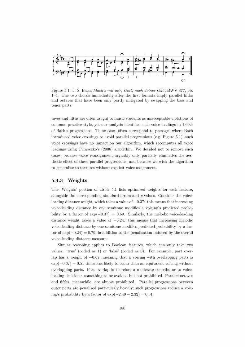
Figure 5.1: J. S. Bach, Mach’s mit mir, Gott, nach deiner Güt’, BWV 377, bb.1–4. The two chords immediately after the first fermata imply parallel fifthsand octaves that have been only partly mitigated by swapping the bass andtenor parts.

taves and fifths are often taught to music students as unacceptable violations ofcommon-practice style, yet our analysis identifies such voice leadings in 1.09%of Bach’s progressions. These cases often correspond to passages where Bachintroduced voice crossings to avoid parallel progressions (e.g. Figure 5.1); suchvoice crossings have no impact on our algorithm, which recomputes all voiceleadings using Tymoczko’s (2006) algorithm. We decided not to remove suchcases, because voice reassignment arguably only partially eliminates the aes-thetic effect of these parallel progressions, and because we wish the algorithmto generalise to textures without explicit voice assignment.

5.4.3 Weights

The ‘Weights’ portion of Table 5.1 lists optimised weights for each feature,alongside the corresponding standard errors and p-values. Consider the voice-leading distance weight, which takes a value of −0.37: this means that increasingvoice-leading distance by one semitone modifies a voicing’s predicted proba-bility by a factor of exp(−0.37) = 0.69. Similarly, the melodic voice-leadingdistance weight takes a value of −0.24: this means that increasing melodicvoice-leading distance by one semitone modifies predicted probability by a fac-tor of exp(−0.24) = 0.79, in addition to the penalisation induced by the overallvoice-leading distance measure.

Similar reasoning applies to Boolean features, which can only take twovalues: ‘true’ (coded as 1) or ‘false’ (coded as 0). For example, part over-lap has a weight of −0.67, meaning that a voicing with overlapping parts isexp(−0.67) = 0.51 times less likely to occur than an equivalent voicing withoutoverlapping parts. Part overlap is therefore a moderate contributor to voice-leading decisions: something to be avoided but not prohibited. Parallel octavesand fifths, meanwhile, are almost prohibited. Parallel progressions betweenouter parts are penalised particularly heavily; such progressions reduce a voic-ing’s probability by a factor of exp(−2.49− 2.32) = 0.01.

180

5.4.4 Feature importance

It is difficult to make meaningful comparisons between the weights of continuousfeatures, because each must be expressed in the units of the original feature.This problem is addressed by the permutation-based feature importance metricsin Table 5.1. These metrics operationalise feature importance as the drop inmodel performance observed when the trained model is evaluated on a dataset(in this case the Bach chorale corpus) where the feature is randomly permuted(Breiman, 2001; Fisher et al., 2018).4 Table 5.1 presents two feature importancemetrics corresponding to two previously presented performance metrics: theaccuracy of maximum-probability samples and the accuracy of random samples.Both metrics indicate that voice-leading efficiency, particularly in the melodyline, is the primary contributor to model performance.

It is worth noting that a large feature weight can accompany a small featureimportance. For example, parallel fifths/octaves between the outer parts yieldsa relatively large weight of −2.32, but a relatively small feature importance of0.01 (maximum-probability sampling). This can be rationalised by the observa-tion that parallel fifths/octaves between the outer parts is essentially prohibitedin common-practice voice leading (hence the large weight), but this rule onlyexcludes a tiny proportion of possible voice leadings (hence the small featureimportance).

It is also worth noting how each feature’s importance will necessarily dependon which other features are present. For example, the weight attributed to‘mean pitch height (distance from C4)’ is likely to be attenuated by voice-leadingdistance, because if the previous voicing already had an good mean pitch height,and the next voicing only differs by a small voice-leading distance, then the nextvoicing is guaranteed to have a fairly good mean pitch height. As a result, the‘mean pitch height’ feature only needs to give a slight nudge in the appropriatedirection to prevent mean pitch height from wandering over time.

5.4.5 Statistical significance

Two features received regression weights that did not differ statistically signifi-cantly from zero: Exposed octaves (outer parts) and Number of pitches (differ-ence from previous). The lack of statistical significance for the exposed-octavesfeature is particularly interesting, given how commonly Western music pedagogyprohibits these progressions. Examining the Moments column of Table 5.1, itis clear that such progressions are extremely rare in the chorale dataset, whichis surprising given the minimal contribution of the corresponding feature. Thissuggests that these progressions are being penalised by other features. Three

4Note that the feature is only permuted in the test dataset, not the training dataset.

181

such features seem particularly relevant: Voice-leading distance, Melodic voice-leading distance, and Mean pitch height. According to our definitions, exposedoctaves only occur when both outer parts move by three or more semitones;such large movements are likely to be heavily penalised by the voice-leadingdistance features. Furthermore, the two voices must progress in similar motion,thereby inducing a significant change in mean pitch height. Assuming that theprevious voicing was already at a suitable mean pitch height, this is likely totake the voicing to an unsuitable mean pitch height, resulting in penalisationby the Mean pitch height feature. In sum, therefore, it seems plausible that theexposed-octaves feature is made redundant by the other features.

The non-significant contribution of the feature Number of pitches (differencefrom previous) is arguably unsurprising given the corpus being modelled. Eachof these chorales is written for four voices, and so the primary pressure on thenumber of pitches in the sonority is likely to be the goal of providing these fourvoices with distinct lines; deviations from this four-pitch norm are generallyrare and quickly resolved. This phenomenon can be captured by the featureNumber of pitches (difference from ideal), making the feature Number of pitches(difference from previous) unnecessary. However, this latter feature may becomemore important in corpora where the number of voices is less constrained, suchas in keyboard music.

182

Tabl

e5.

1:D

escr

iptiv

ean

din

fere

ntia

lsta

tistic

sfo

rth

e12

voic

e-le

adin

gfe

atur

esas

appl

ied

toth

eB

ach

chor

ale

data

set.

Mom

ents

Wei

ghts

Feat

ure

impo

rtan

ce

Feat

ure

MSD

Valu

eSE

pM

ax.

prob

abili

tyR

ando

msa

mpl

e

Voic

e-le

adin

gdi

stan

ce5.

961

4.29

5−0.375

0.00

3<

.001

.553

.379

Mel

odic

voic

e-le

adin

gdi

stan

ce1.

133

1.48

6−0.240

0.00

6<

.001

.164

.100

Treb

lepi

tch

heig

ht(d

ista

nce

abov

eC

5)0.

742

1.43

0−0.237

0.00

8<

.001

.103

.052

Bas

spi

tch

heig

ht(d

ista

nce

belo

wC

3)0.

801

1.81

4−0.173

0.00

6<

.001

.072

.038

Inte

rfer

ence

(Hut

chin

son

&K

nopo

ff,19

78)

0.18

90.

076

−8.653

0.23

1<

.001

.068

.037

Para

llelo

ctav

es/fi

fths

(Boo

lean

)0.

011

0.10

4−2.489

0.06

2<

.001

.056

.033

Num

ber

ofpi

tche

s(d

iffer

ence

from

idea

l)0.

080

0.27

8−1.321

0.03

5<

.001

.056

.032

Mea

npi

tch

heig

ht(d

ista

nce

from

C4)

2.50

61.

793

−0.128

0.00

5<

.001

.031

.018

Part

over

lap

(Boo

lean

)0.

028

0.16

4−0.669

0.04

1<

.001

.013

.013

Para

llelo

ctav

es/fi

fths

(out

erpa

rts;

Boo

lean

)0.

001

0.02

3−2.323

0.27

0<

.001

.008

.004

Exp

osed

octa

ves

(out

erpa

rts;

Boo

lean

)0.

001

0.03

7(0.204)

(0.1

64)

.214

.000

.000

Num

ber

ofpi

tche

s(d

iffer

ence

from

prev

ious

)0.

125

0.33

6(0.008)

(0.0

34)

.822

.000

.000

Not

e.M

omen

tspr

ovid

esth

em

ean

and

stan

dard

devi

atio

nof

feat

ure

valu

esin

the

Bach

chor

ale

data

set.

Wei

ghts

prov

ides

the

regr

essio

nwe

ight

sfo

rea

chfe

atur

e,al

ongs

ide

corr

espo

ndin

gst

anda

rder

rors

and

p-va

lues

.Fe

atur

eim

-po

rtan

cepr

ovid

espe

rmut

atio

n-ba

sed

impo

rtan

cem

etric

sfo

rea

chfe

atur

e.

183

5.5 GenerationThe probabilistic model developed in the previous section can be directly appliedto the automatic generation of voice leadings for chord sequences. Given aprespecified chord sequence, the model defines a probability distribution over allpossible voice leadings for that chord sequence, which factorises into probabilitydistributions for each chord voicing conditioned on the previous chord voicing. Itis straightforward to sample from this factorised probability distribution: simplyiterate from the first to the last chord in the sequence, and sample each voicingaccording to the probability distribution defined by the log-linear model, usingthe sampled voicing at position i to define the feature set for chord voicings atposition i+ 1.

If our goal is to approximate a target corpus as well as possible, then thisrandom sampling is a sensible approach. However, if our goal is to generate thebest possible voice leading for a chord sequence, then we must identify someobjective function that characterises the quality of a chord sequence’s voiceleading and optimise this objective function.

Here we propose optimising the sum of the model’s linear predictors. Asdefined previously, the linear predictor characterises a given chord voicing asa weighted sum of feature values, with this linear predictor being exponenti-ated and normalised to estimate the probability of selecting that voicing. Thelinear predictor might be interpreted as the attractiveness of a given voicing,as inversely related to features such as voice-leading distance and interferencebetween partials.

Optimising the sum of the linear predictors is subtly different to optimisingfor probability. Optimising for probability means maximising the ratio of the ex-ponentiated linear predictors for the chosen voicing to the exponentiated linearpredictors for the alternative voicings. This maximisation does not necessarilyentail high values of the linear predictor; in perverse cases, high probabilitiesmay be achieved when the chosen voicing is simply the best of a very bad setof candidates. We wish to avoid such cases, and to identify chord voicings thatpossess good voice-leading attributes in an absolute sense, not simply relativeto their local competition.

The space of all possible voice leadings is large: given 100 candidate voicingsper chord, a sequence of 80 chords has 10160 potential voice-leading solutions.It is clearly impractical to enumerate these voice leadings exhaustively. A sim-ple ‘greedy’ strategy would be to choose the chord voicing with the highestlinear predictor at each chord position; however, this is not guaranteed to max-imise the sum of linear predictors across all chord positions. Instead, we takea dynamic-programming approach that deterministically retrieves the optimal

184

voice-leading solution while restricting the number of linear predictor evalua-tions to approximately a2n, where a is the number of candidate voicings for eachchord and n is the number of chords in the sequence. This approach simplifiesthe computation by taking advantage of the fact that none of our features lookback beyond the previous chord’s voicing. See Algorithm 1 for details.

Several of the features, such as voice-leading distance and part overlap, areundefined for the first chord in the sequence. Correspondingly, the first chord ofeach sequence was excluded from the model-fitting process described in Section5.4. When generating from the model, however, it is inappropriate to excludethese chords from the optimisation. Instead, we set all context-dependent fea-tures to zero for the first chord of each sequence (in fact, any numeric constantwould have the same effect). The initial chord voicings are then optimisedaccording to the context-independent features, such as interference betweenpartials and mean pitch height.

Figure 5.2 demonstrates the algorithm on the first ten sonorities of thechorale dataset: Aus meines Herzens Grunde, BWV 269.5 For comparisonpurposes, Figure 5.2A displays J. S. Bach’s original voice leading, and Figure5.2B displays a heuristic voice leading where the bass pitch class is played inthe octave below middle C and the non-bass pitch classes are played in the oc-tave above middle C, as in Chapter 4. Figure 5.2C displays the voice leadingproduced by the new algorithm, using regression weights as optimised on theoriginal corpus, and generating candidate chords according to the same pro-cedure as described in Section 5.4. Unlike the heuristic algorithm, the newalgorithm consistently employs four notes in each chord, similar to the originalchorale harmonisation. The new algorithm successfully avoids the two parallelfifths produced in the last two bars by the heuristic algorithm, and achievesconsiderably more efficient voice leading throughout.

In chorale harmonisations the soprano line is typically constrained to followthe pre-existing chorale melody. We can reproduce this behaviour by modifyingthe candidate voicing generation function so that it only generates voicingswith the appropriate soprano pitches. Figure 5.2D displays the voice leadingproduced when applying this constraint. Our implementation also supportsfurther constraints such as forcing particular chord voicings to contain particularpitches, or alternatively fixing entire chord voicings at particular locations inthe input sequence.

We were interested in understanding how the trained model would generaliseto different musical styles. In harmony perception studies, it is often desirableto present participants with chord sequences derived from pre-existing music

5Source code is available at https://doi.org/10.5281/zenodo.2613563. Generated voiceleadings for all 370 chorales are available at https://doi.org/10.5281/zenodo.2613646.

185

Figure 5.2: Example voice leadings for J. S. Bach’s chorale Aus meines HerzensGrunde (BWV 269), chords 1–10. A: Bach’s original voice leading. B: Heuristicvoice leading. C: New algorithm. D: New algorithm with prespecified melody.

Figure 5.3: Example voice leadings for the first 10 chords of John Coltrane’s26-2. A: Heuristic voice leading. B: New algorithm.

corpora, such as the McGill Billboard corpus (Burgoyne, 2011) and the iRbcorpus (Broze & Shanahan, 2013). Unfortunately, these corpora just providechord symbols, not fully voiced chords, and so the researcher is tasked withcreating voice leadings for these chord sequences. We had yet to identify suitable

186

Figure 5.4: Example voice leadings for the first 10 chords of You’ve got a friendby Roberta Flack and Donny Hathaway. A: Heuristic voice leading. B: Newalgorithm.

datasets of voiced chord sequences for popular or jazz music, and thereforewished to understand whether Bach chorales would be sufficient for training thealgorithm to generate plausible voice leadings for these musical styles.

From an auditory scene analysis perspective, there are clear differences be-tween Bach chorales and popular/jazz harmony. The chorales consistently usefour melodically independent voices, and Bach’s voice-leading practices are con-sistent with the compositional goal of maximising the perceptual independenceof these voices while synchronising text delivery across the vocal parts (Huron,2001, 2016). In contrast, harmony in popular and jazz music is often deliveredby keyboards or guitars, both of which produce chords without explicit voiceassignment, with the number of distinct pitches in each chord often varyingfrom chord to chord. Correspondingly, voice independence seems likely to beless important in popular/jazz harmony than in Bach chorales. Nonetheless,we might still expect popular/jazz musicians to pay attention to the perceptualindependence of the outer parts, since these voices are particularly salient to thelistener even when the voice parts are not differentiated by timbre. We mightalso expect popular/jazz listeners to prefer efficient voice leadings, even if theyare not differentiating the chord progression into separate voices, because effi-cient voice leading helps create the percept of a stable textural stream (Huron,2016). In summary, therefore, there are reasons to expect some crossover be-tween voice-leading practices in Bach chorales and voice-leading practices inpopular/jazz music.

Figures 5.3 and 5.4 demonstrate the application of the chorale-trained modelto examples from two such corpora: the iRb jazz corpus (Broze & Shanahan,2013) and the Billboard popular music corpus (Burgoyne, 2011). We use both

187

datasets as translated to pitch-class notation in Chapter 2, and use the samemodel configuration as for the Bach chorale voicing.

Figures 5.3A and 5.3B correspond to the first ten bars of the jazz corpus,from the composition 26-2 by John Coltrane. Figure 5.3A displays the heuristicalgorithm described earlier, and Figure 5.3B displays the new algorithm’s voic-ing. Informally, the new algorithm seems to generalise sensibly to this extract,despite the extract’s radical harmonic differences from the Bach chorale har-monisations. The clearest difference from the heuristic algorithm seems to bein the spacing of the voices; the new algorithm enforces a wide gap between thelower voices, presumably on account of the Interference between partials feature.

Figures 5.4A and 5.4B correspond to the first ten bars of You’ve got a friendby Roberta Flack and Donny Hathaway, the second composition in the popularcorpus.6 As before, Figures 5.4A and 5.4B correspond to the heuristic andnew algorithms respectively. Unlike the heuristic algorithm, the new algorithmmaintains four-note voicings at all times, arguably producing a richer and moreconsistent sound as a result. The voice-leading efficiency is also considerablyimproved, particularly in the melody line. At first sight, the new algorithm doesalso produce some unusual voice leadings: for example, the tenor part jumpsby a tritone between the fourth chord and the fifth chord. One might expectthis inefficient voice leading to be heavily penalised by the model. However,the model considers this voice leading to be relatively efficient, as Tymoczko’s(2006) algorithm connects the two voicings by approaching the lower two notesof the fifth chord (C, G) from the bass note of the previous chord (G), andapproaching the second-from-top note in the fifth chord (E) from the second-from-bottom note in the fourth chord (D flat). This suggested voice assignmentis indeed plausible when the extract is performed on a keyboard instrument, butit could not be realised by a four-part ensemble of monophonic instruments. Forsuch applications, it would be worth modifying Tymoczko’s (2006) algorithm toset an upper bound on the number of inferred voices.

5.6 ImplementationWe have implemented these algorithms in an open-source software packagecalled voicer, written for the R programming language, and coded in a mix-ture of R and C++. The source code is available from the open-source reposi-tory https://github.com/pmcharrison/voicer and permanently archived athttps://doi.org/10.5281/zenodo.2613565.

6We originally tried the first composition in this corpus, but it was too repetitive to givemuch insight into the new algorithm.

188

Having installed the voicer package, the following code instructs the packageto voice a perfect (or authentic) cadence:

library(voicer)library(hrep)library(magrittr)# Each chord is represented as a sequence of MIDI note numbers.# The first number is the bass pitch class.# The remaining numbers are the non-bass pitch classes.list(pc_chord("0 4 7"), pc_chord("5 0 2 9"),

pc_chord("7 2 5 11"), pc_chord("0 4 7")) %>%vec("pc_chord") %>%voice(opt = voice_opt(verbose = FALSE)) %>%print(detail = TRUE)

## [[1]] Pitch chord: 48 64 67 72## [[2]] Pitch chord: 53 62 69 72## [[3]] Pitch chord: 55 62 65 71## [[4]] Pitch chord: 48 55 64 72

By default, voicer uses the same regression weights and voicing protocol aspresented in the current chapter. However, it is easy to modify this configura-tion, as demonstrated in the following example:

library(voicer)library(hrep)library(magrittr)chords <- list(pc_chord("0 4 7"), pc_chord("5 0 9"),

pc_chord("7 2 11"), pc_chord("0 4 7")) %>%vec("pc_chord")

# Modify the default weights to promote parallel fifths/octavesweights <- voice_default_weightsweights["any_parallels"] <- 100voice(chords, opt = voice_opt(verbose = FALSE,

weights = weights,min_notes = 3,max_notes = 3)) %>%

print(detail = TRUE)

## [[1]] Pitch chord: 48 55 64## [[2]] Pitch chord: 53 60 69

189

## [[3]] Pitch chord: 55 62 71## [[4]] Pitch chord: 60 67 76

The voicer package also exports functions for deriving regression weightsfrom musical corpora, and using these new weights to parametrise the voicingalgorithm. The following example derives regression weights from the first twopieces in the Bach chorale dataset, and uses these weights to voice a chordsequence.

if (!requireNamespace("hcorp"))devtools::install_github("pmcharrison/hcorp")

library(voicer)library(hrep)# Choose the features to modelfeatures <- voice_features()[c("vl_dist", "dist_from_middle")]# Compute the featurescorpus <- hcorp::bach_chorales_1[1:2]corpus_features <- voicer::get_corpus_features(

corpus, min_octave = -2, max_octave = 1, features = features,revoice_from = "pc_chord", min_notes = 1, max_notes = 4,verbose = FALSE)

# Model the featuresmod <- model_features(corpus_features,

perm_int = FALSE,verbose = FALSE)

as.data.frame(mod$weights)

## feature estimate std_err z p## 1 vl_dist -0.5320266 0.03441282 -15.460129 6.446884e-54## 2 dist_from_middle -0.1910925 0.06838340 -2.794428 5.199166e-03

# Voice a chord sequencechords <- list(pc_chord("0 4 7"), pc_chord("5 0 9"),

pc_chord("7 2 11"), pc_chord("0 4 7")) %>%vec("pc_chord")

voice(chords, opt = voice_opt(weights = mod,features = features,verbose = FALSE)) %>%

print(detail = TRUE)

## [[1]] Pitch chord: 36 52 72 79

190

## [[2]] Pitch chord: 41 53 72 81## [[3]] Pitch chord: 43 50 71 79## [[4]] Pitch chord: 48 52 72 79

5.7 DiscussionWe have introduced a new model for the analysis and generation of voice lead-ings. This model uses perceptually motivated features to predict whether agiven voice leading will be considered appropriate in a particular musical con-text. Applied to a dataset of 370 chorale harmonisations by J. S. Bach, thismodel delivered quantitative evidence for the relative importance of differentmusical features in determining voice leadings. Applied to generation, the modeldemonstrated an ability to create plausible voice leadings for pre-existing chordsequences, and to generalise to musical styles dissimilar to the Bach choralesupon which it was trained.

Combining analysis with generation provides a powerful way to examinewhich principles are sufficient to explain voice-leading practice. While the anal-ysis stage provides quantitative support for the importance of different musicalfeatures in voice leading, the generation stage can provide a litmus test for thesufficiency of the resulting model. Examining the outputs of the model, we cansearch for ways in which the model deviates from idiomatic voice leading, andtest whether these deviations can be rectified by incorporating additional per-ceptual features into the model. If so, we have identified an additional way inwhich voice leading may be explained through auditory perception, after Huron(2001, 2016); if not, we may have identified an important cultural componentto voice-leading practice. To this end, we have released automatically generatedvoicings for the full set of 370 Bach chorale harmonisations;7 we hope that theywill provide useful material for identifying limitations and potential extensionsof the current approach.

The existing literature already suggests several additional features thatmight profitably be incorporated into the voice-leading model. One exampleis the ‘leap away rule’, which states that large melodic intervals (leaps) arebetter situated in the outer voices than the inner voices, and that these in-tervals should leap away from the other voices rather than towards the othervoices (Huron, 2016). This should be straightforward to implement computa-tionally. A second example is the ‘follow tendencies rule’, which states thatthe progressions of individual voices should follow the listener’s expectations,which may themselves derive from the statistics of the musical style (schematic

7https://doi.org/10.5281/zenodo.2613646

191

expectations), the statistics of the current musical piece (dynamic expectations),or prior exposure to the same musical material (veridical expectations) (Huron,2016). Schematic expectations could be operationalised by using a dynamickey-finding algorithm to represent the sonority as scale degrees (e.g. Huron &Parncutt, 1993), and then evaluating the probability of each scale-degree tran-sition with respect to a reference musical corpus; dynamic expectations couldbe operationalised in a similar manner, but replacing the reference corpus withthe portion of the composition heard so far. Veridical expectations would re-quire more bespoke modelling to capture the particular musical experience ofthe listener. An interesting possibility would be to unite these three types ofexpectation using Pearce’s (2005) probabilistic model of melodic expectation(see also Sauvé, 2017). Further rules that could be implemented include the‘semblant motion rule’ (avoid similar motion) and the ‘nonsemblant prepara-tion rule’ (avoid similar motion where the voices employ unisons, octaves, orperfect fifths/twelfths) (Huron, 2016).

Our model also has practical applications in automatic music generation.For example, a recurring problem in music psychology is to construct experi-mental stimuli representing arbitrary chord sequences, which often involves thetime-consuming task of manually constructing voice leadings. Our model couldsupplant this manual process, bringing several benefits including a) scalability,allowing the experimental design to expand to large stimulus sets; b) objectivity,in that the voice leadings are created according to formally specified criteria,rather than the researcher’s aesthetic intuitions; c) reproducibility, in that themethods can be reliably reproduced by other researchers.

Interpreted as a model of the compositional process, the model assumes thatchords are determined first and that voice leading only comes later. This may beaccurate in certain musical scenarios, such as when performers improvise fromfigured bass or from lead sheets, but it is clearly not a universal model of musiccomposition. A more universal model might include some kind of alternationbetween composing the harmonic progression and composing the voice leading,so that the composer can revise the harmonic progression if it proves impossibleto find a satisfactory voice leading.

The model also assumes a one-to-one mapping between the chords of theunderlying harmonic progression and the chord voicings chosen to represent it.While this assumption may hold true for certain musical exercises, it is notuniversally valid for music composition. For example, an improviser playingfrom figured bass may choose to extend a single notated chord into multiplevertical sonorities, for example through arpeggiation or through the introductionof passing notes. It would be interesting to model this process explicitly. Oneapproach would be to use the original model to generate block chords at the level

192

of the harmonic rhythm, and then to post-process these block chords with anadditional algorithm to add features such as passing notes and ornamentation.

While the model deserves further extension and validation, it seems ready tosupport ongoing research in music psychology, music theory, and computationalcreativity. Our R package, voicer, should be useful in this regard: It providesa convenient interface for analysing voice leadings in musical corpora and forgenerating voice leadings for chord sequences. The ongoing development of thispackage may be tracked at its open-source repository (https://github.com/pmcharrison/voicer).

193

Algorithm 1: A dynamic programming algorithm for maximising thesum of the linear predictors f over all chord transitions.

input : candidates, a list of length N ; candidates[i] lists the candidatevoicings for chord i

output: chosen, a list of length N ; chosen[i] identifies the chosen voicing forchord i

best_scores← list(N)

best_prev_states← list(N)

best_scores[1]← vector(length(candidates[1]))

for j ← 1 to length(candidates[1]) dobest_scores[1][j]← f(NULL, candidates[1][j])

endfor i← 2 to N do

best_scores[i]← vector(length(candidates[i]))

for j ← 1 to length(candidates[i]) dobest_prev_states[i][j]← 1

best_scores[i][j]← f(candidates[i− 1][1], candidates[i][j])

for k ← 2 to length(candidates[i− 1])} donew_score← f(candidates[i− 1][k], candidates[i][j])

if new_score > best_scores[i][j] thenbest_prev_states[i][j]← k

best_scores[i][j]← new_scoreend

endend

endchosen← vector(N)

chosen[N ]← which_maxj(best_scores[N ][j])

for n← N − 1 to 1 dochosen[n]← best_prev_states[n+ 1][chosen[n+ 1]]

endreturn chosen

194

Chapter 6

Conclusion

6.1 OverviewThe primary goal of this thesis was to develop an improved understanding ofharmony cognition through the computational modelling of large datasets ofperceptual data and music compositions. A secondary goal was to design, im-plement, and evaluate computational models of harmony that subsequent sci-entists and music theorists could take advantage of in future research. Thesegoals motivated the research described in Chapters 2–5.

Each of the computational studies depends on a shared collection of low-level cognitive representations for harmony, introduced in Chapter 2. Low-levelrepresentations correspond to the early stages of cognitive processing, and arelinked relatively unambiguously to the musical score and the audio signal. Wedefined three classes of low-level representations: symbolic representations, de-fined as succinct and categorical descriptions of chords, acoustic representations,which characterise the musical sound, and sensory representations, which reflectthe listener’s perceptual images of the resulting sound. We defined a network ofrepresentations organised into these three categories and explained the computa-tional operations involved in translating between these different representations.We also defined methods for mapping four of the symbolic representations tointeger encodings, an important prerequisite for many statistical modelling tech-niques. Finally, we discussed ways of deriving these representations from com-mon corpus encodings, and reviewed methods for deriving high-level cognitiverepresentations such as chord roots and tonality from these low-level represen-tations. The chapter is accompanied by the R package hrep, which implementsthe various representations and conversion methods described in the chapter,as well as the hcorp package, which provides several musical corpora encodedusing these representation schemes.

195

The following chapters – Chapters 3, 4, and 5 – addressed three core phe-nomena in harmony cognition: consonance, harmonic expectation, and voiceleading. A recurring research question across these chapters was as follows:

“To what extent is the perception and composition of Western har-mony determined by low-level psychoacoustic processes versus high-level cognitive processes?”

Chapter 3 addressed simultaneous consonance, the sense in which certaincombinations of tones sound ‘well’ together. We began by defining three classesof consonance theories with particular support from the existing literature: in-terference between partials, periodicity/harmonicity, and cultural familiarity.Interference between partials is the most low-level of these phenomena, relatingprimarily to the resolution of partials on the basilar membrane of the innerear (Daniel & Weber, 1997; Vencovský, 2016). Periodicity/harmonicity is amid-level phenomenon, relating to pitch detection processes within the auditorycortex (Wang et al., 2013). Cultural familiarity is a relatively high-level cogni-tive phenomenon, corresponding to the listener’s internalised knowledge of theprevalences of different chord types within a given musical style. We compiledcomputational operationalisations of each of these classes of consonance theory,numbering 20 models in total, and evaluated these models on a) four behaviouralstudies of consonance judgments representing more than 500 participants and b)three large music corpora representing more than 100,000 compositions. Whilerecent work has argued that consonance perception is independent of interfer-ence between partials, we identified a substantial contribution of this inter-ference phenomenon in both our perceptual and our corpus analyses. Theseanalyses also identified sizeable contributions of periodicity/harmonicity andcultural familiarity, suggesting that consonance is not a unitary phenomenonbut rather a composite phenomenon deriving from a combination of low-level,mid-level, and high-level psychological processes. This composite account isrepresented by a three-factor computational model that combines Hutchinson& Knopoff’s interference model, a new harmonicity detection model, and a newdata-driven cultural familiarity model. The chapter is accompanied by the in-con package, which implements this composite consonance model alongside 15other consonance models evaluated in the chapter.

Chapter 4 addressed harmonic expectation, the way in which certain chordprogressions set up expectations for the chords that follow them. We formalisedharmonic expectation probabilistically, supposing that the brain continuallyconstructs predictive probability distributions over the alphabet of all possiblechords, with these probability distributions being conditioned on the precedingchords in the progression. Noting the rich variety of perceptual features that

196

listeners can derive from chord progressions – for example, harmonicity, chordroots, root intervals, and pitch-class sets – we modelled harmonic prediction us-ing a new technique termed ‘viewpoint regression’, which generates predictionsfor chord symbols using statistical regularities acquired from an assortment ofcategorical and continuous perceptual features. We then used this model toinvestigate what strategies an ideal listener would adopt when predicting chordprogressions, and how these strategies might manifest in everyday music listen-ing. We found that the ideal listener paid particular attention to two low-levelconsonance features, namely interference between partials (after Hutchinson &Knopoff, 1978) and periodicity/harmonicity (the new model presented in Chap-ter 3), as well as a high-level feature that captured relative pitch perceptionby expressing each chord relative to the bass note of the previous chord. Wefollowed this ideal-listener analysis with a human-listener analysis, where weconducted a behavioural experiment to elicit surprisal ratings for 300 chordsequences excerpted from real popular music compositions, and compared theresulting data to our ideal-listener model. The ideal-listener model reproducedhuman performance fairly well, predicting mean surprisal ratings with a correla-tion coefficient of .70. Interrogating this model further, we found that variationsin perceived surprisal were primarily driven by a simple repetition-priming pro-cess, whereby listeners expect chords to recur if they have already occurred inthe recent musical context. The simplicity of this repetition-priming processmakes a remarkable contrast with the complexity of recent language-inspiredtheories of harmonic syntax, but is consistent with Bigand et al.’s (2014) asser-tion that much of music syntax processing can be explained by the accumulationand comparison of information in auditory short-term memory.

Chapter 5 addressed voice leading, which describes how a chord’s pitchclasses are assigned pitch heights, and how the pitches in successive chordsconnect to form simultaneous melodies. We developed a cognitive model tocharacterise this process, which uses various perceptually motivated features topredict whether a composer will choose a given voice leading in a given musicalcontext. These features were motivated by Huron’s (2001, 2016) perceptual ac-count of voice leading, which relates Western voice-leading practice to the goalof manipulating psychological processes of auditory scene analysis, by whichthe listener organises the acoustic environment into perceptually meaningfulelements (Bregman, 1990). We applied this model to a corpus of 370 choraleharmonisations by J. S. Bach, and derived quantitative estimates for the rel-ative importance of various perceptual features such as interference betweenpartials, voice-leading distance, and part overlap. We found that almost all ofthe proposed features contributed meaningfully to voice-leading practice, withthe exception of exposed octaves, which seemed to be made redundant by a

197

combination of the voice-leading distance and pitch height features. We thenexamined the model’s ability to generate new voice leadings for pre-existingchord sequences, and found that the model seemed to perform rather effec-tively, even when applied to quite dissimilar musical styles to the original Bachchorales, such as popular music and jazz music. These results imply that, asargued by Huron (2001, 2016), much of voice-leading practice can be effectivelysummarised by a few perceptual principles related to auditory scene analysis,rather than being dominated by arbitrary cultural conventions.

A common conclusion from these studies is clear: many aspects of harmonycognition depend substantially on relatively low-level psychoacoustic processes.Consonance is primarily driven by interference between partials and periodic-ity/harmonicity (Chapter 3); harmonic expectation in Western popular music isstrongly influenced by basic repetition-priming effects (Chapter 4); voice leadingreflects psychological processes of auditory scene analysis (Chapter 5).

Nonetheless, higher-level cognitive processes clearly also contribute to har-mony cognition. Existing psychoacoustic models could only explain part of thevariance in our consonance perception data, and a cultural familiarity modelproved useful in explaining an additional portion of this variance. Likewise,psychoacoustic models were an important part of the ideal-listener model ofharmony prediction, but the ideal model also took advantage of learned tran-sition probabilities between high-level chord representations. Our voice-leadingmodel only addressed relatively low-level contributions to voice-leading prac-tice, but Huron (2016) has argued that voice-leading practice also depends onculturally learned expectations for melodic progressions.

It seems, therefore, that computational models of harmony cognition mustultimately combine low-level psychoacoustic processing with high-level cognitiveprocessing. Our consonance model achieves this through a linear regression ap-proach, which combines two low-level consonance models (interference betweenpartials, periodicity/harmonicity) with a high-level model of cultural familiarity.Our harmonic expectation model achieves this through a viewpoint regressionapproach, which generates predictive probability distributions over chord pro-gressions on the basis of statistical regularities learned from both low-level psy-choacoustic features (e.g. interference between partials, spectral similarity) andhigh-level cognitive features (e.g. chord root progressions). Our voice-leadingmodel is currently limited to low-level psychoacoustic features, but future workcould add higher-level features to this model, such as a feature capturing cul-turally determined transition probabilities between scale degrees.

We have implemented these different computational models as interopera-ble open-source software packages, written for the programming language R. Wehope that these packages will prove useful for subsequent research into harmony

198

cognition. Each of these packages depends on the hrep package, presented inChapter 2, which defines a collection of harmonic representation schemes withinan object-oriented framework. This hrep package should be useful to future re-searchers wishing to develop new harmony models within the R programminglanguage. Chapter 3 presented the incon package, which implements a varietyof consonance models from the literature, alongside the composite consonancemodel developed in the present work. These implementations should be usefulto those wishing to conduct further research into the nature of consonance, andto those wishing to find a ready-made operationalisation of consonance for prac-tical applications such as music classification or music generation. Chapter 4presented the hvr package, which implements the harmonic viewpoint regressionmodel; this should be useful to researchers wishing to model the probabilisticprocessing of harmonic progressions. Chapter 5 presented the voicer package,which implements the feature-based statistical model of voice leading practice.One application of this model is corpus analysis: given a symbolically encodedmusical corpus, the model will quantify the contributions of different percep-tually motivated features (e.g. interference between partials, pitch height) tovoice-leading practice. A second application is generative: given a chord pro-gression, the model can generate a voiced version of that chord progressionusing feature weights that have either been derived from corpus analysis orhand-specified by the user. We expect this generative system to be particularlyuseful for future studies of harmony perception, allowing researchers to takechord sequences from preexisting musical corpora (e.g. the Billboard corpus,Burgoyne, 2011) and convert them to block chords that can be synthesised asstimuli for perceptual experiments.

6.2 Limitations and future directionsAn important priority in this work was to maximise the interpretability of ourcomputational models. Interpretability is crucial if we wish to gain cognitiveinsights from our models. However, interpretability typically requires simplisticassumptions that can reduce the model’s verisimilitude and predictive power.We made several such assumptions in this work. First, we analysed harmonyin isolation from metre, yet metre is known to contribute to harmonic struc-ture. Second, our models take symbolic musical representations as input, andhence neglect the ways in which varying acoustic properties of different musicalinstruments contribute to harmony perception. Third, we adopted relatively re-stricted statistical models such as linear models, Markov models, and log-linearmodels, which cannot capture as complex statistical patterns as their connec-tionist equivalents. Fourth, we glossed over the way in which chord sequences

199

are derived from full musical textures. Music theorists are used to the idea ofreducing passages of polyphonic music to their underlying chord sequences, butthis is a nontrivial task that has yet to receive a fully satisfying cognitive anal-ysis. These different simplifications would be worthwhile to address in futureresearch.

This research was primarily restricted to modelling Western listeners andWestern composers. The motivation for this restriction was twofold: first, har-mony is considered to be particularly characteristic of Western music, and sec-ond, the majority of publicly available perceptual data and music corpora comefrom Western listeners and Western composers. However, many cultures acrossthe world also produce music that involves chordal sonorities, and hence pre-sumably evokes many of the psychological mechanisms studied in the presentwork. Studying such cultures can be particularly useful for differentiating bi-ological, environmental, and cultural contributions to music cognition. A fewcross-cultural scientific studies have been conducted into consonance in musicperception and composition (Butler & Daston, 1968; Gill & Purves, 2009; Ma-her, 1976; McDermott et al., 2016; Sethares, 2005), but very little cross-culturalwork has been conducted into harmonic expectation and voice leading, particu-larly from a computational perspective. This is an important avenue for futureresearch.

We addressed three core aspects of harmony cognition: consonance, expec-tation, and voice leading. There are many other aspects of harmony cognitionthat would be interesting to study using similar computational methods, includ-ing the development of aesthetic preferences, the expression and induction ofemotion, and the articulation of large-scale structure. It seems likely that con-sonance and expectation should be particularly useful for understanding suchphenomena; our computational models of consonance and expectation shouldprove useful for research into this area.

The software documented in this thesis was mostly written for the program-ming language R. The decision to work in R was guided primarily by its widecollection of statistical packages and its popularity among music psychologists.However, Python is a strong competitor language for this kind of work, in that italready possesses a strong collection of music-related open-source packages suchas music21 and Essentia. It would be worthwhile to port some of the softwaredeveloped here to Python in order to take advantage of this ecosystem.

Our perceptual studies were observational in the sense that they used un-manipulated musical stimuli (chords or chord sequences synthesised using apiano timbre) played to participants with no prior interventions, and testeddifferent psychological theories using correlation- or regression-based analyses.This approach is appealing because it facilitates the use of large and ecologi-

200

cally valid stimulus sets. However, such observational approaches struggle toprovide definitive proofs of causation, and so it would be worthwhile to sup-plement these observational approaches with interventional paradigms. Theseinterventions could happen at the level of the stimulus, for example by introduc-ing timbral manipulations (e.g. Geary, 1980; Nordmark & Fahlén, 1988; Pierce,1966; Sethares, 2005; Vos, 1986), or at the level of the participant, for exampleby introducing passive exposure to an artificial harmonic language (e.g. Jonaitis& Saffran, 2009; Loui et al., 2009; Rohrmeier & Cross, 2009). Such interven-tions could help to distinguish theories that deliver correlated predictions, as isthe case in consonance perception (Chapter 3).

Our perceptual studies relied on behavioural methods and did not incorpo-rate any neuroscientific measures. Behavioural methods typically benefit frommore straightforward interpretation and greater statistical power than neuro-scientific methods, but they are typically mediated by conscious introspectionand decision-making. In contrast, neuroscientific methods can complement be-havioural methods by providing more direct access to the listener’s internalperceptual processes, and helping to reveal the neural substrates underpinningthese processes. The computational methods developed in this thesis shouldbe useful for supporting such research. In particular, the computational mod-els should be useful for conducting studies with naturalistic stimuli, providingquantitative operationalisations of different perceptual or cognitive features thatcan be incorporated into model-based analyses. We are currently conductingseveral collaborations to explore these possibilities.

The behavioural studies were limited to two response modes: conso-nance/pleasantness judgements (Chapter 3) and surprisal judgements (Chapter4). We argued that these two approaches capture core perceptual phenomenain harmony cognition: consonance has long been understood to play a foun-dational role in Western listeners’ aesthetic and emotional responses to music(e.g. Helmholtz, 1863; Stumpf, 1898), and more recently the psychological pro-cesses of expectation and surprise have also been recognised as important driversof musical aesthetics and emotion (Egermann et al., 2013; Huron, 2006; Meyer,1956; Pearce, 2005). However, our behavioural paradigms were nonethelessfairly distant from how people usually engage with music in the real world. Inparticular, evaluating music on rating scales is an unusual musical behaviour;music theorists often speak of the consonance of individual intervals or chords,but typically use only two or three categories (e.g. ‘perfect consonance’, ‘im-perfect consonance’, ‘dissonance’) rather than the granular numeric scales usedhere. Moreover, although musical surprisal seemed to be an intuitive conceptto our participants, explicitly rating surprisal on a chord-by-chord basis is nota common musical behaviour outside of the laboratory. Limiting consideration

201

to these two behavioural indices of harmony cognition inevitably limits the gen-eralisations that can be made from the present research. An important futuregoal is to generalise these computational investigations to a broader range ofbehavioural paradigms that better represent everyday musical behaviours.

Our corpus analyses were limited to four specific musical corpora: the Peach-note corpus (Viro, 2011), the Billboard corpus (Burgoyne, 2011), the iRb corpus(Broze & Shanahan, 2013), and a dataset of Bach chorale harmonisations (Sapp,2005). The conclusions of these analyses may yet prove to be sensitive to thesampling methods used for constructing these corpora and the techniques usedfor digitising them. The best way to cement these conclusions will be to fol-low up these initial investigations with further analyses that explore differentmusical corpora constructed using alternative sampling and encoding methods.

Chapters 4 and 5 presented cognitive models of harmonic expectation andvoice leading. Both are formulated as probabilistic models of musical struc-ture: harmonic expectation is modelled as conditional probabilities of futurechords conditioned on previous chords, whereas voice leading is modelled asconditional probabilities of chord voicings conditioned on a prespecified chordsequence. These two models could be combined to form a complete probabilisticmodel of voiced chord progressions. Such a model could function as a cognitivemodel of predictive processing, explaining how listeners predict upcoming mu-sical sonorities on the basis of both harmonic and voice-leading principles. Themodel could also be used for generative applications, automating the generationof fully voiced chord sequences on the basis of statistics learned from a givenmusical corpus. This remains an interesting prospect for future work.

202

References

Aarden, B. J. (2003). Dynamic melodic expectancy (PhD thesis). OhioState University, Columbus, OH.

Albrecht, J., & Shanahan, D. (2013). The use of large corpora to train anew type of key-finding algorithm: An improved treatment of the minormode. Music Perception, 31, 59–67. https://doi.org/10.1525/MP.2013.31.1.59

Ambrazevičius, R. (2017). Dissonance/roughness and tonality perceptionin Lithuanian traditional Schwebungsdiaphonie. Journal of Interdis-ciplinary Music Studies, 8(1&2), 39–53. https://doi.org/10.4407/jims.2016.12.002

Arnal, L. H., Flinker, A., Kleinschmidt, A., Giraud, A. L., & Poeppel, D.(2015). Human screams occupy a privileged niche in the communicationsoundscape. Current Biology, 25(15), 2051–2056. https://doi.org/10.1016/j.cub.2015.06.043

Arthur, C. (2018). A perceptual study of scale-degree qualia in context.Music Perception, 35, 295–314. https://doi.org/10.1525/MP.2018.35.3.295

Arthur, C., & Huron, D. (2016). The direct octaves rule: Testing a scene-analysis interpretation. Musicae Scientiae, 20, 495–511. https://doi.org/10.1177/1029864915623093

Arthurs, Y., Beeston, A. V., & Timmers, R. (2018). Perception of iso-lated chords: Examining frequency of occurrence, instrumental timbre,

203

acoustic descriptors and musical training. Psychology of Music, 46(5),662–681. https://doi.org/10.1177/0305735617720834

Aslin, R. N., Saffran, J. R., & Newport, E. L. (1998). Computation ofconditional probability statistics by 8-month-old infants. PsychologicalScience, 9(4), 321–324. https://doi.org/10.1111/1467-9280.00063

Aures, W. (1984). Berechnungsverfahren für den Wohlklang beliebigerSchallsignale, ein Beitrag zur gehörbezogenen Schallanalyse (PhD the-sis). Technical University of Munich, Germany.

Aures, W. (1985a). Berechnungsverfahren für den sensorichen Wohlklangbeliebiger Schallsignale (A procedure for calculating the sensory conso-nance of any sound). Acustica, 59(2), 130–141.

Aures, W. (1985b). Der sensorische Wohlklang als Funktion psychoakustis-cher Empfindungsgrößen (Sensory consonance as a function of psychoa-coustic parameters). Acta Acustica United with Acustica, 58(5), 282–290.

Aures, W. (1985c). Ein Berechnungsverfahren der Rauhigkeit. Acustica,58(5), 268–281.

Ayotte, J., Peretz, I., & Hyde, K. (2002). Congenital amusia: A groupstudy of adults afflicted with a music-specific disorder. Brain, 125(2),238–251. https://doi.org/10.1093/brain/awf028

Babbitt, M. (1965). The use of computers in musicological research. Per-spectives of New Music, 3(2), 74–83.

Bachem, A. (1950). Tone height and tone chroma as two different pitchqualities. Acta Psychologica, 7, 80–88. https://doi.org/10.1016/0001-6918(50)90004-7

Balaguer-Ballester, E., Denham, S. L., & Meddis, R. (2008). A cascadeautocorrelation model of pitch perception. The Journal of the Acousti-cal Society of America, 124, 2186–2195. https://doi.org/10.1121/1.2967829

204

Barthélemy, J., & Bonardi, A. (2001). Figured bass and tonality recogni-tion. In Proceedings of the Second International Symposium on MusicInformation Retrieval (pp. 129–136). Bloomington, IN.

Bellmann, H. (2005). About the determination of key of a musical excerpt.In R. Kronland-Martinet, T. Voinier, & S. Ystad (Eds.), Proceedings ofthe Third International Symposium of Computer Music Modeling andRetrieval (pp. 76–91). Berlin, Germany: Springer.

Bendor, D., Osmanski, M. S., & Wang, X. (2012). Dual-pitch processingmechanisms in primate auditory cortex. Journal of Neuroscience, 32,16149–16161. https://doi.org/10.1523/jneurosci.2563-12.2012

Benetos, E., & Dixon, S. (2013). Multiple-instrument polyphonic musictranscription using a temporally constrained shift-invariant model. TheJournal of the Acoustical Society of America, 133, 1727–1741. https://doi.org/10.1121/1.4790351

Bernstein, J. G. W., & Oxenham, A. J. (2005). An autocorrelation modelwith place dependence to account for the effect of harmonic numberon fundamental frequency discrimination. The Journal of the Acousti-cal Society of America, 117, 3816–3831. https://doi.org/10.1121/1.1904268

Bharucha, J. J. (1987). Music cognition and perceptual facilitation: Aconnectionist framework. Music Perception, 5, 1–30. https://doi.org/10.2307/40285384

Bharucha, J. J., & Pryor, J. H. (1986). Disrupting the isochrony underlyingrhythm: An asymmetry in discrimination. Perception & Psychophysics,40(3), 137–141. https://doi.org/10.3758/bf03203008

Bidelman, G. M., & Heinz, M. G. (2011). Auditory-nerve responses predictpitch attributes related to musical consonance-dissonance for normal andimpaired hearing. The Journal of the Acoustical Society of America, 130,1488–1502. https://doi.org/10.1121/1.3605559

Bidelman, G. M., & Krishnan, A. (2009). Neural correlates of consonance,dissonance, and the hierarchy of musical pitch in the human brainstem.

205

Journal of Neuroscience, 29, 13165–13171. https://doi.org/10.1523/JNEUROSCI.3900-09.2009

Bigand, E., Delbé, C., Poulin-Charronnat, B., Leman, M., & Tillmann,B. (2014). Empirical evidence for musical syntax processing? Com-puter simulations reveal the contribution of auditory short-term mem-ory. Frontiers in Systems Neuroscience, 8. https://doi.org/10.3389/fnsys.2014.00094

Bigand, E., Madurell, F., Tillmann, B., & Pineau, M. (1999). Effect ofglobal structure and temporal organization on chord processing. Journalof Experimental Psychology: Human Perception and Performance, 25,184–197. https://doi.org/10.1037/0096-1523.25.1.184

Bigand, E., Parncutt, R., & Lerdahl, F. (1996). Perception of musicaltension in short chord sequences: The influence of harmonic function,sensory dissonance, horizontal motion, and musical training. Percep-tion & Psychophysics, 58(1), 124–141. https://doi.org/10.3758/BF03205482

Bigand, E., & Pineau, M. (1997). Global context effects on musical ex-pectancy. Perception & Psychophysics, 59(7), 1098–1107. https://doi.org/10.3758/BF03205524

Bigand, E., Poulin, B., Tillmann, B., Madurell, F., & Adamo, D. A. D.(2003). Sensory versus cognitive components in harmonic priming.Journal of Experimental Psychology: Human Perception and Perfor-mance, 29, 159–171. https://doi.org/10.1037/0096-1523.29.1.159

Bilsen, F. A. (1977). Pitch of noise signals: evidence for a ”central spec-trum”. The Journal of the Acoustical Society of America, 61, 150–161.https://doi.org/10.1121/1.381276

Boersma, P. (1993). Accurate short-term analysis of the fundamental fre-quency and the harmonics-to-noise ratio of a sampled sound. Proceed-ings of the Institute of Phonetic Sciences, 17(1193), 97–110.

Bogdanov, D., Wack, N., Gómez, E., Gulati, S., Herrera, P., Mayor, O., …Serra, X. (2013). Essentia: An audio analysis library for music infor-

206

mation retrieval. In Proceedings of the 14th International Society forMusic Information Retrieval Conference. Curitiba, Brazil.

Boomsliter, P., & Creel, W. (1961). The long pattern hypothesis in harmonyand hearing. Journal of Music Theory, 5, 2–31.

Borchgrevink, H. M. (1975). Musical consonance preference in man eluci-dated by animal experiments (Norwegian). Tidsskrift for Den NorskeLaegeforening, 95(6), 356–358.

Boulanger-Lewandowski, N., Bengio, Y., & Vincent, P. (2013). Audio chordrecognition with recurrent neural networks. In Proceedings of the 14thInternational Society for Music Information Retrieval Conference (pp.335–340). Curitiba, Brazil.

Boulanger-Lewandowski, N., Vincent, P., & Bengio, Y. (2012). Model-ing temporal dependencies in high-dimensional sequences: Applicationto polyphonic music generation and transcription. In J. Langford &J. Pineau (Eds.), Proceedings of the 29th International Conference onMachine Learning (ICML-12). Edinburgh, Scotland. Retrieved fromhttp://arxiv.org/abs/1206.6392

Bowling, D. L., & Purves, D. (2015). A biological rationale for musicalconsonance. Proceedings of the National Academy of Sciences, 112(36),11155–11160. https://doi.org/10.1073/pnas.1505768112

Bowling, D. L., Purves, D., & Gill, K. Z. (2018). Vocal similarity predictsthe relative attraction of musical chords. Proceedings of the NationalAcademy of Sciences, 115(1), 216–221. https://doi.org/10.1073/pnas.1713206115

Bregman, A. S. (1990). Auditory scene analysis: The perceptual organiza-tion of sound. Cambridge, MA: MIT Press.

Breiman, L. (2001). Random forests. Machine Learning, 45(1), 5–32.

Brooks, D. I., & Cook, R. G. (2010). Chord discrimination by pigeons.Music Perception, 27, 183–196. https://doi.org/10.1525/mp.2010.27.3.183

207

Broze, Y., & Shanahan, D. (2013). Diachronic changes in jazz harmony: Acognitive perspective. Music Perception, 31, 32–45. https://doi.org/10.1525/rep.2008.104.1.92

Bunton, S. (1997). Semantically motivated improvements for PPM variants.The Computer Journal, 40(2/3), 76–93. https://doi.org/10.1093/comjnl/40.2_and_3.76

Burgoyne, J. A. (2011). Stochastic Processes & Database-Driven Musicology(PhD thesis). McGill University, Montréal, Québec, Canada. https://doi.org/10.1145/957013.957041

Butler, J. W., & Daston, P. G. (1968). Musical consonance as musicalpreference: A cross-cultural study. The Journal of General Psychology,79, 129–142.

Buus, S. (1997). Auditory masking. In M. J. Crocker (Ed.), Encyclopedia ofAcoustics, Volume Three (pp. 1427–1445). John Wiley & Sons. https://doi.org/10.1002/9780470172537.ch115

Byrd, R. H., Lu, P., Nocedal, J., & Zhu, C. (1995). A limited memory algo-rithm for bound constrained optimization. SIAM Journal on ScientificComputing, 6(5), 1190–1208.

Callender, C., Quinn, I., & Tymoczko, D. (2008). Generalized voice-leading.Science, 320, 346–348. https://doi.org/10.1126/science.1153021

Cambouropoulos, E. (2010). The musical surface: Challenging basic as-sumptions. Musicae Scientiae, 14, 131–147. https://doi.org/10.1177/10298649100140S209

Cambouropoulos, E. (2016). The harmonic musical surface and two novelchord representation schemes. In D. Meredith (Ed.), Computationalmusic analysis (pp. 31–56). Cham, Switzerland: Springer InternationalPublishing.

Cambouropoulos, E., Kaliakatsos-Papakostas, M., & Tsougras, C. (2014).An idiom-independent representation of chords for computational musicanalysis and generation. In Proceedings of the joint 11th Sound and

208

Music Computing Conference (SMC) and 40th International ComputerMusic Conference (ICMC). Athens, Greece.

Cariani, P. A. (1999). Temporal coding of periodicity pitch in the auditorysystem: An overview. Neural Plasticity, 6(4), 147–172.

Cariani, P. A., & Delgutte, B. (1996). Neural correlates of the pitch ofcomplex tones. I. Pitch and pitch salience. Journal of Neurophysiology,76(3), 1698–1716.

Carter, E. (2002). Harmony Book. (N. Hopkins & J. F. Link, Eds.). NewYork, NY: Carl Fischer.

Chen, T.-P., & Su, L. (2018). Functional harmony recognition of symbolicmusic data with multi-task recurrent neural networks. In E. Gómez,Hu Xiao, E. Humphrey, & E. Benetos (Eds.), Proceedings of the 19thInternational Society for Music Information Retrieval Conference (pp.90–97). Paris, France.

Chew, E. (2000). Towards a mathematical model of tonality (PhD thesis).MIT, Cambridge, MA.

Chew, E. (2002). The Spiral Array: An algorithm for determining keyboundaries. In C. Anagnostopoulou, M. Ferrand, & A. Smaill (Eds.),Music and Artificial Intelligence. ICMAI 2002. Lecture Notes inComputer Science, vol. 2445. Berlin, Germany: Springer. https://doi.org/10.1007/3-540-45722-4

Chiandetti, C., & Vallortigara, G. (2011). Chicks like consonant music.Psychological Science, 22(10), 1270–1273. https://doi.org/10.1177/0956797611418244

Chuan, C.-H., & Chew, E. (2011). Generating and evaluating musical har-monizations that emulate style. Computer Music Journal, 35(4), 64–82.https://doi.org/10.1162/COMJ_a_00091

Cleary, J. G., & Witten, I. H. (1984). Data compression using adaptivecoding and partial string matching. IEEE Transactions on Communi-cations, 32, 396–402. https://doi.org/10.1109/TCOM.1984.1096090

209

Clercq, T. de, & Temperley, D. (2011). A corpus analysis of rock har-mony. Popular Music, 30(1), 47–70. https://doi.org/10.1017/S026114301000067X

Cohen, M. A., Grossberg, S., & Wyse, L. L. (1995). A spectral networkmodel of pitch perception. The Journal of the Acoustical Society ofAmerica, 98, 862–879. https://doi.org/10.1121/1.413512

Cohn, R. (2012). Audacious euphony: Chromatic harmony and the triad’ssecond nature. New York, NY: Oxford University Press.

Collins, T., Tillmann, B., Barrett, F. S., Delbé, C., & Janata, P. (2014).A combined model of sensory and cognitive representations underlyingtonal expectations in music: From audio signals to behavior. Psycho-logical Review, 121, 33–65. https://doi.org/10.1037/a0034695

Conklin, D. (2002). Representation and discovery of vertical patterns inmusic. In C. Anagnostopoulou, M. Ferrand, & A. Smaill (Eds.), Musicand Artificial Intelligence: Proc. ICMAI 2002 (pp. 32–42). Berlin,Germany: Springer-Verlag.

Conklin, D., & Witten, I. H. (1995). Multiple viewpoint systems for musicprediction. Journal of New Music Research, 24, 51–73. https://doi.org/10.1080/09298219508570672

Cook, N. D. (2009). Harmony perception: Harmoniousness is more thanthe sum of interval consonance. Music Perception, 27, 25–41. https://doi.org/10.1525/MP.2009.27.1.25

Cook, N. D. (2017). Calculation of the acoustical properties of triadic har-monies. Journal of the Acoustical Society of America, 142, 3748–3755.https://doi.org/10.1121/1.5018342

Cook, N. D., & Fujisawa, T. (2006). The psychophysics of harmony per-ception: Harmony is a three-tone phenomenon. Empirical MusicologyReview, 1(2), 106–126.

Cousineau, M., McDermott, J. H., & Peretz, I. (2012). The basis ofmusical consonance as revealed by congenital amusia. Proceedings of

210

the National Academy of Sciences, 109(48), 19858–19863. https://doi.org/10.1073/pnas.1207989109

Cramer, E. M., & Huggins, W. H. (1958). Creation of pitch through bin-aural interaction. The Journal of the Acoustical Society of America, 30,413–417. https://doi.org/10.1121/1.1909628

Craton, L. G., Lee, J. H. J., & Krahe, P. M. (2019). It’s only rock ’n roll(but I like it): Chord perception and rock’s liberal harmonic palette.Musicae Scientiae. https://doi.org/10.1177/1029864919845023

Creel, S. C., Newport, E. L., & Aslin, R. N. (2004). Distant melodies: Sta-tistical learning of nonadjacent dependencies in tone sequences. Jour-nal of Experimental Psychology: Learning, Memory, and Cognition, 30,1119–1130. https://doi.org/10.1037/0278-7393.30.5.1119

Crespo-Bojorque, P., & Toro, J. M. (2015). The use of interval ratios inconsonance perception by rats (Rattus norvegicus) and humans (Homosapiens). Journal of Comparative Psychology, 129(1), 42–51. https://doi.org/10.1037/a0037991

Crowder, R. G., Reznick, J. S., & Rosenkrantz, S. L. (1991). Perception ofthe major/minor distinction: V. Preferences among infants. Bulletin ofthe Psychonomic Society, 29(3), 187–188. https://doi.org/10.3758/BF03335230

Dahlhaus, C. (1990). Studies on the origin of harmonic tonality. Princeton,NJ: Princeton University Press.

Daniel, P., & Weber, R. (1997). Psychoacoustical roughness: Implementa-tion of an optimized model. Acta Acustica United with Acustica, 83(1),113–123.

Dean, R. T., Milne, A. J., & Bailes, F. (2019). Spectral pitch similarity isa predictor of perceived change in sound- as well as note-based music.Music & Science, 2. https://doi.org/10.1177/2059204319847351

de Cheveigné, A. (1998). Cancellation model of pitch perception. TheJournal of the Acoustical Society of America, 103, 1261–1271. https://doi.org/10.1121/1.423232

211

de Cheveigné, A. (2005). Pitch perception models. In C. J. Plack& A. J. Oxenham (Eds.), Pitch: Neural coding and perception (pp.169–233). New York, NY: Springer. https://doi.org/10.1007/0-387-28958-5_6

DeWitt, L. A., & Crowder, R. G. (1987). Tonal fusion of consonant musicalintervals: The oomph in Stumpf. Perception and Psychophysics, 41(1),73–84.

DiCiccio, T. J., & Efron, B. (1996). Bootstrap confidence intervals. Statis-tical Science, 11(3), 189–212.

Diedenhofen, B., & Musch, J. (2015). cocor: A comprehensive solution forthe statistical comparison of correlations. PLoS ONE, 10(4). https://doi.org/10.1371/journal.pone.0121945

Dienes, Z., & Longuet-Higgins, C. (2004). Can musical transformations beimplicitly learned? Cognitive Science, 28, 531–558. https://doi.org/10.1016/j.cogsci.2004.03.003

Di Giorgi, B., Dixon, S., Zanoni, M., & Sarti, A. (2017). A data-drivenmodel of tonal chord sequence complexity. IEEE/ACM Transactionson Audio, Speech, and Language Processing, 25, 2237–2250. https://doi.org/10.1109/TASLP.2017.2756443

Dillon, G. (2013). Calculating the dissonance of a chord according toHelmholtz. European Physical Journal Plus, 128(90). https://doi.org/10.1140/epjp/i2013-13090-4

Di Stefano, N., Focaroli, V., Giuliani, A., Formica, D., Taffoni, F., &Keller, F. (2017). A new research method to test auditory pref-erences in young listeners: Results from a consonance versus disso-nance perception study. Psychology of Music, 45(5), 699–712. https://doi.org/10.1177/0305735616681205

Duifhuis, H., Willems, L. F., & Sluyter, R. J. (1982). Measurement of pitchin speech: An implementation of Goldstein’s theory of pitch perception.The Journal of the Acoustical Society of America, 71, 1568–1580. https://doi.org/10.1121/1.387811

212

Ebcioğlu, K. (1988). An expert system for harmonizing four-part chorales.Computer Music Journal, 12(3), 43–51.

Ebeling, M. (2008). Neuronal periodicity detection as a basis for the per-ception of consonance: A mathematical model of tonal fusion. TheJournal of the Acoustical Society of America, 124, 2320–2329. https://doi.org/10.1121/1.2968688

Egermann, H., Pearce, M. T., Wiggins, G. A., & McAdams, S. (2013).Probabilistic models of expectation violation predict psychophysiolog-ical emotional responses to live concert music. Cognitive, Affective &Behavioral Neuroscience, 13(3), 533–553. https://doi.org/10.3758/s13415-013-0161-y

Eitan, Z., Ben-Haim, M. S., & Margulis, E. H. (2017). Implicit absolutepitch representation affects basic tonal perception. Music Perception,34, 569–584. https://doi.org/10.1525/MP.2017.34.5.569

Elff, M. (2018). mclogit: Mixed conditional logit models. Retrieved fromhttps://CRAN.R-project.org/package=mclogit

Emura, N., Miura, M., & Yanagida, M. (2008). A modular system gen-erating Jazz-style arrangement for a given set of a melody and itschord name sequence. Acoustical Science and Technology, 29(1), 51–57. https://doi.org/10.1250/ast.29.51

Endress, A. D. (2010). Learning melodies from non-adjacent tones. ActaPsychologica, 135(2), 182–90. https://doi.org/10.1016/j.actpsy.2010.06.005

Escoffier, N., & Tillmann, B. (2008). The tonal function of a task-irrelevantchord modulates speed of visual processing. Cognition, 107, 1070–1083.https://doi.org/10.1016/j.cognition.2007.10.007

Euler, L. (1739). Tentamen novae theoria musicae. Saint Petersburg, Rus-sia: Academiae Scientiarum.

Fedorenko, E., Patel, A., Casasanto, D., Winawer, J., & Gibson, E. (2009).Structural integration in language and music: Evidence for a shared

213

system. Memory and Cognition, 37(1), 1–9. https://doi.org/10.3758/MC.37.1.1

Fernández, J. D., & Vico, F. (2013). AI methods in algorithmic composition:A comprehensive survey. Journal of Artificial Intelligence Research, 48,513–582. https://doi.org/10.1613/jair.3908

Fisher, A., Rudin, C., & Dominici, F. (2018). Model Class Reliance: Vari-able importance measures for any machine learning model class, fromthe “Rashomon” perspective. Retrieved from https://arxiv.org/pdf/1801.01489.pdf

Fletcher, H. (1924). The physical criterion for determining the pitch of amusical tone. Physical Review, 23(3), 427–437. https://doi.org/10.1103/PhysRev.23.427

Florian, G. (1981). The two-part vocal style on Baluan Island ManusProvince, Papua New Guinea. Ethnomusicology, 25(3), 433–446.

Forte, A. (1973). The structure of atonal music. New Haven, CT: YaleUniversity Press.

Frieler, K., Fischinger, T., Schlemmer, K., Lothwesen, K., Jakubowski, K.,& Müllensiefen, D. (2013). Absolute memory for pitch: A comparativereplication of Levitin’s 1994 study in six European labs. Musicae Sci-entiae, 17, 334–349. https://doi.org/10.1177/1029864913493802

Geary, J. M. (1980). Consonance and dissonance of pairs of inharmonicsounds. The Journal of the Acoustical Society of America, 67, 1785–1789. https://doi.org/10.1121/1.384307

Gebhardt, R. B., Davies, M. E. P., & Seeber, B. U. (2016). Psychoacousticapproaches for harmonic music mixing. Applied Sciences, 6. https://doi.org/10.3390/app6050123

Geer, W. J. van de, Levelt, W. J. M., & Plomp, R. (1962). The connotationof musical consonance. Acta Psychologica, 20(4), 308–319. https://doi.org/10.1016/0001-6918(62)90028-8

214

Gill, K. Z., & Purves, D. (2009). A biological rationale for musicalscales. PLoS ONE, 4(12). https://doi.org/10.1371/journal.pone.0008144

Goldstein, J. L. (1973). An optimum processor theory for the central forma-tion of the pitch of complex tones. The Journal of the Acoustical Societyof America, 54, 1496–1516. https://doi.org/10.1121/1.1914448

Grose, J. H., Buss, E., & Hall III, J. W. (2012). Binaural beat salience.Hearing Research, 285(1-2), 40–45. https://doi.org/10.1016/j.heares.2012.01.012

Guernsey, M. (1928). The rôle of consonance and dissonance in music. TheAmerican Journal of Psychology, 40(2), 173–204.

Haas, B. de, Magalhães, J. P., & Wiering, F. (2012). Improving audio chordtranscription by exploiting harmonic and metric knowledge. In A. deSouza Britto Jr., F. Gouyon, & S. Dixon (Eds.), Proceedings of the 13thInternational Society for Music Information Retrieval Conference (pp.295–300). Porto, Portugal.

Hansen, N. C., & Pearce, M. T. (2014). Predictive uncertainty in auditorysequence processing. Frontiers in Psychology, 5. https://doi.org/10.3389/fpsyg.2014.01052

Harnard, S. (2003). Categorical perception. In L. Nadel (Ed.), Encyclo-pedia of Cognitive Science. New York, NY: Nature Publishing Group.Retrieved from https://eprints.soton.ac.uk/257719

Harrison, P. M. C. (2020). psychTestR: An R package for designing andconducting behavioural psychological experiments. PsyArXiv. https://doi.org/10.31234/osf.io/dyar7

Harrison, P. M. C., Bianco, R., Chait, M., & Pearce, M. T. (2020). PPM-Decay: A computational model of auditory prediction with memorydecay. bioRxiv. https://doi.org/10.1101/2020.01.09.900266

Harrison, P. M. C., & Pearce, M. T. (2018). Dissociating sensoryand cognitive theories of harmony perception through computationalmodeling. In R. Parncutt & S. Sattmann (Eds.), Proceedings of

215

ICMPC15/ESCOM10. Graz, Austria. https://doi.org/10.31234/osf.io/wgjyv

Harte, C., Sandler, M., Abdallah, S., & Gómez, E. (2005). Symbolic repre-sentation of musical chords: A proposed syntax for text annotations. InProceedings of the 6th International Conference on Music InformationRetrieval (pp. 66–71). London, UK.

Härmä, A., & Palomäki, K. (1999). HUTear – a free Matlab toolboxfor modeling of human auditory system. In Proceedings of the 1999MATLAB DSP Conference. Espoo, Finland. Retrieved from http://legacy.spa.aalto.fi/software/HUTear/

Hedges, T., & Rohrmeier, M. A. (2011). Exploring Rameau and beyond:A corpus study of root progression theories. In C. Agón, M. Andreatta,G. Assayag, E. Amiot, J. Bresson, & J. Mandereau (Eds.), Mathematicsand Computation in Music – Third International Conference, MCM2011 (pp. 334–337). Berlin, Germany: Springer. https://doi.org/10.1007/978-3-642-21590-2_27

Hedges, T., Roy, P., & Pachet, F. (2014). Predicting the composer andstyle of jazz chord progressions. Journal of New Music Research, 433,276–290. https://doi.org/10.1080/09298215.2014.925477

Hedges, T., & Wiggins, G. A. (2016a). Improving predictions of derivedviewpoints in multiple viewpoint systems. In Proceedings of the 17thInternational Society for Music Information Retrieval Conference (pp.420–426). New York, NY.

Hedges, T., & Wiggins, G. A. (2016b). The prediction of merged attributeswith multiple viewpoint systems. Journal of New Music Research, 45,314–332. https://doi.org/10.1080/09298215.2016.1205632

Heffernan, B., & Longtin, A. (2009). Pulse-coupled neuron models as in-vestigative tools for musical consonance. Journal of Neuroscience Meth-ods, 183(1), 95–106. https://doi.org/10.1016/j.jneumeth.2009.06.041

Helmholtz, H. (1863). On the sensations of tone. New York, NY: Dover.

216

Hild, H., Feulner, J., & Menzel, W. (1984). HARMONET: A neural net forharmonizing chorales in the style of J. S. Bach. In Advances in NeuralInformation Processing Systems (pp. 267–274). Los Altos, CA: MorganKaufmann.

Hindemith, P. (1945). The craft of musical composition. New York, NY:Associated Music Publishers.

Hoch, L., Poulin-Charronnat, B., & Tillmann, B. (2011). The influence oftask-irrelevant music on language processing: Syntactic and semanticstructures. Frontiers in Psychology, 2. https://doi.org/10.3389/fpsyg.2011.00112

Hochreiter, S., & Schmidhuber, J. (1997). Long short-term memory. NeuralComputation, 9(8), 1735–1780.

Hoeschele, M., Cook, R. G., Guillette, L. M., Brooks, D. I., & Sturdy,C. B. (2012). Black-capped chickadee (Poecile atricapillus) and human(Homo sapiens) chord discrimination. Journal of Comparative Psychol-ogy, 126(1), 57–67. https://doi.org/10.1037/a0024627

Houtsma, A. J. M., & Goldstein, J. L. (1972). The central origin of thepitch of complex tones: Evidence from musical interval recognition. TheJournal of the Acoustical Society of America, 51, 520–529. https://doi.org/10.1121/1.1912873

Hörnel, D. (2004). CHORDNET: Learning and producing voice lead-ing with neural networks and dynamic programming. Journal ofNew Music Research, 33, 387–397. https://doi.org/10.1080/0929821052000343859

Hu, D. J., & Saul, L. K. (2009). A probabilistic topic model for unsupervisedlearning of musical key-profiles. In K. Hirata, G. Tzanetakis, & K.Yoshii (Eds.), Proceedings of the 10th International Society for MusicInformation Retrieval Conference. Kobe, Japan.

Hulse, S. H., Bernard, D. J., & Braaten, R. F. (1995). Auditory discrimina-tion of chord-based spectral structures by European starlings (Sturnusvulgaris). Journal of Experimental Psychology: General, 124, 409–423.https://doi.org/10.1037/0096-3445.124.4.409

217

Huron, D. (1991). Tonal consonance versus tonal fusion in polyphonicsonorities. Music Perception, 9, 135–154.

Huron, D. (1994). Interval-class content in equally tempered pitch-classsets: Common scales exhibit optimum tonal consonance. Music Percep-tion, 11, 289–305. https://doi.org/10.2307/40285624

Huron, D. (2001). Tone and voice: A derivation of the rules of voice-leading from perceptual principles. Music Perception, 19, 1–64. https://doi.org/10.1525/mp.2001.19.1.1

Huron, D. (2006). Sweet anticipation: Music and the psychology of expec-tation. Cambridge, MA: MIT Press.

Huron, D. (2016). Voice leading: The science behind a musical art. Cam-bridge, MA: MIT Press.

Huron, D., & Parncutt, R. (1993). An improved model of tonality percep-tion incorporating pitch salience and echoic memory. Psychomusicology,12, 154–171.

Huron, D., & Sellmer, P. (1992). Critical bands and the spelling of verticalsonorities. Music Perception, 10, 129–149.

Hutchinson, W., & Knopoff, L. (1978). The acoustic component of Westernconsonance. Journal of New Music Research, 7, 1–29. https://doi.org/10.1080/09298217808570246

Hutchinson, W., & Knopoff, L. (1979). The significance of the acoustic com-ponent of consonance in Western triads. Journal of Musicological Re-search, 3(1-2), 5–22. https://doi.org/10.1080/01411897908574504

Immerseel, L. V., & Martens, J. (1992). Pitch and voiced/unvoiced deter-mination with an auditory model. The Journal of the Acoustical Societyof America, 91, 3511–3526.

Izumi, A. (2000). Japanese monkeys perceive sensory consonance of chords.The Journal of the Acoustical Society of America, 108, 3073–3078.

218

Jackendoff, R. (1987). Consciousness and the Computational Mind. Cam-bridge, MA: MIT Press.

Jacoby, N., Tishby, N., & Tymoczko, D. (2015). An information theo-retic approach to chord categorization and functional harmony. Jour-nal of New Music Research, 44, 219–244. https://doi.org/10.1080/09298215.2015.1036888

Janata, P., Birk, J. L., Van Horn, J. D., Leman, M., Tillmann, B., &Bharucha, J. J. (2002). The cortical topography of tonal structuresunderlying Western music. Science, 298, 2167–2170. https://doi.org/10.1126/science.1076262

Jaynes, E. T. (1968). Prior probabilities. IEEE Transactions on Sys-tems Science and Cybernetics, 4, 227–241. https://doi.org/10.1109/TSSC.1968.300117

Johnson-Laird, P. N., Kang, O. E., & Leong, Y. C. (2012). On musicaldissonance. Music Perception, 30, 19–35.

Jonaitis, E. M., & Saffran, J. R. (2009). Learning harmony: The role ofserial statistics. Cognitive Science, 33, 951–968. https://doi.org/10.1111/j.1551-6709.2009.01036.x

Ju, Y., Condit-Schultz, N., Arthur, C., & Fujinaga, I. (2017). Non-chordtone identification using deep neural networks. In K. Page (Ed.), Pro-ceedings of the 4th International Workshop on Digital Libraries for Mu-sicology (pp. 13–16). Shanghai, China. https://doi.org/10.1145/3144749.3144753

Kaestner, G. (1909). Untersuchungen über den Gefühlseindruck un-analysierter Zweiklänge. Psychologische Studien, 4, 473–504.

Kameoka, A., & Kuriyagawa, M. (1969a). Consonance theory part I: Con-sonance of dyads. The Journal of the Acoustical Society of America, 45,1451–1459. https://doi.org/10.1121/1.1911623

Kameoka, A., & Kuriyagawa, M. (1969b). Consonance theory Part II:Consonance of complex tones and its calculation method. The Journal

219

of the Acoustical Society of America, 45, 1460–1469. https://doi.org/10.1121/1.1911624

Karrick, B. (1998). An examination of the intonation tendencies of wind in-strumentalists based on their performance of selected harmonic musicalintervals. Journal of Research in Music Education, 46(1), 112–127.

Kneib, T., Baumgartner, B., & Steiner, W. J. (2007). Semiparamet-ric multinomial logit models for analysing consumer choice behaviour.AStA Advances in Statistical Analysis, 91, 225–244. https://doi.org/10.1007/s10182-007-0033-2

Koda, H., Nagumo, S., Basile, M., Olivier, M., Remeuf, K., Blois-Heulin, C.,& Lemasson, A. (2013). Validation of an auditory sensory reinforcementparadigm: Campbell’s monkeys (Cercopithecus campbelli) do not preferconsonant over dissonant sounds. Journal of Comparative Psychology,127(3), 265–271. https://doi.org/10.1037/a0031237

Koelsch, S., Gunter, T. C., Schröger, E., Tervaniemi, M., Sammler, D., &Friederici, A. D. (2001). Differentiating ERAN and MMN: An ERPstudy. NeuroReport, 12(7), 1385–1389. https://doi.org/10.1063/1.4973814

Koelsch, S., Gunter, T. C., Wittfoth, M., & Sammler, D. (2005). Interactionbetween syntax processing in language and in music: An ERP study.Journal of Cognitive Neuroscience, 17(10), 1565–1577. https://doi.org/10.1162/089892905774597290

Koelsch, S., Gunter, T., Friederici, A. D., & Schröger, E. (2000). Brainindices of music processing: “Nonmusicians” are musical. Journal ofCognitive Neuroscience, 12(3), 520–541. https://doi.org/10.1162/089892900562183

Koelsch, S., Rohrmeier, M. A., Torrecuso, R., & Jentschke, S. (2013). Pro-cessing of hierarchical syntactic structure in music. Proceedings of theNational Academy of Sciences of the United States of America, 110(38),15443–15448. https://doi.org/10.1073/pnas.1300272110

220

Koelsch, S., Schroger, E., & Gunter, T. C. (2002). Music matters: Preat-tentive musicality of the human brain. Psychophysiology, 39, 38–48.https://doi.org/10.1111/1469-8986.3910038

Koelsch, S., Vuust, P., & Friston, K. (2019). Predictive processes andthe peculiar case of music. Trends in Cognitive Sciences, 23(1), 63–77.https://doi.org/10.1016/j.tics.2018.10.006

Kopiez, R. (2003). Intonation of harmonic intervals: Adaptability of expertmusicians to equal temperament and just intonation. Music Perception,20, 383–410. https://doi.org/10.1525/mp.2003.20.4.383

Kröger, P., Passos, A., Sampaio, M. da S., & Cidra, G. de. (2008).Rameau: A system for automatic harmonic analysis. In Proceedingsof the 2008 International Computer Music Conference (pp. 273–281).Belfast, Northern Ireland.

Krueger, F. (1910). Die Theorie der Konsonanz. Psychologische Studien, 5,294–411.

Krumhansl, C. L. (1990). Cognitive foundations of musical pitch. NewYork, NY: Oxford University Press.

Krumhansl, C. L., Sandell, G. J., & Sergeant, D. C. (1987). The perceptionof tone hierarchies and mirror forms in twelve-tone serial music. MusicPerception, 5, 31–77.

Kunert, R., Willems, R. M., & Hagoort, P. (2016). Language influencesmusic harmony perception: Effects of shared syntactic integration re-sources beyond attention. Royal Society Open Science, 3. https://doi.org/10.1098/rsos.150685

Lahdelma, I., & Eerola, T. (2016). Mild dissonance preferred over conso-nance in single chord perception. I-Perception. https://doi.org/10.1177/2041669516655812

Lahdelma, I., & Eerola, T. (2019). Exposure impacts the pleasantness ofconsonance/dissonance but not its perceived tension. PsyArXiv. https://doi.org/10.31234/osf.io/fmxpw

221

Landsnes, K., Mehrabyan, L., Wiklund, V., Lieck, R., Moss, F. C., &Rohrmeier, M. A. (2019). A model comparison for chord predictionon the Annotated Beethoven Corpus. In Proceedings of the 16th Sound& Music Computing Conference. Málaga, Spain.

Langhabel, J., Lieck, R., Toussaint, M., & Rohrmeier, M. A. (2017). Fea-ture discovery for sequential prediction of monophonic music. In S. J.Cunningham, Z. Duan, X. Hu, & D. Turnbull (Eds.), Proceedings of the18th International Society for Music Information Retrieval Conference(pp. 649–656). Suzhou, China.

Langner, G. (1997). Temporal processing of pitch in the auditory system.Journal of New Music Research, 26, 116–132. https://doi.org/10.1080/09298219708570721

Large, E. W., & Jones, M. R. (1999). The dynamics of attending: Howpeople track time-varying events. Psychological Review, 106, 119–159.

Lartillot, O., Toiviainen, P., & Eerola, T. (2008). A Matlab toolbox forMusic Information Retrieval. In C. Preisach, H. Burkhardt, L. Schmidt-Thieme, & R. Decker (Eds.), Data analysis, machine learning and ap-plications (pp. 261–268). Berlin, Germany: Springer.

Lee, K. M., Skoe, E., Kraus, N., & Ashley, R. (2015). Neural transformationof dissonant intervals in the auditory brainstem. Music Perception, 32,445–459. https://doi.org/10.1525/MP.2015.32.5.445

Lee, K., & Slaney, M. (2008). Acoustic chord transcription and key ex-traction from audio using key-dependent HMMs trained on synthesizedaudio. IEEE Transactions on Audio, Speech and Language Processing,16, 291–301. https://doi.org/10.1109/TASL.2007.914399

Leeuw, J. R. D. (2015). jsPsych: A JavaScript library for creating be-havioral experiments in a Web browser. Behavioral Research Methods,47(1), 1–12. https://doi.org/10.3758/s13428-014-0458-y

Leman, M. (2000a). An auditory model of the role of short-term memoryin probe-tone ratings. Music Perception, 17, 481–509.

222

Leman, M. (2000b). Visualization and calculation of the roughness of acous-tical music signals using the Synchronization Index Model. In Proceed-ings of the COSTG-6 Conference on Digital Audio Effects (DAFX-00).Verona, Italy.

Leman, M., Lesaffre, M., & Tanghe, K. (2001). Introduction to the IPEMToolbox for Perception-based Music Analysis. In Conference Programand Abstracts of SMPC 2001 Kingston. https://doi.org/10.1080/09298219708570719

Lerdahl, F. (1988). Tonal pitch space. Music Perception, 5, 315–349.

Levelt, W. J. M., Geer, J. P. van de, & Plomp, R. (1966). Triadic com-parisons of musical intervals. The British Journal of Mathematical andStatistical Psychology, 19(2), 163–179.

Levitin, D. J. (1994). Absolute memory for musical pitch: Evidence fromthe production of learned melodies. Perception & Psychophysics, 56(4),414–423. https://doi.org/10.3758/BF03206733

Lewin, D. (1987). Generalized musical intervals and transformations. NewHaven, CT: Yale University Press.

Licklider, J. C. R. (1951). A duplex theory of pitch perception. Experientia,7(4), 128–134.

Loosen, F. (1993). Intonation of solo violin performance with reference toequally tempered, Pythagorean, and just intonations. The Journal ofthe Acoustical Society of America, 93, 525–539. https://doi.org/10.1121/1.405632

Lots, I. S., & Stone, L. (2008). Perception of musical consonance and dis-sonance: An outcome of neural synchronization. Journal of the RoyalSociety Interface, 5(29), 1429–1434. https://doi.org/10.1098/rsif.2008.0143

Loui, P., Wu, E. H., Wessel, D. L., & Knight, R. T. (2009). A generalizedmechanism for perception of pitch patterns. Journal of Neuroscience,29, 454–459. https://doi.org/10.1523/JNEUROSCI.4503-08.2009

223

Lundin, R. W. (1947). Toward a cultural theory of consonance. The Journalof Psychology, 23(1), 45–49. https://doi.org/10.1080/00223980.1947.9917318

Madsen, S. T., & Widmer, G. (2007). Key-finding with interval profiles. InProceedings of the International Computer Music Conference (ICMC).Copenhagen, Denmark.

Maher, T. F. (1976). “Need for resolution” ratings for harmonic musicalintervals: A comparison between Indians and Canadians. Journal ofCross-Cultural Psychology, 7(3), 259–276.

Marin, M. M., Forde, W., Gingras, B., & Stewart, L. (2015). Affec-tive evaluation of simultaneous tone combinations in congenital amu-sia. Neuropsychologia, 78, 207–220. https://doi.org/10.1016/j.neuropsychologia.2015.10.004

Martin, N. (2008). The Tristan chord resolved. Intersections, 28(2), 6–30.https://doi.org/10.7202/029953ar

Martino, D. (1961). The source set and its aggregate formations. Journalof Music Theory, 5, 224–273.

Masada, K., & Bunescu, R. (2017). Chord recognition in symbolic mu-sic using semi-Markov Conditional Random Fields. In S. J. Cunning-ham, Z. Duan, X. Hu, & D. Turnbull (Eds.), Proceedings of the 18thInternational Society for Music Information Retrieval Conference (pp.272–278). Suzhou, China.

Masataka, N. (2006). Preference for consonance over dissonance by hearingnewborns of deaf parents and of hearing parents. Developmental Science,9(1), 46–50. https://doi.org/10.1111/j.1467-7687.2005.00462.x

Mashinter, K. (2006). Calculating sensory dissonance: Some discrepanciesarising from the models of Kameoka & Kuriyagawa, and Hutchinson &Knopoff. Empirical Musicology Review, 1(2), 65–84.

Mauch, M. (2010). Automatic chord transcription from audio using compu-tational models of musical context (PhD thesis). Queen Mary Universityof London, London, UK.

224

Mauch, M., Noland, K., & Dixon, S. (2009). Using musical structure toenhance automatic chord transcription. In K. Hirata, G. Tzanetakis, &K. Yoshii (Eds.), Proceedings of the 10th International Society for MusicInformation Retrieval Conference (pp. 231–236). Kobe, Japan.

McDermott, J., & Hauser, M. (2004). Are consonant intervals music to theirears? Spontaneous acoustic preferences in a nonhuman primate. Cog-nition, 94, B11–B21. https://doi.org/10.1016/j.cognition.2004.04.004

McDermott, J. H., Lehr, A. J., & Oxenham, A. J. (2010). Individual dif-ferences reveal the basis of consonance. Current Biology, 20(11), 1035–1041. https://doi.org/10.1016/j.cub.2010.04.019

McDermott, J. H., Schultz, A. F., Undurraga, E. A., & Godoy, R. A.(2016). Indifference to dissonance in native Amazonians reveals culturalvariation in music perception. Nature, 535(7613), 547–550. https://doi.org/10.1038/nature18635

McFadden, D. (1974). Conditional logit analysis of qualitative choice be-haviour. In P. Zarembka (Ed.), Frontiers in econometrics (pp. 105–142).New York, NY: Academic Press.

McGowan, J. (2011). Psychoacoustic foundations of contextual harmonicstability in jazz piano voicings. Journal of Jazz Studies, 7(2), 156–191.

McLachlan, N., Marco, D., Light, M., & Wilson, S. (2013). Consonance andpitch. Journal of Experimental Psychology: General, 142, 1142–1158.https://doi.org/10.1037/a0030830

Mearns, L. (2013). The computational analysis of harmony in Western artmusic (PhD thesis). Queen Mary University of London, London, UK.

Meddis, R. (2011). MATLAB auditory periphery (MAP): Model techni-cal description. Retrieved from https://code.soundsoftware.ac.uk/projects/map

Meddis, R., & Hewitt, M. J. (1991a). Virtual pitch and phase sensitivity ofa computer model of the auditory periphery. II: Phase sensitivity. The

225

Journal of the Acoustical Society of America, 89, 2883–2894. https://doi.org/10.1121/1.400726

Meddis, R., & Hewitt, M. J. (1991b). Virtual pitch and phase sensitivityof a computer model of the auditory periphery. I: Pitch identification.The Journal of the Acoustical Society of America, 89, 2866–2882. https://doi.org/10.1121/1.400725

Meddis, R., & O’Mard, L. (1997). A unitary model of pitch perception. TheJournal of the Acoustical Society of America, 102, 1811–1820. https://doi.org/10.1121/1.420088

Meeus, N. (2000). Toward a post-Schoenbergian grammar of tonal andpre-tonal harmonic progressions. Music Theory Online, 6(1).

Meyer, L. B. (1956). Emotion and meaning in music. Chicago, IL: TheUniversity of Chicago Press.

Meyer, L. B. (1957). Meaning in music and information theory. The Journalof Aesthetics and Art Criticism, 15(4), 412–424.

Miles, S. A., Rosen, D. S., & Grzywacz, N. M. (2017). A statistical analysisof the relationship between harmonic surprise and preference in popularmusic. Frontiers in Human Neuroscience, 11. https://doi.org/10.3389/fnhum.2017.00263

Milne, A. J. (2013). A computational model of the cognition of tonality(PhD thesis). The Open University, Milton Keynes, England.

Milne, A. J., & Holland, S. (2016). Empirically testing Tonnetz, voice-leading, and spectral models of perceived triadic distance. Journalof Mathematics and Music, 10, 59–85. https://doi.org/10.1080/17459737.2016.1152517

Milne, A. J., Laney, R., & Sharp, D. (2015). A spectral pitch class model ofthe probe tone data and scalic tonality. Music Perception, 32, 364–393.https://doi.org/10.1525/MP.2015.32.4.364

Milne, A. J., Laney, R., & Sharp, D. B. (2016). Testing a spectralmodel of tonal affinity with microtonal melodies and inharmonic spec-

226

tra. Musicae Scientiae, 20, 465–494. https://doi.org/10.1177/1029864915622682

Milne, A. J., Sethares, W. A., Laney, R., & Sharp, D. B. (2011). Mod-elling the similarity of pitch collections with expectation tensors. Jour-nal of Mathematics and Music, 5, 1–20. https://doi.org/10.1080/17459737.2011.573678

Mirand, R. A., & Ullman, M. T. (2007). Double dissociation between rulesand memory in music: An event-related potential study. Neuroimage,38(2), 331–345.

Miyazaki, K. (1988). Musical pitch identification by absolute pitch posses-sors. Perception & Psychophysics, 44(6), 501–512. https://doi.org/10.3758/BF03207484

Moffat, A. (1990). Implementing the PPM data compression scheme. IEEETransactions on Communications, 38, 1917–1921. https://doi.org/10.1109/26.61469

Moffat, A., Neal, R. M., & Witten, I. H. (1998). Arithmetic coding revisited.ACM Transactions on Information Systems, 16(3), 256–294. https://doi.org/10.1109/DCC.1995.515510

Moore, B. C. J., & Ernst, S. M. A. (2012). Frequency difference limens athigh frequencies: Evidence for a transition from a temporal to a placecode. The Journal of the Acoustical Society of America, 132, 1542–1547.https://doi.org/10.1121/1.4739444

Morgan, E., Fogel, A., Nair, A., & Patel, A. D. (2019). Statistical learningand Gestalt-like principles predict melodic expectations. Cognition, 189,23–34. https://doi.org/10.1016/j.cognition.2018.12.015

Müllensiefen, D., Gingras, B., Musil, J., & Stewart, L. (2014). The musi-cality of non-musicians: An index for assessing musical sophistication inthe general population. PLoS ONE, 9(2). https://doi.org/10.1371/journal.pone.0089642

Neuwirth, M., Harasim, D., Moss, F. C., & Rohrmeier, M. A. (2018). TheAnnotated Beethoven Corpus (ABC): A dataset of harmonic analyses

227

of all Beethoven string quartets. Frontiers in Digital Humanities, 5.https://doi.org/10.3389/fdigh.2018.00016

Nobili, R., Vetešník, A., Turicchia, L., & Mammano, F. (2003). Otoacousticemissions from residual oscillations of the cochlear basilar membrane ina human ear model. Journal of the Association for Research in Oto-laryngology, 4, 478–494.

Nordmark, J., & Fahlén, L. E. (1988). Beat theories of musical consonance.STL-QPSR, 29(1), 111–122.

Olsen, K. N., Thompson, W. F., & Giblin, I. (2018). Listener expertiseenhances intelligibility of vocalizations in death metal music. MusicPerception, 35, 527–539. https://doi.org/10.1525/MP.2018.35.5.527

Omigie, D., Dellacherie, D., & Samson, S. (2017). Effects of learning ondissonance judgments. Journal of Interdisciplinary Music Studies, 8(1-2), 11–28. https://doi.org/10.4407/jims.2016.12.001

Omigie, D., Pearce, M. T., & Stewart, L. (2012). Tracking of pitch prob-abilities in congenital amusia. Neuropsychologia, 50(7), 1483–1493.https://doi.org/10.1016/j.neuropsychologia.2012.02.034

Omigie, D., Pearce, M. T., Williamson, V. J., & Stewart, L. (2013). Elec-trophysiological correlates of melodic processing in congenital amusia.Neuropsychologia, 51(9), 1749–1762. https://doi.org/10.1016/j.neuropsychologia.2013.05.010

Oxenham, A. J. (2018). How we hear: The perception and neural codingof sound. Annual Review of Psychology, 69, 27–50. https://doi.org/10.1146/annurev-psych-122216-011635

Pardo, B., & Birmingham, W. P. (2002). Algorithms for chordal analysis.Computer Music Journal, 26(2), 27–49. https://doi.org/10.1162/014892602760137167

Parncutt, R. (1988). Revision of Terhardt’s psychoacoustical model of theroot(s) of a musical chord. Music Perception, 6, 65–94.

228

Parncutt, R. (1989). Harmony: A psychoacoustical approach. Berlin, Ger-many: Springer-Verlag.

Parncutt, R. (1993). Pitch properties of chords of octave-spaced tones.Contemporary Music Review, 9(1-2), 35–50.

Parncutt, R. (1997). A model of the perceptual root(s) of a chord ac-counting for voicing and prevailing tonality. In M. Leman (Ed.), Music,gestalt, and computing: Studies in cognitive and systematic musicol-ogy (pp. 181–199). Berlin, Germany: Springer. https://doi.org/10.1007/BFb0034114

Parncutt, R. (2006a). Commentary on Cook & Fujisawa’s “The psy-chophysics of harmony perception: Harmony is a three-tone phe-nomenon”. Empirical Musicology Review, 1(4), 204–209.

Parncutt, R. (2006b). Commentary on Keith Mashinter’s “Calculating sen-sory dissonance: Some discrepancies arising from the models of Kameoka& Kuriyagawa, and Hutchinson & Knopoff. Empirical Musicology Re-view, 1(4), 201–203.

Parncutt, R., & Hair, G. (2011). Consonance and dissonance in musictheory and psychology: Disentangling dissonant dichotomies. Journalof Interdisciplinary Music Studies, 5(2), 119–166. https://doi.org/10.4407/jims.2011.11.002

Parncutt, R., & Hair, G. (2018). A psychocultural theory of musical inter-val: Bye bye Pythagoras. Music Perception, 35, 475–501.

Parncutt, R., Reisinger, D., Fuchs, A., & Kaiser, F. (2018). Consonance andprevalence of sonorities in Western polyphony: Roughness, harmonicity,familiarity, evenness, diatonicity. Journal of New Music Research, 48.https://doi.org/10.1080/09298215.2018.1477804

Parncutt, R., Sattmann, S., Gaich, A., & Seither-Preisler, A. (2019). Toneprofiles of isolated musical chords: Psychoacoustic versus cognitive mod-els. Music Perception, 36, 406–430.

229

Parncutt, R., & Strasburger, H. (1994). Applying psychoacoustics in com-position: “Harmonic” progressions of “nonharmonic” sonorities. Per-spectives of New Music, 32(2), 88–129.

Patel, A. D. (2003). Language, music, syntax and the brain. Nature Neu-roscience, 6(7), 674–681. https://doi.org/10.1038/nn1082

Patel, A. D., Gibson, E., Ratner, J., Besson, M., & Holcomb, P. J. (1998).Processing syntactic relations in language and music: An event-relatedpotential study. Journal of Cognitive Neuroscience, 10(6), 717–733.

Patterson, R. D. (1986). Spiral detection of periodicity and the spiral formof musical scales. Psychology of Music, 14, 44–61. https://doi.org/10.1177/0305735686141004

Patterson, R. D., & Green, D. M. (2012). Auditory masking. In E.Carterette (Ed.), Handbook of Perception, Volume IV: Hearing (pp.337–361). Amsterdam, The Netherlands: Elsevier.

Pearce, M. T. (2005). The construction and evaluation of statistical modelsof melodic structure in music perception and composition (PhD thesis).City University, London.

Pearce, M. T. (2018). Statistical learning and probabilistic prediction inmusic cognition: Mechanisms of stylistic enculturation. Annals of theNew York Academy of Sciences, 1423, 378–395. https://doi.org/10.1111/nyas.13654

Pearce, M. T., Conklin, D., & Wiggins, G. A. (2005). Methods for com-bining statistical models of music. In Proceedings of the second in-ternational conference on computer music modeling and retrieval (pp.295–312). Berlin, Germany: Springer.

Pearce, M. T., & Müllensiefen, D. (2017). Compression-based modellingof musical similarity perception. Journal of New Music Research, 46,135–155. https://doi.org/10.1080/09298215.2017.1305419

Pearce, M. T., Müllensiefen, D., & Wiggins, G. A. (2010a). The role ofexpectation and probabilistic learning in auditory boundary perception:

230

A model comparison. Perception, 39(10), 1365–1389. https://doi.org/10.1068/p6507

Pearce, M. T., & Rohrmeier, M. A. (2018). Musical syntax II: Empir-ical perspectives. In R. Bader (Ed.), Springer handbook of system-atic musicology (pp. 487–505). Berlin, Germany: Springer-Verlag.https://doi.org/10.1007/978-3-662-55004-5_26

Pearce, M. T., Ruiz, M. H., Kapasi, S., Wiggins, G. A., & Bhattacharya,J. (2010b). Unsupervised statistical learning underpins computational,behavioural, and neural manifestations of musical expectation. Neu-roImage, 50(1), 302–313. https://doi.org/10.1016/j.neuroimage.2009.12.019

Pearce, M. T., & Wiggins, G. A. (2004). Improved methods for statisticalmodelling of monophonic music. Journal of New Music Research, 33,367–385. https://doi.org/10.1080/0929821052000343840

Pearce, M. T., & Wiggins, G. A. (2006). Expectation in melody: Theinfluence of context and learning. Music Perception, 23, 377–405.https://doi.org/10.1525/mp.2006.23.5.377

Peeters, G., Giordano, B. L., Susini, P., Misdariis, N., Susini, P., &McAdams, S. (2011). The Timbre Toolbox: Extracting audio descrip-tors from musical signals. Journal of the Acoustical Society of America,130, 2902–2916. https://doi.org/10.1121/1.3642604

Perani, D., Cristina, M., Scifo, P., Spada, D., Andreolli, G., & Rovelli,R. (2010). Functional specializations for music processing in the hu-man newborn brain. Proceedings of the National Academy of Sciences,107(10), 4758–4763. https://doi.org/10.1073/pnas.0909074107

Perruchet, P., & Poulin-Charronnat, B. (2013). Challenging prior evi-dence for a shared syntactic processor for language and music. Psy-chonomic Bulletin and Review, 20(2), 310–317. https://doi.org/10.3758/s13423-012-0344-5

Pierce, J. R. (1966). Attaining consonance in arbitrary scales. The Journalof the Acoustical Society of America, 40, 249.

231

Plantinga, J., & Trainor, L. J. (2005). Memory for melody: Infants use arelative pitch code. Cognition, 98, 1–11. https://doi.org/10.1016/j.cognition.2004.09.008

Plantinga, J., & Trehub, S. E. (2014). Revisiting the innate preference forconsonance. Journal of Experimental Psychology: Human Perceptionand Performance, 40, 40–49. https://doi.org/10.1037/a0033471

Plomp, R. (1965). Detectability threshold for combination tones. TheJournal of the Acoustical Society of America, 37, 1110–1123. https://doi.org/10.1121/1.1909532

Plomp, R., & Levelt, W. J. M. (1965). Tonal consonance and critical band-width. The Journal of the Acoustical Society of America, 38, 548–560.https://doi.org/10.1121/1.1909741

Ponsford, D., Wiggins, G. A., & Mellish, C. (1999). Statistical learningof harmonic movement. Journal of New Music Research, 28, 150–177.https://doi.org/10.1076/jnmr.28.2.150.3115

Popescu, T., Neuser, M. P., Neuwirth, M., Bravo, F., Mende, W., Boneh,O., … Rohrmeier, M. A. (2019). The pleasantness of sensory dissonanceis mediated by musical style and expertise. Scientific Reports, 9. https://doi.org/10.1038/s41598-018-35873-8

Poulin-Charronnat, B., Bigand, E., Madurell, F., & Peereman, R. (2005).Musical structure modulates semantic priming in vocal music. Cog-nition, 94, B67–B78. https://doi.org/10.1016/j.cognition.2004.05.003

Pressnitzer, D., & McAdams, S. (1999). Two phase effects in roughnessperception. Journal of the Acoustical Society of America, 105, 2773–2782.

Quinn, I. (2010). Are pitch-class profiles really “key for key”? ZeitschriftDer Gesellschaft Für Musiktheorie, 7(2), 151–163.

Quinn, I., & Mavromatis, P. (2011). Voice-leading prototypes and harmonicfunction. In C. Agón, M. Andreatta, G. Assayag, E. Amiot, J. Bresson,& J. Mandereau (Eds.), Mathematics and Computation in Music – Third

232

International Conference, MCM 2011 (pp. 230–240). Berlin, Germany:Springer.

Rabiner, L. R. (1989). A tutorial on hidden Markov models and selectedapplications in speech recognition. Proceedings of the IEEE, 77(2), 257–286. https://doi.org/10.1109/5.18626

Rahn, J. (1980). Basic atonal theory. New York, NY: Schirmer.

Rameau, J.-P. (1722). Treatise on harmony. Paris, France: Jean-Baptiste-Christophe Ballard.

Raphael, C., & Stoddard, J. (2004). Functional harmonic analysis usingprobabilistic models. Computer Music Journal, 28(3), 45–52. https://doi.org/10.1162/0148926041790676

R Core Team. (2017). R: A language and environment for statistical com-puting. Vienna, Austria: R Foundation for Statistical Computing.

Rohrmeier, M. A. (2011). Towards a generative syntax of tonal harmony.Journal of Mathematics and Music, 5, 35–53. https://doi.org/10.1080/17459737.2011.573676

Rohrmeier, M. A., & Cross, I. (2008). Statistical properties of tonal har-mony in Bach’s chorales. In K. Miyazaki, Y. Hiraga, M. Adachi, Y.Nakajima, & M. Tsuzaki (Eds.), Proceedings of the 10th InternationalConference on Music Perception and Cognition (pp. 619–627). Sapporo,Japan.

Rohrmeier, M. A., & Cross, I. (2009). Tacit tonality: Implicit learningof context-free harmonic structure. In J. Louhivuori, T. Eerola, S.Saarikallio, T. Himberg, & P.-S. Eerola (Eds.), Proceedings of the 7thTriennial Conference of European Society for the Cognitive Sciences ofMusic (ESCOM 2009), Jyväskylä, Finland (pp. 443–452).

Rohrmeier, M. A., & Graepel, T. (2012). Comparing feature-based modelsof harmony. In Proceedings of the 9th International Symposium on Com-puter Music Modeling and Retrieval (CMMR) (pp. 357–370). London,UK.

233

Rohrmeier, M. A., & Pearce, M. T. (2018). Musical syntax I: Theoret-ical perspectives. In R. Bader (Ed.), Springer handbook of system-atic musicology (pp. 473–486). Berlin, Germany: Springer-Verlag.https://doi.org/10.1007/978-3-662-55004-5_2

Rohrmeier, M. A., Rebuschat, P., & Cross, I. (2011). Incidental and onlinelearning of melodic structure. Consciousness and Cognition, 20(2), 214–222. https://doi.org/10.1016/j.concog.2010.07.004

Saffran, J. R., Aslin, R. N., & Newport, E. L. (1996a). Statistical learningby 8-month old infants. Science, 274, 1926–1928. https://doi.org/10.1126/science.274.5294.1926

Saffran, J. R., Johnson, E. K., Aslin, R. N., & Newport, E. L. (1999). Statis-tical learning of tone sequences by human infants and adults. Cognition,70, 27–52. https://doi.org/10.1016/S0010-0277(98)00075-4

Saffran, J. R., Newport, E. L., & Aslin, R. N. (1996b). Word segmentation:The role of distributional cues. Journal of Memory and Language, 35(4),606–621. https://doi.org/10.1006/jmla.1996.0032

Salimpoor, V. N., Zald, D. H., Zatorre, R. J., Dagher, A., & McIntosh,A. R. (2015). Predictions and the brain: How musical sounds becomerewarding. Trends in Cognitive Sciences, 19(2), 86–91. https://doi.org/10.1016/j.tics.2014.12.001

Sapp, C. (2007). Computational chord-root identification in symbolic mu-sical data: Rationale, methods, and applications. Computing in Musi-cology, 15, 99–119.

Sapp, C. S. (2005). Online database of scores in the Humdrum file format.In Proceedings of the 6th International Society for Music InformationRetrieval Conference (pp. 664–665).

Sapp, C. S. (2011). Computational methods for the analysis of musicalstructure (PhD thesis). Stanford University, Stanford, CA.

Sauvé, S. A. (2017). Prediction in polyphony: modelling musical auditoryscene analysis (PhD thesis). Quen Mary University of London, London,UK.

234

Sauvé, S. A., Sayed, A., Dean, R. T., & Pearce, M. T. (2018). Effectsof pitch and timing expectancy on musical emotion. Psychomusicol-ogy: Music, Mind, and Brain, 28, 17–39. https://doi.org/10.1037/pmu0000203

Scharf, B. (1971). Fundamentals of auditory masking. Audiology, 10, 30–40.

Schellenberg, E. G., & Trehub, S. E. (1994). Frequency ratios and theperception of tone patterns. Psychonomic Bulletin & Review, 1(2), 191–201.

Schmuckler, M. A., & Tomovski, R. (2005). Perceptual tests of an al-gorithm for musical key-finding. Journal of Experimental Psychol-ogy: Human Perception and Performance, 31, 1124–1149. https://doi.org/10.1037/0096-1523.31.5.1124

Schneider, A. (1997). “Verschmelzung”, tonal fusion, and consonance: CarlStumpf revisited. In M. Leman (Ed.), Music, Gestalt, and Computing:Studies in Cognitive and Systematic Musicology (pp. 115–143). https://doi.org/10.1007/BFb0034111

Schneider, A. (2018). Pitch and pitch perception. In R. Bader (Ed.),Springer handbook of systematic musicology (pp. 605–685). Berlin, Ger-many: Springer. https://doi.org/10.1007/978-3-662-55004-5_31

Schoenberg, A. (1978). Theory of harmony. Berkeley; Los Angeles, CA:University of California Press.

Schouten, J. F. (1938). The perception of subjective tones. Proceedings ofthe Koninklijke Nederlandse Akademie van Wetenschappen, 41, 1086–1093.

Schwartz, D. A., Howe, C. Q., & Purves, D. (2003). The statistical structureof human speech sounds predicts musical universals. The Journal ofNeuroscience, 23, 7160–7168.

Sears, D. R. W., Arzt, A., Frostel, H., Sonnleitner, R., & Widmer, G. (2017).Modeling harmony with skip-grams. In S. J. Cunningham, Z. Duan, X.Hu, & D. Turnbull (Eds.), Proceedings of the 18th International Societyfor Music Information Retrieval Conference. Suzhou, China.

235

Sears, D. R. W., Korzeniowski, F., & Widmer, G. (2018a). Evaluatinglanguage models of tonal harmony. In E. Gómez, Hu Xiao, E. Humphrey,& E. Benetos (Eds.), Proceedings of the 19th International Society forMusic Information Retrieval Conference. Paris, France. Retrieved fromhttp://arxiv.org/abs/1806.08724

Sears, D. R. W., Pearce, M. T., Caplin, W. E., & McAdams, S. (2018b).Simulating melodic and harmonic expectations for tonal cadences usingprobabilistic models. Journal of New Music Research, 47, 29–52. https://doi.org/10.1080/09298215.2017.1367010

Sears, D. R. W., Pearce, M. T., Spitzer, J., Caplin, W. E., & McAdams, S.(2019). Expectations for tonal cadences: Sensory and cognitive primingeffects. Quarterly Journal of Experimental Psychology, 72(6), 1422–1438. https://doi.org/10.1177/1747021818814472

Sethares, W. A. (1993). Local consonance and the relationship betweentimbre and scale. The Journal of the Acoustical Society of America, 94,1218–1228.

Sethares, W. A. (2005). Tuning, timbre, spectrum, scale. London, UK:Springer.

Shamma, S., & Klein, D. (2000). The case of the missing pitch templates:How harmonic templates emerge in the early auditory system. TheJournal of the Acoustical Society of America, 107, 2631–2644. https://doi.org/10.1121/1.428649

Shmulevich, I., & Yli-Harja, O. (2000). Localized key finding: Algorithmsand applications. Music Perception, 17, 531–544.

Sigtia, S., Benetos, E., & Dixon, S. (2016). An end-to-end neural networkfor polyphonic music transcription. IEEE/ACM Transactions on Audio,Speech, and Language Processing, 24, 927–939.

Silverman, B. W. (1986). Density estimation. London, UK: Chapman &Hall.

Skovenborg, E., & Nielsen, S. H. (2002). Measuring sensory consonanceby auditory modelling. In Proceedings of the 5th International Confer-

236

ence on Digital Audio Effects (DAFX-02) (pp. 251–256). Hamburg,Germany.

Slaney, M., & Lyon, R. F. (1990). A perceptual pitch detector. In Interna-tional Conference on Acoustics, Speech, and Signal Processing (Vol. 1,pp. 357–360). https://doi.org/10.1109/ICASSP.1990.115684

Slevc, L. R., & Okada, B. M. (2015). Processing structure in languageand music: a case for shared reliance on cognitive control. Psycho-nomic Bulletin and Review, 22(3), 637–652. https://doi.org/10.3758/s13423-014-0712-4

Slevc, L. R., Rosenberg, J. C., & Patel, A. D. (2009). Making psycholin-guistics musical: Self-paced reading time evidence for shared processingof linguistic and musical syntax. Psychonomic Bulletin & Review, 16(2),374–381. https://doi.org/10.3758/16.2.374

Sloboda, J. A. (1991). Music structure and emotional response: Some em-pirical findings. Psychology of Music, 19, 110–120. https://doi.org/10.1177/0305735691192002

Smoorenburg, G. F. (1972). Combination tones and their origin. TheJournal of the Acoustical Society of America, 52, 615–632. https://doi.org/10.1121/1.1913152

Sorge, G. A. (1747). Vorgemach der musicalischen Composition. Loben-stein, Germany: Verlag des Autoris.

Spagnolo, B., Ushakov, Y. V., & Dubkov, A. A. (2013). Harmony per-ception and regularity of spike trains in a simple auditory model.In AIP Conference Proceedings (Vol. 1510, pp. 274–289). https://doi.org/10.1063/1.4776512

Spyra, J., Stodolak, M., & Woolhouse, M. (2019). Events versus time in theperception of nonadjacent key relationships. Musicae Scientiae. https://doi.org/10.1177/1029864919867463

Stainsby, T., & Cross, I. (2009). The perception of pitch. In S. Hallam,I. Cross, & M. Thaut (Eds.), The Oxford handbook of music psychology(pp. 47–58). New York, NY: Oxford University Press.

237

Steedman, M. J. (1984). A generative grammar for jazz chord sequences.Music Perception, 2, 52–77.

Stewart, L. (2011). Characterizing congenital amusia. Quarterly Journal ofExperimental Psychology, 64(4), 625–638. https://doi.org/10.1080/17470218.2011.552730

Stolzenburg, F. (2015). Harmony perception by periodicity detection. Jour-nal of Mathematics and Music, 9, 215–238. https://doi.org/10.1080/17459737.2015.1033024

Stolzenburg, F. (2017). Periodicity detection by neural transformation. InE. Van Dyck (Ed.), Proceedings of the 25th Anniversary Conference ofthe European Society for the Cognitive Sciences of Music (pp. 159–162).Ghent, Belgium.

Straus, J. N. (1991). A primer for atonal set theory. College Music Sympo-sium, 31, 1–26.

Stumpf, C. (1890). Tonpsychologie. Leipzig, Germany: Verlag S. Hirzel.

Stumpf, C. (1898). Konsonanz und dissonanz. Beiträge Zur Akustik UndMusikwissenschaft, 1, 1–108.

Sugimoto, T., Kobayashi, H., Nobuyoshi, N., Kiriyama, Y., Takeshita, H.,Nakamura, T., & Hashiya, K. (2010). Preference for consonant mu-sic over dissonant music by an infant chimpanzee. Primates, 51, 7–12.https://doi.org/10.1007/s10329-009-0160-3

Tabas, A., Andermann, M., Sebold, V., Riedel, H., Balaguer-Ballester, E.,& Rupp, A. (2017). Early processing of consonance and dissonance inhuman auditory cortex. Retrieved from http://arxiv.org/abs/1711.10991

Tartini, G. (1754). Trattato di musica secondo la vera scienza dell’armonia.Padova, Italy.

Tekman, H. G., & Bharucha, J. J. (1992). Time course of chord priming.Perception & Psychophysics, 51(1), 33–39. https://doi.org/10.3758/BF03205071

238

Tekman, H. G., & Bharucha, J. J. (1998). Implicit knowledge versuspsychoacoustic similarity in priming of chords. Journal of Experi-mental Psychology: Human Perception and Performance, 24, 252–260.https://doi.org/10.1037/0096-1523.24.1.252

Temperley, D. (1997). An algorithm for harmonic analysis. Music Percep-tion, 15, 31–68.

Temperley, D. (1999). What’s key for key? The Krumhansl-Schmucklerkey-finding algorithm reconsidered. Music Perception, 17, 65–100.

Temperley, D. (2007). Music and Probability. Cambridge, MA: MIT Press.

Temperley, D. (2008). A probabilistic model of melody percep-tion. Cognitive Science, 32, 418–444. https://doi.org/10.1080/03640210701864089

Temperley, D. (2009). A unified probabilistic model for polyphonic musicanalysis. Journal of New Music Research, 38, 3–18. https://doi.org/10.1080/09298210902928495

Temperley, D., & De Clercq, T. (2013). Statistical analysis of harmony andmelody in rock music. Journal of New Music Research, 423, 187–204.https://doi.org/10.1080/09298215.2013.788039

Temperley, D., & Sleator, D. (1999). Modeling meter and harmony: Apreference-rule approach. Computer Music Journal, 23(1), 10–27.

Terhardt, E. (1974). Pitch, consonance, and harmony. The Journal of theAcoustical Society of America, 55, 1061–1069.

Terhardt, E. (1982). Die psychoakustischen Grundlagen der musikalis-chen Akkordgrundtöne und deren algorithmische Bestimmung. In C.Dahlhaus & M. Krause (Eds.), Tiefenstruktur. Berlin, Germany: Tech-nical University of Berlin.

Terhardt, E. (1984). The concept of musical consonance: A link betweenmusic and psychoacoustics. Music Perception, 1, 276–295.

239

Terhardt, E., Stoll, G., & Seewann, M. (1982a). Algorithm for extractionof pitch and pitch salience from complex tonal signals. The Journal ofthe Acoustical Society of America, 71, 679–688. https://doi.org/10.1121/1.387544

Terhardt, E., Stoll, G., & Seewann, M. (1982b). Pitch of complex signalsaccording to virtual-pitch theory: Tests, examples and predictions. TheJournal of the Acoustical Society of America, 71, 671–678. https://doi.org/10.1121/1.387543

Thagard, P. (2019). Cognitive science. In E. N. Zalta (Ed.), The StanfordEncyclopedia of Philosophy (Spring 2019). Stanford, CA: MetaphysicsResearch Lab, Stanford University. Retrieved from https://plato.stanford.edu/archives/spr2019/entries/cognitive-science

Tillmann, B., Bharucha, J., & Bigand, E. (2000). Implicit learning of tonal-ity: A self-organizing approach. Psychological Review, 107, 885–913.https://doi.org/10.1037/0033-295X.107.4.885

Tillmann, B., & Bigand, E. (2001). Global context effect in normal andscrambled musical sequences. Journal of Experimental Psychology: Hu-man Perception and Performance, 27, 1185–1196.

Toiviainen, P., & Krumhansl, C. L. (2003). Measuring and modeling real-time responses to music: The dynamics of tonality induction. Percep-tion, 32, 741–766. https://doi.org/10.1068/p3312

Toro, J. M., & Crespo-Bojorque, P. (2017). Consonance processing inthe absence of relevant experience: Evidence from nonhuman ani-mals. Comparative Cognition & Behavior Reviews, 12, 33–44. https://doi.org/10.3819/CCBR.2017.120004

Trainor, L. J., & Heinmiller, B. M. (1998). The development of evalu-ative responses to music: Infants prefer to listen to consonance overdissonance. Infant Behavior and Development, 21(1), 77–88. https://doi.org/10.1016/S0163-6383(98)90055-8

Trainor, L. J., Marie, C., Bruce, I. C., & Bidelman, G. M. (2014). Ex-plaining the high voice superiority effect in polyphonic music: Evidencefrom cortical evoked potentials and peripheral auditory models. Hearing

240

Research, 308, 60–70. https://doi.org/10.1016/j.heares.2013.07.014

Trainor, L. J., Tsang, C. D., & Cheung, V. H. W. (2002). Preference forsensory consonance in 2- and 4-month-old infants. Music Perception,20, 187–194.

Trulla, L. L., Stefano, N. D., & Giuliani, A. (2018). Computational ap-proach to musical consonance and dissonance. Frontiers in Psychology,9. https://doi.org/10.3389/fpsyg.2018.00381

Tymoczko, D. (2003). Progressions fondamentales, fonctions, degrés: Unegrammaire de l’harmonie tonale élémentaire. Musurgia, 10(3/4), 35–64.

Tymoczko, D. (2006). The geometry of musical chords. Science, 313, 72–74.https://doi.org/10.1126/science.1126287

Tymoczko, D. (2008). Scale theory, serial theory and voice leading. MusicAnalysis, 27, 1–49. https://doi.org/10.1111/j.1468-2249.2008.00257.x

Tymoczko, D. (2011). A Geometry of Music. New York, NY: OxfordUniversity Press.

Tymoczko, D. (2016). In quest of musical vectors. In J. B. L. Smith, E.Chew, & G. Assayag (Eds.), Mathemusical conversations (pp. 256–282).London, UK: World Scientific.

Ushakov, Y. V., Dubkov, A. A., & Spagnolo, B. (2010). Spike train statisticsfor consonant and dissonant musical accords in a simple auditory sensorymodel. Physical Review E - Statistical, Nonlinear, and Soft MatterPhysics, 81(4). https://doi.org/10.1103/PhysRevE.81.041911

Vassilakis, P. N. (2001). Perceptual and physical properties of amplitudefluctuation and their musical significance (PhD thesis). UCLA, LosAngeles, CA.

Vassilakis, P. N. (2005). Auditory roughness as a means of musical ex-pression. In R. A. Kendall & R. H. Savage (Eds.), Selected Reports inEthnomusicology: Perspectives in Systematic Musicology (Vol. 12, pp.

241

119–144). Los Angeles, CA: Department of Ethnomusicology, Universityof California.

Vencovský, V. (2016). Roughness prediction based on a model of cochlearhydrodynamics. Archives of Acoustics, 41(2), 189–201. https://doi.org/10.1515/aoa-2016-0019

Viro, V. (2011). Peachnote: Music score search and analysis platform.In Proceedings of the 12th International Society for Music InformationRetrieval Conference (pp. 359–362). Miami, FL.

Virtala, P., Huotilainen, M., Partanen, E., Fellman, V., & Tervaniemi, M.(2013). Newborn infants’ auditory system is sensitive to Western musicchord categories. Frontiers in Psychology, 4. https://doi.org/10.3389/fpsyg.2013.00492

Vos, J. (1986). Purity ratings of tempered fifths and major thirds. MusicPerception, 3, 221–257.

Vuvan, D. T., & Hughes, B. (2019). Musical style affects the strength ofharmonic expectancy. Music & Science, 2. https://doi.org/10.1177/2059204318816066

Vyčinienė, D. (2002). Lithuanian Schwebungsdiaphonie and its south andeast European parallels. The World of Music, 44(3), 55–57.

Wang, Y. S., Shen, G. Q., Guo, H., Tang, X. L., & Hamade, T. (2013).Roughness modelling based on human auditory perception for soundquality evaluation of vehicle interior noise. Journal of Sound and Vi-bration, 332(16), 3893–3904. https://doi.org/10.1016/j.jsv.2013.02.030

Watanabe, S., Uozumi, M., & Tanaka, N. (2005). Discrimination of conso-nance and dissonance in Java sparrows. Behavioural Processes, 70(2),203–208. https://doi.org/10.1016/j.beproc.2005.06.001

Weij, B. van der, Pearce, M. T., & Honing, H. (2017). A probabilistic modelof meter perception: Simulating enculturation. Frontiers in Psychology,8. https://doi.org/10.3389/fpsyg.2017.00824

242

Weisser, S., & Lartillot, O. (2013). Investigating non-Western musical tim-bre: A need for joint approaches. In Proceedings of the Third Interna-tional Workshop on Folk Music Analysis (pp. 33–39). Amsterdam, TheNetherlands.

Wever, E. G., Bray, C. W., & Lawrence, M. (1940). The origin of combi-nation tones. Journal of Experimental Psychology, 27, 217–226.

White, C. W. (2018). Feedback and feedforward models of musical key.Music Theory Online, 24(2). https://doi.org/10.30535/mto.24.2.4

White, C. W., & Quinn, I. (2018). Chord context and harmonic functionin tonal music. Music Theory Spectrum, 40, 314–335O. https://doi.org/10.1093/mts/mty021

Whorley, R. P., & Conklin, D. (2016). Music generation from statisticalmodels of harmony. Journal of New Music Research, 45, 160–183.

Whorley, R. P., Wiggins, G. A., Rhodes, C., & Pearce, M. T. (2013). Mul-tiple viewpoint systems: Time complexity and the construction of do-mains for complex musical viewpoints in the harmonization problem.Journal of New Music Research, 42, 237–266. https://doi.org/10.1080/09298215.2013.831457

Wightman, F. L. (1973). The pattern-transformation model of pitch. TheJournal of the Acoustical Society of America, 54, 407–416. https://doi.org/10.1121/1.1913592

Winograd, T. (1968). Linguistics and the computer analysis of tonal har-mony. Journal of Music Theory, 12, 2–49.

Woolhouse, M., Cross, I., & Horton, T. (2016). Perception of nonadjacenttonic-key relationships. Psychology of Music, 44(4), 802–815. https://doi.org/10.1177/0305735615593409

Zajonc, R. B. (2001). Mere exposure: A gateway to the subliminal. CurrentDirections in Psychological Science, 10(6), 224–228.

Zentner, M. R., & Kagan, J. (1998). Infants’ perception of consonance anddissonance in music. Infant Behavior and Development, 21(3), 483–492.

243

Zou, G. Y. (2007). Toward using confidence intervals to compare correla-tions. Psychological Methods, 12(4), 399–413. https://doi.org/10.1037/1082-989X.12.4.399

Zwicker, E., Flottorp, G., & Stevens, S. S. (1957). Critical band width inloudness summation. The Journal of the Acoustical Society of America,29, 548–557. https://doi.org/10.1121/1.1908963

244