DISCUSSION PAPER SERIES

IZA DP No. 13881

Amanda GuimbeauJames JiNidhiya MenonYana van der Meulen Rodgers

Mining and Gender Gaps in India

NOVEMBER 2020

Any opinions expressed in this paper are those of the author(s) and not those of IZA. Research published in this series may include views on policy, but IZA takes no institutional policy positions. The IZA research network is committed to the IZA Guiding Principles of Research Integrity.The IZA Institute of Labor Economics is an independent economic research institute that conducts research in labor economics and offers evidence-based policy advice on labor market issues. Supported by the Deutsche Post Foundation, IZA runs the world’s largest network of economists, whose research aims to provide answers to the global labor market challenges of our time. Our key objective is to build bridges between academic research, policymakers and society.IZA Discussion Papers often represent preliminary work and are circulated to encourage discussion. Citation of such a paper should account for its provisional character. A revised version may be available directly from the author.

Schaumburg-Lippe-Straße 5–953113 Bonn, Germany

Phone: +49-228-3894-0Email: publications@iza.org www.iza.org

IZA – Institute of Labor Economics

DISCUSSION PAPER SERIES

ISSN: 2365-9793

IZA DP No. 13881

Mining and Gender Gaps in India

NOVEMBER 2020

Amanda GuimbeauBrandeis University

James JiBrandeis University

Nidhiya MenonBrandeis University and IZA

Yana van der Meulen RodgersRutgers University

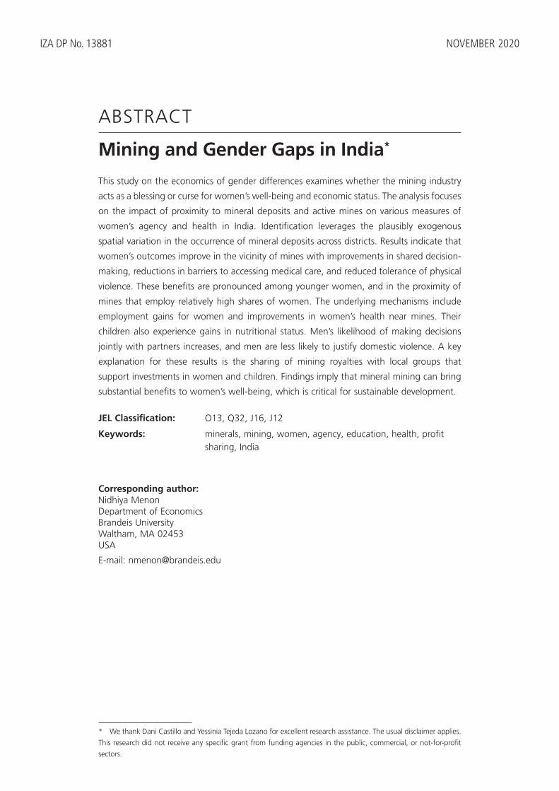
ABSTRACT

IZA DP No. 13881 NOVEMBER 2020

Mining and Gender Gaps in India*

This study on the economics of gender differences examines whether the mining industry

acts as a blessing or curse for women’s well-being and economic status. The analysis focuses

on the impact of proximity to mineral deposits and active mines on various measures of

women’s agency and health in India. Identification leverages the plausibly exogenous

spatial variation in the occurrence of mineral deposits across districts. Results indicate that

women’s outcomes improve in the vicinity of mines with improvements in shared decision-

making, reductions in barriers to accessing medical care, and reduced tolerance of physical

violence. These benefits are pronounced among younger women, and in the proximity of

mines that employ relatively high shares of women. The underlying mechanisms include

employment gains for women and improvements in women’s health near mines. Their

children also experience gains in nutritional status. Men’s likelihood of making decisions

jointly with partners increases, and men are less likely to justify domestic violence. A key

explanation for these results is the sharing of mining royalties with local groups that

support investments in women and children. Findings imply that mineral mining can bring

substantial benefits to women’s well-being, which is critical for sustainable development.

JEL Classification: O13, Q32, J16, J12

Keywords: minerals, mining, women, agency, education, health, profit sharing, India

Corresponding author:Nidhiya MenonDepartment of EconomicsBrandeis UniversityWaltham, MA 02453USA

E-mail: nmenon@brandeis.edu

* We thank Dani Castillo and Yessinia Tejeda Lozano for excellent research assistance. The usual disclaimer applies.

This research did not receive any specific grant from funding agencies in the public, commercial, or not-for-profit

sectors.

1

1. Introduction

Gender equality has become a focal point of scholarly discourse, government policies,

international aid, and advocacy efforts. Pathways to promoting gender equality often include

strengthening women’s agency and improving their human capital through investment in

schooling and the generation of meaningful employment. Some of these improvements for

women accompany structural change and the concomitant shift from agriculture to industry. Yet

economic development and structural change do not necessarily bring gains for women and

improvements in gender equality, especially if unpaid work burdens, biased laws, differential

access to resources, and social norms constrain women’s ability to take advantage of new, well-

paid employment opportunities (World Bank 2011). Adding to these complexities, relatively

little is known about how structural change associated with the mining industry impacts women

and gender equality.

The mining industry has long since been considered an enclave with few beneficial

effects for local economies (Berman et al. 2017). Mineral-rich countries have often seen

stagnation in other industries, particularly agriculture and manufacturing, arising from exchange

rate overvaluation and high wage rates associated with natural resource booms ̶ the so-called

“Dutch Disease” phenomenon. Combined with political economy effects in which investment in

mineral extraction is prioritized over other sectors including social services, these adverse effects

have contributed to the view of mining as a “resource curse” (Auty 1993; Bebbington et al.

2008). However, a recent set of studies for sub-Saharan Africa have challenged this view. For

example, Mamo et al. (2019) find large improvements in living standards as measured by night-

lights in districts with new large-scale mining operations, albeit with few spillover effects to

other districts. Similarly, Lippert (2014) uncovers positive effects from copper mining for

2

household expenditures and other measures of well-being, and Benshaul-Tolonen (2018a) shows

that open-pit gold mining causes a reduction in child mortality.1 In sub-Saharan Africa,

industrial mine operations contributed to a large employment shift for women away from

agricultural self-employment toward wage employment and service-sector jobs that arose around

the mining industry (Kotsadam and Benshaul-Tolonen 2016). However, this structural change

also resulted in greater domestic violence against women in areas where wife beating was more

commonly accepted (Kotsadam et al. 2017).

Our study adds new evidence to this literature in the context of mining in India. In

particular, we causally estimate the impact of proximity to mineral deposits and mines on

women’s agency as measured by improvements in shared decision-making, declining acceptance

of violence, and reductions in reported barriers to accessing medical care. We then analyze the

underlying mechanisms by focusing on how mines affect women’s education and health as well

as child health. We also explore the consequences of legislation that requires mining companies

to invest a fixed proportion of their profits back into local communities.

Our study uses India’s 2015-2016 Demographic and Health Survey, which includes point

coordinates for surveyed clusters, and we match that data with the geo-referenced location of

mineral deposits and mines. Data from many additional sources are used to construct the

sample. The analysis employs difference-in-differences methods to answer three questions.

First, conditioning on the presence of deposits, what are the impacts of being proximate to active

mines on measures of women’s agency? Second, given that mining in general employs

relatively few women, do the results differ if we focus on mines that engage relatively larger

numbers of women? Third, what are the mechanisms that explain these patterns?

1 In related work, Aragón and Rud (2013) find a positive backward linkage in terms of increased real income from a

large-scale gold mine to surrounding areas in Peru.

3

This research contributes to a better understanding of whether mining serves as a

resource curse or blessing, as well as the mechanisms through which the mining industry affects

women’s agency to further or hinder sustainable economic development. It also sheds light on

the relationship between women’s agency and the acceptance of domestic violence. Some

studies have shown that measures of women’s economic agency, such as increased ownership of

assets and greater education for women, are associated with a decline in domestic violence. The

primary transmission mechanism is that improved economic opportunities for women outside the

household strengthen their bargaining power within the home. Even if the budget of the

household remains constant, women’s asset ownership may strengthen their negotiating power

by improving their fallback position and reinforcing their ability to curtail domestic abuse (Panda

and Agarwal 2005, Aizer 2010, Bobonis et al. 2013). However, changes that empower women

economically could also contribute to a backlash effect among husbands. For example, in

Bangladesh, increased female labor force participation is associated with higher rates of violence

for some women as husbands try to counteract the increased autonomy of their wives (Heath

2014). Cools and Kotsadam (2017) also find evidence of backlash across Sub-Saharan Africa as

increased education and employment for women are associated with a higher probability of

experiencing intimate partner violence. Given this mixed evidence, our study furthers research

by shedding light on the determinants of women’s agency in the context of mining in India.

2. Background

India is rich in mineral and metal deposits. The country produces almost 84 minerals

from approximately 3700 mines for an aggregate production of over 1 billion tons (India Bureau

of Mines 2015). The main minerals include iron ore, manganese ore, bauxite, copper ore, lead

and zinc ore, dolomite, limestone, and coal. The country also has stores of copper, gold, silver,

4

diamond, nickel, and cobalt. Mining in India is associated not only with revenue gains but also

environmental losses, especially deforestation (Ranjan 2019). Average daily employment in

mines is around 512,000 workers in the organized sector.2 An unorganized sector exists, but it is

difficult to get a consistent set of employment numbers here. Closely related is small-scale and

artisanal mining, some of which is organized but much is not. Estimates in Ghose (2003) indicate

that India has approximately 3000 small-scale mines accounting for about half of the country’s

non-fuel mineral production, with a total employment of about 300,000 workers.

Female employment shares in mining are on average low. Data from the annual

Government of India Ministry of Labor and Employment publications of the Statistics of Mines

in India Volume – 1 (Coal) and Volume – II (Non-Coal) indicate that from 2010 to 2015, only

7.0 percent of all workers were women across all minerals/metals. However, female

employment shares vary drastically by type of minerals. For example, the female employment

share in quartz mining is 18.3 percent, in apatite rock phosphate mining 14.7 percent, and in

dolomite mining 12.9 percent. Other minerals/metals that employ relatively high shares of

women’s labor include sillimanite, barytes, garnet, fire clay, fluorite, manganese, graphite,

wollastonite, feldspar, and magnesite. Many minerals that have relatively high female

employment shares are classified as precious minerals and metals. In fact, five of the eight

precious minerals/metals employed more than the median share of female employment in 2010-

2 Fuel accounted for 74 percent of total employment during 2013-14, with coal and lignite accounting for 93 percent

of the labor force engaged during the same period. Metallic minerals accounted for 15 percent of total employment

with iron ore, manganese ore, lead and zinc concentrates, bauxite and chromite employing 49 percent, 18 percent, 9

percent, and 8 percent each of total labor, respectively. Non-metallic minerals accounted for 11 percent of total

employment with limestone, dolomite and garnet, steatite, kaolin and quartz employing the highest shares (Indian

Mineral Industry at a Glance, 2013-2014, India Bureau of Mines).

5

2015 (the exceptions being diamond, gold, and kyanite).3 In contrast, coal mining employs only

2.4 percent of women and iron mining employs 3.7 percent of women.

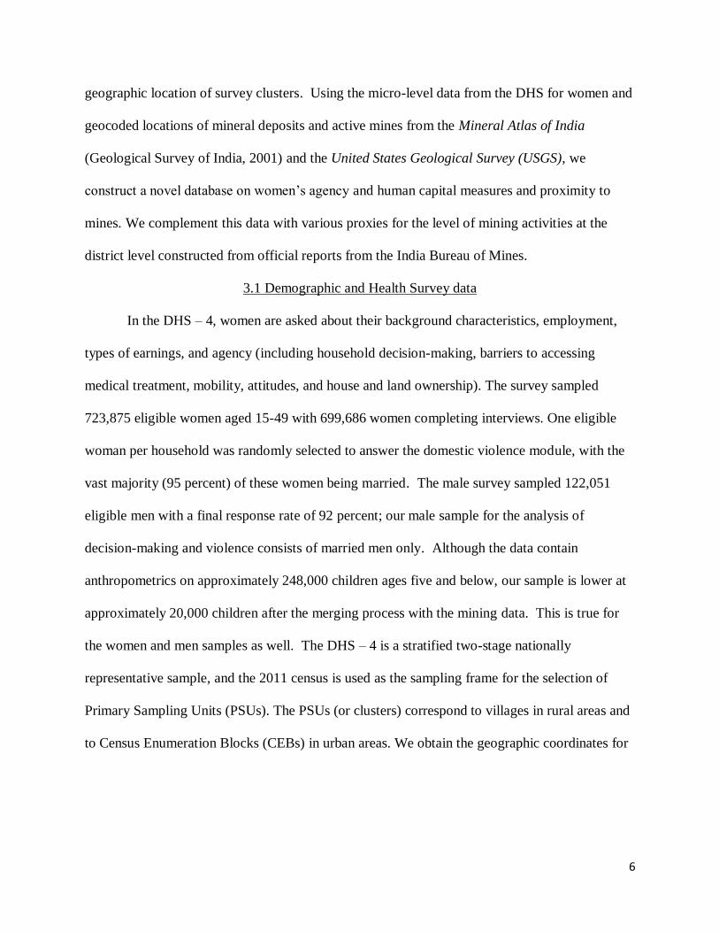
This study examines separately minerals/metals that employ relatively high shares of

female labor, and we denote these as “HFLS” (high female labor shares). The rationale for

highlighting variations in employment shares by gender is to test for Boserup’s (1970)

hypothesis that women’s status is better when their labor is valued. That is, we take the plough-

use versus shifting-cultivation intuition that Boserup developed and apply it to the mining

industry. This application presumes that if men are required for mining minerals that require

greater physical strength as operations are deeper underground, then women’s status is relatively

weaker in the surroundings of such a mine (as in coal mining). In contrast, mining minerals

found closer to the surface does not require brawn-based labor that is as intensive (as in quartz

mining), so then women’s relative overall standing may be higher. To test this hypothesis, we

construct separate measures for the type of active mine (all active mines versus HFLS active

mines) to evaluate whether women’s outcomes are relatively better in and around HFLS active

mines using details on the identity of the mineral/metal mined.4

3. Data

This study uses the 2015-2016 wave of the India’s Demographic and Health Survey

(DHS – 4), a large nationally representative household survey with detailed information on

individual and household characteristics for women aged 15-49, children aged 0-5 years, and

men aged 15-54 years. This wave also includes geocoded spatial data documenting the

3 The list of precious minerals/metals include apatite rock phosphate, diamond, dolomite, fluorite, gold, graphite,

kyanite and sillimanite. 4 We classify 22 minerals/metals as “HFLS” where female employment shares exceed the median value of 3.9

percent. In addition to those in the previous note, they include magnesite, feldspar, silica, vermiculite, wollastonite,

manganese, quartz, calcite, laterite, china clay and white clay, chromite, fire clay, garnet, bauxite, steatite, barytes

and stone.

6

geographic location of survey clusters. Using the micro-level data from the DHS for women and

geocoded locations of mineral deposits and active mines from the Mineral Atlas of India

(Geological Survey of India, 2001) and the United States Geological Survey (USGS), we

construct a novel database on women’s agency and human capital measures and proximity to

mines. We complement this data with various proxies for the level of mining activities at the

district level constructed from official reports from the India Bureau of Mines.

3.1 Demographic and Health Survey data

In the DHS – 4, women are asked about their background characteristics, employment,

types of earnings, and agency (including household decision-making, barriers to accessing

medical treatment, mobility, attitudes, and house and land ownership). The survey sampled

723,875 eligible women aged 15-49 with 699,686 women completing interviews. One eligible

woman per household was randomly selected to answer the domestic violence module, with the

vast majority (95 percent) of these women being married. The male survey sampled 122,051

eligible men with a final response rate of 92 percent; our male sample for the analysis of

decision-making and violence consists of married men only. Although the data contain

anthropometrics on approximately 248,000 children ages five and below, our sample is lower at

approximately 20,000 children after the merging process with the mining data. This is true for

the women and men samples as well. The DHS – 4 is a stratified two-stage nationally

representative sample, and the 2011 census is used as the sampling frame for the selection of

Primary Sampling Units (PSUs). The PSUs (or clusters) correspond to villages in rural areas and

to Census Enumeration Blocks (CEBs) in urban areas. We obtain the geographic coordinates for

7

the surveyed DHS clusters and use them to match respondents to the nearest mineral deposit and

active mine.5,6

3.2 Deposit and Mining Data

We use the Mineral Atlas of India (Geological Survey of India, 2001) to obtain the type,

location, and size of mineral deposits. The Atlas contains 76 map sheets showing the geographic

distribution of mineral deposits across the country. Minerals are classified into four categories:

(i) base metals, light, and precious metals; (ii) chemical, fertilizer, and ceramic; (iii) iron, ferrous,

alloy metals; and (iv) other industrial and precious minerals. The map sheets also provide

information on other geological features including lithology rock type, the age of the host rocks,

the size – which is proportional to the number of metric tons of deposit reserves at each site, and

the main mineral present. We geocode all the map sheets to obtain the deposits’ geographic

coordinates needed to construct our proximity measures. Given information on the presence of

mineral types at each site, we are able to create variables to measure proximity to different types

of minerals (mainly HFLS versus non-HFLS).

Figure 1 shows India with geocoded deposits of various types overlaid on district

boundaries. A higher concentration of deposits exists in the Eastern, Northwestern, and Central

states. In all, our geo-referencing exercise allows us to locate 2,553 deposits across the country.

Our data on the location of mines is obtained from the United States Geological Survey (USGS)

dataset on past, current, and future industrial mines.7 We compile the USGS data using the

5 Since DHS surveys contain sensitive information, the precise location is not provided. Rather, urban clusters and

rural clusters are displaced up to 2 and 5 kilometers, respectively (the displacement method does not move households across any regional boundaries though). This should not affect results as the measurement error is

orthogonal to our variables of interest (Burgert et al. 2013). 6 Out of the 28,522 clusters, we cannot obtain the coordinates of 131 clusters as the source of data used is neither

from the Global Positioning System (GPS) nor from a gazetteer of village/place names. These clusters have (0,0)

coordinates and are excluded from our analysis. 7 The USGS data for India does not provide information on start dates of mines.

8

National Minerals Information Center for Asia and Pacific (2010) which provides the maps of

mineral facilities in India, and by using the Mineral Resources Data System (2007) which

provides a collection of reports for metallic and nonmetallic mineral resources throughout the

world.8 For reference, Appendix Figure 1 shows an example of a map sheet from the Mineral

Atlas, and Appendix Figure 2 shows the distribution of active and inactive mines.

3.3 Other Data

Since new mines often open far from developed areas (Mamo et al. 2019) and since they

are unlikely to take gender norms and women’s outcomes into consideration in making

decisions, we are less concerned about reverse causality in the context of this study. Still, to help

address this potential issue, the empirical model we employ controls for levels of local

development (including the degree of urbanization, population density, and infrastructure) by

incorporating the log of the Global Human Footprint (GHF) provided for each cluster, which

ranges from 0 (extremely rural) to 100 (extremely urban). This index is the normalized version of

the Human Influence Index (HII) - a global dataset available at a spatial resolution of 1 by 1 km

grid cells and created from 9 data layers covering human access (roads, railroads, navigable

rivers, coastlines), human population pressure (population density), human land use, and

infrastructure (nighttime lights, land use/land cover, and built-up areas).9 Indicator variables

from the DHS are also included for whether the main source of drinking water in the household

is piped water, and whether the household has access to electricity.

8 Most records for India are simple reports of the type of minerals in some locations, with a few reporting the deposit

names, location, commodities, geologic characteristics, resources, reserves, and production (these few reports are assigned an A grade by USGS to reflect their diversity of information provided in the database). 9 The data is provided as part of the DHS GIS Data 2015. The GHFI index is the HII normalized by biome and

realm developed by the Last of the Wild Project (LWP-2). The average of an index is for the location within a 2 km

(urban) or 10 km (rural) buffer surrounding the DHS survey cluster. Data for 1995-2004 is used. See Wildlife

Conservation Society, and Center for International Earth Science Information Network-Columbia University-2005:

“Global Human Footprint Dataset.”

9

Our study includes information from various government reports. First, we use the annual

publications Statistics of Mines in India from the Directorate-General of Mines Safety (Ministry

of Labor and Employment) from 2010 to 2015 to compile district-level data on employment.10

To classify Indian districts into high, medium, or low mineral potential districts, we use the

Bulletin of Mining Leases and Prospecting Licenses, an annual publication of the India Bureau

of Mines. These reports are available from 2000 to 2015 and provide district-level mining areas

as well as the state-wise, district-wise, and mineral-wise distribution of mining leases granted,

executed, renewed, and revoked. Appendix Figure 3 shows the share of leased area in 2014

across India with the high/medium mineral potential districts. As of 2014, the Mining Lease

Directory reports that there were 10,982 mining leases granted for 64 different minerals. The five

highest shares of leased areas are for the states of Rajasthan (18.5 percent), Orissa (16.2 percent),

Andhra Pradesh (13.5 percent), Karnataka (10.5 percent), and Madhya Pradesh (7.23 percent).

The district shares vary between 0 and 6.4 percent. Finally, we obtain the district-level

production data from the Indian Minerals Yearbooks (Part III – Mineral Reviews) from 2011 by

digitizing the entire database of 70 minerals and aggregating across minerals. Domestic and

foreign market prices are from the same yearbooks (Part I – General Reviews).

3.4 Summary Statistics

Table 1 reports the summary statistics for women. We construct an index that

encapsulates information provided across several questions in each outcome of interest. Panel A

shows the summary statistics for the binary outcomes that equal 1 if the woman respondent

10 Statistics of Mines, Volume I for coalmines covers all coalmines that come under the purview of the 1952 Mines

Act. These publications contain state and district-level information on number of mines, production, mechanization,

and the number of accidents in mines. Volume II for non-coal mines provide statistics for metalliferous and oil

mines. Data on employment is available on a gender-disaggregated basis. But data on output and average weekly

wages are only reported on an aggregate basis.

10

agrees to the statement that beating is justified for a set of reasons listed. On average, 37 percent

of women consider beating to be justified if the wife neglects children, while 30 percent report

that they agree that domestic violence is justified if she goes out without telling her partner or

husband. An average of 14 percent report that they have experienced at least one form of

emotional violence recently. In Panel B, we consider the barriers women face when seeking

healthcare for themselves. Approximately 18 percent, 26 percent, and 19 percent report that

seeking permission, obtaining money, and the fear of going alone to the health provider,

respectively, are serious hurdles. Summary statistics for variables related to decision-making are

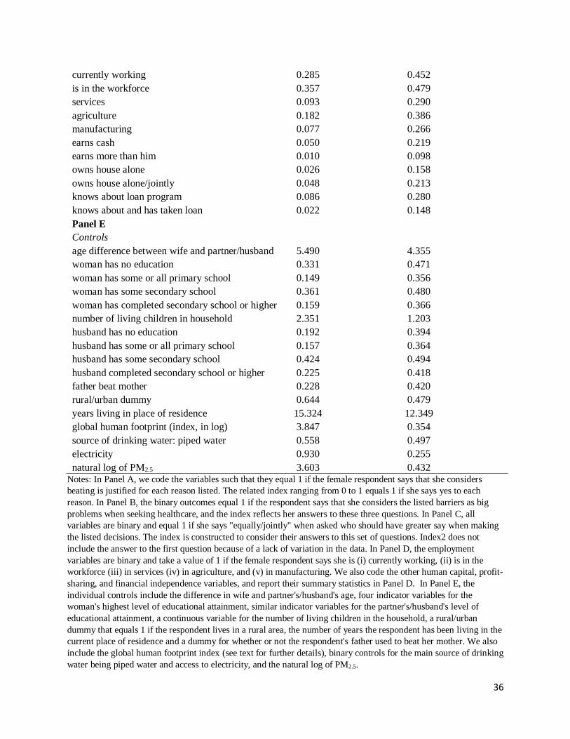
noted in Panel C, and those for the human capital, profit-sharing, and financial independence

variables are in Panel D. In particular, 29 percent of women report that they are currently

working, with the majority of those women working in agriculture (18 percent). Panel E reports

the statistics for the individual/household controls.

In Appendix Table 1, we report and discuss the summary statistics for married male

respondents in the DHS – 4. We use these data to evaluate whether men’s attitudes towards

domestic violence and shared decision-making change in ways consistent with the women’s

results in mining areas.

To quantify treatment, we calculate the distances to the nearest deposit and to the nearest

mine for each cluster’s centroid. These measures vary largely across DHS – 4 clusters, with

means of 29.6 km and 45.25 km, respectively. We then define an indicator variable labeled as

‘deposit’ that equals 1 if there is a mineral deposit within 5 km of the respondent’s cluster.

Another indicator variable labeled as ‘active mine’ equals 1 if there is an active mine within 5

km. Our main treatment variable of interest is the interaction of these two variables. We

construct similar variables for exposure to HFLS and non-HFLS mines. Appendix Table 2

11

reports summary statistics for the proximity variables and for the intensity variables (where

intensity is measured using count variables of mining activities in each cluster).

4. Methodology

In the baseline specification relating measures of women’s agency and human capital to

proximity to active mines, we follow Kotsadam and Benshaul-Tolonen (2016) and Benshaul-

Tolonen (2019) to consider a difference-in-differences (DD) framework that conditions on

treatment and control groups based on distance measures. Equation (1) is as follows:

𝑌𝑖𝑐𝑑 = 𝛽0 + 𝛽1𝑑𝑒𝑝𝑜𝑠𝑖𝑡𝑐 + 𝛽2𝑎𝑐𝑡𝑖𝑣𝑒𝑚𝑖𝑛𝑒𝑐 + 𝛽3(𝑑𝑒𝑝𝑜𝑠𝑖𝑡𝑐 × 𝑎𝑐𝑡𝑖𝑣𝑒𝑚𝑖𝑛𝑒𝑐) + 𝛽4𝑦𝑜𝑢𝑛𝑔𝑖

+ 𝛽5(𝑑𝑒𝑝𝑜𝑠𝑖𝑡𝑐 × 𝑎𝑐𝑡𝑖𝑣𝑒𝑚𝑖𝑛𝑒𝑐 × 𝑦𝑜𝑢𝑛𝑔𝑖) + 𝑋𝑖 + 𝜆𝑑 + 𝜆𝑠 + 𝜖𝑖𝑐𝑑 (1)

where 𝑌𝑖𝑐𝑑 is the outcome for individual “i”, in cluster “c”, in district “d”. The presence of

mineral deposits is an exogenous measure and in equation (1), the indicator variable 𝑑𝑒𝑝𝑜𝑠𝑖𝑡𝑐

equals 1 if there is a deposit within 5 km of a respondent’s cluster. We begin with a cut-off

distance of 5 km (following Von der Goltz and Barnwal 2019), and then consider other radii of

10, 15, 20, 25, and 30 km around mines to track the mining footprint, to obtain an evaluation of

possible spillover effects and to test whether theories of enclave development are validated.11

Appendix Box 1 presents evidence that the proportion of workers who travel 5 km or less to

access their place of work is approximately 70 percent in India. Hence, our focus on the 5km

distance around clusters for a baseline is appropriate.

We define the indicator variable 𝑎𝑐𝑡𝑖𝑣𝑒𝑚𝑖𝑛𝑒𝑐 to equal 1 if there is at least one active

mine within 5 km of the respondent’s cluster. The treatment variable of interest is the interaction

term 𝑑𝑒𝑝𝑜𝑠𝑖𝑡𝑐 × 𝑎𝑐𝑡𝑖𝑣𝑒𝑚𝑖𝑛𝑒𝑐 and the coefficient of interest is 𝛽3. This interaction equals 1

when the respondent is geographically close to an active mineral mine conditional on the

11 Studies in the related literature (e.g. Aragón and Rud 2013, Kotsadam and Benshaul-Tolonen 2016) suggest that

areas within 5-20 km from an active mine are directly exposed.

12

presence of a deposit. The variable 𝑦𝑜𝑢𝑛𝑔𝑖 equals 1 if the respondent is 15-25 years old. We

include the triple interaction term (𝑑𝑒𝑝𝑜𝑠𝑖𝑡𝑐 × 𝑎𝑐𝑡𝑖𝑣𝑒𝑚𝑖𝑛𝑒𝑐 × 𝑦𝑜𝑢𝑛𝑔𝑖) to estimate additional

impacts of proximity for women in this age group. All results tables include F-test statistics that

these differential impacts for young women are significantly different from zero.

The vector of individual controls 𝑋𝑖 include the following individual, household, and

contextual variables: differences in wife and partner’s/husband’s age, indicators for the woman’s

highest level of educational attainment, indicators for the partner’s/husband’s level of

educational attainment, a measure of the number of living children in the household, a

rural/urban dummy, the number of years the respondent has been living in the current place of

residence (to address migration), and the three indicators of local development. When the

outcome variable is related to domestic violence, we additionally control for whether the

respondent’s father used to beat her mother. The parameters 𝜆𝑑 𝑎𝑛𝑑 𝜆𝑠 are district and state

fixed-effects, and 𝜖𝑖𝑐𝑑 is the idiosyncratic error term. We restrict the sample to individuals living

within 100 km from a mineral deposit in keeping with related studies such as Benshaul-Tolonen

(2019). Regressions are weighted and robust standard errors are clustered at the DHS cluster

level. We consider specification (1) for the full sample of deposits and active mines, and

separately for deposits and HFLS active mines.

The use of district and state fixed-effects allows us to control for the time-invariant

characteristics that could explain differences between treated and control groups, including

institutional factors, sectoral composition, cultural norms pertaining to women’s role in the

economy and at home, and district-level extractive industry strategies. These characteristics also

include factors that large mining companies may internalize in their cost-benefit analyses of

location choice. Unobserved differences at the district level such as the ease of doing business,

13

transparency, governance practices, levels of corruption, and other factors not related to resource

endowments are also absorbed by these controls as long as they do not vary over time.

Equation (1) conditions on the presence of deposits which may be thought of as a

measure of proximity. However, the actual number of proximal deposits, which may be thought

of as a measure of intensity, can also matter. Hence, we estimate the effects of the number of

mineral deposits that are within 5 km of each cluster using the same structure as in equation (1)

except that the dummy variable for proximity is replaced with a count variable of the number of

deposits within 5 km. Regression results report parameters for both proximity and intensity.

5. Results for the Impact of Mines

5.1. Women’s Acceptance of Domestic Violence

Table 2 reports the 𝛽3 and 𝛽5 terms from equation (1) for women’s acceptance of

different agency measures. The column headings indicate the specific outcome variables

estimated. Panel A reports results for coefficients that condition on the presence of a HFLS

mineral/metal mine whereas Panel B reports results for all mines. The binary dependent variables

take a value of 1 if the female respondent says that she considers that beating is justified for

reasons reported in each column. In column (6), the index ranging from 0 to 1 is constructed by

considering the answers to the five questions related to attitude towards domestic violence. It

equals 1 if the respondent says that beating is justified in each case. The mean value of the index

is 0.3. In column (7), “emotional violence" is a variable that equals 1 if the respondent says that

she has experienced one of three possible examples of emotional violence listed in the survey

(partner humiliates you, threatens to harm you or someone close to you, and insults you).

Focusing on Panel A, the 𝛽3 coefficients reported are negative in all but one instance

(measured with precision in columns (1) and (3) only though). The estimates in column (1)

14

indicate that in comparison to other women, those in the proximity of deposits and active HFLS

mines are 16.4 percentage points less likely to accept that violence is justified for going out

without permission. Similarly, those near HFLS mines are 38.1 percentage points less likely to

accept that violence is justified for arguing with one’s husband or partner. When we consider the

differential impacts on the young, the only significant coefficient is in column (7) for emotional

violence, whereas net effects for the young are mostly statistically zero except for the case of

having a voice in arguments with the partner. In this case, the estimate indicates that young

women are 37.4 percentage points less likely to accept that violence is justified.

Next, Panel A of Table 2 reports the impacts of the number of deposits. The 𝛽3

coefficients are uniformly negative across all columns although only those in columns (1), (3)

and (6) are measured without error. Focusing on the index measure, the coefficient in column

(6) shows that comparing to other women, women in the vicinity of HFLS mines (conditional

also on the number of deposits) are 16.4 percentage points less likely to accept that any of these

measures are justified. Focusing on net effects, young women are 17.4 percentage points less

likely to accept that abuse is justified if the wife goes out without permission, 35.6 percentage

points less likely to accept that beating is justified if the women argues with the husband and

15.5 percentage points less likely to agree that physical abuse is justified in terms of the

aggregate index indicator.

Panel B reports the mirror results when we condition on all active mines rather than

HFLS mines alone. The results in this panel resonate with many noted in Panel A. In particular,

the coefficient on the index measure indicates that women near deposits and active mines are 8.6

percentage points less likely to agree that physical violence is justified in any of these cases.

Young women see significant net impacts when it comes to emotional violence, not cooking

15

food properly, and refusing sex. Concomitant results that condition on the number of deposits

are similar in sign but mostly insignificant. For the young, the parameters are significant for the

same outcomes as the estimations that condition on proximity to a deposit. Overall, the results in

Table 2 underline that women near active mines and deposits (especially HFLS mines) are less

likely to accept that violence is justified, thus signaling an improvement in their agency.

5.2. Women’s Barriers to Healthcare

Table 3 reports results for the 𝛽3 and 𝛽5 interaction terms when we study variables

related to barriers that women may face while seeking medical care, including whether they need

permission to go, whether they can obtain money for the treatment, and uncertainty/fear involved

in traveling alone. The indicator variables in these columns take the value 1 if the woman

reports that any of these was a “big problem”. Column (4) reports results for the composite

index. It ranges from 0 to 1 if the woman responds that each of these three dimensions was a

“big problem” and has a mean value of 0.2.

Proximity to deposits and active HFLS mines has a negative impact on all the variables:

the need for permission, money, and fear of going alone decline by 7.0 to 24.8 percentage points

(fear is insignificant) for women in close proximity to active mines (Panel A). The net effects

for young women are significantly different from zero. Estimates indicate that fear declines by

41.4 percentage points, while the need to ask for permission decreases by 24.6 percentage points.

However, proximity to HFLS mines increases the need for money among young women by 68.1

percentage points. It is possible that seeking higher quality healthcare might explain this positive

coefficient. The overall index measure, while significant for all women in the proximity of

HFLS mines (and indicating an overall 16.6 percentage point decrease in such barriers), is not

significantly different from zero for young women.

16

The second half of Panel A reports coefficients that condition on the number of deposits.

Again, most coefficients of interest are negative, indicating a beneficial impact on these

measures in the proximity of HFLS mines. The coefficient on the index shows that in

comparison to other women, those in the proximity of HFLS mines conditional on the number of

deposits experience a 15.8 percentage point decline in these barriers. Again, net impacts among

the young are negative with regards to permission and fear, but positive when it comes to money.

Panel B in Table 3 reports results when we condition on all mines. In general, results are

weaker as compared to those in Panel A. In fact, the only estimate that is significant is in the

case of fear of accessing care alone. Women in the close vicinity of mines and deposits report a

7.4 percentage point decline in this measure. Overall, we conclude from Table 3 that proximity

to HFLS mines in particular brings measurable benefits to women in reducing barriers to seeking

healthcare.

5.3. Women’s Attitude to Shared Decision-making

Table 4 has the same structure as the previous two results tables. Women are asked their

opinion when it comes to decisions on five topics. Given we are interested in joint decision-

making processes within the household, the binary dependent variables take a value of 1 if the

respondent says that she thinks such decisions should be taken jointly with her partner or her

husband. In column 6, index 1, ranging from 0 to 1, takes a value of 1 if the respondent answers

"shared equally" when asked who should have greater say for all five decisions. The mean of this

index is 0.8. In column 7, index 2, ranging from 0 to 1, takes a value of 1 if the respondent

answers "shared equally" to the last four of the five decisions (excluding decisions on her own

earnings). The mean of this index is 0.8. We consider these indexes separately to understand the

influence of decision-making when it comes to own earnings.

17

Regarding decision-making about earnings, the HFLS mines sample size is too small to

identify impacts (this is also the case for results for the index 1 variable). The estimate in

column (4) indicates that although shared decision making when it comes to visits to family

actually declines in the proximity of HFLS mines for all women, differential impacts on young

women are all significant and positive (the net impact on the young is not significantly different

from zero in any case though). Conditioning on the number of deposits results in similar

patterns; positive differential patterns for young women in the proximity of HFLS mines but net

impacts that are significantly different from zero only in the case of shared decision making

about husband’s earnings. In this case, young women in the proximity of HFLS mines report an

8.2 percentage point increase.

Panel B reports results that condition on all mines. For the most part, these coefficients

are imprecisely estimated. Parameters in column (3) indicate that young women in proximity of

all mines (and deposits) report greater shared decision making when it comes to large purchases,

husband’s earnings, and the composite index 2 variable. In comparison to their senior

counterparts, young women in the proximity of mines report an 11.7 percentage point increase in

shared-decision making when it comes to index 2, which, given the mean value of this indicator,

is about a 15 percent increase. Conditioning on the number of deposits shows few differential

impacts for young women in the vicinity of mines but overall net significance when it comes to

shared decision-making over large purchases. We conclude that compared to the other measures

of agency discussed above, the effects of mining on shared decision-making are noisier.

6. Mechanisms

Motivated by the literature on mineral wealth and human capital formation (Gylfason

2001, Ahlerup et al. 2019, Mejía 2020), we hypothesize that proximity to active mines might

18

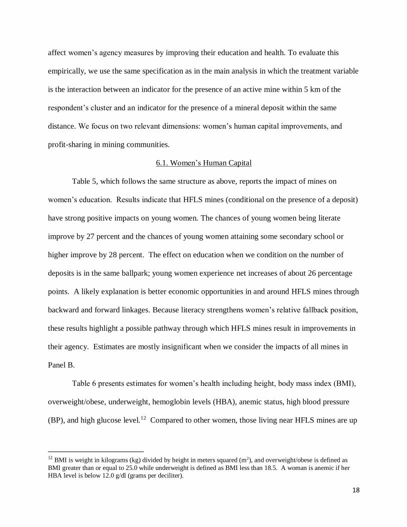
affect women’s agency measures by improving their education and health. To evaluate this

empirically, we use the same specification as in the main analysis in which the treatment variable

is the interaction between an indicator for the presence of an active mine within 5 km of the

respondent’s cluster and an indicator for the presence of a mineral deposit within the same

distance. We focus on two relevant dimensions: women’s human capital improvements, and

profit-sharing in mining communities.

6.1. Women’s Human Capital

Table 5, which follows the same structure as above, reports the impact of mines on

women’s education. Results indicate that HFLS mines (conditional on the presence of a deposit)

have strong positive impacts on young women. The chances of young women being literate

improve by 27 percent and the chances of young women attaining some secondary school or

higher improve by 28 percent. The effect on education when we condition on the number of

deposits is in the same ballpark; young women experience net increases of about 26 percentage

points. A likely explanation is better economic opportunities in and around HFLS mines through

backward and forward linkages. Because literacy strengthens women’s relative fallback position,

these results highlight a possible pathway through which HFLS mines result in improvements in

their agency. Estimates are mostly insignificant when we consider the impacts of all mines in

Panel B.

Table 6 presents estimates for women’s health including height, body mass index (BMI),

overweight/obese, underweight, hemoglobin levels (HBA), anemic status, high blood pressure

(BP), and high glucose level.12 Compared to other women, those living near HFLS mines are up

12 BMI is weight in kilograms (kg) divided by height in meters squared (m2), and overweight/obese is defined as

BMI greater than or equal to 25.0 while underweight is defined as BMI less than 18.5. A woman is anemic if her

HBA level is below 12.0 g/dl (grams per deciliter).

19

to 28.2 percentage points less likely to be underweight. However, these women are also more

likely to be anemic. Focusing on net impacts on young women, they are significantly more

likely to be taller, to have higher BMI, less likely to be underweight, and less likely to have a

high glucose level. These results point towards significant improvements in health status for

young women living in proximity to HFLS mines, even though anemic status does appear to

increase for young women which is consistent with evidence in Von der Goltz and Barnwal

(2019). Many of these results hold when the estimates condition on the number of deposits, both

for women in general and for young women in particular. On the other hand, results in Panel B

which condition on all mines are mostly insignificant. There are some positive impacts on

women in general in the close vicinity of mines when it comes to BMI, overweight/obese and

underweight, but most net effects on the young are statistically zero.

The final set of results we consider for women’s human capital involve their access to

health insurance (Appendix Table 3). Estimates depict a similar story that positive impacts may

be discerned mostly near HFLS mines, and mostly for young women. Young women see an 11.5

percent increase in having some form of health insurance in the case of mining proximity, and by

12.8 percent in the case of mining intensity. The probability of having health insurance from

one’s employer rises for this age group as well. However, the size of the impacts are smaller

(1.0 percentage point and 0.9 percentage points, respectively). There are few significant

coefficients when we condition on all mines.

Overall, we have presented robust evidence indicating that human capital improves for

women living near HFLS mines, and the benefits are especially pronounced among young

women. The gains in human capital spans multiple categories from education to personal health

to insurance coverage, all of which can contribute to stronger agency for women.

20

6.2. Children’s Health

In order to provide direct evidence that improvements in women’s human capital occur

near mines and is thus a mechanism for the positive impacts we document on their agency, we

consider an outcome where mother’s human capital and access to health insurance are crucial

determinants: child health. Analyzing this outcome is thus a robustness check that women’s

education and health are indeed rising in the vicinity of mines. We consider standardized health

measures for children between 0-59 months, including the height for age z-score (HAZ), the

weight for age z-score (WAZ), and the weight for height z-score (WHZ).13 Results are presented

in Appendix Table 4. Estimates in Panel A indicate measurable impacts for children in the

vicinity of HFLS mines in terms of WAZ and WHZ. In particular, WAZ and WHZ improve by

0.9 standard deviations and 0.9 standard deviations respectively, for children of young women

near HFLS mines, which are large effects. Net effects on the children of young women have

similar magnitudes in the case of mining intensity. In Panel B, there is some evidence that HAZ

rises for children of women near all mines in the presence of deposits (0.5 standard deviations,

which amounts to a medium-size effect).

6.3. Profit-Sharing in Mining Communities

Royalty receipts (an important source of revenue for states and local governments), when

distributed properly among the affected population, can potentially explain the beneficial impacts

for women near mines. Our hypothesis is that proximity to active HFLS mines affects women’s

employment and human capital outcomes (and thus agency) primarily because resource rents are

distributed in an equitable way. These rents translate into better living conditions for women who

13 We interpret these results cautiously given the reduced sample sizes (especially for HFLS mines).

21

are affected by mining activities.14 Appendix Box 2 provides further details on our profit-

sharing measure including its construction, the empirical specification that we employ in order to

understand its effects, and the robustness of these results.

The outcomes we consider are related to women’s employment and to variables

potentially measuring the effects of profit sharing on earnings and awareness (and use) of

financial opportunities. Table 7 reports coefficients on the interaction term from equation (3)

where the outcome is a binary variable equal to 1 if the respondent says she was currently

employed at the time of the survey (column 1), if she is involved on a full-time basis in the

workforce (column 2), and if she is employed in agriculture, manufacturing, or services (columns

3-5). Results indicate that conditional on the presence of HFLS mines, increases in profit

sharing per female population result in significant improvements for women’s employment

outcomes. Specifically, profit sharing near HFLS mines increases the probability that the

woman is currently working, is in the workforce, works in the agricultural sector, and works in

the manufacturing sector. On average, profit sharing with local communities and women in

particular improves their employment prospects, which is potentially key to increasing their

agency within the household.

We use four outcomes to measure women’s financial independence in Table 8: in

columns (1) and (2), the binary variable equals to 1 if the respondent reports “cash” as the main

type of earnings and if she reports “earning more than husband/partner” when asked to compare

her earnings with that of her husband/partner. In columns (3) and (4), the dependent variables

14 The District Mineral Foundation (DMF) was officially instituted in March 2015 under the Mines and Minerals

(Development and Regulation) Act (1957). It was implemented to “overturn the decades of injustice meted out to

the thousands people living in deep poverty and deprivation in India’s mining districts…as a non-profit trust, DMFs

in every mining district have the precise objective to work for the interest and benefit of persons and areas affected

by mining affected operations…at least 60 percent of the budget should go to areas such as welfare of women and

children,” (DMF Status Report, 2017).

22

equal 1 if the respondent says that she "owns a house alone" or if she says that she "owns a house

alone and/or jointly", respectively. In columns (5) and (6), the outcomes relate to awareness and

use of financial opportunities with variables coded as 1 if the respondent says that she is aware of

loan programs available for personal or entrepreneurship uses, and if she borrows funds from

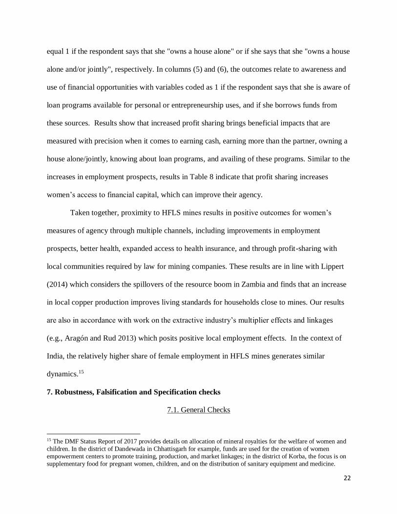
these sources. Results show that increased profit sharing brings beneficial impacts that are

measured with precision when it comes to earning cash, earning more than the partner, owning a

house alone/jointly, knowing about loan programs, and availing of these programs. Similar to the

increases in employment prospects, results in Table 8 indicate that profit sharing increases

women’s access to financial capital, which can improve their agency.

Taken together, proximity to HFLS mines results in positive outcomes for women’s

measures of agency through multiple channels, including improvements in employment

prospects, better health, expanded access to health insurance, and through profit-sharing with

local communities required by law for mining companies. These results are in line with Lippert

(2014) which considers the spillovers of the resource boom in Zambia and finds that an increase

in local copper production improves living standards for households close to mines. Our results

are also in accordance with work on the extractive industry’s multiplier effects and linkages

(e.g., Aragón and Rud 2013) which posits positive local employment effects. In the context of

India, the relatively higher share of female employment in HFLS mines generates similar

dynamics.15

7. Robustness, Falsification and Specification checks

7.1. General Checks

15 The DMF Status Report of 2017 provides details on allocation of mineral royalties for the welfare of women and

children. In the district of Dandewada in Chhattisgarh for example, funds are used for the creation of women

empowerment centers to promote training, production, and market linkages; in the district of Korba, the focus is on

supplementary food for pregnant women, children, and on the distribution of sanitary equipment and medicine.

23

We conduct several robustness checks of the main results. First, we check to ensure that

sorting into mining areas does not change population composition. We do this by restricting the

sample to respondents who report that they have lived in the same village/district for at least ten

or more years. We also ensure that the results hold when the districts’ level of political spending

is controlled for so that the fiscal revenue windfall from mining activities is not a confounding

factor. Sorting or controlling for political spending does not affect our main estimates.

Next, we consider responses provided by men that should mirror those evident in the

women’s samples. Estimates in Appendix Table 5 show some improvement in agricultural work

for men near HFLS mines (conditional on either the presence of a deposit or the number of

deposits). When it comes to all mines, the only estimate that is measured with precision is the

coefficient on whether the man is in the workforce; this estimate indicates that as compared to

other men, those in the close vicinity of active mines conditional on the presence of a deposit are

2.9 percentage points more likely to be in the workforce.

Changes in men’s attitudes towards domestic violence in the proximity of HFLS and all

mines are reported in Appendix Table 6. These results confirm that proximity to mines and

deposits (especially HFLS mines) reduces the tolerance of domestic violence. Five of the six

estimates for all men in the vicinity of HFLS mines are negative and three of these are measured

with precision. Focusing on the index measure and conditioning on the number of deposits,

there is a 15.4 percentage point decline in the acceptance of violence by men near HFLS mines.

This also highlights that women’s agency shows consistent relative improvements mostly in

cases where their labor is valued (in the case of HFLS metal/mineral mining). When we evaluate

changes in attitudes in the presence of all mines, there is some evidence of opposite impacts

especially among the young. This is consistent with evidence in Cools and Kotsadam (2017),

24

Kotsadam et al. (2017), and Eze Eze (2019) that improvements in women’s relative status can

result in greater acceptance of violence.

Appendix Table 7 reports results for men’s attitudes towards making household decisions

in a joint fashion. Most of the estimates that are significant in the vicinity of HFLS mines are

positive in sign, indicating that men are more likely to report shared decision-making.

Considering the composite index measure, overall, men report a 24.4 percentage point increase

in the willingness to share decision making jointly in the proximity of HFLS mines. The index

coefficient is of similar magnitude when we condition on the number of deposits instead (24.9

percentage points higher). In the case of all mines, the increase in the index variable is of a

smaller magnitude (9.6 percentage points) and among young men, there is increased willingness

to make decision jointly when it comes to daily needs and the number of children. When we

condition on the number of deposits instead, there is increased willingness to share decision

making jointly for even more of the indicators. In sum, the results in these tables for men offer

mirror-image support for the main results that mines bring benefits to measures of women’s

agency, especially near HFLS mines.

In terms of other general checks conducted, Appendix Box 3 provides further details on

checks for pre-trends, determining treatment distance non-parametrically, falsification tests, and

results that condition on environmental impacts as measured by PM2.5.

7.2. Spatially Randomized Placebo Test

A concern may be that our results are spuriously driven by a mis-specified model such

that any association between proximity to active mines and our outcomes of interest arises purely

by chance. Therefore, we carry out a spatially randomized placebo test by randomly displacing

the location of active mines and checking to see if the estimated effects still exist. This test is in

25

the spirit of Benshaul-Tolonen (2018b) and Depetris-Chauvin and Ozak (2020). Specifically, we

randomly offset the true location of active mines by up to 50 kilometers 1,000 times; use the

biased locations to calculate new proximity measures; merge them with the DHS – 4 data; and

re-estimate the main specifications to obtain new (biased) parameter estimates. For the sake of

comparison, we present results on acceptance of physical violence only while considering

proximity parameters for all mines.16 Figure 2 shows the density distributions of point estimates

from the 1,000 biased regression models with the proximity measures built from randomly

displaced locations. The dotted red lines in this figure represent the 90 percent confidence

intervals of the empirical distribution from the biased models. We also show the estimated net

effects for the young women coefficients obtained from the main (true) specification for all

mines (Panel B of Table 2) in solid blue lines in Figure 2.

If our result is due to a mis-specified model, then the placebo coefficients will be

significantly different from zero. That is not the case in Figure 2, which indicates that the

placebo effects are centered around zero in all seven measures of women’s agency.17

Furthermore, the placebo effects are distributed distinctly from our baseline estimates, as the

blue lines representing our true coefficients lie to the left of zero to a discernible extent in five of

the seven cases presented. We conclude that our original results cannot be attributed to a mis-

specified model.

8. Conclusions and Policy Implications

This study uses data on individuals in the proximity of active mines in India to

understand the consequences of the mining industry on measures of women’s agency

16 Results for other outcomes, for HFLS mines, and for the intensity measures are available on request. 17 The means of the constructed empirical distributions are not precisely zero in some cases indicating that there

likely exist weak spatial spillovers at a 50km radius, similar to Benshaul-Tolonen (2018b).

26

(acceptance of domestic violence, barriers faced in accessing medical care, and shared decision-

making). We find that proximity to HFLS mineral/metal mines results in measurable benefits for

women: they are less accepting of physical violence, face lower costs of accessing medical care,

and report more equitable decision-making in a variety of spheres. Impacts are especially

pronounced for younger women in the 15-25 year age group. Since HFLS mines are more likely

to value women’s labor as compared to other types of mines (coal for example), women’s status

is relatively stronger in the surroundings of such mines. This set of results supports Boserup’s

(1970) theory that women are regarded well in contexts where their labor is valued. We find

evidence to support our findings on women’s agency as women’s human capital (education and

health), access to health insurance, and children’s health all improve in the vicinity of HFLS

mines. Sharing of profits with local affected populations are another key explanatory factor;

profit-sharing is found to bring substantial benefits in terms of women’s employment and

financial awareness and access. These factors are all ingredients in improving women’s relative

agency, and we document that they change in favorable directions but mostly in the close

proximity of active HFLS mines. We also show that men’s results mostly resonate with those

for women.

Understanding how mining may improve women’s agency and human capital can help to

underline the unseen benefit of an industry that has often been portrayed as extractive and

resource depleting. This study adds to the literature on whether and to what extent the mining

industry contributes to sustainable development and social well-being. The results also have

important implications for policies to protect women engaged in the mining sector, with wider

relevance for other policies to improve social welfare in localities with mining. India’s objective

of eliminating gender-based violence is consistent with multiple aspects underscored in the

27

United Nations’ Sustainable Development Goals (SDGs). There is mounting evidence on the

link between achieving gender equality and empowering women and girls, poverty reduction,

and sustainable use of natural resources. Our results indicate that policy reforms should consider

how structural changes affect gender-based inequities, especially in areas that are in the close

vicinity of an extractive industry.

In India, girls often work at the periphery of mines, with a high incidence of abuse

(Eftimie et al. 2009a). Policies to protect them should include community initiatives with

stakeholders from the government, the mining industry, and civil society. For example,

interventions implemented to prevent and provide treatment for alcohol and substance abuse will

help to protect women and girls. Other recommendations include government and company-led

training programs for service providers on approaching incidents in a gender-sensitive manner

(Eftimie et al. 2009a).

Our results lend themselves to policy reforms that strengthen women’s agency and status

in the mining industry through the enforcement of legislation and policies that support

employment generation. Policy recommendations include capacity building programs for

women to promote employment, training and mentoring to help women advance to higher-level

positions within the mining industry, equal pay for equal work, improved working conditions,

and strong enforcement of anti-harassment policies (Eftimie et al. 2009b). Mining is still a male-

dominated industry. However, women and girls are taking on an increasingly important role in

artisanal and small-scale mining (Bashwira et al. 2014). Small-scale and artisanal mining is

more unsafe than large-scale mining with less protective gear and fewer regulations or

enforcement. Greater emphasis on community dialogues and participatory planning in mining

projects, both large and small, can help to give local women workers a stronger voice, thus

28

ensuring that the extractive industry generates positive economic and social spillovers for local

communities (Pokorny et al. 2019).

Building stronger institutions to help enforce legislation in areas with active mines also

has resonance with the extent to which India’s mining industry contributes to the overall

economy in such a way that India’s natural resource endowment is a blessing rather than a curse

(Mehlum et al. 2006). Researchers, policymakers, and advocates have increasingly shown

interest in exploring the extent to which mining extraction can be transformed from an enclave

sector that generates adverse negative economic effects to a revenue-generating sector with

beneficial effects. Our results suggest that this objective can be achieved in the case of

improving women’s agency in areas close to mines.

29

References

Aizer, A., 2010. “The Gender Wage Gap and Domestic Violence,” American Economic Review

100 (4): 1847–1859.

Ahlerup, P., Baskaran, T. and Bigsten, A., 2019. “Gold Mining and Education: a Long-Run

Resource Curse in Africa?” The Journal of Development Studies, pp.1-18.

Aragón, Fernando, and Juan Pablo Rud. 2013. “Natural Resources and Local Communities:

Evidence from a Peruvian Gold Mine,” American Economic Journal: Economic Policy 5

(2): 1-25.

Auty, Richard. 1993. Sustaining Development in Mineral Economies: The Resource Curse

Thesis. London and New York: Routledge.

Bashwira, Marie-Rose, Jeroen Cuvelier, Dorothea Hilhorst, and Gemma Van der Haar. 2014.

“Not Only a Man’s World: Women’s Involvement in Artisanal Mining in Eastern DRC,”

Resources Policy 40: 109-116.

Bebbington, Anthony, Leonith Hinojosa, Denise Humphreys Bebbington, Maria Luisa Burneo,

and Ximena Warnaars. 2008. “Contention and ambiguity: Mining and the possibilities of

development,” Development and Change 39 (6): 887-914.

Benshaul-Tolonen, Anja. 2018a. “Local Industrial Shocks and Infant Mortality,” The Economic

Journal 129 (620): 1561-1592.

_______. 2018b. “Endogenous Gender Norms: Evidence from Africa’s Gold Mining Industry,”

Columbia Center for Development Economics and Policy CDEP-CGEG Working Paper

no. 62.

Benshaul-Tolonen, Anja. 2019. “Endogenous Gender Roles: Evidence from Africa’s Gold

Mining Industry.” Available at SSRN 3284519.

30

Berman, Nicolas, Mathieu Couttenier, Dominic Rohner, and Mathias Thoenig. 2017. “This Mine

is Mine! How Minerals Fuel Conflicts in Africa,” American Economic Review 107 (6):

1564-1610.

Bobonis, Gustavo J., Melissa Gonzalez-Brenes, and Roberto Castro. 2013 “Public Transfers and

Domestic Violence: The Roles of Private Information and Spousal Control,” American

Economic Journal: Economic Policy 5 (1): 179–205.

Boserup, Ester. 1970. Woman’s Role in Economic Development. New York: St. Martin’s Press.

Burgert, Clara, Josh Colston, Thea Roy, and Blake Zachary. 2013. Geographic Displacement

Procedure and Georeferenced Data Release Policy for the Demographic and Health

Surveys. DHS Spatial Analysis Reports 7. Available at:

https://www.dhsprogram.com/pubs/pdf/SAR7/SAR7.pdf

Cools, Sara and Andreas Kotsadam. 2017. “Resources and Intimate Partner Violence in Sub-

Saharan Africa,” World Development 95: 211–230.

Depetris-Chauvin, E., and O. Ozak. 2020. “The Origins of the Division of Labor in Pre-Modern

Times,” Journal of Economic Growth 25: 297-340.

Eftimie, Adriana, Katherine Heller, and John Strongman. 2009a. Gender Dimensions of the

Extractive Industries: Mining for Equity. Report. Washington, DC: World Bank.

_______. 2009b. Mainstreaming Gender into Extractive Industries Projects: Guidance Note for

Task Team Leaders. Report. Washington, DC: World Bank.

Eze Eze, Donatien. 2019. “Microfinance Programs and Domestic Violence in Northern

Cameroon: The Case of the Familial Rural Income Improvement Program,” Review of

Economics of the Household 17: 947-967.

31

Ghose, M. K. 2003. “Indian Small-Scale Mining with Special Emphasis on Environmental

Management,” Journal of Cleaner Production 11 (2): 159-165.

Gylfason, T., 2001. Natural resources, education, and economic development. European

economic review, 45(4-6), pp.847-859.

Heath, Rachel. 2014. “Women’s access to labor market opportunities, control of household

resources, and domestic violence: Evidence from Bangladesh,” World Development 57:

32–46.

India Bureau of Mines. 2015. Indian Mineral Industry - At a Glance: 2013-14.

Kotsadam, Andreas, Gudrun Østby, and Siri Aas Rustad. 2017. “Structural Change and Wife

Abuse: A Disaggregated Study of Mineral Mining and Domestic Violence in Sub-

Saharan Africa, 1999–2013,” Political Geography 56: 53-65.

Kotsadam, Andreas, and Anja Benshaul-Tolonen. 2016. “African Mining, Gender, and Local

Employment,” World Development 83 (7): 325-339.

Lippert, Alexander. 2014. “Spill-Overs of a Resource Boom: Evidence from Zambian Copper

Mines,” OxCarre Working Papers 131, Oxford Centre for the Analysis of Resource Rich

Economies, University of Oxford.

Mamo, Nemera, Sambit Bhattacharyya, and Alexander Moradi. 2019. “Intensive and Extensive

Margins of Mining and Development: Evidence from Sub-Saharan Africa,” Journal of

Development Economics 139: 28-49.

Mehlum, Halvor, Karl Moene, and Ragnar Torvik. 2006. “Institutions and the Resource Curse,”

The Economic Journal 116 (508): 1-20.

Mejía, L.B., 2020. Mining and human capital accumulation: Evidence from the Colombian gold

rush. Journal of Development Economics, p.102471.

32

Panda, Pradeep, and Bina Agarwal. 2005. “Marital Violence, Human Development and

Women’s Property Status in India,” World Development 33 (5): 823-850.

Pokorny, Benno, Christian von Lübke, Sidzabda Djibril Dayamba, and Helga Dickow. 2019.

“All the Gold for Nothing? Impacts of Mining on Rural Livelihoods in Northern Burkina

Faso,” World Development 119: 23-39.

Ranjan, Ram. 2019. “Assessing the Impact of Mining on Deforestation in India,” Resources

Policy 60: 23-35.

Von der Goltz, Jan, and Prabhat Barnwal. 2019. “The Local Wealth and Health Effects of

Mineral Mining in Developing Countries,” Journal of Development Economics 139: 1-

16.

World Bank. 2011. World Development Report 2012: Gender Equality and Development.

Washington DC: World Bank.

33

Figure 1: Distribution of mineral deposits in India

Source: Mineral Atlas of India (Geological Survey of India, 2001). Geo-referencing exercise carried out

by authors.

34

Figure 2: Spatial randomization placebo test

Notes: This figure presents the density distributions of point estimates from 1000 replications of the regression

model, with the location of active mines randomly displaced by a distance up to 50 kilometers. The estimated net

effect for the young coefficient obtained from the main (true) specification for all mines (Panel B of Table 2) are

depicted as the solid blue lines. The dotted red lines represent 90 percent confidence intervals of the empirical

distributions of the displaced effects.

35

Table 1: Summary statistics for female respondents in DHS 2015-2016 (full sample)

mean standard deviation

Panel A

Justifies beating if

wife goes out without telling 0.300 0.458

neglects children 0.368 0.482

argues with husband 0.320 0.467

refuses sex 0.149 0.356

does not cook food properly 0.209 0.407

index 0.268 0.339

emotional violence 0.140 0.347

Panel B Barriers when seeking healthcare permission 0.176 0.381

money 0.261 0.439

fear to go alone 0.190 0.393

index 0.209 0.314

Panel C Final say in decision-making related to own earnings 0.822 0.383

own healthcare 0.761 0.427

large purchases 0.761 0.427

visits to family 0.774 0.418

husband's earnings 0.716 0.451

index1 0.808 0.309

index2 0.752 0.361

Panel D Mechanism - human capital and profit-sharing literate 0.622 0.485

height 152.078 5.892

BMI 22.314 4.262

overweight/obese 0.230 0.421

underweight 0.183 0.387

HBA 11.644 1.635

anemic 0.541 0.498

high BP 0.109 0.311

high glucose 0.497 0.500

HAZ -1.301 1.693

WAZ -1.457 1.240

WHZ -1.020 1.431

any health insurance 0.277 0.448

health insurance from employer 0.007 0.082

health insurance from central/state government 0.160 0.367

profit-sharing per female population 0.163 0.946

36

currently working 0.285 0.452

is in the workforce 0.357 0.479

services 0.093 0.290

agriculture 0.182 0.386

manufacturing 0.077 0.266

earns cash 0.050 0.219

earns more than him 0.010 0.098

owns house alone 0.026 0.158

owns house alone/jointly 0.048 0.213

knows about loan program 0.086 0.280

knows about and has taken loan 0.022 0.148

Panel E Controls age difference between wife and partner/husband 5.490 4.355

woman has no education 0.331 0.471

woman has some or all primary school 0.149 0.356

woman has some secondary school 0.361 0.480

woman has completed secondary school or higher 0.159 0.366

number of living children in household 2.351 1.203

husband has no education 0.192 0.394

husband has some or all primary school 0.157 0.364

husband has some secondary school 0.424 0.494

husband completed secondary school or higher 0.225 0.418

father beat mother 0.228 0.420

rural/urban dummy 0.644 0.479

years living in place of residence 15.324 12.349

global human footprint (index, in log) 3.847 0.354

source of drinking water: piped water 0.558 0.497

electricity 0.930 0.255

natural log of PM2.5 3.603 0.432 Notes: In Panel A, we code the variables such that they equal 1 if the female respondent says that she considers

beating is justified for each reason listed. The related index ranging from 0 to 1 equals 1 if she says yes to each

reason. In Panel B, the binary outcomes equal 1 if the respondent says that she considers the listed barriers as big

problems when seeking healthcare, and the index reflects her answers to these three questions. In Panel C, all

variables are binary and equal 1 if she says "equally/jointly" when asked who should have greater say when making

the listed decisions. The index is constructed to consider their answers to this set of questions. Index2 does not

include the answer to the first question because of a lack of variation in the data. In Panel D, the employment

variables are binary and take a value of 1 if the female respondent says she is (i) currently working, (ii) is in the

workforce (iii) in services (iv) in agriculture, and (v) in manufacturing. We also code the other human capital, profit-

sharing, and financial independence variables, and report their summary statistics in Panel D. In Panel E, the

individual controls include the difference in wife and partner's/husband's age, four indicator variables for the

woman's highest level of educational attainment, similar indicator variables for the partner's/husband's level of

educational attainment, a continuous variable for the number of living children in the household, a rural/urban

dummy that equals 1 if the respondent lives in a rural area, the number of years the respondent has been living in the

current place of residence and a dummy for whether or not the respondent's father used to beat her mother. We also

include the global human footprint index (see text for further details), binary controls for the main source of drinking

water being piped water and access to electricity, and the natural log of PM2.5.

37

Table 2: Impact of mines on attitudes towards domestic violence

Beating justified if the wife:

goes out

without

permission

neglects

children

argues

with

husband

refuses

sex

does not

cook food

properly index

emotional

violence

(1) (2) (3) (4) (5) (6) (7)

Panel A: HFLS mines Proximity (whether there is a deposit within 5 km): presence of deposit*presence of HFLS active mine -0.164* -0.186 -0.381** 0.001 -0.054 -0.149 -0.066

(0.093) (0.194) (0.161) (0.079) (0.106) (0.098) (0.104)

presence of deposit*presence of HFLS active mine*young 0.017 0.003 0.007 -0.008 0.033 0.010 0.036**

(0.022) (0.024) (0.024) (0.020) (0.023) (0.017) (0.015)

net effect for young -0.147 -0.183 -0.374 -0.007 -0.020 -0.139 -0.030

F-statistic 2.400 0.880 5.400 0.010 0.040 2.140 0.080

[0.121] [0.347] [0.020] [0.936] [0.848] [0.144] [0.774]

Observations 7,534 7,539 7,526 7,483 7,540 7,430 7,567

R-squared 0.212 0.237 0.152 0.087 0.093 0.216 0.115

Intensity (number of deposits within 5km): number of deposits*presence of HFLS active mine -0.191** -0.206 -0.363** -0.011 -0.066 -0.164* -0.0525

(0.088) (0.193) (0.157) (0.076) (0.102) (0.093) (0.102)

number of deposits*presence of HFLS active mine*young 0.017 0.003 0.007 -0.008 0.033 0.010 0.036**

(0.022) (0.024) (0.024) (0.020) (0.023) (0.017) (0.015)

net effect for young -0.174 -0.203 -0.356 -0.020 -0.033 -0.155 -0.016

F-statistic 3.880 1.110 5.140 0.060 0.100 2.780 0.030

[0.049] [0.293] [0.024] [0.799] [0.748] [0.095] [0.871]

Observations 7,534 7,539 7,526 7,483 7,540 7,430 7,567

R-squared 0.212 0.237 0.153 0.087 0.093 0.216 0.115

38

Panel B: All mines Proximity (whether there is a deposit within 5 km): presence of deposit*presence of active mine -0.120* -0.076 -0.108* -0.101** -0.072 -0.086* -0.040

(0.069) (0.065) (0.063) (0.051) (0.057) (0.051) (0.062)

presence of deposit*presence of active mine*young 0.075 0.032 0.131 -0.045 -0.070 0.010 -0.125**

(0.076) (0.078) (0.105) (0.044) (0.054) (0.057) (0.054)

net effect for young -0.045 -0.044 0.023 -0.146 -0.142 -0.076 -0.165

F-statistic 0.330 0.340 0.060 12.170 8.650 2.550 12.830

[0.567] [0.557] [0.810] [0.001] [0.003] [0.111] [0.000]

Observations 30,699 30,707 30,668 30,569 30,701 30,358 30,804

R-squared 0.171 0.200 0.136 0.077 0.092 0.187 0.097

Intensity (number of deposits within 5km): number of deposits*presence of active mine -0.017 -0.031 -0.001 -0.007 -0.008 -0.009 -0.006

(0.018) (0.019) (0.024) (0.017) (0.019) (0.014) (0.019)

number of deposits*presence of active mine*young 0.011 0.011 0.034 -0.033*** -0.035** -0.006 -0.047***

(0.024) (0.023) (0.034) (0.012) (0.016) (0.015) (0.013)

net effect for young -0.007 -0.020 0.033 -0.040 -0.043 -0.015 -0.053

F-statistic 0.060 0.540 0.930 7.490 5.650 0.970 10.670

[0.813] [0.462] [0.334] [0.006] [0.018] [0.324] [0.001]

Observations 30,699 30,707 30,668 30,569 30,701 30,358 30,804

R-squared 0.171 0.200 0.136 0.076 0.092 0.187 0.097 Notes: The table reports the regression results for the interaction terms. Panel A reports the results when only precious minerals and HFLS mines are considered

using either proximity dummies or intensity measured as count variables for the number of deposits and active mines that are within 5km. The binary dependent

variables take a value of 1 if the female respondent says that she considers that beating is justified for reasons reported in each column. In column (6), the index,

ranging from 0 to 1, is constructed by considering the answers to the 5 questions related to attitude towards domestic violence. It equals to 1 if the respondent

says that beating is justified in each case. The mean value of the index is 0.27. In column (7), “emotional violence" is a variable that equals 1 if the respondent

says that she has experienced one of the three possible examples of emotional violence listed. The sample is restricted to women who were interviewed for

39

domestic violence only. The individual controls include the difference in wife and partner's/husband's age, three indicator variables for the woman's highest level

of educational attainment (with the excluded category being "no education at all"), similar indicator variables for the partner's/husband's level of educational

attainment, a continuous variable for the number of living children in the household, a rural/urban dummy that equals 1 if the respondent lives in a rural area, the

number of years the respondent has been living in the current place of residence and a dummy for whether or not the respondent's father used to beat her mother.

We also include the GHF (see text for further details) and binary controls for the main source of drinking water being piped water and access to electricity. All

regressions are weighted, and include district and state fixed-effects. Robust standard errors clustered at the DHS cluster level. presence of deposit*presence of

active mine takes a value of 1 if there is a deposit and an active mine within 5 km of the DHS cluster to which the respondent belongs. number of

deposits*presence of active mine equals the number of deposits within 5 km of the DHS cluster interacted with the dummy for the presence of an active mine

within 5 km of the same cluster. “young” is a binary variable that equals 1 if the female respondent is 15-25 years old. Coefficients and standard errors for the

interactions with the young variable for proximity and intensity are the same in the case of HFLS mines due to rounding to three decimal digits. We report net

effects on the young with associated p-values in square brackets. *** Denotes significance at the 1% level, ** at the 5% level and * at the 10% level.

40

Table 3: Impact of mines on barriers faced by women while seeking medical care

Barriers while seeking medical care related to:

permission money fear of going alone index

(1) (2) (3) (4)

Panel A: HFLS mines Proximity (whether there is a deposit within 5 km): presence of deposit*presence of HFLS active mine -0.248*** -0.180** -0.070 -0.166***

(0.072) (0.073) (0.077) (0.059)

presence of deposit*presence of HFLS active mine*young 0.002 0.861*** -0.345*** 0.173***

(0.016) (0.017) (0.015) (0.013)

net effect for young -0.246 0.681 -0.414 0.007

F-statistic 11.470 84.700 28.470 0.010

[0.000] [0.000] [0.000] [0.907]

Observations 10,715 10,715 10,715 10,715

R-squared 0.133 0.158 0.108 0.149

Intensity (number of deposits within 5km): number of deposits*presence of HFLS active mine -0.232*** -0.177** -0.065 -0.158***

(0.070) (0.071) (0.075) (0.058)

number of deposits*presence of HFLS active mine*young 0.002 0.861*** -0.345*** 0.173***

(0.016) (0.017) (0.015) (0.013)

net effect for young -0.229 0.683 -0.409 0.015

F-statistic 10.600 92.090 29.080 0.060

[0.001] [0.000] [0.000] [0.799]

Observations 10,715 10,715 10,715 10,715

R-squared 0.133 0.158 0.108 0.149

Panel B: All mines

41

Proximity (whether there is a deposit within 5 km): presence of deposit*presence of active mine -0.045 -0.010 -0.074* -0.043

(0.052) (0.051) (0.044) (0.042)

presence of deposit*presence of active mine*young 0.023 -0.004 0.066 0.028

(0.078) (0.057) (0.056) (0.045)

net effect for young -0.023 -0.014 -0.008 -0.015

F-statistic 0.130 0.050 0.020 0.110

[0.723] [0.817] [0.888] [0.744]

Observations 43,723 43,723 43,723 43,723

R-squared 0.119 0.147 0.092 0.139

Intensity (number of deposits within 5km): number of deposits*presence of active mine 0.013 0.019 -0.005 0.009

(0.025) (0.023) (0.021) (0.022)

number of deposits*presence of active mine*young -0.015 -0.014 0.009 -0.007

(0.021) (0.015) (0.013) (0.015)

net effect for young -0.002 0.005 0.004 0.002

F-statistic 0.020 0.110 0.080 0.050

[0.897] [0.742] [0.772] [0.832]

Observations 43,723 43,723 43,723 43,723

R-squared 0.119 0.147 0.092 0.139

Notes: The table reports the regression results for the interaction terms. Panel A reports the results when only precious minerals and HFLS mines

are considered using either proximity dummies or intensity measured as count variables for the number of deposits and active mines that are

within 5 km. Women are asked 8 questions related to barriers they face when seeking medical care for themselves. We focus on three concerns

directly related to women agency. The table shows the results when the binary dependent variables of interest take a value of 1 if the female

respondent says that the reason provided in each column represents a big problem when seeking healthcare for herself. In column (4), the index is

constructed based on answers provided to these three questions only. It ranges from 0 to 1 and takes a value of 1 if the respondent answers "big

problem" when asked if permission, money, and the fear of going alone represent major barriers. The mean of this index is 0.209. The individual

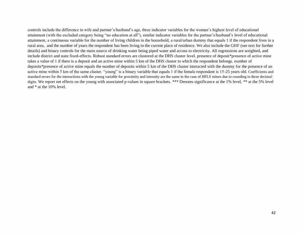
42

controls include the difference in wife and partner’s/husband’s age, three indicator variables for the woman’s highest level of educational

attainment (with the excluded category being “no education at all”), similar indicator variables for the partner’s/husband’s level of educational

attainment, a continuous variable for the number of living children in the household, a rural/urban dummy that equals 1 if the respondent lives in a

rural area, and the number of years the respondent has been living in the current place of residence. We also include the GHF (see text for further

details) and binary controls for the main source of drinking water being piped water and access to electricity. All regressions are weighted, and

include district and state fixed-effects. Robust standard errors are clustered at the DHS cluster level. presence of deposit*presence of active mine

takes a value of 1 if there is a deposit and an active mine within 5 km of the DHS cluster to which the respondent belongs. number of

deposits*presence of active mine equals the number of deposits within 5 km of the DHS cluster interacted with the dummy for the presence of an

active mine within 5 km of the same cluster. “young” is a binary variable that equals 1 if the female respondent is 15-25 years old. Coefficients and

standard errors for the interactions with the young variable for proximity and intensity are the same in the case of HFLS mines due to rounding to three decimal

digits. We report net effects on the young with associated p-values in square brackets. *** Denotes significance at the 1% level, ** at the 5% level

and * at the 10% level.

43

Table 4: Impact of mines on women’s attitude to shared decision making

Final say in decision-making related to:

own own large visits to husband’s

earnings healthcare purchases family earnings index 1 index 2

(1) (2) (3) (4) (5) (6) (7)

Panel A: HFLS mines Proximity (whether there is a deposit within 5 km): presence of deposit*presence of HFLS active mine -0.107 0.020 -0.148** -0.001 -0.058

(0.086) (0.075) (0.067) (0.054 (0.062)

presence of deposit*presence of HFLS active mine*young 0.062*** 0.100*** 0.075*** 0.081*** 0.079***

(0.017) (0.018) (0.017) (0.018) (0.016)

net effect for young -0.045 0.120 -0.072 0.080 0.021

F-statistic 0.260 2.510 1.130 2.320 0.120

[0.609] [0.114] [0.288] [0.128] [0.734]

Observations 3396 10711 10711 10711 10581 3265 10581

R-squared 0.116 0.064 0.067 0.065 0.064 0.12 0.078

Intensity (number of deposits within 5km): number of deposits*presence of HFLS active mine -0.115 0.008 -0.153** 0.001 -0.062

(0.080) (0.070) (0.064) (0.047) (0.058)

number of deposits*presence of HFLS active mine*young 0.062*** 0.100*** 0.075*** 0.081*** 0.079***

(0.017) (0.018) (0.0172) (0.018) (0.015)

net effect for young -0.053 0.108 -0.078 0.082 0.017

F-statistic 0.390 2.290 1.450 2.980 0.080

[0.532] [0.130] [0.229] [0.085] [0.777]

Observations 3396 10711 10711 10711 10581 3265 10581

R-squared 0.116 0.064 0.067 0.065 0.064 0.12 0.078

44

Panel B: All mines Proximity (whether there is a deposit within 5 km): presence of deposit*presence of active mine 0.002 -0.050 0.000 0.033 -0.025 -0.102 -0.017

(0.070) (0.053) (0.053) (0.050) (0.056) (0.076) (0.045)

presence of deposit*presence of active mine*young -0.159 0.141* 0.179*** 0.051 0.159** 0.020 0.135**

(0.190) (0.073) (0.069) (0.074) (0.076) (0.214) (0.058)

net effect for young -0.156 0.090 0.179 0.084 0.134 -0.082 0.117

F-statistic 0.630 1.280 6.550 1.200 2.920 0.140 3.130

[0.428] [0.258] [0.011] [0.274] [0.087] [0.711] [0.077]

Observations 11,395 43,714 43,714 43,714 43,348 11,029 43,348

R-squared 0.097 0.050 0.047 0.055 0.043 0.104 0.059

Intensity (number of deposits within 5km): number of deposits*presence of active mine -0.000 -0.016 0.001 0.016 -0.018 -0.009 -0.007

(0.026) (0.021) (0.017) (0.018) (0.020) (0.029) (0.017)

number of deposits*presence of active mine*young -0.053 0.007 0.034*** -0.012 0.043*** 0.007 0.019*

(0.042) (0.019) (0.013) (0.011) (0.014) (0.051) (0.010)

net effect for young -0.053 -0.009 0.035 0.004 0.025 -0.002 0.012

F-statistic 2.050 0.180 3.270 0.050 1.730 0.000 0.450

[0.152] [0.674] [0.071] [0.819] [0.189] [0.964] [0.503]

Observations 11,395 43,714 43,714 43,714 43,348 11,029 43,348

R-squared 0.097 0.050 0.047 0.055 0.043 0.104 0.059 Notes: The table reports the regression results for the interaction terms. Panel A reports the results when only precious minerals and HFLS mines are considered

using either proximity dummies or intensity measured as count variables for the number of deposits and active mines that are within 5 km. Women are asked who

they think should have greater say when it comes to decisions reported in columns (1) to (5). The binary dependent variables take a value of 1 if the respondent

says that she thinks such decisions should be taken jointly with her partner or her husband. In column 6, index 1, ranging from 0 to 1, takes a value of 1 if the

respondent answers "shared equally" when asked who should have greater say for the set of all five listed decisions. The mean of this index is 0.808. In column 7,

index 2, ranging from 0 to 1, takes a value of 1 if the respondent answers "equally" to the last four listed decisions. The mean of this index is 0.752. The

individual controls include the difference in wife and partner’s/husband’s age, three indicator variables for the woman’s highest level of educational attainment

45

(with the excluded category being “no education at all”), similar indicator variables for the partner’s/husband’s level of educational attainment, a continuous

variable for the number of living children in the household, a rural/urban dummy that equals 1 if the respondent lives in a rural area, and the number of years the

respondent has been living in the current place of residence. We also include the GHF (see text for further details) and binary controls for the main source of

drinking water being piped water and access to electricity. All regressions are weighted, and include district and state fixed-effects. Robust standard errors are

clustered at the DHS cluster level. presence of deposit*presence of active mine takes a value of 1 if there is a deposit and an active mine within 5 km of the DHS

cluster to which the respondent belongs. number of deposits*presence of active mine equals the number of deposits within 5 km of the DHS cluster interacted

with the dummy for the presence of active mine within 5 km of the same cluster. “young” is a binary variable that equals 1 if the female respondent is 15-25

years old. Coefficients and standard errors for the interactions with the young variable for proximity and intensity are the same in the case of HFLS mines due to

rounding to three decimal digits. We report net effects on the young with associated p-values in brackets. *** Denotes significance at the 1% level, ** at the 5%

level and * at the 10% level.

46

Table 5: Impact of mines on women’s education

Binary dependent variable

literate some secondary school or higher

(1) (2)

Panel A: HFLS mines Proximity (whether there is a deposit within 5 km): presence of deposit*presence of HFLS active mine -0.028 -0.159

(0.072) (0.086)

presence of deposit*presence of HFLS active mine*young 0.298*** 0.439***

(0.013) (0.014)

net effect for young 0.270 0.280

F-statistic 14.100 10.530

[0.000] [0.001]

Observations 10,378 10,389

R-squared 0.416 0.437

Intensity (number of deposits within 5km): number of deposits*presence of HFLS active mine -0.042 -0.176**

(0.071) (0.086)

number of deposits*presence of HFLS active mine*young 0.298*** 0.439***

(0.013) (0.014)

net effect for young 0.257 0.263

F-statistic 13.110 9.400

[0.000] [0.002]

Observations 10,378 10,389

R-squared 0.416 0.437

Panel B: All mines

47

Proximity (whether there is a deposit within 5 km): presence of deposit*presence of active mine 0.041 0.047

(0.036) (0.035)

presence of deposit*presence of active mine*young 0.071 -0.010

(0.075) (0.090)

net effect for young 0.112 0.037

F-statistic 2.320 0.170

[0.128] [0.679]

Observations 42,448 42,487

R-squared 0.382 0.412

Intensity (number of deposits within 5km): number of deposits*presence of active mine -0.008 0.005

(0.013) (0.012)

number of deposits*presence of active mine*young -0.011 -0.030

(0.022) (0.019)

net effect for young -0.009 -0.025

F-statistic 0.150 1.510

[0.703] [0.219]

Observations 42,448 42,487

R-squared 0.382 0.412 Notes: The table reports the regression results for the interaction terms. Panel A reports the results when only precious minerals and HFLS mines are considered

using either proximity dummies or intensity measured as count variables for the number of deposits and active mines that are within 5 km. The binary dependent

variables take a value of 1 if the respondent says that she is literate (in column 1), and has achieved some secondary schooling (in column 2). The individual

controls include the difference in wife and partner’s/husband’s age, three indicator variables for the partner’s/husband’s level of educational attainment, a

continuous variable for the number of living children in the household, a rural/urban dummy that equals 1 if the respondent lives in a rural area, and the number

of years the respondent has been living in the current place of residence. We also include the GHF (see text for further details) and binary controls for the main

source of drinking water being piped water and access to electricity. All regressions are weighted, and include district and state fixed-effects. Robust standard

errors are clustered at the DHS cluster level. presence of deposit*presence of active mine takes a value of 1 if there is a deposit and an active mine within 5 km of

48

the DHS cluster to which the respondent belongs. number of deposits*presence of active mine equals the number of deposits within 5 km of the DHS cluster

interacted with the dummy for the presence of active mine within 5 km of the same cluster. “young” is a binary variable that equals 1 if the female respondent is

in the age group 15-25 years old. Coefficients and standard errors for the interactions with the young variable for proximity and intensity are the same in the case

of HFLS mines due to rounding to three decimal digits. We report net effects on the young with associated p-values in brackets. *** Denotes significance at the

1% level, ** at the 5% level and * at the 10% level.

49

Table 6: Impact of mines on women’s health

overweight/ high high

height BMI obese underweight HBA anemic BP glucose

(1) (2) (3) (4) (5) (6) (7) (8)

Panel A: HFLS mines

Proximity (whether there is a deposit within 5 km):

presence of deposit*presence of HFLS active mine 0.438 0.106 -0.019 -0.282*** 0.309 0.228** -0.065 -0.183 (1.243) (0.573) (0.068) (0.056) (0.274) (0.090) (0.067) (0.125)

presence of deposit*presence of HFLS active mine*young 1.904*** 1.667*** 0.116*** -0.246*** -0.093 -0.064*** 0.032*** -0.174*** (0.244) (0.195) (0.020) (0.015) (0.075) (0.020) (0.012) (0.020)

net effect for young 2.342 1.773 0.097 -0.528 0.217 0.164 -0.033 -0.357

F-statistic 3.470 9.650 2.040 86.060 0.600 3.270 0.240 8.130 [0.063] [0.002] [0.154] [0.000] [0.437] [0.071] [0.623] [0.004]

Observations 10,389 10,389 10,389 10,389 10,330 10,330 10,375 10,330

R-squared 0.097 0.275 0.187 0.135 0.096 0.089 0.134 0.058

Intensity (number of deposits within 5km):

number of deposits*presence of HFLS active mine 0.110 -0.099 -0.051 -0.287*** 0.305 0.254*** -0.088 -0.163 (1.189) (0.556) (0.068) (0.054) (0.269) (0.089) (0.064) (0.125)

number of deposits*presence of HFLS active mine*young 1.902*** 1.664*** 0.115*** -0.246*** -0.093 -0.064*** 0.032** -0.173*** (0.244) (0.195) (0.020) (0.015) (0.075) (0.020) (0.012) (0.020)

net effect for young 2.012 1.565 0.064 -0.533 0.212 0.19 -0.056 -0.337

F-statistic 2.800 7.980 0.900 93.690 0.600 4.470 0.770 7.330 [0.095] [0.005] [0.344] [0.000] [0.438] [0.035] [0.381] [0.007]

Observations 10,389 10,389 10,389 10,389 10,330 10,330 10,375 10,330

R-squared 0.097 0.275 0.186 0.135 0.096 0.089 0.134 0.058

Panel B: All mines

50

Proximity (whether there is a deposit within 5 km):

presence of deposit*presence of active mine -0.654 1.222** 0.093** -0.064** 0.092 -0.042 0.040 0.001 (0.667) (0.494) (0.043) (0.030) (0.198) (0.061) (0.036) (0.052)

presence of deposit*presence of active mine*young -1.569 -0.507 -0.058 0.064 0.094 -0.024 -0.019 -0.060 (1.064) (0.525) (0.066) (0.064) (0.365) (0.096) (0.027) (0.068)

net effect for young -2.223 0.715 0.035 0.000 0.187 -0.067 0.021 -0.059

F-statistic 5.300 2.190 0.270 0.000 0.330 0.520 0.260 0.720 [0.021] [0.139] [0.600] [0.998] [0.566] [0.471] [0.609] [0.397]

Observations 42,487 42,487 42,487 42,487 42,196 42,196 42,428 42,195

R-squared 0.103 0.209 0.144 0.097 0.076 0.066 0.128 0.044

Intensity (number of deposits within 5km):

number of deposits*presence of active mine -0.138 0.259 0.030* -0.015 -0.060 0.019 0.008 -0.001 (0.202) (0.187) (0.017) (0.012) (0.052) (0.017) (0.014) (0.018)

number of deposits*presence of active mine*young -0.225 -0.125 -0.023* 0.010 -0.044 0.002 0.004 -0.003 (0.277) (0.165) (0.013) (0.020) (0.074) (0.017) (0.006) (0.017)

net effect for young -0.363 0.134 0.006 -0.005 -0.104 0.021 0.012 -0.004

F-statistic 1.340 1.560 0.290 0.090 2.260 1.380 0.960 0.050 [0.248] [0.212] [0.590] [0.764] [0.133] [0.240] [0.326] [0.822]

Observations 42,487 42,487 42,487 42,487 42,196 42,196 42,428 42,195

R-squared 0.103 0.208 0.144 0.096 0.076 0.066 0.127 0.044

Notes: The table reports the regression results for the interaction terms. Panel A reports the results when only precious minerals and HFLS mines are considered

using either proximity dummies or intensity measured as count variables for the number of deposits and active mines that are within 5 km. BMI is weight in

kilograms (kg) divided by height in meters squared (m2), and overweight/obese is defined as BMI greater than or equal to 25.0 kg/m2 while underweight is

defined as BMI less than 18.5 kg/m2. A woman is anemic if her HBA level is below 12.0 g/dl (grams per deciliter). The individual controls include the

difference in wife and partner’s/husband’s age, three indicator variables for the partner’s/husband’s level of educational attainment, a continuous variable for the

number of living children in the household, a rural/urban dummy that equals 1 if the respondent lives in a rural area, and the number of years the respondent has

been living in the current place of residence. We also include the GHF (see text for further details) and binary controls for the main source of drinking water

being piped water and access to electricity. All regressions are weighted, and include district and state fixed-effects. Robust standard errors are clustered at the

51

DHS cluster level. presence of deposit*presence of active mine takes a value of 1 if there is a deposit and an active mine within 5 km of the DHS cluster to which

the respondent belongs. number of deposits*presence of active mine equals the number of deposits within 5 km of the DHS cluster interacted with the dummy for

the presence of active mine within 5 km of the same cluster. “young” is a binary variable that equals 1 if the female respondent is in the age group 15-25 years

old. We report net effects on the young with associated p-values in brackets. *** Denotes significance at the 1% level, ** at the 5% level and * at the 10% level.

52

Table 7: Profit sharing, proximity to mines and female employment for HFLS mines

currently is in the

working workforce agriculture manufacturing services (1) (2) (3) (4) (5)

Proximity (whether there is a deposit within 5 km):

presence of deposit*presence of HFLS active mine -0.155*** -0.266*** -0.288*** -0.038 0.016 (0.058) (0.057) (0.067) (0.025) (0.062)

presence of HFLS active mine*profit sharing per female pop. 1.280*** 0.943*** 0.965*** 0.084* -0.028 (0.145) (0.130) (0.168) (0.051) (0.160)

Observations 10,715 10,703 10,703 10,566 10,566

R-squared 0.068 0.083 0.195 0.019 0.063 Notes: The table reports the coefficients on the interaction terms. Panel A reports the results when only HFLS mines are considered using proximity dummies

while Panel B reports the results for non-HFLS mines. In column (1), the binary dependent variable equals to 1 if the female respondent says that she is currently

working, and in column (2), the indicator variable takes a value of 1 if she is in the workforce. Columns (3) to (5) consider binary occupational outcomes related

to employment in agriculture, manufacturing, and services. The individual controls include the difference in wife and partner’s/husband’s age, three indicator

variables for the woman’s highest level of educational attainment (with the excluded category being “no education at all”), similar indicator variables for the

partner’s/husband’s level of educational attainment, a continuous variable for the number of living children in the household, a rural/urban dummy that equals 1

if the respondent lives in a rural area, and the number of years the respondent has been living in the current place of residence. We also include the GHF (see text

for further details) and binary controls for the main source of drinking water being piped water and access to electricity. All regressions include state fixed-

effects. Robust standard errors are clustered at the DHS cluster level. All regressions are weighted. presence of deposit*presence of active mine takes a value of 1

if there is a deposit and an active mine within 5 km of the DHS cluster to which the respondent belongs. presence of active mine*profit sharing per female

population is the interaction term between the presence of active mine (HFLS or non-HFLS) within 5 km of the DHS cluster and the continuous variable for

district-level profit sharing per female population. We report net effects with associated p-values in brackets. *** Denotes significance at the 1% level, ** at the

5% level, and * at the 10% level.

53

Table 8: Profit sharing, proximity to mines and female financial independence for HFLS mines

earns earns more owns house owns house knows about knows about

cash than him alone alone/jointly loan program and has loan (1) (2) (3) (4) (5) (6)

Proximity (whether there is a deposit within 5 km):

presence of deposit*presence of HFLS active mine -0.081 0.029 0.087* -0.016 -0.119 0.003 (0.056) (0.029) (0.050) (0.150) (0.133) (0.087)

pres. of prec. active mine*profit sharing per female pop. 0.765*** 1.104*** 0.160 1.130*** 1.046*** 0.528** (0.137) (0.060) (0.119) (0.386) (0.355) (0.220)

Observations 10,715 10,686 10,715 10,715 10,715 10,715

R-squared 0.063 0.032 0.069 0.053 0.126 0.102 Notes: The table reports the coefficients on the interaction terms. Panel A reports the results when only HFLS mines are considered using proximity dummies

while Panel B reports the results for non-HFLS mines. In column (1), the dependent variable equals to 1 if the female respondent says that she earns "cash"

instead of "in-kind" as earnings, and in column (2), the variable is coded as 1 if she reports earning more than her partner/husband. In columns (3) and (4), the

dependent variables equal 1 if the respondent says that she "owns a house alone", and if she says that she "owns a house alone and/or jointly", respectively. In the

last two columns, the variables relate to awareness of financial opportunities and the binary dependent variables equal 1 in column (5) if she says that she is

aware of a program in the area that gives loans to women to start or expand a business, and in column (6), if she says that she has taken a loan, cash or in-kind,

from this program to start or expand a business. The individual controls include the difference in wife and partner’s/husband’s age, three indicator variables for

the woman’s highest level of educational attainment (with the excluded category being “no education at all”), similar indicator variables for the

partner’s/husband’s level of educational attainment, a continuous variable for the number of living children in the household, a rural/urban dummy that equals 1

if the respondent lives in a rural area, and the number of years the respondent has been living in the current place of residence. We also include the GHF (see text

for further details) and binary controls for the main source of drinking water being piped water and access to electricity. All regressions include state fixed-

effects. Robust standard errors are clustered at the DHS cluster level. All regressions are weighted. presence of deposit*presence of active mine takes a value of 1

if there is a deposit and an active mine within 5 km of the DHS cluster to which the respondent belongs. presence of active mine*profit sharing per female

population is the interaction term between the presence of active mine (HFLS or non-HFLS) within 5 km of the DHS cluster and the continuous variable for

district-level profit sharing per female population. We report net effects with associated p-values in brackets. *** Denotes significance at the 1% level, ** at the

5% level, and * at the 10% level.

1

ONLINE APPENDIX

Appendix Box 1: Choice of Baseline Distance

To determine the appropriate treatment distance for our empirical framework, we study

the commuting behavior of workers in India. In 2011, the Census in India reported the mode of

travel and the travel distances of workers in the country for the first time. The data is available

by gender, and for both rural and urban areas in each state.1 Appendix Figure 4 shows that more

than half of the women interviewed report that they walk to work, against 28 percent of male

respondents reporting so. In rural India, two-thirds of women walk to work, while only 28

percent of men do so, and 1 out of 4 men uses a bicycle to access work compared to only 1 out of

20 women who work. Appendix Figure 5 shows the distance to work by gender and by mode of

travel. Out of all workers interviewed, around a quarter of male respondents and 45 percent of

female respondents do not travel at all for work. The corresponding proportions for rural areas

are 33 percent and 55 percent for male and female workers, respectively. Out of all the

respondents reporting that they had to commute to work, 16 percent reported a travel distance of

up to 1 km; 23 percent reported a distance of 2-5 km, with mild differences in the proportions for

male and female respondents, and between rural and urban areas. Taking these together, the

census data reveals that the proportion of workers who travel 5 km or less to access their place of

work is approximately 70 percent. Hence, our focus on the 5km distance around clusters for a

baseline is appropriate.

We also refer to the relevant literature on mining and development to ensure that this

baseline distance is in line with previous studies (indicating treatment effects for communities

within 5-20 km of the mine). Kotsadam and Benshaul-Tolonen (2016) use a baseline distance of

1 These are for workers who were engaged in economic activities; not cultivators or agricultural laborers or in

household industries (Source: censusindia.gov.in/2011Census).

2

20 km to estimate a mine’s footprint. Benshaul-Tolonen (2018) uses a baseline distance of 10 km

when considering the potential impact of opening mines on gender norms, while Benshaul-

Tolonen (2019) relies on a treatment distance of 15 km. Von der Goltz and Barnwal (2019)

define a DHS cluster as being in the direct vicinity of a mine if it is within 5 km of the nearest

mine. In these cases as in ours, the choice of baseline distance is based on the commuting

behavior of workers and on the related literature on the health, development, and employment

effects of mines on local communities.

Appendix Box 2: Profit-Sharing in Mining Communities

We first consider the effects of three different district-level proxies of profit sharing on

women living within 5 km of an active HFLS/non-HFLS mine, and in a district that distributes

royalties in specific ways. To construct these proxies, we use a 2011 official report provided by

the Center for Science and Environment, India.2 Prepared to understand the major implications

of the Draft Mines and Minerals (Development and Regulation) (MMDR) Act Bill of 2011, the

report provides scope to understand the possible effects of district-level profit sharing of mineral

wealth on affected populations.3 Referring specifically to the profit-sharing concept introduced

for the first time under sub-section 2 of Section 43 of the draft, it states that “a mine leaseholder

is to pay annually to the District Mineral Foundation (DMF), as specified in Section 56, an

amount equal to 26 percent of profit after tax or a sum equivalent to the royalty paid during the

year, whichever is higher”. This allows us to proxy for the amount each affected individual,

household, and woman receives from resource abundance in mineral-producing districts, keeping

in mind that the major challenge in the implementation of the DMF is to identify people affected

2 For more details, see “Sharing The Wealth of Minerals: A report on Profit Sharing with Local Communities”,

Center for Science and Environment, New Delhi, India (2011). 3 The Draft MMDR Act Bill of 2011 considers, within a well-defined framework, amongst other things, what goes

to affected people/communities.

3

by mining, and that affected districts adjacent to mineral-producing areas should also receive

compensation for the possible loss of livelihoods, land, and displacement.4

The first proxy considered is profit sharing per affected population. We use the mineral-

specific reports contained in the Indian Minerals Yearbook 2014, digitize the district-level values

of production for each mineral, and then aggregate them to obtain the total value of mineral

production for the period 2013-2014. We also compiled the district-wise total mineral leased

area, manually digitized from the Bulletin of Mining leases and Prospecting Licenses, 2014 from

the Indian Bureau of Mines. This allows us to obtain the total mine leased area for each district

as of 2014.5 Since the Draft MMDR includes the provision that the mining industry should

provide at a minimum the royalty, we assume that the share of profits distributed to local

communities is equal to the royalty. Referring to the royalty contribution of major Indian mining

companies, we set the royalty to be equal to 10.5 percent of the total value of mineral

production.6

To estimate the population affected by mining activities, the report further assumes that

the direct effects of health, displacement, and livelihoods are scattered over at least twice the size

of the leased area, and that the population density over the affected area is in turn directly

proportional to the average population density of the State. We construct the district-wise profit

4 Pradhan Mantri Khanij Kshetra Kalyan Yojana (PMKKKY) guidelines for DMF Trusts define mining-affected

people as people who have legal and occupational rights over the land being mined; people who have usufruct and

traditional rights over the land being mined, displaced families, and families whose health, livelihoods, and quality

of life are directly affected by mining activities. 5 This excludes atomic minerals, coal, lignite, petroleum, and natural gas (but includes the minerals declared as

minor). 6 During the fiscal year of 2009-2010, Coal India Limited (CIL) paid 11.6 percent of gross sales as royalty, cess, and dead rent burden. The other big mining companies-Rajasthan State Mines and Minerals Limited (RSMM) paid 10.6

percent, The Singareni Collieries Company Limited (SCCL) paid 8.6 percent, while Gujarat Mineral Development

Corporation (GMDC) paid 5.7 percent during 2009-2010 (Source: Report from the Centre for Science and

Development, 2011). Any mining company must also pay other taxes like education cess, sales tax, and corporate

tax. If all these taxes are taken into account, then the average tax burden is estimated to be 22 per cent, ranging

between 14 to 34 percent. We assume, as per the official report, a minimum average of 10.5 percent.

4

sharing per affected population following the report, and interact it with the presence of an active

mine. We also construct two other profit-sharing measures that do not rely on the district’s leased

area but is instead on a per capita basis: (i) profit-sharing per household, and (ii) profit-sharing

per female population (on the basis that at least 60 percent of royalties collected is allocated to

the welfare of women and children).7 Given its particular relevance, we report results for profit

sharing per female population in the paper (results for per affected population and profit-sharing

per household are available on request). Our specification is as follows:

𝑌𝑖𝑐𝑑 = 𝛽0 + 𝛽1𝑑𝑒𝑝𝑜𝑠𝑖𝑡𝑐 + 𝛽2𝑎𝑐𝑡𝑖𝑣𝑒𝑚𝑖𝑛𝑒𝑐 + 𝛽3(𝑑𝑒𝑝𝑜𝑠𝑖𝑡𝑐 × 𝑎𝑐𝑡𝑖𝑣𝑒𝑚𝑖𝑛𝑒𝑐)

+ 𝛽4𝑝𝑟𝑜𝑓𝑖𝑡𝑠ℎ𝑎𝑟𝑖𝑛𝑔𝑑 + 𝛽5(𝑎𝑐𝑡𝑖𝑣𝑒𝑚𝑖𝑛𝑒𝑐 × 𝑝𝑟𝑜𝑓𝑖𝑡𝑠ℎ𝑎𝑟𝑖𝑛𝑔𝑑) + 𝑋𝑖 + 𝜆𝑠

+ 𝜖𝑖𝑐𝑑 (3)

where the variables 𝑌𝑖𝑐𝑑 , 𝑑𝑒𝑝𝑜𝑠𝑖𝑡𝑐 , 𝑎𝑐𝑡𝑖𝑣𝑒𝑚𝑖𝑛𝑒𝑐, 𝑋𝑖, 𝜆𝑠, and 𝜖𝑖𝑐𝑑 the same as in the main

specification of equation (1). 𝑝𝑟𝑜𝑓𝑖𝑡𝑠ℎ𝑎𝑟𝑖𝑛𝑔𝑑 is the district-level proxy for profit sharing per

affected population/female population/household. The coefficient of interest is 𝛽5. We report the

coefficients on (𝑑𝑒𝑝𝑜𝑠𝑖𝑡𝑐 × 𝑎𝑐𝑡𝑖𝑣𝑒𝑚𝑖𝑛𝑒𝑐) and on (𝑎𝑐𝑡𝑖𝑣𝑒𝑚𝑖𝑛𝑒𝑐 × 𝑝𝑟𝑜𝑓𝑖𝑡𝑠ℎ𝑎𝑟𝑖𝑛𝑔𝑑) in the

results tables.8

We consider the robustness of our estimates by including additional district-level controls

that could affect both women’s employment opportunities and the value of mineral production

distributed to local communities. In results available on request, we add these controls

sequentially in regressions involving the binary dependent variable for women’s employment

7 The report assumes an average household size of five. We use the number of households for each district provided

by the 2011 Census, but also ensure the results hold if we make the same assumption as in the report. 8 Our framework does not allow us to estimate the possible compensation made to adjacent non-mineral producing districts also facing the detrimental effects of mining activities. For instance, Bastar, Bijapur, Sukma, Kondagaon,

and Narayanpur districts are adjacent to Dantewada in the state of Chhattisgarh and also contain mining-affected

areas. Provisions have been made for compensation from the DMF fund, but since these were not made for 2014-

2015, we assume that royalties collected in a district impact women’s outcomes close to where the mine is located

and that their effects are mostly limited to that district.

5

(“is currently employed”). First, we control for the district’s socio-economic vulnerability. We

use the index constructed from the National Family Health Survey 2015-2016 by Acharya and

Porwal (2020).9 Following Berman et al. (2017), we also proxy for lootability. Since more

precious minerals generate larger royalties and rents, they create incentives for loots and conflict.

Lootability is determined not only by the value of precious commodities but also by the ease

with which they can be extracted with artisanal tools. We use two different proxies for lootability

and the likelihood of mineral-induced conflicts: (i) logged mean distance from each district’s

centroid to the nearest lootable gold or surface deposit, and (ii) a dummy variable that equals one

if the district is affected by Maoist conflicts.10

Since the impact of profit-sharing on the local community depends on how resource rents

are collected and distributed via institutional arrangements (Mehlum et al. 2006), our framework

must also consider the district-level variation in administrative institutions, corruption,

bureaucracy, and rule of law. Governance indicators are not available at such a disaggregated

level so we include the number of intermediate and village panchayats (per 1000 inhabitants)

instead. These are considered important institutions of local governance in Indian districts and

states that ensure accountability and transparency in the collection and use of resource

revenues.11 They are likely to play a key role in ensuring that among other things, royalties are

9 This study provides vulnerability indices that could improve the management and response of the Covid-19

pandemic in India. Three indicators are used to build the socio-economic index: the percentage of the population

belonging to scheduled caste and scheduled tribe (to represent for marginalized groups), the proportion of the

population aged 15 and above who have completed secondary or higher level of education, and an asset deprivation

index (the proportion of households that do not have a motorized vehicle, television, computer, bicycle, and

refrigerator, amongst others). 10 We obtain the distance to the nearest lootable or surface gold deposit using AIDDATA (Source name:

GOLDATA, for more details, see Balestri and Maggioni 2014). We calculate the district’s number of

gold/silver/diamonds from the data compiled to calculate production and profit-sharing values, and obtain the list of

districts affected by Maoist conflicts from the South Asia Terrorism Portal. 11 Data is obtained from the Local Government Directory. See website for more details: lgdirectory.gov.in.

(Accessed on August 25, 2020).

6

not dissipated through leakages.12 We also add as an additional variable the share of mineral-

leased area held by the government to proxy for public/private sector involvement. Increased

access to media may also influence agency measures and the distribution of rents. For this

reason, we construct an index using the DHS data that is a composite variable for whether the

respondent listens to the radio, watches TV, and reads the newspapers often. Results for these

additional checks are available on request.

Appendix Box 3: Further Robustness, Falsification and Specification Checks

Check for Pre-Trends

Validity of the difference-in-differences framework depends on the absence of pre-trends

in the treatment and control groups. We present these tests in Appendix Table 8. In the pre-

treatment phase, the control group has no deposit within 5 km of each cluster and no active mine

within 99 km (since 100 km is the limit of our data, we use a value very close to 100 km). The

treatment group has a deposit within 5 km of each cluster but no active mine within 15 km. We

run tests for pre-trends using future mines only, and then compare treatment and control groups

in years before the mine opens. We report the mean and standard deviation for each of the

control variables, the difference in means, and the standard error of the t-test for this difference

between control and treatment groups in the pre-treatment phase. Although there are significant

differences among some of the variables in this table, note that all regressions condition on these

variables thus taking their influences into account.

Determining Treatment Distance Non-Parametrically

12 Caselli and Michaels (2013) find that royalties from oil production in Brazil lead to significant increases in

municipalities’ spending on public goods and services, but that improvements in provision of public services are

smaller relative to the reported fiscal spending increases. This suggests that there is “missing money” due to

embezzlement.

7

Although we argue that given commuting distance and modes of travel to work for much

of the Indian rural population, 5 km near deposits and mines is an appropriate measure of

treatment distance, we also check for this non-parametrically. These results are presented in

Appendix Figure 6. We follow Benshaul-Tolonen (2019) and use spatial lag models to construct

these measures and concentrate on proximity to HFLS mines as that is where impacts discussed

above are most evident and measured precisely. Although these estimates are mostly

insignificant, the treatment effect is the largest at smaller treatment distances qualitatively,

indicating the existence of spatial spillovers.13 At the treatment distances become larger, the

interaction term between the presence of deposits and the presence of a HFLS active mine for the

acceptance of violence index become either smaller in magnitude or exhibit unexpected signs.

Given this and justification from qualitative data from the 2011 Census on average commuting

distance for workers, we use 5 km as the treatment distance for the analysis.

Falsification Tests and Evaluating Environmental Impacts

Appendix Table 9 presents falsification tests using information on past or future mines.

For purposes of these tests, we present results only on the acceptance of domestic violence

variables.14 Since these mines are not currently active, there should be no significant impacts of

such mines on any of the measures considered in Appendix Table 9. As before, there are too few

past or future HFLS mines to identify impacts. Thus, we focus on those presented in Panel B

that evaluates all mines. Of the three outcomes that are significant in this panel for all women

near mines, one (goes out without permission) has a counter-intuitive sign. Contrasting these

impacts with those in Panel B of Table 2 and focusing on the composite index variable, the

13 Similar to Benshaul-Tolonen (2019), there is substantial noise in these spatially lagged models. 14 Results for barriers to accessing medical care and attitudes towards shared decision-making are available on

request.

8

coefficient on this variable indicated a significant 8.6 percentage point decline in Table 2 but is

statistically zero in Appendix Table 9. Furthermore, net effects on the young were measured with

precision in three of the seven cases in Table 2 but are all insignificant in Appendix Table 9.

Overall, we conclude that it is active mines alone that results in beneficial measurable impacts

for women in the close vicinity of mines as past/future mines have weaker or no impacts.

Next, we consider the environmental impact of mining by evaluating how pollution

measured by PM2.5 affects the incidence of domestic violence given evidence that air pollution

affects cognitive functioning (Zhang et al. 2018). Again, we present results for this category of

outcomes alone given their primary nature as a measure of women’s agency.15 The data on

PM2.5 at the district level are obtained from satellite measurement estimates generated from

aerosol optical depth information collected using techniques developed in Dey et al. (2012).

PM2.5 is measured in micrograms per cubic meter of air, and we use its natural log version in

these models. The results are in Appendix Table 10 which shows that although the effect of air

pollution is measured with significance in some of the outcomes considered, the estimates of our

main variables of interest either remain mostly unaltered or improve when we condition on

PM2.5. More specifically, whereas the composite index variable is insignificant for all women in

the case of HFLS mines in Table 2, it indicates a precise 15.8 percentage point decrease in

acceptance of this form of violence in Appendix Table 10. Considering impacts near all mines

for this variable, again the magnitude is somewhat larger when PM2.5 is taken into account (an

8.6 percentage point decline in Table 2 and a 9.0 percentage point decline in this table).

15 Results for barriers to accessing medical care and attitudes towards shared decision-making are available on

request.

9

Appendix References

Acharya, R. and Porwal, A., 2020. “A Vulnerability Index for the Management of and Response

to the COVID-10 Epidemic in India: An Ecological Study,” The Lancet Global Health

8(9): E1142-E1151.

Balestri, S. and Maggioni, M.A., 2014. Blood diamonds, dirty gold and spatial spill-overs

measuring conflict dynamics in West Africa. Peace Economics, Peace Science and

Public Policy, 20(4), pp.551-564.

Benshaul-Tolonen, Anja. 2018. “Endogenous Gender Norms: Evidence from Africa’s Gold

Mining Industry,” Columbia Center for Development Economics and Policy CDEP-

CGEG Working Paper no. 62.

Benshaul-Tolonen, Anja. 2019. “Endogenous Gender Roles: Evidence from Africa’s Gold

Mining Industry.” Available at SSRN 3284519.

Berman, Nicolas, Mathieu Couttenier, Dominic Rohner, and Mathias Thoenig. 2017. “This Mine

is Mine! How Minerals Fuel Conflicts in Africa,” American Economic Review 107 (6):

1564-1610.

Caselli, F., and Michaels, G. 2013. “Do Oil Windfalls Improve Living Standards? Evidence from

Brazil,” American Economic Journal: Applied Economics 5(1): 208-238.

Dey, S., L. Girolamo, A.V. Donkelaar, S.N. Tripathi, T. Gupta, and M. Mohan. 2012.

“Variability of Outdoor Fine Particular (PM2.5) Concentration in the Indian

Subcontinent: A Remote Sensing Approach,” Remote Sensing of Environment 127: 153-

161.

Kotsadam, Andreas, and Anja Benshaul-Tolonen. 2016. “African Mining, Gender, and Local

Employment,” World Development 83 (7): 325-339.

10

Mehlum, Halvor, Karl Moene, and Ragnar Torvik. 2006. “Institutions and the Resource Curse,”

The Economic Journal 116 (508): 1-20.

Von der Goltz, Jan, and Prabhat Barnwal. 2019. “The Local Wealth and Health Effects of

Mineral Mining in Developing Countries,” Journal of Development Economics 139: 1-

16.

Zhang, Xin, Xi Chen, and Xiaobo Zhang. 2018. “The Impact of Exposure to Air Pollution on

Cognitive Performance,” Proceedings of the National Academy of Sciences 115 (37):

9193-9197.

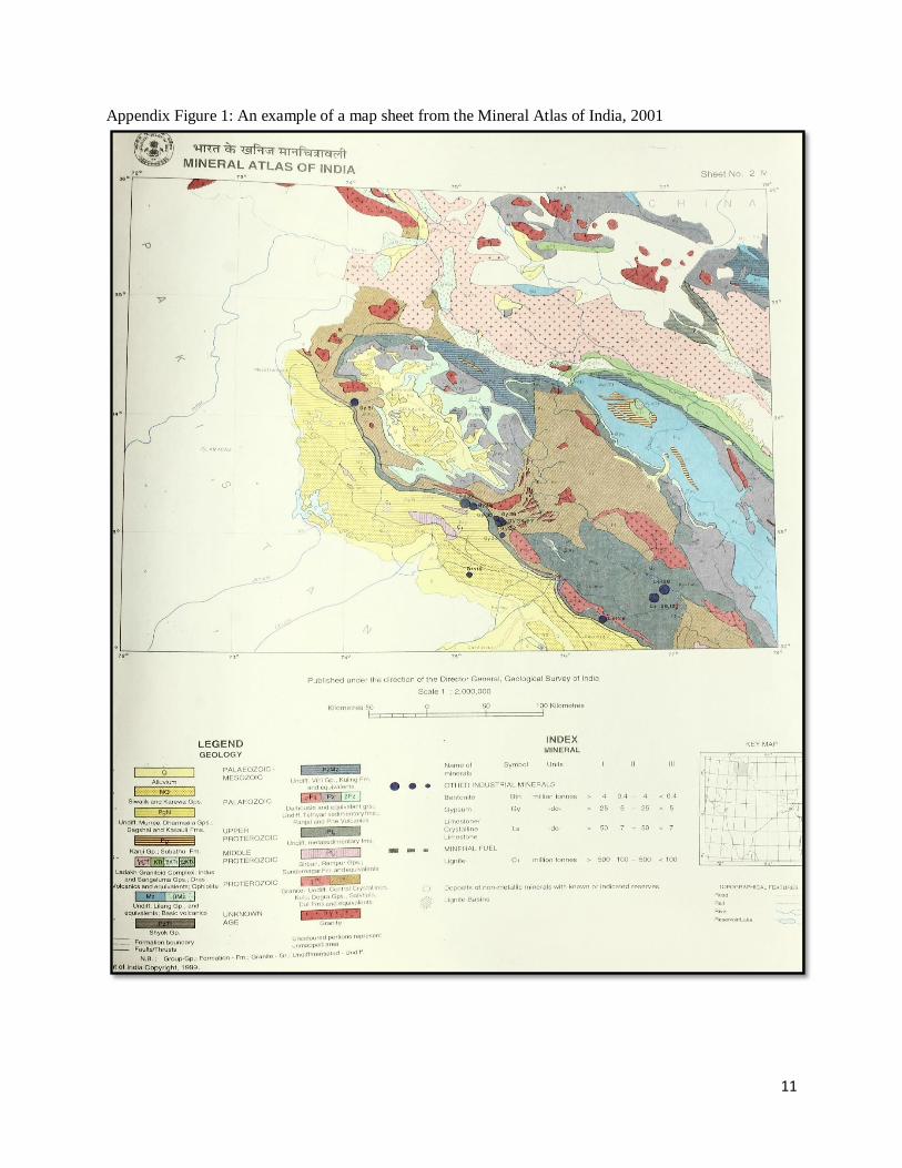
11

Appendix Figure 1: An example of a map sheet from the Mineral Atlas of India, 2001

12

Appendix Figure 2: Distribution of active and inactive mines in India, 2007

Source: United States Geological Survey, 2007

13

Appendix Figure 3: The share of leased area (percent) for districts in India, 2014

Source: Bulletin of Mining Leases and Prospecting Licenses (Indian Bureau of Mines, 2014).

Authors’ calculations from official data.

Note: As of 2014, the Mining Lease Directory reports that there were 10,982 mining leases granted for 64 different

minerals. The five highest shares of leased area are for the states of Rajasthan (18.5 percent), Orissa (16.2 percent),

Andhra Pradesh (13.5 percent), Karnataka (10.5 percent), and Madhya Pradesh (7.23 percent). The district shares vary between 0 and 6.4 percent.

14

Appendix Figure 4: Mode of travel to commute to work for workers in India

Source: Authors’ calculations from the 2011 Census of India

0

10

20

30

40

50

60P

erce

nta

ge o

f w

ork

tri

ps

All Male Female

15

Appendix Figure 5: Distance from Residence to Work for Workers, by gender and by mode of travel, in

India

Source: Authors’ calculations from 2011 Census of India

0

10

20

30

40

50

No travel 0-1 2-5 6-10 11-20 21-30 31-50 51 andmore

% o

f to

tal w

ork

ers

Distance to work (kilometers)

All Male Female

0102030405060

0-1 2-5 6-10 11-20 21-30 31-50 51 andmore

% o

f to

tal w

ork

ers

Distance to work (kilometers)

Walking Bicycle Motorcycle Bus

16

Appendix Figure 6: Non-parametric determination of treatment distance

Notes: This figure plots point estimates of the interaction term “presence of deposit_x km*presence of HFLS active mine_x km” at different cutoff distances. The outcome variables are shown in the heading of each sub-plot. Each figure shows the point estimates

and the 90% confidence intervals. In each model, the individual controls include the age difference between wife and

partner/husband, three indicator variables for the woman’s highest level of educational attainment (with the excluded category

being “no education at all”), similar indicator variables for the partner’s/husband’s level of educational attainment, a continuous

variable for the number of living children in the household, a rural/urban dummy that equals 1 if the respondent lives in a rural

area, and the number of years the respondent has been living in the current place of residence. In models on the beating justified

index, we also control for whether the female respondent's mother was beaten by the father. We also include the GHF (see text for

further details) and binary controls for the main source of drinking water being piped water and access to electricity. All

regressions are weighted, and include district and state fixed-effects. Robust standard errors are clustered at the DHS cluster level.

presence of deposit_x km*presence of HFLS active mine_x km takes a value of 1 if there is a deposit and an active HFLS mine

within x km of the DHS cluster to which the respondent belongs.

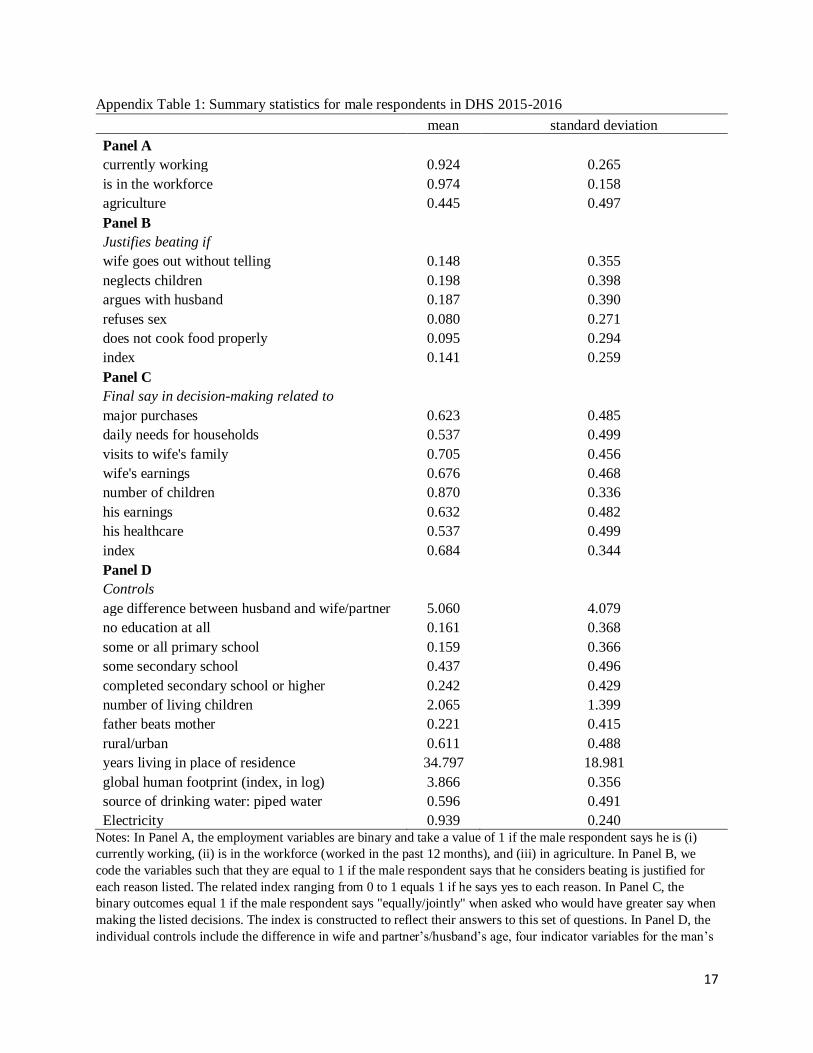
17

Appendix Table 1: Summary statistics for male respondents in DHS 2015-2016

mean standard deviation

Panel A

currently working 0.924 0.265

is in the workforce 0.974 0.158

agriculture 0.445 0.497

Panel B Justifies beating if wife goes out without telling 0.148 0.355

neglects children 0.198 0.398

argues with husband 0.187 0.390

refuses sex 0.080 0.271

does not cook food properly 0.095 0.294

index 0.141 0.259

Panel C Final say in decision-making related to major purchases 0.623 0.485

daily needs for households 0.537 0.499

visits to wife's family 0.705 0.456

wife's earnings 0.676 0.468

number of children 0.870 0.336

his earnings 0.632 0.482

his healthcare 0.537 0.499

index 0.684 0.344

Panel D Controls age difference between husband and wife/partner 5.060 4.079

no education at all 0.161 0.368

some or all primary school 0.159 0.366

some secondary school 0.437 0.496

completed secondary school or higher 0.242 0.429

number of living children 2.065 1.399

father beats mother 0.221 0.415

rural/urban 0.611 0.488

years living in place of residence 34.797 18.981

global human footprint (index, in log) 3.866 0.356

source of drinking water: piped water 0.596 0.491

Electricity 0.939 0.240 Notes: In Panel A, the employment variables are binary and take a value of 1 if the male respondent says he is (i)

currently working, (ii) is in the workforce (worked in the past 12 months), and (iii) in agriculture. In Panel B, we

code the variables such that they are equal to 1 if the male respondent says that he considers beating is justified for

each reason listed. The related index ranging from 0 to 1 equals 1 if he says yes to each reason. In Panel C, the

binary outcomes equal 1 if the male respondent says "equally/jointly" when asked who would have greater say when

making the listed decisions. The index is constructed to reflect their answers to this set of questions. In Panel D, the

individual controls include the difference in wife and partner’s/husband’s age, four indicator variables for the man’s

18

highest level of educational attainment, a continuous variable for the number of living children in the household, a

rural/urban dummy that equals 1 if the respondent lives in a rural area, and the number of years the respondent has

been living in the current place of residence. We also include the global human footprint index (see text for further

details) and binary controls for the main source of drinking water being piped water and access to electricity.

Discussion: In Panel A, we report the statistics for the employment variables. On average, 92 percent of male

respondents report that they are currently working, and 45 percent report an agricultural job. In Panel B, we see that

when it comes to proxies for attitudes towards domestic violence, approximately 19 percent of interviewed men

consider that beating is justified if the wife argues with her partner/husband, while an average of 15 percent agrees

with the statement that it is justified if the wife goes out without telling her partner/husband. Less than 10 percent

report that beating is justified if she does not cook food properly. The index summarizing their answers to the

questions related to domestic violence has a mean value of 0.14. In Panel C, we show variables related to joint

decision-making in the household. Men are asked who they think should have greater say in household decision-

making. The answers to each question are coded such that the binary variables take a value of 1 if the male

respondent says that he thinks that such decisions should be taken “jointly/equally”. Overall, the index indicates that

68 percent of sampled men answered that such decisions should be taken jointly, with 87 percent reporting that the

number of children is a decision that should be taken together and 71 percent reporting that visits to the

partner’s/wife’s family should be decided jointly. About 54 percent believe that both partners should have a say

when making decisions about daily household needs and the respondent’s healthcare. Panel D reports the statistics

for the individual controls.

19

Appendix Table 2: Summary statistics for the treatment variables

mean standard deviation

Panel A: proximity measures deposit 0.067 0.250

active mine 0.034 0.182

HFLS active mine 0.005 0.068

non-HFLS active mine 0.035 0.183

past/future mine 0.017 0.127

distance to nearest deposit 29.567 22.804

distance to nearest active mine 45.254 26.063

distance to nearest HFLS active mine 62.408 23.911

distance to nearest non-HFLS active mine 46.235 26.664

deposit*active mine 0.005 0.073

deposit*HFLS active mine 0.000 0.016

deposit*non-HFLS active mine 0.006 0.074

deposit*past/future mine 0.002 0.040

Panel B: intensity measures number of deposits 0.092 0.418

number of deposits*active mine 0.010 0.192

number of deposits*HFLS active mines 0.000 0.016 Notes: Panel A shows the proximity measures. The variable "deposit" equals 1 if there is a mineral deposit within 5 km

of the respondent's cluster. The variable "active mine" equals 1 if there is an active mine within 5 km of the respondent's

cluster. The interaction term "deposit*active mine" is the variable of interest and equals 1 if there is a mineral deposit

and an industrial scale active mine within 5 km of the respondent's cluster. The same idea applies for HFLS, non-HFLS,

and past/future mines. In Panel B, we report the mean and standard deviation for each intensity measure. We use a count

variable for the number of deposits within 5 km of the cluster. The variable of interest is the interaction between the number of deposits within 5 km and the dummy variable for whether there is an active mine within 5 km of the cluster.

The same idea applies for deposits and HFLS active mines.

20

Appendix Table 3: Impact of mines on women’s health insurance

Insurance

Any employer central/state government

(1) (2) (3)

Panel A: HFLS mines Proximity (whether there is a deposit within 5 km): presence of deposit*presence of HFLS active mine -0.021 0.005 -0.023

(0.068) (0.004) (0.066)

presence of deposit*presence of HFLS active mine*young 0.137*** 0.005** 0.093***

(0.016) (0.002) (0.014)

net effect for young 0.115 0.010 0.069

F-statistic 2.900 3.930 1.090

[0.089] [0.048] [0.298]

Observations 10,389 10,389 10,389

R-squared 0.261 0.039 0.390

Intensity (number of deposits within 5km): number of deposits*presence of HFLS active mine -0.009 0.004 -0.028

(0.062) (0.004) (0.062)

number of deposits*presence of HFLS active mine*young 0.137*** 0.005** 0.093***

(0.016) (0.002) (0.014)

net effect for young 0.128 0.009 0.065

F-statistic 4.140 3.590 1.060

[0.042] [0.058] [0.304]

Observations 10,389 10,389 10,389

R-squared 0.261 0.039 0.390

Panel B: All mines Proximity (whether there is a deposit within 5 km): presence of deposit*presence of active mine 0.012 -0.005 0.011

21

(0.046) (0.012) (0.037)

presence of deposit*presence of active mine*young -0.008 -0.001 0.046

(0.085) (0.008) (0.071)

net effect for young 0.004 -0.005 0.057

F-statistic 0.000 0.400 0.660

[0.958] [0.526] [0.417]

Observations 42,487 42,487 42,487

R-squared 0.236 0.071 0.345

Intensity (number of deposits within 5km): number of deposits*presence of active mine -0.012 -0.001 0.000

(0.021) (0.003) (0.013)

number of deposits*presence of active mine*young -0.014 0.001 -0.001

(0.013) (0.001) (0.010)

net effect for young -0.026 -0.000 -0.000

F-statistic 1.480 0.010 0.000

[0.225] [0.916] [0.977]

Observations 42,487 42,487 42,487

R-squared 0.236 0.071 0.345 Notes: The table reports the regression results for the interaction terms. Panel A reports the results when only precious minerals and HFLS mines are considered using either

proximity dummies or intensity measured as count variables for the number of deposits and active mines that are within 5 km. The individual controls include the difference

in wife and partner’s/husband’s age, three indicator variables for the partner’s/husband’s level of educational attainment, a continuous variable for the number of living

children in the household, a rural/urban dummy that equals 1 if the respondent lives in a rural area, and the number of years the respondent has been living in the current

place of residence. We also include the GHF (see text for further details) and binary controls for the main source of drinking water being piped water and access to

electricity. All regressions are weighted, and include district and state fixed-effects. Robust standard errors are clustered at the DHS cluster level. presence of deposit

*presence of active mine takes a value of 1 if there is a deposit and an active mine within 5 km of the DHS cluster to which the respondent belongs. number of deposits

*presence of active mine equals the number of deposits within 5 km of the DHS cluster interacted with the dummy for the presence of active mine within 5 km of the same

cluster. “young” is a binary variable that equals 1 if the female respondent is in the age group 15-25 years old. Coefficients and standard errors for the interactions with the

young variable for proximity and intensity are the same in the case of HFLS mines due to rounding to three decimal digits. We report net effects on the young with

associated p-values in brackets. *** Denotes significance at the 1% level, ** at the 5% level and * at the 10% level.

22

Appendix Table 4: Impact of mines on child health

height for age weight for age weight for height

z-score z-score z-score

HAZ WAZ WHZ

(1) (2) (3)

Panel A: HFLS mines Proximity (whether there is a deposit within 5 km): presence of deposit*presence of HFLS active mine -0.118 0.835** 1.076**

(0.644) (0.357) (0.428)

presence of deposit*presence of HFLS active mine*young 0.092 0.043 -0.165***

(0.076) (0.053) (0.058)

net effect for young -0.026 0.878 0.910

F-statistic 0.000 6.040 4.570

[0.967] [0.014] [0.033]

Observations 4,759 4,759 4,759

R-squared 0.120 0.160 0.094

Intensity (number of deposits within 5km): number of deposits*presence of HFLS active mine -0.236 0.775** 1.085**

(0.624) (0.346) (0.419)

number of deposits*presence of HFLS active mine*young 0.092 0.044 -0.166***

(0.076) (0.053) (0.058)

net effect for young -0.143 0.819 0.920

F-statistic 0.050 5.600 4.870

[0.817] [0.018] [0.028]

Observations 4,759 4,759 4,759

R-squared 0.119 0.159 0.094

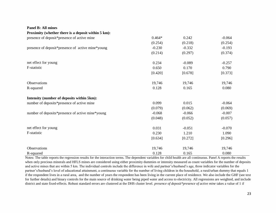
23

Panel B: All mines Proximity (whether there is a deposit within 5 km): presence of deposit*presence of active mine 0.464* 0.242 -0.064

(0.254) (0.218) (0.254)

presence of deposit*presence of active mine*young -0.230 -0.332 -0.193

(0.214) (0.297) (0.374)

net effect for young 0.234 -0.089 -0.257

F-statistic 0.650 0.170 0.790

[0.420] [0.678] [0.373]

Observations 19,746 19,746 19,746

R-squared 0.128 0.165 0.080

Intensity (number of deposits within 5km): number of deposits*presence of active mine 0.099 0.015 -0.064

(0.079) (0.062) (0.069)

number of deposits*presence of active mine*young -0.068 -0.066 -0.007

(0.048) (0.052) (0.057)

net effect for young 0.031 -0.051 -0.070

F-statistic 0.230 1.210 1.090

[0.634] [0.272] [0.296]

Observations 19,746 19,746 19,746

R-squared 0.128 0.165 0.080 Notes: The table reports the regression results for the interaction terms. The dependent variables for child health are all continuous. Panel A reports the results

when only precious minerals and HFLS mines are considered using either proximity dummies or intensity measured as count variables for the number of deposits

and active mines that are within 5 km. The individual controls include the difference in wife and partner’s/husband’s age, three indicator variables for the

partner’s/husband’s level of educational attainment, a continuous variable for the number of living children in the household, a rural/urban dummy that equals 1

if the respondent lives in a rural area, and the number of years the respondent has been living in the current place of residence. We also include the GHF (see text

for further details) and binary controls for the main source of drinking water being piped water and access to electricity. All regressions are weighted, and include

district and state fixed-effects. Robust standard errors are clustered at the DHS cluster level. presence of deposit*presence of active mine takes a value of 1 if

24

there is a deposit and an active mine within 5 km of the DHS cluster to which the respondent belongs. number of deposits*presence of active mine equals the

number of deposits within 5 km of the DHS cluster interacted with the dummy for the presence of active mine within 5 km of the same cluster. “young” is a

binary variable that equals 1 if the female respondent is in the age group 15-25 years old. Coefficients and standard errors for the interactions with the young

variable for proximity and intensity are the same in the case of HFLS mines due to rounding to three decimal digits. We report net effects on the young with

associated p-values in brackets. *** Denotes significance at the 1% level, ** at the 5% level and * at the 10% level.

25

Appendix Table 5: Impact of mines on men’s employment

currently is in the

working workforce agriculture

(1) (2) (3)

Panel A: HFLS mines Proximity (whether there is a deposit within 5 km): presence of deposit*presence of HFLS active mine 0.036 0.008 0.170*

(0.066) (0.027) (0.101)

Observations 8,799 8,789 8,789

R-squared 0.093 0.055 0.333

Intensity (number of deposits within 5km): number of deposits*presence of HFLS active mine 0.038 0.009 0.166*

(0.065) (0.027) (0.098)

Observations 8,799 8,789 8,789

R-squared 0.093 0.055 0.333

Panel B: All mines Proximity (whether there is a deposit within 5 km): presence of deposit*presence of active mine 0.030 0.029* -0.034

(0.028) (0.016) (0.057)

presence of deposit*presence of active mine*young -0.204 -0.224 -0.028

(0.171) (0.181) (0.187)

net effect for young -0.174 -0.195 -0.062

F-statistic 1.010 1.180 0.110

[0.316] [0.278] [0.738]

Observations 35,174 35,129 35,129

R-squared 0.076 0.040 0.303

26

Intensity (number of deposits within 5km): number of deposits*presence of active mine 0.012 0.010 0.014

(0.008) (0.006) (0.024)

number of deposits*presence of active mine*young -0.106 -0.116 -0.035

(0.089) (0.091) (0.085)

net effect for young -0.094 -0.106 -0.021

F-statistic 1.120 1.360 0.060

[0.290] [0.244] [0.805]

Observations 35,174 35,129 35,129

R-squared 0.076 0.040 0.303 Notes: The table reports the coefficients on the interaction terms. Panel A reports the results when only precious minerals and HFLS mines are considered using

either proximity dummies or intensity measured as count variables for the number of deposits and active mines that are within 5 km. Sample sizes for young men

are too small to be able to estimate differential and net effects for young men near HFLS mines. In column (1), the binary dependent variable equals to 1 if the

male respondent says that he is currently working, and in column (2), the indicator variable takes a value of 1 if he is in the workforce. In column (3),

"agriculture" equals 1 if he is employed in farming, fishing, hunting, or logging. The individual controls include the difference in husband and partner’s/wife’s

age, three indicator variables for the man’s highest level of educational attainment (with the excluded category being “no education at all”), a continuous variable

for the number of living children in the household, a rural/urban dummy that equals 1 if the respondent lives in a rural area, and the number of years the

respondent has been living in the current place of residence. We also include the GHF (see text for further details) and binary controls for the main source of

drinking water being piped water and access to electricity. All regressions include district and state fixed-effects. Robust standard errors are clustered at the DHS

cluster level. All regressions are weighted. presence of deposit*presence of active mine takes a value of 1 if there is a deposit and an active mine within 5 km of

the DHS cluster to which the respondent belongs. number of deposits*presence of active mine equals the number of deposits within 5 km of the DHS cluster

interacted with the dummy for the presence of an active mine within 5 km of the same cluster. “young” is a binary variable that equals 1 if the male respondent is

15-25 years old. We report net effects on the young with associated p-values in brackets. *** Denotes significance at the 1% level, ** at the 5% level and * at the

10% level.

27

Appendix Table 6: Impact of mines on men’s attitudes to domestic violence

Beating justified if the wife:

goes out argues does not

without neglects with refuses cook food

permission children husband sex properly index

(1) (2) (3) (4) (5) (6)

Panel A: HFLS mines Proximity (whether there is a deposit within 5 km): presence of deposit*presence of HFLS active mine -0.176* 0.093 -0.047 -0.242** -0.247* -0.148

(0.104) (0.089) (0.105) (0.114) (0.129) (0.091)

Observations 8,389 8,384 8,377 8,356 8,374 8,300

R-squared 0.164 0.170 0.133 0.118 0.116 0.195

Intensity (number of deposits within 5km): number of deposits*presence of HFLS active mine -0.184* 0.080 -0.046 -0.245** -0.250** -0.154*

(0.103) (0.087) (0.104) (0.113) (0.128) (0.090)

Observations 8,389 8,384 8,377 8,356 8,374 8,300

R-squared 0.164 0.169 0.133 0.119 0.116 0.195

Panel B: All mines Proximity (whether there is a deposit within 5 km): presence of deposit*presence of active mine 0.005 -0.016 0.006 -0.003 -0.027 -0.008

(0.057) (0.069) (0.063) (0.051) (0.054) (0.052)

presence of deposit*presence of active mine*young 0.318** 0.284** 0.284** 0.078 0.058 0.200*

(0.135) (0.128) (0.128) (0.135) (0.127) (0.111)

net effect for young 0.323 0.268 0.290 0.074 0.032 0.191

F-statistic 4.820 3.820 4.580 0.280 0.060 2.640

[0.028] [0.051] [0.033] [0.600] [0.809] [0.104]

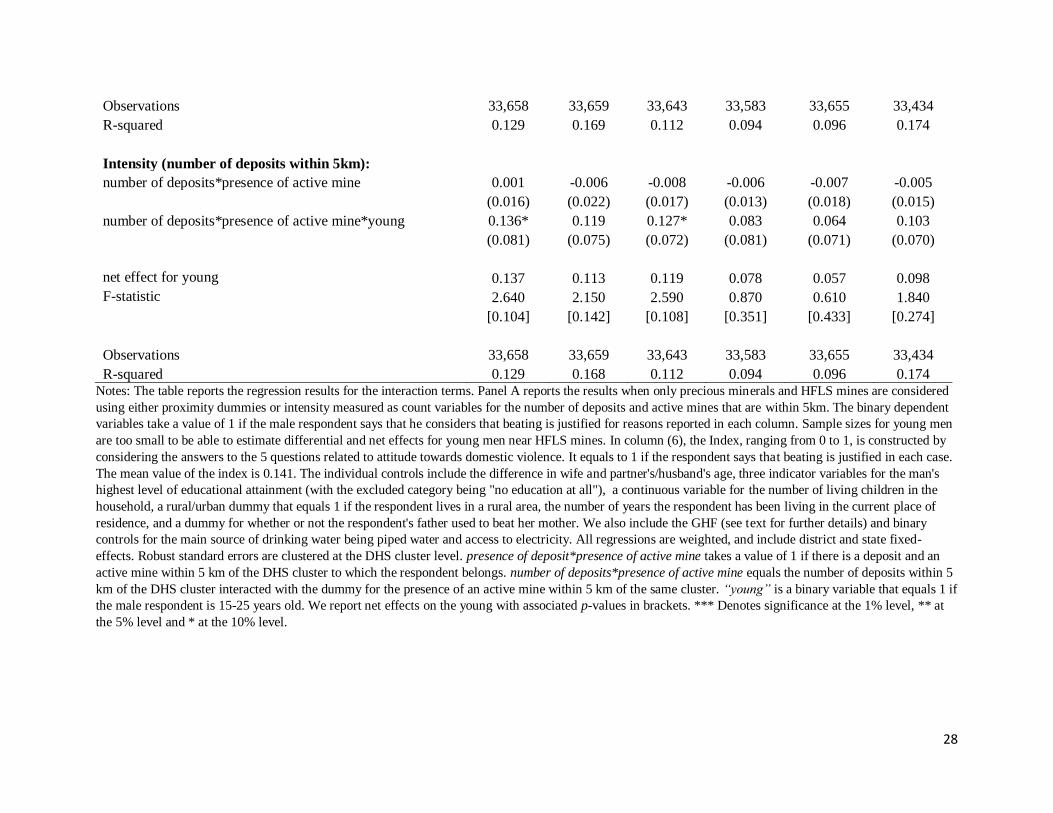
28

Observations 33,658 33,659 33,643 33,583 33,655 33,434

R-squared 0.129 0.169 0.112 0.094 0.096 0.174

Intensity (number of deposits within 5km): number of deposits*presence of active mine 0.001 -0.006 -0.008 -0.006 -0.007 -0.005

(0.016) (0.022) (0.017) (0.013) (0.018) (0.015)

number of deposits*presence of active mine*young 0.136* 0.119 0.127* 0.083 0.064 0.103

(0.081) (0.075) (0.072) (0.081) (0.071) (0.070)

net effect for young 0.137 0.113 0.119 0.078 0.057 0.098

F-statistic 2.640 2.150 2.590 0.870 0.610 1.840

[0.104] [0.142] [0.108] [0.351] [0.433] [0.274]

Observations 33,658 33,659 33,643 33,583 33,655 33,434

R-squared 0.129 0.168 0.112 0.094 0.096 0.174 Notes: The table reports the regression results for the interaction terms. Panel A reports the results when only precious minerals and HFLS mines are considered

using either proximity dummies or intensity measured as count variables for the number of deposits and active mines that are within 5km. The binary dependent

variables take a value of 1 if the male respondent says that he considers that beating is justified for reasons reported in each column. Sample sizes for young men

are too small to be able to estimate differential and net effects for young men near HFLS mines. In column (6), the Index, ranging from 0 to 1, is constructed by

considering the answers to the 5 questions related to attitude towards domestic violence. It equals to 1 if the respondent says that beating is justified in each case.

The mean value of the index is 0.141. The individual controls include the difference in wife and partner's/husband's age, three indicator variables for the man's

highest level of educational attainment (with the excluded category being "no education at all"), a continuous variable for the number of living children in the

household, a rural/urban dummy that equals 1 if the respondent lives in a rural area, the number of years the respondent has been living in the current place of

residence, and a dummy for whether or not the respondent's father used to beat her mother. We also include the GHF (see text for further details) and binary

controls for the main source of drinking water being piped water and access to electricity. All regressions are weighted, and include district and state fixed-

effects. Robust standard errors are clustered at the DHS cluster level. presence of deposit*presence of active mine takes a value of 1 if there is a deposit and an

active mine within 5 km of the DHS cluster to which the respondent belongs. number of deposits*presence of active mine equals the number of deposits within 5

km of the DHS cluster interacted with the dummy for the presence of an active mine within 5 km of the same cluster. “young” is a binary variable that equals 1 if

the male respondent is 15-25 years old. We report net effects on the young with associated p-values in brackets. *** Denotes significance at the 1% level, ** at

the 5% level and * at the 10% level.

29

Appendix Table 7: Impact of mines on men’s attitudes to shared decision-making

Final say in decision-making related to:

visits to

major daily wife’s wife’s no. of his his

purchases needs family earnings children index earnings healthcare

(1) (2) (3) (4) (5) (6) (7) (8)

Panel A: HFLS mines

Proximity (whether there is a deposit within 5 km):

presence of deposit*presence of HFLS active mine 0.331*** 0.478 0.248** 0.280* 0.129 0.244** 0.196 0.362***

(0.105) (0.138) (0.114) (0.146) (0.087) (0.102) (0.174) (0.124)

Observations 8,769 8,769 8,758 8,673 8,764 8,599 8,571 8,799

R-squared 0.130 0.116 0.084 0.071 0.089 0.115 0.108 0.095

Intensity (number of deposits within 5km):

number of deposits*presence of HFLS active mine 0.326*** 0.061 0.250** 0.293** 0.136* 0.249** 0.197 0.352***

(0.010) (0.135) (0.108) (0.139) (0.083) (0.098) (0.169) (0.118)

Observations 8,769 8,769 8,758 8,673 8,764 8,599 8,571 8,799

R-squared 0.130 0.116 0.084 0.082 0.089 0.115 0.108 0.096

Panel B: All mines

Proximity (whether there is a deposit within 5 km):

presence of deposit*presence of active mine 0.157** 0.173** 0.081 0.051 0.054 0.096* 0.075 0.040

(0.074) (0.082) (0.056) (0.061) (0.035) (0.050) (0.073) (0.084)

presence of deposit*presence of active mine*young -0.198 0.080 -0.086 0.005 0.162*** 0.073 0.022 0.134

(0.204) (0.144) (0.136) (0.140) (0.059) (0.106) (0.171) (0.167)

net effect for young -0.040 0.253 -0.005 0.056 0.216 0.170 0.097 0.174

F-statistic 0.030 2.810 0.000 0.130 15.080 2.180 0.300 0.950

[0.852] [0.094] [0.975] [0.718] [0.000] [0.140] [0.582] [0.330]

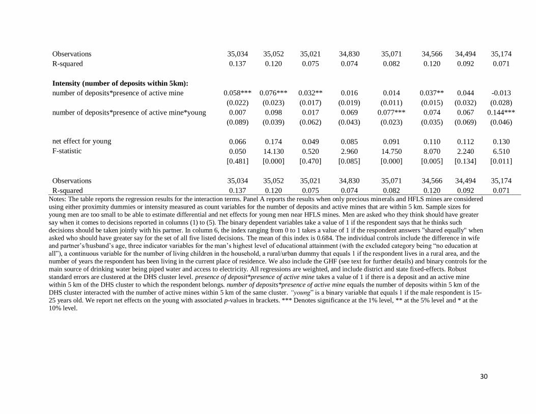
30

Observations 35,034 35,052 35,021 34,830 35,071 34,566 34,494 35,174

R-squared 0.137 0.120 0.075 0.074 0.082 0.120 0.092 0.071

Intensity (number of deposits within 5km):

number of deposits*presence of active mine 0.058*** 0.076*** 0.032** 0.016 0.014 0.037** 0.044 -0.013

(0.022) (0.023) (0.017) (0.019) (0.011) (0.015) (0.032) (0.028)

number of deposits*presence of active mine*young 0.007 0.098 0.017 0.069 0.077*** 0.074 0.067 0.144***

(0.089) (0.039) (0.062) (0.043) (0.023) (0.035) (0.069) (0.046)

net effect for young 0.066 0.174 0.049 0.085 0.091 0.110 0.112 0.130

F-statistic 0.050 14.130 0.520 2.960 14.750 8.070 2.240 6.510

[0.481] [0.000] [0.470] [0.085] [0.000] [0.005] [0.134] [0.011]

Observations 35,034 35,052 35,021 34,830 35,071 34,566 34,494 35,174

R-squared 0.137 0.120 0.075 0.074 0.082 0.120 0.092 0.071 Notes: The table reports the regression results for the interaction terms. Panel A reports the results when only precious minerals and HFLS mines are considered

using either proximity dummies or intensity measured as count variables for the number of deposits and active mines that are within 5 km. Sample sizes for

young men are too small to be able to estimate differential and net effects for young men near HFLS mines. Men are asked who they think should have greater

say when it comes to decisions reported in columns (1) to (5). The binary dependent variables take a value of 1 if the respondent says that he thinks such

decisions should be taken jointly with his partner. In column 6, the index ranging from 0 to 1 takes a value of 1 if the respondent answers "shared equally" when

asked who should have greater say for the set of all five listed decisions. The mean of this index is 0.684. The individual controls include the difference in wife and partner’s/husband’s age, three indicator variables for the man’s highest level of educational attainment (with the excluded category being “no education at

all”), a continuous variable for the number of living children in the household, a rural/urban dummy that equals 1 if the respondent lives in a rural area, and the

number of years the respondent has been living in the current place of residence. We also include the GHF (see text for further details) and binary controls for the

main source of drinking water being piped water and access to electricity. All regressions are weighted, and include district and state fixed-effects. Robust

standard errors are clustered at the DHS cluster level. presence of deposit*presence of active mine takes a value of 1 if there is a deposit and an active mine

within 5 km of the DHS cluster to which the respondent belongs. number of deposits*presence of active mine equals the number of deposits within 5 km of the

DHS cluster interacted with the number of active mines within 5 km of the same cluster. “young” is a binary variable that equals 1 if the male respondent is 15-

25 years old. We report net effects on the young with associated p-values in brackets. *** Denotes significance at the 1% level, ** at the 5% level and * at the

10% level.

31

Appendix Table 8: Summary statistics for individual and district characteristics in control and treatment groups

Control Treatment

mean standard deviation mean standard deviation difference (1) (2) (3) (4) (5)

Individual/districts' characteristics young (age 15-25) 0.145 0.353 0.166 0.372 -0.02

age difference between wife and partner/husband 5.199 3.836 5.236 3.873 -0.037

educational attainment: no education at all 0.344 0.475 0.35 0.477 -0.006

some or all primary school 0.152 0.359 0.138 0.345 0.014

some secondary school 0.37 0.483 0.349 0.477 0.021

completed secondary school or higher 0.135 0.342 0.163 0.369 -0.028*

number of living children in household 2.529 1.228 2.43 1.231 0.099**

husband's educational attainment: no education at all 0.183 0.388 0.204 0.403 -0.021

some or all primary school 0.195 0.398 0.137 0.344 0.058**

some secondary school 0.402 0.492 0.452 0.498 -0.05

completed secondary school or higher 0.207 0.407 0.204 0.403 0.003

rural/urban 0.853 0.354 0.651 0.477 0.202***

years living in place of residence 15.038 11.616 15.777 12.157 -0.739

Global Human Footprint (index, in log) 3.632 0.332 3.842 0.343 -0.210***

water 0.485 0.5 0.553 0.497 -0.068***

electricity 0.9 0.3 0.928 0.258 -0.028***

Main outcomes

domestic violence index 0.242 0.305 0.226 0.324 0.015

barriers to health care index 0.275 0.339 0.212 0.32 0.063***

final-say in decision-making index 1 0.817 0.288 0.802 0.323 0.015

final-say in decision-making index 2 0.785 0.341 0.764 0.362 0.022

Mechanism related outcomes

currently working 0.287 0.454 0.28 0.449 0.007

is in workforce 0.329 0.471 0.356 0.479 -0.026

services 0.043 0.204 0.089 0.285 -0.046**

32

agriculture 0.216 0.413 0.186 0.389 0.03

manufacturing 0.068 0.252 0.08 0.271 -0.012

literate 0.547 0.498 0.617 0.486 -0.070***

height 151.885 5.840 152.263 5.937 -0.378**

BMI 22.045 3.980 22.415 4.225 -0.371***

overweight/obese 0.204 0.403 0.231 0.422 -0.027**

underweight 0.193 0.395 0.173 0.378 0.020*

HBA 11.528 1.702 11.635 1.614 -0.107**

anemic 0.557 0.497 0.544 0.498 0.013

high BP 0.124 0.330 0.109 0.311 0.016*

high glucose 0.503 0.500 0.506 0.500 -0.04

HAZ -1.445 1.58 -1.258 1.702 -0.187*

WAZ -1.561 1.165 -1.476 1.220 -0.086

WHZ -1.071 1.347 -1.081 1.465 0.011

earns cash 0.048 0.215 0.047 0.212 0.001

earns more than him 0.005 0.074 0.011 0.103 -0.005*

owns house alone 0.016 0.124 0.025 0.155 -0.009**

owns house alone/jointly 0.053 0.224 0.061 0.240 -0.008

knows about loan program 0.078 0.269 0.087 0.283 -0.009

knows about and has taken loan 0.022 0.146 0.022 0.146 0.000

any health insurance 0.153 0.360 0.233 0.423 -0.080***

insurance from employer 0.002 0.047 0.005 0.072 -0.003

insurance from central/state government 0.077 0.266 0.130 0.336 -0.053*** Notes: In the pre-treatment phase, the control group has no deposit within 5 km of each cluster and no active mine within 99 km (since 100 km is the limit of our

data, we use a value very close to 100 km). The treatment group has a deposit within 5 km of each cluster but no active mine within 15 km. We run tests for pre-

trends using future mines only, and then compare treatment and control groups in years before the mine opens. We report the mean and standard deviation for

each of the control variables and for differences in the means. See Table 1a for further details on each variable. ***p<0.01, **p<0.05, *p<0.10 for the t-test.

33

Appendix Table 9: Impact of past/future mines on attitudes towards domestic violence

Beating justified if the wife:

goes out

without

permission

neglects

children

argues

with

husband

refuses

sex

does not

cook food

properly index

emotional

violence

(1) (2) (3) (4) (5) (6) (7)

Panel B: All mines Proximity (whether there is a deposit within 5 km): presence of deposit*presence of past/future mine 0.214*** 0.120 0.074 -0.227** -0.050 0.029 -0.186**

(0.077) (0.082) (0.089) (0.073) (0.099) (0.052) (0.093)

presence of deposit*presence of past/future mine*young -0.202 -0.128* -0.062 0.081 0.030 -0.056 0.095

(0.098) (0.074) (0.107) (0.103) (0.126) (0.077) (0.081)

net effect for young 0.013 -0.008 0.012 -0.145 -0.020 -0.027 -0.092

F-statistic 0.010 0.010 0.020 1.480 0.010 0.080 0.880

[0.920] [0.939] [0.901] [0.224] [0.907] [0.773] [0.349]

Observations 20,298 20,316 20,282 20,212 20,305 20,068 20,367

R-squared 0.192 0.221 0.142 0.082 0.101 0.206 0.120 Notes: The binary dependent variables take a value of 1 if the female respondent says that she considers that beating is justified for reasons reported in each

column. In column (6), the index ranging from 0 to 1 is constructed by considering the answers to the 5 questions related to attitude towards domestic violence. It

equals 1 if the respondent says that beating is justified in each case. The mean index is 0.241. In column (7), “emotional violence" is a variable that equals 1 if the

respondent says that she has experienced one of the three possible examples of emotional violence. The sample is restricted to women who were interviewed for

domestic violence only. The individual controls include the difference in wife and partner's/husband's age, three indicator variables for the woman's highest level

of educational attainment (with the excluded category being "no education at all"), similar indicator variables for the partner's/husband's level of educational

attainment, a continuous variable for the number of living children in the household, a rural/urban dummy that equals 1 if the respondent lives in a rural area, the

number of years the respondent has been living in the current place of residence and a dummy for whether or not the respondent's father used to beat her mother.

We also include the GHF (see text for further details) and binary controls for the main source of drinking water being piped water and access to electricity. All

regressions are weighted, and include district and state fixed-effects. Robust standard errors clustered at the DHS cluster level. presence of deposit*presence of

past/future mine takes a value of 1 if there is a deposit and a past/future mine within 5 km of the DHS cluster to which the respondent belongs. “young” is a

binary variable that equals 1 if the female respondent is 15-25 years old. We report net effects on the young with associated p-values in brackets. *** Denotes

significance at the 1% level, ** at the 5% level and * at the 10% level.

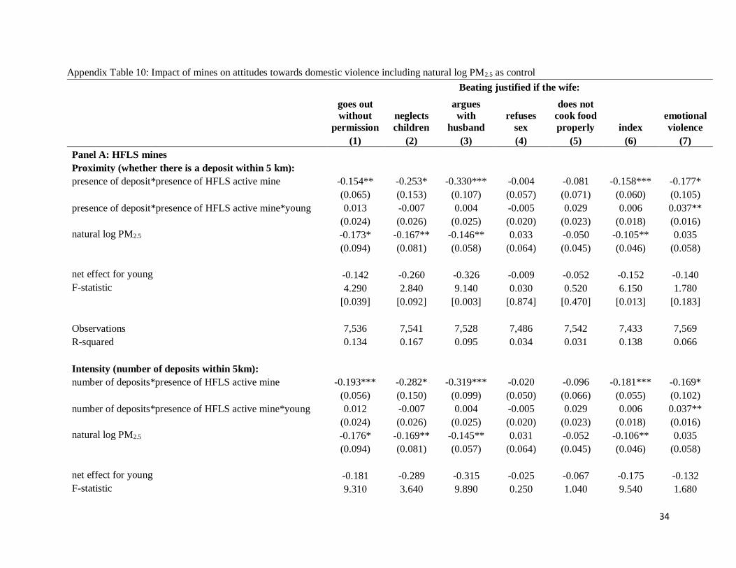
34

Appendix Table 10: Impact of mines on attitudes towards domestic violence including natural log PM2.5 as control

Beating justified if the wife:

goes out

without

permission

neglects

children

argues

with

husband

refuses

sex

does not

cook food

properly index

emotional

violence

(1) (2) (3) (4) (5) (6) (7)

Panel A: HFLS mines Proximity (whether there is a deposit within 5 km): presence of deposit*presence of HFLS active mine -0.154** -0.253* -0.330*** -0.004 -0.081 -0.158*** -0.177*

(0.065) (0.153) (0.107) (0.057) (0.071) (0.060) (0.105)

presence of deposit*presence of HFLS active mine*young 0.013 -0.007 0.004 -0.005 0.029 0.006 0.037**

(0.024) (0.026) (0.025) (0.020) (0.023) (0.018) (0.016)

natural log PM2.5 -0.173* -0.167** -0.146** 0.033 -0.050 -0.105** 0.035

(0.094) (0.081) (0.058) (0.064) (0.045) (0.046) (0.058)

net effect for young -0.142 -0.260 -0.326 -0.009 -0.052 -0.152 -0.140

F-statistic 4.290 2.840 9.140 0.030 0.520 6.150 1.780

[0.039] [0.092] [0.003] [0.874] [0.470] [0.013] [0.183]

Observations 7,536 7,541 7,528 7,486 7,542 7,433 7,569

R-squared 0.134 0.167 0.095 0.034 0.031 0.138 0.066

Intensity (number of deposits within 5km): number of deposits*presence of HFLS active mine -0.193*** -0.282* -0.319*** -0.020 -0.096 -0.181*** -0.169*

(0.056) (0.150) (0.099) (0.050) (0.066) (0.055) (0.102)

number of deposits*presence of HFLS active mine*young 0.012 -0.007 0.004 -0.005 0.029 0.006 0.037**

(0.024) (0.026) (0.025) (0.020) (0.023) (0.018) (0.016)

natural log PM2.5 -0.176* -0.169** -0.145** 0.031 -0.052 -0.106** 0.035

(0.094) (0.081) (0.057) (0.064) (0.045) (0.046) (0.058)

net effect for young -0.181 -0.289 -0.315 -0.025 -0.067 -0.175 -0.132

F-statistic 9.310 3.640 9.890 0.250 1.040 9.540 1.680

35

[0.002] [0.057] [0.002] [0.621] [0.308] [0.002] [0.195]

Observations 7,536 7,541 7,528 7,486 7,542 7,433 7,569

R-squared 0.133 0.167 0.095 0.034 0.031 0.138 0.066

Panel B: All mines Proximity (whether there is a deposit within 5 km): presence of deposit*presence of active mine -0.138** -0.113* -0.117** -0.070* -0.064 -0.090* -0.031

(0.061) (0.067) (0.059) (0.041) (0.050) (0.047) (0.062)

presence of deposit*presence of active mine*young 0.019 -0.007 0.103 -0.073** -0.103** -0.024 -0.126***

(0.080) (0.078) (0.100) (0.037) (0.046) (0.054) (0.046)

natural log PM2.5 -0.052* -0.031 -0.040 -0.002 -0.020 -0.030 0.032*

(0.031) (0.029) (0.026) (0.022) (0.021) (0.020) (0.018)

net effect for young -0.119 -0.121 -0.014 -0.143 -0.167 -0.114 -0.157

F-statistic 1.850 2.460 0.020 16.920 14.250 5.320 12.270

[0.174] [0.117] [0.877] [0.000] [0.000] [0.021] [0.001]

Observations 30,005 30,010 29,973 29,878 30,005 29,670 30,107

R-squared 0.117 0.142 0.080 0.030 0.045 0.122 0.062

Intensity (number of deposits within 5km): number of deposits*presence of active mine -0.030* -0.035* -0.004 -0.001 -0.000 -0.010 -0.001

(0.017) (0.019) (0.025) (0.015) (0.019) (0.014) (0.019)

number of deposits*presence of active mine*young 0.006 0.005 0.034 -0.036*** -0.040** -0.010 -0.048***

(0.026) (0.023) (0.032) (0.011) (0.016) (0.015) (0.013)

natural log PM2.5 -0.052* -0.030 -0.041 -0.002 -0.021 -0.031 0.032*

(0.031) (0.029) (0.026) (0.022) (0.021) (0.020) (0.018)

net effect for young -0.024 -0.030 0.030 -0.037 -0.040 -0.019 -0.048

F-statistic 0.590 1.240 0.770 8.420 4.480 1.280 10.080

[0.444] [0.265] [0.379] [0.004] [0.034] [0.258] [0.002]

36

Observations 30,005 30,010 29,973 29,878 30,005 29,670 30,107

R-squared 0.117 0.142 0.080 0.029 0.045 0.121 0.062 Notes: The table reports the regression results for the interaction terms. Panel A reports the results when only precious minerals and HFLS mines are considered

using either proximity dummies or intensity measured as count variables for the number of deposits and active mines that are within 5km. The binary dependent

variables take a value of 1 if the female respondent says that she considers that beating is justified for reasons reported in each column. In column (6), the index,

ranging from 0 to 1, is constructed by considering the answers to the 5 questions related to attitude towards domestic violence. It equals to 1 if the respondent

says that beating is justified in each case. The mean value of the index is 0.241. In column (7), “emotional violence" is a variable that equals 1 if the respondent

says that she has experienced one of the three possible examples of emotional violence listed. The sample is restricted to women who were interviewed for

domestic violence only. The individual controls include the difference in wife and partner's/husband's age, three indicator variables for the woman's highest level

of educational attainment (with the excluded category being "no education at all"), similar indicator variables for the partner's/husband's level of educational

attainment, a continuous variable for the number of living children in the household, a rural/urban dummy that equals 1 if the respondent lives in a rural area, the

number of years the respondent has been living in the current place of residence and a dummy for whether or not the respondent's father used to beat her mother.

We also include the GHF (see text for further details) and binary controls for the main source of drinking water being piped water and access to electricity. We

exclude district fixed-effects as the PM2.5 data are at the district level. All regressions are weighted and include state fixed-effects. Robust standard errors

clustered at the DHS cluster level. presence of deposit*presence of active mine takes a value of 1 if there is a deposit and an active mine within 5 km of the DHS

cluster to which the respondent belongs. number of deposits*presence of active mine equals the number of deposits within 5 km of the DHS cluster interacted

with the dummy for the presence of an active mine within 5 km of the same cluster. “young” is a binary variable that equals 1 if the female respondent is 15-25

years old. We report net effects on the young with associated p-values in square brackets. *** Denotes significance at the 1% level, ** at the 5% level and * at

the 10% level.