Methodology for Evaluating Static Six-Degree-of-Freedom(6DoF) Perception Systems

Tommy Chang, Tsai Hong,Joe Falco, Michael Shneier

National Institute of Standard and TechnologyGaithersburg, Maryland

{tchang,hongt,falco,shneier}@nist.gov

Mili Shah, Roger EastmanLoyola University Maryland

Baltimore, Maryland{mishah,reastman}@loyola.edu

ABSTRACTIn this paper, we apply two fundamental approaches to-ward evaluating a static, vision based, six-degree-of-freedom(6DoF) pose determination system that measures the po-sition and orientation of a part. The first approach usesgroundtruth carefully obtained from a laser tracker and thesecond approach doesn’t use any external groundtruth. Theevaluation procedure focuses on characterizing both the sys-tem’s accuracy and precision as well as the e!ect of objectviewpoints.

For the groundtruth method, we first use a laser trackerfor system calibration and then compare the calibrated out-put with the surveyed pose. In the method without externalgroundtruth, we evaluate the e!ect of viewpoint factors onthe system’s performance.

Categories and Subject DescriptorsC.4 [Performance of Systems]: Performance attributes;B.8.2 [Performance and Reliability]: Performance Anal-ysis and Design Aids

General TermsPerformance, Measurement, Standardization, Experimenta-tion

KeywordsLaser Tracker, Ground Truth, 6DOF metrology, PerformanceEvaluation

1. INTRODUCTIONAs part of the ongoing e!ort to standardize characteri-

zation and evaluation of 6DoF (six-degree-of-freedom) posedetermination systems, we present a performance evaluationof a static, vision-based 6DoF system that measures the po-sition and orientation of a part, also referred to as an objectin this paper.

(c) 2010 Association for Computing Machinery. ACM acknowledges thatthis contribution was authored or co-authored by a contractor or affiliateof the U.S. Government. As such, the Government retains a nonexclusive,royalty-free right to publish or reproduce this article, or to allow others todo so, for Government purposes only.PerMIS ’10, September 28-30, 2010, Baltimore, MD, USA.Copyright c! 2010 ACM 978-1-4503-0290-6-9/28/10 ...$10.00.

In general, performance evaluation methods can be groupedinto two categories: with and without external groundtruth.We adopt the typical definition of external groundtruth asmeasurements obtained independently and simultaneouslyby an accurate system having better precision by more thanone order of magnitude. Laser tracker, industrial robot arm,and computer graphics simulation are some examples of ex-ternal groundtruth used for evaluating vision-based 6DoFsystems [3, 14, 17].

Regardless of whether external groundtruth is employedor not, the goal is to obtain a quantitative understandingof the performance. “[The task of performance character-ization] can be understood as an entirely statistical task.”[16]

In this paper, we employ methods with and without ex-ternal groundtruth to quantitatively determine the system’saccuracy and precision and the e!ect of di!erent viewpointson its precision. For the groundtruth method, we first usea laser tracker for system calibration and then compare thecalibrated result to the surveyed pose. For the method with-out using any external groundtruth, we estimate the systemprecision under various object viewpoints.

2. RELATED WORKHere we review some common methods applied to perfor-

mance characterization and evaluation of pose determina-tion systems and algorithms [9, 3, 19, 18, 14, 13]. Other rel-evant work includes evaluation and characterization of rang-ing sensors such as LADAR (LAser Detection And Ranging)[8, 23, 1] and stereo vision [11, 17, 22], as well as algorithmsincluding image registration [21, 5, 20, 10, 7], segmentation,and classification [2, 4]. The majority of these articles con-duct experimental studies to characterize the performanceunder a set of controlled conditions.

In typical groundtruth methods, external groundtruth isused to compute error, which are then used to infer theunknown parameters in the error population/distribution.A statistic such as mean, standard deviation, min, and max,is computed from an error sample.

The system under test can be thought of as an estimatorof the true quantity measured independently and simultane-ously by the external groundtruth system. In statistics, anestimator has two properties: bias and variance. The biasmeasures the average accuracy while the variance measuresthe precision or reliability of the estimator [15].

One way to determine the bias of a pose determinationsystem is to first transform data both from the groundtruthand the system under test to a common coordinate frame.

Then, the bias is the averaged di!erences between the twotransformed data sets. However, in most cases, the trans-formation between the two coordinate frames is not knownexactly and any error in the transformation will contributeto the overall bias estimate. A robust calibration system[12] is needed to estimate the transformation.

Approaches without external groundtruth typically com-pute variance from the data. These variances are used tocharacterize and infer the e!ect of system’s precision underdi!erent conditions, or levels of the experimental factor. In[17], a dynamic 6DoF system’s performance was character-ized by the standard deviation of the regression residual; al-though no external groundtruth was used, the motion modelof the object was known. [23] an [8] characterized a LADARsystem’s precision (as well as accuracy) under experimentalfactors including target distance, surface property, and inci-dent angle. Statistical inference could be used to generalizeand test hypotheses about the system performance.

Another approach without external groundtruth relies onan objective metric that correlates with the system’s per-formance. Groundtruth is still involved but only during thedesign and verification of the objective metric. Performanceevaluation can then be done using only that objective metricalone. Examples of this approach include [22, 10, 7, 4]. Ingeneral, the objective metric is shown to vary monotonouslywith the amount of error, which is computed from the ex-ternal groundtruth.

Unlike the previous two approaches, [9] compares the ro-bustness of two pose estimation techniques analytically us-ing sensitivity analysis in terms of variance amplification. [2]shows another example without the use of external ground-truth. Its idea is based on the common agreement metricapplied to brain tissue classification: “if nine out of ten al-gorithms classify voxel x in subject i as white matter thenone says there is a 90% chance this voxel truly is white mat-ter.”

In this paper, we adopt the estimator approach that treatsthe 6DoF system under test as an estimator to the true pose.Performance of the 6DoF system can then be characterizedby the estimator’s bias and variance.

3. METHODSIn this section, we describe approaches with and without

external groundtruth for characterizing a commercial static,vision-based, 6DoF pose determination system.

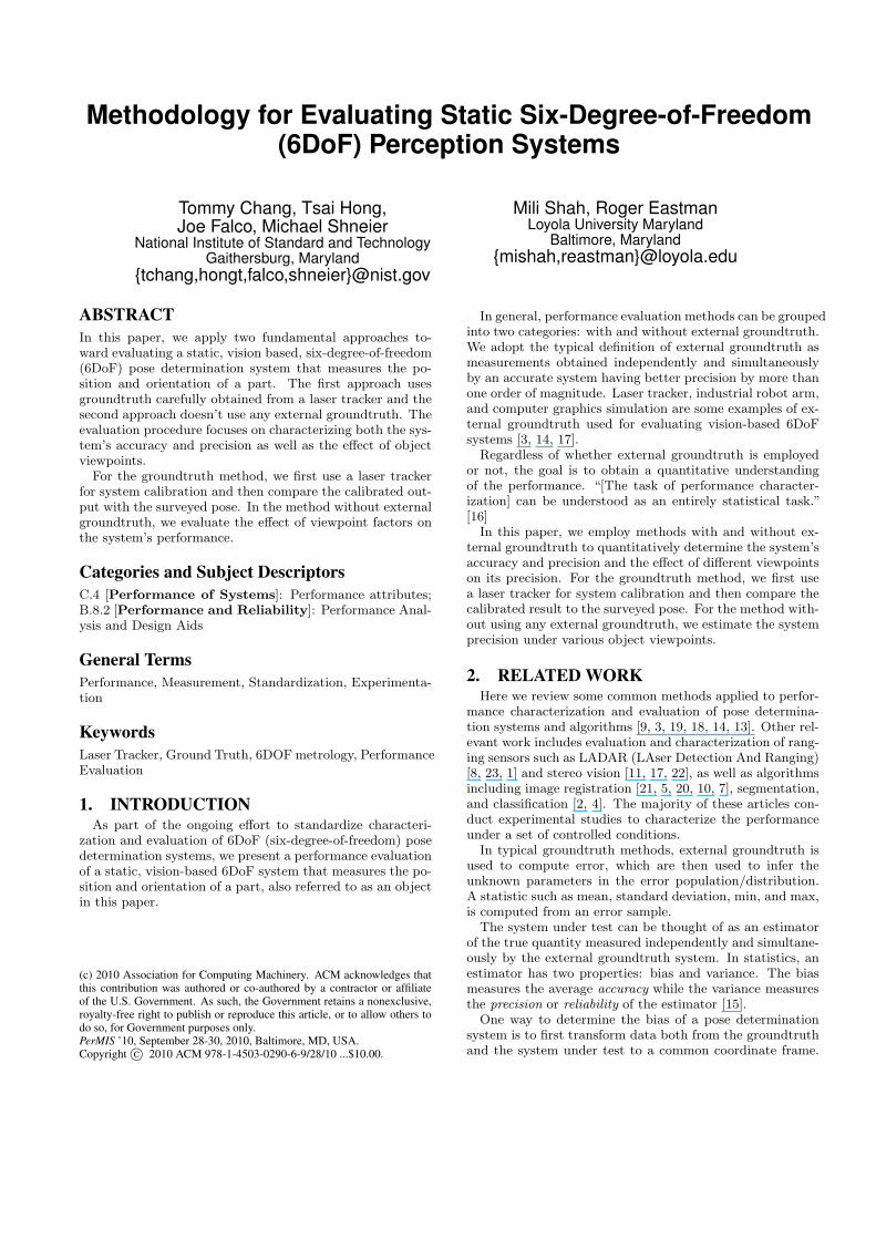
3.1 The Static 6Dof Vision-Based SystemThe vision system consists of a camera mounted on a robot

arm (see Figure 1). The camera used in this study has a focallength of 6mm and a resolution of 782 by 582 pixels. Thereare four coordinate frames involved:

1. Robot Frame: A coordinate frame located and definedat the base of the robot arm.

2. Object Frame (O): The coordinate frame associatedwith the object.

3. Camera Frame (C): The coordinate frame associatedwith the camera, which is fixed on the robot arm.

4. Source Frame (SF ): A user-defined global coordinateframe relative to the robot frame. This frame is usuallyconveniently aligned with the object in order for therobot to perform operations relating to the object.

Figure 1: The vision system and the laser trackergroundtruth system.

The output from the vision-based system consists of ob-ject and camera poses for every measurement. Specifically,the outputs are three 4x4 homogeneous matrices:

(i) SF HO, transformation from the object frame to thesource frame. SF is the source frame and O is theobject. SF is stationary and O is also stationary.

(ii) SF HC , transformation from the camera frame to thesource frame. SF is the source frame and C is thecamera. In this case, SF is stationary and C is moving.

(iii) OHC , transformation from the camera frame to theobject frame. This is obtained by combining (i) and(ii).

Although the measurement takes 130 of a second to acquire

an image, the subsequent processing time varies. The robotarm always stop moving when taking the measurement.

3.2 The GroundTruth SystemThe groundtruth system used in our work is a calibrated

6DoF laser tracker having a precision (two sigma) of ± 5micrometer per meter. The laser tracker has two physicalcomponents: a portable active target that measures its ownorientation and a base unit that measures the position ofthe active target. Together they provide the complete 6DoFpose of the active target.

There are two coordinate frames in the groundtruth sys-tem:

• Laser Tracker Frame (LT ): A coordinate frame locatedat the base unit of the laser tracker.

• Active Target Frame (AT ): The coordinate frame as-sociated with the active target.

In our setup, we attached the active target next to thecamera on the robot arm of the vision system. The outputfrom the groundtruth system is the pose (represented by a4x4 homogeneous matrix) of the active target:

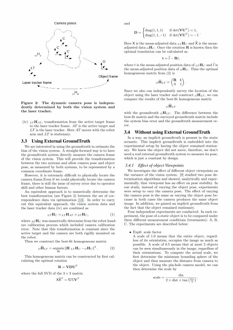
Figure 2: The dynamic camera pose is indepen-dently determined by both the vision system andthe laser tracker.

(iv) LT HAT , transformation from the active target frameto the laser tracker frame. AT is the active target andLT is the laser tracker. Here AT moves with the robotarm and LT is stationary.

3.3 Using External GroundTruthWe are interested in using the groundtruth to estimate the

bias of the vision system. A straight-forward way is to havethe groundtruth system directly measure the camera frameof the vision system. This will provide the transformationbetween the two systems and allow camera pose and objectpose, as measured by both systems, to be represented by acommon coordinate frame.

However, it is extremely di"cult to physically locate thecamera frame.Even if we could physically locate the cameraframe, there is still the issue of survey error due to operatorskill and other human factors.

An equivalent approach is to numerically determine thebest transformation (see Figure 2) between the set of cor-respondence data via optimization [13]. In order to carryout this equivalent approach, the vision system data andthe laser tracker data (iv) are combined as

LT HC =LT HAT "AT HC , (1)

where AT HC was numerically determine from the robot hand-eye calibration process which included camera calibrationerror. Note that this transformation is constant since theactive target and the camera are both rigidly mounted onthe robot.

Then we construct the best-fit homogeneous matrix

ObHLT = argmin

H#H LT HC $OHC#2 . (2)

This homogeneous matrix can be constructed by first cal-culating the optimal rotation

R = VDUT

where the full SVD of the 3" 3 matrix

XbXT = U#VT

and

D =

(diag(1, 1, 1) if det(VUT ) = 1,

diag(1, 1,$1) if det(VUT ) = $1.

Here X is the mean-adjusted data LT HC and bX is the mean-adjusted data OHC . Once the rotation R is known then theoptimal translation can be calculated as

t = bt$Rt,

where t is the mean-adjusted position data of LT HC and bt isthe mean-adjusted position data of OHC . Thus the optimalhomogeneous matrix from (2) is

ObHLT =

„R t0 1

«.

Since we also can independently survey the location of theobject using the laser tracker and construct OHLT , we cancompare the results of the best-fit homogeneous matrix

ObHLT

with the groundtruth OHLT . The di!erence between thebest-fit matrix and the surveyed groundtruth matrix includethe system bias error and the groundtruth measurement er-ror.

3.4 Without using External GroundTruthIn a way, an implicit groundtruth is present in the static

scenario. This implicit groundtruth is embedded into theexperimental setup by having the object remained station-ary. We knew the object did not move, therefore, we don’tneed a real external groundtruth system to measure its pose,which is just a constant by design.

3.4.1 Effect of object ViewpointsWe investigate the e!ect of di!erent object viewpoints on

the variance of the vision system. [9] studied two pose de-termination algorithms and showed, analytically and exper-imentally, that viewpoint has an e!ect on pose stability. Inour study, instead of varying the object pose, experimentswere setup to vary the camera pose. The e!ect of varyingthe camera pose is the same as varying the object pose be-cause in both cases the camera produces the same objectimage. In addition, we gained an implicit groundtruth fromthe fact that the object remained stationary.

Four independent experiments are conducted. In each ex-periment, the pose of a static object is to be compared underthree di!erent measurement conditions (treatments): A, B,C. The experiments are described below:

• Exp0: scale factorA scale of 1.0 means that the entire object, regard-less of its orientation, occupies the image as much aspossible. A scale of 0.5 means that at most 2 objectscan be seen simultaneously in the image, regardless oftheir orientations. To compute the actual scale, wefirst determine the minimum bounding sphere of theobject and then measure the distance from camera tothe object. Using the pin-hole camera model, we canthen determine the scale by

scale =dia

2" dist" tan`

fov2

´ ,

where dia is the diameter of the minimum boundingsphere, dist is the distance between the camera andthe object, and fov is the camera’s vertical field-of-view angle.

– cond A: object seen at low-scale (computed scale= 0.37)

– cond B: object seen at mid-scale (computed scale= 0.55)

– cond C: object seen at full-scale (computed scale= 1.03)

• Exp1: position factor

– cond A: object seen near the image border (actualcamera shift = 100 mm)

– cond B: object seen midway between center ofFoV (field-of-view) and the image border (actualcamera shift = 50 mm)

– cond C: object seen at the center of FoV (0 shift)

• Exp2: azimuth factorUnder this factor, the object is always centered in theimage as the camera rotates about its optical axis.

– cond A: object seen rotated 40 degree

– cond B: object seen rotated 20 degree

– cond C: object seen up-right

• Exp3: polar factorUnder this factor, the object is always centered in theimage as the camera rotates around the object.

– cond A: object seen rotated 25 degree on its side

– cond B: object seen rotated 15 degree on its side

– cond C: object seen up-right

Except experiment Exp0, the object scale is fixed at 0.55throughout the experiments.

4. RESULTSThis section describes the dataset obtained and their pre-

liminary analysis.

4.1 Data without External GroundtruthIn each of the four viewpoint experiments, 10 runs per

treatment were carried out, resulting a total of 30 runs perexperiment. More runs could be used, but 10 were chosen toestablish an initial preliminary study. No groundtruth datawas collected in these viewpoint experiments.

We used the completely randomized design (CRD) paradigm[15] in our viewpoint experiments and identified time androbot repeatability as two nuisance factors that we have nocontrol over. However, we did not randomize the order ofruns (as to neutralize the possible timing and robot e!ect)for two reasons:

1. The condition/treatment order can not be changed.The commercial vision system always perform condi-tions A, B, C, A, B, C, ... in that cyclic order. Theprovided commercial software does not have an optionto change the run order.

2. The robot arm was found1 to have deterministic re-peatability after warming up for 20 minutes. There-fore, the robot’s performance (repeatability as speci-fied by the manufacture) does not change with time.However, it was noted that the robot’s repeatabilitydepends on the motion as well as the initial pose atthe time the motion command was issued. As a result,we always move the robot from a fixed initial pose andset the robot speed to low (as to minimize structuralvibration caused by robot motion).

4.2 Data with External GroundtruthAdditionally, four data sets were collected together with

the groundtruth. Groundtruth was obtained by matchingthe vision data with the corresponding laser tracker data.Since the clocks were synchronized and timestamps recorded,we can match data by their timestamp. For each data set,the camera height was measured to about 457mm.

• For the first data set, we adjusted only the rotationalmotion of the camera. Specifically, we rotated the cam-era about the rotational axes Rx and Ry from ±15degrees in increments of 5 degrees, and Rz from ±10degrees in increments of 5 degrees. (Total of 7x7x5 =245 data; 61 have all image features detected.)

• For the second data set, we adjusted only the trans-lational motion of the camera. Specifically, we movedthe camera in the x and y directions from ±150mm inincrements of 50mm. (Total of 7x7 = 49 data; 37 haveall image features detected)

• For the third data set, we adjusted both the rotationaland translational motion of the camera. Specifically,we rotated the camera about the rotational axes Ry

and Rz from±5 degrees in increments of 5 degrees, andmoved the camera in the x direction from ±150mm inincrements of 50mm. (Total of 3x3x7 = 63 data; 54have all image features detected)

• For the fourth data set, we adjusted both the rota-tional and translational motion of the camera. Specifi-cally, we rotated the camera about the rotational axesRy and Rz from ±5 degrees in increments of 5 de-grees, and moved the camera in the y direction from±150mm in increments of 50mm. (Total of 3x3x7 =63 data, 41 have all image feature detected)

4.3 External GroundTruth ResultTable 1 summarizes error between the optimal homoge-

neous matrix ObHLT computed for each of the four data sets

with the survey from the laser tracker OHLT . The errorshown in this table is the combined e!ect of survey errorand the system bias. It should be noted that certain datapoints were ignored in the calculation of the best homoge-neous matrix O

bHLT . These points correspond to positionswhere all the image features could not be located by the vi-sion system. Outliers were also removed in the constructionof the optimal homogeneous matrix. These outliers wereconstructed using a statistical tool that identifies points asoutliers if they lie outside of one and half times the interquar-tile range.1We used the IS09283 robot performance standard metricand protocol describe in [6].

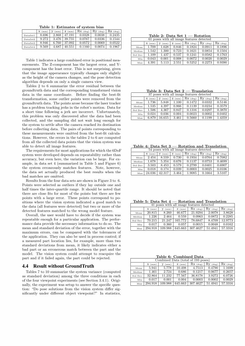
Table 1: Estimates of system biasx (mm) y (mm) z (mm) Rx (deg) Ry (deg) Rz (deg)

DataSet1 8.696 2.868 47.191 0.0328 0.0038 0.2435DataSet2 9.272 3.476 39.755 0.0767 0.0336 0.1544DataSet3 8.946 6.760 37.092 0.0572 0.0069 0.0522DataSet4 9.569 4.687 40.551 0.1160 0.0074 0.1967

Table 1 indicates a large combined error in positional mea-surements. The Z-component has the largest error, and Y-component has the least error. This is not surprising, giventhat the image apperarance typically changes only slightlyas the height of the camera changes, and the pose detectionalgorithm depends on only a single camera view.

Tables 2 to 6 summarize the error residual between thegroundtruth data and the corresponding transformed visiondata in the same coordinate. Before finding the best-fittransformation, some outlier points were removed from thegroundtruth data. The points arose because the laser trackerhas a problem tracking jerks in the robot’s motion. Data fora short time following a jerk are incorrect. Unfortunately,this problem was only discovered after the data had beencollected, and the sampling did not wait long enough forthe system to settle after the camera reached its destinationbefore collecting data. The pairs of points corresponding tothese measurements were omitted from the best-fit calcula-tions. However, the errors in the tables 2 to 6 are computedfrom all the collected data points that the vision system wasable to detect all image features.

The requirements for most applications for which the 6DoFsystem were developed depends on repeatability rather thanaccuracy, but even here, the variation can be large. For ex-ample, in data set 4 (summarized in Table 5 and Figure 6)the system erroneously matches features. Note, however,the data set actually produced the best results when thebad matches are omitted.

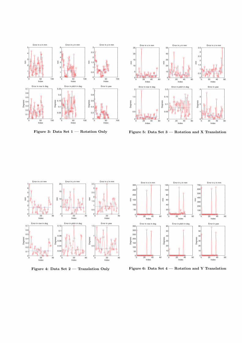
Results from the four data sets are shown in Figure 3 to 6.Points were selected as outliers if they lay outside one andhalf times the inter-quartile range. It should be noted thatthere are close fits for most of the points but there are fewpoints with a large error. These points correspond to po-sitions where the vision system indicated a good match tothe data (all features were detected) but two or more of thedetected features matched to the wrong model feature.

Overall, the user would have to decide if the system wasrepeatable enough for a particular application. The perfor-mance data provide the necessary information to do so. Themean and standard deviation of the error, together with themaximum errors, can be compared with the tolerances ofthe application. They can also be used in process control; ifa measured part location lies, for example, more than twostandard deviations from mean, it likely indicates either abad part or an erronerous match between the part and themodel. The vision system could attempt to reacquire thepart and if it failed again, the part could be rejected.

4.4 Result without GroundTruthTables 7 to 10 summarize the system variance (computed

as standard deviation) among the three conditions in eachof the four viewpoint experiments (see Section 3.4.1). Origi-nally, the experiment was setup to answer the specific ques-tion: “Do pose solutions from the vision system di!er sig-nificantly under di!erent object viewpoint?” In statistics,

Table 2: Data Set 1 — Rotation61 poses with all image features detected

x (mm) y (mm) z (mm) Rx (deg) Ry (deg) Rz (deg)

Mean 1.709 1.628 0.846 0.1824 0.0911 0.1896Median 1.542 1.300 0.723 0.1621 0.0854 0.1504Std Dev 1.109 1.437 0.537 0.1241 0.0582 0.1763

Min 0.043 0.001 0.008 0.0072 0.0020 0.0029Max 4.391 5.113 2.551 0.5252 0.2273 0.9390

Table 3: Data Set 2 — Translation37 poses with all image features detected

x (mm) y (mm) z (mm) Rx (deg) Ry (deg) Rz (deg)

Mean 1.736 5.848 1.100 0.1472 0.0332 0.5146Median 1.535 4.397 0.866 0.1139 0.0234 0.3579Std Dev 1.506 4.367 0.847 0.1316 0.0297 0.3870

Min 0.024 0.036 0.004 0.0023 0.0002 0.0402Max 6.879 16.655 3.461 0.5660 0.1199 1.4359

Table 4: Data Set 3 — Rotation and Translation54 poses with all image features detected

x (mm) y (mm) z (mm) Rx (deg) Ry (deg) Rz (deg)

Mean 2.454 8.559 0.730 0.1934 0.0764 0.7082Median 1.678 5.354 0.676 0.1137 0.0753 0.4699Std Dev 3.503 8.453 0.579 0.2799 0.0401 0.6907

Min 0.018 0.174 0.039 0.0003 0.0025 0.0106Max 24.036 42.317 3.464 1.9085 0.1664 3.5107

Table 5: Data Set 4 — Rotation and Translation41 poses with all image features detected

x (mm) y (mm) z (mm) Rx (deg) Ry (deg) Rz (deg)

Mean 20.815 8.260 46.677 21.9294 2.0078 3.8628Median 1.226 2.464 0.559 0.0963 0.0872 0.2285Std Dev 70.215 21.247 165.772 78.6847 8.4709 12.9773

Min 0.017 0.360 0.057 0.0015 0.0048 0.0162Max 294.918 109.988 645.663 307.4627 51.4941 57.3316

Table 6: Combined DataCombined Data (total of 193 poses)

x (mm) y (mm) z (mm) Rx (deg) Ry (deg) Rz (deg)

Mean 5.941 5.778 10.498 4.7513 0.4790 1.1699Median 1.461 2.724 0.686 0.1217 0.0677 0.2657Std Dev 32.864 11.232 77.567 36.8178 3.9272 6.0726

Min 0.017 0.001 0.004 0.0003 0.0002 0.0029Max 294.918 109.988 645.663 307.4627 51.4941 57.3316

0 50 1000

1

2

3

4

5

Index

mm

0 50 1000

1

2

3

4

5

6

Index

mm

0 50 1000

0.5

1

1.5

2

2.5

3

Index

mm

0 50 1000

0.1

0.2

0.3

0.4

0.5

0.6

0.7

Index

De

gre

es

0 50 1000

0.05

0.1

0.15

0.2

0.25

Index

De

gre

es

0 50 1000

0.2

0.4

0.6

0.8

1

Index

De

gre

es

Error in x in mm Error in y in mm Error in z in mm

Error in row in deg Error in pitch in deg Error in yaw

Figure 3: Data Set 1 — Rotation Only

0 20 400

1

2

3

4

5

6

7

Index

mm

0 20 400

5

10

15

20

Index

mm

0 20 400

0.5

1

1.5

2

2.5

3

3.5

Index

mm

0 20 400

0.1

0.2

0.3

0.4

0.5

0.6

0.7

Index

De

gre

es

0 20 400

0.02

0.04

0.06

0.08

0.1

0.12

Index

De

gre

es

0 20 400

0.5

1

1.5

Index

De

gre

es

Error in x in mm Error in y in mm Error in z in mm

Error in row in deg Error in pitch in deg Error in yaw

Figure 4: Data Set 2 — Translation Only

0 20 40 600

5

10

15

20

25

Index

mm

0 20 40 600

10

20

30

40

50

Index

mm

0 20 40 600

0.5

1

1.5

2

2.5

3

3.5

Index

mm

0 20 40 600

0.5

1

1.5

2

Index

De

gre

es

0 20 40 600

0.05

0.1

0.15

0.2

Index

De

gre

es

0 20 40 600

1

2

3

4

Index

De

gre

es

Error in x in mm Error in y in mm Error in z in mm

Error in row in deg Error in pitch in deg Error in yaw

Figure 5: Data Set 3 — Rotation and X Translation

0 20 40 600

50

100

150

200

250

300Error in x in mm

Index

mm

0 20 40 600

20

40

60

80

100

120Error in y in mm

Index

mm

0 20 40 600

100

200

300

400

500

600

700Error in z in mm

Index

mm

0 20 40 600

50

100

150

200

250

300

350Error in row in deg

Index

De

gre

es

0 20 40 600

10

20

30

40

50

60Error in pitch in deg

Index

De

gre

es

0 20 40 600

10

20

30

40

50

60Error in yaw

Index

De

gre

es

Figure 6: Data Set 4 — Rotation and Y Translation

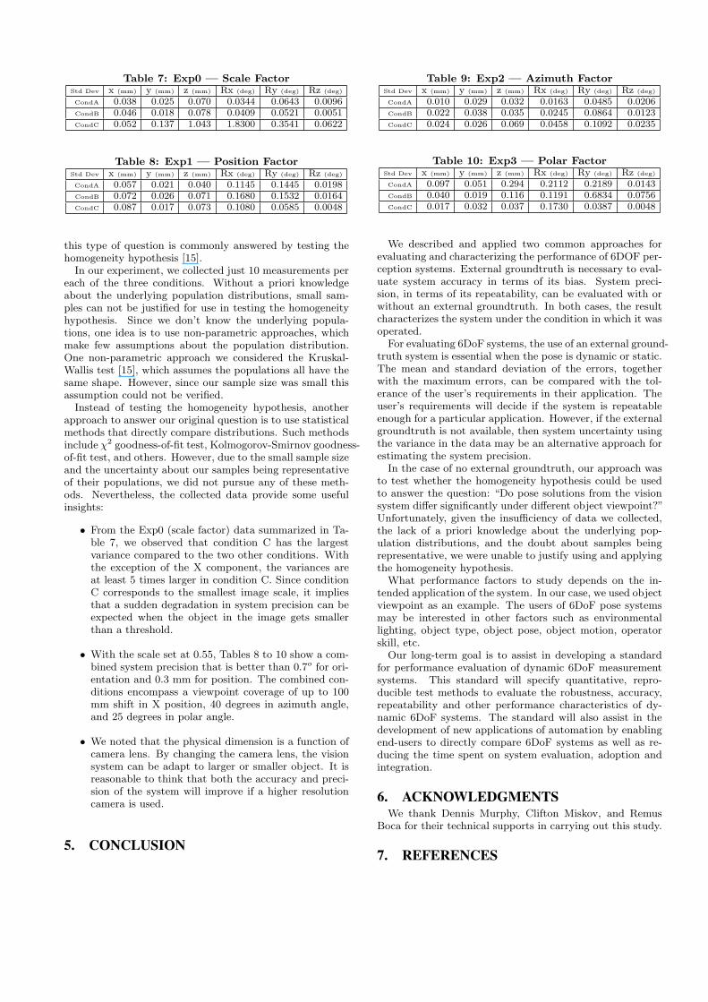
Table 7: Exp0 — Scale FactorStd Dev x (mm) y (mm) z (mm) Rx (deg) Ry (deg) Rz (deg)

CondA 0.038 0.025 0.070 0.0344 0.0643 0.0096CondB 0.046 0.018 0.078 0.0409 0.0521 0.0051CondC 0.052 0.137 1.043 1.8300 0.3541 0.0622

Table 8: Exp1 — Position FactorStd Dev x (mm) y (mm) z (mm) Rx (deg) Ry (deg) Rz (deg)

CondA 0.057 0.021 0.040 0.1145 0.1445 0.0198CondB 0.072 0.026 0.071 0.1680 0.1532 0.0164CondC 0.087 0.017 0.073 0.1080 0.0585 0.0048

this type of question is commonly answered by testing thehomogeneity hypothesis [15].

In our experiment, we collected just 10 measurements pereach of the three conditions. Without a priori knowledgeabout the underlying population distributions, small sam-ples can not be justified for use in testing the homogeneityhypothesis. Since we don’t know the underlying popula-tions, one idea is to use non-parametric approaches, whichmake few assumptions about the population distribution.One non-parametric approach we considered the Kruskal-Wallis test [15], which assumes the populations all have thesame shape. However, since our sample size was small thisassumption could not be verified.

Instead of testing the homogeneity hypothesis, anotherapproach to answer our original question is to use statisticalmethods that directly compare distributions. Such methodsinclude !2 goodness-of-fit test, Kolmogorov-Smirnov goodness-of-fit test, and others. However, due to the small sample sizeand the uncertainty about our samples being representativeof their populations, we did not pursue any of these meth-ods. Nevertheless, the collected data provide some usefulinsights:

• From the Exp0 (scale factor) data summarized in Ta-ble 7, we observed that condition C has the largestvariance compared to the two other conditions. Withthe exception of the X component, the variances areat least 5 times larger in condition C. Since conditionC corresponds to the smallest image scale, it impliesthat a sudden degradation in system precision can beexpected when the object in the image gets smallerthan a threshold.

• With the scale set at 0.55, Tables 8 to 10 show a com-bined system precision that is better than 0.7o for ori-entation and 0.3 mm for position. The combined con-ditions encompass a viewpoint coverage of up to 100mm shift in X position, 40 degrees in azimuth angle,and 25 degrees in polar angle.

• We noted that the physical dimension is a function ofcamera lens. By changing the camera lens, the visionsystem can be adapt to larger or smaller object. It isreasonable to think that both the accuracy and preci-sion of the system will improve if a higher resolutioncamera is used.

5. CONCLUSION

Table 9: Exp2 — Azimuth FactorStd Dev x (mm) y (mm) z (mm) Rx (deg) Ry (deg) Rz (deg)

CondA 0.010 0.029 0.032 0.0163 0.0485 0.0206CondB 0.022 0.038 0.035 0.0245 0.0864 0.0123CondC 0.024 0.026 0.069 0.0458 0.1092 0.0235

Table 10: Exp3 — Polar FactorStd Dev x (mm) y (mm) z (mm) Rx (deg) Ry (deg) Rz (deg)

CondA 0.097 0.051 0.294 0.2112 0.2189 0.0143CondB 0.040 0.019 0.116 0.1191 0.6834 0.0756CondC 0.017 0.032 0.037 0.1730 0.0387 0.0048

We described and applied two common approaches forevaluating and characterizing the performance of 6DOF per-ception systems. External groundtruth is necessary to eval-uate system accuracy in terms of its bias. System preci-sion, in terms of its repeatability, can be evaluated with orwithout an external groundtruth. In both cases, the resultcharacterizes the system under the condition in which it wasoperated.

For evaluating 6DoF systems, the use of an external ground-truth system is essential when the pose is dynamic or static.The mean and standard deviation of the errors, togetherwith the maximum errors, can be compared with the tol-erance of the user’s requirements in their application. Theuser’s requirements will decide if the system is repeatableenough for a particular application. However, if the externalgroundtruth is not available, then system uncertainty usingthe variance in the data may be an alternative approach forestimating the system precision.

In the case of no external groundtruth, our approach wasto test whether the homogeneity hypothesis could be usedto answer the question: “Do pose solutions from the visionsystem di!er significantly under di!erent object viewpoint?”Unfortunately, given the insu"ciency of data we collected,the lack of a priori knowledge about the underlying pop-ulation distributions, and the doubt about samples beingrepresentative, we were unable to justify using and applyingthe homogeneity hypothesis.

What performance factors to study depends on the in-tended application of the system. In our case, we used objectviewpoint as an example. The users of 6DoF pose systemsmay be interested in other factors such as environmentallighting, object type, object pose, object motion, operatorskill, etc.

Our long-term goal is to assist in developing a standardfor performance evaluation of dynamic 6DoF measurementsystems. This standard will specify quantitative, repro-ducible test methods to evaluate the robustness, accuracy,repeatability and other performance characteristics of dy-namic 6DoF systems. The standard will also assist in thedevelopment of new applications of automation by enablingend-users to directly compare 6DoF systems as well as re-ducing the time spent on system evaluation, adoption andintegration.

6. ACKNOWLEDGMENTSWe thank Dennis Murphy, Clifton Miskov, and Remus

Boca for their technical supports in carrying out this study.

7. REFERENCES

[1] D. Anderson, H. Herman, and A. Kelly. Experimentalcharacterization of commercial flash ladar devices. InInternational Conference of Sensing and Technology,November 2005.

[2] S. Bouix, M. Martin-Fernandez, L. Ungar, M. N.M.-S. Koo, R. W. McCarley, and M. E. Shenton. Onevaluating brain tissue classifiers without a groundtruth. NeuroImage, 36:1207–1224, 2007.

[3] T. Chang, T. Hong, M. Shneier, G. Holguin, J. Park,and R. D. Eastman. Dynamic 6dof metrology forevaluating a visual servoing system. In PerMIS ’08:Proceedings of the 8th Workshop on PerformanceMetrics for Intelligent Systems, pages 173–180, NewYork, NY, USA, 2008. ACM.

[4] C. E. Erdem, A. M. Tekalp, and B. Sankur. Metricsfor performance evaluation of video objectsegmentation and tracking without ground-truth.International Conference On Image Processing, 2001.

[5] J. Fitzpatrick and J. West. A blinded evaluation andcomparison of image registration methods. In IEEEWorkshop on Empirical Evaluation Methods inComputer Vision, 1998.

[6] ISO 9283:1998. Manipulating industrial robots —Performance criteria and related test methods. Secondedition. ISO, Geneva, Switzerland.

[7] J. Kybic. Fast no ground truth image registrationaccuracy evaluation: Comparison of bootstrap andhessian approaches. In ISBI, pages 792–795, 2008.

[8] A. M. Lytle, S. Szabo, G. Cheok, K. Saidi, andR. Norcross. Performance evaluation of a 3d imagingsystem for vehicle safety. In Unmanned SystemsTechnology IX. Proceedings of the SPIE, Volume 6561,2007.

[9] C. B. Madsen. A comparative study of the robustnessof two pose estimation techniques. Machine Visionand Applications, 9(5-6):291–303, 1997.

[10] R. Schestowitz, C. J. Twining, T. Cootes, V. Petrovic,B. Crum, and C. J. Taylor. Non-rigid registrationassessment without ground truth. In Medical ImageUnderstanding and Analysis, volume 2, pages 151–155,2006.

[11] S. M. Seitz, B. Curless, J. Diebel, D. Scharstein, andR. Szeliski. A comparison and evaluation of multi-viewstereo reconstruction algorithms. In CVPR ’06:Proceedings of the 2006 IEEE Computer SocietyConference on Computer Vision and PatternRecognition, pages 519–528, Washington, DC, USA,2006. IEEE Computer Society.

[12] M. Shah, T. Chang, and T. Hong. Mathematicalmetrology for evaluation a 6dof visual servoing system.In PerMIS ’09: Proceedings of the 9th Workshop onPerformance Metrics for Intelligent Systems, 2009.

[13] M. I. Shah. Six degree of freedom pointcorrespondences. Technical Report, Loyola UniversityMaryland, TR2009 02., 2009.

[14] F. Smit and R. van Liere. A framework forperformance evaluation of model-based opticaltrackers. EGVE Symposium, 6, 2008.

[15] A. C. Tamhane and D. D. Dunlop. Statistics and DataAnalysis from Elementary to Intermediate. PrenticeHall, Upper Saddle River, NJ 07458, 2000.

[16] N. A. Thacker, A. F. Clark, J. L. Barron, J. R.

Beveridge, P. Courtney, W. R. Crum, V. Ramesh, andC. Clark. Performance characterization in computervision: A guide to best practices. Computer Visionand Image Understanding, 109(3):305–334, 2008.

[17] M. Tonko and H.-H. Nagel. Model-basedstereo-tracking of non-polyhedral objects forautomatic disassembly experiments. InternationalJournal of Computer Vision, 37(1):99–118, 2000.

[18] R. van Liere and A. van Rhijn. An experimentalcomparison of three optical trackers for model basedpose determination in virtual reality. In S. Coquillartand M. Gobel, editors, 10th Eurographics Symposiumon Virtual Environments, pages 25–34, Grenoble,France, 2004. Eurographics Association.

[19] F. Viksten, P.-E. Forssen, B. Johansson, and A. Moe.Comparison of local image descriptors for full 6degree-of-freedom pose estimation. In IEEEInternational Conference on Robotics and Automation,Kobe, Japan, May 2009. IEEE, IEEE Robotics andAutomation Society.

[20] J. B. West and J. M. Fitzpatrick. The distribution oftarget registration error in rigid-body, point-basedregistration. In IPMI ’99: Proceedings of the 16thInternational Conference on Information Processing inMedical Imaging, pages 460–465, London, UK, 1999.Springer-Verlag.

[21] J. B. West, J. M. Fitzpatrick, M. Y. Wang, B. M.Dawant, C. R. M. Jr., R. M. Kessler, and R. J.Maciunas. Retrospective intermodality registrationtechniques for images of the head: Surface-basedversus volume-based. IEEE Trans. Med. Imaging,18(2):144–150, 1999.

[22] Q. Yang, R. M. Steele, D. Nister, and C. Jaynes.Learning the probability of correspondences withoutground truth. In ICCV ’05: Proceedings of the TenthIEEE International Conference on Computer Vision,pages 1140–1147, Washington, DC, USA, 2005. IEEEComputer Society.

[23] C. Ye and J. Borenstein. Characterization of a 2-dlaser scanner for mobile robot obstacle negotiation. InProceedings of the IEEE International Conference onRobotics and Automation, pages 2512–2518, 2002.