Measuring the Impact of Negative Demand Shocks on Car Dealer Networks
43
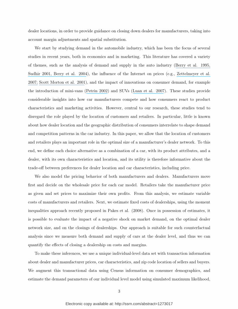
Electronic copy available at: http://ssrn.com/abstract=1273017 MEASURING THE IMPACT OF NEGATIVE DEMAND SHOCKS ON CAR DEALER NETWORKS ∗ Paulo Albuquerque † Bart J. Bronnenberg ‡ November 29, 2010 Abstract The goal of this paper is to study the behavior of consumers, dealers, and manufacturers in the car sector and present an approach that can be used by managers and policy makers to investigate the impact of significant demand shocks on profits, prices, and dealer networks. More specifically, we investigate consumer demand, substitution patterns, and price decisions across different cars and dealer locations, to identify dealerships with low margins or high fixed costs, and measure the value of closing down dealers for manufacturers. Empirically, we apply our model to the San Diego area using a transactional data set with information about locations of dealers and consumers, and manufacturer and retail prices. We find a high disutility for travel, which geographically limits preferences to nearby alternatives, and show that dealers have local demand areas shared with a small set of competitors. We show that a reduction of market demand by 30% over two years, similar to the demand shock caused by the economic crisis of 2008-2009, results in an annual drop in prices of about 11%, which was partially achieved through the “Car Allowance Rebate System” program. We compare predictions and actual dealer closings in the General Motors and Chrysler dealer networks as an application of our approach. Keywords : automobile industry, spatial competition, models of demand and supply ∗ We thank Dan Ackerberg, Andrew Ainslie, Charles Corbett, Sanjog Misra and Minjae Song for comments and suggestions and acknowledge comments made by seminar participants at the BBCRST conference 2007, Erasmus University in Rotterdam, University of Chicago Booth School of Business, and Stanford Graduate School of Business. We also thank an anonymous marketing research firm for providing the data used in the study. We are especially grateful to 2 reviewers, the AE and the Editor for their comments and suggestions. † Assistant Professor at the Simon Graduate School of Business, University of Rochester, [email protected]. Financial support from the Portuguese Foundation for Science and Technology is gratefully acknowledged. ‡ Professor at CentER, Tilburg University, Tilburg, the Netherlands, [email protected]. 1
-
Upload
independent -
Category
Documents
-
view
5 -
download
0
Transcript of Measuring the Impact of Negative Demand Shocks on Car Dealer Networks
Electronic copy available at: http://ssrn.com/abstract=1273017
MEASURING THE IMPACT OF NEGATIVE DEMAND
SHOCKS ON CAR DEALER NETWORKS∗
Paulo Albuquerque† Bart J. Bronnenberg‡
November 29, 2010
Abstract
The goal of this paper is to study the behavior of consumers, dealers, and manufacturersin the car sector and present an approach that can be used by managers and policy makers toinvestigate the impact of significant demand shocks on profits, prices, and dealer networks. Morespecifically, we investigate consumer demand, substitution patterns, and price decisions acrossdifferent cars and dealer locations, to identify dealerships with low margins or high fixed costs,and measure the value of closing down dealers for manufacturers. Empirically, we apply ourmodel to the San Diego area using a transactional data set with information about locations ofdealers and consumers, and manufacturer and retail prices. We find a high disutility for travel,which geographically limits preferences to nearby alternatives, and show that dealers have localdemand areas shared with a small set of competitors. We show that a reduction of marketdemand by 30% over two years, similar to the demand shock caused by the economic crisisof 2008-2009, results in an annual drop in prices of about 11%, which was partially achievedthrough the “Car Allowance Rebate System” program. We compare predictions and actualdealer closings in the General Motors and Chrysler dealer networks as an application of ourapproach.
Keywords: automobile industry, spatial competition, models of demand and supply
∗We thank Dan Ackerberg, Andrew Ainslie, Charles Corbett, Sanjog Misra and Minjae Song for comments andsuggestions and acknowledge comments made by seminar participants at the BBCRST conference 2007, ErasmusUniversity in Rotterdam, University of Chicago Booth School of Business, and Stanford Graduate School of Business.We also thank an anonymous marketing research firm for providing the data used in the study. We are especiallygrateful to 2 reviewers, the AE and the Editor for their comments and suggestions.
†Assistant Professor at the Simon Graduate School of Business, University of Rochester,[email protected]. Financial support from the Portuguese Foundation for Science andTechnology is gratefully acknowledged.
‡Professor at CentER, Tilburg University, Tilburg, the Netherlands, [email protected].
1
Electronic copy available at: http://ssrn.com/abstract=1273017
GM intends to have the right number of brands, sold by the right number of dealers, in the right
locations to obtain maximum profitability to GM and the retailer network.
(General Motors Corporation, “Restructuring Plan for Long-Term Viability,” December 2, 2008)
1 Introduction
In 2009 and the first half of 2010, the car industry suffered a significant decline in demand as a
result of the economic crisis that started in October of 2008. The increase in the price of gas,
combined with the real estate and financial crisis, have lowered the yearly number of vehicles
sold from a usual number of 16.5 million in 2007 to a projected number of about 12 million in
2009 (General Motors, 2008). Due to the decline in demand, several companies including General
Motors (GM) and Chrysler found themselves in a dire situation, since a significant number of
dealerships with reduced demand were not profitable. To respond to the crisis, one of the proposed
actions taken by car manufacturers was to announce a reduction in the size of dealer networks.
An excessively large network of dealers imposes significant costs to the manufacturer, including
distribution costs, marketing, and quality control. It can also have negative impact on the demand
for the manufacturer’s brand. For example, if sales are too infrequent, the dealership owner does
not have the resources to reinvest in the dealership and the manufacturer loses potential buyers who
see old fashioned and poorly maintained showrooms. Additionally, having too many car dealerships
of the same manufacturer in a geographic region leads to high competition intensity, which may
result in lower margins for both dealers and manufacturers. In order to reduce the negative impact
from having too many dealerships, car companies have the option to close the less profitable dealers
in their networks. For example, GM plans to consolidate its dealer network, reducing the number
of dealers from 6,450 in 2008 to 4,700 in 2012 (General Motors, 2008).
In this context, the goal of this paper is to study the behavior of consumers, dealers, and
manufacturers in the car sector and to present an approach that can be used by managers and
policy makers to investigate the impact of significant demand shocks on industry profits, prices,
and market structure. More specifically, in the context of dealer network reductions, we investigate
consumer demand, substitution patterns, and firm price decisions across different cars and different
2
Electronic copy available at: http://ssrn.com/abstract=1273017
dealer locations, in order to provide guidance on closing down dealers for manufacturers, taking into
account margin adjustments and spatial substitution.
We start by studying demand in the automobile industry, which has been the focus of several
studies in recent years, both in economics and in marketing. This literature has covered a variety
of themes, such as the analysis of demand and supply in the auto industry (Berry et al. 1995,
Sudhir 2001, Berry et al. 2004), the influence of the Internet on prices (e.g., Zettelmeyer et al.
2007; Scott Morton et al. 2001), and the impact of innovations on consumer demand, for example
the introduction of mini-vans (Petrin 2002) and SUVs (Luan et al. 2007). These studies provide
considerable insights into how car manufacturers compete and how consumers react to product
characteristics and marketing activities. However, central to our research, these studies tend to
disregard the role played by the location of customers and retailers. In particular, little is known
about how dealer location and the geographic distribution of consumers interrelate to shape demand
and competition patterns in the car industry. In this paper, we allow that the location of customers
and retailers plays an important role in the optimal size of a manufacturer’s dealer network. To this
end, we define each choice alternative as a combination of a car, with its product attributes, and a
dealer, with its own characteristics and location, and its utility is therefore informative about the
trade-off between preferences for dealer location and car characteristics, including price.
We also model the pricing behavior of both manufacturers and dealers. Manufacturers move
first and decide on the wholesale price for each car model. Retailers take the manufacturer price
as given and set prices to maximize their own profits. From this analysis, we estimate variable
costs of manufacturers and retailers. Next, we estimate fixed costs of dealerships, using the moment
inequalities approach recently proposed in Pakes et al. (2008). Once in possession of estimates, it
is possible to evaluate the impact of a negative shock on market demand, on the optimal dealer
network size, and on the closings of dealerships. Our approach is suitable for such counterfactual
analysis since we measure both demand and supply of cars at the dealer level, and thus we can
quantify the effects of closing a dealership on costs and margins.
To make these inferences, we use a unique individual-level data set with transaction information
about dealer and manufacturer prices, car characteristics, and zip code location of sellers and buyers.
We augment this transactional data using Census information on consumer demographics, and
estimate the demand parameters of our individual level model using simulated maximum likelihood,
3
while taking into account consumer heterogeneity and endogeneity between prices and unobserved
car attributes. We use a demand model that accounts for observed heterogeneity at the zip code
level, includes location and dealer effects, and accounts for correlation in the error term across
similar alternatives.
We apply our methodology to the car industry in the San Diego area. Regarding demand, our
results show that consumers treat alternatives of the same car type1 as close substitutes, and do
so even more if cars share the same brand. When deciding where to buy a car, we infer consumers
dislike travel distance to car dealerships and the majority of demand of a car dealership originates
from consumers located in close proximity. As a result, dealers typically have their own local
demand “backyard,” the size of which is determined by the location of competitors. For instance,
we find cases where the highest level of demand is not at the location of the dealer, but instead,
at locations that are furthest from direct substitutes. In addition to characterizing the geographic
trading area of car dealerships, we also compute the geographic areas of demand at the manufacturer
level by consolidating the market areas of its dealers, and we report some interesting patterns
in location decisions. For instance, consistent with theories of spatial competition, we find that
Honda and Toyota target different geographic areas in order to minimize overlap and create spatial
differentiation between the two manufacturers.
Regarding the supply side, we find that the average manufacturer’s gross margin is about 50% of
the final price, which corresponds to an average value of $12,500. Car dealers obtain a much lower
margin on new cars. The observed gross margins of the dealers in the new cars divisions are 6.5%,
with an average value of around $1,600. In addition to having consumer location data, another
unique aspect of our data set is that we observe wholesale prices, which allows us to estimate other
sources of retailer revenues, such as car servicing and parts. Taking our estimate of the latter into
account, dealer margins go up to about $6,000 per vehicle. We estimate dealer fixed costs to be
on average $3.6 million per year. This number is only slightly higher than the national average of
$2.8 million reported by the National American Dealer Association (NADA 2008), which might be
expected given land values of Southern California. Dealer fixed costs are estimated to drop with
distance from the San Diego and Escondido city centers, where real estate prices are higher than in
the suburbs.1Car types are defined as large SUVs, small SUVs, mid-size cars and near luxury cars.
4

Combining demand and supply, we evaluate the impact of a significant reduction of demand
on the dealer network size and we quantify changes in profit, prices, and demand. We simulate a
negative shock of demand of the same magnitude as the one that occurred in the United States
in 2008 and 2009, that is, a drop of about 30% in those two years. In such a scenario, our model
predicts that average dealer and manufacturer prices would decrease by an annual average of 11%
and a drop in the total gross margins of about 35%. We relate this price decrease to the Car
Allowance Rebate System (also known as “Cash for Clunkers”) program that was used by the U.S.
government to provide a temporary price discount to consumers. Finally, we discuss actual dealer
closings in the Chrysler and GM networks as a managerial application of our model, and find that
the implications of our model broadly agree with the actual closings of car dealerships implemented
by these firms.
Our paper is structured as follows. The next section discusses the relevant literature. The
description of the model is included in section 3. Section 4 provides details about the several data
sets used in the paper. The estimation algorithm is presented in section 5 and the results are
analyzed in section 6. Section 7 describes managerial applications and section 8 concludes.
2 Background
Our work is related to previous papers on the car industry, spatial competition, and management
of networks. Berry et al. (1995 and 2004) study the automotive industry in two complementary
papers. The authors develop a model that analyzes demand and supply of differentiated cars using
aggregate-level data (1995) and expand their methodology to combine micro and macro data (2004).
Among other results, they are able to produce demand elasticities of price and other observed
attributes and find considerable variability across types of cars and models. Sudhir (2001) suggests
that manufacturer competitive behavior may depend on the car type. Regarding the introduction of
new products in the car industry, Petrin (2002) analyzes the impact of the introduction of the mini-
van on consumer welfare, while Luan et al. (2007) evaluate the evolution of consumer preferences
and market structure during the introduction and take-off of SUVs. Whereas this literature provides
valuable insights on the interaction between car manufacturers and between car manufacturers and
consumers, it assumes that consumers trade off all alternatives based solely on car attributes, and
5
not on the location of car dealerships.
In contrast, the location of customers relative to retailers is central in the literature on spatial
competition. Indeed, location has been shown to serve as input for managerial decisions on pricing
(e.g., Ellickson and Misra 2008), store customization (e.g., Hoch et al. 1995), and store locations
(e.g., Duan and Mela 2008). Industry research has also shown that a large percentage of variance
in consumer store choice in the grocery trade is explained by location (Progressive Grocer, 1995).
Finally, the role of location of consumers has been investigated in several important industries such
as the hospitality industry (Mazzeo 2002; Venkataraman and Kadiyali 2007), the fast food industry
(Thomadsen 2007) and the movie theater industry (Davis, 2001).2 We believe that the location of
customers relative to dealerships is also of great importance to car manufacturers, especially in the
case where manufacturers seek to change their dealer networks. However, a good understanding of
this competitive environment and its characterization across geography is lacking in the literature.
Our paper seeks to fill this gap by combining a spatial demand model in the auto industry with
the analysis of both manufacturer and retailer pricing decisions, as means to provide a complete
analysis of car dealer networks.
A third important strand of literature is on the management of outlet networks. For example,
Ishii (2008) studies networks of ATM machines, based on consumer demand and bank competi-
tion. Ho (2008) studies networks of hospitals managed by health care insurance and estimates
the division of profits between health plans and hospitals. These studies use recent advances in
empirical methodology from the studies on moment inequalities (Pakes et al. 2008). We combine
such advances in the management of networks with our spatial demand and competition analysis
to evaluate changes in dealer networks in the auto industry, in response to large demand shocks.
3 Model
On the demand side, we model the consumer’s choice of purchasing a car as a function of car and
dealer characteristics, as well as geographic distance between consumer and dealer locations. On the
supply side, we assume profit maximizing behavior by manufacturers and dealers, which provides2There is a recent study on the demand effects of dealer accessibility and concentration in the auto industry
(Bucklin et al. 2008). However, this study neither focuses on the supply side of dealer networks nor measures theimpact of changes in demand for dealers and manufacturers.
6
estimates of variable costs and margins. We then use the realizations of network size and locations
to identify fixed costs of dealerships. Together, the demand and supply models are used to run
counterfactual scenarios in policy simulations and provide guidance to managerial decisions.
3.1 Demand Utility Specification
A number of households Hz living in zip code z consider purchasing a car. The total number of
households in the market is H =
z=1,...,Z Hz. Household i, living in zip code z, chooses either to
purchase a car, or to use a different means of transportation.3 The households who buy a car may
choose among j alternatives, each of them characterized by its dealer, brand, and car type. There
are four car types in our data set: mid-size cars, near luxury cars, small SUVs, and large SUVs.4 We
define our observations at the quarterly level, with individuals who make a car purchase decision in
the same quarter facing the same market conditions, such as car prices and availability.
The indirect utility for consumer i of purchasing car j - a vehicle of brand b, type m, sold at
dealer d - is given by
Uijt = αij + λixjt + βipjt + γ1gij + γ2g2ij + ξjt + eijt
= Vijt + eijt
, (1)
with
eijt = vimjt + (1− σM )vibjt + (1− σB) (1− σM ) εijt. (2)
The first component of the utility αij includes both dealer- and car type-specific intercepts, and
the interaction of these intercepts with demographic characteristics. xjt is a vector of observed car
characteristics, such as engine size and transmission type. pjt represents the price for alternative j
at time t. gij is the geographic distance between individual i and the location of the dealer that
sells j, measured as Euclidean distance between the zip code centroid of i and j. The impact of
distance on utility is modeled as a quadratic function to account for non-linear effects of distance
on utility. ξjt captures the impact of car attributes unobserved to the researcher but taken into3The outside option also includes car purchases made at dealers that are not in our analysis and vehicles not
covered in our data set.4Each car type is defined as a set of car models using the classification defined by the research company that
provided the data in our empirical section. Vehicles that belong to the same type have significant similarities acrossa number of dimensions.
7
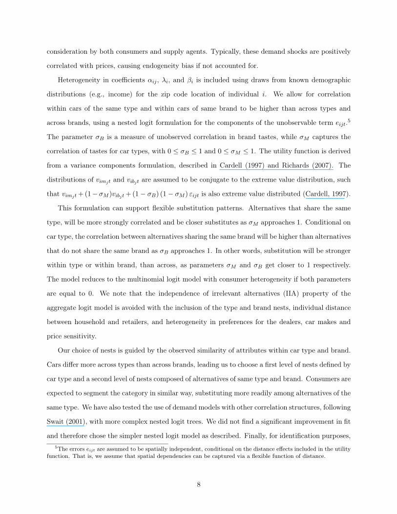
consideration by both consumers and supply agents. Typically, these demand shocks are positively
correlated with prices, causing endogeneity bias if not accounted for.
Heterogeneity in coefficients αij , λi, and βi is included using draws from known demographic
distributions (e.g., income) for the zip code location of individual i. We allow for correlation
within cars of the same type and within cars of same brand to be higher than across types and
across brands, using a nested logit formulation for the components of the unobservable term eijt.5
The parameter σB is a measure of unobserved correlation in brand tastes, while σM captures the
correlation of tastes for car types, with 0 ≤ σB ≤ 1 and 0 ≤ σM ≤ 1. The utility function is derived
from a variance components formulation, described in Cardell (1997) and Richards (2007). The
distributions of vimjt and vibjt are assumed to be conjugate to the extreme value distribution, such
that vimjt +(1−σM )vibjt +(1− σB) (1− σM ) εijt is also extreme value distributed (Cardell, 1997).
This formulation can support flexible substitution patterns. Alternatives that share the same
type, will be more strongly correlated and be closer substitutes as σM approaches 1. Conditional on
car type, the correlation between alternatives sharing the same brand will be higher than alternatives
that do not share the same brand as σB approaches 1. In other words, substitution will be stronger
within type or within brand, than across, as parameters σM and σB get closer to 1 respectively.
The model reduces to the multinomial logit model with consumer heterogeneity if both parameters
are equal to 0. We note that the independence of irrelevant alternatives (IIA) property of the
aggregate logit model is avoided with the inclusion of the type and brand nests, individual distance
between household and retailers, and heterogeneity in preferences for the dealers, car makes and
price sensitivity.
Our choice of nests is guided by the observed similarity of attributes within car type and brand.
Cars differ more across types than across brands, leading us to choose a first level of nests defined by
car type and a second level of nests composed of alternatives of same type and brand. Consumers are
expected to segment the category in similar way, substituting more readily among alternatives of the
same type. We have also tested the use of demand models with other correlation structures, following
Swait (2001), with more complex nested logit trees. We did not find a significant improvement in fit
and therefore chose the simpler nested logit model as described. Finally, for identification purposes,5The errors eijt are assumed to be spatially independent, conditional on the distance effects included in the utility
function. That is, we assume that spatial dependencies can be captured via a flexible function of distance.
8
the deterministic part of the utility of the outside good is set to 0.
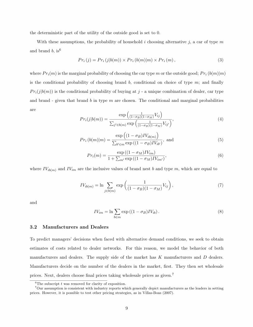
With these assumptions, the probability of household i choosing alternative j, a car of type m
and brand b, is6
Pri (j) = Pri (j|b(m))× Pri (b(m)|m)× Pri (m) , (3)
where Pri(m) is the marginal probability of choosing the car type m or the outside good; Pri (b(m)|m)
is the conditional probability of choosing brand b, conditional on choice of type m; and finally
Pri(j|b(m)) is the conditional probability of buying at j - a unique combination of dealer, car type
and brand - given that brand b in type m are chosen. The conditional and marginal probabilities
are
Pri(j|b(m)) =exp
1
(1−σB)(1−σM )Vij
j∈b(m) exp
1
(1−σB)(1−σM )Vij
, (4)
Pri (b(m)|m) =exp
(1− σB)IVib(m)
b∈m exp ((1− σB)IVib)
, and (5)
Pri(m) =exp ((1− σM )IVim)
1 +
m exp ((1− σM )IVim), (6)
where IVib(m) and IVim are the inclusive values of brand nest b and type m, which are equal to
IVib(m) = ln
j∈b(m)
exp
1
(1− σB)(1− σM )Vij
, (7)
and
IVim = ln
b∈mexp ((1− σB)IVib) . (8)
3.2 Manufacturers and Dealers
To predict managers’ decisions when faced with alternative demand conditions, we seek to obtain
estimates of costs related to dealer networks. For this reason, we model the behavior of both
manufacturers and dealers. The supply side of the market has K manufacturers and D dealers.
Manufacturers decide on the number of the dealers in the market, first. They then set wholesale
prices. Next, dealers choose final prices taking wholesale prices as given.7
6The subscript t was removed for clarity of exposition.7Our assumption is consistent with industry reports which generally depict manufacturers as the leaders in setting
prices. However, it is possible to test other pricing strategies, as in Villas-Boas (2007).
9
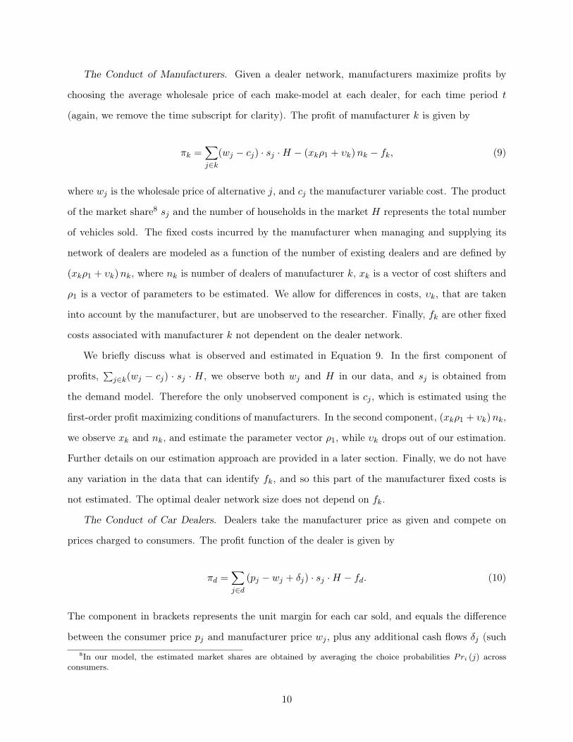
The Conduct of Manufacturers. Given a dealer network, manufacturers maximize profits by
choosing the average wholesale price of each make-model at each dealer, for each time period t
(again, we remove the time subscript for clarity). The profit of manufacturer k is given by
πk =
j∈k(wj − cj) · sj ·H − (xkρ1 + υk)nk − fk, (9)
where wj is the wholesale price of alternative j, and cj the manufacturer variable cost. The product
of the market share8sj and the number of households in the market H represents the total number
of vehicles sold. The fixed costs incurred by the manufacturer when managing and supplying its
network of dealers are modeled as a function of the number of existing dealers and are defined by
(xkρ1 + υk)nk, where nk is number of dealers of manufacturer k, xk is a vector of cost shifters and
ρ1 is a vector of parameters to be estimated. We allow for differences in costs, υk, that are taken
into account by the manufacturer, but are unobserved to the researcher. Finally, fk are other fixed
costs associated with manufacturer k not dependent on the dealer network.
We briefly discuss what is observed and estimated in Equation 9. In the first component of
profits,
j∈k(wj − cj) · sj · H, we observe both wj and H in our data, and sj is obtained from
the demand model. Therefore the only unobserved component is cj , which is estimated using the
first-order profit maximizing conditions of manufacturers. In the second component, (xkρ1 + υk)nk,
we observe xk and nk, and estimate the parameter vector ρ1, while υk drops out of our estimation.
Further details on our estimation approach are provided in a later section. Finally, we do not have
any variation in the data that can identify fk, and so this part of the manufacturer fixed costs is
not estimated. The optimal dealer network size does not depend on fk.
The Conduct of Car Dealers. Dealers take the manufacturer price as given and compete on
prices charged to consumers. The profit function of the dealer is given by
πd =
j∈d(pj − wj + δj) · sj ·H − fd. (10)
The component in brackets represents the unit margin for each car sold, and equals the difference
between the consumer price pj and manufacturer price wj , plus any additional cash flows δj (such8In our model, the estimated market shares are obtained by averaging the choice probabilities Pri (j) across
consumers.
10
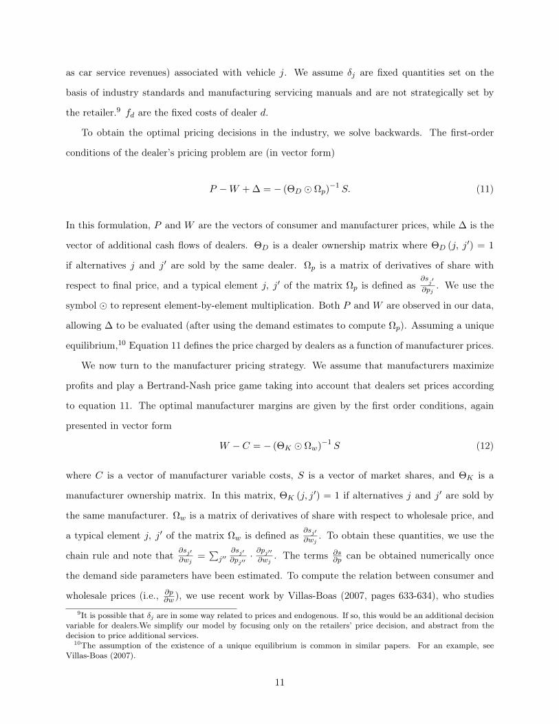
as car service revenues) associated with vehicle j. We assume δj are fixed quantities set on the
basis of industry standards and manufacturing servicing manuals and are not strategically set by
the retailer.9 fd are the fixed costs of dealer d.
To obtain the optimal pricing decisions in the industry, we solve backwards. The first-order
conditions of the dealer’s pricing problem are (in vector form)
P −W +∆ = − (ΘD ⊙ Ωp)−1
S. (11)
In this formulation, P and W are the vectors of consumer and manufacturer prices, while ∆ is the
vector of additional cash flows of dealers. ΘD is a dealer ownership matrix where ΘD (j, j) = 1
if alternatives j and j are sold by the same dealer. Ωp is a matrix of derivatives of share with
respect to final price, and a typical element j, j of the matrix Ωp is defined as
∂sj
∂pj. We use the
symbol ⊙ to represent element-by-element multiplication. Both P and W are observed in our data,
allowing ∆ to be evaluated (after using the demand estimates to compute Ωp). Assuming a unique
equilibrium,10 Equation 11 defines the price charged by dealers as a function of manufacturer prices.
We now turn to the manufacturer pricing strategy. We assume that manufacturers maximize
profits and play a Bertrand-Nash price game taking into account that dealers set prices according
to equation 11. The optimal manufacturer margins are given by the first order conditions, again
presented in vector form
W − C = − (ΘK ⊙ Ωw)−1
S (12)
where C is a vector of manufacturer variable costs, S is a vector of market shares, and ΘK is a
manufacturer ownership matrix. In this matrix, ΘK (j, j) = 1 if alternatives j and j are sold by
the same manufacturer. Ωw is a matrix of derivatives of share with respect to wholesale price, and
a typical element j, j of the matrix Ωw is defined as ∂sj
∂wj. To obtain these quantities, we use the
chain rule and note that ∂sj∂wj
=
j∂sj∂pj
· ∂pj∂wj
. The terms ∂s∂p can be obtained numerically once
the demand side parameters have been estimated. To compute the relation between consumer and
wholesale prices (i.e., ∂p∂w ), we use recent work by Villas-Boas (2007, pages 633-634), who studies
9It is possible that δj are in some way related to prices and endogenous. If so, this would be an additional decisionvariable for dealers.We simplify our model by focusing only on the retailers’ price decision, and abstract from thedecision to price additional services.
10The assumption of the existence of a unique equilibrium is common in similar papers. For an example, seeVillas-Boas (2007).
11
vertical interaction between retailers and manufacturers. Consider that these terms are arranged
in a matrix Ωt, with a typical element j, j consisting of ∂pj∂wj
. When manufacturers set their prices
first and retailers follow, Villas-Boas (2007) shows that the fth column of Ωt is given by Γ−1Gf ,
where Γ is a matrix of size J × J , with element (j, j) given by
Γj, j
=∂sj
∂pj+
J
l=1
ΘD (l, j)∂2sl
∂pj∂pj(pl − wl + δl)
+ΘDj, j
∂sj∂pj
, (13)
and Gf is a vector of size J × 1, with elements
Gf (j, f) = ΘD (f, j)∂sf
∂pj. (14)
Finally, we can compute the unknowns in equation 12, using the chain rule Ωw = ΩtΩp. Once the
demand parameters are estimated and Ωp and Ωt evaluated numerically, we can obtain the implied
manufacturer variable costs C, since in our data set we observe W .
3.3 Car Dealership Networks
To evaluate decisions regarding the size of dealership networks, we also estimate the fixed costs of
each dealership. The manufacturer profits in Equation 9 can be re-written in the following way
πk = Rk (Λ, nk, n−k)− (xkρ1 + υk)nk − fk. (15)
Here, Rk (Λ, nk, n−k) are the variable profits of manufacturer k, nk and n−k are the number of
dealers in the network of manufacturer k and of all other manufacturers −k, and Λ summarizes
the information about the data and remaining parameters. As previously described, (xkρ1 + υk)nk
represents the fixed costs incurred by the manufacturer that are a function of the size of the dealer
network, where xk is a vector of observed cost shifters and ρ1 is a vector of parameters to be
estimated while υk is an unobserved component.
Manufacturer Fixed Cost. We assume that each manufacturer maximizes his expected profit by
choosing the optimal number of dealerships in its network nk. Any deviation from the chosen nk,
for instance nk − 1 or nk +1, is assumed to result in lower profits. This is a necessary condition for
profit maximization that is also sufficient when profits are concave in nk (Ishii, 2009). The choice
12
of nk satisfies the following conditions
πk (Λ, nk, n−k, xk, ρ1) > πk (Λ, nk − 1, n−k, xk, ρ1)
πk (Λ, nk, n−k, xk, ρ1) > πk (Λ, nk + 1, n−k, xk, ρ1),
which implies
xkρ1 + υk ≤ R (Λ, nk, n−k)−Rk (Λ, nk − 1, n−k)
xkρ1 + υk ≥ R (Λ, nk + 1, n−k)−Rk (Λ, nk, n−k). (16)
Once demand parameters and margins for manufacturers are estimated, we can compute manufac-
turer variable profits of counterfactual scenarios. In this particular case, we evaluate the cases when
manufacturer k increases or decreases his network by one dealer, i.e., compute Rk (Λ, nk + 1, n−k)
and Rk (Λ, nk − 1, n−k).
Dealer Fixed Cost. In order to estimate the fixed costs of each dealer, we use a similar approach.
The profit function for car dealership d can be rewritten as
πd = πd (Λ, dz,−dz) = Rd (Λ, dz,−dz)− fd.
Rd (Λ, dz,−dz) represents the variable profits of the dealer, with dealership d and all other dealer-
ships −d located at the observed zip codes. We add a subscript z to dealer d to represent its current
zip code location. fd are the fixed costs of operation. We model these costs as having cost shifters
xd and an unobserved (to the researchers) component υd,
fd = xdρ2 + υd, (17)
where ρ2 is a vector of parameters to be estimated.
In order to estimate the cost parameters ρ2, we make two assumptions: first, dealers remain in
operation if their expected profits are larger than zero; second, the expected profits of the observed
dealer location z are higher than expected profits at other locations z.11 This means that any
geographic configuration of dealers different from the observed one is assumed to produce lower11To create counterfactuals in both the manufacturer and the retailer cases, we are implicitly assuming that agents
have passive expectations, i.e., that the increase or decrease in the number of dealers does not change the agentsperceptions of the market or that of their competitors. This is also an assumption in Pakes et al. (2008) paper.
13
profits. With these assumptions, we obtain the following conditions
xdzρ2 + υdz < R (Λ, dz,−dz)xdzρ2 + υdz
− (xdzρ2 + υdz) > R (Λ, dz ,−dz)−R (Λ, dz,−dz)
, (18)
where z = z. In the estimation, we assume that agents act on expected values of profits and costs
and that the expected value of the unobserved costs υk and υdz are assumed to be zero, in order to
create the innequalities to estimate the vector of parameters ρ1 and ρ2. With these parameters in
hand, combined with the remaining estimates of demand parameters and margins, we can provide
estimates of profits for dealers and manufacturers, as well as run counterfactual scenarios to help
manufacturer decisions of which dealerships to close, in response to negative demand shocks.
4 Data
We combine several data sets to estimate our model. Our main data set was obtained from a large
automobile research company and it includes details about individual car transactions occurring
in the San Diego area and its suburbs between 2004 and 2006.12 We have information about the
car make and model, as well as the following car characteristics: transaction price, engine size,
fuel and transmission type. Our data also contains the zip code of dealer and consumer locations.
Additionally, we have retail and wholesale prices for each car, as well as any manufacturer rebate
given. The data is drawn from a sample of car transactions in the San Diego area, including 20% of
all transactions. We complemented these data with U.S. Census demographic data on income and
population density at the zip code level. Finally, we also collected latitude and longitude data of
both retailer and consumer zip codes from the Zipinfo database.13 With these data, we computed
distances between consumers and dealers measured in 100 miles.
For each vehicle, we use the transaction date and the number of days that the vehicle was kept in
the lot before being sold to compute the arrival date. With this information, we know if alternative12To do a national analysis, we could repeat the analysis for multiple regional markets. For instance, in our case,
we also have data about the Los Angeles market (the closest and largest market to San Diego) and find that thereis only a very small number of transactions between San Diego dealers and Los Angeles consumers. Hence it seemsreasonable to view San Diego as a separate market from Los Angeles, and our study could be repeated for the LosAngeles area without becoming infeasible, and so on for other markets.
13Available at www.zipinfo.com.
14
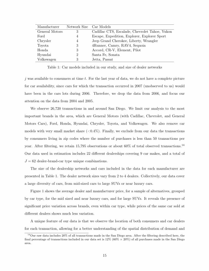
Manufacturer Network Size Car ModelsGeneral Motors 3 Cadillac CTS, Escalade, Chevrolet Tahoe, YukonFord 4 Escape, Expedition, Explorer, Explorer SportChrysler 4 Jeep Grand Cherokee, Liberty, WranglerToyota 3 4Runner, Camry, RAV4, SequoiaHonda 3 Accord, CR-V, Element, PilotHyundai 2 Santa Fe, SonataVolkswagen 3 Jetta, Passat
Table 1: Car models included in our study, and size of dealer networks
j was available to consumers at time t. For the last year of data, we do not have a complete picture
for car availability, since cars for which the transaction occurred in 2007 (unobserved to us) would
have been in the cars lots during 2006. Therefore, we drop the data from 2006, and focus our
attention on the data from 2004 and 2005.
We observe 26,720 transactions in and around San Diego. We limit our analysis to the most
important brands in the area, which are General Motors (with Cadillac, Chevrolet, and General
Motors Cars), Ford, Honda, Hyundai, Chrysler, Toyota, and Volkswagen. We also remove car
models with very small market share (<0.4%). Finally, we exclude from our data the transactions
by consumers living in zip codes where the number of purchases is less than 50 transactions per
year. After filtering, we retain 15,795 observations or about 60% of total observed transactions.14
Our data used in estimation includes 22 different dealerships covering 9 car makes, and a total of
J = 62 dealer-brand-car type unique combinations.
The size of the dealership networks and cars included in the data for each manufacturer are
presented in Table 1. The dealer network sizes vary from 2 to 4 dealers. Collectively, our data cover
a large diversity of cars, from mid-sized cars to large SUVs or near luxury cars.
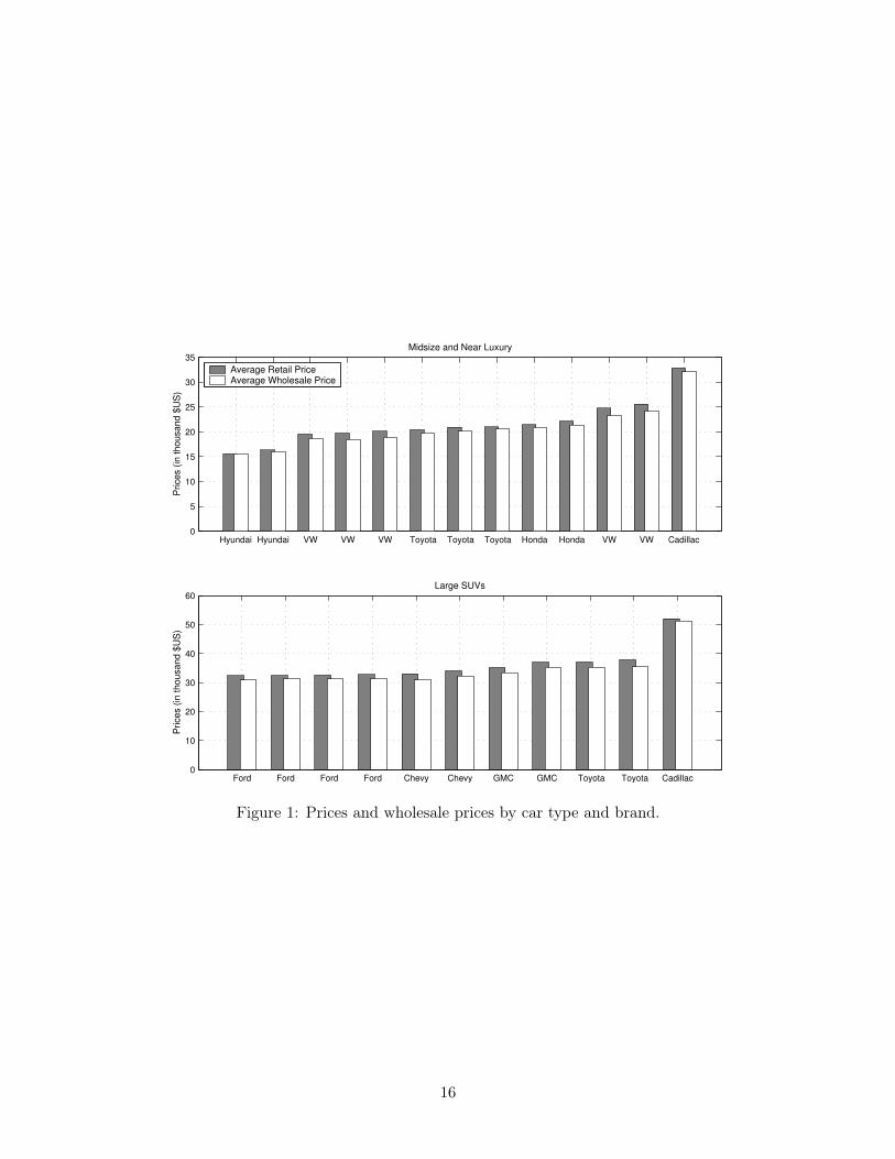
Figure 1 shows the average dealer and manufacturer price, for a sample of alternatives, grouped
by car type, for the mid sized and near luxury cars, and for large SUVs. It reveals the presence of
significant price variation across brands, even within car type, while prices of the same car sold at
different dealers shows much less variation.
A unique feature of our data is that we observe the location of both consumers and car dealers
for each transaction, allowing for a better understanding of the spatial distribution of demand and14Our raw data includes 20% of all transactions made in the San Diego area. After the filtering described here, the
final percentage of transactions included in our data set is 12% (60% × 20%) of all purchases made in the San Diegoarea.
15
Hyundai Hyundai VW VW VW Toyota Toyota Toyota Honda Honda VW VW Cadillac0
5
10
15
20
25
30
35
Price
s (in
th
ou
san
d $
US
)
Midsize and Near Luxury
Average Retail PriceAverage Wholesale Price
Ford Ford Ford Ford Chevy Chevy GMC GMC Toyota Toyota Cadillac0
10
20
30
40
50
60
Price
s (in
th
ou
san
d $
US
)
Large SUVs
Figure 1: Prices and wholesale prices by car type and brand.
16
(a) (b)
(c) (d)
0 5 10 miles
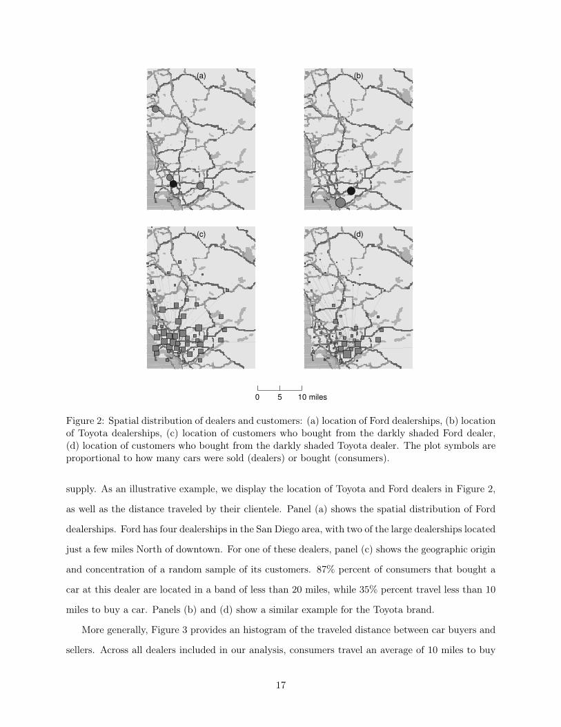
Figure 2: Spatial distribution of dealers and customers: (a) location of Ford dealerships, (b) locationof Toyota dealerships, (c) location of customers who bought from the darkly shaded Ford dealer,(d) location of customers who bought from the darkly shaded Toyota dealer. The plot symbols areproportional to how many cars were sold (dealers) or bought (consumers).
supply. As an illustrative example, we display the location of Toyota and Ford dealers in Figure 2,
as well as the distance traveled by their clientele. Panel (a) shows the spatial distribution of Ford
dealerships. Ford has four dealerships in the San Diego area, with two of the large dealerships located
just a few miles North of downtown. For one of these dealers, panel (c) shows the geographic origin
and concentration of a random sample of its customers. 87% percent of consumers that bought a
car at this dealer are located in a band of less than 20 miles, while 35% percent travel less than 10
miles to buy a car. Panels (b) and (d) show a similar example for the Toyota brand.
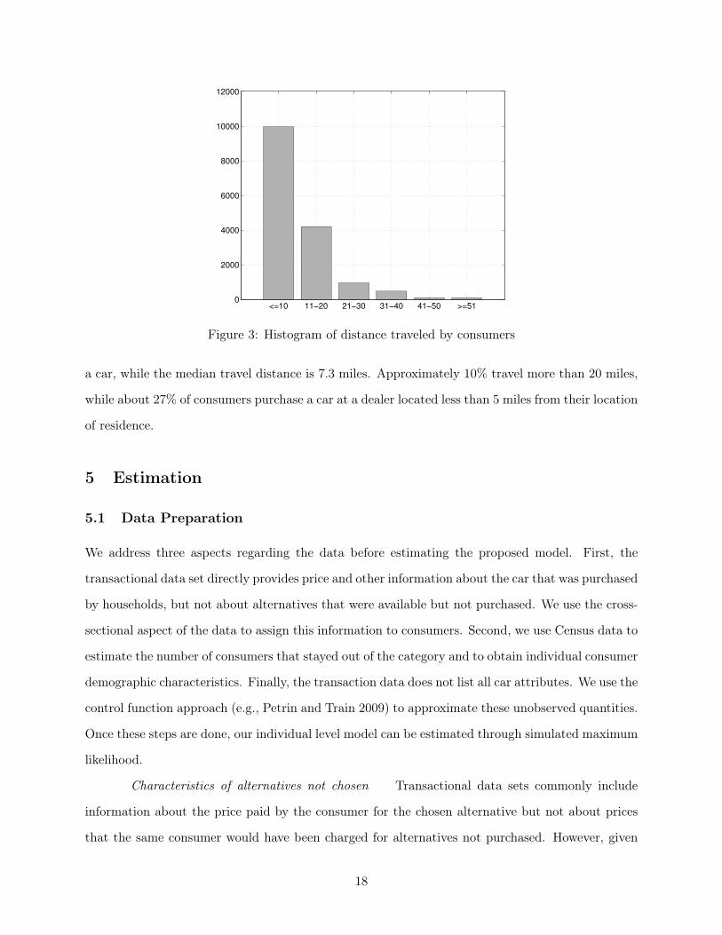
More generally, Figure 3 provides an histogram of the traveled distance between car buyers and
sellers. Across all dealers included in our analysis, consumers travel an average of 10 miles to buy
17
<=10 11!20 21!30 31!40 41!50 >=510
2000
4000
6000
8000
10000
12000
Figure 3: Histogram of distance traveled by consumers
a car, while the median travel distance is 7.3 miles. Approximately 10% travel more than 20 miles,
while about 27% of consumers purchase a car at a dealer located less than 5 miles from their location
of residence.
5 Estimation
5.1 Data Preparation
We address three aspects regarding the data before estimating the proposed model. First, the
transactional data set directly provides price and other information about the car that was purchased
by households, but not about alternatives that were available but not purchased. We use the cross-
sectional aspect of the data to assign this information to consumers. Second, we use Census data to
estimate the number of consumers that stayed out of the category and to obtain individual consumer
demographic characteristics. Finally, the transaction data does not list all car attributes. We use the
control function approach (e.g., Petrin and Train 2009) to approximate these unobserved quantities.
Once these steps are done, our individual level model can be estimated through simulated maximum
likelihood.
Characteristics of alternatives not chosen Transactional data sets commonly include
information about the price paid by the consumer for the chosen alternative but not about prices
that the same consumer would have been charged for alternatives not purchased. However, given
18
the large number of transactions, we can compute expected attribute values for the alternatives
that were not chosen. Our data is similar in this respect to previous data sets used in the literature,
such as Berry et al. (1995) and Petrin (2002), where only the average price and characteristics are
known, and not the specific characteristics of each car sold in the market. Our assumption is that
consumers are aware of the average level of prices at each dealership, but not of the exact prices of
all available cars. Accordingly, we use as prices of non-purchased alternatives the average price of
cars of the same brand and model sold in the same quarter. Similarly, we also compute the average
for the other car characteristics. If a car is not available, it is not part of the choice set of the
consumers.
Total Market Size Any analysis of spatial competition must take into account the lo-
cation of potential demand, as consumers have the option of purchasing a car that is not in our
data set or not buy a car at all. We use census data to obtain the total population size of each zip
code, #Householdsz. The potential market for cars in each zip code will be a proportion of that
value, for two reasons. First, our data cover only a part of all transactions and therefore we limit
the potential market to the same percentage of the total number of households. Additionally, we
account for the fact that consumers that have purchased a car recently will not be looking for a
car and will not be part of the potential market. We use inter-purchase time of cars to reflect this
aspect on the total market potential (7 years; see Sudhir 2001, for a similar approach). Formally,
the total market in zip code z is given by:
Hz =#Householdsz × Observed Transactions
Total Transactions× Years of Data
Interpurchase time(19)
For each zip code z, the sum of "observed" individuals who bought a car in our data set and
"unobserved" individuals whose choice was the outside good will be equal to the total market at
that location, Hz. The Census data shows 993,767 households living in the zip codes included in our
study, which results in the observed number of households for our sample of H =
z Hz = 34, 072.15
For reference, as mentioned in the data section, our data includes 15,795 households who buy a car,
which means that alternatives considered as the outside good represent the remaining 18,277, 56%
of the market. We assume that, for each zip code, consumers who choose the outside good have15993,767(# households) × 12% (percentage of observed transactions) × 2/7 (inter-purchase time, considering 2
years of data) =34,072.
19
the same distribution in terms of demographic characteristics and price expectations as consumers
who bought a car in our data set. Thus, we make draws from the empirical distributions, at the zip
code level, of consumer demographics and assign the values to “outside good” individuals in that
zip code.
Unobserved Attributes One potential source of endogeneity comes from the fact that the
dealer prices and unobserved car characteristics that influence consumer utility, e.g., car accessories,
may be correlated. One way to avoid the bias created by this correlation is to use a control
function approach (Pancras and Sudhir 2007; Petrin and Train 2009), exploiting that prices contain
information about unobserved attributes. This approach has two stages. In the first stage, we
recover ξjt, a one-to-one function of ξjt, by regressing prices on observed exogenous variables and
instrumental variables.
pjt = E [pjt|zjt] + ξjt
where zjt includes exogenous demand and cost shifters, and instruments. The exogenous cost shifters
include dummy variables for the dealer and car type, and the exogenous characteristics are engine
size, fuel and transmission type. Our instruments are similar to the ones in Berry et al. (1995)
and Petrin and Train (2009). We use the sum of each exogenous characteristic across all vehicles
of the same brand sold in other dealers and the sum of each characteristic across all other vehicles
of other brands but of the same type. This gives us 6 instruments for each alternative. Thus, our
price equation is given by:
pjt = ωzjt + ξjt (20)
When estimating the remaining demand parameters, δ1ξjt replaces ξjt in the utility function, where
δ1 is a parameter to be estimated and ξjt is kept fixed .
5.2 Demand Parameters
Since the demand model is fully identified from the choice data and we wish to avoid imposing
structure on the estimation problem, if none is required, we start by estimating the demand pa-
rameters without making any assumptions on the behavior of dealers and manufacturers. Given
our estimates for ξ, the estimation of the demand parameters can proceed via simulated maximum
20
likelihood, using the following likelihood function:
L =
i
j
t
Prijt |data, ξ, θ
yijt
where yijt is an indicator variable that takes the value of 1 for the alternative chosen by individual
i and zero otherwise and θ is the vector of demand parameters to be estimated. In our algorithm,
we maximize the log likelihood function
logL =
i
j
t
yijt · log(Prijt |data, ξ, θ) (21)
5.3 Supply Parameters
In this section, we start by evaluating manufacturer fixed cost C, and dealer revenues ∆, which can
be computed directly from the data and the demand estimates. We then estimate the fixed costs
parameter ρ1 for manufacturers and ρ2 for car dealers. To compute the implied variable costs of
the manufacturers, we use Equation 12. In this equation, we need to evaluate ∂S∂P , the derivative
of shares with respect to prices, and ∂P∂W the derivative of prices with respect to whole sale prices.
∂S∂P can be computed directly from the demand estimates, whereas ∂P
∂W can be evaluated using the
demand estimates and Equations 13 and 14. Along with the observed wholesale prices, we are in
possession of all terms in the right hand side of the resulting expression for manufacturer variable
costs
C = W −[ΘK ⊙ Ωw]
−1S
(22)
Next, we use the approach in Pakes et al. (2008), as it is applied for instance by Ishii (2008)
to the case of ATM networks, to estimate (1) the fixed costs of dealers using as input the observed
decisions in terms of size and location of the dealer networks, and (2) the fixed costs of manufacturers
directly related to the dealer network. As previously described, our optimality assumptions are that
a dealer who is present in the market is assumed to have non-negative profits and that profits at
an alternative dealer location are lower than where the dealer is currently located. At the same
time, the manufacturers also have a say in the size of their networks. In this case, the assumption
is that the observed dealer network size is optimal for the observed market conditions in 2004-2005,
21
which was prior to the economic crisis. Thus, for each car manufacturer, the profits would go down
if either one more dealer was opened or if one dealer closed. These assumptions provide inequality
restrictions that at least set-identify the fixed cost parameters.
5.3.1 Retailer Fixed Costs
Our objective is to estimate the fixed cost parameters for dealers, ρ2. For observed costs shifters at
the dealer level xdz , we use an intercept, the population size at each dealer location and surrounding
locations, distance from downtown San Diego and the city center of Escondido, and a dummy for
large dealers. Regarding the latter, we observe in the data two very different sizes of dealers, which
we allow to have different fixed costs, and thus we include a dummy for being a large dealers,
operationalized as having more than 500 cars in unit sales over the two years in our data. In total,
we estimate to estimate 6 fixed cost parameters.
We have 22 dealers in our data set. Our analysis will be for 20 dealers, because for two occasions,
two dealers at the same zip code of different brands have the same owner (GM and Chrysler), and we
consolidate their profits and fixed costs for this estimation procedure. For each of these 20 dealers,
we relocate one, keeping all others fixed at the observed location. The counterfactual locations
are chosen to be zip codes where there is at least one other dealer, thus making sure that it is
a realistic target for location. In particular, we chose 11 alternative locations for each retailer to
obtain 20x11=220 inequalities.16 We compare each dealer’s predicted profit at the current location
with those at alternative locations. Profits at the current configuration should be larger than at
counterfactual ones, thus satisfying the inequalities in Equation 18. Additionally, each dealer’s
fixed cost needs to be larger or equal than zero, leading to an additional 20 inequalities. Finally, the
profits of the dealer at the actual location have to be positive, which provides 20 more inequalities.
In total, we define and use 260 inequalities.
To construct each inequality, we need the variable profits (revenue-variable costs) for each dealer,
at both the actual location and counterfactual location. This is obtained using the demand and
supply estimates, so that both quantities and prices reflect the reaction of demand and supply to
the relocation of the dealer in the counterfactual scenario. We note that when dealers relocate, their16We could have constructed more inequalities based on other locations, but 11 alternative locations for each dealer
already identify parameters to a point.
22
demand changes, leading to some large dealers becoming small dealers and vice-versa, thus identify-
ing the size-of-dealer parameter. Since the relocation also changes the distance from downtown San
Diego and Escondido, that variation allows us to estimate the sensitivity of fixed costs to distance
from these centers.
We can interact each inequality with instruments. In that case, the number of inequalities
multiplies by the number of instruments. As Pakes, Porter, Ho, and Ishii (2008), we present the
results with instruments Z = 1, i.e., where we construct a sample analogue of the moment conditions
directly from the inequalities. Parameters were estimated minimizing the sum of the absolute value
of inequality-violations, as in Ishii (2008). For example, if the parameters provide gains in the
counterfactual configuration compared to the actual configuration, or some parameters may give
a negative profit for the new location or a negative estimate of fixed costs, we take the absolute
value of all these violations across all observations, sum, and minimize its total. This follows the
approach in Pakes et al. (2008) and Ishii (2008). Additionally, we carried out a robustness check
using population in surrounding zip codes as an instrument in addition to Z = 1. These results
differ significantly nor substantively from the results we present here.
We compute standard errors in a similar fashion as Ishii (2008). That is, we sample from the
distribution of the data by randomly drawing dealerships (with replacement) and for each draw
re-estimate the model. We took a total of 50 bootstrap samples and for each obtained estimates
of the fixed cost parameters, again by minimizing the absolute value of the inequalities. Reported
standard errors are the standard deviations of the parameters across samples.
5.3.2 Manufacturer Fixed Costs
Taking a similar approach, we now move to the estimation of manufacturer fixed cost parameters,
ρ1. In this case, we use an intercept, a dealer size dummy, and distance from the port of San Diego as
cost shifters, i.e., we estimate 3 cost parameters. To formulate inequalities, we look at each of the 20
existing dealers in the market, and in turn, compute the profits for the manufacturer of cars sold at
that dealer when that dealer is removed from the market, i.e., when we reduce that manufacturer’s
dealer network. Additionally, we also test adding dealers to the manufacturer networks. To do so,
we choose one of each of the 20 dealers, in turn, and “launch an exact copy” of that dealer at a
23
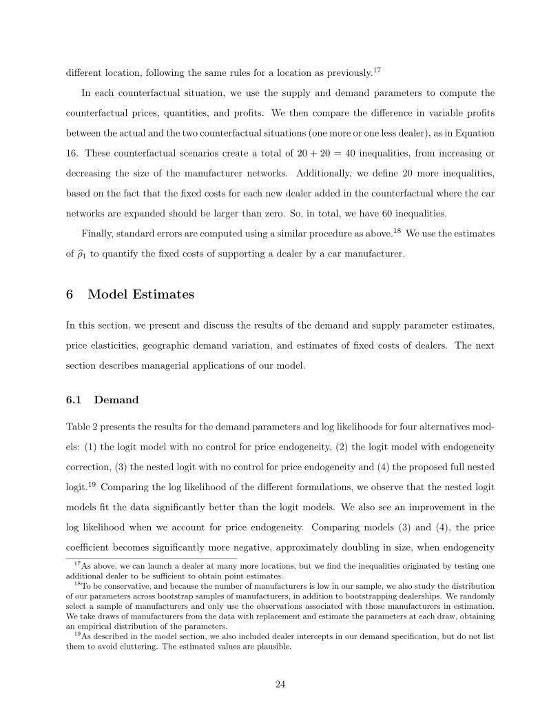
different location, following the same rules for a location as previously.17
In each counterfactual situation, we use the supply and demand parameters to compute the
counterfactual prices, quantities, and profits. We then compare the difference in variable profits
between the actual and the two counterfactual situations (one more or one less dealer), as in Equation
16. These counterfactual scenarios create a total of 20 + 20 = 40 inequalities, from increasing or
decreasing the size of the manufacturer networks. Additionally, we define 20 more inequalities,
based on the fact that the fixed costs for each new dealer added in the counterfactual where the car
networks are expanded should be larger than zero. So, in total, we have 60 inequalities.
Finally, standard errors are computed using a similar procedure as above.18 We use the estimates
of ρ1 to quantify the fixed costs of supporting a dealer by a car manufacturer.
6 Model Estimates
In this section, we present and discuss the results of the demand and supply parameter estimates,
price elasticities, geographic demand variation, and estimates of fixed costs of dealers. The next
section describes managerial applications of our model.
6.1 Demand
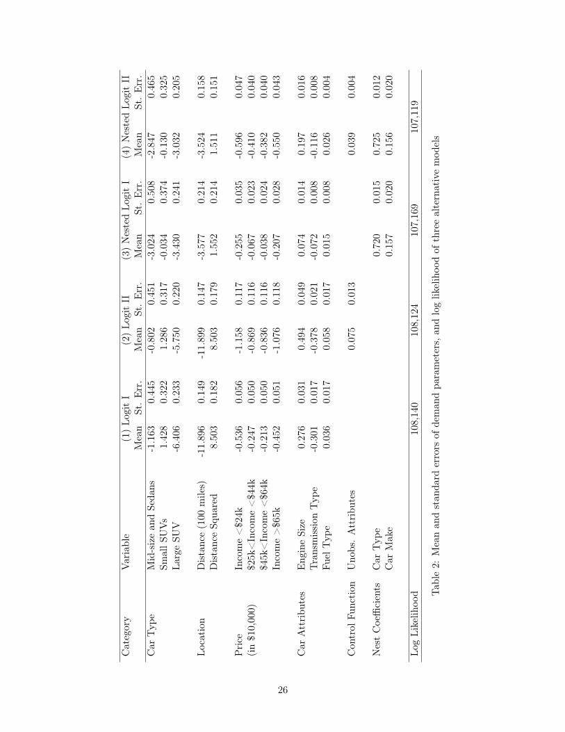
Table 2 presents the results for the demand parameters and log likelihoods for four alternatives mod-
els: (1) the logit model with no control for price endogeneity, (2) the logit model with endogeneity
correction, (3) the nested logit with no control for price endogeneity and (4) the proposed full nested
logit.19 Comparing the log likelihood of the different formulations, we observe that the nested logit
models fit the data significantly better than the logit models. We also see an improvement in the
log likelihood when we account for price endogeneity. Comparing models (3) and (4), the price
coefficient becomes significantly more negative, approximately doubling in size, when endogeneity17As above, we can launch a dealer at many more locations, but we find the inequalities originated by testing one
additional dealer to be sufficient to obtain point estimates.18To be conservative, and because the number of manufacturers is low in our sample, we also study the distribution
of our parameters across bootstrap samples of manufacturers, in addition to bootstrapping dealerships. We randomlyselect a sample of manufacturers and only use the observations associated with those manufacturers in estimation.We take draws of manufacturers from the data with replacement and estimate the parameters at each draw, obtainingan empirical distribution of the parameters.
19As described in the model section, we also included dealer intercepts in our demand specification, but do not listthem to avoid cluttering. The estimated values are plausible.
24
between unobserved attributes and price is accounted for. This corresponds to what is reported in
BLP (1995). Using the best fitting model, the remainder of the analysis is done with the nested
logit model that accounts for price endogeneity (4).
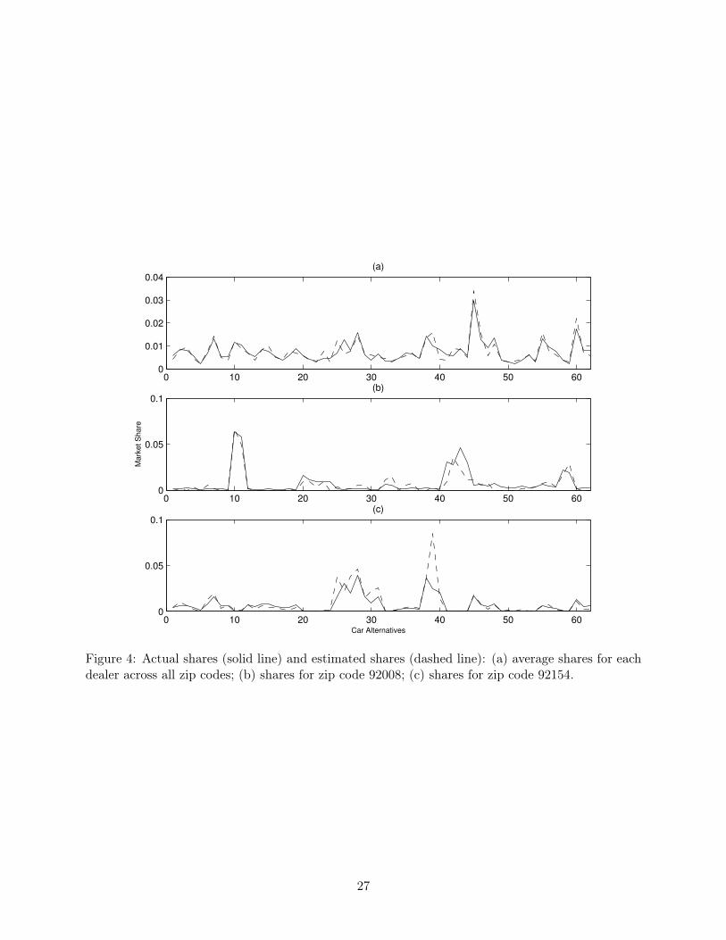
To illustrate the model’s fit, Figure 4 shows the actual and estimated average market shares of
each alternative j (excluding the outside option) for the total San Diego market (panel a) and for
two randomly selected zip codes (panels b and c). We find that the model explains the variation
in car popularity well, not only at the general market level but also at the zip code level, with a
good match between estimated shares and actual shares. The model does equally well for other zip
codes.
Additionally, we did a hold-out test using several zip codes that were left out of the estimation.
In total, these zip codes comprise 700 additional car purchases. We forecast shares among these
700 hold-out purchases, and the actual and predicted shares correlate with r = .79 (R2 = .62). In
view of the number of alternative cars and dealers this is a good hold out validation result.
We now interpret the demand parameters. The price coefficient is negative and significant for
all income levels, with the lowest income group (average income lower than $24,000) being the most
price sensitive. The parameters translate to an average own-price elasticity of -4.1. We analyze the
cross-price elasticities in more detail in sub-section 6.3.
In terms of other car attributes,20 consumers value engine size, automatic transmission, and cars
that use higher octane fuel. Regarding the car type, small SUVs, which include both compact and
mini SUVs, are more popular than both large SUVs and midsized cars.
We also observe that the residuals from the control function, which represent attributes un-
observed to the researcher but considered by consumers, have a positive impact on choice, with
cars that have higher levels of unobserved accessories being more appealing to the final consumer.
Finally, we find that the nest parameter for car type has a value of 0.72, consistent with stronger
substitution between alternatives within car type than across. For the brand nest parameter, the
value is 0.16. These estimates suggest that consumers segment the alternatives by car type, with
additional segmentation by brand. In the next subsections, we further analyze the impact of these
estimates on car substitution patterns.20We code the variable Transmission as "0" if automatic and "1" otherwise. For fuel type, “0” is the basic type of
fuel, “1” if the car uses higher octane fuel.
25
Cat
egor
yVa
riab
le(1
)Lo
git
I(2
)Lo
git
II(3
)N
este
dLo
git
I(4
)N
este
dLo
git
IIM
ean
St.
Err
.M
ean
St.
Err
.M
ean
St.
Err
.M
ean
St.
Err
.C
arT
ype
Mid
-siz
ean
dSe
dans
-1.1
630.
445
-0.8
020.
451
-3.0
240.
508
-2.8
470.
465
Smal
lSU
Vs
1.42
80.
322
1.28
60.
317
-0.0
340.
374
-0.1
300.
325
Larg
eSU
V-6
.406
0.23
3-5
.750
0.22
0-3
.430
0.24
1-3
.032
0.20
5
Loca
tion
Dis
tanc
e(1
00m
iles)
-11.
896
0.14
9-1
1.89
90.
147
-3.5
770.
214
-3.5
240.
158
Dis
tanc
eSq
uare
d8.
503
0.18
28.
503
0.17
91.
552
0.21
41.
511
0.15
1
Pri
ceIn
com
e<
$24k
-0.5
360.
056
-1.1
580.
117
-0.2
550.
035
-0.5
960.
047
(in
$10,
000)
$25k
<In
com
e<
$44k
-0.2
470.
050
-0.8
690.
116
-0.0
670.
023
-0.4
100.
040
$45k
<In
com
e<
$64k
-0.2
130.
050
-0.8
360.
116
-0.0
380.
024
-0.3
820.
040
Inco
me
>$6
5k-0
.452
0.05
1-1
.076
0.11
8-0
.207
0.02
8-0
.550
0.04
3
Car
Att
ribu
tes
Eng
ine
Size
0.27
60.
031
0.49
40.
049
0.07
40.
014
0.19
70.
016
Tran
smis
sion
Typ
e-0
.301
0.01
7-0
.378
0.02
1-0
.072
0.00
8-0
.116
0.00
8Fu
elT
ype
0.03
60.
017
0.05
80.
017
0.01
50.
008
0.02
60.
004
Con
trol
Func
tion
Uno
bs.
Att
ribu
tes
0.07
50.
013
0.03
90.
004
Nes
tC
oeffi
cien
tsC
arT
ype
0.72
00.
015
0.72
50.
012
Car
Mak
e0.
157
0.02
00.
156
0.02
0
Log
Like
lihoo
d10
8,14
010
8,12
410
7,16
910
7,11
9
Tabl
e2:
Mea
nan
dst
anda
rder
rors
ofde
man
dpa
ram
eter
s,an
dlo
glik
elih
ood
ofth
ree
alte
rnat
ive
mod
els
26
0 10 20 30 40 50 600
0.01
0.02
0.03
0.04(a)
0 10 20 30 40 50 600
0.05
0.1
Ma
rke
t S
ha
re
(b)
0 10 20 30 40 50 600
0.05
0.1(c)
Car Alternatives
Figure 4: Actual shares (solid line) and estimated shares (dashed line): (a) average shares for eachdealer across all zip codes; (b) shares for zip code 92008; (c) shares for zip code 92154.
27
6.2 Dealer Demand Areas
From our estimation results, we find that distance between dealers and consumers plays an important
role in the decision of buying a car. The effect of distance is both highly significant and substantial
– the longer the distance between consumer and dealer location, the lower the utility and choice
probability of an alternative. From the squared term of distance, we infer that the effect of distance
is marginally decreasing, revealing that as distances increase, utility still declines, but at a slower
pace.
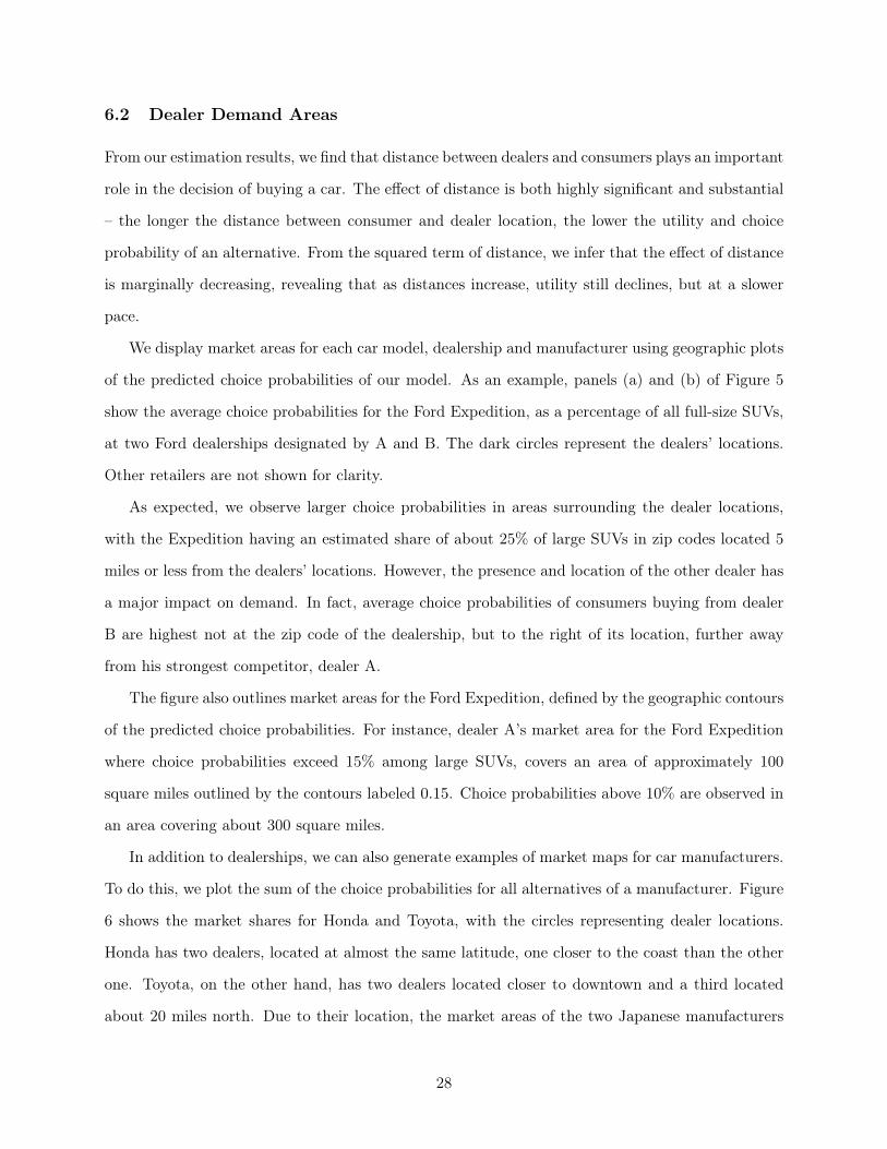
We display market areas for each car model, dealership and manufacturer using geographic plots
of the predicted choice probabilities of our model. As an example, panels (a) and (b) of Figure 5
show the average choice probabilities for the Ford Expedition, as a percentage of all full-size SUVs,
at two Ford dealerships designated by A and B. The dark circles represent the dealers’ locations.
Other retailers are not shown for clarity.
As expected, we observe larger choice probabilities in areas surrounding the dealer locations,
with the Expedition having an estimated share of about 25% of large SUVs in zip codes located 5
miles or less from the dealers’ locations. However, the presence and location of the other dealer has
a major impact on demand. In fact, average choice probabilities of consumers buying from dealer
B are highest not at the zip code of the dealership, but to the right of its location, further away
from his strongest competitor, dealer A.
The figure also outlines market areas for the Ford Expedition, defined by the geographic contours
of the predicted choice probabilities. For instance, dealer A’s market area for the Ford Expedition
where choice probabilities exceed 15% among large SUVs, covers an area of approximately 100
square miles outlined by the contours labeled 0.15. Choice probabilities above 10% are observed in
an area covering about 300 square miles.
In addition to dealerships, we can also generate examples of market maps for car manufacturers.
To do this, we plot the sum of the choice probabilities for all alternatives of a manufacturer. Figure
6 shows the market shares for Honda and Toyota, with the circles representing dealer locations.
Honda has two dealers, located at almost the same latitude, one closer to the coast than the other
one. Toyota, on the other hand, has two dealers located closer to downtown and a third located
about 20 miles north. Due to their location, the market areas of the two Japanese manufacturers
28
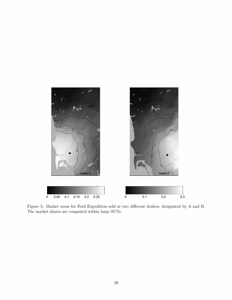
Figure 5: Market areas for Ford Expedition sold at two different dealers, designated by A and B.The market shares are computed within large SUVs.
29
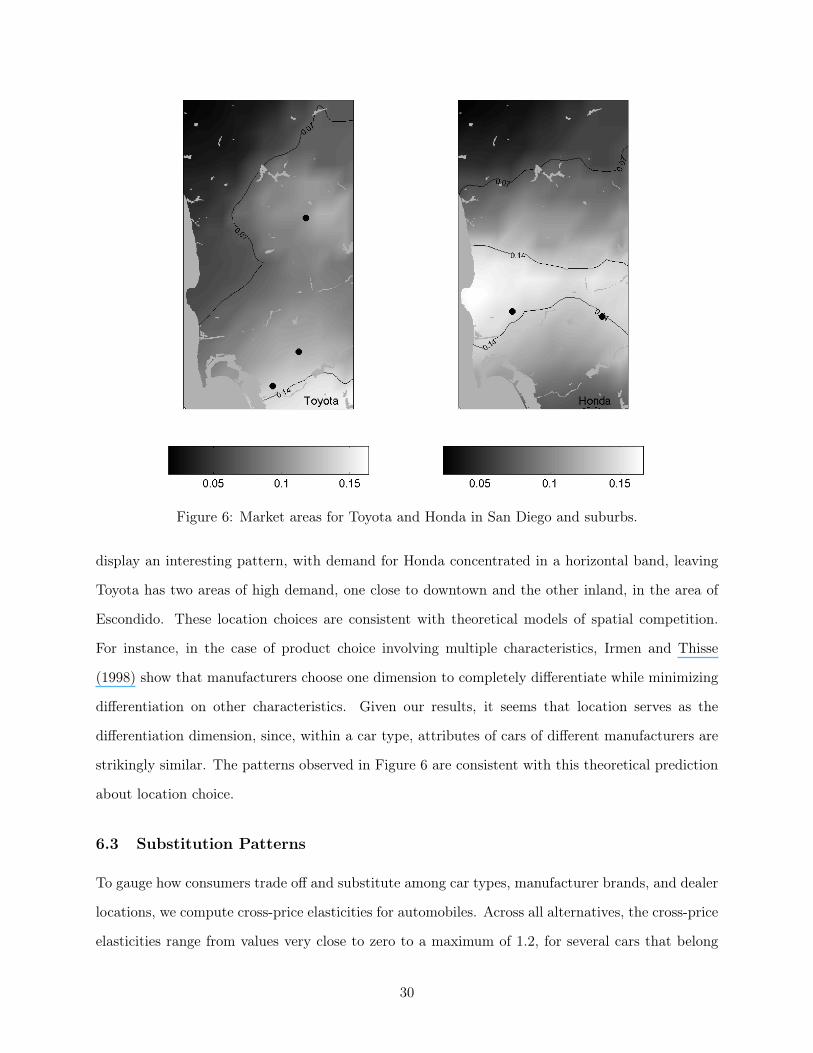
Figure 6: Market areas for Toyota and Honda in San Diego and suburbs.
display an interesting pattern, with demand for Honda concentrated in a horizontal band, leaving
Toyota has two areas of high demand, one close to downtown and the other inland, in the area of
Escondido. These location choices are consistent with theoretical models of spatial competition.
For instance, in the case of product choice involving multiple characteristics, Irmen and Thisse
(1998) show that manufacturers choose one dimension to completely differentiate while minimizing
differentiation on other characteristics. Given our results, it seems that location serves as the
differentiation dimension, since, within a car type, attributes of cars of different manufacturers are
strikingly similar. The patterns observed in Figure 6 are consistent with this theoretical prediction
about location choice.
6.3 Substitution Patterns
To gauge how consumers trade off and substitute among car types, manufacturer brands, and dealer
locations, we compute cross-price elasticities for automobiles. Across all alternatives, the cross-price
elasticities range from values very close to zero to a maximum of 1.2, for several cars that belong
30
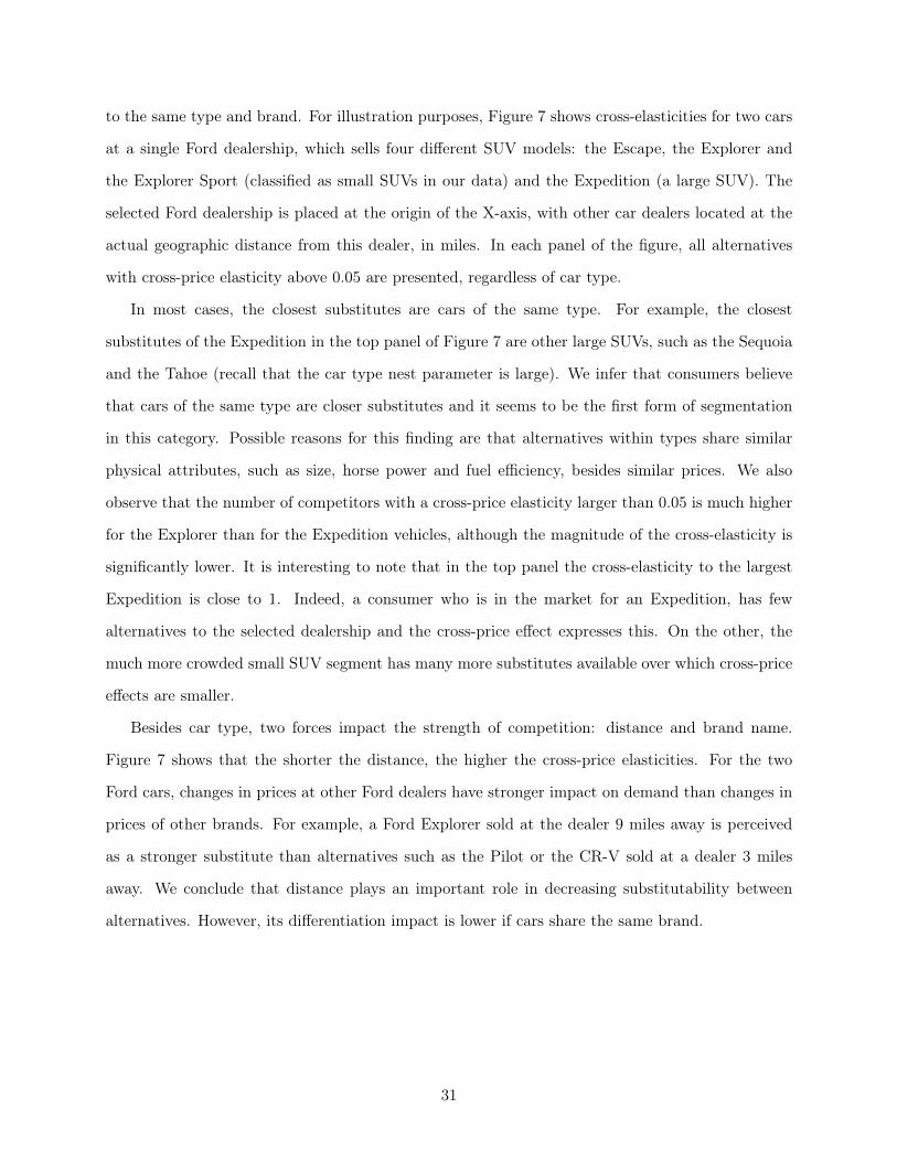
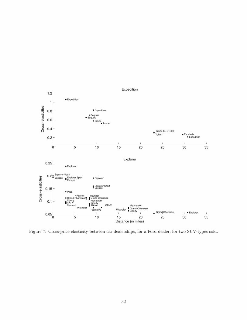
to the same type and brand. For illustration purposes, Figure 7 shows cross-elasticities for two cars
at a single Ford dealership, which sells four different SUV models: the Escape, the Explorer and
the Explorer Sport (classified as small SUVs in our data) and the Expedition (a large SUV). The
selected Ford dealership is placed at the origin of the X-axis, with other car dealers located at the
actual geographic distance from this dealer, in miles. In each panel of the figure, all alternatives
with cross-price elasticity above 0.05 are presented, regardless of car type.
In most cases, the closest substitutes are cars of the same type. For example, the closest
substitutes of the Expedition in the top panel of Figure 7 are other large SUVs, such as the Sequoia
and the Tahoe (recall that the car type nest parameter is large). We infer that consumers believe
that cars of the same type are closer substitutes and it seems to be the first form of segmentation
in this category. Possible reasons for this finding are that alternatives within types share similar
physical attributes, such as size, horse power and fuel efficiency, besides similar prices. We also
observe that the number of competitors with a cross-price elasticity larger than 0.05 is much higher
for the Explorer than for the Expedition vehicles, although the magnitude of the cross-elasticity is
significantly lower. It is interesting to note that in the top panel the cross-elasticity to the largest
Expedition is close to 1. Indeed, a consumer who is in the market for an Expedition, has few
alternatives to the selected dealership and the cross-price effect expresses this. On the other, the
much more crowded small SUV segment has many more substitutes available over which cross-price
effects are smaller.
Besides car type, two forces impact the strength of competition: distance and brand name.
Figure 7 shows that the shorter the distance, the higher the cross-price elasticities. For the two
Ford cars, changes in prices at other Ford dealers have stronger impact on demand than changes in
prices of other brands. For example, a Ford Explorer sold at the dealer 9 miles away is perceived
as a stronger substitute than alternatives such as the Pilot or the CR-V sold at a dealer 3 miles
away. We conclude that distance plays an important role in decreasing substitutability between
alternatives. However, its differentiation impact is lower if cars share the same brand.
31
0 5 10 15 20 25 30 35
0.2
0.4
0.6
0.8
1
1.2
Tahoe
Sequoia
Tahoe
Expedition
Yukon
Yukon XL C1500
Sequoia
Expedition
ExpeditionEscalade
Expedition
Cro
ss!
ela
stic
itie
s
0 5 10 15 20 25 30 350.05
0.1
0.15
0.2
0.25
Escape
Explorer Sport
4Runner
Highlander
Escape
Explorer
Explorer Sport
Santa FeGrand Cherokee
RAV4
Escape
Explorer
Explorer Sport
Grand Cherokee
Liberty
Wrangler
Explorer
CR!VElement
Pilot
Grand CherokeeLiberty
Wrangler
4Runner
Highlander
Grand CherokeeLiberty
CR!V
Explorer
Distance (in miles)
Cro
ss!
ela
stic
ities
Figure 7: Cross-price elasticity between car dealerships, for a Ford dealer, for two SUV-types sold.
32
6.4 Supply
We find that the average manufacturer margin is 51%, which correspond to a value of $12,513.21
For car dealerships, there are two quantities to discuss. First, in our data, we observe the direct
gross margin for each car, i.e., the difference between the manufacturer price and the final price
charged to the consumer by the dealership. On average, this value is $1,630, about 6.5% of the final
price. Thus, compared to dealers, manufacturers get the lion share of gross margins in this industry.
However, given that dealers will have future revenues from the servicing of cars, dealer prices also
take these revenues into consideration, which are denoted in Equation 11 as ∆. Our estimates imply
that dealers get on average a total value of $6,220 per car, which means that additional net revenues
amount to $4,590. This seems to be a reasonable result, since industry reports state that profits
resulting from car servicing are about four times the value of profits from the new cars division
(NADA, 2008).
As described in the estimation section, we obtain the parameters related to fixed costs by shifting
the location of each dealer to 11 hypothetical locations. Our estimates satisfy above 98% of the
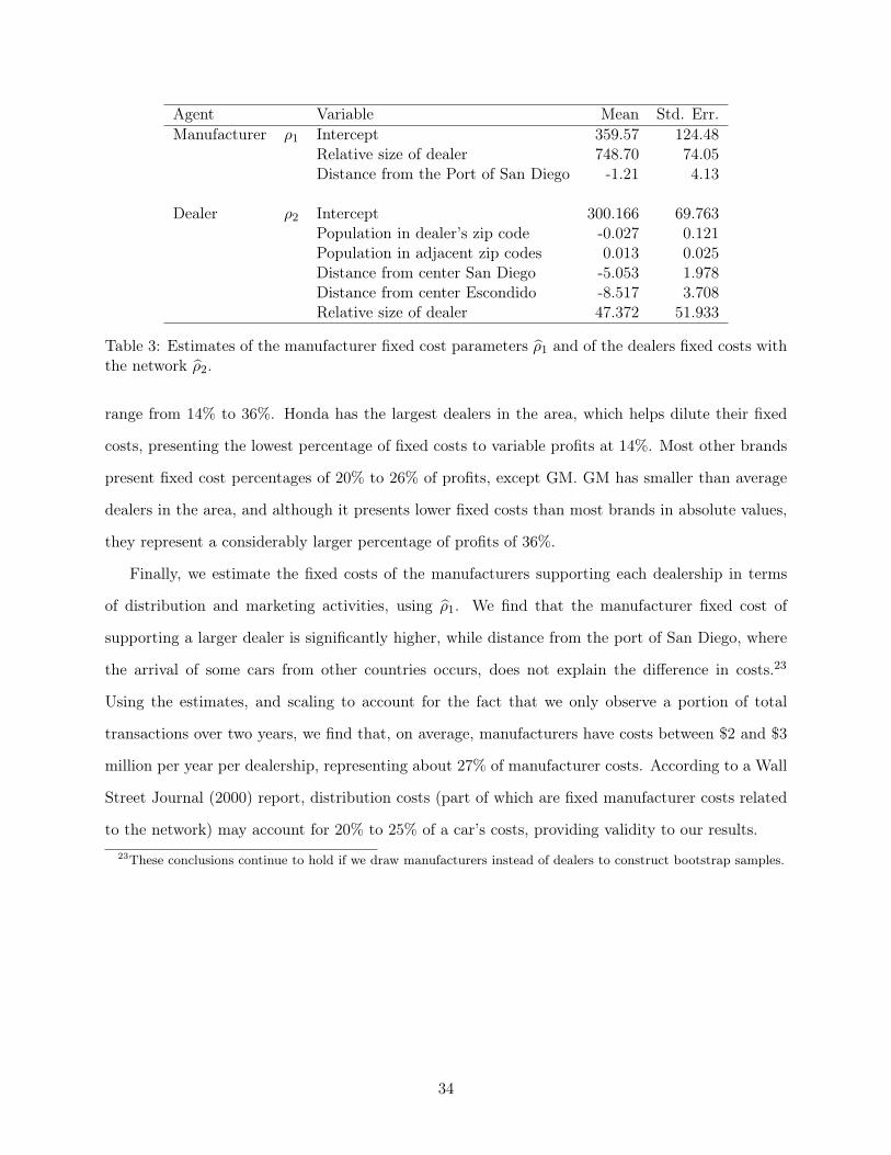
inequality conditions used. The point estimates and standard errors are presented in Table 3. We
observe that the most significant variables are the dealership’s distance to the two main urban
centers. These variables are estimated to have negative effects implying that greater distance to the
city centers lowers the fixed costs of the dealership. The number of inhabitants at the dealer zip
code and surrounding zip codes does not play a significant role in explaining fixed costs.
With the estimates ρ2, we obtain estimated values for the fixed costs of dealerships using fd =
xdρ2. On average, we estimate fixed costs with an annual value of $3.6 million dollars.22 NADA
states in its 2008 report that dealers spend on average about $2.2 million on salaries and another
$600 thousand in other fixed costs, such as advertising and rent (NADA, 2008). Although our
estimate is slightly above this national average, we focus on the most important brands in San
Diego. The high cost of land in California adds further face validity.
Measuring fixed costs as a percentage of the dealer variable profits, we find values that they21We estimate mark-ups that are slightly larger than the ones presented in Berry et al. (1995), 50% vs. 30%. We
conjecture that this is due to the fact that larger and more expensive cars have been introduced and become popularsince 1990 (the time period of Berry et al.’s data).
22Our data set includes only a portion of the total observations, as described in the data section. We scaled thefixed costs obtained from the estimates to take into account the relative size of the observations in our data set.
33
Agent Variable Mean Std. Err.Manufacturer ρ1 Intercept 359.57 124.48
Relative size of dealer 748.70 74.05Distance from the Port of San Diego -1.21 4.13
Dealer ρ2 Intercept 300.166 69.763Population in dealer’s zip code -0.027 0.121Population in adjacent zip codes 0.013 0.025Distance from center San Diego -5.053 1.978Distance from center Escondido -8.517 3.708Relative size of dealer 47.372 51.933
Table 3: Estimates of the manufacturer fixed cost parameters ρ1 and of the dealers fixed costs withthe network ρ2.
range from 14% to 36%. Honda has the largest dealers in the area, which helps dilute their fixed
costs, presenting the lowest percentage of fixed costs to variable profits at 14%. Most other brands
present fixed cost percentages of 20% to 26% of profits, except GM. GM has smaller than average
dealers in the area, and although it presents lower fixed costs than most brands in absolute values,
they represent a considerably larger percentage of profits of 36%.
Finally, we estimate the fixed costs of the manufacturers supporting each dealership in terms
of distribution and marketing activities, using ρ1. We find that the manufacturer fixed cost of
supporting a larger dealer is significantly higher, while distance from the port of San Diego, where
the arrival of some cars from other countries occurs, does not explain the difference in costs.23
Using the estimates, and scaling to account for the fact that we only observe a portion of total
transactions over two years, we find that, on average, manufacturers have costs between $2 and $3
million per year per dealership, representing about 27% of manufacturer costs. According to a Wall
Street Journal (2000) report, distribution costs (part of which are fixed manufacturer costs related
to the network) may account for 20% to 25% of a car’s costs, providing validity to our results.23These conclusions continue to hold if we draw manufacturers instead of dealers to construct bootstrap samples.
34
7 Evaluating the impact of negative demand shocks
7.1 General Approach
Motivated by the quote at the beginning of this paper wherein General Motors plans to revise its
dealer network configuration, we focus our attention on two counterfactuals. First, we analyze the
impact of a reduction of market demand on profits of dealers and manufacturers, which can serve as
potential justification for General Motors desire for a leaner structure. We also discuss the results
in the context of the so-called “cash for clunkers” policy. Second, we discuss the San Diego dealer
network of GM and Chrysler, and compare our predictions of dealer closings to actual data. In each
case, we consider the effects of a negative demand shock similar in concept to an economic crisis on
prices, quantities, and profits of retailers and manufacturers. This analysis can serve as input for
managers and policy makers in the car industry.
Our approach to measuring the effects of an economic crisis is to increase the appeal of the
outside good, making consumers more likely to stay out of the category. To do this, we shift the
utility of the outside good from an exogenously set value of zero to a value of 0.7, leading to the
market drop of about 30% in the general demand for automobiles over two years, similar to the
effect of the economic crisis for the years of 2007-2008. We note that this decrease is general to the
entire market. Our demand shock also affects all zip codes similarly, although it would be easy to
make the demand decrease as a function of demographic characteristics, such as income, leading to
variability across locations.
7.2 Prices and Margins in Response to an Economic Crisis
In this first counterfactual situation, we use our demand model to obtain estimates of market
shares under the shock on the outside good, and next use those estimates to obtain new dealer and
manufacturer prices using the supply equations. We then iterate the demand and supply sides of the
model until they converge, i.e., we stop iterating when maxjdP
τ+1 − Pτ< ι, with P
τ and Pτ+1
being the vectors of prices at iterations τ and τ + 1, and where ι is set to be very small (ι = 0.01).
We find that lower demand levels and more price response both cause lower equilibrium prices,
with dealer and manufacturer prices decreasing by an annual average of 13% and 11% respectively.
The drop in equilibrium prices partially offsets the initial negative demand shock caused by the
35
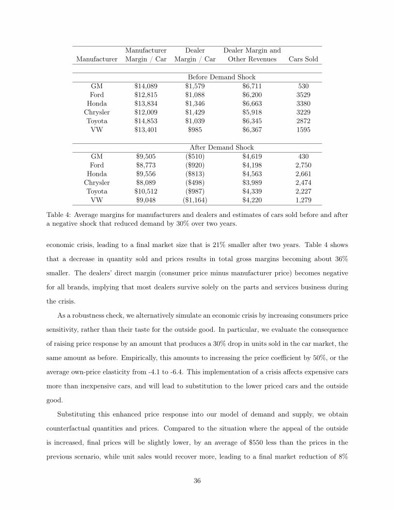
Manufacturer Dealer Dealer Margin andManufacturer Margin / Car Margin / Car Other Revenues Cars Sold
Before Demand ShockGM $14,089 $1,579 $6,711 530Ford $12,815 $1,088 $6,200 3529
Honda $13,834 $1,346 $6,663 3380Chrysler $12,009 $1,429 $5,918 3229Toyota $14,853 $1,039 $6,345 2872VW $13,401 $985 $6,367 1595
After Demand ShockGM $9,505 ($510) $4,619 430Ford $8,773 ($920) $4,198 2,750
Honda $9,556 ($813) $4,563 2,661Chrysler $8,089 ($498) $3,989 2,474Toyota $10,512 ($987) $4,339 2,227VW $9,048 ($1,164) $4,220 1,279
Table 4: Average margins for manufacturers and dealers and estimates of cars sold before and aftera negative shock that reduced demand by 30% over two years.
economic crisis, leading to a final market size that is 21% smaller after two years. Table 4 shows
that a decrease in quantity sold and prices results in total gross margins becoming about 36%
smaller. The dealers’ direct margin (consumer price minus manufacturer price) becomes negative
for all brands, implying that most dealers survive solely on the parts and services business during
the crisis.
As a robustness check, we alternatively simulate an economic crisis by increasing consumers price
sensitivity, rather than their taste for the outside good. In particular, we evaluate the consequence
of raising price response by an amount that produces a 30% drop in units sold in the car market, the
same amount as before. Empirically, this amounts to increasing the price coefficient by 50%, or the
average own-price elasticity from -4.1 to -6.4. This implementation of a crisis affects expensive cars
more than inexpensive cars, and will lead to substitution to the lower priced cars and the outside
good.
Substituting this enhanced price response into our model of demand and supply, we obtain
counterfactual quantities and prices. Compared to the situation where the appeal of the outside
is increased, final prices will be slightly lower, by an average of $550 less than the prices in the
previous scenario, while unit sales would recover more, leading to a final market reduction of 8%
36
smaller relative to the beginning of the recession. However, in terms of the net effect, this scenario
of increased price sensitivity leads to total revenues for manufacturers and dealers similar to the
ones shown in Table 4.
7.3 Car Allowance Rebate System
In 2009, the U.S. government introduced a stimulus program, the Car Allowance Rebate System
(also known by Cash for Clunkers program), to counteract the effects of the economic crisis on the
auto industry, providing $3,500 or $4,500 to a consumer who traded an old car for a new one. In the
previous section, we showed that optimal prices go down by between $3,000 to $6,000 over two years,
as a result of the demand shock, leading to a strong reduction of profits of dealers and manufacturers.
Interestingly, the range of the predicted price reduction from our approach matches the amount given
in the government program. With the financial situation of the American manufacturers and the
effects of a severe economic crisis, it is unlikely that manufacturers could have survived if such a
drastic price cut would have been implemented, leading to severe drops in margins, while fixed
costs remained at pre-recession levels. Viewed in this way, the Cash for Clunkers program offered
a temporary solution to the need to respond to the decrease in the demand, shifting the final prices
paid at the dealer closer to optimal prices, without additional strain on the manufacturers’ already
dire financial situation.
An interesting related question that we can answer using our model pertains to the effects of
such subsidies on retailer behavior, namely prices. Given that retailers know that consumers have
$4,500 additional disposable income to spend on a new car, it is possible that retailers would adjust
final prices to account for that subsidy. With our approach, we are able to form an opinion about
how much of the subsidy offered to consumers would likely stay with the consumers and how much
is transferred to retailers by means of price changes.
To investigate the simultaneous impact of an economic crisis and a car allowance rebate program,
we perform the following counterfactual. After reducing the demand by the amount equivalent to
the economic recession, with an increase in the appeal of the outside good, we apply the subsidy
and reduce the prices faced by consumers by $4,500, which is equivalent to the amount offered
by the government. Thus, in this counterfactual, there is a $4,500 difference between the price
charged by retailers and the price faced by consumers. Demand takes into account the benefit of
37
the car allowance, and manufacturers and retailers set their prices taking into account this windfall
to consumer demand. Given that consumers now face a lower price, the probability of buying a car
goes up, and retailers are likely to move prices up to face this new increase in demand. With these
two conditions, that is, (1) an increase in the popularity of the outside good which would case a
drop in the market by 30%, and (2) a subsidy such that prices faced by the consumer are $4,500
lower than the ones charged by dealers, our results show that, on average, retailers would charge on
average $1,542 more per car than in a situation without the program, leaving an average of $2,958
in the hands of consumers.
7.4 Reducing the number of dealers
The continuous decrease in demand led some manufacturers to close some of the less profitable
dealerships. We show the effects of closing alternative dealers for GM and Chrysler in Table 5. We
implement a drop of 30% of demand for GM and 50% for Chrysler, matching industry reports (The
Detroit Bureau, 2009), and obtain the respective unit sales and margins as previously described.
In each row, for GM and Chrysler, we show the numbers for the current dealer networks and
results from removing a given dealership, identified by its zip code, from the market. For each case,
we present the total number of cars sold, variable profits and fixed costs across all the remaining
dealerships in the manufacturer’s network, as well as the actual decision by the manufacturer to
close the dealership.
Looking at the values presented in the table for GM, we observe that the GMC dealer is the
best candidate to close from the dealer network side, i.e., if that dealer were closed, the remaining
dealers would net a profit of K$675, larger than the current network profit of K$305. At the same
time, closing that dealership will yield only a small drop in the profit to the manufacturer as keeping
it open, since fixed costs of both manufacturer and dealer network go down significantly when the
GMC dealer is closed, and leads to a much leaner structure, one of the desired objectives of GM’s
re-structuring plan. Based on these results, our model supports GM’s and dealer’s decisions to close
down the GMC dealer, which happened at the end of 2009.
Consider now the case of Chrysler. Closure of the dealers located at 91950 and at 92111 would
make the manufacturer and dealer profits of the remaining network drop considerably, leading us
to conclude that these dealers should not be closed in the near future. We predict that the other
38
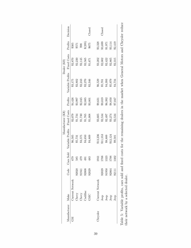
Man
ufac
ture
r(K
$)D
eale
r(K
$)M
anuf
actu
rer
Mak
eC
ode
Car
sSo
ldVar
iabl
eP
rofit
sFix
edC
osts
Pro
fits
Var
iabl
eP
rofit
sFix
edC
osts
Pro
fits
Dec
isio
nG
MC
urre
ntN
etw
ork
679
$6,5
05$2
,079
$4,4
26$3
,175
$2,8
70$3
05C
hevy
9202
058
5$5
,731
$1,7
34$3
,997
$2,8
02$2
,230
$571
Che
vy91
941
479
$4,5
75$1
,730
$2,8
45$2
,243
$2,1
45$9
8C
adill
ac92
008
491
$4,6
50$1
,765
$2,8
85$2
,270
$2,5
65$(
295)
GM
C92
029
483
$4,8
09$1
,008
$3,8
01$2
,346
$1,6
71$6
75C
lose
d
Chr
ysle
rC
urre
ntN
etw
ork
1941
$13,
236
$3,6
05$9
,631
$6,5
29$3
,202
$3,3
28Je
ep92
029
1708
$11,
553
$2,5
34$9
,019
$5,7
01$2
,002
$3,6
99C
lose
dJe
ep91
950
1323
$8,8
89$2
,497
$6,3
92$4
,393
$2,4
22$1
,971
Jeep
9206
417
88$1
2,12
4$3
,274
$8,8
50$5
,979
$2,8
65$3
,114
Jeep
9211
114
02$9
,581
$2,5
34$7
,047
$4,7
34$2
,315
$2,4
19
Tabl
e5:
Vari
able
profi
ts,
cars
sold
and
fixed
cost
sfo
rth
ere
mai
ning
deal
ers
inth
em
arke
tw
hen
Gen
eral
Mot
ors
and
Chr
ysle
rre
duce
thei
rne
twor
kby
ase
lect
edde
aler
.
39
two dealerships, located at zip codes 92029 and 92064, are potential closing targets since fixed costs
for Chrysler reduce significantly, and manufacturer profits stay almost constant. Between these two
dealers, our model recommends the closure of the dealer located at 92029, with better numbers in
terms of cost savings and dealer network profits, matching Chrysler’s only closing decision in this
market. We conclude that these predictions show face validity and demonstrate the usefulness of
our approach regarding decisions on reducing the size of outlet networks of manufacturers.24
8 Conclusion and Future Research
This paper analyzes local demand and supply for cars using transactional data. It provides insight
into the effects of a severe reduction of demand, which can be caused for instance by an economic
crisis, on the car industry and more specifically on dealer networks. We provide a number of
substantive insights and an approach that can help decision-making of manufacturers and policy
makers.
On the demand side, we define a purchase option as a combination of a car, with its product
attributes, and a dealer, with its own characteristics and location. Utilities for such purchase
option are therefore informative about the trade-off between preferences for dealer location and car
characteristics, including price. Using a large transaction-level data set, we show that the effects
of physical distance between buyers and sellers are important and can not easily be ignored when
studying demand and substitution patterns in the car industry. Specifically, our analysis suggests
that substitution even among pairs of cars of the same brand quickly fades as the dealers selling them
are located farther away from each other. We find that each dealership has a localized demand area,
and that choice probabilities decrease at a fast rate with distance between buyers and sellers. For
most choice alternatives, we find that a limited set of close substitutes combined with concentrated
demand leads to private “backyards” of higher demand for each dealer.
Making use of the demand estimates and assuming profit maximizing behavior of both man-
ufacturers and dealers, we then estimate gross margins of agents and fixed costs of running a car24We note that although immediate profits for both GM and Chrysler are predicted to go marginally down when
they close these dealers, their decision is justified by two factors: first, we do not include in our analysis the savingsfrom decreases in other fixed costs, such as production and related salaries, that happened in 2009 as a resultof widespread reductions in production and in the dealer network; second, both GM and Chrysler had the need tocreate much leaner and efficient structures to satisfy government regulation, which increases the importance of cuttingfixed costs in the manufacturer and dealer network.
40
dealership. We find that price-cost margins for manufacturers are about 50% of the selling price,
while dealers obtain an immediate margin of about 5% to 10%, that becomes about 20% when
other revenues are taking into account. Our approach estimates hypothetical profits for dealers and
partially for manufacturers (we do not estimate the total fixed costs of manufacturers) in several
counterfactual scenarios. The first application measures the impact on the size of dealer networks
if a reduction of demand occurred in the car industry, similar to the economic crisis that started in
2008. We find that average dealer and manufacturer prices would decrease by an annual average of
11% and that total gross margins decrease by about 35%. Our second application deals with the
decision to reduce of network size, given the new demand conditions. We exemplify the usefulness
of our model in measuring profits when a manufacturer considers reducing the size of its dealer
network.
Finally, we believe that our approach can be broadly applied to settings outside the car industry.
Specifically, it can be used when manufacturers are interested in evaluating the effects of location
of outlets on demand and competition, e.g., the banking industry, the gasoline industry, etc., where
store location plays an important role in the success of products and services of firms, as well as the
effects of overall shocks in the overall demand of the market. It can also be applicable to categories
in decline, where manufacturers must choose which outlets to remove from the market to maximize
profits of its dwindling products.
41
References
[1] Berry S., J. Levinsohn., and A. Pakes (1995): “Automobile Prices in Market Equilibrium,”Econometrica, Vol. 63, 841-890.
[2] Berry S., J. Levinsohn, and A. Pakes (2004), “Differentiated Products Demand Systems from aCombination of Micro and Macro Data: The New Car Market,” Journal of Political Economy,February, 68-105.
[3] Bucklin, R., S. Siddarth, and J. Silva-Risso (2008), "Distribution Density and New Car Choice,"Journal of Marketing Research, Vol.44, 473-486.
[4] Cardell, N.S. (1997), "Variance Components Structures for the extreme value and logisticdistributions with applications to models of heterogeneity," Economic Theory, 13, 185-213.
[5] Davis, P. (2001): "Spatial Competition in Retail Markets: Movie Theaters," The RAND Jour-
nal of Economics, Vol. 37, No. 4, 964-982.
[6] The Detroit Bureau (2009), “Chrysler Group September 2009 Sales Drop 42%,” October 1st.
[7] Duan, J. and C. Mela (2008): "The Role of Spatial Demand on Outlet Location and Pricing,"forthcoming, Journal of Marketing Research.
[8] Ellickson, P. and S. Misra (2008), "Supermarket Pricing Strategies," conditionally accepted atMarketing Science.
[9] General Motors Corporation (2008), “Restructuring Plan for Long-Term Viability”, submit-ted to Senate Banking Committee & House of Representatives Financial Services Committee,December 2.
[Ho] Ho, Katherine (2009), “"Insurer-Provider Networks in the Medical Care Market," American
Economic Review, 99(1): 393-430.
[10] Hoch, S., B. Kim, A. Montgomery and P. Rossi (1995), "Determinants of Store-Level PriceElasticity," Journal of Marketing Research, Vol. 32, No. 1 (Feb., 1995), 17-29.
[11] Irmen, A. and J.-F. Thisse (1998), "Competition in Multi-characteristics Spaces: HotellingWas Almost Right," Journal of Economic Theory, 78, 76-102.
[12] Ishii, J. (2008), “Compatibility, Competition, and Investment in Network Industries: ATMNetworks in the Banking Industry,” working paper.
[13] Luan, J., Sudhir, K., and B. Norris (2007), "Dynamic Market Structure in a Durable GoodsMarket: The Effect of a New Product Form," working paper.
[14] Mazzeo, M (2002), "Product Choice and oligopoly market structure," RAND Journal of Eco-nomics, Vol. 33, No. 2 (Summer), 1-22.
[15] NADA (2008), “NADA Data,” National Automobile Dealers Association’s Industry AnalysisDivision, AutoExec, May, 43-63.
42
[16] Pakes, A., J. Porter, K. Ho, and J. Ishii (2008), "Moment Inequalities and Their Application,"working paper.
[17] Pancras, J. and K. Sudhir (2007), "Optimal Marketing Strategies for a Customer Data Inter-mediary", Journal of Marketing Research, Vol. 44:4 (November), 560-578.
[18] Petrin, A. (2002), "Quantifying the Benefits of New Products: The Case of the Minivan,"Journal of Political Economy , 110, 705-729.
[19] Petrin, A. and K. Train (2009), "Omitted Product Attributes in Discrete Choice Models,"Journal of Marketing Research, forthcoming.
[20] Progressive Grocer (1995), April.
[21] Richards, T. (2007), "A Nested Logit Model of Strategic Promotion," Quantitative Marketing
and Economics, Vol. 5, 63-91.
[22] Scott Morton, F., Zettelmeyer, F., and J. Silva-Risso (2001), "Internet Car Retailing," The
Journal of Industrial Economics, Vol. 44:4, 501-519,
[23] Sudhir, K. (2001), "Competitive Pricing Behavior in the Auto Market: A Structural Analysis,"Marketing Science, Vol. 20, Winter, 42-60.
[24] Swait, J. (2001), “Choice Set Generation within the Generalized Extreme Value Family ofDiscrete Choice Models,” Transportation Research, 35 (7), 643-666.
[25] Thomadsen, R. (2007), "Product Positioning and Competition: The Role of Location in theFast Food Industry," Marketing Science, 26(6), 792-804
[26] Venkataraman, S. and V. Kadiyali (2007), “An Aggregate Generalized Nested Logit Model ofConsumer Choices: An Application to the Lodging Industry,” Johnson School Research PaperSeries, No. 12-07.
[27] Villas-Boas, S. (2007), “Vertical Relationships between Manufacturers and Retailers: Inferencewith Limited Data,” Review of Economic Studies, Vol. 74, No. 2, pp. 625-652, April.
[28] Wall Street Journal (2000), “Auto Dealers...,” October 5th.
[29] Zettelmeyer, F., F. S. Morton, and J. Silva-Risso (2007), "How the Internet Lowers Prices:Evidence from Matched Survey and Automobile Transaction Data," Journal of Marketing Re-
search, Vol. 43 (May), 168-181.
43