EUROPEAN ORGANISATION FOR NUCLEAR RESEARCH (CERN)

CERN-PH-EP-2014-168LHCb-PAPER-2014-038

July 23, 2014

Measurement of CP asymmetry inB0

s→ D∓s K± decays

The LHCb collaboration†

Abstract

We report on measurements of the time-dependent CP violating observables inB0s→ D∓s K

± decays using a dataset corresponding to 1.0 fb−1 of pp collisions recordedwith the LHCb detector. We find the CP violating observables Cf = 0.53±0.25±0.04,A∆Γf = 0.37 ± 0.42 ± 0.20, A∆Γ

f= 0.20 ± 0.41 ± 0.20, Sf = −1.09 ± 0.33 ± 0.08,

Sf = −0.36 ± 0.34 ± 0.08, where the uncertainties are statistical and systematic,respectively. Using these observables together with a recent measurement of theB0s mixing phase −2βs leads to the first extraction of the CKM angle γ from

B0s→ D∓s K

± decays, finding γ = (115+28−43) modulo 180 at 68% CL, where the error

contains both statistical and systematic uncertainties.

Published in JHEP 11 (2014) 060

c© CERN on behalf of the LHCb collaboration, license CC-BY-4.0.

†Authors are listed at the end of this article.

arX

iv:1

407.

6127

v2 [

hep-

ex]

26

Nov

201

4

ii

1 Introduction

Time-dependent analyses of tree-level B0(s) → D∓(s)π

±, K± decays1 are sensitive to the angle

γ ≡ arg(−VudV ∗ub/VcdV ∗cb) of the unitarity triangle of the Cabibbo-Kobayashi-Maskawa(CKM) matrix [1, 2] through CP violation in the interference of mixing and decay am-plitudes [3–5]. The determination of γ from such tree-level decays is important becauseit is not sensitive to potential effects from most models of physics beyond the StandardModel (BSM). The value of γ hence provides a reference against which other BSM-sensitivemeasurements can be compared.

Due to the interference between mixing and decay amplitudes, the physical CP vi-olating observables in these decays are functions of a combination of γ and the rele-vant mixing phase, namely γ + 2β (β ≡ arg(−VcdV ∗cb/VtdV ∗tb)) in the B0 and γ − 2βs(βs ≡ arg(−VtsV ∗tb/VcsV ∗cb)) in the B0

s system. A measurement of these physical observablescan therefore be interpreted in terms of γ or β(s) by using an independent measurement ofthe other parameter as input.

Such measurements have been performed by both the BaBar [6, 7] and the Belle [8,9] collaborations using B0 → D(∗)∓π± decays. In these decays, however, the ratiosrD(∗)π = |A(B0 → D(∗)−π+)/A(B0 → D(∗)+π−)| between the interfering b→ u and b→ camplitudes are small, rD(∗)π ≈ 0.02, limiting the sensitivity on γ [10].

The leading order Feynman diagrams contributing to the interference of decay andmixing in B0

s→ D∓s K± are shown in Fig. 1. In contrast to B0 → D(∗)∓π± decays, here

both the B0s → D−s K

+ (b → csu) and B0s → D+

s K− (b → ucs) amplitudes are of the

same order in the sine of the Cabibbo angle λ = 0.2252 ± 0.0007 [11, 12], O(λ3), andthe amplitude ratio of the interfering diagrams is approximately |VubVcs/VcbVus| ≈ 0.4.Moreover, the decay width difference in the B0

s system, ∆Γs, is nonzero [13], which allowsa determination of γ − 2βs from the sinusoidal and hyperbolic terms in the decay timeevolution, up to a two-fold ambiguity.

This paper presents the first measurements of the CP violating observables in B0s→

D∓s K± decays using a dataset corresponding to 1.0 fb−1 of pp collisions recorded with the

LHCb detector at√s = 7 TeV, and the first determination of γ − 2βs in these decays.

Vcb × Vus ≈ λ3

B0s

K−

D+s

b

s

s

u

c

s

Vub × Vcs ≈ λ3

B0s

D+s

K−

bu, c, t

W±W±

u, c, t

s

b

s

c

u

s

Figure 1: Feynman diagrams for B0s→ D+

s K− without (left) and with (right) B0

s mixing.

1Inclusion of charge conjugate modes is implied except where explicitly stated.

1

1.1 Decay rate equations and CP violation observables

The time-dependent decay rates of the initially produced flavour eigenstates |B0s (t = 0)〉

and |B0s(t = 0)〉 are given by

dΓB0s→f (t)

dt=

1

2|Af |2(1 + |λf |2)e−Γst

[cosh

(∆Γst

2

)+ A∆Γ

f sinh

(∆Γst

2

)+ Cf cos (∆mst)− Sf sin (∆mst)

], (1)

dΓB0s→f (t)

dt=

1

2|Af |2

∣∣∣∣pq∣∣∣∣2 (1 + |λf |2)e−Γst

[cosh

(∆Γst

2

)+ A∆Γ

f sinh

(∆Γst

2

)− Cf cos (∆mst) + Sf sin (∆mst)

], (2)

where λf ≡ (q/p)(Af/Af ) and Af (Af ) is the decay amplitude of a B0s to decay to a final

state f (f). Γs is the average B0s decay width, and ∆Γs is the positive [14] decay-width

difference between the heavy and light mass eigenstates in the B0s system. The complex

coefficients p and q relate the B0s meson mass eigenstates, |BL,H〉, to the flavour eigenstates,

|B0s 〉 and |B0

s〉

|BL〉 = p|B0s 〉+ q|B0

s〉 , (3)

|BH〉 = p|B0s 〉 − q|B0

s〉 , (4)

with |p|2 + |q|2 = 1. Similar equations can be written for the CP -conjugate decays replacingCf by Cf , Sf by Sf , and A∆Γ

f by A∆Γf

. In our convention f is the D−s K+ final state and f

is D+s K

−. The CP asymmetry observables Cf , Sf , A∆Γf , Cf , Sf and A∆Γ

fare given by

Cf =1− |λf |21 + |λf |2

= −Cf = −1− |λf |21 + |λf |2

,

Sf =2Im(λf )

1 + |λf |2, A∆Γ

f =−2Re(λf )1 + |λf |2

,

Sf =2Im(λf )

1 + |λf |2, A∆Γ

f=−2Re(λf )1 + |λf |2

. (5)

The equality Cf = −Cf results from |q/p| = 1 and |λf | = | 1λf|, i.e. the assumption of no CP

violation in either the decay or mixing amplitudes. The CP observables are related to themagnitude of the amplitude ratio rDsK ≡ |λDsK | = |A(B0

s → D−s K+)/A(B0

s → D−s K+)|,

the strong phase difference δ, and the weak phase difference γ − 2βs by the following

2

equations:

Cf =1− r2

DsK

1 + r2DsK

,

A∆Γf =

−2rDsK cos(δ − (γ − 2βs))

1 + r2DsK

, A∆Γf

=−2rDsK cos(δ + (γ − 2βs))

1 + r2DsK

,

Sf =2rDsK sin(δ − (γ − 2βs))

1 + r2DsK

, Sf =−2rDsK sin(δ + (γ − 2βs))

1 + r2DsK

. (6)

1.2 Analysis strategy

To measure the CP violating observables defined in Sec. 1.1, it is necessary to perform a fitto the decay-time distribution of the selected B0

s→ D∓s K± candidates. The kinematically

similar mode B0s→ D−s π

+ is used as control channel which helps in the determinationof the time-dependent efficiency and flavour tagging performance. Before a fit to thedecay time can be performed, it is necessary to distinguish the signal and backgroundcandidates in the selected sample. This analysis uses three variables to maximise sensitivitywhen discriminating between signal and background: the B0

s mass; the D−s mass; and thelog-likelihood difference L(K/π) between the pion and kaon hypotheses for the companionparticle.

In Sec. 4, the signal and background shapes needed for the analysis are obtained in eachof the variables. Section 5 describes how a simultaneous extended maximum likelihoodfit (in the following referred to as multivariate fit) to these three variables is used todetermine the yields of signal and background components in the samples of B0

s→ D−s π+

and B0s→ D∓s K

± candidates. Section 6 describes how to obtain the flavour at productionof the B0

s→ D∓s K± candidates using a combination of flavour-tagging algorithms, whose

performance is calibrated with data using flavour-specific control modes. The decay-timeresolution and acceptance are determined using a mixture of data control modes andsimulated signal events, described in Sec. 7.

Finally, Sec. 8 describes two approaches to fit the decay-time distribution of the B0s→

D∓s K± candidates which extract the CP violating observables. The first fit, henceforth

referred to as the sFit, uses the results of the multivariate fit to obtain the so-calledsWeights [15] which allow the background components to be statistically subtracted [16].The sFit to the decay-time distribution is therefore performed using only the probabilitydensity function (PDF) of the signal component. The second fit, henceforth referred to asthe cFit, uses the various shapes and yields of the multivariate fit result for the differentsignal and background components. The cFit subsequently performs a six-dimensionalmaximum likelihood fit to these variables, the decay-time distribution and uncertainty, andthe probability that the initial B0

s flavour is correctly determined, in which all contributingsignal and background components are described with their appropriate PDFs. In Sec. 10,we extract the CKM angle γ using the result of one of the two approaches.

3

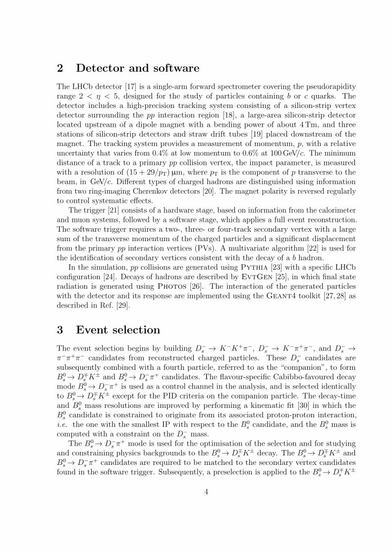
2 Detector and software

The LHCb detector [17] is a single-arm forward spectrometer covering the pseudorapidityrange 2 < η < 5, designed for the study of particles containing b or c quarks. Thedetector includes a high-precision tracking system consisting of a silicon-strip vertexdetector surrounding the pp interaction region [18], a large-area silicon-strip detectorlocated upstream of a dipole magnet with a bending power of about 4 Tm, and threestations of silicon-strip detectors and straw drift tubes [19] placed downstream of themagnet. The tracking system provides a measurement of momentum, p, with a relativeuncertainty that varies from 0.4% at low momentum to 0.6% at 100 GeV/c. The minimumdistance of a track to a primary pp collision vertex, the impact parameter, is measuredwith a resolution of (15 + 29/pT)µm, where pT is the component of p transverse to thebeam, in GeV/c. Different types of charged hadrons are distinguished using informationfrom two ring-imaging Cherenkov detectors [20]. The magnet polarity is reversed regularlyto control systematic effects.

The trigger [21] consists of a hardware stage, based on information from the calorimeterand muon systems, followed by a software stage, which applies a full event reconstruction.The software trigger requires a two-, three- or four-track secondary vertex with a largesum of the transverse momentum of the charged particles and a significant displacementfrom the primary pp interaction vertices (PVs). A multivariate algorithm [22] is used forthe identification of secondary vertices consistent with the decay of a b hadron.

In the simulation, pp collisions are generated using Pythia [23] with a specific LHCbconfiguration [24]. Decays of hadrons are described by EvtGen [25], in which final stateradiation is generated using Photos [26]. The interaction of the generated particleswith the detector and its response are implemented using the Geant4 toolkit [27, 28] asdescribed in Ref. [29].

3 Event selection

The event selection begins by building D−s → K−K+π−, D−s → K−π+π−, and D−s →π−π+π− candidates from reconstructed charged particles. These D−s candidates aresubsequently combined with a fourth particle, referred to as the “companion”, to formB0s→ D∓s K

± and B0s→ D−s π

+ candidates. The flavour-specific Cabibbo-favoured decaymode B0

s→ D−s π+ is used as a control channel in the analysis, and is selected identically

to B0s→ D∓s K

± except for the PID criteria on the companion particle. The decay-timeand B0

s mass resolutions are improved by performing a kinematic fit [30] in which theB0s candidate is constrained to originate from its associated proton-proton interaction,

i.e. the one with the smallest IP with respect to the B0s candidate, and the B0

s mass iscomputed with a constraint on the D−s mass.

The B0s→ D−s π

+ mode is used for the optimisation of the selection and for studyingand constraining physics backgrounds to the B0

s→ D∓s K± decay. The B0

s→ D∓s K± and

B0s→ D−s π

+ candidates are required to be matched to the secondary vertex candidatesfound in the software trigger. Subsequently, a preselection is applied to the B0

s→ D∓s K±

4

and B0s→ D−s π

+ candidates using a similar multivariate displaced vertex algorithm to thetrigger selection, but with offline-quality reconstruction.

A selection using the gradient boosted decision tree (BDTG) [31] implementation in theTmva software package [32] further suppresses combinatorial backgrounds. The BDTG istrained on data using the B0

s→ D−s π+, D−s → K−K+π− decay sample, which is purified

with respect to the previous preselection exploiting PID information from the Cherenkovdetectors. Since all channels in this analysis are kinematically similar, and since no PIDinformation is used as input to the BDTG, the resulting BDTG performs equally wellon the other D−s decay modes. The optimal working point is chosen to maximise theexpected sensitivity to the CP violating observables in B0

s→ D∓s K± decays. In addition,

the B0s and D−s candidates are required to be within m(B0

s ) ∈ [5300, 5800] MeV/c2 andm(D−s ) ∈ [1930, 2015] MeV/c2, respectively.

Finally, the different final states are distinguished by using PID information. This selec-tion also strongly suppresses cross-feed and peaking backgrounds from other misidentifieddecays of b-hadrons to c-hadrons. We will refer to such backgrounds as “fully recon-structed” if no particles are missed in the reconstruction, and “partially reconstructed”otherwise. The decay modes B0 → D−π+, B0 → D−s π

+, Λ0b → Λ−c π

+, B0s → D∓s K

±,and B0

s → D∗−s π+ are backgrounds to B0s → D−s π

+, while B0s → D−s π

+, B0s → D∗−s π+,

B0s → D−s ρ

+, B0→ D−s K+, B0→ D−K+, B0→ D−π+, Λ0

b→ Λ−c K+, Λ0

b→ Λ−c π+, and

Λ0b→ D

(∗)−s p are backgrounds to B0

s→ D∓s K±. This part of the selection is necessarily

different for each D−s decay mode, as described below.

• For D−s → π−π+π− none of the possible misidentified backgrounds fall inside theD−s mass window. Loose PID requirements are nevertheless used to identify the D−sdecay products as pions in order to suppress combinatorial background.

• For D−s → K−π+π−, the relevant peaking backgrounds are Λ−c → pπ+π− in whichthe antiproton is misidentified, and D− → K+π−π− in which both the kaon and apion are misidentified. As this is the smallest branching fraction D−s decay mode used,and hence that most affected by background, all D−s decay products are required topass tight PID requirements.

• The D−s → K−K+π− mode is split into three submodes. We distinguish betweenthe resonant D−s → φπ− and D−s → K∗0K− decays, and the remaining decays.Candidates in which the K+K− pair falls within 20 MeV/c2 of the φ mass areidentified as a D−s → φπ− decay. This requirement suppresses most of the cross-feed and combinatorial background, and only loose PID requirements are needed.Candidates within a 50 MeV/c2 window around the K∗0 mass are identified as aD−s → K∗0K− decay; it is kinematically impossible for a candidate to satisfy boththis and the φ requirement. In this case there is non-negligible background frommisidentified D− → K+π−π− and Λ−c → pπ−K+ decays which are suppressedthrough tight PID requirements on the D−s kaon with the same charge as the D−spion. The remaining candidates, referred to as nonresonant decays, are subject totight PID requirements on all decay products to suppress cross-feed backgrounds.

5

Figure 2 shows the relevant mass distributions for candidates passing and failing thisPID selection. Finally a loose PID requirement is made on the companion track. Afterall selection requirements, fewer than 2% of retained events contain more than one signalcandidate. All candidates are used in the subsequent analysis.

4 Signal and background shapes

The signal and background shapes are obtained using a mixture of data-driven approachesand simulation. The simulated events need to be corrected for kinematic differencesbetween simulation and data, as well as for the kinematics-dependent efficiency of thePID selection requirements. In order to obtain kinematic distributions in data for thisweighting, we use the decay mode B0→ D−π+, which can be selected with very highpurity without the use of any PID requirements and is kinematically very similar to the

]2c) [MeV/

±

π­

K+

m(K

1900 1950 2000 2050

)2c

Can

did

ates

/(1.0

MeV

/

0

2000

4000

6000

8000

10000

12000

LHCb

Failing Selection

Passing Selection

]2c) [MeV/

±

π­

π+

πm(

1900 1950 2000 2050

)2c

Can

did

ates

/(1.0

MeV

/

0

200

400

600

800

1000

1200

1400

1600

1800

2000

LHCb

Failing Selection

Passing Selection

]2c) [MeV/

­

π+

π±

m(K

1900 1950 2000 2050

)2c

Can

did

ates

/(1.0

MeV

/

0

2000

4000

6000

8000

10000

12000

LHCb

Failing Selection

Passing Selection

Figure 2: Mass distributions for D−s candidates passing (black, open circles) and failing (red,crosses) the PID selection criteria. In reading order: D−s → K−K+π−, D−s → π−π+π−, andD−s → K−π+π−.

6

B0s signals. The PID efficiencies are measured as a function of particle momentum and

event occupancy using prompt D∗+ → D0(K−π+)π+ decays which provide pure samplesof pions and kaons [33], henceforth called D∗+ calibration sample.

4.1 B0s candidate mass shapes

In order to model radiative and reconstruction effects, the signal shape in the B0s mass is

the sum of two Crystal Ball [34] functions with common mean and oppositely orientedtails. The signal shapes are determined separately for B0

s→ D∓s K± and B0

s→ D−s π+ from

simulated candidates. The shapes are subsequently fixed in the multivariate fit except forthe common mean of the Crystal Ball functions which floats for both the B0

s→ D−s π+ and

B0s→ D∓s K

± channel.The functional form of the combinatorial background is taken from the upper B0

s

sideband, with its parameters left free to vary in the subsequent multivariate fit. Each D−smode is considered independently and parameterised by either an exponential function orby a combination of an exponential and a constant function.

The shapes of the fully or partially reconstructed backgrounds are fixed from simulatedevents using a non-parametric kernel estimation method (KEYS, [35]). Exceptions to thisare the B0→ D−π+ background in the B0

s→ D−s π+ fit and the B0

s→ D−s π+ background

in the B0s→ D∓s K

± fit, which are obtained from data. The latter two backgrounds arereconstructed with the “wrong” mass hypothesis but without PID requirements, whichwould suppress them. The resulting shapes are then weighted to account for the effect ofthe momentum-dependent efficiency of the PID requirements from the D∗+ calibrationsamples, and KEYS templates are extracted for use in the multivariate fit.

4.2 D−s candidate mass shapes

The signal shape in the D−s mass is again a sum of two Crystal Ball functions with commonmean and oppositely oriented tails. The signal shapes are extracted separately for eachD−s decay mode from simulated events that have the full selection chain applied to them.The shapes are subsequently fixed in the multivariate fit except for the common mean ofthe Crystal Ball functions, which floats independently for each D−s decay mode.

The combinatorial background consists of both random combinations of tracks whichdo not peak in the D−s mass, and, in some D−s decay modes, backgrounds that contain atrue D−s , and a random companion track. It is parameterised separately for each D−s decaymode either by an exponential function or by a combination of an exponential functionand the signal D−s shape.

The fully and partially reconstructed backgrounds which contain a correctly recon-structed D−s candidate (B0

s→ D∓s K± and B0→ D−s π

+ as backgrounds in the B0s→ D−s π

+

fit; B0→ D−s K+ and B0

s→ D−s π+ as backgrounds in the B0

s→ D∓s K± fit) are assumed

to have the same mass distribution as the signal. For other backgrounds, the shapes areKEYS templates taken from simulated events, as in the B0

s mass.

7

4.3 Companion L(K/π) shapes

We obtain the PDFs describing the L(K/π) distributions of pions and kaons from dedicatedD∗+ calibration samples. We obtain the PDF describing the protons using a calibrationsample of Λ+

c → pK−π+ decays. These samples are weighted to match the signal kinematicand event occupancy distributions in the same way as the simulated events. The weightingis done separately for each signal and background component, as well as for each magnetpolarity. The shapes for each magnet polarity are subsequently combined according to theintegrated luminosity in each sample.

The signal companion L(K/π) shape is obtained separately for each D−s decay modeto account for small kinematic differences between them. The combinatorial backgroundcompanion L(K/π) shape is taken to consist of a mixture of pions, protons, and kaons, andits normalisation is left floating in the multivariate fit. The companion L(K/π) shape forfully or partially reconstructed backgrounds is obtained by weighting the PID calibrationsamples to match the event distributions of simulated events, for each background type.

5 Multivariate fit to B0s→ D∓s K± and B0

s→ D−s π+

The total PDF for the multivariate fit is built from the product of the signal and backgroundPDFs, since correlations between the fitting variables are measured to be small in simulation.These product PDFs are then added for each D−s decay mode, and almost all backgroundyields are left free to float. The only exceptions are those backgrounds whose yield isbelow 2% of the signal yield. These are B0→ D−K+, B0→ D−π+, Λ0

b→ Λ−c K+, and

Λ0b→ Λ−c π

+ for the B0s→ D∓s K

± fit, and B0→ D−π+, Λ0b→ Λ−c π

+, and B0s→ D∓s K

± forthe B0

s→ D−s π+ fit. These background yields are fixed from known branching fractions

and relative efficiencies measured using simulated events. The multivariate fit resultsin a signal yield of 28 260 ± 180 B0

s→ D−s π+ and 1770 ± 50 B0

s→ D∓s K± decays, with

an effective purity of 85% for B0s→ D−s π

+ and 74% for B0s→ D∓s K

±. The multivariatefit is checked for biases using large samples of data-like pseudoexperiments, and none isfound. The results of the multivariate fit are shown in Fig. 3 for both the B0

s→ D−s π+

and B0s→ D∓s K

±, summed over all D−s decay modes.

8

lab0_MassFitConsD_M5300 5350 5400 5450 5500 5550 5600 5650 5700 5750 5800

)2c

Can

did

ates

/ (

5 M

eV/

210

310

Data+π

­s D→

0

sSignal B

Combinatorial±

π

±

D→ 0

dB­

π+cΛ → 0

bΛ

+π)*(­

s D→ 0

(d,s)B±K

±

s D→ 0sB

LHCb

]2c) [MeV/+π

s

­m(D

5300 5400 5500 5600 5700 5800­4­2024

lab0_MassFitConsD_M5300 5350 5400 5450 5500 5550 5600 5650 5700 5750 5800

)2c

Can

did

ates

/ (

5 M

eV/

50

100

150

200

250

300

350

400Data

±K

±

s D→ 0

sSignal B

Combinatorial

)­π,­(K+cΛ → 0

bΛ

p)*(­s D→ 0

bΛ

)+ρ,+π()*(­s D→ 0

sB

)±π,±(K

±

D→ 0

dB)*(±K)*(

±

sD→ 0

(d,s)B

LHCb

]2c) [MeV/±K

±

sm(D

5300 5400 5500 5600 5700 5800­4­2024

lab2_MM1930 1940 1950 1960 1970 1980 1990 2000 2010

)2c

Can

did

ates

/ (

0.8

5 M

eV/

200

400

600

800

1000

1200

1400

1600

1800

Data+π

­s D→

0

sSignal B

Combinatorial±

π

±

D→ 0

dB­

π+cΛ → 0

bΛ

+π)*(­

s D→ 0

(d,s)B±K

±

s D→ 0sB

LHCb

]2c) [MeV/+π

­π

±, K±π­

π+π, ±π­

K+m(K

1940 1960 1980 2000­4­2024

lab2_MM1930 1940 1950 1960 1970 1980 1990 2000 2010

)2c

Can

did

ates

/ (

0.8

5 M

eV/

50

100

150

200

250

Data±K

±

s D→ 0

sSignal B

Combinatorial

)­π,­(K+cΛ → 0

bΛ

p)*(­s D→ 0

bΛ

)+ρ,+π()*(­s D→ 0

sB

)±π,±(K

±

D→ 0

dB)*(±K)*(

±

sD→ 0

(d,s)B

LHCb

]2c) [MeV/+π­π±, K±π­π+π, ±π

­K+m(K

1940 1960 1980 2000­4­2024

lab1_PIDK0 20 40 60 80 100 120 140

Can

did

ates

/ 1

.50

10

210

310

410Data

+π­s D→

0

sSignal B

Combinatorial±

π

±

D→ 0

dB­

π+cΛ → 0

bΛ

+π)*(­

s D→ 0

(d,s)B±K

±

s D→ 0sB

LHCb

)K/πCompanion L(

0 50 100 150­4­2024

lab1_PIDK2 2.5 3 3.5 4 4.5 5

Can

did

ates

/ 0

.03

20

40

60

80

100

120

140

160

180 Data±K

±

s D→ 0

sSignal B

Combinatorial

)­π,­(K+cΛ → 0

bΛ

p)*(­s D→ 0

bΛ

)+ρ,+π()*(­s D→ 0

sB

)±π,±(K

±

D→ 0

dB)*(±K)*(

±

sD→ 0

(d,s)B

LHCb

))π/Companion ln(L(K

2 3 4 5­4­2024

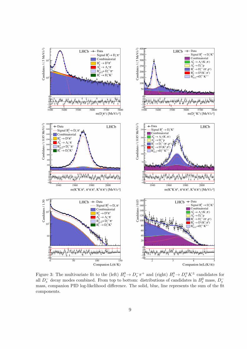
Figure 3: The multivariate fit to the (left) B0s→ D−s π

+ and (right) B0s→ D∓s K

± candidates forall D−s decay modes combined. From top to bottom: distributions of candidates in B0

s mass, D−smass, companion PID log-likelihood difference. The solid, blue, line represents the sum of the fitcomponents.

9

6 Flavour Tagging

At the LHC, b quarks are produced in pairs bb; one of the two hadronises to form thesignal B0

s , the other b quark hadronises and decays independently. The identificationof the B0

s initial flavour is performed by means of two flavour-tagging algorithms whichexploit this pair-wise production of b quarks. The opposite side (OS) tagger determinesthe flavour of the non-signal b-hadron produced in the proton-proton collision using thecharge of the lepton (µ, e) produced in semileptonic B decays, or that of the kaon from theb→ c→ s decay chain, or the charge of the inclusive secondary vertex reconstructed fromb-decay products. The same side kaon (SSK) tagger searches for an additional chargedkaon accompanying the fragmentation of the signal B0

s or B0s.

Each of these algorithms has an intrinsic mistag rate ω = (wrong tags)/(all tags)and a tagging efficiency εtag = (tagged candidates)/(all candidates). Candidates can betagged incorrectly due to tracks from the underlying event, particle misidentifications, orflavour oscillations of neutral B mesons. The intrinsic mistag ω can only be measured inflavour-specific, self-tagging final states.

The tagging algorithms predict for each B0s candidate an estimate η of the mistag

probability, which should closely follow the intrinsic mistag ω. This estimate η is obtainedby using a neural network trained on simulated events whose inputs are the kinematic,geometric, and PID properties of the tagging particle(s).

The estimated mistag η is treated as a per-candidate variable, thus adding an observableto the fit. Due to variations in the properties of tagging tracks for different channels,the predicted mistag probability η is usually not exactly the (true) mistag rate ω, whichrequires η to be calibrated using flavour specific, and therefore self-tagging, decays. Thestatistical uncertainty on Cf , Sf , and Sf scales with 1/

√εeff , defined as εeff = εtag(1−2ω)2.

Therefore, the tagging algorithms are tuned for maximum effective tagging power εeff .

6.1 Tagging calibration

The calibration for the OS tagger is performed using several control channels: B+ →J/ψK+, B+ → D0π+, B0 → D∗−µ+νµ, B0 → J/ψK∗0 and B0

s→ D−s π+. This calibration

of η is done for each control channel using the linear function

ω = p0 + p1 · (η − 〈η〉) , (7)

where the values of p0 and p1 are called calibration parameters, and 〈η〉 is the mean of theη distribution predicted by a tagger in a specific control channel. Systematic uncertaintiesare assigned to account for possible dependences of the calibration parameters on thefinal state considered, on the kinematics of the B0

s candidate and on the event properties.The corresponding values of the calibration parameters are summarised in Table 1. Foreach control channel the relevant calibration parameters are reported with their statisticaland systematic uncertainties. These are averaged to give the reference values including asystematic uncertainty accounting for kinematic differences between different channels. Theresulting calibration parameters for the B0

s→ D∓s K± fit are: p0 = 0.3834± 0.0014± 0.0040

10

Table 1: Calibration parameters of the combined OS tagger extracted from different controlchannels. In each entry the first uncertainty is statistical and the second systematic.

Control channel 〈η〉 p0 − 〈η〉 p1

B+ → J/ψK+ 0.3919 0.0008 ± 0.0014 ± 0.0015 0.982 ± 0.017 ± 0.005

B+ → D0π+ 0.3836 0.0018 ± 0.0016 ± 0.0015 0.972 ± 0.017 ± 0.005B0 → J/ψK∗0 0.390 0.0090 ± 0.0030 ± 0.0060 0.882 ± 0.043 ± 0.039B0 → D∗−µ+νµ 0.3872 0.0081 ± 0.0019 ± 0.0069 0.946 ± 0.019 ± 0.061B0s→ D−s π

+ 0.3813 0.0159 ± 0.0097 ± 0.0071 1.000 ± 0.116 ± 0.047

Average 0.3813 0.0021 ± 0.0014 ± 0.0040 0.972 ± 0.012 ± 0.035

and p1 = 0.972 ± 0.012 ± 0.035, where the p0 for each control channel needs to betranslated to the 〈η〉 of B0

s → D−s π+, the channel which is most similar to the signal

channel B0s→ D∓s K

±. This is achieved by the transformation p0 → p0 + p1(〈η〉 − 0.3813)in each control channel.

The SSK algorithm uses a neural network to select fragmentation particles, givingimproved flavour tagging power [36] with respect to earlier cut-based [37] algorithms. Itis calibrated using the B0

s → D−s π+ channel, resulting in 〈η〉 = 0.4097, p0 = 0.4244 ±

0.0086±0.0071 and p1 = 1.255±0.140±0.104, where the first uncertainty is statistical andsecond systematic. The systematic uncertainties include the uncertainty on the decay-timeresolution, the B0

s→ D−s π+ fit model, and the backgrounds in the B0

s→ D−s π+ fit.

Figure 4 shows the measured mistag probability as a function of the mean predictedmistag probability in B0

s→ D−s π+ decays for the OS and SSK taggers. The data points

show a linear correlation corresponding to the functional form in Eq. 7. We additionallyvalidate that the obtained tagging calibration parameters can be used in B0

s→ D∓s K±

decays by comparing them for B0s → D∓s K

± and B0s → D−s π

+ in simulated events; wefind excellent agreement between the two. We also evaluate possible tagging asymmetriesbetween B and B mesons for the OS and SSK taggers by performing the calibrationssplit by B meson flavour. The OS tagging asymmetries are measured using B+ → J/ψK+

decays, while the SSK tagging asymmetries are measured using prompt D±s mesons whosepT distribution has been weighted to match the B0

s→ D−s π+ signal. The resulting initial

flavour asymmetries for p0, p1 and εtag are taken into account in the decay-time fit.

6.2 Combination of OS and SSK taggers

Since the SSK and OS taggers rely on different physical processes they are largely indepen-dent, with a correlation measured as negligible. The tagged candidates are therefore splitinto three different samples depending on the tagging decision: events only tagged by theOS tagger (OS-only), those only tagged by the SSK tagger (SSK-only), and those taggedby both the OS and SSK taggers (OS-SSK). For the candidates that have decisions fromboth taggers a combination is performed using the calibrated mistag probabilities. Thecombined tagging decision and calibrated mistag rate are used in the final time-dependentfit, where the calibration parameters are constrained using the combination of their as-

11

ηPredicted

0 0.1 0.2 0.3 0.4 0.5 0.6

ηM

easu

red

0

0.1

0.2

0.3

0.4

0.5

0.6

LHCb

ηPredicted

0 0.1 0.2 0.3 0.4 0.5 0.6

ηM

easu

red

­0.1

0

0.1

0.2

0.3

0.4

0.5

0.6

0.7

LHCb

Figure 4: Measured mistag rate against the average predicted mistag rate for the (left) OSand (right) SSK taggers in B0

s→ D−s π+ decays. The error bars represent only the statistical

uncertainties. The solid curve is the linear fit to the data points, the shaded area defines the68% confidence level region of the calibration function (statistical only).

Table 2: Flavour tagging performance for the three different tagging categories for B0s→ D−s π

+

candidates.

Event type εtag [%] εeff [%]OS-only 19.80 ± 0.23 1.61 ± 0.03 ± 0.08SSK-only 28.85 ± 0.27 1.31 ± 0.22 ± 0.17OS-SSK 18.88 ± 0.23 2.15 ± 0.05 ± 0.09Total 67.53 5.07

sociated statistical and systematic uncertainties. The tagging performances, as well asthe effective tagging power, for the three sub-samples and their combination as measuredusing B0

s→ D−s π+ events are reported in Table 2.

6.3 Mistag distributions

Because the fit uses the per-candidate mistag prediction, it is necessary to model thedistribution of this observable for each event category (SS-only, OS-only, OS-SSK for thesignal and each background category). The mistag probability distributions for all B0

s decaymodes, whether signal or background, are obtained using sWeighted B0

s→ D−s π+ events.

The mistag probability distributions for combinatorial background events are obtainedfrom the upper B0

s mass sideband in B0s→ D−s π

+ decays. For B0 and Λ0b backgrounds the

mistag distributions are obtained from sWeighted B0→ D−π+ events. For the SSK taggerthis is justified by the fact that these backgrounds differ by only one spectator quark andshould therefore have similar properties with respect to the fragmentation of the ss pair.For the OS tagger, the predicted mistag distributions mainly depend on the kinematicproperties of the B candidate, which are similar for B0 and Λ0

b backgrounds.

12

7 Decay-time resolution and acceptance

The decay-time resolution of the detector must be accounted for because of the fastB0s–B

0s oscillations. Any mismodelling of the resolution function also potentially biases

and affects the precision of the time-dependent CP violation observables. The signaldecay-time PDF is convolved with a resolution function that has a different width foreach candidate, making use of the per-candidate decay-time uncertainty estimated by thedecay-time kinematic fit. This approach requires the per-candidate decay-time uncertaintyto be calibrated. The calibration is performed using prompt D−s mesons combined with arandom track and kinematically weighted to give a sample of “fake B0

s” candidates, whichhave a true lifetime of zero. From the spread of the observed decay times, a scale factor tothe estimated decay time resolution is found to be 1.37± 0.10 [38]. Here the uncertaintyis dominated by the systematic uncertainty on the similarity between the kinematicallyweighted “fake B0

s” candidates and the signal. As with the per-candidate mistag, thedistribution of per-candidate decay-time uncertainties is modelled for the signal and eachtype of background. For the signal these distributions are taken from sWeighted data,while for the combinatorial background they are taken from the B0

s mass sidebands. Forother backgrounds, the decay-time error distributions are obtained from simulated events,which are weighted for the data-simulation differences found in B0

s→ D−s π+ signal events.

In the case of background candidates which are either partially reconstructed or inwhich a particle is misidentified, the decay-time is incorrectly estimated because eitherthe measured mass of the background candidate, the measured momentum, or both, aresystematically misreconstructed. For example, in the case of B0

s→ D−s π+ as a background

to B0s→ D∓s K

±, the momentum measurement is unbiased, while the reconstructed mass issystematically above the true mass, leading to a systematic increase in the reconstructeddecay-time. This effect causes an additional non-Gaussian smearing of the decay-timedistribution, which is accounted for in the decay time resolution by nonparametric PDFsobtained from simulated events, referred to as k-factor templates.

The decay-time acceptance of B0s→ D∓s K

± candidates cannot be floated because itsshape is heavily correlated with the CP observables. In particular the upper decay-timeacceptance is correlated with A∆Γ

f and A∆Γf

. However, in the case of B0s → D−s π

+, the

acceptance can be measured by fixing Γs and floating the acceptance parameters. Thedecay-time acceptance in the B0

s→ D∓s K± fit is fixed to that found in the B0

s→ D−s π+

data fit, corrected by the acceptance ratio in the two channels in simulated signal events.These simulated events have been weighted in the manner described in Sec. 4. In all cases,the acceptance is described using segments of smooth polynomial functions (“splines”),which can be implemented in an analytic way in the decay-time fit [39]. The splineboundaries (“knots”) were chosen in an ad hoc fashion to model reliably the features ofthe acceptance shape, and placed at 0.5, 1.0, 1.5, 2.0, 3.0, 12.0 ps. Doubling the numberof knots results in negligible changes to the nominal fit result. The decay-time fit to theB0s→ D−s π

+ data is an sFit using the signal PDF from Sec. 1.1, with Sf , Sf , A∆Γf , and

A∆Γf

all fixed to zero, and the knot magnitudes and ∆ms floating. The measured value of

∆ms = 17.772± 0.022 ps−1 (the uncertainty is statistical only) is in excellent agreement

13

5 10 15C

and

idat

es /

( 0

.1 p

s)

­110

1

10

210

310LHCb

Data+

π­

s D→0sB

acceptance

) [ps]+π

­s D→

0

s(Bτ

5 10 15

­2

0

2

Figure 5: Result of the sFit to the decay-time distribution of B0s→ D−s π

+ candidates, which isused to measure the decay-time acceptance in B0

s→ D∓s K± decays. The solid curve is measured

decay-time acceptance.

with the published LHCb measurement of ∆ms = 17.768± 0.023± 0.006 ps−1 [38]. Thetime fit to the B0

s→ D−s π+ data together with the measured decay-time acceptance is

shown in Fig. 5.

8 Decay-time fit to B0s→ D∓s K±

As described previously, two decay-time fitters are used: in one all signal and backgroundtime distributions are described (cFit), and in a second the background is statisticallysubtracted using the sPlot technique [15] where only the signal time distributions aredescribed (sFit). In both cases an unbinned maximum likelihood fit is performed to the CPobservables defined in Eq. 5, and the signal decay-time PDF is identical in the two fitters.Both the signal and background PDFs are described in the remainder of this section,but it is important to bear in mind that none of the information about the backgroundPDFs or fixed background parameters is relevant for the sFit. When performing thefits to the decay-time distribution, the following parameters are fixed from independentmeasurements [12,13,40]:

Γs = 0.661± 0.007 ps−1 , ∆Γs = 0.106± 0.013 ps−1 , ρ(Γs,∆Γs) = −0.39 ,

ΓΛ0b

= 0.676± 0.006 ps−1 , Γd = 0.658± 0.003 ps−1 , ∆ms = 17.768± 0.024 ps−1 .

Here ρ(Γs,∆Γs) is the correlation between these two measurements, ΓΛ0b

is the decay-width

of the Λ0b baryon, Γd is the B0 decay width, and ∆ms is the B0

s oscillation frequency.The signal production asymmetry is fixed to zero because the fast B0

s oscillations washout any initial asymmetry and make its effect on the CP observables negligible. Thesignal detection asymmetry is fixed to (1.0 ± 0.5)%, with the sign convention in which

14

positive detection asymmetries correspond to a higher efficiency to reconstruct positivekaons [41,42]. The background production and detection asymmetries are floated withinconstraints of ±1% for B0

s and B0 decays, and ±3% for Λ0b decays.

The signal and background mistag and decay-time uncertainty distributions, includingk-factors, are modelled by kernel templates as described in Sec. 6 and 7. The taggingcalibration parameters are constrained to the values obtained from the control channels forall B0

s decay modes, except for B0 and Λ0b decays where the calibration parameters of the

SSK tagger are fixed to p0 = 0.5, p1 = 0. All modes use the same spline-based decay-timeacceptance function described in Sec. 7.

The backgrounds from B0s decay modes are all flavour-specific, and are modelled by the

decay-time PDF used for B0s→ D−s π

+ decays convolved with the appropriate decay-timeresolution and k-factors model for the given background. The backgrounds from Λ0

b decaymodes are all described by a single exponential convolved with the appropriate decay-timeresolution and k-factor models. The B0→ D−K+ background is flavour specific and isdescribed with the same PDF as B0

s→ D−s π+, except with ∆md instead of ∆ms in the

oscillating terms, Γd instead of Γs and the appropriate decay-time resolution and k-factorKEYS templates. The B0→ D−π+ background, on the other hand, is not a flavour specificdecay, and is itself sensitive to CP violation as discussed in Sec. 1. Its decay-time PDFtherefore includes nonzero Sf and Sf terms which are constrained to their world-averagevalues [12]. The decay-time PDF of the combinatorial background used in the cFit is adouble exponential function split by the tagging category of the event, whose parametersare measured using events in the B0

s mass sidebands.All decay-time PDFs include the effects of flavour tagging, are convolved with a single

Gaussian representing the per-candidate decay-time resolution, and are multiplied by thedecay-time acceptance described in Sec. 7. Once the decay-time PDFs are constructed,the sFit proceeds by fitting the signal PDF to the sWeighted B0

s → D∓s K± candidates.

The cFit, on the other hand, performs a six-dimensional fit to the decay time, decay-timeerror, predicted mistag, and the three variables used in the multivariate fit. The B0

s massrange is restricted to m(B0

s ) ∈ [5320, 5420] MeV/c2, and the yields of the different signaland background components are fixed to those found in this fit range in the multivariatefit. The decay-time range of the fit is τ(B0

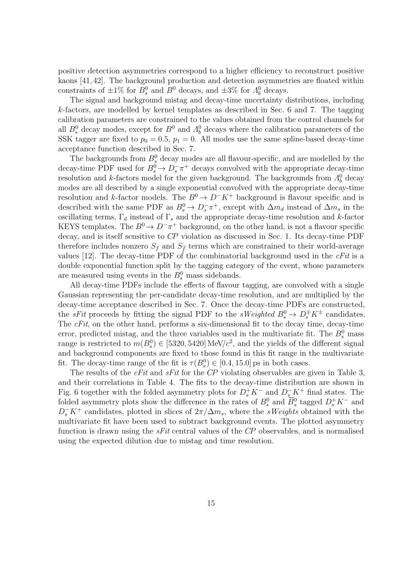
s ) ∈ [0.4, 15.0] ps in both cases.The results of the cFit and sFit for the CP violating observables are given in Table 3,

and their correlations in Table 4. The fits to the decay-time distribution are shown inFig. 6 together with the folded asymmetry plots for D+

s K− and D−s K

+ final states. Thefolded asymmetry plots show the difference in the rates of B0

s and B0s tagged D+

s K− and

D−s K+ candidates, plotted in slices of 2π/∆ms, where the sWeights obtained with the

multivariate fit have been used to subtract background events. The plotted asymmetryfunction is drawn using the sFit central values of the CP observables, and is normalisedusing the expected dilution due to mistag and time resolution.

15

lab0_LifetimeFit_ctau2 4 6 8 10 12 14

Can

did

ates

/ (

0.1

ps)

1

10

210LHCb

Data

±

K±

s D→0sB

) [ps]

±

K±

s D→0

s(Bτ

2 4 6 8 10 12 14

­2

02 K) (ps)s D→s (Bτ

2 4 6 8 10 12 14

Can

dida

tes

/ ( 0

.1 p

s)

1

10

210

datatotal

±K

±

s D→ 0sB +π −s D→ 0sB

) +ρ, +π( −)*(sD→ 0sB X→)

0bΛ, 0

d(BCombinatorial

LHCb

) [ps] ±K

±

s D→ 0s (Bτ2 4 6 8 10 12 14

-202

) [ps] sm∆/π modulo (2τ

0 0.1 0.2 0.3

) −

K + s

A(D

­0.6

­0.4

­0.2

0

0.2

0.4

0.6 LHCb

) [ps]sm∆/π modulo (2τ

0 0.1 0.2 0.3

) +

K − s

A(D

­0.6

­0.4

­0.2

0

0.2

0.4

0.6 LHCb

Figure 6: Result of the decay-time (top left) sFit and (top right) cFit to the B0s → D∓s K

±

candidates; the cFit plot groups B0s→ D∗−s π+ and B0

s→ D−s ρ+, and also groups B0→ D−K+,

B0→ D−π+, Λ0b→ Λ−c K

+, Λ0b→ Λ−c π

+, Λ0b→ D−s p, Λ

0b→ D∗−s p, and B0→ D−s K

+ together forthe sake of clarity. The folded asymmetry plots for (bottom left) D+

s K−, and (bottom right)

D−s K+ are also shown.

Table 3: Fitted values of the CP observables to the B0s → D∓s K

± time distribution for (left)sFit and (right) cFit, where the first uncertainty is statistical, the second is systematic. Allparameters other than the CP observables are constrained in the fit.

Parameter sFit fitted value cFit fitted valueCf 0.52± 0.25± 0.04 0.53± 0.25± 0.04A∆Γf 0.29± 0.42± 0.17 0.37± 0.42± 0.20

A∆Γf

0.14± 0.41± 0.18 0.20± 0.41± 0.20

Sf −0.90± 0.31± 0.06 −1.09± 0.33± 0.08Sf −0.36± 0.34± 0.06 −0.36± 0.34± 0.08

16

Table 4: Statistical correlation matrix of the B0s → D∓s K

± (top) sFit and (bottom) cFit CPparameters. Other fit parameters have negligible correlations with the CP parameters and areomitted for brevity.

Parameter Cf A∆Γf A∆Γ

fSf Sf

sFit Cf 1.000 0.071 0.097 0.117 −0.042A∆Γf 1.000 0.500 −0.044 −0.003

A∆Γf

1.000 −0.013 −0.005

Sf 1.000 0.007Sf 1.000

cFit Cf 1.000 0.084 0.103 −0.008 −0.045A∆Γf 1.000 0.544 −0.117 −0.022

A∆Γf

1.000 −0.067 −0.032

Sf 1.000 0.002Sf 1.000

9 Systematic uncertainties

Systematic uncertainties arise from the fixed parameters ∆ms, Γs, and ∆Γs, and fromthe limited knowledge of the decay time resolution and acceptance. These uncertaintiesare estimated using large sets of simulated pseudoexperiments, in which the relevantparameters are varied. The pseudoexperiments are generated with the average of the cFitand sFit central values reported in Sec. 8. They are subsequently processed by the fulldata fitting procedure: first the multivariate fit to obtain the sWeights, and then the decaytime fits. The fitted values of the observables are compared between the nominal fit, whereall fixed parameters are kept at their nominal values, and the systematic fit, where eachparameter is varied according to its systematic uncertainty. A distribution is formed bynormalising the resulting differences to the uncertainties measured in the nominal fit, andthe mean and width of this distribution are added in quadrature and conservatively assignedas the systematic uncertainty. The systematic uncertainty on the acceptance is stronglyanti-correlated with that due to the fixed value of Γs. This is because the acceptanceparameters are determined from the fit to B0

s → D−s π+ data, where Γs determines the

expected exponential slope, so that the acceptance parameterises any difference betweenthe observed and the expected slope. The systematic pseudoexperiments are also used tocompute the systematic covariance matrix due to each source of uncertainty.

The total systematic covariance matrix is obtained by adding the individual covariancematrices. The resulting systematic uncertainties are shown in Tables 5 and 6 relative tothe corresponding statistical uncertainties. The contributions from Γs and ∆Γs are listedindependently for comparison to convey a feeling for their relative importance. For thiscomparison, Γs and ∆Γs are treated as uncorrelated systematic effects. When computingthe total, however, the correlations between these two, as well as between them and theacceptance parameters, are accounted for, and the full systematic uncertainty which enters

17

into the total is listed as “acceptance, Γs, ∆Γs”. The cFit contains fixed parametersdescribing the decay time of the combinatorial background. These parameters are foundto be correlated to the CP parameters, and a systematic uncertainty is assigned.

The result is cross-checked by splitting the sample into two subsets according tothe two magnet polarities, the hardware trigger decision, and the BDTG response. There is

Table 5: Systematic errors, relative to the statistical error, for (top) sFit and (bottom) cFit. Thedaggered contributions (Γs, ∆Γs) are given separately for comparison (see text) with the otheruncertainties and are not added in quadrature to produce the total.

Parameter Cf A∆Γf A∆Γ

fSf Sf

sFit ∆ms 0.062 0.013 0.013 0.104 0.100scale factor 0.104 0.004 0.004 0.092 0.096∆Γs

† 0.007 0.261 0.286 0.007 0.007Γs† 0.043 0.384 0.385 0.039 0.038

acceptance, Γs, ∆Γs 0.043 0.427 0.437 0.039 0.038sample splits 0.124 0.000 0.000 0.072 0.071total 0.179 0.427 0.437 0.161 0.160

cFit ∆ms 0.068 0.014 0.011 0.131 0.126scale factor 0.131 0.004 0.004 0.101 0.103∆Γs

† 0.008 0.265 0.274 0.009 0.008Γs† 0.049 0.395 0.394 0.048 0.042

acceptance, Γs, ∆Γs 0.050 0.461 0.464 0.050 0.043comb. bkg. lifetime 0.016 0.069 0.072 0.015 0.005sample splits 0.102 0.000 0.000 0.156 0.151total 0.187 0.466 0.470 0.234 0.226

Table 6: Systematic uncertainty correlations for (top) sFit and (bottom) cFit.

Parameter Cf A∆Γf A∆Γ

fSf Sf

sFit Cf 1.00 0.18 0.18 −0.04 −0.04A∆Γf 1.00 0.95 −0.17 −0.16

A∆Γf

1.00 −0.17 −0.16

Sf 1.00 0.05Sf 1.00

cFit Cf 1.00 0.22 0.22 −0.04 −0.03A∆Γf 1.00 0.96 −0.17 −0.14

A∆Γf

1.00 −0.17 −0.14

Sf 1.00 0.09Sf 1.00

18

good agreement between the cFit and the sFit in each subsample. However, when thesample is split by BDTG response, the weighted averages of the subsamples show a smalldiscrepancy with the nominal fit for Cf , Sf , and Sf , and a corresponding systematicuncertainty is assigned. In addition, fully simulated signal and background events arefitted in order to check for systematic effects due to neglecting correlations between thedifferent variables in the signal and background PDFs. No bias is found.

A potential source of systematic uncertainty is the imperfect knowledge on the taggingparameters p0 and p1. Their uncertainties are propagated into the nominal fits by means ofGaussian constraints, and are therefore included in the statistical error. A number of otherpossible systematic effects were studied, but found to be negligible. These include possibleproduction and detection asymmetries, and missing or imperfectly modelled backgrounds.Potential systematic effects due to fixed background yields are evaluated by generatingpseudoexperiments with the nominal value for these yields, and fitting back with theyields fixed to twice their nominal value. No significant bias is observed and no systematicuncertainty assigned. No systematic uncertainty is attributed to the imperfect knowledgeof the momentum and longitudinal scale of the detector since both effects are taken intoaccount by the systematic uncertainty in ∆ms.

Both the cFit and sFit are found to be unbiased through studies of large ensemblesof pseudoexperiments generated at the best-fit point in data. In addition, differencesbetween the cFit and sFit are evaluated from the distributions of the per-pseudoexperimentdifferences of the fitted values. Both fitters return compatible results. Indeed, an importantresult of this analysis is that the sFit technique has been successfully used in an environmentwith such a large number of variables, parameters and categories. The sFit technique wasable to perform an accurate subtraction of a variety of time-dependent backgrounds in amultidimensional fit, including different oscillation frequencies, different tagging behaviours,and backgrounds with modified decay-time distributions due to misreconstructed particles.

10 Interpretation

The measurement of the CP -sensitive parameters is interpreted in terms of γ − 2βs andsubsequently γ. For this purpose we have arbitrarily chosen the cFit as the nominal fitresult. The strategy is to maximise the following likelihood

L(~α) = exp

(−1

2

(~A(~α)− ~Aobs

)TV −1

(~A(~α)− ~Aobs

)), (8)

where ~α = (γ, φs, rDsK , δ) is the vector of the physics parameters, ~A is the vector of observ-

ables expressed through Eqs. 6, ~Aobs is the vector of the measured CP violating observablesand V is the experimental (statistical and systematic) covariance matrix. Confidenceintervals are computed by evaluating the test statistic ∆χ2 ≡ χ2(~α′min)− χ2(~αmin), whereχ2(~α) = −2 lnL(~α), in a frequentist way following Ref. [43]. Here, ~αmin denotes the globalmaximum of Eq. 8, and ~α′min is the conditional maximum when the parameter of interestis fixed to the tested value. The value of βs is constrained to the LHCb measurement from

19

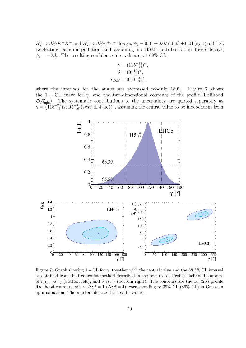
B0s → J/ψK+K− and B0

s → J/ψπ+π− decays, φs = 0.01± 0.07 (stat)± 0.01 (syst) rad [13].Neglecting penguin pollution and assuming no BSM contribution in these decays,φs = −2βs. The resulting confidence intervals are, at 68% CL,

γ = (115+28−43) ,

δ = (3+19−20) ,

rDsK = 0.53+0.17−0.16 ,

where the intervals for the angles are expressed modulo 180. Figure 7 showsthe 1 − CL curve for γ, and the two-dimensional contours of the profile likelihoodL(~α′min). The systematic contributions to the uncertainty are quoted separately asγ =

(115+26

−35 (stat)+8−25 (syst)± 4 (φs)

), assuming the central value to be independent from

]° [γ

1­C

L

0

0.2

0.4

0.6

0.8

1

0 20 40 60 80 100 120 140 160 180

43−

+28115

68.3%

95.5%

LHCb

]° [γ

K sDr

0 20 40 60 80 100 120 140 160 1800

0.2

0.4

0.6

0.8

1

1.2

1.4

LHCb

]° [γ

]° [

K sD

δ

0 50 100 150 200 250 300 350

­50

0

50

100

150

200

250

LHCb

Figure 7: Graph showing 1−CL for γ, together with the central value and the 68.3% CL intervalas obtained from the frequentist method described in the text (top). Profile likelihood contoursof rDsK vs. γ (bottom left), and δ vs. γ (bottom right). The contours are the 1σ (2σ) profilelikelihood contours, where ∆χ2 = 1 (∆χ2 = 4), corresponding to 39% CL (86% CL) in Gaussianapproximation. The markers denote the best-fit values.

20

systematic uncertainties and taking the difference in squares of the total and statisticaluncertainties.

11 Conclusion

The CP violation sensitive parameters which describe the B0s→ D∓s K

± decay rates havebeen measured using a dataset of 1.0 fb−1 of pp collision data. Their values are found to be

Cf = 0.53± 0.25± 0.04 ,

A∆Γf = 0.37± 0.42± 0.20 ,

A∆Γf

= 0.20± 0.41± 0.20 ,

Sf = −1.09± 0.33± 0.08 ,

Sf = −0.36± 0.34± 0.08 ,

where the first uncertainties are statistical and the second are systematic. The results areinterpreted in terms of the CKM angle γ, which yields γ = (115+28

−43), δ = (3+19

−20) and

rDsK = 0.53+0.17−0.16 (all angles are given modulo 180) at the 68% confidence level. This is

the first measurement of γ performed in this channel.

Acknowledgements

We express our gratitude to our colleagues in the CERN accelerator departments for theexcellent performance of the LHC. We thank the technical and administrative staff at theLHCb institutes. We acknowledge support from CERN and from the national agencies:CAPES, CNPq, FAPERJ and FINEP (Brazil); NSFC (China); CNRS/IN2P3 (France);BMBF, DFG, HGF and MPG (Germany); SFI (Ireland); INFN (Italy); FOM and NWO(The Netherlands); MNiSW and NCN (Poland); MEN/IFA (Romania); MinES and FANO(Russia); MinECo (Spain); SNSF and SER (Switzerland); NASU (Ukraine); STFC (UnitedKingdom); NSF (USA). The Tier1 computing centres are supported by IN2P3 (France),KIT and BMBF (Germany), INFN (Italy), NWO and SURF (The Netherlands), PIC(Spain), GridPP (United Kingdom). We are indebted to the communities behind themultiple open source software packages on which we depend. We are also thankful forthe computing resources and the access to software R&D tools provided by Yandex LLC(Russia). Individual groups or members have received support from EPLANET, MarieSk lodowska-Curie Actions and ERC (European Union), Conseil general de Haute-Savoie,Labex ENIGMASS and OCEVU, Region Auvergne (France), RFBR (Russia), XuntaGaland GENCAT (Spain), Royal Society and Royal Commission for the Exhibition of 1851(United Kingdom).

21

References

[1] N. Cabibbo, Unitary symmetry and leptonic decays, Phys. Rev. Lett. 10 (1963) 531.

[2] M. Kobayashi and T. Maskawa, CP Violation in the Renormalizable Theory of WeakInteraction, Prog. Theor. Phys. 49 (1973) 652.

[3] I. Dunietz and R. G. Sachs, Asymmetry Between Inclusive Charmed and AnticharmedModes in B0, Anti-B0 Decay as a Measure of CP Violation, Phys. Rev. D37 (1988)3186.

[4] R. Aleksan, I. Dunietz, and B. Kayser, Determining the CP violating phase γ, Z.Phys. C54 (1992) 653.

[5] R. Fleischer, New strategies to obtain insights into CP violation through B(s) →D±(s)K

∓, D∗±(s)K∓, ... and B(d) → D±π∓, D∗±π∓, ... decays, Nucl. Phys. B671 (2003)

459, arXiv:hep-ph/0304027.

[6] BaBar collaboration, B. Aubert et al., Measurement of time-dependent CP-violatingasymmetries and constraints on sin(2β+γ) with partial reconstruction of B → D∗∓π±

decays, Phys. Rev. D71 (2005) 112003, arXiv:hep-ex/0504035.

[7] BaBar collaboration, B. Aubert et al., Measurement of time-dependent CP asym-metries in B0 → D(∗)±π∓ and B0 → D±ρ∓ decays, Phys. Rev. D 73 (2006) 111101,arXiv:hep-ex/0602049.

[8] Belle collaboration, F. J. Ronga et al., Measurement of CP violation in B0 → D∗−π+

and B0 → D−π+ decays, Phys. Rev. D73 (2006) 092003.

[9] Belle collaboration, S. Bahinipati et al., Measurements of time-dependent CP asym-metries in B → D∗∓π± decays using a partial reconstruction technique, Phys. Rev.D84 (2011) 021101, arXiv:1102.0888.

[10] M. A. Baak, Measurement of CKM angle gamma with charmed B0 meson decays,PhD thesis, Vrije Universiteit Amsterdam, 2007, SLAC-R-858.

[11] L. Wolfenstein, Parametrization of the Kobayashi-Maskawa matrix, Phys. Rev. Lett.51 (1983) 1945.

[12] Particle Data Group, J. Beringer et al., Review of Particle Physics, Phys. Rev. D86(2012) 010001.

[13] LHCb collaboration, R. Aaij et al., Measurement of CP violation and the B0s meson

decay width difference with B0s → J/ψK+K− and B0

s → J/ψπ+π− decays, Phys. Rev.D87 (2013) 112010, arXiv:1304.2600.

[14] LHCb collaboration, R. Aaij et al., Determination of the sign of the decay widthdifference in the B0

s system, Phys. Rev. Lett. 108 (2012) 241801, arXiv:1202.4717.

22

[15] M. Pivk and F. R. Le Diberder, sPlot: a statistical tool to unfold data distributions,Nucl. Instrum. Meth. A555 (2005) 356, arXiv:physics/0402083.

[16] Y. Xie, sFit: a method for background subtraction in maximum likelihood fit,arXiv:0905.0724.

[17] LHCb collaboration, A. A. Alves Jr. et al., The LHCb detector at the LHC, JINST 3(2008) S08005.

[18] R. Aaij et al., Performance of the LHCb Vertex Locator, arXiv:1405.7808, submittedto JINST.

[19] R. Arink et al., Performance of the LHCb Outer Tracker, JINST 9 (2014) P01002,arXiv:1311.3893.

[20] M. Adinolfi et al., Performance of the LHCb RICH detector at the LHC, Eur. Phys.J. C73 (2013) 2431, arXiv:1211.6759.

[21] R. Aaij et al., The LHCb trigger and its performance in 2011, JINST 8 (2013) P04022,arXiv:1211.3055.

[22] V. V. Gligorov and M. Williams, Efficient, reliable and fast high-level triggering usinga bonsai boosted decision tree, JINST 8 (2013) P02013, arXiv:1210.6861.

[23] T. Sjostrand, S. Mrenna, and P. Skands, PYTHIA 6.4 physics and manual, JHEP 05(2006) 026, arXiv:hep-ph/0603175.

[24] I. Belyaev et al., Handling of the generation of primary events in Gauss, the LHCbsimulation framework, Nuclear Science Symposium Conference Record (NSS/MIC)IEEE (2010) 1155.

[25] D. J. Lange, The EvtGen particle decay simulation package, Nucl. Instrum. Meth.A462 (2001) 152.

[26] P. Golonka and Z. Was, PHOTOS Monte Carlo: a precision tool for QED correctionsin Z and W decays, Eur. Phys. J. C45 (2006) 97, arXiv:hep-ph/0506026.

[27] Geant4 collaboration, J. Allison et al., Geant4 developments and applications, IEEETrans. Nucl. Sci. 53 (2006) 270.

[28] Geant4 collaboration, S. Agostinelli et al., Geant4: a simulation toolkit, Nucl. Instrum.Meth. A506 (2003) 250.

[29] M. Clemencic et al., The LHCb simulation application, Gauss: design, evolution andexperience, J. Phys. Conf. Ser. 331 (2011) 032023.

[30] W. D. Hulsbergen, Decay chain fitting with a Kalman filter, NIMA 552 (2005), no. 3566 .

23

[31] L. Breiman, J. H. Friedman, R. A. Olshen, and C. J. Stone, Classification andregression trees, Wadsworth international group, Belmont, California, USA, 1984.

[32] A. Hocker et al., TMVA - toolkit for multivariate data analysis, PoS ACAT (2007)040, arXiv:physics/0703039.

[33] A. Powell et al., Particle identification at LHCb, PoS ICHEP2010 (2010) 020,LHCb-PROC-2011-008.

[34] T. Skwarnicki, A study of the radiative cascade transitions between the Upsilon-primeand Upsilon resonances, PhD thesis, Institute of Nuclear Physics, Krakow, 1986,DESY-F31-86-02.

[35] K. S. Cranmer, Kernel estimation in high-energy physics, Comput. Phys. Commun.136 (2001) 198, arXiv:hep-ex/0011057.

[36] G. A. Krocker, Development and calibration of a same side kaon tagging algorithmand measurement of the B0

s -B0s oscillation frequency ∆ms at the LHCb experiment,

PhD thesis, Heidelberg U., Sep, 2013, CERN-THESIS-2013-213.

[37] LHCb collaboration, Optimization and calibration of the same-side kaon taggingalgorithm using hadronic B0

s decays in 2011 data, LHCb-CONF-2012-033.

[38] LHCb collaboration, R. Aaij et al., Precision measurement of the B0s − B0

s os-cillation frequency in the decay B0

s → D+s π−, New J. Phys. 15 (2013) 053021,

arXiv:1304.4741.

[39] M. Karbach, G. Raven, and M. Schiller, Decay time integrals in neutral meson mixingand their efficient evaluation, arXiv:1407.0748.

[40] LHCb collaboration, R. Aaij et al., Precision measurement of the ratio of the Λ0b to

B0 lifetimes, Phys. Lett. B734 (2014) 122, arXiv:1402.6242.

[41] LHCb collaboration, R. Aaij et al., Measurement of CP asymmetry in D0 → K−K+

and D0 → π−π+ decays, JHEP 07 (2014) 041, arXiv:1405.2797.

[42] LHCb collaboration, R. Aaij et al., Measurement of D0–D0 mixing parameters andsearch for CP violation using D0 → K+π− decays, Phys. Rev. Lett. 111 (2013)251801, arXiv:1309.6534.

[43] LHCb collaboration, R. Aaij et al., A measurement of the CKM angle γ from acombination of B± → Dh± analyses, Phys. Lett. B726 (2013) 151, arXiv:1305.2050.

24

LHCb collaboration

R. Aaij41, B. Adeva37, M. Adinolfi46, A. Affolder52, Z. Ajaltouni5, S. Akar6, J. Albrecht9,F. Alessio38, M. Alexander51, S. Ali41, G. Alkhazov30, P. Alvarez Cartelle37, A.A. Alves Jr25,38,S. Amato2, S. Amerio22, Y. Amhis7, L. An3, L. Anderlini17,g, J. Anderson40, R. Andreassen57,M. Andreotti16,f , J.E. Andrews58, R.B. Appleby54, O. Aquines Gutierrez10, F. Archilli38,A. Artamonov35, M. Artuso59, E. Aslanides6, G. Auriemma25,n, M. Baalouch5, S. Bachmann11,J.J. Back48, A. Badalov36, W. Baldini16, R.J. Barlow54, C. Barschel38, S. Barsuk7, W. Barter47,V. Batozskaya28, V. Battista39, A. Bay39, L. Beaucourt4, J. Beddow51, F. Bedeschi23,I. Bediaga1, S. Belogurov31, K. Belous35, I. Belyaev31, E. Ben-Haim8, G. Bencivenni18,S. Benson38, J. Benton46, A. Berezhnoy32, R. Bernet40, M.-O. Bettler47, M. van Beuzekom41,A. Bien11, S. Bifani45, T. Bird54, A. Bizzeti17,i, P.M. Bjørnstad54, T. Blake48, F. Blanc39,J. Blouw10, S. Blusk59, V. Bocci25, A. Bondar34, N. Bondar30,38, W. Bonivento15,38, S. Borghi54,A. Borgia59, M. Borsato7, T.J.V. Bowcock52, E. Bowen40, C. Bozzi16, T. Brambach9,J. van den Brand42, J. Bressieux39, D. Brett54, M. Britsch10, T. Britton59, J. Brodzicka54,N.H. Brook46, H. Brown52, A. Bursche40, G. Busetto22,r, J. Buytaert38, S. Cadeddu15,R. Calabrese16,f , M. Calvi20,k, M. Calvo Gomez36,p, P. Campana18,38, D. Campora Perez38,A. Carbone14,d, G. Carboni24,l, R. Cardinale19,38,j , A. Cardini15, L. Carson50,K. Carvalho Akiba2, G. Casse52, L. Cassina20, L. Castillo Garcia38, M. Cattaneo38, Ch. Cauet9,R. Cenci58, M. Charles8, Ph. Charpentier38, M. Chefdeville4, S. Chen54, S.-F. Cheung55,N. Chiapolini40, M. Chrzaszcz40,26, K. Ciba38, X. Cid Vidal38, G. Ciezarek53, P.E.L. Clarke50,M. Clemencic38, H.V. Cliff47, J. Closier38, V. Coco38, J. Cogan6, E. Cogneras5, P. Collins38,A. Comerma-Montells11, A. Contu15, A. Cook46, M. Coombes46, S. Coquereau8, G. Corti38,M. Corvo16,f , I. Counts56, B. Couturier38, G.A. Cowan50, D.C. Craik48, M. Cruz Torres60,S. Cunliffe53, R. Currie50, C. D’Ambrosio38, J. Dalseno46, P. David8, P.N.Y. David41, A. Davis57,K. De Bruyn41, S. De Capua54, M. De Cian11, J.M. De Miranda1, L. De Paula2, W. De Silva57,P. De Simone18, D. Decamp4, M. Deckenhoff9, L. Del Buono8, N. Deleage4, D. Derkach55,O. Deschamps5, F. Dettori38, A. Di Canto38, H. Dijkstra38, S. Donleavy52, F. Dordei11,M. Dorigo39, A. Dosil Suarez37, D. Dossett48, A. Dovbnya43, K. Dreimanis52, G. Dujany54,F. Dupertuis39, P. Durante38, R. Dzhelyadin35, A. Dziurda26, A. Dzyuba30, S. Easo49,38,U. Egede53, V. Egorychev31, S. Eidelman34, S. Eisenhardt50, U. Eitschberger9, R. Ekelhof9,L. Eklund51, I. El Rifai5, Ch. Elsasser40, S. Ely59, S. Esen11, H.-M. Evans47, T. Evans55,A. Falabella14, C. Farber11, C. Farinelli41, N. Farley45, S. Farry52, RF Fay52, D. Ferguson50,V. Fernandez Albor37, F. Ferreira Rodrigues1, M. Ferro-Luzzi38, S. Filippov33, M. Fiore16,f ,M. Fiorini16,f , M. Firlej27, C. Fitzpatrick39, T. Fiutowski27, M. Fontana10, F. Fontanelli19,j ,R. Forty38, O. Francisco2, M. Frank38, C. Frei38, M. Frosini17,38,g, J. Fu21,38, E. Furfaro24,l,A. Gallas Torreira37, D. Galli14,d, S. Gallorini22, S. Gambetta19,j , M. Gandelman2, P. Gandini59,Y. Gao3, J. Garcıa Pardinas37, J. Garofoli59, J. Garra Tico47, L. Garrido36, C. Gaspar38,R. Gauld55, L. Gavardi9, G. Gavrilov30, E. Gersabeck11, M. Gersabeck54, T. Gershon48,Ph. Ghez4, A. Gianelle22, S. Giani’39, V. Gibson47, L. Giubega29, V.V. Gligorov38, C. Gobel60,D. Golubkov31, A. Golutvin53,31,38, A. Gomes1,a, C. Gotti20, M. Grabalosa Gandara5,R. Graciani Diaz36, L.A. Granado Cardoso38, E. Grauges36, G. Graziani17, A. Grecu29,E. Greening55, S. Gregson47, P. Griffith45, L. Grillo11, O. Grunberg62, B. Gui59, E. Gushchin33,Yu. Guz35,38, T. Gys38, C. Hadjivasiliou59, G. Haefeli39, C. Haen38, S.C. Haines47, S. Hall53,B. Hamilton58, T. Hampson46, X. Han11, S. Hansmann-Menzemer11, N. Harnew55,S.T. Harnew46, J. Harrison54, J. He38, T. Head38, V. Heijne41, K. Hennessy52, P. Henrard5,

25

L. Henry8, J.A. Hernando Morata37, E. van Herwijnen38, M. Heß62, A. Hicheur1, D. Hill55,M. Hoballah5, C. Hombach54, W. Hulsbergen41, P. Hunt55, N. Hussain55, D. Hutchcroft52,D. Hynds51, M. Idzik27, P. Ilten56, R. Jacobsson38, A. Jaeger11, J. Jalocha55, E. Jans41,P. Jaton39, A. Jawahery58, F. Jing3, M. John55, D. Johnson55, C.R. Jones47, C. Joram38,B. Jost38, N. Jurik59, M. Kaballo9, S. Kandybei43, W. Kanso6, M. Karacson38, T.M. Karbach38,S. Karodia51, M. Kelsey59, I.R. Kenyon45, T. Ketel42, B. Khanji20, C. Khurewathanakul39,S. Klaver54, K. Klimaszewski28, O. Kochebina7, M. Kolpin11, I. Komarov39, R.F. Koopman42,P. Koppenburg41,38, M. Korolev32, A. Kozlinskiy41, L. Kravchuk33, K. Kreplin11, M. Kreps48,G. Krocker11, P. Krokovny34, F. Kruse9, W. Kucewicz26,o, M. Kucharczyk20,26,38,k,V. Kudryavtsev34, K. Kurek28, T. Kvaratskheliya31, V.N. La Thi39, D. Lacarrere38,G. Lafferty54, A. Lai15, D. Lambert50, R.W. Lambert42, G. Lanfranchi18, C. Langenbruch48,B. Langhans38, T. Latham48, C. Lazzeroni45, R. Le Gac6, J. van Leerdam41, J.-P. Lees4,R. Lefevre5, A. Leflat32, J. Lefrancois7, S. Leo23, O. Leroy6, T. Lesiak26, B. Leverington11,Y. Li3, T. Likhomanenko63, M. Liles52, R. Lindner38, C. Linn38, F. Lionetto40, B. Liu15,S. Lohn38, I. Longstaff51, J.H. Lopes2, N. Lopez-March39, P. Lowdon40, H. Lu3, D. Lucchesi22,r,H. Luo50, A. Lupato22, E. Luppi16,f , O. Lupton55, F. Machefert7, I.V. Machikhiliyan31,F. Maciuc29, O. Maev30, S. Malde55, A. Malinin63, G. Manca15,e, G. Mancinelli6, J. Maratas5,J.F. Marchand4, U. Marconi14, C. Marin Benito36, P. Marino23,t, R. Marki39, J. Marks11,G. Martellotti25, A. Martens8, A. Martın Sanchez7, M. Martinelli39, D. Martinez Santos42,F. Martinez Vidal64, D. Martins Tostes2, A. Massafferri1, R. Matev38, Z. Mathe38,C. Matteuzzi20, A. Mazurov16,f , M. McCann53, J. McCarthy45, A. McNab54, R. McNulty12,B. McSkelly52, B. Meadows57, F. Meier9, M. Meissner11, M. Merk41, D.A. Milanes8,M.-N. Minard4, N. Moggi14, J. Molina Rodriguez60, S. Monteil5, M. Morandin22, P. Morawski27,A. Morda6, M.J. Morello23,t, J. Moron27, A.-B. Morris50, R. Mountain59, F. Muheim50,K. Muller40, M. Mussini14, B. Muster39, P. Naik46, T. Nakada39, R. Nandakumar49, I. Nasteva2,M. Needham50, N. Neri21, S. Neubert38, N. Neufeld38, M. Neuner11, A.D. Nguyen39,T.D. Nguyen39, C. Nguyen-Mau39,q, M. Nicol7, V. Niess5, R. Niet9, N. Nikitin32, T. Nikodem11,A. Novoselov35, D.P. O’Hanlon48, A. Oblakowska-Mucha27, V. Obraztsov35, S. Oggero41,S. Ogilvy51, O. Okhrimenko44, R. Oldeman15,e, G. Onderwater65, M. Orlandea29,J.M. Otalora Goicochea2, P. Owen53, A. Oyanguren64, B.K. Pal59, A. Palano13,c, F. Palombo21,u,M. Palutan18, J. Panman38, A. Papanestis49,38, M. Pappagallo51, L.L. Pappalardo16,f ,C. Parkes54, C.J. Parkinson9,45, G. Passaleva17, G.D. Patel52, M. Patel53, C. Patrignani19,j ,A. Pazos Alvarez37, A. Pearce54, A. Pellegrino41, M. Pepe Altarelli38, S. Perazzini14,d,E. Perez Trigo37, P. Perret5, M. Perrin-Terrin6, L. Pescatore45, E. Pesen66, K. Petridis53,A. Petrolini19,j , E. Picatoste Olloqui36, B. Pietrzyk4, T. Pilar48, D. Pinci25, A. Pistone19,S. Playfer50, M. Plo Casasus37, F. Polci8, A. Poluektov48,34, E. Polycarpo2, A. Popov35,D. Popov10, B. Popovici29, C. Potterat2, E. Price46, J. Prisciandaro39, A. Pritchard52,C. Prouve46, V. Pugatch44, A. Puig Navarro39, G. Punzi23,s, W. Qian4, B. Rachwal26,J.H. Rademacker46, B. Rakotomiaramanana39, M. Rama18, M.S. Rangel2, I. Raniuk43,N. Rauschmayr38, G. Raven42, S. Reichert54, M.M. Reid48, A.C. dos Reis1, S. Ricciardi49,S. Richards46, M. Rihl38, K. Rinnert52, V. Rives Molina36, D.A. Roa Romero5, P. Robbe7,A.B. Rodrigues1, E. Rodrigues54, P. Rodriguez Perez54, S. Roiser38, V. Romanovsky35,A. Romero Vidal37, M. Rotondo22, J. Rouvinet39, T. Ruf38, F. Ruffini23, H. Ruiz36,P. Ruiz Valls64, J.J. Saborido Silva37, N. Sagidova30, P. Sail51, B. Saitta15,e,V. Salustino Guimaraes2, C. Sanchez Mayordomo64, B. Sanmartin Sedes37, R. Santacesaria25,C. Santamarina Rios37, E. Santovetti24,l, A. Sarti18,m, C. Satriano25,n, A. Satta24,

26

D.M. Saunders46, M. Savrie16,f , D. Savrina31,32, M. Schiller42, H. Schindler38, M. Schlupp9,M. Schmelling10, B. Schmidt38, O. Schneider39, A. Schopper38, M.-H. Schune7, R. Schwemmer38,B. Sciascia18, A. Sciubba25, M. Seco37, A. Semennikov31, I. Sepp53, N. Serra40, J. Serrano6,L. Sestini22, P. Seyfert11, M. Shapkin35, I. Shapoval16,43,f , Y. Shcheglov30, T. Shears52,L. Shekhtman34, V. Shevchenko63, A. Shires9, R. Silva Coutinho48, G. Simi22, M. Sirendi47,N. Skidmore46, T. Skwarnicki59, N.A. Smith52, E. Smith55,49, E. Smith53, J. Smith47,M. Smith54, H. Snoek41, M.D. Sokoloff57, F.J.P. Soler51, F. Soomro39, D. Souza46,B. Souza De Paula2, B. Spaan9, A. Sparkes50, P. Spradlin51, S. Sridharan38, F. Stagni38,M. Stahl11, S. Stahl11, O. Steinkamp40, O. Stenyakin35, S. Stevenson55, S. Stoica29, S. Stone59,B. Storaci40, S. Stracka23,38, M. Straticiuc29, U. Straumann40, R. Stroili22, V.K. Subbiah38,L. Sun57, W. Sutcliffe53, K. Swientek27, S. Swientek9, V. Syropoulos42, M. Szczekowski28,P. Szczypka39,38, D. Szilard2, T. Szumlak27, S. T’Jampens4, M. Teklishyn7, G. Tellarini16,f ,F. Teubert38, C. Thomas55, E. Thomas38, J. van Tilburg41, V. Tisserand4, M. Tobin39,S. Tolk42, L. Tomassetti16,f , D. Tonelli38, S. Topp-Joergensen55, N. Torr55, E. Tournefier4,S. Tourneur39, M.T. Tran39, M. Tresch40, A. Tsaregorodtsev6, P. Tsopelas41, N. Tuning41,M. Ubeda Garcia38, A. Ukleja28, A. Ustyuzhanin63, U. Uwer11, V. Vagnoni14, G. Valenti14,A. Vallier7, R. Vazquez Gomez18, P. Vazquez Regueiro37, C. Vazquez Sierra37, S. Vecchi16,J.J. Velthuis46, M. Veltri17,h, G. Veneziano39, M. Vesterinen11, B. Viaud7, D. Vieira2,M. Vieites Diaz37, X. Vilasis-Cardona36,p, A. Vollhardt40, D. Volyanskyy10, D. Voong46,A. Vorobyev30, V. Vorobyev34, C. Voß62, H. Voss10, J.A. de Vries41, R. Waldi62, C. Wallace48,R. Wallace12, J. Walsh23, S. Wandernoth11, J. Wang59, D.R. Ward47, N.K. Watson45,D. Websdale53, M. Whitehead48, J. Wicht38, D. Wiedner11, G. Wilkinson55, M.P. Williams45,M. Williams56, F.F. Wilson49, J. Wimberley58, J. Wishahi9, W. Wislicki28, M. Witek26,G. Wormser7, S.A. Wotton47, S. Wright47, S. Wu3, K. Wyllie38, Y. Xie61, Z. Xing59, Z. Xu39,Z. Yang3, X. Yuan3, O. Yushchenko35, M. Zangoli14, M. Zavertyaev10,b, L. Zhang59,W.C. Zhang12, Y. Zhang3, A. Zhelezov11, A. Zhokhov31, L. Zhong3, A. Zvyagin38.

1Centro Brasileiro de Pesquisas Fısicas (CBPF), Rio de Janeiro, Brazil2Universidade Federal do Rio de Janeiro (UFRJ), Rio de Janeiro, Brazil3Center for High Energy Physics, Tsinghua University, Beijing, China4LAPP, Universite de Savoie, CNRS/IN2P3, Annecy-Le-Vieux, France5Clermont Universite, Universite Blaise Pascal, CNRS/IN2P3, LPC, Clermont-Ferrand, France6CPPM, Aix-Marseille Universite, CNRS/IN2P3, Marseille, France7LAL, Universite Paris-Sud, CNRS/IN2P3, Orsay, France8LPNHE, Universite Pierre et Marie Curie, Universite Paris Diderot, CNRS/IN2P3, Paris, France9Fakultat Physik, Technische Universitat Dortmund, Dortmund, Germany10Max-Planck-Institut fur Kernphysik (MPIK), Heidelberg, Germany11Physikalisches Institut, Ruprecht-Karls-Universitat Heidelberg, Heidelberg, Germany12School of Physics, University College Dublin, Dublin, Ireland13Sezione INFN di Bari, Bari, Italy14Sezione INFN di Bologna, Bologna, Italy15Sezione INFN di Cagliari, Cagliari, Italy16Sezione INFN di Ferrara, Ferrara, Italy17Sezione INFN di Firenze, Firenze, Italy18Laboratori Nazionali dell’INFN di Frascati, Frascati, Italy19Sezione INFN di Genova, Genova, Italy20Sezione INFN di Milano Bicocca, Milano, Italy21Sezione INFN di Milano, Milano, Italy22Sezione INFN di Padova, Padova, Italy

27

23Sezione INFN di Pisa, Pisa, Italy24Sezione INFN di Roma Tor Vergata, Roma, Italy25Sezione INFN di Roma La Sapienza, Roma, Italy26Henryk Niewodniczanski Institute of Nuclear Physics Polish Academy of Sciences, Krakow, Poland27AGH - University of Science and Technology, Faculty of Physics and Applied Computer Science,Krakow, Poland28National Center for Nuclear Research (NCBJ), Warsaw, Poland29Horia Hulubei National Institute of Physics and Nuclear Engineering, Bucharest-Magurele, Romania30Petersburg Nuclear Physics Institute (PNPI), Gatchina, Russia31Institute of Theoretical and Experimental Physics (ITEP), Moscow, Russia32Institute of Nuclear Physics, Moscow State University (SINP MSU), Moscow, Russia33Institute for Nuclear Research of the Russian Academy of Sciences (INR RAN), Moscow, Russia34Budker Institute of Nuclear Physics (SB RAS) and Novosibirsk State University, Novosibirsk, Russia35Institute for High Energy Physics (IHEP), Protvino, Russia36Universitat de Barcelona, Barcelona, Spain37Universidad de Santiago de Compostela, Santiago de Compostela, Spain38European Organization for Nuclear Research (CERN), Geneva, Switzerland39Ecole Polytechnique Federale de Lausanne (EPFL), Lausanne, Switzerland40Physik-Institut, Universitat Zurich, Zurich, Switzerland41Nikhef National Institute for Subatomic Physics, Amsterdam, The Netherlands42Nikhef National Institute for Subatomic Physics and VU University Amsterdam, Amsterdam, TheNetherlands43NSC Kharkiv Institute of Physics and Technology (NSC KIPT), Kharkiv, Ukraine44Institute for Nuclear Research of the National Academy of Sciences (KINR), Kyiv, Ukraine45University of Birmingham, Birmingham, United Kingdom46H.H. Wills Physics Laboratory, University of Bristol, Bristol, United Kingdom47Cavendish Laboratory, University of Cambridge, Cambridge, United Kingdom48Department of Physics, University of Warwick, Coventry, United Kingdom49STFC Rutherford Appleton Laboratory, Didcot, United Kingdom50School of Physics and Astronomy, University of Edinburgh, Edinburgh, United Kingdom51School of Physics and Astronomy, University of Glasgow, Glasgow, United Kingdom52Oliver Lodge Laboratory, University of Liverpool, Liverpool, United Kingdom53Imperial College London, London, United Kingdom54School of Physics and Astronomy, University of Manchester, Manchester, United Kingdom55Department of Physics, University of Oxford, Oxford, United Kingdom56Massachusetts Institute of Technology, Cambridge, MA, United States57University of Cincinnati, Cincinnati, OH, United States58University of Maryland, College Park, MD, United States59Syracuse University, Syracuse, NY, United States60Pontifıcia Universidade Catolica do Rio de Janeiro (PUC-Rio), Rio de Janeiro, Brazil, associated to 2

61Institute of Particle Physics, Central China Normal University, Wuhan, Hubei, China, associated to 3

62Institut fur Physik, Universitat Rostock, Rostock, Germany, associated to 11

63National Research Centre Kurchatov Institute, Moscow, Russia, associated to 31

64Instituto de Fisica Corpuscular (IFIC), Universitat de Valencia-CSIC, Valencia, Spain, associated to 36

65KVI - University of Groningen, Groningen, The Netherlands, associated to 41

66Celal Bayar University, Manisa, Turkey, associated to 38

aUniversidade Federal do Triangulo Mineiro (UFTM), Uberaba-MG, BrazilbP.N. Lebedev Physical Institute, Russian Academy of Science (LPI RAS), Moscow, RussiacUniversita di Bari, Bari, ItalydUniversita di Bologna, Bologna, ItalyeUniversita di Cagliari, Cagliari, Italy

28

fUniversita di Ferrara, Ferrara, ItalygUniversita di Firenze, Firenze, ItalyhUniversita di Urbino, Urbino, ItalyiUniversita di Modena e Reggio Emilia, Modena, ItalyjUniversita di Genova, Genova, ItalykUniversita di Milano Bicocca, Milano, ItalylUniversita di Roma Tor Vergata, Roma, ItalymUniversita di Roma La Sapienza, Roma, ItalynUniversita della Basilicata, Potenza, ItalyoAGH - University of Science and Technology, Faculty of Computer Science, Electronics andTelecommunications, Krakow, PolandpLIFAELS, La Salle, Universitat Ramon Llull, Barcelona, SpainqHanoi University of Science, Hanoi, Viet NamrUniversita di Padova, Padova, ItalysUniversita di Pisa, Pisa, ItalytScuola Normale Superiore, Pisa, ItalyuUniversita degli Studi di Milano, Milano, Italy

29