m4c epanet2 example class version.pdf - Robert Pitt's Webpage
24
1 A Step-by-Step Guide to EPANET 2.0 Simulations Robert Pitt (UA), Shirley Clark (Penn State-Harrisburg), and Alex Maestre (UA) February 4, 2004 Step by Step Example Problem ................................................................................................................................. 2 Set-Up for All New Projects ...................................................................................................................................... 4 Creating a New Project .......................................................................................................................................... 4 Setting Project Defaults ......................................................................................................................................... 5 Setting Preferences ................................................................................................................................................ 6 Creating the Project Scenario: Working with Objects ............................................................................................... 7 Adding an Object: Junctions .................................................................................................................................. 7 Establishing the starting point for the water: Adding a Tank ................................................................................ 8 Adding an Object: Links ........................................................................................................................................ 9 Selecting an Object (How to Select Objects from the Map to Add Information) ................................................ 11 Editing an Object (Adding Information to Links and Junctions) ......................................................................... 11 Changing Map Features ....................................................................................................................................... 13 Copying and Pasting Object Properties ............................................................................................................... 15 Deleting an Object ............................................................................................................................................... 15 Moving an Object ................................................................................................................................................ 15 Selecting a Group of Objects ............................................................................................................................... 15 Editing a Group of Objects .................................................................................................................................. 16 Modifying Legends and Setting Preferences ....................................................................................................... 16 Showing a Legend ............................................................................................................................................... 17 Analyzing a Network ............................................................................................................................................... 18 Setting Analysis Options ..................................................................................................................................... 18 Running an Analysis ............................................................................................................................................ 18 Viewing the results in tables: ............................................................................................................................... 20 Demand Patterns ...................................................................................................................................................... 20 Creating a new demand pattern ........................................................................................................................... 21 Creating a Time Series Analysis.......................................................................................................................... 21 Visualizing a Time Series simulation .................................................................................................................. 22 Pumps ...................................................................................................................................................................... 22 Adding a pump .................................................................................................................................................... 23 Reservoir.................................................................................................................................................................. 23 Adding a reservoir ............................................................................................................................................... 23 Urban Water Assignment ........................................................................................................................................ 24 EPANET Website ................................................................................................................................................ 24 Project files contain all of the information used to model a network. This paper describes how to create, open, and save EPANET projects and set certain default properties.
-
Upload
khangminh22 -
Category
Documents
-
view
6 -
download
0
Transcript of m4c epanet2 example class version.pdf - Robert Pitt's Webpage
1
A Step-by-Step Guide to EPANET 2.0 Simulations
Robert Pitt (UA), Shirley Clark (Penn State-Harrisburg), and Alex Maestre (UA)
February 4, 2004
Step by Step Example Problem .................................................................................................................................2 Set-Up for All New Projects......................................................................................................................................4 Creating a New Project..........................................................................................................................................4 Setting Project Defaults .........................................................................................................................................5 Setting Preferences ................................................................................................................................................6
Creating the Project Scenario: Working with Objects ...............................................................................................7 Adding an Object: Junctions..................................................................................................................................7 Establishing the starting point for the water: Adding a Tank ................................................................................8 Adding an Object: Links........................................................................................................................................9 Selecting an Object (How to Select Objects from the Map to Add Information) ................................................11 Editing an Object (Adding Information to Links and Junctions).........................................................................11 Changing Map Features.......................................................................................................................................13 Copying and Pasting Object Properties ...............................................................................................................15 Deleting an Object ...............................................................................................................................................15 Moving an Object ................................................................................................................................................15 Selecting a Group of Objects ...............................................................................................................................15 Editing a Group of Objects ..................................................................................................................................16 Modifying Legends and Setting Preferences .......................................................................................................16 Showing a Legend ...............................................................................................................................................17
Analyzing a Network...............................................................................................................................................18 Setting Analysis Options .....................................................................................................................................18 Running an Analysis............................................................................................................................................18 Viewing the results in tables:...............................................................................................................................20
Demand Patterns......................................................................................................................................................20 Creating a new demand pattern ...........................................................................................................................21 Creating a Time Series Analysis..........................................................................................................................21 Visualizing a Time Series simulation ..................................................................................................................22
Pumps ......................................................................................................................................................................22 Adding a pump ....................................................................................................................................................23
Reservoir..................................................................................................................................................................23 Adding a reservoir ...............................................................................................................................................23
Urban Water Assignment ........................................................................................................................................24 EPANET Website................................................................................................................................................24
Project files contain all of the information used to model a network. This paper describes how to
create, open, and save EPANET projects and set certain default properties.

2
Step by Step Example Problem
1. Assume that you need to calculate the diameter of each pipe, the flow and velocity in each pipe,
and pressure in each node, in the network shown in Figure 1:
Figure 1. Network configuration in step-by-step example.
A 50 ft diameter tank is located in a city to supply drinking water for a small community. The tank is 20
ft. high and is located 400 ft above the city. The tank supplies water with a constant flow of 4 cfs during
the day. All the nodes in the network are located at 0 ft elevation. All the pipes have a roughness
coefficient C = 100. Use Hazen-Williams formula during your calculations. Minor losses are neglected.
Table 1 shows the length and diameters of each pipe.
Table 1. Pipe characteristics
The demand of water in each node is constant during the day. Figure 2 shows the existing demand of
water in each node.
Pipe 1 2 3 4 5 6 7 8 9 10 11 12 13 14 15 16 17 18 19 20 21
Lenght
(ft) 50 50 50 50 50 50 50 50 50 50 50 50 50 100 50 50 50 50 50 50 50
Diameter
(Inches) 12 8 8 12 8 8 8 8 12 8 8 8 12 10 12 12 12 10 8 10 10
P1
P2
P3
P4
P5
P6
P7
P8
P16
P17
P20
P21
P9
P10
P11
P12
P13 P18
P19
P15
P14
Initial level 10 ft, elevation 400 ft, diameter 50 ft, height 20 ft.
3
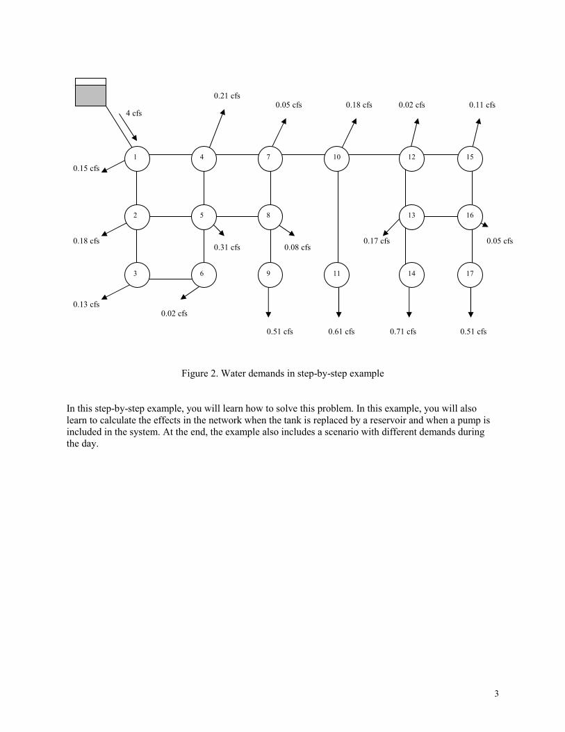
Figure 2. Water demands in step-by-step example
In this step-by-step example, you will learn how to solve this problem. In this example, you will also
learn to calculate the effects in the network when the tank is replaced by a reservoir and when a pump is
included in the system. At the end, the example also includes a scenario with different demands during
the day.
0.13 cfs
0.18 cfs
0.15 cfs
0.21 cfs 0.05 cfs
0.31 cfs
0.02 cfs
0.08 cfs
0.51 cfs 0.61 cfs 0.71 cfs 0.51 cfs
0.18 cfs 0.02 cfs 0.11 cfs
0.17 cfs 0.05 cfs
4 cfs
1
2
3
4
5
6
7
8
9
10
11
12
13
14
15
16
17
4
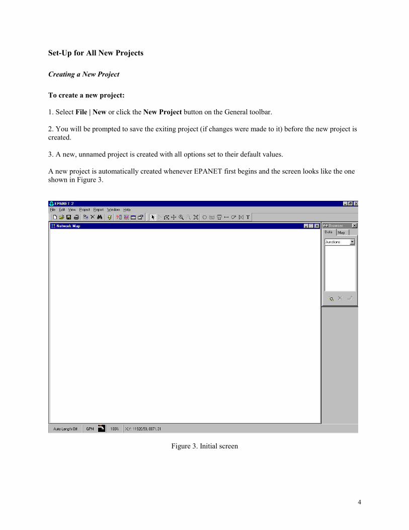
Set-Up for All New Projects
Creating a New Project
To create a new project:
1. Select File | New or click the New Project button on the General toolbar.
2. You will be prompted to save the exiting project (if changes were made to it) before the new project is
created.
3. A new, unnamed project is created with all options set to their default values.
A new project is automatically created whenever EPANET first begins and the screen looks like the one
shown in Figure 3.
Figure 3. Initial screen
5
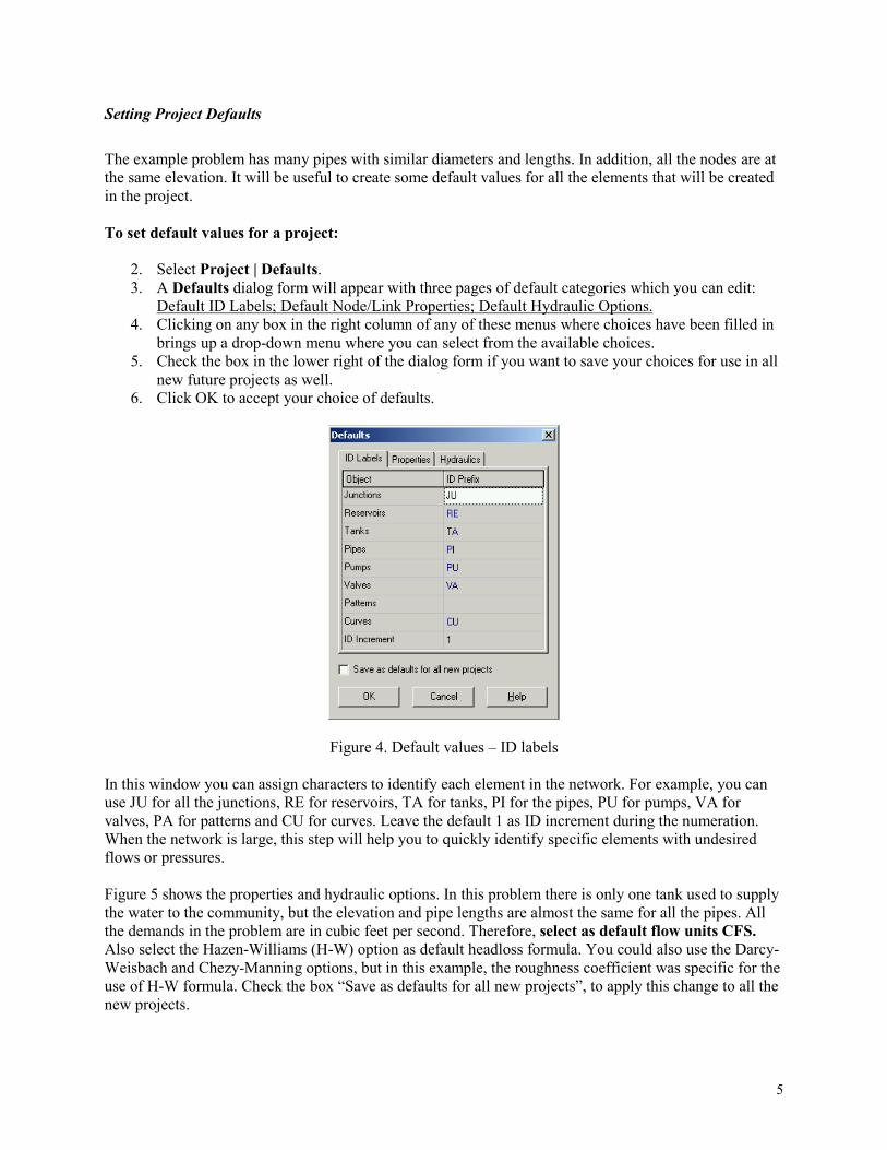
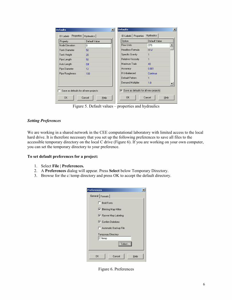
Setting Project Defaults
The example problem has many pipes with similar diameters and lengths. In addition, all the nodes are at
the same elevation. It will be useful to create some default values for all the elements that will be created
in the project.
To set default values for a project:
2. Select Project | Defaults.
3. A Defaults dialog form will appear with three pages of default categories which you can edit:
Default ID Labels; Default Node/Link Properties; Default Hydraulic Options.
4. Clicking on any box in the right column of any of these menus where choices have been filled in
brings up a drop-down menu where you can select from the available choices.
5. Check the box in the lower right of the dialog form if you want to save your choices for use in all
new future projects as well.
6. Click OK to accept your choice of defaults.
Figure 4. Default values – ID labels
In this window you can assign characters to identify each element in the network. For example, you can
use JU for all the junctions, RE for reservoirs, TA for tanks, PI for the pipes, PU for pumps, VA for
valves, PA for patterns and CU for curves. Leave the default 1 as ID increment during the numeration.
When the network is large, this step will help you to quickly identify specific elements with undesired
flows or pressures.
Figure 5 shows the properties and hydraulic options. In this problem there is only one tank used to supply
the water to the community, but the elevation and pipe lengths are almost the same for all the pipes. All
the demands in the problem are in cubic feet per second. Therefore, select as default flow units CFS.
Also select the Hazen-Williams (H-W) option as default headloss formula. You could also use the Darcy-
Weisbach and Chezy-Manning options, but in this example, the roughness coefficient was specific for the
use of H-W formula. Check the box “Save as defaults for all new projects”, to apply this change to all the
new projects.
6
Figure 5. Default values – properties and hydraulics
Setting Preferences
We are working in a shared network in the CEE computational laboratory with limited access to the local
hard drive. It is therefore necessary that you set up the following preferences to save all files to the
accessible temporary directory on the local C drive (Figure 6). If you are working on your own computer,
you can set the temporary directory to your preference.
To set default preferences for a project:
1. Select File | Preferences.
2. A Preferences dialog will appear. Press Select below Temporary Directory.
3. Browse for the c:\temp directory and press OK to accept the default directory.
Figure 6. Preferences
7
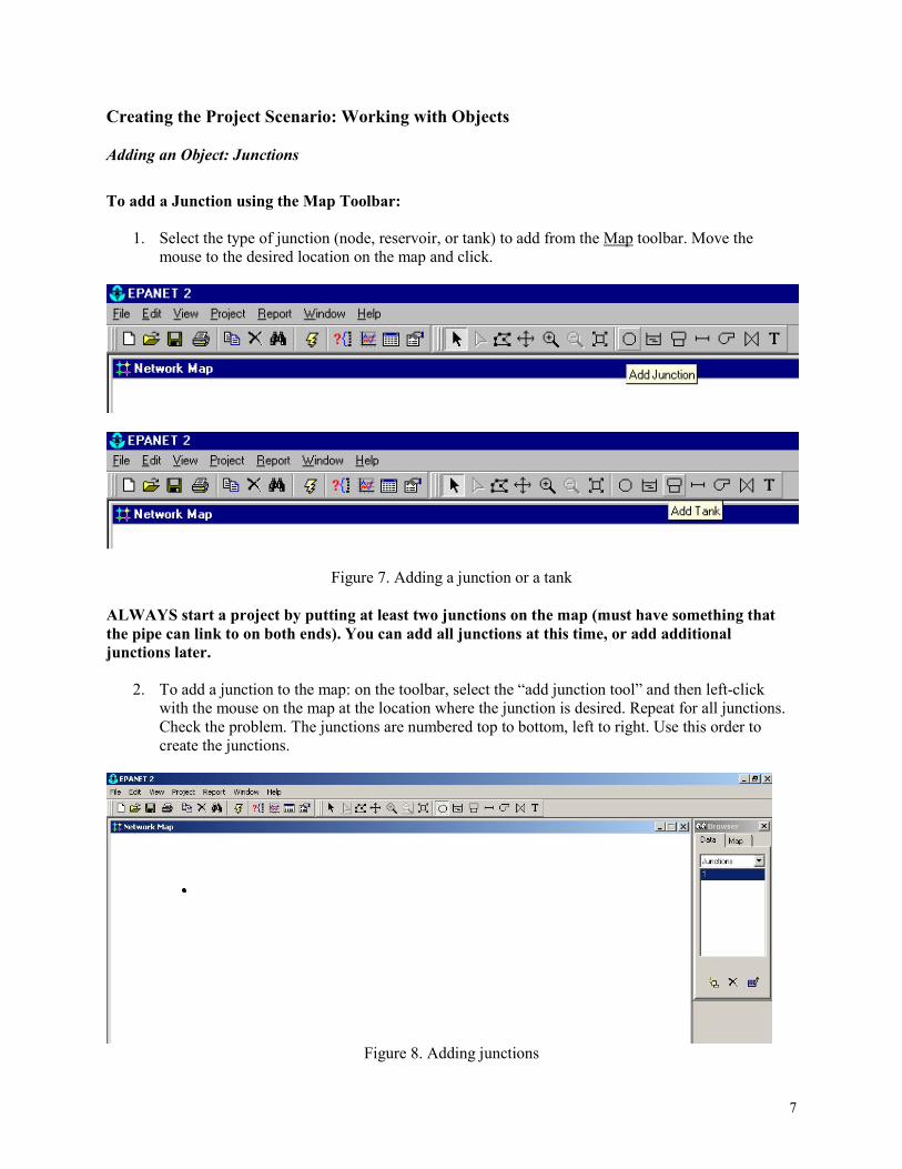
Creating the Project Scenario: Working with Objects
Adding an Object: Junctions
To add a Junction using the Map Toolbar:
1. Select the type of junction (node, reservoir, or tank) to add from the Map toolbar. Move the
mouse to the desired location on the map and click.
Figure 7. Adding a junction or a tank
ALWAYS start a project by putting at least two junctions on the map (must have something that
the pipe can link to on both ends). You can add all junctions at this time, or add additional
junctions later.
2. To add a junction to the map: on the toolbar, select the “add junction tool” and then left-click
with the mouse on the map at the location where the junction is desired. Repeat for all junctions.
Check the problem. The junctions are numbered top to bottom, left to right. Use this order to
create the junctions.
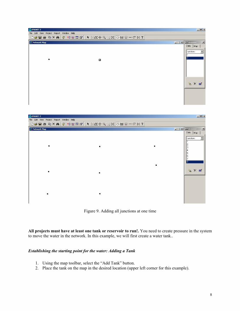
Figure 8. Adding junctions
8
Figure 9. Adding all junctions at one time
All projects must have at least one tank or reservoir to run!. You need to create pressure in the system
to move the water in the network. In this example, we will first create a water tank..
Establishing the starting point for the water: Adding a Tank
1. Using the map toolbar, select the “Add Tank” button.
2. Place the tank on the map in the desired location (upper left corner for this example).
9
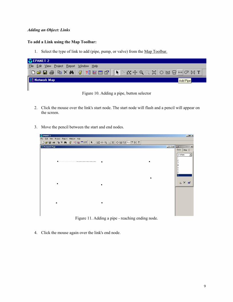
Adding an Object: Links
To add a Link using the Map Toolbar:
1. Select the type of link to add (pipe, pump, or valve) from the Map Toolbar.
Figure 10. Adding a pipe, button selector
2. Click the mouse over the link's start node. The start node will flash and a pencil will appear on
the screen.
3. Move the pencil between the start and end nodes.
Figure 11. Adding a pipe - reaching ending node.
4. Click the mouse again over the link's end node.
10
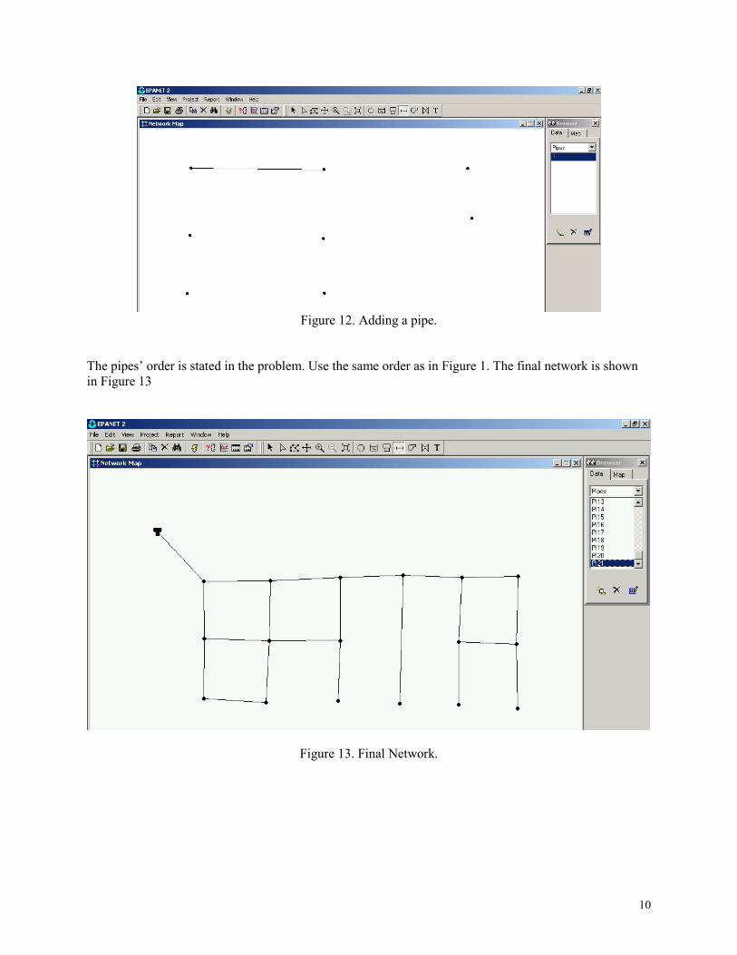
Figure 12. Adding a pipe.
The pipes’ order is stated in the problem. Use the same order as in Figure 1. The final network is shown
in Figure 13
Figure 13. Final Network.
11
Selecting an Object (How to Select Objects from the Map to Add Information)
To select an object on the map:
1. Select Edit | Select or click the Select Object button (Arrow) on the Map Toolbar.
2. Click the mouse over the desired object on the map.
To select an object using the Browser:
1. Select the type of object from the Object listbox of the Database Browser.
2. Select the desired object from the Item listbox.
Editing an Object (Adding Information to Links and Junctions)
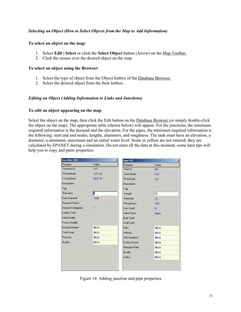
To edit an object appearing on the map
Select the object on the map, then click the Edit button on the Database Browser (or simply double-click
the object on the map). The appropriate table (shown below) will appear. For the junctions, the minimum
required information is the demand and the elevation. For the pipes, the minimum required information is
the following: start and end nodes, lengths, diameters, and roughness. The tank must have an elevation, a
diameter, a minimum, maximum and an initial water level. Items in yellow are not entered; they are
calculated by EPANET during a simulation. Do not enter all the data at this moment, some later tips will
help you to copy and paste properties.
Figure 14. Adding junction and pipe properties
12
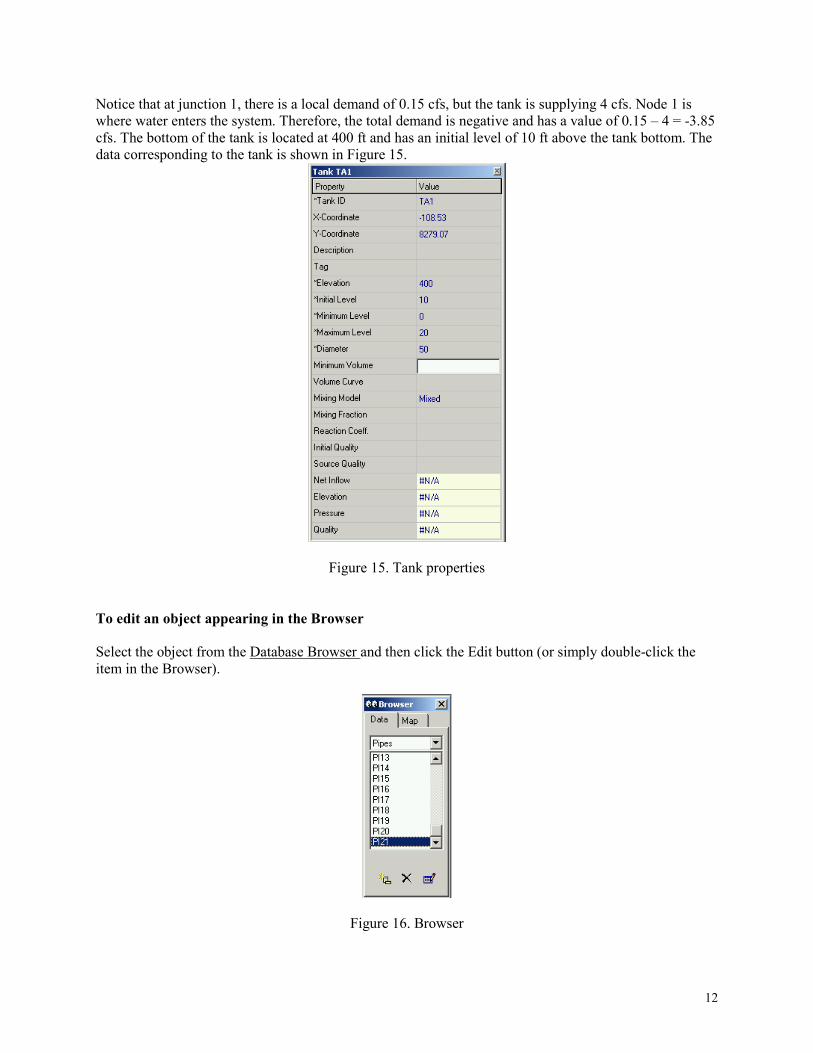
Notice that at junction 1, there is a local demand of 0.15 cfs, but the tank is supplying 4 cfs. Node 1 is
where water enters the system. Therefore, the total demand is negative and has a value of 0.15 – 4 = -3.85
cfs. The bottom of the tank is located at 400 ft and has an initial level of 10 ft above the tank bottom. The
data corresponding to the tank is shown in Figure 15.
Figure 15. Tank properties
To edit an object appearing in the Browser
Select the object from the Database Browser and then click the Edit button (or simply double-click the
item in the Browser).
Figure 16. Browser
13
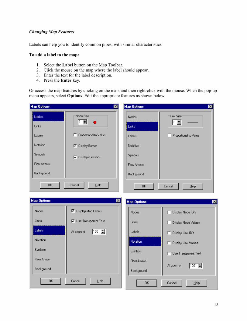
Changing Map Features
Labels can help you to identify common pipes, with similar characteristics
To add a label to the map:
1. Select the Label button on the Map Toolbar.
2. Click the mouse on the map where the label should appear.
3. Enter the text for the label description.
4. Press the Enter key.
Or access the map features by clicking on the map, and then right-click with the mouse. When the pop-up
menu appears, select Options. Edit the appropriate features as shown below.
14
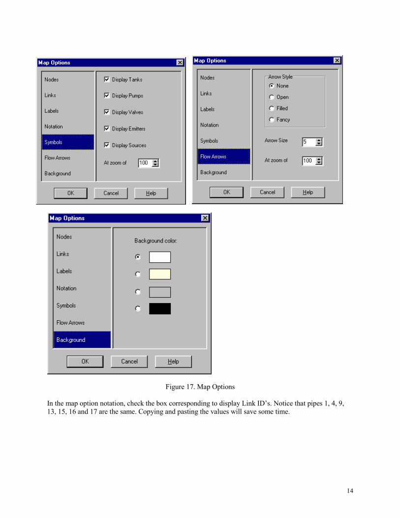
Figure 17. Map Options
In the map option notation, check the box corresponding to display Link ID’s. Notice that pipes 1, 4, 9,
13, 15, 16 and 17 are the same. Copying and pasting the values will save some time.
15
Copying and Pasting Object Properties
The properties of an object displayed on the Network Map can be copied and pasted into another object
from the same category.
To copy the properties of an object to EPANET's internal clipboard:
1. Right-click the object on the map.
2. Select Copy from the pop-up menu that appears.
To paste copied properties into an object:
1. Right-click the object on the map.
2. Select Paste from the pop-up menu that appears.
Deleting an Object
To delete an object:
1. Select the object on the map or from the Database Browser.
2. Either:
• Click the Delete button on the General Toolbar
• Click the Del button on the Database Browser
• Press the Del key.
Note: You can require that all deletions be confirmed before they take effect. See the General Preferences
page of the Program Preferences dialog box for this option, if desired.
Moving an Object
To move a node or label to another location on the map:
1. Select the node or label.
2. With the left mouse button held down over the object. Drag it to its new location.
3. Release the left button.
Alternatively, new X and Y coordinates for the object can be typed in manually in the Property Editor.
Whenever a node is moved, all links connected to it are moved as well.
Selecting a Group of Objects
To select a group of objects that lie within an irregular region of the network map:
1. Select Edit | Group Select or click the Select Group button on the Map Toolbar.
2. Draw a polygon fence line around the region of interest on the map by clicking the left mouse
button at each successive vertex of the polygon.
16
3. Close the polygon by clicking the right button or by pressing the Enter key; Cancel the selection
by pressing the Escape key.
To select all objects currently in view on the map select Edit | Select All. (Objects outside the current
viewing extent of the map are not selected.)
Editing a Group of Objects
To edit a property for a group of objects:
1. Draw a polygon region around the group of objects to be edited if one does not already exist (see
Selecting a Group of Objects) or select Edit | Select All to select all object currently in view on
the map.
2. Select Edit | Group Edit.
3. Define what to edit in the Group Edit Dialog Box that appears:
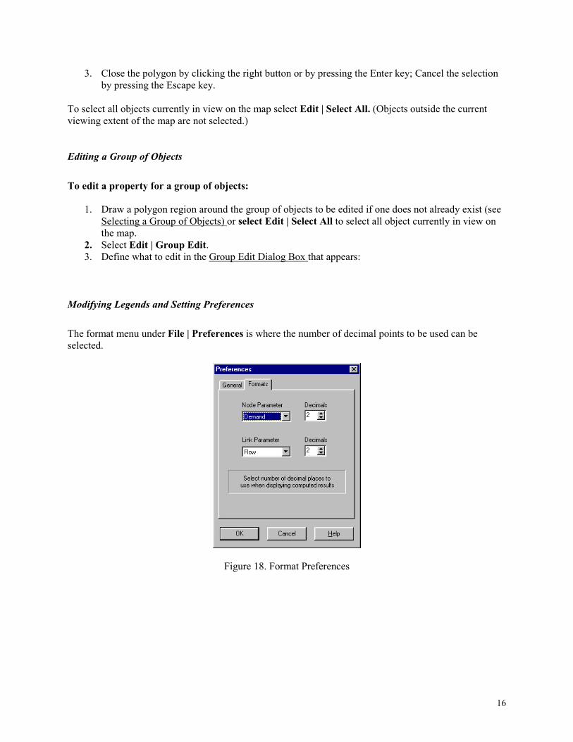
Modifying Legends and Setting Preferences
The format menu under File | Preferences is where the number of decimal points to be used can be
selected.
Figure 18. Format Preferences

17
Showing a Legend
On the Map Browser, select what needs to be displayed, and the appropriate legend will be displayed on
the side of the network map.
The legend can be edited by right-clicking on the legend. EPANET has the ability to allow the user to
select the intervals for the legends.
Figure 19. Diagram with legends.
SAVE YOUR PROJECT AT THIS MOMENT. If you wish, you can save it with another name.

18
Analyzing a Network
After a network has been suitably described, it’s hydraulic and water quality behavior can be analyzed.
This section describes how to specify options to use in the analysis, how to start the analysis and how to
troubleshoot problems that might have occurred with the analysis.
Setting Analysis Options
To set Analysis Options:
1. Select Options from the Object list of the Database Browser.
2. Select Hydraulics, Quality, Reactions, Times, or Energy from the Item list.
3. If the Property Editor is not already visible, click the Edit button.
4. Edit your option choices in the Property Editor.
Running an Analysis
To run a hydraulic/water quality analysis:
1. Select Project | Run Analysis or click the Run button (lightning bolt) on the General Toolbar.
2. The progress of the analysis will be displayed in a Run Status window.
3. Click OK when the analysis ends.
If the analysis runs successfully, the end of run icon will appear in the Run Status section of the Status
Bar at the bottom of the EPANET workspace. Any error or warning messages will appear in a Status
Report window.
Figure 20. Run Button..
19
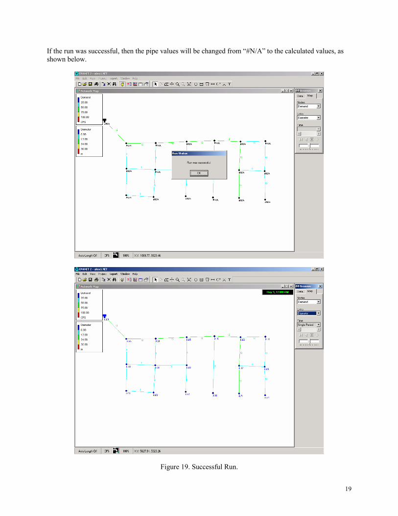
If the run was successful, then the pipe values will be changed from “#N/A” to the calculated values, as
shown below.
Figure 19. Successful Run.
20
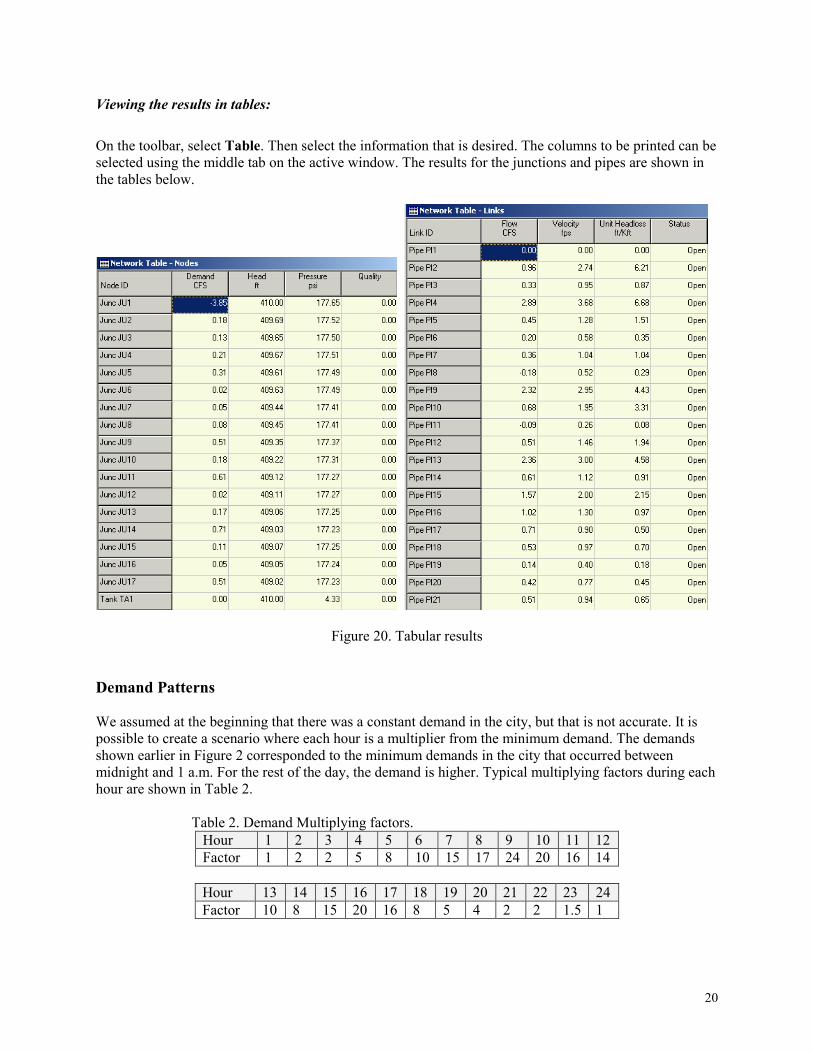
Viewing the results in tables:
On the toolbar, select Table. Then select the information that is desired. The columns to be printed can be
selected using the middle tab on the active window. The results for the junctions and pipes are shown in
the tables below.
Figure 20. Tabular results
Demand Patterns
We assumed at the beginning that there was a constant demand in the city, but that is not accurate. It is
possible to create a scenario where each hour is a multiplier from the minimum demand. The demands
shown earlier in Figure 2 corresponded to the minimum demands in the city that occurred between
midnight and 1 a.m. For the rest of the day, the demand is higher. Typical multiplying factors during each
hour are shown in Table 2.
Table 2. Demand Multiplying factors.
Hour 1 2 3 4 5 6 7 8 9 10 11 12
Factor 1 2 2 5 8 10 15 17 24 20 16 14
Hour 13 14 15 16 17 18 19 20 21 22 23 24
Factor 10 8 15 20 16 8 5 4 2 2 1.5 1
21
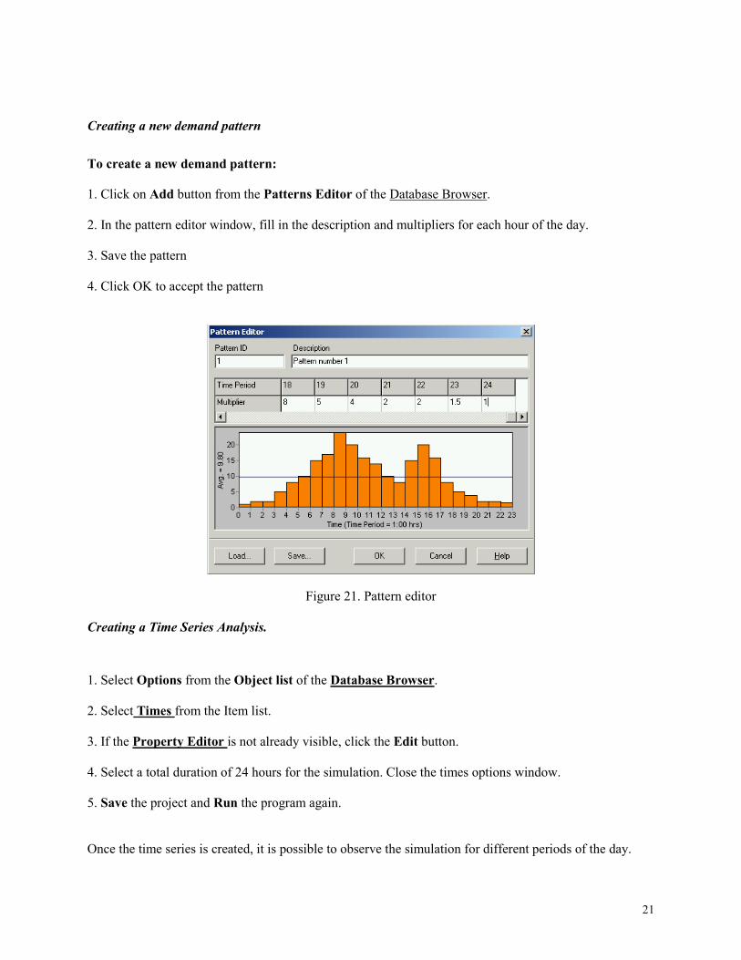
Creating a new demand pattern
To create a new demand pattern:
1. Click on Add button from the Patterns Editor of the Database Browser.
2. In the pattern editor window, fill in the description and multipliers for each hour of the day.
3. Save the pattern
4. Click OK to accept the pattern
Figure 21. Pattern editor
Creating a Time Series Analysis.
1. Select Options from the Object list of the Database Browser.
2. Select Times from the Item list.
3. If the Property Editor is not already visible, click the Edit button.
4. Select a total duration of 24 hours for the simulation. Close the times options window.
5. Save the project and Run the program again.
Once the time series is created, it is possible to observe the simulation for different periods of the day.
22
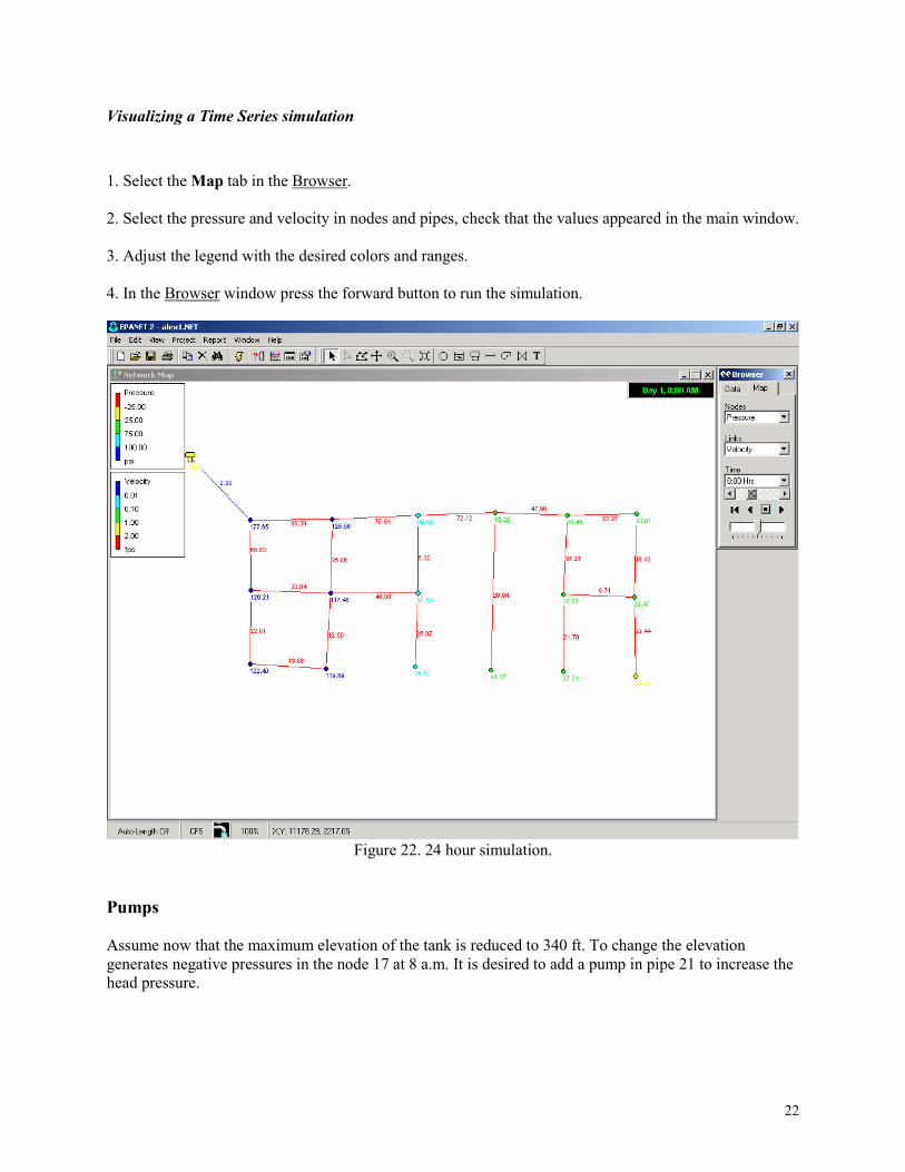
Visualizing a Time Series simulation
1. Select the Map tab in the Browser.
2. Select the pressure and velocity in nodes and pipes, check that the values appeared in the main window.
3. Adjust the legend with the desired colors and ranges.
4. In the Browser window press the forward button to run the simulation.
Figure 22. 24 hour simulation.
Pumps
Assume now that the maximum elevation of the tank is reduced to 340 ft. To change the elevation
generates negative pressures in the node 17 at 8 a.m. It is desired to add a pump in pipe 21 to increase the
head pressure.
23
Adding a pump
To add a pump:
1. Click the pump button on the general toolbar
2. Click on the beginning and end nodes where the pump is located.
3. Select Curves from the data tab in the browser
4. Click the Add button to add a new curve
5. In the curve editor window, select curve type Pump.
6. Enter a pump design flow of 30 cfs and head of 20 ft. This will calculate automatically the equation of
the pump.
7. Save the curve. Click OK.
8. Double-click on the pump to display its properties.
9. Write CU1 in pump curve. Run the program.
Reservoir
Delete the pump and tank. Assume now that there is no tank. Replace the tank with a reservoir at the same
elevation as the city. Because the city and the reservoir are at the same elevation, you will need a Pump to
supply the water.
Adding a reservoir
To add a reservoir:
1. Click the reservoir button on the general toolbar
2. The reservoir is located in the same location where the tank was.
3. Click in the pump button in the general toolbar
4. Connect the reservoir and the node 1 with the pump.
5. Select Curves from the data tab in the browser
6. Click the Add button to add a new curve
7. In the curve editor window, select curve type Pump.
8. Enter a pump design flow of 4 cfs and a head of 300 ft. This will automatically calculate the equation
of the pump, or design your own pump characteristics.

24
9. Save the curve. Click OK.
10. Double-click on the pump to display its properties.
11. Write CU1 in pump curve. Run the program.
Urban Water Assignment This assignment has 3 parts: 1) Develop an EPANET simulation for your neighborhood, using an
appropriate demand curve for the population and other characteristics of the area. Design an alternative
system that will use a dual system. 2) One system will be a conventional system using a water storage
pressure tank for the water supply for potable, and other uses that require high-quality water. 3) A second
system should be designed for fire fighting and irrigation, and possibly other non-potable uses. The
supply for this system should be a storage reservoir (actually a stormwater pond). Determine the water
needs from this pond to satisfy peak fire fighting requirements, along with some supplemental irrigation,
and other appropriate uses.
EPANET Website
http://www.epa.gov/ordntrnt/ORD/NRMRL/wswrd/epanet.html