Long-lived Giant Number Fluctuations in a SwarmingGranular Nematic

Vijay Narayan,1∗ Sriram Ramaswamy,1,2 Narayanan Menon3

1CCMT, Department of Physics, Indian Institute of Science, Bangalore 560012, India2CMTU, Jawaharlal Nehru Centre for Advanced Scientific Research, Bangalore 560064, India

3Department of Physics, University of Massachusetts, Amherst, MA 01003, USA

∗To whom correspondence should be addressed; E-mail: vj@physics.iisc.ernet.in

Coherently moving flocks of birds, beasts or bacteria are examples of living

matter with spontaneous orientational order. How do these systems differ

from thermal equilibrium systems with such liquid-crystalline order? Work-

ing with a fluidized monolayer of macroscopic rods in the nematic liquid crys-

talline phase, we find giant number fluctuations consistent with a standard

deviation growing linearly with the mean, in contrast to any situation where

the Central Limit Theorem applies. These fluctuations are long-lived, decay-

ing only as a logarithmic function of time. This shows that flocking, coherent

motion and large-scale inhomogeneity can appear in a system in which parti-

cles do not communicate except by contact.

Density is a property that one can measure with arbitrary accuracy for materials at thermal

equilibrium simply by increasing the size of the volume observed. This is because a region of

1

arX

iv:c

ond-

mat

/061

2020

v2 [

cond

-mat

.sof

t] 1

4 Ju

n 20

07

volume V , with N particles on average, ordinarily shows fluctuations with standard deviation

∆N ∝√N , so that fluctuations in the number density go down as 1/

√V . Liquid-crystalline

phases of active or self-propelled particles (1-4) are different, with ∆N predicted (2-5) to grow

faster than√N , and as fast as N in some cases (5), making density an ill-defined quantity

even in the limit of a large system. These predictions show that flocking, coherent motion and

giant density fluctuations are intimately related consequences of the orientational order that

develops in a sufficiently dense grouping of self-driven objects with anisotropic body shape.

This has significant implications for biological pattern formation and movement ecology (6):

the coupling of density fluctuations to alignment of individuals will affect populations as diverse

as herds of cattle, swarms of locusts (7), schools of fish (8, 9), motile cells (10), and filaments

driven by motor proteins (11-13).

We report here that persistent, giant number fluctuations and the coupling of particle currents

to particle orientation arise in a far simpler driven system, namely, an agitated monolayer of rod-

like particles shown in (14) to exhibit liquid-crystalline order. These fluctuations have also been

observed in computer simulations of a simple model of the flocking of apolar particles by Chate

et al. (15). The rods we use are cut to a length ` = 4.6±0.16 mm from copper wire of diameter

d = 0.8 mm. The ends of the rods are etched to give them the shape of a rolling-pin. The

rods are confined in a quasi-2-dimensional cell 1 mm tall and with a circular cross-section 13

cm in diameter. The cell is mounted in the horizontal plane on a permanent magnet shaker and

vibrated vertically at a frequency f = 200 Hz, with an amplitude, A, between 0.025 and 0.043

mm. The resultant dimensionless acceleration Γ = (4π2f 2A)/g, where g is the acceleration due

to gravity, varies between Γ = 4 and Γ = 7. We vary the total number of particles in the cell,

Ntotal between 1500 and 2820. Ntotal in each instance is counted by hand. The area fraction, φ,

occupied by the particles is the total projected area of the all rods divided by the surface area of

the cell. φ varies from 35% to 66%. Our experimental system is similar to those used to study

2

the phase behaviour of inelastic spheres (16, 17). Galanis et al. (18) shook rods in a similar

setup, albeit with much less confinement in the vertical direction. The particles are imaged with

a digital camera (Data Acquisition (19)).

The rods gain kinetic energy through frequent collisions with the floor and the ceiling of

the cell. Since the axes of the particles are almost always inclined to the horizontal, these

collisions impart or absorb momentum in the horizontal plane. Collisions between particles

conserve momentum, but also drive horizontal motion by converting vertical motion into motion

in the plane. Inter-particle collisions as well as particle-wall collisions are inelastic, and all

particle motion would cease within a few collision times if the vibrations were switched off. The

momentum of the system of rods is not conserved either, since the walls of the cell can absorb

or impart momentum. The rods are apolar – individual particles do not have a distinct head

and tail that determine fore-aft orientation or direction of motion – and can form a true nematic

phase. The experimental system thus has all the physical ingredients of an active nematic (1-4).

The system is in a very dynamic steady state, with particle motion (see movie S1 (19)) orga-

nized in macroscopic swirls. Swirling motions do not necessarily imply the existence of giant

number fluctuations (20, 21), however, particle motions in our system generate anomalously

large fluctuations in density. Figure 1A shows a typical instantaneous configuration, and the in-

set to Fig. 1B shows the orientational correlation function G2(r) = 〈cos 2(θi − θj)〉, where i, j

run over pairs of particles separated by a distance r and oriented at angles θi, θj with respect to

a reference axis. The angle brackets denote an average over all such pairs and about 150 images

spaced 15 seconds apart in time. The data in the inset show that the systems with Ntotal = 2500

and 2820 display quasi-long ranged nematic order, where G2(r) decays as a power of the sep-

aration, r. On the other hand, the system with Ntotal = 1500 shows only short-ranged nematic

order, with G2(r) decaying exponentially with r. Details of the crossover between these two

behaviours can be found in (The Shaking Amplitude Γ (19)). Autocorrelations of the density

3

field as well as of the orientation of a tagged particle decay to zero on much shorter time-scales

(Statistical Independence of Configurations Sampled (19)), so we expect these images to

be statistically independent. To quantify the number fluctuations, we extracted from each im-

age the number of particles in subsystems of different size, defined by windows ranging in size

from 0.1x0.1 `2 to 12x12 `2. From a series of images we determined, for each subsystem size,

the average N and the standard deviation, ∆N , of the number of particles in the window. For

any system in which the number fluctuations obey the conditions of the Central Limit Theorem

(22), ∆N/√N should be a constant, independent of N . Figure 1B shows that when the area

fraction φ is large, ∆N/√N is not a constant. Indeed, for big enough subsystems, the data

show giant fluctuations, ∆N , in the number of particles, growing far more rapidly than√N

and consistent with a proportionality to N . For smaller average number density, where nematic

order is poorly developed, this effect disappears, and ∆N/√N is independent of N , as in ther-

mal equilibrium systems. The roll-off in ∆N/√N at the highest values of N is a finite-size

effect: for subsystems that approach the size of the entire system, large number fluctuations are

no longer possible since the total number of particles in the cell is held fixed.

We examine a subsystem of size ` x ` (i.e., one rod length on a side) and obtain a time-series

of particle number, N(t), by taking images at a frame rate of 300 frames/sec. From this we

determine the temporal autocorrelation, C(t), of the density fluctuations. As shown in Fig. 2,

C(t) decays logarithmically in time, unlike the much more rapid t−1 decay of random, diffu-

sively relaxing density fluctuations in two dimensions. Thus the density fluctuations are not only

anomalously large in magnitude but also extremely long-lived. Indeed, these two effects are in-

timately related: an intermediate step in the theoretical argument (5) that predicts giant number

fluctuations shows that density fluctuations at a wavenumber q have a variance proportional to

q−2 and decay diffusively. This leads to the conclusion (Long-lived Density Autocorrelation

(19)) that in the time regime intermediate between the times taken for a density mode to diffuse

4

a particle length and the size of the system, the autocorrelation function of the local density de-

cays only logarithmically in time. While the observations agree with the predicted logarithmic

decay, we cannot as yet make quantitative statements about the coefficient of the logarithm. It

is important to note that the size of subsystem is below the scale of subsystem size at which the

standard deviation has become proportional to the mean. In flocks and herds as well, measuring

the dynamics of local density fluctuations will yield crucial information regarding the entire

system’s dynamics, and can be used to test the predictions of Toner and Tu (2,3).

What are the microscopic origins of the giant density fluctuations? Both in active and in

equilibrium systems, particle motions lead to spatial variations in the nematic ordering direc-

tion. However, in active systems alone, such bend and splay of the orientation are predicted

(5) to select a direction for coherent particle currents. These curvature-driven currents in turn

engender giant number fluctuations. We find qualitative evidence for curvature-induced cur-

rents in the flow of particles near topological defects (Curvature-Induced Mass Flow (19)).

In the apolar flocking model of (15) particles move by hopping along their axes and then re-

orienting, with a preference to align parallel to the average orientation of particles in their

neighbourhood. Requiring that the hop be along the particle axis was sufficient to produce giant

number fluctuations in the nematic phase of the system. It was further suggested in (15) that

the curvature-induced currents of (5), although not explicitly put into their simulation, must

emerge as a macroscopic consequence of the rules imposed on microscopic motion. This sug-

gestion is substantiated by the work of Ahmadi et al. (23) who start from a microscopic model

of molecular motors moving preferentially along biofilaments and show by coarse-graining this

model that the equation of motion for the density of filaments contains precisely the term in (5)

responsible for curvature-induced currents.

In our experiments we find anisotropy at the most microscopic level of single particle mo-

tion, even at time scales shorter than the vibration frequency f . In equilibrium, the mean kinetic

5

energy associated with the two in-plane translation degrees of freedom of the particle are equal,

by the equipartition theorem, even if the particle shape is anisotropic. Figure 3 is a histogram

of the magnitude of particle displacements over a time corresponding to the camera frame rate

(1/300 sec, or 23f−1). The displacement along and perpendicular to the axis of the rod are dis-

played separately, showing that a particle is about 2.3 times as likely to move along its length

as it is to move transverse to its length. Since the period of the imposed vibration (f−1) sets the

scale for the mean free time of the particles, this shows that the motion of the rods is anisotropic

even at time scales less than or comparable to the mean free time between collisions.

We have thus presented an experimental demonstration of giant, long-lived, number fluctua-

tions in a 2-dimensional active nematic. The particles in our driven system do not communicate

except by contact, have no sensing mechanisms and are not influenced by the spatially-varying

pressures and incentives of a biological environment. This reinforces the view that in living

matter as well, simple, non-specific interactions can give rise to large spatial inhomogeneity.

Equally important, these effects offer a counterexample to the deeply held notion that density is

a sharply-defined quantity for a large system.

6

References and Notes

1. T. Vicsek, A. Czirok, E. Ben-Jacob, I. Cohen, O. Shochet, Phys. Rev. Lett.

75, 1226 (1995).

2. J. Toner, Y. Tu, Phys. Rev. Lett. 75, 4326 (1995).

3. J. Toner, Y. Tu, Phys. Rev. E 58, 4828 (1998).

4. J. Toner, Y. Tu, S. Ramaswamy, Ann. Phys. 318, 170 (2005).

5. S. Ramaswamy, R. A. Simha, J. Toner, Europhys. Lett. 62, 196 (2003).

6. C. Holden, Science 313, 779 (2006).

7. J. Buhl et al., Science 312, 1402 (2006).

8. N. Makris et al., Science 311, 660 (2006).

9. C. Becco et al., Physica A, 367, 487 (2006).

10. B. Szabo et al., Phys. Rev. E 74, 061908 (2006).

11. F. Nedelec, T. Surrey, A. C. Maggs , S. Leibler, Nature 389, 305 (1997).

12. D. Bray, Cell Movements: From Molecules to Motility (Garland Publishing,

New York, 2001).

13. H. Gruler, U. Dewald, M. Eberhardt, Eur. Phys. J. B 11, 187 (1999).

14. V. Narayan, N. Menon, S. Ramaswamy, J. Stat. Mech. (2006) P01005

15. H. Chate, F. Ginelli, R. Montagne, Phys. Rev. Lett. 96, 180602 (2006).

16. A. Prevost, D. A. Egolf, J. S. Urbach, Phys. Rev. Lett. 89, 084301 (2002).

17. P. M. Reis, R. A. Ingale, M. D. Shattuck, Phys. Rev. Lett. 96, 258001 (2006).

18. J. Galanis, D. Harries, D. L. Sackett, W. Losert, R. Nossal, Phys. Rev. Lett.

96, 028002 (2006).

7

19. Supporting Online Material

www.sciencemag.org

Materials and Methods

SOM Text

Figs. S1, S2, S3, S4, S5, S6

Movie S1, S2

20. D. L. Blair, T. Neicu, A. Kudrolli, Phys. Rev. E 67, 031303 (2003).

21. I. Aranson, D. Volfson, L. S. Tsimring, Phys. Rev. E 75, 051301 (2007).

22. W. Feller, An introduction to Probability Theory and its Applications, Volume

I, (John Wiley & Sons, New York, 3rd edition, 2000)

23. A. Ahmadi, T. B. Liverpool, M. C. Marchetti, Phys. Rev. E 74, 061913 (2006).

1. Acknowledgements. We thank V. Kumaran, P. Nott and A. K. Raychaudhuri for gener-

ously letting us use their experimental facilities. VN thanks Sohini Kar for help with some

of the experiments. VN and SR respectively thank the Council for Scientific and Indus-

trial Research, India and the Indo-French Centre for the Promotion of Advanced Research

(grant 3504-2) for support. The Centre for Condensed Matter Theory is supported by the

Department of Science and Technology, India. NM acknowledges financial support from the

National Science Foundation under nsf-dmr 0606216 and 0305396.

8

Figure 1: Giant number fluctuations in active granular rods. A) shows a snapshot of the nematic

order assumed by the rods. There are 2820 particles (counted by hand) in the cell (area fraction

66%), being sinusoidally vibrated perpendicular to the plane of the image, at a peak acceleration

of Γ = 5. The sparse region at the top between 10 and 11 o’clock is an instance of a large density

fluctuation. These take several minutes to relax and form elsewhere. B) shows the magnitude

of the number-fluctuations (quantified by ∆N , the standard deviation, normalized by the square

root of the mean number, N ) against the mean number of particles, for subsystems of various

sizes. The number fluctuations in each subsystem are determined from images taken every 15

seconds over a period of 40 minutes (Methods (19)). The squares represent the system shown

in A. It is a dense system where the nematic order is well developed. The magnitude of the

scaled number fluctuations decreases in more dilute systems, where the nematic order is weaker

(The Shaking Amplitude Γ (19)). Deviations from the Central Limit Theorem result are still

visible at an area fraction ' 58% (diamonds), but not at an area fraction ' 35% (circles). The

inset shows the nematic-order correlation function as a function of spatial separation.

9

Figure 2: The logarithmic dependence of the local density autocorrelationC(t) =< ϕ(0)ϕ(t) >

( ϕ(t) is the deviation from the mean of the instantaneous number density of particles) is a direct

consequence (Long-lived Density Autocorrelation (19)), and hence a clear signature, of the

large density fluctuations in the system. It is remarkable that such a local property reflects the

dynamics of the entire system so strongly. It is seen that increasing Γ shortens the decay time.

This is consistent with the fact that the magnitude of the giant number fluctuations grows with

the nematic order (The Shaking Amplitude Γ (19)).

10

Figure 3: The microscopic origin of the macroscopic density fluctuations. The probability

distribution of the magnitude of the displacement along and transverse to the particle’s long axis

over an interval of 1/300 of a second shows that short time motion of the rods is anisotropic even

at the time-scale of the collision time. This anisotropy is explicitly forbidden in equilibrium

systems by the equipartition theorem.

11

Supporting Online Material

Methods

Data Acquisition

To study the instantaneous spatial configurations of the system, we used a digital camera (Canon

PowerShot G5) at a resolution of 2592x1944 pixels. Images of the entire cell were taken at

roughly 15-second intervals from which we extracted the position and orientation of all par-

ticles (details of the image analysis are given in the section Image Analysis). The degree of

orientational order was quantified by the nematic order correlation function

G2(r) =< Σi,jcos[2(θi − θj)] >

Here the labels i, j run over all pairs of particles with separation r, and the angular brackets

represent an average over the images. Movie S1 was made from images taken using this camera

(see section Description of the Movie material).

In order to probe the dynamics of the system, we used a high speed camera (Phantom v7)

to track particles in a region of the entire sample consisting of 400 - 500 particles. Images were

taken at 300 frames per second for a period of 20 seconds and at a resolution of 800x600 pixels.

Movie S2 was made using this camera (see section Description of the Movie material).

Image Analysis

The centre-of-mass coordinates and orientation of all the particles were extracted from each im-

age by image analysis routines. Particle identification in the image analysis was complicated by

the high number density of particles and the consequent overlaps in particle footprints. Further-

12

more, the particles are of unusual shape and not perfectly monodisperse. The image analysis

was done using the ImageJ program. To separate particles that were in contact, the contrast at

the edges of the particles was enhanced, followed by a sequence of erosion and opening opera-

tions. Typically 90% of the particles were identified using this procedure. Two further special

cases had to be dealt with for the remaining particles. The first was that erosion often caused the

narrow ends of the particles to detach, yielding spurious identification as individual particles.

To eliminate them, we imposed both a minimum-area threshold as well as a condition that elim-

inated the smaller of a pair of particles if they were lying too close in the longitudinal direction.

The second class of problem came from particle footprints whose tips fused together forming

a composite particle along their length. These cases were easy to identify both by their large

area and their long aspect ratio. We resolved such cases by assigning to the composite object,

two particles lying symmetrically about the original position along the original axis. They were

assigned the same orientation as the originally identified object.

When analysing data to study statics, the focus was on identifying each particle in the sys-

tem. Since we were trying to quantify the fluctuations in the number density, it was imperative

that no spurious number fluctuations arose from the image analysis. Both direct visual verifica-

tion of the accuracy of the identification and the roll-off in Fig. 1B assure us that the fluctuations

due to errors in the image analysis are much smaller than the inherent number fluctuations in

the system.

When studying the dynamics of the particles, we developed a standard particle-tracking code

based on a minimum distance criterion between particles in successive frames. This approach

was effective because particles typically moved only about a fiftieth of their length between

successive images. If no particle was found in a later frame that uniquely corresponded to the

initial one, the particle location was held for comparison to later images, so that a particle “lost”

in a particular frame might be recovered later.

13

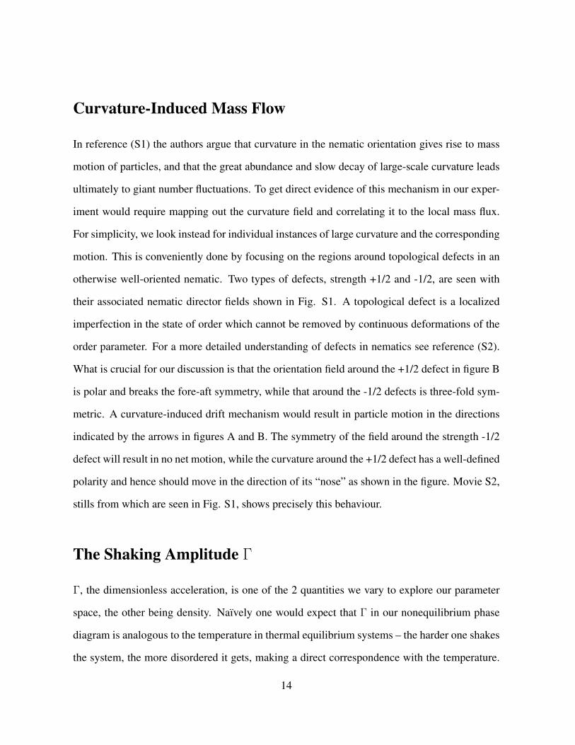
Curvature-Induced Mass Flow

In reference (S1) the authors argue that curvature in the nematic orientation gives rise to mass

motion of particles, and that the great abundance and slow decay of large-scale curvature leads

ultimately to giant number fluctuations. To get direct evidence of this mechanism in our exper-

iment would require mapping out the curvature field and correlating it to the local mass flux.

For simplicity, we look instead for individual instances of large curvature and the corresponding

motion. This is conveniently done by focusing on the regions around topological defects in an

otherwise well-oriented nematic. Two types of defects, strength +1/2 and -1/2, are seen with

their associated nematic director fields shown in Fig. S1. A topological defect is a localized

imperfection in the state of order which cannot be removed by continuous deformations of the

order parameter. For a more detailed understanding of defects in nematics see reference (S2).

What is crucial for our discussion is that the orientation field around the +1/2 defect in figure B

is polar and breaks the fore-aft symmetry, while that around the -1/2 defects is three-fold sym-

metric. A curvature-induced drift mechanism would result in particle motion in the directions

indicated by the arrows in figures A and B. The symmetry of the field around the strength -1/2

defect will result in no net motion, while the curvature around the +1/2 defect has a well-defined

polarity and hence should move in the direction of its “nose” as shown in the figure. Movie S2,

stills from which are seen in Fig. S1, shows precisely this behaviour.

The Shaking Amplitude Γ

Γ, the dimensionless acceleration, is one of the 2 quantities we vary to explore our parameter

space, the other being density. Naıvely one would expect that Γ in our nonequilibrium phase

diagram is analogous to the temperature in thermal equilibrium systems – the harder one shakes

the system, the more disordered it gets, making a direct correspondence with the temperature.

14

We observe a more complicated, non-monotonic trend.

Figure S2 shows the nematic order in the system as a function of density and Γ. Increasing

density clearly increases nematic order. At the three lowest densities, increasing Γ increases

the nematic order. At Ntotal = 2820 however, increasing Γ decreases the nematic order. The

crossover in the behaviour occurs atNtotal = 2500 where we see thatG2(r) for Γ = 5 and Γ = 6

are nearly indistinguishable. Put together, this suggests that these points are near a re-entrant

portion of the isotropic-nematic transition.

The complicated role Γ plays in the system’s dynamics is apparent even in the giant number

fluctuations. Figure S3 shows ∆N/√N as a function of N for 4 different densities. We see

that there are two regimes of fluctuations, most clearly distinguishable in the Ntotal = 2500

curve: (i) ∆N ∝√N at small N , and (ii) ∆N ∝ N , the giant fluctuations, at large N . The

√N at smaller N arises from uncorrelated short-time diffusion of particles and exists even in

the isotropic phase. The giant fluctuations dominate, as expected from (S1), at large N , and

should be larger in systems with stronger nematic order. And indeed, increasing density (and

hence the nematic order) suppresses the√N -fluctuations and enhances the N -fluctuations, as

is seen in the Ntotal = 2000 and Ntotal = 2500 curves in Fig. S3. At lower subsystem sizes

the√N -fluctuations will dominate. Since these are stronger for dilute systems, the magnitude

of fluctuations is greater for N = 2000. For large enough subsystems, the contribution scaling

as N , peculiar to the active nematic, will overwhelm the component that grows as√N . The

Ntotal = 2500 curve shows a sharper rise than the Ntotal = 2000 curve and ultimately the

fluctuations in the former outgrow those in the latter system.

To verify whether increased nematic order does indeed increase the magnitude of fluctua-

tions, we plot ∆N/√N as a function of N for 2 different values of Γ in Fig. S4. As expected

in the dilute systems, where Γ increases the nematic order, it increases the magnitude of fluc-

tuations, whereas for Ntotal = 2820, increasing Γ reduces the magnitude of fluctuations. This

15

suggests that Γ sets the scale of two different stochastic processes at the level of an individual

rod – fore-aft motion, which promotes nematic order, and rotational motion, which disrupts it.

Long-lived Density Autocorrelation

The principal result described in (S1) is that density modulations at long-wavelength λ = 2π/q

in active nematics have a variance proportional to q−2, i.e., at larger and larger length scales,

the system shows larger and larger statistical inhomogeneities. Defining ϕ(r, t) ≡ ρ(r, t) − ρ0

where ρ(r, t) is the density at r at time t and ρ0 its time average, the prediction is that the

static structure factor S(q) ≡ (1/ρ0)∫r

eiq·r〈ϕ(0)ϕ(r)〉 ∝ 1/q2. Converting to real space, the

standard deviation ∆N would therefore grow as N12+ 1

d in d space dimensions. In 2 dimensions,

thus, ∆N ∝ N : fluctuations grow linearly with the mean.

Dynamics

This global result has a sharp signature in the dynamics and statistics of the number of particles

in a local region, as measured by the local density autocorrelation function

C(t) = 〈ϕ(x, 0)ϕ(x, t)〉. (1)

For independently diffusing Brownian particles

C(t) =

∫ddq

(2π)de−q

2Dt ∼ t−d/2 (2)

so that the local density autocorrelation function for a two-dimensional thermal equilibrium

system of non-interacting Brownian particles decays as t−1. This holds even for a diffusing

density field coupled to the director field in a nematic liquid crystal at thermal equilibrium. For

16

an active nematic, however, as shown in (S1), Eq. (2) has to be modified to account for the

anomalous q−2 abundance of the Fourier modes of the density at small wavenumber:

C(t) ∼∫ 2π/a

2π/L

dqqd−1 e−q2Dt

q2(3)

with limits of integration determined by the coarse-graining scale a that we use to define the

density, and the system-size L. This implies that for timescales between those corresponding to

a and to L, C(t) should decay as ln(L2/Dt). Our experimental results are consistent with such

a decay. We also find that coefficient of this logarithm depends on the coarse-graining scale a

(Fig. S5).

The Statistical Independence of Configurations Sampled

To verify whether the images taken at 15-second intervals were indeed statistically indepen-

dent, we calculated two quantities: 1) the local density autocorrelation C(t) (discussed in sec-

tion Dynamics) and 2) the autocorrelation of the orientation of a tagged particle, Cθ(t) =<

cos[2{θ(0) − θ(t)}] >. The angular brackets denote an average over all particles. Figure S6

shows that after an initially slow decay, for about a tenth of a second, Cθ decays logarithmically

to zero as in two-dimensional thermal equilibrium nematics. This decay is over about 10 sec-

onds. Thus, both Cθ(t) and C(t) decay fast enough for us to be certain that the configurations

we are sampling are statistically independent.

Description of the Movie Material

Movie S1 is a recording of a typical experimental run. The system is characterised by large

inhomogeneities and large mass-fluxes. The system contains 2,820 (φ ' 66%) particles and is

17

being agitated at Γ = 5. The time is indicated at the bottom-left in minutes:seconds.

Movie S2 zooms into a small region of the sample. In particular, it compares the behaviour

of +1/2 and −1/2 defects. A strength +1/2 defect is seen to move across the field of view of

the camera starting at the bottom-left and the strength −1/2 defect is seen to remain relatively

stationary as is argued in the section Curvature-Induced Mass Flow. The time is indicated in

seconds at the bottom-left.

18

Figure S1. Schematic image A) shows the the motion predicted (S1) to arise in response to

a curvature in the nematic director field. Fig B) applies this idea to the director fields around

topological defects of strength +1/2 and -1/2. Particle orientations are shown in grey and the

resulting particle currents are in the direction of the arrow. In B) the three competing parti-

cle streams would hold a -1/2 defect stationary whereas the +1/2 would move along the blue

arrow. The time-lapse images C) through I) show exactly this behaviour in our experiment.

The strength -1/2 defect (in the green circle) moves very little, while the strength +1/2 defect

(encircled in red) moves substantially and systematically along its nose.

19

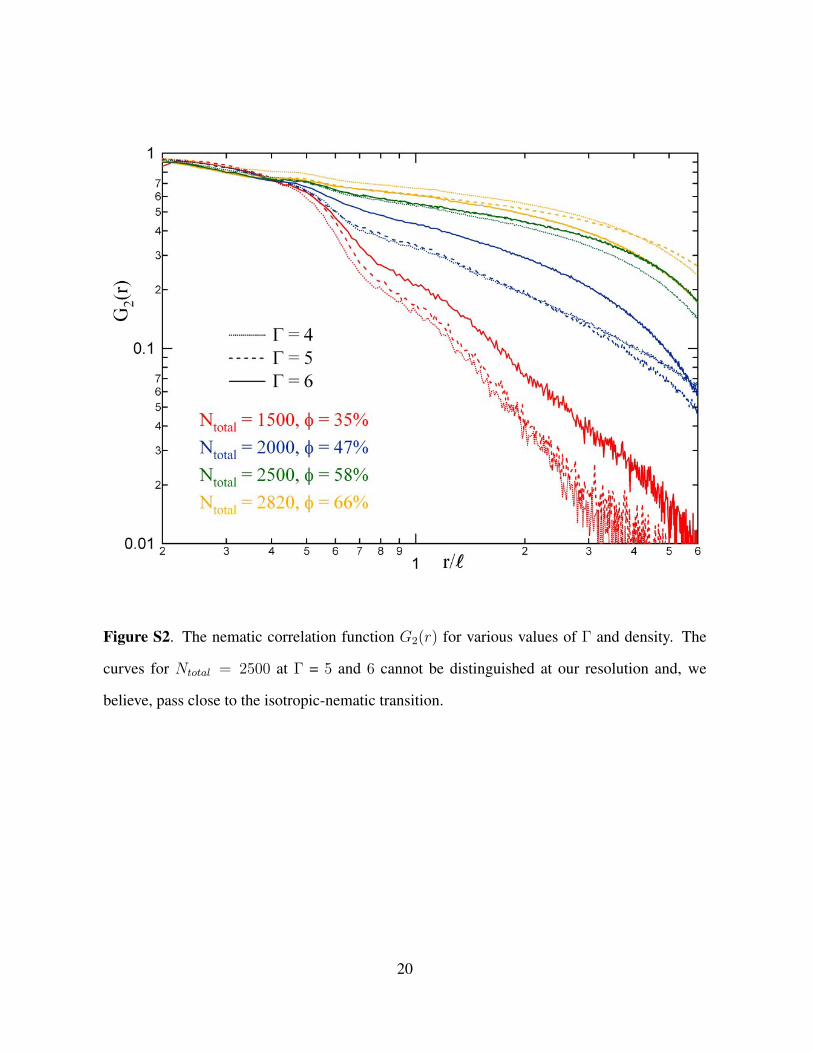
Figure S2. The nematic correlation function G2(r) for various values of Γ and density. The

curves for Ntotal = 2500 at Γ = 5 and 6 cannot be distinguished at our resolution and, we

believe, pass close to the isotropic-nematic transition.

20

Figure S3. Number fluctuations at different densities: the magnitude of the density fluctuations

grows with increasing nematic order.

21

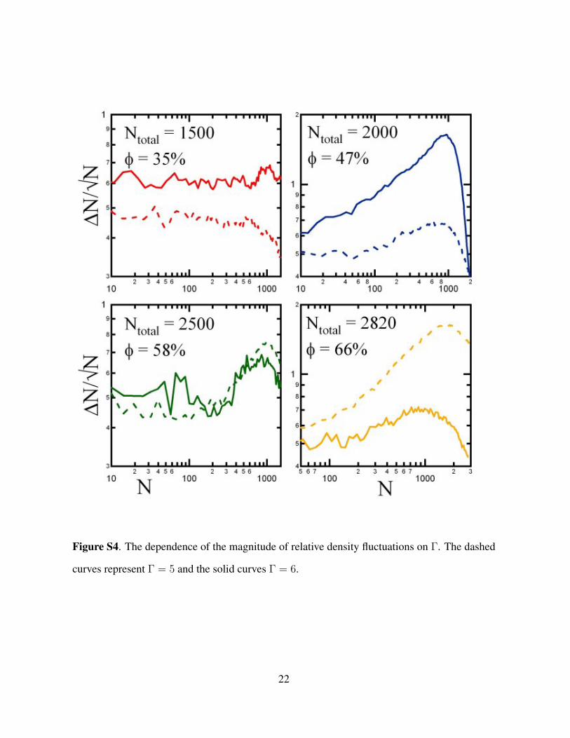
Figure S4. The dependence of the magnitude of relative density fluctuations on Γ. The dashed

curves represent Γ = 5 and the solid curves Γ = 6.

22

Figure S5. The figure shows C(t) evaluated using for three different subsystems of linear size,

a. The data for the two larger subsystem sizes has been scaled up by the subsystem area to

facilitate viewing.

23

Figure S6. The autocorrelation of the orientation of a tagged particle, Cθ(t) = 〈cos[2{θi(τ)−

θi(τ + t)}]〉i,τ where i runs over all particles.

References

S1. S. Ramaswamy, R. A. Simha, J. Toner, Europhys. Lett. 62, 196 (2003).

S2. P. G. de Gennes, J. Prost, The Physics of Liquid Crystals, Clarendon, (Clarendon, Oxford

1993); chap. 4, p. 169

24