lnrroducflon fo

ond DifbrenliclEquofions

, ' ' ' \

John\V Detfrnon

DOVER BOOI$ ON MATHEMATICSH{vosoox or M,crHeMATrcru. FuNcrrons, Milton Abramowitz and lrene A.

Stegun. (612724)TsNson Annrvss ox M.rurops, Richard L. Bishop and samuel l. Goldberg.

(6403s6)T.qBt.us or INoenNm lvrecnars, G. petit Bois. (6022S7)Vecron nxo Tenson At.tlrysrs wmr Appucmrons, A. l.

Tarapov. (638332)THr Hrsronv oF TnE crculus arp lrs cor{csmJAl DevEloprvrsrfl., carl B.

Boyer. (605094)THs Qulr-rmrve Tueonv oF onorrulnv DrrrrneNrrll Equ.morus: Arv

lrrnoouctrol, Fred Brauer and John A. Nohel. (65g4GS)Alconmms roR MnilMrzAnon wmrow DERrvATnEs, Richard p. Brent. (4lgg&3)Pruncpr es or Srnnsrtcs, M. G. Bulmer. (6376G3)THs THrony or Senons, Elie Cartan. (6407G1)Aovuceo NuruseR THeonv, Harvey Cohn. (64023X)srmsrcs MAnuAL, Edwin L. crow, Francis Davis, and Margaret Maxfield.

(605ee-DFouruen SEruss axp OnrHoconr FwcnoNs, Harry F. Davis. (659Z&9)Corrrpwasil-rry AND UNsoLvnsLrry, Martin Davis. (6147l-9)Asyrurronc Menroos rN ANALysrs, N. G. de Bruijn. (6422l{-)PnosLE[,ts rN Gnoup THEonv, John D. Dixon. (6lS74X)Tue MrrusuATrcs oF GlMes op SrncrEcy, Melvin Dresher. (642lGDAppueo PlRrrru. DrrrensNrhl Eeunnons, paul Duchateau and David

Zachmann. (4l97&l?)Asyrupronc ExpANsroNs, A. Erd6lyi. (6031&0)corrapLp( VarulslEs: Hmuonrc lNo ANlnmrc Funcnons, Francis J. Flanigan.

(6138&r)

Borisenko and I. E.

Oru Fonuru-ly UxoecDasLs PRoposntoNs oFReLnrsD SysrEMs, Kurt Gddel. (66g8GT)

A Hsrony or GRssr MarHervrArrcs, Sir Thomas

Pruncrpn M.qruruarrcA AND

Heath. (2407n,2407+6)

oF Tr{E MlrHel{lncx. THeony, C. R. Heathcote.

Two-volume setPnoaABLrrY: ElErrlsNrs

(4rr4e4)IvrRopucnon ro Nur'trrucru- Arru-vsrs, Francis B. Hildebrand. (6536&3)Me-rHoos or Appuno Mlrnil,t,crrcs, Francis B. Hildebrand. (67002-3)Torolocv, John G. Hocking and Gail S. Young. (6562G4)MerrnM,crrcs rlo Locrc, Mark Kac and Stanislaw M. Ulam. (67085{)MrrHsMATrc.cL Four{oATroNs oF lxponnaanon THeonv, A. I. Khinchin. (604349)AnrrHurnc RTTREsHER, A. Albert KIaf. (21241{)Cru-culus REFRESHER, A. Albert Klaf. (203704)Pnoeul,r Boor n rHs THEony or FUncnons, Konrad Knopp. (4l4Sl-5)Ivrnopucronv Rml ANALysrs, A. N. Kolmogorov and s. v. Fomin. (6r22ffi)

(continued on bach flap)

Inrroducrion fo LineorAlgebro ond Differenflol Equoflons

John W DerrrnonWritten for the undergraduate who has completed a year of calculus, this clear,skillfully organizedtext combines two important topici in modern matirematics inone comprehensive volume.

As Professor Dettman (oakland university, Rochester, Michigan) points out, ..Not

only is linear_algebra indispensable to the mathematicsmajor,"U"i . . . it ir tnat p"itof algebra which is most useful in the application of mathemaiical analysis to oilierareas,. e'g., linear programming, systems_analysis, statistics, numerical

"nalyrir,combinatorics, and mathematical physics."

The book- progresses from familiar ideas to more complex and difficult concepts,with applications introduced along the way, to clarify or illustrate theoreticalmaterial.

Among the -topics covered are complex numbers, including two-dimensionalvectors and functions _o{ a complex variable; matrices and delerminants; ,r""to,sPfces; symmetric and hermitian matrices; first order nonlinear equations; lineardifferential equations; power-series methods; Laplace transforms; Bessel functions;systems of differential equations; and boundary value problems.

To reinforce and expand each -chapter, numerous worked-out examples areincluded. A-unique pedagogical feature is the starred section at the end of eachchapter. Although-these sections are not essen_tial to the sequence of the b;J, th;iare related to the basic material and offer advanced topics to stimulate the morlambitious student' These_topics include power series; existence and ,rniquenlsthe.or.emS Hilbert spaces; Jordan forms; Gieen's functions; Bernstein polynbmials;and the Weierstrass approximation theorem.

This carefully structured textbook provides an ideal, step-by-step transition fromfirst-year calculus to multivariable calculus and, u[ tt e same time, enables theinstructor to offer special challenges to students ready for more advanced material

Unabridged and correctg-$ _Dov91 (1936) republication of the edition originally

published by JVIcGraw-Hill, Inc., New York, tgz l. +Ablack-and- white illustritions.Exercises with solutions. Index. 4t6pp. 5g6 x gli. paperbound.

ALSO AVAILABLE

LtNBen ALnsnna, Georgi Shilov. 387pp. S%xg,/2.6351g-XonnrNnnv DrrrnRrnrrlr EqurrroNi, Morris Tenenbaum and Harry pollard. slspp.

53/s x 8%. 64940-7onurnaRv DrrpnnsNrrrar- EgunrroNs, Edward L. Ince. 55gpp. s% x B%. 60349_0

Free Dover Mathematics and Science Cataloe(59065-8) available upon request.

See every Dover book in print atwww.doverpublications.com

ISBN D- ' { gb -b51 ,11 , -b

ilililil|fiilililI+ 1,5se3

15 TN USA15 TN CANADA tlillffiilltil6519

(continued from hont flap)

Spuclu- FuNcrroxs Ar\D THErR Arpucrrrons, N. N. Lebedev. (606244)CHANcE, Lucr rulo Srlrsrrcs, Horace C. Levinson. (a1997-5)TEnsoRs, Dtmnrvrm FoRtvts, lt.tn VnRrlloux- PRItrctpLts, David Lovelock

and Hanno Rund. (658404)Sunvny or Marntx THeony Nlo MATRD( h.rseuN-mes, Marvin Marcus and

Henryk Minc. (67102-DAgsrR.ccr ALcrsRA lr.ro SoltmoN By RADrcals, John E. and Margaret W.

Maxfield. (67121-6)FutvolrvrEr.r'rAt- CoNcspts or AtcEeRA, Bruce E. Meserve. (61470-0)FuNnnMeNrAL ConcEpts or Geoumny, Bruce E. Meserve. (6341t9)Ftrrv CuanENcrNc Pnosler\ls rN PRosngrLITy wtrH Solurrons. Frederick

Mosteller. (6535t2)NuMern THrony aNo lrs Hnronv, Oystein Ore. (65620-9)Marrucrs mto TnnnsroRMATtoNS, Anthony J. Pettofrezzo. (63634€)PRosABrr-rry THsony: A Coxcrss CouRsr, Y. A. Rozanov. (63544.9)OnpwlRy Drrrenevrnl Eeumons AND Srngrury THEoRy: An lvrnooucrroN,

David A. Sdnchez. (6382&6)LNr.qR ALcreRa, Georgi E. Shilov. (6351&DEssetww- Cx-culus wnu Appr-rcATroNS, Richard A. Silverman. (660974)A ConcsE Hrsrony or MrrHruancs, Dirk J. Struik. (60255-9)PnosLgMs ttr PRoeABLrry THEoRy, Mlrurvlrrcll Srnnsrrcs AND THuony op

RnNnou FulcrroNs, A. A. Sveshnikov. (637174)TuNson CALcuLUs, J. L. Synge and A. Schild. (63612-7)Cu-culus or VlRr,rrrons wtrH Appucltrolls ro Puvslcs ltro EtrclNmnrnc, Robert

Weinstock. (63069-2)Ivrnooucrroru ro VscroR lNn TsNsoR AwALysrs, Robert C. Wrede. (61879-DDtsrruBwroru TuroRy lxo TnaNsroRu Axalysls, A. H. Zemanian. (65479-6)

Paperbound unless otherwise indicated. Available at your book dealer,online at www.doverpublications.com, or by writing to Dept. 23, DoverPublications, Inc.,3l East Znd Street, Mineola, NY 11501. For currentprice information or for free catalogs (please indicate field of interest),write to Dover Publications or log on to www.doverpublications.comand see every Dover book in print. Each year Dover publishes over 500books on fine art, music, crafts and needlework, antiques, languages, lit-erature, children's books, chess, cookery, nature, anthropology, science,mathematics, and other areas.

Manufactured in the U.S.A.

Introduction toUnearAlgebra and

Differential Equations

JouN'W'. DprrvtANProfessor of Mathematics

Oakland UniversityRochester, Michigan

Dover Rrblications, Inc.

Copyright @ 1974,1986 by John W. Dettman.All rights reserved under Pan American and Intemational Copy-

right Conventions.

This Dover edition, first published in 1986, is an unabridged,corrected republication of the work originally published by theMcGraw-Hill Book Company, New York, 1974.

Manufactured in the United States of AmericaDover Publications, Inc., 31 East 2nd Street, Mineola, N.Y. 11501

Library of Congress Cataloging-in-Publication Data

Dettman, John W. (John Warren)Introduction to linear algebra and differential equations.

Originally published: New York : McGraw-Hill,1974.lncludes bibliographical references and index.l. Algebras, Linear. 2. Differential equations. I. Title'

QAl84.D47 1986rsBN 0-486-6519r-6

512', .5 86-6311

CONTENTS

Preface ix

1 Complex Numbers I

I.I Introduction I1.2 The Algebra of Complex Numbers 21.-? The Geometry of Complex Numbers 61.4 Two-dimensional Vectors 131.5 Functions of a Complex Variable 2l1.6 Exponential Function 25

*1.7 Power Series 30

2 Linear Algebraic Equations 4l

2.1 Introduction 4l2.2 Matrices 422.3 Elimination Method 482.4 Determinants 592.5 Inverse of a Matrix 7l

*2.6 Existence and Uniqueness Theorems 7g

vi CONTENTS

3 Vector Spaces 84

3.1 Introduction 843.2 Three-dimensional Vectors 853.3 Axioms of a Vector Space 963.4 Dependence and Independence of Vectors 1033.5 Basis and Dimension 1103.6 Scalar Product ll73.7 Orthonormal Bases I24

*-1.8 Infinite-dimensional Vector Spaces 129

4 Linear Transformations 139

4.1 Introduction 1394.2 Definitions and Examples4.3 Matrix Representations4.4 Change of Bases 1604.5 Characteristic Values and4.6 Symmetric and Hermitian

*4.7 Jordan Forms 188

5 First Order Differential Equations 198

5.1 Introduction 1985.2 AnExample 1995.3 Basic Definitions 205-i.4 First Order Linear Equations 2085.5 First Order Nonlinear Equations 2135.6 Applications of First Order Equations 2215.2 Numerical Methods 225

x-i.8 Existence and Uniqueness 232

6 Linear Differential Equations 244

6.1 Introduction 2446.2 General Theorems 2456.3 Yariation of Parameters 2506.4 Equations with Constant Coefficients 254

6.5 Method of Undetermined Coefficients 260

6.6 Applications 264*6.7 Green's Functions 271

r401 5 1

Characteristic VectorsMatrices 177

166

CONTENTS Yii

7 Laplace Transforms 282

7.1 Introduction 2827.2 Existence of the Transform 2g37.3 Transforms of Certain Functions Zgg7.4 Invercion of the Transform 2957.J Solution of Differential Equations 3017.6 Applications 306

*7.7 Uniqueness of the Transform 310

8 Power-Series Methods 315

8.1 Introduction 3158.2 Solution near Ordinary points 3168.3 Solution near Regular Singular points 3228.4 Bessel Functions 3288.5 Boundary-value Problems 338

*8.6 Convergence Theorems 346

9 Systems of Differential Equations lS29.1 Introduction 2539.2 First Order Systems 3539.3 Linear First Order Systems 3599.4 Linear First order Systems with constant coefficients 3649.5 Higher Order Linear Systems 370

*9.6 Existence and Uniqueness Theorem 374

Answers and Hints for Selected Exercises 3gl

fndex 399

PREFACE

since 1965, when the committee on the Undergraduate program inMathematics (CUPM) of the Mathematical Association of America recom-mended that linear algebra be taught as part of the introductory calculussequence, it has become quite common to find substantial amounts of linearalgebra in the calculus curriculum of all students at the sophomore level.This is a natural development because it is now pretty well conceded thatnot only is linear algebra indispensable to the mathematics major, but thatit is that part of algebra which is most useful in the application of math-ematical analysis to other areas, e.g., linear programming, systems analysis,statistics, numerical analysis, combinatorics, and mathematical physics. Evenin nonlinear analysis, linear algebra is essential because of the commonly usedtechnique of dealing with the nonlinear phenomenon as a perturbation of thelinear case. We also find linear algebra prerequisite to areas of mathematicssuch as multivariable analysis, complex variables, integration theory, functionalanalysis, vector and tensor analysis, ordinary and partial differential equations,integral equations, and probability. So much for the case for linear algebra.

The other two general topics usually found in the sophomore programare multivariable calculus and differential equations. In fact, modern calculus

X PREFACE

texts have generally included (in the second volume) large portions of linearalgebra and multivariable calculus, and, to a more limited extent, differentialequations. { have written this book to show that it makes good sense to packagelinear algebra with an introductory course in differential equations. On theother hand, the linear algebra included here (vectors, matrices, vector spaces,linear transformations, and characteristic value problems) is an essential pre-requisite for multivariable calculus. Hence, this volume could become thetext for the first half of the sophomore year, followed by any one of a numberof good multivariable calculus books which either include linear algebra ordepend on it. The prerequisite for this material is a one-year introductorycalculus course with some mention of partial derivatives.

I have tried throughout this book to progress from familiar ideas to themore difficult and abstract. Hence, two-dimensional vectors are introducedafter a study of complex numbers, matrices with linear equations, vector spacesafter two- and three-dimensional euclidean vectors, linear transformations aftermatrices, higher order linear differential equations after first order linearequations, etc. Systems of differential equations are left to the end after thestudent has gained some experience with scalar equations. Geometric ideasare kept in the forefront while treating algebraic concepts, and applications arebrought in as often as possible to illustrate the theory. There are worked-outexamples in every section and numerous exercises to reinforce or extend thematerial of the text. Numerical methods are introduced in Chap. 5 in connec-tion with first oider equations. The starred sections at the end of each chapterare not an essential part of the book. In fact none of the unstarred sections

depend on them. They are included in the book because (l) they are related toor extend the basic material and (2) I wanted to include some advanced

topics to challenge and stimulate the more ambitious student to further study.These starred sections include a variety of mathematical topics such as:

I Analytic functions of a complex variable.2 Power series.

3 Existence and uniqueness theory for algebraic equations.4 Hilbert spaces.

5 Jordan forms.6 Picard iteration.

7 Green's functions.

8 Integral equations.9 Weierstrass approximation theorem.

I0 Bernstein polynomials.

I I Lerch's theorem.

PREFACE Xi

I2 Power series solution of differential equations.I3 Existence and uniqueness theory for systems of differential equations.I4 Gr<jnwald's inequality.

The book can be used in a variety of different courses. The ideal situationwould be a two-quarter course with linear algebra for the first and differentialequations for the second. For a semester course with more emphasis on linearalgebra, Chaps. 1-6 would give a fairly good introduction to linear differentialequations with applications to engineering (damped harmonic oscillator). Ifone wished less emphasis on linear algebra and more on differential equations,Chap. 4 could be skipped since the characteristic value problem is not used inan essential way until Chap. 9. Chapters 7, 8, and 9 are independent so that avariety of topics could be introduced after Chap. 6, depending on the interestsof the class. For a class with a good background in complex variables andlinear algebraic equations, Chaps. I and 2 could be skipped.

About half of the book was written during the academic year 1970-JIwhile I was a Senior Research Fellow at the University of Glasgow. I want tothank Professors Ian Sneddon and Robert Rankin for allowing me to use thefacilities of the University. I also wish to thank Mr. Alexander McDonald andMr. Iain Bain, students at the University of Glasgow, who checked the exercisesand made many helpful suggestions. The first six chapters have been used in acourse at Oakland University. I am indebted to these students for their patiencein studying from a set of notes which were far from polished. Finally, I wantto thank my family for putting up with my lack of attentiveness while I was inthe process of preparing this manuscript.

JOHN W. DETTMAN

ICOMPLEX NUMBERS

1.1 INTRODUCTION

There are severa! reasons for beginning this book with a chapter on complexnumbers. (l) Many students do not feel confident in calculating with complexnumbers, even though this is a topic which should be carefully covered in thehigh school curriculum. (2) The complex numbers represent a very elementaryexample of a vector space. we shall, in fact, use the complex numbers tointroduce the two-dimensional euclidean vectors. (3) Even if we were to attemptto avoid vector spaces over the complex numbers by using only real scalarmultipliers, we would eventually have to deal with complex characteristicvalues and characteristic vectors. (a) The most efficient way to deal with thesolution of linear differential equations with constant coefficients is throughthe exponential function of a complex variable.

we shall first define the algebra of complex numbers and then thegeometry of the complex plane. This will lead us in a natural way to a treat-ment of two-dimensional euclidean vectors. Next we shall introduce complex-valued functions, both of a single real variable and of a single complex variable.This will be followed by a careful treatment of the exponential function. The

2 INTRoDUCTIoN To LINEAR ALGEBRA AND DIFFERENTIAL EQUATIoNs

last section (which is starred) is intended for the more ambitious students. Itdiscusses power series as a function of a complex variable. Here we shall justifythe properties of the exponential function and lay the groundwork for thestudy of analytic functions of a complex variable.

I.2 THE ALGEBRA OF COMPLEX NUMBERS

We shall represent complex numbers in the form z : .x * ry, where x and yare real numbers. As a matter of notation we say that x is the real part ofz lx : Re (z)] and y is the tmaginary part of t ly : Im (z)]. We say that twocomplex numbers are equal if and only if their reflLarts are equal and theirimaginary parts are equal. we could say that i : ^J - I except that for a personwho has experience only with real numbers, there is no number which whensquared gives - 1 (if a is real, a' > 0). It is better simply to say that i is acomplex number and then define its powersi i, i2 - -1, i3 : -i, i4: l,etc. We can now define addition and multiplication of complex numbers in anatural way:

21 * 22 : (xr + iy) I (xz + iy): (x, + x) * i(yr * yz)

z1z2 : (xr * iy)(xz + i!) : xrx2 I i'yr!2 * ix1y2 * iyp2: (xfiz - !r!) * i(xry, I y$z)

With these definitions it is easy to show that addition and multiplication areboth associative and commutative operations, that is,

( z t i z ) + 2 3 : z r * Q z * z r )

z 1 * 2 2 : 2 2 * 2 1

zr(2223) : (zrz2)23

Z1Z2 : Z2Z1

If a is a real number, we can represent it as a complex number as follows:e : a + t0. Hence we see that the real numbers are contained in the complexnumbers. This statement would have little meaning, however, unless thealgebraic operations of the real numbers were preserved within the contextof the complex numbers. As a starter we have

a + b : (a *t0) + (6 + t0) : (a *b) + t0

ab: (a + t0XD + t0) : ab + i0

We can, of course, verify the consistency of the other operations as they aredefined for the complex numbers.

@MPLE ( NUMBERS 3

Letaberealandlet z: x * ry. Then az: (a + t0Xx + iy): ax * iay.In other words, multiplication of a complex number by a real number c isaccomplished by multiplying both real and imagtrnary parts by the real numbera. With this in mind, we define the negatiue of a complex number z by

. z : ( - l ) z : ( - x ) + t ( - y )

The zero of the complex numbers is 0 + i0 : O and we have the obviousproperty

z * ( -z ' ) : . r * iY + (-x) + t ( -Y): 0 + f 0: Q

We can now state an obvious theorem, which we put together for a reason whichwill become clear later.

Theorem 1.2.1(i) For all complex numbers z, and 22, zr * 22 : z, * zy(iD For all complex numbers zL, zz, and 23,

z 1 * ( 2 2 * z ) : ( z r * 2 2 ) + z t

(iiD For all complex numbers z, z * O : Z.(iv) For each complex number z there exists a negative -z such that

z * ( - z ) : Q .

We define subtraction in terms of addition of the negative, that is,

z'l - zz li:,*-'.1r".;J1'j ;:r"

* (-x) + i(-vz)

Suppose z : x * iy, and we look for a reciprocal complex numberz-r : u * iu such that zz-r : l. Then

(x + iy)(u * iu) : (xu - yu) * i(xu + yu) : I + i0

Then xu - yu : I and xu + yu : 0. These equations have a unique solutionif and only if x2 + y2 # 0. The solution is

x - v: * \ y ' ' : Ty '

Therefore, we see that every complex number z, except zero, has a uniquereciprocal,

_ i y' x '

+ y '- - t _

x 2 + y 2

4 INTRoDUCTIoN To LINEAR ALGEBRA AND DIFFERENTIAL EQUATIoNs

we can now define diuision by any complex number, other than zero, interms of multiplication by the reciprocal; that is, if z2 * 0,

: z r Z 2 t - ( x r */ - v t \

t _ v r ) { , 4 - i " = l- " \*rt + yzz xzz + y22,1

: xz l r - x r l z' x r67

iy)(xz - iy) - xz2 + y22 and hence

xrxz * y tyz * i (xzyt - x ryr )

xz2 * yz2

z!

z2

:Tl#*As a mnemonic, note that (x, +

z , _ 4 r * i y rxz - i l z _22 x2 * iy2 xz - ilz

EXAMPLE 1.2.1 Let zr : 2 * 3i and Zz : -l + 4i. Then z1 * z2( 2 - l ) + ( 3 + 4 ) i : | + 7 i , z r - Z z : ( 2 + l ) + ( 3 - 4 ) i : J - i , z r z 2(-2 - 12) + (8 - 3) : -t4 + Si,and

z, _ 2 + 3 i -+ - o : _ -2 + 12 - 3 i - B i : lg _ 11,2 2 - 1 + 4 i - t - 4 i 1 + 1 6 t 7 1 7 "

The reader should recall the important distributiue law from his studyof the real numbers. The same property holds for complex numbers; that is,

z r ( 2 2 * z s ) : z F 2 + z F 3

The proof will be left to the reader.We summarize what we have said so far in the following omnibus theorem

(the reader will be asked for some of the proofs in the exercises).

Theorem 1.2.2 The operations of addition, multiplication, subtrac-tion, and division (except by zero) are defined for complex numbers. Asfar as these operations are concerned, the complex numbers behave likereal numbers.t The real numbers are contained in the complex numbers,and the above operations are consistent with the previously definedoperations for the real numbers.

There is one property of the real numbers which does not carry over to thecomplex numbers. The complex numbers are not ordered as the reals are.

I In algebra we say that both the real and complex numbers are algebraic fields. Thereals are a subfield of the complex numbers.

s 5

Recall that for real numbers I and - I cannot both be positive. Also if a * 0,then a2 is positive. If the complex numbers had the same properties of order,both 12 : I and i2 : -l would be positive. Therefore, we shall not try toorder the complex numbers and/or write inequalities between complexnumbers.

We conclude this section with two special definitions which are importantin the study of complex numbers. The first is absolute ualue, which we denotewith the symbol lzl. The absolute value is defined for every complex numberz : x * l y a s

t ' l: J*\ Y'

It is easy to show that lzl > 0 and lzl : 0 if and only if z : 0.The other is the conjugate, denoted by Z. The conjugate of z : x * iy

is defined as2 : x - i !

The proof of the following theorem will be left for the reader.

Theorem 1.2.3( i ) z r + 2 2 : 2 r * Z z .

( i D z t j : z ,( i l r ) z1z2 : 2122.

( iv) zr l4 :2JZz.(v) zZ : lzl2.

EXERCISES 1.2

I L e t z r : 2 * i a n d 2 2 : - 3 + 5 i . C o m p u t e z 1 * z 2 , z L - z 2 , z p 2 , z 1 f z 2 , E y

Zz, lztl, and, lz2l.2 L e t z 1 - - 1 * 3 i a n d z z : 2 - 4 i . C o m p u t e z 1 * 2 2 , Z L - 2 2 , z 1 z 2 , z 1 l z 2 ,

Zt , Ez, lz l , and lz2l .Prove that addition of complex numbers is associative and commutative.Prove that multiplication of complex numbers is associative and commutative.Prove the distributive law.Show that subtraction andcontext of complex numbers.

of real numbers is consistent within the

7 Showthattheequations xu - yu: l and xu + yu:0haveauniquesolut ionfor z and u if and only if x2 + y2 + O.

3456

6 INTRoDUcTIoN To LINEAR AIGEBRA AND DIFFBRENTIAL EQUATIoNS

FIGURE 1

8 Let a and 6 be real and zl and z2 be complex. prove the following:(a) a(21 * zz) : azr + az2 @) (a * b)2, : ozr * bz1(c) a(bz) : (ab)21 @) lz1 : 21

9 Show that lzl > 0 and lzl : O if and only if z : A.10 Prove Theorem 1.2.3.ll Show that

Re (z) : !(z + z) Im (z) : ^!.e - z)zt

12 Show that the definition of absolute value for real numbers is consistent withthat for complex numbers.

13 l * tz : x * iy and w: u * rb . prove that (xu * yu)2. l r l r l r l " andhencethat lxu + yul < lrl l*1.

14 Use the result of Exercise 13 to show thatlz * rrl < lzl + lrryl.15 Use the result of Exercise 14 to show that

l z 1 * z 2 + . . . + z , l = l z r l + l r r l + . . . + l z )

16 Show that lz - wl > l l " l - l " l l .

1.3 THE GEOMETRY OF COMPLEX NUMBERS

It will be very useful to give the complex numbers a geometric interpretation.This will be done by associating the complex number z : x * iy with thepoint (x,y) in the euclidean plane (see Fig. l). It is customary to draw an arrowfrom the origin (0,0) to the point (x,y). For each complex number z : x * ilthere is a unique point (x,y) in the plane and (except for z : 0) a unique arrowfrom the origin to the point (x,y).

There is also a polar-coordinate representation of the complex numbers.Let r equal the length of the arrow and 0o be the minimum angle measured

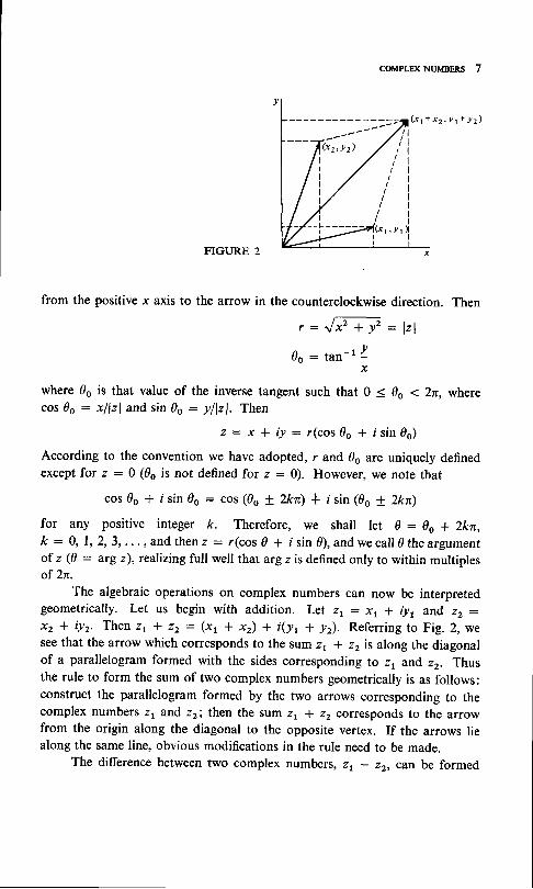
COMPLEX NUMBERS 7

( x t + x z , Y r + Y z )

FIGURE 2

from the positive x axis to the arrow in the counterclockwise direction. Then

, : , / * , * y 2 : l z l

0o : tan-L I

where 0s is that value of the inverse tangent such that I = ,, 1 zn,wherecos 0o : xllzl and sin 0o : yllzl. Then

According to the convention J; ;;,;,':::j;J":I":;lery dennedexcept for z : 0 (gs is not defined for z : 0). However, we note that

cos do * i sin 0o : cos (0o + 2kn) * i sin (0o ! 2kn)

for any positive integer k. Therefore, we shall let 0 : 0o * 2kn,k : 0 ,1 ,2 ,3 , . . . , and t henz : , , ( cos 0 + i s i n 0 ) , andwe ca l l ? t hea rgumen tof z (0 : arg z), realizing full well that arg z is defined only to within multiplesof 2n.

The algebraic operations on complex numbers can now be interpretedgeometrically. Let us begin with addition. Let z, : x1 * iy1 and z, :x2 * iy2. Then z1 * zr: (xr I xz) * t(yt * y). Referring to Fig. 2, wesee that the arrow which corresponds to the sum z1 * z2 is along the diagonalof a parallelogram formed with the sides corresponding to z, and zr. Thusthe rule to form the sum of two complex numbers geometrically is as follows:construct the parallelogram formed by the two arrows corresponding to thecomplex numbers z, and zr; then the sum z, * z2 corresponds to the arrowfrom the origin along the diagonal to the opposite vertex. If the arrows liealong the same line, obvious modifications in the rule need to be made.

The difference between two complex numbers, Zr - 22, can be formed

8 rNrnooucrloN To LINEAR ALGEBRA AND DIFFERENTTAL EeuATIoNs

FIGURE 3

geometrically by constructing the diagonal of the parallelogram formed byz, and - z, (see Fig. 3).

To interpret the product of two complex numbers geometrically we usethe polar-coordinate representation. Let z1 : rl(cos 0, * f sin 0r) andz2 : r2(cos 02 + f sin 0r). Then

zrz2 : rrrr(cos 0r + i sin or)(cos 02 + i sin 0r): rrrr[(cos 0, cos 0, - sin 0, sin gr)

* i(sin 0, cos 02 + cos 0, sin 0r)]: rrr2Lcos (0r + 0r) + i sin (0, + 0z)]

Figure 4 shows the interpretation of this result geometrically. This result alsogives us an important theorem.

Theorem 1.3.1 For all complex numbers z, and zr, lzrz2l: lzl lz2l.For all nonzero complex numbers z, and 22, arg ztz2 : arg zr * arg zr.

The quotient of two complex numbers can be similarly interpreted. Letz2 * 0andztf z, - zs. Then 21 : z2z3andlzr l : lz2l lzr l ,argzr: arg22 +arg4. Since lzrl + 0, Izrl: lzrl l lz2l; and if z1 * 0, z3 * 0, then a;tgz3:atg zr - arg 22.

FIGURE 4

s 9

This proves the following theorem:

Theorem 1.3.2 For all complex numbers z, and z2 * 0, lzrlzzl :

lzrlllzrl. For all nonzero complex numbers z, and 22, arg(zrlzz):arg z1 - arg 22.

Powers of a complex number z have the following simple interpretation.Let z : r(cos 0 + tsin 0); then z2 : r'(cos 20 + isin 2g), and by inductionz' : rn(cos n0 + i sin n0) for all positive integers n. For all z + 0 we definezo : l , and of course z-r : r- l [cos (-0) + i sin (-d)]. Then for al lposit ive integers ff i , z-^: r- ' [cos (-m0) * isin (-m0)]. Therefore, we

have for all integers n and all z * 0

zn : rn(cos n0 + f sin n0)

Having looked at powers, we can study roots of complex numbers. We

wish to solve the equation zn : c, where n is a positive integer and c is a com-plex number. If c : 0, clearly z : 0, so let us consider only c * 0. Let

lcl : p and arg c : 0, keeping in mind that Q is multiple-valued. Then

zn : r ,(cos n0 * isin n0) : p(cos O + isin {)

and rn : p, n0 : $. Let Q : Qo * 2kn, where do is the smallest non-

negative argument of c. Then 0 : (6o + Zkn)ln and r : prln, where k is anyinteger. However, not all values of k will produce distinct complex roots z.

Suppose k : 0 , 1 ,2 , . . . ) n - l . Then the angles

Qo- l

n0 o + ( 2 n - 2 ) n

n

6 o * Q n - 2 ) n

a re a l l d i s t i nc t ang les . Howeve r , i f we l e t k : f l , n * | , f l * 2 , . . . , 2n - l ,we obtain the angles

Q o , t - 6 o * 2 n , r - 6 o * 4 n , 1 -| - . r t . . . t

n n n

which differ by 2n from the angles obtained above and therefore do not producenew solutions. Similarly for other values of k we shall obtain roots included fork : 0, 1,2,. . . , n - l. We have proved the following theorem.

Theorem 1.3.3 For 6 : p(cos 0o + f sin fo), p + 0, the equationzn : c, n a positive integer, has precisely n distinct solutions

z : p1,^ ( "ordo * 2kn * i s in do + z tz)

\ n n /k : 0 , 1 ,2 , . . . , n - l . Theseso lu t i onsa rea l l t hed i s t i nc tn th roo t so f c .

* 2 n

IO INTRODUCTION TO LINEAR ALGEBRA AND DIFFERENTIAL EQUATIONS

FIGURE 5

EXAMPLE 1.3.1 Find all solutions of the equation z* + | : 0. Since

24 : -l : cos (n + 2kn) * isin (n + 2kn)

according to Theorem 1.3.3, the only distinct solutions are

3nc o s - +

4

5nc o s - *

4

7nc o s - *

4

These roots can be plotted on a unit circle separated by an angle of 2nl4 : nl2

(see Fig. 5).

EXAMPLE 1.3.2 Find all solutions of the equation z2 + 2z + 2 : 0.

This is a quadratic equation with real coefficients. However, we write the

variable as z to emphasize that the roots could be complex. By completing

the square, we can write z2 * 2z * l : (z + l)2: -1. Then taking the

square root of -1, we get z * 1 : cos (nl2) + i sin(nl2) : f and z I I :

cos (3n/2) * i sin (3n12) - -i. Therefore, the only two solutions are

z : - l + i a n d z : - l - i . N o t e t h a t i f w e h a d w r i t t e n t h e e q u a t i o n a s

. o r I +4

n l it S l n - : - =""' 4 J' ,/t

3 n 1 ii s i i - i _ : - _ _ = :' - " 4 J t 'J t

5 n 1 tI s l n - : _ - - - F" " "4

J t J 'T n l i

r s i n _ : _ :' " . 4 J t J '

COMPLE'( NUMBERS 11

az2 + bz * c :0,a: l ,b :2, c :2 and applied the quadraticformula

- b + J o z - q a c

" : - - - ; -

we would have got the same result by saying t J{ : *i. The reader willbe asked to verify the quadratic formula in the exercises in cases where a, b,and c are real or complex.

We conclude this section by proving some important inequalities whichalso have a geometrical interpretation. We begin with the Cauchy-Schwarzinequality

l x p 2 * l g z l < l z r l l z r l

where z! : xr * iyr and z, : x2 * i!2. Consider the squared version

(xrxr. * yryr)' : xr2xz2 * Zxp2yryz * ylyz2

(xfiz * yryr)' < ltr l ' lrr l ' : (xr' + y12)(x22 * h2)(xfiz * yryr)' I xt2xzz + yL2yzz + x:y22 + yL2x22

This inequality will be true if and only if

2xrx2yry2 3 xtzyz2 + yr2xz2

But this is obvious from(xp2 - xzlt)2 > 0. This proves the Cauchy-schwarzinequality.

We have the following geometrical interpretation of the Cauchy-Schwarzinequality. Let 01 : ats 21 and 02 : iltg 22. Then xr : lzl cos 01,y t : l z l s in 0 r , x2 : l z2 l cos 02 , yz : l zz l s in 0 r , and

xrx2 * ltIz : lzrllz2l@os 0, cos 0, + sin 01 sin 02): lzi lz2l cos (0t - 0r)

and hence the inequality merely expresses the fact that lcos (0, - 0)l < l.Next we consider the triangle inequality

Again we consider the squared version 'lzt * zzl 3 lzl + lzzl

lzt * zzlz : (xr * xz)z I (y, + yr)'- xr' * !t2 + x22 + y22 * 2xrx, * 2ylz

lzt * zzl2 < lrr l ' + lrr l ' + 2lxp2 * yyzl

< lrr l ' + lzzl2 * 2lzr l lzzl : Mrl + lzzD2

12 INTRODUCTIoN TO LINEAR ALGEBRA AND DIFFERENTIAL EQUATIONS

FIGURE 6

making use of the Cauchy-Schwarz inequality. The triangle inequality followsby taking the positive square root of both sides. The geometrical interpretationis simply that the length of one side of a triangle is less than the sum of the lengthsof the other two srdes (see Fig. 6).

Finally, we prove the following very useful inequality:

l z r - z z l 2 l l z r l - l t r l l

Consider lz,,l : lz, - z2 * z2l S lzt - zzl + lzzlandlz2l : lzz - zt * zil 3lzt - zzl + lzrl. Therefore,lz, - zzl 2lzl - lzrl and lz, - zzl 2lzzl - lzi.Since both inequalities hold, the strongest statement that can be made islzt - zzl + lzrl. Therefore,lz, - zzl 2lzl - lzrl and lz, - zzl 2lzzl - lzi.

lz, - zzl 2 max (lzrl - lzrl,lzzl - lzrl) : llzrl - lzrll

EXERCISES 1.3

,l Draw arrows corresponding to z, :

zp2, and zrlz2, For each of thesepositive argument.

2 D r a w a r r o w s c o r r e s p o n d i n g t o z r : l + i , 2 , - I - . J 3 i , z r * 2 2 , 2 1 - 2 2 ,z(2, ?trd zrf 22. For each of these arrows compute the length and the least positiveargument.

3 Give a geometrical interpretation of what happens to z I 0 when multiplied bycosd + f s i na .

4 Give a geometrical interpretation of what happenscosd + f s i nc .

5 Give a geometrical interpretation of what happens

6 Give a geometrical interpretation of what happens to z * 0 under the operationof conjugation.

t-- l + i , 22 : V3 + i , z , * 22 , 21 - 221

arrows compute the length and the least

t o z * 0 w h e n d i v i d e d b y

t o z * 0 w h e n m u l t i p l i e d

8

9t0II

I2

13

I4

15

COMPLEX NUMBERS 13

Give a geometrical interpretation of what happens to z # 0 when one takes itsreciprocal. Distinguish between cases lzl < l, l"l : l, and l"l > l.How many distinct powers of cos an * i sin cz are there if a is rational?Irrational? Hint : If c is rational, assume d : plQ,wherep and q have no commondivisors other than 1.Find all solutions of e3 + 8 : 0.Find all solutions of z2 + 2(l + i)z * 2i : 0.Show that the quadratic formula is valid for solving the quadratic equationaz2 + bz * c - 0 when a, b, and c are complex.Find the zth roots of unity; that is, find all solutions of zn : l. If w is an nthr o o t o f u n i t y n o t e q u a l t o l , s h o w t h a t I * w * w 2 + . . . * w n - l : 0 .Show that the Cauchy-Schwarz inequality is an equality if and only if zf2 : QOt Z2 : AZt, a teal.

Show that the triangle inequality is an equality if andonlyif zp2: 0 or 22 : d,Zed a nonnegative real number.

Show thatlzl - z2lis the euclidean distance between the points z1 = x1 * iy1and z2 : x2 * iy2. lf d(zyz2) : lzr - z2l, show that:(a) d(zr,z2) : d(22,21) (b) d(zyz) 2 O(c) d(zyz2) : 0 if and onlY if z1 : 2,(d) d(zyz2) s d(zy4) * d(z2,zs), where z3 is any other point.

16 Describe the set of points z in the plane which satisfy I, - ,ol: r, where zois a fixed point and r is a positive constant.

17 Describe the set of points z in the plane which satisfy l, - ,rl : lz - zrl, wherez, and, z2 are distinct fixed points.

I8 Describe the set of points z in the plane which satisfy lt - trl < lz - zrl, whercz1 and 22 ?te distinct fixed points.

19 Describe the set of points z in the plane which satisfy l" - "rl

. 21, - zzl,where z, and 22 are distinct fixed points.

I,4 TWO.DIMENSIONAL VECTORS

In this section we shall lean heavily on the geometrical interpretation of com-plex numbers to introduce the system of two-dimensional euclidean vectors.The algebraic properties of these vectors will be those based on the operationof addition and multiplication by real numbers (scalars). For the moment weshall completely ignore the operations of multiplication and division of complexnumbers. These operations will have no meaning for the system of vectorswe are about to describe.

We shall say that a two-dimensional euclidean vector (from now on weshall say simply uector) is defined by a pair of real numbers (x,y), and we shallwrite v : (x,y). Two vectors y1 : (xryr) and v, : (xz,!z) arc equal if and

14 INTRODUCTION TO LINBAR AIfEBRA AND DIFFERENTIAL EQUATTONS

FIGURE 7

only if xl : x2 arrd lt : !2. We define addition of two vectors vr : (rr,/r)

and v2 : (xz,yz) by vt * yz: (xr * xz, lr + y2). We see that the result is

a vector and the operation is associative and commutative. We define the

zero vector as 0 : (0,0), and we have immediately that v * 0 : (x,y) +(0,0) : (x,y) : vforal lvectorsv. Thenegativeofavectorvis -v : (-x,-.y),

and the following is obviously true: v * (*v) : 0 for all vectors v.t

We define the operation of multiplication of vector v -- (x,y) by a real

scalar a as follows: av : (ax,ay). The result is a vector, and it is easy to verify

that the operation has the following properties:{

I a(vt * vz) - cvr I cvz.

2 ( a + b ) v : a v * b v .

3 a(bv): (ab)v.

4 l v : v .

The geometrical interpretation of vectors will be just a little different from

that for complex numbers for a reason which will become clearer as we proceed.

Consider a two-dimensional euclidean plane with two points (a,b) and (cd)

( seeF ig .7 ) . Le t x : c - aand ! : d - b . Ageomet r i ca l i n te rp re ta t i ono f

the vector v : (x,./) is the arrow drawn from (a,b) to (c,d). We think of this

vector as having length lvl : Vxt * yt : Jk - a)2 + @ - b)' and direc-

tion (if lvl + 0) specified by the least nonnegative angle 0 such that x : lvl cos 0

and y : lvl sin 0. There is a difficulty in this geometrical interpretation, how-

ever. Consider another pair of points (a',b') and (c'd') such that c - a :

c' - a' and d - b - d' - b'. According to our definition of equality of

vectors, the vector (c' - a', d' - b') is equal to the vector (c - a, d - b).

In fact, it is easy to see that both vectors have the same length and direction.

t Compare these statements with Theorem 1.2.1 for complex numbers.

$ Compare with Exercise 1.2.8.

COMPLEX NUMBERS 15

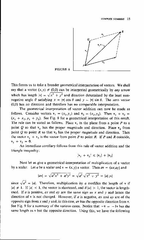
FIGURE 8

This forces us to take a broader geometrical interpretation of vectors. We shallsay that a vector (x,y) I (0,0) can be interpreted geometrically by any arrow

which has length lvl : {x2 * y2 and direction determined by the least non-negative angle 0 satisfying x : lvl cos 0 and y : lvl sin 9. The zero vector(0,0) has no direction and therefore has no comparable interpretation.

The geometrical interpretation of vector addition can now be made asfollows. Consider vectors yt : (xrh) and vz : (xz,/z). Then v1 * v2 :

(xr * xz, lr + !). See Fig. 8 for a geometrical interpretation of this result.The rule can be stated as follows. Place v, in the plane from a point P to apoint Q so that v, has the proper magnitude and direction. Place v, frompoint p to point R so that vr has the proper magnitude and direction. Thenthe vector v1 + v2 is the vector from point P to point R. If P and R coincide,V 1 * v r : Q .

An immediate corollary follows from this rule of vector addition and thetriangle inequality:

l v r * v z l S f v r l * l v r l

Next let us give a geometrical interpretation of multiplication of a vectorbyascalar. Let abeascalarandv : (x,y)avector. Then q : (ax,ay)and

lavl: J77 + ty' : Jt Jf ' +,y'z: lal lvl

since JF : bl. Therefore, multiplication by a modifies the length of v if

lal + t. If lal < l, the vector is shortened, and if lal > l, the vector is length-ened. If a is positive, ax and ay are the same sign as x and y and hence thedirection of v is not changed. However, if a is negative, ax and ay are of theopposite sign liom x and y and, in this case, ov has the opposite direction from v.See Fig. 9 for a summary of the various cases. Notice that -v : - ly has thesame length as v but the opposite direction. Using this, we have the following

v l + 1 2

16 INTRoDUcTION To LINEAR ALGEBRA AND DIFTERENTIAL EQUATIoNs

FIGURE 9

interpretation of vector subtraction yr - vz : y1 * (-vr) (see Fig. l0).Alternatively, v, - v2 is that vector which when added to v2 gives v, (seetriangle PQRin Fig. 10).

There is another very useful operation between vectors known as scalarproduct (not to be confused with multiplication by a scalar). Consider Fig. 11.

vr : (rr, . /r) : ( lvr l cos 0r, lvr l sin 0r)

vz : (xz,!z) : (lvzl cos 0r, lvrl sin 0r)

Then

xfi2 * !r /z : lvr l lvr l(cos 0, cos 0, + sin 0, sin 0r): lyl l lv2f cos (0, - 0r)

This operation, denoted by yr'yz, is called the scalar product, and the result,as we have already seen, is a scalar quantity given by the product of the lengthsof the two vectors times the cosine of the angle between the vectors. If eitheror both of the vectors are the zero vector, then v1 . v2 : Q.

The reader should verify the following obvious properties of the scalarproduct:

I v r ' Y 2 : Y z ' v r .2 vr . (vz + v3) : (v, . vz) * (v, . vr).3 cmr 'Yz : a ( v r 'Yz ) .

4 v . v : l v l r .5 l v r ' v z l < l v r l l v z l .6 If lvll * 0 and lvzl + 0, then Yr'Yz : 0 if and only if v, and v2 areperpendicular.t

( l < c )

f If ivlf # 0 and ltrl + O and v1 . vz : 0, we say that vl and v2 arc orthogonal.

COMPLEX NUMBERS 17

FIGURE IO

EXAMPLE 1.4.1 Find the equation of a straight line passing through thepoint (xo,.yo) in the direction of the vector (a,D). Let (x,y) be the coordinatesof a point on the line. Then the vector from (0,0) to (x,y) is the vector (x,y).This vector is the sum of the vector (xo,.yo) and a multiple of (a,b) (see Fig. 12).Hence the equation of the line is (x,y) : (xo,./o) * t(a,b). We usually referto t as a parameter and to this representation as a parametric representation ofthe line. The parameter t clearly runs between - @ and o.

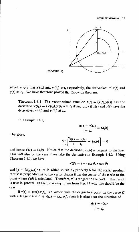
EXAMPLE 1.4.2 What geometrical figure is represented parametrically by(x,y) : (xo,./o) * (r cos 0, r sin 0), where r > 0 is constant and the parameter0 runs between 0 and 2n? In this case, (x - ron I - lo\ : (r cos 0, r sin 0)and f(x - xo, I - l)l : r. The figure is therefore a circle with center at(xo,.yo) and radius r (see Fig. 13).

The two examples illustrate the usefulness of the concept of uector-ualued

functions. Suppose for each value of t in some set of real numbers D, called thedomain of the function, a vector v(t) is unambiguously defined; then we say

FIGURE II

18 INTRoDUcTIoN To LINEAR ALGEBRA AND DIFFERENTIAL EQUATToNS

FIGURE 12

that v is a vector-valued function of t; t is called the independent uariable, andv is called the dependent oariable. The collection of all values of v(l) taken onfor r in the domain is called the range of the function.

In Example 1.4.1, if vs : (xo,yo) and u : (a,b), then we can write(x ,y) : v ( r ) :vs * /u , where -@ < t< oo. Then v is a vector -va luedfunction of r. The domain is the set of all real t, andthe range is the set of allvectors from the origin to points on the line through (xo,.yo) in the directionof u.

In Example 1.4.2, if vo : (xo,yo) and 0 < 0 < 2n, then (x,y) : v(0) :v o * ( r c o s 0 , r s i n 0 ) . T h e d o m a i n t i s t 0 l 0 < 0 < 2 n ] r , a n d t h e r a n g e i s t h eset of vectors from the origin to all points on the circle with center at (x6,y6)and radius r.

The concept of deriuatiue of a vector-valued function is very easy to define.Suppose for some ts and some 6 ) 0, all r satisfying to - d < t < to + dare in the domain of v(t) and there is a vector v'(ro) such that

rlTl(#-v'1ro)l :othen v'(ro) is the derivative of v(r) at ro. Since the length of the vector

v ( r ) - v ( r o ) _ v , ( r o )t - t o

goes to zero as t + to, it follows that if v(r) : (x(r),y(r)) and v'(ro) :(x'(to),y'(t6)), then the above limit is zero if and only if

[T[4#-' ' {ro)] :o

f lT[#- ' ' ( 'o)] :o

f We are using the usual set notation: {d I 0 < 0 < 2n\ is read "the set of all 0 sucht h a t 0 S 0 < 2 n ; '

(xo+ ta, ls+ tb)

@MPLEX NUMBERS

(x, y)

FIGURE 13

which imply that x'(ro) and y'(ro) are, respectively, the derivatives of x(r) andy(t) at t6. We have therefore proved the following theorem.

Theorem 1.4.1 The vector-valued function v(r) : (x(r),y(r)) has thederivative v'(ro) - (x'(to),y'(to)) at ts if and only if x(t) andy(r) have thederivatives x'(to) and y'(r6) at ro.

In Example 1.4.1,

t9

Therefore,

and hence v'(t) : (a,b). Notice that the derivative (a,6) is tangent to the line.This will also be the case if we take the derivative in Example 1.4.2. UsingTheorem 1.4.1, we have

v'(0) : (-r sin 0, r cos 0)

and [v - (xo,yo)]'v' = 0, which shows by property 6 for the scalar productthat Y' is perpendicular to the vector drawn from the center of the circle to thepoint where v'(0) is calculated. Therefore, v' is tangent tci the circle. This result

:::::. in general. In fact, it is easy to see from Fig. 14 why this should be the

If v(t) : (x(t),y(r)) is a vector from the origin to a point on the curve cwith a tangent line z at y(to) : (xo,./o), then it is clear that the direction of

v(r) - v(to)

t - t o

v ( t ) - v ( r o ) _ @ , b )t - t o

rim ["(t) --v(t")

- @,u1] : st - t o l t - t o J

t'\\L_____L__(xs, /s )

N INTRODUcTION TO LINEAR ALGEBRA AND DIEFER"ENTIAL EQUATIoNs

FIGURE 14

approaches the direction of the tangent line &s I + ro, provided v'(to) existsand is not the zero vector. We shall, in fact, use this limit to define the tangentto the curve.

Let v(t) be the vector from the origin to a point on the curve C. The pointmoves along the curve as the parameter t varies. If v(t) has a nonzero derivativev'(to) at v(ro), then C has a tangent line at v(lo) and a tangent vector v'(to) andthe equation of the tangent line is

(x ,y) : v ( ro) +( r - ro)v ' ( to) -@ < l < @

EXERCISES 1.4

1 Lr;t yr: (1,-2) and, v2: (-3,5). Find and draw sketches of v1 * v2,Yl - vz, 2t1 * Y2, &Dd *(vz - vr).

2 A man is walking due east at 2 miles per hour and the wind seems to be comingfrom the north. He speeds up to 4 miles per hour and the wind seems to be fromthe northeast. What is the wind speed, and from what direction is it coming?

3 An airplane is 200 miles due west of its destination. The wind is out of the north-east at 50 miles per hour. What should be the airplane's heading and airspeedin order for it to reach its destination in I hour?

4 Let v: 1t,-Jf;. Find lvl and the least nonnegative angle 0 such thatr : l v l c o s f l y = f v l s i n g .

5 Find the vector equation of the straight line passing through the points (-1,2)and (3,4). Find a vector perpendicular to this line.

6 Find the vector equation of the circle with center at (1,3) passing through thepoint (4,7). Find the equation of the tangent line to this circle at (4,7).

7 A curve is g iven by (x ,y) : (3 t2 - t , t3 -Zt2) ,0< t < 4 . F ind atangenvector to this curve at the point (10,0).

(xs, ts)

v(t) - v(to)

I9

OMPLD( NI.'MBEN.S 2I

verify the six properties of the scalar product listed in this section.Assuming that v(r), vt(r), vr(r) are differentiable vector functions and a(r) is adifferentiable scalar function, show that(a) [v'(t) + vz(t)]': vi(r) + vL(t)(6) [a(t)v(t)]' : a'(t)v(t) + a(t)v'(t)(c) [vr(r) . vz(r)]' : [vr(r) . vL(:)l + [vi(r) .vz(r)](d) ilv(r)l'] ' : 2lv(t).v'(r)lusing part (d) of Example 9, prove that if v(r) has constant nonzero lengthand v'(r) # 0, then v(r) is orthogonal to v'(r).Let v(t) : (x(t),y(t)) represent a curve parametrically. If v,(r) * 0, thenT(r) : v'(r)/lv'(r)l is a unit tangent vector [|Tl : l l. Show that T, is normal tothe curve, that is, T. T' : 0.If a physical particle moves along a curve given parametrically by (r) : (r(r),.y(t)),where t is time, then v(r) : r'(l) is called the oelocity, dr) : lv(r)l is called thespeed, and a(t) : v'(f) is called the acceleration. rf the speed is never zero, showthat a(t) = s(r)T + dr)lT'ln, where T is the unit tangent and n is a unit normal.

1.5 FUNCTIONS OF A COMPLEX VARIABLE

We now return to our study of complex numbers to consider functions of acomplex variable. We do not need an extensive treatment of this subject,concentrating on the things we shall need for our study of differential equations.However, the reader should be aware that there is a vast literature on thesubject.t

Suppose that for each complex number z in some set D (domain of thefunction) of the complex plane there is assigned a complex number/(z); thenwe say that we have a complex-valued function / of the complex variable zdefined in D. The set of values f(z)is called therange of f. Letz: x * iland f(z) : u * lu, where x, l, u, u are all real. Then clearly u(x,y) and a(x,y)are real-valued functions of two real variables x andy defined for z in D.

TO

1t

t2

EXAMPLE 1.5.1 l*t f(z) : z2 a\df(z) : u(x,y) * ia(x,y) : x2 - y2 +example, / ( l + t ) :2 i , f ( - i ) : -1.

D & the entire complex plane. Theni(Zxy). Particular values are, for

EXAMPLE 1.5.2 Let !(z) : J; : pft2lcos g arg z) + i sin g arg z)f,0 < arg z < 2n,./(0) : 0. This function is defined for all z in the complex

tSee, for example, J. W. Dettman, "Applied Complex Variables," Macmillan, New york, 1965(rpt. Dover, New York, 1984).

22 INTRoDUcTIoN To LINEAR ALGEBRA AND DIFFERENTIAL EQUATIoNs

plane. For each z * 0 there are two distinct square roots. The function in thisexample defines one of these square roots. To describe the other square rootwe could define g(z) : -f(z).

There are two concepts of derivative of a function of a complex variablewhich we shall introduce, deriaatiue along a curne and derioatiue at a point.These two notions of derivative are closely related, and as these relations arepointed out, we shall see that our definitions are quite consistent.

Suppose that the domain of/contains a curve C parameterized as follows:z(t): x(r) + iy(t),a < t < D. Then

f(z(t)) : u(x(t),v(t)) + ru(x(l)'v(r)): u(t) + iY(t)

so the real and imaginary parts of/are defined along C as functions of the realparameter t. lf U and V are diflerentiable as functions of l, then the derivativeof/along C is defined by

: U'(t) * iv'(t)

If x'(t) and y'(t) exist and the partial derivatives 0ul0x, 0ul0y, 0ul0x, and 0al0yare continuous as functions of x and y at points on C, then by the chain rule

{ 0 u 0 u A " A nd i : ; x ' ( t ) +

f i f ( t l * r ; x ' ( t ) + t f i f ( t )

Suppose that for some d > 0 all z satisfyinglz - zol < 6 are in the domainof f. Further, suppose that for all z satisfying this inequality 0ul0x, 0ttl6y,0al0x, and Aol6y are continuous and the Cauchy-Riemann equations0ul0x : Atl|y and 0ul0y : -(0ol0x) are satisfied at zo. Then we say that/isdifferentiablet at zs and the derivative is

f '(zo) :

{dt

. 0 u, -0x

. 0 ut -

0yOU: - -0y

where the partial derivatives are evaluated at Zo : xorather arbitrary definition of derivative, but we shallwith our definition of derivative along a curve.

t If /is differentiabte for all z satisfying l, - ,ol <that/is analytic at zq.

* iyo. This seems like ashow that it is consistent

e, for some e ) 0, then we say

COMPLH( NUMBERS 23

Let f be differentiable vt zo : x(fo) * ly(to) on a curve C, where thederivative along C at t6 exists. Then at /o

df. :dt

(+ . i $) g"'116) + ;y'(ro)l\dx ox/

d= (x') : 2xax

: ou :ody

: (P - ,+) [',(ro) + i/,(ro)]\av avl -

: f ,(ziz,(ts)

where z'(to) : x'(to) * iy'(t). Hence, we see that our definition of derivativeat a point is a natural one in that it leads to a natural chain-rule result for thederivative of a function along a curve C. Also the value of the derivative at apoint does not depend on the definition of any particular curve passing throughthe point.t

EXAMPLE 1.5.3 The functionevery point. Since f(z) : x2 -

of Example 1.5.1 has a derivative at

0ul0y : -2y : -(0ul0x) and thesey2 + i(2xy), 0ul0x : 2x : 0ul0y andpartial derivatives are continuous every-

where. We have f'(z) : 2(x + iy)ferentiation formula

This is not just a coincidence.

: 22. Notice the similarity with the dif-

EXAMPLE 1.5.4 Consider the function defined by f(z): lzl2 : x2 * y2.Here u : x2 * yt, a : O. Then 0ul0x - 2x, 0ul0y : 2/, 0uf0x : 0,0t:l0y : 0. These partial derivatives are all continuous. However,\uf 0x : 0ul0yand 0ul0y: -(0ul0x) at only one point; x: !:0. This function is dif-ferentiable at the origin (where the derivative is zero) and at no other point.

EXAMPLE 1.5.5 Consider the function defined byf(z) : lzl : ,/f. +)r.Here a : J* + y', t) : 0. Therefore,

0 u x 0 u y- : - :ox J7T7 ay J7+7

ot)-ox

f For the more conventional approach using limits of difference quotients seeDettman, op. cit.

A INTRoDUCTIoN TO LINEAR ALGBBRA AND DITFERENTIAL EQUATIoNS

The Cauchy-Riemann equations are never satisfied when x and y are differentfrom zero, and when x : ! : 0, the 0ul0x and 0ul0y do not exist. Therefore,this function is never differentiable.

Later on we shall want to discuss complex-valued solutions of differentialequations. Suppose, for example, that we wish to show that /(t) = cos f *i sin I is a solution of the equation d2f ldt2 * f : 0. We can interpret thisto mean we have some function / defined on the x axis parameterized byz(t) : t + i0. We wish to differentiate/along the x axis, and using our abovedefinition, we have

: -sin I * i cos /

Differentiating again, we have

ry " : -cos t - i s in t : - , fdt'

Therefore, dzf 1il2 * .f :0, where the equality is to be interpreted in the sensethat both the real and imaginary parts of the left-hand side are zero.

On the other hand, we may wish to show that a function satisfies a dif-ferential equation where the derivatives are to be interpreted in terms of thecomplex variable z. For example, f(z) : z2 is differentiable everywhere inthe complex plane, and it satisfies the differential equation zf' - 2f : 0. Inany given situation the context of the problem will indicate which interpretationshould be put on the differential equation.

EXERCISES 1.5

.l Consider the function defined by f(z): 23. What is its domain? Find its realand imaginary parts. Where is it differentiable? What is its derivative?

2 Show that f(z) : Re (z) and g(z) : Im (z) are nowhere differentiable.3 Assuming that f(z) and g(z) are both differentiable at zs, prove:

(a) ("f + s)'(z) : f'(zo) + s'(zo).(6) (cf)'(zi : cf'(zo), where c is a complex constant.(c) (fs)'(z) : f(zo)s'(zi + s@if'Qd.(d) (cJ * czg)'(zo) = crf'(zo) * c2g'(zs) where ct and c2 ata complex con-

stants.4 Using part (c) of Exercise 3 and mathematical induction, prove that

tdt

! " ndz

: 4 2 n ^ L n : O ,

IO

COMPLEXNUMBERS 25

5 What is the derivative of the polynomial

p(z) = anzn + er-Lzn-r + .. . + aF * as

where the a's are complex constants?Consider the function defined by f(z): er cos y * id sin y. What is itsdomain? Where is it differentiable? What is its derivative?Consider the function defined bV fQ) : cos x cosh y - i sin x sinh y. What isits domain? Where is it differentiable? What is its derivative?Consider the function defined bV fk) : llz. What is its domain? Where is itdifferentiable? What is its derivative?I*t f(z) : u(x,y) * it\x,y) be differentiable at zs. Show that u and u arecontinuous tt zo : xs * iys. Hint: lJsp the mean-value theorem for functionsof two real variables.Use the result of Exercise 9 to show that the function of Example 1.5.2 is notdifferentiable on the positive x axis. Where is this function differentiable? Whatis its derivative?Considerthefunctiondefined byf(z): ln lzl + iarg 2,0 < argz < 2n.Whatis the domain? where is it differentiable? what is its derivative?show that /(r) : edt cos bt + idt sin 6r satisfies the differential equationf" - 2af' + (a2 + b271 : g. Here prime means derivative with respect to t,and a and b are real constants.Show that the function f(z) : l"1cos ky + i sin ky), where /r is a real constant,satisfies the equation dJ'ldz : kf.

1.6 EXPONENTIAL FUNCTION

In this section we discuss the exponential function of the complex vafiable z,As our point of departure we begin with the power-series definition of the realexponential function

I ]

T2

l3

e" : l +L+ t i * t l + . . . : 3 ' *1 ! 2 t 3 ! ak t

- ; tm (ro)

d k l

e ' : t + I + t * t + . . .1 ! 2 t 3 !

: i**akt

A natural way to extend this to the complex plane is to define e'as follows:t

Of course, we must define what we mean by the infinite series of complexnumbers. Consider the partial sum

id:fukt

i Be_@ *ak l

f We shall also use the notation exp z.

2I' INTRoDUcTIoN To LINEAR ALGEBRA AND DIFFERENTIAL EQUATIoNs

The two series

$ ne (ze)

and $ tm (z*)

Akt kk lboth converge, as can be seen by comparison with the series

$ l ' loAH

which converges for all lzl. The necessary inequalities to see this are

lRe (ze)l < lzrl : lzlr llm (zk)l < l"ol : lzlr

We shall say that the series of complex numberr ,i

t)

"on "rges if and

only if the real series

f ne (z*)

and $ lm (z*)

Ak t Ak lboth converge and has the sum S : U * iZ, where U is the sum of the realparts and V is the sum of the imaginary parts. In this case, it is clear that thecomplex series converges for all z.

Now let z : iy. Then the (2n + l)st partial sum is

+t I r - ' j * tL - 3 ! s !

The series of real parts converges to cos /, and the series of imaginary partsconverges to sin y. This proves the important Euler formula:

e i ! : cos / * i s iny

We shall prove in the next section that the complex exponential functionhas the usual property

,zr.tzz : slrszzAssuming this for the moment, we now have

e ' : d+ i ! - ux t i t : e t cos y * i d s iny

It is now clear that the exponential function is analytic for all z, becauseu(x,y) : er cos y and u(x,y) : et sin y are continuously differentiable andsatisfy the Cauchy-Riemann equations for all z.

Many of the common transcendental functions of a real variable can now

@MPLEX NUMBBRS N

be defined for the complex variable z using the exponential function. Forexample, from etv: cos y + isiny and e-it - cos/ - jsiny it is easy toshow that

c o s y : t t ' + " - "2

s i n Y : e i Y - e - t Y

2iWe then generalize for the complex variable case to

c o s z : t " + ' - "2

s i n z : ' i z - ' - i z

2i

Recalling the definitions of the hyperbolic functions

c o s h x : € ' * e - *

2

s i n h x - d - t - "2

we can express cos z and sin e as follows:

cosz =r;,-,ffi;i:hi**fl1"", x - isinx)

s inz : 4G- t r " - de - , )2

- i--s-r(cosx * isinx) + la1.or x - isinx)z 2

: sin x cosh y + i cos .x sinh y

It is now clear that cos z and sin z are analytic everywhere.In the case of the real variable x, tan I : (sin x)/(cos r). Hence, we

generalize to the complex variable case as follows:

]^_ _ sin z sin xcosh y + icos x sinh yt A n Z : - :c o s z c o s x c o s h y - i s i n x s i n h y

- ( s i n x c o s h y * i c o s x s i n h y x c o s x c o s h y * i s i n x s i n h y )cos2 x

_ s i n x c o s x * i s i n h y c o s h y_

28 INTRODUcTIoN To LINEAR AIGEBRA AND DIFFERENTHL EQUATIoNS

tan z is analytic everywhere except where cos2 x * sinh2 ./ : 0. But sinh ./ : 0only when ! : 0, and cos r : 0 only when x is an odd multiple of nl2. There-fore, the points where tan z is not analytic are

? n + lz - - n

2n :0 , +1 , +2 , . . .

The other trigonometric functions are defined as follows:

c o t z :cos z cos x sin x - i cosh y sinh y_ :sln z s i n 2 x * s i n h 2 y

c o s x c o s h y * i s i n x s i n h y

c o s 2 x * s i n h 2 y

sin x cosh y - i cos x sinh y

s i n 2 x * s i n h 2 y

sec z is analytic everywhere except where cos z : 0 while cot z and csc z are

analytic everywhere except where sin z : 0.The hyperbolic functions are similarly defined in terms of the complex

exponential function:

e" + e-" e= - e - "

tS e C z : - :

cos z

1C S C Z : - - :

sln z

cosh z :

tanh z :

sech z :

sinh z :2

. cosh zc o t n z : -

sinh z

c s c h z : 1

sinh z

2

sinh zcosh z

1

cosh z

We normally think of the logarithmic function as the inverse of theexponential function. However, in the case of the complex exponential functionwe have difficulty defining the inverse because of the property ,z*2ttki : e' forany integer k (see Exercise 1.6.6). Therefore, if we wish to define an inverseof the exponential function, we must restrict the imaginary part of the dependentvariable. We begin with the equation

4+io - e'(cos u * isinu) : z : x * iY

Therefore, x : €u cos u and ! : eu sin u, from which we derive

u : t l n ( x 2 + y \ : l n l z l

u : t a n - r ! : a r 1 z

COMPLEXNUMBERS 29

However, in order to make this single-valued we must restrict atg z to someinterval of length 2n, say 0 < arg z < 2n. With this restriction we can thenwrite

u * io : log z : lnlzl + i argz

This function is analytic everywhere except at the origin and on the positivex axis. Where it is differentiable,

EXERCISES 1.6

Starting with the definition e' : e*(cosy + i siny), prove thatezr+22: s/tsz2.Show that the real and imaginary parts of ez satisfy the Cauchy-Riemann equationseverywhere.Show that7 is never zero.Show that7 : ei.Show thate-" : lle'.Show that e'+2kni : €z for every integer /<.Show that dz satisfies the differential equation f' : af for any complex constanta.

Letting z : r(cos 0 + i sin d), show that

e''" - "-o (l,

cos e) [.* (i'* ,) - i sin (i 'i" ,)]

Prove that ertz takes on every complex value except zero within every circlecentered on zero.Show 11ru1

"2ttki /n, k:0,1,2,.. . ,n - l , are the only dist inct solut ions of

z n : l .

10 Prove that cos z and sin z arc analytic everywhere and obtain the formulas

. d-Stn z - Sln Z : COS zdz

11 Show that cos z and sin z satisfy the differential equation-f' + f : 0.12 Show that lcos zl and lsin zl are not bounded in the complex plane.13 Prove that cosh z and sinh z are analytic everywhere and obtain the formulas

4.ort z : sinh, ! sinh z : cosh zdz dz

14 Find all the points where cosh z : 0.15 Find all the points where sinh z : 0.

! rc* , : !d z z

I

2

34J67

d- c o s z -dz

30 INTRoDUcTIoN To LINEAR ALGEBRA AND DIIFERENTIAL EQUATIoNs

16 Determine where tanh e is analytic.17 Determine where coth z is analytic.18 Show that cosh z and sinh z satisfy the differential equationf'" - f : O.19 Obtaintheformulascoshiz = cos zandsinhd z: isinz.20 Determine where logz = ln lzf + iargz,0 < arg z < 2n, is analytic and

obtain the formula dldz log z : llz.2l Define za : axq @ log z),log z defined as in Exercise 20. Where is this function

analytic, and what is its derivative? Assume a is complex.22 Define az : exg (z log a), a * 0. where is this function analytic, and what is

its derivative?

*I.7 POWER SERIES

The purpose of this section is to develop further the theory of series of complexnumbers and, in particular, the theory of power series of the form

@

2 o*(t - zo)*, where zo is a fixed complex number and the a*'s are complexf t=O

constants. The reader will recall that we used a power series to define theexponential function

,=:i lakt

One of our goals in this section will be to prove the validity of the formula

e z r + 2 2 : p z t g z z

We begin by defining the general concept of convergence of a series of

complex numbers 2 *r. We define the partial sums Sn - ) ,*. We,c= O & = O

say that the series i ,* conoerges to the sum ,S if lim S" : S. If thek = 0 n + e

limit does not exist, then we say that the series dh:erges. The limit of a sequenceof complex numbers {,S"} exists and is equal to Sif and only if, given any e > 0,there exists an ,ff such that lS, - Sl < e whenever n > N.

EXAMPLE 1.7.1 Consider the series j *, where c is a complex number.* = OThe partial sums are

t " : *e

t : | * c * c2 + . . - * c "

COMPLEI( NI.'MBERS 3I

Multiplyingby c, we have

Subtracting, w€ obtain

c S o : c + c 2 + c 3 + " ' + e + '

( 1 - c ) , S " : l - c n + l

lf c * l, then S" : (I - C+\10 - c). If lcl < l, then le*'l tends to zeroas n + @. Hence, we conjecture that for lcl < I lim S, : 1/(l - c). Letus prove this from the definition.

then n + I will be greater thaneache > 0wecanf ind

, ; tct'*': -1 - . 1 11 - c l

ln lcl(ln e * ln ll - cl)/ln lcl. Therefore,

ru - [h e + ln lt - cll

L l n l c l J

[ '"Given s ) 0, we wish to show that lcln+t < rll - cl for n sufficiently large,or (n + l) ln lcl < ln e * ln ll - cl. Dividing by In lc[, which is negative,we wish to show that for sufficiently large n,

n * l >l n e * l n l l - c l

It is now clear that if n is greater than the largest integer in

l n e * l n l l - c l

for

where the bracket stands for the "largest integer in," and when fl 7 N,

I r lls"-r-"1 "

This proves our conjecture. It is clear that when lcl > l, then lclo+l tends to@ as n I @. Hence lS, - ll(L - c)l cannot be made small for large n.This shows that the series diverges for [cf > 1. This still leaves the case f cl : Ito be considered. If c : l, then

S n : I t o : n * lk = O

In this case, Sn -+ @ as n --, @, and the series diverges. If lcl : I and c * l,then c : cos 0 + t sin 0, 0 * O, and

| - c n + r9 n - -

: -

" l - c l - c

I f l i m S o : S :' | - @

32 INTRoDUcTIoN To LINEAR ALGEBRA AND DI}TEnENTIAL EQUATIoNS

cannot remain arbitrarily close to some fixed point for all sufficiently large nbecause C+l : cos (n + 1)0 * i sin (n + l)0 moves around the unit circlein jumps of arc 0. Therefore, the series diverges for lcl : l. In summary,

i r * : I

i f l c l < lk = O l - C

and the series diverges for lcl > l.

The convergence of a series of complex numbers is equivalent to the con-vergence of both the series of real parts and the series of imaginary parts. Let,il* : ttk * iuo, /r : Re (wx), ur : fm (w), and

s , : 2u r+ r i uk :Un+ iV ,l = O , < = O

U + iV, then lim U, : U and lim V,: Z. This is because

l u " -u l< lE-s ll v , -z l < l s " -s l

and given any e > 0, there is an N such that lS, - Sl < e for n > N andtherefore lU"- Ul < e and lV,- Vl <efor n > If. Conversely, supposelim Un: Q and lim Vn = l/. Then, by the triangle inequality with' | + €

, S : U + i V

l^S, - ,Sl < lU" - Ul + ly, - y l

Given s ) 0, there is an N such that lU, - Ul < el2 and lV" - Vl < el2,and hence ls" - sl < e for n > .l/. We have then proved the following theorem.

Theorem 1.7.1 Let uo: Re (w/ and ur : Im (w*). Then the series@ @ @

2 *r converges if and only if both ) ap and Z oo converge, and& = o & = 0 , ( = 0

c o @ o

Z ro: 2 ur + d ) u1./ < = O f t = O f t = O

Next we define absolute conaergence. A series of complex numberso o

I ,o is said to converge absolutely if the series of real numbers ) lw*lt = O & = Oconverges. Absolute convergence implies convergence, as we see in the nexttheorem. However, the converse is not true, as is illustrated by the series

- / - l ) e . o I

x?, k x?r k

Theorem 1.7.2 If the series i tr*t converges,f t = O

PROOF Let uy: Re (wo) and u* : Im (wr).

fu*l < lw*1, and hence the series i lu*l "oa >f t = O t < = O

@

parison with the convergent series 2 lr*1. No*l = O

0 < l z * l - u e < 2 l u p l

0 < l u * l - 4 3 2 l u p l

Then again by comparison, I (lu*l - u*) and ) (lurl - u*) converge,& = O t = O

and therefore by subtraction

@

\ - r l

/ lu* l -t ( = 0

@

coMPLD( NUMBERs 33

@

then so does f ,*.f t = O

Then lurl < lw*l and

fu*l converge by com-

oZ (luol - u*):

olo ,o

@

2 l r * l - I ( l r o l - 0 * ) : } u r, < = o & = o t r = o

the series of real parts and imaginary parts both converge and, by

Theorem l.7.l,the series 2 ,rconverges.k = O

Before we consider power series, we need one more theorem which givesus a necessary condition for convergence. The failure of this condition givesus a test for divergence.

Theorem 1.7.3 If j wk converges, then lim [wof : 0.f t = O r + @

PRooF Since i *rconverges, the limit of the partial sums exists& = O

and l im S": l im So-r : S. Therefore, l im (,S" - S"-r):0, andn+ @ ,l+ co

l im l4f : l im lS, - S"-rl : 0.

EXAMPLE 1.7.2 The divergence of the series I "* for lcl > I follows

k = O

directly from Theorem 1.7.3. For suppose the series converged; then lim lcl"would be zero. However, lcl" > l.

34 INTRoDUcTIoN To LINEAR AIsEBRA AND DIFFERENTIAL EQUATIoNS

That the condition lim lw"l : 0 is not a sufficient condition for conver-n + @ @ l

gence is shown by the divergent series > ; , although lim (l/n) : Q.k = l K n e g o

We can now begin our study of power series of the for- j ao(z - zs)k,f t = O

where zo is a fixed complex number and the a1's are complex constants. Byintroducing the variable ( : z - 26 we can always put the series in the form

@

Z or(. Hence, without loss of generality we study series onry of the form* = O

@

2 ootu.& = O

Theorem 1.7.4 If the power series 2 orto converges for z : c, then

it converges absolutely for all z such IikA < lcl. If the power seriesdiverges for z : c, then it diverges for all z such that lzl > lcl.

pRooF Assume ttrat i arck converges, c # 0. Then lim laockl : g.& = 0 l t + o

Therefore, there is a constant M such that laotl < M for all k. Now let

lzl < lcl, and consider the series 2 borrl. We have la*zk1 : laotl xk = O

lrlclr < Mlzlclk. But the series i a lll* ,onu.rges since lzlcl < t.@ l c = O l C l @

Therefore, by comparison f la*zkl converges, and 2 ortr converges

absolutely for lzl < lcl. This completes the first part of the proof. For

the second part assume that 2 ooro diverges but that 2 orr* converges

tr : O

f t = O

k = O

k = 0

for lzl > lcl. But then i loornlconverges unO i c*ce converges, whichis a contradiction. k=o k=o

There are power series which converge for all z. The series used to definethe exponential function is a good example. There are power series whichconverge only for z : O (all power series converge for z : 0). An exampleo f suchase r i es i r Z k l zk , f o r i f z * O , l im l& ! zk l : a .

k = O k + o

If a power series does not converge for all z but does converge for somez * 0, then Theorcm 1.1.4 implies that there is a positive number R such thatthe power series converges for lzl < R and diverges for lzl > R. In this case,

OOMPLEX NT,|MBERS 35

.R is called the radius of conaergence of the power series, and the circle lzl : Ris called the circle of conoergence. The next two theorems give methods fordetermining the radius of convergence of a power series.

Theorem 1,7,5 Let lim la,*tla) : L * 0. Then the radius of con-

vergence "f

j orrr ir'i1L.

PR@F Considerl n . - r n + l l

1 i . l s ' t + l ' 1 : L l z lr-o I anz' I

Suppose Llzl < l. Then there is an r such that 0 < r < I and an JVsuchthat lan*rzo*'larz'J < rforallz 2 N. Hence lax*rzn*r1 < r1anzN1,

lan*rtn*'l s rlax*rzn*tl < r2lanzNl, etc. In general,

lan*Fn* i l < r t lanzNl i : 1 ,2 ,3 , . . .

The series i ,'converges since 0 < r < l. Hence, by comparison thei = t

c o 0 0

series I larzkl converges, and so does 2 or*. We have then provedk = O & = 0

that the power series converges for lzl < llL.Now suppose Llz| > l. Then there is a constant p > l and an M

such that

f o r a l l n 2 M

By an argument like the one above we have forT : 1,2,3,. . .

lo**iro*il >- dlaozol

But since p t 1,1 + @ as jr -+ @ ord therefore

lou*iru*Jl - o

as j -+ o, which shows that the series diverges for lzl > UL.

Theorem 1.7.6 kt lim laolttn : L * O. Then the radius of conver-@ ' l + @

gence of 2 arzk is llL.

".;;t The proof, which is very similar to that of Theorem 1.7.5,

will be left for the reader.

l#1,-,

36 rNTRoDUcrroN To LINEAR AIIIEBRA AND DTTERENTTAL EeuATroNs

EXAMPLE 1.7.3 Find the radius of convergence of the power series

: qY . Here the ar: (- l)t/k, and, . = 1 , e

:*ltl :1,rft:'Therefore, the radius of convergence is l. This example shows that on thecircle of convergen@ we may have either convergence or divergence. Forexample, at z : I the series converges, but at z : - I the series diverges.

EXAMPLE 1.7.4 Determine where the power seriesConsider

converges.

2 orrr, we obtain the power& = O

.e(#t l l , ; v h l

\ i ( i " ,J :#*o asn '+@

It is clear that there is an r, 0 < r < l, and an N such that

/m" = ' roral ln > N

Hence, llzllln nfo 3 r". Then by comparison with the convergent series@

2 ,r we have absolute convergence for all z.

If we formally differentiate a power series@

series 2 kopo-l. Supposel = 1

l n I[ m l * " + t 1 : L * 0

Then n*o I a' I

r : - f l * l l c " * r l ti1T , l ; l : '

Therefore, the differentiated series has the same radius of convergence as theoriginal series. In fact, it can be shown in general that the differentiated serieshas the same radius of convergence as the original. Moreover, if f(z) :

@

2 orrr, lzl < R, then f(z) is differentiablet inside the circle of convergencef t = O

and @

I'e) : o2

korrr-t

f For proofs s€€ Dettman, op. cit., pp. 145 and 147.

37

By induction we can then difrerentiate as many times as we please and obtainf o r z : 1 , 2 , 3 , . . .

f @ ( z ) : : " k ( k - 1 ) . . . ( k - n + r ) a r z k - n

valid for lzl < R. Evaluating "f(")(0) we have, since all the terms are zero

e x c e p t f o r k : n ,/"(")(0) _ n! an

and hence, ao : f@(O)lnl.We conclude this section by showing that in a certain sense, which we shall

define presently, we may multiply two power series together within their commoncircle of convergence. If we multiplied two polynomials

P(z) : as * aF * a2z2 + "' * aoz"

q(z): bs + brz * b2z2 + " ' t b,z"

together, we would have

p(z)q(z\ : eobo * (asbt * albs)z * (asb2 * arb, + a2bo)22+ " ' * (asbn * a lbo-1 * " ' * an- tb t * arbo)zn + . . .

We use this formula to motivate the definition of the Cauchy product of two series@ @

) z l and ) u l as

We prove the following theorem.

Theorem 1.7.7 The Cauchy product of two absolutely convergentseries converges absolutely to the product of the two series.

pRooF We first show that the Cauchy product converges absolutely.I k . I

Letak: lu*l,b*: lrs*|, and c* : lwrl: I 2 uit)*-i l . Thenl i = o I

n n l k I

2 r r :k = o k = o l j = a I

n k n n

f t = o j = o , . = o l = 0

where ,{ : i t*t and I : i tr*t. Therefore, since the j ;ro1 "r"l = o @

k = o & = o

bounded above, the series 2 *rconverges absolutely.I r = O

2 (t,*,"-*)a = 0 \ l c = o /

38 INTRoDUcTToN TO LINEAR AI$EBRA AND DIFFERENTTAL EQUATIoNs

If a series converges, then the average of its partial sums convergesto the sum of the series. We shall prove this fact and then use it to find thesum of our absolutely convergent cauchy product. suppose lim s, : 5

n * t , n

where ,S" is the partial sum of a convergent series. Let on: I ) S*.

rhen oo - s : 1 i (s* - s) and ton - st s I i lr- - J: -;;."

f l k=e l l x=-o

8 ) 0, there is an M such that ls* - sl < el2 when k > M. Therefore,i f n > M ,

1 M. a n

lon - sl < i ) ls* - sl + jn Eo n o=?*,

M

Havingchosens,wefix M,andthen ) fso - sl : t isfixed. wechoosek = O

n so large that Lln < elz. Then lon - Sl < Lln + (n - M)el2n < e.This shows that j* ",

: ".

Now let Uo : f ur, Vn : t ,r, and Wn : j ,*. We have thatf t = o & = o k = o

Un - U, the sum of the first series, that Vn -a V, the sum of the secondseries, and we wish to show that wn - tJV. To do this we consider theavetage

a m

o^ : : ) ntn ?o

we leave it to the reader to show by a simple induction argument on mthat

2 w,: 2 urv^-rn = O & = O

+ f * . T h e nN o w l e t U x : U * 4 1 a n d V * : V

a m

o ^ :m fjo

:+rv +: ;or*Yf r . r . *> d*f^-*m E o m E o m ? o

As m --r @, the first term approaches (IV, the second term approacheszero since dr, + 0, the third term approaches zero since f* - O, and it canbe shown that the last term approaches zero. In fact, given s ) 0, there

1 I i o*f,-oltrt lk=o I

coMPLBXNUMDERS 39

is an Nsuch that laol < e and l f r l <efor k >,1[and laol < M and

lp*l < M for all ft. Then for tn > 2N

) l"-t l \ ,-olm f=6r / N r n - N m \: ' {>+

m \ * = O l r = . l v + 1 * = m - N + l /

- (2N + l)Me , (m - 2N)e2T -

which can be made less than e2 for n sufficiently large. This completes

the proof of the theorem since we have shown that lim o, : UY.

m

EXAMPLE 1.7.5series, that is,

and we now know that the series converges absolutely for any z. Hence, we maymultiply eztezz as a Cauchy product. Therefore,

Prove that e'tez2 : szt*zz. We have defined d by a power

, ' : i lak l

e , t e , 2 : i T z r k z 2 n - o

3A k t@-k ) t

:S1s , . k , ^n - k- A " t AH ln$ ' t " '

: i ( z r * z z ) ' : s z t t z 2

3 nt'

We conclude this section with an obvious theorem about multiplyingtwo power series together.

Theorem 1.7.8

Then f(z)s(z) :

Let f(z) : 2 ortr and g(z) :k = O

@ / n \

> ( > axbn-r,)zn for lzl < R.z = 0 \ r t = o /

Z botr for fzl < R.k = 0

2

3

& INTRoDUcTIoN To LINEAR AI,GEBRA AND DIFFERENTIAL EQUATIoNs

EXERCISES 1.7

.l Prove that a convergent series can have but one sum; that is, if lim Sn exists, thelimit is unique.

Show that : /c*'converges absolutely for Re (z) > l.k = l

Find the radius of convergence of the power seriesconverge on the circle ofconvergence?

4 Let a6 k :0 ,1 ,2 , . . . , be a sequence such that l im a2: o * 0 . What is

the radius of convergenc e of i oorr? rc+ o

f t = O@ -2k

5 Find the radius of convergence of the power series ) i-- . Htnt: r-et w : z2lz.k?o 2k

6 Prove that absolute convergence of a power series on the circle of convergenceholds either everywhere or nowhere.

7 Find the radius of convergence of the power series

| + y * a ( c - l )

, z * u (a - l ) ( u - 2 )

f + . . .

I 4 . Does the series*?r kz

3 !

where c is complex.I Prove Theorem 1.7.6.g *, jli Nl"^l : L + O. Show that the radius of convergence of

is 1lL.

I0 Prove tha t i t f (z ) : I o r r r : i b r r r fo r lz l < R, then dk : b* ,k :0 ,1 ,2 , . . . .k = O & = O

This exercise shows that a power-series representation of a function is necessarilyunique. m m

I1 Verify the formula 2 W, : 2 tlrv^-o in the proof of Theorem l.?.7.n = 0 k = 0

t ! 2 l

@

k = 1

kaPk-r

LINEAR ALGEBRAIC EQUATIONS

2.I INTRODUCTION

There are at least two main approaches to the study of linear algebra. The more

abstract is to introduce the general discussion of vector spaces first. In this

approach matrices come up in a natural way in the discussion of linear trans-formation, and the usual theorems about the solvability of systems of linear

equations come out in due course. The other approach, which is more concrete,is to begin the discussion with matrices and linear algebraic equations. Theadvantage of this direction is that it introduces the general concepts withexamples in a more familiar setting. We can then build up to the abstractconcept of a vector space with a set of concrete examples to guide and motivatethe student. This is the approach we shall take in this book.

We first introduce the algebra of matrices and show how to write systemsof linear algebraic equations in compact notation. We shall discuss the solutionof such systems by elimination methods and obtain the usual existence anduniqueness theorems for solutions. We introduce the concept of determinantof a square matrix and obtain the usual properties. This leads into a discussionof the inverse of a square matrix, where we teach the reduction method of

42 INTRODUCTIoN To LINEAR AI,GEBRA AND DIFFERENTIAL EQUATIoNS

inverting a matrix. The last section (which is starred) takes up rank of a matrixand collects all the existence and uniqueness theorems we shall need for thediscussion of linear algebraic equations.

2.2 MATRICES

One of the most important applications of matrices is the treatment of linearalgebraic equations. Therefore, we shall use this application to introduce theconcept of a matrix, and in the process the algebra of matrices will come outin a very natural way. IVe begin with an example.

Consider the linear algebraic equations

x1 * 2x2

2xr-xr * x2

- 2x,

We shall leave aside for the moment the question of whether these equationshave a solution. Our immediate objective is to obtain a compact notationfor this set of equations and others like it. Let A be the rectangular array ofnumbers with four rows and three columns

/ =

Let B be the array with four rows and one column

- 3 x r : g

+ x g : 3: Q

* 4 x t : 2

f i -

and let X stand for the unknowns xL, x2, and x3, as follows:

(i | il

f;)0

X _

A, B, andXare allexamples of matrices; r4 is a4 x 3 array, "Bis a4 x Iaffay, and X is a 3 x 1 array. We shall now define a multiplication operationbetween pairs of matrices so that it will be possible to write the system ofalgebraic equations in the compact form AX : B.

LINEAR ALGEBRAIC EQUATIONS 43

First, we should define what we mean by equality of matrices. Twomatrices are said to be equal if they have the same number of rows and columnsand each entry (element) of the one is equal to the corresponding entry (element)of the other. For example, if

and D : (, then we know that D has five rows and four columns and

The multiplication will be defined only in the case where the first factorhas the same number of columns as the second factor has rows. Suppose thefirst factor has / rows and m columns while the second factor has z rows andz columns. We define the product to have / rows and n columns obtained by thefollowing rule. To obtain the element in the ith row and theTth column of theproduct we multiply the elements of the ith row of the first factor by the corre-sponding elements of the 7th column of the second factor and sum. In otherwords, suppose the elements of the ith row of the first factor ate pip,k : 1,2,. .., m,while the elements of theTth column of the second factor areg*i, k : 1,2,. . . , ffii then the element in the fthrow,Tthcolumn of theproductis defined to be

PnQtt * P izQzi + ' ' ' * P i^Q^i

Since i can take on / different values andT can take on n different values, thisdefinition defines /z elements for the product. If the first factor is / x m andthe second factor is rn x n, then the product is I x n.

Using this definition of the product of two matrices and the above definitionof equality of matrices, we have for the example

(l ll ;)ftll il

+ ( - 3 ) ' x s \+ t ' t . I+ O ' , t l+ 4 ' xs /

/ l ' x t

( ,-; :;l\ 0 ' x t

+ 2' xr,+ 0 ' x ,+ l ' x ,* ( -2) ' x ,

:0:nA X :

U INIRoDUcTIoN To LINEAR ALGEBRA AND DIFFERENTIAL EQUATIoNS

so we have achieved our compact notation. In fact, for any system of rn linearalgebraic equations in n unknowns

a n x t * a p x 2 + " ' * a 6 x n : b 1

aztXt * a22x2 + " ' * a2rx, : b2

amLx t * a^2x2+ . . . * a^nxn - b^

we can use the compact matrix notation AX : .B, where

':(rl^)In this case, we usually call A the cofficient matrix of the system. There isanother matrix which plays an important role in the study of systems of linearequations. This is the augmented matrix, which is formed by insertingbr, br, . . . , b^ as a new last column into the coefficient matrix. In other words,the augmented matrix is

O n O L z ' ' ' Q r o b r

Q z t O z z ' ' ' A z o b 2

A m t A m 2 " ' A m n b ^

If the coefficient matrix is rz x n, then the augmented matrix is m x (z + 1).Next we introduce the concepts of addition and subtraction of matrices.

Suppose a certain set .rr, x2,. .. , xn satisfies two systems of equations

attXt * a12x2 + " ' * AyX, : C1

az tX t * a2 rx " + " ' * 42nx r : c2

amLxt * a^2x2 + " d * a^nxn : c^

b n x t * b p x , + " ' * b 6 x n : d 1bzfi t * b22x2 + " ' * b2oxn: d2

b ^ r x t * b ^ 2 x 2 + " ' 1 b ^ n x r - d ^

If we add or subtract the corresponding c's and d's, we have the followingresults

(arr * btt)xt * (an * bp)x2 + "' * (an ! bt)xn : ct * dt(azr * btt)x, * (azz * brr)x2 + "' * (azo * br)xo : cz * dz

(a^, X b^r)xt * (a^z * b^2)x2 + "' * (a^n !. b^)x, : c^ * d^

ALGEBRAIC EQUATTONS 45

we can state this in the compact matrix notation: AX : c, BX: D implies(A t B)X : C ! D provided we define addition and subtraction in a consistentmanner. A definition which makes this work is the following: to add (subtract)at m x n matrix B to (from) an m x n matrix l, form the m x z matrixA + B (A - ,) by adding (subtracting) elements of I to (from) correspondingelements of l.

Finally, we define the operation of multiplication of a matrix by a number(scalar). Suppose we multiply every equation of the system AX : C by thesame number a. Then the system becomes

oa11x1 * tu t12x2 + ' . . * aa roxo - acL

aa21x1 * 4 la22x2 +' . . * ea2rxo - ac2

aan11X1 I aa^2x2 +' ' ' * aa^nxn : aCm

This can be written as (aA)X : aC provided we define the matrices aA and aCproperly. This can be done as follows: the matrix formed by multiplying amatrix Aby a scalar a is obtained by multiplying each element of Aby the samescalar a.

Let us summarize all the definitions we have made so far in a more precisemanner.

Definition 2,2.1 A matrix is a rectangular array of numbers (real orcomplex). If the matrix has m rows and n columns, the matrix is said tobe m x n. lf m : n, the matrix is said to be square and of order m.The number in the fth row and theTth column is called the (a.;)th element;in the double-subscript notation for elements the first subscript is the rowsubscript, and the second subscript is the column subscript.

Definition 2.2.2 Two m x z matrices ,4 and B are equal if the (tj}helement of ,4 is equal to the corresponding (,,J)th element of I for allpossible i and j.

Definition 2.2.3 If ,4 is an m x n matrix with elements as; and a is ascalar (real or complex), then aA is the m x n matrix with elements aa11.

Definition 2.2.4 If ,{ and B are rn x n matrices with elements ai.; and4;, then A + Bis the m x nmatrixwith elements a;; * bii and A - Bis the m x n matrix with elements a;; - bii.

Definition 2.2.5 If I is the m x z matrix with elements a,, and .B is

6 INTRODUCTION TO LINEAR ALGEBRA AND DIFTERENTIAL EQUATIOI

the z x p matrix with elemerrts D;*, then AB is the m x p matrix withn

elements I aiib;*.J = L

Definition 2.2.6 The m x n zero matrix, denoted by 0, is the m x n

matrix all of whose elements are zero.

Definition 2.2.7 The zth order identity matrix, denoted by d is the

nth order square matrix whose elements are I on the principal diagonal(upper left to lower right) and 0 elsewhere.

We conclude this section with some theorerns whose proofs are straight-forward applications of these definitions. The only part which is particularlyhard is associativity of matrix multiplication (Theorem 2.2.4). In this case thereader should at least see what the calculations involve by multiplying out somesmall (but general) matrices.

Theorem 2.2.t If ,,{ and B arc m x n matrices and a and b are scalars,then:

(r) (a + b)A : aA t bA.(iD a(A + B): aA * aB.(iiD (ab)A : a(bA) : b(aA).

Theorem 2,2,2 If ,{ is an m x n matrix, -B is an n x p matrix, and ais a scalar, then a(AB) : (aA)B : A(aB).

Theorem 2.2.3 If A,B,andCarem x zmatrices,then A + B: B + Aa n d A + ( B + C ) : ( A + B ) + C .

Theorem 2.2,4 If I is anm x nmatrix, -Bis an n x p matrix, and Cis ap x g matrix, then A(BC) : (AB)C.

Theorem2.z.S I f , { is anm x z matr ix and I and C arenxpmatrices, then A(B t C) : AB + AC.

The reader may be wondering at this point why no mention has beenmade of division. Actually, we shall be able later to define a kind of divisionby a certain type of square matrix. However, for the moment the reader shouldponder the implication, as far as division is concerned, of the following product

( r r \ f r r \ to o \\ r r / \ - r - t / : (o o)

Here we have a product AB : 0 where neither A nor .B itself is a zero matrix.

ALGEBRAICEQUATIONS N

EXERCISES 2.2

,l Consider the system of linear algebraic equations

x 1 - 2 x 2 * 3 x t : 72 x 2 * x a * 5 x 5 - - 6

. f r - X s * X + : O

Identify the coefficient matrix and the augmented matrix of the system.2 L€t

l r o -3 2\ /-z 6 | 5\. t - I I I, : l g - r 7 s f , : l 2 0 -3 4 l

\2 3 -4 ol \ I -5 0 r l

Compute A + B,A - 8,3A, -28,5A - 78.3 I€t

/ t 2 \c: l - r o l

l r -z l\ o 5 /

Compute AC and BC, where A and B are defined in Exercise 2.4 Let

1 1 0 t \ l 0 2 3 \n: l - , ro l B: l r -z 4 l

\ 0 3 s 1 \ 5 0 - 7 1

Compute AB and, BA. ls AB : BA?5 L e t A b e a n m x n m a t r i x , a n d l e t 0 b e a n m x n z s t o m a t t i x . S h o w t h a t

A + O : 0 * A : Aandthat A + (-1)l : 0.6 LetAbeanm x zmatrix, andlet0bean n x p zeromatrix. Findl0.7 I*t A be an nth order square matrix and ^I the rnth order identity. Show that

A I : I A : A .8 Let

A:(1 1 \\ - l r l

Find a 2 x 2 matrix.B such that AB : L compute BA. can the same thing bedone if

' q : ( l 1 \ur l

9 Let

'':(i lil E':(3;il '':(liil

t0

il

48 INTRoDUcTIoN To LINEAR AIrEBRA AND DIFFERENTIAL EQUATIoNs

Compute ELA, EzA, E3l where

lol drz dts ar+\. t l

^ : lo2r

Ctzz a2g ornl

\Arr dsz Azt Az+l

Generalize. Hint: ^E is obtained from .t by multiplying the second row by &,.82 is obtained from .I by interchanging rows I and 3, and E, is obtained from 1by adding the second row to the first row.Powers of square matrices are defined as follows: AL : A, A2 : AA, As : AA2,etc. Prove that A2 - I - (A - I)(A + f): U + I)(A - /) and A3 - I:(A - r)(A2 + A + r) : (A2 + A + r)(A - r).I€t

I t : a t t x t * a p x 2 * a ' 3 x 3

12: QztXt * a22X2 * A23X3

x 1 : b 1 1 2 1 * b p z 2

x2: b2121 * b2222

X3: b3121 * b3rz2

Find c11, cL2, czb and c22, where

I t : C t t Z t l C p Z 2

l z : C Z t Z t * C 2 2 2 2

and verify the following matrix notation: Y : AX, X : BZ, y : CZ whereC : A B .

2.3 ELIMINATION METHOD

In this section, we shall take up an elimination method which is general enoughto find all solutions of a system of linear algebraic equations (if it has any)and which will, in fact, tell us whether a given system has solutions. The ideais quite simple. We try to eliminate the first variable from all but the firstequation, the second variable from all but the first and second equations, thethird variable from all but the first, second, and third equations, etc. Thiswill not always be possible, but in the attempt we shall find out what is possible,and it will turn out that this is good enough to achieve our purpose.

Let us return to the example of Sec. 2.2:

r r - F 2 x r - 3 x . : 6-2xt ra : -3

- x r * X 2 : Q

- 2 x r * 4 x r : 2

ALGEBRAIC EQUATIONS 49

If we add 2 times the first line to the second line and then add the first line to thethird line, we have

x r * 2 x z - 3 x r - 0

4 x r - 7 x t - - 3

3 x r , - 3 x r : g- 2 x r * 4 x r : 2

and we have eliminated x, from all but the first equation. Next we multiplythe fourth equation bV (-*) and interchange it with the second equation. Thisleads to the system

x L + 2 x 2 - 3 x r : g

X 2 - 2 x r : - 1

3 x r - 3 x r : g

4 x r - 7 x t : - 3

Next we add (-3) times the second equation to the third equation and (-4)times the second equation to the fourth equation, and we have

x r * 2x , - 3x r : 6

X 2 - 2 x t : - 1

3 x r - 3x r : l

Finally, we can multiply the third equation bV (-i) and add it to the fourthequation. The result is

x t * 2 x 2 - 3 x . - 0x 2 - 2 x s : - l

r r : 10 : 0

We call this the reduced system. Itis now apparent that x3 : 1, and substitutingthis value into the second equation, we find that x, : 1. Finally, substitutingthese values into the first equation, we have xL : l. This is obviously the onlysolution of the reduced system. We can substitute it into the original systemand verify that it is a solution. However, are there other solutions of the originalsystem which we have not uncovered? The answer is no, and we shall prove thislater when we show that any solution of the original system is a solution of thereduced system and vice versa.

We notice in the above example that there is redundancy in the system.This became apparent at the third stage of reduction, when we had twoequations xr : I and 3x3 : 3, and it showed itself further in the fourth stage,

50 INTRoDUCTIoN To LINEAR ALGEBRA AND DIFFERENTIAL EQUATIoNs

when the last equation dropped out altogether. This redundancy was notobvious in the original system, and it became so only as we reduced the system.In this case, it did not keep us from having a solution. However, suppose thefourth equation in the original system had read -2xz * 4x, : 4. Then thereduced system would have been

x 1 * 2 x 2 - 3 x . : gX 2 - 2 x u : - 2

x l : 20 : 3

Since this is impossible, we would have to conclude that there are no solutionsof the reduced system and therefore that there are no solutions of the originalsystem. Hence, we can expect that the reduction method will uncover redun-dancy in a system of equations and will also tell us when a system has nosolutions.

Now let us go back over the original example again for further insightand possible simplification. First we note that there were only three basicoperations involved in the reduction: (l) multiplication of an equation by anonzero constant, (2) interchange of a pair of equations, and (3) addition of oneequation to another. Second, we note that all the information contained in thevarious systems obtained in the process is contained in their respective aug-mented matrices. In other words, writing down a sequence of augmentedmatrices is just as good as writing down the various systems of equations.Finally, as operations on matrices our three basic operations are respectively(l) multiplication of a row by a nonzero constant, (2) interchange of a pair ofrows, and (3) addition of one row to another.

To make this all clear let us review the example again, this time workingwith the augmented matrices. The original augmented matrix is

Adding 2 times the first row to the second and adding the first row to the third,we obtain

(.i l-i il

ilfi243

- 2

- 3- 7- 3

4

LINEAR ALGEBRAIC EQUATIONS 5I

Multiplying the fourth row bv (-*) and interchanging it with the second row,we have

Adding (-3) times the second row to the third and (-4) times the second to thefourth, we obtain

Finally, we multiply the third row by (-$) and add it to the fourth and obtainthe augmented matrix of the reduced system

At this point we can reconstruct the reduced system from its augmented matrixand solve as we did above.

In making such calculations we shall want to write down the originalaugmented matrix, the final augmented matrix, and the various intermediatematrices with some kind of connective symbol to indicate that we go from oneto the other by some combination of the three basic row operations. Of coursethese matrices are not equal, so we should not use an equal sign. we shallinstead use an arrow to mean that one is obtained from the other by rowoperations. Hence,t

fi 1 _1_ilfi tl)fi l-1 il

(i I-3 0 \-2 -r I

l l f0 0 /

- 301 / r 2

-" -i l- {3 I4 2 / \ 0 4

- 301 / r 2-i -ll-13 ;

r t l \ oo

fifi

; il. 243

- 2

2I00

- 3- 2- 3- 7

f Actually, a double arrow {+ would rnake pcrfectly good sense because one can goeither way by basic row operations. The relation is, in fact, an equivalence relation(see Exercise 2.3.5).

52 INTRODUcTIoN To LINEAR ALcEBRA AND DIFFERENTIAL EQUATIoNS

Before we state the general method, let us consider one more example toillustrate what may happen in other cases. Consider the system of linear equa-tions

x1 * 2x2 - 5xr - xa * 2xr: -3

x 2 - 2 x 3 1 x a - 4 x r : l2 x t - 3 x 2 * 4 4 * 2 x + - x s : 9

The augmented matrix of the system is

If we add (-2) times the first row to the third, we have

- l 2 - 3 \

l -4 1 l4 -5 rsl

Next we add 7 times the second row to the third, to obtain

/ l 2 - 5 - l 2 - 3 rt l

l 0 | -2 | -4 r l\0 0 0 l l -33 22/

Notice that this last step eliminated both the second and third variables fromthe last equation (as indicated by the zeros in the second and third columns),showing that the process may proceed faster than one variable per row.

Finally, we may multiply the last row by fi, and we have

This is as far as the reduction can be carried, and it leads to all solutions of theoriginal system. The reduced system is

xr * 2x, - 5x, - xa * 2x, - -3

x 2 - 2 x s * x + - 4 x r - 1x a - 3 x r : )

The last equation tells us that xa : 2 * 3xr. Substituting this into the secondequation yields x2 : -l + 2xt * xs. Finally, substituting x, and xn intothe first equation yields rr : I * .r'a - xr. Hence, lve see that x1, x2, and xacan be expressed in terms of x, and x5, which are completely arbitrary. Any

l t 2 -5 - r 2 -3 \

(;-l -iL-i)

l l 2 - 5

{o | -z\0 -7 14

l l 2 - 5 - l 2 - 3 \

(3 l-', l:i t)

ALGEBRAIC EQUATIONS 53

particular values of x3 and x, will lead to a solution of the system, and anysolution can be obtained by some special values of x, and xr.

We are now ready to state the elimination method in general terms. Givenany coefficient matrix, at least one of the elements of the first column is nonzero(otherwise xr would not have appeared in the equations). By an interchange ofrows this nonzero element can be put in the first row, and it can be made Iby multiplying the first row by its reciprocal. Next, by a series of multiplicationsof the first row by nonzero constants and additions to other rows the rest of thefirst column can be made zero. By row operations alone, we have eliminatedx, from all but the first equation.

The next step is to look at the second column. If all of the elements belowthe first row are zero, we go on to the third column. If not, some element of thesecond column (below the first row) is nonzero. By an interchange we putthis element in the second row and make it I by multiplying the second row byits reciprocal. Next we make all elements of the second column below thesecond rolv zero by a series of multiplications and additions. At this stagewe have eliminated x, from all but possibly the first and second equations.

We then go on to the third column and proceed as above until either werun out of rows or find that all the rows below a certain point consist entirelyof zeros. It is clear that any coefficient matrix can be reduced to the followingform:

/ The element in the first row first column is l.2 The first nonzero element in each row is l.3 The first nonzero element of any row is to the right of the first nonzeroelement of the row above.4 Any row consisting entirely of zeros is below all rows with nonzeroelements.

We shall call a matrix in this form a reduced matrix. We can now state theelimination method in precise terms.

Elimination Method of Solving Linear Algebraic Equations

/ Write down the augmented matrix of the system.2 Using only the three basic row operations on the augmented matrix,change the coefficient matrix to a reduced matrix.3 The equations will have a solution if and only if for every row of thecoefficient matrix, consisting entirely of zeros, the corresponding row ofthe augmented matrix of the reduced system consists entirely of zeros.4 If the equations have solutions, solve the reduced system by starting

54 INTRODUcTIoN TO LINEAR ALGEBRA AND DIFFERENTIAL EQUATIONS

with the last nontrivial equation (not of the form 0 : 0). Solve thisequation for the variable with minimum subscript. Substitute this valueinto the next equation above and solve it for the variable with minimumsubscript. Proceed in this way upward until x, is obtained from the firstequation.

A proper understanding of the elimination method leads to severaltheorems about the solution of systems of linear algebraic equations, but firstlet us settle the question of the equivalence of the original and reduced systems ofequations.

Theorem 2.3.1 A system of linear algebraic equations has a solutionif and only if the corresponding reduced system has the same solution.

pRooF It is clear from the way lve reduce the system that if a certainset of numbers xb x2,. . . , xn satisfies the original system, then they alsosatisfy the reduced system. Now turn the roles of original and reducedsystems around. If we start with the reduced system, the original systemcan be obtained from it by some combination of the three basic operations.Now it is clear that any solution of the reduced system is also a solutionof the original. This completes the proof.

A system of linear algebraic equations AX : .B, where B + 0, is said tobe nonhomogeneous. If .B : 0, then the equations are said to be homo-geneous. The homogeneous equations AX :0 always have the triuial solutionX : 0. If there is a solution X * 0 of the homogeneous equations, then it iscalled a nontriaial solution.

Theorem 2.3.2 A homogeneous system of zz linear algebraic equationsin z unknowns has nontrivial solutions if n > m.

pRooF When the coefficient matrix has been reduced, the aug-mented matrix of the reduced system has a last column consisting entirelyof zeros. Therefore, the system has a solution, but there may be no non-trivial solutions. However, consider the elements 4,,, i : 1, 2, . . . , m, ofthe reduced coefficient matrix. They are either 0 or l. Suppose an : 0for some k and k is the smallest integer for which this occurs. Then thesolution can be written in terms of x* and possibly some other variables.But these variables are arbitrary, and so by picking xy * 0, we have anontrivial solution. If all the a6, i : 1,2,. . . , m, are l, then the lastrow of the augmented matrix of the reduced system is

0 , 0 , . . . , 0 , l , Q ^ , m + t t a m , m * 2 t . . . , Q ^ n r O

LINEAR ALCEBRAIC EQUATIONS 55

and

X ^ : - A m , m + l X m * L - A m , m + 2 X m + Z - . . - O ^ o X n

while xm+rt xm+2t..., x, are arbitrary. pickin1 x^+r + 0 will give us anontrivial solution.

Theorem 2.3.3 A homogeneous system of mlinear algebraic equationsin z unknowns has no nontrivial solutions if and only if the reducedcoefficient matrix has no row consisting entirely of zeros.

pRooF Consider the elements aii, i : 1,2,. . ., m, of the reducedcoefficient matrix. If ar, : I for all l, then the augmented matrix of thereduced system looks like

2 "

dzg

I

0

and the only solution is xt : x2: Jf3 : r, : 0. Some of theaii iltQ zero if and only if the last row of this matrix consists entirely ofzeros. Thus the system has nontrivial solutions if and only if the lastrow of the reduced coefficient matrix consists entirely of zeros.

Theorem 2.3.4 A solution of a system of linear algebraic equationsAX :,8 is unique if and only if the homogeneous equations AX : 0have no nontrivial solutions.

pRooF Suppose X and Y arc both solutions. Then AX :.8 andAY : ,8, and by subtraction A(X - Y) : 0. However, if the homo-geneous equations have no nontrivial solutions, then x - y - 0 andx : Y. This shows uniqueness. conversely, suppose z * o is a solutionof the holnogeneous equations, that is, AZ : 0, while x is a solution ofAX : B. But then X + Z is also a solution, since A(X + Z) : AX *AZ : B + 0: ,8. This is a contradiction to uniqueness and completesthe proof.

Theorem 2.3.5 A nonhomogeneous system of z linear algebraic equa-tions in m unknowns has a unique solution if and only if the reducedcoefrcient matrix has no row consisting entirely of zeros.

00

:

0

ale

Q1

I0

0

I0

:

0

56 INTRODUcTIoN To LINEAR ALcEBRA AND DIFFERENTIAL EQUATIoNs

pRooF The coefficient matrix of the reduced system has no rowconsisting entirely of zeros if and only if the corresponding augmentedmatrix looks like

| o p b L

0 1 a t t b 2

: : l ?:::::0 0 0 | b ^

Clearly the system has a solution, and it is unique. If the last row of thereduced coefficient matrix were entirely zeros, the system would have nosolution unless b^ : 0. However, in this case the solution would not beunique since, by Theorem 2.3.3, the corresponding homogeneous systemwould have nontrivial solutions. This completes the proof.

As we have seen, when a system of equations has solutions, it may havemany solutions. In fact, the general situation (when solutions are not unique)is that certain of the variables can be written in terms of the others, which arecompletely arbitrary. We may think of these arbitrary variables as parameterswhich can be varied to generate various solutions. We shall say that we havethe general solution of a system if we have all the variables expressed in terms ofceftain parameters, such that every possible particular solution can be obtainedby assigning appropriate values to these parameters. For example, in the second

| + 2 ( 2 ) - 5 ( l ) - 0 + 2 ( 0 ) : s2 - 2 ( 1 ) + 0 - 4 ( 0 ) : s

2(l) - 3Q) + 4(1) + 2(0) - 0 : Q

This shows that the numbers (1,2,1,0,0) form a solution of the correspondinghomogeneous equations. The reader should also verify that the numbers

ALGEBRAIC EQUATIONS 57

(- 1,1,0,3,1) satisfy the homogeneous equations. In fact, the part of the generalsolution of the nonhomogeneous equations

,/ \ / \/ r \ / - r \Iz l t,\ol r l+a l o I

\s/ \/is the general solution of the homogeneous equations. This is the situation,in general, as indicated by the next theorem. This theorem shows that findingthe general solution of the homogeneous system goes a long way toward solvingthe nonhomogeneous system.

Theorem 2.3.6 The general solution of the nonhomogeneous system ofequations, AX : B, can be obtained by adding the general solution of thehomogeneous system AX :0 to any particular solution of the non-homogeneous system.

PRooF Suppose Z is a particular solution of the nonhomogeneoussystem; then AZ :,8. Suppose xis any other particular solution. ThenAX : B, and

A ( X - Z ) ; A X - A Z : B - B : O

Therefore, Y : x - Z is a solution of the homogeneous equations andso can be obtained from the general solution of the homogeneous equa-tions by the appropriate choice of certain parameters. Hence, x : Z * y,

and since Xwas any particular solution, we can obtain the general solutionof the nonhomogeneous system by adding the general solution of thehomogeneous system to a particular solution of the nonhomogeneoussystem.

EXERCISES 2.3

/ Which of the following matrices are in reduced form?

(,) (; l) t,) (i i)

lil,(i li;il ,fi ill t 2.,(3 3,(i

?;)0 0 1

iil

58 INTRODUcTION TO LINEAR ALGEBRA AND DIFFERENTIAL EQUATToNS

2 Using the three basic row operations only, change the following matrices toreduced form:

3 The following matrix is in reduced form:

Show that by using the basic row operations only, the matrix can be changedto the form

Find a and b.(a) If .B can be obtained from A by multiplying a row of A by k + 0, can A &

obtained from B by a basic row operation?(6) If I can be obtained from I by interchanging two rows, can A be obtained

from B by a basic row operation?(c) If Bcan be obtained from I by adding one row to another, can A be obtained

from .B by basic row operations?Let A --+ B stand for the property "B can be obtained from ,{ by basic rowoperations." Prove that this is an equivalence relation. In other words, prove

(a) A --+ A.(b) If A -+ B, then B'-+ A.(c) lf A -+ Band B -, C,thenl + C.

Find all possible solutions of the following systems of equations:

x 1 - 2 x 2 * 3 x 3 - x + : 0 ( b )- x 1 * 2 x 3 * r + : 02 x 1 * x 2 - Z x n = g

X 1 * 2 x 3 - r + : 02 x 1 * x 2 - x 3 - 5

-xr * 2x2 * xs * 2xa: 33 x z - 2 x 3 * 5 x n : 1

l r 2 3 4 5 \(") t_i I I _i ,)

'(-i ii) '(,i ,1,1 'l)\ - z o 7 / \ r g 1 4 1 5

ft t I I ill t 0 a 0 0 \

{; ; x r r}\o o o o t /

LINEAR ALCEBRAIC EQUATIONS 59

( d ) x 1 - 2 x 2 * x 3 - x + * x s : l2 x 2 - x 3 * 3 x a - 2

3 x 1 * x 2 * 2 x 3 - 2 t r : - l4 x 1 * x 2 + z x t * 2 x o - x s : 2

( e ) x r - 2 x 2 * x 3 - x a * 2 x 5 - - 7x z * x s * 2 x a - x s : 5

x 1 - x 2 * 2 x 3 * 2 x a * 2 x , - - l

For parts (d) and (e) of Exercise 6 find the general solutions of the correspondinghomogeneous equations, and then find the general solution of the nonhomo-geneous equations by adding the general solution of the homogeneous systemto a particular solution of the nonhomogeneous system.Let

l r 2 3 4 5 \l o | 2 3 4 l

lo o o , , l\ 0 0 0 0 o /

be the reduced coefficient matrix of a system of homogeneous equations. Findthe general solution of the system. How many arbitrary parameters are there inthe solution?Let AX: 0 stand for a homogeneous system of linear algebraic equations.Show that if xt and X2 are solutions, then ax, + bX2 is a solution for anyscalars a and b.Referring to Exercise 3, suppose a reduced system is

x1 I 2x2 * 3x3 * 4xa * 5x, : 1X 2 - X 3 * Z x t : g

x + * X s : 2r s : - l

Solve the system by changing (by row operations only) the coefficient matrix to theform given in Exercise 3.

11 The following are reduced coefficient matrices of systems of linear algebraicequations. Which has a unique solution?

t0

il) ,(i,(i2 3l 20 l0 0

2 3t 20 00 0

2.4 DETERMINANTS

Consider a system of two equations in two unknowns:

a r t x t * e 1 2 x 2 : b 1

A z t X r * A 2 2 x 2 : b 2

60 INTRODUCTION TO LINEAR ALGEBRA AND DIFFERENTIAL EQUATIONS

If arra22 - atzazr * 0, then we can solve them by elimination, as explained

in Sec. 2.3, and we haveb$zz - bzat2

' - t - -

Atf lzz - 0nAzt

b z a t r - b r a z t^ 2 : ; r t a ; - a t 2 a 2 r

The quantity arrar, - dr2a2L, which is associated with the 2 x 2 coefficient

matrix of the system, has a special significance in the solution. In fact, we shall

define the determinant of the coefficient matrix as

l ^ ^ |l ; : , ; : : l :

d "azz - a ' l zaz ' l

The numerators b(tzz - bzarz andb2as - bflzt are also determinants. Weshall discuss this solution later as a special case of Cramer's rule, but first weshall define determinants of square matrices in general.

A permutation of the integers 1,2,. . ., n is an arrangement of the nintegers. For example, there are six different permutations of the integers1 , 2 , 3 ; t h a t i s , 1 , 2 , 3 ; 2 , 3 , 1 ; 3 , 1 , 2 ; 1 , 3 , 2 ; 2 , 1 , 3 ; a n d 3 , 2 , 1 . I f w einterchange any pair of integers in a given permutation, we shall have changedthe permutation. We call this process inaersion Given any permutation, by afinite number of inversions, we can put the n integers in normal order1,2,3,. . . , n. We classify permutations as euen or odd according to whether ittakes respectively an even or odd number of inversions to put them in normalorder. From this def in i t ion, the permutat ions 1,2,3;2,3,1; and 3,1,2 areeven while 1,3,2; 2,1,3; and 3,2, I are odd. It can be shown that evennessor oddness of a permutation is independent of the particular set of inversionsused to put the permutation in normal order.

Definition 2.4.1 The determinant of a I x I matrix with elementall is arr. To compute the determinant of an n x n matrix, form allpossible products of elements one from each row and no two of whichcome from the same column. To each such product affix a plus or minussign according to whether the column subscripts form respectively aneven or odd permutation of 1,2,3,. . .,n when the factors are arrangedso that the row subscripts are in normal order. Finally, form the sumof the terms so determined.

According to this definition, for a 2 x 2 matrix, the various products

which can be formed Afa a11a22 and arza2r. With the row subscripts in normal

ALGEBRAIC EQUATIONS 6I

order in each case, the permutations of the column subscripts are l, 2 and 2, l.Therefore the first product is introduced with a plus sign and the second with aminus sign. Hence,

lo-" atz l : orrazz - erze2rlo" azzl

For a 3 x 3 matrix the possible products are at.azza,3, eLzdzseirepa21e321 e11a23a327 ar2a2La3j, a13a22o3p with the row subscripts in normalorder. The permutations of the column subscripts are respectively even, even,even, odd, odd, odd. Therefore, the determinant of the 3 x 3 matrix is

lo ' orz anl _ ^ -lo,', ,,: o,',1

: a11o22o33 * a12a23o31 * I13aztatz

l - - ' ^ - ' l - a t ro23asz - arzazrat t - a3a22a31

latr atz asrl

Of course, the expansion of the determinant of a 4 x 4 matrix will have24 terms in it, while for a 5 x 5, we shall have 120 terms. However, as we shallsee, one seldom uses Definition 2.4.1 to compute determinants of large ordermatrices. In fact, one of the main purposes of this section is to find alternativeways of computing determinants. We shall first need, for the purpose of proving

theorems, a more compact way of writing our basic definition. We define afunction which takes on the values 0, l, - I as follows, depending on the nin tegers i , j , k , . . . ,p , which can each take on the va lues 1,2 , . . . , f l l

0 if any pair of subscripts are equalI if the n integers i,7, k, . . ., p form an even

permutation of l, 2,3,. . . , n- l i f thez in tegers i , j , k , . . . ,p fo rmanodd

permutation of l, 2,3,. . . , n

We can now write, in general,

n\': z € i i g . . . o a y a z f t 3 p " ' O n o

i , j , . . . , p

where the sum is to be taken over all possible values of i, j, k, . . . , p.We are now ready to prove several theorems about determinants. In some

cases, the proofs are self-evident from the definition. In other cases, where theproofs are more complicated, we shall do the 3 x 3 case, which is sufficientlycomplex to show what is involved and yet keep the details down to a level wherethe reader can see the basic idea in the general case.

" " - , : {

62 INTRoDUcTIoN To LINEAR ALGEBRA AND DIFFEREN?IAL EQUATIoNs

Theorem 2.4.1 If every element in a given row of a square matrix iszero, its determinant is zero.

PRooF Since every term in the expansion contains a factor from thegiven row of zeros, every term in the expansion is zero.

Theorem 2.4.2 If every element in a given row of a square matrix ismultiplied by the same number a, the determinant is multiplied by a.

PRooF Since every term in the expansion contains a factor from thegiven row, if the row is multiplied by fl, every term in the expansioncontains a, which can be factored out as a common multiplier.

Theorem 2.4.3 If two rows of a square matrix are interchanged, thesign of the determinant is changed.

PRooF Consider the 3 x 3 case. Let

i { -

a t z

4zz

a t zB _

aszQzza t 2 ii)ht,;;:)

a t t /hi';The expansiont of lBf is

lBl : , t ," , ioo,orioro

3s

: Z eij*a*az1a3ii , j , *

: f 'r,,o*o,orri, j,k

The last step is possible because in summing over all possible values ofi, j, and k the expression is not changed if we formally change the namesof the summation indices; for example,

,i o, : ri o, : r2ooNow compate etjkwith eol for the same values of i, j, and,k. The valuesof both are zero if any pair of indices are the same. rf not both zero, thevalues are of opposite sign. This is because if i, j,k is an even permutation,then k,7, i is an odd permutation or vice versa, since the one permutation

t We use the symbol lBl to denote the determinant of ,B. Note that this is not absolutevalue, even when Bis a I x I matrix.

LINEAR AL,GEBRAIC EQUATIONS 63

is one inversion away from the other. This shows that3 3

l8 l : I er i rarp2 jazk: -2 e , i rar iaz jasr , : - lA li,i,k t,i,k

The same general principle is involved in the interchange of any pair ofrows of a matrix.

Theorem 2.4.4 If two rows of a square matrix are proportional, thenthe determinant of the matrix is zero.

pRooF Proportional in this case means that we can obtain one rowfrom the other by multiplying the whole row by a constant. From Theorem2.4.2, the value of the determinant is a constant times the value of thedeterminant of a matrix in which two rows are equal. If we interchangetwo equal rows, we do not change the value of the determinant. However,Theorem 2.4.3 tells us that the sign of the determinant is changed and theonly real or complex number which remains unchanged when its sign ischanged is zero.

Theorem 2.4.5 If each element of a given row of a square matrix canbe written as the sum of two terms, then its determinant can be writtenas the sum of two determinants of matrices each of which contains oneof the terms of the corresponding row but is otherwise like the originalmatrix.

PRooF We again do the 3 x 3 case. Let

/an an ars\ /bttn: lo^ azz or t l t : lo^

\asr asz azsl \0sr

la t t * b11 ar , * br2 a t , + Dt r \

C : I clcr azz azt I

\ . ; ; atz ets /

We shall show that lCl : lAl + l8l. Now

lCl : l r , ,o@r, * b1)a2iarol,i,k

3: | (eii*avazid3v * errobrrarrarr)

i,l,k

: lAl + lBlThe same general principles are involved with other rows.

bt, Drr\azz orrlatz azil

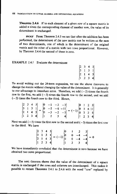
& INTRoDUcTIoN m LINEAR ALGEBRA AND DIFFERENTIAL EQUATIoNS

Theorem 2.4.6 If to each element of a given row of a square matrix isadded a times the corresponding element of another row, the value of itsdeterminant is unchanged.

PRooF From Theorem 2.4.5 we see that after the addition has beenperformed, the determinant of the new matrix can be written as the sumof two determinants, one of which is the determinant of the originalmatrix and the other of a matrix with two rows proportional. However,by Theorem 2.4.4 the second of these is zero.

EXAMPLE 2.4.1 Evaluate the determinant

To avoid writing out the 2fiterm expansion, we use the above theorems tochange the matrix without changing the value of the determinant. It is generallyto our advantage to introduce zeros. Therefore, we add (-2) times the fourthrow to the first, we add (-3) times the fourth row to the second, and we add(-2) times the fourth row to the third. Hence,

Next we add (- 5) times the first row to the second and (- 3) times the first rowto the third. We have

We have immediately concluded that the determinant is zero because we haveobtained two rows proportional.

The next theorem shows that the value of the determinant of a squarematrix is unchanged if the rows and columns are interchanged. This makes itpossible to restate Theorems 2.4.1 to 2.4.6 with the word ..row,' replaced by

1234s ll : I 3 r l12r43ll r 2341

lz34 5 l l o - r -2 -31 lo t2 3 l

l: i i ll : l3 :; :i lll : (-')13 ; i'lll r234 l l r 2 3 4 l l r2 341

lz34 s l lo | 2 3 l13 I 3 l l , , , lo o -4 -41

lz r4 r l : ( - t ) ls o -4 -o l :o

l r2 341 l r 2 3 4 l

the word "column" everywhere and means that we canas well as row properties to evaluate determinants.

Theorem 2.4.1 The value of the determinantunchanged if the rows and columns of the matrix

LINEAR ALGEBRAIc EQUATIoNs 65

use column properties

of a square matrix isare interchanged.

PRooF We do the 3 x 3 case. Let

Then

lBl : I eiiyaipiza*ti,i,k

For the terms in this expansion which are not zero, i, j, and k are different.Therefore, 1,2, and 3 are all represented as row subscripts in these terms.By rearranging the order of the factors, the row subscripts can be put innormal order, that is,

0i1A;zAn : A1142^C\1

where l, m, n is the permutation of l, 2, 3 induced by the inversions

needed to put i, j, k into normal order. Clearly i, j, k and /, m, n are even

or odd together as permutations. There is a term a11o2^e3, in the expan-

sion of the determinant of ,,{ for each and every term arrai2a*r in the

expansion of the determinant of .8, and vice versa. These terms appear

with the same sign. Therefore,

3

lB l : I e i ipna l2a*3:i,i,k

3

I ,m,n

€6,411A2^AS^ : lAl

This completes the proof.

Consider the expansion of the determinant of a 3 x 3 matrix

l o ' a r z a r s l 3

lo^ ezz arsl : I e,roa'a2rarn

I o . , d tz asr I i ' i ' k

: 2 o,, )',,oo,,orri= 1 j , k

3: 2 aucn

where cri: f ,rroorror,,. The quantity "r,

tr."r"to the cofactor of a1i. Let usi ,k

lal orz arr\ lal azt asr\

n: lo^ azz or r l t : lo '

ozz or t l\asr atz ats/ \arr azt at t /

6 INTRoDUcTIoN To LINEAR ALcEERA AND DIFFERENTIAL EQUATIoNS

look at the cofactors c1,:

3

cr r : le r i , ra2;a3k: a22a33 - az3a3z =j,k

3c72 : le r rna2ra3t : a23a3t - a2 te ts :

3

Cr3 : lq i raara3 t : Q2Lat2 - a22a31 :

j ,k

lo" o" ll a t , ax l

lo^ arr l- lo t a r . |

lot ' o"ll a t t a t z l

\-. - z e i j . . . p a t i a z j . . . a n P

i , i ,k , . . . ,p

Therefore, we can expand the determinant as follows

lo' otz ari

l::; ::: ::1: ",,1::: :::)- ",,1::: :::). ",,1::: ::,)latr asz aasl

Notice that the 2 x 2 determinants appearing in this expansion are obtainedby striking out the first row of the original and respectively the first, second, andthird columns. In the general case, we define the cofactors of all as (-l)1+,times the (z - l) x (n - l) determinant formed by striking out the first rowand ith column of the original. It is easy to verify that

n n

2 o , ,i = 1 j , k , . . . , p

t o,,,,,i = l

;1:t. c Li are the cofactors of c, ,. We call this the cofactor expansion by the first

Suppose we wish to expand a determinant using a row other than thefirst, say theTth row (,t + l). Then, using Theorem 2.4.3, we can interchangethe first and 7th row and then use the above expansion. We must rememberthat the interchange of two rows has changed the sign of the determinant.With this method the elements of the original first row will not appear in thefirst row of the determinants in the cofactors. However, by interchanging theelements from the original first row [now appearing in the (7 - l)st row ofthe cofactor determinants] with the 7 - 2 rows above it, we have the rows inthe natural order except for the missing 7th row. Keeping track of all thesign changes, we find we have the factor

( _ l ) t + i + L + i - 2 : ( _ l ) i + t

in front of the (n - l) x (n - l) determinants appearing in the expansion.We summarize this in the following theorem. The expansion obtained is calledthe cofactor expansion by rows.

LINEAR AI.GEBRAIC EQUATIONS 67

Theorem 2.4.8 If we define the cofactor ciJ of the (t,i)th element asyof a square n x n matrix ,{ as (-l)'*J times the (z - l) x (z - l)determinant formed by striking out the ith row and jth column, then

lAl : i o,,r,.,j = L

The next theorem follows immediately from Theorem 2.4.7. The resulting

expansion is called the cofactor expansion by columns.

Theorem 2.4.9 If c;i is the cofactor of the (r;i)th element att of a squaren x n m a t r i x A , t h e n

lAl : i o,,rui = 1

EXAMPLE 2.4.2 Evaluate the determinant

sl0l2l

-213l

l 22 - l0 33 ll 0

r234s l 1 r234o -s -3 - lo -101 l0 r - r -40 3 - r 4 2 l :2 lo 3 - r 40 -s -7 -7 - r7 l l 0 s 7 70 - 2 2 8 - 2 1 l 0 5 3 1 0

5 l l r234st l lo r - r -4 r1 l : 6 1 0 0 2 1 6 - l

t l2 l l 0 0 0 - 2 3 67 l l 0 0 0 12 -3

1 r234l0 l - r - 4

:210 0 2 16

l0 0 1227l0 0 -4 3

lA l :

3 43 - 2

- 1 42 55 1 2

We try to put zeros into the determinant in a systematic manner, beginningwith the first column, by adding multiples of the first row to the other rows.We obtain

ilill

In the last step we have interchanged the second and fifth rows and taken outcommon factors from the second, fourth, and fifth rows. Next we add (- 1)times the fourth row to the fifth and multiples of the second row to the third andfourth rows. We obtain

68 INTR.DU.TI.N To LINEAR ALGEBRA AND DIFFERENTIAL EQUATI.NS

where we have taken a factor of 3 out of the fourth row, added the fourth to thefifth, and added (-2) times the third row to the fourth. Finally, we take a factorof 3 out of the fifth row and add 4 times the fifth column to the fourth column.We obtain

l r z 324 s ll 0 I - l 0 l l

l ' { l : 18 10 0 2 12 - t l

l 000 r6 ll 0 0 0 0 - l l

The last determinant is easy to evaluate. In fact, if we expand by the firstcolumn, expand the first cofactor by the first column, etc., we soon see that thevalue of the determinant is just the product of the elements along the principaldiagonal. Therefore, lAl : -36.

Let A be a 3 x 3 matrix with elements c;r, i, j :1,2,3. Consider thequantities

Qhn: f eukana^ianpi,J,k

f o r / , n t , n : 1 , 2 , 3 . I f / : l , m : 2 , n : 3 , t h e n

Qtz3 : l r,roorroz;a3y : lAli,j,k

If any pair of l, m, and n are equal, then qr^, represents the expansion of adeterminant in which two rows are equal. Hencen the value is zero. lf l, m, nis an even permutation of l, 2, 3, then we have the expansion of f ll but with therows not necessarily in normal order. However, the rows can be put innormal order by an even number of interchanges, and by Theorem 2.4.3 thevalue is lr{1. lf l, m,n is an odd permutation, then it takes an odd number ofinterchanges of rows to put them ip normal order. Therefore, the value is - lll.fn summary,

Qt^n : !'rroorro^iank : lAlemni, j,k

Similarly, using Theorem 2.4.7,

| ",rrouor^akn : lAlem,

i.J,k

Now consider two 3 x 3 matrices l, with elements arr, and g, with

elements b,r. Then if D : AB, the elements of D are dij : 2 o*bri. Now

we consider the product of the determinants of A and B.

LINEAR ALGEBRAIC EQUATIONS 69

lAl lBl : lAl ) e6nblftnzbnsI ,m,a

3: f lAler^^bnb^zb,t

I ,m,n

3 3:

l ,m,n i , i ,k

3 3 3 3: 2 trrr 2 orbr, I ai^b^z 2 or,bn,

i , j ' k l = l m = l n = l

3: I ei;ldndizd*t

i , j ,k

: lABl

It is easy to see that the same type of proof will go through in the general case.Therefore, we have the following theorem.

Theorem 2.4.10 If I and B arc n x n matrices, then

lABl : lAl lBl : lBAl

We conclude this section with one more definition which we shall needin the next section.

Deftnition 2.4,2 The transpose of arl m x n matrix .,{ is the n x mmatrix obtained from ,4 by interchanging the rows and columns. Wedenote transpose of A by A.

lf A is square, then I is also square and Theorem 2.4.7 gives us thefollowing theorem immediately.

Theorem 2.4.11 If I is a square matrix, then l.il : lAl.

Another important theorem has to do with multiplication of the transposesof two matrices.

Theorem2.4.12 If I is anm x n matrix and B is ann x p matrix,

then TB : E^4.

pRooF S ince A ism x n , i i sn x m. A lso .B isp x n . Hence,Ei can be computed. If a,, is the (r,J)th element of A, then d;r : a;; isthe (7,i)th element of .I. If D,, is the (i,j)th element of .8, then 6r, is the

70 INTRoDUCTIoN To LINEAR ALGEBRA AND DIFFERENTIAL EQUATIoNS

fu,t}h element of ^8. Aho

(,J)th element ot fr is

oi&u is the (,;j)th element of AB. The

: 26odrt

which is the (rJ)rh element of E.r. This completes the proof.

EXERCISES 2.4

/ showthatthere aren!: n(n - lXz - 2).. .2.Ldif ferentpermutations of thei n t e g e r s 7 , 2 , 3 , , . . , n .

2 Given a permutation P1 of z integers. obtain p2 from p, by one inversion.obtain P3 from Pr by one inversion. show that p, can be obtained from p2by an even number of inversions. use this to show that evenness or oddness of apermutation is independent of the particular set of inversions used to put it innormal order.

3 Show that a permutation is even or odd according to whether it takes respectivelyan even or odd number of inversions to obtain it from the normal order.

4 Write out all permutations of l, 2,3,4, and classify them according to whetherthey are even or odd.

5 Write out the complete expansion of the determinant of a general 4 x 4 matrix.There should be Z terms.

6 Evaluate the following determinants

t& = l

prouur,: *i d*t6o

, ll 'l .'li ; il ,l_i3 - 1 2 l

:_i ll| 2 -31

7 Evaluate the following determinant by showing that it is equal to an upp€r-triangular determinant (one in which all elements below the principal diagonalare zero).

I Consider the three basic row operations of Sec. 2.3. Show that if a square matrixhas a zero determinant, after any number of basic row operations the resultingmatrix will have a zero determinant. Also show that if a square matrix has anonzero determinant, after any number of basic row operations the resultingmatrix will have a nonzero determinant.

I r 2 - t 3 -21

l z o 4 -5 r ll - 3 | 6 o - 7 1

l 0 3 l - s 2 ll - z 6 i - r 2 l

10

I1

LINEAR AI,GEBRAIC EQUATIONS 7I

Prove that a square matrix has a zero determinant if and only if it can be reduced

to upper-triangular form with at least one zero element on the principal diagonal.

Restate Theorems 2.3.3 and 2.3.5 in terms of the vanishing or nonvanishing of

the determinant of the coefficient matrix.Determine whether or not the following system of equations hasa unique solution

by evaluating the determinant of the coefficient matrix:

2 x 1 * x 2 - x s * x + : - 2

X 1 - X 2 - X l * X + : l

x1 - 4x2 - Zxs * 2xn: 64 x 1 * x 2 - 3 x s * 3 x a : - l

Determine the values of I for which the following system of equations has anontrivial solution:

9 x r - 3 x z : I x t-3x1 * l2x2 - 3x3: ) 'x2

3x2 * 9x3: 1x3

Determine the values of l, for which the following system of equations has anontrivial solution:

x1 * x2 : l x t- x t * X 2 : ) ' X 2

For what values of ,1is there a real nontrivial solution?Let A and,B be m x n matrices. Show that

+( b ) A + B : A + B(d) ffi: afr

T2

I3

T4( a ) A : A_( c ) A - B : A - B

2.5 INVERSE OF A MATRIX

One of the most important concepts in the matrix theory is the notion ofinverse of a square matrix.

Definition 2.5.1 If ,{ is an n x n matrix, then z{ has an inverse if thereexists an n x n matrix r{-1 such that A-rA: AA-t - f, where /isthe nth order identitv.

Theorem 2,5.1 If a square matrix has an inverse, it is unique.

pRooF Suppose B + A-r was also an inverse for A. ThenBA : AB : ^L But then

A-r : A-LI : A-r(AB) : (A-LA'18 : IB : B

72 INTRoDUCTIoN To LINEAR ALGEBRA AND DIFFERENTIAL EQUATIoNs

which is a contradiction, proving that there can be only one inverse for agiven matrix.

One way to construct the inverse of a square matrix A (it it has one) is towork with the cofactor expansion of the determinant of A. Let the elements ofA be a,i and the cofactors of aii be ci;. Consider the quantities

eri : 2 o,rr,ok = l

If i :7, then gii is the cofactor expansion of lral bv the ith row and so7ii: lAl. If i + 7, then Q6 : 0. This is because the expansion then in-volves the elements of the fth row and the cofactors of a different row, andwhat we have, in effect, is the expansion of a determinant in which two rowsare the same. Therefore,

n

) ai{i* : lAlSuk = L

where 6i j : I i f i : , tand 6i j :0 i f i + j . LetC be the matr ix of cofactorswith elements c,r. Then e, the transpose of C, has elements d;; : c;;. There-fore,

*i oT

"o: -i

ai*c*i : lAl6'i

or, in other words, 1( : lAlI. similarly, using the cofactor expansion of lllby columns, we have

{ n

o2 aucri:

*:), tixa*i : lAllit

or e A -- lAlI. Therefore, if lAl + 0, we have

I e ,E : rq ,Le : IlAl lAl

This proves the following theorem.

Theorem 2,5.2 Let A be a square matrix with nonzero determinant.Let C be the matrix of cofactors; that is, c,, is the cofactor of arr. Then

A - L - , E

tAl

Theorem 2.5.3 A square matrix has an inverse if and only if it has anonzero determinant.

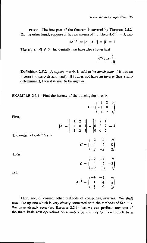
IAIC EQUATIONS 73

pRooF The first part of the theorem is covered by Theorem 2.5.2.On the other hand, suppose Ahas an inverse,4-1. Then AA-r : f, and

l q , q - t l : l A l l A - ' l : l 1 l : I

Therefore, lAl + 0. Incidentally, we have also shown that

lA- t l : #

Deffnition 2.5.2 A square matrix is said to be nonsingular if it has aninverse (nonzero determinant). If it does not have an inverse (has a zerodeterminant), then it is said to be singular.

Then

and

There are, of course, other methods of computing inverses. We shallnow take up one which is very closely connected with the methods of Sec. 2.3.We have already seen (see Exercise 2.2.9) that we can perform any one ofthe three basic row operations on a matrix by multiplying it on the left by a

matrix

t 2 l \- r o r l

r23 l

2 1 l2 r l :o0 2 1

4 -2\2 0 l

-2 2/

/ -2 -4 2 \': l-i t -i)

*':(_:,r i il

74 INTRoDUcTIoN To LINEAR AIcEERA AND DIFFERENTIAL EQUATIoNs

matrix obtained from the identity by the same row operation. Suppose E isobtained from the identity bv (l) multiplication of a row by a nonzero constant,or (2) interchange of a pair of rows, or (3) addition of one row to another.Clearly since l/l : l, then lEl + 0, so .E is nonsingular. Now EA is obtainedfrom ,{ by one of the basic row operations, and since lEAl : lEl lAl, we havethat EA is nonsingular if and only if A is nonsingular. The same goes for anynumber of basic row operations, which shows that if ,{ is reduced to B bybasic row operations, then I is nonsingular if and only if B is nonsingular.

Let us reconsider Example 2.5.1 in the light of these comments. Let

Let

Then

Then

This is in reduced form (as defined in sec. 2.3), but for the present purposeswe go further. Let

Then

l) :'

0 0 \

;l]2 1 \22l ,0 2 1

0 0 \

l')

ilil)

l r - 2 0 \ l r 0r r : {o I o l t r : fo I

\ 00u \00

'':(i iil

,,:(i ;il

": (_l

E2ErA: (i

/ lr - : (o

l l 2 l \E4E3E2E'!A: (3 I ll

/ lE,:(3

E7E6E,E4E3E2E,A: (j ;

E7E6EyE4EsE2ELIA : A- | A

ALCEBRAIC EQUATIONS 75

and multiplying on the right by A- 1, we have

E7E6,E7E44E2ELI : A-L

This tells us that if we perform the same basic row operations on the identity,

we shall produce A-r. Itwill not be necessary to write out the E's if we arrange

the calculation as follows:

I00

l l 2 I

(-l i I ?3)0u

-fi-(i-(i

I22

III

- l

0I

II

- 1

I,

* ,

0I

_ ,

-1,

I- ,

220

2I0

0I0

0I0

il0I0

0 0 \

3')- l 0 \

3r)-ft 0

0I 3',

We display A on the left and the identity on the right. We then change .,{ intoI by a sequence of basic row operations. Performing these same operations onthe identity, wo obtain,4-1, which appears in the last step on the right with theidentity on the left.

If the coefficient matrix of a system of n linear homogeneous equations inz unknowns is nonsingular, then the equations have only the trivial solution.Conversely, if the coefficient matrix is singular, the equations have nontrivialsolutions. These results follow from Theorcm 2.3.3 (see Exercise 2.4.10).

Theorem 2.5.4 A system of n linear homogeneous algebraic equationsin z unknowns has nontrivial solutions if andonlyif thedeterminantofthecoefficient matrix is zero.

Theorem 2.5.5 A system of z linear algebraic equations in n unknownshas a unique solution if and only if the coefficient matrix is nonsingular.

76 INTRoDUCTIoN To LINEAR ALGEBRA AND DIFFERENTIAL EQUATIoNS

pRooF This follows from Thsorem 2.3.5 and our above remarksabout the singularity or nonsingularity of the reduced coefficient matrix.

In the case covered by Theorem 2.5.5, we can find a formula for thesolution. we can write the equations as ,{x : lg, with ,4 nonsingular. There-fore, A- 1 exists, and

If c is the matrix of cofacto* or rrci ::;;:

x : A-tB

and x : LentAl

The produ ct e B has elemen$ : t,ibi : t ,,,b,. Therefore,j = t j = L

l - a '*t :

lo-l )'ciiDij = 1

But the sum is just the expansion by columns of a determinant formed from thecoefficient matrix A by replacing the ith column by the D's. This gives uscramer's rule: if the coefficient matrix A of the system of n equations in nunknowns, AX : ,8, is nonsingular, then the value of the ith variable is givenby lllAl times the determinant of the matrix formed by replacing the ith columno f A b y b r , b r , . . . , b , .

In terms of total calculations, Cramer's rule is not very practical. Itinvolves the calculation of n * | determinants of order n. Compared with theelimination method it is marginal for n : 3 and is at a disadvantage for n 2 4.However, if the value of only one of the unknowns is needed, only two deter-minants need be calculated.

We conclude this section with a couple of definitions of special non-singular matrices which involve the concept of inverse.

Definidon 2.5.3 Let A be an n x n matrix with real elements. Then,{ is said to be orthogonal if A-' : A.

Definition 2.5.4 Let A be a matrix with complex elements. Then theconjugate of ,,4 (written A) is the matrix formed ftom A by taking theconjugate of each of its elements.

Definition 2.5.5 Let A be an n x n matrix with complex elements.

Then ,,4 is said to be unitary if A-t : i.

A - L : I EtAt

LINEAR ALGEBRAIC EQUATIONS 77

EXERCISES 2.5

/ Which of the following matrices have inverses?

,(i ') 0,(l l)

2 Find inverses of matrices in Exercise I which are nonsingular.3 Find the inverse of the diagonal matrixt

When does a diagonal matrix have an inverse? State a general rule for finding theinverse of a diagonal matrix.

4 Show that an upper-triangular matrix with nonzero elements on the principaldiagonal has an inverse which is upper-triangular.

5 Solve the following system of equations using Cramer's rule.

x t * x 2 - x t = 7- x r * 2 x 2 * x a : - 3zxL - x2 * 3x3: J

6 Solve the matrix equation AB : C for.B if

l r l - l \ / 2 o t \, : l - t 2 t f ano c :13 - t 4 l

\ 2 - r 3 l \1 s -u

7 Let AX : B be a system of n equations in z unknowns with lll : 0. Showthat there are no solutions unless all z determinants of matrices formed ftom Aby inserting .B in the n columns of A arc zero. If solutions exist, are they unique?Hint : Multiply both sides of AX : B on the left by i, the transpose of the matrixof cofactors of l.

f A diagonal matrix is a square matrix with zero elements off the principal diagonal.

,(i i ilI 3 - 1 2 \', ', -tr ll2 | 2 - 3 /

/ r 2 3 4 \'"|,l s i'l

",(i i il ,,(_

ft;;il

78 rNrRoDUc[oN T1o LTNEAR ALcEBRA AND DTFFERENTTAL EeuATIoNs

8 L€t

Find l-1. Is I orthogonal?9 If A and,I are nonsingular, show that AB is nonsingular. Show that

(An)-t : B'rA-L

10 I.Et Abe nonsingular. Show that.F : (.d)-1.II I'et A be nonsingular. Show that (l-1)- 1 = A.12 If AB : q .B + q isl nonsingular?13 lf A2 = 0, is I nonsingular?14 If I is orthogonal, what are the possible values of lAl?15 lf A and B arc orthogonal, is AB orthogonal? Is l-1 orthogonal?16 If I and B arc unitary, is AB unitary? Is r{-1 unitary?17 Define Ao = I and l-" : (A-t)o, n a positive integer. Let A be nonsingular.

Prove the general exponential formulas (APf : An and, ApAc : AP+q, wherep and q are integers.

I8 rf c is the matrix of cofactors of the elements of ,,{, what is the value of I c | ?

*2.6 EXTSTENCE AND UNIQUENESS THEOREMS

The two main questions concerning systems of linear algebraic equations(other than methods of finding explicit solutions) are (l) whether solutionsexist (exrstence) a\d (2) if a solution exists, is it unique (uniqueness)? we havedealt with these questions to some extent in Sec. 2.3. In this section, we shallgive a more systematic discussion of these two questions, but first we mustintroduce a new concept about matrices which can be defined in terms ofdeterminants.

Every matrix, whether square or not, has square matrices in it which canbe obtained by deleting whole rows and/or whole columns. There are of courseonly a finite number of such square matrices. Suppose we compute the deter-minants of all these matrices. We define the rank of the original matrix interms of these determinants.

Definition 2.6.1 The rank of a matrix ,{ is the order of the largest ordernonsingular matrix which can be obtained from.,{ by deleting whole rowsandlor whole columns. We denote this number by rank (l); rank (0) : 0.

,:(:ij; T;)

LTNEAR ALCiEBRATC EQUATTONS 79

EXAMPLE 2.6.1 Find the rank of the matrix

Since ,{ has some nonzero elements, rank (l) ) l. Also, since there are no4 x 4 matrices, rank(,,{) < 3. It iseasytofind a2 x 2matrixwithnonzerodeterminant, so rank (A) > 2. Now the 3 x 3 matrices are all singular since

ll _? il :o ll _?l z r3 l l z r

I r 341 lz3

ll I 1l :' l-l 3Therefore, rank (A) : ).

The proofs of the next two theorems are left to the reader.

Theorem 2.6,1 If ,,4 is anm x n matrix, then 0 S rank (,{) < minlm,nf.

Theorem 2.6.2 If I is an n x n matrix, then rank (A) : n if and onlyif I is nonsingular.

Let us consider the effect, if any, on the rank of a matrix I when one of thebasic row operations is performed on ,4. We shall consider each operationseparately. Suppose rank (l) : r, and suppose theTth row of I is multipliedbyk * 0toformanewmatrix.B. Thereissome r x rmatrix CinAsuchthatfcl + o. Now, if ccontains all or part of theTth row of A, then there is ar x r matrix in .B whose determinant is klcl + O. If C does not involve the7th row of l, then C is also in B and B again contains an rth order nonsingularmatrix. If ,{ contains any square matrix D of order larger than r, lDl : 0.Any square matrix in .B of order larger than r either does not involve the 7throw of A, and is therefore already in A, or it does involve theith row of A, inwhich case its determinant is zero because it is k times a zero determinant froml. Therefore, multiplication of a row of a matrix by a nonzero constant doesnot change the rank.

Next we consider the interchange of two rows. Suppose I is obtainedfrom I by an interchange of the ith and jth rows of l. suppose rank (A) : r.

^:(Li tl

: Q

: Q

80 INTRoDUcTIoN To LINEAR A,IcEBRA AND DIFFERENTIAL EQUATIoNS

Thenthereis anr x rmatrix CinA suchthat lcl * 0. If cinvolvesbothther'th andTth rows of l, then there is an r x r matrix C*in,BsuchthatlC*l :*lcl * 0. If C involves neither the ith norTth row, then C is also containedin 8. If c involves the ith but not the 7th row, then there is an r x r matrixin ,,{ with the fth row deleted and containing the.Tth row, which after the inter-change becomes C except for the order of the rows. This matrix is obviouslynonsingular. If ,4 contains any square matrices of order larger than r, theyare singular. This is also true of .B because any square matrix of order largerthan r in ,B is either in ,,4 or can be obtained from such a matrix in ,4 by aninterchange of rows. Hence, interchanging two rows of a matrix does not alterthe rank.

Finally, we consider the operation of adding one row of ,,4 to anotherrow. Suppose ,B is obtained from ,4 by adding the i th row to the 7th row. Ifrank (l) : r, then there is a nonsingular matrix C of order r in A. If C involvesboth the fth andTth rows of A, then there is a matrix C* in I obtained from Cby adding two rows. Hence, lC*l : lcl + O. If C involves neither theith nor theTth row, then C is also in ^8. If C involves the ith row but not thejth row, then C is also in .8. If C involves theTth row but not the fth row, thenthere is an r x r matrix in .B whose determinant is lcl + lC*1, where C* isobtained from C by replacing those elements from the /h row of .,{ by thecorresponding elements from the ith row. If lcl + lc*l : 0, then lC*l + 0and C* is an rth order nonsingular matrix in .8. Any matrix in .B of orderlarger than r will either already be in A, and hence be singular, or will have adeterminant which is the sum of determinants of singular matrices in ,4. Wehave shown that none of the three basic row operations will change the rankof a matrix. We summarize this in the following theorem.

Theorem 2.6,3 Let A and ,B be m x n matrices, where B can be ob-tained from ,,4 by a sequence of basic row operations. Then rank (l) :

rank (B).

We are now ready to state the fundamental existence theorem for systemsof linear algebraic equations. However, first for convenience we shall considerone additional operation on matrices, the interchange of two columns. Itis clear that this operation does not change the rank of a matrix. Now let usconsider the effect on a system of equations if two columns of the coefficientmatrix are interchanged. Suppose the ith and 7th columns are interchanged.Then the coefficients of the x; unknown become the coefficients of the x,unknown and vice versa. So this has the effect of just relabeling the xr and x;unknowns.

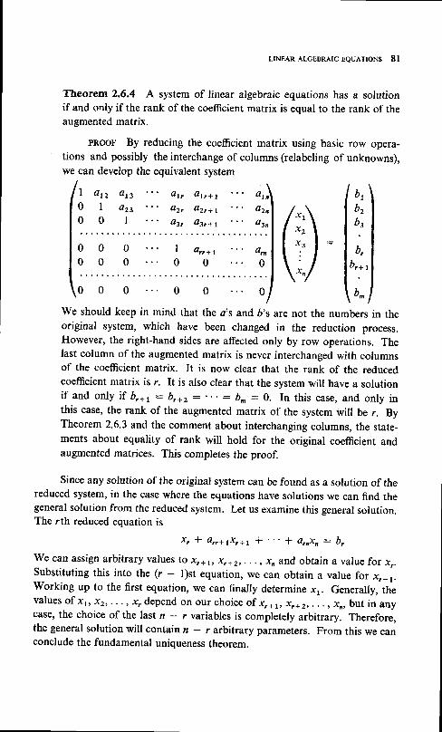
LINEAR ALGEBRAIC EQUATIONS 8I

Theorem 2.6.4 A system of linear algebraic equations has a solutionif and only if the rank of the coefficient matrix is equal to the rank of theaugmented matrix.

tionswe ca

Iatz o t l

I az,0 l

a r , a b + t

Q2, azr+ to3, a3r+ |

pRooF By reducing the coefficient matrix using basic row opera-and possibly the interchange of columns (relabeling of unknowns),n develop the equivalent system

000

ar,azn

o3n

b1

b2u:

b,u,:,

b^

00

I arr+ t0 0

We should keep in mind that the a's and 6's are not the numbers in theoriginal system, which have been changed in the reduction process.However, the right-hand sides are affected only by row operations. Thelast column of the augmented matrix is never interchanged with columnsof the coefficient matrix. It is now clear that the rank of the reducedcoefficient matrix is r. It is also clear that the system will have a solutionif and only if br+r : br+z : b^ : 0. In this case, and only inthis case, the rank of the augmented matrix of the system will be r. ByTheorem 2.6.3 and the comment about interchanging columns, the state-ments about equality of rank will hold for the original coefficient andaugmented matrices. This completes the proof.

Since any solution of the original system can be found as a solution of thereduced system, in the case where the equations have solutions we can find thegeneral solution from the reduced system. Let us examine this general solution.The rth reduced equation is

x , * au* r l r+ t * + arnxn: b,

We can assign arbitrary values to xr*Lt xrr2t..., xnand obtain a value for xr.substituting this into the (r - l)st equation, we can obtain a value for x,_r.working up to the first equation, we can finally determine xr. Generally, thevalues of xr, x2, . .. , x. depend on our choice of xr* lr xr+ 2t . . . , xn, but in anycase, the choice of the last n - r variables is completely arbitrary. Therefore,the general solution will contait n - r arbitrary parameters. From this we canconclude the fundamental uniqueness theorem.

82 INTRODUCTIoN To LINEAR ALGEBRA AND DIFFERENTIAL EQUATIoNS

Theorem 2,6.5 A solution of a system of z linear algebraic equationsin n unknowns is unique if and only if the rank of the coefficient matrix isn.

The final theorem follows from Theorems 2.6.5 and 2.6.1.

Theorem 2.6.6 A solution of a system of m linear algebraic equationsin n unknowns is never unique if n > m.

pRooF If I is the coefficient matrix, rank (A) < m < n.

EXAMPLE 2.6.2 Determine whether the following system of equations has asolution; if so, is it unique?

X 1 - x 2 * 2 x 3 - X + : l2 x 1 * x 2 - x t * x + : - 2

2x2 * x3 - 3xn: 1

3 x , + x 3 : - l

3x t * 2x2 * 2xt - 3xn: g

The augmented matrix of the system is

)

(iti )Using row

(t -r

\i t

operations,

2 - l- l I

I - 3

l 02 - 3

- l

3235

we have

)2 - l

- 5 3I - 3

- 5 3- 4 0

- l 2 - l \

i _l -1 _rl0 0 0 0 ls - 4 0 - 3 /

/ - r 2 - r \ / - r 2 - r \[o 2 r -3 r \ Io 2 r -3 r \

- ,1 o 3 -5 3 -+ ; - ,1 o 3 -5 3 - ; l\ o 3 -5 3 -+ l \o o o o o l\ o o o t/ \ o o o t/

It is apparent that the rank of the coefficient matrix equals the rank of theaugmented matrix, which is 3. Therefore, the system has a solution, but it isnot unique because 3 < 4, the number of unknowns. The general solutionof the system will contain one arbitrary parameter.

LTNEAR ALcEBRAIc EeuATroNs 83

EXERCISES 2.b

.l Prove that the rank of the augmented matrix of a system of linear algebraicequations cannot be less than the rank of the coefficient matrix.

2 Consider the three basic column operations on matrices: (l) multiplication of acolumn by k * 0, (2) interchange of two columns, (3) addition of one columnto another. Prove that these column operations cannot change the rank of amatrix.

3 State Theorem 2.3.3 in terms of the rank of the coefficient matrix. Prove yourversion.

4 State Theorem 2.3.5 in terms of the rank of the coefficient matrix. Prove your

5 Determine whether the following systems of equations have solutions; if so,are they unique?

( a ) x L + x z - r s : l2x1 * x2 * 3x r : /

x 2 - 5 x 3 : l

( 6 ) x r * * 2 x s - x a : 0Z x t * x 2 - . r 3 = J

- x r * b z * x 3 * 2 x n : t3 x z - 2 x 3 * 5 x n : 1

( c ) 2 x r - x z * r g : l ( d )xt + 2x2 - 3x3 : g

- x t * 3 x z - x t : 2x r - x 2 - 2 x 3 - - 3

x r - Z x r * 3 x 3 - x + * r s : 5- x r * 3 x 2 * 4 x 3 * x 4 - 2

2 x r + x 3 - 2 x a * 2 x 5 - - l

x 2 * 5 x 3 - 2 x + - r s : 0

consider the system of equations AX: B, where A is m x rr. suppose thatrank (l) : m - l. Prove that the system has a solution if and only if the mmatrices formed from A by replacing the columns by .B are all singular.

3VECTOR SPACES

3.1 INTRODUCTION

We have already seen two examples of vector spaces, the complex numbers andthe two-dimensional vectors of Sec. 1.4. There are many more examples, andone of the objectives of this chapter is to give some idea of the scope of thissubject. Before introducing the abstract concept of a vector space, we take upthe three-dimensional euclidean vectors, partly because of their intrinsic impor-tance in applications and partly to give the reader one more concrete examplebefore we begin the general discussion of vector spaces. After introducing theaxioms of a vector space and proving some basic theorems, we take up the veryimportant concepts of dependence and independence of vectors. We thendefine basis and dimension of vector spaces. The scalar product is then intro-duced, and this leads to a discussion of orthonormal base. The last section(which is starred) takes up some of the fundamental properties of infinite-dimensional vector spaces.

85

3.2 THREE.DIMENSIONAL VECTORS

We shall define the three-dimensional euclidean vectors (from now on we shallsay simply uector) by a simple extension of the two-dimensional vectors ofSec. 1.4. A three-dimensional vector is defined by a triple of real numbers(x,y,z), and we shall write v : (x,y,z). Two vectors v1 : (xr,yr,zr) and,yz : (xz,!z,zr) are equal if and only if xL : xz, lr : !2, and z, : 22. Wedefine additionof twovectorsvr : (xr,/r,zr)and yz : (xz,!z,zz)byv1 * y2 :(xt * xz, lt * !2, z, * z2). we see that the result is a vector and the oper-ation is associative and commutative. We define the zero aector as 0 : (0,0,0),and itfollows immediatelythatv * 0 : (x,y,z) + (0,0,0) = (x,y,z): vforall vectors v. The negatiue of a vector v : (x,y,z) is defined by -v :(-x,-y,-z) and the following is obviously true: v + (-v):0 for allvectors Y.

we define the operation of multiplication of a vector y : (x,y,z) by areal scalar a as followsr drv : (ax,ay,az). The result is a vector, and it is easyto verify that the operation has the following properties:

I a(v, * vz) : 0rt1 * cyz.2 ( a + b ) v : m * b v .3 a(bv): (ab)v.4 l v : y .

The geometrical interpretation of three-dimensional vectors is similarto that for the two-dimensional vectors of Sec. 1.4. Consider a three-dimensionaleuclidean space with two points (a,b,c) and (d,e,f) (see Fig. l5). Let x : d. - e,!: e - b,z:f - c. Ageometricalinterpretationof thevector v: (x,y,z)is the arrow drawn from the point (a,b,c) to the point (d,e,f). The length of thevector is defined as

1v1 :Jf ia] :

The direction of the vector (if fvl # 0) is specified by the least nonnegativeangles (01,02,03) from the positive coordinate axes to the arrow of the vector.The cosines of these angles are given by

c o s 0 r : I c o s g r : I

These cosines are usually called direction cosines. Since

x2 + y2 * 22 : tvl2(cos2 0, + cos2 0, + cos2 0r\

cos2 0, * cos2 0, + cos2 0s : I

c o s O " : a- lvl

+ ( f - c ) '

86 INTRoDUcTIoN To LINEAR ALGEBRA AND DIFFERENTHL EQUATIoNS

FIGURE 15

If there is another pair of points (a',b',c') and (d',e',/') such that x : d' - a,,! : e' - b', z : f' - c', then the arrow from (a'rb,rc,) to (d,re,rf') has thesame length and direction as that from (a,b,c) to (d,e,f). Therefore, we saythat the vector v : (x,y,z) is represented by any arrow with length lvl anddirection specified by (0t,0r,0r). The zero vector has no direction and so has noarrows associated with it.

The geometrical interpretation of vector addition is as follows (see Fig.lQ. Place an arrow representing v, from point P to point Q. Place an arrowrepresenting v, from point Q to point R. Then the arrow from P to R representsthe sum vr + y2. If P and R coincide, then y1 * v, : Q. Since the pointsP, Q, and.R determine a plane, if they are distinct and not collinear, the triangleinequality simply states that

l v r * Y z l S l v l l + l v r l

It is easy to see that the inequality continues to hold if P, Q, and R are not alldistinct or are collinear.

Next let us give a geometrical interpretation of the operation of multi-plication of a vector bya scalar. Leta be a scalarand v: (x,y,z) a vector.Then m: (ax,ay,az)and.

lm l : JW: l a l l v lTherefore, multiplication by a modifies the length by a factor of lal if lal * l.Suppose cos 0, : xllvl, cos 0, : yllvl, cos 0, : zllvl. The new directioncosines are

cos 0i : L cos g, cos 0! : !, cos 92 cos g', : +cos g,' lal lal lal

J

If c > 0, the direction is unchanged. If a < 0, the direction is reversed. Ifa : 0, av : 0, which has no direction. The vector -v : (- l)v is the negative

VECTOR SPACES 87

FIGURE 16

of v, and we see that it has the same length as v but has the opposite direction(provided v * 0). The geometrical interpretation of subtraction of two vectorscan be obtained from that for addition by writirig yr - v2 : v1 * (-vr).

We also have the notion of scalar product for three-dimensional vectors.Let v, : (xylrzr) and v2 : (x2,y2,22). Then we define the scalar product(dot product) as

y r . y e : x l . x z * l v z * z r z ,

we see immediately that this definition leads to the following properties:

I v t ' t . 2 : Y z ' Y r .

2 vr . (yz * vs) : (yr . vz) * (v, . vs).3 ( N t ' Y z : a ( v r ' Y z ) .4 y . v : l " l r t 0 .5 v . v : 0 i f a n d o n l y i f v : 0 .

Let us look for a geometrical interpretation of the scalar product. Supposev1 and Y2 are not zero and do not have the same or opposite directions. Weplace arrows representing the two vectors starting from the origin (see Fig. l7).The points o, P, Q determine a plane. consider the triangle ope. The lawof cosines gives the cosine of the angle g between v, and vr:

cos o _ lvt - vrl2 - lvrl2 - lvrl2-2 lv r I lv2 l

w€ can evaluate the numerator

Y r ' Y r - Y z ' Y z'vz) - Yr . Yr - yz . yz

Using the properties of the scalar product,

l v , - v z l ' - l v r l ' - l v r l t

: !;e?'tl'"' -"ln'

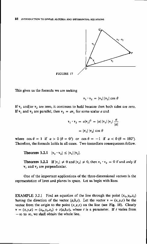
88 INTRODUCTIoN To LINEAR ALGEBRA AND DIFFERENTIAL EQUATIoNs

FIGURE 17

This gives us the formula we are seeking

yt. yz : ly l l lvr l cos 0

If vt and/or v2 are zero, it continues to hold because then both sides are zero.If v, and v2 are parallel, then v, - ayr for some scalar a and

Yr . Yz : olvrl ' : lal l"rl l"rl *p l

: lyl l lvrl cos 0

w h e r e c o s 0 : 1 i f a > 0 ( 0 : 0 " ) o r c o s O - - l i f a < 0 ( 0 = 1 8 0 ' ) .Therefore, the formula holds in all cases. Two immediate consequences follow.

Theorem 3.2.1 lv, . vrl S lvll lvrl.

Theorem 3.2.2 If lvll * 0 and lvrl + 0, then yr 'vz : 0 if and only if

v, and v2 are perpendicular.

One of the important applications of the three-dimensional vectors is the

representation of lines and planes in space. Let us begin with lines.

EXAMPLE 3.2.1 Find an equation of the line through the point (xo,yo,zo)

having the direction of the vector (a,b,c). Let the vector v : (x,y,z) be the

vector from the origin to the point (x,y,z) on the line (see Fig. l8). Clearly

v : (x,y,z) : (xo,.yo,zo) * t(a,b,c), where t is a parameter. If t varies from- oo to co, we shall obtain the whole line.

VECTOR SPACES 89

FIGURE 18

EXAMPLE 3.2.2 Find an equation of the line passing through the two points(xplyzt) and (xr,y2,zr). A vector which specifies the direction of the line is(a,b,c) : (xz,!z,zr) - (xr,ypzt) : (x, - xr, lz - lt zz - zr). Therefore,following Example 3.2.1, an equation for the line is

( x , y , z ) : ( x y l r , z ) + t ( x r - x t , l z - l r , z z - z r ) - m < t < @

To discuss planes effectively we need the notion of linear combinationsof two vectors. Let v, : (aybr,cr) and v2 : (a2,b2,c2) be nonzero vectorswhich are not parallel (v, is not a scalar times vl or vice versa). Let s and Ibe scalars. Consider arrows representing v, and v, starting from the origin(see Fig. l9). If all arrows originate from the origin, then sv, is collinear withyy ty2 is collinear with v2, ard sv, * tv, is in the plane determined by v, andy2. As s and t vary, we obtain different points in the plane determined by v,and vr.

EXAMPLE 3.2.3 Find an equation of the plane containing the point (xo,yo,zo)and parallel to the two vectors y, : (ar,bycr) and v2 : (a2,b2,cr), which arenot parallel to each other. Let (x,y,z) be the vector from the origin to a pointon the plane. Then

(x,y,z) : (xo,!o,ze) * s(cr,br,cr) * t(a2,b2,c2)

As s and I range through values from - @ to oo, we obtain all possible pointsin the given plane.

EXAMPLE 3.2.4 Find an equation of the plane containing three distinctnoncollinear points (xo,yo,zo), (xr,yr,zr), and (xr,yr,zr). Since the points are

90 INTRODUcTIoN To LINEAR ALGEBRA AND DIFFERENTIAL EQUATIoNS

FIGURE 19

distinct and noncollinear, the vectors (x, - xo, lt - !o, zt - zo) and(xt * xo, lz - !o, zz - zo) are nonzero and not parallel. Therefore, if(x,y,z) is the vector from the origin to a point on the plane, an equation is

(x,y,z) : (xo,!o,ze) + s(x, - xo, lt - !o, zt - za)

* t(x, - xo, lz - !o, zz - zo)

where -@ < J < @ and - @ < t < oo.

The equations given in Examples 3.2.1 to 3.2.4 arc all parametric equatiotxs,

where we have given the three coordinates of points on the geometrical figurein terms of one or two parameters. The fact that it took one parameter for theline and two parameters for the plane reflects the fact that the line is essentiallya one-dimensional figure whereas the plane is essentially two-dimensional.There are also implicit representations for lines and planes. In the implicit

representation we state one or more equations which the coordinates of a point

on the figure must satisfy, while points not on the figure will not satisfy these

equations.

EXAMPLE 3.2.5 Find an implicit representation of the plane containing thepoint (xo,yo,zo) perpendicular to the vector (a,b,c). Let (x,y,z) be the displace-ment vector from the origin to a point in the plane (see Fig. 20). The vector(x - xo, ! - /o, z - zo) is parallel to the plane and hence the scalar product

( a , b , c ) ' ( x - i o , y - ! o , z - z o ) : a ( x - x o ) * b ( y - . / o ) + c ( z - z o ) : 0

VECTOR SPACES 9I

FIGURE 20

This is an implicit equation for the plane since the coordinates of all pointson the plane will satisfy it, while the coordinates of points off the plane will notsatisfy it. The equation can be put in the form

ax * by * cz : axo * byo * czo - 4

Conversely,everyequationof theformax + fy * yz: d,where (u,fl,y) * A,is the equation of some plane. There is at least one point (xo,yo,zo) such thatu x s * F y o * T z o : 6 . B u t t h e n a x * F y + y z : o ' x o * F y o * y z o a n da(x - xo) * f(y - yo) * y(z - zo) :0 states the geometrical fact that thevector (x - xo, ! - !o, z - zo) is perpendicular to (a,B,y).

EXAMPLE 3.2.6 suppose two planes given implicitly by ax + by + cz : dand q,x + fy * yz - d intersect in a single line L. Find an equation for z.We must find the coordinates of all points which satisfy both equations simul-taneously. The two equations do not represent the same plane or parallelplanes; hence the vectors (a,b,c) and (a,B,y) are not proportional. Therefore,at least one of the determinants

l: 'd lx '1 or l: '1is different from zero. suppose, for the sake of the argument, it is the first.Then we can solve the equations

a x * b y : d - c z

u x * F y : 6 - y z

(xs, y6, z9)

92 INTRoDUc.TIoN To LINEAR ALGEBRA AND DIFFERENTIAL EQUATIoNS

for x and y in terms of z. Wher z : 0

ll 'A,t:TU,' !.:v^and the general solution is

x : x o * t l t

! : Y o * t oZ : t

where u :

l ) -

bv -c f ra p - b ac a - a ya B - b u

In other words, (x,y,z) : (x0,./0,0) + t(u,u,l), - co < / ( @, and we havethe equation of a line passing through (xo,.yo,0) and having the direction of(ururl),

The concepts of a vector-valued function and derivative of a vector-valuedfunction follow as extensions of the two-dimensional case of Sec. 1.4.

Definition 3,2.1 Suppose for each value of r in some set of real numbersD, called the domain of the function, a vector v(t) is unambiguouslydefined; then we say that y is a vector-valued function of t; t is called theindependeni oariable, and v is called the dependent aariable. The collectionof all values of v(t), taken on for r in the domain, is called the range of thefunction.

EXAMPLE 3.2.7 Let v(t) = (x,y,z) : (a cos t, a sin t, bt),0 < t 3 2n, wherea and D are real constants. Then v is a vector-valued function of r. The domainis the interval {t l0 < t 3 2n}. If we think of y as the vector from the originto a point in the three-dimensional space, then the range of the function is a

spiral of radius o : ,/*' + y2 joining the initial point (a,0,0) and the finalpoint (a,0,2nb) (see Fig. 2l).

Deftnition 3.2.2 Suppose for some /6 and some 6 ) 0, all t satisfyingto - 6 < t < to + 6 are in the domain of v(t) and there is a vectorv'(lo) such that

ITlry-"'1ro1l :othen v'(ts) is the derivative of v(t) at ro.

VECTOR SPACES 93

FIGURE 2I

Just as in the two-dimensional case, we have the following theorem.

Theorem 3.2.3 The vector-valued function v, with values v(l) :(x(t),y(t),2(l)), has a derivative v'(le) : (a,b,c) if and only if x(t), y(t),and z(t) have derivatives at /o such that x'(ro) : a, y'(to) : b, andz'(to) : s.

EXAMPLE 3.2.8 The vector-valued function of Example3.2.1 has a derivativeat ts such that 0 < to < 2n. ln fact,

v'(to) : (-a sin ts, a eos to, b)

Similarly, we have the notion of tangent to a curve in three-dimensionalspace.

Definition 3.2.3 Suppose a curve is given parametrically by the vectorfrom the origin v(t) : (x(t),y(t),2(r)), a < t < P. If v(t) has a nonzeroderivative v'(ro) at /o, then v'(ro) is a tangent vector at the point v(ro).The tangent line at v(ro) is given parametrically by the equation

w(t; : v(ro) + (r - to)v'(ro) -@ < t < oo

EXAMPLE 3.2.9 The tangent vector to the spiral of Example 3.2.7 atto : nl2 is v'(nl2) : (-a,O,b). The tangent line at the point v(nl2) :(O,a,nbl2) is given by

w(r) : (",+)* ( ' - t)r-a,o,b)

94 INTRoDUCTIoN To LINEAR ALGEBRA AND DIFFERENTIAL EQUATIoNs

EXERCISES 3.2

Let u = (1,-2,1) and y: (3,1,-4). Compute u + y, r _ v, 2u, _]v, and-u * 2v. Make sketches of arrows representing each of these vectors.Let u : (1,-2,1). compute lul and 0t, 02,0r, the minimum nonnegative anglesfrom the positive coordinate axes to the arrow of the vector.A force in pounds is exerted on a body as designated by the vector (3,1,-2).Find the magnitude and direction of this force. Another force of (-4,5,3), alsomeasured in pounds, is exerted on the same body. Find the combined effect(resultant) of the two forces acting together. Find the magnitude and directionof the resultant. Hint: The resultant is the vector sum of the two forces.Let u : (2,0,-3) and v : (-1,4,5). Find the cosine of the angle between thetwo vectors. If cos 0r, cos 021 cos 0s are the direction cosines of u and cos /r,cos Q2, cos /3 are the direction cosines ofv, show that cos d : cos 0, cos /1 +cos 0, cos {2 * cos d. cos /r, where g is the angle between the two vectors.consider a nonzero vector u represented by the arrow from o to p. Considerthe vector v represented by the arrow from o to O. The projection of v on u isdefined to be the vector O to N, where N is the foot of the perpendicular drawnfrom Q to the line of u. Show that this projection is given by

lJolu l '

Compute the projection of (1,-2,1) on (3,1, -4).consider a plane represented implicitty by ax * by + cz : d. consider avector v represented by an arrow from the point (x6,y6,zs) in the plane to thepoint O. The projection of v on the plane is defined to be the vector from(xo,yo,zo) to N, the foot of the perpendicular drawn from e to the plane. Leta : (a,b,c). Show that the projection of v on the plane is given by

" - TlJ"lul-

Compute the projection of (2,3,- 1) on the plane given by x - 3y + 2z = 7.show that the distance from the point (x1,y r,zr) to the plane represented byax * bY * cz : dis given by

l a x l * b y r * c z 1 - d l

JF;oz * cCompute the distance from (1, - 2,3) to the plane represented by 2x - | * 3z : 7.Find an equation of the line through the point (1,2,-3) in the direction of thevector (-2,3,5).Find an equation of the line through the two points (3,-5,2) and (- 2,1,4).Find an equation of the line through the point (4,3,*5) and perpendicutar to theplane given by 2x * 3y * 4z -- 3.

910

I1

12

t3

I4

t5

16

VECTOR SPACES 95

Find an equation of the line of intersection of the two planes given by2x * 3y - 4z : 5and -x * 7y I 5z : 2.Find an equation of the plane through the origin and parallel to the vectors(1,-2,3) and (5,0,7).Find an implicit representation of the plane containing the three points (1,-3,4),(2,5,-l), (A,7,-4).Find an equation of the plane containing the two lines (x,y,z): (1,-3,4) +t(2,5,- 1) and (x,y,t) : (1,- 3,4) + s(0,7,-4).Find an equation of the plane containing the point (1,2,3) and perpendicular

to the line (x,y,z) : (1,- 3,4) + t(2,5,-l).One way to compute a three-dimensional vector perpendicular to two givenvectors is to use the uector product. Let u : (uyu2,u3) and v : (uyt2,u3) be twononzero and nonparallel vectors. Show that

w : u X v : (uztss - tl3o27 tl3t)1 - urU3, ura2 - u1s1)

is a vector perpendicular (orthogonal) to both u and v. The vector product hasno counterpart in other spaces.Show that lu X vl : lul lvl lsin 01, where d is the angle between u and v. Hint:Write u : lul(cos d12 coS d2, coS gs) and y : lvl(cos /1, cos (r, cos fi).Repeat Exercise 13, using the vector product to compute a vector perpendicularto the required plane.Let u, v, w be three vectors whose arrow representations from the origin form thethree edges of a parallelepiped. Show that lu. (v x w)l is equal to the volumeof the parallelepiped.Show that:

lu,. u2 ,rl(a) u'(v x tt) :

lr, 02 ,r

Ilw, h,2 wsl

(b ) u ' ( v x w ) : w ' ( u X y ) : v ' (w x u ) .( c ) u ' ( w x v ) : - u ' ( v x w ) .Consider three planes given implicitly by

a 1 l x * a n ! * a 1 3 2 : b 1

a 2 t x + a z z ! * a 2 3 z : b 2

a 3 1 x * a * ! * a 3 3 2 : b 3

The intersection of these three planes could be (1) empty, (2) a line, (3) a plane,or (4) a point. In terms of the solutions of the three equations in three unknownsgive an algebraic condition for each of the cases.A point moves along a curve in three-dimensional space with its displacementvector from the origin given by the vector-valued function of time r(t) :(x(t),y(t\,2(r)), where x, y, alnid zhave first and second derivatives. The first deriv-ative r'(t) : v(r) : (x'(t),y'(t),2'(t)\ is called the aelocity of the point, and thesecond derivative a(t) : r"(t) : v'(t) : (x"(t),!'(t'5,2"(t)) is called the acceleration.

I7

I8

19

20

21

22

96 INTRoDUcTIoN To LINEAR ALGEBRA AND DIFFERENTIAL EQUATIoNS

If v(r) I 0, show that the velocity is tangent to the curve. The magnitude of thevelocity is called the speed. If the speed is constant and positive, show that theacceleration is normal to the curve (perpendicular to the tangent vector).

23 If thespeeds(r) : lv(r)lofapointisnotzero, showthat a(t) : s,(r)T + .r(r)lT,ln,where T is a unit tangent vector and n is a unit normal vector.

3.3 AXIOMS OF A VECTOR SPACE

We have already seen several examples of algebraic systems which, at least incertain respects, behave similarly. We have in mind those properties of complexnumbers, two-dimensional euclidean vectors, three-dimensional euclideanvectors, and matrices with respect to addition and multiplication by a scalar.We now take the modern mathematical point of view and define abstractsystems with those properties we wish to study. These systems we shall callaector spaces. This approach will have the distinct advantage that any propertieswe derive from this definition wilt be true of all vector spaces, and we shall nothave to study each system separately as it comes up. We begin with the axiomsfor a vector space.

Definition 3.3.1 consider a system z of objects, called uectors, forwhich we have defined two operations, addition and multiplication by ascalar, either real or complex. Then V is a vector space if these operationssatisfy the following properties:

A I I f u a n d v a r e i n V , t h e n u + v i s i n Z .A 2 u * v : y + u .A 3 u * ( v * w ) : ( u + v ) + w .A4 Thereisazerovector0invsuchthatu * 0 : uforal lu in z.A5 If u is in z, then there is a vector -u in v, called, the negativeof u, such that u * (-u) : g.

MI If a is a scalar and u is in V, then au is in Z.M 2 a ( u * v ) : a u * m .M 3 ( a + 6 ) u : a t * b a .M4 (ab)u : a(b$.M 5 l u : u .

If the set of scalars is the set of all real numbers, then we say that V is areal oector space. If the set of scalars is the set of all complex numbers,then we say that Y is a complex nector space.

VECTOR SPACES 97

The reader should verify that the system of complex numbers is a realvector space. Here the vectors are complex numbers of the form x * ly and thescalars are real numbers. Addition is the ordinary addition of complex numbers,and multiplication by a scalar is defined by a(x + iy) : ax * iay.

The reader should also verify that the systems of two-dimensional andthree-dimensional euclidean vectors are real vector spaces.

EXAMPLE 3.3.1 Show that the system of m x n matrices with real elementsis a real vector space, where addition is defined as ordinary matrix addition andmultiplication by a real scalar is defined as in Sec. 2.2. Let A, B, and C bem x n matrices with real elements. Then clearly sums are defined, and theresult is an m x z matrix with real elements. This verifies A1. A2 and A3follow immediately from Sec. 2.2. A zero is the m x n zero matrix all of whoseelements are zero. If ,{ is anrn x n matrix with real elements a;;, then a negative-l is an m x n matrix with real elements -a;;. Then A4 and A5 follow atonce. If ,,{ is an m x n matrix with real elements aii, then aA is an rn x nmatrix with elements aa,r. Properties M2 to M5 follow easily.

EXAMPLE 3.3.2 Consider a system of n-tuples of real numbers(ur, ur, u3,. . ., ur). If .tr : (uu u2, tr3r. . ., un)and v : (ut t)21 u3;. . ., un) anda is a real scalar, then we define addition and multiplication by a real scalar asfollows:f

u + v : ( u r * u r r t t 2 * o 2 r u 3 * t ) 3 , . . . r u n * u n )

au : (auy au2, au3r. . ., duo)

Show that this is a vector space. It is clear that Al and Ml are already satisfied.For A2 we have

u + v : ( u t * u r , t t 2 * 0 2 , . . . r u n * u r ): (0 t * ur , ls2 * u2, . . . , 0o * u^): V + u

For A3 we have

u * ( v + w ): ( u t * @t * w t ) , u2 * ( u2 * w r ) , . . . , i l n * ( un+ wJ ): ( ( a r * u r ) * * r , ( u , * u ) * w 2 , . . . , ( i l , * u n \ * r o ): ( u * v ) + w

f It is understood that in each vector space the equality of two vectors is defined. Int h i s c a s e , u : v i f a n d o n l y i f n l : o b i : 7 , 2 , . . , , f t .

98 INTRoDUCTIoN To LINEAR ALGEBRA AND DIFFERENTIAL EQUATIoNs

A zero vector is defined to be 0 : (0, 0, . . . , 0), and 44 follows immediately:

u + o =t:,!,,1:,.,,:.f :o ,," * o)I fu : (ur, t tr , . . . , i ln), thenanegative -uisdefinedtobe(-ur, -u2, . . . , _uo)and A5 follows:

u + ( - u ) : ( u , - u L , u 2 - t t 2 , . . . , u n - u , ): ( 0 , 0 , " ' , 0 ) : 0

The rest of the properties, M2 to M5, follow easily:

a(u * v) : (a(\ * ur), a(u2 * oz),. . . , a(uo+ o")): (au, * aur , au2 * euzr . . . , oun * aur): a u * ( N

(a + b)a : ((a * b)ur, (a * b)u2,.. . , (a * b)u,)- (au1 * bur ,au2 * bur , . . . , aun * bur): a u * D u

(ab)t : ((ab)u1, (ab)u2, . . ., (ab)u,): (a(bu), a(bu),. . ., a(buo)) : a(Du)

M2:

M 3 :

M4:

M 5 : l u : ( z 1 r u 2 , . . . r u n ) : \

The vector space of this example is called Rn.

The reader will be asked to show (see Exercise 3.3.3) that the system ofn-tuples of complex numbers is a complex vector space, where addition andmultiplication by a complex scalar is defined as in Example 3.3.2. This vectorspace we shall refer to as Cn.

EXAMPLE 3.3.3 Consider the collection P, of all polynomials in the realvariable x with real coefficients of degree n or less. If P"(x) : eo * arx *arx2 + " '+ aoxn a\d q , (x) : bo + bp * brxz +. . . + b^ f are two suchpolynomials and a is a real scalar, we shall define addition and multiplicationby a scalar as follows:

p,(x) + q^(x) : (ao * 6o) + @, * b)x * (az * br)*' + . . . + (ao + b,)f

ap,(x) - aeo * (aa1)x * (aa)x2 +... * (aao)x"

Show that P, is a real vector space. Before checking the axioms we must agreeon the definition of equality. There are at least two definitions of equality which

99

make good sense. One would be to say that two polynomials are equal ifcoefrcients of like powers of x arc equal. The other, since polynomials arefunctions, would be to say that polynomials are equal if their values are the samefor every value of x. It turns out that these two definitions are equivalent.Clearly if coefficients of like powers of x are equal, then the two polynomials

are equal for all values of x. Conversely, we can show that if the two poly-

nomials are equal for all values of r, then coefficients of like powers of r areequal. Suppose p,(x) -- q,(x) for all x. Then p,(0) : ao : 4,(0) - bo.Polynomials are differentiable everywhere, so p'r(x) : q',(x\. Hence, pl(O) :

a, : qi,(O) - br. Similarly, for

k : 2,3, . . . , n, PJ:) fo) - ak :qJ:) lo) : b*k t - k t

We may now complete the example. Clearly Al and Ml are satisfied.A zero polynomial is the constant function with the value zero everywhere.I f p , ( x ) : a s * a 1 x + " ' * a o f , t h e n a n e g a t i v e - p " ( x ) : ( - c s ) *

(-ar)x + "' * (-a,)f. The rest of the axioms clearly follow from ourdefinition.

EXAMPLE 3.3.4 Consider the collection of all real-valued continuousfunctions of the real variable x defined on the interval {" l0 S x < 1}. Byequality we shall mean that two such functions are equal if their values agreefor all values of x in the interval; that is,lf : g itf(x) : g(x) for all x satisfying0 < x < l. By addition of two functions we shall mean the pointwise additionoftheir values; that is,/ * g : h if h(x) : f(x) + g(x)for all x in the interval.By multiplication by a real scalar a we shall define the function af to have thevalues af(x). We can show that this is a real vector space. It is clear that theoperations of addition and multiplication by a real scalar will yield real-valuedfunctions defined on the interval. That these functions are also continuousfollows from two of the basic theorems of the calculus. This verifies Al and Ml.For A2 we simply have

f(x) + s(x): g(x) + f(x)

and for A3 we have

"f(x) + (s(x) + &(x)) : U@) + g(x)) + h(x)

A zero function is simply the constant function with value zero everywhere inthe interval. Then for A4 we have "f(x) + 0 : "f(x). If / has the value /(x),

IOO INTRoDUCTIoN To LINEAR ALGEBRA AND DIFFERENTIAL EQUATIoNs

then a negative a/has the value -f(x). A5 follows at once;/(x) + (-/(x)) : 0for all x in the interval. For M2 to M5, we have

M2:

M3:

M4:

M5:

a(f(x) + e(x)) : af(x) + ag(x)

(a + b)f(x): af(x) + bf(x)

(ab)f(x): a(bf(x))

rf(x) : f(x)Vector spaces of functions, as in this example, are sometimes called functionspaces,

By now it should be clear that the concept of a vector space is very usefulbecause of the many examples of vector spaces which occur in mathematics.Therefore, it is appropriate that we study abstract vector spaces in some detail.We begin by proving some basic theorems.

Theorem 3.3.1 There is only one zero vector in a given vector space V.

pRooF Suppose 0 and 0* are both zero vectors. Then, by 44,0 : 0 * 0 * : 0 * .

Theorem 3.3,2 corresponding to a given vector u in a vector space v,there is a unique negative.

pRooF Suppose v and w were both negatives for u. Then u + v : 0a n d u * w : 0 . H o w e v e r , ( w * u ) + v : w * 0 : w . B u t w * u : 0a n d O * v : v . H e n c e , y : w .

Theorem 3.3.3 For all vectors u in a vector space Z,0u : 0.

pRooF By M3 and M5 we have u : lu : (l + 0)u : lu * 0u :u * 0u. Then adding -u to both sides, we have 0 : u * (-u) :u + ( - u ) + 0 u : 0 u .

Theorem 3.3.4 For all vectors u in a vector space V, (-l)u : -u.

pRooF By M3, M5, and Theorem 3.3.3, we have 0 : 0u :(l - l)u: lu * (-l)u : u * (-l)u. Nowadding -u to both sides,w e h a v e - u : - u * u + ( - l ) u : 0 + ( - l ) u : ( - l ) u .

Theorem 3.3.5 For all vectors u in a vector space V and. all scalars a,-(au) : (-a)u.

lVECTOR SPACES 101

PRooF By Theorem 3.3.4 and M4, we have -(au) : (-l)(au) :

(-a)u.

Theorem 3.3.6 For all scalars a, a0 : 0.

PRooF Let u be any vector in the vector space. Then au * il :

a(u * 0) : au. Then by Theortim 3.3.5, aa + (-a)u : 0 : cllr *( - a ) u * d ) : 0 + 4 0 - a 0 .

We conclude this section with a discussion of subspaces.

Definition 3.3.2 Let U be a nonempty set of vectors from a vector

space Z. Then U is a subspace of V if whenever u and v belong to 4 then

au * bv belongs to U for all scalars a and b. If a is not all of V, then we

say that U is a proper subspace of V.

There are two trivial subspaces in every vector space. One is the whole

space, and the other is the zero subspace consisting of the zero vector alone.t

In any case, a subspace is a vector space in its own right with the operationsof addition and multiplication by a scalar inherited from the vector space Z.Axioms Al and Ml follow from the definition of subspace. A2 and A3 areinherited from Z. The zero must be in U; and given u in U, the negative-u : (- l)u must be in (1. The rest of the axioms M2 to M5 are inheritedfrom Z.

EXAMPLE 3.3.5 Characterize alL the subspaces of R3. We shall visualize R3as points (x,y,z) in a three-dimensional euclidean space (or alternatively asvectors from the origin to points in the three-dimensional space). As we havealready observed, the origin (0,0,0) and the whole space are subspaces. Alsolines through the origin, that is, points of the form (at,pt,yt), form a subspace.Let us check this. Suppose ir : (u,tyft1,yr1) and v - (at2,ft2,yt2); then

au * bv : (a(at1 + btr),p(at, * btz),y(att + btr))

is also on the line. Another type of subspace is a plane through the origin.Suppose such a plane is given implicitly by the equation ax * fy + yz : 0.If u : (xuyrzr) and v : (xz,lz,zz) are points in the plane, then

d , x 1 * f y t * T z t : 0d , x 2 * f y r + T z z : 0

t Every subspace must contain the zero vector since U must be nonempty and& t + 0 v : 0 m u s t b e i n U .

IO2 INTR.DUCTI.N To LINEAR ALGEBRA AND DIFFERENTIAL EQUATI.N'

Multiplying the first equation by a and the second by b and adding, we have

u(ax1 * bxr) + f(ayr + by) * y(az, * bzr) : g

Therefore, aa * Dv is in the plane. We argue geometrically to show that theseare all the subspaces. If there is a point (xo,yo,zo) * 0 in the subspace,then the whole line (txo,tyo,tzo), - @ < r { oo, is in the subspace. rr iheseare all the points in the subspace, then we have a line through the origin. Ifthere are two points u : (xr,.yr,zr) and y : (xz,y2,z2), such that 0, u, and vare noncollinear, then the subspace contains the plane through the origin givenby ou * Dv, where a and D are any real numbers. If these are all the points, thenwe just have a plane through the origin. If there is a point w offthe plane in thesubspace, then we have the whole space because the subspace then contains allpoints of the form au + bv + cw, where a, b, and, c arc any real numbers.

EXAMPLE 3.3.6 Let ur, u2, u3, . . . , uo be a finite number of vectors from avector space z. consider the subset u of all vectors of the form

u : c 1 u 1 * c 2 a 2 * c r u , + . . . * c n u n

where cL, c2, c3,..., cn is any set of scalars (real if v is a real vector spaceor complex if v is a complex vector space). Show that u is a subspace. Letu be as shown above and

Then

a a * b v : ( a c t * b y 1 ) u ,

so that aa * bv is in Z.spans the subspace U.

v : ? r u r * y z a z * y s u r + . . . * ? n u o

* (ac, * by2)12 + . . . * (ac, * byn)un

In this case, we say that the set [1, u2, u3r . . . r un

EXERCISES 3.3

I (a) Consider a vector space consisting of one vector 0 with addition and multi-plication defined bv (i) 0 + 0 : 0 and (ii) a0 : 0. prove that this space(the zero space) is a vector space.

(6) Show that all other vector spaces contain an infinite number of vectors.2 Show that the system of m x n matrices with complex elements is a complex

vector space where addition and multiplication by complex scalars are the usualmatrix operations.

VECTOR SPACES 103

Show that the system of z-tuples of complex numbers is a complex vector spacewhere addition and multiplication by a scalar are defined as in Example 3.3.2.Show that the collection of all polynomials of degree z or less in the complexvariable z with complex coefficients is a complex vector space, with addition andmultiplication by a complex scalar as defined in Example 3.3.3.Consider the collection of all real-valued Riemann-integrable functions of the realvariable x defined on the interval {r | 0 . x < 1}. Show that this is a real vectorspace with addition and multiplication by a scalar as defined in Example 3.3.4.Is the space of Example 3.3.4 a subspace of this space? Is it a proper subspace?Consider the collection of all real-valued differentiable functions of the real variablex defined on the interval {*lo. x 3 b). Show that this is a real vector spacewith addition and multiplication by a scalar as defined in Example 3.3.4. Is this asubspace of real-valued continuous functions on {x I o . * < b}? Is it a propersubspace?Given a vector space V. Prove that in V, arr : 0 implies a : 0, u : 0, or both.Characterize all the subspaces of R2.Consider the system of homogeneous linear algebraic equations AX :0 in therea l var iab les (xyxz, . . . ,xJ wi th rea l coef f ic ients a t i , i :1 ,2 , . . . , f f i ij :1,2,. . . , f l . Any solut ions wil l be found in Rn. Prove that the set of al lsolutions is a subspace of Rn.

3.4 DEPENDENCE AND INDEPENDENCE OF VECTORS

We now come to the important concepts of dependence and independence ofvectors. Suppose ul, u2, . . . , u& is some finite set of vectors from a vectorspace V. A linear combination of these vectors is a sum of the form

789

crur

where cr, czr. . ., ck are scalars. such a linear

u1e u2r. . . , u& in Z is dependent if

: 0 with the scalars cy c2t. . . , ck

* c2u2 *k

) ",u,i = 1

combination is 0k

ifall the c's are zero. We say that u1, u2, . . .,uft are dependent if )ciui : 0 for

some set of scalars, not all zero. If this is impossible, then *. J"rl that the setof vectors is independmt.

Definition 3.4.1 A set of vectors

there is a linear combination j ",o,k i = L

not all zero. If ) c;u; : 0 only fori = 1

set of vectors is independent.

v l - v 2 - 0, then the

lM INTRoDUCTIoN To LINEAR ALGEBRA AND DIFFERENTLI,L EQUATIoNS

EXAMPLE 3.4.1 Determine whether the set of vectors u1 : (l,l,l),u2 : (0,1,1), ur = (0,0,1) is dependent or independent in R3. We write thelinear combination

c 1 u 1 * c 2 \ 2 * c 3 [ 3 : Iand see if we can determine possible values of cr, cr, andca. The three equationsdetermined are

c 1 * c 2 * c a : 6

c 2 * c r - 0

c s : 0we immediately see that the only solution of these equations is c, : c2 : ca : 0.Therefore, the set u1, u2, u. is independent.

EXAMPLE 3.4.2 Determine whether the set of vectors ur : (1,-1,1,-l),a, : (2,3,-4,1), us : (0, -5,6,-3) is dependent or independent in Ra. Letus represent the given vectors as column matrices:

Then the equation clul

ril (il- 0 becomes

or AC : 0, where ,,{ is the 4 x 3 matrix formed by placing the given vectorsin columns and c is the column matrix of the unknowns cb cz, and ca. Thequestion of dependence and independence of the vectors then becomes a questionof whether these homogeneous equations have nontrivial solutions or not.We reduce the coefficient matrix,,{ using row operations:

(_l l_il -ft 1_;) -ft ;

ti)il-il .'.

crur

" (

* c2ut

fi)C1

tl 1-il (il:

il

105

The reduced system of equations is then c, * 2c, : 0, cz - cr : 0. Let

ct : l, then c, : 1 and cr : -2. We have found a nontrivial solution so thegiven set of vectors is dependent.

Theorem 3.4.1 Any set of rn vectors in Rn is dependent if m > n.

PRooF The m vectors are in the form of n-tuples of real numbers.Placing these m n-tuples in the columns of a matrix l, as in Example 3.4.2,w e h a v e a s y s t e m A C : 0 , w h e r e A i s n x m a n d C i s m x l . W e h a v ea system of n homogeneous equations in z unknowns with m > n.Therefore, by Theorem 2.3.2, the system has nontrivial solutions. There-fore, the set of vectors is dependent.

Theorem 3.4.2 Let ur, tr2, . . . , un be an independent set of vectors inRo. Then any vector u in Rn can be written as a linear combination ofl l l r U 2 r . . . r U n .

PRooF Consider the set ur ,u2, . . . ,un, u . Th is is a set o f n * |

vectors in Rn. By Theorem 3.4.1, this set is dependent, and hence

c1u1 * cru2 * " '+ crl lo * cr.. 1l l : 0

where the c's are not al l zero. I f co*1 : 0, then the set ur, u2,.. . , un is

dependent, contrary to assumption. Therefore, cn+ r * 0, and

u - - c t u r

4 I - 2 u z * . . . + - c n u n

as we wished to prove.

cnlr cnlr cnlr

Theorem 3.4.3 In a vector space Y, a set u1, u2,.. . ,1tf t , k >- 2, is

dependent if and only if at least one of the vectors in the set can be written

as a linear combination of the others.

pRooF Suppose ul can be written as a linear combination of

u2, u3, . . . , r,.. If not ur, then we can make it u, by relabeling the vectors.

Then

and we have for ct : -ll l 1 : C2U2 * CaU, + " ' * C*Un

c1u1 * c2til2 * "' + CpUl : 0

showing that the set is dependent.Conversely, suppose the set is dependent. Then

c r u l * c r t u 2 * " ' + c s u ; , : 0

106 INTRoDUcTIoN To LINEAR ALGEBRA AND DIFFERENTIAL EQUATIoNS

where the c's are not all zero. Suppose cr + 0.labeling we can make it cr. Hence,

u1 : . I-1 u, 1 I-cs u. l * ' . .c 1 c L

which completes the proof.

If not cr, then by re-

+ -ck

u*C 1

EXAMPLE 3.4.3 Consider the vector space of continuous real-valuedfunctions defined on the interval tr I

- | < x < U. Determine whether thefunctions l, x, xz are dependent or independent. We shall do the example twoways. we write ct + c2x * crx2 : 0, where the equality is to hold every-where in the interval. Putting rc : 0, we have cr : 0. putting x : l, we havec2 + ca: 0. Putting x - -1, we have -cz * cs : 0. But these equationshave the unique solution ct : c2 : c3 : 0. Therefore, the functions areindependent. Alternatively, since the functions l, x, x2 are differentiable on thegiven interval, we can proceed as follows. Let p(x) : c, * c2x * caxz : 0.T h e n p ( 0 ) : c r : 0 , p ' ( 0 ) : c z : 0 , a n d p " ( 0 ) : 2 c t : 0 .

In dealing with function spaces, the question of dependence and in-dependence of sets of functions is related to the interval over which the space isdefined. Consider the same interval as in Example 3.4.3, and consider thefunctionsl g, and ft defined as follows:

- f ( x ) : 1 - l < x < I

_ , , - . \ f o - 1 < x < o , , \ f o - l < x < og \ x ) : { ^ _ , . h ( x ) : 1 - "

[ x 0 < x S 1 [ * ' 0 < x < 1

These functions are independent. Let p(x) : cJ@) * c2g@) * ca&(x) : Q.T h e n p ( 0 ) : c t : O , p ( l ) : c 2 * c a : 0 , a n d p ( + ) : t c , + t c s : 0 . T h e s eequations have only the trivial solution cr : cz: c3 : 0. Therefore, thefunctions are independent. However, if we restrict these same functions to theinterval {" | -l < x < 0}, then they are dependent because

O.f(x) + l. g(x) + I .ft(x) : Ifor - l < x < 0.

In dealing with sets of functions which have a certain number of derivativeson the interval of definition, the concept of the Wronskian is very useful.Suppose the set of real-valued functions/r(x), fz@),...,fr@) are all definedand are differentiablet k - I times on the interval {*lo< x <b}. The

f we require only one-sided ditrerentiability at the end points of the interval.

VECTOR SPACES IO7

Wronskian of the set of functions is defined on the interval to be the determinant

ft(x\fl(x)

W ( x ) : | f i @ )III'il-')(")

Theorem 3,4.4 A set of real-valued functions /r(x), .fz@), . . . , fr(x),differentiablek - ltimesontheinterval {*lo ( x ( b\,areindependentif W(x) * 0 at some point xs in the interval.

pRooF We write cJ{x) * c2fr@) + ... * cjo(x) : g, wherethis is to hold everywhere in the interval. Differentiating k - I times,we have

cJ{x) * c2f2@) + . . . * cf1,(x) : QcJl(x) + czf\@) + . . . + cxfl@) -- 0cJi@) + czfi@) + . . . + cpff(x) : Q

c'ff-tt1x1 * crft-')(") + ... + cr.ff!- 1)(g : 0

If we put * : xo, then we have a system of homogeneous linear equationssuch that the coefficient matrix W(xi is nonsingular. This implies thatct : cz : "' - rr : 0 is the only solution, which implies that the setof functions is independent. Another way to state this theorem is to saythat if the given set of functions is dependent, then W(x) : 0.

The converse of Theorem3.4.4 is not true. In other words, the Wronskianof an independent set of functions may be identically zero. Consider theinterval {r | - | < x < l}, and consider the two functions defined. by

( x 2 - t < x ( oa ( x ) : l *

[ 0 0 < x < 1

These functions are both differentiable, but the Wronskian is given by*':{ll fl- 1 < x < 0

0 < x < l

So IU(x) = 0, and yet the set of functions is independent.

IO8 INTRoDUcTIoN To LINEAR ALGEBRA AND DIFFERENTIAL EQUATIoNS

EXAMPLE 3.4.4 Show that the functions l, x, x2,..., xk are independentin the vector space of continuous real-valued functions on the interval{t | 0 1 x I 1}. We use Theorem3.4.4. The Wronskian of the set of functionsis

I t x x2 / - ll0 | 2x k*-L I

w(x) : l0 0 2t k(k - l)f-rlt lt " " " " " " " ' llo0 o k t I

: ( 2 ! X 3 ! ) . . . ( k ! )

Since W(x) # 0, the functions are independent. We note that the result is thesame no matter how large the value of k. We shall see in the next section thatthis implies that this space of functions is infinite-dimensional.

EXAMPLE 3.4.5 Show that the functions sin x, sin 2x, sin 3x, . . ., sin kxare independent in the vector space of continuous real-valued functions on theinterval tr l0 < x < 2n\. We could use the Wronskian again, but this time,because of a special property of the trigonometric functions given, there isanother method available. We write

c, sin x * c2sin 2x * ca sin 3x * * c 1 s i n k x = 0

Multiplying by sin x and integrating, we have

P 2 t z f z o f 2 "r t I s i n 2 x i t x + c 2 l s i n x s i n Z x d x + . . . * r o I s i n x s i n k x d x : 0

J o J o J o

Now

l'" ,,n, x dx : !^ f^ (r - cos 2x) dx : nJo ZJo

On the other hand, if n * m,

f2" I f2*I s i n n x s i n m x d x : ; | [ c o s ( n - m ) x - c o s ( n + r n ) x f d x : 0J o L J o

Therefore, all the integrals are zero except the first, and this implies that c, : Q.Similarly, mult iplying by sin nx,n:2,3,.. . ,k and integrating shows thatcz : c3 :

"r : 0. Again k is an arbitrary positive integer.

VECTOR SPACES 109

EXERCISES 3.4

/ Show that any set of vectors from a vector space Zis dependent if the set containsthe zero vector.

2 Show that in R3 a set of two nonzero vectors is dependent if and only if they areparallel.

3 Show that in R3 a set of three nonzero vectors is dependent if and only if they areall parallel to a given plane.

4 Show that in R3 any set of three mutually perpendicular vectors is independent.This shows by Theorem 3,4.2 that any vector in rR3 can be written as a linearcombination of a given set of three mutually perpendicular vectors.

5 Determine whether the vectors (1,0,1), (0,1,1), (1,-1,1) are dependent or in-dependent in R3. Can the vector (1,2,3) be expressed as a linear combination ofthese vectors?

6 Determine whether the vectors (1, - 1,1, - 1), (2,0, - 3,1), (0,1,2, - 1), (4, - 3, - 3,0)are dependent or independent in Ra. Can the vector (1,2,3,4) be expressed as alinear combination of these vectors?

7 Determine whether the vectors (1,0,1,0), (0,2,-1,3), (1,4,2,- 1) are dependent orindependent in Ra. Can the vector (4,6,7,- 5) be expressed as a linear combinationof these vectors?

8 Determine whether the vectors (l,i,-l), (1 + r, 0, | - i), (i,-l,-i) aredependent or" independent in C3.

9 In the space of continuous real-valued functions defined on the interval

{r10. r < l}, are the functions x, x2 - 1, and x2 + 2x * l dependentorindependent?

I0 In the space of real-valued polynomials of degree 3 or less, show that thepolynomials

po(x) : -t(x - lXx - 2)(x - 3)p t ( x ) : * x ( x - Z ) ( x - 3 )pz(x): -Ix(x - lXx - 3)ps(x): tx(x - t)(x - 2)

are independent. Show that any real-valued polynomial p(x) of degree 3 or lesscan be expressed uniquely by

p(x) : p(O)po@) + p(DpL@) + pQ)p2@) + p(3)p3(x)II Let A be an z x z matrix with real elements. Show that the following statements

are all equivalent:(a) ,{ is nonsingular.(b) AX : 0 has only the trivial solution.(c) The columns of I are independent in Rn.(d) The rows of A are independent in Rn.S h o w t h a t t h e f u n c t i o n s l , x * l , x 2 + x * 1 , . . . , * + * - r + . . . + x * |are independent on the interval {r | 0 . x < 1}. Does the result depend on k?Show that the functions d, e2', e3* areindependent on the interval {* | 0 . x < I }.

I2

I3

b

16

1 10 INIRoDUcTIoN To LINEAR ALGEBRA AND DIFIERENTIAL EQUATIoNS

14 Are the functions ex, xex, x2e" dependent or independent on the interval

{ * l o < x s 1 } ?Are the functions sin x, cos x, r sin x, r cos r dependent or independent on thei n t e r v a l t r l 0 . x < 2 n \ 2Suppose /(x) and g(x) satisfy the differential equation y, * p(x)y : 0 on theinterval {t | 0 . t s I }, wherep(x) is continuous. All functions are real-valued.Show that the Wronskian of f and g is constant. Ifl(O) : l, f, (O) : 0, 9(0) : 0,g'(0) = 1, are/andgindependent? Hint: Compute (f,g - g,f),.

3.5 BASIS AND DIMENSION

We have already seen several examples of vector spaces in which every vectorcan be expressed as a linear combination of some finite set of vectors. Thecollection of polynomials of Example 3.3.3 can all be expressed as linearcombinations of the polynomials l, x, x2,. . ., f . Theorem 3.4.2 shows thatany vector in ,R" can be expressed as a linear combination of some independentset of n vectors. In Example 3.3.6, we showed that the collection of all linearcombinations of a given set of vectors in Z forms a subspace of Z. But a sub-space is a vector space, so this is another example of a vector space with such arepresentation. We formalize this situation by giving the following definition.

Definition 3.5.1 A given set u1, u2,. . ., u* from a vector space z issaid to span V if every vector in V can be written as a linear combinationo f u r , u 2 r . . . r u k .

Theorem 3.5.1 rf v is not the zero space and is spanned by a setul, n2,. . ., uk, then there is an independent subset which also spans Z.

PRooF If Zis not the zero space (consisting of the zero vector only),there is at least one nonzero vector in Z. Therefore, there is at least onenonzeto vector in the given spanning set. Hence, there are subsets of thespanning set which are independent. Now suppose the given setf i t ,u2 , . . . , t r& is dependent . Then c1u1 * c1u2* . . .+ c*u1 :0 w i ththe c's not all zero. Suppose cr # 0 (if cr : 0, we can relabel the vectorsso that the kth scalar is different from zero). Then

u p : I c l u l + - : : 2 u z * . . . + - c e - t

u * - ,Ck Ck Cy

Now since any vector in V can be written as a linear combination ofu1; lt2, . . ., u&, and since u& can be written in terms ofur, u2, . . ., \_1, the

VECTOR SPACES 111

latter set actually spans Z. In this way, if the original set is dependent,we can reduce by I the number of spanning vectors. Next, if the settr1, u2,.. . , uk-, is dependent, we can proceed in the same way to reducethe number of spanning vectors by 1. This process will continue untilwe obtain an independent subset of spanning vectors from the originalset. This subset must contain at least one vector since V is not the zerospace. This completes the proof.

We have a special name for an independent spanning set.

Definition 3.5.2 If a vector space V has an independent spanning set,we call such a set a bosis for Y.

EXAMPLE 3.5.1 Show that the set of vectors

e r : ( 1 , 0 , 0 , . . . , 0 )€ z : ( 0 , 1 , 0 , . . . , 0 )e s : ( 0 , 0 , 1 , . . . , 0 )

€ n : ( 0 r 0 r 0 , . . . , 1 )

is a basis for Rn. Clearly these vectors span the space since

(xr, x2,. . . , xn) : x1el * x2e, + " ' * r , ,e,

Also, they are independent since

c r e l * c 2 e 2 * " ' + c n a r : ( c r , c 2 , . . . , c n ) : 0

implies that c1 * c2 : cn : 0. This basis is called the standard basisfor Rn.

EXAMPLE 3.5.2 Show that the set of vectors

u 1 : ( l r l , l , 1 )

u3 : (I,2r3r4)

spans Ra. Consider an arbitrary vector in Ra, v :to find a linear combination of the u's equal to v.c3, c4 such that

ll2

u4

: ( 1 , - 1 , 1 , - 1 )

: (1,0,2,0)

(b L,b 2,b3,b4). We attemptHence, we look for cy c2,

ctu, * c2u2 * cau3 * c4u4 : y

Representitrg trr, u21 ll3r u4, and v as column matrices, we have

/1\ I 1\ / ' \ /1\ /b' \(il ."(_i/ ."'(;J ."(;l :\r)l r I I l \ / " \ / r , \(i _i i i) \il:\r,)

If the determinant of the coefficient matrix is not zero, there will be a uniquesolution for the c's for a given v.

ll -l "

;l :Ii _i i il :,-,, l_i _i illl -l '^ 3l

:l-l -l 4 o',-, ^t

II2 INTRoDUcTIoN To LINEAR ALGEBRA AND DIFFERENTIAL EQUATIoNS

I r o: ( - r ) l_r _z

l r 0 il:,r, 1r: ^This shows that the set ur, u2, n3, u4 spans Ra. The fact that the coefficientmatrix is nonsingular shows that the set is independent, since if y : 0, there isonly the trivial solution ct : c2 - c3 : c+ : 0.

EXAMPLE 3.5.3 consider the space of m x n matrices with complexelements. Show that the set of matrices Ei;, with I as the (t jxh element and 0everywhere else, is a basis for the space. Clearly these matrices span the space,since

lo-t, ot, ot, \

lo . ' . ' ! . ' : . . . ' . . ' . l : : l : a t rEr l * apE12 * " ' * a^nE^n1 " "\o', am2 o^ /

Also if ctrErt * cpEr, + ... * c^oE^n : 0, then

/c' ctz crr\ 10 0 0\

(:, ": :::l:(: ? ::: :l\cnr cm2 c^o/ \0 0 O/

and so all the c's are zero, showing that the given set of matrices is independent.

1 1 3

EXAMPLE 3.5.4 Show that the polynomials pr(x) : lx(x - 1), pz(x) :-(x - l)(x + l), ps(x) : lx(x * 1) form a basis for the space of real-valuedpolynomials of degree 2 or less. We first note that ptG 1) : 1, pr(0) : 0,pt( l) : 0, pz(- 1) : 0, pzp) : l , p2(l) : 0, pr(- 1) : 0, ps(Q) : 0, and

/r(l) : 1. Letp(x) : a * bx * cx2. We wish to find scalars c1, c2, c, suchthat

cp{x) I c2p2(x) * capr(x) : a * bx + cxz

Subst i tu t ing x : -1 , then x :0 , then x : 1 , we have c , : c t - b + c ,cz : a, and c. : a I b + c. This shows the given set spans the space becauseif two quadratic polynomials agree at three distinct points, they agree every-where. If a : b : c: 0, then cr : 0, cz : 0, ct : 0, showing that the setis independent.

Theorem 3.5.2 The representation of a given vector v in the vectorspace Z in terms of a given basis is unique.

pRooF Let u1, u2, . . . , un be the given basis. Let v be a givenvector v. Then y can be expressed as a linear combination

Suppose v has another ,ror.r.rLu:o;ut

* c2u2 * '" * cnun

y : I r t r r * T z l n z + . . . * l n u n

Subtracting, we have

0 : ( c r - ? r )u r * @z - yz )uz + . . . * ( cn - I n )un

But this implies that c, - Tt : cz - Tzset u1, v2,. . ., u,, is independent.

Definition 3.5.3 If Z is a vector space with a basis ur, t2,. . ., uo andv is a vector in z such that v : c ru l * c2u, + . . . * cnun, then c . ; ,j : l, 2, . . . , n, is theTth coordinate of v with respect to the given basis.

EXAMPLE 3.5.5 Find the coordinates of the vector (-2,0,3,1) in Ra withrespect to the basis of Example 3.5.2. Representing the vectors as columnmatrices, we have

0:(ilfi) ..,(il"fi)* c z * c +

fi I i tH:(il\ r - l

We know that these equations have a unique solution since the coefficient matrixis nonsingular. Solving by the method of sec. 2.3, we change the augmentedmatrix by basic row operations:

/ r I I I - 2 \

t r -1 2 0 0 l[ r r 3 2 3 l\ t - r 4 0 1 /

/ t I I 1 -? \ l l I r 1 -2 \/o -2 I - l z l __lo -2 r - t r l- lo o 2 r s l * [o o 2 l s l\ o -2 3 - r 3 / \o 0 2 0 t l

/ r I I I -2 \ / r I I I _2 \

-(3 -t t -l :)-(t I -i I -;)\o o o -r -+/ \o o o i 4l

Hence, the coordinates are cr : -1514, c2 : -lll4, c, : *, c+ : 4.

I14 INTRoDUcTIoN To LINEAR ALGEBRA AND DIFFERENTIAL EQUATIoNS

or

Theorem 3.5.3 If a vector space Y has a basis consisting of n vectors,then any other basis will also contain n vectors.

pRooF Suppose there are two bases in V, trI, u2, . . ., uo andyr,12,.. . , v.. Now v, can be expressed as a l inear combination

v1 : clul * c2tl , + " '* cnu,,

with at least one of the c's not zero. Suppose cl I 0 (if not we can relabelthe u's). Then

I t , : 1 v , 1 2 1 1 z * " ' +

- t n o n

cr cr cL

Therefore, in any linear combination of the u's used to represent a vectorwe can substitute for u, in terms of v1, u2, u3, . . . , un. This shows thatthe vectors v1' u21 tr3, . . . , u,, span the space. Hence, v2 can be written asa linear combination

Yz : l tYt. * yztrz + .. . * Inuo

VECTOR SPACES I15

w i t h a t l e a s t o n e o f t h e 1 ' s n o t z e r o . | f y , + 0 w h i l e T z : T s

?o : 0, then v, : ?ryr and the set of v's would be dependent, contradict-ing the fact that the v's form a basis. Therefore, at least one of!2, Tt,. . ., To is not zero. Suppose y2 # 0, then

| - r rU 2 : i v 2 * - ! J v ,

Tz lz+

-7t us

Tz Tz* J u n

and hence, the set yr,1t2, [3,...,u,, spans the space. We continue thisprocess. lf m > n, we shall eventually cast out all of the u's and end upwith some v expressed as a linear combination of a subset of the v's. Butthis is impossible since the v's are independent. Therefore, m < n.Reversing the roles of the u's and the v's in the above discussion, we provethat n S z. Hence, m : n, as we wished to prove.

Since the number of basis vectors (when a vector space has a basis) is acharacteristic of the space which does not depend on the particular basis chosen,we can use this number to define the dimension of the space.

Definition 3.5.4 The zero space or any vector space with a basis issaid to be finite-dimensional. The zero space has dimension zero. Thedimension of any vector space with a basis is the number of basis vectors.

From this definition it is clear that the dimension of R" is n since thestandard basis consists of n vectors. The space of real-valued polynomials ofdegree n or less has the dimension n * l. The space of m x n matrices withcomplex elements is mn (see Example 3.5.3). We have not mentioned thedimension of the function space of Example 3.3.4 for a very good reason;it is not finite-dimensional. This witl be implied by the next theorem.

Theorem 3.5.4 In a finite-dimensional vector space of dimension n,any set of m vectors with m > n is dependent.

pRooF The proof is similar to that of rheorem 3.5.3. The givenvector space Vhas a basis u1, u2,..., [n. Suppose the set y1,y2,..., y.in Y is independent, where m > n. we can represent vr as a linearcombination of the u's,

y 1 : C 1 U 1 * c 2 a , + . . . * c n u o

with the c's not all zero. Suppose c1 * 0 (we can relabel if necessary).Then

1[ r : - Y r *

c r

- c 2 a 2 + " ' +

- c ' u o

c1 c r

116 INTRODUcTIoN To LINEAR ALGEBRA AND DIFFERENTIAL EQUATIoNS

which shows that v1, u2, u3, . . ., ro span Z. Proceeding as in the proofof Theorem 3.5.3, casting out u's and replacing them with v's, we even-tually end up with n of the y's as a spanning set. But then, since ffi ) il,there are v's which can be expressed as linear combinations of z of the v's,contradicting the independence of the v's. This completes the proof.

There are vector spaces with arbitrarily larget independent sets of vectors(see Examples 3.4.4 and 3.4.5). These vector spaces cannot be finite-dimensional.We simply say that such spaces are infinite-dimensional.

Deffnition 3.5.5 A vector space with independent sets of arbitrarilymany vectors is said to be infinite-dimensional.

We conclude this section with a theorem which will simplify the searchfor bases of finite-dimensional vector spaces.

Theorem 3,5,5 In an n-dimensional vector space (n > l) a set of zvectors is a basis if (D it spans the space or (ii) it is independent.

pR@F (i) If a set of vectors spans the space but is dependent, thenthere is a subset of la vectors which spans the space and is independentwith m < n. But this implies that there is a basis with fewer than nvectors, contradicting Theorem 3.5.3.

(ii) If a set of n vectors 11, u2, . . . , un is independent but does notspan the space, there is at least one vector v which cannot be written as alinear combination of the u's. Consider a linear combination

c v * c 1 u 1 * c 2 t t 2 + . . . * c , r u n : 0

lf c * 0, then v is a linear combination of the u's. Therefore, c : 0.If any of c1, cz,. . . n cn is not zero, then the u's are dependent. Therefore,the set v, u1, t2,. . ., un is independent. But this contradicts Theorem3.5.4. Hence, tt1, u2,. . . , [n span the space.

EXERCISES 3.5

/ Determine which of the following sets of vectors, if any, is a basis for R3:(a) (1,1,1), (7, - 1,1), (0,1,0)(D) (1,2,3), (1,0,1), (0,- 1,2)(c) (0,0,I), (0,1,- 1), (0,- 1,1)

f Here "large" refers to the number of vectors in the set.

VECTOR SPACES II7

Each of the following sets of vectors spans some subspace of R4. Find the dimen-sion of the subspace in each case.(a) (1,1,1,1), (1,0,1,0), (0,1,0,1), (1,- 1,1,- 1)(b) (1,2,3,4), (- 1,0,1,3), (0,1,- 1,2), (1,2,-1,4)(c) (1,2,3,0), (1,0,1,0), (0,- 1,2,0), (- 1,1,3,0)(d) (- 7,3,4,2), (1, - 3, - 4, - 2), (- 2,6,9,4), (2, - 6,- g, - 4)Show that the vectors (1,1,1), (1,-1,1), (2,0,3) form a basis for R3. Find thecoordinates of (4,5,6) with respect to this basis.The vectors (1,1,1,1), (1,0,1,0), (0,1,0,1), (1,-1,1,-l) span a subspace of Ra.Is the vector (4,-2,4,-2) in that subspace? If so, express the vector as a linearcombination of the given vectors.Which of the following sets of vectors is a basis for Ca?(a) (i,0,0,0), (0,r,0,0), (0,0,i,0), (0,0,0,i)(b) (1,0,0,0), (1,1,0,0), (1,1,1,0), (1,1,1,1)(c) (1,1,1,1), (i,i,i,i), (0,1,0,1), Q,0,1,0)Show that the space of differentiable real-valued functions defined on the interval{r l0 < x < 1}isinf inite-dimensionat.Show that the space of Riemann-integrable real-valued functions defined on theinterval {r l0 . x < | } is infinite-dimensional.Prove that a vector space with an infinite-dimensional subspace is infinite-dimensional. Is the converse true?Show that the set of vectors (1,1,1,1), (0,1,0,1), (1,0,2,0) is independent in Ra.Construct a basis in ,rRa containing the three vectors.Let V be an n-dimensional vector space. Given a set of vectors tl1, u2, . . . , uk,k 1 n, which are independent, prove that there is a basis for v containing thegiven set.

3.6 SCALAR PRODUCT

We have already seen a couple of vector spaces in which it was useful tointroduce a kind of scalar-valued product between pairs of vectors. We did thisin the systems of two- and three-dimensional euclidean vectors when we defineda scalar productt (dot product). The concept is, in fact, so useful that we shallnow postulate a set of properties for a scalar product in general and studythe properties of such a product. Then any particular vector space which has asuitable scalar product will have these additional properties. It is not necessaryto have a scalar product defined in the space in order to have a vector space,but in most cases of interest to us we shall have a scalar product.

t rhis is not to be confused with multiplication by a scalar, where the product isbetween a scalar and a vector with the result a vector.

IO

1 18 INTRoDUcTIoN To LINEAR ALGEBRA AND DIFFERENTIAL EQUATIoNS

We shall give the properties of a scalar product for a complex vectorspace. Here the product is between a pair of vectors, and its value is a complexnumber. The corresponding thing for a real vector space is for the scalar pro-duct to have real values. The corresponding properties for real vector spacescan be obtained by simply removing the conjugation symbol, since for realnumbers conjugation has no effect.

Definition 3.6.1 Let V be a complex vector space. Let u and v bevectors in V. We define a complex-valued product (u. v) to be a scalarproduct if it has the following properties:

( r ) (u .v ) :m.( i i ) (u. v * w) : (u.v) + (u .w).( i i i ) (au'v) : a(u 'v) .(iv) (u. u) > 0.( v ) ( u ' u ) : 0 i f a n d o n l y i f u : 0 .

EXAMPLE 3.6.1 Consider the complex vector space Cn of n-tnples ofcomplexn u m b e r s . L e t u : ( u y i l z , . . . , u r ) a n d y : ( t ) r u z , . . . , o n ) . W e d e f i n e(u'v) : utat * u2D2 + "' * u,6n. Show that this is a scalar product. Wecan easily verify the five required properties:

( i) : (v 'u) : ut i l t * urfrr + " ' 4 tsnfrn: 6{tt * D2u2 + "' I anuo: u t $ t * a 2 a , + " ' * u n D r : ( u ' v )

(ii) : (u' v + w) : x';ffi ,\'wl : : : :?'m

* urfrt * u2fi, + "' * u,fin(u. v) + (u. w)

(iii):

(iv):

(au'v) : au1i1 4 auri , + " ' * auoln: a(up1 * u2u2 + "' * uod): a (u ' v )

(u'u) : uri l t * uru, + " ' * uni ln: lu lz + lur l ' + . . . * ]u"12 > 0

( v ) I f u : 0 , i l 1 - u z : u n : 0 a n d ( u ' u ) : l u r l t + l u z l ' + " '+ lu^12 : 0. Conversely, since lz;12 > 0for7 : l, 2,..., nand equal to zetoonly i f u j : O,(u 'u) : 0 impl iesuL : t r2 : " ' : un : 0.

VECTOR SPACES II9

If we consider, on the other hand, Rn the space of n-tuples of real numbers,we have a real-valued scalar product (u.v) : uruL * uru, +... * unaoandthe verification of the properties is exactly like Example 3.6.1, where all con-jugation symbols are removed.

EXAMPLE 3.6.2 Consider the vector spacefunctions defined on the interval {x | 0 < x < 1}.by

(f ' s)

Show thatfollows:

(i):

(ii) :

this is a scalar product. The five properties are easily verified as

of real-valued continuousDefine a real-valued product

l r: I f(x)o@) dx

J o

(f ' f): fi lf@)f' dx > o

(i i i):

(f . s): f

f(x)s(x) dx - ['

o@fo dx : (g .f)

(f ' s + h) : J'rr'lf

nt x) + h(x)l dx

: fi f(x)s(x) dx *

[' r*l^t*> o*- (.f .s) + (f .h)

(af . s): fi

af@)g(x) dx : o ['

ff*ldc;) dx

: a( f . g)

(iv):

(v) If f(x) = 0, then "ffi [ft"l]' dx : 0. Conversely, if Ji lf(x)f, dx : O,then /(x) = 0. This is because ]f lf(xs))z > 0, then rhere wourd be (by thecontinuity) an interval containing xe where ["f(x)]' > 0 and henceIt UfOl' dx > o.

EXAMPLE 3.6.3 Consider the space P" of real-valued polynomials of degreen o r l ess in the rea l va r i ab lex . l f p , ( x ) : oo * a r x * a r xz + . . . + a , f andqn(x): bo + brx * b2x2 +... + bnf, then we can define the product

(P, ' q,) : oobo * atb, + " ' * anbn

(iii) :

(iv):

I2O INTRoDUcTIoN To LINEAR ALcEBRA AND DIFFERENTIAL EQUATIoNS

Show that this is a scalar product. We verify the five properties as follows:

(i): (p,'q,) : aobo * atb, + "' * anbn: boeo * bra, + ." * bnan : (qr. p,)

(ii): ( p n ' q o * r ) : a o ( b o * c o )

* ar(b, * cr) + . . . * an(bn * cn): aobo * arbt + " ' * arbn

* a s c , * a r c , + . . . i a n c n: (pn. q,) + (p,. rn)

(ap' q.) =yi^,:;_:,ltr:y l * j.oS'.r.

(p , .p , ) - ao2 + a : + . . . + ao2 > 0

(v) I f p . (x) = 0 , then a6 : ar : . . . - an: 0 and (p , .p , ) : ao2 +at2 + " ' * ao2 : Q. Converse ly , i f aoz + a : + . . .+ an2 : 0 , thena o : a L

We can add to the list of properties of the scalar product by proving sometheorems, assuming of course that we are dealing with a complex vector spacewith a scalar product.

Theorem 3.6.1 (u * v. w) : (u. w) + (v. w).

pRooF Using property (i) of the definition, we have

( u * v . w ) : @ : ( w . u 1 + ( w . y ) : ( u . w ) + ( v . w )

Theorem 3.6.2 (u. av) : d(u. v).

pRooF Using property (i) of the definition, we have

(u. av) : @D : ,i(".o) : a(v u) : E(u. v)

The quantity (u. u) is nonnegative and is zero if and only if u : 0. There-fore, we associate with it the square of the length of the vector. In fact, wedefine the length (or norm) of u to be (u . u)r/2 and designate it by the symbolllull. Some of the properties of the norm are given by the next theorem.

Theorem 3.6.3 If z is a vector space with a scalar product (u. v) thenthe norm llull : (u. u;trz has the following properties:

/ECTOR SPACES I2I

(i) l lull > 0.(ii) llull : 0 if and only if u : 0.(ii i) l laull : lal llull.(iv) l(u.v)l < llull llvll (Cauchy inequality).(v) llu + vll < llull + llvll (triangle inequality).

pRooF (i) This follows from property (iv) of the scalar product.(ii) This follows from property (v) of the scalar product.( i i i ) l laal l2 : (aa.au): aa(u,u): la l2 l lu l l2.Theresul t fo l lowsby

taking positive square roots.(iv) For any complex scalar a

0 < l lu + ovllz: (u * (r ' 'rr + arD: (u. u) + (av. u) + (u. av) + (m . av): llull' + a@-v) + d(u.Y) + lal' llvll'

If (u'y) : 0, then the inequality (iv) is satisfied. Therefore, assume( u ' v ) * 0 a n d l e t

,t(u. v)

l 1 u . v ) l

where ,t is real. Then

0 < l lu + ml l ' : l lu l l2 + 2, t l (u.v) l + ) , ' l lv l l ': d * D ' f i + A 2 y

This is a nonnegative quadratic expression in the real variable 1.. There-fore, the discriminant 482 - 4ay must be nonpositive. Therefore, sinces : I lu l l t , f : l (u.v)1, andy : l lv l l2, we have

l (u .v ) l ' < l lu l l ' l l v l l '

and the Cauchy inequality follows when we take positive square roots.

( v ) l i u + v l l 2 : ( u * v . u * v ): l l u l l2 + (u .v ) + @l + l l v l l ': l l u l l ' * 2 Re (u .v ) + l l v l l2< l lu l l ' + 2 l (u .v ) l + l l v l l2< llul l ' + 2llul l l lvl l + l lvl l '< (llull + llvll)'

The triangle inequality follows when we take positive square roots.

I22 INTRoDUcTIoN To LINEAR ALGEBRA AND DIFFERENTIAL EQUATIoNS

EXAMPLE 3.6.4 Let f be a complex-valued continuoust function of the realvariable x defined on the interval {, I o ( x ( b}. Prove that

t p b I

| | f$) dxl = ta - a)M,where M : rnarx l/(x)lI J, I

We can consider f as a vector in the complex vector space of complex-valuedcontinuous functions defined on the interval {* | o ( x ( D}. The reader shouldverify that this is a vector space. In this space we introduce the scalar product

(f ' s) : f' il*lnt*l o,J o

The reader should check the five properties. Using this scalar product and theCauchy inequality for/and g : l, we have

Ifrt'r o.l=(f rrr"rr o)'''< [(b - a)M2f i t21b

/ r b \ 1 l z( | d* l\ J o /

a ) ' t ' : ( b - a ) M

It is very common to refer to vectors in a vector space as points. Forexample, in R3 if we have a vector (x,y,z), we could consider the three numbersas the coordinates of a point in three-dimensional euclidean space. Thinking,in general, of vectors as points in a vector space V with a scalar product, we canintroduce the concept of distance between two points. Let u and v be in V;then we define the distance between u and v as llu - vll. This distance functionhas the following four desirable properties:

(i) l lu - vil : l lv - ull.(ii) llu - vll > 0.(iiD llu - vll : 0 if and only if u : v.(iv) llu - vll < llu - wll + llw * vll (triangle inequality).

These properties follow easily from Theorem 3.6.3. For example, for (i),

l lu - v l l : l l ( - l ) (v - u) l l : l - l l l lv - u l l : l lv - u l [ . For( iv) ,wehave

llu - vli : l l(u - w) + (w - v)ll < llu - wll + llw - vll'Whenever

a vector space has a distance between pairs of points defined satisfyingproperties (i) to (iv), we say it is a metric space. We have therefore shown that

t Continuous here means that both real and imaginary parts are continuous functionsof x. Ifl(x) = u(x) * iu(x), where a and u are real, then

I'"t<.> d* : Io"u(x\ dx + t J: o(x) dx

VECTOR SPACES I23

every vector space with a scalar product is a metric space. There are, however,

distance functions which are not derivable from a scalar product (see Exercise

3.6.11). There are even vector spaces which do not have a dlstance function,

but such discussions are beyond the scope of this book.

EXERCISES 3.5

I l ,etru - (1,-2.3,0) and v : (-2,4,5,- l) . Compute (u'v), (v.u), (2u.v), and(u.4u + 3v).

2 Consider the space of continuous real-valued functions defined on the interval

{t l0 < x < 2n\. Let/(x) = sinxand s(x): cosx. Compute (f .s), l l / l l ,and

l lg l l .3 Show that the space of Example 3.6.4 is a complex vector space. Show that the

product of this example is a scalar product. Let f(x) : et' and g(x) : e21".Compu te ( f . g ) ,whe re4 :0andD :2n .

4 Let V be a complex vector space with scalar product (u . v). Let llull : (u . u)1/2be the nonn. Show that llu - vll > lttrrtt

- tt"ttl. Hint: Apply the triangleinequal i ty tou: (u - v ) * vandv: (v - u) + u .

5 l-at V be a real vector space with scalar product (u . v). Let llull : (u . u)1/2 bethenorm. Provethepythagoreantheorem: l lu + vl l t : l lol l" + l lvl l '?i fandonlyif (u'v) : 0. Why is this called the pythagorean theorem?

6 Tx;t V be a complex vector space with scalar product (u . v). Let llull : (u . u)1/2be the norm. Prove the parallelogxam rule: llu + vll2 + llu - vll2 : 2llull'z +2llvll'. Why is this called the parallelogram rule?

7 Show that Cauchy's inequality is an equality if and only if the two vectors areproportional. Hint: Consider the proof for the case when the discriminant iszero.

8 Show that the triangle inequality (Theorem 3.6.3) is an equality if and only ifthe two vectors are proportional and the constant of proportionality is a non-negative real number.

9 Let/be a continuous real-valued function defined on the interval {r I o < x < b}.Prove that

Let V be the vector space of n-tuples of real numbers. If u : (ur uz,. . . , u),let llull* : lrrl + luzl + ... + lanl. Show that llu - vll* satisfies the fourproperties of a distance function.Show that llullf of Exercise l0 cannot be derived from a scalar product. Hint:See Exercise 6.

f" ve>t, * = ({' v<,>t ,*)''' (f va>r *)'''

TO

TI

124 INTRoDUcrroN To LTNEAR ALGEBRA AND DTFFERENTIAL EeuATtoNs

12 hove that a scalar product can be defined for any finite-dimensional vector space.Hint: lf the dimension is n 2 l,there is a basis u1; u2,..., ua. Then (v. w) :

n

Z ,rnt is a scalar product, where as and wl alta coordinates with respectto the

f"lt'.

3.7 ORTHONORMAL BASES

In finite-dimensional vector spaces with a scalar product, we can select baseswith special properties. These are called orthonormal bases, and they havemany desirable properties, which we shall bring out in this section.

Definition 3.7.1 Let v be a vector space with a scalar product (u.v).Two nonzero vectors are orthogonal if (u. v) : 0. A vector u is normal-ized if l lul l : l . A set of vectors t!r,r2,...,Jk is orthonormal if(u; ' uy) : 6r j , i : 1, 2, . . . , k; j : 1,2, . . . , k.

Theorem 3.7.1 A set of orthonormal vectors is independent.

pRooF Let ul, u2,. . ., uk be an orthonormal set. Considerc r u , * c 2 u 2 * . . . + c f r u k : 0 . L e t l S j S k . T h e n

0 : ( c 1 u 1 * c 2 u , + . . . * c 1 u * . u . ; ) : c -

Theorem 3.7.2 Every finite-dimensional vector space which is not thezero space has an orthonormal basis.

pRooF I f Zhasd imens ion f l ) 0 , then i thasabas isvr , y2 , . . . , yo ,none of which is zero. We shall now discuss a process for constructing anorthonormal basisfrom a given basis. We start with vr. Let u, : vr/llvrll.Then llutll : l. Next let

1 - - Y 2 - c r u r

- l lvz - crur l l

where ct : (vz. ur). Then

(u , 'u r ) - (v ' ' u t ) - c t (u t ' ' u t ) - ollv, - crur ll

and llurll : 1. We must check that llv2 - crurll + O. If not, v, wouldbe a multiple of v, and the v's would not be independent. We now haveu, and u2 orthonormal. Next we let

Y 3 - C 2 U 1 - C g n z

" t - M

VECTOR SPACES I25

where cz : (vr . ur) and cs : (vs . u2). Then

(u r 'u r )l l v r - c 2 u 1 - c a u 2 l l

( v r . u r ) - c a(u3 'ur ) : : Q

l l v r - czu t - c ruz l l

and llurll : 1. Again if llv3 - cztrt - cruzll : 0, then v, is a linearcombination of v, and v, and that contradicts the independence of thev's. This process, which is known as the Gram-Schmidt process, is con-tinued until all the v's are used up and as many u's are computed as therewere y's. The u's have to form a basis because there are n of them andthey are independent (see Theorem 3.5.5).

EXAMPLE 3.7.1 The standard basis is an orthonormal basis in either Rn orCn. Recal l that thestandardbasis isel : (1, 0, 0, . . . , 0) ,€z : (0, l , 0, . . . , 0) ,€ r : ( 0 , 0 , 1 , . . . , 0 ) , € n : ( 0 , 0 , 0 , . . . , l ) . c l e a r l y l l e ; l l : l , j : 1 , 2 , . . . , n ,a n d ( e r . e ; ) : 6 r i , i : 1 , 2 , . . . , f l i j : 1 , 2 , . . . , f r .

EXAMPLE 3.7.2 Considerthebasisvr : (1,0,0, . . . ,0) , vz : (1, l , 0, . . . ,0) ,v r : (1 , l , 1 , . . . , 0 ) , . . . , vn : (1 , l , 7 , . . . , l ) in R" . Const ruc t an or thonormalbasis from it by the Gram-Schmidt process. We let ur : v1 and thenl lur l l : l . Now

Ur : ; ; 4l lvz - crurl l

where cr : (Yz. rr) : l . Then

Next

where cz : (Ys

t r z : ( 1 , l , 0 , . . . , 0 ) - ( 1 , 0 , 0 , . . . , 0 ): ( 0 , 1 r 0 , . . . , 0 )

V 3 - C 2 l l 1 - C t | I z-3-m

: I and cs : (v: . uz) : 1. Hence,

u r : ( 1 , l , 1 , 0 , . . . , 0 ) - ( 1 , 0 , 0 , . . . , 0 ) - ( 0 , 1 , 0 , . . . , 0 ): ( 0 , 0 , l , 0 , . . . , 0 )

126 INTRoDU.TI'N To LINEAR ALGEBRA AND DIFFERENTIAL EQUATIoNs

In this case, the process leads us back to the standard basis. However, thereader should not get the impression that in Ro (or for that matter in C') theGram-Schmidt process will always yield the standard basis (see Exercise 3.7.1).

The coordinates of a vector v relative to an orthonormal basis are partic-ularly easy to calculate. In fact, if v : c1u1 * c2a2 *. . . + cnuo, wherenr, u2,. . . , un is an orthonormal basis, then

"- : (v. u;)

Also, since u, is a normalized vector,cjrj : (v. u)u,

is just the projection of v onto u;r so that the vector v is just the sum of theprojections of v onto the basis vectors.

Let Y be any n-dimensional complex vector space with an orthonormalbasis ur, t2, . .. , un. Let v and w be two vectors in Z such that

;:;'": **"i)j,'**'

: i;so that u, is theTth coordinate of v and w.; is theTth coordinate of w with respectto the given basis. Now let us compute the scalar product of v and w.( v . w ) : ( D r u r * a 2 u , + . . . * D o u n . w r u r * w 2 u , + . . . * w o u n )

: (orur . wrur) * (u2ar. wzaz) + ... * (unuo. wnun): t ) r f r t * a r f r , + . . . * unDn

Also, since (v' w) does not depend on the particular basis used, the result mustbe independent of the basis. Incidentally, we have also proved the followingtheorem.

Theorem 3.7.3 If zis an n-dimensional complex vector space (n > l),thenV hasa scalarproduct(v.w) : t ) t f r r * u2w, +. . . * unfrn, whereut and wj ate coordinates of v and w with respect to any orthonormalbasis in V. The result also holds without the conjugation symbol for realvector spaces.

This discussion suggests that somehow C'characterizes all r-dimensionalcomplex vector spaces and ,P similarly characterizes all z-dimensional realvector spaces. This is indeed the case. The underlying concept is isomorphism,which we shall now define.

Definition 3.7.2 Let Y and V* be two complex (real) vector spaces.Then V and V* are isomorphic (V <.+ V*) if there is a one-to-one corre-

t27

spondence between the vectors v of V and vx of V*(v *t v*) such that

(i) if v{-+v* and w s-rw*, then v + w ++ v* + wx and (ii) if v *tvx,

then av <-+ rv* for every complex (real) scalar.

EXAMPLE 3.7.3 Show that Rn+l and P, (the space of real-valued poly-

nomials of degree n or less in the real variable x) are isomorphic. Let pn(x) :

a o + a l x * a r x 2 + " ' * a n x n b e i n P r . T h e n ( a o , a t , a 2 " ' , a n ) i s a n

(n + l ) - tup le o f rea l numbers in R '+1. Converse ly , i f (bo,br ,bz, " ' ,bn) is

an (n * l)-tuple of real numbers, there is a polynomial q,(x) : bo * btx *

brxz +. . . + bnf in Pn. Therefore, there is a one-to-one correspondence

between the polynomials of Pn and the (n + l)-tuples of Rn+ 1. Now if

(ao, ar, 42, . . . , ar) <-+ Pn(x)

(bo, br, br, . . . , bn) <-+ q,(x)

( ao , a r , a2 , . . . , on ) + (bo , b r , b r , . . . , bn ):

9;,u;'[:rl'd;, *'n'j.*]11 . * (a. + b.)x2: pn(x) + q"(x)

Also

a(as, ab a2, . . . , a 'n) : (aas, aQb Qaz, . . . , aar )

,1 aao + aaLx * aa2x2 + "' * aanf

: aPn(x)

Theorem 3.7.4 Every n-dimensional complex (real) vector space Z is

isomorphic to C'(R"), n > 1.

PRooF By Theorem3.T.2, Y hasan orthonormal basis u1e u2: . . ., un.

We set up the correspondence ul .4 €1r u2 +-+ a2,. . ., un € eo between

the u's and the standard basis. If v is in Z, then it has unique coordinates

(ur, ur,. . ., ur) with respect to the basis u1, u2, . . . , un. The n-tuple

(ur, rrr, . . . , u) is in C" (R"). Hence, Y* : (ur, o2,. . . , u) is in C" (R"),

and we set up the correspondence Y *t v*. This is clearly one to one.

Also, (N : autvl I au2t2 + " ' + al]rn <'+ (aue au2t.. . , aDn) : gv*.

I f w : w r u l * w r 1 2 * . . . + w n u n i n Y r t h e n

Y + w : 31,;.T1,*,,'?

L,"'::,:* ,"i (un + wn)a'

where w* : (wr,wr,.. .,w,) is in C' (R"). This isomorphism also has

the advantage that it preserves scalar products (see Theorem 3.7.3).

I28 INTRoDUcTIoN To LINEAR ALGEBRA AND DIFFERENTIAL EQUATIoNS

EXERCISES 3.7

1 Test the following set of vectors in R3 for independence and construct from it anorthonormal basis: (1,0,1), (1,- l,l), (0,1,1).

2 Test the following set of vectors in Ra for independence and construct from it anorthonormal basis: (1,0,1,0), (1,- 1,0,1), (0,1,_ 1,1), (1,_ 1,1,_ l) .

3 Consider the space of real-valued polynomials of degree 2 or less defined on theinterval tr l - l < x < t). Using the scalar product (p.q):. [1, p@lq@)dx,construct an orthonormal basis from the independent polynomiils l, x, x".

4 Consider the n-dimensional real vector space V. Let rr, u2,. . ., un and

v1, v2,..., vn be two orthonormal bases for Z such that vi : t o*rrr,fc= Ii : 7,2, . . . , fi. Prove that the matrix A with erements aly is ortholonar.

Express the u's in terms of the v's.5 Consider the z-dimensional complex vector space V. Let ur, u2,. . ., un and

y!,y2,.. . ,vn be two orthonormal bases for Z such that vi : t orrur,

i: 1, 2,...,n. Prove that the matrix,4 with elements a,, is unitary.*=tt*nrr5the u's in terms of the v's.

6 Given two arbitrary bases ul, u2, . . . , un and v1, y2,. . ., vn in a vector space z

such that ",

: .i

411u1. Prove that the matrix I with elements as, is nonsingular.

Express trre u'slilterms of the y,s.7 Consider the plane given implicitly by the equation x * y + z: 0 in euclidean

three-dimensional space -R3. Construct an orthonormal basis as follows: select anorthonormal basis for the subspace consisting of those points in the given planeand then find a third unit vector orthogonal to the given plane.

8 consider the subspace of Ra spanned by the two vectors u1 : (1,0,1,0) anduz : (1,-1,1,-1). construct an orthonormal basis yt, yz for this subspace.Now construct an orthonormal basis for Ra containing v1 and v2.

9 Given any subspace U of dimension m > | in an n-dimensional vector space V(m < n), prove that V has an orthonormal basis consisting of rz vectors in Uand n - m vectors orthogonal to all vectors in U.

I0 Given a vector v in an z-dimensional vector space V and given a subspace U ofdimension m(l < m < n).Provethatvcanbeexpresseduniquelyasy : u + w,where u is in U and w is orthogonal to U (orthogonal to all vectors in U). u iscalled the projection of v on U.

1I Find the projection of (1,2,3) on the plane given implicitly by x * ! * z: a(see Exercise 7).

12 Find the projection of (1,2,3,4) on the subspace of Ra spanned by u, : (1,0,1,0)and u2 : (1,- 1,1,- 1) (see Exercise 8).

13 Show that the space of m x n real matrices is isomorphic to Rn.. Exhibit aone-to-one correspondence.

14

t5

t6

VECTOR SPACES I29

Show that the space of m x n complex matrices is isomorphic to Cn . Exhibit

a one-to-one corresPondence.Show that the space of complex-valued polynomials in the complex variable z

of degree n or less is isomorphic to Cn+ 1.

prove that two finite-dimensional vector spaces which are isomorphic have the

same dimension.

*3.8 INFINITE-DIMENSIONAL VECTOR SPACES

We have already established the existence of infinite-dimensional vector spaces;

for example, the space of real-valued continuous functions defined on the

interval {" | 0 < x 31}. However, we have not had much to say about such

spaces for a couple of good reasons. One is that our primary concern in this

book is with finite-dimensional vector spaces. The other is that the theory of

infinite-dimensional spaces is quite a bit more complicated than that for finite-

dimensional spaces. This theory is properly a part of the branch of mathematics

calledfunctional analysls. However, it is possible to give a very brief introduction

to the subject, which we propose to do in this section.

One of the easiest ways to obtain an infinite-dimensional vector space is

to extend from Rn, the space of n-tuples of real numbers, to the space of infinite

sequences of real numbers (infinite-tuples). Let u : (ut uz, us, . . .) and

y : (ar, o2, t)3;. . .) be infinite sequences of real numbers. We shall say that

u : v if u, : ui, for all positive integers i. We define the sum u * v :

(u. * t)r, trz * ur, us * 03,. . .) and multiplication by a real scalar a as

qv - (au1, eu2t aus,...). The zero vector we can define as 0 : (0, 0, 0, " ')

and the negative by -u : (-ilp -u2, -u3,. . .). It is easy to verify that we

have a real vector space. However, since we shall want to have a scalar product

in this space, we shall restrict the sequences somewhat. We shall want to define

the scalar product a

and hence tr* nor,,' lr' '

: u1s1 * u2u2 * u'tt3 * 2 u'' '

Since we are now dealing with infinite sequences, in order to ensure convergence

we shall restrict our sequences to those such that 2ur'< @. Since we havei = 1

put a restriction on the sequences which we have in the space, we shall have to

recheck the axioms. The only ones which can cause trouble are Al and

trult : (,a ,t)"'

130 INTR'DU.TI'N To LINEAR AL.EBRA AND DIFFERENTIAL EQUATI.NS

Ml. For Al, we have to show that if i ur, .o i = l

Z @t * u,)' < oo. Since 0 < (larl - ir,l)' - ai2i = I

that2lururl S ui' * u?. Therefore,

@ t + u ) ' : u i 2 * u r 2 + 2 u r u ,and

@ @

. l ( u , * r , ) t < 2 > u i 2 *i : l i = t

For Ml, we have

oo and 2 ,r '< oo, theni = 1

* ui2 - 2luru,l, we have

< 2(ui2 + ui2)

@

2 1 u , 2 < mi = I

.5 @u,)t : o' 2 uiz 1 qi = I i = 1

Checking the other axioms is completely straightforward. We also have toshow that the scalar product is defined for a pair of vectors in the space. Wehave that lura,l S *(u,t + a,21. Therefore,

i tr,r,t = l i ui2 * 1 i,,,i= - r 22 Z ?

which shows ttrat j uiui cottyatges absolutely. The five properties of a scalari = I

product are easily checked. Hence, we have shown that we have a real vectorspace with a scalar product.

Cons ider the in f in i te se t o f vec tors e r : (1 ,0 ,0 , . . . ) ,ez : (0 , 1 ,0 , . . . ) ,€e : (0 , 0 , l , 0 , . . . ) , e tc . Then i fu : ( r t r , u r ,u t , . . . ) ,we have tha t

u : u1e l I u2er* u re3 + . . . - 2 u , " ,

i = 1

This is an infinite series of vectors, so we must define what we mean by con-

vergence of such a series. Let uo be the vector of partial surnS un : t ur"r.Then / q \r/2

i='

l l u , - u l l : (\,=ii,

. /

as n --+ co, because the serie, 2 ur, converges.i - 1

Definition 3.8.1 Let V be an infinite-dimensional vector space with anorm. f Then a sequence of vectors {ur } , , : 1 ,2 ,3 , . . . , converges to

u if llu" - ull * 0 as n -+ €). An infinite series f ", "onuerges to v if

the sequence of partial ,rr-, j yi converg., to ".t=ti = 1

t The norm is to have properties (D, (iD, (iii), and (v) of Theorem 3.6.3.

131

In the above example, the vectors aL,e*2, €3, . . . are orthonormal because

(e;'e;) - 6ii. The coordinate of u with respect to e, is a; : (u'er), and theo

series 2 u,"rconyerges to u for all u. When these conditions all hold, we sayl = 1

that we have an orthonormal basis.t

Deffnition 3.8.2 Let V be an infinite-dimensional vector space with a

scalar product. Then yr,y2, y3,... is an orthonormal basis for V if

( i ) ( v , ' y ; ) : 6 , j , i : 1 , 2 , 3 , . . . ; i : 1 , 2 , 3 , . . . , ( i ) t h e s e r i e s . 2 . u r r ,

converges to u for all u in % where z; : (u' v;) is the coordinate oi=,iwittt

respect to vi.

Definition 3.8.3 Let V be an infinite-dimensional vector space with a

norm. A sequence of vectors {un}, n : l, 2,3,.. ., is a Cauchy sequenceif

lim llu" - un,ll : 0; alternatively, given any 6 > 0, there is an -lf suchn + @

m + 6

that llu, - u,ll < e when n > N andm > if.

Theorem 3.8.1 Let Y be an infinite-dimensional vector space with a

norm. I f a sequence of vectors {un}, n: 1,2,3, . ' . ' convergestouin Z,

then the sequence is a Cauchy sequence.

PRooF We have for arbitrary s > 0 an N such that llu" - ull < *eforn>.1/. Therefore,

l lu" - u.ll

f o r n > N a n d m > N .

: l l u n - u * u - u , , l l

< llu" - ull + llu'' - ull < e

The converse of this theorem is not, in general, true. That is, we may have

a Cauchy sequence which does not converge to a vector in the space. For

example, if in the example of infinite sequences of real numbers we restrict

our space to infinite sequences of rational numbers, then we shall still have a

vector space with all the properties we have listed so far. However, it will

now be possible to have Cauchy sequences which do not converge to sequences

of rat ional numbers. Suppose {t(n)}, n: 1,2,3,.. . , is the Cauchy sequence

with r(o) : (rr0),7"fu), rrh),. . .) . Then

lr,(nl - r,(.1; a i lr( ' l - r(n)ll --+ 0

t It is possible to define more general bases, but for the sake of brevity we shallrestrict our attention to orthonormal bases.

I32 INTR.DU.TI'N To LINEAR AL.EBRA AND DIFFERENTIAL EQUATI'NS

as n --+ oo and m -+ @ for each i. Therefore, {rJ")} is a Cauchy sequence ofrationals for each coordinate. But there are Cauchy sequences of rationalswhich converge to a real number, not a rational.

There are vector spaces in which every cauchy sequence converges to avector in the space. such spaces are called complete spaces.

Definition 3.8.4 Let v be a vector space with a norm. Then v is acomplete space if every cauchy sequence in z converges to a vector in z.A complete normed vector space is called a Banach space. If the norm isderived from a scalar product, the space is called a Hilbert space.

Theorem 3.8.2 The space of infinite sequences of real numbers, that is,u : (ar, u2, tr3,. . .), wher" i ,,, ( @, with scalar product (u . v) :

c o i = l

2 u,uris completei= 1

pRooF Let {uo)} be a cauchy sequence such that

o(n) : (ur@\, t trb), urb),. . .)

Then lu.bt - ur@)l < ilu(nl - u(n)lf -+ 0 as z --+ o and m + @. There_fore, each coordinate sequence {a,(,)} is a cauchy sequence of real num-bers. It is a well-known property of real numbers that a cauchy sequenceconverges to a unique real number. Therefore, we can assume that

]lyu;" : u,

for each l. We now define u : (ur, tt2, r3,. . .) and prove that u is in thespace and that {ut"l1 converges to u. For some fixed M consider

M

2 @, _ y.(n)yz. Thenj = 1

M M

2 @, - u,@t!z - Z @, - u.@) + u.tu) - u,b5zi3i i= 1

= r,L(u, - t t .@)12 *, t r (u.@t

- a.@)12

wecanfindanNsuchtt"t j (u.@) - 11.b)12 < *r"and(z; - u,@tsz .e214M for n > N and ,o.Jll > .tr. Then f. tu, - y.(n)12 < ez. Thisis possible for arbitra ry M. Letting M -+ *,

=rrt, nuu"

l lu - ut")1;z : 2 @, - u.Q)yz < 62i = I

VECTOR SPACES I33

when n > N. This shows that 1u(n)) converges to u. Finally,

@ @ s

2 u,' < 2 > (u, - u.@\)' + 2 > 11'1");z < ooi ='1 i7t

' i:-t

which shows that u is in the space.

Now let us consider some infinite-dimensional function spaces. We can

find infinite sets of orthonormal functions.

EXAMPLE 3.8.1 Find a set of polynomials which are orthonormal in the

space of continuous real-valued functions on the interval {, | - 1 < x < l}.

The scalar product is similar to the one introduced in Example 3.6.2, (f ' g) :

It-rf(*)g(x) dx. Starting with a constant function 4r@): c' we determine c

so that J1, [dr(")]2 dx: l. The result is c : UrlZ. Next we take a linear

function Qr@) : ax * D and determine a and b from the two conditions

"[t-, [dr(r)]z dx : I and f '-

t dt(")d 2(x) dx : 0. We have

f ,Vdx: ' fzu:o and

PL 'T ̂2I a 2 x 2 d x : o n : l

J - ' 3

Hence, o: JltJZ. Nextwetakeaquadraticfunctiondr(x) : dx2 + Fx + y

and determine the constants a, B, and 7 from the three conditions

f r l l

I [drt")fz dx : | | o'Q)h(x) dx : oJ - t J - r

and

[' dr(x)dr(x) dx : oJ - 1

We have ,_

[ ' a x2 + bc + Y dx :g + J i y : sJ- ' J i 3

and

f l # t ) . ^ . - . \ r - - / ;

J, # x (ax2 + f ix + y ) dx :# f : o

Soc: -3y,andr t j ! , Q* ' - l )2 dx: Ey2: l . Therefore, y :J i t tzJ i>.The first three polynomials are then

o,$) : + or ' ,) :#* dr(x) :43x2'- r'12 'lz J, 2

I34 INTR.DU.TI.N To LINEAR ALGEBRA AND DIFFERENTIAL EQUATI'NS

This process can be continued indefinitely. At the nth step there are n constantsto determine from n - | orthogonality conditions plus a normalization con-dition. The general polynomial is

,-, r \ l 2 n - l -t4nlx) :

V- P"-t(x)

where P"(x) is the Legendre polynomialt given by

p.(x) : | !"z,nt ain,(x'

- 1)'n = 0 , 1 r 2 r . . . .

EXAMPLE 3.8.2 Show that set offunction, tlJ2n, <ttJilcos x, OlJasin x,!!Nh cos2x,olJbsin2x, . . . is orthonormal ontheinterval {" | 0 < x < 2n}.We first check the normalization:

f * !dx : IJo 2n

:l:" cos2 nxdx - + l'" (1 + cos 2nx) dx : I

Jo zn Jo

: l : s in2 nx dx : +l^ (r - cos 2nx) dx : 1

J o . ' J o

Next we check the orthogonality. lf n * m,

12" 1 f2n

f " c o s n x c o s r . l r x d * : ; l f c o s ( n * m ) x * c o s ( n _ m ) x f d x : 0

J o z J o

f2" I f2"

f " s i n n x s i n m x d * : ; l f c o s ( n - m ) x _ c o s ( n + m ) x ] d x : 0

J o z J o

12" 1 f zrc

f ^ c o s n x s i n m x O * :

* l f s i n ( n * m ) x _ s i n ( n _ m ) x f d x : oJ o z J o

f2" 1 f2n

l ^ s innxcosnx d* : | | s in2nxdx : 0

J o z J o

t See J' W. Dettman, "Mathematical Methods in Physics and Engineeri ng,,, 2d ed.,p,202, McGraw-Hill, New york, 1969.

r35

Consider the space of continuous real-valued functions on the interval

{rlo < x < b\. Suppose the set of functions Qt$),0r@), d.(x)'... is

orthonormal and/(x) is any function in the space. Consider the integral

f b f ! 1 2

I f r t . l - ) c ,$ ' ( x ) ldxJ ' L i = 1 J

where c; is the coordinate of/with respect to Qi; that is,

ci : lu f$)6,@) o*J a

Then we have

o = J" [rr.r - ,l ,,d(')] Fo,

- ,2,,,0,{*t)ax0 <

| [,r(x)]' dx ' z f"

x.> 2,,,rl*, dx *} ,i ,,,,

I: Q{x)Q;(x) dx

P b n n n

o< I [ f l * ) ] ' d x -22 r , ' + )J o i = L t = l i = 1

lbo < | [ft'l]' dx - .2. ','

J o i = I

Therefore, 2 ,r, < Jl trt"l], d* and this holds for arbitrary n. Lettingi = l

n -+ @, we obtain Bessel's inequality

This shows that the series i ,,' converges, which in turn implies thati = 1

lim cn : 9. This does not imply, however, that the series converges ton - @ @

I',ltt*ll" dx. If itwere true that for atlf(x)in the space 2 ,,' : I|lf@)f' d*,then we would have that

i=r

l l n l l 2 f b f n 1 2

rim llf - 2 r,q,,ll- : lim I l ft.ln - * l l i = r ; ; n - - J o L i = r J

and this would imply that the set of functions Qt@),0r@),0t@),. . . is an

orthonormal basis for the space.Whether a given orthonormal set of functions is an orthonormal basis

depends on the choice of the set and the function space being considered.

The sets of functions of Examples 3.8.1 and 3.8.2 are orthonormal bases for the

2,,; = f

lf(x)f2 dx

136 INTRoDUcTIoN To LINEAR ALGEBRA AND DIFFERENTIAL EQUATIoNs

space of continuous real-valued functions defined on the appropriate interval.This, however, is not easy to prove. Usually it is better to consider the givenspace as a subspace of a larger complete space.t

Theorem 3.8.3 suppose z is an infinite.dimensional space of real-valued functions defined on the interval {*lo < x < b}, complete withrespect to the norm derived from the scalar product (f . g) : Iu, f(*)g(x) dx.Let dr(x), 6r@), dr(x),... be an orthonormal set in V. Let {c,},

i :1,2,3, . . . , be a sequence of real numbers such that 2 rr , < co.. o j = l

Then 2 t,Q,@) convergesf to a function /(r) in Z such that c. :

lb,f(x)s,@) dx.

PRooF Letf,(x) : ciQt@). Then if n > m,

ll"f,(x) - f^(x)ll' :

asn,m * @r since the series ,Zrtr'

< @. Therefore, {,6(x)} is a Cauchy

sequence, and since z is complete, f^(x) converges to a functi onf(x) in v.Hence, llf@) - f,(x)ll + 0 as n -, @t and by the Cauchy inequality

l ( f - . f " 'Q) l < l l f -"411 * oso that

rb'- : jiT (f,'Q) : (f '0) : I f(x)Qr?) dx

J a

This completes the proof.

Theorem 3.8.3 does not say that an arbitrary orthonormal set in a com-plete space is a basis for that space. Consider an orthonormal set in a completespace (Hilbert space), Qr@),Qr@),d.(x),.... If we delete dr(x), the set0r@), dr(x) , Q+@),. . . is st i l l or thonormal. However, for k :2,3,4, . . .

c * : ( 6 r ' Q ) : O

fThespaceofcontinuousreal-valuedfunctionsdefinedontheinterval{xla<x<b)is not complete. It is possible to find Cauchy sequences of continuous functionswhich do not converge to continuous functions.

f Convergence here means in the sense of Definition 3.8.1.

n

i = I

P b f n 1 2

| |J a l i = n + l J

i c i z - 0i = m + |

VECTOR SPACES I37

Now the function 0 : 2 ,oho(iis in the space, butl,(x) : ) co{fix) doesk = 2 k = 2

not converge to rpr(x). Therefore, the orthonormal set 0r@), Qr@), Qn@),. . .cannot be a basis. However, there is an alternative characterization of anorthonormal basis.

Theorem 3.8.4 Let V be a Hilbert space. Then the orthonormal setQr, 6t, Qr,. . . in V is an orthonormal basis if and only if there is nononzero vector in Z orthogonal to every member of the set.

P R o o F S u p p o s e l l / l l > 0 a n d ( f ' Q t ) - c i : 0 f o r f : 1 , 2 , 3 , . . . .Now

ll n ll2

l:t llt - ,4 ''d'1 : ttrtt + o

showing that the orthonormal set is not a basis. Conversely, suppose theorthonormal set is not a basis. Then there is a vectorlf such that

l l n l l 2 @r im l l /- z , ,d, l l :1f| , - z,, , , on - @ l l , = I l l t = t

where ct : ( f .0) .However, the sequenee gn: 2 r ,6, is a Cauchyi = L

sequence and, since the space is complete, converges to a vector g in V.Now consider the vector h : g - / which is orthogonal to the set

6 t , d r , 0 t , . . . s i n c e

( h ' 6 ) : ( s ' 6 ' \ - U ' 6 , \ - c ; c i : o

However, l[bll : llg - fllllg - g"ll -' 0 and lim lll - g"ll > 0. This completes the proof.

In Theorem 3.8.3, we did not state which definition of the integral we wereusing. As a matter of fact, the Riemann integral is not good enough sincethe space of Riemann-integrable functions is not complete. In order for thetheorem to be meaningful, we would have to use the Lebesgue definition of theintegral. Since the constant function g : I is in the space, we require that(f '1) : llf@) dx exists as a Lebesgue integralfor eachfin the space. Alsowe require that J! lf(x)f' dx exists as a Lebesgue integral. Therefore, theproper setting for the theorem is the space of Lebesgue square integrablefunctions, Lt(a,b). A famous theorem of analysis, the Riesz-Fischer theorem,asserts that Lr(a,D) is a Hilbert space. If an orthonormal set is a basis forL2(a,b), then it is also a basis for any subspace of L2@,b), say the space ofcontinuous functions defined on the interval {*1" < x < b}.

138 INTRoDUcTIoN To LINEAR ALGEBRA AND DIFFERENTIAL EQUATIONS

EXERCISES 3.8

1 Consider the space of infinite-tuples of complex numbers as an extension of Cn.I f u : (ur r rz , u* . . . ) and v : (ur , oz , oz , . . . ) , then def ine u + v :

(ut * ur, trz * u2, t t3 * ,r , . . .) . Also define au : (aur, oi l2, au3,.. .) where cis a complex scalar. Prove that this is a complex vector space. Restrict the space

to those sequences such that i lurlt < oo. Prove that the restricted space is ai = l @

complex vector space with a scalar product (o. r) : 2 ur|r.i = 1

2 Prove that the restricted space of Exercise I is complete.3 Prove that the limit of a sequence (if it exists) in a normed vector space is unique.4 Prove that Rn is complete.5 Prove that Cn is complete.6 Prove that any finite-dimensional vector space is complete. Hint : Make use of the

isomorphism with R'or Cn.7 Consider the space of infinite-tuples of complex numbers, t : (ur, uz, us,. . .)

@

such that ) lrrl < m. Show that this is normed vector space with norm definedi -- t

bv llull : f lr,l. Prove that the space is complete with respect to this norm.i-- |

8 Consider the space of continuous real-valued functions defined on the interval

{*lo. x < b\, with the norm ll/ll : max lf(x)|. Prove that the space iscomplete. a < x < b

9 Construct the first three of a set of orthonormal polynomials in the space ofcontinuous real-valued functions defined on the interval {r l 0 . x < | } with thescalar product

rL( f ' g ) :

I f ( x )o@)dxJo

10 Let V be a complex Hilbert space with orthonormal

ui : (f . S) and ut : (g . /1), then show that (f . S) :

U's) -

ll Starting from the formula

basis

6

tZ4

i = l

n n

2 u ,a t : ( f ' s -i = 1 i = 1

dr 62, dr , . . . . I f

u$i. Hint:

uidi )

| ' ln (x2 - l \nPn(x):

f^nt.ar^prove that

[' ,r,{*)r^(x) dx : dn

;r-

12 Prove that (1/J;) sin nx, n : 1,2, 3,.. . , is not an orthonormal basis for thespace of continuous real-valued functions defined on the interval {" | 0 . x < 2n}.

LINEAR TRANSFORMATIONS

4.I INTRODUCTION

A large part of linear algebra is the study of linear transformations from onevector space to another. We begin the discussion with some concrete examples.The next section takes up the fundamental theorem about representing a lineartransformation in terms of a matrix. Then we consider how the representationdepends on the bases used in the domain and range space of the linear trans-formation. The notion of change of basis then leads to a discussion of similarityand diagonalization of matrices. This will get us into a discussion of character-istic values and characteristic vectors. Not all matrices are similar to diagonalmatrices. We shall prove some theorerns which will tell us when they are.This will include a discussion of symmetric and hermitian matrices. The lastsection will take up (without complete proof) the Jordan form, which is the"best you can do" in the general case when a matrix is not similar to a diagonalmatrix. This will be extremely important later, when we are discussing systems ofdifferential equations.

IN INTRoDUcTIoN To LINEAR ALGEBRA AND DIFFERENTIAL EQUATIoNs

4.2 DEFINITIONS AND EXAMPLES

A linear transformation is a linear function from a vector space (J to avectorspace Y. To be more specific we give the following definitions.

Definition 4.2.1 Suppose that for each vector u in some subset of avector space u (domain space of f) there is unambiguously defined avector v in a vector space V (range space of"f). Then we have a function/defined from u to z such that v :,f(u). The subset of vectors u in u,on which the function is defined, is called the domain of/ The subset ofvectors v in V, which are values of the function, is called the range of f.

Definition 4.2.2 A function f from U to V is a linear transformationif:

(t) U and V arc both real vector spaces or both complex vector spaces.(iD The domain oflis all of U.

(iii) For all scalars a and b and all vectors u, and t, in (1,

"f(aq, * bl0,r) : af(v) + bf@r\

EXAMPLE 4.2.1 Let U be C" and v be C^, and let/(u) : 0 for all u in U.Then/is a linear transformation. The domain space is cn, and the range spaceis c', both complex vector spaces. The domain is all of u, and

0 : -f(nt * Dur) : a0 * b0 : af(a) + bffur)

The range of/is the zero subspace of Z.

EXAMPLE 4.2.2 Let Il be C" and V be C", and letl(u) : u for all u in U.Then/is a linear transformation. The domain and range spaces are both Cn.The domain is all of (J, and, f(aa, * bur) : aul * ba" : af(rr) + bf(ur).The range of f is V.

EXAMPLE 4.2.3 Let (t be R2 and v be ,R,, and let the value of/(u) be thevector which is obtained by rotating u through an angle 0 in the counterclockwisedirection. We can show that f is a linear transformation by arguing eithergeometrically or algebraically. consider Fig. 22. The geometric argument issimply this: if u1 and u2 are rotated through an angle g, then so are au1 and bur.

LINEAR TRANSFORMA.TIONS I4I

au1+ [ttt

FIGURE 22

Therefore, the parallelogram formed by aur and bu2 is rotated through the

angle 0, and so is the diagonal mt i bt2 of that parallelogram. Hence,

f(au, * Dur): af(u) + bf(ur)

since the left-hand side is the rotation of au, * bu'2 and the right-hand sideis the sum of the rotations of au, and ba2. The algebraic argument is the follow-ing (see Fig. 23). Let u : (x,y) and u' : (x' ,!'), where u' is the rotation of uthrough the angle 0 in the counterclockwise direction. Then

llull cos s

llull sin a

llull cos (0 + a) : llull cos d cos 0 - llull sin a sin 0. x c o s 0 - y s i n 0

llull sin (0 + a) : llull cos d sin 0 * llull sin a cos 0x s i n 0 * y c o s 0

v :

* ' :

v ' :

FIGURE 23

I42 INTRoDUCTION TO LINEAR ALGEBRA AND DIFFERENTIAL EQUATIONS

If u1 - (x,,.yr), tz : (xz,!z), ui : (x\,y't), and ui : (x't,y'r), then

ax\ * u*' ::,i:l T'i,,,{:;Yl;,'fil;

o*;0" sin o)

aY\ * u" :-i*l'l f"l, ll;'.'l;,'f;il:Ji2

cos o)

which shows that the rotation of au1 * ba, is equal to a times the rotation ofu1 plus D times the rotation of ur. This calculation can be handled very nicelyif we introduce the matrix

Then

Now let u stand for the column matrix (t\ una v stand for the column matrix/r'\ \Y/| :., I . Then the rotation is given by v : ,4u, and clearly\ y /

A(mr * Dur) : aAtt * bAa, : (N1 * bv,

where Y1 : ./u1 and v2 - Avz.

EXAMPLE 4.2.4 LetU: Ro andV: R'. LetA bean m x n matrixwith

real elements. We shall represent a vector in U by a column matrix

/t t \

": f "i lu"/

Now let v :,f(u) -- At, where v is in R', represented by a column matrix

Let a and b be any real scalars. Then

f(nt * bar): A(ut\ * bar)- aAal * bArt2: af(a) + bf(rt2)

,: (:fi3 ;:L')

(;,) :(n3 ;;tJx,

" : ( : )

LINEARTRANSFORMATIONS I43

FIGURE 24

This shows that the transformation given by,f(u) : Au is linear. In fact, itshows that any time we can represent a function in this way we have a lineartransformation.

EXAMPLE 4.2.5 Let II : R2 and V : R2. Let u be any vector in R2 and

/(u) be the projection of u on the line y : x in euclidean two-dimensionalspace (see Fig. 24). Let z be a unit vector along the line .x : y; then

z: UJt , t lJ i ) , and i f u : (x , ! ) , , f (u) : (a .* : (x * y)G, t ) . Let(x',y') be coordinates of/(u) relative to the standard basis. Then

(*'\ : (+ +\ f"\\y'l

- \+ +)\y)

Therefore, by the result of Example 4.2.4, this is a linear transformation. Thereader should try to verify the same result by a geometric argument.

FIGURE 25

a/ (u1)+bf ( r2 )

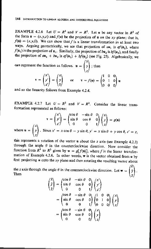
IU INTRoDUcTIoN To LINEAR ALGEBRA AND DIFFERENTIAL EQUATIoNS

o r v : ; f ( u ) :

m Example 4.2.4.

EXAMPLE 4.2.7 Let (J : R3 and v : R3. consider the linear trans_formation represented as follows:

EXAMPLE 4.2.6 Let u : x3 and, y: R3. Let u be any vector in R3 oftheform rr: (x,y,z) and/(u) be theprojection of u on the xyplane; thatis,"f(u)

: (x,.v,0). We can show thatfis a linear transformation in atleast twoways. Arguing geometrically, we see that projection of au, is a/(ur), where"/(ut) is the projection of ur. Similarly, the projection of 6u, is b/(ur), and finallythe projection of Nr r Du2 is af(u) + bf(ur) (see Fig. 25). Algebraically, we

/x\can represent the function as follows. u :

I I | ; then\z l

/"'\ /cos 0 -sin 0 0\ /x\v: l r ' ,1 : l s ino co1 g q l l r | :e (o)/r\

\z' l \ o 0 t l \ ' lw h e r e u :

l f f . S i n c e x ' : x c o s 0 - y s i n 0 , ! , : x s i n g + / c o s 0 , 2 , : 2 ,

\z/this represents a rotation of the vector u about the z axis (see Exam pre 4.2.3)through the angle 0 in the counterclockwise direction. Now consider thefunction from R3 to R3 given by w : glflif, where/is the linear transfor-mation of Example 4.2.6. In other words, w is the vector obtained from u byfirst projecting u onto the xy plane and then rotating the resulting vector about

/t\thez axis through the angle 0 in the counterclockwise direction. Let w : I ll .rhen \t)

(il :ft3 ;;T il (t):(:ti3 ;;:T ilf; iil(l: (:ti3 r*' il(i)

f; ; il'" :

( : : ) : ( ; )

and so the linearity follows fro

145

This example illustrates how two linear transformations can be composed. Inthis case, it is obvious that the composition of two linear transformations is alinear transformation. In fact, this is a special case of Theorem 4.2.6. Thisexample also illustrates the usefulness of the matrix algebra in composing acouple of linear transformations.

EXAMPLE 4.2.8 Let U be the space of all real-valued functions of the realvariable x which are continuously differentiable on the interval {x | 0 < x < l}.Let V be the space of real-valued continuous functions on the same interval.Consider the operation of differentiation. In other words, if u : f and y : g,theng(x) : - f ' (x ) fora l lxsat is fy ing0 < x S l . Obv ious ly , / is in Uandgisin Z, where Uand V arercalvector spaces. Also by a theorem from the calculus,

lafr(x) + bf2@)f' : afi(x) + bfi@)which shows the linearity.

EXAMPLE 4.2.9 Let U be the space of real-valued Riemann-integrablefunctions defined on the interval {*lo < x < D}. Let v be Rl, and let thefunction be the operation of computing the Riemann integral; that is, if a : f,then

fb

I f(x) dxJ o

, and linearity follows from a basic theorem of the calculus,

czfz@)f dx : cr t c z

Now that we have seen several examples of linear transformations, wecan begin to study some of the important properties of these transformations.

Theorem 4.2.1 The range of a linear transformation is a subspace ofthe range space.

pRooF we have to show that if v, and v, are in the range, then so isN t * bv 2 for any pair of scalars. Now if v, and v 2 are in the range, thenthere are vectors u, and u2 in the domain such that v, : /(ur) andvz : .f(az). Therefore,

N t * bY, - af(tJ + bf(ar) : f(mr * btr)

and m, * bv, is in the range because aa1 * 6u, is in the domain.

Obviously v is in Rlthat is,

fb

| [cr,f'(x) +J a ['

r,@) o*[' r,<,t,.

T46 INTRoDUcTIoN To LINEAR ALcEBRA AND DIFFERENTIAL EQUATIoNs

An important role in the theory is played by the set of vectors in the domainfor which the value of the linear transformation is 0. We call this the null spaceof the linear transformation. The null space is always nonempty since/(0) : gfor any linear transformation (see Exercise 4.Z.lZ).

Definition 4.2.3 Let f be a Iinear transformation from u to v. Thenull space of/is the set of vectors u in {/such that/(u) : 0.

Theorem 4.2.2 The null space of a linear transformation is a subspaceof the domain.

PRooF We have to show that if "f(ur) : 0 and f(ur) : 0, then

f(mt * bar) : 0. This is obvious, since

.f(mt * bur) : af(u) + bf$) : a0 * D0 : 0

Theorem 4.2.3 If the domain of a linear transformation is finite-dimensional, then the dimension of the domain is equal to the dimensionof the range plus the dimension of the null space.

pRooF By Theorem 4.2.2, the null space is a subspace of the domain,and therefore the null space is either the zero space or it has a finite basisu1, u2,..., u,. By Exercise 3.7.9, the domain has an orthonormal basisul , u2r. . . , u ' wl , w2r. . . , w", whgre r + s : n, the dimension of thgdomain. If the null space is the zero space, then there are no u's andr : 0. Let v be any vector in the domain. Then

Y : c 1 u 1 * c 2 | n 2 + . . . * c r u , * c r * r w r - F c r + 2 y 2 + . . . * c r + " w "

Since the u's are in the nul l space,,f(ur) : 0, i : 1,2,. . . , r . Therefore,

"f(v): c,*t f(w) * c,*2f(wr) +...* c,. ."/(w"). Clearly any vectorin the range can be expressed as a linear combination of/(wr), f(wr),. . .,

"f(wJ. If these vectors are independent, then they form a basis for the

range. Consider a linear combination

y r " f (w r ) + y2 f$ ) + . . . + ? " , f (w " ) : , f ( y rw r * yzwz + . . . * y "w" ) : 0

But this implies that yrw, * Tzwz + . . . * ?"w" is in the null space, andtherefore

T rwr * Tzwz * " ' + ? rW" : c1u1 * u ru2 * . . . * d ru ,

Now we use the orthogonality of the u's and the w's to show that

Tt : Tz: . . . : Is : 0. Hence,/(wr),"f(wz),. . . ," f(w")areindependent,and the dimension of the range is s. This completes the proof.

EXAMPLE 4.2.10 Find the null space of the iinear transformation ofExample 4.2.5. We represent the transformation by

(r,\ : (! 1\ r"\\v'/ U il \v)

where (x,y) is the vector before projection and (x',y') is the vector after. Tofind the null space we put (x',!') : (0,0) and solve the homogeneous equations

/0\ (+ A /'\\o/

: \i i)\r)

The null space consists of those vectors (x,y) such that x * y -- 0. This is aIine through the origin perpendicular to the line of projection, x: y. In thiscase, the range is the line x : y. The dimension of the domain is 2, the dimen-sion of the null space is 1, and the dimension of the range is l, in agreement withTheorem 4.2.3.

If there is a one-to-one correspondence between the vectors of the domainof a function and the vectors of the range, then the roles of the range and domaincan be interchanged and we shall have a new function, which we call the inuerse.

Definition 4.2.4 If /is a function which sets up a one-to-one corre-spondence between the vectors of its domain and range [for each v in therange there is precisely one u in the domain such that v :

"f(u)], then /has an inverse/-1 defined by u : "f

-t(v) when v :,f(u). The domain of

,f-t is the range of/and vice versa.

Theorem 4.2.4 A linear transformation has an inverse if and only ifthe null space is the zero space.

pRooF Suppose that the vector u : 0 is the only vector such that/(u) : 0. Suppose v is a vector in the range of / such that /(ur) :

/(ur) : v. Then 0 : "f(ur)

- f(a) :,f(ur - uz). Therefore, u1 : 12,and/has an inverse. conversely, suppose/has an inverse. If there was anonzero w such that /(w) : 0, then "f(u)

: /(u) + 0 :,f(u) + /(w) :

"f(u + w) with u # u * w. This would contradict the assumption that/has an inverse.

EXAMPLE 4.2.11 Show that the linear transformation of Example 4.2.3 hasan inverse. We represented the transformation by

(;):(:r; ;r,)0

148 INTRoDUcTIoN To LINEAR ALGEBRA AND DIFFERENTIAL EQUATIoNS

where (x,y) is the vector before rotation and (x',y') is the vector after rotation.We look for the null space when we set (x',y') : (0,0). However, the homo-geneous equations

have only the trivial solution x : !

lcos 0 -sin 0ll; ';; ;;l

: cos2 o + sin2 o : I

(3) : (:l;; ;r,)(,: 0, because

, : (:il3 ;;Ii)sin g\ /x'\

"o' e)\t')

a rotation through the

Therefore, the transformation has an If

then

A - r : / c o s 0 s i n 0 \

\-sin 0 cos 0)

, / \ /and /t) : /

cos o

\Y) \-sin o

and we have a representation of the inverse. This isangle 0 in the clockwise direction.

Theorem 4.2.5 The inverse of a linear transformationtransformation.

a linear

pRooF If /is a linear transformation with inverse/-1, then thedomain of f- 1 is the range of/and vice versa. Therefore, conditions (i)and (ii) of Definition 4.2.2 are met. To check condition (iii), let vr :.f(ur)and vz : f(az). Then f(m, * bur) : af(al + bf(a) : (N1 * bv2,andf-t(o", + bvr) : aur * blu, : af-r(v) + bf-r(vr).

We conclude this section with a definition of composition of two lineartransformations.

Definition 4.2.5 Suppose f is a linear transformation with d,omain Uand range V. Suppose g is a linear transformation with domain V andrange W. The composition f"g is defined as follows: if v:;f(u) andw : 9(v), then [/.9](u) : w. The domain of f"g is U, and the range off"g is W.

Theorem 4.2.6 The composition of two linear transformations is alinear transformation.

LINEARTRANSFORMATIONS I49

pRooF Clearly f"g is defined on all of U. Also, if U and Y aredefined on the same scalars and so are V and W, then the same is true ofU and W. Finally,

lf.gf(aut * bn2): glf(aat + 6ur)]

: glaf\t) + bf(t2)f

: aslf(a)f + bslf(\r)f: alf.sllt) + blf"sl@r)

EXERCISES 4.2

I I,et U be R2 and Y be R2. I*t /(u) be the reflection of u in the x axis; that is,if u : (x,y), then./(u) : (x,-y). Show that/is a linear transformation. Findthe null space and range ofl

2 Let U be R2 and. V be R2. Let /(u) be the orthogonal complement of u withrespect to the line x : y; that is, if z is a unit vector along the given line, then(u' z)z is the projection on the line and u - (u . z)z is the orthogonal complement.Show that/is a linear transformation. Find the null space and range ofl

3 l.et U be R3 and Y be .R3. Let/(u) be the reflection of u in the xy plane; that is,if u : (x,y,z), then /(u) : (x,y,-z). Show that f is a linear transformation.Find the null space and range of/.

4 l'et U be R3 and ltbe R3. Let/(u) be the reflection of u in the z axis; that is,if u : (x,y,z), then/(u) : (-x,-!,2). Show thatf is a linear transformation.Find the null space and range ofl

5 Irt Ube R3 and V& R3. Letl(u) be the orthogonal complement of u with respectto the plane represented implicitly by r * y + z: 0. Show that f is a lineartransformation. Find the null space and range ofl

6 Let U be C" and V & Cn. Let f(u) : an, where c is a complex number. Showthat/is a linear transformation. Find the null space and range ofl

7 Let Il : ,tR4 and Y: fi3. I-et (xex2,xs,x4) be coordinates of u relative to thestandard basis in U. Let (!ttz,ys) be the coordinates of /(u) relative to thestandard basis in V, and

l t : x 1 - x 2 * 2 x 3 - x a

lz : -x r * 2x2 - 3x3 * x4

l s - x 1 - 3 x 2 * 4 x 3 - x a

Show thatlis a linear transformation. Find the null space and range of f.8 }.et U : Cn and, Y : Cr. Let/(u) : ar. Show that/is a linear transformation.

Find the null space and mnge of f.

I5O INTRoDUcTIoN To LINEAR ALGEBRA AND DIFFERENTIAL EQUATIoNS

9 L e t u : c n a n d v : c t . L e t / ( u ) : ! r 1 - F u z * . . . * u n . S h o w t h a t / i s alinear transformation. Find the null space and range ofl

I0 Il,t U be the space of continuous real-valued functions defined on the interval{ "10 < x < 1} . Let T l f l : f@i ,O < xo < l ,wherexo is f ixed. Showthat?is a linear transformation. Find the null space and range of T.

II Find the null space and range of the linear transformations of Examples 4.2.8and 4.2.9.

12 Prove that for any linear transformation / ,f(0) : 0.13 Show that condition (iii) of Definition 4.2.2 can be replaced by the two conditions

f(au) = af(u) andf(ur * uz) :,f(ur) + ,f(uJ.14 Find the most general linear transformation from Rl to nl.15 l*t f be a linear transformation from .Rn to Rn represented bv"f(u) : Arr, where

A is n x n, rr is the column matrix of coordinates relative to the standard basisin U, and/(u) is the column matrix of coordinates relative to the standard basis inZ. Show that the following statements are all equivalent by citing the appropriatetheorems:

(a) I is nonsingular.(b) l,ql * a.(c) The null space of/is the zero space.(d) The dimension of the range of f is n.(e) I is invertible.

6 /has an inverse.(g) The columns of I are independent.(h) The rows of A are independent.(t) The equations AX : ,B have a unique solution.0 The equations AX: 0 have only the trivial solution.

16 r-etf be a linear transformation from Rn to R. represented by.f(u) : At,whereA is m x z. Prove that/is not invertible if n > m.

17 A linear transformation/is said to be onto if every vector in the range space is avalue of/(u) for at least one u in the domain. If the domain is finite-dimensional,show that / is onto if and only if the dimension of the domain is equal to thedimension of the null space plus the dimension of the range space.

18 Which of the linear transformations in Exercises I to 10 have inverses? Find theinverses where they exist.

19 rf the domain and range of a linear transformation are the same and /(u) = u,then / is called the identity transformation Show that the composition of aninvertible linear transformation with its inverse (in either order) is the identity.

2A Find the compositions of the linear transformations of Example 4.2.5 and.Exercise I in both orders. Is the operation of composition commutative? Is theoperation of composition associative?

151

4.3 MATRIX REPRESENTATIONS

We saw in many examples of the previous section that it was possible to rep-resent linear transformations in terms of matrices. This was convenientbecause we could then study the transformation using the methods developedin Chap. 2. ln fact, whenever we are dealing with a linear transformation froma finite-dimensional vector space to another we can find a matrix representation.We shall prove this fundamental theorem and then show how the various aspectsof the theory of linear transformations can be treated using matrix algebra.

Theorem 4.3.1 Let f be a linear transformation from C" to C' (orRn to R'). If X is the column matrix of coordinates of u relative to thestandard basis in (I and Y is the column matrix of coordinates of /(u)relative to the standard basis in V, then the transformation can be rep-resented by Y : AX, wherc r4 is the m x n complex (real) matrix suchthat the kth column of A is the set of coordinates of/(e*) referred to thestandard basis in Z.

pRooF Let u : xrer + xzez + ... + xoqn. Then /(u) :

xJ@t) * x2f@r) + ." * xnl(e"). Now suppose

"f(et) : artor * a2g2 + " ' * a^1e^

.f(er): at2aL * a22a2 + " ' * a^2e^

Then-f(e") : crsey * a2re2 * . . . + a^oe^

" f (u) : (anxt * apx2 +. . . * aexr )e ,

* ( a 2 p , * a 2 2 x , + . . . * a 2 n ) e , + . . .* (a^1x, * a^2x2 +. ' . * a^nxr)eo

Therefore, if/(u) : lrur I yzez + . . . * yre., then

l r : At tXt * ar2X2 *

lz : QztXt * A22X2 *

l m : A m t X t * a ^ 2 X 2 * * a^nxo

or Y - AX, as we wished to show. Clearly if the domain and rangespaces are both complex vector spaces, then ,{ will be complex. If thedomain and range spaces are both real vector spaces, then A will be real.

The proof of Theorem 4.3.1 was carried out in such a way as to illustratethat the bases used in the domain and range spaces need not be the standard

* arfrn* d2nXn

I52 INTRoDUCTIoN To LTNEAR ALGEBRA AND DIFFERENTTAL EQUATIoNS

bases. In fact, the proof would be exactly the same if we substituted the basis[ 1 , u 2 , . . . , u n f o r a L r e 2 r . . . , e n i n U a n d t h e b a s i s y r r y 2 , . . . r y ^ f o rEy 821. . . , E^ in Z. We therefore have the following theorem.

Theorem 4.3.2 Let f be a linear transformation from u to v. lf xis the column matrix of coordinates of u relative to the basis ur, u2, . . . , uoin Uand Yis the column matrix of coordinates of/(u) relative to the basisyr,y2,...,v. in v, then the transformation can be represented byY : AX, where .,4 is the m x n matrix such that the kth column of ,,rlis the set of coordinates of /(u) referred to the basis vr, y2, . . . , yoin V.

EXAMPLE 4.3.1 Let u : R2 and v: R2. Let u be any vector in R2 and/(u) be the projection of u on the line y : x in euclidean two-dimensionalspace. We showed in Example 4.2.5 that f is a linear transformation. If werefer u and /(u) to the standard basis in R2, then the transformation can berepresented by

where the first column of ,4 is f (er) and the second column of ,4 is /(er) (seeFig. 26). Clearly

r(e,): (}) r@,): (}) and

(;): ^0

A:G T)

(;;) :(l lX;)

Next let us refer the transformation to a different basis, namely u, along theline y : x and u, perpendicular to the line. Referred to this basis,-f(ur) : o,and f (ur) : 0. Thereforen the transformation can be expressed as

where (xrxr) and (ypy) are now coordinates relative to the new basis.

EXAMPLE 4.3.2 Let (I : R3 and v: R3. Let u be any vector in R3 and/(u) be the projection of u on the plane given implicitly by x - 2y * z : 0.The unit vector w: (1, -2,DlJ6 is perpendicular to the given plane, and if

LINEAR TRANSFORMATIONS 153

FIGURE 26

u : (x,y,z), then (u. w)w is the projection of u on w. Therefore, "f(u) :

u - (u 'w)w, and

"f(ut) : (1,1,1)

f(a) : (1,0,- 1)

,f(uJ : (0,0,0)

1 0 \

-?s)

"f(m, * Dut) : eltrt * bat - (mt * brt2 'w)w

: 0rrr - (aut 'w)w * ba, - (bur'w)w: af(u) + bf(at)

This shows that the transformation is linear. To find a matrix representation,

Iet us refer all vectors to the standard basis. Then

f(er): (1,0,0) - (+,-+,+) : (8,+,-+)

f(er): (0,1,0) + (+,-3,*) : (+,+,+)

f(et): (0,0,1) - (+,*+,*) : (-+'+'t)

and the transformation has the representation

/x ' \ l z + -+ \ /x \' r ' l : l + + +l lr l\ , ' t \-+ + El \z/

relative to the standard basis. Suppose we use the basis u1 : (l,l,l),

u, : (1,0,-l), us : (1,-2,1) in the domain and the standard basis in the

range space. Then

(,'):fi

(::)

and

154 turnooucrroN To LTNEAR ALGEBRA AND DTFFERENTTAL EeuArloNs

is another representation, where (u1,u2,u3) are coordinates relative to the basisu1, ll2, u, in U.

EXAMPLE 4.3.3 Let U : Po, the space of real-valued polynomials of degree3orlessintherealvariablex. Let v : ps. I fp(x) : ao * arx + azxz * atx3in Po, then we shall define a linear transformation by differentiation, namely

Tlp(*)] : at * 2arx * 3a3x2

we shall find a matrix representation of zrelative to the basis l, x, x2, x3 inU and l, x, x2 in Z. Now

7 [ 1 ] : Q : 0 ' l * 0 ' x * O ' x 2

T L { : l : l . l * 0 . r * 0 . x 2

T l * t J : 2 x : 0 ' 1 * 2 ' x * 0 . x 2

f [ t ' ] : 3 x 2 : 0 ' I * 0 . x * 3 . x 2

Therefore, the desired representation is

Now that we see the intimate connection between linear transformationsand matrices, we should try to exploit the matrix algebra in studying lineartransformations. The pertinent operations in matrix algebra are addition,multiplication by a scalar, multiplication, and inversion, each of which has itscounterpart in the theory of linear transformations.

Definition 4.3.1 Let f and g be rinear transformations from (I to v.The sum/ * s is defined bv lf + gl(u) : f(u) + g(u).

Theorem 4.3,3 The sum of two linear transformations is a lineartransformation.

pRooF since f and g have the same domain u and range space v,f + g has domain u and range space z. Hence, conditions (i) and (ii)of the definition are met. To check (iii) we have

f;:) :f; s Zil (':)

NSFORMATIONS T55

lf + gf(a\ * ba) : f(a\ * bu,) * s(mt * bar): af(a) + bf$r) * as(rrr) + bg(rr2): alf(u) + g(ur)l + blf(ar) + s$)f: alf + gl(ur) + blf + sl(ur)

Theorem 4.3.4 Let f and, g be linear transformations with finite-dimensional domain U andrange space V. If Ais the matrix representationof/with respect to given bases in U and V, and if .B is the matrix representa-tion ofg relative to the same bases, then the matrix representation of f * gi s A * 8 .

pRooF If U has dimension n and V has dimension m, then bothA and B are m x n and can be added. Let u have the coordinates Xrelative to the given basis in U. Then/(u) and g(u) have the coordinatesYt : AX and Y, - BX, respectively, with respect to the given basis in Z.Therefore, lf + 911"1 has the coordinates yl + Yz : AX * BX :(A + B)x.

Definition 4.3.2 Let f be a linear transformation from the complex(real) vector space U to the complex (real) vector space V. The trans-formation/can be multiplied by a complex (real) scalar c to give the newfunction c/defined by [c/](u) : cf(t).

Theorem 4.3.5 The function cf is a linear transformation.

pRooF Clearly cf has the same domain and range space as /.Therefore, conditions (i) and (ii) of the definition are met. To checkcondition (iii) we have

rcr)(ou'*6u') =_WM,,

Theorem 4.3.6 Letlbe a linear transformation with finite-dimensionaldomain U andrange space V. If A is the matrix representation oflrelativeto given bases in U and V, then cA is the matrix representation of cfrelative to the same bases in U and Y.

pRooF Let X be the coordinates of u relative to the given basis inu. Then Y : AX are the coordinates of/(u) relative to the given basisin z. Therefore, the coordinates of k/](u) relative to the same bases arec Y : c ( A X ) : ( c A ) X .

156 INTRoDUcTIoN To LINEAR ALGEBRA AND DIFFERENTIAL EQUATIoNs

The difference between two linear transformations can be defined in theobvious manner, combining the operations of addition and multiplication by ascalar; that is, f - g:.f + (-l)g. If f and g have matrix representationA and 8, respectively, with respect to given bases in the domain and range spaces,then the difference f - g will have the representation A + (-l)B: A - Bwith respect to the same bases.

The next theorem, which deals with the collection of all linear trans-formations from a given domain u to a given range space z, is one level ofabstraction beyond that of the basic definition of a vector space. No specialuse will be made of it in this book, and therefore it may be omitted on the firstreading.

Theorem 4.3.7 Let u and v be complex (real) vector spaces. Thenw, the collection of all linear transformations from u to v, is a complex(real) vector space. If u is of dimension n and z is of dimension *, ih"nW is of dimension nn.

PRooF To define a vector space we need two operations, additionand multiplication by a scalar. These operations in w are defined inDefinitions 4.3.1 and 4.3.2. The closure properties, Al and Ml, areverified by Theorems 4.3.3 and 4.3.5. we verify the other axioms asfollows:t

A2:lf + gl(u):,f(u) + g(u): s(u) +,f(u) : ls +,f](u)

A3: lf + (g + ,)l(u):

"f(u) + lg + ftl(u) : "f(u) + g(u) + ft(u): Lf + gl(u) + ft(u) = l(f + g) + /,1(u)

A4: The zero transformation is the transformation which takesevery vector of U to the zero vector of V; that is, 0(u) : 0 for all u in U.Clearly ["f + 011u1 : "f(u) + 0(u) :,f(u) + 0 :,f(u).

A5: The negative of/is the linear transformation -f defined by thefollowing: if /(u) : v, then [-/](u) - -v. Then tf + Gnl(u) :, f ( u ) + t - l ] ( u ) : v - y : $ f o r a l l u i n U .

Iv 2:

M 3 :

alf + gl(u): alf(u) +g(u)l :af(r)+ag(u): [a/](u) + [ae](u)

[(o + r)/](u) : (a * r)"f(u) : af(a) + bf(i: [a/](u) + [6/](u)

f By equality of two linear transformations we mean y: g if "f(u): g(u) for allu i n U .

Kab)/l(u) : (ab)f(u) : a(bf(u)) : albff(a)

tyl(u) : l ' l(u):"f(u)

To verify the statement about dimension, we note that if Uis n-dimensionaland V is z-dimensional, then for each linear transformation there is aunique m x n matrix ,{, assuming given bases in U and Z (see Theorem4.3.2 and Exercise 4.3.11). Conversely, for each m x n matrix A thereis a linear transformation f (see Example 4.2.4). Therefore, there is aone-to-one correspondence between the collection of linear transforma-tions and the collection of m x n matrices. Therefore, the vector spaceof linear transformations from U to V has dimension nm (see Exercise3.7.16).

Next we come to the correspondence between composition of two lineartransformations and the product of two matrices.

Theorem 4.3.8 Letfbe a linear transformation from the n-dimensionalspace U to the m-dimensional space Z, represented by the m x n matrix,4 wi th respect to the basis ur, u2, . . . , un in U and the basis yr ,y2, . . . ,y^

in V. Let g be a linear transformation from V to thep-dimensional spaceW,represented by thep x m matrix.Bwith respect to the basis vr, y2, . . .,v, in V and the basis w1, ry2, . . . , wp in W. Then the composition /.9has the representation BA relative to the basis ur, u2,. . . , un in U andW l , W 2 r . . . , W p i n W .

PRooF Let u have coordinates X relative to the given basis in Uand /(u) have the coordinates Y : AX rclative to the given basis in Z.If v has the coordinates Iwith respect to the given basis in V,then Z : BYate the coordinates of gft) relative to the given basis in }|/. Therefore,Z : B(AX) : (BA)X are the coordinates of g[/(u)] with respect to thegiven basis in W. But [/.g](u) : g["f(u)], which completes the proof.

Finally, we come to the correspondence between the inverse of a lineartransformation and the inverse of a matrix. By Exercise 4.2.16, a linear trans-formation from an n-dimensional vector space to an z-dimensional vectorspace is never invertible if n > m. On the other hand, even if m > n, therange cannot have dimension greater than n by Theorem 4.2,3. Therefore, ifwe wish to study the invertibility of transformations with n-dimensional domains,we may as well consider only n x n matrix representations. This does not mean,of course, that every linear transformation from an n-dimensional space to ann-dimensional space is invertible.

M4:

M 5 :

158 INTRoDUcTIoN To LIMAR ALGEBRA AND DIFFERENTIAL EQUATIoNs

Theorem 4.3-9 Letf be a linear transformation from the n-dimensionalspace u to the n-dimensional space z, represented by the n x n maftix Awi th respec t to the bases u1 ,u2 , . . . ,un in U and v1 ,y2 , . . . , v r in V .Then / has an inverse f

-t it and only if ,,{ is invertible. The matrix

representation of/- I is ,{ - 1 with respect to the given bases in u and, y.

pRooF Let X be the coordinates of u with respect to ur, t2, . . . , ro.Then Y : AX are the coordinates of /(u) with respect to the basisYL,!2,. . . , Yo. Furthermore, / is invertible if and only if the dimensionof the null space is zero. Therefore,/is invertible if and only if Ax : 0has only the trivial solution, and AX: 0 has only the trivial solution ifand only if ,{ is invertible. Now suppose ,{-1 exists. Then A-ry:A-'(An: (A-'A)X: X. Therefore, X: A-1I expresses the co_ordinates of u in terms of the coordinates of v : ,f(u). Therefore, A- | isthe matrix representation of/-l relative to the given bases in v and u.

EXAMPLE 4.3.4 Let (I : .R3 and, V: .R3. Letf(a) be the vector obtainedfrom u by first rotating u about the z axis through an angle of 90. in the counrer-clockwise direction and then through an angle of 90' in the counterclockwisedirection about the x axis. We shall find a matrix representation of / withrespect to the standard bases in U and v.

f(er) : (0,0,1)

"f(er) : (-1,0,0)

f(e) : (0,- 1,0)Therefore, / has the representation

0Now the matrix of the transformation is orthogonal and is therefore invertible.The inverse of the transformation has the representation

In the next section, we study the question of how the representation of alinear transformation changes when we change the bases in the domain andrange spaces.

:fi s )(,

(r:(l ? il(;)

LINEARTRANSFORMATIONS 159

EXERCISES 4.3

/ Find the matrix representation of the linear transformation of Example 4.2,1with respect to the standard bases. Find the representation with respect toarbitrary bases.

2 Find the matrix representation of the linear transformation of Example 4.2.2with respect to arbitrary bases.I-et U : R3 and V : R2. Let u be any vector in R3, and let/(u) be the projectionof u on the xy plane. Find the matrix representation of/with respect to the stand-ard bases.Let U be the space of real-valued polynomials of degree n or less in the realvariable x. Letfbetheoperationof integrationovertheinterval {r l0 . x < 1}.Find the matrix representation oflwith respect to the basis 1, x, x2,. . . , xn in ILFind the matrix representation of the linear transformation of Exercise 4.2.1with respect to the standard bases. Find the representation with respect to thebasis (1,1), (1, - 1) in both domain and range spaces.Find the matrix representation of the linear transformation of Exercise 4.2.2with respect to the standard bases. Find the representation with respect to thebasis (1,1), (1,- l) in both domain and range spaces.Find the matrix representation of the linear transformation of Exercise 4.2.4 withrespect to the standard bases. Find the representation of the inverse with respectto the standard bases.Find the matrix representation of the linear transformation of Exercise 4.2.7with respect to the standard bases. Find a basis for the null space of the trans-formation and a basis for the domain consisting of this basis and other vectorsorthogonal to the null space. Find a representation of the linear transformationwith respect to this new basis and the standard basis in the range space.Find matrix representations of the linear transformations in Exercises 4.2.8 and4.2.9 with respect to the standard bases in domain and range spaces.Let U : R3 and V : R3. Let A be the representation of a linear transformation/with respect to the standard bases. Which transformations are invertible? Findthe inverse if its exists.

IO

(a, ^:(i i i) (b),:(_i 1 i)1T Show that the representation of a linear transformation from a finite-dimensional

domain U to a finite-dimensional range space Zwith respect to given bases in Uand V is unique. Hint:If Y: AX and Y: BX, then 0 : (A - B)Xfor allvectors X.r-etf be a linear transformation from uwith basis u1, u2,..., uo to zwith basisy11y2t...,vn. l*t g be a linear transformation from Y to W with basis wr,w2, . . ., wr. If / has the representation A and g has the representation B with

I2

160 INTRoDUcTIoN To LINEAR ALGEBRA AND DIFFERENTHL EQUATIoNS

respect to the given bases, where A and B are nonsingular, show that (f.g)-Lhas the representation A'1 B- | .

4.4 CHANGE OF BASES

In this section, we shall again consider linear transformation with a finite-dimensional domain and range space. If we pick a basis in the domain and abasis in the range space, we shall have a unique matrix representation of thetransformation. If we change the bases in the domain and the range spaces,we shall, in general, change the representation. our purpose is to find an easyway to find the new representation. our approach will be the following.We shall first show that a change of basis in an n-dimensional vector space canbe interpreted as an invertible linear transformation from C" Io Cn orRtr to Rn,depending on whether the space is complex or real. Then we shall show thatthe change of representation of a linear transformation can be obtained bycomposing three linear transformations.

Theorem 4.4.1 Let u be an z-dimensional vector space with a basisu1, u2, . . . , uo. Let u'1, \i,. . ., uj be another basis for U, such that

u t : p ^ u i * p z f l L + . . . t p n 4 , ,t rz: przai * pzztL +. . . I pnzu' ,

u, , : Plnl t \ * Pzn\L +. . . * Pnnt lIf xis the column matrix of coordinates of u with respect to ul, n2, . . .; n1and x' is the column matrix of coordinates of u with respect toul ,aL, . . . , t r | , thenx' - px,wherepisthe n x nmatr ixwithelementsPi.;. Also, P is invertible and X : p-rX,.

p R o o F L e t u : x l u 1 * x 2 1 , + . . . * r n u n . T h e n

u : x r ( p r r u i * p z $ L + . . . + p , r u , i )* x2(prr l | * pzzlL +. . . * p,ral)+ . . . * xn(plal * pznuL + . . . * p, ,a l )

= (p r rx r * p rzxz + . . . * ppxo)a , ,* (pzf i t * pzzxz +. . . * p2nx,)al ,+ " . * ( p n r x r * p n z x z + . . . * p , n x n ) u j

: xiui + x'ru!2 + ... + xiu'^

x t 1 : p 1 1 x t * p n x z + . . . * p r n x nx L : p z $ t * p z z x z + . . . * p z n x n

Therefore,

x 'n : pn rx t * p rzxz + . . . * p roxn

161

or X' : PX. To show that P is invertible, we show that PX : 0 has

only the trivial solution X : 0. Suppose there was a nontrivial solution

( Y r , Y z , . . ' , Y n ) # 0 ' T h e n

Trur * Tz luz * . ' ' + Tnrn : 0u ' t + 0u! + " ' + Ouj : g

B u t u , , l 2 , , . . , u n i s a b a s i s , a n d t h e r e f o r e , y , : T 2 :

contrary to our assumption. Finally, solving for x in terms of x" we

have X : P- rX ' .

EXAMPLE 4.4.1 Let (I be R3, Iet ur, ll2, 13 be the standard basis, and let

lr \ ,r i tL,u! be the independent vectors (1,0,1), (1,-1,1), (1,1,-1). Find the

matrix P which represents the change of basis. Let us write

\ \ : p t r - t a , * p z r - t " , + p r r - t e r

\ L : p t z - t a , + pzz - tez * P r r - t e t

l r ' r : p r : - t a , + p r { t } , * P r r - 1 e s

Then it is clear that the first column of P-l is the set of coordinates (with

respect to the standard basis) of ui, the second column the coordinates of u!,

and the third column the coordinates of ui. Therefore,

/1 tp- ' : lo - l

u lComputing the inverse, we have

Let u

In other words,( 1 , 2 , 3 ) : 5 ( 1 , 0 , 1 ) - 3 ( 1 , * 1 , 1 ) - ( 1 , 1 , - 1 )

Theorem 4.4.2 Let {.1 be an n-dimensional real vector space with an

orthonormal basis u1e ll2: . . . , un. Let u'1, \'2,. . ., ui be another ortho-

n o r m a l b a s i s f o r ( / s u c h t h a t u , : 2 p i r o i , t : 1 , 2 , . - . , f l . T h e n t h ei = t

matrix P with elements pi; is orthogonal.

r)":€ i-i)

: (1,2,3) be a vector referred to the standard basis. Then

0):G i_l) (i) :(-r)

162 INTRoDU.TI.N To LINEAR ALGEBRA AND DIFFERENTIAL EQUATI.N'

PRooF Since both bases are orthonormal, we have the followingcomputation:

dij : (u, 'u;) P*iui ' t o,ro;)m = 7 /

PnP^i(ai'a^)

PxtP^i61r

P*iP*i

which shows that the columns of the matrix P are orthonormal vectors inRn. This is enough to show that p is orthogonal and hence that p-r : F(transpose). The corresponding theorem for complex vector spacesresults in the conclusion that P is unitary. The proof of this will be teftfor the reader (see Exercise 4.4.3).

We now come to the most important theorem of this section, which showshow the matrix representation of a linear transformation changes when wechange the basis in both the domain and the range space.

Theorem 4.4.3 Letfbe a linear transformation from the n-dimensionalvector space [/ to the z-dimensional vector space V. Let I be the matrixrepresentation of/relative to the basis ur, tr2, . . ., un in u and, the basisYr, !2, . . . , v- in v. Let P be the matrix which represents the change ofbasis in U from ul, u2,. . . , un to ui, v;, . . . , uj . Let e be the matrixwhich represents the change of basis in V from yr, y2,. . . , v, toyl, y'2, . . . , vL. Then the matrix which represents f rclative to the newbases is QAP-r.

PRooF Let X be the column matrix of coordinates of u with respectto the basis ur, u2, . . . , un, and let y be the column matrix of coordinatesof /(u) with respect to the basis vr, y2, . . . , y^. Then y : AX. Let X,be the column matrix of coordinates of u with respect to the basisu\, uL,. . . , u;. r',t Y' be the column matrix of coordinates of /(u) withrespec t t o t he bas i s v l , vL , . . . , v , ^ . Then X , : pX , X :p - r x , ,Y' : QY,and I : e-r y,. Therefoft, e-ry, : A(p-tX,) : (Ap-|;X,,and y' : (gAp- 1)X,. This completes the proof.

:[an

tn= 1

n

sZ-

m = l

tk = 1

n

k = 1

n

:k = 1

LINEARTRANSFORMATIONS 163

EXAMPLE 4.4.2 In Example 4.3.2, we considered a linear transformation ffrom R3 to R3 consisting of projection on the plane given implicitly by

x - 2y * z : 0. Relative to the standard basis in both domain and range

space, the representation oflwas

If we now change the basis in both domain and range space to (1,1,1), (1,0,- l),

(1,-2,1), we change the representation. In this case, Q : P, and

Computing the inverse, we have

The new representation of/is then

B : PAP-1 -

)

)

The case illustrated in this example will turn out to be especially important,

that is, the case where (J : V,,4 is the representation of a linear transformation

with respect to some basis u1, u2, . . . o un in both the domain and range space'

and P is the matrix which gives the change of coordinates when a new basis

ui, u'2,. . ., 4 is introduced in both domain and range spaces. The new rep-

resentation of the linear transformation is B: PAP-I. In this case, all

the matrices are n x n, where n is the common dimension of the domain and

range spaces. The transformation of an n x n matrix according to the equation

B : PAP-1 is called a similarity transformation, and we say that B is similar

to A.

(;i) :(- i il,

)

il

l l l

"-' : ll -?

":€ Iil(i It+ + +\ tz +

I t o -+l | + +\+ -+ +l \-+ *t+ + + \ l t Il+ o -+l l r o\o o 0/ u -l

l r 0 0 \

lo r o l\ 0 0 0 1

IQ INTRoDUcTIoN To LINEAR AITIEBRA AND DIFFERENTIAL EQUATIoNS

Definition 4.4.1 r-et A and .B be n x n matrices. If there exists aninvertible n x n matrix P such that .B : PAP- t, then we say that .B issimilar to A and,.B is obtained from Aby a similarity transformation.

Theorem 4.4.4t l-et A,.8, and C be n x z matrices. Then (i) ,{ issimilar to l, for all A, (ii) if ,4 is similar to B, then.B is similar to A, and(iiD if ,4 is similar to B, and,B is similar to C, then I is similar to C.

pRooF (i) The n x n identity matrix is invertible, and A : IAI-I.(iD If ,{ is similar to B, there is an invertible matrix P such that

A : PBP-| . But then.B : P-IAP : P-rA(P-t)- t .(iiD If ,4 is similar to B, there is an invertible matrix P such that

A : PBP - 1. If -B is similar to C, there is an invertible matrix Q such that

B : eCe-l. Then

A : pBp-t : p(ece-\p-L : (pe)C(e-tp- r) : ,SC,S-t

where S : Pe.

Some of the other important properties of similarity transformations aregiven by the next theorem.

Theorem 4.4.5(i) If z4 is similar to .8, then lAl : lBl.

(iD lf Ar is similar to .8, and A2 is similar to B, under the samesimilarity transformation, then Ar * A2 is similar to B, * Bz.

(iiD If ,,{ is similar to.B, then r{ft is similar to Bk under the same similaritytransformation for any positive integer k.

(iv) If ,{ is similar to B, then p(A) is similar to p(B) under the samesimilarity transformation, where p is a polynomial.f

(v) If ,,{ is similar to I and I is nonsingular, then .B is nonsingular andl-1 is s imi lar to 3-1.

PRooF (i) There exists a nonsingular matrix P such that A : PBP-\

Hence l l l : lPl lBl lP- ' l : l8l lpl lp-1| : lBl, since lplIPP-, | : l l l : l .

(ii) There exists a nonsingular matrix P such that A, :

and A2 : PBzP-I. Then

Ar * Az : PBLP-I + PB,P-L : P(Br + B2\P-1

t This theorem shows that similarity is an equivalence relation.I If ,{ and B are real, p is to have real coefficients; while if A and B are complex,

p is to have complex coefficients.

l P - ' l :

PBP-r

165

(iii) There exists a nonsingular matrix P such that A: PBP-|.

Then A2 : (PBP-\(PBP-t) : PB(P-rf1nf-L : P(BB)P-I : PB2P-L

The rest follows by induction.(iv) There is a nonsingular matrix P such lhat A: PBP-L. Let

cbe a scalar. Then cA : c(PBP-t) : P(rB)P-t. Therefore, similarity

is preserved under multiplication by a scalar. Now let p(A) : aol *

arA + arAz + ' ' ' + aoAk. Then by (ii) and (iii) of this theorem,

Pp(B)P-' =::':: :,; ;'f,:,; I :'i'::;':i,

+ arPBkP-L

(v) There is a nonsingular matrix P such that A - PBP-[. By (i),

lal : lAl + 0. Therefore, Bisnonsingular. Also A-r : (PBf-t1-r -

PB-rP- 1, showing that A- 1 is similar to B-1.

EXERCISES 4.4

1 l;lt (J : V - R2, and let,f(u) be the reflection of u in the line x : y. Find the

matrix representation of /:(a) Relative to the standard basis in both U and Z.(6) Relative to the standard basis in U and the basis (1,1), (1, - 1) in Z.

(c) Relative to the standard basis in V and the basis (1,1), (1,- 1) in U'

(d) Relative to the basis (1,1), (1,- 1) in both U and V.

2 l,et U : V : R3, and let /(u) be the reflection of u in the plane given implicitly

byx * y + z:0. Findthematrixrepresentationof/:(a) Relative to the standard basis in both U and' Y.(b) Relative to the standard basis in U and the basis (1,0, - 1), (1, -2,1), (1,1'1)

in V.(c) Relative to the standard basis in V and the basis (1,0,- 1), (1, -2,1), (l'1'1)

in U.(d) Relative to the basis (1,0,- 1), (1, -2,1), (1,1,1) in both U and V.

3 Show that the matrix representing the change of basis from one orthonormal set

to another in a complex vectoi space is a unitary matrix.

4 Consider the linear transformation of Example 4.3.4. Find a vector which is

transformed into itself. Use this vector and two other vectors orthogonal to it

and to each other as a basis. Find the representation with respect to the new basis

in both domain and range space.

S Show that if I is similar to I and I is nonsingular, then Ak is similar to Bk fot all

integers &.6 Suppose I is similar to a diagonal matrix D with diagonal elements Xr, 1",. . .o lo

s u c h t h a t l f , l < l f o r i : 1 , 2 , . . . , n . I n t p * ( A ) : I + A + A 2 + " ' * A k :

P(I + D + D2 +...+ D*)P-t, sincel : PDP-I. Consider l impl( l) . Show

16 INTR.DU.TI.N To LINEAR ALGEBRA AND DIFFERENTIAL EQUATI.NS

that this limit exists. rf we denote the series I + A + A2 +. . . by g, prove thatB: (I - A\-r. Hint: consider lim (r - A)pr@)and lim p*(A)(I - A).

7 Suppose r is similar to a diagonuii?rr,* D with ciueon"*i"Lments Ar, ).r:,,. .., An.Let

P*(A\ : r*** o4* .#

since I : PDp-r. Show that lim p*(A) exists and is equal to& + @

4.5 CHARACTERISTIC VALUES AND CHARACTERISTICVECTORS

In this section, we consider only linear transformations for which the domainis a subspace of the range space. Suppose the range space of / is a comprexvector space' and suppose there is a complex number,l, and a nonzero vectoru such that/(u) : )u. Then we say that A is a characteristic aalue (eigenvalue)of/and u is a characteristic uector (eigenvector) of/corresponding to ,1.

Definition 4.5.r Let f be a rinear transformation from the comprex(real) vector space U to Y,where Uis contained in v. Let )"be acomplex(real) number and u be a nonzero vector in U such thatf(u) : Au. Then'1 is a characteristic value ofl and u is a characteristic vector of f cone-sponding to,l..

EXAMPLE 4.5.r r-et f be the identity transformation from the comprexvector space U to U. Then "f(u)

: u, and clearly )" : I is a characteristicvalue of / with corresponding characteristic vector u * 0. Therefore, everynonzero vector is a characteristic vector ofl

EXAMPLE 4'5'2 Letf be the zero transformation from the complex vectorspace U to U. Then/(u) : 0 : 0u, and clearly 0 is a characteristic value of/

:r(,*fr*N. .#) ,-'

"f. {' ,,, j) "'

LINEARTRANSFORMATIONS 167

with corresponding characteristic vector u # 0. Therefore, every nonzero

vector is a characteristic vector off

EXAMPLE 4.5.3 Let f be the rotation from R2 to R2 of Example 4.2.3.

Since R2 is a real vector space, any characteristic values must be real. However,

it is clear geometrically that there are no nonzero vectors which are totated

into multiples of themselves unless 0 is a multiple of 180'. If 0 is an even multiple

of 180o, then every nonzero vector is rotated into itself and is therefore a

characteristic vector corresponding to the characteristic value 1. If 0 is an odd

multiple of 180", then every nonzero vector is reversed in direction and is a

characteristic vector corresponding to the characteristic value - l. For all

other values of 0 there are no characteristic values or characteristic vectors.

We can reach the same conclusions algebraically by the following method.

Relative to the standard basis we have the representation

Now if/(u) : ha, u : (x,Y), then

These equations have nontrivial solutions if and only if

[ c o s g - , t - s i n 0 |

I s i n g c o s g - , t l : 1 2 - z l c o s o * I : o

or ).: cos 0 t Jcost 0 - 1. But cos2 0 < l, and so all solutions will be

complex unless cos 0 : *1 or, in other words, 0 is a multiple of 180'. If 0 is

an even multiple of 180', then ,1 : I is the only characteristic value. If 0 is an

odd multiple of 180', then ,t : - | is the only characteristic value. In eithercase,

and so (x,y) is arbitrary, confirming that every nonzero vector is a characteristic

vector.

(^;):(Hg ;:tix,('":,'";' ;;Y)(r: (3)

(;):(n; ;;ri)(;)

f":,'";' ;;Y): (3 S)

168 INTRoDUcTIoN To LINEAR AI,GEBRA AND DIFFERENTIAL EQUATIoNS

EXAMPLE 4.5.4 Let f be the linear transformation of Example 4.2.5. Findall characteristic values and characteristic vectors ofl Here the representationrelative to the standard basis is

Ifl(u) : l.u, u : (x,y), then

(+-^\+

which has nontrivial solutions if and only if

l+-r + |l" + + - l l : )uz - ) ' : AQ'- l) : o

There are two characteristic values, 0 and l. If A: 0, the equations reduce tox + y: 0or l : -x. Hence, anynonzeromult ip leof (1,- l ) isacharacter-istic vector corresponding to l. : 0. lf )" : l, the equations reduce tox - y : 0 or x : y. In this case, any nonzero multiple of (l,l) is a character-istic vector corresponding to A : l.

EXAMPLE 4.5.5 Let U be the space of all real-valued continuous functionsof 'the real variable x with a continuous derivative. Let V be the space ofcontinuous functions of x. Let T be the operation of differentiation; that is,flf@)) : f'(x). Find all the characteristic values and characteristic vectorsof T. Let )" be real and consider the equation flf@)l : f'(x) : Lf(x).Multiplyin9by e-^*, we have

e-^Y'(x) : ),e-AY(x)

lr- ^'"f(r)f' : e- ̂ *f ' (x) - \e- tl1x1 : g

e-tY1x'1 : I

where Kis a constant. Hence,/(x) : KeL*, for K I 0, is a characteristic vectorcorresponding to the characteristic value ,1,, where L is any real number.Finally, we show that we have found all the characteristic vectors. Suppose thatcorresponding to l. there is a vector 9(x) such that g'(x) : ).g(x). Let g(0) : g.There is a Ksuch that/(0) : K : g(0) : c (for this part of the discussion K

(;):(i iX,Q):G IX'r! )(r: (s)

r69

maybezero). Nowconsiderh: f - g. Then h' : f ' - g' : l ( f - g): ) .h,

and h(0) : "f(0) - 9(0) : 0. Multiplyin gby e-^*, we have

e- ̂ *h'1x1 - Ae- ̂ 'h(x) : le- L'h(x)]' : o

ande-^*h(x): y (aconstant). Buty : 0 since/r(0) : 0. Therefore, f t(x): Q

and/(x) : g(x).

Now let us consider the case where the domain and range space of the

linear transformation are the same and of dimension n. If we use the basis

u1r u2, . . ., un in both domain and range space, then there is a matrix rep-

resentation Y -- AX, where X is the column matrix of coordinates of u with

respect to the given basis and Y is the column matrix of coordinates of /(u).Now suppose we look for characteristic values of/ Suppose/(u) : .1u. Then

Y : ),X : AX, or (A - AI)X : 0. These equations have nontrivial solutions

if and only if

lA - )"I l : co * ct l + crlz + " ' + (- l)n, l" : 0

The polynomial p(1) : co * cr)" + cr)r2 + "' + (-1)',1" is called the

characteristic polynomial of A, and the equationp(,1) : 0 is called the character-

istic equatiore. From the theory of such equations, we know that the character-

istic equation must have at least one solution and can have at most n distinct

solutions. We also know that p(,1) can be factored as follows:

p(A) : ( i t - ) , )o ' ( ) ' , - 1)o ' ' ' ' ( , - 1)o '

where 7r, )r,. . . , ), are the r distinct roots of p(1) and the positive integers

kekz, . . . ,k , are the mul t ip l ic i t ies o f 1r ,7r , . . . ,1 , , respect ive ly . A lso

k, + k, +''' * k, : n. Therefore, if we can find the factotization of p(,1),

we know all the distinct characteristic values of the linear transformation/with

representation A. If 2; is a characteristic value ofl with multiplicity kt in the

characteristic polynomial, we say that ,t; is a characteristic value with multi-

plicity k,.

Definition 4.5.2 Let A be an n x n complex matrix. Let p(1) :

lA - AII be the characteristic polynomial of l. If 1, is a root of p(1)

with multiplicity ki, then we say that ),, is a characteristic value of I with

multiplicity kr. The nontrivial solutions of (A - LI)X : 0 are called

characteristic vectors of l.

It is important to note that, according to our definition, real matrices

can have complex characteristic values (see Example 4.5.8). After all, real

I7O INTR.DUCTI.N To LINEAR ALGEBRA AND DIFFERENTIAL EQUATI.N'

numbers are just complex numbers with imaginary part zero. Furthermore, alinear transformation defined on a complex vector space could have a realrepresentation with respect to some basis, and we would definitely be interestedin the complex characteristic values of the transformation. FIowever, if thelinear transformation is defined on a real vector space, then it can have onlyreal characteristic values; and if its representative matrix A has a complexcharacteristic value, it cannot be a characteristic value of the transformation(see Example 4.5.3 for the case where g is not a multiple of lg0").

Theorem 4.5.1 Letlbe a linear transformation from the n-dimensionalvector space U to U, with matrix representation A with respect to somebasis. All the characteristic values and characteristic vectors of / can befound by finding the characteristic values and vector s of A. If U is a com-plex vector space,/will have a characteristic value ). if andonly if 2 is acharacteristic value of A. If U is areal vector space,/will have a character-istic value )" if and only if 2 is a real characteristic value of A.

PRooF The proof is included in the above discussion except for theproblem of showing that the characteristic values are independent of theparticular representation of the transformation. If we use a different basis,the representation changes to B : pAp-r, where p is nonsingular.Consider the characteristic polynomial for B:

lB - l r l : lpAp- t _ ) "pp- ' l : l r l lp- t l lA _ Ar l : IA _ ) . r l

This shows that A and B have the same characteristic polynomiar, and sothe characteristic values are independent of the representation.

EXAMPLE 4'5'6 Find all the characteristic values and characteristic vectorsof the matrix

/ 8 9A: l 3 2

\ -e -9 -rilThe characteristic equation is

l 8 - , t 9 s Il 3 2 -A 3 l : - ) .3 *| -9 -9 -10 _ ,11

3 1 + 2 : Q , + t ) ' ( 2 - , 1 ) : o

LINEAR TRANSFORMATIONS I7I

The characteristic values arc ).r: 2, with multiplicity 1, and Az : - l, withmultiplicity 2. lf )" : 1r : 2, we can find characteristic vectors by solving

orZx * 3y * 3z :0 ,x * z : O. Th issystemhasaone-parameter fami lyofnontrivial solutions of the form u : a(3,1,- 3). Therefore, we have a character-istic vector u1 : (3,1, - 3), and any other characteristic vector corresponding to)"twill be a multiple of u1. If ). : 1z : - l, we must solve the following system

or x * ! * z : O. This equation has a two-parameter family of solutions,which can be written &s u : a(1,- 1,0) + b(0,1,- l). Therefore, correspondingto ).2 we have two independent characteristic vectors trz: (1,-1,0) andu3 : (0,1,- 1), and any other characteristic vector corresponding to ,1, will bea linear combination of u, and u..

EXAMPLE 4.5.7 Find all the characteristic values and characteristic vectorsof the matrix

(; r J(l:(l)

(; ; il(l):f;)

':(i 3;)3l3 l :0 -DQ-A) ' :o

2 -11

f; !?){l:fi)

The characteristic equation is

l r - r zI 0 2 - A

lo oThe characteristic values are )., : 1, with multiplicity 1, and 1z : 2, withmultiplicity 2. If ).: lt: l, we can find characteristic vectors by solving

o r 2 y * 3 z : 0 , y * 3 z : 0 , 2 - - 0 . T h i s i m p l i e s t h a t l : z : 0 . H o w e v e r ,

I72 INTR'DU.TI.N To LINEAR ALGEBRA AND DIFFERENTIAL EQUATI.NS

.x is arbitrary, so any vector of the form u : a(1,0,0) is a characteristic vectorcorresponding to )., if a * 0. If )" : Az : 2, we must solve

/-I 2 3\ /x\ /0\

I o o r l {r l : (o}\ o 0 0l \zl \o/

o r - x * 2 y + 3 2 : 0 , z : 0 . T h e r e f o r e , x : 2 y , a n d w e h a v e a o n e _parameter family of solutions of the form u : a(2,1,0). Hence, any character_istic vector corresponding to ,12 will be a multiple of (2,1,0).

EXAMPLE 4.5.8 Find all the characteristic values and characteristic vectorsof the matrix

The characteristic equation is

,:(l -?)l r_^ _z l :I I - r - ^ l : ^ ' * l :Q ' - i ) (A * i ) : g

The characteristic values are )., : i and Az : - i. If ). : trr : i, we mustsolve

( r - i -2 \ f4 : /o \\ r - t - i ) \ r / : \ o /

or .x : (l + t)y. Therefore, characteristic vectors corresponding to )", arcofthe form u : a(l + i, l), a * 0. lf ). : )rz : -i, we must solve

( r l i _2 \ / " \ /o \

\ r - t+ i ) \ r / : \o /

or .x : (l - t)y. Therefore, characteristic vectors corresponding to l, arc oftheform u : a(l - i, l), a * 0.

Let us return to Example 4.5.6. we found a set.of three independentcharacteristic vectors u1 : (3,1,-3), uz : (1,-1,0), and u, : (0,1,_l). I*tus assume for the moment that the matrix

/ 8 e e \n: l3 2 3 l

\ -s -9 -r0l

is the representation of a linear transformation from R3 to R3 relative to thestandard basis. Suppose we introduce the basis ur, u2, u3. we wish to find the

representation of / relative to this basis. Since 11, u2, u3 are characteristicvectors, we have

" f ( u t ) : l r u r - 2 u t

"f(ur) : Aztz - Our

"f(us) : Azu't - 0u1

Therefore, the representation we seek is given by the matrix

* 0u, * Out

u2 * 0u3

* O u r - u 3

0\ol

- r l

see from

/ 2 0

" : l0 - l\ 0 0

which is diagonal. This is not just a coincidence, as wetheorem.

the next

Theorem 4.5.2 Letf be a linear transformation from the n-dimensional

space U to U. Then/has a diagonal representation if and only if f has n

independent characteristic vectors.

pRooF Suppose relative to the basis ur, 12, . . . , tn, .f has the

representation matrix

0120

0013

where the l,'s are not necessarily distinct. This means that/(ur) : lrur,

f(u) : l2\2,. . .,"f(uJ : lntn, which means that 11, u2, . . ., u, arecharacteristic vectors corresponding to the characteristic values 2r,1r, . . ,, in. Conversely, suppose tt1, u2, . . . , un are independent character-istic vectors corresponding to characteristic values ),y )r2,. . . , in (notnecessarily distinct). We obtain the representation relative to ur, 12, . . .,un as a basis.

"f(ur) : lrllr : /,1u1 * Ouz -F "' * fun

f(ur) : I2u.z : 0u1 * ) ' ru2 * ' ' ' ' I Oun

f(an) : )",r to: Our * ou2 * " '* loan

and so the representation is diagonal.

I74 NTRoDUCTIoN To LINEAR ALGEBRA AND DIFFER-ENTIAL EQUATIoNs

Theorem 4.5.3 Letf be a linear transformation from the n-dimensionalspace U to U. Then/will have a diagonal representation if/has n distinctcharacteristic values.

pRooF Let the distinct characteristic values be ).r, )",. . . , )"n andthe corresponding characteristic vectors u1, u2,. . . , un. we shall showthat the u's are independent. suppose that the u's are dependent. Thenthere is an independent set [1, tr2, . . . , uft such that

U&+i : cru l * c2u2 *

k: l*+rf lr+r : \ c;f( t tr \ :

j = r

).r*piu1; subtracting, we have

" ' * cpu*and

"f(u** t)

k

AIso .l** 1u&+ 1 :j = l

k\ . .z ^jcjrrjj = r

0 : j c / ) . i - t r 1 * r ) u i' l = 1

B u t , l , * L r + t j : l , 2 , . . . , k , a n d s o c t : c 2 : . . . : c k : 0 b e c a u s eul, u2, . . . , ur are independent. Therefore, u&+ 1 : 0, which is clearlyimpossible since u**, is a characteristic vector. Hence, ttl, 12,..., unare independent and the theorem follows from Theorem 4.s.2.

EXAMPLE 4.5.9 Letf be a linear transformation from a three-dimensionalreal vector space u to u. suppose relative to some basis ur, lr2, u3,/has therepresentation

/ 9 - 3 0 \n: l - t n -31

\ o -3 e lFind, if possible, a diagonal representation forl We look for the characteristicvalues of l. The characteristic equation is

l g - t -3 o I|

- l n - 1 -3 | = (6 -,rxe -,rxr5 - t) : oI o _3 e_11

The characteristic values are A1 : 6, 1z : 9, |t: 15. They are real anddistinct. Therefore, by Theorem 4.5.3, there is a diagonal representation

/ 6 0 0 \o:{o s o l

\o 0 rsl

LINEARTRANSFORMATIONS I75

Let us find the basis (characteristic vectors) relative to which this is the rep-resentation. lf 1 - lt : 6, we must solve

(i : il0:(l)Ot x - l :0 , 1 t - z :0 . In Other Words, x : / : z Z lnd a character is t icvector is v, : u1 * u2 * u:. If )" : 1z : 9, we must solve

ory :0 ,x * z :O,andacorrespondingcharacter is t icvector isy , : r l r - ur .If ), : 1z : 15, we must solve

or 2x * y : 0, x * y * z : O. A corresponding characteristic vector isY 3 : u l - Z a r * u s .

In Example 4.5.7, we had two characteristic values and only two indepen-dent characteristic vectors in R3. Therefore, it will not always be possible tofind a diagonal representation. On the other hand, Example 4.5.6 illustratesthat there may be n independent characteristic vectors even when there are notn distinct characteristic values. Hence, Theorem 4.5.3 gives a sufficient but notnecessary condition for a diagonal representation. In the next section, we takeup a couple of special cases where it will always be possible to obtain a diagonalrepresentation.

EXERCISES 4.5

1 Find the characteristic values and characteristic vectors of the following matrices:

(b) (; l) (c) (l l) @) (-:

(: i il(l:

(-; -ti(l:(

(a) (l ) i)

176 INTRoDUcTIoN To LINEAR ALGEBRA AND DIFFERENTIAL EQUATIoNs

2 Find the characteristic values and characteristic vectors of the following matrices:

(a)f;;il @,tr ; ilLetU: V: l t2,andlet/(u)bethereflect ionof uinthel ine y _ _x. Findal lthe characteristic values and characteristic vectors ofl Find a representation of/which is diagonal.Let u : v : R3, and let/(u) be the projection of u on the plane given implicitryby x * 2y - z : 0. Find all the characteristic values and characteristic vectorsofl Find a representation of/which is diagonal.Let U : V = R3, and let / be a linear transformation with the representationmatrix relative to the standard basis

Find a basis with respect to which the representation is diagonal.If ,t is a characteristic value of a square matrix l, show that An is a characteristicvalue of An, wheren is a positive integer.Show that a square matrix I is invertible if and only if ).: 0 is not a characteristicvalue of l.Show that if ,1 is a characteristic value of an invertible matrix A, then 2-1 is acharacteristic value of A-1.rf I is a characteristic value of a square matrix l, show that 13 - 3Az + ). - 2is a characteristic value of A3 - 3Az + A _ 21.It p(x): 0 is the characteristic equation of the n x n matrix A and A has nindependent characteristic vectors Xr, Xz, . . . , Xn, prove that p(A) : O. Hint :Show thatp(A)X1 : 0 for f : 1, 2,. . . , f l .Show that if u1, u2,. . ., ur. are a set of characteristic vectors of a linear trans-formation / corresponding to the same characteristic value ,1, then they span asubspace s such that for any u in ^s,/(u) .- ,lu. Note: such subspaces are calledinuariant subspaces.Let / be a linear transformation from (J to u, where u is n-dimensional. Showthat/has a diagonal representation if and only if the sum of the dimensions ofits invariant subspaces is n.suppose we want to find a matrix c such that c2 : A. (c might be called asquare root of l.) suppose I is similar to a diagonal matrix B with diagonale lements Lr lz , . . . ,An, wi th . t rs r 0 . Then B: pAp- l . Let D be a d iagonal

(c) (-; i:)(d) f; r il (e, (; i il

| 4 -20 -10\I : (-: -ls -,1)

10

IT

12

I3

LINEAR TRANSFORMATIONS I77

matrix with diagonal elementsC : P-IDP. Show that C2 :

14 Solve the following system of equations:dx

d r : 2 * * Y

d Y - x + 2 y

dt

Hint: Letu: f ^f

, and write theequations asduldt: An. FindPsuch that\ v l '

v: pu. Hence, p-L dvldt: (Ap-r)vand,dvldt: (pAp-r)v. I f

PAP-L: ( f : , )then the equations are separated.

15 Solve the following system of equations:

3 x * z

3 y + z

x * y * 2 2

16 Consider the differential equationd2x

a* -

Look for solutions of the form x : e^'. Show that I must be a root of theequation A2 - 31 - 4 : 0. Show that the given equation is equivalent to thesystem dxldt - y, dyldt : 4x * 3y. Compare with Exercise 14.

4.6 SYMMETRIC AND HERMITIAN MATRICES

We saw, in the last section, that an n x n matrix is similar to a diagonal matrixif and only if it has n independent characteristic vectors. We also saw squarematrices which are not similar to diagonal matrices. In this section, we shallstudy two types of matrices, real symmetric and complex hermitian, which arealways similar to diagonal matrices. We shall begin with real symmetricmatrices.

LJi , : 'J )o, . . . , tJ , r , . rn .n B: D2. LetA. Use this method to find square roots of

l r 2 l \t l4 : l 0 2 r l\ 0 0 3 1

d * _

dt

d y _dt

d r _

dt

3 4 - 4 x : odt

I78 INTRoDUcTIoN To LINEAR ALGEBRA AND DIFFERENTIAL EQUATIoNs

Definition 4.6.1 An n x n matrix I is symmetric if A : i.

Theorem 4.6.1 AII the characteristic values of a real symmetric n x nmatrix A are real.

PRooF Let X be a characteristic vector of ,4 corresponding to thecharacteristic value ,1. Then, if the bar stands for a complex conjugate,

A X : A XAX : I"X

X , q X : X " X X : X

f r ,qx: ) " f tx :1Subtracting, we have

sineffi : ftAx.the theorem.

Theorem 4.6.2 characteristic vectors corresponding to differentcharacteristic values of a real symmetric matrix A arc orthogonal.

PRooF Let xt and x, be characteristic vectors corresponding tocharacteristic values )"i and,t;, where Ii * Ai. we can assume that x,and X, are real since I and,1, and ),, are all real. Then

AXt : ;rY,

AXi : AiXi

X,AX, : ),,X,X, :Xr,lx, : ).iXrx, :

where (Xt.Xj) is the scalar product of X, and X,.XiAXi, we have

(4, - ),)(xt. x) : 0But ,1, - li * 0 and hence, (Xi. X) : O.

Theorem 4.6.3 If a linear transformation f from R" to R, has a rep-resentation A with respect to the standard basis which is symmetric,then there is an orthogonal matrix P such that the representatian pAF : Dis diagonal, with diagonal elements the characteristic values of A.

tk = l

n

s/-k = L

l*ol '

lxnl '

(1 - X) j I'ol, : rtAX - XAX : ok = 1

n

Therefore, since ) lxol' > 0, )" :,T, which provesk = l

).i(xt. xj)

A j ( X t . X j ).?

Now since XrAX, :

representationis

/, o o o\

I o b , b ^ b r ^ |B :RAR: [O b , b * b to

I\ " " " " ' I\

b,z bns b,"/

/^' o o \lo / \ I:[o / ' . \ I\ \)l

B is symmetric since E : m. : RAfr'. The matrix .B* is (n - 1) x

(z - 1) and is real and symmetric. By the induction hypothesis there is an

orthogonal change of basis in S, represented by Q*, which diagonalizes

.B*. Therefore,

LINEARTRANsFoRMATIoNS 179

pRooF We prove the theorem by induction on n. If n : l, A is

already diagonal and P : I. Let us assume that the theorem is true for

all spaces of dimension up to and including n - l. Let X1 be a unit

characteristic vector corresponding to the characteristic value ,11 (,'{ has

at least one characteristic value, and it is real). Then AXL : AtXt.

Let S be the subspace of Rn orthogonal to Xr. ,S has a basis Zz, Zr, . . . o Zn,

which we can assume is orthonormal. The change from the original basis

(with respect to which the representation is z4) to the basis Xy Zz, 23, . . . ,

Zo is via the orthogonal matrix R. With respect to the new basis the

Q*B*8 :

l) x @ - 1) diagonal matrix. Now consider

Q is orthogonal since Q* is orthogonal, and

eBQ : e(RAnA : (eR)A(ffi) : PnF

)"2

0

0

i s a n ( n -matrix

0 0

t)

180 INTRoDUcTIoN To LINEAR ALcEBRA AND DIFFERENTIAL EQUATIoNS

_ R _ , Q _ , :

0 0which proves the theorem.

Theorem 4.6.4 If a linear transformation/from (I to (1, where U is ann-dimensional real vector space, has a representation matrix ,{ which issymmetric, then/has a diagonal representation with respect to n indepen-dent characteristic vectors.

pRooF Let u1, u2,. . ., un be the basis with respect to which therepresentation matrix is l. Let u: x1u1 * x2a, +... * xoun. Thenx, the column matrix of coordinates of u, is in Ro. Therefore, we can viewthe transformation as a transformation from Rn to Rn. Hence, Theorem4.6.3 applies. If PAF : D, D diagonal, then AF : FO andthe columnsof P are characteristic vectors of A. They are independent since F isorthogonal. Hence, ,{ has n orthonormal characteristic vectors. Suppose(x'r, xL,. . ., x;) is a characteristic vector of A. Then v : x'rul +x\t2 * .'. + xjuo is a characteristic vector of f. Therefore, / has in-dependent characteristic vectors, and, using these vectors as a basis, wehave a diagonal representation forl

EXAMPLE 4.6.1 Letf be a linear transformation from the three-dimensionalreal vector space U to U with the representation matrix

with respect to the basis ur, uz, u3. Find a basis with respect to which therepresentation of/is diagonal. The characteristic equation of ,,{ is

l t - t - t6 -8 IlA - l l l : I

-16 7 - 1 8 | : - ) ,3 + 912 + 4051* 2,187 : 0

l - 8 I - 5 - , i l

The characteristic values arc ).1 - 27,12 : ls - -9. To obtain a character-istic vector corresponding to .1, we must solve (A - I.DX : 0 or 5x * 4y *

where P : QRRA -- fr: p.

P-r = (0R)-tBQ, and we find

0 0l z o0 h

is orthogonal,Now we multiply

QBO .

srnce

out Q

(

l 7 - t 6,e : l_ rc 7

\ - 8 8

LINEAR TRANSFORMATIONS I81

2z :0,4x * 5y - 2z: 0. Asolution is(2,-2,-1). Toobtaincharacteristic

vectors corresponding to ]'z: )'z - -9, we must solve ("{ - )'21)X: 0' or

2x - 2y - z : 0. One solution is (1,0,2). Another solution orthogonal to the

first is (4,5,-2). Notice that both these vectors are orthogonal to (2, -2,-l).

A set of independent characteristic vectors of/is

Y r : 2 u 1 - Z t t z - u 3

y z : u , * 2 u .

y3 :4tr1 * 5u, - 2u,

with respect to these vectors as a basis the representation of/is

/27 0 0\t l

B: l 0 - 9 0 f\ 0 0 - e l

Next we consider the case of hermitian matrices, where the situation is

quite similar.

Definldon 4.6.2 An n x n matrix ,{ is hermitian if A : fr.

Theorem 4.6.5 All the characteristic values of a hermitian n x n

matrix A are real.

pRooF Let Z be a characteristic vector of ,{ corresponding to the

characteristic value ,1. Then if the bar stands for a complex conjugate'

A Z : A Z

dz :122AZ:1ZZ: I> l r * l '

& = 1

2Az:1"22 :s , fEoPk = l

Subtracting, we have

(,i - I) i lrrl' : 2Az - ZAZ : 0& = 1

,in"e ffi : Liz : 2Az. Therefore, since i l"*l' t o, )' : r,which proves the theorem. k=r

Theorem 4,6.6 Characteristic vectors corresponding to different

characteristic values of a hermitian matrix A arc orthogonal.

182 INTRoDUcTIoN To LINEAR ALGEBRA AND DIFFERENTIAL EQUATIoNS

PRooF Let Zi and Zt be characteristic vectors corresponding tocharacteristic values ,t; and l;, where h * Ai. Then

AZt : 7'7'

AZt : ltTt

Z, , lz , : L i (Zi 'Z i )

ZtAZi : Ai(zi 'zi)

where (2,' z) is the scalar product of Z, and Zr. subtracting, we have

(L - I;)(Zt' Zi) : Z,,tZ,' Z,AZ, : g/.-/

sinceZiAZ. : ZiZZi : 7iAZ,. But )r, - ^i # 0and hence, (Zi. Zi) :0.

Theorem 4.6.7 If a linear transformation / from cn to cn has a rep-resentation ,,4 with respect to the standard basis which is hermitian, thenthere is a unitary matrix P such that the representation pAF : D isdiagonal, with diagonal elements the characteristic values of A.

pRooF The proof will be left to the reader. It can be done as aninduction on n very much like that for Theorem 4.6.3. The reader shouldmake the necessary changes in that proof.

Theorem 4.6.8 If a linear transformation/from (J to u, where u is ann-dimensional complex vector space, has a representation matrix ,,{ whichis hermitian, then / has a diagonal representation with respect to nindependent characteristic vectors.

pRooF The proof will be left to the reader.

EXAMPLE 4.6.2 Show that the matrix

is similar to a diagonal matrix with real elements. ",{ is hermitian since A : A.Therefore, Theorem 4.6.7 applies. The characteristic equation of ,,{ is

tA - ̂ rt:12

^: (_?,i ilr l

/ ' 0 l : - l ' ( l - l x , t - 3 ) : 0I - , t l

- 1

LINEAR TRANSFORMATIONS 183

The characteristic values are A, : 0, 1z : l' 1z: 3' To find a characteristic

vector corresponding to /"1 we must solve AZ : 0,

/ 2 t t \ /zt \ /0\

{-; ' ol {"1 : {91\ - i o UV ' l \o /

o r Z z t * i z r * i z r : g , - i z 1 * z z : 0 ' A s o l u t i o n i s u r : ( l ' i ' i ) ' W emust solve

/ | i f\ /21\ 10\

f -; o oll, ' , l : lgl\-; o ol \r'l \o/

corresponding to ) '2, ot zt :0, z2 * z3:0 ' A solut ion is u ' : (0 ' l ' - l ) '

We must solve

l-r i i \ /21\ /0\l -r -z ol l" l : lgl\-; o -21 \',1 \o/

c o r r e s p o n d i n g t o 1 3 , o t z r - i z 2 ^ i z z : O , i z t * 2 z r : g ' A s o l u t i o n i s

u, : (2l,l,l). If we normalize 1t1, lr2, and u' and place them in columns, we

have a unitary matrix

p - 1 _

tilTfl:(l til

ffi1

-V 3

0

2i--F

V 6

and its inverse

P _

The diagonal matrix similar to ,,4 is

PAP_I

184 INTRoDUCTIoN To LINEAR ALGEBRA AND DIFFERENTIAL EQUATIoNs

We conclude this section with a couple of applications of the similarityof symmetric matrices to diagonal matrices. The first of these is in the study ofquadratic forms. The most general quadratic form in two real variables is

q(x,y): ax2 * 2bxy * cyr.If we let X: f") and, Abe the real matrix\ry, n : ( o 6 \

Vc /then we can write q(x,y) : XAX. By analogy we shall define the generalquadratic form in n real variables as q(xr, x2,. . ., xn) : XAX,where A is areal symmetric matrix. Since A is rcal and symmetric, Theorcm 4.6.3 appliesand there is an orthogonal coordinate transformation y : px such thatPAF : D is diagonal. We have X: Fland

Q(xr, x2, . . . , xn) : XAX : VI7.AFSY : tDY: ) , t !r2 * 1z/22 + " ' * 1n!r2

where Ar, 1r, . . . , ln are the characteristic values of A. we have reduced thequadratic form to diagonal form.

EXAMPLE 4.6.3 Identify the figure in the xy plane defined by the equationx2 + 4xy - 2y' : 6. We have a quadratic form q(x,y) : xz *-4xy -2yt : X,qX: 6, where

A:G _)The characteristic equation of ,4 is

I r - , rlz -z : ( -2 )e ,+3)

The characteristic values are )., : 2, 1z :change of coordinates to (x',y') is

The diagonal form after the

q(x,y) : 2(x')2 - 3(y')' : 6

( x ' ) ' _ ( y ' ) ' _ ,3 2

This is the equation of a hyperbola. To locate the axes of symmetry of thehyperbola we must examine the coordinate transformation x' : px, wherethe rows of P (columns of F) are the normalized characteristic vectors u1 andu, of I corresponding respectively to )", and ).r:

",: (*,+J and { I 2 \u z : [ - t = ' E l\ VS '/s/

LINEARTRANSFORMATIONS I85

FIGURE 27

The coordinate transformation is

(;) :

wherecos g : ZIJ Sand sin 0 : l lJ5, or 0 : tan-1 .t isin thefirst quadrant.

The positive x' axis makes an angle of 0 with the positive x axis and points in

the direction of ur. The positive y' axis points in the direction of ur. These

directions serve to locate the given hyperbola (see Fig. 27).

The second application is to the solution of certain systems of differential

equations. Let X(r) be a column matrix with elements xr(t), xz!),. . ., xn(t).

Consider the system of differential equations X' - AX, where ,4 is real and

symmetric and the prime refers to differentiation with respect to r. We wish to

find a solution such that X(0) : Xo, u given column matrix' We make a

coordinate transformation ts - PX, where P is independent of f. Then I' :

pX,, X, - p-Ly, : AP-IY, and y' : (PAP-t)f . By Theorem 4.6.3, there

is a P such that PAP-t - D, a diagonal matrix. Hence, the new system is

dv , ^ dv " dv " t

; : l t t " r ' ; : A z l z ' " ' ' ; : A n l n

where Ar , l r , , . . . , lnarethecharacter is t icva lues of A. Aso lu t ion is .yr - cLex" ,

lz : cz€x"r. . . , ln -- cnel" ' , ot

/2 r \( f i')o:(:T.', x;x)f7; Ts/

(l'::)X(t ) : P- r crel t 'X, * c2e[ ' tX, + " ' + cnel" tXn

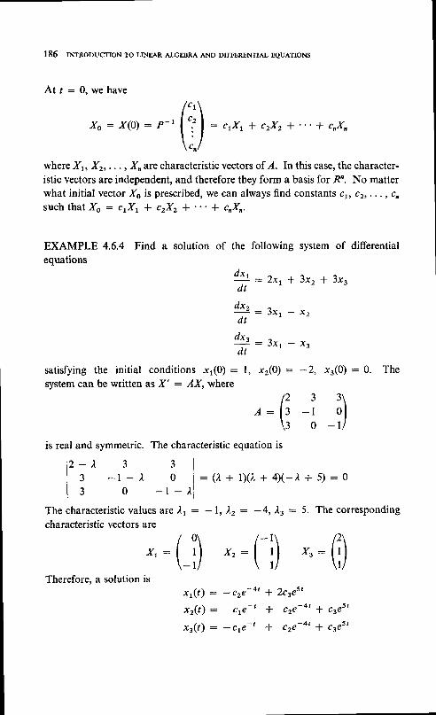
186 INTRODUCTIoN To LINEAR ALGEBRA AND DIFFERENTHL EQUATIoNS

At t : 0, we have

/ t t \

xo : x (o ) : P - ' ( t : l : c r x ' * c r x2 * " ' * c , x ,

\ t^ /

where Xr, Xr, . . . , Xnare characteristic vectors of ,4. In this case, the character-istic vectors are independent, and therefore they form a basis for R'. No matterwhat initial vector Xo is prescribed, we can always find constants cr, c2, . . . , c,such that Xo : ctXl * c2X2 * "' * cnXn.

EXAMPLE 4.6.4 Findequations

a solution of the

dx,

dt

dx,

dt

dx,

d t

following system of differential

- 2xr * 3x, * 3x,

-- 3x1 - x2

satisfying the initial conditions xt(O) : 1,system can be written as X' - AX, where

: 3 x r - x s

xr(O) : -2,

/ 2 3A: 13

- l\ 3 0

x:(0)

n: Q. The

is real and symmetric. The characteristic equation is

l z - t 3 3 |l 3 - l -1 0 l : ( r+1x ,2 '+4x- ,1 +5 ;=gI I o - t - , i l

The characteristic values are .1, - - l, )Lz : -4, Is : 5. The correspondingcharacteristic vectors are

/ 0\ /- 1\ /2\Xt: l t l xz: l t l

" . : l t l\ _U \ I / \UTherefore, a solution is

x r ( t ) : - c z € - n ' * 2 c r e s '

x r ( t ) : c t € - t + c 2 e - 4 ' * c a e s t

x . ( r ) : - c r € - t + c 2 e - 4 ' + c r e s t

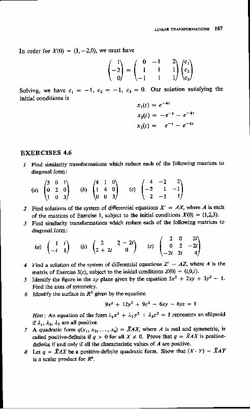
In order for X(0) : (1, -2,0), we must have

Solving, we have cL : -1, c2

initial conditions is

(a) (-l i) (r) (,'* ,, '-,\

LTNEARTRANsFoRMATIoNs 187

I 0 -l 2\ /c'\: l r I t l l" l\ - l I U \csl

cr : 0. Our solution satisfying the

x1(t) : s-+t

x z ( t ) : - e - t - e - 4 '

x r ( r ) : e - t - e - 4 t

(c,(riil

(il- - l ,

f;;il

EXERCISES 4.6

/ Find similarity transformations which reduce each of the following matrices to

diagonal form:

(a)flil (b)Find solutions of the system of differential equations X' : lX, where .,4 is each

of the matrices of Exercise 1, subject to the initial conditions X(0) : (1'2,3).

Find similarity transformations which reduce each of the follorring matrices to

diagonal form:

(c, (; i t;)Find a solution of the system of differential equations Z' : AZ, whete I is the

matrix of Exercise 3(c), subject to the initial conditions Z(O\ : (r,0'f).

Identify the figure in the xy plane grven by the equation 3x2 + 2xy * 3y2 : 1'

Find the axes of symmetry.Identify the surface in R3 given by the equation

9x2 + l2y2 + 922 - 6xY - 6Yz : I

Hint: An equation of the form )rrx2 * )uzy2 * ).s22 : I represents an ellipsoid

if 11, A2, ls arc all positive.A quadratic form q(xv x2,.- ., x) : XAX, where A is tf\fll and symmetric, is

calledpositive-definiteif q > Oforall X + O. Prove thatq: XAX ispositive-

definite if and only if all the characteristic values of z{ are positive.

I*t q - fr,eX ue a positive-definite quadratic form. Show that (X ' Y) : X.lY

is a scalar product for Ro.

rc

188 INTR.DU.TI'N To LINEAR ALGEBRA AND DIFFERENTIAL EQUATI.NS

A hermitian form h(zv 22,..., z) - 2Az, where r is hermitian, is calledpositive-definiteif ft > Oforall Z + O. prove thath: ZAZispositive-definiteif and only if all the characteristic values of A are positive.l*t Z,eZ be a positive-definite hermitian form. Show that (21 . Zr) : ZreZ, isa scalar product for Cn.

*4.7 JORDAN FORMS

Theorem 4.5.2 gives necessary and sufficient conditions for an n x n matrixto be similar to a diagonal matrix, namely that it should have n independentcharacteristic vectors. We have also seen square matrices which are similarto no diagonal maiiix. In this section, we shall discuss the so-call ed Jordmcanonical form, a form of matrix to which every square matrix is similar. TheJordan form is not quite as simple as a diagonal matrix but is neverthelesssimple enough to make it very applicable, particularly in the solution of systemsof differential equations.

Before we embark upon the discussion of Jordan forms, it will be con-venient to introduce the concept of partitioning of matrices. Suppose we write

u: (A r \\C Dl

where I is an m x nmatrix, Bis an m x pmatrix, cis a q x nmatrix, andD is a q x p matrix. In other words, M is an (m + q) x (n * p) matrixpartitioned into blocks of matrices so that each block in a given row has thesame number of rows and each block in a given column has the same numberof columns. The reader should convince himself that the following productrule is valid for partitioned matrices. Let

p :

A nAzz

Ar ,Az,

BrzBzz ni)

Bnp/

(:

L L

2 t

Bnz

1

iI

BL

i:Bn

Q :

A^z A-o

/cA cn cro\

pe : l"^ Czz

"rolt " ' " " " " ' f\C-r C^z C^o/

where Crj : ZrA*Boi provided p and e are partitioned in such

lr* has the same number of columns as 8*, has rows for all i, j, and

m l

a way that

k.

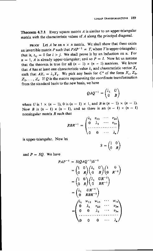
LINEARTRANSTORMATIONS 189

Theorem 4.7.1 Every square matrix r{ is similar to an upper-triangular

matrix with the characteristic values of ,,4 along the principal diagonal'

pRooF Let A be an n x n matrix. we shall show that there exists

an invertible matrix P such that PAP-1 - T,where Iis upper-triangular;

t h a t i s , ' , j : 0 f o r i > j . W e s h a l l p r o v e i t b y a n i n d u c t i o n o n ' , . F o rn : l, r{ is already upper-triangular; and so P : I. Now let us assume

that the theorem is true for all (z - l) x (n - 1) matrices. We know

that A has at least one characteristic value )4 and characteristic vector xt

s u c h t h a t A X r : l r X r ' W e p i c k a n y b a s i s f o t C n o f t h e f o r m X t ' 2 "zr, . . . , zn. If Q is the matrix representing the coordinate transformation

from the standard basis to the new basis, we have

/ t u \QAQ- t : ( ?

\ - BJ

w h e r e U i s l x ( n - l ) , O i s ( t r - 1 ) x l , a n d ' B i s ( n - l ) x ( n - l ) '

Now .B is (n - l) x (n - l), and so there is an (n - l) x (n - l)

nonsingular matrix R such that02,

u3n

In0 0

: (

,,.)

12 Dzs

o )"3,RBR-1

is upper-triangular. Now let

and P : SQ. We have

PAP_T :

':(l x)

"o-r)xlfi-l)

: : :

UB

UB

:,)-/

l { r r

0z l

)""

t 3

2 3

3

)sh t

0

1r0

r - I

f - ' ) ,

)(1)(1UR'R.BR

Q_',

XX

URRB]

S(QA(

(il(li(tr

: (

wtz

12

0

I9O INTR'DU.TI.N To LINEAR AIGEBRA AND DIFFERENTIAL FQUATI.NS

since 7 is upper-triangular, its characteristic values are ).r, xz,. . . , ro.But.,{ has the same characteristic values. This completes the proof.

Theorem 4.7,2 Every square matrix r{ is similar to an upper-triangurarmatrix of the form

where each r, is upper-triangular with diagonal elements /,,, the order of?r is the multiplicity of /., as a characteristic value of l, and k is the numberof distinct characteristic values.

pRooF Theorem 4.7.1 tells us that ,{ is similar to an upper-triangularmatrix. In fact, we can assume that there is a p such that

PAP_I

where zii is upper-triangular with ail of its diagonal elements l;. Theorder of Tii is the multiplicity of ,l,s as a characteristic value of A, and)'r, )'2, - . . , 1o are all distinct. This assumption is justified by the proofof rheorem 4.7.1. clearly we can place any characteristic value ,1, in theupper left-hand corner of ?. If ,1, has multiplicity greater than l, we canplace ,l,t in the upper left-hand corner of R.BR-r. If ,1,1 has multiplicitygreater than 2, we place it again in the third position along the diagonal?. This process can be repeated as many times as the multiplicity of ).r,then with ).2, ).r, etc. consider a given nonzero element t* for p < i,.Let Q : I * c, where c is a matrix all of whose elements are zero exceptthe (p,q)th element, which is c. The inverse of e is e-r : I - C. If wemultiply out QTQ- 1, w€ find that the element too has been changed totpq - c(ton - tuo). lf trn - too * 0, we can choose c so that the (p,q)thelement is now zero. otherwise the transformafion ere-r affects onlythe elements in thepth row to the right of t*andin the gth column abovetpq. By using a finite sequence of such similarity transformations we canreduce T to the form required by the theorem.

T r oo T 20 0

00

T:0 Tk

000

) : '

0 0

Tto

Tt*

Too

Trt T:0 r ,

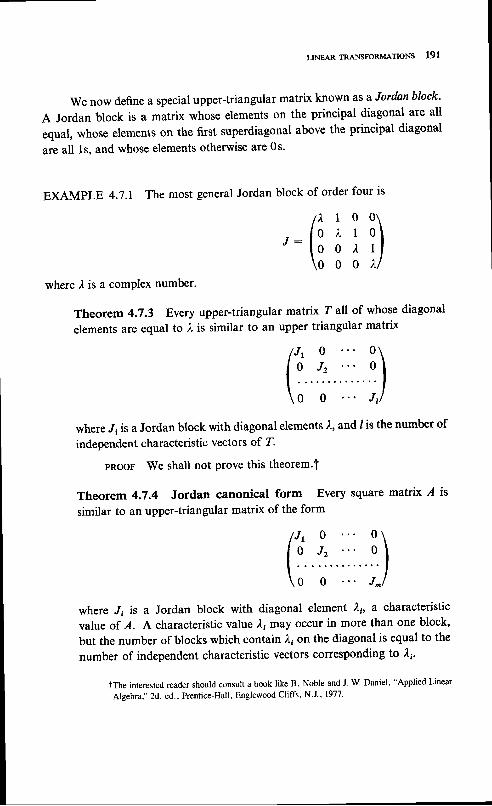
,R TRANSFORMATIONS I9I

We now define a special upper-triangUlar matrix known as a Jordan block'

A Jordan block is a matrix whose elements on the principal diagonal are all

equal, whose elements on the first superdiagonal above the principal diagonal

are all ls, and whose elements otherwise are 0s'

EXAMPLE 4.7.1 The most general Jordan block of order four is

il,:(j

)fi

f: ... )

1 0L 10 10 0

where ri is a comPlex number.

Theorem 4.7.3 Every upper-triangular matrix 7 all of whose diagonal

elements are equal to ,t is similar to an upper triangUlar matrix

0J2

0

where .I; is a Jordan block with diagonal elements l, and / is the number of

independent characteristic vectors of T.

pRooF We shall not prove this theorem.f

Theorem 4.7.4 Jordan canonical form Every square matrix I is

similar to an upper-triangular matrix of the form

where ,[ is a Jordan block with diagonal element ).i, a characteristic

value of A. Acharacteristic value limay occur in more than one block,

but the number of blocks which contain ,t; on the diagonal is equal to the

number of independent characteristic vectors corresponding to ,lt.

tThe interested reader should consult a book like B. Noble and J. W Daniel, "Applied Linear

Algebra," 2d. ed., hentice-Hall, Englewood Cliffs, N'J" 1977'

I92 INTR.DU.TI.N To LINEAR ALGEBRA AND DIFFERENTIAL EQUATI'NS

pRooF By Theorem 4.7.2, there is a nonsingular matrix e suchthat

l \ o o1r : QAQ-I : | ?.. .T: : : : . . : I

\o o : ;-lwhere T, is upper-triangular with the diagonal elements /.,, the order ofz, is the multiplicity of .r; as a characteristic valu e of A, and k is thenumber of distinct characteristic values of A. By Theorem 4.7.3,there arek nonsingular matrices R, such that

l J , , 0 0 \

R,?iRi- ' : ( ! . . . t : : . : : I\ o o r,,,/where J^, Jn,. . ., J,, are Jordan blocks with diagonal elements ,1,, and/r is the number of independent characteristic vectors corresponding to).r. Let

f t :

lR- I

We have

R(QAQ-\R-1 : RrR- l -

0 RkTkRk*r

Clearly,Rfn-l is in the form required by the theorem where * : f, ,r.i = 1

1 0 oR 2 of

0 0 R* - t

R,TrR, - t 0 oo R2T2R2-I o

: ( :

- lL

0

LINEAR TRANSFORMATIONS 193

EXAMPLE 4.7.2 Find a matrix in Jordan canonical form which is similar to

_r ilThe characteristic equation is l'4 * )'Il : 1( - 2)u : 0' The characteristic

values are ).1 : 2 of multiplicity 3 and Az : 0 of multiplicity l' To find

characteristic vectors corresponding to lt : 2 we must solve

,:fi i \ i)

H:fi)

fi i_l ilH:fi)

': (i ilil

fiThe null space of the coefficient matrix has dimension 1' We can find a character-

istic vector Xr : (1,0,1,0), but all other solutions will be a multiple of Xt and

hence not independent. We must solve

co r respond ing toAz :O 'Aga in thed imens iono f t henu l l space i s l ' andwehave a characteristic vector x+: (0,1,0,-1). There are two independent

characteristic vectors, and therefore there are two Jordan blocks in the canonical

form which (except possibly for the order of the blocks) must look like

This answers the question posed in the example. However, let us continue to

demonstrate explicitly a similarity transformation which will produce 'I' Let

P-r - (XpX2,Xs,Xoi, where PAP-L : J. Then AP-L - p- t"r' or

A(X r,X 2,X 3,X +) : (AX bAX z,AX 3'AX 4): (XyX2,X3,X;)I- ()trxb Xr * )"1X2, Xz * lrXr, lzX+)

( A - L J ) X I : 0 , ( a - A J ) X 2 : x r , ( A - ) 4 1 ) & : x 2 ' a n d ( A - L r I ) X n : g '

I94 INTRoDUcTIoN To LINEAR ALGEBRA AND DIFFERENTIAL EQUATIoNS

The first and last of these equations we have already solved. The second equa_tion takes the form

A solution isf,, : (0,+,0,-D- The third equation takes the form

and it has a solution Xs : (0,-t, -+,*). Therefore,

p ' - r _

and multiplying out PAp- 1, we find that pAp-r : J.

There is a certain amount of ambiguity in Theorem 4.7.4. To illustratethe problem' suppose ,4 is a 4 x 4 matrix with a single characteristic value l,of multiplicity 4. Also suppose that there are only two independent character-istic vectors corresponding to 1.. Then we know from Theo rem 4.7.4 that thereare two Jordan blocks on the diagonal of "I, the Jordan form simil ar to A.However the Jordan form could look like (aside from the order of the blocks)

on the other hand, if we write p- | : (x1,x2,xt,x+), then we have fromAP-t - p-rJ, A7Xr,Xr,Xs,X+) : (xr,xz,X3,X4)J. In the first case, we havethe equations (A - AI)X, : g, (A - )J)X, : g, (A _ AI)& : Xr, and(A - lI)X4 : Xz. In the second case, we have the equations (A _ ).1)i, : g,(A - ).1)X2 : Xr, (A - AI)&: 0, and (A - AI)X4 : Xt. Given A, onlyone of these sets of equations wilr have four independent solution s xr, xr, xr,and xo. This will then determine the appropriate Jordan form.

We conclude this section with an application to the solution of svstems

fi ij ilH:0fi l.l ilH:(il

fi i-l il .:f l_l il

fiijil fiilil

R TRANSFORMATIONS 195

of differential equations. Suppose we have a system of differential equations

which can be written in the formd X : A Xdt

where fi:(xr(t),xz(t),...,x"(t)) and "4

is an n x n matrix of constants'

we wish to find a solution of the system .satisfying the initial conditions

x(0) : xs,&given vector. suppose we make a change of coordinates I : PX,

wherePdoesnotdependon l . Then X: P- r Iand X '= P- rY ' : AP- IY '

or Y, : (PAP_\Y, Now suppose PAP_, : J, a Jordan canonical form;

then! ' i : l i l i * F i l i * r i : 1 , 2 , . . . r f l

where .l; is a characteristic valuet of A and p; is either I or 0 depending on '/'

In every case, pn: 0, and the last equation is simply !'n : Xoln Therefore'

yn: ci^^t, where cn is a constant; putting this into the (z - l)st equation,

*. ."r, solve for !n-t. working upward in the system, we can find all the y;'

Finally, we find X from Y : PX and evaluate the constants of integration

using the condition x(0) - xo. we shall show in chap. 9 that such a system

always has a solution satisfying a given set of initial conditions and that the

solution is unique.

EXAMPLE 4.7.3 Find a solution of the system

dx' -- 2x, + x2 * xadt

d x z : x r * 3 x 2 - x 3 * 3 x od t

d x t : x ' t * 2 x t l x +

dt

d x q : x r - x z - x l - x +

dt

satisfying -t1O; : to : (1,0,0,0). We can write the system as X' - AX,

where z4 is the matrix of Example 4.7.2. We have already found a P such that

PAP-I :

1 02 l0 20 0

t In general, the characteristic values are not all distinct. Therefore, it will be expected

that lr is the same for different values of i.

fi il

196 rNrRoDUcrroN To LTNBAR A.$EBRA AND DIFTERENTTAL EeuATroNs

Uader the change of variables I : pX,theequations become !,r : 2yr * yz,lL : 2yz + ls, !'t : 2Iz, lL : 0. Therefore, we have !4: c4, lg = cte2r,and

)

f rUze- " ) : y3e-2 ' : ca

fi) :

so that lz : cate2' * c2e2t. Finally,

f iOrr-') : yze-2' : cst * c2

and y1 : (caf 12 + c2t * c1)e2t. I*t ?o : F(0) : (c1,c2,cs,ca). Then

/"r, te2t *t2 ez' g\ /"r\yc):(l ";' ,f; l)(:: )\o o o r / \ca/

If Ys = PXe, then

il0:fi)| ,,!1,:'):'i,;)I tt + t21e2' - ,z\ - t e 2 t + e 2 . - '

EXERCISES 4.7

I l,et J be a Jordan block with t on the diagonal. Show that the null space ofJ - ).Iis of dimension l.

2 Show that a Jordan canonical matrix with /c Jordan blocks on the diagonal hasexactly /c independent characteristic vectors.

3 Show that if PAP-r : J, alordan canonical matrix, then I has the same numberof independent characteristic vectors as .I.

4 Find Jordan canonical matrices similar to each of the following:

l s 4 3 \ 1 2 I o \ l z 2 _ 1 \(a) t - l : -? l (6) l l - l - l l (c) l - r - r r f

\ I -2 U \o 1 2l \_r _2 2l

/ r 0 0l o I ofz o -z\ 1 - ' - t

X( t ) : P- tY1t 'y :

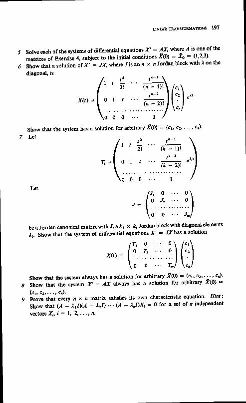
LINEAR TRANSFORMATIONS I97

the

the

5

6

7

solveeach of thesystems of differential equations x' : ax,wherc I is one of

matrices of Exercise 4, subject to the initial conditions .f,10; : & : (1,2,3)'

show that a solution of x' : /jq where Jis an n x nJordan block with 'l on

diagonal, is

/t , '-' -'al" ^ ry\/:,\'ar=[o, t #l ["i1""

\;; ; t '

; i f \ '^t

Show that the system has a solution for arbitrary 'f(O) = (cu cz' ' " ' cJ'

L€t (t ";' + \

?i=| . , o I t #"u,J\ ; ; ; ; /

I.et/r ' o o\

! : f o J2 o l

u; ;^lbe a Jordan canonical matrix with "r1 ak1 x &l Jordan block with diagonal elements

11. show that the system of differential equations x' = "IX has a solution

x(r) :

show that the system always has a solution for arbitrary 'f101 : (cr cz" '-' ' c)'

8 Show that the system X' : AX always has a solution for arbitrary 'f(O) =

(cp c2r . . . , cn) .

g hove that every n x n matrix satisfres its own characteristic equation. Hint:

S h o w t h a t ( l _ u N A - x z l ) . . . ( A _ ) , n l ) x . : 0 f o r a s e t o f z i n d e p e n d e n tvectors Xr, i - l, 2, , . ., n.

5FIRST ORDER DIFFERENTIAL EQUATIONS

5.I INTRODUCTION

This chapter begins our study of ordinary differential equations with first orderequations. In a sense, the last section should come firsi because there we takeup the fundamental existence and uniqueness theorem for first order equations.The proof is the traditional Picard iteration argument. However, because theargument is more sophisticated than the general level of this book, this materialis more appropriately placed in a starred section for the more ambitiousstudents. After a section giving an elementary example of how differentialequations arise in, and are rerated to, applied mathematics, there is a sectionon some of the basic definitions in the subject. Next we take up the solution offirst order linear equations. The following section deals with a few of the specifictypes of nonlinear equations which can be solved in closed form. The last twounstarred sections, Secs. 5.6 and 5.7, are on applications of first order equationsand numerical methods, in that order.

FIRST ORDER DIFFERENTIAL EQUATIONS 199

5.2 AN EXAMPLE

The broad area of applied mathematics usually breaks down into four parts:

/ Formulation of a mathematical model to describe some physical

situation.2 Precise statement and analysis of an appropriate mathematical problem'

3 Approximate numerical calculation of important physical quantities'

4 Comparison of physical quantities with experimental data to check the

validity of the model.

The lines of demarcation are never clear, but generally parts I and 4 ate

the province of the physicist or engineer while parts 2 and 3 are the province of

the mathematician. Part I is very difficult; at the very least it requires an intimate

knowledge of existing physical principles, and at the most it may require the

formulation of some new theory to cover the given situation' It requires great

insight into the question of which effects are the principal effects in the problem

and which are secondary, hence can be neglected. This is because nature is

usually too complicated to be described precisely, and even if we understood

completely all physical principles, we would probably not be able to solve the

,.rulting mathematical problems with enough precision to make this knowledge

pay otr Therefore, when a mathematical model is formulated, one must take

into account both the inability to describe the physical situation precisely and

also the inability to analyze the mathematical model which may be forthcoming.

In a sense, once the mathematical model has been formulated, the analysis

of part 2 has nothing to do with physics. The question of whether the problem

is well formulated, whether it has a solution, and how to find the solution are

purely mathematical in nature. The mathematician cannot, for example, argue

that the solution exists and is unique because the physical situation indicates

this, because by the time the problem reaches him, it is no longer a precise

description of nature but only an approximate model which at best retains only

the principal effects to be studied. Therefore, the mathematician must decide

qu.rtion, of existence and uniqueness within the framework of the math-

ematical model, which will do what it is supposed to only if it has been well

formulated in part l. This is not to say that physical intuition is never valuable

to the mathematician. It may suggest methods of analysis which would not

otherwise be apparent, but the mathematician must not rely on some sort of

vague physical intuition to replace sound mathematical analysis.

The mathematician's work is not done when the mathematical model has

been analy zed to the extent of deciding that a solution exists and is unique. For

knowing that a unique solution exists is of little help to the physicist or engineer

2OO INTRoDUcTIoN To LINEAR ALGEBRA AND DIFFERENTHL EQUATIoNS

Equilibrium

FIGURE 28

if he cannot find it. In many cases, a numerical approximation to some physicalquantity is the best that can be hoped for. In other cases, a more completedescription of a solution may be available, but not in a form from which datacan be quickly and easily extracted. Hence, in either case part 3 may involveconsiderable numerical analysis before meaningful answers can be derived.This will involve finding algorithms from which data can be computed andanalyzing the degree of accuracy of these results compared with some analyticalsolution which is known to exist.

Paft 4 is the province of the experimentalist. It is his job to devise experi-ments to check the data which the mathematical model has provided against thephysical situation. This book is a mathematics book and therefore will notdeal with parts I and 4 of this outline. We shall treat parts 2 and,3 especiallyas they relate to those mathematical models which involve the solution ofordinary differential equations. Before getting on with a systematic study ofordinary differential equations, we shall illustrate some of the foregoing remarksin relation to a simple mass-spring system.

consider a physical system consisting of a mass of rn slugst hanging on ahelical spring (see Fig. 28). We assume that the spring has a certain naturallength L. If the spring is stretched by a small amount e to the length L + e,there is a restoring force ke in the spring which opposes the extension. If thespring is compressed by a small amount e to the length L - e, then there is aforce ke which opposes the compression. If we measure force in pounds andlength in feet, the spring constant k is measured in pounds per foot.

I one slug is a unit of mass such that a force of one pound exerted on it wiil producean acceleration of one foot per second per second.

,ERENTIALEQUATIONS 2OI

Suppose at a given time r the spring has length L + Y(t); then I(l) isthe amount the spring is stretched beyond the natural length. If f(r) is negative,then the spring is under compression. There is a downward force of ntg due togravity acting on the mass, where g is the acceleration of gravity measured infeet per second per second. The spring exerts a force kY(t) on the mass, whichis upward when y(l) is positive and downward when f(t) is negative. Accord-ing to Newton's law of motion,

d 2 Y^# : ms - kY

where d2 Yldt2 is the acceleration of the mass /,,l and time / is measured in seconds.We are neglecting any force due to air resistance, and we are assuming that themass has no horizontal motion. We see that the displacement I(r) satisfies adffirential equation.t

As is the case in many problems, the differential equation can be simplifiedby introducing a new variable. Consider the eqlrilibrium position of the masson the spring, that is, where the mass will hang without motion so that thedownward force of gravity is just balanced by the upward reaction of the spring.If Y" is the amount the spring is stretched in the equilibrium position, thenkY" - mg. Now let y(t) be the displacement of the mass measured positivelydownward from equilibrium. Then Y(t) : y(t) + Y" and

#:#and the differential equation becomes

d 2 v^#: ms - kly(t) + r"l : -ky(t)

Therefore, y(r) satisfies ! * o)'y : 0, where o)2 : klm and the two dots overy stand for the second derivative of y with respect to /.

So far we have said nothing about how the mass will be set into motion.Suppose at time / : 0 the mass is given an initial displacement yo : y(0) fromequilibrium and an initial velocity .po : /(0), measured in feet per second.Then the problemt is to find a function y(r) satisfying y + roty : 0 for I > 0such that y(0) : yo and y(0) : yo. Since the displacement, the velocity, and

f we shall define more precisely in the next section what we mean by a differentialequation.

f rhis type of problem is called a\ initial-oalue problem, All the data are given at asingle time J : 0. Later we shall consider boundary-value problems, where dataare given at more than one value of the independent variable.

202 INTR'DU.TI'N To LINEAR ALGEBRA AND DIFFERENTIAL EQUATI'N'

the forces acting on the mass cannot become infinite or change discontinuously,we further specify that y(t), y(r), and j;(r) should be continuous for r 2 0.In our terminology this means that these functions are all continuous for r > 0and that Jim y(r), 1im y(l), and lim i(r) all exist.

we now have a mathematical model to go with the mass-spring systemdescribed above. To reemphasize that this only approximately desciibes thephysical situation let us list some of the assumptionr *. have tacitly made.

1 The elastic behavior of the spring is such that the restoring force isproportional to the displacement.2 The displacement is small enough to ensure that the elastic limit of thespring is not exceeded.3 There is no air resistance.4 The acceleration of gravity does not vary with height.J The motion is in a straight vertical line.

In addition to these, we could mention that Newton's law is only an approximatetheory which assumes that relativistic effects are negligible. The point is thatthe mathematical model is only an idealization of the actual physical system.If it turns out to be a good approximation to the physical system, it is becausewe have been clever enough to include all the major effects and have neglectedonly secondary effects.

One of the first things we should do with the mathematical model is provethat there exists a solution to the problem. In this case, we shall do so byactually finding a solution.t Let z : dyldt. Then

dz7 -

dy

z d z * a z y d y : g

l ,a , * , ,2 | ta t : ' | * '2 ' - "J J 2 2 2

d2y _ dz dz dy- : - : _ _ :d t 2 d t d y n -

* a z y : g

where c2 is a constant. Then

: tJ c'z - @?y'z

t This type of existence theorem is called constructiae since it actually constructs asolution. There are nonconstructiue existence theorems where solutions are provedto exist without showing how to find them.

dzdy

dvL - -

dt

IERENTIALEQUATIONS 2O3

Ignoring, for the moment, the ambiguity in sign, we have

dy, - : d t

t/ct - a'yt

dy : a d t.,1o, _ y,

sin-1 !- : at * 6

where a : clro and Q is another constant of integration, Finally, we have

! : a s i n ( a t + Q )

where a and $ are constants of integration. We should go back and considerthe other sign. But we see that this is not necessary since

j, : aa cos (crlr * @)

y : -a2a sin (arr + d) : -co2y

and we see that this function satisfies the differential equation for arbitrarya and @. Now

y(0) : asin$ : yo

y(0) : @acosf: j ,ocan be satisfied by

,l;4d : tan- t ' !o

.]/o

where 0 < Q < n. Therefore, we have found an explicit solution to ourproblem.

Next we prove that the solution is unique. Suppose that there are twosolutions yt(r) and yz!). Then y, * a'y, : 0, lz * a2!z: 0, yr(O) =yz(O) : ./o,.trr(O) : .yz(0) : yo. We form the difference w(r) = ./r(t) - yz!).Then w + a2w : 0, w(0) : li,(O) : 0. We compute

E(t '1 :*mf i t * \kw2

E 1 r ; : m f i w * k w t i

. - k: mw * kwt i :0m

a :

?M INTRoDUcTtoN To LINEAR AI,GEBRA AND DIFFERENTIAL EQUATI.N'

This means that .E'(r) is constant. But .E(0) : 0 and, therefore, E(r) = 0.However, we notice that .E(r) is the sum of nonnegative quantities. Therefore,w = 0 and yr(t) = lz!). This completes the proof.

Notice that in the proof of uniqueness we used the function E(ty :*mwt * lkw2, which most readers will recognize as the energy-kinetic energypluspotential energyof the spring. Then d1r; : 0 states the fact thatenergyis conserved. We did not have to know this to complete the proof. On the otherhand, this illustrates how a knowledge of physical principles may aid themathematician in his analysis of the mathematical model.

EXERCISES 5.2

/ Show that y(t) = acos (at * d) and y(t\ = Asinat * gcosarr both satisfyy * a2y = 0 for arbitrary constants o, d, A, and g. Does this contradict theuniqueness theorem? Explain.

2 Find the solution of the initial-value problem i * a2y: 0, , > 0, y(0) : .yo,y(0) : ye in the form {r) : I sin at * B cos @rr.3 Let f(t) be a given function continuous for I > 0. Prove that if there exists a

function y(t) which is continuous and has continuous first and second derivativesforl > Osatisfying i i * at2y = f(t),withr(0):./0,d0) : lo,thenitisunique.

4 The differential equation satisfied by the angular displacement 0 of the planependulum shown in the figure is M + g sin g = 0. consider the total energy

E(t1 : lml202 + wt(r - cos d). show that energy is conserved, that is,E1t1 : 0. If the pendulum has no initial displacement and no initial velocity, canit ever become displaced from equilibrium? Does this prove uniqueness of thesolution of the differential equation subject to specified initial displacement andvelocity in this case? Explain.

5 Assuming in Exercise 4 that l0l < 5", so that sin d s 0, 0 in radians, find anapproximate solution to the initial-value problem. Find the approximate frequencyof the pendulum, that is, the number of complete cycles per second.

FERENTIALEQUATIONS 205

6 Some people insist that an initial-value problem is not well formulated unless thesolution is a continuous function of the initial data; that is, small changes in theinitial data produce small changes in the solution. Prove that this is the case inthe mass-spring problem of this section.

5.3 BASIC DEFINITIONS

Before beginning a systematic study of differential equations, we shall definesome of the basic terms in the subject.

A differential equation is an equation which involves one or more in-dependent variables, one or more dependent variables, and derivatives of thedependent variables with respect to some or all of the independent variables.If there is just one independent variable, then the derivatives are all ordinaryderivatives, and the equation is an ordinary diferential equation. We saw theordinary differential equation

d"yT * c o 2 y : g

in the last section. Another example is Bessel's equation

, ,#+.y;+(x, -n)y:o

where r is the independent variable, ./ is the dependent variable, and n2 is aconstant. If there is more than one independent variable and partial derivativesappear in the equation, the equation is called a partial diferential equation.Some common examples are the heat equation

the wave equationL 02u 02uTat r=#

and, Laplace's equation02u 02ui , r ' * i , y ' : '

It is obvious in these cases which is the dependent variable and which are theindependent variables.

Tbe order of a differential equation is the order of the highest derivativewhich appears in the equation. Bessel's equation is a second order ordina,ry

^ ^ ), ou o-uK - : _

0t 1xz

206 INTRODUCTION TO LINEAR ALGEBRA AND DIFFERENTIAL EQUATIONS

differential equation. The heat, wave, and Laplace equations are examples ofsecond order partial differential equations. The general form of an nth orderordinary differential equation, in which y is the dependent variable and t is theindependent variable, is

F(t, Y, i,,. . ., /(n)) : 0

where the nth derivative must actually appear in this function. Lower orderderivatives may be missing, however. If F is a linear function of the variables

!, !, lr. . . , Y('), that is,

F(t, i, Y,..., y(n)) : ao(t)y(") I ar111y(n-r)+ "' * an-tQ)i ' + a,(t)Y + f(t)

then the differential equation is said to be linear. The two ordinary differentialequations cited above are linear. On the other hand, the equation

d v,fr * y : f(t)

is nonlinear. There are corresponding definitions for nth order and linear nthorder partial differential equations.

We have already indicated how a mathematical model may lead to aproblem in differential equations. Clearly, to define the problem we mustspecify more than the differential equation. We must specify where the solutionis to be found, what continuity conditions must be met by the solution and its

derivatives, and also what values the solution and/or its derivatives must take

on at certain points in its domain of definition. We say that a solution existsif there is at least one function which satisfies all these conditions. We say thatthe solutionis unique if there is no more than one function which satisfies all theconditions. We usually say that the problem is overdetermined if there are no

solutions, that is, too many conditions to be met, and underdetermined if there

are solutions but the solution is not unique, that is, there are not enough

conditions to single out a unique solution.In speaking of ordinary differential equations, we say we have an initial-

ualue problem if all the specified values of the solution and its derivatives are

given at one point. The mass-spring problem of the previous section was an

example. These problems are most frequently encountered in dynamicalproblems where time is the independent variable and the data are given at some

initial time, say I : 0. For this reason, when we are dealing with initial-value

FIRST ORDER DIFFERENTIAL EQUATIONS 2O7

problems we shall usually use t as the independent variable. On the other

hand, if data are given for the solution at more than one point, we say we have

a boundary-ualue problem. These problems occur most frequently when the

independent variable is a space variable. For example, a beam is loaded with

some static load (constant set of forces), and conditions are specified at the

ends of the beam. For this reason, when we are dealing with boundary-valueproblems we shall generally use .r as the dependent variable. Corresponding

definitions of initial-value and boundary-value problems occur in partial

differential equations, but descriptions become more complicated; we shall not

study partial differential equations in this book.

EXERCISES 5.3

/ Classify each of the following ordinary differential equations as linear or nonlinear.Also determine the order of the equation.( a ) t i t * y : s t( b ) ! i , * Y : e t( c ) y + i * . y : 0(d) i,v : v( e ) t 3 ' i ; * t ' i + t Y * Y : 1 4

(f) sin y * x cos y' : g, y ' :4!' d x

@) (l - x')y" - Zxy' * n(n + l)y : O (n : constant)

(h) ""y"'

* x3 : 0

Let u(x,y) be a function of two independent variables. Describe the general nth

order partial differential equation involving a.

Referring to Exercise 2, give the form of the general nth order linear pafiial

ferential equation involving a.Classify each of the following partial differential equations as linear or nonlinear.Also determine the order of the equation.

( a \ o " * a ' u : o7xz 0y'

02u Azu 02u 02u\c) ;; : ;-t

-r- ;-;

-T --ot- ox- ay- oz-

Au . , Au\e) ;- : €- T-

ox oy

Azu 0u@ ) - + ; 1 r - - : Q

ox oy ox

^ ^ ? ^ 2d u _ d - u , O - u

T -^ ^ 1 ^ )ot ox- oy-

Au 0uu - l u - - |

0x Ay

a3u : oAx Ay 0z

0u 0u" ) / ; f X ; - : S m x ; , t

ox ay

(b)

(d)

(f)

(h)

208 INTRoDU.TIoN To LINEAR ALcEBRA AND DIFFERENTIAI. EQUATI.N'

s.4 FrRST ORDER LTNEAR EQUATIONS

The general form of the first order linear ordinary differential equation is

a{ t ) i , * as ( t )y : f ( t )

We shall consider the initial-value problem based on this equation, whichrequiresasolutioncontinuousfor0 :s t < bsatisfyingy(0): y6. Ifar(0): g,we say that t : 0 is a singularity of the differential equation. We shallconsidersingularities later, so for now we assume that ar(0) * 0. we assume that aoe),a(t), andf (t) are continuous for 0 < r s &, and therefore if ar(0) * 0, thereisaB > 0suchthatar( t ) # 0for0 < r < B. Forsimpl ic i ty letusassumethatf : b. Dividing through by ar(t), we can write the equation as

d vd t + q 1 ) y : r ( t )

where q(t) and r(t) are continuous for 0 < t < b.It is convenient to introduce the operator z, which by definition is

Lv:# .q l )vWe observe that Z is linear, since

L (c r y1 t ' d 'c z ! ) :

V (c r l r * cz l ) + q ( t ) ( c r ! t * cz l z )

, r ( *

c1Ly1 *

* nr,) * ,,(* * nr,)

czL! zwhere c, and c2 are arbitrary constants.

The equation y * qy: 0 is called the associated homogeneons equation,where j, + qy : r is considered the nonhomogeneous equation if r * 0. wenote that if yr is a solution of the associated homogeneous equation and y, isany solution of the nonhomogeneous equation, then cy, * y2is a solution ofthe nonhomogeneous equation for an arbitrary constant c. This is because

L(cy, * !z) : cllt * Ly, : r(t)

since Zy, : 0 and Lyr: r. The function y : clt * y, is a one_parameterfamily of solutions. From this family we can select one which satisfies the initialcondition y(0) : yo; that is,

y ( 0 ) : c / r ( O ) * y r ( 0 ) : y o

" : ! o

* ! z ( o )

Yr(0)

FERENTIALEQUATIONS 2O9

provided/1(0) # 0. To prove existence of a solution of the initial-value problemit then remains to show thaty, exists withyr(O) * 0 andy, exists.

Let us consider the homogeneous equation first. Since j, : -qy,

d! : -q1ry d,v

Integrating, we have for 0 < t < b

ln lyl - tn ly(O)l : - | q&) a,J o

l u l r f t - 1

l + l :exp l - l q ( r )d r ll v (o ) l

^L Jo" ' J

It is not clear that we can remove the absolute-value sign. However., if we let

./r : eXp |-- f' q@ ar]L J o J

we see that this is a continuously differentiable solution of the homogeneousequation such that.yr(0) : 1. Hence, we have proved the existence of yr.

Next we show that yr, a solution of the nonhomogeneous equation, exists.

Lett

r l t - 10(t) : exp | | ak) dr 1

L J o IThen multiplying lz * Qlz : r by Q, we have

Q j , z + q Q y z : r Q

4 <ar,> - red t

I tQyz: I r ( r )e@)dc

J o

r l ,t' :

fi) )or(c)Qk) dr

This function is a solution of the nonhomogeneous equation. In fact, sinceyr(0) : I and yz(O) : 0, a solution of the initial-value problem is

! : l o l r * l z

l - f t . l f r t l f l: yo exp | - | q(r) dr | + exp | - | q(t) dr I I r(r)eft) drL r o ) L J o J J o

t O(t) is called an integrating faclor because by multiplying the differential equationthrough by O we make the left-hand side of the equation an exact derivative.

2IO INTRoDUcTIoN To LINEAR ALGEBRA AND DIFFERENTIAL EQUATIoNs

To show that the solution to the initial-value problem is unique, weassume that there are two solutions u(t) and u(r). Then ft * qu : r, u(0) : !o,and , i * qu : r , r ( 01 : ! o . Le tw : L t - u . Then f i * qw :Oandw(0 ) : g .The function QQ) > 0, since it is an exponential function. Also

Q v r + q Q w : 0d

7(Qw) : o

This implies that QQ)w(t) : const. But e(0)w(0) : 0. Thereforc, ee)w(t) =0,whichimpl ies thatw - u- u= 0sincee( l ) > 0. Therefore, u: u. wehave therefore proved the following theorem.

Theorem 5.4.1 Let q(t) and r(l) be continuous for 0 < t < b. Thenthe initial-value problem i + qy : r, y(0) : !0, has a unique solutionf o r 0 < t l b , g i v e n b y

y(r) : Io exp [- f q@ ar]* exp [- f' q@ arf f' re)eg) drL J o J L J o - l J o

wherer f r - l

QG) : expl I a(i arlL J o J

EXAMPLE 5.4.1 Solve the initial-value problem./(0) : 1.

It + l _ r ! : I - t 0 < r < b < l

The integrating factor is

e(t) :.*p I i ' , t - r)- ' dt]L J o J

- e x p [ - l n ( 1 - r ) l : , 1l - t

Multiplyineby QQ), we have

-L1 'a-J- r , : ! ( z_) : rt - t ' ( t - t ) r ' d t \ t _ /

Therefore,

! : t ( l - r ) + c ( l - t )where c is arbitrary. However, y(0) : 1 implies c : l, and so the uniquesolution to the problem is

Y ( t ) : | - t 2

This is an initial-value problem forThe solution is

FrRsr oRDER DTFFERENTTAL EeuATroNs 2ll

EXAMPLE 5.4.2 Radioactive matter is known to decay (change its form)at a rate which is proportional to the amount present at any given time. LetAobe the amount of radioactive material present at the beginning of the process(r : 0). Then

4 : - kAdt

A(0) : 1o

a first order linear differential equation.

A(t) : Ao€-r'

The halfJife r of the radioactive material is defined to be the time required forhalf the original material to decay. Hence,

IAo : Aoe-r'

Therefore, x : (llk\1n2.

EXAMPLE 5.4.3 Initially tank I contains 1@ gallons of salt brine with aconcentration of I pound per gallon, and tank II contains 100 gallons of water.Liquid is pumped from tank I into tank II at a rate of I gallon per minute, andliquid is pumped from tank II into tank I at a rate of 2 gallons per minute. Thetanks are kept well stirred. What is the concentration in tank I after l0 minutes?Let At be the amount of salt in pounds in tank I and Arbe the amount of saltin pounds in tank II. The concentration in tank I is

and the concentration

Therefore, A, and A,

^ A LL r :- 1 0 0 + r

A A 2l u c :- 1 0 0 - r

II is

satisfy

dAt _ 2Az _d t 1 0 0 - t

d A z _ A r _d t 1 0 0 + r

* A z : 1 0 0

A I

1 0 0 + t

2Az1 0 0 - r

AT

2I2 INTRoDUcTIoN To LINEAR ALGEBRA AND DIFFERENTIAL EQUATIoNs

EliminatinE Az, we have

d A r - _ 2 ( 1 0 0 _ / r ) _ A 1d t 1 0 0 - r 1 0 0 + t

dAr _ (300 + r)r{, : 200dt 1002 - t2 l0o - r

This is a first order linear equation with q(r) : (300 + rxl002 - 12) andr(t) : 200(100 - r). According to the above,

r f t - tQ(t) : exp | | ek) dr I

L J o J

_ 100(100 + r)(100 - r)2

We rnultiply the equation by (l0O + r)/(100 - t)r, and we have

{[gQjr t)Ar1_ 200(100 + r):drl(100 - t) , J (100 _ r)3

dffi A'l:K+2oot@*=-- d-b]where K is an arbitrary constant. Therefore,

Also, since lr(0) = 100, K: l,^r:': ffi *

#'

At: tP: * t ' o < r < 1oo1 0 0 * l

c t :g - { o<r<1oo(100 + l)2

When r : 1O Cr : rr*l pounds per gallon.

EXAMPLE 5.4.4 Find a solution of tj, I ay : 0 (a constant), which iscontinuous for t ) 0 and takes the value ys at t : 0. In this case, the equationis

g + ! ! : ot

Hence, q(t) : alt, wbich is not continuous at t : 0. Therefore, the existenceand uniqueness Theorem 5.4.1 does not apply to this initial-value problem.

FERENTIALEQUATIONS 2I3

Nevertheless, we can find a solution, by multiplying by the integrating factorto,

Y(t) : Kt-o

where K is an arbitrary constant. If a :0, then there is a unique solutiony(t) : ys. If a < 0, every solution goes to zero as / -+ 0. Therefore, there is nosolution unless lo : 0, but then the solution is not unique since Kis arbitrary,rf a > 0, then there are no solutions continuous at the origin unless K : 0.Hence, we can have any possibility if q(t) is not continuous.

EXERCISES 5.4

.l Solve the following initial-value problems:(a) ! * ty: l,.y(0) : /o.( b ) t i + y : l * 1 , . y (1 ) =O . H in t :Make thechangeo fva r i ab le r : t - 1 ,(c) i, * ety : et,.y(0) - /o.(d) (l + t)i * y : et, y(0; : 1.(e) y + (tan t)y : se,c t, y(nl4) = O.

2 At a certain time a radioactive material is 90 percent pure (10 percent changed),and I hour later it is 75 percent pure. What is the half-life?

3 A certain radioactive material with a half-life of 5Q000 years is 10 percent pure.When was the material created?A lO0-gallon tank holds salt brine with a conc€ntration of 1 pound per eallon.Brine is drawn off at a rate of 2 gallons per minute while water is added at a rate ofI gallon per minute. What is the concentration l0 minutes after the process isstarted?An object of mass m falls from a great height under the influence of gravity (g =acceleration of gravity) with air resistance proportional to the velocity. What isits terminal velocity?Solve the first order linear equation by the method of oariation of parametersTthat is, look for a solution of the form y : A(t)y{t), where y1 is a solution of theassociated homogeneous equation. Solve part (a) of Exercise I by this method.

s.s FrRST ORDER NONLTNEAR EQUATTONS

A large class of first order equations can be written as

dv

T : fQ,Y)

2I4 INTRoDUcTIoN To LINEAR ALGEBRA AND DIFFERENTIAL EQUATIoNS

or since/(t,y) can always be written as the quotient of two functions, say

.f(t,v) : - M(t'Y)

N(t,y)

then

M(t,y) dt + N(t,y) dy : 0

rn special cases, because of the forms of M(t,y) and if(r,y), we are able to findclosed-form solutions. We shall say that we have a closed-form solution if wecan find an implicit relation F(t,y): F(to,yo) such that dyldt : _FtlFy:

"f (t,y). According to the implicit-function theorem,t if F, and Frarccontinuouswithin some circle with center at (to,yo) and Fr(to,!o) t 0, then provi ded (t,y)is sufficiently close to the point (to,ye), we can solve r'(r, y) : F(ta,yo)explicitly for y(r) such that dyldt : - F,IF, and y(lo) : !0.

In this section, we list a few of the cases where closed-form solutions ofnonlinear equations can be found.

I Reducible to Linear

Some equations, by a special transformation, can be reduced to a linear equa-tion. For example, the Bernoulli equation i, + q(t1y : r(t)y" can be reducedto a linear equation by the substitution

w :

We have

d * _

dt

dy

d t :

Substituting in the differential equation, we have

t t - ")y-'#| , , , dw

L n Y d t

+ q(t)y : r ( t ) ! "

n)q(t)w: (1 - n)r( t )

llf Fr(to,fi: 0 but Ft?o,yo) / 0, we can reverse the roles of r and y and solvefor t in terms of y.

| , ,n dw

| - n Y d t

4! * t -dt

FIRST ORDER DIFFERENTIAL EQUATIONS 2I5

EXAMPLE 5.5.1 Find a solution of the equation ! - (llt)y : -3ty2 suchthat y(l):6. This is a Bernoulli equation. Therefore, let w: y-t. Theequation becomes

l t + 1 w : 3 tt

We multiply byr r t - t

0 ( r ) : e x p l I t - t d r l : e x p ( l n t ) : tLJ r I

t + i * w : ! ( w \ : 3 t 2d t '

t N : t 2 + c t - L

w ( 1 ) : 7 - : I + c

then the equation is said to be separable. A solution satisfying y(to) : yo isthen

f' *1r1 a, * i' ",0, dn : o

J t o J y o

! l t ) : ;#*

2 Separable

lf M(t,y) is a function of I only and N(r,y) is a function of y only, then thevariables are said to be separated. If the given equation can be written in theform

M(t) dt + nr(y) dy : 0

EXAMPLE 5.5.2can write

a solution of dyldt - ty2 satisfying !(I) : a. We

d va : t d tv-

f tq - 2 d r y : l t d r

J r

I _ ! : t ' _ r_a y 2 2

2ai t - -

" 2 * a - a t 2

216 INTRoDUCTIoN To LINEAR ALGEBRA AND DIFFERENTIAL EQUATIoNS

3 Reducible to Separable

Sometimes, by the proper change of variables, an equation can be changed sothat it becomes separable. For example, if

M(t,y) dt + N(t,y) dy : 0

and M and tr/ are both homogeneoust of degree fr, then the change of variable

Y : tu(t)

will produce a separable equation. This is seen as follows:

i : t i * uM (t,tu) + N (t,tu)(tfi * u) : e

tkMql,ul + r*N( l ,u)( t i t + a): oM(l ,u) * uN(t ,u) * tN(t ,u) f i : 0

La t * = . , I ( t , ' ) du :ot l [( l,u) + uN(l,u)

--

ln lrl - ln lrol + f" ,ru, dt, : o

P(u) : N(1,u)M(l ,u) * uN(l ,u)

uo : Y-Pto

EXAMPLE.5.5.3 Solve (t, + y\ dt * 2ty dy :0, y(t) : /o, assuming 6and ys positive. Here M : t2 * !2, N :2ty,and both are homogeneous ofdegree 2.

P(u): - 2='

---1 , + u 2 * 2 u 2 I + 3 u 2

l n r - l n rp * f " , ?u r r d t , : o- J u o l + 3 p "

l n r - l n t s * $ l n ( 1 + 3 u 2 ) _ * l n ( I + 3 u o 2 ) : 0

ln r:(1 + 34'?) _ o

to'( l + 3uo,)

f Afunction/(r,y) issaid-tobehomogeneousof degree of ki f fe,t ,)"y)= ),kf(t ,y),For example, f (t,y) = t2 * y2 * /y is homogeneous of degree 2 because

f (Xt).y') : f ,2f * 12y2 * ).zty: Azf (t ,y)

where

rIRST ORDER DIFFERENTIAL EQUATIONS 2I7

l. + 3u2

u

v3t

: (

:I:I

?)' ,t * 3uo2)

10311 + 3uo') -

3 t l

to(toz + 3yo\ -

t31rt2_Jt311t2-J

EXAMPLE 5.5.4 Show that the equation

(aj * brt * ct) dt * (att * bzt * c) dy : 0

can always be solved by the method of the previous example. First, ifcr : cz : 0, then M and,ly' are homogeneous of degree 1. Second, if ct and c,are not both zero, then we make the substitutions

Then

d y d 4 a j * b r y * c ,- : - : - - : -dt d t a2t * bry * c2

Now the equations

;=;:Ia r r i b f l * ( a r h * b r k + c r )a 2 r * b z 4 * ( a 2 h * b r k + c 2 )

a t h + b t k + c r : 0

a 2 h * b 2 k + c z : 0

have a unique solution for h and k if and only if otbz - a2b1 * 0. In thiscase, values of ft and k can be found which reduce the equation to the case ofhomogeneous M and N. The third case is encountered when atbz - arb, : g,

In this case, we letu :

d r _dt

d y :dt

a2t * brL@- b $

- cr - art)lb1f * c2

b z u - b 2 c r * b p ,- b r t u

a r t * b 1 y * c ,

o , + b r !d t

| ldu- t -b' \dr

- , r )

dt

du

f(")

b z u - b 2 c r + b r c 2

: d t

+ a1 -- f(u)

218 INTRoDUcTIoN To LINEAR ALGEBRA AND DIFFERENTIAL EQUATIoNS

and the variables are separated. lf bru * bzcr * bpr: 0, then az : bz _cz : 0 and this is not possible. If Dr : 0, then this substitution will not workbut the substitutioa tt : art * bzl * c, will work, unless bz : 0. If both D,and b, are zero, then the equation is already separated.

4 Exact

If the form of the differential equation

M(t,y) dt + N(t,y) dy : 0is an exact differential, that is,

M(t,y) dt + N(t,y) dy : y dt + y dy : dF : oAt 0y

for some function F(t,y) which has continuous derivatives, then

F(t,Y) : F(to,Yo)gives a solution of the initial-value problem.

Theorem 5.5.1 Let M(t,y) and N(t,y) have continuous first partialderivatives in the rectangle R : {(r,y) ltr _ tol 1 a, ly _ yol < b}.Then there exists a function F(t,y), defined on R, such that dF :M(t,y) dt + N(t,y) dy : 0 if and only if M, : n[ in R.

pRooF Suppose there is such a function F(t,y) such that Ft : Mand F, : l/. Then lPr, : M, : Fr, : 1/r, since ,ir' has continuous secondpartial derivatives in R. Conversely, suppose Mn : nf, in R; then define

F(t ,v) : , [ :

Mg,ys) dr *f,N(t,rD d?t

Clearly,

Also F(to, !o) : 0, andproblem satisfying y(ro)

AF l t; : M ( t , y o ) * |

N , ( t , 6 a 4

: M(t,yo) * ti

*,rr,r, o,J Y o

: M( t ,yo) + M( t ,y ) - M( t ,yo): M(t,y)

A Pa_ _ N(t,y)oy

so .F(r,y) : 0 gives us a solution to- t o .

the initial

FIRST ORDER DIFFERENIIAL EQUATIONS 2I9

EXAMPLE 5.5.5 Solve (y' - t21 dt * 2ty dy : 0 subject to y(rs) : !o.The equation is exact since, throughout the ty plane,

aM:2v :U0y "0 t

ThenAF: : Y 2 - t 2ot

AF

6: ",Therefore,

It lvF(t,y) :

| (ro' - 12) dt + | zq aaJ to Jyo

+ 3 t 3- t y ' - + - t o ! o 2 + 9 : o. r 3

gives us the desired solution. Solving for y, we have

_ - ( t t - f o t * 3 t o y o z \ t l zJ

- L r - ;- \

3 t , l

The choice of sign will depend on the sign of yo.

5 Reducible to Exact

If the equation M(t,y) dt + N(t,y) dy : 0 has a solution which can be writtenin the form

F(t,y) : F(to,yo)

dF:40 ,+ydy :oot 0y

d y : _ F , _ - M ( t , y )dt Fy N(r,y)

AF

a, : QQ'DM(I,Y)

AF;,r: Q(t'v)N(t'v)

then

Therefore,

22O INTRODUcTIoN To LINEAR ALGEBRA AND DIFFERENIIAL EQUATIoNs

and hence multiplying M dt * N dy : 0 by QQ,D makes the equation

eMdt+eNay :Ta t+Tdy :o- A t 0 y

and it is exact. QQ,D is called an integrating factor. In principle every equationhas an integrating factor. However, it may not be easy to find an integratingfactor in a given case.

Suppose M(t,y) and l[(t,y) satisfy the condition of Theorem 5.5.1 butM, * lf,. If there is an integrating factor QQ,il with continuous first partialderivatives in R, then (QIvO": (QN), or

o(ry-4{ \ :NQ-MaQ- \ a y a t J 0 t 0 y

This equation is not easy to solve in general; however, if Q does not depend ony, then

and

Conversely, if (Uff)(0Ml)y - |.NIft) does not depend on y, then the Q givenby this formula is an integrating factor.

Laa:1(ry_aN\oA

- " \a

- ar)

0: exPtJ* (x #),'l

EXAMPLE 5.5.6 Find a solution of (3ta - y) dt * t dy : g satisfyingy(t) : yo. The equation is not exact since M, = - | # N, : 1. However,

!(aM - 4[\ - -2N\ay a tJ t

is independent of y. Therefore,

eG): "*p(-f 3o') : j\ J t / t n

is an integrating factor. Multiplyineby Q gives the equation

( ' , ' -# ) r ,+ !dy :o

! : t ( ' , ' * ^ ) - t -

which is exact, with solution

FIRST ORDER DIFFERENTIAL EQUATIONS 22I

EXERCISES 5.5

/ Classify and solve the following equations:(a) sin tcos y dt + cos tsin I dy : 0(b') (y' + 2ty) dt - t2 dy : g

( c ) f i + t y + y 3 = O( d ) e t d t + ( y ' + t ) d y : g(e) (2t - y - 2)dt + (4t + y - 4)dy : 0

2 Show that, if QQ,D is an integrating factor for M dt + N dy : O, then QG(F)is an integratingfactor for any differentiable function G if the solution is expressiblein the form F(t,y) : F(/o,./o). Hence, there are an infinite number of integratingfactors.

3 Prove that if M dt + N dy : 0 has an integrating factor O0), which is a functionof y only, then

Q(y) = stot where p(y) : tt-W

-'#) *

Find an integrating factor in each case and solve the equation.( a ) t y d t + ( t 2 + t d ) d y : O(r) 3t2y dt + (y4 - 13) dy : O(c) (y" - 2t2y) dt + (2t3 - ty) dy : QIf M(t,y) and N(r,y) are both homogeneous of the same degree, show that theequation M dt + N dy : 0 is reducible to separable by the substitution a : tly.

5.6 APPLTCATIONS OF FIRST ORDER EQUATIONS

In this section we shall give several examples of applications of first orderdifferential equations.

EXAMPLE 5.6.1 Find a family of orthogonal trajectories for the system ofcurves x2 - y2 : c. Notice that for different values of c * 0, x2 - !2 : crepresents a family of hyperbolas. By an orthogonal trajectory we mean a curvewhich crosses each curve of the given family at right angles. Differentiatingx2 - y2 : crwehave x dx - y dy : 0, or

A curve crossing these curves orthogonally should therefore have slope

dy -y- : -d x x

Y d x * x d y : Q

d y : !d x y

and hence we solve the differential equation

222 INIRoDUcTIoN To LINEAR ALGEBRA AND DIFrERENTIAL EQUATIoNS

FIGURE 29

This differential equation is exact since M, : N* : l. The solution is ob-viously xy : &, where & is an arbitrary constant. The trajectories form anotherfamily of hyperbolas. The original family and the family of orthogonal trajec-tories are indicated in Fig. 29. Note that xy : 0 is a member of the family oftrajectories.

EXAMPLE 5.6.2 An object of mass z is dropped with zero initial velocity.The air resistance is assumed to be proportional to the square of the velocity.At what velocity will the object drop, and what distance will it travel in timet? The acceleration of the object is duldt, and m times this is to be put equalto the force of gravity mg minus ku2,wherc k is a constant. Hence, if s is thedistance from the starting point, the differential equation is

d2s du*# : * ; r - ms - kuz

The initial conditions are at t : 0, o : 0, and s : 0. The differential equationis separable and we can write

: b d ta 2 - n 2

where a2 : mglk and b : klm. Integrating, we have

du

I

,o[Jin(a + a) - ln (c - u)l : bt + c

IIRST ORDER DIFFERENTHL EQUATIONS 223

where cisarbitrary. When / : 0, u : Oandthisimplies that c : 0. Therefore,

we have

l o o * ' : 2 a b ta - u

Solving for u we haveezabt _ |

u : a 7 q 1 : a t a n h a b t

Notice that as t --+ @, t) --+ a, which is usually called the terminal uelocity.

a -

Finally,

a tanh abt

, : I ln cosh aDrb

using the fact that s : 0 when I : 0.

EXAMPLE 5.6.3 Consider the following pursuit problem. An airplane is

flying in a straight line with a constant speed of 200 miles per hour. A second

plane is initially flying directly toward the first on a line perpendicular to its

path. The second plane continues to pursue the first in such a way that the

distance between the planes remains constant (5 miles) and the pursuing plane

is always headed toward the other; that is, the tangent to the path of the pursuer

passes through the other. Consider the problem in the xy plane (see Fig. 30).

Let the coordinates of the pursuing plane be (x,y) and the coordinates of the

other be (s,0). The conditions of the problem can be stated in the following

equations( t - * ) t * y 2 : 2 5

dv _ -vd . - s - x

s : 200t

We wish to find r and y as functions of r subject to the initial conditions att : 0;r : 0, x : 0, ! : 5. Differentiating the first equation, we have

l*sV7

ds_ :dt

(s - x)(* - f). ,#: o

2U INTR.DUCTIoN To LINEAR ALGEBRA AND DIFFERENTIAL EQUATIoN'

FIGURE 30

From the second equation we have

,4 ! : -Y2 d* - (s - x )2 - 25 dx

' d t s - x d t s - x d t

Eliminating y, we havedx

i : 8 ( s - x ) 2 : S ( 2 0 0 r - x ) 2

We introduce the new variable u : 200t - x. Then

d* : 2oo - 4 ! : 8u ,dt dt

du :2oo - guzdt

This equation is separable. Hence,

= = ' u r : 8 d t2 5 - u "

#Fn(5 + u) - ln (5 - u ) f : 8 t + c

When t : 0, u : 0, which implies that c : 0. Solving for a, we have

Finally,x : 200t - u : 200t - 5 tanh40t

9 : -Y d.* - -8uyd t u d t

dY : -8u dt: -40 tanh4ot dtv

ln y - -ln cosh 40t + k

FIRST ORDER DIFFERENTIAL EQUATIONS 225

When I : 0, ! : 5, which gives us

EXERCISES 5.6

/ A ball is thrown straight up with initialdetermine how high the ball will rise.

2 A ball is thrown straight up with initial velocity u6. Suppose air resistance isproportional to the speed (magnitude of velocity). How high will the ball rise?

3 At a point 4,000 miles from the center of the earth a rocket has expended all itsfuel and is moving radially outward with a velocity us. Let the force on the rocketdue to the earth's gravitational attraction be l05mlr2, where ln is the mass of the

rocket, r is the distance to the center of the earth measured in miles, and time ismeasured in seconds. Find the minimum uo such that the rocket will not return tothe earth, sometimes called the escape uelocity. If ue is less than the escape velocity,find the maximum altitude attained by the rocket.

4 Find the family of orthogonal trajectories for each of the given families:

v 2 .+ ' - - c '

9

- 2 c x * Y 2 : l

An airplane with a constant airspeed of 200 miles per hour starts out to a destination300 miles due east. There is a wind out of the north of 25 miles per hour. Theplane always flies so that it is headed directly at the destination. Find the path of theairplane.Find the curve passing through the point (3,4) such that the tangent to the curveand the line to the origin are always perpendicular.Find the equation of the curve passing through (2,4) such that the segment of thetangent line between the curve and the x axis is bisected by the y axis.A ball is dropped from a great height. Assuming that the acceleration of gravityis constant and that air resistance is proportional to the square root of the speed,find the terminal velocity.

5.7 NUMERICAL METHODS

Out of all the nonlinear first order differential equations with solutions, only arelatively small number can be solved in closed form. Therefore, it is veryimportant that there be numerical methods for solving differential equations.In this section, we give a very brief introduction to a very large subject, which isplaying an increasingly important role in applied mathematics as nonlinearanalysis becomes more and more inescapable in modern technology. Of coursethis development has been aided and abetted by the invention of large-scale

! : 5 s e c h 4 0 l

velocity u6. Neglecting air resistance,

(a) y2 : cx

( c ) x 2 - x y * y 2 : c 2

(b)

(d)

x2

7x2

226 INTRoDUcTIoN To LINEAR ALGEBRA AND DIFFERENTHL EQUATIoNs

FIGURE 3I

digital computers. It is not a coincidence that the development of numericalmethods and very fast computers have gone hand in hand over the past 25years.

We shall consider the numerical solution of the initial-value problemj, : "f(t,y), t ) 0, y(0) : !o. Perhaps the simplest method was invented byEuler. We observe that for small L,t, jt x LylLt and therefore

lr - lo - Ly x f(to,yo) Lt : f(to,yo)Qt - ro)

rn other words, we compute the next ualue ofy, namely yr, by the formula

l t : l o * f Q o , y i ( r r - r o )and, in general,

!* : ln-t * fQ*-r!x-r)(tr, - t*-)

k : 1,2,3,.... This is sometimes called the tangent-line method because itgives the next approximation by moving along the tangent line from the givenpoint (see Fig. 31).

EXAMPLE 5.7.1 using the Euler method, find an approximate value of y(r)at t :0.4, where y(t) is the solution of the initial-value problem j, : ty2,.y(0) : 1. we have intentionally picked an example where we could find aclcsed-form solution which could be checked against the numerical solution.The equation is separable, and we easily find the unique solution

v(t) 2, : ; :7 ,

which has the valuey(0.4) : 1.087 correct to three decimal places. On the otherhand, using equal L,t : tr, - tk-r : 0.1, we compute y+ : 1.062 from the

FIRST ORDER DIFFERENTIAL EQUATIONS 227

Euler method. Using a smaller At : 0.05 yields the value le : 1.074, illustrat-

ing the fact that the accuracy of the Euler method tends to improve with smallerincrements in the independent variable. The accompanying table summarizesthe calculations.

' *:l'lli" Ar: 0.1 Ar: o.o500.050.100.150.200.250.300.350.40

1.0001.0011.0051.0111.0201.0321.0471.0651.087

1.000

1.000

1.010

1.030

1.062

1.0001.0001.0031.0081.0151.0251.0381.0551.074

If the solution y(t) has a continuous second derivative,

l r : lo t j ,o1r - /o) * '+ G, - to) '

where 4 is between lo and lr. This would tend to shlw that the error in theEuler method is proportional to the square of At. This is not the whole story,however, for several reasons.

/ We may not have a good estimate of the second derivative, which maygrow as we move away from the initial point.2 The point (ttyt) is not, in general, on the solution curve, so that theestimate j,r : f?uyr) is in error compared with y(rr). The same com-

' ment applies to the values j,t : f(tr,,yx), k > l.3 Whatever computer we are using will have to round off the numbersin the computation, and this can introduce errors which will tend to buildup as the number of steps in the calculation to the final result increases.

These comments have been made to indicate the complexity of erroranalysis. In general, it is very difficult to determine an upper bound on theerror made in the numerical solution of a differential equation by a givenmethod. Therefore, we shall have very little to say on the subject. Muchresearch is still going on in this important matter.

EXAMPLE 5.7.2 Find a numerical solution at t :0.5 by the Euler methodof the second order equation

y 2 t 6- r z ' - l Y - t , - l ' l : u

subject to the initial conditions y(0) : l, i(0) : 0. We have not yet indicated

228 INTR'DU.II'N To LINEAR ALGEERA AND DIFFERENTIAL EQUATI'NS

that the Euler method is adaptable to second order equations. The idea is toconvert the problem to one for a first order system by introdu cing u : y,a = j,, Then the problem can be stated as

f i : a

. 6 2 t' :TTu-v1a

tt(0) : 1, u(0) : 0. we shall use equal intervals a,t :0.1. we shall proceedas follows:

i l r : u o * u q A f

0 r : u o + r o A t

:00* y4-#4qr 0 , o - r

and in general,n k : t t k - 1 * u 1 - 1 A f

t "k: t )k- , + #u*-r -

f f i r r - ,The calculation is summarized in the table. The solution, which we shall showlater how to find, is y - | - 3t2 and so y(0.t : O.25.

00.10.20.30.40.5

1.0001.0000.9400.818o.6340.385

0.000-0.600- 1 .218- 1.835-2.494

The Euler method can be viewed from the following alternative point ofview. If y(t) is the solution of the initial-value problem j, : f(t,y), /(0) : to,then

Ity(t): yo * | f(r , i l r))ar

J toIf we make the approximation

y(tt) : yo * f" fk,t{i1 a,J to

x lo * fQo,yit, - to)

then we have, in effect, approximated the integral by

f' fO,Xa dr x f(to,yi!, - to)

FIRST ORDER DIFFERENTHL EQUATIONS 229

A better approximation to the integral would be

ftr t(to,yo) + /(tr,y(tr)\I f(r,t{i) dt x (t' - to)

J ro 2

This would lead to the approximation

l t : l o r r W ( t , - t o )2

However, this requires the knowledge of y, to compute y1, which is not ac*ept-able. An alternative is to use the approximation to yr obtained by the Euler

method. This leads to the formula

. f(to,yi * fly lo * f$o,yoXtr - ro)\l t : l o * t , - " , . " '

' " t ' ' , " ( r , _ r o )

or in general, with equal intervals Lt : h

! * : ! * - t *f ( to- t ! * - r ) * f ( to , y* - t

This formula is called the modified Euler formula. Using this method

Example 5.7.1, with ft : 0.1, we obtain the approximation ./+ : 1.085.

The Runge-Kutta method is based on an improved approximation of

If three points are knownl,',"fk,t{r))

a,

(to,f(to,y(to)))

(', * 2,r(,, *t:r,, (', * t)(to + h, f(to * h, y(to + ft))

then by passing a parabola of the form p(l) : at2 + bt + c through the threepoints and integrating we obtain the following approximation:

f to+h f to+h

| flr,t(r)) dt x | (or' I br + c) dtJto Jro

:2lru,,v(to)) + +r(to * f;,, (. . l))+ f(to * h, y(to * ,))]

230 INTRoDUcTIoN To LINEAR ALGEBRA AND DIFFERENTIAL EQUATIoNs

This is known as Simpson's rule. In the Runge-Kutta method we attempt tosolve the initial-value problem j, : f(t,y), y(t) : lot by writing

f ty(r) : yq * | f ( r , tkDdt

J to

and approximating the integral by simpson's rule. unfortunately, to find

I t tl t : l o * | " f ( r , i l r ) ) d t

J t o

we would need to know y(to + hl2) and y(to + ft), where h : tt - ro. There-fore, we need to approximate these values. We define the following quantities:

kr : f1o,!o)

. ^ l h f t - \K 2 : l t t o + ; , l o + ; k r l

\ z z /

- / h 1 , . \k r : f l t o + i , l o * ; k r l

\ z z /

k+ : f(to + h, ys + hks)

and make the following approximations:

. - / h / f t \ \a/(to +

;, r(to *

t)) x 2k, + 2k3

.f(to + h, y(to + h)) x kn

The first iteration in the Runge-Kutta method is given by

lt : to * !Or, + 2k2 + 2h + kn)6 ' ^

Further iterations can be made by repeating the process for the initial-valueproblem j, : "f(t,y), y(t) = yr, etc.'

If we apply the Runge-Kutta method to the example of Exercise 5.7.1using h : 0.4, we obtain the following data: kt : O, kz :0.2, k3 : 0.2163.,k+ : 0.4722, and yr: 1.087. Hence, we obtain a result correct to threedecimal places with but one iteration.

The Milne method again starts from the integral equation

f ty( t ) : yo * | f ( t , t? ) )d r

J t o

IERENTIALEQUATIONS 237

and uses a four-point numerical-integration formula for approximating the

integral. Suppose we integrate from to to t4, where Lt,: tt - ti-r: h,

i = 1,2,3, 4. Then the appropdate integration formula is

Ito 4h

I y(r) dr *

T Qi,' - i,, + 2i,r)J t o

Hence, the formula for approximating y(rn) is

! + : l o .+e i , s - i ' z+2 i t )

where j,* : f(t*,!*), k : 1,2,3. To get the method started we need good

approximations for !r,!2, andy.. The usual procedure is to use the Runge-Kutta method to obtain lr, !2, and y3. Then yo is obtained from the aboveformula, which is called the predictor formula. As a check we can then use theSimpson rule for recomputing !+ using the formula

r+ : lz * ! f r , * 4 ! t + i '+ )

This is called the corrector formula, and the Milne method is known as a

predictor-corrector method. Having obtained an approximation for yn, we can

then obtain y, from the predictor formula

ls : lr + ! tzl,^ - j,s + 2j,z)J

This can be checked using the corrector formula

l s : l t + ! O , , * 4 j , t * . y s )

and so on. The corrector formula can be used lu., uno over again until thcchange in the data is less than the error inherent in the Simpson integrationformula, which is of order fts.

EXERCISES 5.7

-l Consider the initial-value problem: j' : !2, /(0) : l. Find the solution andevaluate it correct to three decimal places at equal intervals of At : 0.1 up to andincluding f : 0.5.

232 INTRoDUcTIoN To LINEAR ALGEBRA AND DIFFER.ENTIAL EQUATIoNs

Solve the problem of Exercise I approximately using the Euler method with equalintervals At : 0.1. Compare with the results of Exercise l.Solve the problem of Exercise I approximately using the modified Euler methodwith equal intervals of Al : 0.1. compare with the results of Exercise l.solve the problem of Exercise 1 approximately at t : 0.3 using the Runge-Kuttamethod using the single interval At = 0.3. Compare with the results of Exercise l.Derive Simpson's rule

f(t) dt : |rt,

+ 4f, + fz)

where t z - t r - t L - t o : h l 2 and f o : fQd , f t : f e ) , f z : . f ( t ) . H in t ;Fit a parabolap(t) : at2 + bt + c to the data and then approximate the integralby !i3p@ at.Consider the initial-value problem: t2, + U - y : A, l(l) : Z, .y(1) : 0.show that y - (t' + 1)/r is a solution. rt can be shown that this solution isunique.Using equal intervals of Ar : 0.1 find an approximate solution to the problem ofExercise 6 at t : 0.4 by the Euler method.

*5.8 EXISTENCE AND UNIQUENESS

The most general first order ordinary differential equation can be written in theform

F(t,y,jt) : g

In most cases, although it is not guaranteed, we can solve this implicit relationfor y, giving

: ,f(t,y)

A corresponding initial-value problem is to find a function y(r) which is con-tinuous and has a continuous derivative for 0 < r < o which satisfies y :f(t,y) and y(0) : !o. we shall state and prove an existence and uniquenesstheorem for this initial-value problem, but first we must define a new concept.

Definition 5.8.1 A function f(t,y) satisfies a Lipschitz condition inR : {(r,y) lO . t < b,ly - .yol < c} if there exists a constant K > 0such that l"f(t,y) - -f(t,y)l < Klyr - lzl for each (t,y) and (r,yr) in R.

t::

(!dt

ERENTIAL EQUATIONS 233

EXAMPLE 5.8.1 The function f(t,y) - ty2 satisfies a Lipschitz conditionfor0 < t < b ( @, ly - yol 1 c 1oo, s ince

I ty r ' - t y22 l : l t l l y t * yz l l y , - l z l S b(2c + 2 lyoDly , - l z l

because

lyr * lzl : lyt - lo * lz - yo * 2yols lvr - lol * lyz - lol + 2lyol< 2c + 2lyol

Therefore, we can take K : b(2c + 2lyoD, and we have obtained the result.

EXAMPLE 5.8.2 The function f(t,y) : J, does not satisfy a Lipschitzcondi t ionfor0 < t I b, ly - 1 l < I because

t"/i-Jir--+--+and rt(Ji + Jy,)is not bounded in the given ,.r,""11*ce:::"' take y,

and y, arbitrary close to zero. This example shows that the continuity in theregion does not imply that the function satisfies a Lipschitz condition.

Theorem 5.8.1 If f(t,y) has a continuous partial derivative f, inR : { ( r ,y) lO. r I b 1 q, ly - yol < c <co}, then i t sat isf ies aLipschitz condition in R.

pRooF The mean-value theorem holds in R. Therefore,

f(t,yr) - f(t,y) : fr(t,Dut - rz)

where 4 is between y, and yr. Therefore, (t,rl) is in R, andf"(t,4) is boundedin R. Hence,

I f(t,yr) - f(t,yr)l 3 Klyr

where K : r14X ll,l in R.

We now turn to the main theorem of this section.

Theorem 5.8.2 Let f(t,y) be continuous and satisfy a Lipschitz con-dition in -rR : {(t,y) lO . r 3 b, Iy - tol < e}. Let M: rrlrx lf(t,y)l

234 INTRoDUcTIoN To LINEAR ALGEBRA AND DIFFERENTIAL EQUATIoNS

in R. Then the initial-value problem j, : .f(t,y),./(0) = yo has a uniquesolutionfor0 < I S min lb,clMf.

pRooF We write the integral equation

f ty ( t ) : y o * | f ( t , y ( r ) ) d r

J o

and see that y(t) satisfies the initial-value problem if and only if it satisfiesthe integral equation. Next we propose to solve the integral equation bya method of successive approximation. As a first approximation we take

yr(r) : ," * f"t@,yo)

dt

Then

l y t -

p r o v i d e d 0 < t < a < b .we take

Next we take

Therefore.

and, in general,

yr(r) : yo * I' f{r,ro_re)) drJ o

W e m u s t s h o w t b a t l y 1 , - l o l ( c f o r k : 1 , 2 , 3 , . . . , f o r a l l Isuch that 0 < t < a. This we do by induction. We have already shownthatthis istrue for k : 1. Nowassumethat i t is t rue for k : l , 2, 3, . . . ,n - l. Then

lv, - Iol 3 I ' vi,r,-r(r))l dr 1 Ma 1 cJ o

Therefore, by induction the inequality is correct for all ft.We shall show that the nth approximation converges to a solution

of the integral equation. Observe that

y"(t) : yo * 2 Ur;l - yr-r(r)l

f t. ro l < | l f ( t ,yJldr < Mt < Ma

J o

But we must have that Ma < c.

. l - . c lI : I l l l f l l D . - l

L ' MJ

yz(t) : yo * f' f{",1r{i) a,J o

FIRST ORDER DIFFERENTIAL EQUATIONS 235

Nowl f t I f t

ly' - /ol : | | f(",yJ drl < | lf(r,t)l drl J o I J o

K K

ly, - /rl : ll' trr,n) - f(r,ys) drll J o If t

J o

f t f t< K l l Y r - Y o l d t < K M l t d r

J O J O

_ KMt2 __ M(Kt)z .

M(Ka)2

2 K2! K2t

In general, we can prove that

ly* - "rr-rl S '!:!)r

=M(Ka)k(r - Kkl Kkl

we have already shown this for k : 1,2. Now assume that it is true fork : 1 , 2 r 3 r . . . , n - l . T h e n

f ,ly , - yn-r l s I l f ( r ,1 , - r ) - - f ( r ,y , - ) ldr

J o

= K f ' ly ,- , - yn-zl drJ o

= Y = *n

,. , f ' "^-r dr : M(Kt)^ . M(Ka)

K (n - 1)! Jo Knl Knl

Therefore, the inequality is correct for all fr.From the definition of y,(t), we have that

lim y"(r) : .to * _i trXrl - yr-r(r)l

provided the series converges. Since

r - . . , -M(Ka )kl ! * - l x - t l = f f i

we have, by comparison with the convergent series ; ry, that theK t ( l

236 INTRoDUcTIoN To LINEAR ALGEBRA AND DIFFERENTIAL EQUATIoNS

lim y,(t) exists uniformly in r. Therefore, since y*(r) is continuous forn + @

eachk,for0 < t 1ct ,

lim y"(t) : y(t)

where y(l) is a continuous function for 0 < t < a.The fact that for each /, 0 < r < a, lyo(t) - yol ( c guarantees

that in the limit ly(t) - yol S c. Therefore, if given an s > 0 thereexists an N(e) such that

l y , ( t ) - y ( r ) l < e

for all n > I[(e), it follows that

lf(t,y"(t)) - f(t,y(t))l < Kly"(t) - y(r)l < Ke

which implies that lim f (t,y,(t)) : f(t,y(t)) uniformly in r. This allows

us to take the limit';tfrer the integral sign, and therefore

y(r) = lim y"(r) : lim [r, * f' ,k,y^-r(r)) df,' . o L J o J

: .)ro * f' ri* f(r,yn-rft)) dcJ g n - c o

: lo * f' fft,t{i) a"J o

This proves that y(t) satisfies the integral equation and hence is a solutionof the initial-value problem.

Finally, we have to show that the solution is unique. Let i(t) be anysolution of the initial-value problem, from which it follows as before thatltO) - yol S cfor0 < t < a. Then

Ii - ytl: I f' lf(t,i(t)) - f(t,ys)f dtll J o I

f t< I(

| l"fl - yol dt 3 Kct 1 KcaJ O

l i - vzl: I [ ' lfG,i) - f(r,v1)f drll J o I-- ft . , K2ct2 c(Ka\2= K f^ l i ' - Y lo, =- t =?

J o

ERENTIAL EQUATIONS 237

Inductively, we can prove that

li - v^1. c(Kl)" = t(Kl)" * o

n ! 4 t

as n + o, since it is well known that the nth term of the convergent series€ (Ka)e> + must go to zero as n + o. This proves thatfr, kl

!(t) : lim y"(r) : y(t)

which completes the proof of the theorem.

Corollary 5.8.1 Let f(t,y) be continuous and satisfy a Lipschitz con-di t ioninR: {( t ,y) l -O < t < 0, ly - yol < c} . LetM: rn&xl f ( t ,y) lin.R. Then the initial-value problem j, : f(t,y), y(0) : yo has a uniquesolution for -min lb,clMf < t < 0.

pRooF The proof follows, with very little change in detail, the proofof Theorem 5.8.2. The reader should check the details.

Corollary 5.8.2 Let f(t,y) be continuous and satisfy a Lipschitz con-dition in R : {(t,y) | ltl < b, ly - yol S c}. Let lr'f - max l/(t,y)l inn. Then the initial-value problem j, : f(t,y), /(0) : yo has a uniquesolution for [tl S min lb,clMl.

pRooF The proof combines the results of Theorem 5.8.2 andCorollary 5.8.1. The fact that the solution is continuous and has acontinuous derivative at t : 0 follows from

lim Y(r) : ./o : fi3_ y1t)

,lim ;l(t) :

"f(O,yo) :

,lim y(t)

Corollary 5.8.3 Letf(t,y) be continuous and satisfy a Lipschitz con-di t ioninR: {( t ,y) l t t - to l 3b, ly - yol < c} . LetM: rnax l f ( t ,y) lin R. Then the initial-value problem j, : f(t,y), y(ti : yo has a uniquesolution for lt - rol S minlb,clMf.

pRooF This result is just Corollary 5.8.2 with the origin (r : 0)s h i f t e d t o t : t o .

The result of Corollary 5.8.3 is a local result in the following sense.We start out with an interval {r I lt - tol s 6} and a function/(/,y) continuous

238 INTRoDUcTIoN To LINEAR ALGEBRA AND DIFFERENTIAL EQUATIoNS

FIGURE 32 to t a to+ b

for I in the interval and ly - yol s c. But we end up proving only that theinitial-value problem has a unique solution for ll - tol < a, where a :minlb,clM] and M: ntdxl"f1,ill in R. It is crear why this is the case.consider the utterly trivial case where f(t,y) - !t[ in R. Then j, : M,y(t) : yo has the solution

! : l o + M ( t _ r o )

rf fut < clb, the solution reaches the end of the interval (t : to * 6) before! : lo * c. If M > clb,thesolutionreachesthevalueyo * cbeforeitreachesthe end of the interval. Therefore, existence in the interval 1l I lr - tol s a)is the best result we can hope for, and this will not give us the original intervalunless M < clb (see Fig. 32).

Now consider the following situation. suppose clM < 6. Then corollary5.8.3 does not establish existence of a solution throughout the interval given byIt - tol < b. However, it y(t) is the solution for fr - rol S a : clM, thenthe following left-hand limits exist:

lim y(t) : y,1 + ( t 6 * o ) _

,-,*T,,- Y(') : ,*,llT,,- f(t'Y) : j'"

Now imagine the following situatioir. A graph of y - y(t), to- a<t <ts * a, has been drawn. This is part of the solution curve through (to,y).It reaches the point (lo + a, !o). Suppose there is a rectangle

R' : { ( r , .y) [ t r - to - a l < F, ly - y, l < y]

in which f(t,y) is defined, is continuous, and satisfies a Lipschitz condition.According to Corollary 5.8.3, if c : minlp,ylM'], where M' : max lf(t,y)lin R', then there exists a unique solution of y : .f(t,y), l\o * a) - yo, forIt - to - al < c. Hence,wehave continuedthesolutionfrom to - a < t =

FERENTIALEQUATIONS 239

t s * a t o t o + a < t < t o + a + a . I n a s i m i l a r m a n n e r , i f t h e p o i n t(to - a, !-o), where

!-o : ,-,1iT,,. '(t)

is not on the boundary of the original rectangle, the solution can be continuedcloser to to * b. In fact, the process can be continued in both directions aslong as the solution curve has not yet met the boundary of the original rectangle.tThis does not imply, however, that the solution can always be continued to theends of the interval given by V - tol 3 b, as will be seen in the next example.

EXAMPLE 5.8.3 Solve the initial-value problem i, : y', /(0) : 1. Here

f ( t , y ) : y 2 . L e t b : I a n d c : l . T h e n l f ( t , y ) l : y z < 4 , a n d

lf(t,yr) - -f(t,vr)l : lvt2 - vzzl: l y , - l z l l y t + Yz l< ( ly ' l + ly2Dlyt - lz l3 4lyr - lz l

Therefore, f (t,y) satisfies a Lipschitz condition with K : 4, and there exists a

unique solution forlrl < min lr,*f : I

The integral equation is y(r) : 1 * I',o y' dt, and the method of successive

approximations proceeds as follows:

yr( t ) : 1

YzQ) : I

yr( t ) : 1

: 1

) t 3t ' + -3

+ t tu + * t '

Except for termsoforder tk+ l thekthapprox imat ion is l * t + t2 + " ' + tk .

f The solution may be continued outside the original rectangle if there is a rectangle

centered on a point on the solution curve and extending beyond the original rectangle

where the hypotheses of Corollary 5.8.3 are satisfied.

*f ,o ' : r+t

+J ' f r * i 'd r : r+ t+

. [ ( t

* c * " ' * ! ) ' a "

+ t + t 2 + t t + { t o + * t t

240 INTRODUCTION TO LINEAR ALGEBRA AND DIFFERENTIAL EQUATI(

We seem to be generating the series

l + r + f + I - l < t < l

l - t

Let y(t): U(l - r). This clearly is a solution of the initial-value problem.

Notice, however, that y does not exist for t : l. This shows that the solution

by successive approximations cannot be continued up to and including t : l.

EXAMPLE 5.8.4 Let .f(t,y) : -q(t)y, where q(t) is continuous for

lr - rol < b. Let K : max lq(t)l in the interval. Then lf(t,yt) - f(t,yr)l :

lq(t)lly, - tzl 3 Klyt - !zl, so that f(t,y) satisfies a Lipschitz conditioninR : {(t,y) I lt

- tol < b,ly - yol < c} for any lo and any c. Since lyl :

ly - yo * .vol < c I lyol, and M -- maxlf(t,v)l < K(c + l"vol), minlb,clMf

is either D or is greater than clK(c + l/ol). In the latter case, by taking c latge

clM can be made larger than ll2Kwhatever yo. Hence, the solution can alwaysbe continued to the ends of the interval. Therefore, the initial-value problemj, + q(t)y :0,y(to) : !o, has a unique solution for lt - tol < b. This is incomplete agreement with Theorem 5.4.1.

EXAMPLE 5.8.5 Consider the initial-value problem i : J y, y(0) : 0. Wecan write

f,: a,zJr : t+k

But k : 0 sincey(O) : 0. Therefots,! : tzl4isa solution. However,.y = 0is also a solution. In this case we have existence but not uniqueness of a solution.

Heref(t,y) : J, does not satisfy a Lipschitz condition in

rR : { ( r ,y) lO . t I b,0 < y < c}

(see Example 5.8.2). It can be shown that continuity of/(t,.v) in

n : { ( r , y ) l I r - r o l S b , l y - y o l < c }

is sufficient for existence of a solution of y : f(t,y), y(to) : yo but not foruniqueness.t

tSee E. Coddington and N. Levinson, "Theory of Ordinary Differential Equations," McGraw-Hill, New York, 1955 (rpt. Krieger, Melbourne, Florida, 1984).

FIRST ORDER DIFFERENTIAL EQUATIONS 24I

From the point of view of the physical applications, there is anotherrequirement which we should impose on the mathematical model besideexistence and uniqueness of the solution; that is, the solution should depend

continuously on the initial data. The reason for this is that the data may beonly approximate. They may be the result of some measurement which atbest is somewhat inaccurate, or they may represent some starting configuration

of a physical system which is not exactly reproducible. It would be comforting

to know that for two slightly different starting conditions the solutions vary

only slightly. Let us consider two solutions of the initial-value problem dealtwith in Theorem 5.8.2, u(t) and u(r), such that a(0) : ao &ild a(0) : uo, where

Iuo - uo l : d . Weshal lassumethat bothso lu t ionsex is t inRfor0 < t < a .

Then

u(t) : vo I f(r,u(r)) dr

f(r,u(r)) dru(t) : po +

u(t) - u(t) : us - us *

Using the Lipschitz condition, we have

- f(r,u(r))) dt

J:I

f,lx,,u<"ll

l u ( t ) - u ( t ) l < l u o - u o l

Let w(t) : lu(t) - u(t)l and we : luo -

w(r) < d

It W(t) : J'o w(r) dr, then W1t7 : w(t) and W(0)

Multiplyingby e-*', we have

. "Iuol : 6.

lu(r) - u(r)l dr

Then

f t+ K I w(r)dr

J o

: 0, and

W-xw<a

W e - K , - K W e - K r : ! ( e - x , W ) < 6 e - K ,clt

and when we integrate from 0 to /,

which implies from the above that

e - K , w . ! o - , .K '

lu(t) - a(t)l : w(t) < 6eK' < 6eKo : luo - uoleKo

U2 INTRoDUcTIoN To LINEAR ALGEBRA AND DITFERENTIAL EQUATIoNs

This result states that the absolute value of the difference between two solutionsremains less than or equal to the absolute value of the difference between theirinitial values multiplied by the constant eKo for all r satisfying 0 < t s a.Hence, if the initial values differ by very little, the solutions will be close to oneanother unless the interval considered is very large.

If in the above discussion -a < t 10, then w(r) < d - Kltsw(r)dris the inequality which must be considered. But then we can prove that

-w-

and it follows that

w(r) dr < - 1 )

lu(t) - u(t) l < 5rxtt t < luo - uoleKo

Combining these two results, we have the following inequality to handle thesituation covered by Corollarv 5.8.3.

Iu(t) - u(t) l < lu(t) - u(to)1sxtt - tor

EXERCISES 5.8

Use Theorem 5.8.2 to show that the initial-value problem j,: ty2,./(0): l,hasauniquesolut ionfor0 < t < $.Set up the appropriate integral equation for the successive-approximation solutionof the problem in Exercise 1. Carry out the iteration for three steps.Solve the problem of Exercise I by writing dylyt : t dt and integrating. Comparethis solution with the successive approximations of Exercise 2 by expanding thesolution in powers of r. Is it possible to continue the successive-approximation

solution to the interval0 < t < "/2?

Carry out one continuation of the solution of the initial-value problem of Exercise5.8.1 into an interval of the type * < t < 6. How far can you continue the solu-tion at this stage? why can you not reach t : J, after a finite number ofcontinuations?

Show thata solution of 7: tJy, y(O):0, exists but is not unique. Explain.Show that there are actually infinitely many solutions of this problem.As a numerical method for solving nonlinear equations the method of successiveapproximations given in this section has a distinct advantage in that there is abound on the error. Show that

lY(r) - &(t)l < cKnlt - toln

n l .

Prove the inequality lu(t) - u(t)l < lr(tJ - u(tolleKlt-tol under the hypothesesof Corollary 5.8.3.

u ,"*,,K ..['

9

IO11

FIRST ORDER DIFFERENTIAL EQUATIONS U3

Assuming the existence of solutions only, use the inequality in Exercise 7 toprove uniqueness.Consider the linear equations w + p(t)w : q(t) and W + p(t)W: O(r), for0 < I < D, where p, q, and Q are continuous. If w(0) : W(0): 0 andq(t) < QG) in the interval, prove that w(r) < W(t).Generalize Exercise 3 to the case where w(0) : W(O) + O.Consider the initial-value problem ! + p(t)y : q(t), y(to) : yo. Let p(l) andq(t) be continuous for lr - tol < D. Prove that there exists a unique solutionof the problem for lt - tol < b using Corollary 5.8.3.

LINEAR DIFFERENTIAL EQUATIONS

6,T INTRODUCTION

This chapter deals with higher order linear differential equations. The secondsection deals with general theorems about solutions of the nonsingular initial-value problem (leading coefficient not zero). We state (without proof) thefundamental existence and uniqueness theorem and take up the general questionof representation of solutions. This section depends heavily on the concept ofbasis from the linear algebra. The next section takes up the method of variationof parameters for constructing solutions of nonhomogeneous equations fromfundamental systems of solutions of the corresponding homogeneous equation.The fourth section is a discussion of the very important class of equations withconstant coefficients. Here the use of complex variables and, in particular, theexponential function are extremely important. The fifth section deals with themethod of undeterrrined coefficients, a special method for determining solutionsof nonhomogeneous equations of certain types. The sixth section takes upapplications, and the last section (starred) develops the notion of the Green'sfunction for linear initial-value and boundary-value problems and shows howthese problems are related to the study of certain integral equations.

]FERENTIAL EQUATIONS 245

6,2 GENERAL THEOREMS

The most general zth order linear differential equation can be written as

a , ( t )y {n ) * a , - r ( r )y ( " - t ) * . . .+ a r ( t ) ! * as ( t )y : f ( t )

We shall discuss the initial-value problem .for an interval of the form{t I o < t < b}, in which we shall seek an n-times continuously differentiablefunction y(t) satisfying the differential equation and such that for some te in theinterval y(ti : lo, j,(t) : j)o,..., y(n-t)(ro) : yg-r), the constants !o,j,o,. . . , yg- t) being given. In order for the problem to be well set, we shallhave to put some restrictions on the functions ao?), atQ),. . . , an(t),/(r). Weshall, in fact, assume that they are all continuous on the interval $ | o < t < bIand that a"(l) is not zero in the same interval.t We state, for the purposes ofthis chapter, the basic existence-uniqueness theorem for the initial-value problem.The proof will not be given until Chap. 9, when we discuss systems of differentialequations (see Exercise 6.2.17).

Theorem 6,2,1 Let ao?), a{t),. . . , a,(t), f(t) be continuous on theinterval {t I o < t < b}, where a,(t) is never zero. Then there exists aunique n-times continuously differentiable function y(r) satisfying

a,(t)y{n) * on-rQ)y{n-rt + ... + ar(t)it * ar(t)y :.f(t)

a n d y ( r o ) : l o , y ( t o ) : j , o , . . . , y ( o - t ) ( t o ) : y g - r ) , w h e r e a 1 t s 3 band ye, j,o,. . . , yo@- 1) are given constants.

The linear transformation

L(y ) : a , ( t )y@ * a ,_ r ( t )y (n -1) + . . .+ a tQ) i , * as( t )y

is defined on the space of n-times continuously differentiable functions on{tlo < t < b}. The range space of the linear transformation is the space ofcontinuous functions on the same interval. In terms of Z we can write thedifferential equation as L(y) : f (t). lf f(t) t' 0, then we say that the differentialequation is nonhomogeneous. The equation L(y): 0 is the associated homo-geneous equation. we note the following trivial but important fact. rf y, is asolution of the nonhomogeneous equation L(y) : f(t) and y2is a solution ortn.

f See Example 5.4.4, where we were treating the initial-value problem for a first orderlinear equation in which the leading coefficient was z€ro at / : 0. we failed to haveexistence or uniqueness of the solution in some cases. Actually, if we merely specifyth?t 4lro) * 0, then by the continuity of an(r) ttrere witt exist an interval{r I o < t < fl containing ro where a"(r)is not zero.

2# INTRODUcTION To LINEAR ALGEBRA AND DIFFERENTIAL EQUATIONs

associated homogeneous equation L(y): 0, t}ren lt * yris a solution of thenonhomogeneous equation since

L(yt * !z) : L(yt) + L(y) : f(t)

Furthermore, if y is any solution of the nonhomogeneous equation and ! is aparticular solution of the nonhomogeneous equation, then

L(y - j) : L(y) - L(il : f() - f(t) : o

so that y - t is in the null space of the linear transformation .L. Therefore,y : ! * w, where w is in the null space of L. We shall show that the nullspace of Z is n-dimensional by showing that every function in it can be expressedas a linear combination of n independent solutions of I(y) : g.

Theorem 6,2,2 Letyr?)bethesolut ion otL(y): 0on { t la < t <b}such that for some /o in the interval

( y o ? i , i o ? ) , . . . , y l : - t ) ( t o ) ) : . o k : 1 , 2 , . . . , n

Then yt!), yzf),.. ., y,(t)are independent on {r I a 1 t < b}. Further-more, if y(l) is the solution of I(y) : 0 satisfying y(ro) : cb y(lo) :c2 , . . , , y ( ' - t ) ( ro ) : cn , then

y(t) : cJJt) * c2yr( t ) + ' ' ' * cny^$)

pRooF Theorem 6.2.1 guarantees that there are unique solutions

ly !2,. . . , !,to the n problems set by the conditions

(yrQi, vr(ro), . . ., yl:- t)(ro)) : uo

k : 1,2, . . ., z. Now we compute the Wronskian of the set of functions

l r r l z r . . . r Y r a t t s .

11 o o o ll0 I 0 o l

w( t ) : 10 0 1 . . . 0 l : tl l

t " " " " ' ll o 0 0 1 l

Therefore, by Theorem 3.4.4, the set of functions is independent. Nowconsider the function

y( t ) : cv{ t ) * c2yr ( t ) + ' ' ' * coyo( t )

Clearly this is a solution of L(y) : 0. It satisfies the required conditions

Y ( t o ) : c 1 Y 1 ( t e ) : c 1

y( to) : cz i ,z1) : c2, . . . , y (o- t ) ( to) : c^y : i - t ) ( to) : tn

y( t ) : cJJt ) + c2y2( t ) + ' ' ' * cny^Q)

]ERENTHL EQUATIONS 247

and hence by uniqueness is the required solution. This completes theproof.

In Theorem 6.2.2, we have constructed a basis for the null space of L.This still leaves the question: Are there other bases? we know from Chap. 3that there are sets of independent functions which have a Wronskian which iszero in the given interval. Therefore, if we compute the Wronskian of a set offunctions at a point and find it is zero, this does not show that the set isdependent. However, if each of the n functions is a solution of L(y) : 0, thenthe situation is different, as indicated by the next theorem.

Theorem 6.2.3 Let yr(t), yzQ), . . . , yn|) be solutions of L(y) : 0 onthe in te rva l { t la < t < 6 } . Then ! t , !2 , . . . , lnare independent i f andonly if their Wronskian is never zero in the interval.

PRooF By Theorem 3.4.4 the set of functions is independent if theirWronskian is never zero. Conversely, suppose that yy !2, . . . , yn areindependent. Let tobe any point in the given interval and assume that theWronskian of lr !2, . . . , lnis zero at to. We form the linear combination

y( t ) : c ty { t ) * c2yrQ) + . . . * c ,y , ( t )

Clearly L(y) : 0. Now we choose a set of constants (not all zero) so that

y ( l o ) : c t ! { t o ) * c 2 y 2 Q ) + . . . * c n y , ( r o ) : g

y(to) : cr j ,r !o) + c2i2!) + " ' * cny,(ts) : 0

, a - r ) Q ) : c t ! ? - t ) ( r o ) + c z ! * - t ) ( r o ) + . . . + c , y : i - t , ( r o ) : 0

This is possible because the determinant of the coefficient matrix of thesystem (c's treated as unknowns) W(to1 : g. However, y(t) = 0 is asolution of the same initial-value problem and by uniqueness is the onlysolution. Therefore.

y(t) : cJJt) * c2yrQ) + . . . * cnyn(t) : g

for a set of constants not all zero. This is a contradiction because the set!r, !2,. . . , !, is independent. We conclude that W(td could not havebeen zero. However, to was any point in the interval, and therefore w(t)can never be zero. This completes the proof.

EXAMPLE 6.2.1 Consider the differential equation 'ji - i : t. Find a

solution of this equation satisfying y(0) : 1, i(0) - - 1, y(0) : 0. In this case,

248 INTRoDUcTIoN To LINEAR ALGEBRA AND DIFFERENTIAL EQUATIoNs

L(y) : 'i - j,, and the associated homogeneous equation is y - j, - 0. Weshall see later that when .L is an operator with constant coefficients, the homo-

Seneous equation usually has exponential solutions. Therefore, let us sub-stitute {t into the equation I(y) : g'

L({) : m3{' - me^t - m(m - l)(m + D{t

Now if m:0, 1, or -1, the equation L(y) :0 is satisf ied by ! : e^t. Weshall then take y1 : l , lz: e' , and yr: e-t. Let us check to see i f thesethree functions are independent by computing their Wronskian:

I t e ' t - ' lwQ) : l o e ' - e - t l : z

l o e ' " - ' l

Thereforeo l, e', e- t are independent and form a basis for the null space of I.Any solution of the homogeneous equation can be written in the formc1 * c2et * cse- t. Next we look for a particular solution of the nonhomo-geneous equation L(y) : t. In this case it is fairly easy to guess a solutionsince a constant times I will yield a constant upon one differentiation and willyield zero upon three differentiations. Therefore, L(kt) - -k : I if k : -1,

and a solution is - l. We now know that the solution of the initial-value problemcan be found among functions of the form

Y ( t ) : c 1 * c 2 € t * c a e - ' - t

To evaluate the constants cr, cr, and ca we must solve the system of equations

y ( 0 ) : l : c r * c 2 * c a

y(0) : -f : c, - ca - |

Y ( 0 ) : 0 : c 2 * c a

The so lu t ion is c t : I and c , - c3:0 , and y( t ) : | - t is the un iquesolution to the initial-value problem. Note that the coefficient matrix of theabove system is

and its determinant is Il(0) : 2. This guarantees that the equations deter-mining the c's have a unique solution. This underlines the importance of havinga system of solutions of the homogeneous equation with a Wronskian which isnever zero in an interval where we wish to solve the initial-value problem andshows the importance of Theorem 6.2.3.

ii)f;

LINEAR DIFFERENTIAL EQUATIONS U9

We conclude this section with some terminology which we shall use inwhat is to follow. It should be clear by now that a scheme for solving a giveninitial-value problem is the following:

I Find n independent solutions of the homogeneous nth order equationL(y) : 0. We shall refer to such a set as afundamental system of solutions.2 Form an arbitrary solution of the homogeneous equation by forminga linear combination of a fundamental system with z arbitrary constants.We shall call this a complementary solution and denote it by y"(t).3 Find any particular solution of the nonhomogeneous equationL(y) : /(r). We shall call this a particular solution and denote itby yoQ).4 Add y"(t) and yoQ) and call the sum the general solution.5 Evaluate the n constants in y"(r) so that y(t) : y"(t) + yo?) satisfiesthe initial conditions.

EXERCISES 6.2

1 Show that yt : et and lz : €- t form a basis for the null space of the operatorL ( y \ : y - y .Show that l t : ! , !2: e2t, l t : te2t form a basis for the nul l space of theoPerator L(y) :'ji + +i; + 4i.Show that yr : Sin ott, lz : coS art form a basis for the null space of the operatorL ( y ) : y * a z y .

4 Show that lt = t, lz: t-l form a basis for the null space of the operatorL(y) : t ' j i + t i - yon theinterval {r l0 . a < t < b}.

5 Consider the differential equation L(y) : jj - 5! + 6y : 0. Look for solutionsof the form y : e^t. Find a basis for the null space of the operator I.

6 Find the general solution of i - ! : |(see Exercise 1).7 Find the general solution of I * 4y : | (see Exercise 3).8 Find the general solution of j; + 4ji + 4i : I (see Exercise 2).9 F indthegenera lso lu t ion o f t2y + t i - ! :1 , onthe in terva l { t l l . t < Z} .

10 Find the solution of the initial-value problem y - y: l, /(0) : y(0) : I(see Exercise 6).

1l Find the solution of the initial-value problem y + 4y : 1, y(0) = 1, y(0) : 0(see Exercise 7).

12 Find the solution of the initial-value problem 'j; + 4y + 4i : l, y(0) : i(0) :

l(0) : I (see Exercise 8).13 Find the solution of the initial-value problem *y + tj, - y : l, y(l) :

y(1) : I (see Exercise 9).14 consider two solutions'./r and y2 of the differential equation y + p(t)! +

q(t)y: 0 on the interval {tlo . t . b}, where p and. q are continuous. Showthat the wronskian of y1 and y2 satisfies the differential equation W + pw : 0.

16

17

250 INTRoDUcTIoN To LINEAR ALGEBRA AND DIFFERENTIAL EQUATIoNs

Hence, show that the Wronskian of y1 and y2 is either identically zero or is neverzero on the interval.

15 Consider the determinant

l r , u2 un lt t

D : 1 " u 2 u " l

l llw r w2 w" l

where the rows consist of differentiable functions of t. Prove, by induction, theformula

lu , uz n^ l lu t u2 u^ l lu t t t2 u^ l

D: l r ' u2 , "1* l r ' 02 u " l * . . .+ lu '02 , ^ lt" ' t t t t ll * t t+2 *^ l l * , w2 * ,1 l t , w2 t i ' ^ l

Using the result of Exercise 15, show that the Wronskian of z solutions of thedifferential equation

y(" ) + p t?)yo-L) + . . . + pn()y : o

on the interval Ul" . t < b), where pt, p2,... , pnare continuous, satisfies thedifferential equation ,/ + p,,w : 0. Hence, show that the wronskian of zsolutions either is identically zero or is never zero on the interval.show that any solution y(r) of the nth order linear differential equation

y(n) + p1(r)y{r- t l * + p"(t\y : f(t\

i saso lu t i ono f t he f i r s t o rde rsys tem w ! : ! ,w2 : w1 rw3 : f i 2 , . . . ,wn : *n_1 ,w" : f(t) - pnwr - pn_rwz prwn. Conversely, show that any solutionof the first order system is a solution of the nth order Iinear equation.

6.3 VARIATION OF PARAMETERS

In the last section, we saw that we could find the general solution of the nthorder nonhomogeneous linear differential equation if we could find a funda-mental system of solutions of the associated homogeneous equation and anyparticular solution of the nonhomogeneous equation. In this section, we takeup a method for finding a particular solution using a given system of funda-mental solutions. Let us first illustrate the method with a simple example, andthen we shall take up the general method.

EXAMPLE 6.3.1 Find a particular solution of the differential equationy - y : et. We know from Exercise 6.2.1 that a fundamental system of

iERENTIALEQUATIONS 25I

solutions is 7, : €', lz : e- t. To find a particular solution we seek a solutionof the form yu(t) : A(t)tt(t) + B(t)yr(t) : A(t)et + B(t)e- '. Differentiat-ing, we have

i 'o: A(t)et - B(t)e* ' + Ae' * Be- '

At this point we assume that Aet * Be- t : 0. Then

yo: A(t)e' + B1t1e-' + Ae' - ite-'

Hence,

ip - lp : Ae ' - Be- t : e tWe have to solve the system

A e ' + B e * ' : o

Aet - Be- ' : e '

for A and,6. This is easily done, and we have A: .| and B : -Iert. We cantake any integrals of A and.B; that is,

A : t t B : - I e "Substituting, we find

t r Q ) : + t e t - + e twhich is a particular solution.

The general method of variation of parameters is the following. We areseeking a particular solution of

an!)y@, * an-r!)ytu-t) * . . . * aJ, * aor, : f(t)

on{ t lo . , S b} ,whereweassume tha ta , ( t ) * 0 . Le ty { t ) ,yzG) , . . . , y , ( t )be a fundamental system of solutions of the associated homogeneous equation.We seek a particular solution in the form

yr ( t ) : Ar ( t )y r ( t ) * A2Q)yrQ) + . . .+ A^( t )y , ( t )

Differentiating, we have

j , n : A r ! , * A z i , z + . . . * A n l n * A J t * A z l z + . . . * A , ! o

At this point we put , .

A J t * A z l z * " ' + A n l n : 0Differentiating again, we have

lo : Ar I r * Azy , + " ' * An ln * Ar j , , * Ar j , ,+ . . . + An in

Again we put Arj,, * Azj,, *. . . + Anj,o : o

252 INTRODUcTIoN To LINEAR ALGEBRA AND DIFFERENTIAL EQUATToNs

Continuing in this way, we finally have

! o Q ) : A r y r , ( o ) + A r y z @ )+ " ' + A ,yo@) * A ty f - r t + Ary* - t ) + ' ' . * A ,y@-t t

Substituting in the differential equation, we find that all the terms which involvethe undifferentiated I's will drop out. This is because the functiotrs./r, !2,. . . ,ynate all solutions of the associated homogeneous equation. This leaves us withthe following system of equations to solve for Ay Ar, . . . , A,i

A t l t * A z l z * . . . + A n y , - 0

A r j , , + A z i r + . . . + A n i t n : g

A t y ? - t ) * A r y Y - ' ) + " ' + A , y f - ' ) : 0

Aryf- ' ) + Azyy- t ' + ' ' ' + A,yf - , ) : rya"(t)

This is a system of n equations in r unknowns with the determinant of thecoefficient matrix

,r(,) : Iwhich is the Wronskian of the fundamental system of solutions lt !2, . . . , !,.This Wronskian is never zero. Therefore, we can always solve uniquely forA r , 4 r , . . . , A r . I n f a c t , f o r k : 1 , 2 , . . . , n

, f(t)wrQ)Ak :

"^(r)wawhere ITr(t) is the determinant obtained ftom W(t) by replacing the kth columnby (0, 0, 0, . . . , 0, l). A particular solution of the nonhomogeneous equation isthen

l t lz ls lnj,t iz i,t in

y{i-D yy-r) yy-') y:i-r)

Y r ( t ) : ; Ao(t)yrQ) : _i yr l) f , f f i r*

The lower limit of integration need not be a since any set of integrals of the .ri'swill do.

EXAMPLE 6.3.2 Find the general solution of I + 3i, + 2i =, -e '. To findsolutions of the homogeneous equation / + 3i + 2i :0 we try y : {t.

'ERENTTALEQUATToNS 253

Substituting, we have {t(m3 + 3m2 t 2m) : g. We shall have solutions ifm : 0 , - 1 , o r - 2 . T h e f u n c t i o n s l t : l , l z : e - t , ! 3 : e - 2 ' a r e i n d e p e n -dent since their Wronskian

I t e - t e - 2 r lwO : lo -e- t -2e-2 ' l : -2r - t '

| o e - t 4 t - "1

never vanishes. To find lowe must evaluate

t - t ' I_ 2 e - 2 t

| : _ u - r t

4r-" I

"-r , I-2e -2 ' l : 2e -z '4 t - t ' I

olol : - " - 'r l

Therefore,

_ e"e_2r) dr

- e ' t + e - ' )

The general solution is therefore

! : c t * c2e- ' + cre-2 ' * te- t

We do not include terms in the particular solution if they already appear in thecomplementary solution.

EXERCISES 6.3

/ Find the general solution of i - ! : e-t.2 Find the general solution of y + 4ji + 4i : 2et (see Exercise 6.2.2).3 Find the general solution of I + e)2y : 2 cos at (see Exercise 6.2.3\.4 F indthegenera lso lu t ionof t21; + t i - ! : tonthe in terva l { t |0 . a< t < b}

(see Exercise 6.2.4).5 Find the general solution of i - 5i + 6y : 2t + 3.6 Findthesolut ionofi - ! : e-t satisfyingy(Q): l , i (O) = 2.7 F indthesolu t ionof I + 4y + 4 i :Zet sat is fy ingf (0) : y (0) : .y (0) : 1 .

wr(t) :

W2Q) :

1 1 e - t%( r ) : l 0 -e - t

l o e - t

l o e - t

l 0 - e - t

l 1 e - t

I r 0l0 0l 0 l

r l , ,l o : i | ( - e - " + 2 e - '

- J o

: I ( e - , - 1 + 2 t e - t__ te-t + te-t, _ *

254 INTRoDUcTIoN To LINEAR ALGEBRA AND DIFFERENTIAL EQUATIoNs

Find the general solution of I * 9y : g s9g2 3t, - !- .' 6

Find the general solution ofl * ! : tan r, - i<

r <

6.4 EQUATTONS WITH CONSTANT COEFFTCTENTS

In this section we shall be concerned with the problem of solving the generalnth order linear equation with constant coefficients,

.y (n ) + p ty@-r l * p ry ( " - ' ) + " ' * p r - t i , * poy : - f ( t )

wherepr, pz, . . . , pnate real constants. As we saw in Sec. 6.3, if we can find thegeneral solution of the associated homogeneous equation (the complementarysolution), then we can solve the nonhomogeneous equation by the method ofvariation of parameters. We shall later see two other methods of finding partic-ular solutions, the method of underdetermined coefficients and the method ofthe Laplace transform.

It is convenient, in the present case, to identify differentiation with respectto t with the operator D. Hence, Dy : j,, D2y : f,..., Dn : y(n). In termsof D, we can write the differential equation as

(D" + ptD"-' + prU-2 + . . . * pn-rD * p,)y : .f(t)

If P(z) : zn * pqo-r +write the equation as

* pn- F * p, is a polynomial in z, then we can

P(D)y : f(t)

The associated homogeneous equation is P(D)y : 9. We shall show that thepolynomial P(z) can be factored in a certain way and that the operator P(D)can be factored the same way.

The fundamental theorem of algebrat tells us that if n > l, P(z) : Qhas at least one complex solution rr. Let r be any complex number. If wedivide P(z)by z - r, we obtain

P(z) A, \ R

= r : Q @ ) +

, - ,

where QQ) is a polynomial of degree n - | and R is a constant. Therefore,

P(z): (z - r )QQ) + n

tSee J. W. Dettman, "Applied Complex Variables," p. 116, Macmillan, New York, 1965 (rpt.Dover, New York, 1984).

I L

t < -6

, '

If we now put r :

LINEAR DIFFERENTIAL EQUATIoNs 255

: P(r) : 0. Hence, we have shown that

P ( z ) : ( z - r r ) Q Q )

and we have factored the polynomial. Similarly, if we take P(D) and Q(D) asoperators obtained from P(z) and QQ) by replacing z by D, we find the samefactoization continues to hold, namely

P ( D ) : ( D - r r ) Q @ )

This can be verified by performing the indicated operations and making use of thefact that the operations of multiplying by a constant and differentiating com-mute. It is also clear that the operators D - r, and Q(D) commute, so that

P(D) : (D - r)Q@) : QQ)@ - rr)

If the polynomial Q@) is of degre€ ) 1, then the equation QQ) : 0 hasat least one complex solution r, and we can factor QQ) as follows:

e @ ) : ( z - r r ) S ( z )

2. Hence, the operator Q(D) factors

r r ) S ( D ) : S ( D X D - r z )

P(D): (D - r')(D - r)S@): ^S(DXD - r)(D - r)

Continuing in this way, we can factor P(D) into

P ( D ) : ( D - r ) ( D - r ) . . . ( D - r )

where the complex numbers /1, 12,. . ., rn ate all solutions of P(z) : 0 butare not necessarily distinct. In general, we can write the operator P(D) as

P(D) : (D - rr)k,(D - rr)k, . . .(D - r^)k^

where 11, 12,..., r^ are the rn distinct solutions of P(z) : 0 and the integers

kr, kr, . . . , k^ are the numbers of times the respective factors appear. Clearly,

k r + k r + . . . * k ^ - n

It should be reiterated that the factors in P(D) can be written in any order.Now suppose we wish to solve the homogeneous equation P(D)y : g.

We can write the equation as

(D - rr)o'(D -

( D -

- r^)o^(D - rr)k'y : 0

where S(z) is a polynomial of degree n -

into

Q(D) : (D _

and the operator P(D) into

rr)or(D - rs)ft. . - . (D - r)k^w : 0

256 INTRoDUCTIoN To LINEAR ALGEBRA AND DIFFERENTIAL EQUATIoN.

where w : (D - rr)o'y. Any.y which is a solution of

( D - r r ) o ' y : o

will be a solution of the full equation. For simplicity we start by consideringequations of the form

(D - r ) oy : 0where r is real and k is a positive integer.

The identity

( D - r ) Y : d ' D 1 e - " r 1is easy to verify. Hence,

(D - r)uy: (D * r)o-t(D - r)y

: (D _ r)o-Le,rD1e-,rr1

: (D - r)k-212 - r)e,tD(e-,ty)

: , -:'::;:;:,2k-"v)

Therefore, since dr # 0, the equation (D - r)oy :0 is equivalent to

Dk(e-"y1 : gwhich has as general solution

! : ( c r + c 2 t +

where cr, c2,. . . , ck are arbitrary constants.Now let us return to the full differential equation, but we shall assume

for the moment that the numbers rr, /2, . . . , r^are real (and of course distinct).Each factor (D - rr)kt, J : l, 2, . . ., ffi,will contribute krsolutions of the form

grit , sgri t , t2e,Jt, . . . , tkl- 1 gri t

Taking into account all the different factors, we can list the following solutionscorresponding to the various r's:

There a rek r+ k2+ . . . + k^ :n d i f f e ren t f unc t i ons in t h i s l i s t . I t i s no thard to show, although we shall not do it, that these n functions are independent.They therefore form a fundamental system of solutions of the homogeneousequation P(D)y : 0 in the case where the r's are real and distinct.

ERENTIAL EQUATIONS 257

EXAMPLE 6.4.1 Find the general solution of ', - 4ji * 4y : g. The

differential equation can be written as (Da - 4D3 * 4D2)y: 0, and the

operator can be factored as follows:D ' ( D - 2 ) t y : o

Therefore, rr : 0 and r, : 2, and from the above discussion the functions

lt : l, lz : t, !3 : €2t, !+ : tezt are solutions. We shall show that they are

independent by computing their Wronskian:

I t t e 2 ' t e z ' ,l o 1 2e2 t e2 t + z te2 t lwA) : l ; ; 4e2, 4e2, + +t r r , l :

r6ea '

lo o Be' ' l2e2t + 8te2' l

The general solution is therefore

Y(t) : c, * c2t * cae2' + cnte2'

We now return to the general case where rL, 12,.. . , r^ can be complex.

Actually, the method used above for solving the equation (D - r)oy: 0 is

valid for r complex since it is based on the formulad

a"" : re ' t

which is valid for r complex (see Sec. 1.6). However, since we are assuming that

the coefficients pr, pz, . . . , pn are real, we expect that we shall be able to find a

general solution containing only real-valued functions. Therefore, we shall take

a different approach which will lead to a fundamental system of solutions

consisting of real-valued functions.

We first note the following important

real coefficients and r is a solution of P(z)

solution. This is because

fact. It P(z) is a polynomial with: 0, then the conjugate r is also a

P(r) : P(a :0 : 0

Therefore, the complex solutions of P(z) : 0 occur in conjugate pairs

F : r on l y i f r i s rea l . Suppose t ha t r : a * i b , t hen l : a - i band

(D - r)(D -' :-'t:

. :3 *'u'*

*'

and this operator has real coefficients. Let r1t r2t . . ., tq be the distinct real

258 INTRoDUcTIoN To LINEAR ALGEBRA AND DIFFERENTIAL EQUATIoNs

solutions of P(z): 0 and let sr, j1, J2, sz, . . ., Jo, s-o be the distinct complexsolutions. Then P(D) can be factored as follows:

P(D) : (D - r r )k , . . . (D - ro)k ' l (D - ar )2 * brz ! t . . . | (D - or ) , * bo2f i ,

w h e r e k 1 + k 2 + . . . + k q + 2 1 , + 2 1 , + . . . + 2 l o = n , a n d w h e r es j : a j * i b i , j : 1 , 2 , . . . , p ,

We shall solve the homogeneous equation [(D - a)z + brfty : 0,where a and b arc real and / is a positive integer. The operator can be factoredas follows:

[(D - a)2 + brft : (D _ a _ ib)t(D __ a * ib)l

Therefore, there are complex solutions of the form

e@ + ib)t, 1g(a

+ ib)t, g 2 r(a

+ ib)t r, . ., tt

- t r(a + ib)t

t(a-ib)t, 1r@- ib)t, 12r(a- ib)t,

. . . , t I- tr(a- ib)t

By the linearity of the equation we can add and subtract solutions and obtainsolutions. Hence,

e@+ib)t I g@-ib\t

2

, (a+ib) t _ r (a- ib) t

: eo' cos bt

: e"t sin bt

are both solutions. Similarlv

teot cos bt, t2eot cos bf, . . . , tt-reo, cos bt

teot s in b t , t2eot s in Dt , . . . , t t - reot s in 6r

are all solutions. It is possible to show that these 2/ solutions are independent.In the general case, where we have p operators of the form

[ ( o - a ; ) 2 + b , r f , 'j : 1,2, . . . , p, corresponding to the distinct pairs of complex numberss j : aj + ibj and 5; - aj - ib;, we shall have 2/, independent solutions foreach operator as follows:

eo " cos b { , ea i s i n b r f , . . . , t t t - t da$ cos b r r , { r - | ua i s i n & r t

n .".::: .l!:.::: :11 !:':. . . ' .,.t.t . '-

Leo" cos b,t, tt '- 1e"" sin b,t

eort cos bot, eor' sin brt, . , . , ttr- rar', .o, 6orrr'r:t;:t;;"; ,;;;r';

This accounts for 2lL + 212 + . . . + 2/o solutions, and, of course, the realn u m b e r s r t , 1 2 , . . . , r q a c c o u n t f o r k , + k 2 + . . . + k o s o l u t i o n s . A s w e h a v eseen from above.

k r + k r + + k q + z l L + 2 1 2 + + 2 l p : n

259

so we have achieved our goal of finding a fundamental system of n independent

solutions of the homogeneous equation. We can complete the task of finding thegeneral solution of the nonhomogeneous equation by using the method of

variation of parameters. In the next section, we shall take up another methodfor finding particular solutions when the right-hand side of the equation has theform of a solution of some homogeneous linear differential equation with con-stant coefficients.

EXAMPLE 6.4.2 Find the general solution of

( D t + D 4 - P t - 3 D 2 + 2 ) y : 0

To solve this equation we must find all the distinct solutions of P(z) : zs *z4 - 23 - 322 * 2 : 0. There is a theoremt from algebra which says thatif a polynomial equation with integer coefficients has a rational solution r : Plq,where p and q arc integers, then p divides the constant term and q divides thecoefficient of the highest power of z. ln this case, the only possible rational rootsare -7 ,1 , -2 ,2 .8y subs t i tu t ingwef ind tha tP(1) : P( - l ) :0 . There fore ,

P(z) : (z - L)(z + 1)(23 + z2 - 21

Let QQ) : z3 * z2 - 2. Then we find that QQ) : 0. Hence,

P(z) : (z - l)2(z + l)(22 * 2z * 2) : (z - l)'(t + l)[(z + l)2 + 1]

and the operator P(D) can be written

P(D) : (D - r)r(D + l)[(D + 1), + r]

and the general solution is

! : c f - t * c2e ' * ca te t * c4e - t cos I * c5e - t s in I

EXERCISES 6.4

I I,et y be any twice-differentiable function.(D - b\(D - a)y : fDz - (a + b)D + ably

2 Let / be any three-times-differentiable function.

(D - a)[(D - b)(D - c)ly: l(D -

where a, b, and c are constants.

Show that (D - a)(D - b')y :where a and b are constants.Show that

a ) ( D - b \ X D - c ) y

t The reader will be asked to verify this in Exercise 6.4.5.

260 INTR.DU.TI.N To LIMAR ALGEBRA AND DIFFERENTIAL EQUATI'NS

I * tP(z) : zn * pFn- t * pzzn-2 + . . . + pn_F * pn. I * tp(z) : (z _ r , lee) +-R , whe re QQ) : zn - r + q !n -2 + . . . + en_zz *Ln_ r and R i s a cons tan t .Show that the coefficients Qr, ez,. . . , 4n_r, R are uniquely determined.I-et P(z) and QQ) be as in Exercise 3 and suppose p(r) : 0. Show that for anyn-times-differentiable function y, p(D)y : (D _ r)e(D)y : e(D,)(D _ r)y.I -e t P(z) :onzn*an-12 ' - r +" '+ ap*ao & a porynomiar wi th in tegercoefficients. Suppose r : ple is a rational solution of p(z): 0, where p and qareintegers with no common divisors other than +1. Show thatp must divideae and q must divide an. I/rnr: Show that

anpn * an- tepn-L * an_zq2pn-2 + . . . * a rqn- |p * aoqn - g

Using the result of Exercise 5, find all solutions of p(e) : za * 421 _ 226 _20zs + za + 4023 - gz2 - 322 * 16 : 0. Find the general solution of thedifferential equation P(D)y : g.Find the general solutions of each of the following differential equations:

( a ) ( D ' - 7 D z + t 6 D - 1 2 ) y : s ( b ) ( D n - t ) y : 0(c) (Dn + l)y : 0 (d) (D4 - D)y : o(e) (Do + 3D2 - 4)y : O (n (D8 + BD4 + 16)y = g

6.5 METHOD OF UNDETERMINED COEFFICIENTS

For certain types of right-hand sides we can find a particular solution of theIinear equation with constant coefficients without resorting to the method ofvariation of parameters. The idea is to "guess" the general form of the solution,leaving certain constants to be determined by substitution. We illustrate with thefollowing example.

EXAMPLE 6.5.1 Find the general solution of (D3 - D)y: / * l. Theoperatorcanbefactoredasfollows: pt - D: D(D - IXD + l).Therefore,the complementary solution is c1 * cze' * cz€-r. since the right-hand sideis a polynomial, we guess that a particular solution might be in the form of apolynomial. Therefore, we assume

! p : a t 2 + b t + c

Then j 'p:2at + b, ye - 2a, ip:0. Substituting in the equationwehave-2at - b: t * l . The choice of b - -1, a: -* , and c: 0 gives us asolution. The general solution is then

! : c t * c 2 e t * c r e - ' - t t ' - t

IERENTIAL EQUATIONS 26I

In this example c was superfluous, so we could have left the constant term

out ofyr. Also, why did we stop with the t2 term? The most efficient assumption

would have been lp : at2 + bt, but how do we arrive at this choice? And

what is the assumed form for other types of right-hand sides? To answer these

questions we introduce the concept of an annihilation operator.

We consider only right-hand sides consisting of a finite number of terms

each of which might appear in the complementary solution of some nth order

linear differential equations with constant coefficients. In other words, we

consider only terms of the form tkdt, tkeot cos Bt, and tkeot sin Pt. Let us con-

sider these one at a time. The function tkdt appears in the complementary

solution of the equation (D - r)o*ty : 0. Therefore, (D - r)k+rtkd' : 0,

and we say that (D - r)k*l is an annihilation operator for tke't. Of course,

(D - r)n for n > k * I would also annihilate tkdt,but for simplicity we always

take the operator of minimum order. Similarly, [(p - d)2 + Ptfo* 1 is an

annihilation operator for both tkent cos Bt and tke"t sin Bt.The procedure we follow is this. We write f(t) : f{t) + .fr(t) + "' +

f^(t), where eachf, has a different annihilation operator. Because of the linear-

ity, if we find nc functions which are particular solutions of the differential

equation with /t, f2,...,f^ oi the right-hand side, then the sum of these

functions will satisfy the equation with fi + -fz + " ' I f^ on the right-hand

side. Suppose the differential equation is P(D)y : .f(t). We consider

P(D)yi: f j , j : 1,2,3,.. . , f f i . Suppose Aj(D) is an annihi lat ion operator

for ft. ThenAj(D)P(D)!i : Ai(D)fi : s

Let A/D)P(D) : Qi@). Then Ql is a linear differential operator with constant

coefficients, and the equation Q;(D)l : 0 has a generul solution containing nt

independent functions, where n; is the order of Qi. Now n, where n is the order

of P(D), of these functions are already in the complementary solution of

P(D)y : f(t). Clearly these n functions will be annihilated by P(D), and there

is no point in putting them in the assumed form for yt. Therefore, since

Qi(D)li : 0, comparing the solutions of Qi@)y : 0 and P(D)y : 0 will give

us a definite form to be assumed for yt. This is the form, with undetermined

coefficients, which is inserted in P(D)yi : ft for the purpose of determining the

coefficients. When this is done for each j and the results are summed, we have a

particular solution of P(D'1y : f.Let us reconsider Example 6.5.1 in the light of this discussion. An

annihilation operator for I * I is D2. Therefore,

D ' (D ' - D)yp: D2( t * 1) : g

D ' ( D - l X D * l ) y r : g

262 INTR.DU.TI.N To LINEAR ALGEBRA AND DIIFERENTIAL EQUATI'N'

Hence, lp: ct i c2et * cae-' + bt * at2, omitting the first three termsbecause they are already in the complementary solution, we havey, : at2 + bt,which is the form we know works.

EXAMPLE 6.5.2 Findthegeneralsolutionof (D2 - SD + 6)y : ezt + cos,.Letfr: e2', andconsider(D2 - SD + 6)yt: e2t or (D - Z)(D - 3)y, =e2'. Arrannihilation operator for ezt is D - 2. Hence

(D - 2)r(D - 3)yr: (D - 2)er' : 0

l t : c f 2 t + c z e 3 t + a t e 2 '

Omitting the first two terms because they arc already in the complementarysolution, we have lt : atezt. Then Dyt : a.er, + 2ate2t, Dry, : 4aezt +4ate2t, and substituting gives

4ae2' + 4ate2t - 5ae2, - l\ate2t + 6ate2t : -ae2t - e2t

and a: -1. Next let ,L: cos t , and consider (D, - 5D + 6)yz: cosr.An annihilation operator for cos t is D2 * 1. Hence,

(D' + l)(D, - 5D + 6)yz : (D2 * l) cos I = 0

lz = c!2t + cre3t * acos I * D sin r

Omitting the first two terms because they are in the complementary solution ofthe equation, we have y, : 4cos t + bsin I and Dyz : -a sin t + bcos t,D'y, : -a cos t - b sin r. Substituting, we have

-acos t - bsin / * 5asin t - 5bcos I * 6acos t + 6bsin r : cos I

(5a - 56) cos t * (5a + Sb) sin r : cos t

Therefore, 5a - 5b: I and 5a * 5b = 0, or a : -b: t'. The generalsolution to the problem is then

! : ctezt * c2e3t - te2t + +cos t - $sin r

EXAMPLE 6.5.3 Find the general solution of (D, + 2D + 2)y :t cos 2t * sin 21. This time the right-hand side is annihilated by (D2 + 4)2,

iERENTIALEQUATIONS 263

Therefore,

(D' + 4)'l(D + l)t + 1f!, : (D2 + 4)2(t cos 2t * sin 2t) : g

l p : c ( - t c o s t * c 2 e - t s i n t * a c o s 2 t + b s i n 2 t + c t c o s 2 t + d t s i n 2 t

We omit the first two terms because they are in the complementary solution.Hence, we assume

a n d l p : a c o s 2 t * 6 s i n 2 t + c t c o s 2 t + d t s i n 2 t

Dyp : (c + 2b) cos 2t + (d - 2a) sin 2t + 2dt cos 2t - 2ct sin 2t

D2yp: (4d - 4a)cos 2t + (-4b - 4c) sin2r - 4ctcos2t - 4dt sin2r

(D' + 2D + 2)y, : (-2a + 4b + 2c + 4d) cos 2t+ (-4a - 2b - 4c + 2d)sin2t+ (-2c + 4d)tcos2t + (-4c - 2d)ts in2t

We must solve- 2 a * 4 b + 2 c * 4 d : 0- 4 a - 2 b - 4 c * 2 d : l

- 2 c * 4 d : 1- 4 c - 2 d : 0

Theso lu t ion isa = # , b : - -h ,c : - f 'd : l , and thegenera lso lu t ion is

| : c(-t cos I * c2e-t sin I * -$ cos 2t - -k sin2t - $l cos2t * ft sin 2t

EXERCISES 6.5

/ Find annihilation operators for each of the following functions:( a ) 2 t 2 + 3 t - 5(c) te2t cos t + e2t sin t

(b) (t' + 2t + l)et(d) t3e-t sin 3t + t2e- t cos 3t

2 Find the general solution of each of the following differential equations:(a) (D' + 2D + l)y : 3e'(b) (D' - 5D + 6)y : 2e3t + cos t(c) (D3 - l)y : te'(d\ (D' + 4)y : t cos 2t + sin 2r(e) (Do + 4D2 + 4)y : eos 2t - sin 2t(f) (D2 - 2D + 5)y : tet sinztSolve the initial-value problem (D2 - 2D + l\y : er, y(O) = i(0) : 1.Solve the initial-value problem (D' + D)y : tet, y(0) : .y(0) : 0, l(0) : 1.If r is not a solution of P(z) :0, show thatye: e'tlP(r\ is a particular solutionof P(D)y : e't.

345

2& INTRoDUcTIoN To LINEAR ALGEBRA AND DIFFERENTIAL EQUATIoNs

FIGURE 33

6.6 APPLICATIONS

There are many applications of linear differential equations. We shall illustratewith one from the theory of mechanical vibrations and one from the theory ofelectric networks. It will turn out that both problems lead to the same basicdifferential equation. This will illustrate the unification of two quite differentfields of science through the study of a common differential equation.

consider the following problem (see Fig. 33). A mass of zr slugs ishanging on a spring with spring constant fr pounds per foot. The motion of thespring is impeded by a dashpot which exerts a force counter to the motion andproportional to the velocity. The constant of proportionality is c pounds perfoot per second. There is a variable force of f(t) pounds driving the mass.If we pick a coordinate I(r) measured in feet from the position of naturallength of the spring (unstretched), where f(t) is positive downward, then theforces on the mass are as follows:

rltg : weight of mass- kY : restoring force of spring- cj' : resistive force of dashpotf(t) : driving force

The sum of these forces gives the mass times the accelerationdifferential equation is

Hence. the

m i i : m g - k Y - c Y + f ( t )

Let us introduce a new coordinate y(t) : Y(t) - mglk, which is the displace-ment measured from the equilibrium position (recall Sec. 5.2). In terms of y thedifferential equation becomes

m y + c j t + k y : f ( t )

LINEAR DIFFERENTIAL EQUATIONS 265

Resistance R Capacitance C

FIGURE 34

This is a nonhomogeneous second order differential equation with constantcoefficients. An appropriate initial-value problem is to specify the initial dis-placement y(0) and the initial velocity y(0).

Now let us consider the following electric network (see Fig. 34).Kirchhoff's law states that the impressed voltage is equal to the sum of thevoltage drops around the circuit. If there is an instantaneous charge on thecapacitor of Q coulombs, then the current flowing in the circuit is I : Qamperes and the voltage drops are as follows:

RI : voltage drop across resistance of R ohmsQIC : voltage drop across capacitance of C farads

Li : voltage drop across inductance of I henrys

The appropriate equation is then

In terms of Q this equation becomes

I I - L : E(t)

rQ+nQ E(t)

and if we assume that R, c, and r do not change with time (a reasonableassumption in most cases), then we again have a linear second order equationwith constant coefficients. If E(t) is differentiable, then we can write an equationfor the current I

L I + EG)

which is again of the same type. An appropriate initial-value problem for thefirst equation is to specify the initial charge Q(0) and initial current (0) : 0(0).For the second equation we should specify the initial current /(0) and the initialderivative i(0).

RI +9C

,ot - :

C

n i+ ! :C

lmpressed voltage E (t)

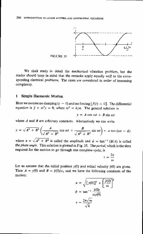
266 INTRoDUcTIoN To LINEAR ALGEBRA AND DIFFERENTTAL EQUATIoNS

FIGURE 35

We shall study in detail the mechanical vibration problem, but thereader should keep in mind that the remarks apply equally well to the corre-sponding electrical problems. The cases are considered in order of increasingcomplexity.

I Simple Harmonic Motion

Here we assume no damping(c : 0) and no forcing lf(t) = 0]. The differentialequation is ! + o)2y : 0, where a2 : klm. The general solution is

! : A cos crrl * .B sin alt

where A and B are arbitrary constants. Alternatively we can write

y : JA'z + B'z (+.coso,r * $ r inrr) : d cos (at - Q)\ V a t + 8 2 t f A z + 8 2 /

where a: ^lAt + Bz is called the amplitude and Q: tan-, (BIA) is calledthe phase angle. This solution is plotted in Fig. 35. The period, whichis the timerequired for the motion to go through one complete cycle, is

" : ' f

Let us assume that the initial position y(0) and initial velocity j(0) are given.Then A : y(0) and ,B : j,(O)lo, and we have the following constants of themotion:

,:Jr*r=eT6 : tan-r Y(0)

ov(0)

znJil k

LINEAR DIFFERENTIAL EQUATIONS 267

FIGURE 36

'!'L',[.I'l|

*.,0.'0,n, I

ou,,u"'',n, |

.,nn" damping

For { we shall take the minimum nonnegative angle such that sin { : jt(0)laatandcos 6: yp) la.

2 Free Vibration with Damping

Inthiscase,wehavek > 0andc > 0 andf( t ) :0. Thedi f ferent ia lequat ionis

( m D ' * c D * k ) y : g

and the associated polynomial equation is P(z) : mz2 * cz * k :0. Thesolutions are

- c * " / c 2 - 4 k mfvf2 :

The independent solutions of the differential equation depend on the value ofc2 - 4km according to the following:

a Oaerdamping:

c2 - 4km > 0 ! : Ae"t * Be"t r, < r, < 0

b Critical damping:

c 2 _ 4 k m : 0 y : ( A * B t ) e , t t , "' t : - f r ,c Underdamping:

c2 - 4km <0 ! : s - (c t2 ' ) r (1 cos c t t t *Bs inco t ) , : JOO\ - *

2m

Some typical motions in cases a and b arc illustrated in Fig. 36. In case c, wecan write alternatively

! = ae-Gl2')t cos (at - Q)

2m

268 INTRoDUcTIoN To LINEAR ALGEBRA AND DIFFER.ENTIAL EQUATIoNS

FIGURE 37

where a: JAz + 82 and @ : tan-t @1,0. The motion is illustrated inFig. 37. The motion is oscillatory, as in the case of simple harmonic motion,but the amplitude is diminishing according to the exponential factor e-Gtznrt.The motion is not periodic, but the time between successive peaks is z : 2nlotIf the damping constant c is very small compared with k and m, then cl2m isvery small and the exponential factor e-G/2m)t is near I for reasonably smallvalues of r. In this case the motion is very nearly simple harmonic motion, andr is approximately a period.

For forcing we shall consider two cases.

3 Forced Vibrations without Damping

In this case c : 0, and for definiteness we shall take f(t) - /e cos orof, where/, is a constant and aro * a : (klm)ttz. The differential equation is

Y * a'Y :& "o"o'

The complementary solution is

!" : A cos @t * B sin alr

To find a particular solution we use the method of undetermined coefficients.We assume a solution of the form

lp : C cosaro t * Ds ino lo /Then

Y, * a"Yn: c(a2 - oh2) cos crrel *

The re fo re ,D :0and

D(ro' - ao')sin arot : & "o,

,0,

e - f om(a2 - crtoz)

0 + 2 r

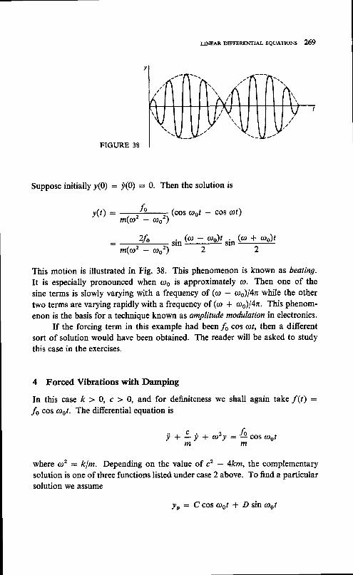
I.JNEARDIFFERENTIALEQUATIONS 269

FIGURE 38

Suppose initially y(0) : y(0) : 0. Then the solution is

y(r) : , Jo ,.(cos orsr - cos cof)m(@' - @o')

: -,2fo- rrn (co - alo)t

,rn (al * coo)/

m ( a z - a o ' ) 2 2

This motion is illustrated in Fig. 38. This phenomenon is known as beating.It is especially pronounced when are is approximately rn. Then one of the

sine terms is slowly varying with a frequency of (al - a)l4n while the other

two terms are varying rapidly with a frequency of (ar * cr.s)|4n. This phenom-

enon is the basis for a technique known as amplitude modulation in electronics.If the forcing term in this example had been /r cos cot, then a different

sort of solution would have been obtained. The reader will be asked to studythis case in the exercises.

4 Forced Vibrations with Damping

In this case k ) 0, c > 0, and for definiteness we shall again take /(r) :

/r cos arol. The differential equation is

y + I i ' + a 2 y : & c o s a r o tm f n

where o2 : klm. Depending on the value of c2 - 4km, the complementary

solution is one of three functions listed under case 2 above. To find a particular

solution we assume

lp: C cos @ot * D sin arot

27A INTRoDUcTIoN To LINEAR AI"GEBRA AND DIFFERENTIAL EQUATIoN'

Then

, r * * r i , o + o t 2 y ,

Therefore,

ao2) + l,,odcosc,otm J

- ao2) - *r"4sin

aror

c(a, - roo2) + *rrro:*,

: [tt''

-

* ['r''

Solving, we have

* ' ( r ' - : c t , o ' ) * c 2 a o 2

We can write

u - : 4 c o s ( @ s t - d )J P J @ - " "

where

d : tan- ' - - ! 'o =m(r' - ttto')

It should be noted that for any one of the complementary solutions

rherefore, arter atong period of time the part of the ,.*:":;,lo "onr,nu*to contribute is !o, For this reason /, is called the steady-state solutloz in this

problem. The other part is called the transient solution. The case @o : o)deserves special comment. The method of solution does not have to be changed,as was the case when there was no damping. However, the amplitude factor

J * t ( c r ' - r a , o z ) * c 2 a o 2

is a maximum when @o : oJ. This phenomenon is known as resonance. Asimilar thing occurs in the electric-circuit case. If the values of Z and C areadjusted so that @ : (LC)- rlz is equal to the crro for the impressed voltage,current flowing will be maximized. This is the basis for tuning a radio or TV.

D(a'

C -

D :

- c o o 2 ) - ! r o c : o

m(a2 - ah2)f,

m 2 ( @ 2 - a o 2 ) + c 2 t t t s 2

c@o"fo

fo

LINEAR DIFFERENTIAL EQUATIONS 27I

EXERCISES 6.6

,l A mass weighing I pound hangs in equilibrium with a spring stretched I inch.The mass is pulled down 1 inch below the equilibrium position and released.

What is the period and frequency of the motion? What is the amplitude?

2 If the mass of Exercise I is given an initial velocity of I foot per second along with

the initial displacement of 1 inch, calculate the amplitude and phase angle.

3 Show that regardless of initial conditions, in the case of free vibrations with

overdamping, the mass can go through the equilibrium position at most once.

4 Find the general solution in the case of forced vibrations without damping for

f(t) : /s cos {Dt, co2 : klm.5 Consider a series electric circuit with no resistance and no impressed voltage.

Show that the current is periodic with period r : LnJLc,where Z is the induct-anceandCis thecapac i tance. F ind t i f L : lhenryandC :4 x 10-6farad.

6 Find the steady-state current in a series circuit if the impressed voltage is E(r) :

110sin 1202lvolts andL: 3 henrys, R : 500ohms, andC: 5 x 10-6 farad.

X6.7 GREEN'S FUNCTIONS

Green's functions are very useful in the treatment of linear differential equations,

both for initial-value problems and boundary-value problems. They are also

important in the study of linear problems in partial differential equations, and

they supply an important link between differential equations and integral

equations.

We shall introduce the ideas involved by finding the general solution of the

simple problem y : f(t), y(0) : a, jt(O) : S. The associated homogeneous

equation is y : 0, and clearly the functiotr !" : a + bt satisfies the homo-geneous equation and the initial conditions. Therefore, we must find a particular

solution /p which satisfies .yo(0) : .yp(0) : 0. We proceed by variation ofparameters. Let lo : A + Bt, where A and B are functions of f. Then

j ' o : B + A + B t

We put A + Bt : 0, and then

: p : f ( t )

: -tf(t)

!o

A

P t

I r'J 0

Integrating, we find

.l/p - - r)f(t) dr

272 INTRoDUcTIoN To LINEAR ALGEBRA AND DIFFERENTIAL EQUATIONs

It is easy to verify that yr(0) : yp(0) : 0, and so the general solution is

! : a+b t+ i ' t r - r ) f ( r ) d rJ o

and this is a solution to the problem as long as f(t) is integrable.Let us define the following Green's function:

G . ( t - t o < r < t

t r ' t ) : { 0 t < r

We think of t as a parameter and r as the variable in the function. If the dotrefers to differentiation with respect to r, we have that G satisfies the followingconditions:

I G(t,f l iscontinuousfor0 < c < oo and G(t,r) = 0for t < x.

2 G : 0 f o r 0 < r < t .3 There is a jump of I in the derivative G at r : t.

These conditions determine G uniquely. Condition 2 requires that G(t,r) :

a * Br. Condition I requires that a * Bt :0, and condition 3 requires that

t i m C ( r , z ) : F : - l

Hence, d, : t andG(t,r) : [ - t forO 1 t 1 t.Let us take another point of view of the example. Let us seek a function

H(t,r) which will produce a yp satisfying 0 : yo(0) : ir(0) upon multiplying

bV "fG) and integrating; that is, yo : I'o H(t,lf(t) dx. If we lett

f t - f t - e

| ,n'1r1 Ar : lin I F(r) drJ o e - o + J o

then

f ,r{,,r)f(r) dr :

lour,,r)yo@) dr

: ito@)H(r,r)lb - f' o6,"1ro a'J o

: ,eH(t,t) - Hvrl' i + l '- ng,r1!p dtJ o

: ieH(t, t) - H(t, t-)yo(t) + l ' - ny, a,J o

t This is necessary because H may not have derivatives at r : t'

L1NEAR DIFFERENTIAL EQUATTONS 273

This last expression will be equal to yoQ) if and only if H(t,t) : 0, H(t,t-) :-1,and E: Ofor0 < r < t. ButthesearetheconditionswhichdeterminedG(r,r). Hence, H(t,r) : G(t,r).

EXAMPLE 6.7.1 Letusconsideranotherinitial-valueproblem: i + q()! :

"f(t), y(0) and )(0) given. We shall assume that q(t) and QQ) are continuous.There exists a complementary solution y"(l) satisfying ./"(0) : y(0) andy"(0) : j'(0). What remains is to determine a particular solution yo(r) satisfying/r(0) : .yp(O) : 0. By analogy we seek a solution in the form li C1t,ry1q ar.Then

j,o(G - qG) dr

: ie!)G(t,t) - yo(G - sG)Wf t '

+ I vo (G-qG-qc )a rJ O

We attempt to determine the Green's function G(t,.c) by the following condi-tions:

1 G(t , t ) iscont inuousfor0 < r < t ,andG(t , r ) = 0for / < c .2 G - S G - S G : 0 f o r 0 < c < t .3 The re i sa jumpo f I i n thede r i va t i ve Ga t r : t .

Under these conditions G(t,t1 :0 and GQ,t-): -1 and hence from above!'o C1t,r'571r1 4t : !0.

We shall now show that conditions 7, 2, and 3 determine G uniquely.The equation in condition 2 can be written as

d; (G -sG) :oCI'E

Therefore, G - qG is constant for 0 < r < t. B:ut if q(t) is continuous andG(t,t):0, then G - qG: G1t,t-1 : -1. Therefore, ourconditionsreduceto G - qG : -1, G(t,t) : 0. The integrating factor is

l,o{,,it@ d' :

f,c(t,iee + qy,) dt

: j,o@)G(t,r)lb - J'

ek) : *'[-f nc) ntf

274 tNrnooucrloN To LINEAR ALcEBRA AND DTFFERENTIAL EQUATIoNS

Then (dldr)(QG) : - Q, and

However, G(t,t; : g, st

G(t,t)

G(t,r)

1 f ' - . . cc : - ; l Q h ) d q + -

Q J o a

- 1 f t P

0( t ) Jo - ' ' '

Q ( t )t ': I Qh) a't

J O

1 f t

Qk) J, -"'

EXAMPLE 6.7.2 Find the solution of Y - ilQ + 1) : /Q) for 0

Y(0) : Y(0) : 0. The solution is rt

y( r ) : I G( t , r \ f ( r )dtJ 0

witht f t

G(t,r) : da )"

Q(ti d,t

where

ek) : . -o i | (6 + t1- ' a( ] : t + rL J o I

Therefore,I r t ( , - t ) ( t * r + 2 )

G(t,.c): -r J. (ry + 1) dn -- Y-frTi:--!-

< t < c o ,

EXAMPLE 6.7.3 Find the general solution of the problem i + y : f(t),y(0) : ./0, .y(0) = yo. Again we shall find a Green's function. The comple-

mentary solution! " : l o c o s t + y o s i n t

satisfies the associated homogeneous equation i + y :0 and the initial

conditions. Hence, we must find a particular solution /, satisfying.yp(0) :

ie(0) : 0. We look for a solution in the form yp(t) : I'"c(t,r)t@ dr. Then

f t l t

)oc{t,r)fG) r. :

J, G(t,r)(ye r y) dr

: 1io(t)c(r,t)lb - J'

(Gio -

: iee)G(t,t) - d(r,t)yo(r)l';

Gyo) dt

+ J' r"tG +G) dr

JAR DIFFERENTIAL EQUATIONS 275

We shall look for a Green's function G(t,z) satisfying G + G: 0, 0 ( r < t,G(t,t):0,and G(t,t-) : -1. From the differential equation we have

G ( t , t 1 : A c o s t * B s i n r

T h e n G ( r , r ) : l c o s l * B s i n t : 0 a n d G ( t , t - ) : - l s i n l + B c o s t : - 1 .Solving for I and B, we have I : sin t and B: -cos l. Therefore.G(t,r1 : sin (r - t). The general solution to the problem is

! : locos r + ye sin / + f 'r in (t - x)f(x) drJ o

Forthe generalnonsingular second orderlinear equation y + qj, * ry :

/(l), where we assume thatf(t), r(r), and QQ) are continuous, we proceed asfollows to obtain a Green's function:

f t f t

I C(t,t)f(r) d" : I G(t,r)(re * ej,p + ry) dtJ o J o

P t -: j , , (c)G(t,r) l lo- | l ! ,1C- qG)_rGyJdt

J o: iee)G(t,t) - yp(G - sG)W

F t -

+ I y , (G -sG-dG+rG)d rJ o

We take the following three properties for G(/,c):

1 G(t , r ) iscont inuousfor0 < r < t ,andG(t , r ) :0 for l < r .2 G - q G - q G * r G : 0 f o r 0 < r < t .3 There is a jump of I in the derivative G at t : t.

satisfying these conditions is equivalent to solving the following initial-value problem for the interval {" l0 < t 4 t}: G - qG - dG + rG : 0,G(t,t): o, GQJ-): -1. By Theorem 6.2.1, this problem has a uniquesolution. The differential equation can be written

d2c d, 7 - * ( ac )

* rG :o

This is called the adjoint differential equation. The reader will be asked roinvestigate the form of the adjoint equation associated with higher orderdifferential equations.

Let us reexamine the problem y + qj, + ry --.f(r), y(0) : i(0) : 0,from a slightly different point of view. Let

G(t,r1 : + f' Q(n) dnQk) J,

-" '

276 rNrnooucrroN To LTNEAR ALGEBRA AND DIFFERENTIAL EeuATIoNs

where Q(t) : exp [-i; sG) d4]. Recall that G(t,t) is the Green's functionassociated with Example 6.7.1. Let y(t) be the solution to the problem, andconsider the function

z(t) : J'rn"r[ ' to *

J O

t : f"lr(") - r(c)v(rlff at

t : l,u@) - r(r)v(r)l ffia,

v:f(t) - 4t)v * f"rr<o - r4)v4)lffijr,

- r(r)y(r)lG(t,r) dr

qy)G(t,r) dr

: 1i(r)c(t,z)l', (G - qc)y dr

: - ( d - q c ) y ( c ) l ' ; + | G - q G - Q G ) y d rJ O

: v(t)

Hence, if y is the solution of the problem, it is also a solution of the followingVolterra integral equation :

where F(/) : llo G(t,r)f Q1 dr. It is not hard to show that any solution of theintegral equation is also a solution of the differential equation, thus showing

that the two problems are equivalent. In fact,

where QQ) : -q(t)QU). Hence, y = "f(t) - r(t)y - S(t)i. Obviouslv,

y(0) : f(0) : 0. There are iterative methods for solving the integral equationeven when the differential equation may not be easy to solve.

We conclude this section with a brief discussion of boundary-valueproblems. Throughout this book we use the independent variable t when we

discuss initial-value problems and the dot to denote differentiation with respect

to t. On the other hand, we shall use the variable x when we discuss boundary-

value problems and a prime to denote differentiation with respect to x.

Consider the following boundary-value problem y" : f(x),0 < x < l,

f t -- lJ O

y(r) : r(r) - lor!)G(t,ly(r)

dr

LTNEAR DIFFERENTIAL EQUATIONS 277

f(0) : y(1) : 0. According to what we did earlier in this section, the generalsolution is

y :a+ bx+ | ( x -o f ( od tJ o

T h e n y ( O ) : c : 0 , a n d

- 0 f@ de :0

Hence,

L)"fG) d4

and

0f@ de

L)f(0 d<

where we have let

( F ( * - l ) 0 S 6 < xG(x,O:1i i l_ ,1 x3€<lG(x,fl is a Green's function associated *r,O ,0. boundary-value problem. Ithas the following properties:

I G(x,() is continuous for 0 < f 3 1.2 G " : 0 f o r 0 < € < x a n d x < ( < 1 .3 C (0 ) : G ( l ) : 0 .4 There is a jump of I in the derivative G' at ( : y.

EXAMPLE 6.7.4 Find the solution of the boundary-value problemy" + y : f(x),0 < x S L, y(0) : y(L): 0. We discovered earlier that thegeneral solution is

y (x ) : 4cosx * bs in * + f ' s i n ( x - E ) fG) d€

J o

)(1): b + J' tr

,:J',n-

,=J 'xG-l) f (Odq+I"(x-

: j, n' - t)r(€) a€ + I' 'G -

: ["

o6'ttt<ct ac

278 rtrnooucnoN To LTNEAR ALcEBRA AND DIFFERENTTAL EeuATroNs

T h e n y ( 0 ) : a : 0 , a n d

Y ( L ) : b s i n L *

Prov ideds inL#0 ,

sin (L - )fG) d( : 0

sin (( - Df(0 de

fL

J,b: r f "

sin L Js

L)f(() dt + J-.in

t*v(x) : ,i".*J:sin ({ -

sin (( -

- of(o dc

sln x L) + s i nLs in (x - € ) , ,t r \ s tsin L

:J;..|l ttt *FrG)dc

: J, "'*:'*g - "'r(od€. I,

*"#g-_a rG)dcfL

: )o

c1x'11761ac

where ttre Green's function is

G(x ,g :

o< {<x

x< t<L

This Green's function satisfies the conditions:

1 G(x,() is continuous for 0 < € < L.2 G" + G : 0for0 < { < xandx < 4, < L.3 G(0) : c(r) :0.4 There is a jump of I in the derivative G' at ( : 16.

These conditions determine the Green's function uniquely, provided sin Z # 0.

It is ofinterest to show how these four conditions can be used directly to

show the representation of the solution of the boundary-value problem.

fsin ( sin (x - L)

J s in l

l s i nxs i n (1 -L )I tttt I

LINEAR DIFFERENTIAL EQUATIONS 279

Consider

fL fL

I c(",O"r(O d( : I G(x,)Q" + y) dEJ o J o

f r fL= | G(x,O(y,' + y) d( + | c$,O(y', + y) d(

Jo t,x-

J'

: y,c(x,Ol6 - | (G,y, - Gy) dEJ o

+ y'G(x,Ol! - f' {o'r' - Gy) d(J x "

: -c,yl6- - c,yl!. * f'- {",, + c)y d€J O

* f' (c' + G)y dE

where we have already used the boundary.""o;";, on G and the continuityof G at I : x to drop certain terms. Finally, we use the boundary conditionson y, the jump of I in G' at ( : x, and condition 2 to show that

I c(x,Q_fG) d( : y(x)lc'(x,x*) - G,(x,x-)l : /(r)J o

Finally, we consider the boundary-value problem y" + q(x)y = f(x),y (0 ) : y ( l ) : 0 , whe re q and f a re con t i nuous on { x lO<x< l } . Le tG(x,€) be the Green's function considered earlier

Gk. t \ : [ c<x -D o< ( .< rl x ( ( - l ) x < ( < l

and consider

PL

I tftO - qG)yfc(x,o dtJ o

: f" o1*'17'' o1J ofx PL

: l G(x,)y', dC + l G(x,Oy,, d(J o J *

f x - f L: y'G(x,Oli- - | G,y' d€ + y,c(x,Olf. - | G,y, d(

Jo r x - FL

J " *

: -c'yl6- - c,yl!. + | yG,, d( + | yc,, de)o J ' .: v(x)

280 rNrnooucrloN To LINEAR ALcEBRA AND DIFFERENTTAL EQUATIoNS

using the properties of the Green's function listed above. Hence, we see that /satisfies the Fredholm integral equation

P L

y(x) : r(x) - | qG)yG)G(x,$ dEJ o

where F(x) is the known function It G(x,Of@ d(. There are ways of solvingthe integral equation available even when the differential equation itself is noteasy to solve.

EXERCISES 6.7

1 Find the Green's function associated with the initial-value problem I + i : f Q),y(0\ : yo, y(0) = yo, by means ofwhich the solution can be written as

y ( t ) : a+ be - t + l ' oQd fG)a ,J o

where a and D are constants depending on yq and /r.2 Find the Green's function associated with the initial-value problem i + a2y :

.f (t), y(0) : /0, y(0) : /0, by means of which the solution can be written

y(t) : yocos al, + & sin cut + f' cg11761 a,(D Jo

3 Find the Green's function associated with the initial-value problem i - 3i +

2y = f(t), /(0) : i(0) : 0, by means of which the solution can be written

,<,> : f' Ge,r)fk) dtJ o

4 Find the Green's function associated with the initial-value problem t - 2i +

y = f(t), /(0) : i(0) : 0, by means of which the solution can be written

/o) = i G(t,r)fG)drJ o

J Find a set of conditions which will uniquely determine a Green's function

associated with the initial-va1ue problem 'Y + p(t)i + s(t)i + r(t\v : f(t),

-/(0) : i(0) : l(O) = 0, bv means of which the solution can be written

Y@: I Gl ' t) f(r)drJ o

Assume that i, ti, r,f are all continuous for 0 < t < m. What is the adjoint

dffirential equation associated with it + p! + oi' I ry : f(t\? Can you give

a general charccterization of the adjoint differential equation for higher order

problems?

LINEAR DIFFERENTHL EQUATIONS 28I

Find a Volterra integral equation equivalent to the initial-value problem ofExercise 3.Show that the linear second order initial-value problem, i + pi * qy : f(t),y(0) = .yo, .y(0) : .ts; c&n always be modified to one in which the initial valuesare zirlro by subtracting from the solution the function h * i,ot.Referring to Sec. 5.8, see if you can devise an iteration method for solving Volterraintegral equations of the type introduced in this section. Can you prove thatthe method converges to a solution?Show that the four conditions listed for the Green's functions associated withthe boundary-value problems of this section determine the Green's functionsuniquely.

I0 Find a Green's function associated with the boundary-value problem y" +(,)2y : f(x), y(0) : y(L) : 0, by means of which the solution can be written

y(x) :

provided sin arl # 0 (see Exercise 2).

G(x,€)f(€) d€

Showthatsinar*x, @x : knlL, k : l , 2, 3,. . . , aresolut ions ofy" * a1r2y : g,

y(0) : flL\ : 0. These functions are called characteristic solutions of y" +etzy : 0, y(0) : y(L) : 0, associated with characteristic ualues aro2. Relate thisto the solution of the boundary-value problem of Exercise 10.Find a Green's function associated with the boundary-value problem y" +p(x)y' : f (x), y(0) : y(1) : 0, by means of which the solution can be written

rI I

I2

f 1y(x): I G(x,€)f(€)d(

J o

l3 Find a Green's function associated with the boundary-value problem !" * tDzy :

f(x), y(0) : y'(L) : 0, bY means of which the solution can be written

v(x) : G(x,$f((\ d€

Show that the linear second order boundary-value problem y" * py' * qy:f(x), y(o\ : a, y(L) : b can always be modified to one in which the boundaryvalues are zero by subtracting from the solution the function a + (b - a)xlL.Show that the Fredholm integral equation introduced in this section is equivalentto the corresponding boundary-value problem by showing that any solution of theintegral equation is also a solution of the boundary-value problem.Find a Fredholm integral equation equivalent to the boundary-value problemy" -f py' * qy : f(x),O < .r < 1, y(0) : y(l) : 0.Referring to Sec. 5.8, see if you can devise an iteration method for solvingFredholm integral equations of the type introduced in this section. Can youprove that the method converges to a solution?

r14

15

I6

17

nI

LAPLACE TRANSFORMS

7.I INTRODUCTION

This chapter deals with the use of the Laplace transform in the solution of

initial-value problems for linear ordinary differential equations. It begins with

a definition of the transform and some sufficient conditions for its existence.

We study some of the general properties of the transform and develop the

transforms of some of the functions most often encountered in the solution of

linear differential equations. We do not treat the general problem of inversion

of the transform but study in some detail the method based on the partial-

fraction expansion of the transform. This is followed by the method of Laplace

transformation in the solution of linear differential equations, especially those

with constant coefficients. The last unstarred section takes up some applica-

tions by this method. The starred section in this chapter discusses the question

of uniqueness of the transform. This is extremely important since the use of the

Laplace transform in the solution of differential equations depends so heavily

on the ability to invert the transform uniquely.

LAPLACE TRANSFORMS 283

7.2 EXISTENCE OF THE TRANSFORM

Letf(t) be Riemann-integrable for 0 < r < ? for any finite T and supposethat for real s

l rlim I e-$f(t) dtr - o Jo

exists. Then we define the Laplace transform of/(l) as

f r f osl"f(t)l:

"fim I e-"f(t) dt : I e-'f(t) dt

r - o J o J o

Generally the transform will exist for more than one value of s. and henceSlf(t)l defines a function of s when it exists.

" ltg II t-"'lf (t)l dr exists, we say that the improper integral conuerges

absolutely. If the integral converges absolutelyn it also converges in the ordinarysense. This can be seen as follows. Since

0 < l"f(t)l + "f(t) < 2lf(t)l

r r f r f r0 < | , - " l f ( t ) l d t + | , - " f ( t ) d t < z l e - ' , l f ( t ) l d t

J o J o J o

and the existence of

f Tl im I e-"lf(t)l dtT - o J o

implies the existence ofl r T

lim I e-"f(t) dt? - o J o

Theorem 7.2.1 Letf (t) be Riemann-integrable for 0 < r < T,for anyflnite T, and of exponential order; that is, there exist constants M and asuch that l/0)l < Meot for all positive /. Then /(r) has a Laplace trans-form for s ) a, and lim glf (t)l : 0.

PRooF From ,;.;.o""tity we have

l r r I f r| | e-"f(t) d,l . I e-"tlf(t)l dtl J o I J o

= * f' e-steat g : . M- - M r@-s)r

J o s - 4 s - d

284 INTRODUcTIoN To LINBAR ALGEBRA AND DIImRENTIAL EQUATIoNs

Ifs > a,s@-s)r -+ 0as T + q. Thisestablishestheabsoluteconvergenceof the integral and the inequality

lsut>Jl < -M-s - a

from which it follows that lim 9lf(t)l : 0.

EXAMPLE 7.2.1 Compute the Laplace transform of/(t) : 1.

s1f : f' ,-" dr : lim f' ,-" a,Jo r-o Jo

l i * 1 - ' - " t : 1

provided s > 0.

EXAMPLE 7.2.2 Compute the Laplace transform of /(r) : eot.

f c o f Tg ld t f : l , (a -s ) td t - l im | ,@-s) td t

J o r - . J o

:l'*#:;=provided s > a.

EXAMPLE 7.2.3 Compute the I"aplace transform of f (t) : sin art.

_ f o f r9lsin otf : | ,-" sin arr dt : lm I ,-"' sin cot dt

Jo r 'o Jo

Integrating by parts, we have

f r| ,-" sin at dtJ o

: - +

sin arrl6 . ? I, e-" cos cot dt

e- tT

: -?s incr rT - f r r - "coso116 -5 f , - "s inot td t

(, * $ ft e-"'sin ot dt : -'-" sin arT - 2 r-" cos aT + |\ t ' / J o s s z s '

LAPLACE TRANSFORMS 285

If s > 0, lim e-tr sin cDT : lim e-'r cos ar? : 0. Therefore,T + o l + c o

gls in @tf : = ' =s 2 + @ 2

It is not essential that /(t) be continuous at I : 0. If it is not, we treatthe Laplace transform as an improper integral Lt t : 0 as well 8s I : @.

Hence,

slf(t)f : lim l' e-"7g1 atiloJ J'

provided the limit exists. For example,

g l t - t r2 l l im f ' , - " r - t t2 d ti1T J'

Near I : 0 the integrand behaves like r - U2, which is integrable, and so the

transform exists if s > 0. We make the change of variable 4 : st, and

f 6 l f @

I e - ' t t - r t z d t : h I t - rn -112 d4J o s ^ ' - J o

The integral exists and is equal to J". Therefore, F

g l t - t r '1 : Ysrlz

One of the most important properties of the Laplace transform is thatit is a linear transformation. Let a and 6 be any scalars, and let f (t) and g(t)

be any two functions with Laplace transforms. Then

glaf(t) + bg(t)f : f* or-"rrt) itt + f* u"-"n1r1 o,J o J O

f o - f *- a I e-"f(t) dt + b I e-'tg(t) dtJ o J o

: aelf(t)l + bsls(t)l

There are various operations on Laplace transforms which lead to usefulformulas for transforms. One of these is change of variable. Suppose /(t)satisfies the hypotheses of Theorem 7.2.1. Then its transform

d(s) : !-

e-*f(t) dt

286 INTRODUCTION TO LINEAR ALGEBRA AND DIFFERENTIAL EQUATIONS

exists for s > a. If s - b > a. then we can obtain

f @d ( s - b ) : l r - " r " f ( t ) d t

J owhich gives us the formula

Vleb'1t1f : glf(t)1"-"- a

Another operation is differentiation of the transform with respect to s.lf f (t\ satisfies the hypotheses of Theorem 7.2.1, then

f 6

d(s) : I e-" f ( t )d tJ o

converges uniformlyt for s > ro ) d. This allows us to differentiate under theintegral sign. Hence,

f ad ' ( s ) : - l e - s t f ( t ) d t

J owhich leads to the formula

d

Atlt<r>l : -eftf(t)f

Finally, we shall consider what happens when we take the product of twotransforms. It is not the case that the transform of a product is the productof the transforms. On the other hand, let {(s) : glf (t)f and r/(s) : glg(t)f

be the transforms of two functions satisfying the hypotheses of Theorem 7.2.1.Then

4(s)fG) : lim f' ,-"'1r7 o, f' e-ss(t) dtt - ' ' 1 . ' o

P l .

: lim | | e-"r'*'rf(t)g(r) dt drt-- JoJo

The las t in tegra l i soverasquare{ (1 , " )10 < r < T ,0 1 r < -T} . Wemakeachange of variables 4 : t + r,r : T, and we have

T TP F f T f T + t

| | ,-n'*'\f(t)s(") dt dt : I of') | e-rf(tt - r) dq dr

J J J o J "o 0

where the integration is now over the region indicated in Fig. 39. Assuming

tSee J. W. Dettman, "Applied Complex Variables," pp. 186-191, Macmillan, New York, 1965(rpt. Dover, New York, 1984).

LAPLACE TRANSFORMS 287

FIGURE 39

that we can interchange the order of integration (this is certainly the case if /and g are continuous), we have

f r f r + tI o(t) | ,-"4"f(n - r) dry dt

J o J t

Taking the limit as T -+

of the function

l r f n: | ,-'o I o@ffu - r) dr d4J O J O

f2r r r+ | t-"' I o@f@ - r) dr drl

J r J n - r

m, the first integral becomes the Laplace transform

h(t1 : f' s!)ft - r) drJ o

and we can show that the second integral goes to zero as 7 --+ co, In fact, if

l/(r)l < Meot and lg(t)l <.ly'eb', then both / and g are of order e"', where

c : max Lo,bf. Then

l f r I r r| | g(r)f(n - r) drl < MN I e""e"@-') dr : MNe"q(2r - n)I J q - t I J r t - r

But Jf 4e-snsc| d4 converges provided s > c, which shows that

f 2 T f o

lT J , "-"'t'"0 dn 3l* J.

e-s,vecn dq : o

AlsoP 2 T

lim 2T I et'-'ro d4 :T + c o J r

We have shown that

li^ 2T

(s2(c-s'tt - ,tc-s)r) - 0

slf(t)lsls(t)) : slf"o!)f{t - n o')

288 INTR.DU.TI.N To LINEAR ALGEBRA AND DIFFERENTIAL EQUATI.NS

The function Ji g(r)!(t - r) dr is called the conaolution integral andusua l l ydeno tedby f *g .Byas imp lechangeo f va r i ab le f romr t on - t -we can show that

(f* s)(t) g(r)f(t - r) dt

fQDsO - Ddn : k * f ) ( t )

Some of the other properties of the convorution integrar are

f * ( s+h ) : f * s+ f *h( f * g ) * h : f * ( g * h )

o * . f : g

However, (l *f)(t) : IL[G) dz, which is not in general equal tof(t).

EXERCISES 7.2

1 Find the Laplace transform of tn, n a positive integer.2 Find the Laplace transform of cos crrr.3 Show that if f(t) is Riemann-integrable for every interval of the form

{t10. e < t < T}, is of exponentiar order eot as t+ oo, and of order t-p,p < l, as t --r 0+, then it has aLaplae- transform for s > a.4 Find the Laplace transform of f, a > -1. Hint: The integral It n"-re-, drt

exists for x > 0 and is called the gammafunctionl f(x).5 Find the Laplace transform of cosh at and sinh arr.6 By differentiating under the integral sign, find the Laplace transform of toeor,

z a positive integer.7 By differentiating under the integral sign, find the Laplace transform of I sin arr

and t cos art.8 Find the Laplace transforms of ebt sin art and ebr cos crrt.9 Find the Laplace transforms of tebt sin a;t and tubt cos @r.

10 Find the Laplacr transform of "fL fr

_ r) sin at dr.II Assuming thatf(t) is a Riemann_integrable function of exponential order, findglJL f(c) d4. -Frrnr.' consider the integrar as a convorution.12 Assuming that f(t) is continuous for t > 0, ,f(0) : 0, and / has a derivative

satisfying the hypotheses of Theorem 7.2.1, prove that rim sglf(t)l : g.

:.l::T

t See ibid., pp. l9l-199.

LAPLACE TRANSFORMS 289

13 Find a function whose transform is 1/s(s2 + @2). Hint: Consider the transform

as the product of two transforms.14 Find a function whose transform is (s - a)-l(s - b)-t, a * b.

15 lf f(t) and g(r) are continuous for 0 < /, show that (f * dG\ is continuous for

0 < t .16 If /and g are Riemann-integrable and of exponential order, show that (f * s)Q)

is of exponential order.17 Prove:

( a ) f * ( s + h ) : f * s * f * h .( b ) ( f r s ) * f t : f * ( g * h ) .( c ) 0 * / : g .

(d) 1 * f + / (in general). As a matter of fact there is no Riemann-integrable

function/such that | * f : 7.

7.3 TRANSFORMS OF CERTAIN FUNCTIONS

We already know how to compute the Laplace transforms of many functions

commonly encountered in the solution of differential equations, such as tt',

cos @t, sin atf, eo', t'eo', tn cos tDt, tn sin arf, tneot cos tDt, tneot sin @t' For

example, if we start with

g l s i n a t f : = ' -s ' + a 2

then we have, by differentiating twice with respect to s,

9 l t 2 s i n a r t l : { / " '

t )L J ds' \s ' * a' /

6as2 - 2at3: G ' z + o " f

Then by making a change of variable we obtain

nft2e"'sin arr] : #--{-:29:*[ ( r - a ) 2 + @ 2 f 3

We could obtain transforms of many more functions by taking convolutions of

functions whose transforms are already known. However, given a function, it

is not easy to determine if it is the convolution of two functions of the right

type.

2N INTRODUcTION TO LINEAR ALGEDRA AND DIFFERENTIAL EQUATIONS

FIGURE 40

We can add to our list of functions with known transforms by consideringoperations on the transformed function. Let c > 0, and consider

elf(ct)l : l* ,-"71cty atJ o

1 f .: : | , - * t '7@)dtc J o

1: ; nutr)]"*"r"

Next we consider a shift in the independent variable. We shall find thetransform of u(t - a)f(t - a), where a > 0 and u(t) is the unit step function

f t r > ou ( t ) : I '[ 0 r < 0

The functionu(t - a)f (t - a) is graphed in Fig. 40. we compute the transformas follows

slu(t - a)/'(t - 4)l : f* "-"71, - a) dt

J a

f o:

I e-"t '+o\1r1 dtJ o

f o: e-as

I e-"'f(r) dr

J o

: e-"'glf(t))

EXAMPLE 7.3.1 Find the Laplace transform of the function graphed inFig. 41, consisting of one positive half-cycle of sin crrl shifted by t : a. Thefunction can be represented by the formula f (t) : u(t - a) sin a(t - a) +

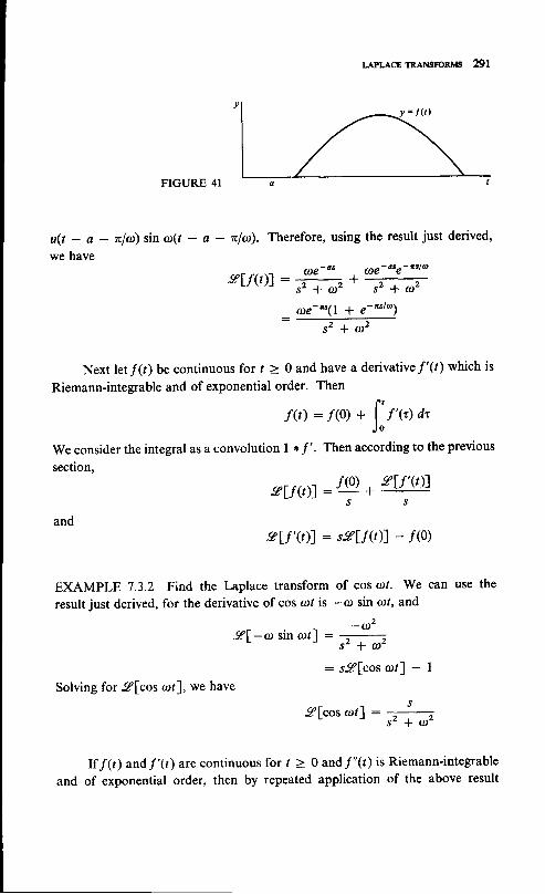
LAPLACE TRANSFORMS 29I

FIGURE 4I

u(t - a - nlco) sin co(t - a - nfatp). Therefore, using the result just derived,

we have

:tlf(t)f :

If/(r) and f '(t) are continuous for t > 0 and f"(t) is Riemann-integrable

and of exponential order, then by repeated application of the above result

q!-o" -L 0)e-ase-tsl@

f f i? -Wae-as(l + e-tsl@)

s t + u '

Next let/(t) be continuous for I > 0 and have a derivative/'(r) which is

Riemann-integrable and of exponential order. Thenf t

f(t) :.r(0) + | f'G1 a"J o

We consider the integral as a convolution | * f '. Then according to the previous

section,

elf(t)l:ry.ryand

slf'(t)f : self (t)l - /(0)

EXAMPLE 7.3.2 Find the Laplace transform of coscrll. We can use the

result just derived, for the derivative of cos a;t is *al sin art, and

A l - r s i n a r t ] : , - ' . " =s- + 012

: sglcos @tl - |

Solving for 9[cos arl], we have

glcos laltl : ^j_-s 2 + a z

292 INTRODUcTIoN To LINEAR AI,GBBRA AND DIFFERENTHL EQUATIoNs

we can obtain glf"(t)f. First we have to show that /'(t) is of exponentialorder. This follows from the inequality l/'0)l 3 Md', where a > 0, and

f tf,(t) : "f,(o) +

)of,'{r) o"

lf '(t)l < l,f'(o)l + f' V"{r)l o"J O

f l< l , f ' ( 0 ) l + M l { ' d t

J o

< l,f'(o)l + Md' - M

a a

= (v'e)t * {) n'\ a /

Applying the above result, we have

slf'(t)f : self(t)l - /(o)glf"(t)f : sslf'(t)l - /'(0)

: s2sff(r)l - .f(o) - /'(o)Repeated applications of these principles give us the following theorem.

Theorem 7,3.1 Let f,f ' ,...,f6- 1) be continuous for / > 0 and letf(o) be Riemann-integrable and of exponential order. Thenglfa>(t)f : s"9lf(t)l -

"" y(0) - s"-2f'(0) - 1<a-rr(0)

EXAMPLE 7.3.3 Find the Laplace transform of I cos art. Here we use atechnique based on the fact that the given function is the unique solution of aninitial-value problem in ordinary differential equations. An annihilationoperator for the function is (D2 + a')'. Therefore, the function satisfies thedifferential equation (D' + o')'y : O. It also satisfies the initial conditionsy(0):0, i (0) : l , y(0):0, y(0): -3a2. The di f ferent ia l equat ion is(Do + 2ot2D2 * o4)y: g. We take transforms using Theorem 7.3.1. Ifd(s) : 9lt cos col], then

snf - s2 + 3rtt2 + 2@2(s2O - l) + a4d : 0

(to + 2a2s2 + rcoo)d : s2 - (D2

6:, ' ! - !^=1s2 + ra212

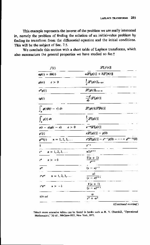
LAPLACETRANSFORMS 293

This example represents the inverse of the problem we are really interested

in, namely the problem of finding the solution of an initial-value prdblem by

finding its transform from the differential equation and the initial conditions.

This will be the subject of Sec. 7.5.We conclude this section with a short table of Laplace transforms, which

also summarizes the general properties we have studied so far.t

f (t) 9If Q)l

as(t) + bh(t) avl,so\l + bgth(trl

g(ct') c > 0 Lgane)|"-,,"

d'sQ) 9lg(t)1"-,-o

ts{lt) jvw,>t

fook\ntt - i)dt 9ls(t)l9lh(t,)l

f"^, o, \ stoo't

u ( t - a ) s ( t - a ) a > O e-'z9IsQ)l

g'(t) s"gIct)l - s(o)

g 6 ' ( t ) n : 1 , 2 , 3 , . , . s\?Jst)l - s"-rr(0) ,ta-tr(0)

J - r

t n n = 1 r 2 r 3 , . . . nlls"+ |

a > - l r(a + 1)Sa+ I

(s - a)- '

t 'd' n : l r 2 1 3 r , . .n l

( J - a ) ' - t

tnd' a > - l r(c * l)(s - a)n* t

sin rot(D

; r + @ ,

(Continued ooerleaf)

tMuch more extensive tables can be found in books such as R. V. Churchill, "Operational

Mathematics," 3d ed., McGraw-Hill, New York, 1971.

294 INTR'DU.TI.N To LINEAR ALGEBRA AND DIFFERENTIALEQUATI.N'

f(t) 9VQ)I

,sr-EZ

eft sin art

d'cos at s - a

C - q Y + @ ' z

I sin art 2os(s' + .r),

t cos cDt s 2 - a 2

C" + @'Y

t4'sin at 2ro(s - a)

[ ( s - c ) ' + c o z j 2

td' eas at ( s - a 1 z q r ,

iGrffiTsinh arl a)

T;'

cosh art J

s r - o , ,

EXERCISES 7.3

/ Find the Laplace transform of rcot cos @r.2 Find the Laplace transform of sinh at : *(e., _ e-rr).3 Find the Laplace transform of cosh at : t(e., +

"-.i).4 Find the Laprace transforms of r sinh at and t cosh arr.5 Find the Laplace transforms of teot sinh arr and tuot cosh arl.6 F i n d t h e L a p l a c e t r a n s f o r m o f f ( t \ i f f ( t ) : 1 , 0 < a < t = b , a n d / ( r ) : 0

for all other values of r.Find the Laplace transform of f( t) i f f( t , ; : 1,0 < r < c, f( t \ _ _1,c S t < 2c, and repeats periodically with period 2c.Findthelaplacetransform of f(t)rf .t(t) : t,O < t < c,andrepeatsperiodicallywith period c.

9 Find a differential equation and a set of initial conditions satisfied by f(t) :eot sin at, and use the initial-value problem to determine the Laplace transformot f(t).

10 Find a differential equation and a set of initial conditions satisfied by f(t) :teot sin at, and use the initial-value problem to determine the Laplace transformof f(t\.

LAPLACE TRANSFORMS 295

7.4 INVERSION OF THE TRANSFORM

There are general formulas for finding a function whose Laplace transform is a

given function.t However, these formulas are not easily applied, and in many

cases there are simpler techniques for inverting the transform. We shall take up

a few of these in this section. In the starred section of this chapter, we shall

prove a uniqueness theorem for the Laplace transform which will assure us that

once we have found a function with the given transform, there are essentially

no others with the desired properties.

EXAMPLE 7.4.1 Find a function whose Laplace transform is

( s - a ) - t 1s -b ) - r whe re a * b

We know that 9le"t]: (t - a)-1 and glto'f : (s - b)-1. Hence, using

the convolution integral, we have that (s - a)-t(s - b)-1 is the Laplace

transform off , f t

I gatgb(t-t) dr : eb, | ,(o-b)t 4t

J o J o

: 1 e d - J - e b t

a - b a - b

The form of the answer suggests that the transform should be expressed as

1 1 1 1 1

( s - d ) G - b ) :

; b s - d +

b - a s - b

which suggests a partial-fraction expansion. Indeed, if we write

I A B

( s - d ) G - b ) : r - o - t - 6

_ ( A + B ) s - A b - B a( s - a ) ( s - b )

this must be an identitv in s. For this to be so we must have

A + B : 0

A b + B a : - l

Solving these equations, we have A: (a - b)-1 and B: (b - a)-r.

t See Dettman op. cit., p. 400.

296 INTRoDUcTIoN To LINEAR ALGEBRA AND DIFFERENTIAL EQUATIoNS

The method based on the convolution integral is generally unwieldy ifthe given transform is the product of more than two recognizable transforms,and even then the integral may not be easy to evaluate. Generally, the methodof the partial-fraction expansion is preferred when it is applicable, and, aswe shall see in the next section, it will be applicable in problems involving lineardifferential equations with constant coefficients. We shall now review some ofthe methods for finding partial-fraction expansions.

Suppose we are asked to find a function whose Laplace transform js

d(s) :p(s)

( s - a , ) ( s - a ) . . . ( s - a n )

where p(s) is a polynomialt of degree less than n and e1. a2; . . . , an are alldifferent. we seek a partial-fraction expansion in the form

p(s) A r( s - a r ) ( s - a ) . . . ( s - a ) s - d r

, A r A n -i- -

S - O Z S - O n

Suppose we multiply through by s - at, I S k 3 n, an operation which isvalid for s # an. Then

p(s)( s - a r ) . . . ( s - d y _ r X s - a x + r ) . . . ( s - a ^ )

: Ar (s - ax ) + . . . *

Ao- rG - a r )S - Q t S - O * _ t

* A * * A * * t ( s - a x )

+ . . . +s - Q k + r

A,(s - a*)

s - Q n

The equality holds for all s sufficiently close to ap, where both sides are con-tinuous functions of s. Therefore, we may take the limit as J approaches a1,and we have

A * :p(ax)

(a * - a ) . . . ( ao - a r , _ ) (a *

If D(s) : (r - arXr - a). . .(s - a,) isD*(s) : D(s)/(s - a*), then

- or,+ r) " ' (ar - a^)

the denominator in d(s) and

A,. : P(ak)-

Do@o)

t For C(s) to be the transform of a function satisfying the hypotheses of Theorem 7.2. I ,limr*. d(c) : 0.

297

EXAMPLE 7.4.2 Find a function whose Laplace transform is

2s2 - s * IP(s ) : ( s - l x s - r xs -3 )

We look for a partial-fraction expansion in the form

d(s ) : ++ A ,^ * Ar -

' s - l s - 2 s - 3

a n d i f D : ( s - l X s - 2 X s - 3 ) , t h e n D t : ( s - 2 ) ( s - 3 ) , D z :(s - l)(s - 3), Dt : (s - lXs - z),andp(s) : 2s2 - s * l. Therefore,

A ' : p ( 1 ) - t' D'(r)

, p(2) -n l : : - l-

Dr(2)

A ^ : p ( 3 ) - S

" D'(3)

d(s):*-3.*: 9le' - 7e2' * 8e3t]

We now consider the case where one of the factors in the denominator isrepeated. Suppose

d(s):#s4(,)where 4(s) is a polynomial of degree n such that q(a) * 0 and p(s) is a poly-

nomial of degree less than n + m. We shall assume an expansion of the form

p(s) _ A, - A2 _r . . . - - A,

(s - a) q(ri: "a *

ft + "'* (":b + ft(s)

where i(s) represents the sum of all the terms due to q(s). We multiply throughby (s - a)', and then

ry = Ar(s - a)il- t * A2g - a)n-z + "' * A^+ i(s)(s - a)^q(s)

298 INTRoDUcTIoN To LINEAR ALGEBRA AND DIFFERENTIAL EQUATIoNS

where the equality holds up to and including s : a by the continuity of bothsides at .i : a. If we let s : a, we have A^ : p(a)lq@). Assuming that ft(s)is differentiable at s : a, we differentiate and

d f p(il1- l * l : (m * l ) , { r (s - a)^- ' + (m - 2)Ar(s - a)n- t

ds lq(s)l+ ' . ' * A^_1 * h'(s)(s - a)^ + mh(s)(s - a)n-t

If m > 2 and r(s) : p(s)lq(s), then A^_t : r,(a). Differentiating again, wehave

r"(s) : (m - l)(m - 2)Ar(s - a)n-z| ( m - 2 ) ( m - 3 ) A 2 g - a ) ^ - 3 + . . . + 2 A ^ _ 2F fr"(s)(s - a)^ + 2mh'(s)(r - c)'r-rI m(m - l)r(sXs - a)n-z

lf m > 3, then A^-z : lr"(a). continuing in this way, we obtain the generalformula

A ^ - i : ! r " ' 1 o 1j l

j : 0 , 1 ,2 , . . . , f f i - l , where 0 ! : I and rs(a) : r (a) . I f q(s) has a fac tor(s - 6)n, then of course i(s) will contain terms of the form ,Br(s - b)- r,Br(s - b)-t , . . . , 4(s - b)-0, but these can be handled in a similar wav.

EXAMPLE 7.4.3 Find a function whose Laplace transform is

d(s) :( s - t ) 3 ( s - 2 )

We look for a partial-fraction expansion in the form

d ( s ) : A t

+ A ' = + A '

* B

s - l ( s - 1 ) ' ( s - l ) . s - 2

Then .B : lim (s - 2)6G) : 2. Let r(s) : (r - l)3d(r) : s/(s _ 2) : | -s r 2

2 ( s - 2 ) - 1 . T h e n A t : r ( l ) : - 1 , A z : r , ( l ) - - 2 , A r : * r , , ( l ) : _ ) .Therefore,

d ( s ) : = + - * 2 - l 2

s - l ( r - l f * 1 r - 1 y + r - 2- gl-2e, - ztet - $t2e, + 2e2,)

299

Now suppose rf(s) : p(s)lqb), where q(s) is a polynomial of degree zand p(s) is a polynomial of degree less than n (both with real coefficients).Suppose further that q(s) has a nonrepeated complex root a * ib. Then, ofcourse, q(s) has a nonrepeated complex root a - ib (see Sec. 6.4), and q(s) canbe written as

q(s) : (s - a - rrXs - a * rb)r(s) : [(s - a)2 + D2]r(s)

Notice that the factor (s - a)' + D2 has real coefficients. This factor is calledan irreducible quadratic factor because it cannot be factored further withoutintroducing complex coefficients. It can be shown that every polynomial inthe real variable s of degree n 2 I with real coefficients can be factored intolinear factors with real coefficients and irreducible quadratic factors, somepossibly repeated. We now consider a partial-fraction expansion involving anonrepeated irreducible quadratic factor.

Let

d(s) :p(s)

[ ( r - a ) 2 + b 2 f r ( s )

where r(a * ib) + O. We look for a partial-fraction expansion of the form

? ( t - 1 t 1 B , r + / r ( s )

[(r - a)t + b]r(s) (s - a)2 + b"

where lr(s) accounts for all the terms in the expansion due to the polynomialr(s). We multiply through by (s - a)2 + 02. Then

p(s)'it : As * B + ft(r)[(r - a)2 + b'f

LetC: p(a + ib)lr(a + ib). Then

p ( a - i b ) _ F @ + i b ) _ ,

r(a - ib) r(a + ib)

and we have the equations

Solving for A and B, we obtain

c-e

A ( a * i b ) + B : C

A ( a - i b ) + B : e\

Im (C)

zib

C + e

b

- a A : R e ( c ) - 2 m G )b

300 tNTRoDUcrroN To LINEAR ALGEERA AND DIFTERENTTAL EQUATIoNS

EXAMPLE 7.4.4 Find a function whose Laplace transform is

O ( - I

t ) : @

We look for a partial-fraction expansion of the form

d ( s ) : . n t t . ! . r t , , + A ,

. + = A t = , -

7 \ - / ( s + l ) 2 + 4 s - l ( s - l ) '

According to the above discussion, if we letI

cr : e2 {2if

: *i

then At: * and.B, : +. Also, At : * and Az : -fr. Therefore,

d(s):*#r-o-*j..i#: 9l*e- 'cos 2t - *"' + +tet]

There are also methods for handling partial-fraction expansions withrepeated irreducible quadratic factors. The reader will be asked to work oneout in Exercise 7.4.3.

EXERCISES 7.4

/ Show that

" l f , , = g lA"orcos 6r * t * roneots in Dr l( s - a ) z + b ' L b I

2 Show thatA s * B

f f i :elh(t) lwhere

h( t ' 1 :+ l " [ z .o rbzs in

b ( t - t ) *B + aA s inhs inb( r - r y ]a ,b J

Evaluate the integral.3 Let dG) : g(s)/[(s - a)2 + b'l', where g(s) : p(s)/r(s), p(s) is a polynomial

of degree less than n * 4, and r(s) is a polynomial of degree n, p(a + ib) * O,r(a * tD) + 0. If

d(s):ff i . f f i+ft(s)

,ACE TRANSFIORMTT 3OI

where i(s) is the part of the partial-fraction expansion which does not involve(s - a)2 * b2, show that

IA t : ] I m ( C r )

b

Br : Re(c r ) - l ^ r r r ,

IA z : ] I m ( C 2 )

b

8z = Re (c) - lm9r)b

where

r \ - g ' ( o + i b ) - A 2" ' -v iF-4 Find a function whose Laplace transform is

6 Find a function whose Laplace transform is

7 Find a function whose Laplace transform is

and Cz : g(a + ib)

2 s 3 - s 2 + s - 3

s ( s + l ) ( s - l X s - 3 ) ( s - a )

5 Find a function whose Laplace transform is2 s 2 + 3 s + 5(;tG

s a - s + 7

s ( s + 1 ) 2 ( s 2 + 2 s + 2 )

s 2 - 2 s + l

.r2(r2 - ?-s + 2)(s2 + 2r + 5)

8 Find a function whose Laplace transform iss * 2

@9 Find a function whose Laplacc transform is

e- 2t

( s + l X s - l ) 2 ( s 2 + 2 r + 5 )

7.5 SOLUTTON OF DTFFERENTTAL EQUATTONS

In this section we come to the main concern of this chapter, the solution oflinear differential equations using the Laplace transform. We shall illustratethis technique in a series of examples. The first of these will involve the solution

3O2 INTRoDUcTIoN To LINEAR ALGEBRA AND DIFFBRENTIAL EQUATIoNs

of an initial-value problem for a nonhomogeneous equation with constantcoefficients, which could be solved readily using the method of undeterminedcoefficients. However, the next three examples will deal with problems whichcannot be solved easily by other techniques. This should show that the Laplacetransform method is quite versatile.

EXAMPLE 7.5.1 Solve the initial-value problem y + si * 6y - e-2' +e-'cos 2t, y(0) : ro, y(0) : yo. we take the Laplace transform and retY(s) : sly(t)). Then

s2Y(s) - ,s/o - /o * 5sy(s) - 5/o * 6y(s) :

Solving for Y(s), we have

Y(s) :( s + 2 ) ( s 2 + 5 s + 6 )

s * l

[ ( t + l ) t + 4 ] ( s 2 + 5 s + 6 )

using partial-fraction expansions as in the last section, we have

Y(s) :3yo * j,o

_2yo * ios * 2 r + 3 s + 2 ( s + 2 ) 2I I I I I s _ 5

+ _ _5 s + 2 4 s * 3 2 0 ( s + l ) 2 + 4

Inverting the transform, we have the solution

y( t ) : (3yo + yo - €)e- r , + (_2yo _. /o * f )s - l* te-zt - fie-t cos 2t + Lro€-, sin 2l

One advantage of the method is that it automatically incorporates theinitial conditions and there is no need to solve a system of linear equations forthe values of the constants in the complementary solution.

EXAMPLE 7.5.2 Solvetheinit ial-valueproblemi + 2j,+ y: f( t) ,y(0): to,y(0) : yo, where

a < t 1 a * n

elsewhere

I s * Is + 2 ( s + l ) 2 + 4

I+-

s * 3

{ ; " ' - " '

( s + 5 ) y o + y o

s 2 + 5 s + 6

f(t) :

303

We can write f(t) : u(t - c)sin (t - a) * u(t - a - n)sin (t - a - n)

where ru(r) is the unit step function. The Laplace transform of/(r) is

sl f i l l : I o"

. * " ; t "*" ]"s - + r s 2 + l

Letting Y(s) : :tly(t)f, we have

s2Y1s; - syo - ./o * 2sY(s) - 2yo +

Solving for Y(s) gives

Y(s) :( s + 2 ) y o + y o

(s + 1)2

Using partial-fraction expansions, we have

( s + 2 ) y o * y o l o , l o * i o

" + l - 1 r * t y- + -- r ( r+D-z1 r *1y

e - o t + " - ( a + n l sY(s) : -

s ' + l

e-o" + , - (a l -n )s- G + 1 A r ' + l )

(s + l)2

I

( s + l ) 2 ( s ' + l ) 2(s2 + 1)

Inverting the transform, we obtain the solutionY o :' i'A: l!: i!ll!:,:lil'*

( - a)Lu(t - a - n) cos (t - a - 7t)

EXAMPLE 7.5.3 Solve the initial-value problem y + 2i * y : lsin tf,

y(0) : 0, y(0) : g. Comparing this problem with the previous one, we can

obtain the contribution to the solution of one positive half-cycle of sin r byputting a : nn. This contribution will be

yn!) : *u(t - nn)s-(t*"", + +(, - nn)u(t - nn)e-(t-"")

- *u(t - n/) cos (r - nTE) + lu(t - nn - n)e-o-ntt-n)

+ +(t - nn - n)u(t - nn - n)e-(t-nn-t'7

- Lu(t - nn - z)cos (t - nn * n)

By the linearity of the equation the solution is the sum

O

v(t) : 2 v"Q)n = 0

3O4 INTRoDUCTIoN To LINEAR ALGEBRA AND DIFFERENTIAL EQUATIoNS

There is no problem with convergence of this series since for any finite I thereare only a finite number of nonzero terms.

EXAMPLE 7.5.4 Solve the differential equationt l! + i + ty : 0 subjectto the initial conditions y(0) : l, y(0) : Q. Using the fact that gftf(t)f :-(dlds)9lf (t)f, we have y(s) : gly(t)],

/1 d-*[r 'y(s) - sl + sy(s) - I - $ r1r; : ed s -

J , A s

#.il"Y:oThis time, instead of obtaining an algebraic equation for y(s) we obtain adifferential equation; however, the equation is first order linear. Solving thisequation, we have

Y(s): -Lr / l + s '

where c is an arbitrary constant. We can evaluate c by the following device.We shall show in Sec. 8.4 that the derivative of the solution of our problem isbounded for all r. Therefore, assuming that ly(r)l S M, we have

s l i ( t ) l : sY (s ) -1 : -S - rV l + s 2

lsu<,>ll I j ,(t) lef o

J o

Ms

Therefore,

I\ nti'<')l : ::t (Jfr -') : c - I : o

f Note that this equation does not have constant coefficients.

LAPLACE TRANSFORMS 305

Hence, c : I and Y(s) : (l + s2)-1t2. Using the binomial expansion, validfor lsl > l, we have

y (s ) :1 -11* 13 I -1 :3 ' s1* . . .s 2 s 3 2 2 . 2 1 s 5 2 3 . 3 ! s 1

- t (l'(2n)t-AWr,* '

Assumingt that we can invert the transform term by term, we obtain

c^

s f - 1 )n t2ny(t):1ff iThis series converges for all t andhence may be Oif"rrntiuted as many timesas we please. It is now a matter of showing that y satisfies the differentialequation. It clearly satisfies the initial conditions.

EXERCISES 7.5

,l Solve the following initial-value problems using the Laplace transform:

(a ) i i + 5 i * 4y : e t + 2cos2 t , y (0 ) : . yo , . y ($ ) : . t r o(b) ! + 4i' l 4y : 3e-2',y(0) = yo, i'(0) : i,o(c) i; + 2i * 5y : sin 3r, y(0) : yo, j,(0) : yo(d ) ' y

+ 3 ! + 4 i + 2y : e - ' cos r , y (0 ) : h , j , ( 0 \ : i ( 0 ) : 0

2 Solve the following initial-value problem using the Laplace transform:

Y + 3 i + 2 y : f ( t )

where f(t) : t, 0 < t I a, f(t) : 2a - t, a < t = 2a, f(t) : 0, elsewhere;y(0) : yo, j,(O) : i,o.

-l Solve the following initial-value problem using the Laplace transform: j; + 3j, +2y : f(t), y(0) : v(0) : 0, where/(r) is periodic with period ?a and is given forO < t < 2a, as in Exercise 2.

4 Solve the following system of differential equations for x(l) and y(t) subject to theinitial conditions x(0) = xo, .p(0) : ./o r

* + i - x * 3 Y : e - t* - i * 2 x - 2 y : e - 2 '

Hint: Transform each equation and then solve for the Laplace transforms ofx(t) and y(t\.

t All of this can be justified by showing that the solution we finally obtain satisfiesthe differential equation and the initial conditions.

56

306 INTRODUCTION TO LINEAR ALGEBRA AND DIFFERENTIAL EQUATIONS

Solve the following initial-value problem: i; + ty : 0, y(0) : l, y(0) : 0.

Solve the following initial-value problem: f! + ti + Q2 - l\y: 0, y(0) : 0,

.Y(0) : 1.

7.6 APPLICATIONS

In this section, we shall consider some further applications to electric-circuit

problems using the Laplace transform method.

EXAMPLE 7.6.1 Find the steady-state current in the circuit shown in Fig. 42

if the input voltage is ,E6 sin all. The equation for the current is

,4 *Rr+ l [n , * f ' r , , , o '1 :Eos incord t C L J o - 1

Let 1(0) : 1o and q(0) : qo. Then if d(s) is the Laplace transform of I(t),

we have

r/(sd - ro) + Rd + + (qo + Q) : =Eo@ =Ls s2 + u l2

andEosar

d(s) : ( r t + a 2 1 1 H s 2 * R s + l l c )

eoC ( H s 2 * R s + l l c )

It is clear that the second and third terms will lead to terms in the solution which

decrease in amplitude exponentially. Therefore, we need only concern ourselves

with the inversion of the first term. In fact, for the steady-state solution we

only have to obtain the term in the partial-fraction expansion of the form(As + B)l@' + @\. Using the technique of Sec. 7.4, we can find this term

, Hros-

rrr ' + Rr + l /c

FIGURE 42

,APLACE TRANSFORMS 307

without bothering about the rest of the expansion. Let K be the value ofEscosl(Hsz * Rs + llc) at r : io. Then

e. _(iEs@\LQlc - Ha') - rRarl

' . _

and A: Im (K)la and B : Re (K). Therefore,

- Eo(aH - r lu lC)A : = " '

R ' + ( a H - tla,C\z

f r -( r o H - l l o C ) z + R 2

Let X : aH - llotC, Z : R + iX.impedance, and 0 : ar8 Z the phase.

We call X the reactance, Z the complex

-Es sin 0

and

and the steady-state solution is

s2 + t l 2

A s + B Eo

tzl

lzln coEo cos 0I t : -

lzl

@ c o s 0 - s s i n 0

We have

l -

s2 + at'

& rin tutt - o)lzl

EXAMPLE 7.6.2 Consider the electric circuit shown in Fig. 43. Assumingthat the initial currents and charges are zero, find Eo,,,. /, and I, must satisfythe following equations

E,n : R/r + \ f' ,r<tl dt * H + - H +- c l o d t d t

o : R/z + H+ - H+* : f ' r , ( r )dr

Taking the Laprace transform., ',". n"li

dt c Jo

IE,n : RIL + 7- 11 * HsI,

c3

0 : R / z * H s I 2 - H s I ,

- HsI2

* * , ,

308 INTRoDUcTIoN To LINEAR ALGEBRA AND DIFFERENTHL EQUATIoNS

Etut

FICURE 43

Eou, = R12

where, for simplicity, we have let rr Iz, dn stand for the Laplace transform ofthe corresponding function. solving for .I, and Ir, we obtain

r _ E 6 ( H s + f i + t l C s )-

( H s + R + l l C s ) 2 - H 2 s 2

The Laplace transform of Eor, is

Eou, : RI2 :

where

r z :

( I / s + R + l / C s ) z - g z t z

Erns3HR

EinsH

( ^ F / s + R + l / C s ) 2 - H z s 2

d,sI/R

- 2 H

: (sEiJ"(s)

s2HRr(s) :2HRs3 + (2HlC + R2)s2 + (2RlC)s +-ne

Actually, T(s) is the transform of 4", if 4n is a constant unit voltage. LetA(t) be the inverse transform of (s), and assume that 8,"(0) : 0. Then sErnis the transform of .d,"1t), and by the convolution theorem

Eou,(r) : f' ,,^1"yo1t - r) drJo

EXAMPLE 7.6.3 consider the electric circuit of Fig. 44. we are assumingthat the two circuits are coupled by mutual inductance M and that the switch is

LAPLACE TRANSFORMS 309

FIGURE 44

closed at t : 0 when I, and I, are zero. The equations for I, and I, are

H r i r + R 1 4 : M i r + v o

H r I r + R r I r : 1 4 1 ,

Taking Laplace transforms and letting I, and /2 stand for the transforms gives

Solving for 1, and Ir, we have

HrsI, * Rr/, - MsIz +Vo

H2sI, + R2I2 - MsIt s

(Vols)(Hrs * Rz)r r :

r z :

(.F/ts * RrX//zs + Rr) - M2s2

VoM

(I/rs * firXf/zs + Rr) - M2s2

The denominators are of the form asz + Ds * c. Let

I

a s ' + b s * c: slA(t)l

Then

1r(t) : YoHrA(t) +

Ir(t) : VoMA(t)

EXERCISES 7.6

1 In a series circuit as in Example7.6.l , let R: 600ohms, H:0.5 henry, andC : 0.2 microfarad. If the frequency of the input voltage is 400 cycles, computethe reactance, the impedance, and the phase angle. If Eo : 100 volts, computethe steady-state current.

,"*, foAft)

dr

I

3IO INTRODUCTION TO LINEAR ALGEBRA AND DIFFERENTIAL EQUATIONS

Eo.t = R/z

FIGURE 45

2 Repeat Exercise I with an input-voltage frequency of 600 cycles.3 Find the steady-state output voltage, 4ut : RI2, in the circuit shown in Fig. 45.4 Find the steady-state output voltage,4ut : RI2,in the circuit shown in Fig.46.

M is the mutual inductance.

*7.7 UNTQUENESS OF THE TRANSFORM

From time to time we have commented on the importance of being able to

invert the Laplace transform uniquely. This is especially important in solving

differential equations where we have first found the transform of the unknown

function and then inverted to find the solution. Of course, once we have apossible solution to the differential equation satisfying certain initial conditions,

we can check it directly and then use a uniqueness theorem of the differentialequation to guarantee that it is the only solution. Nevertheless, it is still ofinterest in analysis to know that in some sense the transform is unique, andin the proof we shall introduce some mathematical techniques which are of

independent interest.

We cannot of course prove that the Laplace transform is unique. Suppose,

for example, that f (t) and g(t) are both Riemann-integrable for all r such that

0 < t < oo and that/(t) : g(t) except at t : to. Then clearly, i f /has a

Laplace transform,

slf(t)f : f* f(r)r-" dt : f- nrrrr-" dt : slg(t)fJ o J o

In other words, the values of /(r) and g(t) at the one point /e have no effect

on the value of the integral. We could in fact have/ and g differing at a count-

able set of points and they would still have the same Laplace transform. Toprove that two functions which have the same Laplace transform are "equal" we

must have a more general definition of equal. If they differ, they must differ

only at points which do not affect the Riemann integral. Therefore, we shall

LAPLACE TRANSFORMS 311

FIGURE 46

say, for the purpose of our uniqueness theorem, that two Riemann-integrablefunctions f and g are equal if for all positive r

I' fG) r" : f' sG) a,J o J o

If two functions have the same Laplace transform, then by the linearityof the transform their difference will have a zero transform. We shall thereforeprove the following uniqueness theorem.

Theorem 7.7.1 If f (t) is of exponential order, d(s) : Jf /(r)"-', dt : 0for s > a, then F(t) : [Lf@ dr : 0.

Before we prove this theorem, we shall need some preliminary results.One of these, known as the Weierstrass approximation theorem, states that anycont inuousfunct iononl : { r l0 < t < | }canbeuni formlyapprox imatedbya polynomial.

Theorem 7.7.2 Letf(t) be continuous on I: { t lO = r < l} . Thengiven any € > 0, there is a polynomial p(r) such that l/0) - p(t)l < efor all t in I.

pRooF we shall prove this theorem using the Bernstein poly-nomials

B,(t;f) : > rft\ /'\ r-<r - t)n-xr?o' \ " ) \ t /

'

where f) : , . ." .--are the binomial coefficients. We shall need to\k/ kt (n - k)t

evaluate B,(t;l), B^(t;t), and Bn(;t2). By the binomial theorem, we have

(a + b)^: -l Q oou^-r

312 INTRoDUCTIoN To LINEAR ALcEBRA AND DTFFERENTTAL EeuATloNs

Therefore, putting a

Nextd

a - ( a rd a -

Againput t ing a : t ,

Differentiating again,

a2n(n -

Bn(t ; t2) :

j

:t2*ryw h e n a : t , b : l - t .

we shall show that the polynomial B^(t;f) can be made arbitrarilyclose to /(l) (uniformly in r) for n sufficiently large. we can write

B.(t;f) _ f(t): _l lr(t _ fo)(;),ru _ t)n-x

We sum the series in two parts, S, the terms where lt - klnl 1n-rt4and s, the terms where lt - klnl ) n- 1/4. since/is uniformly continuouson d given € ) 0, there is an N, such that

: t r b : I - / , w e h a v e

" 1'\ *(r - r)'-ft : lB,(t;l; : ) ,.u/

b)' : na(a * b)^- r - i ( l) po*6n-*rA \k/

b : l - r , w e h a v e

B^(t;t1 : t ft) (1) '-r, - t)'-k : tk=0 \r4l \,t

we have

1)(a + b)n-z - : f i ) k (k - r )ak6n-x

-a(;) #'r":'Y!ra2n(n - l)(a * b1'-z i an(a * b1-r

ln'r -rf)l .:| \n/ l 2

for ft - klnl < n-rta for alln > Nr. Therefore,

ls , l < : > ( i ) r - , t - t )n-k - e2 e6\k/ 2

Since/is continuous, l/(t)l < M on lfor some positive M and

ls , l < 2M >' / i ) r - t t - t )n-*- \k/

where the sum is taken over those k for whichhave from the above calculations

-e(;) ( '-t ' tk(L - 11^-*: t2Bn(t i l ) - 2tB,(t ; t) + B,(t ; tz) :

The function r(l - t)ln has its maximum of f,nsumming over the same k's as in S, gives

The next result we need asserts that if all the momentscontinuous on 1 are zero, then the function is identically zero.

Theorem 7.7.3 Let f(t) be continuous on 7: 1r l0l t t " f ( t ) d t : } fo r n : 0 , 1 ,2 , . . . , then f ( t ) : O.

l,ua t t

LAPLAcE TRANSFoRMS 313

It - klnl 2 n-rt+. We

Therefore.

of a function

< r < l ) . I f

- t )

_ l- 2 ,

I

47itI

ffi

n't'2'(;X' - t'

r0 - t)n-x '

t ' ( ; ) {0 - t )n-o <

tB^( t ; f ) - . f ( t ) t s lsr l + tszt . i * f f i . ,if we pick n > max [N,,Nr], where Nz ] M,lE,. This completes theproof of Theorem 7.7.2.

pRooF The proof is based on the weierstrass approximationtheorem. Given any s ) 0, there is a polynomial p(t) such thatlf(t) - p(t)l < e for all t in I. However,

where M :

Proof ofJ > 4 r W e

max lf (t)l and e is arbitrary. Therefore, f (t)

Theorem 7.7.1 Since d(s) : [3 "-',f(r)

: 0 .

d t : O f o rwith 6 > 0.k n o w t h a t $ ( a + n b ) : 0 f o r n : 1 , 2 , 3 , . . .

3I4 INTRoDUcTIoN To LINEAR ALGEBRA AND DIFFERENTIAL EQUATIoNS

Now F(l) : Ji flr) dz is continuous for r > 0 and of exponential order.Therefore, for some suitable a,

,l$ r-"'f1t) : 0

Integrating by parts, we can show that for r > d

d(s ) : , f - , -oo ( t ) d t : s r / (s )J o

a n d w e k n o w t h a t r l t ( a + n b ) : 0 f o r n : 1 , 2 , 3 , . . . . W e l e t u : e - b t .and then t : b- I ln 1l/u) and

/ ( s ) : ! I t u@or+ " , - tF (b - t l n u - r1 r - -+ { " - a ) / b dub J o

where rn is an integer so large that (alb) * m - | > (alb). Then

u@lb)+m-1F@- I ln n-1)

is continuous for u e I, and all its moments are zero. Therefore, F(t) : 0,as we wished to prove,

EXERCISES 7.7

1 show that if /(r) and s(t) arc continuous for l > 0 and ILXrlat: ILgk)drfor all I Z 0, then /(r) = SQ).

2 Compute BnQ;t3).3 c o n s i d e r / ( r ) d e f i n e d o n 1 : { r l a < t < b } . S h o w t h a t f t @ - a ) x + a l i s

def inedon/* : { "10 < x < l } . Useth is todef ineBernste inpolynomia lsonL4 Find,B"(t; l t l ) for -I < x < 15 let Q$):9[f(t) ] , and suppose l im f(t) l t exists. show that g[f(t) l t ] :

t i 461ao. 'ro+

6 use the result of Exercise 5 to find the Laplace transform of:

/ . \ sin art oat - | sinh or(a)t t t

8POWER-SERIES METHODS

8.1 INTRODUCTION

This chapter takes up the method of power-series solution of linear second orderequations with nonconstant coefficients. The second section deals with power-series solutions near an ordinary point of the differential equation. The thirdsection discusses the Frobenius method, which uses a modifred power seriesfor a solution near a regular singular point. This is followed by a completediscussion of the Bessel differential equation, partly because it is importantin its own right and partly because it illustrates the earlier discussion so well.The next section takes up boundary-value problems for second order equations.Here again we encounter the notion of characteristic values and characteristicfunctions (characteristic vectors). The starred section in this chapter is devotedto the proofs of convergence which have been glossed over in the earlier discus-sion of power-series solutions.

315 INTRoDUcTIoN To LINEAR ALGEBRA AND DIFFER-ENTIAL EQUATIoNs

8.2 SOLUTION NEAR ORDINARY POINTS

We shall be dealing exclusively with second order linear equations with non-constant coefficients. The most general equationt of this type is

y"(x) + p(x)y'(x) + q(x)y(x): r(x)

I f p , q , andr arecont inuous forx in someinterva l I : {x lo . , < b} andxo is in d then there is a unique solution in 1 satisfying given conditions.y(to) : !o,.y'(x.) : l'o. In Chap. 6 we gave the general theory of this initial-value problem. If we can find a fundamental system of independent solutionsy{x) and y2(x), then the complementary solution of the homogeneous equationis

y " ( x ) : c J { x ) * c 2 y 2 ( x )

and the general solution of the nonhomogeneous equation is

y(x) : cr !{x) * c2y2(x) + yr(x)

where ,yr(x) is a particular solution, which can always be determined by themethod of variation of parameters.

In the present case, with nonconstant coefficients, we have yet to determinegeneral methods for finding fundamental systems of solutions of the associatedhomogeneous equation. With this in mind, we concentrate on the homogeneousequation

y " * p ( x ) y ' * q ( x ) y : Q

rf p(x) and q(x)have Taylor series representationsf converging for lx - xol ( R,then we say that xo is an ordinary point of the differential equation. Before webegin discussing solutions near an ordinary point, we first show that by a simplechange of variable, we can always consider an equation where the ordinaryp o i n t i s a t x : 0 . L e t ( : x - x e . T h e n x : x o i m p l i e s t h a t ( : 0 , a n d t h edifferential equation becomes

{ } *p (E+d++qG*xq )y : sa<_ d€

Also p(( * xo) and q(( * xo) will have Taylor series representations forl{l < X. Hence, the new equation has an ordinary point at { : 0.

In Sec. 8.6 we shall prove the following theorem.

f since these equations occur most frequently in boundary-value problems, we haveswitched to x as the independent variable. The prime denotes differentiation withrespect to .r.

{ If p and 4 have different radii of convergence .R1 and R2, then ,R : min [Rr,Rz].

3r7

Theorem 8.2.1 If the equation y" * p(x)y' * q(x)y : g has 3

ordinary point at x : 0, due to the fact that p and q have power-seriesrepresentations converging for lxl < R, then there are independentsolut ions y(x) and y2(r) sat isfy ing.yr(0): I , y ' r (0) :0, y2(0):0,y;(0) : I and each having a power-series representation converging for

lxl < R.

Assuming the validity of this theorem, let us determine the power-seriessolutions yr(x) and y.r(x). Let

y ( x ) : c s 1 - c t x * c r x 2 { " ' : 2 r o * o

be a solution where the series is known to converge for lxl . "

OrU.rentiatingtwice, we have

@

y'(x) : o2

kcr*o-t

y " ( x ) : 2 o f u - t ) c p x k - 2

Assuming that

p ( x ) : p o * p f i * p r x ' f . . . : 2 p o * o

and -: '

q (x) : eo * e$ * qr* ' { . . ' : 2 qo*o

we have

2 c 2 * 6 c a x * l 2 c a x z + " '

* fuo * p f i * prx ' + " 'Xcr * 2c2x * 3cax2 + " ' )

* @o * q$ * qrx ' + " ' ) (co * c1x * c2x2 * " ' ) : 0

Equating the coefficients of various powers of x to zero, we have

2 c 2 * p o c r * Q o c o : 0

6ca * p(r * 2poc, * q(o * qoc, : O

l2c4 * pzcr * 2prc, * 3poc, * Qzco * Q(r + qoc2 : 0

etc. We can assign arbitrary values to co and c, and solve the first equation forc2. Then we can solve the second equation for ca, the third equation for ca, etc.To find./r wo let ca : l, cr : 0, and we have

y r ( x ) : | - ? * ' * P o Q o - - Q t x 3 + . . .2 6

318 rNTRoDUcrroN To LTNEAR ALGEBRA AND DFTERENnAL EeuATIoNs

To find lz wE let cs : 0, cr : l, and we have

y ,6) : x - 4 * , * Po2 - P- : - qox3 + . . .

2 6

These two solutions are independent because their Wronskian is nonzero at theorigin.

EXAMPLE 8.2.1 Findthegeneralsolutionoftheequation y,' + xy, * 2y:g.H e r e p : x , s o t h a t p s = 0 , p r : l , a n d p r : 0 , k : 2 , 3 , . . . . A l s o i : 2 ,s o t h a t Q o : 2 , Q * : 0 , k : 1 , 2 , 3 , . . . . T h e r e f o r e , x : 0 i s a n o r d i n a r ypoint of the equation. Assuming y(x) : 2 ,r* and substituting in theequation, we have t=o

-Zoro - r)cpk-2.

; kcvxk *

-e 2c*xk : o

In the first summation we let m : k - 2, while in the second and third sum_mations we let m : k. Therefore,

@ . o @

_l t, + l)(m + 2)c^*rx^ + f mc^x^ + i 2c^x^ : o

or

n=o ^Eo ^?o

A f,t + l)(m * 2)c^*2 + (m * 2)c,]x' : o

Equating the coefficients of { to zero, we have the recurrence relation form : O r l r 2 r . , .

cm*2 : -cm

-' m + l

To determine the first solution yr(x) described in Theorem g.2.l,we put co : l,c r : O . T h e n c 2 : - c o - - 1 , c 4 : - c r l 3 : * , c o : - - c n l l : - f i , e t c .Therefore,

l { x ) - 1 - * ' + * n x 6

T -

3 .s + " '

_ t (-2)kkt x2k-A Qkr

319

It is easy to show by the ratio test that this series converges for all x. To deter-

minethesecondsolu t ion yz(x) ,weputco:0, c r : l , Thenc3 : -c r f2 : -5 ,

cs : -caf4 : t , ct : -cr l6: -a5, etc. Therefore,

v 3 v 5 v 1

yz / : . ) : x - 7 * , * - ; ^ *+

" '

$ r - l)ex2k:*Aw-: xe-x212

It is again clear that the series converges for all x. The general solution of the

equation isy ( x ) : c J J x ) * c 2 Y 2 ( x )

It is sometimes convenient to use the following device to find a second

independent solution of a second order linear equation after a first solution

has been obtained by another method. Suppose the equation is y" + py' +

4l : 0 and rz(x) is a solution. We attempt to find a second solution in the form

u(x) : A(x)u(x). We havet : ' ( x ) :Au ' ( x ) *uA ' ( x )

substituting, we have

u"(x) : Au"(x) * 2u'(x)A'(x) + uA"(x)

A(u" + pu' + qu) + uA" * (2u' + pu)A' : 0

The first term vanishes because u is a solution of the equation. Therefore, we

are left with the equation

A" + (u * r) r' : o\ z /

This equation is first order linear in A'. The integrating factor is

/ f u, \ f | -l

- f F' 'I

" *p (z l?a* ) . *p l l p@)d .x l : z 'exp l I p@dt l

\ J u / L J J L J ' o IWe have

d ( r | x - l )

a*le'""*P LJ'" ott' atl| : owhich implies that

A' : 4*'[-J; o<,) o]

320 INTR.DU.TI.N To LINEAR ALGEBRA AND DIFFERENTIAL EQUATIoN'

where c is an arbitrary constant. We let c : l. and then

1- f ' u- , . *p[ - i ' p(O ar ]atand

J'o L J"" -

J

u(x) : ut') [ b(t)f-,.*p [- f' prrl ar] atJ *o -

- L J " " " ' J

lf u(t) is continuous and does not vanish in the interval I : {t | ,o . / S x},then the integration can arways be carried out and we do get a solution. Thefunctions u(x) and u(x) are independent, because if not, one would be a multipleof the other, which is clearly not the case. If u(x): I and u,Qco): 0, thenu(ro) = 0 and

u,(xo) : [u(xo)]-, .rp [- f"" p(r) drlL J , o Jleading to the conclusion that D,(xo) : l.

EXAMPLE 8.2.2 Find the general solution of y,, _ xy,_ .p : 0. Sincep(x) : -x and q(x) : - I have Tayror e"pansions about x : 0, zero is anordinary point of the differential equation. Assuming a solution of the form

y(x): 2 ,n"rwe have, upon substituting in the differential equation,

rZoru - t)coxk -

_i (k + l)coxft : o

In the first summation we let k : m t 2, andin the second summation we letk = m. Then we have

2"rr* + L)(m * 2)c^*, - (m* l)c',lx. : oEquating coefficients to zero, we obtain for m: 0, l, 2, . . .

c m + 2 : c m

m + 2lf we put co : I and cr: 0, we obtain the solution

y r ( x ) : 1 + { + * n

+ t u

+ . . .2 2 . 4 2 . 4 . 6

@

a 1 r r \ z /

POWER-SERIESMETHODS 32I

We can get another series solution by putting co : 0, cr : l, but this time let

us look for a solution of the form yz(x) : A(x)e"t2. According to the above,

the differential equation satisfied by,4 isA " + x A ' : 0

which has an integrating factor d't2. Then

)* (A'r"r\ : oax

ar - ' -x2lz

Yz@) e- "12 d t

Notice that y2(0) : 0, y!(0) : l, so y1 and y2 are clearly independent.

EXERCISES 8.2

1 Show that each of the following equations has an ordinary point at x : 0. In each

case determine the minimum radiust of convergence of the power-series solution:(a) y" + x2y' * xy: g

(b\ y" + ( l - x)y' * x2y: g

( c ) ( l - x ) y ' + y ' + x l , : 0

( d \ ( l - x ' ) y " * x y ' + l ! : O2 I x

(e) y" - Zxy' I )uy : 0 (Hermite equation), .l constant(f) Y" : xY (AirY equation)

@) (1 - x2\y" - 2xy' * )'y : 0 (Legendre equation), ,1, constant(h\ (l - x')y" - xy' * )'y :0 (Tchebysheffequation), i constant

2 Determine two independent power-series solutions of the Airy differential equation,y" - xy : 0. Where do theY converge?

3 Determine two independent power-series solutions of the Hermite equation,y' - Zxy' * ),.y : g. Where do they converge? Show that if )" : 2n,

n : 0, 7,2,3,. . . , then there is a polynomial solution. These polynomials areproportional to the Hermite polynomials.

4 Determine two independent power-series solutions of the Legendre equation,(1 - x')y" - 2xy' * )uy : g. Where do they converge? Show that if

) , = n(n * l) ,n: 0, 1,2,.. . , then there is a polynomial solut ion' These poly-

nomials are proportional to the Legendre polynomials.

5 Determine two independent power-series solutions of the Tchebysheff equation,(l - *")y" - xy' * Ay. Where do they converge? Show that if )' : n2,

f Note that Theorem 8.2.1 does not preclude the possibility that the power-series

solutions could converge for lxl 2 .R.

: ,t''t [l

322 rNTRoDUcrroN To LTNEAR ATcBBRA AND DTFFERENTTAL EeuATroNs

n : o, 1,2,. .. , then there is a porynomiar sorution. These porynomiars areproportional to the Tchebysheff polynomials.

6 Suppose y' * p(x)y' * q(x)y: 0 has an ordinary point at x : 0. If y(0) : s,v'(0): D,showdirectlyfromthedifferentialequationthaty"(0) : *p(O)b q(o)a.similarly determine .p'(0), yta)10;, etc. Write down the first few terms of thepower-series expansion for y(x).

7 Find the general solution of y" + xy, + 2y : x in the form of a power series.Iltnt.' Assume a power series for yo@).

8 suppose y" + p(x)y' + q(x)y: 0 has an ordinary point at x : 0. Is it possiblefor the differential equation to have solutions x and x2? Explain.

8.3 SOLUTION NEAR REGULAR

We again consider the equation

SINGULAR POINTS

Y" * p(x)y' * q(x)y: r(x)If any of p, q, or r fails to be continuous at x : ro, then we say that xo is asingular point of the differential equation. we cannot, in general, solve theequation subject to given initial conditions y(xo) : !o,.y,(ro) : y,o in someinterval I - {xlo., < b} containing the singular point xo. There are,however, certain kinds of singular points where we can obtain special solutions.These come up frequently in the applications, and so they deserve special atten-tion' As in the previous section, we note that we can, without loss of generality,assume that the singular point is at x : 0. suppose we multiply the homo-geneous equation through by xr. Then

x2y" + x2p(x)y' * x2q(x)y : g

0 if xp(x) andWe say that the equation has a regular singular point atx2q(x) have Taylor series expansionst converging for lxl <

Let

xp(x) : ao * afi * azx2 +

x 'q(x) : bo * brx * brxz +

: 2 oo*n, r = O

@

: 2 br*ok = 0

For very small x, xp(x)approximately

x ao and x'q(x) N bo, and the differential equation is

x r y , , + o o x l , * b o y : g

t In other words, we are assuming that

{ (power series;p(x) :1 (power series)

xq(x) :

32t

This is an Euler differential equation (see Sec. 6.2). If we assume a solutionof the form y : {, we have

L ^ @ - l ) + a o m * b o f { : 0

Setting rn(m - l) + aom + bo :0, we obtain at least one and possibly twodistinct solutionst t' and {'. If m, and m2 are distinct real roots, then wehave two solutions. lf m1 : mz,we have one solution. lf m1 : a * ifl,then

nt2 : d - iP and we have two solutions, xn cos (B ln x) and xn sin (f ln x).In the general case, we shall assume that our solutions are of the form

Differentiating, we have

Y(x) : x^(co * c1x * c2x2 + " ' )

: xm 2 to*ok = O

@

y ' : ) f t a m ) c r x k * ^ - rJ < = O

@

y" : ) tt + m)(k * m - l)crxk+^-zt t = O

Substituting in the equation, we obtain

o d o @

I tL + m)(k * m - l)coxk+^ + Z or*o ) tL + m)crxk+^k=b i=O &=o

+ i aor* ! r**o*': ok = O & = O

There is a term in this equation containing.x' with coefficient

cslm(m - l) + asm * b6f

If we set this equal to zero, we obtain the indicinl equationl

m ( m - l ) + a o m * D o : g

This equation has at most two distinct roots m, andn2, which may be real or

complex. We shall have to consider all possible cases, but before we do, let us

consider the coefficients of other powers of x. For the power {*t, we have

crlm(m + l) + ao(m * l) + 6o] * cs(ma, * 6t) : 6

f We are assuming that x > 0. However, if x is replaced by -x in the differentialequation, the equation does not change. Therefore, we can write all our solutionswith x replaced by lxl.

{ If we set ca : 0, we shall obtain only the trivial solution .v = 0.

3U INTR.DU.TI.N To LINEAR, ALGEBRA AND DIFFERENTIAL EQUATI'N'

If we assign any value to co, we can solve this equation for c, providedm(m * l) + ao(m + l) + bo + o, assuming that we have determined rzfrom the indicial equation. For the power {lz,we haveczl@ + r)(m + 2) + ao(m * 2) + bof

* cs(ma, + br) * crlQn + l)ar * Dr] : g

Having determined c, from the previous equation, we can solve this equationfor c2 provided (m + l)(m + 2) + as(m i ,) * bo * 0.

For the power {*r, k : 1,2,3, .. . , we havecr,l(m + k - t)(n + k) + as(m + k) + bol

. ;i

cil(m * j)a*-i* b*-rl : s

which we can solve for c* provided that

(m + k - t)(m+ k) + as(m * k) + bo * OLet I(m) : m(m - l) + aom * &0, which is the reft-hand side of the indiciarequation. Then the criticar factor is I(m + k), and. ateach stage in sorving forc& we requi re that I (m + k) # 0 , k :1 ,2 ,3 , . . . . We are now prepared toconsider the various cases in what we shall call the Frobenius method.

c'l'sn I The roots of the indicial equation are real, distinct, and do notdiffer by an integer. Let m1 and m2 be the roots. Then l(mr):0, butI(m1 * k) * 0 because the only other root of I(m) is m2,which does not differfrom m, by an integer. If we assign an arbitrary value to co (other than zero),we obtain a solution of the form

y r ( x ) : x - t 2 r o * o

Actually, it is clear from the above that every coefficient c, is a multiole ofTherefore,

r from the above that every coefficient "-:rt"

multiple of co.

yr(x) : cswl(x)

where w, is a unique nontrivial solution of the form x't times a power series.we shall show in Sec. 8.6 that this power series converges at least for fxl < R.Also I(m.): 0 but I(m2 * k) + 0, so we can repeat the determination of thecoefficients using m, and obtain a second solutiont

y z | r ' ) : l s m z t y r * o

-- ,rrr;)

t Wearecal l ingthecoeff icientsy*,k = 0, l ,2,. . . , toavoiddouble_subscriptnotat ion.

325

where w2 is a unique solution. The solutions w1 and w, are, in general, notsolutions at x : Obecause ofthefactors.rf' and.r/t. However, for0 < x < Rthey are solutions and are clearly independent since mt * m2. Thetefore, thegeneralsolut ionfor0 < x < Ris

y(x ) :cow1(x) *ysw2(x)

where ca and yo are arbitrary constants.

cmn 2 The roots of the indicial equation are real and distinct but differ

by an integer. Let m1 and m, be the roots and m, : trt2 * p, where p is apositive integer. Then l(mr) : g, btrt l(mt + k) : I(m2 * p + k) + 0,

k : 1,2,3,.... Therefore, as in Case l, we can determine a solution@

yt(x) : {' 2 "o* : cowt(x) containing one arbitrary constant cq. If we

& = O

attempt to find a second solution usiqg the root t/t22 wa may have trouble

because I(m2 * p) : I(m) : 0. The equation for yn is

TeI(m, + p) + * i)ao-i * bo-;] : 0

This equation cannot be solved for yo. In fact there is no solution unless

p - L

2 ytl(*, * i)ao-i + br-r] : 6j = o

In the latter case, yp is arbitrary, and we may continue to determine the co-

efficients in the series since I(m, + k) + 0 for k : p + l, p * 2, p * 3,....

In this case, the second solution obtained using the root m2 contains arbitrary

constants ye and yr. This does not mean that the general solution contains

three arbitrary constants. If we write the linear combination

y(x) : cowt(x) * ynwt(x) * yowt(x)

then wr, w2, til3 are not independent. However, wr and w, must be independent

because w, starts off with x'' and w, starts off with ./', where m, * m2. In

summary, we always obtain one solution using the larger of the two roots.

We may or may not get a second solution. If we do not, we can always look

for a solution in the form A(x)w{x), as in the previous section.

cnsp 3 The roots of the indicial equation are real, butm, : tn2. Clearly

the Frobenius method will give but one solution.

csE 4 The roots of the indicial equation are complex. Let tTtr : a * ip,

F + a . Thenmr : f i r : a - iBandmL - f r r z :2 iB ,wh i ch i sno tan in tege r .

In this case, both series using m, and m2 can be determined. However, the

p - l

Z vtl(*,j = o

326 INTR'DU.TI'N To LINEAR ALGEBRA AND DIFFERENTHL EQUATI.N'

series will have complex coefficients. Let w{x) : u{x) * l.ur(x) be the firstsolution, where u, and t)r ate real_valued. Then

wi + ilx)w', * 4(x)w, : gand since p and q arc real-valued, we have, upon taking real and imaginaryparts,

u i + p @ ) u ' r + q ( x ) u r : 0u i + p @ ) u 1 * q ( x ) t s r : g

Hence, ulandoLarereal-valuedsolutions. Similarly, if w2(x) : uz(x) * iu2@)is the second series solution, then u2 and. u2are real-valued solutions. Clearly,ttr, u1, u2, and u2 ate not independent. rn fact, no more than two of themcan form an independent set of solutions. The situation here is analogous to thecase of conjugate complex exponential solutions in the case of second orderequations with constant coefficients.

EXAMPLE 8.3.1 Find two independent sorutions of the equationxy" + (x - l)y' - ./ : 0. The origin is a singurar point because of the co-efficient x of y',. If we multiply by x, we have

x r y , , + x ( - I * x ) y ' _ x ! : 0

where xp(x) - -l * x and, xrq(x): -x. Therefore, .r:0 is a regularsingular point. Now po - - I and qs : 0, so that the indicial equation is

m ( m - l ) - m : m ( m _ 2 ) : 0The roots are mr : 2 and t/t2 :0, and so we have Case 2. We know that weshall get a solution using zr. We let

yr(x) : rt .i_ cpxk = 2 ,o*o*,

Substituting in the differential equation, *r;:

t=o

@

,_l fu + 2)(k * l)cpk+2 - i fo + Z)cpxk+zrtrb

'

* i ( k + 2 ) c p x k + 3 - ! c o x * * r : grlb ' *?o'

In the first and second summations we put k : tlt,while in the third and fourthsummationsweput k = m - l. Then

Z. l*(^ * 2)c^ * mc^_1]x'+2 : 0m = l

POWER-SERIES METHODS 327

The first coefficient co is arbitrary, while the remaining coefficients are deter-mined by the recurrence relation

: - c ^ - l

m * 2

m : 1 , 2 , 3 , . . . . W e h a v e r e c u r s i v e l y c r : - c s l 3 , c 2 : - c t l 4 : c o l 3 ' 4 ,

c 3 : - c 2 f 5 : - c o l 3 ' 4 ' 5 , e t c . I f w e l e t c o : a l 2 , t h e n

/_2 _3 _4 \

Yr (x ) : " l : - i + + - " ' ) : a (e - * - 1 + x )

\ 2 ! 3 ! 4 t )

One can easily check that e-* - I + x is a solution of the equation.Since the roots of the indicial equation differ by an integer, we cannot

be sure that a series corresponding to ttt2 : 0 can be determined' Nevertheless

we try a series of the form

Yz@)

Therefore, we put Tt : -To. The coefficient0. But this is satisfied for arbitrarY Tz. Torelation we put m : k - I in the first andthe second and fourth summations. This

co

S ^ r - kL TKN

k = O

Substituting, we have

@ @ c o @

2 nO, - thoxo-t + I kyo*r - 2 kyo*o-rE-r tE-t tE-t k=t

The coefficient of xo is -y, - To.o f x l i s 2 y , * l r - 2 y , - y t :

determine the general recurrence

third summations and k : m in

leads to

m = 2

r n : 2 ,

T m * L : - l ^

m * I

Letting Tz : fi12, we have

y z ( x ) : r o ( 1 - x ) + p ( { - ! . { - )\ 2 ! 3 ! 4 t /

: I o ( 1 - x ) + f i ( e - * * 1 + x )

Since ye and P are arbitrary, we know that I - x and e-x - I + x are

separately solutions, and since they are independent, y2(x) gives us the general

solution.

328 rNTRoDUcrroN To LINEAR ALcEBRA AND DTFFERENTIAL EeuATroNs

EXERCISES 8.3

/ Show that the Bessel equation x2y" + xy' + (*" - v2)y :0 has a regularsingular point at x : 0. v2 is a constant. Find the roots of the indicial equation.

2 Showthatthel,egendreequation(l - x2)y" - 2xy' * ly :0hasregularsingularpo in t s a t x : I andx : - 1 . , t i sacons tan t . F i nd the roo tso f t he ind i c i a lequation at each point.

3 Show that the Laguerre differential equation xy" + (l - x)y' * Ay : g(l constant) has a regular singular point at x : 0. Find the roots of the indicialequation. Find one series solution of the equation.

4 Showtha t xy " +2y '+ x ! : 0 hasa regu la rs i ngu la rpo in ta t x :0 . F ind theroots of the indicial equation and at least one solution of the equation.

5 Show that xy' + y' - xy: 0 has a regular singular point at x : 0. Find theroots of the indicial equation and at least one solution of the equation.

6 Show thatZx(l - x)y" + ( l - 4x)y'* ! :O has aregular singular point atx : 0. Find the roots of the indicial equation and two independent solutions ofthe equation.

7 Find a power-series solution of the zeroth order Bessel equation xy" + !' * xy : g.

Determine a second solution by means of the substitution A(x)y{x), where y1is the solution already found.

8 Show that the method of Frobenius fails to give a nontrivial solution of x3y" +x2y' + ! : Ovalidnearx : 0. Notethat the singularity at x : 0 is not aregularsingularity.

8.4 BESSEL FUNCTIONS

In this section, we shall study solutions of Bessel's differential equation

x'y" + xy' + (*t - u')y :0

which has a regular singular point at x : 0. This is a good example to study

because the equation occurs frequently in the applications, its solutions (the

Bessel functions) are very important, and depending on the constant v, all the

cases of the previous section are illustrated.

According to the notation of th'e last section, p(x) : llx and q(x) :

(x' - v\lx'. Therefore, the indicial equation is

m 2 - y 2 : 0

with roots t/t7 : v and t?t2 : - v. Depending on v, we have four cases.

cASE I If v is real and 2v is not an integer, then the roots are real and

distinct and do not differ by an integer.

independent solutions of the form

powER-sERrEsMETHoDS 329

In this case, we can always find two

@

J " ( x ) : x n l c o x kI t = O

J - " ( x ) : x - v 2 y o * ok = O

For certain choices of co and 7o these solutions are called Bessel functions of the

first kind. The general solution, in this case, is

y ( x ) : A J " ( x ) * B J - " ( x )

where A and B arc arbitrary constants.

cAsE 2 If v is real and 2v is a positive integer, then the roots of the indicial

equation are real and distinct but differ by an integer. Assuming that v ispositive, the Frobenius method always gives a solution of the form

" / n ( x ) : x ' i c o x ok : 0

Again, for a certain choice of cs, this is called a Bessel function of the first kind.In the case where 2v is an odd integer, the method also yields a second indepen-dent solution

J - " ( x ) : x - n 2 Y o * ok = O

and the general solution is as in Case 1. If 2v is an even integer, the methodfails to give a second solution, but by the substitution considered in Sec. 8.2,we can obtain an independent solution I"(x), which is called a Bessel functionof the second kind.

cASE 3 If v : 0, the roots of the indicial equation are equal. In this case,we get a power-series solution

J6(x) : 2 ,r*ok = O

To obtain a second solution we must use the substitution considered in Sec. 8.2.

cASE 4 If v2 is negative, the roots are mr: fy and ffiz : -iv. In thiscase, mL * rltz, they do not differ by an integer, and there are two independent

solutions of the form Re (x'" i +*) and Im (x'" i n"-). We shall not\ t 1 b " / \ r l o /

consider this case further here.

330 INTRoDUcTIoN To LINEAR ALGEBRA AND DIFFERENTIAL EQUATIoNS

In Cases I to 3, we always get a solution of the form (v > 0)

y(x) : 2 coxn*ok = O

Differentiating, we havea

y'(x) : ) (u * k)coss,+*-tk = O

@

y"(x) : I (n + k)(v + k - l)coxn+k-2k = O

We substitute in the differential equation

6 @

"Z t(r + kXv + k - 1) + (v + k) - v2)cnxu+k + I .or,*o*2 :0f t :O &Eo

or

,i otu + 2v)cox,+k + 2 ro*n*o*2 : ok= | *=b

consider the term k : I in the first sum, which is cr(2v * l)xn+ 1. Since thereis no term in x"+1 in the second sum and 2v * | > 0, cr : 0. Therefore, in thefirst sum we can let k : m * 2, and we have

6

Z^lf* + 2)(m + Z + 2v)c^*, * c^fxn+*+2 : 0m = O

and the recurrence relation is

cm+z

m : 0, lr 2, . . ., However, since c, :

So we let m : 2n, n : 0, l , 2,. . . , and

C 2 n + z

To begin with co is arbitrary. Then

+ 2 ) ( m * 2 * 2 v )

have c,n : 0 for all

C 2 o

(m

0, we

thenodd m.

- C s' z -

Y q u . l - t )

,o:rffi i:cu:ffi-31:

2 2 ( n * l ) ( n + v + l )

2421 (v + 2)(v + 1)- C 6

Cs

263! 1v + 3)(v + 2Xv + 1)

331

etc. In general,

and

I(v +

If we let co :

e 2 n -(- 1)"co

22"n1(v + n) (v * n - t ) . . . (v + 2 ) (v + 1 )

(-11'v'"*tx fr5 7nnr. (2n

There is a function, called the gamma function, defined by the improperintegral

fcof ( x ) : I t . - t e - ' d t

J o

the integral converging for all x > 0. Integrating by parts, we find that

f(x + 1) : f- t*e-, dtJ o

- - t*e-, l i i + x f* , ' - te- t dtJ o

: xl(x)

n + l ) : (v * n) l (v + n): (v * n)(v + n - l)I(v + n - l): (v * n ) (v + n - l ) . . . (v + t ) f (v + l )

[2"f(v + l)]-1, then

y(x) : ;# - : / " (x )f r6n! f (v + n * t1

is a particular solution of Bessel's equation for v > 0. /,(r) is the Bessel func-tion of the first kind of order v. The series converges for all x, as one can easilysee by comparison with

! t"t/+l' : 42t+H n l

Some particular examples of Bessel functions are

'ro(x) : i Gr)'\!!z)'^A (nD'

r,(x) : i (-!)i@12)2'*L

H n ! ( n + 1 ) !

n + L l 2

t2)'

+) (x lF(n

- 1

n !

(J u r ( * ) :

:

/ t i- ,1;A+ t)(2n - 1) .. . 3 .r(+)

332 INrRoDUcrIoN To LIN&IR ALcEBRA AND DTFTERENTTAL EeuATroNs

FIGURE 47

Since r(*) : Ji,/ : 6

J,, , (x\ : i3 t ( - l )o* 'o* '\,1 m fr6 (2n + l)l

t-

: 12 , in ,V zrx

The graphs of ,Io(x), Jrtr(x), and,rr(x) are shown in Fig. 47.We have shown that J"(x) is a solution of the Bessel equation in Cases

I to 3. Now we have to show how to get a second solution in each case. Incase l, the root tn2: -v should give us a solution. In fact the solutionobtained above (up to the point of introducing the gamma function) is valid.Hence,

is a solution for arbitrary co. The integral we used to define the gamma functiondoes not converge for x < 0. We know that for x > 0

F(x + n) : (x r n - l ) (x + n - z ) . . . xF(x )

For x < 0 there is some positive integer z such that F(x * n) is defined by theintegral. Now if x is not a negative integer, the quantity

F(x + n)

./(x) : co

(x * n - lXx * n - 2 ) . . . ( r + l ) . r

333

is defined, so we define

r(x) : l(x + n)

( x + n - l ) ( x * n - 2 ) . . . ( x + l ) x

for x < 0 and not a negative integer.With this definition we can let cs : [2-"f(-v + l)]-1, and then

Y(x) : f 'L--'txx/z)'"-"f r 6n ! r ( - v *n *1 )

is def ined for al l v * 1,2,3, . . . .We def ine th is ser ies as, I -"(x) , the Besselfunction of the first kind of order - v.

In Case 2, where 2v is a positive integer, we have two different situations.The easier case is when 2v is odd; that is, when v is half an odd integer,,, ,, *,. . . . In this case, /-,(x) is defined and can be verified as a solution bydirect substitution. Another way to see this is to proceed with the substitutionof

v ( x ) : t - " i t * t o

As above, we arrive at the necessary condition (l - 2v)yr:=0. ,ry : {, th€n7t is arbitrary and we obtain a series with odd powers of x and the recurrencerelation is

n : l r 21 3 , , . . . Then

and, in general,

t 2 n * l -

If we let y1 : lzrtzf (+ + l)] - 1, then the series is

Tzn+t _ _

-^ lzr_t

?nQn + l)

. r - - - ? t : - I t

' J 2 . 3 2 2 ( + + l )

. - ,= :a - T ,'J 4.5 242t (t + 2)(+ + t)

(- l )"yt

22'nt 14 + lX+ + 2). . . (* + n)

J,rr(x) : i (:1)-(xl2)2',+ |tz

f r6n! r (+ + n + r )

Now the other part of the solution is based on the recurrence relation

-Tzn'lzn+z

2 2 ( n * 1 ) ( n + D

334 rNrRoDUcuoN To LTNEAR ATcEBRA AND DTFFERENTHL EeuATroNs

n : 0 r 1 r 2 r 3 r . . . . T h e n

and, in general,242! Gt + 1X-t + 2)

T 2 n :

This series gives us the solution, when To : V-tt2retr + l)]-t,

J -r1-(x\ : i ( - l ) (x l2)2 ' -Lt2z\*)-aff iTherefore, for the case y : |, the general solution is

v(x) = AJ11r@) + Br - rp(x)where A and B are arbitrary.

lf 2v : p is odd and larger than 1, we have a similar situation. To satisfythe necessary condition t{-2v * l) : g, we must put }r : 0. ThenIr : ?s : ?p-z : 0. But the relation p(p - 2v)yo :0 must be satisfied, so7n is arbitrary. The resulting series of odd po*.tr starts out with a term inx-"xP : N". For the correct choice of y, this series will give "r"(x), and the otherpart of the series with even powers wilr give ,I-"(x). So in the case when 2v isodd the Frobenius method gives two independent solutions, "/n(x) and ,I_,(x).

The situation is different when 2v is even and not zero. The condition(-2v + I)tr = 0 requires that }lr : 0 and hence all the odd powers are zero.The recurrence relation

Qn + 2)Qn + 2 - 2v)y2n+z * !2, : 0

cannot be satisfied when 2n * 2: 2v since lzn * 0. Therefore, the Frobeniusmethod fails to give a second solution in the case where 2v is a positive eveninteger. In this case, to get a second solution we must make a substitution.y(x) : A(x)J"(x). This is also required in the case y : 0, when the roots of theindicial equation are equal. We start with this case since it is the easiest toconsider.

We can write the Bessel equation of order zero in the following form:

x y " + ! ' * x y : g

We assume a solution of the form y(x) : A(xVo@). Then, upon substitutingin the differential equations, we have

r ^ : i 7 0 - -' ' 2rG+ + t)

n, _ -T,'+

222G+ + 2)?o

A(xJ',( + J6 + xJe) * xA"Js * 2xA'J[ * A'Js: Q

POWER.SERIES METHODS 335

The first term is zero since./o is a solution of the differential equation. Therefore,solving for A"lA', we obtaint

A " : - ! - Z t 6A ' x J o

ln A' : - ln x - 2ln Jo : -lnxlo2

o':#The power series for ,16 starts with the constant 1, and therefore so does thepower series for Joz. It can be shown that Jo-2 has a power-series representationstarting with l. This shows that

IA ' : J * p o w e r s e r i e s

x

A : l n x + p o w e r s e r i e s

Since the product of two power series is a power series, our second solutionis of the form

y(x) : Jo(x ) lnx * 2 ro*ok = e

Substituting in the differential equation, we have

(xJ ' [ + J I + xJ) lnx * 2Jd + i k 'co*o- '+ 2 r r*o*1 :0f t = 1 k = O

The first term is zero since ,16 is a solution. Now

@

J;a\: S GDk(xl2)2k-lF ( k - r ) ! k !

so the only constant term in the equation is cr. Therefore, cr : 0, and we canwrite

- 3 - r t ' r , k - - 2 k - l @

) ' =,\?' / t

: : : ; : + > Kk * 2)2c1,*2 * cplxk+l : 0f i 2 'o - ' r k - r ) t k ! o?o '

Since there are only odd powers in the series for,Ij the even-power terms in theo t h e r s e r i e s m u s t b e z e r o . T h i s m e a n s t h a t c r : c j - c s : . . . : Q . I n t h esecond sum we can replace k + | by 2k - I if we sum from I to infinity. Wehave

o l - ( - 1 ) k I - .> | =+_=_ + (2k)2c21, * czx_z lx2ft-r : 0

*?1122*-z(k - 1) ! k ! I

f We are assuming throughout that x > 0.

336 INTRoDUcTIoN To LINEAR ALGEBRA AND DIFFERENTIAL EQUATIoNS

This gives us the recurrence relation

(2k)2c2o * cz*-z: . (- 1)e+1

- z .x-z(k _ l ) l k l

for k : 1,2,3,. . . . Start ing with k : l , we have

4 c 2 * c o : I

l 6 c a t c z : - *

36c6 * c+: r tz

etc. The constant co is arbitrary. If we putt ca : 0, then cz : t, c+ : _&,co : Ts+4, etc. The solution is

y(x): "rs(x)ln x * f,x2 -,rr-grrxo * 1t'$ox6

Obviously y(x) and "Io(x) are independent.we have already observed that when | : /t, a positive integer, the

Frobenius method fails to give two independent solutions. So we try to find asolution of the equation

of the form y(x) : A(x)r,(x). ,"rJ;, ;:";":',

- n')v : a

elxzt ' ; + xJi, + (x, - n)J,] + x2(2A,J, + JA,) * xA,J:0

The first term is zero since Jois asolution of the differential equation. Therefore,we have

A" - _ ! _U ' , "A ' x J n

ln A' : - ln x - 2lnln : - ln xJnz

A ' : I

xJ nt

The series for Jn2 begins with a term of the form axz". Therefore,

A' : -]^ (power series)a x ' " ' -

Integrating, we find

A : l n * + + ( p o w e r s e r i e s )

t If co * 0, this has the effect of adding a multiple of .Io to the solution.

POWER.SERTESMETHODS 337

and so we look for a solution of the form

y(x): " r"(x) ln* * *-" j c*xkf t = O

We shall leave the determination of the coefficients for the exercises.

EXERCISES 8.4

/ Consider the Besel equation of order *, x2y" * xy' + (x2 - Dy : 0. Make the

change of variable ilx) : w($lJx, and show that the general solution is of the

form y(x) : (l sin x * B cos x)/Vi. Reconcile this with the Bessel functionsolution.

2 Show that "Ii,ft) : -Jt(x).

3 Certain equations can be solved by reducing them to the Bessel equation. Showthat the Airy equation y" * xy : 0 can be solved by making the change ofvariables y(x\ : xtt2w(t), where t : !1s3/2.

4 Show that the equation x2y" + (a2pzyzl + + - v2f2)y:0 can be reducedtothe Bessel equation by the change of variables y(x) = xrt2w(axf).

5 Prove the following identities:

(a) ,/,-r(x) + /"+r(x) :! ,,(*) (b) ,/"-r(x) - /"*r(x) : 2li,(x)x

(c) I l"(r) + Ji,@): , I"-r(x) (d) !- L@\ - J;o):"rn.*r(x)x x

6 Determine the coefficients in a solution of the form y -- Jn(x\ ln x * f ,r*-"of theequation x2y" + xy' + (*' - n2)y = O. k=o

7 Cons ide r thep rob lemxy " * y ' + Axy :0 ,0 < x ( l , , l cons tan t , y (0 ) f i n i t e ,./(t) : 0.(a) Show that if the problem has a nontrivial solution (l # O7, then l. is real.

Evaluate (A - D [ro xyy dx.(b) Show that if the problem has a nontrivial solution, then ,t is positive. Evaluate

A l[ xyz dx.(c) Show that any nontrivial solution will be of the form ,/6(V/, x), where

,ro1v,t; : o.(d) It can be shown that "rs(x) has a sequence of positive zeros xi such that

l imxi : eo. I f 1i2: x1, show that Jo(Jix) and Lo(^l lrx), i #7, arei + o

orthogonal in the following sense:

f rI xJooJ ).tx)Js(4 A1x) dx : o

J o

338 INTRODUcTIoN To LINEAR ALGEBRA AND DIFFERENTIAL EQUATIoNS

u(x , t ),t

F-.G-x : 0 T g ,

Z _FIGURE 48

8.5 BOUNDARY.VALUEPROBLEMS

In order to introduce the subject of boundary-value problems, let us considerthe following physical problem. A uniform elastic string is stretched betweentwo fixed points a distance L apart (see Fig. 48). Assuming that the weightof the string can be neglected, that the tension is uniform along the string, andthat the vertical displacement u(x,t) is small, we can show that the displace-ment satisfies the following conditions:

02u | 02u; _ ; : - : ; t > 0 0 < x < Lox' c' dt'

u ( O , t ) : u ( L , t ) : 0 t > 0

u(x 'O):" f (x) 0 < x < I

u , ( x , 0 ) : 9 ( x ) 0 < x S L

where c2 is a positive constant depending on the density of the string and thetension. The given functions /(x) and g(x) are the prescribed initial displace-ment and velocity, respectively.t

We shall not attempt the complete solution of this problem, which isbeyond the scope of this book, but shall indicate the metho d of separation ofaariables. We look for solutions of the form

u(x,t) : y(x)w(t)

Substituting in the differential equation, we have

Iw(t)y"(x) : - y(x)w"(t)

y"(x) _ | w"(t)

y(x) c2 w(t)

The left-hand side is a function of x only, while the right-hand side is a functionof t only. Therefore, for equality each side must be equal to the same constant,

t For the derivation of these conditions see J. w. Dettman, "Mathematical Methodsin Physics and Engineering," 2d ed,, McGraw-Hill, New York, 1969.

which for convenience we call -12. Then y and w satisfy the following dif-ferential equations

y " + 1 2 y - o

w " + c 2 A 2 w : 0

For the boundary conditions to be satisfied for all r, y(0) = y(L) : 0. Weare led naturally to the boundary-value problem for y: !,, + lzy - g,0 < x < L, y(0) : y(L) : 0. Of course we must also determine for whatconstants 1.2 there are solutions.

We first show that 12 must be real. lf ),2 and y arc complex, theny' + X2, : 0, t(0) : y(L): 0. Therefore,

fL fL( ' - X ' ) l l f dx : | { I ' , t - y , , y )dx : I , y l | - y , . y -13 :0J o J o

Since | t ly f dx> 0i f y +0, 1 ' - X2,whichshows that12 isreal . Nextweshow that 12 > 0. In fact.

I L P L1 ' l y 2 d x : - l y " y d x

J o J o P L: -v 'v l | * | o) ' ,a*

t 'L Jo

: | ( v ' ) ' d x > 0J o

unless y' = 0. However, if y' - 0, then y is constant and this constant mustbe zero to satisfy the boundary conditions. Thereforen unless.y = 0 (the trivialsolution), A2 > 0.

The general solution of y" + |'y : 0 it

! : A cos rtx * .B sin 2x

But y(0) : A : 0. The other boundary condition requires that.B sin .lL = 0.This is possible if .B : 0 or ).L - rrTEt n : 1,2,3, .. .. If Jl : 0, we have thetrivial solution, | = 0, which is of no interest. The other possibility is that)' : nnlL and ^B is arbitrary. These are the solutions which are of interest.The constants 1n2 : n2n2ll] are called characteristic ualues, and the functions./o : sin (nnxlL) are called characteristicfunctions.

I f l , : nn f L , n : 1 ,2 ,3 , . . . , thenc2n2*2

w ' l + ; w n : 0

and this has the general solution

w n ( t ) : B n c o s Y * ^ c n r c t.

L L n s l n -

340 INTRoDUcTIoN To LINEAR ALGEBRA AND DIFFERENTIAL EQUATIoNs

The functions

uo(x,r) = (r, "or

tTt * cngr,

tnd) ,in nlt

1 L " L J L

are solutions of the partial differential equation and boundary conditions forn:1,2,3, . . . . The f inal step of thesolut ionisto obtaina l inear combina-tion of these functions which satisfies the initial conditions. The idea is to seeka solution of the form

u(x,t) : j (r, .o, Y * cn sin gg\ sin nlt

s u c h t h a t ; = t \ " L " L / L

n(x,o): i Asin$ : f (x)n = I l -

u,(x,O) : T, ZnC"

sin ff : o@l

This involves the question of when a given function can be represented as a sumof trigonometric functions (Fourier series).t We shall not pursue the subjectfurther here.

EXAMPLE 8.5.1 For what values of 12 does the boundary-value problemy" + ] r ty :0 ,0 s x < L ,y (0) : y ' (L ) :0have nont r i v ia l so lu t ions? Wefirst show that A2 is real. If 12 and y arc complex, then

f L I L(A' - X.t) | ly dx : I O"y - y"y) dx

J o J o: (!'y - y'.y-)18 : o

Therefore, since Jf lyl' dx > 0 unless .y = 0, I, : X.2. Next we show that/.2 > 0, since

\ t' = 0, then y = 0. Hence, for nontrivial solutions Jf y2 dx > 0 andIt O)' dx > 0, and 12 > 0. The general solution is y(x) : A cas )"x + B sin ,lr.

- f L f L^' J"

y2 dx: - J.

y"y dx

: -y'ylt + f' o)' a*rL

Jo:

Jo (r')' dx > o

t See ibid.

However, y(0) : A : 0 and y'(L) :nontrivial, AL : (2n - l)n12, n : l,must be

powER-sERrEsMETHoDs 34L

,tB cos ).L : 0. If the solution is to be2,3,.. ., and the characteristic values

, t 2 f 2 n - l ) n 1 ', - n : l . T l

L 2L Jand the characteristic functions must be

_. /-.\ _,_ (2n - I)nx/ n ( x ) : s l n -

'

We shall consider the following general homogeneous boundary-valueproblem: y" + p(x,)')y' + q(x,)').J/:0, 0 < x g l, ao!(O) * bsy'(0): Q,aly[) * bg'(l) : 0, where the real-valued functions p and 4 are continuousfor all x in the given interval and all real values of ,l and the constants as, be, aband b, are real-valued. The unit interval {r | 0 S x < l} is general becauseany finite interval {*lo ( x ( b} can be reduced to it by the change ofvariable € : (x - a)l@ - a). We seek real values ,1 for which the problem hasnontrivial solutions. For a given value ,1. suppose that the general solution is

The boundary conditions require that y@'1) : Au(x'l) * Bu(x)")

Alaou(O,)') * bsu'(0,1)] + f[aoa(O,],) * bsu'(O,],)] : 0

Alap(\,l) * bp'(1,1)l + ;[aru(l,X) + bp'(t,]v)l : 0

Considering this as a system of homogeneous linear equations for A and B,we see that if the determinant of coefficients is not zero, then A : B : 0 andwe have the trivial solution. Therefore, the condition for nontrivial solutions is

D():l"*\0.'1>,+ !ou',\! 't ') aoa(0'1) t bsu'.(O,)']l : olaru(|, l ) * bru'(1,7) ap(1,1) * bru'( | , l ) l

Any real value of L for which D(1) : 0 is a characteristic value for the problem.

EXAMPLE 8.5.2 Find all the characteristic values and characteristic func-tions ofthe boundary-valueproblemy" + ),ty : 0, 0 < x < l,y(O) * y,(0) = e,y(1) + ./'(l) : 0. We first show that the characteristic values are real. lf 12and y are complex-valued, then

(f"y - y"I) dx

Y - Y ' f l l r o : 0

l.(r'

(1' - ^, [:

l r dx :

342 INTRoDUcrroN To LTNEAR ALcEBRA AND DIFFERBNTHL EeuATroNs

Therefore, for nontrivial solutionS.l.2 : X2. In this case, we cannot show thatA2 > 0. Therefore, we consider three cases.

cAsE I A2 : 0 In this case 7(x) : A)c 1 ^8, and

D(0) : 11 ll : -tt o 1 l

Therefore, ).2 : 0 is not a characteristic value.

c'c'sn2 12 < O Then if 12 : -1t2, y(x): AeF* + Be-p', arrd

D( ) : lu' |,I,, t t _- uf,_,|

: 20tt - l) sinh p

S i n c e s i n h p I 0 , f o r D ( ) : 0 , F ' - I : 0 , F 2 : l . I n t h i s c a s e , , 1 . 2 - - lis a characteristic value with a corresponding characteristic function e-'.

cesn 3 A2 > 0 In this case, y(r) : ,4 cos ),,x * B sin )rx, and

Dn\ : l t ) ' Ilcos 2 - )" sin I sin I + ,t cos ,11

: (l + )i2) sin )"

For D( ,1 ' ) :0 , s in A :0 , and l , : f l f r , n :1 ,2 ,3 , . . . . The charac ter is t i cvalues are )"nz : n2n2 with corresponding characteristic functions y"(x) :nft cos nTEx - sin nnx.

It is possible to solve boundary-value problems where there is a singularpoint in the interval.

EXAMPLE 8.5.3 Find all characteristic values and characteristic functionsfor the boundary-value problem xy" + !' * ),xy : 0, 0 < x < l, y(0) finite,.y(l) : 0. The differential equation can be written as (xy')' * )"xy : n. If ,.and y are complex-valued, then (xy')' + X"x! : 0, y-(0) finite, .F(l) : 0. Then

e, - r) t.r,

dx : J' [tr.D,, - (xy,),i] dx

: (xy'y - xy'f)16 : 0

Since lyl2

powER-sERrEs METHoDs 343

: .X. Next we show that ), > 0. since

xy2 dx :

:

Now we make the change of variable ( : J ),x. The differential equationbecomes (y" * y' * ty : 0, which is the Bessel equation of order zero. Sincethe solution must be finite at ( :0, the only possible solution is ,{,Io(O :

AJo(Jii. To satisfy the other boundary condition lo1ll) : O. It can beshown that Jo has an infinite sequence of positive zeros Fr Fz, lrt, . .. , &p-proaching infinity. Therefore, the characteristic values are ln : Fr2,n : 1,2,3,.. . , and the characterist ic function are yr(x) : Jo(.,{7,x).

We conclude this section by considering some nonhomogeneous boundary-value problems.

> 0 u n l e s s y : 0 , 4

f l), 1

IJ o

- f'

,*r','y dx

-xv'vlt. fi

x(v')2 dx

[ " . " ' ' ' d x > o

EXAMPLE 8.5.4 Find all possible solutions of y" + l,y - d, 12 > 0,0 < x < l, y(0): 0,.y(l) : l. The general solution of the differential equa-tion is

Y ( x ) : , 4 c o s ) , x * B s i n , l . x + J - e xl + 1 '

To satisfy the boundary conditions we must have

y ( 0 ) : 4 1 - - J - " : Ol + 1 "

y ( 1 ) : r 4 c o s t r + n s i n , i + l . e : 1l + 7 '

The determinant of the coefficients of ,,{ and I is

D(1 ) : l t . . 0 ^ l : r i n , Llcos /t sm /. I

If sin I + 0, or, in other words, if ,12 is not a characteristic value of the homo-geneous problem y" + A'y : 0, y(0) : y(1) : 0, then there is a unique

34 INTRoDUcTIoN To LINEAR ALGEBRA AND DIFFERENTIAL EQUATIoNS

solution for A and B and there is a solution of the nonhomogeneous boundary-value problem. In that case, A : - 1/(l + Az), and

u : (, - -:-- 1 19!"=)"r"2\ l + ) " 2 1 + | t )

In this ca$e, we can prove that the solution is unique. Suppose there were twosolutions y, and y2. Then if w : lt * !2, w,, + ).2w :0, w(0) : w(l) : 0.But w : 0 if /,2 is not a characteristic value. Therefora, lr = !2. lf ).: nn,n : 1,2,3, .. . , then we have a different situation in which De) : g. Nowwe know from linear algebra that there may still be solution s for A and .B butthey will not be unique. To determine this we could check the values of a coupleof 2 x 2 determinants. However, there is an analytical way to proceed. wefirst convert the problem to one with homogeneous boundary conditions bysubtractingt r from y. Let a(x) : y(x) - x. Then

u" + 121s : e' * 12x: g(x)

and o(0) : u(l) : 0. If there were a solution u(x), then

g(x) sin lx dx (u" +,12u) sin ).x dx

(u' cos ix - fus sin ,tx) dx

: -Au(x) cos ,1xlf

Therefore, if there is a solution of the nonhomogeneous boundary-valueproblem in the case where )r2 is a cbaracteristic value, then necessarilyJt g@ sin ,tx dx - 0, where sin ,tx is the corresponding characteristic function.It can be shown that this is also a sufficient condition for a solution, which,however, is not unique because if u(x) exists, any multiple of sin,tx can beadded to it. In the present example, ft g@) sin ,tx dx # 0, so there is nosolution.

EXAMPLE 8.5.5 Find all possible solutions of the nonhomogeneousboundary-value problem y" + r:2y : cos nx, 0 < x < l, y(0) : y(l) : 0.In this case, n2 is a characteristic value of the homogeneous boundary-valueproblem y" + Ity : 0, y(0) : y(L): 0. However,

x) sin hl6 -

:I- u'(.

J. ^I:- 0

J' , in 7rx cos nx dx :; [ :

f The function u(x) : x satisfies the nonhomogeneous boundary conditions but doesnot satisfy the differential equation.

POWER.SERIESMBTHODS 345

and therefore there is a nonunique solution of the boundary-value problem.The general solution of the differential equation is

.Y(x) : ,4 cos nx * .B sin nx *

For the boundary conditions we have

Y ( 0 ) : A : 0

Y ( 1 ) : 8 s i n n :s

: . B s i n n x *and .B is arbitrary. Therefore, all solutions are of the form y(x)(ll2n)x sin nx.

EXERCISES 8.5

Find all the characteristic values and characteristic functions of the boundary-valueproblemy" + 12y : 0, 0 < x < L,y'(Q\ - /(L) : 0.Find all the characteristic values and characteristic functions of the boundary-valueproblemy" + A'y : 0, 0 < x < L, y'(0) : y(L) : 0.Show that the characteristic ,functions yn@) of the boundary-value problemy" + 12y :0 , y (0 ) : y (L \ :Oa reo r thogona lon the in te r va l { x l 0 s x < L ) ;that is,

y n @ ) y ^ ( x ) d x : O f o r n * m

Hint: This can be shown directly from the differential equation and boundaryconditions without explicitly knowing the characteristic functions.show that the characteristic functions yn(x) of the boundary-value problemy" + ) ,2y :0 , .y ' (0) : y ' (L) areor thogonal onthe in terva l {x l0 < x < L} .Find the characteristic values and characteristic functions of the boundary-valuep r o b l e m y " + l z y : 0 , 0 < x < l , y ( 0 ) : . y ( 1 ) * y ' ( 1 ) : g . S h o w t h a t t h e s echaracteristic functions are orthogonal on the interval {r I 0 < .x < I }.Show that the characteristic functions of Example 8.5.3 are orthogonal on theinterval {r l0 . x < 7 }; that is, show that

xyn(x)y^(x) dx : 0 for n # m

Find the characteristic values and characteristic functions of the boundary-va lue prob lem (xy ' ) '+ (Ax - I lx )y :0 , 0 < x < l , y (0) f in i te , y ( l ) :0 .Show that the characteristic functions are orthogonal on the interval{" l0 . x < 1}; that is, show that

I- x s l n n x2n

sln n+_2n

I:

T

Txyn(x)y^(x) dx : 0 for n # m

910

II

3M INTRoDUcTIoN To LINE^A,R ALGEBRA AND DIFFERENTIAL EQUATIoNS

Show that the boundary-value problem xzy" - lxy, * ),"y :0, 1 < x < Z,y(1) : y(2) : 0, has no characteristic values. Hint: The differential equation isan Euler equation.F ind a l l poss ib leso lu t ions o f y" + . lz : s inx ,0 < x < l ,y (0) : / ( l ) = l .Find all possible solutions of y" * nry: sin 2.tr, 0 < x < l, y(0) : 0,.Y(l) = 1.Find all possible solutions of y" + n2y : n2x,0 < x < l, y(0) : 0, y(l) : 1.

*8 .6 CONVERGENCETHEOREMS

In this section, we give the proofs of the twobasictheorems of Secs.8.2andg.3,dealing with the convergence of the series solutions near ordinary points andregular singular points. Before we begin these proofs, we recall the followingimportant facts about real power series.

The power series i oo#,with real coefficients, (l) converges for x : 0

and for no other *, oro(rJit converges absolutely for all x,or (3) there existsan,R > 0 such that the series converges absolutely for all lxl < R and divergesfor all lxl > R. In case 3 we call R the radius of convergence.

co

If > ay# : f (x) for lxl < R, then f (x) is continuous for lxl < R.

If[: series i oo*uconverges for lxl < R, then the series can be dif-

ferentiated ,.r* UJ13rm as many times as we wish and all the differentiated

series converge for lxl < R. If/(x) : i oo"o, then

f(^)(*): uf nft, - t> . . . (k - n * r)anxk-n

n : 1 , 2 , 3 , . . . .

If the series i aoxr and, 2 no*o both converge for lxl < R, thenf t = O k = O

q c o @

Z o*f + > bk# : 2 @o * b)xk and the latter series converges for

fi ' . n. k=o &=o

If the series f aoxo and i uoro both converge for lxl < R, then the

cauchy product iia

',ur-,)r:converses for lxl < R and

l a \ / c o l - * \ - q / + \

( f o o " o l ( : - r * ) - o 4 \ , ! o o , b o - , ) * n\ r , = 0 , / \ k = O

347

If the series 2 o,,i converges to zero for [xl < R, then at : A for all

k : 0 , 1 , 2 , 3 , : t

If the series 2 o,,f converges absolutely for lxl ( r, then there exists a

positive constant f 3".n that laol 3 Mr-k, k : 0, l, 2, 3, . . ..We now restate and prove Theorem 8.2.1 (p. 317), dealing with power-

series solutions near ordinary points.

Theorem 8.2.1 If the equation y" * p(x)y' * q(x)y : g has anordinary point at x : 0, due to the fact that p(x) and q(x) have power-series representations converging for lxl < R, then there are independentsolutions yr(x) and yt(x) satisfying yr(0) : I, yi(0) : 0, y2(0) : 0,yLQ) : I and each having a power-series representation converging forlxl < R.

PRooF As in Sec. 8.2, if we assume

p(x) : po * p$ I prx ' { . . . :

q (x ) : eo * e$ * q rx ' { . . . :

@

k = O

@

* = O

P*xk

Q*xk

then we define recursively the coefficients for a possible power-seriessolution

y ( x ) : c s * c 1 x * c 2 x 2 f . . . : 2 r o * r

by the equations

2 c 2 * p o c r * Q o c o : 0

6ca * 2poc, * p(t * qoct * q(s : 0

l2ca * 3poq * 2ptc2 * pzct * Qocz * qtcr * q2co : 0

etc. The first equation defines c2 in terms of co and c1, which are arbitrary;the second equation defines cr; the third equation defines co; etc. Sincethe series for p(x) and 4(x) converge absolutely for lxl < r < R, thereare constants M and N such that lprl < Mr-k and lqol < Nr-k. Let Kbe the larger of M and Nr; then lpol < Kr-k and lqrl < Kr-k-r. If

lcol : asand lct l : aythen

2 l c z l < a l p o l * a o l q o l

3 2Ka, * Kasr-r

348 INTRoDUcTIoN To LINEAR ALGEBRA AND DIFFERENTIAL EQUATIoNS

so that lczl < cr, where 20, : KQar * aor-1). Furthermore,

6lcrl < 2azlpol * ailpJ * alqol * aolql< 3a2K * 2a1Kr-r * asKr-z

and

l2lcol < 3arlpol * 2arlprl * alpzl * azlqol * alqtl + aolqrl< 4arK I 3a2Kr-L + 2arKr-z * aoKy-t

Therefore, lcrl S arand fcol < 4o, where

6a, : K(3a2 * 2arr- ' + oor- '1

l2ao - K(4a, * 3a2r-r + Zarr-, + aor-31

Continuing in this w&y, we have lcol 3 ao, where (k - l)kao :K lkao_t + (k - l )ao_r r - l + . . . + 2ar r -k*2 + aor -k* r f fo r k -2, 3, 4,. . .. If k > 3, we can write

( k - 2 ) ( k - r ) a o _ r r - L: K[(k - l )ao-rr- l + . . . * 2arr-k+2 + aor-o*t f

Subtracting, we have

(k - l)kao - (k - 2)(k - t)ao_ rr- 7 : Kka1,_ 1

from which it follows that

o r : k - 2 + Ka * - r k r k - l

Now consider the series 2 oo*o. Applying the ratio test, we have

um aol{l : 14 . 1k - q 6 l k _ 1 f

for lxl < r. Therefore, i or* converges absolutely for lxl < r, whereoo f t=O

the series 2 ,r# also converges absolutely by comparison. However,

r is any o"fitt". number less than R, so that : cof converges absolutely

for lxl < R. It is now a simple matter to lilrtitute the series into rhedifferential equation and, using the known properties of power series, toverify that it is a solution. Finally, since co and c, are arbitrary, we canfind two independent solutions yr(x) and yr(x) by assumirg ce : l,cr : 0, foryt and co : 0, c1 : l, foryr. Thiscompletes theproof.

POWER.SERIESMETHODS 349

We now turn to the question of series representation of solutions nearregular singular points. Recall that the differential equation y" + p(x)y' +q(x)y : 0 has a regular singular point at x :0 if xp(x) and x2q(x) havepower-series representations converging for lxl < R. We assume that

xP(x) : do * arx * arxz +

xtq(x) : bo * brx * brxz +

@

: 2 oo*o, (= O

O

: 2 bn*of t = O

where the coefficients a1 and bo are real. The indicial equation is

I ( m ) : m ( m - l ) + a 6 m * b o : 6

We assume that the roots of the indicial equation, m1 and rfi2, a,te both realt

and that m, ) m2.

Theorem 8.6.2 If the equation y" * p(x)y' + q(x)y : 0 has a regular

singular point at rc : 0 due to the fact that xp(x) : i oo"o ando o k = O

x2q(x) : 2 Uof converge for lxl < R, and if the roots m, and m, ofk = O

the indicial equation are both real, m, 2 *r, then for x > 0 there is a

solution of the form y(x) : {' 2 ,o* where the series converges for

lx l < R.

pRooF We begin by assigning an arbitrary nonzero value to co.

Then the other coefficients are determined by

k = O

col(m, + k)

where I(m) : m(m - l)

fore, I(m, + k) : k(k +write the inequality

k(k - mt * m)lcxl 3

: -ot c i l (m, * j )ax- i + b*- i )j - -o

* asm * bo - @ - m)(m - m). There-

mt - mz). For all k > m, - ftr2 we can

l l (m, + k) l lcolk - 7

2 trtll<t^,| + r)lar-.il +j = o

Let lc;l - Ci forT < n, where n is some integer greater than mt - m,

tA similar theorem holds if m, and m, are complex, but the proof involves complex-variabletechniques beyond the scope of this book. See J. W. Dettman, "Applied Complex Variables,"Macmillan, New York, 1965 (rpt. Dover, New York, 1984).

350 INTRoDU.TIoN To LINEAR ALGEBRA AND DIFFERENTIAL EQUATIoNS

Then

n(n - mt * mz)lc,l = i cil(^l + illa,-il+ lb,-illj = o

There exists a positive constant K such that lal < Kr-k and lb*l < 17,,-*for0 < r < R. Then

n(n - mr r mz)lc) < K 5 Ci}mrl + j + t)r-n+ij = 0

and lc"f I Cn, where

n ( n - m t * m z ) C n : . K i C i ( m r l + j + l ) r - n + i

j = 0

Fur thermore , fo rk>n

k(k - mt * mz)lcnl< I( i Ci(mrl+ / + t)r-r+ij = o

and fcol = C*, where

k(k - mt * mz)C*: I ( - i

Ci(mrl + j + l ) r - t+ lj = o

Replacing k by k - I and dividing by r, we have

(k - 1 ) (k - 1 - mt * mz)C*- l r - l : Kr i C ,qmt l+ / + l ) r - r+ lj = o

Subtracting, w€ obtain

k(k - mt * m)Cr. - (k - lxk - | - m, * m2)Cr_rr-l- KCt - { lmr l * k ) r - l

Co _ (k - 1)(/c - 1 - r n t + r n) * K ( l n r ' l + t )

Co-, k(k - m1 * mr)r k ( k - m r * m r ) r

we compare the series i c*,l with i "-*.

The latter converges

absolutely for lxl < r by iiJ ru,io t.rt, ,ir,11

1. crlxl _- J.! . 1* - q C * - 1 t

Therefore, the series 2 ,o* converges absorutely for lxl < R, since r

is any positive nrr^uriiJ,s than R. It remains to substitute the proposed

solution y(x) : g, i "-#

and use the properties of power series to

show that it satisfies iil atr"r.ntial equation. This completes the proof.

POWER-SERIES METI{ODS 351

If m, does not differ from m, by a positive integer, then there is a solution

of the differential equation of the form

y (x ) : x^ ' f coxok = O

where the series converges for lxl < R. This can be proved using the aboveproof with slight modifications. The important thing is that I(m2 * k) + af o r k : 1 , 2 , 3 , . . . .

EXERCISES 8.6

1 Referring to Theorem 8.6.1, show that if m1 - rt2 is not a positive integer, thereis a solution of the differential equation in the form

v(x) = /'f "**k = O

where the series converges for l-xl < .l?.2 Consider the differential equation y" + p(z)y' + q(z\y : 0 where prime means

derivative with respect to the complex variable z. Assume that

zp(z): 2 orrr,zzq(z): i brrrk = O k = O

where the series converge for lzl < -R. Prove the complex-variable version ofTheorem 8.6.1, where m, and m2need not be real. Does this take care of the real-variable case where ml and m2 ate complex?

oJ

SYSTEMS OF DIFFERENTIAL EQUATIONS

9.I INTRODUCTION

The modern theory of ordinary differential equations is best discussed in termsof systems of equations, usually of the first order. Here the ability to manipulatewith vector-vaiued functions is extremely important. In dealing with linearsystems all the methods of the Iinear algebra discussed earlier play an importantrole. Hence, in this final chapter we come full circle and unite in an essentialway the linear algebra and the differential equations. We treat first ordersystems, especially linear first order systems, and to a limited extent higherorder systems. Finally, in the starred section we prove the basic existence anduniqueness theorem for first order systems which includes nonlinear as well aslinear problems.

SYSTEMS OF DIFFERENTIAL EQUATIONS 353

9.2 FIRST ORDER SYSTEMS

Systems of differential equations are quite basic in the applications. For example,

we have already seen how systems arise in the study of electric networks. As

another example, consider n particles moving in a force field which is a function

of the positions of the n particles . If mo is the mass of the kth particle with

coordinates Xrr, Xzk, x.,k, which are functions of time f, then the differential

equations satisfied, according to Newton's law, are

m,ri io : F;*(Xtr x21, X3rt. - ' , xLn, Xz* Xln)

j : l , 2, 3; k : 1,2, 3,. . . ,n, where 4o is theTth coordinate of force on the

kth particle. This is a second order system. However, it can easily be turned

into a first order system by introducing the velocity variables ui11 : *;rc. The

system then becomes a first order system in the 6n variables xip, o1*>

m1r0ix : Fix(xt1t X2rt X3L, , . . , XLn, Xzno xln)

* i p : D i *

j : 1 , 2 , 3 ; k : 1 , 2 , 3 , . . . , n .Consider the nth order linear differential equation

y(n) + ary@-t) 1 rry@-z) * . . . + an_J) * any : f(t)

I f we i n t roduce t he va r i ab les a r : ! , u2 : i ) , t 4 : ! , . . . , un : y (n - l ) , t hen

the single nth order equation is equivalent to the first order system:

i t : U 2 r i l z : L l l r . . . r i l r - t : U n ,

i l " : f ( t ) - c t ,ur - an- { tz - " ' - drun

In this section, we shall begin our study of first order systems of the form

Y t ( / ) : f t ( t , Y t , ! 2 , . . . , Y n )

j,r(t) : fr( t , yr, !2, . . . , !n)

j ,^ ( t ) : fn( t , y r , !2 , . ' . , !o )

We can simplify the notation if we introduce vector notation. Let

(yt(t), yz?),. . . . , y,(t)) : Y(r) be the n-dimensional vector depending on I

which denotes the n dependent variables. Let (f1,fr, . . . , fn): F be the

n-dimensional vector of given functionscan then be written as

354 INTR'DU.TI.N To LINEAR ALGEBRA AND DIFFERDNTIAL EQUATI.N'

on the right-hand side. The system

t1r; : F(r,Y)Except for the vector notation, this appears as a single first order equation.In fact' after one makes allowances for the vector notation, much of the analysisof the first order system follows the analysis of a single first order equation ofChap' 5' This is the principal reason for reducing -uny problems to first ordersystems.

we shall say that y0) is a sorution of f : FU,y) on the interval{tla < t < b} if there exists a vector y(r) : (yr(t), yzU),..., y"(r)) dif_ferentiable in the interval and satisfying, for each t, th. diff.r"ntial equation.If the interval includes either or both of its end points, then we shali expectthe obvious one-sided derivative to exist at the end point included. We shallconsider the following initial-value problem :

Y : F ( / , Y ) a < t < b

Y ( t ) : S a < t o < b

where ro is given and A : (dt, a2,. . ., an) is a given vector. Consider the(n + l)-dimensional rectangle

R n + 1 : { ( t , y r , ! 2 , . . . , y , ) l V - t o l 3 r o , l y r - a r l S r r , . . . , l l n - a n l S r , }

where rsl r11... , r , are al l posit ive. I f F(r,y) is continuous in Rn*r, then i t ispossible to show that there is a positiv e h such that the initial-value problemhas a solution for lr - hl < h. However, this condition is not sufficient toprove that the solution is unique. In Sec. 9.6, we shall prove an existence-uniqueness theorem for the initial-value problem based on a Lipschitz conditionwhich we shall define.

Definition 9.2.1 The vector-valued function F(r,y) satisfies a Lip_schitz condition with Lipschitz constant K in the ,.rectangle"

R n + 1 : { Q , y r , ! 2 , . . . , y , ) l V - t o l 3 r o , l l t - a r l1 r r , . . , , l y n - a n l s r , )

if for everyt (r,Yr) and (l,yr) in Rn*,

l lr '(r,Y,) - F(t,y )ll < Klly, - yzll

t The reader is reminded that llyll2 : yf * yz2 * , ,. + yn2.

SYSTEMS OF DIFFERENTIAL EQUATIONS 355

EXAMPLE 9.2.1 Let F : (yr * /2, yrz * yz2). Show that F satisfi.es a

Lipschitz condition in R3 : {(/, lp !z) | ltl < l, lyrl 3 l, lyrl < l}. Let

Yr : (Yrt ,Yrr) ,Yz : (Yt" ,Yrr) . Then

llF(Yr) - F(Yr)ll

: l l(yr t - ln * lzt - lzz,ytJ * yzt2 - !n2 - yzzz)ll

< l . v , t - ln l * l yz r - l zz l * l y r r ' - y r r ' l * l yzJ - yzzz l

< ly, - ln l * l tz t - lzz l + ( lyrr l + lypl) lyn - ln l

* ( lyzr l + lyzzl) l lz t - lzz l

< 3 lYr r - ln l * 3 lYzr - l zz l

< 6 max [ l . y t t - ln l , l l z t - l zz l )

< 6l(yr, - !n)' * (yzt - yrr) 'ftt2 : 6llYr - Yzll

This establishes the Lipschitz condition with Lipschitz constant 6.

EXAMPLE 9.2.2 Show that F : (ybJy) does not satisfy a Lipschitz

condition in R. : {(t, yr, yt I l t l < 1, LytlYr : (Yn,Yz t ) ,Yz : (Yn,Yr r ) ' Then

llrg,) - rgr)ll : ll(yr r - !rz,Jy^ - JTS|

I f we let y1r : l rz: 0, then

l i F (Y , ) -F (Y , ) l l : $4 - l lY ' -Y ' l l

"/y^ + Jy* Jy^ + Jy-

gut (0r, + 6)-1 can be made larger than any constant by taking yl

and yr2 close enough to zero. This example shows that continuity in Ro*, doesnot imply a Lipschitz condition.

Theorem 9.2.1 If F(r, lr lz, . . ., y,)has acontinuous partial derivativewith respect to each of the variables ly !2,. . . , ./n in

: { ( t , ! r , ! 2 , . . . , ! n ) | t r - / o l S / o , l y , - a l 3 r 1 s . . . s

l y " - a o l 3 r n j

then F satisfies a Lipschitz condition in

356 INTR.DU.TI'N To LINBAR ALGEBRA AND DIFFBR"ENTIAL EQUATI.N'

PRooF For simplicity consider the case where F and y have twocoordinates Ilt, !r,lz) and fr(t, Ir, !z). Let yr : (yrr,y,,r) andYz : (yrr,y"r) be in Rr. Then

llF(t,Yr) - F(r,yr)ll < lfr(t,yrrtrz) - f{t,yzt,yzr)l* lfzQ,yrt,fn) - fz1,yzyyzz)l

By the mean-value theorem

. f r ( t , y r t , !n ) - f r ( t , yz r , !zz ) : {0 r , - !n ) + +( !z t - ! zz )olr dyz

- --

. f r ( t ,yr t , !n) - f r ( t ,yrr , !zz): *rrr t - !n) +

a+(!zr - !zz)olr dyz -'

where the partial derivatives are evaluated, in each case, at a pointbetweenYt and Y, which is in Rr. Since the partial derivatives are all continuousin R., let M stand for the maximum of the absolute values of the four firstpartial derivatives in R3. Then

llF(r,Yr) - F(r,yr)l l < 2Mlyrt _ lzzl * 2Mlyr, _ lzzl< 4M max [ ly, r - !n l , lyz, - yzzl f

< 4M llYr _ Yzll

This completes the proof in the simple case. The general case follows by anobvious extension of these ideas.

In Sec. 9.6, we shall prove the following theorem.

Theorem 9.2,2 If F(r,y) is continuous and satisfies a Lipschitz con_dition in

R n + l : { Q , y r , ! 2 , . . . , y r ) l l r - r o l 3 , o ,

l y t - a l < r r , . . . , l y n - a , l 3 r n \

rs1 r1e12,...,rnallpositive, then there exists a unique solution of theinitial-value problem Y : F(t,y), y(ro; : A : (ar, a2,. . ., an) forI t - t o l 3 h : m i n [ r o , r J M , r z l M , . . . , r ^ l M f w h e r e M : m a x l l F f t , y ) l lin ,rRn* r.

EXAMPLE 9.2.3 Show that there exists a unique solution of the initial-valueproblem lr : l t * /2, lz : !r2 * yz2,yr(0) : 0, yr(O): 0. AccordingtoExample 9.2.1, F : (.vr * !2, y] I yr2) satisfies a Lipschitz condition in

ERENTIAL EQUATIONS 357

Rr : {Q,yr,yr) | lrt s l, lyrl < l, lyzl < 1} which contains the point (0'0,0).

According to Theorem 9.2.2, there exists a unique solution to the initial-value

problem. Clearly the constant function y : (0,0) satisfies all the conditions.

Therefore, this is the unique solution.

EXAMPLE 9.2.4 Show that the initial-value problem i)r : /t, lz :

./r(0) : 0, yr(O) : 0, has a nonunique solution. clearly lt : 0, lz

satisfies all the conditionrs. However, so does the solutiotl lr : 0, lz :

Notice that F : (yy',/y) does not satisfy a Lipschitz condition in

R s : { Q , y r , y r ) | l t l . 1 , l y t l < 1 , 0 < t z 3 l \

EXAMPLE 9.2,5 Show that the initial-value problem i)t : ort!)y, +

anQ)yz + br(t), lz : azr(t)yr * azz?)yz + br(t), yr(to) : cr, yz(ti : c2,

where drr, erz, e2L, az2, br, and b, arc all continuous for l l - lol Lo, has a

unique solution in the entire interval I: {t I tt - tol < ro}. Consider the

"rectangle" R3 : {Q,yr,yr)l tt - /ol < ro, l lr - crl 3 rr, lyz - czl < rz}.

Let f, : arrlt * anlz * br, fz : aztlr * azzlz * bz. Since }frl}yt :

arr?),0f , ,1|yr : an(t) , Ofr l |yr : azr( t ) , \ f r l |yr : a|z?) are al l cont inuous

for fr - tol ( ro for all y, and yr,F : (fr,fr) satisfies aLipschitz condition

for arbitrary positive r, and rr. It can be shown (Exercise 9.2.1) that M :

max ffFll 1at1 * frz * y,where u,fl,andyarepositiveconstants. Therefore,

minlro,rrf M,r2lM) is either /6 of sorle fixed positive number independent of

where the initial conditions are taken in L Hence, Theorem 9.2.2 gives us

existence and uniqueness in the entire interval or gives us a minimum positive

distance away from the initial point where a unique solution can be obtained.

In the latter case, a finite sequence of initial-value problems can be solved to

continue the solution uniquely throughout the interval L The situation covered

in this example is typical of the general linear first order system, which will be

discussed in the next two sections.

EXERCISES 9.2

Referring to Example 9.2.5, show that M : max |lFll < dr1 * Brz * y, where

u, f , and y are positive constants. (a and f depend only on all, ar2t azr, azz.)

Find a fust order system equivalent to the second order equation y + 5it * 6y : st.

Use Theorem 9.2.2 to prove that the initial-value problem y(0) : .yo, y(0) = .yohas a unique solution.

6,: Q

t214.

358 INTRoDUcTIoN To LINEAR ALGEBRA AND DIFFERENTIAL EQUATIoNS

Find a first order system equivarent to the second order equa tion f ji + 6tj, +6y : o- use Theorem 9.2.2 to prove that the initiar-varue probrem ./(r) = 0,v(l) : I has a unique solution. Find the solution and state where it is valid.show that F : (t(yr2 + y22>, yJ - yr2) satisfies a Lipschitz condition inj: : .{(t,yryz)lt,

- tol < ro, lyr - arl 3 rr, ly, _ a2l s r2}. Find aLipschitz constant.Show that the initial-value problem j,r = t(yf + y22), lz : O, /r(0) : l,yz(O) : 0, has a unique solution. can the solution be continued up to t : ,/it

9.3 LINEAR FIRST ORDER SYSTEMS

A first order system is called linear if it can be written in the form

! : M e ) y + B ( r )where M(t) is ann x n matrix and B(r) is an n x I vectorwhich do not dependon Y. In this notation y is considered an n x I vector. Exampre 9.2.5 Jowedthat for such a system, in which M(t) and B(r) are continuous in some intervalU I lt - tol S ro), the initial-value problem

't : tur7)y + ,B(r), y(ro) : 4

always has a unique solution in the entire interval. The proof of this generalcase is exactly like the example, taking into account the higher dimension.Therefore, we state without further comment the basic theorem of this section.

Theorem 9.9.1 The initial-value problem i : M$)y + B(l), y(ro; :A has a unique sorution in the interval I : {t I tr - rol s ro} pronid.dM(t) and B(r) are continuous in ^L

In the remainder of this section, we discuss the general question of findingsolutions of the initial-value problem, and in the next section we deal with thespecial case where M is constant. It is convenient to write the linear system as(D - M)Y : B, where Dy : i'. we first observe that if z isa solution of thehomogeneous equation (D - M)y : 0 and w is a solution of the nonhomo_geneous equation (D - M)y : B, then z + w is a solution of the nonhomo-geneous equation since

(D - tur)(z + w): (D _ M)z + (D _ M)W: g

Conversely, if Yp is a particular solution of the nonhomogeneous equation andY is any other solution, then y* - y - y, is in the nulr space of tne operatorD - M; that is,

(D - M)Y" : (D - M)(y - yr) : [ - B : 0

IERENTTALEQUATIONS 359

Therefore, Y : Y* * Yo and the problem reduces to finding the general rep-

resentation of vectors in the null space. We shall find that the null space is

spanned by n independent vectors and is therefore n-dimensional.

Suppose that Y is any particular solution of the homogeneous equation.

Then Y is the unique solution of some initial-value problem i : MY,

Y(to; : A, where rs is in the interrral {tla s t < b}, where M is continuous.

Suppose Yr, Yr, . . ., Y, is a set of solutions of the homogeneous equation

which is independent in the interval. Clearly,

Y " : c r Y , + c r Y 2 * " ' * c o Y n

is a solution of the homogeneous equation for arbitrary constants c1, c2t . . . , cn.

It remains to show that Y : Y" for some particular choice of constants. We

have to show that

A: crYr( to) + crYr( t l + " '+ c ,Y"( ro)

has a unique solution for constants cr, c2, . . . , cn. But this is assured by the

independence of Yr, Yr, . . . , Yn, since the given vector A has a unique rep-

resentation in terms of Yt(ro), Yr(ro), . . . , Yn(ro). We have therefore shown

that the general solution of the homogeneous equation can be written in the

formY " : c r Y , + c 2 Y 2 * . . . f c n Y n

where Yr, Yr, ...,Yn is a set of independent solutions in the interval where

M is continuous. We call such a system of solutions a fundamental system.

Finally, we have shown that the general solution of the nonhomogeneous equa-

tion can be written in the formY : Y " * Y ,

where Yo is any particular solution of the nonhomogeneous equation. We call

Y" the complementary solution, and we can see that it contains n arbitrary

constants.If Yr(t), Yr(t), . . . , Y"(l) arc n n-dimensional vector functions defined in

the in terva l l : { t I o . , < b) , thenwedef inetheWronsk ian ofYr ,Yr , . . . ,Ynas the determinant

l . r , t t(r) yrz?) y' ,(r) l

w(t) : l:':.YI ..'.:'.(.'! .. . . :. . ::"::llly"r(t) y"r(t) y""(t) l

We shal l now show that i f YtYr,. . . , Yn are solut ions of the homogeneousequation ! : MG)Y in d where M is continuous, then Yr, Yr,. .. , Yn is a

3ffi INTR'DU.TI'N To LINEAR ALGEBRA AND DIFFERENTIAL EQUATI.NS

fundamental system if and only if their Wronskian never vanishes in L Firstsuppose that w (t) is never zero, and consider the equation

c r Y r ( r 6 ) + c r y r ( t o ) + . . . * c n y , ( l o ) : 6

as a homogeneous system of linear equations for the unknowns c11 c2; . . . , co.The determinant of the system is w(t), which is not zero. Hence, ,, : ,, -

But lo is any point in 1, which shows that yr, yr,. .. , yo are independent on.f.conversely, suppose that Yr, Yr,. .. , yn are independent in I uid w1to1 : gfor some to in I. consider the initial-value problem i : My, vlrj : o.This problem has the unique solution y = 0. On the other hand, accordingto the above discussion, there is a unique set of constants cl, c2, . . ., cn satisfying

0 : c r y , * c r y , + . . . + c n y n

However, w (tJ : 0 implies that a set of constants, not all zero, can be foundsatisfying this equation. This contradicts the independence of yr, yr, . . . , ynon L Therefore, W (tJ * 0, and since to was any point in { W (t) nevervanishes. This result simplifies the search for fundamental systems, since acheck of the Wronskian will determine whether or not a given set of n solutionsis fundamental.

We can now complete the discussion of the dimension of the null space ofD - M by showing the existence of a fundamental system. Consider theinitial-value _ problems Y* : MYo, &(ro) : €&, where e1, e2,. . . , €n is thestandard basis. Each of these problems has a unique solution, by Theorem9.3.1. Now we compute the Wronskian of yr, yz, . . . , yn at to,

I rlo

I4l(ro) : l0t 'l 0

0 01 00 l - l

0 0

and since W (to) * 0, W (t) willis a fundamental system.

never vanish in .f and hence Yr, Y,

EXAMPLE 9.3.1 Find the general solution of the system lr : lr * 2yz,j'z : 3!t * 2yz. we can easily eliminate yzby the following computation:

lt : i'r * 2,z: ;: I :::,.*rrrlr'r_ ,,3jt, + 4y,

000

SYSTEMS OF DIFFERENTIAL EQUATIONS 361

In other words, we must solve the equation

! rThe general solution of this equation is

Substituting into i,z : 3!t * 2yr, we have

j , t * Z y z : 3 a e a t * 3 b e - t

This is a linear first order equation with general solution

, r : |aea ' - be- ' + cez '

However, y, and y, must satisfy the equatior.4 : lt * 2!2. Hence,

4aeat - be-t : aea, + be-t + 3aea, - Zbe-t * 2ce2,

Therefore, c : 0, and the general solution of the system is

/ r , \ : ( o "o ' + be - ' \ / ea ' \ b (

e - ' \

\'r;) : ('*o"n' - nr-, )

: o \trn, 1

* \-,-,/

Consider the vectors

Yr : (1) r" Yz : f t . ) r - '

\*/ -

\- 1/

It is easy to show that Y, and Y, are independent solutions of the given system.In fact, their Wronskian is

w(D: l : t l r ' , : - te3 ,

l i -11

Furthermore, the numbers 4 and -1, appearing in the exponentials, are thecharacteristic values of the matrix (r )of the system. This is seen from the characteristic equation

lM -A r l : l t - ' l : s " , - i i - 4 : o| 3 2 -11

Finally, the vectors (1,3) and (1,- 1) are corresponding characteristic vectors.We could have seen this if we had looked for exponential solutions in the formY : Xex', where X is constant. Then Y : lXe^t, and

AXett : MXe^t

( M - 2 1 ) X : 0

- 3 i t - 4 y t - - 0

y r : a e 4 t * b e - t

362 INTR.DU.TI'N To LINEAR AL.EERA AND DIFFERENTIAL EQUATI'NS

which would require that lM - lll : 0 and that X be a characteristic vector.The condition that W(t) + 0 is exactly the condition that X, and X, beindependent. So we come back to the sarire question raised in Chap. 4, namelywhen does an n x n matrix of constants have n independent characteristicvectors? We shall look at linear first order systems with constant coefficientsfrom this point of view in the next section.

EXAMPLE 9.3.2 Find the general solution of the system

j , r : 9 ! t - 3 y ,

j ) z : - 3 y r t l 2 y r - 3 y 3

j l t : - 3 y r t 9 y 3

we look for solutions of the form y : Xei'. Substituting, we have

( 2 X - M X ) e ^ ' : 0

A necessary condition for nontrivial solutions is

l M - 1 I l =9 - 1 - 3 0

- 3 t 2 - 1 - 3

0 - 3 9 - 1: - (1 - 6)()"- e)( _ 15)

The characteristic values are ),, : 6,characteristic vectors are

lz : 9, trz : 15. The corresponding

| ' \ | r \: l o l Xr : { - t l

\ * r / \ t l

/r\*, : I,l\ l /

The general solution is therefore

Y : f, /l) ".'\ t /

where cr, c2, and c, are arbitrary

x2

."(_i) ee,+'.(-)n,,

constants.

If the linear system is nonhomogeneous and we have a fundamental systemof solutions Yr, Yr, . . . , Y, of the homogeneous system, then it is always pos-sible to find a solution of the nonhomogeneous system by the method of uariationof parameters. We write the system as

y - M y : B ( r )

SYSTEMS OF DIFFBRENTIAL MUATIONS 363

and look for a solution in the form

Y: r4r(r)Yr * At( t )Y2 * " '+ A.Q\Y"

Differentiating, we have

i : A t i r + A 2 i 2 + " ' + A J , + A : Y L + A 2 Y 2 + " ' + A n Y o

Subst i tu t ing and us ing the fac t tha t t l - MYr :0 ,k :1 ,2 , " ' , n , g ives

ArY, + A2Y2 + " ' + A,Yo: B(t)

This is a system of linear algebraic equations for the unknowns Ar, Ar,..., An.

The determinant of the coefficient matrix is the Wronskian of Y1, Y",. .. , Yn,

which is never zero. Hence, we can always solve for Ar, Ar,. . ., An. Integrat-

ing, we obtain Ay A2,..., An, giving us the required solution.

EXAMPLE 9.3.3 Findthegeneralsolutionofthesystem ilr -- !t * 2y2 + et,

j)z : 3!r + 2yz - e-t. This system is nonhomogeneous so we uSe the method

of variation of parameters. We have already determined a fundamental system

of solutions of the homogeneous equations, namely Y, : ('"\U' and Y, :\r/

( l\"-'. We seek a solution of the nonhomogeneous syst# of the form\- r/

Y ( t ) : A r ( t ) Y r + A r ( t ) Y ,

According to the above, we must solve

/rYr + A2Y2: B(r)

2Area' + A2e

3Apa' - Are

Solving for A, and Ar, we haveA r : t e - t ' . l e - t '

Az : t r "+?

A r : - * e - t ' * f i s - s t

A z : $ e 2 ' + l t

- tr-t)Yr * (tr" + tt)Y,

: ( - : )

- t : € t

- t : - € - t

and the general solution is

Y(l) : crYl * c2Y2 * (*t-t '

364 INTR.DU.TI.N To LINEAR ALGEBRA AND DIFFERENTIAL EQUATI.NS

EXERCISES 9.3

I I ,etMbr- aconstant n x nmatrix. showthatthesystem ir: My hasfunda-mental system of solutions of the form Xreirr,Xr/rr,...,Xnexn, if M has nindependent characteristic vectors xr, Xz,. . . , & with corresponding character-istic values 1r, )rr,. . ., An.

2 r.etM beaconstantn x n matrix. showthatthesystemi: Myhasafunda-mental system of solutions of the form XteTtr, X2"7rr, . . . , Xoexn, whereXr, Xz,. . . , Xn are characteristic vectors of M, if the characteristic values1r Az,. . . , An are distinct.

3 LetM beaconstantn x nmatt ix. showthatthesystem * : Myhasafunda_mental system of solutions of the form Xrextr,X2e|zt,. . .,Xnlnr, whereXr, Xz,. . . , Xn are characteristic vectors of M, if M is real and symmetric.

4 Find the general solution of the system 2it : lr * !z,2j,z : h * lz.5 Find the particular solution of the system in Exercise 4 satisfying .lr(0) : l,

/z(0) : - t.6 Findthegeneralsolut ionofthesystem2yr: l t * lz + et,2j,r : l t * lz _ t .7 Find the general solution of the system j,r : glt + 9yz * 9yt, j,z : 3yt *

2yz * 3ys, j's - -9!r - 9yz - lOyg.8 Find the particular solution of the system in Exercise 7 satisfying /r(0) : l,

y z (0 ) : 0 , y r (0 ) - - 1 .9 Find the general solution of the system Jrr : g./r + 9yz + 9ts * e-r,

i rz :3 ! t * 2yz + 3h - t , ! t : -9 ! t - 9yz - l1y t + e2t .I0 Find the general solution of y, : yt * 2lz * 3ys, yz: 2yz *

Flrnt.' solve the third equation, then the second. then the first.3ye, yz : 2yt.Compare this

: lt - yr. Express

solution with that obtained using characteristic vectors.11 Find the general solution of the system lr : lr _ 2yz, yz

the answer using real-valued functions onlv.12 consider the linear first order system t : My, with a fundamental systemof

solut ions Yr, Y2,.. . , &. Show that , l r : (mr1 * m22 +... + mnn)W, wherelTis the wronskian. This is another way to show that either w = 0 or w * o.whYt

9.4 LINEAR FIRST ORDER SYSTEMS WITH CONSTANTCOEFFICIENTS

In this section, we consider only first order systems of the form y : My,where M is a constant n x n matrix. If M hasn distinct characteristic valueslr, ir, Ar,. . ., An, then, according to Theorem 4.5.3, M has n independentcharacteristic vectors Xr, Xr, X., . . . , Xn. In this case, a fundamental system

sysrEMs oF DrrrnRExTtlL EQUATToNS 365

of solutions of the differential equations ! : MY is Yr : XreT't, Yz : Xre^'|,Yr : Xrelst,. . ., Yn : Xrexn'. The Wronskian of Yr, Yr,.. ' , Yn is

W (t) : lX, X2 X"l exp (1, + 1z * " ' + 1")t

which is not zero by the independence of the characteristic vectors. The generalsolution of the system i : MY is therefore

Y(t) : crXrex't + c2x2e12t +' ' ' * cnXnel"t

where cr, c2,..., coarearbitraryconstants. Therearecaseswherethecharacter-

istic values are not distinct but where we can still get a complete set of indepen-

dent characteristic vectors.t The general solution is as shown,but )"r, )2, . . . , l,

are not distinct.

lf M is real and the initial values Y(16) are real, then the solution should

be real and it should be possible to express the general solution with real-valued

functions and constants cr, cz, . . ., cn. However, one or more of the character-

istic values may be complex. If )" : a + iP is a complex characteristic value,

then .[ : a - lf is also a characteristic value. This is because the coefficients

in the characteristic equation are real. Also, the equation for the characteristic

vector (M -,1)X : 0 implies that (M - ;)X : 0 and hence that X is a

characteristic vector. In this case, X and X are independent because they

correspond to different characteristic values since B * 0. Let g : Re (X) and

f : Im (X). ThenRe (Xe2) : e"'(9 cos Bt - $ sin p.t)

lm (Xett) : eo'(tp sin Bt + r/ cos Br)

are real-valued solutions of the system. They are independent because if a

linear combination

,4. Re (xe^') * B Im (x"^') : axe^' + 7e1' * ,xe^'

--xer' - o2 2 i

then

ryxek ++EXeL: oimplies that A - iB : 0 and A + iB : 0. But this implies that A : .B : 0.Therefore, if there are n distinct characteristic values with some of them complex,we may express the general solution of the system in terms of real-valuedfunctions.

t For example, if M is real and symmetric or M is hermitian.

366 INTRoDUcTIoN To LINEAR ALGEBRA AND DIFFERENTIAL EQUATIoNS

EXAMPLE 9.4.1 Find the general solutionlz : lt * yz. The matrix M in this case is

of the system lt : lr - !2,

, : ( : . t \\ 1 r )

and the characteristic equation is lMistic values are ,1., : I * i and ),,vectors are

Therefore,

- Ml : 12 - 2A + 2: 0. The character-: | - i. The corresponding characteristic

R e [ X r e ' ( c o s r * i s i n

Im [Xre'(cos f *

are independent real-valued solutions. The general solution is then

* ' : ( l ) Xz : ( , ' )

,)l : (;;:l),)r : (r:il )

Y(r) : ,,(;:rir1) . ,,(';:il )Now we consider the nature of the general solution when some of the

characteristic values of M are repeated roots of the characteristic equation andthere are not enough independent solutions of the form Xert to span the nullspace of D - M. For this to be the case there must be some characteristicvalue ,t of multiplicity mwith only k < m conesponding independent character-istic vectors.t Let Xr, X2,..., & be a set of independent characteristic vectorscorresponding to 1. Then the solutions y, : Xr€tr, yz : Xzexr,. . . , y* : Xre^tare independent fundamental solutions. However, corresponding to this charac-teristic value we are deficient by m - k solutions. To generate more solutionswe try something of the form|

ThenY ( t ) : Z r € ^ ' + X ' e ^ '

!: ).2(1t + IXrte^, +xre^,(D - M)y : lW - M)2, + X,ler' + (M _ M)Xle^t

We already know that (AI - M)X, : 0, and so for y to be a solution we musthave

(M - AI)2, - Xl

I In other words, the dimension of the null space of M - lI is k.I The rationale for this is given in Sec. 4.7.

SYSTEMS OF DIFFERENTIAL EQUATIONS 367

This is a nonhomogeneous system of equations which may or may not have asolution Z, since lM - ,t/l : g. If it does have a solution, then X, and Z,

are independent, because if Xl : aZr, then

l M - ( + d . ) I l z r : 0

which implies that Zl is a characteristic vector corresponding to )" + a. But

characteristic vectors corresponding to different characteristic values are

independent. This presents a contradiction to Xr : dZr.

lf Z, can be found and m - k > l, then next we try for a solution of the

form

Y(t) : wre^' + zrte^t * Xr * r^'L

Then

* : ),W fL' + Azrte^'

(D - M)Y : l(tt - M)Wr +

+ [(,1/ - M)z'

Since (AI - M)Xt : 0 and (AI -of

r 2l x , L e ^ ' + x r t e ^ '' 2

t 2(AI - M)Xt?t^ '

I

+ Zrel' +

zrlr^'

+ xl]reit +

M)Zt * Xr : 0, we seek W, as a solution

( M - , 1 / ) w 1 - z L

If a W1 can be found and m - k > 2, then we look for another solution of the

form

Y ( t ) : Y r € ^ ' + w r t e ^ t * Z r ! r ^ ' * X r ! r "' ' 2 t - 3 !

etc. If this sequence of trials does not give the required number (m - ft) of

missing solutions corresponding to /., then we repeat the procedure with

Xr, Xr, . . ., X*. The theory of Jordan forms of Sec. 4.7 guarantees that the

method will give all the required solutions.

EXAMPLE 9.4.2 Find the general solution of the system

j ) r : 2 ! t * y z * y +

j ) z : l t * 3 y z - l s * 3 ! +

j ) t : l z * 2 y 3 * y 4

! + : l r * l z - l t - ! +

368 INTRODUCTION TO LINEAR AI.GBBRA AND DIFFERENTIAL EQUATIONS

The matrix M is

and its characteristic equation is

lM - l l l : A(1 - 2)3 :0

The characteristic values are Ar: 0 with multiplicity l, and 1z:2 withmultiplicity 3. There is a characteristic vector Xr : (0,1,0,-l) correspondingto,l,, and a characteristic vector Xr: (1,0,1,0) corresponding to Ar, but thenull space of l,I - U is of dimension l, so we cannot find more independentcharacteristic vectors. Instead. we look for a solution of the form

Y : Z z e 2 ' + l K r t e 2 '

The equation for 22 is (M - 2I)22 - X2. Solving, we have Zz : (0,*,0, - +).Next we look for a solution of the form

Y : Wze2 ' + Zr te2 ' * Xz | , ' '- 2

The equation for W2 is (M - 2I)W 2 - 22. Solving, we have Wz :

(0,-+, -r,t). The general solution is therefore

Y(t) : crXl * c2x2e2' * ca(22e2' + xttez'1

If some of the repeated characteristic values are complex, then we cancarry out the above procedure with these complex values, but we should expectthe vectorsZ,W, V, etc., to be complex even if M isreal. In the end we canexpress the general solution in terms of real-valued functions. We shouldexpect these solutions to involve functions like teot cos Bt, teot sin ft,tzent cos Bt, t2e"'sin Br, etc.

We conclude this section by considering the solution of first order systemswith constant coefficients by the use of Laplace transforms. The idea here isthat in transforming the differential equations we change the system into asystem of algebraic equations. We solve these algebraic equations for the trans-forms of the unknowns and then invert to find the solution.

':fi i _1 i)

* ,o (*rr " + zrte'' * X, :

r)

SYSTEMS OF DIFFERENTIAL EQUATIONS 369

EXAMPLE 9.4.3 Find the solution of the system * : 5x - y, i : 3x * !satisfying x(0) : ro, -/(0) : !o. Transforming each equation we have, lettingX(s) : 9lx(t)f, Y(s) : gly(t)f,

s X - x o : 5 X * Y

s Y - ! o : 3 X + YSolving for X and Y, we have

t - x o s - x o - / o

s 2 - 6 s + 8

Inverting the transforms, we obtain

x(t) : L}o - xo)ez' + !(3xo - yo)eo'

y(t) : *Uo - xo)e2'+ ](3xo - yo)en'

EXERCISES 9.4

/ Find the general solution of each of the following systems:

1 y o - x o 1 3 x o - y s: - -2 s - 2 2 s - 43 y o - x o , l 3 x o - y e: - -2 s - 2 2 s - 4

f : / o s - 5 y e * 3 x es 2 - 6 s + 8

(a) i,r = 2yt * yzj ) z : l r + Z y z

( c ) l r : l t * l zj ' z : - 4 Y r * Y z

(a) yr : 3yr * yz

j , z : l r * 3 y z

j'c : 2Ys(c) j,t : -8-y1 + 5y2 * 4ys

j , z : 5 ! t * 3 y 2 * y 3

i h : 4 y t * y z

2 Find the general solution of each of the following systems:

(6) lr : lr - 2yz

l z : l r - l z(d) Zi,t : 3yr * yz

2 ! z : - ! r * l z

( b ) j \ : 5 ! t * y z * y z

j ' z : -3Y t * l z - 3 l sj ) t : - 2 h - Z Y r + 2 Y "

( d ) j ) t : l t * y z * y t

j ' z : 2 y r * y z - y t

i \ : - ! z * l t34

Find the general solution of yt : lr - 2lz * sin t,!z : lr - lz + cos t.

Find the general solution of .rr : lr * lz * h - 3e-', lz : 2h * lz -

l s * 6 e - t , l t : - ! z * ! s .Find the general solution of the system:

j ' t : * 7 Y t - 4 Y +

j ' z : - l 3 y t - 2 y z - y t - 8 1 +

j , s : 6 ! t * y z + 4 y +

j '+: l iYt * Y2 * 9Yn

Express the solution in terms of real-valued functions.

370 INTR9DUSTI9N TO LINEAR ALGEBRA AND DIFFERENTIAL EQUATIONS

6 Solve part (a) of Exercise I using the Laplace transform.

7 Solve part (d) of Exercise I using the Laplace transform.8 Solve part (c) of Exercise 2 using the Laplace transform.9 Solve Exercise 3 using the Laplace transform.

l0 Solve Exercise 4 using the Laplace transform.

9.5 HIGHER ORDER LINEAR SYSTEMS

In this section we consider some additional techniques for solving higher order

linear systems. In most cases, these can be reduced to first order systems, but

it is not necessary to do so to solve them. We begin with an example.

EXAMPLE 9.5.1 Find the general solution of the system

Y t - 3 i ' t * i ' z : - 2 Y r * Y ,

j , r * j , z : 2 ! r - l z

If we let D stand for the derivative with respect to t, then we can write the system

(D' - t ri !7'r"

**' ri ;

"','i,::ooTo eliminate yz, we operate with D * I on the first equation and with D - |

on the second equation and subtract. The result is

[(o + r)(D' - 3D + 2) - (D - IXD - 2))y, : o

D ( D - l X D - 2 ) Y t : 0

The general solution of this last equation is

l r : c r * c r e t * c a e z t

Substituting in the second equation, we have

Solving for y, gives @ + 1)y' : -(D - 2)y' : 2c' + c2et

l z : 2 c t * 7 r ' * c o e - t

The y, and y2 found above satisfy the second equation, but do they satisfy the

first equation? Substituting, we have

(D' - 3D + 2)yt * (D - l)Yz : -2coe-' : 0

SYSTEMS OF DIFFERENTIAL EQUATIONS 371

In order for this equation to be satisfied ct : 0. Therefore, the solutioncontains three arbitrary constants, and it is

l t : c t * c 2 e t * c a e z t

l z : 2 c r * 2 r r '

This example raises a couple of interesting questions. Do we have thegeneral solution? How many arbitrary constants should the solution contain?

The answer to both questions can be obtained by finding an equivalent first

order system. Let z, : !r, Zz : ly zt : !2. Then

2 t : z z

2 r + 2 t - - 2 z r * 3 2 2 * 2 3

2 t : 2z r - zz - zc

or2 t : z z

2 z : - 4 2 1 * 4 2 2 * 2 2 ,

2 s : 2 z t - z z - z t

Therefore, since the given system can be written as a first order linear system

with three unknowns, the general solution exists with three arbitrary constants.

These constants could be taken as initial values zt(0) : ./r(0), zr(0) : .yr(0),and z3(0) : ./z(0). As we have displayed the solution,

I r ( 0 ) : c 1 * c 2 * c 3

Y r ( O ) : c 2 + 2 c aIl

Yz(O) : 2c, *

Since the determinant of the coefficients of cr, c2, c3 is not zero, our solution is

equivalent to the general solution of the first order system containing 21,, 22, 23.

Example 9.5.1 illustrates what one should do to solve higher order linear

systems. If the highest order of the derivatives of yt in the system is kr, then

in t roduce k , new va r i ab les z r : ! r , z z : i ) r . . . , z k r : y (& r - l ) . S im i l a r l y

i n t roduce new va r i ab les f o r ! 2 , ! 2 , . . . , y f ' - t ) , ! r , ! 2 , . . . , y y ' - r ) , . . . , ! n ,j , , , . . . , y,"- 1), where kr, kr,. . . , kn are the highest orders of the derivatives

of Ir, !s, . .. , Jp,,, respectively. Letp be the number of new variables introduced;

that is,

P : k r + k 2 + " ' * k n

CZ

2

372 INTRoDUcTIoN TO LINEAR ALGEBRA AND DIFFERENTIAL EQUATIONS

We then write the svstem as

a t t l , + an i z + " ' * a ro io : b rF t * bpz2+ " '

azr i t * a2r2, + " ' * a t r2 , : bzrzr * b2rzr+ " '

bt4o * fr

b r f o * f ,

aetit I 4oz2z + "' I aoo2o : boFr * bnzzz + "' * borzo * fo

If the determinant of the coefficients of 2r, 2r, . . . , 2o is different from zero onsome interval, then we can write a linear first order system of the type we studiedin Sec. 9.3 equivalent to the original system in that interval. In this case, thegeneral solution of the system will contain p arbitrary constants. If the deter-minant of the coefficients of 2r, 2r,. . . ,2ois zero, then we say that the system isdegmerate. In this case, the original system may or may not have solutions,depending on other considerations. We shall illustrate with some examples.

EXAMPLE 9.5.2 Find all possible solutions of the system

y r - j , r * j , z - l z : 0

l r * ! ) r * j , z * 2 y z : 0

This system is degenerate because if we introduce the variables z, : !1,zz : j)y zt : 12, the system becomes

2 t : z z

2 2 + 2 3 : 2 2 * 2 3

2 2 + 2 3 - - 2 2 - 2 2 ,

and the determinant of the coefficient matrix of 2r, 22, 2s is zero. However,subtracting the first equation from the second, we can show that lz : -&!r

from which it follows that yr - j,, : 0. The general solution is

l t : c r * c 2 e t

Y, : - lc2et

It only contains two arbitrary constants, not the expected three.

EXAMPLE 9.5.3 Find all possible solutions of

y r - 4 y r * j , z - 2 y z

y r + 2 y r + y 2

++

- l

: e t

ERENIfAL EQUATIONS 373

The system is degenerate because if we introduce the variables z, : !1,zz : j)r, zt : lz the system becomes

2 t : z z

2 2 + 2 3 - 4 z r * 2 2 3 * t

0 : - 2 z t - z z - z r * e t

and the determinant of the coefficient matrix of 2r, 22, 2s is zero. If we operatewith D - 2 on the second equation, we have

yt - 4yt * j,z - 2yz : @ - 2)e' : -et

But this is clearly inconsistent with the first equation, so we have no solutionsin this case.

If a linear system is nondegenerate and has constant coefficients, exceptfor the nonhomogeneous terms, then it can be solved using theLaplace transformwith the initial values of zy 22,..., z, serving as arbitrary parameters.

EXAMPLE 9.5.4 Solve the following system

(D' - 3D + z)x(t) + (D - l)y(r) : s3t

(D - 2)x(t) + (D + r)y(t): s

subject to x(0): l , *(0):0, y(0) - -1. Let x(s):$lx(t)f and Y(s):gly(t)1. Then taking Laplace transforms we have,

( r ' - 3 s + 2 ) X + ( s - 1 ) Y :

( s - 2 ) X + ( s * 1 ) Y :

Solving for X(s) and Y(s) gives

* s - 4

x(s) : s * 1 ( s + 1 ) ( s - 4 )s ( s - 1 ) ( s - 2 ) ( s

- 1

2)

Is - 3

0

s ( s - l X s - 3 )s - 4

rtr - rlr(s)

374 rNTRoDUcrroN To LTNEAR ALcEBRA AND DIFFERENTTAL EeuATIoNs

They can be written, using partial fraction expansions, as

X(s) : -

I(s) : -

Inverting, we obtainx(r) : -aui + 7e' - |e2' + le3'

y ( t ) : - f + t r ' - t t t ,

EXERCISES 9.5

1 Show that each of the following systems is nondegenerate and find the generalsolution.(a) 2yt + 2j,r * yz - 3j,z : lr - 2!z

j , r * j , z - - 2 ! r * Z y z

(b) j,r * j,z - -2yr - Tyz + e2tj \ * j ' z : 2 y r * 2 l z - e - 2 ,

1 3 1 , 7 g 1 , 2 16 s s - 1 2 s - 2 3 s - 3

1 3 1 7 1 1 1- - +3 s 2 s - 1 6 s - 3

(b) 3yt + tr * tz * 3yr: g

2 i r + t r * i l z * 2 y r : g(c) j'r * ts : 8/r t 4yz * l}ys * sin 3r

j , r * j , z * 2 j , s : - ! t - l s

3-h + 2i'z * ys * Sj,s : 6yt * 4yz * lly3(d) yr - 4j'r + 3j,z = -4lr * I

j , r * i z : 2 y r - 2 y 2 * t2 Show that each of the following systems is degenerate and find the general solution

if possible.( a ) j t r t f z : l r - l z

i , r * i t z : - 2 y r * y z(c) j,r * j,z + Zj,s : lr I I

j , r - i , z * . y s : - y z * t

i'r * Si,z * 4i,z : 3yt + Zts * 4 - 2t3 Solve Exercise I using the Laplace transform.

*9.5 EXTSTENCE AND UNIQUENESS THEOREM

The main purpose of this section is to prove Theorem g.2.2,which is an existenceand uniqueness theorem for solutions of linear or nonlinear first order systems ofdifferential equations. The method of proof is based on the famous picarditeration method, which was also used in the corresponding proof for a singlefirst order equation in Sec. 5.8.

Before proceeding with the proof, the reader should be reminded of thefollowing simple facts about n-dimensional real vectors. Let U : (ut, uz, . . . , u).

SYSTEMS OF DIFFERENTIAL EQUATIONS 375

Then

l l l J l l : ( u r , * u z z * . . . + , n ) r t ,

l u o l : . J r : < ( u r ' + u r ' * . . . + u n t ) ' t , : l l l J l l

I f p : max [ l rzr l , luzl , . . . , lanl ] , then

l l lJ l l : (ur ' + uzz * ' . .+ un') ' t ' < Jr t i : J i p

In fact, p < l l l .Jl l < J; pr and n-ttzllull < p < l l lJl l.

Theorem 9.2.2 If F(r,Y) is continuous and satisfies a Lipschitz con-dition in

R n + 1 : { Q , y r , ! 2 , . . . , ! n ) l t t - t o l S r o , l y r - a l 1 r ,

. . . , l y r - a r l 3 r n \

rs2 11> 12, . . ., rn all positive, then there exists a unique solution of theinitial-value problem t : F(t,Y), Y(ro) : A : (ar, ar,. . ., an) for

It tolmax llF(r,Y)ll in R"*t.

pRooF We begin by writing the equivalent integral equation

Y(t) : Y(to) + f' ";''"1';1 a'

J t o

It is clear that the system Y : F(r,Y) will have a unique solution if and

only if the integral equation has a unique solution. We shall assume that

t 7 to. Otherwise, the proof can be repeated with minor modifications.

We define the following iterates:

Yo : Y(fo)

Yr : Yo * f' ,g,"o1 a"J ro

Yz : Yo -F f' a;r,"r1lf drJ t o

Yr : Yo * J' "[r,"*-

,(r)f dr

376 INTRoDUcTIoN To LINEAR ALGEBRA AND DIFFERENTIAL EQUATIoNs

We must first show that for all k > I the iterates are in the "rectangle"Rn+r if t - to is not too large. We begin with yr. Letyu be the jthcoordinate of Y, and {, be theTth coordinate of F. Then

ty,i - ait : l,[' "r,r,t,)

rrl = fi

p,e,y]l dr

J to

Wewan t t - t o < roand l y r i - a ) < r i f o r j : l ,we take

/ vre < min ( " , # ,# ,#

- a r l a r l f o r i : 1 , 2 , . . .

to)

Therefore.

t - ,.'.,#), n r w e h a

- h

Assuming that ly,

l y , , * r i - a ; l : ll" "u',*, ,'ll,',,,0u""r, o'

Jto

This shows by induction that (r,y*) is in Rn*, for all k and t - to < h.The next part of the proof is to show that the iterates converge to a

vector Y(r) which is a solution of the integral equation. This will use theLipschitz condition

llF(r,Y) - F(r,Y*)ll _< ,KllY - Y*ll

for each (r,Y) and (l,Y*) in Rn* r. Let .pr; be theTth coordinate of yo, andconsider the series

-yo .X(y , * , -y , )

k_-*1

: a j * Z ( y , * r i - ! u )i = O

Ye

with jth coordinate

!xi

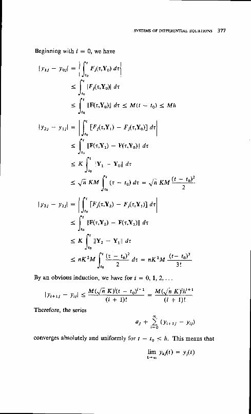
Beginning with i : 0, we have

l r ' IlYt i - Yo;l : | | FiQ,Y) dt l

I J ro If t

J t o

l ' t

J to

lJ' t.,r',Y,) -l Y z i - l t i l :

= l,',,llF(r,Y1)

-

=" l " l tY, -Y

: Jn" r=A

lysi ' lzil : lJ'

ttrtt,Yr) - rlt,v')l drl

< n K r M l ' k - t J ' d r :J,o 2

By an obvious induction, we have for f :

l ! i * r i - y i i l ' pr(Jrc

{<)r(r--- ro) t*1

Therefore, the series

(t + 1) !

a i * ) ( y , * r i - l i i )i = 0

converges absolutely and uniformly for t - to < i. This means that

lim y1;(t) : yj(t), ( j @

sysrnMs oF DTFFERENTTAL EeuATroNs 377

< M h

nK2M ( t - ro) '

3 !

0 r 1 r 2 , . . .

_ M(J i K) th t* l

( t + 1 ) !

- to)

I

)l drlI

dr

T,Y

1o) ll

dr

Ft('

?,Y

dt

f")

t

)

_ F

F(",

o l l a

= ,["

llF(r,Y2) - F(r,Y,)ll dr

= " , [ :

lY , - Y , l d r

378 NTR.DU.TIoN To LINEAR ALGEBRA AND DIFFERENTIAL EQUATI'N'

exists and is continuous for t - to S ft. We know that

yxi1) : ai * f' "r;r,"0 -rQ)f itr

J t o

and taking the limit of both sides, we have

f t! iQ) :a t+ | F r [ r ,Y( r ) f d r

J to

This shows that Y(r) : (ylt), yze), . . ., y,(t)) is a solution of theintegral equation and therefore a solution of the system of differentialequations.

To prove uniqueness assume that there is another solution Y* suchthat

Thent

Y*(r) : Yo * f' r;r,v*1 r)l drJ 'o

1Y* - yoll : jl i' r1r,"-l arlll lJ ' " l lf t

= J,"

ilF(?,Y*)ll dr < M(t _ ro) < Mh

llY* - Y,ll : ll i' tt,r,"*) - F(r,Y,)l drlll l J r o l l

J t o

f t< K l l l Y * - Y o l l d r

J t o

< KM l"'"n

- ts) dt

: KM (t - tJ' < KMh22 - 2

Again we can show by induction that

l ly* - yoi l < MKk-(t - to)k+t < MKkhk+l

(k + 1) ! ( /c + 1) !

f The inequality used here can be proved by approximating the integral with Riemannsums and then using the triangle inequality. Alternately, one can work with coor-dinates in this part of the proof as we did in the flrst part.

AL EQUATIONS 379

Ask--' @, llY* - &ll -0uniformlyfor t - to < ft. Therefore,

llY* - Yll : l lY* - Y* * Yo - Yll< llY* - Yoll + llYo - Yll -* o

as k + o. Hence Y* : Y, which proves uniqueness. Finally we noticethat the inequality

l ly _ y,. l l < MKk(t - to)k+r

(k + 1) !

MKkhk+r- ( k + 1 ) !

gives an upper bound on the error made by approximating the solution Yby the ftth iterate. This completes the proof of Theorem 9.2.2.

Theorem 9.2.2, is a local result in that it only guarantees sone positivelz such that a unique solution exists for lr - hl < h. However, having foundsuch a solution, we reach a point t : to * h where the solution has valuesY(tg + &). We can then pose another initial-value problem with initial valuesY(to + h). If there is an appropriate rectangle centered on (lo + h,Y(to + h))for the application of Theorem 9.2.2, then the solution can be uniquely con-tinued beyond the point to + h. This process can be repeated indefinitely aslong as the theorem continues to apply. However, there is no guarantee ingeneral that a solution can be found up to and including the point t : ts * rs.We can also consider the possibility of continuing the solution beyond thepoint t : to - h. ln the linear case, we have already shown that we can obtaina unique solution throughout the interval given by lr - tol 1 ro. This isbecause at each stage h can be found independently of the initial value of I(provided it satisfies lr - tol s ro). Therefore, the continuation proceeds aminimum distance at each stage, and so after some finite number of steps wemust reach the end of the original interval. This does not always happen in thenonlinear case, as we saw in Example 5.8.3.

Finally, we remark that existence alone can be proved under the hypo-theses of Theorem 9.2.2 without the Lipschitz condition.t However, the methodsused are more advanced than we care to use in this book, so we shall not givethe proof.

EXERCISES 9.6

1 Prove the inequalities involving lllJll and p : max |url,lrrl,... ,lull forcomplex vectors.

tThis is done in E. Coddington and N. Levinson, "Theory of Ordinary Differential Equations,"McGraw-Hill, New York, 1955 (rpt. Krieger, Melbourne, Florida, 1984).

380 INTRoDUcTIoN To LINEAR ALGEBRA AND DIFFERENTHL EQUATIoNs

Prove that p(U) : max tlorl,lurl,. . . ,lu)l is a norm; that is, show that:(a) p(U) > 0.( b ) p ( U ) : 0 i m p l i e s U : 0 .(c) p(aU) : lolp(IJ) andp(Ur + Ur) s pN) + p(uz).Completetheproof of Theorem 9.2.2for thecase -/6 < t - ta < 0.consider two solutions u(l) and v(r) of the system 'f : F(r,y) where u(ro) : goand V(to) : Vo and F(r,Y) satisfies a Lipschitz condition with Lipschitz constantK. show that llu(r) - v0)ll < lluo - vqllerlr-'ol. How does this show thatthe solution depends continuously on the initial data?

34

ANSWERS AND HINTS FORSELECTED EXERCISES

EXERCISES 1.2

L t + 2 2 - - - 1 + 6 i , z r ' z z : t - , ! r , z 1 z 2 : - l l + 7 i , z 1 l z 2 : - + - l 3 i l 3 4 ,

2 r : 2 - i , | z : - l - 5 r ' , l z l l : V 5 , l r r l = 4 l + .2 t r + z z : l - i , z t - 2 2 : - 3 I T i , z r z z = 1 O + l 4 i , z r l z z : - * + i l t O ,

2 r : - l - 3 i , Z z : 2 * 4 i , l z i l : V l 0 , l t " l : Z , J S .6 a * O i - ( b + 0 i ) : a - b + O i

(a + oi)l(b + 0i) = (ab + oi)lb2 = (alb) + oi, b * o7 Subst i tute u:x l (x2*!2) , D: -y l (x2*yr) . Conversely, solve for a and u by

elimination, given that x' + y' * 0.9 x 2 + y 2 2 0 , a n d x 2 + y 2 = O i f a n d o n l y i f x : ! : O .

12 lx + 0rl - (x2 * 02)'rz - (x')'t' : lxl1 3 I f a a n d b a r e r e a l , 0 < ( a - b ) ' = a 2 + b 2 - 2 a b , H e n c e , a 2 + b 2 2 2 a b ,14 lz + wl2 : (r * u)2 * (y * u)2

: x 2 + y 2 + u 2 * a 2 + L x u * 2 y u

< l r l ' + lwl ' * 2 lxu + yal1 6 l z l : l z - r t , * w l < l z - w l + l w l

lw l : lw - z * z l < lw - z l + l z l

EXERCISES 1.3

1 arg zt = 3n14, Ltg 22 : nl6, arg ztZz : llnll2, arg z1lz2 : 7rll2.3 The arrow ofz is rotated through the angle a.

568

9t2

I4

382 INTRoDUcTIoN To LINEAR ALGEBRA AND DIFFERENTIAL EQUATIoNs

The arrow of z is reversed.The arrow ofz is reflected in the x axis.If c : plq then there are q distinct powers if p is even, and 2q distinct powers if p is odd.If a is irrational there are infinitely many distinct powers.z : - 2 , 1 + t J t , 1 - r \ 6 .z : cos Q* ln ) + i s in (Z rk ln ) , k : O ,1 ,2 , . . . , n _ l ;z ' - | - ( z - l ) ( s n - t * z o - 2 + . . . + z * l ) .The triangle inequality is an equality if and only if zrz2 :0 or the arrows of z1 and z2point in the same direction.

16 The circle with center at z6 and radius r.17 The bisector of the line segment join ing z1 and 22.19 A circle and its exterior. The center of the circle is on the line through z1 and 22. Can you

find the center and radius?

EXERCISES r.4I

256

7]TI2

vr * vz : (-2,3), vr - vu = (4,_7\2vr * vz = (_l, l ) , te, _v1) = (_2,|).The wind is from the northwest at ZJl miles per hour.f,yl: (-1,2) + t(5,2),-oo < r < o. Thevector e,-s)is perpendicular to the line.(x,y): (1,3) + 5(cosd,sin0),0 < 0 < 2r.Tangentl ine: '(*,y) = (4,7) + t1_4,31,- @ < t < c o .

(x'(2), y'(2)) = (11,4).lT( t ) l '= I impl iesT ' .T = 0 .v(r) : s(r)T, a(t) : s'(/)T + s(r)lT,lT,ilT,l.

EXERCISES 1.5/ The domain is ail z. ,23

: x3 - 3xy, * i(3x2y - y.) is differentiabre everywhere.f'(z) :3x2 - 3y, + i(6xy) : J2z.

2 0xl0x : 1 * tul7y : O; -Ayfty - -l * tul\x = 0.4 dzldz:7zo,dz"+rfdz: z,(dzldz) * z(dz,fdz): (n * l)2".6 Thedomainisallz. f(z)isdifferentiableeverywhere.f,(z): e'cos/* ie"siny =f(z).8 The domain is all z except z = 0. f(z) is diffirentiabie everywtrere except

"t , = g.'

f '(z) : -1lz'.

10 The function is not continuous on the positive real axis. The function is differentiableeverywhere except at z :0 and on the positive real axis. f,(z) = llzf(z\.

1I The domain is all z except z = o. f(z) is differentiable everywhere except at z : 0 andon the positive real axis. f'(z) : llz.

EXERCISES 1.62 AuFx: e"cos y: 0ul0y,0ul0y: -e'sin y = -0ul0x.4 V = d cos/ - r 'e"s in t : dcos(-y) * je"s in ( -y) : e;6 e"+2k8t - e'cos(y * 2nk) * r'ersin (l + 2rkS =

"i9 e2nkttn : cos (2nkln) + ; sin (2nkln)I0 (d ldz )coss = - ( s inxcosh / + i cos . rs inh .y ) : _s inz

(d ldz )s in z = cosxcoshy - i s inxs inhy : cosz12 fcos zf 2 - cos2 x cosh2.y * sin2 x sinh2 y

lsin zl2 = sin2 x cosh2 / * cos2 x sinh2 y1 4 z - ( ? n * l \ n i l 2 ; n = 0 , 1 1 , t 2 , . . . .1 5 z : n n i ; n : 0 , 1 1 , ! 2 , . . , .

383

17 Everywhere except where sinh z : O.20 @ftx)t In (x2 + y') : xl(x2 * y2) : (010y)tan-I (ylx)

(AftDt ln (x2 + y') : yl(x2 + y') : -(010x)tan-'(ylx\

log z is not differentiable at z : O and on the positive real axis.22 a" is analytic everywhere. (dldz)a" : a' log a.

EXERCISES 1.7

2 lk- ' l : k* ' ,ana j , f t -* converges for x > l .

, ,h

ln2l(n * l)tl : l. The series converges absolutely for lzl < l.

4 "tT

l@, * r)la,l: lall lal: I

5 Theseriesconvergesabsolutely for lwi : lzl2l2 < I and diverges for lwl > 1. The radius

of convergence is V2.7 I f a i sanonnega t i ve in teger , theser ies i sapo lynomia landR: oo .Otherw iseR = 1 .

I0 f(,)(0) - ntlon - nlb,

EXERCISES 2.21 Coefficient matrix /l -2 3\

l z r 5 l\ r - l t l

Augmented matrix /l -2 3 7\

l z r s - 61\ r - l I o l

/ - t 6 - 2 7 \ / 3 0 - 9 6 \2 A - B : l 2 - t 4 s f : , 1 = l o - 3 2 r l s l

\ 3 - 2 - 4 t l \ 6 e - t 2 o l/ 3 - 6 - 4 - 3 \ / 4 - t 2 - 2 - 1 0 \

A - B : l - 2 - l l o l l - 2 8 = l - 4 o 6 - 8 1\ t 8 - 4 - t / \ - 2 1 0 o - 2 1

/ 1 9 - 4 2 - 2 2 - 2 5 \s A - 7 B : l - r + - s 5 6 - 3 1

\ l 50 -2o -71

| - 8 1 8 \ l - s l e \t , q c : l z z r r l B C : l - 7 3 0 1

\ - 1 3 r 2 l \ 6 7 l

' (-l lX: "):l:I:

-nil=(tr ?)a : t , b = - * , c : L r d : I .

I A t t Q r z Q t s a r + \ l A r t Q t z Q g s A s l \g Ei :

lOoy kazz ka4 karnl E2A :

la21 azz ozs ornl

\ Q s r A s z Q t t q s t / \ 4 r r Q t z O t t A r t l

l a 1 1 * a 2 1 o 1 2 I o 2 2 a 1 s I a 2 s a r + * a z + \

EsA : I

or, 4zz ctzs oz+ |

\ d r r O s z Q t s A t + I

384 INTRoDU.TI.N To LINEAR ALGEBRA AND DIFFERBNTIAL EQUATI.NS

10 (A _ r)(A * I I iyi ?:,ir! flrn, _ ,(A + I)(A - ,,

: 1rl: jr** j,! , Jrn, _ ,(A - I)(A2 + A + I) : A(A2 + A + I) - I(A2 + A + I)

: A 3 * A 2 + A _ A 2 _ A _ I : 4 3 _ I

(A2 + A + I)(A - 1): (A, + A + I)A - (A" + A + I.)I: A t * A 2 + A _ A z _ A _ I : A 3 _ I

EXERCISES 2.3I (a), (c),(f).

/ 1 22 (a) l-z o

\ 0 1

/ t z 3l s 6 7\ c ) [ l r o r l

u 3 1 4 1 5

i i ;) -fi i i e j)4 / r 2 3 + \

,;)'{3 l3;)1 6 l \ o o o o l

(d, B:(-il..( il.,( il

36

a : 5 r b : - 1 ,(a) xr = e, xz : xt : 0, xt - -a, a arbitrary.

l"] y,, : -ft, xz : E*, rs : -;*, xt : -2.

(e ) x r = -3a * 3b ,x2 : J - a l -3b ,x3 : o , x+ : | - b , xs : [ ,a and b arbitrary.

'

fi) ="(

il.,(-il a.ndbarbi,rary

1 0 r r = - 1 0 - 5 x 3 , x z = 2 * x s , x a = 3 , r s - - l , x 3 a r b i t r a r y .II (a) Has a unique solution.

(6) If solution exists it is not unique.

EXERCISES 2.46 (a) -2 (b) 0 (c) il87 3,431

10 Theorem 2.3.3 A homogeneous system of n linear algebraic equations in nr unknownshas no nontrivial solutions if and only if the determinant of the coefficient matrix is notzero.Theorem 2.3.5 A nonhomogeneous systern of m lineat algebraic equations in ze un-

f;:.t has a unique solution if and only if the determinant of the coefficient matrix is not

ANSWERS AND HINTS FOR SELECTED EXERCISES 385

1 r 1 2 r - l 1 l l 2 l - l o l

l l _'- _t, l l : l l _l _L 3l :ol + r - 3 3 l 1 4 | - 3 o l

12

13

The system does not have a unique solution.

l q - 1 - 3 o l

l - : n - ) . - 3 | : ( 6 - i x e - x x l 5 - r ) : ol 0 - 3 e - r lSystem has nontrivial solutions for ,t : 6, 9, or 15.

I t - , r t If - - t " I - l l

: ) ' 2 - 2 A + 2 : o ' l : l t i

There are no real nontrivial solutions.

, (.) (-l _il (c) (i i i)(d, (i i i) u,ft i i il

4 Use the formula given in Theorem 2.5.2.5 x r : 4 ? , x z : I t , r : : - l '

u o-': (_i i il B: A-',': (f

EXERCISES 2.5

I (a),(c),(d),(l).

EXERCISES 2.6

3 A homogeneous system of rz linear algebraic equations in ra unknowns has no nontrivialsolution if and only if the rank of the coefficient matrix is rn.

4 A nonhomogeneous system of n linear algebraic equations in rn unknowns has a uniquesolution if and only if the rank of the coefficient matrix is ze.

5 (a) The rank of the coefficient matrix is 2. The rank of the augmented matrix is 3. Nosolutions.

(D) The ranks of the coefficient matrix and the augmented matrix are 4. There is a uniquesolution.

4 r

i')79

IOt2I415I8

lf a solution Xexists, eAX : eB : O.l .an1 : lA l lB l + 0 . (B- tA- ' ) (AB) : B- ' (A- tA)B =

l 7 l : l A l + o . I : i : . f f - ' : F i .l f lAl * 0, then A'|(AB) : B : A-rO : O.t f AA : / then lA l , : l , l l l : +1.. F r : ( i \ - t : ( A - t . S - r .If lAl : O then lCl : 0. It IAI + 0 then lcl : lAl'-l

24579

1I13I4I5

386 INTR'DU.TI.N To LINEAR ALGEBRA AND DIFFERENTIAL EQUATI.N'

(c) The rank of the coefficient matrix is 3. The rank of the augmented matrix is 4. Nosolutions.(d) The ranks of the coefficient matrix and the augmented matrix are 4. There are solutions

but they are not unique because 4 < 5, the number ofunknowns.6 The system has a solution if and only if the rank of the augmented matrix is m - I ; For thisto happen all of the determinants containing the column B must be zero.

EXERCISES 3.2, l u * v : ( 4 , - 1 , - 3 ) , u - v : ( _ 2 , _ 3 , 5 ) , ) r r : ( 2 , _ 4 , 2 ) , _ * v : ( _ i , _ + , 2 ) ,_ u * 2 v : ( 5 , 4 , _ 9 ) .

lul = Vo, ot : ot: 65o54,, oz : 744o44,,0 : 136o40'(-A-,-*'-'*)9Vt+( x , y , z ) : (30 -5 ,2 ) + t ( -5 ,6 , -3 ) , -m < , < oo .(x,y,z): (0,i*,-:+) + r(1,_u$,#),_oo < , < oo.l 4 x - 1 3 y - 7 8 2 : - 1 9(x,y,z) : (1,-3,4) + s(0,7,-4) + t (2,5,-1) ,_co < s <2 x * 5 y - z : 9

EXERCISES 3.31 (b ) I f v # 0anda t ' l , t hen av * v .J The space of Example 3.3.4 is a proper subspace.6 This is a proper subspace of the space of continuous functjons.7 I f a * 0 , then o - t (au )= u = a - r0 : 0 .8 The origin,lines through the origin, or the whole space.9 It AXt : O, AX2: 0, then A(aX1 + bX2): 0, for all a and b.

EXERCISES 3.45 Independent, (I,2,3) : (1,0,1) + 2(0,1,1).6 Dependent. (l ,2,3,4) cannot be expressed.7 Independent. (4,6,7,-5) : 2(1,0,1,0) - (0,2,- 1,3) + 2(1,4,2,_ l ) ,8 Dependent.9 Indepeirdent.

1 2 l l I I I Il o l t r l

t r (O ) :10 o 2 2 l :

l r ro . r : lIndependent.

1 4 l r o 0wto ) :h t o l : z

I r z2 lIndependent.

I5 Independent.16 l/'(x) : 0. /and g are independent.

< t < 0 0 .

ANSWERS AND HINTS FOR SELECTED EXERCISES 387

EXERCISES 3.5

r (b)2 ( a ) 2 ( b ) a k \ 3 ( d ) lJ (4,5,6) = 1(l, l, l) - *(t,-l, l) + (2,0,3)4 (4,-2,4,-2) = 4(1,0,1,0) - 2(0,1,0,1)5 (a),(b).6 The functions 7,x,x2,...,xk ate independent for arbitrary k.8 The converse is not true.9 ( l , l , l , l ) , (0,1,0,1) , (1 ,0,2,0) , (0,1,0, - l ) .

EXERCISES 3.6

1 ( u ' v ) : 5 : ( v ' u ) , ( 2 u ' v ) : 1 0 , ( u ' 4 u * 3 v ) : 7 1 '2 (f 's) : 0,ll,fll : J",llsll : .l;.3 ( f ' e ) : o5 l lu + vll2 * l lull ' - l lvl l2 : 2(u'v) : I6 l lu * v l l2 + l lu - v l l2: (u * v 'u * v) * (u - v 'u - v) = 2l lu l l2 + 2l lv l l?8 Re(u'v) = l (u 'v) l = l lu l l l lv l l9 Apply the Cauchy inequality to lflrtz and l/13/2.

11 This norm does not satisfy the parallelogram rule.

EXERCISES 3.7

t o lJi,o,t I Ji), (0,-1,0), (- t I J z,ol I'l z>.3 tt.li,G*,JiG*' - +)'4 6r t : (v r ' t ) :

, .E , o11Q1a1, t \ : j oo , r , .

t U,l : (vr '"r l : -E,

QylVyl,rry: ,F,

U*,", .

6 Z crvr : O + AC : Ohasonlythetr ivialsolut ion.i = l

u* : ,E,

b11Y1, wh€re B : A- r.

7 e Nr, - t I Ji,o), o N e l NG, - zt "/ e), e I Ji J t Ji I t rlll.I1 Let u1, u2, u3 b€ the basis of Exercise 7. Then projection of v : (1,2,3) on the given plane

is (v ' ur)ur * (v 'u2)u2 : ( - 1,0,1) .I2 (2,3,2,3)

EXERCISES 3.8

4 Each coordinate of a Cauchy sequence is a Cauchy sequence of real numbers.5 Each coordinate of a Cauchy sequence is a Cauchy sequence of complex numbers.6 Each coordinate (with respect to some basis) of a Cauchy sequence is a Cauchy sequence of

real numbers (or complex numbers).I It f, is a Cauchy sequence, it converges uniformly to a continuous function on

{rlo.f x < b}.

9 1 , t / 3 (2x - l ) ,V5 (ex2 - 6x t 1 ) .12 . f l " ao . x s in nx dx : 0 , n : 1 ,2 ,3 , . . . .

388 INTR.DU.TI.N To LINEAR ALGEBRA AND DIFFERENTIAL EQUATI.N'

EXERCISES 4.2I f(au, * buz) : (ax, 1- bx2, -ayr _ by2)

: a(xr , -yr) * b(xr , -yr lNull space : {0}; range - R2.

3 f(aut * Duz) - (a,x, * bx2,a/r * b!2, -az1 _ bzz)= a(xt l r ,_z) * b(x2,yz,_zz)

Null space : {0}; range - R3.5 Ft z: (t lJi,t lJ111.,l31.Then/(u) - (u.z)2.

f(aut + bur) : (au, + ba2, z)z =- a(ur . z)z * b(ur. z)2.Nu l l space : { ( x , y , z ) l x * y + z= 0 } l r iDgo = { ( xs ,z ) l x : y : z } .'&):(-i -? i-i) k.)

] I

12I416r8

Null space : subspace spanned by (1,0,0,1), (_ 1,1,1,0);11t9"

: {(yryz,y)lyt * 2y" * ye :0}.f(au + bv) : ou, I bu1 I auz * bu, +... * au, * bun

: a(ur * a, + . . . * u, , ) * b(a, * uz * . . . * a,)Null space : {ular I u, + ... * uo = 0}; range : Ct.(a) Null space : {flf^7- consranr}; rung" : ilf :

[io@ dt + fo,g continuous].!b) Nu[ space : {fltittO dx = 0}; range : X,.I l t a : b : O . f ( a u + - 6 v ) = / ( 0 ) : 0 .f(x) : cx, c : real constant.lu : 0 always has nontrivial solutions if n > m.(l) ,f- '(v) : (x, -y)(3) ,f- '(v) : (x,y,-z)(4) " f - ' (v) : ( -x, -y,z)(6)

"f-t(v) : (l/c)v, c * O

z0 fJ9: *(x * y, x + y), s$) : (x,-y)U"d@): Lk * y, -x - y)(S. , fXu): * (x _ y,x - y)composition is not commutative, composition is associative.

EXERCISES 4.3I Zero matrix in either case.'(i;s)' (o) (l -?)7 / - l 0

( a ) f o - r\ 0 0

I I I _ l( a )

l - t 2\ l - 3

(? l)l - r 0

(b) | o - l

\ 0 0

(b)

0\

N2

_ J

4

?)_r)

(r)

(c)

(a)

(b)

ANSWERS AND HINTs FoR SELEcTED ExERcIsEs 389

Basis for null space: (lpp,1), (- 1,1,1,0).Basis for domain: (1,0,0,1), (- 1,1,1,0), (1,0,1,- l), (1,1,0,- l).

l o o 4 l \l o o - s o l\ o o 6 - r l

l Z Z -1 \Inver t ib le , ,s- ' : l L -+ 0 l

\ - t - t r lNot invertible.

EXERCISES 4.4

' (o) (? l)(c) (l - l)

(b) (-I i)(d) 6 _?)

4 f ( | , - 1 ,1 ) : (1 , - 1 ,1 ) . Bas is : (1 , - l , l ) , (1 ,1 ,0 ) , (1 , -1 , -Z ) .

l t o o \Representation, lo -+ t I

\o -* -+l5 B : P A P - | , B - t - P A - | P - 1 .

Bz - (pAp- ryTrep- r) : pA2p-t, etc.B -2 : (pA- tp - t11pA- rp - r ) : pA-2p-1 , e tc .

6 Clearly J111

ft + D + D2 + . '.+ Dt) :

EXERCISES 4.5

1 (a ) A r : 7 , u r : a ( I , - l )Az : 3, uz : a( l , l )

(c) Ar : 7, ur : a(l,O)1z : 2, uz :_a(1,1)

(d \ L t : | - i t l , 9 , \ : a ( i . J612 ,1 )

l z : | * i t / 6 , 1 2 : a ( 1 , i i 6 l 3 )2 (a) ) r : 2, ur : a(1,- 1,0)

1z : 2, uz : a(0,0,1)1z : 4, uc : a( l ,1,0)

(c) 1r : 4, ur : a(1,- 1,0)

b = 2Ji , lz : a(-1,3,2 - zJt)h : -2^12, u3 : a(1,1,2 + 2Jt)

(e) l r : 0, u1 = a(1,-4,7)] z : 6 , u 2 : A ( 1 , 2 , 1 )L t : - l l , u 3 : a ( - 3 ' 1 , 1 )

t - ) r ) * l o 0 . . . 00 ( l - 1 ) - 1 0 0o o ( l - 1 . ) - ' 0

0 0 0 . . . ( l - t " ) - '

390 rNTRoDUcrIoN To LTNEAR AL.EBRA AND DTFFERENTIAL EeuATIoNs

il3 Relative to the basis (1,- l), (l, l), the representation is (f _?)

/ 0 0J Relative to the basis (5,1,0), (0,1,_2), (2,0,1), the represent"tion i. {O ;

6 I f AX - lX ,X * O , thenA2X = ) .AX: l 2X ,e tc . \ 0 0

8 I f AX - J "X ,1* O , X + O, then ,4 - t (AX) : X : tA - rX .I0 p(A)X1 : p(X)Xt = 0, since p ()) : 0. Let X be any vector.

Then X : c rX r * c2X2 + . . .+ c ,Xn and p (A)X :0 . Now success ive lve2r€3r . . . r€7.

0 0 \

i ')

fis:),:(i ; il PAP-':(i?)

_i)

le t X : €r ,

I2 characteristic vectors corresponding to different characteristic values are independent.14 x: ae' r be3' , ! : -aet * be3t ,where aandbarearbi t raryconstants.16 (d2xldt2) - 3(dxldt) - 4x : (t2 _ 3), _ 4)e^t : O

EXERCISES 4.6

r l l 0( a ) P - r = l 0 I

\ - l 0

l r 0(c ) P- t : 12 I

\0 I ": (_i i-+\

f I PAP-' :_+t2ea'.

ptp-' : (o i)

2 (a) xr : -e2t * 2eat, xz = 2e2t, x3 : ezt +(c) xr : €6t, xz : t

- Ieur, xt : sz * *eur.

3 (o) r-, : (,t -l) " = (_i _,1;\

= fi I ;i) ": (_i i _il PAP-' : (i s l)x1: (il2)e2' + (+ + *t) - (* - *i)eu'x2 : (il2)e2' - G + +t) + (* - *j)eu'x 3 : $ i - * ) + ( ? t + * ) e u 'An ellipsoid 6(*')" + 9(y'), + 1S(z')2: l. The axes are the lines through theand the points (1,1,1), (1,0,- l), (1,-2,1), respectively.

EXERCISES 4.7

3 (A - )"1)X : P-1(J - AI)pX

4 / - 2 0 0 \ f i 0 0 \(a) | I 1 l l (c ) lo I 1 l\ 0 o 4l \o o 1l

5 (a) x, : - je-,, + 1"o, I 3teatx r : 3 e - 2 t - t e 4 . - 3 f u 4 t

x3 : ]e -z t + te4 . + 3 rc41(c) xr : et * 2tet

x z : Z e t - z t e t

xt : 3et - 2te'

ANSWERS AND HINTS FOR SELECTED EXERCISES 39I

EXERCISES 5.2

2 y(t) : (j,olca) sin arl * /o cos col

4 Since the differential equation is nonlinear the difference between two solutions does not

satisfy the equation'

s (tl2d"l slt6 y(t) - /6 cos rot * (j,ol(,) sin arr is a continuous function of y6 and ye for fixed t.

EXERCISES 5.3

I (a) First order linear. (c) Second order linear.(e) Third order linear. (g) Second order linear'

2 F(x,y,u,ur ,uy,uxxtul l t . . . ,O"uf 0x ' ,0 'uf0x ' - t 0y, . . . ,Auf Ax 0y ' - ' , A"ul0y") : g

where at least one of the nth order partial derivatives appears'

3 f(x,y) * as(x,y)u * ato(x,y)u, * as1(x,y)u, * azo(x,y)u,,

I all(x,y)u'" t as2(x,y)ury * "' * a,s(x,y)Auf 0x"

* en-r , {x,y)(A^u\0x"- t 0y) + ' " + ar , , - {x,y)(Tuf Ax Ay' - \ )-t ao^(x,Y)(0nulAY") : g

where at least one of Qns,Qn-t , r ; . . . ,Qt ,n-1,4e, is not ident ical ly zero '

4 (a) Second order linear. (c) Second order linear.(e) First order nonlinear. (g) Second order nonlinear.

EXERCISES 5.4

I (a) y(t) : I * (ro - l) exP (- i t ' )(b) y(t) : (1 - lxl + 3)l2t(c) y(r) : l + (yo - l )etr - ' t r(d ) Y ( t ) : e ' l ( l t t )(e) Y(t) : sin / - cos I

2 Approximately 3 hours 48 minutes.3 Approximately 166,000 years ago.4 .9 pounds per gallon.5 mglk, k : air resistance/unit velocity.6 A : r(t)lylt), y{t) :

"xp (-Jl qft) d).

EXERCISES 5.5

I (a) Separable: cos y : cos 16 cos /o sec t'(c) Bernoulli: t2 : 3tl(3ct' - 2), where c depends on initial conditions.(e ) Reduc ib le to separab le : ( y+ t - 1 )3 ( l +2 t -Z ) - ' : c , where c depends on

initial conditions. Note thaty : 1 - r and | : 2 - 2t arealso solutions'

2 :(QMG(F)): (QM)yG(F) + QMG',(F)Fyoy

: (QN)IG(F) + QNG',(F)F,

: ! p*ctrl>dt

a @) Integrating factor is l l t : yt * ev - loto - e'o : 0.

(c) Integrating factor is llty(y - 2t2): y : tyolto. Note that ! : 2t2 is also a solution.

I2

35

392 INTR'DUCTI.N To LINEAR ALGEBRA AND DIFFERENTIAL EQUATI.NS

EXERCISES 5.62 (ryrrl*) - (mrslkr) In (l * kuolmg)3 VSO miles per second.4 ( a ) t y ' + x 2 : k 2

(c) (x * y)31(x - y) = kandy - x5 xs * 3oo(y - /*ilJ,;' : e7 Y ' = 8 x

EXERCISES 5.7I y : ( 1 - y ) - t

EXERCISES 5.8T a k e 6 - l , c : l ; t h e n M : 4 , a : t .y ( t ) : 1 + J : r y 2 d tl r : l + l i " d r = l + ( t 2 1 2 )l z = | + J ' 4 1 + ( t 2 1 2 ) l 2 d t : | + Q 2 l 2 ) + ( t n l 4 ) + ( t 6 1 2 4 \y : 2 l (2 - t r ) : 1 + (1212) + ( to l4)+ . . . , v l . J ty = 0 , 0 < r s a .y : IG, - a2) l4 l2 ,a < t .

EXERCISES 6.2' *o t : l ! l l : - ,

l r - r l

t ,o t : lo , f l :_ , ,+oS e2t . egt .

| |

7 y = * * c r s i n 2 r * c 2 c o s 2 t9 y : - l + c J * c z t - r

1 I y = * * f , c o s 2 r13 y . : - l + f r + t t - '14 W(t) : (dldt)(y}, - yzj,) : !i)z - lzyr : -p(yJ2 - tzl)

W(t) : W(ts\ exp G[i"oG\ dt)

16 ly, lz lo Il.r ,r, !, Iv i t 1 t1 :1 t , ,

,t . " " ' . . . . . . . . 1lYr'"' Yztn) Y,'n'l

EXERCISES 6.3I y : - t t e - r l c f t t * c 2 e - t3 y : (llat)t sin @t + cr sin rot + c2 cos ort5 y : + t + g * c p 2 r * c 2 e t t7 y : 3"' + * * -fr"zt - *t"r,9 y : - c o s t l n ( s e c t + t a n t ) + c r s i n r * c 2 c o S t

ANSWERS AND HINTS FOR SELECTED EXERCISES 393

EXERCISES 6.4

3 q , : p r * f , Q z : P z * r Q t , Q s : P t I r 4 2 , . " '

6 y : c p t * c z t e ' + c i 2 " t - a " i t " t - *

c s e - 2 t + c u t e - " * c ' t " e - 2 t + c a l 3 e - 2 t

7 ( b ) ! : c t e ' * c 2 e - t * c s s i n t ] - c t c o s t

(d) ! : cr + "rJ

* cae-<ttz1t cos (JJr/2) * cae-otz)t sin (J: l iZ)

(f) ! : cqtsin t * czet cost + e3tet sinl * c4tet cos t

+ c5e-t sin t I c6e-t cos t + cule-t sin t + cste-t cos t

EXERCISES 6.5

I (a) D3(c) (D' - 4D + 5)2

2 (b) ! : c?2t I cz€3' + 2te3' * f l -cosl - t 'os inr(d) f : cr cos 2r + czsin2t + tt2 sin 2t - j6t cos 2t

( f ) ! : cre ' s in 2t + c2et cos2t * - f6tet s in2t - St2e'cos2t3 y : e ' + t t ze t4 y : 2 + t s in r - cos t + L te ' - e '

EXERCISES 6.6

1 Period : n{JZseconds; frequency : +JSI" hertz; amplitude = I inch.

2 Amplitude = -ir[l + *lrt2 ft; phase : tan-t V* : 31"30"

4 y : c1 coS at t c2 sin ar, 'l (fol2am)t sin cot

5 r :42 l0-3 seconds.6 I :.141 sin (l20nt - 0) amperes' 0 : 57"22'.

EXERCISES 6.7

I G ( t , r \ : l - e c - t )

3 G( t , i : s2( t - t7 - e ( - t )

6 y(t\: i J: (s3(t-'r - 1),f(') d' - 4 Ji 1""'-" - l)y(z) dt

. sin ar€ sin ar (L - x)i0 G\x,1) - -------------:-

(I) sln arl

sin c,rx sin ar (I - {): _or sin arl

QG)1Q(0) - Q@)lQQ)P(1)

Q@)TQQ) _ QG)Io(1)P(€)

o < ( < x

x < € < L

0 5 { 5 x

x < 1 < l

12 G(x,€) :

where P(x) - exp t- Jfrte) d0 and Q@) : I; P@ d1.16 y(x') : [ic(x,€)fG) d€ - IL c{x,OotilvG) d€

where G(x,f) is the Green's function of Exercise 12.

EXERCISES 7.2

2 gfcos rl,tl : s11tz + (D2)

4 9l t " l : 1. (a * 1)sr- t "+t ;

6I

10I113

I4

394 INTRoDUcTIoN To LINEAR ALGEBRA AND DIFFERENTIAL EQUATIoNs

9l tne"t l : n! (s - a)-{n+t t9[ebt sin at] : q111t - b), + .,rl9febt cos arll : (s - b)/t(s - b)2 + @21cols2(sz * ro,)slf?)lls[1 - cos at]lo2

l 1e"' * :-- ebt

a - D b - a

EXERCISES 7.34 9[t sinh arl ] : 2salbz - ,or)t

9[t cosh atl : (s2 + ar2)/(s, - -r),6 (e-"" - e-'")ls

^ I c e - " .d - -

s t J l - e - " '

10 (Dt - 2aD * a2 + ar72y : 0, {0) : 0, y(0) : 0, }(0) :

EXERCISES 7.44 +_- * "-'

- -h "' }t "t '

+ tutdt "o,6 i - 9te- ' - 4e- ' + Je- 'cos r i 4e-r s in t

8 e- ' * te- t - e- 'cos t - |e- t s in I - l te- t s in t9 u(t - 2)f(t - 2) where/(/) : 1Le-' + -|6re, - -Le' I -]y-, sin 2r.

EXERCISES 7.51 (a) v(t): -|oe' j- ]sin2r + (-+ + tvo * ! i,Je-'+ (+ - *vo - *i,o)e-o'

(c) y(t) : -7| cos 3t - Jr; sin 3r * (* + yie-' cos 2,+ t+ + 0ol2) + (j,sl2)le-, sin 2t

2 y ( t ) : (2yo * i r )e - ' - ( yo + i de - , , + f ( t )- 2u(t - a)f(t - a) + u(t _ 2a)f(t _ 2a)

where/(l) : +/ + e-, - *e-t, - *.

y(t) : f(t) + 2 > (-1)k u(t - ka)f(t - ka)

f(t) as in Exercise 2.x( / ) : ( t l2)e- t - ( r l2)e-r , + e- , ( t * t r*o - *yd + e-r , ( - t _ Ixo + Iyo)y( t ) : ( t l2)e- t - 2t"-2t + e- t ( t t l ro - !y) + e-r , ( - t - 2ro + iy" l

. . , , \ € ( - l ) ' t 3n (3n - 2 ) (3n - 5 ) . . . (4 ) ( l )t \ t ) :

: " ( - t Y r 2 n + ' ( 3 n ) !

r ' ( l ) : t ' ' "

, f -s 2zn+ | nt(n * l ) l

EXERCISES 7.6I X : - 7 3 3 o h m s , Z : 9 4 7 . 3 o h m s , d - - 5 0 o 4 ' 1 , , 1 : . 1 0 5 6 s i n ( g 0 0 z l _ d ) .. l L e t a : ( l l R C ) + ( R l z H ) , b : l l H C , d : t l 2 R H C 2 .

ANSWERS AND HINTS FOR SELECTED EXERCISES 395

Eo co3(a3 - bco)Tnenz-ou, - - -5Sr -uwi

z \a - a@2)2 + (txo - cPtl' -

Eo at(d - aaz).

_ : ^ ^ 6 . . a t

' 2 ( d - a @ 2 ) 2 + ( k o - @ ' ) '

4 Eo,, -- RMEy Ji sin arz A(t - r) dt

.t3

where 9lA(t)l:@ + [R + (zHlc)lsz + (2Rlc)s + (l/c'z)

EXERCISES 7.7I

2 B,(t;t3) : Ttnln

- lXn - 2)t' * 3n(n - l)t2 * ntl

3 B^(t;r(t)r: # *fl (;)t[, b - a)t.. ,)(t - a)k(b - t)n-t

4 B^(t; l t l) = 2-^E (;) l- ' . z|ltr + t)t(r -.t)n-r

6 (a') tan-' (o/s) (b) ln [(s - a)/s] (c) ] ln [(s + ar)/(s - <o)]

EXERCISES 8.2

I ( a ) R : o o ( c ) R : l ( e ) R : c o ( s ) R = l

2 y , = i ( 3 k -2)(3k - 5) . . . (4Xl) I- x r & l x l < m

(3k)!

€ ( 3 k -! z : L -

k = O

t ) (3k - 4 ) . . . (2X l ) a-:-j------------- _yJlt+l lXl < OO

(3k + r) !* ( - l ) ( 4 - 1 X 8 - r ) . . . ( 4 k - 4 - ^ ) , ,

3 y r : i + I - x " F t < &

k=r Qk) l

+ s ( 2 - 1 ) ( 6 - 1 ) . . ' ( 4 k - ? - ' \! z : x ' , l ' -

- " ' * z t - i r x i < rk = r ( 2 k + l ) l

* ( - t ) (4 - i x l6 - 1 ) . . . (4k2 - 8k + 4 - 1 ) . .5 y r = l + I \ - t ' 2 k l x l < l

k = I (2k)'!

. € ( l - r ) (9 - r ) . . , (4k ' - 4k + | - 1 ) akL ,l z = x r , ? -

e r a t - '

k=r (2k + l ) l

7 y : c t l r * c 2 Y 2 * l x

where y, : 76s-x2t2, y, : 2 l(-2)kklx2kllQk)lk = O

EXERCISE,S 8.3

I m 1 = t ) r l f l 2 = - Y .

2 A tx : l , t t t t : t r t z : 0 ; a t x : - l , t t t r : t f l z : O.

3 m r : f f l z : O

- ( - rx l - ] ' ) (2 - r ) . . . (k - I - ,1 )l : i + f . i ' 1 , r 1 ( . ; J

k = r & l \ 2

396 INTRoDUcTIoN To LINEAR ALGEBRA AND DIFFERENTTAL EQUATIoNS

5 m t : t l l z : O

g x z kY :

* L = o W l x l < m

6 m r : L r n t z : O .l t : | - x - ! x 2 - - f * * " - . . . l x l < 1

, , : x t r z ( t * i *H* I t : l ( 9 ] } , , + . . . ) r x r < r\ 6 t20 (t2o\(72,) |

EXERCISES 8.4.l Prove the identities {r2(x) = Jil" Gin x/r/i) and J_t,z(x) : Jilo(cos.r/Jr).3 t 2 f i t + t w + ( r 2 - $ ) w = 04 t2ri ' + t;v + (t2 - v2)w :0 t : dx0

6 y : r^(x)tn, - F, W + rftffi*,,*,- n2 (n2 -+ 4n + l \

] zn++ I . . .2 + 7 ( n * 2 ) !

^

EXERCISES 8.51 Xn' : n2n2lL2, n = 0rlr2r.. . i ln : cos (nnxlL\.2 Ln' : (2n * l )2n214L2, n : O,1,2, . . . . , ! r : cos [ (2n * l )nxl2 L] .5 yo: s inXnx,wherethe Aoareal l theposi t ivesolut ionsof tanl - _1.7 yn : Jr(J\,i, where the )n are all the positive solutions of tr(Ji) : O.9 y : ( 1 - } x ) c o s . x + J l s i n x , w h e r e , B : + + | t a n l * s e c 1 .

I0 No solutions.II y : x * .B sin zx, where .B is arbitrary.

EXERCISES 9.22 fi1 - u2, it2 : et - 6u1 - Sur.3 i l 1 : t r 2 , i t 2 : - 6 t - r u t - 6 u z i y : t - 2 - t - 3 . 0 < t < c O .5 yt : 2l(2 - t'), y, : 0.

EXERCISES 9.3/ l \ / l \4 Y :

" ' ( _ i / + , , \ 1 ) " '

/ 1 \5 Y : ( - i )

6

I0

y: cr (_i) . " fi) e, + (re,+ tt") (_l) . (it + *te-, + +"-,>(lle

Y : c r ( i ) ' . " ' ( ; )

e2 ' + ca( " ' : ' ) . '

y : cr [(i) *. ' - (|) sin r] + ", [(l) sin r + (i) *, 'J] I

ANSWERS AND HINTS FOR SELECTED EXERCISES 397

EXERCISES 9.4

t ( a ) Y : c r ( - l ) " * ' ( l ) " "

(c) y : c ,€ ' [ ( i ) * ' " - $)s in2r ] * c2e ' | [ ( l ) ' "

r , * ( l )coszr ]

z /0 \ / l \ / l \(a) Y : c r lo l r " + , r l - r l r " + c r l l f ea '

u/ \ 0/ \0/

(d) y:c,( i l

e-,tc2( i l

e2'+cal( i)"".(_i)""]

3 y : (c , + r - |cosr r r ( "o k r t t " t ) + t " , - + t - {s in2r ) ( t " " r l : * t )

6 y, : ry e, + Y{o) t2Y2(o) d,

.. vz0) -y2: ----t- e- r V-

c

7 y , :a{9 ; -4 r , * ' *@(e, + te , )

yr(o) -./r(0) v'(0) * vz(o) ,l z : ' _ \ - " , n ' -T (e , - t e t )

e y :",(-i) e'' t c2( il

e2' + ca[(i)"" . (-i) ""]/ - 3 \ / 0 \

+ | +1 rc - ' - 3 l t l " - '\ 2 l \ - r l

. v r ( O ) + y z ( 0 ) + y g ( O )W n € I € C I : T

",: f f+?".=W

t ^ \ , / ^

Y " ,

I e - ( t 3 > t s i n v ' l1

- l ?

EXERCISES 9.5

1 (b) lr : cr€t * c2e-t * ca cos I + c4 sin t

l z : -c f t - cz€- t * cs cos I * c+ s in f

(d) lr : cre-t r cz€2t * csea' - $

l z : 3 c p - t - ! c * n ' + + t - 3

2 (a) !1 : c1€-<ti 3)t cos { , * c2s-(tt3rtrn f ,3 3

/ - l ; \ . / t /f , : l c , + !=

" , 1 " -< r r t ) t s s5 Y : t + l c ,

-1 2

-1 3 \

(c) No solutions.

Acceleration . 2l, 95Adjoint differential equation, 275Airy equation, 321Amplitude, 266Angle between two vectors, 87Annihilation operator, 261Arrow representation:

of complex numbers, 6-7of vectors, 15, 86

Associated homogeneous equation, 208, 245Augmented matrix,44

Banach space, 132Basis, 111

change of, 160-165coordinates relative to, 113orthonormal . L24, l3lstandard,111

Bernoulli equation, 214Bernstein polynomials, 31 1-312Bessel equation, 328Bessel functions:

of first kind, 329, 331orthogonality of, 337of second kind, 329

INDEX

Bessel's inequality, 135Boundary-value problems, ?nln., 276-2U,

338-34s

c" . 98(See also Vector spaces)

Capacitance, 265Cauchy product, 37-39Cauchy-Riemann equations, 22Cauchy-Schwarz inequality,l l, 12, 16, l l7Cauchy sequence, 131Characteristic equation, 169Characteristic function, 339Characteristic polynomial, 169Characteristic value, 166-175, 339

multiplicity of, 169Characteristic vector, 166-175Charge, electric, 265Coefficient matrix, 44Cofactor, 65-67Cofactor expansion, 66-67Column operations, basic, 80, 83Complementary solution, 249, 359Complete spaces, 132Complex impedance,307

4fi) rNoEx

Complex numbers, 1-40absolute value of, 5addition of,2,7

associative law for,2commutative law for. 2

algebra of, 1-5algebraic field of, 4n.argument of,7-9Cauchy-Schwarz inequality for, !1, 12conjugate of, 5distributive law for, 4division of, 4geometry ot,6-12imaginary part of, 2multiplication of,2,8

associative law for, 2commutative law for, 2

negative of, 3polar-coordinate form of., 6-7powers of, 9real numbers in, 2-4real part of, 2reciprocal of, 3roots of, 9-10

quadratic formula for, 11series of. 25-26.30-39subtraction of. 3. 7-8triangle inequality tor, ll-12zero of, 3

Composition of linear transformations,r5'7

Continuation of solutions, 23'7-24t, ?39n.,379

Convolution, 286-288Laplace transform of., ?A7

Coordinates, 113Cramer's rule. 76Current, electric, 265

Damping:forced vibrations with. 269-270forced vibrations without, 268-269free vibrations with, 267-268

critical damping in, 267overdamping in,267underdampin g in, 267 -268

Degenerate system, 372Dependence of vectors, 103Determinants, 59-'70

cofactor expansion of, 65by columns, 67by rows, 66-6?

of products of matrices, 69sums of determinants, 63of transposes of matrices, 69

Diagonal matix,77n.

Differential equations:exact,218-279linear, 206nonlinear, 213order of, 205-206ordinary, 205partial, 205reducible to exact, 2I9-22nreducible to linear, 214-215reducible to separable, 2t6-2t9separable, 215systems of, 185-187, 195-196, 352-379

Differential operators, 208, 254-259Dimension, 115Direction cosines, 85Distributive law:

for complex numbers, 4for matrices, 46

Domain of a function, 17,92, MADot product (see Scalar product)

Eigenfunction (see Characteristic function)Eigenvalue (see Characteristic value)Eigenvector (see Characteristic vector)Electrical circuits. 265. 306*309Element of a matrix, 43, 45Elimination method, 48-57Energy,204Equivalence relation, 51n., 164n.Escape velocity, 225Euler formula, 26Euler method,226-228

modified, 229Exact equation, 218-219Existence theorem, 202, n6-20'7, 232-242.

356. 375constructive, 202n.nonconstru c tiv e, 202n,

Exponential function, 25-29Euler formula for. 26power series for, 25, 30product formula for, 39

Finite-dimensional vector spaces, I l5Fourier series, 340Fredholm integral equation, 280Frobenius method, 324-327Function{s):

of a complex variable,2l.-29analytic,2Zn. ,chain rule for, 23derivative of: along a curve,22

at a point,22domain of, 21exponential, 25-29

Function(s):hyperbolic, 28logarithmic, 28-29runge oI,2ltrigonometric, /7-28veitor-value d, l7 -20, 92-93, I4O

composition of, 148dependent variable of, 18, 92derivative of, 18-19, 92-93domain gf, 17, 92, lNdomain space of, 140independent variable of, t'l, 92inverse oI,147range of, 18,92, 140range space of,140

Function spaces (see Yector spaces)Fundamental system of solutions, 249,359Fundamental theorem of algebra, 254

Gamma function, 288General solution:

for linear algebraic equations, 56-57for linear differential equations, 249for linear first order sYstems, 359

Gram-Schmidt process, 124-125Green's functions, nF2W

for boundary-value problems, 276-280for initial-value Problems, nFn6

Half-life, 211Heat equation, 205Hermite equation, 32-Hermitian torm, 187-188Hermitian matrix, 181Hilbert space, 132Homogeneous algebraic equations, 54-55Homogeneous differential equation, ?X8, 245Homogeneous function, 216n.Hyperbolic functions, 28

Identity matrix, 46Impedance, complex, 307Implicit function theorem, 214Implicit representation' 90Independence of vectofs, 103Indicial equation, 323Inductance, 265Infinite-dimensional vector spaces, 129-138

Cauchy sequence in, 131completeness of, 132convergence in, 130orthonormal basis in, 131

Initial-value problem, ?-01n., 206, 245, 354,358

INDEX 40I

lnner product (see Scalar product)Integrating factor, N9n.' 2N-221lnvariant subspace, 176Inverse of a function, 147Inverse of a matrix, ?1-77

uniqueness of, 7lIsomorphism, 126-lnIteration, method ot, ?34-237, 3'14-379

Jordan block, 191Jordan form, 188-196

Kernel (see Null space)Kirchhoff's law, 265

Ls(a,bl, 137Laplace transform, 283-314, 368-369, 373-

374of convolution. 286-288ol derivative s, 29 l-292differentiation of, 286existence of, 283inversion of, 295-300method for solving differential equations,

30 1-305, 368-369, 373-37 4table of, 293-294uniqueness of, 310-314

Laplace's equation, 205Legendre equation, 321Legendre polynomials, 134Length of a vector, 14-15, 85

(See also Norm of a vector)Linear algebraic equations, 4l-83

augmented matrix of, 44basic column operations, 50-53, 79-80basic row operations, 50-53, 79-80coefficient matrix of, 44Cramer's rule for, 76elimination method for, 48-5?existence theorems for, 55-57, 75-76,

78-83homogeneous, 54-57, 75

nontrivial solution of, 54-55' 75trivial solution of, 54-55, 75

nonhomogeneous, 54-57, 75-76reduced system for,49, 51redundancy in, 50solution of: existence of, 55-57, 75'!76,

78-83general, 5G57, 81uniqueness of, 55-57, 75-76,78-83

Linear combination of vectors, 89, 103Linear differential equations, 206, 208-213,

244-zffi

402 rNDEx

Linear differential equations:with constant coefficients, 254-263systems oI, 358-374

with constant coefficients, 364_374Linear operator, n8, 254-Z5gLinear transformations, 140-197

change of representation, 160-165composition of, 148-149, 157inverse of, 148, 157-159matrix representation of, 151-159multiplication by a scalar, 155null space of,146sum of, 154

Lines:equation of, 17, 88parametric representation of, 17

Lipschitz condition, 232-?33, 354-356Logarithm function, 28-29

Matrices, 42-48addition of, 45

associative law for, 46commutative law for. 46

characteristic equation, 169characteristic polynomial of, 169characteristic value of, 169

multipliciry of, 169characteristic vector of, 169coefficient, 44column operations on, 80, 83conjugate, 76diagonal77n.distributive laws for, 46element of,43, 45elementary, 47 -48, 73-1 5equality ot, 43, 45hermitian, 181identity, 46inverse of,7l-77multiplication of, 43, 45-46

associative law for, 46multiplication by a scalar, 45, 46nonsingular, 73orthogonal, 76partitioning of, 188products of, 43, 45-46

determinants of, 69rank of, 78-83reduced, 53row operations on,47-48, 50-53, 74-75,

79-80singular, 73square, 45

order of, 45subtraction of, 45

Matrices:symmetric, 178transpose ot,69-71

determinant of, 69product of, 69-70

unitary, 76zeto,46

Metric space,722Milne method,230-nl

corrector formula in, ?31predictor formula in, 231

Mixing problem, 2ll-212Modified Euler metho d, 228-Z2g

Newton's law of motion, 353Nonhomogeneous differential equations,

208, 245,358Nonlinear differential equations, Zl3-220,

233-242, 374-3'.79Nonsingular matrix, 73Norm of a vector, 1n-123Null space, 146Numerical methods, 225-231

Order of a differential equation, 205Order of a square matrix, 45Ordinary differential equation, 205Ordinary point, 316

solution near, 3L'7 -321Orthogonal matrix, 76Orthogonal trajectories, 221-222Orthogonality of vectors, 16n., 124Orthonormal basis, 124, l3I

Parametric equations, 90Partial differential equations, 205Partial fraction expansion, 295-300Particular solution, 57, 249,359Pendulum, 204Period, 266Permutations, 60-61

even, 60inversion of, 60odd, 60

Phase, 307Picard method, 234-23'r. , 3i4-379Plane, equation of, 89Power series, 30-40

absolute convergence of, 32Cauchy product ot, 37 -39circle of convergence of, 35convergence of, 30differentiabiliry of. 36-37

Power series:divergence of, 30geometric, 30-31, 33partial sums of, 30radius of convergence of, 34-35ratio test for, 35root test for, 35

Predictor'corrector method (see Milnemethod)

Pursuit problem, 223-225

Quadratic form, 184-185, 187

R'r, 97-98(See also Vector sPaces)

Radioactive decay,2llRank of a matrix,78-80Reactance, 307Reduced matrix, 53Reduced system, 49*54Regular singular Pint, 322

solution near, 322-32i7Resistance, 265Resonance,270Riesz-Fischer theorem, 137Row operations, basic, 50-53' 79-80Runge'Kutta method, 229-230

Scalar product:for threedimensional vectors, 87-88for twodimensional vectors' 16in vector spaces, tl'l-123

Scalars, multiplication by, 13-15, 85-86' 96Separable equation, 215Separation of variables, 338-340Set notation, 18n.Similar matrices, 163-165Similarity transformation, 163-165Simple harmonic motion, 266Simpson's rule, 230Singular point,322Slug, 200n.Speed, 21, 96Square matrix, 45Steady-state solution, 270Subspace, 101Symmetric matrix, 178Systems of differential equations, 353-379

first order, 353-369linear, 358-364

with constant coefficients' 364-369higher order, 370

degenerate, 372

INDEX 403

Tangent to a curve, 19-20Tangent line, 20, 93Tangent line method (see Euler method)Tchebysheff equation, 321Transient solution, 270Transpose of a matrix, 69-71Triangle inequality, 11-12, 15' 86, 121Trigonometric function, 27-28Trivial solution, 54-55' 75Tuning,270

Undetermined coefficients, method of, 2ffi-263

Uniqueness theorem, 203-204, 207, 232-242'356, 375

Unitary matrix, 76

Variation of parameters, 213, 250-253,362-363

Vector spaces, 96-116addition in, 96axioms for, 96basis in, l l lc? r ,98complex,96dimension of, 115finite-dimensional, 115infinite-dimensional, 116, 129-137isomorphism of, 126-127multiplication bY scalars in, 96negative vector in, 96Rn, y7

real, 96scalar produ ct in, lI7 -l?i

Vectors:coordinates of, 113dependence of, 103independence of, 103linear combination of' 103three-dimensional, 85-94

addition of, 85direction of, 85equality of, 85geometrical interpretation of , 85-86length of, 85multiplication bY scalars, 85-86negative of, 85scalar product of, 8?-88triangle inequalitY for, 86vector product of,95zero, 85

two-dimensional, 13-2.0addition of, 14, 15direction of, 14

404 rNoex

Vectors:two-dimensional:

equality of, 13-14geometrical interpretation of, 14-15length of, 14multiplication by scalars, 13-15negative of, 14orthogonal, 16n.scalar product for, 16subtraction of. 17triangle inequality for, 15zero, 14

Velocity, 21,95,353Vibrations:

forced, 268-270free,266-267with damping, 267, 269-270

Vibrations:without damping, 268-269

Voltage, 265Volterra integral equation, 276

Weight, 264Wronskian, 106, 246-249, 252, 359-3ffi , 365

Zero:complex number, 3matrix. 46three-dimensional vector, 85two-dimensional vector, 14vector space, 96

Zero subspace, 101

A CATALOG OF SELECTED

DOVER BOOKSIN SCIENCE AND MATHEMATICS

CATALOG OF DOWR BOOKS

AstronomyBURNHAM'S CELESTIAL HANDBOOK, Robert Burnham,Jr. Thorough guide!o F" stars.beyond our solar sy:t9T. Exhaustive heatment. Alpiiabetical Uy'.oiJ"t-lation: Andromeda to Cetus in Vol. l; Chamaeleon to orion in vot. 2; an|pavo tovulpecula in vol. 3. Hundreds of illusbations. Index in vol. 3. 2,000pp. 6\6 x gyr.

Vol. I: 23567-XVol. II: 23568-8

Vol. III: 23673-0

EXPLORING THE MOON THROUGH BINOCULARS AND SMALL TELE-SCOPES, Ernest H. Cherrington,Jr.Informative, profusely illustrated guide to locat-ing and identifying craters, rills, seas, mountains, other lunar features. [lewlv revised|n{ updated with special section of new photos. Over 100 photos and diagrams.240pp.87n x 11. Z++gt_t

THE EXTRATERRESTRIAL LIFE DEBATE, 1250-1900, MichaelJ. crowe. Firstdetailed, scholarly study in English of the many ideas that developei from 1750 tol_900 regarding the existence of intelligent exiraterrestrial life. Examines ideas ofKant, Herschel, Voltaire, Percival Lowe[ many other scientists and thinkers. 16 illus-trations. 704pp. 53A x 8k. 40625_X

THEORIES OF THE WORLD FROM ANTIqUITY TO THE COPERNICANREVOLUTION, MichaelJ. Crow-e. Newly revisdd edition of an accessible, enlight-ening book recreates the^9!ange_from an-earth-centered to a sun-centered conc"ep-tion of the solar system. 2a2pp. 53h x 8Y,. 41444-2

A HISTORY OF ASTRONOMY, A. Pannekoek. Well-balanced, carefully reasonedstudy covers such topics as Ptolemaic theory, work of Copernicus, Keplei, Newton,Eddington's work on stars, much more. Illuitrated. References. 52lpp. s% x gu.

65994-r

A COMPLETE MANUAL oF AMATEUR ASTRoNoMy: Tools and rechniquesfor Astronomical observations, P. Clay Sherrod with Thomas L. Koed. Coniise,highly readable book discusses: selecting, setting up and maintaining a telescope;amateur studies of the sun; lunar topography and ocCulbtions; observJtions of Mars,Jupiter, Saturn, the minor planets and the stars; an introduction to photoelectric pho-tometry; more. 1981 ed. 124 figures. 26 halftones. 37 tables. 335pp. 6,hxg,L.

42820-6

AMATEUR ASTRONOMEFTS HANDBOOKJ. B. Sidgwick. Timeless, compre-hensive coverage of telescopes, mirrors, lenses, mountings, telescope drives, micr^om-eters, spectroscopes, more. 189 illustrations. 576pp. 55A x 8tL. (Available in U.S. only.)

24034-7

srARS AND REI.arIVITY, Ya. B. Zel'dovich and L D. Novikov. vol. I ofRehtiuistic TLsnophysia by famed Russian scientists. General relativity, properties ofmattgr under astrophysical conditions, stars, and stellar systems.

- Diep- physicar

insights, clear presentation. l97l edition. References. 544pp. Ssax8t/+. agaz+-o

CATALOG OF DOVER BOOKS

ChemistryTHE SCES1ICAL CHYMIST: The Classic 1661 Text, Robert Boyle. Boyle defines

the term "element " asserting that all natural phenomena can-be explained by the

motion and organization of primary particles. 1911 ed. viii+232PP. 53Ax8',4.42825-7

RADIOACTIVE SUBSTANCES, Marie Curie. Here is the celebrated scientist's

doctoral thesis, the prelude to her receipt of the 1903 Nobel Prize' Curie discusses

establishing atomic tharacter of radioaciivity found in compounds of uranium and

thorium;einaction from pitchblende of polonium and radium;isolation.of pure radi-

um chloride; determination of atomic w-eight of radium; plus electric, photograpiic^,

luminous, heat, color effects of radioactivity. ii+94pp. 53l/ x 8'h. 42550-9

CHEMICAL MAGIC, Leonard A. Ford. Second Edition, Revised by E. Winston

Grundmeier. Over 100 unusual stunts demonstrating cold fire, dust explosions,

much more. Text explains scientific principles and stresses safety precautions.'

128pp. 534 x 8%. -

67628-5

THE DEVELOPMENT OF MODERN CHEMISTRY, AaronJ' Ihde. Authorita-

tive history of chemistry from ancient Greek theory-to 2Oth-century innovation'

Covers major chemisis and their discoveries. 209 illustrations' 14 tables.

Bibliographies. Indices. Appendices. Sslpp. S'laxg'h. 64235-6

CATALYSIS IN CHEMISTRY AND ENZYMOLOGY, William P. Jencks.Exceptionally clear coverage of mechanisms f9r catalysis, forces in aq-ueou^s solution,

carbonyl- and acyl-group rbactions, practical kinetics, more. 86app. 53A x 8'h.^ _ . ̂ ^

65460-5

ELEMENTS OF CHEMISTRY, Antoine Lavoisier. Monumental classic by founder

of modern chemistry in remarkable reprint of rare 1790 Kerr translation. A must for

every student of chemistry or the history of science. 539pp. 53t x 8%. 64624-6

THE HISTORICAL BACKGROUND OF CHEMISTRY, Henry M. Leicester.

Evolution of ideas, not individual biography. Concentrates on formulation of a coher-

ent set of chemical laws. 260pp . 5'l x 8'h. 61053-5

A SHORT HISTORY OF CHEMISTRY, J. R. Partington. classic exposition

explores origins of chemistry, alchemy, early medical chemistry, nature of atmos-

phere, theor! of valency, laws and structure of atomic theory, much more. 4?^qPJ''5.6

* g',1. (Available in U.S. only.) 65977-l

GENERAL CHEMISTRY, Linus Pauling. Revised 3rd edition of classic first-year

text by Nobel laureate. Atomic and molecular structure, quilntum mechanics, statis-

tical mechanics, thermodynamics correlated with descriptive chemistry' Pr9bl91s.

992pp. 5% x 81[. 6s622'5

FROM ALCHEMY TO CHEMISTRY,John Read. Broad, humanistic treatment

focuses on great figures of chemistry and ideas that revolutionized the science. 50

illustrations. ZlOpp. 5% x 8'6. 28690-8

CATALOG OF DOVER BOOKS

Engineering

DE RE METALLICA, Georgius Agricola. The famous Hoover translation of great-est treatise on technological chemistry, engineering, geology, mining of early inod_ern times (1556). All 289 original woodcutJ. O3gppl {'t

" tl. ooooo-g

FUNDAMENTALS oF ASTRODYNAMICS, Roger Bate et aI. Modern approachdeveloped by u.!: Air Force Academy. Designed is a first course. problems, exer-cises. Numerous illustrations. 455pp. 5% x 8'[. 60061_0

DYNAMICS oF FLUIDS IN PoRous MEDIA,Jacob Bear. For advanced stu-dents of ground water hydroloSl, soil mechanics and ihysics, drainage and irrigationengineering, and more. 335 illuskations. Exercises, with answers. dapp. 617";gyr.

65675-6

THEORY OF VISCOELASTICITY (Second Edition), Richard M. Christensen.Complete, consistent description of the linear theory of the viscoelastic behavior ofmaterials. Problem-solving techniques discussed. lgg2 edition. 29 figures.xiv+364pp. 6'6 x 9Y.,. 4Z5AO-X

MECHANJCS,J. Pr Den Hartog. A classic introductory text or refresher. Hundredsof applications and design problems illuminate fundamentals of trusses, loadedbeams and cables, etc. 334 answered problems. 412pp.5% x 8'1. 6ozs4-2

MECHANICAL VIBRATIONS, J. P. Den Hartog. Classic textbook offers lucidexplanations and illustrative models, applyin_g theoiies of vibrations to a variety ofpractical industrial engineenng problems. Numerous figures. 2JB proble-r, ,tlu-tions. Appendix. Index. keface. 436pp. 5% x 8'6. 64Zg5-4

STRENGTH oF MATERIAI-S, J. P. Den Hartog. Full, clear treatment of basic-tt9ti4 (tension, torsion, bendinlg, etc.)_plus advanced material on engineeringmethods, applications. 350 answered problims. 323pp. 5% x 8b.

-60755-d

A HISTORY oF MECHANICS, Ren6 Dugas. Monumental study of mechanicalprinciple_s from anti_quity to quantum mechanics. Contributions of ancient Greeks,Galileo, Leonardo, Kepler, Lagrange, many others. 6zlpp. 5% x 8b. 6s6g2-i

STABILITY THEORY AND ITS APPLICATIONS TO STRUCTURALMECHANICS, Clive L. Dym. Self-contained text focuses on Koiter postbucklinganalyse;, with mathematical notions of stability of motion. Basing minimum utt"tgiprinciples for static stability upon dynamic concepts of stability df motion, it devJi-ops asymptotic- buckling and,postbuckling analysei from potenfr al energy considera-tions, with applications to columns, plates, and arches. tiz+ ed. zOspp. sr,t x 8u.

42541-X

METAL FATIGUE, N. E. Frost, K.J. Marsh, and L. P. Pook. Definitive, clearly writ-ten, and well-illustrated volume addresses all aspects of the subjecl from the histori-cal development of understanding metal fatigue to vital concepts of the cyclic stressthat causes a crack to grow. Includes 7 appendixes. 544pp. ssa x By^ 40927-9

CATALOG OF DOVER BOOKS

ROCKETS, Robert Goddard. Two of the most significantpublications in the hi{or1

of rocketry and jet p.opJri.", 'A Method of Riachin-g-Extreme Altitudes" (1919)

*a;,Uqia noi"U"rt n"cket Development' (1936). 128pp. 534 x 8'6. 42537'l

STATISTICAL MECHANICS: Principles and Applications, Terrell L' Hill'

Standard text covers fundamentals of statiitical mechanics, applications to fluctuation

;h;;t;i-perfect gases, distribution functions, more. 448pp. 5'A x B'/2. 65390-0

ENGINEERING AND TECHNOLOGY 1650-1750: Illustrations and Texts from

OJgi""l Sources, MartinJensen. Highly readable text with more than 200 contem-

;;r"ty drawings and detailed *g-t"yTgt of engineering projects dealing with survey-

ins, leveting, riraterials, hand toJls, lifti:ng equl-pmeng fansport and erecti-on, piling,

uiii"g, *ui'", supply, hydraulic engineering, and more. Among.ftg lp":i!:.proj3ctsoudinld-nan.pottitig.50-ton ston-e to the-l,ouwe, erecting an obelisk, building^ti^m-

ber locks, "rrd'dtudgi"g

canals. 207pp.8% x 117n' 42232-l

THE VARIATIONAL PRINCIPLES OF MECHANICS, COTNCIiUS LANCZOS'

Graduate level coverage of calculus of variations, equations of motion, relativistic

mechanics, more. Firsi inexpensive paperbound edihon of classic treatise' Index'

OiUtiogt"pity. 418pp. 5% x 8'['. 65067-7

PROTECTION OF ELECTRONIC CIRCUITS FROM OVERVOUTAGES'

Ronald B. Standler. Five-part treatment presents practical rules and strategies for cir-

.rritr a"rigted to protectllectronic systems fromdamage by transient overvolta-g-es'

1989 ed. ixiv+a34pp. 6',6 x 97n. 42552-5

ROTARY WING AERODYNAMICS, W. Z. Stepniewski. clear, concise text cov-

"tr u"toay"amic phenomena of the rotor and offeis-guidelines f-ortrelic^opter perfor-

mance eJaluation. originally prepared for NASA. 537 figures. 640pp' 6tA x9t/t,. ^ ._64647-5

INTRODUCTION TO SPACE DYNAMICS, William Tyrrell Thomson. com-

pt"n.".i"", classic introduction to space-flight engineering for advanced undergrad-

l"t" .rrd graduate students. Includes vectJr algebra, kinematics, transformation of

coordinatJs. Bibliography. Index. 352pp.5'Ax8'h- 65113-4

HISTORY OF STRENGTH OF MATERIALS, Stephen P. Timoshenko. Excellent

nirl*i*t survey of the strength of materials with_many references to the theories of

elasticity and stiucture.24i dgtt"t. 452pp.5'/"x8'/'' 61187-6

ANALYTICAL FRACTURE MECHANICS, DavidJ. Unger. Self-contained text

supplements standard fracture mechanics texts by focusing on analytical methods for

diirmining crack-tip stress and strain fields. 336pp. 6% x 97*. 41737-9

STATISTICAL MECHANICS OF EI,ASTICITY,J. H. Weiner. Advanced, self-con-

tained txeatrnent illustrates general principles and elastic behavior of solids. Part l,

based on classical mechanici, studies thermoelastic behavior of crystalline and poly-

meric solids. Part 2, based on quantum mechanics, focuses on interatomic force laws,

behavior of solids, and thermally activated processes. For shrdents of physics ?ldchemistry and for polymer physiiists. 1983 ed. 96 figures. a96pp. S',A x 8'/t' 42260:7

CAZZLLOG OF DOVER BOOKS

Mathematics

FUNCTIONAL ANA.I:YSIS (second corrected Edition), George Bachman andLawrence Narici. Excellent treatment of subject geared torv*a students with back-grould in linear algebra, advanced calculus, phy"sics, and engineering. Text coversintroduction to inner-product-spaces, ngrmed, altric spaces, a:nd topoiogi;Jrp.."r;complete orthonormal sets, the Hahn-Banach Theorem and its .onr"qirurr.ei, andmany other related subjects. lg66 ed. S44pp. 6'A x g,L. 40251-7

ASYMPTOTIC EXPANSIONS OF INTEGRALS, Norman Bleistein & Richard A.Handelsman. Best introduction to important field with applications in a variety of sci-9TIfi. di^sciplines. New preface. pro-blems. Diagrams. t"bl"r. Btbh;grih;.'I;l;;.448pp.5% x 8'l. 65082-0

vECToR AND TENSOR ANALYSIS WITH APPLICATIONS, A. I. Borisenko]|g I. E:^I*}Po". Concise introduction. Worked-out problems, solutions, exercises.257pp. 55A x 8rL. 63ggg_2

THE ABSOLUTE DIFFERENTIAL CALCULUS (CALCULUS OF TENSORS),Tullio Levi-Civita. Great 20th-century mathematician's classic work on material nec-essaxy for mathematical grasp of theory of relativity. 4s2pp. ss/- x gt/n. 68401-9

AN INTRODUCTION TO ORDINARY DIFFERENTIAL EqUATIoNS, EaTIA. coddington. + thorough and systematic first course in elemlntary diff";;;;equations

fol,undergraduates in mathematics and science, with many 6*"t.iru* *iproblems (with answers). Index. B04pp. SsA x gt/t. 65942_9

FOURIER SERIES AND oRTHocoNAL FUNCTIONS, Harry F. Davis. Anincisive text combining theory and practical example to introduce Fourier series,orthogonal_functions and applications of the Fourier method to bo'.ra"ry:;;problems. 570 exercises. Answers and notes. 4l6pp. 5% x g}1. 65923-9

COMPUTABILITY AND UNSOLVABILITY, Martin Davis. Classic graduate-level introduction to theory of computability, usually referred to as theory%f r""".rent functions. New preface and appendix. i8gpp. i'/, * gr/r. 61471-9

ASYMPTOTIC METHODS IN ANALYSISIN. G.de Bruijn. An inexpensive, com-prehensive sulde to asymptotic methods-th^e^ pioneering work tha't turches tyexplaining worked examples in detail. Index. 22app.5% x E'l 6422r-6

APPUED COMPLEX VARIABTES,John W Dettman. Step-by-step coverage offundamentals of analytic function. theJry--plus lucid exposition'of firre i-po?t"ntapplications : Potential Theory ; Ordinary biiferential Equations ; Fourier tanlforms ;Laplace-tansforms; Asymptotic Expansions. 66 figures. Exercises at chapter ends.512pp .5%x8%. ' 64670_X

INTRODUCTION TO LINEAR ALGEBRA AND DIFFERENTIAL EOUA.TIONS, John_W. Dettman. Excellent text covers complex numbers, determiiants,orthonormal bases, Laplace transforms, much more. Exercises with solutions.Undergraduate level. 416pp. 5% x 8'1. 65191-6

CATALOG OF DOWR BOOKS

CALCULUS OF VARIATIONS WITH APPLICATIONS, George.M' Ewing'

Aoolications-oriented introduction to variationd theory develops ls1ght and pro-

-ti". understanding of specialized books, research PaPe$. Suitable lbr advanced

;;;;dJ"atelgradiate students as primary, supplementary text.352pp.s'A:.P'!.^ -64856:7

COMPLEX VARIAB LES, FrancisJ. Flanigan. unusual approach, delaying.compfex

alsebra till harmonic functions haie been analyzed from real variable viewpoinl

h?il4;t;obl"** with answers. 364pp' 53,6 x 8'A' 61388-7

AN INTRODUCTION TO THE CALCULUS OF VARIATIONS, ChATIES FOX.

Graduate-level text covers variations of an integral, isoperimetrical -prob^lems, least

,"U"", special relativity, approximations, more. References . 279pp. 53A x 8k. ̂65499-0

COUNTEREXAMPLES IN ANALYSIS, Bernard R. Gelbaum and John M. H.

olmsted. These counterexamples deal mostly with the part of analysis hoYl T*real variables." The first half covers the reaf number syitem, and the second h-alf

"*o-p.r."s higher dimensions. 1962 edition. xxiv+l98pp. 5% x 8'6. 42875-3

CATASTROPHE THEORY FOR SCIENTISTS AND ENGINEERS, RObCTt

Gilmore. Advanced-level treatment describes mathematics of theory grounded in the

work of Poincar6, R. Thom, other mathematicians. Also important appliratigT to

problems in mathematics, physics, chemistry, and engin-eering. -1981..edition''R"f"r"r,."r. 28 tables. 397 black-and-white illustrations. xvii+666pp. 616 x 9Yr.

67539-4

INTRODUCTION TO DIFFERENCE EqUATIONS, Samuel Goldberg. Excep-

tionally clear exposition of important discipline with ap_plications to sociology, psy-

chology, ".orro*i"..

M*y illustrative examples;over 250 problems' 260pp' ftl9%'65084t

NUMERICAL METHODS FOR SCIENTISTS AND ENGINEERS, RiChATd

Hamming. Classic text stresses frequency approach in coverage of algorithms, Pgly-nomial alproximation, Fourier approximation, exPonential approximation,_other

fopi.s. RiJired and eniarged 2nd biition. 72lpp.5% x 8'1. 65241-6

INTRODUCTION TO NUMERICAL ANALYSIS (2nd Edition), F B. Hilde-

brand. Classic, fundamental treatment covers computation, approximation, inter-

polation, numerical differentiation and integration, other topics. 150 new Pt99l9Tr.'ooopp. i'/- * 8Y,.

- 65363-3

THREE PEARLS OF NUMBER THEORY, A. Y. Khinchin. Three compelling

puzzles require proof of a basic law gov_erning the world of numbers' Challeng_es con-

."rn rr"11 der Waerden's theorem, tie Landau-Schnirelmann hypothesis and Mann's

theorem, and a solution to Waring's problem. Solutions included. 64pp. 5% 1^81: ̂40026-3

THE PHILOSOPHY OF MATHEMATICS: An Introductory Essay, StephanKijrner. Surveys the views of Plato, Aristotle, Leibniz & Kant concerning proposi-

tions and theories of applied and pure mathematics. Introduction, Two upp:111.^"t'Index. 198pp. 5% x 8'1.

- 25048-2

CATALOG OF DOWR BOOKS

INTRODUCTORY REA! ANALYSIS, A.N. Kolmogorov, S. v. Fomin. Tianslatedby Richard A. Silverm-an. Self-contained, evenly p".uf,irrt oJuction to real and func-tional analysis. Some 350 problems. 403pp. S%; g'/-. 61226_0

APPLIED ANALYSIS, Cornelius Lanczos. Classic work on analysis and design offinite. processes for approximating solution of analytical problems. Aigebraic "qorfo.rr,matrices, harmonic analysis, quadrature methods, -o.". ssopp . sr/. x gt/.. 65656-x

AN INTRODUCTION To ALGEBRAIC srRUCTURES,Joseph Landin. Superbself-contained text covers_"abstract algebra": sets and numbe;c thJ.t;g;;r,",i;;ory of rings, much more. Numerous *"ll-chor"n examples, exercises. 2 nzip. ix"au.

6594A-2

qu.4l,IT4TIVE THEORY oF DIFFERENTJAL EquATroNS, v. v. Nemytskiiand V'V. Stepanov. gl"tlit graduate-level text by twolrominent Soviet mathemati-cians covers classical differenti_al^equations_ as'well as topological dynami* ,"aergodic theory. Bibliographies. 523pp. 5% x g%. 6 SgS4_2

THEORY OF MATRICES, Sam Perlis. Outstanding text covering rank, nonsingu-lyity -and inverses in connection with the developmJnt of canonical matrices underthe relation of equivalence, and without the intervention of determinants. Includesexercises. 237pp.5% x 8'1. 66g10-X

INTRODUCTION TO ANALYSIS, Maxwell Rosenlicht. Unusually clear, accessi-ble coverage of set theory' real number_ system, metric spaces, continuous functions,Riemann.integration, multipl^e_lnteqars, more. wide iange of probrem.. u;;;;graduate level. Bibliography. 214pp. S'/. x Bh. 6503g_3

MODERN NONLINEAR EqUATIONS, Thomas L. Saaty. Emphasizes practicalsolution of problems; covers seven types of equations. ,,. . . i welctme.orrtibrrtiolto the existing literature. . . . "-Math ilniews. +lg0pp. 5% x g'1. 642g2-l

MATRICES AND LINEAR ALGEBRA, Hans Schneider and George phillipBarker' Basic textbook covers theory-of matrices and its applications to systJms of liri-ear equatio_ns and related topics such as determinants, eigenvalu"r, *d differentialequations. Numerous exercises. 412pp. S% x 8Nt. 6 6014_l

MATHEMATICS APPLIED To CONTINUUM MECHANICS, Lee A. Segel.Analyzes models of fluid flow and solid deformation. For upper-lerrei math, scienle,and engineering students. 608pp. SzA x Bh. 65869_2

ELEMENTS OF REAL ANALYSIS, David A. Sprecher. Classic text covers funda-me.ntal concepts, real number system, point sets, flnctions of a real variable, Fourierseries, much more. Over 500 exercises-. 352pp. 5% x 8'1. 653g5_4

SET THEORY AND LOGIC, Robert R. Stoll. Lucid introduction to unified theoryof mathematical concepts. Set theory and logic seen as tools for conceptual undei-standing of real number system. ag6pp. SsA x-8'/n. 6gg29_4

CATALOG OF DOVER BOOKS

TENSOR CALCULUS, J.L. Sytg" and A' Schild' Widely

.o.r"r, spaces and tensori basii operations in Riemannian

spaces, etc. 324PP. 5'Ax8'1.

used introductorY text

space, non-Riemannian- 63612-7

ORDINARY DIFFERENTIAL EqUATIONS, Morris Tenenbaum and Harry

pollard. Exhaustive ."*"y of ordina! differential egultiory for undergraduates in

mathematic., "rgrr""rini,

science. bhorough analysis of theorems' Diagrams'

iiitir's'.thi. r"a?*. sispi. 53,6 x 8'r' 64e40:7

INTEGRAL EqUATIONS, F. G. ticomi. Authoritative, well-written treatment of

"",."-*.fy o."fii -uth"-uti.al tool with wide applications' Volterra- Equations'

Fredholm Equationl ;;;h -or". Advanced undergraduate to graduate.l:"^"1:

Exercises. niUfiograPiry' tt8PP. 5% x 8%' -

64828-1

FOURIER SERIES, Georgi P. Tolstov. Tianslated by $c\r{A. Silverman' A valu-

able addition to the ift"i.t"? on the subjec! moving clearly from subject to subjec.t

and theorem to theorem. 107 problem., "",'r*"rr. 336pp. 5'Ax8'h. 63317-9

INTRODUCTION TO MATHEMATICAL THINKING, FTiCdTiCh WAiSMANN'

Examinations of arithmetic, geometry, and theory of integers; rational and natural num-

;"t.;;;;pl"te indoclon; Utilt ana poittt of "..o*ol.Uott;

remarkable curves; co-mplex

;J'ht;"mplex rrrr-b"rr, -or".'1959 ed.27 figrues. xii+260pp' 53r,xBV,. 42804-4

POPULAR LECTURES ON MATHEMATICAL LOGIC, Hao Wang. Noted logr-

cian's lucid treatment of historical developments, set theory' qo49l theory, recursion

tfr"ory and constructirri.m, proof theory, '*or".

3 appendixes. Bibliography' t^9-a^t^9d'

xi idspp.5uAx}Y,. t ' 67632-3

CALCULUS OF VARIATIONS, Robert weinstock. Basic introduction covering

isoperimetric problems, theory of elasticity, quantum mechanics, electrostatic!, -etc';;;;;,h;"i'sh; ezopp.'s',l "

a'r. 6306e-2

THE CONTINUUM: A Critical Examination of the Foundation of Analysis,

ff"r-r"" Weyl. Classic of 20th-century foundational research deals with the con-

;A;J problJm posed by the continuum' 156pp' 53/" x 8k' 67982-9

CHALLENGING MATHEMATICAL PROBLEMS WITH ELEMENTARY

SOLUTIONS, A. M. Yaglom and I. M. Yaglom. over-170 challengrng problems on

probability theory, combinatorial analysis, points and lines,lopology' convex PoIy-

;;;;,;;y othei iopics. Solutions. totar of ++s* +j,::[r}ffitJ""i rr:6ss37_7

INTRODUCTION TO PARTIAL DIFFERENTIAL EqUATJOTS WJTHAPPLICATIONS, E. C. Zachmanoglou and Dale w. Thoe. Essentials of partial dif-

feiential equations applied to comm6n_problems in engineering and the physicalsci

ences. koblems "rrd'

Lrr*"ts' 416pp. li/. x 8'h. 6525I-3

THE THEORY OF GROUPS, HansJ. Zassenhaus. Well-written qraduatllevel text

""q"i"tr reader with group-theoretic

-methods and demonstrates their usefulness in

mathematics. Axioms,"the calculus of complexes, homomorphic mapping, p^flo:P

tilt more. 276pp. E'*"aY,. '

40922-8

CATALOG OF DOWR BOOKS

Mattr-Decision Theory, statistics, prob"bilityELEMENTARY DECISION THEORY, Herman chernoff and Lincoln E.Moses' Clear introduction to statistics and shtistical theory covers data process-ln8' Probability and random variables, testing rtyf.irr"."l much more. Exercises.364pp .5%x8%. / r - - - - - - - - '

612 tg_ r

STATTSTICS MANUAL, Edwin L' Crow e-t -al. Comprehensive, practical collectionof classical and modern methods prepared by U.S-'N;;J brarr*"e Test station.Stress on use. Basics of statistics "r*-ld.

ZaApp.-S'f "

tt.* -

605gg_X

soME THEORY or.sAMpLING, william Edwards Deming. Anarysis of theproblems, ft"gty, and design of sampring t".h"i!""r r", *.i"r ,Iierrtir( l"a"rt ramanagers' and others who find statistics important at work. 61 tables. SO ng"rer. x;ii+602pp.53|x8,h. I - 646g4_X

LINEAR PROGRAMMING AND ECONOMIC ANALYSIS, Robert Dorfman,Paul A' Samuelson and Robert M. Solow First compr"t ".rrl.ru

treatment of linearprogramming in- standard economic analysis. Game theory, modern welfare eco_nomics, Leontief input-output, more. SZSlip. S% x g,l. r ' 65491_5

PROBABILITY: An Introduction, Samuel Goldberg. Excellent basic text covers setF:^ory, probability- theory for !$e sample spaces,%i""*i"i trreorem, -o.h ;o;;.360 problems. Bibliographies. B22pp. 5% x g.l. 6 SZSZ_I

GAMES AND DECISIONS: Introduction and Critical Surve/, R. Duncan Luceand Howard Raiffa. superb nontechnical introduction to g.*L'th""ry; p;i-;iliapplied to social scienrei..utility the_ory, zero-sum games, n-person giunes, decision-making, much more. Bibliography. 50gpp. 5% x g,l] 6Sg4J_7

INTRODUCTION To rHE THEoRy or GAMES,J.c.c. McKinsey. This com_prehensive overview of the mathematical theory of gafres illustrates applications to::yl|oi._]l:"I:"q

conllicts of_interest, incJuding Economic, sociar, pthucar, and1t]]:1?.confexls'

Appropriate for advanced undergraduate and graduate courses;advancect catculus a prerequisite. l9S2 ed.. x+B72pp. S% x gll. 42gll_z

FIFTY CHALLENGING PROBLEMS IN PROBABILITY WITH SOLUTIONS.Frederick Mosteller. Remarkable puzzlers,graded in d.ifficulty, ilh;;;;;;r;and advanced aspects of probability. oetailEd solutions. aap1i. s;l-" sn.-

""6';i';;i

PROBABILITY THEoRy: A concise course, y. A. Rozanov. Highly readable,self-contained introduction covers combination of events, depeidJnt

"rr"rrir,Bernoulli hials, etc. 148pp. S% x Br/,. 68544-9

STATISTICAL METHOD FROM THE VIEWPOINT OF qUALITY CON-TROL' Walter A. Shewhart. Important text explains regulation oivariabl"r, .r.", ofstatistical control to achieve quatity conhol in inanrtiy, agriculture, other areas.192pp.5%x8%. " 6szg2_Z

CATALOG OF DOWR BOOKS

Math-Geomet47 and ToPologY

ELEMENTARY CONCEPTS OF TOPOLOGY, Paul Alexandroff. Elegant, intu-

iti* .ppror.t to topology from set-theoretic topology to_Bettigroups; how c91_cepj1

"f t p5f"Sy rr" ,rr"ilrl in"'math and physics. 25 hgd;. 57pp. lil' x 8'h' 60747-X

COMBINATORIAL TOPOLOGY, P. S. Alexandrov. clearly written, -well-orga-nized, three-part text begins by dealing with certain classic Problems without using

the formal te'chniques ofho.nology thJory and advances to the central concep!-the

nutU gtoopr. Numeroos detailed E'*"mpl".. 654pp' 53/. x 8Yz' 40179-0

EXpERIMENTS IN TOPOLOGY, Stephen Barr. Classic,lively explanation of one

of tn" byways of mathematics. Klein boitles, Moebius strips, projective planes,,map

;.lon"d, pttbt"- of the Koenigsberg bridges, much more, described with clarity

""J Jtl'l'i figures. 210pp. 5'6 x E'6. 25933-1

coNFoRMAL MAPPING ON RIEMANN SURFACES, Harvey Cohlr. Lucid,

insightful book presents ideal coverage of subject. 334 exercises make book^perfect

for leH-study. S5 figures. 352pp. su|;8'/. 64025-6

THE GEOMETRY OF RENE DESCARTES, Ren6 Descartes. The great work

founded analytical geometry. Original French texl Descartes's own dilqlTt:

together with definitive smith-Lathim translation. 244pp. 536 x 8'6. 60068-8

PRACTICAL CONIC SECTIONS: The Geometric Properties of Ellipses,parabolas and Hyperbolas, J. W. Downs. This text shows how to create ellipses,parabolas, and hyperbolas. It also presents historical background on their ancient

frigins ,t d detc.ibes the reflective properties and roles of curves in design ryf!9"-tiois. 1993 ed. 98 figures. xii+l00pp. 6'/, x9'ln' 42876-l

THE THIRTEEN BOOKS OF EUCLTD'S ELEMENTS, hanslated With iNNOdUC-tion and commentary by Thomas L. Heath. Definitive edition. Textual and-linguisticnotes, mathematical aniysis.2,500 years of critical commentary. tjnlU_idg_e_d.]41fp.sx x b'1.. Three-vol. set. Vol. I: 60088-2 Vol. II: 60089-0 Vol. III: 60090-4

GEOMETRY OF COMPLEX NUMBERS, Hans Schwerdtfeger. Illuminating,widely praised book on analytic geometry of circ^les, the_,Moebius transformation,and two-dimensional non-Euclidein geometries. 200pp. Suls x 8'/n. 63830-8

DIFFERENTIAL GEOMETRY, Heinrich W Guggenheimer. Local differentialgeometry as an application of advanced calculus and linear algebra. Curvature, hans-iormation groups, surfaces, mole. Exercises. 62 figures. 378pp' 5% x 8'A. 63433-7

CURVATURE AND HOMOLOGY: Enlarged Edition, Samuel I. Goldberg.Revised edition examines topology of differentiable manifolds; curvature, homologyof Riemannian manifolds;-compact Lie Sroups; complex manifolds; curvahre,homology of Kaehler manifolds. New keface. Four new appendixes. 416pp. 51^l_8?

40207-X

CATALOG OF DOWR BOOKS

Hi"to"y of MathTHE woRKS oF ARCHIMEDES, Archimedes (T. L. Heath, ed.). Topics includethe famous problems of the ratio of the areas of a rylinde, ur,J'.rlirr;;ril ;;;the measurement of a circle; the properties of conoids, spheroids, u"arpirriq ffi;;quadrature of the parabola. Informitive introduction. it""""i+'gZ6pp; r"pif"-urrt,52pp. 5% x 8'l. 420g4_r

A sHoRT ACCOUNT oF THE HISTORY oF MATHEMATICS, w. w. RouseBall' One of cleares! most authoritative surveys from the ngyptians and phoeniciansthrough,lgth-century figures such as Grassman, Galois, ff"'-*n. Fourth edition.522pp.5% x 816. 20630_0

THE HISTORY OF THE CALCULUS AND ITS CONCEPTUAL DEVELOP-l{lNI'Carl

B. Boyer' prigrns_in antiquity, medieval contributions, work of Newton,Lerbnrz, ngorous tormulation. Tieatment is verbal. B46pp. 5% x g'1. 60s0g_4

THE HISTORICAL ROOTS OF ELEMENTARY MATHEMATICS, Lucas N. H.Bunt, Phillip-S.Jones, andJack D. Bedient. Fundamental underpinnings of modernarithmetic, alg_ebra, geometry, and number systems derived from unlient civiliza-tions. 320pp. 5% x 8%. 2556A_g

A HISTORY OF MATHEMATICAL NOTATIONS, Florian Cajori. This classicstudy notes the first aPPearance,of a mathematical symbol and its origin, the corn-petition it encountered, its spread among writers in different countries, iir rir. to pop-ularity, its _eventual decline or ultimate survival. Original 1g2g two-volum"

"ditiJ.,presented here in one volume. xxviii+82Opp. 5% x g'i-. 67766_4

GAMES, GODS & GAMBUNG: A History of kobabilig arrd Statistical Ideas, F. N.lavid. Episodes from the lives of Galileo, Fermal Pascal, and others illustrate thisfascinating_account of the roots of mathematics. Features thought-provoking refer-gnces to classics, archaeolory, biography, poetry. 1962 editioir. e'o+pp. 5ri x B'r.(Available in U.S. only.) 4002A-9

oF MEN AND NUMBERS: The Story of the Great Mathematicians,Jane Muir.Fascinating accounts of the lives and accomplishments of history's greaiest mathe-Satical minds-Pythagoras, Descartes, Euler, Pascal, Cantor, *.tri *6r". Anecdotal,illuminating. 30 diagrams. Bibliography. 256pp. s% x 8Nz. 2gg7}:7

HISTORY oF MATHEMATICS, David E. smith. Nontechnical survev fromancient Greece and Orient to late 19th century; evolution of arithmetic, geometry,gigoryry*I, cllculating devices, algebra, thi calculus. 362 illustraUons."t,SSSpi.5% x 8'd. Two-vol. set. Vol. I: 20429-L Vol. II: 2043b:S

A CONCISE HISTORY oF MATHEMATICS, DirkJ. struik. The best brief his-lgty tf mathematics. Stresses grigrns and covers eve{ major figure from ancientNear East to 19th century. 41 illushations. lgSpp. ss/" x Bh. 60255-9

CATALOG OF DOVER BOOKS

Physics

OPTICAL RESONANCE AND TWO-LEVEL ATOMS, L' Allen andJ. H. Eberll

cl""r, comprehensive introduction to basic principlestehind-all quanfu"lggF:tl

,"rorrurr." ph"rro-"rru. 53 illustrations. Prefaie. Index' 256pp' iuhx8'l'' 65533-4

OUANTUM THEORY, David Bohm. This advanced undergraduate-level text pre-

r?rU ttr" quantum theory in terms of qualitative andimagrnative-conc-epts, followed

fy .p""ini applications worked out in mathematical detail. Preface. Index'-655pP,

5% x I'h. 65969-0

ATOMIC PHYSICS: 8th edition, Mar, Born. Nobel laureate's lucid treatment of

kinetic theory of gases, elementary particles, nuclear atom, wave,corpuscles, atomic

structure und rpeittal lines, much tttot". Over 40 appendices, bibliography.^19lqp;5% x 8[- 65984-4

A SOPHISTICATE S PRIMER OF REI-ATIVITY, P. W. Bridgman. Geared

toward readers already acquainted with special relativity, this book transcends the

view of theory * . -orkirrg tool to answei nutgtd questi,ons: What is a frame of ref-

erence? f,Vnult is a "law oinature"? What is the role of the "observer"? Extensive

txeatrnent, written in terms accessible to those without a scientific background' _1983ed. xlviii*172pp.53|x8'h. 42549-5

AN INTRODUCTION TO HAMILTONIAN OPTICS, H. A. BUChdAhI. DEtAiIEdaccount of the Hamiltonian treatment of aberration theory in geometrical optics.M*y classes of optical systems defined in terms of the symm€tries they P^9:Tjl.Probiems with detailed soiutions. 1970 edition. xv+360pp. 5'A x 8k' 67597-l

PRIMER OF qUANTUM MECHANICS, Marvin Chester. Introductory text

examines the clasiical quantum bead on a track: its state and represenlations;-opera-tor eigenvalues; harmonic oscillator and bound bead in a symmetric force field; and

beadl a spherical shell. Other topics include spin, matrices, and the structure ofquantum m-echanics; the simplest atom; indistinguishable particles; and stationary-siate perturbation theory. 1992 ed' xiv+314pp. 6'AxStL. 42878-8

LECTURES ON qUANTUM MECHANICS, Paul A. M. Dirac. Four concise, bril-liant lectures on

-mathematical methods in quantum mechanics from Nobel

Prize-winning quantum pioneer build on idea of visualizingquantum theory th19_t1Shthe use of classiial mech-anics. 96pp. 5% x 8'1. 417I3-l

THIRTY YEARS THAT SHOOK PHYSICS: The Story of Qyantum Theory,George Gamow. Lucid, accessible introduction to influential theory _of energy andmattJr. Careful explanations of Dirac's anti-particles, Bohr's model of the atom'much more. 12 plales. Numerous drawings. 24App. 5'A x \Yz. 24895-X

ELECTRONIC STRUCTURE AND THE PROPERTIES OF SOUDS: The Physicsof the Chemical Bond, Walter A. Harrison. Innovative text offers basic understandingof the electronic structure of covalent and ionic solids, simple metals, transition metalsand their compounds. koblems. 1980 edition. 582pp. 6'6 x 97n. 6602I-4

CATALOG OF DOWR BOOKS

HYDRODYNAMIC AND HyD ROMAGNETIC STABILITY, S. chandrasekhar.Lucid examination of the Rayleigh-Benard problem; clear coverage of the tt"ory ofinstabilities causing convection. 7O+pp.5% x gy.. 64071_X

Ii{VESTIGATIONS ON THE THEORY OF THE BROWNIAN MOVEMENTAlbert Einstein' Five papers (1905-8) investigating dynamics of Brownian motioriand evolving elementary-theory. Notes by R. Furthl tizpp. s,a x g,h. 60304-0

THE PHYSICS oF WAVES, william c. Elmore and Mark A. Heald. uniqueoverview of classical wave theory Acoustics, optics, electromagnetic radiatiorr, -oru.Ideal as classroom text or for seif-study. problems..azTpp.s%; g'r. 64926-l

PHYSICAL PRINCIPLES oF THF, qUANTUM THEoRy, werner Heisenberg.Nobel Laureate discr.sses quantum theiry, uncertainty, wave mechanics, work JfDirac, schroedinger, complon, wilson, Einstein, etc. 1'g4pp. sB/. x gh. 60113-7

ATOMIC SPECTRA AND ATOMIC STRUCTURE, Gerhard Herzberg. one ofbest introductionsl u..P":i1l|y,..for specialist in other fields. Treatment i." phyri.airather than mathematical. 80 illustraUons. 257pp. 536 x g}5. 60115_3

AN INTRODUCTION To STATISTICAL THERMODYNAMICS, Terrelt L. Hill.Excellent basic text offers wide-ranging coverage of quantum statistical mechanics,systems of interacting molecules, quantum statistics, more. 523pp. 5% x g|1. 65242-4

THEORETICAL PHYSICS, GeorgJoos, with Ira M. Freeman. Classic overviewcovers essential math, mechanics, electromagnetic theor/, thermodynamics, quan-tum mechanics, nuclear physics, other topics.-xxiii+gg5pir. sx x sr.

' 6si27-0

PROBLEMS AND SOLUTIONS IN qUANTUM CHEMISTRY ANDPHYSICS, Charles S.Johnson,Jr.-and Lee G. Federsen. Unusually varied problems,detailed solutions in coverage of quantum mechanics, wave mechanics, angularmomentum, molecular spectroscopy, more. 280 problems, l3g supplementary 6xer-cises. 430pp . 6lz x 9,A. OliZgO_X

THEORETICAL soLID srATE PHYSICS, vol. I: perfect Lattices inEquilibrium; Vol. II: Non-Equilibrium and Disorder, WilliamJones and Norman H.March. Monumental reference work covers fundamental tl"ory of equilibriumproperties of perfect crystalline solids, non-equilibrium properties, defects and dis-ordered systems. Total of 1,301pp. 5',i x 8'6. vol. i osots-+ vol. II: 65016-2

WHAT IS RELATIVITY? L. D. Landau and G. B. Rumer. written by a Nobel prizeghysicist and his distinguished colleague, this compelling book explains the special49"ty of relativity- to readers with no scientific background, ,rsitrg such familiarobjects as trains, rulers, and clocks. 1960 ed. vi+72pp.igbtw illustritions.5% x 8rA.

42806-0 $6.95

A TREATISE oN ELECTRICITY AND MAGNETISM, James Clerk Maxwell.Important foundation work of modern physics. Brings to final form Maxwell's theo-ry of elecgomagnetism and rigorously derives his general equations of field theory.1,084pp. 5% x 8'1. Two-vol. set. Vol. I: 60636-g vol. II: 60637:6

CATALOG OF DOWR BOOKS

OUANTUM MECHANICS: Principles and Formalism, Roy McWeeny. Graduate

frrJ*t--iented volume develops subSect as fundamental discipline, opening with

review of origins of Schrijdinger-'s equations and v€ctor sPaces. Focusing on main

principles of "quantum mechaiics ani theit immediate consequences, it concludes

-itft fi"a generalizations covering alternative "languages" or representations. 1972

"i. U figuies. xi+155pp. 5'Ax8'/,."

' 42829-X

INTRODUCTION TO qUANTUM MECHANICS WITH APPLICATIONS TO

CHEMISTRY, Linus PauTing & E. Bright Wilson,Jr. Classic un-de-rgradrlate text by

Nobel Prize winner applies q-uantum mechanics toihemical and physical problems'Numerous tables andfigurejenhance the text. Chapter bibliographies. Appendices.Index. a68pp. 5% x 8'1.

- 6487I-0

METHODS OF THERMODYNAMICS, Howard Reiss. Outstanding text focuseson physical technique of thermodynamics, typical P1.9l9T areas of understanding,and signific"nce .nd use of thermodynamic pbtential. 1965 edition. 238pp' l'1 :.9%;

69445-3

TENSOR ANALYSIS FOR PHYSICISTS, J. A. Schouten. Concise exposition of

the mathematical basis of tensor analysis, integrated with well-chosen physic4:lg^-ples of the theory. Exercises. Index. ilibtiogrJphy. 289pp. 53l, x 8',h. 65582-2

THE ELECTROMAGNETIC FIELD, Albert Shadowitz. Comprehensive under-graduate text covers basics of electric and magnetic fields, bu1!d1 up to electrornag-ietic theory. Also related topics, including relativity. Over 900 problems.^768.PP.5% x 8Yn. 65660-8

GREAT EXPERIMENTS IN PHYSICS: Firsthand Accounts from Galileo toEinstein, Morris H. Shamos (ed.). 25 crucial discoveries: Newton's laws of motion,Chadwick's study of the neutron, }irefiz on electromagnetic waves, more. Origrlalaccounts clearly annotated. 370pp.5% x 8'l. 25346-5

RELATIVITY, THERMODYNAMICS AND COSMOLOGY, Richard C'Tolman. Landmark study extends thermodynamics to special, general relativity; alsoapplications of relativiitic mechanics, thermodynamics to cosmological models.5-0ipp. 5% x 8.l. 65383-8

STATISTICAL PHYSICS, Gregory H. Wannier. Classic text combines thermody-namics, statistical mechanics, and kinetic theory in one unified presentation of ther-mal physics. hoblems with solutions. Bibliography. 532pp. 53h x 8'A. 65401-X

Paperbound unless otherwise indicated. Available at your took dealer, online atwunrr.doverpublications.com, or by writing to Dept. GI, Dover Publications,Inc., 31 East 2nd Street, Mineola, NY 11501. For current price information or for freecatalogs (please indicate field of interest), write to Dover Publications or log on tonnwnr.doverpublications.com and see every Dover book in print. Dover pub-lishes more than 500 books each year on science, elementary and advanced mathe-matics, biology, music, arf literary history, social sciences, and other areas.