
LNCS 8084 - Search Based Software Engineering
339
Günther Ruhe Yuanyuan Zhang (Eds.) 123 LNCS 8084 5th International Symposium, SSBSE 2013 St. Petersburg, Russia, August 2013 Proceedings Search Based Software Engineering
-
Upload
khangminh22 -
Category
Documents
-
view
0 -
download
0
Transcript of LNCS 8084 - Search Based Software Engineering

Günther RuheYuanyuan Zhang (Eds.)
123
LNCS
808
4
5th International Symposium, SSBSE 2013St. Petersburg, Russia, August 2013Proceedings
Search BasedSoftware Engineering

Lecture Notes in Computer Science 8084Commenced Publication in 1973Founding and Former Series Editors:Gerhard Goos, Juris Hartmanis, and Jan van Leeuwen
Editorial Board
David HutchisonLancaster University, UK
Takeo KanadeCarnegie Mellon University, Pittsburgh, PA, USA
Josef KittlerUniversity of Surrey, Guildford, UK
Jon M. KleinbergCornell University, Ithaca, NY, USA
Alfred KobsaUniversity of California, Irvine, CA, USA
Friedemann MatternETH Zurich, Switzerland
John C. MitchellStanford University, CA, USA
Moni NaorWeizmann Institute of Science, Rehovot, Israel
Oscar NierstraszUniversity of Bern, Switzerland
C. Pandu RanganIndian Institute of Technology, Madras, India
Bernhard SteffenTU Dortmund University, Germany
Madhu SudanMicrosoft Research, Cambridge, MA, USA
Demetri TerzopoulosUniversity of California, Los Angeles, CA, USA
Doug TygarUniversity of California, Berkeley, CA, USA
Gerhard WeikumMax Planck Institute for Informatics, Saarbruecken, Germany

Günther Ruhe Yuanyuan Zhang (Eds.)
Search BasedSoftware Engineering
5th International Symposium, SSBSE 2013St. Petersburg, Russia, August 24-26, 2013Proceedings
13

Volume Editors
Günther RuheUniversity of Calgary2500 University Drive NWCalgary, AB T2N 1N4, CanadaE-mail: [email protected]
Yuanyuan ZhangUniversity Colleage LondonDepartment of Computer ScienceGower StreetWC1E 6BT London, UKE-mail: [email protected]
ISSN 0302-9743 e-ISSN 1611-3349ISBN 978-3-642-39741-7 e-ISBN 978-3-642-39742-4DOI 10.1007/978-3-642-39742-4Springer Heidelberg Dordrecht London New York
Library of Congress Control Number: 2013943912
CR Subject Classification (1998): D.2, D.4, D.1, F.1-2, H.3
LNCS Sublibrary: SL 2 – Programming and Software Engineering
© Springer-Verlag Berlin Heidelberg 2013This work is subject to copyright. All rights are reserved by the Publisher, whether the whole or part ofthe material is concerned, specifically the rights of translation, reprinting, reuse of illustrations, recitation,broadcasting, reproduction on microfilms or in any other physical way, and transmission or informationstorage and retrieval, electronic adaptation, computer software, or by similar or dissimilar methodologynow known or hereafter developed. Exempted from this legal reservation are brief excerpts in connectionwith reviews or scholarly analysis or material supplied specifically for the purpose of being entered andexecuted on a computer system, for exclusive use by the purchaser of the work. Duplication of this publicationor parts thereof is permitted only under the provisions of the Copyright Law of the Publisher’s location,in its current version, and permission for use must always be obtained from Springer. Permissions for usemay be obtained through RightsLink at the Copyright Clearance Center. Violations are liable to prosecutionunder the respective Copyright Law.The use of general descriptive names, registered names, trademarks, service marks, etc. in this publicationdoes not imply, even in the absence of a specific statement, that such names are exempt from the relevantprotective laws and regulations and therefore free for general use.While the advice and information in this book are believed to be true and accurate at the date of publication,neither the authors nor the editors nor the publisher can accept any legal responsibility for any errors oromissions that may be made. The publisher makes no warranty, express or implied, with respect to thematerial contained herein.
Typesetting: Camera-ready by author, data conversion by Scientific Publishing Services, Chennai, India
Printed on acid-free paper
Springer is part of Springer Science+Business Media (www.springer.com)

Preface
Message from the SSBSE 2013 General Chair
It is my pleasure to welcome you to the proceedings of the 5th Symposiumon Search-Based Software Engineering, SSBSE 2013, held in St. Petersburg,Russia, once the imperial capital of Russia. For the second time in the history ofSSBSE, the symposium was co-located with the joint meeting of the EuropeanSoftware Engineering Conference and the ACM SIGSOFT Symposium on theFoundations of Software Engineering, ESEC/FSE. With work on search-basedsoftware engineering (SBSE) now becoming common in mainstream softwareengineering conferences like ESEC/FSE, SBSE offers an increasingly popularand exciting field to work in. The wide range of topics covered by SBSE isreflected in the strong collection of papers presented in this volume.
Many people contributed to the organization of this event and its proceed-ings, and so there are many people to thank. I am grateful to Bertrand Meyer,the General Chair of ESEC/FSE, and the ESEC/FSE Steering Committee forallowing us to co-locate with their prestigious event in St. Petersburg. Thanksin particular are due to Nadia Polikarpova and Lidia Perovskaya, who took careof the local arrangements and the interface between ESEC/FSE and SSBSE.
It was a pleasure to work with Yuanyuan Zhang and Guenther Ruhe, ourProgram Chairs. Many thanks for their hard work in managing the ProgramCommittee, review process, and putting the program together. Thanks also go toGregory Kapfhammer, who managed the Graduate Student Track with a recordnumber of submissions. I would also like to thank Phil McMinn, who fearlesslyaccepted the challenge of setting up the new SSBSE challenge track. The SSBSEchallenge is a wonderful opportunity to showcase the advances and achievementsof our community, and will hopefully become an integral part of this series ofevents. I would like to thank the Program Committee, who supported all thesetracks throughout a long and fragmented review process with their invaluableefforts in reviewing and commenting on the papers. I am very happy we were ableto host two outstanding keynote speakers, Xin Yao and Westley Weimer, andDavid White with a tutorial. Finally, the program could not be formed withoutthe work of the authors themselves, whom we thank for their high-quality work.
Thanks are also due to the Publicity Chairs, Shin Yoo, Kirsten Walcott-Justive, and Dongsum Kim. In particular I would like to thank Shin Yoo formanaging our social networks on Twitter and Facebook, and maintaining ourwebpage, even from within airport taxis. Thanks to Fedor Tsarev, our LocalChair. I am grateful to Springer for publishing the proceedings of SSBSE. Thanksalso to the Steering Committee, chaired by Mark Harman, and the General Chairof SSBSE 2012, Angelo Susi, who provided me with useful suggestions duringthe preparation of the event.

VI Preface
Finally, thanks are due to our sponsors, and to Tanja Vos for her supportin securing industrial sponsorship. Thanks to UCL CREST, Google, MicrosoftResearch, Berner & Mattner, IBM, the FITTEST project, the RISCOSS project,and Softeam. Thanks also to Gillian Callaghan and Joanne Suter at the Univer-sity of Sheffield, who assisted me in managing the finances of this event.
If you were not able to attend SSBSE 2013, I hope that you will enjoy readingthe papers contained in this volume, and consider submitting a paper to SSBSE2014.
June 2013 Gordon Fraser

Preface VII
Message from the SSBSE 2013 Program Chairs
On behalf of the SSBSE 2013 Program Committee, it is our pleasure to presentthese Proceedings of the 5th International Symposium on Search-Based SoftwareEngineering. This year, the symposium was held in the beautiful and historiccity of St. Petersburg, Russia. SSBSE 2013 continued the established traditionof bringing together the international SBSE community in an annual event todiscuss and to celebrate the most recent results and progress in the field.
For the first time, SSBSE 2013 invited submissions to the SBSE ChallengeTrack. We challenged researchers to use their SBSE expertise and apply theirexisting tools by analyzing all or part of a software program from a selected list.We were happy to receive submissions from 156 authors coming from 24 differentcountries (Australia, Austria, Brazil, Canada, China, Czech Republic, Finland,France, Germany, India, Ireland, Luxembourg, New Zealand, Norway, Portugal,Russia, Spain, Sweden, Switzerland, The Netherlands, Tunisia, Turkey, UK andUSA).
In all, 50 papers were submitted to the Research, Graduate Student and SBSEChallenge Tracks (39 to the Research Track - full and short papers, 4 to theSBSE Challenge Track, and 9 to the PhD Student Track). All submitted paperswere reviewed by at least three experts in the field. After further discussions, 28papers were accepted for presentation at the symposium. Fourteen submissionswere accepted as full research papers and six were accepted as short papers. Sixsubmissions were accepted as Graduate Student papers. In the SBSE ChallengeTrack, two papers were accepted.
We would like to thank all the members of the SSBSE 2013 ProgramCommit-tee. Their continuing support was essential in improving the quality of acceptedsubmissions and the resulting success of the conference. We also wish to espe-cially thank the General Chair, Gordon Fraser, who managed the organizationof every single aspect in order to make the conference special to all of us. Wethank Gregory Kapfhammer, SSBSE 2013 Student Track Chair, for managingthe submissions of the bright young minds who will be responsible for the futureof the SBSE field. We also thank Phil McInn, who managed the challenge of at-tracting submissions and successfully running the new challenge track. Last, butcertainly not least, we would like to thank Kornelia Streb for all her enthusiasticsupport and contribution in preparation of these proceedings.
Maintaining a successful tradition, SSBSE 2013 attendees had the opportu-nity to learn from experts both from the research fields of search as well as soft-ware engineering, in two outstanding keynotes and one tutorial talk. This year,we had the honor of receiving a keynote from Westley Weimer on “Advancesin Automated Program Repair and a Call to Arms” and providing a survey onthe recent success and momentum in the subfield of automated program repair.Furthermore, we had a keynote from Xin Yao, who talked about the state ofthe art in “Multi-objective Approaches to Search-Based Software Engineering.”In addition, a tutorial was presented by David White on the emerging topic of“Cloud Computing and SBSE.”

VIII Preface
We would like to thank all the authors who submitted papers to SSBSE 2013,regardless of acceptance or rejection, and everyone who attended the conference.We hope that with these proceedings, anybody who did not have the chance tobe in St. Petersburg will have the opportunity to feel the liveliness, growth andincreasing impact of the SBSE community. Above all, we feel honored for theopportunity to serve as Program Chairs of SSBSE and we hope that everyoneenjoyed the symposium!
June 2013 Guenther RuheYuanyuan Zhang

Conference Organization
General Chair
Gordon Fraser University of Sheffield, UK
Program Chairs
Guenther Ruhe University of Calgary, CanadaYuanyuan Zhang University College London, UK
Doctoral Symposium Chair
Gregory M. Kapfhammer Allegheny College, USA
Program Committee
Enrique Alba University of Malaga, SpainNadia Alshahwan University of Luxembourg, LuxembourgGiuliano Antoniol Ecole Polytechnique de Montreal, CanadaAndrea Arcuri Simula Research Laboratory, NorwayMarcio Barros Universidade Federal do Estado do Rio de
Janeiro, BrazilLeonardo Bottaci University of Hull, UKFrancisco Chicano University of Malaga, SpainJohn Clark University of York, UK
Mel O Cinneide University College Dublin, IrelandMyra Cohen University of Nebraska at Lincoln, USAMassimiliano Di Penta University of Sannio, ItalyRobert Feldt University of Blekinge, Chalmers University of
Technology, SwedenVahid Garousi University of Calgary, CadanaMathew Hall University of Sheffield, UKMark Harman University College London, UKRob Hierons Brunel University, UKColin Johnson University of Kent, UKFitsum Meshesha Kifetew University of Trento, ItalyYvan Labiche Carleton University, CanadaKiran Lakhotia University College London, UKSpiros Mancoridis Drexel University, USAPhil McMinn University of Sheffield, UK

X Conference Organization
Alan Millard University of York, UKLeandro Minku University of Birmingham, UKPasqualina Potena University of Bergamo, ItalySimon Poulding University of York, UKXiao Qu ABB Corporate Research, USAMarek Reformat University of Alberta, USAMarc Roper University of Strathclyde, UKFederica Sarro University College London, UKJerffeson Souza State University of Ceara, BrazilAngelo Susi Fondazione Bruno Kessler – IRST, ItalyPaolo Tonella Fondazione Bruno Kessler – IRST, ItalySilvia Vergilio Universidade Federal do Parana, BrazilTanja Vos Universidad Politecnica de Valencia, SpainJoachim Wegener Berner and Mattner, GermanyWestley Weimer University of Virginia, USADavid White University of Glasgow, UK
Challenge Chair
Phil McMinn University of Sheffield, UK
Publicity Committee
Shin Yoo University College London, UK (Chair)Kristen Walcott-Justice University of Colorado/Colorado Spring, USADongsun Kim Hong Kong University of Science & Technology,
Hong Kong
Local Chair
Fedor Tsarev St. Petersburg State University of InformationTechnologies, Mechanics and Optics,Russia
Steering Committee
Mark Harman UCL, UKAndrea Arcuri Simula, NorwayMyra Cohen University of Nebraska Lincoln, USAMassimiliano Di Penta University of Sannio, ItalyGordon Fraser University of Sheffield, UKPhil McMinn University of Sheffield, UK
Mel O Cinneide University College Dublin, IrelandJerffeson Souza Universidade Estadual do Ceara, BrazilJoachim Wegener Berner and Mattner, Germany

Conference Organization XI
Sponsors

Table of Contents
Keynote Addresses
Advances in Automated Program Repair and a Call to Arms . . . . . . . . . . 1Westley Weimer
Some Recent Work on Multi-objective Approaches to Search-BasedSoftware Engineering . . . . . . . . . . . . . . . . . . . . . . . . . . . . . . . . . . . . . . . . . . . . . 4
Xin Yao
Tutorial
Cloud Computing and SBSE . . . . . . . . . . . . . . . . . . . . . . . . . . . . . . . . . . . . . . 16David R. White
Full Papers
On the Application of the Multi-Evolutionary and Coupling-BasedApproach with Different Aspect-Class Integration Testing Strategies . . . . 19
Wesley Klewerton Guez Assuncao, Thelma Elita Colanzi,Silvia Regina Vergilio, and Aurora Pozo
An Experimental Study on Incremental Search-Based SoftwareEngineering . . . . . . . . . . . . . . . . . . . . . . . . . . . . . . . . . . . . . . . . . . . . . . . . . . . . . 34
Marcio de Oliveira Barros
Competitive Coevolutionary Code-Smells Detection . . . . . . . . . . . . . . . . . . 50Mohamed Boussaa, Wael Kessentini, Marouane Kessentini,Slim Bechikh, and Soukeina Ben Chikha
A Multi-objective Genetic Algorithm to Rank State-Based TestCases . . . . . . . . . . . . . . . . . . . . . . . . . . . . . . . . . . . . . . . . . . . . . . . . . . . . . . . . . . . 66
Lionel Briand, Yvan Labiche, and Kathy Chen
Validating Code-Level Behavior of Dynamic Adaptive Systems in theFace of Uncertainty . . . . . . . . . . . . . . . . . . . . . . . . . . . . . . . . . . . . . . . . . . . . . . 81
Erik M. Fredericks, Andres J. Ramirez, and Betty H.C. Cheng
Model Refactoring Using Interactive Genetic Algorithm . . . . . . . . . . . . . . . 96Adnane Ghannem, Ghizlane El Boussaidi, and Marouane Kessentini
A Fine-Grained Parallel Multi-objective Test Case Prioritizationon GPU . . . . . . . . . . . . . . . . . . . . . . . . . . . . . . . . . . . . . . . . . . . . . . . . . . . . . . . . 111
Zheng Li, Yi Bian, Ruilian Zhao, and Jun Cheng

XIV Table of Contents
Search-Based Refactoring Detection Using Software MetricsVariation . . . . . . . . . . . . . . . . . . . . . . . . . . . . . . . . . . . . . . . . . . . . . . . . . . . . . . . 126
Rim Mahouachi, Marouane Kessentini, and Mel O Cinneide
Automated Model-in-the-Loop Testing of Continuous Controllers UsingSearch . . . . . . . . . . . . . . . . . . . . . . . . . . . . . . . . . . . . . . . . . . . . . . . . . . . . . . . . . . 141
Reza Matinnejad, Shiva Nejati, Lionel Briand,Thomas Bruckmann, and Claude Poull
Predicting Regression Test Failures Using Genetic Algorithm-SelectedDynamic Performance Analysis Metrics . . . . . . . . . . . . . . . . . . . . . . . . . . . . . 158
Michael Mayo and Simon Spacey
A Recoverable Robust Approach for the Next Release Problem . . . . . . . . 172Matheus Henrique Esteves Paixao and Jerffeson Teixeira de Souza
A Systematic Review of Software Requirements Selection andPrioritization Using SBSE Approaches . . . . . . . . . . . . . . . . . . . . . . . . . . . . . . 188
Antonio Mauricio Pitangueira, Rita Suzana P. Maciel,Marcio de Oliveira Barros, and Aline Santos Andrade
Regression Testing for Model Transformations: A Multi-objectiveApproach . . . . . . . . . . . . . . . . . . . . . . . . . . . . . . . . . . . . . . . . . . . . . . . . . . . . . . . 209
Jeffery Shelburg, Marouane Kessentini, and Daniel R. Tauritz
Provably Optimal and Human-Competitive Results in SBSEfor Spectrum Based Fault Localisation . . . . . . . . . . . . . . . . . . . . . . . . . . . . . . 224
Xiaoyuan Xie, Fei-Ching Kuo, Tsong Yueh Chen, Shin Yoo, andMark Harman
Short Papers
On the Synergy between Search-Based and Search-Driven SoftwareEngineering . . . . . . . . . . . . . . . . . . . . . . . . . . . . . . . . . . . . . . . . . . . . . . . . . . . . . 239
Colin Atkinson, Marcus Kessel, and Marcus Schumacher
Preference-Based Many-Objective Evolutionary Testing GeneratesHarder Test Cases for Autonomous Agents . . . . . . . . . . . . . . . . . . . . . . . . . . 245
Sabrine Kalboussi, Slim Bechikh, Marouane Kessentini, andLamjed Ben Said
Efficient Subdomains for Random Testing . . . . . . . . . . . . . . . . . . . . . . . . . . . 251Matthew Patrick, Rob Alexander, Manuel Oriol, and John A. Clark
Applying Genetic Improvement to MiniSAT . . . . . . . . . . . . . . . . . . . . . . . . . 257Justyna Petke, William B. Langdon, and Mark Harman

Table of Contents XV
Using Contracts to Guide the Search-Based Verification of ConcurrentPrograms . . . . . . . . . . . . . . . . . . . . . . . . . . . . . . . . . . . . . . . . . . . . . . . . . . . . . . . 263
Christopher M. Poskitt and Simon Poulding
Planning Global Software Development Projects Using Genetic Algorithms 269Sriharsha Vathsavayi, Outi Sievi-Korte, Kai Koskimies, andKari Systa
Challenge Track Papers
What Can a Big Program Teach Us about Optimization? . . . . . . . . . . . . . 275Marcio de Oliveira Barros and Fabio de Almeida Farzat
eCrash: An Empirical Study on the Apache Ant Project . . . . . . . . . . . . . . 282Ana Filipa Nogueira, Jose Carlos Bregieiro Ribeiro,Francisco Fernandez de Vega, and Mario Alberto Zenha-Rela
Graduate Track Papers
A Multi-objective Genetic Algorithm for Generating Test Suites fromExtended Finite State Machines . . . . . . . . . . . . . . . . . . . . . . . . . . . . . . . . . . . 288
Nesa Asoudeh and Yvan Labiche
An Approach to Test Set Generation for Pair-Wise Testing UsingGenetic Algorithms . . . . . . . . . . . . . . . . . . . . . . . . . . . . . . . . . . . . . . . . . . . . . . 294
Priti Bansal, Sangeeta Sabharwal, Shreya Malik,Vikhyat Arora, and Vineet Kumar
Generation of Tests for Programming Challenge Tasks UsingHelper-Objectives . . . . . . . . . . . . . . . . . . . . . . . . . . . . . . . . . . . . . . . . . . . . . . . . 300
Arina Buzdalova, Maxim Buzdalov, and Vladimir Parfenov
The Emergence of Useful Bias in Self-focusing Genetic Programmingfor Software Optimisation . . . . . . . . . . . . . . . . . . . . . . . . . . . . . . . . . . . . . . . . . 306
Brendan Cody-Kenny and Stephen Barrett
Exploring Optimal Service Compositions in Highly Heterogeneous andDynamic Service-Based Systems . . . . . . . . . . . . . . . . . . . . . . . . . . . . . . . . . . . 312
Dionysios Efstathiou, Peter McBurney, Steffen Zschaler, andJohann Bourcier
Applying Search in an Automatic Contract-Based Testing Tool . . . . . . . . 318Alexey Kolesnichenko, Christopher M. Poskitt, and Bertrand Meyer
Author Index . . . . . . . . . . . . . . . . . . . . . . . . . . . . . . . . . . . . . . . . . . . . . . . . . . 325

Advances in Automated Program Repair
and a Call to Arms
Westley Weimer
University of [email protected]
Abstract. In this keynote address I survey recent success and momen-tum in the subfield of automated program repair. I also encourage thesearch-based software engineering community to rise to various chal-lenges and opportunities associated with test oracle generation, large-scale human studies, and reproducible research through benchmarks.
I discuss recent advances in automated program repair, focusing on thesearch-based GenProg technique but also presenting a broad overviewof the subfield. I argue that while many automated repair techniquesare “correct by construction” or otherwise produce only a single repair(e.g., AFix [13], Axis [17], Coker and Hafiz [4], Demsky and Rinard [7],Gopinath et al. [12], Jolt [2], Juzi [8], etc.), the majority can be cate-gorized as “generate and validate” approaches that enumerate and testelements of a space of candidate repairs and are thus directly amenableto search-based software engineering and mutation testing insights (e.g.,ARC [1], AutoFix-E [23], ARMOR [3], CASC [24], ClearView [21], De-broy and Wong [6], FINCH [20], PACHIKA [5], PAR [14], SemFix [18],Sidiroglou and Keromytis [22], etc.). I discuss challenges and advancessuch as scalability, test suite quality, and repair quality while attempt-ing to convey the excitement surrounding a subfield that has grown soquickly in the last few years that it merited its own session at the 2013International Conference on Software Engineering [3,4,14,18]. Time per-mitting, I provide a frank discussion of mistakes made and lessons learnedwith GenProg [15].
In the second part of the talk, I pose three challenges to the SBSE com-munity. I argue for the importance of human studies in automated soft-ware engineering. I present and describe multiple “how to” examples ofusing crowdsourcing (e.g., Amazon’s Mechanical Turk) and massive on-line education (MOOCs) to enable SBSE-related human studies [10,11].I argue that we should leverage our great strength in testing to tacklethe increasingly-critical problem of test oracle generation (e.g., [9]) —not just test data generation — and draw supportive analogies withthe subfields of specification mining and invariant detection [16,19]. Fi-nally, I challenge the SBSE community to facilitate reproducible researchand scientific advancement through benchmark creation, and support theneed for such efforts with statistics from previous accepted papers.
G. Ruhe and Y. Zhang (Eds.): SSBSE 2013, LNCS 8084, pp. 1–3, 2013.c© Springer-Verlag Berlin Heidelberg 2013

2 W. Weimer
References
1. Bradbury, J.S., Jalbert, K.: Automatic repair of concurrency bugs. In: Interna-tional Symposium on Search Based Software Engineering - Fast Abstracts, pp. 1–2(September 2010)
2. Carbin, M., Misailovic, S., Kling, M., Rinard, M.C.: Detecting and escaping infiniteloops with jolt. In: Mezini, M. (ed.) ECOOP 2011. LNCS, vol. 6813, pp. 609–633.Springer, Heidelberg (2011)
3. Carzaniga, A., Gorla, A., Mattavelli, A., Perino, N., Pezze, M.: Automatic recoveryfrom runtime failures. In: International Conference on Sofware Engineering (2013)
4. Coker, Z., Hafiz, M.: Program transformations to fix C integers. In: InternationalConference on Sofware Engineering (2013)
5. Dallmeier, V., Zeller, A., Meyer, B.: Generating fixes from object behavior anoma-lies. In: Automated Software Engineering, pp. 550–554 (2009)
6. Debroy, V., Wong, W.E.: Using mutation to automatically suggest fixes for faultyprograms. In: International Conference on Software Testing, Verification, and Val-idation, pp. 65–74 (2010)
7. Demsky, B., Ernst, M.D., Guo, P.J., McCamant, S., Perkins, J.H., Rinard, M.C.:Inference and enforcement of data structure consistency specifications. In: Inter-national Symposium on Software Testing and Analysis (2006)
8. Elkarablieh, B., Khurshid, S.: Juzi: A tool for repairing complex data structures.In: International Conference on Software Engineering, pp. 855–858 (2008)
9. Fraser, G., Zeller, A.: Mutation-driven generation of unit tests and oracles. Trans-actions on Software Engineering 38(2), 278–292 (2012)
10. Fry, Z.P., Landau, B., Weimer, W.: A human study of patch maintainability. In:Heimdahl, M.P.E., Su, Z. (eds.) International Symposium on Software Testing andAnalysis, pp. 177–187 (2012)
11. Fry, Z.P., Weimer, W.: A human study of fault localization accuracy. In: Interna-tional Conference on Software Maintenance, pp. 1–10 (2010)
12. Gopinath, D., Malik, M.Z., Khurshid, S.: Specification-based program repair us-ing SAT. In: Abdulla, P.A., Leino, K.R.M. (eds.) TACAS 2011. LNCS, vol. 6605,pp. 173–188. Springer, Heidelberg (2011)
13. Jin, G., Song, L., Zhang, W., Lu, S., Liblit, B.: Automated atomicity-violationfixing. In: Programming Language Design and Implementation (2011)
14. Kim, D., Nam, J., Song, J., Kim, S.: Automatic patch generation learned fromhuman-written patches. In: International Conference on Sofware Engineering(2013)
15. Le Goues, C., Dewey-Vogt, M., Forrest, S., Weimer, W.: A systematic study ofautomated program repair: Fixing 55 out of 105 bugs for $8 each. In: InternationalConference on Software Engineering, pp. 3–13 (2012)
16. Le Goues, C., Weimer, W.: Measuring code quality to improve specification mining.IEEE Transactions on Software Engineering 38(1), 175–190 (2012)
17. Liu, P., Zhang, C.: Axis: Automatically fixing atomicity violations through solvingcontrol constraints. In: International Conference on Software Engineering, pp. 299–309 (2012)
18. Nguyen, H.D.T., Qi, D., Roychoudhury, A., Chandra, S.: SemFix: Program repairvia semantic analysis. In: International Conference on Sofware Engineering, pp.772–781 (2013)
19. Nguyen, T., Kapur, D., Weimer, W., Forrest, S.: Using dynamic analysis to dis-cover polynomial and array invariants. In: International Conference on SoftwareEngineering, pp. 683–693 (2012)

Advances in Automated Program Repair and a Call to Arms 3
20. Orlov, M., Sipper, M.: Flight of the FINCH through the Java wilderness. Transac-tions on Evolutionary Computation 15(2), 166–192 (2011)
21. Perkins, J.H., Kim, S., Larsen, S., Amarasinghe, S., Bachrach, J., Carbin, M.,Pacheco, C., Sherwood, F., Sidiroglou, S., Sullivan, G., Wong, W.-F., Zibin, Y.,Ernst, M.D., Rinard, M.: Automatically patching errors in deployed software. In:Symposium on Operating Systems Principles (2009)
22. Sidiroglou, S., Keromytis, A.D.: Countering network worms through automaticpatch generation. IEEE Security and Privacy 3(6), 41–49 (2005)
23. Wei, Y., Pei, Y., Furia, C.A., Silva, L.S., Buchholz, S., Meyer, B., Zeller, A.: Auto-mated fixing of programs with contracts. In: International Symposium on SoftwareTesting and Analysis, pp. 61–72 (2010)
24. Wilkerson, J.L., Tauritz, D.R., Bridges, J.M.: Multi-objective coevolutionary auto-mated software correction. In: Genetic and Evolutionary Computation Conference,pp. 1229–1236 (2012)

Some Recent Work on Multi-objective
Approaches to Search-Based SoftwareEngineering
Xin Yao
CERCIA, School of Computer ScienceUniversity of Birmingham
Edgbaston, Birmingham B15 2TT, [email protected]
http://www.cs.bham.ac.uk/~xin
Abstract. Multi-objective algorithms have been used to solve difficultsoftware engineering problems for a long time. This article summarisessome selected recent work of applying latest meta-heuristic optimisa-tion algorithms and machine learning algorithms to software engineeringproblems, including software module clustering, testing resource alloca-tion in modular software system, protocol tuning, Java container testing,software project scheduling, software project effort estimation, and soft-ware defect prediction. References will be given, from which the detailsof such application of computational intelligence techniques to softwareengineering problems can be found.
1 Introduction
Although multi-objective algorithms has been applied to software engineering formany years, there has been a renewed interest in recent years due to the avail-ability of more advanced algorithms and the increased challenges in softwareengineering that make many existing techniques for software engineering inef-fective and/or inefficient. This paper reviews some selected work in recent yearsin computational intelligence techniques for software engineering, including soft-ware module clustering, testing resource allocation in modular software system,protocol tuning, Java container testing, software project scheduling, softwareproject effort estimation, and software defect prediction. The key computationalintelligence techniques used include multi-objective evolutionary optimisation,multi-objective ensemble learning and class imbalance learning.
In addition to existing work, this article will also introduce some speculativeideas of future applications of computational intelligence techniques in softwareengineering, including negative correlation for N-version programming and fur-ther development of co-evolution in software engineering.
G. Ruhe and Y. Zhang (Eds.): SSBSE 2013, LNCS 8084, pp. 4–15, 2013.c© Springer-Verlag Berlin Heidelberg 2013

Some Recent Work on Multi-objective Approaches 5
2 Multi-objective Approach to Software ModuleClustering
2.1 Software Module Clustering Problem
Software module clustering is the problem of automatically organizing softwareunits into modules to improve the program structure [1]. A well-modularizedsoftware system is easier and cheaper to develop and maintain. A good modulestructure is regarded as one that has a high degree of cohesion and a low degree ofcoupling. Cohesion refers to the degree to which the elements of a module belongtogether. High cohesion is associated with several desirable traits of softwareincluding robustness, reliability, reusability, and understandability. Coupling ordependency is the degree to which each module relies on other modules.
Define Modularisation Factor, MF (k), for cluster k as follows [1]:
MF =
{0 if i = 0i
i+ 12 j
if i > 0. (1)
where i is the number of intra-edges and j is that of inter-edges. That is, j is thesum of edge weights for all edges that originate or terminate in cluster k. Thereason for the occurrence of the term j/2 in the above equation (rather thanmerely j) is to split the penalty of the inter-edge across the two clusters thatconnected by that edge. If the module dependency graph (MDG) is unweighted,then the weights are set to 1.
Modularisation quality (MQ) has been used to evaluate the quality of moduleclustering results. The MQ can be calculated in terms of MF (k) as [1]
MQ =
n∑k=1
MFk (2)
where k is the number of clusters.The software module system is represented using a directed graph called the
Module Dependency Graph (MDG) [1]. The MDG contains modules (as nodes)and their relationships (as edges). Edges can be weighted to indicate a strengthof relationship or unweighted, merely to indicate the presence of absence of arelationship.
Bunch [1] was the state-of-the-art tool for software module clustering. It usedhill-climbing to maximise the MQ. Two improvements can be made to improvebunch: one is to use a better search algorithm algorithm than hill-climbing, andthe other is to treat cohesion and coupling as separate objectives, rather thanusing MQ, which is a combination of the two.
2.2 Multi-objective Approaches to Software Module Clustering
In order to implement the above two improvements, a multi-objective approachto software module clustering was proposed [2]. In addition to cohesion and

6 X. Yao
coupling, MQ was considered as a separate objective in order to facilitate thecomparison between the new algorithm and Bunch, which used MQ. Becauseof the flexibility of the multi-objective framework, we can consider another ob-jective where we want to maximise the number of modularised clusters. Twodifferent multi-objective approaches are investigated. The first one is called theMaximizing Cluster Approach (MCA), which has the fifth objective for min-imising the number of isolated clusters (i.e., clusters containing a single moduleonly). The second one is the Equal-size Cluster Approach (ECA), which has thefifth objective for minimising the difference between the maximum and minimumnumber of modules in a cluster.
Because most existing algorithms were not designed to handle a large numberof objectives [3], a two-archive algorithm for dealing with a larger number ofobjectives [4] was adopted in our study.
2.3 Research Questions
Five research questions were investigated through comprehensive experimentalstudies [2]:
1. How well does the two-archive multi-objective algorithm perform when com-pared against the Bunch approach using the MQ value as the assessmentcriterion?Somewhat surprisingly, ECA was never outperformed by the hill-climber,which was the state-of-the-art that specifically designed to optimise MQ.In particular, ECA outperformed the hill-climber for all weighted MDGssignificantly.
2. How well do the two archive algorithm and the Bunch perform at optimizingcohesion and coupling separately?For both cohesion and coupling, in all but one of the problems studied,the ECA approach outperforms the hill-climbing approach with statisticalsignificance. The remaining case has no statistically significant differencebetween ECA and Bunch.
3. How good is the Pareto front achieved by the two approaches?Our results provide strong evidence that ECA outperforms hill climbing forboth weighted and unweighted cases.
4. What do the distributions of the sets of solutions produced by each algorithmlook like?The resulting locations indicate that the three approaches produce solutionsin different parts of the solution space. This indicates that no one solutionshould be preferred over the others for a complete explanation of the moduleclustering problem. While the results for the ECA multi-objective approachindicate that it performs very well in terms of MQ value, non-dominatedsolutions, cohesion and coupling, this does not mean that the other twoapproaches are not worthy of consideration, because the results suggest thatthey search different areas of the solution space.

Some Recent Work on Multi-objective Approaches 7
5. What is the computational expense of executing each of the two approachesin terms of the number of fitness evaluations required?Hill climbing is at least two orders of magnitude faster. Whether the addi-tional cost is justified by the superior results will depend upon the applicationdomain. In many cases, re-modularization is an activity that is performedoccasionally and for which software engineers may be prepared to wait forresults if this additional waiting time produces significantly better results.Given the same amount of time, the hill-climber was still outperformed byECA.
It is important to note that this work neither demonstrates nor implies any nec-essary association between quality of systems and the modularization producedby the approach used in this paper. Indeed, module quality may depend on manyfactors, which may include cohesion and coupling, but which is unlikely to belimited to merely these two factors. However, no matter what quality metricsmight be, the multi-objective approach as proposed here would be equally useful.
3 Multi-objective Approach to Testing ResourceAllocation in Modular Software Systems
A software system is typically comprised of a number of modules. Each mod-ule needs to be assigned appropriate testing resources before the testing phase.Hence, a natural question is how to allocate the testing resources to the modulesso that the reliability of entire software system is maximized.
We formulated the optimal testing resource allocation problem (OTRAP) astwo types of multi-objective problems [5], considering the reliability of the systemand the testing cost as two separate objectives. NSGA-II was used to solve thistwo-objective problem.
The total testing resource consumed was also taken into account as the thirdobjective. A Harmonic Distance Based Multi-Objective Evolutionary Algorithm(HaD-MOEA) was proposed and applied to the three-objective problem [5] be-cause of the weakness of NSGA-II in dealing with the three objective problems.
Our multi-objective evolutionary algorithms (MOEAs) not only managed toachieve almost the same solution quality as that which can be attained by single-objective approaches, but also found simultaneously a set of alternative solutions.These solutions showed different trade-offs between the reliability of a systemand the testing cost, and hence can facilitate informed planning of a testingphase.
When comparing NSGA-II and HaD-MOEA [5], both algorithms performedwell on the bi-objective problems, while HaD-MOEA performed significantlybetter than NSGA-II on the tri-objective problems, for which the total testingresource expenditure is not determined in advance. The superiority of HaD-MOEA consistently holds for all four tested systems.
8 X. Yao
4 Protocol Tuning in Sensor Networks UsingMulti-objective Evolutionary Algorithms
Protocol tuning can yield significant gains in energy efficiency and resource re-quirements, which is of particular importance for sensornet systems in whichresource availability is severely restricted.
In our study [6], we first apply factorial design and statistical model fit-ting methods to reject insignificant factors and locate regions of the problemspace containing near-optimal solutions by principled search. Then we applythe Strength Pareto Evolutionary Algorithm 2 and Two-Archive evolutionaryalgorithms to explore the problem space.
Our results showed that multi-objective evolutionary algorithms (MOEAs)can significantly outperform a simple factorial design experimental approachwhen tuning sensornet protocols against multiple objectives, producing higherquality solutions with lower experimental overhead. The two-archive algorithmoutperformed the SPEA2 algorithm, at each generation and in the final evolvedsolution, for each protocol considered in this paper.
This work shows that MOEAs can be a vert effective approach to consideringtrade-offs between functional and non-functional requirements of a system andthe trade-offs among different non-functional requirements. Multi-objective ap-proaches enable us to incorporate different requirements easily It enables us tounderstand the trade-off between functional and non-functional requirements,as well as the trade-off among different non-functional requirements.
5 Multi-objective Ensemble Learning for Software EffortEstimation
Software effort estimation (SEE) can be formulated as a multi-objective learningproblem, where different objectives correspond to different performancemeasures [7]. A multi-objective evolutionary algorithm (MOEA) is used to bet-ter understand the trade-off among different performance measures by creat-ing SEE models through simultaneous optimisation of these measures. Such amulti-objective approach can learn robust SEE models, whose goodness does notchange significantly when different performance measure was used. It also natu-ral fits to ensemble learning, where the ensemble diversity is created by differentindividual learner using different performance measures. A good trade-off amongdifferent measures can be obtained by using an ensemble of MOEA solutions.This ensemble performs similarly or better than a model that does not considerthese measures explicitly. Extensive experimental studies have been carried outto evaluate our multi-objective learning approach and compare it against ex-isting work. In our work, we considered three performance measures, i.e., LSD,MMRE and PRED(25), although other measure can also be considered easilyin the multi-objective learning framework. The MOEA used is HaD-MOEA [5].The base learner considered is MLP. The results show clearly the advantages ofthe multi-objective approach over the existing work [7].

Some Recent Work on Multi-objective Approaches 9
5.1 Online Learning Approach to Software Effort Estimation UsingCross-Company Data
Few work in SEE considered temporal information in learning the model, es-pecially about concept drift. We have proposed a novel formulation of SEE asa online learning problem using cross-company data [8]. First, we learn a SEEmodel using the cross-company data. Then as individual in-company projectdata become available, the SEE model will be further learned online. Contraryto many previous studies, our research showed that cross-company data can bemade useful and beneficial in learning in-company SEE models. Online learningwith concept drifts played an important role.
6 Class Imbalance Learning for Software DefectPrediction
Software defect prediction (SDP) has often been formulated as a supervisedlearning problem without any special consideration of class imbalance. However,the class distribution for SDP is highly imbalanced, because defects are also avery small minority in comparison to correct software. Our recent work demon-strated that algorithms that incorporate class imbalance handling techniquescan outperform those that do not in SDP [9].
We propose a dynamic version of AdaBoost.NC that adjusts its parameterautomatically during training based on a performance criterion. AdaBoost.NCis an ensemble leanring algorithm that combines the advantages of boostingand negative correlation. The PROMISE data set was used in the experimentalstudy.
Instead of treating SDP as a classification problem, wteher balanced or not,one can also rank software modules in order of defect-proneness because this isimportant to ensure that testing resources are allocated efficiently. Learning-to-rank algorithms can be used to learn such a rank directly, rather than trying topredict the number of defects in each module [10].
7 From SBSE to AISE
Artificial intelligence (AI) techniques have provided many inspirations for im-proving software engineering, both in terms of the engineering process as well asthe software product. The application of AI techniques in software engineeringis a well established research area that has been around for decades. There havebeen dedicated conferences, workshops, and journal special issues on applicationsof AI techniques to software engineering.
In recent years, there has been a renewed interest in this area, driven by theneed to cope with increased software size and complexity and the advances in AI.Search-based software engineering [18] provided some examples of how difficultsoftware engineering problems can be solved more effectively using search andoptimisation algorithms.

10 X. Yao
It is interesting to note that search-based software engineering does not pro-vide merely novel search and optimisation algorithms, such as evolutionary al-gorithms, to solve existing software engineering problems. It helps to promoterethinking and reformulation of classical software engineering problems in dif-ferent ways. For example, explicit reformulation of some hard software engineer-ing problems as true multi-objective problems, instead of using the traditionalweighted sum approach, has led to both better solutions to the problems as wellas richer information that can be provided to software engineers [19, 20]. Suchinformation about trade-off among different objectives, i.e., competing criteria,can be very hard to obtained using classical approaches.
However, most work in search-based software engineering has been focused onincreasing the efficiency of solving a software engineering problem, e.g., testing,requirement prioritisation, project scheduling/planning, etc. Much fewer workhas been reported in the literature about AI techniques used in constructingand synthesizing actual software. Automatic programming has always been adream for some people, but somehow not as popular as some other researchtopics.
The advances in evolutionary computation, especially in genetic programming[21], has re-ignited people’s interest in automatic programming. For example,after the idea of automatic bug fixing was first proposed and demonstrated [11],industrial scale software has been tested using this approach and bugs fixed [22].The continuous need to test and improve a software system can be modelled as acompetitive co-evolutionary process [12], where the programs try to improve andgain a higher fitness by passing all the testing cases while all the testing caseswill evolve to be more challenging to the programs. The fitness of a testing caseis determined by its ability to fail programs. Such competitive co-evolution cancreate ”arms race” between programs and testing cases, which help to improvethe programs automatically. In fact, competitive co-evolution has been used inother engineering design domains with success.
In the rest of this article, we will describe briefly a few future research di-rections in combining AI with software engineering. Some research topics arerelated to better understanding of what we have been doing and how to advancethe state-of-the-art based on the insight gained. Some other topics are more ad-venturous and long-term. Of course, these are not meant to be comprehensive.They reflect the biased and limited views of the author.
8 Fundamental Understanding of Algorithms andProblems
Many AI techniques have been applied to solve difficult software engineeringproblems with success. For example, many search and optimisation algorithmshave been applied to software engineering [23]. In almost all such cases, onlyresults from computational experiments were reported. Few analyses of the al-gorithms and the problems were offered. It was not always clear why a particularalgorithm was used, whether a better one could be developed, which features of

Some Recent Work on Multi-objective Approaches 11
the algorithm make it a success, what software engineering problem characteris-tics were exploited by the algorithm, what is the relationship between algorithmfeatures and problem characteristics. It is essential to have deep theoretical un-derstanding of both algorithms and the problems in order to progress the researchto a higher level than currently is.
Some recent work in understanding search algorithms has been on scalability,especially from computational time complexity’s point of view [13]. If a searchalgorithm is used to solve a software engineering problem, how will the algorithmscale as the problem size increases? How do different features of an algorithms in-fluence the algorithm’s performance?While there have been experimental studieson such issues, more rigorous theoretical analyses are needed. In fact, theoreticalanalyses could reveal insights that are not easily obtainable using experimentalstudies. For example, a recent study [24] first showed rigorously that not onlythe interaction between mutation and selection in an evolutionary algorithmis important, the parameter settings (e.g., the mutation rate) can also drasti-cally change the behaviour of an algorithm, from having a polynomial time toexponential time. Such theoretical results are important because it shows thatoperators should be designed and considered collectively, not in isolation, duringthe algorithm design process. Parameter settings may need more than just a fewtrial-and-error attempts.
The research in the theoretical analysis of search algorithms for software engi-neering problems is still at its initial stage with few results [14, 25]. Much morework is needed in this area.
A research topic that is inherently linked to the computational time complex-ity analysis of search algorithms is the analysis of software engineering problems.Unlike the classical analysis of computational time complexity, which considersthe problem hardness independent of any algorithms, we are always very in-terested in the relationship between algorithms and problems so that we cangain insight into when to use which algorithms to solve what problems (or evenproblem instances). Fitness landscapes induced by an algorithm on a softwareengineering problem can be analysed to gain such insight. Although the resultsso far (e.g., [26]) are very preliminary, research in this direction holds muchpromise because any insight gained could potentially be very useful in guidingthe design of new algorithms. Furthermore, one can use the information fromthe fitness landscape to guide search dynamically, which is one of our on-goingresearch work [27].
9 Constructing Reliable Software Systems from MultipleLess Reliable Versions
Correctness and reliability have always been paramount in software engineer-ing, just like in every other engineering fields. Nobody is interested in incorrectand unreliable software systems. Two major approaches, broadly speaking, insoftware engineering to software correctness and reliability are formal methodsand empirical software testing. Formal methods try to prove the correctness of

12 X. Yao
software mathematically, while testing tries to discover as many defects in thesoftware as possible. Neither approach is perfect and neither scales well to largesoftware systems.
Furthermore, almost all the existing approaches to enhancing software relia-bility assume prior knowledge of the environments in which the software will beused. While this is indeed the case for some applications, it is not true for someother applications where the environments in which the software will be usedare unknown and contain uncertainty. A functionally correct software, whichhas been proven mathematically to be correct, may not be operating correctlyin an uncertain environment because of unexpected memory space shortage orlimited communications bandwidth. In addition to software correctness, there isan increasing need for software robustness, i.e., the ability of software to operatecorrectly in unseen environments.
We can learn from other engineering design domains where ensemble ap-proaches have been used to design fault-tolerant circuits [15] and better machinelearning systems [16]. The idea behind the ensemble approach to designing largeand complex software systems is straightforward. Instead of trying to develop amonolithic system with an ever-increasing size and complexity, it seems to bemore practical to develop a number of different software components/versions,as a whole they will perform the same functions as the monolithic system, butmore reliably.
The ensemble idea actually appeared in very different domains in differentforms. Not only is it popular within the machine learning community [16], italso has its incarnation in software engineering, i.e., in N-version programming[28–30], where “N-version programming is defined as the independent generationof N ≥ 2 functionally equivalent programs from the same initial specification.”It was proposed as an approach to software fault-tolerance. Many key issueswere discussed then, including the need of redundancy in the software systemand notions of design diversity and software distinctness [28–30]. One of themain hypothesis was that different versions were unlikely to have the same typesof defects and hence created opportunities for the entire ensemble to be morereliable than any individual versions. However, N-version programming was criti-cised over the years, because independence among different software developmentteams can hardly be achieved [31].
What has changed since then? Why should we re-visit this old idea? Therehave been some recent developments in machine learning and evolutionary com-putation, which could help to move the old idea forward. First, instead of relyingon human programming teams, it is now possible to produce programs or algo-rithms automatically through genetic programming, although for small scaleprograms for the time being. Second, we now understand much better what “di-versity” and ”distinctness” mean. There are various diversity measures [17, 32]that we can use and adapt for the software engineering domain. Third, we cando better than just maintaining independence among different versions by ac-tively creating and promoting negative correlation [16] among different versions.We can learn from the initial success of using negative correlation in designing

Some Recent Work on Multi-objective Approaches 13
fault tolerant circuits and transfer such knowledge to software engineering. Inthe future, we will automatically generate N diverse versions of the software suchthat the integration of the N versions, e.g., the ensemble, will be more reliablethan any individual versions. Lessons, and algorithms, from constructing diverseand accurate machine learning ensembles [33] can be learnt for the benefit ofdeveloping reliable software systems from multiple unreliable versions.
10 Concluding Remarks
This article covers two major parts. The first part reviews selected work relatedto search-based software engineering. The second part includes some speculationson possible future research directions, which go beyond search-based softwareengineering towards artificial intelligence inspired software engineering.
Acknowledgement. This work was supported by EPSRC DAASE project (No.EP/J017515/1) and a Royal Society Wolfson Research Merit Award.
References
1. Mancoridis, S., Mitchell, B.S., Chen, Y., Gansner, E.R.: Bunch: A clustering toolfor the recovery and maintenance of software system structures. In: ICSM 1999:Proceedings of the IEEE International Conference on Software Maintenance, Wash-ington, DC, USA, pp. 50–59. IEEE Computer Society (1999)
2. Praditwong, K., Harman, M., Yao, X.: Software module clustering as a multi-objective search problem. IEEE Transactions on Software Engineering 37, 264–282(2011)
3. Khare, V.R., Yao, X., Deb, K.: Performance scaling of multi-objective evolutionaryalgorithms. In: Fonseca, C.M., Fleming, P.J., Zitzler, E., Deb, K., Thiele, L. (eds.)EMO 2003. LNCS, vol. 2632, pp. 376–390. Springer, Heidelberg (2003)
4. Praditwong, K., Yao, X.: A new multi-objective evolutionary optimisation algo-rithm: the two-archive algorithm. In: Proc. of the 2006 International Conferenceon Computational Intelligence and Security (CIS 2006), pp. 286–291. IEEE Press(2006)
5. Wang, Z., Tang, K., Yao, X.: Multi-objective approaches to optimal testing resourceallocation in modular software systems. IEEE Transactions on Reliability 59, 563–575 (2010)
6. Tate, J., Woolford-Lim, B., Bate, I., Yao, X.: Evolutionary and principled searchstrategies for sensornet protocol optimisation. IEEE Trans. on Systems, Man, andCybernetics, Part B 42(1), 163–180 (2012)
7. Minku, L.L., Yao, X.: Software effort estimation as a multi-objective learning prob-lem. ACM Transactions on Software Engineering and Methodology (to appear,2013)
8. Minku, L.L., Yao, X.: Can cross-company data improve performance in software ef-fort estimation?. In: Proc. of the 2012 Conference on Predictive Models in SoftwareEngineering (PROMISE 2012). ACM Press (2012), doi:10.1145/2365324.2365334
9. Wang, S., Yao, X.: Using class imbalance learning for software defect prediction.IEEE Transactions on Reliability 62(2), 434–443 (2013)

14 X. Yao
10. Yang, X., Tang, K., Yao, X.: A learning-to-rank algorithm for constructing defectprediction models. In: Yin, H., Costa, J.A.F., Barreto, G. (eds.) IDEAL 2012.LNCS, vol. 7435, pp. 167–175. Springer, Heidelberg (2012)
11. Arcuri, A., Yao, X.: A novel co-evolutionary approach to automatic software bugfixing. In: Proceedings of the 2008 IEEE Congress on Evolutionary Computation(CEC 2008), Piscataway, NJ, pp. 162–168. IEEE Press (2008)
12. Arcuri, A., Yao, X.: Coevolving programs and unit tests from their specification.In: Proc. of the 22nd IEEE/ACM International Conference on Automated SoftwareEngineering (ASE 2007), New York, NY, pp. 397–400. ACM Press (2007)
13. Lehre, P.K., Yao, X.: Runtime analysis of search heuristics on software engineeringproblems. Frontiers of Computer Science in China 3, 64–72 (2009)
14. Arcuri, A., Lehre, P.K., Yao, X.: Theoretical runtime analyses of search algorithmson the test data generation for the triangle classification problem. In: Proceedingsof the 2008 IEEE International Conference on Software Testing Verification andValidation Workshop (ICSTW 2008), pp. 161–169. IEEE Computer Society Press(2008)
15. Schnier, T., Yao, X.: Using negative correlation to evolve fault-tolerant circuits.In: Tyrrell, A.M., Haddow, P.C., Torresen, J. (eds.) ICES 2003. LNCS, vol. 2606,pp. 35–46. Springer, Heidelberg (2003)
16. Liu, Y., Yao, X.: Ensemble learning via negative correlation. Neural Networks 12,1399–1404 (1999)
17. Brown, G., Wyatt, J.L., Harris, R., Yao, X.: Diversity creation methods: A surveyand categorisation. Information Fusion 6, 5–20 (2005)
18. Harman, M., Jones, B.F.: Search-based software engineering. Information and Soft-ware Technology 43, 833–839 (2001)
19. Praditwong, K., Harman, M., Yao, X.: Software Module Clustering as a Multi-Objective Search Problem. IEEE Transactions on Software Engineering 37(2),264–282 (2011)
20. Wang, Z., Tang, K., Yao, X.: Multi-objective Approaches to Optimal Testing Re-source Allocation in Modular Software Systems. IEEE Transactions on Reliabil-ity 59(3), 563–575 (2010)
21. Cramer, N.L.: A Representation for the Adaptive Generation of Simple SequentialPrograms. In: Grefenstette, J.J. (ed.) Proc. of ICGA 1985, pp. 183–187 (1985)
22. Weimer, W., Nguyen, T., Goues, C.L., Forrest, S.: Automatically Finding PatchesUsing Genetic Programming. In: Proc. of the 2009 International Conference onSoftware Engineering (ICSE), pp. 364–374 (2009)
23. Harman, M., Mansouri, A., Zhang, Y.: Search Based Software Engineering: Trends,Techniques and Applications. ACM Computing Surveys 45(1), Article 11 (2012)
24. Lehre, P.K., Yao, X.: On the Impact of Mutation-Selection Balance on the Run-time of Evolutionary Algorithms. IEEE Transactions on Evolutionary Computa-tion 16(2), 225–241 (2012)
25. Lehre, P.K., Yao, X.: Crossover can be constructive when computing unique input-output sequences. Soft Computing 15(9), 1675–1687 (2011)
26. Lu, G., Li, J., Yao, X.: Fitness-Probability Cloud and a Measure of Problem Hard-ness for Evolutionary Algorithms. In: Proc. of the 11th European Conference onEvolutionary Computation in Combinatorial Optimization (EvoCOP 2011), pp.108–117 (April 2011)
27. Lu, G., Li, J., Yao, X.: Embracing the new trend in SBSE with fitness-landscapebased adaptive evolutionary algorithms. In: SSBSE 2012, pp. 25–30 (September2012)

Some Recent Work on Multi-objective Approaches 15
28. Avizienis, A.: Fault-tolerance and fault-intolerance: Complementary approaches toreliable computing. In: Proc. of 1975 Int. Conf. Reliable Software, pp. 458–464(1975)
29. Avizienis, A., Chen, L.: On the implementation of N-version programming for soft-ware fault-tolerance during execution. In: Proc. of the First IEEE-CS Int. Com-puter Software and Application Conf (COMPSAC 1977), pp. 149–155 (November1977)
30. Avizienis, A.: The N-Version Approach to Fault-Tolerant Software. IEEE Trans-actions on Software Engineering 11(12), 1491–1501 (1985)
31. Knight, J.C., Leveson, N.G.: An experimental evaluation of the assumption ofindependence in multiversion programming. IEEE Transactions on Software Engi-neering 12(1), 96–109 (1986)
32. Tang, E.K., Suganthan, P.N., Yao, X.: An Analysis of Diversity Measures. MachineLearning 65, 247–271 (2006)
33. Chandra, A., Yao, X.: Evolving hybrid ensembles of learning machines for bettergeneralisation. Neurocomputing 69(7-9), 686–700 (2006)

Cloud Computing and SBSE
David R. White
School of Computing Science, University of Glasgow, Scotland, G12 [email protected]
Abstract. Global spend on Cloud Computing is estimated to be worth$131 billion and growing at annual rate of 19% [1]. It represents one ofthe most disruptive innovations within the computing industry, and offersgreat opportunities for researchers in Search Based Software Engineering(SBSE).
In the same way as the development of large scale electricity gen-eration, the physical centralisation of computing resources that CloudComputing involves provides opportunities for economies of scale [2].Furthermore, it enables more extensive consolidation and optimisationof resource usage than previously possible: whereas in the past we havebeen resigned to the phenomenon of wasted spare cycles, the Cloud of-fers opportunities for large-scale consolidation, along with standardisedmeasurement and control of resource consumption.
There are two key stakeholders within the Cloud Computing sector:providers, such as Amazon and Google, and clients, the consumers ofCloud services paying for infrastructure and other utilities by the hour.Both providers and clients are greatly concerned with solving optimisa-tion problems that determine their resource usage, and ultimately theirexpenditure. Example resources include CPU time, physical RAM usage,storage consumption, and network bandwidth.
From the point of view of the provider, improving utilisation leadsto greater return on capital investment – hence the emergence of over-subscription policies [3], where more resources are promised to clientsthan are physically provisioned. Similarly, clients wish to reduce their re-source demands because there is a direct relationship between resourceconsumption and operating cost. The rise of Cloud Computing has inmany cases made explicit the cost of computation that was previouslyconsidered only as depreciation of capital investment.
Example optimisation problems include: the configuration of servers,virtualisation, and operating systems to reduce storage and memory us-age; transformation of software and architectures to adapt them to aCloud platform; the intelligent placement of virtual machines to improveconsolidation, reduce business risks and manage network usage; exten-sive, online and continuous testing to improve robustness; policy-leveldecisions such as management of scalability, demand modelling and spotmarket participation; and automated online software maintenance andimprovement [4].
A relentless focus on efficiency offers researchers in SBSE the oppor-tunity to make an important contribution. The field has an establishedrecord in solving similar optimisation problems within software engineer-ing, and treating non-functional concerns as first class objectives.
G. Ruhe and Y. Zhang (Eds.): SSBSE 2013, LNCS 8084, pp. 16–18, 2013.c© Springer-Verlag Berlin Heidelberg 2013

Cloud Computing and SBSE 17
The way in which software is deployed within Cloud systems alsooffers exciting possibilities for SBSE researchers, principally due to itscentralised nature. Software is no longer deployed or versioned in the tra-ditional manner, and this consequently enables dynamic, controlled andsometimes partial deployment of new code (a procedure known as “ca-narying” [5]). A key insight is that many different versions of softwarecan be employed simultaneously, and that manipulation of this multi-faceted distribution solves some of the problems traditionally faced bySBSE practitioners.
For example, consider recent work in bug fixing [6] [7]. One of thegreatest challenges facing automatically and dynamically applying suchwork is ensuring that the existing semantics of a program are not dis-turbed in the process of correcting a bug. By running a form of N-Versionprogramming on a Cloud platform, differences in behaviour caused byautomated software repair could be rejected or reported.
Similarly, the extensive use of virtualisation improves the repeata-bility of execution. Technologies such as Xen [8] provide snapshotting,enabling a virtual machine to be paused, cloned and restarted (with somelimitations). This lends itself to improving the robustness of automatedrepair and optimisation methods: we can rollback servers and examinehypothetical scenarios. Furthermore, due to the elasticity of the Cloud,we can quickly procure extra execution environments to test software ondemand.
Applying traditional SBSE work to the Cloud will not be straightfor-ward, and requires further development of both theory and implemen-tation: many problems in the Cloud are real-time and dynamic; thereare competing objectives and complex relationships between concerns;the problems faced and the software itself are distributed. One excitingexample of how we may begin to adapt to this environment is Yoo’sproposed amortised optimisation [9].
The process of researching Cloud Computing is in itself a challenge,because the nature of the industry is secretive and closed. There is com-petitive advantage to be gained in proprietary technology, and as a resultmuch detail of how deployed systems function is not available. Thus, wemust occasionally re-invent the wheel and in some cases restrict ourselvesto synthetic case studies or else recognise the limited reach we can havewithin certain subdomains.
More pressing is the concern about research evaluation: how can weevaluate our research ideas effectively? This problem is not limited toSBSE alone. There are parallels with difficulties carrying out network-ing research, and we may adopt that field’s existing methods of mod-elling, simulation, testbed construction, and instrumentation. A recentand novel alternative is to construct a scale model, such that a low-costsystem with similar logical properties to a commercial Cloud can be usedfor prototyping [10].
In summary, the rise of Cloud Computing provides great opportunitiesfor SBSE research, both in terms of the problems that SBSE may be usedto solve, and also the capabilities that Cloud Computing provides, whichoffer truly new methods of deploying SBSE techniques.

18 D.R. White
References
1. Columbus, L.: Gartner Predicts Infrastructure Services Will Accelerate CloudComputing Growth. Forbes (February 19, 2013)
2. Carr, N.: The Big Switch: Rewiring the World, from Edison to Google. W.W.Norton & Company (2009)
3. Williams, D., Jamjoom, H., Liu, Y., Weatherspoon, H.: Overdriver: Handling Mem-ory Overload in an Oversubscribed Cloud. SIGPLAN Not. 46(7), 205–216 (2011)
4. Harman, M., Lakhotia, K., Singer, J., White, D.R., Yoo, S.: Cloud Engineeringis Search Based Software Engineering Too. Systems and Software (November 23,2012) (to appear)
5. Barroso, L., Holzle, U.: The Datacenter as a Computer. Morgan & Claypool Pub-lishers (2009)
6. Le Goues, C., Nguyen, T., Forrest, S., Weimer, W.: GenProg: A Generic Methodfor Automatic Software Repair. IEEE Trans. Software Engineering 38(1), 54–72(2012)
7. Arcuri, A., Yao, X.: A Novel Co-evolutionary Approach to Automatic SoftwareBug Fixing. In: Proceedings of the IEEE Congress on Evolutionary Computation,CEC 2008 (2008)
8. Barham, P., Dragovic, B., Fraser, K., Hand, S., Harris, T., Ho, A., Neugebauer,R., Pratt, I., Warfield, A.: Xen and the Art of Virtualization. SIGOPS Oper. Syst.Rev. 37(5), 164–177 (2003)
9. Yoo, S.: NIA3CIN: Non-Invasive Autonomous and Amortised Adaptivity Code In-jection. Technical Report RN/12/13, Department of Computer Science, UniversityCollege London (2012)
10. Tso, F., White, D.R., Jouet, S., Singer, J., Pezaros, D.: The Glasgow RaspberryPi Cloud: A Scale Model for Cloud Computing Infrastructures. In: InternationalWorkshop on Resource Management of Cloud Computing (to appear, 2013)

On the Application of the Multi-Evolutionary
and Coupling-Based Approach with DifferentAspect-Class Integration Testing Strategies
Wesley Klewerton Guez Assuncao1,2, Thelma Elita Colanzi2,Silvia Regina Vergilio2, and Aurora Pozo2,�
1 DInf - Federal University of Parana, CP: 19081, CEP 81531-980, Curitiba, Brazil2 COINF - Technological Federal University of Parana, CEP: 85902-490,
Toledo, Brazil{wesleyk,thelmae,silvia,aurora}@inf.ufpr.br
Abstract. During the integration test of aspect-oriented software, it isnecessary to determine an aspect-class integration and test order, asso-ciated to a minimal possible stubbing cost. To determine such optimalorders an approach based on multi-objective evolutionary algorithms wasproposed. It generates a set of good orders with a balanced compromiseamong different measures and factors that may influence the stubbingprocess. However, in the literature there are different strategies proposedto aspect-class integration. For instance, the classes and aspects can beintegrated in a combined strategy, or in an incremental way. The fewworks evaluating such strategies do not consider the multi-objective andcoupling based approach. Given the importance of such approach to re-duce testing efforts, in this work, we conduct an empirical study andpresent results from the application of the multi-objective approach withboth mentioned strategies. The approach is implemented with four cou-pling measures and three evolutionary algorithms that are also evaluated:NSGA-II, SPEA2 and PAES. We observe that different strategies implyin different ways to explore the search space. Moreover, other resultsrelated to the practical use of both strategies are presented.
Keywords: Integration testing, aspect-oriented software, MOEAs.
1 Introduction
Testing aspect-oriented (AO) software is an active research area [1,6,16,25]. Sev-eral testing criteria have been proposed, as well as, testing tools have been de-veloped exploring specific characteristics of the AO context, where new kind offaults and difficulties for testing are found. For example, some authors point outthe importance of testing adequately existing dependencies between aspects andclasses. To address this kind of test, existing works suggest different strategies.In the Incremental strategy [6,17,25,26] the classes are tested first, and after, the
� We would like to thank CNPq and Araucaria Foundation for financial support.
G. Ruhe and Y. Zhang (Eds.): SSBSE 2013, LNCS 8084, pp. 19–33, 2013.c© Springer-Verlag Berlin Heidelberg 2013

20 W.K.G. Assuncao et al.
aspects are integrated. This strategy presents some advantages such as easy im-plementation and fault localization. The Combined strategy generates sequencesto test the interactions among classes and aspects in a combined way [21]. Thisstrategy seems to be more practical since classes and aspects probably are testedtogether if both are under development.
Both strategies present points in favour and against. However to apply both itis necessary to establish an order of classes and aspects to be tested. The problemof determining such order, which minimizes the costs for stubs construction, isreferred as CAITO (Class and Aspect Integration and Test Order) [8]. The costsare associated to the number of stubs and other factors related to differentmeasures, to the test plans, and to the software development context.
Solutions to this problem are proposed based on a dependency graph, theextended ORD (Object Relation Diagram) [20]. In such graph the nodes repre-sent either aspects or classes, and the edges represent the relationships betweenthem. When dependency cycles exist in the graph, it is necessary to break thedependency and to construct a stub. There are evidences that is very commonto find complex dependency cycles in Java programs [18]. In the AO contextis very usual to find crosscutting concerns that are dependent of other cross-cutting concerns, implying in dependency between aspects, and between classesand aspects [21]. To break the cycles and establish the test order, different ap-proaches, from the object-oriented (OO) context, were adapted. The work ofRe et al. [20] uses the approach of Briand et al. [5] based on the Tarjan’s algo-rithm. Other works use search-based algorithms [4]. Similarly to what happens inthe OO context [22], most promising results were obtained with multi-objectivealgorithms [4]. These algorithms allow generation of more adequate solutions,evaluated according to Pareto’s dominance concepts [19] and represent a goodtrade-off between objectives that can be in conflict.
In a previous work [8], we introduced a multi-objective and evolutionarycoupling-based approach, named MECBA, to solve the CAITO problem. Theapproach treats the problem as a constrained combinatorial multi-objective op-timization problem, where the goal is to find a test order set that satisfies con-straints and optimizes different factors related to the stubbing process. Theapproach consists of some generic steps that include: the definition of a modelto represent the dependency between classes and aspects, the quantification ofthe stubbing costs, and the optimization through multi-objective algorithms. Atthe end, a set of good solutions is produced and used by the testers accordingto the test goals and resources. However, the evaluation results reported in theAO context [4,8] were obtained with the Combined strategy, which integratesclasses and aspects without any distinction among them.
Considering this fact, and following up on our previous work [8], in this paperwe present results from MECBA evaluation with three evolutionary algorithms:NSGA-II, SPEA2 and PAES, and both strategies: Incremental and Combined.In the evaluation, we used the same systems and methodology adopted in ourprevious work [8] with the goal of answering the following questions:

MECBA Approach with Different Integration Testing Strategies 21
– RQ1. How are the Incremental and Combined strategies results with respectto the stubbing process? It is important to know which strategy presentsbetter solutions regarding costs related to the number of stubs and otherfactors. To evaluate costs, in our paper we consider four objectives (couplingmeasures) that consist on the number of: attributes, operations, types ofreturn and types of operation parameters.
– RQ2. Does the kind of used evolutionary algorithm influence on the perfor-mance of the strategies? This question aims at investigating the performanceof each integration strategy used with different kind of evolution strategiesimplemented by the three algorithms.
– RQ3. Does the selected strategy influence on the performance of the al-gorithms? This question aims at investigating the fact that some strategycan impose restrictions for the search space and maybe this influence in theresults of the evolutionary algorithms.
– RQ4. How is the behaviour of each strategy to exploring the search spacein the presence of four objectives? This question is derived from RQ3. Itis expected that the Incremental strategy influences the exploitation on thesearch space due to its rule that integrates classes first and aspects later.
In our study context, both strategies achieve good results in order to make theintegration test of aspect-oriented software less labour-intensive and expensive.The kind of evolutionary algorithm seems not to influence on the strategy per-formance, but we observed that the Incremental strategy explores the searchspace in a different way and finds the best results with PAES for one system.
The paper is organized as follows. Section 2 contains related work. Section 3reviews the MECBA approach. Section 4 describes how the evaluation was con-ducted: systems, strategies and algorithms used. Section 5 presents and analysesthe results, comparing the performance of algorithms and strategies, and an-swering our research questions. Section 6 concludes the paper.
2 Related Work
The use of the search-based multi-objective approaches to solve different testingproblems is subject of someworks found in the literature [15,24].On the other hand,we observe works that studied the application of search-based techniques for AOtesting, where in general the approaches are adapted from the OO context [8,13].Among such works we can include that ones addressing the CAITO problem.
In the OO context the solution of the integration and test order is an ac-tive research area, subject of a recent survey [23]. Most promising approachesare based on search-based algorithms [3,22]. In the AO context, other relationsand ways to combine the aspects are necessary. The work of Ceccato et al. [6]uses a strategy in which the classes are first tested without integrating aspects.After this, the aspects are integrated and tested with the classes, and, at theend, the classes are tested in the presence of the aspects. Solutions based ongraphs were investigated by Re et al. [20,21]. The authors propose an extendedORD to consider dependency relations between classes and aspects, and different

22 W.K.G. Assuncao et al.
graph-based strategies to perform the integration and test of AO software. Theyare: i) Combined: aspects and classes are integrated and tested together; ii) In-cremental: first only classes are integrated and tested, and after the aspects; iii)Reverse: applies the reverse combined order; and iv) Random: applies a randomselected order. As a result of the study, the Combined and Incremental strategiesperformed better than the other ones, producing a lower number of stubs. Dueto this, only these strategies are being considered in our evaluation.
The use of evolutionary algorithms in the AO context is recent. Galvan etal. [11] introduced a simple and mono-objective GA that uses an aggregation offunctions to the CAITO problem. This algorithm presented better solutions thanthe approach based on graphs and on the Tarjan’s algorithm, proposed by Re etal. After this, the multi-objective algorithms were successfully explored in the AOcontext using two objectives, number of attributes and operations [4] reachingbetter results than traditional and simple GA-based approaches. Motivated bythis fact we introduced in a previous work [8] the MECBA approach to theCAITO problem. This approach, described in the next section, produces a setof good (non-dominated) solutions considering all the objectives.
The work of Re et al. [21] provides some idea about the strategies perfor-mance. However, the strategies were only evaluated with a kind of algorithmand approach: the Tarjan’s algorithm and Briand et al’s approach [5]. Otherlimitations are: the strategies were applied to only one small system, with sixclasses and five aspects; and the different factors that may influence the stubbingcosts were not considered, since the traditional approaches are very difficult to beadapted to consider such factors. In comparison with the traditional approaches,the evolutionary approaches do not have such limitation and present better re-sults [4], but the strategy used in all evaluations [8] is always the Combined one.Considering this fact, a comparison of both strategies with the multi-objectiveapproach using four coupling measures is the goal of the present paper. To dothis, the Incremental approach was also implemented in the MECBA approach,subject of the next section.
3 The MECBA Approach
The MECBA approach includes a set of steps that produce artifacts and allowsthe use of different coupling measures for solving the CAITO problem throughmulti-objective evolutionary algorithms. It has the following steps: constructionof the dependency model, definition of the cost model, multi-objective optimiza-tion, and selection of test orders. Next, we present how the steps were conductedin our study. The methodology adopted is similar to our previous work [8].
3.1 Construction of Dependency Model
This model specifies the kind of dependencies that should be considered. Itcan be obtained from a design model or from the source code. This last onegenerally provides more information and were used in our study. The modeladopted is the extended ORD [20]. In the ORD the vertexes are classes, and

MECBA Approach with Different Integration Testing Strategies 23
the edges represent the dependencies between classes. In the extended ORD,the vertexes represent a module that can be both classes and aspects, and thefollowing new relationships were proposed: Crosscutting Association: associationgenerated by a pointcut with a class method or other advice; Use: is generated bya relation between advices and pointcuts, and between pointcuts; Association:occurs between objects involved in pointcuts; Intertype Declaration: occurs whenthere are intertype relationships between aspects and the base class; Inheritance:represents inheritance relationships among aspects or among classes and aspects.
As in other related works [20,21], we consider that Inheritance and Intertypedeclarations dependencies cannot be broken. This means that base modules mustprecede child modules in any test order. The dependencies that cannot be brokenare an input for the algorithms, called dependency matrix. In the algorithmsthese constraints are checked during the generation of initial population andin the application of mutation and crossover operators. The treatment strategyinvolves a scan of the constraints from beginning to end of the chromosome,making sure that the precedence among the modules are not being broken.
3.2 Definition of the Cost Model
Our model is composed by a set of objectives to be minimized: these objectivesare related to collected measures that serve as fitness functions. As mentionedbefore, several possible measures and factors can be used, such as coupling,cohesion and time constraints. We used the same coupling measures adopted bymost related works [3,8,21]. They generally measure the dependencies betweenserver and client modules. Considering that: (i) mi and mj are two coupledmodules and mi depends on mj , (ii) modules are either classes or aspects, and(iii) the operation term represents class methods, aspect methods and aspectadvices. The measures are defined as:
Attribute Coupling (A): number of attributes locally declared in mj whenreferences or pointers to instances of mj appear in the argument list of someoperations in mi, as the type of their return value, in the list of attributes of mi,or as local parameters of operations of mi. It counts the number of attributesthat would have to be handled in the stub if the dependency were broken.
Operation Coupling (O): number of operations locally declared in mj whichare invoked by operations of mi. It counts the number of operations that wouldhave to be emulated in the stub if the dependency were broken.
Number of distinct return types (R): number of distinct return types of theoperations locally declared in mj that are called by operations of mi. Returnsof type void are not counted as return type.
Number of distinct parameter types (P): number of distinct parameters ofoperations locally declared in mj and called by operations of mi. When there isoverloading operations, the number of parameters is equal to the sum of all dis-tinct parameter types among all implementations of each overloaded operation.The worst case is considered, represented by situations in which the couplingconsists of calls to all implementation of a given operation.

24 W.K.G. Assuncao et al.
The measures A and O are commonly used in related work. In the other hand,the measures R and P allow to consider different factors related directly to thestub complexity. Furthermore, O, R and P are interdependent.
3.3 Multi-Objective Optimization
This step is the application of the multi-objective evolutionary algorithm(MOEA). In our study we used three variants of GAs, which adopt different evolu-tion and diversificationmethodologies. They are: NSGA-II (Non-dominated Sort-ingGenetic Algorithm) [9], SPEA2 (StrengthParetoEvolutionaryAlgorithm) [27]and PAES (Pareto Archived Evolution Strategy) [14]. Such MOEAs were chosendue to twomain reasons. First, evolutionary algorithms have presented better per-formance, in the OO context, than other bio-inspired algorithms, such as PACOand MTabu [22]. Second, they implement different evolution strategies, and thishelp us to investigate the influence of the strategies in the search space.
For each generation NSGA-II sorts the individuals, from parent and offspringpopulations, considering the non-dominance relation, creating several fronts and,after the sorting, solutions with lower dominance are discarded. These frontscharacterize the elitism strategy adopted by NSGA-II. This algorithm also usesa diversity operator (crowding distance) that sorts the individuals according totheir distance from the neighbours of the border for each objective, in order toensure greater spread of solutions.
SPEA2 maintains an external archive that stores non-dominated solutions inaddition to its regular population. Some of them are selected for the evolutionaryprocess. For each solution in the archive and in the population, a strength valueis calculated, which is used as fitness of the individuals. The strength value of asolution i corresponds to the number j of individuals, belonging to the archiveand to the population, dominated by i. The archive size s is fixed. When thenumber n of solutions exceeds s, a clustering algorithm is used to reduce n.
PAES works with a population concept that is different from other evolu-tionary algorithms strategies, since only one solution is maintained in each gen-eration. The strategy to generate new individuals is to use only the mutationoperator. As the algorithm works with only one solution for generation there isno possibility to use the crossover operator. Like in SPEA2, there is an exter-nal archive that is populated with the non-dominated solutions found along theevolutionary process. If the external archive size is exceeded, a diversity strategyis applied on the set of solutions in order to remove the similar solutions and tomaintain wide the exploitation of a search space.
The implementation of those three algorithms used the same problem repre-sentation (chromosome). Since the CAITO problem is related to permutationsof modules (classes and aspects), which form testing orders, the chromosome isrepresented by a vector of integers where each vector position corresponds to amodule. The size of the chromosome is equal to the number of modules of eachsystem. Thus, being each module represented by a number, an example of a validsolution for a problem with 5 modules is (2, 4, 3, 1, 5). In this example, the firstmodule to be tested and integrated is the module represented by number 2.

MECBA Approach with Different Integration Testing Strategies 25
For both strategies (Combined and Incremental), the crossover operator fol-lows the technique of Two Points Crossover, which swaps two genes inside tworandomly selected points to form the children. The remaining genes are usedto complete the solution, from left to right. There is no difference for crossoverbetween the strategies. Despite of the division of classes and aspects, in theIncremental strategy implementation, the Two Points Crossover preserves therestriction. The technique Swap Mutation was used for the mutation operator.In the Incremental strategy if the randomly selected gene is a class, the gene tobe swapped must be another class. In the other hand, if the gene is an aspect, itmust be swapped by another aspect, in order to maintain the boundary betweenclasses and aspects in the chromosome.
The use of crossover and mutation operators can generate test orders thatbreak the precedence constraints between the modules. As mentioned, Inheri-tance and Intertype declarations dependencies cannot be broken. This meansthat base modules must precede child modules in any test order. The strategyadopted to deal with these constraints consists in to check the test order, andif an invalid solution is generated, the module that breaks the dependency con-straint is placed at the end of the test order according to the module type, forinstance, in the Incremental, if the module is a class, it must be placed at theend of the classes space; and analogously for aspects.
The fitness function (objectives) is calculated from five matrices, inputs to thealgorithms, associated to (i) dependencies between modules; (ii) measure A; (iii)measure O; (iv) measure R; and (v) measure P. These measures are generally cal-culated during the software design, however it is difficult to obtain architecturaldesign documentation of complex systems to conduct experiments. So, reverseengineering was performed to identify the existing dependencies between mod-ules from programs code using the same parser adopted in our previous work [8].Based on the dependency matrices, the precedence constraints are defined. Thesum of the dependencies between the modules for each measure corresponds toan objective, and the goal is to minimize all objectives.
4 Evaluation Study Description
In order to answer the research questions we conduct an empirical study with foursystems following the same methodology for the MOEAs application describedin [8], now with the additional strategy - Incremental. The used systems aremost complex systems than that ones used in related work, in terms of numberof lines of code and dependencies (see their characteristics in Table 1).
We used the NSGA-II, SPEA2 and PAES versions available at jMetal [10] withthe same parameters values adopted in our previous work [8], where an empirical
Table 1. Used Systems
System LOC# # # Dependencies
Classes Aspects I U As It PointCuts Advices Total
AJHotDraw 18586 290 31 234 1177 140 40 0 1 1592AJHSQLDB 68550 276 15 107 960 271 0 0 0 1338
HealthWatcher 5479 95 22 64 290 34 3 1 7 399Toll System 2496 53 24 24 109 46 4 0 5 188

26 W.K.G. Assuncao et al.
parameters tuning was done [2]. Such values are: population size = 300; numberof fitness evaluation = 60000; mutation rate = 0.02; crossover rate = 0.95; andarchive size = 250 (required only by SPEA2 and PAES). The MOEAs executedthe same number of fitness evaluations in order to analyse whether they producesimilar solutions when they are restricted to the same resources. Each algorithmwas executed 30 runs for each AO system. In each run, each MOEA found anapproximation set of solutions named PFapprox. Furthermore, for each MOEAit is obtained a set, called PFknown, formed by all non-dominated solutionsachieved in all runs. Considering that PFtrue is not known, in our study, thisset was obtained by the union of the non-dominated solutions from all PFapprox
found by NSGA-II, SPEA2 and PAES according to [28]. PFapprox, PFknown
and PFtrue are necessary to calculate the quality indicators used to evaluate theresults. The quality indicators are described below.
The most accepted indicator for performance assessment of multi-objective al-gorithms is the Hypervolume (HV) [28]. Comparing two PFapprox sets: wheneverone PFapprox completely dominates another PFapprox, the HV of the former willbe greater than the HV of the latter. The HV indicator calculates the volume inthe region enclosed from the PFapprox to a reference point. A reference point isa point dominated by the solutions of all the PFsapprox found.
The Coverage (C) [28] indicator calculates the dominance between two setsof solutions. C provides a direct comparison of how many solutions achieved byan algorithm A are dominated by those achieved by an algorithm B. C(PFa,PFb) represents a value between 0 e 1 according to how much the set PFb isdominated by set PFa. When dealing with many-objective optimization (fouror more objective functions), then this measure will likely fail because the non-dominance probability among two solutions randomly drawn from the decisionspace rapidly goes to one as the number of objectives increases. Therefore, thecoverage, here it is used as secondary indicator.
The third indicator, Euclidean Distance from the Ideal Solution (ED), it isnot a quality indicator, instead, it is used as a measure to help the decisionmaker in his/her final decision, i.e., from all the solutions provided which oneto select. ED is used to find the closest solution to the best objectives. An idealsolution has the minimum value of each objective, considering a minimizationproblem [7]. These minimum values are obtained from all PFtrue’s solutions.
5 Results and Analysis
In this section the results are analysed considering the number of solutions found(test orders), the three indicators, solutions distribution on the search space, andnumber of stubs for classes and aspects. After that, we summarize our findingsin order to answer our research questions.
Table 2 presents the number of solutions achieved by the MOEAs using eachstrategy. The number of solutions achieved in each strategy that belong to theset PFtrue is presented in parentheses. The total number of solutions in PFtrue
is observed in the second and fifth columns. It is possible that the same solutionwas found by different algorithms or strategies.

MECBA Approach with Different Integration Testing Strategies 27
Table 2. Number of Solutions
MOEAAJHotDraw AJHSQLDB
PFtrue Combined Incremental PFtrue Combined Incremental
NSGA-II 95 (93) 122 (1) 244 (0) 205 (0)PAES 106 68 (3) 77 (8) 393 428 (112) 318 (281)SPEA2 76 (0) 188 (2) 317 (0) 172 (0)
HealthWatcher Toll System
NSGA-II 1 (1) 1 (1) 1 (1) 1 (1)PAES 1 1 (1) 1 (1) 1 1 (1) 1 (1)SPEA2 1 (1) 1 (1) 1 (1) 1 (1)
Regarding to the system AJHotDraw, we can notice that the number of solu-tions found by all MOEAs is greater for the strategy Incremental. On the otherhand, for AJHSQLDB, the MOEAs achieved the greatest number of solutionswith the strategy Combined. For the systems HealthWatcher and Toll System weobserve that the objectives are not interdependent, since only one solution wasfound. Taking into account AJHotDraw and AJHSQLDB, the greatest numberof solutions found in PFknown does not imply in the quality of solutions, sincethere are cases in which lower number of solutions in PFknown represents greaternumber of solutions in PFtrue considering the objectives, i.e., lower values foreach objective, for instance, the solutions found by NSGA-II with Combinedstrategy for AJHotDraw. According to the results presented in Table 2, NSGA-II found more solutions in PFtrue for AJHotDraw (93) whereas PAES achievedthe greatest number for AJHSQLDB (281). For HealthWatcher and Toll System,all algorithms found the optimal solution for both strategies. Hence, they werenot considered in the analysis hereafter.
Table 3 presents mean and standard deviation for HV indicator, consideringthe 30 runs of each MOEA. Friedman statistical test [12] was applied to assessthe statistical difference among all MOEAs with both strategies. For all cases,the test did not point out difference, except for AJHSQLDB, where PAES is thebest with any strategy, and NSGA-II and SPEA2 are equivalent. In this case,there is no statistical difference between PAES with Incremental or Combinedstrategy. For Health Watcher and Toll System, the test did not point out anysignificant difference considering this indicator.
Table 4 presents the comparison between both strategies using the Coverageindicator. Considering NSGA-II, the solutions found by Combined are better.For PAES, the solutions found by Incremental cover the most solutions foundby Combined. And, for SPEA2, Combined was better for AJHotDraw and In-cremental was better for AJHSQLDB.
Taking into account AJHotDraw and AJHSQLDB, Figures 1 and 2, respec-tively, allow analysing how the MOEAs explore the search space using eachstrategy. These pictures present the solutions distributed on the search space.
Table 3. Mean and Standard Deviation of Hypervolume
SystemNSGA-II PAES SPEA2
Combined Incremental Combined Incremental Combined Incremental
AJHotDraw8.31E+06 8.05E+06 7.45E+06 7.67E+06 7.46E+06 7.52E+06(1.08E+06) (1.08E+06) (1.17E+06) (1.00E+06) (9.49E+05) (1.04E+06)
AJHSQLDB2.09E+10 2.06E+10 4.62E+10 4.61E+10 1.81E+10 1.57E+10(8.04E+09) (7.42E+09) (4.53E+09) (5.58E+09) (5.96E+09) (6.70E+09)

28 W.K.G. Assuncao et al.
Table 4. Coverage Indicator for the Strategies
MOEAAJHotDraw AJHSQLDB
C(Com,Inc) C(Inc,Com) C(Com,Inc) C(Inc,Com)
NSGA-II 0.991803 0.0210526 0.609756 0.389344PAES 0.311688 0.485294 0.116352 0.738318SPEA2 0.702128 0.210526 0.0639535 0.33123
We grouped the measures that are more related in two pictures: (i) one withthe measures (A,O), and (ii) another with the measures (O,R,P) in order topresent them in three-dimensional graphics. Regarding the graphics presentedin Figure 1 it is possible to observe that solutions achieved with the Incremen-tal strategy are more spread on the search space. It seems that the restrictionof the strategy enforces the MOEAs to explore other regions of search space,consequently increasing the number of solutions, and achieving as a result, thegreatest number of solutions.
In Figure 2 we can notice that the Incremental strategy solutions form groups,they are restricted to certain areas of the search space. As observed in Table 2,the number of Combined strategy solutions, for AJHSQLDB, is greater thanthe solutions found for AJHotDraw, therefore for AJHSQLDB the restrictionof Incremental seems to limit the search space, justifying the lowest number ofsolutions.
Table 5 presents the cost of solutions with the lowest Euclidean distance fromthe ideal solution. Based on such results we cannot state that some strategy isbetter. It is possible to observe that the best ED solutions, independently of thestrategy, were achieved by NSGA-II and PAES, respectively for AJHotDraw andAJHSQLDB, as pointed by indicator HV (Table 3).
Table 5. Lowest ED’s and Solutions Cost
SystemIdeal
Strategy NSGA-II PAES SPEA2Solution
AJHotDraw (37,13,0,18)Combined
17.492856 18.220867 21.610183(45,17,1,33) (46,18,1,33) (52,17,1,33)
Incremental17.029386 18.275667 18.681542(46,19,2,31) (44,18,2,34) (45,18,2,34)
AJHSQLDB(1270,212,
Combined304.417477 181.207064 245.224387
89,136)(1428,403,172,292) (1335,329,140,247) (1441,337,139,249)
Incremental237.981092 171.802212 274.581500
(1374,369,160,263) (1334,322,143,238) (1459,367,157,241)
Table 6 presents the mean numbers of stubs, stubs for classes and stubs foraspects considering all solutions for each strategy and MOEA. Orders requiringaspect stubs were found only for AJHSQLDB, with NSGA-II and PAES whenusing the Combined strategy. This was expected since in the Incremental strat-egy, aspects are at the order end. Again we cannot point some strategy as thebest, since a lower mean was not found by a single strategy. Among the MOEAs,NSGA-II with Combined strategy achieved the lowest mean number of stubs forAJHotDraw, and PAES with Incremental strategy, for AJHSQLDB.
In order to analyse the number of stubs required for each strategy whensolutions with the same cost were found, we composed two sets with all MOEAssolutions: (i) one set with solutions of the Combined strategy; and (ii) another

MECBA Approach with Different Integration Testing Strategies 29
15
20
25
30
40 50 60 70 80 90 100 110 120 130
Ope
ratio
n
Attribute
CombinedIncremental
(a) NSGA-II (A,O)
12 14 16 18 20 22 24 26 28 30
0 2
4 6
8 10
12 14
16
18 21 24 27 30 33 36
Para
met
er
CombinedIncremental
Operation
Return
Para
met
er
(b) NSGA-II (O,R,P)
15
20
25
30
20 40 60 80 100 120 140
Ope
ratio
n
Attribute
CombinedIncremental
(c) PAES (A,O)
12 14 16 18 20 22 24 26 28 30 32
0 2
4 6
8 10
12 14
16
20 25 30 35 40 45 50
Para
met
er
CombinedIncremental
Operation
ReturnPa
ram
eter
(d) PAES (O,R,P)
15
20
25
30
40 50 60 70 80 90 100 110 120 130 140
Ope
ratio
n
Attribute
CombinedIncremental
(e) SPEA2 (A,O)
12 14 16 18 20 22 24 26 28
0 2
4 6
8 10
12 14
16
18 21 24 27 30 33 36
Para
met
er
CombinedIncremental
Operation
Return
Para
met
er
(f) SPEA2 (O,R,P)
Fig. 1. Search Space of AJHotDraw
Table 6. Mean Number of Stubs for Classes and Aspects
Algorithm StrategyAJHotDraw AJHSQLDB
# Stubs # StubsSol. Total Class Aspect Sol. Total Class Aspect
NSGA-IICombined 95 98.04 98.04 0 244 165.81 163.87 1.93Incremental 122 100.93 100.93 0 205 163.69 163.69 0
PAESCombined 68 107.47 107.47 0 428 132.27 132.26 0.01Incremental 77 110.13 110.13 0 318 129.21 129.21 0
SPEA2Combined 76 99.87 99.87 0 317 157.01 157.01 0Incremental 188 102.61 102.61 0 172 157.99 157.99 0
set with solutions of the Incremental strategy. From both sets we obtained thesolutions with same cost. The solutions with the same cost were found only forAJHotDraw and they are presented in Table 7. In these cases, both strategiesachieved solutions with the lowest number of stubs for classes and aspects, thennone overcame the other at this point.

30 W.K.G. Assuncao et al.
240
260
280
300
320
340
360
380
400
420
1000 1500 2000 2500 3000 3500 4000
Ope
ratio
n
Attribute
CombinedIncremental
(a) NSGA-II (A,O)
240 260 280 300 320 340 360 380 400 420
100 110
120 130
140 150
160 170
180 190
180 210 240 270 300 330
Para
met
er
CombinedIncremental
Operation
Return
Para
met
er
(b) NSGA-II (O,R,P)
200
220
240
260
280
300
320
340
360
380
400
1000 1500 2000 2500 3000 3500 4000 4500 5000 5500
Ope
ratio
n
Attribute
CombinedIncremental
(c) PAES (A,O)
200 220 240 260 280 300 320 340 360 380 400
80 90
100 110
120 130
140 150
160 170
180
150 180 210 240 270 300
Para
met
er
CombinedIncremental
Operation
ReturnPa
ram
eter
(d) PAES (O,R,P)
260
280
300
320
340
360
380
400
420
440
1200 1400 1600 1800 2000 2200 2400 2600 2800 3000
Ope
ratio
n
Attribute
CombinedIncremental
(e) SPEA2 (A,O)
260 280 300 320 340 360 380 400 420 440
110 120
130 140
150 160
170 180
190
180 210 240 270 300
Para
met
er
CombinedIncremental
Operation
Return
Para
met
er
(f) SPEA2 (O,R,P)
Fig. 2. Search Space of AJHSQLDB
Table 7. Number of Stubs for AJHotDraw Solutions with the Same Cost
Solution CostCombined Incremental
Total Class Aspect Total Class Aspect
(44,18,2,34) 91 91 0 99 99 0(56,18,3,30) 101 101 0 93 93 0(94,14,2,29) 101 101 0 116 116 0(57,15,0,31) 101 101 0 99 99 0(66,18,5,27) 100 100 0 98 98 0
Finally, aiming at answering our research questions, we summarize our find-ings as follows:
– RQ1: From the results we cannot point out one strategy as the best, sincein all analysis about the stubbing process, considering all the four measures,both strategies achieved good solutions. Although, we use only four AOsystems, what can be not significant to find particularities of each strategy.

MECBA Approach with Different Integration Testing Strategies 31
– RQ2: During the experiment, we did not observe any influence of the algo-rithm used on the performance of the strategies. It seems that the charac-teristics of the program have an important role.
– RQ3: Independently of the adopted strategy, the behaviour of the MOEAswas the same. All MOEAs found the optimal solution for Toll System andHealthWatcher with both strategies. NSGA-II was the best MOEA forAJHotDraw and PAES was the best for AJHSQLDB. Similar results wereobtained in the previous work [8] where only the Combined strategy wasused. So, in the context of our exploratory study, the answer for this ques-tion is that the strategies do not influence on the MOEA performance.
– RQ4: When a lower number of solutions was achieved by Combined strat-egy, the restriction of Incremental seems to enforce the MOEAs to exploredifferent areas of the search space (Figure 1). On the other hand, when thenumber of solutions found by Combined was greater, the restriction imposedby Incremental limits the solutions in certain areas of search space, so thesolutions form groups (Figure 2). So, to answer the question, we can statethat the strategy influences on the search space exploitation, however it doesnot represent significant difference in the stubbing process.
Besides the findings regarding the research questions, we observed that the per-formance of both strategies and algorithms is related to the systems character-istics under development and test. The low number of aspects in relation to thenumber of classes can explain why it was not necessary to develop stubs foraspects. Other possible explanation is on the kind of dependencies between as-pects and classes. However, it was not possible to establish this kind of relationbetween system characteristics and strategy/algorithm. Other empirical studiesare necessary involving a greater number of AO systems in order to identifysuch characteristics, that can be size, complexity, number of classes and aspects,number and types of dependency relations, number of dependency cycles, etc.
We observe in the experiment that the Combined strategy is able to generatesome solutions obtained by the Incremental strategy. If they are good solutionsit will be chosen anyway in the evolution process independently of the strategyadopted and can be selected by the tester in the last MECBA step. From this,we can state a guideline to choose a strategy. The Combined strategy may bechosen for any case, except in the presence of restrictions related to the softwaredevelopment requiring the integration of aspects after classes, when Incrementalone should be applied. With respect to the algorithms if the systems are simple,any evolutionary algorithms can be selected. In more complex cases, PAES isthe best choice among the MOEAs.
6 Conclusions
This work presented results from the application of the MECBA approach withtwo different integration strategies (Combined and Incremental) and three dis-tinct MOEAs (NSGA-II, SPEA2 and PAES) with four objectives for solving theCAITO problem in four AO real systems.

32 W.K.G. Assuncao et al.
We observe that both strategies achieve good orders to integrate and testAO systems independently of the used MOEA. We could not pointed out whichstrategy has the best performance with respect to the stubbing cost since theyachieved similar results in all points that we analysed. However, we observedthat the MOEA does not influence on the strategy performance, and Incrementalstrategy obliges the MOEAs to explore the search space in a different way. Hence,in the context of our study, we conclude that both strategies can be used withMECBA to solve efficiently the CAITO problem. NSGA-II and PAES have betterresults than SPEA2, so one of them can be adopted in further studies.
The main threat of our study is that the results are limited to the systemsused and can not be generalized. So, to obtain better evidences about the inte-gration strategies, it is interesting to perform a larger study involving other AOsystems. Other points to be considered in further studies include the analysis ofthe aspects details, such as the dependencies between them and their complex-ity; the number of dependency cycles between modules; and the proportion ofclasses/aspects in the system. Such kind of analysis allow the identification ofthe most suitable situations to apply each strategy.
References
1. Alexander, R.T., Bieman, J.M., Andrews, A.A.: Towards the Systematic Testingof Aspect-Oriented Programs. Tech. rep., Colorado State University (2004)
2. Arcuri, A., Fraser, G.: On parameter tuning in search based software engineering.In: Cohen, M.B., O Cinneide, M. (eds.) SSBSE 2011. LNCS, vol. 6956, pp. 33–47.Springer, Heidelberg (2011)
3. Assuncao, W.K.G., Colanzi, T.E., Pozo, A., Vergilio, S.R.: Establishing integra-tion test orders of classes with several coupling measures. In: 13th Genetic andEvolutionary Computation Conference (GECCO), pp. 1867–1874 (2011)
4. Assuncao, W., Colanzi, T., Vergilio, S., Pozo, A.: Generating integration test or-ders for aspect-oriented software with multi-objective algorithms. RITA-Revistade Informatica Teorica e Aplicada 20(2), 301–327 (2013)
5. Briand, L.C., Labiche, Y.: An investigation of graph-based class integration testorder strategies. IEEE Trans. on Software Engineering 29(7), 594–607 (2003)
6. Ceccato, M., Tonella, P., Ricca, F.: Is AOP code easier or harder to test than OOPcode. In: Workshop on Testing Aspect-Oriented Program, WTAOP (2005)
7. Cochrane, J., Zeleny, M.: Multiple Criteria Decision Making. University of SouthCarolina Press, Columbia (1973)
8. Colanzi, T.E., Assuncao, W.K.G., Vergilio, S.R., Pozo, A.: Integration test ofclasses and aspects with a multi-evolutionary and coupling-based approach. In:Cohen, M.B., O Cinneide, M. (eds.) SSBSE 2011. LNCS, vol. 6956, pp. 188–203.Springer, Heidelberg (2011)
9. Deb, K., Pratap, A., Agarwal, S., Meyarivan, T.: A fast and elitist multiobjec-tive genetic algorithm: NSGA-II. IEEE Transactions on Evolutionary Computa-tion 6(2), 182–197 (2002)
10. Durillo, J., Nebro, A., Alba, E.: The jMetal framework for multi-objective optimiza-tion: Design and architecture. In: IEEE Congress on Evolutionary Computation(CEC), Barcelona, Spain, pp. 4138–4325 (July 2010)

MECBA Approach with Different Integration Testing Strategies 33
11. Galvan, R., Pozo, A., Vergilio, S.: Establishing Integration Test Orders for Aspect-Oriented Programs with an Evolutionary Strategy. In: Latinamerican Workshopon Aspect Oriented Software (2010)
12. Garcia, S., Molina, D., Lozano, M., Herrera, F.: A study on the use of non-parametric tests for analyzing the evolutionary algorithms’ behaviour: a case studyon the CEC’2005 Special Session on Real Parameter Optimization. Journal ofHeuristics 15(6), 617–644 (2009)
13. Harman, M., Islam, F., Xie, T., Wappler, S.: Automated test data generationfor aspect-oriented programs. In: 8th ACM International Conference on Aspect-Oriented Software Development (AOSD), pp. 185–196. ACM (2009)
14. Knowles, J.D., Corne, D.W.: Approximating the nondominated front using thePareto archived evolution strategy. Evol. Comput. 8, 149–172 (2000)
15. Lakhotia, K., Harman, M., McMinn, P.: A multi-objective approach to search-based test data generation. In: Annual Conference on Genetic and EvolutionaryComputation (GECCO), pp. 1098–1105 (2007)
16. Lemos, O.A.L., Vincenzi, A.M.R., Maldonado, J.C., Masiero, P.C.: Control anddata flow structural testing criteria for aspect-oriented programs. The Journal ofSystems and Software 80, 862–882 (2007)
17. Massicotte, P., Badri, L., Badri, M.: Aspects-classes integration testing strategy:An incremental approach. In: Guelfi, N., Savidis, A. (eds.) RISE 2005. LNCS,vol. 3943, pp. 158–173. Springer, Heidelberg (2006)
18. Melton, H., Tempero, E.: An empirical study of cycles among classes in Java.Empirical Software Engineering 12, 389–415 (2007)
19. Pareto, V.: Manuel D’Economie Politique. Ams Press, Paris (1927)20. Re, R., Lemos, O.A.L., Masiero, P.C.: Minimizing stub creation during integration
test of aspect-oriented programs. In: 3rd Workshop on Testing Aspect-OrientedPrograms, Vancouver, British Columbia, Canada, pp. 1–6 (March 2007)
21. Re, R., Masiero, P.C.: Integration testing of aspect-oriented programs: a charac-terization study to evaluate how to minimize the number of stubs. In: BrazilianSymposium on Software Engineering (SBES), pp. 411–426 (October 2007)
22. Vergilio, S.R., Pozo, A., Arias, J.C., Cabral, R.V., Nobre, T.: Multi-objective opti-mization algorithms applied to the class integration and test order problem. Soft-ware Tools for Technology Transfer 14, 461–475 (2012)
23. Wang, Z., Li, B., Wang, L., Li, Q.: A brief survey on automatic integration testorder generation. In: Software Engineering and Knowledge Engineering Conference(SEKE), pp. 254–257 (2011)
24. Yoo, S., Harman, M.: Pareto Efficient Multi-Objective Test Case Selection. In:International Symposium on Software Testing and Analysis, pp. 140–150 (2007)
25. Zhao, J.: Data-flow based unit testing of aspect-oriented programs. In: 27th Con-ference on Computer Software and Applications, Washington, DC (2003)
26. Zhou, Y., Ziv, H., Richardson, D.J.: Towards a practical approach to test aspect-oriented software. In: Workshop on Testing Component-based Systems (TECOS),vol. 58, pp. 1–16 (2004)
27. Zitzler, E., Laumanns, M., Thiele, L.: SPEA2: Improving the Strength ParetoEvolutionary Algorithm. Tech. Rep. 103, Swiss Federal Institute of Technology(ETH) Zurich, CH-8092, Zurich, Switzerland (2001)
28. Zitzler, E., Thiele, L., Laumanns, M., Fonseca, C.M., da Fonseca, V.G.: Perfor-mance assessment of multiobjective optimizers: An analysis and review. IEEETransactions on Evolutionary Computation 7, 117–132 (2003)

G. Ruhe and Y. Zhang (Eds.): SSBSE 2013, LNCS 8084, pp. 34–49, 2013. © Springer-Verlag Berlin Heidelberg 2013
An Experimental Study on Incremental Search-Based Software Engineering
Márcio de Oliveira Barros
Post-graduate Information Systems Program – PPGI/UNIRIO Av. Pasteur 458, Urca – Rio de Janeiro, RJ – Brazil
Abstract. Since its inception, SBSE has supported many different software en-gineering activities, including some which aim on improving or correcting existing systems. In such cases, search results may propose changes to the or-ganization of the systems. Extensive changes may be inconvenient for develop-ers, who maintain a mental model about the state of the system and use this knowledge to be productive in their daily business. Thus, a balance between op-timization objectives and their impact on system structure may be pursued. In this paper, we introduce incremental search-based software engineering, an ex-tension to SBSE which suggests optimizing a system through a sequence of restricted search turns, each limited to a maximum number of changes, so that developers can become aware of these changes before a new turn is enacted. We report on a study addressing the cost of breaking a search into a sequence of restricted turns and conclude that, at least for the selected problem and instances, there is indeed huge penalty in doing so.
Keywords: incremental optimization, interactive optimization, Hill Climbing, software module clustering.
1 Introduction
In the course of twelve years since it was given a name, Search-based Software Engi-neering (SBSE) has been applied to many problems, including but not limited to test-ing [6, 14], requirement selection [3, 8], software design [7, 9, 10, 15], cost estimation [4, 11], project planning [2, 5], and process analysis [12, 13].
For many of these problems, heuristic search is performed when the software de-velopment project is in a planning stage. In such context, the solution found by the search algorithm eventually imparts new knowledge to the person or group responsi-ble for making a decision regarding the problem. After a decision is made, the devel-opment team is given the task to put the solution to practice. For instance, consider the next release problem [3], which involves selecting a set of requirements to be implemented and deployed in a new version of a software product. Heuristic search supports the product manager in planning the features that will be added in the next release. The product manager may examine one or more search results, change them according to restrictions and assumptions which were not informed to the search

An Experimental Study on Incremental Search-Based Software Engineering 35
process, and create a release plan to be implemented by the team. Nevertheless, search results are taken into account before the development of the new release is started.
On the other hand, some problems addressed through SBSE approaches are related to scenarios in which a system already exists and heuristic search is applied to correct or improve the current state of that system. For instance, consider the problem of selecting a set of refactoring transformations to be applied to a software component in order to make it easier to reuse. In such a case, a version of the component already exists and the search process is applied to transform it into something better, accord-ing to the fitness functions driving the optimization. This is a typical SBSE applica-tion for maintenance purposes, which involves issues such as refactoring [16], soft-ware module clustering [9, 10], and design reorganization [15].
In scenarios related to the second group of problems there are developers who know about the state of the system before search results are applied. Such knowledge helps them in their daily job, pointing possible sources for a fault or parts of the de-sign or source code which are related to a given feature. If the search comes out with a solution which is completely different from the current state of the system and this solution is put to practice, developers may find it difficult to work on the system be-cause, despite the benefits brought by optimization, they might have to learn about its new organization. This may result in loss of quality, productivity, and ultimately re-sistance against using automated optimization approaches.
In this paper, we introduce the concept of incremental search-based software engi-neering (ISBSE) which takes into consideration the current state of a system and a maximum level of disturbance that can be applied to it without extensive loss of de-veloper’s knowledge (and the problems derived from this loss). ISBSE suggests ap-plying automated search as a sequence of time-spaced small changes to a system, instead of a single, unrestricted and extensive change to its organization. By preserv-ing the knowledge held by developers, adoption of heuristic search to support maintenance projects may increase. Moreover, due to its periodic interventions in the software development process, ISBSE may be a useful vehicle to collect information about human intention, as required by interactive search processes [10].
Despite of the advantages related to preserving developer’s knowledge, there may be penalties associated with breaking an unrestricted search into smaller parts. We report on an experimental study that analyzed these potential losses on the context of the software clustering problem. We have observed that restricted optimization turns may lead the system to many local minima, proposing changes to the state of the system which are undone by further turns. The contributions of this paper include:
• Introducing the concept of incremental search-based software engineering, in the sense of breaking an unrestricted search into a sequence of restricted searches;
• Proposing an incremental approach to deal with the software module clustering problem in the context of software maintenance;
• The design, execution, and reporting of an experimental study that evaluated the penalties incurred in adopting ISBSE for the software module clustering problem.

36 M. de Oliveira Barros
This paper is organized into 6 sections. The first section conveys this introduction. Sec-tion 2 discusses the concepts underlying ISBSE. Section 3 proposes an ISBSE approach to software module clustering. Section 4 presents an experimental study on the penalties incurred by performing a sequence of restricted optimizations turns instead of an unre-stricted search. Section 5 discusses the relation between ISBSE and interactive search-based optimization. Finally, Section 6 closes the report with our concluding remarks.
2 Incremental Search-Based Software Engineering
Search-based software engineering suggests reformulating Software Engineering problems as optimization problems and using search techniques to find (close to) optimal solutions for them. Incremental Search-based Software Engineering inherits this definition and adds a constraint requiring search techniques to be applied in a sequence of small steps, so that the solution proposed by each optimization turn does not substantially change the state of the system. This is a contrast to the “big bang” approach (suitable in a planning stage) in which extensive changes may be required to take the system from its current state to one representing the optimal solution. ISBSE takes a long term view on improvements to be garnered from optimization, each turn bringing the system closer to overall search objectives but also allowing developers to swiftly incorporate the suggested changes to their knowledge about the organization of the system. Optimization becomes integrated to the software development process, serving human developers with bits of insight while improving the system towards a better picture on regard of the selected fitness functions.
This “optimization with a human perspective” is strongly related with the mainten-ance of a mental model for the current state of the system [17, 25, 26]. Typically, software developers remember the structure of modules, classes, attributes, and me-thods for the parts of the system on which they have worked. They use this know-ledge as leverage to perform their job, knowing in the large what parts of the software they have to change to add, modify, or correct a feature. If the system’s structure is extensively disrupted, despite of the benefits brought by the new organization (such as more cohesion or less coupling), the short-term benefits of having the leverage pro-vided by the mental model are gone and developers may require more time to perform their tasks and introduce more errors in the process. Thus, ISBSE accepts a smooth and potentially slow move towards long-term optimization goals in order to allow time for developers to become aware of the required changes to system structure.
Harman suggests that a problem must present two ingredients to be amenable to assessment through heuristic optimization [1]: a representation for the problem and a fitness function to drive the optimization process towards solutions which maximize expected benefits or minimize potential hazards. ISBSE adds two ingredients to these requirements: a representation for the current state of a system, using the same encod-ing selected for the problem, and a function which receives two search solutions, say A and B, and returns a set of transformations required to convert solution A into B. The first ingredient enables the representation of the current state of the system as a solution, while the second identifies changes that must be applied to a system to build a solution. The function allows calculating the cognitive distance (developer’s perspective) between the state of the system and any solution produced by the search.

An Experimental Study on Incremental Search-Based Software Engineering 37
Suppose a problem having n fitness function, f1, ..., fn, each requiring a vector of parameters X representing a solution. Mono-objective SBSE approaches to this prob-lem might be represented as O(f1,…,fn) → X. Let this formulation be known as an unrestricted optimization, in the sense that no limits are imposed in the number of changes required to take a system from its current state to that suggested by solution X. Accept that there exists a function Δ, Δ(X, X’) → {T}, where X and X’ represent solutions and T represents an elementary transformation that converts a solution XA to a solution XB, so that T(XA) → XB. Thus, {T} is the list of transformations that con-verts solution X to solution X’. Then, an ISBSE approach to the same problem could be defined as a sequence of restricted optimizations Ot(f1, …, fn, X0, Xt-1, Δ, α) → Xt, where t > 0, X0 represents the current state of the system, Xt represents the result of an optimization turn Ot, and α represents the maximum number of changes acceptable in an optimization turn, that is, |Δ(Xt-1, Xt)| ≤ α for all t > 0.
Thus, besides creating the representation for the current state of the system and providing the transformation identification function, an analyst resorting to an ISBSE approach has to define the size of each optimization turn (step size, or α) and the frequency under which a new restricted optimization turn will be performed. Step size may influence the number of required restricted turns to achieve the same objective values produced by a single, unrestricted optimization. This relation is explored in the experimental study reported on Section 4.
There may be at least two ways to incrementally address a Software Engineering problem from a search perspective. The first alternative involves performing an unre-stricted optimization to identify all transformations that should be applied to the sys-tem to attain the results presented by its solution. Afterwards, a sequence of optimiza-tion turns would be executed to select the best permutation in which these transforma-tions should be applied, so that each turn would involve up to the maximum number of changes accepted by the analyst. This strategy is depicted in Algorithm 1.
O1(f1,…,fn, X0, X0, Δ, α): Xtarget = O(f1,…,fn) Ttarget = Δ(X0, Xtarget) T1 = Permutation Selection (f1,…,fn, Ttarget, X0, α) Ttarget = Ttarget – T1 return T1(X0)
Ot(f1,…,fn, X0, Xt-1, Δ, α): If Ttarget = ∅ then stop Tt = Permutation Selection (f1,…,fn, Ttarget, Xt-1, α) Ttarget = Ttarget – Tt
return Tt(Xt-1)
Algorithm 1. – ISBSE through permutations of results selected by an unrestricted search
The second alternative involves performing a sequence of independent, restricted optimization turns considering the present state of the system at the start of each turn and a constraint on the number of changes to be applied to the solution. In such a
38 M. de Oliveira Barros
case, the transformation identification function becomes part of the evaluation process, prohibiting solutions which involve more changes than the maximum number accepted by the analyst. This strategy is presented in Algorithm 2.
Ot(f1,…,fn, X0, Xt-1, Δ, α): loop
Xt = O(f1,…,fn) Tt = Δ(Xt-1, Xt) until | Tt | ≤ α return Tt(Xt-1)
Algorithm 2. – ISBSE through a sequence of independent restricted searches
Each alternative has its own advantages and disadvantages. As each turn optimizes the solution bounded by the distance constraint, the second alternative may not walk a straight path from the current state of the system to the (close to) optimal state. Cer-tain changes might be considered useful on a given optimization turn, just to be un-done after a few more turns, as a large number of changes might take the system from local minima to states with better fitness. We call these changes downturns, as they may confuse developers, who might see the optimization process as a random walk, changing the system back and forth in unpredictable ways. Downturns, on the other hand, do not happen in the first alternative, since all transformations toward the best solution found by the unrestricted search are known beforehand.
Despite of downturns, we defend the adoption of the second alternative because it can incorporate changes made by developers into the optimization. Since useful soft-ware tends to be constantly changed to remain useful and it may take considerable time to perform the complete sequence of restricted optimization turns, it seems rea-sonable to accept that developers may change the system during this period and that those changes should be taken into account in the optimization. Also, as will be dis-cussed on Section 5, the execution of several independent, restricted optimizations may allow capturing information about developer’s intention and feeding these data into an interactive optimization process. Thus, in the next sections we present an ap-plication of ISBSE and experimentally evaluate the cost of downturns in this context.
3 An Application of ISBSE on Software Module Clustering
Software module clustering addresses the problem of finding a proper distribution for the modules representing domain concepts and computational constructs comprising a software system into larger, container-like structures. A good module distribution aids in identifying modules responsible for a given functionality [22], provides easier na-vigation among software parts [18] and enhances source code comprehension [21]. Therefore, it supports the development and maintenance of a software system.
A high-quality module distribution usually presents two characteristics: (i) mod-ules pertaining to a given cluster depend on other modules from the same cluster to perform their duties; and (ii) modules pertaining to a given cluster do not depend on many external modules, that is, from other clusters, to perform their job. Thus, finding

An Experimental Study on Incremental Search-Based Software Engineering 39
a good module distribution requires knowing which modules depend on one another in order to distribute them to clusters according to these dependencies. A module A depends on a module B if it requires some function, procedure, or definition declared in module B to perform its duties.
The software module clustering problem can be modeled as a graph partition prob-lem which minimizes coupling (inter-edges or edges between different clusters) and maximizes cohesion (intra-edges or edges within a cluster). In a seminal work in the field, Mancoridis et al. [19] used a Hill Climbing search to find the best module dis-tribution for a system. The search is guided by a fitness function called modulariza-tion quality (MQ), which looks for a balance between the number of intra- and inter-cluster edges, rewarding clusters with many internal dependencies and penalizing them for dependencies on other clusters.
Harman et al. [23] compare MQ with a second fitness function called EVM [24] regarding its robustness to the presence of noise in a set of dependencies. EVM is calculated as a sum of cluster scores and a given cluster’ score is calculated as fol-lows: starting from zero, for each pair of modules in the cluster the score is incre-mented if there is dependency between the modules; otherwise, it is decremented. EVM rewards modules which depend on other modules pertaining to the same cluster and penalizes those depending on modules from other clusters. When compared to a baseline module distribution, clusterings based on EVM were found to degrade more slowly in the presence of noise (random dependencies added to the original module dependency structure) than clusterings based on MQ. Barros [9] also found that the convergence of search processes based on EVM is faster than that based on MQ. Thus, EVM was used as the main fitness function for the software clustering problem throughout our experimental study and MQ was used as a surrogate measure.
Software clustering is a good candidate problem for introducing ISBSE. First and foremost, it is a maintenance problem, usually addressed for systems that already exist and, thus, there also exists developer memory on their current distribution of modules to clusters. Next, it presents the aspects that make it amenable for SBSE approaches: a large search space and quickly calculated fitness functions (MQ and EVM). The most frequently used strategy to encode solutions for this problem (see section 4.1) makes it simple to represent the current state of the system as a solution (first ISBSE requirement). Finally, the Hill Climbing search algorithm, which is fre-quently used to find solutions for the problem, can accommodate annotations on which modules are being moved from cluster to cluster as the search proceeds. Thus, one can modify the algorithm to record the set of transformations required to take an initial solution to the optimal state on each turn (second ISBSE requirement).
4 Empirical Design
This section conveys the design for an experimental study addressing the software module clustering problem through the tenets of ISBSE. This is a characterization study, in which we assess the number of restricted optimization turns required to take a problem instance (a software system) from its current state (a given distribution of modules to clusters) to the best solution found by an unrestricted optimization

40 M. de Oliveira Barros
(another distribution of modules to clusters) and the number of downturns observed in the process. We do not compare different optimization techniques, but observe the relative loss incurred by performing a set of restricted optimization turns instead of an unrestricted, single optimization search.
4.1 Algorithm and Solution Encoding
The experiment used Hill Climbing searches to find solutions for the software cluster-ing problem. Given a software system with N modules, an unrestricted search started by creating N clusters and assigning each module to a cluster according to the current state of the system. That is, modules located in the same cluster in the present system design occupied the same cluster in the initial solution. Thus, if the system had m < N clusters, N-m clusters remained empty (without modules) in the initial solution. A solution is represented as a vector with one entry per module, each entry containing an integer number in the [0, N-1] interval which indicates the cluster to which the related module is associated. Solution fitness was calculated, stored as the best solu-tion found so far, and the main loop of the search followed.
The main loop attempted to find solutions with better fitness by iteratively moving a single module to a distinct cluster. The first module was selected and a move to any other cluster than the currently occupied one was evaluated. After all clusters had been evaluated for the first module, the search followed a similar procedure for the second one, the third, and so on. Whenever a solution with higher fitness was found, the new solution replaced the best known so far, and the main loop repeated its trials from the first module. If no movement could improve fitness, the search stopped. The search also stopped after a predefined budget of 2,000 times N2 fitness evaluations was consumed, where N is the number of modules. The search approach was similar to the one followed Mancoridis et al. [19] and evaluation budget size was compatible with other works on the field [9, 20].
Restricted Hill Climbing searches representing the turns proposed by ISBSE were applied in sequence and followed the same search strategy described above, except for two differences: (a) while the first optimization turn used the current state of the system as starting solution, the following turns used the results of their preceding turn as starting point; and (b) after a predetermined number of module movements to dis-tinct clusters were performed, the search was interrupted regardless of achieving a local maxima or consuming the available evaluation budget. Item (a) represented the sequence of improvements from an initial architecture to an improved one (on the perspective of the fitness function at hand), while item (b) enforced a maximum number of changes to be performed on each optimization turn.
4.2 Instances Used in the Experiment
The experiment was executed upon 32 real-world instances. We have selected open-source or free-software projects of distinct sizes, all developed in Java. We have also included a small IS developed for a Brazilian company in our instance pool (the SEEMP instance). Module dependency data was collected using the PF-CDA open-source static analysis tool. Table 1 presents the characteristics of the instances.

An Experimental Study on Incremental Search-Based Software Engineering 41
Table 1. Characteristics of the instances used in the experiment
Problem Instance Modules Clusters Dependencies jodamoney: Money type management library v0.6 26 2 102 jxlsreader: Library for reading Excel files v1.0 27 1 73 seemp: Small information system 31 9 61 apache_zip: File compression utility 36 2 86 udtjava: Native implementation for the UDT protocol v0.5 56 7 227 javaocr: Written text recognition library 59 13 155 servletapi: Java Servlets API v2.3 63 4 131 pfcda_base: Source code analisys software - model classes v1.1.1 67 8 197 forms: GUI form handling library v1.3.0 68 5 270 jscatterplot: Library for scatter-plot charts (part of JTreeview) v1.1.6 74 1 232 jfluid: Java profiler v1.7.0 82 4 315 jxlscore: Library to represent Excel files v1.0 83 10 330 jpassword96: Password management program - model classes v0.5 96 7 361 junit: Unit testing library v3.8.1 100 6 276 xmldom: Java XML DOM classes v1.0 119 9 209 tinytim: Topic Maps Engine v2.0 134 9 564 jkaryoscope: Library for karyoscope charts (part of JTreeview) v1.1.6 136 1 460 gae_core: Google App Engine core classes v2.5.1 140 22 375 javacc: Yacc implementation for Java v1.7 154 6 722 javageom: Java geometry library v0.11.0 172 21 1,445 jdendogram: Library for dendogram charts (part of JTreeview) v1.1.6 177 1 583 xmlapi: Java XML API v1.0 184 17 413 jmetal: Heuristic search algorithms library v3.1 190 46 1,137 dom4j: Alternative XML API for Java v1.5.2 195 16 930 pdf_renderer: Java PDF file renderer v0.2.1 199 10 629 jung_model: Jung Graph - model classes v2.0.1 207 21 603 jconsole: Java Console (part of JDK) v1.7.0 220 4 859 jung_visualization: Jung Graph - visualization classes v2.0.1 221 11 919 pfcda_swing: Source code analisys software - GUI classes v1.1.1 252 37 885 jpassword269: Password management program - complete v0.5 269 10 1,348 jml: Java MSN Messenger Library v1.0 270 15 1,745 notelab: Digital notebook for tablets v0.2.1 299 50 1,349
These instances were selected to cover a wide range of software products of differ-ent sizes, smoothly covering the space from small systems with less than 30 modules to mid-size systems with about 300 modules. For all further analysis, a module is a source code file, possibly conveying more than a single class. Since larger applica-tions are usually divided into smaller deployment units, which can be independently subjected to the clustering process, we believe that the selected instances are repre-sentative of real systems. Finally, concentration on the Java language was due to the availability of an open-source static analysis tool.
4.3 Data Collection
For each instance we first collected the EVM value for the current distribution of modules to clusters (EVM0), that is, the fitness of the solution as designed by the software development team. Then, we performed an unrestricted Hill Climbing search and computed the EVM value for the best solution found (EVMC), as well as the number of module movements required to achieve this fitness (MOVC) departing from the current distribution of modules to clusters.
Afterwards, we performed a sequence of restricted Hill Climbing searches, using 5 module movements as the maximum acceptable number of changes on each

42 M. de Oliveira Barros
optimization turn (step size = 5). We recorded the number of turns (TRN5) required to take the system from its initial state to a module distribution compatible with the EVM value found by the unrestricted search. We have also computed the number of downturns (DTN5) incurred during the search, that is, the number of modules which were moved to a cluster A in a given turn, but then moved to a cluster B, A ≠ B, in a later turn.
The step size for the sequence of restricted optimizations was selected as a lower bound to the number of module movements which a development team could reme-morize after each optimization turn. As this number is related to developers’ short-term memory, we have used the 7±2 Miller number [27] as a reference and selected 5 as a lower bound to the number of movements. To determine how much this parame-ter affected our results, we performed similar sequences of restricted optimizations using 6, 7, 8, and 9 as step sizes. Thus, we produced and recorded the number of op-timization turns (TRN6 … TRN9) and downturns (DTN6 … DTN9) on each scenario.
This experimental study aimed to determine if the nominal difference between EVM0 and EVMC or the number of module movements required by the unrestricted search (MOVC) were correlated to instance size (number of modules) or complexity (number of dependencies). Similarly, we wanted to evaluate if the number of optimi-zation turns or downturns were correlated to instance characteristics. Finally, we wanted to observe whether varying the step size would significantly change the num-ber of required turns or downturns for our selected instances.
4.4 Analysis and Results
Table 2 presents the results collected from our experimental study for each instance listed in Table 1. The EVM0 column presents the EVM value for the initial design of the referred instance (that is, the current state of the system). The EVMC column presents the EVM found by the unrestricted Hill Climbing search. The MOVC column conveys the number of module movements required to take the system from its present distribu-tion of modules to clusters to the best distribution found by the unrestricted search. The TRN5 column presents the number of restricted optimization turns, each with up to 5 module movements, required to achieve the same fitness of the unrestricted search. The DTN5 column presents the number of downturns observed during the sequence of re-stricted optimizations. Columns TRNX and DTNX, where X varies from 6 to 9, represent similar values to TRN5 and DTN5 for step sizes 6, 7, 8, and 9, respectively. All numbers in Table 2 are deterministic, since all searches depart from the current solution and no random restart is enacted during the searches.
From Table 2 we observe that the difference between EVM0 and EVMC is quite large: it is 2,372 on average, strongly influenced by jdendogram (14,778), jpassword (8,970), and jkaryoscope (8,587). If these instances are suppressed, the average dif-ference becomes 1,502. In relative terms, the average difference between the initial EVM and that found by the unrestricted search is more than 20 times larger than EVMC (for no instance this difference is smaller than 170%). This is an interesting result because either all these programs have bad design or we (as a research commu-nity interested in the clustering problem) seem to be pursuing a different quality indi-cator than developers. To check whether the metric we have used would influence

An Experimental Study on Incremental Search-Based Software Engineering 43
this result, we have performed a similar optimization procedure using MQ instead of EVM. The optimization with MQ fared better, producing an average nominal differ-ence of 3.5 (max 14.91) and a percentile difference of 46% (max 100%).
Table 2. Results collected from unrestricted and restricted optimization turns. It can be observed that, even for small instances, a long sequence of restricted optimization turns is required to achieve the same results provided by an unrestricted optimization process.
Problem Instance EVM0 EVMC MOVC TRN5 DTN5 TRN6 DTN6 TRN7 DTN7 TRN8 DTN8 TRN9 DTN9 jodamoney -33 28 14 6 10 4 5 4 8 3 6 2 3 jxlsreader -205 26 25 8 11 6 9 5 6 5 8 4 6 seemp -51 19 17 5 6 4 6 4 6 3 5 3 3 apache_zip -302 29 34 12 24 10 21 8 15 7 19 6 17 udtjava -126 65 33 12 22 10 19 8 13 7 17 6 11 javaocr -28 39 29 8 7 7 7 6 9 5 6 4 7 servletapi -338 49 59 21 41 19 49 14 34 12 35 10 27 pfcda_base -410 45 58 20 39 18 44 13 26 12 30 10 29 forms -412 77 56 18 32 15 28 11 19 11 26 9 20 jscatterplot -2,355 58 73 26 54 20 44 17 46 14 37 12 32 Jfluid -964 60 75 30 73 23 60 20 61 17 53 15 55 jxlscore -200 81 62 22 44 19 45 16 42 13 38 11 32 jpassword96 -523 79 80 30 66 24 61 19 51 17 50 14 43 junit -1,229 52 88 30 60 24 54 20 46 16 38 14 36 xmldom -1,654 41 102 35 70 28 63 24 61 20 54 17 45 tinytim -915 133 113 41 88 34 84 27 74 23 66 20 61 jkaryoscope -8,484 103 135 48 101 38 89 31 79 27 79 24 74 gae_core -929 65 97 34 68 26 52 22 50 17 37 14 28 javacc -3,695 154 142 52 110 40 90 34 87 28 77 24 67 javageom -295 359 118 44 92 35 83 29 79 25 71 22 69 jdendogram -14,656 122 176 64 142 50 119 41 111 35 100 31 97 xmlapi -1,841 98 151 53 107 41 90 35 87 30 86 26 74 jmetal -470 170 124 44 86 34 72 28 65 25 63 22 63 dom4j -1,851 180 167 59 123 49 120 40 104 35 107 30 97 pdf_renderer -2,171 108 171 69 165 52 133 44 122 38 119 32 107 jung_model -1,373 147 176 58 109 47 100 39 89 32 77 28 72 jconsole -11,198 163 212 80 186 61 153 50 134 43 125 37 115 jung_visualization -2,541 186 189 75 175 59 154 48 140 41 130 36 127 pfcda_swing -674 215 175 60 116 46 94 39 87 32 76 29 78 jpassword269 -8,725 245 250 87 185 68 154 56 137 49 142 42 128 jml -2,750 266 224 85 184 67 162 55 148 47 137 42 137 notelab -788 251 198 59 92 48 82 39 65 34 70 29 59
We observe medium correlation between EVM0 and the number of modules (-0.72) and the number of dependencies (-0.61). Throughout this paper, all correlations were calculated using the non-parametric Spearman rank-order coefficient and the R Statis-tics System, v2.15.3. We also observe strong correlation between EVMC and the number of modules (+0.91) and the number of dependencies (+0.98). The same hap-pens for the number of module movements on the unrestricted optimization, which is strongly correlated with both the number of modules (+0.98) and the number of de-pendencies (+0.90). Thus, we observe that the larger or the more complex the soft-ware system, the more module movements will be required to take the system from its present state to the module distribution found by the unrestricted optimization. The same results hold for MQ, though the unrestricted search with this metric required fewer module movements than the search using EVM for 31 out of 32 instances.
To assess the impact of running a sequence of restricted optimizations instead of a single, unrestricted search we must observe the TRN and DTN columns in Table 2.

44 M. de Oliveira Barros
The average number of restricted optimization turns required with a step size of five module movements is 40, while the average number of downturns is 84. These num-bers are strongly correlated to the number of modules (+0.96 for TRN5 and +0.93 for DTN5) and dependencies (+0.89 for TRN5 and +0.87 for DTN5). If we take a large system, such as jml, 85 restricted turns would be required to take the system from its present state to the best EVM found by the unrestricted search. Moreover, 184 mod-ules would be moved to a cluster in a turn just to be moved to another cluster later. To depict how large are these numbers, if an architect decided to perform one turn per week, it would take almost 20 months to fully optimize the system. Moreover, the unrestricted search requires 224 module movements, but a total of 408 movements would be required by restricted optimization due to the large number of downturns. Thus, we observe that there is significant cost in breaking the unrestricted search into small chunks, both in terms of the time required to reach the (close to) optimal state and the number of module movements that are later discarded.
These results present improvements if larger step sizes are acceptable. Table 3 shows the average TRN and DTN values for different step sizes. All results are strongly correlated with both the number of modules and dependencies. If we consid-er the jml instance with a step size of 9 movements, incremental optimization required 42 turns and incurred in 137 downturns to reach the effectiveness of the unrestricted search. Thus, it seems reasonable to use larger step sizes for large instances, possibly a fraction of their number of modules with a lower bound of 5 for small instances. Optimization with the MQ and a step size of 5 module movements confirms the pat-tern observed with EVM, but requires less restricted turns for 26 out of 32 instances (on average, EVM requires 6.4 times more turns) and produces less downturns in 24 out of 32 instances (on average, EVM produces 11.9 times more downturns).
Table 3. Average number of restricted optimization turns required to achieve the EVM value found by the unrestricted optimization and average number of downturns observed, according to step size
TRN5 DTN5 TRN6 DTN6 TRN7 DTN7 TRN8 DTN8 TRN9 DTN9 Average value per instance
40 84 32 73 26 66 23 62 20 57
Figure 1 presents the evolution of EVM values over restricted optimization turns in an instance basis and using a step size of 5 module movements. The vertical axis of each chart represents EVM values, varying from EVM0 (at the bottom) to EVMC (at the top). The horizontal axis represents the number of optimization turns, from zero to TRN5 for the related instance. We observe that some instances present super-linear growth in the first optimization turns (see jxlsreader), while others present a closer to linear behavior (see javaocr). Other instances also lag behind linear behavior on the first turns before increasing the pace towards EVMC (see xmldom). Smaller step sizes may be considered for instances which present expressive improvements on their first turns, attaining gains from optimization while preserving developers’ knowledge. On the other hand, larger step sizes may be considered for those instances which are reacting more slowly to the optimization process, fastening their evolution towards the best solution found by the unrestricted optimization process.

An Experimental Study on Incremental Search-Based Software Engineering 45
Fig. 1. EVM evolution over the restricted optimization turns for the selected instances
-30
-10
1030
jodamoney
-200
-100
0
jxlsreader
-50
-30
-10
10
seemp
-300
-150
-50
apache_zip
-100
050
udtjava-3
0-1
010
30javaocr
-300
-100
0
servlet
-400
-200
0
pfcda_base
-400
-200
0
forms
-200
0-1
000
0
jscatterplot
-100
0-6
00-2
00
jfluid
-200
-100
050
jxlscore
-500
-300
-100
100 jpassword96
-120
0-6
00-2
00
junit
-150
0-5
000
xmldom
-800
-400
0
tinytim
-800
0-4
000
0
jkaryoscope
-800
-400
0
gae_core
-300
0-1
000
0
javacc
-300
020
0
javageom
-150
00-5
000
0
jdendogram
-150
0-5
000
xmlapi
-400
-200
0
jmetal
-150
0-5
000
dom4j
-200
0-1
000
0
pdf_renderer
-100
00
jung_model
-100
00-4
000
0
jconsole
-250
0-1
000
0
jung_visualization
-600
-200
200
pfcda_swing
-800
0-4
000
0
jpassword269
-250
0-1
000
0
jml
-800
-400
0
notelab

46 M. de Oliveira Barros
Thus, overall we can conclude, at least for the software module clustering problem and the selected instances, that there is a high penalty for breaking an unrestricted search into a sequence of restricted optimization turns. This penalty takes the form of a large number of required restricted optimization turns and module movement down-turns, which are both strongly correlated with instance size (number of modules) and complexity (number of dependencies). Possibly more important, the size of the penalty depends on the fitness function selected for the optimization.
5 Incremental x Interactive SBSE
According to its definition, ISBSE is not intrinsically interactive, at least in the sense of stopping the search to collect information from human operators in order to help converging to a better solution. Instead of putting humans in the loop, ISBSE puts optimization as part of their daily business, that is, as part of a software process.
Nevertheless, as the turns comprising the sequence of restricted optimizations that characterize an ISBSE approach are spaced in time and human intervention in the software is expected to occur between consecutive turns, we can collect information on how developers have interacted with the changes suggested by the optimization to guide further optimization turns. ISBSE allows capturing developer’s intention in a non-obstructive way: the optimization process can monitor whether the development team has reverted one or more changes proposed by former optimization turns and take such undesired changes as constraints to be attended by the following turns, add-ing the benefit of interactive optimization to the incremental perspective without hav-ing to directly question developers about their needs or perceptions.
For instance, suppose a given restricted turn suggested moving a module A from cluster C1 to cluster C2. Let it be that the development team disagreed with this change and moved the module back to C1. When a new restricted optimization turn is ready to run, it may check whether changes suggested by former turns are still res-pected in the software design. Those which were not performed as suggested or were rewound by developers may be recorded as constraint so that they are not suggested again by further restricted turns. This may lead to a reduction in the number of down-turns, as some moves will be prevented and some optimization paths will be closed to further investigation. Thus, a composition of incremental and interactive optimization may be an interesting research area for SBSE.
6 Concluding Remarks
In this paper we introduced the concept of incremental search-based software engi-neering, an extension to SBSE approaches which suggests that optimization should be performed in small bits at a time, preventing the application of search results to pro-mote extensive changes to the state of a system and, thus, disrupt the mental models maintained by developers on regard of its structure. We have performed an experi-mental study to address potential losses in breaking large optimization processes into sequences of restricted optimization turns for the software clustering problem.

An Experimental Study on Incremental Search-Based Software Engineering 47
Results suggest that the penalty for breaking the search may be large, but it also de-pends on instance size, instance complexity, the number of changes accepted on each restricted optimization turn, and (most interestingly) on the fitness function driving the search. The experiment used a deterministic Hill Climbing search, but further work may explore stochastic search by shuffling the order in which modules are con-sidered.
One of the most interesting results found during our research is the dependence be-tween the size of penalties incurred by adopting a sequence of restricted optimization turns and the fitness function used to drive the search. Despite of being less resilient to noisy dependencies between modules, the MQ fitness function required less re-stricted optimization turns to achieve the same performance of an unrestricted search than the EVM function for 26 out of 32 instances. Moreover, MQ induced the search to significantly less downturns than EVM (almost 12 times less, on average). Thus, as it occurs with dynamic adaptive SBSE [28, 29], the adoption of ISBSE adds new requirements for fitness functions: a regular fitness landscape which allows a se-quence of neighborhood-limited optimizations to follow a path as straight as possible to the one followed by an unrestricted search. Once again we see the two-fold rela-tionship between SBSE and metrics [30], in which the first requires the latter to guide search processes but, at the same time, may help shaping new metrics as it prescribes new requirements and purposes for them. Further works may extend the present one to address this issue, as well as generalize and refine the terms used as part of ISBSE definition, such as turns, downturns, and restricted optimization.
Acknowledgements. The authors would like to express their gratitude to CNPq, the research agency that financially supported this project.
References
1. Harman, M.: The Current State and Future of Search Based Software Engineering. In: 29th International Conference on Software Engineering (ICSE 2007), Future of Software Engi-neering (FoSE), Minneapolis, USA, pp. 20–26 (May 2007)
2. Antoniol, G., Penta, M., Harman, M.: Search-based techniques applied to optimization of project planning for a massive maintenance project. In: 21st IEEE International Confe-rence on Software Maintenance, Los Alamitos, California, USA, pp. 240–249 (2005)
3. Bagnall, A., Rayward-Smith, V., Whittley, I.: The next release problem. Information and Software Technology 43(14), 883–890 (2001)
4. Dolado, J.J.: A validation of the component-based method for software size estimation. IEEE Transactions on Software Engineering 26(10), 1006–1021 (2000)
5. Barreto, A., Barros, M., Werner, C.: Staffing a software project: A constraint satisfaction and optimization based approach. Computers and Operations Research (COR) focused is-sue on Search Based Software Engineeering 35(10), 3073–3089 (2008)
6. McMinn, P.: Search-based software test data generation: A survey. Software Testing, Veri-fication and Reliability 14(2), 105–156 (2004)
7. Mitchell, B., Mancoridis, S.: On the automatic modularization of software systems using the bunch tool. IEEE Transactions on Software Engineering 32(3), 193–208 (2006)

48 M. de Oliveira Barros
8. Durillo, J.J., Zhang, Y., Alba, E., Nebro, A.J.: A Study of the Multi-objective Next Release Problem. In: Proceedings of the 1st Symposium on Search-based Software Engineering, Windsor, UK, pp. 49–58 (2009)
9. Barros, M.: An Analysis of the Effects of Composite Objectives in Multiobjective Soft-ware Module Clustering. In: Proceedings of the Genetic and Evolutionary Computation Conference (GECCO 2012), Philadelphia, USA (2012)
10. Bavota, G., Carnevale, F., De Lucia, A., Di Penta, M., Oliveto, R.: Putting the Developer in-the-loop: an Interactive GA for Software Re-Modularization. In: Proc. of the 4th Sym-posium on Search-based Software Engineering, Riva del Garda, Italy, pp. 75–89 (2012)
11. Ferrucci, F., Gravino, C., Sarro, F.: How Multi-Objective Genetic Programming is Effec-tive for Software Development Effort Estimation? In: Proceedings of the 3rd Symposium for Search-based Software Engineering, Szeged, HU, pp. 274–275 (2011)
12. Francescomarino, C., Marchetto, A., Tonella, P.: Cluster-based modularization of processes recovered from web applications. Journal of Software: Evolution and Process 25(2), 113–138 (2013)
13. Magdaleno, A.: An optimization-based approach to software development process tailor-ing. In: Proc. of the 2nd Symposium for Search-based Software Engineering, Benevento, IT (2010)
14. Yoo, S., Harman, M.: Regression Testing, Minimisation, Selection and Prioritisation: A Survey. Software: Testing, Verification & Reliability 22(2), 67–120 (2012)
15. Bowman, M., Briand, L., Labiche, Y.: Solving the Class Responsibility Assignment Prob-lem in Object-oriented Analysis with Multi-Objective Genetic Algorithms. IEEE Transac-tions on Software Engineering 36(6), 817–837 (2010)
16. O’Keeffe, M., Cinnéide, M.: Search-based Refactoring: An Empirical Study. Journal of Software Maintenance and Evolution: Research and Practice 20(5), 345–364 (2008)
17. Deligiannis, I., Shepperd, M., Roumeliotis, M., Stamelos, I.: An empirical investigation of an object-oriented design heuristic for maintainability. Journal of Systems and Soft-ware 65(2) (2003)
18. Gibbs, S., Tsichritzis, D., et al.: Class Management for Software Communities. Communi-cations of the ACM 33(9), 90–103 (1990)
19. Mancoridis, S., Mitchell, B.S., Chen, Y., Gansner, E.R.: Bunch: A Clustering Tool for the Recovery and Maintenance of Software System Structures. In: Proceedings of the IEEE In-ternational Conference on Software Maintenance, pp. 50–59 (1999)
20. Praditwong, K., Harman, M., Yao, X.: Software Module Clustering as a Multiobjective Search Problem. IEEE Transactions on Software Engineering 37(2), 262–284 (2011)
21. Larman, C.: Applying UML and Patterns: An Introduction to Object-Oriented Analysis and the Unified Process. Prentice Hall, Upper Saddle River (2002)
22. Briand, L.C., Morasca, S., Basili, V.R.: Defining and Validating Measures for Object-based High-Level Design. IEEE Transactions on Software Engineering 25(5) (1999)
23. Harman, M., Swift, S., Mahdavi, K.: An Empirical Study of the Robustness of two Module Clustering Fitness Functions. In: Proceedings of the Genetic and Evolutionary Computing Conference (GECCO 2005), Washington, DC, USA (2005)
24. Tucker, A., Swift, S., Liu, X.: Grouping Multivariate Time Series via Correlation. IEEE Transactions on Systems, Man, & Cybernetics, B: Cybernetics 31(2), 235–245 (2001)
25. LaToza, T.D., Venolia, G., DeLine, R.: Maintaining Mental Models: A Study of Developer Work Habits. In: Proc. of the 28th International Conference on Software Engineering, Shangai, CH (2006)

An Experimental Study on Incremental Search-Based Software Engineering 49
26. Ko, A., DeLine, R., Venolia, G.: Information Needs in Collocated Software Development Teams. In: Proc. of the 29th International Conference on Software Engineering, EUA (2007)
27. Miller, G.A.: The magical number seven, plus or minus two: Some limits on our capacity for processing information. Psychological Review 63(2), 81–97 (1956)
28. Harman, M., Clark, J.A., Cinnédie, M.Ó.: Dynamic Adaptive Search Based Software En-gineering Needs Fast Approximate Metrics. In: Proceedings of the 4th International Work-shop on Emerging Trends in Software Metrics, San Francisco, USA (2013)
29. Harman, M., Burke, E., Clark, J.A., Yao, X.: Dynamic Adaptive Search Based Software Engineering. In: 6th IEEE International Symposium on Empirical Software Engineering and Measurement (ESEM 2012), Lund, Sweden, pp. 1–8 (2012)
30. Harman, M., Clark, J.A.: Metrics are fitness functions too. In: Proceedings of the 10th In-ternational Symposium on Software Metrics, pp. 58–69 (2004)

G. Ruhe and Y. Zhang (Eds.): SSBSE 2013, LNCS 8084, pp. 50–65, 2013. © Springer-Verlag Berlin Heidelberg 2013
Competitive Coevolutionary Code-Smells Detection
Mohamed Boussaa1, Wael Kessentini1, Marouane Kessentini1, Slim Bechikh1,2, and Soukeina Ben Chikha2
1 CS, Missouri University of Science and Technology Missouri, USA {bm217,marouanek,wa235,bechikhs}@mst.edu
2 University of Tunis Tunis, Tunisia [email protected]
Abstract. Software bad-smells, also called design anomalies, refer to design situations that may adversely affect the maintenance of software. Bad-smells are unlikely to cause failures directly, but may do it indirectly. In general, they make a system difficult to change, which may in turn introduce bugs. Although these bad practices are sometimes unavoidable, they should be in general fixed by the development teams and removed from their code base as early as possible. In this paper, we propose, for the first time, the use of competitive coevolutionary search to the code-smells detection problem. We believe that such approach to code-smells detection is attractive because it allows combining the generation of code-smell examples with the production of detection rules based on quality metrics. The main idea is to evolve two populations simutaneously where the first one generates a set of detection rules (combination of quality metrics) that maximizes the coverage of a base of code-smell examples and the second one maximizes the number of generated “artificial” code-smells that are not covered by solutions (detection rules) of the first population. The statistical analysis of the obtained results shows that our proposed approach is promising when compared to two single population-based metaheuristics on a variety of benchmarks.
1 Introduction
In general, object oriented software systems need to follow some traditional set of design principles such as data abstraction, encapsulation, and modularity [8]. However, some of these non-functional requirements can be violated by developers for many reasons like inexperience with object-oriented design principles, deadline stress, and much focus on only implementing main functionality.
As a consequence, there has been much research focusing on the study of bad design practices, also called code-smells, defects, anti-patterns or anomalies [8, 9, 11] in the literature. Although these bad practices are sometimes unavoidable, they should be in general prevented by the development teams and removed from their code base as early as possible. In fact, detecting and removing these code-smells help developers to easily understand source code [9]. In this work, we focus on the detection of code-smells.

Competitive Coevolutionary Code-Smells Detection 51
The vast majority of existing work in code-smells detection relies on declarative rule specification [19, 20]. In these settings, rules are manually defined to identify the key symptoms that characterize a code-smell using combinations of mainly quantitative (metrics), structural, and/or lexical information. However, in an exhaustive scenario, the number of possible code-smells to manually characterize with rules can be large. For each code-smell, rules that are expressed in terms of metric combinations need substantial calibration efforts to find the right threshold value for each metric. Another important issue is that translating symptoms into rules is not obvious because there is no consensual symptom-based definition of code-smells [9]. When consensus exists, the same symptom could be associated to many code-smells types, which may compromise the precise identification of code-smell types. These difficulties explain a large portion of the high false-positive rates reported in existing research.
In this paper, we start from the observation that most of existing works related to the use of SBSE or machine learning techniques [12, 13] require a high number of code-smell examples (data) to provide efficient solutions that can be based on detection rules or classification algorithms. However, code-smells are not usually documented by developers (unlike bugs report). To this end, we introduce an alternative approach based on the use of a Competitive Co-Evolutionary Algorithm (CCEA) [2]. We believe that a CCEA approach to code-smells detection is attractive because it allows us to combine the generation of code-smell examples with the generation of detection rules based on quality metrics. We show how this combination can be formulated as two populations in a Competitive Co-evolutionary search. In CCEA, two populations of solutions evolve simultaneously with the fitness of each depending upon the current population of the other. The first population generates a set of detection rules (combination of quality metrics) that maximizes the coverage of a base of code-smell examples and simultaneously a second population tries to maximize the number of generated “artificial” code-smells that are not covered by solutions (detection rules) of the first population. The artificial code-smell examples are generated based on the notion of deviance from well-designed code fragments.
We implemented our CCEA approach and evaluated it on four systems [14, 15, 16, 17] using an existing benchmark [19, 13]. We report the results on the effectiveness and efficiency of our approach, compared to different existing single population-based approaches [12, 18]. The statistical analysis of our results indicates that the CCEA approach has great promise; CCEA significantly outperforms both random and single population-based approaches with an average of more than 80% of precision and recall based on an existing benchmark containing four large open source systems [14, 15, 16, 17].
The primary contributions of this paper can be summarized as follows: (1) the paper introduces a novel formulation of the code-smell’s problem using Competitive Co-evolution and, to the best of our knowledge, this is the first paper in the literature to use competitive co-evolution to detect code-smells; (2) The paper reports the results of an empirical study with an implementation of our co-evolutionary approach, compared to existing single population approaches [12, 18]. The obtained results

52 M. Boussaa et al.
provide evidence to support the claim that competitive co-evolution is more efficient and effective than single population evolution.
The remainder of this paper is as follows: Section 2 presents the relevant background and the motivation for the presented work; Section 3 describes the search algorithm; an evaluation of the algorithm is explained and its results are discussed in Section 4; Section 5 is dedicated to related work. Finally, concluding remarks and future work are provided in Section 6.
2 Code-Smells Detection Overview
In this section, we first provide the necessary background of detecting code-smells and discuss the challenges and open problems that are addressed by our proposal.
2.1 Definitions
Code-smells, also called design anomalies or design defects, refer to design situations that adversely affect the software maintenance. As stated by [9], bad-smells are unlikely to cause failures directly, but may do it indirectly. In general, they make a system difficult to change, which may in turn introduce bugs. Different types of code-smells, presenting a variety of symptoms, have been studied in the intent of facilitating their detection [20] and suggesting improvement solutions. In [20], Beck defines 22 sets of symptoms of code smells. These include large classes, feature envy, long parameter lists, and lazy classes. Each code-smell type is accompanied by refactoring suggestions to remove it. Brown et al. [9] define another category of code-smells that are documented in the literature, and named anti-patterns. In our approach, we focus on the three following code-smell types: Blob: It is found in designs where one large class monopolizes the behavior of a system (or part of it), and the other classes primarily encapsulate data; Spaghetti Code: It is a code with a complex and tangled control structure; Functional Decomposition: It occurs when a class is designed with the intent of performing a single function. This is found in code produced by non-experienced object-oriented developers. We choose these code-smell types in our experiments because they are the most frequent and hard to detect and fix based on a recent empirical study [19, 13].
The code-smells’ detection process consists in finding code fragments that violate structure or semantic properties such as the ones related to coupling and complexity. In this setting, internal attributes used to define these properties, are captured through software metrics and properties are expressed in terms of valid values for these metrics [21]. This follows a long tradition of using software metrics to evaluate the quality of the design including the detection of code-smells [11]. The most widely-used metrics are the ones defined by [21]. These metrics include Depth of Inheritance Tree, Weighted Methods per Class, Cohesion and Coupling Between Objects (CBO), etc. In this paper, we use variations of these metrics and adaptations of procedural ones as well, e.g., the number of lines of code in a class, number of lines of code in a method, number of attributes in a class, number of methods, lack of cohesion in methods, number of accessors, and number of private fields. We are using in this paper these metrics to generate code-smell examples and also detection rules.

Competitive Coevolutionary Code-Smells Detection 53
2.2 Detection Issues
Overall, there is no general consensus on how to decide if a particular design fragment is a code-smell. In fact, deciding which classes are Blob candidates heavily depends on the interpretation of each analyst. In some contexts, an apparent violation of a design principle may be consensually accepted as normal practice. For example, a “Log” class responsible for maintaining a log of events in a program, used by a large number of classes, is a common and acceptable practice. However, from a strict code-smell definition, it can be considered as a class with an abnormally large coupling. Another issue is related to the definition of thresholds when dealing with quantitative information. For example, the Blob detection involves information such as class size. Although we can measure the size of a class, an appropriate threshold value is not trivial to define. A class considered large in a given program/community of users could be considered average in another.
Most of existing work related to the use of SBSE or machine learning techniques require a high number of code-smell examples to provide efficient solutions that can be based on detection rules or classification algorithms. However, code-smells are not usually documented by developers (not like bugs for example that are documented in bug reports). Thus, it is difficult to find these code-smell examples except in few open-source systems that are evaluated manually.
Finally, detecting dozens of code-smells occurrences in a system is not always helpful except if the list of code-smells is sorted by priority. In addition to the presence of false positives that may create a rejection reaction from development teams, the process of using the detected lists, understanding the code-smell candidates, selecting the true positives, and correcting them is long, expensive, and not always profitable. Thus, it is important to identify the type of code-smells when detecting them to help developers to prioritize the list of detected code-smells.
3 Competitive Coevolution for Code-Smells Detection
This section address the different issues described in Section 2 using CCEA. We first present an overview of the competitive coevolution algorithms and, subsequently, provide the details of our adaptation of CCEA to detect code-smells.
3.1 Approach Overview
3.1.1 Competitive Co-evolution Algorithms The idea of Co-evolutionary algorithms (CCEAs) comes from the biological observation which shows that co-evolving some number of species defined as collections of phenotypically similar individuals is more realistic than simply evolving a population containing representatives of one species. Hence, instead of evolving a population (globally or spatially distributed) of similar individuals representing a global solution, it is more appropriate to co-evolve subpopulations of individuals representing specific parts of the global solution [1]. There are two types of co-evolution in the related literature: (1) Cooperation and (2) Competition.

54 M. Boussaa et al.
Cooperation consists in subdividing the problem at hand into different sub-problems of smaller sizes than the original one and then solving it in a cooperative manner. In fact, each sub-population helps the others with the aim to solve the original problem. Competition consists in making solutions belonging to different species competing with each others with the goal to create fitter individuals in each species. Since we are interested in this paper in competitive co-evolution, we just detail, in what follows, competitive CCEAs. Differently to canonic EAs, in competitive CCEAs the population is subdivided into a pre-specified number of sub-populations (each denoting a species) where the fitness value of a particular individual depends on the fitness values of other individuals belonging to other sub-populations. The interaction in terms of fitness assignment could be seen as a competition between the individuals because an improvement of the fitness value of a particular individual leads to the degradation of the fitness value of some others. Such competition between different solutions belonging to different species allows not only guiding the search of each sub-population towards fitter individuals but also escaping from local optima [2]. Several competitive CCEAs have been demonstrated to be effective and efficient in solving different kinds of problems such as the sorting network problem [3] and the integrated manufacturing planning and scheduling one [4]. Within the SBSE community, there are three works using competitive CCEAs such as: (1) Wilkerson et al. [5] tackling the software correction problem, (2) Arcuri and Ya [6] handling the bug fixing problem and (3) Adamopoulos et al. [7] tackling the mutation testing problem. In this paper, we present the first adaptation of CCEA to detect code-smells.
3.1.2 Competitive Co-evolution-Based Code-Smells Detection The concept of co-evolution is based on the idea that two populations are evolved in parallel with a specific designed genetic algorithm (GA) [2]. The main component of our proposal is the competitive co-evolutionary algorithm. This type of co-evolution is comparable to what happens between prey and predators. Preys are the potential solutions to the optimization problem, while the predators are individuals aiming to check the survival ability of prey. In general, faster prey escape predators easily, thus they have higher chance of generating offspring. This influences the predators, since they need to evolve as well to get faster if they need to survive.
As described in Figure 1, based on this metaphor two populations evolves in parallel to reach two objectives in a competitive way. The first population uses knowledge from code-smells’ examples (input) to generate detection rules based on quality metrics (input). It takes as inputs a base (i.e. a set) of code smells’ examples, and takes, as controlling parameters, a set of quality metrics [21] and generates as output a set of rules. The rule generation process chooses randomly, from the metrics provided list, a combination of quality metrics (and their threshold values) to detect a specific code-smell. Consequently, a solution is a set of rules that best detect the code-smells of the base of examples. For example, the following rule states that a class c having more than 10 attributes and more than 20 methods is considered as a blob smell: R1: IF NAD(c)≥10 AND NMD(c)≥20 Then Blob(c). In this exemplified sample rule, the number of attributes (NAD) and the number of methods (NMD) of a class correspond to two quality metrics that are used to detect a blob. The detection rules solutions are evaluated based on the coverage of the base of code-smell

Competitive Coevolutionary Code-Smells Detection 55
examples (input) and also the coverage of generated “artificial” code-smells by the second population. These two measures are to maximize by the population of detection rules solutions.
Fig. 1. Approach overview
The second population executed in parallel uses well-designed code examples to generate “artificial” code-smells based on the notion of deviation from a reference (well-designed) set of code fragments [18].The generation process of artificial code-smell examples is performed using a heuristic search that maximizes on one hand, the distance between generated code-smell examples and reference code examples and, on the other hand, minimizes the number of generated examples that are not detected by the first population (detection rules). The similarity function used is based on the distance (difference) between quality metrics [21].
Fig. 2. Competitive co-evolutionary algorithm for code-smells detection
Figure 2 describe the overall process of CCEA for code-smells detection. The first step of the algorithm consists of generating randomly two populations. In our case, a first population generates detection rules from the list of metrics (input) and a second population generates “artificial” code-smell examples. Each population is evaluated using a fitness function. The first population maximizes the coverage of both: code-smells in the base of examples and generate “artificial” code-smell examples generated by the second population. The second population maximizes the number of generated code-smell examples that are not covered/detected by the first population

56 M. Boussaa et al.
and the distance with a reference (well-designed) set of code fragments. Then, change operators (selection, cross-over and mutation) are applied to generated new solutions (populations). The process is iterated until a termination criterion is met (e.g. number of iterations). Next we describe our adaptation of CCEA [2] to the test cases generation problem in more details.
3.2 Competitive Co-evolutionary Adaptation
In this section, the main contribution of the paper is presented, namely, a method for evolving test case models in parallel with mutation analysis using CCEA.
3.2.1 Solution Representations For the first population that generated detection rules, a solution is composed of terminals and functions. After evaluating many parameters related to the code-smells detection problem, the terminal set and the function set are decided as follows. The terminals correspond to different quality metrics with their threshold values (constant values). The functions that can be used between these metrics are Union (OR) and Intersection (AND). More formally, each candidate solution S in this problem is a sequence of detection rules where each rule is represented by a binary tree such that:
(1) each leaf-node (Terminal) L belongs to the set of metrics (such as number of methods, number of attributes, etc.) and their corresponding thresholds generated randomly.
(2) each internal-node (Functions) N belongs to the Connective (logic operators) set C = {AND, OR}.
The set of candidates solutions (rules) corresponds to a logic program that is represented as a forest of AND-OR trees.
For the second population, the generated code-smell examples represent artificial code fragments composed by code elements. Thus, these examples are represented as a vector where each dimension is a code element. We represent these elements as sets of predicates. Each predicate type corresponds to a construct type of an object-oriented system: Class (C), attribute (A), method (M), parameter (P), generalization (G), and method invocation relationship between classes (R). For example, the sequence of predicates CGAAMPPM corresponds to a class with a generalization link, containing two attributes and two methods. The first method has two parameters. Predicates include details about the associated constructs (visibility, types, etc.). These details (thereafter called parameters) determine ways a code fragment can deviate from a notion of normality.
To generate initial populations, we start by defining the maximum tree/vector length (max number of metrics/code-elements per solution). The tree/vector length is proportional to the number of metrics/code-elements to use for code-smells detection. Sometimes, a high tree/vector length does not mean that the results are more precise. These parameters can be specified either by the user or chosen randomly.

Competitive Coevolutionary Code-Smells Detection 57
3.2.2 Fitness Functions The fitness function quantifies the quality of the proposed solutions (individuals). For the first population, to evaluate detection-rules solutions the fitness function is based on: (1) maximizing the coverage of the base of code-smell examples (input) and (2) maximizing the number of covered “artificial” code-smells generated by the second population executed in parallel. For the second population, executed in parallel, to evaluate generated code-smell examples the fitness function is based on: (1) a dissimilarity score, to maximize, between generated code-smells and different reference code fragments and (2) maximizing the number of generated code-smell examples un-covered by the solutions of the first population (detection rules). In the following, we detail these functions.
The objective function of the first population checks to maximize the number of detected code-smells in comparison to the expected ones in the base of examples (input) and the generated “artificial” code-smells by the second population. In this context, we define this objective function of a particular solution S, normalized in the range [ ]1,0 as follows:
2
)()(
)(cov_
11
p
Sa
t
Sa
rSeragefMax
p
i i
p
i i == ++=
where r is the minimum number (among all generated detection solutions) of detected “artificial” code-smells divided by the number of generated ones (precision), p is the number of detected code-smells after executing the solution (detection rules) on systems of the base of code-smell examples, t is the number of expected code-smells to detect in the base of examples and )(Sai is the ith component of S such that:
=otherwise0
examples of base in the exists smell code detected i theif1)(
th
Sai
The second population should seek to optimize the following two objectives:
(1) Maximize the generality of the generated “artificial” code-smells by maximizing the similarity with the reference code examples;
(2) Maximize the number of un-covered “artificial” code-smells by the solutions of the first population (detection rules)
These two objectives define the cost function that evaluates the quality of a solution and, then guides the search. The cost of a solution D (set of generated code-smells) is evaluated as the average costs of the included code-smells. Formally, the fitness function to maximize is
zcMdMMaxdtw
j
l
kjkiki +−=
= =
))()(()(cos1 1
where w is the number of code elements (e.g. classes) in the reference code (c), l is the number of metrics, M is a metric (such as number of methods, number of attributes, etc.) and z is the minimum number of artificial code-smells (among all

58 M. Boussaa et al.
solutions) un-covered by the solutions of the first population over the number of generated “artificial” code-smells.
3.2.3 Change Operators Selection In this work, we use an elitist scheme for both selection phases with the aim to: (1) exploit good genes of fittest solutions and (2) preserve the best individuals along the evolutionary process. The two selections schemes are described as follows. Concerning parent selection, once the population individuals are evaluated, we select the 2/P best individuals of the population P to fulfill the mating pool, which size is
equal to 2/P . This allows exploiting the past experience of the EA in discovering
the best chromosomes’ genes. Once this step is performed, we apply genetic operators (crossover and mutation) to produce the offspring population Q, which has the same size as P ( QP = ). Since crossover and mutation are stochastic operators, some
offspring individuals can be worse than some of P individuals. In order to ensure elitism, we merge both population P and Q into U ( PQPU 2=+= ), and then the
population P for the next generation will be composed by the P fittest individuals
from U. By doing this, we ensure that we do not encourage the survival of a worse individual over a better one.
Mutation For the first population, the mutation operator can be applied to a function node, or a terminal node. It starts by randomly selected a node in the tree. Then, if the selected node is a terminal (quality metric), it is replaced by another terminal (metric or another threshold value); if it is a function (AND-OR), it is replaced by a new function; and if tree mutation is to be carried out, the node and its subtree are replaced by a new randomly generated subtree.
For the second population, the mutation operator consists of randomly changing a predicate (code element) in the generated predicates.
Crossover For the first population, two parent individuals are selected and a subtree is picked on each one. Then crossover swaps the nodes and their relative subtrees from one parent to the other. This operator must ensure the respect of the depth limits. The crossover operator can be applied with only parents having the same rules category (code-smell type to detect). Each child thus combines information from both parents. In any given generation, a variant will be the parent in at most one crossover operation.
For the second population, the crossover operator allows to create two offspring o1 and o2 from the two selected parents p1 and p2. It is defined as follows:
(1) A random position k, is selected in the predicate sequences. (2) The first k elements of p1 become the first k elements of o1. Similarly, the
first k elements of p2 become the first k elements of o2. (3) The remaining elements of, respectively, p1 and p2 are added as second parts
of, respectively, o2 and o1.

Competitive Coevolutionary Code-Smells Detection 59
For instance, if k = 3 and p1 = CAMMPPP and p2 = CMPRMPP, then o1 = CAMRMPP and o2 = CMPMPPP.
4 Validation
In order to evaluate our approach for detecting code-smells using CCEA, we conducted a set of experiments based on four large open source systems [14] [15] [16] [17].
4.1 Research Questions and Objectives
The study was conducted to quantitatively assess the completeness and correctness of our code-smells detection approach when applied in real-world settings and to compare its performance with existing approaches [12] [18]. More specifically, we aimed at answering the following research questions (RQ):
• RQ1: To what extent can the proposed approach detect efficiently code-smells (in terms of correctness and completeness)?
• RQ2: To what extent does the competitive co-evolution approach performs better than the considered single-population ones?
To answer RQ1, we used an existing corpus [19] [13] containing an extensive study of code-smells on different open-source systems: (1) ArgoUML v0.26 [16], (2) Xerces v2.7 [15], (3) Ant-Apache v1.5 [14], and (4) Azureus v2.3.0.6 [17]. Our goal is to evaluate the correctness and the completeness of our CCEA code-smells detection approach. For RQ2, we compared our results to those produced, over 30 runs, by existing single-population approaches [12] [18]. Further details about our experimental setting are discussed in the next subsection.
4.2 Experimental Settings
Our study considers the extensive evolution of different open-source Java analyzed in the literature [13] [18] [19]. The corpus [19] [13] used includes Apache Ant [14], ArgoUML [16], Azureus [17] and Xerces-J [15]. Table 1 reports the size in terms of classes of the analyzed systems. The table also reports the number of code-smells identified manually in the different systems. More than 700 code-smells have been identified manually. Indeed, in [13] [18] [19], authors asked different groups of developers to analyze the libraries to tag instances of specific code-smells to validate their detection techniques. For replication purposes, they provided a corpus of describing instances of different code-smells that includes blob classes, spaghetti code, and functional decompositions. These represent different types of design risks. In our study, we verified the capacity of our approach to locate classes that correspond to instances of these code-smells.
We choose the above-mentioned open source systems because they are medium/large-sized open-source projects and were analyzed in the related work.

60 M. Boussaa et al.
The initial versions of Apache Ant were known to be of poor quality, which has led to major revised versions. Xerces-J, ArgoUML, and Azureus have been actively developed over the past 10 years, and their design has not been responsible for a slowdown of their developments.
Table 1. The Systems Studied.
Systems Number of classes Number of code-smells
ArgoUML v0.26 1358 138 Xerces v2.7 991 82 Ant-Apache v1.5 1024 103 Azureus v2.3.0.6 1449 108
For the first population, one open source project is evaluated by using the remaining systems as a base of code-smells’ examples to generate detection rules. For the second population, JHotdraw [22] was chosen as an example of reference code because it contains very few known code-smells. Thus, in our experiments, we used all the classes of JHotdraw as our example set of well-designed code.
When applying precision and recall in the context of our study, the precision denotes the fraction of correctly detected code-smells among the set of all detected code-smells. The recall indicates the fraction of correctly detected code-smells among the set of all manually identified code-smells (i.e., how many code-smells have not been missed).
We remove the system to evaluate from the base of code-smell examples when executing our CCEA algorithm then precision and recall scores are calculated automatically based on a comparison between the detected code-smells and expected ones. We compared our results with existing single-population approaches [12, 18]. We used precision and recall scores for all these comparisons over 51 runs. Since the used algorithms are meta-heuristics, they produce different results on every run when applied to the same problem instance. To cope with this stochastic nature, we used the Wilcoxon rank sum test [23] in the comparative study. For our experiment, we generated at each iteration up-to 150 “artificial” code-smells from deviation with JHotDraw (about a quarter of the number of reference examples) with a maximum size of 256 characters. We used the same parameter setting for CCEA and single-population algorithms [12, 18]. The population size is fixed to 100 and the number of generations to 1000. In this way, all algorithms perform 100000 evaluations. A maximum of 15 rules per solution and a set of 13 metrics are considered for the first population [21]. These standard parameters are widely used in the literature [2, 6, 7].
4.3 Results and Discussions
Tables 2 and 3 summarize our findings. Overall, as described in table 2, we were able to detect code-smells on the different systems with an average precision higher than 83%. For Xerces, and Ant-Apache, the precision is highest than other systems with more than 92%. This is can be explained by the fact that these systems are smaller than

Competitive Coevolutionary Code-Smells Detection 61
others and contain lower number of code-smells to detect. For ArgoUML, the precision is also high (around 90%) and most of detected code-smells are correct. This is confirms that our CCEA precision results are independent from the size of the systems to evaluate. For Azureus, the precision using CCEA is the lowest (71%) but still acceptable. Azureus contains a high number of spaghetti-code that are difficult to detect using metrics. For the same dataset, we can conclude that our CCEA approach performs much better (with a 99% confidence level) than existing single-population approaches (Genetic Programming and Artificial Immune Systems) [12, 18] on the different systems since the median precision scores are much higher by using CCEA. In fact, CCEA provides better results since both single-population approaches (GP and AIS) are using only manually collected examples however CCEA has the strength to generate also automatically code-smell examples during the optimization process. GP and AIS requires high number of examples to achieve good detection results.
Table 2. Precision median values of CCEA, GP, and AIS over 30 independent simulation runs
CCEA GP [18] AIS [12]
Systems Precision Precision p-value Precision p-value
Azureusv2.3.0.6 71 62 < 0.01 65 < 0.01
Argo UMLv0.26
91 81 < 0.01 77 < 0.01
Xercesv2.7 93 84 < 0.01 83 < 0.01
Ant-Apachev1.5
93 86 < 0.01 86 < 0.01
The same statistical analysis methodology is performed to compare the recall median values. According to table 3, all median recall values of GP/AIS are statistically different from the CCEA ones on almost problem instances. Thus, it is clear that CCEA performs better than GP and AIS. The average recall score of CCEA on the different systems is around 85% (better than precision). Azureus has the lowest recall score with 74%. In fact, Azureus has the highest number of expected code-smells. Single-population approaches (GP and AIS) provide also good results (an average of 72%) but lower than CCEA ones. Overall, all the three code smell types are detected with good precision and recall scores in the different systems since the average precision and recall scores on the different systems is higher than 85%.
The reliability of the proposed approach requires an example set of good code and code-smell examples. It can be argued that constituting such a set might require more work than identifying and adapting code-smells detection rules. In our study, we showed that by using JHotdraw directly, without any adaptation, the CCEA method can be used out of the box and this will produce good detection results for the detection of code-smells for the eight studied systems. In an industrial setting, we could expect a company to start with JHotDraw, and gradually transform its set of good code examples to include context-specific data. This might be essential if we consider that different languages and software infrastructures have different best/worst practices.

62 M. Boussaa et al.
Figures 2 shows that only code-smell examples extracted from three different open source systems can be used to obtain good precision and recall scores. In fact, since CCEA generates “artificial” code smell examples thus only few manually collected code-smells are required to achieve good detection results. This reduces the effort required by developers to inspect systems to produce code-smell examples.
Table 3. Recall median values of CCEA, GP, and AIS over 30 independent simulation runs
CCEA GP [18] AIS [12]
Systems Recall Recall p-value Recall p-value
Azureus v2.3.0.6 74 62 < 0.01 66 < 0.01
ArgoUMLv 0.26 84 79 < 0.01 88 < 0.01
Xercesv2.7 88 83 < 0.01 86 < 0.01
Ant-Apachev1.5 92 80 < 0.01 84 < 0.01
Fig. 3. The impact of number of systems in the base of examples on the detection results (Xerces)
Finally, all the algorithms under comparison were executed on machines with Intel Xeon 3 GHz processors and 8 GB RAM. We recall that all algorithms were run for 100 000 evaluations for all algorithms. This allows us to make fair comparisons in terms of CPU times. The average execution time for all the three algorithms over 30 runs is comparable with an average of 1h and 22 minutes for CCEA, 1h and 13 minutes for GP, and finally 1h and 4 minutes for AIS. We consider that this represents scalable results since code-smells detection algorithms are not used in real-time settings.
5 Related Work
In the literature, the first book that has been specially written for design smells was by Brown et al. [9] which provide broad-spectrum and large views on design smells, and

Competitive Coevolutionary Code-Smells Detection 63
antipatterns that aimed at a wide audience for academic community as well as in industry. Indeed, in [20], Fowler and Beck have described a list of design smells which may possibly exist on a program. They suggested that software maintainers should manually inspect the program to detect existing design smells. In addition, they specify particular refactorings for each code-smell type.
Moha et al. [19] described code-smell symptoms using a domain-specific-language (DSL) for their approach called DECOR. They proposed a consistent vocabulary and DSL to specify antipatterns based on the review of existing work on design code-smells found in the literature. Symptoms descriptions are later mapped to detection algorithms. Similarly, Munro [24] have proposed description and symptoms-based approach using a precise definition of bad smells from the informal descriptions given by the originators Fowler and Beck [20]. The characteristics of design code-smells have been used to systematically define a set of measurements and interpretation rules for a subset of design code-smells as a template form. This template consists of three main parts: (1) a code smell name, (2) a text-based description of its characteristics, and (3) heuristics for its detection. Marinescu [10] have proposed a mechanism called "detection strategy" for formulating metrics-based rules that capture deviations from good design principles and heuristics. Detection strategies allow to a maintainer to directly locate classes or methods affected by a particular design code-smell. As such, Marinescu has defined detection strategies for capturing around ten important flaws of object-oriented design found in the literature.
Our approach is inspired by contributions in the domain of Search-Based Software Engineering (SBSE) [25]. SBSE uses search-based approaches to solve optimization problems in software engineering. Once a software engineering task is framed as a search problem, many search algorithms can be applied to solve that problem. In [18], we have proposed another approach, based on search-based techniques, for the automatic detection of potential code-smells in code. The detection is based on the notion that the more code deviates from good practices, the more likely it is bad. In another work [12], we generated detection rules defined as combinations of metrics/thresholds that better conform to known instances of bad-smells (examples). Then, the correction solutions, a combination of refactoring operations, should minimize the number of bad-smells detected using the detection rules. Thus, our previous work treats the detection and correction as two different steps. In this work, we combine between our two previous work [12, 18] using CCEA to detect code-smells.Based on recent SBSE surveys [25], the use of parallel metaheuristic search is still very limited in software engineering. Indeed, there is no work that uses cooperative parallel metaheuristic search to detect code smells. This is the first adaptation of cooperative parallel metaheuristics to solve a software engineering problem. However, there is mainly three works that used CCEA for SBSE problems: Wilkerson et al. [5] tackling the software correction problem, Arcuri and Ya [6] handling the bug fixing problem and Adamopoulos et al. [7] tackling the mutation testing problem.

64 M. Boussaa et al.
6 Conclusion
In this paper, we described a new search-based approach for code-smells detection. In our competitive co-evolutionary adaptation, two populations evolve simultaneously with the objective of each depending upon the current population of the other. The first population generates a set of detection rules that maximizes the coverage of code-smell examples and “artificial” code smells, and simultaneously a second population tries to maximize the number of “artificial” code-smells that cannot be detected by detection rules generated by the first population. We implemented our approach and evaluated it on four open-source systems. Promising results are obtained where precision and recall scores were higher than 80% on an existing benchmark [19] [13].
Future work should validate our approach with more open-source systems in order to conclude about the general applicability of our methodology. Also, in this paper, we only focused on only three types of code-smell. We are planning to extend the approach by automating the detection various other types.
References
1. Rosin, C.R., Belew, R.K.: New Methods for Competitive Coevolution. Evolutionary Computation 5(1), 1–29 (1997)
2. Stanley, K.O., Miikkulainen, R.: Competitive Coevolution through Evolutionary Complexification. Journal of Artificial Intelligence Research 21(1), 63–100 (2004)
3. Hillis, W.D.: Co-Evolving Parasites Improve Simulated Evolution as an Optimization Procedure. In: Langton, et al. (eds.) Articial Life II, pp. 313–324. Addison Wesley (1992)
4. Husbands, P.: Distributed Coevolutionary Genetic Algorithms for Multi-Criteria and Multi-Constraint Optimisation. In: Fogarty, T.C. (ed.) AISB-WS 1994. LNCS, vol. 865, pp. 150–165. Springer, Heidelberg (1994)
5. Wilkerson, J.L., Tauritz, D.R., Bridges, J.M.: Multi-objective Coevolutionary Automated Software Correction. In: GECCO 2012, pp. 1229–1236 (2012)
6. Arcuri, A., Yao, X.: Novel Co-evolutionary Approach to Automatic Software Bug Fixing. In: IEEE Congress on Evolutionary Computation, pp. 162–168 (2008)
7. Adamopoulos, K., Harman, M., Hierons, R.M.: How to Overcome the Equivalent Mutant Problem and Achieve Tailored Selective Mutation Using Co-Evolution. In: Deb, K., Tari, Z. (eds.) GECCO 2004. LNCS, vol. 3103, pp. 1338–1349. Springer, Heidelberg (2004)
8. Meyer, B.: Object Oriented Software Construction, 2nd edn. Prentice Hall, New Jersey (1997)
9. Brown, W.J., Malveau, R.C., Brown, W.H., Mowbray, T.J.: Anti Patterns: Refactoring Software,Architectures, and Projects in Crisis, 1st edn. John Wiley and Sons (March 1998)
10. Marinescu, R.: Detection strategies: metrics-based rules for detecting design flaws. In: Proceedings of the ICSM 2004, pp. 350–359 (2004)
11. Fenton, N., Pfleeger, S.L.: Software Metrics: A Rigorous and Practical Approach, 2nd edn. International Thomson Computer Press, London (1997)
12. Kessentini, M., Kessentini, W., Sahraoui, H., Boukadoum, M., Ouni, A.: Design Defects Detection and Correction by Example. In: 19th ICPC 2011, Canada, pp. 81–90 (2011)

Competitive Coevolutionary Code-Smells Detection 65
13. Ouni, A., Kessentini, M., Sahraoui, H., Boukadoum, M.: Maintainability Defects Detection and Correction: A Multi-Objective Approach. In: Journal of Automated Software Engineering (JASE). Springer (2012)
14. http://ant.apache.org/ 15. http://xerces.apache.org/xerces-j/ 16. http://argouml.tigris.org/ 17. http://sourceforge.net/projects/azureus/ 18. Kessentini, M., Vaucher, S., Sahraoui, H.: Deviance from Perfection is a Better Criterion
than Closeness to Evil when Identifying Risky Code. In: 25th IEEE/ACM ASE 2010 (2010)
19. Moha, N., Guéhéneuc, Y.-G., Duchien, L., Le Meur, A.-F.: DECOR: A Method for the Specification and Detection of Code and Design Smells. TSE 36, 20–36 (2010)
20. Fowler, M., Beck, K., Brant, J., Opdyke, W., Roberts, D.: Refactoring – Improving the Design of Existing Code, 1st edn. Addison-Wesley (1999)
21. Chidamber, S.R., Kemerer, C.F.: A metrics suite for object-oriented design. IEEE Trans. Softw. Eng. 20(6), 293–318 (1994)
22. http://www.jhotdraw.org/ 23. Wilcoxon, F., Katti, S.K., Roberta, A.: Critical Values and Probability Levels for the
Wilcoxon Rank Sum Test and the Wilcoxon Signed-rank Test. In: Selected Tables in Mathematical Statistics, vol. I, pp. 171–259. American Mathematical Society (1973)
24. Munro, M.J.: Product Metrics for Automatic Identification of “Bad Smell” Design Problems in Java Source-Code. In: 11th METRICS Symp. (2005)
25. Harman, M., Afshin Mansouri, S., Zhang, Y.: Search-based software engineering: Trends, techniques and applications. ACM Comput. Surv. 45, 61 pages (2012)
G. Ruhe and Y. Zhang (Eds.): SSBSE 2013, LNCS 8084, pp. 66–80, 2013. © Springer-Verlag Berlin Heidelberg 2013
A Multi-objective Genetic Algorithm to Rank State-Based Test Cases
Lionel Briand1, Yvan Labiche2, and Kathy Chen2
1 SnT Centre, University of Luxembourg, Luxembourg [email protected]
2 Systems and Computer Engineering, Carleton University, Ottawa, Canada [email protected], [email protected]
Abstract. We propose a multi-objective genetic algorithm method to prioritize state-based test cases to achieve several competing objectives such as budget and coverage of data flow information, while hopefully detecting faults as early as possible when executing prioritized test cases. The experimental results indi-cate that our approach is useful and effective: prioritizations quickly achieve maximum data flow coverage and this results in early fault detection; prioritiza-tions perform much better than random orders with much smaller variance.
Keywords: State-based testing, Prioritization, Multi-objective optimization, Genetic algorithm.
1 Introduction
The earlier defects are detected the better. During testing this can be achieved by pri-oritizing test case executions: test cases with higher (estimated) defect detection capa-bilities are executed earlier than others. Such a prioritization (or ranking) also allows one to stop test case execution when the budget dedicated to this activity is exhausted.
In this paper, we address the problem of ordering the execution of black-box test cases. Specifically, we rank state-based test cases derived according to the well-known transition tree method [1] as it has been shown to be a good compromise among available selection criteria [2] (e.g., all-transition pairs, all-transitions [3]). Prioritization is performed according to the data-flow the test cases cover in the test model since this relates to fault detection [4], and tester-defined constraints: goal to reach in terms of data-flow coverage and/or maximum budget (cost) of the execution of prioritized test cases. As a result, finding a ranking is a multi-objective optimiza-tion problem, which we solve with a multi-objective genetic algorithm. The solution is an optimal test sequence in the sense that it aims to find as many defects as possible as early as possible when executing prioritized test cases. We evaluate how optimal is approach on a data structure class that exhibits a state-based behavior.
Section 2 discusses related work. Section 3 describes our multi-objective genetic algorithm. Section 4 reports on a case study. Conclusions are drawn in Section 5.

A Multi-objective Genetic Algorithm to Rank State-Based Test Cases 67
2 Related Work
Our work relates to state-based testing, data-flow identification from operation con-tracts, and test case prioritization.
State-based testing consists in devising transition sequences to exercise different elements of the state model, as stated by a selection criterion [3]. Several alternative criteria exist [1, 3], including all transitions, all transition pairs, full predicates (an adaptation of MC/DC to guards), and round-trip path (transition) tree. Binder’s round-trip path tree [1] adapts Chow’s W method [5] to UML state machines, and has been shown empirically to be a good compromise in terms of cost and effectiveness (at detecting faults) between all transitions and all transition pairs (or full predicate) [2], even though effectiveness depends on the way the tree has been built [6]. The reader interested in more details on this criterion is referred to the above literature.
To ascertain the state reached by an implementation at the end of a test case execu-tion and use that information in a test oracle, one can rely on the state invariant (when the system state is observable, as in our case) or other characteristics of the state ma-chine as in protocol conformance testing [5, 7].
One of the main challenges of state-based testing is the path feasibility problem, that is, determining whether a transition sequence derived according to a selection criterion is feasible (i.e., one can find test inputs for the sequence such that it ex-ecutes). This problem, akin to the path sensitization problem in white-box testing [8], is known to be un-decidable [9]. We assume test cases (i.e., transition sequences) are feasible and we focus on prioritizing them.
Operation contracts include pre- and post-conditions. In UML, they can be ex-pressed using the OCL [10]. Briand et al. [4] provided rules for identifying definitions and uses of model elements from OCL operation contracts and transition guard condi-tions, and applied those rules to UML state machine diagrams. Then, they used well-known criteria such as all-definitions and all-DU-paths to define test cases. One important observation they made on three different case studies is that the set of DU-paths equals the set of DU-pairs in the test model obtained when applying their strategy (i.e., only one definition-clear path from the definition to the use for each DU-pair). It is therefore sufficient to determine DU-pairs to cover DU-paths. This may not be the case in general though, and only further studies will confirm (or not) this result. They also noticed that the data flow analysis they propose can be used as an indicator of the defect revealing power of a test suite. A general rule is that in a set of alternative transition trees derived from a state machine diagram, the transition tree covering the most data flow information (in the model) has a better capability to detect defects. Since the other data-flow analysis methods for UML state machines were less complete (e.g., support the UML notation to a lesser extent) [4], we adopted the rules defined by Briand et al.
Test case prioritization has received a lot of attention in two areas of software testing [11]: ranking system level test cases, and prioritization during regression test-ing. In both cases the objective is to rank the test cases such that the most beneficial ones (according to some criterion) are executed first. Criteria for prioritization are varied, e.g., coverage (e.g., code, model element, requirements), priority, criticality.

68 L. Briand, Y. Labiche, and K. Chen
Prioritization algorithms mostly employ greedy algorithms (e.g., [12]) or single objec-tive meta-heuristic search (e.g., [13]). Harman concludes that test prioritization re-quires a multi-objective optimization [14]. To the best of our knowledge, there is no technique prioritizing state-based test cases using data flow information.
3 Genetic Algorithm
As advocated by Harman [14], we present below a multi-objective optimization (with four, possibly conflicting objectives), relying on a genetic algorithm, to produce a test order of transition tree paths [1] for state based testing, while accounting for several criteria (see below). The conflicting objectives place a partial ordering on the search space. GAs are well suited to this situation as they rely on a population of solutions: Individuals in the population can represent solutions that are close to an optimum and represent different tradeoffs among the various objectives.
For a given multi-objective problem, the Pareto (optimal) front refers to optimal trade-off solutions between the objectives. Because a GA works on a population of individual solutions it is possible to find many solutions in the Pareto optimal set, which thus present the many possible tradeoffs. Deciding which solution to select from that set is left with a decision maker, rather than the optimization algorithm. We have not explored ways to present the result of the optimization to a decision-maker.
We used SPEA2 [15] to implement our multi-objective GA. With SPEA2, a popu-lation P and an archive A evolve. During fitness assignment at iteration t, individuals in both Pt and At are evaluated. During selection, the non-dominated individuals of Pt and At (i.e., the interesting tradeoffs) are copied into archive At+1. SPEA2 has a clus-tering mechanism that removes some non-dominated solutions (that are too close to others) and therefore maintains the size of the archive constant while preserving di-versity in the archive. Next, the genetic selection operator is applied on the individu-als of At+1 to fill a mating pool, and cross-over and mutation operators are applied to that pool to generate Pt+1. This continues until a number of generations is reached.
3.1 Chromosome Representation
Given our objective, a chromosome is a sequence of test cases. Since the data flow analysis method we use is based on data definitions and uses along transitions, we need to record the sequence of transitions in test cases forming the chromosome. (As transitions are uniquely identified, the chromosome also includes information about the sequence of states.) The chromosome is therefore made of genes and each gene is a test case (test path in the state machine). Chromosomes have the same number of genes (length) since the number of test paths in a test suite does not change, once set.
3.2 Objectives for Optimization: Cost, Data Flow, User-Defined Criteria
The cost of testing is related to time and resources needed to execute messages (events) in test cases [1]. There is no general way to quantify test design costs, set up costs, execution costs. The number of test cases has been used as a surrogate measure of cost. Since we have test cases (paths) of varying lengths, we instead assume test case cost to be proportional to the number of transitions triggered by the test case.

A Multi-objective Genetic Algorithm to Rank State-Based Test Cases 69
Following our previous work [4], we compute two different data flow coverage rates: CallDefs(tp), resp. CallDU(tp), is the number of definitions (resp. DU-pairs) covered by test path tp divided by the total number of definitions (resp. DU-pairs) that can be covered by the whole test suite. We also use similar, finer grained measures for indi-vidual transitions triggered in test paths: CallDefs(t) and CallDU(t) for transition t. (There may be definitions and DU-pairs in the model that are not covered by the whole test suite. These are not considered here.) In the rest of the paper, we simply write C(tp) or C(t) when the criterion is not relevant to the discussion.
In practice, in addition to the desire to obtain a ratio coverage to cost as high as possible, a user may want to achieve a specific data flow coverage rate or may have a limited budget to execute test cases, resulting in additional constraints to consider.
3.3 Fitness Functions
In general, a user would expect a good solution to the prioritization problem to in-crease cumulative coverage as fast as possible, so as to (hopefully) detect faults as early as possible, while keeping cost as low as possible. In addition, when there is a target coverage rate, we expect a good solution to reach that value as early as possi-ble, and when a budget is provided, we expect a good solution to achieve a coverage rate as high as possible for that budget. We first discuss the fitness functions and then discuss the necessary change of budget and coverage objectives during optimization.
Four Fitness Functions. When a tester has a limited budget T (i.e., maximum al-lowed cost, which is smaller or equal to the total cost of the whole test suite) but needs to have enough confidence in the SUT by specifying a minimum coverage rate SC to achieve, the tester wants to (see illustration in Fig. 1):
- Maximize the sum of the cumulative coverage rates within the specified test
cost, i.e., maximize ; where C(i,j) denotes the cumula-
tive coverage rate at test cost j for chromosome i (i.e., up to transition j of chro-mosome i), i.e., C(j) of chromosome i as we defined it earlier.
- Maximize the cumulative coverage rate at the specified budget, i.e., maximize
.
Objective SC may not be achievable given T, in which case the tester would still want to maximize coverage reached at T, that is (see illustration in Fig. 1):
- Minimize the area bounded by the solution’s cumulative coverage rate curve, the y-axis and the straight (horizontal) line defined by SC, i.e., minimize
, where , the
first test cost l for which the cumulative coverage rate reaches or exceeds SC.
- Minimize the test cost to reach SC, i.e., minimize .
f1(i) = (T − j +1) *C(i, j)j=1
j=T
f2(i) = C (i,T )
f3 (i) = (Tj=1
j=T −1
− j +1)* (SC −C( i, j)) T = l | C(i,l −1) < SC ∧C (i,l) ≥ SC
f 4 (i) = T

70 L. Briand, Y. Labich
f1(i) is an approximation oflative coverage by test cosstance with 3rd degree splinthat our sum, though an appecially since the x-axis is cost of a transition to be onthousands of evaluations of
Using these four objectivtions to choose from: The sachieve SC with a smalle(though smaller than the on
(a)
Fig. 1. Illustrating fitn
Reducing Specified Cost olarge, all solutions in a popsolutions then have the samtimization has one fewer osuggests it is feasible to achT’ would likely be of interespecified) test cost T to a sinstead of T: for instance Trent solutions reach SC. We
In fact, we believe that reach SC within T to substchoose a threshold S (e.g., 8within T then the heuristic petition between individual
A similar heuristic is uwhen the value of SC is sotion can reach SC within T:then does not contribute to
he, and K. Chen
f the area under the curve formed when plotting the cumst. An alternative can be to extrapolate the curve, for nes, and compute the integral of the splines. We consipproximation, would be a lower bound approximation (
split into equal segments of value one, as we assume e) and would be more efficient (the GA will likely perfo
f this function). ves, the test engineer will possibly obtain alternative sosolution that can achieve SC within T, the solution that er budget than T, the solution that maximize cover
ne targeted) within T.
(b)
ness functions f1(i) and f2(i) (part a), f3(i) and f4(i) (part b)
or Rate When Needed. If the tester-specified cost T is pulation may reach SC before T as illustrated in Fig. 2. me fitness value for f2, i.e., 100%. The multi-objective objective since f2 does not contribute any more. Since hieve SC at a lower cost than T, say for T’, and the valueest to the tester, we suggest to change the maximum (usmaller value T’ and let the optimization continue with
T’ can be set to the average value of test costs at which ce implemented this heuristic in our search algorithm. it is not necessary to wait for all the retained solutiontitute T with T’. Our search algorithm allows the teste80) such that if S percent of the retained solutions reach discussed above is used. The rationale is to increase co solutions.
used to reduce the user-defined cumulative coverage o high (and the specified test cost is so small) that no so: all solutions will get the same value for function f4, wh
o the search any more. Our search algorithm automatica
mu-in-
ider (es-the
orm
olu-can
rage
too All op-this e of ser-
h T’ cur-
s to r to SC om-
SC olu-hich ally

A Multi-objective Genetic Algorithm to Rank State-Based Test Cases 71
substitutes the user specified SC with SC’ using the following heuristic: SC’ is the average of cumulative coverage rates at T of all solutions in the set of retained solu-tions. Once again, the rationale is to encourage the competition between individual solutions by using all the fitness functions.
One question remains to be answered: When should SC be lowered to SC’? In par-ticular, it is unlikely that any solution in the initial population will reach SC within T if we assume the initial population to be constructed randomly (which is often the case in optimizations), and this does not necessarily mean that SC is too high. We only want to substitute SC with SC’ if no solution reaches SC within T after the search reaches a steady state, for example when the population average coverage rate at T does not improve by more than 3% over 50 generations. This is what we used in our GA, and we let the test engineer provide values for the number of generations to monitor for improvements (50 in the above example) and the minimum percentage of improvement in population average coverage rate (3 in the above example).
Fig. 2. Illustrating test cost update
3.4 Genetic Algorithm Operators
Crossover: Partially Matched Crossover [16]. Two crossing points are randomly picked for two parent chromosomes. The section between the two crossover points is called the matching section. The GA then swaps the matching sections in the two parents to form two children. This will (likely) result into duplicated genes in chro-mosomes: in our case, a test case appearing twice. A matching relationship is then identified to remove gene duplication, i.e., to identify how the duplicated genes before and after the matching section have to be changed. The matching relationship between two genes, one from the child chromosome (gc) in the matching section and one from the parent chromosome (gp), is defined as follows: gc matches gp if and only if gc and gp appear at the same place in the two chromosomes (i.e., at the same index in the sequences of genes). For each gene c outside of the matching section in a child chro-mosome, the GA identifies a gene c’ in the matching section of that chromosome that is a duplicate of c (same gene but at a different position in the chromosome). If such a duplicate gene c’ exists, the GA recursively applies the matching relationship to c’

72 L. Briand, Y. Labiche, and K. Chen
until the result is a gene that does not appear in the matching section of the chromo-some. The result then replaces gene c in the child chromosome.
Consider the example of Fig. 3 with parent chromosomes Parent1 and Parent2 and matching section comprising genes 2 to 5. Swapping the matching sections results in the “proto” children 1 and 2. In proto child 1, genes A, B and I are duplicated. A at index 5 in proto child 1 matches F at index 5 in Parent1, and F at index 2 in proto child 1 matches C at index 2 in Parent 1. Therefore A at index 0 in proto child 1 is replaced by C to remove duplication. This is repeated for all the genes outside of the matching section. The result is child 1 and child 2.
Fig. 3. Crossover example
Mutation (Reordering Mutation). We used three mutation operators [17]:
- Inversion: This operator converts a (randomly selected) sub-sequence of genes into its inverse. For instance, chromosome G1G2G3G4G5G6 would be trans-formed into chromosome G1G2G5G4G3G6, assuming the randomly selected sub-sequence is the one underlined.
- Insertion: This operator randomly takes one gene and randomly moves it at any position in the chromosome. For instance, chromosome G1G2G3G4G5G6 would be transformed into chromosome G1G4G2G3G5G6, assuming the gene at posi-tion 3 is randomly selected and is randomly moved to position 1 (we start at 0).
- Reciprocal exchange (a.k.a. swap mutation): This operator randomly selects two genes and exchanges their positions. For instance, chromosome G1G2G3G4G5G6 would be transformed into chromosome G1G4G3G2G5G6, assuming genes at positions 1 and 3 are randomly selected.
3.5 Genetic Algorithm Parameters
The efficiency of a GA is highly dependent on a number of parameters, such as the population size, the archive size, the number of generations (as a stopping criterion), the crossover rate and the mutation rate. An inadequate selection of parameter values can lead to premature convergence or loss of good solutions.
A GA with a too small population may not adequately explore the search space while a GA with a too large population may take a long time to converge. Following Goldberg’s work [16], De Jong applied a population size of 50 in a study for five optimizations [18]. Grefenstette [19] instead suggested a population size of 30. In other GA applications, a population size of 50 to 100 is widely used by many re-searchers (e.g., [20, 21]). But for a multi-objective GA, some authors tend to use a larger population size than for a traditional GA, and suggest a size of 30 to 80 for each objective (e.g., [22]). In our GA application, we use a population size of 50 for each objective, i.e., 200 in total.
Proto chi ld 1 A B F I B A G H I Child 1 C E F I B A G H DProto chi ld 2 E D C D E F G H C Child 2 B I C D E F G H A
Parent 2 E D F I B A G H CParent 1 A B C D E F G H I
A->F->C, B->EB->E, I->D

A Multi-objective Genetic Algorithm to Rank State-Based Test Cases 73
In SPEA2, the size of the archive set determines how elitist the algorithm is. A small archive set will strengthen elitism, but the risk is that some (interesting) non-dominated solutions may not have room in the archive and may therefore not be kept by the GA. Archive sizes in the range [1/4, 4] of the population size are acceptable and perform well [22]. To keep computation time within reasonable bounds, we set the archive size to half the population size.
If the number of generations is too small, the evolution may stop although existing solutions may have a high probability of improving. If the number of generations is too large, the computation time may not be acceptable. Balancing budget and evolu-tion, as studied in the literature where SPEA2 is used [23, 24], we used 500 genera-tions for each trial execution of our GA.
The crossover rate is an important factor as well. A moderate crossover rate is able to achieve a good balance between exploration in the whole search space and exploi-tation of a specific area in the search space. Consistent with some studies that observe a crossover rate in the range [0.45, 0.95] performs well [25], we set it to 0.7.
The mutation rate also affects the performance of the genetic algorithm (e.g., [16, 19, 22]). We selected the widely used GA mutation rate of 0.01 [19, 23, 26].
4 Case Study
4.1 Design
We first generated a transition tree test suite. We then applied the multi-objective GA to generate test case sequences. We tried different values for user inputs (cost T, cov-erage SC) to study their impact on trends in coverage and mutation rates. (We tried several executions of the GA for each configuration to account for its stochastic na-ture. We observed similar results and only discuss results for one execution of each configuration.) Then we seeded mutants into the source code of the case study system and executed GA-evolved test case sequences to obtain their mutant detection capa-bility. As a baseline of comparison, we generated random orders of test case se-quences and determined their mutant detection capability. Finally, we compared the data flow coverage rate and the mutant detection capability of the different orders to verify whether the GA-evolved test case sequences detect these mutants earlier, and whether with a user-specified test cost, the GA-evolved sequences detect more mutants.
Our case study aims to answer the three following research questions: Can the data flow information derived at the model level help testers identify interesting (data flow coverage, fault detection) test cases prioritizations (Q1)? Do the GA-evolved test case sequences detect defects in source code earlier than randomly ordered test case se-quences, or detect more defects within a limited budget (Q2)? What is the variation (standard deviation) in defect detection of GA-evolved test case sequences (using data flow information at the model level), and how does it compare with the variation in defect detection of random test case sequences (Q3)?

74 L. Briand, Y. Labiche, and K. Chen
Random Test Case Sequences. As a baseline of comparison with SPEA2 solutions, we generated the same number of random test case sequences as the size of the SPEA2 archive set at the end of an SPEA2 evolution. In addition, since GA ordered non-dominated solutions entail the same cost, we ensured the generated random test case sequences matched that cost.
Criteria to Compare Test Case Sequences. To answer the research questions, we compare data flow coverage and mutant detection rates. Because at the end of each GA execution we obtain a set of non-dominated solutions, we compare the average rate of the whole set with the average rate of a set of randomly ordered test case sequences.
Comparing Data Flow. With N test case sequences, the data flow coverage rate at
each test cost i on average is: .
Comparing Mutation Rate. The average of the percentage of faults detected (APFD) metric [12], and its APFDc extension (“cost-cognizant APFD”) that accounts for va-rying test case costs and varying faults severities [27] were defined for comparing test case prioritizations during regression testing. Since solutions returned by our GA executions may not have the same number of test cases, we cannot use APFD (APFDc). We therefore defined our own metric.
Let m(k,i) be the mutation rate of test case sequence k at test cost i, i.e., the number of detected mutants up to the i-th test cost divided by the number of all known detect-able mutants. With N test case sequences, the mutation rate at each test cost on aver-
age is . We then compare the set of mutation rate M(i) from the
GA-evolved sequences with the set of mutation rate M(i) from a set of random sequences.
User-Defined Inputs (Cost and Coverage). In our GA application, a tester has to define a goal in terms of minimum data-flow coverage and maximum cost. Since 100% coverage can be too expensive and empirical results indicate 90% is a reasona-ble target (e.g., [2, 28]), we selected data flow coverage rates of 90% and 80% (both for all-definitions and all-DU pairs) as inputs.
With respect to budget (cost) input, since our GA can provide a reduced test cost, which satisfies data flow coverage requirements, we set the cost to 80% and 90% of the total cost of the full test suite because we want to reduce test costs in proportion to the specified data flow coverage rates (which we set to 80% and 90%). To comple-ment the study of the impact of a specified test cost, we then use test cost values a bit larger and smaller than the one discovered by the GA. For example, if with user input data (T=90%, SC=90%) our GA reduces test cost T to T’=45 (i.e., a cost of 45 is suf-ficient to reach SC), we then try the optimization again twice, with pairs of input data (T=50%, SC=90%) and (T=40%, SC=90%). In the former case, we expect our GA application to return similar results as with input (T=90%, SC=90%). Since these results might be very similar to the initial inputs, we will not report all detailed
DF i( ) = 1N
C k,i( )k=1
N
M i( ) = 1N m k,i( )k=1
N∑

A Multi-objective Genetic Algorithm to Rank State-Based Test Cases 75
results. In the latter case, we expect our GA application to present solutions that can reach a cumulative coverage SC’ (smaller than SC) for test cost T=40% and we will discuss them when presenting results.
Mutation Operators. We used MuJava [29], using all its mutation operators (me-thod-level and class-level), to automatically generate mutants for our case study since this is a well-accepted procedure to study effectiveness of test techniques [30]. We do not discuss further the list of mutation operators we used because of lack of space and since MuJava automatically decides which operators it could use on our case study.
Since we prioritize the test cases in an existing test suite, the best mutation rate of the prioritizations is the one of that initial test suite. Since this test suite may not kill all mutants created by MuJava, we only consider the mutants killed by the initial test suite when comparing the mutation rate of prioritizations.
There is significant variation in terms of detection rates across faults/mutants: mu-tants that are only killed by less than 1.5% of the initial test cases are considered to be “very hard to kill” whereas mutants that are killed by 1.5% to 5% of the test cases are considered to be “hard to kill” [30]. In our case study, 4.9% of the mutants are hard to kill whereas 0.7% of the mutants are very hard to kill.
The OrderedSet Case Study. The case study is a data structure that implements a set of integer values and has the capability to resize itself when more room is required to add elements. We chose this case study since it has a complex state-based behaviour (because of the resizing capability), even though it is small in size, and events trigger-ing inputs have parameters (the elements to add/remove to/from the set). The case study is 232 LOC (24 methods), the test suite to prioritize has 165 test cases, includ-ing 916 triggered transitions. The test cases exercise 152 definitions and 619 DU pairs in the model. MuJava created 575 mutants. The test case average mutation rate is 27.1%.
Although it represents a typical case where a state machine is used to model beha-vior (a complex data structure) the case study system is admittedly small. However, this kind of complex data structure is usually modeled using state machines in UML-based development [31]. Additionally, it is very uncommon in practice to model sub-systems or entire systems using state machines, as this is far too complex in realistic cases. So we believe our case study is representative of a large set of situations.
4.2 Results
Following the procedure described earlier, with 80% and 90% data flow coverage rates (SC) and 80% and 90% of total costs (T), we analyzed the coverage and muta-tion rates of GA-evolved sequences (all the sequences from the Pareto front are considered) and random sequences. Fig. 3 (a) shows example results for definition coverage and specific values for SC and T, but other results for DU-pairs (Fig. 4) and other values of SC and T show similar trends. We can clearly see that GA-evolved sequences increase their data flow coverage rates quicker than random sequences, which is the intended behaviour, except for the initial part of the sequence (as further

76 L. Briand, Y. Labich
discussed below), and reacalso show much higher varifor each cost value, the mifor the set of GA-evolved latter does not represent anvery little variation in the Gimation of the coverage rate
(a)
Fig. 4. Coverage vs. cost (a), m(optimizing for definitions) an
To explain why in the inperform better than randomthe cumulative coverage rapears early in the sequencelarge (T-j+1) factor value, alar to the random average. elements to cover is very lacoverage rates are all smalland each of the 165 test casmall portion of those data pairs coverage, it then takquences. This trend is mo(Fig. 3) because there are al
Since our GA applicatioevolved sequences reach Sthan T’ is first used to verifif T is large enough to satiGA application will presenenough to satisfy SC but tfurther discuss these results
he, and K. Chen
ch SC with lower test cost than T. The random sequeniation than GA-evolved sequences. Though Fig. 3 (a) plinimum, maximum and average definition coverage va
and random test sequences, the maximum value for n actual sequence of test cases. In contrast, since there
GA-evolved curves (they overlap), these are a close appre of each GA-evolved sequence.
(b)
mutation rate vs. cost (b) when comparing GA-evolved sequend random sequences, both with SC=80%, T=80%
nitial part of the sequence the GA-evolved sequences do m ones, recall objective function f1(i). If the value of C(iate at test cost j for chromosome i, is small and gene j e (j is small), it does not contribute much though it haand therefore the coverage curve grows slowly and is siThis happens in particular if the total amount of data flarge. If test cases are not extremely long, their cumulat. This is the case here: the test model shows 619 DU-pa
ases, with a maximum of 18 transitions, therefore coverflow elements. Since the GA optimized according to D
kes a few test cases to see differences with random ore pronounced with DU pairs (Fig. 4) than definitilways many more DU-pairs than definitions to cover. on shortens T to T’ (the average test cost where the GC), we use T’ in a second set of GA runs. A larger va
fy whether our GA application consistently shortens T tosfy SC. A smaller value than T’ is also used to verify nt a new SC’ and tell the user that the cost budget is the user could expect SC’ within T’. Although we do s due to space constraints, we confirm that when the new
nces lots, alue the
e is rox-
nces
not i, j), ap-
as a imi-flow tive airs, rs a
DU-se-
ions
GA-alue o T’ our not not
w T

A Multi-objec
(a)
Fig. 5. Coverage vs. cost (a), m(optimizing for DU-pairs) and
values are larger than T’ ou(+/- 3% of T’ due to randomsimilar to those presented e
With respect to mutationbetter (mutation rates) thaabove the random average (Fig. 4 (b)), especially earlSC and T values are presen80% of the mutants at (appdifferent initial cost inputs.tion rate by cost value 35.though the coverage contin(i) the way the test suite, iinformation is identified frosition has a guard conditiontruth value combination thain the tree therefore contasequences for all-definitiontriggering events in the stadepending on the run), howis sufficient to exercise onctherefore reach a mutation teau corresponds to the coval combinations of truth valhave already been covereexplaining the plateau.
The early sharp increasekills around 54% of the mu
ctive Genetic Algorithm to Rank State-Based Test Cases
(b)
mutation rate vs. cost (b) when comparing GA-evolved sequenrandom sequences, both with SC=80%, T=80%
ur GA application again shortens them to values aroundm variations). Results with reduced T values lead to curarlier, except that the achieved coverage is lower. n rate, it appears that the all-definitions criterion perforan all-DU pairs: the all-definitions curve is consisten
(Fig. 3 (b)) whereas this is not the case for all-DU ply during the sequence. All-definitions results for specnted in Fig. 3 (b), where the GA-evolved sequences deprox.) cost values 15 and 20, under different GA runs w On average, random sequences do not reach a 80% mu After that, the curve in Fig. 3 (b) then enters a plate
nues to slightly increase. This plateau is a consequencei.e., the transition tree is built, and (ii) the way data flom the tree. When building the transition tree [1], if a trn that is a disjunction, a branch is added to the tree for eat is sufficient to make the guard true. Each added braains uses of the same model variables. In GA-evolns, after test cost value 20, we observe that all states ate machine diagram are covered. By cost value 15 (orwever, only a subset of the uses have been covered. Sincce some methods to kill a large proportion of mutants, rate slightly above 80% by cost value 15 (or 20). The p
verage of additional uses due to branch exercising additilues to make guards true. Since the corresponding methd, this does not increase much the mutation rate, t
e of mutation rate is due to a very effective test case whutants by covering eight definitions and seven du-pairs w
77
nces
d T’ rves
rms ntly airs
cific etect with uta-eau, e of flow ran-each anch ved and r 20 ce it
we pla-ion-
hods thus
hich with

78 L. Briand, Y. Labiche, and K. Chen
cost 2. Since many mutants are killed by simply executing the methods where they are seeded, and a large proportion of the mutants are seeded in the methods (in)directly called in this test case, that test case becomes a quite effective test case.
We notice the random sequences do very well in terms of mutation rate. We found that 42% of the mutants are seeded into method union(), that around 45% of the test cases invoke this method, and that 2/3 of those test cases exercise the system in a way similar to the effective test case discussed previously. These form a powerful set of test cases, with mutation rates between 40% and 55%. The fact that random sequences are close to GA-evolved sequences (for low cost values only) is therefore a result of test cases that exercise a lot of the functionalities at once and kill easy to find mutants.
Similar observations can be made from Fig. 4 (b) when optimizing for DU-pairs and observing mutation rate. We find a large number of very effective test cases to randomly select from, thus the good performance of the random order. A plateau can also be observed for the GA-evolved orders, though at a much higher cost (around 60) than when optimizing for definitions.
5 Conclusion
In this paper, we presented a solution to the problem of ordering the execution of black-box test cases derived from state machines, and proposed a heuristic search technique for obtaining test case sequences maximizing chances of early fault detec-tion. Specifically, we rank state-based test cases derived according to the transition tree method according to the amount of data-flow the test cases cover in the test model. Prioritization aims to achieve maximum data flow coverage as soon as possi-ble, while accounting for user-defined criteria such as maximum testing budget or minimum data flow coverage. As a result we propose a multi-objective optimization with four different objective functions. We dedicated a fair amount of the paper to the design of our GA and our case study to facilitate replications and comparisons.
We evaluated our approach on one case study that exhibits a state-based behaviour: a complex data structure class. Results indeed show that our optimization leads to test case sequences that have a sharp increase in data flow coverage early, which is the desired behaviour, and that this translates into early fault detection, with much less variance, when compared to randomly generated sequences. Data is available for two other case studies that confirm these results, which could not be included here.
Another lesson we have learnt regarding multi-objective optimization, though we did not have room to elaborate on this in the paper, is the likely presence of deceptive attractors in the search space [32]. In our optimization, a deceptive attractor is a sub-sequence in the chromosome that will lead to a local optimum rather than a global optimum. We identified that, in our solution, the presence of deceptive attractors is likely a by-product of the genetic algorithm we used (i.e., SPEA2) since it relies on the phenotype to maintain diversity in solutions, while optimization should also rely on the genotype to maintain diversity. We did not try to change the implementation of the well-known, multi-objective optimization algorithm (SPEA2) we used to solve this problem, and leave this to future work.

A Multi-objective Genetic Algorithm to Rank State-Based Test Cases 79
Future work should include the following: Using a greedy algorithm which takes into account a single metric being optimized, such as coverage rate, to produce priori-tizations is another baseline of comparison that can be considered; Studying the im-pact of the ease of detection of mutants on results (e.g., easy to kill mutants, i.e., those killed by 90% of the test cases for instance could be removed from the analysis).
References
1. Binder, R.V.: Testing Object-Oriented Systems - Models, Patterns, and Tools. Addison-Wesley (1999)
2. Briand, L.C., Labiche, Y., Wang, Y.: Using Simulation to Empirically Investigate Test Coverage Criteria. In: IEEE/ACM International Conference on Software Engineering, pp. 86–95 (2004)
3. Ammann, P., Offutt, A.J.: Introduction to Software Testing. Cambridge University Press (2008)
4. Briand, L.C., Labiche, Y., Lin, Q.: Improving the Coverage Criteria of UML State Ma-chines Using Data Flow Analysis. Software Testing, Verification and Reliability 20, 177–207 (2010)
5. Chow, T.S.: Testing Software Design Modeled by Finite-State Machines. IEEE Transac-tions on Software Engineering SE-4, 178–187 (1978)
6. Khalil, M., Labiche, Y.: On the Round Trip Path Testing Strategy. In: IEEE International Symposium on Software Reliability Engineering, pp. 388–397 (2010)
7. Lee, D., Yannakakis, M.: Principles and Methods of Testing Finite State Machines - A Survey. Proceedings of the IEEE 84, 1090–1123 (1996)
8. Beizer, B.: Software Testing Techniques. Van Nostrand Reinhold, New York (1990) 9. Kalaji, A.S., Hierons, R., Swift, S.: An integrated search-based approach for automatic
testing from extended finite state machine (EFSM) models. Information and Software Technology 53, 1297–1318 (2011)
10. Warmer, J., Kleppe, A.: The Object Constraint Language. Addison Wesley (2003) 11. Yoo, S., Harman, M.: Regression testing minimization, selection and prioritization: a sur-
vey. Software Testing, Verification and Reliability 22, 67–120 (2012) 12. Rothermel, G., Untch, R.H., Chu, C., Harrold, M.J.: Prioritizing test cases for regression
testing. IEEE Transactions on Software Engineering 27, 929–948 (2001) 13. Li, Z., Harman, M., Hierons, R.: Search Algorithms for Regression Test Case Prioritiza-
tion. IEEE Transactions on Software Engineering 33, 225–237 (2007) 14. Harman, M.: Making the Case for MORTO: Multi Objective Regression Test Optimiza-
tion. In: IEEE International Conference on Software Testing, Verification and Validation Workshops, pp. 111–114 (2011)
15. Zitzler, E., Laumanss, M., Thiele, L.: SPEA2: Improving the Strength Pareto Evolutionary Algorithm. Technical Report, Swiss Federal Institute of Technology, Computer Engineer-ing and Networks Laboratory (2001)
16. Goldberg, D.E.: Genetic Algorithms in Search, Optimization & Machine Learning. Addi-son Wesley (1989)
17. Affenzeller, M., Winkler, S., Wagner, S., Beham, A.: Genetic Algorithms and Genetic Progrmming-Modern concetps and practical applications. CRC Press (2009)
18. De Jong, K.A.: Learning with Genetic Algorithms: An Overview. Machine Learning 3, 121–138 (1988)

80 L. Briand, Y. Labiche, and K. Chen
19. Grefenstette, J.J.: Optimization of control parameters for genetic algorithms. IEEE Trans-actions on Systems, Man and Cybernetics 16, 122–128 (1986)
20. Pargas, R.P., Harrold, M.J., Peck, R.: Test-Data Generation Using Genetic Algorithms. Software Testing, Verification and Reliability 9, 263–282 (1999)
21. Tiwari, A., Vergidis, K., Majeed, B.: Evolutionary Multiobjective Optimization of Busi-ness Processes. In: IEEE Congress on Evolutionary Computation, pp. 3091–3097 (2006)
22. Laumanns, M., Zitzler, E., Thiele, L.: On The Effects of Archiving, Elitism, an Density Based Selection in Evolutionary Multi-objective Optimization. In: Zitzler, E., Deb, K., Thiele, L., Coello Coello, C.A., Corne, D.W. (eds.) EMO 2001. LNCS, vol. 1993, pp. 181–196. Springer, Heidelberg (2001)
23. Zitzler, E., Thiele, L.: Multiobjective Evolutionary Algorithms: A Comparative Case Study and the Strength Pareto Approach. IEEE Transactions on Evolutionary Computa-tion 3 (1999)
24. Rivas-Dávalos, F., Irving, M.R.: An Approach Based on the Strength Pareto Evolutionary Algorithm 2 for Power Distribution System Planning. In: Coello Coello, C.A., Hernández Aguirre, A., Zitzler, E. (eds.) EMO 2005. LNCS, vol. 3410, pp. 707–720. Springer, Hei-delberg (2005)
25. Haupt, R.L., Haupt, S.E.: Practical Genetic Algorithms. Wiley-Interscience (1998) 26. Bui, L.T., Essam, D., Abbass, H.A., Green, D.: Performance analysis of evolutionary mul-
ti-objective optimization algorithms in noisy environment. In: Asia Pacific Symposium on Intelligent and Evolutionary Systems, pp. 29–39 (2004)
27. Elbaum, S., Malishevsky, A.G., Rothermel, G.: Incorporating varying test costs and fault severities into test case prioritization. In: ACM/IEEE International Conference on Soft-ware Engineering, pp. 329–338 (2001)
28. Hutchins, M., Froster, H., Goradia, T., Ostrand, T.: Experiments on the Effectiveness of Dataflow- and Controlflow-Based Test Adequacy Criteria. In: ACM/IEEE International Conference on Software Engineering, pp. 191–200 (1994)
29. Ma, Y.-S., Offutt, A.J., Kwon, Y.-R.: MuJava: A Mutation System for Java. In: ACM/IEEE International Conference on Software Engineering, pp. 827–830 (2006)
30. Andrews, J.H., Briand, L.C., Labiche, Y., Namin, A.S.: Using Mutation Analysis for As-sessing and Comparing Testing Coverage Criteria. IEEE Transactions on Software Engi-neering 32, 608–624 (2006)
31. Gomaa, H.: Designing Concurrent, Distributed, and Real-Time Applications with UML. Addison Wesley (2000)
32. Kargupta, H., Deb, K., Goldberg, D.E.: Ordering genetic algorithms and deception. In: Pa-rallel Problem Solving from Nature, pp. 47–56 (1992)

Validating Code-Level Behavior of Dynamic
Adaptive Systems in the Face of Uncertainty
Erik M. Fredericks, Andres J. Ramirez, and Betty H.C. Cheng
Michigan State University, East Lansing, Michigan 48824-1226, USA{freder99,ramir105,chengb}@cse.msu.edu
Abstract. A dynamically adaptive system (DAS) self-reconfigures atrun time in order to handle adverse combinations of system and environ-mental conditions. Techniques are needed to make DASs more resilientto system and environmental uncertainty. Furthermore, automated sup-port to validate that a DAS provides acceptable behavior even throughreconfigurations are essential to address assurance concerns. This paperintroduces Fenrir, an evolutionary computation-based approach to ad-dress these challenges. By explicitly searching for diverse and interestingoperational contexts and examining the resulting execution traces gen-erated by a DAS as it reconfigures in response to adverse conditions,Fenrir can discover undesirable behaviors triggered by unexpected en-vironmental conditions at design time, which can be used to revise thesystem appropriately. We illustrate Fenrir by applying it to a dynami-cally adaptive remote data mirroring network that must efficiently diffusedata even in the face of adverse network conditions.
Keywords: search-based software engineering, novelty search, geneticalgorithm, software assurance.
1 Introduction
A dynamically adaptive system (DAS) can self-reconfigure at run time by trig-gering adaptive logic to switch between configurations in order to continuallysatisfy its requirements even as its operating context changes. For example, ahand-held device may need to dynamically upload an error-correction communi-cation protocol if the network is lossy or noisy. Despite this self-reconfigurationcapability, a DAS may encounter operational contexts of which it was not ex-plicitly designed to handle. If the DAS encounters such an operational context,then it is possible that it will no longer satisfy its requirements as well as exhibitother possibly undesirable behaviors at run time. This paper presents Fenrir,a design-time approach for automatically exploring how a broad range of com-binations of system and environmental conditions impact the behavior of a DASand its ability to satisfy its requirements.
In general, it is difficult to identify all possible operating contexts that a DASmay encounter during execution [7,6,18,28]. While design-time techniques have
G. Ruhe and Y. Zhang (Eds.): SSBSE 2013, LNCS 8084, pp. 81–95, 2013.c© Springer-Verlag Berlin Heidelberg 2013

82 E.M. Fredericks, A.J. Ramirez, and B.H.C. Cheng
been developed for testing a DAS [4,20,21,22,24,25,31], these are typically re-stricted to evaluating requirements satisfaction within specific operational con-texts and do not always consider code-level behaviors. Researchers have alsoapplied search-based heuristics, including evolutionary algorithms, to efficientlygenerate conditions that can cause failures in a system under test to providecode coverage [2,15,16]. Automated techniques are needed to make a DAS moreresilient to different operational contexts as well as validate that it providesacceptable behavior even through reconfigurations.
This paper introduces Fenrir,1 an evolutionary computation-based approachthat explores how varying operational contexts affect a DAS at the code levelat run time. In particular, Fenrir searches for combinations of system andenvironmental parameters that exercise a DAS’s self-reconfiguration capabilities,possibly in unanticipated ways. Tracing the execution path of a DAS can provideinsights into its behavior, including the conditions that triggered an adaptation,the adaptation path itself, and the functional behavior exhibited by the DASafter the adaptation. At design time, an adaptation engineer can analyze theresulting execution traces to identify possible bug fixes within the DAS code, aswell as optimizations to improve the run-time self-adaptation capabilities of theDAS.
Fenrir leverages novelty search [17], an evolutionary computation technique,to explicitly search for diverse DAS execution traces. Specifically, Fenrir usesnovelty search to guide the generation of diverse DAS operational contexts com-prising combinations of system and environmental conditions that produce pre-viously unexamined DAS execution traces. Since we do not know in advancewhich combinations of environmental conditions will adversely affect system be-havior, we cannot define an explicit fitness function for generating the opera-tional contexts. Instead, we opt for diverse operational contexts with the intentof considering a representative set of “all” operational contexts. Fenrir thenexecutes the DAS under these differing operational contexts in order to evalu-ate their effects upon the DAS’s execution trace. As part of its search for novelexecution traces, Fenrir analyzes and compares the traces to determine whichoperational contexts generate the most diverse behaviors within the DAS.
We demonstrate Fenrir by applying it to an industry-provided problem,management of a remote data mirroring (RDM) network [12,13]. An RDM net-work must replicate and distribute data to all mirrors within the network as linksfail and messages are dropped or delayed. Experimental results demonstrate thatFenrir provides a significantly greater coverage of execution paths than can befound with randomized testing. The remainder of this paper is as follows. Sec-tion 2 provides background information on RDMs, evolutionary algorithms, andexecution tracing. Section 3 describes the implementation of Fenrir with anRDM network as a motivating example. Following, Section 4 presents our ex-perimental results, and then Section 5 discusses related work. Lastly, Section 6summarizes our findings and presents future directions.
1 In Norse mythology, Fenrir is the son of Loki, god of mischief.

Validating Code-Level Behavior of Dynamic Adaptive Systems 83
2 Background
In addition to overviewing the key enabling technologies used in this work, thissection also overviews the remote data mirroring application.
2.1 Remote Data Mirroring
Remote data mirroring (RDM) [12,13] is a data protection technique that canmaintain data availability and prevent loss by storing data copies, or replicates,in physically remote locations. An RDM is configurable in terms of its networktopology as well as the method and timing of data distribution among datamirrors. Network topology may be configured as a minimum spanning tree orredundant topology. Two key data distribution methods are used. Synchronousdistribution automatically distributes each modification to all other nodes, andasynchronous distribution batches modifications in order to combine edits madeto the data. Asynchronous propagation provides better network performance,however it also has weaker data protection as batched data could be lost whena data mirror fails. In our case, an RDM network is modeled as a DAS todynamically manage reconfiguration of network topology and data distribution.
2.2 Genetic Algorithms
A genetic algorithm (GA) [11] is a stochastic search-based technique grounded inDarwinian evolution that leverages natural selection to efficiently find solutionsfor complex problems. GAs represent a solution as a population, or collection,of genomes that encode candidate solutions. A fitness function evaluates thequality of each individual genome within the population in order to guide thesearch process towards an optimal solution. New genomes are produced throughcrossover and mutation operators. In particular, crossover exchanges portions ofexisting genomes and mutation randomly modifies a genome. The best perform-ing individuals are retained at the end of each iteration, or generation, via theselection operator. These operations are repeated until a viable solution is foundor the maximum number of generations is reached.
Novelty search [17] is another type of genetic algorithm that explicitly searchesfor unique solutions in order to avoid becoming caught in local optima. Noveltysearch replaces the fitness function in a traditional genetic algorithm with anovelty function that uses a distance metric, such as Euclidean distance [3], todetermine the distance between a candidate solution and its k -nearest solutions.Furthermore, a solution may be added to a novelty archive in order to trackareas of the space of all possible solutions that have been already thoroughlyexplored.
2.3 Execution Tracing
Following the execution path of a software system can provide insights intosystem behavior at run time, as it may behave differently than intended due

84 E.M. Fredericks, A.J. Ramirez, and B.H.C. Cheng
to uncertainty within its operating context. Tracing system execution has beenapplied to various aspects of software analysis, from understanding the behaviorof distributed systems [19] to identifying interactions between the software andhardware of superscalar processors [23]. An execution trace can be generated byintroducing logging statements. Many different approaches to software loggingexist [34], however for this paper we consider a subset of branch coverage [10]as our metric for tracing execution paths. Branch coverage follows all possiblepaths that a program may take during execution, such as method invocations,if-else, or try-catch blocks.
3 Approach
Fenrir is a design-time assurance technique for exploring possible executionpaths that a DAS may take in response to changing environmental and systemcontexts. Conceptually, we consider a DAS (see Figure 1) to comprise a collectionof target (non-adaptive) configurations, TCi, connected by adaptive logic, Aij ,that moves execution from one target configuration (TCi) to another (TCj) [35].Therefore, the functional logic of the system (i.e., requirements) is implementedby the target configurations, where each target configuration may differ in howit implements the requirements (e.g., different performance requirements), andhow it may handle specific environmental conditions.
Fenrir starts with instrumented code for both the adaptive logic and func-tional logic for a DAS. Then the set of operating contexts that can trigger DASself-reconfigurations are generated using novelty search, in order to provide adiverse and representative set of environmental and system contexts that theDAS may encounter during execution. These operating contexts are based ondifferent combinations of identified sources of uncertainty that may affect theDAS at run time, where the combinations may be unintuitive, but feasible, andtherefore not anticipated by a human developer. Next, the instrumented DAS isexecuted for different operational contexts, where each operational context willhave a corresponding execution trace that reflects the execution path of a DASas it self-reconfigures and executes its target configurations. This trace providesinformation necessary to fully realize the complexity inherent within the DASas it executes and performs self-reconfigurations.
Figure 2 provides an overview of a DAS that has been instrumented withlogging statements. The instrumented DAS is split into two parts: Configurationand Adaptation Manager. The Configuration refers to the collection of targetconfigurations connected by the adaptive logic as shown in Figure 1, and theAdaptation Manager comprises a monitoring, decision logic, and reconfigurationengine to manage the self-adaptation capabilities for the DAS. Together, thesetwo parts make up the system that can reconfigure itself at run time in order tohandle uncertainties within its operating context.
Logging statements are then inserted into both the Configuration and Adapta-tionManager to provide an engineer with information regarding the target configu-ration state, conditions that trigger adaptations, and steps taken during

Validating Code-Level Behavior of Dynamic Adaptive Systems 85
...
An1
A1n
TC1 TCnTC2
A21
A12
An2
A2n
targetconfiguration
adaptivelogic
Legend:
Fig. 1. DAS comprising a collection of target configurations TCi connected by adap-tation logic Aij
operational context
ExecutionTrace (
Adaptation Manager
Instrumented DAS
TC1 TC2 TCn
A12
A21 An2
A2n
TC1condA12…AjiTCi )...
Fig. 2. Overview of an instrumented DAS
self-reconfiguration at each time step throughout execution. Furthermore, the in-strumented DAS requires an operational context to specify the sources of environ-mental and system uncertainty, as previously identified by the domain engineer.The DAS generates a trace that represents the execution path for a given set ofenvironmental conditions.
The remainder of this section describes how Fenrir generates novel execu-tion traces. First, we present an overview of Fenrir and state its assumptions,required inputs, and expected outputs. We then discuss each step in the Fenrirprocess.
3.1 Assumptions, Inputs, and Outputs
Fenrir requires instrumented executable code for a DAS to exercise the adap-tive logic and functional logic triggered by different operational contexts. Inparticular, the instrumented code within the DAS should provide a measure ofbranch coverage in order to properly report the various execution paths that aDAS may traverse. Furthermore, the logging statements should monitor possibleexceptions or error conditions that may arise.

86 E.M. Fredericks, A.J. Ramirez, and B.H.C. Cheng
Fenrir produces a collection of operational contexts, each with a correspond-ing execution trace generated by the DAS. The operational contexts specifysources of system and environmental uncertainty, their likelihood of occurrence,and their impact or severity to the system. Each operational context may triggeradaptations within the DAS, thereby creating a vast set of possible executionpaths. Execution traces contain information specific to each explored path, pro-viding insights into the overall performance of the DAS throughout execution. Inparticular, information regarding the invoking module, line number, a descrip-tion of intended behavior, and a flag indicating if an exception has occurred isprovided for further analysis.
3.2 Fenrir Process
The data flow diagram (DFD) in Figure 3 provides a process overview for usingFenrir. Each step is described next in detail.
Instrumented DAS
Compute Novelty and
Archive Solutions
Operational Contexts
Fenrir Archive
operationalcontexts
(novel operational contexts,operational traces)
operationalcontexts
(operational contexts,operational traces)
operationalcontexts
Generate Operational
Contexts
(1)(2)
process data store
agent data flow
Legend:
Sources of Uncertainty
sources ofuncertainty
DomainEngineer
Fig. 3. DFD diagram of Fenrir process
Genome:
Sources of Uncertainty
DroppedMessage
DelayedMessage
... Link Failure
0.15 0.10
Probability Severity
Fig. 4. Genome representation
(1) Generate Operational Contexts. Fenrir uses novelty search [17],an evolutionary computation-based technique, to generate operational contextsthat specify the sources of environmental and system uncertainty. Operationalcontexts are represented as genomes within a population. Each genome comprisesa vector of genes of length n, where n defines the number of environmental andsystem sources of uncertainty. Each gene defines the likelihood and impact ofoccurrence for each source. Figure 4 illustrates a sample genome used by Fenrirto configure sources of uncertainty. For instance, the displayed genome has aparameter for a network link failure that has a 15% chance of occurrence, and,at most, 10% of all network links within the RDM network can fail at any giventime step. Each generated operational context is then applied to an instrumented

Validating Code-Level Behavior of Dynamic Adaptive Systems 87
DAS, resulting in an execution trace. Both the operational context and executiontrace are provided as inputs to the novelty value calculation, as is described inthe following subsection.
Novelty search is similar in approach to genetic algorithms [11], however itdiffers in the search objective. Novelty search aims to create a set of diversesolutions that are representative of the solution space, whereas a genetic algo-rithm searches instead for an optimal solution. The novelty search process isconstrained by a set of parameters that govern how new solutions are created.These include population size, crossover and mutation rates, a termination cri-terion, and a novelty threshold value. Population size determines the numberof genomes created per generation, and a starting population is randomly gen-erated that specifies different sources of uncertainty based on the system andenvironmental conditions. The crossover and mutation rates define the num-ber of new genomes that may be created through recombination and randommodifications, respectively. The termination criterion defines the number of gen-erations that the novelty search algorithm will run before termination, and thenovelty threshold provides a baseline value for inclusion of a solution withinthe novelty archive. New genomes are created in each subsequent generationvia the crossover and mutation operators. Crossover creates new genomes byswapping genes between two candidate genomes, and mutation produces a newgenome by randomly mutating a gene within the original candidate.
(2) Compute Novelty and Archive Solutions. Fenrir calculates a nov-elty value for each solution within a population by first constructing a weightedcall graph (WCG) [1] from each corresponding execution trace then calculat-ing the difference against every other solution within the novelty archive in apair-wise fashion. The WCG is an extension to a program call graph [27] and isrepresented as a directed graph, with nodes populated by unique identifiers corre-sponding to each logging statement, directed edges symbolizing execution order,and weights representing execution frequency. Figures 5(a) and 5(b) present anexample of a WCG with corresponding example code, respectively, where eachnode represents a statement from the execution trace, and each edge label rep-resents the execution frequency (i.e., weight).
The novelty value is computed by calculating the differences in nodes andedges between two WCGs, as shown in Equation 1, and then applying a Man-hattan distance metric [3] to measure the distance between each WCG, as shownin Equation 2. Any novelty value that exceeds the novelty archive threshold, oris within the top 10% of all novelty values, is then added to the novelty archiveat the end of each generation.
dist(μi, μj) = len({v ∈ gi} ⊕ {v ∈ gj}) + len({e ∈ gi} ⊕ {e ∈ gj})) (1)
p(μ, k) =1
k
k∑i=1
dist(μi, μj) (2)

88 E.M. Fredericks, A.J. Ramirez, and B.H.C. Cheng
a:
c:d:
a
c
b1
1 d2
3
void main() { wrapper(TRUE);}
b:
void wrapper(bool flag) { int i, k = 0; if (flag) { while (i < 3) ++i; else while (k < 2) --k; callFunction(i, k);}
a. WCG b. Corresponding code.
Fig. 5. WCG Example
Upon completion, Fenrir returns a set of operational contexts, each with theircorresponding execution trace stored in the novelty archive. Together, theseoutputs provide insight into the behavior of the DAS throughout execution,including triggers to self-reconfigurations, parameters for each target configura-tion, raised exceptions, and unwanted or unnecessary adaptations. Unnecessaryadaptations refer to adaptations that may occur as the DAS transitions back andforth between target configurations before finally settling on a new target con-figuration to handle the current operating context. Unacceptable behaviors maythen be corrected through bug fixes, augmentation of target configurations, or byintroducing satisfaction methods such as RELAX [6,33] that tolerate flexibilityin DAS requirements.
4 Experimental Results
This section describes our experimental setup and discusses the experimentalresults found from applying Fenrir to an RDM application.
4.1 Experimental Setup
For this work, we implemented an RDM network as a completely connectedgraph. Each node represents an RDM and each edge represents a network link.Our network was configured to comprise 25 RDMs and 300 network links thatmay be activated and used to transfer data between RDMs. Logging statementscomprise a unique identifier, module information such as function name, linenumber, and a custom description, and are inserted into the RDM source codeto properly generate an execution trace. The RDM was executed for 150 timesteps, with 20 data items randomly inserted into varying RDMs that were then

Validating Code-Level Behavior of Dynamic Adaptive Systems 89
responsible for distribution of those data items to all other RDMs. Furthermore,the novelty search algorithm was configured to run for 15 generations with a pop-ulation size of 20 individual solutions per generation. The crossover, mutation,and novelty threshold rates were set to 25%, 50%, and 10%, respectively.
Environmental uncertainties, such as dropped messages or unpredictable net-work link failures, can be applied to the RDM network throughout a given ex-ecution. The RDM network may then self-adapt in response to these adverseconditions in order to properly continue its execution. A self-adaptation resultsin a target system configuration and series of reconfiguration steps that en-ables a safe transition of the RDM network from the current configuration totarget configuration. This adaptation may include updates to the underlyingnetwork topology, such as changing to a minimum spanning tree, or updatingnetwork propagation parameters, such as moving from synchronous to asyn-chronous propagation.
In order to validate our approach, we compared and evaluated the resultingexecution traces produced by Fenrir with the novelty metric previously intro-duced in Equations 1 and 2. To demonstrate the effectiveness of novelty search,we compared Fenrir execution traces with those generated for random opera-tional contexts. We compared Fenrir results to random testing since we couldnot define an explicit fitness function because we do not know a priori whichoperational contexts adversely impact the system. As such, Fenrir provides ameans for us to consider a representative set of all possible operational contexts.For statistical purposes, we conducted 50 trials of each experiment and, whereapplicable, plotted or reported the mean values with corresponding error barsor deviations.
4.2 DAS Execution in an Uncertain Environment
For this experiment, we define the null hypothesis H0 to state that there isno difference between execution traces generated by configurations produced bynovelty and those created by random search. We further define the alternate hy-pothesis H1 to state that there is a difference between execution traces generatedfrom novelty search (Fenrir) and random search.
Figure 6 presents two box plots with the novelty distances obtained by thenovelty archive generated by Fenrir and a randomized search algorithm. As thisplot demonstrates, Fenrir generated execution traces that achieved statisticallysignificant higher novelty values than those generated by a randomized search al-gorithm (p < 0.001, Welch Two Sample t-test). This plot also demonstrates thatFenrir discovered execution traces with negative kurtosis, thereby suggestingthat the distribution of operational contexts were skewed towards larger noveltyvalues. These results enable us to reject our null hypothesis, H0. Furthermore,these results enable us to accept our alternate hypothesis, H1, as novelty searchdiscovered a significantly larger number of unique DAS execution paths whencompared to the randomized search algorithm. Figure 6 also demonstrates thatthe solutions generated by Fenrir provide a better representation of the solutionspace with fewer operational contexts, as the Fenrir box plot contains novelty

90 E.M. Fredericks, A.J. Ramirez, and B.H.C. Cheng
Fig. 6. Novelty distance comparison between novelty and random search
values from 30 solutions, and the randomized search box plot contains noveltyvalues from 300 solutions. As such, using Fenrir enables a DAS developer toassess behavior assurance of a DAS in uncertain environments more efficiently,both in terms of computation time and information to be analyzed.
Figure 7 presents two separate RDM network execution paths that were gen-erated by novelty search, with each represented as a WCG. Each node representsa unique logging point and each directed edge represents a sequential executionfrom one node to the next. The weight on each edge indicates the frequency thatthe statement was executed. For instance, in Figure 7(a), the weight on the edgebetween Nodes (g) and (h) shows that Node (g) was executed 28 times and thenNode (h) was executed once. Further analysis of the execution trace indicatesthat the RDM network consisted of 28 data mirrors. Visual inspection of Fig-ures 7(a) and 7(b) indicates that Fenrir is able to find execution paths that varygreatly in both structure and in frequency of executed instructions. The largevariance in structure helps us to better understand the complexity of the DASbehavior in response to different operational contexts. Furthermore, the diver-sity of execution traces can be used to focus our efforts in revising the functionaland/or adaptive logic in order to reduce complexity, optimize configurations, orrepair erroneous behavior and code.
Threats to Validity. This research was a proof of concept study to deter-mine the feasibility of using execution trace data for a DAS to determine whatevolutionary computation-generated system and system and environmental con-ditions warrant dynamic adaptation. We applied our technique to a problem thatwas provided by industrial collaborators. Threats to validity include whether this
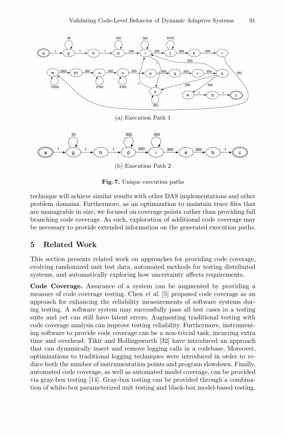
Validating Code-Level Behavior of Dynamic Adaptive Systems 91
da g 1
b c 1e 1
i300
h 1
z
300
j300 1
k l 300
m b1 1620 300o p
300n 300q r300
1
s
300
300 300
300 300
1
28 300 8100
300
10200 8100 8100
300
300
(a) Execution Path 1
da g 1
b c 1
e 300
i 300
h 1
34
300 1
300 300
(b) Execution Path 2
Fig. 7. Unique execution paths
technique will achieve similar results with other DAS implementations and otherproblem domains. Furthermore, as an optimization to maintain trace files thatare manageable in size, we focused on coverage points rather than providing fullbranching code coverage. As such, exploration of additional code coverage maybe necessary to provide extended information on the generated execution paths.
5 Related Work
This section presents related work on approaches for providing code coverage,evolving randomized unit test data, automated methods for testing distributedsystems, and automatically exploring how uncertainty affects requirements.
Code Coverage. Assurance of a system can be augmented by providing ameasure of code coverage testing. Chen et al. [5] proposed code coverage as anapproach for enhancing the reliability measurements of software systems dur-ing testing. A software system may successfully pass all test cases in a testingsuite and yet can still have latent errors. Augmenting traditional testing withcode coverage analysis can improve testing reliability. Furthermore, instrument-ing software to provide code coverage can be a non-trivial task, incurring extratime and overhead. Tikir and Hollingsworth [32] have introduced an approachthat can dynamically insert and remove logging calls in a codebase. Moreover,optimizations to traditional logging techniques were introduced in order to re-duce both the number of instrumentation points and program slowdown. Finally,automated code coverage, as well as automated model coverage, can be providedvia gray-box testing [14]. Gray-box testing can be provided through a combina-tion of white-box parameterized unit testing and black-box model-based testing.

92 E.M. Fredericks, A.J. Ramirez, and B.H.C. Cheng
In this approach, oracle-verified test sequences are combined with a suite of pa-rameter values to maximize code coverage, and provides insights into systembehaviors at both the model and code levels. Each of these approaches is con-cerned with providing an overall measure of code coverage, where Fenrir targetscode segments that provide differing paths of execution in the DAS, includingbranching and self-reconfiguration paths, thereby providing a finer-grained mea-sure of execution.
Evolved Randomized Unit Testing. A diverse set of system tests can becreated automatically with evolutionary computation. Nighthawk [2] uses a ge-netic algorithm to explore the space of parameters that control the generationof randomized unit tests with respect to fitness values provided by coverageand method invocation metrics. EvoSuite [9] uses evolutionary algorithms tocreate whole test suites that focus on a single coverage criterion (i.e., introduc-ing artificial defects into a program). In contrast to each of these approaches,Fenrir instead provides feedback through execution traces to demonstrate thevast amount of possible states that a DAS may encounter at run time, as opposedto defining test suites for validation.
Automated Testing of Distributed Systems. Distributed systems compriseasynchronous processes that can also send and receive data asynchronously, andas a result can contain a large number of possible execution paths. Sen andAgha [30] have proposed the use of concolic execution, or simultaneous concreteand symbolic execution, in order to determine a partial order of events incurredin an execution path. Concolic execution was proven to efficiently and exhaus-tively explore unique execution paths in a distributed system. Furthermore, au-tomated fault injection can explore and evaluate fault tolerance to ensure that adistributed system continually satisfies its requirements specification [8] and en-sures system dependability [29]. Conversely, Fenrir explores how a system canhandle faults by studying its reaction to varying operational contexts, ratherthan by direct injection of faults into the system.
Automatically Exploring Uncertainty in Requirements. Ramirez etal. [26] introduced Loki, an approach for creating novel system and environmen-tal conditions that can affect DAS behavior, and in doing so uncover unexpectedor latent errors within a DAS’s requirements specification. Fenrir extends Lokiby exploring uncertainty at the code level in an effort to distinguish how a DASwill react in uncertain situations and attempt to uncover errors made in theimplementation of a DAS.
6 Conclusion
In this paper we presented Fenrir, an approach that applies novelty searchat design time to automatically generate operational contexts that can affect aDAS during execution at the code level. Specifically, Fenrir introduces loggingstatements to trace a DAS’s execution path and then uses the distance betweenexecution paths to measure the level of novelty between operational contexts.

Validating Code-Level Behavior of Dynamic Adaptive Systems 93
By creating a set of configurations that more extensively exercise a DAS, it is pos-sible to identify undesirable behaviors or inconsistencies between requirementsand system implementation. We demonstrated the use of Fenrir on an RDMnetwork that was responsible for replicating data across a network. This networkwas subjected to uncertainty in the form of random link failures and droppedor delayed messages. Experimental results from this case study established thatFenrir was able to successfully generate more unique execution paths with asmaller set of execution traces than purely random search. Future directions forFenrir will extend the technique and apply it to additional applications. Weare investigating different distance metrics for novelty search as well as otherevolutionary strategies to generate unique execution traces.
Acknowledgements. We gratefully acknowledge conceptual and implementa-tion contributions from Jared M. Moore.
This work has been supported in part by NSF grants CCF-0854931, CCF-0750787, CCF-0820220, DBI-0939454, Army Research Office grant W911NF-08-1-0495, and Ford Motor Company. Any opinions, findings, and conclusions orrecommendations expressed in this material are those of the author(s) and donot necessarily reflect the views of the National Science Foundation, Army, Ford,or other research sponsors.
References
1. Ahn, S.-Y., Kang, S., Baik, J., Choi, H.-J.: A weighted call graph approach for find-ing relevant components in source code. In: 10th ACIS International Conference onSoftware Engineering, Artificial Intelligences, Networking and Parallel/DistributedComputing, SNPD 2009, pp. 539–544 (2009)
2. Andrews, J.H., Menzies, T., Li, F.C.H.: Genetic algorithms for randomized unittesting. IEEE Transactions on Software Engineering 37(1), 80–94 (2011)
3. Black, P.E.: Dictionary of Algorithms and Data Structures. U.S. National Instituteof Standards and Technology (May 2006)
4. Camara, J., de Lemos, R.: Evaluation of resilience in self-adaptive systems us-ing probabilistic model-checking. In: Software Engineering for Adaptive and Self-Managing Systems, pp. 53–62 (June 2012)
5. Chen, M.-H., Lyu, M.R., Wong, E.: Effect of code coverage on software reliabilitymeasurement. IEEE Transactions on Reliability 50(2), 165–170 (2001)
6. Cheng, B.H.C., Sawyer, P., Bencomo, N., Whittle, J.: A goal-based modeling ap-proach to develop requirements of an adaptive system with environmental uncer-tainty. In: Schurr, A., Selic, B. (eds.) MODELS 2009. LNCS, vol. 5795, pp. 468–483.Springer, Heidelberg (2009)
7. Cheng, B.H.C, De Lemos, R., Giese, H., Inverardi, P., Magee, J., Andersson, J.,Becker, B., Bencomo, N., Brun, Y., Cukic, B., et al.: Software engineering forself-adaptive systems: A research roadmap. Springer (2009)
8. Dawson, S., Jahanian, F., Mitton, T., Tung, T.-L.: Testing of fault-tolerant andreal-time distributed systems via protocol fault injection. In: Proceedings of AnnualSymposium on Fault Tolerant Computing, pp. 404–414. IEEE (1996)
94 E.M. Fredericks, A.J. Ramirez, and B.H.C. Cheng
9. Fraser, G., Arcuri, A.: Evosuite: automatic test suite generation for object-orientedsoftware. In: Proceedings of the 19th ACM SIGSOFT Symposium and the 13thEuropean Conference on Foundations of Software Engineering, ESEC/FSE 2011,Szeged, Hungary, pp. 416–419. ACM (2011)
10. Gupta, R., Mathur, A.P., Soffa, M.L.: Generating test data for branch coverage.In: Proceedings of the 15th IEEE International Conference on Automated SoftwareEngineering (ASE 2000), pp. 219–227 (2000)
11. Holland, J.H.: Adaptation in Natural and Artificial Systems. MIT Press, Cam-bridge (1992)
12. Ji, M., Veitch, A., Wilkes, J.: Seneca: Remote mirroring done write. In: USENIX2003 Annual Technical Conference, Berkeley, CA, USA, pp. 253–268. USENIXAssociation (June 2003)
13. Keeton, K., Santos, C., Beyer, D., Chase, J., Wilkes, J.: Designing for disasters.In: Proceedings of the 3rd USENIX Conference on File and Storage Technologies,Berkeley, CA, USA, pp. 59–62. USENIX Association (2004)
14. Kicillof, N., Grieskamp, W., Tillmann, N., Braberman, V.: Achieving both modeland code coverage with automated gray-box testing. In: Proceedings of the 3rd In-ternational Workshop on Advances in Model-Based Testing, pp. 1–11. ACM (2007)
15. Lajolo, M., Lavagno, L., Rebaudengo, M.: Automatic test bench generation forsimulation-based validation. In: Proceedings of the Eighth International Work-shop on Hardware/Software Codesign, San Diego, California, United States,pp. 136–140. ACM (2000)
16. Ledru, Y., Petrenko, A., Boroday, S.: Using string distances for test case prioriti-sation. In: Proceedings of the 2009 IEEE/ACM International Conference on Au-tomated Software Engineering, ASE 2009, Auckland, New Zealand, pp. 510–514.IEEE Computer Society (November 2009)
17. Lehman, J., Stanley, K.O.: Exploiting open-endedness to solve problems throughthe search for novelty. In: Proceedings of the Eleventh International Conference onArtificial Life (ALIFE XI), Cambridge, MA, USA. MIT Press (2008)
18. McKinley, P.K., Sadjadi, S.M., Kasten, E.P., Cheng, B.H.C.: Composing adaptivesoftware. Computer 37(7), 56–64 (2004)
19. Moc, J., Carr, D.A.: Understanding distributed systems via execution trace data.In: Proceedings of the 9th International Workshop on Program Comprehension(IWPC 2001), pp. 60–67. IEEE (2001)
20. Nguyen, C.D., Perini, A., Tonella, P., Kessler, F.B., Tonella P.: Automated contin-uous testing of multiagent systems. In: Fifth European Workshop on Multi-AgentSystems, EUMAS (2007)
21. Nguyen, C.D., Perini, A., Tonella, P., Miles, S., Harman, M., Luck, M.: Evolution-ary testing of autonomous software agents. In: Proceedings of the Eighth Inter-national Conference on Autonomous Agents and Multiagent Systems, Budapest,Hungary, pp. 521–528. International Foundation for Autonomous Agents and Mul-tiagent Systems (May 2009)
22. Nguyen, D.C., Perini, A., Tonella, P.: A goal-oriented software testing methodology.In: Luck, M., Padgham, L. (eds.) AOSE 2007. LNCS, vol. 4951, pp. 58–72. Springer,Heidelberg (2008)
23. Ramırez, A., Larriba-Pey, J.-L., Navarro, C., Torrellas, J., Valero, M.: Softwaretrace cache. In: Proceedings of the 13th International Conference on Supercom-puting, pp. 119–126. ACM (1999)

Validating Code-Level Behavior of Dynamic Adaptive Systems 95
24. Ramirez, A.J., Cheng, B.H.C.: Verifying and analyzing adaptive logic throughuml state models. In: Proceedings of the 2008 IEEE International Conference onSoftware Testing, Verification, and Validation, Lillehammer, Norway, pp. 529–532(April 2008)
25. Ramirez, A.J., Fredericks, E.M., Jensen, A.C., Cheng, B.H.C.: Automatically re-laxing a goal model to cope with uncertainty. In: Fraser, G., Teixeira de Souza, J.(eds.) SSBSE 2012. LNCS, vol. 7515, pp. 198–212. Springer, Heidelberg (2012)
26. Ramirez, A.J., Jensen, A.C., Cheng, B.H.C., Knoester, D.B.: Automatically ex-ploring how uncertainty impacts behavior of dynamically adaptive systems. In:Proceedings of the 2011 International Conference on Automatic Software Engi-neering, ASE 2011, Lawrence, Kansas, USA (November 2011)
27. Ryder, B.G.: Constructing the call graph of a program. IEEE Transactions onSoftware Engineering SE-5(3), 216–226 (1979)
28. Sawyer, P., Bencomo, N., Letier, E., Finkelstein, A.: Requirements-aware systems:A research agenda for re self-adaptive systems. In: Proceedings of the 18th IEEEInternational Requirements Engineering Conference, Sydney, Australia, pp. 95–103(September 2010)
29. Segall, Z., Vrsalovic, D., Siewiorek, D., Yaskin, D., Kownacki, J., Barton, J.,Dancey, R., Robinson, A., Lin, T.: Fiat-fault injection based automated testingenvironment. In: Eighteenth International Symposium on Fault-Tolerant Comput-ing, FTCS-18, Digest of Papers, pp. 102–107. IEEE (1988)
30. Sen, K., Agha, G.: Automated systematic testing of open distributed programs. In:Baresi, L., Heckel, R. (eds.) FASE 2006. LNCS, vol. 3922, pp. 339–356. Springer,Heidelberg (2006)
31. Stott, D.T., Floering, B., Burke, D., Kalbarczpk, Z., Iyer, R.K.: Nftape: a frame-work for assessing dependability in distributed systems with lightweight fault injec-tors. In: Computer Performance and Dependability Symposium, pp. 91–100 (2000)
32. Tikir, M.M., Hollingsworth, J.K.: Efficient instrumentation for code coverage test-ing. ACM SIGSOFT Software Engineering Notes 27, 86–96 (2002)
33. Whittle, J., Sawyer, P., Bencomo, N., Cheng, B.H.C., Bruel, J.-M.: RELAX: Incor-porating uncertainty into the specification of self-adaptive systems. In: Proceed-ings of the 17th International Requirements Engineering Conference (RE 2009),Atlanta, Georgia, USA, pp. 79–88 (September 2009)
34. Yuan, D., Park, S., Zhou, Y.: Characterizing logging practices in open-source soft-ware. In: Proceedings of the 2012 International Conference on Software Engineer-ing, ICSE 2012, Piscataway, NJ, USA, pp. 102–112. IEEE Press (2012)
35. Zhang, J., Cheng, B.H.C.: Model-based development of dynamically adaptive soft-ware. In: Proceedings of the 28th International Conference on Software engineering,ICSE 2006, Shanghai, China, pp. 371–380. ACM (2006)

G. Ruhe and Y. Zhang (Eds.): SSBSE 2013, LNCS 8084, pp. 96–110, 2013. © Springer-Verlag Berlin Heidelberg 2013
Model Refactoring Using Interactive Genetic Algorithm
Adnane Ghannem1, Ghizlane El Boussaidi1, and Marouane Kessentini2
1 École de Technologie Supérieure, Montréal, Canada [email protected], [email protected]
2 Missouri University of Science and Technology, Rolla, MO, USA [email protected]
Abstract. Refactoring aims at improving the quality of design while preserving its semantic. Providing an automatic support for refactoring is a challenging problem. This problem can be considered as an optimization problem where the goal is to find appropriate refactoring suggestions using a set of refactoring ex-amples. However, some of the refactorings proposed using this approach do not necessarily make sense depending on the context and the semantic of the sys-tem under analysis. This paper proposes an approach that tackles this problem by adapting the Interactive Genetic Algorithm (IGA) which enables to interact with users and integrate their feedbacks into a classic GA. The proposed algo-rithm uses a fitness function that combines the structural similarity between the analyzed design model and models from a base of examples, and the designers’ ratings of the refactorings proposed during execution of the classic GA. Ex-perimentation with the approach yielded interesting and promising results.
Keywords: Software maintenance, Interactive Genetic Algorithm, Model refac-toring, Refactoring by example.
1 Introduction
Software maintenance is considered the most expensive activity in the software sys-tem lifecycle [1]. Maintenance tasks can be seen as incremental modifications to a software system that aim to add or adjust some functionality or to correct some design flaws. However, as the time goes by, the system’s conceptual integrity erodes and its quality degrades; this deterioration is known in the literature as the software decay problem [2]. A common and widely used technique to cope with this problem is to continuously restructure the software system to improve its structure and design. The process of restructuring object oriented systems is commonly called refactoring [3]. According to Fowler [2], refactoring is the disciplined process of cleaning up code to improve the software structure while preserving its external behavior. Many research-ers have been working on providing support for refactoring operations (e.g., [4], [2], and [5]). Existing tools provide different environments to manually or automatically apply refactoring operations to correct, for example, code smells. Indeed, existing work has, for the most part, focused on refactorings at the source code level. Actually, the rise of the model-driven engineering (MDE) approach increased the interest and

Model Refactoring Using Interactive Genetic Algorithm 97
the needs for tools supporting refactoring at the model-level. In MDE, abstract models are successively refined into more concrete models, and a model refactoring tool will be of great value within this context.
The search-based refactoring approaches proved their effectiveness to propose refactorings to improve the model’s design quality. They adapted some of the known heuristics methods (e.g. Simulated annealing, Hill_climbing) as proposed in [6-8] and Genetic Algorithms as in [9]. These approaches relied, for the most part, on a combi-nation of quality metrics to formulate their optimization goal (i.e., the fitness func-tion). A major problem founded in these approaches is that the quality metrics con-sider only the structural properties of the system under study; the semantic properties of the system are not considered. In this context, Mens and Tourwé [3] argue that most of the refactoring tools cannot offer a full-automatic support because part of the necessary knowledge especially those related to the semantics for performing the refactoring remains implicit in designers’ heads. Indeed, recognizing opportunities of model refactoring remains a challenging issue that is related to the model marking process within the context of MDE which is a notoriously difficult problem that requires design knowledge and expertise [10].
To take into account the semantics of the software system, we propose a model refactoring approach based on an Interactive Genetic Algorithm (IGAs) [11]. Two types of knowledge are considered in this approach. The first one comes from the examples of refactorings. For this purpose, we hypothesize that the knowledge re-quired to propose appropriate refactorings for a given object-oriented model may be inferred from other existing models’ refactorings when there is some structural simi-larities between these models and the given model. From this perspective, the refac-toring is seen as an optimization problem that is solved using a Genetic Algorithm (GA). The second type of knowledge comes from the designer's knowledge. For this purpose, the designer is involved in the optimization process by continuously interact-ing with the GA algorithm; this enables to adjust the results of the GA progressively exploiting the designer’s feedback. Hence the proposed approach (MOREX+I: MOdel REfactoring by eXample plus Interaction) relies on a set of refactoring examples and designer's feedbacks to propose sequences of refactorings. MOREX+I takes as input an initial model, a base of examples of refactored models and a list of metrics calcu-lated on both the initial model and the models in the base of examples, and it gener-ates as output a solution to the refactoring problem. In this paper, we focus on UML class diagrams. In this case, a solution is defined as a sequence of refactorings that maximize as much as possible the similarity between the initial and revised class dia-grams (i.e., the class diagrams in the base of examples) while considering designer's feedbacks.
The primary contributions of the paper are 3-fold: 1) We introduce a model refac-toring approach based on the use of examples. The approach combines implicitly the detection and the correction of design defects at the model-level by proposing a se-quence of refactorings that must be applied on a given model. 2) We use the IGA to allow the integration of feedbacks provided by designers upon solutions produced during the GA evolution. 3) We report the results of an evaluation of our approach.

98 A. Ghannem, G. El Boussaidi, and M. Kessentini
The paper is organized as follows. Section 2 is dedicated to the background where we introduce some basic concepts and the related work. The overall approach is de-scribed in Section 3. Section 4 reports on the experimental settings and results, while Section 5 concludes the paper and outlines some future directions to our work.
2 Background
2.1 Class Diagrams Refactorings and Quality Metrics
Model refactoring is a controlled technique for improving the design (e.g., class dia-grams) of an existing model. It involves applying a series of small refactoring opera-tions to improve the design quality of the model while preserving its behavior. Many refactorings were proposed and codified in the literature (see e.g., [2]). In our ap-proach, we consider a subset of the 72 refactorings defined in [2]; i.e., only those refactorings that can be applied to UML class diagrams. Indeed, some of the refactor-ings in [2] may be applied on design models (e.g. Move_Method, Rename_method, Move_Attribute, Extract_Class etc.) while others cannot be (e.g. Extract_Method, Inline_Method, Replace_Temp_With_Query etc. ). In our approach we considered a list of twelve refactorings (e.g. Extract_class, Push_down_method, Pull_up_method, etc.) based on [2]. The choice of these refactorings was mainly based on two factors: 1) they apply at the class diagram-level; and 2) they can be link to a set of model metrics (i.e., metrics which are impacted when applying these refactorings).
Metrics provide useful information that help assessing the level of conformance of a software system to a desired quality [12]. Metrics can also help detecting some simi-larities between software systems. The most widely used metrics for class diagrams are the ones defined by Genero et al. [13]. In the context of our approach, we used a list of sixteen metrics (e.g. Number of attributes: NA, Number of methods: NMeth, Number of dependencies: NDep, etc.) including the eleven metrics defined in [13] to which we have added a set of simple metrics (e.g., number of private methods in a class, number of public methods in a class). All these metrics are related to the class entity which is the main entity in a class diagram.
2.2 Interactive Genetic Algorithm (IGA)
Heuristic search are serving to promote discovery or learning [14]. There is a variety of methods which support the heuristic search as hill_climbing [15], genetic algo-rithms (GA) [16], etc. GA is a powerful heuristic search optimization method inspired by the Darwinian theory of evolution [17]. The basic idea behind GA is to explore the search space by making a population of candidate solutions, also called individuals, evolve toward a “good” solution of a specific problem. Each individual (i.e., a solu-tion) of the population is evaluated by a fitness function that determines a quantitative measure of its ability to solve the target problem. Exploration of the search space is achieved by selecting individuals (in the current population) that have the best fitness values and evolving them by using genetic operators, such as crossover and mutation. The crossover operator insures generation of new children, or offspring, based on

Model Refactoring Using Interactive Genetic Algorithm 99
parent individuals while the mutation operator is applied to modify some randomly selected nodes in a single individual. The mutation operator introduces diversity into the population and allows escaping local optima found during the search. Once selec-tion, mutation and crossover have been applied according to given probabilities, indi-viduals of the newly created generation are evaluated using the fitness function. This process is repeated iteratively, until a stopping criterion is met. This criterion usually corresponds to a fixed number of generations.
Interactive GA (IGAs) [18] combines a genetic algorithm with the interaction with the user so that he can assign a fitness to each individual. This way IGA integrates the user's knowledge during the regular evolution process of GA. For this reason, IGA can be used to solve problems that cannot be easily solved by GA [19]. A variety of application domains of IGA include development of fashion design systems [19], music composition systems [20], software re-modularization [21] and some other IGAs’ applications in other fields [11]. One of the key elements in IGAs is the man-agement of the number of interactions with the user and the way an individual is evaluated by the user.
2.3 Related Work
Model refactoring is still at a relatively young stage of development compared to the work that has been done on source-code refactoring. Most of existing approaches for automating refactoring activities at the model-level are based on rules that can be expressed as assertions (i.e., invariants, pre-and post-conditions) [22, 23], or graph transformations targeting refactoring operations in general [24, 25] or design patterns’ applications in particular (e.g., [26]). In [22] invariants are used to detect some parts of the model that require refactoring and the refactorings are expressed using declara-tive rules. However, a complete specification of refactorings requires an important number of rules and the refactoring rules must be complete, consistent, non-redundant and correct. In [26] refactoring rules are used to specify design patterns’ applications. In this context, design problems solved by these patterns are represented using models and the refactoring rules transform these models according to the solutions proposed by the patterns. However, not all design problems are representable using models. Finally an issue that is common to most of these approaches is the problem of se-quencing and composing refactoring rules. This is related to the control of rules’ ap-plications within rule-based transformational approaches in general.
Our approach is inspired by contributions in search-based software engineering (SBSE) (e.g. [6, 7, 9, 27, 28]). Techniques based on SBSE are a good alternative to tackle many of the above mentioned issues [9]. For example, a heuristic-based ap-proach is presented in [6, 7, 27] in which various software metrics are used as indica-tors for the need of a certain refactoring. In [27], a genetic algorithm is used to sug-gest refactorings to improve the class structure of a system. The algorithm uses a fit-ness function that relies on a set of existing object oriented metrics. Harman and Tratt [6] propose to use the Pareto optimality concept to improve search-based refactoring approaches when the evaluation function is based on a weighted sum of metrics. Both the approaches in [27] and [6] were limited to the Move Method refactoring

100 A. Ghannem, G. El Boussaidi, and M. Kessentini
operation. In [7], the authors present a comparative study of four heuristic search techniques applied to the refactoring problem. The fitness function used in this study was based on a set of 11 metrics. The results of the experiments on five open-source systems showed that hill-climbing performs better than the other algorithms. In [28], the authors proposed an automated refactoring approach that uses genetic program-ming (GP) to support the composition of refactorings that introduce design patterns. The fitness function used to evaluate the applied refactorings relies on the same set of metrics as in [12] and a bonus value given for the presence of design patterns in the refactored design. Our approach can be seen as linked to this approach as we aim at proposing a combination of refactorings that must be applied to a design model. Our approach was inspired by the work in [21] where the authors apply an Interactive Genetic Algorithm to the re-modularization problem which can be seen as a specific subtype of the refactoring problem. Our work is also related to the approach in [29] where the authors apply an SBSE approach to model transformations. However this approach focuses on general model transformations while our focus is on refactorings which are commonly codified transformations that aim at correcting design defaults.
To conclude, most of the approaches that tackled the refactoring as an optimization problem by the use of some heuristics suppose, to some extent, that a refactoring op-eration is appropriate when it optimizes the fitness function (FF). Most of these ap-proaches defined their FF as a combination of quality metrics to approximate the quality of a model. However, refactoring operations are design transformations which are context-sensitive. To be appropriately used, they require some knowledge of the system to be refactored. Indeed, the fact that the values of some metrics were im-proved after some refactorings does not necessarily mean or ensure that these refac-torings make sense. This observation is at the origin of the work described in this paper as described in the next section.
3 Heuristic Search Using Interactive Genetic Algorithm
3.1 Interactive Genetic Algorithm Adaptation
The approach proposed in this paper exploits examples of model refactorings, a heu-ristic search technique and the designer’s feedback to automatically suggest se-quences of refactorings that can be applied on a given model (i.e., a UML class dia-gram). A high-level view of our adaptation of IGA to the model refactoring problem is given in Fig. 1. The algorithm takes as input a set of quality metrics, a set of model refactoring examples, a percentage value corresponding to the percentage of a popula-tion of solutions that the designer is willing to evaluate, the maximum number of iterations for the algorithm and the number of interactions with the designer. First, the algorithm runs classic GA (line 2) for a number of iterations (i.e., the maximum num-ber of iterations divided by the number of interactions). Then a percentage of solu-tions from the current population is selected (line 3). In lines 4 to 7, we get designers' feedbacks for each refactoring in each selected solution and we update their fitness function. We generate a new population (p+1) of individuals (line 8) by iteratively

Model Refactoring Using Interactive Genetic Algorithm 101
selecting pairs of parent individuals from population p and applying the crossover operator to them; each pair of parent individuals produces two children (solutions). We include both the parent and child variants in the new population. Then we apply the mutation operator, with a probability score, for both parent and child to ensure the solution diversity; this produces the population for the next generation. The algorithm terminates when the maximum iteration number is reached, and returns the best set of refactorings’ sequences (i.e., best solutions from all iterations).
Input: Set of quality metrics Input: Set of model refactoring examples Input: Percentage (P%) Input: MaxNbrIterations Input: NbrOfInteractions Output: A sequence of refactorings 1: for i = 1 . . . NbrOfInteractions do 2: Evolve GA for NbrIterations 3: Select P% of best solutions from the current population. 4: for-each selected solution do 5: Ask the designer whether each refactoring within the selected solution makes sense. 6: Update the FF of the selected solution to integrate the feedback. 7: end for-each 8: Create a new GA population using the updated solutions 9: end for 10: Continue (non-interactive) GA evolution until it converges or it reaches maxNbrIterations
Fig. 1. High-level pseudo-code for IGA adaptation to our problem
In the following subsections we present the details of the regular GA adaptation to the problem of generating refactoring sequences and how we collect the designers’ feedbacks and integrate it in the fitness function computation.
3.2 Representing an Individual and Generating the Initial Population
An individual (i.e., a candidate solution) is a set of blocks. The upper part of Fig. 2 shows an individual with three blocks. The first part of the block contains the class (e.g. Order) chosen from the initial model (model under analysis) called CIM, the second part contains the class (e.g Person) from the base of examples that was matched to CIM called CBE, and finally the third part contains a list of refactorings (e.g. Pull_Up_Method(calc_taxes(), LineOrder, Orde)) which is a subset of the refac-torings that were applied to CBE (in its subsequent versions) and that can be applied to CIM. In our approach, classes from the model (CIMs) and the base of examples (CBEs) are represented using predicates that describe their attributes, methods and relationships. In addition, the representation of a CBE class includes a list of refactor-ings that were applied to this class in a subsequent version of the system’s model to which CBE belongs. The subset of a CBE subsequent refactorings that are applicable to a CIM class constitutes the third part of the block having CIM as its first part and

102 A. Ghannem, G. El Boussaidi, and M. Kessentini
CBE as its second part. Hence, the selection of the refactorings to be considered in a block is subjected to some constraints to avoid conflicts and incoherence errors. For example, if we have a Move_attribute refactoring operation in the CBE class and the CIM class doesn’t contain any attribute, then this refactoring operation is discarded as we cannot apply it to the CIM class.
Hence the individual represents a sequence of refactoring operations to apply and the classes of the initial model on which they apply. The bottom part of Fig. 2 shows the fragments of an initial model before and after the refactorings proposed by the individual (at the top of the figure) were applied.
Order ProductLineOrder
Pull_Up_Method(calc_taxes(), LineOrder, Order) Rename_Attribute(tax, taxStatus) Move_Attribute(quantity, Product, LineOrder)
Pull_Up_Method(calc_SubTotal(), LineOrder, Order) Rename_Attribute(tax, taxStatus)Move_Attribute(quantity, Product, LineOrder)
Person Teacher Agency
Fig. 2. Individual representation
To generate an initial population, we start by defining the maximum individual size. This parameter can be specified either by the user or randomly. Thus, the indi-viduals have different sizes. Then, for each individual we randomly assign: 1) a set of classes from the initial model that is under analysis and their matched classes from the base of examples, and 2) a set of refactorings that we can possibly apply on the initial model class among the refactorings proposed from the base of examples class.
3.3 Genetic Operators
Selection: To select the individuals that will undergo the crossover and mutation op-erators, we used the stochastic universal sampling (SUS) [17], in which the probabil-ity of selection of an individual is directly proportional to its relative fitness in the population. For each iteration, we use SUS to select 50% of individuals from popula-tion p for the new population p+1. These (population_size/2) selected individuals will “give birth” to another (population_size/2) new individuals using crossover operator.
Crossover: For each crossover, two individuals are selected by applying the SUS se-lection [17]. Even though individuals are selected, the crossover happens only with a certain probability. The crossover operator allows creating two offspring p’1 and p’2

Model Refactoring Using Interactive Genetic Algorithm 103
from the two selected parents p1 and p2 as follows: A random position, k, is selected. The first k refactorings of p1 become the first k elements of p’2. Similarly, the first k refactorings of p2 become the first k refactorings of p’1. The rest of refactorings (from position k+1 until the end of the sequence) in each parent p1 and p2 are kept. For instance, Fig. 3 illustrates the crossover operator applied to two individuals (parents) p1 and p2 where the position k takes the value 2.
Mutation: The mutation operator consists of randomly changing one or more elements in the solution. Hence, given a selected individual, the mutation operator first ran-domly selects some refactorings among the refactoring sequence proposed by the individual. Then the selected refactorings are replaced by other refactorings. Fig. 4 illustrates the effect of a mutation on an individual.
Fig. 3. Crossover operator
Fig. 4. Mutation operator
3.4 Evaluating an Individual within the Classic GA
The quality of an individual is proportional to the quality of the refactoring operations composing it. In fact, the execution of these refactorings modifies various model fragments; the quality of a solution is determined with respect to the expected refac-tored model. However, our goal is to find a way to infer correct refactorings using the knowledge that has been accumulated through refactorings of other models of past projects and feedbacks given by designers. Specifically, we want to exploit the simi-larities between the actual model and other models to infer the sequence of refactor-ings that we must apply. Our intuition is that a candidate solution that displays a high similarity between the classes of the model and those chosen from the examples base should give the best sequence of refactorings. Hence, the fitness function aims to
Order ProductLineOrder
Pull_Up_Method(calc_taxes(), LineOrder, Order) Rename_Attribute(tax, taxStatus) Move_Attribute(quantity, Product, LineOrder)P1:
School Pilot
Add_parameter(version : String) Move_Attribute(typePlane, Pilot, Plane)
P2:
P’1:
P’2:
Teacher Agency
Course Student
School Pilot
Add_parameter(version : String) Move_Attribute(typePlane, Pilot, Plane)
Course Student
Order LineOrder
Pull_Up_Method(calc_taxes(), LineOrder, Order) Rename_Attribute(tax, taxStatus)
Person Teacher
Product
Move_Attribute(quantity, Product, LineOrder)
Agency
K = 2
Person
Order ProductLineOrder
Pull_Up_Method(calc_taxes(), LinePrder, Order) Rename_Attribute(tax, taxStatus) Move_Attribute(quantity, Product, LineOrder)
Order ProductLineOrder
Pull_Up_Method(calc_taxes(), LinePrder, Order) Rename_Method(calc_SubTotal, calc_TotalLine) Move_Attribute(quantity, Product, LineOrder)
Person Teacher Agency
Person AgencyStudent

104 A. Ghannem, G. El Boussaidi, and M. Kessentini
maximize the similarity between the classes of the model in comparison to the revised ones in the base of examples. In this context, we introduce first a similarity measure between two classes denoted by Similarity and defined by formula 1 and 2. , ∑ , (1)
, 1 0 0 0
(2)
Where m is the number of metrics considered in this project. CIMi is the ith metric value of the class CIM in the initial model while CBEi is the ith metric value of the class CBE in the base of examples. Using the similarity between classes, we define the fitness function of a solution, normalized in the range [0, 1], as: ∑ , (3)
Where n is the number of blocks in the solution and CMIBj and CBEBj are the classes composing the first two parts of the jth block of the solution. To illustrate how the fitness function is computed, we consider a system containing two classes as shown in Table 1 and a base of examples containing two classes shown in Table 2. In this ex-ample we use six metrics and these metrics are given for each class in the model in Table 1 and each class of the base of examples in Table 2.
Table 1. Classes from the initial model and their metrics values
CMI NPvA NPbA NPbMeth NPvMeth NAss NGen LineOrder 4 1 3 1 1 1 Product 2 2 6 0 1 0
Table 2. Classes from the base of examples and their metrics values
CBE NPvA NPbA NPbMeth NPvMeth NAss NGen Student 2 1 3 0 3 0 Plane 5 1 4 0 1 0
Consider an individual/solution I1 composed by two blocks (LineOrder/Student
and Product/Plane). The fitness function of I1 is calculated as follows: 112 24 1 1 0 13 0 25 12 46 0 1 0 0,45

Model Refactoring Using Interactive Genetic Algorithm 105
3.5 Collecting and Integrating the Feedbacks from Designers
Model refactoring is a design operation that is context-sensitive. In addition, depend-ing on the semantics of the system under analysis and the system’s evolution as foreseen by different designers, a refactoring proposed by the classic GA can be con-sidered as mandatory by a designer and as acceptable by another. Even if a sequence of refactorings optimizes the fitness function (as defined in the previous section), that does not ensure that these refactorings conform to and preserve the semantics of the system. Consequently, we use Interactive GA (IGA) to partly tackle this problem by interacting with designers and getting their feedbacks on a number of the proposed refactoring sequences. To do so, we adopted a five level scale to rate the proposed refactorings; i.e., we distinguish five types of rating that a designer can assign to a proposed refactoring. The meaning and the value of each type of rating are as follows:
• Critical (value = 1): it is mandatory to apply the proposed refactoring; • Desirable (value = 0.8): it is useful to apply the refactoring to enhance some aspect
of the model but it’s not mandatory; • Neutral (value = 0.5): the refactoring is applicable but the designer does not see it
as necessary or desirable; • Undesirable (value = 0.3): the refactoring is applicable but it is not useful and
could alter the semantics of the system; • Inappropriate (value = 0): the refactoring should not be applied because it breaks
the semantics of the system.
As described in section 3.1., during the execution of IGA, the designer is asked to rate a percentage of the best solutions found by the classic GA after a defined number of iterations. For each of the selected solutions, the designer assigns a rating for each refactoring included in the solution. Depending on the values entered by the designer, we re-evaluate the global fitness function of the solution as follows. For each block of the solution, we compute the block rating as an average of the ratings of the refactor-ings in the block. Then we compute the overall designer’s rating as an average of all blocks ratings. Finally, the new fitness function of the solution is computed as an average of its old fitness function and the overall designer’s rating. The new values of the fitness functions of the selected solutions are injected back into the IGA process to form a new population of individuals.
4 Experiments
The goal of the experiment is to evaluate the efficiency of our approach for the gen-eration of the refactorings’ sequences. In particular the experiment aimed at answer-ing the following research questions:
• RQ1: To what extent can the interactive approach generate correct refactorings’ sequences?
• RQ2: What types of refactorings are correctly suggested?

106 A. Ghannem, G. El Boussaidi, and M. Kessentini
To answer these questions we implemented and tested the approach on open source projects. In particular, to answer RQ1, we used an existing corpus of known models refactorings to evaluate the precision and recall of our approach, and to answer RQ2, we investigated the type of refactorings that were suggested by our tool. In this sec-tion, we present the experimental setup and discuss the results of this experiment.
4.1 Supporting Tool and Experimental Setup
We implemented our approach as a plugin within the EclipseTM development envi-ronment. Fig. 5 shows a screenshot of the model refactoring plugin perspective. This plugin takes as input a base of examples of refactored models and an initial model to refactor. The user specifies the population size, the number of iterations, the individ-ual size, the number of mutations, the number of interactions, and the percentage of the solutions shown in each interaction. It generates as output an optimal sequence of refactorings to be applied on the analyzed system.
Fig. 5. Model Refactoring Plugin
To build the base of examples, we used the Ref-Finder tool [43] to collect the refactoring that were applied on six Java open source projects (Ant, JabRef, JGraphx, JHotDraw, JRDF, and Xom). Ref-Finder helps retrieving the refactorings that a sys-tem has undergone by comparing different versions of the system. We manually vali-dated the refactorings returned by Ref-finder before including them in the base of examples. To answer the research questions reported above, we analyzed two open-source Java projects in our experiment. We have chosen these open source projects because they are medium-sized open-source projects and they have been actively developed over the past 10 years. The participants in the experiment were three Ph.D students enrolled in Software Engineering and all of them are familiar with the two analyzed systems and have a strong background in object-oriented refactoring.
4.2 Results and Discussions
To assess the accuracy of the approach, we compute the precision and recall of our IGA algorithm when applied to the two projects under analysis. In the context of our

Model Refactoring Using Interactive Genetic Algorithm 107
study, the precision denotes the fraction of correctly proposed refactorings among the set of all proposed refactorings. The recall indicates the fraction of correctly proposed refactorings among the set of all actually applied refactorings in the subsequent ver-sions of the analyzed projects. To assess the validity of the proposed refactorings, we compare them to those returned by Ref-Finder when applied to the two projects and their subsequent versions. The precision and recall results might vary depending on the refactorings used, which are randomly generated, though guided by a meta-heuristic. Fig. 6 and Fig. 7 show the results of 23 executions of our approach on Xerces and GanttProject, respectively. Each of these figures displays the precision and the recall values for each execution.
Fig. 6. Multiple execution results for Xerces Fig. 7. Multiple Execution results for GanttProject
Generally, the average precision and recall (around 88%) allows us to positively
answer our first research question RQ1 and conclude that the results obtained by our approach are very encouraging. The precision in the two projects under analysis (on average 90% of all executions) proves that a big number of the refactorings proposed by our approach were indeed applied to the system’s model in its subsequent version (i.e., the proposed refactorings match, in most cases, those returned by Ref-Finder when applied on the system’s model and its subsequent version). To ensure that our results are relatively stable, we compared the results of the multiple executions (23) of the approach on the two analyzed projects shown in Fig. 6 and Fig. 7. The precision and recall scores are approximately the same for different executions in the two con-sidered projects. We also compared the sequences of refactorings returned by differ-ent executions of our algorithm on the same project. We found that when a class (from the model under analysis) is part of two different returned sequences, the refac-toring operations proposed for this class within these sequences are similar. We con-sequently conclude that our approach is stable.
Our experiment through the interactions with designers allowed us to answer the second research question RQ2 by inferring the types of refactorings they recognized as good refactorings. Fig. 8 shows that 82% of the the Move_method and Pull_up_method refactorings proposed during the executions are recognized as good refactoring versus only 70% of the Rename_method refactorings. We noticed also,
80
82
84
86
88
90
92
94
1 2 3 4 5 6 7 8 9 10 11 12 13 14 15 16 17 18 19 20 21 22 23
Xerces 2.5 Precision (%)
Xerces 2.5 Recall (%)
74
76
78
80
82
84
86
88
90
92
94
1 2 3 4 5 6 7 8 9 10 11 12 13 14 15 16 17 18 19 20 21 22 23
GanttProject 2.0.10 Precision (%)
GanttProject 2.0.10 Recall (%)

108 A. Ghannem, G. El Boussaidi, and M. Kessentini
that only 9 of 12 refactorings used in the approach are considered in this analysis. This may result from the quality of the base of examples or from the random factor which characterizes genetic algorithm. We made a further analysis to understand the causes of such results. We found out that through the interactions, the designers have to recognize the meaningless refactorings and penalize them by assigning them a 0 as a rating value; this has significantly reduced the number of these types of refactorings in the optimal solution.
6570758085
Fig. 8. Distribution of refactorings recognized as correct refactorings through intercations
Despite the good results, we noticed a very slight decrease in recall versus preci-sion in the analyzed projects. Our analysis pointed out towards two factors. The first factor is the project domain. In this study we tried to propose refactorings using a base of examples which contains different projects from different domains. We noticed that some projects focus on some types of refactorings compared to others (i.e., some projects in the base of examples has a big frequency of «pull_up_Attribute» and «pull_up_method»). The second factor is the number and types of refactorings con-sidered in this experimentation. Indeed, we noticed that some refactorings (e.g., «pull_up_method», «pull_up_Attribute», «add_parameter») are located correctly in our approach. We have no certainty that these factors can improve the results but we consider analyzing them as a future work to further clarify many issues.
4.3 Threats to Validity
We have some points that we consider as threats to the generalization of our ap-proach. The most important one is the use of the Ref_finder Tool to build the base of examples and at the same time we compare the results obtained by our algorithm to those given by Ref_finder. Other threats can be related to the IGAs parameters set-ting. Although we applied the approach on two systems, further experimentation is needed. Also, the reliability of the proposed approach requires an example set of ap-plied refactoring on different systems. It can be argued that constituting such a set might require more work than these examples. In our study, we showed that by using some open source projects, the approach can be used out of the box and will produce good refactoring results for the studied systems. In an industrial setting, we could expect a company to start with some few open source projects, and gradually enrich its refactoring examples to include context-specific data. This is essential if we con-sider that different languages and software infrastructures have different best/worst
Model Refactoring Using Interactive Genetic Algorithm 109
practices. Finally, since we viewed the model refactorings’ generation problem as a combinatorial problem addressed with heuristic search, it is important to contrast the results with the execution time. We executed the plugin on a standard desktop com-puter (i7 CPU running at 2.67 GHz with 8GB of RAM). The number of interactions was set to 50. The execution time for refactorings’ generation with a number of itera-tions (stopping criteria) fixed to 1000 was less than seventy minutes. This indicates that our approach is reasonably scalable from the performance standpoint.
5 Conclusion and Future Work
In this article, we presented a new approach that aims to suggest appropriate se-quences of refactorings that can be applied on a given design model and in particular on a UML class diagram. To do so, we adapted Interactive Genetic Algorithms (IGAs) to build an algorithm which exploits both existing model refactoring examples and the designer's knowledge during the search process for opportunities of model refactorings. We implemented the approach as a plugin integrated within the Eclipse platform and we performed multiple executions of the approach on two open source projects. The results of our experiment have shown that the approach is stable regard-ing its correctness, completeness and the type and number of the proposed refactor-ings per class. IGA has significantly reduced the number of meaningless refactorings in the optimal solutions for these executions. While the results of the approach are very promising, we plan to extend it in different ways. One issue that we want to ad-dress as a future work is related to the base of examples. In the future we want to extend our base of examples to include more refactoring operations. We also want to study and analyze the impact of using domain-specific examples on the quality of the proposed sequences of refactorings. Actually, we kept the random aspect that charac-terizes genetic algorithms even in the choice of the projects used in the base of exam-ples without prioritizing one or more specific projects on others to correct the one under analysis. Finally, we want to apply the approach on other open source projects and further analyze the type of refactorings that are correctly suggested.
References
1. Lientz, B.P., Swanson, E.B., Tompkins, G.E.: Characteristics of application software maintenance. Commun. ACM 21(6), 466–471 (1978)
2. Fowler, M.: Refactoring: Improving the Design of Existing Code. Addison-Wesley (1999) 3. Mens, T., Tourwé, T.: A Survey of Software Refactoring. IEEE Trans. Softw. Eng. 30(2),
126–139 (2004) 4. Opdyke, W.F.: Refactoring: A Program Restructuring Aid in Designing Object-Oriented
Application Frameworks, U. Illinois at Urbana-Champaign (1992) 5. Moha, N.: DECOR: Détection et correction des défauts dans les systèmes orientés objet,
p. 157. UdeM & USTdeLille, Montréal (2008) 6. Harman, M., Tratt, L.: Pareto optimal search based refactoring at the design level. In: Pro-
ceedings of the 9th Annual GECCO 2007, pp. 1106–1113. ACM, London (2007) 7. O’Keeffe, M.: Search-based refactoring: an empirical study. J. Softw. Maint. Evol. 20(5),
345–364 (2008)
110 A. Ghannem, G. El Boussaidi, and M. Kessentini
8. O’Keeffe, M., Cinneide, M.O.: Search-based software maintenance. In: CSMR (2006) 9. Kessentini, M., Sahraoui, H.A., Boukadoum, M.: Model Transformation as an Optimiza-
tion Problem. In: Czarnecki, K., Ober, I., Bruel, J.-M., Uhl, A., Völter, M. (eds.) MODELS 2008. LNCS, vol. 5301, pp. 159–173. Springer, Heidelberg (2008)
10. El-Boussaidi, G., Mili, H.: Detecting Patterns of Poor Design Solutions Using Constraint Propagation. In: Czarnecki, K., Ober, I., Bruel, J.-M., Uhl, A., Völter, M. (eds.) MODELS 2008. LNCS, vol. 5301, pp. 189–203. Springer, Heidelberg (2008)
11. Takagi, H.: Interactive evolutionary computation: fusion of the capabilities of EC optimi-zation and human evaluation. Proceedings of the IEEE 89(9), 1275–1296 (2001)
12. Fenton, N.E., Pfleeger, A.S.L.: Software Metrics: A Rigorous and Practical Approach, 2nd edn., p. 656. PWS Pub., Boston (1998)
13. Genero, M., Piattini, M., Calero, C.: Empirical validation of class diagram metrics. In: Proceedings of the International Symposium on ESE (2002)
14. Pearl, J.: Heuristics: intelligent search strategies for computer problem solving, p. 382. Addison-Wesley Longman Publishing Co., Inc. (1984)
15. Mitchell, M.: An Introduction to Genetic Algorithms, p. 209. MIT Press (1998) 16. Goldberg, D.E.: Genetic Algorithms in Search, Optimization and Machine Learning,
p. 372. Addison-Wesley Longman Publishing Co., Inc. (1989) 17. Koza, J.R.: Genetic programming: on the programming of computers by means of natural
selection, p. 680. MIT Press (1992) 18. Dawkins, R.: The BlindWatchmaker, 1st edn., p. 358. Longman, Essex (1986) 19. Kim, H.S., Cho, S.B.: Application of interactive genetic algorithm to fashion design. In:
Engineering Applications of Artificial Intelligence (2000) 20. Chen, Y.-P.: Interactive music composition with the CFE framework. SIGEVOlution 2(1),
9–16 (2007) 21. Bavota, G., Carnevale, F., De Lucia, A., Di Penta, M., Oliveto, R.: Putting the developer
in-the-loop: an interactive GA for software re-modularization. In: Fraser, G., Teixeira de Souza, J. (eds.) SSBSE 2012. LNCS, vol. 7515, pp. 75–89. Springer, Heidelberg (2012)
22. Van Der Straeten, R., Jonckers, V., Mens, T.: A formal approach to model refactoring and model refinement. J. SoSyM 6(2), 139–162 (2007)
23. Van Kempen, M., et al.: Towards proving preservation of behaviour of refactoring of UML models. In: Proceedings of the annual SAICSIT 2005, pp. 252–259. White River, South Africa (2005)
24. Mens, T., Taentzer, G., Runge, O.: Analysing refactoring dependencies using graph trans-formation. J. SoSyM 6(3), 269–285 (2007)
25. Biermann, E.: EMF model transformation based on graph transformation: formal founda-tion and tool environment. In: Ehrig, H., Rensink, A., Rozenberg, G., Schürr, A. (eds.) ICGT 2010. LNCS, vol. 6372, pp. 381–383. Springer, Heidelberg (2010)
26. El Boussaidi, G., Mili, H.: Understanding design patterns — what is the problem? Soft-ware: Practice and Experience (2011)
27. Seng, O., Stammel, J., Burkhart, D.: Search-based determination of refactorings for im-proving the class structure of object-oriented systems. In: Proc. of the 8th Annual GECCO 2006, pp. 1909–1916. ACM, Seattle (2006)
28. Jensen, A.C., Cheng, B.H.C.: On the use of genetic programming for automated refactor-ing and the introduction of design patterns. In: Proc. of the 12th Annual GECCO 2010, pp. 1341–1348. ACM, Portland (2010)
29. Kessentini, M., et al.: Search-based model transformation by example. J. SoSyM 11(2), 209–226 (2012)

A Fine-Grained Parallel Multi-objective
Test Case Prioritization on GPU
Zheng Li1, Yi Bian1, Ruilian Zhao1, and Jun Cheng2
1 Department of Computer ScienceBeijing University of Chemical Technology
Beijing 100029, P.R. China2 Chongqing Institute of Green and Intelligent Technology
Chinese Academy of SciencesChongqing 401122, P.R. China
Abstract. Multi-Objective Evolutionary Algorithms (MOEAs) havebeen widely used to address regression test optimization problems, in-cluding test case selection and test suite minimization. GPU-based par-allel MOEAs are proposed to increase execution efficiency to fulfill theindustrial demands. When using binary representation in MOEAs, thefitness evaluation can be transformed a parallel matrix multiplicationthat is implemented on GPU easily and more efficiently. Such GPU-based parallel MOEAs may achieve higher level of speed-up for test caseprioritization because the computation load of fitness evaluation in testcase prioritization is more than that in test case selection or test suiteminimization. However, the non-applicability of binary representation inthe test case prioritization results in the challenge of parallel fitness eval-uation on GPU. In this paper, we present a GPU-based parallel fitnessevaluation and three novel parallel crossover computation schemes basedon ordinal and sequential representations, which form a fine-grained par-allel framework for multi-objective test case prioritization. The empiricalstudies based on eight benchmarks and one open source program showa maximum of 120x speed-up achieved.
Keywords: Test Case Prioritization, Mulit-Objective Optimization,NSGA-II, GPU, CUDA.
1 Introduction
Test suite optimization has been widely used to reduce the cost of regressiontesting [1], in which test case prioritization [2] is a technique that sorts testcases order so that those test cases with the highest priority, according to sometest adequacy criteria, can run as soon as possible. Many related studies havebeen proposed in literature [3,4,5,6]. One dimension of the research is to considertest case prioritization as a search problem [7], where search based optimizationalgorithms are used to find optimal solution with respect to a certain adequacycriterion. Li et al. [7] compared the effectiveness of several search algorithms ontest case prioritization, but just for single objective optimization. However, test
G. Ruhe and Y. Zhang (Eds.): SSBSE 2013, LNCS 8084, pp. 111–125, 2013.c© Springer-Verlag Berlin Heidelberg 2013

112 Z. Li et al.
case prioritization can address a wide variety of objectives in regression testing.Such test case prioritization becomes a multi-objective optimization problem.
Over the past few decades, a number of different EAs were suggested to solvemulti-objective optimization problems, including Zitzler and Thiele’s SPEA [8],Knowles and Corne’s Pareto-archived PAES [9], and Rudolph’s elitist GA [10].Deb et al. proposed a fast multi-objective genetic algorithm (NSGA-II) [11],which enabled much better spread of solutions and better convergence close tothe truly optimal set for most optimization problems. NSGA-II has also beenwidely used in search based software engineering (SBSE), such as regression testcase selection [12] and requirements management [13].
Since EAs work with a population of solutions, they have classified as “embar-rassingly parallel” because of their scalability in parallel fitness evaluations [14].Recently, GPU computing has been recognized as a powerful way to achievehigh-performance on long-running scientific applications [15]. Consequently EAson GPU have attracted a growing interest and a lot of research work on GPUhave been proposed: genetic algorithm [16], hybrid of genetic algorithm and lo-cal search [17], island model evolutionary algorithm [15]. Yoo et al. [14] appliedGPU-based MOEAs to multi-objective test suite minimization, in which thefitness computation was transformed into a matrix multiplication that can beimplemented on GPU easily and more efficiently.
This paper focuses on the GPU-based parallelism for multi-objective test caseprioritization. The motivation is that the fitness evaluation in test case prioritiza-tion is much more complex than that in test case selection or test suite minimiza-tion, as test case prioritization is to re-order test suite that all test cases have tobe involved in fitness evaluation. Such parallel computation can be more scalable.However, the challenge comes from chromosome representation, where the binarycoding, which is used in test case selection and test suite minimization, cannot beused in test case prioritization. Consequently the technique proposed by Yoo etal. [14] would not be able to be adapted into test case prioritization.
We present a new GPU-based parallel fitness evaluation algorithm for testcase prioritization, namely the coarse-grained GPU-based parallel framework.Furthermore, we propose parallel crossover computation schemes for ordinal andsequential coding, namely the fine-grained parallel framework. The primary con-tributions of this paper are as follows:
1. The paper firstly proposes three types of GPU-based parallel crossoverschemes using ordinal representation and sequential representations in EAs.Experimental results show that the best scheme achieves up to 14x timesspeed-up than that of CPU-based.
2. This paper presents a fine-grained parallel framework for multi-objectivetest case prioritization using graphic processing units, where both fitnessevaluation and crossover computation are implemented on GPU.
3. Empirical studies based on eight benchmark subjects and one large opensource program are implemented, of which a maximum of dramatic speed-up over 120x are achieved, and the results also suggest that it will get increasemore as the program size increased.

A Fine-Grained Parallel Multi-objective Test Case Prioritization on GPU 113
The rest of this paper is organized as follows. Section 2 presents backgrounds ofmulti-objective test case prioritization and GPU-based evolutionary computa-tion. Section 3 describes the details of how to parallel multi-objective test caseprioritization on GPU through different parallel schemes of genetic operations.The empirical study and corresponding results analysis are described in section 4and Section 5. Section 6 discusses related work and Section 7 is the conclusion.
2 Backgrounds
2.1 Multi-objective Test Case Prioritization
The purpose of test case prioritization is to increase the likelihood that if thetest cases are used for regression testing in the given ordering, they will be muchcloser to meet some objectives than they would if they are executed in someother ordering [2]. Various prioritization criteria are often applied to a test suitein reality. The multi-objective test case prioritization is defined as follows:
Definition 1 (Multi-objective Test Case Prioritization). Given: a testsuite, T , the set of permutations of T , PT ; a vector of M objective functions,fi, i = 1, 2, . . . ,M .
Problem: to find T ′ ⊂ PT such that T ′ is a Pareto-optimal permutation setwith respect to the objective functions, fi, i = 1, 2, . . . ,M .
Here, the objective functions are the mathematical descriptions of the concernedprioritization criteria. Pareto-optimal is a notion from economics with a broadrange of applications in engineering, which means that given a set of alterna-tive allocations and a set of individuals, allocation A is an improvement overallocation B, without making any other worse off.
2.2 Parallel Multi-Objective Evolutionary Algorithms
Scalability problem is one of the main barrier to widely use of evolutionary al-gorithms in Software Engineering [14]. A simple engineering problem may costseveral hours or even months by using MOEAs due to the huge scale of popula-tion size and large number of iterations. The request for greater MOEA efficiencyhas integrated MOEAs and parallel processing to yield parallel MOEAs. In orderto parallelize MOEAs, researchers were aware of intuitively executed either sev-eral MOEAs on different processors or distributing an MOEA population amongmulti-processors in a natural manner [18]. Three major parallel paradigms areimplemented on CPU in the current MOEA literature, and they are Master-slave, Island and Diffusion models. The master-slave model MOEAs [19,20] arebased on the idea that the computational bottleneck in MOEAs is fitness evalu-ation, so objective function evaluations are distributed among several slave pro-cessors while a master processor manages the entire process. The island modelMOEAs [21] are based on the phenomenon of natural populations relatively iso-lated from each other. The straightforward implementation runs a number of

114 Z. Li et al.
MOEA populations independently, which are trying to obtain the Pareto opti-mal solutions and migrations that take place between sub-populations accordingto a certain rate.
2.3 GPU Computing
Over the past several decades, the major architectures exploited for parallelismare distributed, clustered and multi-core, whereas General-purpose computingon graphics processing units (GPGPU) is a huge shift of paradigm in paral-lel computing in recent years. GPU has evolved into a highly parallel, multi-threaded, multi-core processor with tremendous computational horsepower andvery high memory bandwidth. For example, NVIDIA GeForce GTX480 (thegraphic card used for this research), based on the Fermi architecture, whichprovides 168GFlops peak double-precision arithmetic rate and 177.4GB/s mem-ory bandwidth, is faster compared to the CPU. In general, the growth rate ofthe GPU’s computational capabilities significantly outpaces the often-quotedMoore’s Law as applied to traditional microprocessors [22]. Regarding the log-ical organization of GPU, a thread on GPU can be seen as an element of thedata to be processed and threads are organized into so called thread blocks. Akernel is executed by multiple thread blocks and blocks can be organized intoone-dimensional or two-dimensional grid.
3 Parallel NSGA-II Framework on CPU+GPUArchitecture
NSGA-II is one of the most well known MOEAs, in which fitness evaluation isa task with a high frequency and large data size computation. In traditionalimplementations of NSGA-II, binary representation is often used to representindividuals, and accomplishes the genetic operations in a bit-wise way for eachgeneration. However, this representation is no longer suitable in multi-objectivetest case prioritization, because an order of test cases cannot be transformedinto a binary string. This, in hence, may lead to another issue that the principleof the genetic operations in other representations is different from that in binaryrepresentation, as well as in the parallel schemes. In this section we consider theordinal and sequential representations and present a coarse-grained frameworkwith only parallel fitness evolution on GPU and a fine-grained framework withadditional parallel crossover computation on GPU.
Figure 1 presents the parallel framework on CPU+GPU architecture. Thetask distribution is clearly defined: CPU manages the entire NSGA-II evolutionprocess except fitness evaluation and crossover which are paralleled on GPU.
3.1 Coarse-Grained Parallel Framework on GPU
Although NSGA-II adds elitism to the simple evolution, fitness evaluation is stillthe most time-consuming part. Fortunately, the parallel feature of fitness eval-uation is more intuitive than any other parts of the algorithm. During fitness

A Fine-Grained Parallel Multi-objective Test Case Prioritization on GPU 115
Initialization
Fitness evaluation (Initial population)
Selection
Crossover
Mutation
Elitism
Fitness evaluation (offspring population)
EndNo
CPUI1 I2 I3 In…
Global memory Population and fitness
I1 …I1 I1 I1
Evaluation kernel
Block
(Global memory) Selected parents and crossover points
I1 I2
Sequential coding crossover kernel
Block
(Global memory) Population and crossover point
Sequential coding crossover kernel
Block
…T2T1 T3 T4 Tm
(Global memory) Selected parents
Ordinal coding crossover kernel
Block
…T2T1 T3 Tm
GPU GPU
Coarse-grained Fine-grained
(a)
(b)
(c)
(d)
Ii :
Ii :
(Shared memory) Cross-over
points
I3 I4 Ii Ij…
(Shared memory) numOnes
Fig. 1. The parallel NSGA-II framework on CPU+GPU architecture, in which (a)is the coarse-grained GPU-based parallel, where fitness evaluation is implemented onGPU; (b), (c), (d) are three types of fine-grained GPU-based parallel, where crossovercomputation is implemented on GPU
evaluation, multiple individuals in a population can be seen as multiple data,while the calculation of fitness for these individuals is regarded to be singleinstruction. This Single Instruction Multiple Data (SIMD) architecture facili-tates the massive data-parallelism of GPGPU computing and results in higherperformance.
Figure 1(a) illustrates the parallel fitness evaluation scheme (PFES) on GPU.CPU sends a number of individuals to GPU where the kernel function of fitnessevaluation is executed and then the evaluation results return back to CPU. Sincethere is no dependence among individuals at the population level, fitness evalu-ations can simultaneously run on each individual without latency. However, atthe individual level, fitness evaluation needs to traverse each gene according totheir positions. The parallelism is therefore restricted by the order relationshipamong genes. Therefore, the parallelism of PFES is only on the population level.The GPU computing resource can be divided as follows: one GPU thread is asso-ciated with one individual and the number of GPU threads equals to populationsize. This is so called a “coarse-grained” scheme.
However, depending on population size and the number of iterations, thedata transmission between CPU and GPU will become more frequent, whichmay cause a performance decrease and thus directly influences the acceleratingeffect of PFES.
3.2 Fine-Gained Parallel Framework on GPU
This section focuses on fine-grained strategywith three parallel crossover schemes.With binary representation, it is easy to divide the GPU computing resource

116 Z. Li et al.
naturally, where one GPU thread is associated with one gene of the chromosome.However there is no research that contribute to further discussion about the par-allelism with other representations. In the following subsections, we present threeparallel crossover schemes with ordinal and sequential representations.
Parallel General Crossover Scheme (PGCS). General crossover scheme isbased on sequential coding. For a test suite with N test cases in multi-objectivetest case prioritization problem, an individual is encoded as an N -sized array insequential representation, and the value of each element indicates the positionof a particular test case in the sequence string. Therefore, the sequence stringthat contains order dependency information cannot accomplish crossover in abit-wise way. Among the number of sequential representation based crossoveroperators, we apply the one adopted by Antoniol et al. [23]. Two offsprings (o1and o2) are formed from two parents (p1 and p2) as follows:
1. A random position k is selected in the chromosome.2. The first k elements of p1 become the first k elements of o1.3. The last N − k elements of o1 are the sequence of the N − k elements which
remain when the k elements selected from p1 are removed from p2.4. o2 is obtained similarly, composed of the first N − k elements of p2 and the
remaining elements of p1 (when the first N − k elements of p2 are removed).
In order to execute crossover computation on GPU, all individuals and crossoverpoints are transmitted to GPU global memory where two chromosomes are as-signed to one GPU thread, and then generate two offspring. Figure 1(b) givesan illustration of two particular parents executing the general crossover in oneGPU thread, where I1,I2...Ii and Ij are all individuals stored in GPU globalmemory. The kernel function takes input array of selected parents and crossoverpoints from global memory, and generates the same number of offspring in theglobal memory.
Although this parallel scheme is simple and easy to implement, it doesn’t fullyutilize the parallel capability of GPU. The computational task of each threadin this scheme is too heavy and GPU only allocates popsize/2 (popsize denotesthe number of the individuals in a population) threads, so the speed-up may notbe very high due to the poor degree of parallelism.
Parallel Ordinal Crossover Scheme (POCS). Besides the sequential repre-sentation of individuals, some other representations are also suggested, in whichthe research on ordinal representation is one of the essential branches. The mainidea is to enable a sequential representation to do a bit-wise crossover that usedin binary representation. It eliminates the order dependency of each elementin sequential representation by transformation, and then binary representationbased crossover operation can be reused.
Ordinal representation is firstly proposed for Travelling Salesman Problem [24],in which it refers to represent a travelling path by using an order list that iscomposed by all cities. For a travelling path, each city in the path gets a gene

A Fine-Grained Parallel Multi-objective Test Case Prioritization on GPU 117
representation according to its position in the order list, then all city genesthat are connected become the representation of the travelling path. Mean-while, in multi-objective test case prioritization problem, we can get the or-dinal string of each individual in the same way. For instance, if the order list isC = (1, 2, 3, 4, 5, 6, 7, 8, 9), and one sequence string of the test cases is 1 − 2 −4− 3− 8− 5− 9− 6− 7, according to the above mentioned, this sequence stringis converted to the ordinal string l = (112141311).
Hence, this parallel crossover scheme is to associate one individual with oneGPU thread block, and each thread is associated with one element in an ordi-nal string. From this point, the degree of parallelism is higher than PGCS. Anillustration of two selected parents is doing ordinal crossover in one GPU blockis shown in Figure 1(c). It can be clearly seen that Ii is an individual in globalmemory, and Ti is a test case of Ii. We implemented the ordinal crossover in akernel function: the inputs of this kernel are the selected parents Ii and an arrayof crossover points, while the outputs are the generated offsprings. Individualsare represented as ordinal strings, each Ti in parent string would know its rightposition in offspring string after simultaneously comparing the crossover pointswith the gene’s position in the parent string. Since one thread block representsan individual, the corresponding crossover points are stored in shared memory,so that all threads in a block can access the crossover points at the same timeand in a faster way.
Even if this scheme improves the efficiency of the parallelism, there still existstwo limitations :
1. The transformation between ordinal string and sequence string can becomefrequent and thus leads to a considerable performance decrease;
2. The maximum size of test suite, which depends on the number of threads,is constrained by the graphic card.
Parallel Scan Crossover Scheme (PSCS). Regarding the sequential repre-sentation based crossover, the output position of each element to be written inoffspring should have been known before implementing crossover. It depends on,in other words, what the other threads output if one thread is associated withone element. This parallel crossover scheme is to use Scan operation (or theall-prefix-sums operation), which is one of the simplest and most useful parallelalgorithms to build blocks. The operation is defined as follows [25]:
Definition 2 (Scan operation). Scan operation takes a binary associativeoperator with identity I, and an ordered set of n elements
[a0, a1, . . . , an − 1],
and returns the order set
[I, a0, (a0 ⊕ a1), . . . , (a0 ⊕ a1 ⊕ . . .⊕ an−2)](exclusive)
[a0, (a0 ⊕ a1), . . . , (a0 ⊕ a1 ⊕ . . .⊕ an−1)](inclusive)

118 Z. Li et al.
P1
P2
O1
O2
5 3 2 7 6 0 1
2 1 4 6 7 5 0
4
3
5 3 2 7 6 0 1
2 1 4 6 7 0
4
35
2 1 4 5 3 7 6
2 5 3 1 4 6 7
0
0
2 1 4 5 3 7 6
5 3 2 1 4 6 7
0
0
P1
P2
P’1
P’2
scan
Fig. 2. An example of sequential representation based crossover using scan operation
Scan operation has a variety of applications in many fields. The partition parallelpattern, which is widely used in radix sort, building trees and cell-list etc, is oneof its basic implementations. Scan operation can parallelly merge the same typeof elements and give the new locations of the elements. Figure 2 illustrates howthe scan operation can be used in sequential representation based single pointcrossover. As shown in the dot box of Figure 2, scan operation can move a numberof marked elements forward to the front in a chromosome. For two chromosomesP1 and P2 with decided crossover point, all elements before the crossover pointof P1 are marked in P2, and vice verse. Then scan operation is applied to thetwo marked chromosomes and P ′
1 and P ′2 are generated. Finally the crossover
operation is applied between P1 and P ′2, where all elements before the cross point
of P ′2 are replace by the elements at the same position of P1, and the offspring
O2 is produced. Similarly, P2 and P ′1 would produce O1.
4 Experimentation
4.1 Research Questions
The following two research questions motivated this study:
RQ1 What are effectiveness of three types crossover parallel schemes?
RQ2 What are the speed-up achieved by using fine-grained parallel frameworkover the original CPU-based framework for multi-objective test case priori-tization problem?
4.2 Subjects
In the empirical study,there are a variety of subjects including eight benchmarksfrom the Software-artifact Infrastructure Repository (SIR)1 and an open sourceprogram of V8 2. V8 is an open source JavaScript engine which is written inC++ and used by Google Chrome. In the experiment a core code file, named“objects.cc”, of V8 is selected. Table 1 provides the size of subjects in terms ofsource lines of code (SLOC) and the size of test case pool.
1 http://sir.unl.edu/2 http://code.google.com/p/v8/

A Fine-Grained Parallel Multi-objective Test Case Prioritization on GPU 119
Table 1. Subjects and the corresponding test pool size
Subject SLOC Test Pool Size
printtokens 209 4130printtokens2 198 4115schedule 129 2650schedule2 135 2710replace 273 5542tcas 73 1608flex 3406 1472space 3813 13550V8 11876 9287
4.3 Experiment Implementation
The multi-objective test case prioritization is the target of this paper. Har-man [26] presented several examples of regression test objectives that incorpo-rated into Multi-objective Regression Test Optimization (MORTO) approaches.Such objectives are categorized into two types, those to be maximized (called‘value’) and those to be minimized (called ‘cost’). In this study, we instantiatethe objectives with statement coverage as a measure of test adequacy (‘value’)and execution time as a measure of cost, because these have been widely studiedfrom the outset and natural candidates for a MORTO. The Average Percentof Statement Coverage(APSC) and Effect Execute Time(EET) are defined asfollowing:
APSC = 1− TS1 + TS2 + ...+ TSM
NM+
1
2N(1)
EET =
N′∑
i=0
ETi (2)
Where T is a test suite containing N test cases, S is statements of the softwareunder test, TSi means the first test case covering the statement i, N ′ is thenumber of test case which firstly achieves the biggest coverage rate, and ETi isthe time consuming of test case i in this generation.
In order to measure the effect of multi-object criteria to the test case prioriti-zation, NSGA-II[11], which is one of the most popular Pareto dominance basedmulti-objective evolutionary algorithms(MOEAs), is used in the experiments.NSGA-II algorithm is configured with the parameters as follows:
– Population size: 256– Test suite size: 256– Maximum number of generation: 250– Selection: roulette selection– Mutation: simple inversion mutation [24]– Probability of crossover and mutation: 0.9 and 1/n (n is the test suite size)– Independent execution times: 30

120 Z. Li et al.
Because of the limit of the shared memory on GPU, the population size and testsuite size is set to 256.
All configurations have been evaluated on a machine with Intel Core i5-2300CPU (2.80GHz clock speed and 4GB memory), and a NVIDIA GeForce GTX480 graphic card (15 multiprocessors), running on Windows 7 64bit.
4.4 Evaluation
The object of the following experiments is to evaluate the impact of the GPUversion of parallel schemes in terms of efficiency. So execution time and speed-up rate have been reported to compare with the CPU version. Execution timeof each step of NSGA-II for each generation is recorded by using system clock.Speed-up is calculated by dividing the time that the corresponding part of theCPU version took with the time that the GPU version of parallel schemes took.
5 Results
This section mainly answers the two research questions proposed in section 4.1.Section 5.1 presents the speed-up results of fitness with general crossover onGPU and the coarse-grained of parallel schemes, section 5.2 compares the threetypes of GPU-based parallel crossover schemes of fine-grained strategy.
5.1 Speed-Up of Parallel Crossover Schemes
In order to address RQ1, the experiment compares the three types of GPU-basedparallel crossover schemes in term of average execution time of each crossovercomputation.
Subjects TCPU TPGCS TPOCS TPSCS
printtokens 0.1571 0.0644 0.0376 0.0113printtokens2 0.1513 0.0746 0.0375 0.0107replace 0.1590 0.0703 0.0372 0.0108schedule 0.1567 0.0841 0.0372 0.0108schedule2 0.1594 0.0625 0.0373 0.0108tcas 0.1565 0.0820 0.0373 0.0110flex 0.1584 0.0717 0.0396 0.0118space 0.1582 0.0648 0.0370 0.0109v8 0.1566 0.0784 0.0397 0.0109
02468
10121416
Spee
d U
p
PGCSPOCSPSCS
Fig. 3. The average execution time of crossover (in seconds) and speed-up results ofthree different parallel algorithm
In Figure 3 we can see the details of execution time with CPU approach andfine-grained approach and the speed up rate. The first column is the executiontime on CPU and other columns are fine-grained approach execution time with

A Fine-Grained Parallel Multi-objective Test Case Prioritization on GPU 121
speed-up rate. Compared with the serial execution result, the speed-up of PGCSis more than almost 2x times in the programs, the POCS is more than 4x times,and the PSCS is the best, nearly 14x times than the serial execution result. Themost important is that all the speed-up rate is all stable in different scale ofthe programs, because the crossover speed-up rate is only related to number oftest case which we used in experiment. The PGCS parallel scheme is simple andeasy to implement, but it doesn’t fully use the parallel capability of GPU thatonly popsize/2 threads are allocated. In POCS scheme, since one thread blockrepresents an individual, the corresponding crossover points are stored in sharedmemory which different block has its own shared memory and every thread canvisit it more quick than global memory, so all the threads in a block can accessthe crossover point at the same time and in a faster way. But compared withsequence string, transformation from an ordinal string may become frequent andthus may lead a considerable performance decrease. The PSCS scheme would bebetter than POCS because genes do not need to compare with the crossoverpoint, and no data dependence during the whole process, so the speed-up ofPSCS is the best in the three schemes.
Table 2. The standard deviation σ for three types of crossover parallel schemes.(inseconds)
Subjects σPGCS σPOCS σPSCS
printtokens 13.946 × 10⁻³ 0.870 × 10⁻³ 0.200 × 10⁻³
printtokens2 12.359 × 10⁻³ 0.338 × 10⁻³ 0.238 × 10⁻³
replace 17.331 × 10⁻³ 0.247 × 10⁻³ 0.290 × 10⁻³
schedule 15.889 × 10⁻³ 0.324 × 10⁻³ 0.268 × 10⁻³
schedule2 14.566 × 10⁻³ 0.298 × 10⁻³ 0.304 × 10⁻³
tcas 16.874 × 10⁻³ 0.305 × 10⁻³ 0.258 × 10−3
flex 12.213 × 10−3 0.231 × 10⁻³ 0.210 × 10⁻³
space 12.450 × 10⁻³ 0.234 × 10⁻³ 0.245 × 10⁻³
V8 14.576 × 10⁻³ 0.256 × 10⁻³ 0.256 × 10⁻³
Table 2 presents the standard deviation of the three parallel crossover schemesfor all the subjects, the results show that PGCS has much bigger standarddeviation than the other two. This indicates that the accelerated effectiveness ofPGCS is less stable. The reason for this result is that there is one GPU threadresponsible for the crossover of a couple of individuals in PGCS, so the executiontime of each GPU thread is associated with the complexity of the crossoveralgorithm that has been chosen(Antoniol’s single point crossover [27] was usedin this experiment). The complexity of Antoniol’s algorithm is O(x(n − x)),where x is crossover position and n is the length of the chromosome. Because xis randomly generated, so the complexity changes are effected only by x. Thusthe execution time of each GPU thread is unstable and the overall executiontime of PGCS is also unstable.

122 Z. Li et al.
5.2 Speed-Up of Fine-Grained Parallel Framework
In the previous section, we empirically compared three types of crossover schemes,in which the scan-based crossover scheme achieves the largest speed-ups and thelowest standard deviation. In this section, we combine the parallel fitness evalu-ation and scan-based parallel crossover computation together, to investigate thewhole speed-up achieved.
Figure 4 presents the table with data of execution time of each generation ofNSGA-II on CPU and GPU, and the figure of the speed-up. The table showsthat GPU execution speed-up effect is very different between different programs.About V 8 program, the speed-up rate of parallel execution is more than 100xthan serial execution results and tcas also has more than 2x speed-up. It maybecause we use C with CUDA run-time API in the parallel execution code, wecan have more obvious speed-up effect. The former six programs are less than300 lines code, and their speed-up rates are all less than 10x times. Comparedwith these programs, other three programs are all large scale programs, and theirspeed-up rates are all more than 90x times, specially the speed-up rate of V 8,the biggest program, is also having the largest speed up.
Subjects TCPU TGPU Speed up
printtokens 4.719s 0.567s 8.32printtokens2 2.328s 0.553s 4.20replace 4.623s 0.559s 8.27schedule 2.054s 0.561s 3.66schedule2 2.326s 0.552s 4.21tcas 1.434s 0.558s 2.56flex 134.193s 1.406s 95.44space 142.206s 1.477s 96.28V8 939.882s 7.291s 128.90
0
20
40
60
80
100
120
140
Spee
d U
p
Fig. 4. The average execution time of each generation on CPU and on GPU usingfine-grained parallel framework and the speed-up
6 Related Work
Test case prioritization had been considered as a single-objective optimizationproblem [7]. Yoo and Harman [12] introduced the Multi-Objective EvolutionaryAlgorithm(MOEA) to test case selection and test suite minimization. For testcase prioritization, Islam et al. [28] applied MOEA to prioritize test cases basedon latent semantic indexing on multi-objects of code coverage and requirementcoverage information.
Parallel execution of MOEAs had been suggested and investigated as a so-lution to the efficiency problem suffered by, in which the study of GPU basedparallel MOEAs is a new orientation proposed recently.
Because of GPU based parallel computing mechanism and fast float-point op-eration, it has shown great advantages in scientific computing fields, and achieved

A Fine-Grained Parallel Multi-objective Test Case Prioritization on GPU 123
many successful applications. Kromer et al. [29] implemented Genetic Algorithm(GA) on GPU for clustering problem, where the fitness function of computingthe distance between pins and objects is parallelly implemented on GPU and anlarge speed-up is achieved. Zhou and Tan [30] presented a GPU based parallelParticle Swarm Optimization (PSO) algorithm. To further improve the speed-up, dual or multi GPU graphics card was introduced in the architecture. Qin etal. [31] presented an improved differential evolution with multi-kernel functionon GPU platform.
GPU-based MOEAs are first introduced to multi-objective optimization onregression testing by Yoo et al. [14], where NSGA-II is implemented with openCLon GPU to multi-objective test suite minimization problem. In this study, onlybinary representation is considered and the fitness computation is turned intoa matrix multiplication that can be implemented on GPU easily and more effi-ciently. This paper focuses on test case prioritization where binary representationis not suitable, so sequential coding and ordinal coding are used in NSGA-II in-stead. Further to implement fitness evaluation on GPU, we proposed three typesof parallel crossover schemes in which the scan-based parallel crossover is the firstapplied in sequential representation.
7 Conclusion and Future Work
This paper presents a highly efficient GPU-based parallel fitness evaluationscheme and three novel parallel crossover computation schemes in the NSGA-IIbased multi-objective test case prioritization. It is the first exploration for theparallelism of genetic operations, and the empirical results based on eight bench-marks and one open source subject show that the speed-up rates of at least 2xto 10x times. The results also show that the proposed combination of parallelfitness evaluation and crossover computation can achieve a speed-up of over 100xtimes compared to CPU based, and the larger the scale of program under test,the higher speed-up rate of GPU achieves.
For future work, we will evaluate the proposed parallel schemes for morelarge real-world applications to prove their availability. Moreover, GPU-basedimplementations of other MOEAs will be attempted.
Acknowledgements. This research work is supported in part by NationalNatural Science Foundation of China No.61170082 and No.61073035 and byProgram for New Century Excellent Talents in University NCET-12-0757.
References
1. Yoo, S., Harman, M.: Regression testing minimization, selection and prioritization:a survey. Software Testing, Verification and Reliability 22(2), 67–120 (2012)
2. Rothermel, G., Untch, R.H., Chu, C., Harrold, M.J.: Test case prioritization: Anempirical study. In: Proceedings of the IEEE International Conference on SoftwareMaintenance, Los Alamitos, California, USA, pp. 179–188. IEEE Computer SocietyPress (1999)

124 Z. Li et al.
3. Rothermel, G., Untch, R., Chu, C., Harrold, M.J.: Prioritizing test cases for regres-sion testing. IEEE Transactions on Software Engineering 27(10), 929–948 (2001)
4. Elbaum, S., Malishevsky, A., Rothermel, G.: Test case prioritization: a familyof empirical studies. IEEE Transactions on Software Engineering 28(2), 159–182(2002)
5. Wong, W.E., Horgan, J.R., London, S., Bellcore, H.A.: A study of effective regres-sion testing in practice. In: Proceedings of the Eighth International Symposium onSoftware Reliability Engineering (ISSRE 1997), vol. 264. IEEE Computer Society(1997)
6. Kim, J.M., Porter, A.: A history-based test prioritization technique for regressiontesting in resource constrained environments. In: Proceedings of the 24th Interna-tional Conference on Software Engineering, ICSE 2002, pp. 119–129 (2002)
7. Li, Z., Harman, M., Hierons, R.: Meta-heuristic search algorithms for regressiontest case prioritization. IEEE Transactions on Software Engineering 33(4), 225–237(2007)
8. Zitzler, E.: Evolutionary algorithms for multiobjective optimization: Methods andapplications, vol. 63. Shaker, Ithaca (1999)
9. Knowles, J., Corne, D.: The pareto archived evolution strategy: a new baseline algo-rithm for pareto multiobjective optimisation. In: Proceedings of the 1999 Congresson Evolutionary Computation, CEC 1999, vol. 1, p. 105 (1999)
10. Rudolph, G.: Evolutionary search under partially ordered fitness sets.HT014601767 (2001)
11. Deb, K., Pratap, A., Agarwal, S., Meyarivan, T.: A fast and elitist multiobjec-tive genetic algorithm: NSGA-II. IEEE Transactions on Evolutionary Computa-tion 6(2), 182–197 (2002)
12. Yoo, S., Harman, M.: Pareto efficient multi-objective test case selection. In: In-ternational Symposium on Software Testing and Analysis (ISSTA 2007), London,United Kingdom, pp. 140–150. Association for Computer Machinery (July 2007)
13. Zhang, Y., Harman, M., Lim, S.L.: Empirical evaluation of search based re-quirements interaction management. Information and Software Technology 55(1),126–152 (2013)
14. Yoo, S., Harman, M., Ur, S.: Highly scalable multi objective test suite minimisationusing graphics cards. In: Cohen, M.B., O Cinneide, M. (eds.) SSBSE 2011. LNCS,vol. 6956, pp. 219–236. Springer, Heidelberg (2011)
15. Luong, T.V., Melab, N., Talbi, E.G.: GPU-based island model for evolutionaryalgorithms. In: Proceedings of the 12th Annual Conference on Genetic and Evolu-tionary Computation, GECCO 2010. ACM, New York (2010)
16. Tsutsui, S., Fujimoto, N.: Solving quadratic assignment problems by genetic algo-rithms with GPU computation: a case study. In: GECCO, vol. 9, pp. 2523–2530(2009)
17. Munawar, A., Wahib, M., Munetomo, M., Akama, K.: Hybrid of genetic algorithmand local search to solve MAX-SAT problem using nVidia CUDA framework. Ge-netic Programming and Evolvable Machines 10(4), 391–415 (2009)
18. Veldhuizen, D.A.V., Lamont, G.B.: Multiobjective evolutionary algorithms: Ana-lyzing the state-of-the-art. Evolutionary Computation 8(2), 125–147 (2000)
19. Cantu-Paz, E.: Designing efficient master-slave parallel genetic algorithms (1997)
20. Makinen, R., Neittaanmaki, P., Periaux, J., Sefrioui, M., Toivanen, J.: Parallel ge-netic solution for multiobjective mdo. In: Parallel Computational Fluid Dynamics:Algorithms and Results Using Advanced Computers, pp. 352–359 (1997)

A Fine-Grained Parallel Multi-objective Test Case Prioritization on GPU 125
21. Horii, H., Miki, M., Koizumi, T., Tsujiuchi, N.: Asynchronous migration of islandparallel ga for multi-objective optimization problem. In: Asia-Pacific Conferenceon Simulated Evolution and Learning, vol. 1, pp. 86–90 (2002)
22. Owens, J.D., Luebke, D., Govindaraju, N., Harris, M., Krger, J., Lefohn, A.E., Pur-cell, T.J.: A survey of general-purpose computation on graphics hardware. Com-puter Graphics Forum 26(1), 80–113 (2007)
23. Antoniol, G., Penta, M.D., Harman, M.: Search-based techniques applied to op-timization of project planning for a massive maintenance project. In: 21st IEEEInternational Conference on Software Maintenance, Los Alamitos, California, USA,pp. 240–249. IEEE Computer Society Press (2005)
24. Larraaga, P., Kuijpers, C., Murga, R., Inza, I., Dizdarevic, S.: Genetic algorithmsfor the travelling salesman problem: A review of representations and operators.Artificial Intelligence Review 13(2), 129–170 (1999)
25. Harris, M., Sengupta, S., Owens, J.D.: Parallel prefix sum (scan) with CUDA. GPUGems 3(39), 851–876 (2007)
26. Harman, M.: Making the case for morto: Multi objective regression test optimiza-tion. In: 2011 IEEE Fourth International Conference on Software Testing, Verifi-cation and Validation Workshops (ICSTW), pp. 111–114 (2011)
27. Antoniol, G., Di Penta, M., Harman, M.: A robust search-based approach to projectmanagement in the presence of abandonment, rework, error and uncertainty. In:Proceedings of the 10th International Symposium on Software Metrics, pp. 172–183(2004)
28. Islam, M.M., Marchetto, A., Susi, A., Scanniello, G.: A multi-objective technique toprioritize test cases based on latent semantic indexing. In: Proceedings of the 201216th European Conference on Software Maintenance and Reengineering, CSMR2012, Washington, DC, pp. 21–30. IEEE Computer Society (2012)
29. Kromer, P., Platos, J., Snasel, V.: Genetic algorithm for clustering accelerated bythe CUDA platform. In: 2012 IEEE International Conference on Systems, Man,and Cybernetics (SMC), pp. 1005–1010 (2012)
30. Zhou, Y., Tan, Y.: GPU-based parallel particle swarm optimization. In: IEEECongress on Evolutionary Computation, CEC 2009, pp. 1493–1500 (2009)
31. Qin, A.K., Raimondo, F., Forbes, F., Ong, Y.S.: An improved CUDA-based im-plementation of differential evolution on GPU. In: Proceedings of the FourteenthInternational Conference on Genetic and Evolutionary Computation Conference,GECCO 2012, pp. 991–998. ACM, New York (2012)

G. Ruhe and Y. Zhang (Eds.): SSBSE 2013, LNCS 8084, pp. 126–140, 2013. © Springer-Verlag Berlin Heidelberg 2013
Search-Based Refactoring Detection Using Software Metrics Variation
Rim Mahouachi1, Marouane Kessentini1, and Mel Ó Cinnéide2
1 CS, Missouri University of Science and Technology, Missouri, USA {rimmah,marouanek}@mst.edu
2 School of CS and Informatics, University College Dublin, Ireland [email protected]
Abstract. Software is frequently refactored to improve its design, either as part of an agile development process or as part of a major design overhaul. In either case, it is very useful to determine what refactorings have recently taken place in order to comprehend better the software and its development trajectory. To this end, we have developed an approach to automate the detection of source code refactorings using structural information extracted from the source code. Our approach takes as input a list of possible refactorings, a set of structural metrics and the initial and revised versions of the source code. It generates as output a sequence of detected changes expressed as refactorings. This refactor-ing sequence is determined by a search-based process that minimizes the me-trics variation between the revised version of the software and the version yielded by the application of the refactoring sequence to the initial version of the software. We use both global and local heuristic search algorithms to ex-plore the space of possible solutions. In applying our approach to several ver-sions of four open source projects we find the average Precision and Recall to be over 90%, thus confirming the effectiveness of our detection approach.
Keywords: Search-based software engineering, refactoring, software metrics.
1 Introduction
Software systems are frequently refined and restructured for many reasons such as bug-fixing or source code modification to accommodate requirement changes. To perform these activities, one of the most widely used techniques is refactoring which improves design structure while preserving external behavior [6]. Many techniques to support refactoring have been proposed in the literature [9][10][16][18]. The majority of these techniques enable the application of manual or automated refactoring to fix design problems, e.g., bad smells [10].
A related but distinct problem arises when a software developer is faced with a version of an application that has been recently refactored. They may wish to com-prehend what changes have occurred since the previous version, or the changes may require that other parts of the software be changed as well [2]. It would be very useful for them to know what refactorings have been applied to the previous version of the
Search-Based Refactoring Detection Using Software Metrics Variation 127
software to create the current, revised version. In addition, the detection of changes between different code versions can be used for regression testing. We address this problem in this paper, by using a stochastic search through the space of possible re-factorings, using the metrics profile of the revised software to guide the search. The approach proposed in this paper is best suited to the root canal refactoring scenario where the software has undergone significant refactoring, rather than the floss refac-toring scenario where refactorings are interspersed with changes to functionality [26].
A number of existing approaches attempt to detect changes between two software versions by identifying the specific refactoring operations that lead from the initial pro-gram to the revised version. We distinguish between two categories in this existing work: the first category [3][4][5] detects only atomic differences (elementary refactor-ings), while the second category [18] is also able to detect complex differences (compo-site refactorings). Our approach can be classified in the second category. In general, existing approaches attempt to detect differences between software versions using the pre- and post-conditions that are specified for each refactoring. In this case, the specified pre- and post-conditions are compared with the changes that are detected by comparing the source and revised code. It may be relatively easy to detect explicit refactoring oper-ations using pre- and post-conditions by performing code matching, however complex refactorings that represent a composition of atomic operations are far more difficult to detect. In addition to this problem, the number of possible changes between initial and revised software versions can be very large, so calculating pre- and post-conditions for these possible changes is likely to be a very onerous task.
To overcome the above-mentioned limitations, we propose to consider the detec-tion of refactorings between software versions as an optimization problem using structural metrics. Our approach takes as input a complete set of refactoring types and a set of software metrics, and generates as output a list of detected changes expressed as refactorings. In this case, a solution is defined as the sequence of refactoring opera-tions that minimizes the metrics variation between the revised version of the software and the version yielded by the application of the refactoring sequence to the initial version of the software. Due to the large number of possible refactoring combinations, an enumerative approach is infeasible, so a heuristic method is used to explore the space of possible solutions. To this end, we adapt and use a genetic algorithm [12] to perform a global heuristic search. The list of refactorings generated can be used by software engineers in a practical context to understand how the software has evolved since its previous revision.
The primary contributions of the paper can be summarized as follows: (1) we in-troduce a novel refactoring detection approach using structural measures. Our propos-al does not require an expert to write conditions for each possible combination of refactorings. Indeed, we identify hidden (implicit) refactorings that are difficult to detect by other means. (2) We report the results of an evaluation of our approach; we used four large open-source systems that have an extensive evolution history [23]. These systems were analyzed manually to find the applied refactorings between dif-ferent versions. (3) We report the comparison results of our approach as applied using a genetic algorithm, random search, simulated annealing [13] and our previous work [18] over 30 runs.

128 R. Mahouachi, M. Kessentini, and M. Ó Cinnéide
The remainder of this paper is organized as follows. Section 2 is dedicated to the problem statement, while Section 3 describes the details of our approach. Section 4 explains the experimental method, the results of which are discussed in Section 5. Section 6 introduces related work, and the paper concludes with Section 7.
2 Problem Statement
In this section, we start by providing the definitions of important concepts used in our proposal. Following this, we detail the challenges that are addressed by our approach.
2.1 Background: Software Metrics and Refactoring
In general, internal attributes are captured through software metrics and higher-level properties are expressed in terms of valid values for these metrics [27]. In this paper, we use a number of metrics including Depth of Inheritance Tree (DIT), Weighted Methods per Class (WMC) and Coupling Between Objects (CBO). We also use varia-tions of the following metrics: the number of lines of code in a class (LOCCLASS), number of lines of code in a method (LOCMETHOD), number of attributes in a class (NAD), number of methods (NMD), lack of cohesion in methods (LCOM5), number of accessors (NACC), and number of private fields (NPRIVFIELD).
Refactoring is the standard technique used in practice to improve the design of software either as part of radical restructuring or as a component of an agile develop-ment methodology. The best-known catalog of software refactorings is that of Fowler et al. [6], which include refactorings such as push down field: moves a field from some class to those subclasses that require it, add parameter: adds a new parameter to a method, move method: moves a method from one class to another. In our work, we make use of a subset of Fowler’s refactorings.
2.2 Challenges
Several notable techniques have been proposed to detect the changes applied to source code by either recording the changes directly as they are applied by a develop-er, or by analyzing two versions of a model and computing the differences between them. Although change recording produces a very precise change log efficiently, this technique is often not applicable in practice because a tight integration with the editor is necessary. Existing model comparison tools are capable of detecting atomic changes only. However, the composition of these atomic changes can lead to complex refactoring that cannot be detected using such comparison tools [14]. Only a few ap-proaches have been proposed that address also the detection of high-level changes [18]. These approaches search for change patterns of pre-defined high-level opera-tions among the atomic changes obtained from model comparison tools and, if a change pattern of a high-level operation is found, the pre- and post-conditions of the respective operation are evaluated before an occurrence of the operation is reported. A detailed case study of such an approach revealed that good results can be achieved as

Search-Based Refactoring Detection Using Software Metrics Variation 129
long as there are no overlapping sequences of systematic operations; that is, opera-tions are applied in a sequence, whereas one operation is necessary before a subsequent operation can be applied. Moreover, in several scenarios the subsequent operations render the post-conditions of the preceding operations invalid such that current approaches are not able to detect the operations correctly. However, overlap-ping sequences of systematic operations occur quite frequently, and the problem of finding the appropriate sequence in which to apply a given set of refactorings has been addressed [17]. Moreover, the graph-comparison approaches [18] cannot detect, on average, all changes. In fact, this problem has the same complexity as the graph isomorphism problem, which is NP-hard. In particular, we can find a generated model/code and an expected model that look different (contain different model/code elements) but have the same meaning (semantics).
To address these challenges, we describe in the next section how to consider the detection of refactorings between different software versions as an optimization problem using structural metrics.
3 Refactoring Detection by Studying Metrics Variation
This section shows how the above-mentioned issues can be addressed and describes the principles that underlie the proposed method for detecting refactorings from struc-tural information. Therefore, we first present an overview of the search-based algo-rithm employed and subsequently provide the details of the approach and our adaptation of a genetic algorithm to detect refactorings.
3.1 Overview
The general structure of our approach is introduced in Fig. 1. The approach takes as input the initial and revised source code, a set quality metrics and a complete set of refactoring types. The approach generates a set of refactorings that represents the evolution from the initial source code to the revised one. An Eclipse plug-in [25] is used to calculate metrics values from the revised code version and the new version obtained after applying the proposed solution (refactoring sequence). The process of detecting refactorings can be viewed as the mechanism that finds the best way to combine refactoring operations of the input set of refactoring types, in order to mi-nimize the dissimilarity between the metrics value of the revised code and the code that results from applying the detected refactorings.
Fig. 1. Overview

130 R. Mahouachi, M. Kessentini, and M. Ó Cinnéide
Due to the large number of possible refactoring solutions, we consider the detec-tion of refactoring between different software versions as an optimization problem. The algorithm explores a huge search space. In fact, the search space is determined not only by the number of possible refactoring combinations, but also by the order in which they are applied. To explore this huge search space, we use a global search by the use of a Genetic Algorithm (GA). This algorithm and its adaptation to the refac-toring problem are described in the next section.
3.2 Genetic Algorithm Adaptation
This section describes how a Genetic Algorithm (GA) is adapted to detect refactorings using software metrics variation.
3.2.1 Genetic Algorithm Genetic algorithms (GA) are a heuristic search optimization method inspired by the Darwinian theory of evolution [12]. The basic idea is to explore the search space by creating a population of candidate solutions, also called individuals, and evolve them towards an optimal solution of a specific problem. In GA, a solution can be represented as a vector. Each dimension of this vector contains symbols that are ap-propriate for the target problem. Each individual of the population is evaluated by a fitness function that determines a quantitative measure of its ability to solve the target problem. The exploration of the search space is achieved by evolution of candidate solutions using selection and genetic operators, such as crossover and mutation. Once selection, mutation and crossover have been applied according to given probabilities, individuals of the newly created generation are evaluated using the fitness function. This process is repeated iteratively, until a stopping criterion is met.
3.2.2 Adaptation A high level view of our GA approach to the refactoring detection problem using structural information is described in this section. The algorithm takes as input two versions of the same object-oriented system, a set of structural metrics and a complete set of refactoring types; and generates as output a solution, which corresponds to a sequence of refactoring operations that minimize the dissimilarity in the metrics varia-tion between the revised code and the new code version (after applying the refactoring sequence to the initial code).
The algorithm starts by extracting the structural information (metrics measure) from the expected code version. Then it constructs an initial population of solutions
(refactorings combination), generated randomly using a set of refactorings and eva-luates them. The next step includes the main GA loop, which explores the search space. During each iteration, we evaluate the quality of each solution (individual) in the population, and the solution having the best fitness is saved. A new code version is obtained after applying the proposed refactoring operations (solution). Then the algorithm calculates the new metrics value of the obtained code. The next step com-pares (dissimilarity score) between the expected metrics value and those obtained in the new code. We generate a new population of solutions using the crossover operator

Search-Based Refactoring Detection Using Software Metrics Variation 131
to the selected solutions; each pair of parent solutions produces two children (new solutions). We include the parent and child variants in the population and then apply the mutation operator to each variant; this produces the population for the next gener-ation. An invalid child can simply be replaced by a new one randomly. The algorithm terminates when it achieves the termination criterion (maximum iteration number), and returns the best refactoring sequence found. The following three subsections de-scribe more precisely our adaption of GA to the refactorings detection problem.
3.2.2.1 Solution Representation We consider the potential solution as a vector of refactoring operations. Figure 2 shows an example where the solution represents a sequence of refactoring operations to be applied. The order of application of the refactorings corresponds to their order in the table (dimension number). The execution of these refactorings must conform to certain semantics and postconditions (to avoid conflicts and incoherence semantic errors). For example, we cannot remove a method from a class that was already moved to another class, thus the preconditions of each refactoring have to be fulfilled before its execution. If the preconditions are not met, we partially regenerate the solution randomly.
For instance, the solution represented in Figure 2 comprises two dimensions cor-responding to two refactoring operations to apply in an initial version (V1). In fact, the two refactorings are Push Feature that is applied to the reference description and Unfold Class that is applied to the class Description. After applying the proposed refactorings we obtain a new model that will be compared with the expected revised model using a fitness function.
To generate an initial population, we start by defining the maximum vector length including the number of refactorings. These parameters can be specified either by the
RESTService
Service Description
version : Stringdescription
1
WebService
RESTService
Service
version : String
WebService
version : String
RESTService
Service Description
version : String
WebService
R1: PushFeature(description)
R2: UnfoldClass(Description)
description 1description 1
Description
version : String
V1(initial model)
PushFeature(description) UnfoldClass(Description)
Solution i
V1’
V2(generated
revised model)
Fig. 2. Solution representation
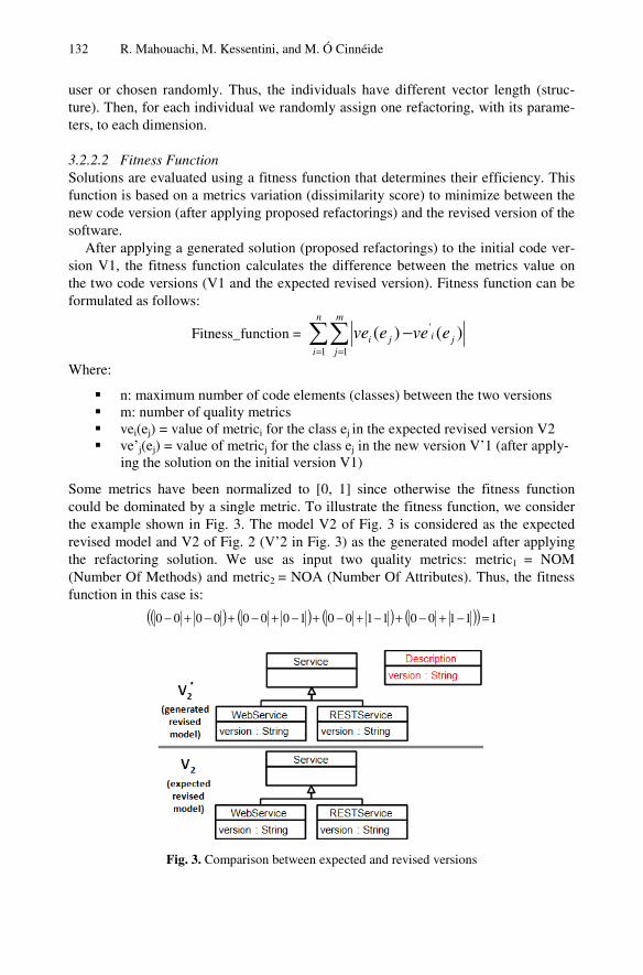
132 R. Mahouachi, M. Kessentini, and M. Ó Cinnéide
user or chosen randomly. Thus, the individuals have different vector length (struc-ture). Then, for each individual we randomly assign one refactoring, with its parame-ters, to each dimension.
3.2.2.2 Fitness Function Solutions are evaluated using a fitness function that determines their efficiency. This function is based on a metrics variation (dissimilarity score) to minimize between the new code version (after applying proposed refactorings) and the revised version of the software.
After applying a generated solution (proposed refactorings) to the initial code ver-sion V1, the fitness function calculates the difference between the metrics value on the two code versions (V1 and the expected revised version). Fitness function can be formulated as follows:
Fitness_function = )()( '
1 1ji
n
i
m
jji eveeve
= =
−
Where:
n: maximum number of code elements (classes) between the two versions m: number of quality metrics vei(ej) = value of metrici for the class ej in the expected revised version V2 ve’j(ej) = value of metricj for the class ej in the new version V’1 (after apply-
ing the solution on the initial version V1)
Some metrics have been normalized to [0, 1] since otherwise the fitness function could be dominated by a single metric. To illustrate the fitness function, we consider the example shown in Fig. 3. The model V2 of Fig. 3 is considered as the expected revised model and V2 of Fig. 2 (V’2 in Fig. 3) as the generated model after applying the refactoring solution. We use as input two quality metrics: metric1 = NOM (Number Of Methods) and metric2 = NOA (Number Of Attributes). Thus, the fitness function in this case is:
( ) ( ) ( ) ( )( ) 11100110010000000 =−+−+−+−+−+−+−+−
Fig. 3. Comparison between expected and revised versions

Search-Based Refactoring Detection Using Software Metrics Variation 133
3.2.2.3 Change Operators Selection. To select the individuals that will undergo the crossover and mutation op-erators, we use Stochastic Universal Sampling (SUS) [12], in which the probability of selection of an individual is directly proportional to its relative fitness in the popula-tion. SUS is a random selection algorithm that gives higher probability of selection to the fittest solutions, while still giving a chance to every solution.
Crossover. For each crossover, two individuals are selected by applying SUS selec-tion. Even though individuals are selected, the crossover happens only with a certain probability.
The crossover operator allows creating two offspring P1’ and P2’ from the two se-lected parents P1 and P2. It is defined as follows. A random position k is selected. The first k refactorings of P1 become the first k elements of P1’. Similarly, the first k refactorings of P2 become the first k refactorings of P2’.
Fig. 4 shows an example of the crossover process. In this example, P1 and P2 are combined to generate two new solutions. The right sub-vector of P1 is combined with the left sub-vector of P2 to form the first child, and the right sub-vector of P2 is com-bined with the left sub-vector of P1 to form the second child. In Fig. 4, the position k takes the value 1. The second refactoring of P1 becomes the second element of P2. Similarly, the second refactoring of P2 become the second refactorings of P1.
Mutation. The mutation operator consists of randomly changing one or more dimen-sions (refactoring) in the solution (vector). Given a selected individual, the mutation operator first randomly selects some dimensions in the vector representation of the individual. Then the selected dimensions are replaced by other refactorings. Further-more, the mutation can only modify the parameters of some dimensions without changing the type of the refactoring involved.
Fig. 4. The Crossover operator
Push feature(Description) Unfold Class(Description)
Push feature(version) Unfold Class(Description)
Mutation
P1
Q1
Fig. 5. The Mutation operators
134 R. Mahouachi, M. Kessentini, and M. Ó Cinnéide
Fig. 5 illustrates the effect of a mutation that replaced the dimension number one Push Feature (description) by Push Feature (version).
4 Evaluation
In order to evaluate the feasibility of our approach for detecting refactorings, we con-ducted an experiment based on different versions of real-world large open source systems [19][20][21][22]. We start by presenting our research questions. Then, we describe and discuss the obtained results.
4.1 Goals and Objectives
The study was conducted to quantitatively assess the completeness and correctness of our approach when applied to a real-world scenario and to compare its performance with existing approaches. More specifically, we aimed at answering the following research questions RQ1) To what extent can the proposed approach detect changes between different code versions (in terms of correctness and completeness)? RQ2) What types of changes (refactorings) does it detect correctly? RQ3) How does the performance of the GA compare with that of random search and local search (simu-lated annealing 13)?
To answer RQ1, we used an existing corpus [23][16] containing an extensive evo-lution of four large open source systems to evaluate the correctness and completeness of our approach. To answer RQ2, we investigated the type of changes that were found. For the remaining question RQ3, we compared our GA results to those pro-duced by random search and simulated annealing (SA). Further details about our experiments setting are discussed in the next subsection.
4.2 Experimental Setup
We used an existing corpus 2316 of 81 releases of four open source Java projects, namely Apache Ant [19], ArgoUML [20], JHotdraw [21], and Xerces-J [22]. Apache Ant is a build tool and library specifically conceived for Java applications. ArgoUML is an open source UML modeling tool. Xerces is a family of software packages for parsing and manipulating XML, and implements a number of standard APIs for XML parsing. JHotdraw is a framework used to build graphic editors. Table I reports cha-racteristics of the analyzed systems. The table also reports the number of refactoring operations (as well as the number of different kinds of refactorings) identified ma-nually for the different systems. In all, we identified more than 16000 refactoring applications. However, we selected some specific versions of these open source sys-tem to analyze the results manually (since it is a very tedious task). Thus, as described in table I, we are considering a total of around 9586 refactorings applied between different versions.
We choose Xerces-J, JHotDraw, ArgoUML, and Apache Ant because they are me-dium-sized open-source projects and were analyzed in related work. The initial

Search-Based Refactoring Detection Using Software Metrics Variation 135
versions of GMF and Apache Ant are known to be of poor quality, which has led to major revised versions. Xerces-J, ArgoUML, and JHotDraw have been actively de-veloped over the past 10 years, and their design has not been responsible for a slowdown of their developments.
For this experiment, Ref-Finder [5] was used in [23] to automatically detect refac-toring operations of 34 different types on 72 releases of the different open source systems. From the refactorings detected by Ref-Finder, 9586 refactorings have been manually validated as correct refactorings. In total, 34 different types of refactoring operations have been applied. The evolution of the different versions provides a rela-tively large set of revisions. In total, the evolution of the considered versions compris-es 81 revisions that involved at least one refactoring operation. Overall, 9586 refactor-ing operations have been applied, whereas one transition between two revisions con-tains on average 116 refactorings. Most of the commits comprise between 1 and 29 refactorings. Table 1 describes the number of expected refactorings to be detected by our approach on the different code versions. These operations cover 34 refactoring types (e.g. move method, move feature, etc.). Finally, we used a set of 18 quality metrics that are available on an existing Eclipse plug-in [25].
Table 1. The Systems Studied
System Number of expected refactoring Classes (min, max)
Apache Ant 1094 87, 1191 ArgoUML 1967 777, 1519 JHotdraw 1884 291, 603 Xerces-J 4641 181, 776
To assess the accuracy of our approach, we compute the standard Information Re-trieval measures of Precision and Recall. In the context of our study, Precision de-notes the fraction of correctly detected refactoring operations among the set of all detected operations. Recall indicates the fraction of correctly detected refactoring operations among the set of all expected refactorings (i.e., how many operations have not been missed). In general, Precision denotes the probability that a detected opera-tion is correct while Recall is the probability that an actually applied operation is de-tected. Thus, both values may range from 0 to 1, whereas a higher value is better than a lower one. The quality of our results was measured by two methods: Automatic Correctness (AC) and Manual Correctness (MC). Automatic correctness consists of comparing the detected changes to the reference/expected ones, operation-by-operation using Precision (AP) and Recall (AR). AC method has the advantage of being automatic and objective. However, since different refactoring combinations exist that describe the same evolution (different changes but same new code version), AC could reject a good solution because it yields different refactoring operations from reference/expected ones. To account for those situations, we also use MC, which in-volves manually evaluating the detected changes, here again operation-by-operation. In addition, we compared the performance of random search and simulated annealing, using AC scores for these comparisons.

136 R. Mahouachi, M. Kessentini, and M. Ó Cinnéide
4.3 Results and Discussions
Table 2 summarizes our results over 30 runs. Our approach detects 9387 refactoring operations. Overall, we were able to find 8912 refactoring operations correctly among all 9586 operations (i.e., Recall of 93%), whereas fewer than 600 operations have been incorrectly detected, which leads to a Precision of around 92%. It is worth not-ing that the evolution history of these four open source systems is very different. As the studied evolution of the remaining systems covers a time period of ten years, they have a large number of refactorings to be detected. However, our proposal performs well on the large evolutions of these systems. For Apache, most of the detected changes are correct with 96% and 94% respectively for Precision and Recall. For ArgoUML and JHotDraw, they have approximately the same number of refactorings to detect and our approach detected most of them with an average Precision of 98% and average Recall of 95%. Xerces-J is the larger system that we studied with more than 4646 refactoring applied over 10 years and our proposal succeeds in detecting almost all of them with a Precision and Recall of more than 91%. Thus, overall we can conclude that using our approach we could identify most of the applied operations correctly with an average of 92% of Precision and 94% of Recall. We noticed also that our technique does not have a bias towards the types of refactoring since most of them were detected (RQ2).
With regards to manual correctness (MC), the Precision and Recall scores for all the four open source systems were improved since we found interesting refactoring alternatives that deviate from the reference ones proposed by the developers/experts. In addition, we found that the sequence of applying the refactoring is sometimes dif-ferent between generated refactoring and reference ones. We found that sometimes a different sequence can reduce the number of refactorings required. Another observa-tion is that the Precision and Recall scores depend on the number of changes. When the number of changes increases then Precision and Recall decrease. However, we still have acceptable scores even when a large number of changes has occurred.
Table 2. Average Detection Results
Model AP: Precision AR: Recall MP:Precision MR: Recall
Apache Ant 1033/1073= 96%
1033/1094 = 94%
1037/1073 = 96%
1037/1094 = 95%
ArgoUML 1874/1904 = 98%
1874/1967 = 95%
1877/1904 = 98%
1877/1967 = 95%
JHot-Draw 1769/1874 = 94%
1769/1884 = 93%
1791/1874 = 95%
1791/1884 = 94%
Xerces-J 4236/4536 = 93%
4236/4641 = 91%
4247/4536 = 93%
4247/4641 = 91%
Fig. 4 illustrates the comparison between the results obtained using GA, random search and simulated annealing (SA). The detection results for SA were also accepta-ble. Especially, with the smaller system (ApacheAnt) the Precision is better using SA than GA. In fact, GA is a global search that gives good results when the search space

Search-Based Refactoring Detection Using Software Metrics Variation 137
is large. For this reason, GA performs well with large systems. However, compared to GA, SA takes a lot of time to converge to an optimal solution as it requires many more iterations. In our experiments, we used the same number of iterations as a ter-mination criterion (10000 iterations). In addition, to ensure the stability of the results during the comparison we calculated an average of Precision and Recall over 30 runs. Finally, the random search did not perform well on all the systems due to the huge search space to explore.
The correlation between the number of used metrics and the Recall and Precision values is analyzed in Figure 5 based on the data gathered in our study. More precisely, we calculate the Precision and Recall for different versions of the larger system Xerces-J. We conclude that the Precision and Recall depends on the number of me-trics employed. When the number of metrics decreases then the Precision and Recall decrease. For example, the Recall/Precision decreases from 90% to 62% when the number of metrics decreases from 18 to 8. However, number of metrics used on our experiments can be considered as reasonable.
Fig. 6. Comparison between GA, SA and Random Search (average Precision and Recall over 30 runs)
Fig. 7. The impact of the number of used metrics on the detection results (Xerces-J)

138 R. Mahouachi, M. Kessentini, and M. Ó Cinnéide
Finally, it is important to contrast the results with the execution time. The execu-tion time for finding the optimal refactoring solution with a fixed number of 10000 iterations (stopping criteria) was less than 30 minutes on the larger open source sys-tem (Xerces-J). This indicates that our approach is reasonably scalable from the per-formance standpoint.
Our proposal has some limitations that we will address in our future work. The ma-jor challenge in this work lies in the assumption made in section 3.2.1.2, that each class in the original source maps to one class in the revised version. Sometimes after radical refactoring it becomes very difficult to understand/detect the changes with a high precision score. One possibility is to explore the use of semantic measures in order to find a suitable matching between the names of classes. Another challenge that is not addressed, in this work, is conflict and dependency in the refactoring se-quence. This only appears experimentally when a large number of refactorings are applied to a small number of classes. We will address this problem in our future work by finding the best sequence that minimizes the number of conflicts.
5 Related Work
With respect to the contribution of this work, we survey existing work in the area of refactoring detection and we also state further applications of search-based techniques in the field of software engineering.
The easiest way to detect applied refactorings is to track their execution in the de-velopment environment directly. Refactoring tracking is realized by [1] in program-ming environments and by [2] in modeling environments. All these approaches highly depend on the development environment, which has to track the refactorings as they are applied. Furthermore, manual refactorings are not detectable and refactorings that have in fact been made obsolete by successive changes are likely to be wrongly de-tected. In contrast to refactoring tracking approaches, state-based refactoring detection mechanisms aim to reveal refactorings a posteriori on the base of the two successive versions of a software artifact. Several approaches are tailored to detect refactorings in program code. For instance, Dig et al. [2] propose an approach to detect applied refactorings in Java code. They first perform a fast syntactic analysis and, subsequent-ly, a semantic analysis in which operational aspects like method call graphs are also considered. Weissgerber and Diehl [3] take a similar approach where after a prepro-cessing and a syntactical analysis have been conducted, conditions indicating the application of a refactoring are evaluated. Recent work by Kim et al. [4][5] on the Ref-Finder tool involves an approach for refactoring detection that improves on sev-eral issues left open in previous approaches. In particular, the Ref-Finder tool is capa-ble of detecting complex refactorings that comprise a set of atomic refactorings by using logic-based rules executed by a logic programming engine.
Our approach is inspired by contributions in Search-Based Software Engineering (SBSE) [24]. As the name indicates, SBSE uses a search-based approach to solve optimization problems in software engineering. Once a software engineering task is framed as a search problem, by defining it in terms of solution representation, fitness function and solution change operators, there are many search algorithms that can be applied to solve that problem. To the best of our knowledge, the idea of detecting

Search-Based Refactoring Detection Using Software Metrics Variation 139
refactorings from structural information using search-based techniques was not stu-died before. However, several other works are proposed to find refactoring opportuni-ties using search-based techniques [15, 16, 18]. We proposed a search-based approach to detect changes between different model versions by comparing them [18]. Howev-er, the comparison between two model versions is a difficult task. In fact, this prob-lem has the same complexity as the graph isomorphism problem, which is NP-hard. In particular, we can find a generated model and an expected model that look different (i.e., contain different model elements) but have the same semantics. Moreover, in [18] detected refactorings are related only to the model level. In the work of O’Keeffe and Ó Cinnéide [15], software design improvement is treated as an optimization prob-lem. The authors use a combination of 12 metrics to measure the improvements achieved when sequences of simple refactorings are applied, such as moving methods between classes. The goal of the optimization is to refactor a program to a revised version that has improved quality based of a set of software metrics. Another applica-tion of this approach by Ó Cinnéide et al. [16] uses search-based refactoring to assess software metrics and explore relationships between them.
6 Conclusion
In this paper we introduce a novel, search-based approach to software refactoring detection between an initial software version and a refactored software version. Our approach is based on representing a proposed solution as a sequence of refactorings, and evaluating this solution in terms of its metrics profile as compared with the me-trics profile of the refactored software version. Framing the problem in this manner enables us to use a Genetic Algorithm to evolve better solutions whose metric profiles more closely match that of the refactored software version. Our key hypothesis is that as the metric profiles converge, so too will the evolved refactoring sequence converge to the actual refactoring sequence that was originally applied to generate the refac-tored version from the initial version.
We evaluated our approach on four real-world, open source software applications involving a total of 81 different versions and a total of 9,586 refactorings (as verified manually). Experiments show the Precision of our approach to be 92% and the Recall 93%, which provide strong evidence of the validity of our approach. As part of future work, we will investigate situations where no direct mapping exists between the ele-ments of the initial software version and the refactored version, study the effects vari-ous metrics have on the quality of refactoring sequences obtained and attempt to classify the detected model changes as risky or not in terms of quality improvement.
References
1. Robbes, R.: Mining a Change-Based Software Repository. In: Proceedings of MSR 2007, pp. 15–23. IEEE Computer Society (2007)
2. Dig, D., Comertoglu, C., Marinov, D., Johnson, R.: Automated Detection of Refactorings in Evolving Components. In: Thomas, D. (ed.) ECOOP 2006. LNCS, vol. 4067, pp. 404–428. Springer, Heidelberg (2006)
3. Weissgerber, P., Diehl, S.: Identifying Refactorings from Source-Code Changes. In: Pro-ceedings of ASE 2006, pp. 231–240. IEEE (2006)

140 R. Mahouachi, M. Kessentini, and M. Ó Cinnéide
4. Kim, M., Notkin, D., Grossman, D., Wilson Jr., G.: Identifying and Summarizing Syste-matic Code Changes via Rule Inference. TSE: IEEE Transactions on Software Engineer-ing, 45–62 (2013)
5. Prete, K., Rachatasumrit, N., Sudan, N., Kim, M.: Template-based reconstruction of com-plex refactorings. In: ICSM 2010, pp. 1–10 (2010)
6. Fowler, M., Beck, K., Brant, J., Opdyke, W., Roberts, D.: Refactoring – Improving the Design of Existing Code, 1st edn. Addison-Wesley (June 1999)
7. Liu, H., Yang, L., Niu, Z., Ma, Z., Shao, W.: Facilitating software refactoring with appro-priate resolution order of bad smells. In: Proc. of the ESEC/FSE 2009, pp. 265–268 (2009)
8. Harman, M., Tratt, L.: Pareto optimal search based refactoring at the design level. In: Pro-ceedings of the Genetic and Evolutionary Computation Conference (GECCO 2007), pp. 1106–1113 (2007)
9. Seng, O., Stammel, J., Burkhart, D.: Search-based determination of refactorings for im-proving the class structure of object-oriented systems. In: GECCO 2006, pp. 1909–1916 (2006)
10. Du Bois, B., Demeyer, S., Verelst, J.: Refactoring—Improving Coupling and Cohesion of Existing Code. In: Proc. 11th Working Conf. Reverse Eng., pp. 144–151 (2004)
11. Mens, T., Tourwé, T.: A Survey of Software Refactoring. IEEE Trans. Software Eng. 30(2), 126–139 (2004)
12. Koza, J.R.: Genetic Programming: On the Programming of Computers by Means of Natu-ral Selection. MIT Press, Cambridge (1992)
13. Kirkpatrick, S., Gelatt Jr., C.D., Vecchi, M.P.: Optimization by simulated annealing. Sciences 220(4598), 671–680 (1983)
14. Langer, P.: Adaptable Model Versioning based on Model Transformation By Demonstra-tion, PhD Thesis, Vienna University of Technology (2011)
15. O’Keeffe, M., Cinnéide, M.Ó.: Search-based Refactoring for Software Maintenance. Jour-nal of Systems and Software 81(4), 502–516
16. Ó Cinnéide, M., Tratt, L., Harman, M., Counsell, S., Hemati Moghadam, I.: Experimental as-sessment of software metrics using automated refactoring. In: Proceedings of the Internation-al Symposium on Empirical Software Engineering and Measurement (Septembrer 2012)
17. Hemati Moghadam, I., Cinnéide, M.Ó.: Automated refactoring using design differencing. In: Proc. of European Conference on Software Maintenance and Reengineering, Szeged (March 2012)
18. Fadhel, A.B., Kessentini, M., Langer, P., Wimmer, M.: Search-based detection of high-level model changes. In: ICSM 2012, pp. 212–221 (2012)
19. http://www.eclipse.org/gmf http://www.eclipse.org/gmf; 20. http://argouml.tigris.org 21. http://www.jhotdraw.org 22. http://xerces.apache.org 23. Bavota, G., De Carluccio, B., De Lucia, A., Di Penta, M., Oliveto, R., Strollo, O.: When
does a Refactoring Induce Bugs? An Empirical Study. In: Proceedings of the WCRE 2012, IEEE Press (2012)
24. Harman, M., Afshin Mansouri, S., Zhang, Y.: Search-based software engineering: Trends, techniques and applications. ACM Comput. Surv. 45(1), 11 (2012)
25. http://metrics.sourceforge.net 26. Murphy-Hill, E., Parnin, C., Black, A.P.: How We Refactor, and How We Know It. IEEE
Transactions on Software Engineering (2011) 27. Briand, L.C., Wüst, J., Daly, J.W., Victor Porter, D.: A Comprehensive Empirical Valida-
tion of Design Measures for Object-Oriented Systems. In: IEEE METRICS 1998, pp. 246–257 (1998)

Automated Model-in-the-Loop Testing of ContinuousControllers Using Search
Reza Matinnejad1, Shiva Nejati1, Lionel Briand1, Thomas Bruckmann2,and Claude Poull2
1 SnT Center,University of Luxembourg, Luxembourg
{reza.matinnejad,shiva.nejati,lionel.briand}@uni.lu2 Delphi Automotive Systems Luxembourg
{thomas.bruckmann,claude.poull}@delphi.com
Abstract. The number and the complexity of software components embedded intoday’s vehicles is rapidly increasing. A large group of these components mon-itor and control the operating conditions of physical devices (e.g., componentscontrolling engines, brakes, and airbags). These controllers are known as contin-uous controllers. In this paper, we study testing of continuous controllers at theModel-in-Loop (MiL) level where both the controller and the environment arerepresented by models and connected in a closed feedback loop system. We iden-tify a set of common requirements characterizing the desired behavior of contin-uous controllers, and develop a search-based technique to automatically generatetest cases for these requirements. We evaluated our approach by applying it to areal automotive air compressor module. Our experience shows that our approachautomatically generates several test cases for which the MiL level simulationsindicate potential violations of the system requirements. Further, not only do ourapproach generates better test cases faster than random test case generation, butwe also achieve better results than test scenarios devised by domain experts.
1 Introduction
Modern vehicles are increasingly equipped with Electronic Control Units (ECUs). Theamount and the complexity of software embedded in the ECUs of today’s vehicles israpidly increasing. To ensure the high quality of software and software-based functionson ECUs, the automotive and ECU manufacturers have to rely on effective techniquesfor verification and validation of their software systems. A large group of automotivesoftware functions require to monitor and control the operating conditions of physicalcomponents. Examples are functions controlling engines, brakes, seatbelts, and airbags.These controllers are widely studied in the control theory domain as continuous con-trollers [1,2] where the focus has been to optimize their design for a specific platform ora specific hardware configuration [3,4]. Yet a complementary and important problem,of how to systematically and automatically test controllers to ensure their correctnessand safety, has received almost no attention in the control engineering research [1].
In this paper, we concentrate on the problem of automatic and systematic test casegeneration for continuous controllers. The principal challenges when analyzing such
G. Ruhe and Y. Zhang (Eds.): SSBSE 2013, LNCS 8084, pp. 141–157, 2013.c© Springer-Verlag Berlin Heidelberg 2013

142 R. Matinnejad et al.
controllers stem from their continuous interactions with the physical environment, usu-ally through feedback loops where the environment impacts computations and viceversa. We study the testing of controllers at an early stage where both the controllerand the environment are represented by models and connected in a closed feedbackloop process. In model-based approaches to embedded software design, this level isreferred to as Model-in-the-Loop (MiL) testing.
Testing continuous aspects of control systems is challenging and is not yet sup-ported by existing tools and techniques [4,1,3]. There is a large body of research ontesting mixed discrete-continuous behaviors of embedded software systems where thesystem under test is represented using state machines, hybrid automata, hybrid petrinets, etc [5,6,7]. These techniques, however, are not amenable to testing purely continu-ous controllers described in terms of mathematical models, and in particular, differentialequations. A number of commercial verification and testing tools have been developed,aiming to generate test cases for MATLAB/Simulink models, namely the Simulink De-sign Verifier software [8], and Reactis Tester [9]. Currently, these tools handle onlycombinatorial and logical blocks of the MATLAB/Simulink models, and fail to gener-ate test cases that specifically evaluate continuous blocks (e.g., integrators) [1].
Contributions. In this paper, we propose a search-based approach to automate gen-eration of MiL level test cases for continuous controllers. We identify a set of com-mon requirements characterizing the desired behavior of such controllers. We developa search-based technique to generate stress test cases attempting to violate these re-quirements by combining explorative and exploitative search algorithms [10]. Specifi-cally, we first apply a purely explorative random search to evaluate a number of inputsignals distributed across the search space. Combining the domain experts’ knowledgeand random search results, we select a number of regions that are more likely to lead torequirement violations in practice. We then start from the worst case input signals foundduring exploration, and apply an exploitative single-state search [10] to the selected re-gions to identify test cases for the controller requirements. Our search algorithms relyon objective functions created by formalizing the controller requirements. We evaluatedour approach by applying it to an automotive air compressor module. Our experimentsshow that our approach automatically generates several test cases for which the MiLlevel simulations indicate potential errors in the controller or the environment models.Furthermore, the resulting test cases had not been previously found by manual testingbased on domain expertise. Our industry partner is interested to investigate these testcases further by evaluating them in a more realistic setting (e.g., by testing them on theirHardware-in-the-Loop (HiL) platform). In addition, our approach computes test casesbetter and faster than a random test case generation strategy.
2 MiL Testing of Continuous Controllers: Practice and Challenges
Control system development involves building of control software (controllers) to in-teract with mechatronic systems usually referred to as plants or environment [2]. Anexample of such controllers is shown in Figure 1. These controllers are commonly usedin many domains such as manufacturing, robotics, and automotive. Model-based devel-opment of control systems is typically carried out in three major levels described be-low. The models created through these levels become increasingly more similar to real

Automated Model-in-the-Loop Testing of Continuous Controllers Using Search 143
controllers, while verification and testing of these models become successively morecomplex and expensive.
Model-in-the-Loop (MiL): At this level, a model for the controller and a model forthe plant are created in the same notation and connected in the same diagram. In manysectors and in particular in the automotive domain, these models are created in MAT-LAB/Simulink. The MiL simulation and testing is performed entirely in a virtual envi-ronment and without any need to any physical component. The focus of MiL testing isto verify the control algorithm, and to ensure that the interactions between the controllerand the plant do not violate the system requirements.
Software-in-the-Loop (SiL): At this level, the controller model is converted to code(either autocoded or manually). This often includes the conversion of floating pointdata types into fixed-point values as well as addition of hardware-specific libraries.The testing at the SiL-level is still performed in a virtual and simulated environmentlike MiL, but the focus is on controller code which can run on the target platform.Further, in contrast to verifying the algorithms, SiL testing aims to ensure correctness offloating point to fixed-point conversion and the conformance of code to control models(particularly in the case of manual coding).
Hardware-in-the-Loop (HiL): At this level, the controller software is fully installedinto the final control system (e.g., in our case, the controller software is installed on theECUs). The plant is either a real piece of hardware, or is some software that runs on areal-time computer with physical signal simulation to lead the controller into believingthat it is being used on a real plant. The main objective of HiL is to verify the integrationof hardware and software in a more realistic environment. HiL testing is the closest toreality, but is also the most expensive and slowest among the three testing levels.
In this paper, among the above three levels, we focus on the MiL level testing. MiLtesting is the primary level intended for verification of the control algorithms logicand ensuring the satisfaction of their requirements. Development and testing at thislevel is considerably fast as the engineers can quickly modify the control model andimmediately test the system. Furthermore, MiL testing is entirely performed in a virtualenvironment, enabling execution of a large number of test cases in a small amount oftime. Finally, the MiL level test cases can later be used at SiL and HiL levels eitherdirectly or after some adaptations.
Currently, in most companies, MiL level testing of controllers is limited to runningthe controller-plant Simulink model (e.g., Figure 1) for a small number of simulations,and manually inspecting the results of individual simulations. The simulations are oftenselected based on the engineers’ domain knowledge and experience, but in a ratherad hoc way. Such simulations are useful for checking the overall sanity of the controlalgorithms, but cannot be taken as a substitute for MiL testing. Manual simulations failto find erroneous scenarios that the engineers might not be aware of a priori. Identifyingsuch scenarios later during SiL/HiL is much more difficult and expensive than duringMiL testing. Also, manual simulation is by definition limited in scale and scope.
Our goal is to develop an automated MiL testing technique to verify controller-plantsystems. To do so, we formalize the properties of continuous controllers regarding thefunctional, performance, and safety aspects. We develop an automated test case gener-ation approach to evaluate controllers with respect to these properties. In our work, the

144 R. Matinnejad et al.
test inputs are signals, and the test outputs are measured over the simulation diagramsgenerated by MATLAB/Simulink plant models. The simulations are discretized wherethe controller output is sampled at a rate of a few milliseconds. To generate test cases,we combine two search algorithms: (1) An explorative random search that allows us toachieve high diversity of test inputs in the space, and to identify the most critical regionsthat need to be explored further. (2) An exploitative search that enables us to focus oursearch and compute worst case scenarios in the identified critical regions.
3 Background on Continuous Controllers
Figure 1 shows an overview of a controller-plant model at the MiL level. Both thecontroller and the plant are captured as models and linked via virtual connections. Werefer to the input of the controller-plant system as desired or reference value. For ex-ample, the desired value may represent the location we want a robot to move to, thespeed we require an engine to reach, or the position we need a valve to arrive at.Thesystem output or the actual value represents the actual state/position/speed of the hard-ware components in the plant. The actual value is expected to reach the desired valueover a certain time limit, making the Error, i.e., the difference between the actual anddesired values, eventually zero. The task of the controller is to eliminate the error bymanipulating the plant to obtain the desired effect on the system output.
Plant Model
Controller(SUT)
Desired value Error
Actual value
System output+-
Fig. 1. MiL level Controller-Plant Model
The overall objective of the controller in Figure 1 may sound simple. In reality, how-ever, the design of such controllers requires calculating proper corrective actions for thecontroller to stabilize the system within a certain time limit, and further, to guaranteethat the hardware components will eventually reach the desired state without oscillatingtoo much around it and without any damage. Controllers design is typically capturedvia complex differential equations known as proportional-integral-derivative (PID) [2].For example, Figure 2(a) represents an example output diagram for a typical controller.As shown in the figure, the actual value starts at an initial value (here zero), and gradu-ally moves to reach and stabilize at a value close to the desired value. To ensure that acontroller design is satisfactory, engineers perform simulations, and analyze the outputsimulation diagram with respect to a number of requirements. After careful investiga-tions, we identified the following requirements for controllers:
Liveness (functional): The controller shall guarantee that the actual value will reachand stabilize at the desired value within x seconds. This is to ensure that the controllerindeed satisfies its main functional requirement.
Smoothness (safety): The actual value shall not change abruptly when it is close tothe desired one. That is, the difference between the actual and desired values shall not

Automated Model-in-the-Loop Testing of Continuous Controllers Using Search 145
exceed w, once the difference has already reached v for the first time. This is to ensurethat the controller does not damage any physical devices by sharply changing the actualvalue when the error is small.
Responsiveness (performance): The difference between the actual and desired valuesshall be at most y within z seconds, ensuring the controller responds within a time limit.
The above three generic requirements are illustrated on a typical controller outputdiagram in Figure 2 where the parameters x, v, w, y, and z are represented. As shownin the figure, given specific controller requirements with concrete parameters and givenan output diagram of a controller under test, we can determine whether that particularcontroller output satisfies the given requirements.
<=
~= 0 >=
time time time
Des
ired
Val
ue &
Act
ual V
alue
Desired Value
Actual Value
(a) (b) (c)Liveness Smoothness Responsiveness
xy
zv
w
Fig. 2. The controller requirements illustrated on the controller output: (a) Liveness, (b) Smooth-ness, and (c) Responsiveness
Having discussed the controller requirements and outputs, we now describe howwe generate input test values for a given controller. Typically, controllers have a largenumber of configuration parameters that affect their behaviors. For the configurationparameters, we use a value assignment commonly used for HiL testing, and focus ontwo essential controller inputs in our MiL testing approach: (1) the initial actual value,and (2) the desired value. Among these two inputs, the desired value can be easilymanipulated externally. However, since the controller is a closed loop system, it is notgenerally possible to start the system from an arbitrary initial state. In other words, theinitial actual state depends on the plant model and cannot be manipulated externally. Forthe same reason, in output simulation diagrams (e.g., Figure 2), it is often assumed thatthe controller starts from an initial value of zero. However, assuming that the systemalways starts from zero is like testing a cruise controller only for positive car speedincreases, and missing a whole range of speed decreasing scenarios.
To eliminate this restriction, we provide two consecutive signals for the desired valueof the controller (see Figure 3(a)): The first one sets the controller at the initial desiredvalue, and the second signal moves the controller to the final desired value. We referto these input signals as step functions or step signals. The lengths of the two signalsin a step signal are equal (see Figure 3(a)), and should be sufficiently long to givethe controller enough time to stabilize at each of the initial and final desired values.Figure 3(b) shows an example of a controller output diagram for the input step functionin Figure 3(a). The three controller properties can be evaluated on the actual outputdiagram in Figure 3(b) in a similar way as that shown in Figure 2.

146 R. Matinnejad et al.
InitialDesired Value
FinalDesired Value
time time
Desired Value
Actual Value
(a) (b)
T/2 T T/2 T
Fig. 3. Controller input step functions: (a) Step function. (b) Output of the controller (actual)given the input step function (desired).
In the next section, we describe our automated search-based approach to MiL testingof controller-plant systems. Our approach automatically generates input step signalssuch as the one in Figure 3(a), produces controller output diagrams for each input signal,and evaluates the three controller properties on the output diagram. Our search is guidedby a number of heuristics to identify the input signals that are more likely to violatethe controller requirements. Our approach relies on the fact that, during MiL, a largenumber of simulations can be generated quickly and without breaking any physicaldevices. Using this characteristic, we propose to replace the existing manual MiL testingwith our search-based automated approach that enables the evaluation of a large numberof output simulation diagrams and the identification of critical controller input values.
4 Search-Based Automated Controller MiL Testing
In this section, we describe our search-based algorithm for automating MiL testingof controllers. We first describe the search elements and discuss how we formulatecontroller testing as a search problem in Section 4.1. We, then, show how we combinesearch algorithms to guide and automate MiL testing of controllers in Section 4.2.
4.1 Search Elements
Given a controller-plant model and a set of controller properties, our search algorithms,irrespective of their heuristics, perform the following common tasks: (1) They generateinput signals to the controller, i.e., step function in Figure 3(a). (2) They receive theoutput, i.e., Actual in Figure 3(b), from the model, and evaluate the output against thecontroller properties formalizing requirements. Below, we first formalize the controllerinput and output, and define the search space for our problem. We then formalize thethree objective functions to evaluate the properties over the controller output.
Controller input and output: Let T = {0, . . . , T } be a set of time points during whichwe observe the controller behavior, and let min and max be the minimum and maximum

Automated Model-in-the-Loop Testing of Continuous Controllers Using Search 147
values for the Actual and Desired attributes in Figure 1. In our work, since input is as-sumed to be a step function, the observation time T is chosen to be long enough so thatthe controller can reach and stabilize at two different Desired positions successively(e.g., see Figure 3(b)). Note that Actual and Desired are of the same type and boundedwithin the same range, denoted by [min . . . max]. As discussed in Section 3, the testinputs are step functions representing the Desired values (e.g. Figure 3(a)). We definean input step function in our approach to be a function Desired : T → {min, . . . , max}such that there exist a pair Initial Desired and Final Desired of values in[min . . .max] that satisfy the following conditions:
∀t · 0 ≤ t < T2 ⇒ Desired(t) = Initial Desired
∧∀t · T
2 ≤ t < T ⇒ Desired(t) = Final Desired
We define the controller output, i.e., Actual, to be a functionActual : T → {min, . . . , max} that is produced by the given controller-plant model,e.g., in MATLAB/Simulink environment.
Search Space: The search space in our problem is the set of all possible input func-tions, i.e., the Desired function. Each Desired function is characterized by the pairInitial Desired and Final Desired values. In control system development, it iscommon to use floating-point data types at MiL level. Therefore, the search spacein our work is the set of all pairs of floating point values for Initial Desired andFinal Desired within the [min . . . max] range.
Objective Functions: Our goal is to guide the search to identify input functions in thesearch space that are more likely to break the properties discussed in Section 3. To doso, we create three objective functions corresponding to the three controller properties.
– Liveness: Let x be the liveness property parameter in Section 3. We define theliveness objective function OL as: maxx+T
2 <t≤T {|Desired(t)− Actual(t)|}I.e., OL is the max of the difference between Desired and Actual after time x+ T
2 .– Smoothness: Let v be the smoothness property parameter in Section 3. Let tc ∈ T
be such that tc > T2 and
|Desired(tc)− Actual(tc)| ≤ v∧
∀t · T2 ≤ t < tc ⇒ |Desired(t)− Actual(t)| > v
That is, tc is the first point in time after T2 where the difference between Actual
and Final Desired values has reached v. We then define the smoothness objectivefunction OS as: max tc<t≤T {|Desired(t)− Actual(t)|}That is, OS is the maximum difference between Desired and Actual after tc.
– Responsiveness: Let y be the responsiveness parameter in Section 3. We definethe responsiveness objective function OR to be equal to tr such that tr ∈ T andtr > T
2 and|Desired(tr)− Actual(tr)| ≤ y
∧∀t · T
2 ≤ t < tr ⇒ |Desired(t)− Actual(t)| > y
That is, OR is the first point in time after T2 where the difference between Actual
and Final Desired values has reached y.
We did not use w from the smoothness and z from the responsiveness properties in def-initions of OS and OR. These parameters determine pass/fail conditions for test cases,and are not required to guide the search. Further, w and z depend on the specific hard-ware characteristics and vary from customer to customer. Hence, they are not known

148 R. Matinnejad et al.
at the MiL level. Specifically, we define OS to measure the maximum overshoot ratherthan to determine whether an overshoot exceeds w, or not. Similarly, we define OR tomeasure the actual response time without comparing it with z.
The three above objective functions are heuristics and provide numerical approxi-mations of the controller properties, allowing us to compare different test inputs. Thehigher the objective function value, the more likely it is that the test input violates therequirement corresponding to that objective function. We use these objective functionsin our search algorithms discussed in the next section.
4.2 Search Algorithms
Figure 4 shows an overview of our automated MiL testing approach. In the first step,we receive a controller-plant model (e.g., in MATLAB/Simulink) and a set of objectivefunctions obtained from requirements. We divide the input search space into a set ofregions, and assign to each region a value indicating the evaluation of a given inputobjective function on that region based on random search (Exploration). We refer to theresult as a HeatMap diagram [11]. Based on domain expert knowledge, we select someof the regions that are more likely to include critical and realistic errors. In the secondstep, we focus our search on the selected regions and employ a single-state heuristicsearch to identify within those regions the worst-case scenarios to test the controller.
+Controller-
plant model
Objective Functions
HeatMap Diagram
Worst-Case Scenarios
List of Critical Regions
2. Singl-State Search
DomainExpert
1. Exploration
Fig. 4. An overview of our automated approach to MiL testing of continuous controllers
In the first step of our approach in Figure 4, we apply a random (unguided) search tothe entire search space. The search explores diverse test inputs to provide an unbiasedestimate of the average objective function values at different regions of the search space.In the second step, we apply a heuristic single-state search to a selection of regions inorder to find worst-case scenarios that may violate the controller properties.
Figure 5(a) shows the random search algorithm used in the first step. The algorithmtakes as input a controller-plant model M and an objective function O, and produces aHeatMap diagram (e.g., see Figure 5(b)). Briefly, the algorithm divides the search spaceS of M into a number of equal regions. It then generates a random point p in S in line4. The dimensions of p characterize an input step function Desired which is given toM as input in line 6. The model M is executed in Matlab/Simulink to generate theActual output. The objective function O is then computed based on the Desired andActual functions. The tuple (p, o) where o is the value of the objective function at p isadded to P . The algorithm stops when the number of generated points in each regionis at least N . Finding an appropriate value for N is a trade off between accuracy andefficiency. Since executingM is relatively expensive, it is not efficient to generate manypoints (large N ). Likewise, a small number of points in each region is unlikely to give

Automated Model-in-the-Loop Testing of Continuous Controllers Using Search 149
(a)Algorithm. RANDOMEXPLORATION
Input: A controller-plant model M with input search space S.An objective function O. An observation time T .
Output: An overview diagram (HeatMap).
1. Partition S into equal sub-regions2. Let P = {}3. repeat4. Let p = (Initial Desired, Final Desired) be
a random point in S5. Let Desired be a step function generated based on p and T6. Run M with the Desired input to obtain the Actual output7. o = O(Desired, Actual)8. P = {(p, o)} ∪ P9. until there are at least N points in each region of S do10. Create a HeatMap diagram based on P
(b)
Initial Desired Value
Fin
al D
esire
d V
alue
0.0
0.1
0.2
0.3
0.4
0.5
0.6
0.7
0.8
0.9
1.0
0.0 0.1 0.2 0.3 0.4 0.5 0.6 0.7 0.8 0.9 1.0
Fig. 5. The first step of our approach in Figure 4: (a) The exploration algorithm. (b) An exampleHeatMap diagram produced by the algorithm in (a).
us an accurate estimate of the average objective function for that region. In Section 5,we discuss how we select a value for N for our controller case study.
The output of the algorithm in Figure 5(a) is a set P of (p, o) tuples where p is apoint and o is the objective function value for p. We visualize the set P via HeatMapdiagrams [11] where the axes are the initial and final desired values. In HeatMaps, eachregion is assigned the average value of the values of the points within that region. Theintervals of the region values are then mapped into different shades, generating a shadeddiagrams such as the one in Figure 5(b). In our work, we generate three HeatMap dia-grams corresponding to the three objective functions OL, OS and OR (see Section 4.1).We run the algorithm once, but we compute OL, OS and OR separately for each point.
The HeatMap diagrams generated in the first step are reviewed by domain ex-perts.They select a set of regions that are more likely to include realistic and criticalinputs. For example, the diagram in Figure 5(b) is generated based on an air compres-sor controller model evaluated for the smoothness objective function OS . This con-troller compresses the air by moving a flap between its open position (indicated by 0)and its closed position (indicated by 1.0). There are about 10 to 12 dark regions, i.e.,the regions with the highest OS values in Figure 5(b). These regions have initial flappositions between 0.4 to 1.0 and final flap positions between 0.5 and 1.0. Among theseregions, the domain expert chooses to focus on the regions with the initial value be-tween 0.8 and 1.0. This is because, in practice, there is more probability of damagewhen a closed (or a nearly closed) flap is being moved.
Figure 6(a) presents our single-state search algorithm for the second step of the pro-cedure in Figure 4. The single-state search starts with the point with the worst (highest)objective function value among those computed by the random search in Figure 5(a).It then iteratively generates new points by tweaking the current point (line 8) and eval-uates the given objective function on the points. Finally, it reports the point with theworst (highest) objective function value. In contrast to random search, the single-statesearch is guided by an objective function and performs a tweak operation. The designof the tweak is very important and affects the effectiveness of the search. In our work,

150 R. Matinnejad et al.
(a)Algorithm. SINGLESTATE-SEARCH
Input: A controller-plant model M . A region r.The set P computed by the algorithm in Figure 5(a).An objective function O.
Output: The worst case scenario testCase .
1. P ′ = {(p, o) ∈ P | p ∈ r}2. Let (p, o) ∈ P ′ s.t. for all (p′, o′) ∈ P ′, we have o ≥ o′
3. worstFound = o4. for K iterations :5. Let Desired be a step function generated by p6. Run M with the Desired input to obtain
the Actual output7. v = O(Desired, Actual)8. if v > worstFound :9. worstFound = v
testCase = p10. p = Tweak(p)11. return testCase
(b)
time
Desired Value
Actual Value
0 1 2
0.0
0.1
0.2
0.3
0.4
0.5
0.6
0.7
0.8
0.9
1.0
Initial Desired
Final Desired
undershoot
Fig. 6. The second step of our approach in Figure 4: (a) The single-state search algorithm. (b) Anexample output diagram produced by the algorithm in (a)
we use the (1+1) EA tweak operator [10]. Specifically, at each iteration, we shift p inthe space by adding values x′ and y′ to the dimensions of p. The x′ and y′ values areselected from a normal distribution with mean μ = 0 and variance σ2. The value of σenables us to control the degree of exploration vs. exploitation in the search. With a lowσ, (1+1) EA becomes highly exploitative allowing to reach an optimum fast. But for anoisy landscape, we need a more explorative (1+1) EA with a high σ [10]. We discussin Section 5 how we select σ. Since the search is driven by the objective function, wehave to run the search three times separately for OL, OS and OR.
Figure 6(b) shows the worst case scenario computed by our algorithm for the smooth-ness objective function applied to an air compressor controller. As shown in the figure,the controller has an undershoot around 0.2 when it moves from an initial desired valueof 0.8 and is about to stabilize at a final desired value of 0.3.
5 Evaluation
To empirically evaluate our approach, we performed several experiments reported inthis section. The experiments are designed to answer the following research questions:
RQ1: In practice, do the HeatMap diagrams help determine a list of critical regions?RQ2: Does our single-state search algorithm effectively and efficiently identify worst-case scenarios within a region?RQ3: Can we use the information in the HeatMap diagrams to explain the performanceof the single-state search in the second step?
Setup. To perform the experiment, we applied our approach in Figure 4 to a case studyfrom our industry partner. Our case study is a Supercharger Bypass Flap PositionControl (SBPC) module. SBPC is an air compressor blowing into a turbo-compressor to

Automated Model-in-the-Loop Testing of Continuous Controllers Using Search 151
increase the air pressure, and consequently the engine torque at low engine speeds. TheSBPC module includes a controller component that determines the position of a me-chanical flap. In SBPC, the desired and actual values in Figure 1 represent the desiredand actual positions of the flap, respectively. The flap position is a float value boundedwithin [0...1] (open when 0 and closed when 1.0). The SBPC module is implementedand simulated in Matlab/Simulink. Its Simulink model has 21 input and 42 output vari-ables, among which the flap position is the main controller output. It is a complex andhierarchical function with 34 sub-components decomposed into 6 abstraction levels. Onaverage, each sub-component has 21 Simulink blocks and 4 MATLAB function blocks.We set the simulation time (the observation time) to 2 sec, i.e., T = 2s. The controllerproperty parameters were given as follows: x = 0.9s, y = 0.03, and v = 0.05.
We ran the experiment on Amazon micro instance machines which is equal to twoAmazon EC2 compute units. Each EC2 compute unit has a CPU capacity of a 1.0-1.2GHz 2007 Xeon processor. A single 2-sec simulation of the SBPC Simulink model(e.g., Figure 6(b)) takes about 31 sec on the Amazon machine.
RQ1. A HeatMap diagram is effective if it has the following properties: (1) The regionshades are stable and do not change on different runs of the exploration algorithm.(2) The regions are not so fine grained that it leads to generating too many points duringexploration. (3) The regions are not too coarse grained such that the points generatedwithin one region have drastically different objective function values.
(a) Liveness (b) Smoothness (c) Responsiveness
Fig. 7. HeatMap diagrams generated for our case study for the Liveness (a), Smoothness (b) andResponsiveness (c) requirements
For the SBPC module, the search space S is the set of all points with float dimensionsin the [0..1]× [0..1] square. We decided to generate around 1000 points in S during theexploration step. We divided up S into 100 equal squares with 0.1 × 0.1 dimensions,and let N = 10, i.e., at least 10 points are simulated in each region during exploration.The exploration algorithm takes on average about 8.5 hours on an Amazon machineand can therefore be run overnight.
We executed our exploration algorithm three times for SBPC and for each of ourthree objective functions. For each function, the region shades remained completelyunchanged across the three different runs. In all the resulting HeatMap diagrams, thepoints in the same region have close objective function values. On average, the varianceover the objective function values for an individual region was about 0.001. Hence, weconcluded that N = 10 is suitable for our case study.

152 R. Matinnejad et al.
The resulting HeatMap diagrams, shown in Figure 7, were presented to our industrypartner. They found the diagrams visually appealing and useful. They noted that thediagrams, in addition to enabling the identification of critical regions, can be used inthe following ways: (1) They can gain confidence about the controller behaviors overthe light shaded regions of the diagrams. (2) The diagrams enable them to investigatepotential anomalies in the controller behavior. Specifically, since controllers have con-tinuous behaviors, we expect a smooth shade change over the search space going fromclear to dark. A sharp contrast such as a dark region neighboring a light-shaded regionmay potentially indicate an abnormal behavior that needs to be further investigated.
RQ2. For the second step of our approach in Figure 4, we opt for a single-state searchmethod in contrast to a population search such as Genetic Algorithms (GA) [10]. In ourwork, a single computation of the fitness function takes a long time (31s), and hence,fitness computation for a set of points (a population) would be very inefficient. Weimplemented the Tweak statement in the algorithm in Figure 6(a) using the (1+1) EAheuristic [10] by letting σ = 0.01. Given σ = 0.01 and a point located at the centerof a 0.1 × 0.1 region, the result of the tweak stays inside the region with a probabilityaround 99%. Obviously, this probability decreases when the point moves closer to thecorners. In our search, we discard the points that are generated outside of the regions,and never generate simulations for them. In addition, for σ = 0.01, the (1+1) EA searchtends to converge to a point not far from the search starting point. This is because withthe probability of 70%, the result of the tweak for this search does not change neitherdimension of a point further than 0.01.
0.315
0.316
0.317
0.319
0.321
0.323
0.324
0.326
0.327
0.329
0.330
0 10 20 30 40 50 60 70 80 90 100
(a). Average
0.328
0.325
0.320
0.318
0 10 20 30 40 50 60 70 80 90 100
(c). Random Search Distribution
0 10 20 30 40 50 60 70 80 90 100
(b). (1+1) EA Distribution
(d). Average (e). (1+1) EA Distribution
Random Search(1+1) EA
0 10 20 30 40 50 60 70 80 90 100
0.0166
0.0168
0.0170
0.0176
0.0180
0.0178
0.0172
0.0160
0.0162
0.0164 Random Search(1+1) EA
(f). Random Search Distribution
0 10 20 30 40 50 60 70 80 90 100 0 10 20 30 40 50 60 70 80 90 100
0.0174
Fig. 8. Comparing (1+1) EA and random search average and distribution values for two represen-tative HeatMap regions: (a)-(c) Diagrams related to the region specified by dashed white circle inFigure 7(b). (d)-(f) Diagrams related to the region specified by dashed white circle in Figure 7(a).

Automated Model-in-the-Loop Testing of Continuous Controllers Using Search 153
We applied (1+1) EA to 11 different regions of the HeatMap diagrams in Figure 7that were selected by our domain experts among the regions with the highest objec-tive function average values. Among these, three were chosen for Liveness, four forSmoothness and four for Responsiveness. As shown in Figure 6(a), for each region, westart the search from the worst point found in that region during the exploration step.This enables us to reuse the existing search result from the first step. Each time werun (1+1) EA for 100 iterations, i.e., K = 100. This is because the search has alwaysreached a plateau after 100 iterations in our experiments. On average, both (1+1) EAand random search took about around one hour to run for 100 iterations.
We identified 11 worst case scenarios. Figure 6(b) shows the simulation for oneof these scenarios concerning smoothness. The simulations for all 11 regions indicatepotential violations of the controller requirements that might be due to errors in thecontroller or plant models. To precisely identify the sources of violations and to takethe right course of action, our industry partner plans to apply the resulting scenarios atthe HiL testing level. In our work, we could identify better results than test scenariosdevised by domain experts. For example, Figure 6(b) shows an undershoot scenarioaround 0.2 for the SBPC controller. The maximum identified undershoot/overshoot forthis controller by manual testing was around 0.05. Similarly, for the responsivenessproperty, we found a scenario in which it takes 200ms for the actual value to get closeenough to the desired value while the maximum corresponding value in manual testingwas around 50ms.
Note that in all the 11 regions, the results of the single-state search (step 2 in Figure4) showed improvements over the scenarios identified by pure exploration (step 1 inFigure 4). On average, the results of the single-state search showed a 12% increasefor liveness, a 35% increase for smoothness, and a 18% increase for responsivenesscompared to the result of the exploration algorithm.
Random search within each selected region was used as a baseline to evaluate theefficiency and effectiveness of (1+1) EA in finding worst-case scenarios. In order toaccount for randomness in these algorithms, each of them was run for 50 rounds. Weused 22 concurrent Amazon machines to run random search and (1+1) EA for 11 re-gions. The comparison results for two representative HeatMap regions are shown inFigure 8. Figures 8(a)-(c) are related to the HeatMap region specified in Figure 7(b),and Figures 8(d)-(f) are related to that in Figure 7(a). Figures 8(a) and (d) compare theaverage objective function values for 50 different runs of (1+1) EA and random searchover 100 iterations, and Figures 8(b) and (e) (resp. (c) and (f)) show the distributionsof the objective function values for (1+1) EA (resp. random search) over 100 iterationsusing box plots. To avoid clutter, we removed the outliers from the box plots.
Note that the computation time for a single (1+1) EA iteration and a single randomsearch iteration are both almost equal to the computation time for an objective function,i.e., 31s. Hence, the horizontal axis of the diagrams in Figure 8 shows the number ofiterations instead of the computation time. In addition, we start both random search and(1+1) EA from the same initial point, i.e., the worst case from the exploration step.
Overall in all the regions, (1+1) EA eventually reaches its plateau at a value higherthan the random search plateau value. Further, (1+1) EA is more deterministic than ran-dom, i.e., the distribution of (1+1) EA has a smaller variance than that of random search,

154 R. Matinnejad et al.
especially when reaching the plateau (see Figure 8). In some regions (e.g., Figure 8(d)),however, random reaches its plateau slightly faster than (1+1) EA, while in some otherregions (e.g. Figure 8(a)), (1+1) EA is faster. We will discuss the relationship betweenthe region landscape and the performance of (1+1) EA in RQ3.RQ3. We drew the landscape for the 11 regions in our experiment. For example, Fig-ure 9 shows the landscape for two selected regions in Figures 7(a) and 7(b). Specifically,Figure 9(a) shows the landscape for the region in Figure 7(b) where (1+1) EA is fasterthan random, and Figure 9(b) shows the landscape for the region in Figure 7(a) where(1+1) EA is slower than random search.
0.30
0.31
0.32
0.33
0.34
0.35
0.36
0.37
0.38
0.39
0.40
0.70 0.71 0.72 0.73 0.74 0.75 0.76 0.77 0.78 0.79 0.80
0.00
0.01
0.02
0.03
0.04
0.05
0.06
0.07
0.08
0.09
0.10
0.30 0.31 0.32 0.33 0.34 0.35 0.36 0.37 0.38 0.39 0.40
(a) (b)0
( )
Fig. 9. Diagrams representing the landscape for two representative HeatMap regions: (a) Land-scape for the region in Figure 7(b). (b) Landscape for the region in Figure 7(a).
Our observations show that the regions surrounded mostly by dark shaded regionstypically have a clear gradient between the initial point of the search and the worst casepoint (see e.g., Figure 9(a)). However, dark regions located in a generally light shadedarea have a noisier shape with several local optimum (see e.g., Figure 9(b)). It is knownthat for regions like Figure 9(a), exploitative search works best, while for those like Fig-ure 9(b), explorative search is most suitable [10]. This is confirmed in our work wherefor Figure 9(a), our exploitative search, i.e., (1+1) EA with σ = 0.01, is faster and moreeffective than random search, whereas for Figure 9(b), our search is slower than randomsearch. We applied a more explorative version of (1+1) EA where we let σ = 0.03 to theregion in Figure 9(b). The result (Figure 10) shows that the more explorative (1+1) EAis now both faster and more effective than random search. We conjecture that, from theHeatMap diagrams, we can predict which search algorithm to use for the single-statesearch step. Specifically, for dark regions surrounded by dark shaded areas, we suggestan exploitative (1+1) EA (e.g., σ = 0.01), while for dark regions located in light shadedareas, we recommend a more explorative (1+1) EA (e.g., σ = 0.03).
6 Related Work
Testing continuous control systems presents a number of challenges, and is not yet sup-ported by existing tools and techniques [4,1,3]. The modeling languages that have been

Automated Model-in-the-Loop Testing of Continuous Controllers Using Search 155
Random Search(1+1) EA. = 0.01
(1+1) EA. = 0.03
=
Fig. 10. Comparing average values for (1+1) EA with σ = 0.01, (1+1) EA with σ = 0.03, andrandom search for the region in Figure 7(a)
developed to capture embedded software systems mostly deal with discrete-event ormixed discrete-continuous systems [5,1,7]. Examples of these languages include timedautomata [12], hybrid automata [6], and Stateflow [13]. Automated reasoning tools builtfor these languages largely rely on formal methods, e.g., model checking [4]. Formalmethods are more amenable to verification of logical and state-based behaviors suchas invariance and reachability properties. Further, their scalability to large and realisticsystems is still unknown. In our work, we focused on pure continuous systems, andevaluated our work on a representative industrial case study.
Search-based techniques have been previously applied to discrete event embeddedsystems in the context of model-based testing [14]. The main prerequisite in these ap-proaches, e.g [15], is that the system or its environment has to be modeled in UML orits extensions. While being a modeling standard, UML has been rarely used in controlsystem development. In our work, we apply our search to Matlab/Simulink models thatare actually developed by our industry partner as part of their development process.Furthermore, our approach is not specifically tied to any particular modeling language,and can be applied to any executable controller-plant model.
Continuous controllers have been widely studied in the control theory domain wherethe focus has been to optimize their design for a specific platform or a specific hard-ware configuration [3,4]. There has been some approaches to automated signal anal-ysis where simulation outputs are verified against customized boolean properties im-plemented via Matlab blocks [16]. In our work, we automatically evaluate quantita-tive objective functions over controller outputs. In addition, the signal analysis methodin [16] does neither address systematic testing, nor does it include identification andformalization of the requirements.
Finally, a number of commercial verification and testing tools have been developed,aiming to generate test cases for MATLAB/Simulink models, namely the Simulink De-sign Verifier software [8], and Reactis Tester [9]. To evaluate requirements using thesetools, the MATLAB/Simulink models need to be augmented with boolean assertions.The existing assertion checking mechanism, however, handles combinatorial and log-ical blocks only, and fails to evaluate the continuous MATLAB/Simulink blocks (e.g.,

156 R. Matinnejad et al.
integrator blocks) [1]. As for the continuous behaviors, these tools follow a methodol-ogy that considers the MiL models to be the test oracles [1]. Under this assumption, theMiL level testing can never identify the inaccuracies in the controller-plant models. Inour work, however, we rely on controller requirements as test oracles, and are able toidentify requirement violations in the MiL level models.
7 Conclusions
In this paper, we proposed a search-based approach to automate generation of Model-in-the-loop level test cases for continuous controllers. We identified and formalizeda set of common requirements for this class of controllers. Our proposed techniquerelies on a combination of explorative and exploitative search algorithms. We evaluatedour approach by applying it to an automotive air compressor module. Our experimentsshowed that our approach automatically generates several test cases that had not beenpreviously found by manual testing based on domain expertise. The test cases indicatepotential violations of the requirements at the MiL level, and our industry partner isinterested in investigating them further by evaluating the test cases at the Hardware-in-the-loop level. In addition, we demonstrated the effectiveness and efficiency of oursearch strategy by showing that our approach computes better test cases and is fasterthan a pure random test case generation strategy.
In future, we plan to perform more case studies with various controllers and from dif-ferent domains to demonstrate generalizability and scalability of our work. In addition,we are interested to experiment with various search methods and improve our resultsby tuning and combining them. Finally, in collaboration with our industry partner, weplan to expand upon our current MiL testing results and investigate the identified testcases at the HiL level.
References
1. Skruch, P., Panel, M., Kowalczyk, B.: Model-Based Testing in Embedded Automotive Sys-tems, 1st edn. CRC Press (2011)
2. Nise, N.S.: Control Systems Engineering, 4th edn. John-Wiely Sons (2004)3. Lee, E., Seshia, S.: Introduction to Embedded Systems: A Cyber-Physical Systems Approach
(2010), http://leeseshia.org4. Henzinger, T., Sifakis, J.: The embedded systems design challenge. In: Misra, J., Nipkow, T.,
Sekerinski, E. (eds.) FM 2006. LNCS, vol. 4085, pp. 1–15. Springer, Heidelberg (2006)5. Pretschner, A., Broy, M., Kruger, I., Stauner, T.: Software engineering for automotive sys-
tems: A roadmap. In: FOSE, pp. 55–71 (2007)6. Henzinger, T.: The theory of hybrid automata. In: LICS, pp. 278–292 (1996)7. Stauner, T.: Properties of hybrid systems-a computer science perspective. Formal Methods
in System Design 24(3), 223–259 (2004)8. Inc., T.M.: Simulink, http://www.mathworks.nl/products/simulink9. Inc. Reactive Systems,
http://www.reactive-systems.com/simulink-testing-validation.html
10. Luke, S.: Essentials of Metaheuristics. Lulu (2009),http://cs.gmu.edu/˜sean/book/metaheuristics/

Automated Model-in-the-Loop Testing of Continuous Controllers Using Search 157
11. Grinstein, G., Trutschl, M., Cvek, U.: High-dimensional visualizations. In: 7th Workshop onData Mining Conference KDD Workshop, pp. 7–19 (2001)
12. Alur, R.: Timed automata. In: Halbwachs, N., Peled, D.A. (eds.) CAV 1999. LNCS,vol. 1633, pp. 8–22. Springer, Heidelberg (1999)
13. Sahbani, A., Pascal, J.: Simulation of hyibrd systems using stateflow. In: ESM, pp. 271–275(2000)
14. Neto, A.C.D., Subramanyan, R., Vieira, M., Travassos, G.H.: A survey on model-based test-ing approaches: A systematic review. In: ASE, pp. 31–36 (2007)
15. Iqbal, M.Z., Arcuri, A., Briand, L.: Combining search-based and adaptive random testingstrategies for environment model-based testing of real-time embedded systems. In: SBSE(2012)
16. Zander-Nowicka, J.: Model-based Testing of Real-Time Embedded Systems in the Automo-tive Domain. PhD thesis, Elektrotechnik und Informatik der Technischen Universitat, Berlin(2009)

Predicting Regression Test Failures Using
Genetic Algorithm-Selected DynamicPerformance Analysis Metrics
Michael Mayo and Simon Spacey
Waikato University, Hamilton, New Zealand{mmayo,sspacey}@waikato.ac.nz
http://cs.waikato.ac.nz/
Abstract. A novel framework for predicting regression test failures isproposed. The basic principle embodied in the framework is to use per-formance analysis tools to capture the runtime behaviour of a program asit executes each test in a regression suite. The performance information isthen used to build a dynamically predictive model of test outcomes. Ourframework is evaluated using a genetic algorithm for dynamic metric se-lection in combination with state-of-the-art machine learning classifiers.We show that if a program is modified and some tests subsequently fail,then it is possible to predict with considerable accuracy which of theremaining tests will also fail which can be used to help prioritise tests intime constrained testing environments.
Keywords: regression testing, test failure prediction, program analysis,machine learning, genetic metric selection.
1 Introduction
Regression testing is a software engineering activity in which a suite of testscovering the expected behaviour of a software system are executed to verify asystem’s integrity after modification. As new features are added to a system,regression tests are re-run and outputs compared against expected results toensure new feature code and system changes have not introduced bugs into oldfeature sets.
Ideally, we would like to run all regression tests as part of the normal develop-ment process when each new feature is committed. However, regression testingthe large number of tests required to cover (an ever expanding) previous featureset can take considerable time. For example, the regression test suite [14, 15]used in Section 4 of this work takes approximately 12 hours to execute fully inour environment which makes on-line regression testing difficult.
Recently authors concerned with regression testing have began looking toperformance analysis and machine learning to aid software engineering [1] andin this paper we propose a method that joins performance analysis [2], machine
G. Ruhe and Y. Zhang (Eds.): SSBSE 2013, LNCS 8084, pp. 158–171, 2013.c© Springer-Verlag Berlin Heidelberg 2013

Predicting Regression Test Failures 159
learning [3] and genetic algorithms [4] to predict the outcome of unexecutedregression tests in a large regression test suite. A contribution of our work isthe inclusion of a set of unique execution metrics measured from the dynamicexecution path of the program to compliment the pass/fail and coverage metricsused in previous work [5]. Since the dynamic execution paths corresponding todifferent test inputs on the same program, to greater or lesser degrees, overlap,this information is useful for modelling the interrelationships between tests andtherefore for predicting test outcomes as we will soon show.
One problem with modelling interactions based on execution paths is that evensmall programs can have a very high execution path trace length and thereforethere can be an extremely large number of dynamic metrics describing even asimple test’s execution [6]. We solve this problem by using dynamic analysistools to compress the program’s execution trace information into a set of keymetrics that we consider could be important determiners and then we use agenetic algorithm to select the best subset of these metrics for a final predictivemodel as detailed later in this paper.
Our results show that it is indeed possible to predict, with high accuracy,which future regression tests will fail. Additionally we present results showingwhich of our measurement metrics has the greatest impact on model predictionaccuracy. For software engineers, the results presented in this paper demonstratethat the proposed approach could be useful for either ranking tests (e.g. in orderto execute those most likely to fail first) or for skipping tests (e.g. in order toavoid executing both tests in a pair if the test outcomes have high correlation).For dynamic instrumentation tool makers and quality assurance professionalsthe results indicate the value of key performance analysis metrics and could helpfocus future research in dynamic measurement tool development.
2 Dynamic Performance Analysis
Before we introduce our algorithm to predict regression test correlations, we firstpresent an overview of the Open Performance Analysis Toolkit (OpenPAT) [2]which provides the dynamic execution path measurements we need. OpenPAT [2]is an open source performance analysis toolkit that analyses program executionpaths.
OpenPAT is derived from 3S [7,8] and, like its predecessor, OpenPAT instru-ments programs by inserting measurement stubs at critical points in a program’sassembly code as illustrated in Figure 1(a). At runtime, the stubs back-up themain program’s state and measure characteristics such as timing informationwhich they pass on to one or more analysis tools for consolidation and laterreporting as illustrated in Figure 1(b).
The approach of static assembly instrumentation and dynamic analysis can beused with any program that compiles to assembly [7,8] and combines the low exe-cution overhead advantages of traditional one time instrumentation toolkits suchas SUIF [9] with the dynamic performance measurement accuracy advantagesof modern frameworks such as Gilk [10], Valgrind [11] and Pin [12]. OpenPAT

160 M. Mayo and S. Spacey
ProgramAssembly
InstrumentedAssembly
InstrumentedExecutable
Program
Compile Instrument
Stub Tool
Link
Runtime
Pro
gram
Too
l
Run
time
(a) Source assembly is statically instrumented with stubs at critical points.
PerformanceAnalysis Tool
Report
Pro
gram
Too
l
Run
time
Instrumented Executable
(b) Stubs pass dynamic measurements (dotted line) on toanalysis tools at runtime.
Fig. 1. The Open Performance Analysis Toolkit (OpenPAT) approach of combiningstatic instrumentation with dynamic analysis
extends the 3S meaning of a “program that compiles to assembly” to includeprograms that compile to assembly bytecodes running on a virtual machine [2]such as .NET and Java so that the same tools can be used to analyse pro-grams targeted for native and interpreted environments. In addition to allowingthe same tools to gather runtime measurements for a wide range of languages,OpenPAT adds several other features that can be of value for regression testingincluding test case code coverage metrics, ranged instrumentation and assemblyblock to source code correspondence information [2].
OpenPAT comes with a number of analysis tools that provide unique dynamicand structural analysis metrics. We will concentrate on the metrics provided by

Predicting Regression Test Failures 161
just one of these tools, the OpenPAT version 3.0.0 hotspot tool discussed furtherin Section 3.2, which will be sufficient for demonstrating that we can providehigh regression test prediction accuracy with our approach of combining dynamicperformance metrics with machine learning and genetic algorithms which wedescribe next.
3 Approach to Predicting Regression Test Failures
We now describe the framework we have constructed for building predictivemodels of regression test outcomes based on dynamic execution measurements.We begin with an overview of the framework followed by a subsection describingthe role of evolutionary search in our approach.
3.1 Framework Overview
Our framework for predicting test failures and ranking tests is explained withreference to Figure 2. The hypothesis underlying our framework is that dynamicexecution metrics measured for a correct execution of a program contain char-acteristics that describe how the program needs to operate internally in orderto produce valid outputs and that machine learning can use this information tobetter discern the relationships between different tests than simply relying onthe test code coverage intersection metrics of previous work [5].
The basic framework process is to run a suite of initial regression tests on aprogram at a time when the program is known to be correct and to save thecorrect test results for future comparison as in an unguided traditional testingapproach. At the same time, we also record dynamic and structural metrics forthe program’s execution for every test case using OpenPAT. These additionalOpenPAT metrics are referred to as “per test metrics” in Figure 2.
After the program has been modified we re-run the same tests. If the modifi-cation has introduced a bug in previous tested features one or more tests will fail.As each test completes, our framework takes the set of tests that have alreadybeen executed (where the executed tests are labelled with either “P” or “F” forpass or fail respectively), combines them with the dynamic metrics measured forthe correct version of the program, and constructs a table of labelled examplessuitable for machine learning.
The table consists of one row for each test that has been executed withcolumns corresponding to the metrics measured by OpenPAT for the original“correct” version of the program and the known pass/fail results from the “in-correct” version. The table is used to build a dynamically predictive model oftest failure as shown in Figure 2. This model in turn is used to label all ofthe remaining outstanding tests with a failure probability based on the originalOpenPAT measurements that can be used to rank tests.
With the test failure rank predictions, a developer is equipped to decidewhether to:

162 M. Mayo and S. Spacey
Regression Test Suite
��
��
Pre-modification Time
Correct Versionof Program
�� Per Test Metrics
��
Post-modification Time
Faulty Versionof Program
�� Per Test Labelsfrom Partially Executed Tests
��Labelled Dataset
from Partially Executed Tests
��Genetic Algorithm-based
Metric Selection
��Build Model from Labelled Examples
and Selected Metrics
��Predictions of Failureover Remaining Tests
Fig. 2. Flow of information in the test failure prediction system. The inputs are theregression test suite and two versions of the program, one correct and one faulty.

Predicting Regression Test Failures 163
Table 1. Structural and dynamic metrics measured by our version of the OpenPAThotspot tool. We added the ticks min and ticks max timing metrics to the basichotspot tool provided in the OpenPAT version 3.0.0 pre-release 1 distribution ourselves by simply inserting min and max counters in the OP MEASUREMENT T and perentrance updates in the OpenPAT version 3.0.0 hotspot OP TOOL ANALYSE function.
Metric Class Description
source file Structural Source file where a code section is locatedsource line Structural Line in the source file being executedinstructions Structural Number of assembly instructions in a code sectionorder Dynamic Order in which code sections were first executedentries Dynamic Number of times a code section was executedticks min Dynamic Minimum CPU cycles a code section took to executeticks max Dynamic Maximum CPU cycles a code section took to executeticks sum Dynamic Total CPU cycles to execute a code section
1. execute the remaining tests that are most likely to fail first in order to provideadditional information to support their debug process or
2. execute the remaining tests that are not likely to fail first to identify ifunrelated features are affected or
3. execute the remaining tests that the learning classifier is not sure about(probability of failure around 50%) in order to strengthen the predictionprobabilities for the remaining tests, which requires retraining the model.
The exact decision will be developer, context and business process dependent,but the decision is supported by our algorithm’s predictions which we need tobe of high quality to be of any practical value.
3.2 Program Test Metrics
The OpenPAT toolkit includes a wide range of metrics available at a fine-grainedlevel for each code section aka “assembly basic block”, in the program. Becausea typical program can have a large number of code sections [22], we can quicklyobtain an extremely high dimensionality (that being code sections times metricsper section) in the dataset. Unfortunately, many machine learning algorithmsdo not perform well when data dimensionality is high compared to the numberof labelled examples used for training [21]. Therefore it is desirable to reducethe data dimensionality somehow and we discuss our use of a genetic algorithmfor metric selection later in this work. First however, we describe the specificOpenPAT metrics that we used to measure each program’s execution per-test.
The OpenPAT 3.0.0 hotspot tool provides a number of useful program anal-ysis metrics that we use for machine learning. These metrics fall broadly intotwo categories: structural metrics and dynamic metrics. These are described inTable 1.
The source file and source line structural measures of the hotspot
tool together with the dynamic entries measure give, in effect, test coverage

164 M. Mayo and S. Spacey
information. Specifically, each code section that is executed will have an entries
figure of at least one and as the static metrics map the number of entries backto specific code lines we know that every code section that is executed by a testwill have entries ≥ 1 and 0 otherwise.
The structural instructions metric can be considered a measure of sourceline complexity. Code that is more complex such as long formulas will, in general,expand to more assembly instructions than simpler code and so the numberof assembly instructions associated with a code section can be an importantindicator of potential logical issue points.
The dynamic order metric is a program execution path indicator. Programcode sections that execute earlier in a program’s execution path are assignedan earlier execution order by OpenPAT. For example, if a program consists ofthree code sections A, B and C, and A is executed first, then B executes in aloop 100 times followed finally by C, the OpenPAT execution order for the threeblocks would be 1, 2 and 3 respectively (with B having an entries figure of100 because of the loop). While it is true that a program’s execution path canbe test input data dependent, the internal path of tests is expected to provideinformation about dependent chains of sub-feature tests through predictablesub-path patterns. Thus (a possibly shifted) order metric chain can be usefulin identifying test dependencies in addition to the traditional measure of thestructural intersection of covered lines which is also identified by the hotspot
tool as explained above.The dynamic ticks min, ticks max and ticks sum metrics provide actual
CPU execution cycle measurements for the blocks of code executing in a pro-gram. The ticks min and ticks max can be used to ascertain information aboutcache and data access patterns in a program’s execution. For example, if codesection B executes repeatedly in a loop on a single set of data obtained frommain memory, then the second time B executes it could take considerably lesstime than the first if the data being operated on is still in the CPU’s cache.As another example, if the same data is used by A and B and A executes be-fore B then B’s ticks max figure could be close to its ticks min figure becausethe overhead of initial cache loading was suffered by A. The ticks sum met-ric is the total time a code section takes to execute and can compliment theinstructions and entries figures in providing an execution time dimension tothe computational complexity for a line of source code.
While the eight metrics of Table 1 are expected to provide useful informationfor test case outcome correlation prediction for the reasons outlined above, somecan be expected to be of more predictive importance than others. Thus we willevaluate the importance of the different metrics as predictors of regression testset outcomes in Section 4.5 using a genetic search to find the best subset of themetrics to train a machine learning classifier with.
4 Evaluation
In this section we describe the actual implementation of our framework conceptand provide comprehensive practical evaluation results.

Predicting Regression Test Failures 165
Table 2. Siemens HR Variant v 2.2 [14,15] programs and their test suites. The CodeLines column is the source lines excluding comments and blank lines in the program,the Code Sections column refers to OpenPAT version 3.0.0 compiled program basicblocks, #Faulty Versions is the number of faulty versions of the programs supplied,#Tests is the number of feature tests in the benchmark suite and #Failing Tests is theaverage number of failing feature tests for each of the faulty program versions.
Program Name Code Lines Code Sections #Faulty Versions #Tests #Failing Tests
print tokens 472 315 7 4,072 69print tokens2 399 286 10 4,057 224replace 512 442 31 5,542 107schedule 292 244 8 2,638 96schedule2 301 264 9 2,638 33tcas 141 150 41 1,592 39tot info 440 259 23 1,026 84
4.1 Programs and Regression Test Suites
In order to evaluate our method, we need one or more programs, each with acorresponding suite of regression tests. We require correct and faulty versions ofthe programs so that pass and fail test results can be used to test the predictivepower of our approach. To this end, we used the public benchmark of faultyprograms originally developed by Siemens and discussed in [14, 15].
Table 2 describes the program suite. There are in total seven different pro-grams, all written in the C programming language, each program accompaniedby over a thousand feature tests. Each program also comes with a varying num-ber of faulty, buggy variants.
The figures in Table 2 reflect some minor adjustments we made to the originaldataset. In particular, there are three faulty versions that fail no tests. This leaves129 buggy variants of the seven programs in total. Many of the test suites alsohave a small number of duplicate tests, and the number of tests in the tablereflects the test suite sizes after removal of these duplicates.
4.2 Metric Volume and Balance for the Benchmarks
We took measurements for the correct versions of each program as they exe-cuted every test. These measurements were used to compute the metrics for ourdatasets.
We then compiled each faulty program and re-ran the tests again, this timeto determine which tests would pass or fail as a consequence of the bugs injectedinto the faulty versions. These pass/fail outcomes became the ground truth labelsfor our datasets. Note that there are 129 datasets in total, one for each faultyprogram version, with the number of instances in each dataset being equal tothe number of (non-duplicate) tests in the corresponding program’s test suite.
The dynamic performance execution measurements that we used were acquiredusing OpenPAT’s hotspot tool. Specifically, we measured the eight metrics of

166 M. Mayo and S. Spacey
Table 1 for each code section in the program as described in Section 3.2. As thenumber of code sections in the benchmark set ranged from 150 for tcas to 442for replace, the total metric measurements for each program test case rangedfrom 1,262 to 3,653. Such a large number of metrics can cause issues for machinelearning algorithms [21] as introduced in Section 3.2 and is the justification forour inclusion of Genetic Algorithms in this work which we discuss further in Sec-tion 4.4.
In addition to the large number of metrics caused by the fine measurementgranularity available in OpenPAT, there was also quite a large degree of classimbalance in the datasets as the number of failing tests for the faulty benchmarksof Table 2 is only a small proportion of the total number of regression tests foreach program. This class imbalance has severe impact on how any predictivemodelling scheme can be evaluated as discussed in the next section.
4.3 Prediction Quality Assessment
In order to evaluate the effectiveness of our method, it was necessary to decideon a scheme for measuring and comparing regression test outcome predictionsmade by different implementations of our basic approach. The simplest measure,prediction accuracy, is not ideal for the Siemens test suite [14,15] because thereare only a small percentage of failing tests for each program as shown in Table 2.In fact the average number of failing tests is only 3% for the programs of Table 2,so even a naıve prediction scheme that simply classified all tests as passing wouldalready achieve an average accuracy of around 97% for the regression test suite.
An alternative, and the prediction quality metric we use in this paper, is toreport Area Under the Curve (AUC) [16], a different machine learning perfor-mance metric that focusses on the trade-off between true positives and falsepositives as the classification threshold changes. AUC reports a number between0.5 (for a random classifier) and 1.0 (for a perfect classifier). The advantage ofthis metric is that it is not sensitive to class imbalance, and therefore a classifierpredicting that all tests pass will achieve the worst possible AUC of 0.5.
4.4 Predictive Algorithm Selection
In total, we evaluated nine different combinations of test class (pass/fail) pre-diction algorithms on our datasets, as detailed in Table 3. The prediction algo-rithms consist of three machine learning approaches: Naive Bayes [18], a simplebayesian classifier that assumes conditional independence of metrics; Sequen-tial Minimal Optimization [19], a linear support vector machine classifier; andRandom Forests [20], a state-of-the-art method based on an ensemble of trees.We used the implementations of these algorithms from Weka 3.7.7 [3] with alldefault settings, except for the Random Forests algorithm that had its numberof trees set to 100.
To allow us to evaluate the relative importance of different dynamic measure-ment metrics on regression test prediction quality we used three versions of each

Predicting Regression Test Failures 167
Table 3. The nine algorithmic combinations used to predict regression test outcomes.Each of the machine learning algorithms has three forms: one with all eight Open-PAT dynamic metrics as input, a second with the metrics pre-selected by a GeneticAlgorithm and the third with coverage-only metrics.
Class Prediction Algorithm Metric Selection Algorithm
NB: Naive Bayes ALL eight hotspot metrics orSMO: Sequential Minimal Opt. × GA: metrics selected by a Genetic Algorithm orRF: Random Forests CV: Coverage only metrics
dataset for each of the three machine learning approaches: the first dataset ver-sion comprised all of the OpenPAT metric measurement information; the secondversion comprised a subset of the metric information; and the third supplied onlythe coverage information from Table 1. To select the metric subset for the secondvariant of the datasets we used a Simple Genetic Algorithm [4] with a fitnessfunction that rewards correlation of the metrics with the test outcomes (i.e. passor fail) while explicitly penalising redundancy between metrics as described inHall [13]. Our genetic algorithm (GA) was again a Weka 3.7.7 implementationand was a simple binary GA with “1” on a chromosome to indicate the presenceof a particular OpenPAT metric or coverage feature and a “0” to indicate its ab-sence. The GA was executed for 100 generations with all other default settings,and it was applied only to the training split of the dataset as described below.
We trained and tested each combination of class prediction and metric selec-tion algorithm with randomly selected subsets of the regression tests for each ofthe faulty versions of the benchmark programs. In all cases, the selected trainingtests comprised 25% of the total tests (simulating 25% of the regression suite be-ing executed), and the remainder of the tests (i.e. 75%) were used for evaluatingthe model’s predictive power.
We performed ten randomised training and predictive power assessment runsfor each of the nine algorithmic combinations of Table 3 and the 129 faultyprogram versions of our test suite yielding a total of 129 × 10 × 9 = 11, 610individual experimental runs. Prediction quality figures were computed to assessthe quality of each experimental run as discussed next.
4.5 Results
The average Area Under the Curve (AUC) performance quality results of ournine experimental runs across the 129 faulty program versions and nine algorithmcombinations are presented in Table 4 below. The best performing classifieralgorithm for each program has been emphasised in the tables for the reader’sconvenience.
From the table, three observations can be made. Firstly, the Random Forestsalgorithm is clearly the best performing classification method. The linear supportvector machine classifier Sequential Minimal Optimization frequently comes aclose second, but overall it is unable to improve on Random Forests. The Naive

168 M. Mayo and S. Spacey
Table 4. Average Area Under the Curve (AUC) prediction quality results by programand algorithmic classifier. Each column provides results for one of the machine learningclassifiers used with a subset of OpenPAT metric data from Table 3. For example thefirst three columns give the results for the Naive Bayes machine learning classifierused with all the OpenPAT metrics, a subset of the metrics selected by a GeneticAlgorithm (GA) and just the OpenPAT coverage metrics (CV) respectively as discussedin Section 4.4.
Naive Bayes Seq. Min. Opt. Random Forestsprogram ALL GA CV ALL GA CV ALL GA CV
print tokens 0.614 0.677 0.500 0.793 0.807 0.761 0.866 0.872 0.810print tokens2 0.820 0.858 0.500 0.934 0.937 0.931 0.968 0.967 0.936replace 0.726 0.812 0.500 0.917 0.914 0.884 0.913 0.916 0.877schedule 0.644 0.718 0.500 0.817 0.823 0.789 0.831 0.843 0.791schedule2 0.613 0.714 0.500 0.856 0.851 0.778 0.879 0.872 0.845tcas 0.820 0.857 0.500 0.868 0.864 0.734 0.860 0.857 0.883tot info 0.765 0.823 0.500 0.925 0.931 0.879 0.944 0.944 0.887
Bayes classifier is universally the worst classifier. It is also apparent that the bestalgorithmic classifier’s predictive abilities are always much more accurate thanrandom guessing.
Secondly, the inclusion of the OpenPAT metrics improves performance in mostcases compared to using simple code coverage. This is most obvious in the caseof Naive Bayes, where code coverage (i.e. CV) features alone are insufficient totrain the model at all, as demonstrated by the AUC measures being at 0.5 whichindicates no predictive power.
The third observation is that for four of seven benchmarks, the best predictionquality was achieved using a Genetic Algorithm to select a subset of the Open-PAT metrics so as not to “overwhelm” the machine learning algorithm with allthe OpenPAT metrics as discussed in Section 4.2. In fact, considering each ofthe machine learning algorithms in isolation, we see that the GA variant of theclassification algorithm gives the best results for:
1. all seven of the benchmarks using the Naive Bayes algorithm
2. four of the seven benchmarks using Sequential Minimal Optimization and
3. four of the seven benchmarks using Random Forests
which indicates the value of the GA metric sub-selector in these tests.In order to examine the performance of the GA more closely, we looked at
the OpenPAT metrics selected by it during all runs for Naive Bayes over all129 datasets. The results are shown in Table 5, and they give the probability ofeach metric being selected by the GA, averaged over faulty version and run. Theresults show that while the different metrics are selected fairly uniformly, thereis a slight bias towards ticks sum, entries and order. It is also valuable tonote that while the GA only selects 30% of the available attributes for use withthe Naive Bayes algorithm, the predictive quality of the GA variant is better

Predicting Regression Test Failures 169
Table 5. Importance of the OpenPAT hotspot tool metrics as indicated by theprobability that each metric was selected by the Genetic Algorithm for the NaiveBayes machine learning algorithm
Metric Class GA Selection Prob.
source file Structural 29%source line Structural 29%instructions Structural 29%order Dynamic 30%entries Dynamic 31%ticks min Dynamic 29%ticks max Dynamic 29%ticks sum Dynamic 31%
than the Naive Bayes approach using all the available metrics as shown by theALL column of Table 4 for every benchmark considered here.
As previously indicated, the genetic algorithm allows the Naive Bayes classi-fier to perform better with larger initial metric volumes (number of metrics usedtimes program code sections the metrics are measured for) than would other-wise be possible. While the GA metric subset selection improvement was less pro-nounced for the other machine learning algorithms for these small benchmarks,the Genetic Algorithm improvements are already valuable for these benchmarksand are expected to become more pronounced for larger commercial and opensource programs as the metric volume increases [22].
5 Conclusion
We have presented a framework for using dynamic execution measurements takenduring the regression testing of correct versions of a program for predicting futureregression test failures using genetic search and machine learning algorithms. Ourexperiments demonstrate that combining dynamic performance metric informa-tion with machine learning and genetic algorithms can provide improved testresult accuracy predictions over approaches that use test code coverage metricintersections alone. This increased prediction accuracy could lead to reductionsin regression testing time and allow regression testing to be more frequentlyapplied to feature modifications to support on-line software quality assessment.
While we restricted our experiments to the well known Siemens test suite [14,15] and eight OpenPAT metrics [2] in this paper, the approach as presentedis directly applicable to larger software programs and additional dynamic pro-gram analysis metrics. Future work may consider incorporating dynamic metricinformation gathered during testing (not just prior information gathered forthe correct program version) into the method, adding new dynamic measure-ment metrics from OpenPAT including for example detailed internal control flow

170 M. Mayo and S. Spacey
information, evaluating the accuracy of the approach with different training setssizes, different prediction quality metrics, and different code section sizes, andevaluating the benefits of the GA metric selection feature with different machinelearning algorithms on larger commercial and open-source programs [22].
References
1. Nori, A.V., Rajamani, S.K.: Program analysis and machine learning: A win-windeal. In: Yahav, E. (ed.) Static Analysis. LNCS, vol. 6887, pp. 2–3. Springer, Hei-delberg (2011)
2. The OpenPAT Project. The Open Performance Analysis Toolkit,http://www.OpenPAT.org (accessed March 20, 2013)
3. Hall, M., Frank, E., Holmes, G., Pfahringer, B., Reutemann, P., Witten, I.H.: TheWEKA data mining software: An update. SIGKDD Explorations 11(1), 10–18(2009)
4. Goldberg, D.E.: Genetic algorithms in search, optimization and machine learning.Addison-Wesley (1989)
5. Harman, M., McMinn, P., de Souza, J.T., Yoo, S.: Search Based Software Engineer-ing: Techniques, Taxonomy, Tutorial. In: Meyer, B., Nordio, M. (eds.) EmpiricalSoftware Engineering and Verification. LNCS, vol. 7007, pp. 1–59. Springer, Hei-delberg (2012)
6. Spacey, S., Wiesmann, W., Kuhn, D., Luk, W.: Robust software partitioning withmultiple instantiation. INFORMS Journal on Computing 24(3), 500–515 (2012)
7. Spacey, S.: 3S: Program instrumentation and characterisation framework. TechnicalPaper, Imperial College London (2006)
8. Spacey, S.: 3S Quick Start Guide. Technical Manual, Imperial College London(2009)
9. Aigner, G., Diwan, A., Heine, D., Lam, M., Moore, D., Murphy, B., Sapuntzakis,C.: An overview of the SUIF2 compiler infrastructure. Technical Paper, StanfordUniversity (2000)
10. Pearce, D.J., Kelly, P.H.J., Field, T., Harder, U.: GILK: A dynamic instrumenta-tion tool for the Linux kernel. In: Field, T., Harrison, P.G., Bradley, J., Harder, U.(eds.) TOOLS 2002. LNCS, vol. 2324, pp. 220–226. Springer, Heidelberg (2002)
11. Nethercote, N., Seward, J.: Valgrind: A program supervision framework. ElectronicNotes in Theoretical Computer Science 89(2), 44–66 (2003)
12. Luk, C.-K., Cohn, R., Muth, R., Patil, H., Klauser, A., Lowney, G., Wallace, S.,Reddi, V.J., Hazelwood, K.: Pin: Building customized program analysis tools withdynamic instrumentation. In: Proc. of the ACM SIGPLAN Conference on Pro-gramming Language Design and Implementation, pp. 190–200 (2005)
13. Hall, M.A.: Correlation-based Feature Subset Selection for Machine Learning.Ph.D. Thesis, University of Waikato, Hamilton, New Zealand (1998)
14. Siemens, HR Variants v 2.2.http://pleuma.cc.gatech.edu/aristotle/Tools/subjects/
15. Hutchins, M., Foster, H., Goradia, T., Ostrand, T.: Experiments on the effective-ness of dataflow- and controlflow-based test adequacy criteria. In: Proc. of the 16thInternational Conference on Software Engineering, pp. 191–200 (1994)
16. Fawcett, T.: An introduction to ROC analysis. Pattern Recognition Letters 27,861–874 (2006)

Predicting Regression Test Failures 171
17. Yoo, S.: Evolving human competitive spectra-based fault localization techniques.In: Fraser, G., Teixeira de Souza, J. (eds.) SSBSE 2012. LNCS, vol. 7515,pp. 244–258. Springer, Heidelberg (2012)
18. John, G.H., Langley, P.: Estimating Continuous Distributions in Bayesian Clas-sifiers. In: Proceedings of the Eleventh Conference on Uncertainty in ArtificialIntelligence, pp. 338–345. Morgan Kaufmann, San Mateo (1995)
19. Platt, J.C.: Fast training of support vector machines using sequential minimaloptimization. In: Scholkopf, B., Burges, C., Smola, A. (eds.) Advances in KernelMethods – Support Vector Learning. MIT Press (1998)
20. Breiman, L.: Random Forests. Machine Learning 45(1), 5–32 (2001)21. Domingos, P.: A Few Useful Things to Know about Machine Learning. Communi-
cations of the ACM 55(10), 78–87 (2012)22. Spacey, S., Luk, W., Kuhn, D., Kelly, P.H.J.: Parallel Partitioning for Distributed
Systems using Sequential Assignment. Journal of Parallel and Distributed Com-puting 73(2), 207–219 (2013)

A Recoverable Robust Approach
for the Next Release Problem
Matheus Henrique Esteves Paixao and Jerffeson Teixeira de Souza
Optimization in Software Engineering Group, State University of Ceara,1700 Avenida Paranjana, 60.714-903, Fortaleza, Brazil
{matheus.paixao,jerffeson.souza}@uece.br
Abstract. Selecting a set of requirements to be included in the nextsoftware release, which has become to be known as the Next ReleaseProblem, is an important issue in the iterative and incremental softwaredevelopment model. Since software development is performed under adynamic environment, some requirements aspects, like importance andeffort cost values, are highly subject to uncertainties, which should betaken into account when solving this problem through a search technique.Current robust approaches for dealing with these uncertainties are veryconservative, since they perform the selection of the requirements consid-ering all possible uncertainties realizations. Thereby, this paper presentsan evolution of this robust model, exploiting the recoverable robust opti-mization framework, which is capable of producing recoverable solutionsfor the Next Release Problem. Several experiments were performed oversynthetic and real-world instances, with all results showing that the re-covery strategy handles well the conservatism and adds more quality tothe robust solutions.
Keywords: Recoverable robustness, next release problem, search basedsoftware engineering.
1 Introduction
In an iterative and incremental software development model, the selection of aset of requirements to be added to the next software release is known as theNext Release Problem (NRP). In such problem, each requirement is representedby an importance, which refers to the value aggregated to the client when therequirement is included in the next release, and a cost value, related to the effortrequired to implement the requirement. In that context, the next release problemconsists in selecting a subset of requirements in such a way that the sum of theirimportance is maximized, with the cost needed to implement those requirementsrespecting the release’s available budget [1].
Therefore, in order to employ a search technique to solve the NRP, it is nec-essary to obtain the importance and cost values of each requirement. The im-portance values could be indicated by the client and the costs determined by thedevelopment team. In both cases, these values are acquired through estimations,
G. Ruhe and Y. Zhang (Eds.): SSBSE 2013, LNCS 8084, pp. 172–187, 2013.c© Springer-Verlag Berlin Heidelberg 2013

A Recoverable Robust Approach for the Next Release Problem 173
which can be hard to make due to the dynamic environment in which softwaredevelopment takes place.
In fact, changes in the requirements characteristics can be fairly dangerous forthe whole system development. As can be perceived in the sensitivity analysisby Harman et. al [2], small changes in the requirements features may have a highimpact on the requirements selection. Thereby, it is paramount to consider theuncertainties related to the requirement’s importance and cost when solving theNRP through optimization techniques [3].
The robust optimization is an operational research framework that identifiesand quantifies uncertainties in generic optimization problems [4]. It started togain more visibility after the first works in [5] and [6]. The robust optimizationframework consists of two steps. The first step seeks to identify and quantify alluncertainties related to the problem. Using these information about the uncer-tainties, the second step consists of building a model which seeks robust solutions,that is, solutions which are feasible for every realization of the uncertainties.
The robust optimization framework has been previously applied to the NRP[7]. In that paper, it was considered that the requirements importance couldassume different values due to the occurrence of certain events. The require-ment’s importance was then calculated by taking into account all these possiblevalues and the respective occurrence probabilities. In order to examine the costuncertainties, it was defined a robustness control parameter, which indicated theexpected level of failure in the team cost estimations. This parameter actuallystipulates how many requirements will have their real cost higher than the orig-inal estimate. Since there is no way to know in advance which requirementswill have different real cost values, this approach guaranteed that, even if theteam missed the cost of the most expensive requirements, the produced solutionwould still be feasible. Experiments showed that the penalization with regard tosolution quality due to robustness is relatively small. This approach, however,can still be considered conservative, because it assumes that, invariably, somerequirements are wrongfully estimated, and their real costs will be as high aspossible. Since the requirements selection is made considering the worst possiblecost uncertainty values, any different requirements’ cost realization will cause awaste of resources.
In the work by Liebchen et. al [8], seeking to handle the conservatism ofthe “classical” robust optimization, named strict robustness, it was introduceda new concept of robustness, the recoverable robustness. A recoverable robustsolution is the one which, for a limited set of uncertainties realizations, can bemade feasible or recovered, by a limited effort [9]. Accordingly, the recoverablerobustness framework can improve the model in [7], producing a more “realist”requirements selection for the next release problem.
In this context, this papers aims at answering the following research questions:
– RQ1: How to model the Next Release Problem considering the recoverablerobustness framework?
– RQ2: How much is gained in solution quality with the new recoverable robustmodel when compared with the strict robust model?

174 M.H.E. Paixao and J.T. de Souza
Consequently, the original and main contribution of this paper relates to thetackling of the uncertainties in the Next Release Problem using the recoverablerobustness framework.
The remaining of this paper is organized as follows: in Section 2 the recover-able robustness framework is explained in more details, while in Section 3, therecoverable robust NRP model is evolved. Section 4 exhibits and examines theexperiments designed to evaluate the proposed formulation. Finally, Section 5concludes the paper and points out some future research directions.
2 The Recoverable Robustness Framework
The recoverable robustness framework is composed of three main steps, as dis-cussed in [9] and presented next:
1. Identify the uncertainties related to the problem (step Ω)2. Develop a model which produces recoverable solutions (step M)3. Define a set of possible recovery algorithms (step A)
These three steps are intrinsically connected. The model M is developed byconsidering the uncertainties identified in Ω. The recovery algorithms A recoversolutions generated by M . Therefore, the triple (Ω,M,A) does not only statesthat recovery is possible, but explicitly demonstrates how this recovery can beperformed.
For steps Ω and M , different modeling techniques can be employed from thestrict robustness literature, however, step A is a little trickier and can be formal-ized as follows:
Definition 1. Let Fω be the set of feasible solutions under uncertainties real-ization ω. A recovery algorithm A is the one which for every solution x underrealization ω, it generates a feasible solution, i.e., A(x, ω) ∈ Fω
Therefore, the output of a recoverable robust problem is genuinely a pair (x,A),called precaution, which is composed of the solution x and a recovery algorithmA. In the case where some uncertainty realization makes the solution x unfeasible,it can be recovered by applying the algorithm A.
A generic recoverable robust problem can then be stated as follows:
optimize: f(x)
subject to: ∀ω ⊆ Ω : A(x, ω) ∈ Fω
In a practical context, one way to limit the effort needed to recover a solution isto consider the number of changes to that solution during the recovery process.Employing this bound in the recovery phase, the concept of k-recoverable robust-ness was proposed by Busing et. al [10][11]. This new approach is an attempt tocontrol the recovery phase. The recovery control parameter k acts as a limit tothe recovery algorithm, i.e., A(x, ω, k) must recover the solution making at mostk changes to the original solution. A k -recoverable robust problem can be statedas:

A Recoverable Robust Approach for the Next Release Problem 175
optimize: f(x)
subject to: ∀ω ⊆ Ω : A(x, ω, k) ∈ Fω
In the next section, this framework will be employed to the Next ReleaseProblem.
3 Evolving a Recoverable Robust Next Release ProblemFormulation
Given a set of requirements R = {r1, r2, . . . , rN}, the requirement ri importanceand cost values are represented by vi and ci, respectively. A classic formulationof the Next Release Problem is presented next:
maximize:N∑i=1
vixi (1)
subject to:N∑i=1
cixi ≤ b (2)
where b is the release budget. The solution X can be represented as a vector{x1, x2, . . . , xN} where xi = 1 indicates that the requirement ri is included in thenext release, xi = 0 otherwise.
As discussed earlier, the occurrence of certain events can change some re-quirements’ characteristics, including the importance value. Thereby, this typeof uncertainty seems adequate to be treated in a discrete and probabilistic way,using the concept of scenarios, as in [7].
A scenario can be defined as a set of importance values due to the occur-rence of certain event. Thus, it is defined a set of scenarios S = {s1, s2, . . . , sM},where each scenario is represented by s ⊂ S|s = {vs1, vs2 , . . . , vsN}, with vsi indicat-ing the importance of requirement ri under scenario s. The range a requirementimportance value can vary is discrete and depends on the set of scenarios. Inthe assignment of these importance values, the probability of each event takingplace can be considered. Thus, for each scenario s it is defined an occurrenceprobability ps, with
∑Ms=1 ps = 1. The requirement importance value vi is then
defined as:
vi =
M∑s=1
vsi ps (3)
The uncertainty related to the requirement’s cost is different. Usually, the costvariation is different from one requirement to another and this difference maynot be discrete. Thus, it is unlikely that one would be able to raise a set ofscenarios based on possible events. Thereby, the requirement’s cost uncertaintywill be quantified in a continuous and deterministic way. Let ci be the estimated

176 M.H.E. Paixao and J.T. de Souza
requirement cost. It is defined a value ci, which indicates the maximum expectedcost variation. These values are used to generate lower and upper bounds to thereal requirement cost ci, so that ci − ci ≤ ci ≤ ci + ci.
An alternative robust formulation to the release total cost is presented next:
N∑i=1
cixi +
N∑i=1
cixi (4)
In the above case, besides the requirements’ costs, it is also considered the costvariation of all requirements selected to the next release. This approach guaran-tees that, even in the worst possible case, i.e., when all requirements will costtheir upper bounds (ci + ci), the budget constraint will be satisfied. Clearly, thismodel is very conservative since it assumes that the development team will missall cost estimates by the maximum amount.
In order to minimize this conservatism, the release cost considered in the NRProbust formulation proposed in [7] can be seen below:
N∑i=1
cixi +maxW⊆R,|W |≤Γ
∑i∈W
cixi (5)
In this model, a control parameter Γ is defined, indicating the maximum numberof requirements that may have real costs different from the original estimates.For instance, in a situation where the development team estimates are histor-ically 20% incorrect, in a project with 50 requirements, the control parameterwould be Γ = 10. In order to calculate the release total cost, the variation ofall requirements will no longer be considered, but only the variation of the Γ
requirements in which the cost variation sum is maximum, represented by thesubset W ⊆ R. This model guarantees that, even if the team misses the costs ofthe requirements with highest variations, the generated solution would still befeasible.
Both robust approaches assume that some requirements cost estimates arewrong, and the real cost of these requirements will be the highest possible. Fromthese assumptions, these models find solutions to all possible uncertainties real-izations, which characterize them as strict robust approaches. As stated earlier,these kind of robust solutions are still conservative and may waste a considerablyamount of resources.
This paper evolves the formulation in [7] by proposing a k-recoverable robustmodel to the NRP. This improved model would be able to find non-conservativesolutions when the requirements costs are correctly estimated, i.e, solutions asclose as possible to the classic NRP model. At the same time, if some costuncertainty realization makes the solution unfeasible due to budget constraints,the solution would be recovered by removing at most k requirements. In order tomodel the release total cost so that the produced solution has the aforementionedcharacteristics, the following functions are defined:

A Recoverable Robust Approach for the Next Release Problem 177
basicCost(X) =
N∑i=1
cixi (6)
uncertaintyLoss(X,Γ ) = maxW⊆R,|W |≤Γ
∑i∈W
cixi (7)
recoveryGain(X, k) = minY⊆R,|Y |=k
∑i∈Y
cixi (8)
The function basicCost() returns the classic NRP release total cost, i.e, the costsum of all requirements selected to the next release. The function uncertaintyLoss(Γ )
represents the robustness level [7] and calculates the sum of the Γ maximum re-quirements cost variations. Finally, recoveryGain(k) is controlled by the recoveryparameter k and can be considered as the recovery level. It represents the sum ofthe k minimum requirements cost estimates. For a certain solution, this recoverylevel indicates the minimum cost that can be removed from the release in caseof recovery.
Thus, in the recoverable robust NRP model proposed in this paper, the releasetotal cost is computed as:
max(basicCost(X), basicCost(X) + uncertaintyLoss(X,Γ )− recoveryGain(X, k)) (9)
The robustness parameter Γ indicates how many requirements could have beenwrongfully estimated while the recovery parameter k denotes the number of re-quirements that can be removed during the recovery operation. Depending on therobustness and recovery paramaters configuration, the value of recoveryGain(k)
may be bigger than the uncertaintyLoss(Γ ) value, which would cause a robust re-lease cost smaller than the classic release cost. Such solution would be necessaryto recover even if all requirements costs were correctly estimated, which does notmake sense in a practical next release planning environment. In order to avoidthis situation, the above release cost formulation guarantees that a solution willnot have its total cost lower than the classic NRP model.
Interestingly, this recoverable robust formulation for the release cost can beseen as a generalization of the strict robust and classic models. When consideringthe recovery parameter k = 0, meaning that recovery is not allowed, we get thesame robust formulation present in [7]. Using k = 0 and Γ = N , there is no recoveryand all cost variations will be considered, characterizing the conservative caseshown in Equation (4). Finally, considering k = Γ = 0, the model falls back intothe classic NRP model in Equation (2).
Accordingly to the importance and cost uncertainties quantification (step ω)presented above, it is presented next the proposed formal model that seeks k-recoverable solutions to the Next Release Problem (step M), partially answeringthe research question RQ1.
The proposed formulation generates a feasible solution to the NRP, guarantee-ing that, even if some cost uncertainty realization makes this solution unfeasibledue to budget constraints, by removing at most k requirements, the solution will

178 M.H.E. Paixao and J.T. de Souza
be recovered to be once again feasible. To perform this recovery, the proposed al-gorithm (Algorithm 1) can recover a solution by losing the minimum importanceamount.
maximize:N∑i=1
M∑s=1
vsi psxi
subject to: max(basicCost(),
basicCost() + uncertaintyLoss(Γ )− recoveryGain(k)) ≤ b
where, basicCost() =
N∑i=1
cixi
uncertaintyLoss(Γ ) = maxW⊆R,|W |≤Γ
∑i∈W
cixi
recoveryGain(k) = minY⊆R,|Y |=k
∑i∈Y
cixi
xi ∈ {0, 1}R is the set of requirements
N is the number of requirements
M is the number of scenarios
ps is the scenario s occurrence probability
vsi is the value of requirement ri in scenario s
ci is the cost of requirement ri
ci is the cost variation of ri
Γ is the robustness control parameter
k is the recovery control parameter
b is the release budget
Algorithm 1. Minimum Value Loss Recovery Algorithm
while release is unfeasible doremove the less valuable requirementif new release cost ≤ b then
return recovered solutionend if
end while
This recovery algorithm is straightforward and consists in removing less valu-able requirements until the solution becomes feasible once again. As the modelguarantees that any k requirements can be removed, the model can recover therelease by losing the minimum importance value as possible.

A Recoverable Robust Approach for the Next Release Problem 179
This proposed recovery algorithm represents the last step (step A) in theapplication of the recoverable robustness framework to the NRP, fully answeringthe research question RQ1.
4 Experimental Evaluation
In order to ensure robustness to a solution, some loss regarding quality is in-evitable. This measure of loss has become to be known in the literature as the“price of robustness” [12]. As mentioned earlier, strict robust models are conser-vative approaches that usually waste a significant amount of resources. Underspecific conditions, these models may present a relatively high “price of robust-ness”. The research question RQ2 is related to how much is gained in solutionquality when we employ the proposed recoverable robustness model instead ofthe strict model presented in [7].
In order to permit the full replication of all experiments, all synthetic andreal-world instances are available at the paper supporting webpage - http://www.larces.uece.br/ jeff/recoverablenrp -, which also contains all resultsthat have to be omitted from this paper due to space constraints.
4.1 Settings
Experiments were performed over 7 synthetic and 14 real-world instances. In thesynthetic instance set, each instance has 3 scenarios in which the requirementsimportance values vsi can assume integer values between 1 and 10. The effort costalso varies from 1 to 10. The instances were generated with different numbers ofrequirements, from 50 to 200. In this paper, the synthetic instance name is in theformat I S R, where R is the number of requirements. The instance I S 120, forexample, is a synthetic one and has 120 requirements. The real-world instanceswere adapted from the work by Xuan et. al [13]. These instances were extractedfrom bug repositories of two big open source projects, Eclipse (a java integrateddevelopment environment) [14] and Mozilla (a set of web applications) [15]. Eachbug is considered a requirement. Its importance is calculated by the number ofusers that commented on that bug report. The bug severity is mapped to therequirement’s cost. Both importance and cost values were normalized to the1 to 10 interval. Seven instances were extracted from each bug repository. Theinstances are formed by the most important requirements and contain from 50 to200 requirements. The real-world instance name is in the format I Re P R, whereP represents the project (E for Eclipse and M for Mozilla) and R indicates thenumber of requirements. The instance I Re M 200, for example, was extractedfrom the Mozilla bug repository and has 200 requirements.
For all instances, synthetic and real, the cost variation ci of each requirementwas configured as a random number between 0 and 50% of the respective re-quirement cost ci. To make the selection problem more complex, we ensure thatit is not possible to select all requirements to the next release by setting therelease available budget to 70% of the sum of all requirements’ costs.

180 M.H.E. Paixao and J.T. de Souza
Different configurations of the robustness parameter Γ and the recovery pa-rameter k were evaluated. For each instance, the parameter Γ was set to Γ =
{0, 0.2N, 0.4N, . . . , N}, where N is the number of requirements, while the recoveryparameter k was set to k = {0, 0.1N, 0.2N, . . . ,N}.
In [7], both Genetic Algorithm and Simulated Annealing were employed tosolve the NRP strict robust model. Since the Genetic Algorithm [16] achievedbetter results overall, in this paper we apply only this metaheuristic. In ourGA, the population is composed by N (number of requirements) individuals.The initial population is randomly generated. All individuals that have a re-lease cost bigger than the available budget are discarded and new individualsare randomly generated. This process is repeated until the initial populationis composed only by feasible individuals. Crossover probability is set to 0.9,using one point crossover. Mutation is performed for each requirement with a1/(10N) probability. It consists of a single requirement inclusion/exclusion. Bothcrossover and mutation operators might generate invalid individuals. Therefore,a repairing method was designed, randomly removing requirements from the in-dividual until the solution becomes feasible. The implementation employs theelitism strategy, with 20% of the best individuals in the population being au-tomatically included in the next generation. The algorithm returns the bestindividual after 10000 generations. These parameters were all set based on theresults of experiments specifically designed to this purpose.
All results, including fitness value averages and standard deviations, wereobtained from 10 executions of the algorithm for each instance.
As mentioned early, ensuring robustness to a solution causes some loss regard-ing quality. In order to measure this “price of robustness”, a ‘reduction metric’is introduced, which indicates the percentage of loss in fitness value in a certainconfiguration of the parameters k and Γ , when compared with the classic NRPmodel (k = Γ = 0). Thus, assuming αi
j as the fitness value average for k = i.N and
Γ = j.N , the ‘reduction metric’ δij is calculated as follows:
δij = 100 × (1−αij
α00
) (10)
4.2 Results and Analysis
Table 1 presents the fitness values computed by the Genetic Algorithm for someof the synthetic instances. The Γ = 0 rows represent the classic NRP while thek = 0 column presents the results for the strict robust model in [7].
Considering the results for the strict robust model in [7], as the robustnessparameter Γ increases, there is a loss in solution quality. By allowing recovery, theproposed recoverable model improves the solutions. As the recovery parameterk increases, there is a gain in solution quality when compared with the strictmodel fitness values. For a recovery level of 20%, for example, the generatedsolutions are in average 2.9% better in terms of quality. Also, in average, a 10%recovery level represents a 1.5% improvement in fitness value, when comparingthe proposed recoverable model with the strict model in [7].

A Recoverable Robust Approach for the Next Release Problem 181
Table 1. Fitness values results for some of the synthetic instances, regarding differentvalues for both robustness and recovery parameters
Instance Γk
0 0.2N 0.3N 0.5N 0.7N N
IS
50
0 256.83 ± 0.30 256.83 ± 0.30 256.83 ± 0.30 256.83 ± 0.30 256.83 ± 0.30 256.83 ± 0.30
0.2N 243.69 ± 0.00 251.78 ± 0.43 256.93 ± 0.00 256.81 ± 0.36 256.93 ± 0.00 256.93 ± 0.00
0.4N 237.31 ± 0.55 246.08 ± 0.00 253.61 ± 0.41 256.83 ± 0.30 256.93 ± 0.00 256.93 ± 0.00
0.6N 233.93 ± 0.41 242.33 ± 0.49 250.34 ± 0.53 256.69 ± 0.48 256.93 ± 0.00 256.93 ± 0.00
0.8N 233.03 ± 0.25 241.13 ± 0.30 249.05 ± 0.00 256.93 ± 0.00 256.93 ± 0.00 256.93 ± 0.00
N 233.08 ± 0.26 241.25 ± 0.07 249.05 ± 0.00 256.93 ± 0.00 256.93 ± 0.00 256.93 ± 0.00
IS
120
0 581.21 ± 0.38 581.21 ± 0.38 581.21 ± 0.38 581.21 ± 0.38 581.21 ± 0.38 581.21 ± 0.38
0.2N 544.49 ± 0.70 563.05 ± 0.75 578.32 ± 0.49 581.37 ± 0.31 581.34 ± 0.46 581.53 ± 0.25
0.4N 531.82 ± 0.62 549.96 ± 0.28 564.25 ± 0.66 581.37 ± 0.34 581.24 ± 0.58 581.45 ± 0.19
0.6N 526.27 ± 0.70 544.28 ± 0.53 559.02 ± 0.41 581.45 ± 0.44 581.08 ± 0.76 581.51 ± 0.32
0.8N 525.98 ± 0.49 543.27 ± 0.56 557.17 ± 0.61 581.54 ± 0.29 581.32 ± 0.48 581.15 ± 0.60
N 525.58 ± 0.58 543.51 ± 0.43 557.70 ± 0.31 581.43 ± 0.53 581.55 ± 0.43 581.46 ± 0.40
IS
200
0 946.62 ± 1.24 946.62 ± 1.24 946.62 ± 1.24 946.62 ± 1.24 946.62 ± 1.24 946.62 ± 1.24
0.2N 886.95 ± 0.69 923.70 ± 1.12 947.08 ± 1.05 947.37 ± 0.76 946.96 ± 1.04 947.92 ± 0.58
0.4N 861.32 ± 1.51 898.55 ± 1.13 928.37 ± 1.15 947.55 ± 1.12 946.56 ± 0.96 946.95 ± 0.80
0.6N 851.83 ± 0.97 887.56 ± 1.44 917.67 ± 0.68 947.54 ± 0.86 947.36 ± 1.33 947.61 ± 1.05
0.8N 850.16 ± 1.17 885.93 ± 0.90 915.04 ± 0.93 947.72 ± 1.38 947.08 ± 1.17 947.84 ± 0.77
N 850.64 ± 1.01 885.93 ± 1.29 914.99 ± 1.70 946.94 ± 0.79 946.99 ± 1.18 946.77 ± 1.27
As the recovery level grows, the fitness values converge to the classic NRPmodel. The recovery stability point is around 40% for most instances. Thereby,a lower robustness parameter (a small quantity of wrongfully estimated require-ments) reaches the classic NRP model with a lower recovery parameter.
It is also noteworthy the considerably low standard deviation presented bythe Genetic Algorithm. For most experimental results shown in the table, thestandard deviation is less than 1, reaching no more than 1.7.
Figure 1 presents the fitness results for some of the instances that were notshown in Table 1. The solutions clearly converge to the classic NRP as k increases,as stated above. Since k = 0 represents the fitness value for the strict model in [7],for all robustness parameters values, every recovery level increase adds qualityto the solution.
305
310
315
320
325
330
335
340
345
0 0.1N 0.2N 0.3N 0.4N 0.5N 0.6N 0.7N 0.8N 0.9N N
Fitn
ess
Val
ue
Recovery Parameter (k)
Instance I_S_70
Γ = 0Γ = 0.2NΓ = 0.4NΓ = 0.6N
Γ = N 760
770
780
790
800
810
820
830
840
850
860
0 0.1N 0.2N 0.3N 0.4N 0.5N 0.6N 0.7N 0.8N 0.9N N
Fitn
ess
Val
ue
Recovery Parameter (k)
Instance I_S_170
Γ = 0Γ = 0.2NΓ = 0.4NΓ = 0.6N
Γ = N
Fig. 1. Fitness value results for synthetic instances I S 70 and I S 170

182 M.H.E. Paixao and J.T. de Souza
Table 2 presents the reduction factors for some of the synthetic instances. Asit has been mentioned, this value indicates the percentage of fitness value lossof some robust solution when compared to the classic NRP (Γ = k = 0).
Table 2. Reduction factor results for some of the synthetic instances, regarding dif-ferent values for both robustness and recovery parameters
Instance Γk
0 0.2N 0.3N 0.5N 0.7N N
IS
50
0.2N 5.12 1.97 0.04 0.01 0.04 0.040.4N 7.60 4.19 1.25 0.00 0.04 0.040.6N 8.92 5.65 2.52 0.06 0.04 0.040.8N 9.26 6.11 3.03 0.04 0.04 0.04N 9.25 6.07 3.03 0.04 0.04 0.04
IS
120 0.2N 6.32 3.12 0.50 0.03 0.02 0.06
0.4N 8.50 5.38 2.92 0.03 0.01 0.040.6N 9.45 6.35 3.82 0.04 0.02 0.050.8N 9.50 6.53 4.14 0.06 0.02 0.01N 9.57 6.49 4.04 0.04 0.06 0.04
IS
200 0.2N 6.30 2.42 0.05 0.08 0.04 0.14
0.4N 9.01 5.08 1.93 0.10 0.01 0.030.6N 10.01 6.24 3.06 0.10 0.08 0.100.8N 10.19 6.41 3.34 0.12 0.05 0.13N 10.14 6.41 3.34 0.03 0.04 0.02
The conservatism of the strict model in [7] produces a reduction factor higherthan 9% for most of the robustness levels. By allowing recovery, the proposedmodel becomes less conservative and there is an improvement in the reductionfactor measure. In average, the reduction factor is 40% lower for each 10% re-covery level increase. As the recovery stability point is reached, the reductionfactor is almost none, i.e, the solution is virtually equal to the one generated bythe classic NRP model. These results are consistent to state the improvement insolution quality for all recovery levels, even the small ones.
Figure 2 presents the reduction factors for some of the synthetic instances.The results are very similar to those presented in Table 2, as the reduction factorhas a 40% decrease for each 10% recovery level increase, in average.
0
1
2
3
4
5
6
7
8
0 0.1N 0.2N 0.3N 0.4N 0.5N 0.6N 0.7N 0.8N 0.9N N
Red
uctio
n F
acto
r
Recovery Parameter (k)
Instance I_S_100Γ = 0
Γ = 0.2NΓ = 0.4NΓ = 0.6N
Γ = N
0
2
4
6
8
10
12
0 0.1N 0.2N 0.3N 0.4N 0.5N 0.6N 0.7N 0.8N 0.9N N
Red
uctio
n F
acto
r
Recovery Parameter (k)
Instance I_S_150Γ = 0
Γ = 0.2NΓ = 0.4NΓ = 0.6N
Γ = N
Fig. 2. Reduction factor results for synthetic instances I S 100 and I S 150

A Recoverable Robust Approach for the Next Release Problem 183
Table 3 presents the fitness values for some real-world instances. Due to spaceconstraints, only one instance from each bug repository is presented.
Table 3. Fitness values results for real-world instances I Re E 100 and I Re M 150
Instance Γk
0 0.2N 0.3N 0.5N 0.7N N
IR
eE
100
0 296.73 ± 0.60 296.73 ± 0.60 296.73 ± 0.60 296.73 ± 0.60 296.73 ± 0.60 296.73 ± 0.60
0.2N 270.55 ± 1.01 286.64 ± 0.71 297.00 ± 0.42 296.73 ± 0.45 296.82 ± 0.61 296.82 ± 0.45
0.4N 259.73 ± 1.52 274.45 ± 0.76 294.09 ± 0.61 296.91 ± 0.60 296.36 ± 0.70 296.82 ± 0.73
0.6N 254.45 ± 1.31 268.82 ± 1.08 288.36 ± 0.36 296.82 ± 0.73 296.82 ± 0.45 296.73 ± 0.83
0.8N 254.55 ± 1.35 267.00 ± 1.41 286.82 ± 0.45 296.64 ± 0.58 296.82 ± 0.61 296.55 ± 0.89
N 254.55 ± 1.22 268.36 ± 0.79 286.82 ± 0.45 296.73 ± 0.45 296.45 ± 0.76 296.55 ± 0.68
IR
eM
150 0 423.64 ± 0.59 423.64 ± 0.59 423.64 ± 0.59 423.64 ± 0.59 423.64 ± 0.59 423.64 ± 0.59
0.2N 394.93 ± 0.50 419.00 ± 0.97 423.93 ± 0.48 423.93 ± 0.36 423.93 ± 0.58 424.00 ± 0.35
0.4N 379.64 ± 0.73 402.79 ± 0.87 423.71 ± 0.62 423.93 ± 0.36 423.79 ± 0.56 423.71 ± 0.62
0.6N 375.57 ± 0.43 397.29 ± 0.70 423.43 ± 0.53 424.07 ± 0.46 423.86 ± 0.35 424.14 ± 0.43
0.8N 375.43 ± 0.80 396.50 ± 0.59 422.57 ± 0.65 424.00 ± 0.65 423.79 ± 0.33 424.14 ± 0.29
N 374.93 ± 0.67 396.57 ± 0.83 422.71 ± 0.77 424.00 ± 0.57 424.00 ± 0.65 423.86 ± 0.47
As can be seen, the proposed recoverable model performs nearly the same forboth synthetic and real-world instances, which helps to validate the first results.When recovery is not allowed, the fitness value tends to get worse as the robust-ness level increases. As recovery is enabled, this conservatism is handled and thesolutions converge to the classic NRP. Once again, even for small recovery levels,there is already a gain in solution quality when compared with the strict modelin [7]. The standard deviation remains considerably small, reaching at most 1.41.
Figure 3 presents fitness value results for some real-world instances, where oneinstance of each bug repository is presented. The behavior of these real instanceresults are very similar to the synthetic ones, as could have been seen in Table3. There is a gain in solution quality for all recovery levels under all robustnessparameters values.
146
148
150
152
154
156
158
160
162
164
0 0.1N 0.2N 0.3N 0.4N 0.5N 0.6N 0.7N 0.8N 0.9N N
Fitn
ess
Val
ue
Recovery Parameter (k)
Instance I_Re_E_50
Γ = 0Γ = 0.2NΓ = 0.4NΓ = 0.6N
Γ = N 450
460
470
480
490
500
510
0 0.1N 0.2N 0.3N 0.4N 0.5N 0.6N 0.7N 0.8N 0.9N N
Fitn
ess
Val
ue
Recovery Parameter (k)
Instance I_Re_M_200
Γ = 0Γ = 0.2NΓ = 0.4NΓ = 0.6N
Γ = N
Fig. 3. Fitness value results for real-world instances I Re E 50 and I Re M 200
Table 4 presents the reduction factor results for some real-world instances.The conservatism of the model in [7], regarding the real instances, produced areduction factor even higher than the synthetic instances, reaching more than

184 M.H.E. Paixao and J.T. de Souza
Table 4. Reduction factor results for real-world instances I Re E 100 and I Re M 150
Instance Γk
0 0.2N 0.3N 0.5N 0.7N N
IR
eE
100 0.2N 8.82 3.40 0.09 0.00 0.03 0.03
0.4N 12.47 7.51 0.89 0.06 0.12 0.030.6N 14.25 9.41 2.82 0.03 0.03 0.000.8N 14.22 10.02 3.34 0.03 0.03 0.06N 14.22 9.56 3.34 0.00 0.09 0.06
IR
eM
150 0.2N 6.78 1.10 0.07 0.07 0.07 0.08
0.4N 10.39 4.92 0.02 0.07 0.03 0.020.6N 11.35 6.22 0.05 0.10 0.05 0.120.8N 11.38 6.41 0.25 0.08 0.03 0.12N 11.50 6.39 0.22 0.08 0.08 0.05
14% in some cases. The proposed recoverable robust model behavior was nearlyidentical of the synthetic instances, despite the high reduction factor when k = 0,a recovery level of 20% decreased the reduction almost to the half.
In conclusion, all results are consistent to show that the proposed recoverablerobust model have improved previous robust models to the NRP, in order tohandle the conservatism by allowing a release recovery. Results are very similarfor both synthetic and real-world instances, pointing out the model’s reliabilityand applicability.
Finally, all presented results have helped in answering the research questionRQ2, stating the improvement in solution quality when using the new recoverablerobust model for the Next Release Problem.
4.3 Recovery Analysis
In this section, it will be analysed the fitness value behavior when some require-ments are wrongfully estimated and, consequently, recovery becomes necessaryto fulfill the budget constraint.
The fitness value before recovery is the same as presented in the early sections.The fitness value after recovery is computed assuming that the costs of the Γ
requirements with highest variations were the ones wrongfully estimated, forcingthe recovery algorithm to remove a considerably number of requirements in orderto make the release feasible once again.
Since the proposed model performs nearly identical for both synthetic andreal-world instances, as shown in previous sections, only a synthetic instancewill be considered in the analysis.
Table 5 presents the fitness value results before and after recovery for theinstance I S 120, with the results after recovery being highlighted.
Since the fitness values before recovery are the same as in this previous sec-tions, as the recovery parameter k increases, the fitness values converge to theclassic NRP. However, the fitness values after recovery behaves the opposite,since as the recovery levels grow, the solutions lose in quality if the recovery isperformed, as can be seen in the table. That behavior highlights an interestingcharacteristic of the recoverable robust framework, that is, the recovery possi-bility can be considered a bet, that is, if the requirements’ costs are correctly

A Recoverable Robust Approach for the Next Release Problem 185
Table 5. Before and after recovery fitness values comparison for the instance I S 120
Instance Γk
0 0.2N 0.3N 0.5N 0.7N N
IS
120
0581.21 ± 0.38 581.21 ± 0.38 581.21 ± 0.38 581.21 ± 0.38 581.21 ± 0.38 581.21 ± 0.38
581.21 ± 0.38 581.21 ± 0.38 581.21 ± 0.38 581.21 ± 0.38 581.21 ± 0.38 581.21 ± 0.38
0.2N544.49 ± 0.70 563.05 ± 0.75 578.32 ± 0.49 581.37 ± 0.31 581.34 ± 0.46 581.53 ± 0.25
544.49 ± 0.70 533.24 ± 3.58 521.99 ± 3.95 515.28 ± 7.82 517.84 ± 4.76 510.28 ± 7.45
0.4N531.82 ± 0.62 549.96 ± 0.28 564.25 ± 0.66 581.37 ± 0.34 581.24 ± 0.58 581.45 ± 0.19
531.82 ± 0.62 522.84 ± 2.98 510.81 ± 5.07 486.17 ± 5.10 484.22 ± 6.75 482.69 ± 6.01
0.6N526.27 ± 0.70 544.28 ± 0.53 559.02 ± 0.41 581.45 ± 0.44 581.08 ± 0.76 581.51 ± 0.32
526.27 ± 0.70 518.04 ± 2.67 509.58 ± 4.55 480.49 ± 7.82 478.16 ± 5.39 478.11 ± 6.70
0.8N525.98 ± 0.49 543.27 ± 0.56 557.17 ± 0.61 581.54 ± 0.29 581.32 ± 0.48 581.15 ± 0.60
525.98 ± 0.49 518.07 ± 1.39 509.17 ± 3.28 482.48 ± 7.41 478.70 ± 3.40 485.00 ± 5.51
N525.58 ± 0.58 543.51 ± 0.43 557.70 ± 0.31 581.43 ± 0.53 581.55 ± 0.43 581.46 ± 0.40
525.58 ± 0.58 518.89 ± 2.43 509.38 ± 4.35 478.75 ± 4.28 481.24 ± 5.74 480.83 ± 8.82
estimated, the solutions will behave very similarly to the ones from the classicNRP and significantly better than the results produced by the original robustframework. On the other hand, if the requirements’ costs are wrongfully esti-mated, the solution after recovery will be worse than the conservative robustmodel. The decision maker must be aware of this trade-off to choose the robust-ness and recovery parameters which fit better in a particular release planningsituation.
It is also worthwhile to highlight the considerable increase in the standarddeviation for the fitness values after recovery. While for the before recoveryvalues the highest standard deviation is 0.76, when considering the after recoveryvalues, the highest standard deviation was 8.82.
Due to space constraints, it is not possible to show more after recovery resultsand analyis in this paper, but all results and instances are available at the papersupporting webpage, as mentioned previously.
5 Conclusion and Future Works
The Next Release Problem is an important activity in the iterative and incremen-tal software development model. Since the requirements’ characteristics, such asimportance and cost, may change during the release development, robust ap-proaches have been proposed to address this uncertainty in the NRP. However,the current robust methods to the NRP are very conservative because they selecta subset of requirements in order to fulfill all possible uncertainties realizations.
This paper proposed an improvement to the state-of-art robust models to theNRP by considering the recoverable robust optimization framework. This mod-eling technique can handle the conservatism of the classic robust methods byadding a recovery possibility to the solution. If some cost uncertainty realiza-tion make the solution unfeasible due to budget constraints, the release can berecovered removing a controlled quantity of requirements.
The improved recoverable robust method was applied to both synthetic andreal-world instances, varying the number of requirements in each instance. Thereal-world instances were extracted from bug repositories of two big open source

186 M.H.E. Paixao and J.T. de Souza
projects, Eclipse and Mozilla. Experiments were performed in order to measurehow much is the gain in solution quality when using the improved recoverablemodel instead of the conservative robust models.
For all instances and for all robustness level configurations, a small recoverylevel allows the production of solutions with more quality than the conservativestrict robust models. Furthermore, as the recovery possibility increases, there ismore gain in solution quality. However, if recovery is necessary, depending onthe uncertainty realization, the solution quality after recovery can be worse thanthe conservative model. Therefore, the recovery possibility is a risky decision tomake and it is fundamental to perform a deep analysis in order to choose thebest robustness and recovery levels for each situation.
As a future research direction, the recoverable robust optimization frameworkcan be used to tackle other problems that have to cope with uncertainty in theSBSE field. Specifically related to the next release problem, the interdependen-cies between requirements could be considered. Furthermore, other experimentscould be performed, varying the release available budget and using other strate-gies to cope with the cost uncertainty.
Acknowledgment. This paper is a partial result of theUbiStructure project sup-ported by CNPq (MCT/CNPq 14/2011 - Universal) with number 481417/2011-7.
References
1. Bagnall, A., Rayward-Smith, V., Whittley, I.: The next release problem. Informa-tion and Software Technology 43, 883–890 (2001)
2. Harman, M., Krinke, J., Ren, J., Yoo, S.: Search based data sensitivity analysisapplied to requirement engineering. In: Proceedings of the 11th Annual Conferenceon Genetic and Evolutionary Computation, pp. 1681–1688. ACM (2009)
3. Zhang, Y.-Y., Finkelstein, A., Harman, M.: Search based requirements optimisa-tion: Existing work and challenges. In: Rolland, C. (ed.) REFSQ 2008. LNCS,vol. 5025, pp. 88–94. Springer, Heidelberg (2008)
4. Beyer, H., Sendhoff, B.: Robust optimization–a comprehensive survey. ComputerMethods in Applied Mechanics and Engineering 196, 3190–3218 (2007)
5. Bai, D., Carpenter, T., Mulvey, J.: Making a case for robust optimization models.Management Science 43, 895–907 (1997)
6. Mulvey, J., Vanderbei, R., Zenios, S.: Robust optimization of large-scale systems.Operations Research 43, 264–281 (1995)
7. Paixao, M., Souza, J.: A scenario-based robust model for the next release problem.In: ACM Genetic and Evolutionary Computation Conference (GECCO 2013) (toappear, 2013)
8. Liebchen, C., Lubbecke, M., Mohring, R.H., Stiller, S.: Recoverable robustness(2007)
9. Liebchen, C., Lubbecke, M., Mohring, R., Stiller, S.: The concept of recoverable ro-bustness, linear programming recovery, and railway applications. In: Ahuja, R.K.,Mohring, R.H., Zaroliagis, C.D. (eds.) Robust and Online Large-Scale Optimiza-tion. LNCS, vol. 5868, pp. 1–27. Springer, Heidelberg (2009)
10. Busing, C., Koster, A.M., Kutschka, M.: Recoverable robust knapsacks: the discretescenario case. Optimization Letters 5, 379–392 (2011)

A Recoverable Robust Approach for the Next Release Problem 187
11. Busing, C., Koster, A.M.C.A., Kutschka, M.: Recoverable robust knapsacks:γ-scenarios. In: Pahl, J., Reiners, T., Voß, S. (eds.) INOC 2011. LNCS, vol. 6701,pp. 583–588. Springer, Heidelberg (2011)
12. Bertsimas, D., Sim, M.: The price of robustness. Operations Research 52, 35–53(2004)
13. Xuan, J., Jiang, H., Ren, Z., Luo, Z.: Solving the large scale next release prob-lem with a backbone-based multilevel algorithm. IEEE Transactions on SoftwareEngineering 38, 1195–1212 (2012)
14. Eclipse (January 2013), http://www.eclipse.org/15. Mozilla (January 2013), http://www.mozilla.org/16. Holland John, H.: Adaptation in natural and artificial systems: an introductory
analysis with applications to biology, control, and artificial intelligence. Universityof Michigan, USA (1975)

G. Ruhe and Y. Zhang (Eds.): SSBSE 2013, LNCS 8084, pp. 188–208, 2013. © Springer-Verlag Berlin Heidelberg 2013
A Systematic Review of Software Requirements Selection and Prioritization Using SBSE Approaches
Antônio Mauricio Pitangueira1,3, Rita Suzana P. Maciel1, Márcio de Oliveira Barros2, and Aline Santos Andrade1
1 Federal University of Bahia Computer Science Department
{antoniomauricio,aline}@ufba.br, [email protected] 2 Post-graduate Information Systems Program
[email protected] 3 Federal Institute of Bahia
Abstract. Selection and prioritization of software requirements represents an area of interest in Search-Based Software Engineering (SBSE) and its main fo-cus is finding and selecting a set of requirements that may be part of a software release. This paper uses a systematic review to investigate which SBSE ap-proaches have been proposed to address software requirement selection and prioritization problems. The search strategy identified 30 articles in this area and they were analyzed for 18 previously established quality criteria. The re-sults of this systematic review show which aspects of the requirements selection and prioritization problems were addressed by researchers, the methods ap-proaches and search techniques currently adopted to address these problems, and the strengths and weaknesses of each of these techniques. The review pro-vides a map showing the gaps and trends in the field, which can be useful to guide further research.
Keywords: requirements selection, requirement prioritization, systematic review.
1 Introduction
Requirements engineering is the branch of software engineering concerned with the real-world goals for functions and constraints on software systems. It is also con-cerned with the relationship of these factors to precise specifications of software structure, behavior, and to their evolution over time and across software families (Zave, 1997).
Requirements engineering process goals are to create and maintain system re-quirement artifacts. In this process multiple activities are performed, such as require-ments elicitation, analysis and management of changes throughout the software development life-cycle (Somerville, 2007).
Software engineering practices aim to ensure that a software product meets the needs of its users (Cheng & Atlee, 2007). Software requirements should express the

A Systematic Review of Software Requirements Selection and Prioritization 189
needs and constraints fixed for a software product that contribute to the solution of some real world problem (Kotonya & Sommerville, 1998). Software is becoming complex and the number of requirements that must be met is increasing and conse-quently software development processes are commonly performed in an incremental way. An increment is composed of a set of requirements that form an operational product a version of software, for the user (Pressman, 2002). Thus, the requirements engineer is faced with a scenario that will have several decisions, constraints (such as, budgetary limitations and technical issues) and specifications regarding the selection of requirements that will be part of the next version of the software.
Consequently, the main objective in selecting software requirements is to identify optimal choices for a set of requirements and to exploit trade-off decision-making to satisfy the demands of stakeholders, while at the same time making sure that there are sufficient resources to undertake the selected task (Zhang ,2010).
In a requirements engineering process a human expert faces a scenario in which there are several decisions and considerations to be taken into account, such as requirement interdependencies, project costs, different kinds of customers, budget constraints, etc. An analysis of software requirements, selection and prioritization of them is important because mistakes and misunderstandings as this early stage in the software development lifecycle can be extremely costly (Zhang, 2010).
Several approaches have been proposed in the literature to support selecting and prioritizing requirements in software development projects (Karlsson et al. 1998), such as Analytical Hierarchy Process(Saaty, 1980), Cost-Value (Karlsson & Ryan, 1997), B-tree(Heger, 2004), and other traditional methods (Aasem et al. 2010; Wieg-ers, 1999; Fellow & Hooks, 1998; Boehm et al., 2001). Some of these approaches use techniques that can assist in finding a better set of software requirements according to a set of goals and constraints.
Recently, non-exhaustive and automated search methods have emerged as an alter-native strategy to solve some problems of software requirements selection to meet the demands of the users of software. A well known strategy to solve this problem is Next Release Problem (NRP). According to Bagnall (Bagnall et al, 2001), the objective of NRP is to select a set of requirements that are deliverable within a company budget and which meet the demands of their customers. According to Zhang (Zhang, 2010) this objective allows stakeholders to receive an increment that is a complete system as soon as possible and ensures that the most important requirements are delivered first. Thus, new software requirements can be released during each increment according to stakeholder’ feedback.
NRP is an area within a field named Search-Based Software Engineering (SBSE). Currently, several types of these techniques have been proposed and significant re-sults have been obtained in the selection process of software requirements. It is there-fore necessary to understand how applications are being used in this area, what techniques are being used, the type of modeling to use in addressing this selection problem and what the current trends are in this area focusing on requirements selec-tion and prioritization. As there is still no consensus about which techniques to apply, a systematic review was performed in order to obtain a better understanding and com-prehension about software requirements selection and prioritization and trends in this area.

190 A.M. Pitangueira et al.
In the systematic review presented in this paper we are interested in understanding what has been proposed to solve the problems about the selection and prioritization of requirements using Search-Based Software Engineering. This review followed the guidelines proposed by Kitchenham et al (2004) and (Kitchenham, 2004). The paper is structured as follows. The next section has some background about requirements selection and prioritization with the SBSE approach. Section 3 formally presents the systematic review process. The results obtained and discussions about these are de-scribed in Section 4. Finally, in section 5 conclusions are drawn and future work is proposed.
2 Software Requirements Selection and Prioritization
In the context of software development, the systematic review conducted here focuses on the selection of a set of requirements for the release of the next version of software (Harman et al. 2012). More specifically, this approach was launched when Bagnall (Bagnall et al. 2001) formulated the "Next Release Problem" (NRP) as a search problem.
This problem is illustrated in Figure 1, which can be identified by a set R = {r1, r2, r3, ... rn} software requirements, which are offered by another set C = {c1, c2, c3,..., cn) formed by customers. It is assumed that all requirements are independent, i.e. no requirements depend on requirements.
Fig. 1. The structure of the next release problem (Bagnall, 2001)
With these two sets, Bagnall assumed that there is a cost vector for the require-ments in R called cost = [cost1,cost2,cost3,...,costn]. Each cost ci is associated to fulfilling the requirement ri.

A Systematic Review of Software Requirements Selection and Prioritization 191
As each customer has a degree of importance for the company, there is the exis-tence of a set of relative weights W = {w1, w2, w3, ..., wn} associated with each cus-tomer in the set C. In various situations, the same requirements are desired by more than one customer, however, its importance may be different for each customer (Del Sagrado et al, 2011). Thus, the importance that a requirement ri has for customer i is given by value (ri, ci) where a value higher than 0 means the customer ci gets the requirement ri and 0 otherwise (Harman et al., 2012). Under these assumptions, the overall satisfaction or score is measured as a weighted sum of its importance values for all the customers and this can be formalized as:
score=∑ . , . (1)
In general, the single-objective NRP can be modeled as follows:
Maximize ∑ . , (2)
subject to ∑ . c ≤ B (3)
where B is the budget designated by the company and ci =1 means if the customer i will have its requirements satisfied and ci =0 otherwise.
Consequently, NRP consists of selecting a set among all the requirements of a software package such that the cost, in terms of money or resources, of fulfilling these requirements is minimum and the satisfaction of all the users of that system is maxi-mum (Durillo et al,, 2009). Thus, it ensures that the most important requirements are released first so that the maximum attainable benefits of the new system are gained earliest (Zhang et al. 2008).
From this initial comprehension of the problem new studies have emerged in the area with a more specific focus, for example using more than one objective to be op-timized (Zhang et al., 2007), requirements interdependencies (Carlshamre et al., 2001), requirement selection and scheduling (Li et al, 2007), requirements interaction (Del Sagrado et al., 2011) and release planning (Van den Akker, 2008; Greer & Ruhe, 2004).
2.1 SBSE Techniques Applied to the Software Requirements Selection and Prioritization
To obtain solutions for software requirements selection and prioritization through SBSE approaches, there is a need for techniques that assist in the process of under-standing, analyzing, and interpreting results obtained for inclusion of requirements for the next version of the software. The types of techniques can be differentiated accord-ing to the way they approach the problem, e.g. single or multiple objective (Harman et al., 2012). In the simplest cases (single objective), a fair comparison between some algorithms (for example, simulated annealing and Hill Climbing) observing the amount of effort required by each search and elementary statistical analysis can be used to analyze the best solution for a set of requirements (Harman et al., 2012) to here.
192 A.M. Pitangueira et al.
However, in practice, a software engineer is more likely to have many conflicting ob-jectives to address when determining the set of requirements to include in the next release of the software. As such, the multiple objective formulation is more likely to be appropri-ate than the single objective NRP (Zhang et al. 2007). Therefore, when the goal of mod-eling the problem is the optimization of multiple objectives and multiple constraints, there is a need for more advanced techniques to improve the search for solutions, because, contrary to single objective optimization, the solution of a multi-objective prob-lem is not a single point, but a set of solutions. One technique is the use of Pareto Optim-al, in which several optimization objectives are combined, but without needing to decide which takes precedence over the others (Harman et al., 2012, Harman, 2007). Given its efficiency, several studies have emerged using this technique in software requirements (Durillo et al., 2009, Saliu & Ruhe, 2007, Zhang et al.,2007).
Another type of technique that has been widely used by researchers in this area is Genetic Algorithm (GA), a bio-inspired search algorithm based on the evolution of the collection of individuals resulting from natural selection and natural genetics (Goldberg, 1989). According to Talbi (Talbi, 2009), A GA usually applies a crossover operator to two solutions which play a major role, plus a mutation operator that ran-domly modifies the individual contents to promote diversity.
One of the most commonly used is NSGA-II developed by Deb (Deb et al., 2002), which is often used in complex problems involving the selection and prioritization of requirements (Zhang & Harman, 2010, Finkelstein et al.2008).
Another way of approaching NRP problems is the use of hybridisation. According to Harman (Harman et al., 2012), hybridisation with non-SBSE techniques can also be bene-ficial, for example, the Greedy algorithm (Talbi, 2009) has been used to inject solution into other evolutionary algorithms in order to accelerate the process of finding solutions.
3 Systematic Review Process
A systematic review (SR) is a technique to identify, evaluate and interpret relevant research in a particular area of interest, a research question or a specific phenomenon of interest (Kitchenham 2004). More specifically, systematic reviews provide a con-cise summary of evidence available regarding a given area of interest. This approach uses explicit and rigorous methods to identify, critically evaluate and synthesize rele-vant studies on a particular topic (Dyba et al. 2007). There are several reasons for performing a systematic review (Kitchenham 2004), for example to summarize the available evidence regarding a treatment of a technology; identify gaps in current research in order to suggest areas to promote new research and provide a framework in order to properly position new research activities.
A SR usually comprises the steps of a) planning (identification of the need for a review and development of a review protocol), b) conducting (identification of re-search, selection of primary studies, study quality assessment, data extraction and data synthesis) and c) report writing.
This systematic review is for a PhD project, showing the strengths and weaknesses of software requirements selection and prioritization using SBSE approaches and identifying possible research trends and fields of interest. The phases of the work are demonstrated and discussed. Two researchers participated in the process: a doctoral student who was responsible for carrying out the three steps outlined above, and a

A Systematic Review of Software Requirements Selection and Prioritization 193
senior researcher who was responsible for validating the review protocol and monitor-ing all the steps comprising the systematic review.
3.1 Planning the Review – Fundamental Questions
As previously mentioned, a systematic review requires a well specified protocol that describes the dynamics of the process. One of the most important activities at the planning stage is the proper formulation of a research question or specific questions that must be answered by the systematic review. All other phases of the process are dependent on this formulation (Dyba et al. 2007).
The aim of our study was to examine the current state of software requirements se-lection and prioritization methods, focusing in Search-Based software engineering methods. From this, our research question (RQ) for this systematic review is:
“What is the state of the art for the application of search-based optimization in the process of software requirements selection and prioritization?”
This is a topic of scientific and professional importance because this is becoming in-creasingly used, given the power to support the attainment of (close to) optimum solutions in a problem as complex as the selection and prioritization of requirements in software projects (Zhang et al. 2008). This question can be split into other questions:
─ RQ1: What types of modeling are being used in selection and prioritization of software requirements with a focus on SBSE?
─ RQ2: What methods are used for selection and prioritization of software require-ments with a focus on SBSE?
─ RQ3: What search techniques are used for the process of selecting and prioritizing requirements with a focus on SBSE?
In RQ1 aspects concerning modeling relate to how the problem of software require-ments selection and prioritization are covered and how they are addressed to find possible solutions. In other words, how organized the fitness function and the con-straints are to form the model representation (Harman & Jones 2001).
Regarding methods (RQ2), these can be understood as a way of obtaining solutions to the problem at hand, in general, such as meta-heuristics or hybridization. In this case, approaches to operations research techniques can be used as a solution to the problem of selecting and prioritizing software requirements (Harman, 2007). Finally, RQ3 addresses search techniques for selecting and prioritizing software requirements. In this case, the term search technique refers to the ways to tackle the problem by observing their proposed goals and objectives, for example, the use of a genetic algo-rithm or exact algorithm. The question RQ3 is derived from RQ2 showing in details the search techniques that were used in methods of approach.
These questions were essential for determining the structure and content of this re-view, and also for guiding the process because all other parts of this systematic review are derived from these issues.
3.2 Identification of Research – Search Strategy
In order to perform an exhaustive search for primary studies, our search strategy consisted of a manual search in the major conference and online search in relevant

194 A.M. Pitangueira et al.
libraries. To ensure the quality of this review, we manually searched in the major conference in this area, the Symposium on Search-Based Software Engineering (SSBSE) (2009-2012). After this, the following electronic databases were searched as we considered these to be most relevant: IEEE Xplore, ACM Digital Library, ISI Web of Science, SpringerLink, and Science Direct.
For the online search in digital libraries, search keywords are very important to ob-tain good results, so they have to be chosen carefully. Finding an answer to the re-search question includes selecting appropriate information resources and executing an accurate search strategy. Then, based on our research question, we experimented with different search criteria using different combinations of strings. The following basic search strings were considered the most appropriate for the SR:
1. Software requirements AND selection 2. Software requirements AND prioritization 3. Search Based AND requirements optimization 4. Search Based and requirements selection 5. Search Based AND requirements prioritization
All these search terms were combined by using the Boolean “OR” operator, which implies that an article only had to include any one of the terms to be retrieved. That is, we searched: 1 OR 2 OR 3 OR 4 OR 5. The search terms “software requirements”, “selection” and “prioritization” are derived from the terms of the specific area. The inclusion of the term “Search Based” was due to the need to restrict the search to articles that were in the area of software engineering with SBSE approach, to avoid recovering articles that focused on requirements selection and/or prioritization in research fields other than SBSE. We applied the search terms to the titles, abstracts, and keywords of the articles in the identified electronic databases.
Due to the different functions and features of search engines, the search strings for the digital libraries were similar and we had to implement the search strategy indivi-dually for each database. This created considerable extra work as we had to perform several trial searches only to find out how each of the databases handled different Boolean expressions. The stages of the study can be seen in Figure 2.
Fig. 2. Stages of the study selection process
Stage 1 Identify relevant studies - Search databases and conference proceedings n=1446
Stage 2 Exclude studies on the basis of title n=728
Stage 3 Exclude studies on the basis of abstracts n=167
Stage 4 Obtain primary papers and critically appraise studies n=30

A Systematic Review of Software Requirements Selection and Prioritization 195
3.3 Study Selection Criteria and Procedures
The inclusion and exclusion criteria were defined in the review protocol that we de-veloped for this systematic review. The included primary studies should belong to one of the following categories:
• Category A: Studies which propose a new model or approach using SBSE that can be applied in software requirement selection and/or prioritization; or
• Category B: Studies which apply existing models and techniques to software re-quirement selection and/or prioritization using SBSE.
The following studies would be excluded during the study selection phase:
• Studies on software requirements selection or prioritization that do not use a Search-Based Software Engineering approach
• Studies on training, editorials, article, summaries, interviews, prefaces, news, re-views, correspondence, tutorials, poster session, workshops and panels.
Thus, studies were eligible for inclusion in our review if they presented all the charac-teristics from SBSE and passed the minimum quality threshold (Table 1- Section Quality Assessment). The SR included studies published from 2001 to 2012 and only studies written in English were included.
The reason for choosing studies from 2001 was due to usage optimization methods in software engineering as described in (Harman & Jones 2001), when the term SBSE was created and the studies in this area were categorized in the SBSE field.
As can be seen in Figure 2, our study selection started searching for relevant stu-dies based on their titles, abstracts and keywords. Relevant studies are the potential candidates for primary studies and the full papers were fully analyzed. We reviewed each relevant study to determine whether it was a primary study. This was necessary because in the software requirements engineering area, title, abstract and keywords are not usually enough to determine the content of a paper. Therefore, we reviewed the full paper before making a final decision on whether to include or exclude it. More specifically, at stage 1, duplicate citations were identified and removed. In the second stage, we excluded studies that were clearly not about software engineering requirements. Titles that were clearly outside the scope of the systematic review were removed. However, in case of doubt, some articles were considered for the third stage. In this phase, studies were excluded on the basis of abstracts if their focus was not software requirements selection or prioritization using the SBSE approach. How-ever, some abstracts are poor or misleading and several gave little information about what was in the article. Therefore, at this stage we included all the studies that shared some characteristics with our proposed SR. Finally, if the article was not clear from the title, abstract and keywords it was included for a deep quality assessment.
3.4 Quality Assessment
We chose eighteen criteria to obtain and assess each primary study resulting from stage 4. These criteria were based on a study presented in (Barros & Dias-neto, 2011)

196 A.M. Pitangueira et al.
in which the authors developed a systematic approach to assess experimental studies in the SBSE field.
From this, we developed a checklist in which every question has “yes” or “no” an-swer. Table 1 presents this study quality assessment checklist. For a better under-standing of the evaluation, we decided to divide these criteria into five groups. The first one refers to general aspects and structural information about the article and is to assess whether the selected work is within the context of experiments in the area of software engineering (Jedlitschka & Pfahl, 2005; Kitchenham et al., 2010; Sjoberg, Hannay, Hansen & Kampenes, 2005).
Table 1. Quality Criteria
The other groups are related to threats to the validity of experiments in SBSE. As proposed by Wohlin (Wohlin et al, 2000) threats to validity are risks associated with the design, implementation and analysis of results from experimental studies. The criteria included in the group of internal validity are to evaluate if the relationship is between the observed treatment and the outcome. That is, the experiment must ensure that it is a relationship of cause and not the result of a factor over which the researcher has no control.
The group about conclusion validity contains criteria that relate treatment and out-comes, therefore statistical procedures must be used to evaluate the significance of
Quality Criteria
General 1- Is there a proper introduction to the article? 2-Does it have a clear idea of the research objectives? 3- Is there a clear statement of the results? 4- Are there any limitations or restrictions on the results? 5- Does the study make a projection of value for research and practice? Internal Validity 6- Is the source code used in the study discussed and made available to other researchers? 7- Does the article details the procedure for collecting the data used in the experiment? 8-Does the article present an explicit definition of the target instance (random and real)? Conclusion Validity 9- Does the experiment consider random variations (different runs) in the algorithms presented? 10- Is the hypothesis of the study formally presented? 11- Are statistical inference tests used? 12- Is there a significant basis for comparison between the techniques used and the best known solutions? Construction Validity 13- Does the article discuss the model adopted for the optimization process? 14- Does the article discuss the validity of effectiveness measures? External Validity 15- Does the study clearly show the strategy of selecting instances? (real data or randomly generated) 16- Does the study treat the variation in the complexity of the instances used in the experiment? 17- Does the study use real world instances in the experiment? 18- Does the study present the parameter values used in the experiment?

A Systematic Review of Software Requirements Selection and Prioritization 197
results (Barros & Dias-neto, 2011).The construction validity group contains criteria concerned with the relationship between theory and observation (Wohlin et al., 2000). Finally, the last set of criteria deals with external validity by focusing on the generali-zation of the results observed in an experiment for a larger population, beyond the instances that make up the sample used in the study (Barros & Dias-neto, 2011).
In the remainder of this work, each quality criterion is identified with the Q and the number of the criteria, for example, Q1 refers to the first Quality criteria in Table 1.
4 Results and Discussion
We identified 30 studies on software requirements selection and prioritization. Table 2 presents the articles that were selected after applying the inclusion and exclusion criteria depicted in our systematic review protocol. As can be seen in this table, the selected studies are sorted and given an identification number (id), year of publica-tion, and paper title.
First of all, the quantitative data (Figures 3 to 8) relating to the problem of select-ing and prioritizing software requirements are presented in the following sequence: (i) problem addressed discussed in the selected studies, (ii) methods/approaches used for solving the problem, (iii) search techniques adopted and, finally, (iv) analysis of ar-ticles through quality criteria adopted for assessment of experimental studies in SBSE (Table 1).
After the presentation of these results, the qualitative data extracted was analyzed, showing recent trends and possibilities, strengths and weaknesses in the field. Initial-ly, the results indicated a growing number of publications from 2009 (Table 2). In this case, this is the result of the increase in the total publication number, due to the crea-tion of the International Symposium on Search-Based Software Engineering, where the program adopted multiple areas, and specifically in 2010 when an area was dedi-cated to requirements selection and prioritization alone.
With regard to problem addressed in software requirements selection, Figure 3 shows quantitative data about selection and prioritization requirements approaches presented in the selected papers. Five kinds of works were identified: NRP (Next Release Problem), MONRP (Multiple Objective Next Release Problem), RP (Release Planning), Prior (Prioritization of requirements), RIM (Requirements Interaction Management). The most frequently addressed problem is the Next Release Problem, however, more recent articles show a growing interest in MONRP.
These data answer the first research question (RQ 1) about what types of modeling are being used in selection and prioritization of software requirements with a focus on SBSE. Observing Table 2 and the data in Figure 3, it can be seen that initially the studies focused on single objective modeling. However, MONRP is a recent trend as in 2007 (Zhang, Harman, & Mansouri, 2007) published their work arguing that the multi-objective formulation is more realistic than the single objective one, because requirements engineering is characterized by the presence of many complex and con-flicting demands.

198 A.M. Pitangueira et al.
Table 2. Selected Studies
Year Title References
2009 Search Based Data Sensitivity Analysis applied to Requirement Engineering
Harman, M., Krinke, J., Ren, J., Yoo, S.
2010 Search Based Optimization of Requirements Interaction Manage-ment
Zhang, Y, Harman, M
2007 The Multi-Objective Next Release Problem Zhang, Y, Harman, M. & Mansouri, S.A
2009 A Study of The Multi-Objective Next Release Problem Durillo, J.J. et al
2008 Software Product Release Planning Through optimization and what-if Analysis.
Van den Akker, M. et al
2010 Using Interactive GA for Requirements Priorization Tonella, P., Susi, A. & Palma, F
2001 The Next Release Problem Bagnall, A., Rayward-Smith, V.;Whittley, I
2004 Software Release Planning: an evolutionary and iterative approach Greer, D ;Ruhe, G
2011 Software Next Release Planning Approach Through Exact Optimi-zation
Freitas, F., Coutinho, D. & T. Souza, J.,.
2009 A New Approach to The Software Release Planning Colares, F. et al.
2010 An Integrated Approach for Requirement Selection and Scheduling in Software Release Planning
Li, C. et al
2007 Flexible Release Planning using Integer Linear Programming Van Den Akker, J.M. et al
2009 A search based approach to fairness analysis in requirement as-signments to aid negotiation, mediation and decision making
Finkelstein, A., Harman, M., Mansouri, S. A., Ren, J., Zhang, Y.
2008 A systematic approach for solving the wicked problem of software release planning
Ngo-The, A,Ruhe, Guenther
2011 A Study of The Bi-Objective Next Release Problem Durillo, J.J. et al.
2010 Comparing The Performance of Metaheuristics for the Analysis of Multi-stakeholder Tradeoffs in Requirements Optimisation
Zhang, Y. et al.
2012 Empirical Evaluation of Search Based Requirements Interaction Management
Zhang, Y., Harman, M., Lim, S.L
2006 Search Based Approaches to Component Selection and Priorization for the Next Release Problem
Baker et al.
2007 Bi-Objective Release Planning for Evolving Software Saliu, M. Ruhe, G
2010 Ant Colony Optimization for the Next Release Problem Del Sagrado, J., Del Aguila, I., Orellana, F.
2003 Quantitative Studies in Software Release Planning under Risk and Resource Constraints
Ruhe, Günther, Greer, Des
2005 Supporting Software Release Planning Decision for Evolving Sys-tems
Saliu, O.,Ruhe, G
2010 A Hybrid ACO Algorithm for The Next Release Problem Jiang, H., Zhang, J., et al..
2012 Software Requirements Selection using Quantum-inspired Elitist Multi-objective Evolutionary Algorithm
Kumari, A.C., Srinivas, K. & Science, C
2005 Determination of the Next Release of a Software product: an Ap-proach using Integer Linear Programming
Van Den Akker,J.M et al.
2012 Interactive Requirements Priorization using a Genetic Algorithm Tonella, P., Susi, A,Palma, F
2012 Solving the Large Scale Next Release Problem with a Backbone-based Multilevel Algorithm
Xuan, J. et al.
2005 Software Release Planning for Evolving Systems Saliu, Omolade,Ruhe, Guenther
2010 Approximate Backbone Based Multilevel Algorithm for Next Re-lease Problem
Jiang, H., Xuan, J. , Ren, Z.
2011 An Ant Colony Optimization Approach to the software Release Planning Problem with Dependent Requirements
Souza, J.T. et al

A Systematic Review of Software Requirements Selection and Prioritization 199
Regarding Research Question 2 (RQ2), about what methods are used for selection and prioritization of software requirements with a focus on SBSE, the results can be seen in Figure 4. They can be divided into four groups: 1) Metaheuristics 2) exact search techniques to obtain optimal solutions 3) hybrid methods containing both the meta-heuristics and exact search techniques; and 4) a new formulation created to tackle the problem. It was observed that meta-heuristics is arguably the most com-monly applied method in experiments in search of solutions for requirements selec-tion and prioritization problems. Indeed, given the complex interrelationships between requirements, generally it is quite costly to find an optimal solution. Therefore, the use of meta-heuristics may be more appropriate when there is uncertainty and diffi-culty in finding a single optimal solution.
Fig. 3. Problem addressed Fig. 4. Methods adopted
Fig. 5. Search Techniques
NRP 55%
RIM 7%
Prior 7%
RP 14%
MONRP 17%
Problem Addressed Exact 7%
Meta-heuristic
69%
Hibrid 10%
New 14%
Methods adopted

200 A.M. Pitangueira et al.
With regard to which methods are used for the process of selecting and prioritizing requirements with a focus on SBSE (RQ 3), the results obtained in our systematic review can be seen in Figure 5. Multiple search techniques are used in experiments to obtain good solutions. According to the data obtained, it is evident that the NSGA-II (Non-Sorted Genetic Algorithm II) is the most frequently used algorithm, followed by Genetic Algorithm, Integer Linear Programming, and Greedy.
Random Search is used for comparison of results and is not considered as a method to solve the problem of selecting and prioritizing requirements. Many authors consider NSGA-II to be the fastest and most effective solution for a search in large and complex spaces, therefore the choice of this method is probably the most remembered.
With respect to the constructs of quality criteria (see Table 1), initially, as to the general validity, practically all items showed excellent rates.
Figure 6 shows the results obtained regarding internal validity. These data show that nearly half of the articles do not provide the source code used in the experiments (Q6) and more than 20 articles do not detail the procedure for collecting the data used in the experiment (Q7). Regarding question 8, definition of instance destination (ran-dom or real), more than 20 studies meet this criterion.
Regarding conclusion validity, Figure 7 shows the data. About Q9 (if the experi-ment consider random variations (different runs) in the algorithms presented), only 16 papers did this. In the case of Q10 (the hypothesis of the study formally presented), 19 papers do not do this. Concerning the quality criterion 11 (Q11- use of statistical infe-rence test), only 12 papers did this, and finally, Q12- if there is a significant basis for comparison between the techniques used and the best known solutions), 17 articles fulfill this.
In relation to items that address construct validity, good numbers are obtained, 29 items match criterion 13 (the article discusses the model adopted for the optimization process) and 24 meet criterion 14 (the article discusses the validity of effectiveness measures).
Finally, with regard to external validity, Figure 8 shows the results obtained. In this Figure it is possible to identify that criterion 18 concerning the presentation of the parameter values used in the study, almost all the studies did this however, in Q15 (if the study clearly shows the strategy of selecting instances (real data or randomly generated) only16 observed this and for Q16 (if the study deals with the variation in the complexity of the instances used in the experiment) only 10 did this. About whether the study used real world instances in experiment (Q17), 17 articles did this.
Overall, the quality criteria discussed here and found by the systematic review show which criteria should be best observed for more robust and reliable experiments. As for the qualitative aspect of the articles, some important observations can be sum-marized:

A Systematic Review of Software Requirements Selection and Prioritization 201
Fig. 6. Internal Validity Fig. 7. Conclusion Validity
Fig. 8. External Validity
(a) Recent trend to use of multi-objective modeling (b) Incorporation of new search techniques (c) Focus on randomly generated data (d) Little comparison between real and experimental data (e) Lack of generalization of the models (f) Experiments with data on a small scale (g) No categorization of requirements (functional or nonfunctional) (h) Few studies consider interdependency between software requirements (i) Modeling consideration only restriction related to budget or costs.
In the studies analyzed in this systematic review it can be seen that there is a recent trend for the use of multi-objective modeling, something to be expected given the power of this type of modeling to solve many conflicting objectives relating to a set of requirements to include in the next release of the software.
0
10
20
30
Q6 Q7 Q8
criterionobserved
criterio notobserved
0
5
10
15
20
Q9 Q10 Q11 Q12
criterionobserved
criterion notobserved
0
10
20
30
Q15 Q16 Q17 Q18
criterionobserved
criterion notobserved

202 A.M. Pitangueira et al.
Additionally new techniques have been incorporated to help obtain solutions, espe-cially from technical Metaheuristics (see Figure 5). However, many still consider modeling only cost and budget constraints, something that is useful, but is not practiced in reality in the process of software development. Besides this, all of the studies analyzed did not distinguish non-functional from functional requirements, and only a few consider interdependence between requirements. Regarding experiment format, most studies use only experimental data on a small scale, which restricts the application of results in real situations, on larger scales and generalization.
According to qualitative and quantitative data shown here, we have identified some gaps and trends in the area (Figure 9) and propose some points of interest that can be taken into consideration for new research undertaken by the scientific community.
Use of experiments with large scale
Proposition new modeling including the insertion of user judgment
Inclusion of new restrictions: Risk Uncertainty Temporality Alignment with type of software process
Hybridization
Adoption of multi objective modelling
Approach with inclusion of new interdependencies between the requirements
Usage of Multilevel approach to get a better solution
Inclusion of requirements categorization (functional and non-funcional)
Fig. 9. Gaps and tendencies in SBSE focusing on requirements selection and prioritization

A Systematic Review of Software Requirements Selection and Prioritization 203
Some items are being researched, such as: (i) the adoption of multi-objective mod-eling, (ii) usage of hybrid methods to get better solutions, for example, the Hill Climbing Local search in conjunction with Ant Colony Optimization (Jiang, Zhang, et al, 2010), (iii) the interdependencies between requirements, exploring the most com-mon interaction types, such as, precedence, value-related, cost-related, AND operator and exclusive OR, and (iv) usage of experiments on a large scale and multilevel approach, however, there are few studies that use these features. Therefore, there is the possibility of using exact optimization (e.g. mathematical programming and con-straint programming) combined with several metaheuristic, such as, evolutionary algorithms, parallel metaheuristics to improve the results obtained in a search.
Recently, a multilevel approach proposes to solve large scales NRP instances ex-ploring iteratively the search spaces by multilevel reductions and refinements (Jiang, Xuan & Ren, 2010). It is a recent trend in SBSE filed and may be further explored in cases of experiments on a large scale experiments.
In terms of innovation for the area three factors may contribute to performing ex-periments closer to the reality of a software engineer:
(i) Conduct experiments in SBSE that categorize and differentiate functional and non-functional requirements given that there are differences between them, thus, further experiments can be performed and the results obtained may correspond the reality of the software industry. Currently, there are no studies in NRP that achieves this differentiation and its consequences,
(ii) Add user judgment in modeling the problem of selecting and prioritizing requirements. This may lead to better results and experiments closer to the user requirements,
(iii) The inclusion of new restrictions could make the experiments closer to the reali-ty of the software industry, where uncertainties, risks, factors related to project deadlines and the use of software process have a significant impact on software development.
A promising area that can be observed for software requirements selection is robust optimization, where various aspects of risks and uncertainties are added to optimiza-tion models. According to Ben-Tal and Nemirovski (Ben-Tal & Nemirovski, 2001), Robust Optimization is a modeling methodology, combined with computational tools, to process optimization problems in which the data are uncertain and is only known to belong to some uncertainty set. This method can be very effective in the engineering process requirements since human experts faces a scenario with multiple decisions where there are several associated uncertainties and risks.
Figure 9 presents the gaps and tendencies in SBSE focusing on requirements selec-tion and prioritization according to the results obtained in this systematic review. It is important to note that the eight areas present in that figure can be used in conjunction, may enable studies and experiments in the selection and prioritization of software requirements more effective, achieving better results and closer to the reality of the software industry.

204 A.M. Pitangueira et al.
5 Conclusions
Requirements engineering is a complex discipline that covers multiple activities in the software development process. Some important tasks such as selecting and prioritiza-tion requirements can be an extremely arduous and exhaustive task throughout the process, depending on the size of the software features of the application domain, interdependence between requirements, among others.
In order to support the search for automated and less exhaustive solutions Search-Based Software Engineering has emerged with the characteristic to address the prob-lems of software engineering as a search based optimization problem.
Given the growth of this approach and obtaining meaningful results, the work de-veloped here studied and identified the state of the art applications of optimization in the process of software requirements selection and prioritization using SBSE approach.
It was possible to identify the techniques and approaches which are already estab-lished in the area, such as mono-objective modeling and NSGA-II, as well as identify some gaps in conducting experiments and possible future trends in this field.
This systematic review not only identified the techniques and methods most fre-quently used in the experiments, but also analyzed some quality criteria that must be taken into consideration when approaching the arduous task of selecting and priori-tizing requirements. Some key points can be considered for further experiments:
• Insertion of statistical inference tests that can support the results obtained. • Formal presentation of the hypothesis for a better understanding of what is
the desired result • Adoption of real world instances (for example, data from the software indus-
try) to be closer to software industry reality.
From the qualitative results extracted from the analyzed articles it can be seen that multi-goal modeling is a trend that is growing in the current studies, however, there is much room to create models even closer to the reality of software engineers. Insertion of the user judgment and the inclusion of new restrictions, such risks and uncertain-ties, constitute an open field for exploration. Consideration of the interdependence between requirements already being used, however, still requires further elaboration.
Future work includes studying the use of robust optimization to include new fitness functions and new restrictions in the modeling process.
References
Aasem, M., Ramzan, M., Jaffar, A., Islamabad, E.S.: Analysis and optimization of software requirements prioritization techniques. In: Information and Emerging Technologies (ICIET) (2010)
Bagnall, A.J., Rayward-Smith, V.J., Whittley, I.M.: The next release problem. Information and Software Technology 43(14), 883–890 (2001)
A Systematic Review of Software Requirements Selection and Prioritization 205
Baker, et al.: Search Based approaches to Component Selection and prioritization for the Next Release Problem. In: 22nd IEEE International Conference on Software Maintenance (ICSM 2006), pp. 176–185 (2006)
Barros, M.D.O., Dias-neto, A.C.: Developing a Systematic Approach to Evaluation of Experimental Studies on Search-Based Software Engineering. Brazilian Conference on Software: Theory and Practic (2011) (in Port uguese)
Ben-Tal, A., Nemirovski, A.: Robust Optimization – methodology and applications. Mathematical Programming 92(3), 453–480 (2002)
Boehm, B., Grunbacher, P.: Developing Groupware for Requirements Negotiation:Lessons Learned. IEEE Software 18(2) (2001)
Carlshamre, P., Sandahla, K., Lindvallb, M., Regnellc, B., Natt, J.: An Industrial Survey of Requirements Interdependencies in Software Product Release Planning. In: Fifth IEEE International Symposium on Requirements Engineering (RE 2001), pp. 84–92 (2001)
Cheng, B., Atlee, J.: Research Directions in Requirements Engineering. In: Future of Software Engineering Conference (FOSE 2007) (2007)
Colares, F., et al.: A New Approach to the Software Release Planning. In: XXIII Brazilian Symposium on Software Engineering, pp. 207–215 (2009)
Deb, K., Pratap, A., Agarwal, S., Meyarivan, T.: A Fast and Elitist Multiobjective Genetic Algorithm: NSGA-II. IEEE Transactions on Evolutionary Computation 6(2), 182–197 (2002)
Del Sagrado, J., Del Aguila, I.M., Orellana, F.J.: Ant Colony Optimization for the Next Release Problem: A Comparative Study. In: 2nd International Symposium on Search Based Software Engineering, pp. 67–76 (2010)
Del Sagrado, J., Águila, I.M., Orellana, F.J.: Requirements Interaction in the Next Release Problem. In: GECCO 2011, pp. 241–242 (2011)
Durillo, J.J., et al.: A Study of the Bi-objective Next Release Problem. Empirical Software Engineering 16(1), 29–60 (2011)
Durillo, J.J., et al.: A Study of the Multi-objective Next Release Problem. 1st International Symposium on Search Based Software Engineering, 49–58 (2009)
Dyba, T., Dingsoyr, T., Hanssen, G.K.: Applying Systematic Reviews to Diverse Study Types: An Experience Report. In: First International Symposium on Empirical Software Engineering and Measurement (ESEM 2007) (2007)
Felows, L., Hooks, I.: A Case for Priority Classifying Requirements. In: 8th Annual International Symposium on Systems Engineering, Seattle, Washington (1998)
Finkelstein, A., Harman, M., Mansouri, S.A., Ren, J., Zhang, Y.: A search based approach to fairness analysis in requirement assignments to aid negotiation, mediation and decision making. Requirements Engineering 14(4), 231–245 (2009)
Finkelstein, A., Harman, M., Mansouri, S., Ren, J., Zhang, Y.: Fairness Analysis in Requirements Assignments. In: Proceedings of the 16th IEEE International Requirements Engineering Conference (RE 2008), September 8-12, pp. 115–124. IEEE Computer Society, Barcelona (2008)
Freitas, F., Coutinho, D.P., Souza, J.T.: Software Next Release Planning Approach through Exact Optimization. International Journal of Computer Applications 22(8), 1–8 (2011)
Goldberg, D.E.: Genetic Algorithms in Search, Optimizatiom, and Machine Learning. Adisson-Wesley, EUA (1989)

206 A.M. Pitangueira et al.
Greer, D., Ruhe, G.: Software release planning: an evolutionary and iterative approach. Information and Software Technology 46(4), 243–253 (2004)
Harman, M.: The Current State and Future of Search Based Software Engineering The Current State and Future of Search Based Software Engineering. Techniques (2007)
Harman, M., Jones, B.F.: Search-based software engineering. Information and Software Technology 43(14), 833–839 (2001)
Harman, M., Krinke, J., Ren, J., Yoo, S.: Search Based Data Sensitivity Analysis Applied to Requirement Engineering. Analysis, 1681–1688 (2009)
Harman, M., McMinn, P., de Souza, J.T., Yoo, S.: Search Based Software Engineering: Techniques, Taxonomy, Tutorial. In: Meyer, B., Nordio, M. (eds.) LASER Summer School 2008-2010. LNCS, vol. 7007, pp. 1–59. Springer, Heidelberg (2012)
Heger, D.A.: A Disquisition on The Performance Behavior of Binary Search Tree Data Structures. European Journal for the Informatics Professional (2004)
Jedlitschka, A., Pfahl, D.: Reporting Guidelines for Controlled Experiments in Software Engineering Dietmar Pfahl. In: ISESE, pp. 95–104 (2005)
Jiang, H., Zhang, J., et al.: A Hybrid ACO Algorithm for the Next Release Problem. In: Proceedings of 2nd International Conference on Software Engineering and Data Mining (SEDM 2010), pp. 166–171 (2010)
Jiang, H., Xuan, J., Ren, Z.: Approximate backbone based multilevel algorithm for next release problem. In: Proceedings of the 12th Annual Conference on Genetic and Evolutionary Computation (GECCO 2010), p. 1333 (2010)
Karlsson, J., Wohlin, C., Regnell, B.: An evaluation of methods for prioritizing software requirements. Information and Software Technology 39(14-15), 939–947 (1998)
Karlsson, J., Ryan, K.: A Cost-Value Approach for Prioritizing Requirements. IEEE Software 14(5), 67–74 (1997)
Kitchenham, B.: Procedures for Performing Systematic Reviews (p. 28). Keele UniversityTecnical Report TR/SE-0401 ISSN:1353-776, Australia (2004)
Kitchenham, B.A., Dybå, T., Jorgensen, M.: Evidence-based Software Engineering. In: Proceedings of 26th International Conference on Software Engineering. IEEE Computer Society (2004)
Kitchenham, B., Sjøberg, D.I.K., Brereton, O.P., Budgen, D., Dybå, T., Höst, M., Pfahl, D., et al.: Can we evaluate the quality of software engineering experiments? In: Proceedings of the ACM-IEEE International Symposium on Empirical Software Engineering and Measurement (ESEM 2010) (2010)
Kotonya, G., Sommerville, I.: Requirements Engineering: Processes and Techniques. Wiley (1998)
Kumari, A.C., Srinivas, K., Science, C.: Software Requirements Selection using Quantum inspired Elitist Multi-objective Evolutionary Algorithm. In: IEEE ICAESM (2012)
Li, C., van den Akker, J.M., Brinkkemper, S., Diepen, G.: Integrated Requirement Selection and Scheduling for the Release Planning of a Software Product. In: Sawyer, P., Heymans, P. (eds.) REFSQ 2007. LNCS, vol. 4542, pp. 93–108. Springer, Heidelberg (2007)
Li, C., et al.: An integrated approach for requirement selection and scheduling in software release planning. Requirements Engineering 15(4), 375–396 (2010)
Ngo-The, A., Ruhe, G.: A systematic approach for solving the wicked problem of software release planning. Soft Computing 12(1), 95–108 (2007)
Pressman, R.: Software Engineering, 5th edn. McGraw-Hill (2002)

A Systematic Review of Software Requirements Selection and Prioritization 207
Ruhe, G., Greer, D.: Quantitative Studies in Software Release Planning under Risk and Resource Constraints University of Calgary. Empirical Software Engineering, 1–10 (2003)
Saaty, T.L.: The Analytic Hierarchy Process, McGraw-Hill, Inc. (1980) Saliu, M., Ruhe, G.: Bi-Objective Release Planning for Evolving Software Systems. In:
Proceedings of the 6th Joint Meeting of the European Software Engineering Conference and the ACM SIGSOFT International Symposium on Foundations of Software Engineering (ESEC/FSE), pp. 105–114 (2007)
Saliu, O., Ruhe, G.: Supporting Software Release Planning Decisions for Evolving Systems. In: 29th Annual IEEE/NASA Software Engineering Workshop, pp. 14–26 (2005)
Saliu, O., Ruhe, G.: Software release planning for evolving systems. Innovations in Systems and Software Engineering 1(2), 189–204 (2005)
Sjøberg, D.I.K., Hannay, J.E., Hansen, O., Kampenes, V.B.: A Survey of Controlled Experiments in Software Engineering. ISESE 31, 733–753 (2005)
Sommerville, I.: Software Engineering, 8th edn. Pearson-Addison Wesley (2007) De Souza, J.T., et al.: An Ant Colony Optimization Approach to the Software Release Planning
with Dependent Requirements. In: Proceedings of the Third International Conference on Search Based
Talbi, E.-G.: Metaheuristics: from design to implementation. John Wiley & Sons (2009) Tonella, P., Susi, A., Palma, F.: Interactive Requirements Prioritization using a Genetic
Algorithm. Information and Software Technology, 1–15 (2012) Tonella, P., Susi, A., Palma, F.: Using Interactive GA for Requirements Prioritization. In: 2nd
International Symposium on Search Based Software Engineering (Section II), pp. 57–66 (2010)
Van Den Akker, J.M., et al.: Determination of the Next Release of a Software Product: an Approach using Integer Linear. In: Proceedings of CAISE 2005, vol. 03018, pp. 119–124 (2005)
Van Den Akker, J.M., et al.: Flexible Release Planning using Integer Linear Programming. In: Proceedings of the 11th International Workshop on Requirements Engineering for Software Quality (RefsQ 2005) (2005)
Van den Akker, M., et al.: Software product release planning through optimization and what-if analysis. Information and Software Technology 50(1-2), 101–111 (2008)
Wiegers, K.: First Thing First: Prioritizing Requirements. Software Developmnet (September 1999)
Wohlin, C., Runeson, P., Host, M., Ohlsson, M., Regnell, B., Wesslen, A.: Experimentation in Software Engineering; An Introduction. Kluwer Academic Publishers (2000)
Xuan, J., et al.: Solving the Large Scale Next Release Problem with a Backbone-Based Multilevel Algorithm 38(10), 1–18 (2012)
Zave, P.: Classification of Research Efforts in Requirements Engineering. ACM Computing Studis 29(4), 315–321 (1997)
Zhang, Y., et al.: Comparing the performance of metaheuristics for the analysis of multi-stakeholder tradeoffs in requirements optimisation. Information and Software Technology 53(7), 761–773 (2011)
Zhang, Y., Harman, M.: Search Based Optimization of Requirements Interaction Management. In: 2nd International Symposium on Search Based Software Engineering, pp. 47–56 (2010)
Zhang, Y.: Multi-Objective Search-based Requirements Selection and Optimisation. King’s College London, UK (2010)

208 A.M. Pitangueira et al.
Zhang, Y., Harman, M., Lim, S.L.: Empirical evaluation of search based requirements interaction management. Information and Software Technology (2012)
Zhang, Y., Harman, M., Mansouri, S.A.: The multi-objective next release problem. In: Proceedings of the 9th Annual Conference on Genetic and Evolutionary Computation (GECCO 2007), p. 1129 (2007)
Zhang, Y.-Y., Finkelstein, A., Harman, M.: Search Based Requirements Optimisation: Existing Work and Challenges. In: Rolland, C. (ed.) REFSQ 2008. LNCS, vol. 5025, pp. 88–94. Springer, Heidelberg (2008)

Regression Testing for Model Transformations:
A Multi-objective Approach
Jeffery Shelburg, Marouane Kessentini, and Daniel R. Tauritz
Department of Computer ScienceMissouri University of Science and Technology, Rolla, MO, USA
{jssdn2,marouanek}@mst.edu, [email protected]
Abstract. In current model-driven engineering practices, metamodelsare modified followed by an update of transformation rules. Next, theupdated transformation mechanism should be validated to ensure qual-ity and robustness. Model transformation testing is a recently proposedeffective technique used to validate transformation mechanisms. In thispaper, a more efficient approach to model transformation testing is pro-posed by refactoring the existing test case models, employed to test pre-vious metamodel and transformation mechanism versions, to cover newchanges. To this end, a multi-objective optimization algorithm is em-ployed to generate test case models that maximizes the coverage of thenew metamodel while minimizing the number of test case model refac-torings as well as test case model elements that have become invalid dueto the new changes. Validation results on a widely used transformationmechanism confirm the effectiveness of our approach.
Keywords: search-based software engineering, testing, model transfor-mation, multi-objective optimization.
1 Introduction
Model-Driven Engineering (MDE) considers models as first-class artifacts dur-ing the software lifecycle. The number of available tools, techniques, and ap-proaches for MDE are growing that support a wide variety of activities such asmodel creation, model transformation, and code generation. The use of differentdomain-specific modeling languages and diverse versions of the same languageincreases the need for interoperability between languages and their accompa-nying tools [1]. Therefore, metamodels are regularly updated along with theirrespective transformation mechanism.
Afterwards, the updated transformation mechanism should be validated toassure quality and robustness. One efficient validation method proposed recentlyis model transformation testing [1,2] which consists of generating source modelsas test cases, applying the transformation mechanism to them, and verifying theresult using an oracle function such as a comparison with an expected result. Twochallenges are: (1) the efficient generation of test cases, and (2) the definition ofthe oracle function. This paper focuses on the efficient generation of test casesin the form of source models.
G. Ruhe and Y. Zhang (Eds.): SSBSE 2013, LNCS 8084, pp. 209–223, 2013.c© Springer-Verlag Berlin Heidelberg 2013
210 J. Shelburg, M. Kessentini, and D.R. Tauritz
The generation of test case models for model transformation mechanisms ischallenging because many issues need to be addressed. As explained in [3], testingmodel transformation is distinct from testing traditional implementations; theinput data are models that are complex when compared to simple data typeswhich complicates the generation and evaluation of test case models [4]. Thebasis of the work presented in this paper starts from the observation that mostexisting approaches in testing evolved transformation mechanisms regenerate alltest cases from scratch. However, this can be a very fastidious task since theexpected output for all test cases needs to be completely redefined by hand.Furthermore, when the number of changes made between metamodel versionsis relatively small in comparison to metamodel sizes, redefining all test caseoutput is inefficient. A better strategy is to revise existing test cases to covernew changes in metamodels to reduce the effort required to manually redefineexpected test case output.
In this paper, a multi-objective search-based approach is used to generate testcase models that maximizes the coverage of a newly updated metamodel whileminimizing the number of refactorings applied to existing test case models inaddition to minimizing the number of test case model elements that have be-come invalid due to the new changes. The proposed algorithm is an adaptationof multi-objective simulated annealing (MOSA) [5] and aims to find a Paretooptimal solution consisting of test case model refactorings that will yield thenew test case models when applied to existing test case models of the previousversion metamodel that best satisfy the three criteria previously mentioned. Thisapproach is implemented and evaluated on a known case of transforming UML1.4 class diagrams to UML 2.0 class diagrams [6]. Results detailing the effective-ness of the proposed approach are compared to results of a traditional simulatedannealing (SA) approach (whose single objective is to maximize metamodel cov-erage) to create UML 2.0 test case models in two scenarios: (1) updating testcase models for UML 1.4 and (2) creating new test case models from scratch.Results indicate that the proposed approach holds great promise as using MOSAfrom previous test case models attains slightly less metamodel coverage than us-ing SA with, however, significantly less refactorings and invalid model elementswhile always outperforming both methods starting from scratch.
The primary contributions of this paper are summarized as follows: (1) A novelformulation of the model transformation testing problem is introduced using anovel multi-objective optimization technique, and (2) results of an empiricalstudy comparing the proposed MOSA approach to a traditional SA approach inscenarios starting from previous test case models and from scratch are reported.The obtained results provide evidence supporting the claim that the proposedMOSA approach requires less manual effort to update expected output than SAand starting from existing test case models is more effective than regeneratingall test case models from scratch.

Regression Testing for Model Transformations: A Multi-objective Approach 211
2 Methodology
In this section, the three main components of any search-based approach aredefined: the solution representation, change operators, and objective function.
2.1 Solution Representation
Since the proposed approach needs to modify test case models in response tochanges at the metamodel level, the solution produced should yield a modifiedversion of the original test case models that best conforms to the updated meta-model. This can be done primarily in one of two different ways: the solutioncould either consist of the actual updated test case model itself, or representa structure that, when applied to the original test case models, produces theupdated test case models. The latter was chosen for this problem in the formof lists of model refactorings, because it allows a sequence of refactorings to bemodified at any point in the sequence.
For example, if a search-based method was employed to generate the new testcase models and a suboptimal refactoring was included in the best found test casemodel solution at some point in the search process, it would be difficult to reversethe application of the suboptimal refactoring to the best found test case modelsolution if the test case model was modified directly. This is because it wouldneed to search and find the refactoring in the space of all possible refactorings toapply to the test case model to reverse or change the suboptimal refactoring. Bymodifying a list of model refactorings, it is easier for the search process to removeor modify the suboptimal refactoring because it has direct access to the modelrefactorings included in the best found solution. Furthermore, maintaining a listof the best sequence of refactorings found during the search process gives directinformation about what exactly was changed from the previous version test casemodels that makes updating the expected output a simpler task.
Each element in the lists of refactorings solution representation is a list ofmodel refactorings that corresponds to a test case model. Each list of modelrefactorings is comprised of model refactorings that are applied to the corre-sponding test case model in the order in which they appear in the list. Applyingthese refactorings transforms the existing test case models into the updated testcase models for the updated metamodel. An example of model refactorings thatcan be applied to UML class diagrams are shown in Table 1. Figure 1 shows anexample of a possible list of UML refactorings for a test case model that movesmethod getAge from class Employee to class Person, adds a Salary field to theEmployee class, and then removes the Job class, in that order.
MoveMethod(getAge, Employee, Person) AddField(Salary, Employee) RemoveClass(Job)
Fig. 1. Example list of UML class diagram model refactorings

212 J. Shelburg, M. Kessentini, and D.R. Tauritz
Table 1. UML class diagram model refactorings
Add Field Add Association Move Field Push Down Field
Add Method Add Generalization Move Method Push Down Method
Add Class Remove Method Extract Class Pull Up Field
Remove Field Remove Association Extract Subclass Pull Up Method
Remove Class Remove Generalization Extract Superclass Collapse Hierarchy
Change Bi- to Uni-Directional Association Change Uni- to Bi-Directional Association
2.2 Change Operators
The only change operator employed in MOSA is mutation. When mutating agiven test case model’s list of refactorings, the type of mutation to perform isfirst determined from a user-defined probability distribution that chooses be-tween inserting a refactoring into the list, removing a refactoring from the list,or modifying a refactoring in the list. When inserting a refactoring into a list ofrefactorings, an insertion point between refactorings is first chosen, including ei-ther ends of the list. The refactorings that appear in the list before the insertionpoint are first applied to the test case model in the order in which they appearin the list. A refactoring is then randomly generated for the refactored test casemodel as it exists at the selection point, applied to the model, and inserted intothe list at the insertion point. The refactorings that appear after the insertionpoint in the list are then validated in the order in which they appear by firstchecking their validity and subsequently applying them to the test case model ifthey are valid. If a refactoring is found to be invalid due to a conflict caused bythe insertion of the new refactoring into the list, the refactoring is removed fromthe list. An invalid refactoring could occur, for example, if a new refactoring isinserted into the front of a list that removes a specific class attribute that is refer-enced in an existing refactoring later in the list. If such an occurrence happened,the existing refactoring that references the now-removed class attribute will beremoved from the list. When performing a mutation that removes a refactoringfrom a list of refactorings, a refactoring is selected at random and removed fromthe list. Validation is performed in the same manner as when inserting a refac-toring for those refactorings that appear after the removed refactoring in the listof refactorings.
When mutating a refactoring in the list of refactorings, a refactoring is firstrandomly selected. Then, one of three types of mutations is selected for appli-cation to the selected refactoring using a user-defined probability distribution:(1) replace the selected refactoring with a new randomly-generated refactoring,(2) replace the selected refactoring with a new randomly-generated refactoringof the same refactoring type (e.g., replace a MoveField refactoring with a newrandomly generated MoveField refactoring), or (3) mutate a parameter of theselected refactoring. An example of a refactoring parameter mutation is chang-ing the target class of a MoveMethod refactoring to another randomly chosenclass in the model. Validation for all three types of refactoring mutations areperformed in the same manner as described previously.

Regression Testing for Model Transformations: A Multi-objective Approach 213
2.3 Objective Functions
Objective functions are a very important component of any search-based algo-rithm, because they define the metrics upon which solutions are compared thatultimately guides the search process. In the context of determining the quality oflists of refactorings to be applied to test case models in response to metamodelchanges, three objective functions that define characteristics of a good solutionare: (1) maximize updated metamodel coverage, (2) minimize model elementsthat do not conform to the updated metamodel, and (3) minimize the numberof refactorings used to refactor the existing test case models.
Maximizing the coverage of the updated metamodel is imperative becausethe sole purpose of test case models is to ensure that the model transformationmechanisms are robust. Minimizing the number of invalid test case model ele-ments due to metamodel changes ensures that the test case models themselvesare free of defects in order to properly assess the quality of the model transfor-mation mechanism being tested. Finally, minimizing the number of refactoringsused to refactor the test case models reduces the amount of effort required toupdate the expected output for the test case model transformations.
Metamodel Coverage. Since UML metamodels are utilized in the experi-mentation described in this paper, UML metamodel coverage is described here;however, note that different methods of calculating metamodel coverage may ex-ist for different metamodel types. The method used to derive UML metamodelcoverage was first introduced in [4]. This method begins by a priori performingpartition analysis in which the types of coverage criteria taken into considerationfor a given problem are chosen. For metamodel coverage, an adaptation of thesame three coverage criteria from [4] are used. These criteria are association-endmultiplicities (AEM), class attributes (CA), and generalizations (GN). AEMrefers to the types of multiplicities used in associations included in a metamodelsuch as 0..1, 1..1, or 1..N. CA refers to the types of class attributes included in ametamodel such as integer, string, or boolean. Since the metamodels used in theempirical tests in this paper support class operations in addition to attributes,class method return types are included in CA. GN refers to the coverage ofclasses that belong to each of the following categories: superclass, subclass, bothsuperclass and subclass, and neither superclass nor subclass.
Each coverage criterion must be partitioned into logical partitions that, whenunioned together, represent all the value types each criterion could take on. Thesepartitions are then assigned representative values to represent each coveragecriterion partition. For example, if a metamodel allows for classes to have aninteger attribute, then the integer class attribute element is included in the CAcoverage criterion. The values an integer class attribute can take on can be splitinto partitions whose representative values are <-1, -1, 0, 1, and >1, for example.An example of partition analysis and a subset of the coverage items generatedfrom its representative values are shown in Table 2 and Table 3, respectively.
After representative values are defined, a set of coverage items for the updatedmetamodel is created. In our adaptation of the coverage item set creation method

214 J. Shelburg, M. Kessentini, and D.R. Tauritz
Table 2. Partition analysis example showingassociated representative values for given cov-erage criteria
Coverage Criteria Representative ValuesCA: boolean true, falseCA: integer <-1, -1, 0, 1, >1CA: float <-1.0, -1.0, 0.0, 1.0, >1.0CA: string Null, ‘’, ‘something’AEM: 1..1 1AEM: 1..N 1, NGN sub, super, both, neither
Table 3. Subset of coverageitems created from representa-tive values found in Table 2
Coverage ItemsCA: -1 AEM: NCA: ‘something’ GN: superAEM: 1 AEM: NAEM: 1 GN: neitherCA: false CA: >1.0CA: Null AEM: 1
introduced in [4], this is done by calculating all possible 2-tuple combinationsof representative values from all partitions of all coverage criteria types that areincluded in the updated metamodel. The only exception to this are coverageitems containing two different GN representative values, because they wouldbe impossible to satisfy. This is done to ensure the robustness of the modeltransformation mechanism for all possible valid combinations of representativevalues. The metamodel coverage objective value for given test case models andupdated metamodel is determined by calculating the percentage of metamodelcoverage items the test case models satisfy. For example, if a given updatedmetamodel included associations with end multiplicities of 1..1 → 1..N, thenthe derived coverage items would include associations with end-multiplicities of1 → 1 and 1 → N. Additionally, if a given updated metamodel also includedboolean class attributes, then the additional coverage items would include classeswith a boolean attribute and association end multiplicity of true and 1, false and1, true and N, and false and N, respectively. For a more in-depth example ofa model and the coverage items it would satisfy, refer to Figure 2 and Table 4,respectively.
Fig. 2. Example test case model
Table 4. Coverage items satisfiedby the example shown in Figure 2
Coverage Items
CA: ‘something’ CA: 1.0
CA: ‘something’ AEM: 1
CA: 1.0 AEM: 1
CA: ‘something’ GN: super
CA: 1.0 GN: super
AEM: 1 GN: super
CA: -1 GN: sub
CA: false AEM: N
AEM: 1 AEM: N
AEM: N GN: neither
CA: false GN: neither

Regression Testing for Model Transformations: A Multi-objective Approach 215
Metamodel Conformity. Unlike the bacteriological approach used to auto-matically generate test case models from scratch in [4], the proposed approachis initialized with test case models that were created to conform to a metamodelthat may contain metamodel elements that are not compatible with the updatedmetamodel. Because of this, there may exist test case model elements that donot conform to the updated metamodel, and if so, should be removed or modifiedto improve the validity of the test case models by reducing the number of invalidmodel elements. Calculating the metamodel conformity objective value of giventest case models and updated metamodel is done by summing up the number oftest case model elements from all test case models that do not conform to theupdated metamodel. For example, say Metamodel v1.0 includes integer classattributes while Metamodel v2.0 does not. All integer model elements from thetest case models for Metamodel v1.0 are invalid in Metamodel v2.0, so they needto be removed or modified to a valid class attribute type to improve the validityof the test case models themselves.
Number of Refactorings. While automatically generating test case modelsin an attempt to maximize metamodel coverage has been previously exploredand improving metamodel conformity of test case models by itself can be ac-complished trivially by removing or modifying nonconforming test case modelelements, performing these tasks by finding a minimal number of refactoringsto apply to existing test case models has not yet been explored to our knowl-edge. By minimizing the number of refactorings required to update existing testcase models for an updated metamodel, the task of updating expected test casemodel transformation output is simplified. The challenge of finding a minimalset of refactorings to apply to test case models to maximize metamodel coverageand minimize the number of nonconforming test case model elements stems fromthe fact that there are a multitude of different refactoring sequences that can beapplied to achieve the same resulting test case models. Calculating the numberof refactorings is done by summing up the number of refactorings in the lists ofrefactorings.
2.4 Search-Based Approach
Simulated Annealing (SA). SA is a local search heuristic inspired by theconcept of annealing in metallurgy where metal is heated, raising its energyand relieving it of defects due to its ability to move around more easily. As itstemperature drops, the metal’s energy drops and eventually it settles in a morestable state and becomes rigid. This technique is replicated in SA by initializing atemperature variable with a “high temperature” value and slowly decreasing thetemperature for a set number of iterations by multiplying it by a value α everyiteration, where 0 < α < 1. During each iteration, a mutation operator is appliedto a copy of the resulting solution from the previous iteration. If the mutatedsolution has the same or better fitness than the previous one, it is kept and usedfor the next iteration. If the mutated solution has a worse fitness, a probabilityof keeping the mutated solution and using it in the next iteration is calculated

216 J. Shelburg, M. Kessentini, and D.R. Tauritz
using an acceptance probability function. The acceptance probability functiontakes as input the difference in fitness of the two solutions as well as the currenttemperature value and outputs the acceptance probability such that smallerdifferences in solution fitness and higher temperature values will yield higheracceptance probabilities. In effect, this means that for each passing iteration, theprobability of keeping a mutated solution with worse fitness decreases, resultingin a search policy that, in general, transitions from an explorative policy to anexploitative policy. The initial lenience towards accepting solutions with worsefitness values is what allows simulated annealing to escape local minima/maxima.
Multi-Objective Simulated Annealing (MOSA). Traditional SA is notsuitable for the automatic test case model generation as described previouslybecause a solution’s fitness consists of three separate objective functions and SAcannot directly compare solutions based on multiple criteria. Furthermore, evenif SA had the ability to determine relative solution fitness, there would still bethe problem of quantifying the fitness disparity between solutions as a scalarvalue for use in the acceptance probability function. MOSA overcomes theseproblems. When comparing the relative fitness of solutions, MOSA utilizes theidea of Pareto optimality using dominance as a basis for comparison. SolutionA is said to dominate solution B if: (1) every objective value for solution A isthe same or better than the corresponding objective value for solution B, and(2) solution A has at least one objective value that is strictly better than thecorresponding objective value of solution B. If solution A does not dominatesolution B and solution B does not dominate solution A, then these solutionsare said to belong to the same non-dominating front. In MOSA, the mutatedsolution will be kept and used for the next iteration if it dominates or is inthe same non-dominating front as the solution from the previous iteration. Todetermine the probability that the mutated solution dominated by the solutionfrom the previous iteration will be kept and used for the next iteration of MOSA,there are a number of possible acceptance probability functions that can beutilized. Since previous work has noted that the average cost criteria yields goodperformance [5], we have utilized it. The average cost criteria simply takes theaverage of the differences of each objective value between two solutions, i and j,over all objectives D, as shown in Equation 1. The final acceptance probabilityfunction used in MOSA is shown in Equation 2.
c(i, j) =
|D|∑k=1
(ck(j)− ck(i))
|D| (1)AcceptProb(i, j, temp) = e
−abs(c(i,j))temp
(2)
MOSA Adaptation for Generating Test Case Models. When using thenumber of refactorings fitness criterion along with mutations that add, modify,or remove refactorings in MOSA, a slight modification of the definition of domi-nance is required in order to obtain quality results. The problem with using the

Regression Testing for Model Transformations: A Multi-objective Approach 217
traditional definition of dominance in this case is that “remove refactoring” mu-tations will always generate a solution that is at least in the same non-dominatedfront as the non-mutated solution because it utilizes less refactorings, thus mak-ing it strictly better in at least one objective. In MOSA, this means that thenon-mutated solution will always be discarded in favor of the mutated solutionthat it will use in the following iteration. The problem with this is that the prob-ability of an add refactoring or modify refactoring mutation yielding a mutatedsolution that is in the same non-dominated front or better is much less than thatof a mutation removing a refactoring (100%). This is because the only way anadd or modify refactoring mutation could at least be in the same non-dominatedfront is if it satisfied a previously unsatisfied metamodel coverage item, removedan invalid model element, or modified an invalid model element to make it valid.As a result, solutions tend to gravitate towards solutions with less refactoringsthat eventually results in solutions with the least possible number of refactorings,one refactoring per each test case model. This was found to be the case in exper-iments executed with the traditional dominance implementation. The problemis alleviated by modifying how dominance is determined in MOSA such that amutated solution with less refactorings and less metamodel coverage or moreinvalid model elements than the non-mutated solution is considered to be dom-inated by the non-mutated solution. In other words, MOSA will only transitionfrom the non-mutated solution from the previous iteration to the new mutatedsolution (using the “remove refactoring” mutation) with 100% probability if themutated solution dominates the non-mutated solution. If the mutated solutionhas less refactorings but also less metamodel coverage or more invalid modelelements, then it will only be accepted and used for the next iteration given theprobability calculated by the acceptance probability function.
The second problem to overcome is how to use the metamodel coverage, num-ber of invalid model elements, and number of refactoring values in the acceptanceprobability function in a meaningful way. As they are, these three values take onvalues in different scales: metamodel coverage takes on values between 0% and100% (0.0 and 1.0), number of invalid model elements takes on values between0 and the initial number of invalid model elements before MOSA begins, andthe number of refactorings takes on the value of any nonnegative integer. In or-der to make the average of differences between fitness criteria values meaningful,normalization is performed. Metamodel coverage does not require any normaliza-tion as its values already lie between 0.0 and 1.0 and thus all differences betweenmetamodel coverage values will as well. The only operation necessary is to takethe absolute value of the difference to ensure it is positive as shown in Equa-tion 3. To normalize the difference between numbers of invalid model elements,simply take the absolute value of the difference between the number of invalidmodel elements values and divide by the number of invalid model elements fromthe initial test case models as shown in Equation 4.
CovDiff = abs(Cov(i)− Cov(j)) (3) InvDiff =abs(Inv(i)− Inv(j))
Inv0(4)

218 J. Shelburg, M. Kessentini, and D.R. Tauritz
To normalize the difference in number of refactorings, the maximum number ofrefactorings should be used as a divisor. Since there is theoretically no upperbound to the possible number of refactorings that the lists of refactorings couldhave, a reasonable estimate is required. For this estimate, the sum of the initialnumber of unsatisfied coverage items and the number of invalid model elementsof the starting test case models is used because it assumes that each coverageitem and invalid model element will take one refactoring to satisfy and remove,respectively. As shown in Equation 5, the normalization of the difference innumber of refactorings is calculated by taking the absolute value of the differencein number of refactorings divided by the sum of the initial number of unsatisfiedcoverage items and the number of invalid model elements of the starting testcase models.
NumRefDiff =abs(NumRef(i)−NumRef(j))
UnsatCovItems0 + Inv0(5)
2.5 Implementation
Before using MOSA to generate the lists of refactorings, a maximum model sizemust be declared to ensure a balance between the size of the test cases and thenumber of test cases is maintained. As explained in [4], smaller test cases allowfor easier understanding and diagnosis when an error arises while the numberof test cases should be reasonable in order to maintain an acceptable executiontime and amount of effort for defining an oracle function.
After the maximum model size is declared, the automatic test case modelgeneration begins. The algorithm iterates through all test case models once. Foreach test case model, its corresponding list of refactorings is initialized withone randomly-generated refactoring before the adapted MOSA algorithm is exe-cuted. After the algorithm has iterated over every test case model, the final listsof refactorings for each test case model are output along with the resulting testcase models yielded from the application of the refactorings. The pseudocode forthis algorithm is shown in Algorithm 1. It is important to note that althoughsearch is done for refactorings at the test case model level, the objective func-tions are executed on the overall running solution of the entire set of updatedtest case models at any given iteration. This means that, for example, if thespace of refactoring lists for a particular test case model is being searched and amutation is performed that covers a new coverage item for that test case model,but a list of refactorings for another test case model from a previous iterationalready covered that particular coverage item, then there is no increase in themetamodel coverage objective function. The value yielded from the metamodelcoverage objective function will only increase if a coverage item is covered thathas not already been covered by any other test case model with their refactoringsin the overall solution.

Regression Testing for Model Transformations: A Multi-objective Approach 219
Algorithm 1. Pseudocode for adapted MOSA for generating test case models
function MOSA(testCaseModels, maxModelSize, initialTemperature, α)ListOfRefactorings.setMaxModelSize(maxModelSize)solution ← list()for testCaseModel in testCaseModels do
refactorings ← ListOfRefactorings(testCaseModel)temp ← initialTemperaturefor iteration = 1 → maxIterations do
newRefactorings ← copy(refactorings)newRefactorings.mutate()if newRefactorings.dominates(refactorings) then
refactorings ← newRefactoringselse if u[0.0,1.0] < AcceptProb(refactorings,newRefactorings,temp) then
refactorings ← newRefactoringstemp ← temp × α
solution.push(refactorings)return listsOfRefactorings
3 Experimentation
3.1 Experimental Setting
To test the effectiveness of the proposed approach, experiments were carried outto evolve test case models for the UML 2.0 metamodel. In the implementationused, the UML 2.0 metamodel generated 857 coverage items that needed to besatisfied in order to obtain 100% metamodel coverage. To discover if initializingthe test case models with those of a previous metamodel version was beneficial,experiments were done starting from a set of test case models that conform toUML 1.4 as well as a set of new test case models. Each test case model in theset of UML 1.4 test case models consists of between 17 and 23 model elementsthat collectively satisfy 46.58% of the UML 2.0 metamodel coverage items andhave 60 model elements that are invalid with respect to the UML 2.0 metamodel,while each test case model in the set of new test case models consists of only fiveclass model elements, collectively satisfy 0% of the UML 2.0 metamodel coverageitems, and have no invalid model elements. Both sets are comprised of 20 testcase models each.
To justify the multi-objective approach proposed in this paper, the same ex-periments were carried out using an SA approach utilizing only metamodel cov-erage like in previous works [4]. All experiments were run 30 times in order toestablish statistical significance. For each of the 20 test case models, 10,000 it-erations of SA were performed with a starting temperature of 0.0003 and analpha value of 0.99965. The starting temperature and alpha values were chosenbecause they yielded the best results in empirical preliminary tests for both SAand MOSA. All probability distributions used by the search process (e.g., todetermine the type of mutation to execute or refactoring to generate) were suchthat each discrete possibility had equal chance of being selected.

220 J. Shelburg, M. Kessentini, and D.R. Tauritz
3.2 Results
The complete results from all four experiment configurations can be found inTable 5. The SA approaches outperformed the corresponding MOSA approachesin the metamodel coverage objective as shown in Figure 3 while, however, usinga far greater number of refactorings as shown in Figure 5. Figure 4 shows thatthe MOSA experiment that started with the UML 1.4 test case models removedall 60 test case model elements every run while the corresponding SA experimentremoved less than half of the invalid test case model elements on average. Alldifferences in results were determined to be statistically significant employing atwo-tailed t-test with α = 0.05.
Table 5. Empirical results with standard deviations in parentheses
From Scratch From Existing ModelsSA MOSA SA MOSA
Coverage 83.82% (0.05%) 63.36% (0.04%) 96.20% (<0.01%) 91.70% (0.01%)
Invalid - - 35.47 (4.03) 0.00 (0.00)
Num. Ref. 1185.87 (176.69) 315.17 (18.08) 726.87 (34.15) 348.90 (13.60)
Fig. 3. Metamodel coverage versusiterations
Fig. 4. Invalid model elements versusiterations
3.3 Discussion
With respect to the metamodel coverage objective, it is intuitive that the SA ap-proaches would outperform the MOSA approaches, albeit by a relatively smallmargin when starting from existing test case models, because the MOSA ap-proaches must balance conflicting objectives while the SA approaches do not.As a result, the lists of refactorings yielded from the MOSA approaches aremore effective in terms of metamodel coverage per refactoring than the onesyielded from SA. Combined with the fact that the total number of refactoringsyielded by the MOSA approaches are drastically less than those yielded by theSA approaches, this means that the effort required to implement the changes

Regression Testing for Model Transformations: A Multi-objective Approach 221
Fig. 5. Refactorings versus iterations
to expected output is less and overall more effective using the MOSA approachunder the assumption that an increase in refactorings made to test case modelsincreases the amount of effort required to update the test case expected output.
Furthermore, the results show that the approaches that start with existing testcase models of a previous metamodel version outperform the same approachesthat generate completely new models. This also helps reduce the effort requiredto update the expected test case output because portions of the expected outputfor the existing test cases will not need to be modified. Furthermore, if a user isalready familiar with the previous test case models that were initially used as abasis for the new test case models, that knowledge can be leveraged to furtherdecrease the amount of effort required to update expected output.
4 Related Work
Fleurey et al. [4,7] and Steel et al. [8] discuss the reasons why testing modeltransformations is distinct from testing traditional implementations: the inputdata are models that are complex in comparison to simple data types. Bothpapers describe how to generate test data in MDE by adapting existing tech-niques, including functional criteria [2] and bacteriologic approaches [3]. Lin etal. [9] propose a testing framework for model transformation built on their mod-eling tools and transformation engine that offers a support tool for test caseconstruction, test execution, and test comparison; however, the test case modelsare manually developed in this work.
Some other approaches are specific to test case generation for graph transfor-mation mechanisms. Kuster [10] addresses the problem of model transformationvalidation in a way that is very specific to graph transformation by focusing onthe verification of transformation rules with respect to termination and conflu-ence. This work is concerned with the verification of transformation propertiesrather than the validation (testing) of their correctness. Darabos et al. [11] inves-tigate the testing of graph transformations by considering graph transformation

222 J. Shelburg, M. Kessentini, and D.R. Tauritz
rules as the transformation specification and propose to generate test data fromthis specification. Darabos et al. propose several faulty models that can occurwhen performing pattern matching as well as a test case generation techniquethat targets those particular faults. Compared to the multiobjective search-basedapproach proposed in this paper, Darabos’ work is specific to graph-based trans-formation testing. Mottu et al. [1] describe six different oracle functions to eval-uate the correctness of an output model. In [12], the authors suggest manuallydetermining the expected transformation outcome and comparing it with theactual transformation outcome using a simple graph-comparison algorithm.
Themulti-objective search-basedapproachproposed in this paper is inspired bycontributions in the domain of Search-Based Software Engineering (SBSE) [13].SBSE uses search-based approaches to solve optimization problems in softwareengineering, and once a software engineering task is framed as a search problem,many search algorithms can be applied to solve that problem. These search-basedapproaches are also used to solve problems in software testing [14,15,12]. The gen-eral idea behind the proposed approach is that possible test case model refactor-ings define a search space and multiple conflicting test case model criteria are in-tegrated into multiple objective functions. These components guide the search ap-proach in an attempt to find an optimal set of test case model refactorings thatyields a set of adequate updated test case models.
Although the problem of generating test cases at the code level is well-studied,there are few works that generate test cases at the model level to test transforma-tion mechanisms. To our knowledge, there is currently no other work that utilizesexisting test case models of a previous metamodel to generate test case modelsfor an updated metamodel. Furthermore, this is the first adaptation of heuristicsearch algorithms to take into consideration multiple objectives when generatingsource models (test cases) similar to the data that will be transformed.
5 Conclusion and Future Work
Empirical results show that MOSA can automatically generate quality test casemodels from existing test case models in response to metamodel changes. Thenew test case models are generated with minimal refactorings so the effort re-quired to update expected test case model transformation output is reduced.While SA is able to achieve slightly better overall metamodel coverage, thenumber of refactorings, and thus required effort, is substantially greater. Further-more, the MOSA approach is able to reliably remove test case model elementsthat become invalid due to metamodel changes.
To generalize our proposed approach and ensure its robustness, we plan toextend our validation to other metamodels such as Petri nets and relationalschema. Furthermore, comparative studies will be performed between differentmultiobjective metaheuristic algorithms as well as between processing all testcase models at once to yield an overall single list of refactorings and the proposedmethod of processing each test case model one at a time.

Regression Testing for Model Transformations: A Multi-objective Approach 223
References
1. Mottu, J., Baudry, B., Le Traon, Y.: Model Transformation Testing: Oracle Issue.In: IEEE International Conference on Software Testing Verification and ValidationWorkshop, ICSTW 2008, pp. 105–112 (2008)
2. Brottier, E., Fleurey, F., Steel, J., Baudry, B., le Traon, Y.: Metamodel-basedTest Generation for Model Transformations: An Algorithm and a Tool. In:17th International Symposium on Software Reliability Engineering, ISSRE 2006,pp. 85–94 (2006)
3. Baudry, B., Fleurey, F., Jezequel, J.M., Traon, Y.L.: Automatic Test Cases Opti-mization Using a Bacteriological Adaptation Model: Application to.NET Compo-nents. In: Proceedings of ASE 2002 (Automated Software Engineering), Edinburgh(2002)
4. Fleurey, F., Steel, J., Baudry, B.: Validation in Model-Driven Engineering: TestingModel Transformations. In: Proceedings of First International Workshop on Model,Design and Validation, pp. 29–40 (2004)
5. Nam, D., Park, C.H.: Multiobjective Simulated Annealing: A Comparative Studyto Evolutionary Algorithms. International Journal of Fuzzy Systems 2(2), 87–97(2000)
6. Brosch, P., Egly, U., Gabmeyer, S., Kappel, G., Seidl, M., Tompits, H., Widl, M.,Wimmer, M.: Towards Scenario-Based Testing of UML Diagrams. In: Brucker,A.D., Julliand, J. (eds.) TAP 2012. LNCS, vol. 7305, pp. 149–155. Springer, Hei-delberg (2012)
7. Fleurey, F., Baudry, B., Muller, P.A., Traon, Y.: Qualifying Input Test Data forModel Transformations. Software & Systems Modeling 8(2), 185–203 (2009)
8. Steel, J., Lawley, M.: Model-based Test Driven Development of the Tefkat Model-Transformation Engine. In: 15th International Symposium on Software ReliabilityEngineering, ISSRE 2004, pp. 151–160 (2004)
9. Lin, Y., Zhang, J., Gray, J.: A Testing Framework for Model Transformations. In:Research and Practice in Software Engineering - Model-Driven Software Develop-ment, pp. 219–236. Springer (2005)
10. Kuster, J.M., Abd-El-Razik, M.: Validation of Model Transformations – First Ex-periences using a White Box Approach. In: Kuhne, T. (ed.) MoDELS 2006. LNCS,vol. 4364, pp. 193–204. Springer, Heidelberg (2007)
11. Darabos, A., Pataricza, A., Varr, D.: Towards Testing the Implementation of GraphTransformations. In: Proceedings of the 5th International Workshop on GraphTransformations and Visual Modeling Techniques, pp. 69–80. Elsevier (2006)
12. McMinn, P.: Search-based Software Test Data Generation: A Survey: ResearchArticles. Softw. Test. Verif. Reliab. 14(2), 105–156 (2004)
13. Harman, M., Mansouri, S.A., Zhang, Y.: Search-based Software Engineering:Trends, techniques and applications. ACM Comput. Surv. 45(1), 11:1–11:61 (2012)
14. Baresel, A., Binkley, D., Harman, M., Korel, B.: Evolutionary Testing in the Pres-ence of Loop-Assigned Flags: A Testability Transformation Approach. In: Proceed-ings of the 2004 ACM SIGSOFT International Symposium on Software Testing andAnalysis, ISSTA 2004, pp. 108–118. ACM, New York (2004)
15. Baresel, A., Sthamer, H., Schmidt, M.: Fitness Function Design To Improve Evolu-tionary Structural Testing. In: Proceedings of the Genetic and Evolutionary Com-putation Conference, GECCO 2002, pp. 1329–1336. Morgan Kaufmann PublishersInc., San Francisco (2002)

Provably Optimal and Human-Competitive
Results in SBSE for Spectrum Based FaultLocalisation
Xiaoyuan Xie1, Fei-Ching Kuo1, Tsong Yueh Chen1, Shin Yoo2,and Mark Harman2
1 Swinburn University, John St, Hawthorn VIC3122, Australia{xxie,dkuo,tychen}@swin.edu.au
2 University College London, Gower Street, London WC1E 6BT, UK{shin.yoo,mark.harman}@ucl.ac.uk
Abstract. Fault localisation uses so-called risk evaluation formulæ toguide the localisation process. For more than a decade, the design andimprovement of these formulæ has been conducted entirely manuallythrough iterative publication in the fault localisation literature. How-ever, recently we demonstrated that SBSE could be used to automat-ically design such formulæ by recasting this as a problem for GeneticProgramming(GP). In this paper we prove that our GP has producedfour previously unknown globally optimal formulæ. Though other humancompetitive results have previously been reported in the SBSE literature,this is the first SBSE result, in any application domain, for which hu-man competitiveness has been formally proved. We also show that someof these formulæ exhibit counter-intuitive characteristics, making themless likely to have been found solely by further human effort.
1 Introduction
Early work demonstrated the wide applicability of SBSE to many different soft-ware engineering domains, perhaps surprising some software engineers, who hadpreviously thought computational search inadmissible in their areas of activity.However, now that SBSE is a mature [7] and well-established ‘standard’ ap-proach to software engineering [9,11], the SBSE research agenda should becomemore ambitious in order to continue to stimulate further development.
One area in which more work is needed lies in the development of techniquesthat are human competitive, a long-sought goal of all optimisation approaches.Such results are inherently compelling demonstrations of the value of SBSEfor which the scientific evidence should be sufficient to convince even the mostskeptical software engineer.
Recent work has produced specific claims for human competitive results inSBSE [19], while much other SBSE work is already implicitly partly humancompetitive, since it automates aspects of software engineering for which humaneffort is simply too expensive [11, 15, 17]. In this paper we seek to go a stepfurther. We seek not only to demonstrate that our SBSE results are human
G. Ruhe and Y. Zhang (Eds.): SSBSE 2013, LNCS 8084, pp. 224–238, 2013.c© Springer-Verlag Berlin Heidelberg 2013

Provably Optimal and Human-Competitive Results 225
competitive, but also that we have provably optimal results in an area for whichmany years of human effort have been expended by very capable scientists toconstruct just such optimal results.
The area for which we are able to demonstrate provably optimal and humancompetitive results is fault localisation. We focus on Spectrum-Based Fault Lo-calisation (SBFL), a well-known and widely-studied fault localisation approach.SBFL ranks statements according to a risk evaluation formula. The faulty state-ment should ideally be ranked at the top. Designing an effective risk evaluationformula has been one of the most widely studied aspects of SBFL: known for-mulæ include Tarantula [14], Ochiai [1], Wong [20] and many others.
There has been more than a decade of risk evaluation formulæ development,all of which has remained entirely manual. This development has called upon theconsiderable ingenuity of many different groups of researchers, all of which havepeer-reviewed expertise and results on the introduction of each of their proposedformulæ. Therefore, any approach which could automatically find an equivalentor better performing formula would clearly be human competitive, and at thehighest level of intellectual challenge too.
Recently, Genetic Programming (GP) has been successfully applied to au-tomatic design of risk evaluation formulæ [23]. Empirical results showed that,among the 30 GP-evolved formulæ, six are very effective and can outperformsome human-designed formulæ. However, this analysis was entirely empirical;we cannot be sure that the evaluation formulæ found by our GP approach arealways superior.
Fortunately, Xie et al. developed a framework to support the theoretical anal-ysis of risk evaluation formulæ performance [21,22]. Xie et al. analysed 30 manu-ally designed risk evaluation formulæ, identifying a fault localisation effectivenesshierarchy between formulæ. The results of the theoretical analysis showed thatthere exist two maximal groups of human defined formulæ, namely ER1 andER5, for programs with single fault.
In this paper, we apply the same theoretical framework to the 30 GP-evolvedformulæ discovered by GP and reported by Yoo at SSBSE 2012 [23]. The resultsshow that, among these 30 GP-evolved formulæ, four formulæ, namely GP02,GP03, GP13, and GP19 are optimal: GP13 is proved to be equivalent to thehuman-discovered optima ER1, while the remaining three formulæ form threedistinct and entirely new groups of optima.
Interestingly, some of the optimal GP-evolved formulæ display characteristicsthat are best described as ‘unintuitive’. This is a common observation for compu-tational search; it finds niche results that are not always obvious and sometimeshighly counter-intuitive; SBSE is no exception [11]. Since our results are bothoptimal, yet counter-intuitive, they are not only human competitive with respectto the past decade of human effort, but also unlikely to have been discovered byfurther decade of human effort.
The contributions of this paper are as follows:
– We prove that one of the risk-evaluation formulæ from the previous work [23]belongs to the same equivalence group as two known maximal formulæ,

226 X. Xie et al.
extending the maximal group ER1 [21] to ER1’. This shows provable humancompetitiveness for the first time in SBSE.
– We also prove that three other formulæ from the previous work [23] formtheir own maximal groups.
– Our analysis of the evolved formulæ shows the flexibility of GP in designingrisk evaluation formulæ. For some formulæ, GP follows the same designintuition as humans; for others, GP does not conform to the human intuitionbut still produces maximal formulæ.
The rest of the paper is organised as follows. Section 2 describes the foundationsof Spectrum-Based Fault Localisation (SBFL) and the theoretical frameworkthat uses set-membership to provably compare risk evaluation formulæ. Section 3contains proofs of maximality for GP02, GP03, GP13, and GP19. Section 4discusses the insights gained from an in-depth analysis of GP-evolved formulæ.Section 5 presents related work and Section 6 concludes.
2 Background
2.1 Spectrum-Based Fault Localisation (SBFL)
SBFL uses testing results and program spectrum to do fault localisation. Thetesting result is whether a test case is failed or passed. While the program spec-trum records the run-time profiles about various program entities for a specifictest suite. The program entities could be statements, branches, paths, etc.; andthe run-time information could be the binary coverage status, the execution fre-quency, etc. The most widely used program spectrum involves statement and itsbinary coverage status in a test execution [2, 14].
TS:(t1 t2 . . . tm
)
PG:
⎛⎜⎜⎜⎜⎜⎜⎝
s1s2...sn
⎞⎟⎟⎟⎟⎟⎟⎠MS:
⎛⎜⎜⎜⎜⎜⎜⎝
1/0 1/0 . . . 1/01/0 1/0 . . . 1/0
. . .
. . .
. . .1/0 1/0 . . . 1/0
⎞⎟⎟⎟⎟⎟⎟⎠
RE:(p/f p/f . . . p/f
)
Fig. 1. Information for conventional SBFL
Consider a program PG=<s1, s2, ..., sn> with n statements and a test suiteof m test cases TS={t1, t2, ..., tm}. Figure 1 shows the information required bySBFL. RE records all the testing results, in which p and f indicate passed andfailed, respectively. Matrix MS represents the program spectrum, where the (ith,jth) element represents the coverage information of statement si, by test casetj , with 1 indicating si is executed, and 0 otherwise. In fact, the jth columnrepresents the execution slice of tj .

Provably Optimal and Human-Competitive Results 227
For each statement si, its relevant testing result can be represented as a tuplei=(eif , e
ip, n
if , n
ip), where e
if and eip represent the number of test cases in TS that
execute it and return the testing result of failure or pass, respectively; nif and
nip denote the number of test cases that do not execute it, and return the testing
result of failure or pass, respectively. A risk evaluation formula R is then appliedto the tuple corresponding to each statement si to calculate the suspiciousnessscore that indicates its risk of being faulty. Ideally, the faulty statement shouldbe at or near the top of the ranking, so that the developer can save time if theprogram statements are examined following the ranking order.
The most commonly adopted intuition in designing risk evaluation formulæ isthat statements associated with more failed or less passed testing results shouldnot have lower risks. Formulæ that comply with this intuition include Taran-tula [12], Jaccard [4], Ochiai [1], Naish1 and Naish2 [16], among others.
2.2 Theoretical Framework
With the development of more and more risk evaluation formulæ, people began toinvestigate their performance. Xie et al. [21] have recently developed a theoreticalframework to analysis the performance between different formulæ. Since we willapply this theoretical framework in this paper, thus we briefly describe it beforepresenting the analysis on GP-evolved formulæ.
Definition 1. Given a program with n statements PG=<s1, s2, ..., sn>, a testsuite of m test cases TS={t1, t2, ..., tm}, and a risk evaluation formula R, whichassigns a risk value to each program statement. For each statement si, a vectori=<eif , e
ip, n
if , n
ip> can be constructed from TS, and R(si) is a function of i. For
any faulty statement sf , following three subsets are defined.
SRB = {si∈S|R(si)>R(sf ), 1≤i≤n}
SRF = {si∈S|R(si)=R(sf ), 1≤i≤n}
SRA = {si∈S|R(si)<R(sf ), 1≤i≤n}
That is, SRB , S
RF and SR
A consist of statements of which the risk values are higherthan, equal to and lower than the risk value of sf , respectively.
In practice, a tie-breaking scheme may be required to determine the order ofthe statements with same risk values. The theoretical analysis only investigatesconsistent tie-breaking schemes, which are defined as follows.
Definition 2. Given any two sets of statements S1 and S2, which contain el-ements having the same risk values. A tie-breaking scheme returns the orderedstatement lists O1 and O2 for S1 and S2, respectively. The tie-breaking schemeis said to be consistent, if all elements common to S1 and S2 have the samerelative order in O1 and O2.
The effectiveness measurement is referred to as Expense metric, which is thepercentage of code that needs to be examined before the faulty statement isidentified [23]. A lower Expense of formula R indicates a better performance.

228 X. Xie et al.
Let E1 and E2 denote the Expenses with respect to the same faulty statementfor risk evaluation formulæ R1 and R2, respectively. We define two types ofrelations between R1 and R2 as follows.
Definition 3 (Better). R1 is said to be better than R2 (denoted as R1 → R2)if for any program, faulty statement sf , test suite and consistent tie-breakingscheme, we have E1≤E2.
Definition 4 (Equivalent). R1 and R2 are said to be equivalent (denoted asR1 ↔ R2), if for any program, faulty statement sf , test suite and consistenttie-breaking scheme, we have E1=E2.
It is obvious from the definition that R1 → R2 means R1 is equal to or moreeffective than R2. As a reminder, if R1 → R2 holds but R2 → R1 does not hold,R1 → R2 is said to be a strictly “better” relation. In the theoretical framework,there are several assumptions, which are listed as follows.
1. A testing oracle exists, that is, for any test case, the testing result of eitherfail or pass can be decided.
2. We have the assumption of perfect bug detection that the fault can alwaysbe identified once the faulty statement is examined.
3. We exclude omission faults, because SBFL is designed to assign risk valuesto the existent statements.
4. We assume that the test suite contains at least one passing test case and onefailing test case.
As a reminder, our analysis only focuses on statements that are covered by thegiven test suite (that is, any statement si such that eip+eif > 0). This is becausea statement that is never covered by any test case in the given test suite cannotbe the faulty statement that triggers the observed failure and hence should beignored (or effectively deemed to have the lowest risk values). For readers whoare interested in all the detailed justifications, validity and impacts of the aboveassumptions, please refer to [21].
Given a test suite TS, let T denote its size, F denote the number of failedtest cases and P denote the number of passed test cases. Immediately after thedefinitions and the above assumptions, we have 1≤F<T , 1≤P<T , and P+F=T ,as well as the following lemmas.
Lemma 1. For any i=<eif , eip, n
if , n
ip>, we have eif+eip>0, eif+ni
f=F , eip+nip=
P , eif≤F and eip≤P .
Lemma 2. For any faulty statement sf with f=<eff , efp , n
ff , n
fp>, if sf is the
only faulty statement in the program, we have eff=F and nff=0.
A sufficient condition for the equivalence between two risk evaluation formulaeis as follows.

Provably Optimal and Human-Competitive Results 229
Theorem 1. Let R1 and R2 be two risk evaluation formulæ. If we have SR1
B =
SR2
B , SR1
F =SR2
F and SR1
A =SR2
A for any program, faulty statement sf and testsuite, then R1 ↔ R2.
Xie et al. [21] have applied the above theoretical framework on 30 manually de-signed formulæ, identifying two groups of most effective formulæ for programswith single fault, namely the maximal groups of formulæ. The definition of max-imal formula is as follows.
Definition 5. A risk evaluation formula R1 is said to be a maximal formula ofa set of formulæ, if for any element R2 of this set of formulæ, R2 → R1 impliesR2 ↔ R1.
3 Theoretical Analysis of GP-Evolved Risk EvaluationFormulæ
3.1 Risk Evaluation Formulæ Generated by GP
Yoo [23] has generated 30 GP-evolved formulæ. There are 10 out of the 30 for-mulæ which need unreasonable additional assumptions, and, hence, are excludedin this study1. Therefore, our investigation will focus on the remaining 20 for-mulæ (namely, GP01, GP02, GP03, GP06, GP08, GP11, GP12, GP13, GP14,GP15, GP16, GP18, GP19, GP20, GP21, GP22, GP24, GP26, GP28 and GP30).As a reminder, the following analysis is for programs with single fault.
The above mentioned theoretical framework has proved the equivalence ofthe formulae within ER1 (consists of Naish1 and Naish2) and ER5 (consists ofWong1, Russel & Rao, and Binary), as well as their maximality, for programswith single fault [22]. By using the theoretical framework above, we are able toprove that among the 20 GP-evolved formulæ, GP02, GP03, GP13 and GP19are maximal formulæ for programs with single fault. More specifically, GP02,GP03 and GP19 are distinct maximal formulæ to ER1 and ER5; while GP13is equivalent to ER1. In the following discussion, the group which consists ofNaish1, Naish2 and GP13 will be referred to as ER1’. We have also proved thatER1’ is strictly better than all the other remaining 16 GP-evolved formulæ underinvestigation. However, since the focus of this paper is to identify the maximal(that is, maximally effective) GP-evolved formulæ, we will only provide the de-tailed proofs for the maximality of GP02, GP03, GP13 and GP19. Definitionsof the involved formulæ are listed in Table 1.
3.2 Maximal GP-Evolved Risk Evaluation Formulæ
Before presenting our proof, we need the following lemmas for ER1 (consists ofNaish1 and Naish2) and GP13.
1 The reason for exclusion is primarily to avoid division by zero. For example,GP04 [23] contains 1
ep−np, i.e., it assumes ep �= np. We consider assumptions of
this kind unrealistic.

230 X. Xie et al.
Table 1. Investigated formulæ
Name Formula expression
ER1’Naish1
{−1 if ef<FP − ep if ef=F
Naish2 ef − epep+np+1
GP13 ef (1 +1
2ep+ef)
ER5Wong1 ef
Russel & Raoef
ef+nf+ep+np
Binary
{0 if ef<F1 if ef=F
GP02 2(ef +√np) +
√ep
GP03√|e2f −√
ep|
GP19 ef√|ep − ef + nf − np|
Lemma 3. For Naish1 and Naish2, which are shown to be equivalent to eachother in the previous work [22], we have SN1
B =SN2B =XOp, SN1
F =SN2F =Y Op and
SN1A =SN2
A =ZOp, where
XOp={si|eif=F and efp>eip, 1≤i≤n} (1)
Y Op={si|eif=F and efp=eip, 1≤i≤n} (2)
ZOp=S\XOp\Y Op (3)
Lemma 4. For GP13, we have SGP13B =XOp, SGP13
F =Y Op and SGP13A =ZOp,
respectively.
Proof. Since eff=F , it follows immediately from the definition of GP13 that
SGP13B ={si|eif (1+
1
2eip + eif)>F (1+
1
2efp+F), 1≤i≤n} (4)
SGP13F ={si|eif (1+
1
2eip + eif)=F (1+
1
2efp+F), 1≤i≤n} (5)
1. To prove that SGP13B = XOp.
(a) To prove XOp⊆SGP13B .
For any si∈XOp, we have F (1+ 12eip+F )>F (1+ 1
2efp+F) because efp>eip and
F>0. Since eif=F , we have eif(1+1
2eip+eif
)>F (1+ 1
2efp+F), which implies
si∈SGP13B . Thus, we have proved XOp⊆SGP13
B .(b) To prove SGP13
B ⊆XOp.For any si∈SGP13
B , we have eif(1+1
2eip+eif)>F (1+ 1
2efp+F). Let us consider
the following two exhaustive cases.

Provably Optimal and Human-Competitive Results 231
– Case (i) eif<F . First, consider the sub-case that eif=0. Then we
have eif(1+1
2eip+eif)=0. It follows from the definition of SGP13
B that
0>F (1+ 1
2efp+F), which is however contradictory to F>0 and efp≥0.
Thus, it is impossible to have eif=0. Now, consider the sub-case
that 0<eif<F . After re-arranging the terms, the expression
eif (1+1
2eip+eif) − F (1+ 1
2efp+F) becomes (
eif2eip+eif
− F
2efp+F) − (F−eif).
Since 0<eif<F , this expression can be further re-written as ( 1
1+2eip
eif
− 1
1+2efpF
)−(F−eif ). Sinceeipeif≥0 and
efpF ≥0, we have 0< 1
1+2eip
eif
≤1 and
0< 1
1+2efpF
≤1. As a consequence, we have ( 1
1+2eip
eif
− 1
1+2efpF
)<1. Since
both F and eif are positive and non-negative integers, respectively,
eif<F implies (F−eif )≥1. Thus, we have ( 1
1+2eip
eif
− 1
1+2efpF
)−(F−eif)
<0, which however is contradictory to eif (1+1
2eip+eif)>F (1+ 1
2efp+F).
Therefore, it is impossible to have 0<eif<F . Therefore, we have
proved that if si∈SGP13B , we cannot have eif<F .
– Case (ii) eif=F . Assume further eip≥efp . Obviously, we have F (1 +1
2eip+F )≤F (1+ 1
2efp+F), which can be re-written as eif (1+
12eip+eif
) ≤F (1+ 1
2efp+F). However, this is contradictory to F (1+ 1
2eip+F ) > F (1+
1
2efp+F). Thus, the only possible case is efp>eip.
Therefore, we have proved that if si∈SGP13B , then eif=F and efp>eip,
which imply si∈XOp. Therefore, SGP13B ⊆XOp.
In conclusion, we have proved XOp⊆SGP13B and SGP13
B ⊆XOp. Therefore,SGP13B = XOp.
2. To prove that SGP13F = Y Op.
(a) To prove Y Op⊆SGP13F .
For any si∈Y Op, we have eif (1+1
2eip+eif)=F (1+ 1
2efp+F) because eif=F and
efp=eip. After the definition of SGP13F , si∈SGP13
F . Thus, we have proved
Y Op⊆SGP13F .
(b) To prove SGP13F ⊆Y Op.
For any si∈SGP13F , we have eif(1+
12eip+eif
)=F (1+ 1
2efp+F). Let us consider
the following two exhaustive cases.– Case (i) eif<F . First, consider the sub-case that eif=0. Then we
have eif(1+1
2eip+eif)=0. It follows from the definition of SGP13
F that
0=F (1+ 1
2efp+F), which is however contradictory to F>0 and efp≥0.
Thus, it is impossible to have eif=0. Now, consider the sub-case
that 0<eif<F . Similar to the above proof of SGP13B ⊆XOp, we can

232 X. Xie et al.
prove that ( 1
1+2eip
eif
− 1
1+2efpF
)<(F−eif ), which is however contradic-
tory to eif (1+1
2eip+eif)=F (1+ 1
2efp+F). Therefore, it is impossible to
have 0<eif<F . Therefore, we have proved that if si∈SGP13F , then we
cannot have eif<F .
– Case (ii) eif=F . Assume further eip =efp . Obviously, we have F (1 +1
2eip+F ) = F (1+ 1
2efp+F), which can be re-written as eif(1+
12eip+ei
f
) =F (1 + 1
2efp+F). However, this is contradictory to eif (1 + 1
2eip+eif) =
F (1 + 1
2efp+F). Thus, the only possible case is efp=eip.
We have proved that if si∈SGP13F , then eif=F and efp=eip, which imply
si∈Y Op. Therefore, SGP13F ⊆Y Op.
In conclusion, we have proved Y Op⊆SGP13F and SGP13
F ⊆Y Op. Therefore, wehave SGP13
F = Y Op.3. To prove that SGP13
A = ZOp.After Definition 1, we have SGP13
A =S\SGP13B \SGP13
F and ZOp=S\XOp\Y Op,where S denotes the set of all investigated statements. Since we have provedSGP13B = XOp and SGP13
F = Y Op, it is obvious that SGP13A = ZOp.
Now, we are ready to prove that GP13, Naish1 and Naish2 belong to the samegroup of equivalent formulæ (referred to as ER1’).
Proposition 1. GP13 ↔ Naish1 and GP13 ↔ Naish2.
Proof. Refer to Lemma 3 and Lemma 4, we have SN1B = SN2
B = SGP13B , SN1
F =SN2F = SGP13
F and SN1A =SN2
A =SGP13A , respectively. After Theorem 1, GP13 ↔
Naish1 and GP13 ↔ Naish2.
Apart from GP13, we have three new maximal GP-evolved formulæ for programswith single fault, namely, GP02, GP03 and GP19. Unlike GP13, these threeformulæ do not belong to ER1’ or ER5.
Proposition 2. GP02, GP03, GP19, ER1’ and ER5 are distinct maximal for-mulæ (or groups of equivalent formulæ).
Proof. To prove this, we will demonstrate that neither R1 → R2 nor R2 →R1 is held, where R1 and R2 are any two of these five formulæ (or groups ofequivalent formulæ). Consider the following two program PG1 and PG2 as shownin Figure 2 and Figure 3, respectively. Suppose two test suites TS11 and TS12are applied on PG1 and two test suites TS21 and TS22 are applied on PG2.Vector i with respect to these test suites and programs are listed in Table 2.
Table 3 lists the statement divisions for these five formulæ with respect toTS11 and TS12 applied on PG1, while Table 4 lists the statement divisions forthese five formulæ with respect to TS21 and TS22 applied on PG2.
Suppose we adopt the “ORIGINAL ORDER” as the tie-breaking scheme.Then the corresponding rankings of the faulty statement for these five formulæare as Table 5. From this table, we have demonstrated that

Provably Optimal and Human-Competitive Results 233
Fig. 2. Program PG1 Fig. 3. Program PG2
Table 2. i for PG1 and PG2 with different test suites
Statementi=<eif , e
ip, n
if , n
ip>
TS11 TS12 TS21 TS22
s1 <1, 6, 0, 0> <1, 8, 0, 0> <2, 15, 0, 0> <10, 15, 0, 0>
s2 <0, 1, 1, 5> <0, 6, 1, 2> <0, 1, 2, 14> <0, 1, 10, 14>
s3 <1, 5, 0, 1> <1, 2, 0, 6> <2, 14, 0, 1> <10, 14, 0, 1>
s4 <1, 4, 0, 2> <1, 1, 0, 7> <1, 7, 1, 8> <9, 0, 1, 15>
s5 <0, 1, 1, 5> <0, 1, 1, 7> <1, 7, 1, 8> <1, 14, 9, 1>
s6 <1, 5, 0, 1> <1, 2, 0, 6> <2, 14, 0, 1> <10, 14, 0, 1>
s7 <1, 4, 0, 2> <1, 1, 0, 7> <1, 8, 1, 7> <5, 6, 5, 9>
s8 <0, 1, 1, 5> <0, 1, 1, 7> <1, 6, 1, 9> <5, 8, 5, 7>
s9 <1, 5, 0, 1> <1, 2, 0, 6> <2, 14, 0, 1> <10, 14, 0, 1>
s10 <1, 4, 0, 2> <1, 1, 0, 7> <1, 9, 1, 6> <1, 12, 9, 3>
s11 <0, 1, 1, 5> <0, 1, 1, 7> <1, 5, 1, 10> <9, 2, 1, 13>
– With TS12 ER1’ → GP02 does not hold; with TS21 GP02 → ER1’ doesnot hold.
– With TS12 ER5 → GP02 does not hold; with TS21 GP02 → ER5 does nothold
– With TS11 ER1’ → GP03 does not hold; with TS12 GP03 → ER1’ doesnot hold.
– With TS11 ER5 → GP03 does not hold; with TS12 GP03 → ER5 does nothold.
– With TS11 ER1’ → GP19 does not hold; with TS12 GP19 → ER1’ doesnot hold.
– With TS11 ER5 → GP19 does not hold; with TS12 GP19 → ER5 does nothold.

234 X. Xie et al.
Table 3. Statement division for PG1 with TS11 and TS12
Statement TS11 TS12
ER1’SRB = {s4, s7, s10} SR
B = {s4, s7, s10}SRF = {s3, s6, s9} SR
F = {s3, s6, s9}SRA = {s1, s2, s5, s8, s11} SR
A = {s1, s2, s5, s8, s11}
ER5SRB = ∅ SR
B = ∅SRF = {s1, s3, s4, s6, s7, s9, s10} SR
F = {s1, s3, s4, s6, s7, s9, s10}SRA = {s2, s5, s8, s11} SR
A = {s2, s5, s8, s11}
GP02SRB = {s4, s7, s10} SR
B = ∅SRF = {s3, s6, s9} SR
F = {s3, s6, s9}SRA = {s1, s2, s5, s8, s11} SR
A = {s1, s2, s4, s5, s7, s8, s10, s11}
GP03SRB = {s1} SR
B = {s1, s2, s5, s8, s11}SRF = {s3, s6, s9} SR
F = {s3, s6, s9}SRA = {s2, s4, s5, s7, s8, s10, s11} SR
A = {s4, s7, s10}
GP19SRB = {s1} SR
B = {s1, s4, s7, s10}SRF = {s3, s6, s9} SR
F = {s3, s6, s9}SRA = {s2, s4, s5, s7, s8, s10, s11} SR
A = {s2, s5, s8, s11}
– With TS11 GP02 → GP03 does not hold; with TS12 GP03 → GP02 doesnot hold.
– With TS11 GP02 → GP19 does not hold; with TS12 GP19 → GP02 doesnot hold.
– With TS21 GP03 → GP19 does not hold; with TS22 GP19 → GP03 doesnot hold.
In summary, we have proved that for any two of these five formulæ (or groups ofequivalent formulæ)R1 and R2, neither R1 → R2 norR2 → R1 is held. Therefore,GP02, GP03, GP19, ER1’ and ER5 are five distinct maximal formulæ (or groupsof equivalent formulæ).
4 Discussion
Yoo [23] used a small number of programs and faults to evolve new risk evaluationformulæ: more precisely, four subject programs and 20 mutants for evolution.To quote Yoo, “the results should be treated with caution” since “there is noguarantee that the studied programs and faults are representative of all possibleprograms and faults”.
In this paper, we use the theoretical framework recently proposed by Xieet al. [21] to analyse Yoo’s GP-evolved risk evaluation formulæ for programswith single fault. Among Yoo’s formulæ, four have been proved to be maximal,namely, GP02, GP03, GP13 and GP19, where GP13 forms a new maximal groupof equivalent formulæ with Naish1 and Naish2. This new maximal group is re-ferred to as ER1’); while GP02, GP03 and GP19 are distinct to ER1’ and ER5.Moreover, ER1’ is strictly better than the remaining 16 GP-evolved formulæunder investigation.
Results in this paper are exempt from the inherent disadvantages of exper-imental studies, and hence are definite conclusions for any program and fault

Provably Optimal and Human-Competitive Results 235
Table 4. Statement division for PG2 with TS21 and TS22
Statement TS21 TS22
ER1’SRB = ∅ SR
B = ∅SRF = {s3, s6, s9} SR
F = {s3, s6, s9}SRA = {s1, s2, s4, s5, s7, s8, s10, s11} SR
A = {s1, s2, s4, s5, s7, s8, s10, s11}
ER5SRB = ∅ SR
B = ∅SRF = {s1, s3, s6, s9} SR
F = {s1, s3, s6, s9}SRA = {s2, s4, s5, s7, s8, s10, s11} SR
A = {s2, s4, s5, s7, s8, s10, s11}
GP02SRB = {s4, s5, s7, s8, s10, s11} SR
B = {s4, s11}SRF = {s3, s6, s9} SR
F = {s3, s6, s9}SRA = {s1, s2} SR
A = {s1, s2, s5, s7, s8, s10}
GP03SRB = {s2, s4, s5, s7, s8, s10, s11} SR
B = ∅SRF = {s3, s6, s9} SR
F = {s3, s6, s9}SRA = {s1} SR
A = {s1, s2, s4, s5, s7, s8, s10, s11}
GP19SRB = {s1} SR
B = {s1, s4, s11}SRF = {s3, s6, s9} SR
F = {s3, s6, s9}SRA = {s2, s4, s5, s7, s8, s10, s11} SR
A = {s2, s5, s7, s8, s10}
Table 5. Rankings of faulty statement for five formulæ
StatementPG1 (sf=s9) PG2 (sf=s3)
TS11 TS12 TS21 TS22
ER1’ 6 6 1 1
ER5 6 6 2 2
GP02 6 3 7 3
GP03 4 8 8 1
GP19 4 7 2 4
under the assumptions that are commonly adopted by the SBFL community. Itis a surprise that without exhausting all possible programs and faults, GP canstill deliver maximal formulæ. Moreover, the process of evolving a risk evaluationformula is totally automatic and does not need any human intelligence. Thus,the cost of designing risk evaluation formulæ can be significantly reduced.
From analysing formulæ in ER1’, we note some common features. First, theyall involve two independent parameters2 ef and ep. Secondly, all these threeformulæ comply with the commonly adopted intuition that statements asso-ciated with more failed or less passed testing results should never have lowerrisks. Finally, in all these three formulæ, any statement si with eif<F always
has lower risk value than statement sj with ejf=F . With respect to ER1’, theevolved formula follows the known intuition. However, interestingly enough, theother maximal formulæ, GP02, GP03, and GP19, do not conform to the sameintuition. Let us elaborate. Given two statements, s1 and s2:
2 By definition, np = P−ep and nf = F−ef .

236 X. Xie et al.
– GP02: If ep1=ep
2, then ef1>ef
2 implies GP02(s1)>GP02(s2), which is con-sistent with the commonly adopted intuition. However, if ef
1=ef2, then
ep1<ep
2 does not necessarily imply GP02(s1)≥GP02(s2). For example, ef1 =
ef2 = 1, P=8, ep
1=1 and ep2=2, then we have GP02(s1)=2·(1+
√8− 1)+1,
which is less than GP02(s2)=2 · (1 +√8− 2) +
√2. This does not comply
with the commonly adopted intuition.– GP03: If ep
1 = ep2, then ef
1 > ef2 does not necessarily imply GP03(s1)
≥ GP03(s2). For example, ep1=ep
2=25, ef1=2 and ef
2=1, then we haveGP03(s1)=1, which is less than GP03(s2)=2. This does not comply with thecommonly adopted intuition. Moreover, if ef
1=ef2, then ep
1<ep2 does not
necessarily imply GP03(s1)≥GP03(s2). For example, ef1=ef
2=1, ep1=16
and ep2=25, then we have GP03(s1)=
√3, which is less than GP03(s2)=2.
As a consequence, the commonly adopted intuition is not complied.– GP19: If ep
1=ep2, then ef
1>ef2 does not necessarily imply GP19(s1) ≥
GP19(s2). For example, P=20, ep1=ep
2=10; F=4, ef1=2 and ef
2=1, thenwe have GP19(s1)=0, which is less than GP19(s2)=
√2. This example demon-
strates that the commonly adopted intuition is not complied. Moreover,if ef
1=ef2, then ep
1<ep2 does not necessarily imply GP19(s1)≥GP19(s2).
For example, F=2, ef1=ef
2=1; P=10, ep1=8 and ep
2=9, then we haveGP19(s1)=
√6, which is less than GP19(s2)=
√8. This does not comply with
the commonly adopted intuition.
Formulæ defined by human beings are more likely to be confined to the perceivedintuition and background of the designer. Thus, it is possible that some maximalformulæ may be overlooked by humans. However, GP does not suffer from thisproblem and has the advantage of being unbiased. As explained in the aboveexamples for GP02, GP03 and GP19, GP is able to define maximal formulæbased on intuitions that humans would rarely consider.
5 Related Work
Spectrum-Based Fault Localisation (SBFL) is also referred to as statistical faultlocalisation: it aims to identify statements that are suspected to contain the rootcause for software failure by examining a large number of passing and failingtest executions. Tarantula [14] was the first SBFL risk evaluation formula thatoriginally started its life as a visualisation tool. Many other formulaæ followed,applying different statistical analysis to compute the ranking of suspiciousnessstatements [2, 3, 5, 18, 20], all of which have been designed manually: Yoo [23] isthe first to use Genetic Programming to automatically evolve an SBFL formula.
The predominant method for evaluating SBFL risk evaluation formulæ inthe literature has been empirical studies [6, 13, 24]. However, recent advances intheoretical analysis of SBFL have provided optimality proof for specific programstructures [16], as well as proofs of equivalence/dominance relations for arbitrarycombinations of faulty source code and test suites [21].

Provably Optimal and Human-Competitive Results 237
6 Conclusion
Search-based techniques have been widely used in software engineering, suchas testing, maintenance, etc [8, 10]. Recently, Yoo [23] has successfully utilizeda search-based technique, namely, Genetic Programming, to generate effectiverisk evaluation formulæ for SBFL. In this paper, by using the recently developedtheoretical framework by Xie et al. [21] on Yoo’s GP-evolved formulæ, we havedemonstrated that four formulæ are maximal for programs with single fault,namely, GP02, GP03, GP13 and GP19. The results provide a strong supportthat Genetic Programming can be an ideal tool for designing risk evaluationformulæ. GP not only can deliver maximal formulæ having the same features assome maximal formulæ designed by humans, but also can help to provide novelinsights and intuitions about effective formulæ that humans may overlook.
Acknowledgement. This work was partly funded by the Engineering andPhysical Sciences Research Council [grant no. EP/J017515/1] and the AustralianResearch Council [grant no. DP 120104773].
References
1. Abreu, R., Zoeteweij, P., van Gemund, A.J.C.: An evaluation of similarity co-efficients for software fault localization. In: Proceedings of the 12th Pacific RimInternational Symposium on Dependable Computing, pp. 39–46. Riverside, USA(2006)
2. Abreu, R., Zoeteweij, P., van Gemund, A.J.C.: An observation-based model forfault localization. In: Proceedings of the 2008 International Workshop on DynamicAnalysis: Held in Conjunction with the ACM SIGSOFT International Symposiumon Software Testing and Analysis (ISSTA 2008), WODA 2008, pp. 64–70. ACM,New York (2008)
3. Artzi, S., Dolby, J., Tip, F., Pistoia, M.: Directed test generation for effective faultlocalization. In: Proceedings of the 19th International Symposium on SoftwareTesting and Analysis, ISSTA 2010, pp. 49–60. ACM, New York (2010)
4. Chen, M., Kiciman, E., Fratkin, E., Fox, A., Brewer, E.: Pinpoint: problem determi-nation in large, dynamic internet services. In: Proceedings of the 32th IEEE/IFIPInternational Conference on Dependable Systems and Networks, Washington DC,USA, pp. 595–604 (2002)
5. Dallmeier, V., Lindig, C., Zeller, A.: Lightweight bug localization with ample. In:Proceedings of the Sixth International Symposium on Automated Analysis-drivenDebugging, AADEBUG 2005, pp. 99–104. ACM, New York (2005)
6. DiGiuseppe, N., Jones, J.A.: On the influence of multiple faults on coverage-basedfault localization. In: Proceedings of the 2011 International Symposium on SoftwareTesting and Analysis, ISSTA 2011, pp. 210–220. ACM, New York (2011)
7. de Freitas, F.G., de Souza, J.T.: Ten years of search based software engineering: Abibliometric analysis. In: Cohen, M.B., O Cinneide, M. (eds.) SSBSE 2011. LNCS,vol. 6956, pp. 18–32. Springer, Heidelberg (2011)
8. Harman, M., Jones, B.: Search based software engineering. Information and Soft-ware Technology 43(14), 833–839 (2001)
238 X. Xie et al.
9. Harman, M.: The current state and future of search based software engineering. In:FOSE 2007: 2007 Future of Software Engineering, pp. 342–357. IEEE ComputerSociety, Washington, DC (2007)
10. Harman, M.: The relationship between search based software engineering and pre-dictive modeling. In: Proceedings of the 6th International Conference on PredictiveModels in Software Engineering, Timisoara, Romania, pp. 1:1–1:13 (2010)
11. Harman, M., Mansouri, S.A., Zhang, Y.: Search-based software engineering:Trends, techniques and applications. ACM Computing Surveys 45(1), 11:1–11:61(2012)
12. Jones, J.A., Harrold, M.J., Stasko, J.: Visualization of test information to assistfault localization. In: Proceedings of the 24th International Conference on SoftwareEngineering, Florida, USA, pp. 467–477 (2002)
13. Jones, J.A., Harrold, M.J.: Empirical evaluation of the tarantula automatic fault-localization technique. In: Proceedings of the 20th International Conference onAutomated Software Engineering (ASE 2005), pp. 273–282. ACM Press (2005)
14. Jones, J.A., Harrold, M.J., Stasko, J.T.: Visualization for fault localization. In:Proceedings of ICSE Workshop on Software Visualization, pp. 71–75 (2001)
15. McMinn, P.: Search-based software test data generation: A survey. Software Test-ing, Verification and Reliability 14(2), 105–156 (2004)
16. Naish, L., Lee, H.J., Ramamohanarao, K.: A model for spectra-based soft-ware diagnosis. ACM Transactions on Software Engineering Methodology 20(3),11:1–11:32 (2011)
17. Raiha, O.: A survey on search-based software design. Computer Science Re-view 4(4), 203–249 (2010)
18. Renieres, M., Reiss, S.: Fault localization with nearest neighbor queries. In: Pro-ceedings of the 18th International Conference on Automated Software Engineering,pp. 30–39 (October 2003)
19. de Souza, J.T., Maia, C.L., de Freitas, F.G., Coutinho, D.P.: The human competi-tiveness of search based software engineering. In: Proceedings of 2nd InternationalSymposium on Search based Software Engineering (SSBSE 2010), pp. 143–152.IEEE Computer Society Press, Benevento (2010)
20. Wong, W.E., Qi, Y., Zhao, L., Cai, K.Y.: Effective fault localization using codecoverage. In: Proceedings of the 31st Annual International Computer Software andApplications Conference, COMPSAC 2007, vol. 1, pp. 449–456. IEEE ComputerSociety, Washington, DC (2007)
21. Xie, X.Y., Chen, T.Y., Kuo, F.C., Xu, B.W.: A Theoretical Analysis of the RiskEvaluation Formulas for Spectrum-Based Fault Localization. Accepted by theACM Transactions on Software Engineering and Methodology (2012)
22. Xie, X.: On the analysis of spectrum-based fault localization. Ph.D. thesis, Swin-burne University of Technology (May 2012)
23. Yoo, S.: Evolving human competitive spectra-based fault localisation techniques.In: Fraser, G., Teixeira de Souza, J. (eds.) SSBSE 2012. LNCS, vol. 7515,pp. 244–258. Springer, Heidelberg (2012)
24. Yu, Y., Jones, J.A., Harrold, M.J.: An empirical study of the effects of test-suitereduction on fault localization. In: Proceedings of the International Conference onSoftware Engineering (ICSE 2008), pp. 201–210. ACM Press (May 2008)

On the Synergy between Search-Based
and Search-Driven Software Engineering
Colin Atkinson, Marcus Kessel, and Marcus Schumacher
University of Mannheim, Software Engineering Group,68131 Mannheim, Germany
{atkinson,kessel,schumacher}@informatik.uni-mannheim.de
http://swt.informatik.uni-mannheim.de/
Abstract. Two notions of “search” can be used to enhance the soft-ware engineering process — the notion of searching for optimal archi-tectures/designs using AI-motivated optimization algorithms, and thenotion of searching for reusable components using query-driven searchengines. To date these possibilities have largely been explored separatelywithin different communities. In this paper we suggest there is a syn-ergy between the two approaches, and that a hybrid approach whichintegrates their strengths could be more useful and powerful than eitherapproach individually. After first characterizing the two approaches wediscuss some of the opportunities and challenges involved in their syner-getic integration.
Keywords: Search-Based Software Engineering, Search-DrivenSoftware Engineering, Software Metric, Software Measurement, Test-Driven Search.
1 Introduction
The concept of “search-based” software engineering (SBSE) [1] has gained agreat deal of traction over the last few years as a paradigm for software devel-opment driven by the use of sophisticated optimization algorithms to find the“best” realization of a software system according to some quantified measureof quality or goodness [2]. There is a well-established research community pur-suing this vision with a successful workshop (now symposium1) series bearingthis name. However, this is not the only meaningful and useful interpretation of“search” in connection with software engineering. Another interpretation of theterm, which has its roots in the software reuse community, is software engineer-ing driven by engines and tools that “search” for components, tests and otheruseful software artefacts within the vast amounts of software available in pub-lic and private repositories. In this second interpretation, “search” is meant inthe sense of google-like search engines rather than “search” algorithms from therealm of artificial intelligence. This second interpretation, which we will refer to
1 e.g. SSBSE, http://ssbse.org/
G. Ruhe and Y. Zhang (Eds.): SSBSE 2013, LNCS 8084, pp. 239–244, 2013.c© Springer-Verlag Berlin Heidelberg 2013

240 C. Atkinson, M. Kessel, and M. Schumacher
in the remainder of the paper as “search-driven” software engineering (SDSE),also has an active research community, with associated workshops2, althoughthe term has not become the label for that community. At first glance SBSEand SDSE might appear to be unrelated, and perhaps even incompatible. It iscertainly true that they have different foci and use different concepts, tools andtechniques to fulfil their goals. However, we believe that far from being unre-lated and incompatible, the two interpretations are in fact highly synergistic andreinforce each other’s strengths whilst compensating for each other’s weaknesses.
The main weakness of SBSE approaches is scalability. Optimizing fitness mea-sures over all possible realizations of a software system, right down to the small-est grained components, is not a practical proposition for all but the smallestsystems because of the sheer number of possible realizations to consider. This iswhy research based on the use of optimization algorithms in software engineeringhas tended to focus on high-level architectural choices rather than on detailedcomponent implementations. The latest generation of software-search engines, incontrast, can support rapid searches over vast indexes of software components,often with very high precision. For example, merobase3 currently has an indexof around nine million components and has the ability, in certain circumstances,to return results with 100% precision [3].
The main weakness of SDSE is lack of goal orientation. More specifically, thecurrent generation of search engines and code recommendation tools based onthem provide little help to developers to select the “best” component from themany candidates in the result set. Although they do employ ranking algorithms(e.g. [4][5]) to try to prioritize components according to “how well” they matchthe search query, the ranking algorithms are application independent and de-velopers usually have to browse through the returned candidates manually andmake ad hoc judgements about their “fitness” to their application. This, how-ever, is precisely the strength of artificial intelligence (AI) based optimizationalgorithms [6] — finding the best solution for the problem in hand in a goaldriven way.
Combining the goal orientation of SBSE approaches with the efficiency ofSDSE approaches therefore has the potential to yield more scalable approachesthat are able to more effectively find optimum solutions to software engineeringproblems using reusable components. The key to achieving this synergy is tofind the optimal interface between SBSE (AI-based) search algorithms and SDSE(query-driven) search engines based on the right kinds of metrics [7]. The key is tofind the most effective criteria and level of granularity to decide when to call upona query-driven search engine from within a goal-driven, optimization algorithm,and to align the metrics that they use to rank components or solutions.
In the remainder of this paper we present a vision for how such a hybridapproach might be realized and how it might be used. For want of a better termwe refer to it as “search-enhanced software engineering” (SESE).
2 e.g. SUITE, http://resuite.org/3 http://merobase.com/

On the Synergy between Search-Based and Search-Driven 241
2 Realizing Search-Enhanced Software Engineering
Figure 1 provides a schematic picture of how SESE might work. The top left ofthe picture shows two alternative ways of architecting a system, S, from com-ponents. The top architecture of S has three types of components, A, B, andC, while the bottom architecture has two types of components X and Y. Thetop center of the picture schematically represents functionality matching re-suable components that have been discovered by a code search engine. Thus,for example, A1, A2 and A3 are different realizations of A with different imple-mentations and non-functional properties. An example of such a non-functionalproperty might be energy efficiency. Ideally the search engine ranks the com-ponents according to their energy efficiency. The top right of the figure showsdifferent energy efficiency curves for different possible ways of building S fromalternative combinations of the reusable candidates. The figure shows that theconfiguration with the highest global maximum is composed of X1 and Y2, eventhough Y2 is not the most energy efficient variant of Y.
A code search engine (i.e. SDSE) by itself could not arrive at such a conclusionbecause it is not able to optimize the selection of components based on the global,emergent properties of the different architecture. An AI search algorithm (i.e.SBSE) could in principle arrive at such a conclusion but only if it walked over allcomponents in the index of the search engine, which is usually in the millions. Inpractice this is not possible within a reasonable time frame. The only effectiveway of finding the best architecture and component configuration is thereforeto combine SDSE and SBSE, as indicated in the bottom part of the figure.This shows the general situation in which the lower level components in theeventual architecture have been “discovered” by a search engine while the besthigher level composition of the candidate components has been “discovered” bythe AI search algorithm. While this hybrid approach may theoretically miss apossible optimum, in practice it facilitates the consideration of a significantlylarger number of possible configurations. The key challenge, therefore is to findthe optimal level of granularity at which to integrate SDSE into SBSE. If thelevel is too high, too many possible global optimal solutions could be missed,but if the level is too low, the time taken to reach a conclusion could be too long.
To realize such a vision of SESE, the code search engines that support theSDSE ingredient must have two important properties which currently lie outsidethe capabilities of most search engines at the current time — the ability to returnsearch results with very high precision (i.e. that match the requirements) andthe ability to rank components according to some purpose-relevant criteria.
High-Precision Search Results. Most of the code search engines availabletoday still use relatively simple text-based queries (similar to those of generalpurpose search engines like google) which have very low precision. The latestgeneration of code search engines support more sophisticated interface and sig-nature based queries which offer much better results [8], but these are still tooimprecise to drive the SESE scenario described above because the likelihood ofany individual in the result set being fit for purpose is too low. What is required,

242 C. Atkinson, M. Kessel, and M. Schumacher
AC
B
System architectures Reusable components
X
Y
Problem-aware search (SBSE)
Problem-unaware search (SDSE)
A1
(A1,B2,C1)
(A2,B1,C2)
A2A3
X1X2
Y1Y2
Y3Y4
C1C2
B1B2
B3B4
(X1, Y2)
(X1, Y1)
……
Problem-oriented optimizations
S
S
Fig. 1. Schematic illustration of envisioned hybrid SESE approach
ideally, is a search engine that is able to deliver results that are 100% certainto be “fit-for-purpose” from a functional perspective. At the present time theonly practical, working example of a search mechanism able to return resultswith this level of precision is test-driven search (TDS) [3]. As its name implies,a test-driven search takes a test definition, similar to those used in test-drivendevelopment approaches [9], and applies it to each of the candidates returnedin a standard search to filter out those components that do not pass. The re-sulting filtered result set therefore contains only those components that are fit-for-purpose according to the tests [10]. Merobase is the only code search enginewhich currently offers such a TDS capability online.
Purpose-Relevant Ranking. TDS addresses the problem of returning com-ponents that are 100% fit-for-purpose according to the tests defined for them.However, it does not address the problem that the returned components arenot ranked according to criteria that match the overall optimization goals of theproject. The aim of the ranking algorithms used in the current generation of codesearch engines is to order components according to how likely they are to matchthe functionality that the searcher is looking for [4]. In other words they rankthe components according to functional rather than non-functional criteria. Forexample, Hummel [5] ranks the set of candidates according to the “closeness” oftheir syntactic matches, leading to the presentation of candidates with high syn-tactic matches first. When TDS is used as the basis for establishing the resultset, however, such a ranking approach is superfluous because the componentsare guaranteed to be functionally fit-for-purpose. It is therefore possible to rankthe components according to non-functional criteria such as metrics used in theSBSE optimization algorithms (i.e. “Metrics as Fitness Functions” [7], [11]).
While it is relatively easy to determine so called “internal”, structural metricson components (e.g. lines of code, cyclomatic complexity etc.) it is much moredifficult to determine “external”, user-relevant metrics that could serve as the

On the Synergy between Search-Based and Search-Driven 243
basis for a fitness function. The only class of metrics for which this is possibleare dynamic metrics that can be measured by observing running software (e.g.execution time, energy usage). By definition, therefore, TDS provides a perfectfoundation for calculating such metrics because it involves the execution of eachcomponent in the initial result set returned by a basic search. Nevertheless,instrumenting software execution platforms to measure useful properties is anon-trivial task. One of our current research goals at the University of Mannheimis to obtain energy-usage metrics for components during the TDS processes byusing specially instrumented hardware.
3 Bottom-Up, Optimized Development
The SBSE approach described in the previous section essentially assumes a top-down process of software development in which the candidate architectures arefirst designed independently, without any knowledge of the available components,and then code search engines are used to explore the component repository to seeif any suitable components are available. This is acceptable if the architectureis just represented by a component diagram, but when a lot of effort has to beput into defining the architecture and desired components (e.g. test cases) thisapproach becomes itself suboptimal. It would be much better if the architecturecandidates could be designed with some knowledge of the available components— in other words, if the process could proceed in a more bottom-up way. This,however, creates the new challenge of defining metrics that make it possible tocompare the non-functional properties of components with different functionality— so called “Functionality-independent Metrics” (FIMs).
Coming up with end-user relevent FIMs is a major challenge because sometechnique is needed to judge the “work done” [12] by components in order toindicate whether one operates in a “better” way than another even it does some-thing different. For example, to compare the effective power of two types of carit is much better to use the power-to-weight ratio than the raw power metric.To support such FIMs for software components some abstract way of comparingfunctionality such as “feature points” is needed. This is another one of the chal-lenges we are working on at the University of Mannheim. By observing softwarecomponents during TDSs and applying various static analysis techniques, we arein the processes of creating a database of profiles and metrics for the merobasecomponent repository. This provides the basis for calculating FIMs to supportthe efficient, bottom-up development of optimized software architectures.
Optimization algorithms in SBSE are chosen depending on the individual op-timization problem under investigation [6]. To use FIM-based fitness functionsin SBSE approaches, it is therefore necessary to select an appropriate optimiza-tion algorithm. This, in general means that single- as well as multi-objectiveoptimization problems need to be accommodated. Single optimization problemsexist in cases where only one FIM is applied. Experiments are required to deter-mine a well-suited optimization algorithm based on FIM-based fitness functions.Multi-objective optimization problems exist, for instance, if several FIM dimen-sions need to be optimized. Pareto optimality [6] may be a candidate for such a

244 C. Atkinson, M. Kessel, and M. Schumacher
case, for example, as it supports the optimization of multiple, possibly conflictingdimensions.
4 Conclusion
In this paper we have explained why we believe that a hybrid mix of SBSE andSDSE technologies offer the most effective way of creating optimized softwaresystems based on the available reusable components. However, to support such ahybrid approach, which we refer to as SESE, enhanced code search engines pro-viding high precision results, ranked according to user-relevant, non-functionalmetrics are needed. Ideally, they should also support the use of functionality-independent metrics. When such search engines become available the challengewill be to integrate them effectively into SBSE optimization algorithms. At theUniversity of Mannheim we are focussing on the SDSE aspect of this challengeby developing suitable metrics and ranking approaches.
References
1. Harman, M., Jones, B.F.: Search-based software engineering. Information and Soft-ware Technology 43(14), 833–839 (2001)
2. Harman, M., Mansouri, S.A., Zhang, Y.: Search based software engineering: A com-prehensive analysis and review of trends techniques and applications. Departmentof Computer Science, Kings College London, Tech. Rep. TR-09-03 (2009)
3. Hummel, O., Janjic, W., Atkinson, C.: Code conjurer: Pulling reusable softwareout of thin air. IEEE Software 25(5), 45–52 (2008)
4. Inoue, K., Yokomori, R., Yamamoto, T., Matsushita, M., Kusumoto, S.: Rankingsignificance of software components based on use relations. IEEE Transactions onSoftware Engineering 31(3), 213–225 (2005)
5. Hummel, O.: Semantic component retrieval in software engineering, vol. 151 (2008)6. Harman, M., McMinn, P., de Souza, J.T., Yoo, S.: Search based software engi-
neering: Techniques, taxonomy, tutorial. In: Meyer, B., Nordio, M. (eds.) LASERSummer School 2008-2010. LNCS, vol. 7007, pp. 1–59. Springer, Heidelberg (2012)
7. Harman, M., Clark, J.: Metrics are fitness functions too. In: Proceedings of the10th International Symposium on Software Metrics, 2004, pp. 58–69. IEEE (2004)
8. Hummel, O., Janjic, W., Atkinson, C.: Evaluating the efficiency of retrieval meth-ods for component repositories. In: SEKE, pp. 404–409 (2007)
9. Beck, K.: Test driven development: By example. Addison-Wesley Professional(2003)
10. Hummel, O., Atkinson, C.: Extreme harvesting: Test driven discovery and reuse ofsoftware components. In: Proceedings of the 2004 IEEE International Conferenceon Information Reuse and Integration, IRI 2004, pp. 66–72. IEEE (2004)
11. O Cinneide, M., Tratt, L., Harman, M., Counsell, S., Hemati Moghadam, I.: Experi-mental assessment of software metrics using automated refactoring. In: Proceedingsof the ACM-IEEE International Symposium on Empirical Software Engineeringand Measurement, pp. 49–58. ACM (2012)
12. Johann, T., Dick, M., Naumann, S., Kern, E.: How to measure energy-efficiency ofsoftware: Metrics and measurement results. In: 2012 First International Workshopon Green and Sustainable Software (GREENS), pp. 51–54 (2012)

G. Ruhe and Y. Zhang (Eds.): SSBSE 2013, LNCS 8084, pp. 245–250, 2013. © Springer-Verlag Berlin Heidelberg 2013
Preference-Based Many-Objective Evolutionary Testing Generates Harder Test Cases for Autonomous Agents
Sabrine Kalboussi1, Slim Bechikh1, Marouane Kessentini2, and Lamjed Ben Said1
1 SOIE Lab, ISG-Tunis, University of Tunis, Tunisia {sabrine.kalboussi,slim.bechikh}@gmail.com,
[email protected] 2 CS, Missouri University of Science and Technology, Missouri, USA
Abstract. Despite the high number of existing works in software testing within the SBSE community, there are very few ones that address the problematic of agent testing. The most prominent work in this direction is by Nguyen et al. [13], which formulates this problem as a bi-objective optimization problem to search for hard test cases from a robustness viewpoint. In this paper, we extend this work by: (1) proposing a new seven-objective formulation of this problem and (2) solving it by means of a preference-based many-objective evolutionary method. The obtained results show that our approach generates harder test cases than Nguyen et al. method ones. Moreover, Nguyen et al. method becomes a special case of our method since the user can incorporate his/her preferences within the search process by emphasizing some testing aspects over others.
Keywords: Agent testing, many-objective optimization, user’s preferences.
1 Introduction
Software testing is a software development phase that aims to evaluate the product quality and enhance it by detecting errors and problems [11]. Despite the big efforts performed in the software testing research field, such activity remains complex and so expensive from the effort viewpoint and also the cost one. For this reason, researchers have proposed a new testing approach called Search-Based Software Testing (SBST) [7]. The latter consists in modeling the software testing problem as an optimization problem and then solving it by using a particular search method (usually metaheuris-tic) such as Evolutionary Algorithms (EAs), tabu search, etc. The SBST approach is a sub area of Search Based Software Engineering (SBSE) [7] and it is applied to several testing types [9], [10]. It has shown a great effectiveness and efficiency in achieving the testing goals.
There is little work in testing autonomous agents in regard what has already achieved in software testing [4], [14]. The pro-activity characteristic of software agent makes its test a hard task since it may react in different manners for the same input over time. Recently, Nguyen et al. [13] have proposed a search-based method to test autonomous agents. In fact, Nguyen et al. identified two soft goals that are robustness

246 S. Kalboussi et al.
and efficiency to test an autonomous Cleaner agent that has to keep clean a square area of an airport. However, they detailed/used only the robustness soft goal by pro-posing only two objective functions that drive the used multi-objective EA (i.e., NSGA-II [5]). The proposed Evolutionary Testing (ET) method has demonstrated its effectiveness in finding test cases that reply to the two considered objective functions belonging to the robustness soft goal.
In this paper, we propose a Preference-based Many-Objective Evolutionary Testing (P-MOET) method which corresponds to an extension of Nguyen et al.’s work [13]. The main idea is to propose additional objective functions corresponding to different soft goals with the aim to generate harder test cases ( a hard test case is a test case that urges the agent to not achieve the soft goals) than Nguyen et al.’s method ones, and then solving the new obtained problem by considering all objective functions simultaneously. The main contributions of this work are as follows: (1) proposing five additional objective functions corresponding to different soft goals, (2) solving the obtained problem in a many-objective fashion [8], (3) Offering the user the ability to incorporate his/her preferences by emphasizing some objectives (testing aspects) over others by means of the use of the reference point concept [3], [2] and (4) outperform-ing in average an existing approach [13] when generating test cases on the same expe-rimental environment.
2 Proposed Approach
2.1 New Many-Objective Formulation for Autonomous Agent Testing Problem
We propose a new many-objective formulation for the ET problem that considers simultaneously seven objectives. This formulation is stated as follows:
TufufufufMin )](),...,(),([)( 721= (1)
where the test case u is encoded as follows ),,...,,,,( 2211 nn yxyxyxu = such that xi
and yi are respectively the abscissa and the ordinate of the object i in the area to clean. Table 1 summarized the seven used objective functions (the two first ones are defined in [13] and the five new ones are proposed by us). The latter are classified into four families based on the ensured soft goal where TPC(u) is the Total Power Consump-tion, NEO(u) is the Number of Encountered Obstacles, ACW(u) is the Amount of Collected Waste during a specified amount of time that we fixed to 10 seconds in this work, NDNW(u) is the Number of times that the agent Drops to collect the Nearest Waste, NDND(u) is the Number of times that the agent Drops to put the waste in the Nearest Dustbin, NDNC(u) is the Number of times that the agent Drops to go to the Nearest Charging station when its battery is low, and NRSD(u) is the Number of times that the agent does not Respect the Safety Distance. All these quantities are computed when executing the Cleaner agent on the test case u. The expected outcomes are hard test cases that obstruct the agents under test from reaching the soft-goals under con-sideration. When multiple soft-goals are considered at once, we expect to obtain test cases that satisfy multiple hard-to-find conditions simultaneously.

Preference-Based Many-Objective Evolutionary Testing 247
Table 1. Classification of used objectives with their objective functions
Soft goal family Objective Objective function Robustness Maintain battery )(/1)(1 uTPCuf =
Avoid obstacle )(/1)(2 uNEOuf =
Efficiency Clean up waste )()(3 uACWuf =
Stability Collect the nearest waste )(/1)(4 uNDNWuf =
Put the waste into the nearest dustbin )(/1)(5 uNDNDuf = Go to the nearest charging station )(/1)(6 uNDNCuf =
Safety Maintain a separation distance from obstacle )(/1)(7 uNRSDuf =
2.2 P-MOET: Preference-Based Many-Objective Evolutionary Testing Method
To solve our many-objective ET problem, we use a proposed preference-based MOEA, called r-NSGA-II (reference solution-based NSGA-II) [3]. Fig. 1 describes the adaptation of r-NSGA-II algorithm to our many-objective autonomous agent test-ing problem. The algorithm basic iteration begins by generating the parent population Pt of size N. After that, each test case from Pt is executed on the Cleaner agent mod-ule. Once all Pt test cases are evaluated, we apply binary tournament selection and genetic operators (crossover and mutation) to generate the offspring population Qt of
Generate randomly the initial population P0 of test cases
t � 0; Evaluate the initial population (Pt) of test cases
Apply binary tournament selection and then genetic opera-tors on Pt to generate the offspring population Qt
Test case execution
with Cleaner agent module
Evaluate the offspring population Qt
Merge Pt and Qt to obtain the union population Ut
No Apply r-dominated sorting to Ut
Yes END Assign crowding distance to the different fronts of Ut
t � t+1; Apply environmental selection to form Pt
Test case to execute Output Pt (i.e., the ROI) Collected data required for functions’ evaluations
Fig. 1. Adaptation schema of r-NSGA-II to the many-objective agent testing problem

248 S. Kalboussi et al.
size N. We form Ut by merging Pt and Qt (the size of Ut is then 2N). We apply non-r-dominated sorting based on the r-dominance relation to sort Ut into several non-r-dominated fronts. After that, Pt+1 is filled with individuals of the best non-r-dominated fronts, one at a time. Since overall population size is 2N, not all fronts may be ac-commodated in N slots available in the new population Pt+1. When the last allowed front is being considered, it may contain more solutions than the remaining available slots in Pt+1. Hence, only least crowded solutions of the last considered front are saved and the others are rejected. Concerning the Cleaner agent module, we have downloaded it from its authors’ Web site via the URL [12], and then we have ad-justed it to our work. We note that the overall adaptation of r-NSGA-II to the many-objective autonomous agent testing problem is named P-MOET.
3 Experimental Study
When generating test cases for agents based on the considered soft goals or goals (objectives), the user may prefer: (1) emphasizing some soft goals/goals over others or (2) emphasizing all soft goals/goals simultaneously. For this reason, different sce-narios are used and summarized in table 2.
Table 2. Used scenarios with their reference points
Scenario N° Preferred soft goal(s) Used reference point 1 Robustness A = (0.1, 0.1, 0.9, 0.7, 0.8, 0.7, 0.8) 2 Efficiency B = (0.7, 0.8, 0.1, 0.6, 0.8, 0.7, 0.8) 3 Stability C = (0.7, 0.8, 0.9, 0.1, 0.1, 0.1, 0.8) 4 Safety D = (0.7, 0.8, 0.9, 0.7, 0.8, 0.6, 0.1) 5 All soft goals E = (0.1, 0.2, 0.1, 0.2, 0.2, 0.1, 0.1)
Table 3. Median values of the test case hardness metrics for the 5 P-MOET scenarios and Nguyen et al. work [13] over 51 runs on Cleaner agent module. The p-values of the Wilcoxon test, with α = 0.05, have shown that all the results are statistically different from each others. Best values regarding hardness are mentioned in bold.
Scenario N° TPC NEO ACW NDNW NDND NDNC NRSD 1 335 4 2 1 1 1 4 2 300 2 1 0 0 1 0 3 295 1 2 4 3 3 2 4 250 3 2 2 1 1 8 5 330 3 2 3 2 2 6
Nguyen et al. 335 4 2 1 0 0 4
For instance, for scenario 1, we emphasize only the objectives related to the ro-bustness soft goal with the aim to generate test cases that consume so much power and increase the probability of crashing with the different existing obstacles. This is achieved by using the reference point A= (0.1, 0.1, 0.9, 0.7, 0.8, 0.7, 0.8) where we emphasize just the two first objectives (mentioned with bold numbers) by fixing them

Preference-Based Many-Objective Evolutionary Testing 249
(a) (b) (c)
Fig. 2. Representative test cases for: (a) scenario 3, (a) scenario 5 and (b) Nguyen et al. work
to a low value (< 0.4) and the other aspiration (i.e., desired) values are set to high values (> 0.6). We restricted each objective value to the normalized interval [0,1] in order to ease the expression of user’s preferences. For each scenario, we run the P-MOET method with a population of 50 individuals for 100 generations. Then we select ran-domly a representative test case from the obtained ROI [1]. The difficulties related to the obtained test cases are assessed based on the following metrics: (1) TPC, (2) NEO, (3) ACW, (4) NDNW, (5) NDND, (6) NDNC and (7) NRSD. In fact, each scenario test case is executed 51 times on the Cleaner agent module and the different metrics’ values are recorded. After that, we record the median values in table 3. Due to the stochastic as-pects of the results, we use the Wilcoxon rank sum hypothesis test in a pairwise com-parison fashion, with a 95% confidence level (α = 0.05), in order to detect whether the results are significant or not. According to table 3, we observe that the P-MOET method has demonstrated its ability and flexibility in replying to the requirements of each sce-nario. For example, scenario 3 has the maximal values regarding the stability metrics (NDNW, NDND and NDNC). This observation shows the effectiveness of our method in solving the 7-objective agent testing problem while respecting user’s preferences. Simi-lar observations are obtained for the scenarios 1, 2 and 4. Although scenario 5 does not present any best value regarding the test case hardness metrics, it seems to be the sce-nario that provides the hardest test case set. In fact, this scenario emphasizes all the soft goals simultaneously, which is demanding. Consequently, it makes a compromise be-tween: (1) robustness, (2) efficiency, (3) stability and (4) safety. For this reason, it fur-nishes the hardest test cases. This result is emphasized by fig. 2(a-b) which illustrates two test cases for the third scenario and the fifth one.
Next, we compare the P-MOET scenario 5 against Nguyen et al.’s work. From table 3, we remark that Nguyen et al. method’s representative test case has the maximal values for the TPC and NEO metrics. The same observation is obtained for scenario 1. We can say that the P-MOET can reproduce the Nguyen et al. method test cases by running scenario 1. Fig. 2(c) illustrates the test case of Nguyen et al. method. When comparing the latter with the test case of P-MOET scenario 5, we remark that although the fifth scenario test case does not present any best value in terms of the considered hardness metrics in table 3, we observe from fig. 2(b-c) that the scenario 5 test case is harder than Nguyen et al. method one. This is illustrated by the locations of the different objects in the environment for each test case in regard to the semantic meaning of objects’ locations.

250 S. Kalboussi et al.
4 Conclusions and Future Works
In this paper, we have proposed, for the first time, a preference-based many-objective method for autonomous agent testing. The latter has shown its ability to generate harder test cases than Nguyen et al. method ones. The obtained results confirm the effectiveness of our method. For future research, we plan to extend this work to test a multi-agent system in an attempt to evaluate cooperation, coordination and competi-tion between different agents that can have different internal architectures. Moreover, it would be interesting to analyze test cases residing in knee regions [2] where the trade-offs between the testing objectives are maximal.
References
1. Adra, S.F., Griffin, I., Fleming, P.J.: A Comparative Study of Progressive Preference Arti-culation Techniques for Multiobjective Optimisation. In: Obayashi, S., Deb, K., Poloni, C., Hiroyasu, T., Murata, T. (eds.) EMO 2007. LNCS, vol. 4403, pp. 908–921. Springer, Hei-delberg (2007)
2. Bechikh, S., Ben Said, L., Ghédira, K.: Searching for Knee Regions of the Pareto Front us-ing Mobile Reference Points. Soft Computing 15(9), 1807–1823 (2011)
3. Ben Said, L., Bechikh, S., Ghédira, K.: The r-Dominance: A New Dominance Relation for Interactive Evolutionary Multicriteria Decision Making. IEEE Trans. on Evolutionary Computation 14(5), 801–818 (2010)
4. Coelho, R., Kulesza, U., Staa, A., Lucena, C.: Unit Testing in Multi-agent Systems using Mock Agents and Aspects. In: International Workshop on Software Engineering for Large-Scale Multi-agent Systems, pp. 83–90 (2006)
5. Deb, K., Pratap, A., Agarwal, S., Meyarivan, T.: A Fast and Elitist Multiobjective Genetic Algorithm: NSGA-II. IEEE Trans. on Evolutionary Computation 6(2), 182–197 (2002)
6. Harman, M., Ph, U., Jones, B.F.: Search-Based Software Engineering. Information and Software Technology 43, 833–839 (2001)
7. Harman, M., Mansouri, S.A., Zhang, Y.: Search-Based Software Engineering: Trends, Techniques and Applications. ACM Computing Surveys 45(1), 11 (2012)
8. Hughes, E.J.: Evolutionary Many-objective Optimization: Many Once or One Many? In: IEEE Congress on Evolutionary Computation, pp. 222–227 (2005)
9. McMinn, P.: Search-Based Software Testing: Past, Present and Future. In: 4th Internation-al Workshop on Search-Based Software Testing, pp. 153–163 (2011)
10. McMinn, P.: Search-based software test data generation: A survey. Software Testing, Veri-fication and Reliability 14(2), 105–156 (2004)
11. McMinn, P., Harman, M., Lakhotia, K., Hassoun, Y., Wegener, J.: Input Domain Reduc-tion through Irrelevant Variable Removal and Its Effect on Local, Global, and Hybrid Search-Based Structural Test Data Generation. IEEE Trans. on Software Engineer-ing 38(2), 453–477 (2012)
12. Nguyen, C.D.: Web page, tools, http://selab.fbk.eu/dnguyen/public/cleaner-agent.tgz
13. Nguyen, C.D., Miles, S., Perini, A., Tonella, P., Harman, M., Luck, M.: Evolutionary Test-ing of Autonomous Software Agents. Autonomous Agents and Multi-Agent Sys-tems 25(2), 260–283 (2012)
14. Nunez, M., Rodriguez, I., Rubio, F.: Specification and Testing of Autonomous Agents in E-Commerce Systems. Software Testing, Verification and Reliability 15(4), 211–233 (2005)

Efficient Subdomains for Random Testing
Matthew Patrick1, Rob Alexander1, Manuel Oriol1,2, and John A. Clark1
1 Department of Computer Science, University of York, UK{mtp,rda,manuel,jac}@cs.york.ac.uk
2 ABB Corporate Research, Baden-Dattwil, [email protected]
Abstract. Opinion is divided over the effectiveness of random testing.It produces test cases cheaply, but struggles with boundary conditionsand is labour intensive without an automated oracle. We have createda search-based testing technique that evolves multiple sets of efficientsubdomains, from which small but effective test suites can be randomlysampled. The new technique handles boundary conditions by targetingdifferent mutants with each set of subdomains. It achieves an average230% improvement in mutation score over conventional random testing.
1 Introduction
Random testing is a straightforward and inexpensive software testing technique[1]. It generates a large number of test cases, then verifies the results using anautomated oracle. Although formal analysis has shown random testing can beefficient [2], experienced practitioners still see it as ineffective [3]. This paperuses meta-heuristic search to identify sets of input subdomains whose samplingincreases fault finding capability and efficiency. The evolved subdomains can beused for program analysis and regression testing. In common with much testingresearch, we adopt mutation score as the measure of fault finding effectiveness;for details of mutation testing the reader is referred to Jia and Harman [4].
A subdomain is a specific range within the program input domain. Generatingtests from the entire domain can require an infeasible number of test cases, sosubdomains are used to make random testing more efficient. It can be difficult todetermine a priori which subdomains to use in random testing. The well knownTriangle program, commonly used in testing research, has three integer inputs(a, b and c) and its branches contain conditions such as a=b=c. Michael et al.[5] selected over 8000 test cases from the entire input domain, but exercised lessthan half of the branches. Duran [1] selected 25 test cases from the subdomains((1..5), (1..5), (1..5)) and exercised all the branches. We address the followingproblems of conventional random testing by evolving efficient subdomains:
1. It is inefficient for faults that require specific boundary conditions– We evolve multiple sets of subdomains to target boundary conditions moreefficiently than sampling over a single large subdomain.
2. Without an automated oracle, random testing is labour intensive– Our technique requires fewer test cases than is typical for random testing,thus reducing the human effort required to create test oracles.
G. Ruhe and Y. Zhang (Eds.): SSBSE 2013, LNCS 8084, pp. 251–256, 2013.c© Springer-Verlag Berlin Heidelberg 2013

252 M. Patrick et al.
2 Background
2.1 Evolution Strategies
Evolution strategies are optimisation algorithms inspired by the process of adap-tation in nature [6]. In contrast to some genetic algorithms, they optimise numer-ical values rather than bit strings and emphasise mutation over recombination[6]. New candidate solutions are produced by applying a (typically Gaussian)update function (F ) to existing sets of values, x′
1 . . . x′n = F (x1 . . . xn). Evolu-
tion strategies are suited to fine tuning numerical properties, as disruption fromcrossover is largely avoided. Amongst many other applications, they have beenused to optimise image compression [7], network design [8] and web crawling [9].
2.2 CMA-ES
Covariance Matrix Adaptation Evolution Strategies (CMA-ES) represent thesearch neighbourhood with a multivariate normal distribution [10]. They use amean vector for the currently favoured solution, a scaling factor for the step sizeand a covariance matrix for the shape. Adaptation is performed to achieve fast,but not premature convergence, taking into account pairwise dependencies inthe covariance matrix and fitness in both time and space [10].
CMA-ES are popular because they can solve difficult optimisation problemswithout the need for manual parameter tuning. CMA-ES have been shown to beparticularly effective at non-linear optimisation. In a recent black-box compar-ison study with 25 benchmark functions, CMA-ES outperformed eleven otheralgorithms in terms of the number of function evaluations before the global op-timum value is reached [11].
3 Subdomain Optimisation
In previous work [12] we evolved a single subdomain for each input parameter.This increased the mutation score of eight benchmark programs. Yet, one of theprograms (Tcas) required manual scaling of its constants and another program(Replace) still had less than 50% mutation score. In the new approach, multiplesets of subdomains are evolved for each program. Each set targets a differentgroup of mutants. This enables us to kill more mutants with fewer test cases.
A candidate solution consists of subdomains in the following three forms:
Numerical subdomainsare represented with a lower and upper value. Test input values are selectedonly between these two values (inclusive).
Boolean probability valuesare described with an integer value between 0 and 100. This value representsthe percentage probability that a generated parameter value is ‘true’.
Character array distributionsare fixed in length (by default to five characters). Each special character(wildcard, closure etc.) is given its own probability of inclusion.

Efficient Subdomains for Random Testing 253
Algorithm 1. Optimisation for subdomains [al..au], [bl..bu], .. [Nl..Nu]
1: Select initial random values for al, au, bl, bu, .. Nl and Nu.2: repeat3: for s = 1 → 100 do4: Generate 5 test cases from [al..au], [bl..bu], .. [Nl..Nu].5: Count and record the number of times each mutant is killed by the test cases.6: end for7: Calculate subdomain fitness (see Equation 1).8: Sample new values from multivariate normal distribution centred around current
best candidate: (al, au, bl, bu, ..Nl, Nu, σ2) → (a′
l, a′u, b
′l, b
′u, ..N
′l , N
′u, σ
2).9: until ∃m ∈ M,T imesKilled(m) ≥ 95
Algorithm 1 outlines the main process used in searching for subdomains. Dueto limitations in space, only numerical subdomains are described, but a simi-lar process occurs with Boolean probabilities and character array distributions.Subdomains are preferred that consistently kill the same group of mutants. Thisis achieved by maximising variance in the number of times each mutant is killedand minimising variance in the number of times the same mutant is killed (seeEquation 1). A mutant is considered to be covered if it is killed at least 95 timesout of 100 by 5 test cases sampled from the subdomains. Once subdomains arefound to cover a group of mutants, the search continues with the remaining mu-tants. If no new mutants have been covered after 50 generations, the program isstretched to make one of the mutants easier to kill. We terminate the search if,after the stretching process is completed, no new mutants have been covered.
∑s∈S
∑m∈M
(Ks,m − Km)2
(Km − K)2(1)
(S is the set of test suites, M is the set of mutants, K is the number of kill events)
4 Program Stretching
Stretching a program [13] involves transformation of its code and a new fitnessfunction. Instead of targeting a group of mutants, we maximise the number oftimes a particular single mutant is killed, targeting mutants that have been killedthe most number of times first. By gradually restoring the program back to theoriginal mutant, we drag the subdomain values along with it.
The following three ‘stretch’ modes are used in this research:
Path stretchingforces branch conditions leading up to a mutant to be true or false, dependingon whether the branch was taken the last time the mutant was killed.
Mutation stretchingalters the mutation by an offset of 100, for example x >= y → x > y becomesx > y + 100 with the aim of increasing its impact on the program.
Branch condition stretchingadds an offset of 100 to a difficult branch condition in order to make it easierto meet, for example x == y becomes (x <= y + 100)&&(y <= x+ 100).

254 M. Patrick et al.
Path stretching is applied first to ensure the mutation is reached. If the mutantstill cannot be killed a sufficient number of times, the mutation is stretched. Oncethe stretchedmutant has been covered, it is gradually unstretchedbydecrementingthemutation offset and removing restrictions on the branch conditions. If restoringa branch condition prevents the mutant from being covered, the difficult branchcondition is also stretched then gradually restored. The aim in program stretchingis to dynamically alter the fitness landscape so as tomake the necessary subdomainvalues more readily available to the search process. Once stretching is completed,the main fitness function is reapplied to take advantage of the stretching processon other mutants that are killed by similar input values.
5 Experiments
We applied the new technique to four programs (see Table 1). Tcas has 10 numer-ical and 2 Boolean input parameters. Its subdomains can be represented with 10lower and upper values, along with 2 percentage probabilities. Replace requires asearch pattern, a replacement string and a source file. We limit the search and re-placement strings to 5 characters and the source file to 10 characters (or copies ofthe search string). SingularValueDecomposition and SchurTransformation takematrices. We generate diagonals of a four-by-four matrix for SingularValueDe-composition and values of a three-by-three matrix for SchurTransformation.
Table 1. Test programs used in the experiments)
Program Mutants LOC Function
Tcas 267 120 Air traffic controlReplace 1632 500 Substring replacementSingularValueDecomposition 2769 298 Matrix decompositionSchurTransformation 2125 497 Matrix transformation
6 Results
We compared our approach for evolving multiple sets of subdomains with ourprevious approach [12] (which evolves a single set without program stretching)and random testing in the interval [0..100]. The results are presented graphicallyin Figure 1 and numerically in Table 2. To allow a fair comparison, we usedthe same number of test cases in each approach. The number of test cases isdetermined by sampling 5 test cases from each subdomain in the new approach.
Multiple sets of subdomains achieved 33% higher mutation score on averagethan single sets and 230% higher than random testing. The new technique is par-ticularly effective at meeting difficult branch conditions. To achieve the resultsshown in Figure 1, single sets required manual parameter scaling [12]. Multiplesets did not need this. Unlike the single set approach, multiple sets achieveda higher mutation score for Tcas and Replace than previous experiments withdynamic symbolic execution [12]. Random testing outperformed multiple sets onSchurTransformation, but each approach scored close to 100% on this program.

Efficient Subdomains for Random Testing 255
(a) Tcas (b) Replace
(c) SingularValueDecomposition (d) SchurTransformation
Fig. 1. Percentage of mutants covered by evolved subdomains (averaged over 100 trials)
On average, the time required to evolve multiple sets of subdomains is 11.6%greater than single sets. Yet, on a case by case basis there are more significantdifferences. It took over seven times longer to evolve single sets of subdomainsfor Tcas than multiple sets, but almost twice as long to evolve multiple sets forReplace than single sets. Depending on the program under test, there are cogentadvantages to using multiple sets for mutation score and computational expense.
Similar mutation scores were previously achieved for random testing and thesingle set approach using fewer test cases [12]. It seems sensible to considerwhether the number of subdomains in the multiple sets approach can be reduced.We can use k-means clustering to select a diverse subset of subdomains. Selecting10 sets of subdomains (50 test cases) for Replace gave a mutation score of 0.549,higher than that of the single set approach, but lower than that for the completeset of subdomains. This compares with a mutation score of 0.514 when selecting10 subdomains at random.
Table 2. Summary of results (averaged over 100 trials)
ProgramMutation Score Time (mins)
Test CasesSingle Multiple Single Multiple
Tcas 0.457 0.780 364 50.6 205Replace 0.520 0.566 746 1410 455SingularValueDecomposition 0.397 0.632 524 546 125SchurTransformation 0.986 0.920 958 885 45
256 M. Patrick et al.
7 Conclusions
Evolving multiple sets of subdomains achieved a higher mutation score thansingle sets, except for one trivially easy to test program. It was computation-ally more expensive to evolve multiple sets for Replace, but cheaper for Tcas.Subdomain optimisation is expensive to perform but cheap to re-use and it signif-icantly reduces human cost in the absence of an automated oracle. It is efficientat meeting boundary conditions (e.g. those in the Tcas program) and can beused to predict fault-finding ability. Further work will investigate the potentialfor a two-stage process, starting with single set optimisation then progressing tomultiple sets for more difficult to kill mutants. Research effort will also be spentfinding ways to select smaller subsets of subdomains to minimise labour cost.
Acknowledgment. Dr Yue Jia for his suggestions and helpful discussion.
References
1. Duran, J.W.: An Evaluation of Random Testing. IEEE Transactions on SoftwareEngineering 10(4), 438–444 (1984)
2. Arcuri, A., Iqbal, M.Z., Briand, L.: Random Testing: Theoretical Results andPractical Implications. IEEE Transactions on Software Engineering 38(2), 258–277(2012)
3. Myers, G.J., Badgett, T., Sandler, C.: The Art of Software Testing. Wiley (2011)4. Jia, Y., Harman, H.: An Analysis and Survey of the Development of Mutation
Testing. IEEE Transactions on Software Engineering 37(5), 649–678 (2011)5. Michael, C.C., McGraw, G., Schatz, M.A.: Generating Software Test Data by Evo-
lution. IEEE Transactions on Software Engineering 27(12), 1085–1110 (2001)6. Back, T.: Evolutionary Algorithms in Theory and Practice, pp. 66–90. Oxford
(1996)7. Babb, B., Moore, F., Aldridge, S., Peterson, M.R.: State-of-the-Art Lossy Com-
pression of Martian Images via the CMA-ES Evolution Strategy. In: InternationalSociety for Optics and Photonics, vol. 8305, pp. 22–26. SPIE (2012)
8. Nissen, V., Gold, S.: Survivable Network Design with an Evolution Strategy. In:Jung, J., Shan, Y., Bui, L.T. (eds.) Success in Evolutionary Computation. SCI, pp.263–283. Springer, Heidelberg (2008)
9. Jung, J.: Using Evolution Strategy for Cooperative Focused Crawling on SemanticWeb. J. Neural Comput. Appl. 18(3), 213–221 (2009)
10. Hansen, N.: The CMA Evolution Strategy: A Comparing Review. In: Lozano, J.A.,Larranaga, P., Inza, I., Bengoetxea, E. (eds.) Towards a New Evolutionary Com-putation. StudFuzz, vol. 192, pp. 75–102. Springer, Heidelberg (2006)
11. Hansen, N., Auger, A., Ros, R., Finck, S., Posik, P.: Comparing Results of 31Algorithms from BBOB-2009. In: 12th Genetic and Evolutionary ComputationConference, pp. 1689–1696. ACM (2010)
12. Patrick, M., Alexander, R., Oriol, M., Clark, J.A.: Using Mutation Analysis toEvolve Subdomains for Random Testing. In: 8th International Workshop on Mu-tation Analysis. IEEE (2013)
13. Ghani, K., Clark, J.: Widening the Goal Posts: Program Stretching to Aid SearchBased Software Testing. In: 1st International Symposium on Search Based SoftwareEngineering, SSBSE (2009)

Applying Genetic Improvement to MiniSAT
Justyna Petke, William B. Langdon, and Mark Harman
CREST Centre, University College London,Gower Street, London,
WC1E 6BT,United Kingdom
Abstract. Genetic Programming (GP) has long been applied to several SBSEproblems. Recently there has been much interest in using GP and its variantsto solve demanding problems in which the code evolved by GP is intended fordeployment. This paper investigates the application of genetic improvement toa challenging problem of improving a well-studied system: a Boolean satisfia-bility (SAT) solver called MiniSAT. Many programmers have tried to make thisvery popular solver even faster and a separate SAT competition track has beencreated to facilitate this goal. Thus genetically improving MiniSAT poses a greatchallenge. Moreover, due to a wide range of applications of SAT solving tech-nologies any improvement could have a great impact. Our initial results showthat there is some room for improvement. However, a significantly more efficientversion of MiniSAT is yet to be discovered.
Keywords: Genetic Improvement, GISMOE, SAT.
1 Introduction
Genetic improvement [2,8,9,12,15] seeks to use SBSE to automatically improve pro-grams according to one or more fitness function. Typically, an evolutionary algorithmhas been used based on genetic programming [2,12,15] or a hybrid of genetic program-ming and other techniques [8,9].
This paper investigates the application of genetic improvement to a challenging prob-lem of improving the MiniSAT [5] system. This is a significant challenge, because Mini-SAT has been iteratively improved over many years by expert human programmers, toaddress the demand for more efficient SAT solvers and also in response to repeated callsfor competition entries in the MiniSat hack track of SAT competitions [1].
We therefore chose MiniSAT because it represents one of the most stringent chal-lenges available for automated genetic improvement using SBSE. Our goal is to inves-tigate the degree to which genetic improvement can automatically improve a systemthat has been very widely and well studied and for objectives that have been repeatedlyattacked by expert humans.
We report initial results of experiments aimed at the genetic improvement of Mini-SAT using the GISMOE approach to genetic improvement [8]. Our primary findingsare that one can achieve a more efficient version of MiniSAT by simply getting rid offassertions and statements related to statistical data. Moreover, deleting certain optimisa-tions leads to faster runs on some SAT instances. However, a significantly more efficientversion of the system is yet to be discovered.
G. Ruhe and Y. Zhang (Eds.): SSBSE 2013, LNCS 8084, pp. 257–262, 2013.c© Springer-Verlag Berlin Heidelberg 2013

258 J. Petke, W.B. Langdon, and M. Harman
2 MiniSAT
MiniSAT is a well-known open-source C++ solver for Boolean satisfiability problems(SAT). It implements the core technologies of modern SAT solving, including: unitpropagation, conflict-driven clause learning and watched literals [13], to name a few.The solver has been widely adopted due to its efficiency, small size and availability ofample documentation. It is used as a backend solver in several other tools, includingSatisfiability Modulo Theories (SMT) solvers, constraint solvers and solvers for de-ciding Quantified Boolean Formulae (QBF) . MiniSAT has also served as a referencesolver in SAT competitions.
In the last few years progress in SAT solving technologies involved only minorchanges to the solvers’ code. Thus in 2009 a new track has been introduced into theSAT competition, called MiniSAT hack track. In order to enter this track one needs tomodify the code of MiniSAT. This solver has been improved by many expert humanprogrammers over the years, thus we wanted to see how well an automated approachscales. We used genetic improvement in order to find a more efficient version of thesolver. In our experiments we used the latest version of the solver - MiniSAT-2.2.01.
3 Our Approach to the Genetic Improvement of MiniSAT
Our objective is to find a version of MiniSAT that is correct, i.e answers whether aninstance is satisfiable or not, and that is faster than the unmodified solver. We usedtest cases from SAT competitions2. The training test suite was divided into five groups:satisfiable/unsatisfiable instances on which MiniSAT runs for less than 1 second, sat-isfiable/unsatisfiable instances on which MiniSAT runs for between 1 and 10 secondsand a mixture of satisfiable and unsatisfiable SAT instances on which MiniSAT runs forbetween 10 and 20 seconds.
We modified the SAT solver at the level of source code. We used a specialised BNFgrammar to make sure that the evolved code is syntactically correct. Thus individualsproduced have a good chance of compiling and thus high chances of running. We usedtime-outs to force termination of individuals which run significantly longer than theunmodified solver. We changed the code by using three operations:
– copy : copies a line of code in another place,– replace : replaces a line of code with another line of code,– delete : deletes a line of code.
There were a few special cases involving loops and if conditions, namely the samethree operations (copy, replace and delete) were applied to conditions in if statements,while and for loops3.
1 Solver available at: http://minisat.se/MiniSat.html.2 Instances available at: http://www.satcompetition.org/.3 Note here, however, that a part of a for loop, for instance, could have only been replaced
with the same part of another for loop. For instance, ‘i + +’ could have been replaced with‘j ++’, but not ‘j = 0’.

Applying Genetic Improvement to MiniSAT 259
We modified two C++ files: Solver.cc, containing the core solving algorithm (321out of 582 lines of code), and SimpSolver.cc, which simplifies the input instance (327out of 480 lines of code).
Furthermore, we were evolving a list of changes, that is, a list of copy, replace anddelete instructions. We only kept such lists in memory, instead of multiple copies of anevolved source code.
For each generation the top half of the population was selected. These were eithermutated, by adding some of the three operations mentioned above, or crossover wasapplied, which simply merged two lists of changes together. Mutation and crossovertook place with 50% probability each. New individuals were created by selecting oneof the three mutation operations.
For each generation five problems were randomly chosen from the five groups of testcases. Fitness was evaluated as follows: if correct answer was returned by an individual,2 points were added; if, additionally, the modified program was faster, 1 more pointwas added. Only individuals with 10 or more points were considered for selection. Inorder to avoid environmental factors, we counted the number of lines used to establishwhether a mutated program was more efficient than the original one. The whole processis presented in Figure 1.
Fig. 1. GP improvement of MiniSAT
4 Initial Results
A summary of our results is shown in Table 1. We refer to versions of MiniSAT that runfaster than the unmodified solver on the maximum set of instances as ‘best individuals’.
We ran our experiments on a test suite with 71 test cases taken from the 2011 SATcompetition. Each generation contained 20 individuals. Time limit was set to 25 secondsand it took 14 hours to produce 100 generations. We only modified the Solver.cc file,containing the core solving algorithm. Of all programs generated 73% of them com-piled. The best one was more efficient than the unmodified solver on 70 SAT instances,in terms of lines of code used. However, the modified versions mostly just removedassertions as well as some statistical data. Some optimisations have also been deleted,but these in turn led to longer runtimes on certain instances.
Next, we selected the test cases from only the application tracks of SAT competitions.MiniSAT was able to find an answer for 107 problems out of 500 instances tested within

260 J. Petke, W.B. Langdon, and M. Harman
Table 1. Results of genetically improving MiniSAT. The ‘Improved’ column shows the numberof test cases on which the best generated version of the solver was more efficient. The ‘Bestimprovement’ column shows the highest decrease in lines used for some test case, not necessarilyachieved by the best individual.
Test cases Type Population size Generations Compiles Improved Best improvement71 various 20 100 73% 70 0.937%
107 application 20 100 73% 107 0.859%107 application 100 20 66% 106 0.858%
the time limit, which was set to 25 seconds for each instance. Therefore, the 107 SATproblems were used for GP. Again we set population size to 20 and the number ofgenerations to 100 and around 73% of individuals compiled. In 34 generations there wasan individual that was more efficient than the unmodified solver on all five randomlyselected test cases. The best one was more efficient on all 107 instances. However,it only removed assertions and operations on variables used for statistical purposes.We also ran the experiments with population size 100 for 20 generations and achievedsimilar results (with the exception that 66% of modified programs compiled). In allcases the number of lines used by a ‘better’ version of MiniSAT generated was less byat most 1% and the average number of lines used during each solver run was in the orderof 1010. None of the individuals produced led to large performance improvements. Mostof the changes involved deletion of assertions, operations used for gathering statisticaldata or deletion of minor optimisations.
To sum up, in our experiments genetic improvement has mostly found ways to paredown MiniSAT implementation. This was achieved by removing non-essential codelike assertions. Another type of change performed by GP was removal of minor op-timisations. We will provide an example: A SAT instance is composed of constraintscalled clauses, hence SAT solvers try to find a variable assignment that satisfies all theclauses. MiniSAT contains a function called satisfied that checks the satisfiabilityof a clause and removes it from the database if it’s already satisfied by some variableassignment that cannot be changed. GP disabled this function by setting the second partof the main for loop to zero. Thus, during a run of such a modified solver at each vari-able assignment all clauses were checked for satisfiability, even though some of themcould have already been satisfied. On the other hand, the main body of the satisfiedfunction was not executed.
5 Related Work
Genetic Programming (GP) has long been applied to several SBSE problems includingproject management and testing.
More recently, there has been much interest in using GP and variants and hybridsof GP to solve demanding problems in which the code evolved by GP is intended fordeployment, rather than merely as a source of decision support (but not ultimate deploy-ment as a working software system). Much of the recent upsurge in interest in GP canbe traced back to the seminal work of Arcuri and Yao on bug fixing using GP [3] andthe development of this agenda into practical, scalable systems for automated programrepair [11,14]. Recent results indicate that these automated repairs may prove to be as
Applying Genetic Improvement to MiniSAT 261
maintainable as human generated patches [6] and that the patches can be computedcheaply using cloud computing [7].
While previous work on bug fixing has already scaled to large real world systems,work on whole system genetic improvement has not previously scaled as well. How-ever, recently Langdon and Harman [10] demonstrated scalability of whole programgenetic improvement for a system of 50,000 Lines of Code on a real-world bioinfor-matics system. They were able to use a GP hybrid to find new evolved versions of theDNA sequence analysis system Bowtie2 that are, on average, 70 times faster than theoriginal (and semantically slightly improved) when applied to DNA sequences fromthe 1,000 genome dataset.
A general framework of genetic improvement in set out on the ASE 2012 keynotepaper by Harman et al. [8]. In the work reported here we adapt the approach developedby Langdon and Harman [10] applied to the Bowtie2 system to seek to optimise theMiniSAT system. Any improvements for implementations of SAT solving that we areable to achieve may have benefits for the wide and diverse applications of SAT solving.Even if we can only optimise a SAT solver for a subdomain of application (such asall constraints of a particular type), then this may allow us to use genetic improvementto achieve a kind of partial evaluation [4]. Such partial evaluation of SAT solving bygenetic improvement may be useful in specific applications for which a known subsetof formulae of the desired type are prevalent.
6 Conclusions and Future Work
Genetic improvement has successfully been applied to systems such as Bowtie2, lead-ing to significant speed-ups. Therefore, we wanted to investigate if this could beachieved on a well-known software system that is easy to analyse and has been engi-neered by many expert human programmers. Hence we chose MiniSAT, a very popularBoolean satisfiability (SAT) solver that has been thoroughly studied. MiniSAT hacktrack of SAT competitions was specifically designed to encourage people to make mi-nor changes to MiniSAT code that could lead to significant runtime improvements, andhence some new insights into SAT solving technology. We wanted to check how anautomated approach scales.
If Genetic Programming (GP) is allowed to only apply mutations and crossover atthe level of lines of source code, it turns out that little can be done to improve the currentversion of MiniSAT. Most changes simply pare down MiniSAT implementation. Theseinvolve deletion of assertions as well as operations used for producing statistical data.Some minor optimisations have also been removed by GP. A version of the solver thatis significantly more efficient than the unmodified MiniSAT solver is yet to be discov-ered. We intend to conduct further experiments. We plan to remove assertions from theGP process and also conduct mutations on smaller constructs than a line of code. Onepossibility is to mutate mathematical expressions. Further experiments with varyingpopulation and generation size are also desirable. Furthermore, using a certain type oftest cases, exhibiting, for instance, similar structure, could help find improvements spe-cific for such classes of problems. We have already started experiments in this directionby considering test cases from the application tracks of SAT competitions. However,other classes of problems are yet to be investigated.

262 J. Petke, W.B. Langdon, and M. Harman
References
1. MiniSAT hack competition. In 2013 this is part of the 16th International Conference onTheory and Applications of Satisfiability Testing (2013)
2. Arcuri, A., White, D.R., Clark, J., Yao, X.: Multi-objective Improvement of Software UsingCo-evolution and Smart Seeding. In: Li, X., et al. (eds.) SEAL 2008. LNCS, vol. 5361,pp. 61–70. Springer, Heidelberg (2008)
3. Arcuri, A., Yao, X.: A novel co-evolutionary approach to automatic software bug fixing. In:Wang, J. (ed.) 2008 IEEE World Congress on Computational Intelligence, Hong Kong, June1-6. IEEE Computational Intelligence Society, IEEE Press (2008)
4. Bjørner, D., Ershov, A.P., Jones, N.D.: Partial evaluation and mixed computation. North–Holland (1987)
5. Een, N., Sorensson, N.: An extensible SAT-solver. In: Giunchiglia, E., Tacchella, A. (eds.)SAT 2003. LNCS, vol. 2919, pp. 502–518. Springer, Heidelberg (2004)
6. Fry, Z.P., Landau, B., Weimer, W.: A human study of patch maintainability. In: InternationalSymposium on Software Testing and Analysis (ISSTA 2012), Minneapolis, Minnesota, USA(July 2012) (to appear)
7. Goues, C.L., Dewey-Vogt, M., Forrest, S., Weimer, W.: A systematic study of automated pro-gram repair: Fixing 55 out of 105 bugs for $8 each. In: International Conference on SoftwareEngineering (ICSE 2012), Zurich, Switzerland (2012)
8. Harman, M., Langdon, W.B., Jia, Y., White, D.R., Arcuri, A., Clark, J.A.: The GISMOEchallenge: Constructing the pareto program surface using genetic programming to find bet-ter programs (keynote paper). In: 27th IEEE/ACM International Conference on AutomatedSoftware Engineering (ASE 2012), Essen, Germany (September 2012)
9. Langdon, W.B., Harman, M.: Evolving a CUDA kernel from an nVidia template. In: Sobre-villa, P. (ed.) 2010 IEEE World Congress on Computational Intelligence, Barcelona, July18-23, pp. 2376–2383. IEEE (2010)
10. Langdon, W.B., Harman, M.: Genetically improving 50000 lines of C++. Research NoteRN/12/09, Department of Computer Science, University College London, Gower Street,London WC1E 6BT, UK (September 19, 2012)
11. Le Goues, C., Nguyen, T., Forrest, S., Weimer, W.: GenProg: A generic method for automaticsoftware repair. IEEE Transactions on Software Engineering 38(1), 54–72 (2012)
12. Orlov, M., Sipper, M.: Flight of the FINCH through the Java wilderness. IEEE Transactionson Evolutionary Computation 15(2), 166–182 (2011)
13. Silva, J.P.M., Lynce, I., Malik, S.: Conflict-driven clause learning SAT solvers. In: Biere, A.,Heule, M., van Maaren, H., Walsh, T. (eds.) Handbook of Satisfiability. Frontiers in ArtificialIntelligence and Applications, vol. 185, pp. 131–153. IOS Press (2009)
14. Weimer, W., Nguyen, T.V., Goues, C.L., Forrest, S.: Automatically finding patches usinggenetic programming. In: International Conference on Software Engineering (ICSE 2009),Vancouver, Canada, pp. 364–374 (2009)
15. White, D.R., Arcuri, A., Clark, J.A.: Evolutionary improvement of programs. IEEE Transac-tions on Evolutionary Computation 15(4), 515–538 (2011)

Using Contracts to Guide the Search-Based
Verification of Concurrent Programs
Christopher M. Poskitt1 and Simon Poulding2
1 ETH Zurich, [email protected]
2 University of York, [email protected]
Abstract. Search-based techniques can be used to identify whether aconcurrent program exhibits faults such as race conditions, deadlocks,and starvation: a fitness function is used to guide the search to a re-gion of the program’s state space in which these concurrency faults aremore likely occur. In this short paper, we propose that contracts speci-fied by the developer as part of the program’s implementation could beused to provide additional guidance to the search. We sketch an exampleof how contracts might be used in this way, and outline our plans forinvestigating this verification approach.
1 Introduction
Concurrency is often necessary if programs are to make the most efficient useof modern computing architectures. In particular, multiprocessor manufacturershave shifted focus from increasing CPU clock speeds to producing processorswith multiple cores in the pursuit of better performance. For a program to realisethis potential performance improvement it must be able to use more than oneof the cores at the same time.
However, multi-threaded programs may exhibit concurrency-specific faultswhich are both difficult to avoid during development and to identify duringtesting. Race conditions can occur when more than one thread manipulates ashared data structure simultaneously, potentially resulting in the corruption ofthe data structure and consequential functional faults in the program. Raceconditions may be avoided by an arbitration mechanism, such as locking, thatcontrols access to shared resources. However, such mechanisms may give rise tonon-functional faults such as deadlocks when a cycle of threads are each waitingto acquire a lock held by the next thread in the cycle and so none of them areable to proceed; and starvation when one thread is continually denied access toa shared resource as a result of the method of arbitration.
Verification of concurrent programs is thus complicated by the need to con-sider not only input data, but also the relative times at which key events occur,such as lock acquisitions and accesses to shared resources, across all of the pro-gram’s threads. The temporal order of such events is referred to as an interleavingof the threads. The timings of such key events are not typically constrained and
G. Ruhe and Y. Zhang (Eds.): SSBSE 2013, LNCS 8084, pp. 263–268, 2013.© Springer-Verlag Berlin Heidelberg 2013

264 C.M. Poskitt and S. Poulding
so each invocation of the program can have a different interleaving as a result ofnon-determinism in the hardware and software platform on which the programruns. Therefore verification techniques—both dynamic testing as well as moreformal static approaches—must consider many possible interleavings in order toassess the likelihood of a concurrency fault.
A number of effective search-based techniques have been demonstrated forthis purpose, each using a fitness function to guide the search algorithm tointerleavings that could cause concurrency faults.
In this short paper, we propose that contracts provided by the developer couldprovide additional information with which to guide the search, and thereforeimprove the practicality of verifying concurrent programs using search-basedtechniques.
2 Background and Related Work
One approach to detecting concurrency faults is model checking, a static tech-nique that builds an abstract model of the concurrent program from its de-sign or implementation. The model is used to determine all possible states ofthe program and the valid transitions between these states. By exhaustivelyanalysing all reachable model states for the existence of concurrency faults, allthread interleavings—not just those that occurred in a single invocation of theprogram—may be verified. However, since the set of model states is formed bya product of the states of each thread in the program, the number of states tobe checked grows very quickly with the size of the program and the number ofthreads.
Alternatively, the set of possible interleavings can be explored during dynamictesting of the program itself by exerting control over the relative timings of keyevents in each thread. This can be achieved by inserting instructions that intro-duce delays around critical operations such as the acquisition of locks. However,as for the model checking, the number of potential interleavings that must beexplored grows very quickly with the program size.
Search-based techniques can be used to locate counterexamples—specificthread interleavings (or equivalently, model states) in which concurrent faultsarise—rather than an exhaustive exploration of the entire space. Such an ap-proach does not guarantee the absence of such faults, but can demonstrate thepresence of faults. If the metaheuristic algorithm can efficiently locate regionsof the search space (i.e. the set of possible thread interleavings or model states)that potentially give rise to concurrency faults, this is a practical alternative toexhaustive exploration of all possible interleavings/model states.
An important factor that determines the efficiency of a search is the fitnessfunction which guides the metaheuristic algorithm. For many types of concur-rency faults, the fault either exists or it does not: for example, a deadlock cannotbe ‘partial’. Thus a fitness function based only on the existence of the fault it-self would provide no guidance to the metaheuristic algorithm, and the functionmust instead utilise other information to identify interleavings/model states thatare ‘closer’ to one that exhibits the concurrency fault.

Using Contracts to Guide Search-Based Verification 265
For example, Godefroid and Khurshid [4], Alba et al. [1], and Shousha et al.[7], each describe the use of a genetic algorithm to locate deadlocks in models ofconcurrent programs; Staunton and Clark [8] describe an estimation of distribu-tion algorithm using N-grams with the same objective. The fitness function usedby Godefroid and Khurshid utilises the total number of transitions out of modelstates visited on the path to the current state. The rationale is that minimisingthis sum will guide the search to states with no outgoing transitions: such a staterepresents a deadlock. The fitness functions used by the other three algorithmsall utilise the number of blocked threads (those waiting to acquire locks) in thecurrent state as one of the metrics to guide the search. The rationale in thiscase is that the more threads that are waiting to acquire locks, the more likelya deadlock state is to occur.
Bhattacharya et al. [2] use hill climbing and simulated annealing to identifypotential race conditions through dynamic testing. A simulator is used to executethe program as this allows control of the thread interleaving by injecting timingdelays while removing other sources of non-determinism. The fitness functionis based on the timing between write accesses to the same memory locationby different threads. The rationale is that by reducing the gap between writeaccesses, a race condition is more likely to arise.
3 Using Contracts to Guide Search
3.1 Our Proposed Use of Contracts
The search-based techniques discussed in the previous section used a fitnessfunction to efficiently guide the search to regions of the space of thread in-terleavings/model states in which concurrency faults are most likely to occur.Nevertheless, some of the fitness functions return values from only a small rangeof discrete values. For example, the metric of the number of blocked threads—used in the functions that guide the search to deadlock states during modelchecking—takes only integer values between 0 and the total number of threadsin the program. Thus many states may have the same fitness, and the search isprovided with no guidance as to how to choose between them in order to reacha state that has, in this example, more blocked threads.
We propose that there is opportunity to provide additional guidance to thesearch by utilising developer-specified contracts. The objective would be to im-prove the efficiency of the search algorithm by incorporating additional informa-tion into the fitness function.
We do not envisage contracts taking the form of exhaustive specifications.Instead we propose the use of formal contracts of the type used in the Designby Contract approach to software development. Examples of this type of con-tract are the preconditions, invariants and postconditions specified in the Eiffelprogramming language using the require, invariant, and ensure constructs re-spectively [5]; and equivalent constructs in the Java Modeling Language (JML)[3]. Such contracts do not necessarily change the semantics of a program un-less the developer chooses to enable runtime checking for contract violations

266 C.M. Poskitt and S. Poulding
(for example, in order to localise bugs in development builds), and there is norequirement on them to be exhaustive. However they do document the behaviourof the program intended and assumed by the developer in a form that might nototherwise be easily inferable from the program code itself. It is this informationthat we believe could be used to guide the search.
For example, a contract could document the assumption that the developerhas made as to how other threads will access the shared resources used by aparticular section of code. The search could then attempt to locate thread inter-leavings that break this assumption using a fitness function derived automati-cally from the contract. The rationale would be that if the assumption made bythe developer can be invalidated, it is likely that such interleavings could giverise to concurrency faults.
Alternatively, a contract could be used to guide the search to particular datastates that increase the likelihood of concurrency faults. This possibility is mo-tivated by the observation that most of the existing fitness functions consideronly metrics related to interleavings—such as the number of blocked threadsor time between access to a shared memory location—but not the data that,for example, satisfies guards on code that performs operations likely to causeconcurrency faults. This additional information in the fitness function could beused to guide the selection of input data as well as thread interleavings.
Our proposal to use developer-specified assumptions in search-based algo-rithms contrasts with their use in more analytical approaches. For example,the approach of [10] uses an SMT solver to construct sequences of interferinginstructions that drive a program under test to break the assumptions.
3.2 An Example
As a motivating example, we consider a program written in concurrent Eiffelwith SCOOP (for Simple Concurrent Object-Oriented Programming). SCOOP[5,6] is an experimental object-oriented concurrency model which has contractsas a central concept, making it an interesting starting point for our work.
An object in the model can be declared with a special type using the keywordseparate, meaning that applications of routines to it may occur on a differentprocessor (an abstraction of threads, physical cores, etc.), and that calls to com-mands (i.e. routines that do not return results) are executed asynchronously.Every object belongs to exactly one processor; no other processor can access itsstate. Calls to separate objects are only allowed if the current processor con-trols the processors owning those objects; this is guaranteed if they are passedas arguments, in which case they are automatically and exclusively locked forthe duration of the routine’s execution.
SCOOP supports pre- and postconditions for routines (preceded by requireand ensure respectively). In a sequential setting, preconditions are (optionally)checked before executing the routine. In a concurrent setting, preconditions areinterpreted as wait conditions. That is, the execution of the routine is delayeduntil simultaneously the precondition is satisfied and the processors handling theseparate objects controlled.

Using Contracts to Guide Search-Based Verification 267
Suppose we have a simple program that has a bounded buffer, on which we canstore integers and from which we can consume them—provided that respectively,the buffer is not full or empty. We give possible implementations of a store
routine below, using both the Eiffel SCOOP model (left) and Java (right). Bothimplementations involve waiting if the buffer is full. In the SCOOP version, an(asynchronous) execution would first wait for the separate a_buffer object tobecome available and for the precondition to hold; then, the buffer is locked, anew element is pushed, and the lock released. The Java version is intended todo the same, but when waiting for buffer space to become available (with thecall to buffer.wait()), relies on an (unspecified) consumer object notifying thisstore thread that it has consumed an element from the buffer.
store ( a_buffer : separateBOUNDED_BUFFER [INTEGER] ;an_element : INTEGER)
requirea_buffer . count < a_buffer . size
doa_buffer . put ( an_element )
ensurenot a_buffer . is_emptya_buffer . count = old a_buffer .
count + 1end
public void store ( BBuffer<Integer>buffer , int element ) {
synchronized ( buffer ) {while ( ! ( buffer . size ( ) <
buffer . maxSize ( ) ) ) {try {
buffer . wait ( ) ;} catch( InterruptedException e ) {}
}buffer . push ( element ) ;
} }
We have only given fragments of the whole programs, but already, with theprecondition in the SCOOP version, we can infer a “region of interest” in thestate space, i.e. a region where concurrency bugs may be more likely to revealthemselves. In our example, this region involves states in which the buffer is ap-proaching its bound. A poor design of the SCOOP program might, for example,lead to a call of store waiting for an unacceptably long time, e.g. if consumersare starved of access to a full buffer. In the Java version, threads that are blockedbecause of a full buffer may never be awoken, for example, if the implementa-tion of consumers fails to notify threads when the buffer is no longer full. Thesebugs would not be observed outside of that region of interest, and with a suffi-ciently large bound on the buffer, naive testing strategies might not encounterthem. The information provided by the precondition should be incorporated intothe fitness function to guide the search towards this region of interest, perhapsby converting the contract’s Boolean condition to a metric similar in nature tothe branch distance [9] used in other forms of search-based testing. Note thatthe precondition is essentially exposing information that is present in the Javaprogram, but would be more difficult for search to extract in that form.
This is a simple motivating example, and though illustrated with SCOOP,we hope that the approach will generalise to other concurrent object-orientedlanguages by allowing routines to be annotated with some notion of contract.Furthermore, the example we considered used a functional precondition. We arealso interested in how search might be guided by a contract language offeringnon-functional preconditions, such as expressions about patterns of access ordeadlock-free resource usage.
268 C.M. Poskitt and S. Poulding
4 Conclusions and Next Steps
In this short paper, we have proposed the use of contracts in concurrent programsfor guiding search-based techniques towards regions of the state space whereconcurrency faults may be more likely. We placed our proposal within the contextof the state-of-the-art, and sketched an example in a concurrent object-orientedprogramming model to discuss how contracts might be exploited.
Our next step is to empirically evaluate our proposal on realistic softwarewith preconditions expressed in JML, the wait conditions of SCOOP, or anothersuitable language. We also plan to investigate whether and how search-basedtechniques can benefit from simple non-functional contracts in the code.
Acknowledgements. This work is funded in part by ERC grant agreementno. 29138, CME: Concurrency Made Easy, and by EPSRC grant EP/J017515/1,DAASE: Dynamic Adaptive Automated Software Engineering.
References
1. Alba, E., Chicano, F., Ferreira, M., Gomez-Pulido, J.: Finding deadlocks in largeconcurrent Java programs using genetic algorithms. In: Proc. 10th Annual Confer-ence on Genetic and Evolutionary Computation, pp. 1735–1742 (2008)
2. Bhattacharya, N., El-Mahi, O., Duclos, E., Beltrame, G., Antoniol, G., Le Diga-bel, S., Gueheneuc, Y.-G.: Optimizing threads schedule alignments to expose theinterference bug pattern. In: Fraser, G., Teixeira de Souza, J. (eds.) SSBSE 2012.LNCS, vol. 7515, pp. 90–104. Springer, Heidelberg (2012)
3. Chalin, P., Kiniry, J.R., Leavens, G.T., Poll, E.: Beyond assertions: Advanced spec-ification and verification with JML and ESC/Java2. In: de Boer, F.S., Bonsangue,M.M., Graf, S., de Roever, W.-P. (eds.) FMCO 2005. LNCS, vol. 4111, pp. 342–363.Springer, Heidelberg (2006)
4. Godefroid, P., Khurshid, S.: Exploring very large state spaces using genetic algo-rithms. In: Tools and Algorithms for the Construction and Analysis of Systems,pp. 266–280. Springer (2002)
5. Meyer, B.: Object-Oriented Software Construction, 2nd edn. Prentice Hall (1997)6. Nienaltowski, P.: Practical framework for contract-based concurrent object-
oriented programming. Ph.D. thesis, ETH Zurich (2007)7. Shousha, M., Briand, L.C., Labiche, Y.: A UML/MARTE model analysis method
for uncovering scenarios leading to starvation and deadlocks in concurrent systems.IEEE Transactions on Software Engineering 38(2), 354–374 (2012)
8. Staunton, J., Clark, J.A.: Searching for safety violations using estimation of distri-bution algorithms. In: Proc. 3rd International Workshop on Search-Based SoftwareTesting, pp. 212–221 (2010)
9. Tracey, N.J.: A Search-Based Automated Test-Data Generation Framework forSafety-Critical Software. Ph.D. thesis, The University of York (2000)
10. West, S., Nanz, S., Meyer, B.: Demonic testing of concurrent programs. In: Aoki,T., Taguchi, K. (eds.) ICFEM 2012. LNCS, vol. 7635, pp. 478–493. Springer, Hei-delberg (2012)

G. Ruhe and Y. Zhang (Eds.): SSBSE 2013, LNCS 8084, pp. 269–274, 2013. © Springer-Verlag Berlin Heidelberg 2013
Planning Global Software Development Projects Using Genetic Algorithms
Sriharsha Vathsavayi, Outi Sievi-Korte, Kai Koskimies, and Kari Systä
Department of Pervasive Computing, Tampere University of Technology, Tampere, Finland
Abstract. Planning a Global Software Development project is a challenging task, as it involves balancing both technical and business related issues. On the other hand, the selected software architecture also influences the distributed de-velopment, making the separate development of components either easier or more difficult. This kind of planning problem with multiple variables is difficult to solve using deterministic methods. In this work, we propose an approach based on genetic algorithms for planning global software projects.
Keywords: global software development, work assignment, work scheduling, project planning, software architecture, genetic algorithms.
1 Introduction
Global Software Development (GSD) is a major trend in software engineering. GSD is usually characterized by engagements with different national and organizational cultures in different geographic locations and time zones, using various traditional and IT-enabled means to collaborate [1]. Project planning activities such as work assignment and work scheduling need to be performed carefully in GSD, because performing them improperly may increase the cost and duration of the project. Plan-ning of GSD is challenging, because it involves multiple choices related not only to assigning and scheduling the work in a heterogeneous environment but also to the ways software architecture supports the work division. While planning a GSD project, the communication problems caused by geographical, time-zone, and socio-cultural distances between the teams [1] should be considered. Moreover, the software archi-tecture decisions that support the work assignment should also be taken into account.
Software architecture may ease or hamper distributed development [2]. In order to assign the work, first the target system needs to be divided into a set of components, which can be developed as independently as possible. Since the architecture dictates the decomposition of the system and dependencies between the components, it deter-mines the potential work units, too. In particular, the solutions that influence coupling between components are important for the work allocation: the more loosely coupled two components are, the easier it is to develop them separately [3]. Here we call such decisions decoupling solutions.

270 S. Vathsavayi et al.
Given the large variety of different, partly conflicting factors that have to be taken into account in finding an optimal GSD work plan and the huge search space, using a deterministic search method is difficult. For example, the problem of assigning 10 tasks to 10 available teams has a search space of 10 billion (1010). In this paper we propose a genetic algorithm (GA) based approach as a novel method to solve the GSD work plan optimization problem. The approach takes information about the target system and the organization as input and finds a near-optimal work assignment plan and work schedule, together with supporting decoupling solutions.
Several studies, such as [4] and [5], have applied genetic algorithms in the area of project management. However, we have not found any studies that applied genetic algorithms to project management problems in GSD. Moreover, our study differs from those concerning project management by taking into account architectural solu-tions and considering the team distribution effect on cost and duration of the project.
The paper is structured as follows. In the following section we formulate the prob-lem to be solved by the proposed approach. In Section 3 we present our GA-based approach for solving the GSD optimization problem. The results from early experi-ments are discussed in Section 4. Finally, we conclude with some remarks on future work in Section 5. We assume that the reader is familiar with the basics of GAs, as given, e.g., by Michalewicz [6].
2 GSD Optimization Problem and Work Plan
2.1 GSD Optimization Problem
The GSD optimization problem can be formally expressed as a tuple (C, T), where C is a component graph and T is the team graph. The component graph C is a labeled graph representing two relationships between the components (nodes): dependency and precedence (edges). Dependency relationships are determined based on the func-tional decomposition of system, which is assumed to be decided by the architect. If component c1 needs the services of component c2, then c1 depends on c2. This implies that when developing component c1, some information is needed of component c2 (e.g. service interfaces, service protocols, and the meaning of services), implying need for communication between the teams developing the components. On the other hand, precedence is a relationship expressing the preferred development order of the com-ponents: if component c1 precedes component c2, then c1 should be developed before c2. The precedence relationships are assumed to be determined by the architect based on various facts known about the components. For example, a situation where com-ponent c1 produces large data entities used by component c2, implies that component c1 precedes component c2. Using this relationship, the architect or project manager can express various types of additional information concerning the development order, which cannot be deduced by any automatic means.
The team graph T is a labeled graph, where the teams are nodes connected by edges representing the communication between the teams. Each edge is labeled by the communication distance [7] of the two teams. The communication distance is as-sumed to take into account factors like geographical, time-zone, language, cultural

Planning Global Software Development Projects Using Genetic Algorithms 271
and social differences. The communication distance is assumed to be estimated by the project manager using appropriate coarse scale (e.g. short, medium, long).
Each component ci in the component graph is characterized by several attributes. These attributes include the estimated effort and skills required for developing the component. We assume that the effort can be estimated using any known software cost estimation method, such as COCOMO II [8]. Similarly, each team has several characteristics. These include the capacity of the team in person hours per day, the set of skills possessed by the team, average cost of the team per day and maximum num-ber of hours the team can spend on the project.
2.2 Work Plan
The solution produced by the genetic algorithm is expressed in the form of a work plan. A work plan provides the decoupling solutions introduced between the compo-nents, allocation of components to suitable teams and a schedule specifying the order in which teams should develop the components. Moreover, a work plan should satisfy the following constraints: every component should be assigned to a team that has necessary skills to develop it and no team should be assigned more work than the maximum number of hours they can spend on the project. The work plan can be for-mally expressed as a tuple (C’, wf), where C’ is a component graph extended with decoupling solutions and wf is the work allocation function: wf(c) = (i, k) indicates that component c will be developed by team i as its k:th work item. In the component graph C’, some of the dependency relationships of C have been refined into specific decoupling solution relationships, indicating that the components are interacting through a particular decoupling solution.
2.3 Decoupling Solutions
Above we have assumed that decoupling solutions can be applied between components to reduce the need for communication between the teams. There are different decoupl-ing solutions, such as various message-based communication techniques [9] (like JMS [10] or IBM WebSphere MQ [11]), REST interfaces [12], broker-based service infra-structures like CORBA [13] or Web services [14], Publisher-Subscriber solutions [3], or just well-defined, documented and properly maintained interfaces. Messaging is typical-ly used in system integration as a powerful decoupling pattern [3], reducing the mutual dependencies of subsystems. The application of REST interfaces also reduces the coupl-ing between components, as components interact through uniform interfaces rather than using specific methods. Similarly, brokers detach the client and server components from each other. The application of each decoupling solution influences the amount of coupl-ing between the components, and therefore the amount of communication needed to develop the components. For example, if two components are communicating using messages, they rely only on the messaging infrastructure and can be developed to large extent independently. In this work, we use two decoupling solutions, taken from the opposite ends of the spectrum: messaging (representing strong decoupling) and well-defined interfaces (representing weak decoupling).

272 S. Vathsavayi et al.
3 A GA Based Approach to Solve GSD Optimization Problem
The overall setup is presented in Fig. 1. The initial work plan is given as input to the approach. The initial work plan consists of a component graph (without decoupling solutions) and a random assignment of components to teams and a random develop-ment order for the teams. The initial work plan is encoded into a chromosome form by specifying the information about each available component. The chromosome is then used to generate an initial population of chromosomes (i.e., work plans).
During the evolution, the work plans are subjected to mutations and crossover. The mutations include introducing or removing a decoupling solution between the compo-nents, changing the assignment of a component from one team to another team, and changing the schedule, i.e., changing the position of the component in the team’s development order. The mutation that changes the team assignment is applied only if the application does not violate the constraints to be satisfied by a work plan. The crossover operation is implemented as a traditional one-point crossover. Each muta-tion is selected with a roulette wheel selection [6]. Null mutation and crossover are also included in the wheel. The size of each slice of the wheel is in proportion to the given probability of the respective mutation.
In each generation, the fitness function is used to evaluate the goodness of the work plan in terms of cost and duration. In calculating the duration, the basic effort of the component, the effort required by the component for communicating with compo-nents in other teams, the effort required by the component for using the introduced decoupling solution, and the time spent by the team waiting before developing the preceded component are taken into account. The communication distance between the teams and coupling resulted due to the applied decoupling solution are considered in calculating the communication effort required by a component. In calculating the effort required for using a decoupled solution, the complexity of the applied decoupl-ing solution is considered. The team’s development order is used in calculating the waiting time spent by the team. The cost is calculated by summing the money paid to the teams for the time they spent on the project. For each generation, the Selection of the individuals for each generation is made with the same kind of roulette wheel me-thod as was used for choosing the mutations.
As the result, the genetic algorithm produces a work plan proposal, which contains work assignment plan and schedule plan along with the applied decoupling solutions. Moreover, it also estimates the duration and cost required to realize the work plan.
Fig. 1. GA based approach to solve GSD optimization problem
Planning Global Software Development Projects Using Genetic Algorithms 273
4 Preliminary Experiments
To experiment with our approach, we use an example project in which a sketched home control system is planned to be developed with four teams, which are T1, T2, T3 and T4. The communication distance is short between teams T1-T3, medium between teams T2-T4, and long between teams T1-T2, T1-T4, T3-T2, T3-T4. The average cost per day is high for teams T1 and T3, medium for team T2, low for team T4. As discussed earlier, each team is also given additional characteristics such as skills possessed by the team, maximum time the team can spend on the project, etc. The component graph of home control system contains 12 components, 15 dependency relationships and 8 precedence relationships. Moreover, each component is given an estimated effort and skill required to develop the component. The initial work plan for home control sys-tem is obtained by randomly assigning each component to a team and giving it a ran-dom position in the team’s development order.
In the experiments, our main interest was to study whether GA produces work plans that are in line with common sense reasoning when either cost or duration is emphasized over the other. To study this phenomenon, we performed two different tests using the initial work plan of home control system. Each test was run for 10 times and for both the tests GA was executed with a population of 100 individuals for 250 generations.
In the first test, we emphasized duration over cost. In this test, the GA favored so-lutions that have few inter-team dependencies between distant teams (T1-T4, T3-T4), and moved majority of work to closer teams (T1, T3). The decrease in the inter-team dependencies decreases the need for communication effort, which decreases the dura-tion of the planned software. However, the cost of the planned software increased as the majority of work was moved to expensive teams (T1, T3). The cost was empha-sized over duration in the second test. In this test, the GA favored solutions in which majority of work was moved to low cost team (T4). This decreased the cost of the planned software, but increased the duration, as the number of inter-team dependen-cies between distant teams (T1-T2, T1-T4, T3-T2, T3-T4) were increased. The generated work plans showed that GA was behaving in a sensible way demonstrating the con-flicting nature of cost and duration, i.e., duration required to realize the work plan can be decreased at the expense of cost and vice-versa.
5 Conclusions
We have proposed a GA based approach to plan GSD projects. Planning a GSD project is challenging as it involves organization, personnel, business and architecture. For this kind of problem, the project manager does not necessarily want to just see an optimal solution produced by a tool, but rather she needs guidance on how prioritizing or constraining different factors will influence the result. A major advantage of the proposed approach is that it can be used to develop a guidance tool for choosing the right balance of the different factors. Developing this kind of tool support is our main

274 S. Vathsavayi et al.
research objective in the future. Furthermore, our future work involves applying the approach on industrial data, and evaluating the results together with practitioners.
References
1. Hossain, E., Bannerman, P.L., Jeffery, D.R.: Scrum practices in global software develop-ment: a research framework. In: Proceedings of the 12th International Conference on Product-Focused Software Process Improvement, Berlin, Heidelberg, pp. 88–102 (2011)
2. Clerc, V., Lago, P., van Vliet, H.: Global Software Development: Are architectural Rules the Answer? In: Proc. of ICGSE 2007, pp. 225–234. IEEE CS Press (2007)
3. Hohpe, G., Woolf, B.: Enterprise Integration Patterns. Addison-Wesley (2004) 4. Di Penta, M., Harman, M., Antoniol, G.: The use of search-based optimization techniques
to schedule and staff software projects: an approach and an empirical study. Software: Practice and Experience, 495–519 (2011)
5. Alba, E., Chicano, F.: Software Project Management with Gas. Information Sciences 177, 2380–2401 (2007)
6. Michalewicz, Z.: Genetic Algorithms + Data Structures = Evolutionary Programs. Springer (1992)
7. Herbsleb, J.D., Grinter, R.E.: Architectures, coordination, and distance: Conway’s law and beyond. IEEE Software, 63–70 (1999)
8. Boehm, B., Abts, C., Brown, A., Chulani, S., Clark, B., Horowitz, E., Madachy, R., Reifer, D., Steece, B.: Software Cost Estimation with COCOMO II. Prentice Hall (2000)
9. Shaw, M., Garlan, D.: Software Architecture - Perspectives on an Emerging Discipline. Prentice Hall (1996)
10. Java Messaging service, http://www.oracle.com/technetwork/java/jms/index.html
11. IBM WebSphere MQ, http://www.ibm.com/software/integration/wmq/ 12. Architectural Styles and the Design of Network-based Software Architectures,
http://www.ics.uci.edu/~fielding/pubs/dissertation/top.htm 13. Object Management Group, The Common Object Request Broker: Architecture and Speci-
fication, Revision 3.3 (November 2012) 14. Web service architecture, http://www.w3.org/TR/ws-arch/

G. Ruhe and Y. Zhang (Eds.): SSBSE 2013, LNCS 8084, pp. 275–281, 2013. © Springer-Verlag Berlin Heidelberg 2013
What Can a Big Program Teach Us about Optimization?
Márcio de Oliveira Barros1 and Fábio de Almeida Farzat2
1 Post-graduate Information Systems Program – PPGI/UNIRIO Av. Pasteur 458, Urca – Rio de Janeiro, RJ – Brazil
2 Computers and System Engineering Program – COPPE/UFRJ Cx Postal 68501, Cidade Universitária – Rio de Janeiro, RJ – Brazil [email protected], [email protected]
Abstract. In this paper we report on the evolution of Apache Ant, a build au-tomation tool developed in Java. We observed a typical case of architectural mismatch in this system: its original simple design was lost due to maintenance and addition of new features. We have applied SBSE techniques to determine whether the search would be able to recover at least parts of the original design, in a metrics-based optimization. We observed that current SBSE techniques produce complex designs, but they also allow us to study the limitations of present design metrics. In the end, we propose a new research perspective join-ing software clustering and refactoring selection to improve software evolution.
Keywords: Apache Ant, Hill Climbing search, software module clustering.
1 Assessing the Evolution of Apache Ant’s Architecture
Apache Ant (or simply Ant) is a build automation tool frequently used to support conti-nuous integration (CI). CI is a software development practice in which members of a team integrate their work frequently, usually once per day and person [1]. Integration involves executing a set of tasks, which build and verify the software. Some of these tasks are mechanical and repetitive, and a build automation tool (such as Ant) automates their execution. Ant uses XML files to describe what tasks must be executed (and in which order) during integration. These tasks typically involve downloading code from a version control system, copying files, compiling code, executing unit tests, building deployment descriptors, and so on. They must be properly sequenced and specific per-sons must be notified if errors are found during their execution.
Twenty-four versions of Ant were released since its inception in 2003, including 9 major and 15 minor versions. All versions were implemented in Java. The first ver-sion (v1.1.0) had 102 classes distributed into 4 packages. The software grew over the last years, as a large number of task definitions were added. The current version (v1.9.0, released in March, 2013) surpasses 1,100 classes organized in 60 packages.
Figure 1 presents Ant’s conceptual architecture, with its major packages and de-pendencies among them. The architecture has 3 major components: a utility library (util), an automation and notification framework (ant), and a set of task definitions (taskdefs). Task definitions may use the utility library and the framework to perform their tasks, while the framework may use the libraries to provide its services.

276 M. de Oliveira Barros and F. de Almeida Farzat
Figure 2 shows package dependency charts for 6 versions of Ant: points represent packages and lines represent dependencies between two packages. A package A depends on a package B if at least one class from A depends on at least one class from B to implement its features. Due to space limitation, only versions introducing major architectural changes are presented, and dependency direction and package names are sup-pressed.
ant.taskdefs
ant
util
Fig. 1. – Reference architecture for Ant
(a) Version 1.1.0 (b) Version 1.2.0
(c) Version 1.4.0 (d) Version 1.6.0
(e) Version 1.8.0 (f) Version 1.9.0
Fig. 2. – Architecture overview for six major versions of Apache Ant

What Can a Big Program Teach Us about Optimization? 277
Instead of presenting a detailed description for the project’s architecture evolution, the charts in Figure 2 intend to show how complexity is incorporated to originally simple software as it evolves. Many package dependencies were created and the com-ponents of the original architecture cannot be easily found in charts for recent ver-sions. This reduces reusability, understandability, and testability. In a typical case of architectural mismatch [9], small changes made by developers on a daily basis over the course of the software life-cycle, have increased the distance between the current implementation and the original design. It’s a creeping fact of software development: useful software is required to change; changed software (frequently) slowly decays.
2 But, Can SBSE Help Rescuing the Architecture?
Software module clustering addresses the problem of finding a proper distribution for the modules representing domain concepts and computational constructs comprising a program into larger, container-like structures. In this sense, software clustering is strongly associated to the definition of components and their connections in software architectures. Due to the huge number of alternative module distributions for non-trivial programs, this problem has been addressed with SBSE approaches.
The most commonly used mono-objective models for the software clustering prob-lem rely on graphs describing dependencies among classes and optimize (maximize) one of two alternative fitness functions: MQ and EVM. Using different formulations, these fitness functions aim for a balance between coupling (related to the number of dependencies between packages, to be minimized) and cohesion (related to the num-ber of dependencies within packages, to be maximized). For more information on the problem, its models, and fitness functions, the interested reader may refer to [2, 3, 4].
(a) EVM fitness function (b) MQ fitness function
Fig. 3. – Optimized architecture for Apache Ant version 1.8.2
We have optimized Ant’s version 1.8.2 according both to EVM and MQ in order to improve its module dependency structure and observe whether the search process might reverse the architectural mismatch. Figure 3 presents the solutions found after executing the search based on EVM (Figure 3.a) and MQ (Figure 3.b). We have used a Hill Climbing search with random restarts, consuming a fitness function evaluation budget of 1,000 N2, where N is the number of classes in the program (1,090 classes

278 M. de Oliveira Barros and F. de Almeida Farzat
for Ant version 1.8.2). This was a large-scale optimization process, considering that published papers addressing the software clustering problem usually report on in-stances up to 300 modules. Each optimization process (one for EVM, one for MQ) took about 4 days in a dedicated 2.6 GHz Core i7 computer with 4 Gb RAM.
But how can we evaluate whether the optimized versions have improved the design presented of Ant version 1.8.2? One possible way is to consider metrics. Table 1 presents 6 structural metrics for version 1.8.2 and the two module distributions result-ing from optimization based on distinct fitness functions. Table columns represent, from left to right, the number of packages on each version, EVM value, MQ value, average class elegance (NAC), and average values for variations of LCOM [6] and CBO [7].
Table 1. – Metrics for the original and optimized versions of Apache Ant
Version Packages EVM MQ NAC LCOM CBO
Original v1.8.2 59 -51,615 21.37 39.2 0.79 55.6 EVM-optimized 363 -8,170 51.71 7.2 0.46 10.6 MQ-optimized 103 -12,336 43.09 14.2 0.71 32.1
Class elegance (NAC) was proposed by Simons and Parmee [5] as a way to eva-luate the concentration of classes in a few packages in a software design. It is calcu-lated as the standard deviation of the number of classes on each package and is expected to be a small number, denoting that all packages have roughly the same number of classes. Both optimized versions improve class elegance, which is quite high in the original version. Special attention must be given to the EVM-optimized version, which presents an expressive reduction for this measurement.
LCOM was proposed by Henderson-Sellers [6] and calculates the lack of cohesion in a class according to common usage of attributes by its methods – the more methods sharing attributes, the smaller (more desirable) the value for this metric. Being de-fined in the [0, 1] interval, LCOM values close to zero denote greater cohesion. Here, we have borrowed and adapted the concept for package cohesion: instead of methods referencing attributes, we consider the number of classes from a given package which depend on other classes residing on the same package. Lack of cohesion is observed when most classes in a package do not depend on other classes from the same pack-age, leading to a large LCOM value. As can be observed in Table 1, both optimized versions improve LCOM, specially the EVM-optimized version.
CBO was introduced by Chidamber and Kemerer [7] and calculates the coupling of a class A by counting the number of classes upon which A depends to implement its features. Again, we have adapted the concept to packages: the coupling of a package A is calculated as the number of packages on which it depends to perform its duties, that is, the number of packages conveying classes upon which classes residing on package A depend to implement their features. Again, both optimized versions im-prove this measure when compared to the original version. And again, the EVM-optimized version outperforms the MQ-optimized one in improving this metric.
Finally, both optimized versions improve their related fitness functions. The EVM-optimized version even provides a module distribution with better MQ than the

What Can a Big Program Teach Us about Optimization? 279
MQ-optimized version. They also improve cohesion (both decrease the original LCOM) and coupling (both decrease the original CBO). Finally, they also increase class elegance when compared to the original version. Thus, from a metrics perspective, both optimized versions seem superior to the original version. But why is their design so complex? Do they really take the software to a state in which maintenance, reusability, and testability are easier than in version 1.8.2? The visual impression given by the meshes of dependen-cies in Figure 3 do not contribute much to such a perception.
One major problem with the optimized versions is that they excessively increase the number of packages in the design. As a result of this increase, the average package has fewer classes – those few classes which are strongly interrelated (decreasing aver-age LCOM). The increased number of packages also decreases average CBO – there are so many packages and so few classes on each package that the average number of dependencies between packages is relatively small. Finally, the reduced number of classes on each package also contributes to reducing the standard deviation used to calculate NAC, thus yielding a sense of better elegance.
Overall, the optimized versions seem to be “cheating” the software engineer: they are “improving the design” from a metrics point-of-view by spreading the classes along a large number of packages, which might not be a real improvement in the eyes of the development team. To serve as a reference, Lanza and Marinescu [8] suggest that the average number of classes per package in Java programs is 17 (with 6 consi-dered as a lower-bound and 26 as an upper-bound).
3 Then, Can We Conclude that SBSE Is Not Helpful?
That can hardly be true! First and foremost, without performing the optimization we would never be able to observe the behavior of even simple metrics in a large system, such as Apache Ant. Even using simple techniques, it took four days to optimize the program. Finding (close to) optimal solutions would probably be an unfeasible task in any other way except using algorithmic optimization.
Moreover, we have to acknowledge that optimization worked as commanded, though not as expected. EVM and MQ values increased significantly, but as one might pick the shortest path to a given destination, the optimization process opted to increase the number of packages in order to improve metrics. Although a large num-ber of packages with few classes might not be considered a good design [8], the search leveraged on an aspect which was not covered by the selected metrics.
Thus, in the least SBSE helps determining to which extent metrics might be useful in searching for solutions for a given problem. As seen in the former section, it seems that using the simple metrics we teach our students to pursue while designing soft-ware may not help in the large. We may need more complex metrics. We may need more than metrics. In this sense, SBSE-style optimization helps to improve our body of knowledge on software architecture and software design.
4 So, Given These Perceptions, What Can We Do?
We have not further investigated the field (though we intend to), but since current metrics seem unable to produce credible optimization results starting from scratch,

280 M. de Oliveira Barros and F. de Almeida Farzat
one possible alternative is to leverage knowledge possessed by developers [12]. May-be the package organization conceived for the reference architecture of a given pro-gram or its present architecture can be used as starting point for module distribution.
One direction we intend to investigate is using Dependency Structure Matrices (DSM), as proposed by Sangal and Waldman [10]. The authors, who have also ana-lyzed Apache Ant, suggest that dependencies between packages might be depicted in the lower triangular part of a square dependency lattice and that dependencies appear-ing out of this region might be signaled to and corrected (refactored) by developers.
A problem arising from this suggestion is determining which refactoring transfor-mations should be applied to get rid of these undesired dependencies and in which order might they be employed. Considering that we might be able to handle large programs with severely mismatched architectures, the number of possible transforma-tions (along with their permutations) may be huge. Supported by a history of success-ful attempts to use SBSE approaches to select refactoring strategies [11], search-based techniques may be useful to produce permutations of refactoring transformations sought to recover a project towards its reference architecture.
Acknowledgements. The authors would like to express their gratitude to CNPq, the research agency that financially supported this project. We also acknowledge and are grateful for the discussions held with Prof. Guilherme Travassos regarding the topic addressed in this paper.
References
1. Fowler, M.: Continuous Integration, http://www.martinfowler.com/ articles/continuousIntegration.html (last accessed on March 26, 2013)
2. Mitchell, B., Mancoridis, S.: On the automatic modularization of software systems using the bunch tool. IEEE Transactions on Software Engineering 32(3), 193–208 (2006)
3. Harman, M., Swift, S., Mahdavi, K.: An Empirical Study of the Robustness of two Module Clustering Fitness Functions. In: Proceedings of GECCO 2005, Washington, USA (2005)
4. Barros, M.: An Analysis of the Effects of Composite Objectives in Multiobjective Soft-ware Module Clustering. In: Proceedings of the Genetic and Evolutionary Computation Conference (GECCO 2012), Philadelphia, USA (2012)
5. Simons, C.L., Parmee, I.C.: Elegant Object-Oriented Software Design via Interactive, Evo-lutionary Computation. IEEE Transactions on Systems, Man, and Cybernetics, Part C (Applications and Reviews) 42(6), 1797–1805 (2012), doi:10.1109/TSMCC.2012.2225103
6. Henderson-Sellers, B.: Software Metrics. Prentice Hall, Hemel Hempstead (1996) 7. Chidamber, S., Kemerer, C.: A Metrics Suite for Object Oriented Design. IEEE Transac-
tions on Software Engineering 20(6), 476–493 (1994) 8. Lanza, M., Marinescu, R.: Object-oriented Metrics in Practice: using Software Metrics to
Characterize, Evaluate, and Improve the Design of Object-Oriented Systems. Springer, Heidelberg (2006)
9. Garlan, D., Allen, R., Ockerbloom, J.: Architectural Mismatch or, Why it’s hard to build systems out of existing parts. IEEE Software 12(6), 17–26 (1995)

What Can a Big Program Teach Us about Optimization? 281
10. Sangal, N., Waldman, F.: Dependency Models to Manage Software Architecture. CROSSTALK: The Journal of Defense Software Engineering, 8–12 (November 2005)
11. Cinnéide, M.Ó., Tratt, L., Harman, M., Counsell, S., Moghadam, I.H.: Experimental As-sessment of Software Metrics Using Automated Refactoring. In: Proc. of the 6th Int. Sym-posium on Empirical Software Engineering and Measurement, Sweden, pp. 49–58 (2012)
12. Hall, M., Walkinshaw, N., McMinn, P.: Supervised Software Modularisation. In: Proc. of the International Conference on Software Maintenance, Riva del Garda, pp. 472–481 (2012)

eCrash: An Empirical Study
on the Apache Ant Project
Ana Filipa Nogueira1, Jose Carlos Bregieiro Ribeiro2,Francisco Fernandez de Vega3, and Mario Alberto Zenha-Rela1
1 University of Coimbra,CISUC, DEI, 3030-290, Coimbra, Portugal
{afnog,mzrela}@dei.uc.pt2 Polytechnic Institute of Leiria,
Morro do Lena, Alto do Vieiro, Leiria, [email protected]
3 University of Extremadura,C/ Sta Teresa de Jornet, 38, Merida, Spain
Abstract. The eCrash tool employs Strongly-Typed Genetic Program-ming to automate the generation of test data for the structural unittesting of Object-Oriented Java programs. This paper depicts the re-sults attained by utilising eCrash to generate test data for the classes ofthe Apache Ant project.
Keywords: Evolutionary Testing, Search-Based Test Data Generation,Structural Coverage.
1 Introduction
The application of Evolutionary Algorithms (EAs) to test data generation is of-ten referred to as Evolutionary Testing [8] or Search-Based Test Data Generation[4]. Significant success has been achieved by applying EAs and other metaheuris-tics to automate the generation of test data for Object-Oriented (OO) softwaretesting. eCrash is a Java-based test data generation tool for OO software, whichwas developed in order to support the research steps which led to the presenta-tion of Ribeiro’s PhD thesis [7]; it embodied the Evolutionary Testing approachproposed and allowed experimenting with novel techniques.
The empirical studies which supported previous research were conducted util-ising container classes as Test Objects; these were considered suitable subjectsfor experimentation in the absence of a set of adequate benchmark programs.This paper depicts the results attained by applying the eCrash tool to generatetest data for the (much more complex) Apache Ant1 project. These results wereanalysed and compared to those yielded by the Randoop [6] and EvoSuite [1]test data generation tools.
1 https://ant.apache.org/
G. Ruhe and Y. Zhang (Eds.): SSBSE 2013, LNCS 8084, pp. 282–287, 2013.c© Springer-Verlag Berlin Heidelberg 2013

eCrash: An Empirical Study on the Apache Ant Project 283
2 The eCrash Tool
The eCrash tool employs EAs to automate the generation of test data for thestructural unit testing of OO Java programs. For evolving test data, the Strongly-Typed Genetic Programming (STGP) paradigm [5] is utilized. STGP is espe-cially suited for this purpose: it allows the definition of constraints that eliminateinvalid combinations of operations, thus restraining the search space to the setof compilable Test Programs; and has already been extended to support morecomplex type systems, including generics, inheritance, and polymorphism. TheTest Data evaluation process involves instrumenting the Test Object, and ex-ecuting it using the generated Test Programs as inputs; the trace informationcollected during execution allows deriving coverage metrics. The aim is that ofefficiently guiding the search process towards achieving full structural coverageof the Test Object.
Test Object analysis is performed offline, before Test Data generation takesplace. The main tasks involved in this process are those of: defining the Test Clus-ter, i.e. the transitive set of classes which are relevant for testing the class undertest; building the Control Flow Graphs required for assessing the structural cov-erage attained and the quality of the generated Test Programs; generating theFunction Set defining the STGP constraints (automatically and solely with basison Test Cluster information); and parametrizing the Test Program generationprocess, namely the ECJ framework [3] which is utilized for evolving individuals.
Test Data generation involves the iterative evolution of potential solutions tothe problem with basis on the STGP technique. Test Programs are synthesisedwith basis on the generated STGP individuals, and then executed and evaluateddynamically. Those Test Programs that exercise previously untraversed struc-tures of the Test Object (i.e., the method under test) are selected for inclusionon the Test Set, which may then be provided to an external unit testing frame-work (e.g., JUnit). Additional outputs include statistics about the Test Datageneration process, such as the level of coverage attained, the number of TestPrograms generated, and the time spent performing these tasks.
3 Experimental Study
The experiments detailed in this Section involved the generation of structuraltest data for the public members of the Apache Ant project, Release 1.8.4 forposterior execution and analysis. The results obtained by eCrash were measuredup against those obtained by applying Randoop, a widely-used random testingframework, and EvoSuite, a state of the art search-based test data generationtool, to the same Test Object and in similar conditions. Cobertura2 was utilisedfor gathering structural coverage (line and branch) information; even thougheCrash and Evosuite provide this data, the usage of Cobertura ensured that theresults yielded by the different test data generation tools were analysed in thesame manner.
2 http://cobertura.sourceforge.org

284 A.F. Nogueira et al.
3.1 Setup
The Apache Ant project encompasses a total of 1188 classes. However, given thatat its current stage of development the eCrash tool is limited (as is Randoop) togeneration of test data for the public members (i.e., methods and constructors)of public, concrete and outer classes, the set of classes under test was restrictedto the subset of 684 classes which fit these restrictions. The 684 classes testedencompassed a total of 5342 public methods and 861 public constructors. Threeruns were executed for each tool, in which each class was tested individuallyusing the set of configurations described in the remaining of this Section.
The stopping criteria considered were: eCrash – achieving full structural cov-erage of the method under test, or a maximum of 50 generations (each with apopulation of 30 individuals/test programs); Evosuite – achieving full structuralcoverage of the class under test (non-public members included), or a maximum of13605 test programs; and Randoop – reaching a maximum of 13605 test programsper class. The reason for defining an upper limit to the number of test programsper class for the EvoSuite and Randoop tools has to do with the fact that theirgeneration approach is class-oriented, whereas eCrash’s is method-oriented; giventhat the classes under test include an average of 9.07 public members, and thateCrash generated a maximum of 1500 test programs per method, EvoSuite andRandoop where allowed a maximum of 13605 (9.07 * 1500) test programs perclass. The other parameters for eCrash remained with their default values, in-cluding the probabilities for the GP operators (mutation=0.34, crossover=0.33,reproduction=0.33) and the size for the GP trees (min-size=4, max-size=18).
3.2 Results
This Section summarizes and discusses the results attained in this experimentalstudy. The full data set is available online at:
– http://eden.dei.uc.pt/~afnog/ssbsechallenge2013.html
Table 1 presents an overview of the results obtained for each tool. The coveragevalues achieved by the test set provided in the Apache Ant’s distribution arealso presented for comparison purposes. In this test set, 261 files contain validJUnit tests: 218 files correspond to a specific class under test; 41 files seem totest simultaneously features from several classes; and a total of 1828 test cases(methods starting with “test”) were identified. The number of members to betested is difficult to infer due to the structural characteristics of the test code.
The analysis of this data allows concluding that Evosuite’s runs achieved thebest values for coverage (51% LC and 41% BC by Evosuite, 44% LC and 28%BC by eCrash, and 34% LC and 22% BC), which is, in a way, consistent with ourexpectations, mostly due to the fact that: (i) Randoop is not oriented towardsachieving coverage; and (2) eCrash is still in a prototype stage of development,while Evosuite has evolved greatly in recent years. Even though we may considerit natural for Evosuite to have achieved better results, we must highlight thatthe results achieved by eCrash are quite remarkable if we take into account its

eCrash: An Empirical Study on the Apache Ant Project 285
Table 1. Number of classes and members successfully tested; global percentage of lineand branch coverage attained by each tool
Property Crash Evosuite Randoop Manual
Number of tested classes 652 646 614 >= 218Number of tested members 5868 7830 3735 N/APercentage of global Line Coverage 44% 51% 34% 45%Percentage of global Branch Coverage 28% 41% 22% 40%
current approach – testing only public members – and some of the eCrash’sidentified limitations. It is also interesting to note that the test set included inthe Apache Ant release achieved a total of 45% BC and 40% LC. No detailswere provided about the methodology utilised to generate these tests or theirpurpose, which makes it difficult to make comparisons and draw conclusions;nevertheless, the test set appears to have been defined manually by a softwaretester, which may explain the higher percentage of BC achieved.
It should be pointed out that all tools faced issues that impeded some classesand members from being tested. eCrash was unable to generate tests for someinstance methods which blocked the process (either by stopping it, which wasthe case with the class Launcher, or by entering an infinite loop), and somestatic methods in situations in which there were no public constructors providinginstances of necessary data types. The former issue is due to a problem with theTest Object, whereas the latter is related with a limitation of the eCrash toolwhich should be addressed in future releases; nevertheless, they prevented a totalof 32 classes from being tested. Likewise, Randoop failed to generate tests fora total of 70 classes for reasons unknown to the authors. Evosuite managed togenerate test suites for 646 classes; 24 were qualified as classes with untestablemethods; and for 24 classes, the test data generation failed due to classpathrelated issues which we were unable to solve in a timely manner. In summary,eCrash generated tests for 95.32% of the classes and 94.60% of their publicmembers; Randoop generated tests for 89.77% of the classes and 60.21% of theirpublic members; and Evosuite created test suites for 94.44% of the classes, andtested 88.45% of the methods identified as testable (8852 methods in 646 classes).
Figures 1a and 1b report the box-plots of the coverage values achieved by eachtool (eC - eCrash, R - Randoop and Ev - Evosuite) for the set of classes analysed.It is possible to observe that the worst results were obtained by Randoop, andthat Evosuite attained the best values. In turn, eCrash has encouraging values:almost 75% of the classes with LC over 40 %; and 50 % of the classes with BCover 40 %. Also, there are no substantial differences in the amount of collateralcoverage generated by the tests in the project. Collateral coverage is the coverageobtained for class A during the process of testing class B.
By analysing the classes in which eCrash was unable to achieve BC it is pos-sible to pinpoint some problematic methods, which: use reflection and try toaccess a particular method or class that is not specified (e.g., TaskAdapter);try to access/load a set of jars or classes (e.g., Launcher, SplitClassLoader);perform logging tasks (e.g., ProfileLogger); deal with input requests and gen-erate tasks and threads (e.g., DemuxInputStream); wait for valid inputs (e.g.,

286 A.F. Nogueira et al.
(a) Line Coverage (b) Line Coverage
Fig. 1. Coverage values for eCrash, Randoop and Evosuite; blue boxes: coverage with-out collateral coverage; green boxes: coverage values with collateral coverage
DefaultInputHandler); manage files/folders that do not exist, send e-mails ordownload files (e.g., MimeMailer); implement compilers (e.g., JavacExternal) orextensions for compilers (e.g., ForkingSunRmic); perform operations on com-pressed files (e.g., Untar); manage, import or execute a set of sequential ApacheAnt’s tasks (e.g., Sequential); encapsulate Unix commands (e.g., Chown); anddeal with audio and image (e.g., Draw). Some of these issues were pointed outin [2] as problems that should be addressed by testing tools.
Randoop and Evosuite also encountered problems to successfully address thehindrances posed by those methods. Randoop was only able to achieve somelevel of BC in 1/79 classes in which eCrash failed to do so (TaskAdapter: 25%),whereas Evosuite had a higher success rate achieving values for BC in 26/79classes, e.g.: TaskAdapter (62.50%), Untar (40%) and Sequential (100%).
4 Conclusions
This paper presents an experimental study in which the eCrash EvolutionaryTesting tool was utilised to generate structural Test Data for the Apache Antproject. Positive results were achieved, providing strong indicators of the effec-tiveness and efficiency of the approach, the quality and robustness of the tool,and its applicability to large and complex software products. The results weremeasured up against those obtained by applying Randoop and EvoSuite. eCrashyielded better coverage results than Randoop; the fact that eCrash utilizes asearch-based technique to actively seek the goal of attaining structural coveragemakes it more adequate to automate the generation of Test Data that is able toexercise a higher percentage of the Test Object’s instructions. When comparedto the results yielded by EvoSuite, however, eCrash’s performance fell short; itwas, nevertheless, promising, and the discussion of the results obtained leads tothe conclusion that there is clear potential for improvement.
This was, in fact, the first time that eCrash was applied to a Test Object of thiscomplexity. In future releases, we expect to be able to address several problems,

eCrash: An Empirical Study on the Apache Ant Project 287
most notably that of including private members and inner classes as searchgoals. Additional tasks include defining strategies for refining the Test Clusterso as to sample the search space as adequately as possible, e.g. by performinga preliminary static analysis of the Test Object; improving the techniques fordealing with static methods and inner classes; and supporting the testing ofclasses that handle files and folders, class loaders, and threads. In the past, wehave also proposed several techniques for enhancing the automated test datageneration process which we did not utilise in this study (e.g., input domainreduction, adaptive constraint selection, object reuse [7]) and that may have asignificant impact on the eCrash’s performance in future studies.
Future work also includes utilising eCrash in a different scope, namely that ofgenerating Test Data with the intention of gathering information about softwareproperties which are only observable during runtime, for the purpose of obtaininginsight about certain software properties (e.g., maintainability).
Acknowledgements. The research reported in this paper has been supportedby the Portuguese Foundation for Science and Technology under contract CMU-PT/ELE/0035/2009, Project Affidavit- Automating the Proof of Quality At-tributes for Large Scale Software Architectures.
References
1. Fraser, G., Arcuri, A.: Evosuite: automatic test suite generation for object-orientedsoftware. In: Proceedings of the 19th ACM SIGSOFT Symposium and the 13thEuropean Conference on Foundations of Software Engineering, ESEC/FSE 2011,pp. 416–419. ACM, New York (2011)
2. Fraser, G., Arcuri, A.: Sound empirical evidence in software testing. In: 34th Inter-national Conference on Software Engineering, ICSE 2012, Zurich, Switzerland, June2-9, pp. 178–188. IEEE (2012)
3. Luke, S.: ECJ 20: A Java evolutionary computation library (2013),http://cs.gmu.edu/~eclab/projects/ecj/
4. McMinn, P.: Search-based software test data generation: A survey. Software Testing,Verification and Reliability 14(2), 105–156 (2004)
5. Montana, D.J.: Strongly typed genetic programming. Evolutionary Computa-tion 3(2), 199–230 (1995)
6. Pacheco, C., Ernst, M.D.: Randoop: feedback-directed random testing for Java. In:OOPSLA 2007 Companion, Montreal, Canada. ACM (October 2007)
7. Ribeiro, J.C.B.: Contributions for Improving Genetic Programming-Based Ap-proaches to the Evolutionary Testing of Object-Oriented Software. PhD thesis, Uni-versidad de Extremadura, Espana (November 2010)
8. Tonella, P.: Evolutionary testing of classes. In: ISSTA 2004: Proceedings of the2004 ACM SIGSOFT International Symposium on Software Testing and Analysis,pp. 119–128. ACM Press, New York (2004)

G. Ruhe and Y. Zhang (Eds.): SSBSE 2013, LNCS 8084, pp. 288–293, 2013. © Springer-Verlag Berlin Heidelberg 2013
A Multi-objective Genetic Algorithm for Generating Test Suites from Extended Finite State Machines
Nesa Asoudeh and Yvan Labiche
Department of Systems and Computer Engineering, Carleton University, Ottawa, Canada {nasoudeh,labiche}@sce.carleton.ca
Abstract. We propose a test suite generation technique from extended finite state machines based on a genetic algorithm that fulfills multiple (conflicting) objectives. We aim at maximizing coverage and feasibility of a set of test cases while minimizing similarity between these cases and minimizing overall cost.
1 Introduction
Extended Finite State Machines (EFSMs) are widely used in system modeling and a great volume of research exists in the area of state-based testing. Due to the presence of guard conditions and action in the EFSM, not all the paths in an EFSM are feasible [1]. Another challenge is decreasing cost and increasing effectiveness of generated test suites to make them scalable to large industrial applications. This can be achieved for instance through increasing test case diversity [2].
Search-Based Software Engineering (SBSE) has emerged in the field of software engineering since the nature of software engineering problems makes them perfect for the application of meta-heuristic search techniques. Search-based methods can be very helpful in solving problems in which there are tradeoffs between different con-straints. They can provide solutions when optima are either theoretically impossible or practically infeasible [3]. SBSE has proved to be very successful and there has been a significant increase in the interest and research contributions in this field in the past five years [5]. One of the first applications of SSBSE has been in software testing and dates back to 1976 [6]. In search-based software testing (SBST) a meta-heuristic search method is used to automate or partially automate a testing task [4].
In this paper, we propose an SBST technique for test suite generation from EFSMs. We use a multi-objective genetic algorithm to search for an adequate test suite that is most likely feasible, has minimum cost, and has low similarity between its test paths.
2 Related Work
Others before us have investigated the application of SBST to state-based testing. Hemmati et al. proposed a similarity based test case selection technique that uses search based techniques to maximize test case diversity [2]. In a series of case studies they used different similarity measures as fitness function and considered different

A Multi-objective Genetic Algorithm for Generating Test Suites 289
search based algorithms: greedy, clustering-based, hill climbing and GA. Kalaji et al. [8] use a GA to generate (likely) feasible test paths from EFSMs and then generate input sequences that trigger those test paths. The GA is used to find a (likely) feasible (their fitness function) test path that executes each transition.
Fraser and Arcuri [12] proposed to generate a complete test suite at once (instead of one test case at a time) from Java program code. To the best of our knowledge, generating a complete test suite from software development artifacts other than code, as we do, has not been addressed before.
Our approach differs from previous contributions in the following aspects. (1) We create an adequate test suite at once rather than one test case at a time. We believe the latter is a sub-optimal strategy/optimization, and that our solution is a more global optimization. This is one among other benefits of generating a complete test suite [12]. (2) We use a multi-objective GA to simultaneously account for test case diversi-ty within the test suite, feasibility of individual test cases, cost and coverage. We note that addressing multiple test objectives is one of the open problems in SBT [4].
3 Proposed Approach
This section presents our solution to the problem of generating a test suite for an EFSM using a multi-objective GA. We first describe what a chromosome and its genes represent (section 3.1) and then discuss the other components of the GA: muta-tion and crossover operators (sections 3.2 and 3.3), fitness functions (section 3.4). We finish this section by discussing some GA parameters (section 3.5).
3.1 Chromosomes and Genes
A chromosome is a solution to the optimization problem, that is, in our context an entire test suite. The genes are the elements that compose a chromosome (test suite). A gene is therefore a test case, that is, a sequence of transitions of the state model (a.k.a. test path). One of the objectives of test suite construction is to achieve a certain level of coverage according to a selection criterion. Since different adequate (i.e., satisfying a criterion) test suites usually exist and have varying number of test cases, our GA has chromosomes of variable length (i.e., variable number of test cases). The test paths (genes) have variable length too. We generate the initial population random-ly. To make every randomly generated traversal of the graph representing an EFSM valid, we use an encoding similar to the one in [8].
3.2 Mutation Operator
Since a chromosome contains many different pieces of information, a chromosome can be mutated in many different ways. We have defined seven different mutation operators. During each mutation one of the following operators is selected randomly with equal probability: (1) Adding a gene to a chromosome, i.e., a randomly generat-ed gene (i.e., test path) is added to the chromosome (test suite); (2) Removing a gene

290 N. Asoudeh and Y. L
from a chromosome, i.e., a (3) Replacing a gene, i.e., generated gene; (4) Removselected gene (i.e., test patfrom the path; (5) Adding gene is mutated by randomtest path (gene), i.e., a randof its transitions with a netween randomly selected tmechanism we borrow fromly to the random generationof the graph representing th
3.3 Crossover Operato
Crossover creates two new exchanging some genetic iagain, we shall ask ourselvent) chromosomes. Similaexchange two genes (test pcan also exchange genetic can select two parent chroments, and exchange transitio
3.4 Fitness Functions
As previously mentioned, wneeds to be maximized, Sineeds to be maximized and
To determine the feasibianalysis of data flow depentypes of data flow dependenare assigned penalty values defined in one transition osubsequent transitions in thsigned a penalty. This infogene (test path) in a chromfor the chromosome as the sa chromosome ci, made of where feasibility(gj) is comp
Our intuition, as well aspossible to increase fault delarities between pairs of te(chromosome). Different sithe measures [2], which is nlength chromosomes), is
Labiche
randomly selected gene is removed from the chromosoma randomly selected gene is replaced by a new random
ving a transition from a test path (gene), i.e., a randomth) is mutated by removing a randomly selected transita transition to a test path (gene), i.e., a randomly selec
mly adding a transition to it; (6) Changing a transition odomly selected gene is mutated by randomly replacing ew one; (7) Exchanging randomly selected transitions est paths (genes) of the same test suite (chromosome
m [8]. Each time a test path is modified, we ensure, simin of a entire path, that the resulting path is a valid travehe EFSM.
or
chromosomes from two existing (parent) chromosomesnformation, i.e., genes, from/between those parents. O
ves what information can be exchanged between two (parly to traditionally defined crossover operators, we paths) between two parent chromosomes (test suites). information at the transition level between test paths.
mosomes, select one gene (test path) in each of those pon sequence information between those two genes.
we are considering four fitness functions: Feasibility, whimilarity, which needs to be minimized, coverage, whcost, which needs to be minimized.
ility of a test path, we reuse previous work that relies onndencies between the transitions of a test path [8]. Differncies that might exist between two transitions of a test pbased on their possible effect on feasibility. If a variablf a path and it is used in a guard condition of one of
his path the path can become unfeasible and should be ormation is used to obtain a feasibility measure for e
mosome (test suite) and then to obtain a feasibility meassum of the feasibility values of its genes. This feasibilityn genes is then: puted as explained by Kalaji and colleagues [8]. s others’ [2], is that test paths should be as dissimilaretection. We are therefore interested in computing the siest paths (genes) to obtain a similarity value for a test suimilarity measures can be used as fitness function. Onenot limited to identical length sequences (we have variathe Levenshtein distance [9]. To change the dista
me; mly mly tion cted of a one be-
e), a ilar-ersal
s by Once
par-can We We par-
hich hich
n an rent path le is the as-
each sure y of
r as mi-uite e of able ance

A Multi-
measure into a similarity mepoint and penalize mismatcpoint). More sophisticated matches and gaps can be ussome) is the sum of the simiin that chromosome. The ofollows:
Different coverage criteage criterion to compute bwill be the number of distThe fitness function is to m
The last objective is redfine cost of test path as its ltest suite is the sum of its te
3.5 Genetic Algorithm
There are a number of facpopulation size of 200, wh[7]: i.e., a value in range objective functions. Basedcrossover rate of 0.7 and a trols elitism in a multi-objePareto set (elite members).maximum size of the Parepopulation is between ¼ an
4 Initial Results
We performed a case studyWe selected a Cruise Contnot have guards or actions (quence we have really threof our approach and focuscustomized the MATLAB G
Fig. 2 shows a sample Pcase study. It plots coveraging to the Pareto front. Nucorresponding test suite (thcorresponds to a test suite w
• Test path 1: < T1, T6, T4
T2, T3, T5, T9, T14, T16, T• Test path 2: < T5, T14, T1
• Test path 3: < T5, T9, T11
-objective Genetic Algorithm for Generating Test Suites
easure we reward each match between two sequences by ches and gaps by simply ignoring them (i.e., assigningmeasures (e.g. Needleman-Wunsch) which penalize m
sed as well. The similarity measure for a test suite (chromilarity measures computed for each pair of test paths (genbjective function needs to be minimized, and is defined
. eria can be used as objective function. One possible covbased on the current encoding is transition coverage. Ttinct transitions covered by each test suite (chromosom
minimize the number of uncovered transitions. ducing the cost of a test suite as much as possible. We length (i.e., number of transitions it exercises). The cosest paths’ cost. This fitness functions is to be minimized
Parameters
ctors that highly affect success of a GA. We selectehich conforms to what has been suggested in the literat
[30, 80] (we selected 50) multiplied by the numberd on results from previous studies [11] we selectedmutation rate of 0.01. The Pareto Fraction parameter c
ective GA since it limits the number of individuals on Based on a previous study [7], which suggests to set to set such that the ratio of the Pareto set over the en
nd 4, we set the maximum size of the Pareto set to 0.35.
y to have an initial evaluation of our proposed approatrol system as a first case study because, although it d(Fig. 1) and therefore all test paths are feasible (as a con
ee fitness functions), it allowed us to check the correctns on the three other fitness functions. To run our GA Global Optimization Toolbox [10] multi-objective GA. Pareto front after running our multi-objective GA for
ge level versus similarity measure in each test suite beloumerical values above each point represent the cost of he third fitness function). The point marked with an arrwhich consists of the following three test paths:
4, T5, T13, T12, T8, T6, T7, T4, T1, T2, T4, T2, T5, T8, T6, T18, T21, T24 ,T28 , T17, T20 >
16, T15, T3 > 1, T10, T14, T16, T19, T23, T25, T26, T23, T22, T6 >
291
one g no mis-mo-nes) d as
ver-This me).
de-st of .
ed a ture r of d a
con-the the
ntire
ach. does nse-ness
we this
ong-the
row
T2,

292 N. Asoudeh and Y. Labiche
Fig. 1. Cruise Control State Machine
The total number of transitions (cost) in this test suite is 48. Both test paths 2 and 3 start with T5, so similarity measure is one and because T27 is not covered coverage penalty is one as well.
5 Plan and Future Work
As previously mentioned, although we have implemented all four fitness functions, we only used three of them in the case study. We are currently working on another case study where paths are not necessarily feasible, thus requiring all four fitness functions. Also we aim at investigating different ways of improving the GA itself (e.g., using test paths that improve one or more fitness measure, instead of randomly generated ones, in the mutation operator, using different mutation operators with dif-ferent probabilities and observing the effects). We also plan to study other possible
Fig. 2. Pareto front corresponding to cruise control case study

A Multi-objective Genetic Algorithm for Generating Test Suites 293
measures to compute coverage (e.g., transition pairs) and similarity (see [2]) of a test suite. Another interesting variation of our GA is one in which fitness functions have different weights. Also we plan to examine different strategies for creating the initial population. Last, we plan on studying the effectiveness at finding faults of the differ-ent test suites we generate and compare our test suites with others (e.g., [8]).
Acknowledgment. This work was performed under the umbrella of a NSERC-CRD grant. The authors would like to thank NSERC, CRIAQ, CAE, CMC Electronics, and Mannarino Systems & Software for their financial support.
References
1. Dual, A.Y., Uyar, M.U.: A method enabling feasible conformance test sequence generation for EFSM models. IEEE Transactions on Computers 53(5), 614–627 (2004)
2. Hemmati, H., Arcuri, A., Briand, L.: Achieving scalable model-based testing through test case diversity. ACM Transactions on Software Engineering and Methodology (TOSEM) 22(1) (2013)
3. Harman, M., Jones, B.F.: Search-based software engineering. Information and Software Engineering, 833–839 (2001)
4. MacMinn, P.: Search-based software testing: Past, Present and Future. In: Fourth Interna-tional Conference on Software Testing, Verification and Validation Workshops, Berlin, Germany (2011)
5. Harman, M., McMinn, P., de Souza, J.T., Yoo, S.: Search based software engineering: Techniques, taxonomy, tutorial. In: Meyer, B., Nordio, M. (eds.) LASER Summer School 2008-2010. LNCS, vol. 7007, pp. 1–59. Springer, Heidelberg (2012)
6. Miller, W., Spooner, D.: Automatic generation of floating point test data. IEEE Transac-tions on Software Engineering 2(3), 223–226 (1976)
7. Laumanns, M., Zitzler, E., Thiele, L.: On The Effects of Archiving, Elitism, an Density Based Selection in Evolutionary Multi-objective Optimization. In: Zitzler, E., Deb, K., Thiele, L., Coello Coello, C.A., Corne, D.W. (eds.) EMO 2001. LNCS, vol. 1993, pp. 181–196. Springer, Heidelberg (2001)
8. Kalaji, A.S., Hierons, R.M., Swift, S.: An integrated search-based approach for automatic testing from extended finite state machine (EFSM) models. Information and Software Technology 53(12), 1297–1318 (2011)
9. Gusfield, D.: Algorithms on Strings, Trees and Sequences: Computer Sience and Compu-tational Biology. Cambridge University Press, Cambirdge (1997)
10. Global Optimization Toolbox, Mathworks, http://www.mathworks.com/products/global-optimization/ (accessed April 25, 2013)
11. Haupt, R.L., Haupt, S.E.: Practical Genetic Algorithms. Wiley, New york (1998) 12. Fraser, G., Arcuri, A.: Whole test suite generation. IEEE Transactions on Software Engi-
neering 39(2), 276–291 (2013)

G. Ruhe and Y. Zhang (Eds.): SSBSE 2013, LNCS 8084, pp. 294–299, 2013. © Springer-Verlag Berlin Heidelberg 2013
An Approach to Test Set Generation for Pair-Wise Testing Using Genetic Algorithms
Priti Bansal, Sangeeta Sabharwal, Shreya Malik, Vikhyat Arora, and Vineet Kumar
Netaji Subhas Institute of Technology, New Delhi, India [email protected], [email protected],
{malik.shreya12,arora.vikhyat}@gmail.com, [email protected]
Abstract. Instead of performing exhaustive testing that tests all possible com-binations of input parameter values of a system, it is better to switch to a more efficient and effective testing technique i.e., pair wise testing. In pair wise test-ing, test cases are designed to cover all possible combinations of each pair of input parameter values. It has been shown that the problem of finding the min-imum set of test cases for pair-wise testing is an NP complete problem. In this paper we apply genetic algorithm, a meta heuristic search algorithm, to find an optimal solution to the pair-wise test set generation problem. We present a me-thod to generate initial population using hamming distance and an algorithm to find crossover points for combining individuals selected for reproduction. We describe the implementation of the proposed approach by extending an open source tool PWiseGen and evaluate the effectiveness of the proposed approach. Empirical results indicate that our approach can generate test sets with higher fitness level by covering more pairs of input parameter values.
Keywords: pair-wise testing, genetic algorithms, hamming distance, crossover points.
1 Introduction
For exhaustive testing of a system having n input parameters where, each parameter can take k1, k2,…kn discrete values respectively, a total of k1 * k2 *…kn number of test cases will be required to test all possible combinations of input parameter values. Exhaustive testing is either not feasible or very expensive and time consuming. In-stead of performing exhaustive testing, it is better to switch to a more efficient and effective testing technique i.e., combinatorial testing. Combinatorial testing is a tech-nique that is based on the principle that most of the faults in a system are triggered due to the interaction of two or more parameters. Extensive research has been done in the area of applying combinatorial testing techniques for testing traditional applica-tions [1-4] as well as GUI [5] and web applications [6-7]. In combinatorial testing, test sets are generated to cover all possible t-way (2-way, 3-way etc.) combination of input parameters. However, empirical studies show that test set covering all possible 2-way combination of input parameter values is effective for many software systems

An Approach to Test Set Generation for Pair-Wise Testing Using Genetic Algorithms 295
[1-3]. Pair-wise testing is a combinatorial testing technique that can reduce cost and increase effectiveness of testing by generating test sets to cover every possible pair of input parameter values for a system, without losing much of the fault detection capa-bility [4]. However, the problem of finding minimum number of test cases for pair-wise testing is an NP-complete problem [4]. In this paper, we explore how genetic algorithms (GAs) can be effectively applied to find a solution to pair-wise test set generation problem.
The remainder of this paper is organized as follows. Section 2 briefly presents the related work. Section 3 describes the proposed approach. Section 4 reports some ex-perimental results. Section 5 concludes the paper and future plans are discussed.
2 Related Work
Existing methods to generate optimal test set for pair-wise testing are broadly classi-fied into algebraic methods [8], recursive methods [9], greedy methods [1-4] and meta heuristic methods [10-17]. Since finding an optimal test set is an NP complete prob-lem, hence most of the existing solutions are approximate in a sense that although a solution has been found in reasonable time but it is not necessarily an optimal solu-tion. Algebraic methods mostly used by mathematicians, use an orthogonal array approach to construct covering arrays. In recursive methods, large covering arrays are constructed from smaller ones. Greedy methods generate a test set by creating one test at a time until all the combinations are covered. Meta heuristic methods use stochastic algorithms like simulated annealing [10], tabu search [11], ant colony optimization [12], swarm optimization [13] and GAs [14-17]. Ghazi and Ahmed [14] applied GA to find pair-wise test set. They presented the results of experimental studies; however their input set was small and the generated test set was not optimal. McCraffey [15] proposed a technique, Genetic Algorithm for Pairwise Test Sets (GAPTS) to generate an optimal pair-wise test set. Empirical studies performed by the author in [16] showed that the size of test sets generated by GAPTS were comparable to or better than other algorithms proposed in past. Flores and Cheon [17] applied GA to find an optimal solution to pair-wise test set generation problem. They proposed many va-riants of crossover and mutation to prevent stagnation and to generate good solution. They developed an open source tool PWiseGen to implement their approach.
3 Pair-Wise Test Set Generation
This paper aims at developing a powerful GA for finding an optimal pair-wise test set to achieve 100% pair-wise combination of input parameter values. As compared to existing GA based approaches, our approach enhances the performance by a) using maximum hamming distance to create an initial population and b) proposing an algo-rithm to determine crossover points during reproduction. Below we explain these features in detail.

296 P. Bansal et al.
3.1 Initial Population
In GAs, an initial population is created randomly that represents possible solutions to the given problem. In our case, an individual (chromosome) represents a test set, which is a set of test cases wherein the size of a test case is equal to the number of input parameters. A test case contains one value corresponding to each input parame-ter and we use integer encoding to encode test cases, as suggested in [15]. This paper presents a hamming distance based approach to create an initial population of test sets. Hamming distance between two test cases in a test set is the number of elements in which they differ. Let M be the population size and N be the test set (TS) size. For each test set in M, 50% (first N/2) of the test cases in TS are created randomly. Let tc1, tc2 … tci represents the test cases in TS generated till now. To create the next test case tcj where j=i+1, a candidate test case cj is generated randomly and the hamming distance of cj from tci, for all i: 1 ≤ i≤ j-1, denoted by distance (cj), is calculated as:
∑ HD tc , c (1)
Where, HD (tci, cj) is the hamming distance between tci and cj. An average distance denoted by avg_distance (cj) is calculated as follows. _ / 1 (2)
Candidate test case cj is included in the test set TS only if
_ α (3)
Where, α is a diversity factor whose value ranges from 0.3 to 0.4 and NIP is the num-ber of input parameters. Equation 3 implies that a candidate test case cj is included only if it covers at least 30%-40% distinct input parameter values as compared to those covered by (j-1) test cases. We performed extensive study with varying diversi-ty factor and reached to a conclusion that a value lower than 0.3 will allow almost identical test cases in the test set which may lead to premature convergence to a non optimal solution while a value higher than 0.4 increases the population diversity which leads to slow convergence. The process is repeated until remaining N/2 test cases are generated for the test set TS. Each test set in the population is associated with a fitness value. The fitness function is defined as the number of distinct pairs of input parameter values covered by the test set. The use of hamming distance to create N/2 test cases in each test set enhances the quality of initial population. Although this approach slightly increases the time to generate initial population, but it results in the generation of better quality test set in less number of iterations as compared to ran-dom technique used to generate initial population. Hence, there is a trade-off between fitness and time.
3.2 Single or Multipoint Crossover
During crossover, individuals are selected from the population with the intention of producing better individuals by combining features of selected parents. Crossover can

An Approach to Test Set Generation for Pair-Wise Testing Using Genetic Algorithms 297
be performed either at a single point or at multiple points. A number of variants of single crossover point and multiple crossover points are presented in [17], where the crossover points are either fixed or are determined randomly. An algorithm to deter-mine crossover points is presented in Figure 1. The algorithm takes as input a test set TS and the desired number of crossover points, k. It returns crossover points by se-lecting test cases in the test set TS that covers least number of distinct pairs. If there is more than one test case that covers least number of distinct pairs, each test case will have equal probability of getting selected for crossover. Application of this algorithm to determine crossover points, either single or multiple, produces offspring with high-er fitness values as compared to those produced when random crossover points are used.
begin count the number of times each pair is covered by the test set TS
for each test case tci ϵ TS Count the number of unique pairs covered by tci and store it in list L endfor initialize counter i=0 while (i < k) find the test case tcj that covers least number of unique pairs set boundaries of tcj as crossover point mark entry corresponding to tcj in L as integer.max endwhile end
Fig. 1. Algorithm to find crossover points
4 Experimental Setup and Empirical Evaluation
The key features discussed in previous section are implemented using an open source tool: PWiseGen available at [18]. PWiseGen is an extensible, reusable and configura-ble tool written in java to generate pair-wise test set using GAs [17]. We extended PWiseGen by adding to it the capability to generate initial population using hamming distance. We created a concrete class HammingPopulationInitializer () which imple-ments the interface PopulationInitializer() to create initial population using hamming distance. Next we created a concrete class crossoverpoint () that extends the abstract class CrossoverStrategy(), to find crossover points using the algorithm shown in Fig-ure 1. These two features are incorporated in PWiseGen by adding information about the new components in the XML based configuration file.
We studied empirically the effectiveness of the proposed approach by conducting a series of experiments. The experiments were conducted on the existing tool: PWiseGen and its three variants namely a) PWiseGen-I - uses hamming distance to create initial population and crossover points are generated randomly b) PWiseGen-II - initial popu-lation is generated randomly and uses algorithm in Figure 1 to find crossover points and c) PWiseGen-III - uses hamming distance to create initial population and algorithm in Figure 1 to find crossover points. The efficiency of proposed approach was evaluated

298 P. Bansal et al.
using six benchmark problems of different sizes: 34, 313, 415317229, 41339235, 2100 and 1020 where xy means a problem with y input parameters, each with x distinct values. These six benchmark input sets were supplied to PWiseGen and its three variants. Single point crossover is used during experimentation. The effectiveness of the proposed approach was evaluated in terms of the fitness level of the generated test set for all the six bench-mark problems. The fitness level for each problem is calculated after multiple runs of GA. In all the three variants of PWiseGen, values of other GA parameters (mutation rate, population size etc.) are kept same as in PWiseGen. The results of conducted expe-riments are shown in Figure 2. As can be seen from Figure 2, PWiseGen-III yields supe-rior or equal results as compared to other variants except in the last case. PWiseGen-I and PWiseGen-II also generates higher fitness test set as compared to PWiseGen.
Fig. 2. Comparison of fitness level of test set generated by PWiseGen and its three variants for the six benchmark problems
5 Conclusion and Future Work
In this paper, we have presented an approach to generate test set for pair-wise testing. Our approach has two salient features. First, an approach to generate initial population using hamming distance is employed. Second, an algorithm to determine crossover points is proposed. Empirical results show that the proposed approach generates test set with higher fitness level in less number of iterations as compared to the test set generated when random techniques are used for population initialization and determi-nation of crossover points. In future, we plan to conduct experiments on more input sets to thoroughly check the effectiveness of our approach and explore the trade-off between fitness and time.
References
1. Cohen, D.M., Dalal, S.R., Kajla, A., Patton, G.C.: The automatic efficient test generator. In: Proceedings of the IEEE International Symposium on Software Reliability Engineer-ing, pp. 303–309 (1994)
98.400% 98.600% 98.800% 99.000% 99.200% 99.400% 99.600% 99.800%
100.000%
Prob 1 Prob 2 Prob 3 Prob 4 Prob 5 Prob 6
Fitn
ess(
%) PWiseGen
PWiseGen-I
PWiseGen-II
PWiseGen-III

An Approach to Test Set Generation for Pair-Wise Testing Using Genetic Algorithms 299
2. Cohen, D.M., Dalal, S.R., Fredman, M.L., Patton, G.C.: The combinatorial design ap-proach to automatic test generation. IEEE Software, 83–87 (1996)
3. Cohen, D.M., Dalal, S.R., Fredman, M.L., Patton, G.C.: The AETG system: An approach to testing based on combinatorial design. IEEE Transactions on Software Engineer-ing 23(7), 437–443 (1997)
4. Lei, Y., Tai, K.C.: In-parameter-order: A test generation strategy for pairwise testing. In: The 3rd IEEE International Symposium on High-Assurance Systems Engineering, HASE 1998, Washington, DC, pp. 254–261 (1998)
5. Yuan, X., Cohen, M.B., Memon, A.: Covering Array Sampling of Input Event Sequences for Automated GUI Testing. In: Proceedings of the 22nd International Conference on Au-tomated Software Engineering, pp. 405–408 (2007)
6. Wang, W., Sampath, S., Lei, Y., Kacker, R.: An interaction – based test sequence genera-tion approach for testing web applications. In: Proceedings of 11th Int’l IEEE HASE Sym-posium, pp. 209–218 (2008)
7. Nguyen, C.D., Marchetto, A., Tonella, P.: Combining model-based and combinatorial test-ing for effective test case generation. In: Proceedings of International Symposium on Software Testing and Analysis, ISSTA, pp. 100–110 (2012)
8. Mandl, R.: Orthogonal Latin Squares: An Application of Experiment Design to Compiler Testing. Communications of the ACM 28(10), 1054–1058 (1985)
9. Hartman, A.: Software and Hardware Testing Using Combinatorial Covering Suites. In: Graph Theory, Combinatorics and Algorithms. Operations Research/Computer Science In-terfaces Series, vol. 34, pp. 237–266. Springer, US (2005)
10. Avila-George, H., Torres-Jimenez, J., Hernández, V., Gonzalez-Hernandez, L.: Simulated annealing for constructing mixed covering arrays. In: Omatu, S., Paz Santana, J.F., González, S.R., Molina, J.M., Bernardos, A.M., Rodríguez, J.M.C. (eds.) Distributed Computing and Artificial Intelligence. AISC, vol. 151, pp. 657–664. Springer, Heidelberg (2012)
11. Gonzalez-Hernandez, L., Rangel-Valdez, N., Torres-Jimenez, J.: Construction of Mixed Covering Arrays of Variable Strength Using a Tabu Search Approach. In: Wu, W., Daescu, O. (eds.) COCOA 2010, Part I. LNCS, vol. 6508, pp. 51–64. Springer, Heidelberg (2010)
12. Shiba, T., Tsuchiya, T., Kikuno, T.: Using artificial life techniques to generate test cases for combinatorial testing. In: Proceedings of the 28th Annual International Computer Software and Applications Conference, pp. 72–77. IEEE Computer Society (2004)
13. Jia-Ze, S., Shu-Yan, W.: Generation of Pairwise Test Sets using Novel DPSO algorithm. In: Yang, Y., Ma, M. (eds.) Green Communications and Networks. LNEE, vol. 113, pp. 479–487. Springer, Heidelberg (2012)
14. Ghazi, S.A., Ahmed, M.A.: Pair-wise test coverage using genetic algorithms. In: The 2003 Congress on Evolutionary Computation, vol. 2, pp. 1420–1423. IEEE Computer Society, Australia (2003)
15. McCaffrey, J.D.: Generation of pairwise test sets using a genetic algorithm. In: Proceed-ings of 33rd Annual IEEE International Computer Software and Applications Conference, pp. 626–631. IEEE Press, Los Alamitos (2009)
16. McCaffrey, J.D.: An empirical study of pairwise test set generation using a genetic algo-rithm. In: ITNG 2010: 6th International Conference on Information Technology: New Generations, pp. 992–997. IEEE Computer Society, Las Vegas (2010)
17. Flores, P., Cheon, Y.: Pwisegen: Generating test cases for pairwise testing using genetic algorithms. In: IEEE International Conference on Computer Science and Automation En-gineering (CSAE), vol. 2, pp. 747–752 (2011)
18. http://code.google.com/p/pwisegen/
Generation of Tests
for Programming Challenge TasksUsing Helper-Objectives
Arina Buzdalova, Maxim Buzdalov, and Vladimir Parfenov
St. Petersburg National Research Universityof Information Technologies, Mechanics and Optics,
49 Kronverkskiy prosp., Saint-Petersburg, Russia, 197101{abuzdalova,mbuzdalov}@gmail.com,
Abstract. Generation of performance tests for programming challengetasks is considered. A number of evolutionary approaches are comparedon two different solutions of an example problem. It is shown that us-ing helper-objectives enhances evolutionary algorithms in the consid-ered case. The general approach involves automated selection of suchobjectives.
Keywords: test generation, programming challenges, multi-objectiveevolutionary algorithms, multi-objectivization, helper-objectives.
1 Introduction
Programming challenge tasks are given at programming contests [1, 2]. Generally,a task consists of a problem formulation, input data format and output dataformat. Solutions are checked using pre-written tests. A test represents inputdata. In order to pass the test, a solution should provide correct output datawithin certain time and memory limits.
The goal of our research is to automatically generate performance tests. Toclarify what exactly a performance test in this paper is, we say that the aimof performance test generation is to create such a test that running time of thetested solution on this tests exceeds the time limit. In order to generate tests,evolutionary algorithms [3] are used, as proposed in our previous work [4].
Although the running time is the objective to optimize, using it as a fitnessfunction is not efficient. We propose using some helper-objectives [5] instead ofor along with the running time objective. Such approach is inspired by multi-objectivization and helper-objective optimization techniques [5–7].
The exclusive part of this paper is consideration of helper-objectives for twodifferent solutions and comparative analysis of 10 algorithms which were usedto generate tests against these solutions.
G. Ruhe and Y. Zhang (Eds.): SSBSE 2013, LNCS 8084, pp. 300–305, 2013.c© Springer-Verlag Berlin Heidelberg 2013

Generation of Tests for Programming Challenge Tasks Using Helpers 301
2 Research Goal
The goal of the research is to explore different evolutionary approaches for per-formance test generation. The approaches to be explored are listed in Section 3.We generate performance tests against two different solutions of an exampleprogramming challenge task. The task, its solutions and corresponding helper-objectives are described below.
2.1 Programming Challenge Task
As in [4], we consider a programming challenge task “Ships. Version 2”. Thistask is located at the Timus Online Judge [2] under the number 1394.
The task formulation is as follows. There are N ships, each of length si, andM havens, each of length hj . It is needed to allocate ships to the havens, suchthat the total length of all ships assigned to the j-th haven does not exceed hj .It is guaranteed that the correct assignment always exists. The constraints areN ≤ 99, 2 ≤ M ≤ 9, 1 ≤ si ≤ 100,
∑si =
∑hj. The time limit is one second,
and the memory limit is 64 megabytes.Due to the fact that this problem is NP-hard [8] and the high limits on the
input data, it is very unlikely that every possible problem instance can be solvedunder the specified time and memory limits. However, for the most sophisticatedsolutions it is very difficult to construct a test which makes them exceed the timelimit.
2.2 Helper-Objectives
The target objective to be maximized is running time of a programming challengetask solution. However, it is inefficient to use running time as a fitness function,since it is platform-dependent, quantified and noisy [4]. In order to solve thisissue, we suggest including counters in the solution code. The counters can beused as helper-objectives [5]. The pseudocodes of the Solution-1 and Solution-2with the included helper-objectives are shown below.
Solution-1 with included helper-objectives: I, P, R
Read the input data
I := 0, P := 0, R := 0
while(solution not found)
Randomly shuffle ships
Call the recursive dynamic programming based ship arranging procedure
For each call to this procedure, R := R + 1
In each innermost loop, P := P + 1
if (solution is found)
Write the answer
else
I := I + 1
end if
end while

302 A. Buzdalova, M. Buzdalov, and V. Parfenov
Solution-2 with included helper-objectives: I, L, Q
Read the input data
I := 0, L := 0, last := 0
while (solution not found) do
Randomly shuffle ships and havens
last := 0
Call the recursive ship arranging procedure
For each call to this procedure, last := last + 1
if (solution is found) then
Write the answer
else
I := I + 1
L := L + last
last := 0
end if
end while
Q := 1000000000 * I + last
The main difference between the solutions is the implementation of the shiparranging procedure. Unfortunately, we are not able to put more detailed code inthis article, because of the programming challenge rules that prevent publicationof solutions. However, it will be obvious from the experiment results that thesolutions have different performance.
3 Approach
In this section different evolutionary approaches of test generation are described.Evolutionary algorithms can be used to optimize either a single objective orseveral ones. The objective can stay the same during the evolutionary algorithmrun (a fixed objective), or we can select the objective to be optimized at each stageof the optimization process (a dynamic objective). The evolutionary algorithms,as well as helper-objective selection strategies are described below.
3.1 Evolutionary Algorithms
Single-Objective Genetic Algorithm (GA). The single-objective evolu-tionary algorithm is a genetic algorithm (GA) with the population size of 200.To create a new population a tournament selection with tournament size of 2and the probability of selecting a better individual of 0.9 is used. After that,the crossover and mutation operators similar to [4] are applied with the prob-ability of 1.0. To form a new population, the elitist strategy is used with theelite size of five individuals. If for 1000 generations the best fitness value doesnot change, then the current population is cleared and initialized with newlycreated individuals.

Generation of Tests for Programming Challenge Tasks Using Helpers 303
Multi-Objective Evolutionary Algorithm (NSGA-II). For optimizationof more than one objective, a fast variant of the NSGA-II algorithm [9] proposedin [10] is used. Except for the version of tournament selection and nondominatedsorting based selection strategy, which is traditionally used in NGSA-II algo-rithms, the evolutionary operation pipeline is the same as in the single-objectivecase.
3.2 Helper-Objective Selection
Selection by M. T. Jensen. We consider two selection methods. The first onewas proposed by M. T. Jensen [5]. According to this method, a helper-objectiveis chosen randomly from the set of helper-objectives and is being optimized fora fixed number of populations. Then the next helper-objective is chosen, and soon. This method implies using two-objective evolutionary algorithm, where thefirst objective is the running time and the second one is a helper-objective.
Reinforcement Learning Selection (RL). The other selection method isEA + RL method [7]. The fitness function is chosen with reinforcement learningfrom a set that includes the target objective and the helper ones. The choice is in-fluenced by a reward that depends on the target objective (running time) growth.So the target objective is already taken into account and a single-objective evo-lutionary algorithm can be used.
In this work, delayed Q-learning algorithm [11] is used. It is restarted every 50generations, which aims at preventing stagnation. The update period is m = 5,the bonus reward is ε = 0.001 and discount factor is γ = 0.1. The discountparameter used to calculate the reward is set to k = 0.5. All the parametervalues are set on the basis of preliminary experiment results.
4 Experiment
Tests for each considered solution were generated using all the considered algo-rithms with each compatible objective. Each algorithm was run for 100 times,then the results were averaged. The termination condition was either evolvingof a test that made the solution to exceed the time limit (a successful run), orreaching the population number limit, which was 10000 populations.
The results for the Solution-1 are shown in the Table 1. T denotes the run-ning time of the solution, σ is the diversity of the population number in a run.Populations refer to the mean number of populations needed to exceed the timelimit, the smaller it is the more efficient the corresponding algorithm is. Notethat using running time as a fitness function is inefficient, as was expected.
In the fixed objective case, multi-objective optimization significantly outper-forms single-objective one, no matter what helper-objective is used. In the dy-namic objective case, multi-objective optimization is also good enough. Althoughin this example NSGA-II with a fixed objective outperforms all the other ap-proaches, using dynamic objective can be more preferable in general, as shownbelow.

304 A. Buzdalova, M. Buzdalov, and V. Parfenov
Table 1. Results of test generation for the Solution-1
Algorithm Fitness functions Successful runs, %PopulationsMean σ
Fixed objective
GA I 99 2999 1986GA R 93 3153 3742GA P 54 12621 12770GA T 0 – –NSGA-II T, I 100 203 119NSGA-II T, R 100 440 381NSGA-II T, P 100 448 360
Dynamic objective
GA + RL all 65 9636 9538NSGA-II + RL all 99 895 1215NSGA-II + Jensen all 100 882 786
The results for the Solution-2 are shown in the Table 2. In the fixed objectivecase, only the objective Q is efficient. Although this objective provides the bestperformance, we usually do not know this in advance and should perform runswith each helper-objective.
At the same time, all the dynamic objective methods are efficient. In dynamicobjective approach one run is enough, the most efficient objective is chosenautomatically. So the dynamic helper objective approach is both general andefficient one.
Table 2. Results of test generation for the Solution-2
Algorithm Fitness functions Successful runs, %GenerationsMean σ
Fixed objective
GA Q 95 3815 3466GA I 54 12669 12873GA L 51 13755 14082GA T 0 – –NSGA-II T, Q 95 2217 3136NSGA-II T, I 45 15861 16723NSGA-II T, L 20 41330 44768
Dynamic objective
GA + RL all 80 5817 6160NSGA-II + RL all 72 6679 7764NSGA-II+Jensen all 75 6103 7076

Generation of Tests for Programming Challenge Tasks Using Helpers 305
5 Conclusion
A number of approaches for generation of performance tests against program-ming challenge solutions were compared. It was shown that using helper-objectives significantly improves the optimization process. We suggest usingmulti-objective evolutionary algorithms with dynamic helper-objectives, whichis a general and efficient method. Further work involves formalization of a classof problems that can be efficiently solved using the proposed approach. Anotherfuture goal is implementation of automated insertion of helper-objectives in thesolution code, since currently such insertion is made manually.
References
1. ACM International Collegiate Programming Contest,http://cm.baylor.edu/welcome.icpc
2. Timus Online Judge. The Problem Archive with Online Judge System,http://acm.timus.ru
3. Eiben, A.E., Smith, J.E.: Introduction to Evolutionary Computing. Springer (2003)4. Buzdalov, M.: Generation of Tests for Programming Challenge Tasks Using Evolu-
tion Algorithms. In: GECCO Conference Companion on Genetic and EvolutionaryComputation, pp. 763–766. ACM, New York (2011)
5. Jensen, M.T.: Helper-Objectives: Using Multi-Objective Evolutionary Algorithmsfor Single-Objective Optimisation. Journal of Mathematical Modelling and Algo-rithms 3(4), 323–347 (2004)
6. Knowles, J.D., Watson, R.A., Corne, D.W.: Reducing Local Optima in Single-Objective Problems by Multi-objectivization. In: Zitzler, E., Deb, K., Thiele, L.,Coello Coello, C.A., Corne, D.W. (eds.) EMO 2001. LNCS, vol. 1993, pp. 269–283.Springer, Heidelberg (2001)
7. Buzdalova, A., Buzdalov, M.: Increasing Efficiency of Evolutionary Algorithms byChoosing between Auxiliary Fitness Functions with Reinforcement Learning. In:11th International Conference on Machine Learning and Applications, pp. 150–155.IEEE (2012)
8. Pisinger, D.: Algorithms for Knapsack Problems. PhD Thesis, University of Copen-hagen (1995)
9. Deb, K., Pratap, A., Agarwal, S., Meyarivan, T.: A Fast and Elitist MultiobjectiveGenetic Algorithm: NSGA-II. Transactions on Evolutionary Computation 6(2),182–197 (2002)
10. D’Souza, Rio G. L., Chandra Sekaran, K., Kandasamy, A.: Improved NSGA-II Based on a Novel Ranking Scheme. Computing Research Repository. ID:abs/1002.4005 (2010)
11. Strehl, A.L., Li, L., Wiewora, E., Langford, J., Littman, M.L.: PAC model-freereinforcement learning. In: 23rd International Conference on Machine Learning,pp. 881–888 (2006)

The Emergence of Useful Bias in Self-focusing
Genetic Programming for Software Optimisation
Brendan Cody-Kenny and Stephen Barrett
Distributed Systems Group,School of Computer Science and Statistics, Trinity College Dublin
{codykenb,stephen.barrett}@scss.tcd.ie
Abstract. The use of Genetic Programming (GP) to optimise increas-ingly large software code has been enabled through biasing the appli-cation of GP operators to code areas relevant to the optimisation ofinterest. As previous approaches have used various forms of static biasapplied before the application of GP, we show the emergence of biaslearned within the GP process itself which improves solution findingprobability in a similar way. As this variant technique is sensitive to theevolutionary lineage, we argue that it may more accurately provide biasin programs which have undergone heavier modification and thus findsolutions addressing more complex issues.
1 Introduction
By posing software modification as a search problem [8], Genetic Programming[16] can be used to modify software for various purposes [17,18,23,21]. A gen-eral issue with the use of GP is that when larger programs are considered,the increased number of possible sub-tree and location combinations reducesthe chance of finding a solution [6,4]. This poses a problem for the applicationof GP to source code modification as many programs contain complex inter-dependencies.
Previous approaches have used node selection bias to shape and scale softwareto within the practical ability of GP algorithms [21,13]. While bias has beenapplied statically in these approaches, we inspect how bias can emerge as anintegral part of the GP algorithm. In previous work, bias was allocated to nodesinvolved in offspring generation through observing parent-offspring functionalitydifferences [5] with the effect of dis-improving GP.
In this paper we present a bias allocation rule dependent on the primarysoftware trait of interest, the objective of our optimisation being improvementof performance or reduction in cost of executing the program. The magnitude ofbias is calculated from the difference between parent and offspring performancemeasures as opposed to being fixed [5] or random [2]. Our results show this rulecan improve GPs ability to find a better solution and demonstrate the emergenceof appropriate bias.
G. Ruhe and Y. Zhang (Eds.): SSBSE 2013, LNCS 8084, pp. 306–311, 2013.c© Springer-Verlag Berlin Heidelberg 2013

The Emergence of Useful Bias in Self-focusing Genetic Programming 307
2 Related Work
GPs utility for various software modification tasks, including software optimi-sation, has been demonstrated at different levels of abstraction such as designpattern [19,14], line of code [21], statement [13], Java source code [3,23,5] andbytecode [15]. These works raise the question of there being a tension betweenthe granularity of change and the optimisations that GP can practically find. Itwould appear that as the granularity of change becomes finer, the search spaceincreases, and GP is less able to adequately search the solution space. If a morecoarse granularity is used, GP can make larger jumps across the search spacebut risks entirely excluding a range of potentially important solutions.
As real-world software may have multiple requirements, and only a singleone is required to change as in the case of bug fixing, the portion of the codewhich needs to be modified can be expected to be small [21,13]. Portions of codewhich are likely to be relevant can be highlighted through runtime analysis of thecode using various test cases for bug fixing [21] or by observing how executionfrequency of statements increases with input size for optimisation [13]. The resultof analysis provides probabilities for each modification point in the code anddetermines how likely GP will make a change at each point when applied. Theprobabilities are specific to the initial version of the software and not to anyversions which emerge under evolution. What is distinct about these works isthat a software patch is evolved as opposed to the entire program representation.
Finding good locations for modification (good nodes to apply operators to)within programs can be done “online” as part of the GP algorithm and canbe achieved in a number of ways. The best offspring program can be found byrepeatedly pruning sub-trees [9]. This approach is computationally intensive dueto the large number of re-evaluations performed. The usefulness of each sub-treein a program can be stored in a central location and updated as it occurs innew individuals [12]. This is a sub-tree centric approach mainly concerned withexploration of the search space by avoiding trees which appear correct or havenot been executed. By assigning fitness to subtrees, evolutionary search can befocused on subtrees which have a low fitness measure [10].
Measuring the frequency of terminals in successful programs can be used tobias the distribution of these terminals in future programs [7]. This approachis concerned with removing terminals superfluous to the problem at hand. It isunclear how this would help in scenarios where the initial population is seededwith programs which presumably contain mostly relevant terminals. Bias canbe introduced at the grammar level to influence how new code segments aregenerated [22].
Attaching parameters to every node in a program yields bias which can beunique to each program [2]. Updating bias is achieved by the addition of randomnoise to the parameters at each node and a useful bias is allowed to emergethrough standard evolutionary pressure. While Angeline’s approach is beneficial,we speculate that a promising individual could be changed in a less-than-optimallocation in a non-optimal direction due to arbitrary allocation of noise withinthe parameter tree.

308 B. Cody-Kenny and S. Barrett
3 Experimental Setup
Our GP setup involves per-individual node bias [2] applied to a Java implemen-tation of naive bubble-sort [23], using Eclipse’s Java Development Tools (JDT)[20] to modify an Abstract Syntax Tree representation (AST) of the sort andenforce typing. Primitives for our GP system are gathered from the seed pro-gram with the manual addition of the equal to operator (“==”) and postfixdecrement operator (“- -”). A population size of 250 is used for 100 generationscreated with a crossover rate of 0.8 and a mutation rate of 0.2. The max programlength is set to 20 lines and the max number of operator applications is 100.
The initial GP population is created by repeatedly mutating the seed programshown in Listing 1.1. Mutation operates by selecting a node from the AST andthen deciding whether to mutate or delete that node. When applying crossover,a clone is made of the first chosen parent. Our crossover operator selects a nodein the parent clone, and then selects a node of matching type from the secondparent.
The fitness function we use is a value calculated using normalised performanceand functionality measures as shown in Figure 1. We measure performance asthe number of instructions executed by the JVM when the program is passeda series of test arrays using a bytecode counter [11]. Arrays of size 10, 100 and1000 are randomly populated with values that are almost sorted, reverse sortedand completely random in location.
F =Cindividual
Cseed+ 100 · Smax − Sindividual
Smax(1)
Fig. 1. Fitness is the weighted sum of normalised performance (individual instructioncount over seed instruction count) and functionality score (test case error over maxtest case score)
Random node selection is used as the control benchmark against which ourversion of node bias and selection is compared. We introduce node selectionbias through the use of a parameter tree [2]. When deciding where to applyour crossover or mutation operator, we perform tournament selection based onvalues in the parameter tree. Parameter tree values are initially set to 1 for everynode in the program. Where mutation is performed on a node, the nodes existingvalue is inherited and updated. Where crossover is performed, all values fromthe cloned parent are inherited. Values for nodes in the selected subtree from thesecond parent are kept as the subtree replaces a subtree in the cloned parent.
We extend previous work [5] with a bias update rule which depends on whetherfunctionality has been entirely lost after offspring creation. Bias is decreased if allfunctionality has been lost by a magnitude of how much functionality has beenlost as per the normalised functionality score. If some functionality is maintained,bias is increased by the parent fitness over offspring fitness. Bias is updated inboth the parent and offspring.

The Emergence of Useful Bias in Self-focusing Genetic Programming 309
Listing 1.1 shows a naive version of bubble sort which presents a problemthat requires at minimum 2 changes to find the optimisation [23], replacing“i++” with “length- -”. While this is a simple problem, it presents an exampleof imperative code with which we can observe the probability of various GPtechniques in finding this optimisation.
Listing 1.1. Inefficient bubble sort
public static void sort( Integer[] a, Integer length){
for (int i=0; i < length; i++) {
for (int j=0; j < length - 1; j++) {
if (a[j] > a[j + 1]) {
int k=a[j];
a[j]=a[j + 1];
a[j + 1]=k;
}
}
}
}
0 20 40 60 80 100
0.975
0.980
0.985
0.990
0.995
1.000
Generation No.
Fitness(N
orm
alised)
o
oooooo
ooo
oooooo
ooooooo
oooooooooo
ooo
ooooo
oooooo
ooo
o
Canonical GP
Self-focusing GP
Fig. 2. Comparison of average best fitness for canonical GP against self-focusing GP

310 B. Cody-Kenny and S. Barrett
Our results as graphed in Figure 2 show the averages of the best fitness-esfound in each generation for standard GP and GP with our node bias mechanism.The bias introduced by the rule set outperforms unbiased node selection, andon average has a higher probability of finding the optimisation yielding a loweraverage fitness.
A post-analysis of bias in programs shows high bias among leaf nodes. Ide-ally our approach should not just culminate in a bias which only distinguishesbetween leaf and internal nodes, but should also highlight locations for changethroughout all program nodes.
4 Conclusion
As our work and that of Angeline [2] show improvement in GP, we seek to morerigorously inspect how this behaviour emerges. Initially our research will expandour experimentation by tuning the rules we use for allocating bias.
We believe that updating bias as part of the GP algorithm, as opposed tobefore the application of GP, should allow the algorithm to find improvementsin more complex code given that bias can emerge and evolve as the individualsevolve. Bias may remain more predictive for producing offspring if it is updatedin the specific context of the parent program. A comparison with other biastechniques would show whether different techniques yield different improvementsin terms of complexity.
To inspect how our approach scales, software which shows gradual perfor-mance improvement through a succession of changes as found in a typical coderepository would be ideal. Code that has gone through incremental evolution atthe hands of human programmers would provide an excellent test case to ob-serve how GP can compare. We seek to inspect the type of problems that thisform of GP can address with the hope that the improvement of this techniquecan find more complex solutions. If we can find evidence of its utility on morecomplex software, we may then proceed to generalise the technique on differ-ent types of software. While our results are preliminary with regard to analysis,many research questions are exposed for future work.
References
1. Angeline, P.: Genetic programming and emergent intelligence2. Angeline, P.: Two self-adaptive crossover operations for genetic programming
(1995)3. Arcuri, A.: Automatic software generation and improvement through search based
techniques. PhD thesis (2009)4. Banzhaf, W., Miller, J.: The challenge of complexity. In: Frontiers of Evolutionary
Computation, pp. 243–260 (2004)5. Cody-Kenny, B., Barrett, S.: Self-focusing genetic programming for software opti-
misation. In: Proceedings of the Eighteenth International Conference on Geneticand Evolutionary Computation Conference Companion. ACM (2013)

The Emergence of Useful Bias in Self-focusing Genetic Programming 311
6. de Jong, E., Watson, R., Thierens, D.: On the complexity of hierarchical prob-lem solving. In: Proceedings of the 2005 Conference on Genetic and EvolutionaryComputation, pp. 1201–1208. ACM (2005)
7. Friedlander, A., Neshatian, K., Zhang, M.: Meta-learning and feature ranking usinggenetic programming for classification: Variable terminal weighting. In: 2011 IEEECongress on Evolutionary Computation (CEC), pp. 941–948. IEEE (2011)
8. Harman, M., Mansouri, S., Zhang, Y.: Search based software engineering: A com-prehensive analysis and review of trends techniques and applications. Departmentof Computer Science, Kings College London, Tech. Rep. TR-09-03 (2009)
9. Hengpraprohm, S., Chongstitvatana, P.: Selective crossover in genetic program-ming. Population 400, 500 (2001)
10. Jackson, D.: Self-adaptive focusing of evolutionary effort in hierarchical geneticprogramming. In: IEEE Congress on Evolutionary Computation, CEC 2009,pp. 1821–1828. IEEE (2009)
11. Kuperberg, M., Krogmann, M., Reussner, R.: ByCounter: Portable RuntimeCounting of Bytecode Instructions and Method Invocations. In: Proceedings ofthe 3rd International Workshop on Bytecode Semantics, Verification, Analysis andTransformation, ETAPS 2008, 11th European Joint Conferences on Theory andPractice of Software, Budapest, Hungary, April 5 (2008)
12. Langdon, W., et al.: Directed crossover within genetic programming. Advances inGenetic Programming 2 (1996)
13. Langdon, W.B., Harman, M.: Genetically improving 50000 lines of C++. ResearchNote RN/12/09, Department of Computer Science, University College London,Gower Street, London WC1E 6BT, UK (September 19, 2012)
14. O’Keeffe, M., Cinneide, M.: Search-based refactoring: an empirical study. Journalof Software Maintenance and Evolution: Research and Practice 20(5), 345–364(2008)
15. Orlov, M., Sipper, M.: Flight of the finch through the java wilderness. IEEE Trans-actions on Evolutionary Computation 15(2), 166–182 (2011)
16. Poli, R., Langdon, W., McPhee, N.: A field guide to genetic programming. LuluEnterprises UK Ltd. (2008)
17. Raiha, O.: A survey on search-based software design. Computer Science Re-view 4(4), 203–249 (2010)
18. Ryan, C.: Automatic re-engineering of software using genetic programming, vol. 2.Springer, Netherlands (2000)
19. Simons, C.: Interactive evolutionary computing in early lifecycle software engineer-ing design (2011)
20. The Eclipse Foundation. Java development tools (November 2012),http://www.eclipse.org/jdt/
21. Weimer, W., Forrest, S., Le Goues, C., Nguyen, T.: Automatic program repair withevolutionary computation. Communications of the ACM 53(5), 109–116 (2010)
22. Whigham, P.: Inductive bias and genetic programming (1995)23. White, D., Arcuri, A., Clark, J.: Evolutionary improvement of programs. IEEE
Transactions on Evolutionary Computation (99), 1–24 (2011)
Exploring Optimal Service Compositions
in Highly Heterogeneous and DynamicService-Based Systems�
Dionysios Efstathiou1, Peter McBurney1,Steffen Zschaler1, and Johann Bourcier2
1 Department of Informatics, King’s College London{dionysios.efstathiou,peter.mcburney}@kcl.ac.uk, [email protected]
2 IRISA, University of Rennes [email protected]
Abstract. Dynamic and heterogeneous service-oriented systems presentchallenges when developing composite applications that exhibit specifiedquality properties. Resource heterogeneity, mobility, and a large numberof spatially distributed service providers complicate the process of com-posing complex applications with specified QoS requirements. This PhDproject aims at enabling the efficient run-time generation of service com-positions that share functionality, but differ in their trade-offs betweenmultiple competing and conflicting quality objectives such as applicationresponse time, availability and consumption of resources. In this paperwe present a research roadmap towards an approach for flexible servicecomposition in dynamic and heterogeneous environments.
1 Introduction
Pervasive and mobile computation is about systems consisting of a large num-ber of computational nodes with heterogeneous capabilities communicating overhighly dynamic networks. Service composition [1] is an appropriate paradigm forcreating complex applications in such environments where nodes’ resources, suchas data, network and hardware components, are offered as software services.
Mobile computing and pervasive applications present unique challenges whentrying to compose applications with specified QoS due to the resource hetero-geneity and high dynamism of both nodes and underlying networks caused bytheir inherent mobility. When composing services in such systems, continuousadaptation and optimisation must maintain the required functional and QoSlevels of the application as the system evolves. The motivating scenario of ourresearch is a fire-fighter decision support system [2]. The goal of the system is tocombine services provided by heterogeneous devices such as sensors and tablets,to compose complex applications for assisting fire-fighters to make well-informeddecisions within a crisis. For example, during a forest fire, a commanding officermay combine information (e.g. fire position, weather conditions) and prediction
� This work has been supported by the European FP7 Marie Curie Initial TrainingNetwork “RELATE” (Grant Agreement No. 264840).
G. Ruhe and Y. Zhang (Eds.): SSBSE 2013, LNCS 8084, pp. 312–317, 2013.c© Springer-Verlag Berlin Heidelberg 2013

Exploring Optimal Compositions in Heterogeneous and Dynamic Systems 313
services for estimating the evolution of the fire. The composed application mustexhibit minimum response time to respect the above time-critical scenario.
Traditional approaches try to optimise the QoS of a composite application byconsidering only the selection of which concrete services to be coordinated bya central orchestrator [3,4]. However, they neglect to consider how the coordi-nation of a composite application may affect its quality. To address this issue,we propose a flexible service composition model which considers the followingthree degrees of freedom (DoFs) for modifying the quality of a composition: (a)service selection, (b) orchestration partitioning, and (c) orchestrator node selec-tion. These DoFs formulate the space of candidate configurations all of whichrealise the functionality of the targeted composite application, but each of whichexhibits different QoS properties. The highly dynamic nature of the studied sys-tems require timely exploration of configurations which best satisfy user’s goals.This PhD aims to provide a run-time optimisation-based approach for auto-matic exploration of trade-off composite applications that share functionality,but where each of them differs in their quality trade-offs.
The paper is organised as follows. Section 2 presents the background to ourresearch followed by Section 3 which states our research problem and roadmap.Section 4 describes the proposed approach. Section 5 discusses related work,before Section 6 summarises the expected contributions of this PhD.
2 Background
Service composition creates complex applications by aggregating services to pro-vide composite functionality that none of the services could provide by itself. Weuse the concepts of Concrete Service (CS) which refers to an invocable service,and Abstract Service (AS) which abstractly defines the functionality of a service.Let a composite application be represented as a directed graph, as shown in Fig.1, consisting of a node set AS = 〈AS1, AS1, · · · , ASn〉 of abstract services and anedge set DF = 〈(ASi, ASj) : i = j, 1 ≤ i ≤ n, 1 ≤ j ≤ n〉 of data flow betweenabstract services, where ASi is the source and ASj the data destination.
Fig. 1. An example abstract workflow plan
Currently, service composition is identified with Orchestration where a cen-tral entity coordinates the control and data flow between participating services.Choreography defines the interaction protocol between services from a globalperspective with an emphasis on P2P collaboration. Decentralised Orchestration[5] lies between these two extremes where the coordination of the application isdistributed to many nodes. Each orchestrating node integrates a local workflowengine and has only a partial view of the overall composition. The orchestratorscooperate with one another towards realising the complete application.

314 D. Efstathiou et al.
3 Problem Statement and Our Research Roadmap
In systems consisting of a large number of highly dynamic and heterogeneousnodes, the approaches of centralised orchestration and fully decentralised chore-ography result in suboptimal configurations [6] as they do not exploit the dy-namic resource heterogeneity of both the nodes and the underlying networks.
Fig. 2. The research roadmap of this PhD
To fill this gap, we propose the research plan depicted in Fig. 2 where darkercolours indicate higher progress achieved so far. The first goal of this PhD projectis to select an appropriate application scenario. The chosen scenario is a fire-fighter decision support system where heterogeneous nodes are deployed in anarea of interest and form an ad-hoc network [2]. Then, we focus on provid-ing a service composition model by enabling flexible coordination of compositeapplications. In step 3, based on the chosen model, we choose an appropriate rep-resentation of the space of possible composition configurations. Step 4 concernsthe identification of the metrics of interest which will be used as the optimisa-tion objectives towards exploring trade-off configurations. To estimate the realobjective function of a configuration we use a resource-consuming simulation. Assearch algorithms require a large number of objective function evaluations to con-verge to a set of optimal solutions, we propose the replacement of the expensivesimulation by surrogate models for approximating the quality values of a com-position configuration (step 5). After choosing the problem representation andan appropriate (surrogate) objective function for guiding the search process, thenext step is to define a suitable search algorithm for exploring trade-off, wherewe will particularly investigate the applicability of stochastic metaheuristics. Fi-nally, we plan to validate the applicability of the overall approach and use thefinding to refine the chosen representation, simulation, and optimisation.
4 The Proposed Approach
We now present our approach to enable automated exploration of optimal com-posite applications in dynamic and heterogeneous service-based environments.
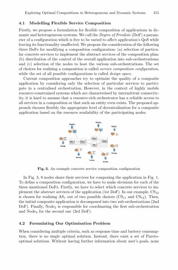
Exploring Optimal Compositions in Heterogeneous and Dynamic Systems 315
4.1 Modelling Flexible Service Composition
Firstly, we propose a formulation for flexible composition of applications in dy-namic and heterogeneous systems. We call the Degree of Freedom (DoF) a param-eter of a configuration which is free to be varied to affect application’s QoS whileleaving its functionality unaffected. We propose the consideration of the followingthree DoFs for modifying a composition configuration: (a) selection of particu-lar concrete services to implement the abstract services of the composition plan;(b) distribution of the control of the overall application into sub-orchestrations;and (c) selection of the nodes to host the various sub-orchestrations. The setof choices for realising a composition is called service composition configuration,while the set of all possible configurations is called design space.
Current composition approaches try to optimise the quality of a compositeapplication by considering only the selection of particular services to partici-pate in a centralised orchestration. However, in the context of highly mobileresource-constrained systems which are characterised by intermittent connectiv-ity, it is hard to assume that a resource-rich orchestrator has a reliable access toall services in a composition or that such an entity even exists. The proposed ap-proach chooses flexibly the appropriate level of decentralisation for a compositeapplication based on the resource availability of the participating nodes.
Fig. 3. An example concrete service composition configuration
In Fig. 3, 8 nodes share their services for composing the application in Fig. 1.To define a composition configuration, we have to make decisions for each of thethree mentioned DoFs. Firstly, we have to select which concrete services to im-plement the abstract services of the application (1st DoF). In our example, CS12is chosen for realising AS1 out of two possible choices (CS11 and CS12). Then,the initial composite application is decomposed into two sub-orchestrations (2ndDoF). Finally, Node2 is responsible for coordinating the first sub-orchestrationand Node4 for the second one (3rd DoF).
4.2 Formulating Our Optimisation Problem
When considering multiple criteria, such as response time and battery consump-tion, there is no single optimal solution. Instead, there exist a set of Pareto-optimal solutions. Without having further information about user’s goals, none

316 D. Efstathiou et al.
of these trade-off solutions can be said to be better than another. To enable theexploration of trade-off configurations, we define the following:
Definition 1. Distributed Service Orchestration Problem
Given: A set of m abstract services that compose the service composition planP , a set of n nodes where each node provides a single concrete service and cancoordinate a single orchestration, a mapping between concrete service implemen-tations and abstract services, and a set of q quality objectives Q = {Q1, · · · , Qq}.Problem: Find a representative set of composition configurations, all of whichimplement the functionality described by P , but differ in their quality trade-offsaccording to Q, by using different design options for the mentioned DoFs.
To solve an optimisation problem we have to define two key ingredients [7]:(i) a problem representation, and (ii) an objective function. The last step is toemploy an optimisation algorithm for exploring the solution space.
Representation. We have designed a metamodel for specifying the space ofpossible composition configurations that realise a composite application, whichis omitted due to lack of space. Based on this metamodel, we are able to producemodel instances like the one described in Fig. 3.
Objective Function. To simulate the studied scenario, we plan to use the NS-31
to measure the QoS properties (or else optimisation objectives) of candidate con-figurations. Search-based algorithms require a large number of objective functionevaluations to explore a set of trade-off solutions. However, the high computa-tional cost of the simulator makes impossible its usage for runtime explorationof trade-off configurations.
Surrogate-Based Optimisation (SBO) [8] aims at reducing the computationaltime of optimisation problems by replacing expensive objective functions withsurrogate models. The goal of surrogate models is to approximate the values ofthe real objective functions as close as possible and also be orders of magni-tude cheaper to compute. Surrogate models can be built by using data samplesproduced by simulation runs for predicting quality properties of compositionconfigurations, such as response time and battery consumption.
4.3 Validation Strategy
The goal is to understand the ability of our approach to explore promising com-position configurations by various simulation-based empirical studies. The use ofsimulation avoids the costly and impractical physical testing of such systems andgives us statistical power by allowing repeated experiments. Firstly, we aim tostudy the suitability of the proposed formulation for composing applications inhighly dynamic and heterogeneous environments. Then, we will investigate theability of the developed surrogate models to guide the search towards promisingareas of the search space. Finally, we plan to study the ability of the developedSBO technique to provide configurations of high-quality during runtime by mea-suring the execution time for exploring solutions of acceptable quality.
1 http://www.nsnam.org/

Exploring Optimal Compositions in Heterogeneous and Dynamic Systems 317
5 Related Work
QoS-aware service composition approaches can be grouped into centralised anddecentralised. In the first category, the goal is to find the set of concrete servicesto participate in a centralised orchestration that offer the required functionality,respect user’s preferences and constraints, and optimise composition’s QoS [3,4].However, these approaches focus on networks with abundant bandwidth andstationary nodes and neglect to study the problems of centralised orchestration.
On the other hand, Schuhmann et al. [6] proposed a hybrid configuration ofdistributed applications in the context of pervasive environments by adjustingthe level of decentralisation based on the number of available resource-rich nodes.Fdhila et al. [9] proposed a decentralised approach for composing applicationsby decentralising a composition into partitions of services that communicatefrequently, towards optimising the overall QoS of the composition. However,existing approaches do not adapt automatically to changing conditions such asresource availability and network connectivity.
6 Contributions
The expected contributions of this PhD can be summarised as: (i) a designspace formulation for flexible composition of applications in highly dynamic andheterogeneous service-based environments; (ii) a search-based approach for effi-ciently exploring trade-off compositions ; and (iii) a surrogate-assisted approachfor accelerating the search process of optimal configurations.
References
1. Papazoglou, M., Georgakopoulos, D.: Introduction: Service-Oriented Computing.Comm. of ACM 46, 24–28 (2003)
2. Efstathiou, D., McBurney, P., Plouzeau, N., Zschaler, S.: Improving the Quality ofDistributed Composite Service Applications. In: ICCSW (2012)
3. Canfora, G., Di Penta, M., Esposito, R., Villani, M.L.: An Approach for QoS-AwareService Composition Based on Genetic Algorithms. In: GECCO (2005)
4. Cardellini, V., Casalicchio, E., Grassi, V., Iannucci, S., Presti, F.L., Mirandola, R.:MOSES: A Framework for QoS Driven Runtime Adaptation of Service-OrientedSystems. TSE 99 (2011)
5. Sheng, Q.Z., Benatallah, B., Dumas, M., Yan Mak, E.O.: SELF-SERV: A Platformfor Rapid Composition of Web Services in a Peer-to-Peer Environment (2002)
6. Schuhmann, S., Herrmann, K., Rothermel, K.: Efficient Resource-Aware HybridConfiguration of Distributed Pervasive Applications. In: The 8th PerCom (2010)
7. Harman, M., McMinn, P., de Souza, J.T., Yoo, S.: Search Based Software Engi-neering: Techniques, Taxonomy, Tutorial. In: Meyer, B., Nordio, M. (eds.) LASERSummer School 2008-2010. LNCS, vol. 7007, pp. 1–59. Springer, Heidelberg (2012)
8. Jin, Y.: Surrogate-assisted evolutionary computation: Recent advances and futurechallenges. Swarm and Evolutionary Computation 1(2), 61–70 (2011)
9. Fdhila, W., Dumas, M., Godart, C., Garcıa-Banuelos, L.: Heuristics for CompositeWeb Service Decentralization. In: SoSyM, pp. 1–21 (2012)

Applying Search in an Automatic
Contract-Based Testing Tool
Alexey Kolesnichenko, Christopher M. Poskitt, and Bertrand Meyer
ETH Zurich, Switzerland
Abstract. Automated random testing has been shown to be effectiveat finding faults in a variety of contexts and is deployed in several test-ing frameworks. AutoTest is one such framework, targeting programswritten in Eiffel, an object-oriented language natively supporting exe-cutable pre- and postconditions; these respectively serving as test filtersand test oracles. In this paper, we propose the integration of search-basedtechniques—along the lines of Tracey—to try and guide the tool towardsinput data that leads to violations of the postconditions present in thecode; input data that random testing alone might miss, or take longerto find. Furthermore, we propose to minimise the performance impact ofthis extension by applying GPU programming to amenable parts of thecomputation.
1 Introduction
Automated random testing has become widely used, in part because it is inex-pensive to run, relatively simple to implement, and most importantly has beendemonstrated to be effective at finding bugs in programs; the technique havingbeen implemented in several testing frameworks including AutoTest [7], Korat[1], and Randoop [8]. Using random testing comes with the cost of only usingstraightforward strategies, and in particular, not leveraging information fromprevious executions or specifications that—if provided—might otherwise helpguide towards test data revealing undiscovered bugs.
The AutoTest framework targets programs written in the object-orientedlanguage Eiffel, which natively supports contracts [6], i.e. executable pre- andpostconditions for routines (although the framework could be adapted to othercontract-equipped languages such as Java with JML). Contracts go hand-in-hand with random testing, with preconditions serving as filters for test data,and postconditions serving as test oracles. Furthermore, there are techniques toguide the selection of inputs towards ones that satisfy preconditions, e.g. theprecondition-satisfaction strategy of AutoTest [12]. We claim in this short pa-per however that there is still more to be gained from contracts in automatedtesting. In particular, we propose that contracts are ideal for integration withsearch-based techniques for test data generation [5]; passing tests could be “mea-sured” against how close they are to violating the postconditions, with fitnessfunctions then favouring input data that optimises this measure. This strategy
G. Ruhe and Y. Zhang (Eds.): SSBSE 2013, LNCS 8084, pp. 318–323, 2013.© Springer-Verlag Berlin Heidelberg 2013

Applying Search in an Automatic Contract-Based Testing Tool 319
exploits ready-to-use contracts to focus the generation of test data towards ob-jects that get closer to violating postconditions, hence possibly revealing bugsthat random testing alone might miss, or take longer to find.
Applying search to test data generation is of course a computationally moreexpensive task—whilst the envisaged techniques might reveal individual bugsthat random testing might miss, the approach quickly loses appeal if the ratioof bugs encountered over time suffers. Hence, we propose to investigate howto implement the computationally expensive parts on modern GPU devices,following on from previous work in the search community (e.g. [13]).
The rest of the paper is structured as follows: Section 2 provides an overviewof AutoTest and how search-based techniques might be applied; Section 3 spec-ulates on measuring how “close” input data is to deriving outputs that vio-late postconditions; Section 4 discusses the application of GPU computation tosearch; and Section 5 outlines our plans and concludes.
2 Extending the AutoTest Workflow
Having introduced the idea of AutoTest in the previous section, we illustrateits workflow via a simple example. Consider the square root routine in List-ing 1; implementation details are not given, but we provide its contract. Theprecondition, given after require, expresses that the input is non-negative; thepostcondition, given after ensure, expresses the same. Recall that in AutoTest,preconditions are filters and postconditions are oracles. Hence in this example,sqrt is only tested on non-negative inputs, and any negative output indicatesthat its implementation does not meet its specification.
sqrt ( a : DOUBLE) : DOUBLErequire
a >= 0ensure
Result >= 0end
Listing 1. Square root contracts
The current workflow of AutoTest is roughly as follows: firstly, random inputssatisfying the routine’s precondition are generated. Secondly, the routine is exe-cuted on the generated data. If there is a postcondition violation, then the testfails and is recorded. Otherwise, the test passes. The overall picture is shown inFigure 1.
This workflow however does not take into account information from successfultest cases. Currently, we can say that they satisfied the test oracle; but moreinterestingly, can we measure how “close” they came to failing it, and use thisinformation in search to derive input data that gets even closer? A high-levelpicture of the proposed extension to AutoTest is shown in Figure 2. We discussthe issues of search and measuring “closeness” in the following section.

320 A. Kolesnichenko, C.M. Poskitt, and B. Meyer
Fig. 1. High-level overview of the AutoTest workflow
Fig. 2. High-level overview of the proposed extension to the AutoTest workflow
We remark that search was applied to AutoTest previously in [10]; however,their approach differs in that they use genetic algorithms to generate an effi-cient testing strategy by evolving random ones. Other authors [3] have suggestedthat condition coverage on postconditions—in a testing tool for Java programsequipped with contracts—seems promising in generating test data, but as far aswe know, did not publish implementations or evaluations of such algorithms.
3 Optimising Postcondition Violations
A key part of our proposal involves evaluating how “close” input data is toderiving a postcondition violation. We propose to follow Tracey [11], who definedobjective functions for logical connectives and relations over data of primitivetypes. The concepts can be applied to similarly simple contracts, so we illustratewith an example (based on the counter algorithm presented in [11,5]). A faultywrapping counter is shown in Listing 2. It is supposed to take an integer between0 and 10 (see the precondition), returning that integer incremented by 1 if it wasless than 10, and 0 otherwise (see the postcondition).
We can negate the postcondition, and add it in conjunction to the precondi-tion to form a constraint only satisfiable by input data that derives a fault; forexample:
(n ≥ 0 ∨ n ≤ 10) ∧ ¬((n = 10 → Result = 0) ∧ (n = 10 → Result = n+ 1)).
We can apply Tracey’s objective functions to the relations and connectives of theconstraint, yielding a value indicating the “closeness” to satisfying it (smallervalues indicating that we are closer). For example, for relations a = b, we candefine obj(a = b) to return the absolute difference between the values of a and

Applying Search in an Automatic Contract-Based Testing Tool 321
cyclic_increment ( n : INTEGER) : INTEGERrequire
n >= 0 and n <= 10do
i f ( n > 10) thenResult := 0
elseResult := n + 1
endensure
( n = 10 implies Result = 0) and ( n /= 10 implies Result = n + 1)end
Listing 2. Faulty wrapping counter
b. Other relational predicates can be measured in a similar fashion. Objectivefunctions are defined inductively for logical connectives. For example, considerthe formula a∨b. A suitable definition of obj(a∨b) would be min(obj(a), obj(b)),i.e. the minimum value of the two parameters. With a fitness function includingsuch a measure, we hope to apply metaheuristic search techniques [4], optimisingthe search towards input data that gets closer to violating postconditions (i.e.revealing bugs).
In our wrapping counter example, the smallest output of the objective functionshould be yielded for n = 10, since the implementation incorrectly incrementsthe counter for this value.
For real object-oriented programs, we encounter the challenge of hidden states:objects tend to conceal their implementation details. For example, a routine ofa bounded buffer might assert in its postcondition that the buffer is not full.Expressed as buffer.count < buffer.size, we can apply objective functionsas we have described. However, the postcondition might instead be expressedas not buffer.is_full, i.e. a Boolean query. Boolean queries are not informa-tive for metaheuristic search because of their “all or nothing” nature. In thisexample, we cannot distinguish between a buffer that is completely empty andanother that is close to being full. Postconditions containing Boolean queriesshould be transformed into equivalent postconditions that are more amenablefor testing. A solution proposed by [2] is to “expand” Boolean queries usingtheir specifications; an approach compatible with our contract-based one. Forexample, the postcondition of is_full might express that the result is true ifand only if count >= size; this being an assertion to which objective functionscan be applied more successfully.
4 Performance Considerations
The ideas described in the previous sections do not come for free. Additionalcomputation increases the running time of the tool, and may adversely affect theratio of bugs found over time. In order to keep the performance as reasonable aspossible, we propose to apply GPU computing to speed-up the computationally

322 A. Kolesnichenko, C.M. Poskitt, and B. Meyer
intensive aspects of the search. Consider for example the family of genetic algo-rithms (GAs). The population can be encoded as a numerical vector, and thefitness function as a vector function f : Rn → R.
Essentially, the GA input can be represented as a matrix m× n, where m isthe population size, and n is the size of the chromosome vector. Thus, to evaluatea fitness function, one just needs to apply some vector function to each matrixrow. A mutation operation (changing chromosomes of some species subset) canalso be performed row-wise. Crossover operation is also essentially row-based.
GPUs are very different to conventional CPUs. Whereas CPUs are designedas general-purpose computing devices, with lots of optimisations like branch pre-diction, multi-level caches, etc., the processing units of GPUs are much simpler.A GPU’s processing unit cannot handle the processing of arbitrary data as effi-ciently as CPUs can; they do not possess sophisticated hardware optimisations.However, there are many more processing cores on a GPU device, compared tothe CPU. GPUs are tuned for data parallelism, implementing the SIMD (SingleInstruction - Multiple Data) processing model, allowing the execution of thou-sands of threads in parallel. GPUs have proven to be extremely efficient withmatrix-style computations [9], providing a convincing speed-up of 2-3 orders ofmagnitude.
GPU acceleration was used for the problem of minimising test suite size in [13],and demonstrated that speed-ups of over 25x are possible using GPU computing.
5 Research Plans and Conclusion
The proposed ideas—namely implementing search-based techniques to improvethe fault discovery rate of a contract-based random testing tool, and using GPUacceleration to limit the performance hit—need to be carefully evaluated. Whilewe believe that search will enhance the quality of inputs in AutoTest, there areseveral risks and challenges to be dealt with along the way to confirming ordisproving this hypothesis.
A first challenge is the previously mentioned implementation hiding in object-oriented languges, that makes guided search ineffective without first transformingBoolean queries into postconditions that are better suited for objective functions.A second challenge: one should never forget that the goal of testing tools is toreveal as many faults as possible. That is why the enhanced tool needs to betested against previously successful strategies, e.g. the precondition-satisfactionstrategy [12] of AutoTest.
Thirdly, some thought needs to be given as to the particular type of searchalgorithm to apply (e.g. a genetic algorithm), and how to best encode the objectsand data on which these algorithms operate. The final choice will be determinedby the quality of inferred data and amenability to GPU-style computations. Fi-nally, one needs to take into account, that GPU acceleration may be overwhelmedby the additional overhead of copying data from main memory to the GPU, andvice versa. Thus, GPU computing should only be applied to computationallyintensive parts of the proposed AutoTest workflow.

Applying Search in an Automatic Contract-Based Testing Tool 323
Acknowledgments. The research leading to these results has received fund-ing from the European Research Council under the European Union’s SeventhFramework Programme (FP7/2007-2013) / ERC Grant agreement no. 291389,the Hasler Foundation, and ETH (ETHIIRA). The authors would like to thankSimon Poulding for helpful discussions.
References
1. Boyapati, C., Khurshid, S., Marinov, D.: Korat: automated testing based on Javapredicates. In: Proc. International Symposium on Software Testing and Analysis(ISSTA 2002), pp. 123–133. ACM (2002)
2. Cheon, Y., Kim, M.: A specification-based fitness function for evolutionary test-ing of object-oriented programs. In: Proc. Genetic and Evolutionary ComputationConference (GECCO 2006), pp. 1953–1954. ACM (2006)
3. Cheon, Y., Kim, M., Perumandla, A.: A complete automation of unit testing forJava programs. In: Proc. International Conference on Software Engineering Re-search and Practice (SERP 2005), pp. 290–295. CSREA Press (2005)
4. Harman, M.: The current state and future of search based software engineering.In: Proc. Future of Software Engineering (FOSE 2007), pp. 342–357. IEEE (2007)
5. McMinn, P.: Search-based software test data generation: a survey. Software Testing,Verification and Reliability 14(2), 105–156 (2004)
6. Meyer, B.: Object-Oriented Software Construction, 2nd edn. Prentice Hall (1997)7. Meyer, B., Fiva, A., Ciupa, I., Leitner, A., Wei, Y., Stapf, E.: Programs that test
themselves. IEEE Computer 42(9), 46–55 (2009)8. Pacheco, C., Lahiri, S.K., Ball, T.: Finding errors in. NET with feedback-directed
random testing. In: Proc. International Symposium on Software Testing and Anal-ysis (ISSTA 2008), pp. 87–96. ACM (2008)
9. Ryoo, S., Rodrigues, C.I., Baghsorkhi, S.S., Stone, S.S., Kirk, D.B., Hwu, W.W.:Optimization principles and application performance evaluation of a multithreadedGPU using CUDA. In: Proc. Symposium on Principles and Practice of ParallelProgramming (PPOPP 2008), pp. 73–82. ACM (2008)
10. Silva, L.S., Wei, Y., Meyer, B., Oriol, M.: Evotec: Evolving the best testing strat-egy for contract-equipped programs. In: Proc. Asia Pacific Software EngineeringConference (APSEC 2011), pp. 290–297 (2011)
11. Tracey, N.J.: A Search-Based Automated Test-Data Generation Framework forSafety-Critical Software. PhD thesis, The University of York (2000)
12. Wei, Y., Gebhardt, S., Oriol, M., Meyer, B.: Satisfying test preconditions throughguided object selection. In: Proc. International Conference on Software Testing,Verification and Validation (ICST 2010), pp. 303–312. IEEE (2010)
13. Yoo, S., Harman, M., Ur, S.: Highly scalable multi objective test suite minimisationusing graphics cards. In: Cohen, M.B., O Cinneide, M. (eds.) SSBSE 2011. LNCS,vol. 6956, pp. 219–236. Springer, Heidelberg (2011)

Author Index
Alexander, Rob 251Andrade, Aline Santos 188Arora, Vikhyat 294Asoudeh, Nesa 288Assuncao, Wesley Klewerton Guez 19Atkinson, Colin 239
Bansal, Priti 294Barrett, Stephen 306Barros, Marcio de Oliveira 34, 188, 275Bechikh, Slim 50, 245Ben Chikha, Soukeina 50Ben Said, Lamjed 245Bian, Yi 111Bourcier, Johann 312Boussaa, Mohamed 50Briand, Lionel 66, 141Bruckmann, Thomas 141Buzdalov, Maxim 300Buzdalova, Arina 300
Chen, Kathy 66Chen, Tsong Yueh 224Cheng, Betty H.C. 81Cheng, Jun 111Cinneide, Mel O 126Clark, John A. 251Cody-Kenny, Brendan 306Colanzi, Thelma Elita 19
de Souza, Jerffeson Teixeira 172de Vega, Francisco Fernandez 282
Efstathiou, Dionysios 312El Boussaidi, Ghizlane 96
Farzat, Fabio de Almeida 275Fredericks, Erik M. 81
Ghannem, Adnane 96
Harman, Mark 224, 257
Kalboussi, Sabrine 245Kessel, Marcus 239
Kessentini, Marouane 50, 96, 126, 209,245
Kessentini, Wael 50Kolesnichenko, Alexey 318Koskimies, Kai 269Kumar, Vineet 294Kuo, Fei-Ching 224
Labiche, Yvan 66, 288Langdon, William B. 257Li, Zheng 111
Maciel, Rita Suzana P. 188Mahouachi, Rim 126Malik, Shreya 294Matinnejad, Reza 141Mayo, Michael 158McBurney, Peter 312Meyer, Bertrand 318
Nejati, Shiva 141Nogueira, Ana Filipa 282
Oriol, Manuel 251
Paixao, Matheus Henrique Esteves 172Parfenov, Vladimir 300Patrick, Matthew 251Petke, Justyna 257Pitangueira, Antonio Mauricio 188Poskitt, Christopher M. 263, 318Poulding, Simon 263Poull, Claude 141Pozo, Aurora 19
Ramirez, Andres J. 81Ribeiro, Jose Carlos Bregieiro 282
Sabharwal, Sangeeta 294Schumacher, Marcus 239Shelburg, Jeffery 209Sievi-Korte, Outi 269Spacey, Simon 158Systa, Kari 269

326 Author Index
Tauritz, Daniel R. 209
Vathsavayi, Sriharsha 269
Vergilio, Silvia Regina 19
Weimer, Westley 1
White, David R. 16
Xie, Xiaoyuan 224
Yao, Xin 4Yoo, Shin 224
Zenha-Rela, Mario Alberto 282Zhao, Ruilian 111Zschaler, Steffen 312