lecturenotes-4AB00.pdf - Mathematics and Computer Science
98
Lecture Notes 4AB00 Version: January 31, 2018 Edited by: Ivo Adan, Erjen Lefeber, Sasha Pogromsky Department of Mechanical Engineering Eindhoven University of Technology P.O. Box 513, 5600 MB, Eindhoven, The Netherlands
-
Upload
khangminh22 -
Category
Documents
-
view
0 -
download
0
Transcript of lecturenotes-4AB00.pdf - Mathematics and Computer Science
Lecture Notes 4AB00Version: January 31, 2018
Edited by: Ivo Adan,Erjen Lefeber,Sasha Pogromsky
Department of Mechanical EngineeringEindhoven University of Technology
P.O. Box 513, 5600 MB, Eindhoven, The Netherlands

Contents
Contents 3
1 Introduction 5
2 Basics 9
2.1 Permutations and combinations . . . . . . . . . . . . . . . . . . . . . . . . . . . . . . . 9
2.2 Standard series . . . . . . . . . . . . . . . . . . . . . . . . . . . . . . . . . . . . . . . . 9
3 Probability Models 11
3.1 Basic ingredients . . . . . . . . . . . . . . . . . . . . . . . . . . . . . . . . . . . . . . . 11
3.2 Conditional probabilities . . . . . . . . . . . . . . . . . . . . . . . . . . . . . . . . . . . 15
3.3 Discrete random variables . . . . . . . . . . . . . . . . . . . . . . . . . . . . . . . . . . 19
3.4 Continuous random variables . . . . . . . . . . . . . . . . . . . . . . . . . . . . . . . . 29
3.5 Central limit theorem . . . . . . . . . . . . . . . . . . . . . . . . . . . . . . . . . . . . . 37
3.6 Joint random variables . . . . . . . . . . . . . . . . . . . . . . . . . . . . . . . . . . . . 38
3.7 Conditioning . . . . . . . . . . . . . . . . . . . . . . . . . . . . . . . . . . . . . . . . . 41
4 Manufacturing Models 47
4.1 Terminology . . . . . . . . . . . . . . . . . . . . . . . . . . . . . . . . . . . . . . . . . . 49
4.2 Key performance measures . . . . . . . . . . . . . . . . . . . . . . . . . . . . . . . . . 49
4.3 Capacity, flow time and WIP . . . . . . . . . . . . . . . . . . . . . . . . . . . . . . . . . 50
4.4 Little’s law . . . . . . . . . . . . . . . . . . . . . . . . . . . . . . . . . . . . . . . . . . . 54
4.5 Variability . . . . . . . . . . . . . . . . . . . . . . . . . . . . . . . . . . . . . . . . . . . 57
4.6 Process time variability . . . . . . . . . . . . . . . . . . . . . . . . . . . . . . . . . . . 58
4.6.1 Natural variability . . . . . . . . . . . . . . . . . . . . . . . . . . . . . . . . . . . 59
4.6.2 Preemptive outages . . . . . . . . . . . . . . . . . . . . . . . . . . . . . . . . . 59
4.6.3 Non-Preemptive outages . . . . . . . . . . . . . . . . . . . . . . . . . . . . . . 60
4.6.4 Rework . . . . . . . . . . . . . . . . . . . . . . . . . . . . . . . . . . . . . . . . 61
4.7 Flow variability . . . . . . . . . . . . . . . . . . . . . . . . . . . . . . . . . . . . . . . . 61
4.8 Variability interactions - Queueing . . . . . . . . . . . . . . . . . . . . . . . . . . . . . 64
4.9 Zero-buffer model . . . . . . . . . . . . . . . . . . . . . . . . . . . . . . . . . . . . . . 66
4.10 Finite-buffer model . . . . . . . . . . . . . . . . . . . . . . . . . . . . . . . . . . . . . . 67
4 Contents
4.11 Single machine station . . . . . . . . . . . . . . . . . . . . . . . . . . . . . . . . . . . . 69
4.12 Multi machine station . . . . . . . . . . . . . . . . . . . . . . . . . . . . . . . . . . . . . 72
4.13 Serial production lines . . . . . . . . . . . . . . . . . . . . . . . . . . . . . . . . . . . . 75
4.14 Batching . . . . . . . . . . . . . . . . . . . . . . . . . . . . . . . . . . . . . . . . . . . . 79
Appendices 85
A KIVA model 87
B Zero-buffer model 89
C Finite-buffer model 91
D Single machine model 93
E Multi machine model 95
F Serial production line 97

1Introduction
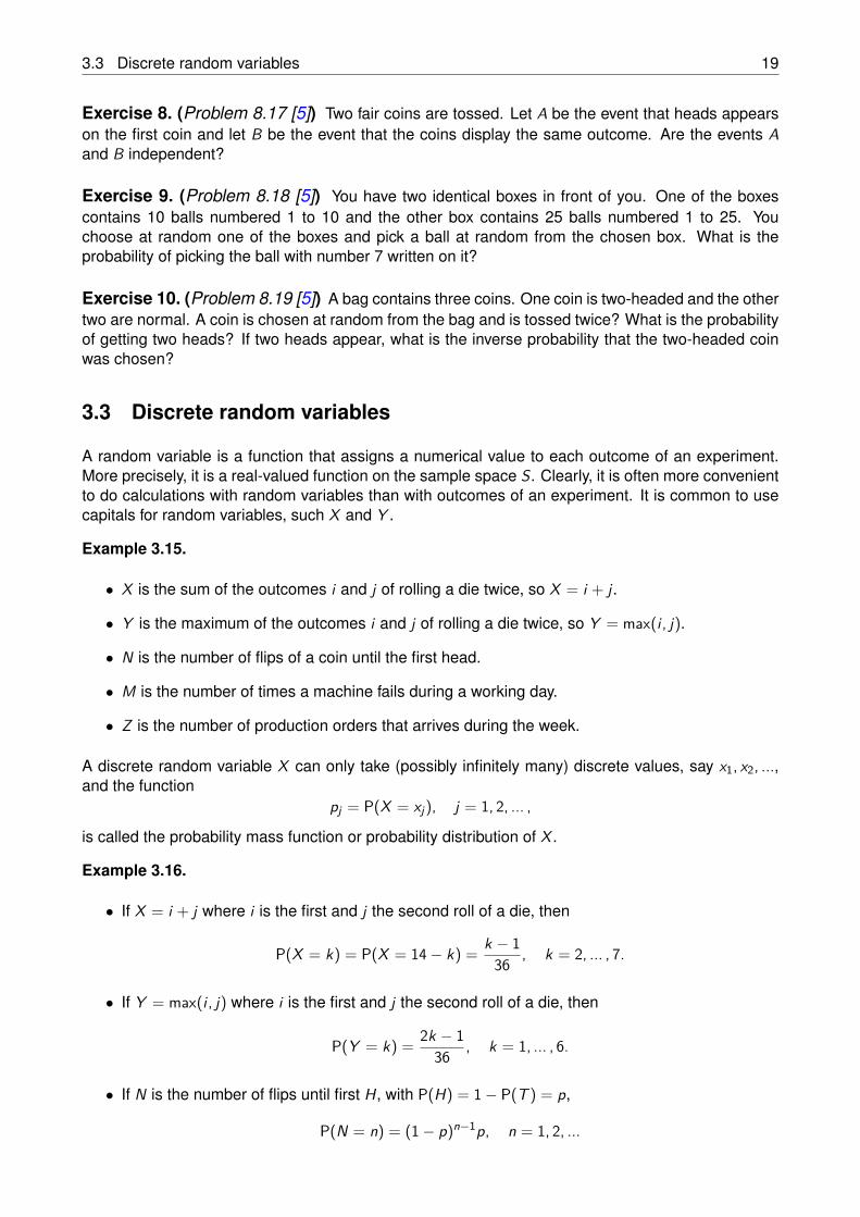
In the course Analysis of Manufacturing Systems we study the behavior of manufacturing systems.Understanding its behavior and basic principles is critical to manufacturing managers and engineerstrying (i) to develop and control new systems and processes, or (ii) to improve existing systems. Theimportance of manufacturing management should not be underestimated: the success of a companystrongly depends on the effectiveness of its management. One might say that the future of the Dutchmanufacturing industry, which constitutes about 17% of the Dutch gross national product and employsabout 15% of the Dutch work force, depends on how well manufacturing managers and engineers areable to exploit the newest developments in information and manufacturing technology, also referredto as Smart Industry or the fourth industrial revolution.
Figure 1.1: Smart Industry – Dutch industry fit for the future
The aim of this course is to develop understanding of manufacturing operations, with a focus onthe material flow through the plant and key performance indicators, such as throughput, equipmentefficiency, investment in equipment material, work in process and so on. Clearly, managers andengineers need to rely on their “manufacturing intuition” in order to fully understand the consequencesof the decisions they make on system design, control and maintenance.
This course is based on the book Factory Physics [2]. This book provides the basis for manufacturingscience, by offering (i) a clear description of the basic manufacturing principles (i.e., the physicallaws underlying manufacturing operations), (ii) understanding and intuition about system behavior,and (iii) a unified modeling framework to facilitate synthesis of complex manufacturing systems.
As we will see, a crucial and disrupting element in manufacturing operations is variability. Theoriesthat effectively describe the sources of variability and their interaction, are Probability Theory andQueueing Theory. So, not surprisingly, Factory Physics is firmly grounded on these theories, since agood probabilistic intuition is a powerful tool for the manager and engineer. This also explains whythe present course consists of two main parts:
• Manufacturing models.This part is devoted to Manufacturing Science. It is based on the book Factory Physics [2],
6 Introduction
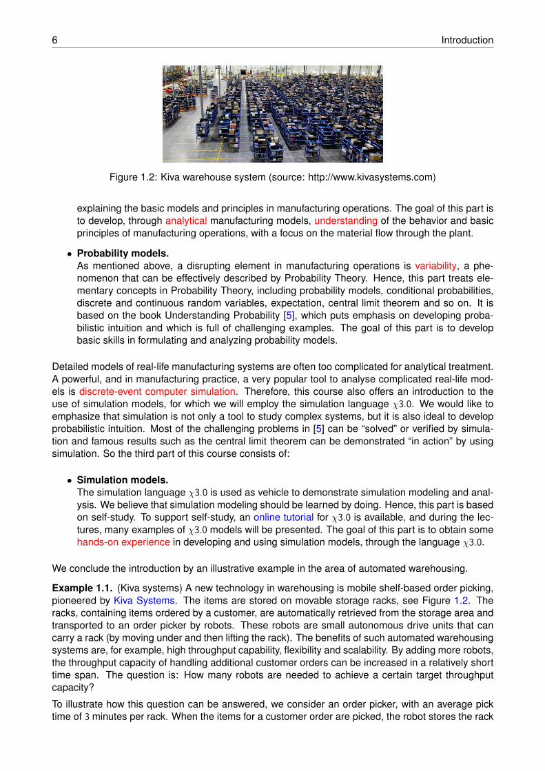
Figure 1.2: Kiva warehouse system (source: http://www.kivasystems.com)
explaining the basic models and principles in manufacturing operations. The goal of this part isto develop, through analytical manufacturing models, understanding of the behavior and basicprinciples of manufacturing operations, with a focus on the material flow through the plant.
• Probability models.As mentioned above, a disrupting element in manufacturing operations is variability, a phe-nomenon that can be effectively described by Probability Theory. Hence, this part treats ele-mentary concepts in Probability Theory, including probability models, conditional probabilities,discrete and continuous random variables, expectation, central limit theorem and so on. It isbased on the book Understanding Probability [5], which puts emphasis on developing proba-bilistic intuition and which is full of challenging examples. The goal of this part is to developbasic skills in formulating and analyzing probability models.
Detailed models of real-life manufacturing systems are often too complicated for analytical treatment.A powerful, and in manufacturing practice, a very popular tool to analyse complicated real-life mod-els is discrete-event computer simulation. Therefore, this course also offers an introduction to theuse of simulation models, for which we will employ the simulation language χ3.0. We would like toemphasize that simulation is not only a tool to study complex systems, but it is also ideal to developprobabilistic intuition. Most of the challenging problems in [5] can be “solved” or verified by simula-tion and famous results such as the central limit theorem can be demonstrated “in action” by usingsimulation. So the third part of this course consists of:
• Simulation models.The simulation language χ3.0 is used as vehicle to demonstrate simulation modeling and anal-ysis. We believe that simulation modeling should be learned by doing. Hence, this part is basedon self-study. To support self-study, an online tutorial for χ3.0 is available, and during the lec-tures, many examples of χ3.0 models will be presented. The goal of this part is to obtain somehands-on experience in developing and using simulation models, through the language χ3.0.
We conclude the introduction by an illustrative example in the area of automated warehousing.
Example 1.1. (Kiva systems) A new technology in warehousing is mobile shelf-based order picking,pioneered by Kiva Systems. The items are stored on movable storage racks, see Figure 1.2. Theracks, containing items ordered by a customer, are automatically retrieved from the storage area andtransported to an order picker by robots. These robots are small autonomous drive units that cancarry a rack (by moving under and then lifting the rack). The benefits of such automated warehousingsystems are, for example, high throughput capability, flexibility and scalability. By adding more robots,the throughput capacity of handling additional customer orders can be increased in a relatively shorttime span. The question is: How many robots are needed to achieve a certain target throughputcapacity?
To illustrate how this question can be answered, we consider an order picker, with an average picktime of 3 minutes per rack. When the items for a customer order are picked, the robot stores the rack
7
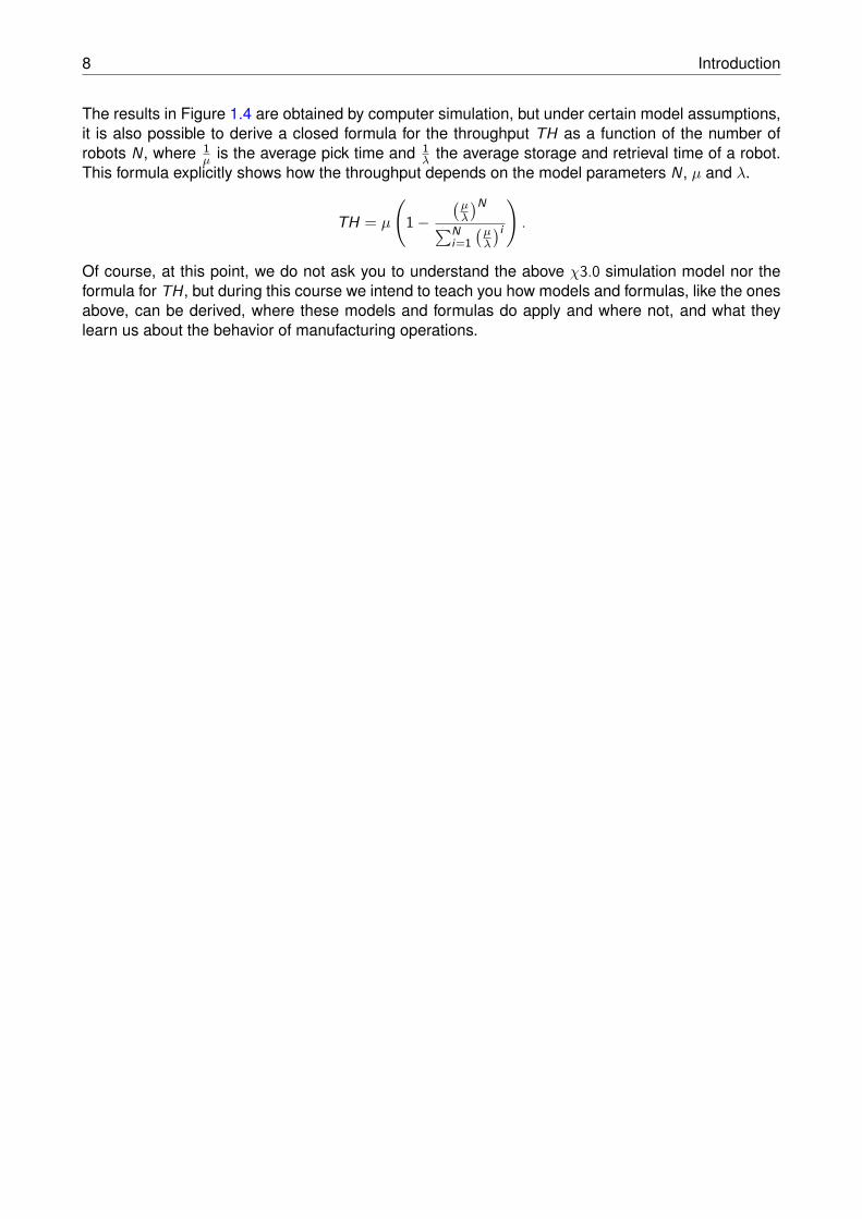
at some place in the storage area and then retrieves the next rack from another place and brings it tothe order picker. The average time required by a robot to store and retrieve a rack from the storagearea is 15 minutes. Clearly, the variability of the storage and retrieval times will be high, since theracks can be located anywhere, and intensive traffic of robots will cause unpredictable congestionin the storage area. On arrival at the pick station, the robot joins the queue of robots waiting forthe order picker, and once its items are picked, the robot returns to the storage area and the cyclerepeats. This storage and retrieval process is illustrated in Figure 1.3.
Storage area
N circulating robots
Pick station
Buffer
Figure 1.3: Storage and retrieval cycle of robots
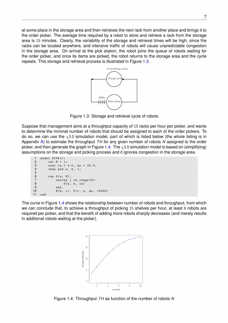
Suppose that management aims at a throughput capacity of 15 racks per hour per picker, and wantsto determine the minimal number of robots that should be assigned to each of the order pickers. Todo so, we can use the χ3.0 simulation model, part of which is listed below (the whole listing is inAppendix A) to estimate the throughput TH for any given number of robots N assigned to the orderpicker, and then generate the graph in Figure 1.4. The χ3.0 simulation model is based on (simplifying)assumptions on the storage and picking process and it ignores congestion in the storage area.
1 model KIVA ():2 int N = 1;3 real la = 4.0, mu = 20.0;4 chan pod a, b, c;56 run G(a, N),7 unwind j in range(N):8 S(a, b, la)9 end ,
10 B(b, c), P(c, a, mu, 10000)11 end
The curve in Figure 1.4 shows the relationship between number of robots and throughput, from whichwe can conclude that, to achieve a throughput of picking 15 shelves per hour, at least 6 robots arerequired per picker, and that the benefit of adding more robots sharply decreases (and merely resultsin additional robots waiting at the picker).
2 4 6 8 10
05
1015
20
nr of robots
Thr
ough
put (
rack
s/ho
ur)
Figure 1.4: Throughput TH as function of the number of robots N
8 Introduction
The results in Figure 1.4 are obtained by computer simulation, but under certain model assumptions,it is also possible to derive a closed formula for the throughput TH as a function of the number ofrobots N, where 1
µ is the average pick time and 1λ the average storage and retrieval time of a robot.
This formula explicitly shows how the throughput depends on the model parameters N, µ and λ.
TH = µ
(1−
(µλ
)N
∑Ni=1(µλ
)i
).
Of course, at this point, we do not ask you to understand the above χ3.0 simulation model nor theformula for TH, but during this course we intend to teach you how models and formulas, like the onesabove, can be derived, where these models and formulas do apply and where not, and what theylearn us about the behavior of manufacturing operations.
2Basics
In this chapter we briefly summarize some basic results, useful for studying probability models (seealso the Appendix in [5]).
2.1 Permutations and combinations
The total number of ways you can arrange the letters A, B, C and D is 24, since for the first positionyou have 4 possibilities, for the second 3 and so on, so the total number is 4 · 3 · 2 · 1 = 24. In general,the total number of ways n different objects can be ordered in a sequence is n · (n − 1) · · · 2 · 1. Thisnumber is abbreviated as n!, so
n! = 1 · 2 · · · (n − 1) · n,
where by convention, 0! = 1. Another question is in how many ways can you choose three lettersfrom A, B, C and D? Two answer this question, you first count the number of ordered sequences ofthree letters, which is 4 · 3 · 2. Then, to obtain the number of three letter combinations, you have todivide this number by 3!, since the order of the three letter sequence is not relevant. In general, thetotal number of ways you can choose k different objects (irrespective of their order) from n differentobjects is equal to
n · (n − 1) · · · (n − k + 1)k! = n!
k!(n − k)! .
This number is abbreviated as (nk
)= n!
k!(n − k)! ,
which is also referred to as binomial coefficient (since it is the coefficient of xk in (1 + x)n), and thuscounts the number of (unordered) combinations of k objects out of a set of n objects.
2.2 Standard series
In this section we briefly mention some standard series, that are used in many probability models.The first one is the sum 1 + 2 + · · · + n. This sum is equal to n (the number of terms) times theiraverage (1 + n)/2, so for any n ≥ 0,
1 + 2 + · · ·+ n = n(n + 1)2 .
The next sum is 1 + x + x2 + · · ·+ xn. To calculate this one, we set
s = 1 + x + x2 + · · ·+ xn.
10 Basics
Multiplying s by x givesxs = x + x2 + · · ·+ xn+1
and then subtracting xs from s yields
(1− x)s = 1− xn+1.
So we can conclude that
1 + x + x2 + · · ·+ xn = 1− xn+1
1− x , (2.1)
where x should be not equal to 1 (in which case the right hand side is equal to n). We now considerthe infinite sum
1 + x + x2 + · · · =∞∑
i=0x i ,
valid for |x | < 1 (since, otherwise, the infinite sum does not exist). Taking n to infinity in (2.1) yields
∞∑
i=0x i = 1
1− x , |x | < 1. (2.2)
The above series is also referred to as the geometric series. Based on (2.2) several variations of thegeometric series can be calculated, such as for example, when we have an extra i ,
∞∑
i=0ix i = x
(1− x)2 .
This follows from∞∑
i=0ix i = x
∞∑
i=0ix i−1 = x
∞∑
i=0
ddx x i = x d
dx
∞∑
i=0x i = x d
dx1
1− x = x(1− x)2 .
Similarly we have
∞∑
i=0i2x i =
∞∑
i=0i(i−1)x i +
∞∑
i=0ix i = x2
∞∑
i=0i(i−1)x i−2 +x
∞∑
i=0ix i−1 == 2x2
(1− x)3 + x(1− x)2 = x2 + x
(1− x)3 .
The next series is the exponential series or Taylor expansion of ex , given by
ex =∞∑
i=0
x i
i! .
Note that, for example,
∞∑
i=0i x i
i! =∞∑
i=1
x i
(i − 1)! = x∞∑
i=1
x i−1
(i − 1)! = xex ,
∞∑
i=0i(i − 1)x i
i! =∞∑
i=2
x i
(i − 2)! = x2∞∑
i=2
x i−2
(i − 2)! = x2ex ,
∞∑
i=0i2 x i
i! =∞∑
i=0i(i − 1)x i
i! +∞∑
i=0i x i
i! = (x2 + x)ex .
3Probability Models
In this chapter we briefly review the main concepts of probability models.
3.1 Basic ingredients
Over time several definitions of probability have been proposed. Probabilities can be defined beforean experiment. For example, in the experiment of throwing a die, it is reasonable to assume that alloutcomes are equally likely. Alternatively, probabilities can be defined after an experiment, as therelative frequencies of the outcomes by repeating the experiment many times. Sometimes it is notpossible to repeat experiments (think of predicting the weather), in which case probabilities can beestimated subjectively. Fortunately, there is a unifying and satisfying approach to define probabilitymodels, due the Russian mathematician Andrej Kolmogrov, where probabilities are defined as afunction on the subsets of the space of all possible outcomes, called the sample space, which shouldobey some appealing rules.
The ingredients of a probability model are as follows:
• The sample space S (often denoted by Ω) which is the set of all possible outcomes;
• Events are subsets of the possible outcomes in S;
• New events can be obtained by taking the union, intersection, complement (and so on) ofevents.
The sample space S can be discrete or continuous, as shown in the following examples.
Example 3.1. Examples of the sample space:
• Flipping a coin, then the outcomes are Head (H) and Tail (T ), so S = H, T.
• Rolling a die, then the outcomes are the number of points the die turns up with, so S =1, 2, ... , 6.
• Rolling a die twice, in which case the outcomes are the points of both dies, S = (i , j), i , j =1, 2, ... , 6.
• Process time realizations on a machine, which can be any nonnegative (real) number, so S =[0,∞).
• Sometimes process times have a fixed off-set, say 5 (minutes), in which case S = [5,∞).
• The number of machine failures during a shift, S = 0, 1, 2, ....
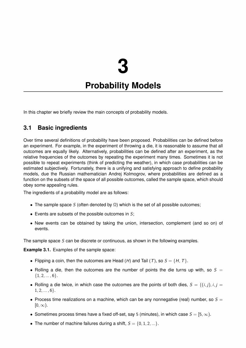
12 Probability Models
E1 E2 E3 E4
S
Figure 3.1: Disjoint events E1, E2, E3 and E4
• Throwing darts where the target is the unit disk, S = (x , y),√
x2 + y2 ≤ 1.
The events are all subsets of the sample space S (though in case of a continuous sample space Sone should be careful and exclude “weird” subsets).
Example 3.2. Examples of events of the sample spaces mentioned in the previous example are:
• Flipping a coin, E = ∅ (i.e., the empty set), E = H, E = T and E = H, T = S (these areall possible events).
• Rolling a die, E = 1, 2, E = 1, 3, 5 (the odd outcomes).
• Rolling a die twice, E = (1, 2), (3, 4), (5, 6), E = (1, 1), (1, 2), (1, 3), (1, 4), (1, 5), (1, 6) (thefirst die turned up with 1).
• Process times, E = (0, 1), E = (1,∞)
• Process times with offset, E = (10, 15)
• Number of failures, E = 3, 4, ...
• Throwing darts, E = (x , y), 0 ≤ x ≤ 14 , 0 ≤ y ≤ 1
4.
The other ingredient of a probability model are, of course, probabilities. These are defined as afunction of events, and this function should obey the following elementary rules.
For each event E there is a number P(E ) (the probability that event E occurs) such that:
• 0 ≤ P(E ) ≤ 1 (a probability should be a number between 0 and 1).
• P(S) = 1 (the probability that something happens is 1).
• If the events E1, E2, ... are mutually disjoint (the sets Ei have nothing in common), then
P(E1 ∪ E2 ∪ · · · ) = P(E1) + P(E2) + · · ·
(probability of the union of disjoint events is the sum of the probabilities of these events, seeFigure 3.1).
Example 3.3.
• Flipping a fair coin, P(H) = P(T) = 12 , P(H, T) = 1.
• Rolling a die, P(E ) is the number of outcomes in E divided the total number of outcomes (whichis 6), so P(1) = 1
6 , P(1, 2) = P(1) + P(2) = 13 and so on.
• Rolling a die twice, P(i , j) = 136 for i , j = 1, ... 6.
• Throwing darts, P(E ) is the area of E , divided by area of unit disk (which is π).
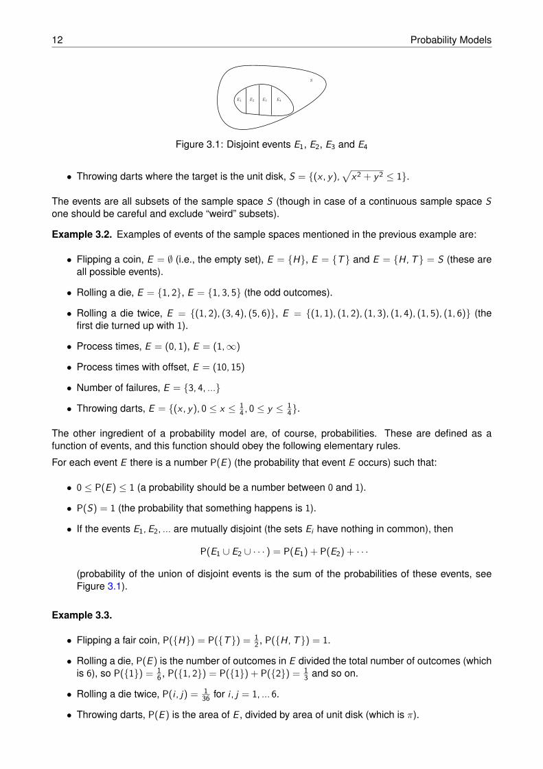
3.1 Basic ingredients 13
E FEF
Figure 3.2: Probability of union of two events E and F
In case the sample space S is discrete, so S = s1, s2, ..., then we can assign probabilities P(s) toeach s ∈ S, which should be between 0 and 1 and add up to 1. Then
P(E ) = sum of the probabilities of the outcomes in the set E =∑
s∈EP(s). (3.1)
If S is a finite set, S = s1, s2, ... , SN , and all outcomes are equally likely, so P(si) = 1/N, then (3.1)reduces to
P(E ) = N(E )N
where N(E ) is the number of outcomes in the set E . An example is the experiment of rolling two dice.
Based on the ingredients of a probability model, the following properties of probabilities can be math-ematically derived. Note that these properties all correspond to our intuition.
Property 3.1.
• P(∅) = 0 (probability of nothing happening is 0).
• If event F includes E , then its probability is greater,
P(E ) ≤ P(F ) if E ⊂ F .
• If finitely many E1, E2, ... , En are mutually disjoint (they have nothing in common), then
P(E1 ∪ E2 ∪ · · · ∪ En) = P(E1) + P(E2) + · · ·+ P(En).
• If the event E c is the complement of E (all outcomes except the ones in E ), so E c = S \ E , then
P(E c) = 1− P(E ).
• For the union of two events (so event E or F occurs),
P(E ∪ F ) = P(E ) + P(F )− P(EF ),
where EF = E ∩ F is the intersection of both events (so event E and F occur), see Figure 3.2.
It is remarkable that based on the simple ingredients of a probability model the frequency interpreta-tion of probabilities can be derived, i.e., the probability of event E can be estimated as the fraction oftimes that E happened in a large number of (identical) experiments.
Property 3.2. (Law of large numbers)If an experiment is repeated an unlimited number of times, and if the experiments are independent ofeach other, then the fraction of times event E occurs converges with probability 1 to P(E ).
14 Probability Models
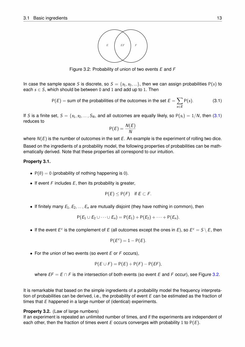
−1 1
−1
1
Figure 3.3: Randomly sampling points from the square [−1, 1]× [−1, 1]
For example, if we flip a fair coin an unlimited number of times, then an outcome s of this experimentis an infinite sequence of Heads and Tails, such as
s = (H, T , T , H, H, H, T , ...).
Then, if Kn(s) is the number if Heads appearing in the first n flips of realization s, we can concludethat, according to the law of large numbers,
limn→∞
Kn(s)n = 1
2
with probability 1.
The method of computer simulation is based on this law.
Example 3.4. The number π can be estimated by the following experiment. We randomly sample apoint (x , y) from the square [−1, 1] × [−1, 1], see Fig. 3.3 and the experiment is successful if (x , y)falls in unit circle. Then by the law of large numbers:
number of successful experimentstotal number of experiments
≈ area unit circlearea square
= π
4 .
Exercise 1. (Problem 7.3 [5]) Four black socks and five white socks lie mixed up in a drawer. Yougrab two socks at random from the drawer. What is the probability of having grabbed one black sockand one white sock?
Exercise 2. (Problem 7.5 [5]) Two players A and B each roll one die. The absolute differenceof the outcomes is computed. Player A wins if the difference is 0, 1, or 2; otherwise, player B wins.What is the probability that player A wins?
Exercise 3. (Problem 7.7 [5]) You have four mathematics books, three physics books and twochemistry books. The books are put in random order on a bookshelf. What is the probability ofhaving the books ordered per subject on the bookshelf?
Exercise 4. (Problem 7.29 [5]) A small transport company has two vehicles, a truck and a van.The truck is used 75% of the time. Both vehicles are used 30% of the time and neither of the vehiclesis used for 10% of the time. What is the probability that the van is used on any given day?
Exercise 5. (Problem 7.33 [5]) You roll a fair die six times in a row. What is the probability that allof the six face values will appear? What is the probability that one or more sixes will appear?
3.2 Conditional probabilities 15
3.2 Conditional probabilities
Conditional probabilities are an intuitive concept: intuitively the conditional probability P(E |F ) is theprobability that event E occurs, given that we are being told that event F occurs. Suppose we do anexperiment n times, and we observe that event F occurs r times together with E , and s times withoutE . Then the relative frequency of occurring E and F is
fn(EF ) = rn
and for F ,fn(F ) = r + s
n .
The frequency fn(E |F ) of event E in those experiments in which also F occurred, is given by
fn(E |F ) = rr + s = fn(EF )
fn(F ) .
Since fn(EF ) ≈ P(EF ) and fn(F ) ≈ P(F ), this motivates the definition of the conditional probability as
P(E |F ) = P(EF )P(F ) ,
We call P(E |F ) the conditional probability of E given F .
Example 3.5. Suppose we roll a die twice, so S = (i , j), i , j = 1, 2, ... , 6 and P(i , j) = 136 .
• Given that i = 4, what is probability that j = 2? Note that F = (4, j), j = 1, 2, ... , 6 andE = (i , 2), i , = 1, 2, ... , 6. Hence P(F ) = 1
6 and P(EF ) = P((4, 2)) = 136 , so
P(E |F ) =13616
= 16.
This corresponds to our intuition: knowing that the first roll is 4 does not tell us anything aboutthe outcome of the second roll.
• Given that one of the dice turned up with 6, what is the probability that the other one turned upwith 6 as well? Now F = (6, j), j = 1, 2, ... , 5∪(i , 6), i = 1, 2, ... , 5∪(6, 6) and EF = (6, 6).Hence
P(E |F ) =1361136
= 111.
Example 3.6. Consider the experiment of throwing darts on a unit disk, so S = (x , y),√
x2 + y2 ≤ 1and P(E ) is the area of E , divided by area of unit disk, which is π . Given that the outcome is in theright half of the unit disk, what is the probability that its distance to the origin is greater that 1
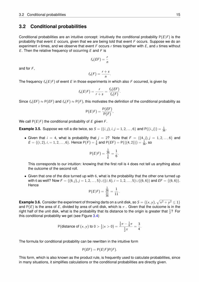
2? Forthis conditional probability we get (see Figure 3.4)
P(distance of (x , y) to 0 > 12 |x > 0) =
12π − 1
8π12π
= 34.
The formula for conditional probability can be rewritten in the intuitive form
P(EF ) = P(E |F )P(F ).
This form, which is also known as the product rule, is frequently used to calculate probabilities, sincein many situations, it simplifies calculations or the conditional probabilities are directly given.
16 Probability Models
1−1
Figure 3.4: Conditional probability that distance > 12 given that outcome is in right half of unit disk
Example 3.7. (Champions League [5]) Eight soccer teams reached the quarter finales, two teamsfrom each of the countries England, Germany, Italy and Spain. The matches are determined bydrawing lots, one by one. What is the probability that the two teams from the same country playagainst each other in all four matches? This probability can be calculated by counting all outcomesof the lottery. The total number of outcomes of the lottery, in which only teams from the same countryplay against each other, is 24 ·4! (for example, (E1, E2; G2, G1; I2, I1; S1, S2) is a possible outcome). Thetotal number of outcomes is 8!. Hence,
P(Only teams of the same country play against each other) = 24 · 4!8! . (3.2)
It is, however, easier to use conditional probabilities. Imagine that the first lot is drawn. Then, giventhat the first lot is drawn, the probability that the second lot is the other team of the same country is17 . Then the third lot is drawn. Given that first two lots are of the same country, the probability that thefourth one is of the same country as the third one is 1
5 , and so on. This immediately gives
P(Only teams of the same country play against each other) = 17 ·
15 ·
13,
which is indeed the same answer as (3.2).
The special case thatP(E |F ) = P(E ),
means that knowledge about the occurrence of event F has no effect on the probability of E . In otherwords, event E is independent of F . Substitution of P(E |F ) = P(EF )/P(F ) leads to the conclusionthat events E and F are independent if
P(EF ) = P(E )P(F ).
Example 3.8. (Independent experiments) The outcomes of n independent experiments can be mod-eled by the sample space S = S1 × S2 × · · · × Sn = (s1, ... , sn), s1 ∈ S1, ... , sn ∈ Sn, where Si is thesample space of experiment i . To reflect that the experiments are independent, the probability of theevent E = E1 × E2 × · · · × En = (s1, ... , sn), s1 ∈ E1, ... , sn ∈ En is defined as
P(E1 × E2 × · · · × En) = P(E1) · · ·P(En).
Example 3.9. (Coin tossing) Two fair coins are tossed. E is the event that the first coin turns upwith H and F is the event that both coins turn up with the same outcome. Are the events E and Findependent? Straightforward calculations yield
P(EF ) = P((H, H)) = 14,
P(E ) = P((H, H), (H, T )) = P((H, H)) + P((H, T )) = 12,
P(F ) = P((H, H), (T , T )) = 12,
so P(EF ) = P(E )P(F ), and thus E and F are independent.
3.2 Conditional probabilities 17
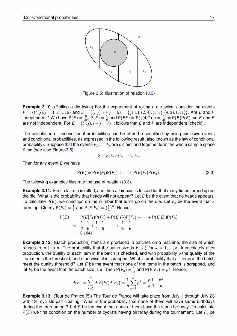
F1
F2 F3 F4
E
S
Figure 3.5: Illustration of relation (3.3)
Example 3.10. (Rolling a die twice) For the experiment of rolling a die twice, consider the eventsF = (4, j), j = 1, 2, ... , 6 and E = (i , j), i + j = 6 = (1, 5), (2, 4), (3, 3), (4, 2), (5, 1). Are E and Findependent? We have P(E ) = 5
36 , P(F ) = 16 and P(EF ) = P((4, 2)) = 1
36 6= P(E )P(F ), so E and Fare not independent. For E = (i , j), i + j = 7 it follows that E and F are independent (check!).
The calculation of unconditional probabilities can be often be simplified by using exclusive eventsand conditional probabilities, as expressed in the following result (also known as the law of conditionalprobability). Suppose that the events F1, ... , Fn are disjoint and together form the whole sample spaceS, so (see also Figure 3.5)
S = F1 ∪ F2 ∪ · · · ∪ Fn.
Then for any event E we have
P(E ) = P(E |F1)P(F1) + · · ·+ P(E |Fn)P(Fn). (3.3)
The following examples illustrate the use of relation (3.3).
Example 3.11. First a fair die is rolled, and then a fair coin is tossed for that many times turned up onthe die. What is the probability that heads will not appear? Let E be the event that no heads appears.To calculate P(E ), we condition on the number that turns up on the die. Let Fk be the event that kturns up. Clearly P(Fk) = 1
6 and P(E |Fk) =(1
2)k . Hence,
P(E ) = P(E |F1)P(F1) + P(E |F2)P(F2) + · · ·+ P(E |E6)P(F6)
= 12 ·
16 + 1
4 ·16 + · · ·+ 1
64 ·16
= 0.1641.
Example 3.12. (Batch production) Items are produced in batches on a machine, the size of whichranges from 1 to n. The probability that the batch size is k is 1
n for k = 1, ... , n. Immediately afterproduction, the quality of each item in the batch is checked, and with probability p the quality of theitem meets the threshold, and otherwise, it is scrapped. What is probability that all items in the batchmeet the quality threshold? Let E be the event that none of the items in the batch is scrapped, andlet Fk be the event that the batch size is k. Then P(Fk) = 1
n and P(E |Fk) = pk . Hence,
P(E ) =n∑
k=1P(E |Fk)P(Fk) = 1
n
n∑
k=1pk = p
n1− pn
1− p .
Example 3.13. (Tour de France [5]) The Tour de France will take place from July 1 through July 23with 180 cyclists participating. What is the probability that none of them will have same birthdaysduring the tournament? Let E be the event that none of them have the same birthday. To calculateP(E ) we first condition on the number of cyclists having birthday during the tournament. Let Fk be
18 Probability Models
the event that exactly k of them have birthday during the tournament. Then F0, ... , F180 are disjointevents. To calculate P(Fk), note that you can choose
(180k)
different groups of size k from the 180cyclists, and the probability each one in the group has his birthday during the tournament of 23 daysis( 23
365)k , while the probability that the other 180 − k cyclists do not have their birthday during the
tournament is(365−23
365)180−k . Hence,
P(Fk) =(
180k
)(23365
)k (365− 23365
)180−k, k = 0, 1, ... , 180,
Clearly P(E |F0) = 1, and
P(E |Fk) = 2323 ·
2223 · · ·
32− k + 123 , k = 1, ... , 23
and P(E |Fk) = 0 for k ≥ 24. Hence
P(E ) =180∑
k=0P(E |Fk)P(Fk) =
23∑
k=0P(E |Fk)P(Fk) = 0.8841.
In some applications, the probabilities P(E ), P(F ) and P(E |F ) are given, while we are interested inP(F |E ). This probability can then be calculated as follows
P((F |E ) = P(EF )P(E ) = P(E |F )P(F )
P(E ) .
This is also known as Bayes’ rule (see Section 8.3 in [5]).
Example 3.14. The reliability of a test for a certain disease is 99%. This means that the probabil-ity that the outcome of the test is positive for a patient suffering form the disease, is 99%, and it isnegative with probability 99% for a patient free from this disease. It is known that 0.1% of the pop-ulation suffers from this disease. Suppose that, for a certain patient, the test is positive. What isthe probability that this patient indeed suffers form this disease? Let E be the event that the test ispositive, and F is the event that the patient has the disease. Then we need to calculate P(F |E ). It isgiven that P(E |F ) = P(E c |F c) = 0.99, P(F ) = 0.001 and thus P(E ) = P(E |F )P(F ) + P(E |F c)P(F c) =0.99 · 0.001 + 0.01 · 0.999 = 0.01098. Hence
P(F |E ) = P(E |F )P(F )P(E ) = 0.99 · 0.001
0.01098 = 0.09.
Note that this number is much smaller than might have been suggested by the reliability of the test!
Exercise 6. (Problem 8.3 [5]) Every evening, two weather stations issue a weather forecast nextday. The weather forecasts of the two stations are independent of eachother. On average, theweather forecast of station 1 is correct in 90% of the cases, irrespective of the weather type. Thispercentage is 80% for station 2. On a given day, station 1 predicts sunny weather for the next day,whereas station 2 predicts rain. What is the probability that the weather forecast of station 1 will becorrect?
Exercise 7. (Problem 8.5 [5]) You simultaneously grab two balls at random from an urn containingtwo red balls, one blue ball and one green ball. What is the probability that you have grabbed twonon-red balls given that you have grabbed at least one non-red ball? What is the probability that youhave grabbed two non-red balls given that you have grabbed the green ball? Can you give an intuitiveexplanation of why the second probability is larger than the first one?
3.3 Discrete random variables 19
Exercise 8. (Problem 8.17 [5]) Two fair coins are tossed. Let A be the event that heads appearson the first coin and let B be the event that the coins display the same outcome. Are the events Aand B independent?
Exercise 9. (Problem 8.18 [5]) You have two identical boxes in front of you. One of the boxescontains 10 balls numbered 1 to 10 and the other box contains 25 balls numbered 1 to 25. Youchoose at random one of the boxes and pick a ball at random from the chosen box. What is theprobability of picking the ball with number 7 written on it?
Exercise 10. (Problem 8.19 [5]) A bag contains three coins. One coin is two-headed and the othertwo are normal. A coin is chosen at random from the bag and is tossed twice? What is the probabilityof getting two heads? If two heads appear, what is the inverse probability that the two-headed coinwas chosen?
3.3 Discrete random variables
A random variable is a function that assigns a numerical value to each outcome of an experiment.More precisely, it is a real-valued function on the sample space S. Clearly, it is often more convenientto do calculations with random variables than with outcomes of an experiment. It is common to usecapitals for random variables, such X and Y .
Example 3.15.
• X is the sum of the outcomes i and j of rolling a die twice, so X = i + j .
• Y is the maximum of the outcomes i and j of rolling a die twice, so Y = max(i , j).
• N is the number of flips of a coin until the first head.
• M is the number of times a machine fails during a working day.
• Z is the number of production orders that arrives during the week.
A discrete random variable X can only take (possibly infinitely many) discrete values, say x1, x2, ...,and the function
pj = P(X = xj), j = 1, 2, ... ,
is called the probability mass function or probability distribution of X .
Example 3.16.
• If X = i + j where i is the first and j the second roll of a die, then
P(X = k) = P(X = 14− k) = k − 136 , k = 2, ... , 7.
• If Y = max(i , j) where i is the first and j the second roll of a die, then
P(Y = k) = 2k − 136 , k = 1, ... , 6.
• If N is the number of flips until first H, with P(H) = 1− P(T ) = p,
P(N = n) = (1− p)n−1p, n = 1, 2, ...
20 Probability Models
For a random variable X with probability mass function pj = P(X = xj), j = 1, 2, ..., its expected value(or expectation or first moment or “centre of probability mass”) is defined as
E [X ] =∞∑
j=1xjpj ,
where we assume that the infinite sum exists. So the expected value of X is a weighted average ofpossible values of X . It is not the same, however, as the most probable value, nor is it restricted topossible values of X .
Example 3.17.
• If X is the number that turns up when rolling a die, then
E [X ] = 16 + 2
6 + · · ·+ 66 = 3.5.
• If N is the number of flips until the first Head, with P(H) = 1− P(T ) = p, then
E [N] =∞∑
n=1n(1− p)n−1p = 1
p .
For example, by repeatedly rolling a die, the average value of the numbers that turn up, gets closerand closer to 3.5 as the number of rolls increases. This is the law of large numbers for the expectedvalue. More general, if Xk is the outcome of the kth repetition of an experiment, then the average1n (X1 + · · ·+ Xn) over the first n repetitions converges with probability 1 to E (X ). Hence, the expectedvalue E (X ) can thus be interpreted as the long run average of X .
Example 3.18. Let Y be the total number that shows up by rolling a die twice. Then
E [Y ] =6∑
i=1
6∑
j=1(i + j) 1
36 = 7 = 2× 3.5,
so E [Y ] is two times the expected value of a single roll. This is no coincidence, since by writingY = X1 + X2 where X1 is first roll and X2 is second roll, we get
E [Y ] =6∑
i=1
6∑
j=1(i + j)P(X1 = i , X2 = j)
=6∑
i=1
6∑
j=1iP(X1 = i , X2 = j) +
6∑
i=1
6∑
j=1jP(X1 = i , X2 = j)
=6∑
i=1i
6∑
j=1P(X1 = i , X2 = j) +
6∑
j=1j
6∑
i=1P(X1 = i , X2 = j)
=6∑
i=1iP(X1 = i) +
6∑
j=1jP(X2 = j)
= E [X1] + E [X2] = 7.
Example 3.18 shows that E [X1 + X2] = E [X1] + E [X2] where X1 is the first roll of a die and X2 the
3.3 Discrete random variables 21
second one. This property is true in general. For any two random variables X and Y we have
E [X + Y ] =∞∑
i=1
∞∑
j=1(xi + yj)P(X = xi , Y = yj)
=∞∑
i=1
∞∑
j=1xiP(X = xi , Y = yj) +
∞∑
i=1
∞∑
j=1yjP(X = xi , Y = yj)
=∞∑
i=1xi
∞∑
j=1P(X = xi , Y = yj) +
∞∑
j=1yj
∞∑
i=1P(X = xi , Y = yj)
=∞∑
i=1xiP(X = xi) +
∞∑
j=1yjP(Y = yj),
soE [X + Y ] = E [X ] + E [Y ] .
Hence the expectation of the sum is the sum of the expectations. More general, for any number ofrandom variables X1, X2, ... , Xn,
E [X1 + · · ·+ Xn] = E [X1] + · · ·+ E [Xn] .
Example 3.19.
• (Tour de France [5]) What is the expected number of joint birth days during the tournament? LetXi be 1 if there is a joint birthday on day i of the tournament, and 0 otherwise. If none or exactlyone of the cyclists has its birthday on day i , then day i is not a joint birth day, so Xi = 0. Hence,
P(Xi = 0) = 1− P(Xi = 1) =(
364365
)180+ 180 · 1
365
(364365
)179= 0.912,
so E [Xi ] = 0 ·P(Xi = 0) + 1 ·P(Xi = 1) = P(Xi = 1), and the expected number of joint birthdaysis
E [X1] + E [X2] + · · ·+ E [X23] = 23(1− 0.912) = 2.02.
• (Tall children [5]) Suppose that n children of different lengths are placed in line at random. Youstart with the first child and then walk till the end of the line. When you encounter a taller childthan seen so far, she will join you. Let X be the number that joins you. What is E (X )? Let Xibe 1 if child i in line joins you, and 0 otherwise. Then X = X1 + · · · + Xn. Child i joins you ifshe is the tallest among the first i children in line. Since the first i are ordered at random, theprobability that the tallest is at place i is 1
i . Hence
P(Xi = 1) = 1− P(Xi = 0) = 1i ,
and E [Xi ] = 0 · P(Xi = 0) + 1 · P(Xi = 1) = 1i , thus
E [X ] = E [X1] + E [X2] + · · ·+ E [Xn] = 1 + 12 + · · ·+ 1
n .
A convenient property is that for any function g(x), the expectation of the random variable Y = g(X )can be directly calculated as
E [Y ] = E [g(X )] =∑
xi
g(xi)P(X = xi) =∑
xi
g(xi)pi .
22 Probability Models
Example 3.20. Let N be the number of flips of a fair coin until the first Head. Then P(N = i) = 12i and
E (N) = 2 (see Example 3.17). For g(x) = x2, we get
E [g(N)] = E[N2] =
∞∑
i=1i2 1
2i = 6.
In general, E [g(X )] 6= g(E [X ]) (for the example above, we have E[N2] = 6 and (E [N])2 = 22 = 4).
However, linear functions g(x) = ax + b are an exception, since for any constants a and b,
E [aX + b] =∑
xi
(axi + b)P(X = xi)
= a∑
xi
xiP(X = xi) + b∑
xi
P(X = xi)
= aE [X ] + b. (3.4)
An important measure for the spread of the possible values of X is the variance, defined as theexpected squared deviation from the mean,
Var [X ] = E[(X − E (X ))2] .
In many situations it is, however, more convenient to consider the standard deviation of X , which isthe square root of the variance,
σ[X ] =√
var(X ).
This quantity has the same units as E (X ). The variance Var [X ] can be calculated as
Var [X ] = E[(X − E [X ])2]
=∑
xi
(xi − E [X ])2 P(X = xi)
=∑
xi
(x2
i − 2E [X ] xi + (E [X ])2)P(X = xi)
=∑
xi
x2i P(X = xi)− 2E [X ]
∑
xi
xiP(X = xi) + (E [X ])2∑
xi
P(X = xi)
= E[X 2]− 2E [X ] E [X ] + (E [X ])2
= E[X 2]− (E [X ])2
and for Y = aX + b we then get
Var [aX + b] =∞∑
j=1(axj + b − (aE [X ] + b))2pj
= a2∞∑
j=1(xj − E [X ])2pj
= a2Var [X ] .
Example 3.21. Let N be the number of flips of a fair coin until the first head. Then P(N = i) = 12i ,
E (N) = 2 and E (N2) = 6 (see Example 3.20), so
Var [N] = E[N2]− (E [N])2 = 6− 4 = 2.
For the number of tails hat appear before the first head, which is N − 1, we get
Var [N − 1] = Var [N] = 2.
3.3 Discrete random variables 23
We have seen that E [X + Y ] = E [X ]+E [Y ] for any two random variables X and Y . However, usuallyVar [X + Y ] is not equal to Var [X ]+Var [Y ], though it is true for independent random random variablesX and Y . This is shown below.
The random variables X and Y are independent if for all x , y , the events X ≤ x and Y ≤ y areindependent, thus
P(X ≤ x , Y ≤ y) = P(X ≤ x)P(Y ≤ y)
or equivalently, when X and Y are discrete random variables,
P(X = x , Y = y) = P(X = x)P(Y = y).
It is clear that when X and Y are independent, then so are the random variables f (X ) and g(Y ) forany functions f (x) and g(y). Further, if X and Y are independent, then
E [XY ] =∞∑
i=1
∞∑
j=1xiyjP(X = xi , Y = yj)
=∞∑
i=1
∞∑
j=1xiyjP(X = xi)P(Y = yj)
=∞∑
i=1xiP(X = xi)
∞∑
j=1yjP(Y = yj)
= E [X ] E [Y ] ,
and as a consequence,
Var [X + Y ] = E[(X + Y )2]− (E [X ] + E [Y ])2
= E[X 2 + 2XY + Y 2]− ((E [X ])2 + 2E [X ] E [Y ] + (E [Y ])2)
= E[X 2]+ 2E [XY ] + E
[Y 2]− ((E [X ])2 + 2E [X ] E [Y ] + (E [Y ])2)
= E[X 2]+ 2E [X ] E [Y ] + E
[Y 2]− ((E [X ])2 + 2E [X ] E [Y ] + (E [Y ])2)
= E[X 2]− (E [X ])2 + E
[Y 2]− (E [Y ])2
= Var [X ] + Var [Y ] .
So the variance of the sum is the sum of the variances, provided the random variable are independent!
Suppose that the random variables X1, ... , Xn have the same probability distribution, so in particular
E [X1] = · · · = E [Xn] , Var [X1] = · · · = Var [Xn] .
For the mean of the sum X1 + · · ·+ Xn we get
E [X1 + · · ·+ Xn] = E [X1] + · · ·+ E [Xn] = nE [X1] ,
and if X1, ... , Xn are independent, then also
Var [X1 + · · ·+ Xn] = Var [X1] + · · ·+ Var [Xn] = nVar [X1] .
Hence, for the standard deviation of the sum of X1, ... , Xn we obtain
σ[X1 + · · ·+ Xn] =√
nσ[X1].
So the mean of X1 + · · · + Xn grows linear in n, but its standard increases more slowly at a rateof√
n as n tends to infinity. The latter is due to cancelation of random errors (i.e., some of the Xiwill be greater than their mean, whereas others will be smaller). This property is also known as thesquare-root law or variability pooling.
24 Probability Models
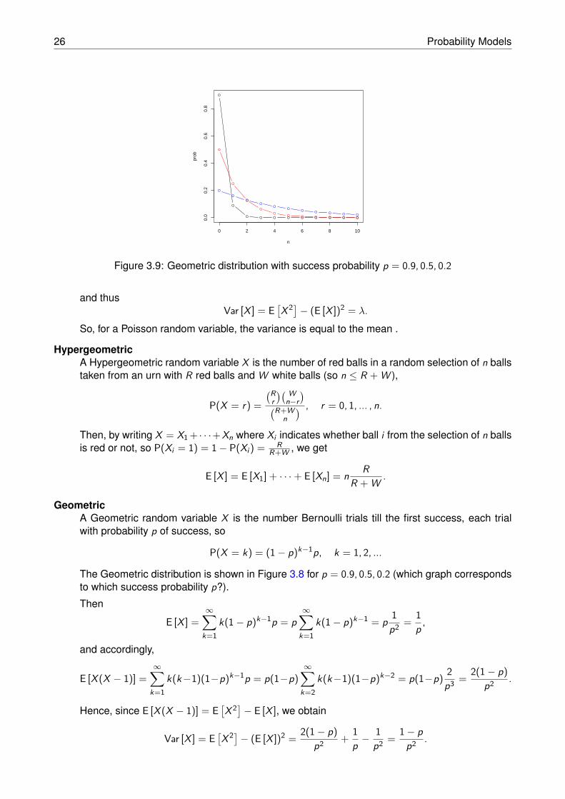
Stock level
Day
0 1 2
1
2
3 Base-stock
3
Figure 3.6: Base-stock policy with a base-stock level of 3 products
Example 3.22. (Variability pooling) A company offers 100 configurations of a product, all requiringcomponent A. The mean demand per day for each configuration is 10 products, with a standarddeviation of 3 products. To satisfy demand, the company uses a base-stock policy: all demand thatoccurs during the day is immediately ordered at the supplier and arrives at the beginning of the nextday. Hence the stock level at the beginning of each day is always the same, and referred to as thebase-stock level, see Figure 3.6.
The company sets the base-stock level equal to the mean demand plus a safety stock which is 2times the standard deviation of the demand. The rational is that for this stock level, approximately95% of the demand can be satisfied from stock. The company considers two options to keep productson stock: (i) Stock all product configurations, (ii) Stock only components A and assemble to order.What is the total stock level of components A for these two options? For option (i), the stock level foreach configuration is 10 + 2 · 3 = 16. Hence, since we have 100 configurations, the total stock levelof components A is 100 · 16 = 1600. For option (ii), note that the mean total demand for componentsA is 100 · 10 and the standard deviation of the total demand is 3
√100. Hence, the total stock level for
components A is 100 · 10 + 2 ·√
100 · 3 = 1060, which is a reduction of more than 30% in stock levelcompared to option (i)!
Below we list some important discrete random variables.
BernoulliA Bernoulli random variable X with success probability p, takes the values 0 and 1 with proba-bility
P(X = 1) = 1− P(X = 0) = p.Then
E [X ] = 0 · P(X = 0) + 1 · P(X = 1) = pE[X 2] = 02 · P(X = 0) + 12 · P(X = 1) = p
andVar [X ] = E
[X 2]− (E [X ])2 = p − p2 = p(1− p).
BinomialA Binomial random variable X is the number of successes in n independent Bernoulli trialsX1, ... , Xn, each with probability p of success,
P(X = k) =(
nk
)pk(1− p)n−k , k = 0, 1, ... n.
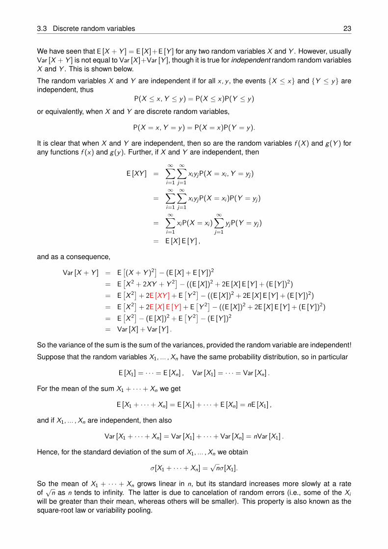
The Binomial distribution is shown in Figure 3.7 for n = 20 and p = 0.25, 0.5, 0.65 (which graphcorresponds to which parameter p?). Since X = X1 + · · ·+ Xn, we get
E [X ] = E [X1] + · · ·+ E [Xn] = np, Var [X ] = Var [X1] + · · ·+ Var [Xn] = np(1− p).
3.3 Discrete random variables 25
0 5 10 15 20
0.00
0.05
0.10
0.15
0.20
n
prob
Figure 3.7: Binomial probability distribution with parameters n = 20 and p = 0.25, 0.5, 0.65
0 5 10 15 20
0.0
0.1
0.2
0.3
n
prob
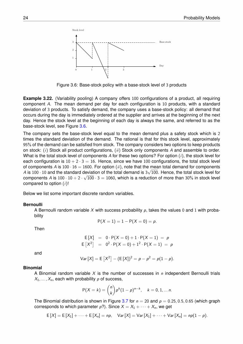
Figure 3.8: Poisson distribution with parameter λ = 1, 5, 10
PoissonA Poisson random variable X with parameter λ > 0, has probability distribution
P(X = k) = e−λλk
k! , k = 0, 1, 2, ...
The Poisson distribution is shown in Figure 3.8 for λ = 1, 5, 10 (which graph corresponds towhich parameter λ?).
Then
E [X ] =∞∑
k=0kP(X = k) =
∞∑
k=1ke−λλ
k
k! = λe−λ∞∑
k=1
λk−1
(k − 1)! = λe−λeλ = λ
and accordingly,
E [X (X − 1)] =∞∑
k=0k(k − 1)P(X = k) =
∞∑
k=2k(k − 1)e−λλ
k
k! = λ2e−λ∞∑
k=2
λk−2
(k − 2)! = λ2.
Hence, since E [X (X − 1)] = E[X 2]− E [X ], we get
E[X 2] = λ2 + λ
26 Probability Models
0 2 4 6 8 10
0.0
0.2
0.4
0.6
0.8
n
prob
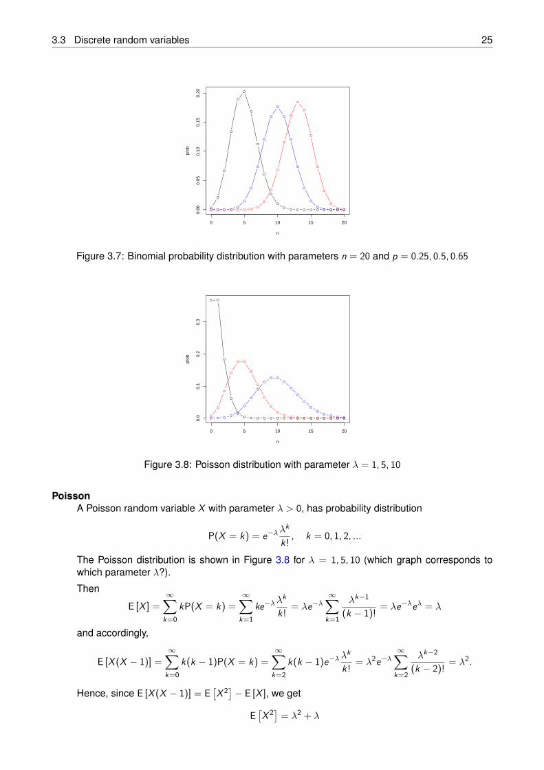
Figure 3.9: Geometric distribution with success probability p = 0.9, 0.5, 0.2
and thusVar [X ] = E
[X 2]− (E [X ])2 = λ.
So, for a Poisson random variable, the variance is equal to the mean .
HypergeometricA Hypergeometric random variable X is the number of red balls in a random selection of n ballstaken from an urn with R red balls and W white balls (so n ≤ R + W ),
P(X = r) =(R
r)( W
n−r)
(R+Wn) , r = 0, 1, ... , n.
Then, by writing X = X1 + · · ·+Xn where Xi indicates whether ball i from the selection of n ballsis red or not, so P(Xi = 1) = 1− P(Xi) = R
R+W , we get
E [X ] = E [X1] + · · ·+ E [Xn] = n RR + W .
GeometricA Geometric random variable X is the number Bernoulli trials till the first success, each trialwith probability p of success, so
P(X = k) = (1− p)k−1p, k = 1, 2, ...
The Geometric distribution is shown in Figure 3.8 for p = 0.9, 0.5, 0.2 (which graph correspondsto which success probability p?).
Then
E [X ] =∞∑
k=1k(1− p)k−1p = p
∞∑
k=1k(1− p)k−1 = p 1
p2 = 1p ,
and accordingly,
E [X (X − 1)] =∞∑
k=1k(k−1)(1−p)k−1p = p(1−p)
∞∑
k=2k(k−1)(1−p)k−2 = p(1−p) 2
p3 = 2(1− p)p2 .
Hence, since E [X (X − 1)] = E[X 2]− E [X ], we obtain
Var [X ] = E[X 2]− (E [X ])2 = 2(1− p)
p2 + 1p −
1p2 = 1− p
p2 .
3.3 Discrete random variables 27
Negative binomialA Negative binomial random variable X is the number Bernoulli trials till the r th success, eachtrial with probability p of success,
P(X = k) =(
k − 1r − 1
)(1− p)k−r pr , k = r , r + 1, ...
We can write X = X1+· · ·Xr , where Xi are independent and Geometric with success probabilityp, so
E [X ] = E [X1] + ... + E [Xr ] = rp , Var [X ] = Var [X1] + ... Var [Xr ] = r(1− p)
p2 .
Remark 3.1. (Relation between Binomial and Poisson) The total number of successes X in n inde-pendent Bernoulli trials, each with success probability p, is Binomial distributed, so
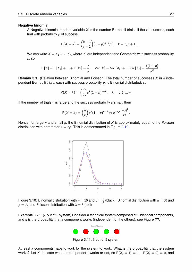
P(X = k) =(
nk
)pk(1− p)n−k , k = 0, 1, ... n.
If the number of trials n is large and the success probability p small, then
P(X = k) =(
nk
)pk(1− p)n−k ≈ e−np (np)k
k! .
Hence, for large n and small p, the Binomial distribution of X is approximately equal to the Poissondistribution with parameter λ = np. This is demonstrated in Figure 3.10.
0 5 10 15 20
0.00
0.05
0.10
0.15
0.20
0.25
n
prob
Figure 3.10: Binomial distribution with n = 10 and p = 12 (black), Binomial distribution with n = 50 and
p = 110 and Poisson distribution with λ = 5 (red)
Example 3.23. (k out of n system) Consider a technical system composed of n identical components,and q is the probability that a component works (independent of the others), see Figure ??.
3 out of 5 system
Figure 3.11: 3 out of 5 system
At least k components have to work for the system to work. What is the probability that the systemworks? Let Xi indicate whether component i works or not, so P(Xi = 1) = 1 − P(Xi = 0) = q, and
28 Probability Models
let X be the total number of components that work, X = X1 + · · · + Xn. Then X is Binomial withparameters n and q, and the probability Q that the system works is equal to
Q = P(X ≥ k) =n∑
i=kP(X = i) =
n∑
i=k
(ni
)qi(1− q)n−i .
Example 3.24. (Coincidence) Two people, complete strangers to one another, both living in Eind-hoven, meet each other in the train. Each has approximately 200 acquaintances in Eindhoven. Whatis the probability that these two strangers have an acquaintance in common? Eindhoven has (approx-imately) 200000 inhabitants. To find the desired probability, imagine that the acquaintances of the firststranger are colored red, and all other inhabitants of Eindhoven are colored white. Assuming that theacquaintances of the second strangers are randomly distributed among the population of Eindhoven,then the question can be translated into: What is the probability by randomly selecting 200 inhabitantsthat at least one of them is red? Let X denote the number of red inhabitants found in this randomselection. Then X is Hypergeometric with parameters n = R = 200 and W = 200000− 200. So
P(X ≥ 1) = 1− P(X = 0) = 1−(200000−200
200)
(200000200
) = 1− 0.818 = 0.182.
So, actually, it is quite likely to have an acquaintance in common!
Example 3.25. Consider a workstation perform tasks. The time to perform a task takes exactly 1 timeunit. Each task is checked after completion. With probability p the task is done correctly. If not, thetask has to be repeated till it is eventually correct. What is the distribution of the total time till the taskhas been done correctly? Let X denote the total time till correct completion, so it is the total effectivetask time. Clearly, X is Geometric with success probability p,
P(X = k time units) = (1− p)k−1p, k = 1, 2, ...
Hence, the mean and variance of X are given by
E [X ] = 1p , Var [X ] = 1− p
p2 .
Exercise 11. (Problem 9.3 [5]) A bag contains three coins. One coin is two-headed and the othertwo are normal. A coin is chosen at random from the bag and is tossed twice. Let the random variableX denote the number of heads obtained. What is the probability mass function of X?
Exercise 12. (Problem 9.7 [5]) You throw darts at a circular target on which two concentric circlesof radius 1 cm and 3 cm are drawn. The target itself has a radius of 5 cm. You receive 15 points forhitting the target inside the smaller circle, 8 points for hitting the middle annular region, and 5 pointsfor hitting the outer annular region. The probability of hitting the target at all is 0.75. If the dart hits thetarget, the hitting point is a completely random point on the target. Let the random variable X denotethe number of points scored on a single throw of the dart. What is the expected value of X?
Exercise 13. (Problem 9.15 [5]) What is the expected number of distinct birthdays within a ran-domly formed group of 100 persons? What is the expected number of children in a class with rchildren sharing a birthday with some child in another class with s children? Assume that the yearhas 365 days and that all possible birthdays are equally likely.
Exercise 14. (Problem 9.17 [5]) What is the expected number of times that two consecutivenumbers will show up in a lotto drawing of six different numbers from the numbers 1, 2, ... , 45?
3.4 Continuous random variables 29
Exercise 15. (Problem 9.33 [5]) In the final of the World Series Baseball, two teams play a seriesconsisting of at most seven games until one of the two teams has won four games. Two unevenlymatched teams are pitted against each other and the probability that the weaker team will win anygiven game is equal to 0.45. Assuming that the results of the various games are independent of eachother, calculate the probability of the weaker team winning the final. What are the expected value andthe standard deviation of the number of games the final will take?
Exercise 16. (Problem 9.42 [5]) In European roulette the ball lands on one of the numbers0, 1, ... , 36 in every spin of the wheel. A gambler offers at even odds the bet that the house num-ber 0 will come up once in every 25 spins of the wheel. What is the gambler’s expected profit perdollar bet?
Exercise 17. (Problem 9.44 [5]) In the Lotto 6/45 six different numbers are drawn at random fromthe numbers 1, 2, ... , 45. What are the probability mass functions of the largest number drawn and thesmallest number drawn?
Exercise 18. (Problem 9.46 [5]) A fair coin is tossed until heads appears for the third time. Letthe random variable X be the number of tails shown up to that point. What is the probability massfunction of X? What are the expected value and standard deviation of X?
Exercise 19. (Homework exercises 1) Consider a bin with 10 balls: 5 are red, 3 are green and 2are blue. You randomly pick 3 balls from the bin. What is the probability that each of these balls hasa different color?
Exercise 20. (Homework exercises 2) Jan and Kees are in a group of 12 people that are seatedrandomly at a round table (with 12 seats). What is the probability that Jan and Kees are seated nextto each other?
3.4 Continuous random variables
A continuous random variable X can take continuous values x ∈ R. Its probability distribution functionis of the form
F (x) = P(X ≤ x) =∫ x
−∞f (y)dy , (3.5)
where the function f (x) satisfies
f (x) ≥ 0 for all x ,∫ ∞
−∞f (x)dx = 1.
the function f (x) is called the probability density of X . The probability that X takes a value in theinterval (a, b] can then be calculated as
P(a < X ≤ b) = P(X ≤ b)− P(X ≤ a)
=∫ b
−∞f (x)dx −
∫ a
−∞f (x)dx
=∫ b
af (x)dx ,
and the probability that X takes a specific value b is equal to 0, since
P(X = b) = lima↑b
P(a < X ≤ b) = lima↑b
∫ b
af (x)dx =
∫ b
bf (x)dx = 0.
30 Probability Models
The function f (x) can be interpreted as the density of the probability mass, that is, we have for small∆ > 0 that
P(x < X ≤ x + ∆) =∫ x+∆
xf (y)dy ≈ f (x)∆,
from which we can conclude (or from (3.5)) that f (x) is the derivative of the distribution function F (x),
f (x) = ddx F (x).
Example 3.26. (Uniform)
• The Uniform random variable X on the interval [a, b] has density
f (x) = 1
b−a a ≤ x ≤ b,0 else.
and the distribution function is given by
F (x) =
0 x ≤ 0,x 0 < x ≤ 1,1 x > 1.
• The Uniform random variable X on the interval [a, b] has density
f (x) = 1
b−a a ≤ x ≤ b,0 else.
A simple recipe for finding the density is to first determine the distribution F (x) = P(X ≤ x) (which isin many cases easier) and then differentiate F (x).
Example 3.27.
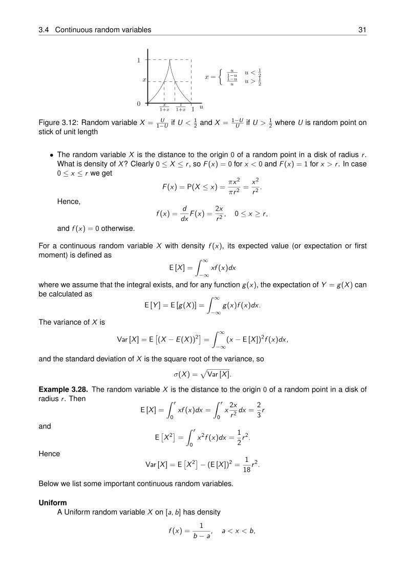
• (Example 10.1 in [5]) Break a stick of length 1 at random point in two pieces and let X be theratio of shorter piece and longer piece (so 0 < X < 1). What is F (x) = P(X ≤ x) for 0 ≤ x ≤ 1?Let U be the point where the stick is broken. Then X = U
1−U if U < 12 and X = 1−U
U otherwise.Hence the event X ≤ x is valid for all U satisfying 0 ≤ U ≤ x
1+x or 11+x ≤ U ≤ 1 (see Figure
3.12), so
F (x) = P(X ≤ x) = P(
U ≤ x1 + x
)+P
(U ≥ 1
1 + x
)= x
1 + x +1− 11 + x = 2x
1 + x , 0 < x < 1.
The density of X is obtained by taking the derivative of F (x), yielding
f (x) = ddx F (x) = 2
(1 + x)2 , 0 < x < 1.
• Let X = − ln(U)/λ where U is random on (0, 1). What is density of X? Clearly X ≥ 0, soF (x) = 0 for x < 0. For x ≥ 0 we get
F (x) = P(X ≤ x) = P(− ln(U)/λ ≤ x) = P(ln(U) ≥ −λx) = P(U ≥ e−λx ) = 1− e−λx .
Hence,
f (x) = ddx F (x) = λe−λx ), x ≥ 0,
and f (x) = 0 for x < 0. This distribution is called the Exponential distribution.
3.4 Continuous random variables 31
x
x1+x
11+x u
x =
u
1−u u < 12
1−uu u > 1
2
1
10
Figure 3.12: Random variable X = U1−U if U < 1
2 and X = 1−UU if U > 1
2 where U is random point onstick of unit length
• The random variable X is the distance to the origin 0 of a random point in a disk of radius r .What is density of X? Clearly 0 ≤ X ≤ r , so F (x) = 0 for x < 0 and F (x) = 1 for x > r . In case0 ≤ x ≤ r we get
F (x) = P(X ≤ x) = πx2
πr2 = x2
r2 .
Hence,
f (x) = ddx F (x) = 2x
r2 , 0 ≤ x ≥ r ,
and f (x) = 0 otherwise.
For a continuous random variable X with density f (x), its expected value (or expectation or firstmoment) is defined as
E [X ] =∫ ∞
−∞xf (x)dx
where we assume that the integral exists, and for any function g(x), the expectation of Y = g(X ) canbe calculated as
E [Y ] = E [g(X )] =∫ ∞
−∞g(x)f (x)dx .
The variance of X is
Var [X ] = E[(X − E (X ))2] =
∫ ∞
−∞(x − E [X ])2f (x)dx ,
and the standard deviation of X is the square root of the variance, so
σ(X ) =√
Var [X ].
Example 3.28. The random variable X is the distance to the origin 0 of a random point in a disk ofradius r . Then
E [X ] =∫ r
0xf (x)dx =
∫ r
0x 2x
r2 dx = 23 r
andE[X 2] =
∫ r
0x2f (x)dx = 1
2 r2.
HenceVar [X ] = E
[X 2]− (E [X ])2 = 1
18 r2.
Below we list some important continuous random variables.
UniformA Uniform random variable X on [a, b] has density
f (x) = 1b − a , a < x < b,
32 Probability Models
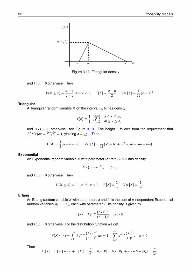
f(x)
a b xm
h = 2b−a
Figure 3.13: Triangular density
and f (x) = 0 otherwise. Then
P(X ≤ x) = x − ab − a , a < x < b, E [X ] = a + b
2 , Var [X ] = 112(b − a)2.
TriangularA Triangular random variable X on the interval [a, b] has density
f (x) =
h x−am−a a ≤ x ≤ m,
h b−xb−m m ≤ x ≤ b,
and f (x) = 0 otherwise, see Figure 3.13. The height h follows from the requirement that∫ ba f (x)dx = (b−a)h
2 = 1, yielding h = 2b−a . Then
E [X ] = 13(a + b + m), Var [X ] = 1
18(a2 + b2 + m2 − ab − am − bm).
ExponentialAn Exponential random variable X with parameter (or rate) λ > 0 has density
f (x) = λe−λx , x > 0,
and f (x) = 0 otherwise. Then
P(X ≤ x) = 1− e−λx , x > 0, E [X ] = 1λ
, Var [X ] = 1λ2 .
ErlangAn Erlang random variable X with parameters n and λ, is the sum of n independent Exponentialrandom variables X1, ... , Xn, each with parameter λ. Its density is given by
f (x) = λe−λx (λx)n−1
(n − 1)! , x > 0,
and f (x) = 0 otherwise. For the distribution function we get
P(X ≤ x) =∫ x
0λe−λx (λx)n−1
(n − 1)!dx = 1−n−1∑
i=0e−λx (λx)i
(i)! , x > 0.
ThenE [X ] = E [X1] + · · ·+ E [Xn] = n
λ, Var [X ] = Var [X1] + · · ·+ Var [Xn] = n
λ2 .
3.4 Continuous random variables 33
GammaA Gamma random variable X with parameters α > 0 and λ > 0, has density
f (x) = 1Γ(α)λ
αxα−1e−λx , x > 0,
and f (x) = 0 otherwise, where Γ(α) is the gamma function,
Γ(α) =∫ ∞
0e−y yα−1dy , α > 0.
ThenE [X ] = α
λ, Var [X ] = α
λ2 .
NormalA Normal random variable X with parameters µ and σ > 0, has density
f (x) = 1σ√
2πe−
12 (x−µ)2/σ2 , −∞ < x <∞.
ThenE (X ) = µ, var(X ) = σ2.
The density f (x) is denoted as N(µ,σ2) density.
Standard NormalA Standard Normal random variable X is a Normal random variable with mean µ = 0 andstandard deviation σ = 1. So it has the N(0, 1) density,
f (x) = φ(x) = 1√2π
e−12 x2
and
P(X ≤ x) = Φ(x) = 1√2π
∫ x
−∞e−
12 y2dy .
The Exponential distribution has some remarkable properties.
Property 3.3. (Exponential)
• Memoryless: For all t, s > 0, we have (see Figure 3.14)
P(X > t + s|X > s) = P(X > t). (3.6)
s s+ tt
X
Figure 3.14: Exponential X overshooting s with more than t
Thinking of X as the lifetime of a component, then this property states that, if at time s thecomponent is still working, then its remaining lifetime is again Exponential with exactly the samemean as a new component. In other words, used is as good as new! This memoryless property
34 Probability Models
is important in many application and can be straightforwardly derived from the definition ofconditional probabilities,
P(X > t + s|X > s) = P(X > t + s, X > s)P(X > s)
= P(X > t + s)P(X > s)
= e−λ(t+s)
e−λs
= e−λt .
An alternative form of (3.6) is that for small ∆ > 0
P(X ≤ s + ∆|X > s) = 1− e−λ∆ ≈ λ∆, (3.7)
stating that, when the component is operational at time s, it will fail in the next time interval ∆with probability λ∆.
• Minimum: Let X1 and X2 be two independent Exponential random variables with rates λ1 andλ2. Then we obtain for the distribution of the minimum of the two,
P(min(X1, X2) ≤ x) = 1− P(min(X1, X2) > x)= 1− P(X1 > x , X2 > x)= 1− P(X1 > x)P(X2 > x)= 1− e−(λ1+λ2)x .
Hence, the minimum of X1 and X2 is again Exponential, and the rate of the minimum is the sumof the rates λ1 and λ2.
Remark 3.2. By integrating the gamma function by parts we obtain
Γ(α) = (α− 1)Γ(α− 1).
So, if α = n, thenΓ(n) = (n − 1)Γ(n − 1) = · · · = (n − 1)!Γ(1) = (n − 1)!,
since Γ(1) = 1. Hence, the Gamma distribution with parameters n and λ is the same as the Erlangdistribution.
The Normal distribution has the following useful properties.
Property 3.4. (Normal)
• Linearity: If X is Normal, then aX + b is Normal. This can be shown by calculating
P(aX + b ≤ x) = P(X ≤ x − ba ) =
∫ x−ba
−∞
1σ√
2πe−
12 (y−µ)2/σ2dy ,
where we assumed that a > 0 (but the same calculations can be done for a < 0). Substitutingz = ay + b yields
P(aX + b ≤ x) =∫ x
−∞
1aσ√
2πe−
12 (z−(aµ+b))2/(aσ)2dz ,
from which we can conclude that aX + b is Normal with parameters aµ+ b and aσ.
• Additivity: If X and Y are independent and Normal, then X + Y is Normal.
3.4 Continuous random variables 35
• Excess probability: The probability that a Normal random variable X lies more than z timesthe standard deviations above its mean is
P(X ≥ µ+ zσ) = 1− P(X ≤ µ+ zσ) = 1− P(X − µσ≤ z) = 1− Φ(z),
since X−µσ is Standard Normal.
• Percentiles: The 100p% percentile zp of the Standard Normal distribution is the unique point zpfor which
Φ(zp) = p.
For example, for p = 0.95 we have z0.95 = 1.64, and z0.975 = 1.96 for p = 0.975.
We conclude this section by the concept of failure rate for positive random variables. Thinking of X asthe lifetime of a component, then the probability that the component will fail in the next ∆ time unitswhen it reached the age of x time units, is equal to
P(X ≤ x + ∆|X > x) = P(x < X ≤ x + ∆)P(X > x) ≈ f (x)∆
1− F (x) .
Dividing this probability by ∆ yields the rate r(x) at which the component will fail at time x given thatit reached time x . This rate is called the failure rate or hazard rate of X , and it given by
r(x) = f (x)1− F (x) .
Example 3.29. (Exponential) If X is Exponential with rate λ, then (see also (3.7))
r(x) = f (x)1− F (x) = λe−λx
e−λx = λ.
Hence, the failure rate of an Exponential random variable is constant: at any point in time the compo-nent is equally likely to fail, or in other words, the coomponents is always as good as new. In fact, thisis the only distribution for which the failure rate is constant. In practice, however, many componentshave a bath-tube failure rate, reflecting that initially and at the end of the lifetime of a component ishigher than average.
Exercise 21. (Problem 10.1 [5]) The life time of an appliance is a continuous random variable Xand has a probability density f (x) of the form f (x) = c(1 + x)âĹŠ3 for x > 0 and f (x) = 0 otherwise.What is the value of the constant c? Find P(X ≤ 0.5), P(0.5 < X ≤ 1.5) and P(0.5 < X ≤ 1.5|X > 0.5).
Exercise 22. (Problem 10.3 [5]) Sizes of insurance claims can be modeled by a continuousrandom variable with probability density f (x) = 1
50(10 − x) for 0 < x < 10 and f (x) = 0 otherwise.What is the probability that the size of a particular claim is larger than 5 given that the size exceeds2?
Exercise 23. (Problem 10.4 [5]) The lengths of phone calls (in minutes) made by a travel agentcan be modeled as a continuous random variable with probability density f (x) = 0.25e−0.25x for x > 0.What is the probability that a particular phone call will take more than 7 minutes?
Exercise 24. (Problem 10.5 [5]) Let X be a positive random variable with probability densityfunction f (x). Define the random variable Y by Y = X 2. What is the probability density function ofY ? Also, find the density function of the random variable W = V 2 if V is a number chosen at randomfrom the interval (−a, a) with a > 0.
36 Probability Models
Exercise 25. (Problem 10.8 [5]) A stick of unit length is broken at random into two pieces. Let therandom variable X represent the length of the shorter piece. What is the probability density of X?Also, use the probability distribution function of X to give an alternative derivation of the probabilitydensity of the random variable X/(1− X ), which is the ratio of the length of the shorter piece to thatof the longer piece.
Exercise 26. (Problem 10.11 [5]) The javelin thrower Big John throws the javelin more than xmeters with probability P(x), where P(x) = 1 for 0 ≤ x < 50, P(x) = 1200−(x−50)2
1200 for 50 ≤ x < 80,P(x) = (90−x)2
400 for 80 ≤ x < 90, and P(x) = 0 for x ≥ 90. What is the expected value of the distancethrown in his next shot?
Exercise 27. (Problem 10.19 [5]) A point Q is chosen at random inside a sphere with radius r .What are the expected value and the standard deviation of the distance from the center of the sphereto the point Q?
Exercise 28. (Problem 10.20 [5]) The lifetime (in months) of a battery is a random variable Xsatisfying P(X ≤ x) = 0 for x < 5, P(X ≤ x) = [(x −5)3 +2(x −5)]/12 for 5 ≤ x < 7 and P(X ≤ x) = 1for x ≥ 7. What are the expected value and the standard deviation of X?
Exercise 29. (Problem 10.23 [5]) In an inventory system, a replenishment order is placed whenthe stock on hand of a certain product drops to the level s, where the reorder point s is a given positivenumber. The total demand for the product during the lead time of the replenishment order has theprobability density f (x) = λe−λx for x > 0. What are the expected value and standard deviation ofthe shortage (if any) when the replenishment order arrives?
Exercise 30. (Problem 10.27 [5]) The lifetime of a light bulb has an uniform probability density on(2, 12). The light bulb will be replaced upon failure or upon reaching the age 10, whichever occursfirst. What are the expected value and the standard deviation of the age of the light bulb at the timeof replacement?
Exercise 31. (Problem 10.28 [5]) A rolling machine produces sheets of steel of different thickness.The thickness of a sheet of steel is uniformly distributed between 120 and 150 millimeters. Any sheethaving a thickness of less than 125 millimeters must be scrapped. What are the expected value andthe standard deviation of a non-scrapped sheet of steel?
Exercise 32. (Problem 10.30 [5]) Limousines depart from the railway station to the airport from theearly morning till late at night. The limousines leave from the railway station with independent inter-departure times that are exponentially distributed with an expected value of 20 minutes. Supposeyou plan to arrive at the railway station at three o’clock in the afternoon. What are the expected valueand the standard deviation of your waiting time at the railway station until a limousine leaves for theairport?
Exercise 33. (Homework exercises 12) The lifetimes of two components in an electronic systemare independent random variables X1 and X2, where X1 and X2 are exponentially distributed with anexpected value of 2 respectively 3 time units. Let random variable Y denote the time between thefirst failure and the second failure. What is the probability density distribution f (y) of Y ?
Exercise 34. (Homework exercises 14) Consider an equilateral triangle (gelijkzijdige driehoek).Denote the length of each of the edges by X , where X is a continuous variable with a uniform densityover interval (1, 3). What is the expected area of the equilateral triangle?
3.5 Central limit theorem 37
3.5 Central limit theorem
One of the most beautiful and powerful results in probability is the Central Limit Theorem. Considerindependent random variables X1, X2, ..., all with the same distribution with mean µ and standarddeviation σ. Clearly, for the sum X1 + · · ·+ Xn we have
E [X1 + · · ·+ Xn] = nµ, σ[X1 + · · ·+ Xn] = σ√
n
But what is the distribution of X1 + · · · + Xn when n is large? The Central Limit Theorem states that,for any a < b,
limn→∞
P(a ≤ X1 + · · ·+ Xn − nµσ√
n≤ b) = Φ(b)− Φ(a),
or in words: the sum X1 + · · ·+ Xn has approximately a normal distribution when n is large, no matterwhat form the distribution of Xi takes! This also explains why the Normal distribution often appearsin practice, since many random quantities are addition of many small random effects.
Example 3.30. (Coin tossing [5]) A friend claims to have tossed 5227 heads in 10000 tosses. Do youbelieve your friend? Let Xi indicate whether head turns up in toss i or not, so P(Xi = 1) = P(Xi =0) = 1
2 (assuming your friend has a fair coin). Then the total number of heads is
X = X1 + · · ·+ X10.000.
Clearly, E [X ] = 10000 · 12 = 5000 and Var [X ] = 10000 · 1
4 = 2500, so σ[X ] = 50. According to theCentral Limit Theorem, the distribution of X is approximately Normal with µ = 5000 and σ = 50, sothe probability of a realization greater or equal to 5227 = µ+ 4.54σ is 1− Φ(4.54) ≈ 3.5 · 10−6. So doyou believe your friend?
An important application of the Central Limit Theorem is the construction of confidence intervals.Consider the problem of estimating the unknown expectation µ = E (X ) of a random variable X .Suppose n independent samples X1, ... , Xn are generated, then by the law of large numbers, thesample mean is an estimator for the unknown µ = E (X ),
X (n) = 1n
n∑
k=1Xk
The Central Limit Theorem tells us that
X1 + · · ·+ Xn − nµσ√
n= X (n)− µ
σ/√
n
has approximately a Standard Normal distribution, where σ is the standard deviation of X . Hence
P(−z1− 1
2α≤ X (n)− µ
σ/√
n≤ z1− 1
2α
)≈ 1− α, (3.8)
where the percentile z1− 12α
is the point for which the area under the Standard Normal curve betweenpoints −z1− 1
2αand z1− 1
2αequals 100(1−α)%. Rewriting (3.8) leads to the following interval containing
µ with probability 1− α,
P(
X (n)− z1− 12α
σ√n≤ µ ≤ X (n) + z1− 1
2α
σ√n
)≈ 1− α. (3.9)
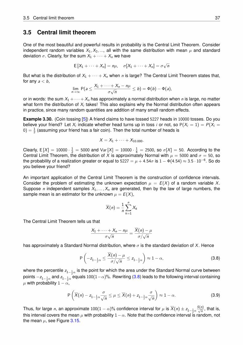
Thus, for large n, an approximate 100(1 − α)% confidence interval for µ is X (n) ± z1− 12α
S(n)√n , that is,
this interval covers the mean µ with probability 1−α. Note that the confidence interval is random, notthe mean µ, see Figure 3.15.
38 Probability Models
-0.25
-0.2
-0.15
-0.1
-0.05
0
0.05
0.1
0.15
0.2
0.25
0.3
0 10 20 30 40 50 60 70 80 90 100
Figure 3.15: 100 confidence intervals to estimate the mean 0 of the Uniform random variable on(−1, 1), where each interval is based on 100 samples
Remark 3.3.
• If the standard deviation σ is unknown, it can be estimated by square root of the sample variance
S2(n) = 1n
n∑
k=1
[Xk − X (n)
]2
and then this estimate S(n) can be used in (3.9) instead of σ.
• About 100 times as many samples are needed to reduce the width of a confidence interval by afactor 1
10 !
3.6 Joint random variables
If X and Y are discrete random variables, then
p(x , y) = P(X = x , Y = y)
is the joint probability mass function of X and Y . The marginal probability mass functions of X and Yfollow from
PX (x) = P(X = x) =∑
yP(X = x , Y = y),
PY (y) = P(Y = y) =∑
xP(X = x , Y = y).
Example 3.31. We repeatedly draw a random number from 1, ... , 10. Let X be number of draws untilthe first 1 appears and let Y be the number until the first 10 appears. What is joint probability massof X and Y ? Let us calculate the probability P(X = n, Y = n + k) for n, k = 1, 2, ... (the probabilitiesP(X = n + k, Y = n can be calculated along the same lines, and in fact, P(X = n, Y = n + k) =P(X = n + k, Y = n) by symmetry). This means that we first draw n− 1 numbers different from 1 and10, then we draw 1, and subsequently we draw k − 1 numbers different from 10 (so there could alsobe some 1s) and finally, the number 10 appears. Hence
P(X = n, Y = n + k) =(
810
)n−1 110
(910
)k−1 110.
3.6 Joint random variables 39
If X and Y are continuous random variables, then
P(X ≤ a, Y ≤ b) =∫ a
x=−∞
∫ b
y=−∞f (x , y)dxdy
is the joint probability distribution function of X and Y , where f (x , y) is the joint density, satisfying
f (x , y) ≥ 0,∫ ∞
x=−∞
∫ ∞
y=−∞f (x , y)dxdy = 1.
The function f (x , y) can be interpreted as the density of the joint probability mass, that is, for small∆ > 0
P(x < X ≤ x + ∆, y < Y ≤ y + ∆) ≈ f (x , y)∆2
The joint density f (x , y) can be obtained from the joint distribution P(X ≤ x , Y ≤ y) by taking partialderivatives,
f (x , y) = ∂2
∂x∂y P(X ≤ x , Y ≤ y).
The marginal densities of X and Y follow from
fX (x) =∫ ∞
−∞f (x , y)dy ,
fY (y) =∫ ∞
−∞f (x , y)dx .
The random variables X and Y are independent if
f (x , y) = fX (x)fY (y) for all x , y .
Example 3.32.
• The random variable X is the distance to the origin 0 and Y is angle (in radians) of a randompoint in a disk of radius r . What is the joint distribution and joint density of X and Y ?
P(X ≤ x , Y ≤ y) =πx2 y
2ππr2 = x2
r2y2π , 0 ≤ x ≤ r , 0 ≤ y ≤ 2π
and by taking the partial derivatives, the joint density is found to be
f (x , y) = 2xr2
12π , 0 ≤ x ≤ r , 0 ≤ y ≤ 2π.
Hence the marginal densities are
fX (x) =∫ 2π
y=0f (x , y)dy = 2x
r2 , 0 ≤ x ≤ r , fY (y) =∫ r
x=0f (x , y)dx = 1
2π , 0 ≤ y ≤ 2π,
so f (x , y) = fX (x)fY (y), and thus X and Y are independent.
• Let X1 and X2 be two independent Exponential random variables, with rates λ1 and λ2. What isthe probability that X1 is the smallest one? We need to calculate
P(X1 ≤ X2) =∫ ∞
x1=0
∫ ∞
x2=x1
f (x1, x2)dx2dx1.
Since X1 and X2 are independent, the joint density f (x1, x2) is equal to
f (x1, x2) = λ1e−λ1x1λ2e−λ2x2 ,
40 Probability Models
so
P(X1 ≤ X2) =∫ ∞
x1=0
∫ ∞
x2=x1
λ1e−λ1x1λ2e−λ2x2dx2dx1
=∫ ∞
x1=0λ1e−λ1x1
∫ ∞
x2=x1
λ2e−λ2x2dx2dx1
=∫ ∞
x1=0λ1e−λ1x1e−λ2x1dx1
= λ1λ1 + λ2
.
Thus the probability that X1 is the smallest one is proportional to the rates.
• Let X be random on (0, 1) and Y be random on (0, X ). What is the density of the area of therectangle with sides X and Y ? So we need to calculate the density of Z = XY . First note thatthe joint density of X and Y is equal to
f (x , y) = 1x , 0 ≤ y ≤ x ≤ 1,
and f (x , y) = 0 elsewhere. Hence, for 0 ≤ z ≤ 1,
P(Z ≤ z) = P(XY ≤ z)
=∫ √z
x=0
∫ x
y=0f (x , y)dydx +
∫ 1
x=√
z
∫ zx
y=0f (x , y)dydx
=∫ √z
x=0
∫ x
y=0
1x dydx +
∫ 1
x=√
z
∫ zx
y=0
1x dydx
=√
z +∫ 1
x=√
z
1x2 dx
=√
z +√
z − z= 2
√z − z .
Taking the derivative yields the density
fZ (z) = ddz P(Z ≤ z) = 1√
z− 1, 0 ≤ z ≤ 1.
The expectation of the random variable g(X , Y ), where g(x , y) is any function, can be calculated as
E [g(X , Y )] =∫ ∞
−∞
∫ ∞
−∞g(x , y)f (x , y)dxdy .
For example, taking g(x , y) = ax + by , where a and b are constants,
E [aX + bY ] =∫ ∞
−∞
∫ ∞
−∞(ax + by)f (x , y)dxdy
= a∫ ∞
−∞x∫ ∞
−∞f (x , y)dydx + b
∫ ∞
−∞y∫ ∞
−∞f (x , y)dxdy
= a∫ ∞
−∞xfX (x)dx + b
∫ ∞
−∞yfY (y)dy
= aE [X ] + bE [Y ] .
and similarly, if X and Y are independent (so f (x , y) = fX (x)fY (y)),
E [XY ] = E [X ] E [Y ] . (3.10)
3.7 Conditioning 41
Example 3.33. Pick two points X and Y at random from the interval (0, 1). What is the mean distancebetween these two points? We need to calculate E [|X − Y |]. The joint density of X and Y is f (x , y) =1 for 0 ≤ x , y ≤ 1, so
E [|X − Y |] = 2∫ 1
x=0
∫ x
y=0(x − y)dydx = 2
∫ 1
x=0
12x2dx = 1
3,
as expected.
The covariance of two random variables X and Y is defined as
cov[X , Y ] = E [(X − E [X ])(Y − E [Y ])]= E [XY ]− E [X ] E [Y ]
and the correlation coefficient of X and Y is a normalized version of the covariance,
ρ[X , Y ] = cov[X , Y ]σ[X ]σ[Y ] .
It can be shown (check!) that −1 ≤ ρ[X , Y ] ≤ 1. The correlation coefficient is often used as ameasure for dependence between the random variables X and Y . If X and Y are independent, thenit follows from (3.10) that cov[X , Y ] = 0, and thus that ρ[X , Y ] = 0. If X = aY , then ρ[X , Y ] = 1 ifa > 0 and ρ[X , Y ] = −1 if a < 0, which express maximal positive and negative correlation.
Exercise 35. (Problem 11.8 [5]) Let the joint probability density function of the random variablesX and Y be given by f (x , y) = ce−2x for 0 < y ≤ x < ∞ and f (x , y) = 0 otherwise. Determine theconstant c. What is the probability density of X − Y ?
Exercise 36. (Problem 11.12 [5]) The joint density of the random variables X and Y is given byf (x , y) = 4xe−2x(1+y) for x , y > 0. What are the marginal densities of X and Y ?
Exercise 37. (Homework exercises 17) We select a point (x , y) at random from a square withsides 1. Let X be the random variable for the x -coordinate and Y the random variable for the y -coordinate of that point. What is the probability that X > 1.5− Y ?
3.7 Conditioning
In this section we summarize the concepts of conditional probabilities and conditional expectationsfor random variables. Conditioning is a fruitful technique to calculate probabilities and expectations.
Let X and Y be discrete random variables. The conditional probability mass function of X givenY = y is defined as
P(X = x |Y = y) = P(X = x , Y = y)P(Y = y) .
Then the unconditional probabilities P(X = x) can be calculated by conditioning on the possiblevalues of Y ,
P(X = x) =∑
yP(X = x |Y = y)P(Y = y).
Example 3.34. Simultaneously roll 24 dice and next roll with those that showed 6. Let X be numberof sixes in the first roll and let Y be those in the second roll.
• What is P(Y = y |X = x)? This means that in the second roll, x dice are used. Hence, theprobability that y dice out of x show six is
P(Y = y |X = x) =(
xy
)(16
)y (56
)x−y. (3.11)
42 Probability Models
• What is P(Y = y)? To calculate this probability we condition on the outcome of X and then usethe above result, so
P(Y = y) =24∑
x=yP(Y = y |X = x)P(X = x)
=24∑
x=yP(Y = y |X = x)
(24x
)(16
)x (56
)24−x
=24∑
x=y
(xy
)(16
)y (56
)x−y (24x
)(16
)x (56
)24−x. (3.12)
• And what is P(X = x |Y = y)? Using the definition of conditional probability,
P(X = x |Y = y) = P(X = x , Y = y)P(Y = y) = P(Y = y |X = x)P(X = x)
P(Y = y) ,
so this probability can be calculated by substituting (3.11) and (3.12) and
P(X = x) =(
24x
)(16
)x (56
)24−x.
Now let X and Y be continuous random variables with joint density f (x , y) and marginal densitiesfX (x) and fY (y). The conditional density of X given Y = y is defined analogously to the discretecase,
fX (x |y)dx = P(x < X ≤ x + dx |y < Y ≤ y + dy)
= P(x < X ≤ x + dx , y < Y ≤ y + dy)P(y < Y ≤ y + dy)
= f (x , y)dxdyfY (y)dy
= f (x , y)fY (y) dx ,
so the conditional density of X given Y = y is
fX (x |y) = f (x , y)fY (y) .
Then the conditional probability P(X ≤ x |Y = y) follows from
P(X ≤ x |Y = y) =∫ x
z=−∞fX (z |y)dz
and the unconditional probability P(X ≤ x) can be calculated by conditioning on the possible valuesof Y ,
P(X ≤ x) =∫ ∞
−∞P(X ≤ x |Y = y)fY (y)dy .
Example 3.35.
• Point (X , Y ) is randomly chosen in the unit circle. What is the conditional density of X givenY = y? We have
f (x , y) = 1π
, x2 + y2 ≤ 1,
3.7 Conditioning 43
and f (x , y) = 0 otherwise. So for −1 ≤ y ≤ 1,
fY (y) =∫ √1−y2
−√
1−y2
1π
dx = 2π
√1− y2.
Hence, for −√
1− y2 ≤ x ≤√
1− y2,
fX (x |y) = f (x , y)fY (y) =
1π
2π
√1− y2
= 12√
1− y2,
which is the Uniform density on the interval (−√
1− y2,√
1− y2), as expected.
• You are waiting for the metro. Once the metro has stopped, the distance to the nearest metrodoor is Uniform between 0 and 2 metres. If the distance to the nearest door is y metres, thenyou are able to find a place to sit with probability
1−√
12y
What is the probability Mr Johnson finds a place to sit? Let the random variable Y be thedistance to the nearest door and X indicate whether you find a place to sit (so X = 1 if you cansit and X = 0 otherwise). To calculate the probability P(X = 1), note that Y is Uniform on (0, 2),so
fY (y) = 12, 0 < y < 2,
and fY (y) = 0 elsewhere. Also,
P(X = 1|Y = y) = 1−√
12y .
Hence
P(X = 1) =∫ 2
y=0P(X = 1|Y = y)fY (y)dy =
∫ 2
y=0(1−
√12y)1
2dy = 13.
Note that this probability is not equal to 1−√
12E [Y ] = 1−
√12 !
Conditioning is a fruitful technique, not only to calculate probabilities, but also to calculate expecta-tions. For discrete random variables X and Y , the conditional expectation of X given Y = y is definedas
E [X |Y = y ] =∑
xxP(X = x |Y = y),
and then the (unconditional) expectation of X can be calculated by conditioning on the possible valuesof Y ,
E [X ] =∑
yE [X |Y = y ] P(Y = y).
Analogously, for continuous random variables X and Y , we have
E [X |Y = y ] =∫ ∞
−∞xfX (x |y)dx ,
andE [X ] =
∫ ∞
−∞E [X |Y = y ] fY (y)dy .
Example 3.36.
44 Probability Models
• Generate two random numbers X1 and X2 from (0, 1). Let X be the smallest of X1 and X2 andY the largest. What are E [X |Y = y ] and E [X ]? Note that
f (x , y) = fX1(x)fX2(y) + fX1(y)fX2(x) = 1 + 1 = 2, 0 < x < y < 1,
andfY (y) = P(X1 < y)fX2(y) + fX1(y)P(X2 < y) = 2y , 0 < y < 1.
So
fX (x |y) = f (x , y)fY (y) = 1
y , 0 < x < y ,
which means that X is uniform on (0, y) if Y = y (as expected). Hence,
E [X |Y = y ] =∫ y
x=0x 1
y dx = 12y ,
and
E [X ] =∫ 1
y=0E [X |Y = y ] fY (y)dy =
∫ 1
y=0y2dy = 1
3.
Of course, since fX (x) = 2(1 − x) for 0 < x < 1, the expectation of X can also be calculateddirectly,
E [X ] =∫ 1
x=0xfX (x)dx =
∫ 1
x=02x(1− x)dx = 1
3.
• A batch consists of a random number of items N, where P(N = n) = (1 − p)pn−1, n ≥ 1.The production time of a single item is Uniform between 4 and 10 minutes. What is the meanproduction time of a batch? Let B denote the production time of the batch, and Xi the productiontime of a single item (so E [Xi ] = 7 mins). Then we can write
B =N∑
i=1Xi .
To calculate E [B] we condition on N = n, yielding
E [B|N = n] = E [X1 + · · ·+ Xn] = E [X1] + · · ·+ E [Xn] = 7n.
Hence
E [B] =∞∑
n=1E [B|N = n] P(N = n) =
∞∑
n=17n(1− p)pn−1 = 7
1− p (mins).
• Process time X is Exponential with rate Λ, where Λ itself is also random with density
fΛ(λ) = λe−12λ
2 , λ > 0.
What is the mean process time? To calculate E [X ] we first condition on the rate Λ = λ, whichleads to
E [X |Λ = λ] = 1λ
,
and then we get
E [X ] =∫ ∞
λ=0E [X |Λ = λ] fΛ(λ)dλ =
∫ ∞
λ=0
1λλe−
12λ
2dλ =√
2π 1√2π
∫ ∞
λ=0e−
12λ
2dλ =√
2πΦ(0) =√π
2 .
3.7 Conditioning 45
Example 3.37. (Random setups) Suppose that a machine needs a setup after having produced onaverage k jobs. This means that, after having produced a job, the machine needs a setup Y withprobability p = 1
k . Let X denote the natural process of a job, Y the setup time, and Z denotes theeffective process time, i.e., Z is X plus the possible setup Y ,
Z =
X + Y with probability p,X with probability 1− p.
What is the mean and variance of the effective process time Z? To calcute E [Z ] and Var [Z ] wecondition on having a setup or not,
E [Z ] = E [X + Y ] p + E [X ] (1− p)= (E [X ] + E [Y ])p + E [X ] (1− p)= E [X ] + pE [Y ] ,
and similarly
E[Z 2] = E
[(X + Y )2] p + E
[X 2] (1− p)
= (E[X 2]+ 2E [X ] E [Y ] + E
[Y 2])p + E
[X 2] (1− p)
= E[X 2]+ 2pE [X ] E [Y ] + pE
[Y 2] .
SoVar [Z ] = E
[Z 2]− (E [Z ])2 = Var [X ] + pVar [Y ] + p(1− p)(E [Y ])2.
Clearly, Var [Z ] is greater than Var [X ] (even when Var [Y ] = 0, i.e. Y is constant).
Exercise 38. (Problem 13.4 [5]) Two dice are rolled. Let the random variable X be the smallestof the two outcomes and let Y be the largest of the two outcomes. What are the conditional massfunctions P(X = x |Y = y) and P(Y = y |X = x)?
Exercise 39. (Problem 13.7 [5]) Let X and Y be two continuous random variables with the jointprobability density f (x , y) = xe−x(y+1) for x , y > 0 and f (x , y) = 0 otherwise. What are the conditionalprobability densities fX (x |y) and fY (y |x)? What is the probability that Y is larger than 1 given thatX = 1?
Exercise 40. (Problem 13.8 [5]) Let X and Y be two continuous random variables with the jointprobability density f (x , y) = 27(2x + 5y) for 0 < x , y < 1 and f (x , y) = 0 otherwise. What are theconditional probability densities fX (x |y) and fY Y (y |x)? What is the probability that X is larger than0.5 given that Y = 0.2?
Exercise 41. (Problem 13.23 [5]) You generate three random numbers from (0,1). Let X bethe smallest of these three numbers and Y the largest. What are the conditional expected valuesE(X |Y = y) and E (Y |X = x)?
Exercise 42. (Homework exercises 15) Let X be a positive random variable with cumulativedensity function
P(X ≤ x) = FX (x) = 1− c2 + x .
(a) Determine the constant c.
(b) Calculate the conditional probability P(X > 8|X ≤ 10).

46 Probability Models
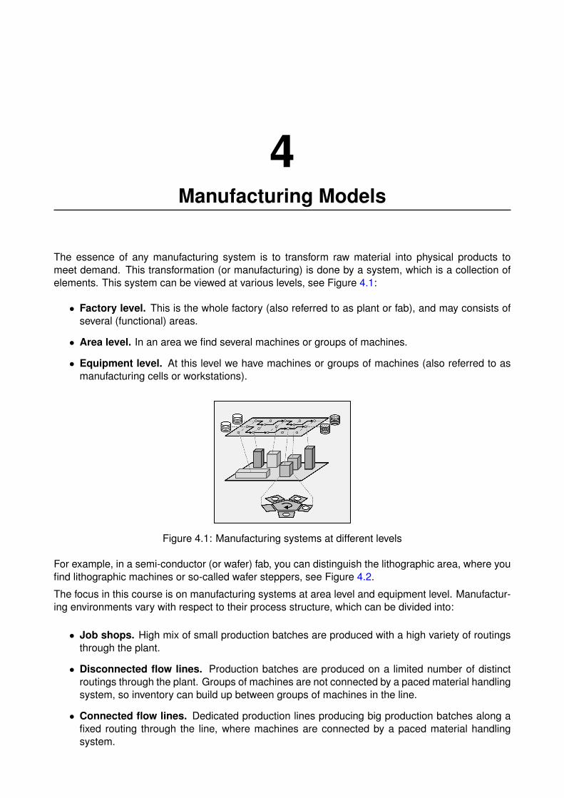
4Manufacturing Models
The essence of any manufacturing system is to transform raw material into physical products tomeet demand. This transformation (or manufacturing) is done by a system, which is a collection ofelements. This system can be viewed at various levels, see Figure 4.1:
• Factory level. This is the whole factory (also referred to as plant or fab), and may consists ofseveral (functional) areas.
• Area level. In an area we find several machines or groups of machines.
• Equipment level. At this level we have machines or groups of machines (also referred to asmanufacturing cells or workstations).
Figure 4.1: Manufacturing systems at different levels
For example, in a semi-conductor (or wafer) fab, you can distinguish the lithographic area, where youfind lithographic machines or so-called wafer steppers, see Figure 4.2.
The focus in this course is on manufacturing systems at area level and equipment level. Manufactur-ing environments vary with respect to their process structure, which can be divided into:
• Job shops. High mix of small production batches are produced with a high variety of routingsthrough the plant.
• Disconnected flow lines. Production batches are produced on a limited number of distinctroutings through the plant. Groups of machines are not connected by a paced material handlingsystem, so inventory can build up between groups of machines in the line.
• Connected flow lines. Dedicated production lines producing big production batches along afixed routing through the line, where machines are connected by a paced material handlingsystem.
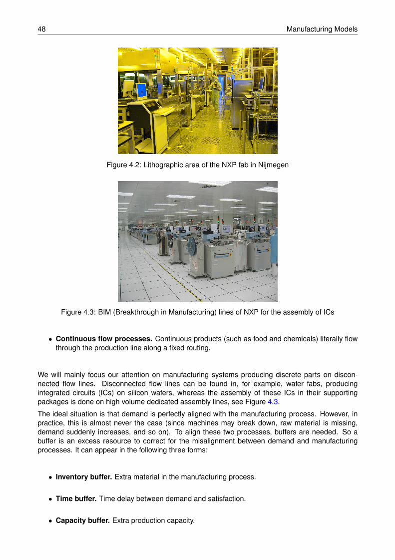
48 Manufacturing Models
Figure 4.2: Lithographic area of the NXP fab in Nijmegen
Figure 4.3: BIM (Breakthrough in Manufacturing) lines of NXP for the assembly of ICs
• Continuous flow processes. Continuous products (such as food and chemicals) literally flowthrough the production line along a fixed routing.
We will mainly focus our attention on manufacturing systems producing discrete parts on discon-nected flow lines. Disconnected flow lines can be found in, for example, wafer fabs, producingintegrated circuits (ICs) on silicon wafers, whereas the assembly of these ICs in their supportingpackages is done on high volume dedicated assembly lines, see Figure 4.3.
The ideal situation is that demand is perfectly aligned with the manufacturing process. However, inpractice, this is almost never the case (since machines may break down, raw material is missing,demand suddenly increases, and so on). To align these two processes, buffers are needed. So abuffer is an excess resource to correct for the misalignment between demand and manufacturingprocesses. It can appear in the following three forms:
• Inventory buffer. Extra material in the manufacturing process.
• Time buffer. Time delay between demand and satisfaction.
• Capacity buffer. Extra production capacity.
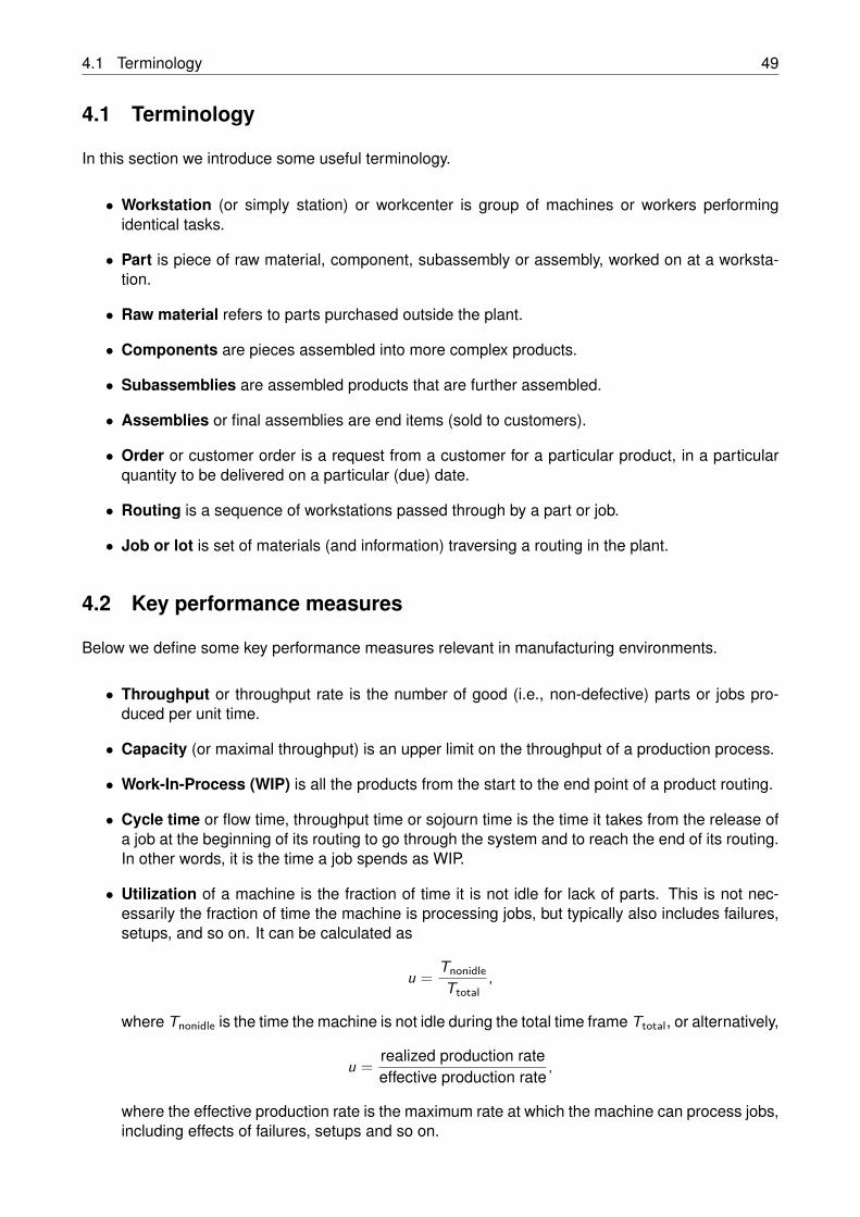
4.1 Terminology 49
4.1 Terminology
In this section we introduce some useful terminology.
• Workstation (or simply station) or workcenter is group of machines or workers performingidentical tasks.
• Part is piece of raw material, component, subassembly or assembly, worked on at a worksta-tion.
• Raw material refers to parts purchased outside the plant.
• Components are pieces assembled into more complex products.
• Subassemblies are assembled products that are further assembled.
• Assemblies or final assemblies are end items (sold to customers).
• Order or customer order is a request from a customer for a particular product, in a particularquantity to be delivered on a particular (due) date.
• Routing is a sequence of workstations passed through by a part or job.
• Job or lot is set of materials (and information) traversing a routing in the plant.
4.2 Key performance measures
Below we define some key performance measures relevant in manufacturing environments.
• Throughput or throughput rate is the number of good (i.e., non-defective) parts or jobs pro-duced per unit time.
• Capacity (or maximal throughput) is an upper limit on the throughput of a production process.
• Work-In-Process (WIP) is all the products from the start to the end point of a product routing.
• Cycle time or flow time, throughput time or sojourn time is the time it takes from the release ofa job at the beginning of its routing to go through the system and to reach the end of its routing.In other words, it is the time a job spends as WIP.
• Utilization of a machine is the fraction of time it is not idle for lack of parts. This is not nec-essarily the fraction of time the machine is processing jobs, but typically also includes failures,setups, and so on. It can be calculated as
u = TnonidleTtotal
,
where Tnonidle is the time the machine is not idle during the total time frame Ttotal, or alternatively,
u = realized production rateeffective production rate
,
where the effective production rate is the maximum rate at which the machine can process jobs,including effects of failures, setups and so on.

50 Manufacturing Models
• Cycle time factor is the ratio of the cycle time and the raw process time t0, so
Cycle Time Factor = Cycle Timet0
,
where t0 is the sum of the average process times of each workstation in the line, or in otherwords, it is the average time it takes a single job to go through the empty line.
Example 4.1. (Capacity) A workstation consists of 2 identical machines. The raw process time of amachine is t0 = 0.2 hours. Then the capacity (or maximal throughput) of each machine is 1
t0= 5 jobs
per hour, and the capacity of the workstation is 10 jobs per hour.
Example 4.2. (Utilization) The raw process time of a machine is t0 = 0.15 hours and its (realized)production rate is 5 lots per hour. Then the utilization u of the machine is u = 5 · 0.15 = 0.75.
4.3 Capacity, flow time and WIP
Let us consider the manufacturing flow line in Figure 4.4. We have a two machine line. Machine M1has a process time of 2 hours, machine M2 has a process time of 3 hours.
dl
t0 = 2 hours t0 = 3 hours
B1 M1 B2 M2
Figure 4.4: Manufacturing flow line
We assume that the buffers have ample capacity. The line in Figure 4.4 has a maximal throughput of1/3 lots/hour (machine M2 is the bottleneck). A basic approach for determining the flow time of a lotis with a lot-time diagram. Herein, we plot the state of individual lots against time. Figure 4.5(a) and(b) show the lot-time diagram for the line in which lots are released every 3 hours, and every 2 hours,respectively.
t [ hrs]
lot
1 21 2
1 21 2
0123
2 4 6 8 10 12 j [hrs]
1
5555
lot
1 21 2
1 21 2
0123
2 4 6 8 10 12 j [hrs]
1
5678
(a)
(b)
l = 1/3 lots/hour
l = 1/2 lots/hour
14
j2
j3
lot isprocessed on M1
processed on M2
waiting in queue
1
2
q
Figure 4.5: Lot-time diagram for release rate of (a) 1/3 lots/hour and (b) 1/2 lots/hour
For a release rate of 1/3 lots/hour we determine from Figure 4.5(a) that the flow time is 5 hours.For a release rate of 1/2 lots/hour we see in Figure 4.5(b) that the flow time keeps increasing. Forany release rate under the maximal throughput, the flow time is 5 hours, for any release rate abovethe maximal throughput, the flow time grows unlimited. We can also use the lot-time diagram todetermine the mean WIP level. In Figure 4.6 we derive the WIP level over time from the lot-timediagram. For instance, for a release rate of 1/3 lots/hour, at t = 7 there are two lots in the system (lot1 and 2).
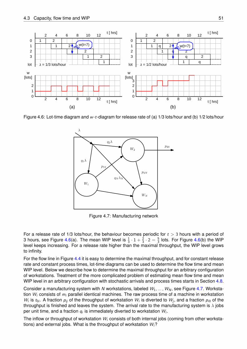
4.3 Capacity, flow time and WIP 51
t [ hrs]
lot
1 21 2
1 21 2
0123
2 4 6 8 10 12
1
w [lots]
012
t [ hrs]2 4 6 8 10 12
t [ hrs]
lot
1 21 2
1 21 2
0123
2 4 6 8 10 12
1
w [lots]
012
t [ hrs]2 4 6 8 10 12
3
(a) (b)
l = 1/3 lots/hour l = 1/2 lots/hour
w(t=7) w(t=7)
Figure 4.6: Lot-time diagram and w -t-diagram for release rate of (a) 1/3 lots/hour and (b) 1/2 lots/hour
W1
W2
WN
λ
q1λ
q2λ
qNλN
p12
p2N
p20
Figure 4.7: Manufacturing network
For a release rate of 1/3 lots/hour, the behaviour becomes periodic for t > 3 hours with a period of3 hours, see Figure 4.6(a). The mean WIP level is 1
3 · 1 + 23 · 2 = 5
3 lots. For Figure 4.6(b) the WIPlevel keeps increasing. For a release rate higher than the maximal throughput, the WIP level growsto infinity.
For the flow line in Figure 4.4 it is easy to determine the maximal throughput, and for constant releaserate and constant process times, lot-time diagrams can be used to determine the flow time and meanWIP level. Below we describe how to determine the maximal throughput for an arbitrary configurationof workstations. Treatment of the more complicated problem of estimating mean flow time and meanWIP level in an arbitrary configuration with stochastic arrivals and process times starts in Section 4.8.
Consider a manufacturing system with N workstations, labeled W1, ... , WN , see Figure 4.7. Worksta-tion Wi consists of mi parallel identical machines. The raw process time of a machine in workstationWi is t0i . A fraction pij of the throughput of workstation Wi is diverted to Wj , and a fraction pi0 of thethroughput is finished and leaves the system. The arrival rate to the manufacturing system is λ jobsper unit time, and a fraction qi is immediately diverted to workstation Wi .
The inflow or throughput of workstation Wi consists of both internal jobs (coming from other worksta-tions) and external jobs. What is the throughput of workstation Wi?
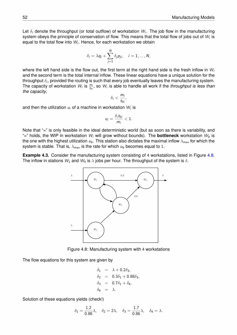
52 Manufacturing Models
Let δi denote the throughput (or total outflow) of workstation Wi . The job flow in the manufacturingsystem obeys the principle of conservation of flow. This means that the total flow of jobs out of Wi isequal to the total flow into Wi . Hence, for each workstation we obtain
δi = λqi +N∑
j=1δjpji , i = 1, ... , N,
where the left hand side is the flow out, the first term at the right hand side is the fresh inflow in Wiand the second term is the total internal inflow. These linear equations have a unique solution for thethroughput δi , provided the routing is such that every job eventually leaves the manufacturing system.The capacity of workstation Wi is mi
t0i, so Wi is able to handle all work if the throughput is less than
the capacity,δi <
mit0i
,
and then the utilization ui of a machine in workstation Wi is
ui = δi t0imi
< 1.
Note that “=” is only feasible in the ideal deterministic world (but as soon as there is variability, and“=” holds, the WIP in workstation Wi will grow without bounds). The bottleneck workstation Wb isthe one with the highest utilization ub. This station also dictates the maximal inflow λmax for which thesystem is stable. That is, λmax is the rate for which ub becomes equal to 1.
Example 4.3. Consider the manufacturing system consisting of 4 workstations, listed in Figure 4.8.The inflow in stations W1 and W4 is λ jobs per hour. The throughput of the system is δ.
W1 W2
W3
W4
λ
λ 0.3
0.8
δ
Figure 4.8: Manufacturing system with 4 workstations
The flow equations for this system are given by
δ1 = λ+ 0.2δ3,δ2 = 0.3δ1 + 0.88δ3,δ3 = 0.7δ1 + δ4,δ4 = λ.
Solution of these equations yields (check!)
δ1 = 1.20.86λ, δ2 = 2λ, δ3 = 1.7
0.86λ, δ4 = λ.
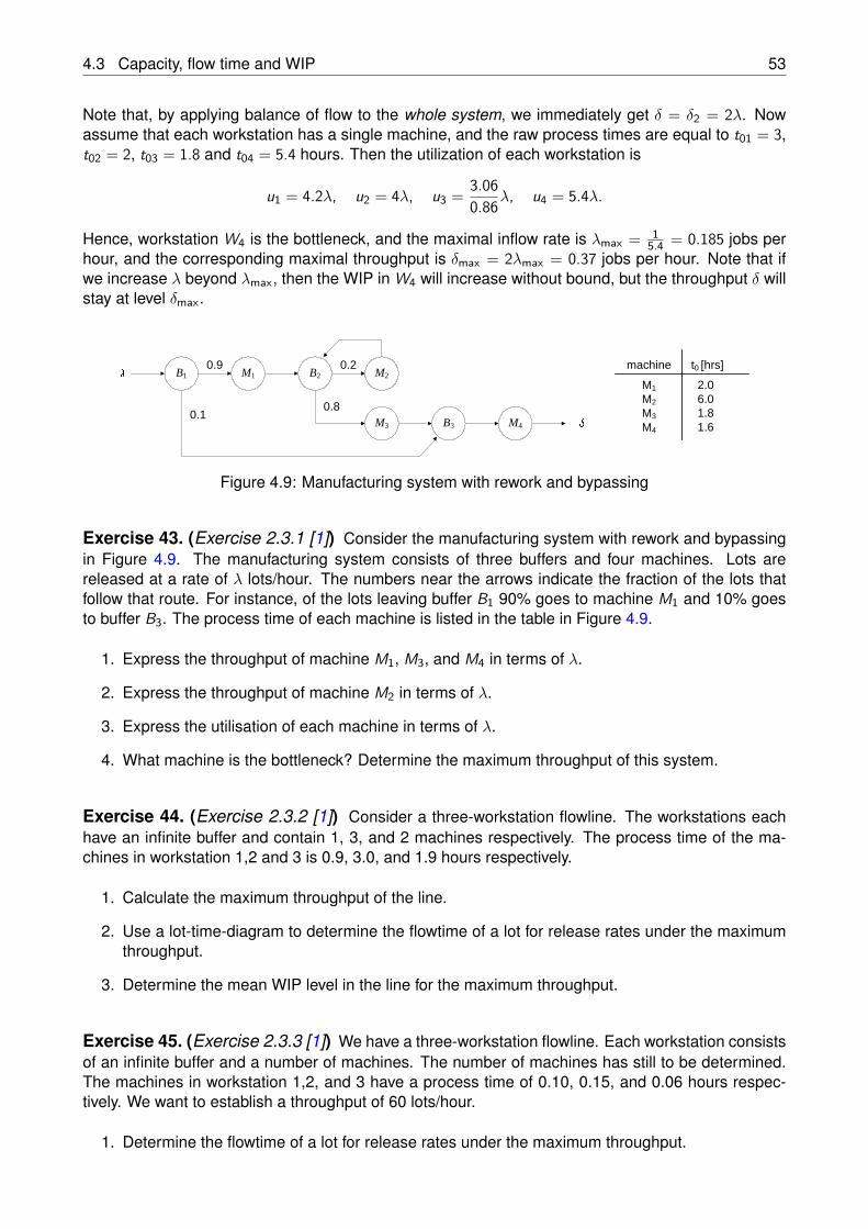
4.3 Capacity, flow time and WIP 53
Note that, by applying balance of flow to the whole system, we immediately get δ = δ2 = 2λ. Nowassume that each workstation has a single machine, and the raw process times are equal to t01 = 3,t02 = 2, t03 = 1.8 and t04 = 5.4 hours. Then the utilization of each workstation is
u1 = 4.2λ, u2 = 4λ, u3 = 3.060.86λ, u4 = 5.4λ.
Hence, workstation W4 is the bottleneck, and the maximal inflow rate is λmax = 15.4 = 0.185 jobs per
hour, and the corresponding maximal throughput is δmax = 2λmax = 0.37 jobs per hour. Note that ifwe increase λ beyond λmax, then the WIP in W4 will increase without bound, but the throughput δ willstay at level δmax.
B1t0 [hrs]l machine
M1
M2
M3
M4
2.06.01.81.6
0.9
0.1
0.2
0.8 dM1 B2 M2
M3 M4B3
Figure 4.9: Manufacturing system with rework and bypassing
Exercise 43. (Exercise 2.3.1 [1]) Consider the manufacturing system with rework and bypassingin Figure 4.9. The manufacturing system consists of three buffers and four machines. Lots arereleased at a rate of λ lots/hour. The numbers near the arrows indicate the fraction of the lots thatfollow that route. For instance, of the lots leaving buffer B1 90% goes to machine M1 and 10% goesto buffer B3. The process time of each machine is listed in the table in Figure 4.9.
1. Express the throughput of machine M1, M3, and M4 in terms of λ.
2. Express the throughput of machine M2 in terms of λ.
3. Express the utilisation of each machine in terms of λ.
4. What machine is the bottleneck? Determine the maximum throughput of this system.
Exercise 44. (Exercise 2.3.2 [1]) Consider a three-workstation flowline. The workstations eachhave an infinite buffer and contain 1, 3, and 2 machines respectively. The process time of the ma-chines in workstation 1,2 and 3 is 0.9, 3.0, and 1.9 hours respectively.
1. Calculate the maximum throughput of the line.
2. Use a lot-time-diagram to determine the flowtime of a lot for release rates under the maximumthroughput.
3. Determine the mean WIP level in the line for the maximum throughput.
Exercise 45. (Exercise 2.3.3 [1]) We have a three-workstation flowline. Each workstation consistsof an infinite buffer and a number of machines. The number of machines has still to be determined.The machines in workstation 1,2, and 3 have a process time of 0.10, 0.15, and 0.06 hours respec-tively. We want to establish a throughput of 60 lots/hour.
1. Determine the flowtime of a lot for release rates under the maximum throughput.
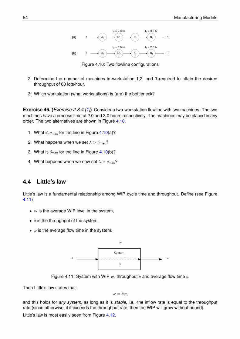
54 Manufacturing Models
t0 = 2.0 hr t0 = 3.0 hrl dt0 = 3.0 hr t0 = 2.0 hrl d
(a)
(b)
B1 M1 B2 M2
B1 M1B2M2
Figure 4.10: Two flowline configurations
2. Determine the number of machines in workstation 1,2, and 3 required to attain the desiredthroughput of 60 lots/hour.
3. Which workstation (what workstations) is (are) the bottleneck?
Exercise 46. (Exercise 2.3.4 [1]) Consider a two-workstation flowline with two machines. The twomachines have a process time of 2.0 and 3.0 hours respectively. The machines may be placed in anyorder. The two alternatives are shown in Figure 4.10.
1. What is δmax for the line in Figure 4.10(a)?
2. What happens when we set λ > δmax?
3. What is δmax for the line in Figure 4.10(b)?
4. What happens when we now set λ > δmax?
4.4 Little’s law
Little’s law is a fundamental relationship among WIP, cycle time and throughput. Define (see Figure4.11)
• w is the average WIP level in the system,
• δ is the throughput of the system,
• ϕ is the average flow time in the system.
System
δ δ
w
ϕ
Figure 4.11: System with WIP w , throughput δ and average flow time ϕ
Then Little’s law states thatw = δϕ,
and this holds for any system, as long as it is stable, i.e., the inflow rate is equal to the throughputrate (since otherwise, if it exceeds the throughput rate, then the WIP will grow without bound).
Little’s law is most easily seen from Figure 4.12.
4.4 Little’s law 55
time t
total number w
ϕ
δ
Figure 4.12: Illustration of Little’s law, where the solid line is the total input to the system in (0, t), andthe dashed line the total output in (0, t)
The power of Little’s law is its generality (no specific assumptions for the system are required) andflexibility (as it applies to any system). For example, it can be applied to the buffer of a specificworkstation W , in which case it gives the relation
WIP in the buffer of workstation W = Throughput of W × Time spent in buffer,
and when it is applied to the whole manufacturing system, we get
WIP in the whole manufacturing system = Throughput of the system× Cycle time.
According to Little’s law, the same throughput δ can be achieved with
• large WIP w and long flow times ϕ, but also with
• small WIP w and short flow times ϕ.
What causes the difference? In most cases the answer is: Variability! The concept of variability willbe studied in the following sections, and in particular, its corrupting effect on system performance.
t0 = 2.0 hr t0 = 2.0 hrlG EB1 M1 B2 M2
Figure 4.13: Re-entrant flowline
Exercise 47. (Exercise 2.3.5 [1]) Consider the re-entrant flowline in Figure 4.13. Lots are releasedin the line by generator G at a rate of λ lots/hour. Each lot passes through the flowline twice and hasthe same fixed route, namely M1, M2, M1, M2. If a newly released lot and a re-entrant lot arrive at amachine at the same time, the re-entrant lot is processed first.
1. Express the utilisation of machine 1 in terms of release rate λ and determine the maximumthroughput.
2. Construct a lot-time diagram (in which the state of individual lots is shown over time) for λ = 15
lots/hour and determine the (mean) flowtime of a lot.
3. From the lot-time diagram, derive a WIP-time diagram (in which the WIP is shown over time),and determine the mean WIP-level in steady state.
4. Verify your result using Little’s law.
56 Manufacturing Models
W1
0.8
W2 W3
W4W5 W60.2 d
l
Figure 4.14: Manufacturing line
Exercise 48. (Exercise 2.4.1 [1]) The manufacturing system in Figure 4.14 consists of 6 worksta-tions. 20% of the lots processed by workstation W4 need rework. The lot is first stripped in workstationW5 and then reprocessed by workstation W2 and W3. The numbers at the arrows indicate the fractionof the lots that follow that route.
1. Calculate the total throughput of workstation 2,3, and 5 in terms of release rate λ.
2. Calculate the throughput δW4W5 and δW4W6 for workstation 4.
3. Verify that conservation of mass holds for system W2W3W4W5.
W1 W2 W3 W4l d0.1
0.10.1
0.7
Figure 4.15: Manufacturing line with bypassing
Exercise 49. (Exercise 2.4.2 [1]) Figure 4.15 shows a flow line with bypassing loops going fromworkstation 1 to workstation 2, 3, and 4. The numbers at the arrows indicate the fraction of the lotsthat follow that route.
1. Use mass conservation to determine the throughput of workstations 1,2,3, and 4.
2. Verify that conservation of mass holds for system W1W2W3W4.
W1 W2 W3 W4l d0.8 0.70.8
0.2 0.30.2
Figure 4.16: Manufacturing line with rework
Exercise 50. (Exercise 2.4.3 [1]) Figure 4.16 shows a flowline of workstations with rework loops.20% of the lots processed by workstation 2 need rework on workstation 1 and 2. 20% of the pro-cessed by workstation 3 need rework on workstation 2 and 3. Finally, 30% of the lots processed byworkstation 4 need rework on 3 and 4.
1. Intuitively, what workstation will have to process the most lots?
2. Write down the mass conservation equations for workstation 1 through 4.
Mass conservation on system W1W2W3W4 yields that δ = λ. For the total throughput of workstation4 we have δW4 = δ + δW4W3 .
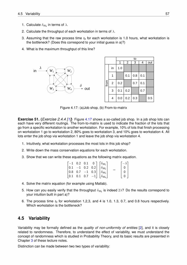
4.5 Variability 57
1. Calculate δW4 in terms of λ.
2. Calculate the throughput of each workstation in terms of λ.
3. Assuming that the raw process time t0 for each workstation is 1.0 hours, what workstation isthe bottleneck? (Does this correspond to your initial guess in a)?)
4. What is the maximum throughput of this line?
W1 W2
W3 W4
in
out
l
d
to
from
1 2 3 4 out
in
1
2
3
4
1.0
0.5
0.1 0.8 0.1
0.1
0.7
0.70.2
0.1
0.0 0.2
0.2
0.3
Figure 4.17: (a)Job shop, (b) From-to-matrix
Exercise 51. (Exercise 2.4.4 [1]) Figure 4.17 shows a so-called job shop. In a job shop lots caneach have very different routings. The from-to-matrix is used to indicate the fraction of the lots thatgo from a specific workstation to another workstation. For example, 10% of lots that finish processingon workstation 1 go to workstation 2, 80% goes to workstation 3, and 10% goes to workstation 4. Alllots enter the job shop via workstation 1 and leave the job shop via workstation 4.
1. Intuitively, what workstation processes the most lots in this job shop?
2. Write down the mass conservation equations for each workstation.
3. Show that we can write these equations as the following matrix equation.
−1 0.2 0.1 00.1 −1 0.2 0.20.8 0.7 −1 0.30.1 0.1 0.7 −1
δW1
δW2
δW3
δW4
=
−λ000
4. Solve the matrix equation (for example using Matlab).
5. How can you easily verify that the throughput δW4 is indeed 2λ? Do the results correspond toyour intuition built in part a)?
6. The process time t0 for workstation 1,2,3, and 4 is 1.0, 1.3, 0.7, and 0.8 hours respectively.Which workstation is the bottleneck?
4.5 Variability
Variability may be formally defined as the quality of non-uniformity of entities [2], and it is closelyrelated to randomness. Therefore, to understand the effect of variability, we must understand theconcept of randomness which is studied in Probability Theory, and its basic results are presented inChapter 3 of these lecture notes.
Distinction can be made between two two types of variability:
58 Manufacturing Models
Controllable variation. This is the result of (bad) decisions. For example, variability is introduced bythe mix of products produced in the plant, where each type of product can have its own process-ing characteristics and routing through the plant. Another example is use of batch transportationof material, where the first finished part in the batch has to wait longer for transportation thanthe last one in the batch.
Random variation. This is the result of events beyond our control. For example, the time elapsingbetween customer demands, or machine failures.
Our intuition is quite good with respect to first-moment effects (i.e., the mean): we understand that weget more products out by speeding up the bottleneck machine, or by adding more product carriers.This type of intuition is based on a deterministic world. However, most of us have a much lessdeveloped intuition for second-moment effects (i.e., the variance). For example:
• Which is more variable: the time to process an individual part or the time to produce a wholebatch of those parts?
• Which results in greater improvement of line performance: Reduce variability of process timescloser to raw materials (upstream the line), or closer to the customers (downstream the line)?
• Which are more disruptive to line performance: Short frequent machine failures, or long infre-quent machine failures?
In the next section we will first pay attention to understanding the mean and variance in process timesand flows, and then to the interaction of these two sources of randomness.
4.6 Process time variability
Instead of looking at the “clean or natural” process time, it makes sense to consider the effectiveprocess time, which is the total time seen by a job at a workstation. This includes the natural processtime, setups, rework, operator unavailability, and all sorts of other shop floor realities. The reasonis that from a logistical point of view, it only matters that the job is at the machine, not so much thereason why (for example, because it is actually being processed or because it is waiting for material).
A standard measure for variability is the standard deviation σ. This absolute measure does notimmediately tell you whether variability is low or high, unless you relate it to, for example, the mean.For example, σ = 1 hour is big for a mean process time t = 10 minutes, but it is small for t = 10hours. A useful relative measure for variability is the coefficient of variation c, defined as
c = σ
t ,
where t is the mean and σ the standard deviation. We say that variability is low if c < 0.75, moderateif 0.75 ≤ c < 1.33 and high if c ≥ 1.33. There are various sources of process time variability, such as:
• “Natural” variability;
• Random outages;
• Setups;
• Operator (un)availability;
• Rework.
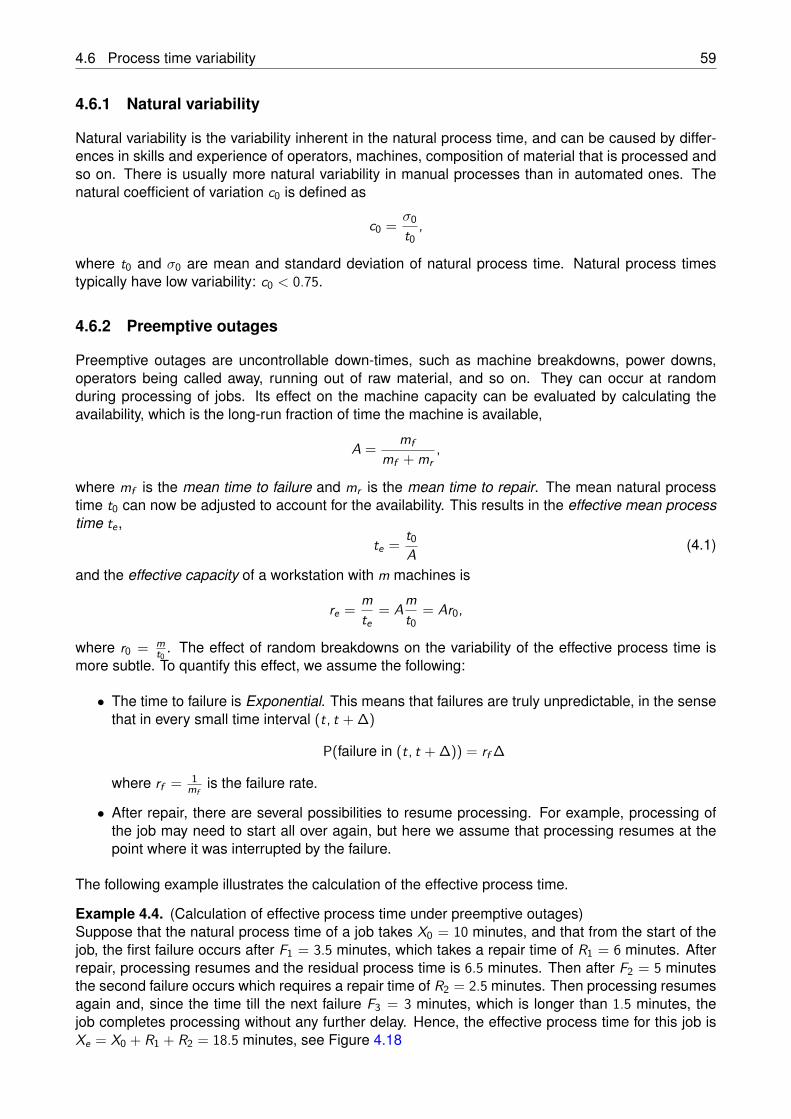
4.6 Process time variability 59
4.6.1 Natural variability
Natural variability is the variability inherent in the natural process time, and can be caused by differ-ences in skills and experience of operators, machines, composition of material that is processed andso on. There is usually more natural variability in manual processes than in automated ones. Thenatural coefficient of variation c0 is defined as
c0 = σ0t0
,
where t0 and σ0 are mean and standard deviation of natural process time. Natural process timestypically have low variability: c0 < 0.75.
4.6.2 Preemptive outages
Preemptive outages are uncontrollable down-times, such as machine breakdowns, power downs,operators being called away, running out of raw material, and so on. They can occur at randomduring processing of jobs. Its effect on the machine capacity can be evaluated by calculating theavailability, which is the long-run fraction of time the machine is available,
A = mfmf + mr
,
where mf is the mean time to failure and mr is the mean time to repair. The mean natural processtime t0 can now be adjusted to account for the availability. This results in the effective mean processtime te ,
te = t0A (4.1)
and the effective capacity of a workstation with m machines is
re = mte
= Amt0
= Ar0,
where r0 = mt0
. The effect of random breakdowns on the variability of the effective process time ismore subtle. To quantify this effect, we assume the following:
• The time to failure is Exponential. This means that failures are truly unpredictable, in the sensethat in every small time interval (t, t + ∆)
P(failure in (t, t + ∆)) = rf ∆
where rf = 1mf
is the failure rate.
• After repair, there are several possibilities to resume processing. For example, processing ofthe job may need to start all over again, but here we assume that processing resumes at thepoint where it was interrupted by the failure.
The following example illustrates the calculation of the effective process time.
Example 4.4. (Calculation of effective process time under preemptive outages)Suppose that the natural process time of a job takes X0 = 10 minutes, and that from the start of thejob, the first failure occurs after F1 = 3.5 minutes, which takes a repair time of R1 = 6 minutes. Afterrepair, processing resumes and the residual process time is 6.5 minutes. Then after F2 = 5 minutesthe second failure occurs which requires a repair time of R2 = 2.5 minutes. Then processing resumesagain and, since the time till the next failure F3 = 3 minutes, which is longer than 1.5 minutes, thejob completes processing without any further delay. Hence, the effective process time for this job isXe = X0 + R1 + R2 = 18.5 minutes, see Figure 4.18
60 Manufacturing Models
X0 = 10
F1 = 3.5 F2 = 5 F3 = 3
R1 = 6 R2 = 2.5
Figure 4.18: Calculation of effective process time Xe = X0 + R1 + R2 = 18.5 minutes
Based on the above assumptions, the following result can be derived for the variance of the effectiveprocess time,
σ2e =
(σ0A
)2+ (m2
r + σ2r )(1− A)t0Amr
, (4.2)
where σ2r is the variance of the repair time. Hence, for the squared coefficient of variation we get
c2e = σ2
et2e
= c20 + (1 + c2
r )A(1− A)mrt0
= c20 + A(1− A)mr
t0+ c2
r A(1− A)mrt0
, (4.3)
where cr = σrmr
is the coefficient of variation of the repair time. The first term in (4.3) is due to thenatural variability, the second one is due to the occurrence of random breakdowns, and the third oneaccounts for variability in the repair times. Note that c2
e increases in mr , so long repair times inducemore variability than short ones. The following example looks into the question: What is better fromthe viewpoint of variability, short frequent machine failures, or long infrequent ones?
Example 4.5. Consider two machines, M1 and M2. For machine M1 we have t0 = 15, σ0 = 3.35,c0 = 0.223, mf = 744, mr = 248 minutes and cr = 1. For M2 the parameters are t0 = 15, σ0 = 3.35,c0 = 0.223, mf = 114, mr = 38 minutes and cr = 1. So M1 has infrequent long stops, M2 has frequentshort ones. For both machines, the availability is
A = 0.75,
so te = 20 minutes. Hence, both machines have the same effective capacity re = 1te
= 120 jobs per
minute (or 3 jobs per hour). From (4.3) we obtain that for machine M1,
c2e = 6.25
and for M2,c2
e = 1.So machine M1 exhibits much more variability than M2!
4.6.3 Non-Preemptive outages
Non-preemptive outages do not randomly occur during the processing of jobs, but rather before orafter jobs and we typically have some control as to exactly when. Examples of non-preemptiveoutages are tool changes, setups, preventive maintenance (as opposed to corrective maintenance,which is repair), shift changes, and so on. The effect of non-preemptive outages on capacity andvariability can be evaluated along the same lines as for preemptive outages. For example, supposethat a machine needs a setup with mean ts and coefficient of variation cs after having produced onaverage Ns jobs. This means that, after having produced a job, the machine needs a setup (withmean ts and coefficient of variation cs ) with probability 1
Ns. It then follows for the mean and variance
of the effective process time that (see Example 3.37)
te = t0 + tsNs
, (4.4)
σ2e = σ2
0 + σ2s
Ns+ Ns − 1
N2s
t2s . (4.5)
4.7 Flow variability 61
Example 4.6. Suppose we have two machines, M1 and M2. Machine M1 is flexible and requires nosetups: t0 = 1.2 hours, c0 = 1
2 . Machine M2 is fast, but it needs a setups, on average after 10 jobs:t0 = 1 hour, c0 = 1
4 , Ns = 10, ts = F2 hours, cs = 0.25. Note that the flexible machine exhibits ahigher natural variability than the fast one. For M1 we have te = 1.2 hours, and for M2 we obtainte = 1 + 1
10 · · · 2 = 1.2 hours from (4.4). Hence both machines have the same effective capacity. Butwhich one is less variability? For M1,
c2e = c2
0 = 0.25and for M2 we find
c2e = σ2
eter =
(14)2 + ( 1
8 )2
10 + 9100 · 22
(1 + 1
10 · 2)2 = 0.29.
So the flexible machine M1 exhibits less variability than M2.
4.6.4 Rework
Another source of variability is quality problems, and its effect can be quantified in the same way asin the previous sections. Suppose that a workstation performs a task, and then checks whether it hasbeen done correctly. If not, the task is repeated until it is eventually correct. The probability that it iscorrect is q, so on average, every taks has to be repeated Nr = 1
q times. If the mean natural task timeis t0 with standard deviation σ0, then we obtain for the effective task time,
te = Nr t0 (4.6)σ2
e = Nrσ20 + Nr (Nr − 1)t2
0 (4.7)
c2e = c2
0Nr
+ Nr − 1Nr
4.7 Flow variability
Another source of variability, besides process time variability, is the variability in job flows through thesystem. A job flow refers to the transfer of jobs from one station to another. Considering a singleworkstation, we can distinguish the arrival flow of jobs to this workstation and the departure flow fromthis station, see Figure 4.19.
Workstation
ta, ca td, cd
Figure 4.19: Arrival and departure flows at workstation
We start with characterizing the arrival flow. The first descriptor of job arrivals is the arrival rate raand the second one is the coefficient of variation ca, defined as
ra = 1ta
, ca = σata
,
where ta is the mean time between arrivals or mean inter-arrival time, and σa is the standard deviationof the time between arrivals. In Figure 4.20 we display arrivals two streams, one with a low variabilityand the other with a high variability. The latter one clearly has a “bursty” character.
An arrival process that deserves special attention because of its practical importance is the Poissonprocess, for which the times between arrivals are independent and Exponential with rate λ. Thisproces has the following properties:
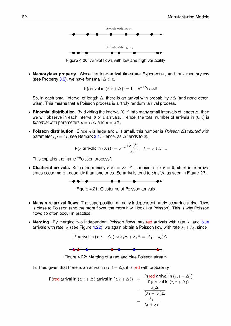
62 Manufacturing Models
Arrivals with low ca
Arrivals with high ca
Figure 4.20: Arrival flows with low and high variability
• Memoryless property. Since the inter-arrival times are Exponential, and thus memoryless(see Property 3.3), we have for small ∆ > 0,
P(arrival in (t, t + ∆)) = 1− e−λ∆≈ λ∆
So, in each small interval of length ∆, there is an arrival with probability λ∆ (and none other-wise). This means that a Poisson process is a “truly random” arrival process.
• Binomial distribution. By dividing the interval (0, t) into many small intervals of length ∆, thenwe will observe in each interval 0 or 1 arrivals. Hence, the total number of arrivals in (0, t) isbinomial with parameters n = t/∆ and p = λ∆.
• Poisson distribution. Since n is large and p is small, this number is Poisson distributed withparameter np = λt, see Remark 3.1. Hence, as ∆ tends to 0),
P(k arrivals in (0, t)) = e−λt (λt)k
k! , k = 0, 1, 2, ...
This explains the name “Poisson process”.
• Clustered arrivals. Since the density f (x) = λe−λx is maximal for x = 0, short inter-arrivaltimes occur more frequently than long ones. So arrivals tend to cluster, as seen in Figure ??.
Figure 4.21: Clustering of Poisson arrivals
• Many rare arrival flows. The superposition of many independent rarely occurring arrival flowsis close to Poisson (and the more flows, the more it will look like Poisson). This is why Poissonflows so often occur in practice!
• Merging. By merging two independent Poisson flows, say red arrivals with rate λ1 and bluearrivals with rate λ2 (see Figure 4.22), we again obtain a Poisson flow with rate λ1 + λ2, since
P(arrival in (t, t + ∆)) ≈ λ1∆ + λ2∆ = (λ1 + λ2)∆.
Figure 4.22: Merging of a red and blue Poisson stream
Further, given that there is an arrival in (t, t + ∆), it is red with probability
P(red arrival in (t, t + ∆)|arrival in (t, t + ∆)) = P(red arrival in (t, t + ∆))P(arrival in (t, t + ∆))
= λ1∆
(λ1 + λ2)∆
= λ1λ1 + λ2
.
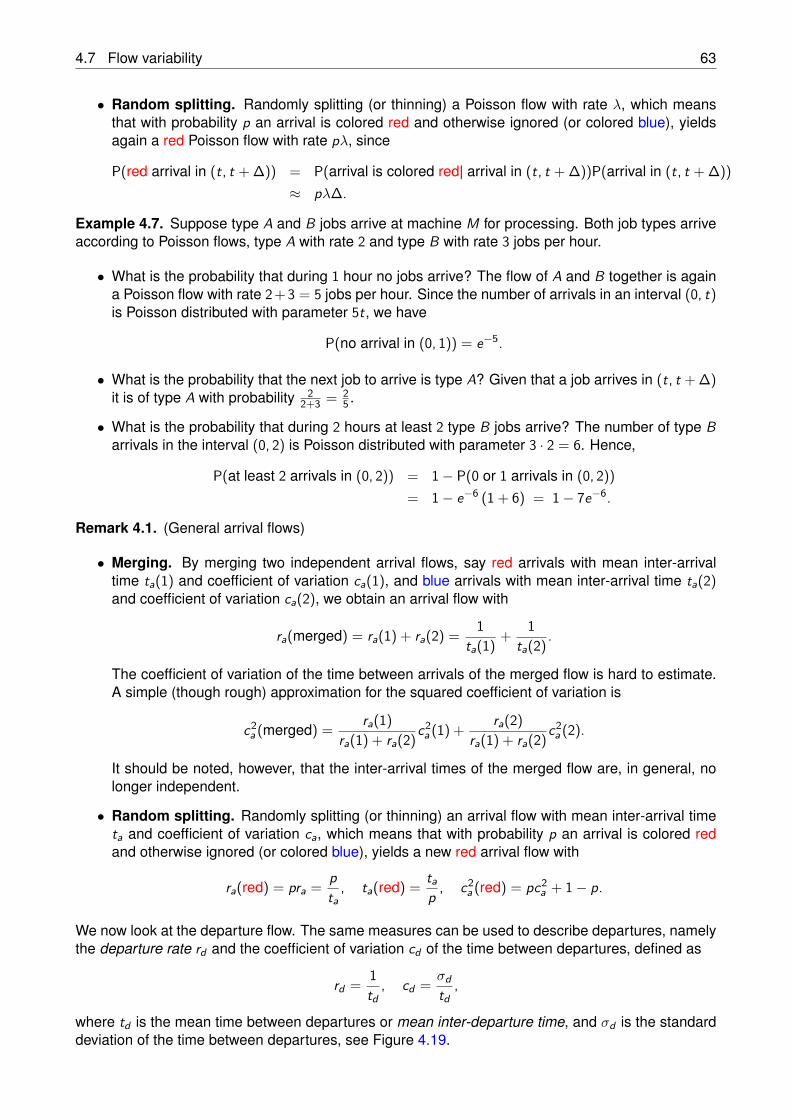
4.7 Flow variability 63
• Random splitting. Randomly splitting (or thinning) a Poisson flow with rate λ, which meansthat with probability p an arrival is colored red and otherwise ignored (or colored blue), yieldsagain a red Poisson flow with rate pλ, since
P(red arrival in (t, t + ∆)) = P(arrival is colored red| arrival in (t, t + ∆))P(arrival in (t, t + ∆))≈ pλ∆.
Example 4.7. Suppose type A and B jobs arrive at machine M for processing. Both job types arriveaccording to Poisson flows, type A with rate 2 and type B with rate 3 jobs per hour.
• What is the probability that during 1 hour no jobs arrive? The flow of A and B together is againa Poisson flow with rate 2+3 = 5 jobs per hour. Since the number of arrivals in an interval (0, t)is Poisson distributed with parameter 5t, we have
P(no arrival in (0, 1)) = e−5.
• What is the probability that the next job to arrive is type A? Given that a job arrives in (t, t + ∆)it is of type A with probability 2
2+3 = 25 .
• What is the probability that during 2 hours at least 2 type B jobs arrive? The number of type Barrivals in the interval (0, 2) is Poisson distributed with parameter 3 · 2 = 6. Hence,
P(at least 2 arrivals in (0, 2)) = 1− P(0 or 1 arrivals in (0, 2))= 1− e−6 (1 + 6) = 1− 7e−6.
Remark 4.1. (General arrival flows)
• Merging. By merging two independent arrival flows, say red arrivals with mean inter-arrivaltime ta(1) and coefficient of variation ca(1), and blue arrivals with mean inter-arrival time ta(2)and coefficient of variation ca(2), we obtain an arrival flow with
ra(merged) = ra(1) + ra(2) = 1ta(1) + 1
ta(2) .
The coefficient of variation of the time between arrivals of the merged flow is hard to estimate.A simple (though rough) approximation for the squared coefficient of variation is
c2a (merged) = ra(1)
ra(1) + ra(2)c2a (1) + ra(2)
ra(1) + ra(2)c2a (2).
It should be noted, however, that the inter-arrival times of the merged flow are, in general, nolonger independent.
• Random splitting. Randomly splitting (or thinning) an arrival flow with mean inter-arrival timeta and coefficient of variation ca, which means that with probability p an arrival is colored redand otherwise ignored (or colored blue), yields a new red arrival flow with
ra(red) = pra = pta
, ta(red) = tap , c2
a (red) = pc2a + 1− p.
We now look at the departure flow. The same measures can be used to describe departures, namelythe departure rate rd and the coefficient of variation cd of the time between departures, defined as
rd = 1td
, cd = σdtd
,
where td is the mean time between departures or mean inter-departure time, and σd is the standarddeviation of the time between departures, see Figure 4.19.
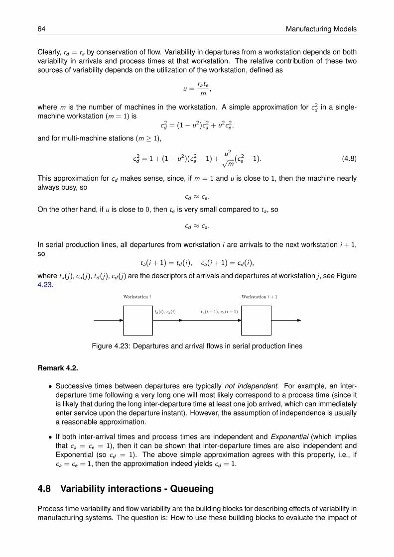
64 Manufacturing Models
Clearly, rd = ra by conservation of flow. Variability in departures from a workstation depends on bothvariability in arrivals and process times at that workstation. The relative contribution of these twosources of variability depends on the utilization of the workstation, defined as
u = ratem ,
where m is the number of machines in the workstation. A simple approximation for c2d in a single-
machine workstation (m = 1) isc2
d = (1− u2)c2a + u2c2
e ,
and for multi-machine stations (m ≥ 1),
c2d = 1 + (1− u2)(c2
a − 1) + u2√
m(c2
e − 1). (4.8)
This approximation for cd makes sense, since, if m = 1 and u is close to 1, then the machine nearlyalways busy, so
cd ≈ ce .
On the other hand, if u is close to 0, then te is very small compared to ta, so
cd ≈ ca.
In serial production lines, all departures from workstation i are arrivals to the next workstation i + 1,so
ta(i + 1) = td(i), ca(i + 1) = cd(i),
where ta(j), ca(j), td(j), cd(j) are the descriptors of arrivals and departures at workstation j , see Figure4.23.
td(i), cd(i) ta(i+ 1), ca(i+ 1)
Workstation i Workstation i+ 1
Figure 4.23: Departures and arrival flows in serial production lines
Remark 4.2.
• Successive times between departures are typically not independent. For example, an inter-departure time following a very long one will most likely correspond to a process time (since itis likely that during the long inter-departure time at least one job arrived, which can immediatelyenter service upon the departure instant). However, the assumption of independence is usuallya reasonable approximation.
• If both inter-arrival times and process times are independent and Exponential (which impliesthat ca = ce = 1), then it can be shown that inter-departure times are also independent andExponential (so cd = 1). The above simple approximation agrees with this property, i.e., ifca = ce = 1, then the approximation indeed yields cd = 1.
4.8 Variability interactions - Queueing
Process time variability and flow variability are the building blocks for describing effects of variability inmanufacturing systems. The question is: How to use these building blocks to evaluate the impact of
4.8 Variability interactions - Queueing 65
ta, ca
buffer
max b jobs
1
2
m
te, ce
ra = 1ta
re = mte
Figure 4.24: Queueing system with parameters
variability on key performance indicators such as WIP, cycle time and throughput? The total processtime is often a small part of the cycle time, where the extra major part of the cycle time is dueto waiting. So the fundamental issue of Factory Physics is to understand the underlying causesof waiting. The science of waiting is Queueing Theory. This theory studies the interactions andconsequences of sources of variability through mathematical modeling. Most queueing systemsconsists of three components:
• Arrival process: Arrivals can consist of single jobs or batches, and there may a single flow ormultiple flows of different jobs.
• Service (or production) process: The workstation can have a single machine, or multiple(non-) identical ones. Processing discipline can be first-come first-served (FCFS), last-comefirst-served (LCFS), shortest process time first (SPTF), random, and so on.
• Queue (or buffer): There may be ample (unlimited) queue space for jobs, or limited (or evenno) queue space.
Clearly there is a large variety of queueing systems. A convenient notation to characterize queueingsystems is the A/B/c notation, due to Kendall, where the letter A specifies the distribution of theinter-arrival times, B the distribution of the service times and c the number of servers. Typical valuesfor A and B are: D (Deterministic), M (Memoryless or Exponential) and G (General, i.e., this maybe any distribution). So an M/M/1 is a single Exponential server serving a Poisson stream of jobs.If only three letters are used, the implicit assumption is that service is FCFS and queueing space isinfinite. Otherwise, letters are added. For example, in an M/M/1/b there is room for at most b jobsin the system. For queueing systems specified with parameters (see Figure 4.24)
• ta, mean time between arrivals,
• ca, coefficient of variation of inter-arrival times,
• ra = 1ta
, rate of arrivals,
• m, number of parallel identical machines in station,
• b, buffer size (i.e., maximum number in station),
• te , mean effective process time,
• ce , coefficient of variation of the effective process time,
66 Manufacturing Models
• re = mte
, capacity of station,
we aim at estimating system performance in terms of
• pn, probability (or long-run fraction of time) of having n jobs at station,
• ϕB, expected waiting time (or flow time) spent in buffer,
• ϕ, expected cycle time or flow time in station,
• wB, average WIP in buffer,
• w , average WIP in station,
• δ, throughput of station.
Note that these measures are related as follows,
w =∞∑
n=0npn, w = wB + mu, ϕ = ϕB + te , w = δϕ, wB = δϕB,
where u is the machine utilization. In case queueing space is unlimited (b = ∞), we have δ = ra(since outflow is then equal to inflow) and the utilization u is given by
u = rare
= ratem = δte
m .
In the next section we start with the zero-buffer model.
4.9 Zero-buffer model
We consider a special production line, with two machines and no buffer in between, see Figure 4.25.
G M
ta te
Figure 4.25: Zero-buffer model with machines G and M
The first machine is G (i.e., the generator of arrivals), and the second one M. Machine G is neverstarved (i.e., there is always raw material available). If machine G completes a job, and M is stillbusy, then G blocks and has to wait till M finishes the job, before it can move the job to M and startprocessing the next one. Machine M never blocks (i.e., it can always get rid of the job), but mayhave to wait for input from G . The mean process time of G is ta, and the mean process time of M iste . What is the throughput δ? The throughput can be easily estimated the following χ3.0 model (thecomplete code is in Appendix B).
1 model real GME():2 real ta = 1.0, te = 1.0;3 int n = 1000;4 chan job a, b;56 run G(a, constant(ta)), M(a, b, constant(te)), E(b, n)7 end
4.10 Finite-buffer model 67
In this model we specified constant process times with mean 1. Process E is only counting thenumber of completed jobs (and once n = 1000 jobs are completed, the program stops and printsthe throughput). Obviously, for constant ta = te = 1, we get δ = 1. However, if we now changeto Exponential process times with mean 1, then the χ3.0 model produces the output δ = 2
3 . So thethroughput of the production line drops with 33%. Why? The reason is variability!
Let the random variable A be the process time of G and B the process time of M. Then the timebetween two departures is maxA, B and
δ = 1E [maxA, B] ≤
1maxE [A] , E [B]) ,
with equality only for constant A and B. It is the randomness in A and B that leads to starvation of M(A > B) and blocking of G(A < B), and thus to capacity loss. To deal with variations in these processtimes, we should use buffers! Indeed, if the buffer between G and M is sufficiently large, then
δ = 1maxE [A] , E [B] .
This can be readily verified by the following χ3.0 model (see Appendix C), to which a buffer betweenG and M has been added.
1 model real GBME ():2 real ta = 1.0, te = 1.0;3 int n = 1000, N = 10;4 chan job a, b, c;56 run G(a, exponential(ta)), B(a, b, N), M(b, c, exponential(te)), E(c, n)7 end
For a buffer of size N = 10, the estimated throughput is already around 0.93. In the next sectionwe study the finite buffer model with Exponential process times, and derive an exact formula for thethroughput as a function of the buffer size.
Remark 4.3. For zero buffer and Exponential process times the throughput can be exactly deter-mined. Suppose A and B are Exponential with rate λ1 and λ2. Then
P(maxA, B ≤ t) = P((A ≤ t)P(B ≤ t) = (1− e−λ1t)(1− e−λ2t) = 1− e−λ1t − e−λ2t + e−(λ1+λ2)t .
Hence, the density of maxA, B is
f (t) = ddt F (t) = λ1e−λ1t + λ2e−λ2t − (λ1 + λ2)e−(λ1+λ2)t ,
so
E [maxA, B] =∫ ∞
t=0tf (t)dt = λ2
1 + λ1λ2 + λ22
λ1λ2(λ1 + λ2) ,
and thus we get for the throughput
δ = 1E [maxA, B] = λ1λ2(λ1 + λ2)
λ21 + λ1λ2 + λ2
2.
4.10 Finite-buffer model
We now consider the production line with machines G and M, with a finite buffer of size b − 2 inbetween. When the first machine G completes a job, and the buffer is full, then G blocks and has towait till M finishes the job, before it can move the job into the buffer and start processing the next one.The process times of G and M are Exponential with rates ra = λ and re = µ (so ta = 1
λ and te = 1µ .
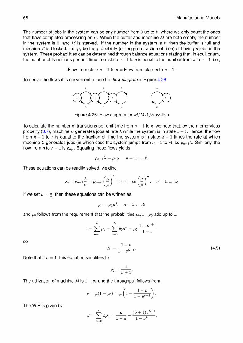
68 Manufacturing Models
The number of jobs in the system can be any number from 0 up to b, where we only count the onesthat have completed processing on G . When the buffer and machine M are both empty, the numberin the system is 0, and M is starved. If the number in the system is b, then the buffer is full andmachine G is blocked. Let pn be the probability (or long-run fraction of time) of having n jobs in thesystem. These probabilities can be determined through balance equations stating that, in equilibrium,the number of transitions per unit time from state n−1 to n is equal to the number from n to n−1, i.e.,
Flow from state n − 1 to n = Flow from state n to n − 1.
To derive the flows it is convenient to use the flow diagram in Figure 4.26.
0 1 2 b
λ
µ
λ λ
µ µ µ
λ
· · · · · ·
Figure 4.26: Flow diagram for M/M/1/b system
To calculate the number of transitions per unit time from n − 1 to n, we note that, by the memorylessproperty (3.7), machine G generates jobs at rate λ while the system is in state n− 1. Hence, the flowfrom n − 1 to n is equal to the fraction of time the system is in state n − 1 times the rate at whichmachine G generates jobs (in which case the system jumps from n − 1 to n), so pn−1λ. Similarly, theflow from n to n − 1 is pnµ. Equating these flows yields
pn−1λ = pnµ, n = 1, ... , b.
These equations can be readily solved, yielding
pn = pn−1λ
µ= pn−2
(λ
µ
)2= · · · = p0
(λ
µ
)n, n = 1, ... , b.
If we set u = λµ , then these equations can be written as
pn = p0un, n = 1, ... , b
and p0 follows from the requirement that the probabilities p0, ... , pb add up to 1,
1 =b∑
n=0pn =
b∑
n=0p0un = p0
1− ub+1
1− u ,
sop0 = 1− u
1− ub+1 . (4.9)
Note that if u = 1, this equation simplifies to
p0 = 1b + 1.
The utilization of machine M is 1− p0 and the throughput follows from
δ = µ(1− p0) = µ
(1− 1− u
1− ub+1
).
The WIP is given by
w =b∑
n=0npn = u
1− u −(b + 1)ub+1
1− ub+1 .
4.11 Single machine station 69
and the average flow time ϕ can then be calculated by Little’s law, ϕ = wδ . Note that the flow time starts
when the job completes processing on G (and then attempts to enter the buffer) and it ends whenthe job leaves machine M. To investigate the effect of blocking and starvation, we also calculate theperformance in case buffer space between G and M is unlimited, assuming u < 1 (since otherwise,the number in the system will grow to infinity). For b =∞ we immediately obtain
δ = µu, w = u1− u , ϕ =
1µ
1− u . (4.10)
By comparing the finite and infinite buffer systems, we can conclude that:
• Finite buffers always force stability, regardless the rates λ and µ.
• WIP is always less than in the infinite buffer system,
w <u
1− u .
• Throughput is always less than in the infinite buffer system,
δ < µu.
So the lesson is that the only way to reduce WIP without sacrificing too much throughput is: variabilityreduction!
Example 4.8. Consider the two machine line with 1/λ = 21 minutes and 1/µ = 20 minutes (seeSection 8.7.1. in [2]). Then u = 20
21 = 0.9524. For b =∞, we get
w = 20 jobs, δ = 0.0476 jobs per minute, ϕ = 420.14 minutes
and for b = 4 (so two buffer places in between G and M),
w = 1.894 jobs, δ = 0.039 jobs per minute, ϕ = 48.57 minutes
This shows that limiting the buffer space in between the two machines greatly reduces the WIP andflow time, but at the price of also reducing the throughput, the cost of which may not be covered bythe savings in inventory cost.
4.11 Single machine station
We start with the simplest interesting system, which is the M/M/1. So we assume a single machinewith unlimited buffer space. Jobs arrive one at a time. The inter-arrival times are Exponential withrate ra = λ. Processing is in order of arrival and jobs are processed one at a time. The process timesare Exponential with rate re = µ. Hence the utilization of the machine is
u = rare
= λ
µ,
which is assumed to be less than 1 (since otherwise the machine can not handle the work).
0 1 2 n− 1
λ
µ
λ λ
µ µ µ
λ
· · · · · ·
λ
µ
· · ·n
Figure 4.27: Flow diagram for M/M/1 system
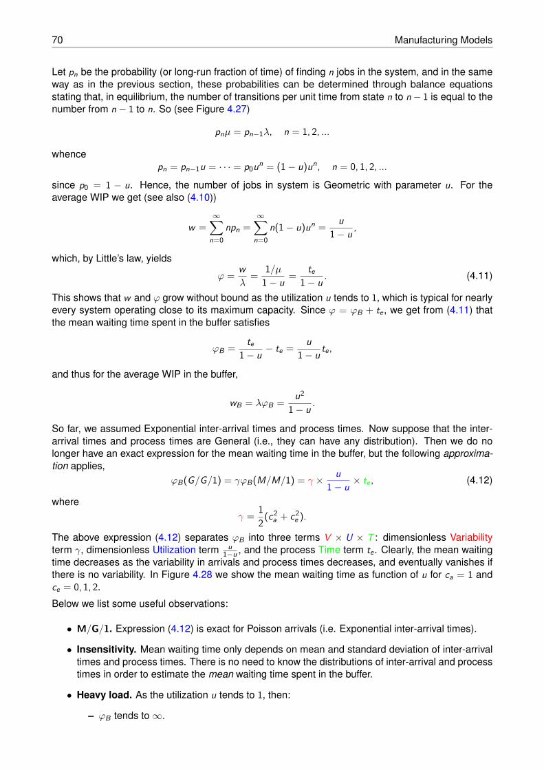
70 Manufacturing Models
Let pn be the probability (or long-run fraction of time) of finding n jobs in the system, and in the sameway as in the previous section, these probabilities can be determined through balance equationsstating that, in equilibrium, the number of transitions per unit time from state n to n− 1 is equal to thenumber from n − 1 to n. So (see Figure 4.27)
pnµ = pn−1λ, n = 1, 2, ...
whencepn = pn−1u = · · · = p0un = (1− u)un, n = 0, 1, 2, ...
since p0 = 1 − u. Hence, the number of jobs in system is Geometric with parameter u. For theaverage WIP we get (see also (4.10))
w =∞∑
n=0npn =
∞∑
n=0n(1− u)un = u
1− u ,
which, by Little’s law, yields
ϕ = wλ
= 1/µ1− u = te
1− u . (4.11)
This shows that w and ϕ grow without bound as the utilization u tends to 1, which is typical for nearlyevery system operating close to its maximum capacity. Since ϕ = ϕB + te , we get from (4.11) thatthe mean waiting time spent in the buffer satisfies
ϕB = te1− u − te = u
1− u te ,
and thus for the average WIP in the buffer,
wB = λϕB = u2
1− u .
So far, we assumed Exponential inter-arrival times and process times. Now suppose that the inter-arrival times and process times are General (i.e., they can have any distribution). Then we do nolonger have an exact expression for the mean waiting time in the buffer, but the following approxima-tion applies,
ϕB(G/G/1) = γϕB(M/M/1) = γ × u1− u × te , (4.12)
whereγ = 1
2(c2a + c2
e ).
The above expression (4.12) separates ϕB into three terms V × U × T : dimensionless Variabilityterm γ, dimensionless Utilization term u
1−u , and the process Time term te . Clearly, the mean waitingtime decreases as the variability in arrivals and process times decreases, and eventually vanishes ifthere is no variability. In Figure 4.28 we show the mean waiting time as function of u for ca = 1 andce = 0, 1, 2.
Below we list some useful observations:
• M/G/1. Expression (4.12) is exact for Poisson arrivals (i.e. Exponential inter-arrival times).
• Insensitivity. Mean waiting time only depends on mean and standard deviation of inter-arrivaltimes and process times. There is no need to know the distributions of inter-arrival and processtimes in order to estimate the mean waiting time spent in the buffer.
• Heavy load. As the utilization u tends to 1, then:
– ϕB tends to∞.
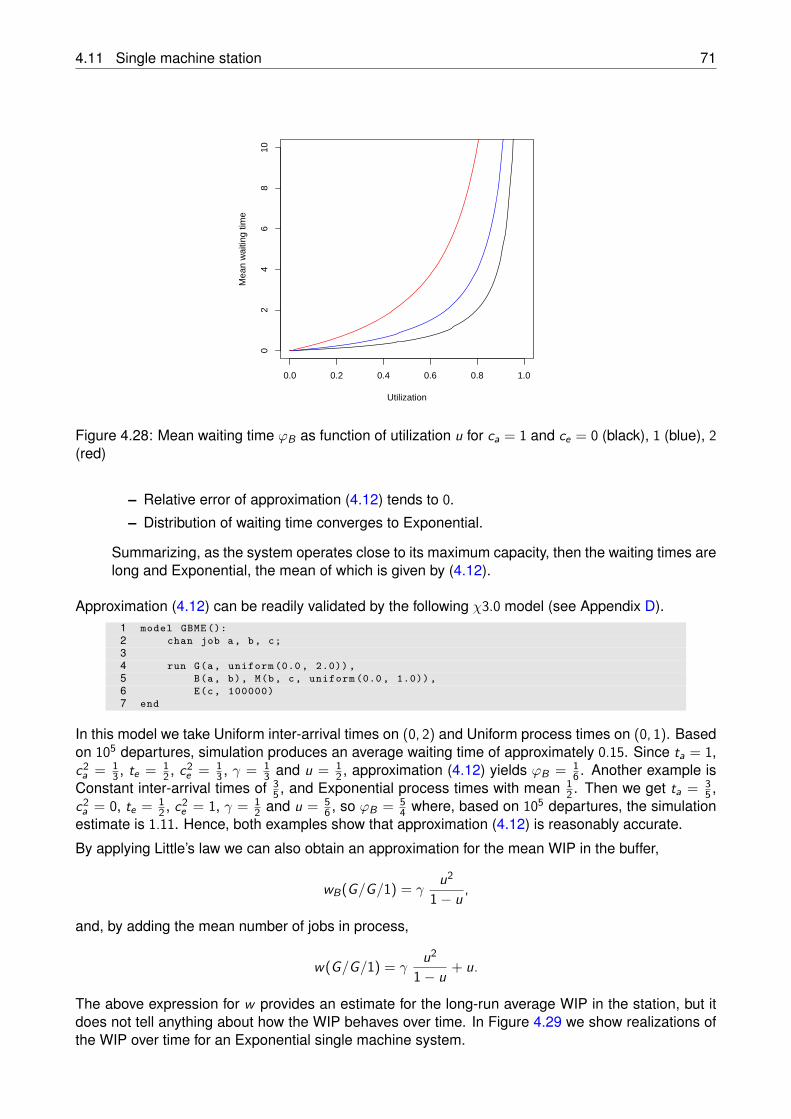
4.11 Single machine station 71
0.0 0.2 0.4 0.6 0.8 1.0
02
46
810
Utilization
Mea
n w
aitin
g tim
e
Figure 4.28: Mean waiting time ϕB as function of utilization u for ca = 1 and ce = 0 (black), 1 (blue), 2(red)
– Relative error of approximation (4.12) tends to 0.
– Distribution of waiting time converges to Exponential.
Summarizing, as the system operates close to its maximum capacity, then the waiting times arelong and Exponential, the mean of which is given by (4.12).
Approximation (4.12) can be readily validated by the following χ3.0 model (see Appendix D).1 model GBME ():2 chan job a, b, c;34 run G(a, uniform (0.0, 2.0)),5 B(a, b), M(b, c, uniform (0.0, 1.0)) ,6 E(c, 100000)7 end
In this model we take Uniform inter-arrival times on (0, 2) and Uniform process times on (0, 1). Basedon 105 departures, simulation produces an average waiting time of approximately 0.15. Since ta = 1,c2
a = 13 , te = 1
2 , c2e = 1
3 , γ = 13 and u = 1
2 , approximation (4.12) yields ϕB = 16 . Another example is
Constant inter-arrival times of 35 , and Exponential process times with mean 1
2 . Then we get ta = 35 ,
c2a = 0, te = 1
2 , c2e = 1, γ = 1
2 and u = 56 , so ϕB = 5
4 where, based on 105 departures, the simulationestimate is 1.11. Hence, both examples show that approximation (4.12) is reasonably accurate.
By applying Little’s law we can also obtain an approximation for the mean WIP in the buffer,
wB(G/G/1) = γu2
1− u ,
and, by adding the mean number of jobs in process,
w(G/G/1) = γu2
1− u + u.
The above expression for w provides an estimate for the long-run average WIP in the station, but itdoes not tell anything about how the WIP behaves over time. In Figure 4.29 we show realizations ofthe WIP over time for an Exponential single machine system.
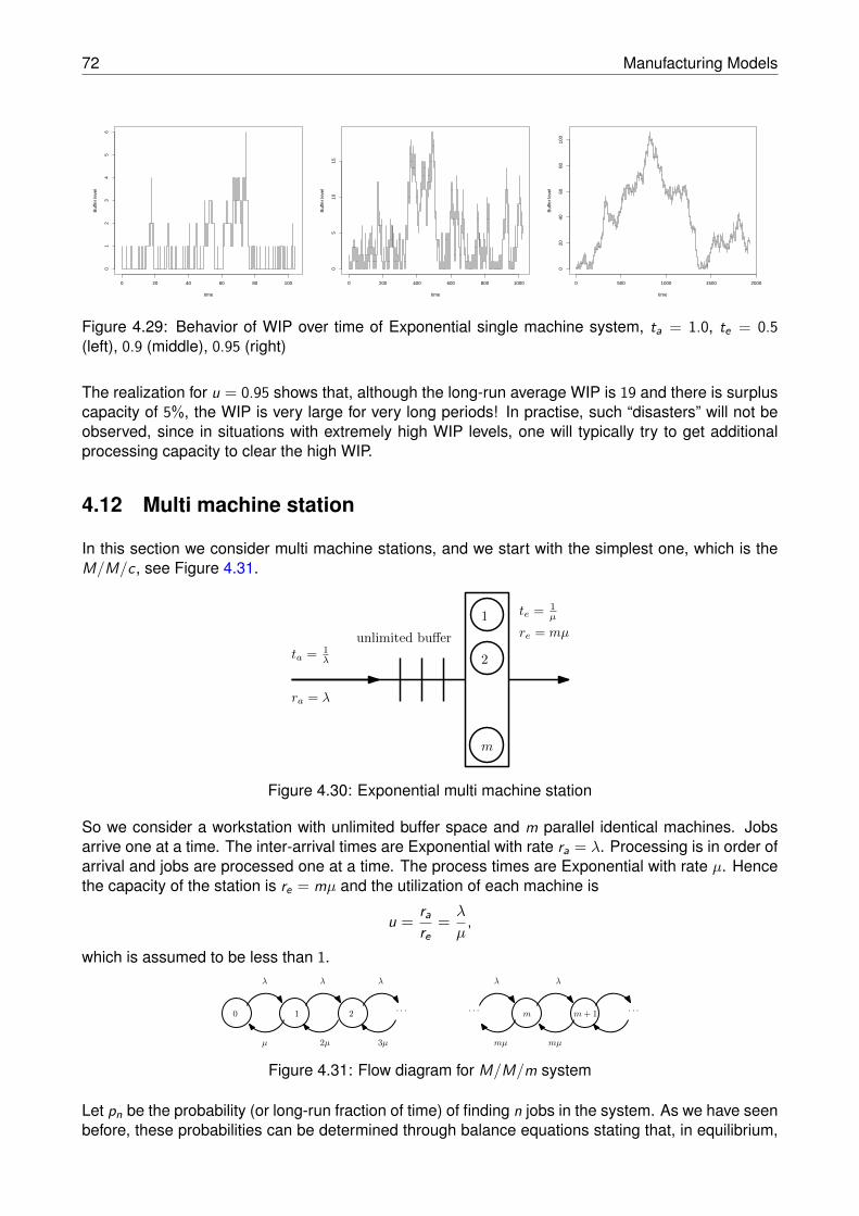
72 Manufacturing Models
0 20 40 60 80 100
01
23
45
6
time
Buf
fer
leve
l
0 200 400 600 800 1000
05
1015
time
Buf
fer
leve
l
0 500 1000 1500 2000
020
4060
8010
0
time
Buf
fer
leve
l
Figure 4.29: Behavior of WIP over time of Exponential single machine system, ta = 1.0, te = 0.5(left), 0.9 (middle), 0.95 (right)
The realization for u = 0.95 shows that, although the long-run average WIP is 19 and there is surpluscapacity of 5%, the WIP is very large for very long periods! In practise, such “disasters” will not beobserved, since in situations with extremely high WIP levels, one will typically try to get additionalprocessing capacity to clear the high WIP.
4.12 Multi machine station
In this section we consider multi machine stations, and we start with the simplest one, which is theM/M/c, see Figure 4.31.
ta = 1λ
unlimited buffer
1
2
m
te = 1µ
ra = λ
re = mµ
Figure 4.30: Exponential multi machine station
So we consider a workstation with unlimited buffer space and m parallel identical machines. Jobsarrive one at a time. The inter-arrival times are Exponential with rate ra = λ. Processing is in order ofarrival and jobs are processed one at a time. The process times are Exponential with rate µ. Hencethe capacity of the station is re = mµ and the utilization of each machine is
u = rare
= λ
µ,
which is assumed to be less than 1.
0 1 2 m
λ
µ
λ λ
2µ 3µ mµ
λ
· · · · · ·
λ
mµ
· · ·m+ 1
Figure 4.31: Flow diagram for M/M/m system
Let pn be the probability (or long-run fraction of time) of finding n jobs in the system. As we have seenbefore, these probabilities can be determined through balance equations stating that, in equilibrium,
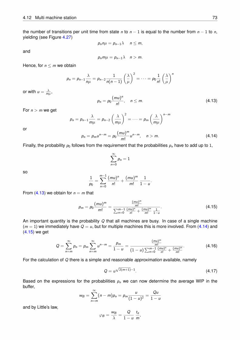
4.12 Multi machine station 73
the number of transitions per unit time from state n to n − 1 is equal to the number from n − 1 to n,yielding (see Figure 4.27)
pnnµ = pn−1λ n ≤ m,
andpnmµ = pn−1λ n > m.
Hence, for n ≤ m we obtain
pn = pn−1λ
nµ = pn−21
n(n − 1)
(λ
µ
)2= · · · = p0
1n!
(λ
µ
)n
or with u = λmµ ,
pn = p0(mu)n
n! , n ≤ m. (4.13)
For n > m we get
pn = pn−1λ
mµ = pn−2
(λ
mµ
)2= · · · = pm
(λ
mµ
)n−m
or
pn = pmun−m = p0(mu)m
m! un−m, n > m. (4.14)
Finally, the probability p0 follows from the requirement that the probabilities pn have to add up to 1,
∞∑
n=0pn = 1
so1p0
=m−1∑
n=0
(mu)n
n! + (mu)m
m!1
1− u .
From (4.13) we obtain for n = m that
pm = p0(mu)m
m! =(mu)m
m!∑m−1n=0
(mu)n
n! + (mu)m
m!1
1−u
. (4.15)
An important quantity is the probability Q that all machines are busy. In case of a single machine(m = 1) we immediately have Q = u, but for multiple machines this is more involved. From (4.14) and(4.15) we get
Q =∞∑
n=mpn = pm
∞∑
n=mun−m = pm
1− u =(mu)m
m!
(1− u)∑m−1
n=0(mu)n
n! + (mu)m
m!
. (4.16)
For the calculation of Q there is a simple and reasonable approximation available, namely
Q = u√
2(m+1)−1. (4.17)
Based on the expressions for the probabilities pn we can now determine the average WIP in thebuffer,
wB =∞∑
n=m(n −m)pn = pm
u(1− u)2 = Qu
1− u
and by Little’s law,
ϕB = wBλ
= Q1− u
tem ,
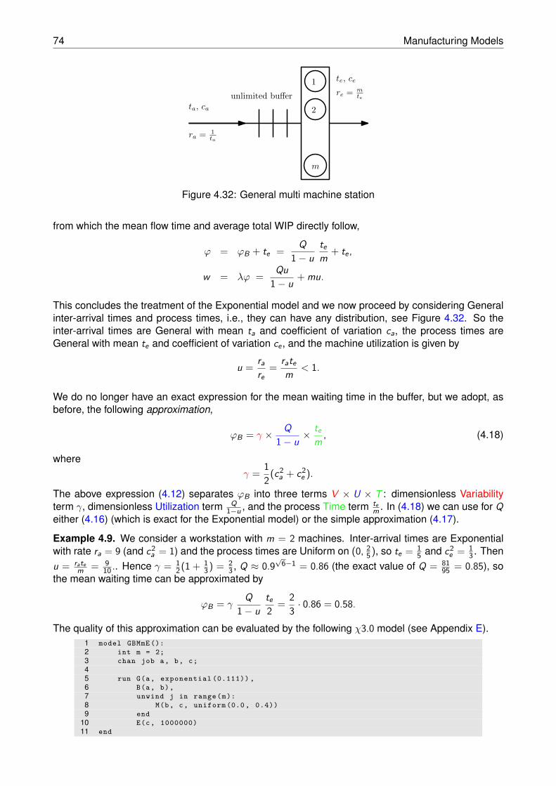
74 Manufacturing Models
ta, ca
unlimited buffer
1
2
m
te, ce
ra = 1ta
re = mte
Figure 4.32: General multi machine station
from which the mean flow time and average total WIP directly follow,
ϕ = ϕB + te = Q1− u
tem + te ,
w = λϕ = Qu1− u + mu.
This concludes the treatment of the Exponential model and we now proceed by considering Generalinter-arrival times and process times, i.e., they can have any distribution, see Figure 4.32. So theinter-arrival times are General with mean ta and coefficient of variation ca, the process times areGeneral with mean te and coefficient of variation ce , and the machine utilization is given by
u = rare
= ratem < 1.
We do no longer have an exact expression for the mean waiting time in the buffer, but we adopt, asbefore, the following approximation,
ϕB = γ × Q1− u ×
tem , (4.18)
whereγ = 1
2(c2a + c2
e ).
The above expression (4.12) separates ϕB into three terms V × U × T : dimensionless Variabilityterm γ, dimensionless Utilization term Q
1−u , and the process Time term tem . In (4.18) we can use for Q
either (4.16) (which is exact for the Exponential model) or the simple approximation (4.17).
Example 4.9. We consider a workstation with m = 2 machines. Inter-arrival times are Exponentialwith rate ra = 9 (and c2
a = 1) and the process times are Uniform on (0, 25), so te = 1
5 and c2e = 1
3 . Thenu = rate
m = 910 .. Hence γ = 1
2(1 + 13) = 2
3 , Q ≈ 0.9√
6−1 = 0.86 (the exact value of Q = 8195 = 0.85), so
the mean waiting time can be approximated by
ϕB = γQ
1− ute2 = 2
3 · 0.86 = 0.58.
The quality of this approximation can be evaluated by the following χ3.0 model (see Appendix E).1 model GBMmE ():2 int m = 2;3 chan job a, b, c;45 run G(a, exponential (0.111)) ,6 B(a, b),7 unwind j in range(m):8 M(b, c, uniform (0.0, 0.4))9 end
10 E(c, 1000000)11 end
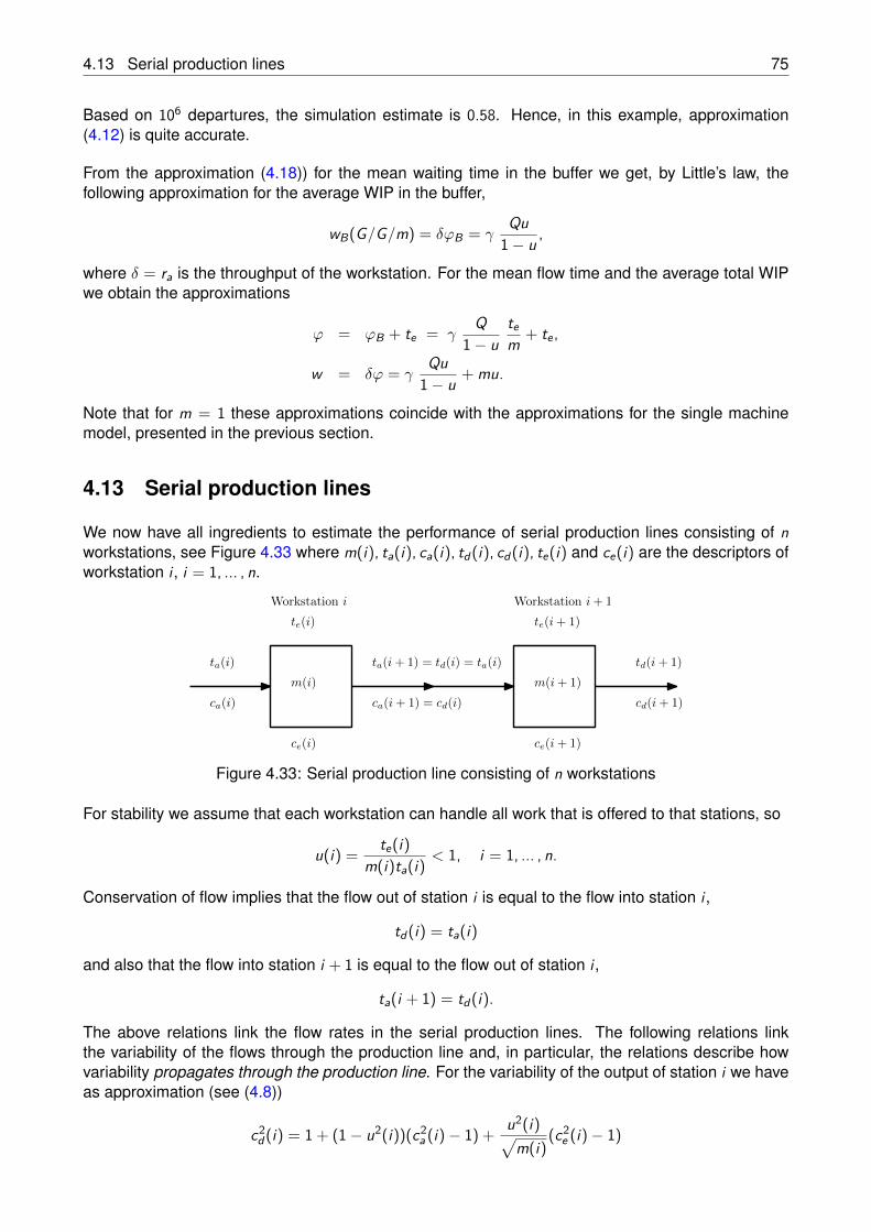
4.13 Serial production lines 75
Based on 106 departures, the simulation estimate is 0.58. Hence, in this example, approximation(4.12) is quite accurate.
From the approximation (4.18)) for the mean waiting time in the buffer we get, by Little’s law, thefollowing approximation for the average WIP in the buffer,
wB(G/G/m) = δϕB = γQu
1− u ,
where δ = ra is the throughput of the workstation. For the mean flow time and the average total WIPwe obtain the approximations
ϕ = ϕB + te = γQ
1− utem + te ,
w = δϕ = γQu
1− u + mu.
Note that for m = 1 these approximations coincide with the approximations for the single machinemodel, presented in the previous section.
4.13 Serial production lines
We now have all ingredients to estimate the performance of serial production lines consisting of nworkstations, see Figure 4.33 where m(i), ta(i), ca(i), td(i), cd(i), te(i) and ce(i) are the descriptors ofworkstation i , i = 1, ... , n.
ta(i)
ca(i)
m(i) m(i+ 1)
te(i)
ce(i)
te(i+ 1)
ce(i+ 1)
ta(i+ 1) = td(i) = ta(i)
ca(i+ 1) = cd(i)
td(i+ 1)
cd(i+ 1)
Workstation i Workstation i+ 1
Figure 4.33: Serial production line consisting of n workstations
For stability we assume that each workstation can handle all work that is offered to that stations, so
u(i) = te(i)m(i)ta(i) < 1, i = 1, ... , n.
Conservation of flow implies that the flow out of station i is equal to the flow into station i ,
td(i) = ta(i)
and also that the flow into station i + 1 is equal to the flow out of station i ,
ta(i + 1) = td(i).
The above relations link the flow rates in the serial production lines. The following relations linkthe variability of the flows through the production line and, in particular, the relations describe howvariability propagates through the production line. For the variability of the output of station i we haveas approximation (see (4.8))
c2d(i) = 1 + (1− u2(i))(c2
a (i)− 1) + u2(i)√m(i)
(c2e (i)− 1)
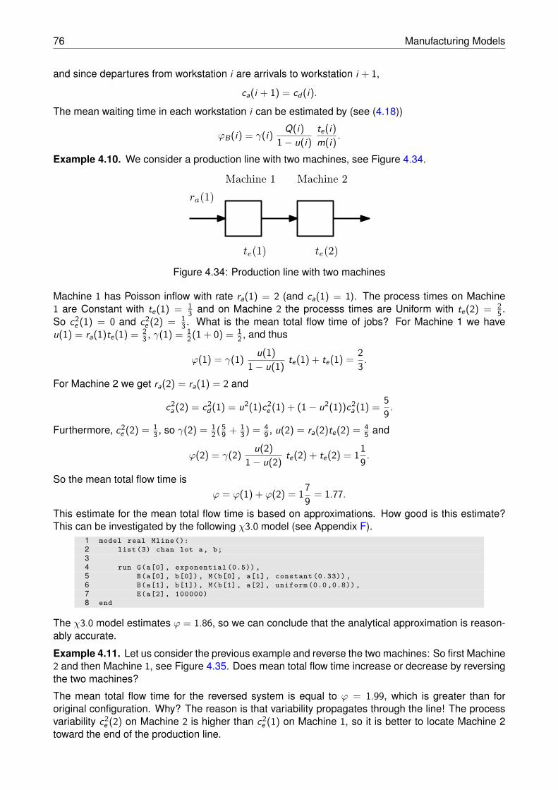
76 Manufacturing Models
and since departures from workstation i are arrivals to workstation i + 1,
ca(i + 1) = cd(i).
The mean waiting time in each workstation i can be estimated by (see (4.18))
ϕB(i) = γ(i) Q(i)1− u(i)
te(i)m(i) .
Example 4.10. We consider a production line with two machines, see Figure 4.34.
Machine 1 Machine 2
ra(1)
te(1) te(2)
Figure 4.34: Production line with two machines
Machine 1 has Poisson inflow with rate ra(1) = 2 (and ca(1) = 1). The process times on Machine1 are Constant with te(1) = 1
3 and on Machine 2 the processs times are Uniform with te(2) = 25 .
So c2e (1) = 0 and c2
e (2) = 13 . What is the mean total flow time of jobs? For Machine 1 we have
u(1) = ra(1)te(1) = 23 , γ(1) = 1
2(1 + 0) = 12 , and thus
ϕ(1) = γ(1) u(1)1− u(1) te(1) + te(1) = 2
3.
For Machine 2 we get ra(2) = ra(1) = 2 and
c2a (2) = c2
d(1) = u2(1)c2e (1) + (1− u2(1))c2
a (1) = 59.
Furthermore, c2e (2) = 1
3 , so γ(2) = 12(5
9 + 13) = 4
9 , u(2) = ra(2)te(2) = 45 and
ϕ(2) = γ(2) u(2)1− u(2) te(2) + te(2) = 11
9.
So the mean total flow time isϕ = ϕ(1) + ϕ(2) = 17
9 = 1.77.
This estimate for the mean total flow time is based on approximations. How good is this estimate?This can be investigated by the following χ3.0 model (see Appendix F).
1 model real Mline ():2 list (3) chan lot a, b;34 run G(a[0], exponential (0.5)) ,5 B(a[0], b[0]), M(b[0], a[1], constant (0.33)) ,6 B(a[1], b[1]), M(b[1], a[2], uniform (0.0 ,0.8)) ,7 E(a[2], 100000)8 end
The χ3.0 model estimates ϕ = 1.86, so we can conclude that the analytical approximation is reason-ably accurate.
Example 4.11. Let us consider the previous example and reverse the two machines: So first Machine2 and then Machine 1, see Figure 4.35. Does mean total flow time increase or decrease by reversingthe two machines?
The mean total flow time for the reversed system is equal to ϕ = 1.99, which is greater than fororiginal configuration. Why? The reason is that variability propagates through the line! The processvariability c2
e (2) on Machine 2 is higher than c2e (1) on Machine 1, so it is better to locate Machine 2
toward the end of the production line.
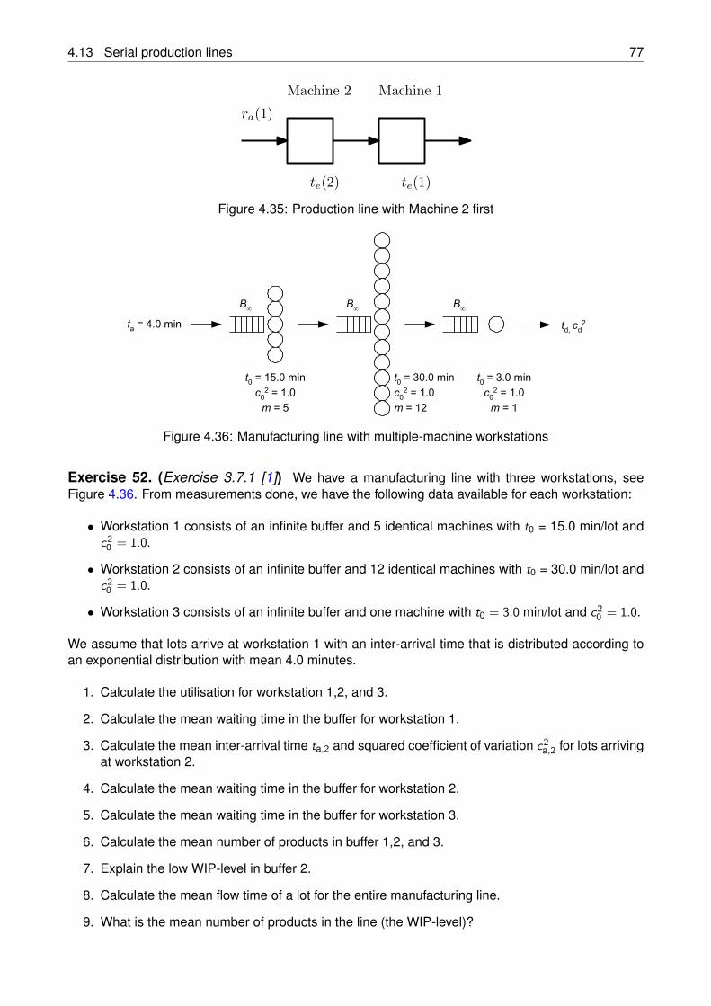
4.13 Serial production lines 77
Machine 2 Machine 1
ra(1)
te(2) te(1)
Figure 4.35: Production line with Machine 2 first
t0
= 15.0 min
td,
cd2
c02 = 1.0
B¥
B¥
B¥
c02 = 1.0
t0
= 30.0 min
c02 = 1.0
t0
= 3.0 min
ta
= 4.0 min
m = 5 m = 12 m = 1
Figure 4.36: Manufacturing line with multiple-machine workstations
Exercise 52. (Exercise 3.7.1 [1]) We have a manufacturing line with three workstations, seeFigure 4.36. From measurements done, we have the following data available for each workstation:
• Workstation 1 consists of an infinite buffer and 5 identical machines with t0 = 15.0 min/lot andc2
0 = 1.0.
• Workstation 2 consists of an infinite buffer and 12 identical machines with t0 = 30.0 min/lot andc2
0 = 1.0.
• Workstation 3 consists of an infinite buffer and one machine with t0 = 3.0 min/lot and c20 = 1.0.
We assume that lots arrive at workstation 1 with an inter-arrival time that is distributed according toan exponential distribution with mean 4.0 minutes.
1. Calculate the utilisation for workstation 1,2, and 3.
2. Calculate the mean waiting time in the buffer for workstation 1.
3. Calculate the mean inter-arrival time ta,2 and squared coefficient of variation c2a,2 for lots arriving
at workstation 2.
4. Calculate the mean waiting time in the buffer for workstation 2.
5. Calculate the mean waiting time in the buffer for workstation 3.
6. Calculate the mean number of products in buffer 1,2, and 3.
7. Explain the low WIP-level in buffer 2.
8. Calculate the mean flow time of a lot for the entire manufacturing line.
9. What is the mean number of products in the line (the WIP-level)?
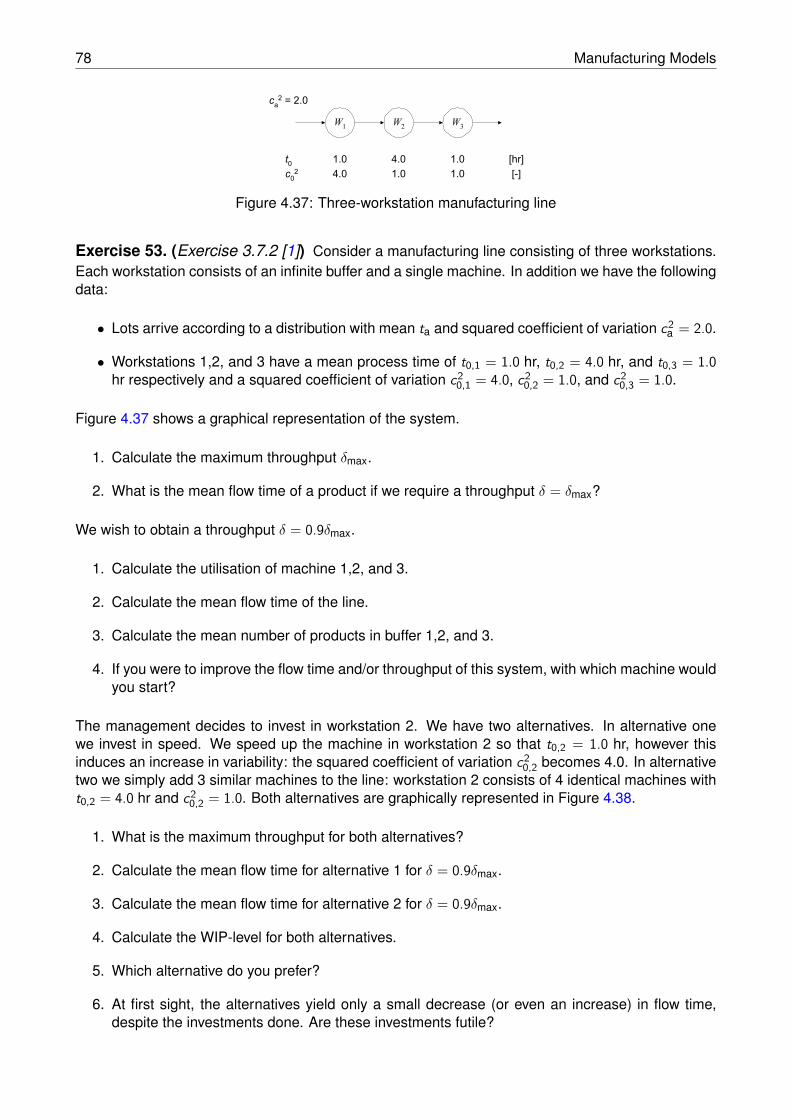
78 Manufacturing Models
W1
ca2 = 2.0
c02
t0
1.0 4.0 1.0
4.0 1.0 1.0
[hr]
[-]
W2
W3
Figure 4.37: Three-workstation manufacturing line
Exercise 53. (Exercise 3.7.2 [1]) Consider a manufacturing line consisting of three workstations.Each workstation consists of an infinite buffer and a single machine. In addition we have the followingdata:
• Lots arrive according to a distribution with mean ta and squared coefficient of variation c2a = 2.0.
• Workstations 1,2, and 3 have a mean process time of t0,1 = 1.0 hr, t0,2 = 4.0 hr, and t0,3 = 1.0hr respectively and a squared coefficient of variation c2
0,1 = 4.0, c20,2 = 1.0, and c2
0,3 = 1.0.
Figure 4.37 shows a graphical representation of the system.
1. Calculate the maximum throughput δmax.
2. What is the mean flow time of a product if we require a throughput δ = δmax?
We wish to obtain a throughput δ = 0.9δmax.
1. Calculate the utilisation of machine 1,2, and 3.
2. Calculate the mean flow time of the line.
3. Calculate the mean number of products in buffer 1,2, and 3.
4. If you were to improve the flow time and/or throughput of this system, with which machine wouldyou start?
The management decides to invest in workstation 2. We have two alternatives. In alternative onewe invest in speed. We speed up the machine in workstation 2 so that t0,2 = 1.0 hr, however thisinduces an increase in variability: the squared coefficient of variation c2
0,2 becomes 4.0. In alternativetwo we simply add 3 similar machines to the line: workstation 2 consists of 4 identical machines witht0,2 = 4.0 hr and c2
0,2 = 1.0. Both alternatives are graphically represented in Figure 4.38.
1. What is the maximum throughput for both alternatives?
2. Calculate the mean flow time for alternative 1 for δ = 0.9δmax.
3. Calculate the mean flow time for alternative 2 for δ = 0.9δmax.
4. Calculate the WIP-level for both alternatives.
5. Which alternative do you prefer?
6. At first sight, the alternatives yield only a small decrease (or even an increase) in flow time,despite the investments done. Are these investments futile?
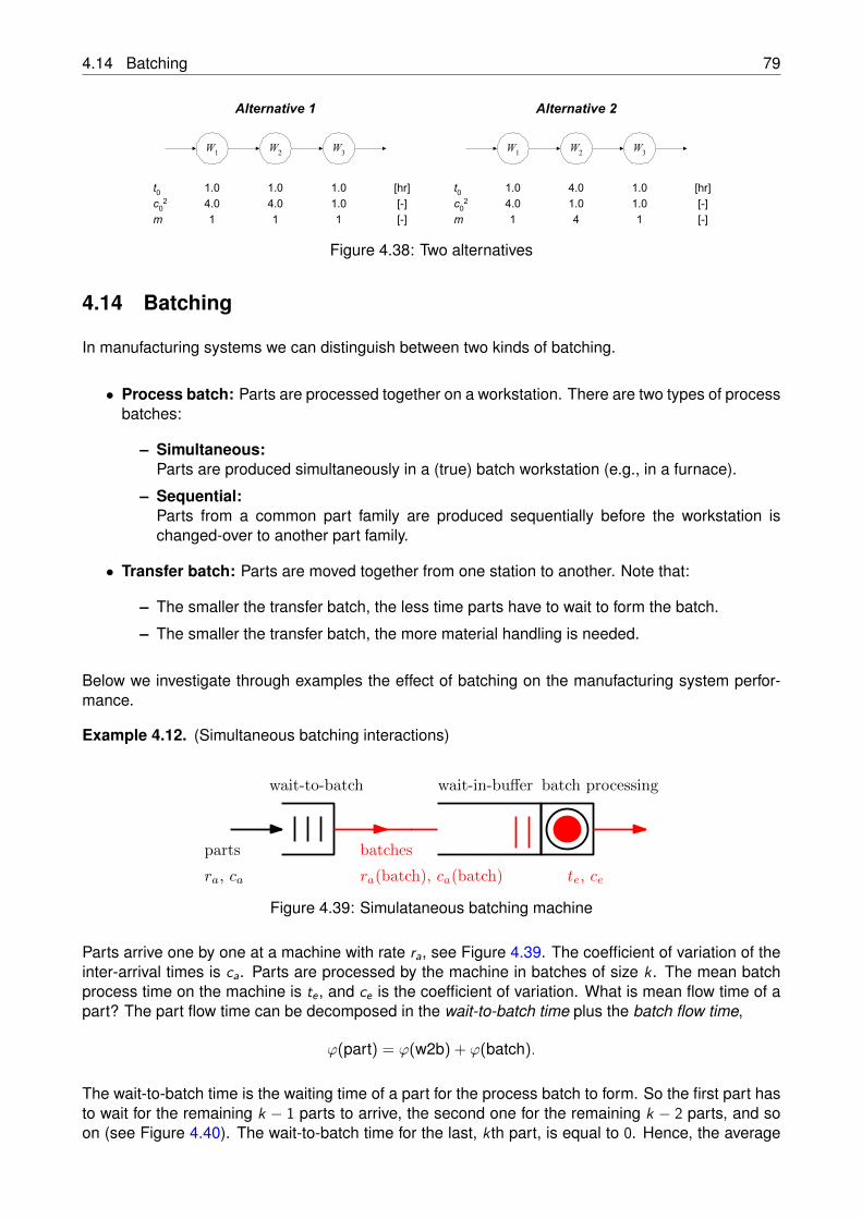
4.14 Batching 79
Alternative 2
W1
c02
t0
1.0 1.0 1.0
4.0 4.0 1.0
[hr]
[-]
W2
W3
m 1 1 1
W1
c02
t0
1.0 4.0 1.0
4.0 1.0 1.0
[hr]
[-]
W2
W3
m 1 4 1[-]
Alternative 1
[-]
Figure 4.38: Two alternatives
4.14 Batching
In manufacturing systems we can distinguish between two kinds of batching.
• Process batch: Parts are processed together on a workstation. There are two types of processbatches:
– Simultaneous:Parts are produced simultaneously in a (true) batch workstation (e.g., in a furnace).
– Sequential:Parts from a common part family are produced sequentially before the workstation ischanged-over to another part family.
• Transfer batch: Parts are moved together from one station to another. Note that:
– The smaller the transfer batch, the less time parts have to wait to form the batch.
– The smaller the transfer batch, the more material handling is needed.
Below we investigate through examples the effect of batching on the manufacturing system perfor-mance.
Example 4.12. (Simultaneous batching interactions)
wait-to-batch wait-in-buffer batch processing
parts batches
ra, ca ra(batch), ca(batch) te, ce
Figure 4.39: Simulataneous batching machine
Parts arrive one by one at a machine with rate ra, see Figure 4.39. The coefficient of variation of theinter-arrival times is ca. Parts are processed by the machine in batches of size k. The mean batchprocess time on the machine is te , and ce is the coefficient of variation. What is mean flow time of apart? The part flow time can be decomposed in the wait-to-batch time plus the batch flow time,
ϕ(part) = ϕ(w2b) + ϕ(batch).
The wait-to-batch time is the waiting time of a part for the process batch to form. So the first part hasto wait for the remaining k − 1 parts to arrive, the second one for the remaining k − 2 parts, and soon (see Figure 4.40). The wait-to-batch time for the last, kth part, is equal to 0. Hence, the average
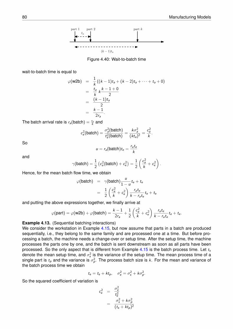
80 Manufacturing Models
ta
(k − 1)ta
part 1 part 2 part k
Figure 4.40: Wait-to-batch time
wait-to-batch time is equal to
ϕ(w2b) = 1k ((k − 1)ta + (k − 2)ta + · · ·+ ta + 0)
= tak k k − 1 + 0
2
= (k − 1)ta2
= k − 12ra
.
The batch arrival rate is ra(batch) = rak and
c2a (batch) = σ2
a(batch)t2a (batch) = kσ2
a(kta)2 = c2
ak .
Sou = ra(batch)te = rate
kand
γ(batch) = 12(c2
a (batch) + c2e)
= 12
(c2
ak + c2
e
).
Hence, for the mean batch flow time, we obtain
ϕ(batch) = γ(batch) u1− u te + te
= 12
(c2
ak + c2
e
)rate
k − ratete + te
and putting the above expressions together, we finally arrive at
ϕ(part) = ϕ(w2b) + ϕ(batch) = k − 12ra
+ 12
(c2
ak + c2
e
)rate
k − ratete + te .
Example 4.13. (Sequential batching interactions)We consider the workstation in Example 4.15, but now assume that parts in a batch are producedsequentially, i.e., they belong to the same family and are processed one at a time. But before pro-cessing a batch, the machine needs a change-over or setup time. After the setup time, the machineprocesses the parts one by one, and the batch is sent downstream as soon as all parts have beenprocessed. So the only aspect that is different from Example 4.15 is the batch process time. Let tsdenote the mean setup time, and σ2
s is the variance of the setup time. The mean process time of asingle part is tp and the variance is σ2
p. The process batch size is k. For the mean and variance ofthe batch process time we obtain
te = ts + ktp, σ2e = σ2
s + kσ2p.
So the squared coefficient of variation is
c2e = σ2
et2e
=σ2
s + kσ2p
(ts + ktp)2
4.14 Batching 81
and the machine utilization,
u = ra(batch)te
= rak te
= ra
(tsk + tp
).
Note that the requirement u < 1 implies that there is minimal feasible batch size: k > rats1−ratp
. Further-more, from the expression for u, we can conclude that the batch size k affects the machine utilization:A larger batch size k leads to a lower utilization. The mean part flow time is the average wait-to-batchtime plus the mean batch flow time, so
ϕ(part) = ϕ(w2b) + ϕ(batch)
= k − 12ra
+ 12
(c2
ak +
σ2s + kσ2
p(ts + ktp)2
)ra( ts
k + tp)1− ra( ts
k + tp)(ts + ktp) + ts + ktp.
Apparently, there is a batch size trade-off: A larger batch size k leads to a lower machine utilization,but also to a higher wait-to-batch and wait-in-batch time. This trade-off is illustrated in Figure 4.41 forthe parameter setting ra = 0.4, ca = 1, ts = 5, σ2
s = 614 , tp = 1 and σ2
p = 14 . In this example the optimal
batch size is k = 5.
5 10 15
2025
3035
4045
batch size k
mea
n to
tal f
low
tim
e
Figure 4.41: Mean part flow time as a function of the batch size k for the parameter setting ra = 0.4,ca = 1, ts = 5, σ2
s = 614 , tp = 1 and σ2
p = 14
Example 4.14. (Sequential batching interactions and job splitting)In the previous example we assumed that the batch is sent downstream as soon as all parts havebeen processed. In this example we consider a different situation: Individual parts are sent down-stream as soon as being processed. In other words, the batch is split and parts proceed individually
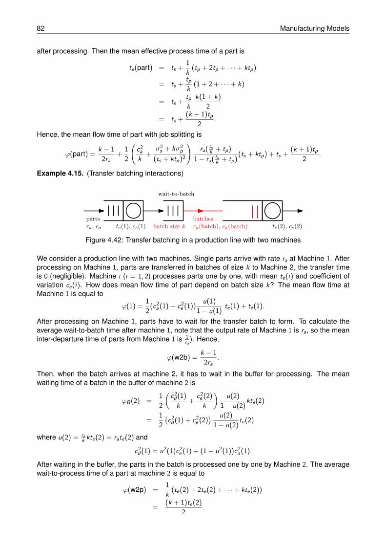
82 Manufacturing Models
after processing. Then the mean effective process time of a part is
te(part) = ts + 1k (tp + 2tp + · · ·+ ktp)
= ts + tpk (1 + 2 + · · ·+ k)
= ts + tpk
k(1 + k)2
= ts + (k + 1)tp2 .
Hence, the mean flow time of part with job splitting is
ϕ(part) = k − 12ra
+ 12
(c2
ak +
σ2s + kσ2
p(ts + ktp)2
)ra( ts
k + tp)1− ra( ts
k + tp)(ts + ktp) + ts + (k + 1)tp
2 .
Example 4.15. (Transfer batching interactions)
wait-to-batch
parts batchesra, ca ra(batch), ca(batch) te(2), ce(2)batch size kte(1), ce(1)
Figure 4.42: Transfer batching in a production line with two machines
We consider a production line with two machines. Single parts arrive with rate ra at Machine 1. Afterprocessing on Machine 1, parts are transferred in batches of size k to Machine 2, the transfer timeis 0 (negligible). Machine i (i = 1, 2) processes parts one by one, with mean te(i) and coefficient ofvariation ce(i). How does mean flow time of part depend on batch size k? The mean flow time atMachine 1 is equal to
ϕ(1) = 12(c2
a (1) + c2e (1)) u(1)
1− u(1) te(1) + te(1).
After processing on Machine 1, parts have to wait for the transfer batch to form. To calculate theaverage wait-to-batch time after machine 1, note that the output rate of Machine 1 is ra, so the meaninter-departure time of parts from Machine 1 is 1
ra). Hence,
ϕ(w2b) = k − 12ra
.
Then, when the batch arrives at machine 2, it has to wait in the buffer for processing. The meanwaiting time of a batch in the buffer of machine 2 is
ϕB(2) = 12
(c2
d(1)k + c2
e (2)k
)u(2)
1− u(2)kte(2)
= 12(c2
d(1) + c2e (2)
) u(2)1− u(2) te(2)
where u(2) = rak kte(2) = rate(2) and
c2d(1) = u2(1)c2
e (1) + (1− u2(1))c2a (1).
After waiting in the buffer, the parts in the batch is processed one by one by Machine 2. The averagewait-to-process time of a part at machine 2 is equal to
ϕ(w2p) = 1k (te(2) + 2te(2) + · · ·+ kte(2))
= (k + 1)te(2)2 .
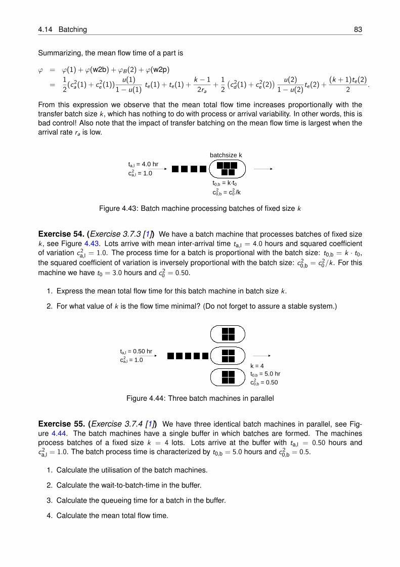
4.14 Batching 83
Summarizing, the mean flow time of a part is
ϕ = ϕ(1) + ϕ(w2b) + ϕB(2) + ϕ(w2p)
= 12(c2
a (1) + c2e (1)) u(1)
1− u(1) te(1) + te(1) + k − 12ra
+ 12(c2
d(1) + c2e (2)
) u(2)1− u(2) te(2) + (k + 1)te(2)
2 .
From this expression we observe that the mean total flow time increases proportionally with thetransfer batch size k, which has nothing to do with process or arrival variability. In other words, this isbad control! Also note that the impact of transfer batching on the mean flow time is largest when thearrival rate ra is low.
batchsize k
t0,b = k·t0c0,b = c0 /k
2 2
ta,l = 4.0 hrca,l = 1.02
Figure 4.43: Batch machine processing batches of fixed size k
Exercise 54. (Exercise 3.7.3 [1]) We have a batch machine that processes batches of fixed sizek, see Figure 4.43. Lots arrive with mean inter-arrival time ta,l = 4.0 hours and squared coefficientof variation c2
a,l = 1.0. The process time for a batch is proportional with the batch size: t0,b = k · t0,the squared coefficient of variation is inversely proportional with the batch size: c2
0,b = c20/k. For this
machine we have t0 = 3.0 hours and c20 = 0.50.
1. Express the mean total flow time for this batch machine in batch size k.
2. For what value of k is the flow time minimal? (Do not forget to assure a stable system.)
k = 4t0,b = 5.0 hrc0,b = 0.502
ta,l = 0.50 hrca,l = 1.02
Figure 4.44: Three batch machines in parallel
Exercise 55. (Exercise 3.7.4 [1]) We have three identical batch machines in parallel, see Fig-ure 4.44. The batch machines have a single buffer in which batches are formed. The machinesprocess batches of a fixed size k = 4 lots. Lots arrive at the buffer with ta,l = 0.50 hours andc2
a,l = 1.0. The batch process time is characterized by t0,b = 5.0 hours and c20,b = 0.5.
1. Calculate the utilisation of the batch machines.
2. Calculate the wait-to-batch-time in the buffer.
3. Calculate the queueing time for a batch in the buffer.
4. Calculate the mean total flow time.

84 Manufacturing Models
Bibliography
[1] I.J.B.F. ADAN, A.T. HOFKAMP, J.E. ROODA AND J. VERVOORT, Analysis of Manufacturing Sys-tems, 2012.
[2] W.J. HOPP, M.L. SPEARMAN, 2012. Factory Physics, 3rd ed., McGraw-Hill, 2008.
[3] D. MORIN, Probability - For the Enthusiastic Beginner, 2016.
[4] R. SURI, Quick Response Manufacturing, Taylor&Francis Inc, 1998.
[5] H.C. TIJMS, Understanding Probability, 3rd ed., Cambridge, 2012.

86 BIBLIOGRAPHY
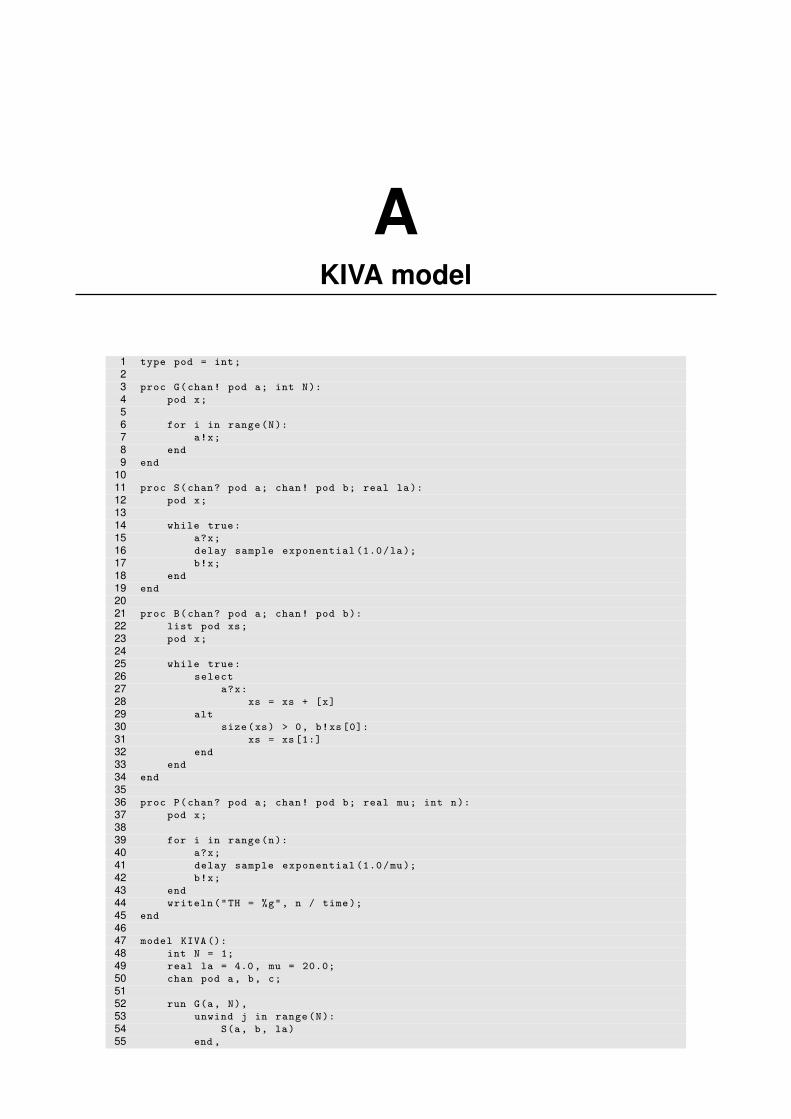
AKIVA model
1 type pod = int;23 proc G(chan! pod a; int N):4 pod x;56 for i in range(N):7 a!x;8 end9 end
1011 proc S(chan? pod a; chan! pod b; real la):12 pod x;1314 while true:15 a?x;16 delay sample exponential (1.0/la);17 b!x;18 end19 end2021 proc B(chan? pod a; chan! pod b):22 list pod xs;23 pod x;2425 while true:26 select27 a?x:28 xs = xs + [x]29 alt30 size(xs) > 0, b!xs[0]:31 xs = xs[1:]32 end33 end34 end3536 proc P(chan? pod a; chan! pod b; real mu; int n):37 pod x;3839 for i in range(n):40 a?x;41 delay sample exponential (1.0/mu);42 b!x;43 end44 writeln("TH = %g", n / time);45 end4647 model KIVA ():48 int N = 1;49 real la = 4.0, mu = 20.0;50 chan pod a, b, c;5152 run G(a, N),53 unwind j in range(N):54 S(a, b, la)55 end ,

88 KIVA model
56 B(b, c), P(c, a, mu, 10000)57 end
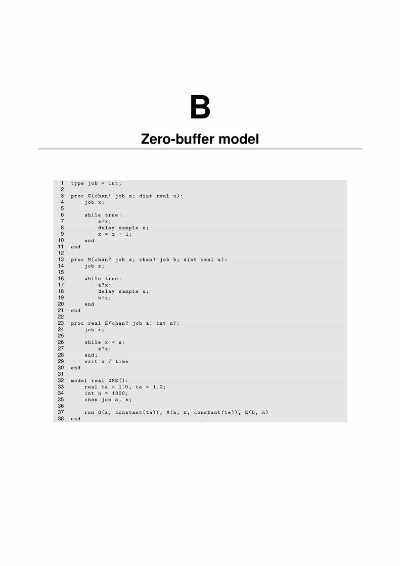
BZero-buffer model
1 type job = int;23 proc G(chan! job a; dist real u):4 job x;56 while true:7 a!x;8 delay sample u;9 x = x + 1;
10 end11 end1213 proc M(chan? job a; chan! job b; dist real u):14 job x;1516 while true:17 a?x;18 delay sample u;19 b!x;20 end21 end2223 proc real E(chan? job a; int n):24 job x;2526 while x < n:27 a?x;28 end;29 exit x / time30 end3132 model real GME():33 real ta = 1.0, te = 1.0;34 int n = 1000;35 chan job a, b;3637 run G(a, constant(ta)), M(a, b, constant(te)), E(b, n)38 end

90 Zero-buffer model
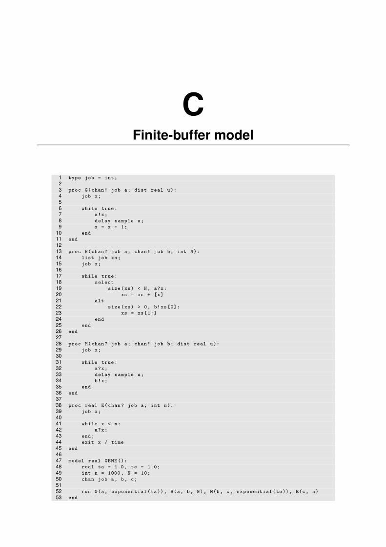
CFinite-buffer model
1 type job = int;23 proc G(chan! job a; dist real u):4 job x;56 while true:7 a!x;8 delay sample u;9 x = x + 1;
10 end11 end1213 proc B(chan? job a; chan! job b; int N):14 list job xs;15 job x;1617 while true:18 select19 size(xs) < N, a?x:20 xs = xs + [x]21 alt22 size(xs) > 0, b!xs[0]:23 xs = xs[1:]24 end25 end26 end2728 proc M(chan? job a; chan! job b; dist real u):29 job x;3031 while true:32 a?x;33 delay sample u;34 b!x;35 end36 end3738 proc real E(chan? job a; int n):39 job x;4041 while x < n:42 a?x;43 end;44 exit x / time45 end4647 model real GBME ():48 real ta = 1.0, te = 1.0;49 int n = 1000, N = 10;50 chan job a, b, c;5152 run G(a, exponential(ta)), B(a, b, N), M(b, c, exponential(te)), E(c, n)53 end

92 Finite-buffer model
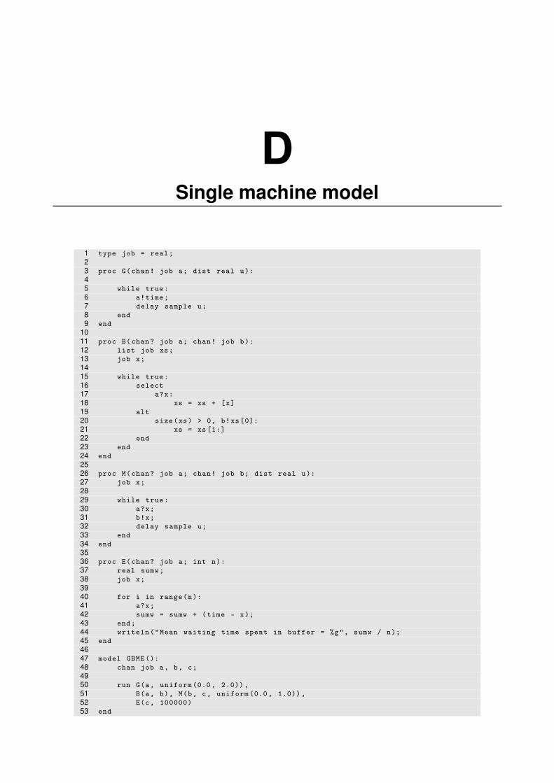
DSingle machine model
1 type job = real;23 proc G(chan! job a; dist real u):45 while true:6 a!time;7 delay sample u;8 end9 end
1011 proc B(chan? job a; chan! job b):12 list job xs;13 job x;1415 while true:16 select17 a?x:18 xs = xs + [x]19 alt20 size(xs) > 0, b!xs[0]:21 xs = xs[1:]22 end23 end24 end2526 proc M(chan? job a; chan! job b; dist real u):27 job x;2829 while true:30 a?x;31 b!x;32 delay sample u;33 end34 end3536 proc E(chan? job a; int n):37 real sumw;38 job x;3940 for i in range(n):41 a?x;42 sumw = sumw + (time - x);43 end;44 writeln("Mean waiting time spent in buffer = %g", sumw / n);45 end4647 model GBME ():48 chan job a, b, c;4950 run G(a, uniform (0.0, 2.0)),51 B(a, b), M(b, c, uniform (0.0, 1.0)) ,52 E(c, 100000)53 end

94 Single machine model
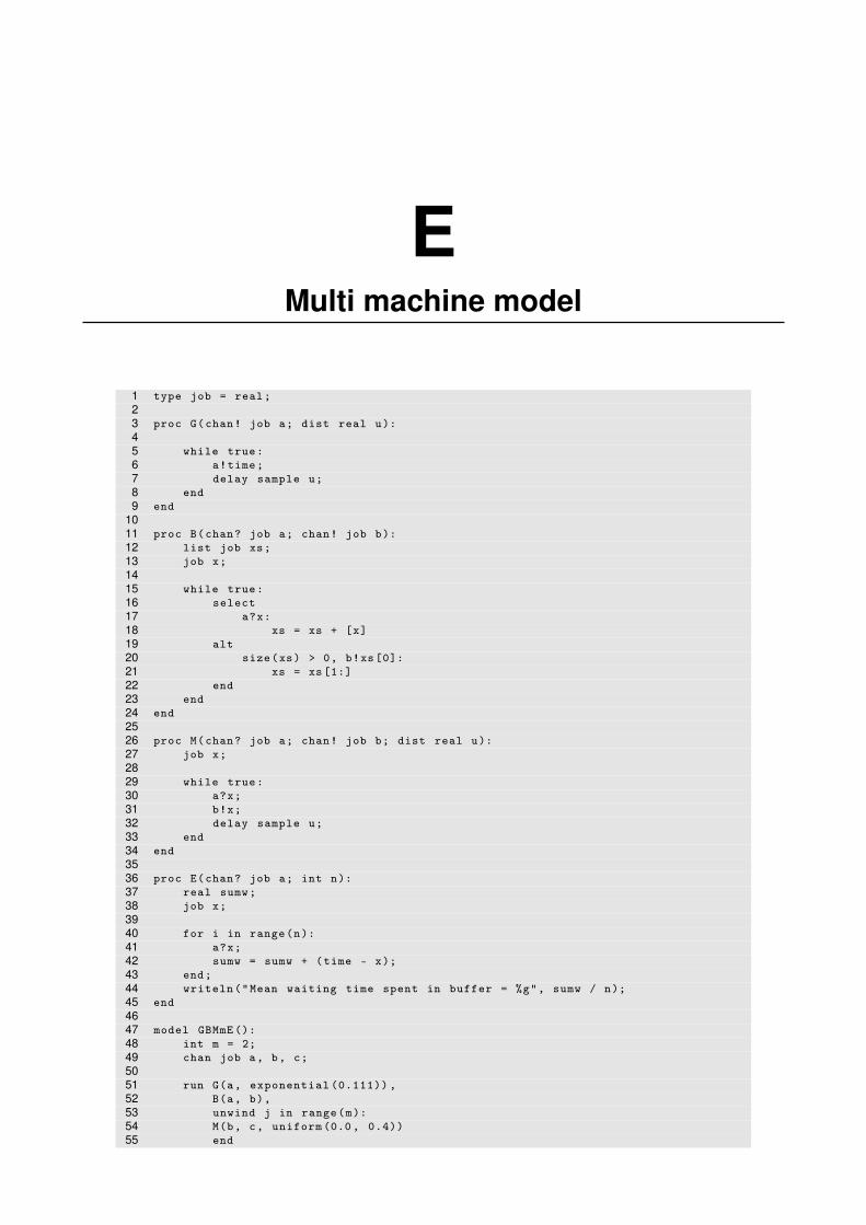
EMulti machine model
1 type job = real;23 proc G(chan! job a; dist real u):45 while true:6 a!time;7 delay sample u;8 end9 end
1011 proc B(chan? job a; chan! job b):12 list job xs;13 job x;1415 while true:16 select17 a?x:18 xs = xs + [x]19 alt20 size(xs) > 0, b!xs[0]:21 xs = xs[1:]22 end23 end24 end2526 proc M(chan? job a; chan! job b; dist real u):27 job x;2829 while true:30 a?x;31 b!x;32 delay sample u;33 end34 end3536 proc E(chan? job a; int n):37 real sumw;38 job x;3940 for i in range(n):41 a?x;42 sumw = sumw + (time - x);43 end;44 writeln("Mean waiting time spent in buffer = %g", sumw / n);45 end4647 model GBMmE ():48 int m = 2;49 chan job a, b, c;5051 run G(a, exponential (0.111)) ,52 B(a, b),53 unwind j in range(m):54 M(b, c, uniform (0.0, 0.4))55 end

96 Multi machine model
56 E(c, 1000000)57 end
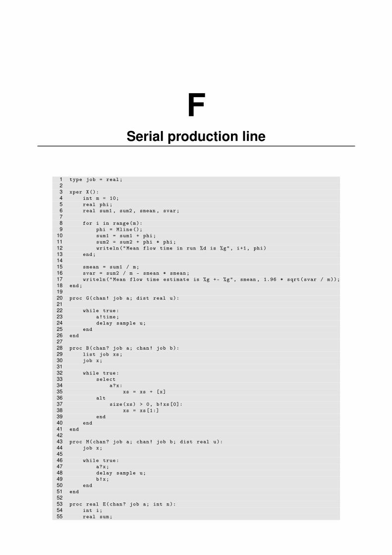
FSerial production line
1 type job = real;23 xper X():4 int m = 10;5 real phi;6 real sum1 , sum2 , smean , svar;78 for i in range(m):9 phi = Mline ();
10 sum1 = sum1 + phi;11 sum2 = sum2 + phi * phi;12 writeln("Mean flow time in run %d is %g", i+1, phi)13 end;1415 smean = sum1 / m;16 svar = sum2 / m - smean * smean;17 writeln("Mean flow time estimate is %g +- %g", smean , 1.96 * sqrt(svar / m));18 end;1920 proc G(chan! job a; dist real u):2122 while true:23 a!time;24 delay sample u;25 end26 end2728 proc B(chan? job a; chan! job b):29 list job xs;30 job x;3132 while true:33 select34 a?x:35 xs = xs + [x]36 alt37 size(xs) > 0, b!xs[0]:38 xs = xs[1:]39 end40 end41 end4243 proc M(chan? job a; chan! job b; dist real u):44 job x;4546 while true:47 a?x;48 delay sample u;49 b!x;50 end51 end5253 proc real E(chan? job a; int n):54 int i;55 real sum;

98 Serial production line
56 job x;5758 while i < n:59 a?x;60 sum = sum + (time - x);61 i = i + 1;62 end;63 exit sum / n64 end6566 model real Mline ():67 list (3) chan job a, b;6869 run G(a[0], exponential (0.5)) ,70 B(a[0], b[0]), M(b[0], a[1], constant (0.33)) ,71 B(a[1], b[1]), M(b[1], a[2], uniform (0.0 ,0.8)) ,72 E(a[2], 100000)73 end