LCQ Operation Course.pdf - Concordia University

1

The world leader in serving science

LCQLCQ OperationsCourse

Thermo Scientific- Training Institute -

2

2

LCQ Operations Course

Welcome to the Thermo Fisher Scientific LCQ Small Molecules Course. Below is a listing of important information for your future use.

Institute Registrar, Technical Support, Parts Ordering

Contract/warranty customers call: 1-877-594-3224 All other customers call: 1-800-532-4752

Thermo Scientific Training Institute1400 Northpointe Parkway, Suite 10West Palm Beach, FL 33407

3

The world leader in serving scienceChapter 1

Introduction

4

4

LCQ Ion Trap Instrument Evolution

ClassicClassic

DuoDuo DecaDeca

5

5

• 400µm capillary

• 2 octopoles

• One rotary pump

LCQ DUO• 500µm capillary

• square quadrupole with split offset voltages

• 2 rotary pumps

LCQ DECA

Deca: approximately 10 x better signal than Duo

DUO / DECA Comparisons

LCQ CLASSIC

6

6

MAX

The Next LCQ Generation – Advantage MAX / DECA XP MAX

MAX

7

7

• 450µm Ion Transfer Tube

• Orthogonal Probes

• 550µm Ion Transfer Tube

• Orthogonal Probes

XP: approximately 10 x better signal than Advantage

Advantage / XP Comparisons

MAXMAX

8

8

Practical

1. Tune and Calibrate

2. ESI compound optimization (Drug Mixture) - Infusion

3. ESI method development (Drug Mixture) - Qualitative

4. ESI data dependent MS/MS runs (Drug Mixture)

5. APCI compound optimization (Steroids) - Infusion

6. APCI method development (Steroids) - Quantitative

7. Quantitative data processing (Steroids)

9


Fundamentals of Mass Spectrometry

10

10

“The basis in MS (mass spectrometry) is the production of ions, that are subsequently separated or filtered according to their mass-to-charge (m/z) ratio and detected. The resulting mass spectrum is a plot of the (relative) abundance of the produced ions as a function of the m/z ratio.”

Niessen, W. M. A.; Van der Greef, J., Liquid Chromatography–Mass Spectrometry: Principles and Applications, 1992, Marcel Dekker, Inc., New York, p. 29.

What is Mass Spectrometry?

In analysis by LC/MS, a sample is injected onto an LC column. The sample is then separated into its various components. The components elute from the LC column and pass into the MS detector where they are analyzed. Analysis by direct infusion or flow injection provides no chromatographic separation of components in the sample before it passes into the MS detector. The data from the MS detector are then stored and processed by the data system.

11

11

Mass Spectrometry “Simplified” (GMSD)

Generate Ion Production

Ion Optics

Linear Ion Trap

Electron Multiplier

Move

Select

Detect

There are four steps to mass spectrometry using the LCQ. The acronym “GMSD” -Generate, Move, Select, Detect is employed to describe this. Initially, ions are Generated in either the solution phase (when using electrospray) or in the gas phase (when using APCI/APPI). The difference among the three will be discussed in later slides when specifically introducing the API ionization modes. Charged ions must be Moved from the source to the analyzer region without contacting any of the solid internal parts of the mass spectrometer (this would neutralize the ion, losing it in mass spectrometric analysis). This is accomplished by a series of ion optics that use a combination of DC voltage, RF voltage, and a vacuum gradient. The Selection of ions and the scan event dynamics are completed within the Linear Ion Trap. After the ion selection occurs, ions are deflected onto the curved surface of the conversion dynode and are accelerated by a voltage gradient into the electron multiplier where they are Detected.

12

12

Ion Generation (API)

• Atmospheric Pressure Ionization

• Source Types:

- Electrospray Ionization (ESI) – Solution phase process (for the most part).- APCI (Atmospheric Pressure Chemical Ionization) - Gas-phase process.

• Source Purpose:

- Desolvate sample flow for introduction into mass spectrometer.- Baffle the first vacuum region of the MS from atmospheric pressure in the source.- Ionize the analyte or transport ion in solution to the gas phase.- Pump away neutrals and opposite charged ions which would otherwise interfere

with the analysis of the desired polarity.

What is API?API (Atmospheric Pressure Ionization) describes a range of three techniques of interfacing LC with mass spectrometry. Mass detectors measure mass to charge ratios of ionized entities, and all three techniques involve ionization of sample molecules at atmospheric pressure. The API techniques are Electrospray (ESI), Atmospheric Pressure Chemical Ionization (APCI), and Atmospheric Pressure Photo-Ionization.

When sampling is performed using the ESI probe, the ions are pre-formed by solution phase chemistry before the analyte ever reaches the source probe. Most commonly this is accomplished by adding a proton donor, such as acetic or formic acid, or a proton acceptor, such as ammonium hydroxide to the mobile phase. When sampling is performed using the APCI probe, the analyte reaches the probe in the neutral state, where it is protonated or de-protonated by gas-phase processes occurring across the corona discharge needle. In APPI, ions are generated from molecules when they interact with photons from a UV-light source.

13

13

ESI:• Ions formed by solution chemistry

• Good for thermally labile analytes

• Good for polar / semi-polar analytes

• Good for large molecules (proteins / peptides)

APCI/APPI:• Ions formed by gas phase chemistry

• Good for volatile / thermally stable

• Good for non-polar / semi-polar

• Good for small molecules (steroids)

• Good for ions containing a chromophore (APPI)

Chemistry Considerations

The ESI mode transfers ions in solution into the gas phase. Many samples that previously were not suitable for mass analysis (for example, heat-labile compounds or high molecular mass compounds) can be analyzed by ESI. ESI can be used to analyze any polar compound that makes a preformed ion in solution. The technique is especially useful for the mass analysis of polar compounds, which include: biological polymers (for example, proteins, peptides, glycoproteins, and nucleotides); pharmaceuticals and their metabolites; and industrial polymers (for example, polyethylene glycols). Like ESI, APCI is a soft ionization technique. APCI provides molecular mass information for compounds of medium polarity that have some volatility. APCI is typically used to analyze heat-stable, small molecules. It is a robust technique that is normally not affected by changes in most variables (i.e. buffer type or buffer strength). In addition, APCI only allows for single charging due to the ionization mechanism.

14

14

Polar

ESIM

olec

ular

Wei

ght

200,000

15,000

1,000

Non Polar

APCI/APPI

GC

Chemistry Considerations - Analyte Compatibility

With ESI, the range of molecular weights that can be analyzed by the LCQ is greater than 100,000 Da, due to multiple charging. APCI is typically used to analyze small molecules with molecular masses up to about 2000 Da.

15

15

Positive or Negative Ionization ?

Basic Molecules [M+H]+(-NH2)

Acidic Molecules [M-H]-(-COOH, -OH)

Basic Molecules [M+H]+(-NH2)

Acidic Molecules [M-H]-(-COOH, -OH)

Basic compounds give rise to protonated molecular ions (positive ion), whereas acidic compounds produce de-protonated molecular ions (negative ion). Positive ion API may be seen as a general ionization mode since protons may loosely associate with a molecule, although it may not contain any basic functional groups. Negative ion API specifically requires the presence of functional groups capable of loosing a proton.

16

16

Ion Transfer TubeESI Needle

+/- 5 kV

Taylor Cone

Solvent Evaporationand Ion Desolvation

Electrospray - Basic Principle

Electrospray is a soft ionization process used to transfer ionized species from liquid solutions into the gas phase. The sample solution is sprayed from a region where it is contact with high voltage (±3 – 5 kV, typically), where excess charges are imparted upon droplets which emerge at the end of the sample tube. The emergence of these droplets occurs at atmospheric pressure. In ESI, ions are produced and analyzed as follows:

1. The sample solution enters the ESI needle, to which a high voltage is applied.2. The ESI needle sprays the sample solution into a fine mist of droplets that are

electrically charged at their surface.3. The electrical charge density at the surface of the droplets increases as solvent

evaporates from the droplets.4. The electrical charge density at the surface of the droplets increases to a critical

point, known as the Rayleigh stability limit. At this critical point, the droplets divide into smaller droplets because the electrostatic repulsion is greater than the surface tension. The process is repeated many times to form very small droplets.

5. From the very small, highly charged droplets, sample ions are ejected into the gas phase by electrostatic repulsion.

6. The sample ions pass through an ion transfer capillary, enter the MS detector and are analyzed.

17

17

Auxiliary GasSheath GasSheath Gas

NozzleNozzleNeedle

Spray Plume

±5kV

Auxiliary Gas

ESI Nozzle Cross Section

When sheath gas is used, nitrogen is applied as an inner coaxial gas (when used in tandem with auxiliary gas), helping to nebulize the sample solution into a fine mist as the sample solution exits the ESI or APCI nozzle. When auxiliary gas is being used, nitrogen flows through the ion source nozzle, the vapor plume is affected; the spray is focused and desolvation is improved. The auxiliary gas also helps lower the humidity in the ion source. Typical auxiliary gas flow rates for ESI and APCI are 10 to 20 units. Auxiliary gas is usually not needed for sample flow rates below 50 µL/min.

18

18

Atmospheric Pressure Chemical Ionization (APCI)

Gas phase ionization via a corona discharge APCI is a three step process

1. High voltage needle interacts with both the nitrogen carrier gas and the vaporized HPLC solvent to produce primary ions.

O2 + e- → O2+. + 2e-

N2 + e- → N2+. + 2e-

2. Through a complex series of reactions primary ions react with solvent molecules forming reagent ions, H3O+ and CH3OH2

+

3. Reagent ions react with analyte molecules forming (M+H)+ in positive ion mode or (M-H)- in negative ion mode

H3O+ + Analyte → (Analyte + H)+ + H2OOH- + Analyte → (Analyte – H)- + H2O

Atmospheric Pressure Chemical Ionization (APCI) is a soft ionization technique that is used to analyze compounds of medium polarity, that have some volatility. APCI is a gas-phase ionization technique. As such, the gas-phase acidities and basicities of the solvent and analyte ions play important roles in the APCI ionization process. APCI is typically used to analyze small molecules with molecular weights up to ~ 1500 daltons. Also, APCI is an extremely robust technique and is not affected by minor changes in buffers and/or buffer strength.

19

19

© 2004 Dr. Paul Gates, University of Bristol

Atmospheric Pressure Chemical Ionization (APCI)

If nitrogen is utilized as the sheath and auxiliary gases with atmospheric vapor (water) present in the APCI ion source, then the type of primary and secondary reactions that occur in the plasma region are as follows:

The most abundant secondary cluster ion is (H2O)2H+, along with significant amounts of (H2O)3H+ and H3O+. The reactions listed above account for the formation of these ions within the gas-plasma.

The protonated analyte ions are then formed by gas-phase ion-molecule reactions of these charger cluster ions with the analyte molecules (given in Slide #19). This results in the abundant formation of [M+H]+ ions.

20

20

ESI Probe (API-1) Assembly – LCQ Classic

21

21

ESI Probe (API-2) Assembly – LCQ Duo / LCQ Deca

22

22

ESI Probe (API-2) Diagram

23

23

ESI Probe (API-2) Positions

400 µl/min

200 µl/min1000 µl/min

infusion

44 3 2 13 2 1

Probe PositionsProbe Positions

24

24

Advantage MAX / DECA XP MAX Ion Max Source

Interchangeable Source Probe (ESI probe shown)

Positional Adjusters for Source Probe

APPI probe inlet

The Ion Max ion source is the part of the API source that is at atmospheric pressure. The Ion Max ion source can be configured to operate in any of several API modes. The Ion Max ion source housing allows you to quickly switch between ionization modes without the need for specialized tools. The ventilation of the ion source housing ensures that the housing is always cool and easy to handle. Pressure in the ion source housing is kept at atmospheric levels, which reduces the chemical noise that can be caused by nebulized gases when they are not properly evacuated from the ion source. The probe mounting angle is fixed at the optimum angle for signal intensity and ion source robustness. Minor adjustment of the probe position in the X, Y, and Z dimensions is allowed, with marked adjustments to allow for freedom in probe position during ionization optimization. View ports are placed at the front and side of the ion source housing, which allows visual aid in positioning the probe during ESI operation, and enables easy addition of accessories.

25

25

Ion Max Source

The ESI probe includes the ESI sample tube, needle, nozzle, and manifold. Sample and solvent enter the ESI probe through the sample tube. The sample tube is a short section of 0.1 mm ID fused-silica or metal capillary tubing that extends from a fitting secured to the ESI source housing, through the ESI probe and into the ESI needle, to within 1 mm from the end of the ESI needle. The ESI needle, to which a large negative or positive voltage is applied (typically ±3 to ±5 kV), sprays the sample solution into a fine mist of charged droplets. The ESI nozzle directs the flow of sheath gas and auxiliary gas at the droplets. The ESI manifold houses the ESI nozzle and needle and includes the sheath gas and auxiliary gas plumbing. The sheath gas plumbing and auxiliary gas plumbing deliver dry nitrogen gas to the nozzle.

26

26

Ion Max Source Design : ESI Probe

New ESI Probe features:• Fixed vertical spray angle (60 degrees)• X,Y,Z-adjustable for further optimization

LC Inlet ESI Needle

In the LCQ, the ESI needle is orthogonal to the axis of the ion transfer capillary that carries ions to the MS detector. This geometry keeps the ion transfer tube clean. The ion transfer tube assists in desolvating ions that are produced by the ESI or APCI probe. Two heater cartridges are embedded in the heater block. The heater block surrounds the ion transfer tube and heats it to temperatures up to 400 °C. A platinum probe sensor measures the temperature of the heater block. Typical temperatures of the ion transfer tube are 270 °C for electrospray and 250 °C for APCI.

27

27

Removable Ion Sweep Cone

The ion sweep cone is a metallic cone located over the ion transfer tube. The ion sweep cone channels the sweep gas towards the entrance of the ion transfer tube, thereby minimizing the accumulation of endogenous or excipient materials in high-pressure region ion optics.

28

28

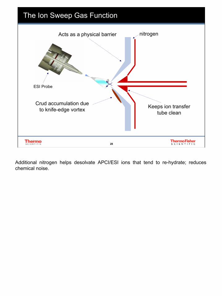
The Ion Sweep Gas Function

nitrogen

Crud accumulation due to knife-edge vortex

Acts as a physical barrier

ESI Probe

Keeps ion transfer tube clean

Additional nitrogen helps desolvate APCI/ESI ions that tend to re-hydrate; reduces chemical noise.

29

29

Elongation of polyimide coating occurs when specific solvents (i.e., acetonitrile) are adsorbed into the sample tube.

The sample tube must be cut square to ensure a stable spray. Best results can be achieved by positioning the sample tube about 1 mm inside the ESI needle.

Sheath Liquid

ESI NeedleESI Needle

Sample

Polyimide

Polyimide

Fused Silica

Fused Silica

ESI Needle

ESI NeedleESI Needle

Sample

Polyimide

Polyimide

Fused Silica

Fused Silica

ESI Needle

ESI Needle

Sheath Liquid

Sheath Liquid

Sheath Liquid

ESI Needle

Elongation of Fused Silica Capillary Sample Tube

When the polyimide coating on the outside of the fused silica of the sample tube elongates, the sample does not come in contact with the ESI needle and sensitivity is decreased. It is good practice to cut the fused silica on a regular basis to minimize problems associated with the elongation of the polyimide coating.

30

30

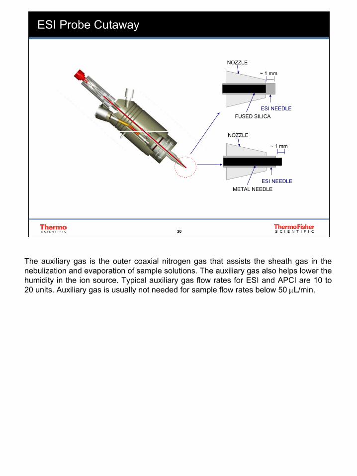
ESI Probe Cutaway

NOZZLE

ESI NEEDLEFUSED SILICA

NOZZLE

ESI NEEDLEMETAL NEEDLE

~ 1 mm

~ 1 mm

The auxiliary gas is the outer coaxial nitrogen gas that assists the sheath gas in the nebulization and evaporation of sample solutions. The auxiliary gas also helps lower the humidity in the ion source. Typical auxiliary gas flow rates for ESI and APCI are 10 to 20 units. Auxiliary gas is usually not needed for sample flow rates below 50 µL/min.

31

31

Spray Voltage : 3 – 4.5 kV

LC F low ( µL / min )

Co lumn S iz e (mm ID)

Ion T ra nsfe r Tube Te mp (°C)

S he a th G a s (P S I)

Aux G a s (Arb . )

≤ 10 Capillary 150 - 200 5 - 15 Off50 - 200 1 200 - 275 20 - 40 0 - 20100 - 500 2 - 3 250 - 350 40 - 60 0 - 20

400 - 1000 4.6 300 - 400 60 - 100 10 - 40

Ion Max Electrospray Source – Operational Conditions

The numbers in the table should be taken as suggested ranges. In essence, the higher the LC flow rate, the greater the solvent evaporation conditions must be to remove the solvents, in terms of increased ion transfer tube temperature and higher sheath/auxiliary gas flow rates. Auxiliary gas is not required for flow rates from 10 µL/min. to 500 µL/min. but can help to reduce solvent background ions.

32

32

Metal Needle Kit

5 - 400High flow32-Gauge(50 µM ID)

0.5 - 10Low flow34-Gauge(30 µM ID)

Solvent Flow Rate(µL/min)

TypeStainless Steel Needle Size

There are 2 types of metal needle kits for the ESI probe. The low flow metal needle kit is recommended for LC flow rates between 0.5 and 10 µL/min and the high flow metal needle kit is recommended for LC flow rates between 5 µL/min and 400 µL/min).

33

33

Electrospray Ionization (ESI) Atmospheric PressureChemical Interface (APCI)

Orthogonal ESI & APCI probes

LCQ Advantage/XP Plus API Probes

34

34

Ion Max Source Design: APCI Probe

In the LCQ, the sample tube in the APCI nozzle (as in the case of the ESI probe) is orthogonal to the axis of the ion transfer capillary that carries ions to the MS detector. This geometry keeps the ion transfer capillary clean.

35

35


The APCI probe ionizes the sample by atmospheric pressure chemical ionization. The APCI probe accommodates liquid flows of 100 µL/min to 2.0 mL/min without splitting. The APCI probe includes the APCI sample tube, nozzle, sheath gas and auxiliary gas plumbing, and vaporizer. Sample and solvent enter the APCI nozzle through the sample tube. The sample tube is a short section of 0.10 mm ID fused silica tubing that extends from the sample inlet to 1 mm past the end of the nozzle. The manifold houses the APCI nozzle and includes the sheath gas and auxiliary gas plumbing. The APCI nozzle sprays the sample solution into a fine mist. The sheath gas and auxiliary gas plumbing deliver dry nitrogen gas to the nozzle. The droplets in the mist then enter the vaporizer. The vaporizer flash vaporizes the droplets at temperatures up to 600 °C.

The sample vapor is swept toward the corona discharge needle by the flow of the sheath and auxiliary gasses. The corona discharge needle assembly is mounted inside of the Ion Max API source housing. The tip of the corona discharge needle is positioned near the vaporizer. A high potential (typically ±3 to ±5 kV) is applied to the corona discharge needle to produce a corona discharge current of up to 100 µA. (A typical value of the corona discharge current is 5 µA.) The corona discharge from the needle produces reagent ion plasma primarily from the solvent vapor. The sample vapor is ionized by ion-molecule reactions with the reagent ions in the plasma.

36

36

New APCI Probe features :

• Removable sprayer• New ceramic heater• Self- cleaning

- internal surfaces can exceed 1000 ºC

• External thermocouple

• No plastics in source housing

• Easy change nozzle assembly

• X,Y,Z adjustable

LC Inlet

Ceramic Vaporizer

Vaporizer Voltage

Connector


The APCI Probe has an external thermocouple for enhanced temperature feedback control. In addition, the probe contains no plastics, thereby reducing the possibility of phthalate contamination. The probe can also be adjusted in the X,Y and Z directions just as in the case of the ESI probe.

37

37

Ion Max APCI Source – Operational Conditions

4505452501000350525250200

VaporizerTemperature

(ºC)

Aux Gas Flow

(arbitrary units)

Sheath Gas Pressure

(psi)

Ion Transfer Tube Temp.

(ºC)*

Liquid Flow Rate

(µL/min)

Corona Discharge Current : 4 µA

Although APCI can accommodate higher LC flow rates than electrospray, an increased ion transfer tube temperature is not necessary. In this case, the solvent evaporation and the ion desolvation processes are driven to completion within the APCI vaporizer tube, where the effluent is exposed to temperatures in the 400 ºC to 550 ºC range. Auxiliary gas is not required but can help to reduce solvent background ions.

38

38

Recommended Flow Rates

• ESI:- 3µL/min to 1.5mL/min- Optimal Flow Rate: 200µL/min- Generally, higher flow rates require higher gas flow rates and higher ion

transfer tube temperatures

• APCI:- 200µL/min to 2mL/min- Optimal Flow Rate: 500µL/min- Generally, higher flow rates require higher gas flow rates but not ion

transfer tube temperatures

The ESI probe can be used at flow rates down to 1.0 µL/min, or up to a 1.0 mL/min. It is recommended that the APCI probe due to the extreme environment in the source (high gas flows and vaporizer temperatures above 400°C), should only be used for LC experiments between 200 µL/min and 2.0 mL/min. For the APCI probe, flows below 200 µL/min require more care to maintain a stable spray.

For both sources, as the flow rate is increased or has a higher aqueous composition, the sheath and aux gasses will optimize at higher flow rates. In the case of the ESI, a higher heated capillary temperature may also be necessary. Although for APCI, the heated capillary temperature will not alter the signal significantly since the sample is already in the gas-phase (passed through the vaporizer tube).

39

39

Divert Valve

The divert valve is most commonly used to divert unwanted flow away from the detector. It is a good idea to use the divert valve whenever analyte peaks are not eluting to increase the ruggedness of the detector. If samples are particularly dirty or have been prepared or stored in an inorganic buffer or solvent, you may want to divert away a few minutes of flow at the initial LC conditions before ramping the organic phase (in reversed phase chromatography). Care should be taken to divert back to the source one to two minutes prior to elution of the first peak, to allow the spray/capillary heater to equilibrate.

The divert valve may also be plumbed as a loop injector, and since it is dynamically controlled by Xcalibur during the run, it may be used for any custom application as well.

40

40

Useful for increased API source ruggedness:

LC

wastePrevents salt and protein build-up from injections of complex (“dirty”) matricesProlongs the lifetime of API source by reducing the frequency of disassembling and cleaning

TO DETECTOR TO WASTE

FROM LCPUMP

TO IONSOURCE

WASTE

FROM LCPUMP

TO IONSOURCE

WASTE

12

3

6

5

4

213

5

64

Divert Valve Mode

It is a good idea to use the divert valve whenever analyte peaks are not eluting to increase the ruggedness of the detector. If samples are particularly dirty or have been prepared or stored in an inorganic buffer or solvent, you may want to divert away a few minutes of flow at the initial LC conditions before ramping the organic phase (in reverse phase chromatography). Care should be taken to divert back to the source one to two minutes prior to elution of the first peak, to allow the spray/capillary heater to equilibrate.

41

41

Removable Ion Transfer Tube

Heated ion transfer tube in-situ

Heated ion transfer tube removed

Metal ball

An easily removable ion transfer tube negates the need to vent the instrument in order to conduct routine maintenance. The vent prevent ball falls into the space occupied by the ion transfer tube when the tube is removed, thus preventing air from entering the vacuum manifold. The vent prevent ball allows the removal of the ion transfer tube for cleaning or exchange without venting the system.

42

42

Removal tool

Ion transfer tube

Heated capillary

Ion Transfer Tube and Removal Tool

43

43

Heater Assembly With Removable Ion Transfer Tube

Vent BallLocation

Dual Heater Assembly

Removable Tube

The heated transfer capillary assembly assists in desolvating ions that are produced by the ESI or APCI probe. Ions in the gas or liquid phase are drawn into the ion transfer capillary in the atmospheric-pressure region of the API source and are transported to the capillary-skimmer region by a decreasing pressure gradient.The ion transfer capillary is a cylindrical metal tube with a cone shaped entrance. This special entrance shape helps to reduce solvent adduction. An external heater block with two standard 60 V / 100 W cartridge heaters heats the capillary to a maximum temperature of 400 °C. Typically, an offset potential of up to ±300 V (positive for positive ions and negative for negative ions) assists in repelling ions from the ion transfer capillary to the skimmer.

44


LC-MS Considerations

45

45

Optimal Flow Rates (Linear Velocities) for LC Columns (Standard Packing 5.0 µm)

Flow Rate Column I.D.

1.0 mL/min 4.6 mm

0.5 mL/min 3.0 mm

0.2 mL/min 2.1 mm

50 µL/min 1.0 mm

<10 µL/min Capillary

It is important to use the correct flow rate for your HPLC column. The limiting factors in choosing a flow rate are, instrument pressure limitations, the effect on the quality of the chromatography, and time. Maintaining linear velocity is the single most important factor when trying to reproduce a chromatographic separation on columns of differing diameters.

46

46

Col. Diameter (mm)Col. Diameter (mm) 1.0 1.0

1000 1000 500500 200200 5050

1 1 55 202.02.0

3.03.04.64.6 2.02.0

Flow Rate (Flow Rate (µµLL/min)/min)

Theoretical IncreaseTheoretical Increase

Theoretical Increase in Response by Using Narrow Bore Columns

The internal diameter of an HPLC column is a critical aspect that determines the quantity of analyte that can be loaded onto the column and also influences sensitivity. The advantage of low I.D. columns is improved sensitivity and lower solvent consumption.

47

47

LC Additives

AcidsDo not use inorganic acids (will cause source corrosion)

Formic and acetic acid are recommended

BasesDo not use alkali metal bases (will cause source corrosion)

Ammonium hydroxide and ammonia solutions are recommended

Surfactants (surface active agents)

Detergents and other surface active agents may suppress ionization

Trifluoroacetic Acid (TFA)

May enhance chromatographic resolution, but causes ion suppression in both negative and positive ion mode

Triethylamine/Trimethylamine (TEA/TMA)

May enhance deprotonation for negative ion formation

This slide lists several recommendations for LC additives. One should avoid the use of inorganic acids and alkali metal bases as both will eventually lead to the damage of source hardware. Formic and acetic acids are recommended as proton donors for positive ion mode and ammonium hydroxide and ammonia solutions are recommended as proton acceptors for negative ion mode. One should avoid the use of surfactants such as Triton-X 100 for use with mass spectrometry as these detergents lead to ion suppression and coating of the ion optics. Both outcomes result in an overall loss in sensitivity. TFA is commonly used in HPLC with UV detection because of its enhancement of chromatographic resolution. Unfortunately, this additive has an adverse effect on negative and positive ion formation. Simply speaking, negative ions cannot be formed in a low pH environment, and TFA suppresses negative ion formation. Also, since TFA contains many electronegative fluorine groups, it is also a proton acceptor which leads to ion suppression in positive ion mode as well. To enhance negative ion sensitivity, or improve the chromatographic separation (as an ion-pairing reagent), the addition of TEA or TMA may be beneficial.

48

48

The effect of increasing TFA levels (in 50:50 ACN:H2O) on MS signal intensity

0.00 0.05 0.10 0.15 0.20 0.25 0.300

20

40

60

80

100

% o

f Con

trol R

espo

nse

% TFA

Results are the mean of 2 experiments. *Note: The results from the no TFA samples were variable due to the lack of peptide protonization. Control sample was 50/50/0.1, MeOH/H2O/FA (N=6, avg. signal intensity = 1.10x106 counts.

* S. Baldwin, K. Stoney, K. Wheeler, I. Mychreest. “Low pH Solvent Alternatives to TFA Solvents and Their Effect on HPLC/ESI-MS of Peptides”, Poster Paper Presented at ASMS 1996.

As the concentration of TFA in the mobile phase increases, there is significant loss of MS signal intensity, therefore, if TFA is necessary, it should be used at low concentrations.

49

49

When using non-volatile buffers, sweep cone should be in place.

If possible, avoid using non-volatile HPLC additives such as:

Alkali-Metal Phosphates

Borates

Citrates

When using buffers, more frequent cleaning of the source housing, sweep cone, ion transfer tube, skimmer, and tube lens is necessary.

Buffers

If the HPLC separation requires a buffer, one should use the ion sweep cone. The ion sweep cone is a metallic cone that is installed over the ion transfer tube. The ion sweep cone channels the sweep gas towards the entrance of the capillary. This helps to keep the entrance of the ion transfer tube free of contaminants.

50

50

* Crawford Scientific, OPDAC (Online Professional Development in Analytical Chemistry) LC-MS training package. Holm Street, Strathaven, Lanarkshire, ML10 6NB, Scotland, UK

Buffers and pH

Electrospray involves the formation of [M+H]+ ions in the positive ion mode and [M-H]-ions in the negative ion mode. The generation of both species is contingent upon the pKa of the analyte and the pH of the mobile phase. Basic samples will protonate in acidic solutions, thereby becoming positively charged (the converse is true for acidic analytes in basic solutions). In-solution ionization is competitive equilibrium process, and ionization efficiency of the analyte depends on the degree of protonation and/or deprotonation. Therefore, knowledge of the analyte’s pKa (or pKb) is essential in determining the most favorable pH of the eluent for obtaining maximum sensitivity in LC-ESI-MS analyses.

In our Phenytoin example, if the pH of the eluent solution is adjusted to match the pKaof the basic functional group, this group will be ionized to a 50% extent. By raising the pH by 2 units, the basic functional group will be quasi-entirely (99.5%) non-ionized (in the ion-suppressed form). Conversely, by lowering the pH by 2 units, the basic functional group will be quasi-entirely (99.5%) ionized (protonated) and will lead to higher levels of analyte detection.

51

51

Proton Donors

Proton Acceptors

Chromatographic Separation

Chromatographic SeparationNegative Ion Formation

Buffers

LC/MS Additives and Buffers (Summary)

Acetic Acid

Formic Acid

Ammonium Hydroxide

Ammonia Solutions

Trichloroacetic Acid (< 0.02% v/v)

Trifluoroacetic Acid (< 0.02% v/v)

Triethylamine (< 0.02% v/v)

Trimethlyamine (< 0.02% v/v)

Ammonium Acetate

Ammonium Formate

52

52

MethanolAcetonitrile

WaterIsopropanol

DichloromethaneChloroform

Hexane

Common LC/MS Solvents

A range of precautions is recommended, to avoid the introduction of contaminants in the system:

1) Use high-purity solvents, made by reputable manufacturers (i.e., J.T. Baker, VWR - Burdick & Jackson, E.M. Sciences, etc.)

2) Use high-purity additives (acids, bases, buffers)3) Avoid transferring, degassing, and filtering the solvents; use original

containers, if possible4) Avoid any contact of solvents and additives with plastics (i.e., syringes)

53


Moving Ions: The LCQ Ion Optics

54

54

LCQ Ion Optics

API Stack Multipole Assembly

Multipole 1 Multipole 2

Gate Lens

The ion source interface (API stack) consists of the components of the API source that are held under vacuum (except for the atmospheric pressure side of the ion sweep cone). Ions emerge from the ion transfer tube and pass through the tube lens and skimmer and then move toward multipole 1. The ion optics focus the ions produced in the API source and transmit them to the mass analyzer. Between multipole 1 and multipole 2 there is a lens called the “gate lens” to which a voltage is applied to start and stop the injection of ions into the mass analyzer. This lens is also known as the intermultipole lens or split lens.

55

55

Pressure Regions in the API Stack

××

××

Peek Holder

Tube LensSkimmerSkimmer1 Torr1 Torr

1010--33 TorrTorrIon Transfer Tube

Ions in the gas or liquid phase are drawn into the heated capillary in the atmospheric-pressure region of the API source and are transported to the capillary-skimmer region by a decreasing pressure gradient. The heated capillary passes through a hole in the center of the spray shield. A potential of typically ±25 V (positive for positive ions and negative for negative ions) assists in repelling ions from the heated capillary to the skimmer.API Tube Lens — A lens in the API source that separates ions from neutral particles as they leave the heated capillary. The tube lens has a potential applied to it to focus the ions toward the opening of the skimmer. The tube lens also serves as a gate to terminate the injection of ions into the mass analyzer. A potential of -200 V is used to deflect positive ions toward the tube lens and away from the skimmer, and a potential of +200 V is used to deflect negative ions toward the tube lens and away from the skimmer. Skimmer — The skimmer acts as a vacuum baffle between the higher pressure capillary-skimmer region (at 1 Torr) and the lower pressure first octapole region (at 10e-3 Torr). The skimmer is at ground potential. The opening in the skimmer is offset with respect to the bore of the heated capillary to reduce the number of large charged particles that pass through the skimmer. (These large charged particles can pass through the ion optics and mass analyzer and create detector noise.) API Capillary-skimmer region —The area between the heated capillary and the skimmer, which is surrounded by the tube lens. The capillary-skimmer region is the area where ions leave the exit end of the heated capillary, experience free-jet expansion, and are sampled by the aperture of the skimmer. It is also the area of first-stage evacuation in the API source. See also heated capillary, skimmer, API source, and atmospheric pressure ionization (API).

56

56

First Multipole

Lens

IntermultipoleLens Second

Multipole Lens

MultipoleMount

Vacuum Baffle

Analyzer Mount

IONS IN IONS OUT

Ion Optics

57

57

Ion Guides

• A multipole rod assembly that is operated with only radio frequency (RF) voltage on the rods. In this type of device, virtually all ions have stable trajectories and pass through the assembly.

• Ion Guides focus and transfer the ion beam between the high-pressure ion source region and the mass analyzer. Also responsible for reducing kinetic energy of transmitted ions.

• The LCQ contains a mixture of square quadrupoles and round octopoles depending on the version of instrument.

• Different multipole arrangements have different transmission properties.

The ion guides decrease the kinetic energy of the transmitted ions and ensure that ions travel in an organized, stable manner towards the ion trap. This is done in a non-selective fashion.

58

58

Multipole Potential Wells

Round Quadrupole

Efficiency

Mass Range

Square Quadrupole

Octapole

In quadrupole instruments (single or triple), the quadrupole(s) can act not only as a focusing device, but more importantly as a selection device. For that reason, it is important to obtain very good transmission efficiency for a specific mass or mass range. Thus round quadrupoles were employed as ion guides. Unfortunately, the excellent transmission efficiency of the round quadrupole does not apply across a large mass range. As a consequence, quadrupole instruments function by scanning (RF and DC) across the mass range in steps to optimize recovery.The octapoles on the other hand, function exclusively as ion focusing devices to transmit ALL ions, and are not scanned (RF only). Therefore, it is necessary to have good efficiency across a much larger range. These poles offer good efficiency, but do not completely preclude the loss of some ions within the transmission mass range.Recent research has shown that square quadrupoles offer the best of both worlds, a mass range similar to that of an octapole with the trapping efficiency nearing that of the round quadrupole.

59

59

What is an RF Field?

Continuously oscillating voltage of a set amplitude positive and negative relative to a center voltage. Responsible for ion movement in the X and Y directions.

0

_

+

The manner by which the quadrupoles focus the desired ions into a concise beam is based on the application of radio frequencies (or RF) on opposing poles. In a quadrupole, opposite poles are connected such that the same voltage is applied to both. This voltage can be oscillated over time in a characteristic sine wave to positive, through neutral, to negative and back again (blue trace). The same exact RF oscillation can be placed on the opposing two poles 180° out of phase such that when one set is positive, the other set is negative and visa versa.

60

60

Multipole Oscillations

* Crawford Scientific, OPDAC (Online Professional Development in Analytical Chemistry) LC-MS training package. Holm Street, Strathaven, Lanarkshire, ML10 6NB, Scotland, UK

Ions are attracted to rods in the multipoles that are opposite in polarity. Since the polarity of the paired rods is alternating, ions move from rod to rod in a motion that resembles a corkscrew.

61

61

4000

-15000

0

5020

-3

-15

-7-10

Ion Optics (DC Offsets)

There is a decreasing potential energy gradient from the front of the instrument where the ions are made to the back of the instrument where the ions are detected.

62


Ion Trap Theory

63

63

IONS IN IONS OUT

Second Octapole

Analyzer Mount

Entrance Endcap Electrode Post

Spacer Rings

Exit Lens

Exit Endcap Electrode

Ring Electrode

Exit Lens

Retaining BoltWasher

Mass Analyzer (Ion Trap)

64

64

rozo

EntranceEndcap

ExitEndcap

RingElectrode

)cos( tV resres Ω

)cos( tV rfrf Ω

-

IonInjection

IonEjection

+

Basic Ion Trap Components

65

65

Steps to Ion Trap Scan Functions

• Trapping- all scans

• Isolation- SIM and MSn

• Excitation- MSn

• Ejection- all scans

Each scan that is done on the LCQ involves trapping and ejection. In the case of SIM (selective ion monitoring), after trapping, a mass range is isolated and then the ions are scanned out (ejected). When doing an MSn experiment, a mass range is isolated, fragmented and then scanned out.

66

66

Trapping of Ions

• RF (applied to ring electrode)

• Helium (stabilize the ions)

Helium is utilized when trapping to decrease the kinetic energy of the ions being trapped and stabilize the ions.

67

67

+

+

+

++

++

+He

He

He

He

He

collision

Potential Well

Helium’s Role as a Damping Gas

Helium is used as a dampening gas inside the ion trap, due to its ability to energetically cool the ions without inducing fragmentation. The collisions of the ions entering the mass analyzer with the helium slow the ions so that they can be trapped by the RF field in the mass analyzer. Larger gas molecules in the trap would cause collision-induced fragmentation of the ions.

68

68

S#:1 RT:0.00 AV:1 SM:7G NL:2.50E7T:+ p Full ms

514 516 518 520 522 524 526 528m/z

0

20

40

60

80

100

Rel

ativ

e Ab

unda

nce

524.3

525.3

S#:23-32 RT:0.71-1.00AV:10 SM:7G NL:5.61E7T:+ p Full ms

500 1000 1500 2000m/z

0

20

40

60

80

100

Rel

ativ

e Ab

unda

nce

1522.04

1621.971322.06

1721.89

1222.14 1821.95524.26

1122.21 1921.88195.15

1022.09

S#:1 RT:0.02 AV:1 SM:7G NL:9.70E6T:+ p Full ms

514 516 518 520 522 524 526 528m/z

0

20

40

60

80

100

Rel

ativ

e Ab

unda

nce

522.6523.0

521.8521.2 523.9

520.7

S#:23-32 RT:0.39-0.54AV:10 SM:7G NL:2.80E7T:+ p Full ms

500 1000 1500 2000m/z

0

20

40

60

80

100

Rel

ativ

e Ab

unda

nce

1620.791520.26

1720.441320.95

1220.75523.01 1919.96

1120.90192.17

Helium flowing into trap

Helium shut off and not flowing into trap

The Effects of No Helium

The presence of helium in the mass analyzer cavity significantly enhances sensitivity and mass spectral resolution. Before their ejection from the mass analyzer cavity, sample ions collide with helium atoms. These collisions reduce the kinetic energy of the ions, thereby damping the amplitude of their oscillations. As a result, the ions are focused to the axis of the cavity rather than being allowed to spread throughout the cavity.

69

69

Ring RF Negative

endcap

endcapringelectrode

ringelectrode

Potential Energy for Injected Ions

70

70

Ring RF Positive

endcap

endcapring

electrode

ringelectrode

Potential Energy for Injected Ions

71

71

Ion Motion in the 3D Ion Trap

72

72

16eUa = variable solution

q = solution

e = charge of trapped ion

U = DC Voltage

V = RF amplitude

m = mass of ion

Ω = angular frequency of rf

z0 = distance between centerof trap to either endcap

r0 = internal radius of ring electrode

Controlled by a culmination of differential equations termed theReduced Mathieu Equations:

qz

= -

= -

Ring Parameters

Ion Stability in the Trap

az

m(r0 + 2z0 )Ω22 2

8eVm(r0 + 2z0 )Ω22 2

The motion of ions in quadrupole fields is described mathematically by the the solutions to a second-order linear differential equation described by Mathieu in 1868. These equations can only be solved numerically, or equivalently by computer simulations. The difference between the DC voltage on the ring and endcap electrodes is 0 and therefore az=0. qz is a calculated number which is dependent upon the difference between the RF power on the ring and endcap electrodes. Qz. is inversely related to the mass-to-charge ratio of the ion and is proportional to the RF power on the endcaps.

73

73

• The blue shaded region indicates (DC) and q (RF) values which provide stable trajectories in the r-direction

• The yellow shaded region indicates the z-stable a and q combinations

• The green area where the r- and z-stable regions overlap indicates the a and q combinations under which ions will be stable in the trap

Ion Trap Stability Diagram

74

74

)/( emVkqz =

Stability Diagram for Commercial Traps

The stability diagram is a graphical representation of the important aspects of the mathematics describing ion motion inside the trap. It answers the two most important questions concerning ion motion. The first being “is the ion I am interested in trapped?”. That is, does the ion have a stable trajectory inside the device or does the ion hit the endcaps? The stability diagram indicates this in terms of the parameters a and q. If the ion has an a and q value which place it inside the stability region then the ion will be trapped, and if it is outside the stability region, it will hit an endcap or be ejected through the holes in the endcap.

75

75

q k Vm ez = ( / )

.908qz axis

Ramp RF, Ions Leave Low m/z to High m/z

Mass Selective Instability

76

76

...with Resonance Ejection

.908Q axis

*Q axis

Increases Resolution …

q=0.83

q=

… with Resonance Ejection

The resonance ejection RF voltage is a small AC voltage, applied to the endcaps of the mass analyzer to minimize space charge effects in the mass analyzer. During mass analysis, this RF voltage facilitates the ejection of ions from the mass analyzer and thus improves mass resolution and sensitivity. The resonance ejection RF voltage is applied at a fixed frequency during the ramp of the main RF voltage. When an ion is to be ejected from the mass analyzer cavity it is brought toward resonance with the frequency of the resonance ejection RF voltage. The application of resonance ejection increases resolution because ions of a specific m/z leave the trap in a more condensed manner

77

77

Normal Scan (5500 amu/sec)- Common full, SIM, or MSn scanning- Resolution (FWHM) = 0.50

Zoom Scan (280 amu/sec)- Increases resolution across a narrow range (allows charge state

determination)- Resolution (FWHM) = 0.15

Turbo Scan (55,000 amu/sec)- Decreases total scan time of a full scan, thus increasing number

of scans across a chromatographic peak - Resolution (FWHM) = 3.0

LCQ Scan-Out (Ejection) Rates

Slower scan out (ejection) rates can provide information about the charge state of one or more mass ions of interest. The data is collected by using slower scans at higher resolution. This can allow for determination of charge state, which in turn allows for the correct determination of molecular mass.

78


AGC – Automatic Gain Control

79

79

530m/z

0

20

40

60

80

100

Rel

ativ

e A

bund

ance

524.3

525.3

526.3

530m/z

0

20

40

60

80

100

Rel

ativ

e A

bund

ance

524.4

525.4

526.3527.5

530m/z

0

20

40

60

80

100

Rel

ativ

e A

bund

ance

524.5

525.5

526.5527.5

530m/z

0

20

40

60

80

100

Rel

ativ

e A

bund

ance

524.8

525.7

526.7

522 522 522 522

~ 300 Ions ~ 1500 Ions ~ 3000 Ions ~ 6000 Ions

Good Resolution Poor Resolution

AGC (Ion Population Control)

Automatic Gain Control (AGC) is utilized in the LCQ to control the number of ions in the trap at any one time. If the ion count is too high, the density of charges per unit area in the center of the trap will be too large, resulting in “space charging.” This phenomena occurs when the charges of neighboring ions affect each other, causing a large decrease in resolution and mass accuracy. However, if the ion count is too low, small deviations in the ion count result in large TIC signal and spectral ratio instability from scan to scan. Therefore, it is necessary to control the number of ions present in the trap for each scan.

80

80

Automatic Gain Control (AGC)

- Measures the # of ions in the trap for a pre-defined time (e.g. 1 ms)

- Allows software to determine optimum ion injection time

Prescan before the analytical scan

The software is used to set the ion injection time to maintain the optimum quantity of ions allowed in the trap for each scan. With AGC on, the scan function consists of a prescan and an analytical scan. The LCQ measures the flux of incoming ions during the prescan. This information allows the LCQ to determine the optimum ion injection time for the analytical scan. The ion injection time information is then used to scale the resulting values obtained by the analytical scan. AGC extends the dynamic range of the MS detector. With AGC on, the LCQ sets the ion injection time (up to a preset maximum) and thus determines the number of ions that enter the analyzer. With AGC off, the user sets the ion injection time, thus controlling the number of ions that enter the analyzer.

81

81

Spectrum of Calibration Mixture, AGC On

Injection time in ms

Injection time (IT)= 0.18 msec. The application of the automatically determined injection time (calculated during the AGC prescan) allows for enhanced resolution and more accurate m/z assignments throughout the entire mass range of interest, by not allowing the ion trap to “overcrowd” with ions, and hence to be subject to space charge distortion.

82

82

Spectrum of Calibration Mixture, AGC Off

System uses the set max. inject time→ approx. 250x overfilling the trap

Injection time (IT)= 50 msec. Note the loss of resolution and the m/z assignment shift, especially across the lower and medium range of the m/z scale. The space charge effects are affecting the higher m/z range to a much lesser extent. As ions leave the trap from low m/z range to high m/z range, the number of total ions in the trap decreases by the time the higher masses are ejected, making them, consequently, less prone to space charge distortion.

83

83

Calculation of Ion Time

AGC Prescan Signal =(3 x 105 counts) (1 ms)

Constant During Prescan

Multiplier Gain x Prescan TimeNumber of Ions x

Target ValueACG Prescan Signal(how long the gate lens is “open”)

Calculated Ion Time =

The calculation above shows how the instrument determines the variable injection time for each analytical scan based on the prescan.

Note: The maximum injection time is set by the user!

84

84

=

IT ActualITPrescan Icurrent)ion (corrected I'

Corrected Ion Current (TIC)

Example:

=

0.1 ms1 ms3.00 x 1073.00 x 108

(Scaled TIC)

The equation used to calculate the scaled TIC value is shown above. Essentially, each scan signal (which is equal to the AGC target or the number of ions) is multiplied by the prescan IT and the inverse of the actual IT.

85

85

0.0E+001.0E+082.0E+083.0E+084.0E+085.0E+086.0E+087.0E+088.0E+08

0 100 200 300 400 500 600Scan Number

Scal

ed T

IC (c

ount

s)

Scan Number

Uns

cale

dTI

C (c

ount

s)

0.0E+002.0E+074.0E+076.0E+078.0E+071.0E+081.2E+081.4E+081.6E+081.8E+082.0E+08

0 100 200 300 400 500 600

Unscaled TIC

0

10

20

30

40

50

60

0 100 200 300 400 500 600Scan Number

Inje

ctio

n Ti

me

(ms)

Injection Time

Scaled TIC

Triplicate Injection of 5 nmol of MRFA (AGC ON)

Due to AGC, the injection time decreases as the concentration of ions increases to limit the number of ions in the trap and prevent space charging. The scaled TIC is inversely related to the actual IT so after correction, the TIC seen represents the corrected ion current.

86

86

Time

Var. Ion Injection Time (IT)

Prescan(sets Ion Time) Analytical Scan

Upload to PC DS

1 Micro Scan

1 Scan Cycle (ST)

Fixed Prescan Ion Injection

Time

Injection

Scan

Upload

Ion Time, Microscan, and Scan Cycle

AGC Cycle – Full Scan MS Summary

This diagram shows the LCQ in Full Scan MS mode with one microscan. The status of various elements of the LCQ during the scan is shown versus time.

87

87

4000

-15000

0

5020

-3

-15

-7-10

Voltage Settings during Injection TimeTrap Fills – ‘Gate Open’

The gate lens is used to start and stop the injection of ions into the mass analyzer. When open, it is an accelerating lens which accelerates ions towards the ion trap.

88

88

Voltage Settings during Injection TimeTrap Fills – ‘Gate Closed’ (Scan Time)

4000

-15000

0

-200

20

-3

100

-7-10

When the gate lens is closed, the flow of ions is stopped electrostatically and ions are not allowed to move past the gate lens.

89


Isolation and Activation

90

90

Isolation of Ions

0.908qz

0.0

Ion we wish to isolateIon we wish to isolate

7

Ions at different qz values oscillate at different frequencies (ωo)

Each frequency corresponds to a unique, specific m/z value

22Ω

≈ zo

qω

To isolate ions of a particular m/z, we take advantage of the fact that ions stored at different q values have different oscillatory frequencies in the ion trap.

91

91

500 Hz

~ m/z 200

16 msec

q axis

q axis

.908

.908

Isolation Waveforms

The ion isolation waveform voltage consists of a distribution of frequencies between 5 and 500 kHz containing all resonance frequencies except for those corresponding to the ions to be trapped. The ion isolation waveform voltage is applied to the endcaps, and in combination with the main RF voltage, ejects all ions except those of a selected mass-to-charge ratio or narrow ranges of mass-to-charge ratios.

92

92

Ion Isolation

prescan analytical scan (one microscan)

Main RF

FFT of Tailored Waveform

Tailored Waveform

RF Power Applied at the Secular Frequencies of All Ions in the Trap BUT THE ION OF INTEREST Causes the Unwanted Ions to be Blown Out of the Trap !!!

93

93

.908 q axis

.908 q axis

30 ms

Resonance Excitation (For Fragmentation)

During the collision induced dissociation step of SRM, CRM, or MSn (n > 1) full scan applications, the resonance excitation RF voltage is applied to the endcaps to fragment parent ions into product ions. The resonance excitation RF voltage is not strong enough to eject an ion from the mass analyzer. However, ion motion in the radial direction is enhanced and the ion gains kinetic energy. After many collisions with the helium dampening gas, which is present in the mass analyzer, the ion gains enough internal energy to cause it to dissociate into product ions. The product ions are then mass analyzed.

94

94

Resonant Excitation qz Value

FragmentationEnergy

0.908

qz

0.00.2250.225

0.908

qz

0.0

0.908

qz

0.0

0.300.30

0.450.45

Fragment ionsnot trapped

Product Ionm/z Range

1/41/4

1/31/3

1/21/2

The q value ions are resonantly excited at influences the m/z range of product ions that can be trapped and the amount of kinetic energy which can de deposited. As the q value is increased, more kinetic energy is deposited and more fragmentation is observed. However, a narrower product ion m/z range results. High q values work well for fragmenting stable ions such as dioxins.

95

95

Ion Trap MS/MS Scan Function (MS2)

Time

Tailored Waveform

FFT of Tailored Waveform

Main RF

Isol

ate

Pre-

curs

or Io

n(s)

Dro

p q

(Coo

ldow

n)

Supp

lem

enta

ryR

F (T

ickl

e)

Isol

ate

Pre-

curs

or Io

n(s)

prescan analytical scan (one microscan)

Pres

can

Scan

Inje

ctio

nTi

me

(I.T.

)(V

aria

ble) Analytical Scan

The ion trap MS2 scan function starts with the isolation of a precursor ion and a prescan to assess the number of precursor ions present in the sample. Following the prescan, the precursor is isolated again and fragmented using supplementary RF applied to the endcap electrodes (tickle voltage). Finally, the main RF voltage is increased to scan out the product ion(s) to the detector.

96

96

q axis

q axis

.908

.908

Isolation

Fragments.908

.908

-H2O

q axis

q axis

Wide Band Activation

Wideband Activation

The Wideband Activation option allows the LCQ to apply collision energy to ions during MS/MS fragmentation over a fixed mass range of 20 u. This option allows the LCQ to apply collision energy to both the precursor ion, as well as to product ions created as a result of non-specific losses of water (18 u) or ammonia (17 u), for example, or to product ions formed from the loss of fragments less than 20 u. When you want enhanced structural information and you do not want to perform MS3 analysis with the LCQ, choose the Wideband Activation option for qualitative MS/MS. Because the collision energy is applied to a broad mass range, signal sensitivity is somewhat reduced when you choose this option. Therefore, increase the value of the collision energy (Activation Amplitude) to compensate somewhat for the reduction of sensitivity.

97

97

100 150 200 250 300 350m/z

311

329330207

MS/MS of 329 m/z

Labetalol C19H24N2O3 - M.W. = 328.2 Da

98

98

100 150 200 250 300 350m/z

311207

190164 329294179147 312208

Wideband Activation

Labetalol C19H24N2O3 - M.W. = 328.2 Da

99

99

4000

-15000

Pote

ntia

l

2050

0

-3

-15

-7-10

0

-23

-35-30

Source CID= 20%

-27

“Source CID”

“Source CID” represents a supplemental DC voltage, added to the overall voltage gradient across the ion path throughout the instrument; it determines an additional acceleration of ions through the lowest vacuum region, inducing “preliminary”, rather non-selective, fragmentation. Employing “source CID” is beneficial when the user wants to reduce the “softness” of electrospray in that the break-up of adducts and clusters is triggered in order to increase sensitivity. “Source CID” may also be detrimental, if overestimated, as the energetically-enhanced collisions may fragment the ions of interest, reducing the sensitivity.

100


Ion Detection and Summary

101

101

Ion Detection System

102

102

The Conversion Dynode

Positive (or negative) ions are pulled toward the conversion dynode. On impact, a proportional stream of opposite-charge particles, including electrons, are ejected.

The conversion dynode operates at either of two set values:

- 15 kV (positive ion mode)+15 kV (negative ion mode)

The conversion dynode is a concave metal surface that is located at a right angle to the ion beam. A potential of +15 kV for negative ion detection or -15kV for positive ion detection is applied to the conversion dynode. When an ion strikes the surface of the conversion dynode, one or more secondary particles are produced. These secondary particles can include positive ions, negative ions, electrons, and neutrals. When positive ions strike a negatively charged conversion dynode, the secondary particles of interest are negative ions and electrons. When negative ions strike a positively charged conversion dynode, the secondary particles of interest are positive ions. These secondary particles are focused by the curved surface of the conversion dynode and are accelerated by a voltage gradient into the electron multiplier.

103

103

The Electron Multiplier

2-Particlesenter the multiplier

Each electron hits the surface of the multiplier resulting in the ejection of more electrons, according to a set amplification factor (“gain”).

The cascading effect of this process will produce a charge on the anode cup.

This charge represents the signal produced by the ion.

Signal is transferred to data system.Signal is transferred to data system.

Applied HighVoltage

Anode cup

Cathode

~~

The electron multiplier includes a cathode and an anode. The cathode of the electron multiplier is a lead-oxide, funnel-like resistor. The anode of the electron multiplier is a small cup located at the exit end of the cathode. The anode collects the electrons produced by the cathode. The anode screws into the anode feed through in the base plate.Secondary particles from the conversion dynode strike the inner walls of the electron multiplier cathode with sufficient energy to eject electrons. The ejected electrons are accelerated farther into the cathode, drawn by the increasingly positive potential gradient. Due to the funnel shape of the cathode, the ejected electrons do not travel far before they again strike the inner surface of the cathode, thereby causing the emission of more electrons. Thus, a cascade of electrons is created that finally results in a measurable current at the end of the cathode where the electrons are collected by the anode. The current collected by the anode is proportional to the number of secondary particles striking the cathode.

104

104

1)Trapping

2)Isolation

3)Excitation

4)Ejection

For Scans: All

By: Ring Electrode

Method: Alternating RF frequency (760 kHz) at a set amplitude along with He dampening gas traps and cools the ions to the center of the trap.

Summary (Ion Trap Functions)

105

105

1)1)TrappingTrapping

2)2)IsolationIsolation

3)3)ExcitationExcitation

4)4)EjectionEjection

For Scans: SIM, MSn

By: Endcap Electrodes

Method: Tailored waveform applied to all ions in the trap except ion of interest. Thus, only ions of interest remain in the trap.


106

106





For Scans: MSn

By: Endcap Electrodes

Method: a) Cool ion of interest back to set q value (default = 0.25).

b) Apply excitation in resonance with the set q value, activation time (default = 30 msec), and optimized activation amplitude.


107

107





For Scans: All

By: Ring and Endcap Electrodes

Method: Ramp the RF amplitude on the ring electrode in combination with a small AC voltage applied at a fixed frequency on the endcaps to consolidate the ions to a group (Resonance Ejection)


108

108

SRM

MS

MS2

Mass Spectrum

Chromatogram

Mass Spectrum

Chromatogram

Trapping Ejection

SIM

Experiments Available on the LCQ

Trapping Isolation Ejection

Trapping EjectionIsolation Excitation

EjectionIsolation Excitation IsolationTrapping

109


Tuning the LCQStep-by-Step

110

110

First – Open a Relevant Tune File

Click to open

111

111

Take the Instrument Out of Standby Mode

Click to takeout of

standby

112

112

Turn on Syringe Pump to Infuse Sample

1. Click to open

2. Set flow rate and syringe type

113

113

Turn on the Flow Rate from the LC Pump

1. Click to open

2. Set solvent composition and flow rate

3. Click to start pump

114

114

Check Source Parameters

1. Click to open

The gas flows or spray voltage

may need to be adjusted before

starting the tuning process

115

115

Check that the Injection Time (IT) is Stable

Check IT to make sure the spray is stable

116

116

1. Click to open

2. Change microscans to 3 and increase max. inject time

3. Narrow scan ranges to range of interest

Open the Define Scan Dialog Box and Modify Parameters

117

117

Open the Tune Dialog Box

1. Click to open

118

118

Automatic Tuning -Record Which Optics in the Graph View do not Give an Optimum Voltage

1. Click to open graph view

2. Type mass of ion

3. Click start

119

119

Automatic Tuning

Optimum voltage for optic (i.e. front lens)

for ion of interest

120

120

Semi-Automatic Tuning -Change the Voltage Range to Optimize the Voltage for Each Optic

2. Type mass of ion

Optimize the voltage range to get an optimum voltage for each optic

3. Click start

1. Choose which optics did not give

an optimum in automatic tuning

121

121

Semi-Automatic Tuning

Click to accept new value if there is an

optimum voltage found

122

122

Manual Tuning -Monitor the Effect of Changing Source Parameters on Signal Intensity

1. Enter mass(es)(Can tune up to 4 masses at once)

2. Click start

123

123

Manual Tuning

1. Click to open

2. Change source parameters to get

the best signal intensity for

ion(s) of interest

124

124

Optimize the MS2 Parameters (Isolation Width and Collision Energy)

1. Click to open*MS2 parameters are not saved so the optimum

isolation width and collision energy must

be recorded

125

125

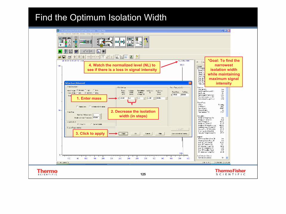
Find the Optimum Isolation Width

2. Decrease the isolation width (in steps)

1. Enter mass

4. Watch the normalized level (NL) to see if there is a loss in signal intensity

*Goal: To find the narrowest

isolation width while maintaining maximum signal

intensity

3. Click to apply

126

126

Apply Collision Energy to the Isolated Ion

1. Apply collision energy (35%) to fragment ion of interest

127

127

Automatically Optimize the Collision Energy

1. Click to open

2. Type mass of product ion

3. Click start

128

128

Automatically Optimize the Collision Energy

Click to accept new value for collision energy

129

129

Save the Tune File!

130

130

Acquiring a RAW File During Tuning

The camera icon can be used to acquire raw files and

run instrument methods directly from LCQ Tune

1. Click to open

131

131

Typical Vacuum Settings

API Stack Region (1.0 – 1.5 Torr)

Ion Trap Region (0.75 – 1.5 x 10-5)

1. Click to open

132


Xcalibur Software –Instrument Method

Development

133

133

Thermo Software Standard

• TSQ Quantum Classic / Discovery / Discovery MAX / Ultra / Ultra AM / EMR

• LCQAdvantage / LCQAdvantage MAX / LCQDeca XP Plus/ LCQDuo / LCQDeca / LCQClassic

• LXQ / LTQ / LTQ-FTMS / LTQ Orbitrap / MAT900XP / MAT900XP-Trap / MAT95XP / MAT95XP-Trap

• Tempus / PolarisQ (Polaris, GCQ)

• TraceDSQ

• TraceMS (Voyager, MD800)

• aQa (Navigator) / MSQ / MSQ+

134

134

Supported LC Peripherals

• Surveyor (LC/MS/MS Plus pumps, AS/ASLite/AS Plus/AS Plus Lite, PDA/PDA Plus, UVvis 2000)

• TSP (P2000/P4000, AS1000/AS3000, UV2000/UV6000)

• CTC Analytics (PAL Autosampler)

• Waters (2690, 2695, 2795, 2487 UV)

• HP/Agilent (LC 1050 / 1090 / 1100, AS 1100, DAD 1100, VWD 1100)

• Shimadzu (LC-10Avp series)

• Flux Instruments AG (Rheos 2000/dual, IC8)

• Dionex/LC Packings (Ultimate)

• Other Analog Devices

135

135

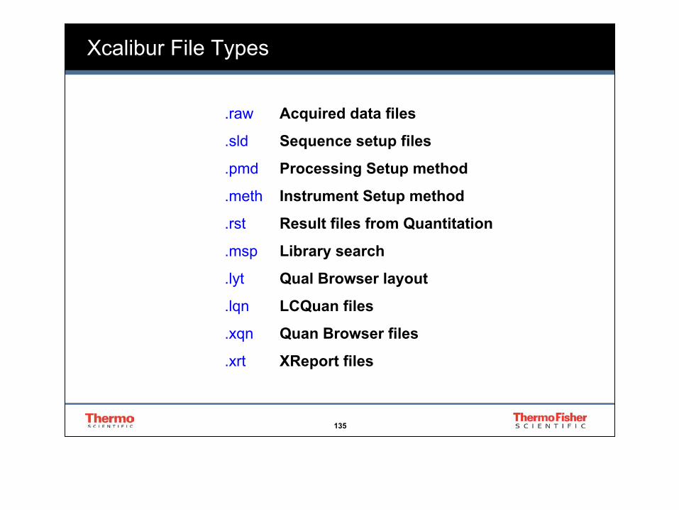
.raw Acquired data files

.sld Sequence setup files

.pmd Processing Setup method

.meth Instrument Setup method

.rst Result files from Quantitation

.msp Library search

.lyt Qual Browser layout

.lqn LCQuan files

.xqn Quan Browser files

.xrt XReport files

Xcalibur File Types

136

136

Instrument Configuration

137

137

Homepage – Status View

Click to set up instrument method

138

138

HPLC Method Setup

139

139

HPLC Method Setup

140

140

Autosampler Setup

Select which injection mode to use

141

141

Full Loop Injection

Volume Pulled = 3 x Injection Volume + Excess volumeThe excess volume is ~26 ul

The Full Loop gives the highest injection precision

142

142

Total volume = Injection Volume + Excess VolumeThe excess volume is 10 ul

The remaining volume is achieved using air plugs

Partial Loop Injection

143

143

Volume Pulled = Injection Volume• The No Waste injection always causes 2 ul of flush solvent to be injected.

This can be cause poor binding of peptides if the flow rates of the system are low and the solvent is strong. Use the sample prep method if needed.

• The user should calibrate the dead volume in a no waste injection against a full loop injection of a known sample.

No Waste Injection

144

144

Flush and Wash Setup – Minimizing Carryover

Wash- Cleans the outside of the needle

Flush- Cleans the injection port and the inside of the needle

145

145

Sample Preparation

146

146

PDA Setup

147

147

LCQ MS Setup

The LCQ Setup page provides a selection of experimental

templates for popular experiments (or you can build

methods from scratch)

148

148

Open Raw FileOpen Raw File

LCQ MS Setup

Segments

1. Open a RAW file using the LCQ drop down menu to set segment time intervals

2. Type the number of segments you want in your method

3. Drag the red line to add segment time intervals

4. Can have one tune file per segment

149

149

LCQ MS Setup

Scan Events

1. Select the number of scan events for each segment. Each scan event is essentially a different acquisition (i.e., a full scan followed by an MS/MS scan is two separate scan events).

2. Must use the same tune file for each scan event within a particular segment.

150

150

LCQ MS Setup

1. Mass Range: Low, Normal or High

2. Scan Mode: MS, MS/MS, MSn

3. Scan type: Full, SRM, Zoom

5. Polarity: + or – ion mode detection

6. Data type: Centroid or Profile

151

151

Other Method Features

1. Select Source Fragmentation On if in-source CID is desired

2. Wideband activation will be active if an MS/MS or MSn scan event is selected

152

152

Selected Ion Monitoring

153

153

Product Ion MS/MS

154

154

Data Dependent Acquisition

1. First scan event is the trigger scan

2. All subsequent scans events may be dependent on Scan event 1

155

155

Time

Inte

nsity

A (1, 2, 3)

B (1, 2, 3)

C (1)Threshold

3. Full Scan MS31. Full Scan MS∗

2. Full Scan MS2

*

* ion selected

Data Dependent Scanning

156

156

Building Double Play (Data Dependent MS/MS)

Steps:1. Full MS 2. Data Dependent (dd) MS2 on the largest ion from the Full MS

spectrum

Pros/Cons:1. Provides MS/MS (structural) information2. Misses co-eluting peaks

157

157

Building Double Play: Scan Event One

1. Add two scan events, set the Acquire time and Tune method

2. Scan event one needs to have the Mass Range set

158

158

Building Double Play: Scan Event Two

1. Check the box next to Dependent scan

2. Click on Settings

159

159

Segment Settings

1. Enter Reject masses (These should be found by examining a blank run in Qual Browser using a Full MS scan)

2. Set the Normalized Collision Energy, Default Charge State, Min. MS signal (Threshold) and Isolation Width

• Enter Parent masses (if desired)


160

160


Scan Event Settings

• Nth most intense ion = 1

• Use Nth most intense from list when parent masses are specified in the Segment settings

161

161

Dynamic Exclusion

1. Choose Global > Dynamic Exclusion

2. Set the Repeat count, Repeat duration, Exclusion list size, Exclusion duration, and Exclusion mass width

• These settings cause three MS/MS events happening within 0.2 min. to trigger the exclusion of the mass for the next 0.3 minutes

• The mass widths can be set asymmetrically to account for isotopes

162

162

Divert Valve Operation

163

163

Experiment Summary

164

164

Common Data Dependent LCQ Experiments

Big 3:

Steps:1. Full MS 2. Data Dependent (dd) MS2 of the Largest, dd MS2 of 2nd Largest, dd MS2 of 3rd Largest

Pros/Cons:1. High ratio of time spent doing MS2

2. Hits peak apex

Double Play with Dynamic Exclusion:

Steps:1. Full MS 2. Data Dependent (dd) MS2 of the Largest with Dynamic Exclusion

Pros/Cons:1. Adds opportunity to analyze coeluting peaks2. May miss peak apex

165


Setting Up and Running Sequences

166

166

Xcalibur Home Page Sequence Setup

To open Sequence Setup, can

click View > Sequence

Setup View

Can also click on Sequence Setup button

167

167

Creating a Sequence

1. Double-click to add Instrument Method

2. If there is no folder created for the Path,

you can type a folder in and it will be created

3. Populate File Name (no spaces),

Position, and Inj Vol

If you have a small number of samples to run, it is easiest to create the sequence from the Sequence Setup Home Page

Minimum Information Required to Run the Sequence: File Name, Path, Inst Meth, Position, Inj Vol

168

168

Creating a Sequence

Hotkey F2 puts the cursor in the boxes and makes

the fields editable

To open the Inst Methfrom the sequence,

right-click and select Open File

169

169

Creating a Sequence Using the New Sequence Template

If you have a larger number of samples to run, it is easier to use the New Sequence Template to create the sequence

1. Click New

170

170

New Sequence Template

1. Choose a Base File Name, Path, & Instrument Method

3. Select the Initial Vial Position2. Enter the number of

unknown samples

4. If you already have a Processing Method, specify it (above) and you can Add

Standards, Blanks and QCs. The sequence will be

populated with these rows as established in the processing method.

171

171

New Sequence Template

Once, you click OK on the New Sequence Template, the File Name is automatically incremented starting

with the Base File Name you specified

172

172

New Sequence TemplateIf you want to type a new File Name:

2. Select Edit and click Fill

Down1. Type File name

173

173

Changing the Sequence Column Arrangement

1. Select Change and click Column

Arrangement

2. Select which columns to add

from the available columns

4. Can also change the order by clicking Move

Up or Down

3. Click Add

174

174

Changing the User Labels

1. Select Change and click User

Labels

2. Modify labels and the new labels will be incorporated as

column headings in the sequence

175

175

Changing the Tray Name

The Tray Types displayed in the list are all of those that are available for the currently configured autosampler

1. Select Change and click Tray

Name

2. Select tray to use

176

176

Exporting a Sequence to Excel

1. Select File and click Export

Sequence

177

177

Exporting a Sequence to Excel

1. Select which columns to export and Click Browse

2. Give a name to your

sequence that will be exported

3. The sequence is exported as a .csv file

178

178

Example of an Exported Sequence

To be able to import the sequence back into Xcalibur, the first row must contain the text Bracket Type=n where n=1-4. Each number represents a particular bracket type as follows:

1= Overlapped, 2= None, 3= Non-overlapped, 4= Open

179

179

Importing a Sequence from Excel

2. Select which columns to

import and Click Browse to find the modified

sequence

1. Select File and

click Import Sequence

180

180

Running the Sequence

1. Can either Run One

Sample or Run Sequence

181

181

Running the SequenceDisplays all instruments that have been configured using

Instrument Configuration

Allows you to process samples automatically

If not checked, the sequence will

not go into the queue until you click Actions > Start Analysis

Make sure these are the rows to run

Select if you want to run sequence ASAP

Can specify Instrument

Method to run before or after the sequence

182

182

The Info View

Acquisition Queue-Sequence ProgressStatus

Can turn the Info View On/Off in the Sequence Setup by clicking View and unchecking Info View

The Status tab shows the status of all configured

instruments When a sequence is submitted, it shows up in

the Acquisition Queue. To delete a sample check the

box next to the sample and hit Delete on the keyboard

183

183

Real Time Plot View

1. Select View and click Real Time Plot

View

If you modify anything in the view, click the lock button to resume

monitoring real-time data collection

184


Qual Browser

185

185

To open Qual Browser, you can right-click on the Qual Browser

button on the Xcalibur Homepage to have options to open various

raw files or sequences

Opening Qual Browser

186

186

Qual Browser Main View

Info Bar

The Amplify Toolbar can be used to amplify a region in a chromatogram or spectrum

Main Toolbar

Can have up to 16 cells in the

window at once and each cell

can contain up to 8 plots

Cells have pins in the top right corner

187

187

Opening Data in Qual Browser

2. Select to replace (the current window, cell or plot), add a new window or plot (by default a new window

will be added), and choose which layout to use

1. Click File and select Open (can also open sequences

or result files)

188

188

The Info Bar

The Cell Info tab gives info about each plot within

a cell

If you open a sequence or

result files, they appear in the

second and third tabs of the Info

Bar, respectively

The Integration tab shows up when

you integrate peaks in a chromatogram.

You can change the parameters to affect how peaks

are integrated.

189

189

The Info Bar – Elemental Composition

2. Set limits for the formulas

3. To change elements in use, right-click and go to Add Isotopes. Select isotope from periodic table.

1. Type mass value or right-click on a mass in the spectrum and select

‘Generate Formula from Mass’

4. Click Calculate and the formulas appear in the table

The Elemental Composition page of the Info Bar allows you to calculate the "best matching" chemical formula for a mass (from a spectrum)

190

190

The Isotope Simulator allows you to create a simulated spectrum for a chemical formula entered

The Info Bar – Isotope Simulator

2. Select the

parameters

1. Enter achemical formula

3. Click new

4. The exact mass appears here and the

simulation appears in a new dialog box

191

191

The MSn Browser of the Info Bar allows you to display and analyze MSn experimental data

The Info Bar – MSn Browser

2. Click to expand

1. If data does not show up in the MSn browser,

pin the spectrum

3. Can double-click to get either the Average

or Composite spectrum

4. Can also right-click and select to Include individual scans

192

192

Qual Browser Layouts

2. Save the layout or save the layout as the

default layout

1. Set the cells, plots, integration, etc. to your

specifications

3. Apply the layout to subsequent samples

193

193

To Zoom In…

1. Pin cell

2. Drag parallel to the X or Y axis or put a box around the region of interest

194

194

Getting an Average Spectrum of a Peak in the Chromatogram

1. Pin spectrum

2. Drag across peak with cursor to get the average spectrum

3. AV tells you how many scans were averaged (e.g. AV: 7 =

average spectrum of 7 scans)

195

195

Extracting an Ion from the Chromatogram

1. Pin chromatogram

2. Either drag across spectral peak with cursor to get an EIC with the range dragged or click on the spectral peak with the cursor and the mass will be

extracted with the mass tolerance specified in the

chromatogram ranges box

196

196

Chromatogram Right-Click Menu – Peak Detection

1. Right-click on the chromatogram and

select Peak Detection

2. Select Toggle Detection in This

Plot or in All Plots

3. Tab appears in the Info Bar to optimize peak detection parameters

197

197

Chromatogram Right-Click Menu – AutoFilter

AutoFilter can be used to pull out scan filters automatically (useful for targeted analysis). First (top) plot has no scan filter applied.

Every other plot corresponds to scan filters set up in the method

(max. 8 chromatogram plots)

198

198

Chromatogram Right-Click Menu – Chromatogram Ranges

1. Right-click on the chromatogram and

select Ranges…

199

199

Chromatogram Right-Click Menu – Chromatogram Ranges

Check to add plots (8 max)

Click to change the raw file name Can change

the Detector,

Peak detection algorithm, and Delay time here

200

200

Chromatogram Ranges – Scan Filter

Can also click down arrow and select any of these

more specific scan filters

Can type any general scan filter here (e.g. Full ms, Full ms2, Full ms3, etc. pulls out all MS, MS2, MS3 scans, respectively). The layout can

then be saved as default so that if the scan ranges are changed, there is no need to modify the scan filter. If you leave the Scan filter blank,

it will show all scans that were acquired (whether MS or MSn)

201

201

Chromatogram Ranges – Plot Types

1. Click to change the Plot type

TIC – plots the sum of all ions for each scan. Base Peak – plots the most intense ion for each scan.

Full ms data normally looks better as a Base Peak chromatogram since much of the noise gets filtered out.

202

202

Chromatogram Ranges – Extracted Ion Chromatogram

1. Change the Scan filter to Full ms or

delete the Scan filter to see all scans

3. Type mass or mass range in the Range(s) box. If one mass is typed, the range will be defined by the mass tolerance set in the Automatic processing tab

2. Can either choose Mass Range (TIC) or Base Peak

There are different ways to extract an ion in your chromatogram using the Chromatogram Ranges box:

203

203

Chromatogram Ranges – Neutral Fragment

1. Delete Scan filter

2. Select Neutral Fragment

3. Type Neutral Fragment mass

The Neutral Fragment Plot type will plot any ions that have a specific neutral loss that you specify (from the MS to the MS2)

204

204

Chromatogram Ranges – Automatic Processing tab

1. Can enable smoothing for the

chromatogram plot

Smoothing points must be an odd number

205

205

Chromatogram Right-Click Menu - Display Options

1. Right-click on the chromatogram and select

Display Options…

The Display Options box allows you to modify the appearance of the chromatogram view (Style, Color, Labels, Axis & Normalization)

Xcalibur displays the results of the current

settings in the graphic on the right side

206

206

Spectrum Right-Click Menu – Spectrum List

The Spectrum List can contain m/z, absolute intensity, and relative

intensity for each of the ions in the spectrum

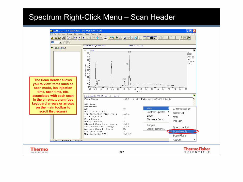
207

207

Spectrum Right-Click Menu – Scan Header

The Scan Header allows you to view items such as scan mode, ion injection

time, scan time, etc. associated with each scan in the chromatogram (use keyboard arrows or arrows

on the main toolbar to scroll thru scans)

208

208

Spectrum Right-Click Menu – Tune and Instrument Methods

Tune and Instrument Methods are stored in

the raw file. When selecting the Instrument Method, the MS method

shows up on the first page. Scroll with the keyboard arrows or arrows on the main

toolbar to get the pump and autosampler

methods.

209

209

Spectrum Right-Click Menu – Spectral Subtraction

1. Get an average spectrum of the peak of interest

2. Right-click on the spectrum and select

Subtract Spectra and 2 Ranges

3. Drag your cursor before and after the peak to select regions to be subtracted

210

210

Spectrum Right-Click Menu - Spectrum Ranges

1. Right-click on the spectrum and select

Ranges…

211

211

Spectrum Right-Click Menu - Spectrum Ranges

The Spectrum Ranges box is similar to the

Chromatogram Ranges box. Can also enable

Background Subtraction for the spectrum here.

212

212

Presentation

1. To add text, click Display

and select Annotate

2. Type Annotation

3. Click on pinned chromatogram to

annotate

213

213

Chromatogram Capture

1. Go to Edit > Copy Cell to copy the pinned cell

2. The cell can then be pasted into other Office

programs (Microsoft Word, Powerpoint, Excel, etc.)

214


Quantitative Processing

215

215

Quantitative Processing

1. Processing Setup» Input known compounds for identification» Set up peak detection/integration parameters» Choose calibration/QC type, levels, weighting» Select advanced chromatographic processing

2. Sample Processing/Reprocessing» Input new sequence setup parameters» Identify calibration file and bracketing type» Process/Reprocess data

3. Quan Browser» View quantitative results» Evaluate standard curve, QCs, and flags» Recalculate peaks with different parameters» Analyze detailed quantitation information

216

216

Quan Processing Setup

Click Processing Setup button on the Xcalibur

Homepage to begin setting up the quantitative

processing method

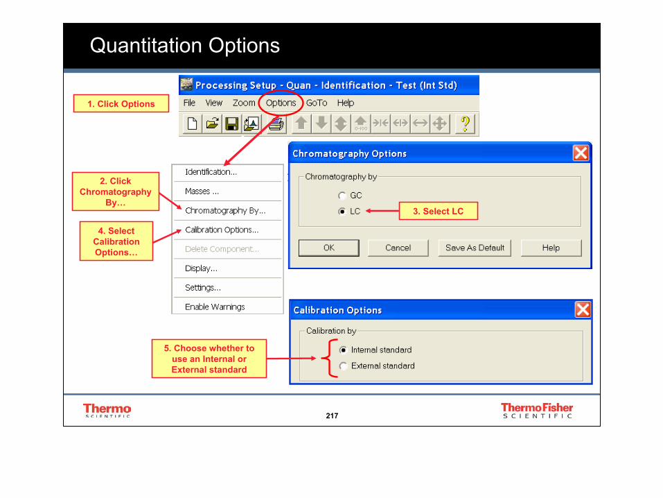
217

217

Quantitation Options

1. Click Options

3. Select LC

4. Select Calibration Options…

5. Choose whether to use an Internal or External standard

2. Click Chromatography

By…

218

218

Open a Raw File to Set Up the Processing Method

1. Click File

2. Click Open Raw File…

219

219

Quan Processing – Identification Tab

1. Select <New> and type name of

component 2. Select Detector type and Peak Detection algorithm

3. Select scan filter and trace type

4. Click OK to update

chromatogram

Chromatogram changes to reflect scan filter and trace type selected

220

220

Quan Processing – Identification Tab

1. Populate Expected RT (min)

Window (sec) = allowable RT window for component elutionIf using an internal standard, you can

select to use it as a RT reference

*Note: If using an internal standard, the ISTD component should be set up first since all target components will refer to the ISTD. For all other components, you can select ‘Adjust using’ and choose the ISTD name.

2. Click OK to update

chromatogram

221

221

Quan Processing – Detection Tab

1. Click on Detection tab

2. Modify parameters to achieve satisfactory peak integration

3. Click OK for changes to update on

chromatogram

222

222

Quan Processing - Calibration Tab Internal Standard Setup

1. Click on Calibration tab

2. Select ISTD

3. Type Amount

and Units for ISTD

223

223

Quan Processing - Calibration Tab Target Compound Setup

1. Select Target compound

If using ISTD, select ISTD here

2. Select how to weight the calibration curve (if at all)

3. Select what to do with the origin on the calibration curve

224

224

Quan Processing – Levels Tab

1. Click on Levels tab

2. Enter name for each

calibration level 3. Enter amount for

each calibration level

4. Enter name, amount and % Test for each QC level

225

225

Copying Levels to All Target Compounds

The information in the Levels tab only needs to be entered for one target

compound. To copy the levels to the other compounds or QCs, right-click and select ‘Copy Levels to All Target Components’.

226

226

Quan Processing/Reprocessing

Click Sequence Setup button to

open the sequence and add information before processing/

reprocessing

227

227

Open the Sequence and Add Extra Columns

2. Add Level, Proc Methand Sample Type columns

into the sequence

1. Click Change and select Column Arrangement

228

228

Enter Information into the Sequence

Add Level, Proc Methand Sample Type

columns into sequence

Populate the Proc Meth, Sample Type and Level

columns in the sequence

229

229

Batch Reprocessing Quantitative Data

2. Check Quan, Peak Detection & Integration and

Quantitation1. Click Actions

and select Batch

Reprocess

3. Click OK to process

230

230

Enabling Quantitative Processing During Acquisition

2. Check Quan

1. Click Actions and select Run Sequence

231

231

Quan Browser

To view the processed data,

click on the QuanBrowser button on

the Xcalibur Homepage

232

232

Quan Browser Main View

Chromatogram Calibration Curve

Select which component to view the data

for that component

You can display either All, Standards, QCs, Blanks, Unknowns

Results Grid

233

233

Changing the Results Grid Display

1. To change what is displayed in the Results Grid, right-

click on the Results Grid

Can change the sorting order of the

columns

Can change the columns that are displayed in the

Results Grid

234

234

Changing Peak Detection/Integration Parameters

1. To change how the peaks are detected and integrated, right-click on the chromatogram 3. Click to Apply

new settings to the selected plot

or to Apply to All Plots

4. Integration Type changes to User Integration

2. Change settings (most used settings are in Identification

and Integration tabs)

235

235

Changing Peak Integration Parameters Manually

1. Drag blue squares with cursor

2. Integration Type changes to Manual Integration

236

236

Changing Back to Original Integration (Method Settings)

1. If you want to change the integration settings back to when the data was first opened, click

Method Settings

2. Integration Type changes back to Method Settings

237

237

Changing Calibration Parameters

1. To change the calibration parameters,

right-click on the calibration curve

238

238

Ways to Exclude a Calibration Curve Point

To exclude a calibration curve

point, you can check to exclude in the

Results Grid

To exclude a calibration curve point, right-click on the calibration curve

Use Exclude to exclude one point at a time or the Exclusion List to

exclude more than one point at a time

239

239

Showing the Spectrum Plot Instead of the Calibration Curve

To show the spectrum at the cursor position, right-click on the calibration curve and select Show Spectrum Plot

240

240

Exporting Data to Excel and Printing Reports

See next slide

Click to export data to Excel

241

241

Printing Reports

1. Click to enable reports

2. Select report template to use

3. Click to select samples

242

242

Selecting Samples to Include in the Report

1. Select which samples to

include from the sample choices (hold CTRL or SHIFT to select

multiple samples)

2. Click Add to add the samples to the selected samples for the report

243


XReport 1.0

244

244

XReport 1.0 : The Reporting Application for Xcalibur 2.0

Simple to create your report templates!

Report as DOC, TXT ,HTML, RTF, XLS

Configurable properties (i.e. size, decimal places, chromatogram summaries, etc.) of objects and sections

245

245

Drag and Drop Interface: Quan Peak Results Canned Template

Available Sectionsand Objects

Report Template Report Outline

246

246

Steps to XReport Reporting

• Open XReport 1.0• Drag and Drop required items into appropriate fields• Specify Data Sources to view example report• Save Report Template

1. XReport

2. Processing Setup• Open Processing Setup• Click on the Reports Icon• Enable Reports and Select the Report Template• Save the Processing Setup

3. Reprocess Selected Files• Go to Home Page - Sequence Setup• Open/Make a Sequence• Click Actions : Batch Reprocess...• Check Reports and Print Reports Boxes

247

247

Before you Start

» Decide what objects you want on the report and how they should be laid out.

248

248

Open XReport

Click Start

All Programs

Xcalibur

XReport

249

249

Specify Data Sources…

1. Click Report and select Data

Sources

2. Specify Data Sources

250

250

Drag and Drop Sections…

251

251

Drag and Drop Sections…

Sections that have been dragged appear here and can be selected

252

252

Drag and Drop Individual Objects…

253

253

Formatting Objects…

• Any inserted object can be formatted to some degree

• Right Click

• Select Properties

• Follow the Instructions

254

254

Viewing the Report…

Click to view the report

255

255

Save, Insert, Use…

1. Click to save

the report

2. In Processing Setup, click

Reports

3. Enable the reports

4. Select how to save the report and

double-click to select the Report Template Name

256

256

Save, Insert, Use…

1. Click to enable reports when you run the sequence

2. Click to enable reports after the

sequence has run

257


Calibration and Maintenance

258

258

Calibration

• Calibration should be performed approximately every 3 to 6 months or after the multipoles and the trap have been removed.

• It is not usually necessary to calibrate more frequently and unnecessary calibration will lead to Ultramark contamination.

• The best procedure is to calibrate before maintaining the stack but after the multipoles and the trap have been cleaned.

259

259

First Make Sure…

Your calibration solutions are fresh

Your calibration solution contains all calibrant masses

Your ion source settings are optimized for the flowrate used

You have a stable spray: Focus on the injection time (IT) and on the normalized level (NL) in the Tune Page scan header

260

260

Automatic Calibration

Start the automatic calibration procedure (takes about 40 min.)

261

261

Semi-Automatic Calibration

Use the semi-automaticcalibration procedureto calibrate parameters that did not pass during automatic calibration.

262

262

LCQ Recommended Maintenance Schedule

Daily:

• Check the convectron and ion gauge pressures. Make sure the vacuum system is operational. Typical LCQ values are: a) convectronpressure 0.9 – 1.1 Torr; b) ion gauge pressure 1.0 -1.5 x 10-5 Torr.

• If bottled nitrogen gas is being used, check nitrogen gas pressure. The recommended value for the LCQ is 80 – 120 psig.

• Check the ESI fused silica sample tube. Make sure the fused silica is not elongated. Trim the tube if necessary.

• Remove the APCI needle (if switching from APCI to ESI).

• Check HPLC solvent levels.

• After completion of analysis place system in stand-by mode.

263

263


Weekly:

• Check the mechanical pump oil level.

• Fill the mechanical pump as needed.

• Ballast the mechanical pump.

• Replace LC solvents to maintain low background levels.

264

264


Monthly:

• Check the helium gas tank pressure. The recommended value for the LCQ is 30 – 50 psig. Replace the tank as needed.

• Check the nitrogen gas supply. Replace or refill as needed.

• Trim / Exchange ESI fused silica sample tube.

• Clean / Replace ion transfer tube. Optional cleaning procedure is sonication for 15 min in methanol or isopropanol.

• Optional (at least quarterly): - Calibrate LCQ. - Clean the API stack. Wipe tube lens and skimmer clean with

methanol or isopropanol. Do not sonicate the tube lens and skimmer in acidic solutions!

- Tune instrument after cleaning the API stack.

265

265


Quarterly:• Calibrate LCQ. • Clean/replace ion transfer tube.• Clean API stack.• Check/replace mechanical pump oil.• Clean air filter pad in the back of the instrument.• Back up data and defragment PC.• Check the Thermo website for available software updates / fixes:

- Thermo Fisher Scientific Fast LC and LC/MS Support http://www.thermo.com/ => Search for “Fast LC and LC/MS”

- Thermo Fisher Scientific Knowledge Base http://198.173.130.188/thermofinnigandb/thermo.nsf

- Thermo Fisher Scientific Customer Download Site http://mssupport.thermo.com/

266

266


Annual:

• Clean oil traps on mechanical pumps.

• Clean ion optics and the ion trap.

• Change oil filter pads on turbomolecular pumps (if present).

Notes:

• Heavy use and dirty samples may require more frequent cleaning of the ion transfer tube, the API stack and the analyzer.

• If the sensitivity starts to drop off and can not be restored byreplacing the ion transfer tube, clean the API stack (and analyzer) as needed.

267


MetWorks

268

268

Workflow for a Data Dependent Experiment(to process one file at a time)

To process the acquired sample data one file at a time, you can first create a background subtracted file to use for your sample data file (optional). The next step is to open a sample data file and a control data file for component detection. To create the MetWorks method, specify your parent drug, define the modifications you expect to your parent drug, define any additional traces you wish to view in the results and configure the processing and display parameters. Click the Results button to process the data and then review the results and confirm the components that are of interest in each of the MetWorks views. After selecting the components of interest from each view, a summary of these components can be viewed in MetView and a report generated using MetReport. There are also other types of summary reports that can be created by clicking on the Reports button.

269

269

Opening the Raw Data Files

Click to open raw files

To open a raw file, on the Info bar Button page, click the Open button and then select the sample data file (.raw) to be processed using the MetWorks method you are creating. For component detection, you can also select a control file (.raw) that will be compared to the sample file. Alternatively, you can choose to open a previously created MetWorks method (.mbx file).

270

270

MetWorks Window After Opening the Raw Data Files(General Trace View)

Base peakchromatogram

Spectrum atcursor position

Use arrows to scrollthru the scans

Total ionchromatogram

After opening the raw data files, the MetWorks window changes to display the total ion chromatogram and base peak chromatogram of the sample raw file and the mass spectrum of the sample raw file at the current cursor position below in the General Trace view. The arrow buttons above the spectrum can be used to scroll thru the scans in the chromatograms.

271

271

Entering the Analyte

3. Click to enterstructure

1. Type a name for thelist then click new item

2. Type information for analyte

4. Click to add new analyte to Working analyte list

One way to specify an analyte for a MetWorks method is to simply Enter a New Analyte. After clicking on the Analyte(s) button, the Analyte(s) Manager dialog box opens. First, type a name for your new Working analyte list and then click New Item to add an analyte to the list. In the New Analyte dialog box, type the name, mass and select the polarity. To enter a structure, click the button next to the Structure file (mol) box. IMPORTANT: MetWorks uses a precursor mass tolerance of +/-0.2 m/z to determine whether an MSn spectrum for a particular mass is from a precursor ion. If you do not specify the mass with the necessary precision, MetWorks cannot display the appropriate MSn indicators (blue tic marks) above the analyte chromatogram in the Expected Modifications view or locate a reference scan for the spectral cross-correlation. Click OK to add the new analyte to the Working analyte list.

272

272

Saving a Working Analyte List

Click “Save” to save workinganalyte list in the masteranalyte list for future use

Click “OK” to use Working analyte list only for current MetWorks method

To use the newly created Working analyte list for only the current MetWorks method, click OK. To use the newly created Working analyte list for future analysis as well as the current analysis, save the Working analyte list before clicking OK. When Save is clicked, you will be prompted to save as list type: Current user only or Shared with all users. Select whether to make the list available for the current user or for all users. You can define the current user from Windows. You might change the current user identity, for example, if you run MetWorks using a computer network. For details, see the Windows documentation.

273

273

Defining the Expected Modifications

4. Click for changes

to appear in list

2. Create a new modification for thelist or edit an existing modification

3. Enterinformation

1. Type name for new list

or keep current name

To create or edit a Working modifications list, either type a name for the new list or keep the existing name. Then, create a new modification for the list or edit an existing modification. In the Edit Modification dialog box, enter the name for the modification and the mass shift. For the mass shift, to calculate the m/z, you can enter the mass shift directly or click the Formula button to open the Enter Elemental Formula dialog box. In the Formula box, type the formula, and then press Update. Click OK and the calculated m/z appears in the Mass shift (m/z) box. Click OK again for the changes to appear in the list.

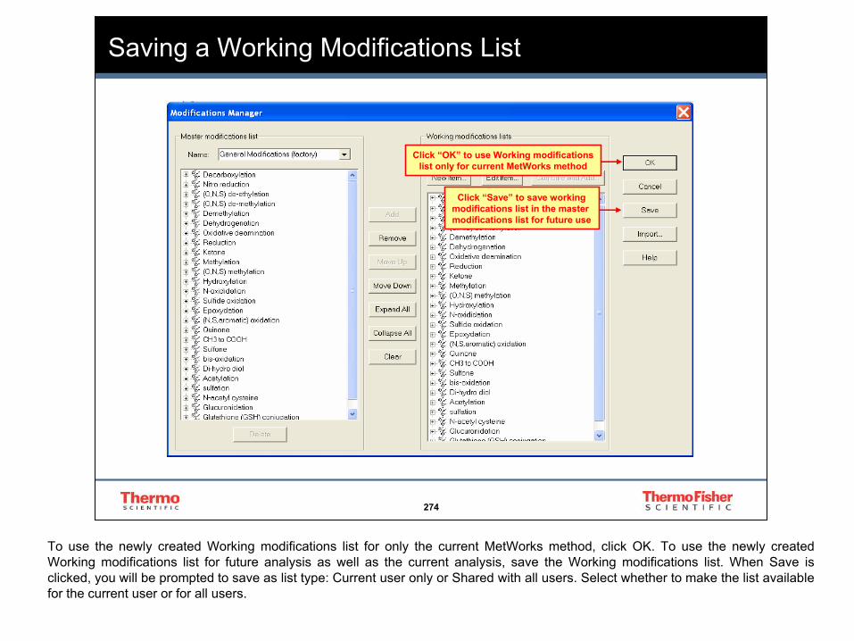
274

274

Saving a Working Modifications List

Click “Save” to save workingmodifications list in the master modifications list for future use

Click “OK” to use Working modificationslist only for current MetWorks method

To use the newly created Working modifications list for only the current MetWorks method, click OK. To use the newly created Working modifications list for future analysis as well as the current analysis, save the Working modifications list. When Save is clicked, you will be prompted to save as list type: Current user only or Shared with all users. Select whether to make the list available for the current user or for all users.

275

275

Defining the User Traces (Optional)

3. Select plot typeand plot properties

Check box if traceis for a radioactively

labeled sample

2. Select detector type (MS, Analog, A/D Card, PDA, or UV) and delay if any

1. Check box to add trace

To define a user trace, click on the User Traces button to open the User Trace Manager dialog box and check a box in the Type column to add the trace. Select whether the data was acquired from an MS, Analog, A/D Card, PDA or UV detector and also select the plot type and properties. If one of the traces is a radioactively labeled trace, check the box next to Radioactive label trace. After processing, the custom plots can appear in the Expected Modifications view and the Component Detection view. Up to 10 chromatograms, including one trace from a radioactivity detector, can appear in addition to the modification chromatograms in the Expected Modifications view. One trace from a radioactivity detector can appear in addition to the chromatograms for the sample and the control in the Component Detection view. When you process the data, the software filters the radioactively labeled sample data and retains only the results that correspond in time to a detected peak in the radioactively labeled trace.

276

276

Configuring the Processing and Display Parameters

The Configuration button allows you to configure settings that MetWorks uses to display and process your data. The processing modes include :1. Display (Expected Modifications view)

• Specifies the types of peak labels, number of traces to display, and how MetWorks displays the MSn scans in the spectrum panes of the workspace.

2. Peak Detection (Expected Modifications, Chro Search Results, Isotope Search Results view)

• Sets the peak detection algorithm and integration parameters. 3. Correlation (Spectral Correlation view)

• Searches for potential components based on the correlation with the MS2 or MSn spectrum from the analyte (or parent drug).

4. Chro Search (Chro Search Results view)• Searches for potential components by sorting the extracted-ion chromatograms (EIC) based on peak

intensity after removing all EICs for the expected modifications. 5. Component Detection (Component Detection view)

• Detects chromatographic components in complex LC/MS data and extracts the mass spectral signals from closely co-eluting components (deconvolution).

6. Isotope (Isotope Search Results view)• Searches for compounds that have specific isotopic patterns.

7. Mass Tolerance• Allows you to set the parameters for accurate mass data.

By clicking on the Configuration button, the Default Display and Processing Settings dialog box opens which allows you to configure settings used to process your data. There are 7 tabs in the Default Display and Processing Settings dialog box and most of these pages contain parameters to configure settings for the 8 different views in MetWorks. The Display page allows you to specify how MetWorks displays the data in the Expected Modifications view. The Peak Detection page allows you to set the peak detection and integration parameters for the Expected Modifications, Chro Search Results and Isotope Search Results view. The Spectral Correlation view searches for potential components based on the correlation of potential components with the MS2 or MSn spectrum of the analyte (or parent drug) and the Correlation page allows you to configure how the data is displayed in this view. With the Chro Search page, you can configure how your data is displayed in the Chro Search Results view which searches for potential components by displaying the most intense EICs based on base peak intensity after removing the EICs from the Expected Modifications view. The Component Detection page allows you to configure parameters for the Component Detection view which detects chromatographic components in complex LC/MS data and groups the mass spectra from closely eluting components. Using the Isotope Search page, you can configure parameters for the Isotope Search Results view which searches for compounds that have isotopic patterns that you specify. The Mass Tolerance page allows you to set the parameters for accurate mass data for all of the views in MetWorks. You can configure MetWorks to use your display preferences and to perform only the types of data processing required for your experiments. MetWorks stores the current configuration settings in an .mbx file when you save a MetWorks method.

277

277

Display

1. Enter # of traces and which MSorder that will appear in the Expected Modifications view

2. Select check boxes of displayoptions you want to include in results

3. Select peaks labels and enter label threshold (percent of the base peak height above which

MetWorks applies any labels to the peaks)

You can use the Display page to configure default display preferences for the modification chromatogram plots (EICs) in the Expected Modifications view. These parameters only affect how your data is displayed in the Expected Modifications view and do not affect the actual processing of the data. First, enter the Number of traces to display during review which are the number of traces to appear in the window at one time in this view and which MS order to display. Always select an MS order that corresponds to the lowest MSn order acquired. For example, if Data Dependent MS/MS data (MS and MS2) are present in the experiment, select MS as the default display parameter. Next, select the check boxes of the display options you want to include in the results. Show modification names displays the modification names in the results views. Show MSn scans displays blue tic marks above the extracted ion chromatogram (EIC). The tick marks correspond to the sites of MSn data and allow for fast searching of MSn data. Show closest MS/MS scan displays a spectrum in the spectrum pane, instead of the message "No MS/MS Data", when there is no MS/MS data at the given retention time. MetWorks displays the MS/MS scan closest to the current retention time within the integrated peak. Finally, select peak labels and enter a label threshold which is the percent of base peak height above which labels are applied to the peaks.

278

278

Peak Detection

Sets the same peak detectionand integration parameters for

all detector types in list

2. Modify parameters to achieve satisfactory peakdetection and integration

1. Select detector type (MS, Analog, A/D Card, PDA, or UV), peak detection algorithm (ICIS or Avalon), and the # of Gaussian smoothing points you want MetWorks to apply to the data

You can use the Peak Detection page to configure the default peak detection and integration settings for the Expected Modifications view, Chro Search Results view, and Isotope Search Results view. For most analyses, the default parameters are sufficient. At the top of the Peak Detection page, select the detector type, the peak detection algorithm and the number of Gaussian smoothing points to apply to the data. For the peak detection algorithm, ICIS provides superior peak detection efficiency at low MS signal levels for MS data, but, you can use ICIS for all detector types. If you want to set the same peak detection and integration parameters for all detector types in the list click the Set same button. Then, modify the parameters to achieve satisfactory peak detection and integration. To improve the peak detection results for selected chromatograms after the processing, you can reset the peak detection parameters by right-clicking on the chromatogram.

279

279

Correlation

Peak intensity must meet or exceed cutoffs before being displayed in

the Spectral Correlation table

Adds a green (high) or yellow (low) highlight to any scan in the Spectral Correlation

table with a cross-correlation factor greater than the specified value

Specifies the minimum cross-correlationfactor required before a scan appears

in the Spectral Correlation table

Normalizes each spectrum to a common base peak intensity

Correlates fragments that are shifted in mass relative to the corresponding fragments in the reference scan

Parameters in the Correlation page affect how your data is displayed in the Spectral Correlation view. MetWorks quantifies the cross-correlation of modifications to an analyte by MS2 or MSn spectral comparison using cross-correlation factors. Metabolites generally give MS/MS spectral patterns similar to their parent drug, but are mass-shifted by their metabolic modifications. Compared to conventional library searches, the results of cross-correlation analyses between parent drugs and the metabolite MS/MS spectra provide scores called cross-correlation factors with much higher confidence levels. If you want to enable Spectral Correlation, check the box next to Enable. A check in the box next to Normalize spectra will normalize each spectrum to a common base peak intensity. To correlate fragments that are shifted in mass relative to the parent data (reference scan), check the box next to Detect mass-shifted fragments. The High and Low highlight thresholds as well as the Correlation cutoff have to do only with how your data is displayed in the Spectral Correlation table on the left hand side of the Spectral Correlation view. Any scan that has a cross-correlation factor above the high or low highlight threshold will be highlighted either green (high) or yellow (low), respectively, and any scan that has a cross-correlation factor below the correlation cutoff will not be included in the table. You can also specify a Minimum Intensity Cutoff in either absolute counts or relative to the base peak intensity so that a peak intensity must meet or exceed these values to be displayed in the Spectral Correlation table.

280

280

Chro Search

Specifies the maximum number of extracted-ion chromatograms (EICs)

MetWorks returns

Only the chromatograms with peaks that meet orexceed the threshold are included in the search results

Generally, use Full MS

Chro Search searches for potential components by sorting the extracted-ion chromatograms (EICs) based on peak intensity after removing all EICs from the Expected Modifications view. Use the Chro Search page to configure the parameters for a chromatogram (Chro) search. After processing the data, MetWorks displays the results in the Chro Search Results view. To activate a chromatogram search, check the box next to Enabled. When you type a number in for the Threshold, only the chromatograms with peaks that meet or exceed the threshold are included in the results. Max chros specifies the maximum number of EICs MetWorks returns. Generally, for the Filter, use Full ms (default), or you can choose to specify a different scan filter for the data. Also, you can specify a Time range and/or a Mass range to look for EICs. Typing in values here can help to more specifically narrow down the EICs in the Chro Search results to chromatograms that are of interest.

281

281

Component Detection - JCD Algorithm

# of scans used to identifya potential component

Any peaks less than thisintensity will be rejected as noise

1. Select Enable and choose the JCD algorithm

Specifies degree of similarity of ion profile shapes

Specifies limit for the timedifference of ion profile maxima

Check box to mergewide components

On the Component Detection page, if you want to perform Component Detection using the JCD algorithm, check the box beside Enable and choose the JCD Algorithm. The Average peak width specifies the peak width (in # of scans) that the JCD algorithm uses to identify a potential component. It is best to start with a lower value and adjust based on the results. Too high of a value for the Average peak width can result in the loss of narrow peaks and too low of a value can split a real component into two different components. For the Baseline threshold, any peaks less than this value will be rejected as noise. The Merging factor specifies a limit for the time difference of the ion profile (chromatogram) maxima. A high value of the Merging factor can cause the merging of randomly coeluting components and a low value can split a component into more false-positive components. The Sharpness tolerance specifies the degree (%) of similarity of ion profile shapes. The Wide component merge mode can be selected to avoid splitting a component into ion peaks that are detected as redundant components in chromatograms with wide peaks.

282

282

Component Detection - TECD Algorithm

3. Enter time or m/z range forcomponent detection, if any

2. Select Enable and adjust the threshold to be near

the baseline for your data

1. Select Enable and choose TECD

Specifies min. # of treesections created fromthe initial spectral tree

Compares spectral trees up to the distance specified by

the Allowed gap value

Min. % two trees must matchbefore being considered

the same component

Max. distance over whichto compare trees for merging

On the Component Detection page, if you want to perform Component Detection using the TECD algorithm, check the box beside Enable and choose the TECD Algorithm. To use TECD based on your Chromatogram Info, check the box next to Enable and adjust the threshold to be near the baseline for your data. The threshold is an important parameter to adjust to be close to the noise level in your data. Max Chros specifies the maximum number of most intense extracted ion chromatograms (EIC) MetWorks can use in component detection. Each EIC can contain several detected peaks, thus the number of components MetWorks detects can be larger than the value you specify for Max Chros. You can also enter a time or mass range to narrow down the number of components generated. If you want to use the TECD algorithm based on General parameters, you can adjust these parameters if necessary. Minimal tree depth specifies the minimum number of tree sections TECD creates from the initial spectral tree. This determines the MS stage where a division takes place. Tree match factor specifies the minimum percentage that two spectral trees within adjacent tree sections must match before TECD can consider the two spectral trees as the same component. Matching spectral trees are defined as having identical precursors up to the level specified by the Minimal Tree Depth value and a Tree Match Factor value that exceeds the specified value. Wide component merge mode activates a comparison of the spectral trees for potential matching and merging, not only in adjacent sections, but also in sections up to the distance specified by the Allowed gap value. The Allowed gap specifies the maximum distance between nonadjacent tree sections over which to compare the spectral trees for potential merging.

283

283

Isotope

Displays a preview of the pattern selected from the

Isotope Pattern Preview list3. Type single # or range of Br and/or Cl

combinations only

1. Click to activate an isotope search

2. Select Elements

Use the Isotope page to configure and preview the settings for an isotope search. After you process the data, you can view and edit the isotope search results. First, click the box next to Enabled to activate an isotope search. Under Input, you can specify various parameters for the isotope search. Time range (min) is the range to specify the search window. To search over the entire time range, type: *. Tolerance is the percentage that the found clusters are allowed to differ from the theoretical clusters in the search. Threshold is the threshold to apply for including found clusters in the search results. Mass range(s) is the mass range or ranges that you want to search. To search the entire mass range, type: *. To enter multiple ranges, separate each range with a comma, for example: 243-265,354-423. Most intense specifies the number of isotopes to include in the search results based on intensity. Next, select Elements and in the Elements table, type a single number or range of Br and/or Cl combinations. The Elements table uses combinations of Cl and Br isotopic clusters only to specify the types of combinations of isotopic atoms. On the right-hand side under Isotope Pattern Preview, this displays a preview of the pattern selected from the Isotope Pattern Preview List.

284

284

Defining a Custom Isotope Pattern

4. Type difference in mass (delta) and

relative abundance

5. Click to save pattern in the list

3. Type name of pattern

2. Select Custom

1. Click to enable

If you want to specify an isotope pattern to search for components with isotopes other than Br and Cl, you can define a custom isotope pattern using the Custom table. First, click the box next to Enabled to enable the isotope search. Click on the dot next to Custom to define a custom isotope pattern. Then, type a name for the custom isotope pattern over <New Pattern Name>. Specify the difference in mass (delta) and the relative abundance of your custom isotope. Finally, click the Add button to save the pattern in the list. The Delete button displays the Custom Pattern Deletion dialog box, which allows you to delete the saved patterns.

285

285

Save the MetWorks Method

To save the settings you specified in a MetWorks method, click on File from the dropdown menu and choose Save As. In the Save As dialog box, type a file name, and then click Save to save the MetWorks method file (.mbx).

286

286

Processing the Data

Click Results toprocess the data

Click the Results button on the left-hand side to process the data. When MetWorks finishes the processing, the results appear in the MetWorks workspace. IMPORTANT: Avoid using software applications other than MetWorks when you perform component detection. MetWorks works interactively with Mass Frontier to detect the components and requires significant computer processing resources.

287

287

Component Detection View

Sample TIC

Control TIC

Sample and Control Spectra

Component Detection Table

= Sample component

= Control component

Sample TIC showing components unique

to the sample

Right-click on table tosort by retention

time, m/z or intensity

The first results view in MetWorks is the Component Detection view. You can also display this view by clicking on the Component Detection button on the toolbar. This view allows you to review and confirm the list of components that MetWorks determined to be unique to the sample data. The Component Detection view displays the Sample TIC on the top right, the Control TIC in the middle, and the Potential Modification TIC as the third trace which shows components unique to the sample. You can click anywhere on these chromatograms and get a comparison of the sample and control spectra at the bottom of the MetWorks window. MetWorks uses different colored triangles on the chromatograms and color coding in the Component Detection table to indicate status of various components. The Green triangles on the chromatograms and in the Component Detection table are components the software determined to be unique to the sample. The Red triangles on the chromatograms and in the Component Detection table are components the software detected in the control as well as the sample (this is not applicable if you did not associate a control with your sample). The Yellow highlighted components in the Component Detection table are components that you manually included or excluded from the list of selected components. If you defined a custom trace from a radioactivity detector, the software uses the trace to filter the sample data and retains only the results that correspond in time to a detected peak in the radioactively labeled trace. The Potential Modification Components chromatogram displays only the components that both pass the radioactive-label trace filter and are unique to the sample.

288

288

Displaying Spectra for a Selected Component

Click above triangle to put red cursor on component

and display spectrum

Use arrows to scroll thru components or scans and

click “I” or “E” to include or exclude components

Click numbers to displayselected MS order and “C” or

“A” to display the composite or averaged spectrum

To display the spectrum for a component, click above a triangle in a chromatogram to put the red cursor on a component or a click a row in the Component detection table. If the component was detected in the sample only, the corresponding spectrum appears in the bottom left spectrum pane. If the component was detected in the sample and control, a spectrum appears in both the spectrum panes. Using the toolbar above the spectrum pane you can display the composite, averaged or single spectrum. Click “C” to display the Composite spectrum, which combines all MSn stages for the component. Click “A” to display the Averaged spectrum and then click 2, 3, or n to display the average of the MS2, MS3, or MSn, respectively, for the component. To display a Single spectrum, click “A” or “C”, if selected, so that neither is selected. Click the 1, 2, 3, or n to display the spectrum of the scan for the selected MS order. Click the arrow buttons to display the spectrum for the previous or next component (composite or averaged spectrum) or the previous or next scan (single spectrum) and “I” or “E” to include or exclude components.

289

289

Editing the Component Selections

Click boxes to includeor exclude components

Triangles of excluded components turn clear

Can also right-click and select exclude to exclude component

There are various ways to include components of interest or exclude components that are not of interest. MetWorks updates the list of candidates you included or excluded in MetView. In the Component detection table, select the check boxes of the components you want to include in the MetView list and clear the check boxes of the components you want to exclude from the candidate list. In the Potential Modification Components chromatogram, MetWorks removes the green triangle and in the sample trace, the triangle turns clear. Alternatively, you can right-click the green triangle, and then choose Exclude to remove a component from the candidate list. Right-click the green triangle, and then choose Include to add a component to the candidate list. Components can also be included or excluded by clicking the “I” or “E” button above the spectrum pane. Choose File > Save to save your edits.

290

290

Expected Modifications View

Modification names are displayed if selected in

the configuration

Extracted ion chromatograms

of expected modification peaks

The second MetWorks view is the Expected Modifications view and you can display this by clicking on the Expected Modifications button on the toolbar. If you defined expected modifications for an analyte when you set up the MetWorks method, the Expected Modifications view displays the extracted ion chromatograms for which MetWorks detected peaks. MetWorks also adds the detected peaks to the list of candidates in MetView. The extracted ion chromatogram (EIC) of the analyte is displayed as the first (top) trace, the modification chromatograms following and User Traces that were set up in the workflow are displayed last (after all of the expected modification chromatograms). If you selected Show modification names in the Display page when configuring the MetWorks method, the modification names are displayed on the top of all of the traces.

291

291

Displaying the Chromatograms

To display blue tick marks (MSn

scan indicators), make sure “Show

MS Scans” is highlighted and

zoom in on chromatogram

In the Expected Modifications view, any MSn scans that were acquired are displayed with blue tick marks above the peaks in the chromatograms. When setting up the MetWorks method, check the box next to Show MSn Scans in the Display page of the Default Display and Processing Settings. If this was not set up in the MetWorks method, right-click a chromatogram, and then choose Show MSn Scans from the shortcut menu to view the MSn scan indicators (blue tick marks).

292

292

Modification Peak Summary View

Can select to view only included Chro

Search data

The Modification Peak Summary can be accessed by clicking on the Modification Peak Summary button. This displays the peak summary of the chromatographic results from the Expected Modifications view. The Modification Peak Summary displays the overall summary of the analyte and the expected modifications you defined, the summary for the analyte chromatogram, the summary for each modification (including any User Traces that were specified as part of the workflow), the summaries from the results of the Chro Search and the summary for each custom trace. You can use the Modification Peak Summary to print or export a peak summary to Excel by right-clicking on the page and selecting Print or Create Excel Summary. There is also the option of selecting to view only data from the Chro Search Results view that you have chosen to include.

293

293

Spectral Correlation View

Spectral CorrelationResults Table

Reference Scan

Spectrum at Cursor Position

Correlation Summary

Chromatogram

Modification Summary

Chromatogram

The Spectral Correlation view can be accessed by clicking on the Spectral Correlation button. The Spectral Correlation view provides the results of the cross-correlation between the MS/MS or MSn spectral patterns in the data to the reference scan which is an MS2 or MSn scan from your analyte or parent drug. This view includes the Spectral Correlation Results table which displays the correlation values from the cross-correlation analysis. MetWorks highlights the rows with either green or yellow depending on the high and low highlight thresholds you set in the Default Display and Processing Settings dialog box. This view also incorporates the Modification Summary chromatogram which displays the total extracted ion chromatogram for all modification chromatograms associated with the analyte and the Correlation Summary chromatogram which graphs the cross-correlation factors that MetWorks calculates by comparing the scans in the data to the reference MS2 or MSn scan. MetWorks graphs the same correlation values in the Correlation Summary chromatogram that appear in the Spectral Correlation results table. The reference scan from your parent drug is displayed beneath the Correlation Summary chromatogram. Click on the Modification Summary Chromatogram or the Correlation Summary Chromatogram to display the corresponding spectrum in the bottom pane and you can compare this to the reference scan.

294

294

Viewing the Results and Selecting the Peaks of Interest

Right-click to sort table rows

Click to expand and show MSn

data associated with m/z

After importing the reference scan, select the check boxes of the candidates you want to include in the MetView list and clear the check boxes of the candidates you want to exclude. You can click on the + box next to the candidate to expand and show MSn data associated with the candidate. To set the sorting order of the table, right-click on the table, and then choose to sort by Retention Time, Parent Mass, Correlation Value or Mass Shift. Use the vertical scroll bar in the table to scroll through the results. The green and yellow color highlights help locate the peaks with correlation scores that match the thresholds you specified in the Correlation page of the Default Display and Processing Settings dialog box. Green color highlights scans with a high cross-correlation factor and yellow highlights scans with a medium cross-correlation factor. No color highlights the scans with cross-correlation factors that fall below the Low highlight threshold, but above the Correlation cutoff threshold. Choose File > Save to save your edits as part of the MetWorks method.

295

295

Chro Search Results View

Total Ion Chromatogram

Base Peak Chromatogram

EIC of Selected m/z from

Results Table

Spectrum at TIC or Base Peak

Chromatogram Cursor Position or Toggle to

Display Reference Scan from Spectral

Correlation View

Spectrum at EIC Cursor Position

Results Table

The Chro Search Results view can be displayed by clicking the Chro Search button. For unknown drugs it is not always possible to decide what the modifications are before you analyze them. The Chro Search Results view can help with this and identifies the extracted ion chromatograms for each of the most intense ions that have an intensity above a specific threshold. MetWorks compares the results of the search to the chromatograms generated from the expected modifications and eliminates any duplicate chromatograms. In the Chro Search Results table, you review the chromatograms and select the masses of interest to be included in the MetView candidate list. Also included in this view is the total ion chromatogram, the base peak chromatogram and the EIC of the selected candidate from the Chro Search Results table. You can click on these chromatograms to obtain the spectrum at the cursor position in the EIC in the bottom left-hand pane. In the bottom right-hand pane, you can either select to view the spectrum at the TIC or base peak chromatogram cursor position or right-click to toggle and display the reference scan.

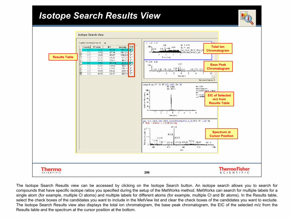
296

296

Isotope Search Results View

Total Ion Chromatogram

Base Peak Chromatogram

EIC of Selected m/z from

Results Table

Spectrum at Cursor Position

Results Table

The Isotope Search Results view can be accessed by clicking on the Isotope Search button. An isotope search allows you to search for compounds that have specific isotope ratios you specified during the setup of the MetWorks method. MetWorks can search for multiple labels for a single atom (for example, multiple Cl atoms) and multiple labels for different atoms (for example, multiple Cl and Br atoms). In the Results table, select the check boxes of the candidates you want to include in the MetView list and clear the check boxes of the candidates you want to exclude. The Isotope Search Results view also displays the total ion chromatogram, the base peak chromatogram, the EIC of the selected m/z from the Results table and the spectrum at the cursor position at the bottom.

297

297

Isotope Peak Summary View

Right-click to select to view included

isotopes only

The Isotope Peak Summary displays a peak detection summary for each of the isotopes from the Isotope Search Results view. To display the data for only the included isotopes, right-click the view, and then choose Show Included Isotopes Only from the shortcut menu. Included isotopes are the rows for which you select the Incl check box in the Isotope Search Results view. Each peak detection summary table contains columns for Peak #, RT (min.), Area, % Area, Height.

298

298

Specifying the MetView Columns and the MetReport Format

1. Click Options > MetReport

2. Select MetView Columns and

MetReport Format

3. Click OK

To specify the MetView columns and the MetReport format, choose Options > MetReports to open the MetView Reports Configuration dialog box. Under MetView, select the check boxes of the columns you want to include in the MetView table. The options include Retention time, Structure, Delta, Number of fragments, Type of modification, Modification name, Elemental composition, Present in (which views included the candidate). Under MetReport, select the check boxes of any traces you want to include in MetReport. Under Layout, select how to display the traces. You can choose either Side by side or Stacked. To close the dialog box, click OK.

299

299

Specifying the MetView Columns and the MetReport Format

1. Click for new settings to

update

The candidate column orders components by first displaying the analyte and then candidates that were selected in: Component Detection, Expected Modifications, Spectral Correlation, Isotope Search, and Chro Search Views

Indicates views where each

candidate was selectedRight-click and

select Import to add structure

In MetView, click the Update button for the new configuration settings to update. The results appear for the preferences that you specified in the MetView Reports Configuration dialog box. If you want to import a structure, right-click and select Import to add a structure to the Structure column. The PresView column indicates the views where each candidate was selected. At a minimum, the MetView table includes Candidate, m/z and Include in MetReport columns. The Candidate column lists the analyte followed by the potential modifications selected from each of the MetWorks results views. The candidate column orders components by displaying the analyte and then candidates that were selected in the Component Detection, Expected Modifications, Spectral Correlation, Isotope Search, and Chro Search views. The m/z column lists the mass (m/z) of the peak of interest. The Include in MetReport column contains check boxes so that you can select the candidates that you want to include in the MetReport. By default all the candidates are selected. Clear the check boxes of any candidates you do not want to include in the MetReport.

300

300

Creating a MetReport

1. Click to create report

2. Or select path

3. Click OK

2. Select Print

The MetReport is a customizable report that compiles the data for the candidates (potential metabolites) you selected from all the other results views into a single report. To generate a MetReport, click Create this report. In the MetReport Format dialog box, select the Enable check box. To print the report without creating a new file, select Print, and then click OK. In the Print dialog box, select the print options, and then click OK. To output to a file, select the PDF, Word, or Excel option. Click to display the Save As dialog box. Select the destination folder, type a file name, and click Save.

301

301

Creating Additional Summary Reports (Optional)

Click to print report

Select which result types to

include

Typically, you use MetView and MetReport to create customized reports for your selected candidates. However, you can also create additional summary reports by using the Reports Configuration and Generation dialog box by clicking on the Reports button at the end of the MetWorks workflow. If you want to change the settings for a given report, click the tab to display the corresponding reports page. The additional reporting options include a Chromatogram Summary, Modification Summary, Peak Summary, Chromatogram/Spectrum Summary, Tabulated Peak Summary and Custom Excel Report. On the specific page from which you want to generate the report, select which result types to include and the click Create this report to print the report.

302


Mass FrontierSoftware Course

Mass Frontier 5.0

303

303

Database Manager

The Database Manager is a module for managing spectral and structural information in Microsoft SQL Desktop Engine (MSDE) database. This module provides powerful library maintenance utilities that enable you to create and organize spectral and chromatographic libraries with chemical structures. In addition, since the program supports ion structures and tree spectra representation you can also create true MSn libraries. Advanced library query and search features provide access to the information needed for compound identification and can help you interpret unknown spectra. A flexible set of search restrictions is available to target your search results, especially useful when you are dealing with large libraries.

304

304

Database Manager

All spectra organizing and manipulation is carried out in the Database Manager

In the Database Manager, each record includes additional information that is arranged in different tabs. The mass spectrum of the selected tree section can be viewed in the Spectrum tab. By clicking on the Structures tab, the record structures can be viewed instead of the record information displayed in the Spreadsheet tab.

305

305

Database Manager

The Compare Spectra tab allows spectra comparisons to be carried out. The bottom spectrum is from the active record in the spreadsheet, while the top spectrum is updated with the active record by pressing the Add or Paste button. The middle spectrum displays the difference between the top and bottom spectrum.

After a spectrum search has been carried out, the query spectrum is automatically pasted to the top spectrum in the Compare Spectra tab to allow viewing of the peak differences of spectra in the hit list and query spectrum.

306

306

Commercially Available Libraries

If a commercially available library is in SQL format, then it can be directly installed in Mass Frontier.

Follow steps 1-5 to installyour library

Mass Frontier library utilities are based on the Microsoft SQL Server 2000 Desktop Engine (MSDE 2000)®. MSDE 2000 is a data engine built and based on core SQL server technology. It is a reliable storage engine and query processor for desktop applications. MSDE 2000 is Mass Frontier's background application. Library utilities are seamlessly integrated in a graphical interface and the user does not need to directly interact with the database engine. database engine allows the creation of databases with a maximum file size of 2 GB. Therefore, libraries created in Mass Frontier cannot exceed this file size. If you try to store data above this limit, Mass Frontier will inform you that this action cannot be completed and you should store the extra data in a new library.

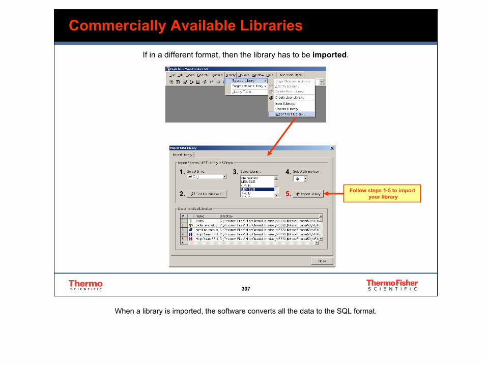
307

307

Commercially Available Libraries

If in a different format, then the library has to be imported.

Follow steps 1-5 to importyour library

When a library is imported, the software converts all the data to the SQL format.

308

308

Creating User Libraries

Follow steps 1-4 to create and install a user library

User libraries can be created in 2 ways:

1

2

Access to all library functions is gained by clicking on this button

from the Database Manager

An empty library is first created and installed. An unlimited number of libraries can be created, but no more than 255 libraries may be installed in Mass Frontier at the same time. To view different libraries than the ones displayed, you would need to uninstall some of them. If you uninstall a library, the library is not deleted, only the library reference is removed from the program without loss of any structural or spectral information. An uninstalled library can be reinstalled at any time.

309

309

Building Libraries in the Database ManagerMass spectra can be opened in the Database Manager in 2 ways:

Open the file in Qual Browserand export spectrum to Mass Frontier

1.

2. Open the file directly into the Database Manager

Mass Frontier supports three file formats for spectra: JCAMP, MSP and Xcalibur® RAW format. The first two formats are ACSII files. Mass spectrain table format or spectral trees stored in Excel can also be imported to Database Manager via the Clipboard. If the spectral table is vertical in Microsoft Excel, the first column must be the m/z value and the second must be abundance. Click the Copy button in Excel and Paste the data into the Database Manager window. More than one spectrum can be imported at a time. In this case your first column, must be the m/z values and all the other columns must be abundance.

310

310

Building Libraries in the Database Manager

Adding Structures

Structures can be added to an entry in the Database Manager in 3 ways:

By opening the Structure Editor directly from the structure pane and drawing a new structure.

By copying and pasting a structure in the Database Manager from anywhere in the program.

By loading a structure from an external file, in .mol or .sdf format.

You can copy a structure you wish to paste into Database Manager, from anywhere in the program. To paste a structure into Database Manager, use the Paste Structure button in the top right corner. The Copy and Paste buttons on the button bar are intended for records, not for single structures. Structures can be imported to Database Manager by loading them from an external MOL-file or SDF-file. In contrast to the pasting of a structure, when you load from an external file you can add structures to more than one record at a time. When adding structures to a spectral tree, different structures can be added for various nodes of the tree (make sure to have the node of interest selected).

311

311

Structure Editor

To begin drawing a chemical structure, click on one of the buttons on the vertical toolbar. The shape of the cursor will change to visually represent the engaged drawing mode.

Atom and Bond properties can be edited in these windows.

The Structure Editor is a full-featured structure drawing tool for editing, importing, exporting and checking chemical structures. Structure Editor is the gateway to four other modules in this program: Database Manager, Fragments and Mechanisms, Fragmentation Libraries, and Isotope Pattern.

312

312

Adding Structures

Chemical structures can also be added to any ion in the spectrum. To add a chemical structure to an ion, right-click on the spectral peak and select Fragment Annotation of Peak.

Building Libraries in the Database Manager

A structure can also be assigned to a peak using the Data tab in the Database Manager window.

Chemical structures can be added to any peak in the spectrum. After you finish drawing, the program will automatically attempt to connect your structure with a spectral peak according to the fragment's m/z value. If, for whatever reason, you need to connect the drawn fragment to a different peak, simply drag the connecting circle with the mouse to the required peak. The drawn fragment can be resized. Fragments generated by Fragments & Mechanisms window can be assigned automatically to peaks in a spectrum. A structure can also be assigned to a peak using the Data page of the Database Manager window, where all peaks in the spectrum are listed. Click on the line where the peak is listed, then click on the button in the Fragment column and Structure Editor will open.

313

313

Adding Entries to User Libraries

1. Click to add to library

Mass Frontier allows you to check whether a structure is already present in a library before adding a new spectrum/structure pair.

Only SELECTED records in a Database Manager Spreadsheet can be added to a user library. Any record information can be changed and saved in a library. If anything is changed in the record, a small circle is displayed in the Database Manager in the ID Number column in the spreadsheet. To save any changes, go to Library > Spectral Library > Save Changes in Library. If you decideto delete a library record, information will be irreversibly lost. This process can be carried out using again the appropriate Library buttons. If you delete a record from a library, the ID numbers will change so that there are no ID gaps.

314

314

Searching Libraries

A (Sub)structure search is the most common type of search in Mass Frontier.

It retrieves compounds that contain a common structural subset.

An Identity search provides an exact match of query and library search

1. Click to search a library

Tree Search - searches for the library spectral tree most closely matching an unknown spectral tree or sub-tree.Spectrum Search - searches for the library spectra most closely matching an unknown spectrum.(Sub)structure Search - searches for an exact match for the structure (structure search) or searches for an exact match for the structure subset (substructure search).Name Search - incremental name search.Molecular Mass Search - searches for compounds with a given molecular mass.Formula Search - searches for compounds with a given molecular formula.ID Number Search - searches for library entries with a given ID number.CAS Number Search - searches for compound(s) with a given Chemical Abstract Service registry number.Retention Time Search - searches for library entries with a range of given retention times.

315

315

Spectral Trees

A spectral tree consists of levels, nodes, node connectors and node items.

Node items can be product, average or composite spectra or chromatograms

The node connectors are a graphical symbol for the precursor m/z values or range, if isolation width is used

The nodes hold the node items

The levels symbolize MSn stages starting at n=1

Mass Frontier uses spectral tree representations for MSn spectra. Complete trees can be stored in a library and updated at any time. Any complementary information associated with a single stage spectrum or a chromatogram can be associated with a node spectrum or node chromatogram.

316

316

Creating Spectral Trees

Reconstruction from raw files

The tree reconstruction feature reads raw files stored in a directory and automatically creates a tree according to the precursor m/z and isolation width values.

1. Click on Open and Import Tree 2. Select the directory that contains the files that are to be used to create the tree

4. Click Import. The tree will appear in the Database Manager window

3. Add the directory by clicking on Add directory. Your directory will be added to the window on the right hand side

All spectra in a directory must come from an identical chemical entity. One directory, per tree, per compound. Each file is considered as a single parallel spectrum. This feature works for files that have been acquired using a single compound. The tree reconstruction feature not only creates levels, nodes and node connections but also automatically assigns node spectra to specific nodes.

317

317

Creating Spectral TreesSpectral tree deconvolution from a chromatogram in the Chromatogram Processor

2. Click Copy

3. Open the Database Manager and paste the tree to import

1. Select component

Mass Frontier allows the exchange of trees between windows, records, chromatographic components or programs (e.g. Excel). This can be done using standard copy and paste commands. When using the paste command, you must distinguish between a single spectrum and a tree so be sure to use the correct paste option when exchanging trees.

318

318

Chromatogram Processor

319

319

Chromatogram ProcessorTo open a raw file in the Chromatogram Processor, click on the Chromatogram Processor button. Select file and click open.

Mass Frontier supports various data file formats for importing GC-MS and LC-MS files: Xcalibur® RAW files (MS and MSn), Finnigan LCQ™, GCQ™, ITS40 and Magnum, Varian Saturn, HP ChemStation, JACAMP (DOS, Windows and UNIX). These files can be imported to Chromatogram Processor but cannot be exported. Single scans can be saved in JACAMP or MSP format. Mass Frontier supports centroid type data for mass spectra. Centroid mass spectra are displayed as a bar graph. Profile type data is not supported.

320

Mass Frontier incorporates an advanced automated system for detecting chromatographic components in complex GC/MS or LC/MS runs and extracting mass spectral signals from closely coeluting components (deconvolution). The Components Detection and Spectra Deconvolution system works fully automatically. The system is designed for broad types of chromatographic runs, for both GC/MS, LC/MS and GC/LC/MSn analyses, for clean and noisy signals, and for simple and for more complex chromatograms. However, some parameter changes may be needed to optimize the system for specific applications. This automated procedure is designed for small and medium size organic compounds and should not be used for the processing of proteins, peptides, oligonucleotides, or other biomolecules.

320


Automatic Components Detection and Spectra Deconvolution

This module of the software is designed to automatically detect the components present in complex mixtures analyzed mainly by data dependent analysis.

Mass Frontier identifies components using the following algorithms:

RCD (Rapid Component Detection)JCD (Joint Component Detection)TECD (Total Extraction Component Detection)Direct Infusion

321

To start automated component detection and the spectra deconvolution procedure, click on the Components Detection and Spectra Deconvolution button. When the parameters setup dialog window appears, change the settings if required, and then click the OK button.

321


To perform component detection (spectra deconvolution):1. Click the arrow beside

the button and select the component detection algorithm to use 2. Click Calculate

and then Close to close box

322

322


Automatic Components Detection and Spectra Deconvolution

Detected Components are marked with a triangle in the original chromatogram. Click on the triangle to display the spectral tree.

Once the components detection and spectra deconvolution process is applied to data dependent scans, the program generates components as spectral trees

323

323

Chromatogram ProcessorTo Import the Component (Spectral Tree) into the Database Manager from the Chromatogram Processor:

2. Click Copy

3. Open the Database Manager and paste the tree to import

1. Select component

A convenient way to detect components, generate spectral trees and store them is to first perform component detection and spectral deconvolution on a data dependent experiment. Components and spectral trees can then be copied and pasted into the Database Manager for editing and storing the data.

324

The Components Editor closely resembles visually the Database Manager module, however, the processing item is a chromatographic component rather than a database record. To ensure the modules are easy to tell apart, Components Editor has a light blue bar on the left side of the window. Both modules handle almost identically, so please refer to the Database Manager description for an explanation of module functionality.

324

Components Editor


The Components Editor allows the user to edit, search and organize chromatographic components found using the automated detection and deconvolution process.

This module presents users with a complete set of management tools to delete unrelated components, add chemical structures, edit extensive data fields, process spectral trees, annotate spectral peaks and sort search hit lists for every component in a processed chromatogram.

Components Editor is accessible from the Database Manager or Chromatogram Processor window using Components Editor button.

325

Each chromatographic component is represented by a single row in the Components Editor. The columns contain component supplementary information. One of the columns lists Model Ion values that have been used for component detection. These values will help you quickly orient yourself and find components of interest. In most cases the model ion is the base peak in the full scan spectrum, however, if closely coeluting components have isobaric base peaks the algorithms select different model ions to distinguish the components.

325


Components Editor

Each chromatographic component is represented by a single row

Lists Model Ion values that have beenused for component detection

326

The Components Editor allows the user to search one selected subset or all the chromatographic components in the spectral or chromatographic libraries at once. To search selected components, select components in the Spreadsheet and click the Search button in the toolbar and then choose the Search Selected Components item from the pop-up menu. To search all the components from the processed chromatogram, click the Search button and choose the Search All Components pop-up menu item.

326


Components Editor Click to search selected components or all components for library matches

327

The Hit Selector window lists the best matches found during the library search. The match factor describes the similarity of the match to your component. If at least one hit was found, the text in the name filed of the component row will appear in red. To process the hit list of a component, select the component row and open the Hit Selector window by clicking on the Hit Selector button (glasses). In Hit Selector you can review the hit list and accept a library record that correspond to the component by selecting the hit and clicking OK button. If you accept a library record for a component, all relevant information (structure, name, mol. mass, ion types etc.) will be adopted and entered in the component fields.

327


Components Editor

Components with library matches are highlighted in red Click on the glasses to view

the Hit Selector showing all the matches for a component

328

328

Fragments and Mechanisms

329

329


The Fragments and Mechanisms module is based on a system which uses a mathematical approach for the simulation of unimolecular ion-decomposition reactions. Two different methods are used:

1. General Fragmentation and Rearrangements rulesThe software generates fragment ions using straight cleavages and hydrogen rearrangements only.Bond creation is not supported with the exception of H bonds and thus, ring contractions, cyclizations and non-hydrogen rearrangements are not supported.Compound specific mechanisms that cannot be applied generally are also not included in this feature.

2. Fragmentation Library“Intelligent” fragmentation mechanism database.The software contains an expert system that automatically extracts a decomposition mechanism for each fragmentation reaction in the database and determines the compound class that the mechanism can be applied to.

One of Mass Frontier´s most outstanding features is the automated generation of possible fragments at an expert level, including complete fragmentation and rearrangement mechanisms, starting from a user-supplied chemical structure. The Fragments & Mechanisms module provides information about basic fragmentation and rearrangement processes that may occur in a mass spectrometer. Mass Frontier comes complete with almost 5,000 fragmentation schemes that contain around 19,000 reactions collected from mass spectrometry literature.

330

330


Fragmentation and rearrangement pathways can be generated from any user-supplied structure using the hammer button

You can specify the way the system will generate the various fragmentation pathways. The options are: General Fragmentation Rules, Fragmentation Library or Both.

Click to Generate Fragments and Mechanisms

Click the hammer button

If you choose the Fragmentation Library, you can select which library should be used from the list of libraries. Please note that the preinstalled HighChem Fragmentation Library™ contains around 19,000 mechanisms, and so calculation times will be significantly longer when it is used.

331

331


You can choose between the various ionization modes available. The Deprotonation option is not supported by general fragmentation rules and can only be used in connection with the Fragmentation Library.

When comparing generated fragments and mechanisms with a mass spectrum, you should always choose the correct ionization method. The program will show a warning message if the reaction restrictions are set for protonation techniques or chemical ionization and you are attempting to compare generated fragments with a spectrum from the NIST library which contains EI spectraonly.

332

332


The Sizes page allows the user to limit the size and the complexity of a reaction pathway generation.

The Reaction Steps Max Number box gives the number of cascaded fragment ion reactions. Increasing this number could exponentially increase the number of fragment ions produced for a given reaction path. Generally, this number should be kept small and if additional fragments need to be generated, individual fragments can be selected by the user and used as starting points for additional reactions.

333

333

Fragments and MechanismsThe Fragments and Mechanisms window displays either the complete mechanisms or the resulting fragment ions only.

To display the desired view for a certain m/z value, choose the appropriate m/z tab or select the ion from the m/z list on the right

Once the reaction-generating process has finished, a Fragments & Mechanisms window is displayed. A Fragments & Mechanisms window allows the display of either complete mechanisms of ion-decomposition reactions, or of resulting fragments only. To display the desired mechanism, or fragment for a particular m/z value, choose the appropriate m/z tab. If you do not like the tab control you can replace it with a combo box in the Options > Reaction Layout dialog window. Several possible isobaric fragments can be generated for a particular m/z value. The isobaric fragments, with their corresponding mechanisms, can be displayed by clicking the numbered buttons next to the hand pointer. The fragments are sorted according to the simplicity of their production mechanism (with #1 being the simplest, shortest mechanism).

334

334


2. Click on the Hammer button to generate fragments of this parent

To link generated fragments to spectral data:

1. Input parent m/z into the Structure Editor window

Product ion spectrum

Mass Frontier offers the ability to link generated fragments with a mass spectrum. If you start a generation of fragments and mechanisms from Database Manager, the generated fragments are automatically linked with peaks in spectrum according to their m/z values. So Mass Frontier helps you to explain peaks in spectrum. While a generation is in progress the Reactions Limit bar gives you an approximate indication of how many temporary internal reactions have been generated from a particular structure. If the reactions limit is reached a message will appear informing you of the fact.

335

335

Fragments and MechanismsIf the generation of fragment ions started from the Database Manager window, the program automatically links the generated fragment ions with the corresponding spectrum in the Database Manager window.

Peaks that have the same m/z value as the generated fragment ions are highlighted in RED

If an unexplained peak is likely to be an isotopic peak of an explained peak, it is depicted in GREEN

Unexplained peaks are depicted in BLUE

*Right-click on the spectrum and select ‘Auto Fragment Annotation of Peaks’ to display simulated fragments on the spectrum

After a generation, highlighted (“explained“) peaks are displayed in a different color (by default red) in the original mass spectrum. Selecting a highlighted peak reveals all the mechanisms leading to it. In addition, generated fragments (a corresponding Fragments & Mechanisms window must be open) can be assigned automatically to peaks in a spectrum in the Database Manager by right-clicking on the spectrum and choosing Auto Fragment Annotation of Peaks.

336

336

Fragmentation Libraries

337

337

Creating Fragmentation Libraries

If a fragmentation reaction is predicted using a library reaction, you can double click on the Lib arrow to see the corresponding mechanism.

After double-clicking Lib in the Fragments and Mechanisms module, the Fragmentation Library opens in a new window. The Fragmentation Library™ module allows the creation and management of fragmentation mechanism databases. This module contains a full-featured graphical editor for entering fragmentation reactions, which can be stored in a database, together with complementary information for the reaction. All the fields of the database can be queried, for example: authors, ionization method, or mass analyzer. All the library structures from the reactions are also fully searchable.

338

338

Creating Fragmentation Libraries

For creating and editing fragmentation libraries, the Reactions Editor in the Fragmentation Library module should be used.

1. Create fragmentation library

2. Open that fragmentation library and either copy and paste the mechanisms from the Fragments and Mechanisms window OR add a new structure

The structures in a reaction scheme must be properly connected by arrows. The system considers standalone structures and disconnected arrows as errors and ignores them. To make a change permanent in a Fragmentation Library, it must be saved. To save changes in the Reaction Editor or Data Editor:

Click on any prior or following record to the edited record in the record grid Or, click the line up or line down key Or, click on the Library button and choose Save Record To Library

339

339

Report Creator

340

340

Creating Reports

A report can be created as follows:

Open one or more modules with the corresponding data you wish to report

Click on the Report Creator button on the main tool bar, or choose Tools > Report Creator from the main menu

Report Creator allows you to create customizable reports from modules displayed on the screen. Reports can be printed or exported as pdf files. Reports can only created using Report Creator from windows which are open. You cannot report data that is stored in Mass Frontier, but does not appear on the screen when Report Creator is launched.

341

When the Report Creator opens, all the modules available for reporting are listed on the left side. If you click on a module name, options and annotation fields specific for the selected module will appear on the right side. To change the general report settings, e.g. header, footer, separation lines, page breaks and orientation, click on the Report Layout button in the Report Creator window.

341

Creating Reports

The Report Creator window is divided into two parts:

In the right part, you can select and annotate a number of text or graphical objects for the selected module.

The left part allows you to manage the modules which you wish to create a report from. You can select a module by highlighting its name and its corresponding customizable items will be displayed on the right side.

The left part of the Report Creator window allows you to add or remove a module from reporting or change the order in which they will appear in the report.

342

342

Report Preview

Once the modules and their objects have been selected and annotated, you can generate a report preview by clicking on the Preview button.

Procedure for Getting into the Technical Support W

ebsite

1. In Microsoft Internet E

xplorer or your internet browser, type the

following in the “A

ddress” box.

http://w

ww

.thermokb.com

(This will get you into the m

ain Thermo S

cientific Know

ledge Base page)

2. Then, click on “Knowledge B

ase for Chrom

atography and Mass

Spectrom

etry” which is located on the top of the page.

3. If you are under w

arranty or have a support plan, you have access to a greater num

ber of technical documents. For access to the

maxim

um num

ber of technical documents, Login using your K

ey C

ard Num

ber (Equipm

ent Num

ber) for both the Usernam

e and P

assword.

LC-M

S CO

NTA

MIN

ATIO

N

430

General D

iscussion C

hemical contam

ination is one of the more com

mon problem

s with LC

/MS

. Therefore, please use the highest purity chem

icals available. • Try B

urdick and Jackson solvents and water. These seem

to be uniformly

better than other suppliers. Sw

itch to this brand if you have contamination

problems.

• Additionally, use high purity acetic acid: A

ldrich p/n 38,012-1 double distilled in Teflon bottle $175 for 500 M

l. C

hemical contam

ination problems (w

ith specific mass peaks) are rarely attributed

to problems deep inside the M

S. P

rioritize like this:

1. HP

LC pre or trap colum

n 2. H

PLC

column

3. HP

LC hardw

are 4. C

hemicals

5. ES

I or AP

CI probe

6. Spray shield area

7. Ion Transfer Tube 8. Tube lens/Skim

mer

9. Q00/Lens 0/Q

0 10. A

nalyzer Quads

11. MS

Dynode

Generally, if 8 – 11 are dirty you w

ill see random peaks not specific m

asses. Identifying the source of contam

ination

1. Is the contamination alw

ays there or does it elute as specific peaks during the H

PLC

run? If the later, the problem is m

ost likely with the

HP

LC.

2. Turn off flow. If the noise disappears take the colum

n out of the flow

path and test again. If the noise is still there try these items, go to step

#3.

3. If you suspect that there is chemical contam

ination from the H

PLC

m

obile-phase, use a clean syringe and tubing to infuse the mobile-

phase components individually into the M

S (e.g. w

ater, then water +

acid, then methanol or acetonitrile. G

enerally, the acid is the source of contam

ination.

amber.kohl

LC-M

S CO

NTA

MIN

ATIO

N

431

HPLC

Troubleshooting M

any times contam

inant peaks occur during a gradient. Try this procedure to locate the source of the contam

ination:

• Inject a solvent blank.

• M

ake a zero volume injection

• R

un a gradient with the injection valve or autosam

pler out of the liquid flow

. C

ontamination in the M

S

If the noise disappears when H

PLC

flow is turned off and you have elim

inated contam

ination in the mobile phase:

•

Trim or replace the sam

ple tube and set it to the correct distance within

the needle. •

Clean the E

SI spray nozzle (cone and needle).

• R

eplace the Teflon needle seal behind the needle •

If still noisy, the cause could be neutral chemical noise (non-ionized

materials). C

hange source conditions (e.g. increase heated capillary tem

perature 10 or 20ºC, increase S

heath gas flow 10 or 20 units,

increase Auxiliary gas flow

10 units. O

ther possibilities

• S

olvent reservoir pickup filters are comm

on sources of contamination.

Usually the aqueous phase one w

ill be the first to go. •

Offline solvent filters are com

mon sources of contam

ination. Serious

contamination has been seen w

ith the Nylon 0.22 µm

filters used for buffer solutions.

• A

ddress the containers used for storing your acetonitrile. A sim

ilar problem

occurs when using glass scintillation vials w

ith polypropylene insert caps to m

akeup solvent. Phthalate C

ontamination

•

391 protonated diisooctyl phthalate [M+H

] + •

413 sodium adduct of diisooctyl phthalate [M

+Na] +

• 798 am

moniated dim

er of diisooctyl phthalate [2M+N

H4 ] +

• 803 sodiated dim

er of diisooctyl phthalate [2M+N

a] +

This is usually from

contaminated solvents. It can concentrate on the

column and elute during a gradient. Follow

the normal solvent

contamination checking procedures.

amber.kohl

LC-M

S CO

NTA

MIN

ATIO

N

432

Glassw

are cleaned by means of a “dishw

asher” often picks up phthalate contam

ination. Rem

ove this with a rinse of 30%

nitric acid, followed by a rinse

with 2M

NH

4 OH

. Please keep in m

ind, that the AP

CI probe can retain this.

How

ever, baking the AP

CI w

ill eliminate this problem

. Try 600ºC for 15 m

in. +44 Series Ions Possible Polym

er Contam

ination If you have analyzed detergent containing sam

ples on the system, that could

explain the +44 series background problem. A

lso, PE

Gs and other ethoxylated

polymers give +44 ion series. The P

EG

's could originate from the w

ater, or extracted polym

ers from plastic w

are and/or silicon coatings. B

ackground Ram

ps Up W

ith Gradient

Background can originate from

contaminated organic phase or the high organic

content maybe eluting retained m

aterials from the colum

n. Substitute w

ith B

urdick and Jackson organic phase and a new colum

n. +59 Series Ions 59 D

a is the mass of the acetate ion (observed w

hen employing am

monium

acetate or acetic acid). Is it possible to have acetate polym

erization? There is another explanation for the +59 ion series. P

olymers of +59 m

ight be iron in som

e form, presum

ably leaching from the steel in acid.

+74 Series Ions P

eaks at 536, 610 and 684 Da have been seen w

ith LCQ

DecaX

P and LC

Q

Advantage and TS

Q Q

uantum. The contam

ination came from

connecting the opaque silicon tube to the A

PI source housing. The proper tubing is Tygon. The

instrument parts kits contain both types of tubing. The TS

Q Q

uantum contains a

12-foot length of clear Tygon tube and a 2.5-foot length of opaque silicon tube. The intended function of the silicon tube is to connect from

the waste container

(P/N

00301-57020) to the fume exhaust system

. If the silicon tube is instead connected to the A

PI source housing, background ions at m

/z 536, 610, and 684 m

ight be observed. Solution: R

emove all silicon tubing from

the solvent waste

system.

+77 Series Ions +77 D

a clusters, mostly across the m

ass range, can be attributed to the ion-transfer tune and K

alrez o-ring. One could postulate that the w

orn o-ring was

allowing leakage into the tube lens skim

mer area and the leak w

as also leaching som

ething out of the o-ring. Norm

ally the o-ring is a total block and any polymers

in it would not enter the M

S.

amber.kohl

LC-M

S CO

NTA

MIN

ATIO

N

433

+ 615.7 and 1229.8 Chaps Ions

615.7 Da is [M

+H] + of C

HA

PS

and 1229.8 Da is [2M

+H] + in the sam

ple. R

emoval can be extrem

ely difficult. Acetone precipitation rem

oves the excess C

HA

PS

, but there may still be an appreciable am

ount remaining (determ

ined by the above ions in the m

ass spectrum). C

HA

PS

won't kill your S

CX

chrom

atography, but it will chrom

atograph nicely on reversed phase and you'll get an intense ion at 615 m

/z [M+H

] +. +136 Series Ions This is exhibited by background (contam

ination) that has a repeating sequence of 136 am

u (TFA sodium

salt is 136 Da). R

emove TFA

from the sam

ple and/or m

obile-phase. TFA m

ay be difficult to remove from

the column, so take off the

column and flow

mobile-phase directly into the M

S. Identify the source by

infusing methanol w

ith a clean syringe and a new piece of tubing.

Pentafluoropropionic Acid

May stick to P

EE

K tubing and fittings. This contam

ination is usually associated w

ith areas that are poorly swept by the flow

ing liquid (e.g. unions). If you have concerns about the pentafluoropropionic acid, then use fused-silica and steel unions. The ferrules should be kel-F, and P

EE

K tube nuts should be ok as they

do not touch the liquids. W

ater If any contam

ination is seen, use high-grade bottled water (B

urdick & Jackson

HP

LC grade.) A

void AN

Y nanoPure or M

illiQ w

ater! +798 and +803 C

ontamination

Both ions are diisooctyl phthalate analytes derived from

plasticizers. Som

etimes,

their origins can be really hard to track down. If the source is your H

PLC

, these species can concentrate on your colum

n until the gradient is ramped and the

compounds eluted. C

heck the HP

LC solvents by infusion to determ

ine if it's com

ing from your H

PLC

or if it's in one of your reagents (e.g., TFA). In the later

case, clean the HP

LC reservoir bottles. These could be cleaned by rinsing w

ell w

ith 30% N

itric Acid follow

ed, after a water rinse, then by 2M

NH

4 OH

. +453.3, +679.5 and +905.7 C

ontamination

Nylon H

PLC

solvent filters can produce nylon (6,6monom

er) peaks at masses of

226 Da, a dim

er 452 Da, trim

er 678 Da and tetram

er 905 Da. The contam

inant is very hard to get rid off since it binds very w

ell to C18.

amber.kohl

LC-M

S CO

NTA

MIN

ATIO

N

434

Peak Clusters at +21, -17, -35, -52

+21 is sodium, -17, -35, -52 are various losses of am

monia and w

ater (if you look at the -17 ion you w

ill probably see a small am

ount of the -18, as well).

Iron-Acetate clusters @

+538, +555 and +534 M

obile-phases with acetic acid can react w

ith iron in the LC/M

S system

to produce Iron-acetate clusters (as established by Ijam

es, Dutky, and Fales: J A

m

Soc M

ass Spec 6 1226 1995.) The general form

ula is Fe3 O

(CH

3 CO

2 )6(L)x where

L is a ligand from the m

obile-phase (water or organic com

ponent, acetonitrile solvent or w

ater. 538 Da could be 6 acetates w

ith no additional ligand. The 555 D

a presumably has additional w

ater. 533.88 Da could be a chrom

ium cluster

similar to the iron 537.88. S

tainless steel in the system contains both iron and

chromium

. Potential sources in the E

SI probe could be the E

SI spray needle or

the with the m

etal needle kit. If necessary, try replacing the needle.

amber.kohl

CO

MM

ON

BA

CK

GR

OU

ND

ION

S FOR

ELECTR

OSPR

AY

(Positive Ion)

m/z

Ion A

nalyte m

/z Ion

Analyte

101 [M

+Na] +

DM

SO

267 [M

+H] +

Tributylphosphate

102 [M

+H] +

Triethylamine

273

M+

Mom

omethoxytrityl cation

104/106 [M

+Cu] +

Acetonitrile

279

[M+H

] + D

ibutylphthalate

105 [2M

+Na] +

Acetonitrile

282

Plasticizer in P

olyethylene 120

[M+N

a+CH

3 CN

] + D

MS

O

301

[M+N

a] + D

ibutylphthalate

122 [M

+H] +

TRIS

317 [M

+K] +

Dibutylphthalate

123 [M

+H] +

Dim

ethylaminopyridine

336

[M+H

] + Tributyl tin form

ate

130 [M

+H] +

Diisopropylethylam

iine

338 [M

+H] +

Erucam

ide

137 [M

+CAN

+NH

4 ] + D

MS

O

360

[M+N

a] + E

rucamide

144 [M

+H] +

TPA

371 [M

+H] +

Polysiloxane, follow

ed by 388

145/147 [2M

+Cu] +

Acetonitrile

391

[M+H

] + D

iisooctyl phthalate

146 [3M

+Na] +

Acetonitrile

413

[M+N

a] + D

iisooctyl phthalate

150 [M

+H] +

Phenyldiethylam

ine

425 [M

+Na] +

Unknow

n plasticiser

153 [M

+H] +

1,8-D

iazabicyclo[5,4,0]undec-7-ene(D

BU)

429

[M+K

] + D

iisooctyl phthalate

157 [2M

+H] +

DM

SO

445 [M

+H] +

Polysiloxane, follow

ed by 462

159 [M

+Na] +

Sopdium

trifluoroacetate

449 [2M

+H] +

Dicyclohexyl urea (D

CU

)

179 [2M

+Na] +

DM

SO

454 [M

+Na+AC

N] +

Diisooctyl phthalate

186 [M

+H] +

Tributylamine

522

U

nknown

214

Unknow

n Surfactant

550

U

nknown

217

Unknow

n Contam

inant

798 [2M

+NH

4] + D

iisooctyl phthalate

225 [M

+H] +

Dicyclohexyl U

rea (D

CU

)

803 [2M

+Na] +

Diisooctyl phthalate

231 [M

+NH

3 ] + U

nknown

P

EG

polymers exhibit peaks spaced @

44 amu intervals

239/241 [(M

.HC

l)2 -Cl] +

Triethylamine

242

M+

Tetrabutylamm

onium

(C4 H

9 )4 N+

C

omm

on Adducts

243 M

+ Trityl cation

257 [3M

+H] +

DM

SO

[M+N

H4 ] +

[M+18]

[M+N

a] + [M

+23]

[M+K] +

[M+39]

* This information is provided courtesy of N

ew O

bjective, Inc. © 2004 435

amber.kohl

CO

MM

ON

FRA

GM

ENT IO

N A

ND

NEU

TRA

L FRA

GM

ENTS

Com

mon Sm

all Ions C

omm

on Neutral Fragm

ents

m/z

Com

position

m/z loss

Com

position

15 C

H3

1 H

17

OH

15

CH

3

18

H2 O

17

OH

19

H3 O

, F

18

H2 O

26

C2 H

2 , CN

19

F

27

C2 H

3

20

HF

28

C2 H

4 , CO

, H2 C

N

27 C

2 H3 , H

CN

29

C2 H

5 , CH

O

28 C

2 H4 , C

O

30

CH

2 NH

2

30

CH

2 O

31

CH

3 O

31 C

H3 O

33

SH

, CH

2 F

32

CH

4 O, S

34

H2 S

33

CH

3 + H2 O

, HS

35(37)

Cl

33 H

2 S

36(38)

HC

l

35(37)

Cl

39

C3 H

3

36(38)

HC

l

41

C3 H

5 , C2 H

3 N

42 C

3 H6 , C

2 H2 O

, C2 H

4 N

42

C3 H

6 , C2 H

2 O, C

2 H4 N

43

C3 H

7 , CH

3 CO

43

C3 H

7 , CH

3 CO

44

CO

2 , CO

NH

2

44

C2 H

4 O

45 C

2 H5 O

46

NO

2

55

C4 H

7

56

C4 H

8

57

C4 H

9

57

C4 H

9

59

C2 H

3 O2

60

CH

4 CO

2

60

C2 H

4 O2

79(81)

Br

64 S

O2

80(82)

HB

r

79(81)

Br

91

I

80(82)

HB

r

127

HI

91 I

127

HI

436

amber.kohl

Notes Pages

LCQ Operation Course.pdf - Concordia University

Documents

Transcript of LCQ Operation Course.pdf - Concordia University